computational damage mechanics for composite materials based on mathematical homogenization
TRANSCRIPT
toheral-ingedge
entk-
ex andumber materi-e that it stiff-s dam-
andmaterialis intro-k orien- the
damageive mate-homog-
o-steprder in
Computational Damage Mechanics for Composite Materials Based on Mathematical Homogenization
Jacob Fish, Qing Yu and KamLun ShekDepartments of Civil, Mechanical and Aerospace Engineering
Rensselaer Polytechnic InstituteTroy, NY 12180
Abstract
This paper is aimed at developing a nonlocal theory for obtaining numerical approximation a boundary value problem describing damage phenomena in a brittle composite material. Tmathematical homogenization method based on double scale asymptotic expansion is geneized to account for damage effects in heterogeneous media. A closed form expression relatlocal fields to the overall strain and damage is derived. Nonlocal damage theory is developby introducing the concept of nonlocal phase fields (stress, strain, free energy density, damarelease rate, etc.) in a manner analogous to that currently practiced in concrete [7], [8], withthe only exception being that the weight functions are taken to be C0 continuous over a singlephase and zero elsewhere. Numerical results of our model were found to be in good agreemwith experimental data of 4-point bend test conducted on composite beam made of BlacglasTM/Nextel 5-harness satin weave.
Keywords: damage, composites, homogenization, nonlocal, asymptotic
1.0 Introduction
Damage in composite materials occurs through different mechanisms that are complusually involve interaction between microconstituents. During the past two decades, a nof models have been developed to simulate damage and failure process in compositeals, among which the damage mechanics approach is particularly attractive in the sensprovides a viable framework for the description of distributed damage including materialness degradation, initiation, growth and coalescence of microcracks and voids. Variouage models for brittle composites can be classified into micromechanical macromechanical approaches. In the macromechanical damage approach, composite is idealized (or homogenized) as an anisotropic homogeneous medium and damage duced via internal variable whose tensorial nature depends on assumptions about cractation [15], [28], [29], [42], [35], [43], [31]. The micromechanical damage approach, onother hand, treats each microphase as a statistically homogeneous medium. Local variables are defined to represent the state of damage in each phase and phase effectrial properties are defined thereafter. The overall response is subsequently obtained by enization [1], [30], [44], [45], [46].
From the mathematical formulation stand point, both approaches can be viewed as a twprocedure. The main difference between the two approaches is in the chronological o
1
anicalanics
oach,
steps math-com-amage localoach istress,lds arer analo-t the
n theaticalmati-
e sim-nd the
of our on the
er-
ticallytinuum
nstitu-posite
) with, as
and
num-
dinatery con- point haveevel of
ave
which the homogenization and evolution of damage are carried out. In the macromechapproach, homogenization is performed first followed by application of damage mechprinciples to homogenized anisotropic medium, while in the micromechanical apprdamage mechanics is applied to each phase followed by homogenization.
The primary objective of the present manuscript is to simultaneously carry out the two(homogenization and evolution of damage) by extending the framework of the classicalematical homogenization theory [3][4][27] to account for damage effects. This is acplished by introducing a double scale asymptotic expansion of damage parameter (or dtensor in general). This leads to the derivation of the closed form expression relatingfields to overall strains and damage (Section 2). The second salient feature of our apprin developing a nonlocal theory by introducing the concept of nonlocal phase fields (sstrain, free energy density, damage release rate, etc.) in Section 3. Nonlocal phase fiedefined as weighted averages over each phase in the characteristic volume in a mannegous to that currently practiced in concrete [7], [8] with the only exception being tha
weight functions are taken to be C0 continuous over a single phase and zero elsewhere. Oglobal (macro) level we limit the finite element size to ensure a valid use of the mathemhomogenization theory and to limit localization. In Sections 4 and 5 we develop a mathecal and numerical model for the case of piecewise constant weight function, which is thplest variant of the model presented in Section 3. The stress update procedure aconsistent tangent stiffness matrix are then derived. Section 6 compares the resultsnumerical model to the experimental data. We consider a 4-point bend test conducted
composite beam made of BlackglasTM/Nextel 5-harness satin weave and compare our numical simulations to experiments conducted at Rutgers University [14].
2.0 Mathematical Homogenization for Damaged Composites
In this section we extend the classical mathematical homogenization theory [3] for statishomogeneous composite media to account for damage effects. The strain-based condamage theory is adopted for constructing constitutive relations at the level of microcoents. Closed form expressions of local strain and stress fields in a multi-phase commedium are derived. Attention is restricted to small deformations.
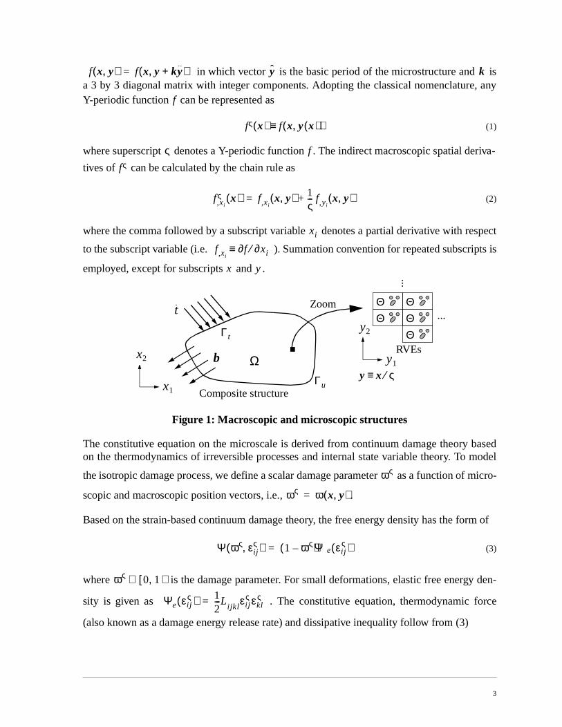
The microstructure of a composite material is assumed to be locally periodic (Y-periodica period defined by a Statistically Homogeneous Volume Element (SHVE), denoted by
shown in Figure 1. Let be a macroscopic coordinate vector in macro domain
be a microscopic position vector in . Here, denotes a very small positive
ber compared with the dimension of , and is regarded as a stretched coorvector in the microscopic domain. When a solid is subjected to some load and boundaditions, the resulting deformation, stresses, and internal variables may vary from point towithin the SHVE due to the high level of heterogeneity. We assume that all quantitiestwo explicit dependencies: one on the macroscopic level , and the other one on the l
microconstituents . For any Y-periodic response function , we h
Θx Ω
y x ς⁄≡ Θ ςΩ y x ς⁄≡
xy x ς⁄≡ f
2
ise, any
eriva-
spect
ipts is
based model
f micro-
orm of
y den-
rce
in which vector is the basic period of the microstructure and a 3 by 3 diagonal matrix with integer components. Adopting the classical nomenclaturY-periodic function can be represented as
(1)
where superscript denotes a Y-periodic function . The indirect macroscopic spatial d
tives of can be calculated by the chain rule as
(2)
where the comma followed by a subscript variable denotes a partial derivative with re
to the subscript variable (i.e. ). Summation convention for repeated subscr
employed, except for subscripts and .
Figure 1: Macroscopic and microscopic structures
The constitutive equation on the microscale is derived from continuum damage theoryon the thermodynamics of irreversible processes and internal state variable theory. To
the isotropic damage process, we define a scalar damage parameter as a function o
scopic and macroscopic position vectors, i.e., .
Based on the strain-based continuum damage theory, the free energy density has the f
(3)
where is the damage parameter. For small deformations, elastic free energ
sity is given as . The constitutive equation, thermodynamic fo
(also known as a damage energy release rate) and dissipative inequality follow from (3)
f x y,( ) f x y ky+,( )= y k
f
fς x( ) f x y x( ),( )≡
ς f
fς
f,xi
ς x( ) f,xix y,( ) 1
ς--- f,yi
x y,( )+=
xi
f,xi∂f ∂xi⁄≡
x y
Ω
t
y1
y2
x1
x2
ΘZoomΘ Θ
ΘΓt
Γu
RVEs
y x ς⁄≡
Composite structure
b
Θ...
...
ως
ως ω x y,( )=
Ψ ως εijς,( ) 1 ως–( )Ψe εi j
ς( )=
ως 0 1),[∈
Ψe εi jς( ) 1
2---L
ijklεi j
ς εklς=
3
m ofurther
ilibrium, prob-
ain ten-
he dis-
defined
(4)
(5)
(6)
With this brief glimpse into the constitutive theory, we proceed to outlining the strong forthe governing differential equations on the fine scale - the scale of microconstituents. Fdetails on the evolution of damage are given in Section 4.
We assume that micro-constituents possess homogeneous properties and satisfy equconstitutive, kinematics and compatibility equations. The corresponding boundary valuelem is governed by the following set of equations:
(7)
(8)
(9)
(10)
(11)
where is a scalar damage parameter; and are components of stress and str
sors; represents components of elastic stiffness satisfying conditions of symmetry
(12)
and positivity
(13)
is a body force assumed to be independent of ; denotes the components of t
placement vector; the subscript pairs with parentheses denote the symmetric gradientsas
(14)
σi jς Ψ ως εi j
ς,( )∂εi j
ς∂---------------------------- 1 ως
–( )Lijkl εklς= =
YΨ ως εij
ς,( )∂
ως∂----------------------------– Ψe ες( )= =
Yω· ς 0≥
σi j x; j
ς bi+ 0 in Ω=
σijς 1 ως–( )Lijkl εkl
ς in Ω=
εi jς u i x, j( )
ς in Ω=
uiς ui on Γu=
σi jς nj ti on Γt=
ως σi jς εij
ς
Lijkl
Lijkl Ljikl Lijlk Lklij= = =
C0 0 Lijkl ξi jς ξkl
ς C0ξijς ξi j
ς ξi jς∀≥,>∃ ξji
ς=
bi y uiς
u i x, j( )ς 1
2--- ui x, j
ς uj x, i
ς+( )≡
4
ry por-
h that
nter-
inter-
with asible.
expan-ithout
arting
ame-
5) into
denotes the macroscopic domain of interest with boundary ; and are bounda
tions where displacements and tractions are prescribed, respectively, suc
and ; denotes the normal vector on . We assume that the i
face between the phases is perfectly bonded, i.e. and at the
face, , where is the normal vector to and is a jump operator.
Clearly, a brute force approach attempting discretization of the entire macro domain grid spacing comparable to that of the microscale features is not computationally feaThus, a mathematical homogenization method based on the double-scale asymptoticsion is employed to account for microstructural effects on the macroscopic response wexplicitly representing the details of the microstructure in the global analysis. As a st
point, we approximate the displacement field, , and the damage par
ter, , in terms of double-scale asymptotic expansions on :
(15)
(16)
Strain expansions on the composite domain can be obtained by substituting (1(9) with consideration of the indirect differentiation rule (2)
(17)
where strain components for various orders of are given as
(18)
and
(19)
Stresses and strains for different orders of are related by the constitutive equation (8)
(20)
(21)
The resulting asymptotic expansion of stress is given as
Ω Γ Γu Γt
ui ti
Γu Γt∩ ∅= Γ Γu Γt∪= ni Γ
σi jς nj[ ] 0= ui
ς[ ] 0=
Γint ni Γint •[ ]
uiς x( ) ui x y,( )=
ως x( ) ω x y,( )= Ω Θ×
ui x y,( ) ui0 x y,( ) ςui
1 x y,( ) …+ +≈
ω x y,( ) ω0 x y,( ) ςω1 x y,( ) …+ +≈
Ω Θ×
εij x y,( ) 1ς---εij
1– x y,( ) εij0 x y,( ) ςεi j
1 x y,( ) …+ + +≈
ς
εi j1– εyij u0( ), εi j
s εxij us( ) εyij us 1+( ), s+ 0 1 …, ,= = =
εxij us( ) u i ,xj( )s , εyij us( ) u i ,yj( )
s==
ς
σij1– 1 ω0–( )Lijkl εkl
1–=
σi js 1 ω0–( )Lijkl εkl
s ωs r– 1+ Lijkl εklr 1– , s
r 0=
s
∑+ 0 1 …, ,= =
5
uation
te-
to Y-
(22)
Inserting the stress expansion (22) into equilibrium equation (7) and making use of eq(2) yield the following equilibrium equations for various orders:
(23)
(24)
(25)
(26)
We consider the equilibrium equation (23) first. Pre-multiplying it by and in
grating over yields
(27)
and subsequently integrating by parts gives
(28)
where denotes the boundary of . The boundary integral term in (28) vanishes due
periodicity on , and hence, with the positivity of and the assumption of
(see Section3), we have
(29)
and
(30)
We proceed to the equilibrium equation (24). From (18) and (20) follow
(31)
To solve for (31) up to a constant we introduce the following separation of variables
(32)
σi j x y,( ) 1ς---σij
1– x y,( ) σ i j0 x y,( ) ςσ ij
1 x y,( ) …+ + +≈
O ς 2–( ): σ i j ,yj
1– 0=
O ς 1–( ): σi j ,xj
1– σij ,yj
0+ 0=
O ς0( ): σi j ,xj
0 σij ,yj
1 bi+ + 0=
O ςs( ): σi j ,xj
s σi j ,yj
s 1++ 0, s 1 2 …, ,= =
O ς 2–( ) ui0
Θ
ui0σij ,yj
1– ΘdΘ∫ 0=
ui0σi j
1– nj ΓΘdΓΘ
∫ 1 ω0–( )u i ,yj( )0 Lijkl u k,yl( )
0 ΘdΘ∫– 0=
ΓΘ Θ
ΓΘ Lijkl ω0 0 1),[∈
εyij u0( ) u i ,yj( )0 0= = ⇒ ui
0 ui0 x( )=
σi j1– x y,( ) εi j
1– x y,( ) 0= =
O ς 1–( )
1 ω0–( )Lijkl εxkl u0( ) εykl u1( )+( ) ,yj0 on Θ=
ui1 x y,( ) Hikl y( ) εxkl u0( ) dkl
ω x( )+ =
6
uced
at if
if
(32)
e fol-
n be
ondi- con-
ion
valueeak
n 3-D
terms of
8]:
where is a Y-periodic function. We assume that is macroscopic damage-ind
strain driven by the macroscopic strain . More specifically we can state th
, then and . Note that vice versa is not true, i.e.,
or , the macroscopic strain may not be necessarily zero. In
both and are symmetric with respect to indices and .
Based on the decomposition given in (32), the equilibrium equation takes thlowing form:
(33)
where
(34)
and is the Kronecker delta, while is known as a polarization function. It ca
shown that the integrals of the polarization functions in vanish due to periodicity ctions. Since equation (33) should be valid for arbitrary macroscopic fields, we may first
sider the case of (and ) but , which yields the following equat
in :
(35)
Equation (35) together with the Y-periodic boundary conditions is a linear boundary problem in . By exploiting the symmetry with respect to the indexes , the wform of (35) is solved for 3 right hand side vectors in 2-D and 6 right hand side vectors i(see for example [20][27]).
In the absence of damage, the asymptotic expansion of strain (17) can be expressed in the macroscopic strain as follows
(36)
where is termed as the elastic strain concentration function defined as
(37)
The elastic homogenized stiffness follows from the equilibrium equation [1
Hikl dklω x( )
εkl εxkl u0( )≡
εkl 0= dklω x( ) 0= ω0 x y,( ) 0=
dklω x( ) 0= ω0 x y,( ) 0= εkl
Hikl dklω k l
O ς 1–( )
1 ω0–( )Lijkl Iklmn Gklmn+( )εxmn u0( ) Gklmndmnω x( )+[ ]
,yj
0 in Θ=
I klmn12--- δmkδnl δnkδml+( )= , Gklmn y( ) H k,yl( )mn y( )=
δmk Gklmn
Θ
dklω x( ) 0= ω0 0= εkl 0≠
Θ
Lijkl I klmn H k,yl( )mn+( ) ,yj
0=
Θ m n,( )
εij
εij Aijkl εkl O ς( )+=
Aijkl
Aijkl I ijkl Gijkl+=
Lijkl O ς0( )
7
nd
o be
eter
erms
nally
(38)
where is the volume of a SHVE.
After solving (35) for , we proceed to find from (33). Premultiplying it by a
integrating it by parts with consideration of Y-periodic boundary conditions yields
(39)
from where the expression of the macroscopic damaged induced strain can be shown t
(40)
Let be a set of continuous functions, then the damage param
is assumed to have the following decomposition
(41)
where is a damage distribution function on the microscale. Rewriting (40) in t
of strain concentration function and manipulating it with (38) and (41) yield
(42)
where
(43)
(44)
(45)
(46)
In conjunction with (32) and (42), the asymptotic expansion of strain field (17) can be ficast as
Lijkl1Θ------- LijmnAmnkl Θd
Θ∫≡ 1Θ------- AmnijLmnstAstkl Θd
Θ∫=
Θ
Himn dmnω Hist
1 ω0–( )GijstLijkl Aklmnεxmn u0( ) Gklmndmnω x( )+( ) Θd
Θ∫ 0=
dmnω x( ) 1 ω0–( )GijstLijkl Gklmn Θd
Θ∫
–1–
= 1 ω0–( )GijstLijklAklmn ΘdΘ∫
εmn
ψ ψ η( ) y( ) 1n≡ C 1–
ω0 x y,( )
ω0 x y,( ) ψ η( ) y( )ω η( ) x( )η 1=
n
∑=
ψ η( ) y( )Aijkl
dmnω x( ) Dklmn x( )εmn=
Dklmn x( ) I klst Bklstη( ) ω η( ) x( )
η 1=
n
∑– 1–
Cstmnη( ) ω η( ) x( )
η 1=
n
∑
=
Bijklη( ) 1
Θ------- Lijmn Lijmn–( ) 1– ψ η( )GstmnLstpqGpqkl Θd
Θ∫=
Cijklη( ) 1
Θ------- Lijmn Lijmn–( ) 1– ψ η( )GstmnLstpqApqkl Θd
Θ∫=
Lijmn1Θ------- Lijmn Θd
Θ∫=
8
at the
by the gov-
train
rm
d (47)
oach,pletely
phys-
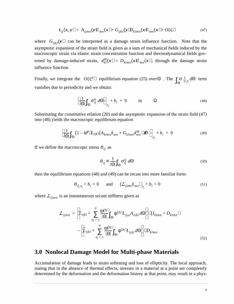
(47)
where can be interpreted as a damage strain influence function. Note th
asymptotic expansion of the strain field is given as a sum of mechanical fields induced macroscopic strain via elastic strain concentration function and thermodynamical fields
erned by damage-induced strain, , through the damage s
influence function.
Finally, we integrate the equilibrium equation (25) over . The te
vanishes due to periodicity and we obtain:
(48)
Substituting the constitutive relation (20) and the asymptotic expansion of the strain fielinto (48) yields the macroscopic equilibrium equation
(49)
If we define the macroscopic stress as
(50)
then the equilibrium equations (48) and (49) can be recast into more familiar form:
(51)
where is an instantaneous secant stiffness given as
(52)
3.0 Nonlocal Damage Model for Multi-phase Materials
Accumulation of damage leads to strain softening and loss of ellipticity. The local apprstating that in the absence of thermal effects, stresses in a material at a point are comdetermined by the deformation and the deformation history at that point, may result in a
εij x y,( ) Aijmn y( )εmn x( ) Gijkl y( )Dklmn x( )εmn x( ) O ς( ) + +=
Gijkl y( )
dklω x( ) Dklmn x( )εmn x( )=
O ς0( ) Θ σij ,yj
1 ΘdΘ∫
1Θ------- σi j
0 ΘdΘ∫
,xj
bi+ 0= in Ω
1Θ------- 1 ω0–( )Lijkl Aklmnεmn Gklmndmn
ω+( ) ΘdΘ∫
,xj
bi+ 0=
σi j
σi j1Θ------- σij
0 ΘdΘ∫≡
σi j ,xjbi+ 0 and = /i jmnεmn( ),xj
bi+ 0=
/ijmn
/i jmn Lijklω η( )
Θ---------- ψ η( )LijstAstkl Θd
Θ∫η 1=
n
∑+
Iklmn Dklmn+( )⋅=
Lijklω η( )
Θ---------- ψ η( )Lijkl Θd
Θ∫η 1=
n
∑+
Dklmn⋅–
9
cal pre-s solu-e beenstrain[8], thecteristic ofation
ristic
racter-
radius
ion of char-aller
e the
moge-acter-
ed inase,
t
RVE;
nd
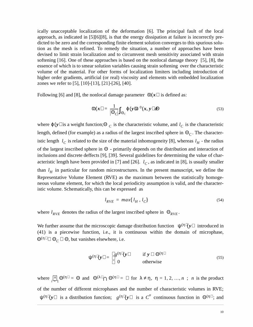
ically unacceptable localization of the deformation [6]. The principal fault of the loapproach, as indicated in [5][6][8], is that the energy dissipation at failure is incorrectlydicted to be zero and the corresponding finite element solution converges to this spurioution as the mesh is refined. To remedy the situation, a number of approaches havdevised to limit strain localization and to circumvent mesh sensitivity associated with softening [16]. One of these approaches is based on the nonlocal damage theory [5], essence of which is to smear solution variables causing strain softening over the charavolume of the material. For other forms of localization limiters including introductionhigher order gradients, artificial (or real) viscosity and elements with embedded localizzones we refer to [5], [10]-[13], [21]-[26], [40].
Following [6] and [8], the nonlocal damage parameter is defined as:
(53)
where is a weight function; is the characteristic volume, and is the characte
length, defined (for example) as a radius of the largest inscribed sphere in . The cha
istic length is related to the size of the material inhomogeneity [8], whereas - the
of the largest inscribed sphere in - primarily depends on the distribution and interactinclusions and discrete deffects [9], [39]. Several guidelines for determining the value ofacteristic length have been provided in [7] and [26]. , as indicated in [8], is usually sm
than in particular for random microstructures. In the present manuscript, we defin
Representative Volume Element (RVE) as the maximum between the statistically honeous volume element, for which the local periodicity assumption is valid, and the charistic volume. Schematically, this can be expressed as
(54)
where denotes the radius of the largest inscribed sphere in .
We further assume that the microscopic damage distribution function introduc(41) is a piecewise function, i.e., it is continuous within the domain of microph
, but vanishes elsewhere, i.e.
(55)
where and ; is the produc
of the number of different microphases and the number of characteristic volumes in
is a distribution function; is a continuous function in ; a
ω x( )
ω x( ) 1ΘC---------- ϕ y( )ω0 x y,( ) Θd
ΘC∫=
ϕ y( ) ΘC lCΘC
lC lHΘ
lClH
lRVE max lH , lC =
lRVE ΘRVE
ψ η( ) y( )
Θ η( ) ΘC Θ⊂ ⊂
ψ η( ) y( ) g η( ) y( ) if y Θ η( )∈0 otherwise
=
Θ η( )i 1=
n∪ Θ= Θ λ( ) Θ η( )∩ ∅ for λ η, η 1= 2 … n, , ,≠= n
ψ η( ) y( ) g η( ) y( ) Co Θ η( )
10

for typi-d
seen
:
is a macroscopically variable amplitude. Figure 2 illustrate two possibilitiesconstruction of RVE in a two-phase medium: one for random microstructure where RVEcally coincides with SHVE, and the other one for periodic microstructure, where an
are of the same order of magnitude.
Figure 2: Selection of the Representative Volume Element
We further define the weight function in (53) as
(56)
where the constant is determined by the orthogonality condition
(57)
and is Kronecker delta. Substituting (41) and (55)-(57) into (53) yields
(58)
which provides the motivation for the specific choice of the weight function. It can be
that has a meaning of the nonlocal phase damage parameter.
The average strains in each subdomain in RVE are obtained by integrating (47) over
(59)
where
ω η( ) x( )
lC lH
lC
lH
lC ( lH )≈
(a)
(b)CharacteristicVolumes
ϕ y( ) µ η( )ψ η( ) y( )=
µ η( )
µ η( )
ΘC---------- g λ( ) y( )g η( ) y( ) Θ δλη , λ,η=d
ΘC∫ 1 2 … n, , ,=
δλη
ω x( ) µ η( )
ΘC---------- g η( ) y( )( )2ω η( ) x( ) Θd
ΘC∫ ω η( ) x( )= =
ω η( )
Θ η( )
εijη( ) 1
Θ η( )-------------- εij Θd
Θ η( )∫ Aijklη( )εkl Gijkl
η( )Dklmnεmn O ς( ) + += =
11

e local
he rela-t smearednsider-
rgy den-
as
(60)
(61)
To construct the nonlocal constitutive relation between the phase averages we define th
average stress in as:
(62)
By combining (21), (41), (55), (59)-(61) we get
(63)
where
(64)
(65)
(66)
The constitutive equation (63) has a nonlocal character in the sense that it represents ttion between phase averages. The response characteristics between the phases are noas the damage evolution law and thermomechanical properties of phases might be coably different, in particular when damage occurs in a single phase.
For the isotropic strain-based damage model adopted in this paper, the phase free enesity corresponding to the nonlocal constitutive equation (63) is given as
(67)
and the corresponding nonlocal phase damage energy release rate can be expressed
(68)
Aijklη( ) 1
Θ η( )-------------- Aijkl Θd
Θ η( )∫=
Gijklη( ) 1
Θ η( )-------------- Gijkl Θd
Θ η( )∫=
Θ η( )
σi jη( ) 1
Θ η( )-------------- σi j
0 ΘdΘ η( )∫≡
σijη( ) I klmn ω η( )Nklmn
η( )–( )Lijklη( )εmn
η( )=
Nklmnη( ) Aklst
η( ) Gklpqη( ) Dpqst+( ) Amnst
η( ) Gmnijη( ) Dijst+( )⋅ 1–=
Aijklη( ) 1
Θ η( )-------------- g η( )Aijkl Θd
Θ η( )∫=
Gijklη( ) 1
Θ η( )-------------- g η( )Gijkl Θd
Θ η( )∫=
Ψ η( ) ω η( ), εi jη( )( ) 1
2--- I klmn ω η( )Nklmn
η( )–( )Lijklη( ) εmn
η( )εi jη( )=
Y η( ) Ψ η( )∂ω η( )∂
--------------– 12---Nklmn
η( ) Lijklη( ) εmn
η( )εi jη( )= =
12
d rein-
nd t dam-
rein-
verall
ction
with
een
trix and
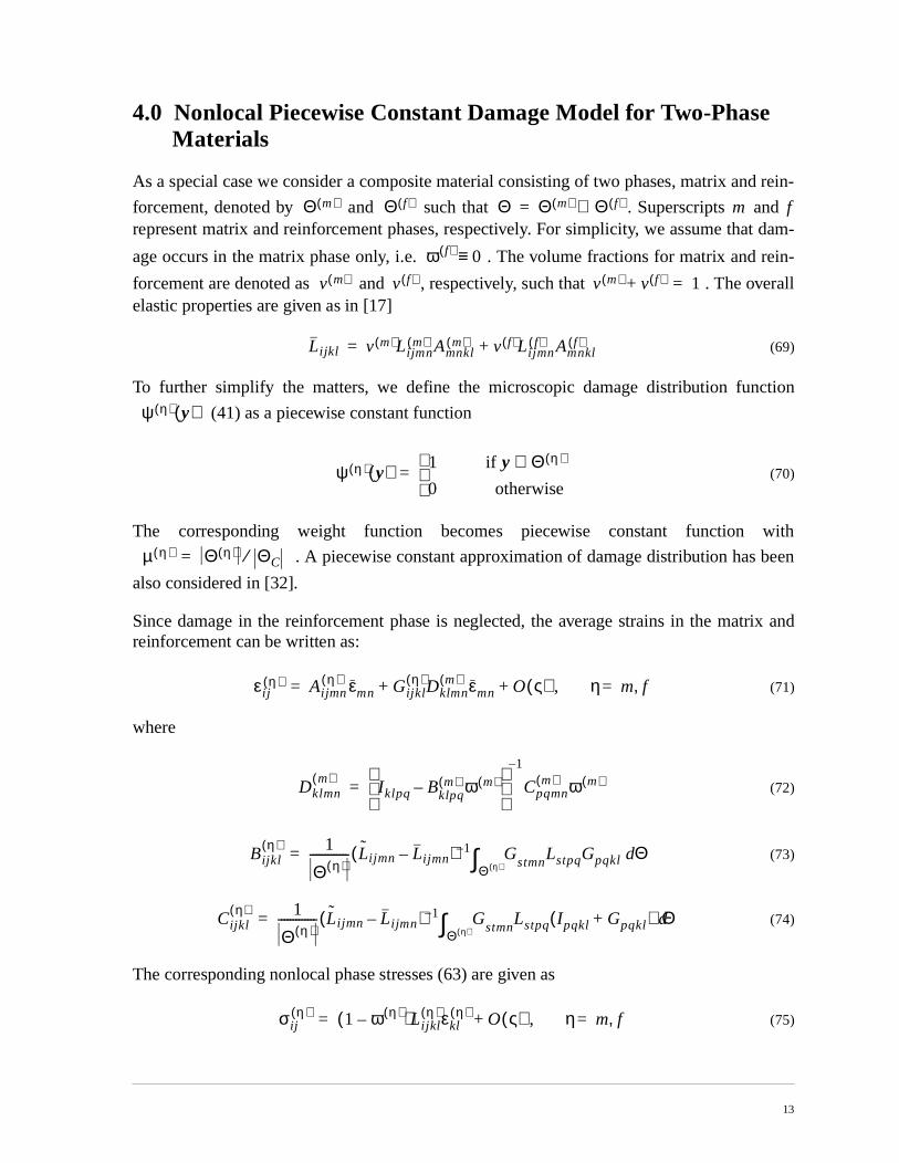
4.0 Nonlocal Piecewise Constant Damage Model for Two-Phase Materials
As a special case we consider a composite material consisting of two phases, matrix an
forcement, denoted by and such that . Superscripts arepresent matrix and reinforcement phases, respectively. For simplicity, we assume tha
age occurs in the matrix phase only, i.e. . The volume fractions for matrix and
forcement are denoted as and , respectively, such that . The oelastic properties are given as in [17]
(69)
To further simplify the matters, we define the microscopic damage distribution fun
(41) as a piecewise constant function
(70)
The corresponding weight function becomes piecewise constant function
. A piecewise constant approximation of damage distribution has b
also considered in [32].
Since damage in the reinforcement phase is neglected, the average strains in the mareinforcement can be written as:
(71)
where
(72)
(73)
(74)
The corresponding nonlocal phase stresses (63) are given as
(75)
Θ m( ) Θ f( ) Θ Θ m( ) Θ f( )∪= m f
ω f( ) 0≡v m( ) v f( ) v m( ) v f( )+ 1=
Lijkl v m( )Lijmnm( ) Amnkl
m( ) v f( )Lijmnf( ) Amnkl
f( )+=
ψ η( ) y( )
ψ η( ) y( ) 1 if y Θ η( )∈0 otherwise
=
µ η( ) Θ η( ) ΘC⁄=
εi jη( ) Aijmn
η( ) εmn Gijklη( )Dklmn
m( )+ εmn O ς( ) , η m f,=+=
Dklmnm( )
I klpq B– klpqm( ) ω m( )
1–
Cpqmnm( ) ω m( )=
Bijklη( ) 1
Θ η( )------------- Lijmn Lijmn–( ) 1– G
stmnLstpqGpqkl Θd
Θ η( )∫=
Cijklη( ) 1
Θ η( )------------- Lijmn Lijmn–( ) 1– G
stmnLstpq Ipqkl Gpqkl+( ) Θd
Θ η( )∫=
σijη( ) 1 ω η( )–( )Lijkl
η( )εklη( ) O ς( ) , η m f,=+=
13
ecome
creas-
2],ry. In
ion of
treme
also
ined as
ntly,
mage
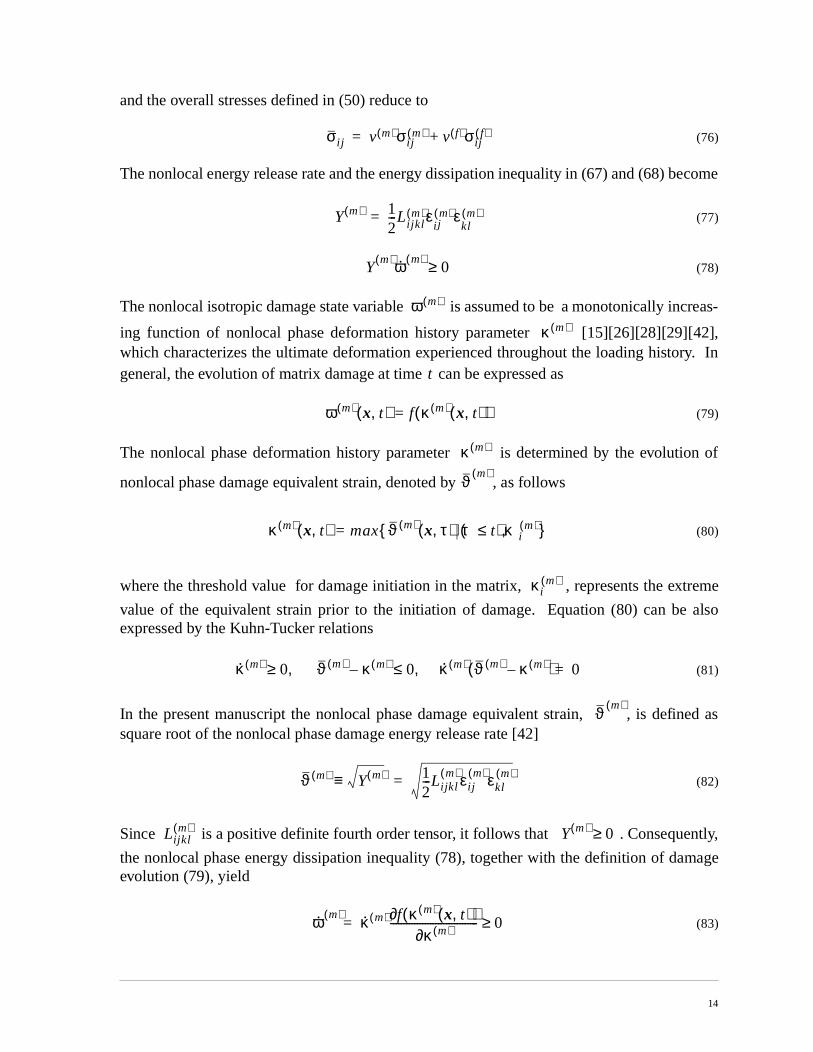
and the overall stresses defined in (50) reduce to
(76)
The nonlocal energy release rate and the energy dissipation inequality in (67) and (68) b
(77)
(78)
The nonlocal isotropic damage state variable is assumed to be a monotonically in
ing function of nonlocal phase deformation history parameter [15][26][28][29][4which characterizes the ultimate deformation experienced throughout the loading histogeneral, the evolution of matrix damage at time can be expressed as
(79)
The nonlocal phase deformation history parameter is determined by the evolut
nonlocal phase damage equivalent strain, denoted by , as follows
(80)
where the threshold value for damage initiation in the matrix, , represents the ex
value of the equivalent strain prior to the initiation of damage. Equation (80) can beexpressed by the Kuhn-Tucker relations
(81)
In the present manuscript the nonlocal phase damage equivalent strain, , is defsquare root of the nonlocal phase damage energy release rate [42]
(82)
Since is a positive definite fourth order tensor, it follows that . Conseque
the nonlocal phase energy dissipation inequality (78), together with the definition of daevolution (79), yield
(83)
σi j v m( )σi jm( ) v f( )σij
f( )+=
Y m( ) 12---Lijkl
m( )εi jm( )ε
klm( )=
Ym( )ω· m( )
0≥
ω m( )
κ m( )
t
ω m( ) x t,( ) f κ m( ) x t,( )( )=
κ m( )
ϑ m( )
κ m( ) x t,( ) max ϑ m( ) x τ,( ) τ t≤( ) κim( ), =
κim( )
κ· m( ) 0 ,≥ ϑ m( ) κ m( )– 0 κ· m( ) ϑ m( ) κ m( )–( ) 0=,≤
ϑ m( )
ϑ m( ) Y m( )≡ 12---Lijkl
m( )εi jm( )εkl
m( )=
Lijklm( ) Y m( ) 0≥
ω· m( ) κ· m( ) f κ m( ) x t,( )( )∂κ m( )∂
---------------------------------= 0≥
14

clu-
of
nt
uct ann lawf evolu-
aged
istory
set
ssary
roc-
amager of theoncen- or if
lastic
age
naly-
Combining this inequality with Kuhn-Tucker relations, we arrive at the following two con
sions: 1) the damage evolution law is an increasing function
since , where is the ultimate equivale
strains at rupture; and 2) the damage evolution condition can be expressed as
(84)
(85)
In accordance with the above thermodynamic considerations, it is possible to constrappropriate damage evolution law. An extensive review of a variety of damage evolutiohas been reported in [26]. In the present manuscript we propose an arctangent form otion law to ensure regularity of the tangent stiffness matrices in almost completely damstate
(86)
where are material parameters; and denotes the threshold of the strain h
parameter beyond which the damage will develop very quickly. For simplicity, we
. From (86), it can be seen that ensures (29) to be the nece
and sufficient conditions for (28). Furthermore, this evolution law accounts for initial micracks which are often present in ceramic composites.
5.0 Computational issues
In this section, we describe computational aspects of the nonlocal piecewise constant dmodel for two-phase materials developed in Section 4.0. Due to the nonlinear characteproblem an incremental analysis is employed. Prior to nonlinear analysis elastic strain ctration factors, , are computed using (35), (37) by either finite element method
possible by analytically solving an inclusion problem. Subsequently, nonlocal phase e
strain concentration factors ( ) and damage strain concentration factors
are precomputed using (60) and (61), respectively.
The stress update (integration) problem can be stated as follows:
Given: displacement vector ; overall strain ; strain history parameter ; dam
parameter ; and displacement increment calculated from the finite element a
f κ m( ) x t,( )( )
κ m( ) κ im( ) κu
m( ),[ ]∈ f κ m( ) x t,( )( )∂κ m( )∂
--------------------------------- 0> κum( )
if ϑ m( ) κ m( )– 0, κ· m( ) 0 damage process: ⇒ ω· m( ) 0>>=
if ϑ m( ) κ m( )– 0< or if ϑ m( ) κ m( )– 0, κ· m( ) 0 = elastic process: ⇒ ω· m( ) 0==
Φ m( ) α β ω m( ) κ m( ) κ0m( ), , , ,( ) ω=
m( )ακ m( )
κ0m( )---------- β–
β( )atan+atan
π2--- β( )atan+
------------------------------------------------------------------ 0=–
α β, κ0m( )
κim( ) 0= ω m( ) 0 1),[∈
Aijkl y( )
Aijklη( ) η m f,= Gijkl
η( )
ut m εt mn κ m( )t
ω m( )t ∆um
15

is the
vious
i.e.,
and
over-
ic
.
(80)
n turn6) is a
s for
sis of the macro problem. Here left subscript denotes the increment step, i.e.,
variable in the current increment, whereas is a converged variable from the pre
increment. For simplicity, we will omit the left subscript for the current increment, .
Find: displacement vector ; overall strain ; nonlocal phase strains
; nonlocal strain history parameter ; nonlocal phase damage parameter ;
all stress and nonlocal phase stresses and .
The stress update procedure consists of the following steps:
i.) Calculate macroscopic strain increment, , and then update macroscop
strains through .
ii.) Compute the damage equivalent strain defined by (82) in terms of and
iii. ) Check the damage evolution conditions (84) and (85). Note that is defined by
and is integrated as .
If damage process, i.e. , then and update for .
Since is governed by the current average strains in the matrix phase, which idepend on the current damage parameter, it follows that the damage evolution law (8
nonlinear function of . Using Newton’s method, we construct an iterative procesthe damage parameter:
(87)
The derivative in (87) can be evaluated by (71), (82), (86) as
(88)
where
t t∆+
t
t t∆+≡
um umt t∆+≡ εmn εmnm( )
εmnf( ) κ m( ) ω m( )
σmn σmnm( ) σmn
f( )
∆εmn ∆= u m x, n( )
εmn εt mn ∆εmn+=
ϑ m( ) ω m( )t εmn
κ m( )
κ· m( ) κ m( )∆ κ m( ) κ m( )t–=
ϑ m( ) κ m( )t> κ m( ) ϑ m( )= ω m( )
ϑ m( )
ω m( )
ω m( )k 1+ ω m( )k Φ m( )∂ω m( )∂
--------------
1–
Φ m( )ω m( )k
–=
Φ m( )∂ω m( )∂
-------------- 1ακ0
m( ) ϑ m( )∂ω m( )∂
--------------⋅
π 2⁄ β( )atan+( ) κ0m( )( )2 αϑ m( ) βκ0
m( )–( )2
+
⋅
-----------------------------------------------------------------------------------------------------------------------–=
16
in his-
tresses
for theng the
(86),
(89)
with
(90)
Otherwise for elastic process: .
vi.) Update the nonlocal strains and using (71) and update the nonlocal stratory parameter in (80).
v.) Update macroscopic stresses defined by (76) and calculate nonlocal phase s
and using (75).
To this end we focus on the computation of a consistent tangent stiffness matrix neededNewton method on the macro level. We start by substituting (71) into (75) and then takimaterial derivative of the incremental form of (75) in the matrix domain, i.e.
(91)
where
(92)
(93)
In order to obtain , we take the material derivative of damage evolution law
, and make use of (75), (82), and (88), which yields
(94)
where
(95)
and is a scalar given as
ϑ m( )∂ω m( )∂
-------------- 1
2ϑ m( )-------------- ε⋅ ij
m( )Lijklm( )
Gklstm( )
Rstmnm( ) εmn=
Rstmnm( ) I stpq B– stpq
m( ) ω m( )( )2–Cpqmn
m( )=
ω m( ) ω m( )t=
εklm( ) εkl
f( )
κ m( )
σi j
σijm( ) σi j
f( )
η m=
σ· i jm( ) Pijmn
m( ) ε·mn Qijmnm( ) εmnω·
m( )+=
Pijmnm( ) 1 ω m( )–( )Lijkl
m( ) Aklmnm( ) Gklst
m( )Dstmnm( )+( )=
Qijmnm( ) 1 ω m( )–( )Lijkl
m( )Gklstm( )Rstmn
m( )Lijkl
m( ) Aklmnm( ) Gklst
m( )Dstmnm( )+( )–=
ω· m( )
Φ· m( )0=
ω· m( ) ℵklm( )σ· kl
m( )–=
ℵklm( ) γεkl
m( )=
γ
17
tion
straintive of
(100)
(96)
Substituting (94) into (91) and manipulating the indices, we get the following relabetween the rate of overall strain and nonlocal phase stresses in the matrix domain
(97)
where
(98)
By using Sherman-Morrison formula (98) reduces to
(99)
A similar result relating the rate of the nonlocal reinforcement stress and the overall rate, can be obtained by substituting (71) into (75) and then taking the material deriva(75) in the reinforcement domain:
(100)
where
(101)
and
(102)
(103)
Finally, the overall consistent tangent stiffness is constructed by substituting (97) andinto the rate form of the overall stress-strain relation (76)
(104)
(105)
γ 1 ω m( )–( )– π 2⁄ β( )atan+( ) κ0m( )( )2 αϑ m( ) βκ0
m( )–( )2
+
αϑ m( )κ0m( )+
1–
=
ακ0m( )
2ϑ m( )--------------⋅
σ· i jm( ) ℘i jmn
m( ) ε·mn=
℘i jmnm( ) δikδjl ℵi j
m( )Qklstm( )εst+( ) 1–
Pklmnm( )=
℘ijmnm( ) δikδjl
ℵi jm( )Qklst
m( )εst
1 ℵijm( )Qijst
m( )εst+----------------------------------------–
Pklmnm( )=
σ· i jf( ) ℘ijmn
f( ) ε·mn=
℘ i jmnf( ) Pijmn
f( ) Qijstf( ) εstℵkl
m( )– ℘klmnm( )=
Pijmnf( ) Lijkl
f( ) Aklmnf( ) Gklst
f( ) Dstmnm( )+( )=
Qijstf( ) Lijkl
f( )Gklmn
f( )Rmnst
m( )=
σ· i j ℘ i jmnε·mn=
℘ijmn v m( )℘ i jmnm( ) v f( )℘ijmn
f( )+=
18
d non-domainicro--strain. Thee with
and
rated in in the
ed the is in
the
totallyrrying. In
phase.e sud-
en the
rply.
6.0 Numerical Examples
6.1 Qualitative Examples for Two-phase Fibrous Composites Under Uniaxial Loading
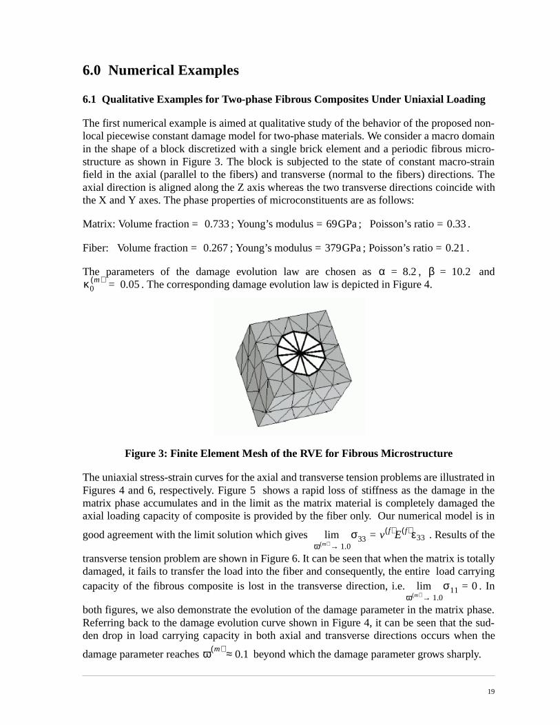
The first numerical example is aimed at qualitative study of the behavior of the proposelocal piecewise constant damage model for two-phase materials. We consider a macro in the shape of a block discretized with a single brick element and a periodic fibrous mstructure as shown in Figure 3. The block is subjected to the state of constant macrofield in the axial (parallel to the fibers) and transverse (normal to the fibers) directionsaxial direction is aligned along the Z axis whereas the two transverse directions coincidthe X and Y axes. The phase properties of microconstituents are as follows:
Matrix: Volume fraction = ; Young’s modulus = ; Poisson’s ratio = .
Fiber: Volume fraction = ; Young’s modulus = ; Poisson’s ratio = .
The parameters of the damage evolution law are chosen as , . The corresponding damage evolution law is depicted in Figure 4.
Figure 3: Finite Element Mesh of the RVE for Fibrous Microstructure
The uniaxial stress-strain curves for the axial and transverse tension problems are illustFigures 4 and 6, respectively. Figure 5 shows a rapid loss of stiffness as the damagematrix phase accumulates and in the limit as the matrix material is completely damagaxial loading capacity of composite is provided by the fiber only. Our numerical model
good agreement with the limit solution which gives . Results of
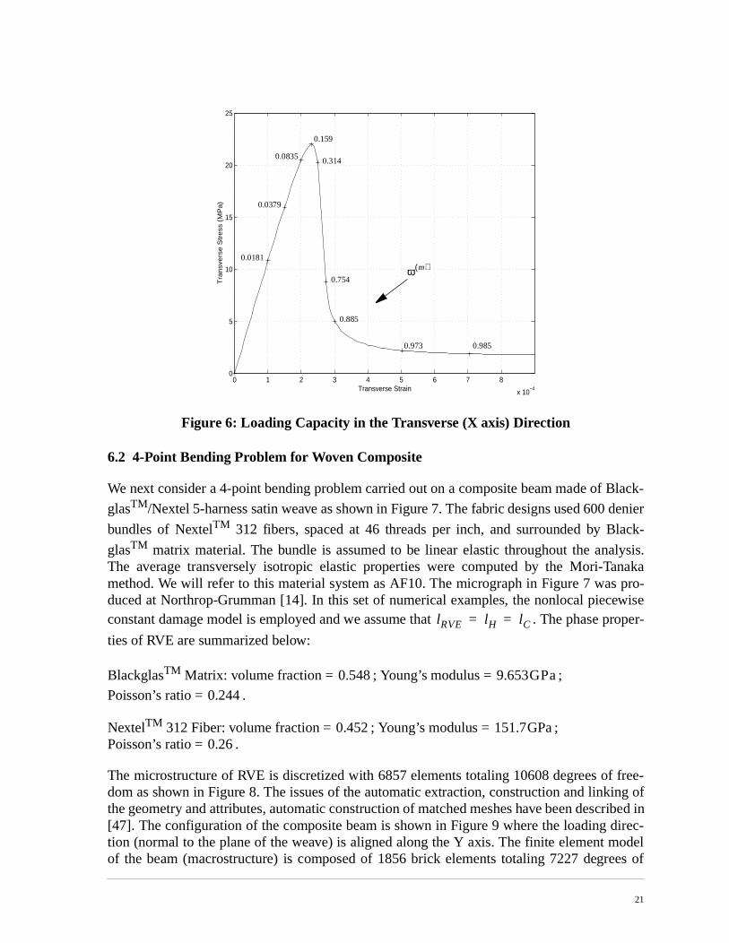
transverse tension problem are shown in Figure 6. It can be seen that when the matrix isdamaged, it fails to transfer the load into the fiber and consequently, the entire load cacapacity of the fibrous composite is lost in the transverse direction, i.e.
both figures, we also demonstrate the evolution of the damage parameter in the matrixReferring back to the damage evolution curve shown in Figure 4, it can be seen that thden drop in load carrying capacity in both axial and transverse directions occurs wh
damage parameter reaches beyond which the damage parameter grows sha
0.733 69GPa 0.33
0.267 379GPa 0.21
α 8.2= β 10.2=κ0
m( ) 0.05=
σ33 v f( )E f( )ε33=ω m( ) 1.0→
lim
σ11 0=ω m( ) 1.0→
lim
ω m( ) 0.1≈
19

Figure 4: Damage Evolution Law for the Titanium Matrix
Figure 5: Loading Capacity in the Axis (Z axis) Direction
0 0.02 0.04 0.06 0.08 0.1 0.12 0.14 0.16 0.180
0.1
0.2
0.3
0.4
0.5
0.6
0.7
0.8
0.9
1
Strain History Parameter
Da
ma
ge
Pa
ram
ete
r
κ m( )
ωm(
)
0 1 2 3 4 5 6 7 8
x 10−4
0
10
20
30
40
50
60
70
80
Axial Strain
Axi
al S
tre
ss (
MP
a)
numerical results lower bound with
0.0220
0.0682
0.133
0.0915 0.837
0.884
0.908
ω m( )0.933
0.273
ω m( ) 1=
20
Black-
denier
lack-
alysis.anaka pro-ewiseroper-
f free-ing of
cribed indirec-
odelees of
Figure 6: Loading Capacity in the Transverse (X axis) Direction
6.2 4-Point Bending Problem for Woven Composite
We next consider a 4-point bending problem carried out on a composite beam made of
glasTM/Nextel 5-harness satin weave as shown in Figure 7. The fabric designs used 600
bundles of NextelTM 312 fibers, spaced at 46 threads per inch, and surrounded by B
glasTM matrix material. The bundle is assumed to be linear elastic throughout the anThe average transversely isotropic elastic properties were computed by the Mori-Tmethod. We will refer to this material system as AF10. The micrograph in Figure 7 wasduced at Northrop-Grumman [14]. In this set of numerical examples, the nonlocal piecconstant damage model is employed and we assume that . The phase p
ties of RVE are summarized below:
BlackglasTM Matrix: volume fraction = ; Young’s modulus = ;
Poisson’s ratio = .
NextelTM 312 Fiber: volume fraction = ; Young’s modulus = ;Poisson’s ratio = .
The microstructure of RVE is discretized with 6857 elements totaling 10608 degrees odom as shown in Figure 8. The issues of the automatic extraction, construction and linkthe geometry and attributes, automatic construction of matched meshes have been des[47]. The configuration of the composite beam is shown in Figure 9 where the loading tion (normal to the plane of the weave) is aligned along the Y axis. The finite element mof the beam (macrostructure) is composed of 1856 brick elements totaling 7227 degr
0 1 2 3 4 5 6 7 8
x 10−4
0
5
10
15
20
25
Transverse Strain
Tra
nsv
ers
e S
tre
ss (
MP
a)
0.0181
0.0379
0.0835
0.159
0.314
0.754
0.885
0.973 0.985
ω m( )
lRVE lH lC= =
0.548 9.653GPa
0.244
0.452 151.7GPa0.26
21

sion is in the
e
own incattered beam
resultshaviorl datad fail-
eam at
increase takes
freedom. Figure 10 depicts the damage evolution law for BlackglasTM matrix with ,
and , which are calibrated to the tensile and shear test data.
Comparison between tensile test data and the numerical simulation for the uniaxial tenshown in Figure 11. It can be seen that the ultimate experimental stress/strain values
uniaxial tension test are and , while th
numerical simulation gives at .
Numerical simulation results as well as the test data for 4-point bending problem are shFigures 12 and 13. Experiments have been conducted on five identical beams and the sexperimental data of force versus the displacement at the point of load application in theare shown by the gray area in Figure 12. It can be seen that the numerical simulationare in good agreement with the experimental data in terms of predicting the overall be(Figure 12) and the dominant failure mode. Both numerical simulation and experimentapredict that the dominant failure mode is tension/compression (so-called bending induceure). Figure 13 illustrates the distribution of the damage parameter in the composite bthe peak load (Point A in Figure 12).
To this end we note that since bundles have been modeled as linear elastic spurious in load carrying capacity of the weave in the in-plane tension/compression eventuallyplace. Remedies are discussed I Section 7
Figure 7: BlackglasTM /Nextel 5-harness Satin Weave
α 7.1=
β 10.1= κ0m( ) 0.22=
σu 150 7MPa±= εu 2.53–×10 0.3
3–×10±=
σu 152MPa= εu 3.2 3–×10=
22

Figure 8: Microstructure of AF10 Woven Composites
Figure 9: Configuration and FE Mesh of 4-Point Bending Problem
1
2
3 1
2
3
40
1.6
6.4
6.3525.4
23
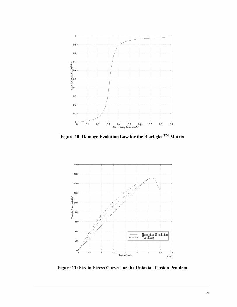
Figure 10: Damage Evolution Law for the BlackglasTM Matrix
Figure 11: Strain-Stress Curves for the Uniaxial Tension Problem
0 0.1 0.2 0.3 0.4 0.5 0.6 0.7 0.8 0.90
0.1
0.2
0.3
0.4
0.5
0.6
0.7
0.8
0.9
1
Strain History Parameter
Da
ma
ge
Pa
ram
ete
r
κ m( )
ωm(
)
0 0.5 1 1.5 2 2.5 3 3.5 4
x 10−3
0
20
40
60
80
100
120
140
160
180
Tensile Strain
Te
nsi
le S
tre
ss (
MP
a)
Numerical SimulationTest Data
24
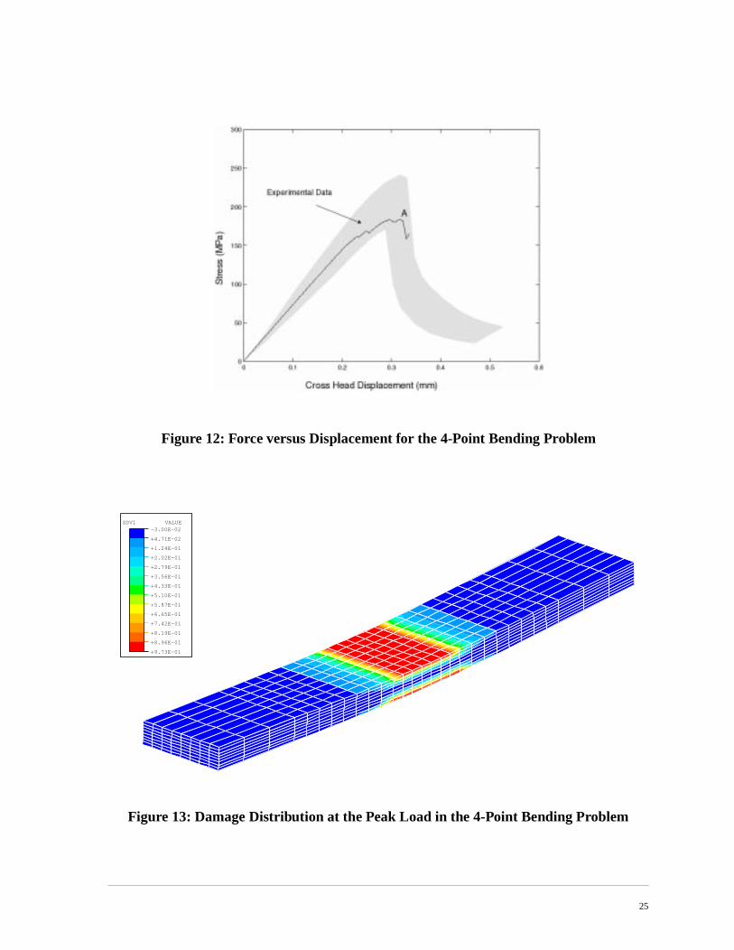
Figure 12: Force versus Displacement for the 4-Point Bending Problem
Figure 13: Damage Distribution at the Peak Load in the 4-Point Bending Problem
SDV1 VALUE-3.00E-02
+4.71E-02
+1.24E-01
+2.02E-01
+2.79E-01
+3.56E-01
+4.33E-01
+5.10E-01
+5.87E-01
+6.65E-01
+7.42E-01
+8.19E-01
+8.96E-01
+9.73E-01
25
ptoticelds to (stress,g func- of the
mericale beenelds,ty of [2] to
ous bundleessionues that
grantCMS-
tinu-olv-
om-
us
eriodic
truc-
nts.
7.0 Summary and future research directions
A nonlocal damage theory for brittle composite materials based on double scale asymexpansion of damage has been developed. A closed form expression relating local fithe overall strains and damage has been derived. The concept of nonlocal phase fieldsstrain, free energy density, damage release rate, etc.) has been introduced via weightintions defined over the microphase. Numerical results revealed an excellent performancemethod.
The present work by no means represents a complete account of all theoretical and nuissues related to damage in composites and we apologize if some important works havomitted. We note that the assumptions of periodicity and uniformity of macroscopic fiwhich are embedded in our formulation, may yield inaccurate solutions in the viciniboundary layers. The remedies to this phenomenon range from changing the RVE sizecarrying out an iterative global-local analysis [37], [38], [33], [24], [25]. Moreover, varifailure modes other than matrix cracking, such as damage at the interface and in thedomain, coupled plasticity-damage effects, different responses in tension and comprhave not been accounted for in the present manuscript. These are just few of the isswill be investigated in our future work.
Acknowledgment
This work was supported in part by the Air Force Office of Scientific Research under number F49620-97-1-0090, the National Science Foundation under grant number 9712227, and Sandia National Laboratories under grant number AX-8516.
References
1 D. H. Allen, R. H. Jones and J. G. Boyd (1994). Micromechanical analysis of a conous fiber metal matrix composite including the effects of matrix viscoplasticity and eving damage. J. Mech. Phys. Solids 42(3), 505-529.
2 I. Babuska, B. Anderson, P. Smith, and K. Levin (1998). Damage analysis of fiber cposites. Part I: Statistical analysis on fiber scale. Special Issue of Comput. Methods Appl. Mech. Engrg. on Computational Advances in Modeling Composites and HeterogeneoMaterials (ed. J. Fish).
3 A. Bakhvalov and G. P. Panassenko. Homogenization: Averaging Processes in PMedia. Kluwer Academic Publisher, 1989.
4 A. Benssousan, J. L. Lions and G. Papanicoulau. Asymptotic Analysis for Periodic Sture. North-Holland, Amsterdam, 1978.
5 Z. P. Bazant (1991). Why continuum damage is nonlocal: micromechanical argumeJ.Engrg. Mech. 117(5), 1070-1087.
26

f non-
ation
the
g in
ent
ort for
non-
for-
s and
ity for.
iodic
orma-
train
with
6 Z. P. Bazant and L. Cedolin. Stability of Structures. Oxford University Press,1991.
7 Z. P. Bazant and G. Pijaudier-Cabot (1989). Measurement of characteristic length olocal continuum. J. Engrg. Mech. 115(4), 755-767.
8 Z. P. Bazant and G. Pijaudier-Cabot (1988). Nonlocal continuum damage, localizinstability and convergence. J. Appl. Mech. 55, 287-293.
9 Z. P. Bazant and L. Cedolin, (1993). Why direct tension specimens break flexing toside. J. of Struct. Engrg., ASCE, Vol. 119 (4), pp. 1101-1113.
10 T. Belytschko and D. Lasry, (1989). A study of localization limiters for strain softeninstatics and dynamics. Computers and Structures, Vol. 33, pp. 707-715.
11 T. Belytschko, J. Fish and B. E. Engelmann (1988). A finite element with embeddedlocalization zones,” Comp. Meth. Appl. Mech. Engng., Vol. 70, pp. 59 - 89.
12 T. Belytschko and J. Fish (1989). Embedded hinge lines for plate elements. Comp. Meth. Appl. Mech. Engng., Vol. 76, No. 1, pp. 67-86.
13 T.Belytschko, J. Fish and A. Bayliss (1990). The spectral overlay on the finite elemsolutions with high gradients. Comp. Meth. Appl. Mech. Engng., Vol 81, pp.71-89.
14 E. P. Butler, S. C. Danforth, W. R. Cannon and S. T. Ganczy, (1996). Technical Repthe ARPA LC3 program, ARPA Agreement No. MDA 972-93-0007.
15 J. L. Chaboche (1988). Continuum damage mechanics I: General concepts. J. Appl. Mech.55, 59-64.
16 G. H. P. deVree, W. A. J. Brekelmans and M. A. J. Van Gils (1995). Comparison oflocal approaches in continuum damage mechanics. Comput. Structures. 55(4), 581-588.
17 G. J. Dvorak, Y. A. Bahei-El-Din and A. W. Wafa (1994). Implementation of the transmation field analysis for inelastic composite materials. Comput. Mech. 14, 201-228.
18 J. Fish, P. Nayak and M. H. Holmes (1994). Microscale reduction error indicatorestimators for a periodic heterogeneous medium. Comput. Mech. 14, 323-338.
19 J. Fish, K. Shek, M. Pandheeradi and M. S. Shephard (1997). Computational plasticcomposite structures based on mathematical homogenization: Theory and practiceCom-put. Meth. Appl. Mech. Engrg. 148, 53-73.
20 J. Fish and A. Wagiman (1993). Multiscale finite element method for locally nonperheterogeneous medium. Comput. Mech. 12, 164-180.
21 J. Fish and T. Belytschko. Elements with embedded localization zones for large deftion problems,” Computers and Structures, Vol. 30, No. 1/2, (1988), pp. 247-256.
22 J. Fish and T. Belytschko (1990). A finite element with a unidirectionally enriched sfield for localization analysis. Comp. Meth. Appl. Mech. Engng., Vol. 78, No. 2, pp. 181-200.
23 J. Fish and T. Belytschko (1990). A general finite element procedure for problems high gradients. Computers and Structures, Vol. 35, No. 4, pp.309-319.
27
.
. Part
Frac-
terials
titutive
analy-es
lami-
nisms ing
odel
teri-
pic
neous
eous
e-
icro-
24 J. Fish and V. Belsky (1995). Multigrid method for a periodic heterogeneous mediumPart I: Convergence studies for one-dimensional case. Comp. Meth. Appl. Mech. Engng., Vol. 126, pp. 1-16.
25 J.Fish and V.Belsky (1995). Multigrid method for a periodic heterogeneous medium2: Multiscale modeling and quality control in multidimensional case,” Comp. Meth. Appl. Mech. Engng., Vol. 126, 17-38.
26 M. G. D. Geers (1997). Experimental and Computational Modeling of Damage andture. Ph.D Thesis. Technische Universiteit Eindhoven, The Netherlands.
27 J. M. Guedes and N. Kikuchi (1990). Preprocessing and postprocessing for mabased on the homogenization method with adaptive finite element methods. Comput.Methods Appl. Mech. Engrg. 83, 143-198.
28 J. W. Ju (1989). On energy-based coupled elastoplastic damage theories: Consmodeling and computational aspects. Int. J. Solids Structures 25(7), 803-833.
29 D. Krajcinovic (1996). Damage Mechanics. Elsevier Science.
30 S. Kruch, J. L. Chaboche and T. Pottier (1996). Two-scale viscoplastic and damagesis of metal matrix composite. In: Damage and Interfacial Debonding in Composit(Edited by G. Z. Voyiadjis and D. H. Allen), pp. 45-56, Elsevier Science.
31 P. Ladeveze and E. Le-Dantec (1992). Damage modeling of the elementary ply for nated composites. Composites Science and Technology. 43, pp. 257-267.
32 P. Ladeveze, (1991). About a Damage Mechanics Approach. Mechanics and Mechaof Damage in Composites and Multimaterials. Ed. D. Baptiste. Mechanical EngineerPublications Limited, London, pp. 119-141.
33 K. Lee, S. Moorthy, and S. Ghosh (1998). Multiple-Scale Adaptive Computational Mfor Damage in Composite Materials. Special Issue of Comput. Methods Appl. Mech. Engrg. on Computational Advances in Modeling Composites and Heterogeneous Maals (ed. J. Fish).
34 F. Lene (1986). Damage constitutive relations for composite materials. Engrg. Fract.Mech. 25, 713-728.
35 A. Matzenmiller, J. Lubliner, R. L. Taylor (1995). A constitutive model for anisotrodamage in fiber-composites. Mech. Mater. 20, 125-152
36 S. Nemat-Nasser and M. Hori. Micromechanics: Overall Properties of HeterogeMaterials, North-Holland, 1993.
37 J. T. Oden, K. Vemaganti and N. Mo s (1998). Hierarchical Modeling of HeterogenSolids. Special Issue of Comput. Methods Appl. Mech. Engrg. on Computational Advances in Modeling Composites and Heterogeneous Materials (ed. J. Fish).
38 J. T. Oden and T. I. Zohdi (1996). Analysis and adaptive modeling of highly heterogneous elastic structures, TICAM Report 56, University of Texas at Austin.
39 J. Ozbolt and Z.P. Bazant, (1996). Numerical smeared fracture analysis: Nonlocal m
e··
28

adient
amic
dels - I.
ng.
n of
age-
ensorses
ven
crack interaction approach. Int. J. for Numerical Methods in Engrg. Vol. 39, pp. 635-661.
40 R. H. J. Peerling, R. de Borst, W. A. M. Brekelmans and J. H. P. de Vree (1996). Grenhanced damage for quasi-brittle materials. Int. J. Num. Methods Engrg. 39, 3391-3403.
41 J. Riehl (1998). Mechanical Property Data Base for New Architecture. Low Cost CarComposite Program, NAWC, Patuxent, Maryland.
42 J. C. Simo and J. W. Ju (1987) Strain- and stress-based continuum damage moFormulation. Int. J. Solids Structures 23(7), 821-840.
43 R. Talreja (1989). Damage development in composite: Mechanism and modeliJ.Strain Analysis 24, 215-222.
44 G. Z. Voyiadjis and T. Park (1992). A plasticity-damage theory for large deformatiosolids-I: Theoretical Formulation. Int. J. Engrg. Sci. 30(9), 1089-1106.
45 G. Z. Voyiadjis and P. I. Kattan (1993). Micromechanical characterization of damplasticity in metal matrix composites. In: Damage in Composite Materials (Edited by G.Z. Voyiadjis), pp67-102, Elsevier Science.
46 G. Z. Voyiadjis and T. Park (1996). Elasto-plastic stress and strain concentration tfor damaged fibrous composites. In: Damage and Interfacial Debonding in Composit(Edited by G. Z. Voyiadjis and D. H. Allen), pp81-106, Elsevier Science.
47 R. Wentorf, R. Collar, M.S. Shephard, J. Fish, “Automated Modeling for Complex WoMesostructures,” Comp. Meth. Appl. Mech. Engng., (1997), in print.
29