Competitive genetic algorithms with applicationto reliability optimal design

C.K. Dimou, V.K. Koumousis*

Institute of Structural Analysis and Aseismic Research, National Technical University of Athens, Athens, Greece

Abstract

Competition is introduced among the populations of a number of genetic algorithms (GAs) having different sets of parameters. The aim is

to calibrate the population size of the GAs by altering the resources of the system, i.e. the allocated computing time. The co-evolution of the

different populations is controlled at the level of the union of populations, i.e. the metapopulation, on the basis of statistics and trends of the

evolution of every population. Evolution dynamics improve the capacity of the optimization algorithm to find optimum solutions and results

in statistically better designs as compared to the standard GA with any of the fixed parameters considered. The method is applied to the

reliability based optimal design of simple trusses. Numerical results are presented and the robustness of the proposed algorithm is discussed.

q 2003 Elsevier Ltd. All rights reserved.

Keywords: Structural optimization; Genetic algorithms; Competition; Population dynamics; Reliability analysis

1. Introduction

Genetic algorithms (GAs) are search algorithms based

on the concepts of natural selection and survival of the

fittest. They guide the evolution of a set of randomly

selected individuals towards good near optimal and/or

optimal solutions. This is accomplished in a number of

generations that are subjected to successive reproduction,

crossover and mutation, based on the statistics of the

generation. The efficiency of the whole process is

problem dependent and relies heavily on the successful

selection of a number of parameters, such as population

size, probability of crossover and mutation, type of

crossover, etc. In this work, a method is proposed that

attempts to automate the evolution of population size

through an adaptive process. This is based on

the competition of populations, with different sets of

GA parameters, struggling for the available resources of

the system.

Competition among different populations is common in

natural systems. Populations evolve by adapting them-

selves to the environment where resources are limited.

The process starts with the generation of number of

populations with different sets of GA parameters. In

subsequent generations, as the populations evolve, a

scheme of competing populations (CP) alters the popu-

lation size in an adaptive manner based on the relative

performance of the populations at the metapopulation

level. By altering the available resources, competition is

activated forcing the system to organize better its overall

search strategy towards optimal solutions. The ability of

every population to adapt to the artificial habitat is used to

calculate the relative performance index at a particular

generation, which represents a comparative measure

between all the populations that comprise the metapopula-

tion. Competition arises when the available resources are

insufficient to sustain the entire metapopulation. This

causes conflicts among the populations where the most-fit

ones survive, whereas the less-fit populations shrink or

become extinct. This coupled scheme manages to arrive at

good near optimal solutions statistically faster, as

compared to the same number of standard GAs with

fixed parameters.

Reliability optimal structural design problems are

computationally intensive and represent a particular class

of optimization problems. Therefore, application of the

proposed algorithm to this class of problems is expected

to reveal the particular features of the algorithm. The

method is applied to the reliability based optimal design

(RBOD) of simple trusses. Numerical results are presented

illustrating the advantages of the proposed method, as

0965-9978/$ - see front matter q 2003 Elsevier Ltd. All rights reserved.

doi:10.1016/S0965-9978(03)00101-7

Advances in Engineering Software 34 (2003) 773–785

www.elsevier.com/locate/advengsoft

* Corresponding author. Fax: þ30-2107721651.

E-mail address: vkoum@central.ntua.gr (V.K. Koumousis).

compared to the same number of standard GAs with fixed

parameters.

2. Genetic algorithms

A simple genetic algorithm (GA) based on binary coding

is employed for every population [1]. No mixing among

individuals of different populations is allowed, to preserve

the characteristics of the populations. Reproduction is based

on a ranking scheme [2],while elitism is adopted [3] allowing

the pair of best individuals to reappear in the next generation.

GAs are used in a wide range of structural optimization

problems [4,5]. One-point and two-point crossover schemes

are used. For the probability of mutation, decreasing

functions with the number of generations are implemented.

For every generation the entire system operates at two levels,

i.e. the level of populations and the level of metapopulation

[6], where all decisions about the characteristics of the next

generation of populations are made.

The optimal structural design problem is usually for-

mulated in non-linear mathematical programming form as

min CijðxÞ

Subject gkðxÞ # 0 k ¼ 1;…;Nc

where x [ Dn

ð1Þ

whereCijðxÞ is the objective function for the ith individual ofthe jth population, gkðxÞ is the kth inequality constraint, Nc is

the number of constraints, x is the vector of design variables

and Dn is the design space. An equivalent unconstrained

maximization problem is determined following a penalty

function formulation as

maxx[Dn

fijðxÞ ¼A

CijðxÞ þX

Nc

k¼1

ckTðgðxÞÞ" #

8

>

>

>

>

<

>

>

>

>

:

9

>

>

>

>

=

>

>

>

>

;

ð2Þ

where ck is the penalty factor associated with the kth

constraint of the problemwhich in this studywas taken as 100

for all constraints, A is an arbitrary constant and operator T is

given as

TðxÞ ¼ffiffiffiffiffiffiffi

x2 1p

x . 1

0 x # 1

(

ð3Þ

where 1 is the tolerance in violating the constraints.

Throughout this study 1 ¼ 0:1:

The maximization problem of Eq. (2) is appropriately

normalized at the metapopulation level as follows

maxx[Dn

f̂ijðxÞ ¼fijðxÞ

½mini;j

fijðxÞ�

8

<

:

9

=

;

ð4Þ

where mini;j {fijðxÞ} is the objective of the less-fit individualin all populations.

Moreover, the probability of mutation at a given

generation t is given as

Ptmut ¼

Pinit t# tinit

PfinalþðPinit2PfinalÞexp 2t2 tinit

nhalf

�� �

t. tinit

8

>

<

>

:

ð5Þ

where Pinit and Pfinal is the initial and final mutation

probability, respectively, tinit is the generation when the

mutation probability starts to vary and nhalf is the parameter

that controls the velocity of the variation of the mutation

probability. Throughout this study these parameters have

the fixed values: tinit ¼ 10 and nhalf ¼ 40:

3. Competition

Competition is common in natural systems. Dimitrova

and Vitanov [7] study the evolution of CPs through

adaptation in a non-linear dynamical system with limited

resources. In the book edited by Hanski and Gilpin [8], Nee

et al. present the important parameters of interaction among

different populations in a natural environment. Co-evolving

populations of different species share the environment in a

state of dynamic equilibrium. Competition among different

species arises when they share the same resources, which

are not sufficient to sustain all the populations.

3.1. Resources

Assuming the computational time needed to process a

single design as constant, the amount of resources required

Rreq; to process all the populations of the metapopulation

consisting of N designs at a specific generation is given as

Rreq ¼X

Np

j¼1

RjNj N ¼X

Np

j¼1

Nj ð6Þ

where Rj and Nj are the resources per individual and the total

number of individuals of the jth population, respectively,

and Np is the number of populations in the system. The

amount of available resources at generation t can be

represented by a step like function with initial resources R

Ravail ¼ R2X

m

j¼1

Hðt2 tjÞDRj ð7Þ

where m specifies the number of changes of the step-like

function at particular instances, i.e. at generation ti with

reduction of resources DRi; and H is the Heaviside function.

If the available resources are less than the required ones,

conflict is introduced into the system. Abrupt changes on

the available resources correspond to drastic events in

C.K. Dimou, V.K. Koumousis / Advances in Engineering Software 34 (2003) 773–785774

the virtual environment that are expected to accelerate the

adaptation of the CPs.

3.2. Fitness

The fitness of a population, in the metapopulation level,

depends not only on the particular characteristics of its

individuals but also on the profiles of all the other

populations. Co-evolution defines the concurrent evolution

of two or more populations where the fitness of a population

depends also on the profiles of the remaining populations.

Ficisi and Pollack [9] examine co-evolutionary algorithms

from game theory viewpoint. Barbosa and Barreto [10]

implement an interactive co-evolutionary GA in a graph

layout problem. Riechmann [11] shows that in economics,

where the fitness of a strategy is directly related to the

adopted strategies of the remaining individuals, every GA is

also a dynamic game. The fitness of a population in the

metapopulation level can be expressed as the sum of the

fitness of its individuals:

Fj ¼X

Nj

i¼1

f̂ijðxÞ ð8Þ

This expresses co-operation among individuals of the same

population, which is common in natural systems and favors

the expansion and survival of larger populations and of

populations with many ‘good’ individuals.

3.3. Diversity

The goal at this stage is to introduce a more stringent

approach, as compared to the GA, that will process the

emerging data and guide the next steps in an adaptive

manner, while taking into account the uncertainties of the

system. Diversity plays an important role for the GA to

improve the existing best solutions [12,14]. Therefore, a

diversity measure Dj of the chromosome of every

population j is evaluated, based on descriptive statistics of

the digits appearing at every position of the chromosome.

Diversity is used as an estimate of the ‘age’ of a population.

‘Younger’ populations exhibit higher diversity as compared

to ‘older’ ones and thus, they appear more promising to

improve further the existing elite solution than ‘older’ ones.

This factor is important in preserving the capacity of the

metapopulation in finding the global optimum [13,14].

Considering that the digits at every position of the

chromosome follow a binomial distribution, their variation

at a specific generation is given as

Var ½ fjm � ¼ Nj·p·ð12 pÞ ð9Þ

where fjm is the population of digits of the jth population at

themth position and p is the probability of occurrence of 1 at

the mth digit. When this probability is equal to 0.5 the

variation takes its maximum value of Nj=4: The diversity

measure over the length of the chromosome is calculated as

the average of the variation at all positions of the

chromosome and is given as

Dj ¼ Em¼1;…;k

{Var ½ fjm �} ð10Þ

where k is the length of the chromosome.

3.4. Relative performance

The fitness of the fittest individual Bj is introduced as an

additional parameter to measure the relative performance of

the populations. The relative performance index of the jth

population PIj; is expressed as the product of the fitness of

its best individual, the population fitness and the population

diversity

PIj ¼ ½Bj�w½Fj�a½Dj�b ð11Þ

where w; a and b are parameters, used to attenuate or

intensify relative variations among the populations. This

expression of relative performance index constitutes a

comparative measure of the performance of a population. In

this analysis a ¼ 1: Expressions like the one presented in

Eq. (11) are frequently used in econometric models [15,16].

4. Engagement rules

4.1. Conflict

The probability of conflict among two different popu-

lations i and j; when shortage of resources is observed, is

given as

Pr½popi; popj� ¼ �TDN

N

� �

PIi 2 PIj

PIiOFi . OFj

0 OFi # OFj

8

>

<

>

:

9

>

=

>

;

DN ¼ðRreq 2 RavailÞE½Nj�

E½RjNj�; ð12Þ

�T½x� ¼

0 x , 0

x

d0 # x # d

1 x . d

8

>

>

>

<

>

>

>

:

where d is a parameter controlling the transition from a state

of no conflict to a state of conflict emerging between two

populations, when lack of resources exists. In this analysis

d ¼ 0:2: This relation assures that no conflict arises if the

available resources are adequate. Moreover, the probability

of conflict increases in proportion to the resource deficit,

while stronger populations fight only weaker ones. The

probability of conflict between two CPs increases linearly

with the relative difference of their performance index. For

every population only one conflict per generation is

allowed. Further details that concern the scheme used

for the selection of conflicting pairs are presented in

C.K. Dimou, V.K. Koumousis / Advances in Engineering Software 34 (2003) 773–785 775

the pseudocode description of the algorithm. Finally,

conflicts cease when the available resources are adequate.

The outcome of a conflict between populations i and j;

determines the size of these populations in the next

generation as follows

N tþ1i ¼ N t

i þ ��T eijPIi 2 PIJ

PIi

�

N tþ1j ¼ N t

j þ ��T1

eij12

PIi 2 PIJ

PIi

�

" # ð13Þ

where ��T is given as

��TðxÞ ¼

max gDN

Np

; 2

( )

0:5þ f , x

0 0:5 # x , 0:5þ f

2max gDN

Np

; 2

( )

0:52 f # x , 0:5

2max g2DN

Np

; 4

( )

x , 0:52 f

8

>

>

>

>

>

>

>

>

>

>

>

>

<

>

>

>

>

>

>

>

>

>

>

>

>

:

ð14Þ

and eij is equal to

eij ¼ 1þeðrand2 0:5Þ

0:5ð15Þ

where e and f are parameters that handle the fuzziness of the

outcome. For this analysis e ¼ 0:2 and f ¼ 0:2: Further-

more, the g factor is used to regulate the velocity of

variation of the size of population. Typical values of g factor

are around unity [17]. Furthermore, populations vanish if

their population size drops to zero.

4.2. Termination criteria

A convergence criterion is introduced that works as a

trade-off between the variability of the population and the

coefficient of Variation (COV) of the objective function.

The variability factor measures the variability of schemata

per design variable in the chromosome. This is calculated as

the average of the variability factor of all design variables

of the problem. Convergence of results and termination of

the evolution of a particular population is considered when

the variability factor is less than 30% and the COV less than

5%. Moreover a hard termination criterion of the GA

optimization process is applied after 250 generations, which

depends on the particular problem. For the problem

addressed in this paper, most of the populations converge

following the first criterion and very rarely the hard

termination criterion was activated.

Therefore, the proposed scheme at the level of

metapopulation is based on the introduction of diversity

measure given in Eq. (10), obtained from formal

descriptive statistics on the different schemata of the

population, the implementation of the conflict scheme and

the fuzzy outcome of the conflict between pairs of

populations.

The proposed algorithm is briefly presented as follows.

4.3. Pseudocode of the proposed algorithm

† Step 0: Start process. Read data for the competition

scheme used in Eqs. (5)–(15). Read parameters for the

GAs (reproduction scheme, type of crossover, prob-

ability of crossover and probability of mutation) for all

populations i ¼ 1;…;Np: Specify the population size N ti

of every population. Read parameters of termination

criteria.

† Step 1: Set t ¼ 0: Generate random initial populations

for all populations ðNpÞ: Evaluate fitness for all designs,

i.e. for i ¼ 1;…;Np and j ¼ 1;…;N ti call the RBOD code

and calculate the fijðxÞ: Perform the statistics of all

populations ðNpÞ:† Step 2:Operate on the metapopulation level to decide for

the new population size of all populations. Calculate the

normalized fitness fijðxÞ using Eq. (4).

† Step 3: Decide about conflict. Calculate the required and

available resources using Eqs. (6) and (7). If Np ¼ 1 or

Rreq ¼ Ravail set Ntþ1i ¼ N t

i for i ¼ 1;…;Np then go to

Step 7 else; if Rreq , Ravail go to Step 6 else go to Step 4.

† Step 4: Calculate the performance index of every

population using Eqs. (8)–(11) and store it in a vector

{A} in a sorted form.

† Step 5: Assign the pairs of possible conflict. Select

the strongest population {Popi} from vector {A}: For

Fig. 1. Statically determinate truss (loads and members).

C.K. Dimou, V.K. Koumousis / Advances in Engineering Software 34 (2003) 773–785776

the remaining populations assign selection probabilities

based on a ranking.

† Step 5.1: Select randomly the ‘weak’ population {Popj}:

Calculate the probability of conflict between {Popi} and

{Popj} using Eq. (12). If Pr½Popi;Popj� $ randð Þ then

assign populations i and j as pair of conflicting

populations and remove their indexes from vector {A}

otherwise remove only {Popi}: If {A} contains more than

one populations then go to Step 5 else,

† Step 5.2: For all pairs of conflicting populations calculate

the N tþ1i ; i ¼ 1;…;Np using Eqs. (13)–(15). For the

remaining populations N tþ1i ¼ N t

i : Go to Step 7.

† Step 6: Distribute the resources in surplus evenly across

the evolving populations and calculate the corresponding

N tþ1i ; i ¼ 1;…;Np:

† Step 7: Set t ¼ t þ 1: For i ¼ 1;…;Np and j ¼ 1;…;N ti

call the standard GA routine using the new population

size for all the populations and calculate the fitness fijðxÞof all the designs calling the RBOD code. Perform the

statistics of all populations.

† Step 8: Check for convergence for all populations. For

all populations i ¼ 1;…;Np check for the satisfaction of

termination criteria. Freeze the available resources

(resources cannot be re-allocated) for populations that

satisfy the termination criteria. UpdateNp: IfNp – 0 then

go to Step 2 else go to Step 9.

† Step 9: End process.

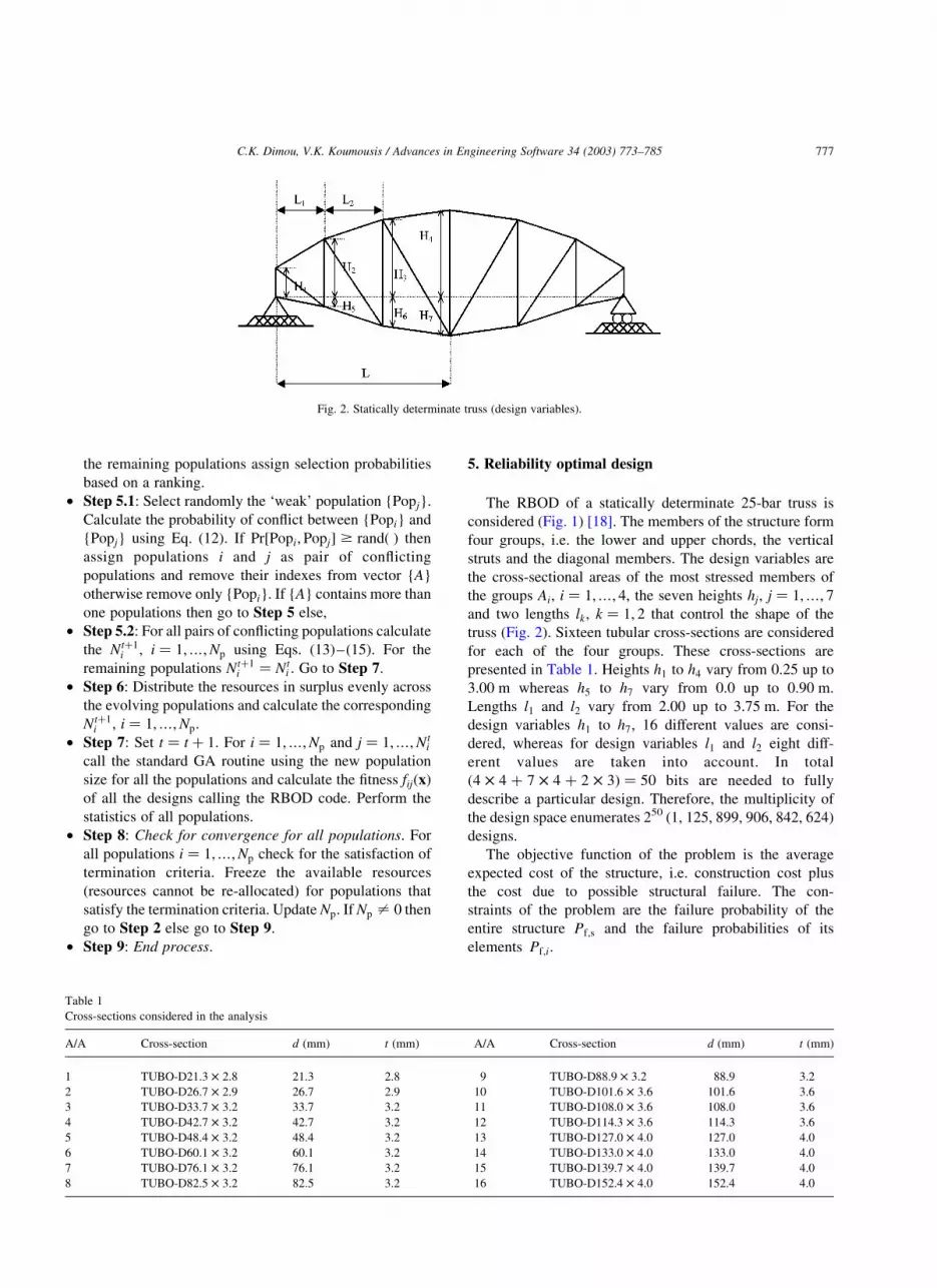
5. Reliability optimal design

The RBOD of a statically determinate 25-bar truss is

considered (Fig. 1) [18]. The members of the structure form

four groups, i.e. the lower and upper chords, the vertical

struts and the diagonal members. The design variables are

the cross-sectional areas of the most stressed members of

the groups Ai; i ¼ 1;…; 4; the seven heights hj; j ¼ 1;…; 7

and two lengths lk; k ¼ 1; 2 that control the shape of the

truss (Fig. 2). Sixteen tubular cross-sections are considered

for each of the four groups. These cross-sections are

presented in Table 1. Heights h1 to h4 vary from 0.25 up to

3.00 m whereas h5 to h7 vary from 0.0 up to 0.90 m.

Lengths l1 and l2 vary from 2.00 up to 3.75 m. For the

design variables h1 to h7; 16 different values are consi-

dered, whereas for design variables l1 and l2 eight diff-

erent values are taken into account. In total

(4 £ 4 þ 7 £ 4 þ 2 £ 3) ¼ 50 bits are needed to fully

describe a particular design. Therefore, the multiplicity of

the design space enumerates 250 (1, 125, 899, 906, 842, 624)

designs.

The objective function of the problem is the average

expected cost of the structure, i.e. construction cost plus

the cost due to possible structural failure. The con-

straints of the problem are the failure probability of the

entire structure Pf;s and the failure probabilities of its

elements Pf;i:

Table 1

Cross-sections considered in the analysis

A/A Cross-section d (mm) t (mm) A/A Cross-section d (mm) t (mm)

1 TUBO-D21.3 £ 2.8 21.3 2.8 9 TUBO-D88.9 £ 3.2 88.9 3.2

2 TUBO-D26.7 £ 2.9 26.7 2.9 10 TUBO-D101.6 £ 3.6 101.6 3.6

3 TUBO-D33.7 £ 3.2 33.7 3.2 11 TUBO-D108.0 £ 3.6 108.0 3.6

4 TUBO-D42.7 £ 3.2 42.7 3.2 12 TUBO-D114.3 £ 3.6 114.3 3.6

5 TUBO-D48.4 £ 3.2 48.4 3.2 13 TUBO-D127.0 £ 4.0 127.0 4.0

6 TUBO-D60.1 £ 3.2 60.1 3.2 14 TUBO-D133.0 £ 4.0 133.0 4.0

7 TUBO-D76.1 £ 3.2 76.1 3.2 15 TUBO-D139.7 £ 4.0 139.7 4.0

8 TUBO-D82.5 £ 3.2 82.5 3.2 16 TUBO-D152.4 £ 4.0 152.4 4.0

Fig. 2. Statically determinate truss (design variables).

C.K. Dimou, V.K. Koumousis / Advances in Engineering Software 34 (2003) 773–785 777

The optimization problem is formulated as follows:

min FðAi; hj; lkÞ ¼X

Nt

m¼1

VmðAi; hj; lkÞCmat þ Pf;sCfail

i ¼ 1;…; 4; j ¼ 1;…; 7; k ¼ 1; 2

ð16Þ

Subject to

gjðAi; hj; lkÞ ¼Pf;j

Pj;lim

2 1:0 # 0;

gsðAi; hj; lkÞ ¼Pf;s

Ps;lim

2 1:0 # 0

ð17Þ

where Nt is the number of elements of the truss, Vm is the

volume of the mth element, Cmat and Cfail is the cost per unit

volume of the structure and the cost of a potential structural

failure, respectively, Pf;s is the overall failure probability,

Pf;j and Pj;lim are the failure probability of the jth element

and the maximum failure probability, respectively, and Pf;s

and Ps;lim are the failure probability and its limit value for

the entire structure. Two shape constraints that control the

height to length ratio are also considered. These constraints

are given as:

gs;1ðH4Þ ¼H4

2L2 0:15 # 0

gs;2ðH7Þ ¼H7

2L2 0:05 # 0

ð18Þ

The probability of failure of an element is given as

Pf;i ¼ Pr½M # 1� ð19Þ

where M is the safety margin which is expressed as follows

M ¼RðAiÞFðhiÞ

ð20Þ

where RðAiÞ and FðhiÞ are the ultimate resistance and the

applied load, respectively, given as

RðAiÞ ¼ suAi fiðhiÞ $ 0

RðAiÞ ¼ xsuAi fiðhiÞ , 0FðhiÞ ¼ fiðhiÞP ð21Þ

and fiðhiÞ are the influence coefficients that result from

the analysis of the truss for a unit load and depend on the

geometry of the structure. The parameter x reduces the

compressive strength of the members due to buckling

considerations and is based on the provisions of Eurocode 3

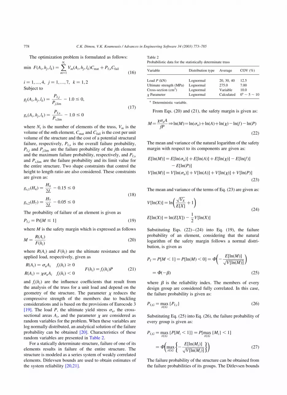
[19]. The load P, the ultimate yield stress su; the cross-

sectional areas Ai; and the parameter x are considered as

random variables for the problem. When these variables are

log normally distributed, an analytical solution of the failure

probability can be obtained [20]. Characteristics of these

random variables are presented in Table 2.

For a statically determinate structure, failure of one of its

elements results in failure of the entire structure. The

structure is modeled as a series system of weakly correlated

elements. Ditlevsen bounds are used to obtain estimates of

the system reliability [20,21].

From Eqs. (20) and (21), the safety margin is given as:

M¼xsuA

fP) lnðMÞ¼ lnðsuÞþ lnðAÞþ lnðxÞ2 lnðf Þ2 lnðPÞ

ð22Þ

The mean and variance of the natural logarithm of the safety

margin with respect to its components are given as:

E½lnðMÞ� ¼ E½lnðsuÞ� þE½lnðAÞ� þE½lnðxÞ�2E½lnðf Þ�2E½lnðPÞ�

V½lnðMÞ� ¼ V½lnðsuÞ� þV½lnðAÞ� þV½lnðxÞ� þV½lnðPÞ�ð23Þ

The mean and variance of the terms of Eq. (23) are given as:

V½lnðXÞ� ¼ ln

ffiffiffiffi

VX

p

E½X�þ 1

�

E½lnðXÞ� ¼ lnðE½X�Þ21

2V½lnðXÞ�

ð24Þ

Substituting Eqs. (22)–(24) into Eq. (19), the failure

probability of an element, considering that the natural

logarithm of the safety margin follows a normal distri-

bution, is given as

Pf ¼ P½M , 1� ¼ P½lnðMÞ, 0� ¼F 2E½lnðMÞ�ffiffiffiffiffiffiffiffiffiffiffiffi

V½lnðMÞ�p

�

¼Fð2bÞ ð25Þ

where b is the reliability index. The members of every

design group are considered fully correlated. In this case,

the failure probability is given as:

Pf;G ¼maxi[G

{Pf;i} ð26Þ

Substituting Eq. (25) into Eq. (26), the failure probability of

every group is given as:

Pf;G ¼maxi[G

{P½Mi , 1�}¼ P½maxi[G

{Mi}, 1�

¼F maxi[G

2E½lnðMiÞ�ffiffiffiffiffiffiffiffiffiffiffiffi

V½lnðMiÞ�p

� � �

ð27Þ

The failure probability of the structure can be obtained from

the failure probabilities of its groups. The Ditlevsen bounds

Table 2

Probabilistic data for the statistically determinate truss

Variable Distribution type Average COV (%)

Load P (kN) Lognormal 20, 30, 40 12.5

Ultimate strength (MPa) Lognormal 275.0 7.00

Cross-section (cm2) Lognormal Variable 10.0

x Parameter Lognormal Calculated 0a , 5 , 10

a Deterministic variable.

C.K. Dimou, V.K. Koumousis / Advances in Engineering Software 34 (2003) 773–785778

for the system’s failure probability are given as:

Pf;s #

X

n

i¼1

P½Mi , 1�2X

n

i¼2

maxj,i

P½Mi , 1>Mj , 1�

Pf;s $ P½M1 , 1� þX

n

i¼2

max

��

P½Mi , 1� ð28Þ

2

X

i21

j¼1

P½Mi , 1>Mj , 1��

;0

�

For the joint probability of events the following expression

is used:

P½Mi , 1>Mj , 1� ¼F2ð2bi;2bj;rÞ ð29Þ

For the evaluation of the joint probability of Eq. (29) the

following bounds are used [20]

maxð pi;pjÞ#P½Mi, 1>Mj, 1�, piþpj r. 0

0#P½Mi, 1>Mj, 1�,minðpi;pjÞ r, 0ð30Þ

where the parameters pi and pj are given as

pi ¼ Fð2biÞ·Fð2gjÞ pj ¼ Fð2bjiÞ·Fð2giÞ ð31Þ

and the gi and gj factors are given by the following relation:

gi ¼bi 2 rij·bj

ffiffiffiffiffiffiffiffiffi

12 r2ij

q gj ¼bj 2 rij·bi

ffiffiffiffiffiffiffiffiffi

12 r2ij

q ð32Þ

5.1. Numerical results

A number of problems are solved for L ¼ 10 m and a

ratio of costs Cfail=Cmat equal to 20,000, that corresponds to

an estimation of real costs, starting with an initial population

size of 40, 60, 80 and 100 designs. The limit probabilities

considered during the analysis are Pj;lim ¼ 1026 and Ps;lim ¼5 £ 1026: Ten runs with different random seeds are

performed to produce data for a statistical evaluation of

the proposed scheme.

Twelve different populations are considered. Their

characteristics are presented in Table 3. The available

resources vary according to the resource variation schemes

(RVS) 1, to 7 as shown in Fig. 3 associated with the

parameters of Table 4. These RVSs are classified in four

different groups namely, the decreasing ones (RVS 1 and 2),

the alternating (RVS 3 and 4), the initially increasing and

subsequently decreasing (RVS 5 and 7) and one scheme

(RVS 6) with alternating–decreasing resources, each

having the same values of b;w exponents in Eq. (11).

These parameters can be set equal to unity indicating no

preference either for the fitness of the population, or the

diversity or the fitness of the elite individual. Although

the values of the parameters presented in Table 4 are not the

optimal, they are selected on the basis of qualitative criteria

for improved performance.

For example for the decreasing RVS 1 and 2, the average

population size is expected to decrease in time and thus,

parameter b is set to a value of 5/6 bigger than parameter w

which is set to a value of 0.5 to favor the evolution of

populations that exhibit higher diversity.

The minimum cost solutions for the load case E½P� ¼ 30

kN and the x parameter considered as deterministic, random

with COV 5 and 10%, respectively, are presented in Fig. 4.

The optimal solutions forx parameter withCOV5% for three

different loads are presented in Fig. 5. In Table 5 the optimal

parameters that control the shape of the trusses are presented.

It is observed that the variation of the x parameter is not

affecting the optimal cost considerably. The shape of the truss

changes and the height to length ratio decreases as the COV

of the x parameter increases. The different average load

affects considerably the shape, the cross-section areas and the

expected cost of the optimal truss, following an almost linear

relation between the average load and the optimal cost. With

regard to the shape of the truss, an increase in the height to

length ratio is observed as the average load increases. In

addition, the l1 design variable and the sum of l1 þ l2decrease as the average load increases.

The evolution of the objective function of the best

individual for E½P� ¼ 40 kN; x parameter treated as random

variable with a COV 10% for an initial population size equal

to 80, that corresponds to RVS 1, is presented in Fig. 6.

Population 12 finds the optimal solution at generation 58

and its evolution is terminated at generation 71. Population

3 follows a path similar to that of population 12. Its

evolution is terminated at generation 58 and a near optimal

solution within 8.9% of the computed optimum is obtained

at generation 55. Population 9 converges at a non-optimal

solution, within 13.5% of the computed optimum, at

generation 88.

The evolution of the population size of the 12 different

GAs is presented in Fig. 7. Competition starts at generation

10 when the first resource reduction is imposed. For

population 12 the population size varies slightly (less than

15% of the initial population size). Similar behavior is

observed for population 9 until generation 50, where two

Table 3

GA parameters

Population 1 2 3 4 5 6 7 8 9 10 11 12

Crossover prob. 0.7 0.7 0.8 0.8 0.7 0.7 0.8 0.8 0.9 0.9 0.9 0.9

Crossover type SP SP SP SP DP DP DP DP SP SP DP DP

Mutation scheme A B A B A B A B B A B A

Scheme A: Pinit ¼ 1%; Pfinal ¼ 1‰ Scheme B: Pinit ¼ 2%; Pfinal ¼ 2‰

C.K. Dimou, V.K. Koumousis / Advances in Engineering Software 34 (2003) 773–785 779

significant increases of the population size are observed,

followed by small variations near the end of the optimiz-

ation process. Finally, the sharp drop observed at generation

72 is attributed to a reduction of the available resources. Due

to intense competition, populations 7 and 10 are forced to

converge prematurely at generations 37 and 53,

respectively.

In Table 6, the schemes that produced the optimal results

are presented. For the case where E½P� ¼ 30 kN and RVS 6,

the initial population size of 100 individuals produced the

best design, whereas for E½P� ¼ 40 kN and RVS 1 the initial

population size of 80 or 100 individuals suggested the best

design. For E½P� ¼ 20 kN; mixed results are observed and

in the case where x is treated as a random variable with

a COV equal to 10% the best design was obtained from the

standard GA scheme.

With regard to the probability of crossover, probability of

mutation and one- or two-point crossover schemes and for

the specific range used in this analysis, no trends favoring

a particular set of parameters are observed. Single point

crossover is used in 6 out of 9 cases as it can be easily

checked from Table 3 from the corresponding column ‘Pop-

ID’. Moreover, for the crossover probability the three

different crossover probabilities appear 4, 3 and 2 times each

for values of 0.7, 0.8 and 0.9, respectively. Mutation scheme

B is applied in 6 out of 9 cases. The number of generations

required to derive the optimum solution shows considerable

variability from a minimum of 24 generations to a

maximum of 161 generations, which are, respectively,

extended to a minimum of 29 generations and a maximum

of 218 generations until termination. Also, from the

different initial random seeds that gave the optimal results,

no trends favoring a particular seed are observed as

expected, which makes the statistics of the results valid.

A more general statistical evidence of the overall perform-

ance of the proposed algorithm is depicted in Figs. 8–11.

The minimum, maximum and average ratio of computing

time for seven different RVSs, for all problems, with respect

to the standard GA is presented in Fig. 8. Moreover,

Fig. 3. Evolution of the resource variation schemes.

Table 4

Problem parameters

Parameter b w

RVS 1 5/6 0.5

RVS 2 5/6 0.5

RVS 3 0.5 1.0

RVS 4 0.5 1.0

RVS 5 5/6 0.5

RVS 6 5/6 0.75

RVS 7 5/6 0.5

C.K. Dimou, V.K. Koumousis / Advances in Engineering Software 34 (2003) 773–785780

the number of problems where the proposed algorithm

outperformed the classical GA with regard to the quality of

the best design is also presented. The most computationally

expensive schemes are RVS 3 followed by RVS 4, whereas

the least computationally intensive scheme is RVS 2

followed by RVS 1. With regard to the quality of the best

design it can be observed that for all RVSs expect RVS 4 the

proposed algorithm manages to produce a better design than

the best optimal design of the std. GA in the majority of the

problems examined. The comparison of groups shows that

RVS 1 is more robust than RVS 2. Equivalently RVS 3 is

more robust than RVS 4 and RVS 7 is more robust than

Fig. 4. Optimal solutions ðE½P� ¼ 30 kNÞ:

Fig. 5. Optimal solutions (x random COV equal to 5%).

Table 5

Optimal values of the shape variables (m)

Design h1 h2 h3 h4 h5 h6 h7 l1 l2

a 1.00 1.50 1.85 2.00 0.0225 0.25 0.425 3.5 3.25

b 0.90 1.30 1.425 1.475 0.0 0.275 0.575 3.0 3.75

c 0.80 1.20 1.30 1.375 0.275 0.575 0.80 3.25 3.75

d 1.00 1.40 1.80 2.025 0.025 0.20 0.45 3.5 3.5

e 0.90 1.30 1.425 1.475 0.0 0.275 0.575 3.0 3.75

f 1.30 1.80 2.30 2.65 0.0125 0.10 0.325 2.75 3.50

C.K. Dimou, V.K. Koumousis / Advances in Engineering Software 34 (2003) 773–785 781

Fig. 7. Evolution of the size of the population (E½P� ¼ 40 kN; (x RV 10%)).

Table 6

Schemes that produced the optimal results

Case Scheme Pop size Pop ID Gen-opt Gen-term Seed

20 kN x; Deta RVS 3 80 4 161 218 2

x; RVb 5% RVS 4 80 5 46 51 9

x; RV 10% GA 60 3 69 94 2

30 kN x; Det RVS 4 100 2 49 67 4

x; RV 5% RVS 6 100 9 63 63 4

x; RV 10% RVS 6 100 8 121 122 8

40 kN x; Det RVS 1 100 2 95 100 4

x; RV 5% RVS 1 80 6 24 33 1

x; RV 10% RVS 1 80 12 58 71 7

a Det, deterministic variable.b RV, random variable.

Fig. 6. Evolution of the objective function (E½P� ¼ 40 kN; (x RV 10%)).

C.K. Dimou, V.K. Koumousis / Advances in Engineering Software 34 (2003) 773–785782

RVS 5. Moreover, RVS 3 managed to outperform the

classical GA in all problems, but one, whereas very good

results are also observed for RVS 6 and RVSs 1 and 7.

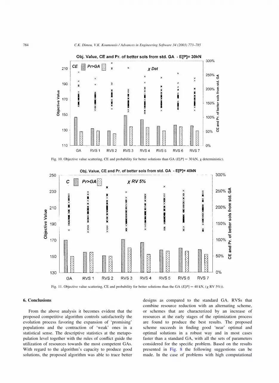
Scattering of the cost for the various RVSs is

presented in Figs. 9–11. In addition, the computational

efficiency (CE) as compared to the standard GA and the

probability of obtaining better solutions than the GA are

presented, for different values of the average load and x

parameter.

In Fig. 9, for resource variation schemes RVS 3 to RVS 6,

the probability to obtain better solutions than the standard

GA, is greater than 50% with a maximum of 72.5% for

RVS 4. The probability for RVS 1 is equal to 50% and thus,

the quality of results is equivalent to those of the GA but

these results are obtained in considerably less time (62% of

the computational time of the standard GA).

From these results it is observed that moderate reduc-

tions of the resources are expected to maximize the

performance of the algorithm. Moreover, schemes exhibit-

ing an increase of available resources at the early stages of

the optimization process, such as RVSs 5 and 7 are expected

to produce statistically better results.

Fig. 8. Average, minimum and maximum values of CE and frequency of surpassing the best design of the std. GA.

Fig. 9. Objective value scattering, CE and probability for better solutions than GA (E½P� ¼ 20 kN; (x RV 10%)).

C.K. Dimou, V.K. Koumousis / Advances in Engineering Software 34 (2003) 773–785 783

6. Conclusions

From the above analysis it becomes evident that the

proposed competitive algorithm controls satisfactorily the

evolution process favoring the expansion of ‘promising’

populations and the contraction of ‘weak’ ones in a

statistical sense. The descriptive statistics at the metapo-

pulation level together with the rules of conflict guide the

utilization of resources towards the most competent GAs.

With regard to the algorithm’s capacity to produce good

solutions, the proposed algorithm was able to trace better

designs as compared to the standard GA. RVSs that

combine resource reduction with an alternating scheme,

or schemes that are characterized by an increase of

resources at the early stages of the optimization process

are found to produce the best results. The proposed

scheme succeeds in finding good ‘near’ optimal and

optimal solutions in a robust way and in most cases

faster than a standard GA, with all the sets of parameters

considered for the specific problem. Based on the results

presented in Fig. 8 the following suggestions can be

made. In the case of problems with high computational

Fig. 10. Objective value scattering, CE and probability for better solutions than GA (E½P� ¼ 30 kN; x deterministic).

Fig. 11. Objective value scattering, CE and probability for better solutions than the GA (E½P� ¼ 40 kN; (x RV 5%)).

C.K. Dimou, V.K. Koumousis / Advances in Engineering Software 34 (2003) 773–785784

cost RVS 1 can be used, since it combines low

computational cost with increased robustness. For

problems where computational cost is not of major

importance RVS 3 can be used since at a small

additional cost the robustness is increased by a factor

of 8. Moreover, RVSs 6 and 7 present also good

alternatives since they combine smaller computational

cost with increased performance.

References

[1] Goldberg DE. Genetic algorithms in search, optimization, and

machine learning. Reading, MA: Addison-Wesley; 1989.

[2] Pezeshk S, Camp CV, Chen D. Design of non-linear framed structures

using genetic optimization. J Struct Engng 2000;126(3):382–8.

[3] Koumousis VK, Georgiou PG. Genetic algorithms in discrete

optimization of steel truss roofs. J Comput Civil Engng 1994;8(3):

309–25.

[4] Grierson DE, Pak WH. Optimal sizing, geometrical and topological

design using genetic algorithms. J Struct Optim 1993;6:151–9.

[5] Hajela P, Lee E. Genetic algorithms in truss topological optimization.

J Solids Struct 1995;32(22):3341–57.

[6] Levins R. Some demographic and genetic consequences of environ-

mental heterogeneity for biological control. Bull Entomol Soc Am

1969;15:237–40.

[7] Dimitrova ZI, Vitanov NK. Influence of adaptation on the nonlinear

dynamics of a system of competing populations. Phys Lett A 2000;

272:368–80.

[8] Hanski IA, Gilpin ME, editors. Metapopulation biology. New York:

Academic Press; 1997.

[9] Ficici SG, Pollack JB. Game Theory and the simple coevolutionary

algorithm: some preliminary results on fitness sharing. Genetic and

Evolutionary Computation Conference, Workshop Program

(GECCO-2001); 2001. p. 2–8.

[10] Barbosa HJC, Barreto AMS. An interactive genetic algorithm with co-

evolution of weights for multiobjective problems. Proceedings of the

Genetic and Evolutionary Computation Conference (GECCO-2001);

2001. p. 203–10.

[11] Riechmann T. Genetic algorithm learning and evolutionary games.

J Econ Dyn Control 2001;25:1019–37.

[12] Shimodaira H. A diversity-control-oriented genetic algorithm

(DCGA): development and experimental results. Proceedings of the

Genetic and Evolutionary Computation Conference (GECCO-99);

1999. 1: p. 603–11.

[13] Fujimoto Y, Tsutsui S. A peak shape identification genetic algorithm

with a radial basis function. The International Conference on

Evolutionary Computation; 1997. p. 249–354.

[14] De Jong ED, Watson RA, Pollack JB. Reducing bloat and promoting

diversity using multi-objective methods. Proceedings of the Genetic

and Evolutionary Computation Conference (GECCO-2001); 2001. p.

11–8.

[15] Sanglier M, Romain M, Flament F. A behavioral approach of the

dynamics of financial Markets. Decis Support Syst 1994;12:405–13.

[16] Sanglier M, Allen PM. Evolutionary models of urban systems—an

application to the Belgian provinces. Environ Plann 1989;21:477–98.

[17] Koumousis VK, Dimou CK. Genetic algorithms in a competitive

environment with application to reliability optimal design. Genetic

and Evolutionary Computation Conference, Workshop Program

(GECCO 2001). ; 2001. p. 79–85.

[18] Dimou CK, Koumousis VK. Genetic algorithms in a competitive

environment with application to reliability optimal design. In:

Topping BHV, Kumar B, editors. Proceedings of the Sixth

International Conference on the Application of Artificial Intelligence

to Civil and Structural Engineering. Stirling, UK: Civil-Comp Press;

2001. paper 38.

[19] ENV 1993-1-1, Eurocode 3 Design of steel structures. Part 1.1.

General rules and rules for buildings. CEN 1992.

[20] Christensen PT, Murotsu Y. Application of structural systems

reliability theory. Berlin: Springer; 1986.

[21] Christensen PT, Baker MJ. Structural reliability theory and its

applications. Berlin: Springer; 1982.

C.K. Dimou, V.K. Koumousis / Advances in Engineering Software 34 (2003) 773–785 785