algorithms - mdpi
TRANSCRIPT
Algorithms 2015, 8, 982-998; doi:10.3390/a8040982OPEN ACCESS
algorithmsISSN 1999-4893
www.mdpi.com/journal/algorithms
Article
Some Matrix Iterations for Computing Generalized Inverses andBalancing Chemical EquationsFarahnaz Soleimani 1,*, Predrag S. Stanimirovic 2 and Fazlollah Soleymani 3
1 Department of Chemistry, Roudehen Branch, Islamic Azad University, 39731 Roudehen, Iran2 Faculty of Sciences and Mathematics, University of Niš, Višegradska 33, 18000 Niš, Serbia;
E-Mail: [email protected] Department of Applied Mathematics, Ferdowsi University of Mashhad, 91779 Mashhad, Iran;
E-Mail: [email protected]
* Author to whom correspondence should be addressed; E-Mail: [email protected];Tel.: +98-912-348-2263.
Academic Editors: Alicia Cordero, Juan R. Torregrosa and Francisco I. Chicharro
Received: 25 June 2015 / Accepted: 26 October 2015 / Published: 3 November 2015
Abstract: An application of iterative methods for computing the Moore–Penrose inverse inbalancing chemical equations is considered. With the aim to illustrate proposed algorithms,an improved high order hyper-power matrix iterative method for computing generalizedinverses is introduced and applied. The improvements of the hyper-power iterative schemeare based on its proper factorization, as well as on the possibility to accelerate the iterations inthe initial phase of the convergence. Although the effectiveness of our approach is confirmedon the basis of the theoretical point of view, some numerical comparisons in balancingchemical equations, as well as on randomly-generated matrices are furnished.
Keywords: generalized inverses; balancing chemical equations; hyper-power method; orderof convergence; matrix inverse
1. Introduction
A chemical equation is only a symbolic representation of a chemical reaction and represents anexpression of atoms, elements, compounds or ions. Such expressions are generated based on balancingthrough reactant or product coefficients, as well as through reactant or product molar masses [1].
Algorithms 2015, 8 983
In fact, equilibrating the equations that represent the stoichiometry of a reacting system is a matterof mathematics, since it can be reduced to the problem of solving homogeneous linear systems.
Balancing chemical equations is an important application of generalized inverses. To discussfurther, the reflexive g-inverse of a matrix has been successfully used in solving a general problemof balancing chemical equations (see [2,3]). Continuing in the same direction, Krishnamurthy in [4]gave a mathematical method for balancing chemical equations founded by virtue of a generalizedmatrix inverse. The method used in [4] is based on the exact computation of reflexive generalizedinverses by means of elementary matrix transformations and the finite-field residue arithmetic, as it wasdescribed in [5].
It is well known that the symbolic data processing, including both rational arithmetic and multiplemodulus residue arithmetic, are time consuming, both for the implementation and for execution.On the other hand, the finite-field exact arithmetic is inapplicable to chemical reactions, which includeatoms with fractional and/or integer oxidation numbers. This hard class of chemical reactions isinvestigated in [6].
Additionally, the balancing chemical equations problem can be readily resolved by computer algebrasoftware, as was discussed in [7]. The approach used in [7] is based on the usage of the Gaussianelimination (also known as the Gauss–Jordan algorithm), while the approach that is exploited in [2] isbased on singular value decomposition (SVD). On the other hand, it is widely known that Gaussianelimination, as well as SVD require a large amount of numerical operations [8]. Furthermore, smallpivots that could appear in Gaussian elimination can lead to large multipliers [9], which can sometimeslead to the divergence of numerical algorithms. Two methods of balancing chemical equations,introduced in [10], are based on integer linear programming and integer nonlinear programming models,respectively. Notice that the linear Diophantine matrix method was proposed in [11]. The method isapplicable in cases when the reaction matrices lead to infinite stoichiometrically-independent solutions.
In the present paper, we consider the possibility of applying a new higher order iterativemethod for computing the Moore–Penrose inverse in the problem of balancing chemical equations.In general, our current research represents the first attempt to apply iterative methods in balancingchemical reactions.
A rapid numerical algorithm for computing matrix-generalized inverses with a prescribed range andnull space is developed in order to implement this global idea. The method is based on an appropriatemodification of the hyper-power iterative method. Furthermore, some techniques for the acceleration ofthe method in the initial phase of its convergence is discussed. We also try to show the applicabilityof proposed iterative schemes in balancing chemical equations. Before a more detailed discussion,we briefly review some of the important backgrounds incorporated in our work.
The outer inverse with prescribed range T and null space S of a matrix A ∈ Cm×nr , denoted by A(2)
T,S ,satisfies the second Penrose matrix equation XAX = X and two additional properties: R(X) = T
and N (X) = S. The significance of these inverses is reflected primarily in the fact that the mostimportant generalized inverses are particular cases of outer inverses with a prescribed range and nullspace. For example, the Moore–Penrose inverse A†, the weighted Moore–Penrose inverse A†M,N , the
Algorithms 2015, 8 984
Drazin inverse AD and the group inverse A# can be derived by means of the appropriate choices ofsubspaces T and S in what follows:
A† = A(2)R(A∗),N (A∗), A†M,N = A
(2)
R(A]),N (A])
AD = A(2)
R(Ak),N (Ak), k ≥ ind(A), A# = A
(2)R(A),N (A), ind(A) = 1
(1)
wherein A] = MAN−1 and ind(A) denotes the index of a square matrix A (see, e.g., [12]).Although there are many approaches to calculate these inverses by means of direct methods,
an alternative and very important approach is to use iterative methods. Among many suchmatrix iterative methods, the hyper-power iterative family has been introduced and investigated(see, for example, [13–15]). The hyper-power iteration of the order p is defined by the following scheme(see, for example, [13]):
Xk+1 = Xk(I +Rk + · · ·+Rp−1k ) = Xk
p−1∑i=0
Rik, Rk = I − AXk (2)
The iteration Equation (2) requires p matrix-matrix multiplications (from now on denoted by mmm)to achieve the p-th order of convergence. The adoption p = 2 yields to the Schulz matrix iteration,originated in [16],
Xk+1 = Xk(2I − AXk) (3)
with the second rate of convergence. Further, choice p = 3 gives the cubically-convergent method ofChebyshev [17], defined as follows:
Xk+1 = Xk(3I − AXk(3I − AXk)) (4)
For more details about the background of iterative methods for computing generalized inverses,please refer to [18].
The main motivation of the paper [19] was the observation that the inverse of the reaction matrixcannot always be obtained. For this purpose, the author used an approach based on row-reduced echelonforms of both the reaction matrix and its transpose. Since the Moore–Penrose inverse always exists,replacement of the ordinary inverse by the corresponding pseudoinverse resolves the drawback that theinverse of the reaction matrix does not always exist. Furthermore, two successive transformations intothe corresponding row-reduced echelon forms are time-consuming and badly-conditioned numericalprocesses, again based on Gaussian elimination. Our intention is to avoid the above-mentioneddrawbacks that appear in previously-used approaches.
Here, we decide to develop an application of the Schulz-type methods. The motivation is based onthe following advantages arising from the use of these methods. Firstly, they are totally applicable onsparse matrices possessing sparse inverses. Secondly, the Schulz-type methods are useful for providingapproximate inverse preconditions. Thirdly, such schemes are parallelizable, while Gaussian eliminationwith partial pivoting is not suitable for the parallelism.
It is worth mentioning that an application of iterative methods in finding exact solutions that involveintegers or rational entries requires an additional transformation of the solution and utilization of toolsfor symbolic data processing. To this end, we used the programming package Mathematica.
Algorithms 2015, 8 985
The rest of this paper is organized as follows. A new formulation of a very high order methodis presented in Section 2. The method is fast and economical at the same time, which is confirmedby the fact that it attains a very high rate of convergence by using a relatively small number ofmmm. Acceleration of the convergence via scaling the initial iterates is discussed, and some novelapproaches in this trend are given in the same section. An application of iterative methods in balancingchemical equations is considered in Section 3. A comparison of numerical results obtained by applyingthe introduced method is shown against the results defined by using several similar methods. Somenumerical experiments concerning the application of the new iterations in balancing chemical equationsare presented in Section 4. Finally, some concluding remarks are drawn in the last section.
2. An Efficient Method and Its Acceleration
A Schulz-type method of high order p = 31 with two improvements is derived and chosen as one ofthe options for balancing chemical equations. The first improvement is based on a proper factorization,which reduces the number of mmm required in each cycle. The second straightening is based on a properaccelerating of initial iterations.
Toward this goal, we consider Equation (2) in the case p = 31 as follows:
Xk+1 = Xk
30∑i=0
Rik, Rk = I − AXk (5)
In its original form, the hyper-power iteration Equation (5) is of the order 31 and requires 31mmm. It is necessary to remark that a kind of effectiveness of a computational iterative (fixedpoint-type) method can be estimated by the real number (called the computational efficiency index)EI = p
1θ , wherein θ and p stand for the whole computational cost and the rate of convergence per
cycle, respectively. Here, the most important burden and cost per cycle is the number of matrix-matrixproducts.
Clearly, in Equation (5), this proportion between the order of convergence and the needed number ofmmm is not suitable, since its efficiency index:
EI = 31131 ≈ 1.1171 (6)
is relatively small. This shows that Equation (5) is not a useful iterative method. To improve theapplicability of Equation (5) and, so, to derive a fast matrix iteration with a reduced number of mmm,i.e., to obtain an efficient method, we keep going as in the following subsection.
2.1. An Efficient Method
We rewrite Equation (5) as:
Xk+1 = Xk(I +Rk(I +Rk)(I −Rk +R2k)(I +Rk +R2
k)(I −Rk +R2k −R3
k +R4k)
× (I +Rk +R2k +R3
k +R4k)(I −Rk +R3
k −R4k +R5
k −R7k +R8
k)
× (I +Rk −R3k −R4
k −R5k +R7
k +R8k))
(7)
Algorithms 2015, 8 986
Subsequently, Equation (7) results in the following formulation of Equation (5):
Xk+1 = Xk
(I + (Rk +R2
k +R3k +R4
k +R5k +R6
k)(I +R6
k +R12k +R18
k +R24k
))(8)
Now, we could deduce our final fast matrix iteration by simplifying Equation (8) more:
Xk+1 = Xk
(I + (Rk +R2
k)(I +R2k +R4
k)(I + (R2
k +R8k)(R
4k +R16
k )))
(9)
where only nine mmm are required. Therefore, the efficiency index of the proposed fast iterativemethod becomes:
EI = 3119 ≈ 1.4645 (10)
The efficiency index 1.4645 of Equation (9) is higher than the efficiency index 1.4142 of Equation (3),higher than the efficiency index 1.4422 of Equation (4) and finally higher than the efficiency index 1.4592of the 30th order method proposed recently by Sharifi et al. [20].
At this point, it would be useful to provide the following theorem regarding the convergence behaviorof Equation (9).
Theorem 1. Let A ∈ Cm×nr be a given matrix of rank r and G ∈ Cn×m
s be a given matrix ofrank 0 < s ≤ r, which satisfy rank(GA) = rank(G). Then, the sequence Xkk=∞k=0 generated bythe iterative method Equation (9) converges to A(2)
R(G),N(G) with 31st-order if the initial approximationX0 = αG satisfies:
‖F0‖ = ‖AA(2)T,S − AX0‖ < 1 (11)
Proof. The proof of this theorem would be similar to the ones in [21]. Hence, we skip it over and justinclude the following error bound:
‖Ek+1‖ ≤ ‖A(2)R(G),N(G)‖ ‖A‖
31 ‖Ek‖31 (12)
wherein Ek = A(2)R(G),N(G) −Xk.
The derived iterative method is very fast and effective, in contrast to the existing iterative Schulz-typemethods of the same type. However, as was pointed out by Soleimani et al. [22], such iterative methodsare slow at the beginning of the iterative process, and the real convergence rate cannot be observed. Anidea to remedy this disadvantage is to apply a multiple root-finding algorithm on the matrix equationF (X) = X−1−A = 0 and to try to accelerate the hyper-power method in its initial iterations. Such adiscussion about a scaled version of the hyper-power method is the main aim of the next subsection.
2.2. Accelerating the Initial Phase
Another useful motivation of the present paper is processed here. The iterative scheme:
Xk+1 = Xk ((β + 1)I − βAXk) , 1 ≤ β ≤ 2 (13)
was applied in [22] to achieve the convergence phase in the main (modified Householder) method muchmore rapidly and to accelerate the beginning of the process. In the second iteration phase, it is sufficient
Algorithms 2015, 8 987
to apply the introduced fast and efficient modified Householder method, which then reaches its own fullspeed of convergence [22].
In the same vein, the iterative expression Equation (13) can be rewritten in the following equivalent,but more practical form:
Xk+1 = Xk
((1− β)I + β
1∑i=0
Rik
), Rk = I − AXk, 1 ≤ β ≤ 2 (14)
One can now observe that Equation (14) is the particular case (p = 2) of the following new scheme:
Xk+1 = Xk
(I + β
((p− 1)I +
p−1∑i=1
(−1)i(
p
i+ 1
)(AXk)
i
))
= Xk
((1− β)I + β
(p−1∑i=0
(−1)i(
p
i+ 1
)(AXk)
i
))
= Xk
((1− β)I + β
p−1∑i=0
Rik
), Rk = I − AXk, 1 ≤ β ≤ 2
(15)
Therefore, Equation (15) can be considered as an important acceleration of the Schulz-type methodEquation (2) in the initial phase, before the convergence rate is practically achievable. We note that suchaccelerations are useful for large matrices, whereas the iterative methods require too much iterations toconverge. Particularly, by following Equation (15), one can immediately notice that the accelerating inthe initial phase of iteration Equation (9) is of the form:
Xk+1 = Xk
((1− β)I + β
(I + (Rk +R2
k)(I +R2k +R4
k)(I + (R2
k +R8k)(R
4k +R16
k ))))
(16)
Remark 1. The particular choice β = 1 in Equation (15) reduces these iterations to the usualhyper-power family of the iterative methods possessing the order p ≥ 2:
Xk+1 = Xk
(pI −
(p
2
)AXk + · · ·+ (−1)p−1
(p
p
)(AXk)
p−1)
= Xk
p−1∑i=0
Rik, Rk = I − AXk
(17)
The choice p = 2 in Equation (15) leads to the scaled Schulz matrix iteration considered recentlyin [23], and the choice p = 2, β = 1 produces the original Schulz matrix iteration, originated in [12].
Finally, a hybrid algorithm may be written now by incorporating Equations (9) and (16) as follows.
Algorithm 1 The new hybrid method for computing generalized inverses.
1: The input is given X0 ∈ Cn×m.
2: Use Equation (16) until ‖Xl+1 −Xl‖ < δ (for an inner loop counter l or ε < δ).3: set X0 = Xl
4: for k = 0, 1, . . . until convergence (‖Xk+1−Xk‖ < ε), use Equation (9) to converge with high order.5: end for
Algorithms 2015, 8 988
Instead of the hybrid Algorithm 1, based on the usage of Equation (16) in the initial phase andEquation (9) in the final stage, our third result here is to define a unique iterative method, which canbe derived by applying variable acceleration parameter β = 1 + βk, 0 ≤ βk ≤ 1. This approach yieldsscaled hyper-power iterations of the general form:
X0 = αG
Xk+1 = Xk
(−βkI + (1 + βk)
p−1∑i=0
Rik
), 0 ≤ βk ≤ 1, k ≥ 0
= Xk
(I + (1 + βk)
p−1∑i=1
Rik
) (18)
where the initial approximation X0 = αG is chosen according to Equation (11).Furthermore, it is possible to propose various modifications of βk in a manner that guarantees
1 + βk → 1. For example:
β0 = 1, βk+1 =βk2, k ≥ 0 (19)
3. Balancing Chemical Equations Using Iterations
In accordance with the intention that was motivated in the first section, in this section, we investigatethe applicability of some iterations from the hyper-power family in balancing chemical equations. It isshown that the iterative methods can be applied successfully without any limitations.
It is assumed that a chemical system is modeled by a single reaction of the general form(see, for example, [2]):
r∑j=1
xj
m∏i=1
Ψiaij→
r+s∑j=r+1
xj
m∏i=1
Ωibij
(20)
In Equation (20), xj, j = 1, . . . , r (resp. xj, j = r+ 1, . . . , r+ s) are unknown rational coefficients ofthe reactants (resp. the products), Ψi,Ωi, i = 1, . . . ,m are chemical elements in reactants and products,respectively, and aij, i = 1, . . . ,m, j = 1, . . . , r and bij, i = 1, . . . ,m, j = r + 1, . . . , r + s are thenumbers of atoms Ψi and Ωi, respectively, in the j-th molecule.
3.1. Balancing Chemical Equations Using Iterative Methods
The coefficients xi are integers, rational or real numbers, which should be determined on the basisof three basic principles: (1) the law of conservation of mass; (2) the law of conservation of atoms;(3) the time-independence of Equation (20), an assumption usually valid for stable/non-sensitivereactions. Let there be m distinct atoms involved in the chemical reaction Equation (20) and n = r + s
distinct reactants and products. It is necessary to form an m × n matrix A, called the reaction matrix,whose columns represent the reactants and products and the rows represent the distinct atoms in thechemical reaction. More precisely, the (i, j)-th element of A, denoted by ai,j , represents the number ofatoms of type i in each compound/element (reactant or product). An arbitrary element ai,j is positive or
Algorithms 2015, 8 989
negative according to whether it corresponds to a reactant or a product. Hence, the balancing chemicalequation problem can be formulated as the homogeneous matrix equation:
Ax = 0 (21)
with respect to the unknown vector x ∈ Rn, where A ∈ Rm×n denotes the reaction matrix and 0 denotesthe null column vector of the order m. In this way, an arbitrary chemical reaction can be formulated as amatrix equation.
We would like to use the symbolic and numerical possibilities of the Mathematica computer algebrasystem in conjunction with the above-defined iterative method(s) for computing generalized inverses toautomatize the chemical reactions balancing process.
The general solution of the balancing problem in the matrix form Equation (21) is given by:
s =(I − A†A
)c (22)
where c is the arbitrarily-selected n-dimensional vector. Let us assume that the approximation of A†
generated by an arbitrary iterative method is given by X := Xk+1.If the iterative method for computingX is performed in the floating point arithmetic, it is necessary to
perform a transition from the solution whose coordinates are real numbers into an exact (integer and/orrational) solution. Thus, the iterative approach in balancing chemical equations assumes three generalalgorithmic steps, as is described in Algorithm 2.
Algorithm 2 General algorithm for balancing chemical equations by an iterative solver.
1: Apply (for example) Algorithm 1 and compute the approximation X := Xk+1 of A†.2: Compute the vector s using Equation (22).3: Transform real numbers included in s into an exact solution.
A clear observation about Algorithms 2 is the following:
- Steps 1 and 2 require usage of real arithmetic (with very high precision);- Step 3 requires usage of symbolic processing and exact arithmetic capabilities to deal with
rational numbers.
As a result, in order to apply iterative methods to the problem of balancing chemical equations, itis necessary to use a software that meets two diametrically-opposite criteria: the ability to carry outnumerical calculations (with very high precision) and the ability to apply the exact arithmetic andsymbolic calculations. The programming language Mathematica possesses both of these properties.More details about this programming language can be found in [24].
The following (sample) Mathematica code can be used to determine the exact solution using realvalues contained in the vector s (defined in Equation (22)).
Id = IdentityMatrix[n]; s = (Id - X.A).ConstantArray[1, n];
s = Rationalize[s, 10^(-300)]; c = s*LCM @@ Denominator /@ s;
(* Multiply s by the Least Common Multiple of denominators in s *)
s = c/Min @@ Numerator /@ c
(* Divide c by the Minimum of numerators in c *)
Algorithms 2015, 8 990
The standard Mathematica function Rationalize[x,dx] yields the rational number with thesmallest denominator within a given tolerance dx of x. Sometimes, to avoid the influence of round-offerrors and possible errors caused by the usage of the function Rationalize, it is necessary to performiterative steps with a very high precision.
An improvement of the vector s can be attained as follows. It is possibleto propose an amplification of the vector s =
(I − A†A
)c, where c is an
n-dimensional column vector. The improvement can be obtained usings =
(I − A†A
) ((I − A†A
)c). In the practical implementation, it is necessary to replace the
expression s = (Id - X.A).ConstantArray[1, n] by s = (Id - X.A).((Id -
X.A).ConstantArray[1, n]).
This replacement can be explained by the fact that A(I − A†A)s is closer to the zero vector zerothan As.
3.2. Balancing Chemical Equations in Symbolic Form
As was explained in [6], balancing ℵ chemical reactions that possess atoms with fractional oxidationnumbers and non-unique coefficients is an extremely hard problem in chemistry. The case when thesystem Equation (21) is not uniquely determined can be resolved using the Mathematica functionReduce. If a ℵ chemical reaction includes n reaction molecules and m reaction elements, then thereaction matrix A is of the orderm×n. In the case n > m, the reaction has
(nm
)general solutions. All of
them can be found applying the following expression:
Reduce[A.x1, x2, ..., xn == 0, 0,...,0,xk1, xk2,...,xkm]
where the zero vector in the right-hand side is of the length m and xk1, xk2, ..., xkm is the list of dependent
variables.
4. Experimental Results
Let us denote the iterations Equation (3) by NM (Newton’s Method), the iterations Equation (4)by CM (Chebyshev’s Method) and Equation (9) by PM (Proposed Method). Here, we apply differentmethods in the Mathematica 10 environment to compute some generalized inverses and to show thesuperiority of our scheme(s). We also denote the hybrid algorithm given in [22] by HAL (HouseholderAlgorithm) and our Algorithm 1 is denoted by APM (Accelerated Proposed Method). Throughout thepaper the computer characteristics are Microsoft Windows XP Intel(R), Pentium(R) 4 CPU, 3.20 GHzwith 4 GB of RAM, unless stated otherwise (as in the end of Example 1).
4.1. Numerical Experiments on Randomly-Generated Matrices
Example 1. [22] In this numerical experiment, we compute the Moore–Penrose inverse of a dense,randomly-generated m× n = 800× 810 matrix, which is defined as follows:
m = 800; n = 810; SeedRandom[12345]; A = RandomReal[-10, 10, m, n];
Algorithms 2015, 8 991
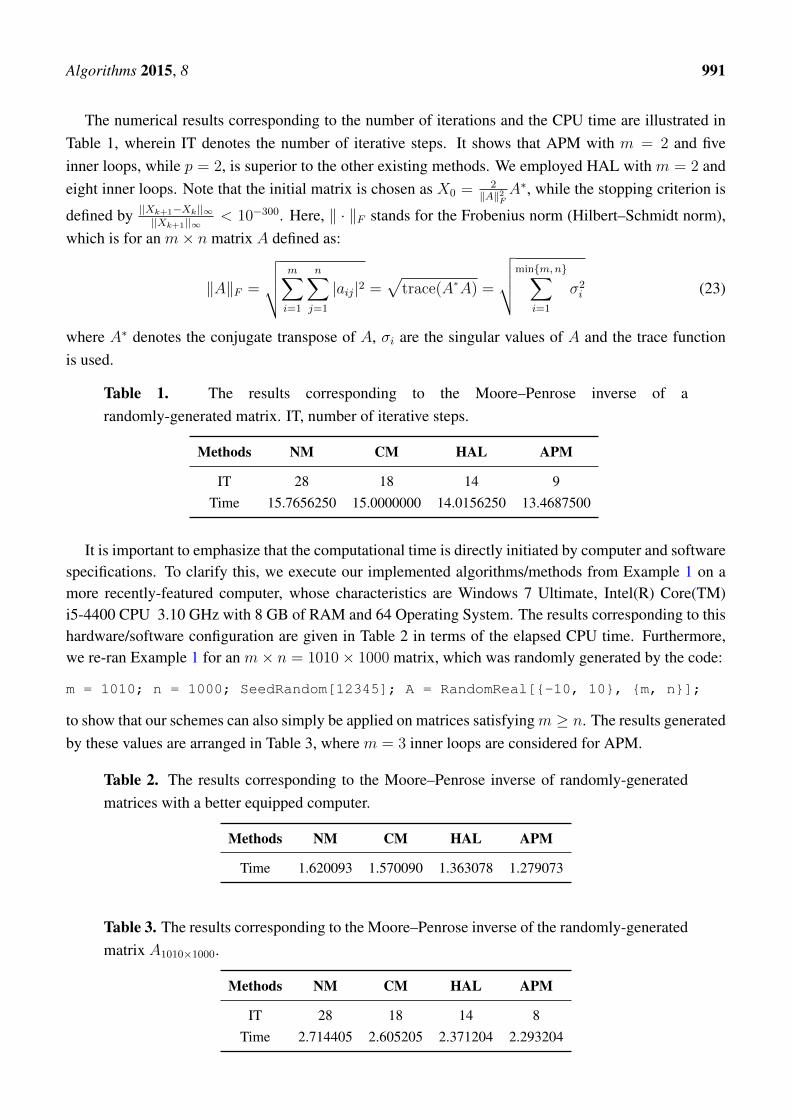
The numerical results corresponding to the number of iterations and the CPU time are illustrated inTable 1, wherein IT denotes the number of iterative steps. It shows that APM with m = 2 and fiveinner loops, while p = 2, is superior to the other existing methods. We employed HAL with m = 2 andeight inner loops. Note that the initial matrix is chosen as X0 = 2
‖A‖2FA∗, while the stopping criterion is
defined by ||Xk+1−Xk||∞||Xk+1||∞
< 10−300. Here, ‖ · ‖F stands for the Frobenius norm (Hilbert–Schmidt norm),which is for an m× n matrix A defined as:
‖A‖F =
√√√√ m∑i=1
n∑j=1
|aij|2 =√
trace(A∗A) =
√√√√minm,n∑i=1
σ2i (23)
where A∗ denotes the conjugate transpose of A, σi are the singular values of A and the trace functionis used.
Table 1. The results corresponding to the Moore–Penrose inverse of arandomly-generated matrix. IT, number of iterative steps.
Methods NM CM HAL APM
IT 28 18 14 9Time 15.7656250 15.0000000 14.0156250 13.4687500
It is important to emphasize that the computational time is directly initiated by computer and softwarespecifications. To clarify this, we execute our implemented algorithms/methods from Example 1 on amore recently-featured computer, whose characteristics are Windows 7 Ultimate, Intel(R) Core(TM)i5-4400 CPU 3.10 GHz with 8 GB of RAM and 64 Operating System. The results corresponding to thishardware/software configuration are given in Table 2 in terms of the elapsed CPU time. Furthermore,we re-ran Example 1 for an m× n = 1010× 1000 matrix, which was randomly generated by the code:
m = 1010; n = 1000; SeedRandom[12345]; A = RandomReal[-10, 10, m, n];
to show that our schemes can also simply be applied on matrices satisfyingm ≥ n. The results generatedby these values are arranged in Table 3, where m = 3 inner loops are considered for APM.
Table 2. The results corresponding to the Moore–Penrose inverse of randomly-generatedmatrices with a better equipped computer.
Methods NM CM HAL APM
Time 1.620093 1.570090 1.363078 1.279073
Table 3. The results corresponding to the Moore–Penrose inverse of the randomly-generatedmatrix A1010×1000.
Methods NM CM HAL APM
IT 28 18 14 8Time 2.714405 2.605205 2.371204 2.293204
Algorithms 2015, 8 992
The numerical example illustrates the theoretical results presented in Section 2. It can be observedfrom the results included in Tables 1–3 that, firstly, like the existing methods, the presented methodshows a stable behavior along with a fast convergence. Additionally, according to results containedin Tables 1–3, it is clear that the number of iterations required in the APM method during numericalapproximations of the Moore–Penrose inverse is smaller than the number of approximations generatedby the classical methods. This observation is in accordance with the fact that the efficiency index isclearly the largest in the case of the APM method. In general, APM is superior among all of the existingfamous hyper-power iterative schemes. This superiority is in accordance with the theory of efficiencyanalysis discussed before.
In fact, it can be observed that increasing the efficiency index by a proper factorization of thehyper-power method is a kind of nice strategy that gives promising results in terms of both the numberof iterations and the computational time on different computers.
Here, it is also worth noting that Schulz-type solvers are the best choice for sparse matrices possessingsparse inverses. Since, in such cases, the usual SVD technique in the software, such as Mathematica orMATLAB, ruins the sparsity pattern and requires much more time, hence such iterative methods and theSVD-type (direct) schemes are both competitive, but have their own fields of applications.
4.2. Numerical Experiments in Balancing Chemical Equations
In this subsection, we present some clear examples indicating the applicability of our approach in thebalancing chemical equations. We also apply the following initial matrix X0 = 1
σ21A∗.
Example 2. Consider a specific skeletal chemical equation from [10]:
x1KNO3 + x2C→ x3K2CO3 + x4CO + x5N2 (24)
where the left-hand side of the arrow consists of compounds/elements called reactants, while theright-hand side comprises compounds/elements called the products. Hence, Equation (24) is formulatedas the homogeneous equation Ax = 0, wherein 0 denotes the null column vector and:
A =
1 0 −2 0 0
1 0 0 0 −2
3 0 −3 −1 0
0 1 −1 −1 0
(25)
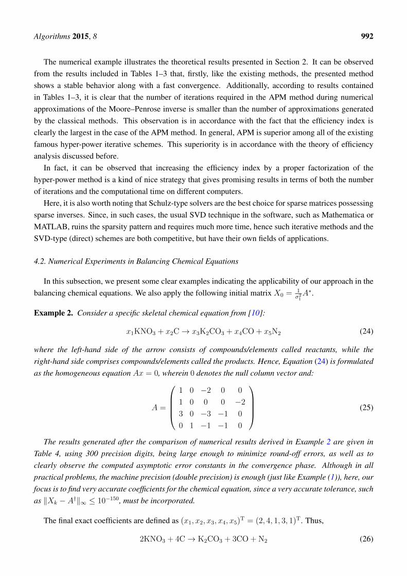
The results generated after the comparison of numerical results derived in Example 2 are given inTable 4, using 300 precision digits, being large enough to minimize round-off errors, as well as toclearly observe the computed asymptotic error constants in the convergence phase. Although in allpractical problems, the machine precision (double precision) is enough (just like Example (1)), here, ourfocus is to find very accurate coefficients for the chemical equation, since a very accurate tolerance, suchas ‖Xk − A†‖∞ ≤ 10−150, must be incorporated.
The final exact coefficients are defined as (x1, x2, x3, x4, x5)T = (2, 4, 1, 3, 1)T. Thus,
2KNO3 + 4C→ K2CO3 + 3CO + N2 (26)
Algorithms 2015, 8 993
Experimental results clearly show that PM is the most efficient method for this purpose. In addition,we remark that since we use iterative methods in floating point arithmetic to obtain the coefficient,we must use the command Round[] in the last lines of our written Mathematica code, so as to attain thecoefficients in exact arithmetic.
Table 4. The results corresponding to balancing Equation (24).
Methods NM CM PM
IT 14 9 3‖Xk+1 −A†‖ 2.59961× 10−161 1.1697× 10−193 9.09312× 10−293
In order to support the improvement described in Section 3, it is worth mentioning that (usingMathematica notations):
A.(Id− X.A).ConstantArray[1, n] = −3.9 ∗ 10−293,−5.0 ∗ 10−294, 2.0 ∗ 10−293,−0.0 ∗ 10−295
and A.(Id− X.A)((Id− X.A).ConstantArray[1, n]) = 0. ∗ 10−295, 0. ∗ 10−295, 0. ∗ 10−295, 0. ∗ 10−295.
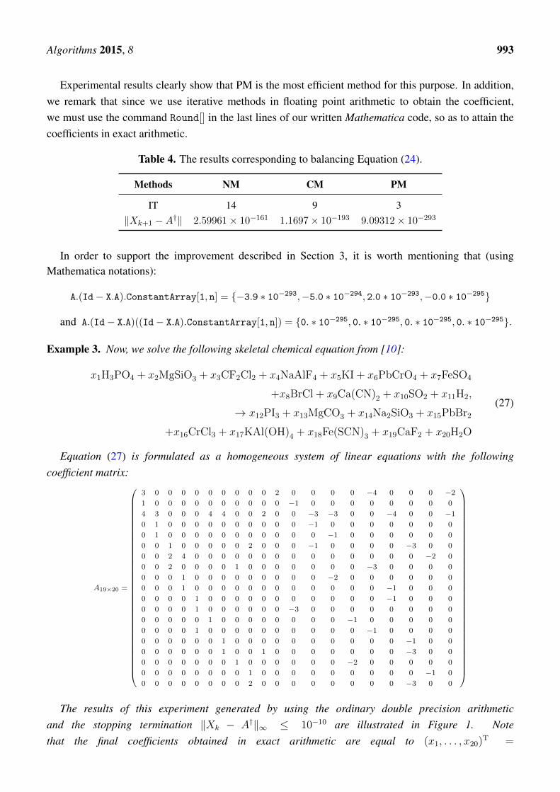
Example 3. Now, we solve the following skeletal chemical equation from [10]:
x1H3PO4 + x2MgSiO3 + x3CF2Cl2 + x4NaAlF4 + x5KI + x6PbCrO4 + x7FeSO4
+x8BrCl + x9Ca(CN)2 + x10SO2 + x11H2,
→ x12PI3 + x13MgCO3 + x14Na2SiO3 + x15PbBr2
+x16CrCl3 + x17KAl(OH)4 + x18Fe(SCN)3 + x19CaF2 + x20H2O
(27)
Equation (27) is formulated as a homogeneous system of linear equations with the followingcoefficient matrix:
A19×20 =
3 0 0 0 0 0 0 0 0 0 2 0 0 0 0 −4 0 0 0 −21 0 0 0 0 0 0 0 0 0 0 −1 0 0 0 0 0 0 0 0
4 3 0 0 0 4 4 0 0 2 0 0 −3 −3 0 0 −4 0 0 −10 1 0 0 0 0 0 0 0 0 0 0 −1 0 0 0 0 0 0 0
0 1 0 0 0 0 0 0 0 0 0 0 0 −1 0 0 0 0 0 0
0 0 1 0 0 0 0 0 2 0 0 0 −1 0 0 0 0 −3 0 0
0 0 2 4 0 0 0 0 0 0 0 0 0 0 0 0 0 0 −2 0
0 0 2 0 0 0 0 1 0 0 0 0 0 0 0 −3 0 0 0 0
0 0 0 1 0 0 0 0 0 0 0 0 0 −2 0 0 0 0 0 0
0 0 0 1 0 0 0 0 0 0 0 0 0 0 0 0 −1 0 0 0
0 0 0 0 1 0 0 0 0 0 0 0 0 0 0 0 −1 0 0 0
0 0 0 0 1 0 0 0 0 0 0 −3 0 0 0 0 0 0 0 0
0 0 0 0 0 1 0 0 0 0 0 0 0 0 −1 0 0 0 0 0
0 0 0 0 1 0 0 0 0 0 0 0 0 0 0 −1 0 0 0 0
0 0 0 0 0 0 1 0 0 0 0 0 0 0 0 0 0 −1 0 0
0 0 0 0 0 0 1 0 0 1 0 0 0 0 0 0 0 −3 0 0
0 0 0 0 0 0 0 1 0 0 0 0 0 0 −2 0 0 0 0 0
0 0 0 0 0 0 0 0 1 0 0 0 0 0 0 0 0 0 −1 0
0 0 0 0 0 0 0 0 2 0 0 0 0 0 0 0 0 −3 0 0
The results of this experiment generated by using the ordinary double precision arithmeticand the stopping termination ‖Xk − A†‖∞ ≤ 10−10 are illustrated in Figure 1. Notethat the final coefficients obtained in exact arithmetic are equal to (x1, . . . , x20)
T =
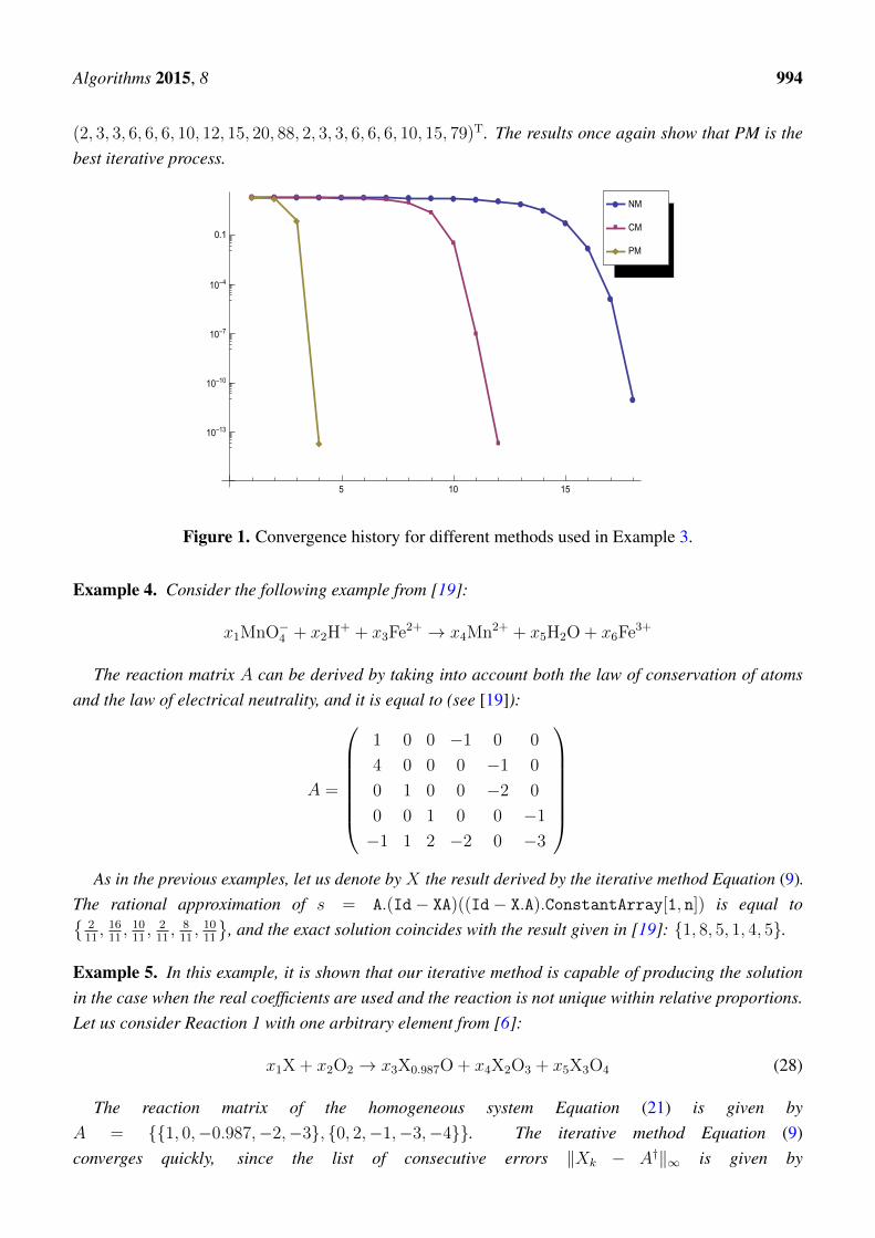
Algorithms 2015, 8 994
(2, 3, 3, 6, 6, 6, 10, 12, 15, 20, 88, 2, 3, 3, 6, 6, 6, 10, 15, 79)T. The results once again show that PM is thebest iterative process.
Figure 1. Convergence history for different methods used in Example 3.
Example 4. Consider the following example from [19]:
x1MnO−4 + x2H+ + x3Fe2+ → x4Mn2+ + x5H2O + x6Fe3+
The reaction matrix A can be derived by taking into account both the law of conservation of atomsand the law of electrical neutrality, and it is equal to (see [19]):
A =
1 0 0 −1 0 0
4 0 0 0 −1 0
0 1 0 0 −2 0
0 0 1 0 0 −1
−1 1 2 −2 0 −3
As in the previous examples, let us denote by X the result derived by the iterative method Equation (9).
The rational approximation of s = A.(Id− XA)((Id− X.A).ConstantArray[1, n]) is equal to211, 1611, 1011, 211, 811, 1011
, and the exact solution coincides with the result given in [19]: 1, 8, 5, 1, 4, 5.
Example 5. In this example, it is shown that our iterative method is capable of producing the solutionin the case when the real coefficients are used and the reaction is not unique within relative proportions.Let us consider Reaction 1 with one arbitrary element from [6]:
x1X + x2O2 → x3X0.987O + x4X2O3 + x5X3O4 (28)
The reaction matrix of the homogeneous system Equation (21) is given byA = 1, 0,−0.987,−2,−3, 0, 2,−1,−3,−4. The iterative method Equation (9)converges quickly, since the list of consecutive errors ‖Xk − A†‖∞ is given by
Algorithms 2015, 8 995
0.163381, 2.220446049250313 × 10⁻¹⁶, 2.7755575615628914 × 10⁻¹⁶. The approximate solutions = A.(Id− X.A)((Id− X.A).ConstantArray[1, n]) is equal to:
s = 1.40225926604, 0.890820221049, 0.657559993896, 0.35925113635, 0.0115817597876
and its fractional approximation is:
c =
44517366795613798
367684821979411,103259812167103006
1342504707428259,67799434016501962
1194167476431641,56436772606792756
1819443496152855, 1
.
Example 6. All possible solutions of the problem considered in Example 5 with respect to x1 and x2
can be generated using the Mathematica function Reduce:
Reduce[A.x1, x2, x3, x4, x5 == 0, 0, x1, x2]
All solutions in the symbolic form are given as follows (using Mathematica notations):
x1 = 0.987x3 + 2.0x4 + 3.0x5 + 0.0 ∧ x2 = 0.5x3 + 1.5x4 + 2.0x5 + 0
wherein x3, x4, x5 are arbitrary real quantities. All possible solutions with respect to x1 and x3 can begenerated using:
Reduce[A.x1, x2, x3, x4, x5 == 0, 0, x1, x3]
All possible(52
)= 10 cases can be solved in the same way.
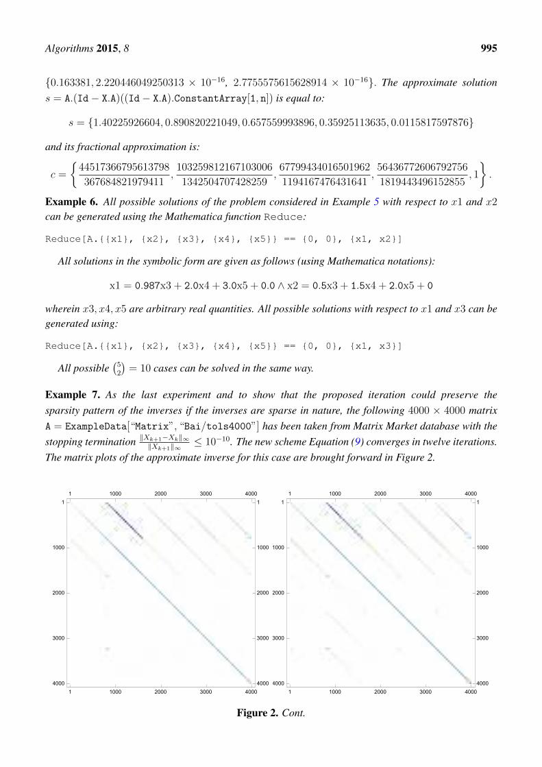
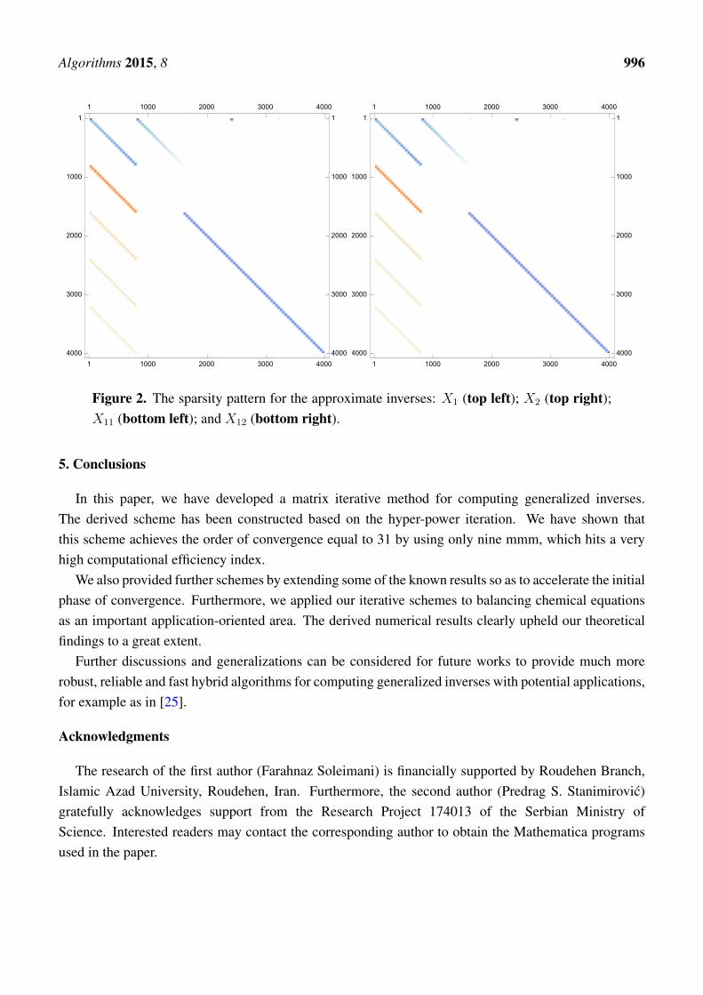
Example 7. As the last experiment and to show that the proposed iteration could preserve thesparsity pattern of the inverses if the inverses are sparse in nature, the following 4000 × 4000 matrixA = ExampleData[“Matrix”, “Bai/tols4000”] has been taken from Matrix Market database with thestopping termination ‖Xk+1−Xk‖∞
‖Xk+1‖∞≤ 10−10. The new scheme Equation (9) converges in twelve iterations.
The matrix plots of the approximate inverse for this case are brought forward in Figure 2.
Figure 2. Cont.
Algorithms 2015, 8 996
Figure 2. The sparsity pattern for the approximate inverses: X1 (top left); X2 (top right);X11 (bottom left); and X12 (bottom right).
5. Conclusions
In this paper, we have developed a matrix iterative method for computing generalized inverses.The derived scheme has been constructed based on the hyper-power iteration. We have shown thatthis scheme achieves the order of convergence equal to 31 by using only nine mmm, which hits a veryhigh computational efficiency index.
We also provided further schemes by extending some of the known results so as to accelerate the initialphase of convergence. Furthermore, we applied our iterative schemes to balancing chemical equationsas an important application-oriented area. The derived numerical results clearly upheld our theoreticalfindings to a great extent.
Further discussions and generalizations can be considered for future works to provide much morerobust, reliable and fast hybrid algorithms for computing generalized inverses with potential applications,for example as in [25].
Acknowledgments
The research of the first author (Farahnaz Soleimani) is financially supported by Roudehen Branch,Islamic Azad University, Roudehen, Iran. Furthermore, the second author (Predrag S. Stanimirovic)gratefully acknowledges support from the Research Project 174013 of the Serbian Ministry ofScience. Interested readers may contact the corresponding author to obtain the Mathematica programsused in the paper.
Algorithms 2015, 8 997
Author Contributions
The contributions of all of the authors have been similar. All of them have worked together to developthe present manuscript.
Conflicts of Interest
The authors declare no conflict of interest.
References
1. Phillips, J.C. Algebraic constructs for the graphical and computational solution to balancingchemical equations. Comput. Chem. 1998, 22, 295–308.
2. Risteski, I.B. A new generalized matrix inverse method for balancing chemical equations and theirstability. Bol. Soc. Qum. Mex. 2008, 2, 104–115.
3. Risteski, I.B. A new pseudoinverse matrix method for balancing chemical equations and theirstability. J. Korean Chem. Soc. 2008, 52, 223–238.
4. Krishnamurthy, E.V. Generalized matrix inverse approach for automatic balancing of chemicalequations. Int. J. Math. Educ. Sci. Technol. 1978, 9, 323–328.
5. Mahadeva, R.T.; Subramanian, K.; Krishnamurthy, E.V. Residue arithmetic algorithms for exactcomputation of g-inverses of matrices. SIAM J. Numer. Anal. 1976, 13, 155–171.
6. Risteski, I.B. A new generalized algebra for the balancing of ℵ chemical reactions. Mater. Technol.2014, 48, 215–219.
7. Smith, W.R.; Missen, R.W. Using Mathematica and Maple to obtain chemical equations. J. Chem.Educ. 1997, 74, 1369–1371.
8. Xia, Y. A novel iterative method for computing generalized inverse. Neural Comput. 2014, 26,449–465.
9. Higham, N.J. Gaussian elimination. WIREs Comp. Stat. 2011, 332–334, 230–238.10. Sen, S.K.; Agarwal, H.; Sen, S. Chemical equation balancing: An integer programming approach.
Math. Comput. Model. 2006, 44, 678–691.11. Balasubramanian, K. Linear variational Diophantine techniques in mass balance of chemical
reactions. J. Math. Chem. 2001, 30, 219–225.12. Ben-Israel, A. An iterative method for computing the generalized inverse of an arbitrary matrix.
Math. Comput. 1965, 19, 452–455.13. Climent, J.-J.; Thome, N.; Wei, Y. A geometrical approach on generalized inverses by
Neumann-type series. Linear Algebra Appl. 2001, 332–334, 533–540.14. Liu, X.; Jin, H.; Yu, Y. Higher-order convergent iterative method for computing the generalized
inverse and its application to Toeplitz matrices. Linear Algebra Appl. 2013, 439, 1635–1650.15. Soleymani, F.; Stanimirovic, P.S.; Haghani, F.K. On hyper-power family of iterations for computing
outer inverses possessing high efficiencies. Linear Algebra Appl. 2015, 484, 477–495.16. Schulz, G. Iterative Berechnung der Reziproken matrix. Z. Angew. Math. Mech. 1933, 13, 57–59.17. Soleymani, F.; Salmani, H.; Rasouli, M. Finding the Moore–Penrose inverse by a new matrix
iteration. J. Appl. Math. Comput. 2015, 47, 33–48.
Algorithms 2015, 8 998
18. Soleymani, F. An efficient and stable Newton-type iterative method for computing generalizedinverse A(2)
T,S . Numer. Algorithms 2015, 69, 569–578.19. Ramasami, P. A concise description of an old problem: Application of matrices to obtain the
balancing coefficients of chemical equations. J. Math. Chem. 2003, 34, 123–129.20. Sharifi, M.; Arab, M.; Khaksar Haghani, F. Finding generalized inverses by a fast and efficient
numerical method. J. Comput. Appl. Math. 2015, 279, 187–191.21. Stanimirovic, P.S.; Soleymani, F. A class of numerical algorithms for computing outer inverses.
J. Comput. Appl. Math. 2014, 263, 236–245.22. Soleimani, F.; Soleymani, F.; Cordero, A.; Torregrosa, J.R. On the extension of Householder’s
method for weighted Moore–Penrose inverse. Appl. Math. Comput. 2014, 231, 407–413.23. Petkovic, M.D.; Stanimirovic, P.S. Two improvements of the iterative method for computing
Moore–Penrose inverse based on Penrose equations. J. Comput. Appl. Math. 2014, 267, 61–71.24. Wolfram, S. The Mathematica Book, 5th ed.; Wolfram Media: Champaign, IL, USA, 2003.25. Soleymani, F.; Sharifi, M.; Karimi Vanani, S.; Khaksar Haghani, F. An inversion-free method for
finding positive definite solution of a rational matrix equation. Sci. World J. 2014, 2014, 560931.
c© 2015 by the authors; licensee MDPI, Basel, Switzerland. This article is an open access articledistributed under the terms and conditions of the Creative Commons Attribution license(http://creativecommons.org/licenses/by/4.0/).