cmb anisotropy power spectrum using linear combinations of wmap maps

arX

iv:0

706.

3567

v1 [

astr

o-ph

] 2

5 Ju

n 20

07

CMB anisotropy power spectrum using linear combinations of WMAP maps

Rajib Saha1,2,3, Simon Prunet3, Pankaj Jain1 & Tarun Souradeep2

1Department of Physics, Indian Institute of Technology, Kanpur, U.P, 208016, India2Inter-University Centre for Astronomy and Astrophysics,

Post Bag 4, Ganeshkhind, Pune 411007, India

and3Institut d’Astrophysique de Paris, 98 bis Boulevard Arago, F-75014 Paris, France.

In recent years the goal of estimating different cosmological parameters precisely has set new chal-lenges in the effort to accurately measure the angular power spectrum of CMB. This has requiredremoval of foreground contamination as well as detector noise bias with reliability and precision. Re-cently, a novel model-independent method for the estimation of CMB angular power spectrum solelyfrom multi-frequency observations has been proposed and implemented on the first year WMAP databy Saha et al. 2006. All previous estimates of power spectrum of CMB are based upon foregroundtemplates using data sets from different experiments. However our methodology demonstrates thatCMB angular spectrum can be reliably estimated with precision from a self contained analysis of the

WMAP data. In this work we provide a detailed description of this method. We also study andidentify the biases present in our power spectrum estimate. We apply our methodoly to extract thepower spectrum from the WMAP 1 year and 3 year data.

I. INTRODUCTION

Starting from the end of the last millenium remarkable progress in cosmology has been made by the precisemeasurements of the anisotropies in CMB from different ground based as well as satellite observations [1, 2, 3, 4].The Wilkinson Microwave Anisotropy Probe (WMAP) measures the CMB anisotropy over the 5 frequency bands at23 GHz (K), 33 GHz (Ka), 41 GHz (Q), 61 GHz (V) and 94 GHz (W). The observation system of the WMAP satelliteconsists of 10 differencing assemblies (DA), [5, 6, 7, 8], one each for K and Ka bands, two for Q band, two for V bandand four for W band. They are labeled as K, Ka, Q1, Q2, V1, V2, W1, W2, W3, and W4 DA respectively. In the 1year and 3 year data release the WMAP science team has provided the science community with large amount of highquality data sets measured by these 10 DAs. However, extracting the primordial signal from these large data set is anon trivial task. The anisotropies in CMB are weak in comparison to those originating due to radiation in the localuniverse, which inevitably contaminate the observed signal. These dominant foreground emissions are from withinthe milky way as well as from extragalactic point sources [9]. In the low frequency microwave regime the strongestcontamination comes from the synchrotron and free free emission [5, 10]. At higher frequencies, where synchrotron andfree free emissions are low, dust emission dominates. A reliable extraction of CMB signal from the multicomponentforeground contaminated data is thus complicated. There exists several methods in literature to remove foregroundsusing foreground tracer templates [10, 11, 12] built from observations from other experiments. However, this requiresa prior model of spatio-spectral dependence for all the foreground components. The effect of uncertanities in theforeground models to estimate CMB anisotropies have been discussed in Refs. [13, 14]. The foreground cleaning isapplicable in the region away from the galactic plane. Detector noise is another important concern that has to beaddressed in order to precisely measure the angular power spectrum. The angular power spectrum from detectornoise is dominant over the CMB power spectrum at the small angular scales. The detector noise, being a randomquantity, is treated differently from foreground contamination which are treated here as fixed templates on the sky.However each of the DA’s of WMAP has uncorrelated noise property [10, 12, 15, 16]. WMAP science team used thisproperty to remove detector noise bias in a cross correlated power spectrum obtained from two different DA [10, 12]using DA maps with frequencies 41 GHz, 61 GHz and 94 GHz.

An interesting model independent method to remove foregrounds from the multi-frequency observations of CMBwithout any assumption about foreground components has been proposed in Ref. [17] and implemented in Ref. [18]in order to extract the CMB signal from the WMAP data. The foreground emissions were removed by exploitingthe fact that their contributions in different spectral bands are considerably different while the CMB anisotropypower spectrum is same in all the bands in unit of thermodynamic temperature due to the Planck blackbody energyspectrum of the CMB, [19, 20]. The main advantage of this foreground cleaning method is that it is totally free fromany assumption about foreground modeling. Another advantage is that it is computationally fast. However the autopower spectrum obtained from a single cleaned map as reported in Ref. [18] is not directly usable for primordial powerspectrum estimation at smaller angular scale. This is because the detector noise bias dominates over the CMB powerspectrum at smaller angular scale, beyond the beam width of WMAP detectors.

In earlier publications [21, 22, 23] we extended this model independent foreground removal method to remove

http://arXiv.org/abs/0706.3567v1

2

detector noise bias also. In this work we describe the basic formalism of our previous work in detail. We apply ourmethod both on the WMAP 1 year and WMAP 3 year data to estimate CMB angular power spectrum. We formseveral cleaned maps using different cross combinations of the DA maps. Finally we form several cross power spectrawhere detector noise bias is removed. The results from this analysis are summarized in figure 9. In this figure weshow the power spectra estimated from the WMAP’s 1 year and 3 year data using the multi-frequency combinationof CMB maps. The bottom part of this figure shows the residual unresolved point source contamination that werecorrected for to obtain these two spectra. These power spectra are obtained without making any explicit model of theforegrounds or the detector noise. In most power spectrum extraction procedures, only the three highest frequencychannels observed by WMAP have been used to extract CMB power spectrum. We present a more general procedurewhere we use observations from all the five frequency channels of WMAP. The primary merit of the foreground removalmethod is that it avoids any need to remove foregrounds based upon extrapolated flux measurements at frequenciesfar away from observational frequencies of WMAP [10, 24, 25].

Presence of a bias in the internally cleaned maps has been reported earlier in the Refs. [12, 26, 27]. In this work wealso perform a detailed study of the nature of bias in the cleaned power spectrum. We show that the cleaned powerspectrum is not an unbiased estimator of the underlying CMB spectrum. Naively one expects that there might besome residual foreground contamination causing a positive bias in the power spectrum. For a simplified approach,which cleans the entire sky simultaneously, without sub-dividing into regions of varying foreground contamination,we are able to analytically compute the cleaned power spectrum in terms of a CMB signal and the foreground plusdetector noise covariance matrix. The existence of bias is easily identified from these results. We also report andquantify an interesting negative bias in the cleaned power spectrum. This negative bias is directly determined bythe underlying CMB power spectrum and is strongest at the lowest multipoles. The analytical results for the biasestimations make the model independent foreground removal method more interesting for use in cosmology. Thebias in the cleaned power spectrum can be removed following models of foreground and noise covariance matricesafter a model independent foreground removal is performed. This makes the estimated power spectrum less prone touncertainties of the foreground modeling compared to a method which tries to minimize foreground using externaltemplates. In this work we debias the CMB anisotropy spectra obtained from WMAP data only at the large multipoleregime, l ≥ 400. It turns out that because of large noise level of WMAP the point source bias is the only issue in thismultipole range. We do not attempt to employ a debiasing method at the low multipoles where the negative bias isexpected to dominate, because of its complicated nature in the case of the iterative, multiregion cleaning method. Amore detailed study on this issue will be reported in a future publication.

The plan of this paper is as follows. The basic formalism and methodology to obtain power spectrum is describedin the section II. Here we also discuss the bias present in this method. The implementation of our methodologyon the WMAP 1 year and 3 year data is discussed in section III. Here we also obtain an analytic expression for theresidual unresolved point source power contamination. The results are described in section IV and finally we concludein section V. Some of the notations used in this report are as follows. We denote matrices and vectors by boldfaced

letters. Any variable (scalar, vector or matrix) which depends on the stochastic component is denoted by a hat on

the top. As an example we note that the CMB power spectrum is a stochastic variable which is represented as Ccl .

II. BASIC FORMALISM AND METHODOLOGY

In this section we outline the mathematical formalism to obtain the underlying power spectrum. We also quantifythe bias present in the estimated power spectrum using our procedure.

A. Foreground Removal

The observed signal at frequency channel i in a differential telescope like WMAP can be modeled as

∆T i(n) =

∫ (∆T c(n′) + ∆T fi(n′)

)Bi(n · n′)dn′ + ∆T ni(n) . (1)

Here ∆T c(n) and ∆T fi(n) are respectively CMB and foreground component of the anisotropy in the channel,i. Thedetector noise in the channel, i, is ∆T ni. The beam function Bi(n · n′) represents the smoothing of the map due tofinite resolution of the antenna of channel, i. The beam is assumed to be circularly symmetric as done in most analysis.We note that the detector noise is not affected by the beam function. An experiment such as WMAP provides multi-

frequency maps ∆T i(n), i = 1, 2, ..., nc corresponding to observation of the CMB at nc different frequency bands.

3

Equivalently, in the spherical harmonic representation

ailm =

(ac

lm + afilm

)Bi

l + anilm . (2)

where alm are respective spherical harmonic contributions to the maps and Bl are Legendre transform coefficients ofthe beam Bi(n · n′). The aim is to linearly combine the maps with appropriate weights to get an optimal estimatorof the CMB anisotropy ∆T c(n′) that minimizes the contribution from ∆T f(n′). The linear combination of the multi-frequency maps available can be carried out in pixel space, or, in the equivalent representation in terms of the sphericalharmonic coefficients. The former has been followed by the WMAP team to produce Internal Linear Combination(ILC) map and also in a related, but more elaborate approach in Ref. [27] to produce LILC map. The approach ofcarrying out a multi-frequency maps combination in the spherical harmonic space was proposed in Ref. [17]. For thefirst year of WMAP data this was implemented in Ref. [18]. This method has the advantage that we can simultaneouslytake into account variation of foreground with sky positions and with different multipoles for a given sky position.

We define a cleaned map as a linearly weighted sum of the maps at different frequencies,

aCleanlm =

i=nc∑

i=1

W il

ailm

Bil

. (3)

Here W il is a weight factor which depends upon the multipole l and the frequency channel, i. Since each of the

channels has a different beam resolution, the maps are deconvolved by the corresponding circularly symmetric beamtransform functions Bl prior to the linear combination. The total power in the cleaned map at a given multipole l isthen

CCleanl =

1

2l + 1

m=l∑

m=−l

aCleanlm aClean∗

lm . (4)

Substituting eq. (3) in eq. (4) we obtain,

CCleanl = WlClW

Tl , (5)

where the matrix Cl is given by

Cl =

C11l

B1lB1

l

.. ..C1nc

l

B1lBnc

l

.. .. .. ..

.. .. .. ..Cnc1

l

Bncl

B1l

.. ..Cncnc

l

Bncl

Bncl

, (6)

Wl is a row vector describing the weights for different channels,

Wl = (w1l , w2

l , , . . . , wnc

l ) (7)

and Ci,jl is the cross power spectrum between the ith and jth channel,

Ci,jl =

m=l∑

m=−l

ailmaj∗

lm

2l + 1=

ail0a

jl0

2l + 1+ 2ℜ

m=l∑

m=1

ailmaj∗

lm

2l + 1. (8)

By construction, the Cl matrix is symmetric. The spherical harmonic coefficients extracted from a map contain CMBsignal and foregrounds, both smoothed by the beam function of the optical instrument used in the experiment, aswell as detector noise. Using eq. (2) we obtain,

alm = Blaslm + Bla

Flm + aN

lm︸︷︷︸ajunk

lm

, (9)

where ajunklm is used to denote the total non-CMB contamination in the map. Since the CMB contribution is indepen-

dent of frequency, the expression forCij

l

BilBj

l

simplifies to

Cijl

BilB

jl

=1

2l + 1

m=l∑

m=−l

(Bi

laSlm + a

i(junk)lm

)

Bil

×

(Bj

l aS∗lm + a

j(junk)∗lm

)

Bjl

= CSl + C

ij(junk)l ,

4

for all values of i and j. Now using eq. (5) we obtain

CCleanl = CS

l Wle0eT0 WT

l + WlC(junk)l WT

l , (10)

where e0 is a column vector with unit elements

e0 =

1....1

. (11)

The CMB signal power in the cleaned map is kept unaltered by imposing the constraint

Wle0 = eT0 WT = 1 , (12)

on weights W il . Using eqs. (10) and (12), the total power at a multipole l in the cleaned map is

CCleanl = CS

l + WlCjunkl WT

l . (13)

Thus the CMB signal power is only an additive positive constant in the expression of the total power of the weighted

map. Hence, choosing weights that minimize CCleanl also minimizes the combined contamination coming from fore-

ground and detector noise. It may be shown easily, using the Lagrange’s multiplier method, that minimizing CCleanl

subject to the constraint eq. (12), gives the following expression for the weight factors [17, 26],

Wl =eT0 C−1

l

eT0 C−1

l e0

. (14)

Following eqs. (5) and (14) we can express the power in the cleaned maps neatly as

CCleanl =

1

eT0 C−1

l e0

. (15)

It is important to note that in cases when Cl is singular, it is possible to generalize the above expressions for weightsand cleaned power spectrum in terms of the Moore-Penrose Generalized inversion (MPGI) of Cl. The generalizedweights and cleaned power spectrum are then given by

Wl =eT0 C

†l

eT0 C

†l e0

, (16)

CCleanl =

1

eT0 C

†le0

. (17)

For further details of the analytic derivation of the weights and cleaned power spectrum we refer to appendix A.

B. Biases in the foreground cleaning method

Although the foreground cleaning is performed with the constraint that CMB power spectrum remains preserved,the method biases the final power spectrum. This section is devoted to a discussion of the full bias in the method.

The existence of some bias is not difficult to anticipate and understand. The method is intended to perform aminimization of the foreground power spectrum which is a positive definite quantity. Unless the foreground cleaningis fully effective at all multipoles, the minimization would leave some residual foreground which naively would giverise to a positive bias in the cleaned power spectrum. However, it is very interesting that there exists an additionalnegative bias in the method. This negative bias is strongest at the lowest multipoles and increases in magnitude withincrease in number of channels that are combined.

Let us consider nc number of channels in the linear combinations for the cleaned map. The maps at each channelconsists of the CMB signal and foreground contamination coming from the different foreground components (syn-chrotron, free-free, dust etc). Although, the number of distinct foreground components could be arbitrary, for brevity

5

and simplicity, here we club the contributions from all the components into a single foreground term. The foregroundcontribution can be described by a covariance matrix. Later, after simplification of the expressions, we can split upthe total foreground covariance matrix in terms of the covariance matrices of the distinct constituent components. Inthe entire discussion that follows we do not treat foregrounds as a stochastic component. Instead we consider them asfixed templates in all the realizations. This is entirely justified. We are simply interested in computing a foregroundfree template rather than estimating information about the distribution of foreground from which they are drawn.We discuss the bias in few different cases depending upon the rank of the covariance matrix Cl.

1. Case: Rank Cl ≤ nc − 1

First we consider an ideal case wherein detector noise remains absent and each foreground component follows arigid frequency scaling on the entire sky. Let the number of foreground components be nf . Then the rank of theforeground covariance matrix, Cf

l , is also nf .The pth foreground component for channel i is denoted by F p

0 (θ, φ)f ip, where the frequency dependence, f i

p and the

spatial (sky) dependence F p0 (θ, φ) are explicitly separable in the rigid scaling assumption. (Here, F p

0 (θ, φ) is the pth

foreground template based on frequency ν0, so that f ip = 1, for frequency ν0.) We denote the CMB component by

C(θ, φ). Full signal map at frequency channel, i, is then given by

Si(θ, φ) = C(θ, φ) +

nf∑

p=1

F p0 (θ, φ)f i

p . (18)

Alternatively, in the spherical harmonic space,

ailm = ac

lm +

nf∑

p=1

f ipa

p0lm . (19)

The auto power spectrum of the ith channel

Cil = Cc

l + 2

nf∑

p=1

f ipC

cf(p)0l +

nf∑

p,p′

f ipf

ip′C

(pp′)0l . (20)

In the above equation, C(pp′)0l is the correlation between any two foreground components p, p′ and C

cf(p)0l denotes

the chance correlation between CMB signal and pth foreground component. The cross power spectrum between twochannels i, j is given by

Cijl = Cc

l +

nf∑

p=1

f ipC

cf(p)0l +

nf∑

p=1

f jpC

cf(p)0l +

nf∑

p,p′

f ipf

jp′C

(pp′)0l . (21)

It is convenient to define the vectors,

fp0l = C

cf(p)0l

f1p

f2p

.fnc

p

, (22)

and

f0l =

nf∑

p=1

fp0l . (23)

A little algebraic manipulation allows us to recast eq. (21) as

Cl = Ccl e0e

T0 + f0l eT

0 + e0f0Tl + Cf

l . (24)

The above equation will be useful to compute the bias in the cleaned power spectrum. On the ensemble average thecleaned power spectrum as given by eq. (17) could be simplified with the help of successive use of a set of theorems

6

reported in Refs. [28, 29]. An elaborate discussion of these theorems is given in appendix E. Assuming statisticallyisotropic CMB sky we obtain the following expression for the ensemble average of the cleaned power spectrum

⟨CClean

l

⟩=⟨Cc

l

⟩− nf

⟨Cc

l

⟩

2l + 1. (25)

We easily note a few interesting aspects of the above equation. First of all there exists a negative bias. Secondly,because of ∼ 1/(2l+1) decay, this bias is important at the lowest multipoles. Another important point to note is thatthe bias depends on the underlying CMB power spectrum. Therefore it is possible to debias any given statisticallyisotropic CMB model in this approach by constructing an appropriately scaled estimator. Lastly, we find that there isno foreground bias. One would naively expect the foregrounds would contribute a positive bias in the power spectrum.However this does not happen in this case as the rigid scaling assumption along with the condition nc ≥ nf +1 ensurethat sufficient amount of spectral information are available to remove all the foregrounds. The negative bias arisesas the weights are to be determined from the empirical covariance matrix to take into account information availablefrom the observed data.

2. Case: Rank (Cfl ) = nc

The rigid scaling assumption for the foreground contaminants considered in the previous section is at best areasonable approximation and is known not to be valid in general. As mentioned in Ref. [9] a foreground componentwith varying spectral index over the sky could be approximated in terms of two templates, provided the variationis small compared to the mean spectral index over the sky. A stronger variation will need more than two templatesfor reasonable modeling. In such a situation, if the number of templates required for modeling of all the foregroundcomponents exceeds the number of maps available for linear combination then Cf

l is of full rank. In this case a positiveforeground bias appears along with a negative bias. The negative bias is similar to the previous case in that it remains

proportional to〈Cc

l 〉2l+1 . Keeping aside the detector noise for the moment, the ensemble average of the cleaned power

spectrum is given by

⟨CClean

l

⟩=⟨Cc

l

⟩+

1

eT0 (Cf

l )−1

e0

+ (1 − nc)

⟨Cc

l

⟩

2l + 1. (26)

Detailed derivation of the above equation is similar to derivation of eq. (25). As Cfl is of full rank and a positive

definite matrix, the second term on the right causes a positive foreground bias.

3. Noise and foreground case

The discussion in the last two sections does not consider any detector noise. We now consider the most general casewhere we have both foreground and detector noise. Following a method similar to that used in derivation of eqs. (25)and (26) we can show that, on the ensemble average the cleaned power spectrum in this case is given by

⟨CClean

l

⟩=⟨Cc

l

⟩+

⟨1

eT0 (Cf+N

l )−1

e0

⟩+ (1 − nc)

⟨Cc

l

⟩

2l + 1. (27)

We have carried out Monte-Carlo simulations to verify the analytical result given by eq. (25). We perform simulationsof foreground cleaning using nc = 3 channels, corresponding to 41, 61 and 94 GHz frequencies. The foregroundmodel consists of a synchrotron and free-free emission. Each of the foreground component is assumed to follow arigid frequency scaling all over the sky. First we generate synchrotron and free-free templates using the Planck SkyModel 1 at the 3 different frequencies. Since these templates do not follow rigid frequency scaling all over the sky, (

1 We acknowledge the use of version 1.1 of the Planck reference sky model, prepared by the members of Working Group 2 and availableat www.planck.fr/heading79.html.

7

eg., synchrotron spectral index varies with the position of the sky), we developed a method to regenerate rigid scalingsynchrotron and free templates at these 3 different frequency channels 2

0

1000

2000

3000

4000

5000

6000

1 10 100

l(l+

1)C

l/(2π

) [µ

K2 ]

200 400 600 800 1000

Cleaned Cl (biased)Input, CMBCleaned + 2Cc

l/(2l+1)

Multipole, l

1

10

100

1 10 100

l(l+

1)C

l/(2π

) [µ

K2 ]

200 400 600 800 1000

Input Ccl - Biased Cleaned Cl

2Ccl/(2l+1)

Multipole, l

FIG. 1: The negative bias in the extracted power spectrum at low l is shown by the red line in the left panel. The bias correctedspectrum is plotted in blue line. However it lies entirely behind the green line and is not visible. The right panel shows howwell the analytic results for bias match with those obtained from Monte Carlo simulations.

The left hand panel of the fig. 1 based on 1000 Monte Carlo simulations shows that there exists a negative biasin the cleaning method. For the assumed model of foreground components with rigid frequency scaling, the second

term on the right in eq. (25) contributes −2⟨Cc

l

⟩/2l + 1 as a negative bias. In the right hand panel of the fig. 1

we explicitly show that the magnitude of the negative bias is exactly compensated by 2〈Cc

l 〉2l+1 . The negative bias is

important at the lowest multipoles and becomes negligible at high l, e.g. the bias is only ≈ 3µK2 at multipole l≈ 800. The bias corrected spectrum plotted in green color in the left panel of this fig. 1 is completely hidden by theblue curve corresponding to the input CMB power spectrum which is used to generate random realizations of CMBmaps.

The bias in the cleaned power spectrum for different cases described so far is computed following the assumptionthat foreground cleaning is simultaneously carried out over the entire sky. However for the cleaning purpose ofWMAP maps we follow a more sophisticated method. The main reason behind opting for a sophistication is that thespectrum of foreground emission as well the amplitude strongly depend on the location in the sky. The effectivenessof the foreground cleaning in varying foreground spectral index has been studied in the existing literature, [9, 14].Following the discussion in section II B 2 a varying foreground spectra would cause a positive foreground bias in thecleaned power spectrum. To minimize this bias we followed Ref. [18] and divide the sky into 9 regions based on asimple estimation of the level of foreground contamination (see appendix B). We then carry out foreground cleaningiteratively taking one region at a time starting with dirtiest region. The advantage of such iterative method is thatdiffuse foreground contamination which is dominant at the low multipoles compared to the detector noise could be veryeffectively minimized without a precise model of residual bias. The main principle for iterative cleaning is to searchfor sky regions where foreground emission could be assumed approximately constant or at least nearly constant. Sucha philosophy of foreground cleaning has been adopted by WMAP team to produce their Internal Linear CombinationMap [11]. In a future publication we would generalize the bias results reported in this article to the most generalmethod of iterative cleaning. Another advantage of iterative method is that one has the freedom to adjust weights ondifferent sky positions depending upon the amplitude of the foreground components leading to a better cleaning.

2 For this purpose, we first note that for each component the approximate normalizationq

Cil/C23

lremains roughly constant for all l.

Here C23l

is the synchrotron (or free -free) power spectrum for frequency 23 GHz and Cil

is the synchrotron ( or free-free) power spectrum

at any of other 3 frequencies. We generate a synchrotron ( or free-free ) template at the ith frequency channel following a scaling of

the 23 GHz template by the numberq

Cil/C23

l. This ensures that the emisssion for each foreground component at different frequencies

follows rigid frequency scaling.

8

nc-channel combination Cleaned Map

D11 + D2

1 + ... + Dnc1 C1

D12 + D2

2 + ... + Dnc2 C2

D13 + D2

3 + ... + Dnc1 C3

.......................... ....

D1d + D2

d + ... + Dncd Cd

TABLE I: List of several possible cleaned maps with uncorrelated detector noise properties. Here we assume nc number offrequency bands with each band having d number of independent detectors.

C. Power spectrum Estimation

The power spectrum is estimated by cross correlating multichannel foreground cleaned maps from independentDifferencing Assemblies (DA). The alternative is to use auto correlation and use a detector noise model to debias thepower spectrum. In this case the detector noise model uncertainty affects the mean of the cleaned power spectrum.We note that the WMAP team too used cross-correlation of independent DA to obtain their power spectrum. Letus consider an hypothetical experiment with nc number of frequency channels each of which is denoted by i. Eachfrequency channel consists of d number of independent detectors denoted by Di

j . Thus Dij is the map observed by

jth detector of ith channel. We then propose to form several cleaned maps in such a way that each cleaned mapconsists of one map from each of the nc number of channels. By choosing appropriate combinations of DA maps weidentify two different cleaned maps having totally disjoint set of detectors. Then assuming that the noise propertiesare uncorrelated in two different detectors, the noise bias will not affect the cross power spectrum of two such cleanedmaps at the 1st order. The final power spectrum could be a simple average of all possible such cross power spectra.In table I we show a set of possible cleaned maps Cj , j = 1, 2, .., d with uncorrelated detector noise properties. Henced(d−1)

2 number of cross power spectra can be obtained that do not have any noise bias. In general the number ofpossible cleaned maps is more than d. If we divide the combination of cleaned map 1 in p number of subsets and thecombination of cleaned map 2 in q number of subsets then one only needs to make sure that these p and q subsetshave uncorrelated noise properties.

III. IMPLEMENTATION ON WMAP DATA

In our method we linearly combine maps corresponding to a set of 4 DAs at different frequencies. 3 We treat the Kand Ka maps effectively as observations of the CMB sky in two different DA at the low frequencies. Therefore, we useeither K or Ka maps in any combination. In case of the W band, 4 DA maps are available. We simply form pairwiseaveraged map taking two of them at a time and form 6 effective DA maps corresponding to W band. Wij representssimply an averaged map obtained from the ith and jth DA of W band. In table II we list all the 48 possible linearcombinations of the DA maps that lead to ‘cleaned’ maps, Ci and CAi’s, where i = 1, 2, . . . , 24. In an alternativeapproach, we form combinations to form cleaned maps excluding the most foreground contaminated K and Ka bands(referred to as the three-channel nc = 3 case). This leads to a total of 24 cleaned maps. All such combinations areshown in the bottom panel of the table II. In this combination the cleaned maps are labeled as Ci s, where i = 1, 2,. . . , 24.

The entire method leading to the power spectrum estimation consists of three main steps. First we performforeground cleaning using several multi-channel combinations of WMAP maps. At the second step we obtain crosspower spectra from these foreground cleaned maps. The foreground cleaning is similar to Refs. [17, 18]. Finally wecorrect for the estimated residual unresolved point source contamination. We note in passing that each of these stepsare logically modular and each of them could be modified or improved independent of the other.

3 In Ref. [18], a single foreground cleaned map is obtained by linearly combining 5 maps corresponding to one each for the differentWMAP frequency channels. For the Q, V and W frequency channels, where more than one maps were available, an averaged map wasused. However, averaging over the DA maps in a given frequency channel precludes any possibility of removing detector noise bias usingcross correlation.

9

4-channel combinations (nc = 4)

(K,KA)+Q1+V1+W12=(C1,CA1) (K,KA)+Q1+V2+W12=(C13,CA13)












3-channel combinations (nc = 3)

Q1+V1+W12=C1 Q1+V2+W12=C13

Q1+V1+W13=C2 Q1+V2+W13=C14

Q1+V1+W14=C3 Q1+V2+W14=C15

Q1+V1+W23=C4 Q1+V2+W23=C16

Q1+V1+W24=C5 Q1+V2+W24=C17

Q1+V1+W34=C6 Q1+V2+W34=C18

Q2+V2+W12=C7 Q2+V1+W12=C19

Q2+V2+W13=C8 Q2+V1+W13=C20

Q2+V2+W14=C9 Q2+V1+W14=C21

Q2+V2+W23=C10 Q2+V1+W23=C22

Q2+V2+W24=C11 Q2+V1+W24=C23

Q2+V2+W34=C12 Q2+V1+W34=C24

TABLE II: The table on the top shows 48 different combinations of the DA maps used in our 4 channel cleaning method. Thebottom table shows the 24 possible combinations in the 3 channel cleaning method.

A. Map cleaning

We use the ‘raw’ DA maps (i.e., that have not undergone any foreground cleaning process) both for the WMAP 1year and WMAP 3 year data release from the LAMBDA website. These maps follow HEALPix 4 pixelization schemeat a resolution level Nside = 512 corresponding to approximately 3 million sky pixels. All these maps are providedin the ‘nested’ pixelization scheme which is suitable for nearest neighbor searches. However for converting mapsto spherical harmonic space and vice versa it is computationally advantageous to convert them to ring format thatfacilitates the use of Fast Fourier transformation method along equal latitudes. Therefore prior to the analysis all themaps corresponding to 10 DA’s were converted to ‘ring’ pixelization scheme. When converting a map to sphericalharmonic space we restricted ourselves to a maximum multipole, lmax = 1024.

The spectrum of foreground emission has some dependency on the location on the sky. A better cleaning maybe achieved if we partition the entire sky into certain number of sky parts depending upon the level of foregroundcontaminations [18]. Then cleaning is done for each sky-parts iteratively. For each regions we will have then differentweights which are chosen to minimize foreground contamination from that particular region. Cleaning becomes moreefficient by allowing the weights to depend on the sky parts rather than using a single set of weights for the entiresky. Following Ref. [18] we partition the sky depending upon the level of foreground contamination. 5

The entire sky is partitioned in a total of r = 9 regions depending upon their foreground contamination. All the rsky parts are shown in the fig. 2. Individual sky parts are color-coded according to the number r assigned to them.The dirtiest part is labeled with the maximum index. The procedure of forming these sky parts are similar to Ref. [18]

4 For comprehensive studies about HEALPix we refer to Ref. [30, 31, 32].5 Although this scheme is found to be effective, it is possible to envisage other schemes such as those that make foreground contamination in

each part closer to rigid scaling approximation. In an ongoing study we have investigated and demonstrated improvement in foregroundcleaning for different levels of partitioning [33].

10

FIG. 2: The 9 different masks in orthographic projection that correspond to the partitions of the sky. Each region is colorcoded to distinguish them visually. The cleanest region is the region farthest away from the galactic plane. The dirtiest region(black spots) lie in the galactic plane.

with small variants. We describe our sky partitioning to identify these r regions in detail in appendix B.For each combination, the cleaning procedure is performed in r iterations starting from the dirtiest region. As

in Ref. [18] we call the initial foreground contaminated maps as the initial temporary maps. At the end of each ofiteration we obtain a set of partially cleaned temporary maps which are used as input in the next iteration. In ith

iteration (i = 1, 2, 3, ..., r) we perform the following three steps :

1. Using the ith mask we select the ith region of the sky from the temporary maps. Then we obtain power spectrummatrix from the ith region only. 6

2. Using the weight factors we obtain a full sky cleaned map using eq. (3).

3. Next we replace the ith region of the temporary maps by the corresponding region of the cleaned map. Beforereplacement the cleaned map is smoothed to the resolution of the different frequency channels. After replacementthe maps define new temporary maps for the next iteration.

The entire cleaning procedure is automated to carry the three steps iterated r times to obtain the final cleanedmaps. The final cleaned maps have the resolution of the W band.

In eq. (7) the weights could have numerical errors if the Cl matrix becomes ill-conditioned at specific values ofl. This can happen if by chance any mode has almost equal contribution combined from the CMB, foreground anddetector noise. Hence, in practice, the numerical implementation obtains weights using the Cl matrix smoothed overa range of ∆l = 11 prior to inversion.

As shown in table II, for the four channel combination (nc = 4), a total of 48 cleaned maps can be obtained usingall the possible combinations of the DA maps for each of the WMAP 1 year and WMAP 3 year data. The cleanedmap C8 for WMAP 1 year data is shown in the left panel of the figure 3. There is some residual foreground left inthe galactic plane as seen in this map. We apply Kp2 mask, supplied by the WMAP team, to flag the contaminatedpixels near the galactic plane. Therefore these residuals do not affect our final estimated power spectrum. A similarmap is obtained from the WMAP 3 year data also. The right panel of the figure 3 shows CA8 map from WMAP-3data. Both the maps look similar.

The weights Wl are shown in the figures 4 for one of the cleaned map (CA1) for the cleanest and second cleanestregion. For low l where the diffuse foregrounds are dominant, the weights take large positive and negative values to

6 These power spectrum matrix is obtained from the partial sky spherical harmonic coefficients. In practice while using 1 year WMAPdata we have not combined K band map for l > 603 (Bl < 0 for K band for l > 603 and the negative values of beam function specified isunphysical.). KA and Q band beam functions are available till l = 850 and l = 1000. Therefore we do not combine these bands beyondthese values. Similar limits determined by the condition Bl > 0 were used for 3 year data analysis also.

11

FIG. 3: The left panel shows the cleaned map C8 using the 1 year WMAP data. There is some residual foreground contami-nation near the galactic regions. The right panel shows the CA8 map using the 3 year WMAP data. The temperature scale ofboth the figures are chosen from the sky part outside the Kp2 mask.

-4

-3

-2

-1

0

1

2

3

4

5

10 100 200 400 600 800 1000

W1W2W3W4

-3

-2

-1

0

1

2

3

4

5

10 100 200 400 600 800 1000

W1W2W3W4

FIG. 4: The left panel of the figure shows the weights for the cleanest region for the combination KA, Q1,V1,W12. The rightpanel show the weights for the same combination but for the second cleanest region. At low multipole foregrounds dominate.Therefore, weights take large positive and negative values to subtract foregrounds.

subtract the foregrounds. At large l the maximum weight is given to the W band channel since it has the highestresolution.

B. Power spectrum estimation

Our final power spectrum is based upon the MASTER estimate introduced in Ref. [34]. Even after performingforeground cleaning the galactic disk region remains significantly contaminated. Hence one needs to exclude thisregion before estimating the cosmological power spectrum. However, flagging the contaminated sky region effectivelyintroduces uneven weighting of the pixels. Those flagged have efectively zero weight and rest have unit weight.Weighting a map in the pixel space causes neighboring multipoles to get correlated. The correlation of the multipolesare described by the coupling matrix which is determined by the geometry of the sky coverage. Moreover, the powerspectrum of such a map is biased low because of less sky coverage. The MASTER method debiases the partial skypower spectrum on the ensemble average by inverting the coupling matrix.

The MASTER method originally implemented in Ref. [34] deals with auto power spectrum only. This can readily begeneralized to the case of cross power spectrum [35]. We first exclude the galactic region from all the 48 cleaned maps(Table II,nc = 4) using Kp2 mask as supplied by the WMAP team. Then map pairs Ci & Cj to be cross correlatedare chosen such that they do not have any DA common between them. This choice ensures that the detector noisebias does not affect any of the cross power spectrum. A total of 24 cross power spectra could be obtained which

12

are unaffected by the detector noise bias. Each of these cross spectra are then debiased from the partial sky effectfollowing Ref. [35] using the coupling (bias) matrix corresponding to the Kp2 mask. The small scale systematic effectsof beam and pixel smoothing were removed using appropriate circularized beam transform [34] and pixel windowfunctions as supplied by the HEALPix package. The 24 cross power spectra are then combined with equal weightsinto a single ‘Uniform average’ power spectrum. 7 The final power spectrum is binned in the same manner as theWMAP’s published result for ease of comparison.

Both one and three year power spectra were obtained following this method. We defer a more detailed discussionon the 3 year power spectrum results to the section IVB. We also estimate a residual contamination in the ‘Uniformaverage’ power spectrum for both WMAP 1 year and WMAP 3 year data from the unresolved point sources. A pointsource model used by WMAP team [10, 12] and estimated entirely from the WMAP data [11] is sufficient for ourestimation. We recover a flat, (approximately 140µK2 for WMAP 1 year data and 100µK2 for WMAP 3 year data),residual point source contamination in the two ‘Uniform average’ power spectra for l ∼> 400. This residual is much lessthan actual point source contamination in Q, KA or K band and intermediate between V and W band point sourcecontamination.

C. Estimation of residual unresolved point source power spectrum

There have been several studies regarding the point source contamination in the CMB maps [36, 37, 38]. Weestimate residual contamination due to unresolved point sources in the ‘Uniform average’ power spectrum followingthe point source model constructed by the WMAP team [10, 12]. The WMAP point source model consists of a

point source covariance matrix in thermodynamic temperature unit following Cps(ij)l = c(ij)A (νi/ν0)

−2(νj/ν0)

−2for

two different frequency channel i and j. Here A is the amplitude of unresolved point source spectrum in antennatemperature at a reference frequency ν0 and cij is the conversion factor from antenna to thermodynamic temperature.We compute the residual unresolved point source contamination in each of the 24 cross power spectra assumingthat the residual (extra galactic) point source contamination has a statistically isotropic distribution in the sky. Asdescribed in section III A, the foreground cleaning procedure consists of r number of iterative steps. The total pointsource contamination in any of the cross power spectra consists of contribution from each of the individual sky parts.The final residual unresolved point source contamination is the uniform average over all such 24 residual point sourcecontamination. Below we describe in detail residual point source contamination in a cross combination of two maps(i, j).

As stated in section III B we apply Kp2 mask on the cleaned maps prior to cross power spectrum estimation. Apartfrom removing the galactic region, Kp2 mask also removes a circular region of 0.6 degree radius around each of theresolved point sources. Therefore the resolved point sources cannot affect the cross power spectra. However in thedetector noise dominated region, l ≥ 400, the iterative foreground cleaning method cannot remove all power fromthe unresolved point sources. As resolved point sources are already masked it is important to estimate only residualunresolved point source contamination in each of the cross power spectrum.

Let us assume that ailm is the spherical harmonic coefficients obtained from cleaned map Ci, where i = 1, 2, ..., 48,

ailm = Bi

laclm + Bi

lap(i)lm . (28)

Here ap(i)lm is the residual unresolved point source contamination. We note that we have not considered any detector

noise contribution in this equation. However this does not imply any loss of generality in the discussion of crosspower spectrum. The noise bias does not affect the cross power spectrum. Also we do not include any residualdiffuse foreground in our study in this section. At the large multipole region where point source contribution becomessignificant diffuse galactic contaminations are entirely subdominant and thus they are not a concern.

We assume a statistically isotropic model of the residual unresolved point source distribution over the sky. Pointsources are uncorrelated with CMB. On the ensemble average a partial cross power spectrum obtained from cleanedmaps i and j is related to the CMB and point source power spectra as follows

⟨Cij

l

⟩= Mll′

(⟨Cc

l′

⟩+⟨C

p(ij)l′

⟩)Bi

l′Bjl′p

2l′ . (29)

7 There exists the additional freedom to choose optimal weights for combining the 24 cross-power spectra which we do not discuss in thiswork.

13

Here, Mll′ is the coupling matrix, Cp(ij)l′ is the estimate for the full sky residual unresolved point source power spectrum

and Bil′B

jl′p

2l′ denote combined effect of beam and pixel smoothing. We can recast the above equation as,

⟨Cc

l

⟩=

M−1ll′

⟨Cij

l′

⟩

Bil′B

jlp

2l

−⟨C

p(ij)l′

⟩. (30)

The next task is to obtain the estimates Cp(ij)l′ themselves in each cross spectra. To compute them, let us assume that

f i(θ, φ) is the residual point source function present in the ith cleaned map. Our cleaning method partitions the skyinto 9 parts. The entire sky is then cleaned in a total of 9 iterations. If gk(θ, φ) is the point source residual presentin the kth sky part, we have

f i(θ, φ) =

k=9∑

k=1

gk(θ, φ) . (31)

After expanding both sides in spherical harmonics we obtain

ailm =

k=9∑

k=1

aklm . (32)

The partial sky unresolved residual point source modes could be written in terms of the full-sky modes using

aklm =

∑

l′m′

Mklml′m′ak

l′m′ . (33)

We note that, akl′m′ represents the residual point source contamination in the entire cleaned map obtained after the

kth iteration. This is different from the contamination, aklm, that is actually present in the kth sky part. The symbol

Mklml′m′ denotes the mode mode coupling matrix for the spherical harmonic modes for the kth sky part. We can

rewrite akl′m′ in terms of the spherical harmonic coefficients of the temporary maps obtained at kth iteration as,

akl′m′ =

i=4∑

i=1

akil′m′wki

l′ , (34)

where wkil is the weight for the ith channel at the kth iteration for multipole l. Following eqs. (32), (33) and (34) we

obtain

ailm =

k=9∑

k=1

∑

l′m′

Mklml′m′

i=4∑

i=1

akil′m′wki

l′ . (35)

The residual unresolved point source spectrum in one cross combination (i, j) is given by

⟨C

ps(ij)l

⟩=

m=l∑

m=−l

〈ailma∗j

lm〉

2l + 1. (36)

Substituting ailm and a∗j

lm we find,

⟨C

ps(ij)l

⟩=

1

2l + 1

m=l∑

m=−l

k,k′=9∑

k,k′=1

∑

l′,m′

∑

l′′,m′′

Mklml′m′M∗k′

lml′′m′′

i,i′=4∑

i,i′=1

⟨aki

l′m′a∗k′i′

l′′m′′wkil′ w′k′i′

l′′

⟩. (37)

We note that the two set of weights corresponding to the two cleaned maps which are cross correlated are not strictlyidentical. Therefore, in the above equation, we have used a prime to distingush between the weights for two cleanedmaps.

We note that the primary foreground contamination at large multipole region comes from (extra-galactic) pointsources. Diffuse galactic foregrounds are subdominant at large l. The beam deconvolution process leads to dominanceof the effective noise of the DA maps over the unresolved point source contamination. As a result weights becomeentirely determined by the noise level of the maps and asymptotically (l → ∞) become constant for all realizations.

14

Moreover, small differeneces in weights from realization to realization due to fluctuations in noise from the meanlevel is not a concern. These fluctuations could be further suppressed by computing binned estimate of the powerspectrum. Using simulations of the cleaning procedure with realistic model of point sources and detector noise wehave verified that the weights remain effectively unchanged whether we use point sources or not. Since the pairs ofcleaned maps that are cross-correlated have uncorrelated noise, the corresponding weights wki and w′k′i′ could betreated as uncorrelated with one another. Also, weights are effectively uncorrelated with unresolved point sourcesas they are determined by the detector noise only. In this case the residual unresolved point source contaminationbecomes

⟨Cpsij

l

⟩=

1

2l + 1

m=l∑

m=−l

k,k′=9∑

k,k′=1

∑

l′,m′

∑

l′′,m′′


lml′′m′′

i,i′=4∑

i,i′=1

⟨aki

l′m′a∗k′i′

l′′m′′

⟩⟨wki

l′ w′k′i′

l′′

⟩. (38)

Next we assume that the distribution of unresolved point sources is statistically isotropic over the full-sky, i.e.

< akil′m′a∗k′i′

l′′m′′ >= Cps(ii′)l′ δl′l′′δm′m′′ . (39)

Here Cps(ij)l′ is the point source model as supplied by the WMAP team. This simplifies the expression for the residual

unresolved point source contribution,

⟨Cpsij

l

⟩=

1

2l + 1

m=l∑

m=−l

k,k′=9∑

k,k′=1

∑

l′,m′


lml′m′

i,i′=4∑

i,i′=1

Cps(ii′)l′

⟨wki

l′ w′k′i′

l′

⟩. (40)

The residual unresolved point source contamination then could be written as,

⟨C

ps(ij)l

⟩=

1

2l + 1

m=l∑

m=−l

k,k′=9∑

k,k′=1

∑

l′,m′


lml′m′

⟨Wk

l′Cpsl′ W′k′

l′

⟩. (41)

Here, Wkl is the row vector of weights for sky part k as in eq. (7). The elements of the point source power spectrum

matrix are given by Cps(ij)l′ . We note in passing that this matrix is not symmetric because we are interested in

residual point source power in the cross combination of two maps obtained from two cleaned maps which are linearcombinations of (K, Q, V, W) and (KA,Q,V, W) respectively. Explicitly we use the following form of the matrix

Cps(ij)l =

CKKAl CKQ

l CKVl CKW

l

CKAQl CQQ

l CQVl CQW

l

CKAVl CQV

l CV Vl CV W

l

CKAWl CWQ

l CWVl CWW

l

. (42)

We note that, in general, point sources may not be perfectly correlated in all the frequencies. The point source powerspectrum assumed by the WMAP team and used in this work assume the existence of a single point source templatewhich may not be perfectly true. However, our point source correction method could easily incorporate the extrainformation of point source decoherence from frequency to frequency in the matrix in eq. (42).

From a detailed study of a single iteration cleaning method we verified that a residual point source bias in theauto or cross power spectrum of the cleaned maps could be very well approximated by WC

psl WT

l , without a need

to compute⟨WC

psl WT

l

⟩. A detailed discussion of this analysis and the corresponding simulations are given in

appendix D. Thus we propose⟨C

ps(ij)l

⟩≈ C

ps(ij)l . This simplifies the expression for the residual unresolved point

source contribution

Cps(ij)l =

1

2l + 1

m=l∑

m=−l

k,k′=9∑

k,k′=1

∑

l′,m′


lml′m′Wkl′C

psl′ W′k′T

l′ . (43)

Eq. 43 can further be written as

Cps(ij)l =

k=9∑

k=1

∑

l′

Mkll′W

kl′C

psl′ W′kT

l′ +1

2l + 1

m=l∑

m=−l

∑

k,k′(k 6=k′)

∑

l′,m′


lml′m′Wkl′C

psl′ W′k′T

l′

. (44)

15

Here Mll′ is the mode mode coupling matrix. The first term of the bracket is obtained in analogous method as shownin Ref. [34]. The last term can also be further simplified. For this purpose we note that

Mklml′m′ =

∑

l′′m′′

wkl′′m′′(−1)m′

[(2l + 1)(2l′ + 1)(2l′′ + 1)

4π

]1/2(

l l′ l′′

0 0 0

)(l l′ l′′

m −m′ m′′

). (45)

where wklm are the spherical harmonic coefficients from the kth mask. Hence

∑

mm′


lml′m′ =(2l + 1)(2l′ + 1)

4π

∑

l′′m′′

∑

l′′′m′′′

wkl′′m′′wk′

l′′′m′′′ ((2l′′ + 1)(2l′′′ + 1))1/2

(l l′ l′′

0 0 0

)

×

(l l′ l′′′

0 0 0

)∑

mm′

(l l′ l′′

m −m′ m′′

)(l l′ l′′′

m −m′ m′′′

). (46)

Using the property of the Wigner 3jm symbol we have

∑

mm′


lml′m′ =(2l + 1)(2l′ + 1)

4π

∑

l′′m′′

∑

l′′′m′′′

wkl′′m′′wk′

l′′′m′′′ ((2l′′ + 1)(2l′′′ + 1))1/2

(l l′ l′′

0 0 0

)

×

(l l′ l′′′

0 0 0

)δl′′l′′′δm′′m′′′

1

2l′′ + 1. (47)

Hence

1

2l + 1

∑

mm′


lml′m′ =(2l′ + 1)

4π

∑

l′′m′′

∑

l′′′m′′′

wkl′′m′′w′k′

l′′′m′′′

(l l′ l′′

0 0 0

)2

. (48)

This is easily written in terms of the cross power spectra wkk′

l′′ of two masks k, k′

1

2l + 1

∑

mm′


lml′m′ =(2l′ + 1)

4π

∑

l′′

(2l′′ + 1)wkk′

l′′

(l l′ l′′

0 0 0

)2

= Mkk′

ll′ . (49)

We have defined Mkk′

l′ as the cross coupling matrix of two masks k, k′. Finally we can write eq. (37) as

Cps(ij)l =

k=9∑

k=1

∑

l′

Mkll′W

kl′C

psl′ W′kT

l′ +∑

k,k′k 6=k′

∑

l′

Mkk′

ll′ Wkl′C

psl′ W′k′T

l′ , (50)

which estimates unresolved residual point source contamination in individual cross power spectrum. After correctingeach of the cross power spectra we form a simple average to obtain final point source corrected spectrum. We notethat the second term on the right hand side of the above equation gives entirely negligible contribution to the totalestimate of the residual point source correction. This is a result of the fact that weights are effectively determined

by the detector noise in the large l limit. Two different sky parts have uncorrelated noises. So weights from two

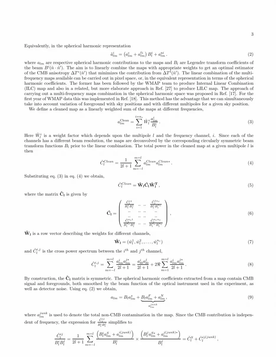
different sky regions are uncorrelated at large l limit. In Ref. [22], we have shown that the residual point sourcecontamination is significantly smaller than the contamination arising from K, Ka, Q or V band. In fact point sourceresidual is intermediate between V and W band point source power. Figure 5 shows, residual unresolved point source

contamination∑k=9

k=1

∑l′ Mk

ll′Wkil′ C

ps(ij)l′ W kj

l′ for different values of i, j. Here i, j are the index representing the 4 DA.All possible combinations (i, j) are explicitly shown in eq. (42). The total unresolved point source spectrum is shownas the pink line with filled circular points. The dominant contributors to the total unresolved point source spectrumat large l are the WW, VW and VV combinations. This is expected since the V and W band share most of theweights at large l because of their higher angular resolutions. Weights are negligible for K, Ka, Q bands in the largel limit and hence point source contamination from these bands is heavily suppressed.

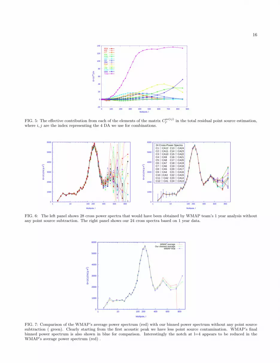
The basis of the WMAP team’s 1 year power spectrum are the 28 cross power spectra which are available from theLAMBDA website in the unbinned form. These 28 cross power spectra are not corrected for the residual unresolvedpoint sources. Following the WMAP team’s 1 year bins we compare these 28 cross power spectra in Fig. 6 with 24cross spectra obtained from our own 1 year results. These 24 cross spectra also are not corrected for the residualunresolved point sources and show very little dispersion compared to the WMAP results. The ‘uniform average’ powerspectrum plotted in green line in fig. 7 has less excess power near the second acoustic peak compared to an ‘uniformaverage’ of the WMAP’s 28 cross spectra (red line). This merely shows that we have removed some amount of pointsources at this range of l during our cleaning.

16

-20

0

20

40

60

80

100

120

140

0 100 200 300 400 500 600 700 800 900

l(l+

1)C

psl/2

π

Multipole, l

KKaKQKVKWKaQQQQVQWKaVVVVWKaWWWTotal

FIG. 5: The effective contribution from each of the elements of the matrix Cps(ij)l′

in the total residual point source estimation,where i, j are the index representing the 4 DA we use for combinations.

0

1000

2000

3000

4000

5000

6000

1 10 100

l(l+

1)C

l/(2π

) [µ

K2 ]

200 400 600 800

Multipole, l

0

1000

2000

3000

4000

5000

6000

1 10 100

l(l+

1)C

l/(2π

) [µ

K2 ]

24 Cross-Power SpectraC1 ⊗ CA12C2 ⊗ CA11C3 ⊗ CA10C4 ⊗ CA9C5 ⊗ CA8C6 ⊗ CA7C7 ⊗ CA6C8 ⊗ CA5C9 ⊗ CA4C10 ⊗ CA3C11 ⊗ CA2C12 ⊗ CA1

C13 ⊗ CA24C14 ⊗ CA23C15 ⊗ CA22C16 ⊗ CA21C17 ⊗ CA20C18 ⊗ CA19C19 ⊗ CA18C20 ⊗ CA17C21 ⊗ CA16C22 ⊗ CA15C23 ⊗ CA14C24 ⊗ CA13

200 400 600 800

Multipole, l

FIG. 6: The left panel shows 28 cross power spectra that would have been obtained by WMAP team’s 1 year analysis withoutany point source subtraction. The right panel shows our 24 cross spectra based on 1 year data.

0

1000

2000

3000

4000

5000

6000

1 10 100

l(l+

1)C

l/(2π

) [µ

K2 ]

200 400 600 800

WMAP averageOur cleaned average

WMAP final

Multipole, l

FIG. 7: Comparison of the WMAP’s average power spectrum (red) with our binned power spectrum without any point sourcesubtraction ( green). Clearly starting from the first acoustic peak we have less point source contamination. WMAP’s finalbinned power spectrum is also shown in blue for comparison. Interestingly the notch at l=4 appears to be reduced in theWMAP’s average power spectrum (red) .

17

D. Computing error bars

We rely upon Monte-Carlo simulation to compute the error bars on our power spectrum. We generate synchrotron,free-free and thermal dust maps corresponding to different frequencies in a given combination using the publiclyavailable Planck Sky Model. Each of the random realizations of CMB and foreground maps are convolved by theappropriate beam function for each detector. Random noise maps corresponding to each detector are generated byfirst sampling a Gaussian distribution with unit variance. In the final step we multiply each Gaussian variable by thenumber σ0/

√Np to form realistic detector noise maps. Here σ0 is the noise per observation of the detector under

consideration and Np the effective number of observations at each pixel. These realistic maps with detector noise,foreground and CMB signal are then passed through the cleaning pipeline. The error-bars for our power spectrumcorrespond to the standard deviation of the power spectrum obtained from Monte-Carlo simulations .

Due to the (Kp2) mask applied to remove potential foreground contaminated regions, the neighboring multipoles

become coupled. In the presence of detector noise, correlation between neighboring Ccl becomes stronger. The

covariance matrix⟨∆Cc

l ∆Ccl′

⟩=⟨(Cc

l −⟨Cc

l

⟩)(Cc

l′ −⟨Cc

l′

⟩)⟩

obtained from simulations is therefore expected to

have non-diagonal elements. It is convenient to bin the power spectrum in order to minimize the correlations anderrors. We have considered a binning identical to that used by the WMAP team in their analysis. Let Cb denotes

the binned power spectrum. Then the covariance matrix of the binned spectrum is obtained as⟨∆Cc

b ∆Ccb′

⟩=

⟨(Cc

b −⟨Cc

b

⟩)(Cc

b′ −⟨Cc

b′

⟩)⟩. The standard deviation obtained from the diagonal elements of the binned covariance

matrix was used as the error-bars on the binned final spectrum extracted from the WMAP data. We also define anormalized covariance matrix of the binned power spectrum following,

Cbb′ =

⟨∆Cb∆Cb′

⟩

√⟨(∆Cb)2

⟩⟨(∆Cb′ )2

⟩ , (51)

wherein all the elements of this matrix are bound to lie between [−1, 1]. This correlation matrix represents the actualbin to bin correlation matrix following the cleaning method. In the left panel of the figure 8 we show the correlationmatrix for WMAP 1 year simulations. The right hand panel of this figure is the corresponding plot for the WMAP 3year analysis. Both these matrices are seen to be sufficiently diagonal dominated.

IV. RESULTS

Figure 9 shows the main result of the power spectrum for CMB anisotropy estimated using our analysis of WMAP1 year and WMAP 3 year data. The blue line shows the WMAP 3 year power spectrum and the red line shows the 1year spectrum. All these spectra are corrected for residual unresolved point source contamination. In the lower panelof this figure we show the residual unresolved point source contamination for 1 year and 3 year respectively. In whatfollows we describe the power spectrum obtained by us for WMAP 1 year data and WMAP 3 year data respectively.

A. WMAP 1 year data

Using the 48 foreground cleaned maps obtained from the WMAP 1 year maps we obtain a ‘Uniform average’ powerspectrum following the method mentioned in section III B. The residual unresolved point source contamination isremoved following III C. The estimated power spectrum with error bars is plotted in red in figure 9.

We find a suppression of power in the quadrupole and octupole moments consistent with the results published bythe WMAP team. However, our quadrupole moment (146µK2) is little larger than the quadrupole moment estimatedby WMAP team (123µK2) and Octupole (455µK2) is less than the WMAP team result (611µK2). The ‘Uniformaverage’ power spectrum does not show the ‘bite’ like feature present at the first acoustic peak in the power spectrumreported by WMAP [10]. We perform a quadratic fit of the form ∆Tl = ∆Tl0 + α(l − l0)

2 to the peaks and troughsof the binned spectrum similar to WMAP analysis [39]. For the residual point source corrected power spectrum weobtain the first acoustic peak at l = 219.8 ± 0.8 with the peak amplitude ∆Tl = 74.1 ± 0.3µK, the second acousticpeak at l = 544±17 with the peak amplitude ∆Tl = 48.3±1.2µK and the first trough at l = 419.2±5.6µK with peakamplitude ∆Tl = 41.7 ± 1µK. The left panel of figure 10 shows the three different ranges of multiples used to findout peak and trough positions and their corresponding amplitudes ∆Tl. (A similar plot for the WMAP 3 year datais shown in the right panel of this figure. The results for WMAP 3 year analysis are summarized in section IVB.)

18

0 5 10 15 20 25 30 350

5

10

15

20

25

30

35

−0.4

−0.2

0

0.2

0.4

0.6

0.8

1

5 10 15 20 25 30 35

5

10

15

20

25

30

35

−0.2

0

0.2

0.4

0.6

0.8

FIG. 8: Correlation matrix<∆Cb∆Cb′>√

<(∆Cb)2><(∆Cb′ )2>

from our simulation plotted with respect to the bin index. As the figure shows

the matrix is mostly dominated by the diagonal elements.

As a cross check of the method, we have carried out the analysis with other possible combinations of the DA maps.

1. The WMAP team also provide foreground cleaned maps corresponding to Q1 to W4 DA (LAMBDA). TheGalactic foreground signal, consisting of synchrotron, free-free, and dust emission, was removed using the 3-band, 5-parameter template fitting method [11]. We also include K and Ka band maps which are not foregroundcleaned. The resulting power spectrum from our analysis matches closely to the ‘Uniform average’ powerspectrum.

2. Excluding the K and Ka band from our analysis we get a power spectrum close to the ‘Uniform average’ results.Notably, we find a more prominent notch at l = 4 similar to WMAP’s published results.

In case of ‘Uniform average’ a maximum difference of 92 µK2 is observed only for octupole. For the large multipolerange the difference is small and for l = 752 it is approximately 48 µK2. This is well within the 1σ error bar (510µK2)obtained from the simulation. This shows that our foreground cleaning is comparable in efficiency to that obtainedby employing template fitting methods that rely on a model of foreground emission to estimate the contamination atthe CMB dominated frequencies.

0

1000

2000

3000

4000

5000

6000

l(l+

1)C

l/(2π

) [µ

K2 ]

0 50

100 150

1 10 100

Res

idua

l. [µ

K2 ]

1yr Residual3yr Residual

Best fit ΛCDM model1yr3yr

200 400 600 800

Multipole, l

FIG. 9: Comparison of 1 year 4 channel with that of 3 year 4 channel power spectrum. The best fit WMAP’s power spectrumis shown in black line along with cosmic variance band. The bottom panel of this figure shows the residual unresolved pointsource contamination for both the power spectra.

The Monte Carlo simulations of our cleaning method also reveals the negative bias in the low l moments. The originof this negative bias is explained in section II B. For l = 2 and l = 3 the bias is −27.4% and −13.8% respectively.However this bias become negligible at higher l, e.g. at l = 22, it is only −0.8%. This bias can be explained in termsof an anti-correlation of the CMB with the residual foregrounds in the cleaned map. For further details of the biaswe refer to appendix E. The standard deviation obtained from the diagonal elements of the covariance matrix is used

19

0

1000

2000

3000

4000

5000

6000

0 100 200 300 400 500 600 700

l(l+

1)C

l/(2

π) [µ

Κ2 ]

Multipole, l

S1

S2

S3

0

1000

2000

3000

4000

5000

6000

0 100 200 300 400 500 600 700

l(l+

1)C

l/(2

π) [µ

Κ2 ]

Multipole, l

S1

S2

S3

FIG. 10: The left panel shows the 3 different multipole ranges used to obtain positions of the first peak, the first trough andthe second peak from our point source subtracted power spectrum using 1 year WMAP data. Before fitting the 1 year powerspectrum was binned in the same manner as the WMAP’s binning. The box error-bars are used to indicate x and y error-bars.The right panel shows the same figure but using the WMAP 3 year data. A correction due to residual unresolved point sourceswas performed prior to fitting.

0

1000

2000

3000

4000

5000

6000

1 10 100

l(l+

1)C

l/(2π

) [µ

K2 ]

200 400 600 800 1000

Multipole, l

0

1000

2000

3000

4000

5000

6000

1 10 100

l(l+

1)C

l/(2π

) [µ

K2 ]

200 400 600 800 1000

Multipole, l

FIG. 11: The left panel shows (in red points) ensemble averaged power spectrum from 110 Monte Carlo simulations of ourpower spectrum estimation method. The simulations were carried out using the 1 year WMAP detector noise maps availablefrom the LAMBDA website. We use publicly available Planck Sky Model to generate the diffuse foreground models. Therecovered spectrum is binned in the same manner as WMAP 1 year power spectrum. The input theoretical spectrum is shownin blue line with cosmic variance. The right panel is same figure but with 3 year noise maps. The 3 year noise maps weregenerated following the method described in the text. The spectrum is binned following the binning scheme of the WMAPteam’s analysis of 3 year data.

as the error bars on the Cl’s obtained from the data. The ensemble average of 110 cleaned power spectrum is shownin the left panel of the figure 11. The presence of bias at the low multipole moments is visible is this figure.

B. WMAP 3 year data

1. 4 channel combinations

We analyse the 3 year WMAP data by using a procedure identical to that used for the 1 year data. The detailsare given in section II. In figure 12 we show each of the 24 cross power. The ‘Uniform average’ of these 24 crosspower spectra is also shown in this figure in red line with blue error-bar. This figure is similar to the 24 individualcross power spectra obtained for WMAP 1 year data [21, 22]. For the 3 year data all the 24 cross power spectra showvery little dispersion till the second trough. In comparison the 1 year data shows small dispersion only till the secondacoustic peak [21]. This may be explained due to the effectively lower detector noise in the 3 year data compared to

20

the 1 year data.

0

1000

2000

3000

4000

5000

6000

1 10 100

l(l+

1)C

l/(2π

) [µ

K2 ]

24 Cross-Power SpectraC1 ⊗ CA12C2 ⊗ CA11C3 ⊗ CA10C4 ⊗ CA9C5 ⊗ CA8C6 ⊗ CA7C7 ⊗ CA6C8 ⊗ CA5C9 ⊗ CA4C10 ⊗ CA3C11 ⊗ CA2C12 ⊗ CA1

C13 ⊗ CA24C14 ⊗ CA23C15 ⊗ CA22C16 ⊗ CA21C17 ⊗ CA20C18 ⊗ CA19C19 ⊗ CA18C20 ⊗ CA17C21 ⊗ CA16C22 ⊗ CA15C23 ⊗ CA14C24 ⊗ CA13

200 400 600 800 1000

Multipole, l

FIG. 12: The 24 cross power spectra for the 3 year WMAP data are shown with the detector noise bias removed. The redline with blue error-bars is the ‘Uniform average’ power spectrum. In the inset of this figure we show all the possible crosscorrelations of the cleaned maps that give rise to the 24 cross spectra.

We perform a peak fitting to the peaks and troughs of the 3 year power spectrum as well. A parabolic functionof the form ∆Tl = ∆Tl0 + α(l − l0)

2 is fitted to the peaks and troughs of the power spectrum amplitude. We usethe 3 year binned data for the fitting purpose. For the point source corrected power spectra, the first acoustic peakhas an amplitude ∆Tl0 = 74.4 ± 0.3µK at the multipole position l = 219.9 ± 0.8. The first trough is located atl = 417.7± 3.2 with an amplitude ∆Tl0 = 41.4± 0.6µK. The amplitude and position of the second acoustic peak aregiven by ∆Tl0 = 49.4 ± 0.4µK, l = 539.5± 3.7. In the right panel of figure 10 we show the different multipole rangesused to obtain the position of the peaks and troughs and their amplitudes.

2. 3 channel combinations

We also follow an alternative approach in which we use only the Q,V and W band DA maps. This is similar tothe 4 channel cleaning, however now we only get 24 cleaned maps. We form a total of 12 cross power spectra fromthese cleaned maps after applying 3 year Kp2 mask. After debiasing all the power spectra by the coupling matrixand removing beam and pixel effect we obtain an ‘3 channel uniform average’ power spectrum. We find that the 3channel spectrum matches well with the 4 channel spectrum.

C. Comparison of 1 year and 3 year power spectra

Fig. 9 compares the power spectra obtained from the 1 year and 3 WMAP data binned identically using theWMAP team’s 1 year binning method. They match closely with one another and also with the WMAP’s best fitpower spectrum available from the LAMBDA website. For the residual point source corrected power spectrum weobtain for WMAP 1 year (WMAP 3 year) data the first acoustic peak at l = 219.8± 0.8 (219.9± 0.8) with the peakamplitude ∆Tl = 74.1 ± 0.3µK (74.4 ± 0.3µK), the second acoustic peak at l = 544± 17 (539.5± 3.7) with the peakamplitude ∆Tl = 48.3 ± 1.2µK (49.4 ± 0.4µK) and the first trough at l = 419.2 ± 5.6µK (417.7 ± 3.2) with peakamplitude ∆Tl = 41.7 ± 1 µK(41.4 ± 0.6µK).

We note that our cleaning method significantly removes unresolved point source contamination. The original l2

dependence of the unresolved point source power spectrum present in the foreground contaminated maps (as wellpresent in template cleaned maps) is significantly reduced and becomes independent of l at large l. We also note thatthe unresolved residual point source contamination is less by about ≈ 50µK2 in 3 year power spectrum than the 1year power spectrum. This is expected. The WMAP supplied 3 year Kp2 mask removes more point sources than the1 year Kp2 mask.

21

V. CONCLUSION

The rapid improvement in the sensitivity and resolution of the CMB experiments has posed increasingly stringentrequirements on the level of separation and removal of the foreground contaminants. We carry out an estimation ofthe CMB power spectrum from the WMAP data that is independent of foreground model. The method does not relyupon any foreground template and employs the lack of noise correlation between independent channels. This paperis a detailed description of the first estimate of the CMB angular power spectrum solely based upon the WMAPdata. In this paper, we present an indepth study of the biases that arise in the foreground cleaning. In particular, weprovide an understanding and correction for the negative bias at low multipoles reported in our earlier work [21].

Usual approaches to foreground removal, usually incorporate the extra information about the foregrounds availableat other frequencies, the spatial structure and distribution in constructing a foreground template at the frequencies ofthe CMB measurements. These approaches may be susceptible to uncertainties and inadequacies of modeling involvedin extrapolating from the frequency of observation to CMB observations that a blind approach, such as presentedhere, evades. The understanding of polarized foreground for CMB polarization maps is rather scarce. Hence modelinguncertainties could dominate the systematics error budget of conventional foreground cleaning. The blind approachextended to estimating polarization spectra after cleaning CMB polarization maps could prove to be particularlyadvantageous.

Acknowledgments

The analysis pipeline as well as the entire simulation pipeline is based on primitives from the HEALPix package. 8

We acknowledge the use of version 1.1 of the Planck reference sky model, prepared by the members of Working Group2 and available at www.planck.fr/heading79.html The entire analysis procedure was carried out on the IUCAA HPCfacility as well as on the computing facilities at IAP. RS acknowledges the Indo-French Sandwich Fellowship granted bythe French Embassy in India and EGIDE in Paris, France. RS thanks IAP for hosting his visit. RS thanks FrancoisBouchet, Christophe Pichon, Karim Benabed, Pawel Bielewicz and Planck group members at IAP for useful andilluminating discussions. We are grateful to Lyman Page, Olivier Dore, Charles Lawrence, Kris Gorski, Hans KristianEriksen and Max Tegmark for thoughtful comments and suggestions. We acknowledge a private communication withGarry Hinshaw on the unresolved point source model. We thank Amir Hajian, Subharthi Ray and Sanjit Mitra inIUCAA for helpful discussions. We thank the WMAP team for producing excellent quality CMB maps and makingthem publicly available.

APPENDIX A: ANALYTIC DERIVATION OF WEIGHTS AND CLEANED POWER SPECTRUM

The main idea behind the blind foreground cleaning method used here is entirely based upon the minimization oftotal power in the cleaned map in multipole space [18]. Weights for different channels are obtained minimizing the

total power CCleanl of the cleaned map. However, we ensure that the CMB angular power spectrum is conserved during

cleaning by imposing the constraint Wle0 = eT0 WT = 1 on the weights. The solution for the weights that satisfy these

conditions is the point in weight space where normals to the functions f(Wl) = WlClWTl and g(Wl) = Wle0 are

parallel to one another. Following Lagrange’s multiplier method, this is cast to an equivalent problem of minimizing

WlClWTl − λWle0 . (A1)

Here λ is the unknown Lagrange multiplier parameter which could be determined from variational principle. At theextrema, the expression in eq. (A1) is unchanged under small variations in Wl leading to

∆WlClWTl + WlCl∆WT

l − λ∆Wle0 = 0 . (A2)

Since the power spectrum matrix, Cl is a symmetric matrix, the first two terms of the left hand side are equal to oneanother. Hence we obtain,

∆Wl

[2ClW

Tl − λe0

]= 0 . (A3)

8 The HEALPix distribution is publicly available from the website http://healpix.jpl.nasa.gov.

http://healpix.jpl.nasa.gov

22

Since this relation is true for any arbitrary variation ∆Wl, we obtain[2ClW

Tl − λe0

]= 0 . (A4)

We introduce a (non zero) square matrix Gl. Later we will identify Gl as the Moore Penrose Generalized Inverse

(MPGI) of the covariance matrix Cl. After multiplication from left by this matrix we can rewrite the above equationas

2GlClWTl − λGle0 = 0 . (A5)

Hence we obtain

λ =2eT

0 GlClWTl

eT0 Gle0

. (A6)

Now we use the constraint Wle0 = 1. Assuming Wl 6= 0 we multiply eq. (A4) from left by Wl and to obtain

2WlClWTl = λWle0 = λ . (A7)

Using eq. (A6) and eq. (A7) we obtain

2WlClWTl = 2

eT0 GlClW

Tl

eT0 Gle0

, (A8)

or,(

Wl −eT0 Gl

eT0 Gle0

)ClW

Tl = 0 . (A9)

If we neglect solutions which belongs to null space of Cl,9 i.e., assuming ClW

Tl 6= 0, we obtain

Wl =eT0 Gl

eT0 Gle0

. (A10)

We impose the restriction on Gl that it is symmetric (since the MPGI of a symmetric matrix is symmetric) to obtain

WTl =

Gle0

eT0 Gle0

. (A11)

The corresponding power spectrum of the cleaned map is given by

WlClWTl =

eT0 Gl

eT0 Gle0

Cl

Gle0

eT0 Gle0

=1

eT0 Gle0

, (A12)

where we have imposed the condition GlCl = ClGl. It is easy to note that the choice of symmetric Gl helps toobtain a simplified expression for the cleaned power spectrum. Also one can verify that, if GlClGl = Gl is satisfiedand Gl is symmetric then Gl satisfies all the defining conditions of MPGI of Cl. Hence, we can identify Gl as theMoore-Penrose Generalized Generalized Inverse (MPGI) of Cl (and vice versa).

Eq. (A12) has an interesting property. It remains valid even when the full covariance matrix Cl is singular. Asingular full covariance matrix is encountered in noiseless case (or numerically very low noise case) when the foregroundcomponents follow a rigid frequency scaling and total number of components (all foregrounds and CMB) become less

than the number of available channels. If Cl is non singular we can replace Gl everywhere by C−1l . This is because

MPGI of a non-singular matrix is its inverse.

9 There is a physical justification behind neglecting this solution. The weights satisfying ClWTl

= 0 do not preserve CMB power while

minimizing total power in the cleaned map. These solution for the weights merely sets the total power in the cleaned map WlClWTl

= 0.

Thus we are not interested in the space of solutions to ClWTl

= 0.

23

APPENDIX B: PARTITIONING THE SKY

An important advantage of the foreground cleaning analyzed here is that we can allow the weights to vary withsky positions as well as with the multipole moment. To allow the weights to vary with sky positions we can partitionthe sky into several regions depending upon the level of foreground contamination. (Alternatively the partition couldbe done directly using the knowledge of expected spectral index dependence on the sky.) We followed the procedureof Ref. [18] to partition the sky. Each of these partitions are identified with a sky masks. The mask takes non zerovalue at all pixels contained within the sky partition represented and is zero outside. In this section we describe theprocedure of constructing these masks.

There are 2 Difference Assemblies for Q band, 2 for V band and 4 for W band. To make the masks we first averagedall the DA maps for a given frequency band. Correspondingly we averaged the beam functions for each frequency band.For the K and KA bands there are only one difference assembly in each case. Therefore for these bands no averagingwas done. We smoothed all the five maps (e.g. K, Ka, Q, V, W) by the resolution function of the K band, whichhas the lowest resolution. We obtained four difference maps W-V, V-Q, Q-K, K-Ka, out of these 5 smoothed maps.The smoothing was performed first obtaining the alm coefficients. As each averaged map was effectively smoothed bythe averaged beam function (corresponding to each channel) during the observations, we decided to first remove thebeam effect. Then we smoothed each map by the common resolution of the lowest frequency band. Mathematically,the difference maps were obtained as follows:

aW−Vlm = aW

lm

BKl

BWl

− aVlm

BKl

BVl

, (B1)

aV −Qlm = aV

lm

BKl

BVl

− aQlm

BKl

BQl

, (B2)

aQ−Klm = aQ

lm

BKl

BQl

− aKlm , (B3)

aK−KAlm = aK

lm − aKAlm

BKl

BKAl

. (B4)

The alm were converted to difference maps using HEALPix supplied subroutine alm2map.Next we construct a junk map out of these four difference maps assigning at each pixel the absolute maximum

value among the four difference maps. We down-sample the junk map using the HEALPix supplied program udgradeto a resolution of Nside = 64. We identify 7 different sky mask partitions from this low resolution junk map afterapplying cutoff corresponding to the following temperature thresholds (in µK) T > 30000, 30000 ≥ T > 10000,10000 ≥ T > 3000, 3000 ≥ T > 1000, 1000 ≥ T > 300, 300 ≥ T > 100 and T < 100. The partition T > 30000is maximally contaminated by foreground emission. The second dirtiest partition is disjoint on the sky and we use3 separate masks corresponding this partition. The resulting 9 masks are then converted back to the HEALPixresolution Nside = 512 using udgrade routine of HEALPix. Next we smooth each mask using a Gaussian beam ofFWHM 30′ and redefine smoother mask boundaries at the threshold of 0.5. 10 In this case we found that almost theentire sky is covered by the 9 masks (except for a few pixels in the sky).

To convert the second dirtiest region into 3 mask files we upgraded the Nside = 64 resolution map to the Nside = 512.Then using IDL task mollcursor, we found out the extension in galactic θ, φ coordinates of the 3 different parts of the

10 We found that if we smooth them by a Gaussian function of FWHM 2 degree (as mentioned in Ref. [18]) and then define the boundariesat the threshold of 0.5 the resulting 9 masks cannot cover the entire sky. In that case there are some regions near the galactic planewhich do not belong to any of our 9 masks. Obviously if such regions are not covered by any of the masks and remain present in ourfinal cleaned map then final power spectrum will be contaminated by the foreground. Therefore we chose to use a Gaussian functionof lower FWHM of 30′ for smoothing. The reason why in our case, masks smoothed by a 2 degree Gaussian function cannot cover theentire sky is clear. This is actually dependent on the common beam function by which we are smoothing each map before forming thedifference maps. We found that the masks near the galactic regions contain a few small isolated regions. Therefore smoothing by aGaussian with FWHM as large as 2 degree, gives this isolated small regions maximum value far less than unity, in fact maximum valuebecomes quite near 0.5, the cutoff value, after smoothing. Consequently applying a cut of 0.5 removes most of the part of these isolatedregions, leading to some part of the sky, uncovered by the masks.

24

second dirtiest region. We then implemented a method which determines the pixel index in ‘ring’ format for these 3regions. Finally we converted them to 3 different masks at Nside = 512. The masks were then smoothed by Gaussianfunction of FWHM =30′. We applied a cutoff of 0.5 to each of them. The 8th, 7th and 6th masks were numberedaccording to the descending order of maximum pixel value in the junk map at resolution Nside = 512.

Figure 2 shows our 9 different masks that partition the sky based on estimated level of foreground contamination.These regions are similar to what is shown in Ref. [18]. As the figure shows, one side of the band near the galacticplane is more severely foreground contaminated.

APPENDIX C: COMBINING CROSS POWER SPECTRA

The basis of our final power spectrum are a set of 24 cross power spectra where the detector noise bias has beenremoved. An uniform weighting of cross spectra is used to obtain the final power spectrum. In this section we describethe procedure to obtain the 24 cross spectra and their combination to form the final spectrum.

Let us assume that ∆T i(θ, φ) represents one of the 48 final cleaned map, where (i = 1, 2, 3, ..., 48). To remove theresidual foreground contamination near the galactic plane (figure 3) we apply the Kp2 mask supplied by the WMAPteam on each of these 48 maps. The masked map can be represented as

∆T ′i(n) = W (n)∆T i(n) . (C1)

Here W (θ, φ) represents the Kp2 mask. In the next step, we obtain a cross power spectrum between pairs of foreground

cleaned maps that have uncorrelated noise (recall that noise in different DAs are uncorrelated). If ailm and aj

lm arethe spherical harmonic coefficients obtained from two such maps

ai,jlm =

∫W (n)∆T i,j(n)dΩ . (C2)

The cross power spectrum is obtained using,

Cijl =

m=l∑

m=−l

ailmaj∗

lm

2l + 1. (C3)

Here the superscript ij represents the cross power spectrum obtained from the ith and jth foreground cleaned maps.Following Ref. [34], the ensemble average of the Cl estimated from the partial sky is related to the Cl from the fullsky as

⟨Cl

⟩=∑

l′

Mll′

⟨Cc

l′

⟩, (C4)

where Mll′ is a coupling matrix. This matrix represents the fact that when we multiply our map by the weightfunction (Kp2 mask) in the pixel space we are effectively performing a smoothing operation and neighboring sphericalharmonic coefficients get coupled. An analytic expression for this coupling matrix is given in Ref. [34],

Ml1l2 =2l2 + 1

4π

l3=l1+l2∑

l3=|l1−l2|

(2l3 + 1)Wl3

(l1 l2 l30 0 0

)2

, (C5)

where the last term is the Wigner-3j symbol and Wl is the power spectrum of the mask under consideration. Althoughin our case we are interested in the partial sky power spectrum which has been obtained by cross correlating twodifferent maps, it is easy to show that in this case also eq. (C4) remains valid. The rank of the coupling matrix islimited to lmax = 1024. We use numerical routines from the netlib package [40] to compute the Wigner -3j symbol.

Eq. (C4) is true only for an ideal observation with infinite angular resolution. In practice all instruments have finiteangular resolution given by the beam function B(θ, φ) of the instrument. Mathematically, we may write the observedtemperature anisotropy,

∆T (n) =

∫∆T ′(n′)B(n, n′)dΩn′ , (C6)

where ∆T ′(n′) is now the full sky map in the absence of the beam. In most of the CMB experiments the beamfunction is circularly symmetric to a good approximation, i.e., depends only on the angle θ′′ = cos−1(n · n′) betweentwo directions n and n′,

B(n, n′) ≡ B(n · n′) . (C7)

25

We may expand this function in terms of Legendre polynomials,

B(n · n′) =

l=∞∑

l=0

2l + 1

4πBlPl(n · n′) . (C8)

Here, Bl’s are Legendre transform of the beam function. Substituting this in eq. (C6) and expanding ∆T and ∆T ′ inspherical harmonics, we obtain

l=∞∑

l=0

m=l∑

m=−l

almYlm(n) =

l′=∞∑

l′=0

m′=l′∑

m′=−l′

a′l′m′

∫Yl′m′(n′)

l′′=∞∑

l′′=0

2l′′ + 1

4πBl′′Pl′′ (n · n′)dΩn′ . (C9)

Using the addition formula

Pl′′(n · n′) =4π

2l′′ + 1

m′′=l′′∑

m′′=−l′′

Yl′′m′′(n)Y ∗l′′m′′(n′) (C10)

and the orthonormality property of spherical harmonics

∫Yl′m′(n′)Y ∗

l′′m′′(n′) = δl′l′′δm′m′′ , (C11)

we obtain,

l=∞∑

l=0

m=l∑

m=−l

almYlm(n) =

l′=∞∑

l′=0

m′=l′∑

m′=−l′

a′l′m′Yl′′m′′(n)Bl′ . (C12)

We again use orthonormality of spherical harmonics to obtain

alm = a′lmBl . (C13)

This relation shows that due to the finite resolution of the instrument spherical harmonic coefficients get multipliedby the Legendre transform of the beam function. Hence it is easier to account for the effect of a circular beam in thespherical harmonic space than deconvolving the map by the beam function in the pixel space.

The effect of finite pixel size of the map has similar effect on the recovered spherical harmonic coefficients. Thepixel window functions pl have been supplied with the HEALPix distribution for different resolutions. Taking intoaccount finite pixel size we have

alm = a′lmBlpl . (C14)

Hence the recovered power spectrum is related to the actual CMB sky power spectrum as

Cl = C′lB

2l p2

l . (C15)

In presence of both beam and finite pixel effects, eq. (C4) obtained for the ideal case 11 is now modified to

⟨Cl

⟩=∑

l′

Mll′

⟨Cc

l′

⟩B2

l′p2l′ . (C16)

A generalization of this expression in case of cross power spectrum has been also reported in Ref. [35]. The partialsky cross power spectrum is related to the full sky power spectrum in the following manner

⟨Cij

l

⟩=∑

l′

Mll′

⟨Cc

l′

⟩Bi

l′Bjl′p

2l′ . (C17)

11 In Ref. [34] the authors followed the convention that Bl represents combined smoothing effect due to pixel as well as beam. Our notationis different from them.

26

Here we note that the noise terms drop out in the cross-correlation procedure.The final estimate of the full-sky spectrum is obtained by simply inverting the coupling matrix. We have used a

singular value decomposition technique to invert our matrix. We checked that this matrix gives unbiased estimatesof the full sky power spectrum using Monte Carlo simulations of CMB maps and using Kp2 cut.

The final full sky estimate of the power spectrum is obtained from

Cil =

∑

l′

(M−1)ll′Cijl′ /Bi

lBjl p

2l . (C18)

with i ≡ (i, j), i = (1, 2, 3, 4, ..., 24) as there are 24 cross-correlations possible that do not have detector noise bias.Using the 24 cross-power spectra we form an averaged power spectrum following

Cl =

i=24∑

i=1

Cil Ncross (C19)

where Ncross = 1/24. Now we bin them in the same manner as the WMAP. The binned power spectrum is defined as

Cb =1

∆l

l=lmax∑

l=lmin

l(l + 1)

2πCl , (C20)

with ∆l = lmax + 1 − lmin. Eqn. (C20) defines our final power spectrum.

APPENDIX D: ESTIMATION OF RESIDUAL UNRESOLVED POINT SOURCE CONTAMINATION

In this appendix we study the point source bias in the auto power spectrum of a cleaned map and in the crosspower of two cleaned maps. From a detailed study of a single iteration cleaning method we verify that a residual pointsource bias in the auto or cross power spectrum of the cleaned maps could be very well approximated by WC

psl WT

l ,

without a need to compute⟨WC

psl WT

l

⟩. For the auto power spectrum we optain an analytic point source bias in

terms of the noise covariance matrix and the point source covariance matrix. We note that, in practice when weestimate cosmological power spectrum from the WMAP data we do not use the auto power spectrum of a cleanedmap. Nevertheless the auto power spectrum is important to study along with the cross power spectrum for a deeperunderstanding of the point source bias. We note that in all the Monte Carlo simulations in this section we treat pointsources as fixed templates. The sources of randomness come from CMB and detector noises.

1. Auto Power Spectrum

Following eq. (27) the cleaned auto power spectrum obeys,

⟨CClean

l

⟩=⟨Cc

l

⟩+

⟨1

eT0 (Cf+N

l )−1

e0

⟩+ (1 − nc)

⟨Cc

l

⟩

2l + 1. (D1)

Clearly the positive bias is given by⟨1/eT

0 (Cf+Nl )

−1e0

⟩which is caused by the detector noise and foreground

covariance matrix of the map. In this appendix we are basically interested in studying point source bias and sincediffuse foreground is not a concern at large l, we do not include any diffuse foreground component in this study.Considering the second term on the right hand side of eq. (D1) we note that it is not possible to identify a biaswhich solely comes from point sources. Another point to note is that we know only the mean noise covariance matrix,CN

l , not the empirical noise covariance matrix, CNl , where CN

l = CNl + δCN

l and δCNl denotes noise fluctuation on

the true noise level. Therefore we express⟨1/eT

0 (Cf+Nl )

−1e0

⟩in terms of a mean noise covariance matrix and the

foreground covariance matrix. As we will see such a simplification helps us to obtain an analytical expression for thepoint source bias. Keeping in mind that WMAP detector noise level is much larger than the point source spectrum,

27

we simplify⟨1/eT

0 (Cf+Nl )

−1e0

⟩analytically by making expanding to first order 12, in terms of C

psl (CN

l )−1

,

(Cf+Nl )

−1= ˆ(CN

l )−1

− ˆ(CNl )

−1

Cpsl

ˆ(CNl )

−1

, (D2)

Due to the low point source contamination relative to the WMAP noise level it is reasonable to assume that

(eT0 (CN

l )−1

Cpsl (CN

l )−1

e0)/(eT0 (CN

l )−1

e0) ≪ 1. Expanding to first order we obtain,

⟨1

eT0 (Cf+N

l )−1

e0

⟩=

⟨1

eT0 (CN

l )−1

e0

⟩+

⟨eT0 (CN

l )−1

eT0 (CN

l )−1

e0

Cpsl

(CNl )

−1e0

eT0 (CN

l )−1

e0

⟩. (D3)

We interprete the first term on the right hand side as the detector noise bias. The second term is the point sourcebias. In the following subsections we recast these results in terms of the mean noise covariance matrix. We also verifyour analytic expressions using Monte Carlo simulations.

a. Noise induced bias

We first turn our attention to the detector noise bias. We estimate this term upto second order in δCNl (CN

l )−1

,

⟨1

eT0 (CN

l )−1

e0

⟩=

⟨1

eT0 (CN

l )−1

e0

(1 +

eT0 (CN

l )−1

δCNl (CN

l )−1

e0

eT0 (CN

l )−1

e0

−eT0 (CN

l )−1

δCNl (CN

l )−1

δCNl (CN

l )−1

e0

eT0 (CN

l )−1

e0

+(eT

0 (CNl )

−1δCN

l (CNl )

−1e0)2

(eT0 (CN

l )−1

e0)2

)⟩. (D4)

The noise fluctuations are assumed to have zero mean,⟨δCN

l

⟩= 0. Hence the second term in the bracket vanishes

on the ensemble average. Only the numerators of the third and fourth terms in the bracket on the right hand side ofeq. (D4) are stochastic variables. On the ensemble average the numerator of the third term becomes,

⟨eT0 (CN

l )−1

δCNl (CN

l )−1

δCNl (CN

l )−1

e0

⟩=

⟨∑

i,j,k

CNil δC

N(ij)l CNj

l δCN(jk)l CNk

l

⟩=∑

i,j,k

CNil CNj

l CNkl

⟨δC

N(ij)l δC

N(jk)l

⟩,

where we have assumed that the noise covariance matrix of WMAP is diagonal. We simplify the ensemble averaged

quantities using the relation eq. (28) of Ref. [35]. If we consider a general term of the form⟨δC

N(ij)l δC

N(kp)l

⟩then

for uncorrelated detector noises, the ensemble averaged quantities will survive only for the same pair, i.e. when(i, j) = (k, p). We further note that,

⟨δC

N(ij)2

l

⟩=

1

2l+1CNil CNj

l , i 6= j2

2l+1CNil CNi

l , i = j. (D5)

Using above relations the third and fourth term in the bracket of eq. (D4) become

⟨eT0 (CN

l )−1

δCNl (CN

l )−1

δCNl (CN

l )−1

e0

eT0 (CN

l )−1

e0

⟩=

(1 + nc)

2l + 1, (D6)

Following a similar method we also simplify the fourth term in eq. (D4). The final result is

⟨(eT

0 (CNl )

−1δCN

l (CNl )

−1e0)2

(eT0 (CN

l )−1

e0)2

⟩=

2

2l + 1. (D7)

12 We note that we cannot use Sherman-Morrison formula to decouple the foreground and detector noise bias from the termfi

1

eT0

(Cf+N

l)−1

e0

fl

in an useful form.

28

-1000

-800

-600

-400

-200

0

200

400

600

800

1000

0 200 400 600 800 1000

l(l+

1)C

l/(2π

) µ

K2

Multipole,l

Empirical-Analytical

FIG. 13: The difference between the empirical noise bias and the theoretical estimate of noise bias given in eq. D8 for V andW bands.

Using eqs. (D4), (D6), (D7) we obtain,

⟨1

eT0 (CN

l )−1

e0

⟩=

⟨1

eT0 (CN

l )−1

e0

(1 −

1 + n

2l + 1+

2

2l + 1

)⟩=

1

eT0 (CN

l )−1

e0

2l + 2 − nc

2l + 1. (D8)

This enables us to compute the noise bias in terms of the theoretical noise models. We verified this equation byMonte-Carlo simulations of 1000 noise covariance matrices corresponding to WMAP V and W bands. The noise mapsfrom which these empirical noise covariance matrices were computed were formed following a method similar to that

mentioned in section III D. In Fig. 13 we show the difference between the empirical noise bias⟨1/eT

0 (CNl )

−1e0

⟩

and the second order analytical expression for noise bias, given by the right hand side of eq. (D8). The difference isconsistent with zero. The large fluctuations at large l is caused by the beam deconvolution effect in the effective noisecovariance matrix.

b. Point source bias

Here we study the point source bias. We perform Monte-Carlo simulations in a single iteration cleaning withCMB, point sources and detector noise having WMAP’s noise level. We compute ensemble averaged cleaned power

spectrum⟨CClean

l

⟩from 1000 such simulations. The validity of eq. (D8) allows us to compute noise bias in terms of

the theoretical noise covariance matrix and subtract this analytical result from⟨CClean

l

⟩. After correcting for noise

bias we find that⟨CClean

l

⟩−(1/eT

0 (CNl )

−1e0

)((2l + 2 − nc)/(2l + 1)) still has a residual positive bias at multipole

range l > 400. This excess is a clear demonstration of the presence of point source bias. The brown line in Fig. 14is the power spectrum, corrected for the noise and the negative CMB bias of the form −Cc

l /(2l + 1). The excess iscaused by the point source bias. We analytically compute the point source bias in terms of theoretical noise covariance

matrix similar to eq (D8). Following a first order expansion in Cpsl (CN

l )−1

and a second order expansion in terms of

δCNl (CN

l )−1

we obtain,

⟨eT0 (CN

l )−1

eT0 (CN

l )−1

e0

Cpsl

(CNl )

−1e0

eT0 (CN

l )−1

e0

⟩=

eT0 (CN

l )−1

eT0 (CN

l )−1

e0

Cpsl

(CNl )

−1e0

eT0 (CN

l )−1

e0

2l

2l + 1+

tr(Cpsl (CN

l )−1

)

(2l + 1)(eT0 (CN

l )−1

e0). (D9)

Again we verify the validity of the above expression following Monte Carlo simulations. We compute the point source

bias from 1000 cleaning simulations following⟨CClean

l

⟩−Cc

l −Ccl /(2l+1)−

(1/eT

0 (CNl )

−1e0

)((2l + 2 − nc)/(2l + 1))

29

0

1000

2000

3000

4000

5000

6000

1 10 100

l(l+

1)C

l/(2π

) [µ

K2 ]

200 400 600 800 1000

Theory ClCleaned Cl+ ps bias

Multipole, l

FIG. 14: The auto power spectrum without correcting for the residual unresolved point source bias is shown in brown line.The blue line shows the theoretical CMB power spectrum.

where Ccl denotes the theoretical CMB power spectrum. In Fig. 15 the green line shows the binned estimate of the

point source bias from simulations. The error-bars plotted in this figure are valid for the mean of 1000 simulationsof random samples. The black line with filled points shows the analytical estimate of the point source bias computedfrom the right hand side of the eq. (D9). These two results match closely except at the last two points. However,one can easily conclude from the error-bars plotted in this figure that differences between the two lines at these twopoints are not significant. We interprete these deviations as noise fluctuations.

Given the large noise level of WMAP maps, one might expect that⟨WlC

psl WT

l

⟩would be a good approximation

of the point source bias that is given by the second term of eq. (D3). In the limit Cl → CNl , applicable when noise

dominates at large l and point source bias is also significant, these two terms are identical. Using the analytical formof weights as in eq. (14), we find that up to the first order in C

psl CN−1

l ,

⟨WlC

psl WT

l

⟩=

⟨eT0 (CN

l )−1

eT0 (CN

l )−1

e0

Cpsl

eT(CNl )

−1

eT0 (CN

l )−1

e0

⟩−

Ccl

2l + 1

⟨eT0 (CN

l )−1

Cpsl (CN

l )−1

e0

eT0 (CN

l )−1

e0

⟩

+Cc

l

2l + 1tr(Cps

l

⟨(CN

l )−1⟩) . (D10)

Here, Ccl is the theoretical CMB power spectrum. However, the last two terms in the above equations are negligibly

small compared to the first term on the right hand side. From simulations we find that these two terms contributeless than 0.1µK2 to the point source residual when multiplied by the prefactor l(l + 1)/(2π). The reason why these

terms become negligible is that, apart from a multiplicative first order term, Cpsl (CN

l )−1

, the first term on the righthand side go as CN

l , whereas the last two terms goes as Ccl /(2l + 1). Indeed, the noise becomes much larger than

CMB power spectrum at large l due to beam deconvolution, making the two last two terms insignificant compared tothe first term. In figure 16 we show magnitude of the individual contributions arising from the second and third termfollowing 1000 Monte Carlo simulations of the cleaning method. We use V and W bands in the simulations usingrealistic WMAP noise levels and residual unresolved point source model. The red line shows the difference betweenthe two terms which is less than 0.01µK2 or even smaller at l > 400. Hence it is justified to assume,

⟨WlC

psl WT

l

⟩=

⟨eT0 (CN

l )−1

eT0 (CN

l )−1

eC

psl

eT0 (CN

l )−1

eT0 (CN

l )−1

e0

⟩. (D11)

In Fig. 14 we show the point source bias computed following⟨WlC

psl WT

l

⟩in blue line. This matches well with the

black line with filled circle, justifying eq. (D11).

The unresolved point source bias is then⟨WlC

psl WT

l

⟩. Now we propose that, the point source bias could also

be taken into account following WlCpsl WT

l ∼⟨WlC

psl WT

l

⟩. The reason is that, at large l where detector noise

dominates. The weights are entirely determined by the mean noise level. Therefore weights become approximately

30

0

50

100

150

200

0 200 400 600 800 1000

l(l+

1)C

l/(2π

) µ

K2

Multipole,l

Emperical PS biasPS bias, seed 500

PS bias, analyticEnsemble averaged PS bias

FIG. 15: The point source bias,D

WlCps

l WTl

E

(blue line), and the approximation WlCps

l WTl (red line) for the case of

auto power spectrum of the cleaned maps. The empirical point source bias computed by usingD

CCleanl

E

− Ccl − Cc

l /(2l +

1) −“

1/eT0 (CN

l )−1

e0

”

((2l + 2 − nc)/(2l + 1)) is shown in green line. The error bars are computed only for the termD

1/eT0 (CN

l )−1

e0

E

without including the cosmic variance. All the data points are binned following the WMAP’s 3 year binning

method. The analytical point source bias computed following eq. (D9) is also shown in black line with black dots.

1e-05

1e-04

0.001

0.01

0.1

1

10

100

0 200 400 600 800 1000

l(l+

1)C

l/(2π

) µ

K2

Multipole,l

PsB2PsB3

PsB3-PsB2

FIG. 16: The contributions arising from the third (blue line) and fourth (pinkline) terms of eq. (D10) and their difference.

constant from realization to realization. Small fluctuations in weights due to noise fluctuations are not important

compared to the magnitude of total point source bias⟨WlC

psl WT

l

⟩. The advantage of this method is that, we can

estimate point source bias in terms of the weights which are the results of a cleaning. In the figure 15 we show how

well WlCpsl WT

l (red line) matches with⟨WlC

psl WT

l

⟩. This result is obtained from 1000 Monte Carlo simulations

of our cleaning method using V and W bands.

2. Cross Power Spectrum

We now consider point source bias in case of cross power spectrum of two cleaned maps. In this case the cleanedpower spectrum is given by,

⟨CClean

l

⟩= Cc

l + 2(1 − nc)Cc

l

2l + 1+ < W1

l Cpsl W2T

l > + < W1l C

N(12)l W2T

l > . (D12)

31

0

1000

2000

3000

4000

5000

6000

1 10 100

l(l+

1)C

l/(2π

) [µ

K2 ]

200 400 600 800 1000

Theory Ccl

Cleaned <Cl> + PS bias

Multipole, l

-50

0

50

100

150

200

250

0 100 200 300 400 500 600 700 800 900 1000

PS bias, from simulation PS bias seed = 500

PS bias, seed = 2PS bias,seed 2,1001

FIG. 17: Left: The point source bias at large multipole range obtained from 1000 Monte Carlo simulations of the cleaningmethod involving V and W bands is shown in blue line. The CMB bias 1−nc

2l+1Cc

l has been removed before plotting the blueline to show the bias coming from point source only. The red line shows the theoretical power spectrum from which random

realization of CMB were drawn.Right: Point source bias computed fromD

CCleanl

E

−Ccl −2(1−nc)

Ccl

2l+1is shown in red line. The

magenta line shows point source bias computed fromD

W1l C

ps

l W2T

l

E

which agrees excellently with W1l C

ps

l W2T

l computed

from two arbitrary realizations shown in green and blue lines.

Here W1l and W2

l are the weight vectors for the two cleaned maps and CN(12)l denotes a chance noise correlation

in the two sets of maps used to obtain two cleaned maps. From Monte-Carlo simulations involving cross spectrum,v1w12⊗ v2w34, v1w13⊗ v2w24, v1w14⊗ v2w23, v1w24⊗ v2w13, v1w34⊗ v2w12 we recover a point source bias at thelarge multipole range. In the left panel of the figure 17 we show the point source bias from 1000 such simulations.

Like the auto power case, here too the point source bias could be obtained as W1l C

psl W1T

l . We show this in the right

panel of the figure 17. The red line shows bias computed from simulations, i.e.⟨CClean

l

⟩− Cc

l − 2(1 − nc)Cc

l

2l+1 . We

compute W1Tl C

psl W2

l for any two arbitrary realizations. These are shown in blue and green colors respectively. The

magenta colored line shows⟨W1

l Cpsl W2T

l

⟩which is in excellent agreement with blue and green lines. This justifies

the approximation⟨W1

l Cpsl W2T

l

⟩∼ W1

l Cpsl W2T

l , so that point source bias could as well be computed from the

weights from a single realization without any need of ensemble average. We have followed this approach of pointsource removal in the multi-region iterative cleaning method described in section III C.

APPENDIX E: BIAS AT LOW-l

Assume that there are nf number of foreground components. Each of these follow rigid frequency scaling. Thenumber of channels is nc, where nc ≥ nf + 1. The rank of full covariance matrix is determined by the number ofindependent components. Therefore, for nf number of independent foreground components and an additional CMBcomponent the rank of the full covariance matrix is nf + 1. In many cases we choose total number of channels nc tobe equal to the rank of the matrix, nf + 1. This ensures that the full covariance matrix is of full rank, (order=rank)so that it is invertible.

However it is also interesting to explore the freedom of using a singular covariance matrix Cl. This may arise, forexample, if we consider nf number of foreground components (each with rigid frequency scaling) but with nc numberof channels with nc > nf + 1. The motivation of this work lies in the fact we have shown that the cleaned powerspectrum could still be defined in terms of Moore Penrose Inversion (in eq. (17)) in case we encounter a singularcovariance matrix. So it is worth investigating whether there is a further simplified form of eq. (17).

The calculations proceed as follows:

• Obtain an analytic expression for the full covariance matrix. We find that the full covariance matrix can beobtained as three successive rank-one updates of three different matrices.

• Identify the appropriate cases of the generalized versions of Sherman Morrison formula which applies to each of

32

three rank-one updates that have to be carried out.

• Apply Sherman Morrison formula successively for the three rank one updates to obtain analytical expressionfor the bias.

Let the pth foreground component for channel i be denoted by F p0 (θ, φ)f i

p. Here, F p0 (θ, φ) is the pth foreground

template based on frequency ν0, so that f ip = 1, for frequency ν0. The full signal map at ith frequency channel is

given by

Si(θ, φ) = C(θ, φ) +

nf∑

p=1

F p0 (θ, φ)f i

p . (E1)

Alternatively, in the spherical harmonic space,

ailm = ac

lm +

nf∑

p=1

f ipa

p0lm . (E2)

The auto power spectrum of the ith channel

Cil = Cc

l + 2

nf∑

p=1

f ipC

cf(p)0l +

nf∑

p,p′

f ipf

ip′C

(pp′)0l , (E3)

where C(pp′)0l is the correlation between any two foreground components p, p′ and C

cf(p)0l is the chance correlation

between CMB and pth foreground component. The cross power spectrum between two channels i, j are given by

Cijl = Cc

l +

nf∑

p=1

f ipC

cf(p)0l +

nf∑

p=1

f jpC

cf(p)0l +

nf∑

p,p′

f ipf

jp′C

(pp′)0l , (E4)

or

Cijl = Cc

l +

nf∑

p=1

f ipC

cf(p)0l +

nf∑

p=1

f jpC

cf(p)0l + F ij

l . (E5)

Introducing explicit matrix notations for the equation, we write

Cl = Ccl

1 1 ... 1

1 1 ... 1

. . ... .

1 . ... 1

(nc×nc)

+

nf∑

p=1

Ccf(p)0l

f1p f1

p ... f1p

f2p f2

p ... f2p

. . ... ..

fncp fnc

p ... fncp

(nc×nc)

+

nf∑

p=1

Ccf(p)0l

f1p f2

p ... fncp

f1p f2

p ... fncp

. . ... ..

f1p f2

p ... fncp

(nc×nc)

+

F 11 F 12 ... F 1nc

F 21 F 22 ... F 2nc

. . ... ..

Fnc1 Fnc2 ... Fncnc

(nc×nc)

. (E6)

We define

fp0l = C

cf(p)0l

f1p

f2p

.

fncp

, (E7)

and

e0 =

1

1

.

1

. (E8)

33

Clearly, fp0l , e0 ∈ Rnc,1, where Rnf ,nc

denotes set of real nf ×nc matrices. Full covariance matrix can then be writtenas,

Cl = Ccl e0e

T0 +

( nf∑

p=1

fp0l

)eT0 + e0

( nf∑

p=1

fp0l

)T

+ A3 . (E9)

Define

f0l =

nf∑

p=1

fp0l , (E10)

then, it is possible to rewrite

Cl = Ccl e0e

T0 + f0l eT

0 + e0f0Tl + A3︸︷︷︸

A2︸︷︷︸A1

, (E11)

with f0l ∈ Rnc,1.

1. Generalized Sherman Morrison Formula for rank one updates

This section discusses some mathematical theorems that will be useful to us. The results are mainly based upon thetwo papers [28, 29]. In Ref. [28] analytic expressions for MPGI of rank one modified matrices of the form M = A+bc∗,(notations changed) are reported. Here M,A are any m × n matrices, i.e. M,A ∈ Cm,n, b ∈ Cm,1 and c ∈ Cn,1.Cm,n is the set of all m×n complex matrices, (*) denotes conjugate transpose. The motivation of the work in Ref. [28]was to generalize the Sherman Morrison formula

M−1 = A−1 −1

λA−1bc∗A−1 (E12)

where λ = 1 + c∗A−1b in case of any arbitrary m × n matrix A. The Sherman Morrison formula given by the aboveequation is valid only for square and nonsingular matrix.

The main results of the Ref. [28] are a set of formulas for the MPGI depending upon the different set of conditions,namely

(i) b /∈ C(A) and c /∈ C(A∗)

(ii) b ∈ C(A) and c /∈ C(A∗) and λ = 0

(iii) b ∈ C(A) and c arbitrary and λ 6= 0

(iv) b /∈ C(A) and c ∈ C(A∗) and λ = 0

(v) b arbitrary and c ∈ C(A∗) and λ 6= 0

(vi) b ∈ C(A) and c ∈ C(A∗) and λ = 0

where C(A) represents the column space of a matrix A.Ref. [29] shows that it is sufficient to consider 5 independent cases only. All these 5 different cases are listed below

along with an useful theorem proved regarding the rank modification that occurs during the rank one update of thematrix A.

2. Theorem

For given A ∈ Cm,n and nonzero b ∈ Cm,1 and c ∈ Cn,1, let M be the modifications of A of the form M = A+bc∗

and let λ = 1 + c∗A†b. Then

r(M) = r(A) − 1 ⇔ b ∈ C(A), c ∈ C(A∗), λ = 0

34

r(M) = r(A) ⇔

b ∈ C(A), c ∈ C(A∗), λ 6= 0

b ∈ C(A), c /∈ C(A∗)

b /∈ C(A), c ∈ C(A∗)

r(M) = r(A) + 1 ⇔ b /∈ C(A), c /∈ C(A∗), λ = 0.

Analytical expressions of the MPGI M† is given in Ref. [28] and in Ref. [29] depending upon the 6 or 5 conditionsthat they find sufficient. The expressions are of the form

M† = A† + G , (E13)

where G is a matrix obtained from only sums and products of A,A†,b, c and their conjugate transposes. We do notmention the explicit form of all the cases here. Instead we give expressions for M† for those cases which will be usefulto us.

a. Case 1

If b ∈ C(A), c ∈ C(A∗), λ 6= 0 then

M† = A† − λ−1de∗ , (E14)

where

d = A†b, e = (A†)∗c. (E15)

b. Case 2

If b /∈ C(A), c /∈ C(A∗) then

M† = A† − ku† − v†h + λv†u† , (E16)

where k = A†b,u = (I − AA†)b,v = c∗(I − A†A),h = c∗A†.

c. Case 3

In Ref. [29], a relation between the unique projectors between on the column spaces of M,A is reported. Ifb /∈ C(A), c ∈ C(A∗) then

MM† = AA† − η−1eeT + η−1ν−1qqT , (E17)

where e = (A†)∗c, η = e∗e,ν = λλ∗ + ηφ, φ = fTf , f = (I − AA†)b.

3. Analytic computation of the bias

The analytic compution of bias employs the Generalized Sherman-Morrison formula and the relation betweenorthogonal projectors mentioned in the above three cases. Consider the previously stated expression for the covariancematrix,

Cl = Ccl e0e

T0 + f0l eT

0 + e0f0Tl + A3︸︷︷︸

A2︸︷︷︸A1

. (E18)

First note that e0 /∈ C(A3), f0l ∈ C(A∗3), so that this is identical to the conditions for case 3 and rank(A3) =

rank(A2) = nf , the number of foreground components. But when we consider matrix A2 we see that f0l /∈ C(A2), e0 /∈C(A∗

2). So here conditions of case 2 apply. Here rank(A1) = rank(A2) + 1 = nf + 1. On the other hand,

e0 ∈ C(A1), e0 ∈ C(A∗1). Hence rank(C1) = rank(A1) = nf + 1. Now one can carry out the analytic simplification

in three steps.

35

a. Step 1 : First application of GSM

We note that e0 ∈ C(A1). Therefore we are in a situation where conditions of case 1 are applicable. Our aim is to

express CCleanl = 1/eT

0 C†le0 in terms of A1. For this purpose we simply need to express C

†l in terms of A1 following

GSM formula appropriate for this case. At the next step we compute eT0 C

†1e0. The analysis is relatively simple and

we do not show the detailed calculation here. Instead we give a similar calculation for a more complicated expressionat the next subsection. The result of this section is,

CCleanl = Cc

l +1

eT0 A

†1e0

. (E19)

b. Step 2 : Second application of GSM

At this step we shall simplify 1/(eT0 A

†1e0) further in terms of some function of A

†2 where A1 = f0l eT

0 + A2. As

mentioned in the previous subsection, this simplification method proceeds in two steps. First, we express A†1 in

terms of A†2 following GSM. At the next stage we would compute 1/(eT

0 A†1e0). We easily see that, f0l /∈ C(A2) and

e0 /∈ C(AT2 ). Therefore GSM formula corresponding to case 2 would be useful for us,

A†1 = A

†2 − ku† − v†h + λv†u† . (E20)

Each of the individual quantities on the right hand side are explained in the section E 2. All the terms starting fromthe second on the right of above equation could be written in terms of the foreground and CMB shape vectors, f0land e0. The vectors k and h are given by k = A

†2f

0l and h = eT

0 A†2 respectively. Moore Penrose Inverse of the other

two vectors u and v could be computed following the definition u† = u∗/‖u‖, where ‖u‖ denotes vector norm. Thuswe have,

u† =f0Tl (I − A2A

†2)

f0Tl (I − A2A

†2)f0l

,v† =(I − A

†2A2)e0

eT0 (I − A

†2A2)e0

. (E21)

All the vectors computed above could be used in eq E20 to express A†1 in terms of A

†2,

A†1 = A

†2 −

A†2f

0l f0T

l (I − A2A†2)

f0Tl (I − A2A

†2)f0l

−(I − A

†2A2)e0e

T0 A

†2

eT0 (I − A

†2A2)e0

+ (1 + eT0 A

†2f

0l )

(I − A†2A2)e0

eT0 (I − A

†2A2)e0

f0Tl (I − A2A

†2)

f0Tl (I − A2A

†2)f0l

.(E22)

Now we can easily compute eT0 A

†1e0. This involves contraction of both the indices of A†

1(ij). After some algebra all

the terms above simplifies a lot and we are left with,

1

eT0 A

†1e0

=f0Tl (I − A2A

†2)f0l

f0Tl (I − A2A

†2)e0

. (E23)

c. Step 3 : Application of a relation of orthogonal projectors

Both the numerator and denominator of eq. E23 contains orthogonal projector A2A†2 on the column space of A2.

At this stage we only need to reexpress this term in terms of A3A†3 which is also an orthogonal projector on the

column space of A3. We recall that A2 = A3 + e0fT0 . The foreground shape vector f0l lies on the column space

of the foreground covariance matrix, A3. However the CMB shape vector is linearly independent on the foregroundtemplates. Therefore the shape vectors follow, e0 /∈ C(A3), f0l ∈ C(A∗

3). Thus the conditions of case 3 are applicable.Following the notations of the Ref. [29] we obtain,

A2A†2 = A3A

†3 − η−1eeT + η−1ν−1qqT (E24)

To proceed further we need to express eeT and qqT in terms of f0l and e0. We note that, e = A†3f

0l and q = λe+ ηf .

Following notations of Ref. [29] we see that f is the component of e0 on a plane orthogonal to the column space of

36

A3, i.e. f = (I − A3A†3)e0. The matrix eeT could immediately be identified as eeT = A

†3f

0l f0T

l A†3. However the

other matrix qqT contains several terms,

qqT = λ2eeT + η2(I − A3A†3)e0e

T0 (I− A3A

†3) + λη

(A

†3f

0l eT

0 (I − A3A†3) + (I − A3A

†3)e0f

0Tl A

†3

). (E25)

It is easy to see that, the numerator of eq. (E23) involves computation of the term f0Tl A2A

†2f

0l . At this point we

have all the necessary expressions to compute this term. First we note that, following eqs. (E24), (E25) the projectoron the column space of A2 could be simplified as,

A2A†2 = A3A

†3 − η−1A

†3f

0l f0T

l A†3 + η−1ν−1(λ2A

†3f

0l f0T

l A†3 + η2(I − A3A

†3)e0e

T0 (I− A3A

†3) +

λη(A

†3f

0l eT

0 (I − A3A†3) + (I − A3A

†3)e0f

0Tl A

†3

)) . (E26)

Now we can easily get an expression for f0Tl A2A

†2f

0l . Using eq. (E26) we obtain,

f0Tl A2A

†2f

0l = f0T

l A3A†3f

0l − η−1(f0T

l A†3f

0l )2 + η−1ν−1(λ2(f0T

l A†3f

0l )2 + η2(f0T

l (I − A3A†3)e0)2 +

2λη(f0Tl A

†3f

0l f0T

l (I − A3A†3)e0

)) . (E27)

Though there are several terms on the right hand side of the above equation as we will see some of them drop. We

note that, f0l ∈ C(A3), so that (A3A†3)f0l = f0l . Hence f0T

l (I − A3A†3)e0 = eT

0 (I − A3A†3)f0l = 0. If we assume

X = f0Tl A3A

†3f

0l and Y = f0T

l A†3f

0l then using eq. (E27) and ν = λ2 + ηφ, as stated earlier, we may easily obtain,

f0Tl A2A

†2f

0l = X +

Y 2φ

ν. (E28)

We now identify X = f0Tl A3A

†3f

0l and obtain numerator of the eq. (E23) as

f0Tl (I− A2A

†2)f0l = −

Y 2φ

ν. (E29)

The denominator of eq. (E23) can be computed in a similar fashion. We do not elaborate the mathematical detailsany more for this part. The final result is

f0Tl (I− A2A

†2)e0 =

1

νY φ . (E30)

Thus using eqs. (E23), (E28), (E30) we obtain

1

eT0 A

†1e0

= −Y = −f0Tl A

†3f

0l . (E31)

The quantity⟨

1

eT

0A

†1e0

⟩−⟨f0Tl A

†3f

0l

⟩constitutes the negative bias in the cleaned power spectrum. Below we further

simply this term in terms of the rank of the foreground covariance matrix A3.

d. Simplification of the bias expression

We note that the elements of the foreground covariance matrix are given by

Aij3 =

nf∑

pp′

f ipf

jp′C

(pp′)0l . (E32)

Also the elements of the chance correlation vector between CMB and all the foregrounds

f0li= f0i

l =

nf∑

p

C(cp)0l f i

p . (E33)

37

We may rewrite the magnitude of the negative bias in terms of the above matrix elements and components of theforeground shape vector. After a little algebra we get,

⟨f0Tl A

†3f

0l

⟩=∑

ij

A†ij3

⟨∑

pp′

C(cp)0l C

(cp′)0l

⟩f i

pfjp′ . (E34)

Using C(cp)0l =

∑m(ac

lmap0∗lm )/(2l + 1) and the fact that CMB anisotropies are statistically isotropic, i.e. 〈almal′m′〉 =

Ccl δll′δmm′ we may obtain,

⟨∑

pp′

C(cp)0l C

(cp′)0l

⟩=

Ccl

2l + 1

∑

pp′

C(pp′)0l . (E35)

Using eq. (E35) and Aij3 =

∑nf

pp′ f ipf

jp′C

(pp′)0l we can rewrite eq. (E34) in terms of following expression consisting of

CMB and foreground covariance matrices,

⟨f0Tl A

†3f

0l

⟩=

Ccl

2l + 1

∑

ij

A†ij3 Aij

3 . (E36)

However we observe that,∑

ij A†ij3 Aij

3 = tr(A†3A3) = rank(A3) = nf . Thus we have

⟨CClean

l

⟩=⟨Cc

l

⟩− nf

⟨Cc

l

⟩

2l + 1. (E37)

which is eq. (25). The other formulae given by eq. (26) and eq. (27) can be obtained similarly but need much lessalgebra.

[1] A. Benoit et al., Astropart. Phys., 17, 101 (2002).[2] G. F. Smoot et al., Astrophys. J. Lett., 316, L1, (1992).[3] W. C. Jones et al., Astrophy. J., 647, 823 (2006).[4] S. Padin, et al., Astrophys. J., 549, 1 (2001).[5] C. L. Bennett et al. , Astrophys. J., Suppl. Ser., 148, 1 (2003a).[6] C. L. Bennett et al. , Astrophys. J., 583, 1 (2003c).[7] M. Limon et al., Wilkinson Microwave Anisotropy Probe (WMAP): Explanatory Supplement, version 1.0, at the LAMBDA

website.[8] G. Hinshaw et al., Astrophys. J., Suppl. Ser., 148, 63 (2003a).[9] F. R. Bouchet and R. Gispert, New Astronomy 4, 443, (1999).

[10] G. Hinshaw et al., Astrophys. J., Suppl. Ser., 148, 135 (2003).[11] C. L. Bennett et al. , Astrophys. J., Suppl. Ser., 148, 97 (2003b).[12] G. Hinshaw et al., astro-ph/0603451, (2006).[13] S. Dodelson, Astrophys. J., 482, 577 (1997).[14] M. Tegmark, Astrophys. J., 502, 1, (1998).[15] N. Jarosik et al., Astrophys. J., Suppl. Ser., 145, 413 (2003)[16] N. Jarosik et al., Astrophys. J., in press, astro-ph/0603452.[17] M. Tegmark and G. Efstathiou, Mon. Not. R. Astron. Soc., 281, 1297 (1996).[18] M. Tegmark, A. de Oliveira-Costa and A. Hamilton, Phys. Rev. D 68, 123523 (2003).[19] J. Mather et al, Astrophys. J., 420, 439 (1994); ibid. Astrophys. J., 512, 511 (1999).[20] D. J. Fixsen et al., Astrophys. J.,473, 576, (1996).[21] R. Saha, P. Jain and T. Souradeep, Astrophys. J. Lett., 645, L89, (2006).[22] T. Souradeep, R. Saha, P. Jain, New Astron. Rev. 50, 854 (2006), astro-ph/0608199.[23] H. K. Eriksen et al., Astrophys.J. 656, 641-652, (2007).[24] P. Fosalba and I. Szapudi, Astrophys. J., 617, 95 (2004).[25] G. Patanchon, J. F. Cardoso, J. Delabrouille and P. Vielva, astro-ph/0410280 (2004).[26] M. Tegmark, D. J. Eisenstein, W. Hu and , A. Oliveira-Costa, Astrophys. J., 530, 133 (2000).[27] Eriksen et al., Astrophys. J., 612 633 (2004).[28] C. D. Meyer, JR, SIAM J. APPL. MATH, vol 24, No 3, May 1973.[29] J. K. Baksalary et al. Linear Algebra and its Applications 372,207-224, (2003).

http://arXiv.org/abs/astro-ph/0603451




38

[30] K. M Gorski et al., astro-ph/9905275 (1999a).[31] K. M. Gorski et al., astro-ph/9812350 (1999b).[32] M. R. Calabretta, astro-ph/0412607 (2004).[33] R. Saha, A. Hajian, P. Jain and T. Souradeep, in preparation.[34] E. Hivon et al., Astrophys. J., 567, 2 (2002).[35] M. Tristram, J. F. Macs-Pez, C. Renault and D. Santos, Mon. Not. R. Astron. Soc., 358, 833 (2005).[36] M. Tegmark and A. de Oliveira-Costa, Astrophy. J. Lett., 500, L83 (1998).[37] E. Komatsu, et al., Astrophys. J., Suppl. Ser., 148, 119 (2003).[38] K. M. Huffenberger et al., Astrophy. J. Lett., 651 81 (2006).[39] L. Page et al, Astrophys. J., Suppl. Ser. , 148, 233 (2003).[40] http://www.netlib.org/ .




http://www.netlib.org/

cmb anisotropy power spectrum using linear combinations of wmap maps

Documents