arX

iv:0

909.

1837

v1 [

astr

o-ph

.CO

] 9

Sep

200

9

Non-Gaussianity in WMAP Data Due to the Correlation of CMB Lensing Potential

with Secondary Anisotropies

Erminia Calabrese1,2, Joseph Smidt2, Alexandre Amblard2, Asantha Cooray2,

Alessandro Melchiorri1, Paolo Serra2, Alan Heavens3, Dipak Munshi3,4

1Center for Cosmology, Dept. of Physics & Astronomy,University of California Irvine, Irvine, CA 92697.

2Physics Department and INFN, Universita’ di Roma “La Sapienza”, Ple Aldo Moro 2, 00185, Rome, Italy3Scottish Universities Physics Alliance (SUPA), Institute for Astronomy,University of Edinburgh, Blackford Hill, Edinburgh EH9 3HJ, UK and

4School of Physics and Astronomy, Cardiff University, CF24 3AA

We measure the skewness power spectrum of the Cosmic Microwave Background (CMB)anisotropies optimized for a detection of the secondary bispectrum generated by the correlationof the CMB lensing potential with integrated Sachs-Wolfe effect and the Sunyaev-Zel’dovich ef-fect. The covariance of our measurements is generated by Monte-Carlo simulations of GaussianCMB fields with noise properties consistent with Wilkinson Microwave Anisotropy Probe (WMAP)5-year data. When interpreting multi-frequency measurements we also take into account the con-fusion resulting from unresolved radio point sources. We analyze Q, V and W-band WMAP 5-yearraw and foreground-cleaned maps using the KQ75 mask out to lmax = 600. We find no significantevidence for a non-zero non-Gaussian signal from the lensing-secondary correlation in all three bandsand we constrain the overall amplitude of the cross power spectrum between CMB lensing potentialand the sum of SZ and ISW fluctuations to be 0.42 ± 0.86 and 1.19 ± 0.86 in combined V andW-band raw and foreground-cleaned maps provided by the WMAP team, respectively. The pointsource amplitude at the bispectrum level measured with this skewness power spectrum is higherthan previous measurements of point source non-Gaussianity. We also consider an analysis wherewe also account for the primordial non-Gaussianity in addition to lensing-secondary bispectrum andpoint sources. The focus of this paper is on secondary anisotropies. Consequently the estimator isnot optimised for primordial non-Gaussianity and the limit we find on local non-Gaussianity fromthe foreground-cleaned V+W maps is fNL = −13 ± 62, when marginalized over point sources andlensing-ISW/SZ constributions to the total bispectrum.

PACS numbers: 98.80.-k 95.85.Sz, 98.70.Vc, 98.80.Cq

I. INTRODUCTION

The all-sky, multi-frequency WMAP maps of CosmicMicrowave Background (CMB) anisotropies [1] have pre-sented cosmologists with an opportunity to test the cos-mological scenario of structure formation at an unprece-dented accuracy. The results on the CMB temperatureand polarization angular power spectra are in very goodagreement with the expectations of the standard cosmo-logical model of structure formation based on primor-dial, adiabatic and scale invariant perturbations, andcold dark matter [2].

In addition to measuring the angular power spectrumand cosmological parameter estimates from it [3], WMAPCMB maps are now routinely used to constrain sta-tistical properties of the CMB beyond the simple two-point angular correlation function. These studies in-clude tests of cosmological isotropy [4, 5, 6], topol-ogy [7, 8], and non-Gaussianity [9, 10, 11, 12], amongother tests. In the standard cosmological model, pri-mordial CMB anisotropies are supposed to be Gaus-sian, however non-Gaussianities may be present in theobserved CMB maps through a combination of primor-dial non-Gaussianity of density perturbations generatedduring inflation [13, 14, 15, 16, 17], the imprint of non-

linear growth of structures as probed by secondary effects[18, 19], and mode-coupling effects by secondary sourcesof temperature fluctuations such as gravitational lensingof the CMB [20, 21].

The detection of these non-Gaussian features will notonly provide additional useful information on the pa-rameters of the standard cosmological model but alsoallow independent tests on constraining the amplitudeof primordial non-Gaussianity due to non-standard ini-tial conditions and, ultimately, inflation after account-ing for secondary non-Gaussian signals generated sincelast scattering. Several recent studies have made use ofthe bispectrum for the study of non-Gaussianities [9, 12].This quantity involves a three-point correlation functionin Fourier or multipole space. The configuration depen-dence of the bispectrum B(k1, k2, k3) with lengths (k1,k2, k3) that form a triangle in Fourier space can be usedto separate various mechanisms for non-Gaussianities,depending on the effectiveness of the estimator used.

In most CMB non-Gaussianity studies [1, 12, 22] theestimator employed involves a measurement that com-presses all information of the bispectrum to a singlenumber called the cross-skewness computed with twoweighted maps. Such a drastic compression limits theability to study the angular dependence of the non-Gaussian signal and to separate any confusing fore-

2

grounds from the primordial non-Gaussianity. More re-cently, some of us have introduced a new estimator thatpreserves some angular dependence of the bispectrum[23, 24]. This recently led to a new measurement of theprimordial non-Gaussianity parameter [9].

The skewness power spectrum is indeed a weightedstatistic that can be tuned to study a particular formof non-Gaussianity, such as what may arise either in theearly Universe during inflation or late-times during struc-ture formation, while retaining information on the natureof non-Gaussianity more than the skewness alone. Whenapplied to the CMB data, this allows a way to explore allnon-Gaussian signals, including those generated by con-taminants such as Galactic foregrounds and unresolvedpoint sources.

In this paper we analyze the recent WMAP datafor the skewness power spectrum associated with cross-correlation between lensing and ISW and SZ effects, re-spectively. The presence of a measurable signal in thissecondary non-Gaussianity, especially with the cross-correlation of lensing with the SZ effect, was identifiedin 2003 by Goldberg & Spergel [20, 21]. We provide firstconstraints on this signal from WMAP data using Q, Vand W-band maps both in the “Raw” and foreground“Clean” form as provided by the WMAP team publicly.

After accounting for the confusion from point sourcesgenerated by the overlap of the point source shot-noisebispectrum and the lensing-secondary anisotropy cross-correlation bispectrum, we find no significant detectionof the lensing effect in existing WMAP data. We con-strain the overall normalization of the lensing-SZ andlensing-ISW angular cross-power spectra to be 0.42 ±0.86 and 1.19 ± 0.86 in combined V and W-band rawand foreground-cleaned maps provided by the WMAPteam, respectively. The point source amplitude we de-termine from the raw map of Q-band with bsrc = (67.8±5.4)×10−25 sr2 is higher than the estimate by the WMAPteam with (6.0 ± 1.3) × 10−5 µK3-sr2 [2] (the value wedetermine is (13.7±1.1)×10−5 µK3-sr2 in the same unitsused by the WMAP team). We find similarly a factor of2 increase in the results from the V-band map. In thecase of clean maps, we find bsrc = (6.2± 5.4)× 10−25 sr2,which is smaller than the WMAP team’s estimate withclean maps for the Q band with (4.3±1.3)×10−5 µK3-sr2

[2] (the value we determine is (1.4± 1.1)× 10−5 µK3-sr2

in the same units used by the WMAP team). We findsimilar differences in the V and W bands as well. It isunclear exactly where these differences come from. Wedo not employ the same E-statistic that is optimized forpoint sources as the WMAP team in the present study.

We also considered the extent to which primordial non-Gaussianity confuse the detection of lensing-secondarycorrelations and found that when including fNL in modelfits, in addition to point sources, leads to a factor of2 degradation in the error of the amplitude of lensing-secondary correlation power spectrum.

This paper is organized as follows: in the next Section,we review the measurement theory. We refer the reader

to Munshi et al. [25] for more details. In Section IIIwe present our results and discuss the evidence for thesecondary non-Gaussianity in WMAP data.

II. SKEWNESS POWER SPECTRUM

ESTIMATOR

If we consider three statistically isotropic fluctua-tion fields, say temperature anisotropies but weightedwith different window functions differently, X(Ω),

Y (Ω) and Z(Ω) described by the multipole momentsaX

l1m1, aY

l2m2, aZ

l3m3, all the information available in the

three-point correlation function is contained in the angu-lar bispectrum BXY Z

l1l2l3defined by a triangle in multipole

space with lengths of sides (l1, l2, l3) :

BXY Zl1l2l3

=∑

m1,m2,m3

(

l1 l2 l3m1 m2 m3

)

〈aXl1m1

aYl2m2

aZl3m3

〉 .(1)

Since measuring the full bispectrum is challenging,many previous measurements have focused mostly on theskewness which is collapse of information in the bispec-trum in some way to a single number. As discussed inMunshi et al. [25], it is useful to pursue instead the skew-ness power spectrum which can be considered as the an-gular power spectrum of the correlation of the productmap X(Ω)Y (Ω) and the Z(Ω). In the absence of sky-cutand instrumental noise, we can write the skewness powerspectrum as :

〈aXYlm aZ

l′m′〉 ≡ CXY,Zl δll′δmm′ , (2)

where aXYlm is the spherical harmonic transform coeffi-

cient of the field XY .It is possible to show that this quantity, in the homo-

geneity and isotropy assumption, is directly connectedwith the mixed bispectrum associated with these threefields according to the relation [23] :

CXY,Zl =

∑

l1,l2

BXY Zll1l2

wl1l2

√

(2l1 + 1)(2l2 + 1)

4π(2l + 1)

(

l1 l2 l30 0 0

)

(3)where wl1l2 is a filter function that needs to be introducedin a more general approach and represents the sphericaltransform of the mask. This power spectrum containsinformation about all possible triangular configurationwhen one of the side is fixed at length l.

We can now relate the X , Y and Z fields introducedabove to quantities that we are interested in studying.We therefore expand the observed CMB temperatureanisotropies δT (Ω) in terms of the primary anisotropyδTP , due to lensing of primary δTL, and the other secon-daries generated by the low-redshift large-scale structureδTS :

δT (Ω) = δTP (Ω) + δTL(Ω) + δTS(Ω) . (4)

3

Expanding these fields in the Fourier space accordingto :

δTP (Ω) =∑

lm

aPlmYlm(Ω),

δTL(Ω) =∑

lm

∇Θ(Ω) · ∇TS(Ω), (5)

δTS(Ω) =∑

lm

aSlmYlm(Ω)

we have an expression for the cross-correlation power-spectra which denotes the coupling of lensing with a spe-cific form of secondary CMB anisotropies. Their bispec-trum is given by :

BPLSl1l2l3

=∑

m1m2m3

(

l1 l2 l3m1 m2 m3

)

×

×〈(δTP )l1m1(δTL)l2m2

(δTS)l3m3〉 (6)

where (δT )lm is the anisotropy map expansion to multi-pole harmonics [20, 21, 26]. With explicit calculations,the bispectrum becomes :

BPLSl1l2l3

= −

Xl3Cl1

l2(l2 + 1) − l1(l1 + 1) − l3(l3 + 1)

2+

+perm.

√

(2l1 + 1)(2l2 + 1)(2l3 + 1)

4π

(

l1 l2 l30 0 0

)

(7)

where Xl3 is the lensing potential and secondaryanisotropies cross-correlation power spectrum and Cl1 isthe unlensed power spectrum of CMB anisotropies.

A. Optimised skew spectrum

Following the discussion in Munshi et al. [25], we de-fine a set of 9 different fields of weighed temperature :

A1

lm =blalm

Clb2

l + NlCl ; B1

lm =l(l + 1)blalm

Clb2

l + Nl; C1

lm = Xl

blalm

Clb2

l + Nl(8a)

A2

lm = − l(l + 1)blalm

Clb2

l + NlCl ; B2

lm =blalm

Clb2

l + Nl; C2

lm = Xl

blalm

Clb2

l + Nl(8b)

A3

lm =blalm

Clb2

l + NlCl ; B3

lm =blalm

Clb2

l + Nl; C3

lm = −Xl

l(l + 1)blalm

Clb2

l + Nl, (8c)

where bl is the beam transfer function; Nl is the noisepower spectrum as obtained from averaging noise mapssimulations; Cl and Cl are the unlensed and the lensedCMB power spectrum, respectively.

From these harmonic coefficients, we also construct 9sky maps :

Ai(Ω) =∑

lm

Ylm(Ω)Ailm,

Bi(Ω) =∑

lm

Ylm(Ω)Bilm, (9)

Ci(Ω) =∑

lm

Ylm(Ω)Cilm

where i = 1, 2, 3.The skewness power spectrum that is weighted to mea-

sure non-Gaussianity associated with lensing-secondarycorrelation can be written as :

C2,1l =

1

2l + 1

∑

m

∑

i

Real

[(

Ai(Ω)Bi(Ω)

)

lm

Ci(Ω)lm

]

(10)The above form is exact for all-sky measurements. To

account for partial sky coverage due to the Galactic andforeground mask and inhomogeneous noise, we also cal-

culate the linear-order correction terms from Ref. [25] :

C2,1l = 1

fsky

∑

i

[

CAB,Cl − CA<B,C>

l − CB,<A,C>l +

−C<AB>,Cl

]i

. (11)

The term above without an averaging is the direct esti-mate from data while the averaged corrective terms such

as CA<B,C>l are obtained by cross-correlating the prod-

uct of the observed A map with the simulated B and Cmaps and then taking an ensemble average over manyrealizations. The reduction in the sky are due to mask iscorrected dividing by the observed sky fraction fsky.

As discussed in Ref. [25], it is possible to show thatthis quantity is directly related to the bispectrum :

C2,1l =

1

2l + 1

∑

ll1l2

Bll1l2

(

BPLSll1l2

)c

ClCl1Cl2

, (12)

where Bll1l2 is the total bispectrum in the data and(

BPLSll1l2

)cis the shape of the bispectrum that we have

employed by weighting the A, B and C maps. This bis-pectrum is equal to the form written in equation (7), with

4

permutations only restricted to l1 → l2 while l3 is keptfixed to Xl3 .

We assume the total bispectrum present in the data isa combination of the both the lensing-secondary bispec-trum and contaminations such as point sources. Whenfitting to measurements, we will construct the map Ci inabove by appropriately weighting it with Xl to study thecross-correlation of lensing potential with SZ and ISWseparately. We assume that the bispectrum in the datais composed by these two effects with two unknown am-plitudes relative to the prediction under the fiducial cos-mological model. The comparison between the data andthe modeled expectation will be used to determine thetwo relative

III. DATA ANALYSIS

We summarize our analysis in the following steps:

A. Data and Simulations

We have considered the WMAP 5-year Stokes-I rawand clean sky maps for the Q, W and V frequency bands,obtained from the public lambda website1. We use theHealpix’s synfast code [27] to generate 250 CMB tem-perature anisotropy Gaussian maps giving in input theWMAP 5-year best-fit CMB anisotropy power spectrumwith cosmological parameters: H0 = 71.9 km/s/Mpc,Ωbh

2 = 0.02273, Ωch2 = 0.1099, ns = 0.963 and

τ = 0.087. We require Nside = 512 and a maximummultipole equal to 600.

In the same way, we generate 250 noise maps with noiseproperties consistent with WMAP Q, W and V frequencybands :

N(Ω) =σ0√Nobs

n(Ω) (13)

where N(Ω) is the final noise map obtained from a

white noise map n(Ω) combined with the WMAP rmsnoise per observation, σ0, and the number of obser-vations per pixel, Nobs. We extract Nobs from theWMAP 5-year Stokes-I sky maps fits files and takeσ0 = 2.197, 3.133, 6.538 mK for the Q, V and W 5-yeardata, respectively, as published on the lambda websiteby the WMAP team.

We analyze both raw maps as well as foreground-cleaned maps provided by the WMAP team. We showand tabulate results separately for these two options.

We use the Healpix anafast code [27] and the KQ75mask to extract the multipole coefficients for each fre-quency band out to lmax = 600 for WMAP maps,

1 http://lambda.gsfc/nasa.gov

aDlm, simulated Gaussian maps, aG

lm, and simulated noisemaps, aN

lm. The noise spectrum needed for computingthe denominators in (8) is obtained averaging the simu-lated noise spectra over the solid angle and consideringthe sky-cut according to the relation :

Nl = Ω

∫

d2n σ20 M(n)

4πfskyNobs(n), (14)

where Ω ≡ 4π/Npixel is the solid angle per pixel, M(n)is the KQ75 mask and fsky = 0.718 is the correspondingobserved sky fraction.

We calculate the lensed and unlensed CMB power spec-trum with the public CAMB code [35] using again thecosmological parameters from the WMAP 5-year best fitmodel.

We put everything together to obtain all coefficientsin (8) and the relative sky maps considering alm = aD

lm

for data instead, in the case of simulations, we needto consider noise and beam contribution to multipoles:alm = aG

lmbl + aNlm, so our gaussian multipoles are con-

volved with the frequency-dependent beam transfer func-tion bl and added to the noise multipoles.

B. Skewness power spectrum

We estimate the C2,1l according to equation (11) for

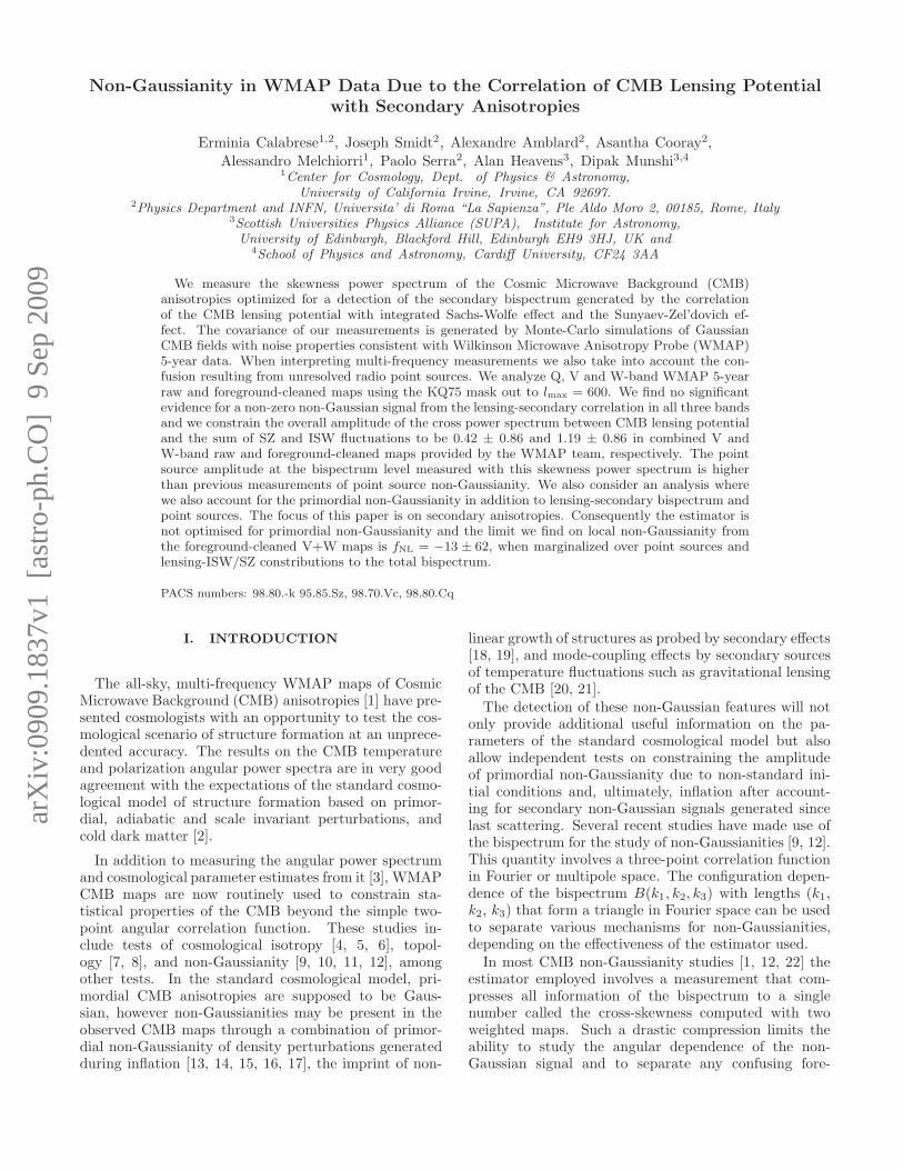
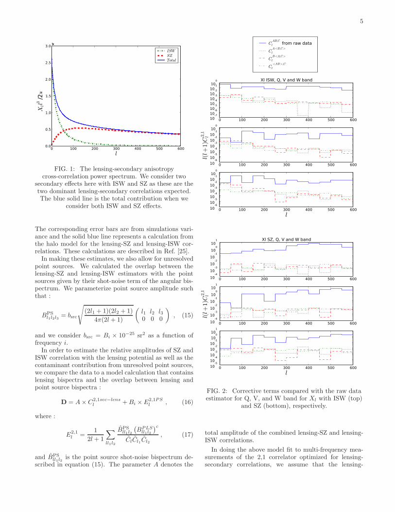
each frequency band and for different lensing-secondaryanisotropy cross-correlation power spectrum; in particu-lar, Xl ISW is the spectrum of cross-correlating lensingwith Integrate Sachs-Wolfe effect [28] and, in the sameway, Xl SZ for Sunyaev-Zel’dovich effect [29] (see Fig-ure 1). We calculate these in the fiducial cosmologicalmodel consistent with WMAP 5-year data and makinguse of the halo model approach to describe the SZ sig-nal [30, 31, 32]. The ISW effect is described throughthe standard linear power spectrum of the potential fieldand the CMB lensing potential is also modeled using thelinear fluctuations [33, 34].

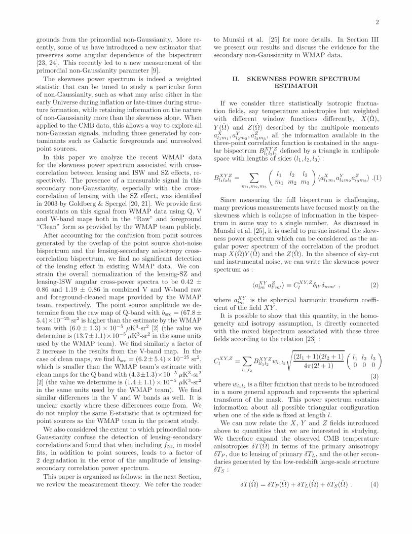
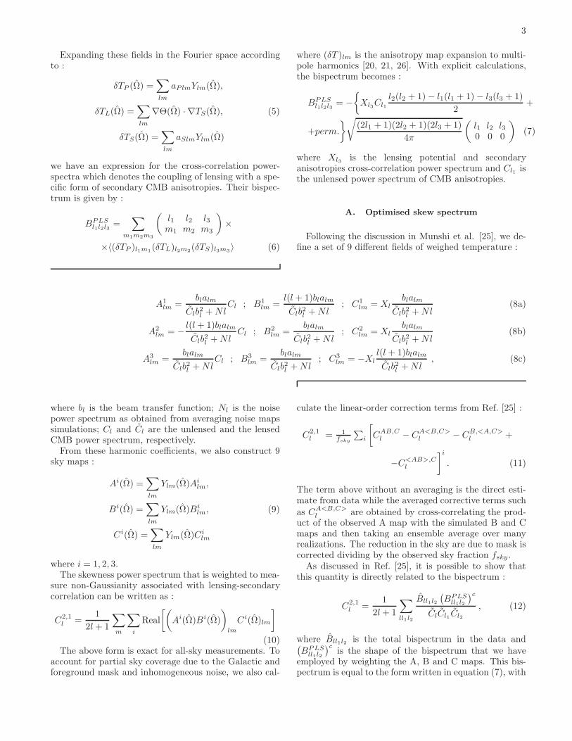
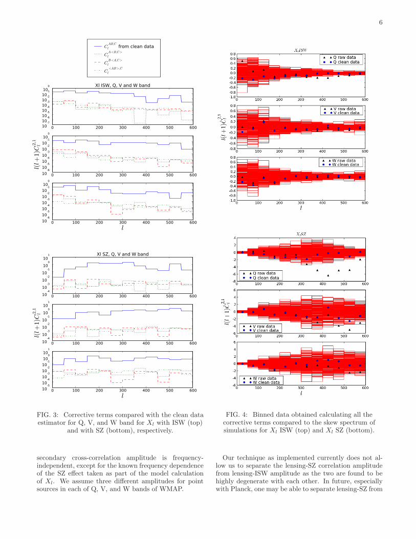
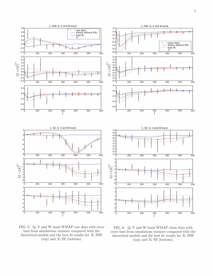
In Figures 2 and 3 we show all terms of equation (11).It’s evident that linear terms are not significant comparedto the others coming from data only. However, we areusing all the contributions when calculating the skewnessspectrum.

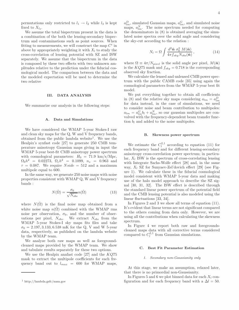
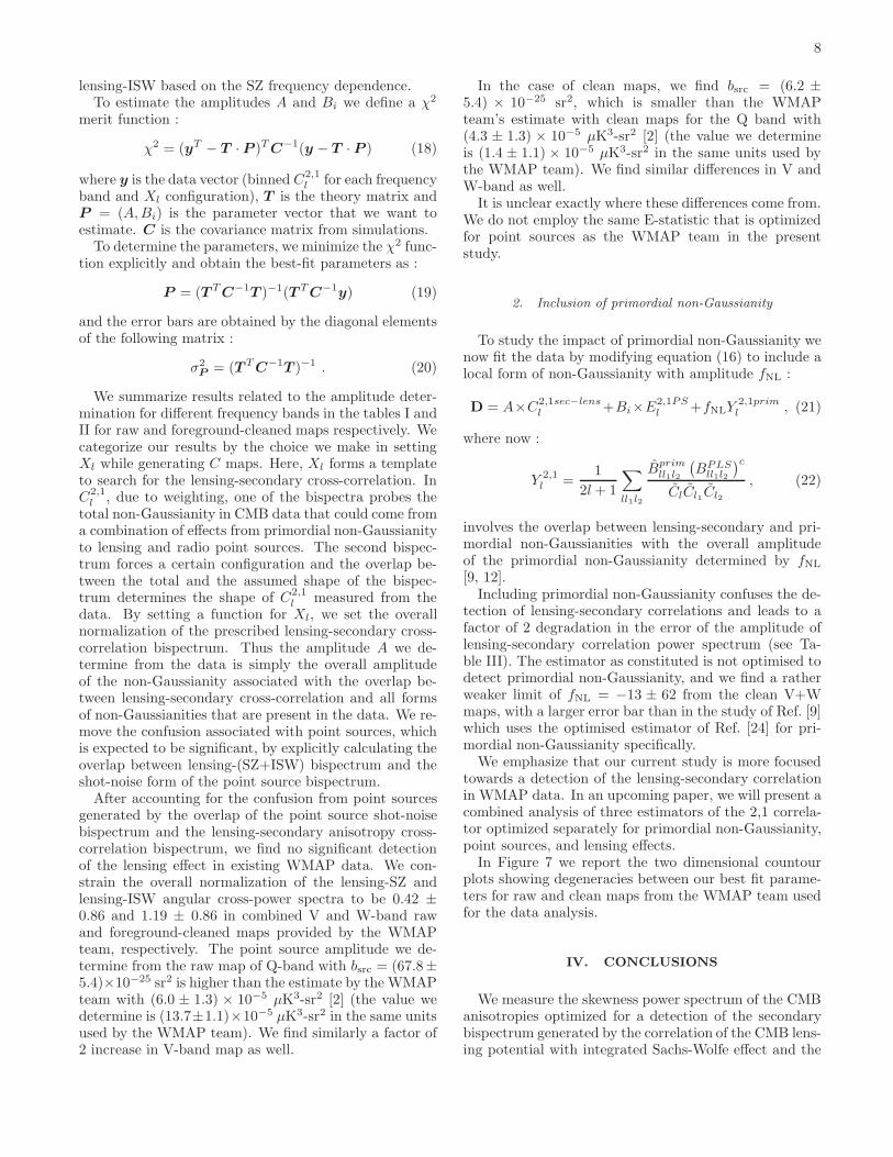
In Figure 4 we report both raw and foregrounds-cleaned maps data with all corrective terms consideredcompared to C2,1

l from Gaussian simulations.

C. Best Fit Parameter Estimation

1. Secondary non-Gaussianity only

At this stage, we make an assumption, relaxed later,that there is no primordial non-Gaussianity.

In Figures 5 and 6 we plot binned data for each Xl con-figuration and for each frequency band with a ∆l = 50.

5

0 100 200 300 400 500 600

l

0.0

0.5

1.0

1.5

2.0

2.5

3.0

Xll3

/2

[K]

1e-9

ISWSZTotal

FIG. 1: The lensing-secondary anisotropycross-correlation power spectrum. We consider two

secondary effects here with ISW and SZ as these are thetwo dominant lensing-secondary correlations expected.The blue solid line is the total contribution when we

consider both ISW and SZ effects.

The corresponding error bars are from simulations vari-ance and the solid blue line represents a calculation fromthe halo model for the lensing-SZ and lensing-ISW cor-relations. These calculations are described in Ref. [25].

In making these estimates, we also allow for unresolvedpoint sources. We calculated the overlap between thelensing-SZ and lensing-ISW estimators with the pointsources given by their shot-noise term of the angular bis-pectrum. We parameterize point source amplitude suchthat :

BPS

l1l2l3= bsrc

√

(2l1 + 1)(2l2 + 1)

4π(2l + 1)

(

l1 l2 l30 0 0

)

, (15)

and we consider bsrc = Bi × 10−25 sr2 as a function offrequency i.

In order to estimate the relative amplitudes of SZ andISW correlation with the lensing potential as well as thecontaminant contribution from unresolved point sources,we compare the data to a model calculation that containslensing bispectra and the overlap between lensing andpoint source bispectra :

D = A × C2,1sec−lensl + Bi × E2,1PS

l , (16)

where :

E2,1l =

1

2l + 1

∑

ll1l2

BPS

ll1l2

(

BPLSll1l2

)c

ClCl1Cl2

, (17)

and BPS

ll1l2is the point source shot-noise bispectrum de-

scribed in equation (15). The parameter A denotes the

0 100 200 300 400 500 60010-710-610-510-410-310-210-1100 Xl ISW, Q, V and W band

CAB,C

l from raw data

CA<B,C>

l

CB<A,C>

l

C<AB>,C

l

0 100 200 300 400 500 600

l10

-610

-510

-410

-310

-210

-110

0

0 100 200 300 400 500 60010-6

10-5

10-4

10-3

10-2

10-1

100

l(l+

1)C

2,1

l

0 100 200 300 400 500 60010-4

10-3

10-2

10-1

100

101 Xl SZ, Q, V and W band

0 100 200 300 400 500 600

l10

-510

-410

-310

-210

-110

010

1

0 100 200 300 400 500 60010-4

10-3

10-2

10-1

100

101

l(l+

1)C

2,1

l

FIG. 2: Corrective terms compared with the raw dataestimator for Q, V, and W band for Xl with ISW (top)

and SZ (bottom), respectively.

total amplitude of the combined lensing-SZ and lensing-ISW correlations.

In doing the above model fit to multi-frequency mea-surements of the 2,1 correlator optimized for lensing-secondary correlations, we assume that the lensing-

6

0 100 200 300 400 500 60010-710-610-510-410-310-210-1100 Xl ISW, Q, V and W band

CAB,C

l from clean data

CA<B,C>

l

CB<A,C>

l

C<AB>,C

l

0 100 200 300 400 500 600

l10

-610

-510

-410

-310

-210

-110

0

0 100 200 300 400 500 60010-6

10-5

10-4

10-3

10-2

10-1

100

l(l+

1)C

2,1

l

0 100 200 300 400 500 60010-4

10-3

10-2

10-1

100

101 Xl SZ, Q, V and W band

0 100 200 300 400 500 600

l10

-510

-410

-310

-210

-110

010

1

0 100 200 300 400 500 60010-4

10-3

10-2

10-1

100

101

l(l+

1)C

2,1

l

FIG. 3: Corrective terms compared with the clean dataestimator for Q, V, and W band for Xl with ISW (top)

and with SZ (bottom), respectively.

secondary cross-correlation amplitude is frequency-independent, except for the known frequency dependenceof the SZ effect taken as part of the model calculationof Xl. We assume three different amplitudes for pointsources in each of Q, V, and W bands of WMAP.

FIG. 4: Binned data obtained calculating all thecorrective terms compared to the skew spectrum ofsimulations for Xl ISW (top) and Xl SZ (bottom).

Our technique as implemented currently does not al-low us to separate the lensing-SZ correlation amplitudefrom lensing-ISW amplitude as the two are found to behighly degenerate with each other. In future, especiallywith Planck, one may be able to separate lensing-SZ from

7

0 100 200 300 400 500 600-0.4

-0.2

0.0

0.2

0.4

0.6

0.8Xl ISW, Q, V and W band

raw datatheory without PSsbest fit1

0 100 200 300 400 500 600-0.3

-0.2

-0.1

0.0

0.1

0.2

0.3

0.4

0.5

l(l+

1)C

2,1

l

0 100 200 300 400 500 600

l

-0.6

-0.4

-0.2

0.0

0.2

0 100 200 300 400 500 600-8

-6

-4

-2

0

2Xl SZ, Q, V and W band

0 100 200 300 400 500 600-7-6-5-4-3-2-1012

l(l+

1)C

2,1

l

0 100 200 300 400 500 600

l

-4

-3

-2

-1

0

1

2

FIG. 5: Q, V and W band WMAP raw data with errorbars from simulations variance compared with the

theoretical models and the best fit results for Xl ISW(top) and Xl SZ (bottom).

0 100 200 300 400 500 600-0.6

-0.5

-0.4

-0.3

-0.2

-0.1

0.0

0.1Xl ISW, Q, V and W band

clean datatheory without PSsbest fit1

0 100 200 300 400 500 600-0.5-0.4-0.3-0.2-0.10.00.10.20.30.4

l(l+

1)C

2,1

l0 100 200 300 400 500 600

l

-0.6

-0.4

-0.2

0.0

0.2

0 100 200 300 400 500 600-3.5-3.0-2.5-2.0-1.5-1.0-0.50.00.51.0

Xl SZ, Q, V and W band

0 100 200 300 400 500 600-4

-3

-2

-1

0

1

2

3

l(l+

1)C

2,1

l

0 100 200 300 400 500 600

l

-3

-2

-1

0

1

2

3

FIG. 6: Q, V and W band WMAP clean data witherror bars from simulations variance compared with thetheoretical models and the best fit results for Xl ISW

(top) and Xl SZ (bottom).

8

lensing-ISW based on the SZ frequency dependence.To estimate the amplitudes A and Bi we define a χ2

merit function :

χ2 = (yT − T · P )T C−1(y − T · P ) (18)

where y is the data vector (binned C2,1l for each frequency

band and Xl configuration), T is the theory matrix andP = (A, Bi) is the parameter vector that we want toestimate. C is the covariance matrix from simulations.

To determine the parameters, we minimize the χ2 func-tion explicitly and obtain the best-fit parameters as :

P = (T T C−1T )−1(T T C−1y) (19)

and the error bars are obtained by the diagonal elementsof the following matrix :

σ2

P= (T T C−1T )−1 . (20)

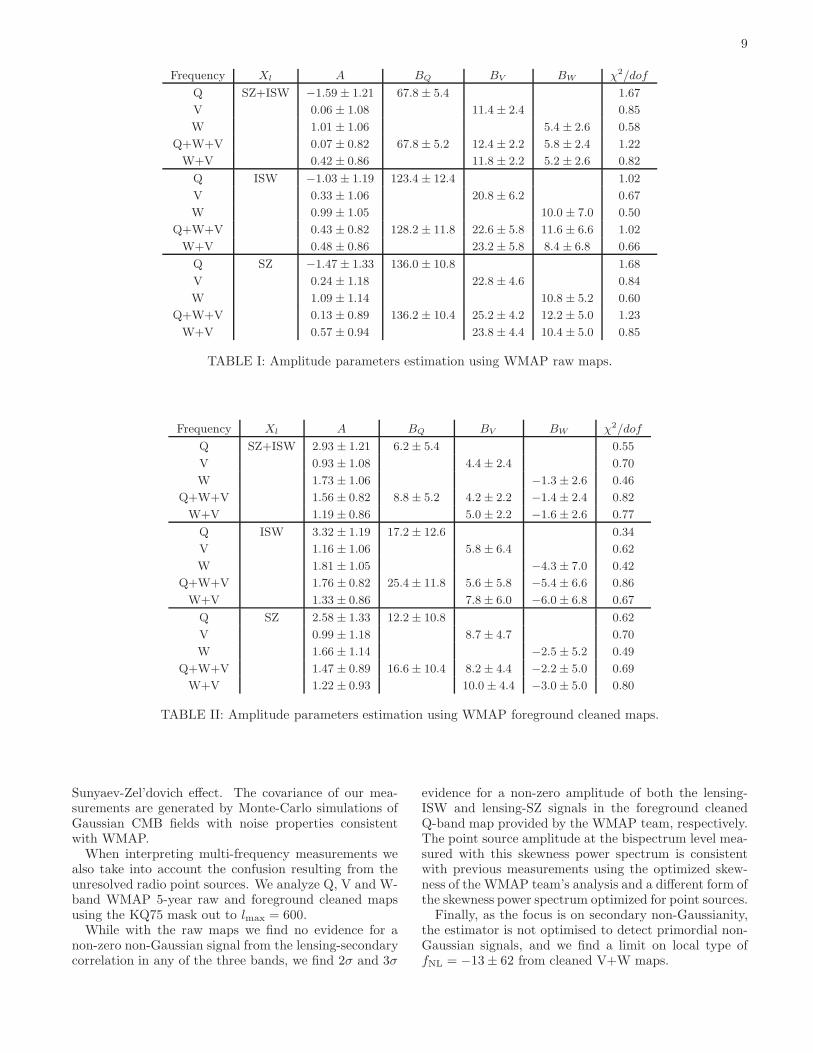
We summarize results related to the amplitude deter-mination for different frequency bands in the tables I andII for raw and foreground-cleaned maps respectively. Wecategorize our results by the choice we make in settingXl while generating C maps. Here, Xl forms a templateto search for the lensing-secondary cross-correlation. InC2,1

l , due to weighting, one of the bispectra probes thetotal non-Gaussianity in CMB data that could come froma combination of effects from primordial non-Gaussianityto lensing and radio point sources. The second bispec-trum forces a certain configuration and the overlap be-tween the total and the assumed shape of the bispec-trum determines the shape of C2,1

l measured from thedata. By setting a function for Xl, we set the overallnormalization of the prescribed lensing-secondary cross-correlation bispectrum. Thus the amplitude A we de-termine from the data is simply the overall amplitudeof the non-Gaussianity associated with the overlap be-tween lensing-secondary cross-correlation and all formsof non-Gaussianities that are present in the data. We re-move the confusion associated with point sources, whichis expected to be significant, by explicitly calculating theoverlap between lensing-(SZ+ISW) bispectrum and theshot-noise form of the point source bispectrum.

After accounting for the confusion from point sourcesgenerated by the overlap of the point source shot-noisebispectrum and the lensing-secondary anisotropy cross-correlation bispectrum, we find no significant detectionof the lensing effect in existing WMAP data. We con-strain the overall normalization of the lensing-SZ andlensing-ISW angular cross-power spectra to be 0.42 ±0.86 and 1.19 ± 0.86 in combined V and W-band rawand foreground-cleaned maps provided by the WMAPteam, respectively. The point source amplitude we de-termine from the raw map of Q-band with bsrc = (67.8±5.4)×10−25 sr2 is higher than the estimate by the WMAPteam with (6.0 ± 1.3) × 10−5 µK3-sr2 [2] (the value wedetermine is (13.7±1.1)×10−5 µK3-sr2 in the same unitsused by the WMAP team). We find similarly a factor of2 increase in V-band map as well.

In the case of clean maps, we find bsrc = (6.2 ±5.4) × 10−25 sr2, which is smaller than the WMAPteam’s estimate with clean maps for the Q band with(4.3 ± 1.3) × 10−5 µK3-sr2 [2] (the value we determineis (1.4 ± 1.1) × 10−5 µK3-sr2 in the same units used bythe WMAP team). We find similar differences in V andW-band as well.

It is unclear exactly where these differences come from.We do not employ the same E-statistic that is optimizedfor point sources as the WMAP team in the presentstudy.

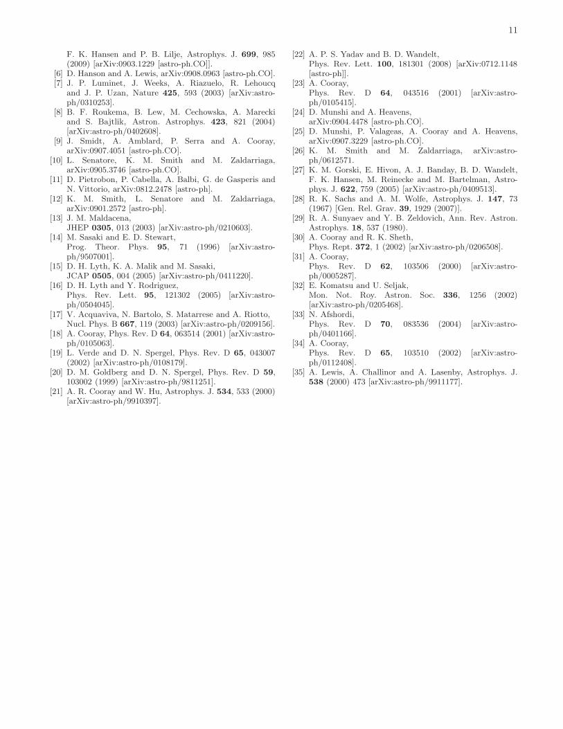
2. Inclusion of primordial non-Gaussianity

To study the impact of primordial non-Gaussianity wenow fit the data by modifying equation (16) to include alocal form of non-Gaussianity with amplitude fNL :

D = A×C2,1sec−lensl +Bi×E2,1PS

l +fNLY 2,1priml , (21)

where now :

Y 2,1l =

1

2l + 1

∑

ll1l2

Bprimll1l2

(

BPLSll1l2

)c

ClCl1Cl2

, (22)

involves the overlap between lensing-secondary and pri-mordial non-Gaussianities with the overall amplitudeof the primordial non-Gaussianity determined by fNL

[9, 12].Including primordial non-Gaussianity confuses the de-

tection of lensing-secondary correlations and leads to afactor of 2 degradation in the error of the amplitude oflensing-secondary correlation power spectrum (see Ta-ble III). The estimator as constituted is not optimised todetect primordial non-Gaussianity, and we find a ratherweaker limit of fNL = −13 ± 62 from the clean V+Wmaps, with a larger error bar than in the study of Ref. [9]which uses the optimised estimator of Ref. [24] for pri-mordial non-Gaussianity specifically.

We emphasize that our current study is more focusedtowards a detection of the lensing-secondary correlationin WMAP data. In an upcoming paper, we will present acombined analysis of three estimators of the 2,1 correla-tor optimized separately for primordial non-Gaussianity,point sources, and lensing effects.

In Figure 7 we report the two dimensional countourplots showing degeneracies between our best fit parame-ters for raw and clean maps from the WMAP team usedfor the data analysis.

IV. CONCLUSIONS

We measure the skewness power spectrum of the CMBanisotropies optimized for a detection of the secondarybispectrum generated by the correlation of the CMB lens-ing potential with integrated Sachs-Wolfe effect and the

9

Frequency Xl A BQ BV BW χ2/dof

Q SZ+ISW −1.59 ± 1.21 67.8 ± 5.4 1.67

V 0.06 ± 1.08 11.4 ± 2.4 0.85

W 1.01 ± 1.06 5.4 ± 2.6 0.58

Q+W+V 0.07 ± 0.82 67.8 ± 5.2 12.4 ± 2.2 5.8 ± 2.4 1.22

W+V 0.42 ± 0.86 11.8 ± 2.2 5.2 ± 2.6 0.82

Q ISW −1.03 ± 1.19 123.4 ± 12.4 1.02

V 0.33 ± 1.06 20.8 ± 6.2 0.67

W 0.99 ± 1.05 10.0 ± 7.0 0.50

Q+W+V 0.43 ± 0.82 128.2 ± 11.8 22.6 ± 5.8 11.6 ± 6.6 1.02

W+V 0.48 ± 0.86 23.2 ± 5.8 8.4 ± 6.8 0.66

Q SZ −1.47 ± 1.33 136.0 ± 10.8 1.68

V 0.24 ± 1.18 22.8 ± 4.6 0.84

W 1.09 ± 1.14 10.8 ± 5.2 0.60

Q+W+V 0.13 ± 0.89 136.2 ± 10.4 25.2 ± 4.2 12.2 ± 5.0 1.23

W+V 0.57 ± 0.94 23.8 ± 4.4 10.4 ± 5.0 0.85

TABLE I: Amplitude parameters estimation using WMAP raw maps.

Frequency Xl A BQ BV BW χ2/dof

Q SZ+ISW 2.93 ± 1.21 6.2 ± 5.4 0.55

V 0.93 ± 1.08 4.4 ± 2.4 0.70

W 1.73 ± 1.06 −1.3 ± 2.6 0.46

Q+W+V 1.56 ± 0.82 8.8 ± 5.2 4.2 ± 2.2 −1.4 ± 2.4 0.82

W+V 1.19 ± 0.86 5.0 ± 2.2 −1.6 ± 2.6 0.77

Q ISW 3.32 ± 1.19 17.2 ± 12.6 0.34

V 1.16 ± 1.06 5.8 ± 6.4 0.62

W 1.81 ± 1.05 −4.3 ± 7.0 0.42

Q+W+V 1.76 ± 0.82 25.4 ± 11.8 5.6 ± 5.8 −5.4 ± 6.6 0.86

W+V 1.33 ± 0.86 7.8 ± 6.0 −6.0 ± 6.8 0.67

Q SZ 2.58 ± 1.33 12.2 ± 10.8 0.62

V 0.99 ± 1.18 8.7 ± 4.7 0.70

W 1.66 ± 1.14 −2.5 ± 5.2 0.49

Q+W+V 1.47 ± 0.89 16.6 ± 10.4 8.2 ± 4.4 −2.2 ± 5.0 0.69

W+V 1.22 ± 0.93 10.0 ± 4.4 −3.0 ± 5.0 0.80

TABLE II: Amplitude parameters estimation using WMAP foreground cleaned maps.

Sunyaev-Zel’dovich effect. The covariance of our mea-surements are generated by Monte-Carlo simulations ofGaussian CMB fields with noise properties consistentwith WMAP.

When interpreting multi-frequency measurements wealso take into account the confusion resulting from theunresolved radio point sources. We analyze Q, V and W-band WMAP 5-year raw and foreground cleaned mapsusing the KQ75 mask out to lmax = 600.

While with the raw maps we find no evidence for anon-zero non-Gaussian signal from the lensing-secondarycorrelation in any of the three bands, we find 2σ and 3σ

evidence for a non-zero amplitude of both the lensing-ISW and lensing-SZ signals in the foreground cleanedQ-band map provided by the WMAP team, respectively.The point source amplitude at the bispectrum level mea-sured with this skewness power spectrum is consistentwith previous measurements using the optimized skew-ness of the WMAP team’s analysis and a different form ofthe skewness power spectrum optimized for point sources.

Finally, as the focus is on secondary non-Gaussianity,the estimator is not optimised to detect primordial non-Gaussian signals, and we find a limit on local type offNL = −13 ± 62 from cleaned V+W maps.

10

Frequency Data A BQ BV BW fNL χ2/dof

Q Raw 0.39 ± 1.99 69.8 ± 5.6 −95 ± 76 1.68

V −0.51 ± 1.78 11.3 ± 2.4 31 ± 70 0.92

W 2.18 ± 1.78 5.6 ± 2.6 −60 ± 73 0.56

Q+W+V 1.58 ± 1.46 68.6 ± 5.2 12.2 ± 2.1 5.8 ± 2.5 −70 ± 56 0.60

W+V 0.75 ± 1.56 11.9 ± 2.2 5.1 ± 2.5 −16 ± 62 0.85

Q Clean 2.02 ± 1.99 5.3 ± 5.6 43 ± 76 0.58

V −0.03 ± 1.78 4.2 ± 2.4 48 ± 70 0.73

W 3.04 ± 1.78 −1.1 ± 2.6 −67 ± 73 0.42

Q+W+V 1.59 ± 1.46 8.9 ± 5.2 4.1 ± 2.2 −1.4 ± 2.5 0 ± 56 0.39

W+V 1.47 ± 1.56 4.9 ± 2.3 −1.6 ± 2.5 −13 ± 62 0.80

TABLE III: Amplitude parameters estimation using WMAP raw and clean maps for Xl total and including an extraparameter related to primordial non-Gaussianity.

80 100 120 140 160 180

BQ

-4

-2

0

2

A

-30 -20 -10 0 10 20 30 40 50

BW

-3

-2

-1

0

1

2

3

4

5

A

-10 0 10 20 30 40 50

BV

-3

-2

-1

0

1

2

3

4

A

Xl ISW

-40 -20 0 20 40 60

BQ

0

2

4

6

8

A-40 -30 -20 -10 0 10 20 30

BW

-2

-1

0

1

2

3

4

5

6

A

-30 -20 -10 0 10 20 30 40

BV

-2

0

2

4

6

A

Xl ISW

100 120 140 160 180

BQ

-6

-4

-2

0

2

A

-20 -10 0 10 20 30 40 50

BW

-3

-2

-1

0

1

2

3

4

5

A

-10 0 10 20 30 40

BV

-4

-2

0

2

4

A

Xl SZ

-40 -20 0 20 40 60

BQ

-2

0

2

4

6

8

A

-30 -20 -10 0 10 20 30

BW

-2

0

2

4

6

A

-20 -10 0 10 20 30

BV

-2

0

2

4

6

A

Xl SZ

40 50 60 70 80 90 100

BQ

-5

-4

-3

-2

-1

0

1

2

A

-10 -5 0 5 10 15 20

BW

-3

-2

-1

0

1

2

3

4

5

A

-5 0 5 10 15 20 25 30

BV

-4

-3

-2

-1

0

1

2

3

4

A

Xl tot

-20 -10 0 10 20 30

BQ

0

2

4

6

A

-15 -10 -5 0 5 10 15

BW

-2

-1

0

1

2

3

4

5

A

-10 -5 0 5 10 15 20

BV

-3

-2

-1

0

1

2

3

4

5

A

Xl tot

(a) (b)

FIG. 7: 2-dimensional countour plots showing the degeneracies at 68%, 95% and 99.7% confidence levels betweenthe best fit parameters from raw (left panel (a)) and clean (right panel (b)) map data analysis for the ISW (top), SZ

(middle) and joint ISW+SZ (bottom) cases.

[1] G. Hinshaw et al. [WMAP Collaboration],arXiv:0803.0732 [astro-ph];

[2] E. Komatsu et al., arXiv:0803.0547 [astro-ph].[3] J. Dunkley et al. [WMAP Collaboration], Astrophys. J.

Suppl. 180, 306 (2009) [arXiv:0803.0586 [astro-ph]].[4] C. Copi, D. Huterer, D. Schwarz and G. Starkman, Phys.

Rev. D 75, 023507 (2007) [arXiv:astro-ph/0605135].[5] J. Hoftuft, H. K. Eriksen, A. J. Banday, K. M. Gorski,

11

F. K. Hansen and P. B. Lilje, Astrophys. J. 699, 985(2009) [arXiv:0903.1229 [astro-ph.CO]].

[6] D. Hanson and A. Lewis, arXiv:0908.0963 [astro-ph.CO].[7] J. P. Luminet, J. Weeks, A. Riazuelo, R. Lehoucq

and J. P. Uzan, Nature 425, 593 (2003) [arXiv:astro-ph/0310253].

[8] B. F. Roukema, B. Lew, M. Cechowska, A. Mareckiand S. Bajtlik, Astron. Astrophys. 423, 821 (2004)[arXiv:astro-ph/0402608].

[9] J. Smidt, A. Amblard, P. Serra and A. Cooray,arXiv:0907.4051 [astro-ph.CO].

[10] L. Senatore, K. M. Smith and M. Zaldarriaga,arXiv:0905.3746 [astro-ph.CO].

[11] D. Pietrobon, P. Cabella, A. Balbi, G. de Gasperis andN. Vittorio, arXiv:0812.2478 [astro-ph].

[12] K. M. Smith, L. Senatore and M. Zaldarriaga,arXiv:0901.2572 [astro-ph].

[13] J. M. Maldacena,JHEP 0305, 013 (2003) [arXiv:astro-ph/0210603].

[14] M. Sasaki and E. D. Stewart,Prog. Theor. Phys. 95, 71 (1996) [arXiv:astro-ph/9507001].

[15] D. H. Lyth, K. A. Malik and M. Sasaki,JCAP 0505, 004 (2005) [arXiv:astro-ph/0411220].

[16] D. H. Lyth and Y. Rodriguez,Phys. Rev. Lett. 95, 121302 (2005) [arXiv:astro-ph/0504045].

[17] V. Acquaviva, N. Bartolo, S. Matarrese and A. Riotto,Nucl. Phys. B 667, 119 (2003) [arXiv:astro-ph/0209156].

[18] A. Cooray, Phys. Rev. D 64, 063514 (2001) [arXiv:astro-ph/0105063].

[19] L. Verde and D. N. Spergel, Phys. Rev. D 65, 043007(2002) [arXiv:astro-ph/0108179].

[20] D. M. Goldberg and D. N. Spergel, Phys. Rev. D 59,103002 (1999) [arXiv:astro-ph/9811251].

[21] A. R. Cooray and W. Hu, Astrophys. J. 534, 533 (2000)[arXiv:astro-ph/9910397].

[22] A. P. S. Yadav and B. D. Wandelt,Phys. Rev. Lett. 100, 181301 (2008) [arXiv:0712.1148[astro-ph]].

[23] A. Cooray,Phys. Rev. D 64, 043516 (2001) [arXiv:astro-ph/0105415].

[24] D. Munshi and A. Heavens,arXiv:0904.4478 [astro-ph.CO].

[25] D. Munshi, P. Valageas, A. Cooray and A. Heavens,arXiv:0907.3229 [astro-ph.CO].

[26] K. M. Smith and M. Zaldarriaga, arXiv:astro-ph/0612571.

[27] K. M. Gorski, E. Hivon, A. J. Banday, B. D. Wandelt,F. K. Hansen, M. Reinecke and M. Bartelman, Astro-phys. J. 622, 759 (2005) [arXiv:astro-ph/0409513].

[28] R. K. Sachs and A. M. Wolfe, Astrophys. J. 147, 73(1967) [Gen. Rel. Grav. 39, 1929 (2007)].

[29] R. A. Sunyaev and Y. B. Zeldovich, Ann. Rev. Astron.Astrophys. 18, 537 (1980).

[30] A. Cooray and R. K. Sheth,Phys. Rept. 372, 1 (2002) [arXiv:astro-ph/0206508].

[31] A. Cooray,Phys. Rev. D 62, 103506 (2000) [arXiv:astro-ph/0005287].

[32] E. Komatsu and U. Seljak,Mon. Not. Roy. Astron. Soc. 336, 1256 (2002)[arXiv:astro-ph/0205468].

[33] N. Afshordi,Phys. Rev. D 70, 083536 (2004) [arXiv:astro-ph/0401166].

[34] A. Cooray,Phys. Rev. D 65, 103510 (2002) [arXiv:astro-ph/0112408].

[35] A. Lewis, A. Challinor and A. Lasenby, Astrophys. J.538 (2000) 473 [arXiv:astro-ph/9911177].