arX

iv:a

stro

-ph/

0502

578v

3 1

Jun

200

5

Non-gaussianity from the second-order cosmological perturbation

David H. Lyth1, ∗ and Yeinzon Rodrıguez1, 2, †

1Department of Physics, Lancaster University, Lancaster LA1 4YB, UK2Centro de Investigaciones, Universidad Antonio Narino, Cll 58A # 37-94, Bogota D.C., Colombia

(Dated: February 2, 2008)

Several conserved and/or gauge invariant quantities described as the second-order curvature per-turbation have been given in the literature. We revisit various scenarios for the generation ofsecond-order non-gaussianity in the primordial curvature perturbation ζ, employing for the firsttime a unified notation and focusing on the normalisation fNL of the bispectrum. When ζ firstappears a few Hubble times after horizon exit, |fNL| is much less than 1 and is, therefore, negligible.Thereafter ζ (and hence fNL) is conserved as long as the pressure is a unique function of energydensity (adiabatic pressure). Non-adiabatic pressure comes presumably only from the effect of fields,other than the one pointing along the inflationary trajectory, which are light during inflation (‘lightnon-inflaton fields’). During single-component inflation fNL is constant, but multi-component infla-tion might generate |fNL| ∼ 1 or bigger. Preheating can affect fNL only in atypical scenarios whereit involves light non-inflaton fields. The simplest curvaton scenario typically gives fNL ≪ −1 orfNL = +5/4. The inhomogeneous reheating scenario can give a wide range of values for fNL. Unlessthere is a detection, observation can eventually provide a limit |fNL| <

∼ 1, at which level it will becrucial to calculate the precise observational limit using second order theory.

PACS numbers: 98.80.Cq

I. INTRODUCTION

Cosmological scales leave the horizon during inflationand re-enter it after Big Bang Nucleosynthesis. Through-out the super-horizon era it is very useful to define aprimordial cosmological curvature perturbation, which isconserved if and only if pressure throughout the Universeis a unique function of energy density (the adiabatic pres-sure condition) [1, 2, 3, 4, 5, 6, 7]. Observation directlyconstrains the curvature perturbation at the very end ofthe super-horizon era, a few Hubble times before cosmo-logical scales start to enter the horizon, when it appar-ently sets the initial condition for the subsequent evolu-tion of all cosmological perturbations. The observed cur-vature perturbation is almost Gaussian with an almostscale-invariant spectrum.

Cosmological perturbation theory expands the exactequations in powers of the perturbations and keeps termsonly up to the nth order. Since the observed curvatureperturbation is of order 10−5, one might think that first-order perturbation theory will be adequate for all com-parisons with observation. That may not be the casehowever, because the PLANCK satellite [8] and its suc-cessors may be sensitive to non-gaussianity of the curva-ture perturbation at the level of second-order perturba-tion theory [9].

Several authors have treated the non-gaussianity ofthe primordial curvature perturbation in the context ofsecond-order perturbation theory. They have adopteddifferent definitions of the curvature perturbation and

∗Electronic address: d.lyth@lancaster.ac.uk†Electronic address: y.rodriguezgarcia@lancaster.ac.uk

obtained results for a variety of situations. In this pa-per we revisit the calculations, using a single definitionof the curvature perturbation which we denote by ζ. Insome cases we disagree with the findings of the originalauthors.

The outline of this paper is the following: in Section IIwe review two definitions of the curvature perturbationfound in the literature, which are valid during and af-ter inflation, and establish definite relationships betweenthem; in section III we review a third curvature pertur-bation definition, which applies only during inflation, andstudy it in models of inflation of the slow-roll variety; inSection IV we describe the present framework for think-ing about the origin and evolution of the curvature per-turbation; in Section V we see how non-gaussianity isdefined and constrained by observation; in Section VI westudy the initial non-gaussianity of the curvature pertur-bation, a few Hubble times after horizon exit; in SectionVII we study its subsequent evolution according to somedifferent models. The conclusions are summarised in Sec-tion VIII.

We shall denote unperturbed quantities by a subscript0, and generally work with conformal time η defined bythe unperturbed line element

ds2 = a2(η)(

−dη2 + δijdxidxj

)

. (1)

Here a is the scale factor whose present value is taken tobe 1, and a prime denotes d/dη. Sometimes though werevert to physical time t, with a dot meaning d/dt definedby d/dt ≡ a−1d/dη. We shall adopt the convention thata generic perturbation g is split into a first- and second-order part according to the formula

g = g1 +1

2g2 . (2)

2

II. TWO DEFINITIONS OF THE CURVATURE

PERTURBATION

A. Preliminaries

Cosmological perturbations describe small departuresof the actual Universe, away from some perfect homo-geneous and isotropic universe with the line elementEq. (1). For a generic perturbation it is convenient tomake the Fourier expansion

g(x, η) =1

(2π)3/2

∫

d3k g(k, η)eik·x , (3)

where the spacetime coordinates are those of the unper-turbed Universe. The inverse of the comoving wavenum-ber, k−1, is often referred to as the scale.

A given scale is said to be outside the horizon duringthe era aH ≫ k, where H ≡ a/a is the Hubble parame-ter. Except where otherwise stated, our discussion applies

only to this super-horizon regime.

When evaluating an observable quantity only a lim-ited range of scales will be involved. The largest scale,relevant for the low multipoles of the Cosmic MicrowaveBackground anisotropy, is k−1 ∼ H−1

0 where H0 isthe present Hubble parameter. The smallest scale usu-ally considered is the one enclosing matter with mass∼ 106M⊙, which corresponds to k−1 ∼ 10−2 Mpc ∼10−6H−1

0 . The cosmological range of scales therefore ex-tends over only six decades or so.

To define cosmological perturbations in general, onehas to introduce in the perturbed Universe a coordinatesystem (t, xi), which defines a slicing of spacetime (fixedt) and a threading (fixed xi). To define the curvatureperturbation it is enough to define the slicing [7].

B. Two definitions of the curvature perturbation

In this paper we take as our definition of ζ the followingexpression for the spatial metric [4, 7, 10, 11, 12, 13, 14]which applies non-perturbatively:

gij = a2(η)γije2ζ . (4)

Here γij has unit determinant, and the time-slicing is oneof uniform energy density1.

It has been shown under weak assumptions [7] thatthis defines ζ uniquely, and that ζ is conserved as longas the pressure is a unique function of energy density.Also, it has been shown that the uniform density slicing

1 It is proved in Ref. [7] that this definition of ζ coincides withthat of Lyth and Wands [15], provided that their slices of uniformcoordinate expansion are taken to correspond to those on whichthe line element has the form Eq. (4) without the factor e2ζ (thismakes the slices practically flat if γij ≃ δij).

practically coincides with the comoving slicing (orthogo-nal to the flow of energy), and with the uniform Hubbleslicing (corresponding to uniform proper expansion, thatexpansion being practically independent of the threadingwhich defines it) [7]. The coincidence of these slicings isimportant since all three have been invoked by differentauthors.

Since the matrix γ has unit determinant it can be writ-ten γ = Ieh, where I is the unit matrix and h is trace-less [7]. Assuming that the initial condition is set byinflation, h corresponds to a tensor perturbation (gravi-tational wave amplitude) which will be negligible unlessthe scale of inflation is very high. As we shall see later(see footnote 10), the results we are going to present arevalid even if h is not negligible, but to simplify the pre-sentation we drop h from the equations. Accordingly, thespace part of the metric in the super-horizon regime issupposed to be well approximated by

gij = a2(η)δije2ζ . (5)

At first order, Eq. (5) corresponds to

gij = a2(η)δij(1 + 2ζ) . (6)

Up to a sign, this is the definition of the first-order cur-vature perturbation adopted by all authors. There is nouniversally agreed convention for the sign of ζ. Ourscoincides with the convention of most of the papers towhich we refer, and we have checked carefully that thesigns in our own set of equations are correct.

At second order we have

gij = a2(η)δij(1 + 2ζ + 2ζ2) . (7)

This is our definition of ζ at second order.Malik and Wands [16] instead defined ζ by Eq. (6) even

at second order. Denoting their definition by a subscriptMW,

ζMW = ζ + ζ2 , (8)

or equivalently

ζMW2 = ζ2 + 2 (ζ1)

2 , (9)

where ζ1 is the first-order quantity whose definitionEq. (6) is agreed by all authors.

To make contact with calculations of the curvature per-turbation during inflation, we need some gauge-invariantexpressions for the curvature perturbation. ‘Gauge-invariant’ means that the definition is valid for any choiceof the coordinate system which defines the slicing andthreading2.

2 In the unperturbed limit the slicing has to be the one on which allquantities are uniform and the the threading has to be orthogonalto it.

3

We shall write gauge-invariant expressions in terms ofζ and ζMW. First we consider a quantity ψMW, definedeven at second order by

gij = a2(η)δij(1 − 2ψMW) . (10)

This definition, which is written in analogy to Eq. (6),applies to a generic slicing. Analogously to Eq. (5) wecan consider a quantity ψ, valid also in a generic slicing,defined by

gij = a2(η)δije−2ψ . (11)

On uniform-density slices, ψ1 = ψMW1 = −ζ1, ψ

MW2 =

−ζMW2 , and ψ2 = −ζ2. We shall also need the energy

density perturbation δρ, defined on the generic slicing,as well as the unperturbed energy density ρ0.

At first order, the gauge-invariant expression for ζ hasthe well-known form

ζ1 = −ψ1 −Hδρ1

ρ′0, (12)

where H = a′/a, and the unperturbed energy densitysatisfies ρ′0 = −3H(ρ0 + P0) with P0 being the unper-turbed pressure. This expression obviously is correct forthe uniform density slicing, and it is correct for all slic-ings because the changes in the first and second termsinduced by a change in the slicing cancel [1, 2, 3, 17, 18].

At second order, Malik and Wands show that [16]

ζMW2 = −ψMW

2 −Hδρ2

ρ′0+ 2H

δρ1

ρ′0

δρ′1ρ′0

+2δρ1

ρ′0(ψ′

1 + 2Hψ1)

−

(

Hδρ1

ρ′0

)2(ρ′′0Hρ′0

−H′

H2− 2

)

, (13)

which is, again and for the same reason as before, obvi-ously correct for all the slices. Accordingly, from Eq. (9),we can write a gauge invariant definition for our second-order ζ: 3

ζ2 = −ψ2 −Hδρ2

ρ′0+ 2H

δρ1

ρ′0

δρ′1ρ′0

+ 2δρ1

ρ′0ψ′

1

−

(

Hδρ1

ρ′0

)2(ρ′′0Hρ′0

−H′

H2

)

, (14)

where the relation

ψMW2 = ψ2 − 2(ψ1)

2 , (15)

coming from Eqs. (10) and (11), has been used.

3 This relation has recently been confirmed in Ref. [19] using anonlinear coordinate-free approach.

III. SLOW-ROLL INFLATION AND A THIRD

DEFINITION

Now we specialize to the era of slow-roll inflation.We consider single-component inflation, during whichthe curvature perturbation ζ is conserved, and multi-component inflation during which it varies. After defin-ing both paradigms, we give a third definition of the cur-vature perturbation which applies only during inflation.

A. Single-component inflation

In a single-component inflation model [20, 21] the in-flaton trajectory is by definition essentially unique. Theinflaton field ϕ parameterises the distance along the in-flaton trajectory. In terms of the field variation, slow-rollinflation is characterised by the slow-roll conditions ǫ≪ 1and |ηV | ≪ 1 [20, 21], where

ǫ ≡ −H/H2, (16)

ηV − ǫ ≡ −ϕ

Hϕ. (17)

The inflaton field can be taken to be canonically nor-malised, in which case these definitions are equivalent toconditions on the potential V

ǫ ≡M2

P

2V 2

(

∂V

∂ϕ

)2

, (18)

ηV ≡M2

P

V

∂2V

∂ϕ2, (19)

which, together with the slow-roll approximation, lead tothe slow-roll behaviour

3Hϕ ≈ −dV

dϕ. (20)

Here MP is the reduced Planck mass (MP ≡ (8πGN )−1).Even without the slow-roll approximation, slices of uni-

form ϕ correspond to comoving slices because a spatialgradient of ϕ would give non-vanishing momentum den-sity. Since comoving slices coincide with slices of uniformenergy density, the slices of uniform ϕ coincide also withthe latter. Also, since ϕ is a Lorentz scalar, its gaugetransformation is the same as that of ρ. It follows [22]that we can replace ρ by ϕ in the above expressions:

ζ1 = −ψ1 −Hδϕ1

ϕ′0

, (21)

ζMW2 = −ψMW

2 −Hδϕ2

ϕ′0

+ 2Hδϕ1

ϕ′0

δϕ′1

ϕ′0

+2δϕ1

ϕ′0

(ψ′1 + 2Hψ1)

−

(

Hδϕ1

ϕ′0

)2(ϕ′′

0

Hϕ′0

−H′

H2− 2

)

, (22)

4

ζ2 = −ψ2 −Hδϕ2

ϕ′0

+ 2Hδϕ1

ϕ′0

δϕ′1

ϕ′0

+ 2δϕ1

ϕ′0

ψ′1

−

(

Hδϕ1

ϕ′0

)2(ϕ′′

0

Hϕ′0

−H′

H2

)

. (23)

B. Multi-component inflation

Now consider the case of multi-component inflation,where there is a family of inequivalent inflationary trajec-tories lying in an N -dimensional manifold of field space.If the relevant part of the manifold is not too big it willbe a good approximation to take the fields to be canoni-cally normalised. Then the inequivalent trajectories willbe curved in field space4. To define the trajectories onecan choose a fixed basis in field space corresponding tofields φ1, · · · , φN .

Assuming canonical normalisation, multi-componentslow-roll inflation is characterised by the conditions

M2P

2V 2

(

∂V

∂φn

)2

≪ 1 , (24)

M2P

V

∣

∣

∣

∣

∂2V

∂φn∂φm

∣

∣

∣

∣

≪ 1 , (25)

3Hφn ≈ − ∂V∂φn

. (26)

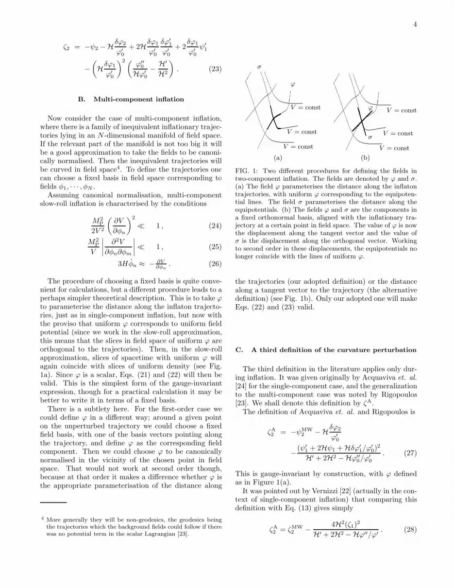
The procedure of choosing a fixed basis is quite conve-nient for calculations, but a different procedure leads to aperhaps simpler theoretical description. This is to take ϕto parameterise the distance along the inflaton trajecto-ries, just as in single-component inflation, but now withthe proviso that uniform ϕ corresponds to uniform fieldpotential (since we work in the slow-roll approximation,this means that the slices in field space of uniform ϕ areorthogonal to the trajectories). Then, in the slow-rollapproximation, slices of spacetime with uniform ϕ willagain coincide with slices of uniform density (see Fig.1a). Since ϕ is a scalar, Eqs. (21) and (22) will then bevalid. This is the simplest form of the gauge-invariantexpression, though for a practical calculation it may bebetter to write it in terms of a fixed basis.

There is a subtlety here. For the first-order case wecould define ϕ in a different way; around a given pointon the unperturbed trajectory we could choose a fixedfield basis, with one of the basis vectors pointing alongthe trajectory, and define ϕ as the corresponding fieldcomponent. Then we could choose ϕ to be canonicallynormalised in the vicinity of the chosen point in fieldspace. That would not work at second order though,because at that order it makes a difference whether ϕ isthe appropriate parameterisation of the distance along

4 More generally they will be non-geodesics, the geodesics beingthe trajectories which the background fields could follow if therewas no potential term in the scalar Lagrangian [23].

ϕ

σ

V = const

V = const

V = const

ϕ

σ

V = const

V = const

V = const

(a) (b)

FIG. 1: Two different procedures for defining the fields intwo-component inflation. The fields are denoted by ϕ and σ.(a) The field ϕ parameterises the distance along the inflatontrajectories, with uniform ϕ corresponding to the equipoten-tial lines. The field σ parameterises the distance along theequipotentials. (b) The fields ϕ and σ are the components ina fixed orthonormal basis, aligned with the inflationary tra-jectory at a certain point in field space. The value of ϕ is nowthe displacement along the tangent vector and the value ofσ is the displacement along the orthogonal vector. Workingto second order in these displacements, the equipotentials nolonger coincide with the lines of uniform ϕ.

the trajectories (our adopted definition) or the distancealong a tangent vector to the trajectory (the alternativedefinition) (see Fig. 1b). Only our adopted one will makeEqs. (22) and (23) valid.

C. A third definition of the curvature perturbation

The third definition in the literature applies only dur-ing inflation. It was given originally by Acquaviva et. al.

[24] for the single-component case, and the generalizationto the multi-component case was noted by Rigopoulos[23]. We shall denote this definition by ζA.

The definition of Acquaviva et. al. and Rigopoulos is

ζA2 = −ψMW

2 −Hδϕ2

ϕ′0

−(ψ′

1 + 2Hψ1 + Hδϕ′1/ϕ

′0)

2

H′ + 2H2 −Hϕ′′0/ϕ

′0

. (27)

This is gauge-invariant by construction, with ϕ definedas in Figure 1(a).

It was pointed out by Vernizzi [22] (actually in the con-text of single-component inflation) that comparing thisdefinition with Eq. (13) gives simply

ζA2 = ζMW

2 −4H2(ζ1)

2

H′ + 2H2 −Hϕ′′/ϕ′. (28)

5

In the limit of slow-roll the denominator of the last termbecomes just 2H2, and then

ζA2 = ζ2 . (29)

In other words, this third definition coincides with ouradopted one in the slow-roll limit.

Making use of the slow-roll parameters defined in Eqs.(16) and (17), the expression in Eq. (28) gives to first-order in the slow-roll approximation

ζA2 = ζ2 − (2ǫ− ηV )(ζ1)

2 . (30)

IV. THE EVOLUTION OF THE CURVATURE

PERTURBATION

The simplest possibility for the origin of the observedcurvature perturbation is that it comes from the vacuumfluctuation of the inflaton field in a single-componentmodel. More recently other possibilities were recognisedand we summarise the situation now. Although thediscussion is usually applied to the magnitude of thecurvature perturbation, it applies equally to the non-gaussianity.

A. Heavy, light and ultra-light fields

On each scale the initial epoch, as far as classical per-turbations are concerned, should be taken to be a fewHubble times after horizon exit during inflation. Thereason is that all such perturbations are supposed to orig-inate from the vacuum fluctuation of one or more lightscalar fields, the fluctuation on each scale being promotedto a classical perturbation around the time of horizonexit.

Considering a fixed basis with canonical normalisation,a light field is roughly speaking one satisfying the flat-ness condition in Eq. (25). The terminology is suggestedby the important special case that the effective poten-tial during inflation is quadratic. Then, a light field isroughly speaking that whose effective mass during infla-tion is less than the value H∗ of the Hubble parameter.More precisely, the condition that the vacuum fluctuationbe promoted to a classical perturbation is [25]

m <3

2H∗ . (31)

From now on we focus on the quadratic potential, andtake this as the the definition of a light field. Conversely aheavy field may be defined as one for which the conditionin Eq. (31) is violated.

During inflation light fields slowly roll according toEq. (26) (with the vacuum fluctuation superimposed)while the heavy fields presumably are pinned down atan instantaneous minimum of the effective potential. Aswe have seen, multi-component inflation takes place in a

subspace of field space. The fields in this subspace arelight, but their effective masses are sufficient to apprecia-bly curve the inflationary trajectories. In the case of bothmulti-component and single-component inflation, therecould also be ‘ultra-light’ fields, which do not apprecia-bly curve the inflationary trajectory and which thereforehave practically no effect on the dynamics of inflation.

B. The evolution of the curvature perturbation

To describe the behaviour of perturbations during thesuper-horizon era, without making too many detailed as-sumptions, it is useful to invoke the separate universe hy-pothesis [2, 5, 15, 26] after smoothing on a given comov-ing scale much bigger than the horizon5. According tothis hypothesis the local evolution at each position is thatof some unperturbed universe (separate universe). Ofcourse the separate universe hypothesis can and shouldbe checked where there is a sufficiently detailed model.However, it should be correct on cosmological scales fora very simple reason. The unperturbed Universe maybe defined as the one around us, smoothed on a scalea bit bigger than the present Hubble distance. In otherwords, the separate universe hypothesis is certainly validwhen applied to that scale. But the whole range of cos-mological scales spans only a few decades. This meansthat cosmological scales are likely to be huge comparedwith any scale that is relevant in the early Universe, andaccordingly that the separate universe hypothesis shouldbe valid when applied to cosmological scales even thoughit might fail on much smaller scales (this expectation wasverified in a preheating example [27] to which we returnlater).

We are concerned with the curvature perturbation,which during the super-horizon era is conserved as longas the pressure is a unique function of the energy density(the adiabatic pressure condition). The adiabatic pres-sure condition will be satisfied if and only if the separateuniverses are identical (at least as far as the relation be-tween pressure and energy density is concerned) 6. Thecondition to have identical universes after a given epochis that the specification of a single quantity at that epochis sufficient to determine the entire subsequent evolution.

In the case of single-component inflation, the initialcondition may be supplied by the local value of the in-flaton field, at the very beginning of the super-horizon

5 When considering linear equations, smoothing is equivalent todropping short wavelengths fourier components. In the nonlin-ear situation the smoothing procedure could be in principle am-biguous. In a given situation one should state explicitly whichquantities are being smoothed.

6 Of course the identity will only hold after making an appropriatesynchronization of the clocks at different positions. Having madethat synchronization, horizon entry will occur at different timesin different positions, which can be regarded as the origin of thecurvature perturbation.

6

era when it first becomes classical. Given the separateuniverse hypothesis, that is the only possibility if the in-flaton is the only light field ever to play a significant dy-namical role. This means that the curvature perturbation

generated at horizon exit during single-component infla-

tion will be equal to the one observed at the approach of

horizon entry, provided that the inflaton is the only light

field ever to play a dynamical role.

If inflation is multi-component, more than one field isby definition relevant during inflation. Then the curva-ture perturbation cannot be conserved during inflation.The variation of the curvature perturbation during multi-component inflation is caused by the vacuum fluctuationorthogonal to the unperturbed inflationary trajectory,which around the time of horizon exit kicks the trajectoryonto a nearby one so that the local trajectory becomesposition-dependent. After inflation is over, the curvatureperturbation will be conserved if the local trajectorieslead to practically identical universes. In other words itwill be conserved if the light (and ultra-light) fields, or-thogonal to the trajectory at the end of inflation, do notaffect the subsequent evolution of the Universe.

The curvature perturbation after inflation will vary ifsome light or ultra-light field, orthogonal to the trajec-tory at the end of inflation, affects the subsequent evolu-tion of the Universe (to be precise, affects the pressure).As we shall describe in Section VII, three types of scenar-ios have been proposed for this post-inflationary variationof the curvature perturbation.

V. NON-GAUSSIANITY

A. Defining the non-gaussianity

A gaussian perturbation is one whose Fourier compo-nents are uncorrelated. All of its statistical propertiesare defined by its spectrum, and the spectrum Pg of ageneric perturbation is conveniently defined [20, 21] by7

〈g(k1)g(k2)〉 =2π2

k3δ3(k1 + k2)Pg(k) , (32)

the normalisation being chosen so that

〈g2(x)〉 =

∫ ∞

0

Pg(k)dk

k. (33)

On cosmological scales a few Hubble times before horizonentry, observation shows that the curvature perturbation

is almost Gaussian with P1/2ζ ≃ 10−5.

7 Technically the expectation values in this and the following ex-pressions refer to an ensemble of universes but, because thestochastic properties of the perturbations are supposed to beinvariant under translations, the expectation values can also beregarded as averages over the location of the observer who definesthe origin of coordinates.

The simplest kind of non-gaussianity that the curva-ture perturbation could possess is of the form

ζ(x) = ζg(x) −3

5fNL

(

ζ2g (x) − ζ2

g

)

, (34)

where ζg is Gaussian with 〈ζg〉 = 0, and the non-linearityparameter fNL is independent of position. We will callthis correlated χ2 non-gaussianity. Note that this defi-nition assumes that 〈ζ〉 = 0, which means that the zeroFourier mode (spatial average) is dropped.

Following Maldacena [10], we have inserted the pref-actor −(3/5) so that in first-order perturbation theoryour definition agrees with that of Komatsu and Spergel[9], which is generally the definition people use whencomparing theory with observation. Working in first-order perturbation theory, these authors write Φ(x) =

Φg(x)+ fNL

(

Φ2g(x) − Φ2

g

)

, and their Φ is equal to −3/5

times our ζ.One of the most powerful observational signatures of

non-gaussianity is a nonzero value for the three-point cor-relator, specified by the bispectrum B defined by [9, 28]

〈ζ(k1)ζ(k2)ζ(k3)〉 = (2π)−3/2B(k1, k2, k3)δ3(k1+k2+k3) .

(35)For correlated χ2 non-gaussianity (with the gaussianterm dominating)

B(k1, k2, k3) = −6

5fNL

[

Pζ(k1)Pζ(k2) + cyclic]

, (36)

where Pζ(k) = 2π2Pζ(k)/k3. For any kind of non-

Gaussianity one may use the above expression to definea function fNL(k1, k2, k3).

Given a calculation of fNL using first-order perturba-tion theory, one expects in general that going to secondorder will change fNL by an amount of order 1. On thisbasis, one expects that a first-order calculation is goodenough if it yields |fNL| ≫ 1, but that otherwise a second-order calculation will be necessary.

The definition Eq. (36) of fNL is made using ouradopted definition of ζ. If ζ in the definition is replacedby ζMW (with the zero Fourier mode dropped) then fNL

should be replaced by

fMWNL ≡ fNL −

5

3. (37)

To obtain this expression we used Eq. (8) and droppedterms higher than second order.

All of this assumes that the non-gaussian componentof ζ is fully correlated with the gaussian component. Analternative possibility [29] that will be important for usis if ζ has the form

ζ(x) = ζg(x) −3

5fNL

(

ζ2σ(x) − ζ2

σ

)

, (38)

where ζg and ζσ are uncorrelated Gaussian perturbations,

normalised to have equal spectra, and the parameter fNL

7

is independent of position. We will call this uncorrelated

χ2 non-gaussianity. It can be shown [29] that in thiscase, fNL as defined by Eq. (36) is given by

fNL ∼

(

fNL

1300

)3

. (39)

B. Observational constraints on the

non-gaussianity

Taking fNL to denote the non-linearity parameter atthe primordial era, let us consider the observational con-straints. Detailed calculations have so far been made onlywith fNL independent of the wavenumbers, and only byusing first-order perturbation theory for the evolution ofthe cosmological perturbations after horizon entry. It isfound [30] that present observation requires |fNL| <∼ 102

making the non-gaussian fraction at most of order 10−3.The use of first-order perturbation theory in this con-text is amply justified. Looking to the future though,it is found that the PLANCK satellite will either detectnon-gaussianity or reduce the bound to |fNL| <∼ 5 [9, 28],and that foreseeable future observations can reach a level|fNL| ∼ 3 [9, 28].

Although the use of first-order perturbation theory isnot really justified for the latter estimates, we can safelyconclude that it will be difficult for observation ever to de-tect a value |fNL| ≪ 1. That is a pity because, as we shallsee, such a value is predicted by some theoretical scenar-ios. On the other hand, other scenarios predict |fNL|roughly of order 1. It will therefore be of great interestto have detailed second-order calculations, to establishprecisely the level of sensitivity that can be achieved byfuture observations. A step in this direction has beentaken in Refs. [31, 32], where the large-scale cosmic mi-crowave background anisotropy is calculated to secondorder in terms of only the curvature perturbation (gen-eralizing the first-order Sachs-Wolfe effect [33]).

VI. THE INITIAL NON-GAUSSIANITY

A. Single-component inflation

At first order, the curvature perturbation duringsingle-component inflation is Gaussian. Its time-independent spectrum is given by [20, 21]

Pζ(k) =

[

(

H

2π

)2(H

ϕ

)2]

k=aH

, (40)

and its spectral index n ≡ d lnPζ/d ln k is given by

n− 1 = 2ηV − 6ǫ . (41)

The spectrum r of the tensor perturbation, defined asa fraction of Pζ , is also given in terms of the slow-roll

parameter ǫ:

r = 16ǫ. (42)

If the curvature perturbation does not evolve after

single-component inflation is over observation constrainsn and r, and hence the slow-roll parameters ηV and ǫ.A current bound [34] is −0.048 < n − 1 < 0.016 andr < 0.46. The second bound gives ǫ < 0.029, but barringan accurate cancellation the first bound gives ǫ <∼ 0.003.In most inflation models ǫ is completely negligible andthen the first bound gives −0.024 < ηV < 0.008 (irre-spective of slow-roll inflation models, the upper bound inthis expression holds generally, and the lower bound isbadly violated only if there is an accurate cancellation).The bottom line of all this is that ǫ and |ηV | are bothconstrained to be <

∼ 10−2.Going to second order, Maldacena [10] has calculated

the bispectrum during single-component inflation (seealso Refs. [12, 13, 14, 35, 36, 37, 38]). His result may bewritten in the form

fNL =5

12(2ηV − 6ǫ− 2ǫf(k1, k2, k3)) , (43)

with 0 ≤ f ≤ 5/6. By virtue of the slow-roll conditions,|fNL| ≪ 1 8. In other words, the curvature perturbationζ, as we have defined it, is almost Gaussian during single-component inflation.

From Eq. (30) ζA is also practically gaussian, but thisquantity is defined only during inflation and thereforecould not be considered as a replacement for ζ. More im-portantly, ζMW has significant non-gaussianity because,from Eq. (37), it corresponds to fMW

NL ≈ −5/3.One may ask why it is our ζ and not ζMW which is

gaussian in the slow-roll limit9. One feature that distin-guishes our ζ, is that any part of it can be absorbed intothe scale factor without altering the rest; indeed

gij = δija2(η)e2ζ1+ζ2 = δij a

2(η)eζ2 , (44)

with a = aeζ1 (if we tried to do that with ζMW, thepart of ζ not absorbed would have to be re-scaled). Thismeans that an extremely long-wavelength and possiblelarge part of ζ has no local significance. It also means,in the context of perturbation theory, that the first-orderpart of ζ can be absorbed into the scale factor when dis-cussing the second-order part. However, the gaussianityof ζ does not seem to be related directly to this feature.

8 Near a maximum of the potential ‘fast-roll’ inflation [39, 40] cantake place with |ηV | somewhat bigger than 1. Maldacena’s cal-culation does not apply to that case but, presumably, it givesinitial non-gaussianity |fNL| ∼ 1. However, the precise initialvalue of fNL in this case is not important because the corre-sponding initial spectral index is far from 1, which means thatthe initial curvature perturbation must be negligible.

9 We thank Paolo Creminelli for enlightening correspondence onthis question.

8

Rather, it has to do with the gauge transformation, re-lating quantities ψA and ψB defined on different slicings.

With our definition [7], the gauge transformation is

ψA(t,x) − ψB(t,x) = −∆NAB(t,x), (45)

where ∆NAB is the number of e-folds of expansion goingfrom a slice B to a slice A, both of them corresponding totime t 10. In writing this expression we used physical timet instead of conformal time, the two related by dt = adη.Along a comoving worldline, the number of e-folds ofexpansion is defined as N ≡

∫

Hdτ where H is the localHubble parameter and dτ is the proper time interval [7].

To understand the relevance of this result, take ψB = 0and ψA = −ζ. The pressure is adiabatic during single-component inflation, which means that dt can be iden-tified with the proper time interval dτ , and the properexpansion rate on slicing A is uniform [7]. As a result, tosecond order,

ζ = H(t)∆t(t,x) +1

2H(t) (∆t(t,x))2

≃ H∆t(t,x) +1

2

H

H2(H∆t(t,x))

2

≃ H∆t(t,x) . (46)

In the last line we made the slow-roll approximation, andfrom the second line we can see that the error in fNL

caused by this approximation is precisely ǫ.We also need the gauge transformation for the inflaton

field ϕ in terms of ∆t. Since the slices correspond to thesame coordinate time, the unperturbed inflaton field canbe taken to be the same on each of them which meansthat the gauge transformation for δϕ is

δϕA(t,x) − δϕB(t,x) = ∆ϕAB(t,x), (47)

where ∆ϕAB is the change in ϕ going from slice B to sliceA. But slice A corresponds to uniform ϕ, which meansthat on slice B to second order

H(t)δϕB(t,x)

ϕ0

= −H(t)∆t(t,x) −1

2H(t)

ϕ0

ϕ0

(∆t(t,x))2

≃ −H∆t(t,x) −1

2

ϕ0

Hϕ0

(H∆t(t,x))2

≃ −H∆t(t,x) , (48)

where in the last line we used the slow-roll approxima-tion. We can see that the fractional error caused by thisapproximation is ϕ0/Hϕ0 = ǫ− ηV .

Combining Eqs. (46) and (48) we have in the slow-rollapproximation

ζ ≃ −H(t)δϕB(t,x)

ϕ0

, (49)

10 This expression is valid even when the tensor perturbation isincluded [7]. As a result, the gauge-invariant expressions men-tioned earlier are still valid in that case, as are the results basedon them including the present discussion.

with fractional error of order maxηV , ǫ (this can alsobe seen directly from Eqs. (21) and (23) evaluated withψ = 0, but we give the above argument because it ex-plains why the result is valid for ζ as opposed to ζMW).

The final and crucial step is to observe that in the slow-roll approximation ϕB is gaussian, with again a fractionalerror of order maxηV , ǫ. This was demonstrated byMaldacena [10] but the basic reason is very simple. Thenon-gaussianity of ϕ comes either from third and higherderivatives of V (through the field equation in unper-turbed spacetime) or else through the back-reaction (theperturbation of spacetime); but the first effect is small[20, 21] by virtue of the flatness requirements on the po-tential, and the second effect is small because ϕ0/H

2 issmall [21]. This explains why ζ with our adopted defi-nition is practically Gaussian by virtue of the slow-rollapproximation.

B. Multi-component inflation

The flatness and slow-roll conditions Eqs. (24), (25),and (26) ensure that the curvature of the inflationarytrajectories is small during the few Hubble times aroundhorizon exit, during which the quantum fluctuation ispromoted to a classical perturbation. As a result, theinitial curvature perturbation in first-order perturbationtheory, is still given by Eq. (40) in terms of the field ϕthat we defined earlier.

What about the initial non-gaussianity generated atsecond order? In the approximation that the curvatureof the trajectories around horizon exit is completely neg-ligible, the orthogonal fields are strictly massless. Suchfields would not affect Maldacena’s second-order calcu-lation, which would therefore still give the initial non-gaussianity. It is not quite clear whether the curvaturecan really be neglected, as it can be in the first-order case,and it may therefore be that the initial non-gaussianityin multi-field inflation is different from Maldacena’s re-sult. Even if that is the case though, we can safely saythat the initial non-gaussianity corresponds to |fNL| ≪ 1,since the curvature of the trajectories is certainly small.

VII. THE EVOLUTION AFTER HORIZON EXIT

A. Single-component inflation and ζA2

During single-component inflation the curvature per-turbation ζ, as we have defined it, does not evolve. Fromits definition Eq. (8), the same is true of ζMW

2 .In contrast ζA

2 , given by Eq. (30), will have the slowvariation [22]

ζA2 ≈ −(2ǫ− ηV )(ζ1)

2 . (50)

This variation has no physical significance, being an ar-tifact of the definition.

9

Using a particular gauge, Acquaviva et. al. [24] have

calculated ζA2 in terms of first-order quantities ψ1, δϕ1,

and their derivatives, and they have displayed the resultas an indefinite integral

ζA2 (t) =

∫ t

A(t)dt+B(t) . (51)

Inserting an initial condition, valid a few Hubble timesafter horizon exit, this becomes

ζA2 (t) = ζA

2 (ti) +

∫ t

ti

A(t)dt+ B|tti . (52)

In view of our discussion, it is clear that these equationswill, if correctly evaluated, just reproduce the time de-pendence of Eq. (50).

The authors of Ref. [24] also present an equation for

ζA2 , again involving only first-order quantities, which is

valid also before horizon entry. Contrary to the claimof the authors, this classical equation cannot by itself beused to calculate the initial value (more precisely, thestochastic properties of the initial value) of ζA

2 . In par-ticular, it cannot by itself reproduce Maldacena’s calcu-lation of the bispectrum.

It is true of course that in the Heisenberg picture thequantum operators satisfy the classical field equations.In first-order perturbation theory, where the equationsare linear, this allows one to calculate the curvature per-turbation without going to the trouble of calculating thesecond-order action [21] (at the nth order of perturbationtheory the action has to be evaluated to order n+ 1 if itis to be used). At second order in perturbation theory itremains to be seen whether the Heisenberg picture canprovide a useful alternative to Maldacena’s calculation,who adopted the interaction picture and calculated theaction to third order.

B. Multi-component inflation

During multi-component inflation the curvature per-turbation by definition varies significantly along a generictrajectory, which means that non-gaussianity is gener-ated at some level. So far only a limited range of modelshas been investigated [41, 42, 43, 44, 45, 46]. To keepthe spectral tilt within observational bounds, the unper-turbed trajectory in these models has to be specially cho-sen, but the choice might be justified by a suitable initialcondition.

We shall consider here a calculation by Enqvist andVaihkonen in Ref. [45]. Following the same line as Ac-quaviva et. al. [24], they study a two-component in-flation model, in which the only important parts of thepotential are

V (ϕ, σ) = V0 +1

2m2σσ

2 +1

2m2ϕϕ

2 . (53)

The masses are both supposed to be less than (3/2)H∗,so that this is a two-component inflation model, and theabove form of the potential is supposed to hold for somenumber ∆N of e-folds after cosmological scales leave thehorizon. They take the unperturbed inflation trajec-tory to have σ0 = 0, and the idea is to calculate theamount of non-gaussianity generated after ∆N e-folds.Irrespective of any later evolution, this calculated non-gaussianity will represent the minimal observed one (un-less non-gaussianity generated later happens to cancelit).

It is supposed that the condition σ0 = 0, as well asthe ending of inflation, will come from a tree-level hybridpotential,

V (ϕ, σ) = V0 −1

2m2

0σ2 +

1

4λσ4 +

1

2m2ϕϕ

2 +1

2g2σ2ϕ2 .

(54)Like the original authors though, we shall not investigatethe extent to which Eq. (54) can reproduce Eq. (53) for atleast some number of e-folds. We just focus on Eq. (53),with the assumption σ0 = 0 for the unperturbed trajec-tory.

Because σ0 = 0, the unperturbed trajectory is straight,and at first order the curvature perturbation ζ is con-served. This is not the case though at second order.Adopting the definition ζA, the authors of [45] give anexpression for ζA

2 similar to that in Eq. (52) describingthe evolution of the second-order curvature perturbationon superhorizon scales11. This equation, in the gener-alized longitudinal gauge, reads (from Eq. (67) in Ref.[45]):

ζA2 (t) − ζA

2 (ti) =

−1

ǫHM2P

∫ t

ti

[

6H∆−2∂i(δσ1∂iδσ1) − 2(δσ1)

2

+4∆−2∂i(δσ1∂iδσ1)

· +m2σ(δσ1)

2

+(ǫ− ηV )6H∆−4∂i(∂k∂kδσ1∂

iδσ1)·

+(ǫ− ηV )H∆−4∂i∂i(∂kδσ1∂

kδσ1)·

−3∆−4∂i(∂k∂kδσ1∂

iδσ1)··

−1

2∆−4∂i∂

i(∂kδσ1∂kδσ1)

··]

dt

+[

− ∆−2∂i(δσ1∂iδσ1) + 3∆−4∂i(∂k∂

kδσ1∂iδσ1)

·

+1

2∆−4∂i∂

i(∂kδσ1∂kδσ1)

·

+3ǫH∆−4∂i(∂k∂kδσ1∂

iδσ1)

+ǫH

2∆−4∂i∂

i(∂kδσ1∂kδσ1)

]∣

∣

∣

t

ti

, (55)

11 The fields ϕ and σ in Eq. (53) are supposed to be canonicallynormalised, which means that ϕ is not the field appearing inthe Rigopoulos definition Eq. (27) of ζA. Instead the authorsof [45] give an equivalent definition in terms of the canonicallynormalised fields.

10

where ∆−2 is the inverse of the Laplacian operator.Assuming that this expression is correct, we consider

the non-gaussianity it may generate. Following the orig-inal authors, we note first that

∣

∣

∣

∣

Hδσ1

ϕ0

∣

∣

∣

∣

∼

∣

∣

∣

∣

Hδϕ1

ϕ0

∣

∣

∣

∣

= |ζ1| ≡ constant, (56)

which is a good approximation since the first-order per-turbation equation of the effectively massless field σ isthe same as the first-order perturbation equation of theinflaton field ϕ on superhorizon scales. Moreover, thetime derivative of the first-order perturbation in σ canbe estimated as

|δσ1| ∼m2σ

H|δσ1| , (57)

assuming slow-roll conditions. If we also assume that Hand m2

σ are almost constants in time, we end up with

ζA2 (t) − ζA

2 (ti) = −1

ǫHM2P

∫ t

ti

[

6H∆−2∂i(δσ1∂iδσ1)

−2(δσ1)2 +m2

σ(δσ1)2]

dt . (58)

For m2/H2 ≪ 1 the first and third term in the inte-grand dominate, whereas all the three terms become ofthe same order of magnitude for m2/H2 ∼ 1 which is thelimit of applicability of the calculation. In any case, thetypical magnitude of the right-hand side is of order

∆Nm2σ

H2|ζ1|

2, (59)

with ∆N the number of e-folds specified by the integrallimits. This looks big, but we have to remember that theright hand side is uncorrelated with the inflaton pertur-bation δφ which generates ζA

1 . Therefore, Eq. (38) as op-posed to Eq. (34) applies, and we would need ∆N ∼ 1300to get even fNL ∼ 1, which is impossible.

These conclusions differ sharply from those of En-qvist and Vaihkonen [45] who actually find ζA2 ∝O(ǫ, ηV ,m

2σ/H

2)(ζ1)2. 12 Their estimate of the right-

hand side of Eq. (58) does not contain our factor ∆N ,but much more importantly they estimate fNL as if theright hand side were fully correlated with ζA

1 to concludethat the model can give fNL ∼ 1.

The reason of the discrepancy lies in the Eq. (71) inRef. [45], which we write in the same form as our Eq.(59):

ζA2 (t) − ζA

2 (ti) = −1

ǫHM2P

∫ t

ti

[

6H∆−2∂i(δσ1∂iδσ1)

12 In the proper treatment of the integral and its initial conditionthe factors ǫ(ζ1)2, ηV (ζ1)2, and m2

σ/H2(ζ1)2 cancel out since

the evaluated quantity is in this case ζA2

(t) − ζA2

(ti), and ζ1 isconserved. This was not taken into account in Ref. [45].

−2(δσ1)2 +m2

σ(δσ1)2]

dt

= −1

ǫHM2P

∫ t

ti

[

− 2∆−2∂i(δσ1∂iδσ1)

−2(δσ1)2]

, (60)

where the equation of motion δσ1 + 3Hδσ1 +m2σδσ1 = 0

has been used. Enqvist and Vaihkonen seem to haveneglected the factor δσ1 in the above expression, keepingonly the term −2(δσ1)

2 in the integrand, which gives thepartial estimate

ζA2 (t) − ζA

2 (ti) ∼ ∆Nm4σ

H4|ζ1|

2<<

m2σ

H2|ζ1|

2. (61)

This last step is wrong because δσ1 can only be neglectedcompared with 3Hδσ1 +m2

σδσ1, which is not present inthe integrand in Eq. (60). Moreover, what we need isthe integral of δσ1, i.e. δσ1, which is in any case non-negligible. That is the origin of our new term

∆Nm2σ

H2|ζ1|

2 , (62)

in Eq. (59). As a conclusion the level of non-gaussianityin this hybrid-type model seems to be much smaller thanpreviously thought as the condition mσ <∼ H is presum-ably not satisfied for a sufficient number of e-folds.

C. Preheating

Now we turn to the possibility that significant non-gaussianity could be generated during preheating. Pre-heating is the term used to describe the energy loss byscalar fields which might occur between the end of infla-tion and reheating [47, 48], the latter being taken to cor-respond to the decay of individual particles which leadsto more or less complete thermalisation of the Universe.Preheating typically produces marginally-relativistic par-ticles, which decay before reheating.

It was suggested a long time ago [49, 50] that preheat-ing might cause the cosmological curvature perturbationto vary at the level of first-order perturbation theory,perhaps providing its main origin. More recently it hasbeen suggested [46, 51, 52] that preheating might causethe curvature perturbation to vary at second order, pro-viding the main source of its non-gaussianity.

If the separate universe hypothesis is correct, a varia-tion of the curvature perturbation during preheating canoccur only in models of preheating which contain a non-inflaton field that is light during inflation. This is notthe case for the usual preheating models that were con-sidered in [46, 51, 52], and accordingly one does not ex-pect that significant non-gaussianity will be generated inthose models13. This is not in conflict with the findings

13 The preheating model considered in [46] contains a field which

11

of [46, 51, 52] because the curvature perturbation is notactually considered there. Instead the perturbation ψMW

in the longitudinal gauge is considered, which is only in-directly related to ζ by Eqs. (8), (12) and (13) 14. Weconjecture that non-gaussianity for the curvature pertur-bation on cosmological scales is not generated in the usualpreheating models, but that instead the curvature per-turbation remains constant on cosmological scales. Thisshould of course be checked, in the same spirit that theconstancy of the curvature perturbation was checked atthe first-order level [27].

The situation is different for preheating models whichcontain a non-inflaton field that is light during inflation.At least three types of models have been proposed withthat feature [46, 53, 54, 55]. Except for [46] only themagnitude of the curvature perturbation has been con-sidered, but in all three cases it might be that significantnon-gaussianity is also generated.

D. The curvaton scenario

In the simplest version of the curvaton scenario [56, 57],the curvaton field σ is ultra-light during inflation and hasno significant evolution until it starts to oscillate duringsome radiation-dominated era. Until this oscillation getsunder way, the curvature perturbation is supposed to benegligible (compared with its final observed value). Thepotential during the oscillation is taken to be quadratic,which will be a good approximation after a few Hubbletimes even if it fails initially. The curvature perturba-tion is generated during the oscillation, and is supposedto be conserved after the curvaton decays. Here we givea generally-valid formula for the non-gaussianity in thecurvaton scenario, extending somewhat the earlier calcu-lations.

The local energy density ρσ of the curvaton field isgiven by

ρσ(η,x) ≈1

2m2σσ

2a(η,x) , (63)

where σa(η,x) represents the amplitude of the oscilla-tions and mσ is the effective mass. It is proportional toa(η,x)−3 where a is the locally-defined scale factor. Thismeans that the perturbation δρσ/ρσ is conserved if theslicing is chosen so that the expansion going from oneslicing to the next is uniform [15]. The flat slicing cor-responding to ψMW = 0 has this property [7, 15] andaccordingly δρσ is defined on that slicing.

Assuming that the fractional perturbation is small(which we shall see is demanded by observation) it is

may be heavy or light; we refer here to the part of the calculationthat considers the former case.

14 The slices of the longitudinal gauge are orthogonal to the threadsof zero shear, and ψMW on them is very different from the cur-vature perturbation ζ.

given by

δρσρσ

= 2δσaσa

+

(

δσaσa

)2

. (64)

We first assume that σ(x) has no evolution between in-flation and the onset of oscillation. Then δσa/σa will beequal to its value just after horizon exit, which we sawearlier will be practically gaussian.

The total density perturbation is given by

δρ

ρ= Ωσ

δρσρσ

, (65)

where Ωσ ≡ ρσ/ρ ∝ a is the fraction of energy densitycontributed by the curvaton. Adopting the sudden-decayapproximation, the constant curvature perturbation ob-taining after the curvaton decays is given by Eqs. (12)and (14), evaluated just before curvaton decay and withψ = 0. In performing that calculation, the exact expres-sion Eq. (64) can, without loss of generality, be identi-fied with the first-order part δρσ1

/ρσ0, the second- and

higher-order parts being set at zero.Adopting the first-order curvature perturbation in

Eq. (12), one finds [57] chi-squared non-gaussianity com-ing from the second term of Eq. (64),

fNL = −5

4r, (66)

with

r ≡3ρσ

4ρr + 3ρσ, (67)

evaluated just before decay (ρr is the radiation den-sity). Going to the second-order expression one finds [58]additional chi-squared non-gaussianity. The final non-linearity parameter fNL = fMW

NL + 5/3 is given by

fNL =5

3+

5

6r −

5

4r, (68)

If Ωσ ≪ 1 then fNL is strongly negative and the presentbound on it requires Ωσ >∼ 0.01 (combined with the typ-

ical value ζ ∼ 10−5, this requires δρσ/ρσ ≪ 1 as ad-vertised). If instead Ωσ = 1 to good accuracy, thenfNL = +5/4. Either of these possibilities may be re-garded as generic whereas the intermediate possibility(|fNL| ∼ 1 but fNL 6= 5/4) requires a special value of Ωσjust a bit less than 1.

Finally, we consider the case that σ evolves betweenhorizon exit and the era when the sinusoidal oscillationbegins. If σa (the amplitude of oscillation at the latterera) is some function g(σ∗) of the value a few Hubbletimes after horizon exit, then

δσa = g′δσ∗ +1

2g′′(δσ∗)

2 , (69)

where the prime means derivative with respect to σ∗.Repeating the above calculation one finds

fNL =5

3+

5

6r −

5

4r

(

1 +gg′′

g′2

)

. (70)

12

The final term is the first-order result (given originallyin [59]), the middle term is the second-order correctionfound in [58], and the first term converts from fMW

NL tofNL.

E. The inhomogeneous reheating scenario

The final scenario that has been suggested for theorigin of the curvature perturbation is its generationduring some spatially inhomogeneous reheating process[60, 61, 62, 63]. Before a reheating process the cosmicfluid is dominated by matter (non-relativistic particles,or small scalar field oscillations which are equivalent toparticles) which then decay into thermalised radiation.At least one reheating process, presumably, has to occurto give the initial condition for Big Bang Nucleosynthesis,but there might be more than one.

The inhomogeneous reheating scenario in its simplestform supposes that the curvature perturbation is negli-gible before the relevant reheating process, and constantafterwards. The inhomogeneous reheating correspondsto a spatially varying value (a perturbation) of the localHubble parameter Hreh(x) at the decay epoch (or equiv-alently of the local energy density), and this generatesthe final curvature perturbation. The perturbation inHreh occurs presumably because it depends on the valueof some non-inflaton ‘modulon’ field χ which was light orultra-light during inflation.

In contrast with the curvaton scenario, where the formρσ can reasonably be taken as ρσ ∝ σ2, the inhomoge-neous reheating scenario does not suggest any particularform for Hreh(χ). Depending on the form, the inhomoge-neous reheating scenario presumably can produce a widerange of values for fNL.

VIII. CONCLUSIONS

We have examined a number of scenarios for the pro-duction of a non-gaussian primordial curvature perturba-tion, presenting the results with a unified notation. Theseare the single-component inflation, multi-component in-flation, preheating, curvaton, and inhomogeneous reheat-ing scenarios. Although the trispectrum may give a com-petitive observational signal [64, 65], we have focusedonly on the bispectrum which is characterised by the pa-rameter fNL. In all cases our treatment is based on exist-ing ones, though we do not always agree with the originalauthors.

The preheating and inhomogeneous reheating scenar-ios cover a range of possibilities, which have not beenfully explored but which can presumably allow a widerange for fNL. The same is true of multi-component in-flation, except that extremely large values comparable

with the current bound |fNL| <∼ 102 seem relatively un-likely. In contrast, the simplest curvaton scenario canproduce a strongly negative value (even violating thecurrent bound). However, in the important special casewhere the curvaton dominates the energy density beforeit decays, it gives precisely fNL = +5/4. Finally, for thesingle-component inflation case, Maldacena’s calculationcombined with current constraints on the spectral tiltshow that it has magnitude less than 10−2. These resultare summarised in the Table I.

TABLE I: Non-gaussianity according to different scenarios forthe creation of the curvature perturbation. For the simplestcurvaton scenario, fNL = +5/4 is a favoured value.

Scenario |fNL| ≪ 1 |fNL| ≃ 1 fNL ≪ −1 fNL ≫ 1

Single-component

inflation yes no no no

Multi-component

inflation likely possible possible possible

Simplest

curvaton scenario unlikely likely likely no

In the near future, results from the Wilkinson Mi-crowave Anisotropy Probe (WMAP) [66] or elsewheremay detect a value |fNL| ≫ 1. If that does not hap-pen, then PLANCK [8] or a successor will either detect avalue |fNL| ∼ 1, or place a bound |fNL| <∼ 1. The preciselevel at which this will be possible has yet to be deter-mined because it would require a second-order calcula-tion of all relevant observational signatures. The exam-ple of the simplest curvaton scenario, where fNL = +5/4is a favoured value, shows that such a calculation and theeventual observations will be well worthwhile.

Acknowledgments

We thank Karim A. Malik for discussions on allaspects of this work, and Kari Enqvist, Asko Joki-nen, Anupam Mazumdar, Tuomas Multamaki, andAntti Vaihkonen for a clarification of their work.We also thank Misao Sasaki and Paolo Creminellifor discussions. D.H.L. is supported by PPARCgrants PPA/G/O/2002/00469, PPA/V/S/2003/00104,PPA/G/S/2002/00098 and PPA/Y/S/2002/00272, andby European Union grant MRTN-CT-2004-503369. Y.R.is fully supported by COLCIENCIAS (COLOMBIA),and partially supported by COLFUTURO (COLOM-BIA), UNIVERSITIES UK (UK), and the Departmentof Physics of Lancaster University (UK).

13

[1] J. M. Bardeen, Phys. Rev. D 22, 1882 (1980).[2] J. M. Bardeen, P. J. Steinhardt, and M. S. Turner, Phys.

Rev. D 28, 679 (1983).[3] D. H. Lyth, Phys. Rev. D 31, 1792 (1985).[4] D. S. Salopek and J. R. Bond, Phys. Rev. D 42, 3936

(1990).[5] D. Wands, K. A. Malik, D. H. Lyth, and A. R. Liddle,

Phys. Rev. D 62, 043527 (2000).[6] G. I. Rigopoulos and E. P. S. Shellard, Phys. Rev. D 68,

123518 (2003).[7] D. H. Lyth, K. A. Malik, and M. Sasaki, JCAP 0505,

004 (2005).[8] ESA’s PLANCK mission homepage: http://planck.

esa.int/.[9] E. Komatsu and D. N. Spergel, Phys. Rev. D 63, 063002

(2001).[10] J. Maldacena, JHEP 0305, 013 (2003).[11] P. Creminelli and M. Zaldarriaga, JCAP 0410, 006

(2004).[12] D. Seery and J. E. Lidsey, astro-ph/0503692.[13] G. I. Rigopoulos, E. P. S. Shellard, and B. J. W. van Tent,

astro-ph/0410486.[14] G. Calcagni, astro-ph/0411773.[15] D. H. Lyth and D. Wands, Phys. Rev. D 68, 103515

(2003).[16] K. A. Malik and D. Wands, Class. Quantum Grav. 21,

L65 (2004).[17] S. Matarrese, S. Mollerach, and M. Bruni, Phys. Rev. D

58, 043504 (1998).[18] M. Bruni, S. Matarrese, S. Mollerach, and S. Sonego,

Class. Quantum Grav. 14, 2585 (1997).[19] D. Langlois and F. Vernizzi, astro-ph/0503416.[20] D. H. Lyth and A. Riotto, Phys. Rep. 314, 1 (1999).[21] A. R. Liddle and D. H. Lyth, Cosmological inflation and

large-scale structure, Cambridge University Press, 2000.[22] F. Vernizzi, Phys. Rev. D 71, 061301(R) (2005).[23] G. Rigopoulos, Class. Quantum Grav. 21, 1737 (2004).[24] V. Acquaviva, N. Bartolo, S. Matarrese, and A. Riotto,

Nucl. Phys. B 667, 119 (2003).[25] M. Mijic, Phys. Rev. D 57, 2138 (1998).[26] M. Sasaki and T. Tanaka, Prog. Theor. Phys. 99, 763

(1998).[27] A. R. Liddle, D. H. Lyth, K. A. Malik, and D. Wands,

Phys. Rev. D 61, 103509 (2000).[28] N. Bartolo, E. Komatsu, S. Matarrese, and A. Riotto,

Phys. Rep. 402, 103 (2004).[29] L. Boubekeur and D. H. Lyth, astro-ph/0504046.[30] E. Komatsu et. al., Astrophys. J. Suppl. Ser. 148, 119

(2003).[31] N. Bartolo, S. Matarrese, and A. Riotto, Phys. Rev. Lett.

93, 231301 (2004).[32] P. Creminelli and M. Zaldarriaga, Phys. Rev. D 70,

083532 (2004).[33] R. K. Sachs and A. M. Wolfe, Astrophys. J. 147, 73

(1967).[34] D. N. Spergel et. al., Astrophys. J. Suppl. Ser. 148, 175

(2003).[35] D. S. Salopek and J. R. Bond, Phys. Rev. D 43, 1005

(1991).[36] S. Mollerach, S. Matarrese, A. Ortolan, and F. Lucchin,

Phys. Rev. D 44, 1670 (1991).[37] G. I. Rigopoulos and E. P. S. Shellard, astro-ph/0405185.[38] G. I. Rigopoulos, E. P. S. Shellard, and B. J. W. van Tent,

astro-ph/0504508.[39] A. Linde, JHEP 0111, 052 (2001).[40] L. Boubekeur and D. H. Lyth, hep-ph/0502047.[41] D. S. Salopek, Phys. Rev. D 45, 1139 (1992).[42] N. Bartolo, S. Matarrese, and A. Riotto, Phys. Rev. D

65, 103505 (2002).[43] F. Bernardeau and J. P. Uzan, Phys. Rev. D 67,

121301(R) (2003).[44] F. Bernardeau and J. P. Uzan, Phys. Rev. D 66, 103506

(2002).[45] K. Enqvist and A. Vaihkonen, JCAP 0409, 006 (2004).[46] K. Enqvist, A. Jokinen, A. Mazumdar, T. Multamaki,

and A. Vaihkonen, hep-th/0502185.[47] J. H. Traschen and R. H. Brandenberger, Phys. Rev. D

42, 2491 (1990).[48] L. Kofman, A. Linde and A. A. Starobinsky, Phys. Rev.

Lett. 73, 3195 (1994).[49] B. A. Bassett, D. I. Kaiser, and R. Maartens, Phys. Lett.

B 455, 84 (1999).[50] B. A. Bassett, F. Tamburini, D. I. Kaiser, and

R. Maartens, Nucl. Phys. B 561, 188 (1999).[51] K. Enqvist, A. Jokinen, A. Mazumdar, T. Multamaki,

and A. Vaihkonen, Phys. Rev. Lett. 94, 161301 (2005).[52] K. Enqvist, A. Jokinen, A. Mazumdar, T. Multamaki,

and A. Vaihkonen, JCAP 0503, 010 (2005).[53] M. Bastero-Gil, V. Di Clemente, and S. F. King, Phys.

Rev. D 67, 103516 (2003).[54] S. Antusch, M. Bastero-Gil, S. F. King, and Q. Shafi,

Phys. Rev. D 71, 083519 (2005).[55] E. W. Kolb, A. Riotto, and A. Vallinotto, Phys. Rev. D

71, 043513 (2005).[56] D. H. Lyth and D. Wands, Phys. Lett. B 524, 5 (2002).[57] D. H. Lyth, C. Ungarelli, and D. Wands, Phys. Rev. D

67, 023503 (2003).[58] N. Bartolo, S. Matarrese, and A. Riotto, Phys. Rev. D

69, 043503 (2004).[59] D. H. Lyth, Phys. Lett. B 579, 239 (2004).[60] G. Dvali, A. Gruzinov, and M. Zaldarriaga, Phys. Rev.

D 69, 023505 (2004).[61] M. Zaldarriaga, Phys. Rev. D 69, 043508 (2004).[62] G. Dvali, A. Gruzinov, and M. Zaldarriaga, Phys. Rev.

D 69, 083505 (2004).[63] F. Vernizzi, Phys. Rev. D 69, 083526 (2004).[64] L. Verde and A. F. Heavens, Astrophys. J. 553, 14

(2001).[65] W. Hu, Phys. Rev. D 64, 083005 (2001).[66] NASA’s Wilkinson Microwave Anisotropy Probe home-

page: http://wmap.gsfc.nasa.gov/.