cosmology with cmb polarization - research explorer
TRANSCRIPT
COSMOLOGY WITH CMB
POLARIZATION: IMPACT OF
FOREGROUND RESIDUALS
A THESIS SUBMITTED TO THE UNIVERSITY OF MANCHESTER
FOR THE DEGREE OF DOCTOR OF PHILOSOPHY
IN THE FACULTY OF SCIENCE AND ENGINEERING
2018
Carlos Eduardo Hervías Caimapo
School of Physics and Astronomy

BLANK PAGE
2

Contents
Abstract 11
Declaration 13
Copyright Statement 15
Acknowledgements 17
1 Cosmology and the CMB 19
1.1 Modern cosmology: the ΛCDM model . . . . . . . . . . . . . . . . . . 21
1.1.1 The cosmological constant Λ . . . . . . . . . . . . . . . . . . . 23
1.1.2 Dark matter . . . . . . . . . . . . . . . . . . . . . . . . . . . . . 26
1.2 Cosmic inflation . . . . . . . . . . . . . . . . . . . . . . . . . . . . . . . 28
1.2.1 Primordial perturbations . . . . . . . . . . . . . . . . . . . . . 32
1.2.2 Models of inflation . . . . . . . . . . . . . . . . . . . . . . . . . 35
1.2.3 Current observational constraints . . . . . . . . . . . . . . . . 37
1.3 The Cosmic Microwave Background Radiation . . . . . . . . . . . . . 38
1.3.1 The CMB polarization . . . . . . . . . . . . . . . . . . . . . . . 39
1.3.2 Sources of E and B anisotropies . . . . . . . . . . . . . . . . . . 43
1.3.3 Cosmological parameters . . . . . . . . . . . . . . . . . . . . . 45
1.3.4 Current observations of CMB B-modes . . . . . . . . . . . . . 48
2 CMB foregrounds 51
2.1 Astrophysical foregrounds . . . . . . . . . . . . . . . . . . . . . . . . . 51
2.1.1 Synchrotron radiation . . . . . . . . . . . . . . . . . . . . . . . 53
2.1.2 Thermal dust radiation . . . . . . . . . . . . . . . . . . . . . . . 54
2.1.3 Anomalous Microwave Emission (AME) . . . . . . . . . . . . 55
2.1.4 Point sources . . . . . . . . . . . . . . . . . . . . . . . . . . . . 55
2.1.5 Other unpolarized foregrounds . . . . . . . . . . . . . . . . . . 56
2.2 Component separation . . . . . . . . . . . . . . . . . . . . . . . . . . . 57
3

2.2.1 Parametric methods . . . . . . . . . . . . . . . . . . . . . . . . 58
2.2.2 Blind methods . . . . . . . . . . . . . . . . . . . . . . . . . . . . 61
3 Simulated observations of the microwave sky 63
3.1 Introduction . . . . . . . . . . . . . . . . . . . . . . . . . . . . . . . . . 63
3.2 Sky model components . . . . . . . . . . . . . . . . . . . . . . . . . . . 64
3.2.1 CMB component . . . . . . . . . . . . . . . . . . . . . . . . . . 64
3.2.2 Foreground templates . . . . . . . . . . . . . . . . . . . . . . . 64
3.2.3 Baseline foreground model . . . . . . . . . . . . . . . . . . . . 67
3.2.4 Spatially-varying spectral indices . . . . . . . . . . . . . . . . . 67
3.2.5 Curved synchrotron spectral index and multiple thermal dust
components . . . . . . . . . . . . . . . . . . . . . . . . . . . . . 68
3.2.6 Additional polarized component: AME . . . . . . . . . . . . . 69
3.3 Simulated observations of CMB polarization experiments . . . . . . . 71
3.3.1 Simulating the instrumental response . . . . . . . . . . . . . . 71
3.3.2 Simulation procedure . . . . . . . . . . . . . . . . . . . . . . . 72
3.4 Comparison with data from Planck and WMAP . . . . . . . . . . . . 72
3.4.1 Foreground model . . . . . . . . . . . . . . . . . . . . . . . . . 72
3.4.2 Data maps . . . . . . . . . . . . . . . . . . . . . . . . . . . . . . 73
3.4.3 Comparison with foregrounds only . . . . . . . . . . . . . . . 76
3.4.4 Including the contribution from noise and CMB . . . . . . . . 76
3.4.5 Optimal spectral index test . . . . . . . . . . . . . . . . . . . . 81
3.5 Forecast and Monte-Carlo capabilities . . . . . . . . . . . . . . . . . . 85
3.6 Conclusions . . . . . . . . . . . . . . . . . . . . . . . . . . . . . . . . . 87
4 Foreground uncertainties 89
4.1 Introduction . . . . . . . . . . . . . . . . . . . . . . . . . . . . . . . . . 89
4.2 Simulated observations . . . . . . . . . . . . . . . . . . . . . . . . . . . 90
4.3 Methodology . . . . . . . . . . . . . . . . . . . . . . . . . . . . . . . . 91
4.3.1 Component separation . . . . . . . . . . . . . . . . . . . . . . . 91
4.3.2 Power spectra estimation . . . . . . . . . . . . . . . . . . . . . 92
4.3.3 Cosmological parameters likelihood . . . . . . . . . . . . . . . 95
4.4 Results . . . . . . . . . . . . . . . . . . . . . . . . . . . . . . . . . . . . 97
4.4.1 Sky model with constant spectral indices (Simple model) . . . 98
4.4.2 Sky model with spatially variable spectral indices (Complex
model) . . . . . . . . . . . . . . . . . . . . . . . . . . . . . . . . 102
4.5 Conclusions . . . . . . . . . . . . . . . . . . . . . . . . . . . . . . . . . 110
4

5 Forecast for Simons Observatory 113
5.1 The Simons Observatory . . . . . . . . . . . . . . . . . . . . . . . . . . 113
5.2 Methodology . . . . . . . . . . . . . . . . . . . . . . . . . . . . . . . . 114
5.2.1 Modelling the foreground spectral parameters errors . . . . . 114
5.2.2 Estimate of power spectrum residuals . . . . . . . . . . . . . . 114
5.2.3 Fisher matrix information . . . . . . . . . . . . . . . . . . . . . 116
5.3 σ(r) forecast results . . . . . . . . . . . . . . . . . . . . . . . . . . . . . 117
5.3.1 Simons Observatory instrument specifications . . . . . . . . . 117
5.3.2 Simulated observations . . . . . . . . . . . . . . . . . . . . . . 118
5.3.3 Forecasted results for the baseline SO specification . . . . . . 119
5.3.4 SO baseline configuration + high-frequency bands . . . . . . . 124
5.4 Optimizing the fraction of the sky for measuring r . . . . . . . . . . . 126
5.5 σ(r) forecasts for SO-EBT . . . . . . . . . . . . . . . . . . . . . . . . . . 129
5.5.1 Spatially-varying foreground spectral indices . . . . . . . . . 130
5.5.2 Estimation of r bias . . . . . . . . . . . . . . . . . . . . . . . . . 131
5.5.3 Results . . . . . . . . . . . . . . . . . . . . . . . . . . . . . . . . 131
6 CORE study on foregrounds 137
6.1 The CORE proposal . . . . . . . . . . . . . . . . . . . . . . . . . . . . . 137
6.2 Results from the CORE foreground study . . . . . . . . . . . . . . . . 138
6.2.1 Simulated observations . . . . . . . . . . . . . . . . . . . . . . 138
6.2.2 Results: Component separation and power spectra estimation 139
6.2.3 Results: Cosmological parameters posterior probabilities . . . 144
6.3 Conclusions . . . . . . . . . . . . . . . . . . . . . . . . . . . . . . . . . 150
7 Conclusions 153
7.1 Summary and Conclusions . . . . . . . . . . . . . . . . . . . . . . . . 153
7.1.1 A new model of the polarized microwave sky . . . . . . . . . 153
7.1.2 Characterizing the impact of foreground residual contamina-
tion . . . . . . . . . . . . . . . . . . . . . . . . . . . . . . . . . . 154
7.1.3 Forecasting the performance of the Simons Observatory . . . 155
7.1.4 CORE proposal forecasts . . . . . . . . . . . . . . . . . . . . . 157
7.1.5 Overall conclusions . . . . . . . . . . . . . . . . . . . . . . . . . 158
7.2 Future work . . . . . . . . . . . . . . . . . . . . . . . . . . . . . . . . . 159
Word count 57105
5

BLANK PAGE
6
List of Tables
4.1 COrE satellite specifications . . . . . . . . . . . . . . . . . . . . . . . . 91
4.2 Summary of runs . . . . . . . . . . . . . . . . . . . . . . . . . . . . . . 97
4.3 Bias on r for simple model . . . . . . . . . . . . . . . . . . . . . . . . . 103
4.4 Bias on r for complex model . . . . . . . . . . . . . . . . . . . . . . . . 107
5.1 Baseline configuration for Simons Observatory Small Aperture Camera117
5.2 Sensitivities per band for the SO configurations considered . . . . . . 132
5.3 Forecasts for the baseline and improved SO-EBT configuration. First
case. . . . . . . . . . . . . . . . . . . . . . . . . . . . . . . . . . . . . . . 132
5.4 Forecasts for the baseline and improved SO-EBT configuration. Sec-
ond case. . . . . . . . . . . . . . . . . . . . . . . . . . . . . . . . . . . . 134
5.5 Forecasts for the baseline and improved SO-EBT configuration.
Third case. . . . . . . . . . . . . . . . . . . . . . . . . . . . . . . . . . . 135
6.1 Instrumental specifications used in the CORE proposal to simulate
full-sky observations . . . . . . . . . . . . . . . . . . . . . . . . . . . . 138
6.2 Summary of simulations considered for the reconstruction of B-
modes. . . . . . . . . . . . . . . . . . . . . . . . . . . . . . . . . . . . . 139
6.3 Measured tensor-to-scalar ratio values from the posterior probabili-
ties for all 5 simulations . . . . . . . . . . . . . . . . . . . . . . . . . . 149
7

BLANK PAGE
8
List of Figures
1.1 Discovery of accelerated expansion of the Universe with supernovae
type Ia . . . . . . . . . . . . . . . . . . . . . . . . . . . . . . . . . . . . 24
1.2 Current constraints on inflation cosmological parameters from Planck 38
1.3 Planck 2015 CMB angular power spectra . . . . . . . . . . . . . . . . . 40
1.4 Generation of polarization by quadrupole anisotropies . . . . . . . . 41
1.5 Polarization pattern produces by pure E and B modes . . . . . . . . 42
1.6 Illustration of scalar and tensor perturbations pattern . . . . . . . . . 44
1.7 Current measurements of the CBB` angular power spectrum . . . . . 48
2.1 SEDs at microwave frequencies in temperature and polarization . . . 52
3.1 Q polarization maps of the foregrounds templates . . . . . . . . . . . 64
3.2 EE power spectra for the foregrounds templates . . . . . . . . . . . . 65
3.3 Maps of spectral indices βdust and βsyn . . . . . . . . . . . . . . . . . . 67
3.4 AME template map constructed in this work . . . . . . . . . . . . . . 70
3.5 Intensity scatter plot of model and observations . . . . . . . . . . . . 73
3.6 Side by side comparison of Q maps between model and observed sky 74
3.7 Side by side comparison of U maps between model and observed sky 75
3.8 Power spectrum comparison for Planck bands . . . . . . . . . . . . . 77
3.9 Power spectrum comparison for WMAP bands . . . . . . . . . . . . . 78
3.10 Correlation between our model and Planck observations at high
Galactic latitudes . . . . . . . . . . . . . . . . . . . . . . . . . . . . . . 80
3.11 Probability for βdust and βsyn . . . . . . . . . . . . . . . . . . . . . . . . 82
3.12 Forecast for BB modes detectability . . . . . . . . . . . . . . . . . . . 83
3.13 Zoomed-in region of intermediate foreground contamination . . . . . 84
3.14 Example capabilities of the creation of random small-scale features . 86
4.1 Example maps of the simulated polarized sky at 105 and 555 GHz . . 90
4.2 Default Galactic mask . . . . . . . . . . . . . . . . . . . . . . . . . . . 94
4.3 Comparison of foreground residuals and foreground templates . . . 95
9
4.4 Example reconstructed BB power spectrum . . . . . . . . . . . . . . 98
4.5 Example likelihoods for runs on the simple model . . . . . . . . . . . 99
4.6 Bias measured for runs in the simple model . . . . . . . . . . . . . . . 101
4.7 Histograms of βdust and βsyn for the complex model with respect to
the mean values . . . . . . . . . . . . . . . . . . . . . . . . . . . . . . . 104
4.8 Optimized Galactic masks . . . . . . . . . . . . . . . . . . . . . . . . . 105
4.9 Posterior for r for the complex model, and assuming constant spec-
tral indices . . . . . . . . . . . . . . . . . . . . . . . . . . . . . . . . . . 106
4.10 Posterior for r for the complex model . . . . . . . . . . . . . . . . . . 108
4.11 Example of the correlation between the ∆βdust residual and the inten-
sity of polarization . . . . . . . . . . . . . . . . . . . . . . . . . . . . . 109
5.1 SO mask with fsky = 0.05 . . . . . . . . . . . . . . . . . . . . . . . . . . 118
5.2 Example Modified Black-Body spectral law for thermal dust . . . . . 120
5.3 Fit of a Modifidied Black-Body spectral law to the simulated thermal
dust . . . . . . . . . . . . . . . . . . . . . . . . . . . . . . . . . . . . . . 121
5.4 Histogram of the synchrotron and thermal dust spectral indices
residuals . . . . . . . . . . . . . . . . . . . . . . . . . . . . . . . . . . . 122
5.5 CBB` residual power spectrum from foregrounds residuals, noise and
cosmic variance . . . . . . . . . . . . . . . . . . . . . . . . . . . . . . . 123
5.6 Empirical correlation between the thermal dust parameters . . . . . . 124
5.7 CBB` residual power spectrum from foregrounds residuals, noise and
cosmic variance for the baseline+high-frequency configuration . . . . 126
5.8 Statistics of the foreground parameter residuals as estimated by CCA 127
5.9 Estimates of σ(r) in the observable sky from the SO site . . . . . . . . 129
5.10 SO mask with fsky = 0.1 . . . . . . . . . . . . . . . . . . . . . . . . . . 133
6.1 EE power spectrum reconstruction by component separation methods140
6.2 BB power spectrum estimations for simulation 1 and 3 . . . . . . . . 142
6.3 BB power spectrum estimations for simulation 4 . . . . . . . . . . . . 143
6.4 Posterior probability for τ . . . . . . . . . . . . . . . . . . . . . . . . . 145
6.5 Posterior probability for r, for simulations 1 and 3 . . . . . . . . . . . 146
6.6 Example low-` BB power spectrum of the reconstructed thermal
dust and foreground residuals . . . . . . . . . . . . . . . . . . . . . . . 147
6.7 Posterior probability for r, for simulations 4 and 5 . . . . . . . . . . . 148
10
The University of ManchesterCarlos Eduardo Hervías CaimapoDoctor of PhilosophyCosmology with CMB polarization: Impact of foreground residualsAugust 20, 2018
In this thesis, I present my work related to the characterization of diffuse Galac-tic foregrounds for observing the polarization of the Cosmic Microwave Back-ground (CMB) radiation, and the impact of these foregrounds on the measurementof cosmological parameters.
One of the most important future challenges for cosmology is the potential de-tection of polarization B-modes of the CMB. Inflation is a theory that explains theextremely early Universe, and solves several problems that were present in clas-sical cosmology. It describes the anisotropies observed in the current Universe asprimordial quantum fluctuations stretched by rapid exponential expansion. A keyprediction of inflation is the production of a background of primordial gravitationalwaves, which could be detected through the associated large-scale B-mode signalin the CMB polarization. The amplitude of the B-mode signal, which depends onthe energy scale of inflation, is parametrized by the tensor-to-scalar ratio r. Diffuseemission from within our Galaxy, and other extra-Galactic sources, collectively re-ferred to as CMB foregrounds, obscure a fraction of the cosmological signal fromthe CMB radiation. This is a huge problem, because they have to be cleaned usingdata analysis methods, called component separation. A significant challenge forthe potential detection of the primordial B-mode signal is that it can be extremelysmall, to the extent that it can be dominated even by the residual foreground con-tamination after component separation.
In this work, we characterize these foreground residuals and assess their impacton the cosmological parameters. We create a method to simulate observations ofthe microwave sky, including diffuse Galactic foregrounds, CMB realizations andinstrumental noise. These simulations are used to propagate errors on the charac-terization of foregrounds through the analysis procedures employed in the obser-vations of the CMB, including component separation, angular power spectra calcu-lation and cosmological parameter estimation. We estimate the bias and the σ errorfor the tensor-to-scalar ratio, to quantify the impact of the foreground residuals inthe cosmological signal. We also propose a novel method to model these residu-als when determining cosmological parameters, in order to avoid a bias on the rparameter.
We performed forecasts and optimization analyses for two proposed CMB po-larization experiments: the Simon Observatory, a funded ground-based telescopethat will observe the polarization of the CMB from the Atacama desert in Chile, andCORE, a proposed next-generation CMB satellite experiment.
All of our work shows that the issue of foreground residuals must be consideredvery carefully in future studies. Foreground spectral parameters must be modelledvery accurately, with errors . 0.5%, if we wish to measure a value r ∼ 10−3. Theseforeground residuals can easily be mistaken as primordial cosmological signals, soour work motivates further research into developing new data analysis techniques.
11

BLANK PAGE
12
Declaration
No portion of the work referred to in the thesis has
been submitted in support of an application for an-
other degree or qualification of this or any other uni-
versity or other institute of learning.
13

BLANK PAGE
14

Copyright Statement
i. The author of this thesis (including any appendices and/or schedules to this the-
sis) owns certain copyright or related rights in it (the “Copyright”) and s/he has
given The University of Manchester certain rights to use such Copyright, includ-
ing for administrative purposes.
ii. Copies of this thesis, either in full or in extracts and whether in hard or electronic
copy, may be made only in accordance with the Copyright, Designs and Patents
Act 1988 (as amended) and regulations issued under it or, where appropriate,
in accordance with licensing agreements which the University has from time to
time. This page must form part of any such copies made.
iii. The ownership of certain Copyright, patents, designs, trade marks and other in-
tellectual property (the “Intellectual Property”) and any reproductions of copy-
right works in the thesis, for example graphs and tables (“Reproductions”),
which may be described in this thesis, may not be owned by the author and may
be owned by third parties. Such Intellectual Property and Reproductions cannot
and must not be made available for use without the prior written permission of
the owner(s) of the relevant Intellectual Property and/or Reproductions.
iv. Further information on the conditions under which disclosure,
publication and commercialisation of this thesis, the Copyright
and any Intellectual Property and/or Reproductions described in
it may take place is available in the University IP Policy (see
http://documents.manchester.ac.uk/DocuInfo.aspx?DocID=24420),
in any relevant Thesis restriction declarations deposited in the
University Library, The University Library’s regulations (see
http://www.library.manchester.ac.uk/about/regulations/) and in The Uni-
versity’s Policy on Presentation of Theses.
15

BLANK PAGE
16

Acknowledgements
I would like to thank all the people that helped me at some point or another during
my PhD, especially my supervisor, Michael Brown, and my co-supervisor, Anna
Bonaldi. Thank you for all your support and guidance. Without it, I could not have
finished my thesis. I also wish to thank Mathieu Remazeilles for his advice and
help during my research.
I thank the Comisión Nacional de Investigación Científica y Tecnológica (CONICYT)
and the Chilean tax-payers for their financial support through the Becas Chile schol-
arship program.
Finally, I would like to thank my family. Para mi familia, especialmente mi mamá
Cecilia, mi hermana Javiera y mi tía Marcela. Muchas gracias por todo el apoyo.
17

BLANK PAGE
18

Chapter 1
Cosmology and the CMB
Our understanding of our Universe as a whole has dramatically increased over
the last 30 years. The study of cosmology has become a precise science thanks to
many astrophysical observations and surveys, such as Supernovae Ia (SNIa), Large
Scale Structure (LSS) redshift surveys, Baryon Acoustic Oscillations (BAOs) mea-
surements, and more recently Gravitational Waves (GWs), among others. One of
the main observables that contributes to this cosmological revolution is the Cos-
mic Microwave Background (CMB) radiation, first discovered by Arno Penzias and
Robert Wilson in 1964 (Penzias and Wilson, 1965). The CMB photons are the left-
over radiation that were able to free-stream, at a time when the Universe was very
young (∼ 380 thousand years old). The primordial particle soup, made of nucleons,
electrons and photons, cooled down enough so that neutral hydrogen atoms could
be formed by the union of protons and free electrons. This time is referred to as the
epoch of recombination. The photons, which previously were (Thomson) scattered
by the ionized free electrons, could then travel freely. Therefore, the Universe went
from being opaque to being transparent, and radiation travelled uninterrupted as
the Universe evolved to our present day and to us (except for small secondary ef-
fects). This background of radiation that was the last to scatter when atoms were
formed, at the so-called last scattering surface, is the CMB we observe today. It is very
close to an uniform and isotropic radiation background across the sky, whose fre-
quency spectrum is consistent with a black-body at a temperature of 2.725 K (Fixsen,
2009), implying that it peaks at ∼ 160 GHz by Wien’s displacement law. However,
it is not the same black-body across the sky, since it exhibits small anisotropies with
a primordial origin at a level of 10−5. These anisotropies are the main observable
of the CMB, since they were set up, for the most part, by primordial mechanisms
when the Universe was born. The statistical properties of the anisotropies allow us
to measure parameters in the cosmological concordance model, known as ΛCDM.
19

20 CHAPTER 1. COSMOLOGY AND THE CMB
Besides the temperature of the CMB, we can also observe its polarization. The
ΛCDM model also predicts the statistical properties of the CMB polarization, which
complement the measurement of its temperature. Both the anisotropies in temper-
ature and polarization can be explained by the theory of inflation, a mechanism of a
very rapid expansion of the Universe shortly after it was born, which solves several
problems that were present in classical cosmology, such as the horizon and flatness
problems. In this framework, these temperature and polarization anisotropies have
its origin in quantum perturbations that get amplified as the Universe expands.
These perturbations can be of two types: scalar, which correspond to density fluc-
tuations; and tensor, which are fluctuations of the space-time, also known as pri-
mordial gravitational waves. The scalar perturbations spectrum is measured by
recent experiments, e.g. Planck (Planck Collaboration et al., 2016i). The tensor-to-
scalar ratio, r, is the ratio between the primordial tensor and scalar power spectra.
A detection of a non-zero value for r would confirm the predicted background of
primordial GWs, and in the process, would prove the nature of inflation, at energy
scales well above what is accessible from Earth particle accelerators. Finally, this
measurement would probe particle physics, reaching energy scales of the Grand
Unified Theory (GUT), ∼ 1016 GeV.
The cosmological community is putting significant effort towards the measure-
ment of r, by the means of planning future experiments, such as CMB-S4 (Abaza-
jian et al., 2016), LiteBIRD (Ishino et al., 2016), CORE (Delabrouille et al., 2018), and
PIXIE (Kogut et al., 2011), among others. This potential detection will depend on
our ability to measure the CMB polarization B-modes, which the inflation theory
predicts are only produced by primordial tensor perturbations. Different models
of inflation predict different values for r, which are tied to the different values of
the energy scale. In principle, r can take any value from ∼ 1 to infinitesimally
small, which obviously would be too small for our instruments to measure. The in-
strumental challenge is that the primordial signal scales linearly with r, so for low
values (∼ 10−2 or smaller), the B-mode angular power spectrum is a few orders of
magnitude smaller than the polarization E-modes, and several orders of magnitude
smaller than the temperature spectrum. This will test the current and future instru-
mentation and sensitivity required to measure such a small signal. Parallel to this,
diffuse Galactic and extra-Galactic foregrounds radiate at the same frequencies as
the CMB. This requires special analysis and techniques to remove this contaminat-
ing signal, known as component separation (Delabrouille and Cardoso, 2009). The
level of foreground residuals left after component separation is likely to be com-
parable to the primordial B-mode signal we are trying to measure, so we need to

1.1. MODERN COSMOLOGY: THE ΛCDM MODEL 21
improve foreground characterization and component separation analysis.
This chapter will describe the basic cosmological framework: the current ΛCDM
model is described in Section 1.1, the theory of inflation and its predictions in Sec-
tion 1.2, and the CMB analysis in Section 1.3.
1.1 Modern cosmology: the ΛCDM model
Our current understanding of how the Universe works, as a single entity, is the
ΛCDM model, which is a geometrically flat (zero curvature) universe, where the
mass/energy density is accounted for by baryonic matter, made of protons and
neutrons (∼ 4 %), by dark matter (∼ 28 %), by dark energy in the form of cosmologi-
cal constant (∼ 68 %), and a very small percentage of photons and neutrinos. This
model takes its name from the cosmological constant Λ and the model of Cold Dark
Matter (CDM), where cold describes it as slow and non-relativistic. This model
can describe successfully the evolution of our Universe, which is probed by several
observables, among them, the CMB radiation. We will delay the discussion of cos-
mological parameters, that characterize the ΛCDM model, until Section 1.3, once
we introduce several concepts regarding the CMB.
We know empirically that the Universe is expanding. Distant galaxies are mov-
ing away from our Milky Way. We know this by measuring their redshift z, which
increases as we measure more and more distant galaxies. This is know as the Hub-
ble flow. The theory implies that, at some point in the past, the Universe must have
been extremely dense, hot and concentrated in a small point, after being born in
the Big-Bang. From there, it expanded through time. The Universe is a dynamical
system, which can be described in a relatively simple way. First, we introduce the
equations of motion that govern the homogeneous isotropic Universe. The starting
point for cosmology are the Friedmann equations, which are derived from the Gen-
eral Relativity (GR) field equations Gµν = 8πTµν . Gµν is the Einstein tensor, which
can be calculated explicitly. The chosen metric contains the geometry information
of the space-time of the universe. Tµν is the energy-stress tensor, which describes the
distribution of matter/energy and momentum of the system. The energy content
of the Universe determines how the space-time bends, and in turn the curvature of
the space-time dictates the mass/energy content’s trajectories. We consider a Fried-
mann–Lemaître–Robertson–Walker (FLRW) metric in 4-dimensional space-time, in
spatial spherical coordinates,
ds2 = dt2 − a(t)
[1
1− kr2dr2 + r2(dθ2 + sin2 θdφ2)
], (1.1)
22 CHAPTER 1. COSMOLOGY AND THE CMB
where we have set c = 1, and k is the spatial curvature, with units of length−2. It
can be positive for an elliptical geometry (like the surface of a sphere), where the
interior angles of a triangle sum more than 180, negative for a hyperbolic geometry,
where the sum of the interior angles in a triangle is less than 180, or zero for an
Euclidean geometry, also known as flat geometry. a(t) corresponds to the unitless
scale factor which can evolve with time and reflects the expansion or contraction of
the Universe. The relation between redshift and scale factor is given by a = 11+z
,
where we normalize a = 1 when z = 0, i.e. at present time. Then, we consider
the Universe to be filled with different components with specific equations of state.
The Einstein field equations originates the Friedmann equation
a2
a2= H2 =
8πGρ
3− k
a2=
ρ
3M2pl
− k
a2, (1.2)
where the Planck mass Mpl is defined as M2pl = ~c
8πGwith ~ = c = 1; and the fluid
equation, which describes the evolution of the density of the component of the Uni-
verse with time
ρ+ 3a
a(ρ+ p) = 0, (1.3)
where G is the gravitational constant, ρ is the density, p is the pressure, and the
derivative is with respect to time. We define the Hubble parameter as H(t) = a(t)a(t)
.
The equation of state of a given component is parametrized as p = wρ. These two
equations can be combined to derive a third equation, the acceleration equation
a
a=−4πG
3(ρ+ 3p) . (1.4)
From now on, we assume a flat Universe for simplicity (k = 0). In this simple
model Universe, the components that constitute it are matter and radiation. Matter
is pressureless, because its energy content is mostly stored in the form of rest matter,
so its kinetic energy is very small. This means w = 0 and p = 0. By solving the fluid
equation for a model universe which only contains matter, we find ρm(a) = ρm,0a−3,
where the sub-index 0 indicates the value at the present time (a0 = 1). Solving
the Friedmann equation, we find a ∝ t2/3. For radiation, the equation of state is
p = ρ/3. If we consider a model universe filled with only radiation, the solution
of the fluid equation is ρr = ρr,0a−4. Solving the Friedmann equation, we find a ∝
t−1/2. In general, the Universe would contain a mixture of components, each with
a different equation of state. Next, we assume a Universe with a mixture of matter
and radiation. The critical density ρc is defined as the density such that the Universe
is flat, so from the Friedmann equation, ρc = 3H2
8πG. The value for it at the present
time is ρc,0 ∼ 10−26 kgm−3. Then, with the assumption of k = 0, we can divide the
1.1. MODERN COSMOLOGY: THE ΛCDM MODEL 23
Friedman equation by H20 , so we have
H2
H20
=ρ
ρc,0
=ρm,0a
−3
ρc,0
+ρr,0a
−4
ρc,0
= Ωm,0a−3 + Ωr,0a
−4, (1.5)
where we define ΩX,0 =ρX,0
ρc,0for component X. In this case, with the flat Universe,
the sum of the Ωs must be 1. It is not straightforward to derive a(t) with an equation
such as this. It can be integrated to yield∫ a
0
da′√Ωr,0a′−2 + Ωm,0a′−1
= H0t. (1.6)
Radiation is composed of the CMB photons, which have an energy density of
ρCMB,0 = 4.6 × 10⁻³¹ kgm−3 (with a temperature of 2.725 K), so ΩCMB = 4.6 × 10⁻⁵.
The ultra-relativistic neutrinos at the early age of the Universe would create a Cos-
mic Neutrino Background Radiation, which theory predicts should have an energy
density similar, but not equal to CMB photons. The total radiation density param-
eter is then Ωr ∼ 10−4, so radiation is not important today, but it was the dominant
component very early in the Universe when a 1. At some point, the radiation
and matter energy density were equal (this epoch is called equality). This happened
when
ρr = ρm = Ωr,0a−4rm = Ωm,0a
−3rm , (1.7)
where arm is the scale factor at the equality. This is arm = Ωr
Ωm. Later, we will show
that Ωm,0 ∼ 0.3, and therefore arm ∼ 1.5 × 10⁻⁴. This corresponds to a redshift of
z ∼ 6500, which is long before the time of last scattering (which we have measured
to be z ∼ 1100).
1.1.1 The cosmological constant Λ
The Einstein field equation can be written as Gµν + Λgµν = 8πTµν , where a constant
(called the cosmological constant) is proportional to the metric. The energy density
is constant, so the principle of conservation is maintained. This constant was in-
troduced by Einstein to allow a steady state Universe, which was supported at the
time, and the equation is unaffected by its presence. Then, equation 1.2 becomes
a2
a2= H2 =
8πGρ
3− k
a2+
Λ
3, (1.8)
and the fluid equation 1.3 is unaffected. The extra term in the Friedmann equation
is equivalent to a new component of the Universe, with an energy density ρΛ = Λ8πG
constant-across-time. The fluid equation then states that for ρ = 0, the equation of
state of this new component must be p = −ρ, or negative pressure. Solving for a

24 CHAPTER 1. COSMOLOGY AND THE CMB
Figure 1.1: Distance modulus (m−M ) as a function of redshift for many supernovaetype Ia. The theory distance modulus as a function of redshift is fitted as a functionof Ωm and ΩΛ. The best fit is for Ωm ∼ 0.3 and Ω ∼ 0.7, which allows for a Universewith an accelerated expansion with a dominant cosmological constant component.Taken from Riess (2000).

1.1. MODERN COSMOLOGY: THE ΛCDM MODEL 25
pure Λ model universe means ρΛ = constant and a(t) = exp(H0(t− t0)), meaning an
exponential (accelerated) expansion of the universe. We can add this new cosmo-
logical constant component to the mixture of the Universe, so equation 1.6 becomes∫ a
0
da′√Ωr,0a′−2 + Ωm,0a′−1 + ΩΛ,0a′2
= H0t. (1.9)
This cosmological constant became unnecessary in the early epoch of cosmology,
when cosmologist realized that the Universe was apparently expanding rather than
stationary. It was reintroduced to cosmology with the discovery of the accelerated
expansion of the Universe in the late 1990s. The luminosity distance in a FLRW
metric universe filled with matter, radiation and cosmological constant, at a given
redshift z is
dL(z) =1
H0
(1 + z)
∫ z
0
dz′√Ωr,0(1 + z′)4 + Ωm,0(1 + z′)3 + ΩΛ,0
, (1.10)
expressed in terms of redshift rather than scale factor.
On the other hand, the luminosity distance to a standard candle (object with
a known absolute flux) is dL =√
L4πF
, where L is the intrinsic luminosity of the
source and F is the flux measured at a distance dL. In term of optical magnitudes,
the relation is
m−M = 5 log10
(dL
Mpc
)+ 25, (1.11)
where m and M are the apparent and absolute magnitude, respectively. Riess et al.
(1998) and Perlmutter et al. (1999) used supernovae type Ia as standard candles to
measure the acceleration of the Universe. Figure 1.1 shows the distance modulus
m−M as a function of redshift z for several supernovae type Ia. The distance mod-
ulus can be calculated by integrating numerically equations 1.10 and 1.11, with the
fitting of Ωm and ΩΛ (the Ωr value is negligible). The best fit values are Ωm ∼ 0.3 and
ΩΛ ∼ 0.7. This means that today, the Universe is composed by roughly 70% of some
component that has negative pressure and has a constant energy density. Since the
Universe is expanding, to maintain a constant density, new energy is created from
vacuum. This is labelled dark energy.
Dark energy is dominant today, but at some previous time matter was the dom-
inant component. At the scale factor of equality amΛ, we have
ρm = ρΛ = Ωa−3mΛ = ΩΛ, (1.12)
so amΛ =(
0.30.7
)1/3= 0.75. This corresponds to a redshift of z ∼ 0.33. We can iden-
tify distinct periods in the evolution of the Universe: following the Big Bang, in
the very early Universe, as we will see in Section 1.2, a very sudden and rapid

26 CHAPTER 1. COSMOLOGY AND THE CMB
expansion of the Universe, the cosmic inflation, that finished ∼ 10−32 s after the be-
ginning. Inflation is followed by a period of reheating, where it is populated by
elementary particles. After the first 10−12 s of the Universe, we have the so called
early Universe, explained by classical cosmology, where we can identify three peri-
ods: radiation-dominated, followed by matter-dominated, followed by cosmologi-
cal constant-dominated, which corresponds to the present time.
1.1.2 Dark matter
There are reasons to believe that the matter content of the Universe is not all bary-
onic (the familiar matter to us, made of protons and neutrons), but also contains
dark matter, meaning that we only know about its existence from its gravitational
effect and not from its interaction with radiation. We have several pieces of ob-
servational evidences that point to the existence of this dark matter. Among them,
the galaxy rotation curves. The tangential velocity of gas and stars in the disk of a
spiral galaxy can be measured, where it is found that it is roughly constant as the
radius increases. On the other hand, from Newtonian dynamics we know that for
tangential velocity from gravitational centrifugal force
GM(< r)m
r2= m
v2
r, (1.13)
whereM(< r) is the mass of the gravitational field within a radius r, v is the tangen-
tial velocity and m is the mass of the particle. From this, v(r) =√
GM(<r)r
, therefore
for v to be constant, the mass must be M ∝ r. However, the mass inferred from
the luminosity of the stars is not enough to explain this mass profile. The gas in
the outskirts of the galaxy still has a constant velocity, even though there are not
enough stars or gas mass to justify this behaviour.
Further evidence comes from galaxy clusters. We can measure their mass from
X-ray observations, from the velocity dispersion of its components, and from grav-
itational lensing of background high redshift sources. All these estimates of mass
cannot be explained by the sole presence of luminous matter. The virial theorem
states that in a system in equilibrium, where the components are bound by a poten-
tial force (gravity), in average over a long period of time, the kinetic energy is −1/2
the amount of potential energy. This allows to derive an estimate of the mass of a
galaxy cluster as a function of its velocity dispersion and its radius. For example, for
the Coma cluster, the mass estimated from this method is ∼ 1015M (Zwicky, 1937;
The and White, 1986). The mass estimate coming from stars is ∼ 1013M, and from
hot intracluster gas (from X-ray observations) is ∼ 1014M. So, about 10 − 15% of
1.1. MODERN COSMOLOGY: THE ΛCDM MODEL 27
the matter content can be explained, with the rest constituting the dark matter. An
independent measurement of the distribution of mass of the galaxy structure is the
use of gravitational lensing effects. The strong gravitational lensing is the deflection
of light from a distant source by the gravitational potential of an intervening mas-
sive galaxy cluster. This creates one (or multiple) arcs of the distant source, whose
analysis allows the estimation of the cluster mass. Weak gravitational lensing is the
same effect, but to a smaller degree. An intervening gravitational field creates small
distortions in the shape of the background galaxies. The latter can be measured sta-
tistically to estimate the mass from the intervening dark matter distribution. In both
lensing cases, the total mass measurements agree with the virial theorem, most of
the matter cannot be explained by known sources.
The current favoured model for dark matter is CDM, meaning that matter is not
relativistic at the early Universe, so its velocity dispersion is very small. This idea
was proposed in 1982 by Peebles (1982); Bond et al. (1982); Blumenthal et al. (1982).
The Large Scale Structure (LSS) of our (local) Universe is made of galaxies and
galaxy clusters, arranged in filaments and sheets with voids within them. This
distribution of visible matter is observed empirically by galaxy redshift surveys,
such as the 2 degree Field Galaxy Redshift Survey (2dFGRS) (Colless et al., 2001) or
the Sloan Digital Sky Survey (SDSS) (York et al., 2000). The picture that the CMB
paints is of very small perturbations on an otherwise smooth background. From
these anisotropies, the LSS formed through the gravitational evolution of dark (and
a small fraction of baryonic) matter. This transition between the z ∼ 1100 and the
z ∼ 1 Universe can be studied through numerical simulations (Springel et al., 2006).
Theory predicts a hierarchical formation of structure, where big dark matter haloes
grow by the aggregation of smaller ones. When gas cools at the centre of overden-
sities, they form stars, which together make up galaxies. The difference between
CDM and stars can be seen in realistic numerical simulations like the Millenium
simulation (Springel et al., 2005), where galaxies outline the clustering nature of
the LSS early on, while the dark matter distribution grows into the LSS from a
smooth distribution. Warm Dark Matter (WDM), for example, with more kinetic
energy than CDM, does not agree with observations of the LSS, as it cannot repro-
duce the necessary degree of clustering of structures. CDM at early times, on the
other hand, brings predictions by simulations and the observations of the LSS into
agreement (e.g. White et al., 1983; Davis et al., 1985; White et al., 1987). However,
simulations and observations do not agree on all aspects. There are the cusp-core
and the missing satellites problems (Weinberg et al., 2015). The former is the fact
that simulations predict the dark matter density profile at the centre of galaxies to
28 CHAPTER 1. COSMOLOGY AND THE CMB
be cuspy, meaning a steep increase at smaller radii, while observations of rotation
curves show that it is more similar to a core, or a flat dependence with radius. The
latter problem is the prediction by simulations that in dark matter haloes, clumpy
substructures are formed. This would mean that the number of satellite galaxies in
a galaxy group, formed from those sub-haloes, should be relatively high. However,
in our Local Group, we only observe ∼ 40 satellites of the Milky Way, when theory
predicts about an order of magnitude more.
Today, the cosmological model measures Ωm ∼ 0.32 (Turner, 2002), with Ωb ∼0.04 and Ωcdm ∼ 0.28. The baryon fraction is determined from Big Bang Nucle-
osynthesis (BBN) and the primordial fraction of deuterium in high-redshift clusters
(Burles et al., 2001a,b). BBN is the very early epoch (∼ 300 s) of the Universe when
nucleons, protons and neutrons, were fused to form light elements (deuterium, He
and Li isotopes), at energies below the binding energy of deuterium (2.2 MeV). Fol-
lowing the rates of the reactions between nucleons, under the conditions of temper-
ature in the early universe, nuclear physics predicts that the primordial fraction of
helium YP is close to 0.25, and the dependence of the primordial abundances of light
elements. One that is significant is the deuterium fraction, which depends critically
with the baryon-to-photon ratio η. The primordial deuterium fraction is measured
by Lyman-α absorption lines of distant quasars by intervening high-redshift clus-
ters. It is measured to be [D/H]P ∼ 3 × 10⁻⁵ (Burles and Tytler, 1998a,b), which
means that the baryon density is measured to be Ωbh2 ∼ 0.02.
The total matter density parameter Ωm = Ωcdm + Ωb is measured from multiple
sources, from which we can deduct Ωcdm. The location and ratio of odd and even
acoustic peaks in the CMB angular power spectrum can constrain both Ωm and Ωb
(e.g. Hancock et al., 1998; Efstathiou et al., 1999). The mass-to-light ratio from
galaxy clusters, described above, can constrain the ratio Ωb/Ωm. Also, the matter
3D power spectrum estimated from the LSS galaxy redshift surveys can constrain
Ωm and Ωb/Ωm (Cole et al., 2005; Percival et al., 2007).
1.2 Cosmic inflation
The development of the theory of inflation has been one of the most important
breakthroughs in physics in the last 30 years. Inflationary cosmology was formu-
lated to try to solve several problems that the classical formulation of cosmology
had. Some of these were

1.2. COSMIC INFLATION 29
• The flatness problem The measurement of cosmological parameters has con-
strained our Universe to be geometrically flat, so Ωtotal = 1. The Friedman
equation with curvature can be written as
1 =8πGρ
3H2− k
a2H2, (1.14)
and using the definition of the critical density ρc = 3H2
8πG, we can rewrite the
Friedmann equation as
(1− Ω)(a2H2) = −k, (1.15)
where we use the definition Ω = Ωtotal = ρρc
. This represents the total density
parameter by the sum of components. In practice, when saying that the Uni-
verse is flat, we mean |1− Ω| ∼ 0 to within some small uncertainty. For exam-
ple, in the time of matter radiation, a ∝ t2/3, therefore H ∝ t−2 and a2 ∝ t4/3,
the factor a2H2 ∝ t−2/3. To keep the left hand side constant, 1 − Ω ∝ t2/3, so
during matter epoch the uncertainty increases with time. Even earlier, when
the Universe was dominated by radiation, a ∝ t1/2, so by the same analysis,
the factor a2H2 ∝ t−1, and 1− Ω ∝ t. If we measure 1− Ω0 ∼ 0 today, then in
the beginning of the Universe Ω should have been extremely close to 1, since
as the Universe evolves, it grows to a present day uncertainty of ∼ 0.01. More
complex calculations say that |1 − Ω| ≤ 10−60 should be true close to the be-
ginning of the Universe. It seems unrealistic that Ω so close to 1 was set just
by coincidence.
• The horizon problem The CMB radiation is a nearly perfect black-body. Since
the anisotropies in temperature are very small, of the order ∼ 10−5, this is
consistent with all the regions of the sky having been causally connected at
some point before the last scattering surface, and therefore, share a common
temperature. However, unless we assume a period of very rapid expansion
in the early Universe, this is not the case. This concept is best explained in
terms of the Hubble radius, which is the radius of the volume around an
observer at which objects recede at a speed greater than the speed of light
because of the expansion of the Universe in between them. It is given by
dHubble = 1H(t)
(remembering that c = 1). The comoving Hubble radius is given
by (aH)−1, once we factor in the scale factor. From equation 1.5, we know that
H(a) = H0
√Ωm,0a−3 in a matter-dominated Universe, where the last scatter-
ing happened. We know that als ∼ 11100
, so we can calculate dHubble ∼ 0.2 Mpc
at last scattering. The Hubble volume was 0.4 Mpc in diameter, which corre-
sponds to an angle in the sky of ∼ 1 at the distance of last scattering. There-
fore, points in the sky, as observed by us, were not causally connected with

30 CHAPTER 1. COSMOLOGY AND THE CMB
each other if they are separated by more than 1 in the sky today, yet they all
have the (almost) same temperature.
• The monopole problem This is related to the standard model of particle
physics, and the Grand Unified Theory (GUT), which unifies the electro-
magnetic, weak and strong forces into a single force at very high energies,
∼ 1016 GeV, at the epoch of inflation. The phase transition at the GUT scale
creates magnetic monopoles, with a considerable energy density. This is so
large that they should be the dominating component of the Universe today,
however we do not observe magnetic monopoles in nature. In principle, these
are hypothetical particles, and there are alternative Grand Unified Theories in
which they are not produced.
The idea of cosmic inflation is that the Universe went through an epoch, just
after being born, of very rapid exponential expansion a small fraction of a second
after the Big Bang ∼ 10−34 s, driven by a scalar field denominated the inflaton. It
was proposed by Guth (1981) to solve the problems outlined above.
The comoving horizon for an observer is the maximum distance light would
travel and that would be able to reach another observer at that distance in the fu-
ture. Light travels at speed c, but as it travels through the Universe, space-time is
also expanding in between. For an observer, it defines the size of the observable
Universe from its point of view. It is given by dH(t) =∫ t
0dt′
a(t′). Using the definition
of the Hubble parameter daa
= Hdt, we have dH(a) =∫ a
0d ln(a′)a′H(a′)
. Today, the comov-
ing Hubble radius is smaller than the comoving horizon. If the comoving Hubble
radius was much larger (than today) in the early Universe, then all points would
be within the comoving Hubble radius and in causal contact. Then, the dramatic
exponential decrease in the comoving Hubble radius pushed out the largest scales
of perturbations (which today are separated by more than ∼ 1). These were left
outside the comoving Hubble radius when the inflation period ended. Eventually,
as the Universe evolved, these large-scale modes re-entered the comoving Hubble
radius. This solves the horizon problem, and moreover, it simultaneously solves
the flatness one. Since we showed that the Hubble radius increases with time as
the Universe evolves, the solution to the this problem is that the Hubble radius
decreases initially, so that a2H2 increases with time and 1 − Ω can decrease. The
Universe could have had any arbitrary curvature value at the beginning, not even
close to flatness. The fact that 1aH
decreases makes 1−Ω converge to∼ 0 eventually.
The monopole problem is solved by considering the fact that inflation expands the
Universe dramatically, so a high density of particles created before inflation would
1.2. COSMIC INFLATION 31
dilute many orders of magnitude. In the period of reheating, after inflation, the
potential energy of the inflaton field decays into Standard model particles, repop-
ulating the Universe with particles. The monopoles are not created after inflation,
since they originate at much higher pre-inflation energies.
The condition for the decrease of the comoving Hubble radius is ddt
1aH
< 0. Per-
forming the derivative, we find ddt
1aH
= −a/(aH)2, which must be negative, mean-
ing that a > 0, in other words, accelerated expansion. The acceleration equation 1.4
implies
H2 + H =a
a=−4πG
3(ρ+ 3p), (1.16)
and dividing by H2 and using the Friedmann equation 1.2 (for a flat Universe), we
findH
H2= −3
2
(1 +
p
ρ
). (1.17)
The accelerated expansion a > 0 in the acceleration equation 1.4 implies that what-
ever is driving inflation, its equation of state must be p/ρ = w < −1/3. This has
negative pressure, like the cosmological constant Λ, which drives an accelerated
expansion.
We do not know what drives inflation. In the simplest models, the idea of a
single scalar field is postulated, the inflaton introduced above, which in principle
can depend on time and space φ = φ(x, t). The energy density and pressure of such
a field is given by
ρφ =1
2
(dφ
dt
)2
+ V (φ) (1.18)
pφ =1
2
(dφ
dt
)2
− V (φ), (1.19)
where V (φ) corresponds to the potential energy associated with the field. The equa-
tion of state p = wρ then is
wφ =12
(dφdt
)2 − V (φ)
12
(dφdt
)2+ V (φ)
, (1.20)
so in order for the pressure to be negative, V > 12φ2 and the potential energy must
dominate over the kinetic energy. Taking the fluid equation for the inflaton, equa-
tion 1.3, replacing aa
= H and using equation 1.18, we find
φφ+ V + 3H(φ2) = 0. (1.21)
Making the change of variables dV/dt = φdV/dφ, we find the equation of motion
that governs the dynamics of the inflaton
φ+ 3Hφ+dV
dφ= 0. (1.22)

32 CHAPTER 1. COSMOLOGY AND THE CMB
The condition for the slow evolution of the kinetic energy of the inflaton is la-
beled slow-roll inflation, so that the potential always dominates. From equation 1.22,
we need |φ| dVdφ
. To enforce the slow-roll conditions, the slow-roll parameters are
defined. These should be 1. Taking equation 1.16, we can write aa
= H2(1 − ε)with
ε = −H/H2 < 1, (1.23)
which defines the first slow-roll parameter. From equation 1.17
ε =3
2(1 + wφ) =
3
2
φ2
12φ2 + V
=1
2
φ2
H2. (1.24)
The condition for equation 1.22, that the acceleration of the inflaton is small, is en-
forced by the definition of the second slow-roll parameter
η = −2H
H2− ε
2Hε= 2ε− ε
2Hε. (1.25)
In the slow-roll approximation, the kinetic energy of the inflation is much
smaller than its potential energy, which is approximately constant. Using the Fried-
mann equation H2 = 13M2
plρφ = 1
3M2pl
(12φ2 + V ) ≈ 1
3V = constant. With a constant
Hubble parameter, maintained during inflation, the scale factor grows exponen-
tially a(t) = a(tinitial)eHt.
In terms of the potential of the inflaton, the slow-roll parameters are
εV (φ) =M2
pl
2
(dV/dφ
V
)2
ηV (φ) = M2pl
d2V/dφ2
V. (1.26)
Inflation generally ends when the conditions for these parameters is violated ε, η ∼1. Another quantity we need to define is the number of exponential folds Ne, or
how many e-folds the scale factor is expanded. It is defined as
Ne = ln(aend/ainitial) =
∫ tend
tinitial
Hdt, (1.27)
between the beginning and end of inflation. To solve the horizon and flatness prob-
lems, the minimum number of e-folds is Ne ∼ 60, but it can be larger than that.
1.2.1 Primordial perturbations
When inflation is happening, we can write in the linear regime small perturbations
in the inflaton (which fills the energy-stress tensor Tµν) and in the metric.
φ(t,x) = φ(t) + δφ(t,x) (1.28)
gµν(t,x) = gµν(t) + δgµν(t,x). (1.29)
1.2. COSMIC INFLATION 33
Because the perturbations are very small, and using the fact that the early Universe
is linear, the Einstein equations are δGµν = 8πδTµν . We can decompose the pertur-
bations into three modes: scalar, vector and tensor, or SVT decomposition. Scalar
and tensor modes corresponds to density perturbations and gravitational waves,
respectively. Vector modes are not created in models of inflation, and will decay
after the rapid expansion process. Mathematically, they can be explained in Fourier
space. For example, for the inflaton perturbation
δφk =
∫δφ(t,x)eix·kdx, (1.30)
where k is the corresponding vector of the wavenumber of the perturbation. If a
rotation around k takes place, by an angle α, the perturbation transforms as δφk →eimαδφk, where m can be either 0 (scalar), ±1 (vector) or ±2 (tensor).
For the metric perturbations δgµν , there are ten possible degrees of freedom.
Four of these can be eliminated by gauge choices, so they are not physical. Of the
remaining six, two are tensor and two are vector. The two last ones are scalar, but
they can be reduced to one. A gauge invariant quantity, is the curvature perturbation
on uniform-density hypersurfaces ζ , which is a combination of inflaton and metric
perturbations. During slow-roll inflation,
−ζ = Ψ +H˙φδφ (1.31)
where Ψ is the perturbation to the spatial section of the metric gij . The comoving
curvature perturbation R is another gauge invariant variable, which in the slow-roll
approximation is equal to ζ (equation 1.31). An important property is that ζ and Rare constant at horizon crossing and at super-horizon scales, when k aH .
Scalar perturbations
A small perturbation in the inflaton is related to a perturbation in the energy-stress
tensor, which will induce a perturbation in the metric by the Einstein field equa-
tions. We can choose a gauge for the inflaton and the metric
δφ = 0, gij = a2[1− 2R]δij . (1.32)
The power spectrum of the comoving curvature perturbation is defined through
the variance
〈Rk(t)Rk′(t)〉 = (2π)3δ(k + k′)H2
hc
2k3
H2hc
φ2hc
, (1.33)
where the subscript “hc” means it is evaluated at horizon crossing (when the size
of the perturbation k−1 is equal to the Hubble radius, k ≈ aH). The dimensionless

34 CHAPTER 1. COSMOLOGY AND THE CMB
power spectrum ∆R is defined as 〈Rk(t)Rk′(t)〉 = (2π)3δ(k+k′)2π2
k3∆2R(k). Then, we
can write
∆2s (k) =
1
8π2H2 1
ε|k=aH , (1.34)
using equation 1.24 and evaluating at horizon crossing k = aH . Also, we changed
fromR to s to reflect the scalar nature of the perturbations.
Finally, for cosmological parameter estimation, the power spectrum is
parametrized by a power law with an spectral index ns, defined by
ns − 1 =d ln ∆2
s
d ln k, (1.35)
and by an amplitude As, defined in
∆2s (k) = As(k?)
(k
k?
)ns(k?)−1+ 12αs(k) ln(k/k?)
, (1.36)
where k? is a predefined pivot scale, and an additional running of the spectral index
αs can be included if needed.
Tensor perturbations
In the case of gravitational waves, the perturbed metric is parametrized by hij ,
which is chosen to be Gauge-invariant,
gij = a(t)2[δij + hij], (1.37)
where hij = h+e+ij +h×e×ij has two polarization modes. For both of them, analogous
to the scalar perturbations, we define a power spectrum through the variance of
h = h+,h×
〈hk(t)hk′(t)〉 = (2π)3δ(k + k′)2π2
k∆2h(k). (1.38)
In this case, the power spectrum is given by ∆2h = 4
(H2π
)2|k=aH . The tensor pertur-
bations power spectrum, ∆2t is equal to twice ∆2
h, because there are 2 polarization
states.
The tensor power spectrum is also parametrized as a power law, with a spectral
index nt defined by
nt =d ln ∆2
t
d ln k, (1.39)
and an amplitude At
∆2t (k) = At(k?)
(k
k?
)nt(k?)
. (1.40)
The tensor-to-scalar ratio r is defined as
r =∆2
s (k?)
∆2t (k?)
, (1.41)

1.2. COSMIC INFLATION 35
with the preferred scale usually being k? = 0.002 Mpc−1 or k? = 0.05 Mpc−1.
Under the slow-roll approximation, we have H2 ≈ V (φ)/3M2pl, as shown above,
so the scalar and tensor spectra can be written as
∆2s (k) ≈ 1
24π2
V
M4pl
1
ε|k=aH ∆2
t (k) ≈ 2
3π2
V
M4pl
|k=aH , (1.42)
evaluated at horizon crossing. From this, the tensor-to-scalar ratio is
r = 16ε. (1.43)
Using the definition of ε and η, the slow-roll parameters, in equations 1.23 and 1.25,
and considering that ∆2s (k) ∝ H2/ε, plus the fact that during inflation H is very
close to constant, we can then make a change of variables between k and a, which
are related by the horizon crossing condition k = Ha. This means d ln(k) ≈ da/a =
Hdt. From equation 1.35, we can derive that
ns − 1 = 2η − 6ε. (1.44)
Under similar arguments, we can find that
nt = −2ε. (1.45)
The last equation and equation 1.43 imply that
r = −8nt, (1.46)
which is a consistency relation between two observables. This relation should be
fulfilled for single field slow-roll models of inflation. The fact that the scalar and
tensor perturbations power spectra are not perfectly scale-invariant (ns = 1 and
nt = 0) supports the idea of slow-roll inflation. If measured, as we will see below,
a significant departure from ns = 1 is strong evidence for the inflationary origin of
our Universe.
1.2.2 Models of inflation
The inflaton determines a given shape for the potential, based on standard or non-
standard physics. Once the potencial V (φ) is given, we can determine the energy
scale of inflation, and further predict the values of the observables ns and r.
The Lyth bound (Lyth, 1997) sets a useful limit to classify models of inflation.
Differentianing the Friedmann equation (and using equation 1.18), we find 2HH =1
2M2plφ[φ+dV/dφ], and using the equation of motion of the inflaton, equation 1.22, we
36 CHAPTER 1. COSMOLOGY AND THE CMB
find H = φ2
2M2pl
. We can rewrite this as dHdφ
= 12M2
plφ, and using this to make a change
of variables (from t to φ) in the definition of the number of e-folds, equation 1.27,
we have
Ne(φ) = − 1
2M2pl
∫ φend
φ
H
dH/dφdφ =
1
Mpl
∫ φ
φend
1√2ε
, (1.47)
where the definition of ε is used in the last equality. Finally, using equation 1.43, we
find the Lyth bound,
∆φ
Mpl
&
√r
10−3
(Ne
10
), (1.48)
where ∆φ is the excursion of the inflaton field, which is the inflaton difference be-
tween the start and end of inflation. Inflation models are usually divided into sub-
and super-Planckian, when ∆φ is smaller or greater than the Planck mass, respec-
tively. For Ne ∼ 60, the boundary between sub- and super-Planckian models is
r ∼ 10−2. A difficulty for large-field super-Planckian models is that it would be dif-
ficult for them to maintain smallness of the slow-roll parameters ε,η 1 at all times
over a large field excursion ∆φ > Mpl. However, this is possible under scenarios
of symmetry of quantum gravity, with models of inflation based on string theory.
Determining whether the excursion of the inflaton is sub- or super-Planckian will
give information on state-of-the-art quantum-gravity physics.
Large-field models
Some of the large-field super-Planckian models of inflation include power-law or
chaotic potentials, with the form
V (φ) ∝(
φ
Mpl
)n. (1.49)
These models predicts ns − 1 ≈ −n(n + 2)M2pl/φ
2? and r ≈ 8n2M2
pl/φ?, with φ2? ≈
nM2pl(4Ne + n)/2. Models based on particle physics have been proposed for n = 2
(Linde, 1983, one of the first and simplest model of inflation), n = 1 (McAllister
et al., 2010), among others.
Natural inflation (Freese et al., 1990) is a model where the potential has the form
V (φ) ∝[1 + cos
(φ
f
)], (1.50)
where f is a periodicity that can have any value in principle. For f & 1.5Mpl, it is a
large-field model. These model are based on axion fields.
1.2. COSMIC INFLATION 37
Small-field models
The Hilltop models have the potential of the form
V (φ) ∝(
1− φp
µp
), (1.51)
where µ Mpl. The value p = 2 is a large-field model, and p > 2 for small-field
excursion of the inflaton. This models predict ns − 1 ≈ − 2Ne
p−1p−2
and an upper limit
r . 8 pNe(p−2)
(8π
Nep(p−2)
)p/(p−2)
.
Another important model is the Starobinsky R2 inflation (Starobinsky, 1980). In
this model, the action has an extra quadratic term in the Ricci scalarR. The potential
has the form
V (φ) ∝(
1− e−√
2/3φ/M2pl
)2
. (1.52)
The predictions of this model are ns−1 ≈ −8(4Ne+9)/(4Ne+3)2 and r ≈ 192/(4Ne+
3)2.
1.2.3 Current observational constraints
The current constraint on the scalar spectral index is ns = 0.968 ± 0.006, from the
Planck 2015 data (Planck Collaboration et al., 2016i). A scale-invariant spectrum
(ns = 1) is ruled-out by more than 5σ, which is a strong evidence for inflation.
In the case of tensor modes, we only have upper limits. The tensor-to-scalar ra-
tio is constrained to r0.002 < 0.11 (2σ confidence level) by Planck Collaboration et al.
(2016h). The joint analysis from Planck and BICEP2/KECK (BICEP2/Keck and
Planck Collaborations et al., 2015) finds an upper limit of r0.05 < 0.12. A more re-
cent analysis from the BICEP2/Keck data from two bands (95 and 150 GHz), yields
r0.05 < 0.09 (BICEP2 Collaboration et al., 2016).
Figure 1.2 shows the current joint constraint on ns and r by Planck Collaboration
et al. (2014d) and by Planck Collaboration et al. (2016h). The two circles represent
the predictions for ns and r for Ne = 50 and Ne = 60 for different inflation models.
The chaotic model ∝ φ2, one of the first models proposed, is ruled out, lying out-
side the 95% confidence level. Natural and Hilltop models are shown as a range,
since they contain a free parameter. Starobinsky R2 inflation is fully within the 68%
confidence interval.
In the future, proposed experiments like CORE could further improve the de-
tection limits of r, down to limits of σ(r) ∼ 4 × 10⁻⁴ (Finelli et al., 2018). This is
enough to improve the current measurement of r up to 2 order of magnitude. The
next milestone for inflation would be to reach the Lyth bound limit of r ∼ 0.01.

38 CHAPTER 1. COSMOLOGY AND THE CMB
Figure 1.2: Current constraints on ns and r by the Planck 2013 and 2015 data release(Planck Collaboration et al., 2014d, 2016h). The predictions (for Ne = 50 and Ne =60) from different models of inflation are shown.
This would provide evidence to confirm or discard large-field inflationary models.
In the not-so-distant future, ∼ 5 years, experiments will target this value, like the
Simons Observatory.
1.3 The Cosmic Microwave Background Radiation
To use the CMB radiation temperature as a cosmological probe, in principle we
need a full-sky map of it. The very small spatial anisotropies can be described com-
pletely by harmonic space statistics (power spectra), if the anisotropies are Gaus-
sian in nature. Current limits are consistent with Gaussianity (Planck Collaboration
et al., 2016g), but the errors still would allow for a small non-Gaussianity. To de-
scribe the statistics on the surface of the sphere, spherical harmonics are used. The
temperature anisotropies field is described as
∆T
T= Θ(θ,φ) =
∞∑`=1
∑m=−`
a`mY`m(θ,φ), (1.53)
where Y`m(θ,φ) are the spherical harmonics in the direction θ,φ, and the coefficients
a`m are the analogous to the coefficients in a Fourier series (harmonic functions in
flat space), which are multiplied by sin and cos. The variance of the a`m coefficients
1.3. THE COSMIC MICROWAVE BACKGROUND RADIATION 39
is the angular power spectra C`, defined as
〈a`m, a∗`′m′〉 = δ``′δmm′C`, (1.54)
where the brackets indicate a statistical average over many realizations in m for a
fixed `. If the field is Gaussian, then C` contains all the information.
The angular power spectrum estimator from the a`m coefficient is calculated as
C` =1
2`+ 1
∑m=−`
|a`m|2. (1.55)
Since for a given `, there are only (2` + 1) a`m coefficients, there is an intrinsic un-
certainty in the calculated value of C` for low-` values because of the low number
of samples. This uncertainty is called Cosmic Variance, and it is a consequence of the
fact that the CMB is a single realization of a random Gaussian field. We only have
a single Universe to observe, therefore a single realization. It is calculated as
∆CCV` =
√2
2`+ 1C`. (1.56)
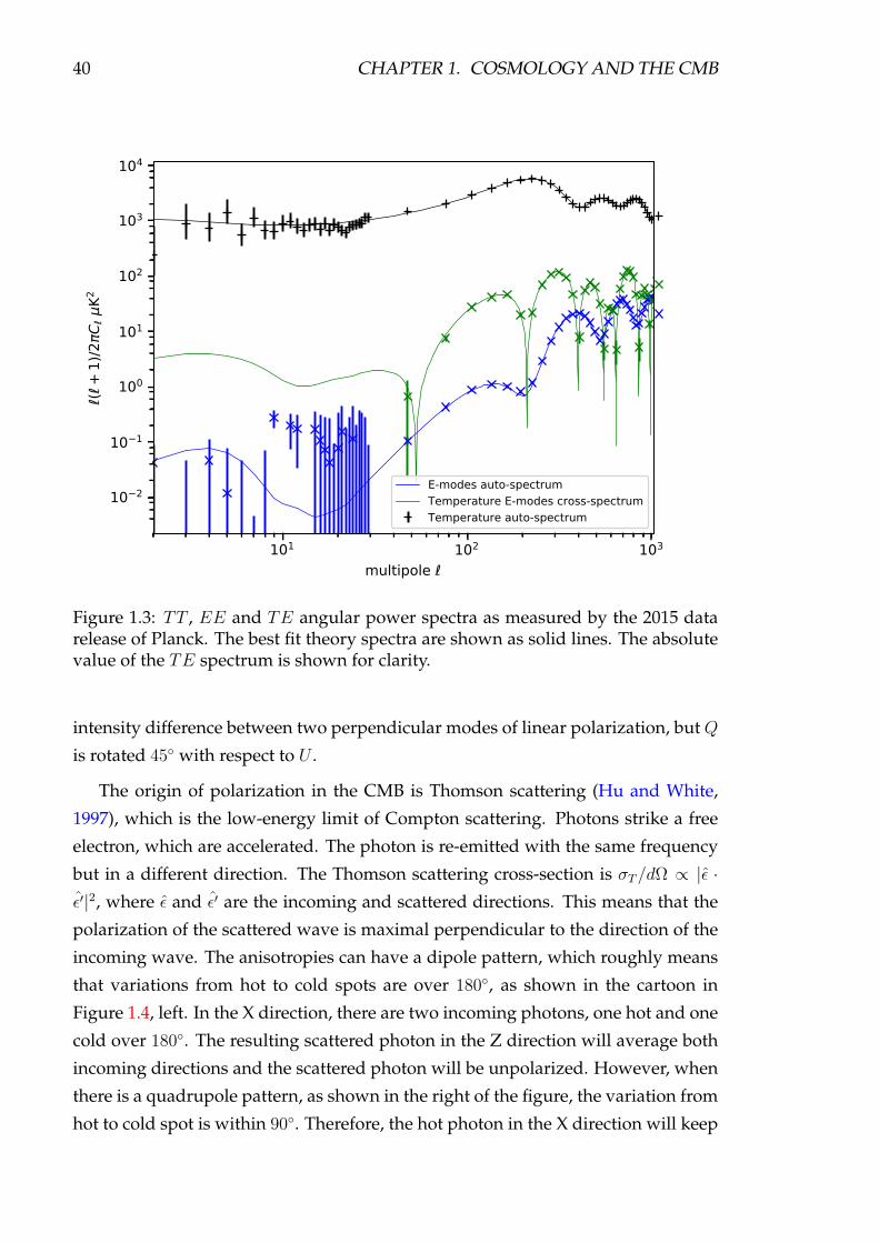
In Figure 1.3, we show the temperature angular power spectrum CTT` , in black,
as measured by Planck in its 2015 data release (Planck Collaboration et al., 2016m).
1.3.1 The CMB polarization
In the epoch of recombination, the quadrupole temperature anisotropies generate
linear polarization. The fraction of polarization is small (∼ 10%), since only the
photons with low optical depth can scatter in these conditions. The optical depth
decreased as the Universe went from opaque to transparent, so the photons with
low optical depth were the last ones to scatter, right before the moment the optical
depth became small. The polarization anisotropies pattern is imprinted by scalar
and tensor perturbations in different ways, which we could use to our advantage
to constrain cosmological theories.
The polarization of an electromagnetic wave is usually parametrized in term of
Stokes parameters: I , Q, U , and V . I measures the total intensity of the radiation,
which is the temperature field of the CMB, previously described. The total polar-
ization intensity is P =√Q2 + U2 + V 2. V measures the amount of circular polar-
ization, which corresponds to the rotation of the electrical (and magnetic) field with
respect to the propagation axis of the wave. The circular polarization is expected to
be 0 for the CMB, since the mechanism that polarizes it would only produce linear
polarization, entirely described by the Q and U parameters. They both measure the
40 CHAPTER 1. COSMOLOGY AND THE CMB
101 102 103
multipole
10 2
10 1
100
101
102
103
104
(+
1)/2
C
K2
E-modes auto-spectrumTemperature E-modes cross-spectrumTemperature auto-spectrum
Figure 1.3: TT , EE and TE angular power spectra as measured by the 2015 datarelease of Planck. The best fit theory spectra are shown as solid lines. The absolutevalue of the TE spectrum is shown for clarity.
intensity difference between two perpendicular modes of linear polarization, but Q
is rotated 45 with respect to U .
The origin of polarization in the CMB is Thomson scattering (Hu and White,
1997), which is the low-energy limit of Compton scattering. Photons strike a free
electron, which are accelerated. The photon is re-emitted with the same frequency
but in a different direction. The Thomson scattering cross-section is σT/dΩ ∝ |ε ·ε′|2, where ε and ε′ are the incoming and scattered directions. This means that the
polarization of the scattered wave is maximal perpendicular to the direction of the
incoming wave. The anisotropies can have a dipole pattern, which roughly means
that variations from hot to cold spots are over 180, as shown in the cartoon in
Figure 1.4, left. In the X direction, there are two incoming photons, one hot and one
cold over 180. The resulting scattered photon in the Z direction will average both
incoming directions and the scattered photon will be unpolarized. However, when
there is a quadrupole pattern, as shown in the right of the figure, the variation from
hot to cold spot is within 90. Therefore, the hot photon in the X direction will keep
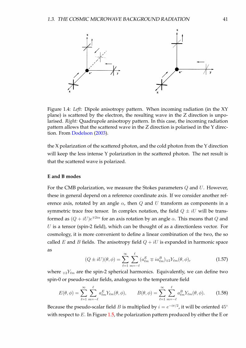
1.3. THE COSMIC MICROWAVE BACKGROUND RADIATION 41
Figure 1.4: Left: Dipole anisotropy pattern. When incoming radiation (in the XYplane) is scattered by the electron, the resulting wave in the Z direction is unpo-larised. Right: Quadrupole anisotropy pattern. In this case, the incoming radiationpattern allows that the scattered wave in the Z direction is polarised in the Y direc-tion. From Dodelson (2003).
the X polarization of the scattered photon, and the cold photon from the Y direction
will keep the less intense Y polarization in the scattered photon. The net result is
that the scattered wave is polarized.
E and B modes
For the CMB polarization, we measure the Stokes parameters Q and U . However,
these in general depend on a reference coordinate axis. If we consider another ref-
erence axis, rotated by an angle α, then Q and U transform as components in a
symmetric trace free tensor. In complex notation, the field Q ± iU will be trans-
formed as (Q + iU)e∓2iα for an axis rotation by an angle α. This means that Q and
U is a tensor (spin-2 field), which can be thought of as a directionless vector. For
cosmology, it is more convenient to define a linear combination of the two, the so
called E and B fields. The anisotropy field Q + iU is expanded in harmonic space
as
(Q± iU)(θ,φ) =∞∑`=1
∑m=−`
(aE`m ∓ iaB`m)∓2Y`m(θ,φ), (1.57)
where ∓2Y`m are the spin-2 spherical harmonics. Equivalently, we can define two
spin-0 or pseudo-scalar fields, analogous to the temperature field
E(θ,φ) =∞∑`=1
∑m=−`
aE`mY`m(θ,φ), B(θ,φ) =∞∑`=1
∑m=−`
aB`mY`m(θ,φ). (1.58)
Because the pseudo-scalar field B is multiplied by i = e−iπ/2, it will be oriented 45
with respect toE. In Figure 1.5, the polarization pattern produced by either the E or
42 CHAPTER 1. COSMOLOGY AND THE CMB
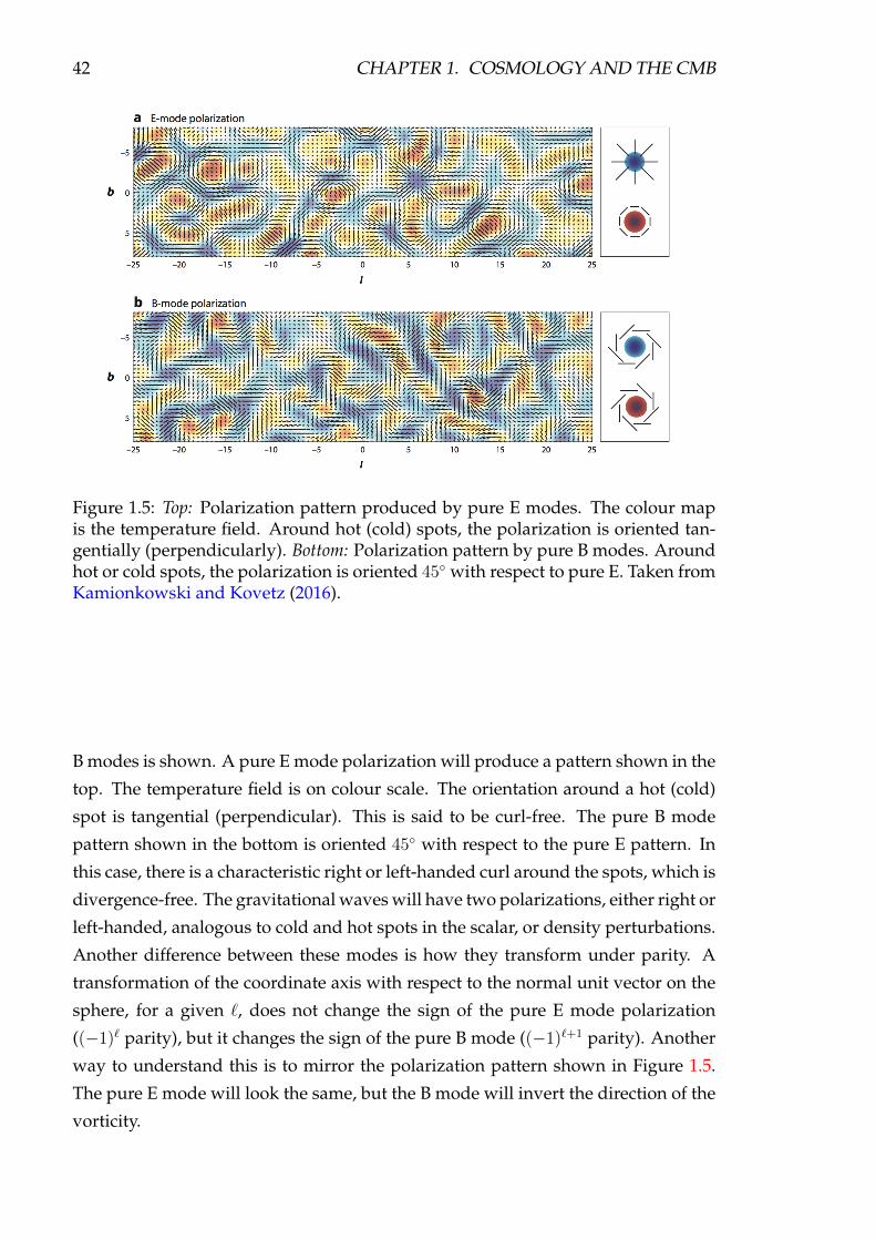
Figure 1.5: Top: Polarization pattern produced by pure E modes. The colour mapis the temperature field. Around hot (cold) spots, the polarization is oriented tan-gentially (perpendicularly). Bottom: Polarization pattern by pure B modes. Aroundhot or cold spots, the polarization is oriented 45 with respect to pure E. Taken fromKamionkowski and Kovetz (2016).
B modes is shown. A pure E mode polarization will produce a pattern shown in the
top. The temperature field is on colour scale. The orientation around a hot (cold)
spot is tangential (perpendicular). This is said to be curl-free. The pure B mode
pattern shown in the bottom is oriented 45 with respect to the pure E pattern. In
this case, there is a characteristic right or left-handed curl around the spots, which is
divergence-free. The gravitational waves will have two polarizations, either right or
left-handed, analogous to cold and hot spots in the scalar, or density perturbations.
Another difference between these modes is how they transform under parity. A
transformation of the coordinate axis with respect to the normal unit vector on the
sphere, for a given `, does not change the sign of the pure E mode polarization
((−1)` parity), but it changes the sign of the pure B mode ((−1)`+1 parity). Another
way to understand this is to mirror the polarization pattern shown in Figure 1.5.
The pure E mode will look the same, but the B mode will invert the direction of the
vorticity.

1.3. THE COSMIC MICROWAVE BACKGROUND RADIATION 43
Just like with the temperature field, we can define the variance of the a`m coeffi-
cients as the auto and cross angular power spectra
〈aE`m, a∗E`′m′〉 = δ``′δmm′CEE` (1.59)
〈aB`m, a∗B`′m′〉 = δ``′δmm′CBB` (1.60)
〈aT`m, a∗E`′m′〉 = δ``′δmm′CTE` (1.61)
〈aT`m, a∗B`′m′〉 = δ``′δmm′CTB` (1.62)
〈aE`m, a∗B`′m′〉 = δ``′δmm′CEB` . (1.63)
The three fields T , E, and B define 6 auto and cross angular power spectra, but
since B has opposite parity with respect to T and E, we expect CTB` and CEB
` to
be zero. The CEE` and CTE
` angular power spectra as measured by the Planck 2015
data release (Planck Collaboration et al., 2016m) are shown in Figure 1.3 in blue and
green, respectively.
1.3.2 Sources of E and B anisotropies
Before the last scattering, the photons are tightly coupled to the baryons in the
baryon-photon fluid. After the photons free-stream, the perturbation to the pho-
ton distribution evolves from the primordial perturbations set up by inflation. A
large-scale super-horizon mode, whose wavevector k is larger than the horizon at
recombination, will hardly evolve at all. The perturbation of another smaller mode,
whose wavevector is of the same size as the horizon at recombination, will peak ex-
actly at this time. There will be a maximum in the fluctuations at this scale, which
will be translated to the first peak in the angular power spectrum of the CMB. The
perturbation of an even smaller mode, which enters the horizon earlier, will have
been through its maximum before recombination, and the oscillation will be going
back to zero just at the time of recombination. Therefore, this mode will be at a
minimum of fluctuations, which will be translated as the first trough in the angular
power spectrum. An even smaller and earlier mode will enter the horizon before re-
combination and will go through a full oscillation at the time of last scattering. The
fluctuations will be at a second maximum at recombination, which will be trans-
lated as a second peak in the angular power spectrum. This will continue forever,
with smaller modes that enter the horizon earlier and earlier, showing as the peaks
and troughs in the CMB angular power spectrum, as shown in Figure 1.3. These
are the acoustic oscillations of the photon perturbations, showing up as anisotropies
in the CMB.

44 CHAPTER 1. COSMOLOGY AND THE CMB
Figure 1.6: Left, scalar perturbation spherical pattern. The direction of the bulk mo-tion is shown. Right, tensor perturbation spherical pattern. A gravitational wavepasses through upwards. A circle being streched is shown as reference. From Huand White (1997)
If the quadrupole temperature anisotropies are decomposed in spherical har-
monics Y m`=2, then m = 0, ±1 and ±2 correspond to scalar, vector, and tensor pertur-
bations, described in Section 1.2.1. First, consider the scalar perturbations. The tem-
perature pattern and the gravitational potential will create a bulk motion. Matter
will move from hot to cold spots (this is cold in the sense of effective temperature,
also considering the effect of the gravitational potential). The pattern created by
this is proportional to Y m=0`=2 ∝ 3 cos2 θ−1. This pattern is shown in Figure 1.6, left. θ
is the colatitude angle of observation, so the temperature pattern peaks at θ = π/2,
when the observer is perpendicular to the bulk flow. It is zero for θ = 0, looking
from the poles. The polarization is all-Q, with U(θ,φ) = 0 and Q(θ,φ) = sin2 θ. With
this, aE`m 6= 0 and aB`m = 0, therefore, scalar modes only produce E-mode polariza-
tion.
In the case of tensor perturbations, the temperature pattern is proportional to
Y m=±2`=2 ∝ sin2 θe±2iφ. This is produced by a single plane gravitational wave, prop-
agating in the z direction, with wavelength k, as shown in Figure 1.6, right. At
the equator, the quadrupole polarization patter is full-Q, with alternating cold and
hot lobes along the azimuthal angle φ. At the poles, the polarization pattern is at
maximum. The full polarization pattern is (Hu and White, 1997)
Q(θ,φ) = (1 + cos2 θ)e2iφ (1.64)
U(θ,φ) = −2i cos θe2iφ. (1.65)
In this case, aB`m 6= 0, as shown by Zaldarriaga and Seljak (1997); Kamionkowski
1.3. THE COSMIC MICROWAVE BACKGROUND RADIATION 45
et al. (1997), so both E and B-modes are non-zero for a gravitational wave. By sum-
ming all Fourier modes, we can obtain the B-mode power spectrum from a back-
ground of gravitational waves (see details in Kamionkowski and Kovetz, 2016)
CBB` =
1
2π
∫dkk2
[`+ 2
2`+ 1∆Q,`−1(k) +
`− 1
2`+ 1∆Q,`−1(k)
]2
, (1.66)
where ∆Q,` = (1/2)∫ 1
−1dµ∆Q(µ)P`(µ), µ = cos θ and ∆Q is the amplitude of the
perturbed distribution function of the photon, which in turn depends on the per-
turbation to the metric (h+ and h×) by the gravitational wave. We note that weak
gravitational lensing, a late time effect, transforms E-mode into B-mode signal.
1.3.3 Cosmological parameters
The ΛCDM cosmological model depends on several parameters. The accepted min-
imum number of independent parameters that fits well all cosmological observa-
tions is six. This is usually labelled as a baseline ΛCDM model. One possible choice
for these six parameters is: Ωbh2 (the density parameter for baryonic matter), Ωch
2
(the density parameter for cold dark matter), As and ns (the amplitude and spectral
index of the power spectrum of inflationary primordial scalar perturbations), τ (the
optical depth to reionization), and θMC (the sound horizon at last scattering). In
this case, some reasonable assumptions are made, such as a flat universe (therefore
ΩΛ = 1−Ωb−Ωc) or an equation of state for dark energy wΛ = −1. The parameters
Ωm, Ωb, ns and As were explained previously.
The cosmological parameters can be measured with the acoustic oscillations in
the CMB angular power spectra (Dodelson, 2003). The morphology of the peaks
and troughs depends on the parameters. For example, the content of baryons in
the Universe (Ωbh2) affects the locations and the relative heights of even and odd
peaks. If the baryon-photon fluid has more baryons, it is heavier, which makes the
sound speed smaller. This means that the acoustic oscillations will have smaller
frequencies (or larger wavenumber), which shifts the locations of the peaks. An-
other example is changing the Λ or matter content of the Universe. If there is no
cosmological constant, the large-scale modes, which are entering the horizon only
recently, are shifted towards smaller scales, which moves the peaks to higher mul-
tipoles. If the total matter of the Universe is lowered, then the acoustic oscillations
fluctuate even more, since there is more radiation content, which facilitates this
process, as opposed to matter which by gravity tends to cluster and slow down
the oscillations. Then, the heights of the peaks increase in the angular power spec-
trum. In the following, some of the cosmological parameters that have not been

46 CHAPTER 1. COSMOLOGY AND THE CMB
introduced will be described.
The epoch of reionization (Zaroubi, 2013) corresponds to the period after the
dark ages (which goes from the CMB last scattering to the formation of the first
stars), when the firsts galaxies formed and their UV radiation eventually ionized
the neutral hydrogen in the Universe. This did not happen instantaneously, but as
a process, at redshifts 15 ≥ z ≥ 6. The Gunn-Peterson trough is the first observa-
tional evidence for a reionization of the neutral hydrogen. Predicted by Gunn and
Peterson (1965), the absorption spectra of distant quasars should show an absorp-
tion trough at wavelengths shorter than the corresponding Lyman-α line, by the
intervening neutral hydrogen. This was not observed for quasars at redshift z . 6,
instead observing a series of small absorption features denominated the Lyman-α
forest, by the intervening ionized hydrogen. However for objects at higher redshift,
the flux beyond the Lyman-α line is effectively zero (Becker et al., 2001), which is
evidence of the Universe going through a process where the neutral hydrogen ion-
ized at around z ∼ 6. Another way to probe the reionization epoch is by using the
CMB, because free electrons cause Thomson scattering of the CMB photons at later
times, while they travel from the last scattering surface to us. This effect is the same
that occurred at recombination, but now it occurs at a much lower rate, since the
density of free electrons has decreased at late times because of the expansion of the
Universe. The parameter τ is the optical depth of the Thomson scattering for the
CMB photons, defined by
τ(η) =
∫ η0
η
σTnea(η′)dη′, (1.67)
where η is the conformal time, σT is the Thomson scattering cross-section, and ne is
the free electron density. Therefore, the reionization optical depth provides an inte-
grated constraint over the entire reionization process, not enabling us to distinguish
the details in reionization history. The effect on the temperature anisotropies of the
CMB is suppression of the power spectra at small scales, while in polarization it
creates features at small scales.
The matter in the primordial fluid, before recombination, created gravitational
potentials along the density perturbations. The photon-baryon fluid is compressed
along by the gravity. At the same time, photons push back with radiation pressure,
and so forth. The acoustic oscillations in the photon-baryon fluid were imprinted
once the photons decoupled at last scattering. The sound horizon to last scattering
θMC is the “angular distance” of the Universe at last scattering. It is defined by θ∗ =rsds
, where rs is the comoving sound horizon of the Universe at recombination (the
maximum distance a wave could have travelled in the primordial photon-baryon

1.3. THE COSMIC MICROWAVE BACKGROUND RADIATION 47
fluid), defined by
rs =
∫ t=t∗
t=0
cs/a∗dt, (1.68)
where cs is the sound speed of the photon-baryon fluid. ds is the comoving angular
distance to the last scattering surface, given by
ds =1
a∗H0
1
1 + z∗
∫ z
0
dz′√Ωr,0(1 + z′)4 + Ωm,0(1 + z′)3 + ΩΛ,0
. (1.69)
By doing some approximations, θ∗ can be measured to a value∼ 1/200. In harmonic
space, the multipole associated with its real space angle is ` = π/θ, so the sound
horizon at last scattering multipole is `∗ ∼ 200, which is approximately where the
first peak of the temperature CMB angular power spectrum is located. In cosmo-
logical models, an approximation of θ∗ is used, labelled θMC.
Based on a six-parameter cosmology, others parameters can be derived, such
as the Hubble constant h, the age of the Universe, the redshift of recombination
z∗, the normalization of the matter power spectrum σ8 (defined as the standard
deviation in the matter density distribution inside a comoving sphere of diameter
8 Mpc), among others. Some other parameters are fixed at fiducial values, and can
be varied when fitting for extensions to the baseline ΛCDM model. For example,
the canonical value of the dark energy equation of state is w = −1, but extended
models can fit a free w parameter, either constant or depending on a (e.g. Planck
Collaboration et al., 2016k).
Using other physics, extensions can be made to the baseline ΛCDM model. Neu-
trino physics can be constrained with cosmology. The baseline model usually as-
sumes a normal mass hierarchy (one neutrino species much more massive than the
other two) with a mass of mν = 0.06 eV, and Neff = 3.046, the effective number
of neutrino-like species (which parametrizes the contribution of neutrinos to the
energy density). We know that the presence of neutrinos will slow the agglomera-
tion of CDM when the mass structure is forming (Lesgourgues and Pastor, 2006), so
there will be an imprint on the CMB weak lensing potential, BAOs, etc. Current con-
straints are∑mν . 0.17 eV and Neff ∼ 3.04± 0.2 (Planck Collaboration et al., 2016i;
Couchot et al., 2017). Another example is primordial nucleosynthesis. The primor-
dial Helium fraction YP can be set to a fiducial value (e.g. YP = 0.2534± 0.0083 Aver
et al., 2012) in the baseline model, however, for example, the CMB spectra damping
tail shape is sensitive to YP. Planck constrains the value to YP = 0.253+0.025−0.026 (Planck
Collaboration et al., 2016i). As a final example, the ΛCDM model is extended regu-
larly to include early Universe physics, that is inflation, as explained in Section 1.2.

48 CHAPTER 1. COSMOLOGY AND THE CMB
Figure 1.7: Current measurements of the CBB` angular power spectrum, from PO-
LARBEAR (The POLARBEAR Collaboration et al., 2017), ACTpol (Louis et al.,2017), SPTPol (Keisler et al., 2015a) and BICEP2/Keck array (BICEP2 and Keck Ar-ray Collaborations et al., 2015).
In this case, the parametrization of the primordial scalar perturbation power spec-
trum, As and ns, and the tensor-to-scalar ratio r, are parameters that are be fitted.
1.3.4 Current observations of CMB B-modes
The recent history of CMB observations has been defined by series of instruments,
both ground-based as well as satellites. The Planck satellite (Planck Collaboration
et al., 2014a, 2016a) observed the CMB from 2009 for 4 years. Ground-based ex-
periments that started observing after 2010 have also measured the CMB at small
and intermediate scales. The South Pole Telescope (SPTpol) polarization instru-
ment (Austermann et al., 2012) and the BICEP2/Keck Array (BICEP2 Collaboration
et al., 2014a) are observing from Antarctica. The Atacama Cosmology Telescope
(ACTpol) polarization instrument (Niemack et al., 2010; Thornton et al., 2016) and
the POLARBEAR (Arnold et al., 2010; The Polarbear Collaboration: P. A. R. Ade
et al., 2014) instrument are observing from the Atacama desert in Chile.
An indirect measurement for B-modes is to cross-correlate a predicted map of
1.3. THE COSMIC MICROWAVE BACKGROUND RADIATION 49
lensing B-modes with observed B-mode maps. The lensing potential φ can be re-
constructed from external data (e.g, the Cosmic Infrared Background is the most
correlated observable, Planck Collaboration et al., 2014c). This potential allows us
to estimate the gravitational lensing contribution from EE to BB spectra. This can
be correlated with a measured B map. Hanson et al. (2013) detected this correla-
tion for the first time with SPTPol, with a 7.7σ non-zero significance. POLARBEAR
(Ade et al., 2014), ACTpol (van Engelen et al., 2015) and Planck (Planck Collabora-
tion et al., 2016j) have also detected this correlation.
The ground based experiments have detected the small/intermediate-scale CBB`
power spectrum from gravitational lensing. POLARBEAR have measured it from 2
seasons of data, in the multipole range 500 ≤ ` ≤ 2100 (4 bins) (The POLARBEAR
Collaboration et al., 2017). This is consistent with gravitational lensing signal (zero
B-mode signal is rejected with 3.1σ), and they measure an amplitude for the lensing
power spectrum CBB,lens` of AL ∼ 0.6± 0.45. ACTPol measured directly the lensing
B-mode spectrum (Louis et al., 2017). This is only in two bins in the multipole
range 500 ≤ ` ≤ 2500, fitting a lensing power spectrum amplitude of AL = 2.03 ±1.01. The SPTpol instrument has measured the lensingBB power spectrum (Keisler
et al., 2015a) at 4.1σ (for B-modes from lensed E-mode polarization). The CBB` are
measured in the multipole range 300 ≤ ` ≤ 2300 for five bins, based on data taken
in a 100 deg2 patch over two seasons.
The BICEP2 experiment measured the large/intermediate-scaleBB power spec-
trum in nine bins at multipoles 20 < ` < 340 (BICEP2 Collaboration et al., 2014b).
They found an excess over the pure lensed BB power spectrum with a significance
of ∼ 5.2σ. If this were due to primordial tensor perturbations, the best fit tensor-
to-scalar ratio would be r = 0.20+0.07−0.05. However, they underestimated the contami-
nation by thermal dust in the observed sky patch. A joint analysis with the Planck
observations at higher frequencies of dust showed that the excess is entirely con-
sistent with foreground contamination (BICEP2/Keck and Planck Collaborations
et al., 2015). Since then, the Keck Array also measured the B-mode spectrum (BI-
CEP2 and Keck Array Collaborations et al., 2015), and also combined with BICEP2
(BICEP2 Collaboration et al., 2016). Their estimate of the lensing power spectrum
is AL = 1.20± 0.17.
The current measurements of the (lensing) CBB` angular power spectrum, de-
scribed above, are shown in Figure 1.7.

BLANK PAGE
50

Chapter 2
CMB foregrounds and component
separation
When trying to extract any cosmological signal from the CMB, the instrumental
sensitivity is not the only issue to be considered. Other sources of electromagnetic
radiation emit at the same frequencies as the CMB, in the local and low-redshift
Universe. Of special consideration is the emission from our own Milky Way, which
is all around us and blocks our clean view of the CMB. Any source of contami-
nation are collectively known as CMB foregrounds. The algorithms and methods
designed to separate these foregrounds from the clean CMB (the primary signal
plus secondary effects), with the objective of reducing (or eliminating all together)
the impact of systematics in the derived cosmology, are known as CMB component
separation (Delabrouille and Cardoso, 2009).
2.1 Astrophysical foregrounds
Several emission mechanisms radiate at the same frequency range where the CMB
peaks. Figure 2.1, top, shows the spectral energy distributions (SEDs) of the CMB,
as well as several of the diffuse Galactic foregrounds for temperature observations1. The CMB is dominating around 50 − 150 GHz outside the Galactic plane, but
the thermal dust is the strongest foreground at higher frequencies. At lower fre-
quencies, synchrotron, free-free and spinning dust emission dominate. Figure 2.1,1The units correspond to brightness temperature TB, using the Rayleigh-Jeans approximation
hν kT , given by TB = Iνc2
2kν2 , where Iν is the intensity (energy per surface area per solid angle perfrequency), c is the speed of light, k is the Boltzmann constant and ν is the frequency. This unit oftemperature is also referred to as Rayleigh-Jeans units. These units are different from Thermody-namic units, where the Rayleigh-Jeans units are normalized with a Planck law with a temperatureequal to the CMB temperature. Therefore, in this units the SED of the CMB is constant across fre-quency and all other components are distorted.
51

52 CHAPTER 2. CMB FOREGROUNDS
Figure 2.1: SEDs of the CMB and diffuse Galactic foregrounds. On top, tempera-ture, and on the bottom, polarization. The Planck observation frequencies are alsoindicated for comparison. The upper and lower limits on each component are con-sidering maks with different sky fractions (81 and 93% outside the Galactic plane).Taken from Planck Collaboration et al. (2016b), figure 51.
2.1. ASTROPHYSICAL FOREGROUNDS 53
bottom, shows the SEDs of the components in polarization, where the CMB is a few
orders of magnitude fainter than its temperature. We know that thermal dust and
synchrotron are strongly polarized and they are more intense that the CMB over
most of the regions of the sky. They constitute the main foreground components
that must be accounted for. Spinning dust is slightly polarized, but no more than
a few percent in active star formation clouds. There are also extra-Galactic sources,
mainly Active Galactic Nuclei (AGNs) or young dusty star forming galaxies, which
are slightly polarized. In the following, we will describe these foregrounds in some
detail.
2.1.1 Synchrotron radiation
This emission is produced by the acceleration of charged particles in interstellar
magnetic fields. The electrons are deflected by the magnetic field, that exerts an
acceleration perpendicular to its velocity. This provokes a spiral trajectory around
the magnetic field lines, through which the particles emit radiation with power
proportional to the magnetic field squared. The SED of synchrotron radiation is
very close to a power law, given by
TA,syn(ν) ∝ νβsyn+C log(ν), (2.1)
with a negative slope βsyn ∼ −3 and an optional curvature parameter C (Davies
et al., 2006; Kogut et al., 2007), to account for the steeping as the frequency increases.
βsyn will vary across the sky, because it is dependent on the particular acceleration
of electrons and their velocities distribution. The synchrotron polarized intensity
consists of filamentary structures, the so-called spurs, which follow the lines of the
Galactic magnetic field away from the Galactic plane. The polarization fraction
can be as high as ∼ 40 percent in some of the filaments (Vidal et al., 2015). How-
ever, most of the Galactic plane is expected to be polarized to smaller levels, from a
few percent to . 20 percent (Page et al., 2007). The morphology of polarized syn-
chrotron and low-frequency foregrounds is constrained with Planck in its 2015 data
release (Planck Collaboration et al., 2016e).
A further complication is the fact that at low frequency, ν ∼ 20 GHz, the spec-
tral laws of synchrotron, free-free and spinning dust are very hard to distinguish,
having a similar slope, as shown in Figure 2.1 for temperature. If spinning dust is
slightly polarized, it can be easily confused with synchrotron, which complicates
the modelling of both components. To overcome this, present and future low-
frequency experiments are being developed to map the sky in this frequency range,

54 CHAPTER 2. CMB FOREGROUNDS
such as C-BASS (Irfan et al., 2015), at 5 GHz; and QUIJOTE (Rubiño-Martín et al.,
2010), at 10-30 GHz.
2.1.2 Thermal dust radiation
This is produced by the presence of dust grains of various sizes in the Interstellar
Medium (ISM). In regions of star formation, the UV radiation from newly formed
stars (compact and ultra-compact HII regions) heats up the surrounding medium,
including dust grains, which in turn radiate in the IR and microwave frequencies.
In principle, each grain at a given temperature should radiate very close to a ther-
malized black-body. In practice, for a given line of sight, there are many different
dust grains populations at different temperatures, all emitting at the same time. In
the simplest model, the SED of thermal dust is well fitted by a Modified Black-Body
(MBB) of the form
TA,dust(ν) ∝ νβdust+1[exp(hν/kTdust)− 1]−1, (2.2)
where Tdust and βdust are a single temperature that collectively describes the dust
grains, and a positive slope representative of the ∼hundreds of GHz frequency
range, respectively. Along the Galactic plane, the parameters are consistent with
Tdust ∼ 19 K, and a spectral index of βdust ∼ 1.51 (for temperature) and βdust ∼ 1.59
(for polarization) (Planck Collaboration et al., 2015b). However, the different dust
populations mean that every pixel has a different MBB spectral law, even away
from the Galactic plane (Planck Collaboration et al., 2017). The 2015 data release
of Planck finds maps of the thermal dust spectral parameters, with average values
across the sky 〈Tdust〉 ∼ 21 K and 〈βdust〉 ∼ 1.53 (Planck Collaboration et al., 2016b).
More complex models have also been proposed, in particular the use of multi-
component MBB spectral laws (e.g. Meisner and Finkbeiner, 2015). In this case,
usually two (or more) populations of thermal dust are considered for each line of
sight. The dust grains are not perfectly spherical, so they tend to align with the
Galactic magnetic field. This means that the microwave emission they radiate is
polarized. In some areas of the Galactic plane, the polarization fraction can reach
up to 20 percent (Planck Collaboration et al., 2015a). The modelling of polarized
thermal dust is more complicated that a MBB spectral law. 3D models of the Galac-
tic emission try to overcome this, by considering that along a line of sight there
is a superposition of MBB laws, whose polarization properties will depend on the
physical conditions of the dust and on the local magnetic field (e.g, O’Dea et al.,
2012; Martínez-Solaeche et al., 2017; Chluba et al., 2017).

2.1. ASTROPHYSICAL FOREGROUNDS 55
2.1.3 Anomalous Microwave Emission (AME)
The Anomalous Microwave Emission (AME) is an emission mechanism that has
been discovered relatively recently. It was first detected directly by Leitch et al.
(1997), where a low-frequency emission strongly correlated with dust was detected.
Now we know that the most likely origin of it are grains of dust rapidly spinning,
with a dipole moment, that emit at microwave frequencies (Draine and Lazarian,
1998). Hence, this emission is sometimes also referred to as spinning dust. Since
then, a lot of knowledge has been gathered on AME from WMAP and Planck,
among others (Génova-Santos et al., 2011; Planck Collaboration et al., 2011, 2014b).
The SED of spinning dust is uncertain. There are numerical templates based
on the dust properties (e.g. Ali-Haïmoud et al., 2009), but also analytical spectral
laws that depends on a few parameters (see e.g. Davies et al., 2006; Bonaldi et al.,
2007; Stevenson, 2014). The polarization of AME is not constrained, and we only
have upper limits on its polarization (Dickinson et al., 2018). It is likely polarized
. 3 percent below 30 GHz, but at higher frequencies it falls to < 1 percent (Rubiño-
Martín et al., 2012). Upper limits have been measured in Galactic star formation
clouds, of only a few percent (Dickinson et al., 2011; López-Caraballo et al., 2011;
Génova-Santos et al., 2017).
2.1.4 Point sources
The extra-galactic sources that contribute in the CMB frequency range are dusty
star-forming sub-mm galaxies and radio galaxies (De Zotti et al., 2015, 2018).
Radio galaxies are distant and bright quasars and blazars that are active. They
emit mostly through the synchrotron mechanism, with the interaction of energetic
output (jets) and the intra-galactic medium. Their spectral properties are consistent
with a power-law Sν ∝ ν−α (Massardi et al., 2016). The slope of the population
emitting in the microwave range is close to flat in flux units, but above 30 GHz, it
steepens to values α ∼ 0.6 2.
Star-forming galaxies are dominated by dust emission in the microwave fre-
quency range. Therefore, they are consistent with MBB spectral laws, with spectral
indices ∼ 1.8 (Clemens et al., 2013).
In polarization, the properties of points sources in the microwave range have
only been recently constrained. Massardi et al. (2013) obtain a complete sample of
polarized sources at few tens GHz with Australia Telescope Compact Array (ATCA)
2As explained above, flux and brightness temperature are related by Iν ∝ Tbν2, therefore the α
index in flux is related to the β index in synchrotron by β = α+ 2

56 CHAPTER 2. CMB FOREGROUNDS
and WMAP data. Most of the sources are weakly polarized, with a distribution of
polarization fractions of a few percent. More recently, Galluzzi et al. (2017) studied a
complete sample of 53 radio sources and characterized their properties in intensity
and polarization. The spectral laws are well described by power-laws, but spectra
in polarization can differ significantly from temperature intensity, since some of the
sources show variability with time scales of a few years.
Bonavera et al. (2017a) and Bonavera et al. (2017b) study the polarization frac-
tion properties of the radio and dusty point sources, respectively, detected by
Planck in their second catalog of compact sources (Planck Collaboration et al.,
2016f). They conclude that the distribution of polarization fractions can be approx-
imated by a log-normal function with a mean value of few percent.
2.1.5 Other unpolarized foregrounds
The other major diffuse Galactic foreground is free-free emission, also known as
bremsstrahlung. This is originated by the scatter and deceleration of electrons by
charged particles in the ISM. Free-free emission is very close to a power-law for
frequencies above 1 GHz, with a spectral index ∼ −2. At even lower frequencies
there is a break in the SED. As mentioned above, at low-frequency free-free is de-
generate with synchrotron. However, free-free is more intense at higher-frequency
since its slope is flatter. This helps to constrain its emission. Free-free is expected to
be essentially unpolarized, since the directions of the scatter processes are random.
Over all the sky, it is measured to be polarized by < 1% (Macellari et al., 2011).
The Sunyaev-Zel’dovich (SZ) clusters are extra-Galactic sources that are de-
tected through their effect in the CMB. The thermal SZ effect is the inverse-Compton
scattering of CMB photons by electrons in the ionized hot intra-cluster medium of
galaxy clusters (Sunyaev and Zeldovich, 1972). The photons gain energy, which dis-
torts the perfect black-body spectrum by a small amount depending on the electron
density of the cluster, shifting the intensity towards higher frequencies. If a black-
body is subtracted from the observed CMB signal, then a lack of CMB photons is
observed at lower frequencies and an excess at higher frequencies. The transition
frequency is located upwards of 200 GHz. Planck mapped the thermal SZ distortion
(Planck Collaboration et al., 2016n). The kinetic SZ effect is produced by the scatter
of CMB photons with electrons that have high-energy because of the bulk motion
of the galaxy cluster with respect to the CMB.

2.2. COMPONENT SEPARATION 57
2.2 Component separation
As explained above, the CMB is obscured by several sources of emission at the same
frequencies, from our Galaxy and from external sources. Several component sep-
aration methods have been proposed to extract the clean CMB (Delabrouille and
Cardoso, 2009). In general, these methods can be categorized as blind or non-blind.
In non-blind methods, usually there are predetermined spectral functions that char-
acterize the SEDs of the components. Therefore, this assumes that we know what
the spectral dependence of a given component is, even though in the real sky it
might not be exact. Blind methods use minimal prior information about the compo-
nents, and mainly use their statistical properties (e.g. their statistical independence,
since we know that the CMB is a Gaussian field, while the diffuse Galactic compo-
nents clearly are not) to disentangle them. We will refer as parametric methods to
a category that is somewhere in between, since they model explicitly the SED of
the foreground components, but allow the estimation of these parameters from the
data directly.
In general, we will assume that in an observed pixel p, we will measure a super-
position of components emitting with their own spectral law (this superposition
is convolved with the beam of the instrument observing) plus some instrumental
noise. This is usually labelled a Linear Mixture. That is, the observed signal y at
band ν is given by
yν(p) =
∫B(p, ν)t(ν)
Nc∑j=0
xj(p, ν)dpdν + n(p, ν), (2.3)
where the upper ∼ means an observed/estimated variable, y is the total intensity
observed by the instrument, xj is the true signal from component j, B(p, ν) is the
beam pattern function, t(ν) is the window function from the instrument at band ν,
n(p, ν) is the instrumental noise, and ν =∫B(p, ν)t(ν)νdνdp is the frequency of each
band (the mean frequency weighted by the beam and window function). Each indi-
vidual band is indexed by an integer ν. In practice, we make some simplifications:
the beam function B is constant within the passband, meaning it only depends on
space and is usually parametrized with the Full Width at Half Maximum (FWHM)
of the main beam, and the true signal of component j has a spatial component s
(an spatial amplitude), and a frequency component a which scales it in frequency
(a SED),
xj(p, ν) = aj(ν)sj(p). (2.4)
58 CHAPTER 2. CMB FOREGROUNDS
Then, we can write a single beam that convolves a superposition of components
yν(p) = Bν(p) ∗Nc∑j=0
ajνsj(p) + nν(p), (2.5)
where ∗ denotes convolution (integration in p), ajν =∫t(ν)aj(ν)dν is the weighted
spectral law of component j, where the weight is the window function of band ν.
In matrix form, it can be written (for every pixel p) as
ˆy = B ∗ As+ n, (2.6)
where ˆy is a Nbands vector that contains the yν elements, A is the mixing matrix,
with size Nbands ×Nc, where Nc is the number of components, and contains the ajνelements, s is a Nc vector that contains the sj elements and n is a Nbands vector that
contains the noise elements nν .
The objective is to get an estimator for s, given by ˆs = Wˆy, where W is the recon-
struction matrix, chosen appropriately. Sometimes, this is calculated as a function
of the mixing matrix. In other methods, especially blind ones, W is estimated it-
eratively to maximize the independence between components. From now on, we
will ignore the beam window function B when working in real space. Usually the
resolution of all the maps at different bands is equalized by smoothing the maps,
to absorb the beam into the mixing matrix. In harmonic space, the convolution is
transformed into a multiplication, which is even simpler. We will also drop the
upper hats to denote vector quantities.
2.2.1 Parametric methods
Usually, the simpler approach is to parametrize analytic spectral laws for each com-
ponent. Then, the mixing matrix A is calculated in a straightforward way, by in-
putting the normalized spectral laws at Nbands frequencies by Nc components. This
requires previous knowledge on how the different mechanisms of emission behave
spectrally. Moreover, in principle we do not know if the parameters assumed or
estimated are a reflection of the true sky. Once a mixing matrix is estimated, it can
be used to compute a suitable W matrix. The accuracy of it will depend on the
accuracy of the mixing matrix.
Choosing the reconstruction matrixW
The simplest way of choosing the reconstruction matrix is to invert the mixing ma-
trix W = A−1 and s = s + A−1n. This is noisy when the signal-to-noise ratio is

2.2. COMPONENT SEPARATION 59
low, and A has to be square (same number of components and bands), which is in-
efficient, since usually we have more bands than components, and therefore some
information is not going to be used.
The Generalized Least Squares (GLS) solution is
W =[A†R−1
n A]−1
A†R−1n , (2.7)
where Rn is the noise covariance matrix. In this case, s = s +[A†R−1
n A]A†R−1
n n.
The solution is unbiased, keeping a noise contribution, and it is also the solution
that minimizes the variance of the error when the signal s is deterministic.
The Wiener filter solution is given by W =[A†R−1
n A + R−1s
]−1A†R−1
n . As op-
posed to the GLS solution, it is assumed that the noise and the data are stochastic,
with known statistics in the form of the noise and signal covariance matrix, Rn and
Rs, respectively. The estimated signal is given by s =[A†R−1
n A + R−1s
]−1A†R−1
n As+[A†R−1
n A + R−1s
]−1A†R−1
n n, which means that it is not unbiased, introducing fore-
ground residuals in s. It is the solution that minimizes the variance of the error for
stochastic signals.
Bayesian parametric methods
In this class of algorithms, the observed sky spectral law is modelled as a sum of
components, controlled by amplitudes and spectral parameters, and noise. The
ability to accurately subtract the foregrounds from the CMB depends on accurately
describing the observations through analytical spectral laws. The COMMANDER
code (Eriksen et al., 2008) uses the Bayesian framework to fit foreground com-
ponents in pixel space through Gibbs sampling and Monte Carlo Markov Chain
(MCMC). The posterior distribution of the parameters Ai (the amplitudes of the
components in both Q and U ), βj (the spectral parameters of the components,
e.g. spectral indices), and C` (the EE and BB angular power spectra of the fitted
model), is given by the Bayes theorem
P (s,β,C`|d) ∝ L(d|s,β,C`)P (s,β,C`), (2.8)
where d is the observed sky data. P (s,β,C`) corresponds to the assumed prior on
parameters and the likelihood minimizes the residuals between the data and model
in pixel space, using the noise covariance matrix (calculated assuming Gaussian
uniform noise uncorrelated across bands).
To sample the multi-dimensional parameter space in order to compute the pos-
terior distribution is prohibitively expensive, and therefore an alternative scheme

60 CHAPTER 2. CMB FOREGROUNDS
is to use Gibbs sampling, where the full joint posterior is sampled by alternatively
sampling the simpler conditional posterior probabilities of each parameter. This
is done iteratively, as steps of a Markov Chain. If the chain is long enough, the
sampled posterior will converge to the true posterior (Wandelt et al., 2004).
A nice feature of this method is that since the angular power spectra is a param-
eter in the sampling of the joint posterior distribution, the cosmological parameters
that control the shape of the angular power spectra of the CMB can be included
as parameters to fit. Therefore, in the same Markov chain, the foreground and
cosmological parameters can be fitted at the same time. This method is compu-
tationally expensive, since the estimation is performed pixel-by-pixel. If all possi-
ble parameters are being fitted (CMB and foregrounds, both spectra and templates,
plus fiducial CMB spectra), then the code is limited to low resolution maps, usu-
ally Nside = 16. However, when fitting for only foregrounds, it can be run at much
higher resolutions.
Correlated Component Analysis (CCA)
This is a method to estimate the spectral parameters of the components assumed to
be present in a set of multi-frequency maps of the sky (Bonaldi et al., 2006; Ricciardi
et al., 2010).
It exploits the second order statistics of the data, that is, the covariance matrices.
For the observations y, we have its covariance matrix given by
Ry(τ ,ψ) = ARs(τ ,ψ)A† + Rn, (2.9)
where A is the mixing matrix, Ry, Rs, and Rn are the covariance matrices of the
observations, true signal, and noise, respectively. (τ ,ψ) represents a shift in the
coordinates of the variable of the covariance matrix. For a given variable X , that
depends on generic coordinates (ε, η), the “shifted” covariance matrix is given by
RX(τ ,ψ) = 〈[X(ε, η)− µ(X)] [X(ε+ τ , η + ψ)− µ(X)]†〉, (2.10)
where µ(X) is the mean of the variable X , and 〈...〉 represents the average over
realizations. Covariance matrices are defined by shifts in the coordinates.
We want to estimate Rs and A. The mixing matrix is parametrized with spec-
tral parameters of the components considered. To this purpose, the functional Φ is
defined
Φ[Rs,A] =∑τ ,ψ
|ARs(τ ,ψ)A† − Ry(τ ,ψ) + Rn(τ ,ψ)|2. (2.11)
This must be minimized for sufficient coordinates shifts.

2.2. COMPONENT SEPARATION 61
The Correlated Component Analysis has also been implemented in the har-
monic domain, where there are many advantages over pixel space. The observed
signal is the angular power spectra C`, and (ε, τ) = (`,m). We do not need to equal-
ize the beams for frequency bands, as we have to do in pixel space. The end result
for the method is the estimation of the spectral parameters of the components mod-
elled and of the mixing matrix A. Then, the reconstruction of the components is
done with the GLS solution of the reconstruction matrix, using the estimated mix-
ing matrix.
2.2.2 Blind methods
These methods assume minimal prior information on the foreground component.
Independent Linear Combination (ILC)
This method does not exploit the spectral information of the foregrounds, but it
does exploit the known black-body spectral shape of the CMB. We represent the
data in thermodynamic units, which is a normalized unit of temperature, normal-
ized to the SED of the CMB. In this way, the CMB SED is a constant across frequency.
ILC assumes that the other components have different frequency spectra. The sky
signal y is a mixture of CMB s, noise n and foregrounds f (everything else), that
is y = s + f + n, written in matrix notation, where the elements of the vector are
the different frequency bands. The reconstruction matrix W (in this case it is square
with size Nbands), such that s = Wy, is given by
s =a†C−1
a†C−1a(s+ f + n), (2.12)
where a is actually a vector of ones, representing the CMB SED in thermodynamic
units, which is constant, and C is the signal covariance matrix. The method tries
to adjust the weights of the reconstruction matrix, such that the contribution of
the foregrounds is minimized. In practice, however, this methods requires perfect
decorrelation between the CMB and everything else, which is not true when dealing
with finite resolutions of maps, and by chance correlation. Examples of this method
are found in Bennett et al. (2003); Tegmark et al. (2003); Eriksen et al. (2004).
Another issue is the fact that the weights are dominated by the low Galactic
latitude emission, where the foregrounds are important, while at high Galactic lat-
itude the noise is dominant. This will bias some of the scales of the CMB, which is
not optimal, since all scales are needed. One implementation of ILC uses spherical
62 CHAPTER 2. CMB FOREGROUNDS
wavelets called needlets, method known as Needlet ILC (NILC Remazeilles et al.,
2011; Basak and Delabrouille, 2012, 2013).
Independent Component Analysis (ICA)
The only assumption this method makes is that each of the components are statisti-
cally independent of each other and of the noise. We do not assume any information
on the SED or mixing matrix A. The signal estimate is s = Wy, where the measured
sky is a sum of Nc = Nbands components and noise, yν =∑
iCi,ν + nν . The Nc × Nc
reconstruction matrix (weights) has to be calculated in such a way that the elements
of the s vector are independent. The condition for independence of the elements of
the s vector, in pixel space, is
1
Np
Np∑p=1
si(p)sj(p) = 0 i 6= j ≤ Nc, (2.13)
where Np is the total number of pixel in the map, p indexes pixels, and i,j in-
dexes components. These conditions are symmetrical, therefore there are only
Nc(Nc − 1)/2 constraining equations, and we need N2c to calculate W. To break
the symmetry, for example, non-linear functions of si are used in the condition 2.13.
Another way is to use local decorrelation, where the sum in condition 2.13 is di-
vided by a number σ2ip, which depends on the pixel p.
An implementation of ICA in harmonic space is Spectral Matching ICA (SMICA
Delabrouille et al., 2003; Cardoso et al., 2008). The Nbands×Nbands covariance matrix
of the observations is calculated at each `
C` =1
2`+ 1
∑m=−`
y`my†`m (2.14)
The weight to mix the bands, the reconstruction matrix, is the same as the one used
for ILC, but in harmonic space, given by
w` =C−1
` a
a†C−1
` a, (2.15)
where a is a vector with the spectral law of the CMB. SMICA models the observed
covariance matrix C` with a model C`(θ), that depends on parameters θ. The model
is assumed to include a CMB component, a general foreground to model for all
Galactic emission, and a noise model given by a noise spectrum N`. The general
foreground model has an arbitrary number of independent templates, with arbi-
trary spectral laws and power spectra. The number of components for this general
foreground can be adjusted to better represent the observations.

Chapter 3
Simulated observations of the
microwave sky
3.1 Introduction
To simulate observations by a CMB experiment in microwave frequencies, we first
need a model of the sky emission, i.e., the intensity and polarization of some of
the sources of emission (components) at the frequencies of interest. Until recently,
full-sky polarization maps of the Galactic emission were based on total intensity
measurements and models of the polarization physical properties, polarization an-
gles and fractions (e.g. Miville-Deschenes, 2011; Delabrouille et al., 2013; O’Dea
et al., 2012). However, the uncertainties in such modelling makes it difficult to cre-
ate polarization templates accurately reproducing the observed morphology in the
sky. The 2015 Planck data release has improved this situation, by providing for the
first time foreground maps extracted directly from the polarization data (Planck
Collaboration et al., 2016b). Before this information can be used to forecast future
polarization experiments, however, it is necessary to overcome the limitations due
to the Planck resolution and noise levels. Moreover, a suite of foreground models
needs to be explored, to reflect the current uncertainties on polarized foregrounds.
In this chapter, we deliver a new sky model of diffuse polarized emission in the mi-
crowave frequency range, using the templates computed by the latest Planck data
release.
In contrast to previous work (e.g. Delabrouille et al., 2013), the model we present
is not a comprehensive model that includes all point-like and diffuse emission in
the microwave sky. Instead, we focus on diffuse polarized emission only and aim
to provide a simpler and more flexible tool, to allow model selection for forecast
purposes, as well as to test and debug data analysis methods on simulated data of
63
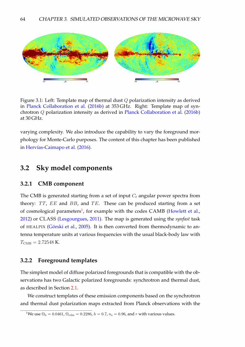
64 CHAPTER 3. SIMULATED OBSERVATIONS OF THE MICROWAVE SKY
-20 20µK -40 40µK
Figure 3.1: Left: Template map of thermal dust Q polarization intensity as derivedin Planck Collaboration et al. (2016b) at 353 GHz. Right: Template map of syn-chrotron Q polarization intensity as derived in Planck Collaboration et al. (2016b)at 30 GHz.
varying complexity. We also introduce the capability to vary the foreground mor-
phology for Monte-Carlo purposes. The content of this chapter has been published
in Hervías-Caimapo et al. (2016).
3.2 Sky model components
3.2.1 CMB component
The CMB is generated starting from a set of input C` angular power spectra from
theory: TT , EE and BB, and TE. These can be produced starting from a set
of cosmological parameters1, for example with the codes CAMB (Howlett et al.,
2012) or CLASS (Lesgourgues, 2011). The map is generated using the synfast task
of HEALPIX (Górski et al., 2005). It is then converted from thermodynamic to an-
tenna temperature units at various frequencies with the usual black-body law with
TCMB = 2.72548 K.
3.2.2 Foreground templates
The simplest model of diffuse polarized foregrounds that is compatible with the ob-
servations has two Galactic polarized foregrounds: synchrotron and thermal dust,
as described in Section 2.1.
We construct templates of these emission components based on the synchrotron
and thermal dust polarization maps extracted from Planck observations with the
1We use Ωb = 0.0461, Ωcdm = 0.2286, h = 0.7, ns = 0.96, and r with various values.
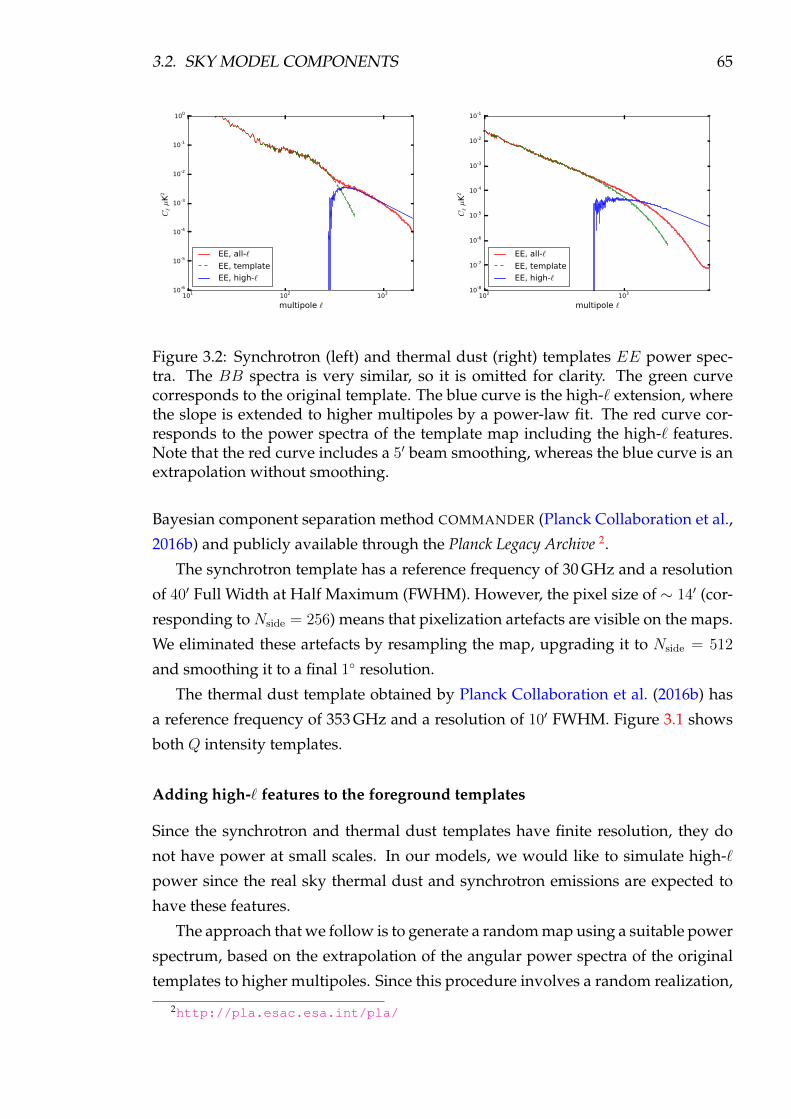
3.2. SKY MODEL COMPONENTS 65
101 102 103
multipole `
10-6
10-5
10-4
10-3
10-2
10-1
100
C` µK
2
EE, all-`
EE, template
EE, high-`
102 103
multipole `
10-8
10-7
10-6
10-5
10-4
10-3
10-2
10-1
C` µK
2
EE, all-`
EE, template
EE, high-`
Figure 3.2: Synchrotron (left) and thermal dust (right) templates EE power spec-tra. The BB spectra is very similar, so it is omitted for clarity. The green curvecorresponds to the original template. The blue curve is the high-` extension, wherethe slope is extended to higher multipoles by a power-law fit. The red curve cor-responds to the power spectra of the template map including the high-` features.Note that the red curve includes a 5′ beam smoothing, whereas the blue curve is anextrapolation without smoothing.
Bayesian component separation method COMMANDER (Planck Collaboration et al.,
2016b) and publicly available through the Planck Legacy Archive 2.
The synchrotron template has a reference frequency of 30 GHz and a resolution
of 40′ Full Width at Half Maximum (FWHM). However, the pixel size of ∼ 14′ (cor-
responding to Nside = 256) means that pixelization artefacts are visible on the maps.
We eliminated these artefacts by resampling the map, upgrading it to Nside = 512
and smoothing it to a final 1 resolution.
The thermal dust template obtained by Planck Collaboration et al. (2016b) has
a reference frequency of 353 GHz and a resolution of 10′ FWHM. Figure 3.1 shows
both Q intensity templates.
Adding high-` features to the foreground templates
Since the synchrotron and thermal dust templates have finite resolution, they do
not have power at small scales. In our models, we would like to simulate high-`
power since the real sky thermal dust and synchrotron emissions are expected to
have these features.
The approach that we follow is to generate a random map using a suitable power
spectrum, based on the extrapolation of the angular power spectra of the original
templates to higher multipoles. Since this procedure involves a random realization,
2http://pla.esac.esa.int/pla/
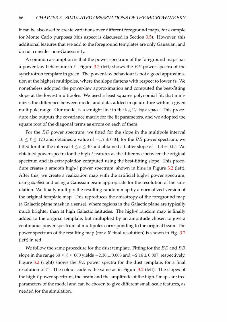
66 CHAPTER 3. SIMULATED OBSERVATIONS OF THE MICROWAVE SKY
it can be also used to create variations over different foreground maps, for example
for Monte Carlo purposes (this aspect is discussed in Section 3.5). However, this
additional features that we add to the foreground templates are only Gaussian, and
do not consider non-Gaussianity.
A common assumption is that the power spectrum of the foreground maps has
a power-law behaviour in `. Figure 3.2 (left) shows the EE power spectra of the
synchrotron template in green. The power-law behaviour is not a good approxima-
tion at the highest multipoles, where the slope flattens with respect to lower `s. We
nonetheless adopted the power-law approximation and computed the best-fitting
slope at the lowest multipoles. We used a least squares polynomial fit, that mini-
mizes the difference between model and data, added in quadrature within a given
multipole range. Our model is a straight line in the logC`–log ` space. This proce-
dure also outputs the covariance matrix for the fit parameters, and we adopted the
square root of the diagonal terms as errors on each of them.
For the EE power spectrum, we fitted for the slope in the multipole interval
10 ≤ ` ≤ 120 and obtained a value of −1.7 ± 0.04; for the BB power spectrum, we
fitted for it in the interval 4 ≤ ` ≤ 40 and obtained a flatter slope of −1.4± 0.05. We
obtained power spectra for the high-` features as the difference between the original
spectrum and its extrapolation computed using the best-fitting slope. This proce-
dure creates a smooth high-` power spectrum, shown in blue in Figure 3.2 (left).
After this, we create a realization map with the artificial high-` power spectrum,
using synfast and using a Gaussian beam appropriate for the resolution of the sim-
ulation. We finally multiply the resulting random map by a normalized version of
the original template map. This reproduces the anisotropy of the foreground map
(a Galactic plane mask in a sense), where regions in the Galactic plane are typically
much brighter than at high Galactic latitudes. The high-` random map is finally
added to the original template, but multiplied by an amplitude chosen to give a
continuous power spectrum at multipoles corresponding to the original beam. The
power spectrum of the resulting map (for a 5′ final resolution) is shown in Fig. 3.2
(left) in red.
We follow the same procedure for the dust template. Fitting for the EE and BB
slope in the range 60 ≤ ` ≤ 600 yields −2.36± 0.005 and −2.16± 0.007, respectively.
Figure 3.2 (right) shows the EE power spectra for the dust template, for a final
resolution of 5′. The colour code is the same as in Figure 3.2 (left). The slopes of
the high-` power spectrum, the beam and the amplitude of the high-` maps are free
parameters of the model and can be chosen to give different small-scale features, as
needed for the simulation.
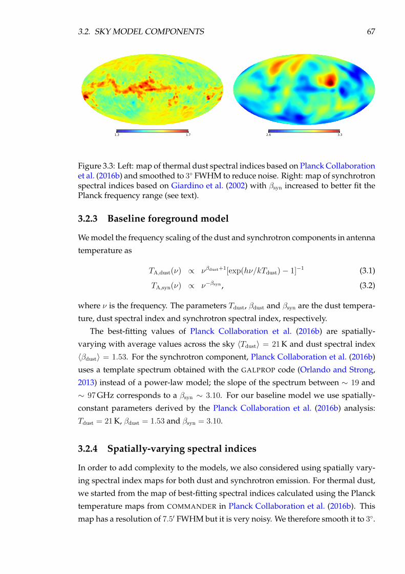
3.2. SKY MODEL COMPONENTS 67
1.3 1.7 2.6 3.3
Figure 3.3: Left: map of thermal dust spectral indices based on Planck Collaborationet al. (2016b) and smoothed to 3 FWHM to reduce noise. Right: map of synchrotronspectral indices based on Giardino et al. (2002) with βsyn increased to better fit thePlanck frequency range (see text).
3.2.3 Baseline foreground model
We model the frequency scaling of the dust and synchrotron components in antenna
temperature as
TA,dust(ν) ∝ νβdust+1[exp(hν/kTdust)− 1]−1 (3.1)
TA,syn(ν) ∝ ν−βsyn , (3.2)
where ν is the frequency. The parameters Tdust, βdust and βsyn are the dust tempera-
ture, dust spectral index and synchrotron spectral index, respectively.
The best-fitting values of Planck Collaboration et al. (2016b) are spatially-
varying with average values across the sky 〈Tdust〉 = 21 K and dust spectral index
〈βdust〉 = 1.53. For the synchrotron component, Planck Collaboration et al. (2016b)
uses a template spectrum obtained with the GALPROP code (Orlando and Strong,
2013) instead of a power-law model; the slope of the spectrum between ∼ 19 and
∼ 97 GHz corresponds to a βsyn ∼ 3.10. For our baseline model we use spatially-
constant parameters derived by the Planck Collaboration et al. (2016b) analysis:
Tdust = 21 K, βdust = 1.53 and βsyn = 3.10.
3.2.4 Spatially-varying spectral indices
In order to add complexity to the models, we also considered using spatially vary-
ing spectral index maps for both dust and synchrotron emission. For thermal dust,
we started from the map of best-fitting spectral indices calculated using the Planck
temperature maps from COMMANDER in Planck Collaboration et al. (2016b). This
map has a resolution of 7.5′ FWHM but it is very noisy. We therefore smooth it to 3.
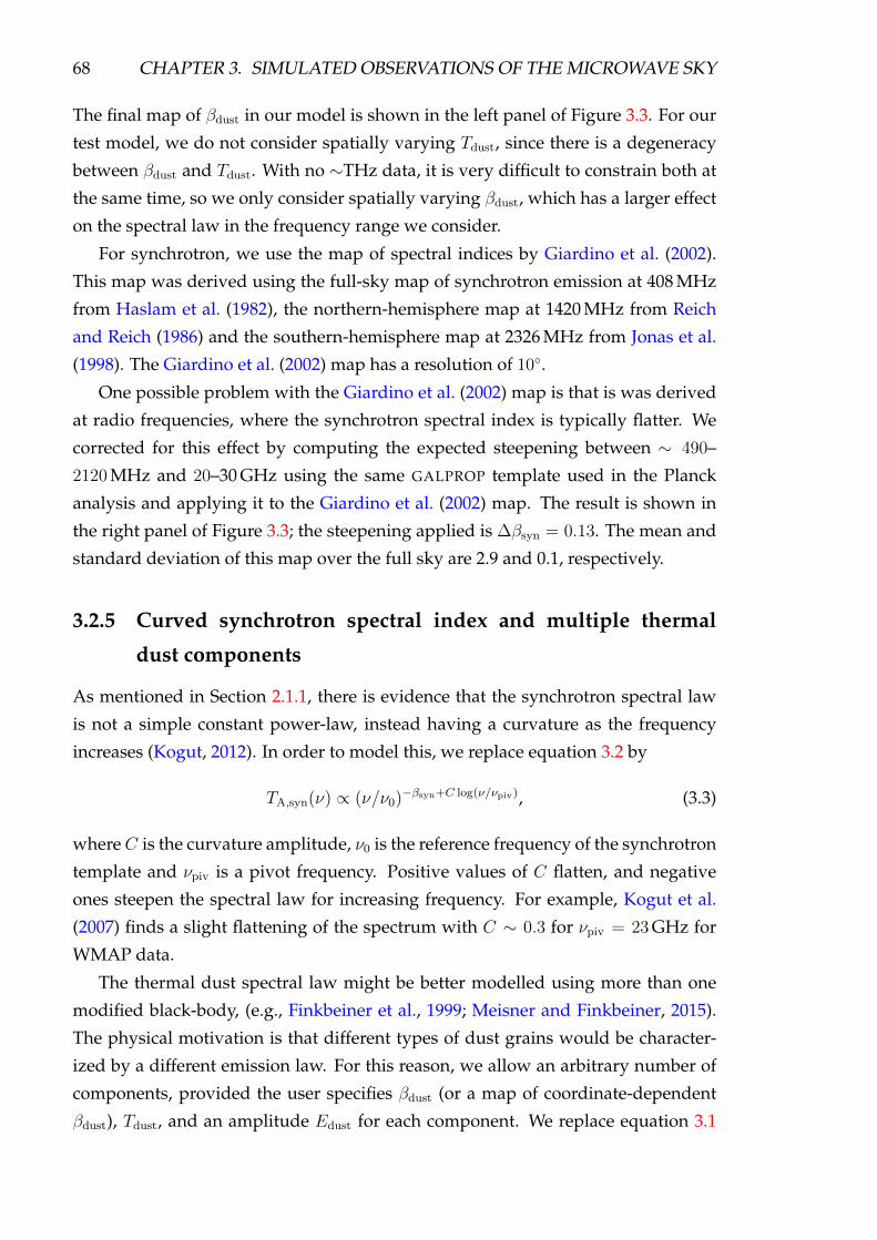
68 CHAPTER 3. SIMULATED OBSERVATIONS OF THE MICROWAVE SKY
The final map of βdust in our model is shown in the left panel of Figure 3.3. For our
test model, we do not consider spatially varying Tdust, since there is a degeneracy
between βdust and Tdust. With no ∼THz data, it is very difficult to constrain both at
the same time, so we only consider spatially varying βdust, which has a larger effect
on the spectral law in the frequency range we consider.
For synchrotron, we use the map of spectral indices by Giardino et al. (2002).
This map was derived using the full-sky map of synchrotron emission at 408 MHz
from Haslam et al. (1982), the northern-hemisphere map at 1420 MHz from Reich
and Reich (1986) and the southern-hemisphere map at 2326 MHz from Jonas et al.
(1998). The Giardino et al. (2002) map has a resolution of 10.
One possible problem with the Giardino et al. (2002) map is that is was derived
at radio frequencies, where the synchrotron spectral index is typically flatter. We
corrected for this effect by computing the expected steepening between ∼ 490–
2120 MHz and 20–30 GHz using the same GALPROP template used in the Planck
analysis and applying it to the Giardino et al. (2002) map. The result is shown in
the right panel of Figure 3.3; the steepening applied is ∆βsyn = 0.13. The mean and
standard deviation of this map over the full sky are 2.9 and 0.1, respectively.
3.2.5 Curved synchrotron spectral index and multiple thermal
dust components
As mentioned in Section 2.1.1, there is evidence that the synchrotron spectral law
is not a simple constant power-law, instead having a curvature as the frequency
increases (Kogut, 2012). In order to model this, we replace equation 3.2 by
TA,syn(ν) ∝ (ν/ν0)−βsyn+C log(ν/νpiv), (3.3)
whereC is the curvature amplitude, ν0 is the reference frequency of the synchrotron
template and νpiv is a pivot frequency. Positive values of C flatten, and negative
ones steepen the spectral law for increasing frequency. For example, Kogut et al.
(2007) finds a slight flattening of the spectrum with C ∼ 0.3 for νpiv = 23 GHz for
WMAP data.
The thermal dust spectral law might be better modelled using more than one
modified black-body, (e.g., Finkbeiner et al., 1999; Meisner and Finkbeiner, 2015).
The physical motivation is that different types of dust grains would be character-
ized by a different emission law. For this reason, we allow an arbitrary number of
components, provided the user specifies βdust (or a map of coordinate-dependent
βdust), Tdust, and an amplitude Edust for each component. We replace equation 3.1
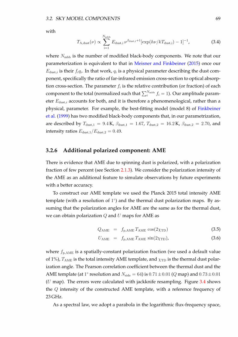
3.2. SKY MODEL COMPONENTS 69
with
TA,dust(ν) ∝Nmbb∑i=1
Edust,i νβdust,i+1[exp(hν/kTdust,i)− 1]−1, (3.4)
where Nmbb is the number of modified black-body components. We note that our
parameterization is equivalent to that in Meisner and Finkbeiner (2015) once our
Edust,i is their fiqi. In that work, qi is a physical parameter describing the dust com-
ponent, specifically the ratio of far-infrared emission cross-section to optical absorp-
tion cross-section. The parameter fi is the relative contribution (or fraction) of each
component to the total (normalized such that∑Nmbb
i fi = 1). Our amplitude param-
eter Edust,i accounts for both, and it is therefore a phenomenological, rather than a
physical, parameter. For example, the best-fitting model (model 8) of Finkbeiner
et al. (1999) has two modified black-body components that, in our parametrization,
are described by Tdust,1 = 9.4 K, βdust,1 = 1.67, Tdust,2 = 16.2 K, βdust,2 = 2.70, and
intensity ratios Edust,1/Edust,2 = 0.49.
3.2.6 Additional polarized component: AME
There is evidence that AME due to spinning dust is polarized, with a polarization
fraction of few percent (see Section 2.1.3). We consider the polarization intensity of
the AME as an additional feature to simulate observations by future experiments
with a better accuracy.
To construct our AME template we used the Planck 2015 total intensity AME
template (with a resolution of 1) and the thermal dust polarization maps. By as-
suming that the polarization angles for AME are the same as for the thermal dust,
we can obtain polarization Q and U maps for AME as
QAME = fp,AME TAME cos(2χTD) (3.5)
UAME = fp,AME TAME sin(2χTD), (3.6)
where fp,AME is a spatially-constant polarization fraction (we used a default value
of 1%), TAME is the total intensity AME template, and χTD is the thermal dust polar-
ization angle. The Pearson correlation coefficient between the thermal dust and the
AME template (at 1 resolution andNside = 64) is 0.71±0.01 (Qmap) and 0.73±0.01
(U map). The errors were calculated with jackknife resampling. Figure 3.4 shows
the Q intensity of the constructed AME template, with a reference frequency of
23 GHz.
As a spectral law, we adopt a parabola in the logarithmic flux-frequency space,
70 CHAPTER 3. SIMULATED OBSERVATIONS OF THE MICROWAVE SKY
-4 4µK
Figure 3.4: Template map of Q AME component, as derived from the total inten-sity AME and the thermal dust polarization maps from Planck Collaboration et al.(2016b). This map has 1 resolution, a reference frequency of 23 GHz and assumeda polarization fraction of 0.01.
proposed by Bonaldi et al. (2007), given by
log(TA,ν) = const.−[
m60 log(νmax)
log(νmax/60GHz)+ 2
]log(ν)+
m60
2 log(νmax/60GHz)(log(ν))2, (3.7)
where the free parameters are m60 (the slope at 60 GHz) in the log(ν)-log(S) space,
and νmax is the peak frequency (for the spectrum in flux units). We adopt as default
values νmax = 19 GHz, from Planck Collaboration et al. (2016b), and 4.0 form60 from
Bonaldi et al. (2007).
Adding dust-correlated high-` features to the AME maps
Similarly to what is done for the synchrotron and thermal dust components in Sec-
tion 3.2.2, the AME polarization maps can be upgraded in resolution by adding
high-` features. However, in this case, we want the high-` thermal dust and AME
maps to exhibit the same level of correlation measured at low resolution. We there-
fore developed a special procedure for this case, that generates both dust and AME
high-` correlated random maps at the same time.

3.3. SIMULATED OBSERVATIONS OF CMB POLARIZATION EXPERIMENTS 71
We followed the procedure described in Brown and Battye (2011), which uses
as input the power spectra and cross-spectra of the set of correlated maps (in our
case, dust E and B, and AME E and B). This information is used to generate
4 correlated random a`m fields, which are finally transformed to Q and U with the
HEALPIX alm2map function. Extending what is described in Section 3.2.2, the spectra
and cross-spectra for the high-` maps are constructed by extrapolating those of the
dust and AME templates to higher multipoles. The last step of our procedure, the
modulation of the random high-` maps with a mask enhancing the Galactic plane,
is unchanged.
3.3 Simulated observations of CMB polarization ex-
periments
3.3.1 Simulating the instrumental response
To simulate the observation of the microwave sky in polarization by a given exper-
iment, we need to know the frequency bands of observation and, for each of the
bands, the point-spread function and the noise level. Each of these properties can
be simulated with different level of complexity, specified by the user, as detailed in
the following.
The frequency response can be either simulated as a single frequency or a more
general transmission window. In the more general case, the Q or U of the sky com-
ponent i at the frequency band νj is given by
Xi(νj) =
∑kWj(νk)XrefSi(νk)∑
kWj(νk), (3.8)
where Si(ν) is the spectral law of the component, Xref is either the Q or U ampli-
tude of the corresponding template, Xi is the Q or U weighted intensity of each
component, and Wj(νk) is the transmission of band j for a set of frequencies νk.
In practice, when simulating a band response, the signal needs to be simulated for
a set of frequencies νk and averaged over the entire band, with weights given by
the transmission Wj(νk). The effect of the instrumental resolution is simulated by
convolving the maps with a Gaussian beam of specified FWHM.
The noise can be modelled either as a uniform white noise, described by an rms
value constant over the sky, or as an anisotropic white noise specifying a map of rms
varying in the sky. For Planck, we model this using the 3 × 3 noise covariance per
pixel containing the Stokes parameter covariance elements TT , QQ, UU , TQ, TU ,
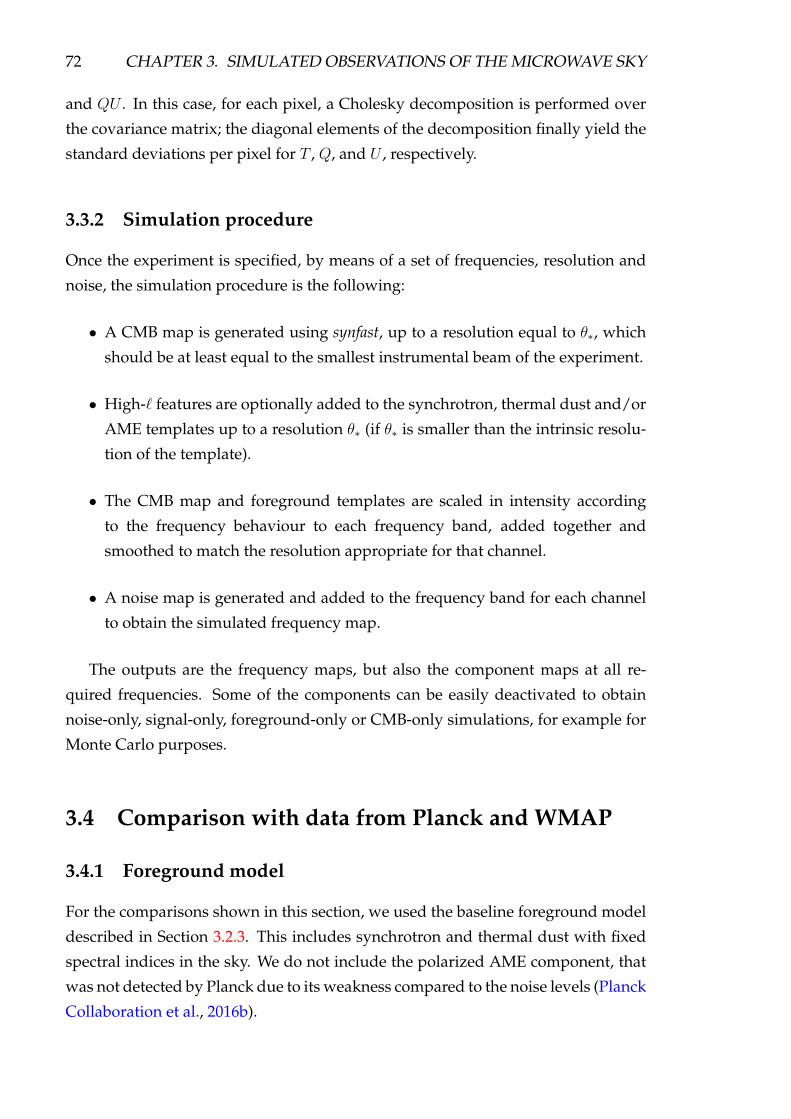
72 CHAPTER 3. SIMULATED OBSERVATIONS OF THE MICROWAVE SKY
and QU . In this case, for each pixel, a Cholesky decomposition is performed over
the covariance matrix; the diagonal elements of the decomposition finally yield the
standard deviations per pixel for T , Q, and U , respectively.
3.3.2 Simulation procedure
Once the experiment is specified, by means of a set of frequencies, resolution and
noise, the simulation procedure is the following:
• A CMB map is generated using synfast, up to a resolution equal to θ∗, which
should be at least equal to the smallest instrumental beam of the experiment.
• High-` features are optionally added to the synchrotron, thermal dust and/or
AME templates up to a resolution θ∗ (if θ∗ is smaller than the intrinsic resolu-
tion of the template).
• The CMB map and foreground templates are scaled in intensity according
to the frequency behaviour to each frequency band, added together and
smoothed to match the resolution appropriate for that channel.
• A noise map is generated and added to the frequency band for each channel
to obtain the simulated frequency map.
The outputs are the frequency maps, but also the component maps at all re-
quired frequencies. Some of the components can be easily deactivated to obtain
noise-only, signal-only, foreground-only or CMB-only simulations, for example for
Monte Carlo purposes.
3.4 Comparison with data from Planck and WMAP
3.4.1 Foreground model
For the comparisons shown in this section, we used the baseline foreground model
described in Section 3.2.3. This includes synchrotron and thermal dust with fixed
spectral indices in the sky. We do not include the polarized AME component, that
was not detected by Planck due to its weakness compared to the noise levels (Planck
Collaboration et al., 2016b).
3.4. COMPARISON WITH DATA FROM PLANCK AND WMAP 73
Figure 3.5: Scatter plot inside the Galactic plane |b| ≤ 20. The Nside is 64. The toprow corresponds to Q intensity, and the bottom row to U intensity. The black linerepresents the perfect one-to-one match. Both the templates and the observed skywere smoothed to a common 1 resolution. In parenthesis, we show the factor bywhich we multiply each data point for display purposes.
3.4.2 Data maps
We compared the output of our model with Planck sky observations in polariza-
tion at 30, 44, 70 and 353 GHz, complemented by the WMAP W band at 94 GHz
and K band at 23 GHz. In the following, we carried out the comparison between
model and data smoothing to a 1 common resolution, which is the resolution of
our synchrotron template. Such resolution is also good for display purposes be-
cause it reduces the noise and allows an easier visual inspection of the foregrounds
morphology.
The Planck frequency maps have been corrected for the polarization leakage
due to bandpass mismatch with the correction maps available on the Planck Legacy
Archive. The WMAP maps have been downloaded from the LAMBDA-WMAP
archive 3.
3http://lambda.gsfc.nasa.gov/product/map/dr5/

74 CHAPTER 3. SIMULATED OBSERVATIONS OF THE MICROWAVE SKY
Sky 2360453015
015304560
Model 2360453015
015304560
Sky 305040302010
01020304050
Model 305040302010
01020304050
Sky 4420161284
048121620
Model 4420161284
048121620
Sky 7020161284
048121620
Model 7020161284
048121620
Sky 9420161284
048121620
Model 9420161284
048121620
Sky 35360453015
015304560
Model 35360453015
015304560
Figure 3.6: Maps comparison between the observed sky and the foreground modelfor Q. The rows are six bands, the left column corresponds to the observed skyand the right one to our foregrounds model. The units are µKA. The maps aresmoothed to a common 1 resolution and degraded to Nside = 32 to suppress thenoise for display purposes.

3.4. COMPARISON WITH DATA FROM PLANCK AND WMAP 75
Sky 23302418126
0612182430
Model 23302418126
0612182430
Sky 30252015105
0510152025
Model 30252015105
0510152025
Sky 44108642
0246810
Model 44108642
0246810
Sky 70108642
0246810
Model 70108642
0246810
Sky 94108642
0246810
Model 94108642
0246810
Sky 353302418126
0612182430
Model 353302418126
0612182430
Figure 3.7: The same as Fig. 3.6, but for U maps.

76 CHAPTER 3. SIMULATED OBSERVATIONS OF THE MICROWAVE SKY
3.4.3 Comparison with foregrounds only
We first compare the data with a model of the sky including only the foregrounds
(with no high-` features) and without CMB and noise. In this way, we only com-
pare the deterministic components of the model, without any random realization.
Also, we subtract the observed CMB from the Planck and WMAP frequency obser-
vations. To this end, we use the CMB map as estimated by COMMANDER (Planck
Collaboration et al., 2016c), with a resolution of 10 arcmin atNside = 1024, smoothed
to 60 arcmin. The true Planck and WMAP frequency responses have been used to
create the model sky as described in Section 3.3.
Figure 3.5 shows a pixel-by-pixel comparison of true versus model Q (top row)
and U (bottom row) maps. We show only the pixels inside the Galactic plane
(|b| ≤ 20) for Nside = 64 to reduce the effect of noise and CMB. Figures 3.6 and
3.7 show the maps in pseudo-colour scale, for 6 frequencies and in Q and U inten-
sity. The modelled foregrounds and the observed sky have the same colour scale.
As expected, the agreement is very good for the foreground-dominated frequen-
cies. At 70 and 94 GHz the agreement is less good, because CMB and noise become
important at these frequencies. The direct comparison of the maps shows that the
foreground model is quite good once the noise is reduced (by means of degrad-
ing to Nside = 32). The U intensity of the 94 GHz band is noisy, which makes the
comparison difficult.
3.4.4 Including the contribution from noise and CMB
For the comparisons presented in this section, we included noise and a CMB re-
alization, which are present in the sky observations, in order to assess the match
of the model when all components are included. In this case we only consider the
power spectra, since the different CMB and noise realizations do not allow a mor-
phological comparison.
The CMB map has been generated starting from the best-fitting model of Planck
(including polarization information, Planck Collaboration et al. (2016i)) and with a
tensor-to-scalar ratio r = 0.1.
In this case, we consider the 30, 44, 70, and 353 GHz Planck bands and all five
of the WMAP bands. The WMAP noise is simulated using the hit counts maps
and RMS information available from the Lambda website. Planck noise has been
simulated using the pixel covariance information.
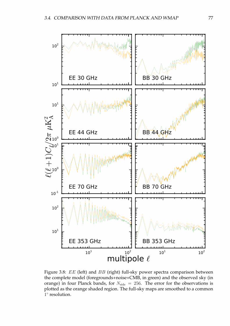
3.4. COMPARISON WITH DATA FROM PLANCK AND WMAP 77
101
102
EE 30 GHz BB 30 GHz
100
101
EE 44 GHz BB 44 GHz
10-1
100
101
EE 70 GHz BB 70 GHz
101 102
101
102
EE 353 GHz
101 102
BB 353 GHz
multipole `
`(`+
1)C`/
2π µ
K2 A
Figure 3.8: EE (left) and BB (right) full-sky power spectra comparison betweenthe complete model (foregrounds+noise+CMB, in green) and the observed sky (inorange) in four Planck bands, for Nside = 256. The error for the observations isplotted as the orange shaded region. The full-sky maps are smoothed to a common1 resolution.
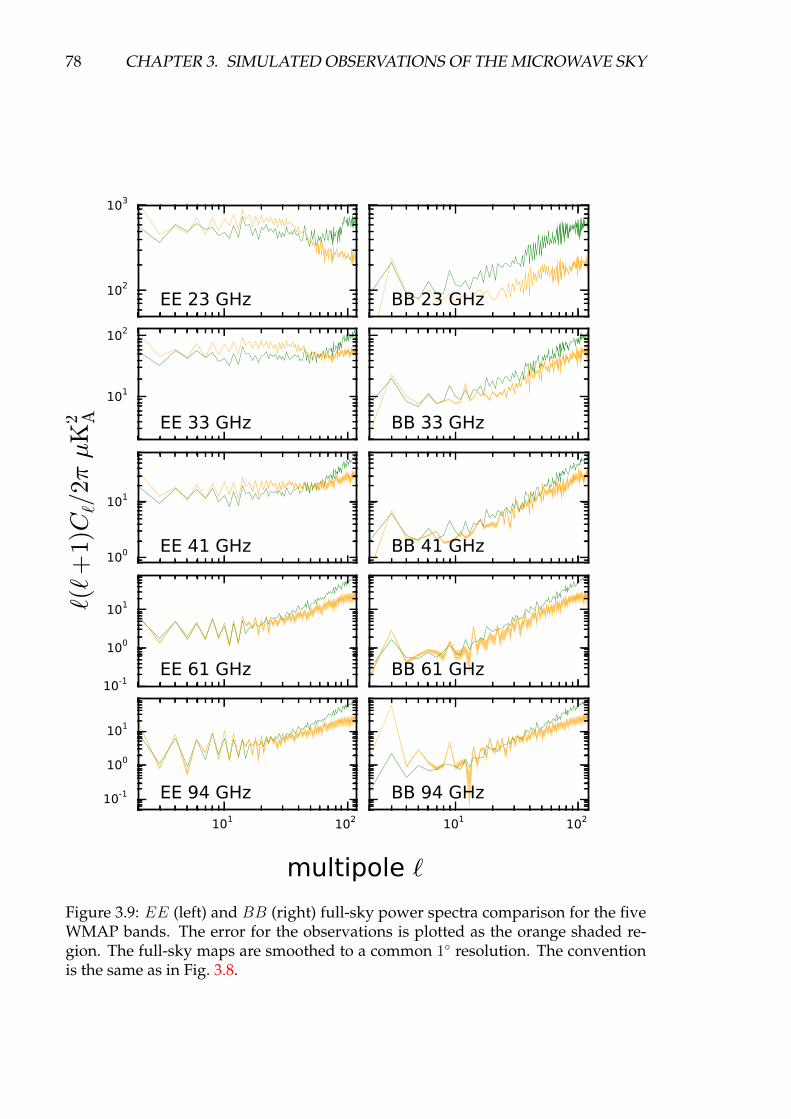
78 CHAPTER 3. SIMULATED OBSERVATIONS OF THE MICROWAVE SKY
102
103
EE 23 GHz BB 23 GHz
101
102
EE 33 GHz BB 33 GHz
100
101
EE 41 GHz BB 41 GHz
10-1
100
101
EE 61 GHz BB 61 GHz
101 102
10-1
100
101
EE 94 GHz
101 102
BB 94 GHz
multipole `
`(`+
1)C`/
2π µ
K2 A
Figure 3.9: EE (left) and BB (right) full-sky power spectra comparison for the fiveWMAP bands. The error for the observations is plotted as the orange shaded re-gion. The full-sky maps are smoothed to a common 1 resolution. The conventionis the same as in Fig. 3.8.
3.4. COMPARISON WITH DATA FROM PLANCK AND WMAP 79
Figure 3.8 shows the comparison of the EE and BB full-sky power spectra be-
tween the complete model (foregrounds model + noise realization + CMB realiza-
tion) and the Planck bands. Figure 3.9 shows the same for the five WMAP bands.
Since these spectra are computed over the full sky, there is no leakage between EE
andBB modes and no correction is needed. In this case, the error on the data power
spectrum (orange shaded region) is just due to sample variance in the noise and the
CMB (the latter corresponds to the Cosmic Variance, explained in Section 1.3), and
it is calculated as
∆C` =
√2
2`+ 1(CCMB
` +N`), (3.9)
where CCMB` is the input CMB power spectrum and N` is the noise bias power spec-
trum, calculated from 100 noise Monte Carlo realizations based on the noise covari-
ance matrix information of each band. This error is generally very small compared
to the foreground signal (< 1%), and in most cases not visible in the figures. The
maximum observed error, considering multipoles up to ` = 100, is∼ 10% at 70 GHz
for Planck and ∼ 23% at 61 GHz for WMAP.
The agreement between the intermediate frequencies (44 and 70 GHz) benefits
from the inclusion of CMB and noise in the comparison. At 70 GHz the CMB po-
larised intensity is strong, so the match improves. The inclusion of noise is particu-
larly important to reconcile model and data towards ` = 100.
Comparison on small patches at high Galactic latitude
As a final assessment of our model, we compare the local angular power spectra
to the latest Planck observations in several small sky patches at intermediate and
high Galactic latitude. This is particularly useful for ground-based CMB polariza-
tion experiments, which target these areas. For example, the BICEP2/KECK array
(BICEP2 Collaboration et al., 2014a) observes with two bands at 100 and 150 GHz.
They target a high Galactic latitude patch visible from the South Pole, with a size of
∼ 800 deg2. The South Pole Telescope has measured the sub-degree scales lens-
ing BB power spectrum in a southern 100 deg2 patch using two bands (95 and
150 GHz) (Keisler et al., 2015b). Another example is the POLARBEAR experiment,
which measured the lensing BB spectrum in three small patches with a total area
of 25 deg2 at 150 GHz (The Polarbear Collaboration: P. A. R. Ade et al., 2014). Given
the frequency coverage of these experiments, observing around 150 GHz, where
the CMB peaks, it is crucial to model correctly the contamination from polarized
thermal dust emission.
For our comparison, we followed a similar procedure to the one described in
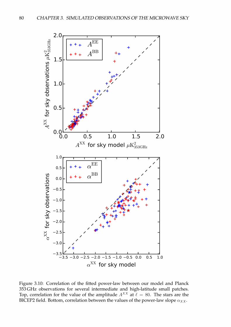
80 CHAPTER 3. SIMULATED OBSERVATIONS OF THE MICROWAVE SKY
0.0 0.5 1.0 1.5 2.0
AXX for sky model µK2353GHz
0.0
0.5
1.0
1.5
2.0
AX
X f
or
sky o
bse
rvati
ons µK
2 353
GH
zAEE
ABB
3.5 3.0 2.5 2.0 1.5 1.0 0.5 0.0 0.5 1.0
αXX for sky model
3.5
3.0
2.5
2.0
1.5
1.0
0.5
0.0
0.5
1.0
αX
X f
or
sky o
bse
rvati
ons
αEE
αBB
Figure 3.10: Correlation of the fitted power-law between our model and Planck353 GHz observations for several intermediate and high-latitude small patches.Top, correlation for the value of the amplitude AXX at ` = 80. The stars are theBICEP2 field. Bottom, correlation between the values of the power-law slope αXX .
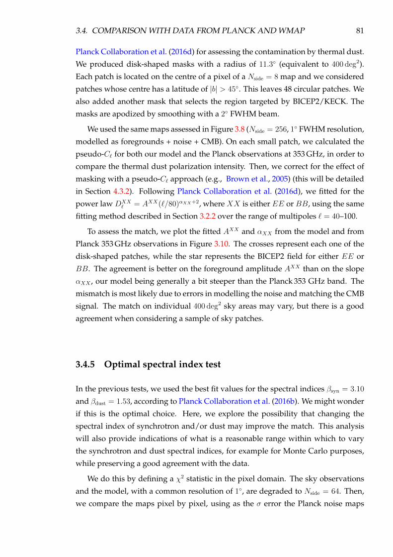
3.4. COMPARISON WITH DATA FROM PLANCK AND WMAP 81
Planck Collaboration et al. (2016d) for assessing the contamination by thermal dust.
We produced disk-shaped masks with a radius of 11.3 (equivalent to 400 deg2).
Each patch is located on the centre of a pixel of a Nside = 8 map and we considered
patches whose centre has a latitude of |b| > 45. This leaves 48 circular patches. We
also added another mask that selects the region targeted by BICEP2/KECK. The
masks are apodized by smoothing with a 2 FWHM beam.
We used the same maps assessed in Figure 3.8 (Nside = 256, 1 FWHM resolution,
modelled as foregrounds + noise + CMB). On each small patch, we calculated the
pseudo-C` for both our model and the Planck observations at 353 GHz, in order to
compare the thermal dust polarization intensity. Then, we correct for the effect of
masking with a pseudo-C` approach (e.g., Brown et al., 2005) (this will be detailed
in Section 4.3.2). Following Planck Collaboration et al. (2016d), we fitted for the
power law DXX` = AXX(`/80)αXX+2, where XX is either EE or BB, using the same
fitting method described in Section 3.2.2 over the range of multipoles ` = 40–100.
To assess the match, we plot the fitted AXX and αXX from the model and from
Planck 353 GHz observations in Figure 3.10. The crosses represent each one of the
disk-shaped patches, while the star represents the BICEP2 field for either EE or
BB. The agreement is better on the foreground amplitude AXX than on the slope
αXX , our model being generally a bit steeper than the Planck 353 GHz band. The
mismatch is most likely due to errors in modelling the noise and matching the CMB
signal. The match on individual 400 deg2 sky areas may vary, but there is a good
agreement when considering a sample of sky patches.
3.4.5 Optimal spectral index test
In the previous tests, we used the best fit values for the spectral indices βsyn = 3.10
and βdust = 1.53, according to Planck Collaboration et al. (2016b). We might wonder
if this is the optimal choice. Here, we explore the possibility that changing the
spectral index of synchrotron and/or dust may improve the match. This analysis
will also provide indications of what is a reasonable range within which to vary
the synchrotron and dust spectral indices, for example for Monte Carlo purposes,
while preserving a good agreement with the data.
We do this by defining a χ2 statistic in the pixel domain. The sky observations
and the model, with a common resolution of 1, are degraded to Nside = 64. Then,
we compare the maps pixel by pixel, using as the σ error the Planck noise maps
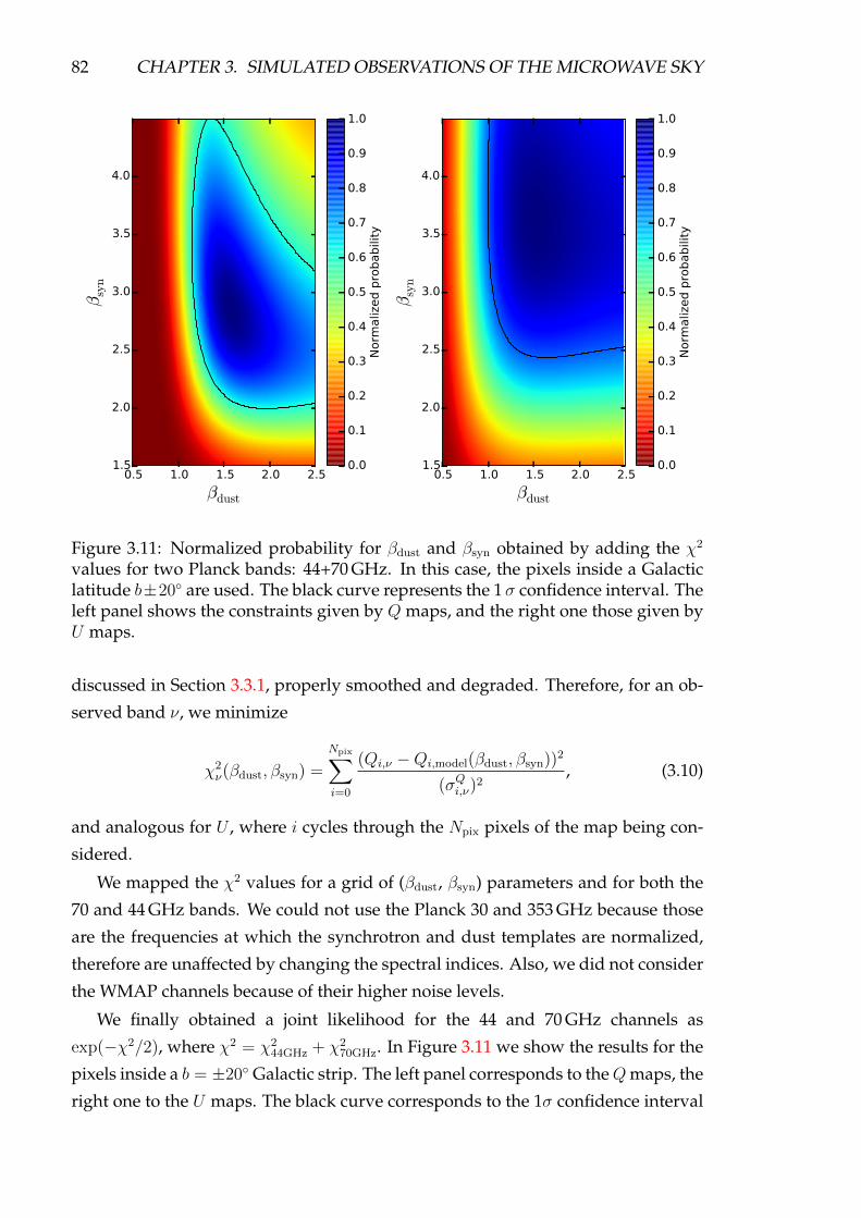
82 CHAPTER 3. SIMULATED OBSERVATIONS OF THE MICROWAVE SKY
0.5 1.0 1.5 2.0 2.5
βdust
1.5
2.0
2.5
3.0
3.5
4.0
βsy
n
0.5 1.0 1.5 2.0 2.5
βdust
1.5
2.0
2.5
3.0
3.5
4.0
βsy
n
0.0
0.1
0.2
0.3
0.4
0.5
0.6
0.7
0.8
0.9
1.0
Norm
aliz
ed p
robabili
ty
0.0
0.1
0.2
0.3
0.4
0.5
0.6
0.7
0.8
0.9
1.0
Norm
aliz
ed p
robabili
ty
Figure 3.11: Normalized probability for βdust and βsyn obtained by adding the χ2
values for two Planck bands: 44+70 GHz. In this case, the pixels inside a Galacticlatitude b±20 are used. The black curve represents the 1 σ confidence interval. Theleft panel shows the constraints given by Q maps, and the right one those given byU maps.
discussed in Section 3.3.1, properly smoothed and degraded. Therefore, for an ob-
served band ν, we minimize
χ2ν(βdust, βsyn) =
Npix∑i=0
(Qi,ν −Qi,model(βdust, βsyn))2
(σQi,ν)2
, (3.10)
and analogous for U , where i cycles through the Npix pixels of the map being con-
sidered.
We mapped the χ2 values for a grid of (βdust, βsyn) parameters and for both the
70 and 44 GHz bands. We could not use the Planck 30 and 353 GHz because those
are the frequencies at which the synchrotron and dust templates are normalized,
therefore are unaffected by changing the spectral indices. Also, we did not consider
the WMAP channels because of their higher noise levels.
We finally obtained a joint likelihood for the 44 and 70 GHz channels as
exp(−χ2/2), where χ2 = χ244GHz + χ2
70GHz. In Figure 3.11 we show the results for the
pixels inside a b = ±20 Galactic strip. The left panel corresponds to theQmaps, the
right one to the U maps. The black curve corresponds to the 1σ confidence interval

3.4. COMPARISON WITH DATA FROM PLANCK AND WMAP 83
101 102 103
multipole `
10-12
10-11
10-10
10-9
10-8
10-7
10-6
10-5
10-4
10-3
`(`+
1)C
BB
`/2π
mK
2
Prim. r=0.1
Prim. r=0.01
Prim. r=0.001
G. Foregrounds 45 GHz
G. Foregrounds 105 GHz
G. Foregrounds 315 GHz
Figure 3.12: Forecast for primordialBB modes detectability. The black curves showprimordial CBB
` for three values of the tensor-to-scalar ratio. We also show theBB power spectra for polarized foregrounds for three frequencies: 45, 105, and315 GHz. The foreground maps were masked with the WMAP polarization dataanalysis mask and deconvolved from pseudo-C` following Brown et al. (2005).
in the βdust-βsyn space considered. Note that we assume a prior on the range of val-
ues these indices can take. The probability distribution is flatter in U (and therefore
the 1σ contour is wider) because the U maps have weaker foreground emission at
the Galactic plane, as can be seen in Figure 3.7.
The best fit values for the 1D marginalized probability of each parameter and
its 1σ confidence interval, adding both bands and both polarizations (44 + 70 GHz
and Q + U ), are βsyn = 3.4+0.7−0.5 and βdust = 1.6+0.5
−0.2 for the pixels inside the Galactic
plane strip, and βdust = 1.6+0.6−0.3 and βsyn = 3.4+0.9
−0.6 when we consider the full sky.
The reason why we obtain relatively weak constraints is because we could only
use data at central frequencies, where foregrounds are not so strong and the two
spectral indices are more degenerate. A test of the model with much lower (higher)
frequency would give a much stronger constraint of the synchrotron (dust) spectral
index.
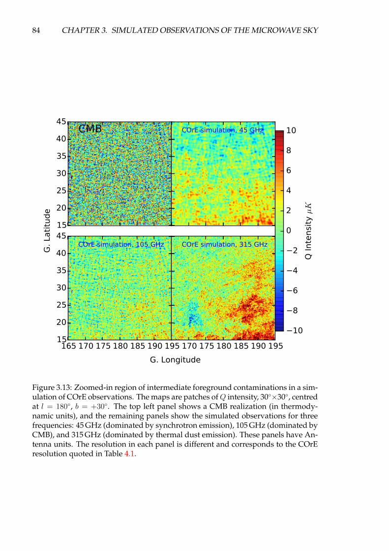
84 CHAPTER 3. SIMULATED OBSERVATIONS OF THE MICROWAVE SKY
15
20
25
30
35
40
45CMB COrE simulation, 45 GHz
165 170 175 180 185 190 19515
20
25
30
35
40
45COrE simulation, 105 GHz
170 175 180 185 190 195
COrE simulation, 315 GHz
10
8
6
4
2
0
2
4
6
8
10
Q Inte
nsi
ty µK
G. Longitude
G. La
titu
de
Figure 3.13: Zoomed-in region of intermediate foreground contaminations in a sim-ulation of COrE observations. The maps are patches ofQ intensity, 30×30, centredat l = 180, b = +30. The top left panel shows a CMB realization (in thermody-namic units), and the remaining panels show the simulated observations for threefrequencies: 45 GHz (dominated by synchrotron emission), 105 GHz (dominated byCMB), and 315 GHz (dominated by thermal dust emission). These panels have An-tenna units. The resolution in each panel is different and corresponds to the COrEresolution quoted in Table 4.1.

3.5. FORECAST AND MONTE-CARLO CAPABILITIES 85
3.5 Forecast and Monte-Carlo capabilities
To illustrate the simulation capabilities of our sky model, we consider the speci-
fications of the first proposal of the Cosmic Origin Explorer (COrE) experiment,
described in The COrE Collaboration et al. (2011). The instrumental specifications
used are listed in Table 4.1. This experiment has 15 frequency bands with frequency
ranging from 45 to 795 GHz and resolution of 23–1.3 arcminutes. The noise is simu-
lated as Gaussian and uniform, with standard deviation of a few µK per arcminute,
as quoted in the Table.
Figure 3.12 shows the forecasted B-mode for foregrounds for COrE as obtained
with our sky model. The CMB BB power spectra for different tensor-to-scalar ra-
tios are compared with the foreground power spectrum at three COrE frequencies:
45, 105 and 315 GHz. The foreground power spectra have been computed with the
WMAP polarization mask (excluding ∼ 37% of the sky); it has been corrected for
again using the pseudo-C` approach of Brown et al. (2005). Although this figure is
qualitatively similar to other forecasts in the literature (e.g. The COrE Collaboration
et al., 2011), the fact that our model is based on actual polarization observations en-
sures a better match with the real sky and therefore improved forecast capabilities.
In Figure 3.13 we show the Q intensity on a 30×30 sky patch located at
l = 180, b = 30 and exhibiting intermediate foreground contamination. The
top left panel shows a CMB realization with 4′ resolution. The remaining pan-
els show the simulated COrE observations in this region at 45 GHz, dominated by
synchrotron emission, 105 GHz, dominated by CMB emission, and 315 GHz, domi-
nated by thermal dust emission. The resolution in each panel is different and corre-
sponds to the COrE resolution quoted in Table 4.1. The features of the foreground
components are easily viewed. On the smallest scales, the foregrounds structures
are those generated with the procedure described in Section 3.2.2, which allows
overcoming the limits imposed by the intrinsic resolution of the templates (1 for
synchrotron and 10′ for thermal dust).
As mentioned, a valuable feature of our sky model is the capability to randomize
to a certain degree the polarized foreground components, for example for Monte-
Carlo purposes. This can be particularly useful to produce simulations that re-
flect our uncertainties on the polarization of the foregrounds. The randomization
method exploits the same procedure described in Section 3.2.2 to upgrade the res-
olution of the templates. By changing the parameters describing the power spec-
trum of the high-` map (such as the slope and normalization), it is possible to ob-
tain fainter/stronger foreground contamination at intermediate and small scales.
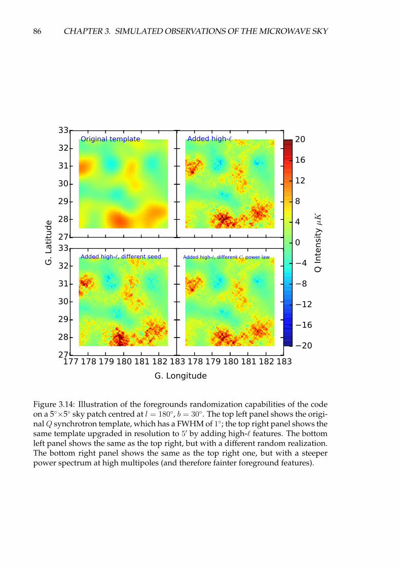
86 CHAPTER 3. SIMULATED OBSERVATIONS OF THE MICROWAVE SKY
27
28
29
30
31
32
33Original template Added high-`
177 178 179 180 181 182 18327
28
29
30
31
32
33Added high-`, different seed
178 179 180 181 182 183
Added high-`, different C` power law
20
16
12
8
4
0
4
8
12
16
20
Q Inte
nsi
ty µK
G. Longitude
G. La
titu
de
Figure 3.14: Illustration of the foregrounds randomization capabilities of the codeon a 5×5 sky patch centred at l = 180, b = 30. The top left panel shows the origi-nalQ synchrotron template, which has a FWHM of 1; the top right panel shows thesame template upgraded in resolution to 5′ by adding high-` features. The bottomleft panel shows the same as the top right, but with a different random realization.The bottom right panel shows the same as the top right one, but with a steeperpower spectrum at high multipoles (and therefore fainter foreground features).
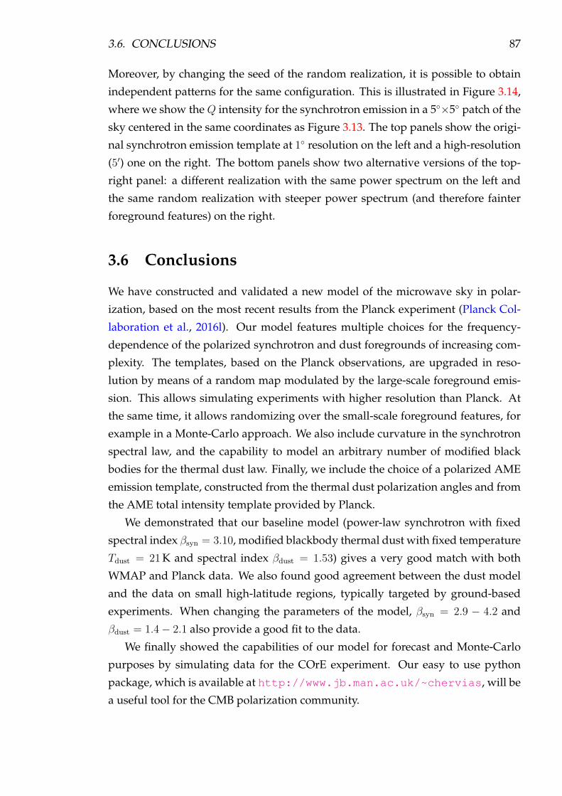
3.6. CONCLUSIONS 87
Moreover, by changing the seed of the random realization, it is possible to obtain
independent patterns for the same configuration. This is illustrated in Figure 3.14,
where we show the Q intensity for the synchrotron emission in a 5×5 patch of the
sky centered in the same coordinates as Figure 3.13. The top panels show the origi-
nal synchrotron emission template at 1 resolution on the left and a high-resolution
(5′) one on the right. The bottom panels show two alternative versions of the top-
right panel: a different realization with the same power spectrum on the left and
the same random realization with steeper power spectrum (and therefore fainter
foreground features) on the right.
3.6 Conclusions
We have constructed and validated a new model of the microwave sky in polar-
ization, based on the most recent results from the Planck experiment (Planck Col-
laboration et al., 2016l). Our model features multiple choices for the frequency-
dependence of the polarized synchrotron and dust foregrounds of increasing com-
plexity. The templates, based on the Planck observations, are upgraded in reso-
lution by means of a random map modulated by the large-scale foreground emis-
sion. This allows simulating experiments with higher resolution than Planck. At
the same time, it allows randomizing over the small-scale foreground features, for
example in a Monte-Carlo approach. We also include curvature in the synchrotron
spectral law, and the capability to model an arbitrary number of modified black
bodies for the thermal dust law. Finally, we include the choice of a polarized AME
emission template, constructed from the thermal dust polarization angles and from
the AME total intensity template provided by Planck.
We demonstrated that our baseline model (power-law synchrotron with fixed
spectral index βsyn = 3.10, modified blackbody thermal dust with fixed temperature
Tdust = 21 K and spectral index βdust = 1.53) gives a very good match with both
WMAP and Planck data. We also found good agreement between the dust model
and the data on small high-latitude regions, typically targeted by ground-based
experiments. When changing the parameters of the model, βsyn = 2.9 − 4.2 and
βdust = 1.4− 2.1 also provide a good fit to the data.
We finally showed the capabilities of our model for forecast and Monte-Carlo
purposes by simulating data for the COrE experiment. Our easy to use python
package, which is available at http://www.jb.man.ac.uk/~chervias, will be
a useful tool for the CMB polarization community.

BLANK PAGE
88
Chapter 4
Impact of foreground uncertainties on
future CMB experiments
4.1 Introduction
The astronomical community has put a significant effort on the search for primor-
dial gravitational waves. Planned future experiments will aim at detecting primor-
dial large-scale B-modes. However, if the true signal turns out to be small, it would
definitively test the limits of our instrumentation and analysis capabilities. Achiev-
ing the required sensitivity is not enough for detecting r, because of the presence
of diffuse polarized Galactic foregrounds. Therefore, component separation tech-
niques must be employed, in order to obtain the cleanest possible CMB maps. The
question is then, how accurately can we model and clean the foregrounds to the
level required for measuring r = 10−2–10−3?
Several forecasts of tensor-to-scalar ratio measurements, including foreground
residuals, have been performed for different experiments in the recent literature
(Betoule et al., 2009; Armitage-Caplan et al., 2012; Errard and Stompor, 2012;
Bonaldi et al., 2014; Remazeilles et al., 2016; Alonso et al., 2017; Remazeilles et al.,
2017b). In this chapter, we study how the error in the diffuse foregrounds compo-
nent separation modelling propagates into the measured cosmology (the tensor-to-
scalar ratio). We model a full pipeline, going from multi-frequency sky observations
to measuring the cosmological parameter r. Our approach is quite agnostic from
the point of view of physical modelling of the Galactic emission, and it focuses
on quantifying the bias on r corresponding to some arbitrary modelling error lev-
els. We also consider component separation and error mitigation techniques with
different levels of complexity. The content of this chapter was published in Hervías-
Caimapo et al. (2017).
89
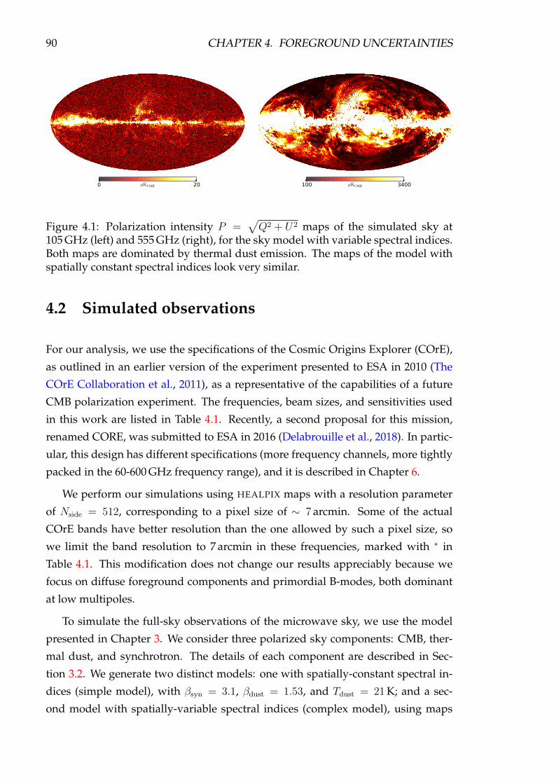
90 CHAPTER 4. FOREGROUND UNCERTAINTIES
0 20µKCMB 100 3400µKCMB
Figure 4.1: Polarization intensity P =√Q2 + U2 maps of the simulated sky at
105 GHz (left) and 555 GHz (right), for the sky model with variable spectral indices.Both maps are dominated by thermal dust emission. The maps of the model withspatially constant spectral indices look very similar.
4.2 Simulated observations
For our analysis, we use the specifications of the Cosmic Origins Explorer (COrE),
as outlined in an earlier version of the experiment presented to ESA in 2010 (The
COrE Collaboration et al., 2011), as a representative of the capabilities of a future
CMB polarization experiment. The frequencies, beam sizes, and sensitivities used
in this work are listed in Table 4.1. Recently, a second proposal for this mission,
renamed CORE, was submitted to ESA in 2016 (Delabrouille et al., 2018). In partic-
ular, this design has different specifications (more frequency channels, more tightly
packed in the 60-600 GHz frequency range), and it is described in Chapter 6.
We perform our simulations using HEALPIX maps with a resolution parameter
of Nside = 512, corresponding to a pixel size of ∼ 7 arcmin. Some of the actual
COrE bands have better resolution than the one allowed by such a pixel size, so
we limit the band resolution to 7 arcmin in these frequencies, marked with ∗ in
Table 4.1. This modification does not change our results appreciably because we
focus on diffuse foreground components and primordial B-modes, both dominant
at low multipoles.
To simulate the full-sky observations of the microwave sky, we use the model
presented in Chapter 3. We consider three polarized sky components: CMB, ther-
mal dust, and synchrotron. The details of each component are described in Sec-
tion 3.2. We generate two distinct models: one with spatially-constant spectral in-
dices (simple model), with βsyn = 3.1, βdust = 1.53, and Tdust = 21 K; and a sec-
ond model with spatially-variable spectral indices (complex model), using maps
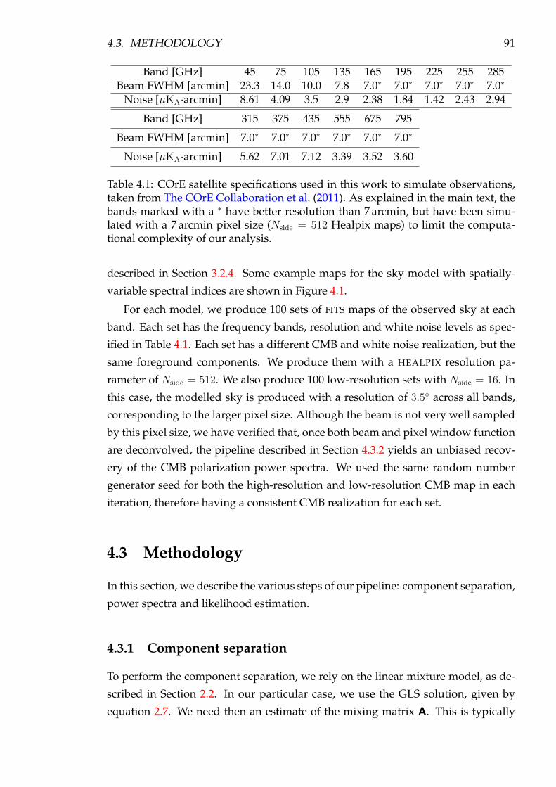
4.3. METHODOLOGY 91
Band [GHz] 45 75 105 135 165 195 225 255 285Beam FWHM [arcmin] 23.3 14.0 10.0 7.8 7.0∗ 7.0∗ 7.0∗ 7.0∗ 7.0∗
Noise [µKA·arcmin] 8.61 4.09 3.5 2.9 2.38 1.84 1.42 2.43 2.94
Band [GHz] 315 375 435 555 675 795
Beam FWHM [arcmin] 7.0∗ 7.0∗ 7.0∗ 7.0∗ 7.0∗ 7.0∗
Noise [µKA·arcmin] 5.62 7.01 7.12 3.39 3.52 3.60
Table 4.1: COrE satellite specifications used in this work to simulate observations,taken from The COrE Collaboration et al. (2011). As explained in the main text, thebands marked with a ∗ have better resolution than 7 arcmin, but have been simu-lated with a 7 arcmin pixel size (Nside = 512 Healpix maps) to limit the computa-tional complexity of our analysis.
described in Section 3.2.4. Some example maps for the sky model with spatially-
variable spectral indices are shown in Figure 4.1.
For each model, we produce 100 sets of FITS maps of the observed sky at each
band. Each set has the frequency bands, resolution and white noise levels as spec-
ified in Table 4.1. Each set has a different CMB and white noise realization, but the
same foreground components. We produce them with a HEALPIX resolution pa-
rameter of Nside = 512. We also produce 100 low-resolution sets with Nside = 16. In
this case, the modelled sky is produced with a resolution of 3.5 across all bands,
corresponding to the larger pixel size. Although the beam is not very well sampled
by this pixel size, we have verified that, once both beam and pixel window function
are deconvolved, the pipeline described in Section 4.3.2 yields an unbiased recov-
ery of the CMB polarization power spectra. We used the same random number
generator seed for both the high-resolution and low-resolution CMB map in each
iteration, therefore having a consistent CMB realization for each set.
4.3 Methodology
In this section, we describe the various steps of our pipeline: component separation,
power spectra and likelihood estimation.
4.3.1 Component separation
To perform the component separation, we rely on the linear mixture model, as de-
scribed in Section 2.2. In our particular case, we use the GLS solution, given by
equation 2.7. We need then an estimate of the mixing matrix A. This is typically

92 CHAPTER 4. FOREGROUND UNCERTAINTIES
calculated by parametrizing the spectral laws of the CMB and foreground compo-
nents; and by estimating the relevant parameters from the data. In this case, we skip
such estimation. Instead, we assume some errors on the estimation of the spectral
parameters describing the true mixing matrix and propagate them through the full
pipeline.
In the pixel domain, the effect of the beam must be equalized across multiple
bands. In practice, this is achieved by smoothing all the frequency maps to the
beam resolution of the band with the lowest resolution. This assumption, that the
instrumental beam does not depend on frequency, is not true in general, nor it is
for COrE, as shown by Table 4.1. Therefore, we pre-process all maps by smoothing
them with a Gaussian beam, thus equalizing their resolution to 23.3 arcmin (the
resolution of the lowest frequency channel, for the high-resolution sets Nside = 512)
or 3.5 (the resolution sampled by the Nside = 16 maps for the low-resolution sets).
4.3.2 Power spectra estimation
We estimated the polarization angular power spectra from CMB maps with a hy-
brid approach: using a Quadratic Maximum Likelihood (QML) estimator at low
multipoles (` < 30), and a pseudo-C` estimator at the remaining intermediate and
high multipoles. The QML estimator is optimal at low multipoles, and it can be
used to recover the reionization bump at ` < 10. The pseudo-C` estimator is appro-
priate for high multipoles, which are unobtainable for the QML estimator, where
it can recover the first acoustic peak at ` ∼ 100 in the BB spectrum. This hybrid
approach has been shown to be nearly optimal in the whole ` range and at the same
time computationally feasible (e.g. Efstathiou, 2004a, 2006). The simulated obser-
vations at Nside = 512 are used for estimating the pseudo-C` angular power spectra,
while the low-resolution maps with Nside = 16 are used for the QML estimator.
QML
This method is based on Tegmark (1997); Tegmark and de Oliveira-Costa (2001), see
also Efstathiou (2004b); Gruppuso et al. (2009). It works in pixel space, constructing
an estimator based on the covariance matrices of the data. Specifically, if x is the
CMB map in pixel space, we aim to recover a set of parameters qi with a quadratic
estimator, Qi
qi = xtQix = tr[Qixxt]. (4.1)
4.3. METHODOLOGY 93
A good choice for the quadratic estimator is
Qi ∝∑j
(B)ijC−1PjC
−1, (4.2)
where C is the covariance matrix of data, B is an arbitrary invertible matrix (we
used the identity matrix, B = I) and
Pj =∂C
∂pi. (4.3)
The normalization of equation (4.2) is such that all window functions sum to unity
Np∑j=1
tr[QiPj] = 1, (4.4)
where Np is the number of parameters (binned power spectra values) considered.
This method gives minimal error bars but it is very computationally demanding,
since it requires matrix inversions and multiplications, of order O(N3d), where Nd
is the number of pixels outside the mask. In practical terms, our limit is to run the
QML estimator for Nside = 16 maps.
Pseudo-C` deconvolution estimator
We use the method described in Brown et al. (2005) and Brown et al. (2009), which
extended to polarization the technique proposed by Hivon et al. (2002). First, we
calculate the pseudo-C` of the masked sky using the HEALPIX anafast function. The
limited sky coverage creates leakage of polarization between E and B modes. The
pseudo-C` (C`) is related to the full sky estimator (C`) through
C` =∑`′
M``′B2`′W
2`′C`′ , (4.5)
where M``′ is the coupling matrix and B` and W` are the beam and pixel window
functions, respectively. Details on the calculation of M``′ are given in Appendix A of
Brown et al. (2005). Once a binning scheme is adopted, the binned coupling matrix
is given by
Kbb′ =∑`
Pb`∑`′
M``′B2`′W
2`′Q`′b′ , (4.6)
where Pb` and Q`b are the binning and inverse binning operators, respectively. Fi-
nally, the deconvolved binned power spectra is given by
Pb =∑b′
K−1bb′
∑`
Pb′`
[C` − 〈N`〉MC
], (4.7)

94 CHAPTER 4. FOREGROUND UNCERTAINTIES
0 1 0 1
Figure 4.2: Default Galactic mask used for the power spectrum estimation, retaininga fraction of the sky fsky = 0.513. Left: Nside = 16 mask used for the QML powerspectrum estimation; right: Nside = 512 apodized mask used for the pseudo-C`power spectrum estimation.
where 〈N`〉MC is the noise bias. This is calculated by averaging the pseudo-C` of
100 noise-only realizations of the simulated observations.
The bandpass window functions are also an output of this procedure, and they
are needed for binning a model power spectra in the same way as the reconstructed
spectra for comparison. These are given by
Wb`
`=
2π
`(`+ 1)W 2` B
2`
∑b′
K−1bb′
∑`′
Pb′`′M`′` (4.8)
for bin b. A given model power spectra C` should be binned with Pb =∑``(`+1)
2πWb`
`C`.
Galactic mask
To exclude the foreground residual contamination due to the Galactic emission, we
estimate the power spectrum outside a Galactic mask. The default mask is con-
structed using the dust and synchrotron polarization templates from Planck Col-
laboration et al. (2016b), smoothing them to a FWHM of 3, and masking every
pixel with an intensity of 14µK or higher. We repeat this procedure for both Q
and U maps, and dust and synchrotron. We combine all of them to produce a fi-
nal mask. For the pseudo-C` power spectrum estimation, it is beneficial to use an
apodized mask, because sharp edges make the deconvolution kernel more compli-
cated. Therefore, we apodize the Nside = 512 mask by using the function
f(d) =
1− cos3(dπ2s
) d ≤ s
1 otherwise, (4.9)
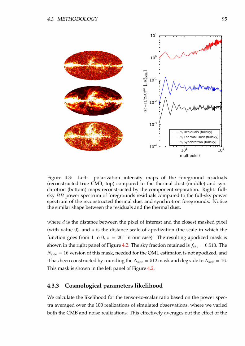
4.3. METHODOLOGY 95
101 102
multipole `
10-4
10-3
10-2
10-1
100
101
`(`+
1)/
2πCBB
` [µK
2 45G
Hz]
C` Residuals (fullsky)
C` Thermal Dust (fullsky)
C` Synchrotron (fullsky)
Figure 4.3: Left: polarization intensity maps of the foreground residuals(reconstructed-true CMB, top) compared to the thermal dust (middle) and syn-chrotron (bottom) maps reconstructed by the component separation. Right: full-sky BB power spectrum of foregrounds residuals compared to the full-sky powerspectrum of the reconstructed thermal dust and synchrotron foregrounds. Noticethe similar shape between the residuals and the thermal dust.
where d is the distance between the pixel of interest and the closest masked pixel
(with value 0), and s is the distance scale of apodization (the scale in which the
function goes from 1 to 0, s = 20 in our case). The resulting apodized mask is
shown in the right panel of Figure 4.2. The sky fraction retained is fsky = 0.513. The
Nside = 16 version of this mask, needed for the QML estimator, is not apodized, and
it has been constructed by rounding theNside = 512 mask and degrade toNside = 16.
This mask is shown in the left panel of Figure 4.2.
4.3.3 Cosmological parameters likelihood
We calculate the likelihood for the tensor-to-scalar ratio based on the power spec-
tra averaged over the 100 realizations of simulated observations, where we varied
both the CMB and noise realizations. This effectively averages out the effect of the
96 CHAPTER 4. FOREGROUND UNCERTAINTIES
cosmic variance, and only leaves the foreground residuals bias, which is of interest
in this case. We define a standard Gaussian χ2 likelihood to calculate the posterior
distribution of the tensor-to-scalar ratio. We define the χ2 as
χ2(r) =∑bb′
[PBBb − CBB,theory
b (r)]C−1bb′ [P
BBb′ − C
BB,theoryb′ (r)], (4.10)
where PBBb is the measured B-mode bandpower at bin b, CBB,theory
b (r) is the binned
B-mode theory spectrum and C−1bb′ is the inverse of the binned signal+noise covari-
ance matrix.
We construct PBBb from the low-multipole and high-multipole analysis, by join-
ing at ` = 30 (with no overlap) the results from the QML and the pseudo-C` estima-
tors.
The theory power spectrum is binned using the bandpass window functions at
the high multiple range and using a top hat function centred at each bin in the low
multipole range. The theory power spectrum is calculated as
CBB,theory` (r) =
r
r?CBB,prim` (r?) + CBB,lensing
` , (4.11)
where CBB,prim` is the primordial (scalar+tensor perturbations) power spectrum at
a given r, and CBB,lens` is the weak gravitational lensed power spectrum, which we
assume as known. r? is a fiducial value for the tensor-to-scalar ratio.
The covariance matrix is calculated using the 100 realizations signal+noise com-
plete runs of the pipeline (including the component separation). Therefore, it ac-
counts for cosmic and noise variance but also foreground residuals effects.
Modelling foreground residuals with nuisance parameters
The likelihood presented in equation (4.10) assumes that the measured power spec-
tra contains only CMB and noise. In reality, there are also some foreground resid-
uals, due to non-perfect component separation. We will extend this likelihood to
explicitly model a foreground residual contribution, using
CBB,newb (r) = CBB,theory
b (r) + AdustCBB,dustb + AsynC
BB,synb , (4.12)
where CBB,dustb and CBB,syn
b are models for the BB power spectrum of thermal dust
and synchrotron residuals, respectively, and the amplitudes Adust and Asyn are two
free nuisance parameters that can be varied, together with r, and marginalized over.
The need for adding one or both such extra parameters can be checked by seeing
whether they improve the fit, by means of the reduced χ2 value.

4.4. RESULTS 97
Simulation run Sky model Componentseparation model
Reference
Simplemodel
r = 0.01 Spatially constantβdust, βsyn
Constant βs, witha ±1,2,3% error 4.4.1; Table 4.3
r = 0.001
Complexmodel
r = 0.01 Spatially variableβdust, βsyn
Constant βs (the average ofthe true variable β maps)
4.4.2;Table 4.4, topr = 0.001
r = 0.001 Variable βs, with aglobal error of 1% and 0.5%
4.4.2;Table 4.4, bottom
Table 4.2: Summary of the different runs performed in this work.
In practice, a good choice for the foreground residual template models CBB,dustb
and CBB,synb is to assume that they are proportional to the dust and synchrotron
power spectrum. In our case, these can be computed from the foreground maps
which are the output of the component separation, as exemplified by Figure 4.3. To
the left, on top, we show the total foreground residual map for one run. The middle
and lower maps corresponds to the dust and synchrotron templates, respectively.
In harmonic space, to the right, the correlation between foregrounds residuals and
foregrounds maps is clearer. The full-sky foreground residual BB angular power
spectrum (black) is compared with the same spectrum for the thermal dust (blue)
and synchrotron (red) templates. The residual and dust spectra are very similar,
which indicates that the foreground residuals are essentially a scaled down dust
template.
In the analysis that follows, CBB,dustb and CBB,syn
b are the binned power spectra
of the thermal dust and synchrotron, respectively, reconstructed by the component
separation. We process these maps through the same procedure we use for the
reconstructed CMB, that is, the power spectra estimation with pseudo-C` for the
high-resolution map and the QML estimator for the low-resolution map, under the
same conditions.
4.4 Results
We run the component separation pipeline, described in Section 4.3, for the two sky
models, with constant and spatially-variable spectral indices. The summary of all
the runs performed in this chapter, together with descriptions and the referenced
section where the results appear, is shown in Table 4.2.
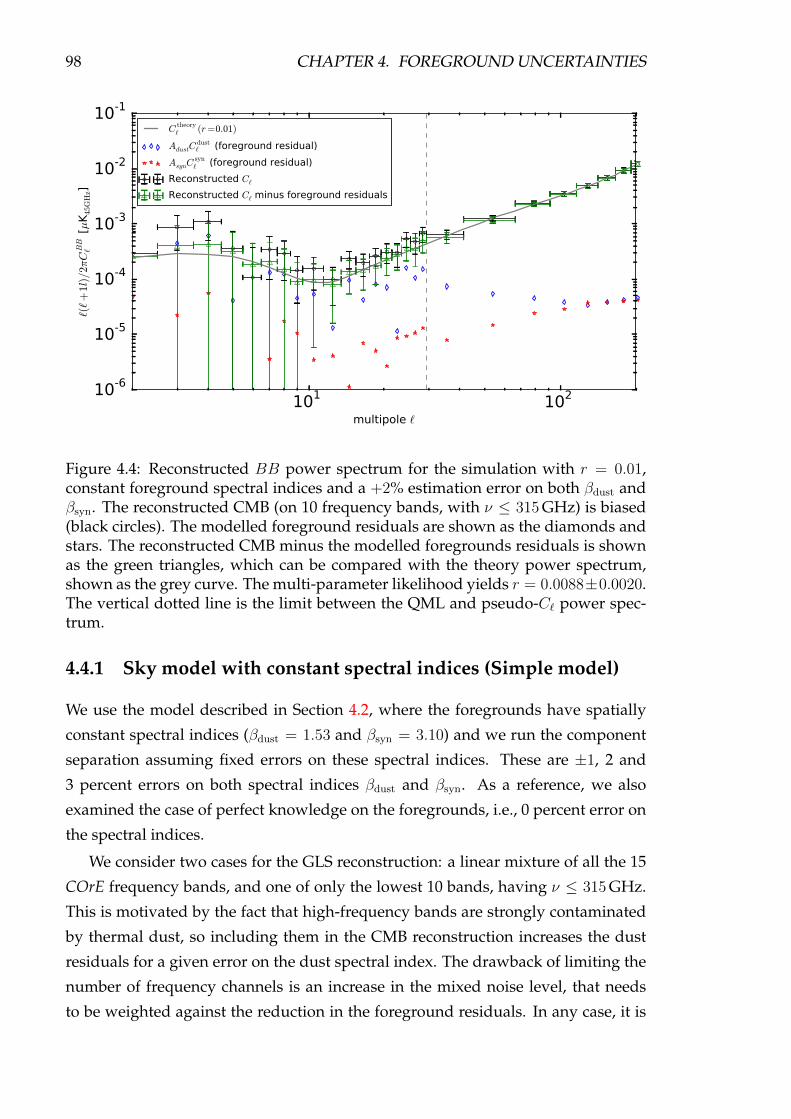
98 CHAPTER 4. FOREGROUND UNCERTAINTIES
101 102
multipole `
10-6
10-5
10-4
10-3
10-2
10-1
`(`+
1l)/
2πCBB
` [µK
45G
Hz]
Ctheory` (r=0.01)
AdustCdust` (foreground residual)
AsynCsyn` (foreground residual)
Reconstructed C`Reconstructed C` minus foreground residuals
Figure 4.4: Reconstructed BB power spectrum for the simulation with r = 0.01,constant foreground spectral indices and a +2% estimation error on both βdust andβsyn. The reconstructed CMB (on 10 frequency bands, with ν ≤ 315 GHz) is biased(black circles). The modelled foreground residuals are shown as the diamonds andstars. The reconstructed CMB minus the modelled foregrounds residuals is shownas the green triangles, which can be compared with the theory power spectrum,shown as the grey curve. The multi-parameter likelihood yields r = 0.0088±0.0020.The vertical dotted line is the limit between the QML and pseudo-C` power spec-trum.
4.4.1 Sky model with constant spectral indices (Simple model)
We use the model described in Section 4.2, where the foregrounds have spatially
constant spectral indices (βdust = 1.53 and βsyn = 3.10) and we run the component
separation assuming fixed errors on these spectral indices. These are ±1, 2 and
3 percent errors on both spectral indices βdust and βsyn. As a reference, we also
examined the case of perfect knowledge on the foregrounds, i.e., 0 percent error on
the spectral indices.
We consider two cases for the GLS reconstruction: a linear mixture of all the 15
COrE frequency bands, and one of only the lowest 10 bands, having ν ≤ 315 GHz.
This is motivated by the fact that high-frequency bands are strongly contaminated
by thermal dust, so including them in the CMB reconstruction increases the dust
residuals for a given error on the dust spectral index. The drawback of limiting the
number of frequency channels is an increase in the mixed noise level, that needs
to be weighted against the reduction in the foreground residuals. In any case, it is
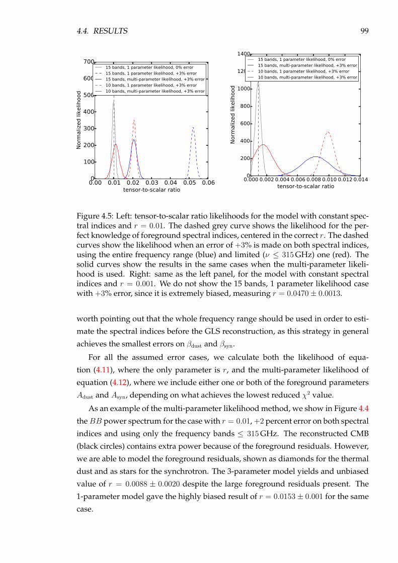
4.4. RESULTS 99
0.00 0.01 0.02 0.03 0.04 0.05 0.06tensor-to-scalar ratio
0
100
200
300
400
500
600
700
Norm
aliz
ed lik
elih
ood
15 bands, 1 parameter likelihood, 0% error
15 bands, 1 parameter likelihood, +3% error
15 bands, multi-parameter likelihood, +3% error
10 bands, 1 parameter likelihood, +3% error
10 bands, multi-parameter likelihood, +3% error
0.000 0.002 0.004 0.006 0.008 0.010 0.012 0.014tensor-to-scalar ratio
0
200
400
600
800
1000
1200
1400
Norm
aliz
ed lik
elih
ood
15 bands, 1 parameter likelihood, 0% error
15 bands, multi-parameter likelihood, +3% error
10 bands, 1 parameter likelihood, +3% error
10 bands, multi-parameter likelihood, +3% error
Figure 4.5: Left: tensor-to-scalar ratio likelihoods for the model with constant spec-tral indices and r = 0.01. The dashed grey curve shows the likelihood for the per-fect knowledge of foreground spectral indices, centered in the correct r. The dashedcurves show the likelihood when an error of +3% is made on both spectral indices,using the entire frequency range (blue) and limited (ν ≤ 315 GHz) one (red). Thesolid curves show the results in the same cases when the multi-parameter likeli-hood is used. Right: same as the left panel, for the model with constant spectralindices and r = 0.001. We do not show the 15 bands, 1 parameter likelihood casewith +3% error, since it is extremely biased, measuring r = 0.0470± 0.0013.
worth pointing out that the whole frequency range should be used in order to esti-
mate the spectral indices before the GLS reconstruction, as this strategy in general
achieves the smallest errors on βdust and βsyn.
For all the assumed error cases, we calculate both the likelihood of equa-
tion (4.11), where the only parameter is r, and the multi-parameter likelihood of
equation (4.12), where we include either one or both of the foreground parameters
Adust and Asyn, depending on what achieves the lowest reduced χ2 value.
As an example of the multi-parameter likelihood method, we show in Figure 4.4
theBB power spectrum for the case with r = 0.01, +2 percent error on both spectral
indices and using only the frequency bands ≤ 315 GHz. The reconstructed CMB
(black circles) contains extra power because of the foreground residuals. However,
we are able to model the foreground residuals, shown as diamonds for the thermal
dust and as stars for the synchrotron. The 3-parameter model yields and unbiased
value of r = 0.0088 ± 0.0020 despite the large foreground residuals present. The
1-parameter model gave the highly biased result of r = 0.0153± 0.001 for the same
case.

100 CHAPTER 4. FOREGROUND UNCERTAINTIES
In Figure 4.5, we show some example tensor-to-scalar ratio likelihoods for the
simple simulations, with r = 0.01 (left) and r = 0.001 (right), respectively. The
grey curves show the perfect knowledge component separation using all the 15 fre-
quency bands, which always yields an unbiased result (r = 0.0099 ± 0.0009 and
r = 0.00095 ± 0.00037). All the other curves assume a +3 percent error on both
spectral indices. The blue curves correspond to a CMB reconstruction using 15 fre-
quency bands, and a 1-parameter (dashed) and multi-parameter (solid) likelihood.
The red curves are the same for a CMB reconstruction using only the first 10 fre-
quency bands.
For both the r = 0.01 and r = 0.001 cases, the multi-parameter likelihood on
the 10 frequency bands case allows removing the large bias corresponding to the
+3 percent spectral index error. However, there is a degradation in the measured
error σ(r). For the r = 0.001 case, this does not allow a detection at the 2σ level any
more, but only corresponds to an upper limit.
We show the summary of all the results for the simulated observations with
r = 0.01 in the top half of Table 4.3 and in Figure 4.6. In the top panel, we show the
measured bias (estimated minus true r); in the bottom panel, we show the width
of the likelihood, σ(r). As expected, when we assume perfect knowledge of the
foregrounds, the result is unbiased. However, when we introduce some error in
the component separation, the likelihood is biased towards higher values of r. If
we adopt the multi-parameter likelihood instead of the 1-parameter one, the bias is
either reduced or removed.
Limiting the frequency bands used in the CMB solution to ν ≤ 315 GHz is also
effective in reducing the bias. In fact, a large fraction of the foreground residuals
is introduced by the high frequency bands that are strongly dominated by thermal
dust. By comparing the red stars (multi-parameter likelihood, full frequency range)
to the green circles (1-parameter likelihood, limited frequency range), we see that
they give similar biases for the same error on the spectral parameters. However,
the green circles have smaller σ(r) values than the red stars, showing that, in this
case, it is preferable to limit the bands used in the component separation than to
introduce a multi-parameter likelihood. Even so, in some cases, when the bias is
large (e.g. ±3 percent spectral index error), both approaches must be used at the
same time (shown by the yellow triangles).
The summary of all the cases for the simulations with r = 0.001 is reported in the
bottom half of Table 4.3 and shown in Figure 4.6 (right). It follows the same scheme
from Figure 4.6, for the same assumed component separation error cases. Getting
an unbiased result is much more difficult in this case, due to the small value of r. In
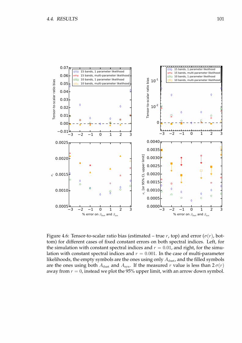
4.4. RESULTS 101
3 2 1 0 1 2 30.01
0.00
0.01
0.02
0.03
0.04
0.05
0.06
0.07
Tenso
r-to
-sca
lar
rati
o b
ias
15 bands, 1 parameter likelihood
15 bands, multi-parameter likelihood
10 bands, 1 parameter likelihood
10 bands, multi-parameter likelihood
3 2 1 0 1 2 3% error on βdust and βsyn
0.0005
0.0010
0.0015
0.0020
0.0025
σr
3 2 1 0 1 2 3
0
10-2
10-1
Tenso
r-to
-sca
lar
rati
o b
ias
15 bands, 1 parameter likelihood
15 bands, multi-parameter likelihood
10 bands, 1 parameter likelihood
10 bands, multi-parameter likelihood
3 2 1 0 1 2 3% error on βdust and βsyn
0.0000
0.0005
0.0010
0.0015
0.0020
0.0025
0.0030
0.0035
0.0040σr [
or
95
% C
L upper
limit
]
Figure 4.6: Tensor-to-scalar ratio bias (estimated – true r, top) and error (σ(r), bot-tom) for different cases of fixed constant errors on both spectral indices. Left, forthe simulation with constant spectral indices and r = 0.01, and right, for the simu-lation with constant spectral indices and r = 0.001. In the case of multi-parameterlikelihoods, the empty symbols are the ones using onlyAdust, and the filled symbolsare the ones using both Adust and Asyn. If the measured r value is less than 2 σ(r)away from r = 0, instead we plot the 95% upper limit, with an arrow down symbol.
102 CHAPTER 4. FOREGROUND UNCERTAINTIES
particular, for errors in the spectral indices larger than ±1 percent, we always need
both the multi-parameter likelihood and the limited frequency range. We note that,
for the perfect knowledge case, the value of σ(r) = 3.7× 10⁻⁴ is only just below the
value allowing a 2σ detection. Therefore, the multi-parameter likelihood increases
σ(r) and only allows for a 95% upper limit.
4.4.2 Sky model with spatially variable spectral indices (Complex
model)
Now, we consider a more realistic model of the sky, where the spectral indices of
the foreground components are spatially variable, as explained in Section 4.2. We
simulate the measurement of the tensor-to-scalar ratio for two levels of component
separation modelling complexity, as detailed in the two following sub-sections.
Modelling the component separation with spatially constant βdust and βsyn
The first approach we adopt is to model the spatially variable spectral indices as a
constant value across the sky. We set this value to be the true average of the βdust
and βsyn maps outside the Galactic mask of Figure 4.2. As such, these values (βdust =
1.53 and βsyn = 2.89) better represent most of the pixels used for the analysis. The
histograms of the spectral index residuals, defined as the difference between the
true indices (at a given pixel) and the true average value, for all the pixels in the sky
outside the mask are shown in Figure 4.7. The standard deviation of these residuals
are 0.0253 for βdust and 0.1074 for βsyn, which corresponds to a 1.7 % and 3.5 % error,
respectively. These errors are qualitatively similar to the ones we considered in
Section 4.4.1.
We start by considering the 1-parameter and multi-parameter likelihood on
the CMB reconstructed using the first 10 frequency bands. This was the best-
performing case in the previous (constant spectral index) exercise. The results are
reported in the top half of Table 4.4 as the base case. As we can see, this case is
not good enough any more, because the bias on r is still significant. We therefore
proceeded to optimize the analysis to reduce the bias on r, and obtained the results
quoted in Table 4.4 as the best case. The modifications we introduced are:
1. Secondary dust component: we use the idea presented in Stolyarov et al.
(2005), which is that a component with spatially variable spectral dependence
can be modelled as a series of components with constant spectral dependence,
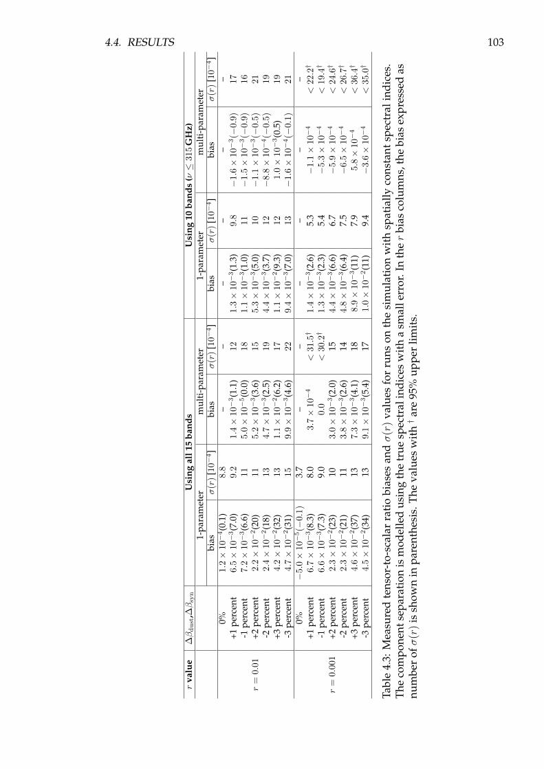
4.4. RESULTS 103
rva
lue
∆βdust
,∆βsy
nU
sing
all1
5ba
nds
Usi
ng10
band
s(ν≤
315
GH
z)1-
para
met
erm
ulti
-par
amet
er1-
para
met
erm
ulti
-par
amet
erbi
asσ
(r)
[10−
4]
bias
σ(r
)[1
0−4]
bias
σ(r
)[1
0−4]
bias
σ(r
)[1
0−4]
r=
0.01
0%1.
2×
10−4(0
.1)
8.8
––
––
––
+1pe
rcen
t6.
5×
10−3(7
.0)
9.2
1.4×
10−3(1
.1)
12
1.3×
10−
3(1
.3)
9.8
−1.6×
10−3(−
0.9
)17
-1pe
rcen
t7.
2×
10−3(6
.6)
115.0×
10−5(0
.0)
18
1.1×
10−
3(1
.0)
11
−1.5×
10−3(−
0.9
)16
+2pe
rcen
t2.
2×
10−2(2
0)11
5.2×
10−3(3
.6)
15
5.3×
10−
3(5
.0)
10
−1.1×
10−3(−
0.5
)21
-2pe
rcen
t2.
4×
10−2(1
8)13
4.7×
10−3(2
.5)
19
4.4×
10−
3(3
.7)
12
−8.8×
10−4(−
0.5
)19
+3pe
rcen
t4.
2×
10−2(3
2)13
1.1×
10−2(6
.2)
17
1.1×
10−
2(9
.3)
12
1.0×
10−3(0
.5)
19
-3pe
rcen
t4.
7×
10−2(3
1)15
9.9×
10−3(4
.6)
22
9.4×
10−
3(7
.0)
13
−1.6×
10−4(−
0.1
)21
r=
0.00
1
0%−
5.0×
10−5(−
0.1)
3.7
––
––
––
+1pe
rcen
t6.
7×
10−3(8
.3)
8.0
3.7×
10−4
<31.5†
1.4×
10−
3(2
.6)
5.3
−1.1×
10−4
<22.2†
-1pe
rcen
t6.
6×
10−3(7
.3)
9.0
0.0
<30.2†
1.3×
10−
3(2
.3)
5.4
−5.3×
10−4
<19.4†
+2pe
rcen
t2.
3×
10−2(2
3)10
3.0×
10−3(2
.0)
154.4×
10−
3(6
.6)
6.7
−5.9×
10−4
<24.6†
-2pe
rcen
t2.
3×
10−2(2
1)11
3.8×
10−3(2
.6)
144.8×
10−
3(6
.4)
7.5
−6.5×
10−4
<26.7†
+3pe
rcen
t4.
6×
10−2(3
7)13
7.3×
10−3(4
.1)
188.9×
10−3(1
1)7.
95.8×
10−
4<
36.4†
-3pe
rcen
t4.
5×
10−2(3
4)13
9.1×
10−3(5
.4)
171.0×
10−2(1
1)9.
4−
3.6×
10−4
<35.0†
Tabl
e4.
3:M
easu
red
tens
or-t
o-sc
alar
rati
obi
ases
andσ
(r)
valu
esfo
rru
nson
the
sim
ulat
ion
wit
hsp
atia
llyco
nsta
ntsp
ectr
alin
dice
s.Th
eco
mpo
nent
sepa
rati
onis
mod
elle
dus
ing
the
true
spec
tral
indi
ces
wit
ha
smal
lerr
or.I
nth
er
bias
colu
mns
,the
bias
expr
esse
das
num
ber
ofσ
(r)
issh
own
inpa
rent
hesi
s.T
heva
lues
wit
h†
are
95%
uppe
rlim
its.

104 CHAPTER 4. FOREGROUND UNCERTAINTIES
0.15 0.10 0.05 0.00 0.05 0.10
βdust(p)−βdust residual
0
2
4
6
8
10
12
14
16
18
Norm
aliz
ed c
ount
0.3 0.2 0.10.0 0.1 0.2 0.3 0.4 0.5
βsyn(p)−βsyn residual
0.0
0.5
1.0
1.5
2.0
2.5
3.0
3.5
4.0
Figure 4.7: Histograms of the dust (left) and synchrotron (right) spectral indexresiduals (true – average spectral index) outside the Galactic mask. The true spec-tral indices are the ones in the sky model from Hervías-Caimapo et al. (2016). Thetrue average βdust is calculated on a Nside = 2048 map, while the true average βsyn
is calculated on a Nside = 512 map. The histograms are normalized so that they in-tegrate to 1. The standard deviations of the distribution of spectral index residualsare equivalent to a 1.7% error for thermal dust and to a 3.5% error for synchrotron.
each one corresponding to a term in a Taylor expansion. In this way, the first-
order thermal dust is the usual grey-body spectral law, and we add a second-
order thermal dust component, whose spectrum is the derivative of that spec-
tral law with respect to βdust. We also explored the possibility to add a second
synchrotron component to account for the variability of the synchrotron spec-
tral index, but this achieved no significant improvement in our case.
2. Optimization of the Galactic mask: we produced a new mask specifically
optimized for B-modes and tailored to the component separation approach
we used. Specifically, we produced an estimate of foreground errors on the
CMB B map with a Monte Carlo (MC) approach, and then excluded all pixels
for which this map was over some threshold. To derive the error B map,
we repeated the GLS CMB reconstruction 100 times by varying randomly the
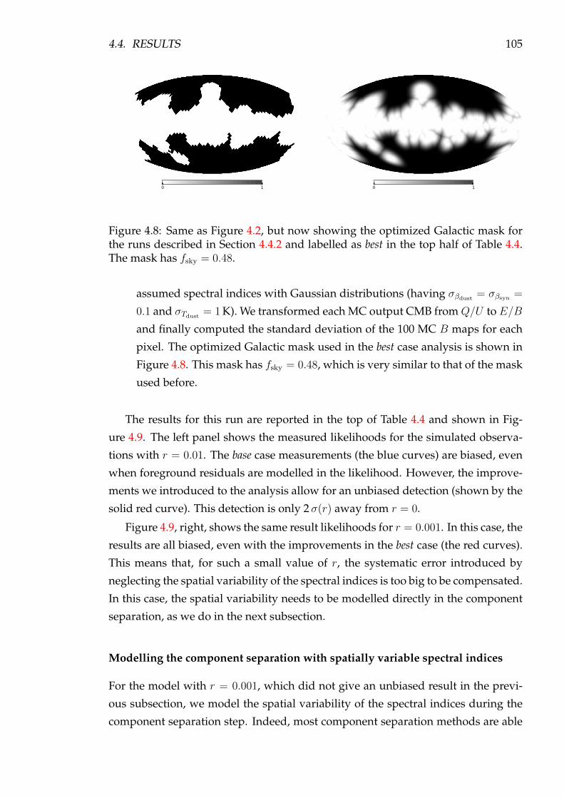
4.4. RESULTS 105
0 1 0 1
Figure 4.8: Same as Figure 4.2, but now showing the optimized Galactic mask forthe runs described in Section 4.4.2 and labelled as best in the top half of Table 4.4.The mask has fsky = 0.48.
assumed spectral indices with Gaussian distributions (having σβdust = σβsyn =
0.1 and σTdust = 1 K). We transformed each MC output CMB from Q/U to E/B
and finally computed the standard deviation of the 100 MC B maps for each
pixel. The optimized Galactic mask used in the best case analysis is shown in
Figure 4.8. This mask has fsky = 0.48, which is very similar to that of the mask
used before.
The results for this run are reported in the top of Table 4.4 and shown in Fig-
ure 4.9. The left panel shows the measured likelihoods for the simulated observa-
tions with r = 0.01. The base case measurements (the blue curves) are biased, even
when foreground residuals are modelled in the likelihood. However, the improve-
ments we introduced to the analysis allow for an unbiased detection (shown by the
solid red curve). This detection is only 2σ(r) away from r = 0.
Figure 4.9, right, shows the same result likelihoods for r = 0.001. In this case, the
results are all biased, even with the improvements in the best case (the red curves).
This means that, for such a small value of r, the systematic error introduced by
neglecting the spatial variability of the spectral indices is too big to be compensated.
In this case, the spatial variability needs to be modelled directly in the component
separation, as we do in the next subsection.
Modelling the component separation with spatially variable spectral indices
For the model with r = 0.001, which did not give an unbiased result in the previ-
ous subsection, we model the spatial variability of the spectral indices during the
component separation step. Indeed, most component separation methods are able
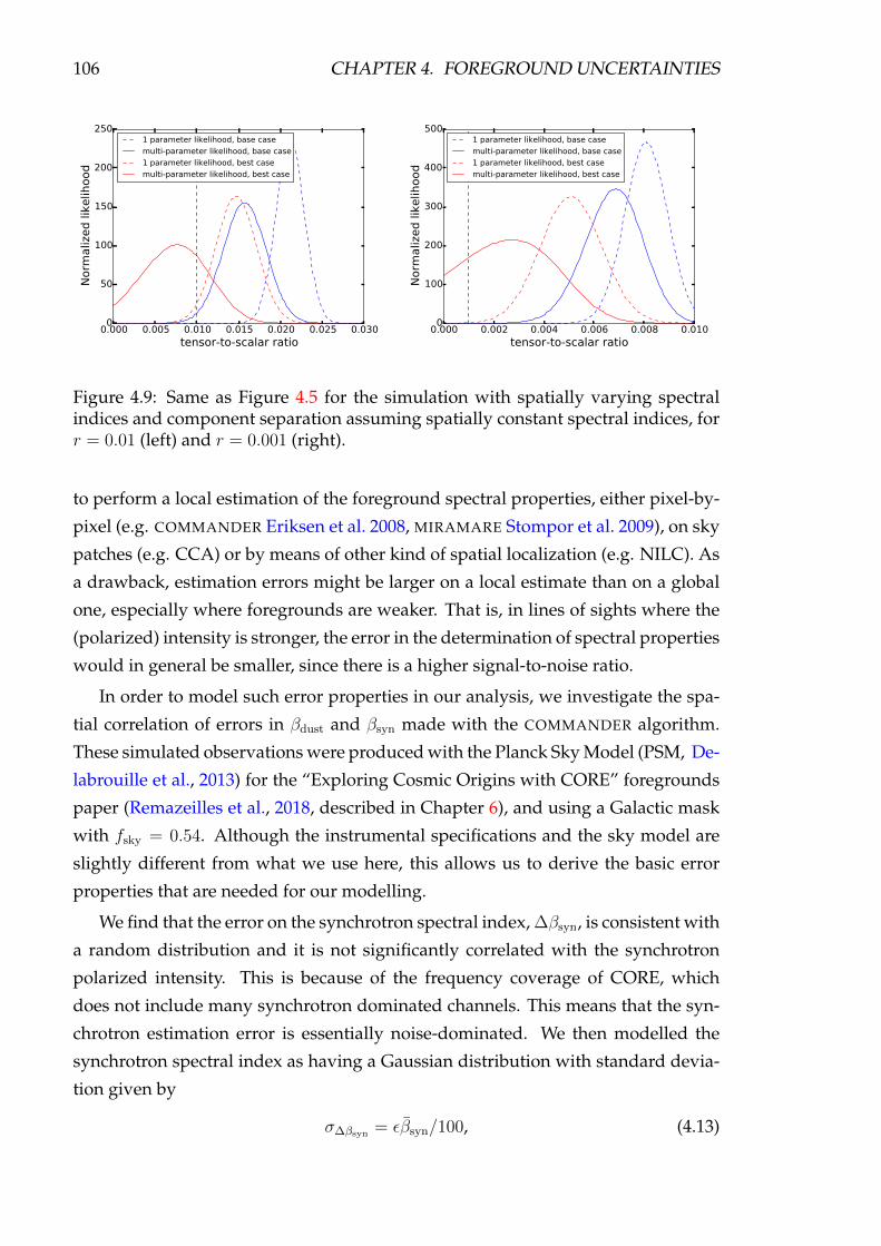
106 CHAPTER 4. FOREGROUND UNCERTAINTIES
0.000 0.005 0.010 0.015 0.020 0.025 0.030tensor-to-scalar ratio
0
50
100
150
200
250
Norm
aliz
ed lik
elih
ood
1 parameter likelihood, base case
multi-parameter likelihood, base case
1 parameter likelihood, best case
multi-parameter likelihood, best case
0.000 0.002 0.004 0.006 0.008 0.010tensor-to-scalar ratio
0
100
200
300
400
500
Norm
aliz
ed lik
elih
ood
1 parameter likelihood, base case
multi-parameter likelihood, base case
1 parameter likelihood, best case
multi-parameter likelihood, best case
Figure 4.9: Same as Figure 4.5 for the simulation with spatially varying spectralindices and component separation assuming spatially constant spectral indices, forr = 0.01 (left) and r = 0.001 (right).
to perform a local estimation of the foreground spectral properties, either pixel-by-
pixel (e.g. COMMANDER Eriksen et al. 2008, MIRAMARE Stompor et al. 2009), on sky
patches (e.g. CCA) or by means of other kind of spatial localization (e.g. NILC). As
a drawback, estimation errors might be larger on a local estimate than on a global
one, especially where foregrounds are weaker. That is, in lines of sights where the
(polarized) intensity is stronger, the error in the determination of spectral properties
would in general be smaller, since there is a higher signal-to-noise ratio.
In order to model such error properties in our analysis, we investigate the spa-
tial correlation of errors in βdust and βsyn made with the COMMANDER algorithm.
These simulated observations were produced with the Planck Sky Model (PSM, De-
labrouille et al., 2013) for the “Exploring Cosmic Origins with CORE” foregrounds
paper (Remazeilles et al., 2018, described in Chapter 6), and using a Galactic mask
with fsky = 0.54. Although the instrumental specifications and the sky model are
slightly different from what we use here, this allows us to derive the basic error
properties that are needed for our modelling.
We find that the error on the synchrotron spectral index, ∆βsyn, is consistent with
a random distribution and it is not significantly correlated with the synchrotron
polarized intensity. This is because of the frequency coverage of CORE, which
does not include many synchrotron dominated channels. This means that the syn-
chrotron estimation error is essentially noise-dominated. We then modelled the
synchrotron spectral index as having a Gaussian distribution with standard devia-
tion given by
σ∆βsyn = εβsyn/100, (4.13)
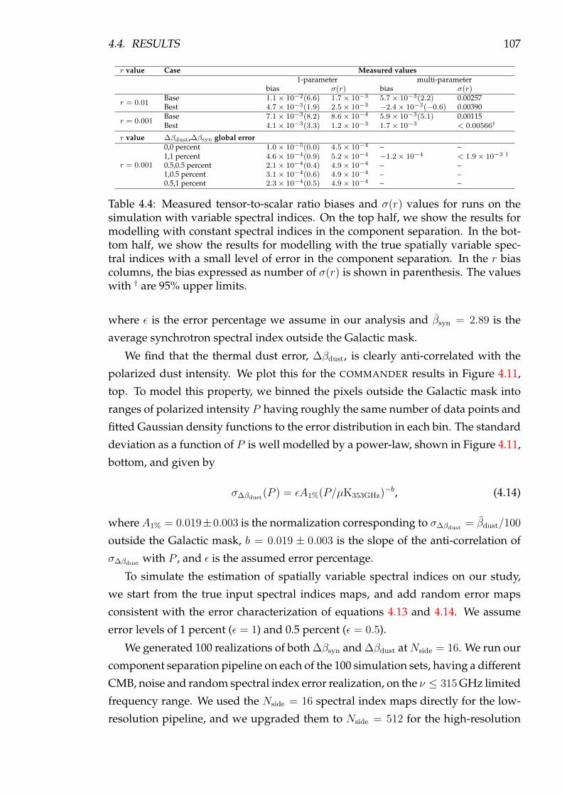
4.4. RESULTS 107
r value Case Measured values1-parameter multi-parameter
bias σ(r) bias σ(r)
r = 0.01Base 1.1× 10⁻²(6.6) 1.7× 10⁻³ 5.7× 10⁻³(2.2) 0.00257Best 4.7× 10⁻³(1.9) 2.5× 10⁻³ −2.4× 10⁻³(−0.6) 0.00390
r = 0.001Base 7.1× 10⁻³(8.2) 8.6× 10⁻⁴ 5.9× 10⁻³(5.1) 0.00115Best 4.1× 10⁻³(3.3) 1.2× 10⁻³ 1.7× 10⁻³ < 0.00566†
r value ∆βdust,∆βsyn global error
r = 0.001
0,0 percent 1.0× 10⁻⁵(0.0) 4.5× 10⁻⁴ – –1,1 percent 4.6× 10⁻⁴(0.9) 5.2× 10⁻⁴ −1.2× 10⁻⁴ < 1.9× 10⁻³ †
0.5,0.5 percent 2.1× 10⁻⁴(0.4) 4.9× 10⁻⁴ – –1,0.5 percent 3.1× 10⁻⁴(0.6) 4.9× 10⁻⁴ – –0.5,1 percent 2.3× 10⁻⁴(0.5) 4.9× 10⁻⁴ – –
Table 4.4: Measured tensor-to-scalar ratio biases and σ(r) values for runs on thesimulation with variable spectral indices. On the top half, we show the results formodelling with constant spectral indices in the component separation. In the bot-tom half, we show the results for modelling with the true spatially variable spec-tral indices with a small level of error in the component separation. In the r biascolumns, the bias expressed as number of σ(r) is shown in parenthesis. The valueswith † are 95% upper limits.
where ε is the error percentage we assume in our analysis and βsyn = 2.89 is the
average synchrotron spectral index outside the Galactic mask.
We find that the thermal dust error, ∆βdust, is clearly anti-correlated with the
polarized dust intensity. We plot this for the COMMANDER results in Figure 4.11,
top. To model this property, we binned the pixels outside the Galactic mask into
ranges of polarized intensity P having roughly the same number of data points and
fitted Gaussian density functions to the error distribution in each bin. The standard
deviation as a function of P is well modelled by a power-law, shown in Figure 4.11,
bottom, and given by
σ∆βdust(P ) = εA1%(P/µK353GHz)−b, (4.14)
where A1% = 0.019±0.003 is the normalization corresponding to σ∆βdust = βdust/100
outside the Galactic mask, b = 0.019 ± 0.003 is the slope of the anti-correlation of
σ∆βdust with P , and ε is the assumed error percentage.
To simulate the estimation of spatially variable spectral indices on our study,
we start from the true input spectral indices maps, and add random error maps
consistent with the error characterization of equations 4.13 and 4.14. We assume
error levels of 1 percent (ε = 1) and 0.5 percent (ε = 0.5).
We generated 100 realizations of both ∆βsyn and ∆βdust at Nside = 16. We run our
component separation pipeline on each of the 100 simulation sets, having a different
CMB, noise and random spectral index error realization, on the ν ≤ 315 GHz limited
frequency range. We used the Nside = 16 spectral index maps directly for the low-
resolution pipeline, and we upgraded them to Nside = 512 for the high-resolution
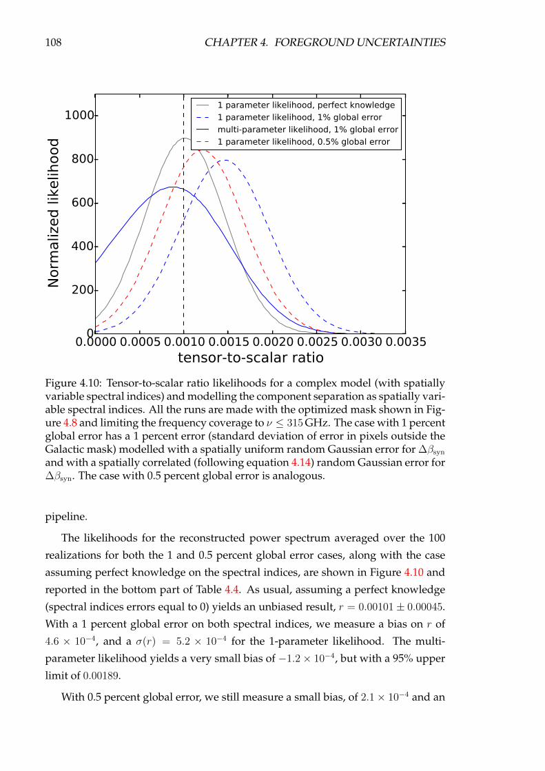
108 CHAPTER 4. FOREGROUND UNCERTAINTIES
0.0000 0.0005 0.0010 0.0015 0.0020 0.0025 0.0030 0.0035tensor-to-scalar ratio
0
200
400
600
800
1000
Norm
aliz
ed lik
elih
ood
1 parameter likelihood, perfect knowledge
1 parameter likelihood, 1% global error
multi-parameter likelihood, 1% global error
1 parameter likelihood, 0.5% global error
Figure 4.10: Tensor-to-scalar ratio likelihoods for a complex model (with spatiallyvariable spectral indices) and modelling the component separation as spatially vari-able spectral indices. All the runs are made with the optimized mask shown in Fig-ure 4.8 and limiting the frequency coverage to ν ≤ 315 GHz. The case with 1 percentglobal error has a 1 percent error (standard deviation of error in pixels outside theGalactic mask) modelled with a spatially uniform random Gaussian error for ∆βsyn
and with a spatially correlated (following equation 4.14) random Gaussian error for∆βsyn. The case with 0.5 percent global error is analogous.
pipeline.
The likelihoods for the reconstructed power spectrum averaged over the 100
realizations for both the 1 and 0.5 percent global error cases, along with the case
assuming perfect knowledge on the spectral indices, are shown in Figure 4.10 and
reported in the bottom part of Table 4.4. As usual, assuming a perfect knowledge
(spectral indices errors equal to 0) yields an unbiased result, r = 0.00101± 0.00045.
With a 1 percent global error on both spectral indices, we measure a bias on r of
4.6 × 10⁻⁴, and a σ(r) = 5.2 × 10⁻⁴ for the 1-parameter likelihood. The multi-
parameter likelihood yields a very small bias of −1.2× 10⁻⁴, but with a 95% upper
limit of 0.00189.
With 0.5 percent global error, we still measure a small bias, of 2.1× 10⁻⁴ and an

4.4. RESULTS 109
0.10
0.05
0.00
0.05
0.10
Err
or
∆β
dust
=β
model
dust−β
estim
ated
dust
0 2 4 6 8 10 12 14 16
P=√Q2 +U2 from thermal dust template [µK353GHz]
0.00
0.01
0.02
0.03
0.04
0.05
0.06
σ∆β
dust f
rom
fit
to h
isto
gra
m
Figure 4.11: Example of the correlation between the ∆βdust residual and the inten-sity of polarization. These residuals are obtained with the CORE analysis using theCOMMANDER code. On top, we show for each pixel inside the Galactic mask ofFigure 4.8, the spectral index residual as a function of the polarization intensity. Wedivide the polarization intensity into 6 bins, whose limits are shown as red dashedlines. In each bin, we calculate the standard deviation of the βdust error as a functionof the polarization intensity. This is shown in the bottom, along with a power lawfit, in green.

110 CHAPTER 4. FOREGROUND UNCERTAINTIES
σ(r) error of 4.9× 10⁻⁴ for the 1-parameter likelihood. Fitting with the foregrounds
nuisance parameters is not well motivated, since the marginalized likelihoods for
Adust and Asyn are consistent with 0.
We have verified that the residual systematic error on r is due mostly to thermal
dust residual contamination (as opposed to synchrotron residuals). In fact, the 1-
parameter likelihood yields r = (13.1 ± 4.9) × 10−4, and r = (12.3 ± 4.9) × 10−4,
respectively, if we consider a 0.5 percent global error only on βsyn and βdust and we
leave the other foreground at 1 percent global error.
4.5 Conclusions
We have performed an analysis on the tensor-to-scalar ratio bias produced by the
mis-modelling of foreground spectral parameters, taking into account a realistic
model of the sky and a full data analysis pipeline.
We have considered two sky models: a very simple one, where the foregrounds
(synchrotron and dust) have spatially-constant spectral parameters across the sky,
and a more complex one, where the spectral dependence is spatially-varying, while
the Tdust parameter is constant. We modelled component separation strategies and
likelihood estimations of increasing complexity. The main results of our analysis
can be summarized as follows: For r = 0.01, we obtain an unbiased estimation of
r for all simulations considered. The requirements on the accuracy of foregrounds
modelling for component separation purposes are not too stringent (for example
modelling spatially-varying foreground spectral indices as spatially-constant still
gives a successful measurement).
Depending on the error level on the synchrotron and thermal dust spectral in-
dices (from 1 to 3 percent), the best results may require exploiting a limited set of
“cleaner” frequency maps to reconstruct the CMB. The use of all channels is always
recommended to obtain accurate estimates of the foreground spectral indices. We
achieve significant improvements by explicitly modelling the synchrotron and dust
foreground residuals in the likelihood, and marginalizing over foreground ampli-
tude nuisance parameters. Furthermore, an important role is played by the Galactic
mask, which needs to be optimized for the component separation method used and
for B-mode detection.
For r = 0.001 and a simple sky model, using a suitable mask, modelling fore-
ground residuals in the likelihood and limiting the frequency range for CMB recon-
struction always yields an unbiased r value. The error on r often does not allow
a detection but just an upper limit; this result is however conservative because the

4.5. CONCLUSIONS 111
Gaussian likelihood we adopted is not optimal in the low-multipole regime.
When increasing the complexity of the sky, large modelling errors, such as ap-
proximating a spatially-varying spectral index with a constant, should not be used,
as they give rise to biases on r that are too large to be corrected for (at the likelihood
level). In such cases, modelling the spatial variability of the spectral indices at the
component separation level is required. For a global error of 0.5 (1) percent in βdust
and βsyn, we obtain an unbiased detection (upper limit) on r. We show that the
foreground residuals biasing the measurement of r = 0.001 are due in greater pro-
portion to thermal dust emission than synchrotron emission, due to the particular
frequency coverage of CORE.
Such level of accuracy in the determination of foreground spectral parameters
is very challenging, and motivates further research on component separation and
foreground characterization. However, our analysis does not take into account po-
larization ancillary data that will become available, such as C-BASS (Irfan et al.,
2015). Our method could also be used to further optimize the instrumental specifi-
cations of future CMB B-modes experiments.

BLANK PAGE
112

Chapter 5
Forecasts on measuring r for the
Simons Observatory
In this chapter, I discuss my work related to the forecasting of the detection levels of
the tensor-to-scalar ratio for the Simons Observatory. In this case, we use a simple
strategy, known as Fisher matrix forecasting, because it uses the Fisher information
matrix to estimate the 1σ error of a parameter given some observable data. This
work corresponds to my contribution to the Simons Observatory collaboration.
5.1 The Simons Observatory
The Simons Observatory is a planned stage-3 CMB experiment that will observe
from the Chajnantor plateau in the Atacama desert in Chile. The collaboration is the
joint effort of two existing experiments that have been observing from the same site:
the Atacama Cosmology Telescope (Swetz et al., 2011) and POLARBEAR/Simons
array (Kermish et al., 2012), and includes more than 45 institutions from 8 countries.
The experiment is planned to begin observing around 2021, and will consist of an
array of microwave polarization-sensitive telescopes: a large aperture telescope of
∼ 6 m, and one or more small aperture telescopes of ∼ 0.5 m.
The science cases the experiment aims to address are the detection of primordial
gravitational waves with polarization B-modes, and to be able to better constrain
the neutrino sector. Also, the dark energy sector, CMB weak lensing and cluster
counts with the SZ effect, among others. It will be an essential stepping stone into
the ultimate ground-based CMB experiment, CMB-S4 (Abitbol et al., 2017).
At the moment, the collaboration is focused on evaluating the performance of
the planned instrumentation and detectors, together with forecasting the impact on
the cosmology that such an instrument could have. I have done some work for the
113
114 CHAPTER 5. FORECAST FOR SIMONS OBSERVATORY
measuring r working group, which is presented in the following sections.
5.2 Methodology
The pipeline to estimate the detection limits of the tensor-to-scalar ratio, that is, σ(r),
consist of several steps: the modelling of foreground spectral parameter errors, the
estimation of power spectrum residuals, and the estimation of the error on r. These
are detailed in Section 5.2.1, 5.2.2, and 5.2.3, respectively.
5.2.1 Modelling the foreground spectral parameters errors
We obtain an estimate of the residual error on the foreground spectral indices by
running the CCA algorithm (detailed in Section 2.2.1) on a set of SO simulated ob-
servations. We tessellate the full sky in small square patches, and therefore we
calculate the statistics using the results from the patches within the SO mask con-
sidered. We estimate an average residual error for each spectral parameter with the
standard deviation of the statistics. More details of the practical application of this
is described in Section 5.3.3.
5.2.2 Estimate of power spectrum residuals
We need a way to estimate the residuals left in the angular power spectra by the
foregrounds in the cleaned CMB once a component separation method has been
used over the multi-frequency maps. In a parametric component separation frame
work, this means estimating a reasonable error on the fitting of the spectral pa-
rameters of the components. This depends on several factors, such as frequency
coverage, ancillary data we could have on the components at lower and higher fre-
quencies, how good our models reflect the true components, etc. The error on the
foreground spectral parameters propagates to a residual in the CMB power spectra;
this error is added to the noise and cosmic variance to give a final error bar on the
CMB angular power spectra (Bonaldi and Ricciardi, 2011; Bonaldi et al., 2014).
We use the parametric linear mixture scheme as our component separation
method and we adopt the GLS solution. The estimated mixing matrix A is cal-
culated with the estimated parameters of the components considered, that is, with
the parameters including errors. Then, the estimated reconstruction matrix by the
GLS solution is W, calculated as shown in Section 2.2.1. The true and estimated

5.2. METHODOLOGY 115
signal are s and s, respectively. The residuals are given by
s− s = (WA− I)c, (5.1)
where A is the true mixing matrix (which uses the true spectral parameters of the
components being considered in the simulated sky), I is the identity matrix (with
dimensions Ncomponents × Ncomponents), and c are the template maps of the compo-
nents in the true simulated model (with dimensions Ncomponents × 1). There will be
a mismatch between the true mixing matrix A and the estimated mixing matrix A
(which enters in the computation of the estimated reconstruction matrix W). This
mismatch of estimated foregrounds spectral parameters will result in residuals in
the CMB cleaned map. In practice, for every pixel in the map, the row correspond-
ing to the CMB in the (WA − I) matrix is multiplied with the vector c, containing
the intensity of each component model template, to obtain T , Q and U maps of
foreground residuals on the CMB.
As an additional step, we need to compute the power spectra of the residual map
to get the contamination on theBB angular power spectrum. We use the pseudo-C`procedure over the residual map, using a mask. This is because the forecasts are be-
ing considered for ground-based experiments, with a partially observed sky away
from the Galactic plane. The pseudo-C` procedure is explained in Section 4.3.2.
Assuming that the noise is Gaussian and uniform over the sky, the angular
power spectrum of the instrumental noise for a given frequency channel ν is given
by
Nν =4πfsky
Npix
σ2νB
2ν , (5.2)
where fsky is the sky fraction observed, Npix is the total number of pixels in the map
(note that the standard deviation of the noise changes depending on the pixel size),
σν is the standard deviation of the white noise at the band ν, corresponding to the
pixel resolution chosen, and Bν is the beam window function, corresponding to the
beam size at band ν.
In the GLS linear mixture solution, the noise bias N on the CMB component is
given by
N =
Nbands∑ν
w2νNν , (5.3)
wherew2ν are the elements of the squared reconstruction matrix W2. Accounting for
sample variance, the uncertainty in the power spectrum measurement due to noise
is given by
∆Cnoise` =
√2/(2`b + 1)
fskynbN, (5.4)

116 CHAPTER 5. FORECAST FOR SIMONS OBSERVATORY
where `b is the multipole in the middle of bin b, and nb is the number of multipoles
included within bin b.
The binned cosmic variance residual is calculated as
∆CCV` =
√2/(2`b + 1)
fskynbC`, (5.5)
where C` is the fiducial angular power spectra of the modelled CMB. This fiducial
spectrum contains both the primordial signal (e.g. the low-` primordial spectrum
that scales with r for B-modes) and signal due to lensing. This last issue is important
to note, since further ahead we will scale this lensing signal to simulate the impact
of delensing to some degree.
To estimate the foreground residual power spectrum, we use a Monte Carlo ap-
proach. We run NMC realizations of foreground errors. Based on a value of the
standard deviation error for the foreground spectral parameters, we generate NMC
realizations of errors for each parameter. Then, we have NMC realizations of the
mixing matrix A and of the reconstruction matrix W. This generates NMC resid-
ual map realizations, and NMC foreground residual angular power spectra. In the
last step, we average over the NMC realizations to calculate the mean foreground
residual power spectra ∆Cforegrounds` .
5.2.3 Fisher matrix information
This is a way of quantifying the amount of information a given observable random
variable has on a given parameter(s), which models the distribution from which the
observable random variable is drawn. In practice, we can determine the 1σ error on
cosmological parameters, propagating the residuals of the cosmological observable
(which is the CMB angular power spectra).
Given the errors on the observable value, i.e. the residuals on the angular power
spectra, ∆C`, the Fisher information matrix is defined as
Fij =m∑`=1
1
σ2`
∂2d`∂pi∂pj
, (5.6)
where ` cycles through the observables data points, pi are the parameters that model
the distribution of the observable d`. The inverse of the Fisher information matrix
corresponds to the covariance matrix of the set of parameters pi. Therefore, the
diagonal of the inverse of the Fisher matrix are the variances of each parameter pi.
In our particular case, σ` are the binned residual angular power spectra ∆CXX`
(with XX is either the EE or BB), m being equal to twice the number of bins (be-
cause we consider as observables both the EE and BB power spectra), d` being

5.3. σ(R) FORECAST RESULTS 117
Frequency [GHz] Number of detectors Sensitivity per detector Sensitivity20 883 284.5 9.5730 883 206.3 6.9440 883 207.1 6.9795 11867 226.9 2.08150 11867 253.9 2.33220 5933 697.2 9.05270 5933 1157.7 15.03
Table 5.1: Baseline configuration for the Simons Observatory Small Aperture Cam-era. The sensitivity units are µKCMB·arcmin.
the fiducial angular power spectra that depends on one or more cosmological pa-
rameters pi. The partial derivative of CXX` with respect to a given cosmological
parameter pi has been calculated numerically. We use the CAMB code to generate
angular power spectra at the fiducial value of pi, and also at a small step above
and below the fiducial value. We calculate with CAMB the fiducial power spectra at
r = 0 and at r = 0 + ∆r = 10−5, fixing all other cosmological parameters values at
fiducial values. The numerical derivative is given by
∆CXX`
∆r(r = 0) =
CXX` (r = 10−5)− CXX
` (r = 0)
10−5. (5.7)
Since we are working with multipole bins, the above equation is used with the
binned fiducial power spectra. Note that we are underestimating the r error since
we are fixing all other parameters at their fiducial values, and we are ignoring the
degeneracies between the parameters. However, this approximation is enough for
our purpose since the uncertainty on r dominates the error budget.
5.3 σ(r) forecast results
In this section, we detail the first σ(r) forecast that was performed for an early Si-
mons Observatory specification. This is outdated now, since the planned configura-
tion of the experiment has changed. This would correspond to observations by the
Small Aperture Camera in a∼ 1 m telescope, whose target is to do a survey as deep
as possible in a small fraction of the sky, targeting small/intermediate multipoles
to constrain the primordial B-mode signal.
5.3.1 Simons Observatory instrument specifications
We use the instrumental specifications for the experiment listed in Table 5.1. In
this configuration, the projected total number of detectors for the Small Aperture

118 CHAPTER 5. FORECAST FOR SIMONS OBSERVATORY
Equatorial
0 1
Figure 5.1: Simons Observatory mask with fsky = 0.05. This mask is plotted inEquatorial coordinates, highlighting the southern Galactic hemisphere patch, andthe northern Galactic hemisphere small patch that is observable from the site inChile.
Camera instrument is ∼ 40, 000. The sensitivity for a given band scales down with
the number of detectors Ndet as σν = σ1ν/√Ndet, where σ1
ν is the sensitivity for a
single detector for band ν.
The simulated noise is Gaussian, and the frequency range includes a 20 GHz
channel which would help to constrain the synchrotron emission. This channel was
discarded in later configurations of the experiment, considering the poor spatial
resolution at this frequency of a 1 m telescope; the idea being to rely on ancillary
low-frequency data, such as C-BASS, for the same goal.
5.3.2 Simulated observations
The Simons Observatory simulated observations are created with the PYSM code
(Thorne et al., 2017), which is a sky simulations code alternative to the one pre-
sented in Chapter 3.
The baseline model includes polarized thermal dust and synchrotron emission,
with spatially variable spectral index maps. The template for the synchrotron po-
larization is the 23 GHz 9-year observations of WMAP. The spectral index βsyn map
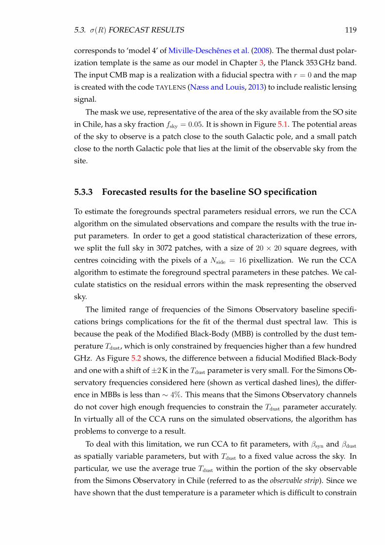
5.3. σ(R) FORECAST RESULTS 119
corresponds to ‘model 4’ of Miville-Deschênes et al. (2008). The thermal dust polar-
ization template is the same as our model in Chapter 3, the Planck 353 GHz band.
The input CMB map is a realization with a fiducial spectra with r = 0 and the map
is created with the code TAYLENS (Næss and Louis, 2013) to include realistic lensing
signal.
The mask we use, representative of the area of the sky available from the SO site
in Chile, has a sky fraction fsky = 0.05. It is shown in Figure 5.1. The potential areas
of the sky to observe is a patch close to the south Galactic pole, and a small patch
close to the north Galactic pole that lies at the limit of the observable sky from the
site.
5.3.3 Forecasted results for the baseline SO specification
To estimate the foregrounds spectral parameters residual errors, we run the CCA
algorithm on the simulated observations and compare the results with the true in-
put parameters. In order to get a good statistical characterization of these errors,
we split the full sky in 3072 patches, with a size of 20 × 20 square degrees, with
centres coinciding with the pixels of a Nside = 16 pixellization. We run the CCA
algorithm to estimate the foreground spectral parameters in these patches. We cal-
culate statistics on the residual errors within the mask representing the observed
sky.
The limited range of frequencies of the Simons Observatory baseline specifi-
cations brings complications for the fit of the thermal dust spectral law. This is
because the peak of the Modified Black-Body (MBB) is controlled by the dust tem-
perature Tdust, which is only constrained by frequencies higher than a few hundred
GHz. As Figure 5.2 shows, the difference between a fiducial Modified Black-Body
and one with a shift of±2 K in the Tdust parameter is very small. For the Simons Ob-
servatory frequencies considered here (shown as vertical dashed lines), the differ-
ence in MBBs is less than ∼ 4%. This means that the Simons Observatory channels
do not cover high enough frequencies to constrain the Tdust parameter accurately.
In virtually all of the CCA runs on the simulated observations, the algorithm has
problems to converge to a result.
To deal with this limitation, we run CCA to fit parameters, with βsyn and βdust
as spatially variable parameters, but with Tdust to a fixed value across the sky. In
particular, we use the average true Tdust within the portion of the sky observable
from the Simons Observatory in Chile (referred to as the observable strip). Since we
have shown that the dust temperature is a parameter which is difficult to constrain

120 CHAPTER 5. FORECAST FOR SIMONS OBSERVATORY
101 102 1030.0
0.5
1.0
1.5
2.0
2.5
Therm
al dust
MB
B
βdust =1.55, Tdust =23 K
±1 K
±2 K
101 102 103
Frequency (GHz)
0.90
0.95
1.00
1.05
Norm
aliz
ed T
herm
al dust
MM
B
Figure 5.2: Example Modified Black-Body spectral law for thermal dust. On top, theblack line shows a fiducial MBB with βdust = 1.53 and Tdust = 23 K. The shaded areasshow the MBB with different values of Tdust. The dashed vertical lines show the SObaseline bands. Bottom, the same MBB laws normalized by the fiducial MBB.
when there are high-frequency bands missing, the error in the uncertainty of this
parameter is transferred to the error in the correlated βdust parameter. In this way,
our estimate is pessimistic in the sense that we consider the error on the Tdust twice,
once due to the fact that we consider it constant even though it is not, and once due
to its correlation with βdust. There is a residual error in the temperature value, thus it
will shift the estimation of βdust by a corresponding amount, since the thermal dust
parameters are correlated with each other. We illustrate this in Figure 5.3. We show,
to the left, the true thermal dust SED in the modelled observations at the baseline
Simons Observatory channels. The grey points are the individual pixels within the
observable strip, and the blue stars are the mean dust SED within the observable
strip. To the right, we show the likelihood of the MBB fit to the mean dust SED
for fixed values of Tdust and variable values of βdust. This fit is performed with a
standard χ2 minimization, where the likelihood is given by exp(−χ2(Tdust)/2). Both
parameters of the thermal dust, βdust and Tdust, are anti-correlated when we try to fit
a MBB. For a given range of Tdust values, the MBB spectral law is a good fit because

5.3. σ(R) FORECAST RESULTS 121
50 100 150 200 250Frequency (GHz)
100
101
102
Therm
al dust
Spect
ral Energ
y D
istr
ibuti
on
10 20 30 40 50 60 70Tdust parameter (K)
0.0
0.2
0.4
0.6
0.8
1.0
Like
lihood o
f fit
to D
ust
SED
0.00
0.05
0.10
0.15
0.20
His
togra
m o
f tr
ue T
dust
Figure 5.3: Fit of a Modifidied Black-Body spectral law to the simulated thermaldust. Left: the spectral law of the simulated dust component. The grey points arethe spectral law of the individual pixels within the observable strip at the SO base-line frequencies. The blue stars are the average spectral law within the observablestrip. Right: posterior distribution of the fit to the average dust spectral law of aMBB, for given values of Tdust (βdust is fitted as the variable). The red line is thehistogram of the true Tdust values in the simulations within the observable band.
we compensate by fitting the value of βdust. In red, we show the histogram of the
true Tdust values (used in the simulated observations) within the observable strip.
For most of the pixels, any reasonable value of Tdust can be used in the fit because
the error will be injected into the βdust parameter. This justifies the choice of using
a constant Tdust in the CCA run, since the residual error in the parameter will be
included in the next step.
The results of the CCA run of the baseline configuration of the Simon Observa-
tory is shown in Figure 5.4. We calculate the residual error for the βsyn and βdust
spectral indices as the subtraction between the estimated (by CCA) index and the
true index in the model, in each small patch within the mask. To the left, the his-
togram of the βsyn residual. To the right, the histogram of the βdust residual. In this
case, there is a shift in the histogram, because of the Tdust-βdust degeneracy described
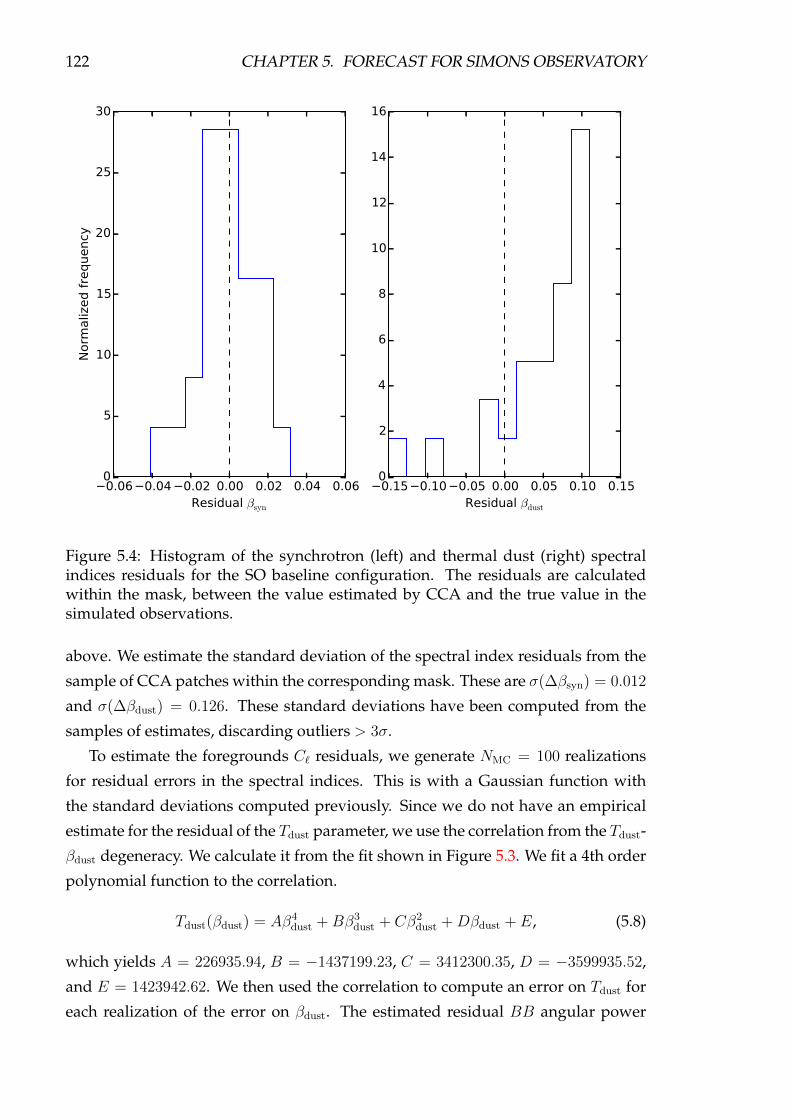
122 CHAPTER 5. FORECAST FOR SIMONS OBSERVATORY
0.06 0.04 0.02 0.00 0.02 0.04 0.06Residual βsyn
0
5
10
15
20
25
30
Norm
aliz
ed f
requency
0.15 0.10 0.05 0.00 0.05 0.10 0.15Residual βdust
0
2
4
6
8
10
12
14
16
Figure 5.4: Histogram of the synchrotron (left) and thermal dust (right) spectralindices residuals for the SO baseline configuration. The residuals are calculatedwithin the mask, between the value estimated by CCA and the true value in thesimulated observations.
above. We estimate the standard deviation of the spectral index residuals from the
sample of CCA patches within the corresponding mask. These are σ(∆βsyn) = 0.012
and σ(∆βdust) = 0.126. These standard deviations have been computed from the
samples of estimates, discarding outliers > 3σ.
To estimate the foregrounds C` residuals, we generate NMC = 100 realizations
for residual errors in the spectral indices. This is with a Gaussian function with
the standard deviations computed previously. Since we do not have an empirical
estimate for the residual of the Tdust parameter, we use the correlation from the Tdust-
βdust degeneracy. We calculate it from the fit shown in Figure 5.3. We fit a 4th order
polynomial function to the correlation.
Tdust(βdust) = Aβ4dust +Bβ3
dust + Cβ2dust +Dβdust + E, (5.8)
which yields A = 226935.94, B = −1437199.23, C = 3412300.35, D = −3599935.52,
and E = 1423942.62. We then used the correlation to compute an error on Tdust for
each realization of the error on βdust. The estimated residual BB angular power
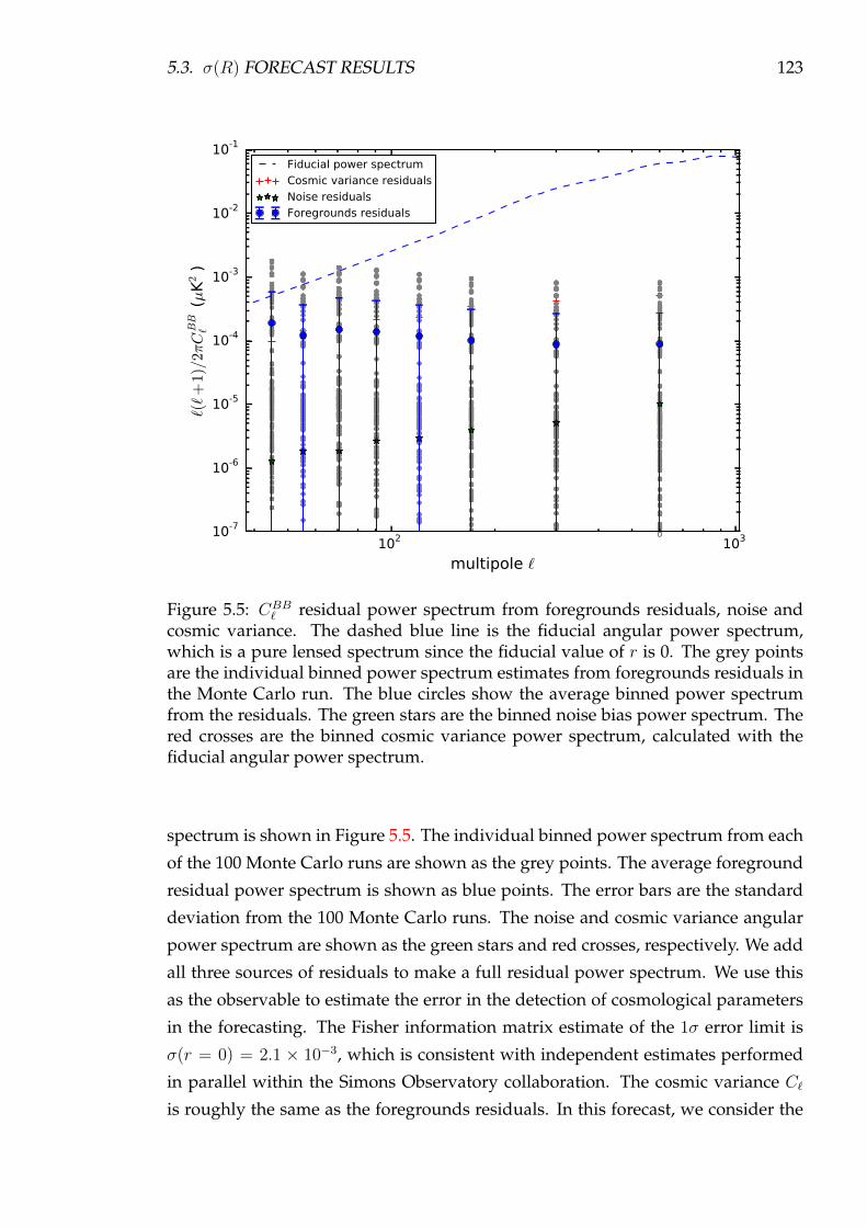
5.3. σ(R) FORECAST RESULTS 123
102 103
multipole `
10-7
10-6
10-5
10-4
10-3
10-2
10-1
`(`+
1)/
2πCBB
` (µK
2)
Fiducial power spectrum
Cosmic variance residuals
Noise residuals
Foregrounds residuals
Figure 5.5: CBB` residual power spectrum from foregrounds residuals, noise and
cosmic variance. The dashed blue line is the fiducial angular power spectrum,which is a pure lensed spectrum since the fiducial value of r is 0. The grey pointsare the individual binned power spectrum estimates from foregrounds residuals inthe Monte Carlo run. The blue circles show the average binned power spectrumfrom the residuals. The green stars are the binned noise bias power spectrum. Thered crosses are the binned cosmic variance power spectrum, calculated with thefiducial angular power spectrum.
spectrum is shown in Figure 5.5. The individual binned power spectrum from each
of the 100 Monte Carlo runs are shown as the grey points. The average foreground
residual power spectrum is shown as blue points. The error bars are the standard
deviation from the 100 Monte Carlo runs. The noise and cosmic variance angular
power spectrum are shown as the green stars and red crosses, respectively. We add
all three sources of residuals to make a full residual power spectrum. We use this
as the observable to estimate the error in the detection of cosmological parameters
in the forecasting. The Fisher information matrix estimate of the 1σ error limit is
σ(r = 0) = 2.1 × 10⁻³, which is consistent with independent estimates performed
in parallel within the Simons Observatory collaboration. The cosmic variance C`is roughly the same as the foregrounds residuals. In this forecast, we consider the
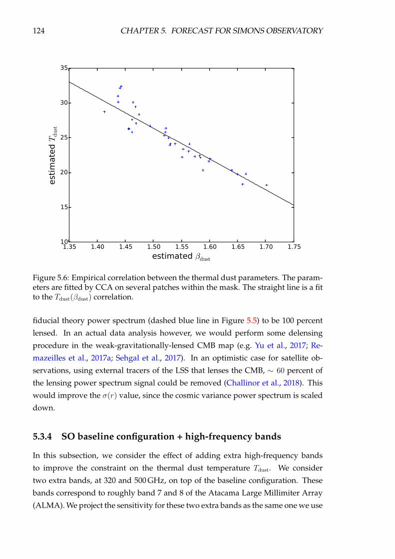
124 CHAPTER 5. FORECAST FOR SIMONS OBSERVATORY
1.35 1.40 1.45 1.50 1.55 1.60 1.65 1.70 1.75
estimated βdust
10
15
20
25
30
35
est
imate
d T
dust
Figure 5.6: Empirical correlation between the thermal dust parameters. The param-eters are fitted by CCA on several patches within the mask. The straight line is a fitto the Tdust(βdust) correlation.
fiducial theory power spectrum (dashed blue line in Figure 5.5) to be 100 percent
lensed. In an actual data analysis however, we would perform some delensing
procedure in the weak-gravitationally-lensed CMB map (e.g. Yu et al., 2017; Re-
mazeilles et al., 2017a; Sehgal et al., 2017). In an optimistic case for satellite ob-
servations, using external tracers of the LSS that lenses the CMB, ∼ 60 percent of
the lensing power spectrum signal could be removed (Challinor et al., 2018). This
would improve the σ(r) value, since the cosmic variance power spectrum is scaled
down.
5.3.4 SO baseline configuration + high-frequency bands
In this subsection, we consider the effect of adding extra high-frequency bands
to improve the constraint on the thermal dust temperature Tdust. We consider
two extra bands, at 320 and 500 GHz, on top of the baseline configuration. These
bands correspond to roughly band 7 and 8 of the Atacama Large Millimiter Array
(ALMA). We project the sensitivity for these two extra bands as the same one we use
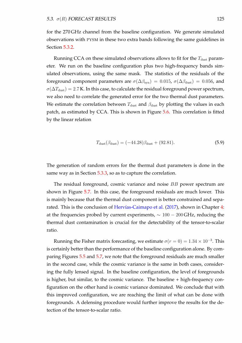
5.3. σ(R) FORECAST RESULTS 125
for the 270 GHz channel from the baseline configuration. We generate simulated
observations with PYSM in these two extra bands following the same guidelines in
Section 5.3.2.
Running CCA on these simulated observations allows to fit for the Tdust param-
eter. We run on the baseline configuration plus two high-frequency bands sim-
ulated observations, using the same mask. The statistics of the residuals of the
foreground component parameters are σ(∆βsyn) = 0.015, σ(∆βdust) = 0.056, and
σ(∆Tdust) = 2.7 K. In this case, to calculate the residual foreground power spectrum,
we also need to correlate the generated error for the two thermal dust parameters.
We estimate the correlation between Tdust and βdust by plotting the values in each
patch, as estimated by CCA. This is shown in Figure 5.6. This correlation is fitted
by the linear relation
Tdust(βdust) = (−44.28)βdust + (92.81). (5.9)
The generation of random errors for the thermal dust parameters is done in the
same way as in Section 5.3.3, so as to capture the correlation.
The residual foreground, cosmic variance and noise BB power spectrum are
shown in Figure 5.7. In this case, the foreground residuals are much lower. This
is mainly because that the thermal dust component is better constrained and sepa-
rated. This is the conclusion of Hervías-Caimapo et al. (2017), shown in Chapter 4:
at the frequencies probed by current experiments, ∼ 100 − 200 GHz, reducing the
thermal dust contamination is crucial for the detectability of the tensor-to-scalar
ratio.
Running the Fisher matrix forecasting, we estimate σ(r = 0) = 1.34× 10⁻³. This
is certainly better than the performance of the baseline configuration alone. By com-
paring Figures 5.5 and 5.7, we note that the foreground residuals are much smaller
in the second case, while the cosmic variance is the same in both cases, consider-
ing the fully lensed signal. In the baseline configuration, the level of foregrounds
is higher, but similar, to the cosmic variance. The baseline + high-frequency con-
figuration on the other hand is cosmic variance dominated. We conclude that with
this improved configuration, we are reaching the limit of what can be done with
foregrounds. A delensing procedure would further improve the results for the de-
tection of the tensor-to-scalar ratio.

126 CHAPTER 5. FORECAST FOR SIMONS OBSERVATORY
102 103
multipole `
10-7
10-6
10-5
10-4
10-3
10-2
10-1
`(`+
1)/
2πCBB
` (µK
2)
Fiducial power spectrum
Cosmic variance residuals
Noise residuals
Foregrounds residuals
Figure 5.7: CBB` residual power spectrum from foregrounds residuals, noise and
cosmic variance. This is analog to Figure 5.5, but for the baseline+high-frequencysimulated observations.
5.4 Optimizing the fraction of the sky for measuring r
In this section, we apply our forecast pipeline to test if the Simons Observatory
default mask is centred on the best portion of the sky to measure the tensor-to-scalar
ratio. An issue that will surface in future polarization CMB experiments, with very
high sensitivity, is the fact that there is a balance between how well foregrounds
can be measured versus how clean the sky patch to observe must be. If we wish
to remove the polarized foregrounds from the CMB with component separation,
we need to be able to measure the properties of the foregrounds with good enough
signal-to-noise. In order to do that, the foregrounds polarization intensity must be
as high as possible. At the same time, if the foregrounds are more intense, they
contaminate more and contribute to the residuals that leak into the cleaned CMB
map.
The approach we follow is to run a forecast for σ(r) across several masks in the
sky, in a declination strip coinciding with the observable sky strip from the SO site
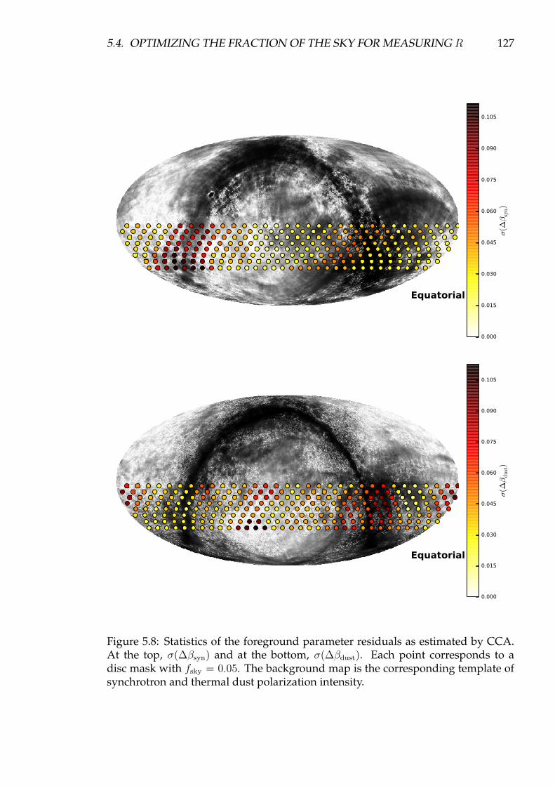
5.4. OPTIMIZING THE FRACTION OF THE SKY FOR MEASURING R 127
Equatorial
0.000
0.015
0.030
0.045
0.060
0.075
0.090
0.105
σ(∆β
syn)
Equatorial
0.000
0.015
0.030
0.045
0.060
0.075
0.090
0.105
σ(∆β
dust)
Figure 5.8: Statistics of the foreground parameter residuals as estimated by CCA.At the top, σ(∆βsyn) and at the bottom, σ(∆βdust). Each point corresponds to adisc mask with fsky = 0.05. The background map is the corresponding template ofsynchrotron and thermal dust polarization intensity.
128 CHAPTER 5. FORECAST FOR SIMONS OBSERVATORY
in Chile. This strip is defined within declinations −22 < δ < +68. We approx-
imate the actual SO mask with a disk-shaped one with the same 5% sky fraction
(which has a 25 radius). The centres of the masks are defined as the coordinates of
the pixels in aNside = 8 HEALPIX map. The number of disc masks that are contained
within the declination strip is 256.
First, we run the estimation of foreground spectral parameters assuming the
same baseline instrument configuration as in Section 5.3.1. We use CCA in patches
of sizes 20 × 20 degrees, whose centres are the pixels of a Nside = 16 map. We run
the estimation of parameters with CCA for the full sky. For each disc mask, we
estimate the statistics of the βsyn and βdust residuals by using the CCA patches that
intersect in area 90% or more with the corresponding disc mask. For each disc mask,
we calculate the statistics using ∼ 65 CCA patches. We use the same technique
described in Section 5.3.3: we calculate the statistics of the errors on the estimated
parameters and discard the patches that lie outside 3σ.
In Figure 5.8, we show the standard deviation of the residuals calculated for ei-
ther βsyn (top) or βdust (bottom). For reference, we show the polarized intensity P of
the corresponding template in the background. The values for the standard devi-
ation of the spectral indices residuals will depend on how intense the foregrounds
are in the corresponding disc mask.
The next step is to calculate the foreground residuals in the EE and BB power
spectra. To do this, we run 200 Monte Carlo samples of a GLS inversion using as
statistics the standard deviation values for β residuals, as described in Section 5.3.3.
We repeat this procedure for each disc mask in the declination strip. For each disc
mask, we also calculate the power spectra for the mixed noise bias and for the cos-
mic variance term with full lensing.
Figure 5.9 shows the main result from this exercise. In the background, we show
the polarized intensity of the thermal dust template at 353 GHz, since dust is the
dominant foreground component in the cleaning process. Each dot corresponds to
the value of σ(r), measured in the corresponding fsky = 5% disc mask, in logarith-
mic scale.
We can see in Figure 5.9 that trying to measure r in the Galactic plane results
in a very high σ(r) error. The centre of the Galaxy, towards the right of the map,
evidences σ(r) ∼ 0.1. The anti-centre of the Galaxy, towards the left of the map,
shows slightly smaller values. The best results are towards the Galactic South Pole,
towards the centre of the map. In this area of the sky, the foregrounds are weaker.
The estimation of the foregrounds spectral indices is not the best, especially for
βdust, but it is accurate enough to allow low foreground residuals power spectra.
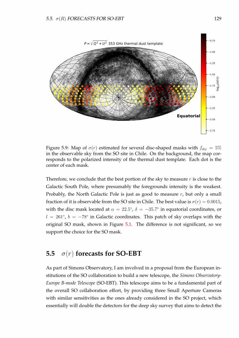
5.5. σ(R) FORECASTS FOR SO-EBT 129
Equatorial
P = Q2 + U2 353 GHz thermal dust template
2.75
2.50
2.25
2.00
1.75
1.50
1.25
1.00
0.75
log 1
0((r)
)
Figure 5.9: Map of σ(r) estimated for several disc-shaped masks with fsky = 5%in the observable sky from the SO site in Chile. On the background, the map cor-responds to the polarized intensity of the thermal dust template. Each dot is thecenter of each mask.
Therefore, we conclude that the best portion of the sky to measure r is close to the
Galactic South Pole, where presumably the foregrounds intensity is the weakest.
Probably, the North Galactic Pole is just as good to measure r, but only a small
fraction of it is observable from the SO site in Chile. The best value is σ(r) = 0.0015,
with the disc mask located at α = 22.5, δ = −35.7 in equatorial coordinates, or
l = 261, b = −78 in Galactic coordinates. This patch of sky overlaps with the
original SO mask, shown in Figure 5.1. The difference is not significant, so we
support the choice for the SO mask.
5.5 σ(r) forecasts for SO-EBT
As part of Simons Observatory, I am involved in a proposal from the European in-
stitutions of the SO collaboration to build a new telescope, the Simons Observatory-
Europe B-mode Telescope (SO-EBT). This telescope aims to be a fundamental part of
the overall SO collaboration effort, by providing three Small Aperture Cameras
with similar sensitivities as the ones already considered in the SO project, which
essentially will double the detectors for the deep sky survey that aims to detect the

130 CHAPTER 5. FORECAST FOR SIMONS OBSERVATORY
polarization B-modes. This project includes the design and construction of detec-
tors using state-of-the-art materials and technology. The proposal will add∼ 40, 000
detectors in three cameras, housed in one Small Aperture Telescope. Therefore, the
SO-EBT would contribute a new and independent telescope capable of doing a deep
survey to detect polarization B-modes. Since it will be part of the SO collaboration,
it will use the infrastructure and resources that will be developed for the already
funded SO effort.
As part of this proposal, I contributed to the tensor-to-scalar ratio forecasting
efforts. The addition of ∼ 40k detectors will eventually double the number of de-
tectors, and therefore the σ(r) error could improve significantly. By running the
forecast pipeline, as the one described in the previous sections, we can quantify the
improvement in the value of σ(r).
We use as a sky model the same model used in the previous runs, described in
Section 5.3.2. This is a simplified model, that contains thermal dust, synchrotron,
and CMB as polarized components, with spatially variable spectral parameters
maps. The basic model also includes Gaussian noise, as specified by the different
configurations and spread of detectors. Later, we will also consider more realistic
atmospheric noise.
We forecast the performance of different configurations by measuring σ(r) using
the forecasting pipeline described in Section 5.2, with two improvements described
in the following subsections: one to account for the pixel-to-pixel spatial variability
of the foreground spectral indices, and one to account for the systematic error for
the estimation of r.
5.5.1 Spatially-varying foreground spectral indices
A more realistic modelling of the estimated foreground spectral parameters would
capture their spatial variability, rather than assuming a constant spectral law across
the sky, as we did in Section 5.2.2. To do this, we perform the following procedure.
For a given foreground realization, we measure the statistics by running CCA
in the same way described above in Section 5.2.1. Then, an error for βsyn and βdust is
generated based on the measured standard deviations, and added to a Nside = 512
map of spatially-variable true spectral indices, described in the simulated observa-
tions, Section 5.3.2. For each pixel, an estimated reconstruction matrix W is calcu-
lated. Then, for the estimation of the residual map, we use Equation 5.1, but using
a different reconstruction matrix for each pixel. To save time, we estimate the resid-
ual map only on the pixels within the corresponding mask, rather than the full sky.

5.5. σ(R) FORECASTS FOR SO-EBT 131
In the next step, the power spectra of the masked map of the residual is calculated.
Then, the pipeline is applied in the same way as described above.
5.5.2 Estimation of r bias
Previously, we calculated the σ(r) error due to random uncertainties, but we did not
consider the systematic uncertainties, which will cause a bias in the calculation of a
cosmological parameter. We are improving our analysis to account for both. If the
data analysis was naive, and assuming we would have complete ignorance on the
foreground residuals, we would mistake these as primordial cosmological signal
that would be measured as an effective r. To compute this value, we ran a likelihood
for r on the residual foreground power spectrum (as performed in Section 4.3.3).
We use the foreground residual power spectrum as the observed data points,
and a fiducial primordial power spectrum (without the lensing signal) as the theory
data points. To estimate the errors, we use the standard deviation from the Monte
Carlo realizations of foreground residuals. The BB power spectrum is used, at the
same multipole bins as used before.
5.5.3 Results
First, we consider a baseline configuration for Simons Observatory: a single Small
Aperture Telescope with three optical tubes, which will constrain the values for
sensitivities at each band. We consider a 2-year survey and an area of observation
of fsky = 0.05, with 6 frequency bands (30, 40, 95, 150, 220, and 270 GHz), and one
optic tube in each frequency range. The sensitivities are listed in the first row of
Table 5.2.
The SO-EBT proposal considers doubling the number of detectors, by adding
three optic tubes in another Small Aperture Telescope. There are several ways to
distribute these extra detectors. We consider 3 improved configurations: SO++ v1
adds all the detectors to the middle frequency range, which effectively is to put
all the extra sensitivity in the CMB-dominant channels. SO++ v2 adds one tube
in each frequency range, spreading the sensitivity over the synchrotron, CMB, and
thermal dust-dominated channels. SO++ v3 adds two tubes to the CMB-dominated
channels and one to the thermal dust-dominated channels. The sensitivities for
these 3 upgraded configurations are listed in the second, third , and fourth rows of
Table 5.2.
For the first run of forecasts, we consider the nominal SO mask with fsky = 0.05,
shown in Figure 5.1. We use the foreground model detailed above, and adding

132 CHAPTER 5. FORECAST FOR SIMONS OBSERVATORY
Experiment Freq ranges No of tubes 30 GHz 40 GHz 95 GHz 150 GHz 220 GHz 270 GHz
SO baselineLF 1
14.98 8.82 3.25 3.83 5.66 13.98MF 1UHF 1
SO++ v1LF 1
14.98 8.82 1.62 1.91 5.66 13.98MF 4UHF 1
SO++ v2LF 2
10.59 6.24 2.29 2.71 4.00 9.89MF 2UHF 2
SO++ v3LF 1
14.98 8.82 1.87 2.21 4.00 9.89MF 3UHF 2
Table 5.2: Sensitivities per band for the SO configurations considered. The unit ofthe sensitivities is µKCMB·arcmin.
Experiment Foregrounds r bias σ(r) Alens = 1.0 σ(r) Alens = 0.5 σ(r) Alens = 0.25
SO baseline ∆βsyn = 0.058 3.57 2.91 2.25 1.91∆βdust = 0.084
SO++ v1 ∆βsyn = 0.059 2.40 2.54 1.87 1.54∆βdust = 0.072
SO++ v2 ∆βsyn = 0.043 2.64 2.55 1.89 1.55∆βdust = 0.061
SO++ v3 ∆βsyn = 0.052 2.90 2.50 1.84 1.50∆βdust = 0.062
Table 5.3: Forecasted bias and σ(r) for the baseline and improved SO configurations.The 1σ errors for the foreground spectral parameters are listed. The bias and σ(r)values are in units of 10−3. These results are for a Galactic mask with fsky = 0.05and Gaussian white noise.
Gaussian noise using the sensitivity values listed in Table 5.2. In Table 5.3, we tab-
ulate the results for this exercise.
We estimate the errors in the spectral indices of the foregrounds made by the
CCA algorithm with the baseline and improved sensitivities. Going from baseline
to SO++ v1, the improvement on the error is not significant, since the sensitivity on
the synchrotron and dust channels is the same. However, from baseline to SO++
v2 the error is improved significantly (∆βsyn goes from 0.058 to 0.043, and ∆βdust
goes from 0.084 to 0.061). In the case of the SO++ v3 improved configuration, the
synchrotron-dominated channels are not improved, but the dust-dominated chan-
nels are. Therefore, the ∆βdust error is significantly improved. The next columns of
Table 5.3 list the r bias and the σ(r) error for the detection.
With these numbers, the power spectrum levels of the foreground residuals are
comparable to the level of B-modes due to lensing. Therefore, there is some im-
provement, ∼ 20%, going from baseline to an improved configuration. This is with
the full lensing signal. We also include the values when we reduce the lensing
signal artificially by calculating the cosmic variance power spectra with a reduced
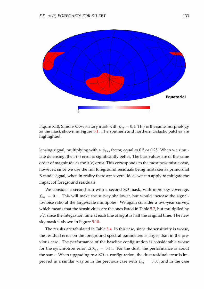
5.5. σ(R) FORECASTS FOR SO-EBT 133
Equatorial
0 1
Figure 5.10: Simons Observatory mask with fsky = 0.1. This is the same morphologyas the mask shown in Figure 5.1. The southern and northern Galactic patches arehighlighted.
lensing signal, multiplying with a Alens factor, equal to 0.5 or 0.25. When we simu-
late delensing, the σ(r) error is significantly better. The bias values are of the same
order of magnitude as the σ(r) error. This corresponds to the most pessimistic case,
however, since we use the full foreground residuals being mistaken as primordial
B-mode signal, when in reality there are several ideas we can apply to mitigate the
impact of foreground residuals.
We consider a second run with a second SO mask, with more sky coverage,
fsky = 0.1. This will make the survey shallower, but would increase the signal-
to-noise ratio at the large-scale multipoles. We again consider a two-year survey,
which means that the sensitivities are the ones listed in Table 5.2, but multiplied by√
2, since the integration time at each line of sight is half the original time. The new
sky mask is shown in Figure 5.10.
The results are tabulated in Table 5.4. In this case, since the sensitivity is worse,
the residual error on the foreground spectral parameters is larger than in the pre-
vious case. The performance of the baseline configuration is considerable worse
for the synchrotron error, ∆βsyn = 0.14. For the dust, the performance is about
the same. When upgrading to a SO++ configuration, the dust residual error is im-
proved in a similar way as in the previous case with fsky = 0.05, and in the case
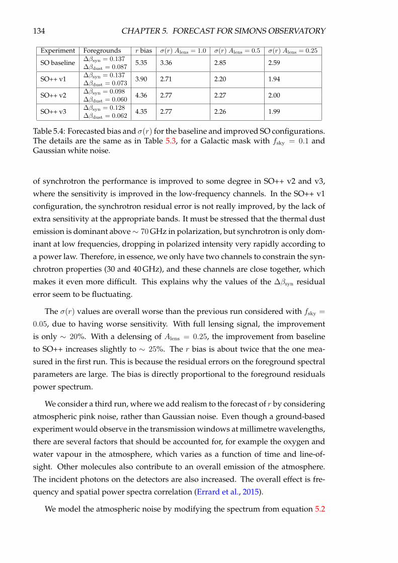
134 CHAPTER 5. FORECAST FOR SIMONS OBSERVATORY
Experiment Foregrounds r bias σ(r) Alens = 1.0 σ(r) Alens = 0.5 σ(r) Alens = 0.25
SO baseline ∆βsyn = 0.137 5.35 3.36 2.85 2.59∆βdust = 0.087
SO++ v1 ∆βsyn = 0.137 3.90 2.71 2.20 1.94∆βdust = 0.073
SO++ v2 ∆βsyn = 0.098 4.36 2.77 2.27 2.00∆βdust = 0.060
SO++ v3 ∆βsyn = 0.128 4.35 2.77 2.26 1.99∆βdust = 0.062
Table 5.4: Forecasted bias and σ(r) for the baseline and improved SO configurations.The details are the same as in Table 5.3, for a Galactic mask with fsky = 0.1 andGaussian white noise.
of synchrotron the performance is improved to some degree in SO++ v2 and v3,
where the sensitivity is improved in the low-frequency channels. In the SO++ v1
configuration, the synchrotron residual error is not really improved, by the lack of
extra sensitivity at the appropriate bands. It must be stressed that the thermal dust
emission is dominant above∼ 70 GHz in polarization, but synchrotron is only dom-
inant at low frequencies, dropping in polarized intensity very rapidly according to
a power law. Therefore, in essence, we only have two channels to constrain the syn-
chrotron properties (30 and 40 GHz), and these channels are close together, which
makes it even more difficult. This explains why the values of the ∆βsyn residual
error seem to be fluctuating.
The σ(r) values are overall worse than the previous run considered with fsky =
0.05, due to having worse sensitivity. With full lensing signal, the improvement
is only ∼ 20%. With a delensing of Alens = 0.25, the improvement from baseline
to SO++ increases slightly to ∼ 25%. The r bias is about twice that the one mea-
sured in the first run. This is because the residual errors on the foreground spectral
parameters are large. The bias is directly proportional to the foreground residuals
power spectrum.
We consider a third run, where we add realism to the forecast of r by considering
atmospheric pink noise, rather than Gaussian noise. Even though a ground-based
experiment would observe in the transmission windows at millimetre wavelengths,
there are several factors that should be accounted for, for example the oxygen and
water vapour in the atmosphere, which varies as a function of time and line-of-
sight. Other molecules also contribute to an overall emission of the atmosphere.
The incident photons on the detectors are also increased. The overall effect is fre-
quency and spatial power spectra correlation (Errard et al., 2015).
We model the atmospheric noise by modifying the spectrum from equation 5.2

5.5. σ(R) FORECASTS FOR SO-EBT 135
Experiment Foregrounds r bias σ(r) Alens = 1.0 σ(r) Alens = 0.5 σ(r) Alens = 0.25
SO baseline ∆βsyn = 0.101 4.62 3.35 2.66 2.31∆βdust = 0.131
SO++ v1 ∆βsyn = 0.104 3.14 2.54 1.88 1.54∆βdust = 0.082
SO++ v2 ∆βsyn = 0.053 2.83 2.50 1.84 1.50∆βdust = 0.062
SO++ v3 ∆βsyn = 0.087 3.43 2.79 2.12 1.78∆βdust = 0.077
Table 5.5: Forecasted bias and σ(r) for the baseline and SO++ configurations. Thedetails are the same as in Table 5.3, for a Galactic mask with fsky = 0.05, but theinput model contains more realistic atmospheric noise.
to
Nν =4πfsky
Npix
σ2ν
(1 +
`
`knee
)nknee
, (5.10)
where `knee = 60 and nknee = −2.6, and where σν corresponds to the sensitivities
per band listed in Table 5.2. After this, we create a correlated noise map at each
band by running the synfast function from HEALPIX with the 1/f noise power spec-
trum, which will be spatially correlated. This noise map is added to the simulated
foregrounds and CMB maps.
However, we run the rest of the pipeline in the same way as before, including
the use of the mask with fsky = 0.05. We are aiming to measure the improvement
on the measurement of r by going from the baseline to the SO++ configurations. In
the CCA code, the noise is assumed to be Gaussian in the input, even though we
are feeding it a more complicated noise.
The results are tabulated in Table 5.5. The baseline configuration performs
poorly in terms of the thermal dust residual error, which is ∆βdust = 0.13, the worst
performance by any of the runs. When going to an improved SO++ run, the dust
residual error is noticeable better, ∆βdust ∼ 0.07. This translates into the σ(r) error.
With full lensing, the improvement is ∼ 25% from baseline to SO++ v2. With a
Alens = 0.5 delensing, the improvement is ∼ 30%, and with a Alens = 0.25 delensing,
the improvement is ∼ 35%. The bias is worse than the first case considered with
Gaussian noise. In this case, we can attribute this to the fact that we are assuming
a simplified noise in the component separation. The level of noise is comparable
to the first case (even though the noise is correlated), which means that the SO++
improved σ(r) errors are similar. Therefore, in terms of absolute σ(r) value, the best
values are obtained by improving the depth of the survey.
The SO-EBT proposal will have a significant impact on the overall SO effort.
It will double the number of detectors, and it can improve the σ(r) uncertainty
upwards of ∼ 20%. This can potentially have a major impact in a deep survey

136 CHAPTER 5. FORECAST FOR SIMONS OBSERVATORY
searching for primordial B-modes.

Chapter 6
CORE study on foregrounds
This chapter discusses my contribution to the proposal for the future CMB polar-
ization satellite CORE, submitted in response to the “M5” call for experiments from
the European Space Agency (ESA). Several articles were prepared to support this
proposal, on different aspects (the “Exploring Cosmic Origins” series, Delabrouille
et al., 2018). Among these, the potential improvements on cosmological parameters
(Di Valentino et al., 2018), on inflation (Finelli et al., 2018), or the mitigation of sys-
tematics (Natoli et al., 2018). My contribution was to the analysis of the impact of
foregrounds on the potential detection of a primordial B-mode signal, published in
Remazeilles et al. (2018). This work is described in this chapter.
6.1 The CORE proposal
The proposed experiment is a space-based telescope, with an array of 2100 cooled,
polarization-sensitive detectors, at the focus of a dish with an aperture of 1.2 m.
The 19 frequency bands proposed are between 60 and 600 GHz, with resolutions
between 18 and 2 arcmin. The aggregate sensitivity of the array in polarization is
1.7µK × arcmin. The experiment is designed to be mounted on a dedicated space
satellite, to observe for a period of 4 years from the L2 Lagrange orbital point, spin-
ning one revolution every 2 minutes with a precession of ∼ 4 days. This strategy
allows observing half of the sky every few days. The broad frequency coverage
ensures that the foregrounds are accurately mapped below and above the CMB
frequencies. The observation of ancillary data at lower frequencies (e.g. C-BASS)
could however be helpful to improve the mapping of synchrotron radiation.
137

138 CHAPTER 6. CORE STUDY ON FOREGROUNDS
Frequency [GHz] 60 70 80 90 100 115 130 145 160 175Beam FWHM [arcmin] 17.9 15.4 13.5 12.1 10.9 9.6 8.5 7.7 7.0 6.5Sensitivity [µKCMB × arcmin] 10.6 10.0 9.6 7.3 7.1 7.0 5.5 5.1 5.2 5.1Frequency 195 220 255 295 340 390 450 520 600Beam FWHM 5.8 5.2 4.6 4.0 4.0 4.0 4.0 4.0 4.0Sensitivity 4.9 5.4 7.9 10.5 15.7 31.1 64.9 164.8 506.7
Table 6.1: Instrumental specifications used in the CORE proposal to simulate full-sky observations. The beam of the higher frequency bands are limited to 4 arcminbecause of the pixel size of the HEALPIX pixelization.
6.2 Results from the CORE foreground study
The objective of the analysis presented in Remazeilles et al. (2018) is to demon-
strate that the proposed instrument can achieve foreground cleaning to the level
necessary to detect a tensor-to-scalar ratio of r = 10−2 − 10−3. This has been done
by performing a full end-to-end data reduction analysis on simulated observations,
including component separation, angular power spectra estimation, and cosmolog-
ical parameter estimation.
6.2.1 Simulated observations
The simulated observations maps are produced with the Planck Sky Model (PSM,
Delabrouille et al., 2013). The instrumental configuration used is shown in Table 6.1.
The maps are created with a resolution Nside = 2048, so we limited the resolution of
the higher frequency bands to 4 arcmin. The emission components included in this
model are CMB, synchrotron, thermal dust, AME and extragalactic point sources,
along with instrumental Gaussian noise.
The CMB is generated from a set of fiducial spectra generated with the CAMB
code, with several values of r in the range r = 10−2 − 10−3 and the optical depth to
reionization, τ = 0.055, based on the recent estimate by Planck Collaboration et al.
(2016o). The input model also included the effects of lensing which are modelled
using a Alens amplitude parameter. Alens = 0 means that only the primordial signal
is included, while Alens = 1 adds the full lensing signal. In practice, an intermediate
Alens value can mimic the effect of subtracting some of the lensing signal using a
delensing procedure.
The synchrotron radiation template is derived from 23 GHz WMAP polariza-
tion observations (Miville-Deschênes et al., 2008). The spectral law we assume is
the usual power law with spectral indices βsyn ∼ −3. The spatial map of the syn-
chrotron spectral index is derived by Miville-Deschênes et al. (2008) extrapolating
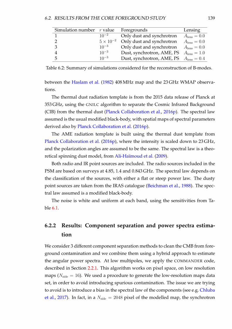
6.2. RESULTS FROM THE CORE FOREGROUND STUDY 139
Simulation number r value Foregrounds Lensing1 10−2 Only dust and synchrotron Alens = 0.02 5× 10⁻² Only dust and synchrotron Alens = 0.03 10−3 Only dust and synchrotron Alens = 0.04 10−3 Dust, synchrotron, AME, PS Alens = 1.05 10−3 Dust, synchrotron, AME, PS Alens = 0.4
Table 6.2: Summary of simulations considered for the reconstruction of B-modes.
between the Haslam et al. (1982) 408 MHz map and the 23 GHz WMAP observa-
tions.
The thermal dust radiation template is from the 2015 data release of Planck at
353 GHz, using the GNILC algorithm to separate the Cosmic Infrared Background
(CIB) from the thermal dust (Planck Collaboration et al., 2016p). The spectral law
assumed is the usual modified black-body, with spatial maps of spectral parameters
derived also by Planck Collaboration et al. (2016p).
The AME radiation template is built using the thermal dust template from
Planck Collaboration et al. (2016p), where the intensity is scaled down to 23 GHz,
and the polarization angles are assumed to be the same. The spectral law is a theo-
retical spinning dust model, from Ali-Haïmoud et al. (2009).
Both radio and IR point sources are included. The radio sources included in the
PSM are based on surveys at 4.85, 1.4 and 0.843 GHz. The spectral law depends on
the classification of the sources, with either a flat or steep power law. The dusty
point sources are taken from the IRAS catalogue (Beichman et al., 1988). The spec-
tral law assumed is a modified black-body.
The noise is white and uniform at each band, using the sensitivities from Ta-
ble 6.1.
6.2.2 Results: Component separation and power spectra estima-
tion
We consider 3 different component separation methods to clean the CMB from fore-
ground contamination and we combine them using a hybrid approach to estimate
the angular power spectra. At low multipoles, we apply the COMMANDER code,
described in Section 2.2.1. This algorithm works on pixel space, on low resolution
maps (Nside = 16). We used a procedure to generate the low-resolution maps data
set, in order to avoid introducing spurious contamination. The issue we are trying
to avoid is to introduce a bias in the spectral law of the components (see e.g. Chluba
et al., 2017). In fact, in a Nside = 2048 pixel of the modelled map, the synchrotron

140 CHAPTER 6. CORE STUDY ON FOREGROUNDS
Figure 6.1: EE power spectrum reconstruction by component separation methods.The COMMANDER, NILC and SMICA estimates of the power spectrum are shownat the top left, top right and bottom, respectively. These results are particular forsimulation 1, but there is no difference for other simulations in the reconstruction oftheEE spectrum. On the bottom of each panel, the residuals between the estimatedand fiducial spectrum at each bin is shown, in number of σ. The bins that are biasedby more than ±3σ are shown as arrows.
will be a perfect power law in any given line of sight, by definition. If we degrade
the resolution of several adjacent pixels into a single Nside = 16 pixel, the resulting
spectral law of that pixel will no longer be a perfect power law. This is because
we are averaging temperatures, not power law indices 1. An effective curvature for
synchrotron is introduced if we degrade the temperature of the components. This
is true for all the other components spectral laws. To avoid this, we degrade in res-
olution the temperature of the templates of each component, and we also degrade
1If we have two pixels whose synchrotron temperature is modelled with power-laws given byA1ν
−β1 and A2ν−β2 , then the average temperature is 1
2 (A1ν−β1 + A2ν
−β2), which is different thanA1+A2
2 ν−12 (β1+β2)

6.2. RESULTS FROM THE CORE FOREGROUND STUDY 141
the maps of the spectral parameters, for example, the map of βsyn. Only after this,
we extrapolate in frequency using the spectral laws of the components.
The analysis on the full resolution maps has been performed with two compo-
nent separation methods, that work on harmonic space: NILC and SMICA, both
described in Section 2.2.2. Both of these methods are blind, exploiting the indepen-
dence between components. The EE and BB power spectra are estimated between
multipoles ` = 48−349 for NILC and between ` = 48−600 for SMICA. Each method
estimates the power spectra using its own procedure.
Figure 6.1 shows the reconstruction of theEE power spectrum for COMMANDER
at low-` (top left), NILC (top right) and SMICA (bottom) for high-`. The fiducial
angular power spectrum is shown in black. The bottom panel of each plot shows
the residuals (in number of σ) at each multipole bin, between the reconstructed
and fiducial spectrum. The residuals that are biased by more than ±3σ are plotted
as arrows. The COMMANDER result is unbiased. The high-` pipelines show large
scatter among bins, but in general within ±2σ of the fiducial spectrum. However,
the SMICA result shows a systematic bias for some of the bins ` > 500.
For the BB angular power spectrum, to measure the tensor-to-scalar ratio, we
consider several cases, summarized in Table 6.2. First, we consider the simplest
model, where the only foreground components are thermal dust and synchrotron.
The CMB realization has no lensing, and three values for the tensor-to-scalar ratio:
realistic values we can approach in the next∼ 5 years, r = 10−2 and 5×10⁻², and r =
10−3, which is the challenging value that CORE aims to measure in 10 to 15 years.
These simulations are referred to as 1, 2, and 3, respectively. Then, we consider a
more realistic simulation, including AME and extragalactic point sources, together
with Galactic dust and synchrotron. Simulation 4 includes the full lensing signal,
with Alens = 1.0, and simulation 5 has Alens = 0.4, which simulates the effect of
applying delensing to the reconstructed CMB, removing 60 percent of the lensing
signal from the reconstructed CMB map with a delensing technique. This level of
delensing is approximately what CORE could potentially achieve (Challinor et al.,
2018).
The measured BB angular power spectra for simulations 1 and 3 are shown in
Figure 6.2. The top, middle, and bottom row are the results from COMMANDER,
NILC, and SMICA, respectively. The left column corresponds to simulation 1, and
the right column corresponds to simulation 3. For simulation 1, r = 0.01 allows a
good reconstruction of the power spectrum. SMICA is more sensitive to the effect
of foreground residuals, so there is a small bias. For simulation 3, it is more diffi-
cult. The value r = 0.001 means that the primordial B-mode signal is smaller, so
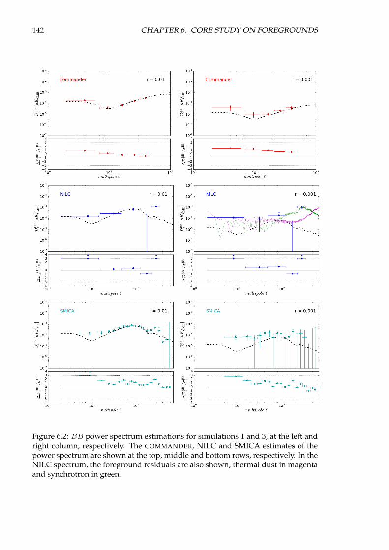
142 CHAPTER 6. CORE STUDY ON FOREGROUNDS
Figure 6.2: BB power spectrum estimations for simulations 1 and 3, at the left andright column, respectively. The COMMANDER, NILC and SMICA estimates of thepower spectrum are shown at the top, middle and bottom rows, respectively. In theNILC spectrum, the foreground residuals are also shown, thermal dust in magentaand synchrotron in green.
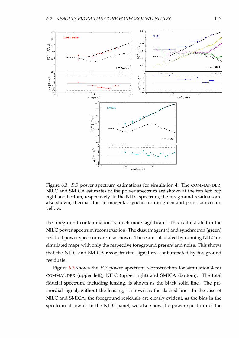
6.2. RESULTS FROM THE CORE FOREGROUND STUDY 143
Figure 6.3: BB power spectrum estimations for simulation 4. The COMMANDER,NILC and SMICA estimates of the power spectrum are shown at the top left, topright and bottom, respectively. In the NILC spectrum, the foreground residuals arealso shown, thermal dust in magenta, synchrotron in green and point sources onyellow.
the foreground contamination is much more significant. This is illustrated in the
NILC power spectrum reconstruction. The dust (magenta) and synchrotron (green)
residual power spectrum are also shown. These are calculated by running NILC on
simulated maps with only the respective foreground present and noise. This shows
that the NILC and SMICA reconstructed signal are contaminated by foreground
residuals.
Figure 6.3 shows the BB power spectrum reconstruction for simulation 4 for
COMMANDER (upper left), NILC (upper right) and SMICA (bottom). The total
fiducial spectrum, including lensing, is shown as the black solid line. The pri-
mordial signal, without the lensing, is shown as the dashed line. In the case of
NILC and SMICA, the foreground residuals are clearly evident, as the bias in the
spectrum at low-`. In the NILC panel, we also show the power spectrum of the
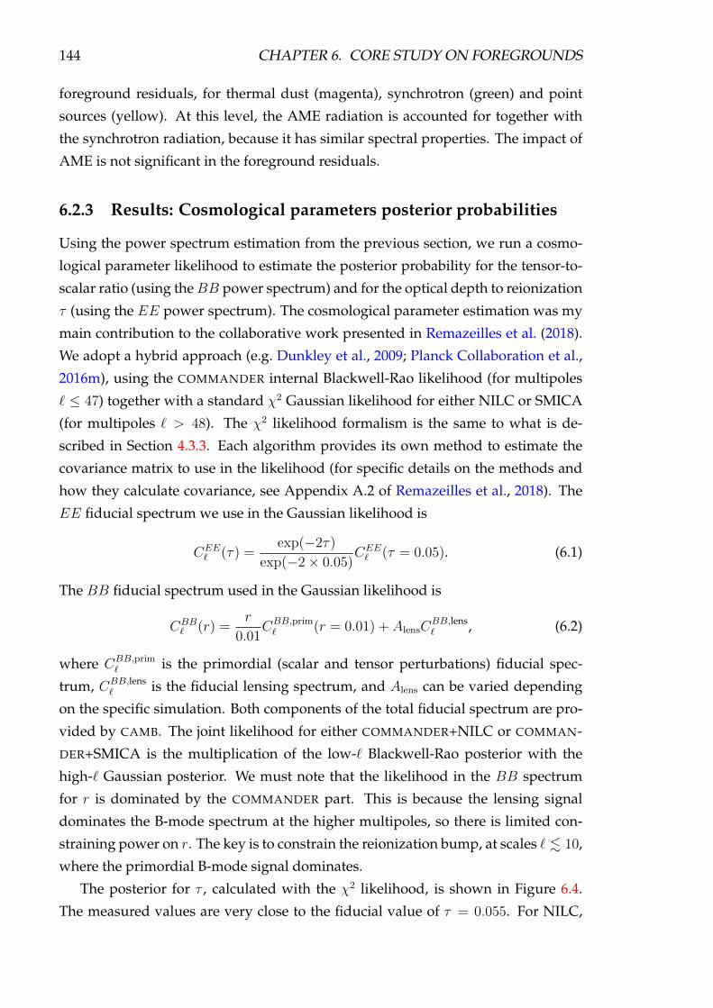
144 CHAPTER 6. CORE STUDY ON FOREGROUNDS
foreground residuals, for thermal dust (magenta), synchrotron (green) and point
sources (yellow). At this level, the AME radiation is accounted for together with
the synchrotron radiation, because it has similar spectral properties. The impact of
AME is not significant in the foreground residuals.
6.2.3 Results: Cosmological parameters posterior probabilities
Using the power spectrum estimation from the previous section, we run a cosmo-
logical parameter likelihood to estimate the posterior probability for the tensor-to-
scalar ratio (using theBB power spectrum) and for the optical depth to reionization
τ (using the EE power spectrum). The cosmological parameter estimation was my
main contribution to the collaborative work presented in Remazeilles et al. (2018).
We adopt a hybrid approach (e.g. Dunkley et al., 2009; Planck Collaboration et al.,
2016m), using the COMMANDER internal Blackwell-Rao likelihood (for multipoles
` ≤ 47) together with a standard χ2 Gaussian likelihood for either NILC or SMICA
(for multipoles ` > 48). The χ2 likelihood formalism is the same to what is de-
scribed in Section 4.3.3. Each algorithm provides its own method to estimate the
covariance matrix to use in the likelihood (for specific details on the methods and
how they calculate covariance, see Appendix A.2 of Remazeilles et al., 2018). The
EE fiducial spectrum we use in the Gaussian likelihood is
CEE` (τ) =
exp(−2τ)
exp(−2× 0.05)CEE` (τ = 0.05). (6.1)
The BB fiducial spectrum used in the Gaussian likelihood is
CBB` (r) =
r
0.01CBB,prim` (r = 0.01) + AlensC
BB,lens` , (6.2)
where CBB,prim` is the primordial (scalar and tensor perturbations) fiducial spec-
trum, CBB,lens` is the fiducial lensing spectrum, and Alens can be varied depending
on the specific simulation. Both components of the total fiducial spectrum are pro-
vided by CAMB. The joint likelihood for either COMMANDER+NILC or COMMAN-
DER+SMICA is the multiplication of the low-` Blackwell-Rao posterior with the
high-` Gaussian posterior. We must note that the likelihood in the BB spectrum
for r is dominated by the COMMANDER part. This is because the lensing signal
dominates the B-mode spectrum at the higher multipoles, so there is limited con-
straining power on r. The key is to constrain the reionization bump, at scales ` . 10,
where the primordial B-mode signal dominates.
The posterior for τ , calculated with the χ2 likelihood, is shown in Figure 6.4.
The measured values are very close to the fiducial value of τ = 0.055. For NILC,

6.2. RESULTS FROM THE CORE FOREGROUND STUDY 145
Figure 6.4: Posterior probability for τ , calculated from the spectra shown in Fig-ure 6.1. The NILC result is shown to the left, and the SMICA result is shown to theright. The fiducial value τ = 0.055 is shown as the vertical dashed line.
shown to the left of the figure, we measure τ = 0.054 ± 0.002 in the multipole
range 20 ≤ ` ≤ 359. For SMICA, shown to the right of the figure, we measure
τ = 0.056± 0.008 in the multipole range 20 ≤ ` ≤ 199.
The results for the joint likelihood for the tensor-to-scalar ratio using the esti-
mated B-mode power spectrum for simulations 1 and 3 are shown in Figure 6.5.
The estimated values for r, along with the 1σ(r) error, are tabulated in Table 6.3.
The r posterior probability for simulation 1 for the joint COMMANDER-NILC and
COMMANDER-SMICA are shown to the top left and top right, respectively, of Fig-
ure 6.5. The fiducial value of r = 0.01 is measured in both cases, to within less than
1σ(r). The results for simulation 2, with a fiducial value r = 0.005, are not shown,
but they are qualitatively similar. For simulation 3, the bottom left and right of the
figure corresponds to the joint COMMANDER-NILC and COMMANDER-SMICA like-
lihoods, respectively. The r posterior is shown as a dashed line. Since the fiducial
value of r = 0.001 is challenging, the foreground residuals are comparable to the
primordial cosmological B-mode signal, and therefore the posterior is biased.
We modelled the foregrounds residuals in the likelihood in terms of nuisance
parameters, as described in Section 4.3.3. The thermal dust residuals have the most
impact on the overall foreground residuals, and they are more important at low
multipoles. In Figure 6.6, the BB power spectrum of the thermal dust, as recon-
structed by COMMANDER, is shown in orange, for simulation 3. In blue, the fore-
ground residual power spectrum is shown, multiplied by 107 to compare them at
the same scale. This is calculated by subtracting the input true CMB map with the
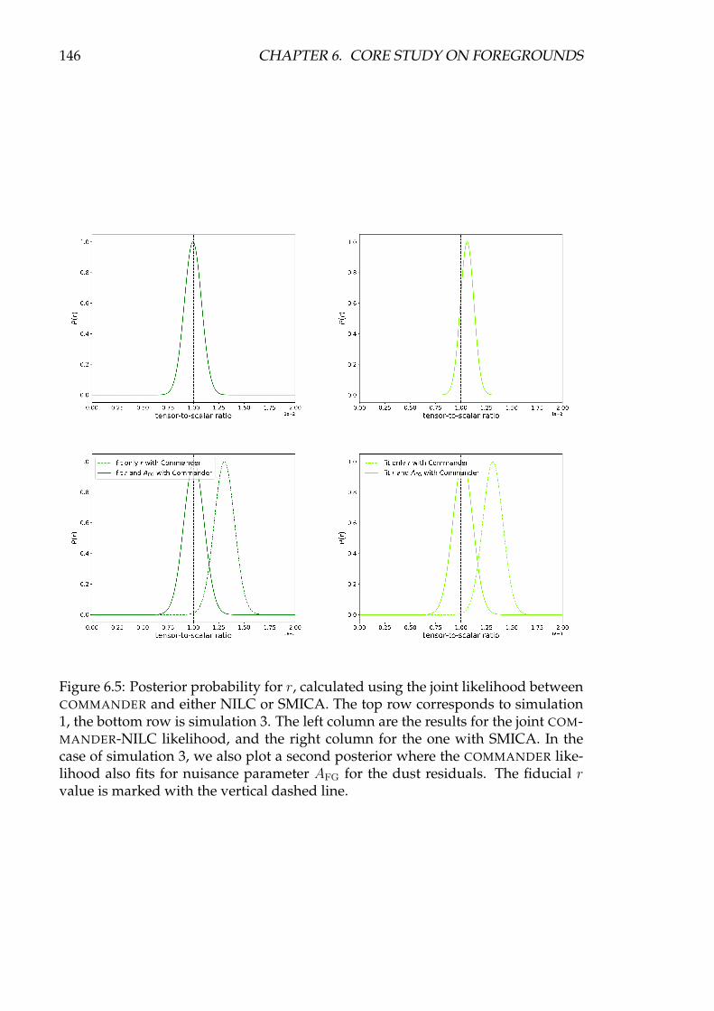
146 CHAPTER 6. CORE STUDY ON FOREGROUNDS
Figure 6.5: Posterior probability for r, calculated using the joint likelihood betweenCOMMANDER and either NILC or SMICA. The top row corresponds to simulation1, the bottom row is simulation 3. The left column are the results for the joint COM-MANDER-NILC likelihood, and the right column for the one with SMICA. In thecase of simulation 3, we also plot a second posterior where the COMMANDER like-lihood also fits for nuisance parameter AFG for the dust residuals. The fiducial rvalue is marked with the vertical dashed line.

6.2. RESULTS FROM THE CORE FOREGROUND STUDY 147
101
multipole
102
103
(+
1)/2
CBB
[K2 CM
B]Power-law fit to thermal dustForegrounds residuals ×107
Reconstructed thermal dust
Figure 6.6: Example low-` BB power spectrum, for simulation 3, of the recon-structed thermal dust by COMMANDER, shown in orange. To compare, we alsocalculated the power spectrum of the foreground residuals, in blue, calculated bysubtracting the input true from the reconstructed CMB map. The residuals are mul-tiplied by 107 to compare them at the same scale. A power-law, fitted to the recon-structed dust, is shown as the dashed line.
reconstructed CMB map, and estimating the power spectrum using a QML esti-
mator (see Section 4.3.2). We fit a power law to the thermal dust power spectrum.
Then, in the COMMANDER r likelihood, this power law is scaled by the nuisance
parameter AFG, which is also fitted to model-out the residuals. The joint likelihood
using the COMMANDER posterior fitting for foregrounds is shown in the bottom
row panels of Figure 6.5 as the solid lines. The values are tabulated in Table 6.3 in
parenthesis. In the case of simulation 3, we are able to remove the bias on r.
The posterior probabilities for r for simulations 4 and 5 are shown in Figure 6.7.
For simulation 4, we are able to measure r with a bias, in the top row of the figure.
In this model, there is full lensing signal. In the likelihood, we assume we know the
fiducial lensing power spectrum, so it is included in the fiducial spectrum. Fitting
for the parameter AFG, the bias on the posterior is slightly reduced. The peak of
the posterior is within the 1σ(r) error. The results from the COMMANDER-NILC

148 CHAPTER 6. CORE STUDY ON FOREGROUNDS
Figure 6.7: Posterior probability for r, calculated using the joint likelihood betweenCOMMANDER and either NILC or SMICA. The top row corresponds to simulation4, the bottom row is simulation 5. The left column are the results for the jointCOMMANDER-NILC likelihood, and the right column for the one with SMICA. Thedashed and solid lines correspond to the fit of r, or to the fit of r and AFG, respec-tively, in the same way plotted in Figure 6.5.
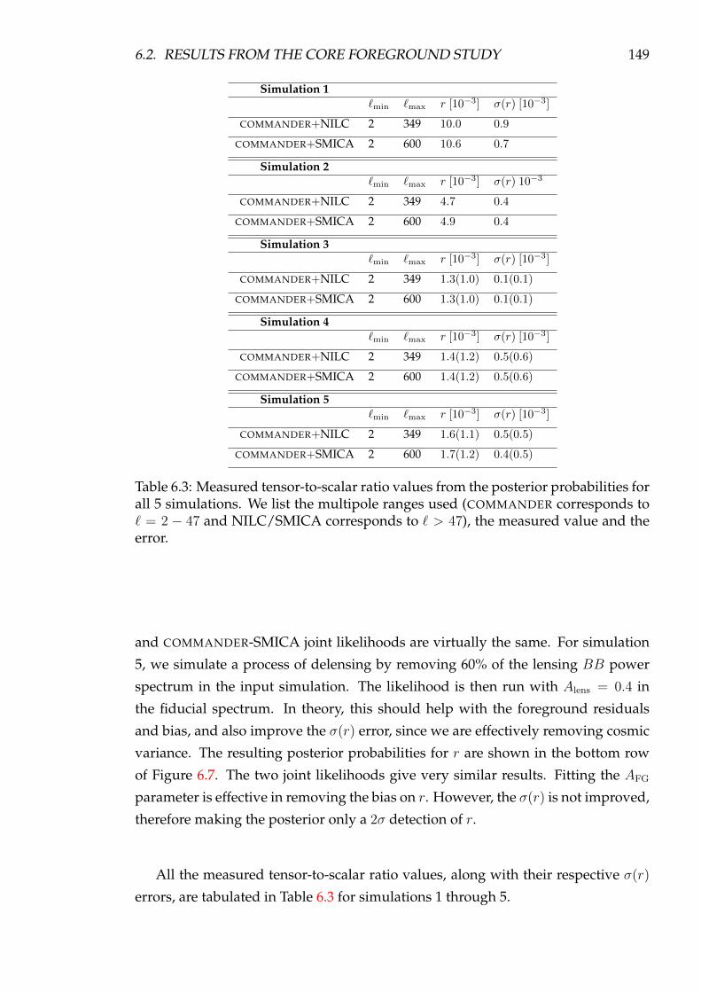
6.2. RESULTS FROM THE CORE FOREGROUND STUDY 149
Simulation 1`min `max r [10−3] σ(r) [10−3]
COMMANDER+NILC 2 349 10.0 0.9
COMMANDER+SMICA 2 600 10.6 0.7
Simulation 2`min `max r [10−3] σ(r) 10−3
COMMANDER+NILC 2 349 4.7 0.4
COMMANDER+SMICA 2 600 4.9 0.4
Simulation 3`min `max r [10−3] σ(r) [10−3]
COMMANDER+NILC 2 349 1.3(1.0) 0.1(0.1)
COMMANDER+SMICA 2 600 1.3(1.0) 0.1(0.1)
Simulation 4`min `max r [10−3] σ(r) [10−3]
COMMANDER+NILC 2 349 1.4(1.2) 0.5(0.6)
COMMANDER+SMICA 2 600 1.4(1.2) 0.5(0.6)
Simulation 5`min `max r [10−3] σ(r) [10−3]
COMMANDER+NILC 2 349 1.6(1.1) 0.5(0.5)
COMMANDER+SMICA 2 600 1.7(1.2) 0.4(0.5)
Table 6.3: Measured tensor-to-scalar ratio values from the posterior probabilities forall 5 simulations. We list the multipole ranges used (COMMANDER corresponds to` = 2 − 47 and NILC/SMICA corresponds to ` > 47), the measured value and theerror.
and COMMANDER-SMICA joint likelihoods are virtually the same. For simulation
5, we simulate a process of delensing by removing 60% of the lensing BB power
spectrum in the input simulation. The likelihood is then run with Alens = 0.4 in
the fiducial spectrum. In theory, this should help with the foreground residuals
and bias, and also improve the σ(r) error, since we are effectively removing cosmic
variance. The resulting posterior probabilities for r are shown in the bottom row
of Figure 6.7. The two joint likelihoods give very similar results. Fitting the AFG
parameter is effective in removing the bias on r. However, the σ(r) is not improved,
therefore making the posterior only a 2σ detection of r.
All the measured tensor-to-scalar ratio values, along with their respective σ(r)
errors, are tabulated in Table 6.3 for simulations 1 through 5.
150 CHAPTER 6. CORE STUDY ON FOREGROUNDS
6.3 Conclusions
We have measured cosmological parameters, r and τ , in simulated polarization ob-
servations of the CMB by the proposed CORE experiment, as described in Table 6.1.
We use a realistic model for the full-sky observations, including foregrounds such as
thermal dust, synchrotron, AME and extra Galactic point sources. We also include
Gaussian uniform noise, and a CMB realization with only primordial cosmological
signal, or also including the dominant lensed signal, that can be scaled with a Alens
parameter.
The E-mode spectrum is reconstructed with a high signal-to-noise ratio. The
NILC and SMICA methods can reconstruct the spectrum and measure τ with a
significance of 24 and 6σ, respectively. The SMICA power spectrum is affected by
bias at high multipoles, which are excluded in the calculation of the τ posterior.
Further work is needed to improve these results.
For the B-mode results, we find that r can be measured without bias for values
r & 0.005. This is addressed by our simulations 1 and 2, with values r = 0.01 and
r = 0.005, respectively. In the absence of lensing, r is measured to a significance of
∼ 10σ, as listed in Table 6.3. Separate tests, made with COMMANDER, indicate that
r can still be measured without bias in the presence of lensing. However, since the
cosmic variance is significantly larger when the dominant lensing signal is present,
the detection drops to a significance of ∼ 4σ.
For r = 0.001, the target that CORE is trying to measure, the analysis is more
difficult. All the considered component separation methods struggle to achieve an
unbiased detection of r. In simulation 3, with a fiducial value r = 0.001, r is biased
by 3σ. In this case, there is only primordial signal in theBB power spectrum, which
makes σ(r) ∼ 10−4. This result can be improved if we model for the foreground
residuals in the likelihood, by means of a nuisance parameter AFG that scales the
reconstructed thermal dust (the dominant source of residuals), in a similar manner
to what is described in Section 4.3.3. Once we apply this procedure, we obtain
an unbiased estimate of r with a ∼ 10σ significance. However, the caveat is that
simulation 3 is lacking the lensing signal.
For realistic scenarios, that include the lensing signal at a 100% and at a 40%
level (simulation 4 and 5, respectively), we measure r with a ∼ 1σ bias. In both
cases, the σ(r) error is∼ 5×10⁻⁴. We note that reducing the lensing by 60% does not
improve the results. This probably occurs because the lensing is not the dominant
component of the residuals. By removing 60% of the lensing BB power spectrum,
we effectively reduce a large fraction of the cosmic variance uncertainty, but the
6.3. CONCLUSIONS 151
foreground residuals are still larger and they are the dominant component in the
uncertainty. The joint likelihood for r is dominated by the COMMANDER likelihood
at low multipoles. For the NILC/SMICA-only likelihood, for example, the effect
of delensing is more noticeable. Since at multipoles ` & 100, the signal is virtually
all coming from lensing, removing a fraction of it will improve σ(r), regarding of
the bias. A more extended discussion of this issue is presented in Section 6.1 of
Remazeilles et al. (2018).
In summary, with the proposed CORE instrument, we predict an unbiased de-
tection for r & 0.005. When we try the challenging value r = 0.001, the dominant
source of error is foreground mis-modelling, which makes the naive analysis bi-
ased. We can model-out the foreground residuals at the likelihood level, and we
can remove the bias to a certain degree, but further research is needed in the com-
ponent separation techniques and in the modelling of foregrounds to improve the
detection error σ(r).

BLANK PAGE
152

Chapter 7
Conclusions
In this thesis, the main issue we have investigated is the impact of Galactic diffuse
foregrounds on the observations of the polarization of the Cosmic Microwave Back-
ground, which entails the measurement of cosmological parameters. The problem
we have tried to address is the contamination by residuals after cleaning said fore-
ground emission. We know that these residuals could be mistaken for polarized
primordial B-mode signal if not properly characterized when we try to measure
cosmological parameters. The work presented in this thesis is a step forward in the
direction of characterizing these residuals and search for ways to limit their impact.
7.1 Summary and Conclusions
7.1.1 A new model of the polarized microwave sky
In order to study the issue of the residual diffuse foreground contamination in the
primordial B-mode signal in a flexible way, we have constructed our own polarized
sky model, which we use to simulate the observation of the full sky at millimetre
wavelengths by a CMB experiment. This model includes the common Galactic dif-
fuse polarized foregrounds: synchrotron, thermal dust and anomalous microwave
emission, as well as CMB realizations. Our model can also simulate the effect of
an observing instrument in a simple way, as Gaussian noise (which can be spatially
constant or pixel-by-pixel), Gaussian beams, and frequency bandpasses.
This model is presented in a very simple code written in PYTHON. The novel as-
pects include the creation of small-scale features for each of the foregrounds compo-
nents. The templates that are the basis of the model are from the 2015 data release of
Planck, so their small-scale signal is dominated by noise. This procedure is achieved
153

154 CHAPTER 7. CONCLUSIONS
by extrapolating the power spectrum of the corresponding template to higher mul-
tipoles. The fact that the foreground emission is concentrated in the Galactic plane
is accounted for by weighting each pixel according to the polarized intensity in the
template. We create the small-scale features of the AME and thermal dust polarized
emission with the same random seed, since these two sources of emission should
be correlated.
We have tested our model against real observational data, both from Planck and
WMAP. We have show that it is a good fit at low/intermediate frequencies. We have
also shown that the model is a good fit to intermediate and high Galactic latitudes
away from the Galactic plane. We looked at the thermal dust emission in these
areas, whose characterization is critical for the analysis of polarized foreground
contamination. Also, we have provided this model publicly, which can be used
to generate multiple random realizations of foregrounds (by generating different
realizations of small-scale features) for Monte Carlo purposes.
7.1.2 Characterizing the impact of foreground residual contamina-
tion
The analysis presented in Chapter 4 is critical for forecasting the cosmological con-
strains obtainable from future polarized CMB experiments. As an example of future
observations, we use the 2010 proposal of the COrE satellite. We have run an end-
to-end simulation that goes from simulated observations maps, to component sep-
aration, power spectra estimation and cosmological parameters likelihood. In the
last step, when calculating the measured tensor-to-scalar ratio, we have developed
a method to model the polarized foreground residuals directly into the likelihood,
to prevent them from biasing the primordial B-modes.
We measure the random and systematic error bias on the tensor-to-scalar ratio
in three cases:
1. Using as input a simplified model with foregrounds with spatially constant
spectral indices.
2. Using as input a more complex model with spatially variable spectral indices,
but assuming spatially constant indices in the component separation.
3. Using the same input as 2., but including spatially variable error in the spec-
tral indices when performing the component separation.
We have found that the amount of r bias is very sensitive to the input value
of r. For a value of r = 0.01, the bias can be managed. We inject a systematic

7.1. SUMMARY AND CONCLUSIONS 155
error in the component separation and we propagate through the simulation. For
errors of . 3% for the simplified case, the estimates are unbiased. Even when we
consider a complex case we are successful; if we approximate the spectral properties
as spatially constant in the component separation, and if using our method to model
the foreground residuals into the likelihood. The value r = 0.01 is small, but with
a future satellite experiment with such a good sensitivity, it can be measured to at
least a 2σ level detection in the most pessimistic case.
For a value of r = 0.001, the analysis is much more challenging. Even for a
simple sky, the bias on r is very sensitive to errors on the foreground spectral pa-
rameters. When trying to correct it, we can only recover an upper limit detection.
For a complex sky, we note that assuming spatially constant spectral parameters
for the component separation results in a large bias that cannot be corrected for.
Therefore, the spectral parameters must be modelled as spatially variable. Simulat-
ing a global residual error of half a percent in the spectral parameters allows a 2σ
detection of r = 0.001.
In this work, we have quantified how bad a problem that we already know ex-
isted really is. If we aim to detect r = 10−3 from a future high-sensitivity satellite,
which is the most advanced experiment we can conceive in the near future to ob-
serve the CMB, we need to characterize and model the Galactic diffuse foregrounds
very carefully. It is easy to mistake foreground contamination for primordial B-
mode signal in the data analysis, so our main message is the critical need to develop
studies of polarized foregrounds in the future.
7.1.3 Forecasting the performance of the Simons Observatory
As part of the Simons Observatory collaboration, I performed forecasts for the de-
tection of the tensor-to-scalar ratio, using the Fisher information matrix and realistic
estimations of foreground spectral parameter errors. We considered instrumental
configurations for a Small Aperture Camera, that would survey a small patch of the
sky as deep as possible to try to detect primordial B-modes.
For an early configuration of the instrument, we forecast σ(r = 0) ∼ 2.1× 10⁻³,
which is consistent with other forecasts within the collaboration. The thermal dust
properties, in particular Tdust, are hard to constrain with a narrow frequency cov-
erage, up to ∼ 270 GHz. If we add high-frequency bands, to ∼ 500 GHz, the dust
temperature is better constrained and the performance improves.
We also conducted an exercise to determine the patch of the sky where it is
best to measure r. Here, we have tried to address the balance between how clean
156 CHAPTER 7. CONCLUSIONS
of foregrounds the sky must be versus how well we can measure the foregrounds
properties in the same region in order to clean them. We forecasted the value of
σ(r) for all the observable sky from the site in Chile, tilling the sky in fsky = 0.05
disc masks. The best results we found, with σ(r) = 1.5×10⁻³, is the patch of the sky
centred in l = 261 b = −78 in Galactic coordinates, very close to the South Galactic
Pole. In general, we conclude that the value of σ(r) is better when the sky is cleaner
of polarized thermal dust emission, which makes the most important impact at the
SO frequencies.
Further work I have done within the SO is related to a proposal for a new
European-funded Small Aperture Camera in a separate telescope to complement
the current planned instrument. The Simons Observatory European B-mode Tele-
scope (SO-EBT) would effectively double the detectors of the deep survey that aims
to measure primordial B-modes. We consider the baseline configuration for the pro-
posal already funded, with 3 optical tubes, and three improved configurations, that
add and spread extra three optical tubes in different frequencies to evaluate how
much the detection of r improves.
We estimated realistic foreground errors with the CCA component separation
method, and then we propagated the foreground residuals into the power spectra.
Using the Fisher information we forecast the uncertainty in the tensor-to-scalar ra-
tio. We considered a survey with a fsky = 0.05 coverage and Gaussian noise. The
improvement in σ(r) is ∼ 20% going from a baseline configuration to an improved
one. The foreground residual level is similar to the cosmic variance lensed signal,
so with these specifications we are leaving the foreground-dominated regime and
almost entering the cosmic variance-dominated regime. Considering this, the effect
of applying delensing to the CMB is important. We show that by simulating de-
lensing by 50 and 75%, the σ(r) error is reduced. Going from baseline to improved
configurations and applying delensing, the enhancement is ∼ 21% at best. We also
consider two more runs, the first one considering a fsky = 0.1 coverage. In this case,
the improvement made by the proposed SO-EBT experiment is ∼ 20% with the full
lensing signal, and ∼ 25% with a delensing of Alens = 0.25. The second run con-
siders realistic atmospheric noise on the simulated observations. The improvement
in the σ(r) error is ∼ 25% with the full lensing signal and ∼ 35% with a delensing
of Alens = 0.25. This is the best improvement we have obtained for forecasting the
effect of doubling the number of detectors.
We note that the value of σ(r) depend on the sensitivity of the channels. The
worst errors we can forecast are in the case with fsky = 0.1 coverage, since the sen-
sitivities are√
2 higher. Also, we note that the spread of the extra optics tubes does
7.1. SUMMARY AND CONCLUSIONS 157
not appear to be an important factor, since the results of the 3 improved configu-
rations are similar. If we compare the forecast runs with fsky = 0.05, Gaussian and
atmospheric noise, the results of σ(r) are close, but the run with Gaussian noise has
better results. We conclude that adding another Small Aperture Camera will have a
significant impact on the detection of r, potentially improving the value of the σ(r)
error by ∼ 20% or more.
In conclusion, we note that we have developed a tool to forecast the performance
of an experiment quickly, which we can use to complement the analysis pipeline
we have also developed, which has an end-to-end approach. Using such a tool,
we conclude that for measuring primordial B-modes, a patch of the sky with no
polarized foregrounds will always be best. Based on our sky model, we find that
the best areas of the sky are located near the South Galactic Pole. In addition, we
have to consider that the sensitivity of the instruments in the future will improve,
so the signal-to-noise ratio will always improve for polarized foregrounds.
7.1.4 CORE proposal forecasts
Part of my work was within the CORE collaboration, and aimed at forecasting the
potential of the proposed satellite experiment to measure the primordial B-mode
signal. We simulated observations of the microwave sky and we performed the data
analysis, considering different component separation algorithms, both parametric
and blind. My particular contribution was the cosmological parameter estimation,
evaluating the posterior probabilities for r and τ . We reach similar conclusions to
the ones we reach in Chapter 4: We can achieve an unbiased measurement of r for
values & 0.005. For a lower value, of r = 10−3, the analysis is more difficult. For a re-
alistic scenario, including synchrotron, thermal dust, anomalous microwave emis-
sion, extragalactic point sources, and CMB lensing signal, we can measure r with
an uncertainty σ(r) = 5 × 10⁻⁴, and a ∼ 1σ bias. Using the technique that models
the foreground residuals in the parameter estimation, described in Section 4.3.3, we
can reduce the bias and make a ∼ 2σ detection of r = 10−3.
We also note that there are no significant differences between the blind methods
(SMICA and NILC) tested at intermediate and high multipoles. However, the r pos-
terior probability is dominated by the low-multipole signal, which is estimated by
the COMMANDER code. The dominant source of errors in the cosmological parame-
ter estimation is polarized foregrounds, above the weak lensing signal, so we stress
the need to improve our techniques in the future to deal with this problem.
158 CHAPTER 7. CONCLUSIONS
7.1.5 Overall conclusions
The main conclusions of this thesis are:
1. The measurement of r is very sensitive to the presence of foreground contam-
ination, especially for future satellite missions, as shown in Chapters 4 and 6.
It is critical that the foreground spectral parameters are estimated with a very
high accuracy. To detect a value of r ∼ 10−3, the spectral parameter errors
must be ≤ 0.5%. We can detect r = 10−3 with a 2σ significance with the 2011
configuration of COrE. We need to account for the foreground residuals suc-
cessfully. In order to do this, an essential step is improving our methods to
characterize and model polarized foregrounds.
2. The issue of modelling foreground residuals at the likelihood stage is impor-
tant. In this work, we explore one method to do this. It is a relatively simple
procedure, but we show how powerful it is to effectively reduce a large frac-
tion of the bias in r. This stresses the need to improve the methods used in
CMB observation and data analysis. As previously remarked, the foreground
residuals are very problematic because they can easily be mistaken as primor-
dial B-mode signal. Therefore, a procedure to mitigate the contamination by
residuals, directly in the component separation step, or further ahead in the
power spectra calculation/cosmological parameter estimation, is essential for
future observations of the polarized CMB.
3. The potential results we could obtain from a ground-based experiment are
really good. The Simons Observatory is a Stage-3 experiment, which will be
observing in the next 4-5 years. It most likely will be capable of detecting
B-modes at least at the level of r = 0.01 at 3σ significance, which is a huge
improvement, of essentially one order of magnitude, over current upper limits
of r . 0.08 (95% C.L.). Considering that in the next few years we will improve
our analysis techniques, we could be able to detect smaller values of r. Given
some reasonable premises, we show that by doubling the number of detectors,
the uncertainty on r improves & 20%. CMB-S4 is the ultimate goal in the
long run, but Simons Observatory will be a very important move in the right
direction.
4. We have developed a quick tool to forecast the performance of cosmological
parameters estimation from CMB observations. This method can be used for
several purposes, for example searching for the best patch of the sky to mea-
sure r, or for the use in the optimization of future experiments.
7.2. FUTURE WORK 159
7.2 Future work
There are several issues we could further develop in the work presented in this
thesis. Also, we can add certain features that were not considered here, such as the
effect of weak gravitational lensing.
A key aspect of the work we presented in this thesis is the modelling of fore-
ground residuals during the cosmological parameter likelihood. As stated before,
the foreground residuals will dominate the sources of error for B-modes signal de-
tection, so developing this technique is important. We can improve the model for
the residuals, by re-processing the foreground component templates or improving
the analytic model in the likelihood by introducing extra parameters, for example.
Even further, we could plan the study of new methods to reduce the r bias, maybe
directly at the CMB map stage, or at the estimation of the angular power spectra.
Overall, the CMB analysis pipeline, described in Chapter 4, can be developed
further to include more features. The simulated observations can be improved to
include more complex components, such as polarized point sources, among others.
We can also account for ground-based atmospheric noise, including correlations.
For satellite experiments, a more realistic noise can be achieved, including scanning
strategies and hits maps, which change the noise considering how much time is
spent in each line of sight. We can also include instrumental systematics effects,
such as bandpass and beam mismatch, among others.
The component separation analysis can be expanded, by testing several meth-
ods, both parametric and blind, as previously mentioned in Section 2.2. We can
expand the cosmological parameter estimation by considering multiple parameters
and using Markov Chain Monte Carlo codes, e.g. CosmoMC (Lewis and Bridle,
2002; Lewis, 2013). We can expand our analysis to include intermediate and high-
multipoles, and we can consider forecasts for other parameters, such as the neutrino
physics ones, or the dark energy equation of state, among others.
One issue that was not considered in detail is the effect of the B-mode lens-
ing signal. We only consider it by scaling up and down the dominant lensing BB
spectrum in the cosmic variance term, therefore simulating a given percentage of
delensing. However, as stated before, there are sophisticated methods to remove
the lensing effect from a CMB map, using either tracers of the Large Scale Struc-
ture or the CMB signal itself. This will add realism to our end-to-end CMB analysis
pipeline or for the Fisher forecasting pipeline.
The Fisher matrix forecasting procedure can be further refined to apply it to
Simons Observatory or any other planned experiment. We can add features to

160 CHAPTER 7. CONCLUSIONS
the Correlated Component Analysis algorithm to manage more foreground com-
ponents and correlated noise. For the delensing procedure, we can upgrade the
analysis to use more sophisticated methods as described above.
Bibliography
K. N. Abazajian, P. Adshead, Z. Ahmed, S. W. Allen, D. Alonso, K. S. Arnold,
C. Baccigalupi, J. G. Bartlett, N. Battaglia, B. A. Benson, C. A. Bischoff, J. Borrill,
V. Buza, E. Calabrese, R. Caldwell, J. E. Carlstrom, C. L. Chang, T. M. Crawford,
F.-Y. Cyr-Racine, F. De Bernardis, T. de Haan, S. di Serego Alighieri, J. Dunkley,
C. Dvorkin, J. Errard, G. Fabbian, S. Feeney, S. Ferraro, J. P. Filippini, R. Flauger,
G. M. Fuller, V. Gluscevic, D. Green, D. Grin, E. Grohs, J. W. Henning, J. C. Hill,
R. Hlozek, G. Holder, W. Holzapfel, W. Hu, K. M. Huffenberger, R. Keskitalo,
L. Knox, A. Kosowsky, J. Kovac, E. D. Kovetz, C.-L. Kuo, A. Kusaka, M. Le Jeune,
A. T. Lee, M. Lilley, M. Loverde, M. S. Madhavacheril, A. Mantz, D. J. E. Marsh,
J. McMahon, P. D. Meerburg, J. Meyers, A. D. Miller, J. B. Munoz, H. N. Nguyen,
M. D. Niemack, M. Peloso, J. Peloton, L. Pogosian, C. Pryke, M. Raveri, C. L.
Reichardt, G. Rocha, A. Rotti, E. Schaan, M. M. Schmittfull, D. Scott, N. Sehgal,
S. Shandera, B. D. Sherwin, T. L. Smith, L. Sorbo, G. D. Starkman, K. T. Story,
A. van Engelen, J. D. Vieira, S. Watson, N. Whitehorn, and W. L. Kimmy Wu.
CMB-S4 Science Book, First Edition. ArXiv e-prints, Oct. 2016.
M. H. Abitbol, Z. Ahmed, D. Barron, R. Basu Thakur, A. N. Bender, B. A. Benson,
C. A. Bischoff, S. A. Bryan, J. E. Carlstrom, C. L. Chang, D. T. Chuss, K. T. Crow-
ley, A. Cukierman, T. de Haan, M. Dobbs, T. Essinger-Hileman, J. P. Filippini,
K. Ganga, J. E. Gudmundsson, N. W. Halverson, S. Hanany, S. W. Henderson,
C. A. Hill, S.-P. P. Ho, J. Hubmayr, K. Irwin, O. Jeong, B. R. Johnson, S. A. Ker-
nasovskiy, J. M. Kovac, A. Kusaka, A. T. Lee, S. Maria, P. Mauskopf, J. J. McMa-
hon, L. Moncelsi, A. W. Nadolski, J. M. Nagy, M. D. Niemack, R. C. O’Brient,
S. Padin, S. C. Parshley, C. Pryke, N. A. Roe, K. Rostem, J. Ruhl, S. M. Simon,
S. T. Staggs, A. Suzuki, E. R. Switzer, O. Tajima, K. L. Thompson, P. Timbie, G. S.
Tucker, J. D. Vieira, A. G. Vieregg, B. Westbrook, E. J. Wollack, K. W. Yoon, K. S.
Young, and E. Y. Young. CMB-S4 Technology Book, First Edition. ArXiv e-prints,
June 2017.
P. A. R. Ade, Y. Akiba, A. E. Anthony, K. Arnold, M. Atlas, D. Barron, D. Boettger,
161
162 BIBLIOGRAPHY
J. Borrill, C. Borys, S. Chapman, Y. Chinone, M. Dobbs, T. Elleflot, J. Errard,
G. Fabbian, C. Feng, D. Flanigan, A. Gilbert, W. Grainger, N. W. Halverson,
M. Hasegawa, K. Hattori, M. Hazumi, W. L. Holzapfel, Y. Hori, J. Howard,
P. Hyland, Y. Inoue, G. C. Jaehnig, A. Jaffe, B. Keating, Z. Kermish, R. Keski-
talo, T. Kisner, M. Le Jeune, A. T. Lee, E. M. Leitch, E. Linder, M. Lungu, F. Mat-
suda, T. Matsumura, X. Meng, N. J. Miller, H. Morii, S. Moyerman, M. J. My-
ers, M. Navaroli, H. Nishino, H. Paar, J. Peloton, D. Poletti, E. Quealy, G. Re-
beiz, C. L. Reichardt, P. L. Richards, C. Ross, K. Rotermund, I. Schanning,
D. E. Schenck, B. D. Sherwin, A. Shimizu, C. Shimmin, M. Shimon, P. Siri-
tanasak, G. Smecher, H. Spieler, N. Stebor, B. Steinbach, R. Stompor, A. Suzuki,
S. Takakura, A. Tikhomirov, T. Tomaru, B. Wilson, A. Yadav, O. Zahn, and Po-
larbear Collaboration. Evidence for Gravitational Lensing of the Cosmic Mi-
crowave Background Polarization from Cross-Correlation with the Cosmic In-
frared Background. Physical Review Letters, 112(13):131302, Apr. 2014. doi:
10.1103/PhysRevLett.112.131302.
Y. Ali-Haïmoud, C. M. Hirata, and C. Dickinson. A refined model for spinning dust
radiation. Monthly Notices of the Royal Astronomical Society, 395:1055–1078, May
2009. doi: 10.1111/j.1365-2966.2009.14599.x.
D. Alonso, J. Dunkley, B. Thorne, and S. Næss. Simulated forecasts for primordial
B -mode searches in ground-based experiments. Physical Review D, 95(4):043504,
Feb. 2017. doi: 10.1103/PhysRevD.95.043504.
C. Armitage-Caplan, J. Dunkley, H. K. Eriksen, and C. Dickinson. Impact on the
tensor-to-scalar ratio of incorrect Galactic foreground modelling. Monthly No-
tices of the Royal Astronomical Society, 424:1914–1924, Aug. 2012. doi: 10.1111/j.
1365-2966.2012.21314.x.
K. Arnold, P. A. R. Ade, A. E. Anthony, F. Aubin, D. Boettger, J. Borrill, C. Can-
talupo, M. A. Dobbs, J. Errard, D. Flanigan, A. Ghribi, N. Halverson, M. Hazumi,
W. L. Holzapfel, J. Howard, P. Hyland, A. Jaffe, B. Keating, T. Kisner, Z. Ker-
mish, A. T. Lee, E. Linder, M. Lungu, T. Matsumura, N. Miller, X. Meng, M. My-
ers, H. Nishino, R. O’Brient, D. O’Dea, C. Reichardt, I. Schanning, A. Shimizu,
C. Shimmin, M. Shimon, H. Spieler, B. Steinbach, R. Stompor, A. Suzuki,
T. Tomaru, H. T. Tran, C. Tucker, E. Quealy, P. L. Richards, and O. Zahn. The
POLARBEAR CMB polarization experiment. In Millimeter, Submillimeter, and Far-
Infrared Detectors and Instrumentation for Astronomy V, volume 7741 of Proceedings
of SPIE, pages 77411E–77411E–11, July 2010. doi: 10.1117/12.858314.

BIBLIOGRAPHY 163
J. E. Austermann, K. A. Aird, J. A. Beall, D. Becker, A. Bender, B. A. Benson, L. E.
Bleem, J. Britton, J. E. Carlstrom, C. L. Chang, H. C. Chiang, H.-M. Cho, T. M.
Crawford, A. T. Crites, A. Datesman, T. de Haan, M. A. Dobbs, E. M. George,
N. W. Halverson, N. Harrington, J. W. Henning, G. C. Hilton, G. P. Holder, W. L.
Holzapfel, S. Hoover, N. Huang, J. Hubmayr, K. D. Irwin, R. Keisler, J. Kennedy,
L. Knox, A. T. Lee, E. Leitch, D. Li, M. Lueker, D. P. Marrone, J. J. McMahon,
J. Mehl, S. S. Meyer, T. E. Montroy, T. Natoli, J. P. Nibarger, M. D. Niemack,
V. Novosad, S. Padin, C. Pryke, C. L. Reichardt, J. E. Ruhl, B. R. Saliwanchik,
J. T. Sayre, K. K. Schaffer, E. Shirokoff, A. A. Stark, K. Story, K. Vanderlinde,
J. D. Vieira, G. Wang, R. Williamson, V. Yefremenko, K. W. Yoon, and O. Zahn.
SPTpol: an instrument for CMB polarization measurements with the South Pole
Telescope. In Millimeter, Submillimeter, and Far-Infrared Detectors and Instrumenta-
tion for Astronomy VI, volume 8452 of Proceedings of SPIE, page 84521E, Sept. 2012.
doi: 10.1117/12.927286.
E. Aver, K. A. Olive, and E. D. Skillman. An MCMC determination of the primordial
helium abundance. Journal of Cosmology and Astroparticle Physics, 4:004, Apr. 2012.
doi: 10.1088/1475-7516/2012/04/004.
S. Basak and J. Delabrouille. A needlet internal linear combination analysis of
WMAP 7-year data: estimation of CMB temperature map and power spectrum.
Monthly Notices of the Royal Astronomical Society, 419:1163–1175, Jan. 2012. doi:
10.1111/j.1365-2966.2011.19770.x.
S. Basak and J. Delabrouille. A needlet ILC analysis of WMAP 9-year polarization
data: CMB polarization power spectra. Monthly Notices of the Royal Astronomical
Society, 435:18–29, Oct. 2013. doi: 10.1093/mnras/stt1158.
R. H. Becker, X. Fan, R. L. White, M. A. Strauss, V. K. Narayanan, R. H. Lupton,
J. E. Gunn, J. Annis, N. A. Bahcall, J. Brinkmann, A. J. Connolly, I. Csabai, P. C.
Czarapata, M. Doi, T. M. Heckman, G. S. Hennessy, Ž. Ivezic, G. R. Knapp, D. Q.
Lamb, T. A. McKay, J. A. Munn, T. Nash, R. Nichol, J. R. Pier, G. T. Richards, D. P.
Schneider, C. Stoughton, A. S. Szalay, A. R. Thakar, and D. G. York. Evidence for
Reionization at z˜6: Detection of a Gunn-Peterson Trough in a z=6.28 Quasar. The
Astronomical Journal, 122:2850–2857, Dec. 2001. doi: 10.1086/324231.
C. A. Beichman, G. Neugebauer, H. J. Habing, P. E. Clegg, and T. J. Chester, edi-
tors. Infrared astronomical satellite (IRAS) catalogs and atlases. Volume 1: Explanatory
supplement, volume 1, 1988.

164 BIBLIOGRAPHY
C. L. Bennett, R. S. Hill, G. Hinshaw, M. R. Nolta, N. Odegard, L. Page, D. N.
Spergel, J. L. Weiland, E. L. Wright, M. Halpern, N. Jarosik, A. Kogut, M. Limon,
S. S. Meyer, G. S. Tucker, and E. Wollack. First-Year Wilkinson Microwave
Anisotropy Probe (WMAP) Observations: Foreground Emission. The Astrophysi-
cal Journal Supplement Series, 148:97–117, Sept. 2003. doi: 10.1086/377252.
M. Betoule, E. Pierpaoli, J. Delabrouille, M. Le Jeune, and J.-F. Cardoso. Measur-
ing the tensor to scalar ratio from CMB B-modes in the presence of foregrounds.
Astronomy & Astrophysics, 503:691–706, Sept. 2009. doi: 10.1051/0004-6361/
200911624.
BICEP2 and Keck Array Collaborations, P. A. R. Ade, Z. Ahmed, R. W. Aikin, K. D.
Alexander, D. Barkats, S. J. Benton, C. A. Bischoff, J. J. Bock, J. A. Brevik, I. Buder,
E. Bullock, V. Buza, J. Connors, B. P. Crill, C. D. Dowell, C. Dvorkin, L. Duband,
J. P. Filippini, S. Fliescher, S. R. Golwala, M. Halpern, S. Harrison, M. Hasselfield,
S. R. Hildebrandt, G. C. Hilton, V. V. Hristov, H. Hui, K. D. Irwin, K. S. Karkare,
J. P. Kaufman, B. G. Keating, S. Kefeli, S. A. Kernasovskiy, J. M. Kovac, C. L.
Kuo, E. M. Leitch, M. Lueker, P. Mason, K. G. Megerian, C. B. Netterfield, H. T.
Nguyen, R. O’Brient, R. W. Ogburn, IV, A. Orlando, C. Pryke, C. D. Reintsema,
S. Richter, R. Schwarz, C. D. Sheehy, Z. K. Staniszewski, R. V. Sudiwala, G. P.
Teply, K. L. Thompson, J. E. Tolan, A. D. Turner, A. G. Vieregg, A. C. Weber,
J. Willmert, C. L. Wong, and K. W. Yoon. BICEP2/Keck Array V: Measurements
of B-mode Polarization at Degree Angular Scales and 150 GHz by the Keck Array.
The Astrophysical Journal, 811:126, Oct. 2015. doi: 10.1088/0004-637X/811/2/126.
BICEP2 Collaboration, P. A. R. Ade, R. W. Aikin, M. Amiri, D. Barkats, S. J. Benton,
C. A. Bischoff, J. J. Bock, J. A. Brevik, I. Buder, E. Bullock, G. Davis, P. K. Day,
C. D. Dowell, L. Duband, J. P. Filippini, S. Fliescher, S. R. Golwala, M. Halpern,
M. Hasselfield, S. R. Hildebrandt, G. C. Hilton, K. D. Irwin, K. S. Karkare, J. P.
Kaufman, B. G. Keating, S. A. Kernasovskiy, J. M. Kovac, C. L. Kuo, E. M. Leitch,
N. Llombart, M. Lueker, C. B. Netterfield, H. T. Nguyen, R. O’Brient, R. W. Og-
burn, IV, A. Orlando, C. Pryke, C. D. Reintsema, S. Richter, R. Schwarz, C. D.
Sheehy, Z. K. Staniszewski, K. T. Story, R. V. Sudiwala, G. P. Teply, J. E. Tolan,
A. D. Turner, A. G. Vieregg, P. Wilson, C. L. Wong, and K. W. Yoon. BICEP2. II.
Experiment and three-year Data Set. The Astrophysical Journal, 792:62, Sept. 2014a.
doi: 10.1088/0004-637X/792/1/62.
BICEP2 Collaboration, P. A. R. Ade, R. W. Aikin, D. Barkats, S. J. Benton, C. A.
Bischoff, J. J. Bock, J. A. Brevik, I. Buder, E. Bullock, C. D. Dowell, L. Duband,

BIBLIOGRAPHY 165
J. P. Filippini, S. Fliescher, S. R. Golwala, M. Halpern, M. Hasselfield, S. R. Hilde-
brandt, G. C. Hilton, V. V. Hristov, K. D. Irwin, K. S. Karkare, J. P. Kaufman, B. G.
Keating, S. A. Kernasovskiy, J. M. Kovac, C. L. Kuo, E. M. Leitch, M. Lueker,
P. Mason, C. B. Netterfield, H. T. Nguyen, R. O’Brient, R. W. Ogburn, A. Or-
lando, C. Pryke, C. D. Reintsema, S. Richter, R. Schwarz, C. D. Sheehy, Z. K.
Staniszewski, R. V. Sudiwala, G. P. Teply, J. E. Tolan, A. D. Turner, A. G. Vieregg,
C. L. Wong, and K. W. Yoon. Detection of B-Mode Polarization at Degree An-
gular Scales by BICEP2. Physical Review Letters, 112(24):241101, June 2014b. doi:
10.1103/PhysRevLett.112.241101.
BICEP2 Collaboration, Keck Array Collaboration, P. A. R. Ade, Z. Ahmed, R. W.
Aikin, K. D. Alexander, D. Barkats, S. J. Benton, C. A. Bischoff, J. J. Bock,
R. Bowens-Rubin, J. A. Brevik, I. Buder, E. Bullock, V. Buza, J. Connors, B. P.
Crill, L. Duband, C. Dvorkin, J. P. Filippini, S. Fliescher, J. Grayson, M. Halpern,
S. Harrison, G. C. Hilton, H. Hui, K. D. Irwin, K. S. Karkare, E. Karpel, J. P. Kauf-
man, B. G. Keating, S. Kefeli, S. A. Kernasovskiy, J. M. Kovac, C. L. Kuo, E. M.
Leitch, M. Lueker, K. G. Megerian, C. B. Netterfield, H. T. Nguyen, R. O’Brient,
R. W. Ogburn, A. Orlando, C. Pryke, S. Richter, R. Schwarz, C. D. Sheehy,
Z. K. Staniszewski, B. Steinbach, R. V. Sudiwala, G. P. Teply, K. L. Thompson,
J. E. Tolan, C. Tucker, A. D. Turner, A. G. Vieregg, A. C. Weber, D. V. Wiebe,
J. Willmert, C. L. Wong, W. L. K. Wu, and K. W. Yoon. Improved Constraints on
Cosmology and Foregrounds from BICEP2 and Keck Array Cosmic Microwave
Background Data with Inclusion of 95 GHz Band. Physical Review Letters, 116(3):
031302, Jan. 2016. doi: 10.1103/PhysRevLett.116.031302.
BICEP2/Keck and Planck Collaborations, P. A. R. Ade, N. Aghanim, Z. Ahmed,
R. W. Aikin, K. D. Alexander, M. Arnaud, J. Aumont, C. Baccigalupi, A. J. Banday,
and et al. Joint Analysis of BICEP2/Keck Array and Planck Data. Physical Review
Letters, 114(10):101301, Mar. 2015. doi: 10.1103/PhysRevLett.114.101301.
G. R. Blumenthal, H. Pagels, and J. R. Primack. Galaxy formation by dissi-
pationless particles heavier than neutrinos. Nature, 299:37, Sept. 1982. doi:
10.1038/299037a0.
A. Bonaldi and S. Ricciardi. Forecast of B-mode detection at large scales in the pres-
ence of noise and foregrounds. Monthly Notices of the Royal Astronomical Society,
414:615–620, June 2011. doi: 10.1111/j.1365-2966.2011.18425.x.
A. Bonaldi, L. Bedini, E. Salerno, C. Baccigalupi, and G. de Zotti. Estimating the
166 BIBLIOGRAPHY
spectral indices of correlated astrophysical foregrounds by a second-order statis-
tical approach. Monthly Notices of the Royal Astronomical Society, 373:271–279, Nov.
2006. doi: 10.1111/j.1365-2966.2006.11025.x.
A. Bonaldi, S. Ricciardi, S. Leach, F. Stivoli, C. Baccigalupi, and G. de Zotti. WMAP
3-yr data with Correlated Component Analysis: anomalous emission and impact
of component separation on the CMB power spectrum. Monthly Notices of the
Royal Astronomical Society, 382:1791–1803, Dec. 2007. doi: 10.1111/j.1365-2966.
2007.12477.x.
A. Bonaldi, S. Ricciardi, and M. L. Brown. Foreground removal requirements for
measuring large-scale CMB B modes in light of BICEP2. Monthly Notices of the
Royal Astronomical Society, 444:1034–1040, Oct. 2014. doi: 10.1093/mnras/stu1495.
L. Bonavera, J. González-Nuevo, F. Argüeso, and L. Toffolatti. Statistics of the frac-
tional polarization of compact radio sources in Planck maps. Monthly Notices of
the Royal Astronomical Society, 469:2401–2411, Aug. 2017a. doi: 10.1093/mnras/
stx1020.
L. Bonavera, J. Gonzalez-Nuevo, B. De Marco, F. Argüeso, and L. Toffolatti. Statis-
tics of the fractional polarisation of extragalactic dusty sources in Planck HFI
maps. ArXiv e-prints, May 2017b.
J. R. Bond, A. S. Szalay, and M. S. Turner. Formation of galaxies in a gravitino-
dominated universe. Physical Review Letters, 48:1636–1639, June 1982. doi: 10.
1103/PhysRevLett.48.1636.
M. L. Brown and R. A. Battye. Polarization as an indicator of intrinsic alignment
in radio weak lensing. Monthly Notices of the Royal Astronomical Society, 410:2057–
2074, Jan. 2011. doi: 10.1111/j.1365-2966.2010.17583.x.
M. L. Brown, P. G. Castro, and A. N. Taylor. Cosmic microwave background temper-
ature and polarization pseudo-Cl estimators and covariances. Monthly Notices of
the Royal Astronomical Society, 360:1262–1280, July 2005. doi: 10.1111/j.1365-2966.
2005.09111.x.
M. L. Brown, P. Ade, J. Bock, M. Bowden, G. Cahill, P. G. Castro, S. Church, T. Cul-
verhouse, R. B. Friedman, K. Ganga, W. K. Gear, S. Gupta, J. Hinderks, J. Ko-
vac, A. E. Lange, E. Leitch, S. J. Melhuish, Y. Memari, J. A. Murphy, A. Orlando,
C. O’Sullivan, L. Piccirillo, C. Pryke, N. Rajguru, B. Rusholme, R. Schwarz, A. N.
BIBLIOGRAPHY 167
Taylor, K. L. Thompson, A. H. Turner, E. Y. S. Wu, M. Zemcov, and QUa D Col-
laboration. Improved Measurements of the Temperature and Polarization of the
Cosmic Microwave Background from QUaD. The Astrophysical Journal, 705:978–
999, Nov. 2009. doi: 10.1088/0004-637X/705/1/978.
S. Burles and D. Tytler. The Deuterium Abundance toward QSO 1009+2956. The
Astrophysical Journal, 507:732–744, Nov. 1998a. doi: 10.1086/306341.
S. Burles and D. Tytler. The Deuterium Abundance toward Q1937-1009. The Astro-
physical Journal, 499:699–712, May 1998b. doi: 10.1086/305667.
S. Burles, K. M. Nollett, and M. S. Turner. Big Bang Nucleosynthesis Predictions
for Precision Cosmology. The Astrophysical Journal Letters, 552:L1–L5, May 2001a.
doi: 10.1086/320251.
S. Burles, K. M. Nollett, and M. S. Turner. What is the big-bang-nucleosynthesis
prediction for the baryon density and how reliable is it? Physical Review D, 63(6):
063512, Mar. 2001b. doi: 10.1103/PhysRevD.63.063512.
J.-F. Cardoso, M. Le Jeune, J. Delabrouille, M. Betoule, and G. Patanchon. Compo-
nent Separation With Flexible Models–Application to Multichannel Astrophys-
ical Observations. IEEE Journal of Selected Topics in Signal Processing, 2:735–746,
Nov. 2008. doi: 10.1109/JSTSP.2008.2005346.
A. Challinor, R. Allison, J. Carron, J. Errard, S. Feeney, T. Kitching, J. Lesgour-
gues, A. Lewis, I. Zubeldia, A. Achucarro, P. Ade, M. Ashdown, M. Ballar-
dini, A. J. Banday, R. Banerji, J. Bartlett, N. Bartolo, S. Basak, D. Baumann,
M. Bersanelli, A. Bonaldi, M. Bonato, J. Borrill, F. Bouchet, F. Boulanger,
T. Brinckmann, M. Bucher, C. Burigana, A. Buzzelli, Z.-Y. Cai, M. Calvo, C.-
S. Carvalho, G. Castellano, J. Chluba, S. Clesse, I. Colantoni, A. Coppolec-
chia, M. Crook, G. d’Alessandro, P. de Bernardis, G. de Gasperis, G. De Zotti,
J. Delabrouille, E. Di Valentino, J.-M. Diego, R. Fernandez-Cobos, S. Ferraro,
F. Finelli, F. Forastieri, S. Galli, R. Genova-Santos, M. Gerbino, J. González-Nuevo,
S. Grandis, J. Greenslade, S. Hagstotz, S. Hanany, W. Handley, C. Hernandez-
Monteagudo, C. Hervías-Caimapo, M. Hills, E. Hivon, K. Kiiveri, T. Kisner,
M. Kunz, H. Kurki-Suonio, L. Lamagna, A. Lasenby, M. Lattanzi, M. Liguori,
V. Lindholm, M. López-Caniego, G. Luzzi, B. Maffei, E. Martinez-González,
C. J. A. P. Martins, S. Masi, S. Matarrese, D. McCarthy, A. Melchiorri, J.-B. Melin,
D. Molinari, A. Monfardini, P. Natoli, M. Negrello, A. Notari, A. Paiella, D. Pao-
letti, G. Patanchon, M. Piat, G. Pisano, L. Polastri, G. Polenta, A. Pollo, V. Poulin,
168 BIBLIOGRAPHY
M. Quartin, M. Remazeilles, M. Roman, J.-A. Rubino-Martin, L. Salvati, A. Tar-
tari, M. Tomasi, D. Tramonte, N. Trappe, T. Trombetti, C. Tucker, J. Valiviita,
R. Van de Weijgaert, B. van Tent, V. Vennin, P. Vielva, N. Vittorio, K. Young,
and M. Zannoni. Exploring cosmic origins with CORE: Gravitational lensing
of the CMB. Journal of Cosmology and Astroparticle Physics, 4:018, Apr. 2018. doi:
10.1088/1475-7516/2018/04/018.
J. Chluba, J. C. Hill, and M. H. Abitbol. Rethinking CMB foregrounds: systematic
extension of foreground parametrizations. Monthly Notices of the Royal Astronom-
ical Society, 472:1195–1213, Nov. 2017. doi: 10.1093/mnras/stx1982.
M. S. Clemens, M. Negrello, G. De Zotti, J. Gonzalez-Nuevo, L. Bonavera, G. Cosco,
G. Guarese, L. Boaretto, P. Salucci, C. Baccigalupi, D. L. Clements, L. Danese,
A. Lapi, N. Mandolesi, R. B. Partridge, F. Perrotta, S. Serjeant, D. Scott, and
L. Toffolatti. Dust and star formation properties of a complete sample of lo-
cal galaxies drawn from the Planck Early Release Compact Source Catalogue.
Monthly Notices of the Royal Astronomical Society, 433:695–711, July 2013. doi:
10.1093/mnras/stt760.
S. Cole, W. J. Percival, J. A. Peacock, P. Norberg, C. M. Baugh, C. S. Frenk, I. Baldry,
J. Bland-Hawthorn, T. Bridges, R. Cannon, M. Colless, C. Collins, W. Couch,
N. J. G. Cross, G. Dalton, V. R. Eke, R. De Propris, S. P. Driver, G. Efstathiou,
R. S. Ellis, K. Glazebrook, C. Jackson, A. Jenkins, O. Lahav, I. Lewis, S. Lums-
den, S. Maddox, D. Madgwick, B. A. Peterson, W. Sutherland, and K. Taylor. The
2dF Galaxy Redshift Survey: power-spectrum analysis of the final data set and
cosmological implications. Monthly Notices of the Royal Astronomical Society, 362:
505–534, Sept. 2005. doi: 10.1111/j.1365-2966.2005.09318.x.
M. Colless, G. Dalton, S. Maddox, W. Sutherland, P. Norberg, S. Cole, J. Bland-
Hawthorn, T. Bridges, R. Cannon, C. Collins, W. Couch, N. Cross, K. Deeley,
R. De Propris, S. P. Driver, G. Efstathiou, R. S. Ellis, C. S. Frenk, K. Glazebrook,
C. Jackson, O. Lahav, I. Lewis, S. Lumsden, D. Madgwick, J. A. Peacock, B. A.
Peterson, I. Price, M. Seaborne, and K. Taylor. The 2dF Galaxy Redshift Survey:
spectra and redshifts. Monthly Notices of the Royal Astronomical Society, 328:1039–
1063, Dec. 2001. doi: 10.1046/j.1365-8711.2001.04902.x.
F. Couchot, S. Henrot-Versillé, O. Perdereau, S. Plaszczynski, B. Rouillé d’Orfeuil,
M. Spinelli, and M. Tristram. Cosmological constraints on the neutrino mass
including systematic uncertainties. ArXiv e-prints, Mar. 2017.

BIBLIOGRAPHY 169
R. D. Davies, C. Dickinson, A. J. Banday, T. R. Jaffe, K. M. Górski, and R. J. Davis. A
determination of the spectra of Galactic components observed by the Wilkinson
Microwave Anisotropy Probe. Monthly Notices of the Royal Astronomical Society,
370:1125–1139, Aug. 2006. doi: 10.1111/j.1365-2966.2006.10572.x.
M. Davis, G. Efstathiou, C. S. Frenk, and S. D. M. White. The evolution of large-scale
structure in a universe dominated by cold dark matter. The Astrophysical Journal,
292:371–394, May 1985. doi: 10.1086/163168.
G. De Zotti, G. Castex, J. González-Nuevo, M. Lopez-Caniego, M. Negrello, Z.-Y.
Cai, M. Clemens, J. Delabrouille, D. Herranz, L. Bonavera, J.-B. Melin, M. Tucci,
S. Serjeant, M. Bilicki, P. Andreani, D. L. Clements, L. Toffolatti, and B. F.
Roukema. Extragalactic sources in Cosmic Microwave Background maps. Journal
of Cosmology and Astroparticle Physics, 6:018, June 2015. doi: 10.1088/1475-7516/
2015/06/018.
G. De Zotti, J. González-Nuevo, M. Lopez-Caniego, M. Negrello, J. Greenslade,
C. Hernández-Monteagudo, J. Delabrouille, Z.-Y. Cai, M. Bonato, A. Achúcarro,
P. Ade, R. Allison, M. Ashdown, M. Ballardini, A. J. Banday, R. Banerji, J. G.
Bartlett, N. Bartolo, S. Basak, M. Bersanelli, M. Biesiada, M. Bilicki, A. Bonaldi,
L. Bonavera, J. Borrill, F. Bouchet, F. Boulanger, T. Brinckmann, M. Bucher,
C. Burigana, A. Buzzelli, M. Calvo, C. S. Carvalho, M. G. Castellano, A. Challi-
nor, J. Chluba, D. L. Clements, S. Clesse, S. Colafrancesco, I. Colantoni, A. Cop-
polecchia, M. Crook, G. D’Alessandro, P. de Bernardis, G. de Gasperis, J. M.
Diego, E. Di Valentino, J. Errard, S. M. Feeney, R. Fernández-Cobos, S. Ferraro,
F. Finelli, F. Forastieri, S. Galli, R. T. Génova-Santos, M. Gerbino, S. Grandis,
S. Hagstotz, S. Hanany, W. Handley, C. Hervias-Caimapo, M. Hills, E. Hivon,
K. Kiiveri, T. Kisner, T. Kitching, M. Kunz, H. Kurki-Suonio, G. Lagache, L. Lam-
agna, A. Lasenby, M. Lattanzi, A. Le Brun, J. Lesgourgues, A. Lewis, M. Liguori,
V. Lindholm, G. Luzzi, B. Maffei, N. Mandolesi, E. Martinez-Gonzalez, C. J. A. P.
Martins, S. Masi, M. Massardi, S. Matarrese, D. McCarthy, A. Melchiorri, J.-B.
Melin, D. Molinari, A. Monfardini, P. Natoli, A. Notari, A. Paiella, D. Paoletti,
R. B. Partridge, G. Patanchon, M. Piat, G. Pisano, L. Polastri, G. Polenta, A. Pollo,
V. Poulin, M. Quartin, M. Remazeilles, M. Roman, G. Rossi, B. F. Roukema, J.-A.
Rubiño-Martín, L. Salvati, D. Scott, S. Serjeant, A. Tartari, L. Toffolatti, M. Tomasi,
N. Trappe, S. Triqueneaux, T. Trombetti, M. Tucci, C. Tucker, J. Väliviita, R. van
de Weygaert, B. Van Tent, V. Vennin, P. Vielva, N. Vittorio, K. Young, and M. Zan-
noni. Exploring cosmic origins with CORE: Extragalactic sources in cosmic mi-
crowave background maps. Journal of Cosmology and Astroparticle Physics, 4:020,
170 BIBLIOGRAPHY
Apr. 2018. doi: 10.1088/1475-7516/2018/04/020.
J. Delabrouille and J.-F. Cardoso. Diffuse Source Separation in CMB Observations.
In V. J. Martínez, E. Saar, E. Martínez-González, and M.-J. Pons-Bordería, editors,
Data Analysis in Cosmology, volume 665 of Lecture Notes in Physics, Berlin Springer
Verlag, pages 159–205, 2009. doi: 10.1007/978-3-540-44767-2_6.
J. Delabrouille, J.-F. Cardoso, and G. Patanchon. Multidetector multicomponent
spectral matching and applications for cosmic microwave background data anal-
ysis. Monthly Notices of the Royal Astronomical Society, 346:1089–1102, Dec. 2003.
doi: 10.1111/j.1365-2966.2003.07069.x.
J. Delabrouille, M. Betoule, J.-B. Melin, M.-A. Miville-Deschênes, J. Gonzalez-
Nuevo, M. Le Jeune, G. Castex, G. de Zotti, S. Basak, M. Ashdown, J. Aumont,
C. Baccigalupi, A. J. Banday, J.-P. Bernard, F. R. Bouchet, D. L. Clements, A. da
Silva, C. Dickinson, F. Dodu, K. Dolag, F. Elsner, L. Fauvet, G. Faÿ, G. Giardino,
S. Leach, J. Lesgourgues, M. Liguori, J. F. Macías-Pérez, M. Massardi, S. Matar-
rese, P. Mazzotta, L. Montier, S. Mottet, R. Paladini, B. Partridge, R. Piffaretti,
G. Prezeau, S. Prunet, S. Ricciardi, M. Roman, B. Schaefer, and L. Toffolatti.
The pre-launch Planck Sky Model: a model of sky emission at submillimetre
to centimetre wavelengths. Astronomy & Astrophysics, 553:A96, May 2013. doi:
10.1051/0004-6361/201220019.
J. Delabrouille, P. de Bernardis, F. R. Bouchet, A. Achúcarro, P. A. R. Ade, R. Alli-
son, F. Arroja, E. Artal, M. Ashdown, C. Baccigalupi, M. Ballardini, A. J. Banday,
R. Banerji, D. Barbosa, J. Bartlett, N. Bartolo, S. Basak, J. J. A. Baselmans, K. Basu,
E. S. Battistelli, R. Battye, D. Baumann, A. Benoít, M. Bersanelli, A. Bideaud,
M. Biesiada, M. Bilicki, A. Bonaldi, M. Bonato, J. Borrill, F. Boulanger, T. Brinck-
mann, M. L. Brown, M. Bucher, C. Burigana, A. Buzzelli, G. Cabass, Z.-Y. Cai,
M. Calvo, A. Caputo, C.-S. Carvalho, F. J. Casas, G. Castellano, A. Catalano,
A. Challinor, I. Charles, J. Chluba, D. L. Clements, S. Clesse, S. Colafrancesco,
I. Colantoni, D. Contreras, A. Coppolecchia, M. Crook, G. D’Alessandro,
G. D’Amico, A. da Silva, M. de Avillez, G. de Gasperis, M. De Petris, G. de Zotti,
L. Danese, F.-X. Désert, V. Desjacques, E. Di Valentino, C. Dickinson, J. M. Diego,
S. Doyle, R. Durrer, C. Dvorkin, H. K. Eriksen, J. Errard, S. Feeney, R. Fernández-
Cobos, F. Finelli, F. Forastieri, C. Franceschet, U. Fuskeland, S. Galli, R. T. Génova-
Santos, M. Gerbino, E. Giusarma, A. Gomez, J. González-Nuevo, S. Grandis,
J. Greenslade, J. Goupy, S. Hagstotz, S. Hanany, W. Handley, S. Henrot-Versillé,
C. Hernández-Monteagudo, C. Hervias-Caimapo, M. Hills, M. Hindmarsh,

BIBLIOGRAPHY 171
E. Hivon, D. T. Hoang, D. C. Hooper, B. Hu, E. Keihänen, R. Keskitalo, K. Ki-
iveri, T. Kisner, T. Kitching, M. Kunz, H. Kurki-Suonio, G. Lagache, L. Lamagna,
A. Lapi, A. Lasenby, M. Lattanzi, A. M. C. Le Brun, J. Lesgourgues, M. Liguori,
V. Lindholm, J. Lizarraga, G. Luzzi, J. F. Macìas-Perez, B. Maffei, N. Mandolesi,
S. Martin, E. Martinez-Gonzalez, C. J. A. P. Martins, S. Masi, M. Massardi,
S. Matarrese, P. Mazzotta, D. McCarthy, A. Melchiorri, J.-B. Melin, A. Mennella,
J. Mohr, D. Molinari, A. Monfardini, L. Montier, P. Natoli, M. Negrello, A. Notari,
F. Noviello, F. Oppizzi, C. O’Sullivan, L. Pagano, A. Paiella, E. Pajer, D. Paoletti,
S. Paradiso, R. B. Partridge, G. Patanchon, S. P. Patil, O. Perdereau, F. Piacen-
tini, M. Piat, G. Pisano, L. Polastri, G. Polenta, A. Pollo, N. Ponthieu, V. Poulin,
D. Prêle, M. Quartin, A. Ravenni, M. Remazeilles, A. Renzi, C. Ringeval, D. Roest,
M. Roman, B. F. Roukema, J.-A. Rubiño-Martin, L. Salvati, D. Scott, S. Serjeant,
G. Signorelli, A. A. Starobinsky, R. Sunyaev, C. Y. Tan, A. Tartari, G. Tasinato,
L. Toffolatti, M. Tomasi, J. Torrado, D. Tramonte, N. Trappe, S. Triqueneaux,
M. Tristram, T. Trombetti, M. Tucci, C. Tucker, J. Urrestilla, J. Väliviita, R. Van
de Weygaert, B. Van Tent, V. Vennin, L. Verde, G. Vermeulen, P. Vielva, N. Vit-
torio, F. Voisin, C. Wallis, B. Wandelt, I. K. Wehus, J. Weller, K. Young, and
M. Zannoni. Exploring cosmic origins with CORE: Survey requirements and mis-
sion design. Journal of Cosmology and Astroparticle Physics, 4:014, Apr. 2018. doi:
10.1088/1475-7516/2018/04/014.
E. Di Valentino, T. Brinckmann, M. Gerbino, V. Poulin, F. R. Bouchet, J. Lesgour-
gues, A. Melchiorri, J. Chluba, S. Clesse, J. Delabrouille, C. Dvorkin, F. Forastieri,
S. Galli, D. C. Hooper, M. Lattanzi, C. J. A. P. Martins, L. Salvati, G. Cabass,
A. Caputo, E. Giusarma, E. Hivon, P. Natoli, L. Pagano, S. Paradiso, J. A. Rubiño-
Martin, A. Achúcarro, P. Ade, R. Allison, F. Arroja, M. Ashdown, M. Ballar-
dini, A. J. Banday, R. Banerji, N. Bartolo, J. G. Bartlett, S. Basak, D. Baumann,
P. de Bernardis, M. Bersanelli, A. Bonaldi, M. Bonato, J. Borrill, F. Boulanger,
M. Bucher, C. Burigana, A. Buzzelli, Z.-Y. Cai, M. Calvo, C. S. Carvalho,
G. Castellano, A. Challinor, I. Charles, I. Colantoni, A. Coppolecchia, M. Crook,
G. D’Alessandro, M. De Petris, G. De Zotti, J. M. Diego, J. Errard, S. Feeney,
R. Fernandez-Cobos, S. Ferraro, F. Finelli, G. de Gasperis, R. T. Génova-Santos,
J. González-Nuevo, S. Grandis, J. Greenslade, S. Hagstotz, S. Hanany, W. Han-
dley, D. K. Hazra, C. Hernández-Monteagudo, C. Hervias-Caimapo, M. Hills,
K. Kiiveri, T. Kisner, T. Kitching, M. Kunz, H. Kurki-Suonio, L. Lamagna,
A. Lasenby, A. Lewis, M. Liguori, V. Lindholm, M. Lopez-Caniego, G. Luzzi,

172 BIBLIOGRAPHY
B. Maffei, S. Martin, E. Martinez-Gonzalez, S. Masi, S. Matarrese, D. McCarthy, J.-
B. Melin, J. J. Mohr, D. Molinari, A. Monfardini, M. Negrello, A. Notari, A. Paiella,
D. Paoletti, G. Patanchon, F. Piacentini, M. Piat, G. Pisano, L. Polastri, G. Po-
lenta, A. Pollo, M. Quartin, M. Remazeilles, M. Roman, C. Ringeval, A. Tar-
tari, M. Tomasi, D. Tramonte, N. Trappe, T. Trombetti, C. Tucker, J. Väliviita,
R. van de Weygaert, B. Van Tent, V. Vennin, G. Vermeulen, P. Vielva, N. Vittorio,
K. Young, and M. Zannoni. Exploring cosmic origins with CORE: Cosmological
parameters. Journal of Cosmology and Astroparticle Physics, 4:017, Apr. 2018. doi:
10.1088/1475-7516/2018/04/017.
C. Dickinson, M. Peel, and M. Vidal. New constraints on the polarization of anoma-
lous microwave emission in nearby molecular clouds. Monthly Notices of the
Royal Astronomical Society, 418:L35–L39, Nov. 2011. doi: 10.1111/j.1745-3933.2011.
01138.x.
C. Dickinson, Y. Ali-Haïmoud, A. Barr, E. S. Battistelli, A. Bell, L. Bernstein,
S. Casassus, K. Cleary, B. T. Draine, R. Génova-Santos, S. E. Harper, B. Hensley,
J. Hill-Valler, T. Hoang, F. P. Israel, L. Jew, A. Lazarian, J. P. Leahy, J. Leech, C. H.
López-Caraballo, I. McDonald, E. J. Murphy, T. Onaka, R. Paladini, M. W. Peel,
Y. Perrott, F. Poidevin, A. C. S. Readhead, J.-A. Rubiño-Martín, A. C. Taylor, C. T.
Tibbs, M. Todorovic, and M. Vidal. The State-of-Play of Anomalous Microwave
Emission (AME) research. , 80:1–28, Feb. 2018. doi: 10.1016/j.newar.2018.02.001.
S. Dodelson. Modern cosmology. 2003.
B. T. Draine and A. Lazarian. Diffuse Galactic Emission from Spinning Dust Grains.
The Astrophysical Journal Letters, 494:L19–L22, Feb. 1998. doi: 10.1086/311167.
J. Dunkley, E. Komatsu, M. R. Nolta, D. N. Spergel, D. Larson, G. Hinshaw, L. Page,
C. L. Bennett, B. Gold, N. Jarosik, J. L. Weiland, M. Halpern, R. S. Hill, A. Kogut,
M. Limon, S. S. Meyer, G. S. Tucker, E. Wollack, and E. L. Wright. Five-Year
Wilkinson Microwave Anisotropy Probe Observations: Likelihoods and Param-
eters from the WMAP Data. The Astrophysical Journal Supplement Series, 180:306–
329, Feb. 2009. doi: 10.1088/0067-0049/180/2/306.
G. Efstathiou. Myths and truths concerning estimation of power spectra: the case
for a hybrid estimator. Monthly Notices of the Royal Astronomical Society, 349:603–
626, Apr. 2004a. doi: 10.1111/j.1365-2966.2004.07530.x.
G. Efstathiou. A maximum likelihood analysis of the low cosmic microwave back-
ground multipoles from the Wilkinson Microwave Anisotropy Probe. Monthly
BIBLIOGRAPHY 173
Notices of the Royal Astronomical Society, 348:885–896, Mar. 2004b. doi: 10.1111/j.
1365-2966.2004.07409.x.
G. Efstathiou. Hybrid estimation of cosmic microwave background polarization
power spectra. Monthly Notices of the Royal Astronomical Society, 370:343–362, July
2006. doi: 10.1111/j.1365-2966.2006.10486.x.
G. Efstathiou, S. L. Bridle, A. N. Lasenby, M. P. Hobson, and R. S. Ellis. Constraints
on Omega_Lambda and Omega_m from distant Type IA supernovae and cosmic
microwave background anisotropies. Monthly Notices of the Royal Astronomical
Society, 303:L47–L52, Mar. 1999. doi: 10.1046/j.1365-8711.1999.02433.x.
H. K. Eriksen, A. J. Banday, K. M. Górski, and P. B. Lilje. On Foreground Removal
from the Wilkinson Microwave Anisotropy Probe Data by an Internal Linear
Combination Method: Limitations and Implications. The Astrophysical Journal,
612:633–646, Sept. 2004. doi: 10.1086/422807.
H. K. Eriksen, J. B. Jewell, C. Dickinson, A. J. Banday, K. M. Górski, and C. R.
Lawrence. Joint Bayesian Component Separation and CMB Power Spectrum Es-
timation. The Astrophysical Journal, 676:10–32, Mar. 2008. doi: 10.1086/525277.
J. Errard and R. Stompor. Astrophysical foregrounds and primordial tensor-to-
scalar ratio constraints from cosmic microwave background B-mode polarization
observations. Physical Review D, 85(8):083006, Apr. 2012. doi: 10.1103/PhysRevD.
85.083006.
J. Errard, P. A. R. Ade, Y. Akiba, K. Arnold, M. Atlas, C. Baccigalupi, D. Barron,
D. Boettger, J. Borrill, S. Chapman, Y. Chinone, A. Cukierman, J. Delabrouille,
M. Dobbs, A. Ducout, T. Elleflot, G. Fabbian, C. Feng, S. Feeney, A. Gilbert,
N. Goeckner-Wald, N. W. Halverson, M. Hasegawa, K. Hattori, M. Hazumi,
C. Hill, W. L. Holzapfel, Y. Hori, Y. Inoue, G. C. Jaehnig, A. H. Jaffe, O. Jeong,
N. Katayama, J. Kaufman, B. Keating, Z. Kermish, R. Keskitalo, T. Kisner, M. Le
Jeune, A. T. Lee, E. M. Leitch, D. Leon, E. Linder, F. Matsuda, T. Matsumura, N. J.
Miller, M. J. Myers, M. Navaroli, H. Nishino, T. Okamura, H. Paar, J. Peloton,
D. Poletti, G. Puglisi, G. Rebeiz, C. L. Reichardt, P. L. Richards, C. Ross, K. M.
Rotermund, D. E. Schenck, B. D. Sherwin, P. Siritanasak, G. Smecher, N. Ste-
bor, B. Steinbach, R. Stompor, A. Suzuki, O. Tajima, S. Takakura, A. Tikhomirov,
T. Tomaru, N. Whitehorn, B. Wilson, A. Yadav, and O. Zahn. Modeling Atmo-
spheric Emission for CMB Ground-based Observations. The Astrophysical Journal,
809:63, Aug. 2015. doi: 10.1088/0004-637X/809/1/63.
174 BIBLIOGRAPHY
F. Finelli, M. Bucher, A. Achúcarro, M. Ballardini, N. Bartolo, D. Baumann,
S. Clesse, J. Errard, W. Handley, M. Hindmarsh, K. Kiiveri, M. Kunz, A. Lasenby,
M. Liguori, D. Paoletti, C. Ringeval, J. Väliviita, B. van Tent, V. Vennin, P. Ade,
R. Allison, F. Arroja, M. Ashdown, A. J. Banday, R. Banerji, J. G. Bartlett,
S. Basak, P. de Bernardis, M. Bersanelli, A. Bonaldi, J. Borril, F. R. Bouchet,
F. Boulanger, T. Brinckmann, C. Burigana, A. Buzzelli, Z.-Y. Cai, M. Calvo,
C. S. Carvalho, G. Castellano, A. Challinor, J. Chluba, I. Colantoni, A. Cop-
polecchia, M. Crook, G. D’Alessandro, G. D’Amico, J. Delabrouille, V. Des-
jacques, G. De Zotti, J. M. Diego, E. Di Valentino, S. Feeney, J. R. Fergusson,
R. Fernandez-Cobos, S. Ferraro, F. Forastieri, S. Galli, J. García-Bellido, G. de
Gasperis, R. T. Génova-Santos, M. Gerbino, J. González-Nuevo, S. Grandis,
J. Greenslade, S. Hagstotz, S. Hanany, D. K. Hazra, C. Hernández-Monteagudo,
C. Hervias-Caimapo, M. Hills, E. Hivon, B. Hu, T. Kisner, T. Kitching, E. D.
Kovetz, H. Kurki-Suonio, L. Lamagna, M. Lattanzi, J. Lesgourgues, A. Lewis,
V. Lindholm, J. Lizarraga, M. López-Caniego, G. Luzzi, B. Maffei, N. Mandolesi,
E. Martínez-González, C. J. A. P. Martins, S. Masi, D. McCarthy, S. Matarrese,
A. Melchiorri, J.-B. Melin, D. Molinari, A. Monfardini, P. Natoli, M. Negrello,
A. Notari, F. Oppizzi, A. Paiella, E. Pajer, G. Patanchon, S. P. Patil, M. Piat,
G. Pisano, L. Polastri, G. Polenta, A. Pollo, V. Poulin, M. Quartin, A. Ravenni,
M. Remazeilles, A. Renzi, D. Roest, M. Roman, J. A. Rubiño-Martin, L. Salvati,
A. A. Starobinsky, A. Tartari, G. Tasinato, M. Tomasi, J. Torrado, N. Trappe,
T. Trombetti, M. Tucci, C. Tucker, J. Urrestilla, R. van de Weygaert, P. Vielva,
N. Vittorio, K. Young, and M. Zannoni. Exploring cosmic origins with CORE:
Inflation. Journal of Cosmology and Astroparticle Physics, 4:016, Apr. 2018. doi:
10.1088/1475-7516/2018/04/016.
D. P. Finkbeiner, M. Davis, and D. J. Schlegel. Extrapolation of Galactic Dust Emis-
sion at 100 Microns to Cosmic Microwave Background Radiation Frequencies Us-
ing FIRAS. The Astrophysical Journal, 524:867–886, Oct. 1999. doi: 10.1086/307852.
D. J. Fixsen. The Temperature of the Cosmic Microwave Background. The Astro-
physical Journal, 707:916–920, Dec. 2009. doi: 10.1088/0004-637X/707/2/916.
K. Freese, J. A. Frieman, and A. V. Olinto. Natural inflation with pseudo Nambu-
Goldstone bosons. Physical Review Letters, 65:3233–3236, Dec. 1990. doi: 10.1103/
PhysRevLett.65.3233.
V. Galluzzi, M. Massardi, A. Bonaldi, V. Casasola, L. Gregorini, T. Trombetti,
C. Burigana, G. De Zotti, R. Ricci, J. Stevens, R. D. Ekers, L. Bonavera, S. di Serego

BIBLIOGRAPHY 175
Alighieri, E. Liuzzo, M. López-Caniego, A. Mignano, R. Paladino, L. Toffolatti,
and M. Tucci. Multifrequency polarimetry of a complete sample of PACO ra-
dio sources. Monthly Notices of the Royal Astronomical Society, 465:4085–4098, Mar.
2017. doi: 10.1093/mnras/stw3017.
R. Génova-Santos, R. Rebolo, J. A. Rubiño-Martín, C. H. López-Caraballo, and
S. R. Hildebrandt. Detection of Anomalous Microwave Emission in the Pleiades
Reflection Nebula with Wilkinson Microwave Anisotropy Probe and the COS-
MOSOMAS Experiment. The Astrophysical Journal, 743:67, Dec. 2011. doi:
10.1088/0004-637X/743/1/67.
R. Génova-Santos, J. A. Rubiño-Martín, A. Peláez-Santos, F. Poidevin, R. Rebolo,
R. Vignaga, E. Artal, S. Harper, R. Hoyland, A. Lasenby, E. Martínez-González,
L. Piccirillo, D. Tramonte, and R. A. Watson. QUIJOTE scientific results - II. Polar-
isation measurements of the microwave emission in the Galactic molecular com-
plexes W43 and W47 and supernova remnant W44. Monthly Notices of the Royal
Astronomical Society, 464:4107–4132, Feb. 2017. doi: 10.1093/mnras/stw2503.
G. Giardino, A. J. Banday, K. M. Górski, K. Bennett, J. L. Jonas, and J. Tauber. To-
wards a model of full-sky Galactic synchrotron intensity and linear polarisation:
A re-analysis of the Parkes data. Astronomy & Astrophysics, 387:82–97, May 2002.
doi: 10.1051/0004-6361:20020285.
K. M. Górski, E. Hivon, A. J. Banday, B. D. Wandelt, F. K. Hansen, M. Reinecke, and
M. Bartelmann. HEALPix: A Framework for High-Resolution Discretization and
Fast Analysis of Data Distributed on the Sphere. The Astrophysical Journal, 622:
759–771, Apr. 2005. doi: 10.1086/427976.
A. Gruppuso, A. de Rosa, P. Cabella, F. Paci, F. Finelli, P. Natoli, G. de Gasperis, and
N. Mandolesi. New estimates of the CMB angular power spectra from the WMAP
5 year low-resolution data. Monthly Notices of the Royal Astronomical Society, 400:
463–469, Nov. 2009. doi: 10.1111/j.1365-2966.2009.15469.x.
J. E. Gunn and B. A. Peterson. On the Density of Neutral Hydrogen in Intergalactic
Space. The Astrophysical Journal, 142:1633–1641, Nov. 1965. doi: 10.1086/148444.
A. H. Guth. Inflationary universe: A possible solution to the horizon and flatness
problems. Physical Review D, 23:347–356, Jan. 1981. doi: 10.1103/PhysRevD.23.
347.
176 BIBLIOGRAPHY
S. Hancock, G. Rocha, A. N. Lasenby, and C. M. Gutierrez. Constraints on cosmo-
logical parameters from recent measurements of cosmic microwave background
anisotropy. Monthly Notices of the Royal Astronomical Society, 294:L1–L6, Feb. 1998.
doi: 10.1046/j.1365-8711.1998.01169.x.
D. Hanson, S. Hoover, A. Crites, P. A. R. Ade, K. A. Aird, J. E. Austermann, J. A.
Beall, A. N. Bender, B. A. Benson, L. E. Bleem, J. J. Bock, J. E. Carlstrom, C. L.
Chang, H. C. Chiang, H.-M. Cho, A. Conley, T. M. Crawford, T. de Haan, M. A.
Dobbs, W. Everett, J. Gallicchio, J. Gao, E. M. George, N. W. Halverson, N. Har-
rington, J. W. Henning, G. C. Hilton, G. P. Holder, W. L. Holzapfel, J. D. Hrubes,
N. Huang, J. Hubmayr, K. D. Irwin, R. Keisler, L. Knox, A. T. Lee, E. Leitch,
D. Li, C. Liang, D. Luong-Van, G. Marsden, J. J. McMahon, J. Mehl, S. S. Meyer,
L. Mocanu, T. E. Montroy, T. Natoli, J. P. Nibarger, V. Novosad, S. Padin, C. Pryke,
C. L. Reichardt, J. E. Ruhl, B. R. Saliwanchik, J. T. Sayre, K. K. Schaffer, B. Schulz,
G. Smecher, A. A. Stark, K. T. Story, C. Tucker, K. Vanderlinde, J. D. Vieira,
M. P. Viero, G. Wang, V. Yefremenko, O. Zahn, and M. Zemcov. Detection of
B-Mode Polarization in the Cosmic Microwave Background with Data from the
South Pole Telescope. Physical Review Letters, 111(14):141301, Oct. 2013. doi:
10.1103/PhysRevLett.111.141301.
C. G. T. Haslam, C. J. Salter, H. Stoffel, and W. E. Wilson. A 408 MHz all-sky contin-
uum survey. II - The atlas of contour maps. Astronomy & Astrophysics, Supplement,
47:1, Jan. 1982.
C. Hervías-Caimapo, A. Bonaldi, and M. L. Brown. A new model of the microwave
polarized sky for CMB experiments. Monthly Notices of the Royal Astronomical
Society, 462:2063–2073, Oct. 2016. doi: 10.1093/mnras/stw1787.
C. Hervías-Caimapo, A. Bonaldi, and M. L. Brown. Impact of modelling foreground
uncertainties on future CMB polarization satellite experiments. Monthly Notices
of the Royal Astronomical Society, 468:4408–4418, July 2017. doi: 10.1093/mnras/
stx826.
E. Hivon, K. M. Górski, C. B. Netterfield, B. P. Crill, S. Prunet, and F. Hansen.
MASTER of the Cosmic Microwave Background Anisotropy Power Spectrum: A
Fast Method for Statistical Analysis of Large and Complex Cosmic Microwave
Background Data Sets. The Astrophysical Journal, 567:2–17, Mar. 2002. doi:
10.1086/338126.
C. Howlett, A. Lewis, A. Hall, and A. Challinor. CMB power spectrum parameter
BIBLIOGRAPHY 177
degeneracies in the era of precision cosmology. Journal of Cosmology and Astropar-
ticle Physics, 4:027, Apr. 2012. doi: 10.1088/1475-7516/2012/04/027.
W. Hu and M. White. A CMB polarization primer. New Astronomy, 2:323–344, Oct.
1997. doi: 10.1016/S1384-1076(97)00022-5.
M. O. Irfan, C. Dickinson, R. D. Davies, C. Copley, R. J. Davis, P. G. Ferreira, C. M.
Holler, J. L. Jonas, M. E. Jones, O. G. King, J. P. Leahy, J. Leech, E. M. Leitch,
S. J. C. Muchovej, T. J. Pearson, M. W. Peel, A. C. S. Readhead, M. A. Stevenson,
D. Sutton, A. C. Taylor, and J. Zuntz. C-Band All-Sky Survey: a first look at
the Galaxy. Monthly Notices of the Royal Astronomical Society, 448:3572–3586, Apr.
2015. doi: 10.1093/mnras/stv212.
H. Ishino, Y. Akiba, K. Arnold, D. Barron, J. Borrill, R. Chendra, Y. Chinone, S. Cho,
A. Cukierman, T. de Haan, M. Dobbs, A. Dominjon, T. Dotani, T. Elleflot, J. Er-
rard, T. Fujino, H. Fuke, T. Funaki, N. Goeckner-Wald, N. Halverson, P. Harvey,
T. Hasebe, M. Hasegawa, K. Hattori, M. Hattori, M. Hazumi, N. Hidehira, C. Hill,
G. Hilton, W. Holzapfel, Y. Hori, J. Hubmayr, K. Ichiki, H. Imada, J. Inatani,
M. Inoue, Y. Inoue, F. Irie, K. Irwin, H. Ishitsuka, O. Jeong, H. Kanai, K. Karatsu,
S. Kashima, N. Katayama, I. Kawano, T. Kawasaki, B. Keating, S. Kernasovskiy,
R. Keskitalo, A. Kibayashi, Y. Kida, N. Kimura, K. Kimura, T. Kisner, K. Kohri,
E. Komatsu, K. Komatsu, C.-L. Kuo, S. Kuromiya, A. Kusaka, A. Lee, D. Li, E. Lin-
der, M. Maki, H. Matsuhara, T. Matsumura, S. Matsuoka, S. Matsuura, S. Mima,
Y. Minami, K. Mitsuda, M. Nagai, T. Nagasaki, R. Nagata, M. Nakajima, S. Naka-
mura, T. Namikawa, M. Naruse, T. Nishibori, K. Nishijo, H. Nishino, A. Noda,
T. Noguchi, H. Ogawa, W. Ogburn, S. Oguri, I. Ohta, N. Okada, A. Okamoto,
T. Okamura, C. Otani, G. Pisano, G. Rebeiz, P. Richards, S. Sakai, Y. Sakurai,
Y. Sato, N. Sato, Y. Segawa, S. Sekiguchi, Y. Sekimoto, M. Sekine, U. Seljak, B. Sher-
win, T. Shimizu, K. Shinozaki, S. Shu, R. Stompor, H. Sugai, H. Sugita, J. Suzuki,
T. Suzuki, A. Suzuki, O. Tajima, S. Takada, S. Takakura, K. Takano, S. Takatori,
Y. Takei, D. Tanabe, T. Tomaru, N. Tomita, P. Turin, S. Uozumi, S. Utsunomiya,
Y. Uzawa, T. Wada, H. Watanabe, B. Westbrook, N. Whitehorn, Y. Yamada, R. Ya-
mamoto, N. Yamasaki, T. Yamashita, T. Yoshida, M. Yoshida, and K. Yotsumoto.
LiteBIRD: lite satellite for the study of B-mode polarization and inflation from
cosmic microwave background radiation detection. In Space Telescopes and Instru-
mentation 2016: Optical, Infrared, and Millimeter Wave, volume 9904 of Proceedings
of SPIE, page 99040X, July 2016. doi: 10.1117/12.2231995.
J. L. Jonas, E. E. Baart, and G. D. Nicolson. The Rhodes/HartRAO 2326-MHz radio

178 BIBLIOGRAPHY
continuum survey. Monthly Notices of the Royal Astronomical Society, 297:977–989,
July 1998. doi: 10.1046/j.1365-8711.1998.01367.x.
M. Kamionkowski and E. D. Kovetz. The Quest for B Modes from Inflationary
Gravitational Waves. Annual Reviews of Astronomy & Astrophysics, 54:227–269,
Sept. 2016. doi: 10.1146/annurev-astro-081915-023433.
M. Kamionkowski, A. Kosowsky, and A. Stebbins. Statistics of cosmic microwave
background polarization. Physical Review D, 55:7368–7388, June 1997. doi: 10.
1103/PhysRevD.55.7368.
R. Keisler, S. Hoover, N. Harrington, J. W. Henning, P. A. R. Ade, K. A. Aird, J. E.
Austermann, J. A. Beall, A. N. Bender, B. A. Benson, L. E. Bleem, J. E. Carlstrom,
C. L. Chang, H. C. Chiang, H.-M. Cho, R. Citron, T. M. Crawford, A. T. Crites,
T. de Haan, M. A. Dobbs, W. Everett, J. Gallicchio, J. Gao, E. M. George, A. Gilbert,
N. W. Halverson, D. Hanson, G. C. Hilton, G. P. Holder, W. L. Holzapfel, Z. Hou,
J. D. Hrubes, N. Huang, J. Hubmayr, K. D. Irwin, L. Knox, A. T. Lee, E. M. Leitch,
D. Li, D. Luong-Van, D. P. Marrone, J. J. McMahon, J. Mehl, S. S. Meyer, L. Mo-
canu, T. Natoli, J. P. Nibarger, V. Novosad, S. Padin, C. Pryke, C. L. Reichardt, J. E.
Ruhl, B. R. Saliwanchik, J. T. Sayre, K. K. Schaffer, E. Shirokoff, G. Smecher, A. A.
Stark, K. T. Story, C. Tucker, K. Vanderlinde, J. D. Vieira, G. Wang, N. Whitehorn,
V. Yefremenko, and O. Zahn. Measurements of Sub-degree B-mode Polarization
in the Cosmic Microwave Background from 100 Square Degrees of SPTpol Data.
The Astrophysical Journal, 807:151, July 2015a. doi: 10.1088/0004-637X/807/2/151.
R. Keisler, S. Hoover, N. Harrington, J. W. Henning, P. A. R. Ade, K. A. Aird,
J. E. Austermann, J. A. Beall, A. N. Bender, B. A. Benson, L. E. Bleem, J. E.
Carlstrom, C. L. Chang, H. C. Chiang, H.-M. Cho, R. Citron, T. M. Crawford,
A. T. Crites, T. de Haan, M. A. Dobbs, W. Everett, J. Gallicchio, J. Gao, E. M.
George, A. Gilbert, N. W. Halverson, D. Hanson, G. C. Hilton, G. P. Holder, W. L.
Holzapfel, Z. Hou, J. D. Hrubes, N. Huang, J. Hubmayr, K. D. Irwin, L. Knox,
A. T. Lee, E. M. Leitch, D. Li, D. Luong-Van, D. P. Marrone, J. J. McMahon,
J. Mehl, S. S. Meyer, L. Mocanu, T. Natoli, J. P. Nibarger, V. Novosad, S. Padin,
C. Pryke, C. L. Reichardt, J. E. Ruhl, B. R. Saliwanchik, J. T. Sayre, K. K. Schaffer,
E. Shirokoff, G. Smecher, A. A. Stark, K. T. Story, C. Tucker, K. Vanderlinde, J. D.
Vieira, G. Wang, N. Whitehorn, V. Yefremenko, and O. Zahn. Measurements of
Sub-degree B-mode Polarization in the Cosmic Microwave Background from 100
Square Degrees of SPTpol Data. The Astrophysical Journal, 807:151, July 2015b. doi:
10.1088/0004-637X/807/2/151.
BIBLIOGRAPHY 179
Z. D. Kermish, P. Ade, A. Anthony, K. Arnold, D. Barron, D. Boettger, J. Bor-
rill, S. Chapman, Y. Chinone, M. A. Dobbs, J. Errard, G. Fabbian, D. Flani-
gan, G. Fuller, A. Ghribi, W. Grainger, N. Halverson, M. Hasegawa, K. Hattori,
M. Hazumi, W. L. Holzapfel, J. Howard, P. Hyland, A. Jaffe, B. Keating, T. Kisner,
A. T. Lee, M. Le Jeune, E. Linder, M. Lungu, F. Matsuda, T. Matsumura, X. Meng,
N. J. Miller, H. Morii, S. Moyerman, M. J. Myers, H. Nishino, H. Paar, E. Quealy,
C. L. Reichardt, P. L. Richards, C. Ross, A. Shimizu, M. Shimon, C. Shimmin,
M. Sholl, P. Siritanasak, H. Spieler, N. Stebor, B. Steinbach, R. Stompor, A. Suzuki,
T. Tomaru, C. Tucker, and O. Zahn. The POLARBEAR experiment. In Millimeter,
Submillimeter, and Far-Infrared Detectors and Instrumentation for Astronomy VI, vol-
ume 8452 of Proceedings of SPIE, page 84521C, Sept. 2012. doi: 10.1117/12.926354.
A. Kogut. Synchrotron Spectral Curvature from 22 MHz to 23 GHz. The Astrophys-
ical Journal, 753:110, July 2012. doi: 10.1088/0004-637X/753/2/110.
A. Kogut, J. Dunkley, C. L. Bennett, O. Doré, B. Gold, M. Halpern, G. Hinshaw,
N. Jarosik, E. Komatsu, M. R. Nolta, N. Odegard, L. Page, D. N. Spergel, G. S.
Tucker, J. L. Weiland, E. Wollack, and E. L. Wright. Three-Year Wilkinson Mi-
crowave Anisotropy Probe (WMAP) Observations: Foreground Polarization. The
Astrophysical Journal, 665:355–362, Aug. 2007. doi: 10.1086/519754.
A. Kogut, D. J. Fixsen, D. T. Chuss, J. Dotson, E. Dwek, M. Halpern, G. F. Hin-
shaw, S. M. Meyer, S. H. Moseley, M. D. Seiffert, D. N. Spergel, and E. J. Wollack.
The Primordial Inflation Explorer (PIXIE): a nulling polarimeter for cosmic mi-
crowave background observations. Journal of Cosmology and Astroparticle Physics,
7:025, July 2011. doi: 10.1088/1475-7516/2011/07/025.
E. M. Leitch, A. C. S. Readhead, T. J. Pearson, and S. T. Myers. An Anomalous
Component of Galactic Emission. The Astrophysical Journal Letters, 486:L23–L26,
Sept. 1997. doi: 10.1086/310823.
J. Lesgourgues. The Cosmic Linear Anisotropy Solving System (CLASS) I:
Overview. ArXiv e-prints, Apr. 2011.
J. Lesgourgues and S. Pastor. Massive neutrinos and cosmology. Physics Report,
429:307–379, July 2006. doi: 10.1016/j.physrep.2006.04.001.
A. Lewis. Efficient sampling of fast and slow cosmological parameters. Physical
Review D, 87(10):103529, May 2013. doi: 10.1103/PhysRevD.87.103529.

180 BIBLIOGRAPHY
A. Lewis and S. Bridle. Cosmological parameters from CMB and other data: A
Monte Carlo approach. Physical Review D, 66(10):103511, Nov. 2002. doi: 10.
1103/PhysRevD.66.103511.
A. D. Linde. Chaotic inflation. Physics Letters B, 129:177–181, Sept. 1983. doi: 10.
1016/0370-2693(83)90837-7.
C. H. López-Caraballo, J. A. Rubiño-Martín, R. Rebolo, and R. Génova-Santos. Con-
straints on the Polarization of the Anomalous Microwave Emission in the Perseus
Molecular Complex from Seven-year WMAP Data. The Astrophysical Journal, 729:
25, Mar. 2011. doi: 10.1088/0004-637X/729/1/25.
T. Louis, E. Grace, M. Hasselfield, M. Lungu, L. Maurin, G. E. Addison, P. A. R. Ade,
S. Aiola, R. Allison, M. Amiri, E. Angile, N. Battaglia, J. A. Beall, F. de Bernardis,
J. R. Bond, J. Britton, E. Calabrese, H.-m. Cho, S. K. Choi, K. Coughlin, D. Crich-
ton, K. Crowley, R. Datta, M. J. Devlin, S. R. Dicker, J. Dunkley, R. Dünner, S. Fer-
raro, A. E. Fox, P. Gallardo, M. Gralla, M. Halpern, S. Henderson, J. C. Hill, G. C.
Hilton, M. Hilton, A. D. Hincks, R. Hlozek, S. P. P. Ho, Z. Huang, J. Hubmayr,
K. M. Huffenberger, J. P. Hughes, L. Infante, K. Irwin, S. Muya Kasanda, J. Klein,
B. Koopman, A. Kosowsky, D. Li, M. Madhavacheril, T. A. Marriage, J. McMa-
hon, F. Menanteau, K. Moodley, C. Munson, S. Naess, F. Nati, L. Newburgh, J. Ni-
barger, M. D. Niemack, M. R. Nolta, C. Nuñez, L. A. Page, C. Pappas, B. Partridge,
F. Rojas, E. Schaan, B. L. Schmitt, N. Sehgal, B. D. Sherwin, J. Sievers, S. Simon,
D. N. Spergel, S. T. Staggs, E. R. Switzer, R. Thornton, H. Trac, J. Treu, C. Tucker,
A. Van Engelen, J. T. Ward, and E. J. Wollack. The Atacama Cosmology Telescope:
two-season ACTPol spectra and parameters. Journal of Cosmology and Astroparticle
Physics, 6:031, June 2017. doi: 10.1088/1475-7516/2017/06/031.
D. H. Lyth. What Would We Learn by Detecting a Gravitational Wave Signal in the
Cosmic Microwave Background Anisotropy? Physical Review Letters, 78:1861–
1863, Mar. 1997. doi: 10.1103/PhysRevLett.78.1861.
N. Macellari, E. Pierpaoli, C. Dickinson, and J. E. Vaillancourt. Galactic fore-
ground contributions to the 5-year Wilkinson Microwave Anisotropy Probe
maps. Monthly Notices of the Royal Astronomical Society, 418:888–905, Dec. 2011.
doi: 10.1111/j.1365-2966.2011.19542.x.
G. Martínez-Solaeche, A. Karakci, and J. Delabrouille. A 3-D model of polarised
dust emission in the Milky Way. ArXiv e-prints, June 2017.
BIBLIOGRAPHY 181
M. Massardi, S. G. Burke-Spolaor, T. Murphy, R. Ricci, M. López-Caniego, M. Ne-
grello, R. Chhetri, G. De Zotti, R. D. Ekers, R. B. Partridge, and E. M. Sadler. A
polarization survey of bright extragalactic AT20G sources. Monthly Notices of the
Royal Astronomical Society, 436:2915–2928, Dec. 2013. doi: 10.1093/mnras/stt1717.
M. Massardi, A. Bonaldi, L. Bonavera, G. De Zotti, M. Lopez-Caniego, and V. Gal-
luzzi. The Planck-ATCA Co-eval Observations project: analysis of radio source
properties between 5 and 217 GHz. Monthly Notices of the Royal Astronomical Soci-
ety, 455:3249–3262, Jan. 2016. doi: 10.1093/mnras/stv2561.
L. McAllister, E. Silverstein, and A. Westphal. Gravity waves and linear inflation
from axion monodromy. Physical Review D, 82(4):046003, Aug. 2010. doi: 10.
1103/PhysRevD.82.046003.
A. M. Meisner and D. P. Finkbeiner. Modeling Thermal Dust Emission with Two
Components: Application to the Planck High Frequency Instrument Maps. The
Astrophysical Journal, 798:88, Jan. 2015. doi: 10.1088/0004-637X/798/2/88.
M. Miville-Deschenes. Diffuse Microwave Emission of the Interstellar Medium:
Intensity and Polarization. In P. Bastien, N. Manset, D. P. Clemens, and N. St-
Louis, editors, Astronomical Polarimetry 2008: Science from Small to Large Telescopes,
volume 449 of Astronomical Society of the Pacific Conference Series, page 187, Nov.
2011.
M.-A. Miville-Deschênes, N. Ysard, A. Lavabre, N. Ponthieu, J. F. Macías-Pérez,
J. Aumont, and J. P. Bernard. Separation of anomalous and synchrotron emissions
using WMAP polarization data. Astronomy & Astrophysics, 490:1093–1102, Nov.
2008. doi: 10.1051/0004-6361:200809484.
S. K. Næss and T. Louis. Lensing simulations by Taylor expansion – not so ineffi-
cient after all. Journal of Cosmology and Astroparticle Physics, 9:001, Sept. 2013. doi:
10.1088/1475-7516/2013/09/001.
P. Natoli, M. Ashdown, R. Banerji, J. Borrill, A. Buzzelli, G. de Gasperis, J. De-
labrouille, E. Hivon, D. Molinari, G. Patanchon, L. Polastri, M. Tomasi, F. R.
Bouchet, S. Henrot-Versillé, D. T. Hoang, R. Keskitalo, K. Kiiveri, T. Kisner,
V. Lindholm, D. McCarthy, F. Piacentini, O. Perdereau, G. Polenta, M. Tris-
tram, A. Achucarro, P. Ade, R. Allison, C. Baccigalupi, M. Ballardini, A. J. Ban-
day, J. Bartlett, N. Bartolo, S. Basak, D. Baumann, M. Bersanelli, A. Bonaldi,
M. Bonato, F. Boulanger, T. Brinckmann, M. Bucher, C. Burigana, Z.-Y. Cai,

182 BIBLIOGRAPHY
M. Calvo, C.-S. Carvalho, M. G. Castellano, A. Challinor, J. Chluba, S. Clesse,
I. Colantoni, A. Coppolecchia, M. Crook, G. D’Alessandro, P. de Bernardis, G. De
Zotti, E. Di Valentino, J.-M. Diego, J. Errard, S. Feeney, R. Fernandez-Cobos,
F. Finelli, F. Forastieri, S. Galli, R. Genova-Santos, M. Gerbino, J. González-Nuevo,
S. Grandis, J. Greenslade, A. Gruppuso, S. Hagstotz, S. Hanany, W. Handley,
C. Hernandez-Monteagudo, C. Hervías-Caimapo, M. Hills, E. Keihänen, T. Kitch-
ing, M. Kunz, H. Kurki-Suonio, L. Lamagna, A. Lasenby, M. Lattanzi, J. Lesgour-
gues, A. Lewis, M. Liguori, M. López-Caniego, G. Luzzi, B. Maffei, N. Mandolesi,
E. Martinez-González, C. J. A. P. Martins, S. Masi, S. Matarrese, A. Melchiorri,
J.-B. Melin, M. Migliaccio, A. Monfardini, M. Negrello, A. Notari, L. Pagano,
A. Paiella, D. Paoletti, M. Piat, G. Pisano, A. Pollo, V. Poulin, M. Quartin, M. Re-
mazeilles, M. Roman, G. Rossi, J.-A. Rubino-Martin, L. Salvati, G. Signorelli,
A. Tartari, D. Tramonte, N. Trappe, T. Trombetti, C. Tucker, J. Valiviita, R. Van
de Weijgaert, B. van Tent, V. Vennin, P. Vielva, N. Vittorio, C. Wallis, K. Young,
and M. Zannoni. Exploring cosmic origins with CORE: Mitigation of system-
atic effects. Journal of Cosmology and Astroparticle Physics, 4:022, Apr. 2018. doi:
10.1088/1475-7516/2018/04/022.
M. D. Niemack, P. A. R. Ade, J. Aguirre, F. Barrientos, J. A. Beall, J. R. Bond, J. Brit-
ton, H. M. Cho, S. Das, M. J. Devlin, S. Dicker, J. Dunkley, R. Dünner, J. W. Fowler,
A. Hajian, M. Halpern, M. Hasselfield, G. C. Hilton, M. Hilton, J. Hubmayr, J. P.
Hughes, L. Infante, K. D. Irwin, N. Jarosik, J. Klein, A. Kosowsky, T. A. Mar-
riage, J. McMahon, F. Menanteau, K. Moodley, J. P. Nibarger, M. R. Nolta, L. A.
Page, B. Partridge, E. D. Reese, J. Sievers, D. N. Spergel, S. T. Staggs, R. Thorn-
ton, C. Tucker, E. Wollack, and K. W. Yoon. ACTPol: a polarization-sensitive
receiver for the Atacama Cosmology Telescope. In Millimeter, Submillimeter, and
Far-Infrared Detectors and Instrumentation for Astronomy V, volume 7741 of Proceed-
ings of SPIE, page 77411S, July 2010. doi: 10.1117/12.857464.
D. T. O’Dea, C. N. Clark, C. R. Contaldi, and C. J. MacTavish. A model for polarized
microwave foreground emission from interstellar dust. Monthly Notices of the
Royal Astronomical Society, 419:1795–1803, Jan. 2012. doi: 10.1111/j.1365-2966.
2011.19851.x.
E. Orlando and A. Strong. Galactic synchrotron emission with cosmic ray propaga-
tion models. Monthly Notices of the Royal Astronomical Society, 436:2127–2142, Dec.
2013. doi: 10.1093/mnras/stt1718.
L. Page, G. Hinshaw, E. Komatsu, M. R. Nolta, D. N. Spergel, C. L. Bennett,
BIBLIOGRAPHY 183
C. Barnes, R. Bean, O. Doré, J. Dunkley, M. Halpern, R. S. Hill, N. Jarosik,
A. Kogut, M. Limon, S. S. Meyer, N. Odegard, H. V. Peiris, G. S. Tucker, L. Verde,
J. L. Weiland, E. Wollack, and E. L. Wright. Three-Year Wilkinson Microwave
Anisotropy Probe (WMAP) Observations: Polarization Analysis. The Astrophysi-
cal Journal Supplement Series, 170:335–376, June 2007. doi: 10.1086/513699.
P. J. E. Peebles. Large-scale background temperature and mass fluctuations due
to scale-invariant primeval perturbations. The Astrophysical Journal Letters, 263:
L1–L5, Dec. 1982. doi: 10.1086/183911.
A. A. Penzias and R. W. Wilson. A Measurement of Excess Antenna Temperature at
4080 Mc/s. The Astrophysical Journal, 142:419–421, July 1965. doi: 10.1086/148307.
W. J. Percival, R. C. Nichol, D. J. Eisenstein, J. A. Frieman, M. Fukugita, J. Loveday,
A. C. Pope, D. P. Schneider, A. S. Szalay, M. Tegmark, M. S. Vogeley, D. H. Wein-
berg, I. Zehavi, N. A. Bahcall, J. Brinkmann, A. J. Connolly, and A. Meiksin. The
Shape of the Sloan Digital Sky Survey Data Release 5 Galaxy Power Spectrum.
The Astrophysical Journal, 657:645–663, Mar. 2007. doi: 10.1086/510615.
S. Perlmutter, G. Aldering, G. Goldhaber, R. A. Knop, P. Nugent, P. G. Castro,
S. Deustua, S. Fabbro, A. Goobar, D. E. Groom, I. M. Hook, A. G. Kim, M. Y.
Kim, J. C. Lee, N. J. Nunes, R. Pain, C. R. Pennypacker, R. Quimby, C. Lidman,
R. S. Ellis, M. Irwin, R. G. McMahon, P. Ruiz-Lapuente, N. Walton, B. Schaefer,
B. J. Boyle, A. V. Filippenko, T. Matheson, A. S. Fruchter, N. Panagia, H. J. M.
Newberg, W. J. Couch, and T. S. C. Project. Measurements of Ω and Λ from 42
High-Redshift Supernovae. The Astrophysical Journal, 517:565–586, June 1999. doi:
10.1086/307221.
Planck Collaboration, P. A. R. Ade, N. Aghanim, M. Arnaud, M. Ashdown, J. Au-
mont, C. Baccigalupi, A. Balbi, A. J. Banday, R. B. Barreiro, and et al. Planck early
results. XX. New light on anomalous microwave emission from spinning dust
grains. Astronomy & Astrophysics, 536:A20, Dec. 2011. doi: 10.1051/0004-6361/
201116470.
Planck Collaboration, P. A. R. Ade, N. Aghanim, M. I. R. Alves, C. Armitage-
Caplan, M. Arnaud, M. Ashdown, F. Atrio-Barandela, J. Aumont, H. Aussel, and
et al. Planck 2013 results. I. Overview of products and scientific results. Astronomy
& Astrophysics, 571:A1, Nov. 2014a. doi: 10.1051/0004-6361/201321529.
Planck Collaboration, P. A. R. Ade, N. Aghanim, M. I. R. Alves, M. Arnaud, F. Atrio-
Barandela, J. Aumont, C. Baccigalupi, A. J. Banday, R. B. Barreiro, E. Battaner,

184 BIBLIOGRAPHY
K. Benabed, A. Benoit-Lévy, J.-P. Bernard, M. Bersanelli, P. Bielewicz, J. Bobin,
A. Bonaldi, J. R. Bond, J. Borrill, F. R. Bouchet, F. Boulanger, C. Burigana, J.-
F. Cardoso, S. Casassus, A. Catalano, A. Chamballu, X. Chen, H. C. Chiang,
L.-Y. Chiang, P. R. Christensen, D. L. Clements, S. Colombi, L. P. L. Colombo,
F. Couchot, B. P. Crill, F. Cuttaia, L. Danese, R. D. Davies, R. J. Davis, P. de
Bernardis, A. de Rosa, G. de Zotti, J. Delabrouille, F.-X. Désert, Dickinson, C. ,
J. M. Diego, S. Donzelli, O. Doré, X. Dupac, T. A. Enßlin, H. K. Eriksen, F. Finelli,
O. Forni, E. Franceschi, S. Galeotta, K. Ganga, R. T. Génova-Santos, T. Ghosh,
M. Giard, J. González-Nuevo, K. M. Górski, A. Gregorio, A. Gruppuso, F. K.
Hansen, D. L. Harrison, G. Helou, C. Hernández-Monteagudo, S. R. Hildebrandt,
E. Hivon, M. Hobson, A. Hornstrup, A. H. Jaffe, T. R. Jaffe, W. C. Jones, E. Kei-
hänen, R. Keskitalo, R. Kneissl, J. Knoche, M. Kunz, H. Kurki-Suonio, A. Läh-
teenmäki, J.-M. Lamarre, A. Lasenby, C. R. Lawrence, R. Leonardi, M. Liguori,
P. B. Lilje, M. Linden-Vørnle, M. López-Caniego, J. F. Macías-Pérez, B. Maffei,
D. Maino, N. Mandolesi, D. J. Marshall, P. G. Martin, E. Martínez-González,
S. Masi, M. Massardi, S. Matarrese, P. Mazzotta, P. R. Meinhold, A. Melchiorri,
L. Mendes, A. Mennella, M. Migliaccio, M.-A. Miville-Deschênes, A. Moneti,
L. Montier, G. Morgante, D. Mortlock, D. Munshi, P. Naselsky, F. Nati, P. Na-
toli, H. U. Nørgaard-Nielsen, F. Noviello, D. Novikov, I. Novikov, C. A. Oxbor-
row, L. Pagano, F. Pajot, R. Paladini, D. Paoletti, G. Patanchon, T. J. Pearson,
M. Peel, O. Perdereau, F. Perrotta, F. Piacentini, M. Piat, E. Pierpaoli, D. Pietrobon,
S. Plaszczynski, E. Pointecouteau, G. Polenta, N. Ponthieu, L. Popa, G. W. Pratt,
S. Prunet, J.-L. Puget, J. P. Rachen, R. Rebolo, W. Reich, M. Reinecke, M. Re-
mazeilles, C. Renault, S. Ricciardi, T. Riller, I. Ristorcelli, G. Rocha, C. Rosset,
G. Roudier, J. A. Rubiño-Martín, B. Rusholme, M. Sandri, G. Savini, D. Scott,
L. D. Spencer, V. Stolyarov, D. Sutton, A.-S. Suur-Uski, J.-F. Sygnet, J. A. Tauber,
D. Tavagnacco, L. Terenzi, C. T. Tibbs, L. Toffolatti, M. Tomasi, M. Tristram,
M. Tucci, L. Valenziano, J. Valiviita, B. Van Tent, J. Varis, L. Verstraete, P. Vielva,
F. Villa, B. D. Wandelt, R. Watson, A. Wilkinson, N. Ysard, D. Yvon, A. Zacchei,
and A. Zonca. Planck intermediate results. XV. A study of anomalous microwave
emission in Galactic clouds. Astronomy & Astrophysics, 565:A103, May 2014b. doi:
10.1051/0004-6361/201322612.
Planck Collaboration, P. A. R. Ade, N. Aghanim, C. Armitage-Caplan, M. Ar-
naud, M. Ashdown, F. Atrio-Barandela, J. Aumont, C. Baccigalupi, A. J. Ban-
day, and et al. Planck 2013 results. XVIII. The gravitational lensing-infrared
background correlation. Astronomy & Astrophysics, 571:A18, Nov. 2014c. doi:

BIBLIOGRAPHY 185
10.1051/0004-6361/201321540.
Planck Collaboration, P. A. R. Ade, N. Aghanim, C. Armitage-Caplan, M. Arnaud,
M. Ashdown, F. Atrio-Barandela, J. Aumont, C. Baccigalupi, A. J. Banday, and
et al. Planck 2013 results. XXII. Constraints on inflation. Astronomy & Astrophysics,
571:A22, Nov. 2014d. doi: 10.1051/0004-6361/201321569.
Planck Collaboration, P. A. R. Ade, N. Aghanim, D. Alina, M. I. R. Alves,
C. Armitage-Caplan, M. Arnaud, D. Arzoumanian, M. Ashdown, F. Atrio-
Barandela, and et al. Planck intermediate results. XIX. An overview of the po-
larized thermal emission from Galactic dust. Astronomy & Astrophysics, 576:A104,
Apr. 2015a. doi: 10.1051/0004-6361/201424082.
Planck Collaboration, P. A. R. Ade, M. I. R. Alves, G. Aniano, C. Armitage-Caplan,
M. Arnaud, F. Atrio-Barandela, J. Aumont, C. Baccigalupi, A. J. Banday, R. B.
Barreiro, E. Battaner, K. Benabed, A. Benoit-Lévy, J.-P. Bernard, M. Bersanelli,
P. Bielewicz, J. J. Bock, J. R. Bond, J. Borrill, F. R. Bouchet, F. Boulanger, C. Buri-
gana, J.-F. Cardoso, A. Catalano, A. Chamballu, H. C. Chiang, L. P. L. Colombo,
C. Combet, F. Couchot, A. Coulais, B. P. Crill, A. Curto, F. Cuttaia, L. Danese,
R. D. Davies, R. J. Davis, P. de Bernardis, G. de Zotti, J. Delabrouille, F.-X. Désert,
C. Dickinson, J. M. Diego, S. Donzelli, O. Doré, M. Douspis, J. Dunkley, X. Du-
pac, T. A. Enßlin, H. K. Eriksen, E. Falgarone, F. Finelli, O. Forni, M. Frailis, A. A.
Fraisse, E. Franceschi, S. Galeotta, K. Ganga, T. Ghosh, M. Giard, J. González-
Nuevo, K. M. Górski, A. Gregorio, A. Gruppuso, V. Guillet, F. K. Hansen, D. L.
Harrison, G. Helou, C. Hernández-Monteagudo, S. R. Hildebrandt, E. Hivon,
M. Hobson, W. A. Holmes, A. Hornstrup, A. H. Jaffe, T. R. Jaffe, W. C. Jones,
E. Keihänen, R. Keskitalo, T. S. Kisner, R. Kneissl, J. Knoche, M. Kunz, H. Kurki-
Suonio, G. Lagache, J.-M. Lamarre, A. Lasenby, C. R. Lawrence, J. P. Leahy,
R. Leonardi, F. Levrier, M. Liguori, P. B. Lilje, M. Linden-Vørnle, M. López-
Caniego, P. M. Lubin, J. F. Macías-Pérez, B. Maffei, A. M. Magalhães, D. Maino,
N. Mandolesi, M. Maris, D. J. Marshall, P. G. Martin, E. Martínez-González,
S. Masi, S. Matarrese, P. Mazzotta, A. Melchiorri, L. Mendes, A. Mennella,
M. Migliaccio, M.-A. Miville-Deschênes, A. Moneti, L. Montier, G. Morgante,
D. Mortlock, D. Munshi, J. A. Murphy, P. Naselsky, F. Nati, P. Natoli, C. B. Net-
terfield, F. Noviello, D. Novikov, I. Novikov, N. Oppermann, C. A. Oxborrow,
L. Pagano, F. Pajot, D. Paoletti, F. Pasian, O. Perdereau, L. Perotto, F. Perrotta,
F. Piacentini, D. Pietrobon, S. Plaszczynski, E. Pointecouteau, G. Polenta, L. Popa,
G. W. Pratt, J. P. Rachen, W. T. Reach, M. Reinecke, M. Remazeilles, C. Renault,
186 BIBLIOGRAPHY
S. Ricciardi, T. Riller, I. Ristorcelli, G. Rocha, C. Rosset, G. Roudier, J. A. Rubiño-
Martín, B. Rusholme, E. Salerno, M. Sandri, G. Savini, D. Scott, L. D. Spencer,
V. Stolyarov, R. Stompor, R. Sudiwala, D. Sutton, A.-S. Suur-Uski, J.-F. Sygnet,
J. A. Tauber, L. Terenzi, L. Toffolatti, M. Tomasi, M. Tristram, M. Tucci, L. Valen-
ziano, J. Valiviita, B. Van Tent, P. Vielva, F. Villa, B. D. Wandelt, A. Zacchei, and
A. Zonca. Planck intermediate results. XXII. Frequency dependence of thermal
emission from Galactic dust in intensity and polarization. Astronomy & Astro-
physics, 576:A107, Apr. 2015b. doi: 10.1051/0004-6361/201424088.
Planck Collaboration, R. Adam, P. A. R. Ade, N. Aghanim, Y. Akrami, M. I. R. Alves,
F. Argüeso, M. Arnaud, F. Arroja, M. Ashdown, and et al. Planck 2015 results. I.
Overview of products and scientific results. Astronomy & Astrophysics, 594:A1,
Sept. 2016a. doi: 10.1051/0004-6361/201527101.
Planck Collaboration, R. Adam, P. A. R. Ade, N. Aghanim, M. I. R. Alves, M. Ar-
naud, M. Ashdown, J. Aumont, C. Baccigalupi, A. J. Banday, and et al. Planck
2015 results. X. Diffuse component separation: Foreground maps. Astronomy &
Astrophysics, 594:A10, Sept. 2016b. doi: 10.1051/0004-6361/201525967.
Planck Collaboration, R. Adam, P. A. R. Ade, N. Aghanim, M. Arnaud, M. Ash-
down, J. Aumont, C. Baccigalupi, A. J. Banday, R. B. Barreiro, J. G. Bartlett, N. Bar-
tolo, S. Basak, E. Battaner, K. Benabed, A. Benoît, A. Benoit-Lévy, J. P. Bernard,
M. Bersanelli, P. Bielewicz, J. J. Bock, A. Bonaldi, L. Bonavera, J. R. Bond, J. Bor-
rill, F. R. Bouchet, F. Boulanger, M. Bucher, C. Burigana, R. C. Butler, E. Calabrese,
J. F. Cardoso, B. Casaponsa, G. Castex, A. Catalano, A. Challinor, A. Chamballu,
R. R. Chary, H. C. Chiang, P. R. Christensen, D. L. Clements, S. Colombi, L. P. L.
Colombo, C. Combet, F. Couchot, A. Coulais, B. P. Crill, A. Curto, F. Cuttaia,
L. Danese, R. D. Davies, R. J. Davis, P. de Bernardis, A. de Rosa, G. de Zotti, J. De-
labrouille, F. X. Désert, C. Dickinson, J. M. Diego, H. Dole, S. Donzelli, O. Doré,
M. Douspis, A. Ducout, X. Dupac, G. Efstathiou, F. Elsner, T. A. Enßlin, H. K.
Eriksen, E. Falgarone, Y. Fantaye, J. Fergusson, F. Finelli, O. Forni, M. Frailis, A. A.
Fraisse, E. Franceschi, A. Frejsel, S. Galeotta, S. Galli, K. Ganga, T. Ghosh, M. Gi-
ard, Y. Giraud-Héraud, E. Gjerløw, J. Gonzá lez-Nuevo, K. M. Górski, S. Gratton,
A. Gregorio, A. Gruppuso, J. E. Gudmundsson, F. K. Hansen, D. Hanson, D. L.
Harrison, G. Helou, S. Henrot-Versillé, C. Hernández- Monteagudo, D. Herranz,
S. R. Hildebrandt, E. Hivon, M. Hobson, W. A. Holmes, A. Hornstrup, W. Hov-
est, K. M. Huffenberger, G. Hurier, A. H. Jaffe, T. R. Jaffe, W. C. Jones, M. Juvela,
E. Keihänen, R. Keskitalo, T. S. Kisner, R. Kneissl, J. Knoche, N. Krachmalnicoff,
M. Kunz, H. Kurki-Suonio, G. Lagache, J. M. Lamarre, A. Lasenby, M. Lattanzi,

BIBLIOGRAPHY 187
C. R. Lawrence, M. Le Jeune, R. Leonardi, J. Lesgourgues, F. Levrier, M. Liguori,
P. B. Lilje, M. Linden-Vørnle, M. López-Caniego, P. M. Lubin, J. F. Macías-Pérez,
G. Maggio, D. Maino, N. Mandolesi, A. Mangilli, M. Maris, D. J. Marshall, P. G.
Martin, E. Martínez- González, S. Masi, S. Matarrese, P. McGehee, P. R. Mein-
hold, A. Melchiorri, L. Mendes, A. Mennella, M. Migliaccio, S. Mitra, M. A.
Miville-Deschênes, D. Molinari, A. Moneti, L. Montier, G. Morgante, D. Mortlock,
A. Moss, D. Munshi, J. A. Murphy, P. Naselsky, F. Nati, P. Natoli, C. B. Netterfield,
H. U. Nørgaard-Nielsen, F. Noviello, D. Novikov, I. Novikov, C. A. Oxborrow,
F. Paci, L. Pagano, F. Pajot, R. Paladini, D. Paoletti, F. Pasian, G. Patanchon, T. J.
Pearson, O. Perdereau, L. Perotto, F. Perrotta, V. Pettorino, F. Piacentini, M. Piat,
E. Pierpaoli, D. Pietrobon, S. Plaszczynski, E. Pointecouteau, G. Polenta, G. W.
Pratt, G. Prézeau, S. Prunet, J. L. Puget, J. P. Rachen, B. Racine, W. T. Reach, R. Re-
bolo, M. Reinecke, M. Remazeilles, C. Renault, A. Renzi, I. Ristorcelli, G. Rocha,
C. Rosset, M. Rossetti, G. Roudier, J. A. Rubiño-Martín, B. Rusholme, M. San-
dri, D. Santos, M. Savelainen, G. Savini, D. Scott, M. D. Seiffert, E. P. S. Shellard,
L. D. Spencer, V. Stolyarov, R. Stompor, R. Sudiwala, R. Sunyaev, D. Sutton, A. S.
Suur-Uski, J. F. Sygnet, J. A. Tauber, L. Terenzi, L. Toffolatti, M. Tomasi, M. Tris-
tram, T. Trombetti, M. Tucci, J. Tuovinen, L. Valenziano, J. Valiviita, F. Van Tent,
P. Vielva, F. Villa, L. A. Wade, B. D. Wandelt, I. K. Wehus, D. Yvon, A. Zacchei, and
A. Zonca. Planck 2015 results. IX. Diffuse component separation: CMB maps. As-
tronomy & Astrophysics, 594:A9, Sept. 2016c. doi: 10.1051/0004-6361/201525936.
Planck Collaboration, R. Adam, P. A. R. Ade, N. Aghanim, M. Arnaud, J. Aumont,
C. Baccigalupi, A. J. Banday, R. B. Barreiro, J. G. Bartlett, and et al. Planck inter-
mediate results. XXX. The angular power spectrum of polarized dust emission
at intermediate and high Galactic latitudes. Astronomy & Astrophysics, 586:A133,
Feb. 2016d. doi: 10.1051/0004-6361/201425034.
Planck Collaboration, P. A. R. Ade, N. Aghanim, M. I. R. Alves, M. Arnaud, M. Ash-
down, J. Aumont, C. Baccigalupi, A. J. Banday, R. B. Barreiro, and et al. Planck
2015 results. XXV. Diffuse low-frequency Galactic foregrounds. Astronomy & As-
trophysics, 594:A25, Sept. 2016e. doi: 10.1051/0004-6361/201526803.
Planck Collaboration, P. A. R. Ade, N. Aghanim, F. Argüeso, M. Arnaud, M. Ash-
down, J. Aumont, C. Baccigalupi, A. J. Banday, R. B. Barreiro, and et al. Planck
2015 results. XXVI. The Second Planck Catalogue of Compact Sources. Astronomy
& Astrophysics, 594:A26, Sept. 2016f. doi: 10.1051/0004-6361/201526914.
188 BIBLIOGRAPHY
Planck Collaboration, P. A. R. Ade, N. Aghanim, M. Arnaud, F. Arroja, M. Ash-
down, J. Aumont, C. Baccigalupi, M. Ballardini, A. J. Banday, and et al. Planck
2015 results. XVII. Constraints on primordial non-Gaussianity. Astronomy & As-
trophysics, 594:A17, Sept. 2016g. doi: 10.1051/0004-6361/201525836.
Planck Collaboration, P. A. R. Ade, N. Aghanim, M. Arnaud, F. Arroja, M. Ash-
down, J. Aumont, C. Baccigalupi, M. Ballardini, A. J. Banday, and et al. Planck
2015 results. XX. Constraints on inflation. Astronomy & Astrophysics, 594:A20,
Sept. 2016h. doi: 10.1051/0004-6361/201525898.
Planck Collaboration, P. A. R. Ade, N. Aghanim, M. Arnaud, M. Ashdown, J. Au-
mont, C. Baccigalupi, A. J. Banday, R. B. Barreiro, J. G. Bartlett, and et al. Planck
2015 results. XIII. Cosmological parameters. Astronomy & Astrophysics, 594:A13,
Sept. 2016i. doi: 10.1051/0004-6361/201525830.
Planck Collaboration, P. A. R. Ade, N. Aghanim, M. Arnaud, M. Ashdown, J. Au-
mont, C. Baccigalupi, A. J. Banday, R. B. Barreiro, J. G. Bartlett, and et al. Planck
2015 results. XV. Gravitational lensing. Astronomy & Astrophysics, 594:A15, Sept.
2016j. doi: 10.1051/0004-6361/201525941.
Planck Collaboration, P. A. R. Ade, N. Aghanim, M. Arnaud, M. Ashdown, J. Au-
mont, C. Baccigalupi, A. J. Banday, R. B. Barreiro, N. Bartolo, and et al. Planck
2015 results. XIV. Dark energy and modified gravity. Astronomy & Astrophysics,
594:A14, Sept. 2016k. doi: 10.1051/0004-6361/201525814.
Planck Collaboration, P. A. R. Ade, N. Aghanim, M. Ashdown, J. Aumont, C. Bacci-
galupi, A. J. Banday, R. B. Barreiro, N. Bartolo, E. Battaner, K. Benabed, A. Benoît,
A. Benoit-Lévy, J.-P. Bernard, M. Bersanelli, P. Bielewicz, A. Bonaldi, L. Bonavera,
J. R. Bond, J. Borrill, F. R. Bouchet, M. Bucher, C. Burigana, R. C. Butler, E. Cal-
abrese, J.-F. Cardoso, A. Catalano, A. Chamballu, R.-R. Chary, P. R. Christensen,
S. Colombi, L. P. L. Colombo, B. P. Crill, A. Curto, F. Cuttaia, L. Danese, R. D.
Davies, R. J. Davis, P. de Bernardis, A. de Rosa, G. de Zotti, J. Delabrouille,
C. Dickinson, J. M. Diego, H. Dole, S. Donzelli, O. Doré, M. Douspis, A. Ducout,
X. Dupac, G. Efstathiou, F. Elsner, T. A. Enßlin, H. K. Eriksen, J. Fergusson,
F. Finelli, O. Forni, M. Frailis, E. Franceschi, A. Frejsel, S. Galeotta, S. Galli,
K. Ganga, M. Giard, Y. Giraud-Héraud, E. Gjerløw, J. González-Nuevo, K. M.
Górski, S. Gratton, A. Gregorio, A. Gruppuso, F. K. Hansen, D. Hanson, D. L.
Harrison, S. Henrot-Versillé, D. Herranz, S. R. Hildebrandt, E. Hivon, M. Hob-
son, W. A. Holmes, A. Hornstrup, W. Hovest, K. M. Huffenberger, G. Hurier,

BIBLIOGRAPHY 189
A. H. Jaffe, T. R. Jaffe, M. Juvela, E. Keihänen, R. Keskitalo, K. Kiiveri, T. S.
Kisner, J. Knoche, M. Kunz, H. Kurki-Suonio, A. Lähteenmäki, J.-M. Lamarre,
A. Lasenby, M. Lattanzi, C. R. Lawrence, J. P. Leahy, R. Leonardi, J. Lesgour-
gues, F. Levrier, M. Liguori, P. B. Lilje, M. Linden-Vørnle, V. Lindholm, M. López-
Caniego, P. M. Lubin, J. F. Macías-Pérez, G. Maggio, D. Maino, N. Mandolesi,
A. Mangilli, P. G. Martin, E. Martínez-González, S. Masi, S. Matarrese, P. Maz-
zotta, P. McGehee, P. R. Meinhold, A. Melchiorri, L. Mendes, A. Mennella,
M. Migliaccio, S. Mitra, L. Montier, G. Morgante, D. Mortlock, A. Moss, D. Mun-
shi, J. A. Murphy, P. Naselsky, F. Nati, P. Natoli, C. B. Netterfield, H. U. Nørgaard-
Nielsen, D. Novikov, I. Novikov, F. Paci, L. Pagano, D. Paoletti, B. Partridge,
F. Pasian, G. Patanchon, T. J. Pearson, O. Perdereau, L. Perotto, F. Perrotta, V. Pet-
torino, E. Pierpaoli, D. Pietrobon, E. Pointecouteau, G. Polenta, G. W. Pratt,
G. Prézeau, S. Prunet, J.-L. Puget, J. P. Rachen, R. Rebolo, M. Reinecke, M. Re-
mazeilles, A. Renzi, G. Rocha, C. Rosset, M. Rossetti, G. Roudier, J. A. Rubiño-
Martín, B. Rusholme, M. Sandri, D. Santos, M. Savelainen, D. Scott, M. D. Seiffert,
E. P. S. Shellard, L. D. Spencer, V. Stolyarov, R. Stompor, D. Sutton, A.-S. Suur-
Uski, J.-F. Sygnet, J. A. Tauber, L. Terenzi, L. Toffolatti, M. Tomasi, M. Tristram,
M. Tucci, J. Tuovinen, L. Valenziano, J. Valiviita, B. Van Tent, T. Vassallo, P. Vielva,
F. Villa, L. A. Wade, B. D. Wandelt, R. Watson, I. K. Wehus, D. Yvon, A. Zacchei,
and A. Zonca. Planck 2015 results. VI. LFI mapmaking. Astronomy & Astrophysics,
594:A6, Sept. 2016l. doi: 10.1051/0004-6361/201525813.
Planck Collaboration, N. Aghanim, M. Arnaud, M. Ashdown, J. Aumont, C. Bacci-
galupi, A. J. Banday, R. B. Barreiro, J. G. Bartlett, N. Bartolo, and et al. Planck
2015 results. XI. CMB power spectra, likelihoods, and robustness of parame-
ters. Astronomy & Astrophysics, 594:A11, Sept. 2016m. doi: 10.1051/0004-6361/
201526926.
Planck Collaboration, N. Aghanim, M. Arnaud, M. Ashdown, J. Aumont, C. Bac-
cigalupi, A. J. Banday, R. B. Barreiro, J. G. Bartlett, N. Bartolo, and et al. Planck
2015 results. XXII. A map of the thermal Sunyaev-Zeldovich effect. Astronomy &
Astrophysics, 594:A22, Sept. 2016n. doi: 10.1051/0004-6361/201525826.
Planck Collaboration, N. Aghanim, M. Ashdown, J. Aumont, C. Baccigalupi,
M. Ballardini, A. J. Banday, R. B. Barreiro, N. Bartolo, S. Basak, R. Battye, K. Ben-
abed, J.-P. Bernard, M. Bersanelli, P. Bielewicz, J. J. Bock, A. Bonaldi, L. Bonavera,
J. R. Bond, J. Borrill, F. R. Bouchet, F. Boulanger, M. Bucher, C. Burigana, R. C.
Butler, E. Calabrese, J.-F. Cardoso, J. Carron, A. Challinor, H. C. Chiang, L. P. L.
Colombo, C. Combet, B. Comis, A. Coulais, B. P. Crill, A. Curto, F. Cuttaia, R. J.

190 BIBLIOGRAPHY
Davis, P. de Bernardis, A. de Rosa, G. de Zotti, J. Delabrouille, J.-M. Delouis, E. Di
Valentino, C. Dickinson, J. M. Diego, O. Doré, M. Douspis, A. Ducout, X. Du-
pac, G. Efstathiou, F. Elsner, T. A. Enßlin, H. K. Eriksen, E. Falgarone, Y. Fantaye,
F. Finelli, F. Forastieri, M. Frailis, A. A. Fraisse, E. Franceschi, A. Frolov, S. Gale-
otta, S. Galli, K. Ganga, R. T. Génova-Santos, M. Gerbino, T. Ghosh, J. González-
Nuevo, K. M. Górski, S. Gratton, A. Gruppuso, J. E. Gudmundsson, F. K. Hansen,
G. Helou, S. Henrot-Versillé, D. Herranz, E. Hivon, Z. Huang, S. Ilic, A. H.
Jaffe, W. C. Jones, E. Keihänen, R. Keskitalo, T. S. Kisner, L. Knox, N. Krach-
malnicoff, M. Kunz, H. Kurki-Suonio, G. Lagache, J.-M. Lamarre, M. Langer,
A. Lasenby, M. Lattanzi, C. R. Lawrence, M. Le Jeune, J. P. Leahy, F. Levrier,
M. Liguori, P. B. Lilje, M. López-Caniego, Y.-Z. Ma, J. F. Macías-Pérez, G. Mag-
gio, A. Mangilli, M. Maris, P. G. Martin, E. Martínez-González, S. Matarrese,
N. Mauri, J. D. McEwen, P. R. Meinhold, A. Melchiorri, A. Mennella, M. Migli-
accio, M.-A. Miville-Deschênes, D. Molinari, A. Moneti, L. Montier, G. Morgante,
A. Moss, S. Mottet, P. Naselsky, P. Natoli, C. A. Oxborrow, L. Pagano, D. Pao-
letti, B. Partridge, G. Patanchon, L. Patrizii, O. Perdereau, L. Perotto, V. Pet-
torino, F. Piacentini, S. Plaszczynski, L. Polastri, G. Polenta, J.-L. Puget, J. P.
Rachen, B. Racine, M. Reinecke, M. Remazeilles, A. Renzi, G. Rocha, M. Ros-
setti, G. Roudier, J. A. Rubiño-Martín, B. Ruiz-Granados, L. Salvati, M. San-
dri, M. Savelainen, D. Scott, G. Sirri, R. Sunyaev, A.-S. Suur-Uski, J. A. Tauber,
M. Tenti, L. Toffolatti, M. Tomasi, M. Tristram, T. Trombetti, J. Valiviita, F. Van
Tent, L. Vibert, P. Vielva, F. Villa, N. Vittorio, B. D. Wandelt, R. Watson, I. K.
Wehus, M. White, A. Zacchei, and A. Zonca. Planck intermediate results. XLVI.
Reduction of large-scale systematic effects in HFI polarization maps and estima-
tion of the reionization optical depth. Astronomy & Astrophysics, 596:A107, Dec.
2016o. doi: 10.1051/0004-6361/201628890.
Planck Collaboration, N. Aghanim, M. Ashdown, J. Aumont, C. Baccigalupi,
M. Ballardini, A. J. Banday, R. B. Barreiro, N. Bartolo, S. Basak, K. Benabed,
J.-P. Bernard, M. Bersanelli, P. Bielewicz, L. Bonavera, J. R. Bond, J. Borrill,
F. R. Bouchet, F. Boulanger, C. Burigana, E. Calabrese, J.-F. Cardoso, J. Car-
ron, H. C. Chiang, L. P. L. Colombo, B. Comis, F. Couchot, A. Coulais, B. P.
Crill, A. Curto, F. Cuttaia, P. de Bernardis, G. de Zotti, J. Delabrouille, E. Di
Valentino, C. Dickinson, J. M. Diego, O. Doré, M. Douspis, A. Ducout, X. Du-
pac, S. Dusini, F. Elsner, T. A. Enßlin, H. K. Eriksen, E. Falgarone, Y. Fantaye,

BIBLIOGRAPHY 191
F. Finelli, F. Forastieri, M. Frailis, A. A. Fraisse, E. Franceschi, A. Frolov, S. Ga-
leotta, S. Galli, K. Ganga, R. T. Génova-Santos, M. Gerbino, T. Ghosh, Y. Giraud-
Héraud, J. González-Nuevo, K. M. Górski, A. Gruppuso, J. E. Gudmundsson,
F. K. Hansen, G. Helou, S. Henrot-Versillé, D. Herranz, E. Hivon, Z. Huang, A. H.
Jaffe, W. C. Jones, E. Keihänen, R. Keskitalo, K. Kiiveri, T. S. Kisner, N. Krachmal-
nicoff, M. Kunz, H. Kurki-Suonio, J.-M. Lamarre, M. Langer, A. Lasenby, M. Lat-
tanzi, C. R. Lawrence, M. Le Jeune, F. Levrier, P. B. Lilje, M. Lilley, V. Lindholm,
M. López-Caniego, Y.-Z. Ma, J. F. Macías-Pérez, G. Maggio, D. Maino, N. Man-
dolesi, A. Mangilli, M. Maris, P. G. Martin, E. Martínez-González, S. Matar-
rese, N. Mauri, J. D. McEwen, A. Melchiorri, A. Mennella, M. Migliaccio, M.-A.
Miville-Deschênes, D. Molinari, A. Moneti, L. Montier, G. Morgante, A. Moss,
P. Natoli, C. A. Oxborrow, L. Pagano, D. Paoletti, G. Patanchon, O. Perdereau,
L. Perotto, V. Pettorino, F. Piacentini, S. Plaszczynski, L. Polastri, G. Polenta, J.-L.
Puget, J. P. Rachen, B. Racine, M. Reinecke, M. Remazeilles, A. Renzi, G. Rocha,
C. Rosset, M. Rossetti, G. Roudier, J. A. Rubiño-Martín, B. Ruiz-Granados, L. Sal-
vati, M. Sandri, M. Savelainen, D. Scott, C. Sirignano, G. Sirri, J. D. Soler, L. D.
Spencer, A.-S. Suur-Uski, J. A. Tauber, D. Tavagnacco, M. Tenti, L. Toffolatti,
M. Tomasi, M. Tristram, T. Trombetti, J. Valiviita, F. Van Tent, P. Vielva, F. Villa,
N. Vittorio, B. D. Wandelt, I. K. Wehus, A. Zacchei, and A. Zonca. Planck interme-
diate results. XLVIII. Disentangling Galactic dust emission and cosmic infrared
background anisotropies. Astronomy & Astrophysics, 596:A109, Dec. 2016p. doi:
10.1051/0004-6361/201629022.
Planck Collaboration, N. Aghanim, M. Ashdown, J. Aumont, C. Baccigalupi,
M. Ballardini, A. J. Banday, R. B. Barreiro, N. Bartolo, S. Basak, K. Benabed, J.-P.
Bernard, M. Bersanelli, P. Bielewicz, A. Bonaldi, L. Bonavera, J. R. Bond, J. Borrill,
F. R. Bouchet, F. Boulanger, A. Bracco, C. Burigana, E. Calabrese, J.-F. Cardoso,
H. C. Chiang, L. P. L. Colombo, C. Combet, B. Comis, B. P. Crill, A. Curto, F. Cut-
taia, R. J. Davis, P. de Bernardis, A. de Rosa, G. de Zotti, J. Delabrouille, J.-M. De-
louis, E. Di Valentino, C. Dickinson, J. M. Diego, O. Doré, M. Douspis, A. Ducout,
X. Dupac, S. Dusini, G. Efstathiou, F. Elsner, T. A. Enßlin, H. K. Eriksen, E. Falgar-
one, Y. Fantaye, F. Finelli, M. Frailis, A. A. Fraisse, E. Franceschi, A. Frolov, S. Ga-
leotta, S. Galli, K. Ganga, R. T. Génova-Santos, M. Gerbino, T. Ghosh, M. Giard,
J. González-Nuevo, K. M. Górski, A. Gregorio, A. Gruppuso, J. E. Gudmundsson,
F. K. Hansen, G. Helou, D. Herranz, E. Hivon, Z. Huang, A. H. Jaffe, W. C. Jones,
E. Keihänen, R. Keskitalo, T. S. Kisner, N. Krachmalnicoff, M. Kunz, H. Kurki-
Suonio, G. Lagache, A. Lähteenmäki, J.-M. Lamarre, A. Lasenby, M. Lattanzi,
192 BIBLIOGRAPHY
C. R. Lawrence, M. Le Jeune, F. Levrier, M. Liguori, P. B. Lilje, M. López-Caniego,
P. M. Lubin, J. F. Macías-Pérez, G. Maggio, D. Maino, N. Mandolesi, A. Mangilli,
M. Maris, P. G. Martin, E. Martínez-González, S. Matarrese, N. Mauri, J. D.
McEwen, A. Melchiorri, A. Mennella, M. Migliaccio, S. Mitra, M.-A. Miville-
Deschênes, D. Molinari, A. Moneti, L. Montier, G. Morgante, A. Moss, P. Nasel-
sky, H. U. Nørgaard-Nielsen, C. A. Oxborrow, L. Pagano, D. Paoletti, B. Partridge,
L. Patrizii, O. Perdereau, L. Perotto, V. Pettorino, F. Piacentini, S. Plaszczyn-
ski, G. Polenta, J.-L. Puget, J. P. Rachen, M. Reinecke, M. Remazeilles, A. Renzi,
G. Rocha, M. Rossetti, G. Roudier, J. A. Rubiño-Martín, B. Ruiz-Granados, L. Sal-
vati, M. Sandri, M. Savelainen, D. Scott, C. Sirignano, G. Sirri, L. Stanco, A.-S.
Suur-Uski, J. A. Tauber, M. Tenti, L. Toffolatti, M. Tomasi, M. Tristram, T. Trom-
betti, J. Valiviita, F. Vansyngel, F. Van Tent, P. Vielva, B. D. Wandelt, I. K. Wehus,
A. Zacchei, and A. Zonca. Planck intermediate results. L. Evidence of spatial vari-
ation of the polarized thermal dust spectral energy distribution and implications
for CMB B-mode analysis. Astronomy & Astrophysics, 599:A51, Mar. 2017. doi:
10.1051/0004-6361/201629164.
P. Reich and W. Reich. A radio continuum survey of the northern sky at 1420 MHz.
II. Astronomy & Astrophysics, Supplement, 63:205–288, Feb. 1986.
M. Remazeilles, J. Delabrouille, and J.-F. Cardoso. Foreground component separa-
tion with generalized Internal Linear Combination. Monthly Notices of the Royal
Astronomical Society, 418:467–476, Nov. 2011. doi: 10.1111/j.1365-2966.2011.19497.
x.
M. Remazeilles, C. Dickinson, H. K. K. Eriksen, and I. K. Wehus. Sensitivity and
foreground modelling for large-scale cosmic microwave background B-mode po-
larization satellite missions. Monthly Notices of the Royal Astronomical Society, 458:
2032–2050, May 2016. doi: 10.1093/mnras/stw441.
M. Remazeilles, C. Dickinson, H. K. Eriksen, and I. K. Wehus. Joint Bayesian estima-
tion of tensor and lensing B-modes in the power spectrum of CMB polarization
data. ArXiv e-prints, July 2017a.
M. Remazeilles, C. Dickinson, H. K. Eriksen, and I. K. Wehus. Joint Bayesian estima-
tion of tensor and lensing B-modes in the power spectrum of CMB polarization
data. ArXiv e-prints, July 2017b.
BIBLIOGRAPHY 193
M. Remazeilles, A. J. Banday, C. Baccigalupi, S. Basak, A. Bonaldi, G. De Zotti, J. De-
labrouille, C. Dickinson, H. K. Eriksen, J. Errard, R. Fernandez-Cobos, U. Fuske-
land, C. Hervías-Caimapo, M. López-Caniego, E. Martinez-González, M. Roman,
P. Vielva, I. Wehus, A. Achucarro, P. Ade, R. Allison, M. Ashdown, M. Bal-
lardini, R. Banerji, J. Bartlett, N. Bartolo, D. Baumann, M. Bersanelli, M. Bon-
ato, J. Borrill, F. Bouchet, F. Boulanger, T. Brinckmann, M. Bucher, C. Burig-
ana, A. Buzzelli, Z.-Y. Cai, M. Calvo, C.-S. Carvalho, G. Castellano, A. Challinor,
J. Chluba, S. Clesse, I. Colantoni, A. Coppolecchia, M. Crook, G. D’Alessandro,
P. de Bernardis, G. de Gasperis, J.-M. Diego, E. Di Valentino, S. Feeney, S. Ferraro,
F. Finelli, F. Forastieri, S. Galli, R. Genova-Santos, M. Gerbino, J. González-Nuevo,
S. Grandis, J. Greenslade, S. Hagstotz, S. Hanany, W. Handley, C. Hernandez-
Monteagudo, M. Hills, E. Hivon, K. Kiiveri, T. Kisner, T. Kitching, M. Kunz,
H. Kurki-Suonio, L. Lamagna, A. Lasenby, M. Lattanzi, J. Lesgourgues, A. Lewis,
M. Liguori, V. Lindholm, G. Luzzi, B. Maffei, C. J. A. P. Martins, S. Masi,
S. Matarrese, D. McCarthy, J.-B. Melin, A. Melchiorri, D. Molinari, A. Monfardini,
P. Natoli, M. Negrello, A. Notari, A. Paiella, D. Paoletti, G. Patanchon, M. Piat,
G. Pisano, L. Polastri, G. Polenta, A. Pollo, V. Poulin, M. Quartin, J.-A. Rubino-
Martin, L. Salvati, A. Tartari, M. Tomasi, D. Tramonte, N. Trappe, T. Trombetti,
C. Tucker, J. Valiviita, R. Van de Weijgaert, B. van Tent, V. Vennin, N. Vittorio,
K. Young, and M. Zannoni. Exploring cosmic origins with CORE: B-mode com-
ponent separation. Journal of Cosmology and Astroparticle Physics, 4:023, Apr. 2018.
doi: 10.1088/1475-7516/2018/04/023.
S. Ricciardi, A. Bonaldi, P. Natoli, G. Polenta, C. Baccigalupi, E. Salerno, K. Kayabol,
L. Bedini, and G. de Zotti. Correlated component analysis for diffuse component
separation with error estimation on simulated Planck polarization data. Monthly
Notices of the Royal Astronomical Society, 406:1644–1658, Aug. 2010. doi: 10.1111/j.
1365-2966.2010.16819.x.
A. G. Riess. The Case for an Accelerating Universe from Supernovae. Publications
of the Astronomical Society of the Pacific, 112:1284–1299, Oct. 2000. doi: 10.1086/
316624.
A. G. Riess, A. V. Filippenko, P. Challis, A. Clocchiatti, A. Diercks, P. M. Garnavich,
R. L. Gilliland, C. J. Hogan, S. Jha, R. P. Kirshner, B. Leibundgut, M. M. Phillips,
D. Reiss, B. P. Schmidt, R. A. Schommer, R. C. Smith, J. Spyromilio, C. Stubbs,
N. B. Suntzeff, and J. Tonry. Observational Evidence from Supernovae for an
Accelerating Universe and a Cosmological Constant. The Astronomical Journal,
116:1009–1038, Sept. 1998. doi: 10.1086/300499.

194 BIBLIOGRAPHY
J. A. Rubiño-Martín, R. Rebolo, M. Tucci, R. Génova-Santos, S. R. Hildebrandt,
R. Hoyland, J. M. Herreros, F. Gómez-Reñasco, C. L. Caraballo, E. Martínez-
González, P. Vielva, D. Herranz, F. J. Casas, E. Artal, B. Aja, L. d. Fuente, J. L.
Cano, E. Villa, A. Mediavilla, J. P. Pascual, L. Piccirillo, B. Maffei, G. Pisano, R. A.
Watson, R. Davis, R. Davies, R. Battye, R. Saunders, K. Grainge, P. Scott, M. Hob-
son, A. Lasenby, G. Murga, C. Gómez, A. Gómez, J. Ariño, R. Sanquirce, J. Pan,
A. Vizcargüenaga, and B. Etxeita. The QUIJOTE CMB Experiment. Astrophysics
and Space Science Proceedings, 14:127, 2010. doi: 10.1007/978-3-642-11250-8_12.
J. A. Rubiño-Martín, C. H. López-Caraballo, R. Génova-Santos, and R. Rebolo. Ob-
servations of the Polarisation of the Anomalous Microwave Emission: A Review.
Advances in Astronomy, 2012:351836, 2012. doi: 10.1155/2012/351836.
N. Sehgal, M. S. Madhavacheril, B. Sherwin, and A. van Engelen. Internal delens-
ing of cosmic microwave background acoustic peaks. Physical Review D, 95(10):
103512, May 2017. doi: 10.1103/PhysRevD.95.103512.
V. Springel, S. D. M. White, A. Jenkins, C. S. Frenk, N. Yoshida, L. Gao, J. Navarro,
R. Thacker, D. Croton, J. Helly, J. A. Peacock, S. Cole, P. Thomas, H. Couchman,
A. Evrard, J. Colberg, and F. Pearce. Simulations of the formation, evolution and
clustering of galaxies and quasars. Nature, 435:629–636, June 2005. doi: 10.1038/
nature03597.
V. Springel, C. S. Frenk, and S. D. M. White. The large-scale structure of the Uni-
verse. Nature, 440:1137–1144, Apr. 2006. doi: 10.1038/nature04805.
A. A. Starobinsky. A new type of isotropic cosmological models without singularity.
Physics Letters B, 91:99–102, Mar. 1980. doi: 10.1016/0370-2693(80)90670-X.
M. A. Stevenson. Derivation of an Analytical Approximation of the Spectrum of
Spinning Dust Emission. The Astrophysical Journal, 781:113, Feb. 2014. doi: 10.
1088/0004-637X/781/2/113.
V. Stolyarov, M. P. Hobson, A. N. Lasenby, and R. B. Barreiro. All-sky component
separation in the presence of anisotropic noise and dust temperature variations.
Monthly Notices of the Royal Astronomical Society, 357:145–155, Feb. 2005. doi: 10.
1111/j.1365-2966.2005.08610.x.
R. Stompor, S. Leach, F. Stivoli, and C. Baccigalupi. Maximum likelihood algorithm

BIBLIOGRAPHY 195
for parametric component separation in cosmic microwave background experi-
ments. Monthly Notices of the Royal Astronomical Society, 392:216–232, Jan. 2009.
doi: 10.1111/j.1365-2966.2008.14023.x.
R. A. Sunyaev and Y. B. Zeldovich. The Observations of Relic Radiation as a Test
of the Nature of X-Ray Radiation from the Clusters of Galaxies. Comments on
Astrophysics and Space Physics, 4:173, Nov. 1972.
D. S. Swetz, P. A. R. Ade, M. Amiri, J. W. Appel, E. S. Battistelli, B. Burger, J. Cherve-
nak, M. J. Devlin, S. R. Dicker, W. B. Doriese, R. Dünner, T. Essinger-Hileman, R. P.
Fisher, J. W. Fowler, M. Halpern, M. Hasselfield, G. C. Hilton, A. D. Hincks, K. D.
Irwin, N. Jarosik, M. Kaul, J. Klein, J. M. Lau, M. Limon, T. A. Marriage, D. Mars-
den, K. Martocci, P. Mauskopf, H. Moseley, C. B. Netterfield, M. D. Niemack,
M. R. Nolta, L. A. Page, L. Parker, S. T. Staggs, O. Stryzak, E. R. Switzer, R. Thorn-
ton, C. Tucker, E. Wollack, and Y. Zhao. Overview of the Atacama Cosmology
Telescope: Receiver, Instrumentation, and Telescope Systems. The Astrophysical
Journal Supplement Series, 194:41, June 2011. doi: 10.1088/0067-0049/194/2/41.
M. Tegmark. How to measure CMB power spectra without losing information.
Physical Review D, 55:5895–5907, May 1997. doi: 10.1103/PhysRevD.55.5895.
M. Tegmark and A. de Oliveira-Costa. How to measure CMB polarization power
spectra without losing information. Physical Review D, 64(6):063001, Sept. 2001.
doi: 10.1103/PhysRevD.64.063001.
M. Tegmark, A. de Oliveira-Costa, and A. J. Hamilton. High resolution foreground
cleaned CMB map from WMAP. Physical Review D, 68(12):123523, Dec. 2003. doi:
10.1103/PhysRevD.68.123523.
L. S. The and S. D. M. White. The mass of the Coma cluster. The Astronomical Journal,
92:1248–1253, Dec. 1986. doi: 10.1086/114258.
The COrE Collaboration, C. Armitage-Caplan, M. Avillez, D. Barbosa, A. Ban-
day, N. Bartolo, R. Battye, J. Bernard, P. de Bernardis, S. Basak, M. Bersanelli,
P. Bielewicz, A. Bonaldi, M. Bucher, F. Bouchet, F. Boulanger, C. Burigana,
P. Camus, A. Challinor, S. Chongchitnan, D. Clements, S. Colafrancesco, J. De-
labrouille, M. De Petris, G. De Zotti, C. Dickinson, J. Dunkley, T. Ensslin, J. Fer-
gusson, P. Ferreira, K. Ferriere, F. Finelli, S. Galli, J. Garcia-Bellido, C. Gauthier,
M. Haverkorn, M. Hindmarsh, A. Jaffe, M. Kunz, J. Lesgourgues, A. Liddle,
M. Liguori, M. Lopez-Caniego, B. Maffei, P. Marchegiani, E. Martinez-Gonzalez,

196 BIBLIOGRAPHY
S. Masi, P. Mauskopf, S. Matarrese, A. Melchiorri, P. Mukherjee, F. Nati, P. Natoli,
M. Negrello, L. Pagano, D. Paoletti, T. Peacocke, H. Peiris, L. Perroto, F. Piacentini,
M. Piat, L. Piccirillo, G. Pisano, N. Ponthieu, C. Rath, S. Ricciardi, J. Rubino Mar-
tin, M. Salatino, P. Shellard, R. Stompor, L. T. J. Urrestilla, B. Van Tent, L. Verde,
B. Wandelt, and S. Withington. COrE (Cosmic Origins Explorer) A White Paper.
ArXiv e-prints, Feb. 2011.
The POLARBEAR Collaboration, P. A. R. Ade, M. Aguilar, Y. Akiba, K. Arnold,
C. Baccigalupi, D. Barron, D. Beck, F. Bianchini, D. Boettger, J. Borrill, S. Chap-
man, Y. Chinone, K. Crowley, A. Cukierman, M. Dobbs, A. Ducout, R. Dünner,
T. Elleflot, J. Errard, G. Fabbian, S. M. Feeney, C. Feng, T. Fujino, N. Galitzki,
A. Gilbert, N. Goeckner-Wald, J. Groh, T. Hamada, G. Hall, N. W. Halverson,
M. Hasegawa, M. Hazumi, C. Hill, L. Howe, Y. Inoue, G. C. Jaehnig, A. H. Jaffe,
O. Jeong, D. Kaneko, N. Katayama, B. Keating, R. Keskitalo, T. Kisner, N. Krach-
malnicoff, A. Kusaka, M. Le Jeune, A. T. Lee, E. M. Leitch, D. Leon, E. Linder,
L. Lowry, F. Matsuda, T. Matsumura, Y. Minami, J. Montgomery, M. Navaroli,
H. Nishino, H. Paar, J. Peloton, A. T. P. Pham, D. Poletti, G. Puglisi, C. L. Re-
ichardt, P. L. Richards, C. Ross, Y. Segawa, B. D. Sherwin, M. Silva, P. Siritanasak,
N. Stebor, R. Stompor, A. Suzuki, O. Tajima, S. Takakura, S. Takatori, D. Tanabe,
G. P. Teply, T. Tomaru, C. Tucker, N. Whitehorn, and A. Zahn. A Measurement
of the Cosmic Microwave Background B-Mode Polarization Power Spectrum at
Sub-Degree Scales from 2 years of POLARBEAR Data. ArXiv e-prints, May 2017.
The Polarbear Collaboration: P. A. R. Ade, Y. Akiba, A. E. Anthony, K. Arnold,
M. Atlas, D. Barron, D. Boettger, J. Borrill, S. Chapman, Y. Chinone, M. Dobbs,
T. Elleflot, J. Errard, G. Fabbian, C. Feng, D. Flanigan, A. Gilbert, W. Grainger,
N. W. Halverson, M. Hasegawa, K. Hattori, M. Hazumi, W. L. Holzapfel, Y. Hori,
J. Howard, P. Hyland, Y. Inoue, G. C. Jaehnig, A. H. Jaffe, B. Keating, Z. Ker-
mish, R. Keskitalo, T. Kisner, M. Le Jeune, A. T. Lee, E. M. Leitch, E. Linder,
M. Lungu, F. Matsuda, T. Matsumura, X. Meng, N. J. Miller, H. Morii, S. Moy-
erman, M. J. Myers, M. Navaroli, H. Nishino, A. Orlando, H. Paar, J. Peloton,
D. Poletti, E. Quealy, G. Rebeiz, C. L. Reichardt, P. L. Richards, C. Ross, I. Schan-
ning, D. E. Schenck, B. D. Sherwin, A. Shimizu, C. Shimmin, M. Shimon, P. Siri-
tanasak, G. Smecher, H. Spieler, N. Stebor, B. Steinbach, R. Stompor, A. Suzuki,
S. Takakura, T. Tomaru, B. Wilson, A. Yadav, and O. Zahn. A Measurement of the
Cosmic Microwave Background B-mode Polarization Power Spectrum at Sub-
degree Scales with POLARBEAR. The Astrophysical Journal, 794:171, Oct. 2014.
doi: 10.1088/0004-637X/794/2/171.
BIBLIOGRAPHY 197
B. Thorne, J. Dunkley, D. Alonso, and S. Næss. The Python Sky Model: software for
simulating the Galactic microwave sky. Monthly Notices of the Royal Astronomical
Society, 469:2821–2833, Aug. 2017. doi: 10.1093/mnras/stx949.
R. J. Thornton, P. A. R. Ade, S. Aiola, F. E. Angilè, M. Amiri, J. A. Beall, D. T.
Becker, H.-M. Cho, S. K. Choi, P. Corlies, K. P. Coughlin, R. Datta, M. J. Devlin,
S. R. Dicker, R. Dünner, J. W. Fowler, A. E. Fox, P. A. Gallardo, J. Gao, E. Grace,
M. Halpern, M. Hasselfield, S. W. Henderson, G. C. Hilton, A. D. Hincks, S. P. Ho,
J. Hubmayr, K. D. Irwin, J. Klein, B. Koopman, D. Li, T. Louis, M. Lungu, L. Mau-
rin, J. McMahon, C. D. Munson, S. Naess, F. Nati, L. Newburgh, J. Nibarger, M. D.
Niemack, P. Niraula, M. R. Nolta, L. A. Page, C. G. Pappas, A. Schillaci, B. L.
Schmitt, N. Sehgal, J. L. Sievers, S. M. Simon, S. T. Staggs, C. Tucker, M. Uehara,
J. van Lanen, J. T. Ward, and E. J. Wollack. The Atacama Cosmology Telescope:
The Polarization-sensitive ACTPol Instrument. The Astrophysical Journal Supple-
ment Series, 227:21, Dec. 2016. doi: 10.3847/1538-4365/227/2/21.
M. S. Turner. The Case for ΩM = 0.33 +/- 0.035. The Astrophysical Journal Letters, 576:
L101–L104, Sept. 2002. doi: 10.1086/343782.
A. van Engelen, B. D. Sherwin, N. Sehgal, G. E. Addison, R. Allison, N. Battaglia,
F. de Bernardis, J. R. Bond, E. Calabrese, K. Coughlin, D. Crichton, R. Datta,
M. J. Devlin, J. Dunkley, R. Dünner, P. Gallardo, E. Grace, M. Gralla, A. Ha-
jian, M. Hasselfield, S. Henderson, J. C. Hill, M. Hilton, A. D. Hincks, R. Hlozek,
K. M. Huffenberger, J. P. Hughes, B. Koopman, A. Kosowsky, T. Louis, M. Lungu,
M. Madhavacheril, L. Maurin, J. McMahon, K. Moodley, C. Munson, S. Naess,
F. Nati, L. Newburgh, M. D. Niemack, M. R. Nolta, L. A. Page, C. Pappas,
B. Partridge, B. L. Schmitt, J. L. Sievers, S. Simon, D. N. Spergel, S. T. Staggs,
E. R. Switzer, J. T. Ward, and E. J. Wollack. The Atacama Cosmology Telescope:
Lensing of CMB Temperature and Polarization Derived from Cosmic Infrared
Background Cross-correlation. The Astrophysical Journal, 808:7, July 2015. doi:
10.1088/0004-637X/808/1/7.
M. Vidal, C. Dickinson, R. D. Davies, and J. P. Leahy. Polarized radio filaments
outside the Galactic plane. Monthly Notices of the Royal Astronomical Society, 452:
656–675, Sept. 2015. doi: 10.1093/mnras/stv1328.
B. D. Wandelt, D. L. Larson, and A. Lakshminarayanan. Global, exact cosmic mi-
crowave background data analysis using Gibbs sampling. Physical Review D, 70
(8):083511, Oct. 2004. doi: 10.1103/PhysRevD.70.083511.
198 BIBLIOGRAPHY
D. H. Weinberg, J. S. Bullock, F. Governato, R. Kuzio de Naray, and A. H. G. Pe-
ter. Cold dark matter: Controversies on small scales. Proceedings of the National
Academy of Science, 112:12249–12255, Oct. 2015. doi: 10.1073/pnas.1308716112.
S. D. M. White, C. S. Frenk, and M. Davis. Clustering in a neutrino-dominated
universe. The Astrophysical Journal Letters, 274:L1–L5, Nov. 1983. doi: 10.1086/
184139.
S. D. M. White, C. S. Frenk, M. Davis, and G. Efstathiou. Clusters, filaments, and
voids in a universe dominated by cold dark matter. The Astrophysical Journal, 313:
505–516, Feb. 1987. doi: 10.1086/164990.
D. G. York, J. Adelman, J. E. Anderson, Jr., S. F. Anderson, J. Annis, N. A. Bahcall,
J. A. Bakken, R. Barkhouser, S. Bastian, E. Berman, W. N. Boroski, S. Bracker,
C. Briegel, J. W. Briggs, J. Brinkmann, R. Brunner, S. Burles, L. Carey, M. A. Carr,
F. J. Castander, B. Chen, P. L. Colestock, A. J. Connolly, J. H. Crocker, I. Csabai,
P. C. Czarapata, J. E. Davis, M. Doi, T. Dombeck, D. Eisenstein, N. Ellman, B. R.
Elms, M. L. Evans, X. Fan, G. R. Federwitz, L. Fiscelli, S. Friedman, J. A. Frieman,
M. Fukugita, B. Gillespie, J. E. Gunn, V. K. Gurbani, E. de Haas, M. Haldeman,
F. H. Harris, J. Hayes, T. M. Heckman, G. S. Hennessy, R. B. Hindsley, S. Holm,
D. J. Holmgren, C.-h. Huang, C. Hull, D. Husby, S.-I. Ichikawa, T. Ichikawa,
Ž. Ivezic, S. Kent, R. S. J. Kim, E. Kinney, M. Klaene, A. N. Kleinman, S. Klein-
man, G. R. Knapp, J. Korienek, R. G. Kron, P. Z. Kunszt, D. Q. Lamb, B. Lee,
R. F. Leger, S. Limmongkol, C. Lindenmeyer, D. C. Long, C. Loomis, J. Loveday,
R. Lucinio, R. H. Lupton, B. MacKinnon, E. J. Mannery, P. M. Mantsch, B. Mar-
gon, P. McGehee, T. A. McKay, A. Meiksin, A. Merelli, D. G. Monet, J. A. Munn,
V. K. Narayanan, T. Nash, E. Neilsen, R. Neswold, H. J. Newberg, R. C. Nichol,
T. Nicinski, M. Nonino, N. Okada, S. Okamura, J. P. Ostriker, R. Owen, A. G.
Pauls, J. Peoples, R. L. Peterson, D. Petravick, J. R. Pier, A. Pope, R. Pordes,
A. Prosapio, R. Rechenmacher, T. R. Quinn, G. T. Richards, M. W. Richmond,
C. H. Rivetta, C. M. Rockosi, K. Ruthmansdorfer, D. Sandford, D. J. Schlegel, D. P.
Schneider, M. Sekiguchi, G. Sergey, K. Shimasaku, W. A. Siegmund, S. Smee, J. A.
Smith, S. Snedden, R. Stone, C. Stoughton, M. A. Strauss, C. Stubbs, M. SubbaRao,
A. S. Szalay, I. Szapudi, G. P. Szokoly, A. R. Thakar, C. Tremonti, D. L. Tucker,
A. Uomoto, D. Vanden Berk, M. S. Vogeley, P. Waddell, S.-i. Wang, M. Watanabe,
D. H. Weinberg, B. Yanny, N. Yasuda, and SDSS Collaboration. The Sloan Digital
Sky Survey: Technical Summary. The Astronomical Journal, 120:1579–1587, Sept.
2000. doi: 10.1086/301513.
BIBLIOGRAPHY 199
B. Yu, J. C. Hill, and B. D. Sherwin. Multi-tracer CMB delensing maps from Planck
and WISE data. ArXiv e-prints, May 2017.
M. Zaldarriaga and U. Seljak. All-sky analysis of polarization in the microwave
background. Physical Review D, 55:1830–1840, Feb. 1997. doi: 10.1103/PhysRevD.
55.1830.
S. Zaroubi. The Epoch of Reionization. In T. Wiklind, B. Mobasher, and V. Bromm,
editors, The First Galaxies, volume 396 of Astrophysics and Space Science Library,
page 45, 2013. doi: 10.1007/978-3-642-32362-1_2.
F. Zwicky. On the Masses of Nebulae and of Clusters of Nebulae. The Astrophysical
Journal, 86:217, Oct. 1937. doi: 10.1086/143864.