can cmb data constrain the inflationary field range?
TRANSCRIPT
Can CMB data constrain theinflationary field range?
Juan Garcia-Bellido,a Diederik Roest,b Marco Scalisib and IvonneZavalab
aInstituto de Fısica Teorica IFT-UAM-CSIC, Universidad Autonoma de Madrid, C/ NicolasCabrera 13-15, Cantoblanco, 28049 Madrid, SpainbCentre for Theoretical Physics, University of Groningen,Nijenborgh 4, 9747 AG Groningen, The Netherlands
E-mail: [email protected], [email protected], [email protected],[email protected]
Abstract. We study to what extent the spectral index ns and the tensor-to-scalar ratio rdetermine the field excursion ∆φ during inflation. We analyse the possible degeneracy of ∆φby comparing three broad classes of inflationary models, with different dependence on thenumber of e-foldings N , to benchmark models of chaotic inflation with monomial potentials.The classes discussed cover a large set of inflationary single field models. We find that the fieldrange is not uniquely determined for any value of (ns, r); one can have the same predictionsas chaotic inflation and a very different ∆φ. Intriguingly, we find that the field range cannotexceed an upper bound that appears in different classes of models. Finally, ∆φ can evenbecome sub-Planckian, but this requires to go beyond the single-field slow-roll paradigm.
Keywords: inflation, physics of the early universe, cosmological parameters from CMBR
ArXiv ePrint: 1405.7399
arX
iv:1
405.
7399
v2 [
hep-
th]
4 S
ep 2
014

Contents
1 Introduction 1
2 Chaotic inflation as benchmark 3
3 Degeneracy of the field range 43.1 Perturbative class 53.2 Logarithmic class 83.3 Non-perturbative class 93.4 Sub-Planckian field ranges 11
4 Discussion 12
1 Introduction
Cosmological inflation [1–3], originally proposed as a natural explanation for the homogene-ity and flatness of our Universe, has been put on very firm grounds thanks to the recentobservations. Data indeed seem to confirm more strongly the inflationary paradigm as theleading mechanism to account for the origin of the anisotropies in the Cosmic MicrowaveBackground (CMB) radiation and, thus, the formation of the large scale structures. In par-ticular, they support two robust predictions of inflation, that is, a nearly scale invariantspectrum of density perturbations and a stochastic background of gravitational waves.
The Planck satellite [4] has reported tighter constraints on the inflationary parameters,specifically for the spectral index ns whose value turns out to be
ns = 0.9603± 0.0073. (1.1)
The BICEP2 collaboration [5], on the other hand, recently claimed the first measurement ofthe tensor to scalar ratio r to be
r = 0.20+0.07−0.05 , (1.2)
with r = 0 disfavored at 5σ. This value is in slight tension with the reported Planck upperbound being r < 0.11 at 95% c.l., although foreground subtraction generically tends todecrease the reported value.1
If confirmed as a primordial signal, such detection would definitively lead to impressiveconsequences. First of all, it would finally provide a strong evidence for the quantizationof the gravitational interaction [8, 9]. Secondly, it would put dramatic constraints on theinflationary variables, ruling out a considerable number of cosmological models. For example,according to the Lyth bound [10], one of the strongest implication of such large value of rwould be a super-Planckian excursion for the inflaton field.
Both data sets come from CMB observations which probe a region corresponding tohorizon crossing at present around 50 to 60 e-foldings before the end of inflation. This is
1In ref. [6] the authors point out a mismatch both between the pivot points of Planck and BICEP2 andtheir assumptions on nt (see also [7]). Taking these differences into account softens the tension between themby lowering the measurement (1.2) to r = 0.16+0.06
−0.05 and the discrepancy becomes of order 1.3σ only.
– 1 –
quantified by the number of e-folds N , defined as
N = N? −Ne ≡ logaea?
=
∫ te
t?
H dt , (1.3)
where the subscripts ? and e refer, respectively, to the scales that cross the Hubble radiusduring inflation and are now crossing back into our present horizon, and those at the end ofinflation, while a is the scale factor and H is the Hubble parameter, which is integrated overthe whole inflationary period. A lower limit on N ∼> 50 can be set by the temperature ofreheating, given the BICEP2 results [11]. On the other hand, there is no compelling reasonto assume the number N has an upper bound on the amount of exponential expansion ofthe Universe; in fact, it seems natural that inflation extends a long way further into the pastthan the portion that we can observe (see [12] for a recent study on this topic).
The above argument seems to suggest 1/N as a natural small parameter to expand ourcosmological variables. Moreover, the percent-level deviation from unity of ns together withthe present measurements of r support even more such idea since their values can be naturallyaccommodated within a perturbative 1/N expansion. Considering large values of N provesto be a powerful tool in order to organize different inflationary models just in terms of theircosmological predictions. As shown in previous works [13–15], it is possible to identify anumber of classes where physically different inflationary scenarios would predict the samevalues of ns and r in the leading approximation in 1/N (see also [16]). In some classes it canbe shown that subleading corrections are irrelevant from the observational point of view.
The inflationary phase can be specified fully in terms of N [15] and this has the directadvantage to go beyond an explicit description of the microscopic mechanism generating theaccelerated expansion and the deviation from a scale invariant spectrum.
In the light of the recent data release, it seems worthwhile to examine features of avariable crucial for the construction of inflationary models at high energies, namely theinflaton field range ∆φ. Assuming that quadratic inflation provides a good fit to both thePlanck and BICEP2 data, does this imply that the field range is necessarily identical to thatof a massive free field? In the present paper we address this question and extend the analysisalso to other chaotic monomial inflation scenarios, which naturally provide a large value of r.However, our approach can be applied to any other model of inflation with given predictionsfor2 (ns, r). In the chaotic example, we prove the existence of an upper bound on ∆φ andthe total number of e-folds N . Finally, we show that in some cases it is possible in principleto have sub-Planckian field ranges, if one goes beyond the requirements of single-field and/orslow-roll inflation [17].
The paper is organized as follows. In section 2, we discuss the large-N behavior ofmodels with natural large r, namely chaotic inflation scenarios with monomial potentials [18].These will be regarded as benchmark models throughout the paper. Then, in section 3, weanalyze three different classes of models with specific dependence on N , which describeseveral inflationary models in the literature. We point out connections among them andpresent the main results on the degeneracy of the field range together with its upper bound.We summarise our results and present an outlook in the discussion 4. Throughout the paperwe set the reduced Planck mass MP = 1.
2In this paper we do not consider the running of the spectral tilt; more precise measurements of the runningcan be used to narrow the admissible window for the inflationary range.
– 2 –
2 Chaotic inflation as benchmark
The classification of inflationary models at large-N [13–15] can be elegantly performed interms of the Hubble parameter H, which encodes the accelerated expansion and its evolutionas a function of the number of e-folds (note that N decreases as time progresses in ourconventions). This is nicely described in terms of the Hubble flow functions εn definediteratively as [19, 20]
εn+1 =d log |εn|dN
. (2.1)
The first of these quantities is identical to the Hubble parameter, ε0 = H. The inflationaryobservables, in particular the spectral index of the scalar density perturbations and thetensor-to-scalar ratio, can then be compactly expressed as
ns = 1 + ε2 − 2 ε1, r = 16 ε1 . (2.2)
In order to connect these to CMB observations, one needs to evaluate these quantities athorizon crossing, denoted by N?.
The formulation in terms of N does not depend on the mechanism that drives theinflationary period, nor on the details of the underlying microscopic model. However, strictlywithin the slow-roll approximation, the Hubble flow functions are equivalent to the flowparameters in terms of the potential V for a scalar field φ, namely:
ε0 = V 1/2 , ε1 = ε , ε2 = −4ε+ 2η , (2.3)
where the slow-roll parameters are defined as
ε =1
2
(VφV
)2
, η =VφφV
. (2.4)
The link between these two equivalent formulations is provided by the usual relation
dφ
dN=√
2ε1 . (2.5)
The Ansatz ε(N) therefore fully determines the scalar potential of a corresponding infla-tionary model, either in terms of a scalar field φ with canonical kinetic terms, or by theLagrangian
L =√−g [12R− ε(N)(∂N)2 − V (N)] , (2.6)
when interpreting the number of e-foldings as a field N . Generically, the functional form ofthe potential V will be very different when expressed in terms of φ or in terms of N .
Motivated by the recent cosmological data, we consider chaotic inflation scenarios asbenchmark models for the following study. However, note that other models can be straight-forwardly studied following the same reasoning. Chaotic scenarios are usually characterizedby monomial potentials when expressed in terms of the canonical scalar field φ. Further,they naturally lead to a large value of r together with a super-Planckian excursion of theinflaton field. In a large-N description, the first three Hubble flow functions turn out to be
ε0 = hNβ , ε1 =β
N, ε2 = − 1
N, (2.7)
– 3 –
where h is an integration constant and β is related to the specific universality class.The description in terms of N is exact for these models (there are no subleading cor-
rections) and hence captures all of their fundamental features. However, even if there wouldbe subleading corrections, e.g. at the level 1/N2, observables calculated at horizon exit, suchas ns and r, will be observationally insensitive to these (as they are too much suppressed forN ∼> 50). Therefore, these are universal predictions of entire classes of models that agree inthe large-N limit.
The same universality holds for the inflaton range. In the case of chaotic models withparameters (2.7), the inflaton excursion ∆φ will be basically determined just by the leadingterm in N [21] through Eq. (2.5).
As these models receive most of their e-foldings at large-N , one can safely assume thatrestricting to the leading term of ε1 is a very good approximation over the relevant part ofthe inflationary trajectory. The expression for the inflaton field range will therefore read
∆φc = 2√
2β(N
1/2? −N1/2
e
), (2.8)
where the subscript c is added in order to refer more easily to the benchmark field excursionof monomial models throughout the paper. Further, Ne = β, when assuming that inflationends at ε1 = 1, and N? is found through (1.3).
With the above relations, potentials of the type V (φ) = λnφn will keep monomial form
even when formulated in terms of N , namely V (N) = h2N2β, and vice versa. The relationbetween the two power coefficients reads
β =n
4, (2.9)
and can be found by using Eq. (2.5). As an explicit example, a quadratic potential corre-sponds to β = 1/2 and an inflationary period of N = 60 leads to ∆φ ' 14.14. Of course, thisis identical to the value of ∆φ calculated through the scalar potential V , within the slow-rollparadigm.
3 Degeneracy of the field range
We now discuss the field range in different classes of models. In particular, we are interestedin exploring the correspondence between a specific point in the (ns, r) plane and the valuesof ∆φ. We will prove that it is possible to have exactly the same cosmological predictions,in terms of the scalar tilt and the amount of gravitational waves, while the field excursionmay vary over several orders of magnitude.
We analyze three classes of inflationary models with a specific dependence on N forthe Hubble flow parameters. Such classes, discussed at length in [15], reproduce the large-Nbehaviour of most of the inflationary models available in the literature.
As a first case, we discuss the so-called perturbative class, characterized by a leadingterm in ε1 scaling as 1/Np, with p being a constant positive coefficient. Then, we analyzemodels where logarithmic terms, such as lnq(N + 1), appear in the leading part of ε1. In athird class of models, we consider the parameter ε1 having a non-perturbative form, in thelimit at large-N , of the type ε1 ∼ exp(−cN). We will consider the possibility of letting thetotal number of e-folds N vary over a certain interval which is related to reheating detailsof the specific model. Interestingly, we find an upper bound on ∆φ and the total number ofe-folds which sets connections among the three classes of models considered.
– 4 –

As final part of our analysis, we focus on the logarithmic class and we explore thepossibility of playing with the power coefficient q, while keepingN fixed. This is an alternativeway to get the same predictions of quadratic inflation, while having quite different values forthe inflaton range. We will consider the possibility of going beyond single-field and/or slow-roll inflation and getting a sub-Planckian ∆φ.
Throughout the paper, we assume that the inflationary parameters ε1 and ε2 of eachclass are exact over the whole inflationary trajectory, as it happens for chaotic scenarios.In several cases, this may be a very good approximation and may capture most of theessential properties of the models falling into the specific universality classes. Anyhow, wewill take advantage of a formulation purely in terms of N and extract the information weare interested in, without referring to the particular form of the scalar potential V (φ). Infact, for any specific parametrization of each class, the latter may be very complicated whenexpressed in terms of the canonical scalar field φ.
In what follows, the benchmark will be the value of ∆φ for chaotic models correspondingto a quasi exponential expansion of N = 60. This sets
N? = β + 60 , (3.1)
as corresponding to horizon exit. Moreover, all symbols with a tilde will be reserved for theclasses being examined, while the benchmark models will have no tilde.
3.1 Perturbative class
We start considering the possible degeneracies within the perturbative class of models. Inthis case, the relevant Hubble flow parameters for determining the observational data havethe following N -dependence:
ε1 =β
Np, ε2 = − p
N. (3.2)
The case discussed in sec. 2 is easily recovered for p = 1 and β = β.We would like to reproduce the same ns and r of the benchmark chaotic model through
a generic pertubative model with p 6= 1. This translates into equating both ε1 and ε2 of (2.7)to the functions (3.2) at horizon exit, respectively at N? and N?. As result, we have thefollowing relations:
β = βNp?
N?, p =
N?
N?. (3.3)
This allows to express β asβ = β ppNp−1
? , (3.4)
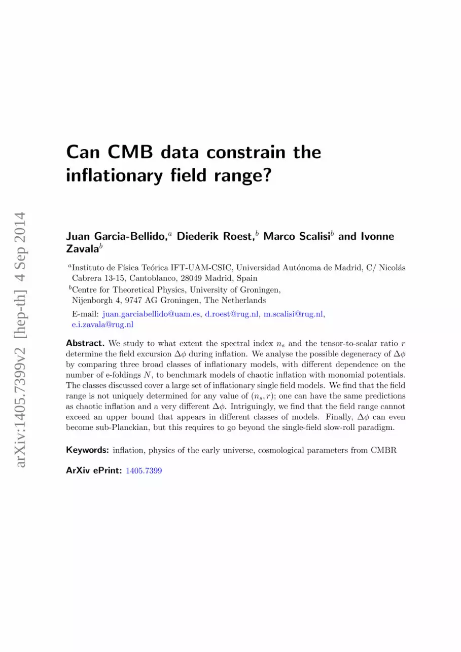
where N? is given by (3.1). Eq. (3.4) gives us an estimate of how fine-tuned the model is inorder to reproduce the same predictions of the chaotic models. Curiously, for any β = O(1)(corresponding to different chaotic models), the corresponding perturbative model will startto be severely fine-tuned in the region p > 2, as is shown in Fig. 1.
Demanding that inflation ends at ε1 = 1 turns into
Ne = N? − N = β1/p , (3.5)
where the total number of e-foldings N in principle could span a range of different valuesrelated to reheating properties of the model. Using (3.3), Eq. (3.5) gives us the functional
– 5 –
0.0 0.5 1.0 1.5 2.0 2.5 3.0
0.01
1
100
104
p
Β"
Β#1!4Β#3!8Β#1!2Β#3!4
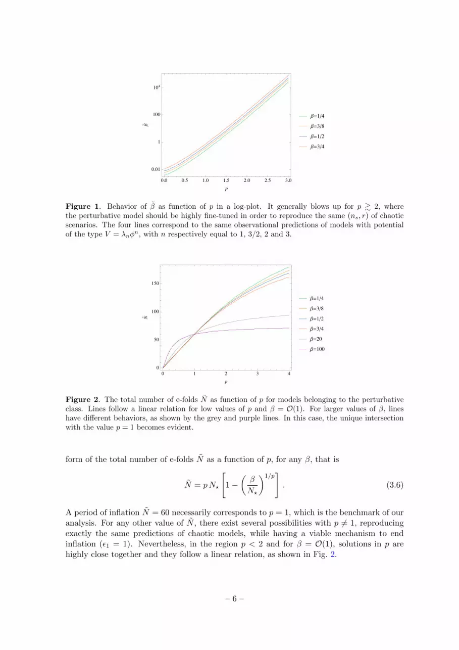
Figure 1. Behavior of β as function of p in a log-plot. It generally blows up for p & 2, wherethe perturbative model should be highly fine-tuned in order to reproduce the same (ns, r) of chaoticscenarios. The four lines correspond to the same observational predictions of models with potentialof the type V = λnφ
n, with n respectively equal to 1, 3/2, 2 and 3.
0 1 2 3 40
50
100
150
p
N!
Β#1!4Β#3!8Β#1!2Β#3!4Β#20
Β#100
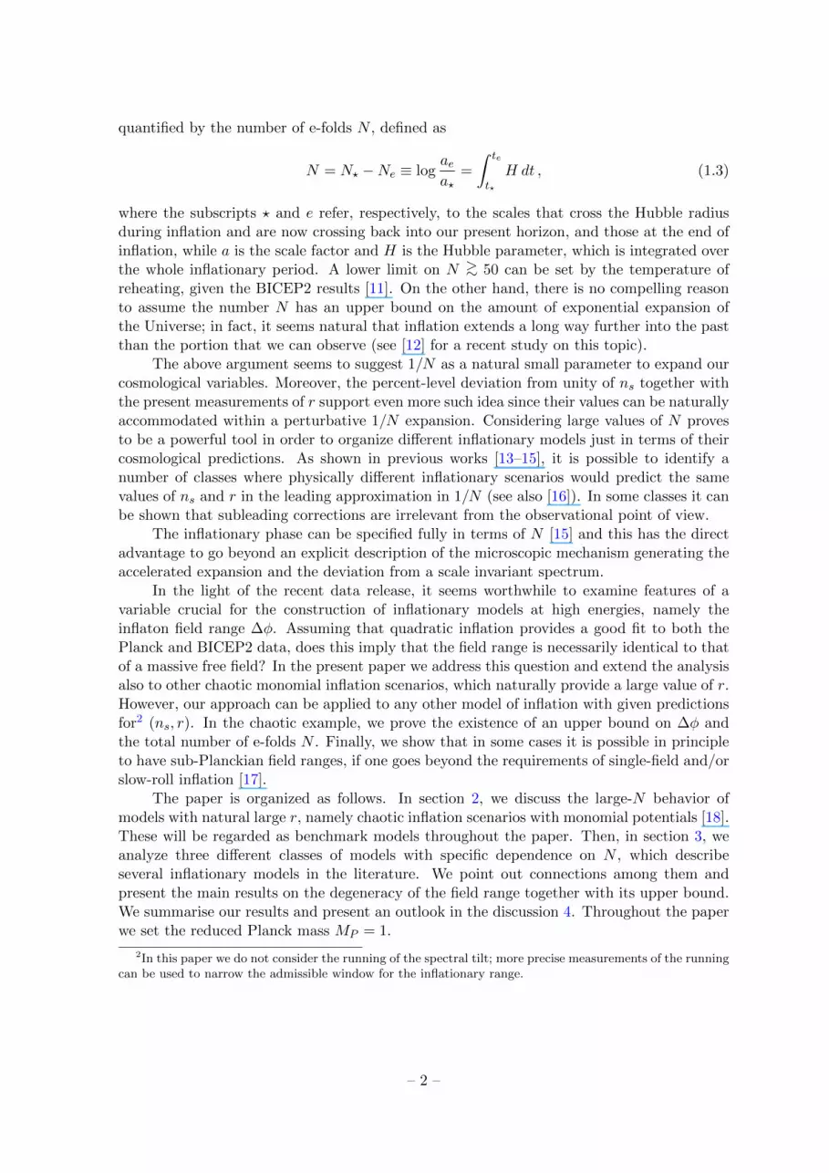
Figure 2. The total number of e-folds N as function of p for models belonging to the perturbativeclass. Lines follow a linear relation for low values of p and β = O(1). For larger values of β, lineshave different behaviors, as shown by the grey and purple lines. In this case, the unique intersectionwith the value p = 1 becomes evident.
form of the total number of e-folds N as a function of p, for any β, that is
N = pN?
[1−
(β
N?
)1/p]. (3.6)
A period of inflation N = 60 necessarily corresponds to p = 1, which is the benchmark of ouranalysis. For any other value of N , there exist several possibilities with p 6= 1, reproducingexactly the same predictions of chaotic models, while having a viable mechanism to endinflation (ε1 = 1). Nevertheless, in the region p < 2 and for β = O(1), solutions in p arehighly close together and they follow a linear relation, as shown in Fig. 2.
– 6 –
0 1 2 3 40
10
20
30
40
50
60
70
p
!Φ
Β$1!4Β$3!8Β$1!2Β$3!4
N!" 330
N!" 307
N!" 290
N!" 266
0 1000 2000 3000 4000 5000
145
150
155
p
#Φ
Β&1!4Β&3!8Β&1!2Β&3!4
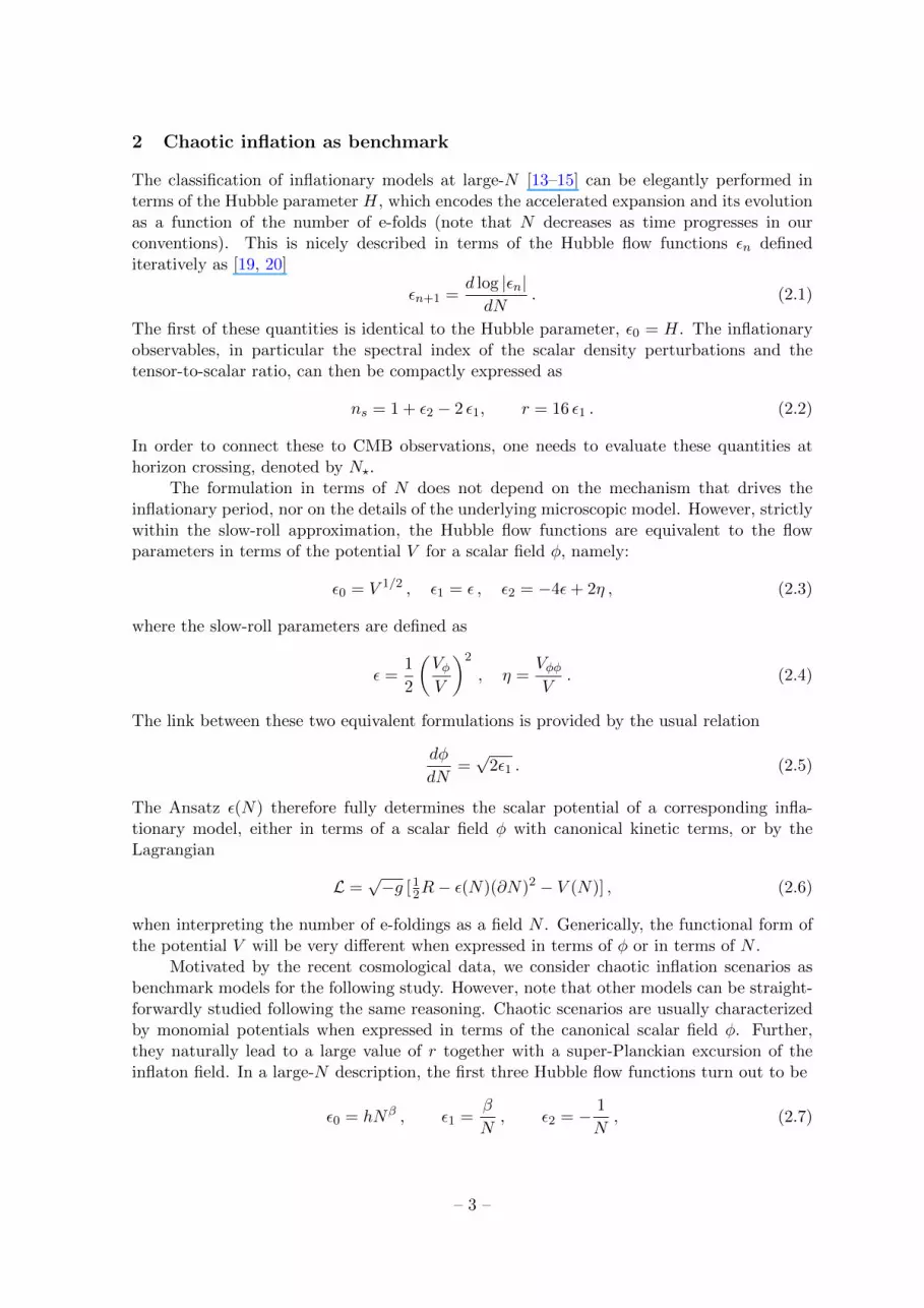
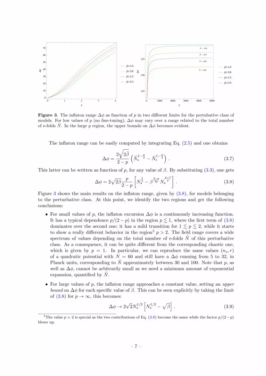
Figure 3. The inflaton range ∆φ as function of p in two different limits for the pertubative class ofmodels. For low values of p (no fine-tuning), ∆φ may vary over a range related to the total numberof e-folds N . In the large p region, the upper bounds on ∆φ becomes evident.
The inflaton range can be easily computed by integrating Eq. (2.5) and one obtains
∆φ =2
√2β
2− p
(N
1− p2
? − N1− p2
e
). (3.7)
This latter can be written as function of p, for any value of β. By substituting (3.3), one gets
∆φ = 2√
2βp
2− p
[N
12? − β
2−p2p N
p−1p
?
]. (3.8)
Figure 3 shows the main results on the inflaton range, given by (3.8), for models belongingto the perturbative class. At this point, we identify the two regions and get the followingconclusions:
• For small values of p, the inflaton excursion ∆φ is a continuously increasing function.It has a typical dependence p/(2− p) in the region p . 1, where the first term of (3.8)dominates over the second one; it has a mild transition for 1 . p . 2, while it startsto show a really different behavior in the region3 p > 2. The field range covers a widespectrum of values depending on the total number of e-folds N of this perturbativeclass. As a consequence, it can be quite different from the corresponding chaotic one,which is given by p = 1. In particular, we can reproduce the same values (ns, r)of a quadratic potential with N = 60 and still have a ∆φ running from 5 to 32, inPlanck units, corresponding to N approximately between 30 and 100. Note that p, aswell as ∆φ, cannot be arbitrarily small as we need a minimum amount of exponentialexpansion, quantified by N .
• For large values of p, the inflaton range approaches a constant value, setting an upperbound on ∆φ for each specific value of β. This can be seen explicitly by taking the limitof (3.8) for p→∞, this becomes:
∆φ→ 2√
2N1/2?
[N
1/2? −
√β]. (3.9)
3The value p = 2 is special as the two contributions of Eq. (3.8) become the same while the factor p/(2−p)blows up.
– 7 –

This corresponds to an upper bound also on N , as can be seen again by taking thelimit for p→∞ of equation (3.6), which gives:
N → N? lnN?
β. (3.10)
This limit cannot be appreciated in Fig. 2, given the reported limited range of p.Plugging the values of the parameters for quadratic inflation into (3.9) and (3.10), onegets the approximate bounds4
∆φ→ 155.56 , N → 290 . (3.11)
Curiously, the hierarchy of ranges is inverted with respect to the one present at smallp, as it is clear by comparing the two pictures of Fig. 3: at higher values of the tensor-to-scalar ratio r, we have smaller ranges.
We will see that the bounds for ∆φ and N found here are recovered in the next twocases we consider in sec. 3.2 and 3.3, within the analysis of the logarithmic and non-perturbative classes of models.
3.2 Logarithmic class
As a second case, we consider models with a first subleading correction to the Hubble flowparameters. While still neglecting higher order 1/N terms, one can imagine including alogarithmic dependence on N such as
ε1 =β
Np lnq(N + 1),
ε2 = − p
N− q
(N + 1) ln(N + 1).
(3.12)
Inflationary models having similar dependence can be found e.g. in [14].As in the previous case, in order to mimic the observational predictions of chaotic models
in terms of (ns, r), we equate (ε1, ε2) of (2.7) to (3.12) at horizon exit, respectively at N?
and N?. As result, we obtain
β = βNp? lnq(N? + 1)
N?(3.13)
q =
(1
N?− p
N?
)(N? + 1) ln(N? + 1) (3.14)
where N? = Ne + N and Ne is determined by the condition ε1 = 1:
β
Npe lnq(Ne + 1)
= 1 . (3.15)
We follow the same approach as in the perturbative case and allow N to vary as functionof p, while fixing q. The range of the inflaton ∆φ can be determined by integrating (2.5) asbefore. However, we have to rely on numerics as obtaining an analytic expression both for
4Such large values of N are not necessarily realistic (see e.g. the discussion in [22] for an upper estimate);nevertheless, it is interesting to study the behaviour of the field range for such models.
– 8 –

N and ∆φ turns out to be not as trivial as in the previous case. For this reason, we restrictour analysis just to the benchmark of a quadratic potential, namely just to β = 1/2.
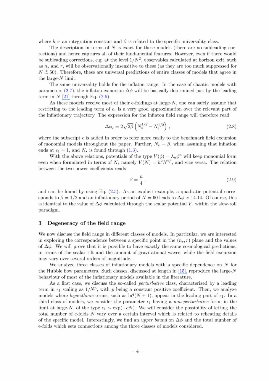
The results for the field range and the total number of e-folds are summarized in Fig. 4,for two different values of q. As we can see, for large values of p, we recover exactly the samebounds (3.11) found within the analysis of the perturbative class. This is a remarkable result,though it may be understood from the large p behaviour of ε1. In this limit, N also increasesand hence subleading terms, in εn for n ≥ 2, will be increasingly irrelevant. The two lines inFig. 4, corresponding to different values of q, do differ for smaller values of p. However, theyshow identical behavior when p increases, which correspond to a large-N limit.
Figure 4. Field range ∆φ and total number of e-folds N as functions of p in the logarithmic class, fortwo fixed values of q. The lines correspond to the same predictions of quadratic inflation (β = 1/2).The bounds on ∆φ and N can be appreciated at large values of p.
3.3 Non-perturbative class
As a third class, we consider models with Hubble flow functions such as
ε1 = e−2cN , ε2 = −2c , (3.16)
where c is a constant. Note that we are not including any coefficient for ε1 as this can be setequal to one by a shift in N .
We proceed as in the previous cases by equating (ε1, ε2) of (2.7) to the functions (3.16)at horizon exit, in order to reproduce the same observational predictions of chaotic inflationmodels. We get the following relations:
N? =1
2clnN?
β, c =
1
2N?. (3.17)
Moreover, imposing that inflation ends at ε1 = 1 translates into
Ne = N? − N = 0 , (3.18)
which can be manipulated, using (3.17), in order to get the following condition on the totalnumber of e-foldings:
N = N? lnN?
β, (3.19)
– 9 –
expressed just in terms of parameters of the benchmark models, where N? is given by (3.1).Eq. (3.19) fixes uniquely the total amount of exponential expansion required to give the same(ns, r) of the chaotic scenarios, with parameter β, and to end inflation via the conditionε1 = 1. Note that this coincides exactly with the large-p limit of the perturbative case,namely Eq. (3.10).
The inflaton range is given by integrating Eq. (2.5) between Ne and N?:
∆φ =
√2
c
(1− e−cN?
). (3.20)
The latter can be written just in terms of the benchmark parameters by using (3.17) and itreads
∆φ = 2√
2(N? −
√βN?
), (3.21)
which yields the field range in terms of β. Note that this again coincides exactly with thelarge-p limit of the field range in the perturbative case, that is (3.9). Fig. 5 shows suchfunctional dependence and the negative slope of the curve makes explicit the inversion ofhierarchy of field ranges with respect to the one which naively one would expect. In fact,lower values of r (lower values of β) will correspond to larger ∆φ. This is exactly the samefinding for the upper bounds in the perturbative class of models. Such behavior becomesexplicit once we express Eq. (3.21) in terms of the typical inflaton range ∆φc for the chaoticmodels, given by Eq. (2.8). The relation turns out to be:
∆φ = 2√
2N −∆φc , (3.22)
where N is the total number of e-folds for the benchmark chaotic models and, throughoutour study, it is fixed to be equal to 60. However, it is not possible to arbitrarily decrease ∆φeven going to really large values of β. In fact, by taking the limit for5 β →∞ of (3.21), weobtain
∆φ→√
2N , (3.23)
as can be seen in the second plot of Fig. 5, where N = 60. This corresponds to a lower-boundon N which, in the same limit, approaches the benchmark number of e-folds N , as it clearby taking the limit of (3.19). The field range of
√2N can then be understood from an ε1
parameter that is approximately equal to one during almost the entire inflationary period.Within the non-perturbative models, it is then possible to mimic chaotic scenarios in
terms of their cosmological observables ns and r. Nevertheless, both the total number ofe-foldings N and the field excursion ∆φ are uniquely determined once we choose the powercoefficient of the chaotic scenario, namely once we fix β. Curiously, the resulting valuesperfectly correspond to the upper-limits we found in the previous sections. In the specificexample of quadratic inflation, that is for β = 1/2, one obtains again ∆φ ≈ 155.56 andN ≈ 290, as expected from the discussion in sec. 3.1 and 3.2.
Note, however, that this limit appears only in the large-N limit of the non-perturbativeclass. We have discussed specific models of this class in [15]. An example is natural inflation[23], which has specific subleading corrections in addition to (3.16). In the limit of a largeperiodicity, corresponding to small c, this model asymptotes to quadratic inflation and there-fore has the same field range as this benchmark model. The origin of this difference with
5Such a limit is anyway not physical as it would correspond to an infinitely large amount of primordialgravitational waves.
– 10 –

Β " 1 ! 4Β " 3 ! 8
Β " 1 ! 2Β " 3 ! 4
0.0 0.5 1.0 1.5 2.0
145
150
155
160
165
170
Β
#Φ
N!" 60
0 100 200 300 400
80
90
100
110
120
130
140
Β
$Φ
Figure 5. The inflaton range ∆φ as function of β in two different limits for the non-perturbative classof models. For low values of β (physical values for the tensor-to-scalar ratio r), ∆φ is a decreasingfunction. The four coloured points correspond to the upper-bounds already found in sec. 3.1 and 3.2.In the large-β limit, the inflaton range cannot arbitrarily decrease and approaches a lower-limit.
(3.21) lies in the subleading corrections, that exactly become increasingly important when cis small (the effective expansion parameter being 1/cN). In other models, like hybrid infla-tion [24], which end by the action of a transverse symmetry breaking field, the excursion canbe even smaller, and still satisfy Planck and BICEP2. We will discuss a similar phenomenonin the next subsection.
3.4 Sub-Planckian field ranges
We now take a different approach within the logarithmic class of models, in order to illustratethe possibility of obtaining smaller field ranges as compared to the benchmark model ofquadratic inflation. The idea is to reproduce the same observational predictions in terms of(ns, r) by fixing N (in what follows, we assume N = 60) and letting q vary as a function ofp through the relation (3.14).
Once again, the inflationary field range ∆φ can be determined by integrating (2.5)numerically. We find a striking difference between values of p that are larger or smaller thanaround 1.1.
We find that setting the end of inflation by ε1 = 1 turns out to be possible only for pnot exceeding a value around 1.1. For p > 1.1 the function ε1(N), given by (3.12), neverreaches the unity and, then, a viable inflationary scenario has to be ended through someother mechanism.
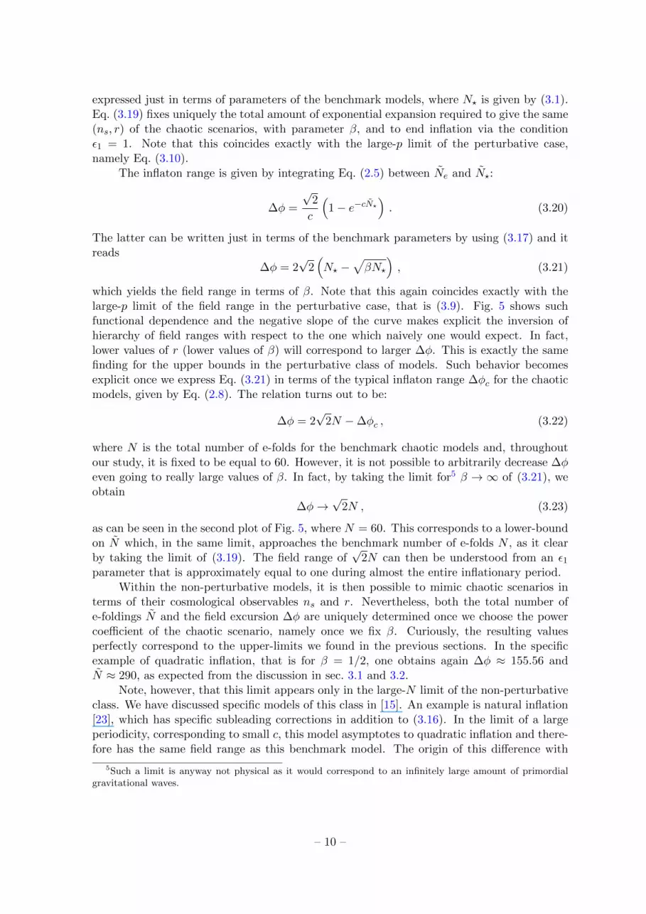
On the other hand, one can still set the end of slow-roll inflation via the condition ε2 = 1.In this case, the field range is a decreasing function of p, as showed in Fig. 6, and the valuesof ∆φ correspond to the distance which the canonical field φ travels within the slow-roll ap-proximation. For sufficiently large p, such excursion becomes even sub-Planckian. However,note that these models generically would not correspond to slow-roll inflation throughout thewhole period of exponential expansion and they would need to end inflation e.g. via a secondfield, or some other mechanism.
– 11 –
Figure 6. Slow-roll field range ∆φ as function of p. The end of slow-roll inflation is set through thecondition ε2 = 1. Sub-Planckian field ranges can be obtained if inflation ends through a second fieldor some other mechanism.
4 Discussion
In this paper, we have investigated the implications of the CMB data for the inflationaryfield range. More precisely, we have tried to answer to what extent one can infer ∆φ from ameasurement of (ns, r). We have analyzed this question by comparing three different classesof models – perturbative, logarithmic and non-perturbative – to the benchmark models ofchaotic inflation, with particular attention to the quadratic scenario.
Surprisingly, we have found that the field range can vary an order of magnitude; whilethe quadratic model implies ∆φ ≈ 14 in Planck units, the non-perturbative class gives thesame observables while ∆φ is a factor 11 larger. Moreover, we have identified a continuousdegeneracy in the other classes: different one-parameter families of models yield identical(ns, r) while ∆φ spans over a quite large range. Remarkably, ∆φ can be increased by exactlythe same factor by varying this parameter in both the perturbative and the logarithmic class.Therefore, this constitutes an upper bound for these classes of models.
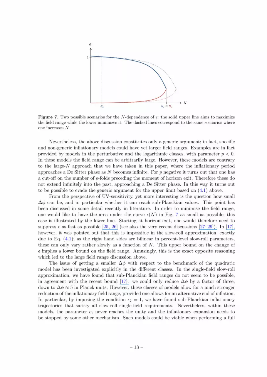
It might be surprising that there is an upper limit on the field range. After all, weare allowing in principle for an infinite number of e-foldings, hence one would expect it tobe possible to hover just below ε1 = 1 for an infinitely long period in terms of N ; such ascenario is illustrated by the upper line in Fig. 7. This period would contribute an infinitelylarge field range ∆φ as well. This raises the question: why do we not find such infinitelylarge field ranges? We suspect that the answer lies in the Hubble flow equations for the slow-roll parameters. For slow-roll inflation, in the approximation where we are only keeping thelowest two slow-roll parameters, these can be written as (where ε = ε1 and η = 2ε1 + 1/2 ε2)
dε
dN= 2ε(η − 2ε) ,
dη
dN= ε(η − 3ε) . (4.1)
Note that one cannot have both right-hand sides vanishing at the same time when ε 6= 0;therefore it is impossible to keep ε constant over a large range of e-foldings. As a consequence,there is a limit on the number of e-foldings between horizon exit and the end of inflation,for a generic slow-roll model. This is a consequence of the generic lower limit on dε/dN , andtranslates into a limit on the field range during this period.
– 12 –
1
כ כ ؠ
Figure 7. Two possible scenarios for the N -dependence of ε: the solid upper line aims to maximizethe field range while the lower minimizes it. The dashed lines correspond to the same scenarios whereone increases N .
Nevertheless, the above discussion constitutes only a generic argument; in fact, specificand non-generic inflationary models could have yet larger field ranges. Examples are in factprovided by models in the perturbative and the logarithmic classes, with parameter p < 0.In these models the field range can be arbitrarily large. However, these models are contraryto the large-N approach that we have taken in this paper, where the inflationary periodapproaches a De Sitter phase as N becomes infinite. For p negative it turns out that one hasa cut-off on the number of e-folds preceding the moment of horizon exit. Therefore these donot extend infinitely into the past, approaching a De Sitter phase. In this way it turns outto be possible to evade the generic argument for the upper limit based on (4.1) above.
From the perspective of UV-sensitivity, yet more interesting is the question how small∆φ can be, and in particular whether it can reach sub-Planckian values. This point hasbeen discussed in some detail recently in literature. In order to minimise the field range,one would like to have the area under the curve ε(N) in Fig. 7 as small as possible; thiscase is illustrated by the lower line. Starting at horizon exit, one would therefore need tosuppress ε as fast as possible [25, 26] (see also the very recent discussions [27–29]). In [17],however, it was pointed out that this is impossible in the slow-roll approximation, exactlydue to Eq. (4.1); as the right hand sides are bilinear in percent-level slow-roll parameters,these can only vary rather slowly as a function of N . This upper bound on the change ofε implies a lower bound on the field range. Amusingly, this is the exact opposite reasoningwhich led to the large field range discussion above.
The issue of getting a smaller ∆φ with respect to the benchmark of the quadraticmodel has been investigated explicitly in the different classes. In the single-field slow-rollapproximation, we have found that sub-Planckian field ranges do not seem to be possible,in agreement with the recent bound [17]: we could only reduce ∆φ by a factor of three,down to ∆φ ≈ 5 in Planck units. However, these classes of models allow for a much strongerreduction of the inflationary field range, provided one allows for an alternative end of inflation.In particular, by imposing the condition ε2 = 1, we have found sub-Planckian inflationarytrajectories that satisfy all slow-roll single-field requirements. Nevertheless, within thesemodels, the parameter ε1 never reaches the unity and the inflationary expansion needs tobe stopped by some other mechanism. Such models could be viable when performing a full
– 13 –

fast-roll analysis, or when embedded e.g. in a multi-field model. Note that this type of multi-field is markedly different from those studied in Ref. [30]; in contrast to that reference, ourentire inflationary trajectory is purely single-field, and we only appeal to the second field fora waterfall transition to end inflation.
Acknowledgments
We acknowledge stimulating discussions with Daniel Baumann and Gianmassimo Tasinato.We acknowledge financial support from the Madrid Regional Government (CAM) underthe program HEPHACOS S2009/ESP-1473-02, from the Spanish MINECO under grantFPA2012-39684-C03-02 and Consolider-Ingenio 2010 PAU (CSD2007-00060), from the Cen-tro de Excelencia Severo Ochoa Programme, under grant SEV-2012-0249, as well as from theEuropean Union Marie Curie Initial Training Network UNILHC PITN-GA-2009-237920.
References
[1] A. H. Guth, “The Inflationary Universe: A Possible Solution to the Horizon and FlatnessProblems”, Phys.Rev. D23 (1981) 347–356.
[2] A. D. Linde, “A New Inflationary Universe Scenario: A Possible Solution of the Horizon,Flatness, Homogeneity, Isotropy and Primordial Monopole Problems”, Phys.Lett. B108 (1982)389–393.
[3] A. Albrecht and P. J. Steinhardt, “Cosmology for Grand Unified Theories with RadiativelyInduced Symmetry Breaking”, Phys.Rev.Lett. 48 (1982) 1220–1223.
[4] Planck Collaboration, P. Ade et al., “Planck 2013 results. XXII. Constraints on inflation”,arXiv:1303.5082 [astro-ph.CO].
[5] BICEP2 Collaboration, P. Ade et al., “Detection of B-Mode Polarization at Degree AngularScales by BICEP2”, Phys.Rev.Lett. 112 (2014) 241101, arXiv:1403.3985 [astro-ph.CO].
[6] B. Audren, D. G. Figueroa, and T. Tram, “A note of clarification: BICEP2 and Planck are notin tension”, arXiv:1405.1390 [astro-ph.CO].
[7] A. Ashoorioon, K. Dimopoulos, M. Sheikh-Jabbari, and G. Shiu, “Non-Bunch-Davis InitialState Reconciles Chaotic Models with BICEP and Planck”, arXiv:1403.6099 [hep-th].
[8] A. Ashoorioon, P. B. Dev, and A. Mazumdar, “Implications of purely classical gravity forinflationary tensor modes”, arXiv:1211.4678 [hep-th].
[9] L. M. Krauss and F. Wilczek, “Using Cosmology to Establish the Quantization of Gravity”,Phys.Rev. D89 (2014) 047501, arXiv:1309.5343 [hep-th].
[10] D. H. Lyth, “What would we learn by detecting a gravitational wave signal in the cosmicmicrowave background anisotropy?”, Phys.Rev.Lett. 78 (1997) 1861–1863,arXiv:hep-ph/9606387 [hep-ph].
[11] L. Dai, M. Kamionkowski, and J. Wang, “Reheating constraints to inflationary models”,Phys.Rev.Lett. 113 (2014) 041302, arXiv:1404.6704 [astro-ph.CO].
[12] G. N. Remmen and S. M. Carroll, “How Many e-Folds Should We Expect from High-ScaleInflation?”, arXiv:1405.5538 [hep-th].
[13] V. Mukhanov, “Quantum Cosmological Perturbations: Predictions and Observations”,Eur.Phys.J. C73 (2013) 2486, arXiv:1303.3925 [astro-ph.CO].
[14] D. Roest, “Universality classes of inflation”, JCAP 01 (2014) 007, arXiv:1309.1285[hep-th].
– 14 –
[15] J. Garcia-Bellido and D. Roest, “The large-N running of the spectral index of inflation”,Phys.Rev. D89 (2014) 103527, arXiv:1402.2059 [astro-ph.CO].
[16] D. Boyanovsky, H. J. de Vega, and N. G. Sanchez, “Clarifying Inflation Models: Slow-roll as anexpansion in 1/Nefolds”, Phys.Rev. D73 (2006) 023008, arXiv:astro-ph/0507595[astro-ph].
[17] S. Antusch and D. Nolde, “BICEP2 implications for single-field slow-roll inflation revisited”,JCAP 1405 (2014) 035, arXiv:1404.1821 [hep-ph].
[18] A. D. Linde, “Chaotic Inflation”, Phys.Lett. B129 (1983) 177–181.
[19] D. J. Schwarz, C. A. Terrero-Escalante, and A. A. Garcia, “Higher order corrections toprimordial spectra from cosmological inflation”, Phys.Lett. B517 (2001) 243–249,arXiv:astro-ph/0106020 [astro-ph].
[20] D. J. Schwarz and C. A. Terrero-Escalante, “Primordial fluctuations and cosmological inflationafter WMAP 1.0”, JCAP 0408 (2004) 003, arXiv:hep-ph/0403129 [hep-ph].
[21] J. Garcia-Bellido, D. Roest, M. Scalisi, and I. Zavala, “The Lyth Bound of Inflation with aTilt”, arXiv:1408.6839 [hep-th].
[22] A. R. Liddle and S. M. Leach, “How long before the end of inflation were observableperturbations produced?”, Phys.Rev. D68 (2003) 103503, arXiv:astro-ph/0305263[astro-ph].
[23] K. Freese, J. A. Frieman, and A. V. Olinto, “Natural inflation with pseudo - Nambu-Goldstonebosons”, Phys.Rev.Lett. 65 (1990) 3233–3236.
[24] A. D. Linde, “Hybrid inflation”, Phys.Rev. D49 (1994) 748–754, arXiv:astro-ph/9307002[astro-ph].
[25] S. Hotchkiss, A. Mazumdar, and S. Nadathur, “Observable gravitational waves from inflationwith small field excursions”, JCAP 1202 (2012) 008, arXiv:1110.5389 [astro-ph.CO].
[26] S. Choudhury and A. Mazumdar, “Reconstructing inflationary potential from BICEP2 andrunning of tensor modes”, arXiv:1403.5549 [hep-th].
[27] G. German, “On the Lyth bound and single field slow-roll inflation”, arXiv:1405.3246[astro-ph.CO].
[28] Q. Gao, Y. Gong, and T. Li, “The Modified Lyth Bound and Implications of BICEP2 Results”,arXiv:1405.6451 [gr-qc].
[29] J. Bramante, S. Downes, L. Lehman, and A. Martin, “Clearing the Brush: The Last Stand ofSolo Small Field Inflation”, Phys.Rev. D90 (2014) 023530, arXiv:1405.7563 [astro-ph.CO].
[30] J. McDonald, “Sub-Planckian Two-Field Inflation Consistent with the Lyth Bound”,arXiv:1404.4620 [hep-ph].
– 15 –