closed-form blind symbol estimation in digital communications

2714 IEEE TRANSACTIONS ON SIGNAL PROCESSING, VOL 43, NO. 11, NOVEMBER 1995

Closed-Form Blind Symbol stimation in Digital Communications

Hui Liu and Guanghan Xu, Member, IEEE

Abstract- We study the blind symbol estimation problem in digital communications and propose a novel algorithm by exploit- ing a special data structure of an oversampled system output. Un- like most equalization schemes that involve two stages-channel identification and channel equalizatiodsymbof estimation-tbe proposed approach accomplishes direct symbol estimation With- out determining the channel characteristics. Based on a detennin- istic model, the new method can provide a closed-form solution to the symbol estimation using a small set of data samples, which makes it particularly suitable for wireless applications with fast changing environments. Moreover, if the symbols belong to a finite alphabet, e.g., BPSK or QPSK, our approach can be extended to handle the symbol estimation for multiple sources. Computer simulations and field RF experiments were conducted to demonstrate the performance of the proposed method. The results are compared to the Cram&-Rao lower bound of the symbol estimates derived in this paper.

I. INTRODUCTION

HANNEL equalization is important in ensuring reliable communication links. Most channel equalization

approaches usually involve two steps: channel identification and equalization (or symbol estimation). Blind channel equalization (BCE) [15], 131, i.e., determining the channel response based solely on the channel output without the use of a training sequence, has received considerable interest recently in communication areas. Two obvious advantages make blind equalization attractive. One merit is the bandwidth savings resulting from elimination of training sequences, while the other is the self-start capability before the communications link is established or after it has an unexpected breakdown.

Since communication channels are not necessarily minimum phase, earlier approaches of blind equalization rely on the higher order statistics of the output to recover the phase information; see 1281, [18], [7], and [13] and the references therein. These higher order statistics-based methods, although being reliable and robust in many scenarios, suffer from a common drawback, namely, a large demand of data samples. For a fast changing environment such as a cellular system, their applications may be limited. To mitigate this problem, Tong, Xu, and Kailath [26] and [27] proposed a parametric model of an oversampled communication signal that allows the blind channel estimation to be accomplished based on

Manuscript received October 17, 1994; revised June 2, 1995. The associate editor coordinating the review of this paper and approving it for publication was Dr. Athina Petropulu.

H. Liu is with the Department of Electrical Engineering, University of Virginia, Charlottesville, VA 22903 USA.

G. Xu is with the Department of Electrical & Computer Engineering, The University of Texas at Austin, Austin, TX 78712-1084 USA.

IEEE Log Number 9415235.

second-order statistics of the channel output. This idea of determining channels immediately drew the attention in this field, and many interesting extensions and new algorithms have been developed. Among them, Tugnait [29] formulated the estimation problem using a time series representation of a scalar cyclostationary process [6] and studied the identifiability condition. Moulines et al. 1111, Slock 1191, Liu et aE. [lo], Ding et al. [4], and Baccala et al. 121 exploited data structures of the system outputs and proposed several data-efficient chamel identification approaches. The resulting methods may be referred to as the deterministic blind estimation methods since the input sequence is treated as an unknown deterministic signal. More recently, Schell et al. [16] extended these earlier approaches by incorporating the prior knowledge of the transmitter pulse that further reduced the required amount of data.

Of aLl the aforementioned algorithms, the focus has been on the estimation of the channel instead of the symbols. The motivation here is to first estimate the channels using a short data sequence and then apply the identified channels to perfom equalization on the succeeding channel outputs. Clearly, such a scheme is most efficient if the channels remain stable for a reasonably long period in relation to the length of data used for channel identification. The fast-changing nature of mobile communications may prohibit the use of the same channels for long data sequence equalization. For instance, in IS-54, the data-to-fading ratio is only 300 at 60mph 1301. If blind approaches were used in such scenarios, it is likely that the identified channels can be used for very few data other than those based on which the channels were identified. In this case, it seems inefficient to involve both channel identification and equalization just to estimate a very short input sequence.

In this paper, we propose an alternative blind estimation scheme that accomplishes symbol estimation directly from the oversampled system outputs [9]. In contrast to some iterative searching methods [25] or the conventional equalization

approach provides a closed-form solution of symbol estimation based on a given set of outputs. This solution makes it more suitable for dynamic systems such as mobile communication channels. Another advantage of the new algorithm is the elimination of the equalization that prevents the inversion of possible ill-conditioned channels. Our main contxibutions in this work include: 1) a new algorithm that estimates the input symbols without identifying the channel is proposed, and more importantly, 2) exploitation of the connection between the input and output data structures, which allows the proposed

methods that use the information from previous data, the new

1053-587W95$04.00 0 1995 IEEE

LIU AND X U CLOSED-FORM BLIND SYMBOL ESTIMATION IN DIGITAL COMMUNICATIONS 2115

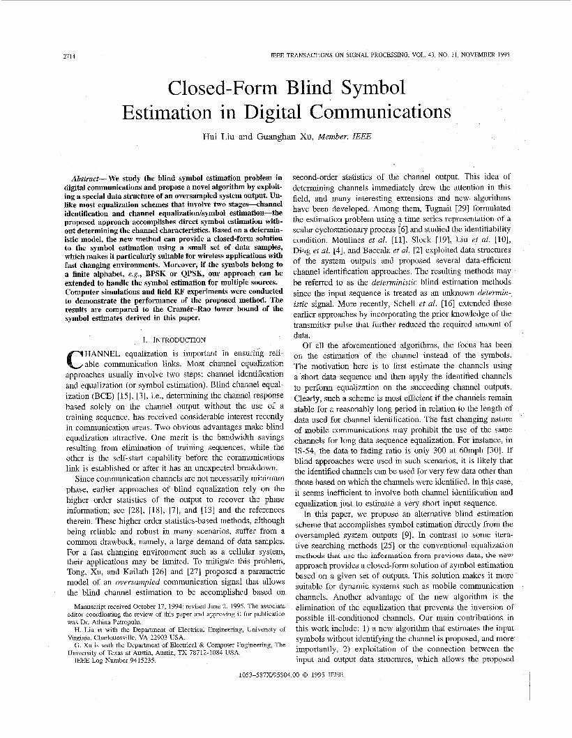
I 4-1 1 z2(g Closed-form 1 i ( k ) s(k) h2(.) Blind Symbol

Estimation

4-Q(k) Fig. 1. Blind symbol estimation from multiple channels output.

method to yield accurate estimates with minimum constraints on the inputs.

This paper is organized as follows. In Section 11, we review the data model for a multichannel communication system and define the problem formulation. In Section 111, we first establish several important results concerning the input and output data structures, and then develop the closed-form blind symbol estimation scheme. We provide discussion and analysis of the new algorithm and derive the Cram&-Rao bound (CRB) covariance matrix for both the input and the channel estimates in Section IV. The extension of the proposed method to multiple sources is briefly described in Section V. Computer simulations were conducted to study the behavior of the new approach and the results are presented in Section VI. Finally, in Section VU, we demonstrate the effectiveness of the new algorithm by applying it to real data collected from field RF experiments.

11. PROBLEM STATEMENT

Consider Fig. 1, which delineates a multichannel system with FIR impulse responses {h,( .)} driven by the same input s (.) . The system output zz (.) are related to s (.) and h, (.) by

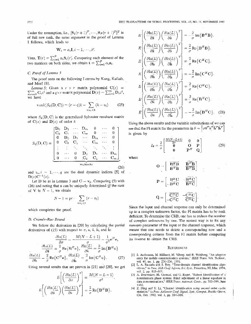
where M is the number of channels and L + 1 the maximum order of the M channels ( M 2 2 and L 2 1). The case of principal interest herein is the estimation of the input symbols s(.) from the outputs without any knowledge of the channels. As shown in [27] and [lo], both temporally and spatially oversampled digital communication signals can be cast into the same multichannel system described above.

Throughout the discussion, we have the following assumptions on the channels and input symbols:

Al: All channels are linear time-invariant (LTI) and are of finite duration.

A2: The input symbols belong to a finite alphabet. The above signal model and assumptions are plausible for

most wireless systems where the intersymbol interference (ISI) is mainly caused by multipath. For A l , we do, however, assume that the knowledge of the length of the channels, which is crucial for most parametric estimation algorithms. Methods that accomplish this are discussed in, e.g., [lo], [33]. The

second assumption A2, as will become clear, is only necessary for the estimation of imultiple sources.

Before we begin thle discussion, let us clarify the notation in this paper. As a general notational convention, symbols for matrices (in capital letters) and vectors are in boldface. The notations ( . ) T , 0 and @ stand for Hermitian, transpose, convolution, and Kronecker product, respectively. U(.) = a(O)+u( l)z+. . .+a(p)zP denotes a polynomial whose coefficients are the elements of a vector a. We define 8, e" and 8 to be the real part, the imaginary part and the estimate of the quantity 8. The syimbol I(0) stands for the identity (zero) matrix or vector with ,a proper dimension. R{A} denotes the row subspace of A.

IlI. BLIND S ~ O L ESTIMATION (BSE)

The prime task here is to recover the input sequence { s ( n ) } from given system outputs {x(n)}. Using vector representa- tions, xk = [x l (k ) . . . . zn( i (k )] and hj = [ h l ( j ) . . . h ~ ( j ) ] ~ , the input-output relation in (1) can be represented in the following more compact form [6] :

T

L

j = O

We only consider the case where the output data samples are finite. For notational convenience, we index the output vectors from x(L+ 1) to x ( N ) so that the input signals to be unraveled are s (1) , . . , s ( N ) . Smooth the data vectors to obtain a data matrix with a Hankel block structure

X ( K ) = x(L -k 1) :u(L + 2) ... x(N - K + 1) x(L-12) : Y ( L + ~ ) . . . x ( N - K f 2 )

. . . x(L $- K) ~ ( 1 5 + K + 1) . . .

N-K-L+I

K = 1,2, . . . . (3)

We define K as the smoothing factor. For the blind estimation problem under consideration, neither the inputs nor the channels are known. A close investigation of (3) will reveal that, due to oversampling, X(K) contains rich structure information of the inputs and channels, which can possibly be exploited for blind estimation of the channel and symbols. In the following, we will present an altemative conceptual framework for understanding the blind estimation problem and demonstrate the feasibility of estimating the input symbols directly from the row span of X.

To simplify the derivation, we temporarily ignore the noise and leave the accommodation of noisy data in later discussion. The following theorem lays the groundwork for the closed-form blind symbol estimation (BSE) algorithm to be developed.

Theorem 1: If i) polynomials { h z ( z ) } z l are coprime' and ii) the input vector s ef [s(l) . . . s(N)IH contains more than T

'Which means that polynomials { h , ( z ) } E , do not share any common zero.

2716 E333 TRANSACTIONS ON SIGNAL PROCESSING, VOL. 43, NO. 11, NOVEMBER 1995

modes2, then s up to a scalar ambiguity, is the unique nontrivial solution of the following overdetermined linear equations

vs = 0 (4)

where

N - 2 r + 1 \ L - 2 I

rblocks ( 5 )

r = L + K and Vo(r) is the null subspace of the row vectors

The above theorem provides a direct link between the input vector and output data matrix. In particular, it asserts that under certain conditions, the row span of the output matrix X contains “sufficient” information of the inputs. To prove Theorem 1, we need to study the relation between the input and output sequences and establish some important properties regarding the identifiability of the inputs. The remainder of this section will be focused on exploitation of the embedded structure in (3).

of X ( K ) .

A. Results on the Input and Output Data Structures

Using some additional notation, we first describe briefly the algebraic relations between the input and output matrices. Express (3) as

H(K) ,K+Lblocks

rs(1) s(2) . . . s(N - T + 111

S ( T ) ,T=L+K

The row subspace of S ( r ) is called the signal subspace and is denoted as V,(T). Its orthogonal complement V,(T) is referred to as the orthogonal subspace. If H(K) is of full column rank, X ( K ) has the same row span as VS(r). Otherwise, the row subspace of X ( K ) is a proper subset of V,(T), i.e.

R { X ( K ) } c WS(r)).

When K = 1, the channel matrix H has a dimension of M x (L + l), it cannot be of full column rank if the oversampling rate is less than the order of the channels, i.e., M < L + 1. It is important to point out that with M 2 2 , we can always smooth the output data vectors to restore the rank of the channel matrix €E( K). As K increases, H( K ) will eventually have more rows than columns and can become full

column rank under certain conditions that we will elaborate later. Throughout this paper, we assume that there are adequate data samples such that the input matrix S ( L + K ) has more rows than columns. The dependence of X, I%, and S on K will often be suppressed for notational convenience.

Note that the input matrix S(T) is afinite Hankel matrix with some interesting features. The following lemma shows that under certain conditions, the row span of the Hankel matrix is a complete description of its elements.

Lemma I : The input vector s can be uniquely determined, up to a scalar multiplier, from the row span of S ( r ) if s contains more than r modes.

Proofi See Appendix A. U Since the row subspace of the input matrix S ( r ) is often

shared by the output data matrix X(K), the physical signif- icance of Lemma 1 lies in the fact that it asserts the input sequence to be identifiable from the row subspace of the data matrix. With this key result, we now are capable of proving Theorem 1.

ProofofTheorem I : If polynomials {ht(.z)}zl are coprime, Tong et aZ. [26] show that the channel matrix H(K) can always be smoothed to be of full column rank. Consequently, the orthogonal subspace of S ( r ) is the same as the null subspace of X ( K ) .

We now need to show that s is the only null vector of V. First, since V , ( T ) S ( T ) ~ = 0, the Hankel structure of S ( r )

suggests that V, (T) is orthogonal to any consecutive N - r + 1 element of s. In other words

Therefore, Vs = 0. Second, if there is another nontrivial solution of (4), say

t, its corresponding Hankel matrix T(r) must be orthogonal to V,(T) due to the Hankel structure, which means R{T} C R { S } . By Lemma 1, t = as with a being a nonzero scalar.

U Hence, as is the unique solution of (4).

B. The Proposed Algorithm

Theorem 1 provides us a simple and effective way of estimating the inputs from the output data. Indeed, since the orthogonal subspace V, ( r ) can be directly calculated from the output data matnx, the inputs are then readily determmed by solving a set of linear equations in (4).

In practical situations, only noise corrupted samples are available. The inputs can then be estimated by finding the least square solution of (4). The complete estimation scheme is summarized as follows.

1) Calculate the orthogonal span of S from X. 2) Construct the V matrix as in (5). 3) Estimate s by solving (4). Obviously, the optimal estimate of s from V depends on

the noise distribution. Without theoretical justification, we use 2Please see [31] for the definition of mode. the least squares solution of (4) as the input estimates.

LIU AND XU: CLOSED-FORM BLIND SYMBOL ESTIMATION IN DIGITAL COMMUNICATIONS 2717

Iv. DISCUSSION AND ANALYSIS

With the establishment of the estimation procedures, our next task is to analyze the fundamental limits of the proposed algorithm for some extreme cases. We will also study the possibility of estimating s using a subset of V to reduce the computational cost. Finally in this section, we will derive the CRB of the input estimates to evaluate the efficiency of the new method.

A. Degenerate Case

For most digital communication signals, the input sequence is generically rich in modes, hence the condition in Theorem 1 can be easily satisfied. Therefore, the newly developed method should be applicable to most communication scenarios. However, degeneration can occur if the data sequence is extremely short. From (6), the minimum order of the input Hankel matrix is L + 1. When the number of modes of s, say P, is no more than L + 1, Lemma 1 indicates that the above approach will not yield a unique solution regardless of the oversampling rate.

In such case, the inputs can now be expressed as P

s ( k ) = a i z y 2=1

where z;, i = l , . . . , P are the modes of s. It is shown in 1311 that (2%) are the common roots of the polynomials of the vectors in V,(T) .

The determination of the modes { z,} is a standard frequency estimation problem. Many existing techniques, e.g., MUSIC [17] and ESPRIT [14], are applicable in such scenarios. To uniquely reconstruct the input symbols, however, one needs to know the remaining parameters-the amplitudes {a,} , which are not identifiable from the subspace. Fortunately, in practical applications, communication signals often bear some properties-eg., the constant modulus property of FM signals, the finite-alphabet property of TDMA signals, and spread spectrum property of CDMA signals-that can be exploited to remove this ambiguity.

B. The Minimum Sample Size

We mentioned in the previous discussion that, due to its deterministic nature, the proposed method can achieve the blind estimation using a small size of data samples. To quantify the minimum required number of samples (necessary condition), we need to examine steps 1 and 3 of the algorithm:

1) The channel matrix H ( K ) in (6) should have no fewer rows than columns to ensure the row span of S( L + K ) be included in that of X ( K ) , i.e.,

M K > K + L . (7)

We simplify the analysis by assuming that H(K) is full rank once it has more rows than columns, which is a fair assumption for most applications.

2) The number of equations in (4) should be no smaller than the number of parameters to be estimated:

(8) ( N - 2r+ 1). 2 N , r = L + K .

Combining (7) and (8) leads to the following result:

1 (9) ML(2ML - M + 1)

( M L - M + 1)(M - 1) " in (M, L ) = r where rz1 stands for the smallest integer that is greater than or equal to z. Note that the actual minimum number of sample vectors is N,,, - L. N,,, is the number of input symbols embedded in these outputs.

We would expect the N,,,(M, L ) to "decrease" when the oversample rate M increases. This intuition holds indeed, as shown in the next lemma.

Lemma 2: When L 2 2, the minimum number of input symbols for a unique solution of (4) satisfies the following order relations

"zn(M' + 1, L ) 5 "2n(M, L) , Nmzn(m, L) 2 2L + 1.

(10) (1 1)

The above results can be obtained by direct calculation. According to Lemma 2, by increasing the oversample rate M , the minimum samlple size for blind estimation decreases. Specifically, the low bound is 2L + 1. This feature is particularly attractive for fast changing channels-the proposed algorithm is applicable: to systems with a data-to-fading ratio as low as 2L + 1.

C. IdentiJication Using a Subset of the Null Vectors

This subsection is concerned with the modification of the proposed algorithm to reduce the computational cost. Notice that the V matrix in (5) is a generalized Sylvester resultant matrix of order T . In a noise-free case, it must be of rank N - 1 to allow the unique determination of s. However, it may not be necessary to use all the row vectors in V,(r) to form a V matrix with rank N - 1. The computational cost of the algorithm can be substantially lowered by selecting appropriate row vectors of V,(r), provided that the corresponding lower dimensional V is already "sufficient" for the estimation. A similar property has been observed in [l 11 for identifying a Toeplitz block matrix.

To provide a theoretic criteria for null vectors selection, we present the following lemma concerning the rank condition of the V constructed from row vectors of V,(r).

vp be a set of different row vectors of V,(r). Denote D I= [VT...V;-~] and let vl,...,vp-l be the dual dynamic indices3 of T(z) = D ( z ) v ~ ( z ) - ~ . The input vector can be uniquely determined from the V matrix constructed from these vectors iff

Lemma 3: Let VI. T

z v,<r

Proofi See Appeindix C. 0 With the above lemma, it is clear that one should choose the

null vectors whose dual dynamic indices satisfy (12). Lemma 3 is theoretically important, since ideally a minimum number of null vectors can be selected according to this criteria, which leads to a least expensive estimation of the inputs. However,

The dual dynamic indices are defined by Fomey in [ 5 ] .

2718 IEEE TRANSACTIONS ON SIGNAL PROCESSING, VOL. 43, NO. 11, NOVEMBER 1995

it is not so useful in real applications where the data is noisy. General rules are not available. Extensive simulations show that the uniqueness is almost guaranteed once the V matrix has more rows than columns. The number of vectors should be chosen by a compromise between increasing the statistical accuracy and decreasing the computational burden on an application-dependent basis.

D. The Crame'r-Rao Bound By treating the input as an unknown deterministic signal,

the proposed algorithm can handle blind estimation without the knowledge of the input statistics, which is desirable in many applications. On the other hand, the neglect of the statistical information may also cause it to be statistically less efficient-a common limitation of deterministic-based estimation schemes [22], [12].

When the additive noise is a zero-mean Gaussian random process with variance 0, the covariance matrix of the unbiased parameter estimates is bounded from below by the CRB. In this section, we follow the derivation of Stoica et al. [21] and Steedly et al. [20] and derive the CRB covariance matrix for the input symbols and the channels. The usefulness of the C m formula derived here is not, of course, limited to evaluating the performance of the proposed algorithm. It may also be used to establish the relative efficiency of other estimators for the symbols or channels in the literature [ll], [19].

We begin the derivation by introducing the notation x(L + 1) e (L + 1)

By stacking all the outputs in a vector form, (2) can then be reformulated as

(14) x = H(N - L) s + e = ( S ( L + 1)' 63 IM) h + e. - - The likelihood function of the data is given by

B C

--[x - BsIH. [x - Bs] 1 L(x) = (,,)M(N-L+l) exp

Thus, the log-likelihood function is

In(L) = - M ( N - L + 1) In(,) - M ( N - L + I) ln(o) 1

- -[x - BsIH . [x - Bs] " The following theorem allows one to calculate the CRB of the covariance matrix of any unbiased estimator of s, h, and CT.

Theorem 2: The Fisher information (FI) matrix for the parameters in t9 = oSTEThThT is given by 1

" " 1 0 P H Q ] where

BLB -BHB -BHB 'I BHB

p z [ -ByC] -BHC BHC

& = [ c_H_c -c"] -CHC CHC .

Pro08 See Appendix D. 0 CRB's €or both the channel and symbol estimates can be

obtained directly from the I3 matrix. It is obvious that both the channel and the input, as well as the noise characteristic, contribute to the CRB values. Although the CRB depends on the input sequence, our extensive numerical study shows that such a dependence is rather weak. In other words, the CRB is generally governed by other parameters, e.g., the channel characteristics, signal and noise powers, and the length of the input sequence.

v. EXTENSION TO HANDLING MULTIPLE SOURCES

Up to now we have primarily been concerned with the blind estimation of a single source. In some communication scenarios, e.g., the space-division-multiple-access (SDMA) systems [l], [23], [31], cochannel users are allowed to transmit signals within the same time frame. The blind parameter estimation problem then becomes a more complicated one. In particular, the ambiguity caused by the interaction among multiple sources may be impossible to remove using only the algebraic relations [31]. The following lemma explains the maximum information we may extract from the span of the input matrices.

Lemma 4: Let s,, i = I, . . . , P be multiple input vectors with its corresponding Hankel matrices {S , ( r ) } and t be another vector with its own Hankel matrix T(r). If

1) R{T(r)} C R{[SL(~)~...SP(~)']'}; 2) [S l ( r + l)T . . . S p ( r + l)'] ' is of full row rank,

then t must be a linear combination of {s,}. Prooj See Appendix B. 0

The above lemma concerns the identificatioa of multiple sources. As the result indicates, the row span of the union of input macrices does not contain sufficient information to determine each individual input vector. However, it is adequate to identify the linear combination of {s , } . In other words, the span of the multiple input vectors R{ [SI determined from R{ [S~(T)' S P ( ~ ) ~ ] ' } . Assuming that the channel matrix is of full column rank, R{ [SI . . . spIT} can then be arectly calculated from X.

Now, we extend the proposed method to multiple sources by taking advantage of the discrete-alphabet property of digital communication signals [32], [24]. The additional information used €or removing the ambiguity is the inherent discrete- alphabet structure of the input symbols. Therefore, the whole estimation process is still blind in nature.

We begin by introducing the signal model for multiple sources:

P X = ~ H , S , = [H1...Hp][ST...S;lT (17)

7 7 1


where P is the number of sources. The above input-output relation also holds for smoothed outputs.

To simplify the discussion, we assume the output vectors have been appropriately smoothed such that [ H ~ H z - Hp] is of full column rank. Denote Vs,a the row subspace of the ith input matrix and let V, be the row subspace of X. It immediately follows that V, =

We may construct the V matrix in (5) in the same way as the single source case. Clearly, V is now orthogonal to all the input vectors. The dimension of its null space is now P. Let Y N ~ P denote the null space of V. Assuming that the conditions in Lemma 4 are satisfied, Y must share the same row span with the input vectors:

P V s , a *

7

T

where W is a P x P full rank matrix. The symbol estimation now becomes the identification of

T and W from Y. It is true that without any constraint, T or A can not be uniquely determined. However, if the input symbols belong to a finite alphabet, [24] and [32] show that they are identifiable given sufficient data samples. For details, the reader is referred to the original papers.

An iterative least squares with projection (ILSP) method along with several variations are given in [24] to determine T from Y. By combining the ILSP technique and our new approach, multiple sources blind symbol estimation can be accomplished by the following steps:

1) calculating the row span of the multiple signal vectors from the null space of V;

2) estimating each input symbol using the ILSP algorithm; 3) estimating the channels by least-squares fitting (if

needed).

VI. COMPUTER SIMULATIONS To demonstrate the efficiency of the proposed method, some

computer simulations have been conducted. The the source symbols were drawn from the QPSK signal constellation with a uniform distribution. The signal-to-noise ratio (SNR) is defined as

S N R = 2010g -((dB). 11x1 I llell

The normalized root-mean square error (RMSE) defined below is employed as a performance measure of the input estimates

where Nt is the number of Monte Carlo trials (500 in our cases), & ( i ) is the estimate of the inputs from the ith trial.

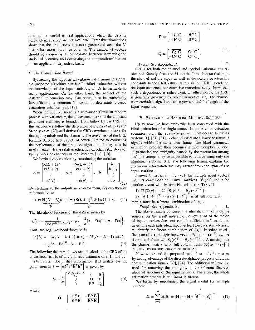
We simulated a three-ray multipath channel being truncated up to 4 symbol periods. The delays were 0.5T and 1.2T. The transmitter waveform is a raised-cosine pulse with 11% roll- off. The channel outpus were received by two antennas and were sampled twice as fast as the symbol rate. The effective number of channels is thus four. Fig. 2 depicts the channels

Chan. 2: Real Part Chan. 2: Itnag. Part

Fig. 2. Channel responses of two receivers.

TABLE I CHANNEL IMPULSE RESPONSES I II

1 2 3

1 & 3 . 3 4 4 9 - 0.45233 I 1.0067 + 1.15241 I 0.3476 + 0.31533 1 hz(r) 11 0.1128 f 0.19331 I -0.4056 + 0.3368 I 0.0503 - 0.19893 I 0.2113 + 0.29131 h.frl 11 -0.8077 - 0.31833 I -0.4307 + 0.2612i I 1.2823 + 1.14561 I -0.3610 - 0.27433

0.0586 + 0.5697i 0.3567 - 0.1487i I 0.3624 + 0.1559i I -0.0817 + 0.0360i

responses from two antennas. Table I gives the corresponding channel parameters.

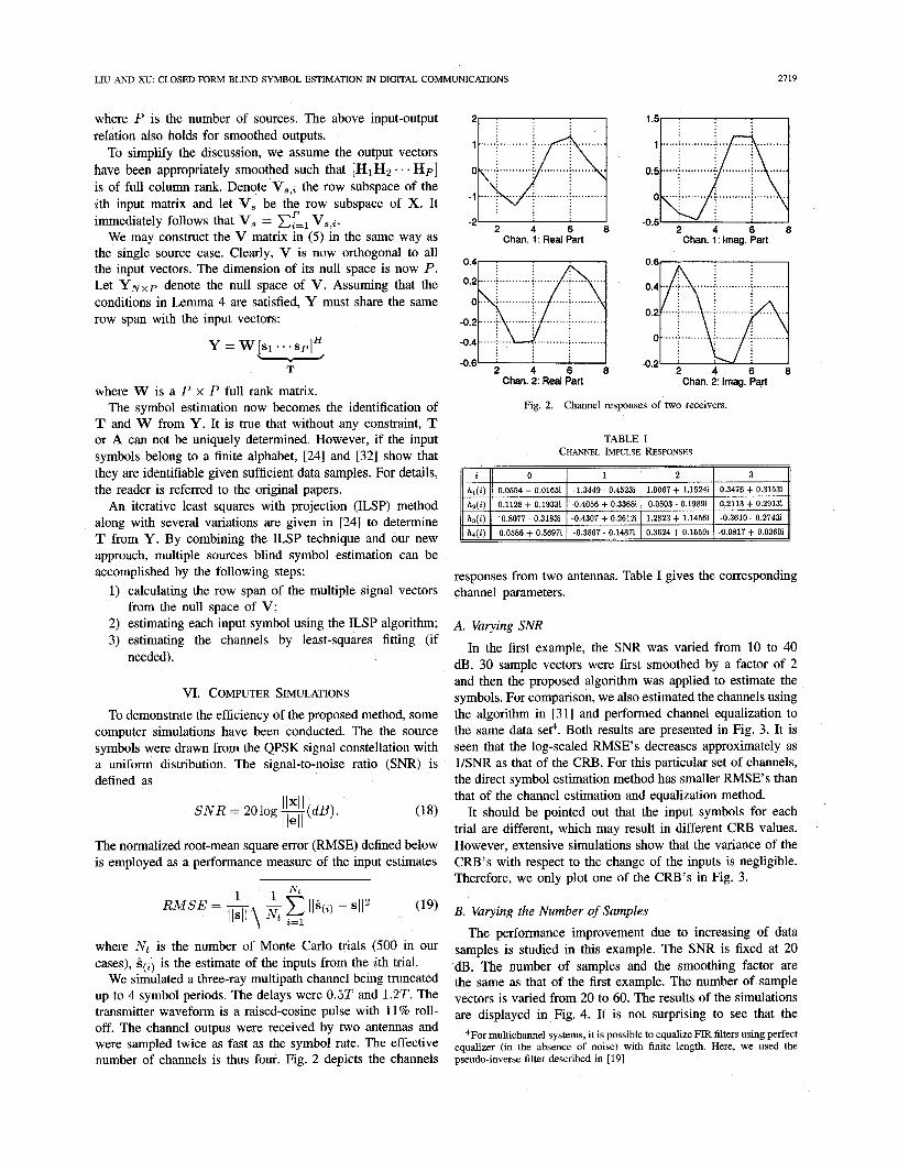
A. Varying SNR

In the first example, the SNR was varied from 10 to 40 dB. 30 sample vectors, were first smoothed by a factor of 2 and then the proposed algorithm was applied to estimate the symbols. For comparison, we also estimated the channels using the algorithm in [31] ,and performed channel equalization to the same data set4. Both results are presented in Fig. 3. It is seen that the log-scaled RMSE’s decreases approximately as 1/SNR as that of the CRB. For this particular set of channels, the direct symbol estimation method has smaller RMSE’s than that of the channel estiimation and equalization method.

It should be pointed out that the input symbols for each trial are different, which may result in different CRB values. However, extensive simulations show that the variance of the CRB’s with respect to the change of the inputs is negligible. Therefore, we only plot one of the CRB’s in Fig. 3.

B. Varying the Number of Samples The performance improvement due to increasing of data

samples is studied in this example. The SNR is fixed at 20 dB. The number of samples and the smoothing factor are the same as that of the first example. The number of sample vectors is varied from 20 to 60. The results of the simulations are displayed in Fig. 4. It is not surprising to see that the

4For multichannel systems, it is possible to equalize FIR filters using perfect equalizer (in the absence of noise) with finite length. Here, we used the pseudo-inverse filter described in [19]

2720 lEEE TRANSACTIONS ON SIGNAL PROCESSWG, VOL. 43, NO. 11, NOVEMBER 1995

-1

-1.5

1 oo

#+

f + ;

: + i + j _ ............ j ............. : ............. :.* .......... ; ............. ; ...........

_ .......................... : ........................ +..; ............. ; .............. : ............

........... i + +i ++k;

i + + ;

+: I

... .+. ..::..:;>.+.. ........... .i.”Wl.*maJ ....... .. -?.:.-.. .......

0,ZC

0.22

0.18

0.16

0.14

a 0.,2-. 2

. I . . ............

............ ............ .......... ...- _._._: r ........... : ........... : > ........... : ........... : - ! :Channd *thod j

. ?+.% ....... i ............ j ........... i ........... i ........... t ........... i

. . . : . - . - I - * _ i

7- - - -+ - - - -* - 2 -- - -i- _ _ _ i _ _ - ........... i.. .......... I. ........... !. ......... . i ......................... j ......... ..; ........ =.a< 0%. :

. - _ _ . e.-.,. j . . . ~ 5 y m b o l ~ t h o d i ?-.-.- :

. -

._ ’

. .

....... : ............ + ........... : .......... w __.^. & .................................... -

........ .;.. ................................... 1 ........... _j .......... . . I ........ ...; ........... -

: -:-.-,c.: : .

.7.--- .- . . ,

-1

1 o-2

SNR [dB]

Fig. 3. Root mean-square-error versus S N R

0,06-.... ...... i... ......... j ............ L ...... aG%mnd..i ............ : ........... i .. ..;..-.- .

O.O%o ;5 i o 3; i o i 5 j, j, 60 Number of Symbols

Fig. 4. Root mean-square-error versus number of symbols.

RMSE decreases monotonically as the number of symbols increases. However, it is also discernable that the reduction is not significant. In fact, the curve tends to be flat as the number of symbols becomes larger. Due to the deterministic nature, the input symbols cannot be consistently estimated. Related analysis can be found in direction-of-arrival estimation where the data model is called ‘‘deterministic” or “conditional” [22], W I .

C. Multiple Sources In addition to Source 1, we add a second source (Source 2)

to simulate a multiple-user situation. The SNR’s for Sources 1 and 2 are set unevenly at 20 and 25dB, respectively. 40 sample vectors are used. Other configurations are identical to that of the single source examples.

Obviously, each user is a strong interference to the other user. Without joint estimation, it is difficult to extract any one source at such a low C/I ratio. By combining the proposed algorithm and the ILSP approach, we can utilize the information of both sources and accomplish the identification

TABLE II MULTIPLE SOURCES SYMBOL ESTIMATION

0.100 4.002

0.085 4.002

Fig. 5. Signal constellation of antenna outputs.

.5

simultaneously. Table I1 summarizes the average results of the multisource symbol estimation from 500 trials. Interestingly, although the SNR for Source 1 is lower than that of Source 2, the percent bit errors (PBE) for Source 2 are lower. This suggests that the channel responses dominate the performance of the blind estimation, at least in this particular example.

w. EXPERIMENTAL RESULTS

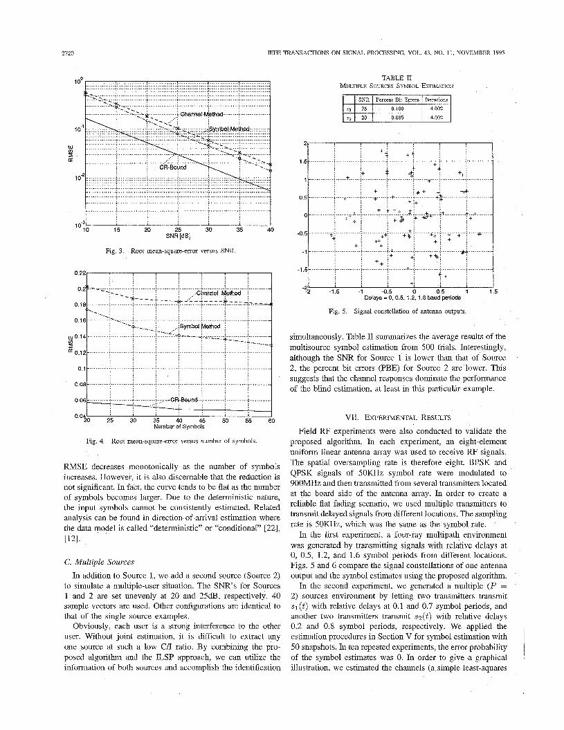
Field RF experiments were also conducted to validate the proposed algorithm. In each experiment, an eight-element uniform linear antenna array was used to receive RF signals. The spatial oversampling rate is therefore eight. BPSK and QPSK signals of 50KHz symbol rate were modulated to 900MHz and then transmitted from several transmitters located at the board side of the antenna array. In order to create a reliable flat fading scenario, we used multiple transmitters to transmit delayed signals from different locations. The sampling rate is SOKHz, which was the same as the symbol rate.

In the first experiment, a four-ray multipath environment was generated by transmitting signals with relative delays at 0, 0.5, 1.2, and 1.6 symbol periods from different locations. Figs. 5 and 6 compare the signal constellations of one antenna output and the symbol estimates using the proposed algorithm.

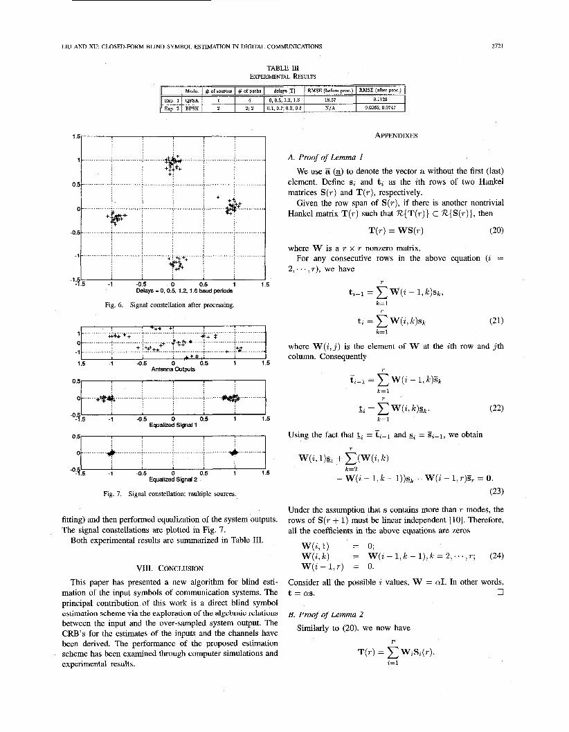
In the second experiment, we generated a multiple ( P = 2) sources environment by letting two transmitters transmit s l ( t ) with relative delays at 0.1 and 0.7 symbol periods, and another two transmitters transmit s2 ( t ) with relative delays 0.2 and 0.8 symbol periods, respectively. We applied the estimation procedures in Section V for symbol estimation with 50 snapshots. In ten repeated experiments, the error probability of the symbol estimates was 0. In order to give a graphical illustration, we estimated the channels (a simple least-squares

LIU AND X U CLOSED-FORM BLIND SYMBOL ESTIMATION IN DIGITAL COMMUNICATIONS

0

2121

_ ............ + .............................. : ................ i ............ +&

TABLE III EXPERIMENTAL RESULTS

[ Modu. I # of sources # of paths I delays [TI I RMSE ( b e f m - 1

Exp. 1 I QPSK I 1 I 4 ] 0, 0.5, 1.2, 1.6 I Exp. 2 I BPSK I 2 I 2; 2 I 0.1, 0.7; 0.2, 0.8 I

Delays - 0, 0.5, 1.2, 1.6 baud periods

Signal constellation after processing. Fig. 6.

Fig. 7. Signal constellation: multiple sources.

fitting) and then performed equalization of the system outputs. The signal constellations are plotted in Fig. 7.

Both experimental results are summarized in Table 111.

VIII. CONCLUSION

This paper has presented a new algorithm for blind estimation of the input symbols of communication systems. The principal contribution of this work is a direct blind symbol

between the input and the over-sampled system output. The CRB's for the estimates of the inputs and the channels have been derived. The performance of the proposed estimation scheme has been examined through computer simulations and experimental results.

estimation scheme via the exploration of the algebraic relations

APPENDIXES

A. Proof of Lemma 1

We use Zi (aJ to denote the vector a without the first (last) element. Define si and t, as the ith rows of two Hankel matrices S (r ) and T( r ) , respectively.

Given the row span of S(r ) , if there is another nontrivial Hankel matrix T(r) such that R{T(r)} c R { S ( r ) } , then

T(r) = WS(r) (20)

where W is a r x r nonzero matrix. For any consecutive rows in the above equation (i =

2 , . . . . r) , we have

k = l r

k = l

where W ( i , j ) is the element of W at the ith row and j th column. Consequently

r

k = l

r

- W(i -- 1, k - 1 ) ) s k - W(i - 1, r)Sr = 0.

(23)

Under the assumption that s contains more than r modes, the rows of S(r + 1) musit be linear independent [lo]. Therefore, all the coefficients in the above equations are zeros

W(i, l ) = 0;

W(i - 1,r ) = 0. W(i,k) z= W ( i - l , I C - l ) , k = 2 , . . . , r ; (24)

Consider all the possible i values, W = aI. In other words, t = as. 0

B. Proof of Lemma 2

Similarly to (20), we now have P

T(r) = WiSi(r). i=l

2122 IEEE TRANSACTIONS ON SIGNAL. PROCESSING, VOL. 43, NO. 11, NOVEMBER 1995

Under the assumption, i.e., [ S l ( r + l)T,. . . , SP(T + l)T]T is of full row rank, the same argument in the proof of L e m a 1 follows, which leads to

w, = a,I, i = 1,. ' . , P.

Thus, T(T) = E,'=, a,S,(r). Comparing each element of the two matrices on both sides, we obtain t =

P a,si.

C. Proof of Lemma 3

and Morf [SI. The proof rests on the following Lemma by Kung, Kailath,

Lemma 5: Given a r x r matrix polynomial C(z) = C,zz and a q x T matrix polynomial D ( z ) = ELO DzzZ,

we have

r ~ n k ( S k ( D , C)) = (T + q ) k - (k - e,) (25) z:v,<k

where S k (D, C) is the generalized Sylvester resultant matrix of C(z) and D(z) of order k

mbblocks (26)

and U,, i = 1, . . . , q are the dual dynamic indices [5] of D( z ) C-l ( z ) .

Let D be as in Lemma 3 and C = vp. Comparing ( 5 ) with (26) and noting that s can be uniquely determined #the rank of V is N - 1, we obtain

N - l = p r - c (T-w,) z.v,<r

which completes the proof.

D. Crume'r-Rao Bound

derivatives of (15) with respect to 0, S, S, h, and h: We follow the derivation in [20] by calculating the partial

dln(L) M ( N - L + 1) 1 dff I 7 ffz

+-e e, - ~- -

dln(L) 2 as 0 as 0

= - Im{BHe} dln(L) 2 -~ = - Re{BHe}, -

Using several results that are proven in [21] and [20], we get

dln(L) 2 E [ (F) (h) ] = -LTIm{BHC}. (28)

Using the above results and the variable see that the FI matrix for the parameters is given by

where

o= [ -ByB] -BHB BHB

-BHC -1 BHC

\

BLC -BHC

& = [ c_H_c -c"] -CHC CHC

Since the input and channel response can only be determined up to a complex unknown factor, the FI matrix has to be rank deficient. To determine the CRB, one has to reduce the number of complex unknowns by one. The easiest way is to fix any nonzero parameter of the input or the channel response, which means that one needs to delete a corresponding row and a corresponding column from the FI matrix before computing its inverse to obtain the CRB.

REFERENCES

[ l ] S . Anderson, M. Millnert, M. Viberg, and B. Wahlberg, "An adaptive array for mobile communication systems," IEEE Trans. Veh. Technol., vol. 40, no. 1, pp. 230-236, 1991.

[2] L. A. Baccala and S . Roy, "Time-domain channel identification algorithms," in Proc. 26th Con$ Inform. Sci. Syst., Princeton, NJ, Mar. 1994, vol. 2, pp. 863-867.

[3] A. Benveniste, M. Goursat, and G. Ruget, "Robust identification of a nonminimum phase system: Blind adjustment of a linear equalizer in data communications," IEEE Trans. Automat. Contr., pp. 385-399, June 1980.

[4] 2. Ding and Y. Li, "Channel identification using second order cyclic statistics," in Proc. Asilomar Con$ Signal, Syst., Comput., Pacific Grove, CA, Oct. 1992, vol. 1, pp. 334338.


G. D. Fomey, “Minimal bases of rational vector spaces, with applications to multivariable linear systems” SZAM J. Contr., vol. 13, no. 3,

W. A. Gardner, Introduction to Random Processes with Application to Signals and Systems. New York Macmillan, 1985. D. Hatzinakos and C. Nikias, “Estimation of multipath channel response in frequency selective channels,” ZEEE J. Select. Areas Commun., vol. 7, no. 1, pp. 12-19, Jan. 1989. S. Y. Kung, T. Kailath, and M. Morf, “A generalized resultant matrix for polynomial matrices,” in Proc. ZEEE Con$ Decision Contr., Florida, 1976, pp. 892-895. H. Liu and G. Xu, “A deterministic approach to blind symbol estimation,” ZEEE Signal Processing Lett., vol. 1, no. 12, Dec. 1994. H. Liu, G. Xu, and L. Tong, “A deterministic approach to blind identification of multi-channel FIR systems,” in ZEEE Proc. ZCASSP’94, Adelaide, South Australia, Apr. 1994, pp. IV-581-V-584. E. Moulines, P. Duhamel, J. Cardoso, and S. Mayrargue, “Subspace methods for the blind identification of multichannel FIR filters,” in Proc. ZEEE ZCASSP’94, Apr. 1994, pp. IV-573-IV-576. B. Ottersten, M. Viberg, and T. Kailath, “Analysis of subspace fitting and ML techniques for parameter estimation from sensor array data,” ZEEE Trans. Signal Processing, vol. 40, pp. 590-600, Mar. 1992. A. P. Petropulu and C. L. Nikias, “Blind deconvolution using signal reconstruction from partial higher order cepstral information,” ZEEE Trans. Signal Processing, vol. 41, no. 6, pp. 2088-2095, June 1993. R. Roy, A. Paulaj, and T. Kailath, “Direction-of-arrival estimation by subspace rotation methods-ESPRIT,” in Proc. IEEE ZCASSP’86, Tokyo, Japan, Apr. 1986, pp. 47-2.1-47-2.4. Y. Sato, “A method of self-recovering equalization for multilevel amplitudemodulation,” ZEEE Trans. Commun., vol. 23, no. 6, pp. 679-682, June 1975. S. V. Schell, D. L. Smith, and S. Roy, “Blind channel identification using subchannel response matching,” in Proc. I994 Con$ Inform. Sei. Syst., Princeton, NJ, Mar. 1994, vol. 2, pp. 858-862. R. 0. Schmidt, “Multiple emitter location and signal parameter estimation,” in Proc. RADC Spectral Estimation Workshop, Griffiss AFB, NY,

pp. 493-520, 1975.

1979, pp. 243-258. 0. Shalvi and E. Weinstein, “New criteria for blind deconvolution of nonminimum phase systems (channels),” ZEEE Inform. Theory, vol. 36, no. 2, pp. 312-320, Mar. 1990. D. T. M. Slock, “Blind fractionally spaced equalization, perfect- reconstruction filter banks and multichannel linear prediction,” in Proc. ZEEE ZCASSP’94, Apr. 1994, pp. IV-585-IV-588. W. M. Steedly and R. L. Moses, “The Cram&-Rao bound for pole and amplitude coefficient estimates of damped exponential signals in noise,” ZEEE Trans. Signal Processing, vol. 41, no. 3, pp. 1305-1318, Mar. 1993. P. Stoica and A. Nehorai, “MUSIC, maximum likelihood and Cramer-Rao bound,” ZEEE Trans. Acoust., Speech, Signal Processing, vol. 37, no. 5, pp. 720-741, May 1989. - , “Performance study of conditional and unconditional direction- of-arrival estimation,” ZEEE Trans. Acoust., Speech, Signal Processing, vol. 38, no. 10, pp. 1783-1795, Oct. 1990. S. C. Swales, M. A . Beach, D. J. Edwards, and J. P. McGreehan, “The performance enhancement of multibeam adaptive base-station antennas for cellular land mobile radio systems,” ZEEE Trans. Veh. Technol., vol. 39, no. 1, pp. 56-67, Feb. 1990. S. Talwar, M. Viberg, and A. Paulraj, “Blind estimation of multiple cochannel digital signals using an antenna array,” ZEEE Signal Processing Letters, vol. 1, no. 2, pp. 29-31, Feb. 1994. L. Tong, “Blind sequence estimation,” ZEEE Trans. Commun., vol. 43, no. 11, Nov. 1995. L. Tong, G. Xu, and T. Kailath, “A new approach to blind identification and equalization of multipath channel,” in Proc. 25th Asilomar Con$ Signals, Syst., Comput., Pacijic Grove, CA, Nov. 1991, vol. 2, pp. 856-860.

[27] -, “Blind identification and equalization using spectral measures, part 11: A time domain approach,” in Cyclostationarity in Communica- tions and Signal Processing, W. A. Gardner, Ed. New York: IEEE Pr., 1993.

[28] J. K. Tugnait, “Identificaiton of linear stochastic system via second- and fourth-order cumulant matching,” ZEEE Trans. Inform. Theory, vol. IT-33, pp. 393-407, May 1987.

[29] J. K. Tugnait, “On blind identifiability of multipath channels using fractional sampling and second-order cyclostationary statistics,” in Proc. Global Telecom. Con$, 1993, pp. 200Cb2005.

[30] J. H. Winters, “Signal acqusition and tracking with adaptive arrays in the digital mobile radio system IS-54 with flat fading,” ZEEE Trans. Veh. Technol., vol. 42, no. 4, pp. 377-384, Nov. 1993.

[31] G. Xu, H Liu, L. Tong, and T. Kailath, “A least-squares approach to blind channel identification,” IEEE Trans. Signal Processing, vol. 43, no. 12, Dec. 1995.

[32] D. Yellin and B. Poral, “Blind identification of FIR systems excited by discrete-alphabet inpuls,” ZEEE Trans. Signal Processing, vol. 41, no.3, pp. 1331-1339, 1993.

[33] Q. T. Zhang, K. M. Wcing, P. C. Yip, and J. P. Reilly, “Statistical analysis of the performance of information theoretic criteria in the detection of number of signals in array processing,” ZEEE Trans. Acoust., Speech, Signal Processing, vol. 37, no. 10, pp. 1557-1567, Oct. 1989.

Hili Liu was born on May 19, 1968, in Shanghai, China. He reccivcd the B.S. degree in 1988 from Fu- dan University, Shanghai, China, the M.S. degree in 1992 from Portland State University, Ponland, OR, and the Ph.D. dcgrce in 1995 from The University of Tcxas at Austin, all in electrical engineering.

From September 1992 to December 1992, he was a sofwarc cngineer at Quantitative technology Corp, Beavenon, OR. During the summer of 1995, he was a consultant for Bcll Northern Resrarch, Richardson, TX. Dr. Liu joined the faculty of the

Department of 13ectrical Engineering at University of Virginia in September 1995.

Guanghan Xu (S’86-M88) was bom on November 10, 1962, in Shanghai, China. He received the B.S. degree with honors in biomedical engineenng from Shanghai Jiao Tong University, Shanghai, China, in 1985, the M.S. degree in electrical engineenng from Anzona State University, Tempe, AZ, in 1988, and the Ph.D. degree in electrical engineering from Stanforfd University, Stanford, CA, in 1991.

Dunng the summer of 1989, he was a Research Fellow at the Insmute of Robotics, Swiss Institute of Technology, Zunch, Switzerland. From 1990

to 1991, he was a General Electric fellow of the Fellow-Mentor-Advisor Program at the Center of Integrated Systems, Stanford University. From 1991 to 1992, he was a Research Associate in the Deparment of Electncal Engineenng, Stanford University, and a short-term visiting scienhst at the Lab. of Information and Decision Systems of MIT. In 1992, Dr. Xu joined the faculty of the Department of Electrical and Computer Engineering at the University of Texas at Austin. He has worked in several areas, including signal processing, comunications, numerical linear algebra, multivariate statistics, and semiconductor manufacituring. His current research interest is focused on smart antenna systems for wireless communications.

Dr. Xu is a member of Plhi Kappa Phi and is a recipient of the 1995 NSF CAREER Award.

closed-form blind symbol estimation in digital communications

Documents