ATMOSPHERIC SCIENCE LETTERSAtmos. Sci. Let. 15: 149–156 (2014)Published online 16 December 2013 in Wiley Online Library(wileyonlinelibrary.com) DOI: 10.1002/asl2.485

Climate change multi-model projections for temperatureextremes in PortugalC. Andrade,1,2* H. Fraga2 and J. A. Santos2

1Mathematics and Physics Department, Polytechnic Institute of Tomar, Tomar 2300-313, Portugal2Centre for the Research and Technology of Agro-Environmental and Biological Sciences, Universidade de Tras-os-Montes e Alto Douro, Vila Real5001-801, Portugal

*Correspondence to:C. Andrade, Mathematics andPhysics Department, PolytechnicInstitute of Tomar, Quinta doContador, Estrada da Serra,Tomar 2300-313, Portugal.E-mail: c.andrade@ipt.pt

Received: 4 August 2013Revised: 21 October 2013Accepted: 18 November 2013

AbstractClimate change projections for spatial-temporal distributions of temperatures in Portugalare analysed using a 13-member ensemble of regional climate model simulations (A1Bscenario for 2041–2070). Bias corrections are carried out using an observational griddeddataset (E-OBS) and equally-weighted ensemble statistics are discussed. Clear shifts towardhigher future seasonal mean temperatures, in central tendency and also in both tails ofthe distributions, are found (2–4 ◦C), particularly for summer and autumn maximumtemperatures. Furthermore, frequencies of occurrence of daily extremes are projected toincrease, particularly in summer maximum temperatures over inland Portugal. Wintertimechanges are weaker than in other seasons.

Keywords: temperature extremes; climate change projections; multi-model ensemble;indices of extremes; Portugal

1. Introduction

Temperature variability and its extremes play a keyrole in many human and economic activities. Therecent warming and the increasing number of heatwaves have had deep impacts on Europe (Kuglitschet al., 2010; Zhang et al., 2011), particularly in theMediterranean, a prominent climate change hotspot(Diffenbaugh and Giorgi, 2012). Portugal, due to itslocation in Southern/Mediterranean Europe, is alreadyhighly vulnerable to the occurrence of temperatureextremes, particularly to extremely high temperaturesand heat waves. Furthermore, in conjunction with agradual warming throughout the next decades, theseextremes are expected to increase, in both frequencyand strength (Beniston et al., 2007; Fischer andSchar, 2010; Nikulin et al., 2011). In this context,the assessment of climate change projections forthese extremes is of foremost relevance to promotesuitable and timely measures for adapting andmitigating their impacts. These projections are alsoan opportunity to potentiate new cost-effective andeco-innovative practices that may warrant a moresustainable development in the future.

Many previous studies have been devoted to theanalysis of temperature extremes in Europe and inPortugal (Klein Tank and Konnen, 2003; Santos et al.,2007; Andrade et al., 2012; Frıas et al., 2012), includ-ing their climate change projections for the nextdecades (Ramos et al., 2011). However, there is alack of studies using multi-model ensembles. Further-more, new observational gridded datasets have beenrecently developed, being more suitable for model

validation and calibration than weather station data(models inherently simulate area-mean fields). Hence,this study aims at developing climate change projec-tions for temperature in Portugal using a state-of-the-art ensemble of model simulations, validated using astate-of-the-art gridded observational dataset.

2. Data and methodology

Simulated daily gridded maximum (TX) and mini-mum temperature (TN) data from a 13-member ensem-ble of regional climate model (RCM) experiments,run within the ENSEMBLES Project (Christensenet al., 1996; Jacob, 2001; Lenderink et al., 2003;Bohm et al., 2006; Elguindi et al., 2007; Jaeger et al.,2008; Collins et al., 2011; Samuelsson et al., 2011),are used herein (Table I). These RCMs are nestedin two widely used global climate models (GCM):ECHAM5 and HadCM3. Data for a recent past period(1961–2000; 40 years) are used as a baseline cli-mate. Further, a future period (2041–2070) underanthropogenic greenhouse gas forcing is selectedfor assessing climate change projections. The A1BSRES scenario (Nakicenovic et al., 2000), whichis an intermediate scenario for future carbon diox-ide equivalent concentrations, is considered for thispurpose. Nonetheless, as the selected future periodends in 2070, the deviations amongst the differ-ent scenario pathways are not yet very expressive(IPCC, 2007; van der Linden and Mitchell, 2009).Data within a geographical sector covering mainlandPortugal (36.625◦N–42.375◦N; 6.125◦W–9.875◦W;Figure S1, Supporting Information) are extracted. Due

2013 Royal Meteorological Society

150 C. Andrade, H. Fraga and J. A. Santos

Table I. GCM-RCM model chains used in this study, along with their developing institutions, relevant citations and original RCMgrids.

GCM RCM Institution Resolution

ECHAM5 HIRHAM Danish Meteorological Institute (Christensen et al., 1996) 0.22◦ × 0.22◦ rotatedRACMO Koninklijk Nederlands Meteorologisch Instituut (Lenderink et al., 2003) 0.22◦ × 0.22◦ rotatedCLM1 Max Planck Institute (Bohm et al., 2006) 0.20◦ × 0.20◦ regularCLM2 Max Planck Institute 0.20◦ × 0.20◦ regularRCA Swedish Meteorological and Hydrological Institute (Samuelsson et al., 2011) 0.22◦ × 0.22◦ rotatedRegCM International Centre for Theoretical Physics (Elguindi et al., 2007) 0.22◦ × 0.22◦ rotatedREMO Max Planck Institute (Jacob, 2001) 0.22◦ × 0.22◦ rotatedCLM Eidgenossische Technische Hochschule Zurich (Jaeger et al., 2008) 0.22◦ × 0.22◦ rotatedRCA Swedish Meteorological and Hydrological Institute (Samuelsson et al., 2011) 0.22◦ × 0.22◦ rotated

HadCM3 RCA3 C4I Center (Samuelsson et al., 2011) 0.22◦ × 0.22◦ rotatedHadRM3Q0 Hadley Centre (Collins et al., 2011) 0.22◦ × 0.22◦ rotatedHadRM3Q16 Hadley Centre 0.22◦ × 0.22◦ rotatedHadRM3Q3 Hadley Centre 0.22◦ × 0.22◦ rotated

to the climate contrasts between northern Portugal,more influenced by the North Atlantic, and itssouthern part, with a more typical Mediterraneanclimate, the target area is divided into two sec-tors: Region 1 (36.625◦N–39.375◦N) and Region2 (39.625◦N–42.375◦N) – southern/northern half ofPortugal (Figure S1). An observational dataset of dailygridded TX and TN (E-OBS, version 8.0), produced bythe EU-FP6 project ENSEMBLES (http://ensembles-eu.metoffice.com) and provided by the European Cli-mate Assessment & Dataset (ECA&D) project (Hay-lock et al., 2008), is used for validating/calibratingthe simulated datasets. Model datasets are bi-linearlyinterpolated to the E-OBS grid. As such, both observa-tional and simulated datasets are defined on a common0.25◦ latitude × 0.25◦ longitude grid (Figure S1) andon a daily basis. As the E-OBS dataset is only avail-able for land grid boxes, all subsequent analysis isconducted for this subset of grid boxes (grid boxesover the North Atlantic are white cells in all maps).

The differences in seasonal mean TX/TN betweenthe ensemble and the E-OBS (1961–2000) showthat TX tends to be less skilfully replicated thanTN (Figure S2). Further, positive differences prevailin the northernmost regions for all seasons. Thepatterns display geographical asymmetries that caneither be explained by model biases (e.g. smoothedorography and deficient representation of dynamicalprocesses) or by limitations inherent to the E-OBSdataset (Hofstra et al., 2009), also considering therelatively low density of the available weather stationsin Portugal (Figure S1). These shortcomings tend to beenhanced in regions with complex topography, suchas the northern half of Portugal (Figure S1). Most ofthe simulations underestimate (overestimate) the meanmonthly TX (TN) when compared to E-OBS (FigureS3), i.e. models underestimate thermal amplitudes.

In this study, however, these biases are correctedprior to the analysis and for each model sepa-rately. The bias, i.e. simulated minus observed meansaveraged over 1961–2000, are computed on themonthly basis and are then interpolated to the daily

basis by regression splines. The biases in each pairmodel/variable and at each grid point are then sub-tracted from the simulated data so that null patternsreplace Figure S2. The same bias corrections areapplied to the future period. These calibrations haveno other effect on the statistical distributions of eachmodel than a mere translation of its full distribu-tion (their shape remains invariant), but have obvi-ous implications in the ensemble probability densityfunctions (PDFs). After bias corrections, the differentmodels still have different skills in reproducing thespatial patterns of TN and TX from E-OBS. Thesediscrepancies are documented by the correspondingTaylor diagrams (Figure S4). All models show rootmean squared deviations (RMSDs) below 2.0 and cor-relation coefficients above 0.8. The empirical PDFsof each model/variable pair, after bias calibration,are plotted in Figure S5 (1961–2000) and Figure S6(2041–2070); PDFs are estimated by kernel densityestimation with normal kernel-smoothing windows.Despite the different model skills, no further correc-tions are carried out and all forthcoming analysesare based on equally-weighted ensemble statistics (cf.ensemble PDFs in Figures S5 and S6), which are com-monly considered more reliable than single-model orweighted statistics (Christensen et al., 2010).

Besides the analysis of changes in the central ten-dency of temperature distributions, percentile-basedextreme temperature indices are computed for boththe recent past and future periods. Owing to thestrong seasonality of the temperature regime in Por-tugal, winter [December to February (DJF)], spring[March to May, (MAM)], summer [June to August(JJA)] and autumn [September to November (SON)]are also individually analysed. In order to quantify thechanges in the inter-annual variability of the seasonalmean temperatures, their 90th and 10th percentiles areselected (TX90p/TX10p and TN90p/TN10p for TXand TN, respectively). These percentiles correspondto thresholds for defining moderate to extreme anoma-lies in the seasonal mean temperatures: anomalously

2013 Royal Meteorological Society Atmos. Sci. Let. 15: 149–156 (2014)

Multi-model ensemble projections for temperature in Portugal 151

(a) (b)

(c) (d)

(e) (f)

(g) (h)

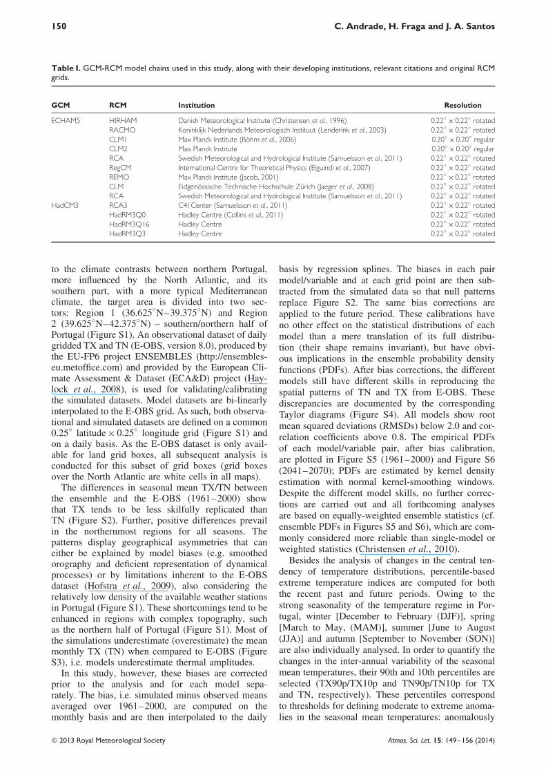
Figure 1. PDFs of seasonal mean (left panels) TX and (right panels) TN, spatially averaged over Portugal, from E-OBS (blackcurves), the ensembles in 1961–2000 (blue curves) and 2041–2070 (red curves) and for: (a, b) winter (DJF), (c, d) spring (MAM),(e, f) summer (JJA) and (g, h) autumn (SON). Area-means are only over land grid boxes within the Portuguese sector in Figure S1.

cold (warm) seasons below (above) TX10p/TN10p(TX90p/TN90p).

Extreme temperature indices are also computed ona daily basis (Peterson, 2005; Zhang et al., 2011).For this purpose, the number of days per season(ND) above TX75p/TX90p/TX99p (warm days) or

TN75p/TN90p/TN99p (warm nights) are chosen.By definition, for the baseline (1961–2000), theirmean values are of approximately 23, 9 and 1 daysper season for NDTX75p/NDTN75p, NDTX90p/NDTN90p and NDTX99p/NDTN99p, respectively.The past period percentiles are then used in the

2013 Royal Meteorological Society Atmos. Sci. Let. 15: 149–156 (2014)

152 C. Andrade, H. Fraga and J. A. Santos

8

12

16

20

24

28

32

36

E-OBS Ens. Past Ens.Future

E-OBS Ens. Past Ens.Future

0

4

8

12

16

20

24

E-OBS Ens. Past Ens.Future

E-OBS Ens. Past Ens.Future

8

12

16

20

24

28

32

36

E-OBS Ens. Past Ens.Future

E-OBS Ens. Past Ens.Future

0

4

8

12

16

20

24

E-OBS Ens. Past Ens.Future

E-OBS Ens. Past Ens.Future

0

4

8

12

16

20

24

E-OBS Ens. Past Ens.Future

E-OBS Ens. Past Ens.Future

0

4

8

12

16

20

24

E-OBS Ens. Past Ens.Future

E-OBS Ens. Past Ens.Future

8

12

16

20

24

28

32

36

E-OBS Ens. Past Ens.Future

E-OBS Ens. Past Ens.Future

8

12

16

20

24

28

32

36

E-OBS Ens. Past Ens.Future

E-OBS Ens. Past Ens.Future

(a) Region 1 TX DJF (°C) (b) Region 2

(e) Region 1 TX MAM (°C) (f) Region 2

(i) Region 1 TX JJA (°C) (j) Region 2

(c) Region 1 TN DJF (°C) (d) Region 2

(g) Region 1 TN MAM (°C) (h) Region 2

(k) Region 1 TN JJA (°C) (l) Region 2

(m) Region 1 TX SON (°C) (n) Region 2 (o) Region 1 TN SON (°C) (p) Region 2

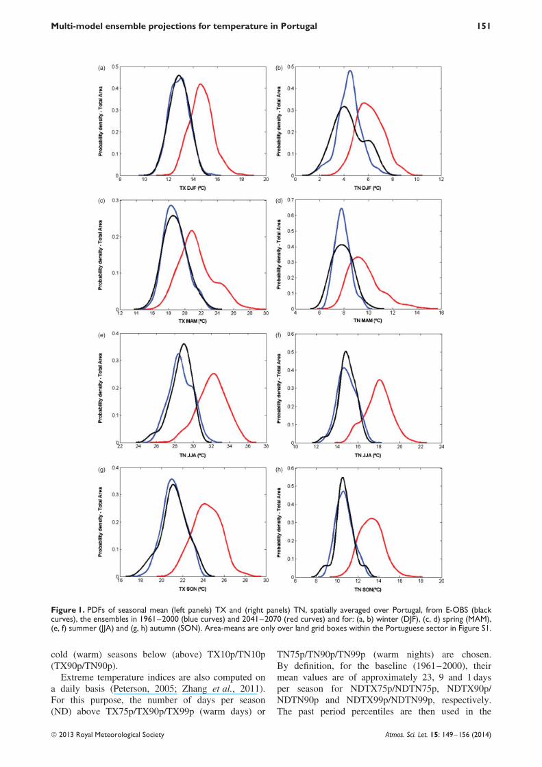
Figure 2. Boxplots of the ensemble distributions of Region 1- and Region 2-mean TX/TN in 2041–2070 (Ens. Future), 1961–2000(Ens. Past) and E-OBS for: (a–d) winter (DJF), (e–h) spring (MAM), (i–l) summer (JJA) and (m–p) autumn (SON).

future (2041–2070) and corresponding changes in theindices are discussed. The respective cold day/nightindices (Figure S7) are of secondary relevance undera warming climate and will not be discussed hereinfor the sake of succinctness.

3. Results

In order to identify changes in climate extremesfrom climate model simulations, the entire empirical

statistical distribution of each variable/parameter hasto be first validated by observational data (simulatedvs observed). The PDFs of TN and TX (Figure 1),for E-OBS (black curves) and the ensemble (bluecurves) in the past period (1961–2000), highlightthe ability of the ensemble to reproduce the baselineclimate. Overall, there is a good agreement betweenthe PDFs. Furthermore, some small discrepancies maybe rather attributed to limitations inherent to the E-OBS dataset itself than to the ensemble (Hofstraet al., 2009).

2013 Royal Meteorological Society Atmos. Sci. Let. 15: 149–156 (2014)

Multi-model ensemble projections for temperature in Portugal 153

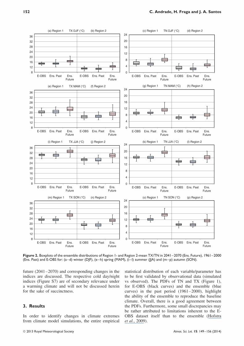
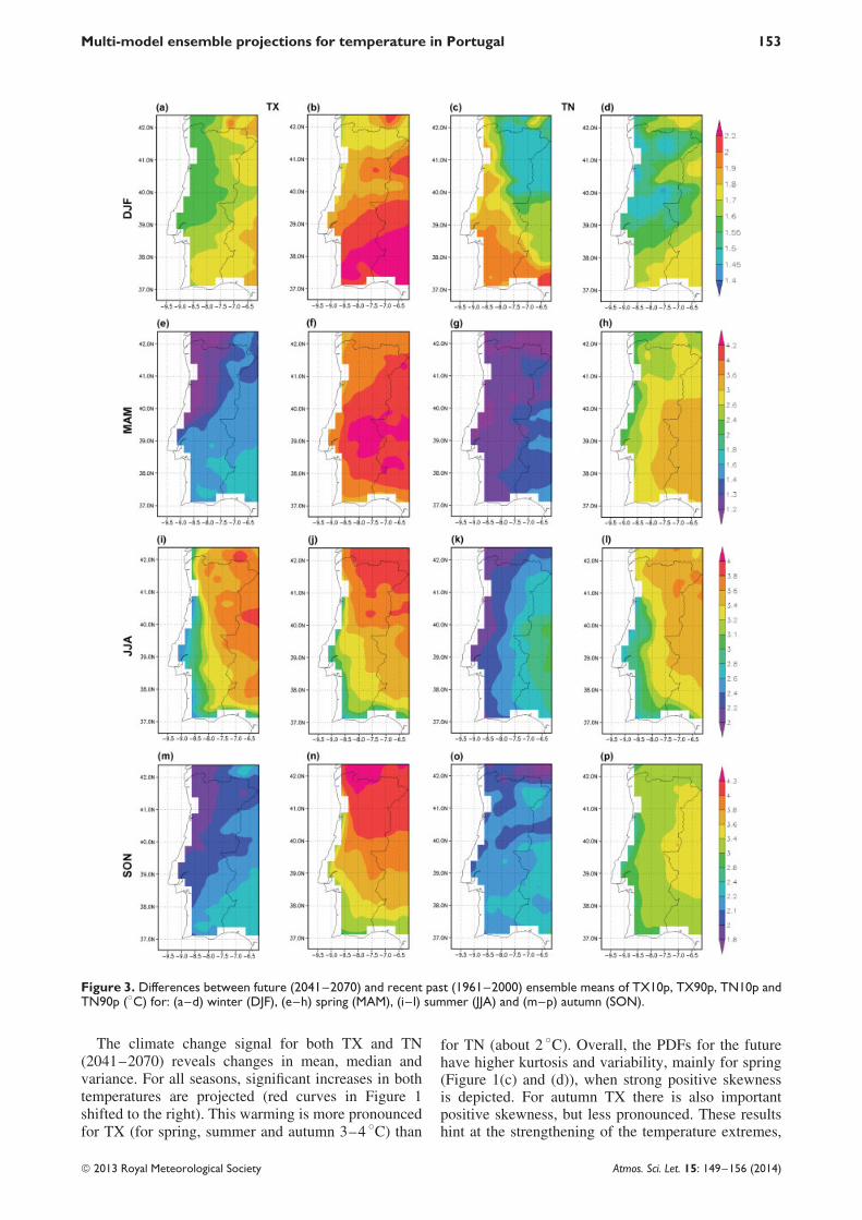
Figure 3. Differences between future (2041–2070) and recent past (1961–2000) ensemble means of TX10p, TX90p, TN10p andTN90p (◦C) for: (a–d) winter (DJF), (e–h) spring (MAM), (i–l) summer (JJA) and (m–p) autumn (SON).

The climate change signal for both TX and TN(2041–2070) reveals changes in mean, median andvariance. For all seasons, significant increases in bothtemperatures are projected (red curves in Figure 1shifted to the right). This warming is more pronouncedfor TX (for spring, summer and autumn 3–4 ◦C) than

for TN (about 2 ◦C). Overall, the PDFs for the futurehave higher kurtosis and variability, mainly for spring(Figure 1(c) and (d)), when strong positive skewnessis depicted. For autumn TX there is also importantpositive skewness, but less pronounced. These resultshint at the strengthening of the temperature extremes,

2013 Royal Meteorological Society Atmos. Sci. Let. 15: 149–156 (2014)

154 C. Andrade, H. Fraga and J. A. Santos

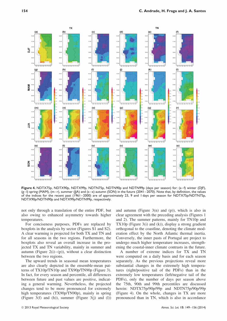
Figure 4. NDTX75p, NDTX90p, NDTX99p, NDTN75p, NDTN90p and NDTN99p (days per season) for: (a–f) winter (DJF),(g–l) spring (MAM), (m–r), summer (JJA) and (s–x) autumn (SON) in the future (2041–2070). Note that, by definition, the valuesof the indices for the recent past (1961–2000) are of approximately 23, 9 and 1 days per season for NDTX75p/NDTN75p,NDTX90p/NDTN90p and NDTX99p/NDTN99p, respectively.

not only through a translation of the entire PDF, butalso owing to enhanced asymmetry towards highertemperatures.

For conciseness purposes, PDFs are replaced byboxplots in the analysis by sector (Figures S1 and S2).A clear warming is projected for both TX and TN andfor all seasons in the two regions. Furthermore, theboxplots also reveal an overall increase in the pro-jected TX and TN variability, mainly in summer andautumn (Figure 2(i)–(p)), without a clear distinctionbetween the two regions.

The upward trends in seasonal mean temperaturesare also clearly depicted in the ensemble-mean pat-terns of TX10p/TN10p and TX90p/TN90p (Figure 3).In fact, for every season and percentile, all differencesbetween future and past values are positive, indicat-ing a general warming. Nevertheless, the projectedchanges tend to be more pronounced for extremelyhigh temperatures (TX90p/TN90p), mainly in spring(Figure 3(f) and (h)), summer (Figure 3(j) and (l))

and autumn (Figure 3(n) and (p)), which is also inclear agreement with the preceding analysis (Figures 1and 2). The summer patterns, mainly for TN10p andTX10p (Figure 3(i) and (k)), display a strong gradientorthogonal to the coastline, denoting the climate mod-eration effect by the North Atlantic thermal inertia.Conversely, the inner pasts of Portugal are project toundergo much higher temperature increases, strength-ening the coastal-inner climate contrasts in the future.

A number of extreme indices for TX and TNwere computed on a daily basis and for each seasonseparately. As the previous projections reveal moresubstantial changes in the extremely high tempera-tures (right/positive tail of the PDFs) than in theextremely low temperatures (left/negative tail of thePDFs), only the number of days per season abovethe 75th, 90th and 99th percentiles are discussedherein: NDTX75p/90p/99p and NDTN75p/90p/99p(Figure 4). On the whole, changes in TX are morepronounced than in TN, which is also in accordance

2013 Royal Meteorological Society Atmos. Sci. Let. 15: 149–156 (2014)

Multi-model ensemble projections for temperature in Portugal 155

with the previous outcomes for their seasonal means(Figures 1–3). The spatial heterogeneity of the climatechange signal is still noteworthy, with strong contrastsbetween northern and southern Portugal (Figures 2 and4). The projected increase in the number of extremelyhot days in summer (Figure 4(o) and (r)) suggests anincrease in both the number of heat waves and in theirintensity (e.g. length and maximum temperature).

4. Conclusions

A state-of-the-art 13-member ensemble, generated byGCM–RCM chains and run within the ENSEMBLESproject, is used to establish climate change projectionsfor temperature in Portugal, more specifically for TXand TN. The use of equally weighted multi-modelensembles in this study is currently the best approachto take into account the uncertainties in climate changeprojections (Raisanen, 2007; Christensen et al., 2010),as is clearly depicted in Figures S3 and S4. The E-OBS observational dataset is used to validate/calibratethe simulated datasets. After calibrating the modelsindividually (correcting bias in their seasonal means ofTX and TN), the full PDFs of the simulated seasonalmeans of TX and TN for the recent past (1961–2000)are validated with the corresponding PDFs from E-OBS. Taylor diagrams document the skill of eachmodel to reproduce the spatial variability of TXand TN. The identified model biases can not onlybe attributed to deficient representation of dynamicalprocesses in the models, such as the upper-levelpolar jet stream (Delcambre et al., 2013), atmosphericblocking (Sillmann and Croci-Maspoli, 2009) andstorm tracks (Woollings et al., 2012), but also tolimitations in the E-OBS dataset (Hofstra et al., 2009).

For the future period (2041–2070), significantwarming trends are projected for TX and TN inboth seasonal and daily scales. The full PDFs ofthe seasonal mean TX and TN are positively shifted(2–4 ◦C), primarily for TX in summer and autumn(3–4 ◦C). Additionally, daily extremes are projectedto become more frequent, particularly in summer TXover the innermost parts of Portugal. Overall, winter-time changes are much weaker than in other seasons.However, the increase in the number of extremelyhot days in spring and summer, particularly in theinner part of the country, is quite remarkable. Thesechanges are associated with alterations in the large-scale atmospheric circulation over the North Atlanticand Western Europe (e.g. Pinto et al., 2007; Sillmannand Croci-Maspoli, 2009; Woollings et al., 2012). Fur-ther, our results are in general agreement with Ramoset al. (2011), which considered only a single model(HadRM3), different scenarios (B2 and A2) and timeperiod (2071–2100).

This climate change footprint might be particularlychallenging for many socio-economic sectors inPortugal. Many agro-forestry systems in Portugal,already under heat and water stresses (e.g. Fraga

et al., 2012; 2013), also threatened by forest fires(Marques et al., 2011), may experience detrimentalimpacts from a changing climate. Energy supply andmanagement may be also severely affected. Furtherimpacts deal with human health, such as mortalityin recent heat waves in Portugal (Nogueira andPaixao, 2008). Therefore, integrating the implicationsof climate change on these systems is a key issuefor developing suitable, cost-effective, environmen-tally sustainable and eco-innovative adaptation andmitigation strategies in Portugal.

Supporting information

The following supporting information is available:

Figure S1. Orographic map showing the Portuguese sec-tor (36.625◦N–42.375◦N; 6.125◦W–9.875◦W) and Regions 1(36.625◦N–39.375◦N) and 2 (39.625◦N–42.375◦N). E-OBSgrid boxes are also plotted.

Figure S2. Differences between the ensemble mean and theE-OBS mean (left panel) TX and (right panel) TN (◦C) in1961–2000 for: (a, b) winter (DJF), (c, d) spring (MAM), (e,f) summer (JJA) and (g, h) autumn (SON).

Figure S3. Climate-mean seasonal cycles (baseline1961–2000) of monthly (a) TX, and (b) TN for allsimulations (Table I) and E-OBS (solid black curves).

Figure S4. Taylor diagrams showing the correlation coeffi-cients, root mean squared differences (RMSD) and standarddeviations of TX and TN relative to E-OBS for all simulationsin 1961–2000 (Table I) and for: (a, b) winter (DJF), (c, d)spring (MAM), (e, f) summer (JJA) and (g, h) autumn (SON).

Figure S5. PDFs of the area-means (only over land grid boxeswithin the Portuguese sector in Figure S1) of (left panels) TXand (right panels) TN from all individual simulations (Table I),for the corresponding ensemble (dashed black curves) and fromE-OBS (solid black curves) in 1961–2000 and for: (a, b) winter(DJF), (c, d) spring (MAM), (e, f) summer (JJA) and (g, h)autumn (SON).

Figure S6. PDFs of the area-means (only over land grid boxeswithin the Portuguese sector in Figure S1) of (left panels) TXand (right panels) TN from all individual simulations (Table I),for the corresponding ensemble (dashed black curves) and fromE-OBS (solid black curves) in 2041–2070 and for: (a, b) winter(DJF), (c, d) spring (MAM), (e, f) summer (JJA) and (g, h)autumn (SON).

Figure S7. NDTX10p and NDTN10p (days/season) for: (a–b)winter (DJF), (c–d) spring (MAM), (e–f), summer (JJA)and (g–h) autumn (SON) in the future (2041–2070). Notethat, by definition, the values of the indices for the recentpast (1961–2000) are of approximately 9 days per season forNDTX10p and NDTN10p.

Acknowledgements

We acknowledge the E-OBS dataset from EUFP6 projectENSEMBLES (http://ensembles-eu.metoffice.com) and thedata providers in the ECA&D project (http://eca.knmi.nl).We thank the German Federal Environment Agency and theCOSMO-CLM consortium for providing COSMO-CLM data.

2013 Royal Meteorological Society Atmos. Sci. Let. 15: 149–156 (2014)

156 C. Andrade, H. Fraga and J. A. Santos

We also acknowledge E-OBS and the data providers in theECA&D project (http://eca.knmi.nl). We thank Joaquim G.Pinto for discussions. This work is supported by EuropeanUnion Funds (FEDER/COMPETE – Operational Competitive-ness Programme) and by national funds (FCT – PortugueseFoundation for Science and Technology) under the projectFCOMP-01-0124-FEDER-022692.

References

Andrade C, Leite SM, Santos JA. 2012. Temperature extremes inEurope: overview of their driving atmospheric patterns. NaturalHazards and Earth System Sciences 12: 1671–1691.

Beniston M, Stephenson D, Christensen O, Ferro CT, Frei C, GoyetteS, Halsnaes K, Holt T, Jylha K, Koffi B, Palutikof J, Scholl R,Semmler T, Woth K. 2007. Future extreme events in Europeanclimate: an exploration of regional climate model projections.Climatic Change 81: 71–95.

Bohm U, Kucken M, Ahrens W, Block A, Hauffe D, Keuler K, RockelB, Will A. 2006. CLM-the climate version of LM: brief descriptionand long-term applications. COSMO Newsletter 6: 225–235.

Christensen JH, Christensen OB, Lopez P, van Meijgaard E, Botzet M.1996. The HIRHAM 4 regional atmospheric climate model. DMIScientific Report 96–4 pp.

Christensen JH, Kjellstrom E, Giorgi F, Lenderink G, RummukainenM. 2010. Weight assignment in regional climate models. ClimateResearch 44: 179–194.

Collins M, Booth BB, Bhaskaran B, Harris GR, Murphy JM, SextonDMH, Webb MJ. 2011. Climate model errors, feedbacks and forc-ings: a comparison of perturbed physics and multi-model ensembles.Climate Dynamics 36: 1737–1766.

Delcambre SC, Lorenz DJ, Vimont DJ, Martin JE. 2013. Diagnosingnorthern hemisphere jet portrayal in 17 CMIP3 global climatemodels: twentieth-century intermodel variability. Journal of Climate26: 4910–4929.

Diffenbaugh NS, Giorgi F. 2012. Climate change hotspots in theCMIP5 global climate model ensemble. Climate Change 114:813–822.

Elguindi N, Bi X, Giorgi F, Nagarajan B, Pal J, Solmon F, RauscherS, Zakey A. 2007. RegCM version 3 .1 user’s guide. PWCG AbdusSalam ICTP.

Fischer EM, Schar C. 2010. Consistent geographical patterns ofchanges in high-impact European heatwaves. Nature Geoscience 3:398–403.

Fraga H, Santos JA, Malheiro AC, Moutinho-Pereira J. 2012. ClimateChange Projections for the Portuguese Viticulture Using a Multi-Model Ensemble. Ciencia Tec Vitiv 27(1): 39–48.

Fraga H, Malheiro AC, Moutinho-Pereira J, Jones GV, Alves F, PintoJG, Santos JA. 2013. Very high resolution bioclimatic zoning ofPortuguese wine regions: present and future scenarios. RegionalEnvironmental Change, DOI: 10.1007/s10113-013-0490-y.

Frıas M, Mınguez R, Gutierrez J, Mendez F. 2012. Future regionalprojections of extreme temperatures in Europe: a nonstationaryseasonal approach. Climatic Change 113: 371–392.

Haylock MR, Hofstra N, Tank KAMG, Klok EJ, Jones PD, NewM. 2008. A European daily high-resolution gridded data set ofsurface temperature and precipitation for 1950–2006. Journal ofGeophysical Research 113: D20119.

Hofstra N, Haylock M, New M, Jones PD. 2009. Testing E-OBSEuropean high-resolution gridded data set of daily precipitation andsurface temperature. Journal of Geophysical Research 114(D21),DOI: 10.1029/2009jd011799.

IPCC. 2007. Climate Change 2007: Synthesis Report. Contribution ofWorking Groups I, II and III to the Fourth Assessment Report of theIntergovernmental Panel on Climate Change, Core Writing Team:RK Pachauri and A Reisinger (eds). IPCC: Geneva, Switzerland,104 pp.

Jacob D. 2001. A note to the simulation of the annual and inter-annualvariability of the water budget over the Baltic Sea drainage basin.Meteorology and Atmospheric Physics 77: 61–73.

Jaeger EB, Anders I, Luthi D, Rockel B, Schar C, Seneviratne SI.2008. Analysis of ERA40-driven CLM simulations for Europe.Meteorologische Zeitschrift 17: 349–367.

Klein Tank AMG, Konnen GP. 2003. Trends in indices of dailytemperature and precipitation extremes in Europe, 1946–99. Journalof Climate 16: 3665–3680.

Kuglitsch FG, Toreti A, Xoplaki E, Della-Marta PM, Zerefos CS,Turkes M, Luterbacher J. 2010. Heat wave changes in the east-ern Mediterranean since 1960. Geophysical Research Letters 37:L04802.

Lenderink G, van den Hurk B, van Meijgaard E, van Ulden A,Cuijpers H. 2003. Simulation of Present-Day Climate in RACMO2:First Results and Model Developments . Ministerie van Verkeer enWaterstaat, Koninklijk Nederlands Meteorologisch Instituut.

van der Linden P, Mitchell JFB. 2009. ENSEMBLES: Climate Changeand its Impacts: Summary of Research and Results From the ENSEM-BLES Project . Met Office Hadley Centre: Exeter; 160.

Marques S, Borges JG, Garcia-Gonzalo J, Moreira F, Carreiras JMB,Oliveira MM, Cantarinha A, Botequim B, Pereira JMC. 2011.Characterization of wildfires in Portugal. European Journal of ForestResearch 130: 775–784.

Nakicenovic N, Alcamo J, Davis G, de Vries HJM, Fenhann J, GaffinS, Gregory K, Grubler A, Jung TY, Kram T, La Rovere EL,Michaelis L, Mori S, Morita T, Papper W, Pitcher H, Price L, RiahiK, Roehrl A, Rogner H-H, Sankovski A, Schlesinger M, ShuklaP, Smith S, Swart R, van Rooijen S, Victor N, Dadi Z. 2000.Emissions scenarios. A special report of Working Group III of theIntergovernmental Panel on Climate Change. Cambridge UniversityPress: Cambridge, UK and New York, NY.

Nikulin G, Kjellstrom E, Hansson U, Strandberg G, Ullerstig A. 2011.Evaluation and future projections of temperature, precipitation andwind extremes over Europe in an ensemble of regional climatesimulations. Tellus A 63.

Nogueira P, Paixao E. 2008. Models for mortality associated withheatwaves: update of the Portuguese heat health warning system.International Journal of Climatology 28: 545–562.

Peterson TC. 2005. Climate change indices. WMO Bulletin 54(2).Pinto JG, Ulbrich U, Leckebusch GC, Spangehl T, Reyers M, Zacharias

S. 2007. Changes in storm track and cyclone activity in three SRESensemble experiments with the ECHAM5/MPI-OM1 GCM. ClimateDynamics 29: 195–210.

Raisanen J. 2007. How reliable are climate models? Tellus Series A-Dynamic Meteorology and Oceanography 59: 2–29.

Ramos A, Trigo R, Santo F. 2011. Evolution of extreme temperaturesover Portugal: recent changes and future scenarios. Climate Research48: 177–192.

Samuelsson P, Jones CG, Willen U, Ullerstig A, Gollvik S, HanssonU, Jansson C, Kjellstrom E, Nikulin G, Wyser K. 2011. The RossbyCentre Regional Climate model RCA3: model description and per-formance. Tellus Series a-Dynamic Meteorology and Oceanography63: 4–23.

Santos JA, Corte-Real J, Ulbrich U, Palutikof J. 2007. Europeanwinter precipitation extremes and large-scale circulation: a coupledmodel and its scenarios. Theoretical and Applied Climatology 87:85–102.

Sillmann J, Croci-Maspoli M. 2009. Present and future atmosphericblocking and its impact on European mean and extreme climate.Geophysical Research Letters 36: L10702.

Woollings T, Gregory JM, Pinto JG, Reyers M, Brayshaw DJ. 2012.Response of the North Atlantic storm track to climate changeshaped by ocean–atmosphere coupling. Nature Geoscience 5:313–317.

Zhang X, Alexander L, Hegerl GC, Jones P, Tank AK, Peterson TC,Trewin B, Zwiers FW. 2011. Indices for monitoring changes inextremes based on daily temperature and precipitation data. WileyInterdisciplinary Reviews: Climate Change 2: 851–870.

2013 Royal Meteorological Society Atmos. Sci. Let. 15: 149–156 (2014)