Seediscussions,stats,andauthorprofilesforthispublicationat:https://www.researchgate.net/publication/28597757

Manohar,C.S.:ProbabilityDistributionofExtremesofVonMisesStressinrandomlyvibratingstructures.J.Vib.Acoust.127,547-555

ArticleinJournalofVibrationandAcoustics·December2005

ImpactFactor:0.71·DOI:10.1115/1.2110865·Source:OAI

CITATIONS

18

READS

45

2authors:

SayanGupta

IndianInstituteofTechnologyMadras

57PUBLICATIONS294CITATIONS

SEEPROFILE

CsManohar

IndianInstituteofScience

101PUBLICATIONS1,279CITATIONS

SEEPROFILE

Allin-textreferencesunderlinedinbluearelinkedtopublicationsonResearchGate,

lettingyouaccessandreadthemimmediately.

Availablefrom:CsManohar

Retrievedon:09May2016

Sayan GuptaResearch Student

Department of Civil Engineering,Indian Institute of Science,

Bangalore 560012, Indiae-mail: gupta.sayan@gmail.com

C. S. Manohar1

ProfessorDepartment of Civil Engineering,

Indian Institute of Science,Bangalore 560012, India

e-mail: manohar@civil.iisc.ernet.in

Probability Distribution ofExtremes of Von Mises Stress inRandomly Vibrating StructuresThe problem of determining the probability distribution function of extremes of Von Misesstress, over a specified duration, in linear vibrating structures subjected to stationary,Gaussian random excitations, is considered. In the steady state, the Von Mises stress is astationary, non-Gaussian random process. The number of times the process crosses aspecified threshold in a given duration, is modeled as a Poisson random variable. Thedetermination of the parameter of this model, in turn, requires the knowledge of the jointprobability density function of the Von Mises stress and its time derivative. Alternativemodels for this joint probability density function, based on the translation process model,combined Laguerre-Hermite polynomial expansion and the maximum entropy model areconsidered. In implementing the maximum entropy method, the unknown parameters ofthe model are derived by solving a set of linear algebraic equations, in terms of themarginal and joint moments of the process and its time derivative. This method is shownto be capable of taking into account non-Gaussian features of the Von Mises stressdepicted via higher order expectations. For the purpose of illustration, the extremes ofthe Von Mises stress in a pipe support structure under random earthquake loads, areexamined. The results based on maximum entropy model are shown to compare well withMonte Carlo simulation results. �DOI: 10.1115/1.2110865�

Keywords: extreme value distribution, Von Mises stress, non-Gaussian random process,maximum entropy method, Laguerre series expansion, Gram-Charlier series expansion

IntroductionAccording to the failure theory based on the Von Mises yield

criterion, failure in ductile structures occur if the Von Mises stressexceeds a permissible limit which signals initiation of yielding.The safety of such structures can be, thus, quantified in terms ofthe probability of exceedance of the Von Mises stress across theyield limits. For structures under random dynamic loads, the VonMises stress is a random process and the structural failure prob-ability can be expressed in terms of the probability of exceedanceof the extremes of Von Mises stress, in a specified time interval.The Von Mises stress is a non-Gaussian random process whoseprobability distribution is hard to determine, even in linear struc-tures under Gaussian excitations. This makes it difficult to esti-mate the probability distribution of the extremes of Von Misesstress. This paper focusses on the development of approximationsfor the probability distribution of extreme values for the VonMises stress in linear structures under Gaussian dynamic loads.

Extreme value distributions of random processes are closelyrelated to the probability distribution of first passage time of therandom processes across specified thresholds, in a specified timeinterval �1,2�. A key feature in this formulation is the assumptionthat for high thresholds, the number of times the process crossesthe threshold in a given duration of time, can be modeled as aPoisson process, whose parameter is the mean outcrossing rate ofthe process across the specified threshold. In applying this formu-lation, one, in turn, needs to know the joint probability densityfunction �PDF� of the random process and its derivative, at thesame instant of time �3�. This knowledge is seldom available fornon-Gaussian processes, such as the Von Mises stress. Techniques

1Corresponding author. Telephone: �91 80 2293 3121; Fax: �91 80 2360 0404.Contributed by the Technical Committee on Vibration and Sound of ASME for

publication in the JOURNAL OF VIBRATION AND ACOUSTICS. Manuscript received May 17,2004; final manuscript received February 22, 2005. Assoc. Editor: Lawrence A. Berg-

man.

Journal of Vibration and Acoustics Copyright © 20

for obtaining approximations for outcrossing probabilities of non-Gaussian processes have been discussed in the literature. Boundson the exceedance probabilities of non-Gaussian processes havebeen obtained by applying linearization schemes �4–6�. Grigoriu�7� obtained approximate estimates for the mean outcrossing rateof non-Gaussian translation processes by studying the outcrossingcharacteristics of a Gaussian process obtained from Nataf’s trans-formation of the parent non-Gaussian process. Madsen �8�adopted a geometrical approach for developing analytical expres-sions for the mean outcrossing rate of Von Mises stress in linearstructures, under stationary Gaussian excitations. It must be noted

that the first order correlation �X�t�X�t��, where X�t� is a zero-

mean, stationary, non-Gaussian random process and X�t� is itstime derivative at the same time instant, is equal to zero. Here, �·�is the expectation operator. However, this does not imply that X�t�and X�t� are stochastically independent. The models for extremevalue distribution for non-Gaussian processes, as discussed byGrigoriu and Madsen, while they correctly take into account the

fact that �X�t�X�t��=0, do not, however, allow for mutual depen-

dence between X�t� and X�t� at the same time instant. Naess �9�developed a numerical procedure for computing the mean out-crossing rate of quadratic transformations of Gaussian processes.Here, the joint characteristic function for the process and its de-rivative is used, rather than their joint PDF. Methods for comput-ing the root mean square of Von Mises stress, resulting from zero-mean, stationary Gaussian loadings, and for estimating theirinstantaneous exceedance probabilities have also been studied�10–12�. The present authors, in an earlier work, have used aresponse surface based method to study exceedance probabilitiesof Von Mises stress in a nonlinear structure under random excita-tions �13�.

In this study, we develop an approximation for the probabilitydistribution of the extremes of Von Mises stress in a randomly

driven linear structure. A key feature of this study lies in appro-

DECEMBER 2005, Vol. 127 / 54705 by ASME

priately modeling the marginal and joint PDF of the Von Misesstress and its time derivative, at a given time instant. This enablesapplication of Rice’s formula �3�, given by,

�+��� =�0

�

vpVV��, v;t�dv , �1�

in determining the mean outcrossing rate �+���, across the speci-fied threshold �, from which one can construct the extreme valuedistribution. It must be noted that the Von Mises stress, �v, is astrictly positive quantity. This implies that P��v���= P��v

2

��2�, where � is a specified threshold and P�·� is the probabilitymeasure. This property becomes useful as it is found to be math-ematically simpler to construct the probability distribution of theextremes of �v

2, rather than �v, as the moments of the square ofthe Von Mises stress are easier to compute. For a given time t, thesquare of the Von Mises stress and its time derivative, are random

variables and are denoted by V and V. A model for the first orderPDF for V, pV�v�, may be constructed using either the Laguerrepolynomial series expansions �14� or the maximum entropymethod �MEM� �15�. Approximations for the mean outcrossingrate may then be obtained by adopting the translation procedureproposed by Grigoriu �7�. This method does not require modelingof the marginal PDF, pV�v�, or the joint PDF pVV�v , v�. Thismodel, however, does not take into account the stochastic depen-

dence that exist between V and V. The effect of mutual depen-

dence between V and V can be included in the model forpVV�v , v�, if models for pV�v� and pVV�v , v� are constructed addi-tionally. Models for pV�v� can be constructed using either Gram-Charlier series expansions �14� or MEM. Subsequently, approxi-mations for pVV�v , v� are constructed by assuming that it ispermissible to expand pVV�v , v� in terms of two sets of orthogonalpolynomials. These orthogonal functions are obtained from Gram-Schmidt orthogonalization and are expressed in terms of the mo-

ments �VmVn� ,m ,n=0,1 , . . . An alternative approach is to employthe method of maximum entropy for constructing the marginal as

well as joint PDFs of V and V. The underlying principle of thismethod lies in constructing a continuous PDF that maximizes en-tropy subject to the constraints of available partial information,such as moments and the range of the random variables �15–17�.The difficulties in the application of MEM are: �a� Usually, higherorder moments are seldom available �18�, and �b� the computa-tional effort required for determining the maximum entropy PDFparameters can be quite expensive as it involves solving a set ofsimultaneous nonlinear equations. Numerical techniques dis-cussed in the literature, include the Newton-Raphson method�19,20� and a Fourier based approach �21�. Recently, Volpe andBaganoff �22�, in their studies on fluid dynamics problems, estab-lished a simple linear relationship between the process momentsand parameters of a univariate maximum entropy PDF. These au-thors demonstrated the important result that if the first 2N−2 mo-ments of the process are available, the first N parameters of themaximum entropy PDF can be obtained by solving a set of Nsimultaneous linear equations.

The focus of this study has been on the development of meth-ods for constructing approximations for the probability densityfunction for the extremes of a special class of non-Gaussian ran-dom process, namely, the von Mises stress in Gaussian excited,linear vibrating structures. The performance of the proposed meth-ods have been compared with those existing in the literature,based on the translation process theory. In this study, we firstextend on the work by Volpe and Baganoff and develop a systemof moment equations for the maximum entropy joint PDF,pVV�v , v�. This requires the knowledge of the marginal and joint

moments of V and V. We assume that the structure is excited by

zero-mean, stationary Gaussian loads and exhibits linear behavior.

548 / Vol. 127, DECEMBER 2005

Consequently, the stress components, in the steady state, are sta-tionary, Gaussian random processes, have zero mean and are com-pletely specified through their covariance matrix. This enablescomputation of the joint moments of the stress components up to

any desired order. The marginal and joint moments of V and V, areexpressible in terms of the joint moments of stress componentsand their time derivatives, and hence, can be computed up to anydesired order. Once the parameters of the joint maximum entropyPDF are established, �+��� is subsequently computed from theRice formula. This, in turn, leads to the solution to the first pas-sage time problem and the problem of determining the extremesover a specified time duration. An alternative method for approxi-mating the joint PDF using combined Laguerre-Hermite polyno-mial expansions from the knowledge of the joint moments, hasalso been studied. The proposed methods for obtaining the ex-treme value distribution of the Von Mises stress is illustratedthrough a numerical example and the results are compared withthose obtained from Monte Carlo simulations. The new contribu-tions that are made in this study can, thus, be summarized asfollows:

1. Development of a formulation for constructing a bivariatemaximum entropy probability density function. This is anextension of the earlier study in the area of fluid dynamics,by Volpe and Baganoff �22� on univariate distributions.Some of the key features of this formulation are:

�a� The fitting of the bivariate maximum entropy distri-butions involves the solution of a set of linear alge-braic equations, and

�b� the method is capable of taking into account the pres-ence of stochastic dependence between the Von Misesstress, in the steady state, and its time derivative at thesame instant.

The study also clarifies a few computational issues in thedetermination of these bivariate probability distributions, es-pecially, with reference to the importance of choice of ap-propriate set of moment equations in successful develop-ment of these models.

2. The performance of the above model is compared with twoalternative analytical models, namely, those based on a com-bined Laguerre-Hermite series expansion and translationprocess model. Relative merits of these alternatives, within aconceptual framework, as well as, in relation to their com-putational requirements and closeness of the model predic-tions to results from Monte Carlo simulations, have alsobeen discussed.

3. The above studies have been conducted in the context ofdetermination of extremes of an important class of non-Gaussian random processes in vibration engineering,namely, the Von Mises stress.

Problem StatementWe consider a linear structure under random dynamic loads.

The loads are modeled as a vector of stationary, zero-mean,Gaussian random processes. The stress components at a specifiedlocation in the structure, ��t�, are linearly dependent on the exci-tations, and in the steady state, are thus, zero-mean stationary,Gaussian random processes. The state of stress at any point in thestructure is defined through the vector ��t�= ��1�t��2�t��3�t��4�t��5�t��6�t��T. Here, subscripts 1–3 denotethe normal stress components, subscripts 4–6 denote the shearstress components, the superscript T denotes matrix transpose andt is the time. The power spectral density �PSD� matrix of the stresscomponents is obtained from a random vibration analysis on thestructure. The square of Von Mises stress, V�t�, at a specified

location, is given by �10,23�

Transactions of the ASME

V�t� = �k=1

6

�l=1

6

Akl�k�t��l�t� , �2�

where,

A = 1 − 0.5 − 0.5 0 0 0

− 0.5 1 − 0.5 0 0 0

− 0.5 − 0.5 1 0 0 0

0 0 0 3 0 0

0 0 0 0 3 0

0 0 0 0 0 3

. �3�

In this study, we define failure as the exceedance of V�t�, across apermissible threshold �, during a specified time interval �t0 , t0+T�. The probability of structural failure is, thus, expressed as

Pf = 1 − P�V�t� � ∀ t � �t0,t0 + T�� . �4�

Note that for stationary random processes t0→�. The evaluationof this probability constitutes a problem in time variant reliabilityanalysis. Introducing the random variable Vm= max

t0tt0+T

V�t�, and

noting that Pf =1− P�Vm��, the problem can be formulated inthe time invariant format. The number of times V�t� exceeds � in�t0 , t0+T�, is a random variable and can be assumed to be Poissondistributed for high threshold levels of �. Expressions for themean outcrossing rate of the stationary process V�t�, across �, isgiven by the well-known Rice’s formula �Eq. �1�� and the failureprobability is given by

Pf = P�Vm �� = 1 − exp�− �+���T� . �5�

For a given time instant t, the stress components, �, are Gaussian

random variables and V and V, are a pair of mutually dependentrandom variables. The calculation of �+��� requires the knowledgeof pVV�v , v� which, in general, is hard to obtain. On the other

hand, the determination of the expectations, �VrVs� is reasonablystraightforward for r=1,2 , . . . ,N1 and s=1,2 , . . . ,N2. To deter-mine pVV�v , v�, we have explored three possible options: �a�Model based on MEM, �b� model based on series representationfor pVV�v , v�, and �c� translation process model for V�t�. The op-

tions �a� and �b� are capable of taking into account �V�t�rV�t�s� forany desired N1 and N2. The third option is based on the work ofGrigoriu. In this model, the process V�t� and its time derivative

V�t�, turn out to be independent, at the same time instant. In thefollowing sections, we discuss the procedure of developing thethree models.

Maximum Entropy PDFThe principle in maximum entropy method for determining

PDF of a random variable Y, lies in finding a continuous PDF,p�y�, that maximizes entropy H, given by

H = −�−�

�

p�y�ln p�y�dp�y� , �6�

subject to the constraints

�−�

�

y1ry2

s¯ yn

t p�y�dy = mrs¯t, �r,s, . . . t = 0,1,2 . . . � . �7�

Here, mrs¯t= �y1ry2

s¯yn

t � denotes the �r+s+ ¯ + t�-th joint mo-ment. Using calculus of variations, it can be shown that the opti-

mal PDF is of the form

Journal of Vibration and Acoustics

p�y� = exp�− ��00 + �k

�kyk + �k,j

�kjykyj + ¯

+ �k,j,. . .,l

�kj. . .lykyj . . . yl �, − � Y � . �8�

Determining the vector of unknown parameters ��� involves thesolution of a set of simultaneous nonlinear equations and the as-sociated difficulties have been a major deterrent in the use of thismethod. The recently developed moment equations by Volpe andBaganoff �22�, however, provides a powerful alternative techniquefor avoiding expensive numerical computations.

Moment Equations. Volpe and Baganoff �22�, in their studieson problems of fluid dynamics, have recently established that asimple linear relationship exists between the parameters of aunivariate maximum entropy PDF and its moments. These linearequations have been termed as moment equations. This method, tothe best of our knowledge, appears not to have been used in thecontext of problems of structural reliability analyses. Using a pro-cedure similar to the one proposed by Volpe and Baganoff, wederive the moment equations for a second-order maximum en-tropy PDF. This we use to construct the joint PDF for the VonMises stress and its time derivative. The procedure for the devel-opment of the moment equations is discussed next. For the sake ofcompleteness, we first review the procedure for establishing themoment equations for the univariate maximum entropy PDF. Sub-sequently, the method for developing the bivariate maximum en-tropy PDF is presented.

Univariate PDF. Assuming that the random variable Y has acontinuous PDF, the maximum entropy PDF for Y is of the form

p�y� = �0 exp�− �k=1

N

�kyk� . �9�

The derivative of p�y�, with respect to y, is given by

�p�y��y

= − �k=1

N

k�kyk−1p�y� . �10�

Multiplying �p�y� /�y with yj and integrating with respect to y, inthe interval �−� ,��, we get

�−�

�

yj�p�y��y

dy = − �k=1

N

k�kmk+j−1. �11�

Here, �−�� yjp�y�dy=mj = �Y j�. Alternatively, if the left hand side of

Eq. �11� is integrated by parts, it can be shown that

�−�

�

yj�p�y��y

dy = − jmj−1, �12�

when N is even. From Eqs. �11� and �12�, we get

�k=1

N

k�kmk+j−1 = jmj−1. �13�

For j=0,1 ,2 , . . ., the above formulation leads to a system of mo-ment equations, of the form

m0 2m1 3m2 . . . NmN−1

m1 2m2 3m3 . . . NmN

· · · . . . ·

· · · . . . ·

mN−1 2mN 3mN+1 . . . Nm2N−2

��1

�2

·

·

�N

� =�0

m0

·

·

�N − 1�mN−2

��14�

with m0=1. These equations are exact and provide a simple linear

relationship between the moments and the vector of unknown pa-

DECEMBER 2005, Vol. 127 / 549

rameters ���. Inspection of Eq. �14� reveals that an infinite set ofequations can be generated for a given set of parameters ���. Thisimplies that ��� does not have a unique solution. However, it hasbeen observed that if the vector of unknown parameters ��� is ofdimension N, then the solution of the simultaneous equations gen-erated by j=0, . . . ,N−1 lead to parameters which yield an accept-able model for the PDF. This would require information on thefirst 2N−2 moments of Y. This is in contrast to other numericaltechniques discussed in the literature, where the knowledge of thefirst N moments is sufficient to determine a N-dimensional param-eter vector ���. However, during the course of this study, we haveobserved that for strictly positive random variables, acceptablemaximum entropy PDF is obtained by solving for ���, the equa-tions generated by j=1, . . . ,N. This, of course, requires knowl-edge of the first 2N−1 moments of Y. The parameter �0 is thenormalization parameter and is obtained as the inverse of�−�

� exp�−�k=1N �ky

k�dy.

Bivariate PDF. For a pair of correlated random variables X andY, the maximum entropy joint PDF is of the form

p�x,y� = �0 exp�− �k+j=1

2N

�kjxkyj� . �15�

Thus, the expression for p�x ,y�, obtained from the above equationwhen N=1, is given by

p�x,y� = �0 exp�− �10x − �20x2 − �01y − �02y2 − �11xy� . �16�

Similarly, the corresponding for p�x ,y� when N=2 is

p�x,y� = �0 exp�− �10x − �20x2 − �30x

3 − �40x4 − �01y − �02y2

− �03y3 − �04y4 − �11xy − �21x2y − �12xy2 − �31x

3y

− �13xy3 − �22x2y2� . �17�

Differentiating p�x ,y� in Eq. �15� with respect to x and y, we get

�p�x,y��x

= − �k+j=1

2N

k�kjxk−1yjp�x,y� , �18�

�p�x,y��y

= − �k+j=1

2N

j�kjxkyj−1p�x,y� . �19�

We consider the integrals �−�� �−�

� xrys�p�x ,y� /�xdxdy and�−�

� �−�� xrys�p�x ,y� /�ydxdy. As for univariate case, we obtain ex-

pressions for the integrals in two different ways: �a� By substitut-ing Eqs. �18� and �19� in the integrals and �b� by carrying outintegration by parts. Equating the expressions obtained from �a�and �b�, we get the following system of equations:

�k+j=1

2N

k�kjmk+r−1,j+s = rmr−1,s, �20�

�k+j=1

2N

j�kjmk+r,j+s−1 = smr,s−1, �21�

where, mr,s=�−�� �−�

� xrysp�x ,y�dxdy, and �r ,s=0,1 ,2 . . . �. We callEqs. �20� and �21� as the generating equations and must be simul-taneously used to construct the moment equations. As in theunivariate case, here also we can construct an infinite set of equa-tions to solve for the unknown parameters ���. However, accept-able models for the PDF are obtained only when the momentequations are generated by varying r and s from 0 in an ascendingorder. However, if X and/or Y is a strictly positive random vari-able, r and/or s is to be varied from 1 in an ascending order.

Maximum Entropy Bivariate PDF for V and V. In this study, we

employ the above principle for constructing the maximum entropy

550 / Vol. 127, DECEMBER 2005

second-order PDF pVV�v , v�. Equations �20� and �21� are used forconstructing the moment equations. We consider N=2 and conse-quently, the dimension of the vector of unknown parameters, M, is

equal to 14. It must be noted that V�0 and −� V�. Thus, inconstructing the moment equations r and s are taken to be inte-

gers, such that, r�1 and s�0. If V and V are considered to be

independent, then pVV�v , v�= pV�v�pV�V� and the unknown param-eters constitute a eight dimensional vector, whose elements are��10,�20,�30,�40,�01,�02,�03,�04�. Solution to these parametersare obtained from the system of equations generated for the �r ,s�combinations �1, 0�, �2, 0�, �3, 0�, �4, 0� for Eq. �20� and �0, 0�, �0,1�, �0, 2�, and �0, 3� for Eq. �21�. It is observed that for Eq. �20�,r= j and s=0, where �� j0� is the vector of unknown parameters forpV�v�. However, for Eq. �21�, r=0 and s= j−1, where ��0j� are thevector of unknown parameters for pV�v�. This is because as V

�0, r�1 and as −� V�, s�0. This essentially implies thattwo sets of four simultaneous equations, of the form in Eq. �14�,with each set corresponding to V and V, respectively, need to besolved separately. However, if the dependence characteristics of V

and V are to be incorporated in the model for pVV�v , v�, one needsto consider, for N=2, six additional parameters��11,�21,�12,�31,�13,�22�T. The presence of these terms ensurethat all 14 equations are coupled. Of the six additional equationsthat need to be constructed, three each are obtained from Eqs. �20�and �21�. This ensures that the moment equations constructedfrom the generating equations are in sequence. The additional�r ,s� combinations are taken to be �1, 1�, �2, 1�, and �3, 1� for Eq.�20� and �1, 1�, �1, 2�, and �2, 2� for Eq. �21�. If ��kj� are thevector of the six additional parameters, the �r ,s� combinationsconsidered are r=k and s= j when Eq. �20� is used and r=k ands= j−1 when Eq. �21� is used to construct the moment equations.It must be noted that Eqs. �20� and �21� are used in constructingthe moment equations when k j and k� j, respectively. If k= j,either of the generating equations may be used, but care must betaken such that M /2 equations each are obtained from each of thegenerating equations, if M is even and for odd M, �M −1� /2 and�M +1� /2 equations are constructed from the generating equa-tions.

Series Expansion Method

Alternatively, the joint PDF pVV�v , v� may be constructed usinga series expansion method. It is well known that many probabilitydensity functions can be approximated by a series of polynomialswhose coefficients are determined from the moments of the pro-cess, for a given time. In particular, it has been shown that thePDF can be readily approximated by a few terms if a fortuitouschoice is made for the expansion polynomials �14�. Here, we pro-vide details for constructing a model for pVV�v , v� using seriesexpansions.

Model for pV„v…. Since the probability distribution vanishes fornegative values of V�t�, pV�v� can be approximated as

pV�v� = �j=0

�

aj exp�− v�v L j �v� . �22�

where, L j �v� is the generalized Laguerre polynomial, defined by

the Rodrigues’s formula

L j �v� =

exp�v�v−

j!

� j

�v j �exp�− v�v j+ � . �23�

The orthogonality relation for the polynomial is given by

Transactions of the ASME

�0

�

exp�− v�v L j �v�Li

�v�dv =�� + j + 1�

j!�ij . �24�

Here, �ij is the dirac-delta function. From Eqs. �22� and �24�, theunknown coefficients aj are obtained as

aj =j!

�� + j + 1��0

�

L j �v�pV�v�dv . �25�

Applying the transformation v=u /�, it can be shown that a0=1/ ���� +1��, a1=a2=0 and a3= �v2 /�2� +3�−v3 /�3� / ���� +4��. Here, and � are arbitrary constants. It is found advanta-geous to take

= v12/v2

2 − 1,�26�

� = �v2 − v12�/v1,

where, vn denotes the nth central moment of V. The coefficientsother than a0 and a3 are too complicated. Retaining only the firstterm a0 in the series expansion given by Eq. �22�, yields a PDFwhich is identical to the gamma probability density function.

Model for pV„V…. Since −� V�t��, pV�V� can be approxi-mated using a Gram-Charlier series expansion, given by

pV�u� = �j=0

�

cj��j��u� , �27�

where, ��u� is the standard normal probability density function,

��j��u� =� j

�uj� 1

2�exp�− u2/2�Hj�u�� , �28�

and Hj�u� are the Hermite polynomials. ��u� and Hj�u� are or-thogonal and satisfy the relation

�−�

�

Hj�u���j��u�du = �ij . �29�

The coefficients cj are expressed in terms of the moments of V.Investigations on the convergence of the Gram-Charlier seriesshow that best results are achieved by grouping the coefficients asper the Edgeworth series �14�. Making the substitution u=v− �v� / ��v2�− �v�2�0.5, the coefficients c1 and c2 vanish and c0

=1/ ��v2�− �v�2�0.5 and c3= �v� / �3!��v2�− �v�2�0.5�. Consideringonly one term expansion leads to a model for pV�v� which isidentical to the Gaussian distribution.

Model for pVV„v , v…. The joint probability density function,pVV�v , v�, can be expressed in terms of the first-order PDFs pV�v�and pV�v� through the series expansion, given by

pVV�v, v� = pV�v�pV�v� �m,n=0

�

mn�m�u��n�v� , �30�

where, ��n�v��n=1� and ��m�v��m=1

� are two sets of orthogonal poly-nomials, such that

�−�

�

pV�v��m�v��n�v�dv = �mn,

�31�

�−�

�

pV�v��m�v��n�v�dv = �mn,

and mn are constants, given by

Journal of Vibration and Acoustics

mn =�−�

�

pV�v�pV�v��m�v��n�v�dvdv . �32�

The orthogonal polynomials ��n�v��n=1� and ��m�v��m=1

� are con-structed using Gram-Schmidt orthogonalization procedure and are

expressed in terms of the moments �VrVs�.

Translation Process ModelThe translation process model has been proposed earlier by

Grigoriu �7�. In this method, estimates of the mean outcrossingrate are obtained by studying the statistics of a Gaussian distrib-uted random process X�t�, obtained from a Nataf’s transformationof the non-Gaussian translation process V�t�. This method thus,requires modeling of pV�v� only. Since it is assumed that V�t� is atranslation process, the outcrossing rate of V�t� is identical to thatof X�t�. Thus, Eq. �1� is written as

�+��� =�X

�2���g−1���� . �33�

Here, ��x� is the normal PDF of X, and it has been shown �7� that

�X

2=

�V2� − �V�2

�−�

��3�x�

�pV�g�x���2dx

, �34�

where, V�t�= PV−1���X�t���=g�X�t��, PV�·� and ��·� are, respec-

tively, the probability distribution functions of V�t� and X�t� andg�·� is a nonlinear function.

Moment Computations for Von Mises Stress

For constructing models for pV�v�, pV�v�, and p�v , v� by the

methods proposed in this paper, the concerned moments �VmVn�need to be computed. V�t� and its time derivative,

V = �i=1

6

�j=1

6

Aij��i� j + �i� j� , �35�

are expressed in terms of the components �i and their time de-rivatives �i, which are Gaussian random variables. Thus, the mo-

ments �VmVn� can be expressed in terms of the moments of��i

p� jq�k

r�ls�, where �i , j ,k , l=1, . . . ,6� and �p+q+r+s=m+n�. A

two step procedure is adopted in computing �VmVn�.

1. We first identify all possible combinations of ��ip� j

q�kr�l

s�,�i , j ,k , l=1, . . . ,6� and �p+q+r+s=m+n�, that are required

for computing the moments �VmVn�.2. Compute the moments ��i

p� jq�k

r�ls�, �i , j ,k , l=1, . . . ,6� and

�p+q+r+s=m+n�.

In computing the moments ��ip� j

q�kr�l

s�, we use the moment gen-erating function,

M��� = exp� 12�TK�� , �36�

where, � is the 12-dimensional vector of random variables �� , ��T

and K is the corresponding covariance matrix. Since the excita-tions are taken to be Gaussian and linear structure behavior isassumed, �i and �i, �i=1, . . . ,6�, for a given t, are zero meanGaussian random variables. Performing a random vibration analy-sis, the elements of the covariance matrix, in the steady state, areobtained from the following relations:

��i� j� =��

�u

S�i�j���d� �37�

l

DECEMBER 2005, Vol. 127 / 551

��i� j� = R���l

�u

− i�S�i�j���d�� �38�

��i� j� =��l

�u

�2S�i�j���d� . �39�

The required moments can be expressed through the relation

��ip� j

q�kr�l

s� = � ��p+q+r+s�M�����i

p�� jq��k

r��ls �

�=0

, �40�

for �i , j ,k , l=1, . . . ,6�. The higher order derivatives of M��� withrespect to � may be computed using symbolic software, such asMAPLE. Alternatively, rewriting M���=exp�z�, where z= 1

2�TK�,

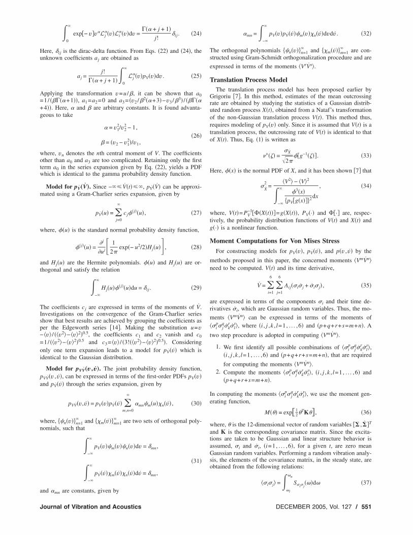
Fig. 1 Schematic diagram of the support for the fire-water sys-tem in a nuclear power plant; all dimensions are in mm

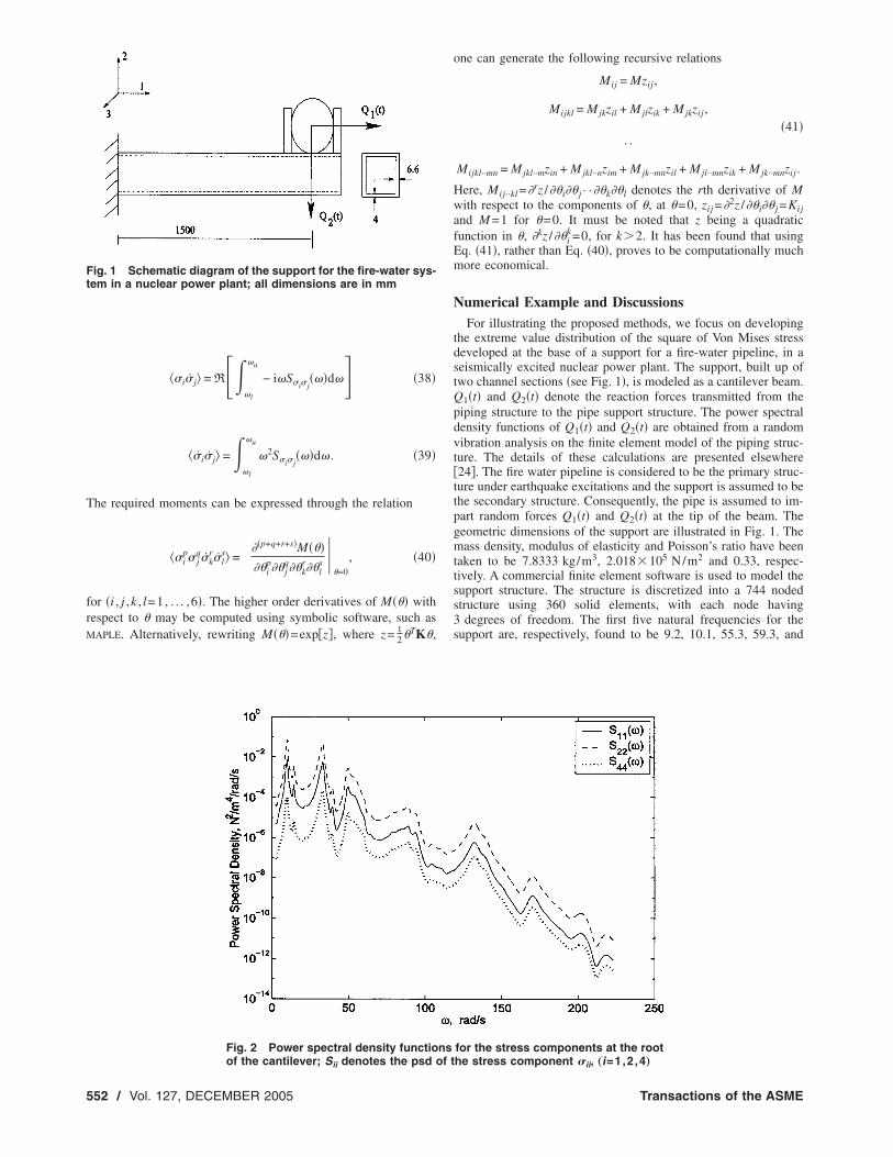
Fig. 2 Power spectral density functio

of the cantilever; Sii denotes the psd of t

552 / Vol. 127, DECEMBER 2005

one can generate the following recursive relations

Mij = Mzij ,

Mijkl = Mjkzil + Mjlzik + Mjkzij ,�41�

. .

Mijkl··mn = Mjkl··mzin + Mjkl··nzim + Mjk··mnzil + Mjl··mnzik + Mjk··mnzij .

Here, Mij··kl=�rz /��i�� j · ·��k��l denotes the rth derivative of Mwith respect to the components of �, at �=0, zij =�2z /��i�� j =Kijand M =1 for �=0. It must be noted that z being a quadraticfunction in �, �kz /��i

k=0, for k2. It has been found that usingEq. �41�, rather than Eq. �40�, proves to be computationally muchmore economical.

Numerical Example and DiscussionsFor illustrating the proposed methods, we focus on developing

the extreme value distribution of the square of Von Mises stressdeveloped at the base of a support for a fire-water pipeline, in aseismically excited nuclear power plant. The support, built up oftwo channel sections �see Fig. 1�, is modeled as a cantilever beam.Q1�t� and Q2�t� denote the reaction forces transmitted from thepiping structure to the pipe support structure. The power spectraldensity functions of Q1�t� and Q2�t� are obtained from a randomvibration analysis on the finite element model of the piping struc-ture. The details of these calculations are presented elsewhere�24�. The fire water pipeline is considered to be the primary struc-ture under earthquake excitations and the support is assumed to bethe secondary structure. Consequently, the pipe is assumed to im-part random forces Q1�t� and Q2�t� at the tip of the beam. Thegeometric dimensions of the support are illustrated in Fig. 1. Themass density, modulus of elasticity and Poisson’s ratio have beentaken to be 7.8333 kg/m3, 2.018�105 N/m2 and 0.33, respec-tively. A commercial finite element software is used to model thesupport structure. The structure is discretized into a 744 nodedstructure using 360 solid elements, with each node having3 degrees of freedom. The first five natural frequencies for thesupport are, respectively, found to be 9.2, 10.1, 55.3, 59.3, and

for the stress components at the root

ns he stress component �ii, „i=1,2,4…

Transactions of the ASME

rib

94.4 rad/s. Damping has been assumed to be viscous and propor-tional, with the mass and stiffness proportional constants taken tobe 0.19 and 0.0021, respectively. This leads to damping in the firsttwo modes to be equal to 2%. Since the pipes are not restrainedaxially, no forces act along the axis of pipe. Consequently, thestress components �3, �5, and �6 are small in comparison to theother three components and are taken to be zero. Thus, � in Eq.�36� is taken to be a six-dimensional vector��1 ,�2 ,�4 , �1 , �2 , �4�T. The PSD functions of the stress compo-nents are obtained from a random vibration analysis. Figure 2illustrates the PSD functions of the stress components �1�t�, �2�t�,and �4�t�. The shape factors for the PSD functions of �1�t�, �2�t�,and �4�t� are found to be, respectively, 0.4796, 0.4762, and0.4315.

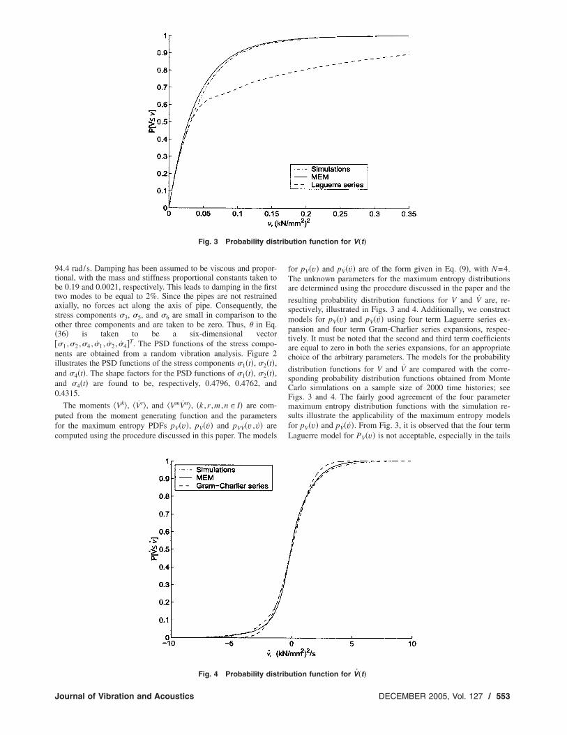
The moments �Vk�, �Vr�, and �VmVn�, �k ,r ,m ,n� I� are com-puted from the moment generating function and the parametersfor the maximum entropy PDFs pV�v�, pV�v� and pVV�v , v� arecomputed using the procedure discussed in this paper. The models

Fig. 3 Probability dist

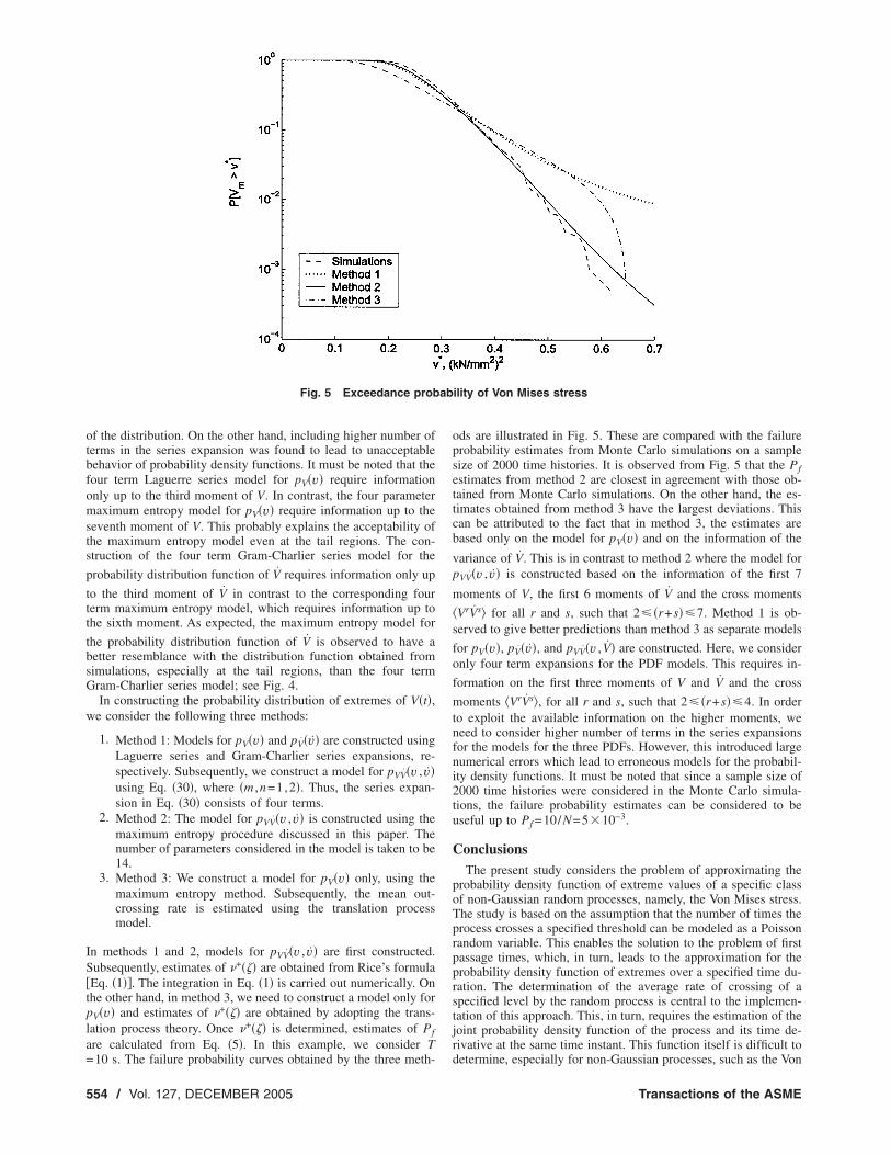
Fig. 4 Probability distrib

Journal of Vibration and Acoustics

for pV�v� and pV�v� are of the form given in Eq. �9�, with N=4.The unknown parameters for the maximum entropy distributionsare determined using the procedure discussed in the paper and the

resulting probability distribution functions for V and V are, re-spectively, illustrated in Figs. 3 and 4. Additionally, we constructmodels for pV�v� and pV�v� using four term Laguerre series ex-pansion and four term Gram-Charlier series expansions, respec-tively. It must be noted that the second and third term coefficientsare equal to zero in both the series expansions, for an appropriatechoice of the arbitrary parameters. The models for the probability

distribution functions for V and V are compared with the corre-sponding probability distribution functions obtained from MonteCarlo simulations on a sample size of 2000 time histories; seeFigs. 3 and 4. The fairly good agreement of the four parametermaximum entropy distribution functions with the simulation re-sults illustrate the applicability of the maximum entropy modelsfor pV�v� and pV�v�. From Fig. 3, it is observed that the four termLaguerre model for PV�v� is not acceptable, especially in the tails

ution function for V„t…

˙

ution function for V„t…

DECEMBER 2005, Vol. 127 / 553

ab

of the distribution. On the other hand, including higher number ofterms in the series expansion was found to lead to unacceptablebehavior of probability density functions. It must be noted that thefour term Laguerre series model for pV�v� require informationonly up to the third moment of V. In contrast, the four parametermaximum entropy model for pV�v� require information up to theseventh moment of V. This probably explains the acceptability ofthe maximum entropy model even at the tail regions. The con-struction of the four term Gram-Charlier series model for the

probability distribution function of V requires information only up

to the third moment of V in contrast to the corresponding fourterm maximum entropy model, which requires information up tothe sixth moment. As expected, the maximum entropy model for

the probability distribution function of V is observed to have abetter resemblance with the distribution function obtained fromsimulations, especially at the tail regions, than the four termGram-Charlier series model; see Fig. 4.

In constructing the probability distribution of extremes of V�t�,we consider the following three methods:

1. Method 1: Models for pV�v� and pV�v� are constructed usingLaguerre series and Gram-Charlier series expansions, re-spectively. Subsequently, we construct a model for pVV�v , v�using Eq. �30�, where �m ,n=1,2�. Thus, the series expan-sion in Eq. �30� consists of four terms.

2. Method 2: The model for pVV�v , v� is constructed using themaximum entropy procedure discussed in this paper. Thenumber of parameters considered in the model is taken to be14.

3. Method 3: We construct a model for pV�v� only, using themaximum entropy method. Subsequently, the mean out-crossing rate is estimated using the translation processmodel.

In methods 1 and 2, models for pVV�v , v� are first constructed.Subsequently, estimates of �+��� are obtained from Rice’s formula�Eq. �1��. The integration in Eq. �1� is carried out numerically. Onthe other hand, in method 3, we need to construct a model only forpV�v� and estimates of �+��� are obtained by adopting the trans-lation process theory. Once �+��� is determined, estimates of Pf

are calculated from Eq. �5�. In this example, we consider T

Fig. 5 Exceedance prob

=10 s. The failure probability curves obtained by the three meth-

554 / Vol. 127, DECEMBER 2005

ods are illustrated in Fig. 5. These are compared with the failureprobability estimates from Monte Carlo simulations on a samplesize of 2000 time histories. It is observed from Fig. 5 that the Pfestimates from method 2 are closest in agreement with those ob-tained from Monte Carlo simulations. On the other hand, the es-timates obtained from method 3 have the largest deviations. Thiscan be attributed to the fact that in method 3, the estimates arebased only on the model for pV�v� and on the information of the

variance of V. This is in contrast to method 2 where the model forpVV�v , v� is constructed based on the information of the first 7

moments of V, the first 6 moments of V and the cross moments

�VrVs� for all r and s, such that 2 �r+s�7. Method 1 is ob-served to give better predictions than method 3 as separate models

for pV�v�, pV�v�, and pVV�v , V� are constructed. Here, we consideronly four term expansions for the PDF models. This requires in-

formation on the first three moments of V and V and the cross

moments �VrVs�, for all r and s, such that 2 �r+s�4. In orderto exploit the available information on the higher moments, weneed to consider higher number of terms in the series expansionsfor the models for the three PDFs. However, this introduced largenumerical errors which lead to erroneous models for the probabil-ity density functions. It must be noted that since a sample size of2000 time histories were considered in the Monte Carlo simula-tions, the failure probability estimates can be considered to beuseful up to Pf =10/N=5�10−3.

ConclusionsThe present study considers the problem of approximating the

probability density function of extreme values of a specific classof non-Gaussian random processes, namely, the Von Mises stress.The study is based on the assumption that the number of times theprocess crosses a specified threshold can be modeled as a Poissonrandom variable. This enables the solution to the problem of firstpassage times, which, in turn, leads to the approximation for theprobability density function of extremes over a specified time du-ration. The determination of the average rate of crossing of aspecified level by the random process is central to the implemen-tation of this approach. This, in turn, requires the estimation of thejoint probability density function of the process and its time de-rivative at the same time instant. This function itself is difficult to

ility of Von Mises stress

determine, especially for non-Gaussian processes, such as the Von

Transactions of the ASME

Mises stress. The focus of the present study has been in examiningthe issues related to the determination of this joint probabilitydensity function. The study has examined the relative merits ofthree alternative approaches for the determination of pVV�v , v ; t�.These are based on a newly developed method that employs maxi-mum entropy principle, series expansion based method on com-bined Laguerre-Hermite series expansion and results based ontranslation process models. The study has focused on stationaryVon Mises stress process and, consequently, the process and itstime derivative, are uncorrelated at the same time instant. Whilelack of correlation between two Gaussian random variables implymutual independence, this, however, is not true for non-Gaussianquantities, such as the Von Mises stress and its time derivative atthe same time instant. The study examines the relative merits ofalternative methods for constructing pVV�v , v ; t� from the point ofview of their ability to handle mutual dependencies between V�t�and V�t�, computational requirements and closeness of the result-ing extreme value distribution to corresponding results fromMonte Carlo simulations. Based on this study, we conclude thatthe method based on bivariate maximum entropy distribution forpVV�v , v ; t� provides relatively, the most robust and satisfactorymeans for determining the extreme value distributions. The mod-els for extreme value distribution developed in this study are ex-pected to be of value in the context of reliability analysis of vi-brating structures in general, and in seismic fragility analysis ofengineering structures, in particular.

AcknowledgmentsThe work reported in this paper forms a part of research project

entitled “Seismic probabilistic safety assessment of nuclear powerplant structures,” funded by the Board of Research in NuclearSciences, Department of Atomic Energy, Government of India.

References�1� Nigam, N. C., 1983, Introduction to random vibrations, MIT Press, Massachu-

setts.�2� Lutes, L. D., and Sarkani, S., 1997, Stochastic analysis of structural and me-

chanical vibrations, Prentice Hall, New Jersey.�3� Rice, S. O., 1944, “Mathematical Analysis of Random Noise,” Bell Syst. Tech.

J., 23, pp. 282–332. Reprinted in Selected Papers in Noise and StochasticProcesses and Stochastic Processes, edited by N. Wax, Dover, New York,1954.

Journal of Vibration and Acoustics

�4� Breitung, K., and Rackwitz, R., 1982, “Nonlinear Combination of Load Pro-cesses,” J. Struct. Mech., 10, pp. 145–166.

�5� Pearce, H. T., and Wen, Y. K., 1985, “On Linearization Points for NonlinearCombination of Stochastic Load Processes,” Struct. Safety, 2, pp. 169–176.

�6� Wen, Y. K., 1990, Structural load modeling and combination for performanceand safety evaluation, Elsevier, Amsterdam.

�7� Grigoriu, M., 1984, “Crossings of Non-Gaussian Translation Processes,” J.Eng. Mech., 110�4�, pp. 610–620.

�8� Madsen, H., 1985, “Extreme Value Statistics for Nonlinear Load Combina-tion,” J. Eng. Mech., 111, pp. 1121–1129.

�9� Naess, A., 2001, “Crossing Rate Statistics of Quadratic Transformations ofGaussian Processes,” Probab. Eng. Mech., 16, pp. 209–217.

�10� Segalman, D., Fulcher, C., Reese, G., and Field, R., 2000, “An EfficientMethod for Calculating r.m.s. Von Mises Stress in a Random Vibration Envi-ronment,” J. Sound Vib., 230, pp. 393–410.

�11� Segalman, D., Reese, R., Field, C., and Fulcher, C., 2000, “Estimating theProbability Distribution of Von Mises Stress for Structures Undergoing Ran-dom Excitation,” J. Vibr. Acoust., 122, pp. 42–48.

�12� Reese, G., Field, R., and Segalman, D., 2000, “A Tutorial on Design AnalysisUsing Von Mises Stress in Random Vibration Environments,” Shock Vib. Dig.,32�6�, pp. 466–474.

�13� Gupta, S., and Manohar, C. S., 2004, “Improved Response Surface MethodFor Time Variant Reliability Analysis of Nonlinear Random Structures UnderNonstationary Excitations,” Nonlinear Dyn., 36, pp. 267–280.

�14� Deutsch, R., 1962, Nonlinear transformations of random processes,Engelwood-Cliffs: Prentice-Hall.

�15� Kapur, J. N., 1989, Maximum entropy models in science and engineering, JohnWiley and Sons, New Delhi.

�16� Rosenblueth, E., Karmeshu, E., and Hong, H. P., 1986, “Maximum Entropyand Discretization of Probability Distributions,” Probab. Eng. Mech., 2�2�, pp.58–63.

�17� Tagliani, A., 1989, “Principle of Maximum Entropy and Probability Distribu-tions: Definition of Applicability Field,” Probab. Eng. Mech., 4�2�, pp. 99–104.

�18� Tagliani, A., 1990, “On the Existence of Maximum Entropy Distributions WithFour and More Assigned Moments,” Probab. Eng. Mech., 5�4�, pp. 167–170.

�19� Sobczyk, K., and Trebicki, J., 1990, “Maximum Entropy Principle in Stochas-tic Dynamics,” Probab. Eng. Mech., 5�3�, pp. 102–110.

�20� Gupta, S., and Manohar, C. S., 2002, “Dynamic Stiffness Method for CircularStochastic Timoshenko Beams: Response Variability and Reliability Analysis,”J. Sound Vib., 253�5�, pp. 1051–1085.

�21� Hurtado, J. E., and Barbat, A. H., 1998, “Fourier Based Maximum EntropyMethod in Stochastic Dynamics,” Struct. Safety, 20, pp. 221–235.

�22� Volpe, E. V., and Baganoff, D., 2003, “Maximum Entropy PDFs and the Mo-ment Problem Under Near-Gaussian Conditions,” Probab. Eng. Mech., 18, pp.17–29.

�23� Chakrabarty, J., 1988, Theory of plasticity, McGraw-Hill, Singapore.�24� Manohar, C. S., and Gupta, S., 2004, “Seismic Probabilistic Safety Assessment

of Nuclear Power Plant Structures,” Project report, submitted to Board ofResearch in Nuclear Sciences, Government of India; Department of Civil En-gineering, Indian Institute of Science, Bangalore.

DECEMBER 2005, Vol. 127 / 555