clifem - climate forcing and erosion modelling in the sele river basin (southern italy

Nat. Hazards Earth Syst. Sci., 9, 1693–1702, 2009www.nat-hazards-earth-syst-sci.net/9/1693/2009/© Author(s) 2009. This work is distributed underthe Creative Commons Attribution 3.0 License.

Natural Hazardsand Earth

System Sciences

CliFEM – Climate Forcing and Erosion Modelling in the Sele RiverBasin (Southern Italy)

N. Diodato1, M. Fagnano2, and I. Alberico3

1TEDASS – Technologies Interdepartmental Center for the Environmental Diagnostic and Sustainable Development,University of Sannio, Via Bartolomeo Camerario 35, Benevento, Italy2DIAAT – Dipartimento Ingegneria Agraria e Agronomia del Territorio, University of Naples Federico II,Via Universita 100, Portici, Italy3CIRAM – Centro Interdipartimentale di Ricerca Ambiente, University of Naples Federico II,Via Mezzocannone 16, Napoli, Italy

Received: 15 January 2009 – Revised: 23 July 2009 – Accepted: 25 Aug 2009 – Published: 14 October 2009

Abstract. This study presents a revised and scale-adaptedFoster-Meyer-Onstad model (Foster et al., 1977) for thetransport of soil erosion sediments under scarce input data,with the acronym CliFEM (Climate Forcing and ErosionModelling). This new idea was addressed to develop amonthly time scale invariant Net Erosion model (NER),with the aim to consider the different erosion processesoperating at different time scales in the Sele River Basin(South Italy), during 1973–2007 period. The sediment de-livery ratio approach was applied to obtain an indirect es-timate of the gross erosion too. The examined period wasaffected by a changeable weather regime, where extremeevents may have contributed to exacerbate soil losses, al-though only the 19% of eroded sediment was delivered atoutlet of the basin. The long-term average soil erosion wasvery high (73 Mg ha−1 per year± 58 Mg ha−1). The estimateof monthly erosion showed catastrophic soil losses during thesoil tillage season (August–October), with consequent landdegradation of the hilly areas of the Sele River Basin.

1 Introduction

The full knowledge of climate drivers of soil erosionneeds extended meteorological, hydrological and land-coverrecords and the knowledge of the processes linking weatherand geomorphology at different time and spatial scales. Thenature of such linkages remains still poorly understood for

Correspondence to:I. Alberico([email protected])

several Mediterranean Europe river basins (Rickson, 2006),where there aren’t satisfactory geo-data series because ofmutability, discontinuity and sparsity of the available data(Poesen and Hooke, 1997a). In these basins, stream andtillage erosion probably are the dominant sediment sources(Poesen and Hooke, 1997b) and are considered an importantlimiting factor of farm soil fertility (Lal, 2001). Prolongedor accelerated erosion events cause irreversible soil losses,thus reducing soil ecological functions such as biomass pro-duction and filtering capacity (Gobin et al., 2004). Changesin the climate time patterns may have important effects onthe interaction among erosive rainfalls, vegetation covers andrunoff, which can affect soil degradation. In Mediterraneanareas, erosion is particularly pronounced both in the semi-arid regions (200–300 mm year−1), and in the sub-humidones (900–1500 mm year−1) and the strong variability in an-nual precipitation with frequent events of extreme rainfallsmay result in time-transgressive susceptibilities of regionalerosion (after Boardman and Favis-Mortlock, 2001). Manystudies were made on erosion simulations and on ecosys-tem responses to future climate changes (e.g., Newson andLewin, 1991; Easterling et al., 2000; Yang et al., 2003; Near-ing et al., 2005; Michael et al., 2005; Phillips et al., 2006;Quilbe et al., 2007), but few researches allowed to quantifythe effects of past climate variability on the dynamics of ge-omorphological processes (Rumsby, 2001; Diodato, 2006;Foster et al., 2008), while they study episodic impacts of ex-treme rainfalls (e.g., Gomez et al., 1997; Hooke and Mant,2000; Coppus and Imeson, 2002; Martınez-Casasnovas etal., 2002; Mul et al., 2008). Other researches are mainlybased on plot covers and soil types and they cannot bescaled up to catchment scales (Dickinson and Collins, 2007).

Published by Copernicus Publications on behalf of the European Geosciences Union.

http://creativecommons.org/licenses/by/3.0/

1694 N. Diodato et al.: CliFEM in the Sele River Basin

Although various models are reported in literature, it is dif-ficult to relate the occurrence of historical soil erosion ratesto climate variability because there aren’t long-term researchprojects in river basins, especially as regards the sedimentdata. Some authors (Larson et al., 1997; Boardman, 2006)stressed the need to study the driving variables of soil losswith an high frequency, for the importance of the extremerain time-clusters on climate aggressiveness and thus on soillosses.

According to the aforementioned Authors, our effort wasto produce monthly sediment budget, for develop a process-based time-scale invariant Net Erosion model (NER). After-wards, monthly, seasonal and annual gross erosion rates werecarried out within adown-scalingapproach by using Sed-iment Delivery Ratio (SDR), on the contrary ofup-scalingprocedure commonly used by RUSLE (Renard et al., 1997).As remarked by Larson et al. (1997), the USLE-RUSLE ap-proach is aimed to simulate the average long-term soil ero-sion, but it neglects land vulnerability during severe rain-storms because it was not designed to accurately simulatesoil losses of single events.

CliFEM approach, derived from Foster et al. (1977), wasdeveloped to include the major conceptual advantages ofsome erosion models. However, while NER model waslargely determined by the required experimental data, theSDR model was constrained by weakness of the availabledata in Sele River Basin. Another important characteristicof the NER model was to consider the different erosion pro-cesses at different time scales (from monthly to annual). Themajor weakness of the approach here proposed may be inthe sediment data quality, and in the consequent uncertaintyin Sediment Delivery Ratio, that is a critical point in manymodels (L. Borselli, personal communication, 2007).

2 Model description

The process-based monthly time scale invariant Net Erosionmodel (NER) was aimed to consider the erosion processesat different time scales. The amount of sediments from abasin (net erosion) is in fact generally much smaller than theamount indicated by soil loss rate (gross erosion). The ratiobetween net and gross erosion is the sediment delivery ratio(SDR). Considering then that only a fraction of the erodedsoils is transported to the basin outlet, as indicated by SDR,we can use this link to evaluate the soil amount removed bywater within the watershed slope. A well known relationshipto convert net erosion to gross soil loss is the following:

GER=NER

SDR(1)

where GER is the monthly gross soil loss, NER is the neterosion, and SDR is the sediment delivery ratio.

Data exploration, development and model performancewere supported by XLStatistics – Excel add-in Software forStatistical Data Analysis© Rodney Carr (1997–2007).

2.1 Process-based monthly Net Erosion (NER) model

In this study we expanded and adapted a sub-routine intro-duced by Foster et al. (1977) to take into account the runoffshear stress effect on soil detachment for single storms. Thenew Time Scale-Invariant process-based monthly Net ERo-sion (NERTSI) model was used for predicting monthly neterosion over medium basins (around 3000 km2). The hydro-logical ecosystem module, considers the interrelationships ofrainfall erosivity, runoff, erodibility and vegetation cover asfollows:

NERTSI=K·(α·EIm+β·Qm

)ψ·

exp(−γ ·

(NDVIm·100

))(2)

where the first term in bracket is the modified erosivity fac-tor as adapted by Foster et al. (1977), while the second termis the modified vegetation erosion exponential function, asadapted by Thornes (1990);K is the RUSLE erodibility fac-tor (Mg h MJ−1 mm−1) changing with basin soils, that wasset equal to 0.0362 (an approximate range ofK values can befounded in van der Knijff et al., 2000);α, β andψ are em-pirical parameters equal to 0.40, 0.60 and 2.05, respectively;γ is the parameter of the vegetation exponential function, setequal to 0.04 (early placed equal to 0.07 by Thornes, 1990).Note that the terms are averaged values upon an area (in ourcase of the basin-area).

Monthly rainfall erosivity at gauged stationEIm(MJ mm ha−1 h−1 month−1) was derived from rainfallmeasurements in the Italian area, according to RUSLEscheme (Diodato, 2005a):

EIm = 0.1174·

(√p · d0.53

· h1.18)

(3)

wherep is the monthly precipitation amount (mm),d isthe monthly maximum daily rainfall (mm), andh is themonthly maximum hourly rainfall (mm), respectively. In thisapproach,d andh are descriptors of the extreme rainfalls(storms and heavy showers respectively) (Diodato, 2005a).Since long series of meteorological variables do not includehourly rainfall intensities (i.e. the termh), the Eq. (3) wassimplified as in the Eq. (4) (Diodato and Bellocchi, 2009a):

EIm = 0.0400·

(p0.35

· d0.60· (d · αm)

0.70)

(4)

whereαm is a seasonal scale-factor in function of the month,m=1, . . . , 12:

αm =

[1 − 0.30 · cos

(2π

(m

26−m

))]3

(5)

Since with Eq. (3) it was not possible to have continuity inerosivity modelling between the first and the last time of the

Nat. Hazards Earth Syst. Sci., 9, 1693–1702, 2009 www.nat-hazards-earth-syst-sci.net/9/1693/2009/

N. Diodato et al.: CliFEM in the Sele River Basin 1695

series, the whole erosivity dataset was subjected to a rigorouscontrol of internal consistency (e.g., inspection and cross-check of the extremes of rain and hourly rain of the closeststations, zero of the erosivity values with temperature closeto zero degrees during cold rains, check of outlier values).

The erosivity value averaged over the basin was calcu-lated according to the following multiple linear regression(r2=0.93):

EIm = 0.684· EIm(P ) + 0.722· EIm(B) (6)

whereEIm(P ) andEIm(B) are the estimated rainfall erosivitywith Eq. (4) at Pontecagnano and Buccino stations, respec-tively.

In lack of experimental measurements (after 1994 year inthis specific case), monthly runoff (Qm) was estimated byadapting the Vandewiele et al. (1992) approach:

Qm = ηm ·

[pm − AETm

(0.5 − exp

(−

pm

AETm

))](7)

wherepm andAETm are the average values of rainfalls andactual evapotranspiration, respectively;ηm are the monthlyexperimental coefficients related to soil (see Table 1, firstrow). The performance of calibration made with 46 monthlydata was significant (r2=0.90).pm was estimated according to the following multiple non-

linear regression (r2=0.94):

pm =(pm(P )

)0.70+ 0.90 · pm(B) (8)

wherepm(P ) andpm(B) are the measured monthly rainfallsat Pontecagnano and Buccino stations, respectively.

Monthly AET was derived from Global Rapid IntegratedMonitoring System (Global-RIMS available at webpagehttp://rbis.sr.unh.edu/). For the last years (2001–2007), whereAET was not updated in RIMS-database, the following em-pirical sub-model was approached to transfer AET frompoint-site to averaged AET over the SRB compatible withRIMS output:

AETm = 0.570· AETm(P ) · (0.4 + νm)3+ 7.60 (9)

where AETm(P ) is the actual evapotranspiration at Pon-tecagnano site in mm month−1 (derived from RAN-UCEANetwork,www.ucea.it/), andνm are the monthly experimen-tal coefficients related to the soil moisture, (see Table 1, sec-ond row). Also in this case, the calibration process, madewith 24 RIMS monthly AET data, gave a significant correla-tion (r2=0.90).

NDVI-biomass seasonal regime was represented bymonthly MODIS (MOderate resolution Imaging Spectrora-diometer) composites, averaged on the 2000–2007 period,downloaded from Northern Eurasia Earth Science Partner-ship Initiative Monthly Products, NASA web site (http://disc.sci.gsfc.nasa.gov/techlab/giovanni/#maincontent/). Inthis first approach the NDVI seasonal regime over SRB was

set constant for the whole simulation period, since MODISNDVI data were not available before 2000 year. However,for accounting tillage erosion in Eq. (2) when running it forerosion reconstruction, the NDVI values were adjusted in au-tumn season multiplying it for the coefficients reported inTable 1 (third row).

2.2 Gross erosion evaluation

The simulation of daily SDR made with the Soil and WaterAssessment Tool – SWAT (Arnold and Williams, 1995) wasconceptually revised and adapted to the monthly scale by thefollowing equation:

SDRm=

(a + b

Qm

EIm

)c(10)

where the terms of the ratio are those described above;a, bandc are three coefficients equal to 0.035, 0.010 and 0.50respectively, derived imposing a values of SDR-long-termequal to 0.19, which, in turn, was supported by human-expert(L. Borselli, personal communication, 2007), and checked byCSIRO abaco (Lu et al., 2003) on the basis of the basin areaand the storm duration.

2.3 Estimation of tolerable soil loss

Since the effects of soil erosion on soil productivity dependon the depth of these soils, it is possible to define the tolerableamount of soil loss when the soil depth of an area is known.Combining the information gathered on topsoil loss depth(Sd) and proportion of land degraded (PLD), the tolerablesoil loss (TSL) may be calculated by using the Bhattacharyyaet al. (2007) approach:

TSL=PLD ·D · Sp

T(11)

where PLD is the proportion of land downgraded to at leastthe next depth class (%, assumed equal to 15%),T is thetime (years, assumed equal to 100),D is the bulk density ofthe soil (assumed equal to 1.4 Mg m−3), Sd is the soil depth(assumed equal to 130 cm).

3 Results and discussions

3.1 Study site

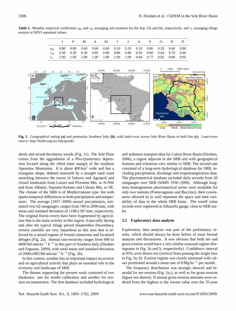
The Sele River Basin (SRB) is located across the SouthernCampania and Western Basilicata regions (Fig. 1). The basincan be divided in two main zones: the dolomitic limestonezone, in the mountainous and hilly areas, and the marine-alluvial zone, in the plainy areas. The 130-km length Seleriver starts in the Cervati Mountains (1855 m a.s.l.), its basincovers an area of about 3000 km2 extending to adjacent Seleplain characterized by different land uses, such as crops,

www.nat-hazards-earth-syst-sci.net/9/1693/2009/ Nat. Hazards Earth Syst. Sci., 9, 1693–1702, 2009

http://rbis.sr.unh.edu/

http://rbis.sr.unh.edu/

www.ucea.it/

http://disc.sci.gsfc.nasa.gov/techlab/giovanni/#maincontent/

http://disc.sci.gsfc.nasa.gov/techlab/giovanni/#maincontent/


Table 1. Monthly empirical coefficientsηm andνm arranging soil moisture for the Eqs. (5) and (6), respectively, andτc arranging tillageerosion in NDVI autumnal values.

J F M A M J J A S O N D

ηm 0.80 0.80 0.60 0.60 0.40 0.10 0.10 0.10 0.06 0.20 0.40 0.80νm 0.30 0.30 0.30 0.85 0.80 0.80 0.80 0.50 0.60 0.64 0.70 0.40τc 1.00 1.00 1.00 1.00 1.00 1.00 1.00 0.94 0.77 0.82 0.89 0.95

17°0'0"E

17°0'0"E

16°0'0"E

16°0'0"E

15°0'0"E

15°0'0"E

14°0'0"E

14°0'0"E

42°0

'0"N

42°0

'0"N

41°0

'0"N

41°0

'0"N

40°0

'0"N

40°0

'0"N

320016008000 KilometersRobinson ProjectionCentral Meridian: 30.00

Atlantic Ocean

Black Sea

Mediterranean Sea

Caspian Sea

Balti

c Sea

North Sea

Arctic Ocean

Arctic Circle

50°

50°

30°

30°

10°

10°

-10°

-10°-30°-50°

80°

80°

60°

60°

40°

40°

20°

20°

a) b)

Meters0 20000 40000

UTM 33 E (m)

UTM

33

N (m

)

490000 525000 560000

4440

000

4480

000

4520

000Sele River Basinc)

ThyrrhenianSea

Crop Shrub Mixed-Decid Forest

Fig. 1. Geographical setting(a) and peninsular Southern Italy(b), with land-cover across Sele River Basin in bold line(c). Land-coversource:http://hydis.eng.uci.edu/gwadi/.

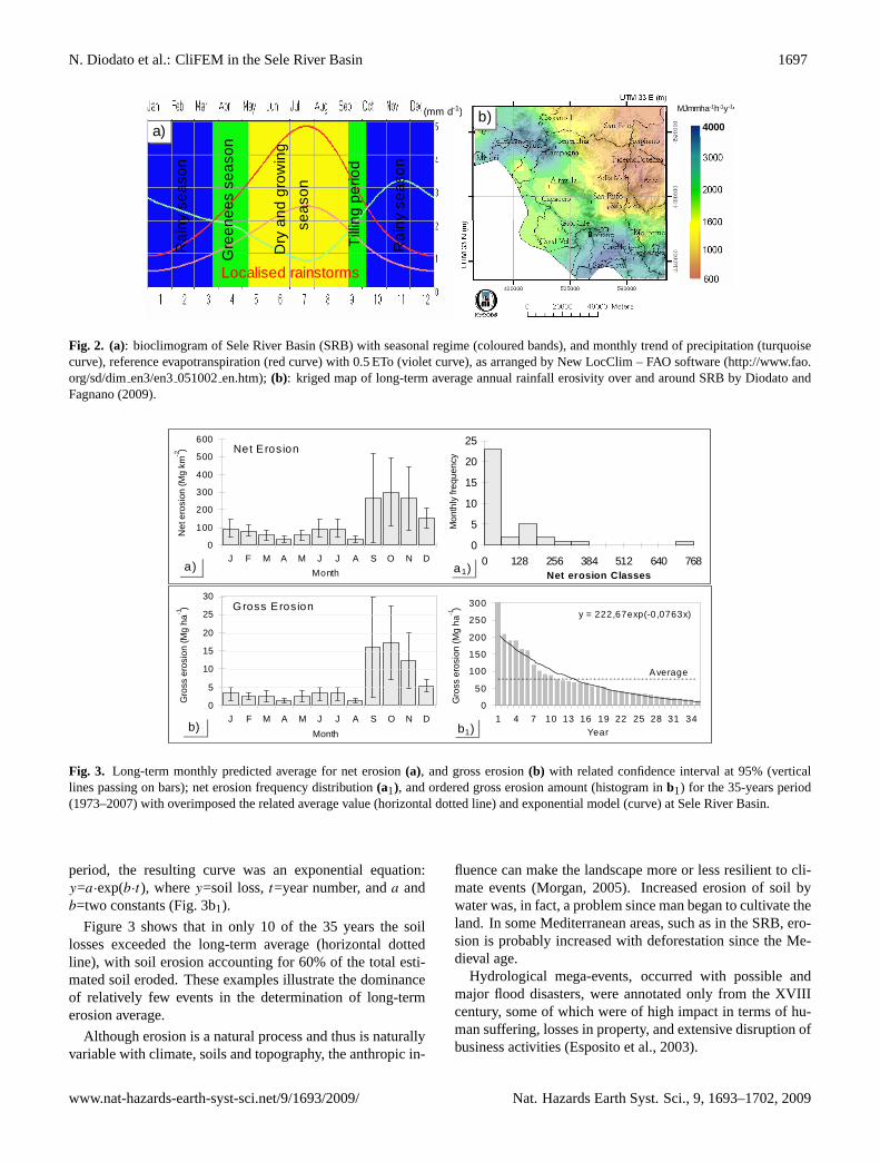
shrub and mixed-deciduous woods (Fig. 1c). The Sele Plaincomes from the aggradation of a Plio-Quaternary depres-sion located along the rifted inner margin of the southernApennine Mountains. It is about 400 km2 wide and has atriangular shape, defined seawards by a straight sand coaststretching between the towns of Salerno and Agropoli andclosed landwards from Lattari and Picentini Mts. to N-NWand from Alburni, Soprano-Sottano and Cilento Mts. to SE.The climate of the SRB is ofMediterraneantype, but withspatio-temporal differences in both precipitation and temper-ature. The average (1957–2000) annual precipitation, esti-mated over 62 raingauges, ranges from 700 to 2000 mm, withmean and standard deviation of 1180±367 mm, respectively.The original forest-covers have been fragmented by agricul-ture that is the main activity in this region. Especially duringand after the typical tillage period (September–December),erosive rainfalls are very hazardous in this area that is af-fected by a mixed regime of frontal rainstorms and localiseddeluges (Fig. 2a). Annual rain-erosivity ranges from 600 to4000 MJ mm ha−1 h−1 in this part of Southern Italy (Diodatoand Fagnano, 2009), with areal mean and standard deviationof 2000±883 MJ mm ha−1 h−1 (Fig. 2b).

In this context, weather has an important impact on erosionand on agricultural activity that plays an essential role in theeconomy and landscape of SRB.

The dataset supporting the present work consisted of twodatabases: one for model calibration and another for ero-sion reconstruction. The first database included hydrological

and sediment transport data for Calore River Basin (Diodato,2006), a region adjacent to the SRB and with geographicalfeatures and extension very similar to SRB. The second oneconsisted of a long-term hydrological database for SRB, in-cluding precipitation, discharge and evapotranspiration data.The pluviometrical database included daily records from 50raingauges over SRB (SIMN 1950–2000). Although long-term homogeneous pluviometrical series were available foronly two stations (Pontecagnano and Buccino), their consis-tence allowed us to well represent the space and time vari-ability of data in the whole SRB basin. The runoff valuerecords were registered at Albanella gauge, close to SRB out-let.

3.2 Exploratory data analysis

Exploratory data analysis was part of the preliminary re-sults, which should always be done before of more formalanalysis and discussions. It was obvious that both net andgross erosion would have a very similar seasonal regime (his-tograms in Fig. 3a and b, respectively). Confidence intervalat 95% were drawn too (vertical lines passing the single barsin Fig. 3a, b). Erosion regime was clearly autumnal with val-ues positioned around a mean rate of 8 Mg ha−1 per month.

The frequency distribution was strongly skewed and bi-modal for net erosion (Fig. 5a1), as well as for gross erosion(figure not shown). If annual gross erosion amounts were or-dered from the highest to the lowest value over the 35-year


http://hydis.eng.uci.edu/gwadi/


a)

Tillin

g pe

riod

Gre

enee

s se

ason

Dry

and

gro

win

gse

ason

Rai

ny s

easo

n

Rai

ny s

easo

n

Localised rainstorms

b)4000

MJmmha-1h-1y-1(mm d-1)

Fig. 2. (a): bioclimogram of Sele River Basin (SRB) with seasonal regime (coloured bands), and monthly trend of precipitation (turquoisecurve), reference evapotranspiration (red curve) with 0.5 ETo (violet curve), as arranged by New LocClim – FAO software (http://www.fao.org/sd/dimen3/en3051002en.htm); (b): kriged map of long-term average annual rainfall erosivity over and around SRB by Diodato andFagnano (2009).

0

5

10

15

20

25

0 128 256 384 512 640 768J

Freq

uenc

y

0

100

200

300

400

500

600

J F M A M J J A S O N DMonth

X

Mon

thly

freq

uenc

y

a 1)a)

Net

ero

sion

(Mg

km -2) Net Erosion

Net erosion Classes

0

50

100

150

200

250

300

1 4 7 10 13 16 19 22 25 28 31 34Year

X

0

5

10

15

20

25

30


X

q

Gross Erosion

b1)

Gro

ss e

rosi

on (M

g ha

-1)

y = 222,67exp(-0,0763x)

Average

Gro

ss e

rosi

on (M

g ha

-1)

b)

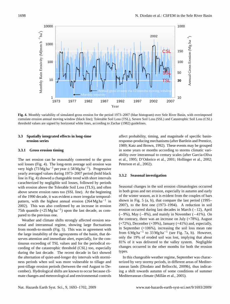
Fig. 3. Long-term monthly predicted average for net erosion(a), and gross erosion(b) with related confidence interval at 95% (vertical

lines passing on bars); net erosion frequency distribution(a1), and ordered gross erosion amount (histogram inb1) for the 35-years period(1973–2007) with overimposed the related average value (horizontal dotted line) and exponential model (curve) at Sele River Basin.

period, the resulting curve was an exponential equation:y=a·exp(b·t), wherey=soil loss,t=year number, anda andb=two constants (Fig. 3b1).

Figure 3 shows that in only 10 of the 35 years the soillosses exceeded the long-term average (horizontal dottedline), with soil erosion accounting for 60% of the total esti-mated soil eroded. These examples illustrate the dominanceof relatively few events in the determination of long-termerosion average.

Although erosion is a natural process and thus is naturallyvariable with climate, soils and topography, the anthropic in-

fluence can make the landscape more or less resilient to cli-mate events (Morgan, 2005). Increased erosion of soil bywater was, in fact, a problem since man began to cultivate theland. In some Mediterranean areas, such as in the SRB, ero-sion is probably increased with deforestation since the Me-dieval age.

Hydrological mega-events, occurred with possible andmajor flood disasters, were annotated only from the XVIIIcentury, some of which were of high impact in terms of hu-man suffering, losses in property, and extensive disruption ofbusiness activities (Esposito et al., 2003).


http://www.fao.org/sd/dim_en3/en3_051002_en.htm

http://www.fao.org/sd/dim_en3/en3_051002_en.htm


1

10

100

1000

10000

1 13 25 37 49 61 73 85 97 109121133145157169181193205217229241253265277289301313325337349361373385397409421

Year

10

100

1000

150

Ann

ual G

ross

Ero

sion

(Mg

ha

-1)

Mon

thly

Rai

n Er

osiv

ity (M

Jmm

h

-1 h

a-1)

30

CSL

TSL

SSL 50

Annual gross erosion via 12-months moving windowMonthly erosivity

2002

1973 1977 1982 1987 1992 1997 2002 2007

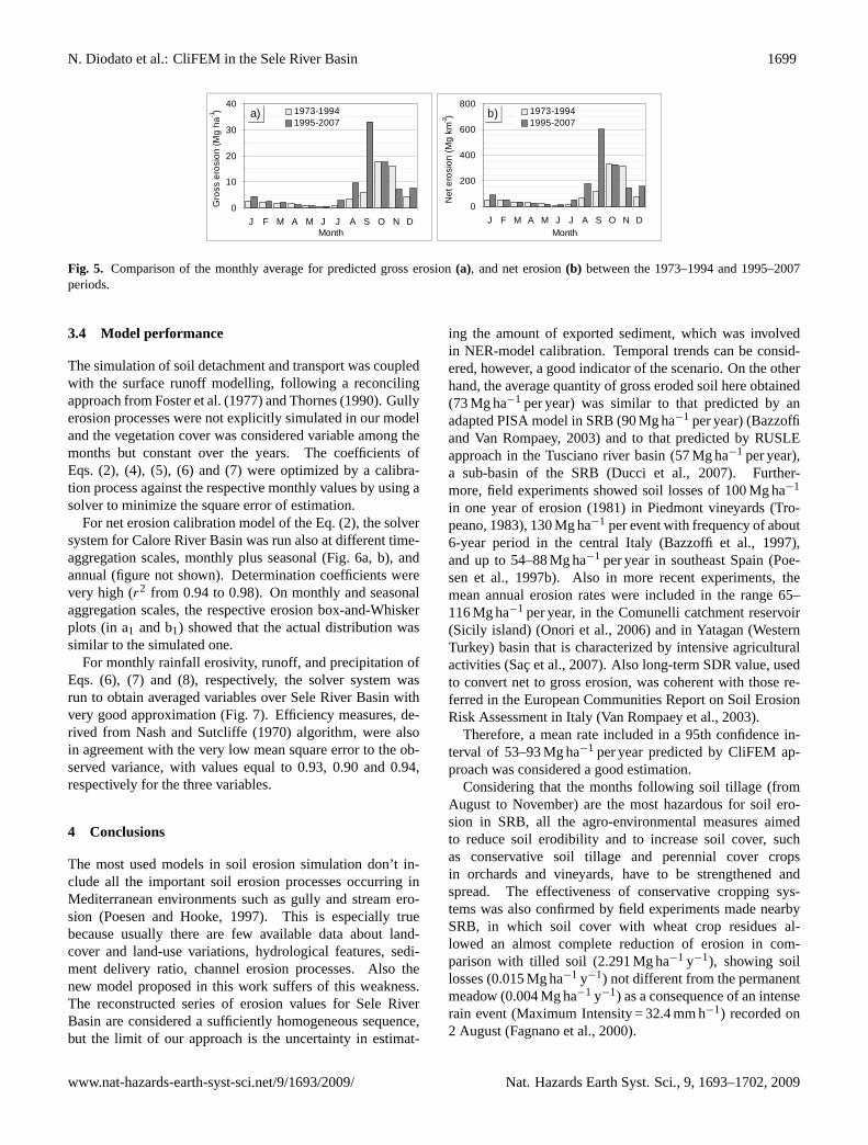
Fig. 4. Monthly variability of simulated gross erosion for the period 1973–2007 (blue histogram) over Sele River Basin, with overimposedcumulate erosion annual moving window (black line); Tolerable Soil Loss (TSL), Severe Soil Loss (SSL) and Catastrophic Soil Loss (CSL)threshold values are signed by horizontal white lines, according to Zachar (1982) guidelines.

3.3 Spatially integrated effects in long-timeerosion series

3.3.1 Gross erosion timing

The net erosion can be reasonably converted to the grosssoil losses (Fig. 4). The long-term average soil erosion wasvery high (73 Mg ha−1 per year± 58 Mg ha−1). Progressiveyearly averaged values during 1973–2007 period (bold blackline in Fig. 4) showed a changeable trend with short intervalscarachterized by negligible soil losses, followed by periodswith erosion above the Tolerable Soil Loss (TLS), and oftenabove severe erosion rates too (SSL line). At the beginningof the 1990 decade, it was evident a more irregular temporal-pattern, with the highest annual erosion (264 Mg ha−1 in2002). This was also confirmed by an increase in erosion75th quantile (+25 Mg ha−1) upon the last decade, as com-pared to the previous one.

Weather and climate shifts strongly affected erosion sea-sonal and interannual regime, showing large fluctuationsfrom month-to-month (Fig. 5). This was in agreement withthe large instability of the agrosystems of the basin, that de-serves attention and immediate alert, especially, for the con-tinuous exceeding of TSL values and for the periodical ex-ceeding of the catastrophic threshold (CSL) too, especiallyduring the last decade. The recent decade in fact showedthe alternation of quiet-and-longer dry intervals with stormi-ness periods when soil was more vulnerable to tillage andpost-tillage erosion periods (between the end August to De-cember). Hydrological shifts are known to occur because cli-mate changes and meteorological and environmental controls

affect probability, timing, and magnitude of specific basin-response-producing mechanisms (after Bartlein and Prentice,1989; Katz and Brown, 1992). These events may be groupedin some years or months according to storms climatic vari-ability over interannual to century scales (after Garcia-Olivaet al., 1995; D’Odorico et al., 2001; Hollinger et al., 2002;Peterson et al., 2002).

3.3.2 Seasonal investigation

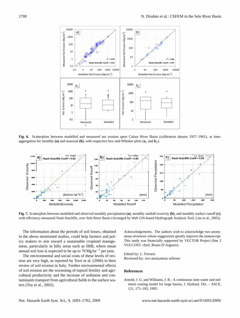
Seasonal changes in the soil erosion climatologies occurredin both gross and net erosion, especially in autumn and earlyof the winter season, as it is evident from the couples of barsshown in Fig. 5 (a, b), that compare the last period (1995–2007), to the first one (1973–1994). A reduction in soilerosion occurred during last decades in March (−12), April(−9%), May (−8%), and mainly in November (−41%). Onthe contrary, there was an increase on July (+78%), August(+72%), December (+39%), January (+41%) and, especially,in September (+106%), increasing the soil loss mean ratefrom 6 Mg ha−1 to 33 Mg ha−1 (see Fig. 7a, b). However,only the 19% of eroded soil was lost, implying that about81% of it was delivered to the valley system. Negligiblechanges occurred in the other months for both the erosiontypes.

In this changeable weather regime, September was charac-terized by very stormy periods, in different areas of Mediter-ranean lands (Diodato and Bellocchi, 2009b), thus indicat-ing a shift towards autumn of some conditions of summerMediterranean climate (Millan et al., 2005).



0

10

20

30

40


%

1973-19941995-2007

0

200

400

600

800


%

1973-19941995-2007

Gro

ss e

rosi

on (M

g ha

-1)

Net

ero

sion

(Mg

km

-2)a) b)

Fig. 5. Comparison of the monthly average for predicted gross erosion(a), and net erosion(b) between the 1973–1994 and 1995–2007periods.

3.4 Model performance

The simulation of soil detachment and transport was coupledwith the surface runoff modelling, following a reconcilingapproach from Foster et al. (1977) and Thornes (1990). Gullyerosion processes were not explicitly simulated in our modeland the vegetation cover was considered variable among themonths but constant over the years. The coefficients ofEqs. (2), (4), (5), (6) and (7) were optimized by a calibra-tion process against the respective monthly values by using asolver to minimize the square error of estimation.

For net erosion calibration model of the Eq. (2), the solversystem for Calore River Basin was run also at different time-aggregation scales, monthly plus seasonal (Fig. 6a, b), andannual (figure not shown). Determination coefficients werevery high (r2 from 0.94 to 0.98). On monthly and seasonalaggregation scales, the respective erosion box-and-Whiskerplots (in a1 and b1) showed that the actual distribution wassimilar to the simulated one.

For monthly rainfall erosivity, runoff, and precipitation ofEqs. (6), (7) and (8), respectively, the solver system wasrun to obtain averaged variables over Sele River Basin withvery good approximation (Fig. 7). Efficiency measures, de-rived from Nash and Sutcliffe (1970) algorithm, were alsoin agreement with the very low mean square error to the ob-served variance, with values equal to 0.93, 0.90 and 0.94,respectively for the three variables.

4 Conclusions

The most used models in soil erosion simulation don’t in-clude all the important soil erosion processes occurring inMediterranean environments such as gully and stream ero-sion (Poesen and Hooke, 1997). This is especially truebecause usually there are few available data about land-cover and land-use variations, hydrological features, sedi-ment delivery ratio, channel erosion processes. Also thenew model proposed in this work suffers of this weakness.The reconstructed series of erosion values for Sele RiverBasin are considered a sufficiently homogeneous sequence,but the limit of our approach is the uncertainty in estimat-

ing the amount of exported sediment, which was involvedin NER-model calibration. Temporal trends can be consid-ered, however, a good indicator of the scenario. On the otherhand, the average quantity of gross eroded soil here obtained(73 Mg ha−1 per year) was similar to that predicted by anadapted PISA model in SRB (90 Mg ha−1 per year) (Bazzoffiand Van Rompaey, 2003) and to that predicted by RUSLEapproach in the Tusciano river basin (57 Mg ha−1 per year),a sub-basin of the SRB (Ducci et al., 2007). Further-more, field experiments showed soil losses of 100 Mg ha−1

in one year of erosion (1981) in Piedmont vineyards (Tro-peano, 1983), 130 Mg ha−1 per event with frequency of about6-year period in the central Italy (Bazzoffi et al., 1997),and up to 54–88 Mg ha−1 per year in southeast Spain (Poe-sen et al., 1997b). Also in more recent experiments, themean annual erosion rates were included in the range 65–116 Mg ha−1 per year, in the Comunelli catchment reservoir(Sicily island) (Onori et al., 2006) and in Yatagan (WesternTurkey) basin that is characterized by intensive agriculturalactivities (Sac et al., 2007). Also long-term SDR value, usedto convert net to gross erosion, was coherent with those re-ferred in the European Communities Report on Soil ErosionRisk Assessment in Italy (Van Rompaey et al., 2003).

Therefore, a mean rate included in a 95th confidence in-terval of 53–93 Mg ha−1 per year predicted by CliFEM ap-proach was considered a good estimation.

Considering that the months following soil tillage (fromAugust to November) are the most hazardous for soil ero-sion in SRB, all the agro-environmental measures aimedto reduce soil erodibility and to increase soil cover, suchas conservative soil tillage and perennial cover cropsin orchards and vineyards, have to be strengthened andspread. The effectiveness of conservative cropping sys-tems was also confirmed by field experiments made nearbySRB, in which soil cover with wheat crop residues al-lowed an almost complete reduction of erosion in com-parison with tilled soil (2.291 Mg ha−1 y−1), showing soillosses (0.015 Mg ha−1 y−1) not different from the permanentmeadow (0.004 Mg ha−1 y−1) as a consequence of an intenserain event (Maximum Intensity = 32.4 mm h−1) recorded on2 August (Fagnano et al., 2000).



Y X1

10

100

1000

10000

aY X0,1

1

10

100

1000

10000

w

Net

Ero

sion

(Mg

km

-2)

a1

Measured ModelledN

et E

rosi

on (M

g km

-2)

b1

Measured Modelled

0

1

10

100

1000

10000

0,1 1 10 100 1000 10000

Modelled Net Erosion (Mg km-2)

1

10

100

1000

10000

1 10 100 1000 10000

Modelled Net Erosion (Mg km-2)

b)

Mea

sure

d N

et E

rosi

on (M

g km

-2)

r2 = 0.94

a)

0,1Nash-Sutcliffe Coeff = 0.94

r2 = 0.95

Nash-Sutcliffe Coeff = 0.97

Mea

sure

d N

et E

rosi

on (M

g km

-2)

Fig. 6. Scatterplots between modelled and measured net erosion upon Calore River Basin (calibration dataset 1957–1961), at time-aggregation for monthly(a) and seasonal(b), with respective box-and-Whisker plots (a1 andb1).

ModelledErosivity

Obs

erve

d E

rosi

vity

a) Nash-Sutcliffe Coeff = 0.93

(MJmm ha-1h-1)

Modelled Runoff

Obs

erve

d R

unof

f

b) Nash-Sutcliffe Coeff = 0.90

Modelled Precipitation

Obs

erve

d P

reci

pita

tion

c) Nash-Sutcliffe Coeff = 0.94

(mm) (mm)

Fig. 7. Scatterplots between modelled and observed monthly precipitation(a), monthly rainfall erosivity(b), and monthly surface runoff(c),with efficiency-measured Nash-Sutcliffe, over Sele River Basin (Arranged by Web GIS-based Hydrograph Analysis Tool, Lim et al., 2005).

The information about the periods of soil losses, obtainedin the above mentioned studies, could help farmers and pol-icy makers to aim toward a sustainable cropland manage-ment, particularly in hilly areas such as SRB, where meanannual soil loss is expected to be up to 70 Mg ha−1 per year.

The environmental and social costs of these levels of ero-sion are very high, as reported by Torri et al. (2006) in theirreview of soil erosion in Italy. Further environmental effectsof soil erosion are the worsening of topsoil fertility and agri-cultural productivity and the increase of sediment and con-taminants transport from agricultural fields to the surface wa-ters (Toy et al., 2002).

Acknowledgements.The authors wish to acknowledge two anony-mous reviewers whose suggestions greatly improve the manuscript.This study was financially supported by VECTOR Project (line 2VULCOST- chief, Bruno D’Argenio).

Edited by: L. FerrarisReviewed by: two anonymous referees

References

Arnold, J. G. and Williams, J. R.: A continuous time water and sed-iment routing model for large basins, J. Hydraul. Div. – ASCE,121, 171–183, 1995.



Bartlein, P. J. and Prentice, I C.: Orbital variations, climate andpaleoecology, Trends Ecol. Evol., 4, 195–199, 1989.

Bhattacharyya, T., Babu, R., Sarkar, D., Mandal, C., Dhyani, B. L.,and Nagar, A. P.: Soil loss and crop productivity model in humidsubtropical India, Curr. Sci. India, 93, 1397–1403, 2007.

Bazzoffi, P., Pellegrini, S., Chisci, G., Papini, R., and Scagnozzi, A.:Erosion and discharge at catchment and field scales in argilloussoils ad different use in Era Valley, Agricoltura Ricerca, 170, 5–20, 1997 (in Italian).

Bazzoffi, P. and Van Rompaey, A.: PISA model to assess off-farm sediment flow indicator at watershed scale in Italy. In Proc.OECD: Agricultural impacts on soil erosion and soil biodiver-sity: developing indicators for policy analysis, Rome, 263–272,25–28 March 2003.

Boardman, J. D. and Favis-Mortlock, T.: How will future climatechange and land-use change affect rates of erosion on agricul-tural land, in: Soil Erosion Research for the 21st Century, Am.Soc. Agric. Biol. Eng., Honolulu, Hawaii, 498–501, 3–5 January2001.

Boardman, J.: Soil erosion science: Reflections on the limitationsof current approaches, Catena, 68, 73–86, 2006.Coppus, R. and Imeson, A. C.: Extreme events controlling ero-sion and sediment transport in a semi-arid sub-Andean Valley,Earth Surf. Proc. Land., 27, 1365–1375, 2002.

Dickinson, A. and Collins, R.: Predicting erosion and sedimentyield at catchment scale, in: Soil Erosion Multiple Scales, editedby: Penning de Vries, F. W. T., Agus, F., and Kerr, J., CABIPublishing, 317–342, 2007.

Diodato, N.: Predicting RUSLE (Revised Universal Soil Loss Equa-tion) monthly erosivity index from readily available rainfall datain Mediterranean area, The Environmentalist, 26, 63–70, 2005.

Diodato, N.: Modelling net erosion responses to enviroclimaticchanges recorded upon multisecular timescales, Geomorphol-ogy, 80, 164–177, 2006.

Diodato, N. and Bellocchi, G.: Assessing and modelling changesin rainfall erosivity at different climate scales, Earth Surf. Proc.Land., 34(7), 969–980, 2009a.

Diodato, N. and Bellocchi, G.: Environmental implications of ero-sive rainfall across the Mediterranean, in: Environmental impactassessments, edited by: Halley, G. T. and Fridian, Y. T., NOVAPublishers, New York, NY, USA, 75–101, 2009b.

Diodato, N. and Fagnano, M.: A simple geospatial model climate-based for designing erosive rainfall pattern, in: The Environ-mental Pollution and its relation to Climate Change, edited by:El Nemr, A., in press, Springer, Nova Science Publishers, USA,2009.

D’Odorico, P., Yoo, J., and Over, T. M.: An assessment of ENSO-induced patterns of rainfall erosivity in the Southwestern UnitedStates, J. Climate, 14, 4230–4242, 2001.

Ducci, D., Giugni, M., and Zampoli, M.: Evaluation of soil ero-sion process of the Tusciano river basin. In Proceeding: Soil andhillslope management using analysis and Runoff-erosion mod-els: a critical evaluation of current technique, COST 634, Flo-rence (Italy), 7–9 May 2007.

Easterling, D. R., Evans, J. L., Ya Groisman, P., Karl, T. R., Kunkel,K. E., and Ambenje, P.: Observed variability and trends in ex-treme climate events: a brief review, B. Am. Meteorol. Soc., 81,417–425, 2000.

Esposito, E., Porfido, S., Violant, C., and Alaia, F.: Disaster induced

by historical floods in a selected coastal area (Southern Italy), in:PHEFRA – Paleofloods, Historical Data & Climatic Variability:Application in Flood Risk Assessmen, edited by: Thorndycraft,V. R., Benito, G., Barriendos, M., and Lalsat, M. C., Barcellona,143–148, 2003.

Fagnano, M., Mori, M., Carone, F., and Postiglione, L.: Sistemicolturali per l’Appennino meridionale: Nota II. Deflussi ed ero-sione, Rivista di Agronomia, 34, 55–64, 2000 (in Italian).

Favis-Mortlock, D. T., Boardman, J., and MacMillan, V. J.: Thelimits of erosion modeling: why we should proceed with care, in:Landscape Erosion and Evolution Modeling edited by: Harmon,R. S. and Doe III, W. W., Kluwer Academic/Plenum Publishing,New York, 477–516, 2001.

Foster, G. R., Meyer, L. D., and Onstad, C. A.: A runoff erosivityfactor and variable slope length exponents for soil loss estimates,T. ASAE, 20, 683–687, 1977.

Foster, G. C., Chiverrell, R. C., Harvey, A. M., Dearing, J. A., andDunsford, H.: Catchment hydro-geomorphological responses toenvironmental change in the Southern Uplands of Scotland, TheHolocene 18, 935–950, 2008.

Garcia-Oliva, F., Maass, J. M., and Galicia, L.: Rainstorm analysisand rainfall erosivity of a seasonal tropical region with a strongcyclonic influence on the Pacific Coast of Mexico, J. Appl. Me-teorol., 34, 2491–2498, 1995.

Gobin, A., Jones, R., Kirkby, M., Campling, P., Govers, G., Kos-mas, C., and Gentile, A. R.: Indicators for pan-European assess-ment and monitoring of soil erosion by water, Environ. Sci. Pol-icy, 7, 25–38, 2004.

Gomez, B., Phillips, J. D., Migilligan, F. J., and James, L. A.:Floodplain sedimentation and sensitivity: summer 1993 flood,Upper Mississippi river valley, Earth Surf. Proc. Land., 22, 923–936, 1997.

Hollinger, S. E., Angel, J. R., and Palecki, M. A.: Spatial distri-bution, variation and trends in storm precipitation characteristicsassociated with soil erosion in the United States, Champaign, IL:United States Department of Agriculture and Atmospheric Envi-ronment Section (Illinois State Water Survey), 2002.

Hooke, D. D. and Mant, J. M.: Geomorphological impacts of aflood event of ephemeral cannels in SE Spain, Geomorphology,34, 163–180, 2000.

Katz, R. W. and Brown, B. G.: Extreme events in a changingclimate: Variability is more important than average, ClimaticChange, 21, 289–302, 1992.

Lal, R.: Soil degradation by erosion, Land Degrad. Dev., 12, 520–539, 2001.

Larson, W. E., Lindstrom, M. J., Schumacher, and T. E.: The roleof severe storm in soil erosion: a problem needing consideration,J. Soil Water Conserv., 52, 90–95, 1997.

Lim, K. J., Engel, B. A., Tang, Z., Choi, J., Kim, K., Muthukrish-nan, S., and Tripathy, D.: Web GIS-based Hydrograph AnalysisTool, WHAT, J. Am. Water Resour. As., 41(6), 1407–1416, 2005.

Lu, H., Moran, C. J., Prosser, I. P., Raupach, R. M., Olley, J., andPetheram, C.: Sheet an rill erosion sediment delivery to streams:a basin wide estimation at hillslope to Medium catchment scale,Report E to Project D10012, CSIRO Technical Report 15/03, 56pp., 2003.

Martınez-Casasnovas, J. A., Ramos, M. C., and Ribes-Dasi, M.:Soil erosion caused by extreme rainfall events: mapping andquantification in agricultural plots from very detailed digital ele-



vation models, Geoderma, 105, 125–140, 2002.Michael, A. J., Schmidt, W., Deutschlander, E. T., and Malitz, G.:

Impact of expected increase in precipitation intensities on soilloss results of comparative model simulations, Catena, 61, 155–164, 2005.

Morgan, R. P. C.: Soil erosion and conservation, 3rd edn., Black-well Publishing Science Ltd., 304 pp., 2005.

Mul, M. L., Savenije, H. H. G., and Uhlenbrook, S.: Spatial rainfallvariability and runoff response during an extreme event in a semi-arid catchment in the South Pare Mountains, Tanzania, Hydrol.Earth Syst. Sci. Discuss., 5, 2657–2685, 2008,http://www.hydrol-earth-syst-sci-discuss.net/5/2657/2008/.

Nearing, M. A., Jetten, V., Baffaut, C., Cerdan, O., Couturier, A.,Hernandez, M., Le Bissonnais, Y., Nichols, M. H., Nunes, J. P.,Renschler, C. S., Souchere, V., and van Oost K.: Modeling re-sponse of soil erosion and runoff to changes in precipitation andcover, Catena, 61, 131–154, 2005.

Newson, M. and Lewin, J.: Climatic change, river flow extremesand fluvial erosion – scenarios for England and Wale, Prog. Phys.Geog., 15, 1–17, 1991.

Nash, J. E. and Sutcliffe, J. V.: River flow forecasting through con-ceptual models. Part I – a discussion of principles, J. Hydrol., 27,282–290, 1970.

Onori, O., De Bonis, P., and Grauso, S.: Soil erosion predictionat the basin scale using the revised universal soil loss equa-tion (RUSLE) in a catchment of Sicily (southern Italy), Environ.Geol., 50, 1129–1140, 2006.

Peterson, T. C., Taylor, M. A., Demeritte, R., Duncombe, D. L.,Burton, S., Thompson, F., Porter, A., Mercedes, M., VillegasmE., Fils, R. S., Tank, A. K., Martis, A., Warner, R., Joyette,A., Mills, W., Alexander L., and Gleason, B.: Recent changesin climate extremes in the Caribbean region, J. Geophys. Res.,107(D21), 4601, doi:10.1029/2002JD002251, 2002.

Phillips, D. L., White, D., and Johnson, B.: Implications of climatechange scenarios for soil erosion potential in the USA, Land De-grad. Rehabil., 4, 61–72, 2006.

Poesen, J. W. A. and Hooke, J. M.: Erosion, flooding and channelmanagement in Mediterranean environments of southern Europe– Part II, Prog. Phys. Geog., 21, 179–199, 1997a.

Poesen, J. W. A. and Hooke, J. M.: Erosion, flooding and channelmanagement in Mediterranean environments of southern Europe– Part I, Prog. Phys. Geog., 21, 157–178, 1997b.

Poesen, J. W. A., van Wesemael, B., Govers, G., Martinez-Fernandez, J., Desmet, P., Vandaele, K., Quine, T., and Degraer,G.: Patterns of rock fragment cover generated by tillage erosion,Geomorphology, 18(3–4), 183–197, 1997.

Quilbe, R., Rousseau, A. N., Moquet, J.-S., Savary, S., Ricard, S.,and Garbouj, M. S.: Hydrological responses of a watershed tohistorical land use evolution and future land use scenarios underclimate change conditions, Hydrol. Earth Syst. Sci., 12, 101–110,2008,http://www.hydrol-earth-syst-sci.net/12/101/2008/.

Renard, K. G., Foster, G. R., Weesies, G. A., McCool, D. K., andYoder, D. C.: Predicting soil erosion by water: a guide to con-servation planning with the revised Universal Soil Loss Equa-tion (RUSLE), Washington DC: Agricultural Handbook, UnitedStates Department of Agriculture, 1997.

Rickson, R. J.: Management of sediment production and preventionin River catcments: a matter of scale?, in: Soil Erosion and Sed-iment Redistribution in River Catchments, edited by: Owens, P.N. and Collins, A. J., CABI Publishing, UK, 228–238, 2006.

Rumsby, B. T.: Valley-floor and floodplain processes, in: Geomor-phological processes and landscape change: Britain in the last1000 years, edited by: Higgitt, D. L. and Lee, E. M., BlackwellPublisher, London, 90–115, 2001.

Sac, M. M., Ugur, A., Yener, G., andOzden, B.: Estimates of soilerosion using cesium-137 tracer models, Enviro. Monit. Assess.,136, 461–467, 2007.

SIMN: Annali del Servizio Idrografico & Mareografico Nazionale,Roma, Istituto Poligrafico dello Stato Italiano, Parts I and II,1950–2000.

Thornes, J. B.: The intercation of erosional and vegetational dy-namics in land degradation: spatial outcomes, in: Vegetation anderosion, edited by: Thornes, J. B., J. Wiley & Sons, 45–55, 1990.

Torri, D., Borselli, L., Guzzetti, F., Calzolari, M. C., Bazzoffi, P.,Ungaro, F., Bartolini, D., and Salvador Sanchis, M. P.: Italy, in:Soil erosion in Europe, edited by: Boardman, J. and Poesen, J.,John Wiley & Sons, Ltd, 245–261, 2006.

Toy, T. J., Foster, G. R., and Renard, K. G.: Soil Erosion: Processes,Prediction, Measurement, and Control, John Wiley & Sons, Inc.,New York, 2002.

Tropeano, D.: Soil erosion problem in north-western Italy: a shortoverview, in: Soil Erosion Abridged Proceedings of the Work-shop on Soil erosion and Conservation, an Assessment of theProblems and the State of the Art in EEC Countries, Florence,19–21 October 1982, ECC, EUR 8427 Luxembourg, 36–41,1983.

Van der Knijff, J. M., Jones, R. J. A., and Montanarella, L.: Soilerosion risk assessment in Italy, European Soil Bureau, JRC –Report EUR 19022EN, 52 pp., 2000.

Vandewiele, G. L., Xu, C. Y., and Lar-Win, N.: Methodology andcomparative study of monthly water balance models in Belgium,China and Burma, J. Hydrol., 134, 315–347, 1992.

Van Rompaey, A. J. J., Bazzoffi, P., Jones, R. J. A., Montanarella,L., and Govers, G.: Validation of soil risk assessment in Italy,European Soil Bureau, Research Report No. 12, EUR 20676 EN,25 pp., 2003.

Yang, D., Kanae, S., Oki, T., Koike, T., and Musiake, K.: Globalpotential soil erosion with reference to land use and climatechanges, Hydrol. Process., 17, 2913–2928, 2003.Zachar, D.: Soil Erosion: Developments in Soil Science 10, El-sevier, 547 pp., 1982.


http://www.hydrol-earth-syst-sci-discuss.net/5/2657/2008/

http://www.hydrol-earth-syst-sci.net/12/101/2008/

clifem - climate forcing and erosion modelling in the sele river basin (southern italy

Documents