chain plot: a tool for exploiting bivariate temporal structures
TRANSCRIPT

Chain Plot: A Tool for Exploiting Bivariate TemporalStructures
C.C. Taylor
Dept. of Statistics,University of Leeds,Leeds LS2 9JT, UK
A. Zempleni
Dept. of Probability Theory & Statistics,Eotvos Lorand University,Pazmany setany 1/C,Budapest, H-1117
Abstract
In this paper we present a graphical tool useful for visualizing thecyclic behaviour of bivariate time series. We investigate its proper-ties and link it to the asymmetry of the two variables concerned. Wealso suggest adding approximate confidence bounds to the points onthe plot and investigate the effect of lagging to the chain plot. Weconclude our paper by some standard Fourier analysis, relating andcomparing this to the chain plot.
Keywords: Asymmetry of Variable Levels; Environmental; Ex-ploratory Data Analysis; Pollution; Symmetry; Periodic Time Series;Visualization.

1 Introduction
The idea we investigate in this paper has emerged during a relativelysimple-looking problem in data analysis. We were given a data setfrom an automatic measurement station located at Szeged, Southeast-ern Hungary. Environmental (climate and pollution) measurementswere collected with readings every half an hour over a 4-year period.For a detailed description and alternative analysis of the data set seeMakra et al. (2001). The method we describe in this paper was foundto be very useful for the data given. It is generally applicable to theanalysis of bivariate time series with cyclic, or seasonal, components.
We suggest the following plot as a visualization of the joint behaviourof the daily pattern of certain pollutants. Let us suppose the time se-ries
������������and
�� ���������have a periodic component with length �
(in our case���
and ��
are half-hourly readings for two pollutants atthe time point � , so � ����� ). Let
��� � � � ������� ��
� �! #" �%$ ��& � '� � � � ������� ��
�! #" �%$ ��& � ( � )+*-,.,-,/*/�0,(1)
Figure 1 is a scatter plot of these values on the 12*!3 axis, labelledby ( , together with the usual separate time series plot of the twocomponents. In this example one of the series has a bimodal structure,whereas the other series is roughly unimodal though asymmetric. Thechain-like pattern gave us some ideas for further investigation whichwe present in the following sections.
15 20 25 30 35 40
2030
4050
60
123456789
10
1112 13 14
1516
17
18
19
20
21
22
23
2425
262728
293031
3233
3435
3637
38
39
40
41
4243444546
4748
PSfragreplacem
ents
time
NO 4
O
5
Chain Plot: NO 4 vs O 6
NO
concentration:half-hourly
means
Oconcentration:
half-hourlym
eansC
ross-correlations:N
Oand
OC
ross-correlations:H
umidity
&Tem
peratureO
lagged1
Olagged
2O
lagged3
Olagged
4O
lagged–1
Olagged
–2O
lagged–3
Olagged
–4
0 10 20 30 40
1520
2530
3540
PSfragreplacem
ents
time
NO
7
OC
hainP
lot:N
Ovs
O
NO 4 concentration: half-hourly means
Oconcentration:
half-hourlym
eansC
ross-correlations:N
Oand
OC
ross-correlations:H
umidity
&Tem
peratureO
lagged1
Olagged
2O
lagged3
Olagged
4O
lagged–1
Olagged
–2O
lagged–3
Olagged
–4
0 10 20 30 40
2030
4050
60
PSfragreplacem
ents
time
NO
O
5
Chain
Plot:
NO
vsO
NO
concentration:half-hourlym
eans
O 6 concentration: half-hourly means
Cross-correlations:
NO
andO
Cross-correlations:
Hum
idity&
Temperature
Olagged
1O
lagged2
Olagged
3O
lagged4
Olagged
–1O
lagged–2
Olagged
–3O
lagged–4
Fig. 1. Half-hourly means for two pollutants: simple chain plot and marginal plots
2

We investigate behaviour of the chain plot for deterministic functionsin Section 2, and bootstrap methodology for inference in Section 3.Some statistical applications are in section 4, and a brief discussionconcludes the paper.
2 Chain plot for deterministic functions
In this section we consider continuous, deterministic functions ratherthan random variables, as this allows us to prove simple results, whichhave obvious applications to the original setup as well. We supposeour functions 1 � � � and 3 � � � to be bounded, continuous and definedfor ��� ��� * )�� . We note here that the time-scale transformations haveno effect on the suggested chain plot. Let us consider the simpler ofthe two, say 1 , as the reference function. As we want to get chainplots rather than open-ended line plots, we confine ourselves to thecases 1 ��� � � 1 � ) � , 3 ����� � 3 � ) � (which automatically holds for themotivating example of periodic time series). In this setup, the formaldefinition of the chain plot is � � � 1 � � � *!3 � � �!� ��� � � * )���� . This isof course a closed curve, and we shall investigate its properties below,which are relevant to the statistical problem under consideration.
As a motivation of our results, we show another example of a chainplot in Figure 2 where we observe an almost one-dimensional be-haviour. This is substantially different from Figure 1. What is themain reason behind these differences?
60 65 70 75 80
810
1214
16
Chain Plot: Humidity vs Temperature
humidity
tem
pera
ture
123456789101112131415
1617
18
19
20
21
22
2324
2526
2728293031323334
3536
3738
3940
4142
4344
4546
4748
PSfragreplacem
ents
time
NOO
Chain
Plot:
NO
vsO
NO
concentration:half-hourlym
eansO
concentration:half-hourlym
eansC
ross-correlations:N
Oand
OC
ross-correlations:H
umidity
&Tem
peratureO
lagged1
Olagged
2O
lagged3
Olagged
4O
lagged–1
Olagged
–2O
lagged–3
Olagged
–4
0 10 20 30 40
6065
7075
80
Humidity: half−hourly means
hum
idity
PSfragreplacem
ents
time
NOO
Chain
Plot:
NO
vsO
NO
concentration:half-hourly
means
Oconcentration:
half-hourlym
eansC
ross-correlations:N
Oand
OC
ross-correlations:H
umidity
&Tem
peratureO
lagged1
Olagged
2O
lagged3
Olagged
4O
lagged–1
Olagged
–2O
lagged–3
Olagged
–4
0 10 20 30 40
810
1214
16
Temperature: half−hourly means
tem
pera
ture
PSfragreplacem
ents
time
NOO
Chain
Plot:
NO
vsO
NO
concentration:half-hourly
means
Oconcentration:
half-hourlym
eansC
ross-correlations:N
Oand
OC
ross-correlations:H
umidity
&Tem
peratureO
lagged1
Olagged
2O
lagged3
Olagged
4O
lagged–1
Olagged
–2O
lagged–3
Olagged
–4
Fig. 2. Half-hourly means for climate variables: connected chain plot and marginal plots
Let us define � � 1 * 3 � as the total area within the closed curve, where
3

we might omit the arguments if it does not cause confusion.
2.1 The simplest case
In this section we introduce the main notions of this paper in a setupwhich allows an easy interpretation.
Definition 1 We say our reference function 1 is simple if it is strictlymonotonically increasing in
��� * ��� � and strictly monotonically de-creasing in
� ���-* ) � .Remark 1 We note that we have not claimed the derivative of 1 toexist at all the points.
We supposed that 1 ��� � � � ��� � 1 � � � �� � ��� * )���� , but it is not a realcondition, as the endpoints of the interval can be chosen arbitrarily.We have not posed any conditions for the set � 1 � � � � � ��� * )���� , butin order to make the chain plot area for different pairs of functions� 1 * 3 � to be comparable, it is advised to normalize all the variables.
There are lots of real-life cases, where one of the components of thebivariate time series can be considered as a simple function (temper-ature over a day being the most obvious example, see also Figure 2).The conditions of the following lemma are not at all unrealistic inreal-life examples.
Let 1 be a simple function and define 1 � ��� * � � ��� as 1� � ��� ����� and1�� � � � * )���� as 1� � ��� � ��� .Lemma 1 Let 1 be simple and suppose that consists of a singlechain (i.e. it is homeomorphic to a circle). Then
� ��������� " ��� &� " � & 3 � 1 $
�� ��� � ������� ��� " ��� &� " � & 3 � 1 $
�� ��� �!����� ����� , (2)
Proof We just have to observe that Definition 1 and the remarksafterwards imply that the chain can uniquely be cut into two parts,where the cutting points are its unique minimal and maximal values
4
along the 1 -axis:
� � 1 � � � *!3 � � � � � � ��� * )���� � � ��� * 3 � 1 $�� ��� �!� � � � � 1 ����� * 1 � � � � ���� � ��� * 3 � 1 $�
� ��� �!� � � � � 1 ����� * 1 � ��� � ���(3)
As the two parts defined in (3) have no intersection points in theirinterior, the assertion (2) is a simple consequence of (3).
In the remainder of this section we use a transformation, which isagain the easiest to be introduced for simple reference functions. It issimilar to the probability-integral transformation — see Embrechts etal. (1999) for example — used to transform marginal distributions ofbivariate random variables to uniform ones. We use the transforma-tion for one coordinate only, in order not to change the value of � . Inour actual deterministic world, the role of the uniform distribution isof course played by the function 1 � � � ��� � or 1 � � � ��� � ) � � � . Let
���1 � � � * �3 � � � � ������ ����� � 1 � � � � *!3 � 1 $
�� �� � 1 � � � � � � � if� � � � � ,��
� � ) � � � 1 � � � � *!3 � 1 $�
� � � ) � � � 1 � � � � � �!� if� ,���� � � )
(4)
Remark 2 It is obvious that transformation (4) does not affect thechain plot.
�1 is a simple function, too.
We now reformulate — and at the same time generalize — our previ-ous result (Lemma 1). This makes it easier to understand the meaningof the area � we investigate and even more importantly it allows fur-ther generalizations.
Proposition 1 Let 1 be simple. Then
� � � ��� �� �3 ��� � � �3 � ) � � � � � , (5)
Proof By Remark 2 we know that � can be calculated using thefunctions
���1 * �3 � . Since 1 is simple � is a union of the areas of simplechains, defined by the intersection points: � � � � � * ) � �3 ��� � � �3 � ) �� � � . For each simple chain, the area can be calculated by Lemma
5

1. It only has to be observed that the continuity of 1 and 3 impliesthat on the whole domain of integration either
�3 ��� ��� �3 � ) � � �or�3 � � � � �3 � ) � � �
, so we can move the absolute value into the integral.
Formula (5) turns out to be important for calculating the area of achain plot for observed data.
Definition 2 The asymmetry index of 3 with respect to a simple 1 isdefined as ��� � 3#*!1 � � � .
Analogues of this definition can be found in the literature: for thedependence function of bivariate extremes, an analogous definitionwas given in Villa-Diharce (2001). Our definition is easily motivated,see the first of the following properties:
(i) ��� � 3�* 1 � � � ��� �3 ��� � � �3 � ) � � �holds for all
� � ��� * )�� .This means that the behaviour of 3 during the period of which1 increases is exactly symmetric to its behaviour during the de-crease of 1 .
(ii) If� � 3 � ) , then
� � ��� � 3�* 1 � � ) , where the latter in-equality can be changed into “smaller or equal” if we allow fornoncontinuous 3 : 3 �� � ��� � � � has ��� � 3�*!1 � � ) .
(iii) The visible asymmetry in Definition 2 can be easily resolved if3 is itself simple, since then we can choose 3 as the referencefunction and thus we are allowed to define ��� � 12*!3 � � � aswell.
Neither co-ordinates of Figure 1 are simple functions (even aftershifting the time scale to ensure 1 ����� � � � � � 1 � � � � ), so we mustintroduce necessary modifications in order to cover this and similarcases.
2.2 Some generalizations
Our aim is by no means to find the possible boundaries of the gen-eralizations, since we are mostly interested in questions arising fromstatistical analysis.
6

So we loosen the conditions imposed for our reference function 1 tosuch an extent only, which allows the investigations of practically allreal-life applications.
Definition 3 We say our reference function 1 is normal if there arepoints
� � � � � � � � � � � ��� � ��� � ����� � ��� � ��� � � )such that 1 is strictly monotonically increasing over
� � � * � � � and 1is strictly monotonically decreasing over
� � � *� � � � or it is constantover the whole interval
� � � *� � � � (� � )+*-,.,., * � ) and � � � � 1 � � � � ���� * )���� � 1 ����� .
Remark 3 The simple reference functions are exactly those normalones, which are non-constant and for which � � ) .
Now the definition of the area of the chain plot is far from straight-forward, as in this more complicated case several inner loops and un-usual configurations might arise (we do not think them to be verycommon in real applications). We choose one possible definition,which is just an iteration of cases defined in the previous section.
Let be a chain plot which intersects itself by finitely many points.Then we define its area recursively as � � � ��� ��� , where � �
isthe area of the first subchain (which is obtained simply by drawingthe plot until it is first closed). We then omit this part from the chain( � is the remainder), and define its area similarly (this is denoted by� � ). More formally:
Step 1 Let� � � � � � � � ���� � � 1 � � � � 1 � � � *!3 ��� � � 3 � � � �
(let � � be the corresponding � ) and the chain � � � � � 1 � � � *!3 � � � � � � � � � � � � , (It should be noted that extreme cases, where onesegment of the chain exactly coincides with another segment, areexcluded from this definition — but one can get rid of such partsby moving one of its components slightly, for example).
Step 2 The remaining part of the chain is then � � 1 � � � *!3 � � �!� � �� � � � � � � � 1 � � � *!3 � � � � � � � � � ) � and go back to Step 1 (tofind the next sub-chain etc.)
Remark 4 Our definition of the area makes it possible to calculate a
7

certain area twice (see Figure 3), but it seems to be logical, as theseparts play a multiple role in the asymmetry.
−1.0 −0.5 0.0 0.5 1.0
−1.
0−
0.5
0.0
0.5
1.0
schematic chain plot
x
y
PSfragreplacem
ents
time
NOO
Chain
Plot:
NO
vsO
NO
concentration:half-hourly
means
Oconcentration:
half-hourlym
eansC
ross-correlations:N
Oand
OC
ross-correlations:H
umidity
&Tem
peratureO
lagged1
Olagged
2O
lagged3
Olagged
4O
lagged–1
Olagged
–2O
lagged–3
Olagged
–4
0.0 0.5 1.0 1.5 2.0
−1.
0−
0.5
0.0
0.5
1.0
marginal plots of x and y
x an
d y
PSfragreplacem
ents
time
NOO
Chain
Plot:
NO
vsO
NO
concentration:half-hourly
means
Oconcentration:
half-hourlym
eansC
ross-correlations:N
Oand
OC
ross-correlations:H
umidity
&Tem
peratureO
lagged1
Olagged
2O
lagged3
Olagged
4O
lagged–1
Olagged
–2O
lagged–3
Olagged
–4
Fig. 3. Left: A schematic chain plot, in which there is a region which is counted twice whenthe total area is calculated. Right: the two functions �
�����(line) and �
�����(dashed).
Now we have reduced our task of calculating the area of a chain plot,to the calculation of � � , which is homeomorphic to a circle — but ofcourse not always simple in the sense of our Definition 1. Practicalcalculations of such an area can easily be performed by numericalmethods. But in order to prepare the statistical procedures of section3 we sketch an iterative algorithm for the reduction of the normal caseto the sum of simple ones as follows.
For a non-intersecting chain plot with a normal reference function, wecan calculate its area iteratively: Let us use the notation of definition3 and let �
� �be so small that � � � � ��� * � � � �1 ��� � � � 1 � � � � � � .
Then the line segment
� � � � 1 � � � � � ��� *!3 � � � � � � 3 � � � � � 3 ��� � � � � � � � � � * ) �is entirely within the closed curve. Now the chain
� � 1 ��� � * 3 � � � � � � � � � � � � � � (6)
is a chain with a simple reference function and the 1 coordinate ofthe remainder chain
� � 1 ��� � * 3 � � � � � � � � � � � � � � � � 1 ��� � *!3 ��� � � � � � � � ) � (7)
8

has exactly one less maximum point, so the iteration is finished in justa finite number of steps.
As a final remark, we mention that the total area of the chain plotis the sum of local asymmetries for subchains, corresponding to theconstructed simple parts of the normal reference function.
3 Statistical applications
3.1 Asymmetry index-calculation for observed data
Using the notions introduced in the previous section, one can calcu-late the asymmetry index for the observed data. In order to do so, oneonly needs to interpolate the values between the observation points� � � * ��� and
� � � � * � � � . The simplest method is the linear inter-polation, which we preferred in the current paper.
Carrying this out for the data under investigation, we got the follow-ing results. After normalizing both variables so that the minimum is0 and the maximum is 1 — which is preferred here to the more usualnormalization based on the standard deviation, since that would allowarbitrarily large values for � in spite of the bounded variance — weget area
� , � ��� for the chain plot in Figure 1 (NO � vs. O � ) and� , � ���
for the chain plot in Figure 2 (humidity vs. temperature). For a chainplot which forms a circle, the (normalized) area is ��� � � � ,��+� � , anda square gives area ) which is the maximal value for plots which onlyinclude areas once. For the plot in Figure 3 the asymmetry index is� , ����� .
3.2 Alignment and Lagging
The structure of the chain plot (its area and number of intersectingpoints) is associated with the general alignment of the two time series.To illustrate this further, and to indicate another possible use of chainplots, we plot lagged versions in Figure 4. In this case we can see that
9
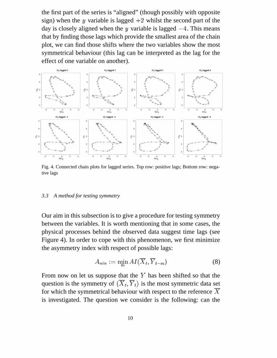
the first part of the series is “aligned” (though possibly with oppositesign) when the 3 variable is lagged
� whilst the second part of the
day is closely aligned when the 3 variable is lagged� � . This means
that by finding those lags which provide the smallest area of the chainplot, we can find those shifts where the two variables show the mostsymmetrical behaviour (this lag can be interpreted as the lag for theeffect of one variable on another).
20 25 30 35 40
2030
4050
60
12345678 910
11
1213 1415
1617
18
19
20
21
22
23
24
2526272829
303132
3334
35 36
3738
39
40
41
42
4344454647
48
PSfragreplacem
ents
time
NO �
O
�
Chain
Plot:
NO
vsO
NO
concentration:half-hourlym
eansO
concentration:half-hourlym
eansC
ross-correlations:N
Oand
OC
ross-correlations:H
umidity
&Tem
perature
O � lagged 1
Olagged
2O
lagged3
Olagged
4O
lagged–1
Olagged
–2O
lagged–3
Olagged
–4
20 25 30 35 40
2030
4050
60
12345678 9 1011
12
13141516
1718
19
20
21
22
23
24
25
26272829 30
313233
3435
36 37
3839
40
41
42
43
4445464748
PSfragreplacem
ents
time
NO �
O
�
Chain
Plot:
NO
vsO
NO
concentration:half-hourly
means
Oconcentration:
half-hourlym
eansC
ross-correlations:N
Oand
OC
ross-correlations:H
umidity
&Tem
peratureO
lagged1
O � lagged 2
Olagged
3O
lagged4
Olagged
–1O
lagged–2
Olagged
–3O
lagged–4
20 25 30 35 40
2030
4050
60
12345678 9 10 11
1213
14151617
1819
20
21
22
23
24
25
26
272829
303132
33 3435
3637 38
3940
41
42
43
44
45464748
PSfragreplacem
ents
time
NO �
O
�
Chain
Plot:
NO
vsO
NO
concentration:half-hourly
means
Oconcentration:
half-hourlym
eansC
ross-correlations:N
Oand
OC
ross-correlations:H
umidity
&Tem
peratureO
lagged1
Olagged
2
O � lagged 3
Olagged
4O
lagged–1
Olagged
–2O
lagged–3
Olagged
–4
20 25 30 35 40
2030
4050
60
12
345678 9 10 11 1213
14
15161718
1920
21
22
23
24
25
26
27
2829
303132
333435
3637
38 39
404142
43
44
45
464748
PSfragreplacem
ents
time
NO �
O
�C
hainP
lot:N
Ovs
ON
Oconcentration:half-hourly
means
Oconcentration:half-hourly
means
Cross-correlations:
NO
andO
Cross-correlations:
Hum
idity&
Temperature
Olagged
1O
lagged2
Olagged
3
O � lagged 4
Olagged
–1O
lagged–2
Olagged
–3O
lagged–4
20 25 30 35 40
2030
4050
60
123456789
10
1112 13 14
1516
17
18
19
20
21
22
23
2425
262728
2930 31
3233
34 35
3637
38
39
40
41
4243444546
4748
PSfragreplacem
ents
time
NO �
O
�
Chain
Plot:
NO
vsO
NO
concentration:half-hourly
means
Oconcentration:
half-hourlym
eansC
ross-correlations:N
Oand
OC
ross-correlations:H
umidity
&Tem
peratureO
lagged1
Olagged
2O
lagged3
Olagged
4
O � lagged –1
Olagged
–2O
lagged–3
Olagged
–4
20 25 30 35 40
2030
4050
60
12345678910
1112 13 14
1516
17
18
19
20
21
22
23
2425
262728293031
3233
3435
3637
38
39
40
41
42 43444546
4748
PSfragreplacem
ents
time
NO �
O
�
Chain
Plot:
NO
vsO
NO
concentration:half-hourlym
eansO
concentration:half-hourlym
eansC
ross-correlations:N
Oand
OC
ross-correlations:H
umidity
&Tem
peratureO
lagged1
Olagged
2O
lagged3
Olagged
4O
lagged–1
O � lagged –2
Olagged
–3O
lagged–4
20 25 30 35 40
2030
4050
60
12345678910
1112 13 14
1516
17
18
19
20
21
22
23
2425
262728
293031
3233
3435
3637
38
39
40
41
42 43 444546
4748
PSfragreplacem
ents
time
NO �
O
�C
hainP
lot:N
Ovs
ON
Oconcentration:half-hourly
means
Oconcentration:half-hourly
means
Cross-correlations:
NO
andO
Cross-correlations:
Hum
idity&
Temperature
Olagged
1O
lagged2
Olagged
3O
lagged4
Olagged
–1O
lagged–2
O � lagged –3
Olagged
–4
20 25 30 35 40
2030
4050
60
123456789
10
111213 14
1516
17
18
19
20
21
22
23
2425
262728
293031
3233
3435
3637
38
39
40
41
42 43 44 4546
4748
PSfragreplacem
ents
time
NO �
O
�
Chain
Plot:
NO
vsO
NO
concentration:half-hourly
means
Oconcentration:
half-hourlym
eansC
ross-correlations:N
Oand
OC
ross-correlations:H
umidity
&Tem
peratureO
lagged1
Olagged
2O
lagged3
Olagged
4O
lagged–1
Olagged
–2O
lagged–3
O � lagged –4
Fig. 4. Connected chain plots for lagged series. Top row: positive lags; Bottom row: nega-tive lags
3.3 A method for testing symmetry
Our aim in this subsection is to give a procedure for testing symmetrybetween the variables. It is worth mentioning that in some cases, thephysical processes behind the observed data suggest time lags (seeFigure 4). In order to cope with this phenomenon, we first minimizethe asymmetry index with respect of possible lags:
������ ��������� ����� ��� � !"�$# �&% (8)
From now on let us suppose that the!
has been shifted so that thequestion is the symmetry of
� � � � ! � % is the most symmetric data setfor which the symmetrical behaviour with respect to the reference
�is investigated. The question we consider is the following: can the
10

symmetry be accepted, based on an observed asymmetry index � ?
In order to tackle this question, we might either use parametric mod-elling with a symmetric model:
� � � � ���
(9)
where in the simplest case ��
can be considered as an i.i.d. sequenceof 0-mean random variables. For such models more or less straight-forward methods for statistical inference are available. An obviousdisadvantage of such an approach is that the cause of the possiblerejection is not clear: it might well happen that there is just an ac-ceptable level of discrepancy from symmetry, and rejection is onlybased on the poor fit of the model. We thus suggest an alternativenonparametric method, focusing only on the symmetry.
Let us first suppose that the reference function constructed by inter-polation is simple. If it is only normal, then the procedure of (6–7)can be used to cut the curve into simple parts and then the symmetryof these parts can be tested independently. Let us use the transforma-tion � defined in the previous section in (4). This is of course basedon the observed averages
�and
, but from now on we omit the
overline, when using � .
Our method relies on the fact that the area for the normalized ��� canbe approximated by
)�
� � � $ ��� �� � � ( � � � � � � ) � ( � � � (10)
(see (5), we supposed � to be an even number). Equation (10) showsthat it is much more useful to base our procedures on the estimatedvalues
� � � ( � � � � rather than the observed� �
, for which the contribu-tion very much depends on the difference
�� � � � �� �. Let us introduce
the notation� � ( � � � � � � � ( � � � ��� � � � ) � ( � � �!� and consider the
increments of the process� � ( � � � : � � � � � ( � � � � � � � ( � ) � � � � for
( � )+* *-,.,-, * � � . It is obvious that �� � �� �� � � � � � ) � � � � ����� � �
and that part of Equation (10) where there is no sign change (i.e. theabsolute value is not needed) can be expressed as �
� � �� �� � � � � ( � � � ,
11

so we get the maximal value if the � values are ordered.
Now we can describe the procedure we suggest: if we generate arandom permutation of the set � )+*.,-,.,/* � � � and permute the vector� � � *-,.,., * � � � � � then we get another closed curve. If there was no asym-metry between the variables, then we could suppose that the originalpermutation was just a typical one, so the area of the original curvewould be near to this generated one.
If we repeat the permutation procedure � times and calculate (10)for all, then we get � different possible values of the symmetry in-dex. If the observed ��� is larger than the 95 (99 etc)% quantile ofthis observed distribution, then the symmetry can be rejected.
There is an open question how to choose � in Equation (10). We sug-gest to use the same number of points as for the original observations.This could be investigated, but for an
�with constant derivative we
use just the original observations. Another point against a too refinedgrid is the extensive computing time and that in such cases almost al-ways there is strong dependence among neighbouring values, whichindicates that there is little gain in using all of them.
The suggested approach shows similarities to the methods presentedin Schmid and Trede (1995), where the classical two sample prob-lem is tested by a method, based on the area between two curves.The asymptotic distribution of their test statistic is the integral of theBrownian bridge (see Shepp, 1982 for its tabulated distribution). Wealso get this limit distribution for the scaled and randomized sequenceif certain mixing conditions can be supposed for the sequence � , butas in our problems we have a definite, not too large number as � , wedo not exploit this idea here.
Applying the above method to the bivariate dataset of sample meansillustrated in Figure and 2 we get an estimated � -value (based on10 000 bootstrap samples) of
� , � �� � , and a few of the simulated chainplots, corresponding to various critical values, are shown in Figure 5.These plots are constructed with the same end points as for the rawdata. This � -value may be surprisingly small, given that the marginal
12

plots have a very similar structure, and the asymmetry index itself wassmall. However, this sample size of � � ) � � � means that the chainplot is very smooth and so there is little variability in the resulting � � .
0.0 0.2 0.4 0.6 0.8 1.0
0.0
0.2
0.4
0.6
0.8
1.0
0.999
x
y
0.0 0.2 0.4 0.6 0.8 1.0
0.0
0.2
0.4
0.6
0.8
1.0
0.99
x
y
0.0 0.2 0.4 0.6 0.8 1.0
0.0
0.2
0.4
0.6
0.8
1.0
0.90
x
y
0.0 0.2 0.4 0.6 0.8 1.0
0.0
0.2
0.4
0.6
0.8
1.0
0.50
x
y
PSfragreplacem
ents
time
NOO
Chain
Plot:
NO
vsO
NO
concentration:half-hourly
means
Oconcentration:
half-hourlym
eansC
ross-correlations:N
Oand
OC
ross-correlations:H
umidity
&Tem
peratureO
lagged1
Olagged
2O
lagged3
Olagged
4O
lagged–1
Olagged
–2O
lagged–3
Olagged
–4
Fig. 5. Simulated chain plots (continuous line) corresponding to the 0.999, 0.99, 0.9 and0.5 quantiles of the empirical distribution of the resampled asymmetry index, based on the(rescaled) chain plot of the data (dashed line) shown in Figure 2.
13
4 Extensions
4.1 Correlations
The cross-covariance between��� ��� ����
and�� ���� ����
at lag � is esti-mated by
� ��� � � � � )� � $������ ��� � � � � �� � � � � ��� ,-,., * � )+* � * )+*.,-,.,and the cross-correlation at lag � is estimated by
� ��� � � � � � ���� � � �
where � �� �� $ �
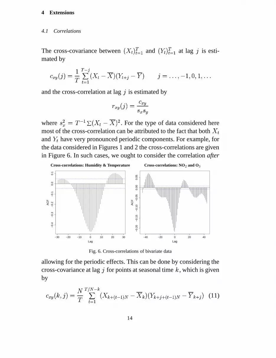
���� � � � � � . For the type of data considered here
most of the cross-correlation can be attributed to the fact that both� �
and �
have very pronounced periodic components. For example, forthe data considered in Figures 1 and 2 the cross-correlations are givenin Figure 6. In such cases, we ought to consider the correlation after
−30 −20 −10 0 10 20 30
−0.
4−
0.3
−0.
2−
0.1
0.0
0.1
Lag
AC
F
PSfragreplacem
ents
time
NOO
Chain
Plot:
NO
vsO
NO
concentration:half-hourly
means
Oconcentration:
half-hourlym
eansC
ross-correlations:N
Oand
O
Cross-correlations: Humidity & Temperature
Olagged
1O
lagged2
Olagged
3O
lagged4
Olagged
–1O
lagged–2
Olagged
–3O
lagged–4
−40 −20 0 20 40
−0.
20−
0.15
−0.
10−
0.05
0.00
0.05
Lag
AC
F
PSfragreplacem
ents
time
NOO
Chain
Plot:
NO
vsO
NO
concentration:half-hourly
means
Oconcentration:
half-hourlym
eans
Cross-correlations: NO � and O �
Cross-correlations:
Hum
idity&
Temperature
Olagged
1O
lagged2
Olagged
3O
lagged4
Olagged
–1O
lagged–2
Olagged
–3O
lagged–4
Fig. 6. Cross-correlations of bivariate data
allowing for the periodic effects. This can be done by considering thecross-covariance at lag � for points at seasonal time ( , which is givenby
� ��� � ( *� � � � � ����� $ ����� ��� �! #" � $ ��& � � ���-� �� �! � #" � $ � & � � � � � (11)
14

for ( � )+*-,.,-,/*/�0* � � ,-,., * � ) * � * )+*.,-,.,!*/� � � where� �
and �! �
are given in Equation (1). The adjusted sample cross-correlation canbe estimated in an analogous manner. Incorporating all of this infor-mation on the chain plot is difficult, since we now have � cross-correlation plots to display. However, if we initially consider ��� �and use a normal approximation to describe the joint distribution of���
and '�
, then we can include ) � ��� ) � � ��� confidence limitsaround each point in the chain plot. An example is shown in Figure7 which shows how the variability in the two variables changes overtime. An efficient way to construct such contours is to use polar co-ordinates as follows.
Let � be a sequence of length � angles in��� * � � , and form the ���
matrix � � ��� � � * � � � � � . Given ( *� form the covariance matrix forthe relevant data, say
� ������ � ���
� ( * � � � ��� � ( *� �� ��� � ( *� � � � � � ( * � �
������
Now solve � � � $ � � �and then plot polar co-ordinates � � � � *��
around� � � * � �
where � � � � is a vector of length � determined by
� � � � � � � �� � ) � � �� � � �
where� � � )+* ) � � and � �� � ) � � � is the ) � ��� ) � � ��� point from a
� � distribution with
degrees of freedom.
It is evident in Figure 7, except around the middle of the day (times20–30), that there is a small negative correlation between O � andNO � . Such a plot also indicates times of greater joint change in thedaily means — in this example between time period 10 and 11 (5:00and 5:30 a.m.), and from time periods 16 to 21 (8:00 to 10:30 a.m.).See Makra et al. (2001) for a more detailed analysis of the data.
15

15 20 25 30 35 40
2030
4050
60
Chain Plot with 90% Confidence Interval
123456789
10
1112 13 14
1516
17
18
19
20
21
22
23
2425
262728
293031
3233
3435
3637
38
39
40
41
4243444546
4748
PSfragreplacem
ents
time
NO �
O
�
Chain
Plot:
NO
vsO
NO
concentration:half-hourly
means
Oconcentration:
half-hourlym
eansC
ross-correlations:N
Oand
OC
ross-correlations:H
umidity
&Tem
peratureO
lagged1
Olagged
2O
lagged3
Olagged
4O
lagged–1
Olagged
–2O
lagged–3
Olagged
–4
Fig. 7. Modified chain plot with 90% confidence intervals (using a multivariate normalapproximation) based on the conditional covariance at each time point
4.2 Fourier Analysis
A straightforward Fourier analysis was made harder by the largenumber of missing values. So, in order to compare with the aboveresults we fitted a linear model corresponding to only daily and 12hourly periods (Bloomfield, 2000). That is, for each time series, wefitted the model:
� � � � ��� � � �.��� � � ��� � � ��� � � � ��� � � ��� � � � ��
where� � * � � * � � )+* are the fitted amplitudes and phases, respec-
tively, corresponding to the frequencies� � , with
� � corresponding to24-hourly and 12-hourly periods for
� � ) * , respectively. The re-sults for the four time series used as examples in this paper are shown
16
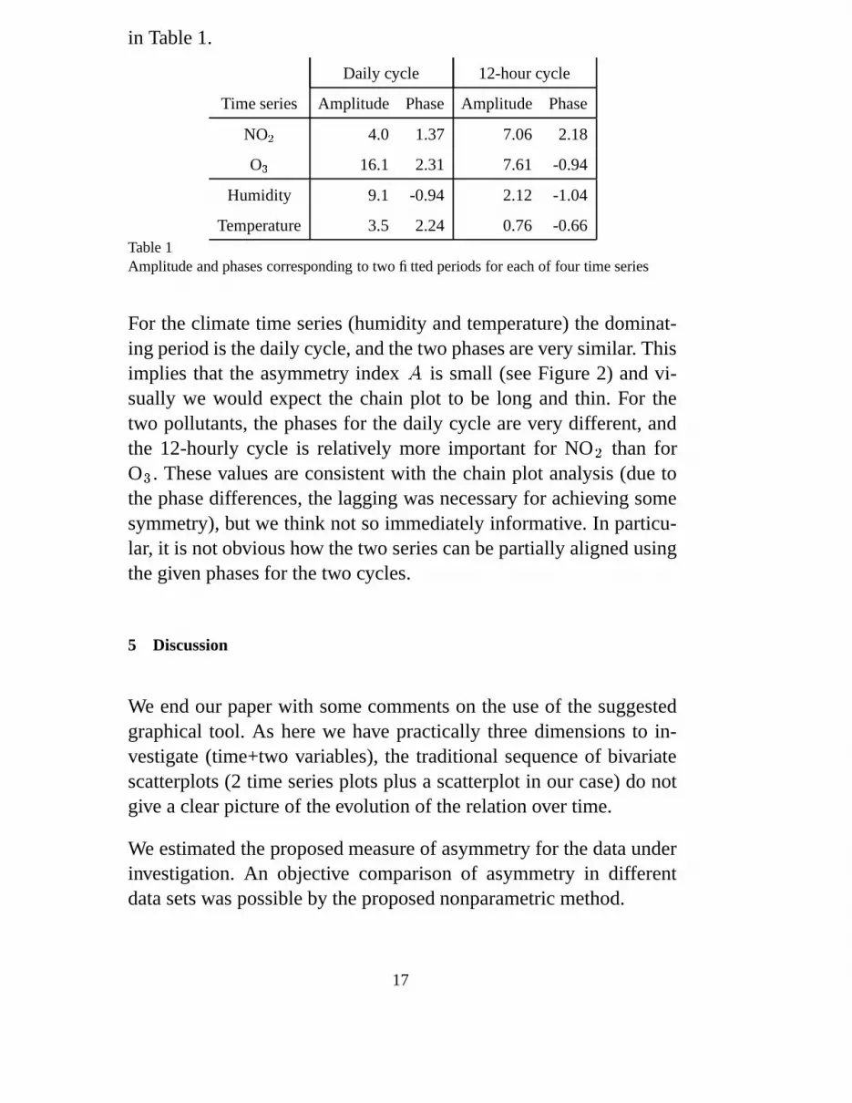
in Table 1.
Daily cycle 12-hour cycle
Time series Amplitude Phase Amplitude Phase
NO � 4.0 1.37 7.06 2.18
O � 16.1 2.31 7.61 -0.94
Humidity 9.1 -0.94 2.12 -1.04
Temperature 3.5 2.24 0.76 -0.66Table 1Amplitude and phases corresponding to two fitted periods for each of four time series
For the climate time series (humidity and temperature) the dominat-ing period is the daily cycle, and the two phases are very similar. Thisimplies that the asymmetry index � is small (see Figure 2) and vi-sually we would expect the chain plot to be long and thin. For thetwo pollutants, the phases for the daily cycle are very different, andthe 12-hourly cycle is relatively more important for NO � than forO � . These values are consistent with the chain plot analysis (due tothe phase differences, the lagging was necessary for achieving somesymmetry), but we think not so immediately informative. In particu-lar, it is not obvious how the two series can be partially aligned usingthe given phases for the two cycles.
5 Discussion
We end our paper with some comments on the use of the suggestedgraphical tool. As here we have practically three dimensions to in-vestigate (time+two variables), the traditional sequence of bivariatescatterplots (2 time series plots plus a scatterplot in our case) do notgive a clear picture of the evolution of the relation over time.
We estimated the proposed measure of asymmetry for the data underinvestigation. An objective comparison of asymmetry in differentdata sets was possible by the proposed nonparametric method.
17

Acknowledgements: We acknowledge support from the BritishCouncil and the Hungarian Ministry of Education under the British-Hungarian Academic Research Programme.
References
Bloomfield, P. 2000. Fourier Analysis of Time Series: An Introduction(second edition). John Wiley, New York.
Embrechts, P., McNeil, A. and Straumann, D. 1999. Correlation anddependency in risk management: properties and pitfalls. PreprintETH, Zurich. www.math.ethz.ch/ � embrechts.
Makra, L., Horvath, Sz., Taylor, C.C., Zempleni, A., Motika, G. andSumeghy, Z. 2001. Modelling air pollution in countryside and urbanenvironment, Hungary. Proc. of the 2nd International Symposium onAir Quality Management at Urban, Regional and Global Scales. Is-tanbul, Turkey. pp. 189-196. Eds.: Topcu, S. Yardim, M.F. and Ince-cik, S.
Schmid, F. and Trede, M. 1995. A distribution free teset for the twosample problem for general alternatives. Comput. Stat., Data Anal.20, p. 409-419.
Shepp, L.A. 1982. On the integral of the absolute value of the pinnedWiener process - calculation of its probability density by numericalintegration. Ann. Probab. 10, p. 240-243.
Villa-Diharce, E. 2001. Estimation of the tail dependence index. Re-search Report of CIMAT, Guanajuato, Mexico.
18