Non–linear modelling of bivariatecomovements in asset prices

Marco Corazza and Elisa Scalco

Dipartimento di Matematica ApplicataUniversita Ca’ Foscari di Venezia

Dorsoduro n. 3825/E – 30123 Venezia, Italy{corazza, scalco}@unive.ithttp://www.dma.unive.it/

Abstract. The phenomenon of comovements among asset prices hasreceived a lot of attention for several reasons (see, for some examples,section 1). The increasing interest in this topic has been the reason of theproduction of a large number of contributions. In this paper we proposean investigating methodology for the non–linear modelling of bivariatecomovements. Our approach leaves the ones presented in the recent lit-erature. In fact, our approach, which is articulated in three steps, allowsthe evaluation and the statistical testing of non–linearly driven comove-ments between two given random variables. Moreover, when such an(unknown) bivariate dependence relationship is detected, our approachallows also to provide a polynomial approximation of it. Finally, we ap-ply our three–steps methodology to some energy asset prices time seriestraded in the U.S.A.. The goodness of the results is encouraging giventhe novelty of the proposed investigating approach.Keywords. Comovement, asset price, bivariate dependence, non–linear-ity, comonotonicity, t-test, polynomial approximation, energy asset.

M.S.C. classification: 41A10.

J.E.L. classification: C59, Q49.

1 Introduction

The issue regarding the phenomenon of comovements among asset prices hasreceived a lot of attention for several reasons:

– firstly, the knowledge of dependence relationships among the prices of givenstocks allows to obtain information about a not–ready–to–observe stock priceby suitably using the ready–to–observe ones. Moreover, it make also possiblecross–hedging and cross-speculation approaches;

– secondly, the presence, or less, of dependence in form of correlation amongthe prices of assets traded in different countries is of interest to investorswho wish to allocate their capitals in mean–variance portfolios since, asknown, international diversification strategies work well when the consideredmarkets are little integrated;

136

– thirdly, dependence among stock prices traded in different countries is ofinterest to policy makers as such comovements can affect domestic consump-tions;

– last, scholars and various institutions are interested in establishing and ininvestigating the extent of integration level among financial markets.

The increasing interest in the topic of comovements in asset prices has beenthe reason of the production of a large number of contributions in the spe-cialized literature. In the next section we provide a short survey of the morerecent of such contributions. In particular, in most of these studies the variousauthors make use of investigating approaches mainly based on autoregressiveheteroskedastic (ARCH) models, error correction models (ECMs), generalizedARCH (GARCH) models, Granger causality based tests, multivariate cointe-grations, structural vector autoregression (VAR) systems, lag–augmented VAR(LA–VAR) systems, forecast error variance decomposition (VDC) approaches,and vector error–correction models (VECMs).

As far as concerns the investigating methodology we propose in this paper,it leaves the approaches listed above. In fact, our approach, which is articulatedin three steps, allow the evaluation and the statistical testing of non–linearlydriven comovements between two given random variables. Moreover, when suchan (unknown) bivariate dependence relationship is detected, our approach allowsalso to provide a polynomial approximation of it.

The remainder of this paper is organized in the way which follows. As prem-ised, in the next section we present a short review of the recent literature. Insection 3 we propose in detail our three–steps methodology. In section 4 weprovide the results of some applications of the proposed methodology to timeseries of the prices of energy assets traded in U.S.A.. Finally, In section 5 wegive some concluding remarks.

2 A short review of the recent literature

In this section we give a short survey of the recent literature about the comove-ments among assets prices.

Before to begin, notice that a significant percentage of the published contri-butions concern cross-country dependence relationships.

In [6] the mechanism of international transmission of stock prices movementsis investigated by using a nine–market VAR system. In particular, the authorstrace out the dynamics of the responses in a given market to the innovations inanother given one. In [5], by using univariate and multivariate GARCH mod-els, it is shown that the prices of several (to all apparencies) unrelated marketsreveal a persistent tendency to comove, even after accounting for the effects ofmacroeconomic shocks. In [11] long–term and short–term dependence relation-ships among the prices of six agricultural futures traded at the Chicago Boardof Trade are analyzed by using the ECM. In [7] the investigation of interde-pendencies among stock prices is performed by using a LA–VAR system based

137

approach. A significant advantage of this methodology consists in the fact thatit can be applied regardless of the presence, or less, of cointegration among theconsidered stock prices. In [1] cointegration among stock prices traded in differ-ent countries is investigated. In particular, the authors put in evidence that thelikelihood ratio tests of Johansen are sensitive to the specification of the timelag amplitude in the VAR system.

Some other methodologies which are worth while mentioning are the onesable to detect the presence, or less, of common cycles among asset prices. In [3]a cointegration technique is utilized for testing the presence of long–run commontrends among stock prices and the interest rate, and co-dependence analyses areperformed for investigating the presence and the features of short–run commoncycles among the same quantities. In [4] linear and non–linear Granger causalitybased tests are used to examine the dynamical dependence relationships betweenspot and future prices. Finally, in [13] proper measures of dependence amongEuropean stock markets are evaluated by using the multivariate extreme valuetheory.

3 Our three–steps methodology

In this section we present in detail our methodology for the non–linear evaluationof bivariate comovements. Since our approach is (softly) based on the conceptof comonotonicity, before of all we spend some words about this notion.

Comonotonicity is one of the strongest measure of dependence existing amongrandom variables. Limiting our interest to the bivariate case, given two randomvariables X1(t) and X2(t), both defined in [t0, t1] with t0 < t1, they are said tobe comonotonic if and only if:1

[X1 (t3)−X1 (t2)] [X2 (t3)−X2 (t2)] ≥ 0 ∀ t2, t3 : t2 6= t3 ∧ t2, t3 ∈ [t0, t1] .

A few remarks about this relationship:

– two random variables are comonotonic if and only if they always vary over thesupport (time) in the same direction, besides the quantitative laws describingthe dynamic behaviour of each of them;

– comonotonicity is an ON/OFF concept, in fact it is sufficient the existenceof a unique pair t2 and t3 for which [X1 (t3)−X1 (t2)] [X2 (t3)−X2 (t2)] < 0to state that X1 and X2 are not comonotonic. Of course, in such a case itshould be hard to uphold that, as X1(t) and X2(t) are not more comonotonic,they are also not more dependent in some sense (in profiling our approachwe start from this latest remark).

Our methodology is articulated in three steps. Before to present in detaileach of them, we give a brief description of their contents:

1 For other equivalent definitions of comonotonicity see [8], [9] and [15].

138

– in the first step we propose a simple index able to evaluate any interme-diate degree of bivariate dependence from full countermonotonicity2 to fullcomonotonicity, and we provide some theoretical results about it;

– as this simple index provides only a point estimation of the considered bi-variate dependence, in the second step we propose a procedure by which totest the statistical meaningfulness of the index itself;

– once the statistical meaningfulness of the simple index has been proved,in the third step we propose an algorithm able to provide a polynomialapproximation of the unknown bivariate dependence relationship.

3.1 The simple index

Let we start by considering two discrete–time time series, {X1(t) , t = t1, . . .,tN} and {X2(t) , t = t1, . . ., tN}. The simple index we propose for evaluating thebivariate dependence between the random variables X1(t) and X2(t) is definedas follows:

δ1,2 =1

N − 1

tN∑t=t2

∆(t)1,2,

∆(t)1,2 ={−1 if [X1 (t)−X1 (t− 1)] [X2 (t)−X2 (t− 1)] < 0

1 if [X1 (t)−X1 (t− 1)] [X2 (t)−X2 (t− 1)] ≥ 0 .

(1)

Some remarks about this index:

– it is trivial to prove that δ1,2 ∈ [−1, 1]. In particular, the two randomvariables are countermonotonic if and only if δ1,2 = −1, and are comonotonicif and only if δ1,2 = 1;

– beyond the property reported in the previous point (property of normaliza-tion of the first type), it is also trivial to prove that δ1,2 is defined for everypair of discrete–time time series (property of existence), and that δ1,2 = δ2,1

(property of symmetry). Therefore, δ1,2 is a scalar measure of dependencein the sense illustrated in [14] at section 6;

– the fact that δ1,2 belongs to [−1, 1] makes this index of dependence directlycomparable with the well known and widely used Bravais–Pearson linearcorrelation coefficient ρ1,2.3

As far as theoretical properties between δ1,2 and ρ1,2 are concerned, we givethe proposition which follows.

2 Two random variables X1(t) and X2(t), both defined in [t0, t1] with t0 < t1, are saidto be countermonotonic if and only if [X1 (t3)−X1 (t2)] [X2 (t3)−X2 (t2)] < 0 forall t2, t3 such that t2 6= t3 and t2, t3 ∈ [t0, t1].

3 Also ρ1,2 is a scalar measure of dependence in the sense illustrated in [14] at section6.

139

Proposition 1. Let f(·): R+ → R+ be the bivariate dependence relationshipbetween X1(t) and X2(t), i.e. X1(t) = f (X2(t)) + ε(t), where ε(t) has the usualmeaning, and let f(·) be infinite times derivable in m2 = E (X2(t)). If

f (i)(m2)i!

(i

i− j

)(−m2)i−j = 0 ∀ j = 2, . . . , +∞, (2)

where f (i)(·) indicates the i−th derivatives of f(·), then the bivariate dependencerelationship is affine.

Proof. As f(·) ∈ C∞, we can expand it in Taylor’s series about m2 as follows:

f (X2(t)) =∑+∞

i=0f(i)(m2)

i! (X2(t)−m2)i

=∑+∞

i=0f(i)(m2)

i!

∑ij=0

(ij

)Xi−j

2 (t)(−m2)j .(3)

After some algebraic manipulations, we can rewrite equation (3) as follows:

f (X2(t)) =+∞∑

j=0

+∞∑

i=j

f (i)(m2)i!

(i

i− j

)(−m2)i−j

Xj

2(t). (4)

Now, by substituting relationships (2) into (4) we obtain the following affinebivariate dependence relationship between X1(t) and X2(t):

X1(t) =∑+∞

i=0f(i)(m2)

i!

(ii

)(−m2)i+

+[∑+∞

i=1f(i)(m2)

i!

(i

i− 1

)(−m2)i−1

]X2(t) + ε(t). 2

(5)

Notice that, if relationship (2) were extended also to j = 1, then relationship(5) should begin

X1(t) =+∞∑

i=0

f (i)(m2)i!

(ii

)(−m2)i + ε(t),

i.e. there not should be more any dependence relationship between X1(t) andX2(t), i.e. X1(t) and X2(t) should be independent.

As premised, the simple index we proposed here provides only a point es-timation of the investigated bivariate dependence. In order to overcome thisdrawback, in the next subsection we propose a procedure able to statisticallytest the meaningfulness of the index itself.

3.2 The testing procedure

The “philosophy” of the procedural approach we propose here for testing thestatistical meaningfulness of δ1,2 is similar to the one of the procedural approachproposed in [10].

In the remainder of this subsection we present in detail our testing procedurein the itemized form which follows:

140

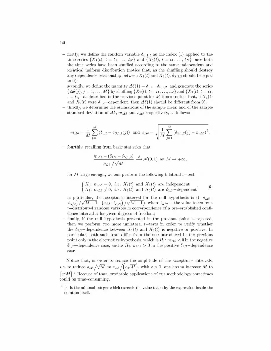
– firstly, we define the random variable δS;1,2 as the index (1) applied to thetime series {X1(t), t = t1, . . ., tN} and {X2(t), t = t1, . . ., tN} once boththe time series have been shuffled according to the same independent andidentical uniform distribution (notice that, as the shuffling should destroyany dependence relationship between X1(t) and X2(t), δS;1,2 should be equalto 0);

– secondly, we define the quantity ∆δ(1) = δ1,2−δS;1,2, and generate the series{∆δ(j), j = 1, . . ., M} by shuffling {X1(t), t = t1, . . ., tN} and {X2(t), t = t1,. . ., tN} as described in the previous point for M times (notice that, if X1(t)and X2(t) were δ1,2−dependent, then ∆δ(1) should be different from 0);

– thirdly, we determine the estimations of the sample mean and of the samplestandard deviation of ∆δ, m∆δ and s∆δ respectively, as follows:

m∆δ =1M

M∑

j=1

(δ1,2 − δS;1,2(j)) and s∆δ =

√√√√ 1M

M∑

j=1

(δS;1,2(j)−m∆δ)2;

– fourthly, recalling from basic statistics that

m∆δ − (δ1,2 − δS;1,2)

s∆δ

/√M

d−→ N (0, 1) as M → +∞,

for M large enough, we can perform the following bilateral t−test:{

H0: m∆δ = 0, i .e. X1(t) and X2(t) are independentH1: m∆δ 6= 0, i .e. X1(t) and X2(t) are δ1,2−dependent ; (6)

in particular, the acceptance interval for the null hypothesis is ((−s∆δ ·tα/2

) /√M − 1 ,

(s∆δ · tα/2

) /√M − 1

), where tα/2 is the value taken by a

t−distributed random variable in correspondence of a pre–established confi-dence interval α for given degrees of freedom;

– finally, if the null hypothesis presented in the previous point is rejected,then we perform two more unilateral t−tests in order to verify whetherthe δ1,2−dependence between X1(t) and X2(t) is negative or positive. Inparticular, both such tests differ from the one introduced in the previouspoint only in the alternative hypothesis, which is H1: m∆δ < 0 in the negativeδ1,2−dependence case, and is H1: m∆δ > 0 in the positive δ1,2−dependencecase.

Notice that, in order to reduce the amplitude of the acceptance intervals,i.e. to reduce s∆δ

/√M to s∆δ

/(c√

M), with c > 1, one has to increase M to⌈

c2M⌉.4 Because of that, profitable applications of our methodology sometimes

could be time–consuming.4 d·e is the minimal integer which exceeds the value taken by the expression inside the

notation itself.

141

3.3 The polynomial approximation

If at the end of the testing procedure the null hypothesis has been rejectedin favour of the negative/positive δ1,2−dependence between X1(t) and X2(t),then we begin to model in analytical way the unknown bivariate dependencerelationship X1(t) = f (X2(t)) + ε(t). In particular, we search for a polynomialapproximation of f(·) which is a properly truncated version of the equation (4),i.e.

f (X2(t)) =J∑

j=0

ajXj2(t) + r(J + 1), (7)

where J is the truncation order of the Taylor’s series (4), aj =∑J

i=jf(i)(m2)

i! ·(i

i−j

)(−m2)i−j , and r(J + 1) is a suitable remainder function.

Of course, in such an approach a crucial role is played by J . In order to detectits “optimal” value, we propose the following algorithm whose search procedureis based on a standard cross–validation technique, as suggested for empiricalwork in [12] at section 4:

– we begin by considering as starting data set D the discrete–time bivariatetime series {(X1(t) , X2(t)), t = t1, . . ., tN};

– secondly, we suitably split D into two data subsets, the learning one DL andthe validation one DV , such that DL ∪DV = D and DL ∩DV = ∅;5

– thirdly, we consider a finite series of polynomials of kind (7) with J = 0, . . .,J , where J is a pre–established integer value;

– fourthly, for each of the polynomials considered in the previous point weestimate the parameters a0, . . ., aJ via ordinary least square regression byusing the data subset DL, and evaluate the index δ1,2 between X1(t) =∑J

j=0 ajXj2(t) and X2(t) by using the data subset DV ;6

– finally, we choose as “best” approximating polynomial the one to which isassociated the highest absolute value of δ1,2.

Notice that the fact of identifying the “optimal” approximating polynomialby using a cross–validation approach, i.e. to perform the ordinary least squareby using the learning data subset and to evaluate the validation criterion |δ1,2|by using the validation data subset, allows to strongly avoid overspecializationof the polynomial itself.

4 Applications to energy asset prices time series

In this section we give the results of some applications of our three–steps method-ology to the prices time series of some energy asset traded in the U.S.A..

In general terms, for each application we act as follows:5 The way in which to suitably split D is made clear in subsection 4.2.6 b· indicates the estimator of the quantity below.

142

– we start by considering the discrete–time bivariate time series {(X1(t) ,X2(t)), t = t1, . . ., tN};

– from the time series introduced in the previous point we split the chronologi-cally last 10 per cent of its realizations in order to utilize them as forecastingdata subset DF at the end of the application for performing a rough out–of–sample check. We use the remaining 90 percent of the discrete–time bivariatetime series as the starting data set D;

– we split D into the learning data subset DL (the chronologically first 70 percent of its realizations) and the validation data subset DV (the chronologi-cally last 30 per cent of its realizations);7

– finally, we perform our methodology by using DL and DV .

4.1 The data

Each discrete–time univariate time series we utilize here is constituted by 2, 026daily spot closing prices of three energy assets traded in U.S.A.: the crude oil,the gasoline, and the heating oil. Such prices have been collected from January3, 1994 to February 6, 2002. In the remainder of this subsection and in the nextone, we refer to these time series respectively as {XCO(t) , t = t1, . . ., t2,026},{XG(t) , t = t1, . . ., t2,026}, and {XHO(t) , t = t1, . . ., t2,026}.

As far as concerns the discrete–time bivariate time series whose non–linearcomovements we investigate here, we consider all the ones forecoming from thesimple disposition of the discrete–time univariate time series listed in the previ-ous paragraph, i.e. {(XCO(t) , XG(t)), t = t1, . . ., t2,026}, {(XCO(t) , XHO(t)),t = t1, . . ., t2,026}, {(XG(t) , XCO(t)), t = t1, . . ., t2,026}, {(XG(t) , XHO(t)),t = t1, . . ., t2,026}, {(XHO(t) , XCO(t)), t = t1, . . ., t2,026}, and {(XHO(t) ,XG(t)), t = t1, . . ., t2,026}.

Notice that, given the percentages set in the previous itemization with regardto the data subsets implied in each application, the cardinalities of these samedata subset are the following: #{DL} = 1, 277, #{DV } = 547, and #{DF } =202.

4.2 The results

As premised, here we provide and illustrate the results of the applications of ourthree–steps methodology to the discrete–time bivariate time series listed in theprevious subsection. The exposition of these results is organized in two tables,and in some figures.

As far Table 1 is concerned, before to report it we need to specify the contentof each of its columns:

– the first column indicates the two random variables specifying the discrete–time bivariate time series which has investigated;

7 The percentages we set for DL and DV are the ones usually utilized in several empir-ical works using cross–validation techniques (see, for example, [2] and the referencestherein).

143

– the second column reports the value of the simple index δi,j , with i, j ∈ {CO,G, HO} and i 6= j, evaluated on the learning data subset DL (see, for moredetails, subsection 3.1);

– the third column provides the response of the bilateral t−test (6):8 label“A” or label “R” for, respectively, the acceptance or the rejection of the nullhypothesis (see, for more details, subsection 3.2);

– if the null hypothesis of the bilateral t−test (6) is rejected, then the fourthcolumn gives the response of the check, based on two more unilateral t−tests,9

whether the δ1,2−dependence between the two investigated univariate timeseries is negative, label “N”, or positive, label “P” (see, for more details,again subsection 3.2);

– the fifth column gives the value of the Bravais–Pearson linear correlationcoefficient ρi,j , with i, j ∈ {CO, G, HO} and i 6= j, evaluated on thelearning data subset DL (we report the value of this coefficient for possiblecomparisons).

Finally, we recall that the property of symmetry holds for the simple index(1), i.e. δi,j = δj,i for all i, j such that i, j ∈ {CO, G, HO}.

Table 1.

Random variables δi,j Bilateral t−test Check on the δ1,2−dep. ρi,j

XCO(t), XG(t) 0.35407 R P 0.94139XCO(t), XHO(t) 0.39259 R P 0.91178

XG(t), XHO 0.48642 R P 0.85118

A few remarks about the results reported in Table 1:

– the fact that δi,j is statistically significantly different from 0 for all i, jsuch that i, j ∈ {CO, G, HO} and i 6= j (see jointly the second and thethird column of Table 1) indicates the existence of a bivariate dependencerelationship between Xi(t) and Xj(t) for all i, j such that i, j ∈ {CO, G,HO} and i 6= j;

– recalling that the Bravais–Pearson coefficient measures only the linear cor-relation, the fact that δi,j is significantly different from ρi,j for all i, j suchthat i, j ∈ {CO, G, HO} and i 6= j (see jointly the second and the fifthcolumn of Table 1) puts in evidence the presence of non–linearities in thebivariate dependence relationships presented in the previous point;

– the fact that δi,j and ρi,j are both positive for all i, j such that i, j ∈ {CO, G,HO} and i 6= j (see jointly the second and the fifth column of Table 1 again)can be interpreted as an indicator of the positiveness of the dependence

8 In performing this bilateral test we set M = 100 and α = 5%.9 Also in performing these unilateral tests we set M = 100 and α = 5%.

144

between Xi(t) and Xj(t) for all i, j such that i, j ∈ {CO, G, HO} andi 6= j.

Also as far Table 2 is concerned, before to report it we need to specify thecontent of each of its columns:

– the first column indicates the two random variables specifying the discrete–time bivariate time series which has investigated;

– the second column provides the estimation of “best” polynomial approxima-tion of the unknown bivariate dependence relationship between Xi(t) andXj(t) for all i, j such that i, j ∈ {CO, G, HO} and i 6= j (see, for moredetails, subsection 3.3).

Table 2.

Random variables Polynomial approximation

XCO(t), XG(t) bXCO(t) = 1.68731 + 31.36198XG(t)

XCO(t), XHO(t)bXCO(t) = −9.38380 + 97.98516XHO(t)− 116.50908X2

HO(t)++63.03937X3

HO(t)

XG(t), XCO(t) bXG(t) = 0.03803 + 0.02687XCO(t)

XG(t), XHO(t) bXG(t) = 0.12943 + 0.79407XHO(t)

XHO(t), XCO(t)bXHO(t) = −3.80625 + 0.87743XCO(t)− 0.06879X2

CO(t)++0.00240X3

CO(t)− 0.00003X4CO(t)

XHO(t), XG(t)bXHO(t) = −0.19987 + 2.37713XG(t)− 2.98411X2

G(t)++1.89758X3

G(t)

Some remarks about the results reported in Table 2:

– the fact that the degree of the “best” polynomial approximation is greaterthan 1 in a significant percentage of the considered cases confirms the pres-ence of non–linearities in some of the investigated bivariate dependence re-lationships;

– with specific regard to the fifth polynomial approximation, the fact thatthe coefficients associated to the highest powers of XCO(t) are evidentlyclose to 0, i.e the fact that their “explanatory contributions” are probablynegligible, i.e the fact that the degree of the approximating polynomial isprobably unnecessarily high, can be interpreted as a symptom of the needthat the validation procedure we propose and use here has to be probably alittle bit refined.

Finally, at the end of this section we utilize all the polynomial approximationsreported in Table 2 applying each of them to the proper data subset DF . By sodoing, we provide an out–of–sample visual check (see Fig. 1 to Fig. 3) of thegoodness of our three–steps methodology.

145

Fig. 1. In both the graphs, the continuous uneven line represents the behaviour ofXCO(t) in the out–of–sample data subset DF . In the graph on the right, the dotteduneven line represents the behaviour in DF of the polynomial approximation of XCO(t)

in terms of XG(t), i.e. bXCO(t) = 1.68731 + 31.36198XG(t). In the graph on the left,the dotted uneven line represents the behaviour in DF of the polynomial approxi-mation of XCO(t) in terms of XHO(t), i.e. bXCO(t) = −9.38380 + 97.98516XHO(t) −116.50908X2

HO(t) + 63.03937X3HO(t).

Fig. 2. In both the graph, the continuous uneven line represents the behaviour of XG(t)in the out–of–sample data subset DF . In the graph on the right, the dotted uneven linerepresents the behaviour in DF of the polynomial approximation of XG(t) in terms of

XCO(t), i.e. bXG(t) = 0.03803 + 0.02687XCO(t). In the graph on the left, the dotteduneven line represents the behaviour in DF of the polynomial approximation of XG(t)

in terms of XHO(t), i.e. bXG(t) = 0.12943 + 0.79407XHO(t).

146

Fig. 3. In both the graph, the continuous uneven line represents the behaviour ofXHO(t) in the out–of–sample data subset DF . In the graph on the right, the dotteduneven line represents the behaviour in DF of the polynomial approximation of XHO(t)

in terms of XCO(t), i.e. bXHO(t) = −3.80625 + 0.87743XCO(t) − 0.06879X2CO(t) +

0.00240X3CO(t) − 0.00003X4

CO(t). In the graph on the left, the dotted uneven linerepresents the behaviour in DF of the polynomial approximation of XHO(t) in terms

of XG(t), i.e. bXHO(t) = −0.19987 + 2.37713XG(t)− 2.98411X2G(t) + 1.89758X3

G(t).

Notice that, although in the graph on the right of Fig. 3 the polynomialapproximation of XHO(t) in DF is generated by the approximating polynomialwhose degree is probably unnecessarily high, only the estimation XHO(21) isevidently poor. We can interpret it as an indication of the robustness of ourthree-steps methodology.

5 Final remarks and open items

In this last section we synthetically present a few remarks concerning possiblelines of investigation for future improvements and developments of the three–steps methodology we propose and use here:

– firstly, recalling that the degree of the fifth approximating polynomial re-ported in Table 2 is probably unnecessarily high, surely all the validationprocedure (determination of the validation data subset, specification of thevalidation criterion, . . .) needs to be carefully verified by means of furtherapplications of our three-steps methodology, and, on the basis of the infor-mation forecoming from such applications, it possibly needs to be properlyrefined;

– secondly, recalling that in subsection 4.2 we provide an out–of–sample checkwhich is only visual, it is surely suitable to develop it in a more formal way

147

(like, for instance, the one given by a set of proper indices) in order to getfrom it more objective validation information;

– finally, we put in evidence that our three–steps methodology offers opportu-nities for possible generalizations. In fact, our investigating approach can bedeveloped in order to analyze, beyond time no–lagged bivariate dependencerelationships like X1(t) = f (X2(t)) + ε(t), also time lagged bivariate depen-dence relationships like X1(t) = f (X2(t) , X2(t− 1), . . ., X2(t−N)) + ε(t),with N ∈ N0, time no–lagged multivariate dependence relationships like,for instance, X1(t) = f (X2(t) , X3(t), . . ., XI(t)) + ε(t), with I ∈ N0,and time lagged multivariate dependence relationships like, for instance,X1(t) = f (X2(t) , X2(t−1), . . ., X2(t−N2), X3(t), X3(t−1), . . ., X3(t−N3),. . ., XI(t), XI(t− 1), . . ., XI(t−NI)) + ε(t), with I, N1, . . ., NI ∈ N0.

References

1. Ahlgren, N., Antell, J.: Testing for cointegration between international stock prices.Applied Financial Economics 12 (2002) 851-861

2. Belcaro, P.L., Canestrelli, E., and Corazza, M.: Artificial neural network forecastingmodels: an application to the Italian stock market. Badania Operacyjne i Decyzje3-4 (1996) 29–48

3. Broome, S., Morley, B.: Long–run and short–run linkages between stock prices andinternational interest rates in the G-7. Applied Economics Letters 7 (2000) 321-323

4. Chen, A., Wun Lin, J.: Cointegration and detectable linear and non linear causality:analysis using the London Metal Exchange lead contract. Applied Economics 36(2004) 1157-1167

5. Deb, P., Trivedi, P.K., Varangis, P.: The excess co–movement of commodity pricesreconsidered. Journal of Applied Econometrics 11(3) (1996) 275-291

6. Eun, C.S., Shim, S.: International transmission of shock market movements. TheJournal of Financial and Quantitative Analysis 24(2) (1989) 241-256

7. Hamori, S., Imamura, Y.: International transmission of stock prices among G7countries: LA-VAR approach. Applied Economics Letters 7 (2000) 613-618

8. Jouini, E., Napp, C.: Comonotonic processes. Insurance: Mathematics and Eco-nomics 32 (2003) 255-265

9. Jouini, E., Napp, C.: Conditional comonotonicity. Decision in Economics and Fi-nance 27(2) (2004) 153-166

10. Kaboudan, M.A.: Genetic programming prediction of stock prices. ComputationalEconomics 16 (2000) 207–236

11. Malliaris, A.G., Urrutia, J.L.: Linkages between agricultural commodity futurescontracts. The Journal of Futures Markets 16(5) (1996) 595-609

12. Poggio, T., Smale, S.: The mathematics of learning: dealing with data. Notices ofthe American Mathematical Society 50 (2003) 537–544

13. Schich, S.: European stock market dependencies when price changes are unusuallylarge. Applied Financial Economics 14 (2004) 165-177

14. Szego, G.: Measures of risk. European Journal of Operational Research 163 (2005)5–19

15. Wei, W., Yatracos, Y.: A stop-loss risk index. Insurance: Mathematics and Eco-nomics 34 (2004) 241-250

148