cassy lab - ld didactic

CASSY® Lab

Руководство (524 210)

2

CASSY Lab

www.ld-didactic.com

Авторские права

Зарегистрированное программное обеспечение может быть использовано только покупателем и исключительно для использования на занятиях в школе, учреждении, включая домашнюю подготовку.

Недопустима передача регистрационного кода коллегам из других школ и учрежде ий.

Фирма LD Didactic GmbH оставляет за собой право преследовать по закону неразрешенное использование программы.

CASSY® является зарегистрированной маркой фирмы LD Didactic GmbH.

Авторы руководства

Dr. Michael Hund Dr. Karl-Heinz Wietzke Dr. Timm Hanschke Dr. Werner Bietsch Dr. Antje Krause Frithjof Kempas Christoph Grüner Mark Metzbaur Barbara Neumayr Bernd Seithe

Графика

Oliver Nießen

Версия от

21.09.2007

CASSY Lab

3

www.ld-didactic.com

Содержание

Авторские права ..................................................................................................................................2 Введение ..............................................................................................................................................7 Важная информация после установки программы CASSY Lab ......................................................7 Собственное программное обеспечение для CASSY-S ..................................................................8

CASSY Lab ................................................................................................................. 9 Измерение ........................................................................................................................................ 14 Измерение (адаптер-МКА) .............................................................................................................. 16 Изменить представление таблицы ................................................................................................. 17 Графическая обработка................................................................................................................... 18 Сложение/вычитание спектров (адаптер-МКА) ............................................................................. 24 Функции Гаусса и скорость счета (адаптер-МКА) ......................................................................... 24

Установки ................................................................................................................ 25 Установки CASSY ............................................................................................................................. 25 Установки Параметр/Формула/FFT ................................................................................................ 26 Установки Представление ............................................................................................................... 27 Установки Модельный расчет ......................................................................................................... 28 Установки Комментарий .................................................................................................................. 29 Общие установки ............................................................................................................................. 29

Правила написания формул ................................................................................ 31 Примеры формул ............................................................................................................................. 35

Sensor-CASSY ......................................................................................................... 36 Технические данные ........................................................................................................................ 37 Установки входа адаптера .............................................................................................................. 38 Измеряемые величины входа адаптера ........................................................................................ 39 Коррекция входа адаптера .............................................................................................................. 45 Установки Реле/Источника напряжения ........................................................................................ 46

Power-CASSY .......................................................................................................... 47 Технические данные ........................................................................................................................ 48 Установки генератора функций ...................................................................................................... 49

Profi-CASSY ............................................................................................................. 50 Технические данные ........................................................................................................................ 51 Установки аналогового входа ......................................................................................................... 52 Установки аналогового выхода X (генератор функций) ............................................................... 53 Установки аналогового выхода Y ................................................................................................... 54 Установки цифрового входа/выхода .............................................................................................. 54

CASSY-Display ........................................................................................................ 55 Блок записи данных ......................................................................................................................... 55

Pocket-CASSY ......................................................................................................... 56 Технические данные ........................................................................................................................ 57 Применение Pocket-CASSY ............................................................................................................ 58

Mobile-CASSY .......................................................................................................... 59 Технические данные ........................................................................................................................ 60 Применение Mobile-CASSY ............................................................................................................. 61

Джоуль-Ваттметр ................................................................................................... 62 Технические данные ........................................................................................................................ 64

Универсальный измерительный прибор ФИЗИКА .......................................... 65 Технические данные ........................................................................................................................ 66

Другие приборы для последовательного порта .............................................. 67 ASCII, Весы, VideoCom, ИК датчик координаты, MFA 2001 ......................................................... 67 MetraHit .............................................................................................................................................. 68

4

CASSY Lab

www.ld-didactic.com

Цифровой термометр ...................................................................................................................... 68 Цифровой спектрофотометр ........................................................................................................... 69 Переносные измерительные приборы и Data Logger ................................................................... 69 Антенная платформа ....................................................................................................................... 69

STM (Science Teaching Modules) .......................................................................... 72 Uniformly accelerated motion - path-time diagram ............................................................................ 73 Uniform motion between two light barriers ........................................................................................ 75 Uniformly accelerated motion between a holding magnet and a light barrier .................................... 77 Relation between acceleration and mass (F=constant) ..................................................................... 79 Relation between acceleration and force (m=constant) .................................................................... 81 Ohm's law .......................................................................................................................................... 83 Series connection of resistors ............................................................................................................ 85 Parallel connection of resistors .......................................................................................................... 87 Adjusting a voltage by means of a potentiometer .............................................................................. 89 Principle of Wheatstone's bridge ....................................................................................................... 91 The effect of the distance between the radiation source and the counter on the pulse rate ............. 93

Experiment examples physics ............................................................................... 95 Uniform motions between two light barriers ....................................................................................... 98 Accelerated motions between holding magnet and light barrier ...................................................... 100 Motions with spoked wheel (Newton definition) ............................................................................... 102 Motions on the linear air track (Newton's equation of motion) ......................................................... 104 Conservation of momentum and energy (collision) ......................................................................... 106 Conservation of linear momentum by measuring the motion of the centre of mass (collision) ....... 109 Confirming the relation action=reaction by measuring accelerations (collision) .............................. 111 Free fall with g-ladder ...................................................................................................................... 113 Free fall with g-ladder (with modelling) ............................................................................................ 115 Rotational motions (Newton's equation of motion) .......................................................................... 117 Conservation of angular momentum and energy (torsion collision) ................................................ 119 Centrifugal force (rotable centrifugal force arm) .............................................................................. 121 Centrifugal force (centrifugal force apparatus) ................................................................................ 123 Oscillations of a rod pendulum......................................................................................................... 125 Oscillations of a rod pendulum (with added mass) .......................................................................... 127 Oscillations of a rod pendulum (with modelling) .............................................................................. 129 Dependency of the period of the oscillation on the amplitude ......................................................... 131 Determination of the acceleration due to gravity on earth by means of a reversible pendulum ...... 133 Pendulum with changeable acceleration due to gravity (variable g-pendulum) .............................. 135 Harmonic oscillations of a spring pendulum .................................................................................... 138 Dependence of the period of oscillation of a spring pendulum on the mass ................................... 140 Oscillations of a spring pendulum (with modelling) ......................................................................... 142 Oscillations of a spring pendulum with solid friction (with modelling) .............................................. 145 Oscillations of a spring pendulum with lubricant friction (with modelling) ........................................ 148 Oscillations of a spring pendulum with laminar liquid friction (with modelling) ................................ 151 Oscillations of a spring pendulum with turbulent liquid friction/air friction (with modelling) ............. 154 Coupled pendulums with two tachogenerators ................................................................................ 157 Coupled pendulums with two rotary motion sensors ....................................................................... 159 Acoustic beats .................................................................................................................................. 161 String vibrations ............................................................................................................................... 163 Velocity of sound in air ..................................................................................................................... 165 Determining the velocity of sound in air with 2 microphones ........................................................... 167 Velocity of sound in gases ............................................................................................................... 169 Velocity of sound in solid bodies ...................................................................................................... 172 Fourier analysis of simulated signals ............................................................................................... 174 Fourier analysis of signals of a function generator .......................................................................... 176 Sound analysis ................................................................................................................................. 178 Sonic synthesis ................................................................................................................................ 180 Conversion of mechanical energy into thermal energy ................................................................... 181 Conversion of electrical energy into thermal energy ....................................................................... 184 pV diagram of a hot-air engine......................................................................................................... 187 Coulomb's law .................................................................................................................................. 190 Force in the magnetic field of an air coil .......................................................................................... 193

CASSY Lab

5

www.ld-didactic.com

Force in the magnetic field of an electromagnet .............................................................................. 196 Force between two current-carrying conductors (ampere definition) .............................................. 198 Impulse of voltage (Faraday's law of induction) ............................................................................... 201 Induction in a variable magnetic field ............................................................................................... 204 Voltage and current curves of a transformer as a function of time .................................................. 208 Power transfer of a transformer ....................................................................................................... 210 Power of arbitrary loads operated with mains AC voltage ............................................................... 212 Charging and discharging of a capacitor ......................................................................................... 214 Charging and discharging of a capacitor (with modelling) ............................................................... 216 Charging and discharging of a small capacitor (cable capacitances) ............................................. 218 Damped oscillator circuit .................................................................................................................. 220 Damped oscillator (with modelling) .................................................................................................. 222 Coupled oscillators ........................................................................................................................... 224 Forced oscillations (resonance) ....................................................................................................... 226 Forced oscillations (resonance, with modelling) .............................................................................. 228 RLC filter (low pass, high pass, band pass) .................................................................................... 230 Low-pass filter (with modelling)........................................................................................................ 233 High-pass filter (with modelling) ....................................................................................................... 236 Characteristic of an incandescent lamp ........................................................................................... 239 Characteristic of a diode .................................................................................................................. 240 Characteristic of a transistor ............................................................................................................ 242 Power characteristic of a solar cell .................................................................................................. 244 Temperature control ......................................................................................................................... 246 Brightness control ............................................................................................................................ 248 Voltage control ................................................................................................................................. 250 Diffraction at a single slit .................................................................................................................. 252 Diffraction at multiple slits ................................................................................................................ 255 Inverse square law for light .............................................................................................................. 258 Velocity of light on air ....................................................................................................................... 260 Velocity of light in various materials ................................................................................................. 262 Millikan's experiment ........................................................................................................................ 264 Franck-Hertz experiment with mercury ............................................................................................ 267 Franck-Hertz experiment with neon ................................................................................................. 270 Moseley's law (K-line x-ray fluorescence)........................................................................................ 273 Moseley's law (L-line x-ray fluorescence) ........................................................................................ 276 Energy dispersive Bragg reflection into different orders of diffraction ............................................. 279 Compton effect on X-rays ................................................................................................................ 283 Poisson distribution .......................................................................................................................... 287 Half-life of radon ............................................................................................................................... 288 spectroscopy of radioactive samples (Am-241) ........................................................................... 290 Determining the energy loss of radiation in air ............................................................................. 292 Determining the energy loss of radiation in aluminium and in gold .............................................. 295 Determining the age of a Ra-226 sample ........................................................................................ 297 Detecting g radiation with a scintillation counter (Cs-137) ............................................................... 299 Recording and calibrating a spectrum ........................................................................................... 301 Absorption of radiation................................................................................................................... 303 Identifying and determining the activity of weakly radioactive samples .......................................... 305 Recording a spectrum using a scintillation counter ...................................................................... 307 Quantitative observation of the Compton effect............................................................................... 309 Recording the complex spectrum of Ra-226 and its decay products ............................................ 311 Recording the complex spectrum of an incandescent gas hood .................................................. 313 Coincidence and - angular correlation in positron decay .............................................................. 315 Measurements with the single-channel analyzer ............................................................................. 317 Electrical conduction in solid bodies ................................................................................................ 319 Hysteresis of a transformer core ...................................................................................................... 321 Non-destructive analysis of the chemical composition (x-ray fluorescence) ................................... 324 Determination of the chemical composition of a brass sample (x-ray fluorescence) ...................... 327

Experiment examples chemistry .......................................................................... 331 The Bunsen burner .......................................................................................................................... 332 pH measurement on foodstuffs ........................................................................................................ 335

6

CASSY Lab

www.ld-didactic.com

pH measurement on cleaning agents .............................................................................................. 338 Determining the pKa value of acetic acid ........................................................................................ 342 Titration of phosphoric acid .............................................................................................................. 346 Melting and solidification point of palmitic acid ................................................................................ 350 Supercooling a sodium thiosulphate melt ........................................................................................ 353 Determining the molar mass by way of freezing-point depression .................................................. 356 Titration of hydrochloric acid with caustic soda solution (pH and conductivity) ............................... 360 Titration of household vinegar.......................................................................................................... 363 Titration of acetic acid with caustic soda solution (pH and conductivity) ......................................... 367 Automatic titration of NH3 with NaH2PO4 (piston burette) .............................................................. 370 Automatic titration (drop counter) .................................................................................................... 373 Gas chromatography (separation of alkanes from lighter gas) ........................................................ 377 Gas chromatography (separation of alcohols) ................................................................................. 379 Gas chromatography (separation of air) .......................................................................................... 381 Recording the spectrum of a solution of crude chlorophyll (with the spectrophotometer 667 3491)383 Reaction of marble with hydrochloric acid (determining the carbonate content) ............................. 385 Splitting of urea by urease (zero-order reaction) ............................................................................. 387 Hydrolysis of tertiary butyl chloride (determining the reaction order) .............................................. 392 Reaction of marble with hydrochloric acid (determining the reaction order) ................................... 395 Alkaline hydrolysis of ethyl acetate (determining the reaction order) .............................................. 399 Alkaline hydrolysis of ethyl acetate (determining the activation parameters) .................................. 403 Differential thermal analysis of copper sulphate .............................................................................. 408 Preparing a freezing mixture ............................................................................................................ 411 Determining the melting enthalpy of ice ........................................................................................... 413 Gas laws .......................................................................................................................................... 417 Determining the conductivity of different solutions .......................................................................... 420 Determining the limiting equivalent conductivity of sodium chloride ............................................... 423 Determining the dissociation constant of acetic acid ....................................................................... 426 Separation of a two-component mixture using the rectification apparatus CE2 .............................. 431 Absorption of UV radiation ............................................................................................................... 433 Simulation of the ozone hole ............................................................................................................ 435 Greenhouse effect of CO2 ............................................................................................................... 438

Experiment examples biology .............................................................................. 441 Pulse ................................................................................................................................................ 442 Skin resistance ................................................................................................................................. 443 Electrocardiogram (ECG) ................................................................................................................. 445 Electromyogram (EMG) ................................................................................................................... 447 Blood pressure ................................................................................................................................. 448 Reaction time ................................................................................................................................... 450 Lung volume (spirometry) ................................................................................................................ 452 Long-term measurement of climate data ......................................................................................... 454

Experiment examples technology ........................................................................ 456 Motor vehicle – ignition systems ...................................................................................................... 457 Motor vehicle – mixture formation systems ..................................................................................... 460 Motor vehicle – on-board computer with radio................................................................................. 464 Motor vehicle – comfort system with CAN bus ................................................................................ 466 Motor vehicle – investigating CAN data bus signals ........................................................................ 468 Pulse code modulation (quantization) .............................................................................................. 470 Physical principles of microwave technology (characteristics of the Gunn oscillator) ..................... 472 Parallel plate line (TEM and TE modes) .......................................................................................... 474 Microwave propagation in waveguides (measurement of the standing wave ratio) ........................ 477 Antenna technology ......................................................................................................................... 480 Drive engineering ............................................................................................................................. 486

Appendix ................................................................................................................ 488

Алфавитный указатель ...................................................................................... 511

CASSY Lab

7

www.ld-didactic.com

Введение

Введение

Данное руководство представляет собой обзор возможностей программы CASSY Lab. Его текст идентичен помощи, доступной в программе по щелчку мыши.

Содержащаяся в программе помощь предоставляет дополнительные возможности:

Работа со ссылками производится непосредственно мышью

Примеры экспериментов и установок загружаются по щелчку мыши

Кроме поиска по предметному указателю, возможен также текстовый поиск

Установка программы

Установка программы CASSY Lab производится

автоматически при вставлении CD-ROM либо

вручную запуском программы autorun.exe

Важная информация после установки программы CASSY Lab

Использование программного обеспечения с модулями CASSY-S (Sensor-CASSY, Power-CASSY, Profi-CASSY, CASSY-Display, Pocket-CASSY und Mobile-CASSY)

При первом запуске программы CASSY Lab необходимо ввести Ваш регистрационный код. Код находится на листе, который Вы получили со счетом или с фактурой, под надписью 524 200. В этом случае программное обеспечение поддерживает работу с модулями CASSY-S на неограниченный срок (в противном случае не более 20 раз).

Использование программного обеспечения с приборами для последовательного порта

CASSY Lab поддерживает другие приборы для последовательного порта, Джоуль-Ваттметр и универсальный измерительный прибор ФИЗИКА без регистрационного кода.

Руководство

Для программы CASSY Lab имеется подробное руководство. Для оптимального использования программы его следует тщательно изучить. Существуют различные возможности работы с руководством:

Загрузить руководство с CD-ROM (запустить файл autorun.exe)

Заказать печатный экземпляр руководства (524 210) Скопировать инструкцию из Интернет (в PDF-формате)

Использовать помощь в программе (идентична печатному экземпляру инструкции, взаимосвязана с контекстом, сопровождается ссылками и расширенными поисковыми возможностями)

Первые шаги

показать введение показать примеры экспериментов

Прилагающиеся к программе примеры экспериментов могут быть открыты без подключенных CASSY модулей и использованы для дальнейшей численной обработки. Использованные в примерах настройки программы могут быть сохранены для новых измерений либо приспособлены к ним.

Поддержка

Несмотря на обширную помощь и многочисленные примеры экспериментов у Вас могут остаться вопросы. В этом случае просьба обращаться по адресу [email protected].

Новые версии программы

Программа CASSY Lab в дальнейшем будет расширяться, в том числе на основе опыта и отзывов пользователей.

http://www.ld-didactic.com/software/cassy-s.html


8

CASSY Lab

www.ld-didactic.com

Собственное программное обеспечение для CASSY-S

Вы можете самостоятельно программировать CASSY-S. Для этого Вы можете бесплатно получить в Интернет описание протокола последовательного порта и Delphi/Lazarus-компонент (с программным кодом).

Загрузить информацию для разработчика из Интернет.

Delphi (Windows) и Lazarus (Linux)

Вы можете легко создавать собственные Delphi- или Lazarus-приложения для работы с CASSY, включив в них выше названный программный пакет.

C/C++/Visual Basic

Работа с CASSY на других языках программирования возможна с помощью библиотеки CASSYAPI.DLL (Windows) или libcassyapi.so (Linux). Для этого необходимо включить соответствующую библиотеку в проект. Описания деклараций для C/C++ находятся в файле CASSYAPI.H, также являющемся частью бесплатного пакета для разработчика, предоставленного в Интернет.

LabVIEW (Windows или Linux)

Бесплатный LabVIEW-драйвер для CASSY также предоставлен в Интернет. Кроме виртуальных инструментов (VI) в него включены примеры программ.

LabVIEW является зарегистрированной маркой компании National Instruments.

CASSY Lab

9

www.ld-didactic.com

CASSY Lab

Введение

Измерение Численная обработка примеры экспериментов Собственное программное обеспечение для CASSY-S

Программа CASSY Lab осуществляет поддержку одного либо нескольких CASSY-S модулей (Sensor-CASSY, Power-CASSY, Profi-CASSY, CASSY-Display, Pocket-CASSY и Mobile-CASSY) через USB-порт либо последовательный порт компьютера. Кроме того, осуществляется поддержка различных других приборов для последовательного порта, Джоуль-Ваттметра и универсального измерительного прибора ФИЗИКА. При первом использовании CASSY-модуля или прибора программа запрашивает сведения о последовательном порте (COM1 до COM4). Необходимо ввести их и сохранить установки. Для модулей CASSY подключенных к USB-порту не требуется указывать последовательный порт - они определяются автоматически. В случае использования модулей CASSY, запрашивается регистрационный код.

Регистрационный код

В случае применения CASSY Lab совместно с модулями CASSY требуется 24-значный регистрационный код. Данный регистрационный код находится на отдельном листе, который Вы получили со счетом или с фактурой, под надписью 524 200. Его необходимо ввести вместе с приведенным на листе именем. После этого программное обеспечение для CASSY зарегистрировано. Просьба соблюдать авторские права.

В случае применения программы CASSY Lab только для работы с другими приборами для последовательного порта, Джоуль-Ваттметром или универсальным измерительным прибором ФИЗИКА регистрационный код не требуется.

В случае отсутствия Вашего регистрационного кода просьба отправить по факсу +49-2233-604607 счет к программе CASSY Lab (524 200). Ваш регистрационный код будет как можно быстрее отправлен Вам по факсу. До получения кода программа CASSY Lab может быть использована без регистрации (не более 20 раз).

Новые версии, представленные, например, в Интернет, также используют этот регистрационный код. Поэтому и новые версии могут быть неограниченно использованы.

скопировать новые версии из Интернет

Первые измерения

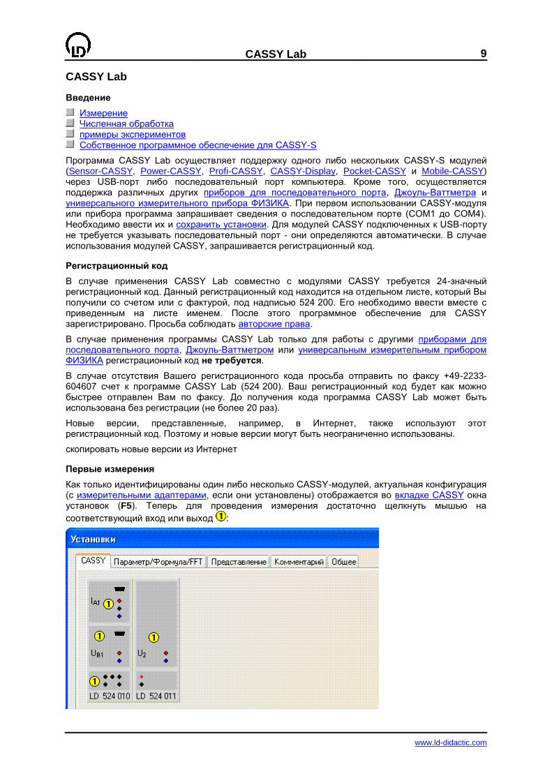
Как только идентифицированы один либо несколько CASSY-модулей, актуальная конфигурация (с измерительными адаптерами, если они установлены) отображается во вкладке CASSY окна установок (F5). Теперь для проведения измерения достаточно щелкнуть мышью на

соответствующий вход или выход :

10

CASSY Lab

www.ld-didactic.com

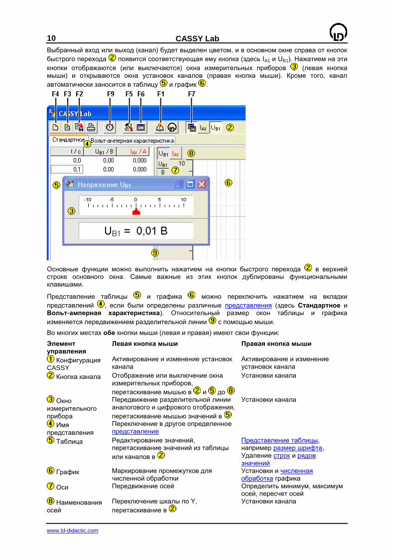
Выбранный вход или выход (канал) будет выделен цветом, и в основном окне справа от кнопок

быстрого перехода появится соответствующая ему кнопка (здесь IA1 и UB1). Нажатием на эти

кнопки отображаются (или выключаются) окна измерительных приборов (левая кнопка мыши) и открываются окна установок каналов (правая кнопка мыши). Кроме того, канал

автоматически заносится в таблицу и график .

Основные функции можно выполнить нажатием на кнопки быстрого перехода в верхней строке основного окна. Самые важные из этих кнопок дублированы функциональными клавишами.

Представление таблицы и графика можно переключить нажатием на вкладки

представлений , если были определены различные представления (здесь Стандартное и Вольт-амперная характеристика). Относительный размер окон таблицы и графика

изменяется передвижением разделительной линии с помощью мыши.

Во многих местах обе кнопки мыши (левая и правая) имеют свои функции:

Элемент управления

Левая кнопка мыши Правая кнопка мыши

Конфигурация CASSY

Активирование и изменение установок канала

Активирование и изменение установок канала

Кнопка канала Отображение или выключение окна измерительных приборов,

перетаскивание мышью в и до

Установки канала

Окно измерительного прибора

Передвижение разделительной линии аналогового и цифрового отображения,

перетаскивание мышью значений в


Имя представления

Переключение в другое определенное представление

Таблица Редактирование значений, перетаскивание значений из таблицы

или каналов в

Представление таблицы, например размер шрифта, Удаление строк и рядов значений

График Маркирование промежутков для численной обработки

Установки и численная обработка графика

Оси Передвижение осей Определить минимум, максимум осей, пересчет осей

Наименования осей

Переключение шкалы по Y,

перетаскивание в


CASSY Lab

11

www.ld-didactic.com

Разделительная линия

Передвижение разделительной линии между таблицей и графиком

Часто удобно использовать клавиши дублирующие кнопки быстрого перехода :

F4

Удаляет либо последнее измерение при сохранении его установок либо, при отсутствии измерений, удаляет актуальные установки.

Двукратное нажатие удаляет измерение и его установки.

F3

Открывает ряд значений (файл) с его установками и численной обработкой.

При этом загружаемый ряд значений может быть дописан к уже имеющемуся (без загружения его установок и численной обработки). Это возможно если в обоих измерениях фигурирует одна и та же измеряемая величина. Альтернативно, новый ряд значений может быть измерен позже и дописан к имеющемуся.

Кроме того, возможно использовать фильтр импорта ASCII-файлов (файлы с расширением *.txt).

F2

Сохраняет ряд значений с его установками и численной обработкой.

Существует также возможность сохранить только установки (без экспериментальных данных) для легкого повторения эксперимента в будущем.

Кроме того, возможно использовать фильтр экспорта ASCII-файлов (файлы с расширением *.txt). Следует отметить, однако, что файлы, производимые программой CASSY Lab (с расширением *.lab) могут быть прочитаны в любом текстовом редакторе.

Распечатывает активную таблицу или график.

F9

Начинает и останавливает новое измерение.

Альтернативно, возможно остановить измерение, предварительно задав длительность измерения.

F5

Изменяет используемые установки (например, CASSY, Параметр/Формула/FFT, Представление, Комментарий, Последовательный порт). Для открытия окна параметров измерения нужно нажать клавишу дважды.

F6

Отображает окно состояния либо закрывает его.

F1

Вызывает справку.

Показывает номер версии программы и дает возможность ввести код регистрации.

12

CASSY Lab

www.ld-didactic.com

F7

Закрывает все открытые окна измерительных приборов или открывает их снова.

CASSY Lab

13

www.ld-didactic.com

Экспорт и импорт ASCII-файлов

При выборе в окне открытия файла расширения *.txt возможен удобный экспорт и импорт ASCII-файлов.

Формат файла: заголовок содержит строки начинающиеся с ключевых слов. Там определены пределы измерений (MIN, MAX), выбор осей (SCALE), число значимых десятичных разрядов после запятой (DEC) и собственно определение измеряемых величин (DEF). Все строки заголовка кроме строки DEF могут быть опущены. После заголовка начинается собственно таблица экспериментальных значений.

Точный синтаксис можно увидеть на примере файла созданного при экспорте данных.

Строка состояния

В строке состояния внизу окна программы отображаются результаты числовой обработки. Содержимое строки состояния может быть выведено в большем по размеру окне состояния

нажатием или F6 (повторное нажатие закрывает это окно).

Перетаскивание с помощью мыши

Результаты численной обработки из строки состояния могут быть перемещены в таблицу с помощью перетаскивания мышью. Таким образом, можно строить графики отображающие результаты численной обработки.

14

CASSY Lab

www.ld-didactic.com

Измерение

F9

Начинает (и останавливает) новое измерение. Во время или после измерения нажатием правой кнопки мыши в таблице открывается меню представления таблицы, а в графике меню численной обработки.

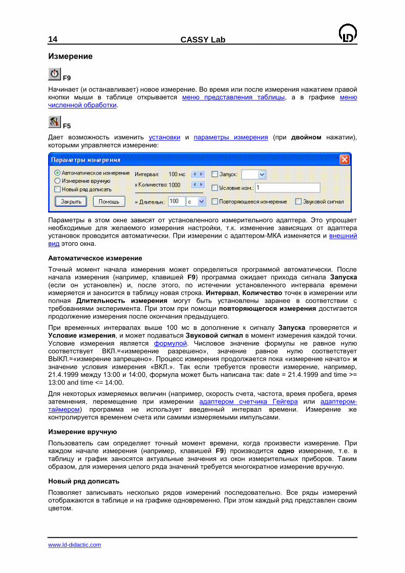
F5

Дает возможность изменить установки и параметры измерения (при двойном нажатии), которыми управляется измерение:

Параметры в этом окне зависят от установленного измерительного адаптера. Это упрощает необходимые для желаемого измерения настройки, т.к. изменение зависящих от адаптера установок проводится автоматически. При измерении с адаптером-МКА изменяется и внешний вид этого окна.

Автоматическое измерение

Точный момент начала измерения может определяться программой автоматически. После начала измерения (например, клавишей F9) программа ожидает прихода сигнала Запуска (если он установлен) и, после этого, по истечении установленного интервала времени измеряется и заносится в таблицу новая строка. Интервал, Количество точек в измерении или полная Длительность измерения могут быть установлены заранее в соответствии с требованиями эксперимента. При этом при помощи повторяющегося измерения достигается продолжение измерения после окончания предыдущего.

При временных интервалах выше 100 мс в дополнение к сигналу Запуска проверяется и Условие измерения, и может подаваться Звуковой сигнал в момент измерения каждой точки. Условие измерения является формулой. Числовое значение формулы не равное нулю соответствует ВКЛ.=«измерение разрешено», значение равное нулю соответствует ВЫКЛ.=«измерение запрещено». Процесс измерения продолжается пока «измерение начато» и значение условия измерения «ВКЛ.». Так если требуется провести измерение, например, 21.4.1999 между 13:00 и 14:00, формула может быть написана так: date = 21.4.1999 and time >= 13:00 and time <= 14:00.

Для некоторых измеряемых величин (например, скорость счета, частота, время пробега, время затемнения, перемещение при измерении адаптером счетчика Гейгера или адаптером-таймером) программа не использует введенный интервал времени. Измерение же контролируется временем счета или самими измеряемыми импульсами.

Измерение вручную

Пользователь сам определяет точный момент времени, когда произвести измерение. При каждом начале измерения (например, клавишей F9) производится одно измерение, т.е. в таблицу и график заносятся актуальные значения из окон измерительных приборов. Таким образом, для измерения целого ряда значений требуется многократное измерение вручную.

Новый ряд дописать

Позволяет записывать несколько рядов измерений последовательно. Все ряды измерений отображаются в таблице и на графике одновременно. При этом каждый ряд представлен своим цветом.

CASSY Lab

15

www.ld-didactic.com

Альтернативно, ряды измерений могут быть записаны и сохранены по-отдельности. Подобные измерения (с одинаковыми величинами измерений) могут быть дописаны друг к другу и позднее - при открытии сохраненных файлов.

Редактирование и удаление измеренных значений / Ввод параметров

Все измеренные значения (кроме времени и формул) можно редактировать в таблице. Для этого нужно щелкнуть мышью в ячейку таблицы и отредактировать значение с клавиатуры. Это является и единственной возможностью ввести в таблицу параметр.

Для удаления измеренных значений существует несколько возможностей. Через контекстное меню таблицы (правая кнопка мыши) можно удалить последнюю строку таблицы или последний дописанный ряд измерений. Через контекстное меню графика (правая кнопка мыши) можно удалить целые промежутки значений.

16

CASSY Lab

www.ld-didactic.com

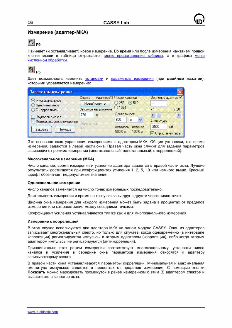
Измерение (адаптер-МКА)

F9

Начинает (и останавливает) новое измерение. Во время или после измерения нажатием правой кнопки мыши в таблице открывается меню представления таблицы, а в графике меню численной обработки.

F5

Дает возможность изменить установки и параметры измерения (при двойном нажатии), которыми управляется измерение:

Это основное окно управления измерениями с адаптером-МКА. Общие установки, как время измерения, задаются в левой части окна. Правая часть окна служит для задания параметров зависящих от режима измерения (многоканальный, одноканальный, с корреляцией).

Многоканальное измерение (МКА)

Число каналов, время измерения и усиление адаптера задаются в правой части окна. Лучшие результаты достигаются при коэффициентах усиления 1, 2, 5, 10 или немного выше. Красный шрифт обозначает недопустимые значения.

Одноканальное измерение

Число каналов заменяется на число точек измеряемых последовательно.

Длительность измерения и время на точку связаны друг с другом через число точек.

Ширина окна измерения для каждого измерения может быть задана в процентах от пределов измерения или как расстояние между соседними точками.

Коэффициент усиления устанавливается так же как и для многоканального измерения.

Измерение с корреляцией

В этом случае используются два адаптера-МКА на одном модуле CASSY. Один из адаптеров записывает многоканальный спектр, но только для случаев, когда одновременно (в интервале корреляции) регистрируются импульсы и вторым адаптером (корреляция), либо когда вторым адаптером импульсы не регистрируются (антикорреляция).

Принципиально этот режим измерения соответствует многоканальному, установки числа каналов и усиления в середине окна параметров измерения относятся к адаптеру записывающему спектр.

В правой части окна устанавливаются параметры корреляции. Минимальная и максимальная амплитуда импульсов задается в процентах от пределов измерения. С помощью кнопки Показать можно маркировать промежуток в ранее измеренном с этим (!) адаптером спектре и вывести его в качестве окна.

CASSY Lab

17

www.ld-didactic.com

Изменить представление таблицы

Формат таблицы может быть изменен после нажатия правой кнопкой мыши в таблице. Нажатием левой кнопки мыши можно отредактировать отдельные значения или перетащить их в другие ячейки таблицы.

Переобозначить столбцы Выбрать размер шрифта Удалить последнюю строку таблицы Удалить последний ряд значений Копировать таблицу/окно

Переобозначить столбцы

Вызывает окно Представление. В нем представлена возможность изменить столбец-X таблицы и до 8 столбцов-Y, а также произвести пересчет их значений.

По-другому изменить порядок столбцов можно перетаскивая их из области кнопок каналов и заголовка таблицы.

Выбрать размер шрифта

Размер шрифта в таблице можно установить. На выбор предоставлены мелкий, средний и крупный шрифт.

Используемые установки можно сохранить для последующих запусков программы в Общих установках.

Удалить последнюю строку таблицы

Удаляет последнюю на текущий момент строку таблицы. При этом стираются также измеренные тогда же невидимые значения измерений других каналов. Альтернативно, можно Удалить последний ряд значений целиком.

Функция предназначена для удаления неправильно измеренного значения при измерении вручную.

Сокращение

Клавиатура: Alt + L

Удалить последний ряд значений

Удаляет последний на текущий момент ряд значений. При этом стираются также измеренные тогда же невидимые значения измерений других каналов. Альтернативно, можно Удалить последнюю строку таблицы.

Функция предназначена для удаления неправильно измеренных значений при автоматическом измерении.

Буфер обмена

С помощью функций Копировать таблицу и Копировать окно таблица в виде текста и окно программы в виде файла Bitmap копируются в буфер обмена Windows и могут быть использованы другими Windows-программами.

18

CASSY Lab

www.ld-didactic.com

Графическая обработка

Многочисленные возможности графической обработки доступны после нажатия правой кнопки мыши в области графика.

Переобозначить оси Отображать координаты Выбрать толщину линий Форма отображения Положение осей Отображать растр Увеличить масштаб Исходный масштаб Поставить маркер Текст Вертикальная линия Горизонтальная линия Измерить разницу Вычислить среднее значение Приближение кривой Вычислить интеграл Распределение Пуассона Распределение Гаусса Центр пика Вычислить форм-фактор Коэффициент пульсаций Приблизить гауссовским профилем Определить точку эквивалентности Определить систолу и диастолу Удалить последнее вычисление Удалить все вычисления Удалить значения в промежутке Копировать график/окно

Переобозначить оси

Вызывает окно Представление. В нем представлена возможность изменить ось-X таблицы и до 8 осей-Y, а также произвести пересчет их значений.

По-другому изменить порядок осей можно перетаскивая их из области кнопок каналов и графика.

Отображать координаты

После активирования этой функции в Строке состояния отображаются актуальные координаты указателя мыши, когда он находится в окне графика. Функция остается активной до тех пор, пока не будет выключена повторным выбором этого пункта меню, или в строку состояния выведется результат одного из следующих действий: Поставить маркер, Вычислить среднее значение, Приблизить кривой, Вычислить интеграл или одного из Других вычислений.

Актуальные координаты могут быть занесены непосредственно в таблицу. Для этого нужно вызвать пункт меню Текст с клавиатуры (с помощью Alt+T), не изменяя положения указателя мыши (иначе будут занесены неверные координаты).



Клавиатура: Alt + C

Выбрать толщину линий

Толщину линий графиков можно установить. На выбор предоставлены тонкие, нормальные и жирные линии.

CASSY Lab

19

www.ld-didactic.com


Форма отображения

Возможны шесть вариантов отображения значений на графиках.

Показывать значения Квадраты, треугольники, круги, ромбы, ... Показывать соединительные линии Соединительные линии между измеренными точками Интерполяция по Акима Значения между точками интерполируются по Акима sinc-интерполяция Значения интерполируются sinc(x)=sin(x)/x Гистограмма Отображение значений столбиками Показывать нулевые линии Нулевые линии оси-X и оси-Y


Интерполяция по Акима и sinc не могут быть рассчитаны во время измерения, а также в местах где параметры не определены. Во время измерения точки соединяются прямыми линиями, которые будут заменены на интерполированные кривые по окончанию измерения. Применение sinc-интерполяции к сигналам, не содержащим частот выше половины частоты оцифровки, приводит к повышению эффективной частоты оцифровки на порядок.

Положение осей

Оси графика могут находиться слева-внизу, слева-вверху или не отображаться


Отображать растр

На поле графика может отображаться или не отображаться растр.


Увеличить масштаб

После выбора этого пункта меню нужно указать участок, который должен быть увеличен. Это производится с помощью левой кнопки мыши.

Увеличивать масштаб можно несколько раз последовательно. Для возвращения к первоначальному масштабу выберите пункт меню Исходный масштаб.


Клавиатура: Alt + Z

Исходный масштаб

Возвращает график к его первоначальным размерам.


Клавиатура: Alt + O

Калибровка энергии (адаптер-МКА)

Изначально, записанные спектры отображаются с номерами каналов по оси-Х. Присвоив одному или двум каналам значения энергии, можно отобразить спектр в виде функции от энергии. После вызова функции «Калибровка энергии» нужно с помощью мыши выбрать желаемый канал (он будет автоматически занесен в соответствующее диалоговое окно). Возможно также введение каналов вручную в диалоговое окно после щелчка мышью. Как третья возможность предлагается приближение функцией Гаусса, результаты которой заносятся в диалоговое окно с помощью перетаскивания мышью из строки состояния. Оба окна ввода уже содержат данные для обычных радиоактивных препаратов.

При выборе функции общая калибровка энергии введенные значения действительны для всех уже записанных и для будущих спектров этого ряда значений. Если эта функция не выбрана, то калибровка применяется к активному спектру и всем последующим в этом ряду.

20

CASSY Lab

www.ld-didactic.com

Калибровка дезактивируется при завершении программы, смене адаптера-МКА или его усиления. При наличии уже калиброванных спектров, их калибровку можно применить к другим.


Клавиатура: Alt + E

Поставить маркер

В программе предусмотрены несколько вариантов маркеров. Редактирование, передвижение или удаление уже существующего маркера производится двойным щелчком по нему левой кнопкой мыши.

Alt+T: Текст

Выбором текстовой функции можно поместить произвольную надпись в желаемом месте графика. После ввода текста нужно лишь поместить рамку на желаемое место и щелкнуть левой кнопкой мыши.

После любого из вычислений, помещенные в строке состояния результаты автоматически заносятся в окно ввода текстового маркера, где их можно использовать для подписи, редактировать или удалить.

Alt+V: Вертикальная линия

Выбором этой функции можно поместить вертикальную линию в желаемом месте графика. Координата линии отображается в строке состояния. Если до этого была выбрана функция Отображать координаты, она будет отключена.

Alt+H: Горизонтальная линия

Выбором этой функции можно поместить горизонтальную линию в желаемом месте графика. Координата линии отображается в строке состояния. Если до этого была выбрана функция Отображать координаты, она будет отключена.

Alt+D: Измерить разницу

После щелчка по точке отсчета можно нарисовать на графике произвольные линии. Разница координат конца и начала линии будет отображена в строке состояния. Если до этого была выбрана функция Отображать координаты, она будет отключена.

Вычислить среднее значение

После включения этой функции нужно с помощью левой кнопки мыши выбрать промежуток, на котором провести усреднение. Среднее значение и его статистическая ошибка будет отображена в строке состояния. Если до этого была выбрана функция Отображать координаты, она будет отключена.

Вычисленное среднее значение можно поместить на графике в виде текста. Удалить линию среднего можно двойным щелчком мыши по ней.

Приблизить кривой

Предусмотрены восемь различных вариантов приближения:

Прямая y=Ax+B Прямая из начала координат y=Ax Парабола из начала координат y=Ax

2

Парабола y=Ax2+Bx+C

Гипербола 1/x y=A/x+B

Гипербола 1/x2 y=A/x

2+B

Экспоненциальная функция y=A*exp(-x/B) Огибающая колебания y=±A*exp(-x/B)+C (затухание из-за вязкости воздуха) Свободное приближение y=f(x,A,B,C,D)

После выбора функции нужно с помощью левой кнопки мыши выбрать промежуток, на котором провести приближение.

CASSY Lab

21

www.ld-didactic.com

При выполнении свободного приближения до выбора промежутка, необходимо указать функцию f(x,A,B,C,D), разумные начальные значения и максимальное время расчета. Ввод функции подчиняется обычным правилам. Чтобы приближение могло быть успешно проведено, начальные значения нужно задать по возможности реалистично. В случае неудовлетворительного приближения можно повторить попытку с другими начальными условиями или увеличенным временем вычислений. Кроме того, отдельные параметры A, B, C или D можно фиксировать на время приближения.

Свободное приближение позволяет автоматически открыть новый канал выбором функции представлять результат автоматически как новый канал (параметр). В этом случае разные приближения могут быть отображены различными цветами и подвергнуты дальнейшей обработке с помощью формул.

Актуальные параметры (A, B, C и D) отображаются во время приближения в строке состояния. Если до этого была выбрана функция Отображать координаты, она будет отключена. Эти значения можно поместить на график, выбрав функцию Текст. Удалить приближение из графика можно двойным щелчком мыши по нему.

Вычислить интеграл

Значение интеграла соответствует площади заключенной между выбранным промежутком кривой и осью-Х либо площади пика. Значение интеграла отображается в строке состояния. Если до этого была выбрана функция Отображать координаты, она будет отключена.

Актуальное значение интеграла можно поместить на график, выбрав функцию Текст.

Другие вычисления —> Распределение Пуассона (имеет смысл только для частотных распределений)

На выделенном промежутке гистограммы рассчитывается полное число событий n, среднее

значение µ и стандартное отклонение . Эти значения отображаются в строке состояния,

вычисленное распределение Пуассона y=nµx/x!*exp(-µ) выводится на график.

Другие вычисления —> Распределение Гаусса (имеет смысл только для частотных распределений)

На выделенном промежутке гистограммы рассчитывается полное число событий n, среднее

значение µ и стандартное отклонение . Эти значения отображаются в строке состояния,

вычисленное распределение Гаусса y=n//Sqrt(2)*exp(-(x-µ)2/2

2) выводится на график.

Другие вычисления —> Центр пика

Для выделенного пика вычисляется «центр тяжести пика» и отображается в строке состояния. Удалить линию из графика можно двойным щелчком мыши по ней.

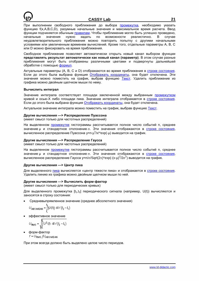
Другие вычисления —> Вычислить форм-фактор (имеет смысл только для периодических кривых)

Для выделенного промежутка [t1,t2] периодического сигнала (например, U(t)) вычисляются и заносятся в строку состояния:

Средневыпрямленное значение (среднее абсолютного значения)

эффективное значение

форм-фактор

При этом всегда должно быть выделено целое число периодов.

22

CASSY Lab

www.ld-didactic.com

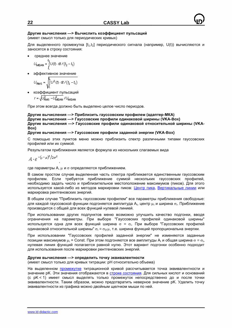
Другие вычисления —> Вычислить коэффициент пульсаций (имеет смысл только для периодических кривых)

Для выделенного промежутка [t1,t2] периодического сигнала (например, U(t)) вычисляются и заносятся в строку состояния:

среднее значение

эффективное значение

коэффициент пульсаций

При этом всегда должно быть выделено целое число периодов.

Другие вычисления —> Приблизить гауссовским профилем (адаптер-МКА) Другие вычисления —> Гауссовские профили одинаковой ширины (VKA-Box) Другие вычисления —> Гауссовские профили одинаковой относительной ширины (VKA-Box) Другие вычисления —> Гауссовские профили заданной энергии (VKA-Box)

С помощью этих пунктов меню можно приблизить спектр различными типами гауссовских профилей или их суммой.

Результатом приближения является формула из нескольких слагаемых вида

,

где параметры A, и определяются приближением.

В самом простом случае выделенная часть спектра приближается единственным гауссовским профилем. Если требуется приближение суммой нескольких гауссовских профилей, необходимо задать число и приблизительное местоположение максимумов (пиков). Для этого используется какой-либо из методов маркировки пиков: Центр пика, Вертикальные линии или маркировка рентгеновских энергий.

В общем случае "Приблизить гауссовским профилем" все параметры приближения свободные:

для каждой гауссовской функции подгоняется амплитуда Ai, центр i и ширина i. Приближение

производится с общей для всех функций нулевой линией.

При использовании других подпунктов меню возможно улучшить качество подгонки, вводя ограничения на параметры. При выборе "Гауссовских профилей одинаковой ширины"

используется одна для всех функций ширина = i. При выборе "Гауссовских профилей

одинаковой относительной ширины" i = 0, т.е. ширина функций пропорциональна энергии.

При использовании "Гауссовских профилей заданной энергии" не изменяются заданные

позиции максимумов i = Const. При этом подгоняются все амплитуды Ai и общая ширина = i, нулевая линия функций полагается равной нулю. Этот вариант подгонки особенно подходит для использования после маркировки рентгеновских энергий.

Другие вычисления —> определить точку эквивалентности (имеет смысл только для кривых титрации: pH относительно объема)

На выделенном промежутке титрационной кривой рассчитывается точка эквивалентности и значение pK. Эти значения отображаются в строке состояния. Для сильных кислот и оснований (с pK < 1) имеет смысл выделять только промежуток непосредственно до и после точки эквивалентности. Таким образом, можно предотвратить неверное значение pK. Удалить точку эквивалентности из графика можно двойным щелчком мыши по ней.

CASSY Lab

23

www.ld-didactic.com

Другие вычисления —> определить систолу и диастолу (имеет смысл только для кривых кровяного давления)

На выделенном промежутке кривой кровяного давления определяются систола и диастола, значения отображаются в строке состояния. Удалить систолу или диастолу из графика можно двойным щелчком мыши по ней.

Удалить последнее вычисление

Последнее на данный момент вычисление может быть отменено. Это возможно для следующих вычислений:

Поставить маркер Вычислить среднее значение Приблизить кривой Вычислить интеграл Другие вычисления


Клавиатура: Alt + Backspace

Удалить все вычисления

Все вычисления будут удалены. Это относится к следующим вычислениям:

Поставить маркер Вычислить среднее значение Приблизить кривой Вычислить интеграл Другие вычисления

Удалить значения в промежутке

Значения на выделенном промежутке кривой будут удалены. Это относится только к значениям представленным по оси-Y. Не могут быть удалены результаты вычислений (например, рассчитанные с помощью какой-либо формулы) и значения по оси-Х.

Буфер обмена

С помощью функций Копировать таблицу и Копировать окно график или окно программы в виде файла Bitmap копируются в буфер обмена Windows и могут быть использованы другими Windows-программами.

Маркирование промежутка кривой

Для проведения некоторых вычислений необходимо маркировать (выбрать) промежуток в котором их провести.

Для этого нужно переместить указатель мыши при нажатой левой кнопке от начала до конца промежутка. Альтернативно, можно щелкнуть мышью на начало и на конец промежутка.

В процессе маркирования выделенная часть кривой показывается зеленым цветом.

24

CASSY Lab

www.ld-didactic.com

Сложение/вычитание спектров (адаптер-МКА)

Сложение/вычитание спектров производится в обзорном представлении. Для этого достаточно перетащить мышью один спектр на другой. Альтернативно, можно перетащить символ спектра из строки символов в график. В соответствующем окне устанавливается арифметическая операция и цель расчета.

Функции Гаусса и скорость счета (адаптер-МКА)

При вычислении суммарной скорости счета под пиком необходимо учитывать некоторые детали связанные с функцией Гаусса.

Суммарная скорость счета в измеренном спектре может быть определена как интеграл по промежутку, например под каким-либо пиком. Однако, в измерениях адаптером-МКА этот результат не является настоящим интегралом по оси-Х, а лишь суммой по каналам и имеет размерность «события».

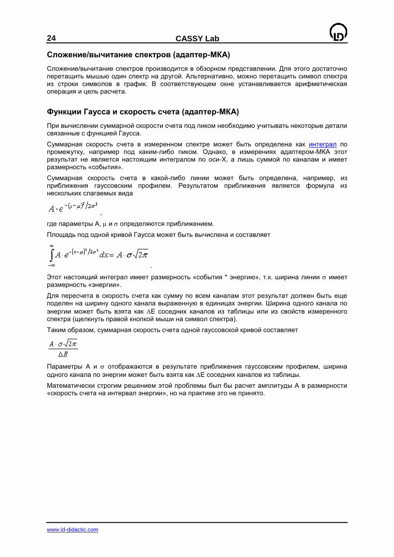
Суммарная скорость счета в какой-либо линии может быть определена, например, из приближения гауссовским профилем. Результатом приближения является формула из нескольких слагаемых вида

,

где параметры A, и определяются приближением.

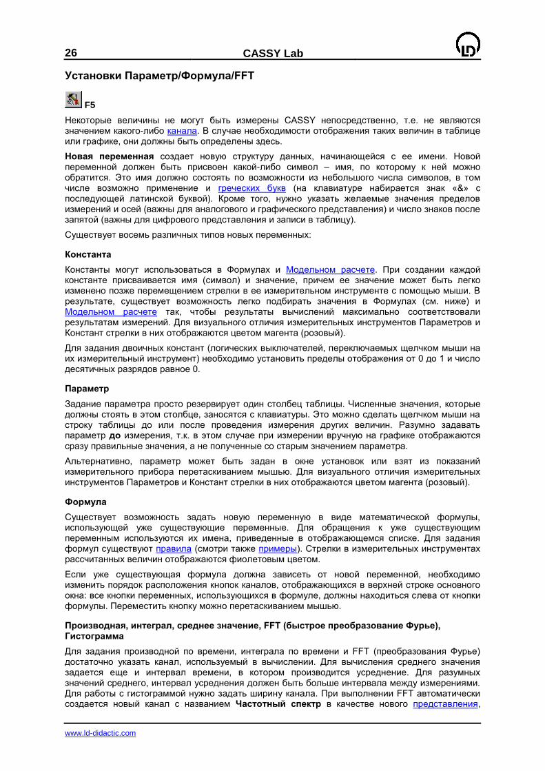
Площадь под одной кривой Гаусса может быть вычислена и составляет

.

Этот настоящий интеграл имеет размерность «события * энергию», т.к. ширина линии имеет размерность «энергии».

Для пересчета в скорость счета как сумму по всем каналам этот результат должен быть еще поделен на ширину одного канала выраженную в единицах энергии. Ширина одного канала по

энергии может быть взята как E соседних каналов из таблицы или из свойств измеренного спектра (щелкнуть правой кнопкой мыши на символ спектра).

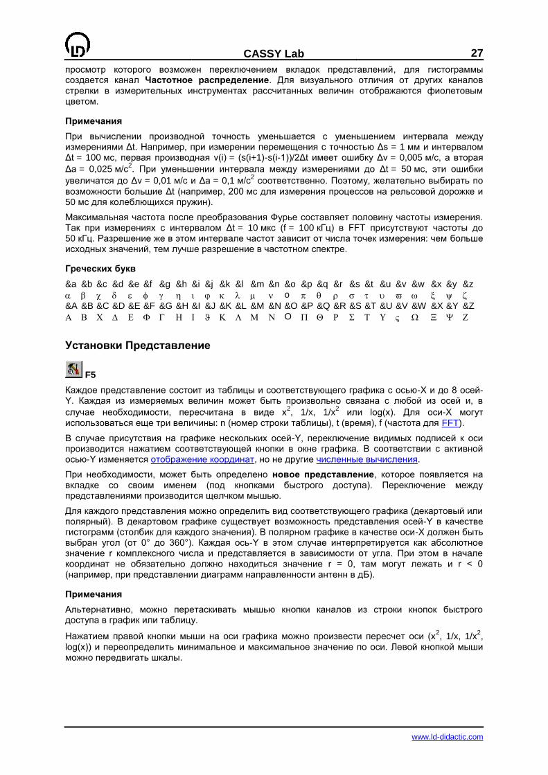
Таким образом, суммарная скорость счета одной гауссовской кривой составляет

Параметры A и отображаются в результате приближения гауссовским профилем, ширина

одного канала по энергии может быть взята как E соседних каналов из таблицы.

Математически строгим решением этой проблемы был бы расчет амплитуды А в размерности «скорость счета на интервал энергии», но на практике это не принято.

CASSY Lab

25

www.ld-didactic.com

Установки

F5

В этом диалоговом окне можно произвести все установки кроме параметров измерения. Эти установки разделены на шесть групп:

CASSY (Определения входов и выходов CASSY-модулей) Параметр/Формула/FFT (Определение дополнительных величин как параметров, через

формулы, быстрое преобразование Фурье) Представление (Изменение присвоения измеряемых величин столбцам таблицы и осям

графика) Модельный расчет (Определение моделей с помощью дифференциальных уравнений) Комментарий (Место для собственного текста) Общее (Выбор прибора для последовательного порта, последовательного порта и

сохранение установок)

Установки CASSY

F5

В этой вкладке изображена актуальная конфигурация модулей CASSY и измерительных адаптеров. Изменение конфигурации (например, новый модуль или адаптер) приводит к соответствующему изменению изображения.

Активирование канала и изменение его установок производится после щелчка мышью по нему. Измеряемые величины зависят от CASSY-модуля и установленного адаптера. Значения измеренные каждым активным каналом заносятся в таблицу и на график. Представление (присвоение столбцов и осей) может быть изменено в соответствующей вкладке.

В случае если уже присутствуют активные каналы, изображается не актуальная конфигурация, а заданная ранее с указанием возможных отклонений от реальной. Таким образом, при загрузке ранее записанного файла, легко восстановить использованную при его записи конфигурацию CASSY-модулей и адаптеров.

При выборе функции актуализировать конфигурацию изображается актуальная конфигурация, но информация об активных каналах теряется.

При наличии активных каналов нажатием на кнопку параметры измерения открывается соответствующее окно.

26

CASSY Lab

www.ld-didactic.com

Установки Параметр/Формула/FFT

F5

Некоторые величины не могут быть измерены CASSY непосредственно, т.е. не являются значением какого-либо канала. В случае необходимости отображения таких величин в таблице или графике, они должны быть определены здесь.

Новая переменная создает новую структуру данных, начинающейся с ее имени. Новой переменной должен быть присвоен какой-либо символ – имя, по которому к ней можно обратится. Это имя должно состоять по возможности из небольшого числа символов, в том числе возможно применение и греческих букв (на клавиатуре набирается знак «&» с последующей латинской буквой). Кроме того, нужно указать желаемые значения пределов измерений и осей (важны для аналогового и графического представления) и число знаков после запятой (важны для цифрового представления и записи в таблицу).

Существует восемь различных типов новых переменных:

Константа

Константы могут использоваться в Формулах и Модельном расчете. При создании каждой константе присваивается имя (символ) и значение, причем ее значение может быть легко изменено позже перемещением стрелки в ее измерительном инструменте с помощью мыши. В результате, существует возможность легко подбирать значения в Формулах (см. ниже) и Модельном расчете так, чтобы результаты вычислений максимально соответствовали результатам измерений. Для визуального отличия измерительных инструментов Параметров и Констант стрелки в них отображаются цветом магента (розовый).

Для задания двоичных констант (логических выключателей, переключаемых щелчком мыши на их измерительный инструмент) необходимо установить пределы отображения от 0 до 1 и число десятичных разрядов равное 0.

Параметр

Задание параметра просто резервирует один столбец таблицы. Численные значения, которые должны стоять в этом столбце, заносятся с клавиатуры. Это можно сделать щелчком мыши на строку таблицы до или после проведения измерения других величин. Разумно задавать параметр до измерения, т.к. в этом случае при измерении вручную на графике отображаются сразу правильные значения, а не полученные со старым значением параметра.

Альтернативно, параметр может быть задан в окне установок или взят из показаний измерительного прибора перетаскиванием мышью. Для визуального отличия измерительных инструментов Параметров и Констант стрелки в них отображаются цветом магента (розовый).

Формула

Существует возможность задать новую переменную в виде математической формулы, использующей уже существующие переменные. Для обращения к уже существующим переменным используются их имена, приведенные в отображающемся списке. Для задания формул существуют правила (смотри также примеры). Стрелки в измерительных инструментах рассчитанных величин отображаются фиолетовым цветом.

Если уже существующая формула должна зависеть от новой переменной, необходимо изменить порядок расположения кнопок каналов, отображающихся в верхней строке основного окна: все кнопки переменных, использующихся в формуле, должны находиться слева от кнопки формулы. Переместить кнопку можно перетаскиванием мышью.

Производная, интеграл, среднее значение, FFT (быстрое преобразование Фурье), Гистограмма

Для задания производной по времени, интеграла по времени и FFT (преобразования Фурье) достаточно указать канал, используемый в вычислении. Для вычисления среднего значения задается еще и интервал времени, в котором производится усреднение. Для разумных значений среднего, интервал усреднения должен быть больше интервала между измерениями. Для работы с гистограммой нужно задать ширину канала. При выполнении FFT автоматически создается новый канал с названием Частотный спектр в качестве нового представления,

CASSY Lab

27

www.ld-didactic.com

просмотр которого возможен переключением вкладок представлений, для гистограммы создается канал Частотное распределение. Для визуального отличия от других каналов стрелки в измерительных инструментах рассчитанных величин отображаются фиолетовым цветом.

Примечания

При вычислении производной точность уменьшается с уменьшением интервала между измерениями Δt. Например, при измерении перемещения с точностью Δs = 1 мм и интервалом Δt = 100 мс, первая производная v(i) = (s(i+1)-s(i-1))/2Δt имеет ошибку Δv = 0,005 м/с, а вторая

Δa = 0,025 м/с2. При уменьшении интервала между измерениями до Δt = 50 мс, эти ошибки

увеличатся до Δv = 0,01 м/с и Δa = 0,1 м/с2 соответственно. Поэтому, желательно выбирать по

возможности большие Δt (например, 200 мс для измерения процессов на рельсовой дорожке и 50 мс для колеблющихся пружин).

Максимальная частота после преобразования Фурье составляет половину частоты измерения. Так при измерениях с интервалом Δt = 10 мкс (f = 100 кГц) в FFT присутствуют частоты до 50 кГц. Разрешение же в этом интервале частот зависит от числа точек измерения: чем больше исходных значений, тем лучше разрешение в частотном спектре.

Греческих букв

&a &b &c &d &e &f &g &h &i &j &k &l &m &n &o &p &q &r &s &t &u &v &w &x &y &z

o &A &B &C &D &E &F &G &H &I &J &K &L &M &N &O &P &Q &R &S &T &U &V &W &X &Y &Z

O

Установки Представление

F5

Каждое представление состоит из таблицы и соответствующего графика с осью-Х и до 8 осей-Y. Каждая из измеряемых величин может быть произвольно связана с любой из осей и, в

случае необходимости, пересчитана в виде x2, 1/x, 1/x

2 или log(x). Для оси-Х могут

использоваться еще три величины: n (номер строки таблицы), t (время), f (частота для FFT).

В случае присутствия на графике нескольких осей-Y, переключение видимых подписей к оси производится нажатием соответствующей кнопки в окне графика. В соответствии с активной осью-Y изменяется отображение координат, но не другие численные вычисления.

При необходимости, может быть определено новое представление, которое появляется на вкладке со своим именем (под кнопками быстрого доступа). Переключение между представлениями производится щелчком мышью.

Для каждого представления можно определить вид соответствующего графика (декартовый или полярный). В декартовом графике существует возможность представления осей-Y в качестве гистограмм (столбик для каждого значения). В полярном графике в качестве оси-Х должен быть выбран угол (от 0° до 360°). Каждая ось-Y в этом случае интерпретируется как абсолютное значение r комплексного числа и представляется в зависимости от угла. При этом в начале координат не обязательно должно находиться значение r = 0, там могут лежать и r < 0 (например, при представлении диаграмм направленности антенн в дБ).

Примечания

Альтернативно, можно перетаскивать мышью кнопки каналов из строки кнопок быстрого доступа в график или таблицу.

Нажатием правой кнопки мыши на оси графика можно произвести пересчет оси (x2, 1/x, 1/x

2,

log(x)) и переопределить минимальное и максимальное значение по оси. Левой кнопкой мыши можно передвигать шкалы.

28

CASSY Lab

www.ld-didactic.com

Установки Модельный расчет

F5

С помощью модельного расчета производится сравнение результатов реальных измерений с математической моделью. В частности, с помощью подбора подходящих констант достигается максимальное сходство модели с реальностью. В отличие от приближения функцией (например, Свободное приближение), где функциональная зависимость должна быть известна заранее, для модельного расчета достаточно задания одного или двух дифференциальных уравнений.

Новая модель создает новую структуру данных, начинающейся с ее имени. Модель описывается одной или двумя переменными, каждой из которых должен быть присвоен какой-либо символ – имя, по которому к ней можно обратится (по умолчанию x и y). Это имя должно состоять по возможности из небольшого числа символов, в том числе возможно применение и греческих букв (на клавиатуре набирается знак «&» с последующей соответствующей латинской буквой). Кроме того, нужно указать желаемые значения пределов измерений и осей (важны для аналогового и графического представления) и число знаков после запятой (важны для цифрового представления и записи в таблицу). Для визуального отличия от других каналов стрелки в измерительных инструментах величин модельного расчета отображаются синим цветом.

Математическое определение модели производится заданием дифференциальных уравнений и начальных значений для времени t и для переменных модели. Эти пять численных значений или формул должны быть введены в соответствии с правилами ввода формул. Все пять формул могут зависеть от Констант, значения которых могут быть изменены позже передвижением стрелки в окнах их измерительных инструментов. Кроме того, оба дифференциальных уравнения могут зависеть от времени измерения t, от обоих определенных переменных модели и от формул, зависящих в свою очередь только от констант и времени измерения. Все разрешенные для использования в дифференциальных уравнениях параметры перечислены в списке перед полем задания уравнения.

Обычно модель определяется заданием одного или двух дифференциальных уравнений первого порядка. Задание уравнения второго порядка облегчается выбором пункта Дифференциальные уравнения 2го порядка: в этом случае первое уравнение автоматически связывает переменные x и y как x'=y, а второе дифференциальное уравнение имеет форму y'=x''=f(t,x',x''). Например, для уравнения движения s=x и v=y=x', дополнительно задается только дифференциальное уравнение s''=v' (=a=F/m).

Выбором Точности определяется критерий остановки численного интегрирования дифференциальных уравнений. Чем меньше Точность, тем короче время вычислений, но выше их ошибка. Точность может быть улучшена также уменьшением интервала отображения первой переменной модели.

Выбором Времени расчета определяется максимальное время численного интегрирования дифференциальных уравнений. В случае задания меньшего времени расчета чем необходимо для достижения заданной точности, укорачивается интервал, в котором производится интеграция.

Примеры

Самым известным примером дифференциального уравнения второго порядка является второй закон Ньютона F=m⋅ a или s''=F(s,v,t)/m. В этом случае переменными модели являются перемещение s и скорость v, и первое дифференциальное уравнение имеет форму s'=v.

Ускоряющая сила F из второго уравнения s''=v'=(F1+F2+F3)/m зависит от проводимого

эксперимента и может быть, например:

F1 = −m⋅ g для экспериментов по свободному падению

F1 = −D⋅ s для экспериментов с пружинным маятником

Кроме того, могут присутствовать различные виды трения, порождающие дополнительные силы:

F2 = −c⋅ sgn(v) для сухого (кулоновского) трения

CASSY Lab

29

www.ld-didactic.com

F2 = −c⋅ sgn(v)⋅ |v| для вязкого (стоксовского) трения, например, при ламинарном течении

жидкости

F2 = −c⋅ sgn(v)⋅ |v|2 для вязкостного (ньютоновского) трения, например, при турбулентном

течении жидкости и трении воздуха

При вынужденных колебаниях (резонанс) в уравнение дополнительно входит вынуждающая сила, например:

F3 = A⋅ sin(360⋅ f⋅ t), sin для аргумента в градусах

F3 = A⋅ rsin(⋅ t), rsin для аргумента в радианах

При комбинации различных сил получается набор экспериментов, которые могут быть исследованы с помощью модельного расчета.

Кроме того, могут быть исследованы, например, зарядка и разрядка конденсатора, фильтры высоких и низких частот, описываемые дифференциальным уравнением первого порядка

Q'=(U0−Q/C)/R для заряда Q на конденсаторе.

Некоторые примеры модельного расчета содержаться в примерах экспериментов:

Свободное падение перфорированной планки (с модельным расчетом)

Колебания пружинного маятника (с модельным расчетом)

Колебания пружинного маятника с сухим трением (с модельным расчетом)

Колебания пружинного маятника с трением смазки (с модельным расчетом)

Колебания пружинного маятника с ламинарным вязким трением (с модельным расчетом)

Колебания пружинного маятника с турбулентным вязким трением/трением воздуха (с модельным расчетом)

Зарядка и разрядка конденсатора (с модельным расчетом)

Колебательный контур с затуханием (с модельным расчетом)

Вынужденные колебания (с модельным расчетом)

Фильтр высоких частот (с модельным расчетом)

Фильтр низких частот (с модельным расчетом)

Установки Комментарий

F5

Здесь предусмотрена возможность, для лучшей документации собственных измерений, вводить текст, сохранять его вместе с файлом измерения и загружать позднее. Ввести текст возможно и с использованием буфера обмена Windows (например, нажатием Ctrl+V).

Общие установки

F5

Здесь можно определить последовательный порт, к которому подключены модули CASSY и / или другие приборы для последовательного порта. Для модулей CASSY подключенных к USB-порту не требуется указывать порт - он определяется автоматически. Кроме того, здесь определяется язык работы с программой.

Чтобы сохранить произведенные установки выберите Сохранить новые установки. Одновременно сохраняются и следующие настройки:

Выбрать размер шрифта Отображать координаты Выбрать толщину линий Форма отображения Положение осей Отображать растр

В списке идентифицированных CASSY-модулей представлены все опознанные приборы и информация о версии микропрограммы в модуле CASSY. В случае, когда микропрограмма CASSY-модуля старее или новее чем версия программы CASSY Lab, выводится

30

CASSY Lab

www.ld-didactic.com

соответствующее сообщение. При нажатии кнопки Актуализировать CASSY-модули CASSY Lab перезаписывает в CASSY-модули микропрограмму (не зависимо от того новее она или старее).

Совет

В случае если используемая программа старее микропрограммы в CASSY-модулях или программу нужно обновить, новую версию можно скопировать с Интернет-страницы http://www.ld-didactic.de.

скопировать новые версии из Интернет



CASSY Lab

31

www.ld-didactic.com

Правила написания формул

Переменные для использования в формуле f(time,date,n,t,...,old)

Формула f(...) может зависеть от всех приведенных ниже каналов. В качестве имени переменной используется имя канала. Например, значение выражения UA1 > 5 равно 1, если напряжение больше 5 В, иначе, оно равно 0.

Формула для Может зависеть от Условие измерения всех каналов Формула входов, констант, приборов для последовательного порта и ранее

определенных формул Реле/Источник напряжения

входов, констант, приборов для последовательного порта, формул

Аналоговый выход входов, констант, приборов для последовательного порта, формул Цифровой выход входов, констант, приборов для последовательного порта, формул Модель переменных модели, констант и формул, зависящих только от

времени t

Кроме того, формула может зависеть от времени суток time в секундах, даты date, времени измерения t в секундах, числа n записанных значений и последнего значения формулы old. В конце формулы может находиться комментарий, отделенный точкой с запятой.

В программе применяются и символы, состоящие из знака & с последующей латинской буквой. В этом случае вместо латинской отображается соответствующая греческая буква, а в формуле должна быть указана исходная форма со знаком &.

Математические функции для использования в формуле

В формуле могут быть использованы следующие функции. В случае сложного аргумента он должен быть заключен в скобки, например, square(t/10).

ramp пилообразная функция (для значений между 0 и 1, ramp(x) = frac(x)) square прямоугольная функция (для значений между 0 и 1, square(x) = ramp(x) < 0.5) saw треугольная функция (для значений между 0 и 1) shift однократная пилообразная функция (равна 0 когда аргумент < 0, 1 когда аргумент >

1, иначе равна аргументу) sin синус для аргумента в градусах (период 360°) cos косинус для аргумента в градусах (период 360°) tan тангенс для аргумента в градусах (период 360°) arcsin арксинус для аргумента в градусах arccos арккосинус для аргумента в градусах arctan арктангенс для аргумента в градусах rsin синус для аргумента в радианах (период 2) rcos косинус для аргумента в радианах (период 2) rtan тангенс для аргумента в радианах (период 2) rarcsin арксинус для аргумента в радианах rarccos арккосинус для аргумента в радианах rarctan арктангенс для аргумента в радианах last аргумент на момент произведения измерения последнего значения (последняя

строка таблицы) delta изменение с момента произведения измерения последнего значения (delta(x) = x-

last(x)) next аргумент на момент произведения измерения следующего значения (следующая

строка таблицы) new равна 1, если аргумент изменился, иначе 0 random случайное число (0 <= random(x) < x) sqr квадратный корень exp экспоненциальная функция ln натуральный логарифм log десятичный логарифм int целая часть (самое близкое снизу целое число) frac дробная часть (разница с самым близким снизу целым числом) abs абсолютное значение

32

CASSY Lab

www.ld-didactic.com

sgn сигнум-функция (равна 1 когда аргумент > 0, -1 когда аргумент < 0, 0 когда аргумент = 0)

odd равна 1 когда аргумент нечетный, 0 когда аргумент четный even равна 1 когда аргумент четный, 0 когда аргумент нечетный not логическая инверсия (равна 1 когда аргумент равен 0, иначе равна 0) defined равна 1 когда аргумент определен, 0 когда аргумент не определен sec округляет время до целых секунд (sec(x) = int(x)) min округляет время до целых минут (min(x) = 60*int(x/60)) day возвращает день недели (1 = понедельник, ...)

Соотношения между переменными и функциями

Все переменные (а также введенные численные значения) могут быть связаны друг с другом обычными математическими операторами.

Для операторов определен порядок выполнения. Чем выше стоит оператор в приведенном ниже списке, тем выше его приоритет при расчете по формуле («умножение до деления»). Для выполнения действий в другом порядке, необходимо заключить желаемые части выражения в скобки.

1) ^ возведение в степень 2) * умножение / деление 3) + сложение - вычитание 4) = сравнение на равенство <> сравнение на неравенство > равнение на «больше» >= сравнение на «больше или равно» < сравнение на «меньше» <= сравнение на «меньше или равно» 5) and логическое И 6) or логическое ИЛИ

Примеры применения переменных time, date, n, t и old

t <= 100

имеет во время первых 100 с измерения значение 1, а после - значение 0. Эта формула может быть использована, например, для задания временного окна и остановки измерения через 100 с.

time >= 12:30:35

позже указанного времени суток (12ч 30м 35с) имеет значение 1, раньше - значение 0. Здесь нужно применять оператор >=, т.к. точное равенство длится только 1/100 с и практически не может быть достигнуто.

min(time) = 11:45 and date = 18.3.1997

имеет значение 1 только в течение одной минуты 18.3.1997 в 11ч 45м, иначе равно 0.

(T < 25) or (T < 27 and old)

реализует регулировку по двум точкам. При температуре T меньше 25 °C имеет значение 1 (например, может обозначать «нагрев включен»). При температуре T меньше 27 °C И нагрев был уже включен, то он и останется включенным. Только при возрастании температуры выше 27 °C нагрев выключится и не включится до тех пор, пока температура не упадет до 25 °C.

0,5 * (n – 1)

вычисляет из номера текущего измерения, например, объем. В примере измерение производится при изменении объема на каждые 5 мл. Первая строка таблицы имеет номер n=1.

CASSY Lab

33

www.ld-didactic.com

Примеры генерации частот

ramp(t/10)

генерирует пилообразное напряжение с периодом 10 секунд (t представляет собой время измерения в секундах и в момент старта измерения равно 0). Наклонная начинается в 0 и заканчивается в 1. Если требуются другие амплитуды, необходимо умножить на нужную амплитуду.

saw(t/5)

генерирует треугольную функцию с периодом 5 секунд.

square(t/5)

генерирует прямоугольную функцию с периодом в 5 секунд. Каждые 2,5 секунды изменяется между 1 и 0 и наоборот.

10*(ramp(t/10) < 0.4)

также генерирует прямоугольную функцию. В данном случае, однако, с амплитудой 10 и коэффициентом заполнения 40%. 40% времени значение выражения в скобках есть 1, остальные 60% времени 0.

shift((time-12:30)/100)

генерирует однократную пилообразную функцию начиная в 12ч 30м продолжительностью 100 секунд. В это время значение формулы растет непрерывно с 0 до 1.

sin(360*t/7)

генерирует синус с периодом в 7 секунд и амплитудой 1.

Примеры, иллюстрирующие порядок арифметических действий в выражении

x+y^z*2

имеет порядок выполнения действий ^,* и +. В результате сначала обрабатывается y^z,затем результат умножается на два и только в конце прибавляется х. Если заданный порядок действий нужно изменить, необходимо соответствующие выражения поставить в скобки.

(x+y)^(z*2)

в отличие от предыдущего примера здесь выполняются сначала сложение x+y и умножение z*2. Только в конце с обоими результатами производится потенцирование.

Примеры выполнения булевских выражений

x < 5

может иметь либо значение 0 (не верно), для x >= 5, либо значение 1 (верно), для x < 5.

x1 < 5 and x2 > 0

имеет значение 1 (верно), если одновременно x1 < 5 и x2 > 0, иначе имеет значение 0. Скобки в этом выражении не требуются, т.к. оператор and имеет меньший приоритет, чем сравнение.

5*(T < 20)

в скобках имеет только значения 0 (не верно) и 1 (верно). Эти значения умножаются на 5. Такая формула имеет смысл только для аналоговых выходов. В этом случае на выход подавалось бы напряжение 5 В, если Т меньше 20 (например, температура).

time >= 12:30

позднее 12ч 30м имеет значение 1, до этого 0. Здесь нужно применять оператор >=, т.к. точное равенство длится только 1/100 с и практически не может быть достигнуто.

34

CASSY Lab

www.ld-didactic.com

sec(time) = 11:45:07 and date = 18.3.1997

истинно (значение 1) только в течение одной секунды в 11ч 45м 07с 18 марта 1997, а в остальное время не верно (значение 0).

day(date) = 1

истинно каждый понедельник (значение 1), а в остальное время не верно (значение 0).

CASSY Lab

35

www.ld-didactic.com

Примеры формул

Простая регулировка: A11<25

имеет значение 1, если температура меньше 25 °C ( введено как &J), иначе равно 0 (например, для управления нагревом).

Регулировка по двум точкам: A11<25 or (A11<27 and old)

имеет значение 1, если температура меньше 25 °C или, в случае если значение и ранее было 1,

даже до 27 °C ( введено как &J), иначе равно 0 (например, для управления нагревом по двум точкам). Таким образом, управление включается ниже 25 °C и выключается выше 27 °C.

Пилообразная функция: 8*ramp(t/10)

генерирует пилообразную функцию от 0 до 8 с периодом 10 с (0,1 Гц).

Прямоугольник с произвольным коэффициентом заполнения: ramp(t/10) < 0.8

генерирует прямоугольную функцию с периодом 10 с (0,1 Гц). 80% периода имеет значение 1, в остальное время 0.

Температурная компенсация для pH: 7+(pHA1-7)*(25+273)/(B1+273)

выполняет коррекцию прокалиброванного при 25 °C значения pH pHA1 для новой температуры

B1 ( введено как &J).

Температурная компенсация для проводимости: CA1/(1+(B1-25)/45)

выполняет коррекцию прокалиброванного при 25 °C значения проводимости CA1 для новой

температуры B1 ( введено как &J).

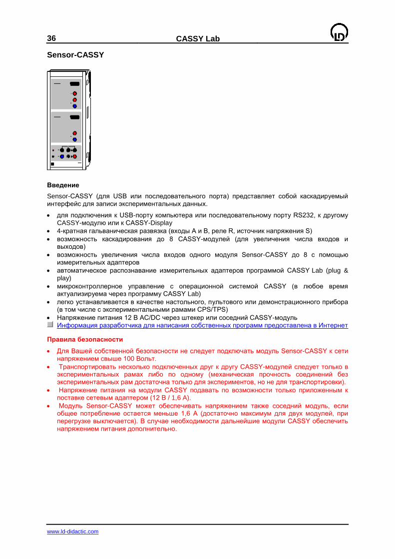
36

CASSY Lab

www.ld-didactic.com

Sensor-CASSY

Введение

Sensor-CASSY (для USB или последовательного порта) представляет собой каскадируемый интерфейс для записи экспериментальных данных.

для подключения к USB-порту компьютера или последовательному порту RS232, к другому CASSY-модулю или к CASSY-Display

4-кратная гальваническая развязка (входы А и В, реле R, источник напряжения S)

возможность каскадирования до 8 CASSY-модулей (для увеличения числа входов и выходов)

возможность увеличения числа входов одного модуля Sensor-CASSY до 8 с помощью измерительных адаптеров

автоматическое распознавание измерительных адаптеров программой CASSY Lab (plug & play)

микроконтроллерное управление с операционной системой CASSY (в любое время актуализируема через программу CASSY Lab)

легко устанавливается в качестве настольного, пультового или демонстрационного прибора (в том числе с экспериментальными рамами CPS/TPS)

Напряжение питания 12 В AC/DC через штекер или соседний CASSY-модуль Информация разработчика для написания собственных программ предоставлена в Интернет

Правила безопасности

Для Вашей собственной безопасности не следует подключать модуль Sensor-CASSY к сети напряжением свыше 100 Вольт.

Транспортировать несколько подключенных друг к другу CASSY-модулей следует только в экспериментальных рамах либо по одному (механическая прочность соединений без экспериментальных рам достаточна только для экспериментов, но не для транспортировки).

Напряжение питания на модули CASSY подавать по возможности только приложенным к поставке сетевым адаптером (12 В / 1,6 A).

Модуль Sensor-CASSY может обеспечивать напряжением также соседний модуль, если общее потребление остается меньше 1,6 А (достаточно максимум для двух модулей, при перегрузке выключается). В случае необходимости дальнейшие модули CASSY обеспечить напряжением питания дополнительно.



CASSY Lab

37

www.ld-didactic.com

Технические данные

5 Аналоговых входов (возможно одновременное использование любых двух входов А и В) 2 Аналоговых входа напряжения A и B с 4-мм безопасными гнездами Разрешение: 12 бит Пределы измерений: ±0,3/1/3/10/30/100 В Ошибка измерений: ±1 % плюс 0,5 % от предела измерений Входное сопротивление: 1 M Частота оцифровки: макс. 200.000 записей/с (= 100.000 записей/с на вход) Количество записей: практически не ограничено (зависит от компьютера) до

100 записей/с, при более высокой частоте измерения макс. 32.000 записей (=16.000 записей на вход)

1 Аналоговый токовый вход A с 4-мм безопасными гнездами Пределы измерений: ±0,1/0,3/1/3 A Ошибка измерений: ошибка измерения напряжения плюс 1 % Входное сопротивление: < 0,5 (за исключением перегрузки) другие данные: смотри входы напряжения 2 Аналоговых входа через разъемы адаптеров A и B

(возможно подключение всех адаптеров и датчиков CASSY) Пределы измерений: ±0,003/0,01/0,03/0,1/0,3/1 В Входное сопротивление: 10 k другие данные: смотри входы напряжения Технические данные изменяются в зависимости от подключенного адаптера

Распознавание возможных величин и пределов измерения производится автоматически программой CASSY Lab после подключения адаптера

4 Входа таймеров с 32-битными счетчиками через разъемы адаптеров A и B (например, для адаптера BMW, адаптера счетчика Гейгера или адаптера-таймера)

Частота счета: макс. 100 кГц Разрешение по времени: 0,25 мкс Интервал между двумя событиями на том же входе: мин. 100 мкс Интервал между двумя событиями на разных входах: мин. 0,25 мкс Память: макс. 10.000 точек (= 2.500 на вход) 1 Переключающее реле (светодиодная индикация включения) Диапазон: 100 В / 2 A 1 Аналоговый выход (выход с ШИМ) (с широтно-импульсной модуляцией, переключаемый

источник напряжения, светодиодная индикация включения, например, для удерживающего электромагнита или питания эксперимента)

Напряжение регулируемо: макс. 16 V / 200 мA (нагрузка ≥ 80 ) Пределы ШИМ: 0 % (выкл.), 5-95 % (разрешение 1 %), 100 % (вкл.) Частота ШИМ: 100 Гц 12 Цифровых входов (TTL) через разъемы адаптеров A и B

(в настоящее время применяются только для распознавания адаптеров) 6 Цифровых выходов (TTL) через разъемы адаптеров A и B

(в настоящее время применяются только для автоматического переключения пределов измерения адаптеров)

1 USB-порт (USB-версия) или последовательный порт RS232 (SubD-9) для подключения к компьютеру

1 CASSY-шина для подключения других CASSY-модулей или CASSY-Display Размеры (ШxВxT): 115 мм x 295 мм x 45 мм Масса: 1 кг

Комплект поставки

1 Модуль Sensor-CASSY 1 Программное обеспечение CASSY Lab для Windows 98/2000/XP/Vista, без регистрационного

кода, с подробной помощью (для 20 сеансов работы, затем может быть использовано как демонстрационная версия)

1 Руководство для установки программы 1 USB-кабель или кабель SubD-9 1 Сетевой адаптер 12 В / 1,6 A

38

CASSY Lab

www.ld-didactic.com

Установки входа адаптера

Модуль Sensor-CASSY имеет два гальванически разделенных измерительных входа А и В, которые могут измерять как напряжение (вход А также и ток), так и другие величины в зависимости от установленного адаптера. Распознавание измерительного адаптера производится автоматически, таким образом, во вкладке конфигурация CASSY отображаются и измерительные адаптеры, если они установлены. Для активирования входа и подготовки измерения нужно щелкнуть мышью на соответствующий вход.

Список величин доступных для измерения зависит от того, какой адаптер установлен в данный момент (если он установлен). Для измерения других величин требуется соответствующий адаптер (см. также каталог продукции).

Выбранная величина может быть измерена в качестве мгновенного значения, усреднена по многим значениям или измерена как эффективное значение. Обычно достаточно не усредненного измерения мгновенных значений. В случае шумного или имеющего сетевые наводки сигнала необходимо использовать усредненные значения. При работе с переменными напряжениями измеряются обычно эффективные значения (двухканальное измерение

эффективных значений автоматически создает соответствующий канал cos ). При использовании интервала измерения менее 10 мс, в последних двух случаях, значение записываемое в таблицу и на график отличается от показаний измерительных инструментов. В результате, возможно одновременно отображать эффективные значения и формы кривых.

По умолчанию, усредненные и эффективные значения рассчитываются на интервале 100 мс. Этот интервал можно изменить (для всех каналов одновременно). При применении Power-CASSY или Profi-CASSY этот интервал изменяется при изменении частоты выходного сигнала таким образом, чтобы использовалось всегда целое число периодов.

В случае недостаточной точности измерения можно ее повысить с помощью коррекции. Это может понадобиться, например, когда конкретный рН-электрод должен быть подогнан к программе.

Специальные кнопки (часто невидимые)

СД вкл./выкл. Светодиод на адаптере включить/выключить, например. SMOOTH (Мостовой адаптер) или COMPENSATION (необходим для установки в ноль в Адаптере В)

—> 0 <— Установка нуля (делает актуальное значение нулевым), например, для перемещения, силы, давления, событий, столкновения

s <—> –s Изменение знака перемещения (датчик движения с адаптером BMW)

Кроме того, есть еще специальные поля ввода, существенно облегчающие работу с адаптером BMW, адаптером счетчика Гейгера и адаптером-таймером (например, время счета, ширина затеняющего флажка). Они отображаются только если установлен один из этих адаптеров.

При работе с адаптером скорости реакции сначала нужно нажать кнопку (ручную или ножную) сигнализирующую о готовности к тесту. Собственно реакция измеряется после появления флажка в окне измерительного инструмента нажатием кнопки соответствующей его цвету (красный, зеленый или желтый).

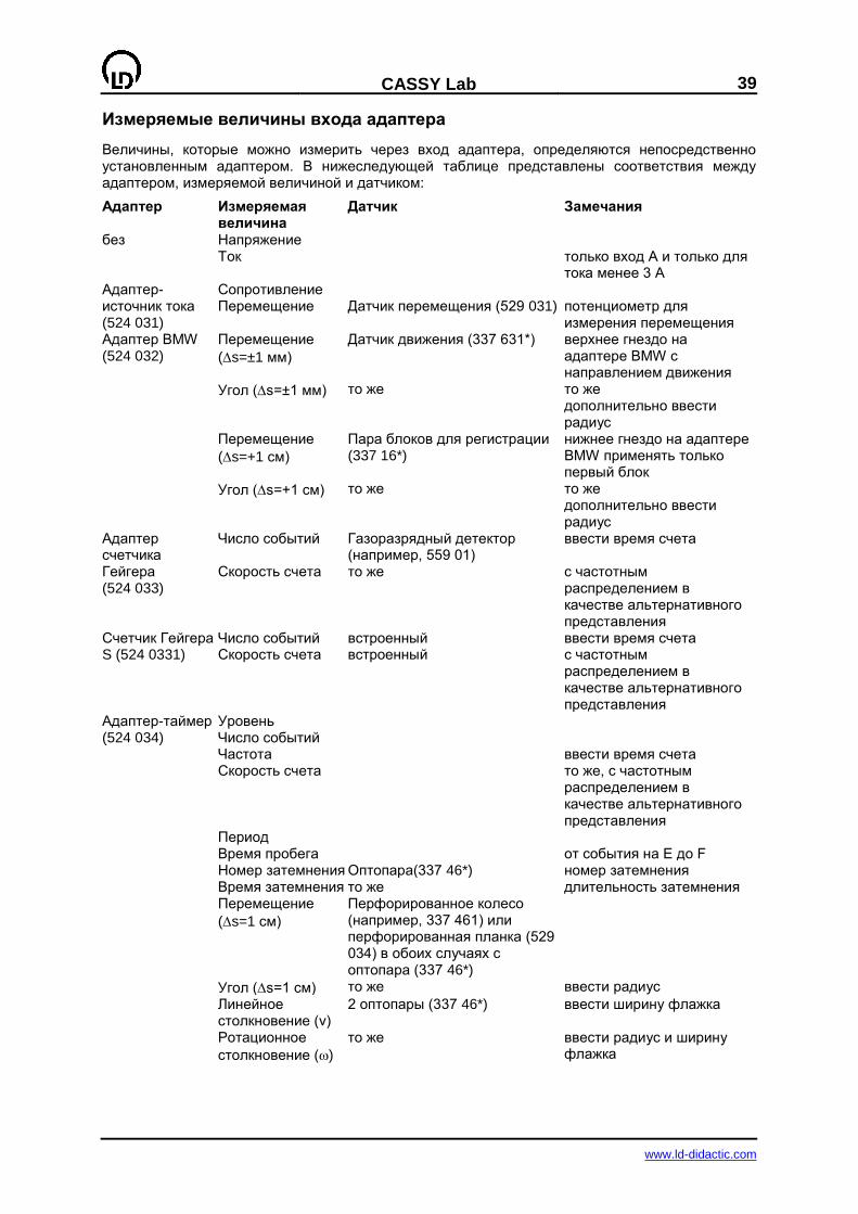
CASSY Lab

39

www.ld-didactic.com

Измеряемые величины входа адаптера

Величины, которые можно измерить через вход адаптера, определяются непосредственно установленным адаптером. В нижеследующей таблице представлены соответствия между адаптером, измеряемой величиной и датчиком:

Адаптер Измеряемая величина

Датчик Замечания

без Напряжение Ток только вход А и только для

тока менее 3 A Адаптер-источник тока (524 031)

Сопротивление Перемещение Датчик перемещения (529 031) потенциометр для

измерения перемещения Адаптер BMW (524 032)

Перемещение

(s=±1 мм)

Датчик движения (337 631*) верхнее гнездо на адаптере BMW с направлением движения

Угол (s=±1 мм) то же то же дополнительно ввести радиус


(s=+1 см)

Пара блоков для регистрации (337 16*)

нижнее гнездо на адаптере BMW применять только первый блок

Угол (s=+1 см) то же то же дополнительно ввести радиус

Адаптер счетчика Гейгера (524 033)

Число событий Газоразрядный детектор (например, 559 01)

ввести время счета

Скорость счета то же с частотным распределением в качестве альтернативного представления

Счетчик Гейгера S (524 0331)

Число событий встроенный ввести время счета Скорость счета встроенный с частотным

распределением в качестве альтернативного представления

Адаптер-таймер (524 034)

Уровень Число событий Частота ввести время счета Скорость счета то же, с частотным


Период Время пробега от события на E до F Номер затемнения Оптопара(337 46*) номер затемнения Время затемнения то же длительность затемнения Перемещение

(s=1 см)

Перфорированное колесо (например, 337 461) или перфорированная планка (529 034) в обоих случаях с оптопара (337 46*)

Угол (s=1 см) то же ввести радиус

Линейное столкновение (v)

2 оптопары (337 46*) ввести ширину флажка

Ротационное

столкновение ()

то же ввести радиус и ширину флажка

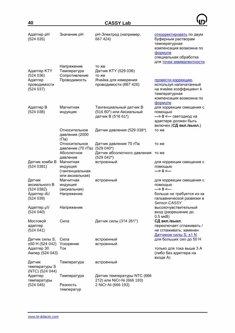
40

CASSY Lab

www.ld-didactic.com

Адаптер pH (524 035)

Значение pH pH-Электрод (например, 667 424)

откорректировать по двум буферным растворам температурная компенсация возможна по формуле специальная обработка для точки эквивалентности

Напряжение то же Адаптер KTY (524 036)

Температура Датчик KTY (529 036) Сопротивление то же

Адаптер проводимости (524 037)

Проводимость Ячейка для измерения проводимости (667 426)

провести коррекцию, используя напечатанный на ячейке коэффициент k температурная компенсация возможна по формуле

Адаптер B (524 038)

Магнитная индукция

Тангенциальный датчик В (516 60*) или Аксиальный датчик В (516 61*)

для коррекции смещения с помощью —> 0 <— светодиод на адаптере должен быть включен (СД вкл./выкл.)

Относительное давление (2000 гПа)

Датчик давления (529 038*) то же

Относительное давление (70 гПа)

Датчик давления 70 гПа (529 040*)

то же

Абсолютное давление

Датчик абсолютного давления (529 042*)

то же

Датчик комби B (524 0381)

Магнитная индукция (тангенциальная или аксиальная)

встроенный для коррекции смещения с помощью —> 0 <—

Датчик аксиального B (524 0382)

Магнитная индукция (аксиальная)

встроенный для коррекции смещения с помощью —> 0 <—

Адаптер dU (524 039)

Напряжение больше не требуется из-за гальванической развязки в Sensor-CASSY

Адаптер µV (524 040)

Напряжение высокочувствительный вход (разрешение до 0,5 мкВ)

Мостовой адаптер (524 041)

Сила Датчик силы (314 261*) СД вкл./выкл. переключает сглаживать / не сглаживать; заменен Датчиком силы S, ±1 N

Датчик силы S, ±50 Н (524 042)

Сила встроенный для больших сил до 50 Н Ускорение встроенный

Адаптер 30 Ампер (524 043)

Ток только для тока выше 3 A (либо без адаптера на входе A)

Датчик температуры S (NTC) (524 044)

Температура встроенный

Адаптер температуры (524 045)

Температура Датчик температуры NTC (666 212) или NiCr-Ni (666 193)

Разность температур

2 NiCr-Ni (666 193)

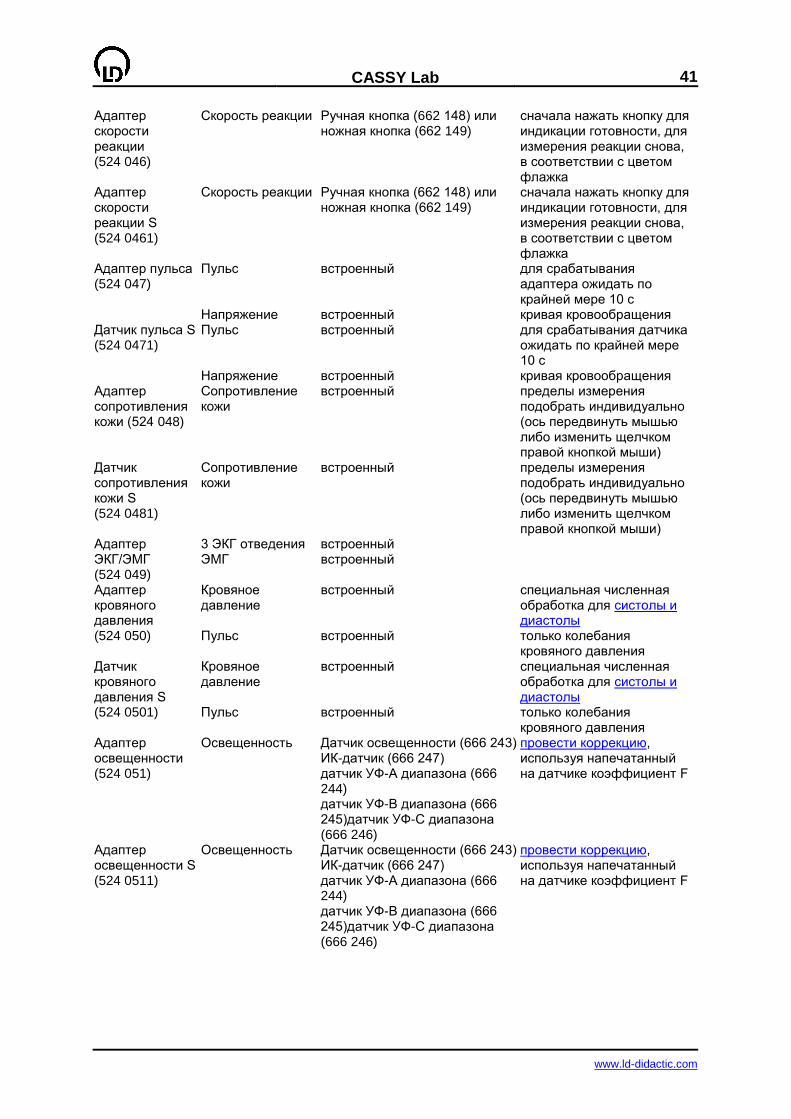
CASSY Lab

41

www.ld-didactic.com

Адаптер скорости реакции (524 046)

Скорость реакции Ручная кнопка (662 148) или ножная кнопка (662 149)

сначала нажать кнопку для индикации готовности, для измерения реакции снова, в соответствии с цветом флажка

Адаптер скорости реакции S (524 0461)

Скорость реакции Ручная кнопка (662 148) или ножная кнопка (662 149)

сначала нажать кнопку для индикации готовности, для измерения реакции снова, в соответствии с цветом флажка

Адаптер пульса (524 047)

Пульс встроенный для срабатывания адаптера ожидать по крайней мере 10 с

Напряжение встроенный кривая кровообращения Датчик пульса S (524 0471)

Пульс встроенный для срабатывания датчика ожидать по крайней мере 10 с

Напряжение встроенный кривая кровообращения Адаптер сопротивления кожи (524 048)

Сопротивление кожи

встроенный пределы измерения подобрать индивидуально (ось передвинуть мышью либо изменить щелчком правой кнопкой мыши)

Датчик сопротивления кожи S (524 0481)

Сопротивление кожи

встроенный пределы измерения подобрать индивидуально (ось передвинуть мышью либо изменить щелчком правой кнопкой мыши)

Адаптер ЭКГ/ЭМГ (524 049)

3 ЭКГ отведения встроенный ЭМГ встроенный

Адаптер кровяного давления (524 050)

Кровяное давление

встроенный специальная численная обработка для систолы и диастолы

Пульс встроенный только колебания кровяного давления

Датчик кровяного давления S (524 0501)

Кровяное давление

встроенный специальная численная обработка для систолы и диастолы

Пульс встроенный только колебания кровяного давления

Адаптер освещенности (524 051)

Освещенность Датчик освещенности (666 243) ИК-датчик (666 247) датчик УФ-А диапазона (666 244) датчик УФ-В диапазона (666 245)датчик УФ-С диапазона (666 246)

провести коррекцию, используя напечатанный на датчике коэффициент F

Адаптер освещенности S (524 0511)

Освещенность Датчик освещенности (666 243) ИК-датчик (666 247) датчик УФ-А диапазона (666 244) датчик УФ-В диапазона (666 245)датчик УФ-С диапазона (666 246)

провести коррекцию, используя напечатанный на датчике коэффициент F

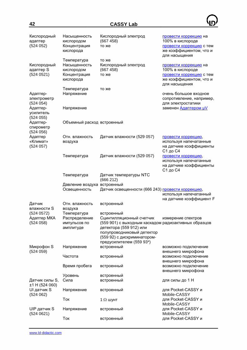
42

CASSY Lab

www.ld-didactic.com

Кислородный адаптер (524 052)

Насыщенность кислородом

Кислородный электрод (667 458)

провести коррекцию на 100% в кислороде

Концентрация кислорода

то же провести коррекцию с тем же коэффициентом, что и для насыщения

Температура то же Кислородный адаптер S (524 0521)

Насыщенность кислородом

Кислородный электрод (667 458)

провести коррекцию на 100% в кислороде

Концентрация кислорода

то же провести коррекцию с тем же коэффициентом, что и для насыщения

Температура то же Адаптер- электрометр (524 054)

Напряжение очень большое входное сопротивление, например, для электростатики

Адаптер- усилитель (524 055)

Напряжение заменен Адаптером µV

Адаптер- спирометр (524 056)

Объемный расход встроенный

Адаптер «Климат» (524 057)

Отн. влажность воздуха

Датчик влажности (529 057) провести коррекцию, используя напечатанные на датчике коэффициенты C1 до C4

Температура Датчик влажности (529 057) провести коррекцию, используя напечатанные на датчике коэффициенты C1 до C4

Температура Датчик температуры NTC (666 212)

Давление воздуха встроенный Освещенность Датчик освещенности (666 243) провести коррекцию,

используя напечатанный на датчике коэффициент F

Датчик влажности S (524 0572)

Отн. влажность воздуха

встроенный

Температура встроенный Адаптер МКА (524 058)

Распределение импульсов по амплитуде

Сцинтилляционный счетчик (559 901) с выходным каскадом детектора (559 912) или полупроводниковый детектор (559 92) с дискриминатором-предусилителем (559 93*)

измерение спектров радиоактивных образцов

Микрофон S (524 059)

Напряжение встроенный возможно подключение внешнего микрофона

Частота встроенный возможно подключение внешнего микрофона

Время пробега встроенный возможно подключение внешнего микрофона

Уровень встроенный Датчик силы S, ±1 Н (524 060)

Сила встроенный для силы до 1 Н

UI датчик S (524 062)

Напряжение встроенный для Pocket-CASSY и Mobile-CASSY

Ток 1 шунт для Pocket-CASSY и Mobile-CASSY

UIP датчик S (524 0621)

Напряжение встроенный для Pocket-CASSY и Mobile-CASSY

Ток встроенный для Pocket-CASSY и

CASSY Lab

43

www.ld-didactic.com

Mobile-CASSY Датчик давления S, 2000 гПа (524 064)

Относительное давление


Датчик абсолютного давления S (524 065)

Абсолютное давление


Датчик давления S, 70 гПа (524 066)

Относительное давление


Химический адаптер (524 067)

Значение pH Датчик pH (667 4172) Проводимость Датчик проводимости (529 670) Температура Датчик проводимости (529 670) Температура Датчик температуры (529 676) Разница температур

2 датчика температуры (529 676)

Потенциал Адаптер проводимости S (524 0671)

Проводимость Датчик проводимости (529 670) Температура Датчик проводимости (529 670)

Адаптер pH S (524 0672)

Значение pH Датчик pH (667 4172) Потенциал

Адаптер NiCr Ni S (524 0673)

Температура Датчик температуры (529 676) Разница температур

2 датчика температуры (529 676)

Прибор центробежной силы S (524 068)

Центробежная сила


Погружной фотометр S (524 069)

Пропускание встроенный Экстинкция встроенный Концентрация встроенный

ультразвук. датчик движения S (524 070)

Перемещение встроенный

Температура встроенный Датчик спирто- содержания S (524 073)

Перемещение встроенный Время пробега встроенный

Таймер S (524 074)

Уровень Число событий Частота ввести время счета Скорость счета то же, с частотным


Период Время пробега от события на E до F Номер затемнения Оптопара (337 46*) номер затемнения Время затемнения то же длительность затемнения Перемещение

(s=1 см)

Перфорированное колесо (например, 337 461) или перфорированная планка (529 034) в обоих случаях с оптопарой (337 46*)

Угол (s=1 см) то же ввести радиус

Линейное столкновение (v)

2 оптопары (337 46*) ввести ширину флажка

Ротационное то же ввести радиус и ширину

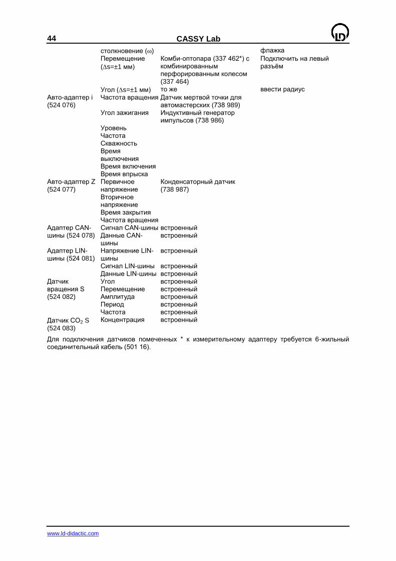
44

CASSY Lab

www.ld-didactic.com

столкновение () флажка


(s=±1 мм)

Комби-оптопара (337 462*) с комбинированным перфорированным колесом (337 464)

Подключить на левый разъѐм

Угол (s=±1 мм) то же ввести радиус

Авто-адаптер i (524 076)

Частота вращения Датчик мертвой точки для автомастерских (738 989)

Угол зажигания Индуктивный генератор импульсов (738 986)

Уровень Частота Скважность Время выключения

Время включения Время впрыска

Авто-адаптер Z (524 077)

Первичное напряжение

Конденсаторный датчик (738 987)

Вторичное напряжение

Время закрытия Частота вращения

Адаптер CAN-шины (524 078)

Сигнал CAN-шины встроенный Данные CAN-шины


Адаптер LIN-шины (524 081)

Напряжение LIN-шины


Сигнал LIN-шины встроенный Данные LIN-шины встроенный

Датчик вращения S (524 082)

Угол встроенный Перемещение встроенный Амплитуда встроенный Период встроенный Частота встроенный

Датчик CO2 S (524 083)

Концентрация встроенный

Для подключения датчиков помеченных * к измерительному адаптеру требуется 6-жильный соединительный кабель (501 16).

CASSY Lab

45

www.ld-didactic.com

Коррекция входа адаптера

Существуют разные возможности коррекции измеряемых значений. Все они представлены в диалоговом окне.

Слева от знака равенства можно ввести смещение и/или фактор, которые используются программой для пересчета показанных слева значений («есть») в значения показанные справа («должно быть»). Для проведения коррекции нужно нажать Исправить смещение или Исправить фактор.

Альтернативно, можно просто ввести оба желаемых значения или одно желаемое значение и один коэффициент. Нажатие кнопки Восстановить отменяет коррекцию.

Сохранение

Коррекция сохраняется вместе с остальными настройками программы. Чтобы быть уверенным в правильности коррекции при новой загрузке файла, нужно удостовериться, что используются те же самые электроды и адаптеры на том же модуле Sensor-CASSY (возможно, будет необходимо подписать их).

Примеры

Для проведения коррекции должны быть использованы буферные растворы с pH 3 и pH 9. Тогда вводятся оба желаемых значения 3 и 9 (справа). Когда рН-электрод погружен в раствор с pH 3, нужно нажать кнопку рядом с желаемым значением 3 (например, Исправить смещение) и в растворе с pH 9 соответственно другую кнопку (например, Исправить фактор).

Для работы с программой должен быть использован электрод для измерения проводимости с К-фактором 1,07. Для правильной коррекции достаточно ввести фактор 1,07 во второй строке и нажать Исправить фактор.

Особенности при работе с адаптером «Климат» (524 057)

До первого измерения влажности адаптером «Климат» с датчиком влажности (529 057), последний необходимо прокалибровать. Для этого на датчике приведены четыре значения: от С1 до С4. После однократного ввода, эти значения будут сохранены в Sensor-CASSY. В последующем, не требуется вводить их даже при измерении без компьютера (с CASSY-Display).

46

CASSY Lab

www.ld-didactic.com

Установки Реле/Источника напряжения

Модуль Sensor-CASSY имеет реле R и регулируемый (с помощью ручки) источник напряжения S. И то и другое может включаться программно. Для этого сначала они должны быть активированы щелчком мышью во вкладке конфигурация CASSY.

Легче всего синхронизировать их работу с началом измерения (например, для удерживающего электромагнита, подключенного к источнику S). Для этого достаточно активировать функцию Переключать во время автоматического измерения.

Возможно также однозначно задать состояние реле или источника напряжения с помощью формулы. Формула может зависеть от всех величин, перечисленных в отображаемом списке, и должна быть написана с учетом правил для формул (смотри также примеры). Значение формулы не равное нулю обозначает ВКЛ.=«включено», значение равное нулю обозначает ВЫКЛ.=«выключено». Значение этой формулы не будет отслеживаться во время измерения, если активирована функция Переключать во время автоматического измерения.

Аналоговый выход с ШИМ

Источник напряжения S является аналоговым выходом с широтно-импульсной модуляцией. Максимальное напряжение устанавливается с помощью ручки. Формула же управляет не только состоянием (ВЫКЛ.=0 или ВКЛ.=1), но и позволяет использовать промежуточные значения (например, 0,41 = попеременно 41 % времени ВКЛ. и 59 % ВЫКЛ. с периодом 10 мс). Для таких промежуточных значений функция Переключать во время автоматического измерения не действует.

Таким образом, с помощью этого аналогового выхода можно управлять элементами, для которых важно только среднее или эффективное значение выходного напряжения (например, формула saw(time/10) могла бы быть использована чтобы изменять яркость маленькой лампочки: 5 с ярче и 5 с тусклее).

Универсальный аналоговый выход имеют Power-CASSY и Profi-CASSY.

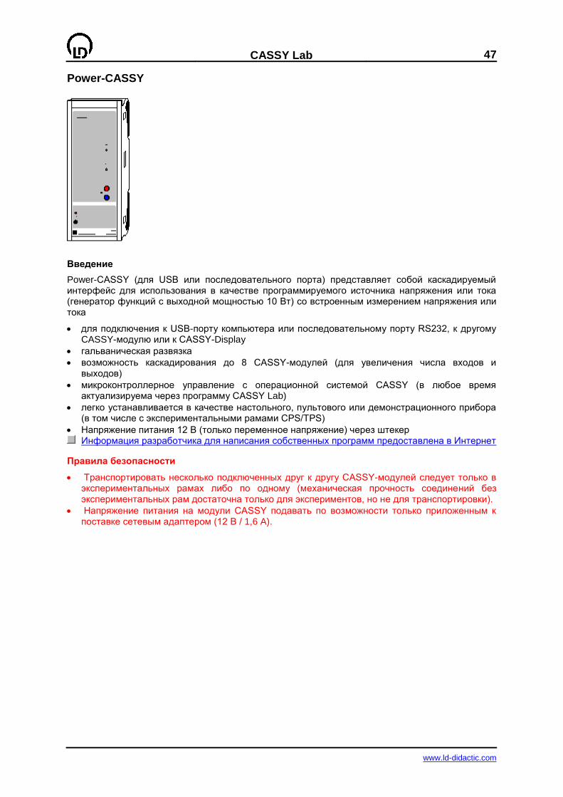
CASSY Lab

47

www.ld-didactic.com

Power-CASSY

Введение

Power-CASSY (для USB или последовательного порта) представляет собой каскадируемый интерфейс для использования в качестве программируемого источника напряжения или тока (генератор функций с выходной мощностью 10 Вт) со встроенным измерением напряжения или тока

для подключения к USB-порту компьютера или последовательному порту RS232, к другому CASSY-модулю или к CASSY-Display

гальваническая развязка

возможность каскадирования до 8 CASSY-модулей (для увеличения числа входов и выходов)



Напряжение питания 12 В (только переменное напряжение) через штекер Информация разработчика для написания собственных программ предоставлена в Интернет






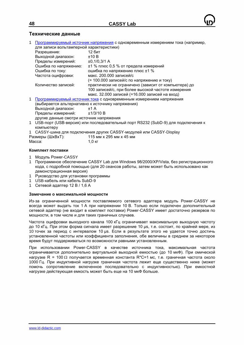
48

CASSY Lab

www.ld-didactic.com


1 Программируемый источник напряжения с одновременным измерением тока (например, для записи вольтамперной характеристики)

Разрешение: 12 бит Выходной диапазон: ±10 В Пределы измерений: ±0,1/0,3/1 А Ошибка по напряжению: ±1 % плюс 0,5 % от предела измерений Ошибка по току: ошибка по напряжению плюс ±1 % Частота оцифровки: макс. 200.000 записей/с

(= 100.000 записей/с по напряжению и току) Количество записей: практически не ограничено (зависит от компьютера) до

100 записей/с, при более высокой частоте измерения макс. 32.000 записей (=16.000 записей на вход)

1 Программируемый источник тока с одновременным измерением напряжения (выбирается альтернативно к источнику напряжения)

Выходной диапазон: ±1 А Пределы измерений: ±1/3/10 В другие данные смотри источник напряжения 1 USB-порт (USB-версия) или последовательный порт RS232 (SubD-9) для подключения к

компьютеру 1 CASSY-шина для подключения других CASSY-модулей или CASSY-Display Размеры (ШxВxT): 115 мм x 295 мм x 45 мм Масса: 1,0 кг


1 Модуль Power-CASSY 1 Программное обеспечение CASSY Lab для Windows 98/2000/XP/Vista, без регистрационного


1 Руководство для установки программы 1 USB-кабель или кабель SubD-9 1 Сетевой адаптер 12 В / 1,6 A

Замечание о максимальной мощности

Из-за ограниченной мощности поставляемого сетевого адаптера модуль Power-CASSY не всегда может выдать ток 1 А при напряжении 10 В. Только если подключен дополнительный сетевой адаптер (не входит в комплект поставки) Power-CASSY имеет достаточно резервов по мощности, в том числе и для таких граничных случаев.

Частота оцифровки выходного канала 100 кГц ограничивает максимальную выходную частоту до 10 кГц. При этом форма сигнала имеет разрешение 10 µs, т.е. состоит, по крайней мере, из 10 точек за период с интервалом 10 µs. Если в результате этого не удается точно достичь установленной частоты или коэффициента заполнения, обе величины в среднем за некоторое время будут поддерживаться по возможности равными установленным.

При использовании Power-CASSY в качестве источника тока, максимальная частота ограничивается дополнительно виртуальной выходной емкостью (до 10 мкФ). При омической

нагрузке R = 100 получается временная константа R*C=1 мс, т.е. граничная частота около 1000 Гц. При индуктивной нагрузке граничная частота лежит еще существенно ниже (может помочь сопротивление включенное последовательно с индуктивностью). При емкостной нагрузке действующая емкость может быть еще на 10 мкФ больше.

CASSY Lab

49

www.ld-didactic.com

Установки генератора функций

Power-CASSY является управляемым компьютером генератором функций с выходной мощностью 10 Вт. Регулируемым значением генератора может быть по выбору напряжение U (источник напряжения) или ток I (источник тока). При работе в качестве источника напряжения одновременно измеряется протекающий ток I, а при работе в качестве источника тока измеряется приложенное напряжение U. Выходной диапазон и пределы измерений при этом можно выбирать.

Работа генератора может быть ограничена только на собственно время измерения выбором функции активен только во время измерения (single shot). В этом случае между двумя измерениями генератор отключен, и вычисление средних или эффективных значений, следовательно, не возможно.

Выходная функция, частота f (в Гц или кГц), амплитуда А (в Вп или Ап), смещение по постоянному напряжению O (в В= или А=) и коэффициент заполнения (в %) могут быть установлены в следующих пределах:

Функция Частота f Амплитуда A Смещение O Заполнение DC - - -10 В .. 10 В / -1 A .. 1 A - Синус 0,01 Гц - 10 кГц -10 В .. 10 В / -1 A .. 1 A -10 В .. 10 В / -1 A .. 1 A 0 % .. 100 % Прямоугольник 0,01 Гц - 10 кГц -10 В .. 10 В / -1 A .. 1 A -10 В .. 10 В / -1 A .. 1 A 0 % .. 100 % Треугольник 0,01 Гц - 10 кГц -10 В .. 10 В / -1 A .. 1 A -10 В .. 10 В / -1 A .. 1 A 0 % .. 100 % Формула 0,01 Гц - 10 кГц -10 В .. 10 В / -1 A .. 1 A -10 В .. 10 В / -1 A .. 1 A -

Прямоугольник и треугольник могут генерироваться в двух вариантах. Симметричная форма лежит между –А и +А, асимметричная форма между 0 и +А.

Отрицательные значения амплитуды разрешены – они производят отраженный относительно нуля сигнал. Коэффициент заполнения определяет отношение между возрастающей и спадающей частью кривой. Так можно легко преобразовать треугольный сигнал (50 %) в пилообразный (100 %).

В дополнение к обычным функциям, с помощью Power-CASSY можно генерировать произвольно заданные. Для этого нужно ввести формулу f(x), описывающую форму кривой. Для определения формы кривой функция от переменной х вычисляется в интервале [0,1[ и выдается с заданной частотой f, амплитудой А и смещением О. Для написания формул действуют обычные правила. Кроме того, функция synth(a:b:c:...) позволяет произвести гармонический синтез по формуле a*sin(360*x)+b*sin(2*360*x)+c*sin(3*360*x)+.... Сигнал будет опять же выдаваться с заданной частотой f, амплитудой А и смещением О (смотри также пример гармонического синтеза).

Поле для ввода формулы имеет относительно небольшой размер. Более длинную формулу можно ввести в обычном текстовом редакторе, после чего скопировать ее в окно программы (правая кнопка мыши).

Напряжение U и ток I могут быть измерены в качестве мгновенного значения, усреднены по многим значениям или измерены как эффективное значение. Обычно достаточно не усредненного измерения мгновенных значений. В случае, когда Power-CASSY непрерывно активен (не только во время измерения) могут быть измерены также усредненные и эффективные значения (измерение эффективных значений автоматически создает

соответствующий канал для фазового угла между напряжением и током). При использовании интервала измерения менее 10 мс, в последних двух случаях, значение записываемое в таблицу и на график отличается от показаний измерительных инструментов. В результате, возможно одновременно отображать эффективные значения и формы кривых.

Совет

Вместо фиксированных числовых значений можно использовать уже определенные каналы для частоты, амплитуды, смещения или коэффициента заполнения. Таким образом, можно гибко управлять, например, частотой синусоидального колебания или выходным напряжением (например, через ввод формулы при записи резонансных кривых или регулировании). Однако, инициализация Power-CASSY для вывода новой частоты (или амплитуды, смещения, коэффициента заполнения) может длиться до нескольких сотен миллисекунд. Поэтому параметры могут быть изменены только шагами, а не непрерывно.

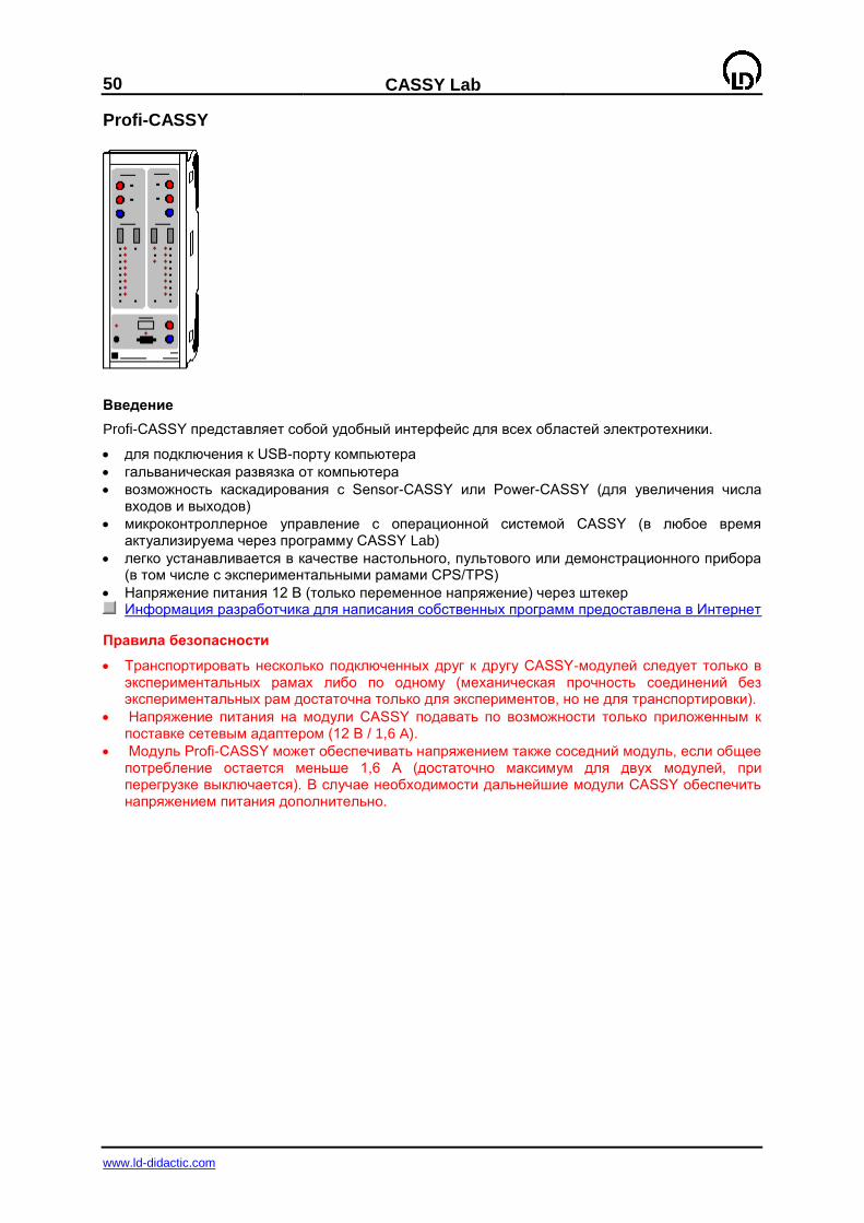
50

CASSY Lab

www.ld-didactic.com

Profi-CASSY

Введение

Profi-CASSY представляет собой удобный интерфейс для всех областей электротехники.

для подключения к USB-порту компьютера

гальваническая развязка от компьютера

возможность каскадирования с Sensor-CASSY или Power-CASSY (для увеличения числа входов и выходов)



Напряжение питания 12 В (только переменное напряжение) через штекер Информация разработчика для написания собственных программ предоставлена в Интернет




Модуль Profi-CASSY может обеспечивать напряжением также соседний модуль, если общее потребление остается меньше 1,6 А (достаточно максимум для двух модулей, при перегрузке выключается). В случае необходимости дальнейшие модули CASSY обеспечить напряжением питания дополнительно.



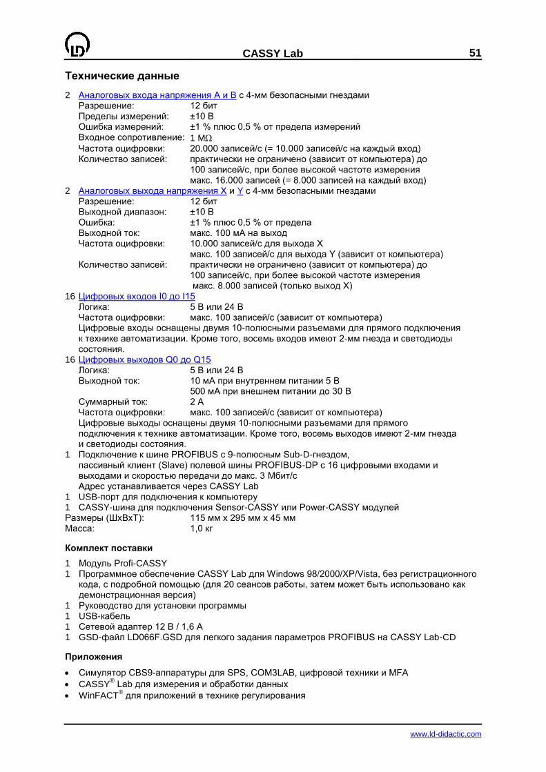
CASSY Lab

51

www.ld-didactic.com


2 Аналоговых входа напряжения A и B с 4-мм безопасными гнездами Разрешение: 12 бит Пределы измерений: ±10 В Ошибка измерений: ±1 % плюс 0,5 % от предела измерений Входное сопротивление: 1 M Частота оцифровки: 20.000 записей/с (= 10.000 записей/с на каждый вход) Количество записей: практически не ограничено (зависит от компьютера) до

100 записей/с, при более высокой частоте измерения макс. 16.000 записей (= 8.000 записей на каждый вход)

2 Аналоговых выхода напряжения X и Y с 4-мм безопасными гнездами Разрешение: 12 бит Выходной диапазон: ±10 В Ошибка: ±1 % плюс 0,5 % от предела Выходной ток: макс. 100 мА на выход Частота оцифровки: 10.000 записей/с для выхода Х

макс. 100 записей/с для выхода Y (зависит от компьютера) Количество записей: практически не ограничено (зависит от компьютера) до

100 записей/с, при более высокой частоте измерения макс. 8.000 записей (только выход Х)

16 Цифровых входов I0 до I15 Логика: 5 В или 24 В Частота оцифровки: макс. 100 записей/с (зависит от компьютера) Цифровые входы оснащены двумя 10-полюсными разъемами для прямого подключения

к технике автоматизации. Кроме того, восемь входов имеют 2-мм гнезда и светодиоды состояния.

16 Цифровых выходов Q0 до Q15 Логика: 5 В или 24 В Выходной ток: 10 мА при внутреннем питании 5 В

500 мА при внешнем питании до 30 В Суммарный ток: 2 А Частота оцифровки: макс. 100 записей/с (зависит от компьютера) Цифровые выходы оснащены двумя 10-полюсными разъемами для прямого

подключения к технике автоматизации. Кроме того, восемь выходов имеют 2-мм гнезда и светодиоды состояния.

1 Подключение к шине PROFIBUS с 9-полюсным Sub-D-гнездом, пассивный клиент (Slave) полевой шины PROFIBUS-DP с 16 цифровыми входами и выходами и скоростью передачи до макс. 3 Мбит/с Адрес устанавливается через CASSY Lab

1 USB-порт для подключения к компьютеру 1 CASSY-шина для подключения Sensor-CASSY или Power-CASSY модулей Размеры (ШxВxT): 115 мм x 295 мм x 45 мм Масса: 1,0 кг


1 Модуль Profi-CASSY 1 Программное обеспечение CASSY Lab для Windows 98/2000/XP/Vista, без регистрационного


1 Руководство для установки программы 1 USB-кабель 1 Сетевой адаптер 12 В / 1,6 A 1 GSD-файл LD066F.GSD для легкого задания параметров PROFIBUS на CASSY Lab-CD

Приложения

Симулятор CBS9-аппаратуры для SPS, COM3LAB, цифровой техники и MFA

CASSY® Lab для измерения и обработки данных

WinFACT® для приложений в технике регулирования

52

CASSY Lab

www.ld-didactic.com

Установки аналогового входа

Модуль Profi-CASSY имеет два аналоговых входа для измерения напряжения А и В.

Напряжение UA или UB может быть измерено в качестве мгновенного значения, усреднено по многим значениям или измерено как эффективное значение. Обычно достаточно не усредненного измерения мгновенных значений. В случае шумного или имеющего сетевые наводки сигнала необходимо использовать усредненные значения. При работе с переменными напряжениями измеряются обычно эффективные значения (двухканальное измерение

эффективных значений автоматически создает соответствующий канал cos ). При использовании интервала измерения менее 10 мс, в последних двух случаях, значение записываемое в таблицу и на график отличается от показаний измерительных инструментов. В результате, возможно одновременно отображать эффективные значения и формы кривых.

По умолчанию, усредненные и эффективные значения рассчитываются на интервале 100 мс. При применении Power-CASSY или Profi-CASSY этот интервал изменяется при изменении частоты выходного сигнала таким образом, чтобы использовалось всегда целое число периодов.

В случае недостаточной точности измерения можно ее повысить с помощью коррекции.

CASSY Lab

53

www.ld-didactic.com

Установки аналогового выхода X (генератор функций)

Profi-CASSY (на выходе Х) является управляемым компьютером генератором функций. Работа генератора может быть ограничена только на собственно время измерения выбором функции активен только во время измерения (single shot). В этом случае между двумя измерениями генератор отключен, и вычисление средних или эффективных значений, по этому, не возможно.

Выходная функция, частота f (в Гц или кГц), амплитуда А (в Вп или Ап), смещение по постоянному напряжению O (в В= или А=) и коэффициент заполнения (в %) могут быть установлены в следующих пределах:

Функция Частота f Амплитуда A Смещение O Заполнение DC - - -10 В .. 10 В - Синус 0,01 Гц - 1000 Гц -10 В .. 10 В -10 В .. 10 В 0 % .. 100 % Прямоугольник 0,01 Гц - 1000 Гц -10 В .. 10 В -10 В .. 10 В 0 % .. 100 % Треугольник 0,01 Гц - 1000 Гц -10 В .. 10 В -10 В .. 10 В 0 % .. 100 % Формула 0,01 Гц - 1000 Гц -10 В .. 10 В -10 В .. 10 В -

Прямоугольник и треугольник могут генерироваться в двух вариантах. Симметричная форма лежит между –А и +А, асимметричная форма между 0 и +А.

Отрицательные значения амплитуды разрешены – они производят отраженный относительно нуля сигнал. Коэффициент заполнения определяет отношение между возрастающей и спадающей частью кривой. Так можно легко преобразовать треугольный сигнал (50 %) в пилообразный (100 %).

В дополнение к обычным функциям, с помощью Profi-CASSY можно генерировать произвольно заданные. Для этого нужно ввести формулу f(x), описывающую форму кривой. Для определения формы кривой функция от переменной х вычисляется в интервале [0,1[ и выдается с заданной частотой f, амплитудой А и смещением О. Для написания формул действуют обычные правила. Кроме того, функция synth(a:b:c:...) позволяет произвести гармонический синтез по формуле a*sin(360*x)+b*sin(2*360*x)+c*sin(3*360*x)+.... Сигнал будет опять же выдаваться с заданной частотой f, амплитудой А и смещением О (смотри также пример гармонического синтеза).

Поле для ввода формулы имеет относительно небольшой размер. Более длинную формулу можно ввести в обычном текстовом редакторе, после чего скопировать ее в окно программы (правая кнопка мыши).

Напряжение UX может быть измерено в качестве мгновенного значения, усреднено по многим значениям или измерено как эффективное значение. Обычно достаточно не усредненного измерения мгновенных значений. В случае, когда Profi -CASSY непрерывно активен (не только во время измерения) могут быть измерены также усредненные и эффективные значения

(измерение эффективных значений автоматически создает соответствующий канал для фазового угла между выходом Х и входом А). При использовании интервала измерения менее 10 мс, в последних двух случаях, значение записываемое в таблицу и на график отличается от показаний измерительных инструментов. В результате, возможно одновременно отображать эффективные значения и формы кривых.

Совет

Вместо фиксированных числовых значений можно использовать уже определенные каналы для частоты, амплитуды, смещения или коэффициента заполнения. Таким образом, можно гибко управлять, например, частотой синусоидального колебания или выходным напряжением (например, через ввод формулы при записи резонансных кривых или регулировании). Однако, инициализация Profi-CASSY для вывода новой частоты (или амплитуды, смещения, коэффициента заполнения) может длиться до нескольких сотен миллисекунд. Поэтому параметры могут быть изменены только шагами, а не непрерывно.

54

CASSY Lab

www.ld-didactic.com

Установки аналогового выхода Y

Кроме аналогового выхода Х, который может быть использован в качестве генератора функций, Profi-CASSY имеет и второй аналоговый выход Y, который может под управлением программы по заданной формуле изменять свое выходное напряжение.

Установки цифрового входа/выхода

Profi-CASSY имеет 16 цифровых входов и 16 цифровых выходов, которые могут быть активированы в группах по 8.

Входы I0 до I15 передают действующий логический уровень. Выходы Q0 до Q15 могут под управлением программы по заданной формуле изменять свой выходной уровень.

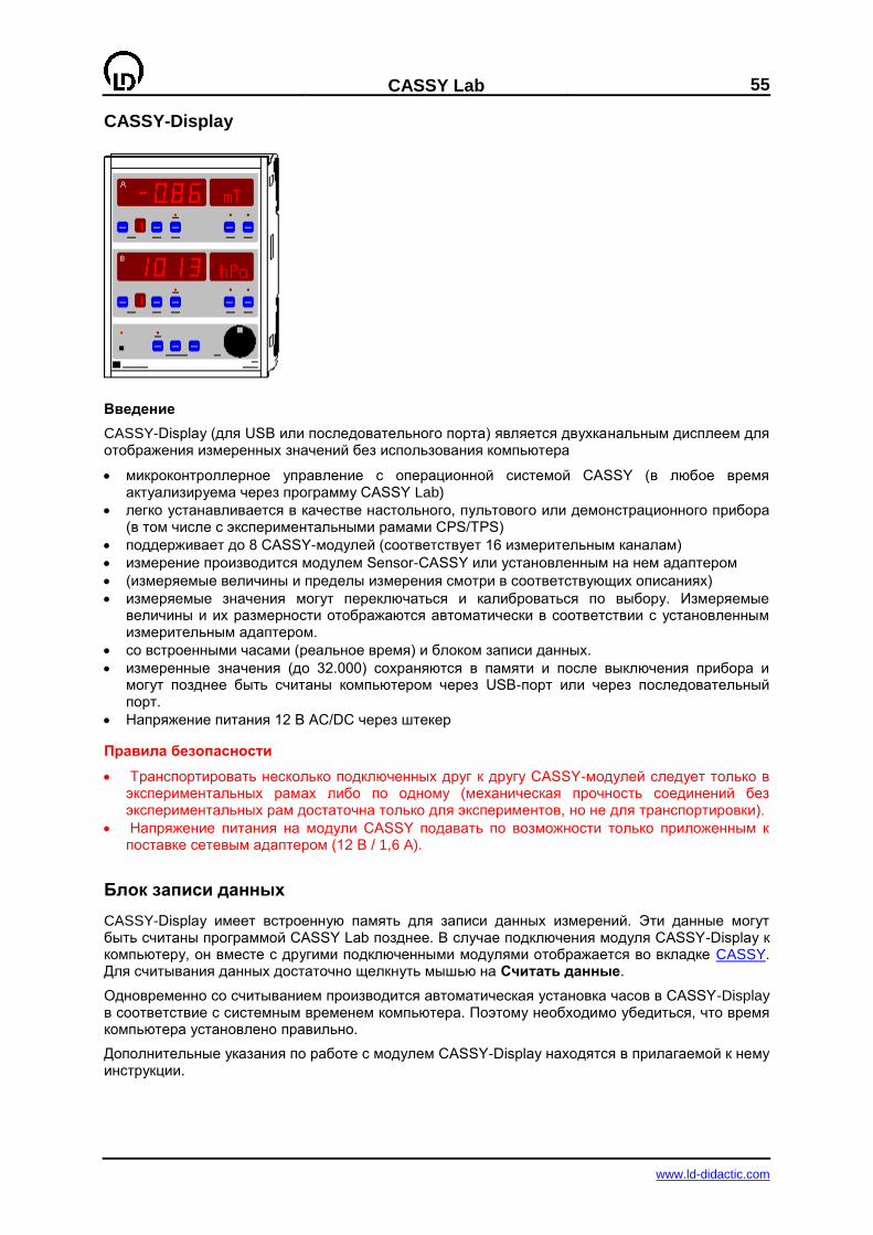
CASSY Lab

55

www.ld-didactic.com

CASSY-Display

Введение

CASSY-Display (для USB или последовательного порта) является двухканальным дисплеем для отображения измеренных значений без использования компьютера



поддерживает до 8 CASSY-модулей (соответствует 16 измерительным каналам)

измерение производится модулем Sensor-CASSY или установленным на нем адаптером

(измеряемые величины и пределы измерения смотри в соответствующих описаниях)

измеряемые значения могут переключаться и калиброваться по выбору. Измеряемые величины и их размерности отображаются автоматически в соответствии с установленным измерительным адаптером.

со встроенными часами (реальное время) и блоком записи данных.

измеренные значения (до 32.000) сохраняются в памяти и после выключения прибора и могут позднее быть считаны компьютером через USB-порт или через последовательный порт.

Напряжение питания 12 В AC/DC через штекер




Блок записи данных

CASSY-Display имеет встроенную память для записи данных измерений. Эти данные могут быть считаны программой CASSY Lab позднее. В случае подключения модуля CASSY-Display к компьютеру, он вместе с другими подключенными модулями отображается во вкладке CASSY. Для считывания данных достаточно щелкнуть мышью на Считать данные.

Одновременно со считыванием производится автоматическая установка часов в CASSY-Display в соответствие с системным временем компьютера. Поэтому необходимо убедиться, что время компьютера установлено правильно.

Дополнительные указания по работе с модулем CASSY-Display находятся в прилагаемой к нему инструкции.

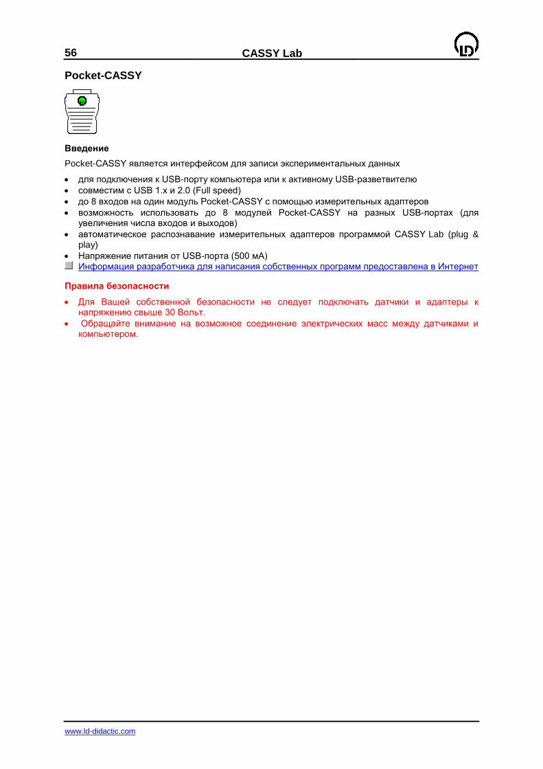
56

CASSY Lab

www.ld-didactic.com

Pocket-CASSY

Введение

Pocket-CASSY является интерфейсом для записи экспериментальных данных

для подключения к USB-порту компьютера или к активному USB-разветвителю

совместим с USB 1.x и 2.0 (Full speed)

до 8 входов на один модуль Pocket-CASSY с помощью измерительных адаптеров

возможность использовать до 8 модулей Pocket-CASSY на разных USB-портах (для увеличения числа входов и выходов)

автоматическое распознавание измерительных адаптеров программой CASSY Lab (plug & play)

Напряжение питания от USB-порта (500 мА) Информация разработчика для написания собственных программ предоставлена в Интернет


Для Вашей собственной безопасности не следует подключать датчики и адаптеры к напряжению свыше 30 Вольт.

Обращайте внимание на возможное соединение электрических масс между датчиками и компьютером.



CASSY Lab

57

www.ld-didactic.com


1 Аналоговый вход через разъем адаптеров (возможно подключение всех адаптеров и датчиков CASSY)

Разрешение: 12 бит Пределы измерений: ±0,003/0,01/0,03/0,1/0,3/1 В Ошибка измерений: ±1 % плюс 0,5 % от предела измерений Входное сопротивление: 10 к Частота оцифровки: макс. 7.800 записей/с Количество записей: практически не ограничено (зависит от

компьютера) до 100 записей/с, при более высокой частоте измерения макс. 16.000 записей

Технические данные изменяются в зависимости от подключенного адаптера Распознавание возможных величин и пределов измерения производится автоматически программой

2 Входа таймеров через разъем адаптеров (например, для адаптера BMW, адаптера счетчика Гейгера или адаптера-таймера)

Частота счета: макс. 10 кГц Разрешение по времени: 1 мкс Интервал между

двумя событиями: мин. 100 мкс

Память: макс. 5.000 точек (= 2.500 на вход) 6 Цифровых входов (TTL) через разъем адаптеров

(в настоящее время применяются только для распознавания адаптеров) 3 Цифровых выхода (TTL) через разъем адаптеров

(в настоящее время применяются только для автоматического переключения пределов измерения адаптеров)

1 USB-порт для подключения к компьютеру и подачи питания (500 мА) Размеры (ШxВxT): 50 мм x 25 мм x 60 мм Масса: 0,1 кг


1 Pocket-CASSY 1 Программное обеспечение CASSY Lab для Windows 98/2000/XP/Vista, без регистрационного


1 Руководство для установки программы 1 USB-кабель

58

CASSY Lab

www.ld-didactic.com

Применение Pocket-CASSY

Pocket-CASSY представляет собой недорогой интерфейс, задуманный для использования школьниками. Поэтому его возможности ограничены по сравнению с Sensor-CASSY. Не смотря на это, большинство описанных экспериментов можно провести и с Pocket-CASSY. Такие эксперименты обозначены значком Pocket-CASSY. Приведенные списки приборов и описания, однако, рассчитаны на применение Sensor-CASSY.

Проведение эксперимента для Sensor-CASSY с Pocket-CASSY

Для измерения напряжения и тока с Pocket-CASSY требуется UI-датчик S (524 062) или UIP-датчик S (524 0621).

В случае использования обоих аналоговых входов А и В модуля Sensor-CASSY, для замены потребуется два Pocket-CASSY (возможно, с двумя UI-датчиками S). При комбинированном измерении напряжения и тока, достаточно одного Pocket-CASSY с UIP-датчиком S.

Обозначения измеряемых величин имеют на один индекс меньше, чем приведено в описании экспериментов, т.к. при использовании Pocket-CASSY не нужно различать входы A

или B, например, U1 и U2 (два Pocket-CASSY) вместо UA1 и UB1 (один Sensor-CASSY).

Ограничения Pocket-CASSY по сравнению с Sensor-CASSY

В наличие имеется только один вход адаптеров. Если возможно использовать несколько USB-портов, то получить несколько входов адаптеров можно одновременной работой с несколькими Pocket-CASSY. Поскольку между отдельными Pocket-CASSY нет прямой связи, может происходить задержка прихода фронтов до 5 мс.

Pocket-CASSY не имеет входов с 4-мм безопасными гнездами. Их можно получить подключением UI-датчика S или UIP-датчика S. Заметьте, что UI-датчик S позволяет использовать только 7 вместо 10 пределов измерений: отсутствуют пределы ±100 В, ±3 A, ±0,1 A. Кроме того, он не может параллельно измерять U и I. В UIP-датчике S отсутствует только предел ±100 В.

Не возможно выбрать временное разрешение Δt < 100 мкс. Pocket-CASSY производит оцифровку с Δt >= 128 мкс, т.е. уже Δt = 100 мкс достигается интерполяцией.

Отсутствуют реле R и источник напряжения S.

Входы таймеров имеют разрешение только 1 мкс. Кроме того, может присутствовать некоторое переменное время задержки до 10 мкс. Максимальная измеряемая частота составляет около 10 кГц.

Pocket-CASSY не имеет гальванической развязки. В зависимости от подключенного адаптера, между ним и компьютером может существовать связь электрических масс. При использовании двух Pocket-CASSY на одном компьютере возможно даже, что адаптеры электрически соединены. Чтобы сгладить возникающие недостатки, часто используемые UI-датчик S (524 062) и UIP-датчик S (524 0621) реализованы в виде дифференциальных усилителей. Их входные гнезда соединены с массой только через высокоомные сопротивления.

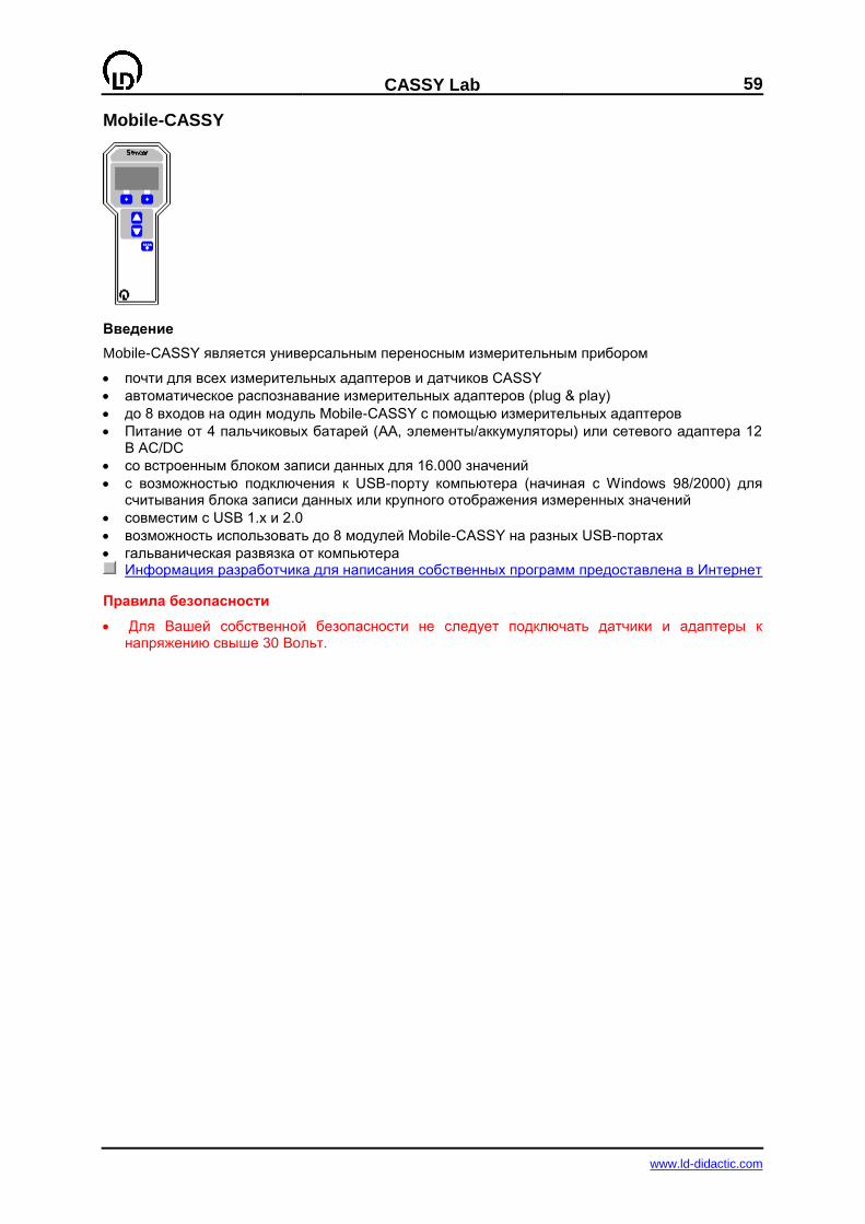
CASSY Lab

59

www.ld-didactic.com

Mobile-CASSY

Введение

Mobile-CASSY является универсальным переносным измерительным прибором

почти для всех измерительных адаптеров и датчиков CASSY

автоматическое распознавание измерительных адаптеров (plug & play)

до 8 входов на один модуль Mobile-CASSY с помощью измерительных адаптеров

Питание от 4 пальчиковых батарей (AA, элементы/аккумуляторы) или сетевого адаптера 12 В AC/DC

со встроенным блоком записи данных для 16.000 значений

с возможностью подключения к USB-порту компьютера (начиная с Windows 98/2000) для считывания блока записи данных или крупного отображения измеренных значений

совместим с USB 1.x и 2.0

возможность использовать до 8 модулей Mobile-CASSY на разных USB-портах

гальваническая развязка от компьютера Информация разработчика для написания собственных программ предоставлена в Интернет


Для Вашей собственной безопасности не следует подключать датчики и адаптеры к напряжению свыше 30 Вольт.



60

CASSY Lab

www.ld-didactic.com


1 Аналоговый вход через разъем адаптеров (возможно подключение почти всех адаптеров и датчиков CASSY)

Разрешение: 12 бит Пределы измерений: ±0,003/0,01/0,03/0,1/0,3/1 В Ошибка измерений: ±1 % плюс 0,5 % от предела измерений Входное сопротивление: 10 к Частота оцифровки: макс. 5 записей/с Количество записей: 16.000 во встроенном блоке записи данных или

практически не ограничено (зависит от компьютера) при измерении с компьютером

Технические данные изменяются в зависимости от подключенного адаптера Распознавание возможных величин и пределов измерения производится автоматически после

1 Дисплей для одновременного отображения до четырех значений с различными размерами шрифтов

1 USB-порт для подключения к компьютеру Размеры (ШxВxT): 87 мм x 215 мм x 30 мм Масса: 0,25 кг


1 Mobile-CASSY 1 Программное обеспечение CASSY Lab для Windows 98/2000/XP/Vista, без регистрационного


1 Руководство для установки программы 1 USB-кабель

CASSY Lab

61

www.ld-didactic.com

Применение Mobile-CASSY

Mobile-CASSY представляет собой интерфейс, задуманный для мобильных измерений. Поэтому его возможности ограничены по сравнению с Sensor-CASSY, но дополнительно встроен блок записи данных. Не смотря на это, некоторые из описанных экспериментов можно провести и с Mobile-CASSY. Такие эксперименты обозначены значком Mobile-CASSY. Приведенные списки приборов и описания, однако, рассчитаны на применение Sensor-CASSY.

Проведение эксперимента для Sensor-CASSY с Mobile-CASSY

Для измерения напряжения и тока с Pocket-CASSY требуется UI-датчик S (524 062) или UIP-датчик S (524 0621).

В случае использования обоих аналоговых входов А и В модуля Sensor-CASSY, для замены потребуется два Mobile-CASSY (возможно, с двумя UI-датчиками S). При комбинированном измерении напряжения и тока, достаточно одного Mobile-CASSY с UIP-датчиком S.

Обозначения измеряемых величин имеют на один индекс меньше, чем приведено в описании экспериментов, т.к. при использовании Mobile-CASSY не нужно различать входы A

или B, например, U1 и U2 (два Mobile-CASSY) вместо UA1 и UB1 (один Sensor-CASSY).

Ограничения Mobile-CASSY по сравнению с Sensor-CASSY

В наличие имеется только один вход адаптеров. Если возможно использовать несколько USB-портов, то получить несколько входов адаптеров можно одновременной работой с несколькими Mobile-CASSY.

Mobile-CASSY не имеет входов с 4-мм безопасными гнездами. Их можно получить подключением UI-датчика S или UIP-датчика S. Заметьте, что UI-датчик S позволяет использовать только 7 вместо 10 пределов измерений: отсутствуют пределы ±100 В, ±3 A, ±0,1 A. Кроме того, он не может параллельно измерять U и I. В UIP-датчике S отсутствует только предел ±100 В.

Не возможно выбрать временное разрешение Δt < 200 мс.

Отсутствуют реле R и источник напряжения S.

Входы таймеров поддерживаются только очень ограниченно.

Блок записи данных

Mobile-CASSY имеет встроенную память для записи данных измерений, содержимое которой сохраняется и после выключения питания. Эти данные могут быть считаны программой CASSY Lab позднее. В случае подключения модуля Mobile-CASSY к компьютеру, он вместе с другими подключенными модулями отображается во вкладке CASSY. Для считывания данных достаточно щелкнуть мышью на Считать данные.

Одновременно со считыванием производится автоматическая установка часов в Mobile-CASSY в соответствие с системным временем компьютера. Поэтому необходимо убедиться, что время компьютера установлено правильно.

Дополнительные указания по работе с модулем Mobile-CASSY находятся в прилагаемой к нему инструкции.

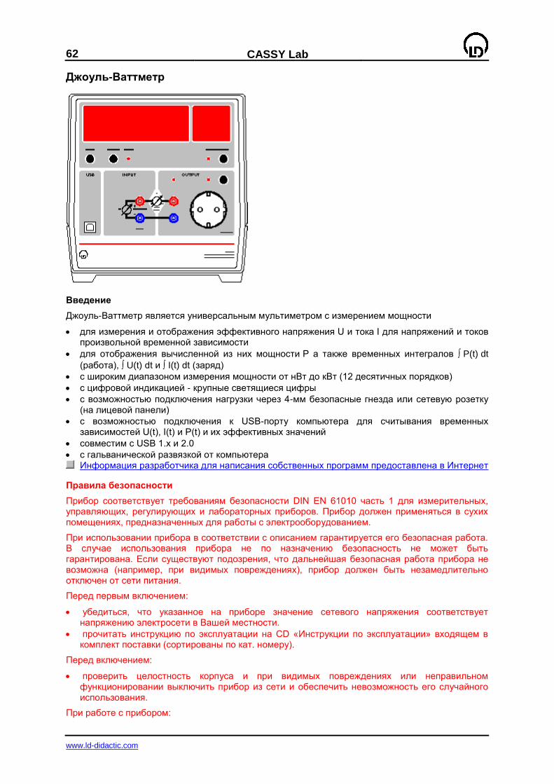
62

CASSY Lab

www.ld-didactic.com

Джоуль-Ваттметр

Введение

Джоуль-Ваттметр является универсальным мультиметром с измерением мощности

для измерения и отображения эффективного напряжения U и тока I для напряжений и токов произвольной временной зависимости

для отображения вычисленной из них мощности P а также временных интегралов P(t) dt

(работа), U(t) dt и I(t) dt (заряд)

с широким диапазоном измерения мощности от нВт до кВт (12 десятичных порядков)

с цифровой индикацией - крупные светящиеся цифры

с возможностью подключения нагрузки через 4-мм безопасные гнезда или сетевую розетку (на лицевой панели)

с возможностью подключения к USB-порту компьютера для считывания временных зависимостей U(t), I(t) и P(t) и их эффективных значений


с гальванической развязкой от компьютера Информация разработчика для написания собственных программ предоставлена в Интернет


Прибор соответствует требованиям безопасности DIN EN 61010 часть 1 для измерительных, управляющих, регулирующих и лабораторных приборов. Прибор должен применяться в сухих помещениях, предназначенных для работы с электрооборудованием.

При использовании прибора в соответствии с описанием гарантируется его безопасная работа. В случае использования прибора не по назначению безопасность не может быть гарантирована. Если существуют подозрения, что дальнейшая безопасная работа прибора не возможна (например, при видимых повреждениях), прибор должен быть незамедлительно отключен от сети питания.

Перед первым включением:

убедиться, что указанное на приборе значение сетевого напряжения соответствует напряжению электросети в Вашей местности.

прочитать инструкцию по эксплуатации на CD «Инструкции по эксплуатации» входящем в комплект поставки (сортированы по кат. номеру).

Перед включением:

проверить целостность корпуса и при видимых повреждениях или неправильном функционировании выключить прибор из сети и обеспечить невозможность его случайного использования.

При работе с прибором:



CASSY Lab

63

www.ld-didactic.com

Прибор включать только в розетку сети с заземленным проводом нуля и проводником заземления.

Не подключать к напряжениям выше 250 В и токам выше 10 А.

Убедиться что соединительные провода, измерительные кабели и адаптеры не имеют повреждений изоляции и оголенных отрезков.

При экспериментах с опасными напряжениями применять только кабеля с 4-мм защищенными штекерами.

Розетка на лицевой панели может находиться под напряжением и при неактивном выходе.

Плавкий предохранитель заменять только на эквивалентный оригинальному (T 10 A / 250 В).

Не допустимо ставить перемычку на плавкий предохранитель.

Не допустимо закрывать вентиляционные щели на корпусе прибора − это может привести к перегреву электроники.

Не подносить металлические предметы к вентиляционным отверстиям, защищать их от попадания воды.

Не включать прибор при попадании в него каких-либо предметов.

Вскрывать корпус прибора может только квалифицированный персонал.

Избегать сильного сотрясения прибора.

64

CASSY Lab

www.ld-didactic.com


1 Аналоговый вход напряжения с 4-мм безопасными гнездами Разрешение: 12 бит Пределы измерений: ±5**/±50**/±500 мВ / ±5/±50/±250 В Ошибка измерений*: 1 % Входное сопротивление: ≥1 M Частота оцифровки: макс. 10.000 записей/с Количество записей: практически не ограничено (зависит от компьютера)

до 100 записей/с, при более высокой частоте измерения макс. 16.000 записей

1 Аналоговый вход напряжения для розетки (альтернативно) Разрешение: 12 бит Пределы измерений: 250 В Ошибка измерений*: 1 % Входное сопротивление: 2 M Частота оцифровки: макс. 10.000 записей/с Количество записей: практически не ограничено (зависит от компьютера)


1 налоговый токовый вход для 4-мм безопасных гнезд и розетки Разрешение: 12 бит Пределы измерений: ±0,2/±2/±20 мА / ±0,2/±2/±10 A Ошибка измерений*: 1 % Входное сопротивление: 10 / около 0,01 Частота оцифровки: макс. 10.000 записей/с Количество записей: практически не ограничено (зависит от компьютера)


Подключение нагрузки: альтернативно через 4-мм безопасные гнезда или розетку (на лицевой панели)

Индикация: 5-разрядный 7-сегментный индикатор для численного значения и матрица 7х15 для единиц измерения

Индикация: 25 мм USB-порт: USB 1.x и 2.0 (full speed), с гальванической развязкой Напряжение питания: 230 В, 50/60 Гц Размеры (ШxВxT): 20 см x 21 см x 23 см Масса: 2 кг

* Указанная точность относится к полному диапазону измерения при измерении постоянного напряжения (DC) и переменного напряжения (AC) частотой 50 или 60 Гц и крест-фактором ≤ 2 (Крест-фактор нагрузки равен отношению пикового значения потребляемого тока к среднедействующему значению).

** Этот предел измерения предназначен только для постоянного напряжения (не для AC).


1 Джоуль-Ваттметр 1 Программное обеспечение CASSY Lab для Windows 98/2000/XP/Vista, с подробной

помощью (без ограничений при работе с Джоуль-Ваттметром) 1 Инструкция по эксплуатации 1 USB-кабель

CASSY Lab

65

www.ld-didactic.com

Универсальный измерительный прибор ФИЗИКА

Введение

Универсальный измерительный прибор ФИЗИКА предназначен

для измерения и отображения многих физических величин

с возможностью подключения к USB-порту компьютера для считывания временных зависимостей


с гальванической развязкой от компьютера Информация разработчика для написания собственных программ предоставлена в Интернет


Прибор соответствует требованиям безопасности DIN EN 61010 часть 1 для измерительных, управляющих, регулирующих и лабораторных приборов. Прибор должен применяться в сухих помещениях, предназначенных для работы с электрооборудованием.

При использовании прибора в соответствии с описанием гарантируется его безопасная работа. В случае использования прибора не по назначению безопасность не может быть гарантирована. Если существуют подозрения, что дальнейшая безопасная работа прибора не возможна (например, при видимых повреждениях), прибор должен быть незамедлительно отключен от сети питания.

Перед первым включением:

убедиться, что указанное на приборе значение сетевого напряжения соответствует напряжению электросети в Вашей местности.

прочитать инструкцию по эксплуатации на CD «Инструкции по эксплуатации» входящем в комплект поставки (сортированы по кат. номеру).

Перед включением:

проверить целостность корпуса и при видимых повреждениях или неправильном функционировании выключить прибор из сети и обеспечить невозможность его случайного использования.

При работе с прибором:

Прибор включать только в розетку сети с заземленным проводом нуля и проводником заземления.

Не допустимо закрывать вентиляционные щели на корпусе прибора − это может привести к перегреву электроники.

Не подносить металлические предметы к вентиляционным отверстиям, защищать их от попадания воды.

Не включать прибор при попадании в него каких-либо предметов.

Вскрывать корпус прибора может только квалифицированный персонал.

Избегать сильного сотрясения прибора.



66

CASSY Lab

www.ld-didactic.com


1 Аналоговый вход для большого числа датчиков S Разрешение: 12 бит Пределы измерений: в зависимости от датчика Ошибка измерений: 1 % плюс ошибка датчика Входное

сопротивление: 10 k

Частота оцифровки: макс. 10.000 записей/с Количество записей: практически не ограничено (зависит от компьютера)


Индикация: 5-разрядный 7-сегментный индикатор для численного значения и матрица 7х15 для единиц измерения

Высота цифр: 25 мм USB-порт: USB 1.x и 2.0 (full speed), с гальванической развязкой Напряжение питания: 230 В, 50/60 Гц Размеры (ШxВxT): 20 см x 21 см x 23 см Масса: 2 кг


1 Универсальный измерительный прибор ФИЗИКА 1 Программное обеспечение CASSY Lab для Windows 98/2000/XP/Vista, с подробной

помощью (без ограничений при работе с Универсальным измерительным прибором ФИЗИКА)

1 Инструкция по эксплуатации 1 USB-кабель

CASSY Lab

67

www.ld-didactic.com

Другие приборы для последовательного порта

Кроме модулей CASSY программа CASSY Lab поддерживает и другие приборы для последовательного порта. Они могут использоваться одновременно с CASSY при подключении к свободному последовательному порту. К ним относятся:

ASCII (конфигурируемо) Весы (различные производители) VideoCom (337 47) ИК датчик координаты (332 11) Измерительный прибор MFA 2001 (727 230) Metra Hit (531 28 - 531 30) Цифровой термометр (666 209 / 666 454) Цифровой спектрофотометр (667 3491) Data Logger (666 252) pH-метр (666 221) Кондуктометр (666 222) Люксметр (666 223 / 666 230) Оксиметр (666 224) Фотометр (666 225) Фонометр (666 231) Газоанализатор CO2-CO-CH4 (666 232) Измеритель оптической мощности (736 435) Антенная платформа (737 405)

ASCII, Весы, VideoCom, ИК датчик координаты, MFA 2001

Кроме весов, VideoCom (337 47), ИК датчика координаты (332 11) и измерительного прибора MFA 2001 (727 230) на последовательном порте поддерживаются любые приборы, передающие ASCII-данные (ASCII-текст, значение и размерность, Mode 8N1 = 8 бит данных, без парности, 1 бит остановки или Mode 7E1 = 7 бит данных, четная парность, 1 бит остановки). Проверяется заданная размерность с переданной размерностью. Если они совпадают, по крайней мере, в начале, то переданное число отображается как значение измерения. В случае отсутствия размерности, отображаются все переданные данные.

Решение возможных проблем

В случае, если не отображаются данные измерений, это может быть вызвано:

Неверно указан порт.

Неверно заданы параметры порта: удостоверьтесь, что прибор передает данные с той же скоростью и в той же моде (8N1 = 8 бит данных, без парности, 1 бит остановки или 7E1 = 7 бит данных, четная парность, 1 бит остановки). VideoCom и ИК датчик координаты всегда выполняют это.

Неправильный кабель: в зависимости от прибора может требоваться не перекрещенный кабель (1:1-кабель) или перекрещенный кабель (нуль-модемный). Для VideoCom, ИК датчика координаты и MFA 2001 требуется 1:1-кабель, для весов обычно нуль-модемный кабель.

Неверная размерность: для проверки можно стереть размерность. Тогда будут отображаться все данные. Для VideoCom, ИК датчика координаты и MFA 2001 размерность всегда задана правильно.

Прибор не передает данные: проверьте это с помощью программы-терминала, например, «Программы связи»(входит в состав Windows, но может потребовать доустановки через Панель управления).

Ограничения при работе с VideoCom

Выбираемый диапазон используется одновременно для калибровки VideoCom по координате, поэтому, он должен соответствовать ширине поля зрения аппарата.

Отображается положение только первого опознанного отражения. Для работы с несколькими объектами используйте программу VideoCom.

Измерение проводится без синхронизации по времени. Хотя VideoCom передает 80 координат в секунду, программа не синхронизируется с ними. Поэтому, следует использовать интервал

68

CASSY Lab

www.ld-didactic.com

измерения не менее 100 мс. Этого достаточно для типичного совместного использования VideoCom и CASSY (регулировка положения).

MetraHit

Программа поддерживает приборы MetraHit 14S до 18S (531 28 - 531 30), если они оборудованы адаптером порта (531 31).

Измеряемая величина должна быть выбрана в соответствии с установками на MetraHit. Пределы отображения никак не связаны с пределом на MetraHit, и их можно изменять по усмотрению. При изменении предела измерения в MetraHit, предел отображения в программе сохраняется до тех пор, пока он не будет изменен и там.

Разные модели MetraHit измеряют с разным количеством знаков после запятой. Для получения одинакового отображения в программе используйте функцию Не показывать младший разряд.




Неправильный кабель: используйте не перекрещенный кабель (1:1-кабель), который поставляется вместе с адаптером порта (531 31).

Неверно выбрана измеряемая величина: установите на приборе и в программе верную измеряемую величину.

Светодиод на адаптере порта не мигает: активируйте передачу данных на MetraHit (одновременно нажать DATA и ON).

Цифровой термометр

Программа поддерживает цифровые термометры 666 209 и 666 454. Для каждой из четырех температур активируется окно измерительного прибора, кнопка которого помещается в основном окне в строке кнопок быстрого доступа.

Предел отображения никак не связан с пределом прибора, и его можно изменять по усмотрению.

Цифровой термометр имеет память для измеренных значений. Для считывания памяти нужно нажать Считать ОЗУ.




Неправильный кабель: используйте не перекрещенный кабель (1:1-кабель).

Неверно указан прибор: сверьте номер прибора с данными в окне диалога. Предыдущие модели цифровых термометров могут работать с установкой ASCII (конфигурируемо).

Не подключен датчик температуры.

CASSY Lab

69

www.ld-didactic.com

Цифровой спектрофотометр

Программа поддерживает цифровой спектрофотометр (667 3491). И для длины волны λ, и для измеряемого пропускания Т активируется окно измерительного прибора, кнопка которого помещается в основном окне в строке кнопок быстрого доступа.

Если, кроме того, требуется отображение поглощения (100-Т) или экстинкции (-log(T/100)), они могут быть рассчитаны по формулам. Готовые формулы содержаться в описании соответствующего эксперимента.




Неправильный кабель: используйте только поставляемый с прибором кабель.

Неверно указан прибор: сверьте номер прибора с данными в окне диалога.

Переносные измерительные приборы и Data Logger

Программа поддерживает все из серии переносных измерительных приборов и входящий в эту серию Data Logger.

Data Logger (666 252)

pH-метр (666 221)

Кондуктометр (666 222)

Люксметр (666 223 / 666 230)

Оксиметр (666 224)

Фотометр (666 225)

Фонометр (666 231)

Газоанализатор CO2-CO-CH4 (666 232)

Измеритель оптической мощности (736 435)

Однако каждый из этих приборов может быть подключен только в единственном экземпляре. В случае необходимости применения нескольких одновременно (например, два pH-метра), они должны быть подключены через Data Logger.

Предел отображения никак не связан с пределом на приборе, и его можно изменять по усмотрению. При изменении предела измерения на приборе, предел отображения в программе сохраняется до тех пор, пока он не будет изменен и там.

Для каждой измеряемой величины активируется окно измерительного прибора, кнопка которого помещается в основном окне в строке кнопок быстрого доступа.

Фонометр и Data Logger имеют память для измеренных значений. Для считывания памяти нужно нажать в программе Считать ОЗУ и на приборе стартовать передачу данных.




Неправильный кабель: используйте только специальный компьютерный кабель (666 251).


Неверно выбрана измеряемая величина: установите на приборе верную измеряемую величину.

Антенная платформа

Программа позволяет работать с антенной платформой (737 405). Можно использовать настройки антенной платформы из многочисленных примеров экспериментов. Нижеследующие параметры можно оптимировать самостоятельно:

Пределы от Ввести начальный угол в градусах, например, –180

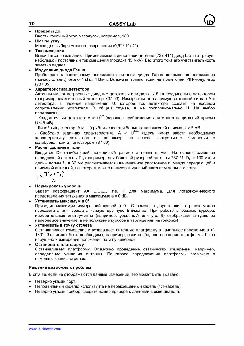
70

CASSY Lab

www.ld-didactic.com

Пределы до Ввести конечный угол в градусах, например, 180

Шаг по углу Меню для выбора углового разрешения (0,5° / 1° / 2°).

Ток смещения Включается по желанию. Применяемый в дипольной антенне (737 411) диод Шоттки требует небольшой постоянный ток смещения (порядка 15 мкА). Без этого тока его чувствительность заметно падает.

Модуляция диода Ганна Прибавляет к постоянному напряжению питания диода Ганна переменное напряжение (прямоугольник) около 1 кГц, 1 Вп-п. Включать только если не подключен PIN-модулятор (737 05).

Характеристика детектора Антенны имеют встроенные диодные детекторы или должны быть соединены с детектором (например, коаксиальный детектор 737 03). Измеряется не напрямую антенный сигнал А с детектора, а падение напряжения U, которое ток детектора создает на входном сопротивлении усилителя. В общем случае, А не пропорционально U. На выбор предложены:

- Квадратичный детектор: A U1/2

(хорошее приближение для малых напряжений приема

U < 5 мВ)

- Линейный детектор: A U (приближение для больших напряжений приема U > 5 мВ)

- Свободно заданная характеристика: A U1/m

(здесь нужно ввести необходимую характеристику детектора m, например, на основе контрольного измерения с калиброванным аттенюатором 737 09).

Расчет дальнего поля

Вводится DT (наибольший поперечный размер антенны в мм). На основе размеров

передающей антенны DQ (например, для большой рупорной антенны 737 21: DQ = 100 мм) и

длины волны λ0 = 32 мм рассчитывается минимальное расстояние r0 между передающей и приемной антенной, на котором можно пользоваться приближением дальнего поля:

Нормировать уровень

Задает коэффициент A= U/Umax, т.е. 1 для максимума. Для логарифмического

представления затухания в максимуме a = 0 dB.

Установить максимум в 0° Приводит максимум измеренной кривой в 0°. С помощью двух клавиш стрелок можно передвигать или вращать кривую вручную. Внимание! При работе в режиме курсора:

измерительные инструменты (например, уровень А или угол ) отображают актуальное измеряемое значение, а не положение курсора в таблице или на графике!

Установить в точку отсчета Останавливает измерение и возвращает антенную платформу в начальное положение в +/-180°. Это может быть необходимо, например, если свободное вращение платформы было нарушено и измерение положения по углу неверное.

Остановить платформу Останавливает платформу. Возможно проведение статических измерений, например, определение усиления антенны. Пошаговое передвижение платформы возможно с помощью клавиш стрелок.




Неправильный кабель: используйте не перекрещенный кабель (1:1-кабель).


CASSY Lab

71

www.ld-didactic.com

Experiment examples

The experiment examples fall into five main subject areas:

STM (Science Teaching Modules) Physics Chemistry Biology Technology

Note that you can print out individual experiment examples or entire collections.

72

CASSY Lab

www.ld-didactic.com

STM (Science Teaching Modules)

The experiment examples help you in using CASSY. The measurement data or settings can be loaded into CASSY Lab directly. Simply click the symbols in the descriptions. New examples are labelled with

a red .

Teacher's versions

The teacher's versions are able to load the examples with measurement data and also contain the answers to questions asked in the text. The STM help has to be installed separately. If you have not yet installed it, please do it now using the CASSY Lab CD-ROM. Afterwards you can download future versions of the STM help from the Internet.

Texts which are written in red in the teacher's versions are not found in the student's versions.

Mechanics

P1.3.1.3 Uniformly accelerated motion - path-time diagram

Uniform motion between two light barriers

Uniformly accelerated motion between a holding magnet and a light barrier

Relation between acceleration and mass (F=constant)

Relation between acceleration and force (m=constant)

Electricity

Ohm's law

P3.2.3.1a Series connection of resistors

P3.2.3.1b Parallel connection of resistors

P3.2.3.2 Adjusting a voltage by means of a potentiometer

P3.2.3.3 Principle of Wheatstone's bridge

Atomic and Nuclear physics

The effect of the distance between the radiation source and the end-window counter on the pulse rate

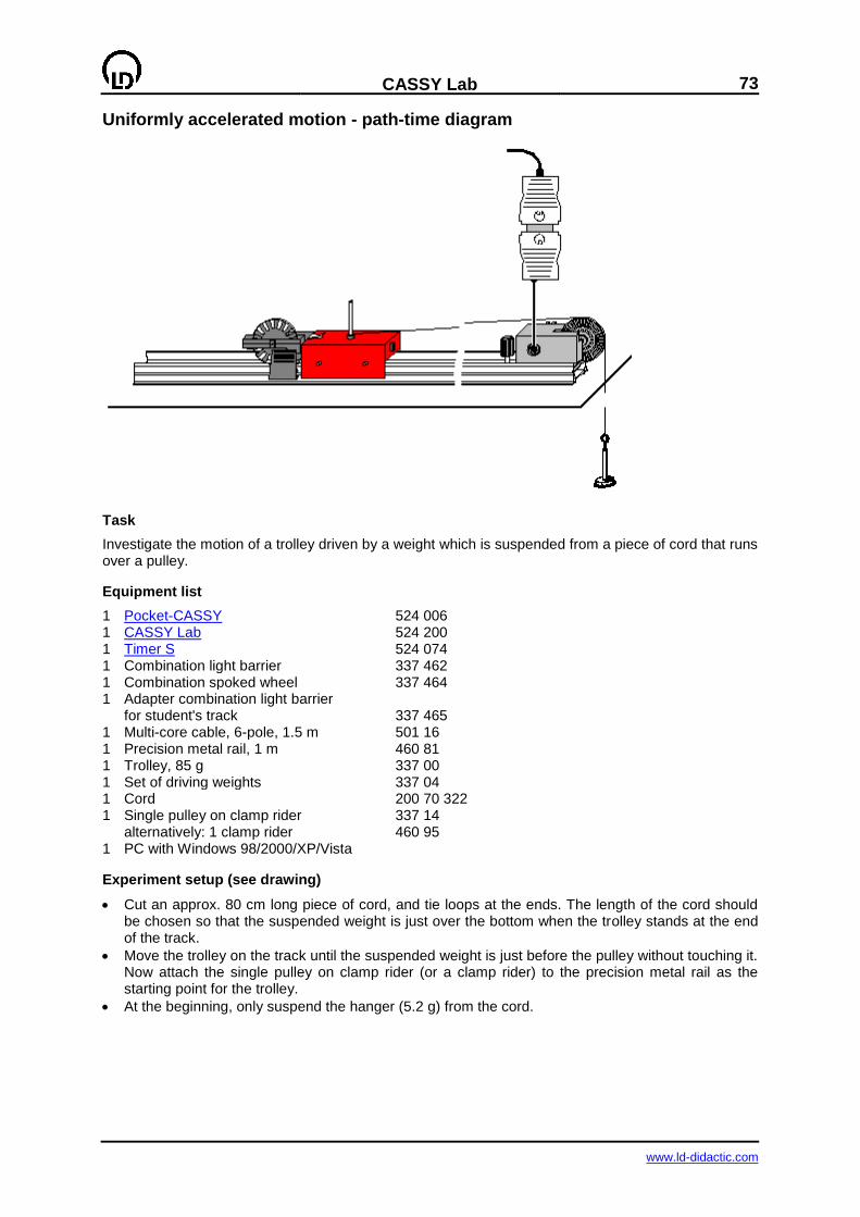
CASSY Lab

73

www.ld-didactic.com

Uniformly accelerated motion - path-time diagram

Task

Investigate the motion of a trolley driven by a weight which is suspended from a piece of cord that runs over a pulley.

Equipment list

1 Pocket-CASSY 524 006 1 CASSY Lab 524 200 1 Timer S 524 074 1 Combination light barrier 337 462 1 Combination spoked wheel 337 464 1 Adapter combination light barrier for student's track 337 465 1 Multi-core cable, 6-pole, 1.5 m 501 16 1 Precision metal rail, 1 m 460 81 1 Trolley, 85 g 337 00 1 Set of driving weights 337 04 1 Cord 200 70 322 1 Single pulley on clamp rider 337 14 alternatively: 1 clamp rider 460 95 1 PC with Windows 98/2000/XP/Vista

Experiment setup (see drawing)

Cut an approx. 80 cm long piece of cord, and tie loops at the ends. The length of the cord should be chosen so that the suspended weight is just over the bottom when the trolley stands at the end of the track.

Move the trolley on the track until the suspended weight is just before the pulley without touching it. Now attach the single pulley on clamp rider (or a clamp rider) to the precision metal rail as the starting point for the trolley.

At the beginning, only suspend the hanger (5.2 g) from the cord.

74

CASSY Lab

www.ld-didactic.com

Carrying out the experiment

Einstellungen laden

Move the trolley to its starting point, keep it there, and define the zero in the window Settings Path

s1 with —> 0 <—. Start the measurement with F9 or by clicking the button and release the trolley.

Lay additional weights on the hanger (each time 5 g), and repeat the experiment.

Evaluation

What was measured in the experiment (see table or diagram)?

What is displayed in the diagram?

How do the path differences covered in equal time intervals behave?

What kind of curve is described by the measured values? Suggestion:

Confirm the suggestion by fitting to a corresponding curve with Fit Function.

What is your conclusion regarding the relation between the path s and the time t?

Display the axes correspondingly in the Check sheet by clicking with the right mouse button. Then

determine the factor of proportionality by Line through origin. The results for the three motions are:

What is your conclusion regarding the general mathematical description of the motion (equation of

motion)?

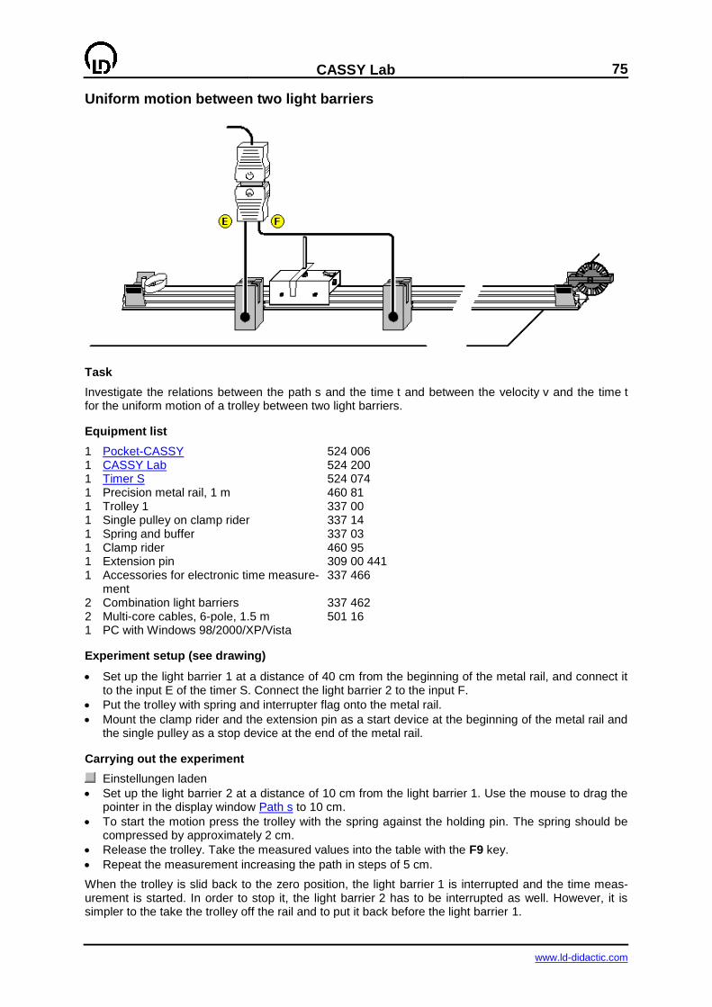
CASSY Lab

75

www.ld-didactic.com

Uniform motion between two light barriers

Task

Investigate the relations between the path s and the time t and between the velocity v and the time t for the uniform motion of a trolley between two light barriers.

Equipment list

1 Pocket-CASSY 524 006 1 CASSY Lab 524 200 1 Timer S 524 074 1 Precision metal rail, 1 m 460 81 1 Trolley 1 337 00 1 Single pulley on clamp rider 337 14 1 Spring and buffer 337 03 1 Clamp rider 460 95 1 Extension pin 309 00 441 1 Accessories for electronic time measure-

ment 337 466

2 Combination light barriers 337 462 2 Multi-core cables, 6-pole, 1.5 m 501 16 1 PC with Windows 98/2000/XP/Vista


Set up the light barrier 1 at a distance of 40 cm from the beginning of the metal rail, and connect it to the input E of the timer S. Connect the light barrier 2 to the input F.

Put the trolley with spring and interrupter flag onto the metal rail.

Mount the clamp rider and the extension pin as a start device at the beginning of the metal rail and the single pulley as a stop device at the end of the metal rail.


Einstellungen laden

Set up the light barrier 2 at a distance of 10 cm from the light barrier 1. Use the mouse to drag the pointer in the display window Path s to 10 cm.

To start the motion press the trolley with the spring against the holding pin. The spring should be compressed by approximately 2 cm.

Release the trolley. Take the measured values into the table with the F9 key.

Repeat the measurement increasing the path in steps of 5 cm.

When the trolley is slid back to the zero position, the light barrier 1 is interrupted and the time meas-urement is started. In order to stop it, the light barrier 2 has to be interrupted as well. However, it is simpler to the take the trolley off the rail and to put it back before the light barrier 1.

76

CASSY Lab

www.ld-didactic.com

Evaluation

Draw a straight line through the origin and the measuring points in the s(t) diagram. What relation

between s and t1 can be derived?

Read the slope A of the straight line.

Determine the mean value vm of the measuring points in the v(t) diagram.

Compare the slope A of the straight line in the s(t) diagram with the mean value vm of the velocity.

What equation of motion can be derived for the uniform motion?

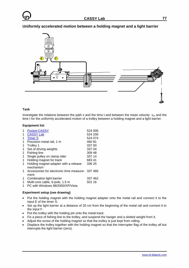
CASSY Lab

77

www.ld-didactic.com

Uniformly accelerated motion between a holding magnet and a light barrier

Task

Investigate the relations between the path s and the time t and between the mean velocity vm and the time t for the uniformly accelerated motion of a trolley between a holding magnet and a light barrier.

Equipment list

1 Pocket-CASSY 524 006 1 CASSY Lab 524 200 1 Timer S 524 074 1 Precision metal rail, 1 m 460 81 1 Trolley 1 337 00 1 Set of driving weights 337 04 1 Fishing line 309 48 1 Single pulley on clamp rider 337 14 1 Holding magnet for track 683 41 1 Holding magnet adapter with a release

mechanism 336 25

1 Accessories for electronic time measure-ment

337 466

1 Combination light barrier 337 462 1 Multi-core cable, 6-pole, 1.5 m 501 16 1 PC with Windows 98/2000/XP/Vista


Put the holding magnet with the holding magnet adapter onto the metal rail and connect it to the input E of the timer S.

Set up the light barrier at a distance of 20 cm from the beginning of the metal rail and connect it to the input F.

Put the trolley with the holding pin onto the metal track.

Fix a piece of fishing line to the trolley, and suspend the hanger and a slotted weight from it.

Adjust the screw of the holding magnet so that the trolley is just kept from rolling.

Displace the trolley together with the holding magnet so that the interrupter flag of the trolley all but interrupts the light barrier (zero).

78

CASSY Lab

www.ld-didactic.com


Einstellungen laden

Position the light barrier at a distance s of 10 cm behind the zero just defined.

Use the mouse to drag the pointer in the display window Path s to 10 cm.

Start the measurement by pressing the pushbutton of the holding magnet adapter.

Take the path s and the travel time t1 into the table with F9.

Increase the distance s of the light barrier in steps of 5 cm each time repeating the measurement.

Evaluation

Draw a normal parabola through the measuring points of the s(t) diagram. What relation between s

and t1 can be derived?

Draw a straight line through the origin and the measuring points in the vm(t) diagram. What relation

between the mean velocity vm and the travel time t1 can be derived?

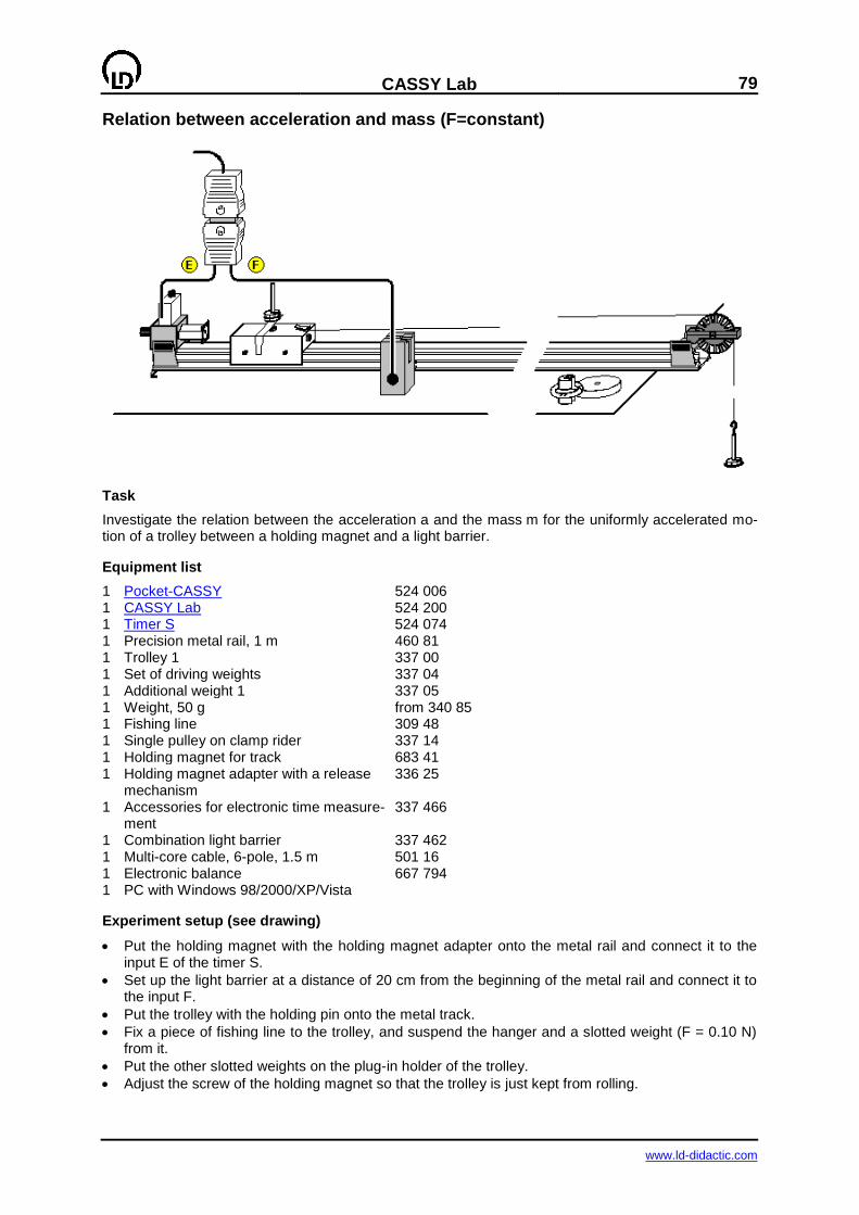
CASSY Lab

79

www.ld-didactic.com

Relation between acceleration and mass (F=constant)

Task

Investigate the relation between the acceleration a and the mass m for the uniformly accelerated mo-tion of a trolley between a holding magnet and a light barrier.

Equipment list

1 Pocket-CASSY 524 006 1 CASSY Lab 524 200 1 Timer S 524 074 1 Precision metal rail, 1 m 460 81 1 Trolley 1 337 00 1 Set of driving weights 337 04 1 Additional weight 1 337 05 1 Weight, 50 g from 340 85 1 Fishing line 309 48 1 Single pulley on clamp rider 337 14 1 Holding magnet for track 683 41 1 Holding magnet adapter with a release

mechanism 336 25


337 466

1 Combination light barrier 337 462 1 Multi-core cable, 6-pole, 1.5 m 501 16 1 Electronic balance 667 794 1 PC with Windows 98/2000/XP/Vista





Fix a piece of fishing line to the trolley, and suspend the hanger and a slotted weight (F = 0.10 N) from it.

Put the other slotted weights on the plug-in holder of the trolley.


80

CASSY Lab

www.ld-didactic.com



Einstellungen laden

Determine the mass m of the trolley (including the hanger and the slotted weights).

Position the light barrier at the distance s = 30 cm from the zero.


Read the travel time t1 in the display window and accept it with F9 for calculating the acceleration.

Increase the mass of the trolley in steps of 50 g and repeat the measurement.

Before recording a new measurement series, use the mouse to select Append New Meas. Series in the Measuring Parameters window (press F5 twice).

Next increase the accelerating force by putting one and two slotted weights, respectively, on the hanger, and repeat the measurements.

Evaluation

How can the acceleration a of the trolley be calculated from the path s and the travel time t1?

Enter the respective masses m (trolley, additional weights, hanger weight and slotted weights) in

the table. Draw hyperbolas (1/x) through the measuring points in the a(m) diagram.

What relation between the acceleration a and the mass m can be derived?

On which physical quantity does the acceleration a of the trolley depend if the mass is constant?

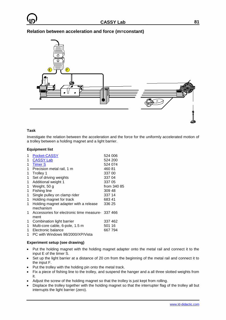
CASSY Lab

81

www.ld-didactic.com

Relation between acceleration and force (m=constant)

Task

Investigate the relation between the acceleration and the force for the uniformly accelerated motion of a trolley between a holding magnet and a light barrier.

Equipment list

1 Pocket-CASSY 524 006 1 CASSY Lab 524 200 1 Timer S 524 074 1 Precision metal rail, 1 m 460 81 1 Trolley 1 337 00 1 Set of driving weights 337 04 1 Additional weight 1 337 05 1 Weight, 50 g from 340 85 1 Fishing line 309 48 1 Single pulley on clamp rider 337 14 1 Holding magnet for track 683 41 1 Holding magnet adapter with a release

mechanism 336 25


337 466

1 Combination light barrier 337 462 1 Multi-core cable, 6-pole, 1.5 m 501 16 1 Electronic balance 667 794 1 PC with Windows 98/2000/XP/Vista





Fix a piece of fishing line to the trolley, and suspend the hanger and a all three slotted weights from it.



82

CASSY Lab

www.ld-didactic.com


Einstellungen laden

Determine the mass m of the trolley (including the hanger and the slotted weights).

Position the light barrier at the distance s = 30 cm from the zero.

Take all three slotted weights from the hanger and put them on the plug-in holder of the trolley.


Read the travel time t1 in the display window and accept it with F9 for calculating the acceleration.

One after another take a slotted weight from the plug-in holder, put it on the hanger, and repeat the measurement.

Before recording a new measurement series, use the mouse to select Append New Meas. Series in the Measuring Parameters window (press F5 twice).

Next increase the mass of the trolley by 0.05 kg and 0.10 kg, respectively, and repeat the meas-urements.

Evaluation

How can the acceleration of the trolley be calculated from the path s and the travel time t1?

Enter the force F acting on the trolley in each case in the table. Draw a straight line through the

origin and the measuring points in the a(F) diagram.

What relation between a and F can be derived from the graphical representation?

On which physical quantity does the acceleration a of the trolley depend if the force acting on the

trolley is constant?

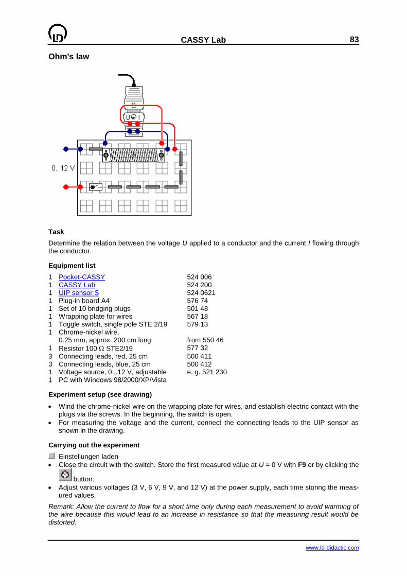
CASSY Lab

83

www.ld-didactic.com

Ohm's law

Task

Determine the relation between the voltage U applied to a conductor and the current I flowing through the conductor.

Equipment list

1 Pocket-CASSY 524 006 1 CASSY Lab 524 200 1 UIP sensor S 524 0621 1 Plug-in board A4 576 74 1 Set of 10 bridging plugs 501 48 1 Wrapping plate for wires 567 18 1 Toggle switch, single pole STE 2/19 579 13 1 Chrome-nickel wire, 0.25 mm, approx. 200 cm long from 550 46 1 Resistor 100 STE2/19 577 32

3 Connecting leads, red, 25 cm 500 411 3 Connecting leads, blue, 25 cm 500 412 1 Voltage source, 0...12 V, adjustable e. g. 521 230 1 PC with Windows 98/2000/XP/Vista


Wind the chrome-nickel wire on the wrapping plate for wires, and establish electric contact with the plugs via the screws. In the beginning, the switch is open.

For measuring the voltage and the current, connect the connecting leads to the UIP sensor as shown in the drawing.


Einstellungen laden

Close the circuit with the switch. Store the first measured value at U = 0 V with F9 or by clicking the

button.

Adjust various voltages (3 V, 6 V, 9 V, and 12 V) at the power supply, each time storing the meas-ured values.

Remark: Allow the current to flow for a short time only during each measurement to avoid warming of the wire because this would lead to an increase in resistance so that the measuring result would be distorted.

84

CASSY Lab

www.ld-didactic.com

Replace the wrapping plate for wires in the circuit with the STE resistor 100 and two bridging plugs.

Tick Append New Measurement Series in the Measuring Parameters window (e.g. by pressing the F5 key).

Repeat the experiment with the STE resistor 100 .

Evaluation

We have the following relation: The greater the voltage U, the

How does the current I flowing through a wire change if the voltage U is doubled?

Perform a fit to a Best-fit straight line in the diagram for both measurement series. How are the

measured values distributed?

What is your conclusion regarding the relation between the voltage U and the current I in the two

experiments?

The electric resistance R is defined as the quotient of U and I:

The unit of the electric resistance is (Ohm):

What can you say about the two resistors used in the experiment?

What is the magnitude of the chrome-nickel wire and of the STE resistor used in the experiment?

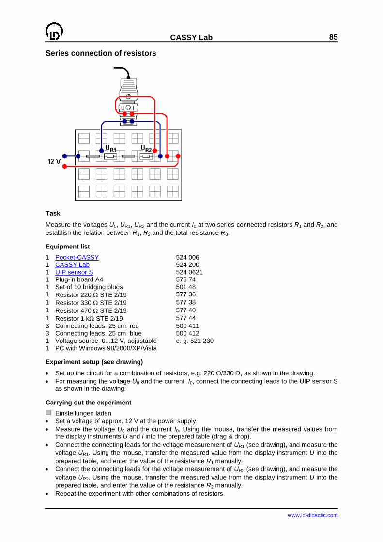
CASSY Lab

85

www.ld-didactic.com

Series connection of resistors

Task

Measure the voltages U0, UR1, UR2 and the current I0 at two series-connected resistors R1 and R2, and

establish the relation between R1, R2 and the total resistance R0.

Equipment list

1 Pocket-CASSY 524 006 1 CASSY Lab 524 200 1 UIP sensor S 524 0621 1 Plug-in board A4 576 74 1 Set of 10 bridging plugs 501 48 1 Resistor 220 STE 2/19 577 36

1 Resistor 330 STE 2/19 577 38

1 Resistor 470 STE 2/19 577 40

1 Resistor 1 k STE 2/19 577 44

3 Connecting leads, 25 cm, red 500 411 3 Connecting leads, 25 cm, blue 500 412 1 Voltage source, 0...12 V, adjustable e. g. 521 230 1 PC with Windows 98/2000/XP/Vista


Set up the circuit for a combination of resistors, e.g. 220 /330 , as shown in the drawing.

For measuring the voltage U0 and the current I0, connect the connecting leads to the UIP sensor S as shown in the drawing.


Einstellungen laden

Set a voltage of approx. 12 V at the power supply.

Measure the voltage U0 and the current I0. Using the mouse, transfer the measured values from the display instruments U and I into the prepared table (drag & drop).

Connect the connecting leads for the voltage measurement of UR1 (see drawing), and measure the

voltage UR1. Using the mouse, transfer the measured value from the display instrument U into the

prepared table, and enter the value of the resistance R1 manually.

Connect the connecting leads for the voltage measurement of UR2 (see drawing), and measure the

voltage UR2. Using the mouse, transfer the measured value from the display instrument U into the

prepared table, and enter the value of the resistance R2 manually.

Repeat the experiment with other combinations of resistors.

86

CASSY Lab

www.ld-didactic.com

Evaluation

For evaluating the experiment, the prepared table Evaluation is provided, from which the relations

between the voltages U0, UR1, UR2 and the resistances R0, R1, R2 become obvious.

The current which flows through the series-connected resistors R1 and R2 is

What is the relation between the voltages UR1 and UR2 and the total voltage U0?

What is the relation between the ratio of the resistances R1 and R2 and the ratio of the voltages

UR1 and UR2?

What is the relation between the total resistance R0 = U0/I0 and the resistances R1 and R2?

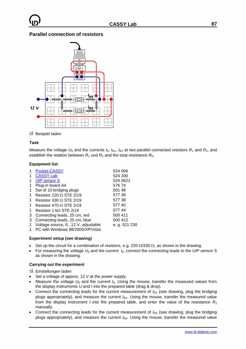
CASSY Lab

87

www.ld-didactic.com

Parallel connection of resistors

Beispiel laden

Task

Measure the voltage U0 and the currents I0, IR1, IR2 at two parallel connected resistors R1 and R2, and

establish the relation between R1 und R2 and the total resistance R0.

Equipment list


1 Resistor 330 STE 2/19 577 38

1 Resistor 470 STE 2/19 577 40




Set up the circuit for a combination of resistors, e.g. 220 /330 , as shown in the drawing.

For measuring the voltage U0 and the current I0, connect the connecting leads to the UIP sensor S as shown in the drawing.


Einstellungen laden

Set a voltage of approx. 12 V at the power supply.

Measure the voltage U0 and the current I0. Using the mouse, transfer the measured values from the display instruments U and I into the prepared table (drag & drop).

Connect the connecting leads for the current measurement of IR1 (see drawing, plug the bridging

plugs appropriately), and measure the current IR1. Using the mouse, transfer the measured value

from the display instrument I into the prepared table, and enter the value of the resistance R1

manually.

Connect the connecting leads for the current measurement of IR2 (see drawing, plug the bridging

plugs appropriately), and measure the current IR2. Using the mouse, transfer the measured value

88

CASSY Lab

www.ld-didactic.com

from the display instrument I into the prepared table, and enter the value of the resistance R2

manually.

Repeat the experiment with other combinations of resistors.

Evaluation

For evaluating the experiment, the prepared table Evaluation is provided, from which the relations

between the currents I0, IR1, IR2 and the resistances R0, R1, R2 become obvious.

The voltages UR1 and UR2 at the resistors R1 and R2 are equal to

What is the relation between the currents IR1 and IR2 and the total current I0?

What is the relation between the ratio of the resistances R1 and R2 and the ratio between the cur-

rents IR1 and IR2?

What is the relation between the total resistance R0 = U0/I0 and the resistances R1 and R2?

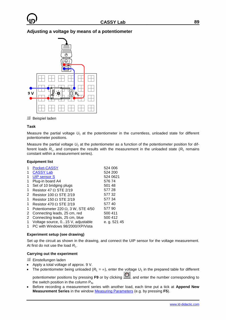
CASSY Lab

89

www.ld-didactic.com

Adjusting a voltage by means of a potentiometer

Beispiel laden

Task

Measure the partial voltage U1 at the potentiometer in the currentless, unloaded state for different potentiometer positions.

Measure the partial voltage U1 at the potentiometer as a function of the potentiometer position for dif-

ferent loads RL, and compare the results with the measurement in the unloaded state (RL remains

constant within a measurement series).

Equipment list


2 Resistor 100 STE 2/19 577 32

1 Resistor 150 STE 2/19 577 34

1 Resistor 470 STE 2/19 577 40

1 Potentiometer 220 , 3 W, STE 4/50 577 90



Set up the circuit as shown in the drawing, and connect the UIP sensor for the voltage measurement.

At first do not use the load RL.


Einstellungen laden

Apply a total voltage of approx. 9 V.

The potentiometer being unloaded (RL = ), enter the voltage U1 in the prepared table for different

potentiometer positions by pressing F9 or by clicking , and enter the number corresponding to

the switch position in the column PN.

Before recording a measurement series with another load, each time put a tick at Append New Measurement Series in the window Measuring Parameters (e.g. by pressing F5).

90

CASSY Lab

www.ld-didactic.com

Insert the STE resistor RL = 470 in the circuit, and record a new measurement series for a

loaded potentiometer.

Repeat the experiment with other loads RL = 100 , 47 .

Evaluation

What is the relation between the partial voltage U1 and the resistance R1at an unloaded potenti-ometer?

What is the effect of loading the potentiometer with a resistance RL?

Where do you expect the curve of the measurement series to be located if the potentiometer is

loaded with a resistance RL < 47 ?

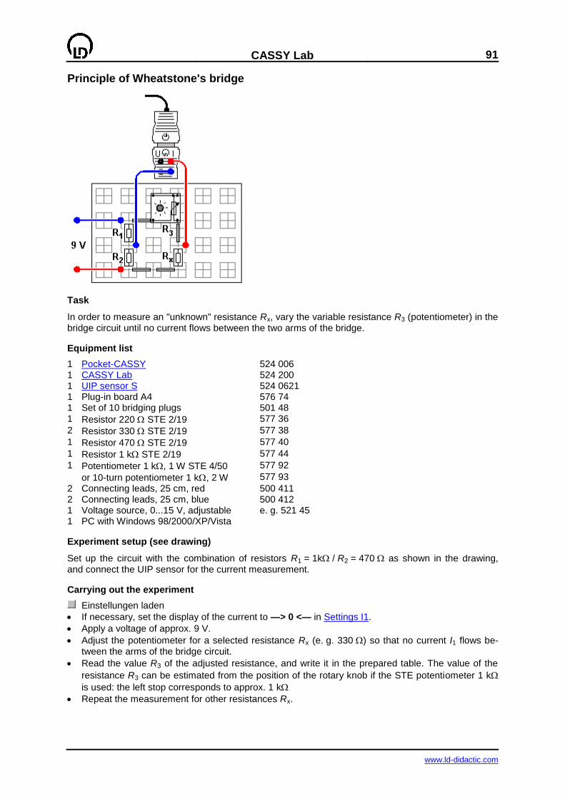
CASSY Lab

91

www.ld-didactic.com

Principle of Wheatstone's bridge

Task

In order to measure an "unknown" resistance Rx, vary the variable resistance R3 (potentiometer) in the bridge circuit until no current flows between the two arms of the bridge.

Equipment list


2 Resistor 330 STE 2/19 577 38

1 Resistor 470 STE 2/19 577 40


1 Potentiometer 1 k, 1 W STE 4/50 577 92

or 10-turn potentiometer 1 k, 2 W 577 93



Set up the circuit with the combination of resistors R1 = 1k / R2 = 470 as shown in the drawing, and connect the UIP sensor for the current measurement.


Einstellungen laden

If necessary, set the display of the current to —> 0 <— in Settings I1.

Apply a voltage of approx. 9 V.

Adjust the potentiometer for a selected resistance Rx (e. g. 330 ) so that no current I1 flows be-tween the arms of the bridge circuit.

Read the value R3 of the adjusted resistance, and write it in the prepared table. The value of the

resistance R3 can be estimated from the position of the rotary knob if the STE potentiometer 1 k

is used: the left stop corresponds to approx. 1 k

Repeat the measurement for other resistances Rx.

92

CASSY Lab

www.ld-didactic.com

Evaluation

What is the relation between the ratios of the resistances in the two arms of the bridge circuit if no

current flows between the two arms (I1 = 0)?

How is Rx determined if the resistances R1, R2 and R3 are known?

What is the relation between the voltage drops U1 and U3 or U2 and Ux, respectively, at the 4 resis-

tances R1 and R3 or R2 and Rx, respectively, if the bridge is balanced (I1 = 0)?

What is the effect of the applied voltage U on the determination of the resistance Rx if the bridge is

balanced (I1 = 0)?

Remark

The resistance Rx could, of course, also be determined by measuring the voltage drop U while a cur-

rent I is flowing, i.e. using the relation Rx=U/I. However, this presupposes that the internal resistances

of the measuring instruments can be neglected, which is usually the case. If the bridge circuit is used, the internal resistance of the ammeter does not play a role at all because no current flows. Therefore the bridge circuit provides an opportunity of an accurate measurement of the fourth resistance if the other three resistances are known precisely.

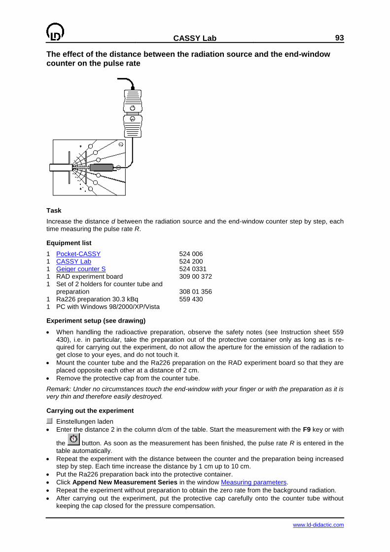
CASSY Lab

93

www.ld-didactic.com

The effect of the distance between the radiation source and the end-window counter on the pulse rate

Task

Increase the distance d between the radiation source and the end-window counter step by step, each time measuring the pulse rate R.

Equipment list

1 Pocket-CASSY 524 006 1 CASSY Lab 524 200 1 Geiger counter S 524 0331 1 RAD experiment board 309 00 372 1 Set of 2 holders for counter tube and preparation 308 01 356 1 Ra226 preparation 30.3 kBq 559 430 1 PC with Windows 98/2000/XP/Vista


When handling the radioactive preparation, observe the safety notes (see Instruction sheet 559 430), i.e. in particular, take the preparation out of the protective container only as long as is re-quired for carrying out the experiment, do not allow the aperture for the emission of the radiation to get close to your eyes, and do not touch it.

Mount the counter tube and the Ra226 preparation on the RAD experiment board so that they are placed opposite each other at a distance of 2 cm.

Remove the protective cap from the counter tube.

Remark: Under no circumstances touch the end-window with your finger or with the preparation as it is very thin and therefore easily destroyed.


Einstellungen laden

Enter the distance 2 in the column d/cm of the table. Start the measurement with the F9 key or with

the button. As soon as the measurement has been finished, the pulse rate R is entered in the table automatically.

Repeat the experiment with the distance between the counter and the preparation being increased step by step. Each time increase the distance by 1 cm up to 10 cm.

Put the Ra226 preparation back into the protective container.

Click Append New Measurement Series in the window Measuring parameters.

Repeat the experiment without preparation to obtain the zero rate from the background radiation.

After carrying out the experiment, put the protective cap carefully onto the counter tube without keeping the cap closed for the pressure compensation.

94

CASSY Lab

www.ld-didactic.com

Evaluation

What is the difference between N1 and the pulse rate R?

How does the pulse rate R change with respect to the distance d between the preparation and the

counter tube?

What curve is described by the measured values? Suggestion:

Confirm your suggestion by fitting a corresponding curve with Fit Function.

What is your conclusion regarding the relation between the pulse rate R and the distance d?

What protective measure derives from this relation for handling radioactive materials?

What is the magnitude of the zero rate R0?

At what distance does the preparation used in this experiment lead to an additional irradiation

which is of the order of magnitude of the background radiation? To determine this distance, acti-vate Zoom in order that the value can be read.

CASSY Lab

95

www.ld-didactic.com

Experiment examples physics

These experiment examples support you in using CASSY Lab. Where applicable, the corresponding experiment number from the General Catalogue of Physics Experiments is also given. The measure-ment data or settings for the examples can be loaded directly into CASSY Lab. Simply click the but-

tons in the descriptions. New examples are labelled with a red .

Mechanics

Uniform motions between two light barriers

Accelerated motions between holding magnet and light barrier

P1.3.2.3a Motions with spoked wheel (newton definition)

P1.3.3.4-6 Motions on the linear air track (Newton's equation of motion)

P1.3.4.1-2ab Conservation of momentum and energy (collision)

Conservation of linear momentum by measuring the motion of the centre of mass (collision)

Confirming the relation action=reaction by measuring accelerations (collision)

P1.3.5.3 Free fall with g-ladder

Free fall with g-ladder (with modelling)

P1.4.1.2 Rotational motions (Newton's equation of motion)

P1.4.2.1-2 Conservation of angular momentum and energy (torsion collision)

Centrifugal force (rotable centrifugal force arm)

P1.4.3.3 Centrifugal force (centrifugal force apparatus)

Oscillations of a rod pendulum

Oscillations of a rod pendulum (with added mass)

Oscillations of a rod pendulum (with modelling)

Dependency of the period of the oscillation on the amplitude

Determination of the acceleration due to gravity on earth by means of a reversible pendulum

Pendulum with changeable acceleration due to gravity (variable g-pendulum)

P1.5.2.1 Harmonic oscillations of a spring pendulum

P1.5.2.2 Dependence of the period of oscillation of a spring pendulum on the mass

Oscillations of a spring pendulum (with modelling)

Oscillations of a spring pendulum with solid friction (with modelling)

Oscillations of a spring pendulum with lubricant friction (with modelling)

Oscillations of a spring pendulum with laminar liquid friction (with modelling)

Oscillations of a spring pendulum with turbulent liquid friction/air friction (with model-ling)

P1.5.4.4 Coupled pendulum with two tachogenerators

Coupled pendulums with two rotary motion sensors

P1.7.1.3 Acoustic beats

P1.7.2.1 String vibrations

P1.7.3.3 Velocity of sound in the air

Determining the velocity of sound in air with 2 microphones

P1.7.3.4 Velocity of sound in gases

P1.7.3.5 Velocity of sound in solid bodies

P1.7.7.1 Fourier analysis of simulated signals

P1.7.7.2 Fourier analysis of signals of a function generator

P1.7.7.4 Sound analysis

Sonic synthesis

Heat

P2.3.3.2 Conversion of mechanical energy into thermal energy

P2.3.4.3 Conversion of electrical energy into thermal energy

P2.6.2.4 pV diagram of a hot-air engine

Electricity

P3.1.2.3 Coulomb's law

96

CASSY Lab

www.ld-didactic.com

P3.3.3.3 Force in the magnetic field of an air coil

P3.3.3.2 Force in the magnetic field of an electromagnet

P3.3.3.4 Force between two current-carrying conductors (ampere definition)

P3.4.1.1 Impulse of voltage (Faraday's law of induction)

P3.4.3.1-2 Induction in a variable magnetic field

P3.4.5.3 Voltage and current curves of a transformer as a function of time

P3.4.5.4 Power transfer of a transformer

Power of arbitrary loads operated with mains AC voltage

Charging and discharging of a capacitor

Charging and discharging of a capacitor (with modelling)

Charging and discharging of a small capacitor (cable capacitances)

Damped oscillator

Damped oscillator (with modelling)

P1.7.7.3 Coupled oscillators

Forced oscillations (resonance)

Forced oscillations (resonance, with modelling)

RLC filter (low pass, high pass, band pass)

Low-pass filter (with modelling)

High-pass filter (with modelling)

Electronics

P4.1.2.1 Characteristic of an incandescent lamp

Characteristic of a diode

Characteristic of a transistor

D3.4.7.7a Power characteristic of a solar cell

Temperature control

Brightness control

Voltage control

Optics

P5.3.1.4 Diffraction at a single slit

P5.3.1.5 Diffraction at multiple slits

P5.5.1.2a Inverse square law for light

Velocity of light on air

Velocity of light in various materials

Atomic and Nuclear Physics

P6.1.2.3-4 Millikan's experiment

P6.2.4.2 Franck-Hertz experiment with mercury

P6.2.4.4 Franck-Hertz experiment with neon

P6.3.5.4 Moseley's law (K-line x-ray fluorescence)

P6.3.5.5 Moseley's law (L-line x-ray fluorescence)

P6.3.5.6 Energy dispersive Bragg reflection into different orders of diffraction

P6.3.7.2 Compton effect on X-rays

P6.4.2.1 Poisson distribution

P6.4.3.2 Half-life of radon

P6.5.4.1 spectroscopy of radioactive samples (Am-241)

P6.5.4.2 Determining the energy loss of radiation in air

P6.5.4.3 Determining the energy loss of radiation in aluminium and in gold

P6.5.4.4 Determining the age of a Ra-226 sample

P6.5.5.1 Detecting radiation with a scintillation counter (Cs-137)

P6.5.5.2 Recording and calibrating a spectrum

P6.5.5.3 Absorption of radiation

P6.5.5.4 Identifying and determining the activity of weakly radioactive samples

P6.5.5.5 Recording a spectrum using a scintillation counter

P6.5.6.1 Quantitative observation of the Compton effect

Recording the complex spectrum of Ra-226 and its decay products

CASSY Lab

97

www.ld-didactic.com

Recording the complex spectrum of an incandescent gas hood

P6.5.5.6 Coincidence and - angular correlation in positron decay

Measurements with the single-channel analyzer

Solid State Physics

P7.2.2.1-2 Electrical conductivity of solids

P7.3.2.1 Hysteresis of a transformer core

P7.5.1.1 Non-destructive analysis of the chemical composition (x-ray fluorescence)

P7.5.1.2 Determination of the chemical composition of a brass sample (x-ray fluorescence)

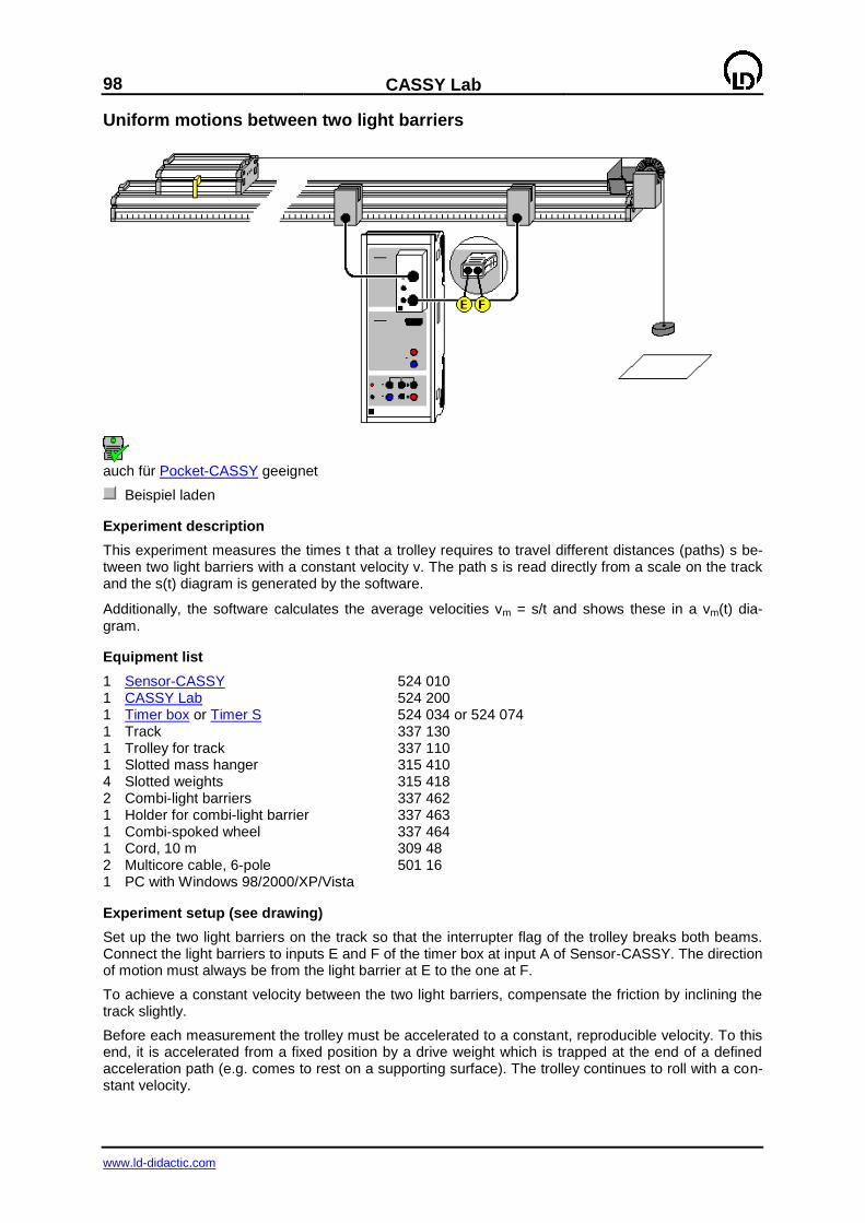
98

CASSY Lab

www.ld-didactic.com

Uniform motions between two light barriers

auch für Pocket-CASSY geeignet

Beispiel laden

Experiment description

This experiment measures the times t that a trolley requires to travel different distances (paths) s be-tween two light barriers with a constant velocity v. The path s is read directly from a scale on the track and the s(t) diagram is generated by the software.

Additionally, the software calculates the average velocities vm = s/t and shows these in a vm(t) dia-

gram.

Equipment list

1 Sensor-CASSY 524 010 1 CASSY Lab 524 200 1 Timer box or Timer S 524 034 or 524 074 1 Track 337 130 1 Trolley for track 337 110 1 Slotted mass hanger 315 410 4 Slotted weights 315 418 2 Combi-light barriers 337 462 1 Holder for combi-light barrier 337 463 1 Combi-spoked wheel 337 464 1 Cord, 10 m 309 48 2 Multicore cable, 6-pole 501 16 1 PC with Windows 98/2000/XP/Vista


Set up the two light barriers on the track so that the interrupter flag of the trolley breaks both beams. Connect the light barriers to inputs E and F of the timer box at input A of Sensor-CASSY. The direction of motion must always be from the light barrier at E to the one at F.

To achieve a constant velocity between the two light barriers, compensate the friction by inclining the track slightly.

Before each measurement the trolley must be accelerated to a constant, reproducible velocity. To this end, it is accelerated from a fixed position by a drive weight which is trapped at the end of a defined acceleration path (e.g. comes to rest on a supporting surface). The trolley continues to roll with a con-stant velocity.

CASSY Lab

99

www.ld-didactic.com


Einstellungen laden

Accelerate the trolley to a constant speed as described above and allow it to pass through both light barriers.

Save your measured values with F9.

Read off path s between the two light barriers and enter this in the table (activate keyboard input in the correct table cell using the mouse).

Repeat the measurement for other paths s; again, accelerate the trolley to the same velocity, let it pass both light barriers and save the measured value with F9.

Evaluation

The s(t) diagram of a uniform motion is a straight line. The slope of the straight line corresponds to the velocity v and can be determined e.g. by fitting a straight line. If you click on the display Average Ve-

locity, you can also read off the respective quotients vm = s/t directly.

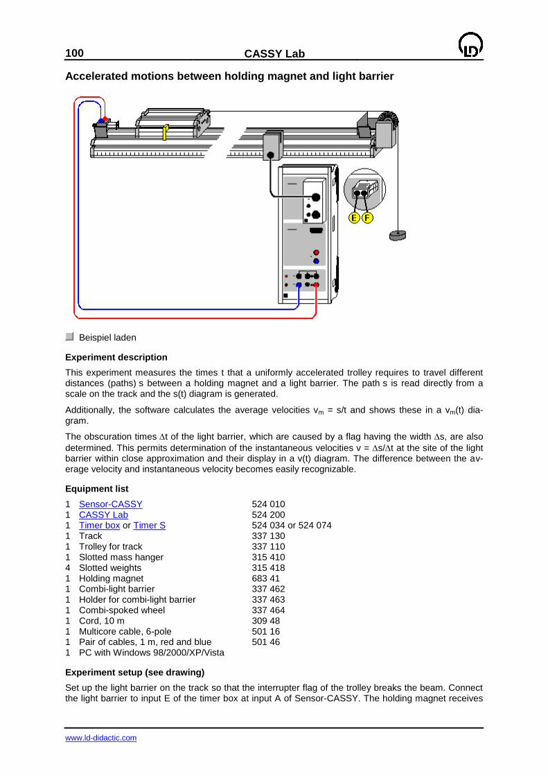
100

CASSY Lab

www.ld-didactic.com

Accelerated motions between holding magnet and light barrier

Beispiel laden


This experiment measures the times t that a uniformly accelerated trolley requires to travel different distances (paths) s between a holding magnet and a light barrier. The path s is read directly from a scale on the track and the s(t) diagram is generated.

Additionally, the software calculates the average velocities vm = s/t and shows these in a vm(t) dia-gram.

The obscuration times t of the light barrier, which are caused by a flag having the width s, are also

determined. This permits determination of the instantaneous velocities v = s/t at the site of the light barrier within close approximation and their display in a v(t) diagram. The difference between the av-erage velocity and instantaneous velocity becomes easily recognizable.

Equipment list

1 Sensor-CASSY 524 010 1 CASSY Lab 524 200 1 Timer box or Timer S 524 034 or 524 074 1 Track 337 130 1 Trolley for track 337 110 1 Slotted mass hanger 315 410 4 Slotted weights 315 418 1 Holding magnet 683 41 1 Combi-light barrier 337 462 1 Holder for combi-light barrier 337 463 1 Combi-spoked wheel 337 464 1 Cord, 10 m 309 48 1 Multicore cable, 6-pole 501 16 1 Pair of cables, 1 m, red and blue 501 46 1 PC with Windows 98/2000/XP/Vista


Set up the light barrier on the track so that the interrupter flag of the trolley breaks the beam. Connect the light barrier to input E of the timer box at input A of Sensor-CASSY. The holding magnet receives

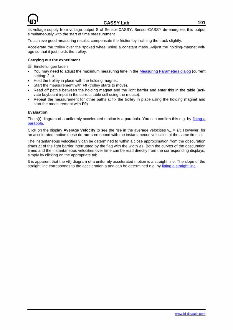
CASSY Lab

101

www.ld-didactic.com

its voltage supply from voltage output S of Sensor-CASSY. Sensor-CASSY de-energizes this output simultaneously with the start of time measurement.

To achieve good measuring results, compensate the friction by inclining the track slightly.

Accelerate the trolley over the spoked wheel using a constant mass. Adjust the holding-magnet volt-age so that it just holds the trolley.


Einstellungen laden

You may need to adjust the maximum measuring time in the Measuring Parameters dialog (current setting: 2 s).

Hold the trolley in place with the holding magnet.

Start the measurement with F9 (trolley starts to move).

Read off path s between the holding magnet and the light barrier and enter this in the table (acti-vate keyboard input in the correct table cell using the mouse).

Repeat the measurement for other paths s; fix the trolley in place using the holding magnet and start the measurement with F9).

Evaluation

The s(t) diagram of a uniformly accelerated motion is a parabola. You can confirm this e.g. by fitting a parabola.

Click on the display Average Velocity to see the rise in the average velocities vm = s/t. However, for an accelerated motion these do not correspond with the instantaneous velocities at the same times t.

The instantaneous velocities v can be determined to within a close approximation from the obscuration

times t of the light barrier interrupted by the flag with the width s. Both the curves of the obscuration times and the instantaneous velocities over time can be read directly from the corresponding displays, simply by clicking on the appropriate tab.

It is apparent that the v(t) diagram of a uniformly accelerated motion is a straight line. The slope of the straight line corresponds to the acceleration a and can be determined e.g. by fitting a straight line.

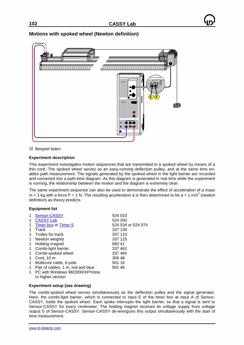
102

CASSY Lab

www.ld-didactic.com

Motions with spoked wheel (Newton definition)

Beispiel laden


This experiment investigates motion sequences that are transmitted to a spoked wheel by means of a thin cord. The spoked wheel serves as an easy-running deflection pulley, and at the same time en-ables path measurement. The signals generated by the spoked wheel in the light barrier are recorded and converted into a path-time diagram. As this diagram is generated in real time while the experiment is running, the relationship between the motion and the diagram is extremely clear.

The same experiment sequence can also be used to demonstrate the effect of acceleration of a mass

m = 1 kg with a force F = 1 N. The resulting acceleration a is then determined to be a = 1 m/s2 (newton

definition) as theory predicts.

Equipment list

1 Sensor-CASSY 524 010 1 CASSY Lab 524 200 1 Timer box or Timer S 524 034 or 524 074 1 Track 337 130 1 Trolley for track 337 110 1 Newton weights 337 115 1 Holding magnet 683 41 1 Combi-light barrier 337 462 1 Combi-spoked wheel 337 464 1 Cord, 10 m 309 48 1 Multicore cable, 6-pole 501 16 1 Pair of cables, 1 m, red and blue 501 46 1 PC with Windows 98/2000/XP/Vista or higher version


The combi-spoked wheel serves simultaneously as the deflection pulley and the signal generator. Here, the combi-light barrier, which is connected to input E of the timer box at input A of Sensor-CASSY, holds the spoked wheel. Each spoke interrupts the light barrier, so that a signal is sent to Sensor-CASSY for every centimeter. The holding magnet receives its voltage supply from voltage output S of Sensor-CASSY. Sensor-CASSY de-energizes this output simultaneously with the start of time measurement.

CASSY Lab

103

www.ld-didactic.com

To obtain an accelerating force of F = 1 N, you need to use a driving mass of 102 g. The trolley (in-cluding the equivalent roller mass) must be augmented to a total mass of 898 g so that the total accel-erated mass m = 1 kg. This is possible using the additional weights for Newton definition.

To achieve good measuring results, compensate the friction by inclining the track slightly.

Adjust the holding-magnet voltage so that it just holds the trolley.


Einstellungen laden

You may want to modify the automatic measuring stop parameter in Settings sA1 (current setting 70 edges for 0.7 m).

You may need to adjust the maximum measuring time in the Measuring Parameters dialog (current setting: 2 s).

Hold the magnet in place with the holding magnet.

Define the path zero point (—> 0 <— in Settings sA1)

Start the measurement with F9 (trolley starts to move).

The measurement stops automatically after the predefined number of edges.

If desired, repeat the measurement for other forces F; fix the trolley in place using the holding magnet, define the path zero point and start the measurement with F9.

Evaluation

The s(t) diagram of a uniformly accelerated motion is a parabola. You can confirm this e.g. by fitting a parabola.

Clicking on the Velocity display shows the calculated velocities v(t). It is apparent that the v(t) diagram of a uniformly accelerated motion is a straight line. The slope of the straight line is the constant accel-eration a and can be determined e.g. by fitting a straight line.

In this example the accelerating force used is F = 1 N and the accelerating mass m = 1 kg (Newton definition). In this case the v(t) diagram gives us of velocity v of 1 m/s after t = 1 s. Also, the straight

line in the f(t) diagram has the slope a = 1 m/s2.

Remark

The individual velocity values v(i) are calculated as

v(i) = ( s(i+1) – s(i-1) ) / ( t(i+1) – t(i-1) )

This is the average velocity in the interval [t(i-1),t(i+1)] and is an initial approximation of the instanta-neous velocity at the time ½ (t(i-1) + t(i+1)), and thus not at time t(i).

However, this was already taken into consideration in the v(t) display by means of suitable conversion of the time axis.

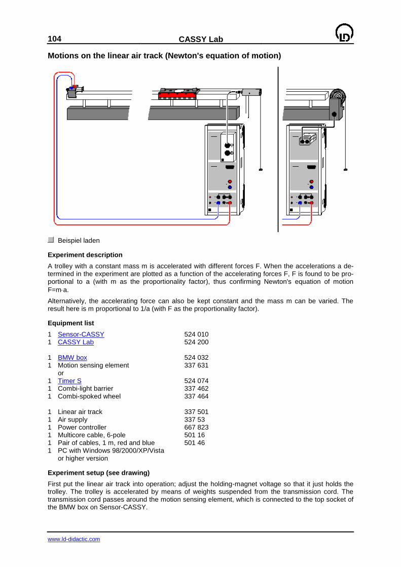
104

CASSY Lab

www.ld-didactic.com

Motions on the linear air track (Newton's equation of motion)

Beispiel laden


A trolley with a constant mass m is accelerated with different forces F. When the accelerations a de-termined in the experiment are plotted as a function of the accelerating forces F, F is found to be pro-portional to a (with m as the proportionality factor), thus confirming Newton's equation of motion

F=ma.

Alternatively, the accelerating force can also be kept constant and the mass m can be varied. The result here is m proportional to 1/a (with F as the proportionality factor).

Equipment list

1 Sensor-CASSY 524 010 1 CASSY Lab 524 200 1 BMW box 524 032 1 Motion sensing element 337 631 or 1 Timer S 524 074 1 Combi-light barrier 337 462 1 Combi-spoked wheel 337 464 1 Linear air track 337 501 1 Air supply 337 53 1 Power controller 667 823 1 Multicore cable, 6-pole 501 16 1 Pair of cables, 1 m, red and blue 501 46 1 PC with Windows 98/2000/XP/Vista or higher version


First put the linear air track into operation; adjust the holding-magnet voltage so that it just holds the trolley. The trolley is accelerated by means of weights suspended from the transmission cord. The transmission cord passes around the motion sensing element, which is connected to the top socket of the BMW box on Sensor-CASSY.

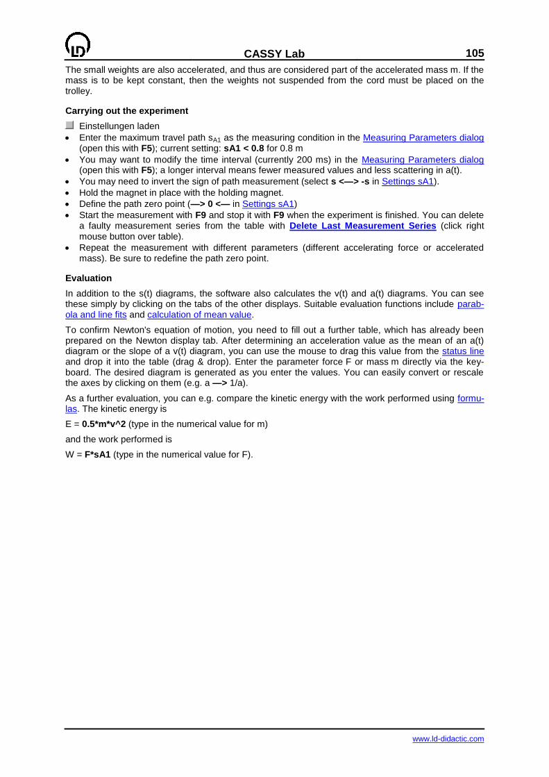
CASSY Lab

105

www.ld-didactic.com

The small weights are also accelerated, and thus are considered part of the accelerated mass m. If the mass is to be kept constant, then the weights not suspended from the cord must be placed on the trolley.


Einstellungen laden

Enter the maximum travel path sA1 as the measuring condition in the Measuring Parameters dialog (open this with F5); current setting: sA1 < 0.8 for 0.8 m

You may want to modify the time interval (currently 200 ms) in the Measuring Parameters dialog (open this with F5); a longer interval means fewer measured values and less scattering in a(t).

You may need to invert the sign of path measurement (select s <—> -s in Settings sA1).

Hold the magnet in place with the holding magnet.

Define the path zero point (—> 0 <— in Settings sA1)

Start the measurement with F9 and stop it with F9 when the experiment is finished. You can delete a faulty measurement series from the table with Delete Last Measurement Series (click right mouse button over table).

Repeat the measurement with different parameters (different accelerating force or accelerated mass). Be sure to redefine the path zero point.

Evaluation

In addition to the s(t) diagrams, the software also calculates the v(t) and a(t) diagrams. You can see these simply by clicking on the tabs of the other displays. Suitable evaluation functions include parab-ola and line fits and calculation of mean value.

To confirm Newton's equation of motion, you need to fill out a further table, which has already been prepared on the Newton display tab. After determining an acceleration value as the mean of an a(t) diagram or the slope of a v(t) diagram, you can use the mouse to drag this value from the status line and drop it into the table (drag & drop). Enter the parameter force F or mass m directly via the key-board. The desired diagram is generated as you enter the values. You can easily convert or rescale the axes by clicking on them (e.g. a —> 1/a).

As a further evaluation, you can e.g. compare the kinetic energy with the work performed using formu-las. The kinetic energy is

E = 0.5*m*v^2 (type in the numerical value for m)

and the work performed is

W = F*sA1 (type in the numerical value for F).

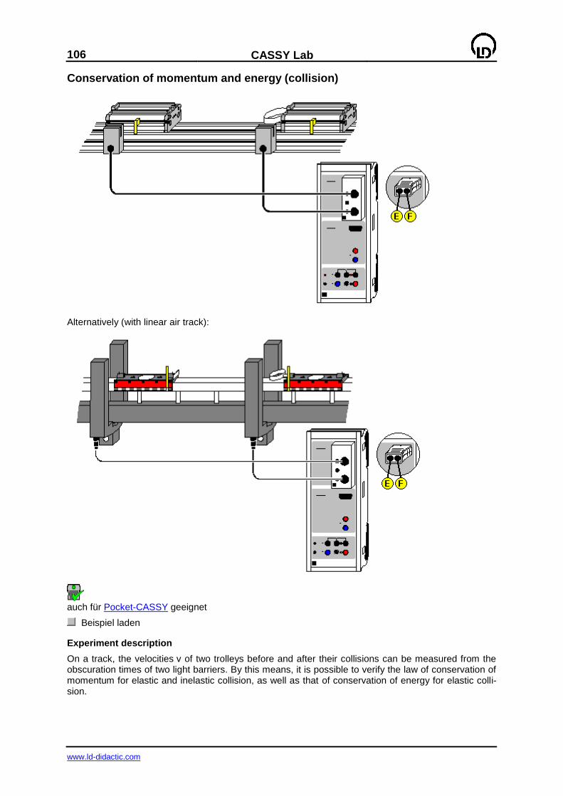
106

CASSY Lab

www.ld-didactic.com

Conservation of momentum and energy (collision)

Alternatively (with linear air track):


Beispiel laden


On a track, the velocities v of two trolleys before and after their collisions can be measured from the obscuration times of two light barriers. By this means, it is possible to verify the law of conservation of momentum for elastic and inelastic collision, as well as that of conservation of energy for elastic colli-sion.

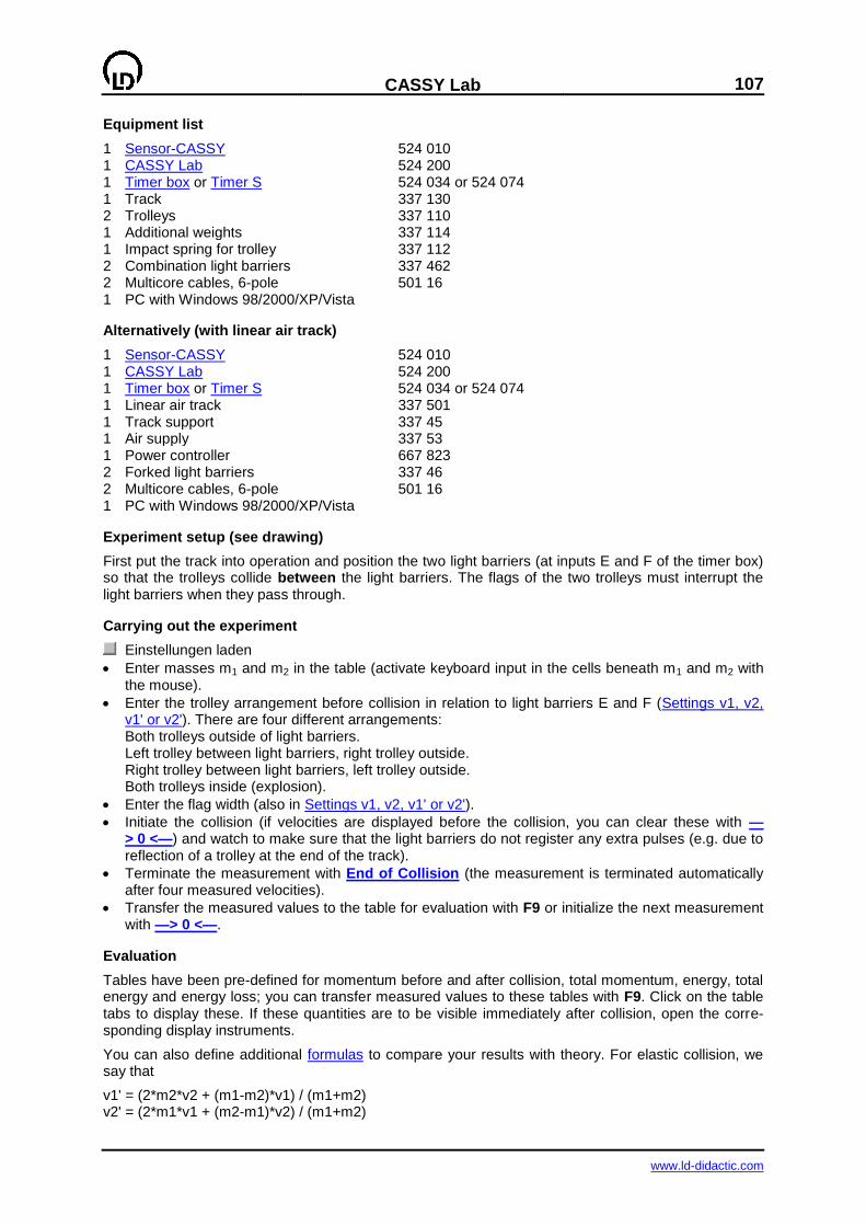
CASSY Lab

107

www.ld-didactic.com

Equipment list

1 Sensor-CASSY 524 010 1 CASSY Lab 524 200 1 Timer box or Timer S 524 034 or 524 074 1 Track 337 130 2 Trolleys 337 110 1 Additional weights 337 114 1 Impact spring for trolley 337 112 2 Combination light barriers 337 462 2 Multicore cables, 6-pole 501 16 1 PC with Windows 98/2000/XP/Vista

Alternatively (with linear air track)

1 Sensor-CASSY 524 010 1 CASSY Lab 524 200 1 Timer box or Timer S 524 034 or 524 074 1 Linear air track 337 501 1 Track support 337 45 1 Air supply 337 53 1 Power controller 667 823 2 Forked light barriers 337 46 2 Multicore cables, 6-pole 501 16 1 PC with Windows 98/2000/XP/Vista


First put the track into operation and position the two light barriers (at inputs E and F of the timer box) so that the trolleys collide between the light barriers. The flags of the two trolleys must interrupt the light barriers when they pass through.


Einstellungen laden

Enter masses m1 and m2 in the table (activate keyboard input in the cells beneath m1 and m2 with the mouse).

Enter the trolley arrangement before collision in relation to light barriers E and F (Settings v1, v2, v1' or v2'). There are four different arrangements: Both trolleys outside of light barriers. Left trolley between light barriers, right trolley outside. Right trolley between light barriers, left trolley outside. Both trolleys inside (explosion).

Enter the flag width (also in Settings v1, v2, v1' or v2').

Initiate the collision (if velocities are displayed before the collision, you can clear these with —> 0 <—) and watch to make sure that the light barriers do not register any extra pulses (e.g. due to reflection of a trolley at the end of the track).

Terminate the measurement with End of Collision (the measurement is terminated automatically after four measured velocities).

Transfer the measured values to the table for evaluation with F9 or initialize the next measurement with —> 0 <—.

Evaluation

Tables have been pre-defined for momentum before and after collision, total momentum, energy, total energy and energy loss; you can transfer measured values to these tables with F9. Click on the table tabs to display these. If these quantities are to be visible immediately after collision, open the corre-sponding display instruments.

You can also define additional formulas to compare your results with theory. For elastic collision, we say that

v1' = (2*m2*v2 + (m1-m2)*v1) / (m1+m2) v2' = (2*m1*v1 + (m2-m1)*v2) / (m1+m2)

108

CASSY Lab

www.ld-didactic.com

For inelastic collision, the following applies:

v1' = v2' = (m1*v1 + m2*v2) / (m1+m2).

Table for converting specified units to SI units

Quantity SI unit = Factor specified unit Mass m kg 1 kg Velocity v m/s 1 m/s Momentum p Ns = kgm/s 1000 mNs Energy E J = kgm

2/s

2 1000 mJ

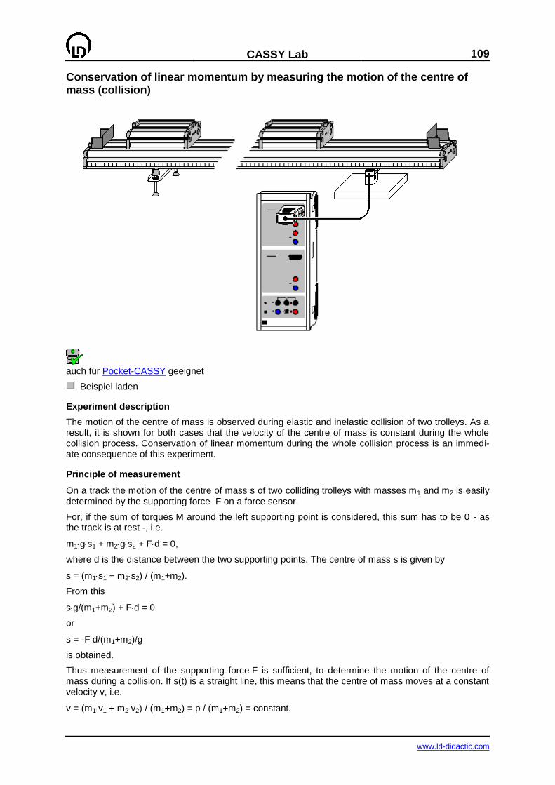
CASSY Lab

109

www.ld-didactic.com

Conservation of linear momentum by measuring the motion of the centre of mass (collision)


Beispiel laden


The motion of the centre of mass is observed during elastic and inelastic collision of two trolleys. As a result, it is shown for both cases that the velocity of the centre of mass is constant during the whole collision process. Conservation of linear momentum during the whole collision process is an immedi-ate consequence of this experiment.

Principle of measurement

On a track the motion of the centre of mass s of two colliding trolleys with masses m1 and m2 is easily determined by the supporting force F on a force sensor.

For, if the sum of torques M around the left supporting point is considered, this sum has to be 0 - as the track is at rest -, i.e.

m1gs1 + m2gs2 + Fd = 0,

where d is the distance between the two supporting points. The centre of mass s is given by

s = (m1s1 + m2s2) / (m1+m2).

From this

sg/(m1+m2) + Fd = 0

or

s = -Fd/(m1+m2)/g

is obtained.

Thus measurement of the supporting force F is sufficient, to determine the motion of the centre of mass during a collision. If s(t) is a straight line, this means that the centre of mass moves at a constant velocity v, i.e.

v = (m1v1 + m2v2) / (m1+m2) = p / (m1+m2) = constant.

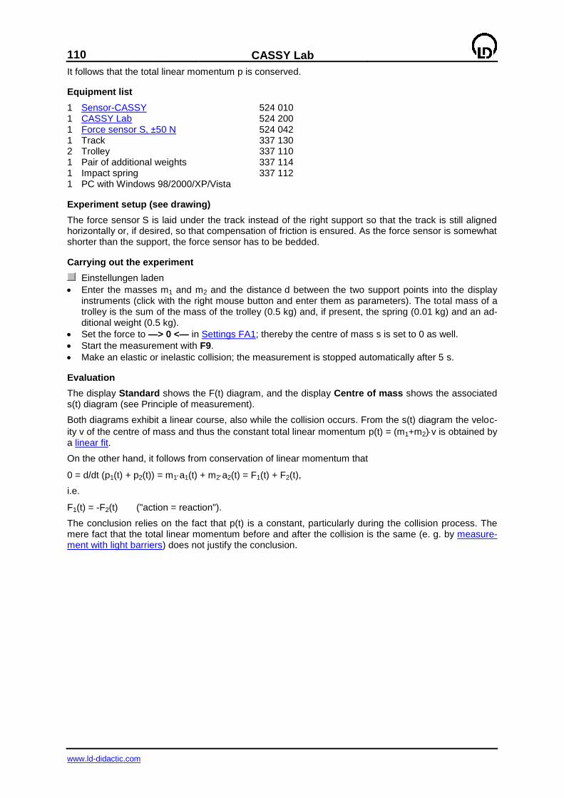
110

CASSY Lab

www.ld-didactic.com

It follows that the total linear momentum p is conserved.

Equipment list

1 Sensor-CASSY 524 010 1 CASSY Lab 524 200 1 Force sensor S, ±50 N 524 042 1 Track 337 130 2 Trolley 337 110 1 Pair of additional weights 337 114 1 Impact spring 337 112 1 PC with Windows 98/2000/XP/Vista


The force sensor S is laid under the track instead of the right support so that the track is still aligned horizontally or, if desired, so that compensation of friction is ensured. As the force sensor is somewhat shorter than the support, the force sensor has to be bedded.


Einstellungen laden

Enter the masses m1 and m2 and the distance d between the two support points into the display instruments (click with the right mouse button and enter them as parameters). The total mass of a trolley is the sum of the mass of the trolley (0.5 kg) and, if present, the spring (0.01 kg) and an ad-ditional weight (0.5 kg).

Set the force to —> 0 <— in Settings FA1; thereby the centre of mass s is set to 0 as well.

Start the measurement with F9.

Make an elastic or inelastic collision; the measurement is stopped automatically after 5 s.

Evaluation

The display Standard shows the F(t) diagram, and the display Centre of mass shows the associated s(t) diagram (see Principle of measurement).

Both diagrams exhibit a linear course, also while the collision occurs. From the s(t) diagram the veloc-

ity v of the centre of mass and thus the constant total linear momentum p(t) = (m1+m2)v is obtained by a linear fit.

On the other hand, it follows from conservation of linear momentum that

0 = d/dt (p1(t) + p2(t)) = m1a1(t) + m2a2(t) = F1(t) + F2(t),

i.e.

F1(t) = -F2(t) ("action = reaction").

The conclusion relies on the fact that p(t) is a constant, particularly during the collision process. The mere fact that the total linear momentum before and after the collision is the same (e. g. by measure-ment with light barriers) does not justify the conclusion.

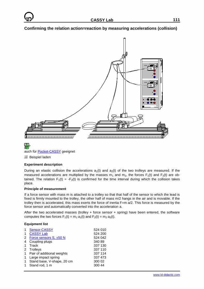
CASSY Lab

111

www.ld-didactic.com

Confirming the relation action=reaction by measuring accelerations (collision)


Beispiel laden


During an elastic collision the accelerations a1(t) and a2(t) of the two trolleys are measured. If the

measured accelerations are multiplied by the masses m1 and m2, the forces F1(t) and F2(t) are ob-

tained. The relation F1(t) = -F2(t) is confirmed for the time interval during which the collision takes

place.

Principle of measurement

If a force sensor with mass m is attached to a trolley so that that half of the sensor to which the lead is fixed is firmly mounted to the trolley, the other half of mass m/2 hangs in the air and is movable. If the

trolley then is accelerated, this mass exerts the force of inertia F=ma/2. This force is measured by the force sensor and automatically converted into the acceleration a.

After the two accelerated masses (trolley + force sensor + spring) have been entered, the software

computes the two forces F1(t) = m1a1(t) and F2(t) = m2a2(t).

Equipment list

1 Sensor-CASSY 524 010 1 CASSY Lab 524 200 2 Force sensors S, ±50 N 524 042 4 Coupling plugs 340 89 1 Track 337 130 2 Trolleys 337 110 1 Pair of additional weights 337 114 1 Large impact spring 337 473 1 Stand base, V-shape, 20 cm 300 02 1 Stand rod, 1 m 300 44

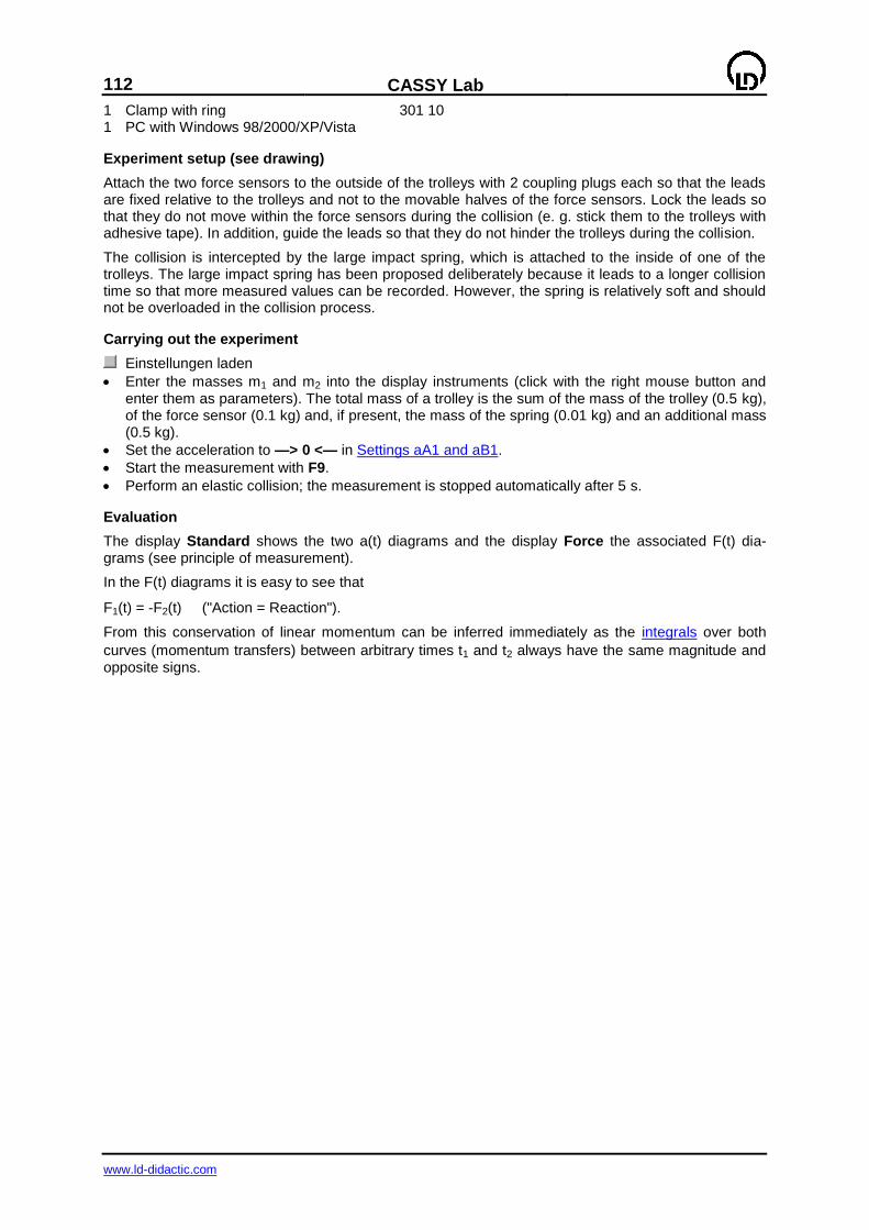
112

CASSY Lab

www.ld-didactic.com

1 Clamp with ring 301 10 1 PC with Windows 98/2000/XP/Vista


Attach the two force sensors to the outside of the trolleys with 2 coupling plugs each so that the leads are fixed relative to the trolleys and not to the movable halves of the force sensors. Lock the leads so that they do not move within the force sensors during the collision (e. g. stick them to the trolleys with adhesive tape). In addition, guide the leads so that they do not hinder the trolleys during the collision.

The collision is intercepted by the large impact spring, which is attached to the inside of one of the trolleys. The large impact spring has been proposed deliberately because it leads to a longer collision time so that more measured values can be recorded. However, the spring is relatively soft and should not be overloaded in the collision process.


Einstellungen laden

Enter the masses m1 and m2 into the display instruments (click with the right mouse button and enter them as parameters). The total mass of a trolley is the sum of the mass of the trolley (0.5 kg), of the force sensor (0.1 kg) and, if present, the mass of the spring (0.01 kg) and an additional mass (0.5 kg).

Set the acceleration to —> 0 <— in Settings aA1 and aB1.


Perform an elastic collision; the measurement is stopped automatically after 5 s.

Evaluation

The display Standard shows the two a(t) diagrams and the display Force the associated F(t) dia-grams (see principle of measurement).

In the F(t) diagrams it is easy to see that

F1(t) = -F2(t) ("Action = Reaction").

From this conservation of linear momentum can be inferred immediately as the integrals over both

curves (momentum transfers) between arbitrary times t1 and t2 always have the same magnitude and opposite signs.

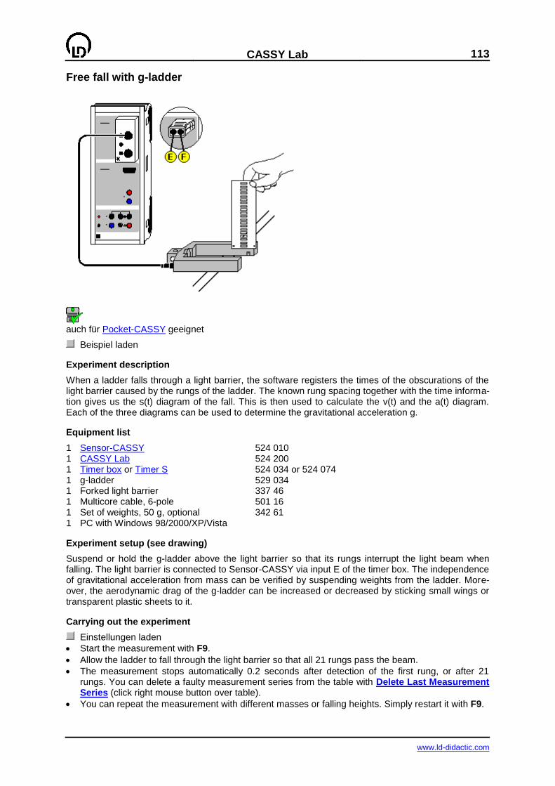
CASSY Lab

113

www.ld-didactic.com

Free fall with g-ladder


Beispiel laden


When a ladder falls through a light barrier, the software registers the times of the obscurations of the light barrier caused by the rungs of the ladder. The known rung spacing together with the time informa-tion gives us the s(t) diagram of the fall. This is then used to calculate the v(t) and the a(t) diagram. Each of the three diagrams can be used to determine the gravitational acceleration g.

Equipment list

1 Sensor-CASSY 524 010 1 CASSY Lab 524 200 1 Timer box or Timer S 524 034 or 524 074 1 g-ladder 529 034 1 Forked light barrier 337 46 1 Multicore cable, 6-pole 501 16 1 Set of weights, 50 g, optional 342 61 1 PC with Windows 98/2000/XP/Vista


Suspend or hold the g-ladder above the light barrier so that its rungs interrupt the light beam when falling. The light barrier is connected to Sensor-CASSY via input E of the timer box. The independence of gravitational acceleration from mass can be verified by suspending weights from the ladder. More-over, the aerodynamic drag of the g-ladder can be increased or decreased by sticking small wings or transparent plastic sheets to it.


Einstellungen laden


Allow the ladder to fall through the light barrier so that all 21 rungs pass the beam.

The measurement stops automatically 0.2 seconds after detection of the first rung, or after 21 rungs. You can delete a faulty measurement series from the table with Delete Last Measurement Series (click right mouse button over table).

You can repeat the measurement with different masses or falling heights. Simply restart it with F9.

114

CASSY Lab

www.ld-didactic.com

Evaluation

This example contains prepared display tabs for path s(t), velocity v(t) and acceleration a(t) which can be accessed by clicking on them. The gravitational acceleration g can be determined in the s(t) dia-gram by fitting a parabola, in the v(t) diagram by fitting a straight line and in the a(t) diagram by finding the mean value. You can enlarge display of the numerical values of the evaluation shown in the status line with F6.

As the ladder had an initial velocity when the light barrier was interrupted by the first rung, the peak of the s(t) parabola is not visible, and the v(t) straight line does not pass through the origin. However, to better illustrate the matter, you can move e.g. the t and s axes with the mouse so that after fitting a parabola its peak is also visible.

Remark

The individual velocity values v(i) are calculated as

v(i) = ( s(i+1) – s(i-1) ) / ( t(i+1) – t(i-1) )

This is the average velocity in the interval [t(i-1),t(i+1)] and an initial approximation of the instantane-ous velocity at the time ½ (t(i-1) + t(i+1)), i.e. not at time t(i). The same is true for the acceleration val-ues:

a(i) = ( v(i+1) – v(i-1) ) / ( ½ (t(i+2) – t(i-2)) ).

However, this has already been taken into consideration in the v(t) and a(t) displays by means of suit-able conversion of the time axis.

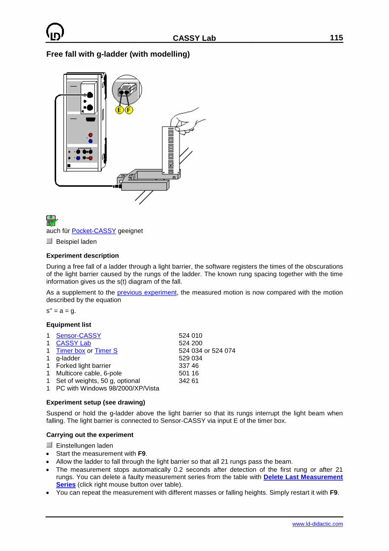
CASSY Lab

115

www.ld-didactic.com

Free fall with g-ladder (with modelling)


Beispiel laden


During a free fall of a ladder through a light barrier, the software registers the times of the obscurations of the light barrier caused by the rungs of the ladder. The known rung spacing together with the time information gives us the s(t) diagram of the fall.

As a supplement to the previous experiment, the measured motion is now compared with the motion described by the equation

s'' = a = g.

Equipment list

1 Sensor-CASSY 524 010 1 CASSY Lab 524 200 1 Timer box or Timer S 524 034 or 524 074 1 g-ladder 529 034 1 Forked light barrier 337 46 1 Multicore cable, 6-pole 501 16 1 Set of weights, 50 g, optional 342 61 1 PC with Windows 98/2000/XP/Vista


Suspend or hold the g-ladder above the light barrier so that its rungs interrupt the light beam when falling. The light barrier is connected to Sensor-CASSY via input E of the timer box.


Einstellungen laden


Allow the ladder to fall through the light barrier so that all 21 rungs pass the beam.

The measurement stops automatically 0.2 seconds after detection of the first rung or after 21 rungs. You can delete a faulty measurement series from the table with Delete Last Measurement Series (click right mouse button over table).

You can repeat the measurement with different masses or falling heights. Simply restart it with F9.

116

CASSY Lab

www.ld-didactic.com

Modelling

In the present example, the two initial conditions s(t=0)=0 and v(t=0)=v0 and the acceleration g=9.81

m/s2 were chosen, whereby g and v0 can be altered by dragging the pointer of the corresponding dis-

play instrument (or by clicking to the left or to the right of the pointer) until the model agrees with the measurement.

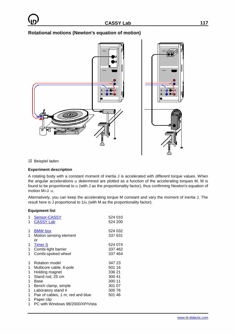
CASSY Lab

117

www.ld-didactic.com

Rotational motions (Newton's equation of motion)

Beispiel laden


A rotating body with a constant moment of inertia J is accelerated with different torque values. When

the angular accelerations determined are plotted as a function of the accelerating torques M, M is

found to be proportional to (with J as the proportionality factor), thus confirming Newton's equation of

motion M=J.

Alternatively, you can keep the accelerating torque M constant and vary the moment of inertia J. The

result here is J proportional to 1/ (with M as the proportionality factor).

Equipment list

1 Sensor-CASSY 524 010 1 CASSY Lab 524 200 1 BMW box 524 032 1 Motion sensing element 337 631 or 1 Timer S 524 074 1 Combi-light barrier 337 462 1 Combi-spoked wheel 337 464 1 Rotation model 347 23 1 Multicore cable, 6-pole 501 16 1 Holding magnet 336 21 1 Stand rod, 25 cm 300 41 1 Base 300 11 1 Bench clamp, simple 301 07 1 Laboratory stand II 300 76 1 Pair of cables, 1 m, red and blue 501 46 1 Paper clip 1 PC with Windows 98/2000/XP/Vista

118

CASSY Lab

www.ld-didactic.com


Tie the transmission thread to the flag of the rotation model (r = 10 cm) or to one of the pins of the extra disk (r = 5 cm, 2.5 cm) and run it over the motion sensing element, which is connected to Sen-sor-CASSY via the top socket of the BMW box. The holding magnet prevents the start of rotation when it is placed close to the paper clip attached to the flag of the rotation model.

The accelerating force is generated e.g. by 3 small suspended weights of 1 g each (F = 0.0294 N). The different torques at a constant moment of inertia are realized using the different pulley radii (M =

rF = 2.94 mNm, 1.47 mNm, 0.73 mNm). Alternatively, you can realize different moments of inertia for a constant torque using extra disks.


Einstellungen laden

Modify the maximum rolling angle A1 in the measuring condition of the Measuring Parameters

dialog (accessible via F5); current setting: &bA1 < 6 for 6 radii, &b stands for )

You may want to modify the time interval (currently 500 ms) in the Measuring Parameters dialog

(accessible with F5); a longer interval means fewer measured values and less scattering in (t).

You may need to invert the sign of angular measurement (s <—> -s in Settings A1).

Allow the rotating disk to fall from the holding magnet.

Define the current rolling radius and the path zero point (both in Settings A1)

Start the measurement with F9 and stop it with F9 when the experiment is finished. You can delete a faulty measurement series from the table with Delete Last Measurement Series (click right mouse button over table).

Repeat the measurement with different parameters (different accelerating torque or accelerated moment of inertia). Be sure to redefine the rolling radius and path zero point.

Evaluation

In addition to the (t) diagrams, the software also calculates the (t) and (t) diagrams. You can see these simply by clicking on the tabs of the other displays. Suitable evaluation functions are parabola and line fits and calculation of mean value.

To confirm Newton's equation of motion, you need to fill out a further table, which has already been prepared on the Newton display tab. After determining an angular acceleration value as the mean of

an (t) diagram or the slope of an (t) diagram, you can use the mouse to drag this value from the status line and drop it into the table (drag & drop). As the parameter, enter the parameter angular mo-mentum M or moment of inertia directly via the keyboard. The desired diagram is generated as you enter the values. You can easily convert or rescale the axes by clicking on them with the right mouse

button (e.g. —> 1/).

As a further evaluation, you can e.g. compare the rotational energy with the work performed using formulas. The rotational energy is

E = 0.5*J*&w^2 (enter the numerical value for J, &w stands for )

and the work performed is

W = M*&bA1 (enter the numerical value for M, &b stands for ).

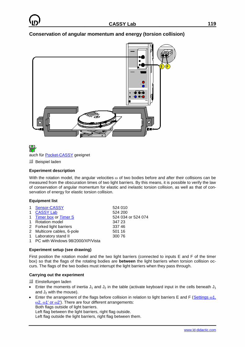
CASSY Lab

119

www.ld-didactic.com

Conservation of angular momentum and energy (torsion collision)


Beispiel laden


With the rotation model, the angular velocities of two bodies before and after their collisions can be measured from the obscuration times of two light barriers. By this means, it is possible to verify the law of conservation of angular momentum for elastic and inelastic torsion collision, as well as that of con-servation of energy for elastic torsion collision.

Equipment list

1 Sensor-CASSY 524 010 1 CASSY Lab 524 200 1 Timer box or Timer S 524 034 or 524 074 1 Rotation model 347 23 2 Forked light barriers 337 46 2 Multicore cables, 6-pole 501 16 1 Laboratory stand II 300 76 1 PC with Windows 98/2000/XP/Vista


First position the rotation model and the two light barriers (connected to inputs E and F of the timer box) so that the flags of the rotating bodies are between the light barriers when torsion collision oc-curs. The flags of the two bodies must interrupt the light barriers when they pass through.


Einstellungen laden

Enter the moments of inertia J1 and J2 in the table (activate keyboard input in the cells beneath J1

and J2 with the mouse).

Enter the arrangement of the flags before collision in relation to light barriers E and F (Settings 1,

2, 1' or 2'). There are four different arrangements: Both flags outside of light barriers. Left flag between the light barriers, right flag outside. Left flag outside the light barriers, right flag between them.

120

CASSY Lab

www.ld-didactic.com

Both flags inside (explosion).

Enter the flag width and radius (also in Settings 1, 2, 1' or 2').

Initiate the collision (if angular velocities are displayed before the collision, you can clear these with —> 0 <—) and watch to make sure that the light barriers do not register any extra pulses (e.g. due to reflection of a rotating body).

Terminate the measurement with End of Collision (the measurement is terminated automatically after four measured angular velocities).

Transfer the measured values to the table for evaluation with F9 or initialize the next measurement with —> 0 <—.

Evaluation

Tables have been pre-defined for angular momentum before and after collision, overall angular mo-mentum, energy, total energy and energy loss; you can transfer measured values to these with F9. Click on the table tabs to display these. If you want these quantities to be visible immediately after collision, open the corresponding display instruments.

You can also define additional formulas to compare your results with theory. For elastic torsion colli-sion, we say that

&w1' = (2*J2*&w2 + (J1-J2)*&w1) / (J1+J2) &w2' = (2*J1*&w1 + (J2-J1)*&w2) / (J1+J2)

For inelastic torsion collision, the following applies:

&w1' = &w2' = (J1*&w1 + J2*&w2) / (J1+J2).

In all formulas, the character combination & plus w is used to represent (and generate) the Greek .

Table for converting specified units to SI units

Quantity SI unit = Factor specified unit Moment of inertia J kgm

2 1000 gm

2

Angular velocity rad/s 1 rad/s

Angular momentum L Nsm = kgm2/s 1000 mJs

Energy E J = kgm2/s

2 1000 mJ

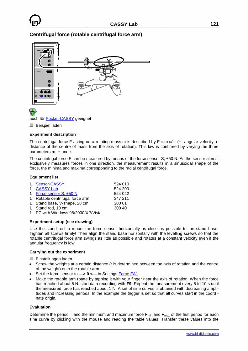
CASSY Lab

121

www.ld-didactic.com

Centrifugal force (rotable centrifugal force arm)


Beispiel laden


The centrifugal force F acting on a rotating mass m is described by F = m2r (: angular velocity, r:

distance of the centre of mass from the axis of rotation). This law is confirmed by varying the three

parameters m, and r.

The centrifugal force F can be measured by means of the force sensor S, ±50 N. As the sensor almost exclusively measures forces in one direction, the measurement results in a sinusoidal shape of the force, the minima and maxima corresponding to the radial centrifugal force.

Equipment list

1 Sensor-CASSY 524 010 1 CASSY Lab 524 200 1 Force sensor S, ±50 N 524 042 1 Rotable centrifugal force arm 347 211 1 Stand base, V-shape, 28 cm 300 01 1 Stand rod, 10 cm 300 40 1 PC with Windows 98/2000/XP/Vista


Use the stand rod to mount the force sensor horizontally as close as possible to the stand base. Tighten all screws firmly! Then align the stand base horizontally with the levelling screws so that the rotable centrifugal force arm swings as little as possible and rotates at a constant velocity even if the angular frequency is low.


Einstellungen laden

Screw the weights at a certain distance (r is determined between the axis of rotation and the centre of the weight) onto the rotable arm.

Set the force sensor to —> 0 <— in Settings Force FA1.

Make the rotable arm rotate by tapping it with your finger near the axis of rotation. When the force has reached about 5 N, start data recording with F9. Repeat the measurement every 5 to 10 s until the measured force has reached about 1 N. A set of sine curves is obtained with decreasing ampli-tudes and increasing periods. In the example the trigger is set so that all curves start in the coordi-nate origin.

Evaluation

Determine the period T and the minimum and maximum force Fmin and Fmax of the first period for each sine curve by clicking with the mouse and reading the table values. Transfer these values into the

122

CASSY Lab

www.ld-didactic.com

display Input (mouse click). If there are inaccuracies in the setup or the zero adjustment of the force

sensor, these are compensated by taking into account Fmin and Fmax.

In the display Centrifugal Force, the result of this evaluation is plotted automatically. The centrifugal

force F = (Fmax-Fmin)/2 shown in the diagram and the angular velocity =2/T are calculated from the

input values. The proportionality F ~ 2 is clearly seen.

For confirming the proportionalities F ~ m and F ~ r, the measurements have to be repeated with other weights and radii and then evaluated all together. It is recommendable to evaluate each measurement individually and to store it in a separate file because several measurements are confusing for an evaluation in a graphic representation. Afterwards several evaluated measurements can be loaded into a common display.

Hint

As the experiment has to be repeated with other masses m and radii r for a complete evaluation, man-

ual evaluation is very tedious. However, the period T and the two forces Fmin and Fmax can also be

determined automatically. For this the display instruments T', F'min, and F'max in the upper line have to be opened. Immediately after an individual measurement, the values calculated there can be shifted into the display Input with the mouse (drag & drop). As long as the rotable arm is still rotating and the

measured force is greater than 1 N, this procedure is repeated for decreasing angular velocities in short intervals.

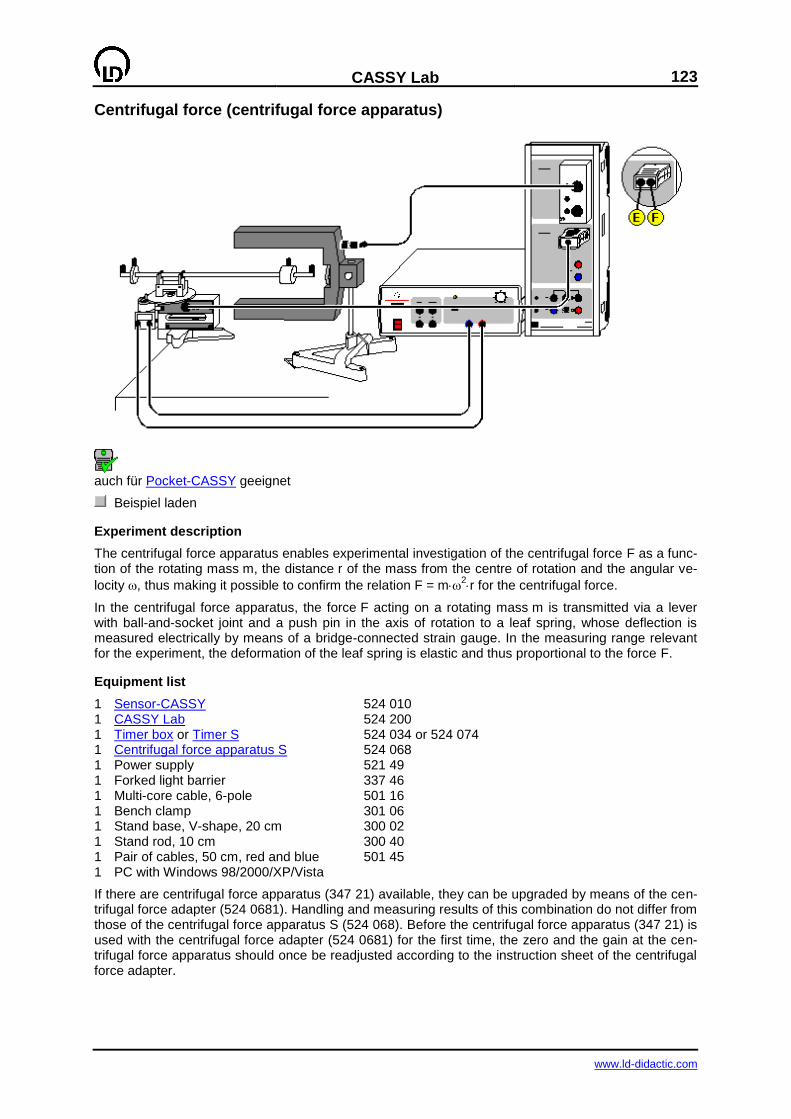
CASSY Lab

123

www.ld-didactic.com

Centrifugal force (centrifugal force apparatus)


Beispiel laden


The centrifugal force apparatus enables experimental investigation of the centrifugal force F as a func-tion of the rotating mass m, the distance r of the mass from the centre of rotation and the angular ve-

locity , thus making it possible to confirm the relation F = m2r for the centrifugal force.

In the centrifugal force apparatus, the force F acting on a rotating mass m is transmitted via a lever with ball-and-socket joint and a push pin in the axis of rotation to a leaf spring, whose deflection is measured electrically by means of a bridge-connected strain gauge. In the measuring range relevant for the experiment, the deformation of the leaf spring is elastic and thus proportional to the force F.

Equipment list

1 Sensor-CASSY 524 010 1 CASSY Lab 524 200 1 Timer box or Timer S 524 034 or 524 074 1 Centrifugal force apparatus S 524 068 1 Power supply 521 49 1 Forked light barrier 337 46 1 Multi-core cable, 6-pole 501 16 1 Bench clamp 301 06 1 Stand base, V-shape, 20 cm 300 02 1 Stand rod, 10 cm 300 40 1 Pair of cables, 50 cm, red and blue 501 45 1 PC with Windows 98/2000/XP/Vista

If there are centrifugal force apparatus (347 21) available, they can be upgraded by means of the cen-trifugal force adapter (524 0681). Handling and measuring results of this combination do not differ from those of the centrifugal force apparatus S (524 068). Before the centrifugal force apparatus (347 21) is used with the centrifugal force adapter (524 0681) for the first time, the zero and the gain at the cen-trifugal force apparatus should once be readjusted according to the instruction sheet of the centrifugal force adapter.

124

CASSY Lab

www.ld-didactic.com


Use the bench clamp to fix the centrifugal force apparatus to the table. The light barrier is set up by means of the stand rod and the stand base so that the rotating arm can freely rotate between the legs of the light barrier; the light beam should not be interrupted by the weight. The centrifugal force appa-ratus is connected to Input B and the light barrier via the 6-pole cable to the timer box at Input A of the Sensor-CASSY. The power supply is connected to the driving motor of the centrifugal force apparatus via two connecting leads. The maximum voltage for driving the motor should be selected so that the force measuring range does not exceed 15 N.


Einstellungen laden

Set the force display to 0 while the rotating arm is at rest. For this set the centrifugal force appara-tus to —> 0 <— in Settings Force FB1 (right mouse button).

Adjust the compensating weight on the short arm of the apparatus so that no force F is measured when the measurement is made without additional weight m but with the safety screw.

Starting with low angular velocities , store the measured force manually with F9 in the table.

Repeat the measurement with higher angular velocities .

After finishing a measurement series, repeat the measurements with other masses m (r=constant) or radii r (m = constant). For this select Append new measurement series in Measuring Pa-rameters (F5) and restart at low angular velocities.

Evaluation

Each individual measurement series immediately confirms the proportionality between the force F and

2 by a fit to a straight line. If you want to confirm the two other proportionalities between F and m (,r

constant) and between F and r (,m constant), the forces F have to be determined for constant angu-

lar velocities . To do this, draw a vertical line at a value of 2 in the diagram and read the coordinates

of the intersections with the F(2) line (switch the coordinate display on). Enter these coordinates

manually into the prepared second display F(m) or. F(r) (click the field in the table with the mouse). There the desired proportionality eventually shows up.

F = m2r is confirmed by determining the proportionality factors.

CASSY Lab

125

www.ld-didactic.com

Oscillations of a rod pendulum


Beispiel laden


The equation of motion for a physical pendulum with moment of inertia J, mass m and distance s be-tween fulcrum and centre of gravity

M = J'' = –mgssin

describes for small deflections (sin ) an harmonic oscillation with period of oscillation

T = 2sqrt(J/mgs).

For a better understanding, the reduced pendulum length lr = J/ms is introduced. Then the period of oscillation is

T = 2sqrt(lr/g).

For mathematical pendulums, the entire pendulum mass is concentrated at a single point. It has there-

fore the moment of inertia J = ms2 and the reduced pendulum length is lr = J/ms = s, which is equiva-

lent to the distance between the pendulum mass (centre of gravity) and fulcrum.

A physical pendulum with the reduced pendulum length lr corresponds to a mathematical pendulum of this length.

In this experiment the reduced pendulum length is determined from the measured period of oscillation and compared with the reduced pendulum length.

Equipment list

1 Sensor-CASSY 524 010 1 CASSY Lab 524 200 1 Rotary motion sensor S 524 082 1 Physical pendulum 346 20 1 Stand rod, 25 cm, d = 10 mm 301 26 2 Stand bases MF 301 21 1 PC with Windows 98/2000/XP/Vista


The pendulum is screwed on the axle of the rotary motion sensor.


Einstellungen laden

Define the zero point in the equilibrium position of the pendulum (—> 0 <— in Settings A1)

Deflect the pendulum by approx. 5° only and release

126

CASSY Lab

www.ld-didactic.com

Start measurement by pressing F9. The measurement will stop automatically after 10 s

Repeat the measurement without the mass or using a further mass

Evaluation

After several oscillations, the duration of these oscillations can be determined by means of a vertical

line and from this the period of oscillation. In the example, the result is T = 0.840 s. With g = 9.81 m/s2

this results in a reduced pendulum length of lr= gT2/4

2 = 17.5 cm.

This corresponds well to the calculated (using an approximation) pendulum length lr of the rod. The

moment of inertia of the rod for rotation through the centre of gravity is JS = 1/12ml2. The axis of rota-

tion of this pendulum is, however, s = 1/3l displaced from the centre of gravity. According to Steiner's

theorem this gives J = JS + ms2 = 7/36 ml

2 and lr= 7/36ml

2 / ms = 7/12l = 17.5 cm (for l = 30 cm).

Conversely, from the calculated reduced pendulum length and the measured period of oscillation the

earth's acceleration due to gravity can also be calculated g = lr42/T

2 .

Experimental determination of the reduced pendulum length

If mass m2 is shifted on the pendulum rod until the period of oscillation T compared to the rod without

added mass is unchanged, then the reduced pendulum length lr will also be unchanged. The position x

when the (point) mass is now found increases the moment of inertia of the pendulum by J2 = m2x2.

Because the reduced pendulum length lr has not been changed, the following applies

lr = J/ms = (J + J2)/(m + m2)/s'

with s' being the distance between the new centre of gravity and the fulcrum, therefore s' =

(ms+m2x)/(m+m2). From this you get

J/ms = (J + m2x2)/(ms+m2x) = J/ms (1 + m2x

2/J)/(1 + m2x/ms) or m2x

2/J = m2x/ms, therefore

x = J/ms = lr.

The (point) mass is then exactly located at the reduced pendulum length. But, because in reality it has a finite size, this is only an approximation.

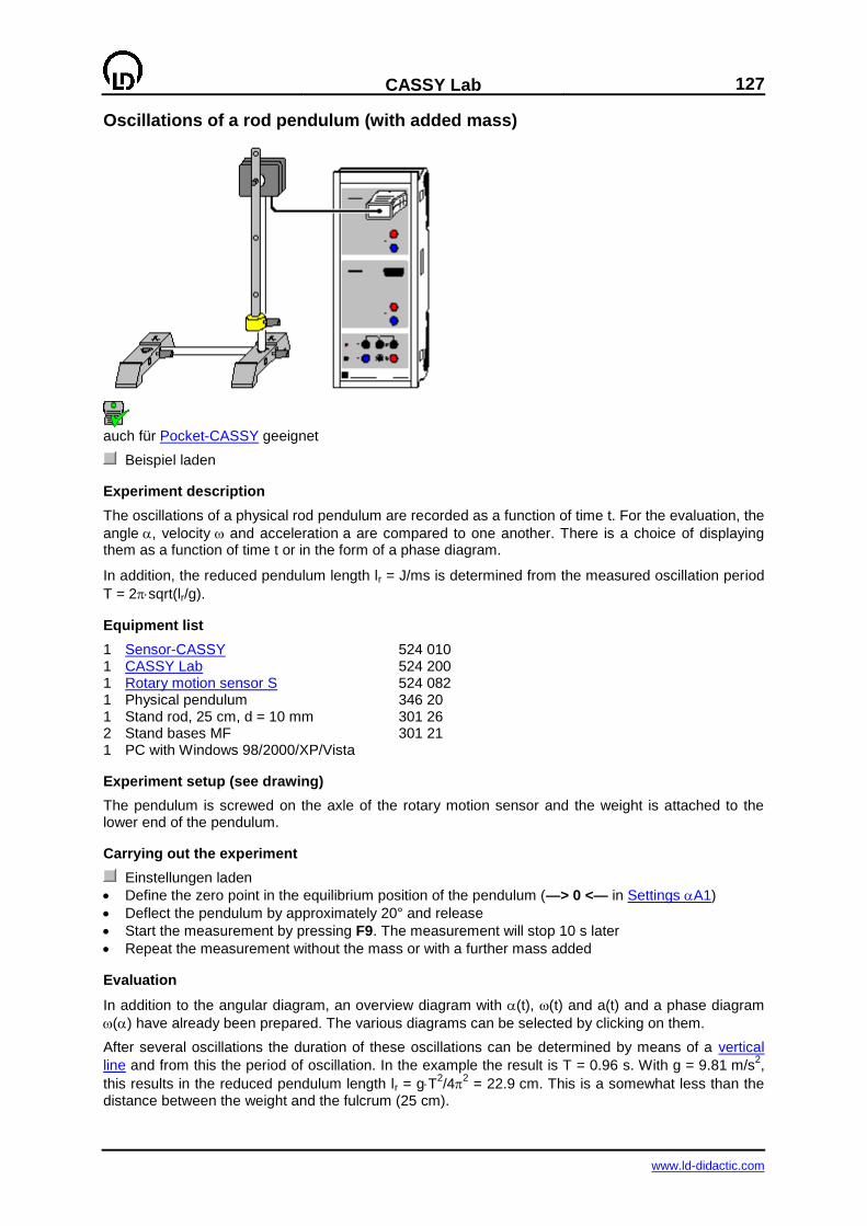
CASSY Lab

127

www.ld-didactic.com

Oscillations of a rod pendulum (with added mass)


Beispiel laden


The oscillations of a physical rod pendulum are recorded as a function of time t. For the evaluation, the

angle , velocity and acceleration a are compared to one another. There is a choice of displaying them as a function of time t or in the form of a phase diagram.

In addition, the reduced pendulum length lr = J/ms is determined from the measured oscillation period

T = 2sqrt(lr/g).

Equipment list



The pendulum is screwed on the axle of the rotary motion sensor and the weight is attached to the lower end of the pendulum.


Einstellungen laden


Deflect the pendulum by approximately 20° and release

Start the measurement by pressing F9. The measurement will stop 10 s later

Repeat the measurement without the mass or with a further mass added

Evaluation

In addition to the angular diagram, an overview diagram with (t), (t) and a(t) and a phase diagram

() have already been prepared. The various diagrams can be selected by clicking on them.

After several oscillations the duration of these oscillations can be determined by means of a vertical

line and from this the period of oscillation. In the example the result is T = 0.96 s. With g = 9.81 m/s2,

this results in the reduced pendulum length lr = gT2/4

2 = 22.9 cm. This is a somewhat less than the

distance between the weight and the fulcrum (25 cm).

128

CASSY Lab

www.ld-didactic.com

Comment

The curves drawn strongly depend on the selected Time interval. The time interval can only be a com-

promise between rapid measuring sequence, clearly marked (t) minima and maxima (short time in-

terval) and low errors in the (t) and a(t) diagram (longer time interval).

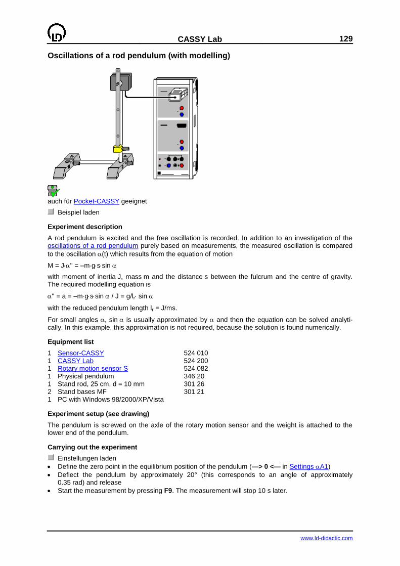
CASSY Lab

129

www.ld-didactic.com

Oscillations of a rod pendulum (with modelling)


Beispiel laden


A rod pendulum is excited and the free oscillation is recorded. In addition to an investigation of the oscillations of a rod pendulum purely based on measurements, the measured oscillation is compared

to the oscillation (t) which results from the equation of motion

M = J'' = –mgssin

with moment of inertia J, mass m and the distance s between the fulcrum and the centre of gravity. The required modelling equation is

'' = a = –mgssin / J = g/lr sin

with the reduced pendulum length lr = J/ms.

For small angles , sin is usually approximated by and then the equation can be solved analyti-cally. In this example, this approximation is not required, because the solution is found numerically.

Equipment list





Einstellungen laden


Deflect the pendulum by approximately 20° (this corresponds to an angle of approximately 0.35 rad) and release

Start the measurement by pressing F9. The measurement will stop 10 s later.

130

CASSY Lab

www.ld-didactic.com

Modelling

In the present example, the two starting conditions are selected (t=0)=0 and (t=0)=0 because the

oscillation was triggered at the origin. The starting speed 0 and reduced pendulum length lr can be

modified by pulling the pointer of the corresponding display instrument (or by clicking on the left-hand button or after clicking on the right-hand button) until Model corresponds to the measurement.

For confirmation of the model, the weight can be moved to a different position and the experiment be repeated. The new measured oscillation will again correspond to the mathematical model.

Influence of the approximation sin

It is very impressive to observe the influence of the otherwise commonly used approximation for small

deflections (sin ). For this the model equation can be reduced from –9.81/lr*rsin &a to –9.81/lr*&a. The change to the period through the influence of the approximation is already clearly apparent for a deflection of 20°.

In the following Example this influence is investigated in more detail.

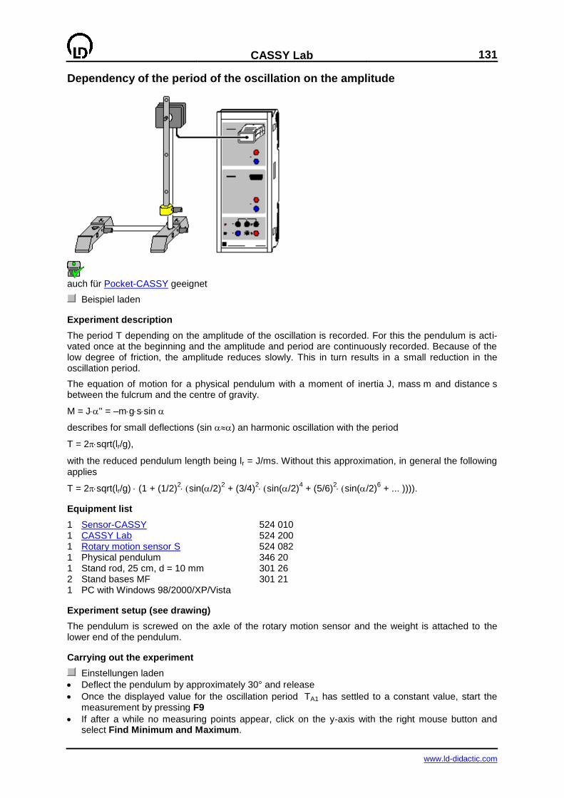
CASSY Lab

131

www.ld-didactic.com

Dependency of the period of the oscillation on the amplitude


Beispiel laden


The period T depending on the amplitude of the oscillation is recorded. For this the pendulum is acti-vated once at the beginning and the amplitude and period are continuously recorded. Because of the low degree of friction, the amplitude reduces slowly. This in turn results in a small reduction in the oscillation period.

The equation of motion for a physical pendulum with a moment of inertia J, mass m and distance s between the fulcrum and the centre of gravity.

M = J'' = –mgssin

describes for small deflections (sin ) an harmonic oscillation with the period

T = 2sqrt(lr/g),

with the reduced pendulum length being lr = J/ms. Without this approximation, in general the following applies

T = 2sqrt(lr/g) (1 + (1/2)2sin(/2)

2 + (3/4)

2sin(/2)

4 + (5/6)

2sin(/2)

6 + ... )))).

Equipment list





Einstellungen laden

Deflect the pendulum by approximately 30° and release

Once the displayed value for the oscillation period TA1 has settled to a constant value, start the measurement by pressing F9

If after a while no measuring points appear, click on the y-axis with the right mouse button and select Find Minimum and Maximum.

132

CASSY Lab

www.ld-didactic.com

Stop the measurement by clicking F9 as soon as the amplitude falls below 5°. Below this the de-termined oscillation period will become unreliable.

Evaluation

During the measurement, the amplitude decreases slowly. This causes a minor reduction in oscillation period. The theoretical connection between amplitude and period is

T = T0 (1 + (1/2)2sin(/2)

2 + (3/4)

2sin(/2)

4 + (5/6)

2sin(/2)

6 + ... ))))

and can be easily confirmed by carrying out a free fit.

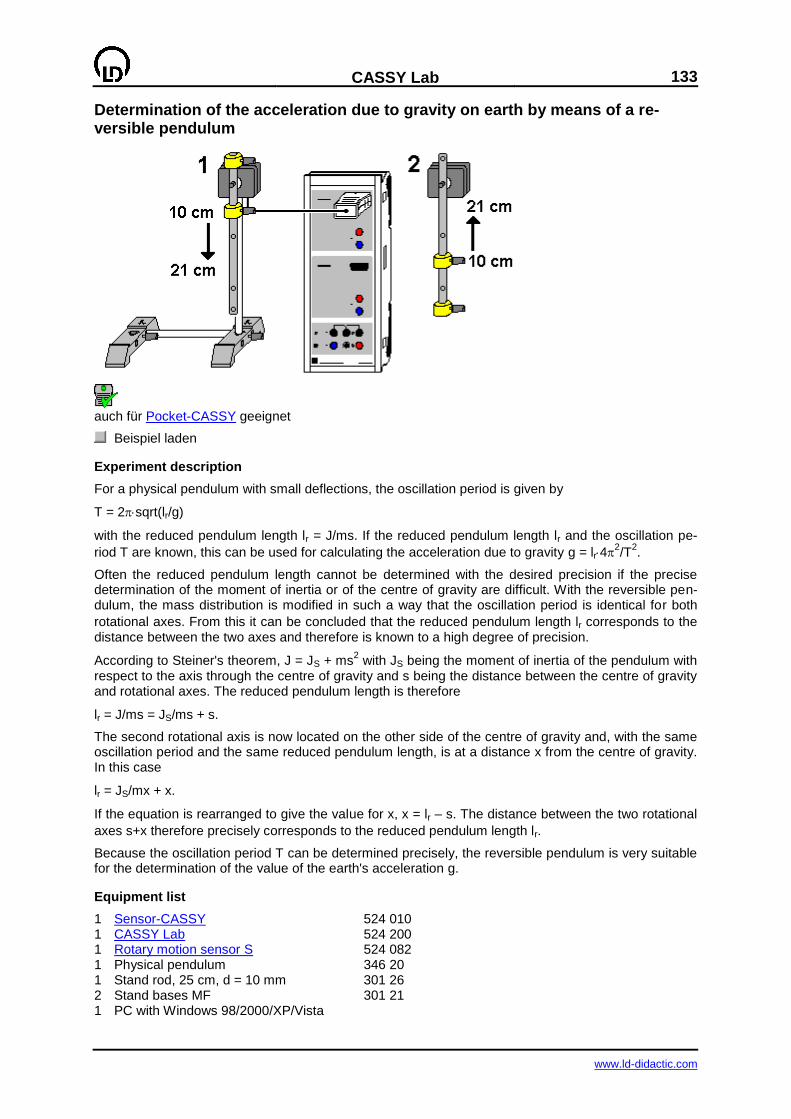
CASSY Lab

133

www.ld-didactic.com

Determination of the acceleration due to gravity on earth by means of a re-versible pendulum


Beispiel laden


For a physical pendulum with small deflections, the oscillation period is given by

T = 2sqrt(lr/g)

with the reduced pendulum length lr = J/ms. If the reduced pendulum length lr and the oscillation pe-

riod T are known, this can be used for calculating the acceleration due to gravity g = lr42/T

2.

Often the reduced pendulum length cannot be determined with the desired precision if the precise determination of the moment of inertia or of the centre of gravity are difficult. With the reversible pen-dulum, the mass distribution is modified in such a way that the oscillation period is identical for both

rotational axes. From this it can be concluded that the reduced pendulum length lr corresponds to the distance between the two axes and therefore is known to a high degree of precision.

According to Steiner's theorem, J = JS + ms2 with JS being the moment of inertia of the pendulum with

respect to the axis through the centre of gravity and s being the distance between the centre of gravity and rotational axes. The reduced pendulum length is therefore

lr = J/ms = JS/ms + s.

The second rotational axis is now located on the other side of the centre of gravity and, with the same oscillation period and the same reduced pendulum length, is at a distance x from the centre of gravity. In this case

lr = JS/mx + x.

If the equation is rearranged to give the value for x, x = lr – s. The distance between the two rotational

axes s+x therefore precisely corresponds to the reduced pendulum length lr.

Because the oscillation period T can be determined precisely, the reversible pendulum is very suitable for the determination of the value of the earth's acceleration g.

Equipment list


134

CASSY Lab

www.ld-didactic.com


The pendulum is screwed on the axle of the rotary motion sensor and the mass is attached to the pendulum as shown in (1).

The rod of the pendulum is marked starting from the top in 1 cm steps using a pencil. A range from 10 cm to approximately 21 cm is adequate for this.


Einstellungen laden

Attach the variable pendulum mass at the position x = 10 cm and deflect by approximately 10°.

Once the value displayed for the oscillation period TA1 has settled to a constant value and the am-

plitude A1 has fallen to approximately 5°, record the measuring value by pressing F9 and enter the

position in column x (click at the cell in the table with the mouse)

Push the pendulum mass 1 cm down and measure again. Repeat until x = 21 cm is reached.

Move the mass back to x = 10 cm and change the suspension point of the pendulum as shown in (2); reverse the pendulum

In the measuring parameter window select Append new measurement series

Again deflect the pendulum by approximately 10° and wait until the value displayed for the oscilla-

tion period TA1 has settled to a constant and the amplitude A1 has fallen to approximately 5°, re-cord the measuring value by pressing F9 and enter the position in column x (click on the cell in the table with the mouse)

Push the pendulum mass 1 cm upwards and measure again. Repeat until x = 21 cm is reached.

Evaluation

In the graphic display, two intersections of the oscillation period curves can be seen. In both intersec-tion the period of oscillation and therefore the reduced pendulum length are equal. It corresponds to

the displacement of the two axes of rotation, that is lr = 0.20 m.

By means of a horizontal mark the corresponding period can be determined. In this example it is T =

0.898 s. This results in an earth's acceleration due to gravity of g = lr42/T

2 = 7.896 m/T

2 = 9.79 m/s

2.

Alternatively, the earth's acceleration due to gravity can be found with somewhat higher resolution in diagram g.

Comments about the measuring error

In addition to the manufacturing error in the rod, which will appear as an error in the reduced pendu-

lum length lr (approximately lr = ±0.1 mm, that is g = ±0.005 m/s2), an error in the oscillation pe-

riod T is to be considered. Besides the simple measuring fault (in this case approximately T =

±0.001T, corresponding to g = ±0.02 m/s2) there is also a systematic fault. As already demonstrated

in the experiment Dependency of the period of the oscillation on the amplitude, the oscillation period

shows a weak dependency on the amplitude. For the 5° amplitude this systematic error is T =

+0.0005T, corresponding to g = -0.01 m/s2. With even smaller amplitudes the determination of the

oscillation period by means of the rotary motion sensor will become unreliable. For greater amplitudes,

this systematic fault will soon exceed the normal measuring fault (for 10° amplitude it is T = +0.002T,

corresponding to g = -0.04 m/s2)

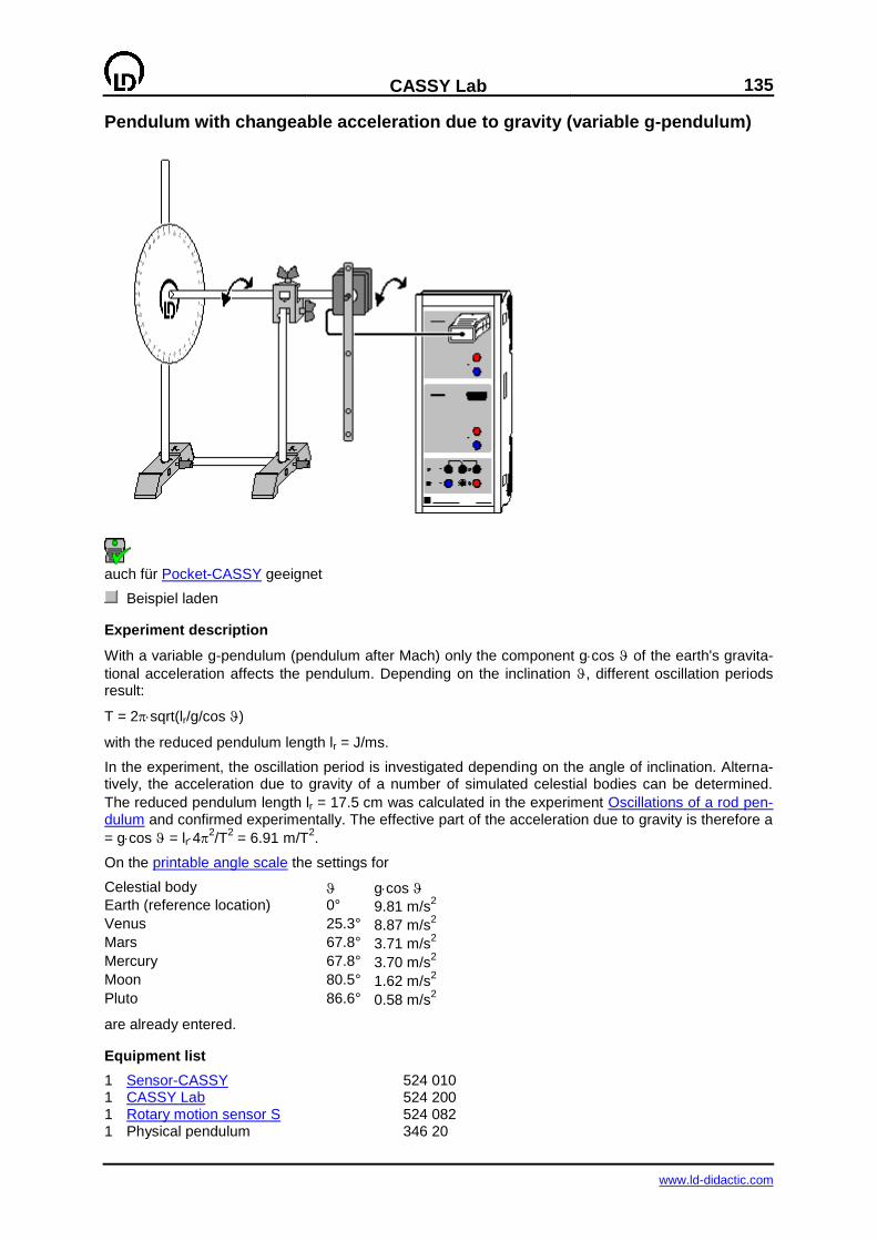
CASSY Lab

135

www.ld-didactic.com

Pendulum with changeable acceleration due to gravity (variable g-pendulum)


Beispiel laden


With a variable g-pendulum (pendulum after Mach) only the component gcos of the earth's gravita-

tional acceleration affects the pendulum. Depending on the inclination , different oscillation periods result:

T = 2sqrt(lr/g/cos )

with the reduced pendulum length lr = J/ms.

In the experiment, the oscillation period is investigated depending on the angle of inclination. Alterna-tively, the acceleration due to gravity of a number of simulated celestial bodies can be determined.

The reduced pendulum length lr = 17.5 cm was calculated in the experiment Oscillations of a rod pen-dulum and confirmed experimentally. The effective part of the acceleration due to gravity is therefore a

= gcos = lr42/T

2 = 6.91 m/T

2.

On the printable angle scale the settings for

Celestial body gcos Earth (reference location) 0° 9.81 m/s

2

Venus 25.3° 8.87 m/s2

Mars 67.8° 3.71 m/s2

Mercury 67.8° 3.70 m/s2

Moon 80.5° 1.62 m/s2

Pluto 86.6° 0.58 m/s2

are already entered.

Equipment list

1 Sensor-CASSY 524 010 1 CASSY Lab 524 200 1 Rotary motion sensor S 524 082 1 Physical pendulum 346 20

136

CASSY Lab

www.ld-didactic.com

1 Angle scale with the entered celestial bodies

print out

1 Leybold clamp 301 01 2 Stand rods, 25 cm, d = 10 mm 301 26 1 Stand rod, 50 cm, d = 10 mm 301 27 2 Stand bases MF 301 21 1 PC with Windows 98/2000/XP/Vista


The pendulum is screwed on the axle of the rotary motion sensor. The scale is pushed onto the stand rod of the rotary motion sensor. To do this cut the scale as indicated by means of a sharp knife.


Einstellungen laden

Set up pendulum vertically ( = 0°), align the experiment setup and deflect the pendulum by ap-proximately 10°

Once the displayed value for the oscillation period TA1 has settled to a constant value, start the

measurement by pressing F9 and enter the angle in column (click with the mouse onto the table cell)

Increase the angle repeatedly by 10° and repeat measurement until = 80° is reached.

Evaluation

During the measurement, the effective part of the acceleration due to gravity a = lr42/T

2 with lr =

17.5 cm is entered into the diagram.

With a free fit the relationship a = gcos can easily be confirmed.

Alternatively, a range of celestial bodies can be simulated and their acceleration due to gravity deter-mined. To do this align the pendulum with the red markers on the angle scale.

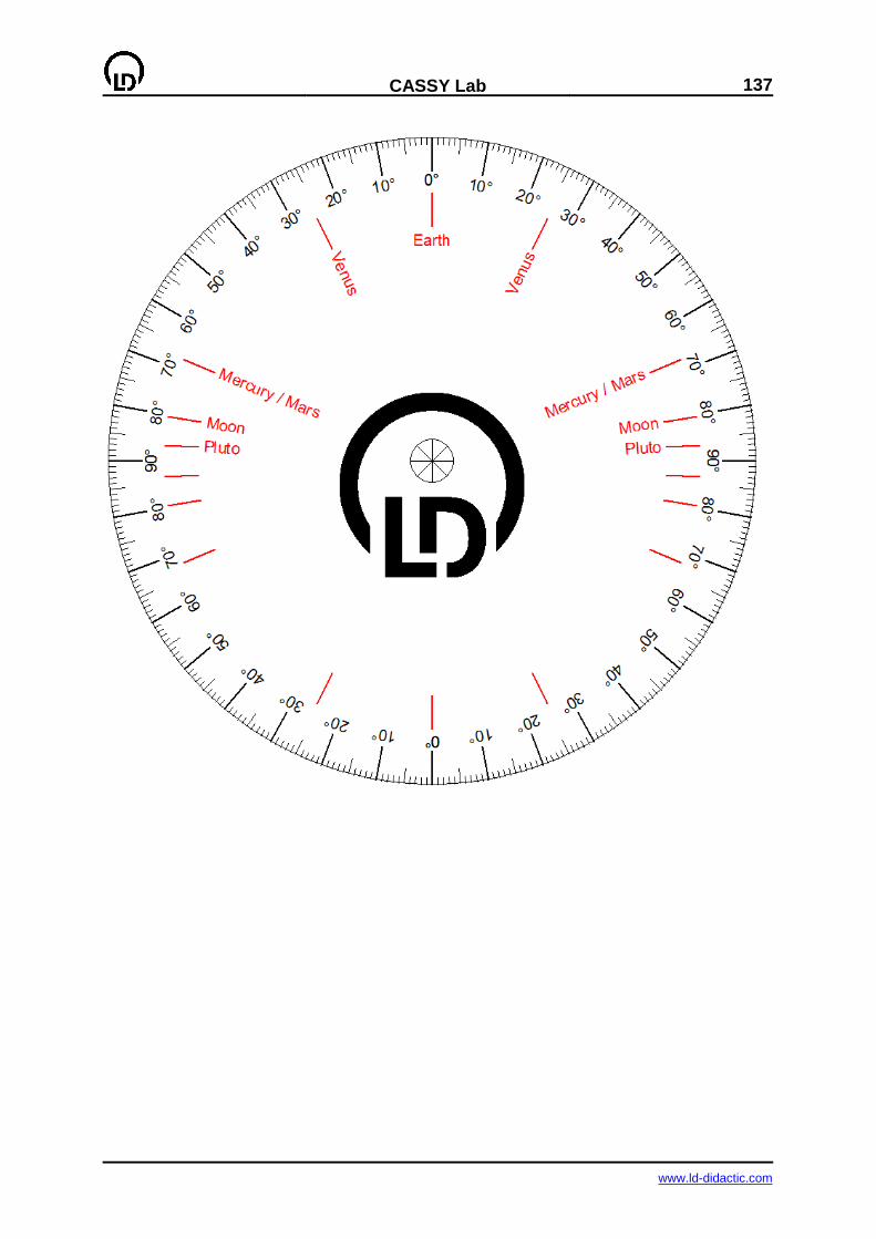
CASSY Lab

137

www.ld-didactic.com

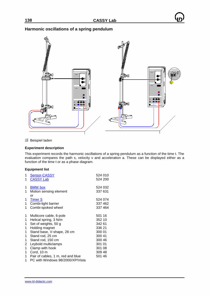
138

CASSY Lab

www.ld-didactic.com

Harmonic oscillations of a spring pendulum

Beispiel laden


This experiment records the harmonic oscillations of a spring pendulum as a function of the time t. The evaluation compares the path s, velocity v and acceleration a. These can be displayed either as a function of the time t or as a phase diagram.

Equipment list

1 Sensor-CASSY 524 010 1 CASSY Lab 524 200 1 BMW box 524 032 1 Motion sensing element 337 631 or 1 Timer S 524 074 1 Combi-light barrier 337 462 1 Combi-spoked wheel 337 464 1 Multicore cable, 6-pole 501 16 1 Helical spring, 3 N/m 352 10 1 Set of weights, 50 g 342 61 1 Holding magnet 336 21 1 Stand base, V-shape, 28 cm 300 01 1 Stand rod, 25 cm 300 41 1 Stand rod, 150 cm 300 46 2 Leybold multiclamps 301 01 1 Clamp with hook 301 08 1 Cord, 10 m 309 48 1 Pair of cables, 1 m, red and blue 501 46 1 PC with Windows 98/2000/XP/Vista

CASSY Lab

139

www.ld-didactic.com


Lay the string of the spring pendulum over the deflection pulley of the motion sensing element so that the oscillation of the pendulum is transmitted to the sensor without slip; connect the sensor to the top socket of the BMW box. The holding magnet enables a defined measurement start by holding the pendulum weight in the bottom reversing point of the oscillation before the start of measurement re-cording.

This experiment can be expanded to investigate air friction (e.g. with a piece of cardboard on the weight) or the effect of a change in the pendulum mass.


Einstellungen laden

If necessary, change the time interval in the measuring parameter window accessed with F5 (a shorter interval enables more measured values and smoother s(t) and v(s) diagram, while a longer interval generates fewer measured values and less scattering in a(t)).

You may need to invert the sign of path measurement (s <—> -s in Settings sA1).

Define the zero point in the equilibrium position of the pendulum (—> 0 <— in Settings sA1)

Deflect the pendulum approx. 10 cm and hold it there with the holding magnet.

Start the measurement with F9 and stop it with F9 when the experiment is finished.

Always check that the path zero point is at the equilibrium position before repeating the experi-ment.

Evaluation

In addition to the path display, this example also contains an overview display with s(t), v(t) and a(t) and a phase diagram v(s). Click on the respective displays to view them.

The phase relations and the damping are easy to see.

Remark

The recorded curve forms depend greatly on the selected time interval. The time interval is necessarily a compromise between a rich sequence of measured values, clearly apparent s(t) minima (shorter interval) and low inaccuracy in the v(t) and a(t) diagram (longer interval).

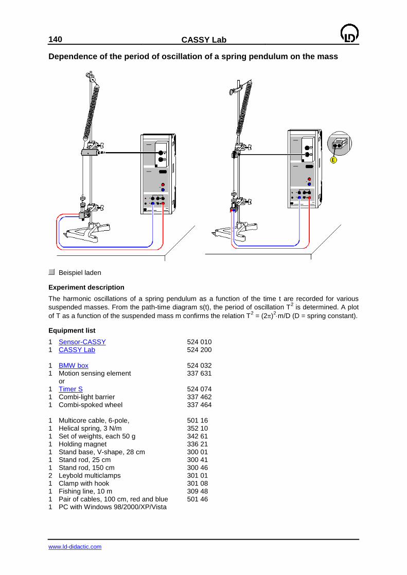
140

CASSY Lab

www.ld-didactic.com

Dependence of the period of oscillation of a spring pendulum on the mass

Beispiel laden


The harmonic oscillations of a spring pendulum as a function of the time t are recorded for various

suspended masses. From the path-time diagram s(t), the period of oscillation T2 is determined. A plot

of T as a function of the suspended mass m confirms the relation T2 = (2)

2m/D (D = spring constant).

Equipment list

1 Sensor-CASSY 524 010 1 CASSY Lab 524 200 1 BMW box 524 032 1 Motion sensing element 337 631 or 1 Timer S 524 074 1 Combi-light barrier 337 462 1 Combi-spoked wheel 337 464 1 Multicore cable, 6-pole, 501 16 1 Helical spring, 3 N/m 352 10 1 Set of weights, each 50 g 342 61 1 Holding magnet 336 21 1 Stand base, V-shape, 28 cm 300 01 1 Stand rod, 25 cm 300 41 1 Stand rod, 150 cm 300 46 2 Leybold multiclamps 301 01 1 Clamp with hook 301 08 1 Fishing line, 10 m 309 48 1 Pair of cables, 100 cm, red and blue 501 46 1 PC with Windows 98/2000/XP/Vista

CASSY Lab

141

www.ld-didactic.com


Clamp the stand rod in the stand base, and fasten the clamp with hook to the upper end of the stand rod.

Suspend the spring from the hook, and elongate it via a piece of fishing line of approx. 45 cm length by means of the desired number of weights.

Fasten a multiclamp with the motion sensing element close to the middle of the piece of fishing line.

Lay the piece of fishing line over the deflection pulley of the motion sensing element so that the oscillations of the pendulum are transmitted to the motion sensing element without slip. In order to keep damping of the oscillation low, see to it that the axis of the spring does not deviate too much from the vertical.

Position the holding magnet at the lower dead point of the oscillation of the spring pendulum.

Connect the motion sensing element via the upper socket of the BMW box to the input A of the Sensor-CASSY.

Connect the holding magnet to the output S of the Sensor-CASSY.

Experiment notes

The holding magnet provides a well-defined start of the oscillation by keeping the weights suspended for a particular measurement in the lower dead point of the oscillation. Depending on the number of suspended weights, the motion sensing element and the holding magnet have to be displaced verti-cally with respect to the position of the hook. The ideal position of the motion sensing element is close to the middle of the fishing line when the pendulum is in its equilibrium position.


Einstellungen laden

Suspend the desired number of weights, and adjust the height of the holding magnet and of the motion sensing element.

Calibrate the zero of the path sA1 in the equilibrium position of the pendulum – to do this, click the —> 0 <— button in Settings sA1.

If required, invert the sign of the path measurement (s <—> –s button in Settings sA1)

Elongate the pendulum so that the weights are held by the holding magnet.


When repeating a measurement, check the zero of the path in the equilibrium position of the pen-dulum before recording data.

Evaluation

For every path-time diagram, the period of oscillation T is determined by clicking Measure Difference with the right mouse button (or Alt+D) and subsequently clicking two corresponding zero passages with the left mouse button. The value of the period of oscillation then displayed in the status line can be transferred into the prepared display Input by means of the mouse (drag & drop). In addition, the mass m associated with T has to be entered in the table. By a fit to a straight line in the display

Evaluation, the proportionality T2 ~ m is confirmed in a further step.

The spring constant D can be determined from the slope of the straight line. Note that the straight line does not pass the origin. For a description of this experiment result, the mass of the spring has also to be taken into account.

Hint

As a complete evaluation requires the experiment to be repeated for various masses m, the period of oscillation T would have to be determined manually in each case. Alternatively, the period of oscillation T can also be determined automatically. For this you only have to open the display instrument T' in the upper line. After the oscillation has been measured, the value display there can be copied directly into the display Input (drag & drop).

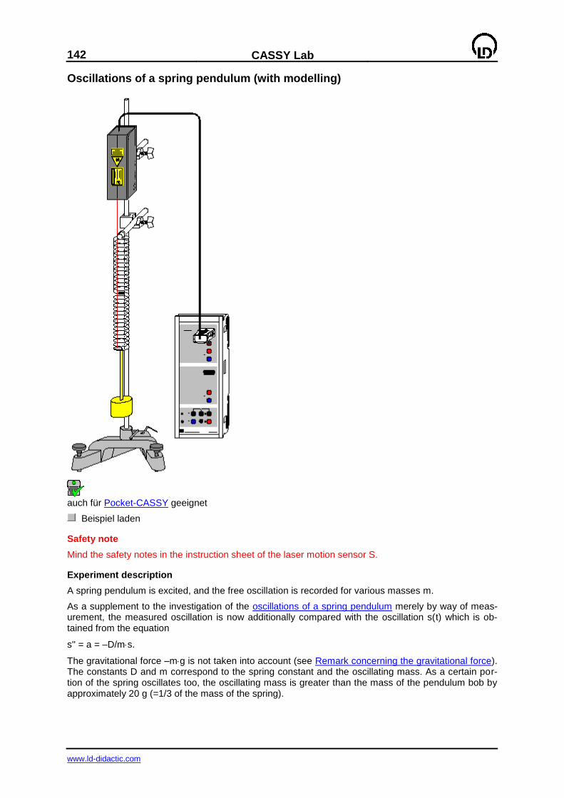
142

CASSY Lab

www.ld-didactic.com

Oscillations of a spring pendulum (with modelling)


Beispiel laden

Safety note

Mind the safety notes in the instruction sheet of the laser motion sensor S.


A spring pendulum is excited, and the free oscillation is recorded for various masses m.

As a supplement to the investigation of the oscillations of a spring pendulum merely by way of meas-urement, the measured oscillation is now additionally compared with the oscillation s(t) which is ob-tained from the equation

s'' = a = –D/ms.

The gravitational force –mg is not taken into account (see Remark concerning the gravitational force). The constants D and m correspond to the spring constant and the oscillating mass. As a certain por-tion of the spring oscillates too, the oscillating mass is greater than the mass of the pendulum bob by approximately 20 g (=1/3 of the mass of the spring).

CASSY Lab

143

www.ld-didactic.com

Equipment list

1 Sensor-CASSY 524 010 1 CASSY Lab 524 200 1 Laser motion sensor S 524 073 1 Stand rod with thread 309 00 335 1 Pair of helical springs 352 15 1 Big slotted mass hanger, 500 g 315 452 1 Slotted weight 100 g 315 456 1 Slotted weight 200 g 315 458 1 Stand rod, 1 m 300 44 1 Stand rod, 25 cm 300 41 2 Leybold multiclamps 301 01 1 Stand base, V-shape, 28 cm 300 01 1 PC with Windows 98/2000/XP/Vista

Alternative

Instead of the laser motion sensor S, the force sensor S, ±50 N (524 042) can also be used for the

path measurement. From the measured force FA1 and the spring constant D, the deflection sA1=FA1/D can be calculated using a formula.


Set up the spring pendulum with the large spring (diameter=3.5 mm). For the path measurement, at-tach a piece of retroreflecting foil to the lowest turn of the spring so that the laser spot of the motion sensor hits the foil during the entire oscillation (if necessary, attach the foil outside the spring).

Due to the reversal of its helical sense in the middle, this particular spring makes possible a free stable up and down oscillation because no torsional oscillation is excited.


Einstellungen laden

If modelling is not yet desired, switch to the Standard display during the measurement.

Define the pendulum's equilibrium position as the zero point of the path (—> 0 <— in Settings sA1; before doing so, you may allow the laser motion sensor S to warm up for some minutes).

Deflect the pendulum bob downwards.


Release the pendulum bob. The measurement starts automatically when the equilibrium position at s=0 is passed for the first time.

After carrying out the evaluation, repeat the experiment for various masses (slotted weights), and compare the results with the prediction of the model.

Modelling

In the present example, the two initial conditions s(t=0)=0 and v(t=0)=v0 were chosen because the

triggering took place in the zero point of the path. The initial velocity v0, the spring constant D and the

mass m can be altered by dragging the pointer of the corresponding display instrument (or by clicking to the left or to the right of the pointer) until the model agrees with the measurement.

In order to confirm the model, you can increase the mass m and repeat the experiment with this in-creased mass. The new measured oscillation will again agree with the mathematical model (you may have to adjust the initial velocity).

Solution of the differential equation

The differential equation can also be solved analytically, and, with the initial conditions s(t=0)=0 and

v(t=0)=v0, we obtain

s(t) = v0/0sin(0t)

with 0=sqr(D/m).

144

CASSY Lab

www.ld-didactic.com

Remark concerning the gravitational force

In the model equation used above, the action of the gravitational force mg on the pendulum mass m was not taken into account. Strictly speaking, the model equation should read

s'' = a = –D/ms – g = –D/ms + mg/D) = –D/ms – s0)

with s0=–mg/D. This shift of the zero point of the pendulum is exactly displayed in the display Model-ling with g, which can be selected with the mouse. As only the zero point is shifted, the gravitational force is usually omitted in the model equation. This is also done in the following examples, where solid friction, lubricant friction, laminar liquid friction and turbulent liquid friction/air friction will be investi-gated.

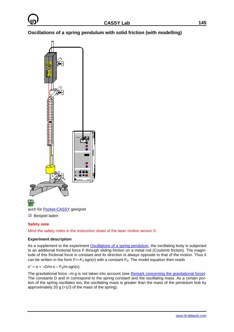
CASSY Lab

145

www.ld-didactic.com

Oscillations of a spring pendulum with solid friction (with modelling)


Beispiel laden

Safety note



As a supplement to the experiment Oscillations of a spring pendulum, the oscillating body is subjected to an additional frictional force F through sliding friction on a metal rod (Coulomb friction). The magni-tude of this frictional force is constant and its direction is always opposite to that of the motion. Thus it

can be written in the form F=–F0sgn(v) with a constant F0. The model equation then reads

s'' = a = –D/ms – F0/msgn(v).

The gravitational force –mg is not taken into account (see Remark concerning the gravitational force). The constants D and m correspond to the spring constant and the oscillating mass. As a certain por-tion of the spring oscillates too, the oscillating mass is greater than the mass of the pendulum bob by approximately 20 g (=1/3 of the mass of the spring).

146

CASSY Lab

www.ld-didactic.com

Equipment list

1 Sensor-CASSY 524 010 1 CASSY Lab 524 200 1 Laser motion sensor S 524 073 1 Stand rod with thread 309 00 335 1 Pair of helical springs 352 15 1 Big slotted mass hanger, 500 g 315 452 1 Stand rod, 1 m 300 44 1 Stand rod, 25 cm 300 41 1 Stand rod, bent at right angles 300 51 3 Leybold multiclamps 301 01 1 Stand base, V-shape, 28 cm 300 01 1 PC with Windows 98/2000/XP/Vista

Alternative


path measurement. From the measured force FA1 and the spring constant D, the deflection sA1=FA1/D can be calculated using a formula.




When the pendulum bob is in its equilibrium position, it should be near the middle of the bent stand rod. During the oscillation, the pendulum bob should always slide along the bent stand rod with fric-tion.


Einstellungen laden






After carrying out the evaluation, repeat the experiment for other frictional forces, and compare the results with the prediction of the model. In order to vary the frictional force, clamp the bent stand rod in slightly varied positions.

Modelling


triggering took place in the zero point of the path. The initial velocity v0, the spring constant D, the

mass m and the frictional force F0 can be altered by dragging the pointer of the corresponding display instrument (or by clicking to the left or to the right of the pointer) until the model agrees with the meas-urement.

The dependence of the model's frictional force on the velocity can be seen in the Frictional force display.

In order to confirm the model, you can increase the frictional force F0 (shift the bent stand rod corre-

spondingly). If the magnitude of the frictional force F0 in the model is increased correspondingly and, if

necessary, the initial velocity v0 is adjusted, the new measured oscillation will again agree with the mathematical model.

CASSY Lab

147

www.ld-didactic.com

Estimating the frictional force

The order of magnitude of the force of sliding friction can be estimated directly from the experiment setup. In the case of sliding friction, the magnitude of the frictional force is

F0 = FN =mgsin

with the coefficient of sliding friction and the normal force FN=mgsin . In this example, the angle

between the vertical and the axis of friction was approximately 2° and =0.12 (coefficient of sliding

friction for steel on steel), and we obtain F0=20 mN, which is in agreement with the model.

Envelope

The linear decrease of the amplitude of the oscillation in the case of a frictional force with constant

magnitude follows from energy conservation. Between two subsequent reversal points s1>0 and s2<0,

the work performed by the friction is W = F0s1+(–F0)s2. Since the kinetic energy at the reversal points

is 0, only the energy of the spring 1/2Ds12 and 1/2Ds2

2 is left (see also Remark concerning the gravi-

tational force).

The energy balance thus is

1/2Ds12 = 1/2Ds2

2 + W or

W = 1/2D(s12–s2

2) = 1/2D(s1+s2) (s1–s2) = F0s1–s2).

From this it follows that the difference of the magnitudes of the amplitudes is |s1|–|s2| = s1+s2 = 2F0/D.

Then it follows that the constant decrease of the amplitude for an entire period is s = 4F0/D.

The initial amplitude s0 of the envelope also derives from the constants of the model from

1/2mv02 = 1/2Ds0

2.

For small frictional forces, the function describing the envelope can be written in the form

±f(t) = s0–4F0/Dt/T = |v0|/0–4F0/Dt/(2/0) = |v0|/01–2/F0/m/|v0|t) = s01–2/kt)

with 0=sqr(D/m), s0=|v0|/0 und k=F0/m/|v0|.

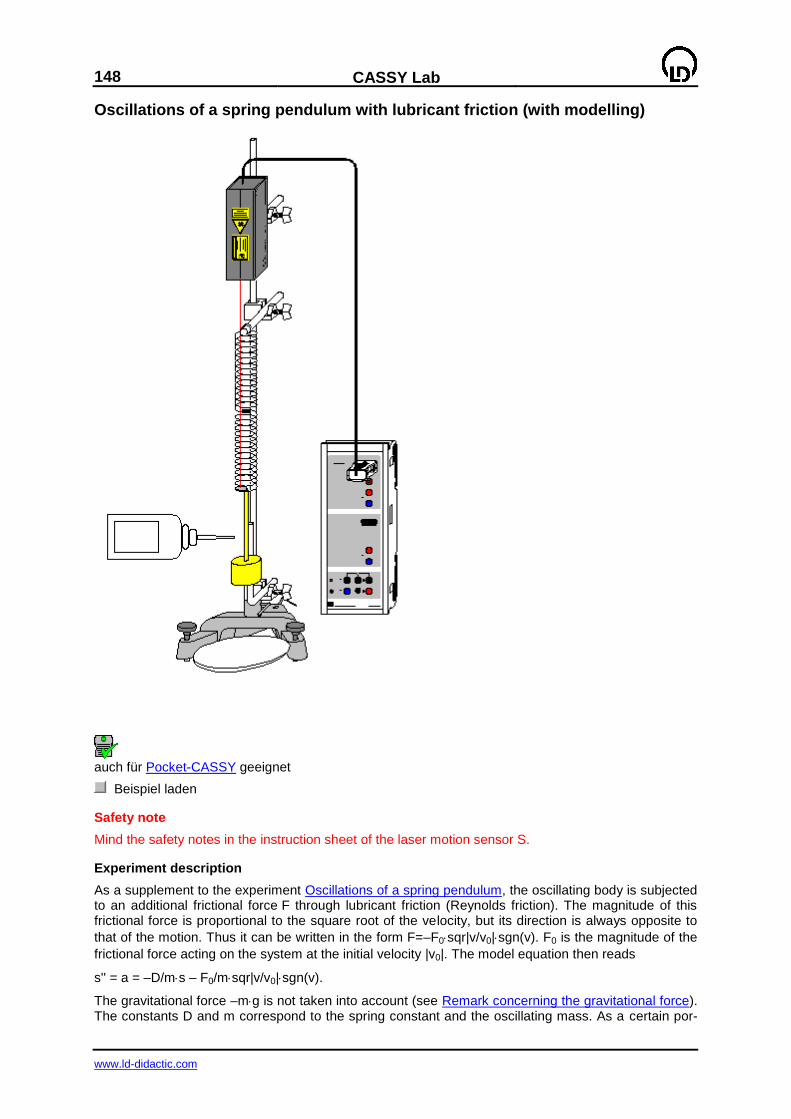
148

CASSY Lab

www.ld-didactic.com

Oscillations of a spring pendulum with lubricant friction (with modelling)


Beispiel laden

Safety note



As a supplement to the experiment Oscillations of a spring pendulum, the oscillating body is subjected to an additional frictional force F through lubricant friction (Reynolds friction). The magnitude of this frictional force is proportional to the square root of the velocity, but its direction is always opposite to

that of the motion. Thus it can be written in the form F=–F0sqr|v/v0|sgn(v). F0 is the magnitude of the

frictional force acting on the system at the initial velocity |v0|. The model equation then reads

s'' = a = –D/ms – F0/msqr|v/v0|sgn(v).

The gravitational force –mg is not taken into account (see Remark concerning the gravitational force). The constants D and m correspond to the spring constant and the oscillating mass. As a certain por-

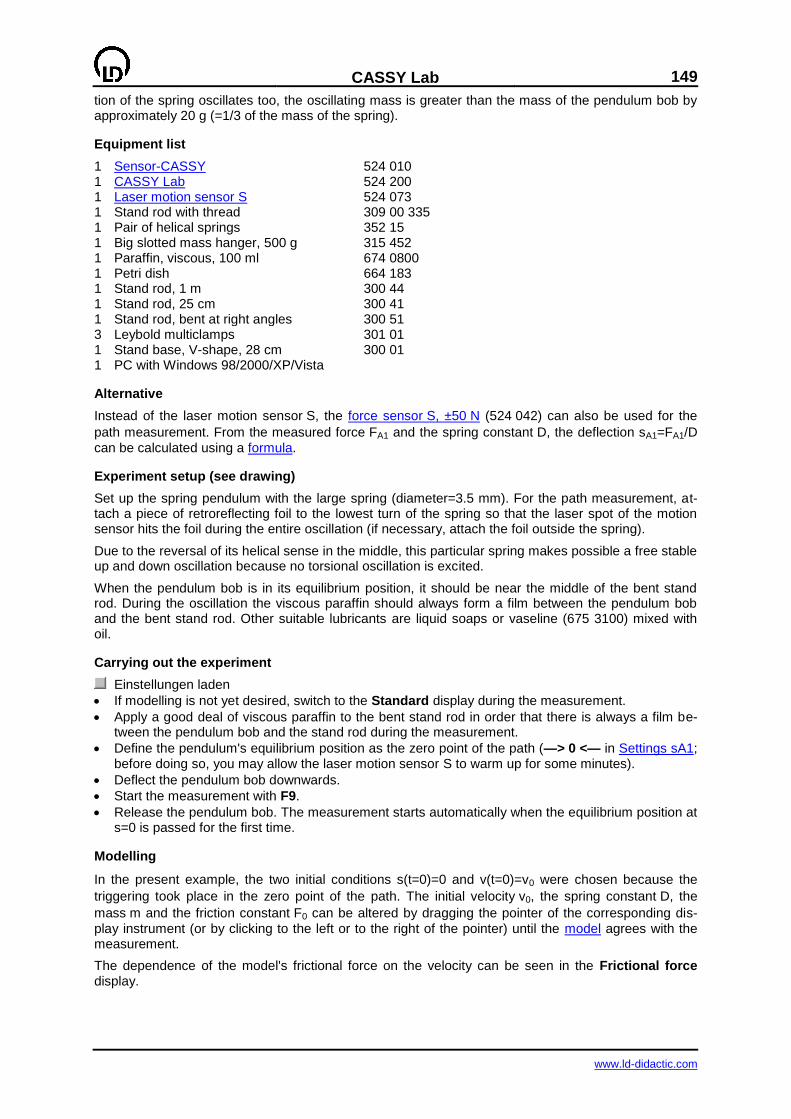
CASSY Lab

149

www.ld-didactic.com

tion of the spring oscillates too, the oscillating mass is greater than the mass of the pendulum bob by approximately 20 g (=1/3 of the mass of the spring).

Equipment list

1 Sensor-CASSY 524 010 1 CASSY Lab 524 200 1 Laser motion sensor S 524 073 1 Stand rod with thread 309 00 335 1 Pair of helical springs 352 15 1 Big slotted mass hanger, 500 g 315 452 1 Paraffin, viscous, 100 ml 674 0800 1 Petri dish 664 183 1 Stand rod, 1 m 300 44 1 Stand rod, 25 cm 300 41 1 Stand rod, bent at right angles 300 51 3 Leybold multiclamps 301 01 1 Stand base, V-shape, 28 cm 300 01 1 PC with Windows 98/2000/XP/Vista

Alternative


path measurement. From the measured force FA1 and the spring constant D, the deflection sA1=FA1/D

can be calculated using a formula.




When the pendulum bob is in its equilibrium position, it should be near the middle of the bent stand rod. During the oscillation the viscous paraffin should always form a film between the pendulum bob and the bent stand rod. Other suitable lubricants are liquid soaps or vaseline (675 3100) mixed with oil.


Einstellungen laden


Apply a good deal of viscous paraffin to the bent stand rod in order that there is always a film be-tween the pendulum bob and the stand rod during the measurement.





Modelling



mass m and the friction constant F0 can be altered by dragging the pointer of the corresponding dis-



150

CASSY Lab

www.ld-didactic.com

Envelope

For small frictional forces proportional to the square root of the velocity, the function describing the envelope is given by

±f(t) = |v0|/0(1–0.2782F0/m/|v0|t)2 = s0(1–0.2782kt)

2

with 0=sqr(D/m), s0=|v0|/0 and k=F0/m/|v0|.

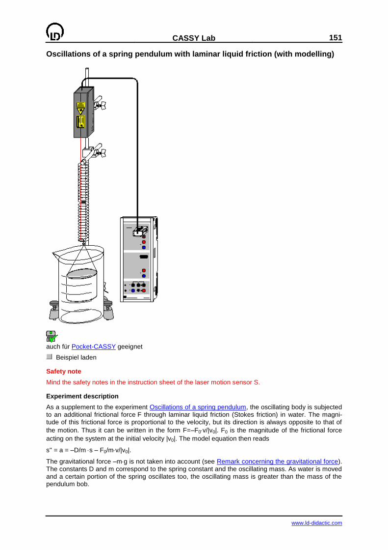
CASSY Lab

151

www.ld-didactic.com

Oscillations of a spring pendulum with laminar liquid friction (with modelling)


Beispiel laden

Safety note



As a supplement to the experiment Oscillations of a spring pendulum, the oscillating body is subjected to an additional frictional force F through laminar liquid friction (Stokes friction) in water. The magni-tude of this frictional force is proportional to the velocity, but its direction is always opposite to that of

the motion. Thus it can be written in the form F=–F0v/|v0|. F0 is the magnitude of the frictional force

acting on the system at the initial velocity |v0|. The model equation then reads

s'' = a = –D/ms – F0/mv/|v0|.

The gravitational force –mg is not taken into account (see Remark concerning the gravitational force). The constants D and m correspond to the spring constant and the oscillating mass. As water is moved and a certain portion of the spring oscillates too, the oscillating mass is greater than the mass of the pendulum bob.

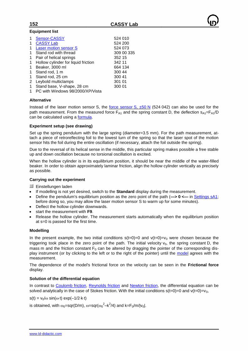
152

CASSY Lab

www.ld-didactic.com

Equipment list

1 Sensor-CASSY 524 010 1 CASSY Lab 524 200 1 Laser motion sensor S 524 073 1 Stand rod with thread 309 00 335 1 Pair of helical springs 352 15 1 Hollow cylinder for liquid friction 342 11 1 Beaker, 3000 ml 664 134 1 Stand rod, 1 m 300 44 1 Stand rod, 25 cm 300 41 2 Leybold multiclamps 301 01 1 Stand base, V-shape, 28 cm 300 01 1 PC with Windows 98/2000/XP/Vista

Alternative







When the hollow cylinder is in its equilibrium position, it should be near the middle of the water-filled beaker. In order to obtain approximately laminar friction, align the hollow cylinder vertically as precisely as possible.


Einstellungen laden



Deflect the hollow cylinder downwards.

start the measurement with F9.

Release the hollow cylinder. The measurement starts automatically when the equilibrium position at s=0 is passed for the first time.

Modelling



mass m and the friction constant F0 can be altered by dragging the pointer of the corresponding dis-play instrument (or by clicking to the left or to the right of the pointer) until the model agrees with the measurement.


Solution of the differential equation

In contrast to Coulomb friction, Reynolds friction and Newton friction, the differential equation can be

solved analytically in the case of Stokes friction. With the initial conditions s(t=0)=0 and v(t=0)=v0,

s(t) = v0/ sin(t) exp(–1/2kt)

is obtained, with 0=sqr(D/m), =sqr(02–k

2/4) and k=F0/m/|v0|.

CASSY Lab

153

www.ld-didactic.com

Envelope

For frictional forces proportional to the velocity, the function describing the envelope therefore has the form

±f(t) = s0exp(–1/2kt)

with s0=|v0|/.

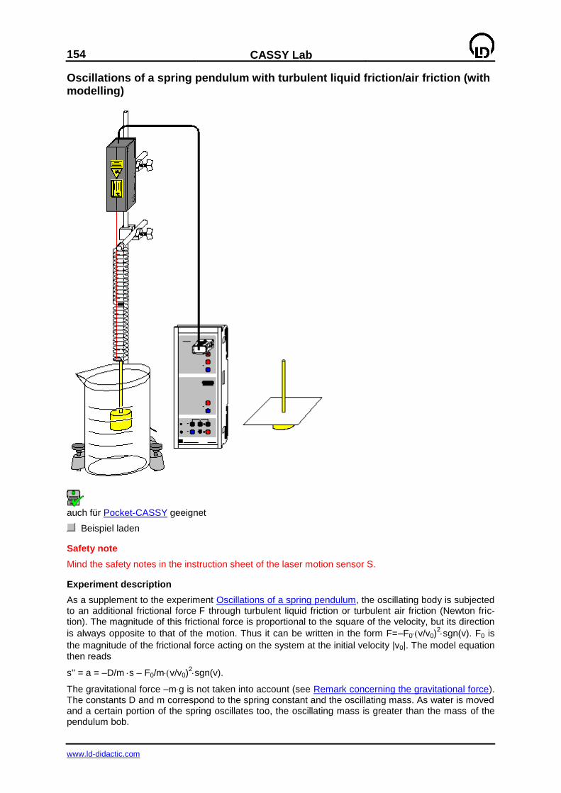
154

CASSY Lab

www.ld-didactic.com

Oscillations of a spring pendulum with turbulent liquid friction/air friction (with modelling)


Beispiel laden

Safety note



As a supplement to the experiment Oscillations of a spring pendulum, the oscillating body is subjected to an additional frictional force F through turbulent liquid friction or turbulent air friction (Newton fric-tion). The magnitude of this frictional force is proportional to the square of the velocity, but its direction

is always opposite to that of the motion. Thus it can be written in the form F=–F0v/v0)2sgn(v). F0 is

the magnitude of the frictional force acting on the system at the initial velocity |v0|. The model equation then reads

s'' = a = –D/ms – F0/mv/v0)2sgn(v).

The gravitational force –mg is not taken into account (see Remark concerning the gravitational force). The constants D and m correspond to the spring constant and the oscillating mass. As water is moved and a certain portion of the spring oscillates too, the oscillating mass is greater than the mass of the pendulum bob.

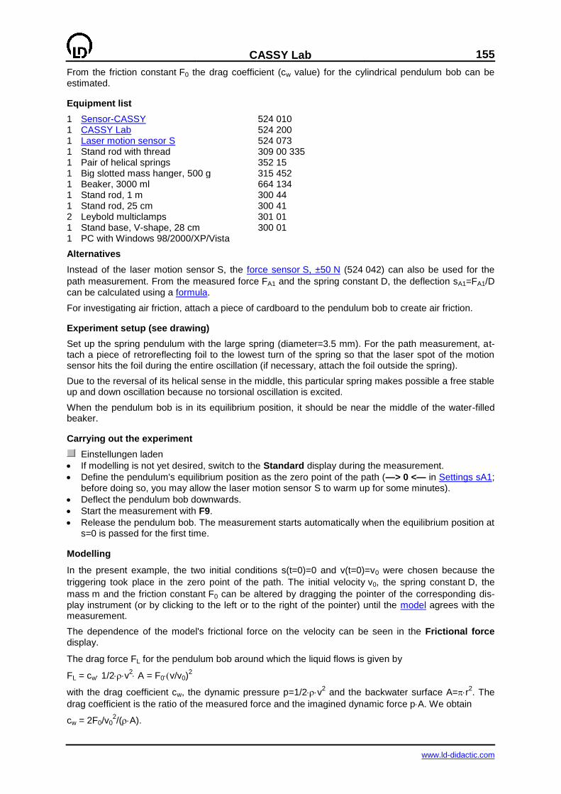
CASSY Lab

155

www.ld-didactic.com

From the friction constant F0 the drag coefficient (cw value) for the cylindrical pendulum bob can be estimated.

Equipment list

1 Sensor-CASSY 524 010 1 CASSY Lab 524 200 1 Laser motion sensor S 524 073 1 Stand rod with thread 309 00 335 1 Pair of helical springs 352 15 1 Big slotted mass hanger, 500 g 315 452 1 Beaker, 3000 ml 664 134 1 Stand rod, 1 m 300 44 1 Stand rod, 25 cm 300 41 2 Leybold multiclamps 301 01 1 Stand base, V-shape, 28 cm 300 01 1 PC with Windows 98/2000/XP/Vista

Alternatives




For investigating air friction, attach a piece of cardboard to the pendulum bob to create air friction.




When the pendulum bob is in its equilibrium position, it should be near the middle of the water-filled beaker.


Einstellungen laden






Modelling



mass m and the friction constant F0 can be altered by dragging the pointer of the corresponding dis-



The drag force FL for the pendulum bob around which the liquid flows is given by

FL = cw 1/2v2 A = F0v/v0)

2

with the drag coefficient cw, the dynamic pressure p=1/2v2 and the backwater surface A=r

2. The

drag coefficient is the ratio of the measured force and the imagined dynamic force pA. We obtain

cw = 2F0/v02/(A).

156

CASSY Lab

www.ld-didactic.com

In the present example, we have r = 2.5 cm and = 1 g/cm3, and therefore A = 1.96 kg/m. The mod-

elling process gives F0 = 0.1828 N and v0 = 0.325 m/s. Thus we find cw = 1.7.

Envelope

For small frictional forces proportional to the square of the velocity, the function describing the enve-lope is given by

±f(t) = |v0|sqr(m/D)/(1+4/3F0/m/|v0|t) = s0/(1+4/3kt)

with 0=sqr(D/m), s0=|v0|/0 and k=F0/m/|v0|.

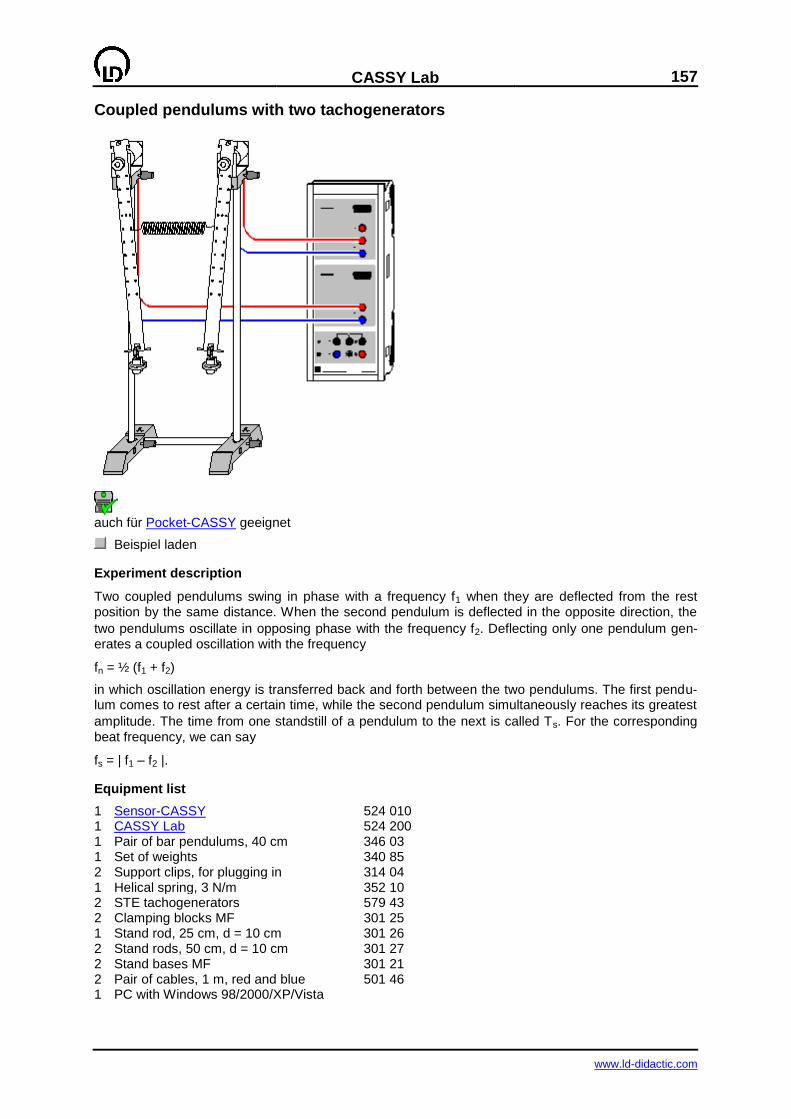
CASSY Lab

157

www.ld-didactic.com

Coupled pendulums with two tachogenerators


Beispiel laden


Two coupled pendulums swing in phase with a frequency f1 when they are deflected from the rest position by the same distance. When the second pendulum is deflected in the opposite direction, the

two pendulums oscillate in opposing phase with the frequency f2. Deflecting only one pendulum gen-erates a coupled oscillation with the frequency

fn = ½ (f1 + f2)

in which oscillation energy is transferred back and forth between the two pendulums. The first pendu-lum comes to rest after a certain time, while the second pendulum simultaneously reaches its greatest

amplitude. The time from one standstill of a pendulum to the next is called Ts. For the corresponding

beat frequency, we can say

fs = | f1 – f2 |.

Equipment list

1 Sensor-CASSY 524 010 1 CASSY Lab 524 200 1 Pair of bar pendulums, 40 cm 346 03 1 Set of weights 340 85 2 Support clips, for plugging in 314 04 1 Helical spring, 3 N/m 352 10 2 STE tachogenerators 579 43 2 Clamping blocks MF 301 25 1 Stand rod, 25 cm, d = 10 cm 301 26 2 Stand rods, 50 cm, d = 10 cm 301 27 2 Stand bases MF 301 21 2 Pair of cables, 1 m, red and blue 501 46 1 PC with Windows 98/2000/XP/Vista

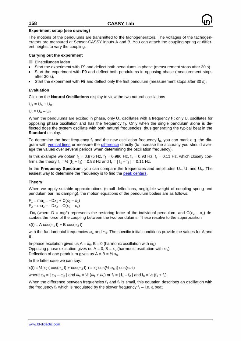
158

CASSY Lab

www.ld-didactic.com


The motions of the pendulums are transmitted to the tachogenerators. The voltages of the tachogen-erators are measured at Sensor-CASSY inputs A and B. You can attach the coupling spring at differ-ent heights to vary the coupling.


Einstellungen laden

Start the experiment with F9 and deflect both pendulums in phase (measurement stops after 30 s).

Start the experiment with F9 and deflect both pendulums in opposing phase (measurement stops after 30 s).

Start the experiment with F9 and deflect only the first pendulum (measurement stops after 30 s).

Evaluation

Click on the Natural Oscillations display to view the two natural oscillations

U+ = UA + UB

U- = UA – UB

When the pendulums are excited in phase, only U+ oscillates with a frequency f1; only U- oscillates for

opposing phase oscillation and has the frequency f2. Only when the single pendulum alone is de-flected does the system oscillate with both natural frequencies, thus generating the typical beat in the Standard display.

To determine the beat frequency fs and the new oscillation frequency fn, you can mark e.g. the dia-gram with vertical lines or measure the difference directly (to increase the accuracy you should aver-age the values over several periods when determining the oscillation frequency).

In this example we obtain f1 = 0.875 Hz, f2 = 0.986 Hz, fn = 0.93 Hz, fs = 0.11 Hz, which closely con-

firms the theory fn = ½ (f1 + f2) = 0.93 Hz and fs = | f1 – f2 | = 0.11 Hz.

In the Frequency Spectrum, you can compare the frequencies and amplitudes U+, U- and UA. The easiest way to determine the frequency is to find the peak centers.

Theory

When we apply suitable approximations (small deflections, negligible weight of coupling spring and pendulum bar, no damping), the motion equations of the pendulum bodies are as follows:

F1 = ma1 = –Dx1 + C(x2 – x1)

F2 = ma2 = –Dx2 – C(x2 – x1)

-Dxi (where D = mg/l) represents the restoring force of the individual pendulum, and C(x2 – x1) de-scribes the force of the coupling between the two pendulums. These resolve to the superposition

x(t) = A cos(1t) + B cos(2t)

with the fundamental frequencies 1 and 2. The specific initial conditions provide the values for A and B:

In-phase excitation gives us A = x0, B = 0 (harmonic oscillation with 1)

Opposing phase excitation gives us A = 0, B = x0 (harmonic oscillation with 2)

Deflection of one pendulum gives us A = B = ½ x0.

In the latter case we can say:

x(t) = ½ x0 ( cos(1t) + cos(2t) ) = x0 cos(½ st) cos(nt)

where s = | 1 – 2 | and n = ½ (1 + 2) or fs = | f1 – f2 | and fn = ½ (f1 + f2).

When the difference between frequencies f1 and f2 is small, this equation describes an oscillation with

the frequency fn which is modulated by the slower frequency fs – i.e. a beat.

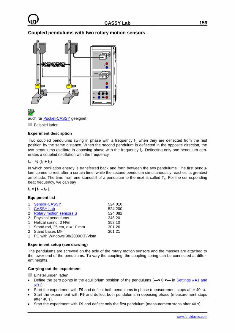
CASSY Lab

159

www.ld-didactic.com

Coupled pendulums with two rotary motion sensors


Beispiel laden


Two coupled pendulums swing in phase with a frequency f1 when they are deflected from the rest position by the same distance. When the second pendulum is deflected in the opposite direction, the

two pendulums oscillate in opposing phase with the frequency f2. Deflecting only one pendulum gen-erates a coupled oscillation with the frequency

fn = ½ (f1 + f2)

in which oscillation energy is transferred back and forth between the two pendulums. The first pendu-lum comes to rest after a certain time, while the second pendulum simultaneously reaches its greatest

amplitude. The time from one standstill of a pendulum to the next is called Ts. For the corresponding

beat frequency, we can say

fs = | f1 – f2 |.

Equipment list

1 Sensor-CASSY 524 010 1 CASSY Lab 524 200 2 Rotary motion sensors S 524 082 2 Physical pendulums 346 20 1 Helical spring, 3 N/m 352 10 1 Stand rod, 25 cm, d = 10 mm 301 26 2 Stand bases MF 301 21 1 PC with Windows 98/2000/XP/Vista


The pendulums are screwed on the axle of the rotary motion sensors and the masses are attached to the lower end of the pendulums. To vary the coupling, the coupling spring can be connected at differ-ent heights.


Einstellungen laden

Define the zero points in the equilibrium position of the pendulums (—> 0 <— in Settings A1 and

B1)

Start the experiment with F9 and deflect both pendulums in phase (measurement stops after 40 s).

Start the experiment with F9 and deflect both pendulums in opposing phase (measurement stops after 40 s).

Start the experiment with F9 and deflect only the first pendulum (measurement stops after 40 s).

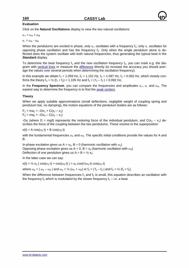
160

CASSY Lab

www.ld-didactic.com

Evaluation

Click on the Natural Oscillations display to view the two natural oscillations

+ = A + B

- = A - B

When the pendulums are excited in phase, only + oscillates with a frequency f1; only - oscillates for

opposing phase oscillation and has the frequency f2. Only when the single pendulum alone is de-flected does the system oscillate with both natural frequencies, thus generating the typical beat in the Standard display.

To determine the beat frequency fs and the new oscillation frequency fn, you can mark e.g. the dia-gram with vertical lines or measure the difference directly (to increase the accuracy you should aver-age the values over several periods when determining the oscillation frequency).

In this example we obtain f1 = 1.059 Hz, f2 = 1.151 Hz, fn = 1.097 Hz, fs = 0.092 Hz, which closely con-

firms the theory fn = ½ (f1 + f2) = 1.105 Hz and fs = | f1 – f2 | = 0.092 Hz.

In the Frequency Spectrum, you can compare the frequencies and amplitudes +, - and A. The easiest way to determine the frequency is to find the peak centers.

Theory

When we apply suitable approximations (small deflections, negligible weight of coupling spring and pendulum bar, no damping), the motion equations of the pendulum bodies are as follows:

F1 = ma1 = –Dx1 + C(x2 – x1)

F2 = ma2 = –Dx2 – C(x2 – x1)

-Dxi (where D = mg/l) represents the restoring force of the individual pendulum, and C(x2 – x1) de-scribes the force of the coupling between the two pendulums. These resolve to the superposition

x(t) = A cos(1t) + B cos(2t)

with the fundamental frequencies 1 and 2. The specific initial conditions provide the values for A and B:

In-phase excitation gives us A = x0, B = 0 (harmonic oscillation with 1)

Opposing phase excitation gives us A = 0, B = x0 (harmonic oscillation with 2)

Deflection of one pendulum gives us A = B = ½ x0.

In the latter case we can say:

x(t) = ½ x0 ( cos(1t) + cos(2t) ) = x0 cos(½st) cos(nt)

where s = | 1 – 2 | and n = ½ (1 + 2) or fs = | f1 – f2 | and fn = ½ (f1 + f2).

When the difference between frequencies f1 and f2 is small, this equation describes an oscillation with

the frequency fn which is modulated by the slower frequency fs – i.e. a beat.

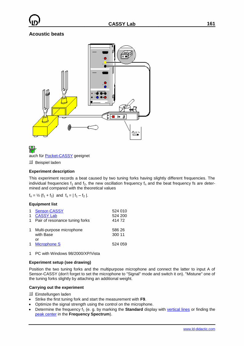
CASSY Lab

161

www.ld-didactic.com

Acoustic beats


Beispiel laden


This experiment records a beat caused by two tuning forks having slightly different frequencies. The

individual frequencies f1 and f2, the new oscillation frequency fn and the beat frequency fs are deter-mined and compared with the theoretical values

fn = ½ (f1 + f2) and fs = | f1 – f2 |.

Equipment list

1 Sensor-CASSY 524 010 1 CASSY Lab 524 200 1 Pair of resonance tuning forks 414 72 1 Multi-purpose microphone 586 26 with Base 300 11 or 1 Microphone S 524 059 1 PC with Windows 98/2000/XP/Vista


Position the two tuning forks and the multipurpose microphone and connect the latter to input A of Sensor-CASSY (don't forget to set the microphone to "Signal" mode and switch it on). "Mistune" one of the tuning forks slightly by attaching an additional weight.


Einstellungen laden

Strike the first tuning fork and start the measurement with F9.

Optimize the signal strength using the control on the microphone.

Determine the frequency f1 (e. g. by marking the Standard display with vertical lines or finding the peak center in the Frequency Spectrum).

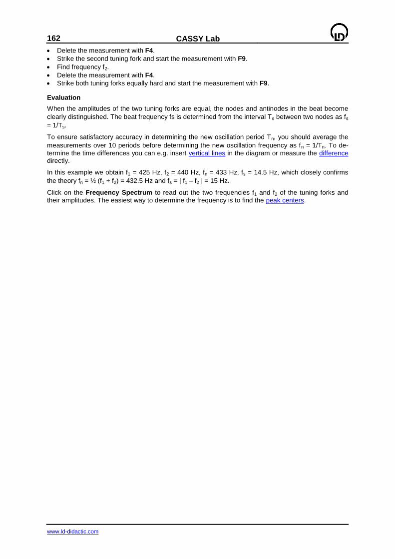
162

CASSY Lab

www.ld-didactic.com

Delete the measurement with F4.

Strike the second tuning fork and start the measurement with F9.

Find frequency f2.

Delete the measurement with F4.

Strike both tuning forks equally hard and start the measurement with F9.

Evaluation

When the amplitudes of the two tuning forks are equal, the nodes and antinodes in the beat become

clearly distinguished. The beat frequency fs is determined from the interval Ts between two nodes as fs

= 1/Ts.

To ensure satisfactory accuracy in determining the new oscillation period Tn, you should average the

measurements over 10 periods before determining the new oscillation frequency as fn = 1/Tn. To de-

termine the time differences you can e.g. insert vertical lines in the diagram or measure the difference directly.

In this example we obtain f1 = 425 Hz, f2 = 440 Hz, fn = 433 Hz, fs = 14.5 Hz, which closely confirms

the theory fn = ½ (f1 + f2) = 432.5 Hz and fs = | f1 – f2 | = 15 Hz.

Click on the Frequency Spectrum to read out the two frequencies f1 and f2 of the tuning forks and their amplitudes. The easiest way to determine the frequency is to find the peak centers.

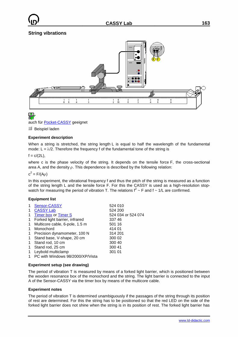
CASSY Lab

163

www.ld-didactic.com

String vibrations


Beispiel laden


When a string is stretched, the string length L is equal to half the wavelength of the fundamental

mode: L = /2. Therefore the frequency f of the fundamental tone of the string is

f = c/(2L),

where c is the phase velocity of the string. It depends on the tensile force F, the cross-sectional

area A, and the density . This dependence is described by the following relation:

c2 = F/(A)

In this experiment, the vibrational frequency f and thus the pitch of the string is measured as a function of the string length L and the tensile force F. For this the CASSY is used as a high-resolution stop-

watch for measuring the period of vibration T. The relations f2 ~ F and f ~ 1/L are confirmed.

Equipment list

1 Sensor-CASSY 524 010 1 CASSY Lab 524 200 1 Timer box or Timer S 524 034 or 524 074 1 Forked light barrier, infrared 337 46 1 Multicore cable, 6-pole, 1.5 m 501 16 1 Monochord 414 01 1 Precision dynamometer, 100 N 314 201 1 Stand base, V-shape, 20 cm 300 02 1 Stand rod, 10 cm 300 40 1 Stand rod, 25 cm 300 41 1 Leybold multiclamp 301 01 1 PC with Windows 98/2000/XP/Vista


The period of vibration T is measured by means of a forked light barrier, which is positioned between the wooden resonance box of the monochord and the string. The light barrier is connected to the input A of the Sensor-CASSY via the timer box by means of the multicore cable.

Experiment notes

The period of vibration T is determined unambiguously if the passages of the string through its position of rest are determined. For this the string has to be positioned so that the red LED on the side of the forked light barrier does not shine when the string is in its position of rest. The forked light barrier has

164

CASSY Lab

www.ld-didactic.com

two small apertures for the infrared beam. The best results are obtained if the string is positioned im-mediately over the smaller one of the two apertures (if necessary, turn the light barrier correspond-ingly).

The string is made vibrate by plucking it parallel to the surface of the resonance box.

The tensile force F is measured manually with the precision dynamometer. For this the hook is re-placed with the precision dynamometer. The tension of the string on the monochord can be varied by means of a tuning key. In the first experiment, the best results are obtained if a string tension of 100 N is adjusted at first and then the measurement is carried out starting from high tension to lower ten-sions.

In the measurement with varying string length L, the string length is varied by displacing the bridge. When plucking the string, do not touch the part which does not vibrate with the other hand. For an optimal measurement of the period of vibration T, always position the forked light barrier in the middle of the vibrating part of the string.


a) Variation of the tensile force

Einstellungen laden

Adjust the desired string tension F by turning the tuning key.

Write the force F displayed on the dynamometer in the prepared column of the table.

Position the forked light barrier under the string at rest and check whether the red LED is out; if necessary, position the forked light barrier anew.

Make the string vibrate by plucking it (while the string vibrates, the LED shines), and immediately transfer the displayed measured value into the table by pressing the F9 key.

b) Variation of the string length

Einstellungen laden

Adjust the desired string length by positioning the bridge.

Read the string length, and write it in the prepared column.

Check whether the red LED is out; if necessary, position the forked light barrier anew.

Make the string vibrate by plucking it (while the string vibrates, the LED shines), and immediately transfer the displayed measured value into the table by pressing the F9 key.

Evaluation

a) Variation of the tensile force

The T(F) and the f(F) diagram already appear while the measurement is running. In the prepared dis-

play Evaluation, the square of the frequency f is plotted against the tensile force F. The relation f2 ~ F

can be confirmed by fitting a line through the origin (right mouse button). That means, the pitch, and thus the frequency, of a vibrating string increases with increasing string tension. Correspondingly, the pitch of a string can be lowered by decreasing the string tension.

b) Variation string length

The T(L) and the f(L) diagram already appear while the measurement is running. In the prepared dis-play Evaluation, the square of the frequency f is plotted against 1/L. The relation f ~ 1/L can be con-firmed by fitting a line through the origin (right mouse button). That means, the pitch, and thus the frequency, of a vibrating string increases with decreasing length.

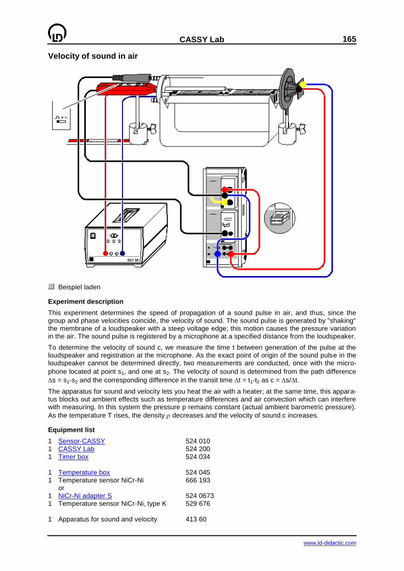
CASSY Lab

165

www.ld-didactic.com

Velocity of sound in air

Beispiel laden


This experiment determines the speed of propagation of a sound pulse in air, and thus, since the group and phase velocities coincide, the velocity of sound. The sound pulse is generated by "shaking" the membrane of a loudspeaker with a steep voltage edge; this motion causes the pressure variation in the air. The sound pulse is registered by a microphone at a specified distance from the loudspeaker.

To determine the velocity of sound c, we measure the time t between generation of the pulse at the loudspeaker and registration at the microphone. As the exact point of origin of the sound pulse in the loudspeaker cannot be determined directly, two measurements are conducted, once with the micro-

phone located at point s1, and one at s2. The velocity of sound is determined from the path difference

s = s1-s2 and the corresponding difference in the transit time t = t1-t2 as c = s/t.

The apparatus for sound and velocity lets you heat the air with a heater; at the same time, this appara-tus blocks out ambient effects such as temperature differences and air convection which can interfere with measuring. In this system the pressure p remains constant (actual ambient barometric pressure).

As the temperature T rises, the density decreases and the velocity of sound c increases.

Equipment list

1 Sensor-CASSY 524 010 1 CASSY Lab 524 200 1 Timer box 524 034 1 Temperature box 524 045 1 Temperature sensor NiCr-Ni 666 193 or 1 NiCr-Ni adapter S 524 0673 1 Temperature sensor NiCr-Ni, type K 529 676 1 Apparatus for sound and velocity 413 60

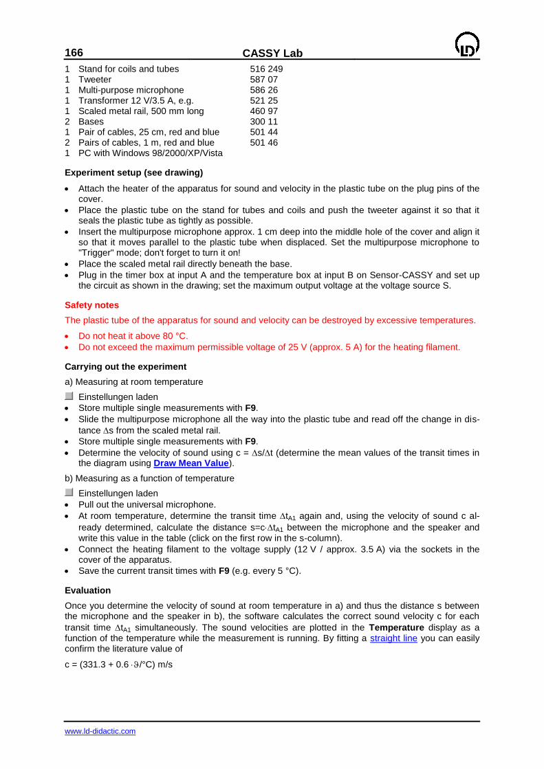
166

CASSY Lab

www.ld-didactic.com

1 Stand for coils and tubes 516 249 1 Tweeter 587 07 1 Multi-purpose microphone 586 26 1 Transformer 12 V/3.5 A, e.g. 521 25 1 Scaled metal rail, 500 mm long 460 97 2 Bases 300 11 1 Pair of cables, 25 cm, red and blue 501 44 2 Pairs of cables, 1 m, red and blue 501 46 1 PC with Windows 98/2000/XP/Vista


Attach the heater of the apparatus for sound and velocity in the plastic tube on the plug pins of the cover.

Place the plastic tube on the stand for tubes and coils and push the tweeter against it so that it seals the plastic tube as tightly as possible.

Insert the multipurpose microphone approx. 1 cm deep into the middle hole of the cover and align it so that it moves parallel to the plastic tube when displaced. Set the multipurpose microphone to "Trigger" mode; don't forget to turn it on!

Place the scaled metal rail directly beneath the base.

Plug in the timer box at input A and the temperature box at input B on Sensor-CASSY and set up the circuit as shown in the drawing; set the maximum output voltage at the voltage source S.

Safety notes

The plastic tube of the apparatus for sound and velocity can be destroyed by excessive temperatures.

Do not heat it above 80 °C.

Do not exceed the maximum permissible voltage of 25 V (approx. 5 A) for the heating filament.


a) Measuring at room temperature

Einstellungen laden

Store multiple single measurements with F9.

Slide the multipurpose microphone all the way into the plastic tube and read off the change in dis-

tance s from the scaled metal rail.

Store multiple single measurements with F9.

Determine the velocity of sound using c = s/t (determine the mean values of the transit times in the diagram using Draw Mean Value).

b) Measuring as a function of temperature

Einstellungen laden

Pull out the universal microphone.

At room temperature, determine the transit time tA1 again and, using the velocity of sound c al-

ready determined, calculate the distance s=ctA1 between the microphone and the speaker and

write this value in the table (click on the first row in the s-column).

Connect the heating filament to the voltage supply (12 V / approx. 3.5 A) via the sockets in the cover of the apparatus.

Save the current transit times with F9 (e.g. every 5 °C).

Evaluation

Once you determine the velocity of sound at room temperature in a) and thus the distance s between the microphone and the speaker in b), the software calculates the correct sound velocity c for each

transit time tA1 simultaneously. The sound velocities are plotted in the Temperature display as a function of the temperature while the measurement is running. By fitting a straight line you can easily confirm the literature value of

c = (331.3 + 0.6 /°C) m/s

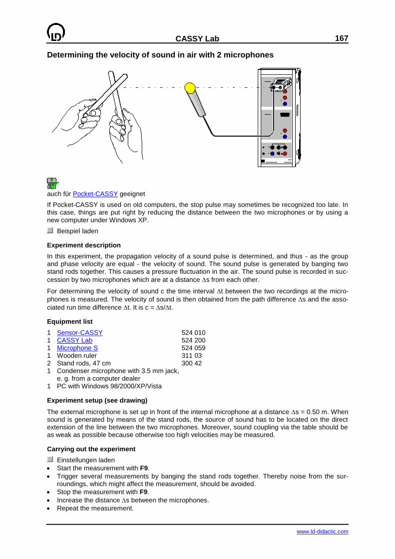
CASSY Lab

167

www.ld-didactic.com

Determining the velocity of sound in air with 2 microphones


If Pocket-CASSY is used on old computers, the stop pulse may sometimes be recognized too late. In this case, things are put right by reducing the distance between the two microphones or by using a new computer under Windows XP.

Beispiel laden


In this experiment, the propagation velocity of a sound pulse is determined, and thus - as the group and phase velocity are equal - the velocity of sound. The sound pulse is generated by banging two stand rods together. This causes a pressure fluctuation in the air. The sound pulse is recorded in suc-

cession by two microphones which are at a distance s from each other.

For determining the velocity of sound c the time interval t between the two recordings at the micro-

phones is measured. The velocity of sound is then obtained from the path difference s and the asso-

ciated run time difference t. It is c = s/t.

Equipment list

1 Sensor-CASSY 524 010 1 CASSY Lab 524 200 1 Microphone S 524 059 1 Wooden ruler 311 03 2 Stand rods, 47 cm 300 42 1 Condenser microphone with 3.5 mm jack,

e. g. from a computer dealer

1 PC with Windows 98/2000/XP/Vista


The external microphone is set up in front of the internal microphone at a distance s = 0.50 m. When sound is generated by means of the stand rods, the source of sound has to be located on the direct extension of the line between the two microphones. Moreover, sound coupling via the table should be as weak as possible because otherwise too high velocities may be measured.


Einstellungen laden


Trigger several measurements by banging the stand rods together. Thereby noise from the sur-roundings, which might affect the measurement, should be avoided.

Stop the measurement with F9.

Increase the distance s between the microphones.

Repeat the measurement.

168

CASSY Lab

www.ld-didactic.com

Evaluation

During the measurement, noise from the surroundings may lead to faulty measurements, which can easily be deleted. For this, just click the faulty value and delete it (backspace).

Next determine the mean values of the run times in the diagram using Draw Mean Value. There is a comfortable way of taking every mean value into the display Velocity of sound (mouse click) immedi-ately after it has been calculated by shifting it from the Status line into the new table (Drag & Drop).

In addition, the associated distance s between the two microphones is entered into the correspond-

ing column, whereby a s(t) diagram is generated. The slope of the straight line in this diagram is c =

s/t.

The velocity of sound obtained at room temperature is approx. c = 346 m/s.

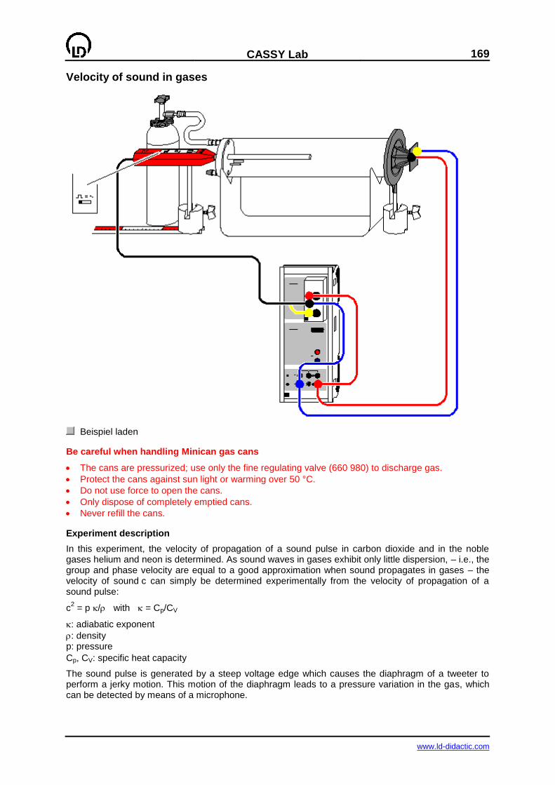
CASSY Lab

169

www.ld-didactic.com

Velocity of sound in gases

Beispiel laden

Be careful when handling Minican gas cans

The cans are pressurized; use only the fine regulating valve (660 980) to discharge gas.

Protect the cans against sun light or warming over 50 °C.

Do not use force to open the cans.

Only dispose of completely emptied cans.

Never refill the cans.


In this experiment, the velocity of propagation of a sound pulse in carbon dioxide and in the noble gases helium and neon is determined. As sound waves in gases exhibit only little dispersion, – i.e., the group and phase velocity are equal to a good approximation when sound propagates in gases – the velocity of sound c can simply be determined experimentally from the velocity of propagation of a sound pulse:

c2 = p / with = Cp/CV

: adiabatic exponent

: density p: pressure

Cp, CV: specific heat capacity

The sound pulse is generated by a steep voltage edge which causes the diaphragm of a tweeter to perform a jerky motion. This motion of the diaphragm leads to a pressure variation in the gas, which can be detected by means of a microphone.

170

CASSY Lab

www.ld-didactic.com

For determining the velocity of sound c in a gaseous medium, the travel time t between the pulse generation at the tweeter and the detection at the microphone is measured. As the sound pulse can-not be located exactly at the tweeter, the effective measuring distance is first determined by determin-

ing the velocity cair of sound in air. To do this, two travel time measurements are carried out with the

microphone being located at the location sA1 in one measurement and at the location sA2 in the other

measurement. The velocity of sound in air is then obtained from the path difference s = sA1-sA2 and

the associated travel time difference t = t1-t2: cair = s/t. This enables the effective measuring dis-

tance seff = cair t1 to be calculated for the location sA1, which eventually enables a direct measurement of the velocity of sound in a gas.

Equipment list

1 Sensor-CASSY 524 010 1 CASSY Lab 524 200 1 Timer box 524 034 1 Apparatus for sound velocity 413 60 1 Stand for tubes and coils 516 249 1 Tweeter 587 07 1 Multipurpose microphone 586 26 1 Scaled metal rail, 0.5 m 460 97 2 Saddle bases 300 11 1 Minican gas can, carbon dioxide 660 999 1 Minican gas can, helium 660 984 1 Minican gas can, neon 660 985 1 Fine regulating valve for Minican gas

cans 660 980

1 Silicone tubing, 7 x 1.5 mm, 1 m 667 194 1 Rubber tubing, d = 4 mm 604 481 1 Tubing connector 604 510 1 Pair of cables, 25 cm, red and blue 501 44 1 Pair of cables, 100 cm, red and blue 501 46 1 PC with Windows 98/2000/XP/Vista


Lay the plastic tube (without heating coil) on the stand for tubes and coils, and turn it so that the two hose nipples are one above the other.

Move the tweeter close to the plastic tube so that the plastic tube is closed as tight as possible.

Insert the multipurpose microphone in the central bore of the cap to a depth of approx. 1 cm, and align it so that it moves parallel to the plastic tube when it is displaced. Set the function switch of the multipurpose microphone to the "Trigger" mode. Do not forget to switch the microphone on.

Lay the scaled metal rail immediately under the saddle base.

Plug the timer box on the input A of the Sensor-CASSY, and set up the circuit as shown in the drawing; set the maximum output voltage at the voltage source S.

Experiment notes

To avoid unintended loss of gas, turn the handwheel of the fine regulating valve to the right stop be-fore screwing the fine regulating valve on the gas can.

Any leakage of the measuring apparatus leads to an escape of gas and thus to a distortion of the measuring result; therefore the tweeter has to be placed as close to the plastic tube as possible.

In order to fill the plastic tube with carbon dioxide, put the silicone tubing on the lower hose nipple of the plastic tube. In this way, the gas is almost completely exchanged because the lighter air is pressed out through the upper hose nipple when carbon dioxide enters. Correspondingly, proceed the other way round when filling the plastic tube with the noble gases helium and neon: when helium or neon, respectively, enters through the upper hose nipple, the air, which is heavier, is pressed out through the lower hose nipple.

Concerning the measurements on helium and neon, keep in mind that the measuring apparatus can-not be perfectly sealed so that part of the highly-volatile gas in the plastic tube escapes. This results in a relatively high proportion of air, which distorts the measurements – therefore the measurements should be carried out quickly.

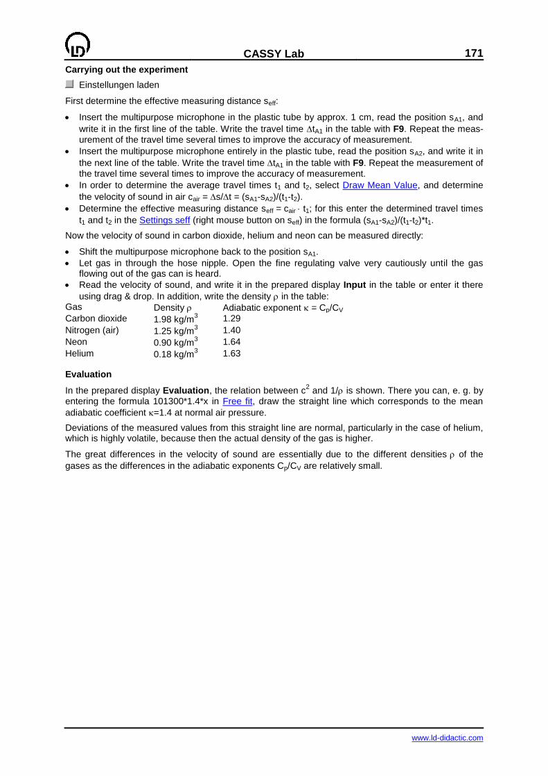
CASSY Lab

171

www.ld-didactic.com


Einstellungen laden

First determine the effective measuring distance seff:

Insert the multipurpose microphone in the plastic tube by approx. 1 cm, read the position sA1, and

write it in the first line of the table. Write the travel time tA1 in the table with F9. Repeat the meas-urement of the travel time several times to improve the accuracy of measurement.

Insert the multipurpose microphone entirely in the plastic tube, read the position sA2, and write it in

the next line of the table. Write the travel time tA1 in the table with F9. Repeat the measurement of the travel time several times to improve the accuracy of measurement.

In order to determine the average travel times t1 and t2, select Draw Mean Value, and determine

the velocity of sound in air cair = s/t = (sA1-sA2)/(t1-t2).

Determine the effective measuring distance seff = cair t1; for this enter the determined travel times

t1 and t2 in the Settings seff (right mouse button on seff) in the formula (sA1-sA2)/(t1-t2)*t1.

Now the velocity of sound in carbon dioxide, helium and neon can be measured directly:

Shift the multipurpose microphone back to the position sA1.

Let gas in through the hose nipple. Open the fine regulating valve very cautiously until the gas flowing out of the gas can is heard.

Read the velocity of sound, and write it in the prepared display Input in the table or enter it there

using drag & drop. In addition, write the density in the table: Gas Density Adiabatic exponent = Cp/CV Carbon dioxide 1.98 kg/m

3 1.29

Nitrogen (air) 1.25 kg/m3 1.40

Neon 0.90 kg/m3 1.64

Helium 0.18 kg/m3 1.63

Evaluation

In the prepared display Evaluation, the relation between c2 and 1/ is shown. There you can, e. g. by

entering the formula 101300*1.4*x in Free fit, draw the straight line which corresponds to the mean

adiabatic coefficient =1.4 at normal air pressure.

Deviations of the measured values from this straight line are normal, particularly in the case of helium, which is highly volatile, because then the actual density of the gas is higher.

The great differences in the velocity of sound are essentially due to the different densities of the

gases as the differences in the adiabatic exponents Cp/CV are relatively small.

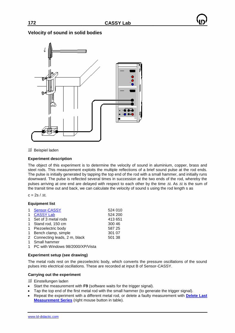
172

CASSY Lab

www.ld-didactic.com

Velocity of sound in solid bodies

Beispiel laden


The object of this experiment is to determine the velocity of sound in aluminium, copper, brass and steel rods. This measurement exploits the multiple reflections of a brief sound pulse at the rod ends. The pulse is initially generated by tapping the top end of the rod with a small hammer, and initially runs downward. The pulse is reflected several times in succession at the two ends of the rod, whereby the

pulses arriving at one end are delayed with respect to each other by the time t. As t is the sum of the transit time out and back, we can calculate the velocity of sound s using the rod length s as

c = 2s / t.

Equipment list

1 Sensor-CASSY 524 010 1 CASSY Lab 524 200 1 Set of 3 metal rods 413 651 1 Stand rod, 150 cm 300 46 1 Piezoelectric body 587 25 1 Bench clamp, simple 301 07 2 Connecting leads, 2 m, black 501 38 1 Small hammer 1 PC with Windows 98/2000/XP/Vista


The metal rods rest on the piezoelectric body, which converts the pressure oscillations of the sound pulses into electrical oscillations. These are recorded at input B of Sensor-CASSY.


Einstellungen laden

Start the measurement with F9 (software waits for the trigger signal).

Tap the top end of the first metal rod with the small hammer (to generate the trigger signal).

Repeat the experiment with a different metal rod, or delete a faulty measurement with Delete Last Measurement Series (right mouse button in table).

CASSY Lab

173

www.ld-didactic.com

Evaluation

You can determine the time differences t of the minima or maxima e.g. using vertical lines, finding the

peak center or by measuring the difference directly. As t is the sum of the transit time out and back, we can calculate the velocity of sound c using the rod length s as

c = 2s / t.

This example gives us the following sound velocity values:

Metal Measurement Literature value Brass 3530 m/s 3500 m/s Copper 3900 m/s 3800 m/s Aluminium 5000 m/s 5110 m/s Steel 5170 m/s 5100 m/s

174

CASSY Lab

www.ld-didactic.com

Fourier analysis of simulated signals

Beispiel laden


Harmonic analysis is a common method in many applications where time-variant signals (or measured values) occur. In acoustics, for example, exact knowledge of the overtones of a sound is important for the artificial generation of sounds or language.

In this experiment, the Fourier transform of simple periodic signals is studied as an introduction to the topic of Fourier transformation. In a first step, the Fourier transform of a numerically simulated signal is calculated and the frequencies of the associated amplitudes are determined (Fourier analysis). Based on this harmonic analysis, the time-variant signal is composed in a second step according to Fourier's theorem and compared with the theoretically calculated Fourier series and the numerically simulated original signal (Fourier synthesis).

Equipment list

1 CASSY Lab 524 200 1 PC with Windows 98/2000/XP/Vista

Experiment setup

Remark: the experiment is a pure simulation experiment on Fourier analysis with CASSY Lab. For an experiment with electric signals of corresponding shapes see the subsequent experiment. The signals

S1 investigated in this experiment are generated by the following functions:

Delta: S1 = 4*(1-2*saw(f*t)) Square wave: S1 = 4*(2*square(f*t)-1)

with the frequency f = 0.5 Hz.

Remarks concerning the Fourier transformation

A continuous time-variant signal S1 is sampled during the computer-aided measurement at certain times. In this way, a digitized signal is obtained, which can be further processed using common meth-ods of digital signal processing (improving the signal-to-noise ratio by means of Fourier transformation, smoothing the signal by averaging, etc.). The sampling theorem tells at what time intervals the signal value has to be measured so that the time dependence of the signal can be recovered from the digi-tized measured values (data points). For a digitization of the signal with a sufficient number of data

points, the sampling frequency fs has to be at least twice the maximum frequency fmax that occurs in

the signal and determines the width of the frequency spectrum. If this condition, fs ≥ 2fmax is not ful-

filled, i.e., if the digitization takes place at a lower sampling frequency fs, the shape of the signal is no

longer captured (aliasing). The sampling frequency fs of the measuring signal is determined by the

interval t=1/fs set in the Measuring Parameters (F5).

Fourier's theorem says that any time-dependent periodic signal S1 can be represented by a weighted

sum of sin or cos functions. For the delta and square-wave functions used in this experiment, the se-

ries expansions of S1 in trigonometric functions up to order 9 read:

Delta:

S3 = 4*8/3.14^2 * (cos(360*f*t) + 1/9*cos(360*3*f*t) + 1/25*cos(360*5*f*t) + 1/49*cos(360*7*f*t)) + 1/81*cos(360*9*f*t)

Square wave:

S3 = 4*4/3.14 * (sin(360*f*t) + 1/3*sin(360*3*f*t) + 1/5*sin(360*5*f*t) + 1/7*sin(360*7*f*t) + 1/9*sin(360*9*f*t)

Thus a discrete frequency spectrum with different amplitudes corresponds to the time-dependent func-

tion S1. The generalization of this decomposition to non-periodic signals leads to the Fourier integral,

which assigns a continuous frequency spectrum F1 to the time-dependent signal S1.

The numerical computation of the frequency spectrum F1 is particularly efficient if a digitized signal of

N=2p data points is taken as a basis. In this case, only approx. N log2(N) arithmetic operations have

CASSY Lab

175

www.ld-didactic.com

to be carried out instead of approx. N2 operations. This procedure, which is significantly less time con-

suming, is called fast Fourier transformation (FFT).

CASSY Lab computes the frequency spectrum F1 using such an algorithm. However, first of all the given measured points are weighted so that non-periodic portions on the boundaries do not play an important role (on the boundaries 0, in the middle maximum, Kaiser-Bessel window(4.0)). In order that

always exactly 2p measuring points are available, zeros are added for measuring points that may be

missing.

As a result of the FFT, CASSY Lab displays a total of N/2 amplitudes (i.e., phase differences are not

evaluated). These amplitudes are represented as "excess" amplitudes, i.e. Ai := Ai-1 + Ai + Ai+1, in or-

der that the amplitudes of sharp peaks are in approximate agreement with theory. Without this excess, an amplitude determination as it is carried out in this experiment would require the calculation of the sum over all amplitudes of a peak.

There are limitations to the use of FFT for frequency analysis due to two basic relations. The first one

relates the highest frequency fmax that can be analysed to the sampling frequency fs:

fmax = fs/2.

Any frequency which is greater than fmax appears in the frequency spectrum between zero and fmax and can then no longer be distinguished from the frequency contributions which really arise from the

range between 0 and fmax. The resulting change in the signal shape is called aliasing.

The second relation relates the resolution of the frequency spectrum f (= distance of neighbouring

points of the frequency spectrum) to the sampling frequency fs:

f = fmax/(N/2-1) = fs/(N-2) = 1/t/(N-2) 1/T

with T = (N-1)t.

That means that the resolution of the frequency spectrum can only be increased by a longer measur-ing time.


Einstellungen laden

Using the mouse, set the pointer of the display instrument f to the desired frequency.

F9 simulates the recording of measured values of the function S1. The simulation takes 50 s and

records 500 values (t = 100 ms).

Longer recording times increase the frequency resolution of the FFT step by step whereas shorter recording times decrease the resolution.

Evaluation

The S1(t) diagram of the numerically simulated signal appears already during the simulation of the

measurement. After the simulation, the Fourier transform F1 is available in the display Frequency Spectrum.

The frequency spectrum exhibits peaks at odd multiples of the set signal frequency f, i.e. at f, 3*f, 5*f, 7*f, etc.. The amplitudes of the peaks can be read by clicking the curve or from the coordinate display.

Now enter the first 5 amplitudes as coefficients of the sin(360*n*f*t) functions in the Settings A1, A3, A5, A7 and A9 for the analysis. In the display Fourier Analysis, the time dependence of the individual

terms A1, A3, A5, A7 and A9 is shown.

In the diagram Fourier Synthesis, the series S2 = A1 + A3 + A5 + A7 + A9 which has been determined

experimentally is compared with theoretical Fourier series S3 and the numerically simulated function

S1. It turns out that in practical applications the periodic signal S1 is satisfactorily approximated by a

trigonometric polynomial S2 or S3, respectively, containing only a few terms.

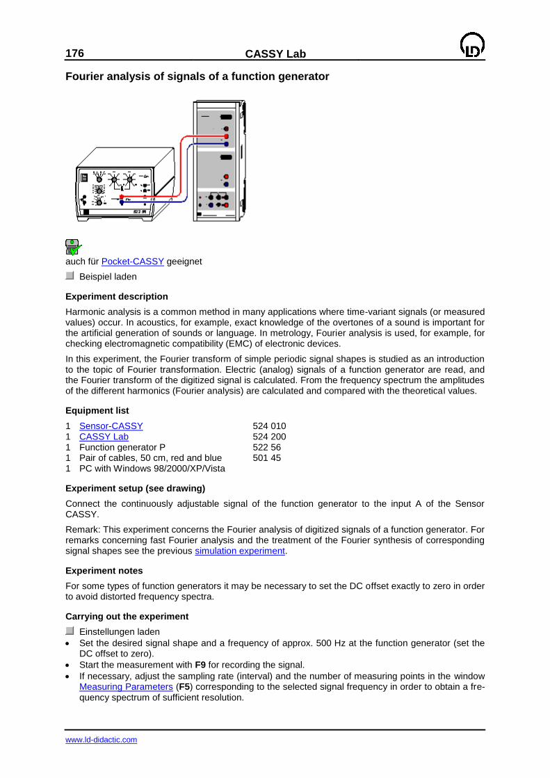
176

CASSY Lab

www.ld-didactic.com

Fourier analysis of signals of a function generator


Beispiel laden


Harmonic analysis is a common method in many applications where time-variant signals (or measured values) occur. In acoustics, for example, exact knowledge of the overtones of a sound is important for the artificial generation of sounds or language. In metrology, Fourier analysis is used, for example, for checking electromagnetic compatibility (EMC) of electronic devices.

In this experiment, the Fourier transform of simple periodic signal shapes is studied as an introduction to the topic of Fourier transformation. Electric (analog) signals of a function generator are read, and the Fourier transform of the digitized signal is calculated. From the frequency spectrum the amplitudes of the different harmonics (Fourier analysis) are calculated and compared with the theoretical values.

Equipment list

1 Sensor-CASSY 524 010 1 CASSY Lab 524 200 1 Function generator P 522 56 1 Pair of cables, 50 cm, red and blue 501 45 1 PC with Windows 98/2000/XP/Vista


Connect the continuously adjustable signal of the function generator to the input A of the Sensor CASSY.

Remark: This experiment concerns the Fourier analysis of digitized signals of a function generator. For remarks concerning fast Fourier analysis and the treatment of the Fourier synthesis of corresponding signal shapes see the previous simulation experiment.

Experiment notes

For some types of function generators it may be necessary to set the DC offset exactly to zero in order to avoid distorted frequency spectra.


Einstellungen laden

Set the desired signal shape and a frequency of approx. 500 Hz at the function generator (set the DC offset to zero).

Start the measurement with F9 for recording the signal.

If necessary, adjust the sampling rate (interval) and the number of measuring points in the window Measuring Parameters (F5) corresponding to the selected signal frequency in order to obtain a fre-quency spectrum of sufficient resolution.

CASSY Lab

177

www.ld-didactic.com

Evaluation

While the signal is recorded, the UA1(t) diagram already appears, representing a digitized version of

the analog signal of the function generator. After the signal UA1 has been recorded, the Fourier trans-

form of UA1 is available for the harmonic analysis in the display Frequency Spectrum.

For determining the amplitudes of the harmonics, carry out the following steps one after another:

Select the display Frequency Spectrum, and determine the amplitudes of the harmonics of order N with a horizontal line (Alt+H).

Go to the display Evaluation, transfer the value of the amplitude from the status line into the pre-pared table in column A using the mouse (drag & drop), and enter the order N of the N-th har-monic.

The theoretical dependence of the amplitudes of the N-th harmonics can be confirmed for the respec-

tive signal shape by a subsequent free fit (Alt+F) to a hyperbola A/x2 (delta: N = 1, 3, 5, ...) or A/x

(square wave: N = 1, 3, 5, ...; sawtooth: N = 1, 2, 3, 4, ...), respectively. Alternatively, the dependence of the amplitudes on N obtained by way of theoretical calculations can be checked by converting the x-

axis into 1/x2 (delta) or 1/x (square wave, sawtooth) and a subsequent fit to a line through the origin.

Depending on the signal shape selected, the frequency spectrum also exhibits contributions of small amplitudes at frequencies between the theoretical frequencies (e.g. between N = 1, 3, 5, ... in the case of the delta signal). This is due to the fact that the signal shape is not ideal and that the signal is not strictly periodic over the range covered by the recording time window.

Remark: for an example of using Power CASSY as a function generator see the experiment on sonic synthesis.

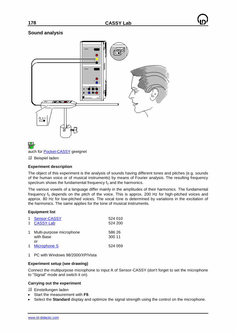
178

CASSY Lab

www.ld-didactic.com

Sound analysis


Beispiel laden


The object of this experiment is the analysis of sounds having different tones and pitches (e.g. sounds of the human voice or of musical instruments) by means of Fourier analysis. The resulting frequency

spectrum shows the fundamental frequency f0 and the harmonics.

The various vowels of a language differ mainly in the amplitudes of their harmonics. The fundamental

frequency f0 depends on the pitch of the voice. This is approx. 200 Hz for high-pitched voices and

approx. 80 Hz for low-pitched voices. The vocal tone is determined by variations in the excitation of the harmonics. The same applies for the tone of musical instruments.

Equipment list

1 Sensor-CASSY 524 010 1 CASSY Lab 524 200 1 Multi-purpose microphone 586 26 with Base 300 11 or 1 Microphone S 524 059 1 PC with Windows 98/2000/XP/Vista


Connect the multipurpose microphone to input A of Sensor-CASSY (don't forget to set the microphone to "Signal" mode and switch it on).


Einstellungen laden


Select the Standard display and optimize the signal strength using the control on the microphone.

CASSY Lab

179

www.ld-didactic.com

Record and compare different sounds (Standard shows the signal form and Frequency Spectrum shows the Fourier analysis).

To stop the measurement, deactivate Repeating Measurement in the Measuring Parameters dialog or press F9 immediately after the end of a recording.

To compare different frequency spectra, select Append New Measurement Series in the Measur-ing Parameters dialog and restart the measurement with F9.

Evaluation

The fundamental frequency and each harmonic can be determined easily in Frequency Spectrum (click with the mouse) using the coordinate display or by finding the peak centers. The amplitudes of the harmonics determine the tone of the recorded sound.

As the human ear perceives sound intensities in a logarithmic fashion, the logarithmic display of the frequency spectrum is better suited to the sensitivity of the human ear than a linear representation. Select the logarithmic representation by clicking on the y-axis of the frequency spectrum with the right mouse button (increase the lower limit, e.g. to –3).

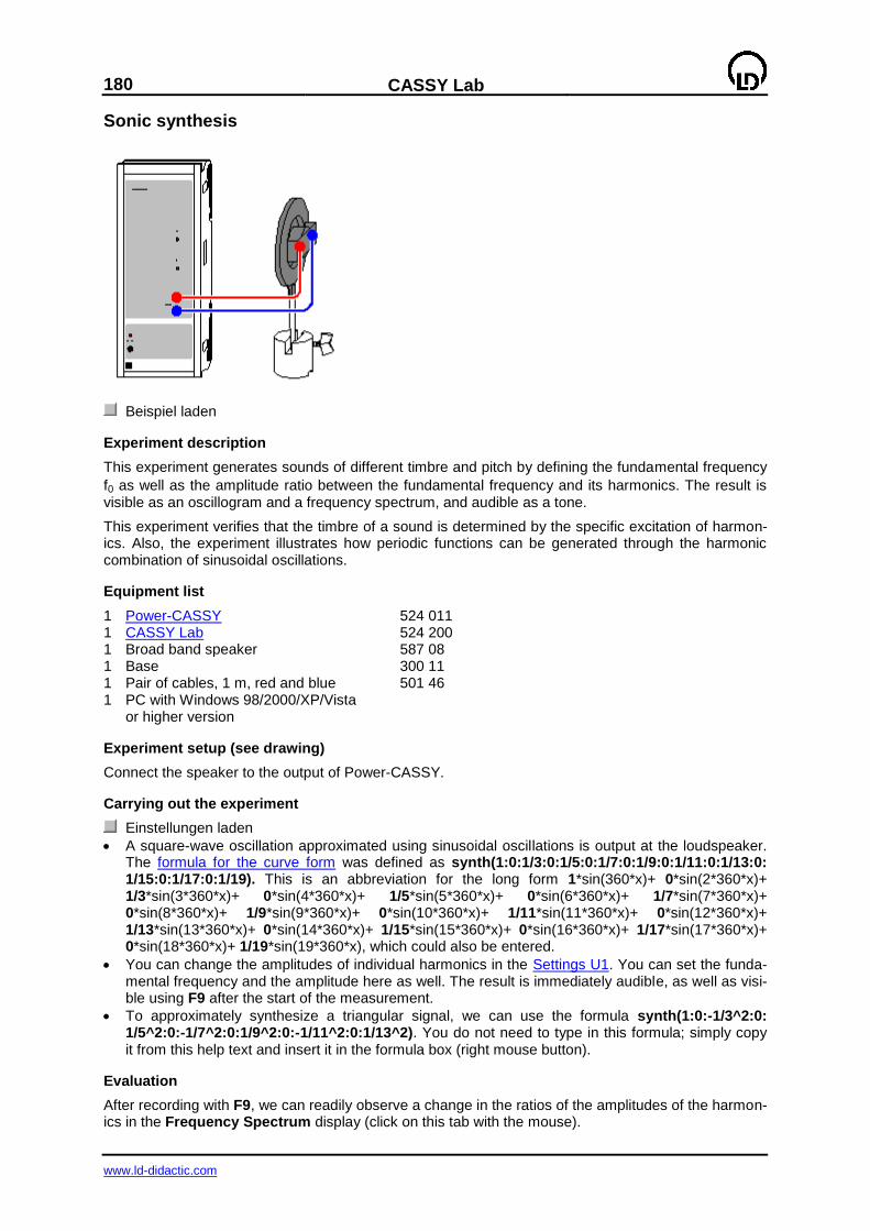
180

CASSY Lab

www.ld-didactic.com

Sonic synthesis

Beispiel laden


This experiment generates sounds of different timbre and pitch by defining the fundamental frequency

f0 as well as the amplitude ratio between the fundamental frequency and its harmonics. The result is visible as an oscillogram and a frequency spectrum, and audible as a tone.

This experiment verifies that the timbre of a sound is determined by the specific excitation of harmon-ics. Also, the experiment illustrates how periodic functions can be generated through the harmonic combination of sinusoidal oscillations.

Equipment list

1 Power-CASSY 524 011 1 CASSY Lab 524 200 1 Broad band speaker 587 08 1 Base 300 11 1 Pair of cables, 1 m, red and blue 501 46 1 PC with Windows 98/2000/XP/Vista or higher version


Connect the speaker to the output of Power-CASSY.


Einstellungen laden

A square-wave oscillation approximated using sinusoidal oscillations is output at the loudspeaker. The formula for the curve form was defined as synth(1:0:1/3:0:1/5:0:1/7:0:1/9:0:1/11:0:1/13:0: 1/15:0:1/17:0:1/19). This is an abbreviation for the long form 1*sin(360*x)+ 0*sin(2*360*x)+ 1/3*sin(3*360*x)+ 0*sin(4*360*x)+ 1/5*sin(5*360*x)+ 0*sin(6*360*x)+ 1/7*sin(7*360*x)+ 0*sin(8*360*x)+ 1/9*sin(9*360*x)+ 0*sin(10*360*x)+ 1/11*sin(11*360*x)+ 0*sin(12*360*x)+ 1/13*sin(13*360*x)+ 0*sin(14*360*x)+ 1/15*sin(15*360*x)+ 0*sin(16*360*x)+ 1/17*sin(17*360*x)+ 0*sin(18*360*x)+ 1/19*sin(19*360*x), which could also be entered.

You can change the amplitudes of individual harmonics in the Settings U1. You can set the funda-mental frequency and the amplitude here as well. The result is immediately audible, as well as visi-ble using F9 after the start of the measurement.

To approximately synthesize a triangular signal, we can use the formula synth(1:0:-1/3^2:0: 1/5^2:0:-1/7^2:0:1/9^2:0:-1/11^2:0:1/13^2). You do not need to type in this formula; simply copy it from this help text and insert it in the formula box (right mouse button).

Evaluation

After recording with F9, we can readily observe a change in the ratios of the amplitudes of the harmon-ics in the Frequency Spectrum display (click on this tab with the mouse).

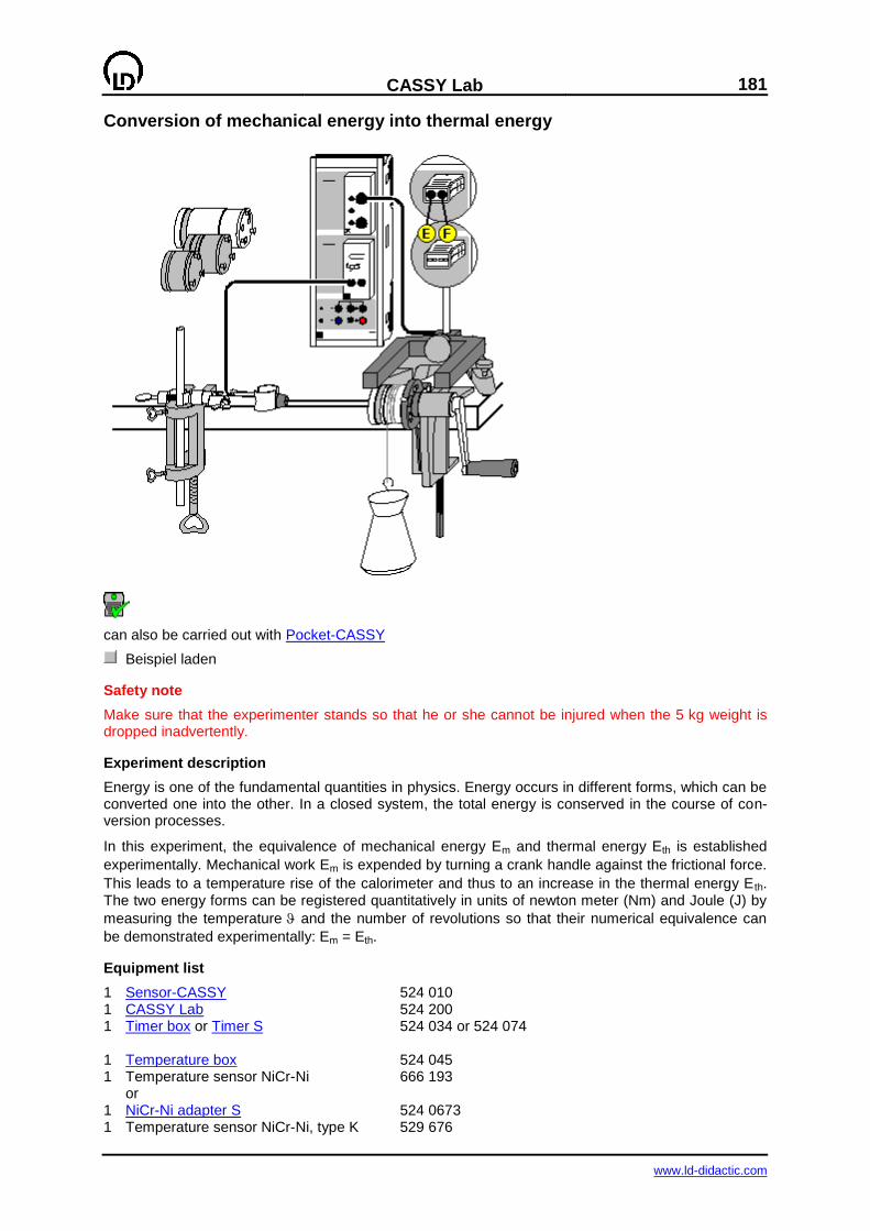
CASSY Lab

181

www.ld-didactic.com

Conversion of mechanical energy into thermal energy

can also be carried out with Pocket-CASSY

Beispiel laden

Safety note

Make sure that the experimenter stands so that he or she cannot be injured when the 5 kg weight is dropped inadvertently.


Energy is one of the fundamental quantities in physics. Energy occurs in different forms, which can be converted one into the other. In a closed system, the total energy is conserved in the course of con-version processes.

In this experiment, the equivalence of mechanical energy Em and thermal energy Eth is established

experimentally. Mechanical work Em is expended by turning a crank handle against the frictional force.

This leads to a temperature rise of the calorimeter and thus to an increase in the thermal energy E th. The two energy forms can be registered quantitatively in units of newton meter (Nm) and Joule (J) by

measuring the temperature and the number of revolutions so that their numerical equivalence can

be demonstrated experimentally: Em = Eth.

Equipment list

1 Sensor-CASSY 524 010 1 CASSY Lab 524 200 1 Timer box or Timer S 524 034 or 524 074 1 Temperature box 524 045 1 Temperature sensor NiCr-Ni 666 193 or 1 NiCr-Ni adapter S 524 0673 1 Temperature sensor NiCr-Ni, type K 529 676

182

CASSY Lab

www.ld-didactic.com

1 Forked light barrier, infrared 337 46 1 Multicore cable, 6-pole, 1.5 m 501 16 1 Equivalent of heat, basic apparatus 388 00 1 Calorimeter e.g. water calorimeter 388 01 or copper calorimeter with heating 388 02 or aluminium calorimeter with heating 388 03 or large aluminium calorimeter with heating 388 04 1 Simple bench clamp 301 07 1 Stand base, V-shape, 20 cm 300 02 1 Stand rod, 10 cm 300 40 1 Stand rod, 25 cm 300 41 1 Clamp with jaw clamp 301 11 1 Weight, 5 kg 388 24 1 PC with Windows 98/2000/XP/Vista


Fasten the equivalent of heat basic apparatus to a corner of the table.

Fasten the bench clamp at the edge of the table at a distance of approx. 40 cm from the plastic mounting of the basic apparatus. Clamp the clamp with jaw clamp with the aid of the stand rod 25 cm in order to be able to fix the temperature sensor as shown in the drawing.

Set up the calorimeter so that the bore points upwards and pour water into the opening.

Insert the gasket in the bore, and hold it with the locking screw.

Attach the filled calorimeter body to the basic apparatus by inserting the rivet pins in the sockets of the plastic mounting and twisting the calorimeter body to lock the pins in place.

Insert the temperature sensor as deeply as possible in the opening of the calorimeter, and tighten the locking screw of the calorimeter. Fix the temperature sensor by means of the stand material that has already been prepared as shown in the drawing.

Put the 5 kg weight under the calorimeter body.

Wind the nylon band approx. 4 times (6 at maximum) around the calorimeter, and attach it to the weight on the floor. The weight has to hang down on the side of the crank on the front.

Operate the crank handle, and check whether the 5 kg weight is lifted a few centimetres and is kept at a constant height when the handle is turned further. If it is lifted too high, reduce the number of turns of the nylon band; if it does not lift at all, increase the number of turns.

For measuring the number of revolutions nEA1 (=number of obscurations), position the forked light

barrier with the aid of the stand base as shown in the drawing, and connect it to the input A of the Sensor-CASSY via the timer box.

Connect the temperature sensor to the input B of the Sensor CASSY via the temperature box

(socket T1) for measuring the temperature B11.


Einstellungen laden

Set the obscuration to zero by clicking —> 0 <— in Settings nEA1.


Turn the crank handle, and measure the increase in temperature as a function of the number of revolutions.

Stop the measurement with F9 at the desired final temperature B11.

Evaluation

The temperature B11 is already displayed graphically as a function of the number of revolutions nEA1 during the measurement. In the prepared diagram Evaluation, the thermal energy is plotted against the mechanical energy that has been provided by turning the crank against the friction. The mechani-

cal energy Em is equal to the product of the frictional force and the covered path s:

CASSY Lab

183

www.ld-didactic.com

Em = Fs

with F = mg

F = frictional force m = mass of the weight = 5 kg

g = acceleration of gravity = 9.81 m/s2

and s = Nd

s = frictional path N = number of revolutions d = diameter of the calorimeter = 0.047 m

Thus the mechanical energy is: Em = mgdN.

The increase in thermal energy as a result of the temperature increase is given by:

Eth = C(2 - 1)

The heat capacity C depends on the calorimeter used and has to be entered in the Settings C accord-ing to the following table:

Calorimeter Heat capacity C/(J/K) Water (388 01) 40 + mH2O/g 4.2 (mass of the water in g) Copper (388 02) 264 + 4.2 (for 1 g of water in the bore) Aluminium (388 03) 188 + 4.2 (for 1 g of water in the bore) Aluminium, large (388 04) 384 + 4.2 (for 1 g of water in the bore)

The equivalence of the mechanical energy Em and the thermal energy Eth can be confirmed by means of a fit to a line through the origin. Usually the slope of the straight line through the origin is somewhat smaller than 1. This is due to heat loss which is not registered, e.g. by thermal contact of the calorime-ter with the nylon band or the plastic mounting.

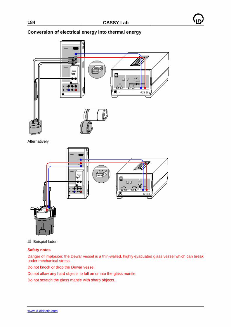
184

CASSY Lab

www.ld-didactic.com

Conversion of electrical energy into thermal energy

Alternatively:

Beispiel laden

Safety notes

Danger of implosion: the Dewar vessel is a thin-walled, highly evacuated glass vessel which can break under mechanical stress.

Do not knock or drop the Dewar vessel.

Do not allow any hard objects to fall on or into the glass mantle.

Do not scratch the glass mantle with sharp objects.

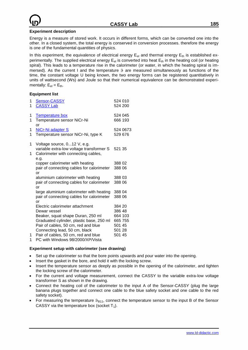
CASSY Lab

185

www.ld-didactic.com


Energy is a measure of stored work. It occurs in different forms, which can be converted one into the other. In a closed system, the total energy is conserved in conversion processes. therefore the energy is one of the fundamental quantities of physics.

In this experiment, the equivalence of electrical energy Eel and thermal energy Eth is established ex-

perimentally. The supplied electrical energy Eel is converted into heat Eth in the heating coil (or heating

spiral). This leads to a temperature rise in the calorimeter (or water, in which the heating spiral is im-

mersed). As the current I and the temperature are measured simultaneously as functions of the time, the constant voltage U being known, the two energy forms can be registered quantitatively in units of wattsecond (Ws) and Joule so that their numerical equivalence can be demonstrated experi-

mentally: Eel = Eth.

Equipment list

1 Sensor-CASSY 524 010 1 CASSY Lab 524 200 1 Temperature box 524 045 1 Temperature sensor NiCr-Ni 666 193 or 1 NiCr-Ni adapter S 524 0673 1 Temperature sensor NiCr-Ni, type K 529 676 1 Voltage source, 0...12 V, e.g. variable extra-low voltage transformer S 521 35 1 Calorimeter with connecting cables, e.g. copper calorimeter with heating 388 02 pair of connecting cables for calorimeter 388 06 or aluminium calorimeter with heating 388 03 pair of connecting cables for calorimeter 388 06 or large aluminium calorimeter with heating 388 04 pair of connecting cables for calorimeter 388 06 or Electric calorimeter attachment 384 20 Dewar vessel 386 48 Beaker, squat shape Duran, 250 ml 664 103 Graduated cylinder, plastic base, 250 ml 665 755 Pair of cables, 50 cm, red and blue 501 45 Connecting lead, 50 cm, black 501 28 1 Pair of cables, 50 cm, red and blue 501 45 1 PC with Windows 98/2000/XP/Vista

Experiment setup with calorimeter (see drawing)

Set up the calorimeter so that the bore points upwards and pour water into the opening.

Insert the gasket in the bore, and hold it with the locking screw.

Insert the temperature sensor as deeply as possible in the opening of the calorimeter, and tighten the locking screw of the calorimeter.

For the current and voltage measurement, connect the CASSY to the variable extra-low voltage transformer S as shown in the drawing.

Connect the heating coil of the calorimeter to the input A of the Sensor-CASSY (plug the large banana plugs together and connect one cable to the blue safety socket and one cable to the red safety socket).

For measuring the temperature B11, connect the temperature sensor to the input B of the Sensor

CASSY via the temperature box (socket T1).

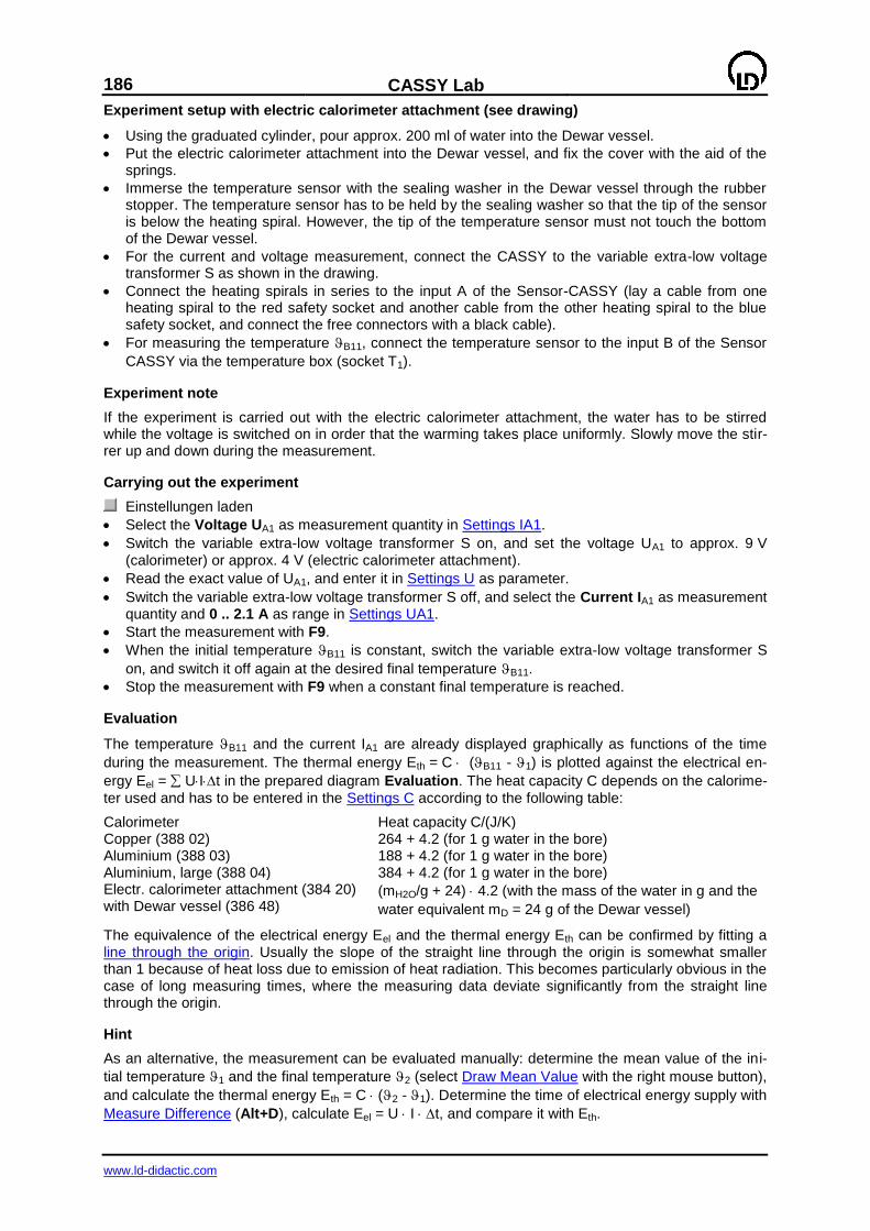
186

CASSY Lab

www.ld-didactic.com

Experiment setup with electric calorimeter attachment (see drawing)

Using the graduated cylinder, pour approx. 200 ml of water into the Dewar vessel.

Put the electric calorimeter attachment into the Dewar vessel, and fix the cover with the aid of the springs.

Immerse the temperature sensor with the sealing washer in the Dewar vessel through the rubber stopper. The temperature sensor has to be held by the sealing washer so that the tip of the sensor is below the heating spiral. However, the tip of the temperature sensor must not touch the bottom of the Dewar vessel.

For the current and voltage measurement, connect the CASSY to the variable extra-low voltage transformer S as shown in the drawing.

Connect the heating spirals in series to the input A of the Sensor-CASSY (lay a cable from one heating spiral to the red safety socket and another cable from the other heating spiral to the blue safety socket, and connect the free connectors with a black cable).

For measuring the temperature B11, connect the temperature sensor to the input B of the Sensor

CASSY via the temperature box (socket T1).

Experiment note

If the experiment is carried out with the electric calorimeter attachment, the water has to be stirred while the voltage is switched on in order that the warming takes place uniformly. Slowly move the stir-rer up and down during the measurement.


Einstellungen laden

Select the Voltage UA1 as measurement quantity in Settings IA1.

Switch the variable extra-low voltage transformer S on, and set the voltage UA1 to approx. 9 V (calorimeter) or approx. 4 V (electric calorimeter attachment).

Read the exact value of UA1, and enter it in Settings U as parameter.

Switch the variable extra-low voltage transformer S off, and select the Current IA1 as measurement quantity and 0 .. 2.1 A as range in Settings UA1.


When the initial temperature B11 is constant, switch the variable extra-low voltage transformer S

on, and switch it off again at the desired final temperature B11.

Stop the measurement with F9 when a constant final temperature is reached.

Evaluation

The temperature B11 and the current IA1 are already displayed graphically as functions of the time

during the measurement. The thermal energy Eth = C (B11 - 1) is plotted against the electrical en-

ergy Eel = UIt in the prepared diagram Evaluation. The heat capacity C depends on the calorime-

ter used and has to be entered in the Settings C according to the following table:

Calorimeter Heat capacity C/(J/K) Copper (388 02) 264 + 4.2 (for 1 g water in the bore) Aluminium (388 03) 188 + 4.2 (for 1 g water in the bore) Aluminium, large (388 04) 384 + 4.2 (for 1 g water in the bore) Electr. calorimeter attachment (384 20) with Dewar vessel (386 48)

(mH2O/g + 24) 4.2 (with the mass of the water in g and the

water equivalent mD = 24 g of the Dewar vessel)

The equivalence of the electrical energy Eel and the thermal energy Eth can be confirmed by fitting a line through the origin. Usually the slope of the straight line through the origin is somewhat smaller than 1 because of heat loss due to emission of heat radiation. This becomes particularly obvious in the case of long measuring times, where the measuring data deviate significantly from the straight line through the origin.

Hint

As an alternative, the measurement can be evaluated manually: determine the mean value of the ini-

tial temperature 1 and the final temperature 2 (select Draw Mean Value with the right mouse button),

and calculate the thermal energy Eth = C (2 -1). Determine the time of electrical energy supply with

Measure Difference (Alt+D), calculate Eel = U I t, and compare it with Eth.

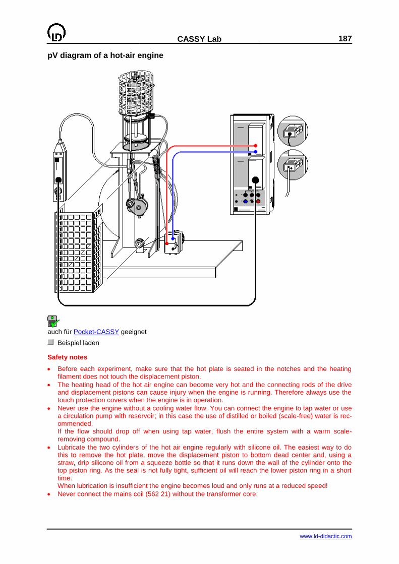
CASSY Lab

187

www.ld-didactic.com

pV diagram of a hot-air engine


Beispiel laden

Safety notes

Before each experiment, make sure that the hot plate is seated in the notches and the heating filament does not touch the displacement piston.

The heating head of the hot air engine can become very hot and the connecting rods of the drive and displacement pistons can cause injury when the engine is running. Therefore always use the touch protection covers when the engine is in operation.

Never use the engine without a cooling water flow. You can connect the engine to tap water or use a circulation pump with reservoir; in this case the use of distilled or boiled (scale-free) water is rec-ommended. If the flow should drop off when using tap water, flush the entire system with a warm scale-removing compound.

Lubricate the two cylinders of the hot air engine regularly with silicone oil. The easiest way to do this to remove the hot plate, move the displacement piston to bottom dead center and, using a straw, drip silicone oil from a squeeze bottle so that it runs down the wall of the cylinder onto the top piston ring. As the seal is not fully tight, sufficient oil will reach the lower piston ring in a short time. When lubrication is insufficient the engine becomes loud and only runs at a reduced speed!

Never connect the mains coil (562 21) without the transformer core.

188

CASSY Lab

www.ld-didactic.com


Thermodynamic cycles are often described as a closed curve in a pV diagram (p: pressure, V: vol-ume). The work added to or withdrawn from the system (depending on the direction of rotation) corre-sponds to the area enclosed by the curve.

This experiment records the pV diagram of a hot air engine operated as a heat engine. The pressure sensor measures the pressure p in the cylinder and a displacement sensor measures the position s, from which the volume is calculated, as a function of the time t. The measured values are displayed on the screen directly in a pV diagram. In the further evaluation, the mechanical work performed as piston friction per cycle

is calculated.

Equipment list

1 Sensor-CASSY 524 010 1 CASSY Lab 524 200 1 Current supply box 524 031 with Displacement transducer and 529 031 Pair of cables, 100 cm, red and blue 501 46 or 1 Rotary motion sensor S 524 082 1 B box 524 038 with Pressure sensor and 529 038 Multicore cable, 6-pole 501 16 or 1 Pressure sensor S, ±2000 hPa 524 064 1 Hot air engine 388 182 1 Cord, 10 m 309 48 1 Helical spring 352 08 1 U-core with yoke 562 11 1 Clamping device 562 12 1 Mains coil, 500 turns 562 21 1 Low-voltage coil, 50 turns 562 18 2 PVC tubing, 8 mm dia. 307 70 1 Immersion pump 12 V 388 181 1 Low-voltage power supply 521 230 1 Can 604 307 2 Connecting leads, 100 cm, black 501 33 1 Water reservoir 10 l 1 PC with Windows 98/2000/XP/Vista


Set up the demountable transformer and clamp the yoke onto it.

Set up the hot plate as described in the experiment setup and connect the heater to the two outermost sockets of the low-voltage coil using the two connecting leads.

Connect the hose of the pressure sensor to the pressure fitting of the working-piston connecting rod. The pressure sensor is connected to the B box at input B of Sensor-CASSY. Attach the displacement transducer to the base plate with two coupling plugs and connect it to input A via the current source box; wind a cord as shown in the diagram. The working piston is provided with a pin with eyelet at the bottom end for attaching the cord. Hang the restoring spring in the hole on the frame head. This must be under tension when the cylinder is at bottom dead center. Wind the cord two times around the pul-ley of the displacement transducer to prevent slip! Set the potentiometer so that a volume of approx.

50 cm3 is indicated when the working cylinder is at top dead center.

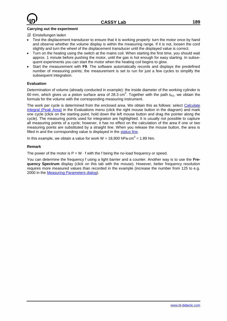
CASSY Lab

189

www.ld-didactic.com


Einstellungen laden

Test the displacement transducer to ensure that it is working properly: turn the motor once by hand and observe whether the volume display is within the measuring range. If it is not, loosen the cord slightly and turn the wheel of the displacement transducer until the displayed value is correct.

Turn on the heating using the switch at the mains coil. When starting the first time, you should wait approx. 1 minute before pushing the motor, until the gas is hot enough for easy starting. In subse-quent experiments you can start the motor when the heating coil begins to glow.

Start the measurement with F9. The software automatically records and displays the predefined number of measuring points; the measurement is set to run for just a few cycles to simplify the subsequent integration.

Evaluation

Determination of volume (already conducted in example): the inside diameter of the working cylinder is

60 mm, which gives us a piston surface area of 28.3 cm2. Together with the path sA1, we obtain the

formula for the volume with the corresponding measuring instrument.

The work per cycle is determined from the enclosed area. We obtain this as follows: select Calculate Integral (Peak Area) in the Evaluations menu (click the right mouse button in the diagram) and mark one cycle (click on the starting point, hold down the left mouse button and drag the pointer along the cycle). The measuring points used for integration are highlighted. It is usually not possible to capture all measuring points of a cycle; however, it has no effect on the calculation of the area if one or two measuring points are substituted by a straight line. When you release the mouse button, the area is filled in and the corresponding value is displayed in the status line.

In this example, we obtain a value for work W = 18,900 hPacm3 = 1.89 Nm.

Remark

The power of the motor is P = W f with the f being the no-load frequency or speed.

You can determine the frequency f using a light barrier and a counter. Another way is to use the Fre-quency Spectrum display (click on this tab with the mouse). However, better frequency resolution requires more measured values than recorded in the example (increase the number from 125 to e.g. 2000 in the Measuring Parameters dialog).

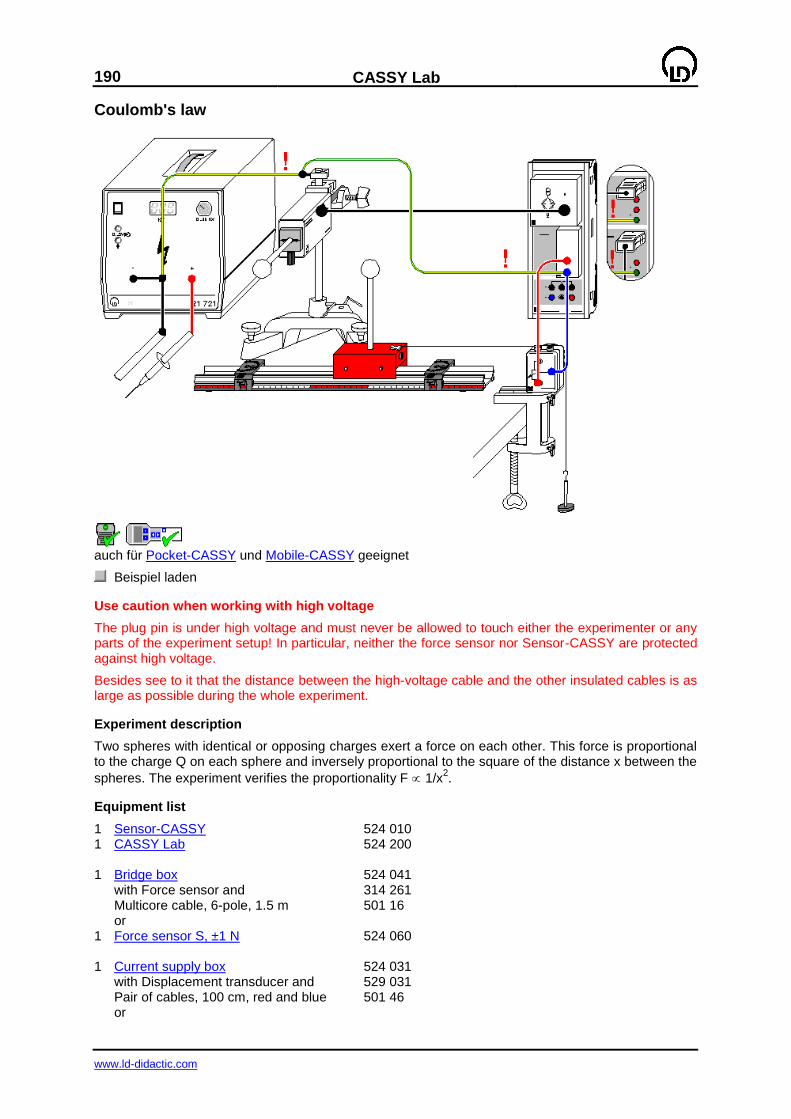
190

CASSY Lab

www.ld-didactic.com

Coulomb's law

auch für Pocket-CASSY und Mobile-CASSY geeignet

Beispiel laden

Use caution when working with high voltage

The plug pin is under high voltage and must never be allowed to touch either the experimenter or any parts of the experiment setup! In particular, neither the force sensor nor Sensor-CASSY are protected against high voltage.

Besides see to it that the distance between the high-voltage cable and the other insulated cables is as large as possible during the whole experiment.


Two spheres with identical or opposing charges exert a force on each other. This force is proportional to the charge Q on each sphere and inversely proportional to the square of the distance x between the

spheres. The experiment verifies the proportionality F 1/x2.

Equipment list

1 Sensor-CASSY 524 010 1 CASSY Lab 524 200 1 Bridge box 524 041 with Force sensor and 314 261 Multicore cable, 6-pole, 1.5 m 501 16 or 1 Force sensor S, ±1 N 524 060 1 Current supply box 524 031 with Displacement transducer and 529 031 Pair of cables, 100 cm, red and blue 501 46 or

CASSY Lab

191

www.ld-didactic.com

1 Rotary motion sensor S 524 082 1 High voltage power supply 25 kV 521 721 1 High-voltage cable 501 05 1 Set of bodies for electric charge 314 263 1 Precision metal rail 460 82 1 Trolley 1, 85 g 337 00 2 Clamp rider 460 95 1 Small clip plug 590 02 1 Connection rod 532 16 1 Stand rod, 25 cm 300 41 1 Stand base, V-shape, 20 cm 300 02 1 Leybold multiclamp 301 01 1 Set of driving weights 337 04 1 Bench clamp, simple 301 07 1 Cord, 10 m 309 48 1 Connecting lead, 25 cm, black 500 414 3 Connecting leads, 100 cm, black 500 444 1 PC with Windows 98/2000/XP/Vista


The force sensor is connected to the bridge box at input A of Sensor-CASSY. Place one of the spheres from the set of bodies for electric charge on the force sensor using the insulating spacer. Place the second sphere on the trolley, which should be able to move freely along the precision metal rail as far as the clamp rider.

The distance between the spheres is measured by the displacement transducer connected to the cur-rent supply box at input B of Sensor-CASSY. To this end, lay a thread from the trolley over the deflec-

tion pulley of the motion transducer and tie a weight to it. Make sure the path indicator sB1 increases with the distance and reads approx. 0 cm at contact.

For safety reasons the current supply box and the force sensor have to be grounded. Connect the force sensor to the ground socket of the high voltage power supply using a clip plug and a connecting lead.

Experiment notes

Imparting sufficient charge to the spheres, and maintaining this charge (at least during the brief period of this experiment), is an essential prerequisite for the success of this experiment. After charging the two spheres, you should be able to measure a force of at least 5 mN at a distance of 0.5 cm, and this force should remain constant for a few seconds. If not:

Clean the insulators and spheres (e.g. with water and dish soap; rinse with distilled water)

Dry the insulators and spheres (e.g. carefully with the non-luminous flame of a Bunsen burner or with hot air from a blow dryer).

Avoid open flames in the vicinity of the experiment while conducting the experiment (otherwise this ionizes the air).

You can try other charge sources (e.g. a PVC rod rubbed in freshly washed hair) as an alternative to the high voltage source.

However, you need dry weather for this.


Einstellungen laden

Calibrate the path zero point: allow the spheres to touch, select Correct in the Settings sB1 dialog, set the first target value to 3.8 cm (distance between sphere centers) and click on Correct Offset.

Put the spheres in the starting position with a gap of about 0.5 cm between them.

Discharge both spheres using the grounded connection rod.

Set the force zero point in Settings FA1 with —> 0 <— (repeat as required) and, where necessary, switch on the smoothing LED of the bridge box with LED On/Off.

Charge the spheres with like or unlike charges by connecting one pole of the high voltage supply to ground and placing the other against the sphere for a few seconds. This should produce a force of

192

CASSY Lab

www.ld-didactic.com

at least 5 mN (see experiment notes above). If necessary, you can change the zero point of the force instrument (and thus the y-axis of the diagram) in Settings FA1 from center to left or right.


Slowly move the trolley away from the force sensor by hand.

Stop the measurement with F9 at approx. 15 cm.

Evaluation

The F(x) diagram appears during the measurement. You can verify Coulomb's law by fitting a hyper-

bola 1/x2 or by converting the x-axis to 1/x

2 (click on the axis with the right mouse button) and then

fitting a straight line.

It becomes apparent that the proportionality F 1/x2 does not apply until a distance of approx. 6 cm

between the two sphere centers is reached. At shorter distances the spacing would have to be cor-rected, as these are not point-shaped charges.

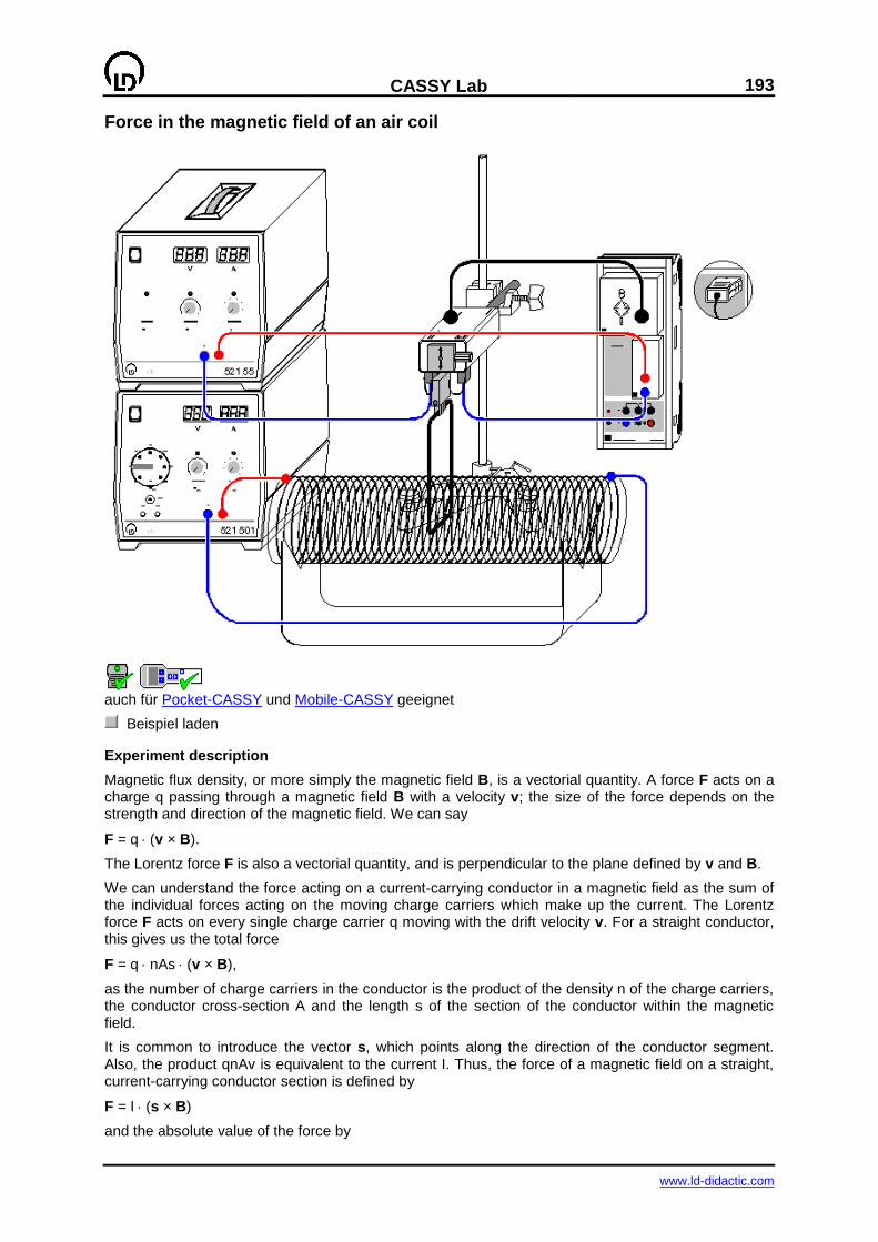
CASSY Lab

193

www.ld-didactic.com

Force in the magnetic field of an air coil


Beispiel laden


Magnetic flux density, or more simply the magnetic field B, is a vectorial quantity. A force F acts on a charge q passing through a magnetic field B with a velocity v; the size of the force depends on the strength and direction of the magnetic field. We can say

F = q (v × B).

The Lorentz force F is also a vectorial quantity, and is perpendicular to the plane defined by v and B.

We can understand the force acting on a current-carrying conductor in a magnetic field as the sum of the individual forces acting on the moving charge carriers which make up the current. The Lorentz force F acts on every single charge carrier q moving with the drift velocity v. For a straight conductor, this gives us the total force

F = q nAs (v × B),

as the number of charge carriers in the conductor is the product of the density n of the charge carriers, the conductor cross-section A and the length s of the section of the conductor within the magnetic field.

It is common to introduce the vector s, which points along the direction of the conductor segment. Also, the product qnAv is equivalent to the current I. Thus, the force of a magnetic field on a straight, current-carrying conductor section is defined by

F = I (s × B)

and the absolute value of the force by

194

CASSY Lab

www.ld-didactic.com

F = I s B,

when s and B are perpendicular to each other. The force F and the current I are thus proportional to each other, and the proportionality factor is B.

This experiment measures the force on a conductor loop in a homogeneous magnetic field of an air coil as a function of the conductor loop current I. The homogeneous magnetic field is generated in a long, slotted air coil, and the conductor loop with the length s = 8 cm attached to the force sensor is inserted in the slit. Only the horizontal part of the conductor generates a force component that can be measured by the force sensor. Thus, the proportionality between force F and conductor loop current I can be used to determine the magnetic flux density B.

The advantage of the air coil is that the magnetic flux density B within it can be calculated easily and compared with the value arrived at through experiment. For a long air coil, we can say

B = 0N IC / L

with the magnetic field constant 0 = 410-7

Vs/Am, the number of turns N of the coils, the coil current

IC and the length L of the air coil.

Equipment list

1 Sensor-CASSY 524 010 1 CASSY Lab 524 200 1 Bridge box 524 041 with Force sensor and 314 261 Multicore cable, 6-pole, 1.5 m 501 16 or 1 Force sensor S, ±1 N 524 060 1 30-A box 524 043 1 Support for conductor loops 314 265 1 Conductor loops for force measurement 516 34 1 Field coil, d = 120 mm 516 244 1 Stand for coils and tubes 516 249 1 High current power supply 521 55 1 AC/DC power supply 0...15 V 521 501 1 Stand base, V-shape, 20 cm 300 02 1 Stand rod, 47 cm 300 42 1 Leybold multiclamp 301 01 1 Connecting lead, 50 cm, blue 501 26 2 Connecting leads, 100 cm, red 501 30 2 Connecting leads, 100 cm, blue 501 31 1 PC with Windows 98/2000/XP/Vista


The force sensor holds the 8 cm long conductor loop via the support and is positioned so that the con-ductor loop is inserted in the slot of the air coil. The conductor loop must not touch the air coil. The two 4-mm sockets on the bottom of the force sensor are intended for supplying the conductor loop support. They are not connected internally. The force sensor is connected to the bridge box at input A of Sen-sor-CASSY.

The current flows from the 20 A supply unit via the 30 A box on input B of Sensor-CASSY through the conductor loop and back to the power supply. The current of the second 5 A power supply flows through the air coil.


Einstellungen laden

Set the force zero point in Settings Force FA1 with —> 0 <— and, where necessary, switch on the smoothing LED of the bridge box with LED On/Off.

You may want to correct the current value to 0 A in Settings Current IB1 (set the first target value to 0 A and click Correct Offset).

CASSY Lab

195

www.ld-didactic.com

At the power supply of the air coil, set about IC = 5 A.

Increase the conductor loop current I from 0-20 A in steps of 2 to 5 A, and record a measured value with F9 each time. You can delete a faulty measurement from the table with Delete Last Ta-ble Row (click right mouse button over table).

If only negative forces are measured, reverse the connections on the conductor loop support.

Carry out the experiment rapidly, as the conductor loop and support may be subjected to loads of 20 A only briefly.

At the end of the experiment, set the conductor loop current to 0 A.

Evaluation

The force increases linearly with the current. The proportionality factor F/I = Bs is derived from the slope of the straight line fit. This in turn enables us to determine the magnetic field strength B.

In this example F/I = 0.138 mN/A and with s = 0.08 m it follows that B = 1.725 mT.

Using B = 0N IC / L the values 0 = 1.257 Vs/Am, N = 120, IC = 4.75 A and L = 0.41 m give us the calculated value B = 1.75 mT. The two results agree very well within the limits of measuring accuracy.

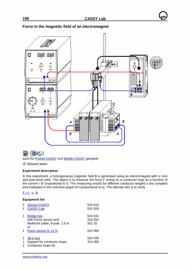
196

CASSY Lab

www.ld-didactic.com

Force in the magnetic field of an electromagnet


Beispiel laden


In this experiment, a homogeneous magnetic field B is generated using an electromagnet with U core and pole-shoe yoke. The object is to measure the force F acting on a conductor loop as a function of the current I (F proportional to I). The measuring results for different conductor lengths s are compiled and evaluated in the overview graph (F/I proportional to s). The ultimate aim is to verify

F = I s B

Equipment list

1 Sensor-CASSY 524 010 1 CASSY Lab 524 200 1 Bridge box 524 041 with Force sensor and 314 261 Multicore cable, 6-pole, 1.5 m 501 16 or 1 Force sensor S, ±1 N 524 060 1 30-A box 524 043 1 Support for conductor loops 314 265 1 Conductor loops for

CASSY Lab

197

www.ld-didactic.com

force measurement 516 34 1 U-core with yoke 562 11 2 Coils with 500 turns 562 14 1 Pole-shoe yoke 562 25 1 High current power supply 521 55 1 AC/DC power supply 0...15 V 521 501 1 Stand base, V-shape, 20 cm 300 02 1 Stand rod, 47 cm 300 42 1 Leybold multiclamp 301 01 2 Connecting leads, 50 cm, blue 501 26 2 Connecting leads, 100 cm, red 501 30 2 Connecting leads, 100 cm, blue 501 31 1 PC with Windows 98/2000/XP/Vista


Slide the two coils onto the U-core. Place the two heavy pole pieces transversely on top of them. You can adjust the height using the lateral stand. The gap can be changed by moving one of the two pole pieces and adjusted with non-magnetic spacers.

The force sensor holds a conductor loop via the support and is positioned so that the conductor loop is inserted in the gap between the pole pieces of the electromagnet. The conductor loop must not touch the pole pieces. The two 4-mm sockets on the bottom of the force sensor are intended for supplying the conductor loop support. They are not connected internally. The force sensor is connected to the bridge box at input A of Sensor-CASSY.

The current flows from the 20 A supply unit via the 30 A box on input B of Sensor-CASSY through the conductor loop and back to the power supply. The current of the second 5 A power supply flows through the two coils on series. Make sure that the magnetic fields of the two coils add together (con-nect A to A and both E to the power supply as shown in the drawing).


Einstellungen laden



At the power supply of the coils, set about 2.5 A.

Increase the conductor loop current I from 0-20 A in steps of 2 to 5 A, and record a measured value with F9 each time. You can delete a faulty measurement series from the table with Delete Last Table Row (click right mouse button over table).




Record additional measurement curves with a different conductor loop length s. In the Measuring Parameters dialog select Append New Meas. Series.

Evaluation

Fit a straight line to each measurement series F(I). After each best-fit straight line, switch to the display Magnetic Field (click the tab with the mouse). Here, an additional table is filled out by dragging the slope F/I just determined from the status line using the mouse and dropping it next to the respective conductor loop length (drag & drop). Enter the conductor loop length s directly via the keyboard. The desired diagram is generated as you enter the values.

In this display, the slope of the best-fit straight line gives us the magnetic field strength B between the

pole pieces, as F/I = Bs (in this example, B = 164 mN/(Am) = 164 mT).

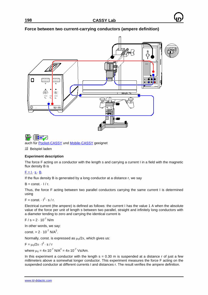
198

CASSY Lab

www.ld-didactic.com

Force between two current-carrying conductors (ampere definition)


Beispiel laden


The force F acting on a conductor with the length s and carrying a current I in a field with the magnetic flux density B is

F = I s B.

If the flux density B is generated by a long conductor at a distance r, we say

B = const. I / r.

Thus, the force F acting between two parallel conductors carrying the same current I is determined using

F = const. I2s / r.

Electrical current (the ampere) is defined as follows: the current I has the value 1 A when the absolute value of the force per unit of length s between two parallel, straight and infinitely long conductors with a diameter tending to zero and carrying the identical current is

F / s = 2 10-7

N/m

In other words, we say:

const. = 2 10-7

N/A2.

Normally, const. is expressed as 0/2, which gives us:

F = 0/2I2s / r

where 0 = 410-7

N/A2 = 410

-7 Vs/Am.

In this experiment a conductor with the length s = 0.30 m is suspended at a distance r of just a few millimeters above a somewhat longer conductor. This experiment measures the force F acting on the suspended conductor at different currents I and distances r. The result verifies the ampere definition.

CASSY Lab

199

www.ld-didactic.com

Equipment list

1 Sensor-CASSY 524 010 1 CASSY Lab 524 200 1 Bridge box 524 041 with Force sensor and 314 261 Multicore cable, 6-pole, 1.5 m 501 16 or 1 Force sensor S, ±1 N 524 060 1 30-A box 524 043 1 Support for conductor loops 314 265 1 Set of conductors for ampere definition 516 33 1 Vertically adjustable stand 516 31 1 High current power supply 521 55 1 Stand base, V-shape, 20 cm 300 02 1 Stand rod, 47 cm 300 42 1 Leybold multiclamp 301 01 2 Connecting leads, 50 cm, blue 501 26 1 Connecting lead, 100 cm, red 501 30 1 Connecting lead, 100 cm, blue 501 31 1 PC with Windows 98/2000/XP/Vista


The force sensor holds the top conductor loop with the support and is positioned so that the distance between the two conductor loops is about 5 mm for medium extension of the vertically adjustable stand.

The two 4-mm sockets on the bottom of the force sensor are intended for supplying the conductor loop support. They are not connected internally. The force sensor is connected to the bridge box at input A of Sensor-CASSY. The current flows from the 20 A supply unit via the 30 A box on input B of Sensor-CASSY through the two conductor loops in series and back to the power supply.

Now, slowly bring the conductor loop on the stand closer to the suspended conductor loop until the two are just touching (the wire centers now have the distance r = 2 mm). Check to make sure that the vertically adjustable stand is still parallel to the conductor loop, and adjust it if necessary using the adjusting screws.

Set the zero-point slider of the vertically adjustable stand to a defined mark and set the desired dis-tance between the two conductor loops using the height adjustment mechanism (e.g. r = 4 mm).

Good measuring results require careful adjustment here.


Einstellungen laden



Increase the conductor loop current I from 0-20 A in steps of 2 A, and record measured values with F9 each time. You can delete a faulty measurement series from the table with Delete Last Table Row (click right mouse button over table).




Record additional measurement curves with different conductor spacings r. In the Measuring Pa-rameters dialog select Append New Meas. Series.

200

CASSY Lab

www.ld-didactic.com

Evaluation

Fit a parabola to each measurement series F(I). After each best-fit straight line, switch to the display Ampere Definition (click the tab with the mouse). Here, an additional table is filled out by dragging

the parameter F/I2 of the parabola just determined from the status line using the mouse and dropping it

next to the respective conductor loop spacing r in the table (drag & drop). Enter the conductor loop spacing r directly via the keyboard. The desired diagram is generated as you enter the values.

In this display, the parameter F/I2r of a hyperbola 1/x gives us the constant for the ampere definition

as

0/2 = F/I2r / s = F/I

2r / 0.3 m.

In our example this means

0/2 = 0.000062 mNm/A2 / 0.3 m = 2.110

-7 N/A

2 = 2.110

-7 Vs/Am.

Alternatively, you can convert the x-axis from r to 1/r in the ampere definition display (click on the axis

with the right mouse button). In this display, we obtain the value 0/2 by fitting a straight line.

Remark

This measurement contains systematic errors. For one thing, the conductor has a finite length. That means that the assumed magnetic field does not exist at the end of the conductor, so that the forces are less. Additionally, a minute opposing force component acts on the suspended conductor due to the conductor segment running upward.

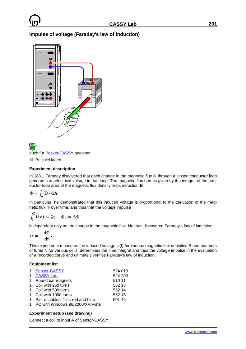
CASSY Lab

201

www.ld-didactic.com

Impulse of voltage (Faraday's law of induction)


Beispiel laden


In 1831, Faraday discovered that each change in the magnetic flux through a closed conductor loop generates an electrical voltage in that loop. The magnetic flux here is given by the integral of the con-ductor-loop area of the magnetic flux density resp. induction B

In particular, he demonstrated that this induced voltage is proportional to the derivation of the mag-

netic flux over time, and thus that the voltage impulse

is dependent only on the change in the magnetic flux. He thus discovered Faraday's law of induction

This experiment measures the induced voltage U(t) for various magnetic flux densities B and numbers of turns N for various coils, determines the time integral and thus the voltage impulse in the evaluation of a recorded curve and ultimately verifies Faraday's law of induction.

Equipment list

1 Sensor-CASSY 524 010 1 CASSY Lab 524 200 2 Round bar magnets 510 11 1 Coil with 250 turns 562 13 1 Coil with 500 turns 562 14 1 Coil with 1000 turns 562 15 1 Pair of cables, 1 m, red and blue 501 46 1 PC with Windows 98/2000/XP/Vista


Connect a coil to input A of Sensor-CASSY.

202

CASSY Lab

www.ld-didactic.com


a) Measuring as a function of the magnetic flux

Einstellungen laden

Connect the coil with 250 turns to input A.


Insert one magnet half-way and remove it.

Stop the measurement with F9 (or the measurement stops automatically after 10 seconds).

Start the measurement with F9 and wait until the new measurement has proceeded far enough so that it no longer covers the old measurement.

Insert two magnets half-way and remove them.


b) Measuring as a function of the number of turns N

Einstellungen laden



Insert the magnet half-way and remove it.










Evaluation

In experiment part a), the integral quickly reveals that the voltage impulses have the same absolute value but different signs when the magnet is inserted in and withdrawn from the coil, i.e.

The use of two magnets additionally verifies the proportionality between the voltage impulses and the number of magnets used resp. the difference in the magnetic flux produced in this manner:

By means of differentiation we verify Faraday's law of induction

The magnetic flux through a coil depends on the number of turns, as each individual turn causes a flux

difference 0 and the total flux is calculated as = N 0.

When we look at experiment part b), the relationship between a voltage impulse and the number of turns N of the respective coil, we can also confirm this relationship. To do this we determine e.g. all positive areas and enter these in the Number of Turns display together with the number of turns N (click on the correct table cells). Once again, the proportionality gives us

The slope of the straight line in the display of voltage impulses as a function of the number of turns

corresponds to the magnetic flux 0 generated by the magnet in each individual coil winding.

CASSY Lab

203

www.ld-didactic.com

Hints on integration

To integrate, you need to find the start of the range, which is not always easy when multiple curves are superimposed. It is easier when the measurement is stopped with F9 immediately following the volt-age impulse (do not wait for the 10 seconds to elapse) and the integral is calculated immediately after measuring. If you wait until after the end of the previous measuring curve before starting the next volt-age impulse measurement, no curve covers the others while integrating.

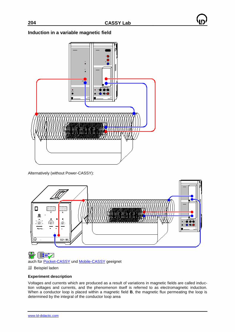
204

CASSY Lab

www.ld-didactic.com

Induction in a variable magnetic field

Alternatively (without Power-CASSY):


Beispiel laden


Voltages and currents which are produced as a result of variations in magnetic fields are called induc-tion voltages and currents, and the phenomenon itself is referred to as electromagnetic induction. When a conductor loop is placed within a magnetic field B, the magnetic flux permeating the loop is determined by the integral of the conductor loop area

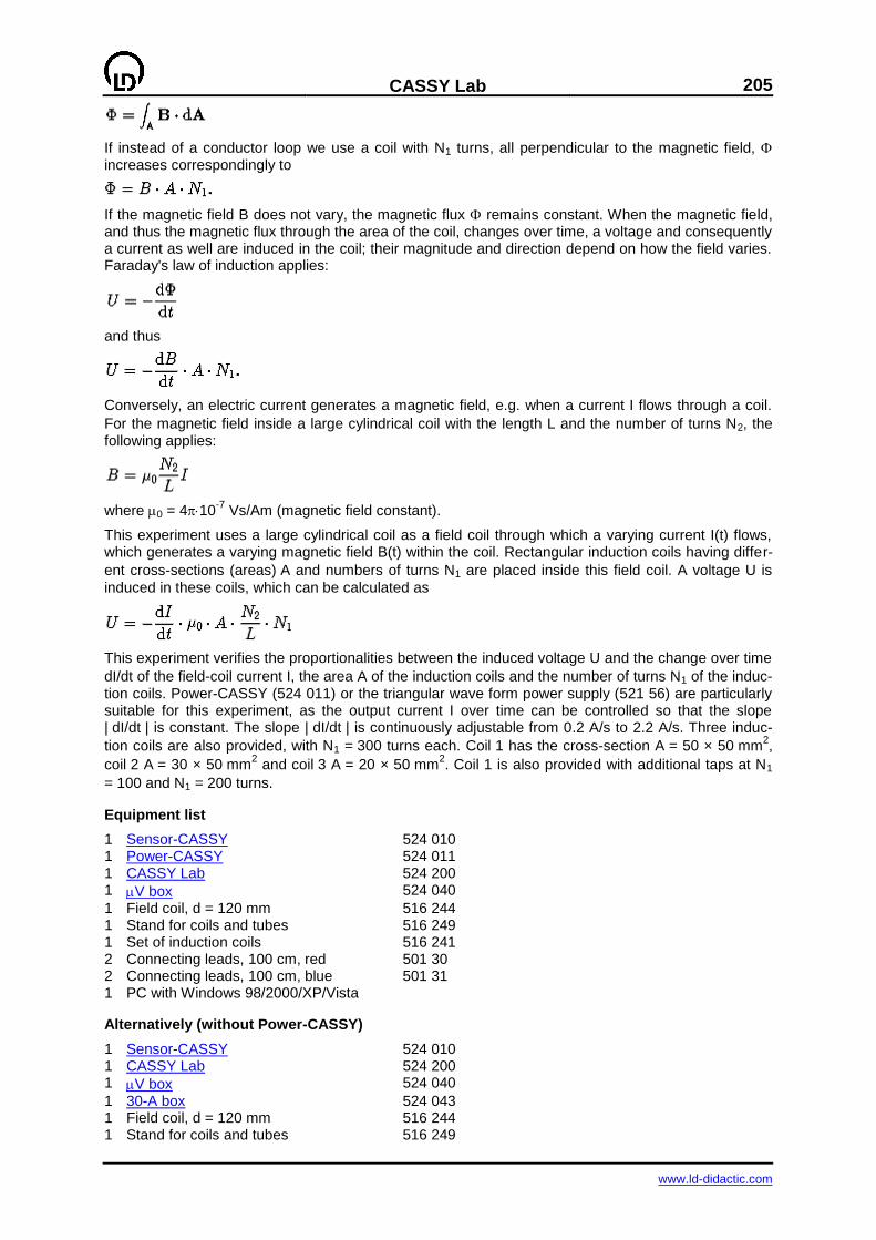
CASSY Lab

205

www.ld-didactic.com

If instead of a conductor loop we use a coil with N1 turns, all perpendicular to the magnetic field, increases correspondingly to

If the magnetic field B does not vary, the magnetic flux remains constant. When the magnetic field, and thus the magnetic flux through the area of the coil, changes over time, a voltage and consequently a current as well are induced in the coil; their magnitude and direction depend on how the field varies. Faraday's law of induction applies:

and thus

Conversely, an electric current generates a magnetic field, e.g. when a current I flows through a coil.

For the magnetic field inside a large cylindrical coil with the length L and the number of turns N2, the following applies:

where 0 = 410-7

Vs/Am (magnetic field constant).

This experiment uses a large cylindrical coil as a field coil through which a varying current I(t) flows, which generates a varying magnetic field B(t) within the coil. Rectangular induction coils having differ-

ent cross-sections (areas) A and numbers of turns N1 are placed inside this field coil. A voltage U is

induced in these coils, which can be calculated as

This experiment verifies the proportionalities between the induced voltage U and the change over time

dI/dt of the field-coil current I, the area A of the induction coils and the number of turns N1 of the induc-tion coils. Power-CASSY (524 011) or the triangular wave form power supply (521 56) are particularly suitable for this experiment, as the output current I over time can be controlled so that the slope | dI/dt | is constant. The slope | dI/dt | is continuously adjustable from 0.2 A/s to 2.2 A/s. Three induc-

tion coils are also provided, with N1 = 300 turns each. Coil 1 has the cross-section A = 50 × 50 mm2,

coil 2 A = 30 × 50 mm2 and coil 3 A = 20 × 50 mm

2. Coil 1 is also provided with additional taps at N1

= 100 and N1 = 200 turns.

Equipment list

1 Sensor-CASSY 524 010 1 Power-CASSY 524 011 1 CASSY Lab 524 200 1 V box 524 040

1 Field coil, d = 120 mm 516 244 1 Stand for coils and tubes 516 249 1 Set of induction coils 516 241 2 Connecting leads, 100 cm, red 501 30 2 Connecting leads, 100 cm, blue 501 31 1 PC with Windows 98/2000/XP/Vista

Alternatively (without Power-CASSY)

1 Sensor-CASSY 524 010 1 CASSY Lab 524 200 1 V box 524 040

1 30-A box 524 043 1 Field coil, d = 120 mm 516 244 1 Stand for coils and tubes 516 249

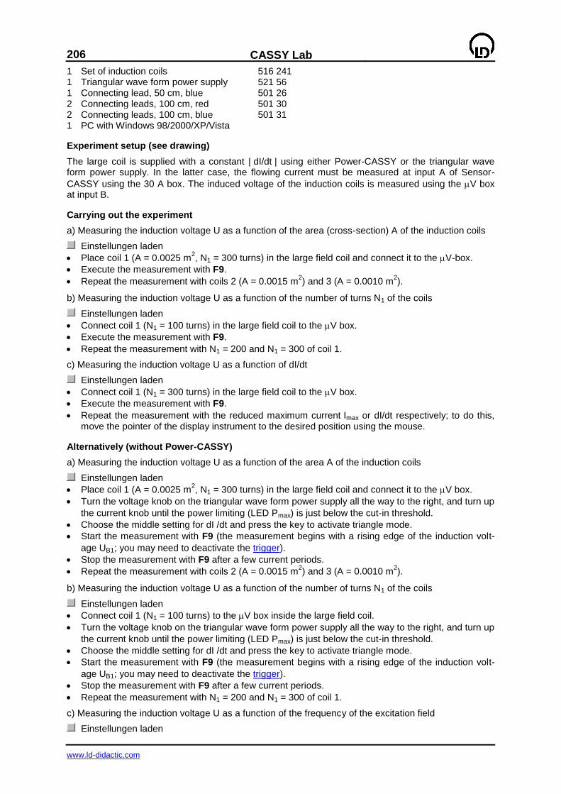
206

CASSY Lab

www.ld-didactic.com

1 Set of induction coils 516 241 1 Triangular wave form power supply 521 56 1 Connecting lead, 50 cm, blue 501 26 2 Connecting leads, 100 cm, red 501 30 2 Connecting leads, 100 cm, blue 501 31 1 PC with Windows 98/2000/XP/Vista


The large coil is supplied with a constant | dI/dt | using either Power-CASSY or the triangular wave form power supply. In the latter case, the flowing current must be measured at input A of Sensor-

CASSY using the 30 A box. The induced voltage of the induction coils is measured using the V box at input B.


a) Measuring the induction voltage U as a function of the area (cross-section) A of the induction coils

Einstellungen laden

Place coil 1 (A = 0.0025 m2, N1 = 300 turns) in the large field coil and connect it to the V-box.

Execute the measurement with F9.

Repeat the measurement with coils 2 (A = 0.0015 m2) and 3 (A = 0.0010 m

2).

b) Measuring the induction voltage U as a function of the number of turns N1 of the coils

Einstellungen laden

Connect coil 1 (N1 = 100 turns) in the large field coil to the V box.


Repeat the measurement with N1 = 200 and N1 = 300 of coil 1.

c) Measuring the induction voltage U as a function of dI/dt

Einstellungen laden

Connect coil 1 (N1 = 300 turns) in the large field coil to the V box.


Repeat the measurement with the reduced maximum current Imax or dI/dt respectively; to do this, move the pointer of the display instrument to the desired position using the mouse.


a) Measuring the induction voltage U as a function of the area A of the induction coils

Einstellungen laden

Place coil 1 (A = 0.0025 m2, N1 = 300 turns) in the large field coil and connect it to the V box.

Turn the voltage knob on the triangular wave form power supply all the way to the right, and turn up

the current knob until the power limiting (LED Pmax) is just below the cut-in threshold.

Choose the middle setting for dI /dt and press the key to activate triangle mode.

Start the measurement with F9 (the measurement begins with a rising edge of the induction volt-

age UB1; you may need to deactivate the trigger).

Stop the measurement with F9 after a few current periods.

Repeat the measurement with coils 2 (A = 0.0015 m2) and 3 (A = 0.0010 m

2).

b) Measuring the induction voltage U as a function of the number of turns N1 of the coils

Einstellungen laden

Connect coil 1 (N1 = 100 turns) to the V box inside the large field coil.





age UB1; you may need to deactivate the trigger).

Stop the measurement with F9 after a few current periods.

Repeat the measurement with N1 = 200 and N1 = 300 of coil 1.

c) Measuring the induction voltage U as a function of the frequency of the excitation field

Einstellungen laden

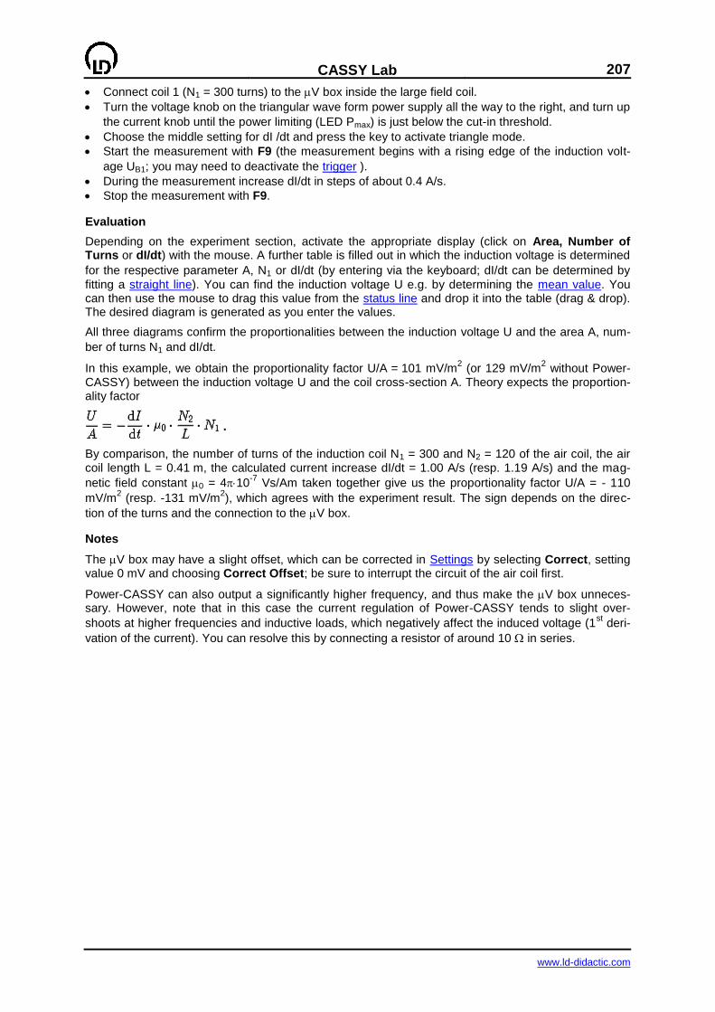
CASSY Lab

207

www.ld-didactic.com

Connect coil 1 (N1 = 300 turns) to the V box inside the large field coil.





age UB1; you may need to deactivate the trigger ).

During the measurement increase dI/dt in steps of about 0.4 A/s.


Evaluation

Depending on the experiment section, activate the appropriate display (click on Area, Number of Turns or dI/dt) with the mouse. A further table is filled out in which the induction voltage is determined

for the respective parameter A, N1 or dI/dt (by entering via the keyboard; dI/dt can be determined by

fitting a straight line). You can find the induction voltage U e.g. by determining the mean value. You can then use the mouse to drag this value from the status line and drop it into the table (drag & drop). The desired diagram is generated as you enter the values.

All three diagrams confirm the proportionalities between the induction voltage U and the area A, num-

ber of turns N1 and dI/dt.

In this example, we obtain the proportionality factor U/A = 101 mV/m2 (or 129 mV/m

2 without Power-

CASSY) between the induction voltage U and the coil cross-section A. Theory expects the proportion-ality factor

By comparison, the number of turns of the induction coil N1 = 300 and N2 = 120 of the air coil, the air coil length L = 0.41 m, the calculated current increase dI/dt = 1.00 A/s (resp. 1.19 A/s) and the mag-

netic field constant 0 = 410-7

Vs/Am taken together give us the proportionality factor U/A = - 110

mV/m2 (resp. -131 mV/m

2), which agrees with the experiment result. The sign depends on the direc-

tion of the turns and the connection to the V box.

Notes

The V box may have a slight offset, which can be corrected in Settings by selecting Correct, setting value 0 mV and choosing Correct Offset; be sure to interrupt the circuit of the air coil first.

Power-CASSY can also output a significantly higher frequency, and thus make the V box unneces-sary. However, note that in this case the current regulation of Power-CASSY tends to slight over-

shoots at higher frequencies and inductive loads, which negatively affect the induced voltage (1st deri-

vation of the current). You can resolve this by connecting a resistor of around 10 in series.

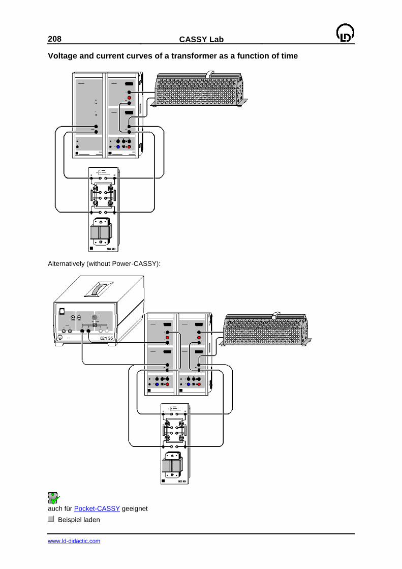
208

CASSY Lab

www.ld-didactic.com

Voltage and current curves of a transformer as a function of time



Beispiel laden

CASSY Lab

209

www.ld-didactic.com


This experiment records the primary and secondary currents and voltages of a transformer under load as time-dependent quantities. From these, CASSY Lab directly calculates the time-dependent power values in the primary and secondary circuit, as well as the RMS values of current and voltage, the phase relation and the active power values.

Equipment list

1 Power-CASSY 524 011 1 Sensor-CASSY 524 010 1 CASSY Lab 524 200 1 Transformer for students' experiments 562 801 1 Rheostat 100 537 34

1 Connecting lead, 25 cm, black 500 414 6 Connecting leads, 100 cm, black 500 444 1 PC with Windows 98/2000/XP/Vista


2 Sensor-CASSYs 524 010 1 CASSY Lab 524 200 1 Variable extra-low voltage transformer S 521 35 1 Transformer for students' experiments 562 801 1 Rheostat 100 537 34

2 Connecting leads, 25 cm, black 500 414 8 Connecting leads, 100 cm, black 500 444 1 PC with Windows 98/2000/XP/Vista


The primary side of the transformer is supplied by Power-CASSY or by the variable transformer

(approx. 6 V AC). In the latter case, the primary voltage, primary current and phase relation (cos ) must be measured using a second Sensor-CASSY unit.

Sensor-CASSY performs the necessary measurements of voltage, current and phase relation (cos )

on the secondary side. The transformer is under resistive load (cos = 1) in the form of a rheostat. However, where available the transformer can also be operated under inductive or capacitive load

(cos < 1). You can improve the response of the transformer to load by connecting two coils each in parallel on the primary and secondary side of the transformer for students' experiments.

In place of the transformer for students' experiments, you can also use the demountable transformer.


Einstellungen laden


Vary the load (e.g. also inductive or capacitive load) and observe the effect on the secondary and primary circuits.

Vary the number of coils on the primary and secondary side of the transformer and observe the behaviour under load.

If desired, alter the curve form or the frequency of the primary voltage in Settings U1 on Power-CASSY and observe the result.


Evaluation

You can change to the Power display with the mouse during or after measuring. This display shows both power values as a function of time.

Hint

You can show and hide all measuring instruments simultaneously with F7.

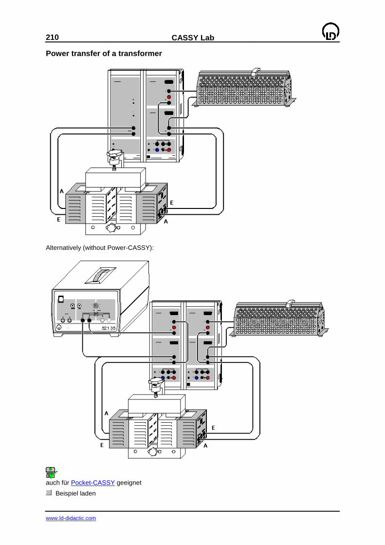
210

CASSY Lab

www.ld-didactic.com

Power transfer of a transformer



Beispiel laden

CASSY Lab

211

www.ld-didactic.com


This experiment examines the power transfer of a transformer. This is done by simultaneously meas-uring the RMS values of the primary and secondary voltage as well as the primary and secondary

current for a variable load resistor R = 0-100 . The experiment also determines the phase shift be-tween the voltage and current on the primary and secondary side. The evaluation determines the pri-

mary power P1, the secondary power P2 and the efficiency = P2/P1 and plots these as a function of

the load resistance R.

Equipment list

1 Power-CASSY 524 011 1 Sensor-CASSY 524 010 1 CASSY Lab 524 200 1 U-core with yoke 562 11 1 Clamping device 562 12 2 Coils with 250 turns 562 13 1 Rheostat 100 537 34

1 Connecting lead, 25 cm, black 500 414 6 Connecting leads, 100 cm, black 500 444 1 PC with Windows 98/2000/XP/Vista


2 Sensor-CASSYs 524 010 1 CASSY Lab 524 200 1 Variable extra-low voltage transformer S 521 35 1 U-core with yoke 562 11 1 Clamping device 562 12 2 Coils with 250 turns 562 13 1 Rheostat 100 537 34

2 Connecting leads, 25 cm, black 500 414 8 Connecting leads, 100 cm, black 500 444 1 PC with Windows 98/2000/XP/Vista


The primary side of the transformer is supplied by Power-CASSY or by the variable transformer

(approx. 6 V AC). In the latter case, the primary voltage, primary current and phase relation (cos ) must be measured using a second Sensor-CASSY unit.

Sensor-CASSY performs the necessary measurements of the RMS values of voltage, current and

their phase relation (cos ) on the secondary side. The transformer is under resistive load (cos = 1) in the form of a rheostat.

Instead of the demountable transformer, you can use the transformer for students' experiments.


Einstellungen laden

Set the rheostat to the minimum position (approx. 0 ).


Increase the resistance in steps and record measured values for each step with F9.

Evaluation

The points of maximum power output and maximum efficiency can be easily read from the diagram.

Hint

You can show and hide all measuring instruments simultaneously with F7.

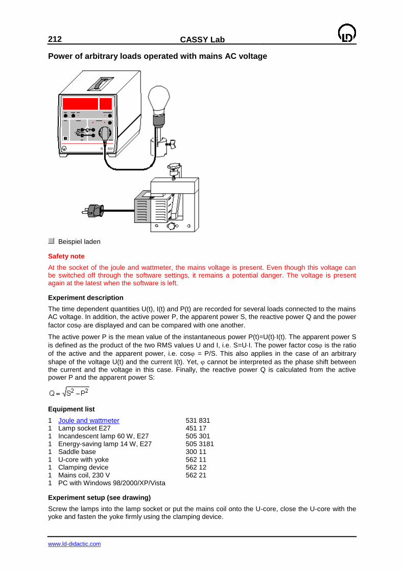
212

CASSY Lab

www.ld-didactic.com

Power of arbitrary loads operated with mains AC voltage

Beispiel laden

Safety note

At the socket of the joule and wattmeter, the mains voltage is present. Even though this voltage can be switched off through the software settings, it remains a potential danger. The voltage is present again at the latest when the software is left.


The time dependent quantities U(t), I(t) and P(t) are recorded for several loads connected to the mains AC voltage. In addition, the active power P, the apparent power S, the reactive power Q and the power

factor cos are displayed and can be compared with one another.

The active power P is the mean value of the instantaneous power P(t)=U(t)I(t). The apparent power S

is defined as the product of the two RMS values U and I, i.e. S=UI. The power factor cos is the ratio

of the active and the apparent power, i.e. cos = P/S. This also applies in the case of an arbitrary

shape of the voltage U(t) and the current I(t). Yet, cannot be interpreted as the phase shift between the current and the voltage in this case. Finally, the reactive power Q is calculated from the active power P and the apparent power S:

Equipment list

1 Joule and wattmeter 531 831 1 Lamp socket E27 451 17 1 Incandescent lamp 60 W, E27 505 301 1 Energy-saving lamp 14 W, E27 505 3181 1 Saddle base 300 11 1 U-core with yoke 562 11 1 Clamping device 562 12 1 Mains coil, 230 V 562 21 1 PC with Windows 98/2000/XP/Vista


Screw the lamps into the lamp socket or put the mains coil onto the U-core, close the U-core with the yoke and fasten the yoke firmly using the clamping device.

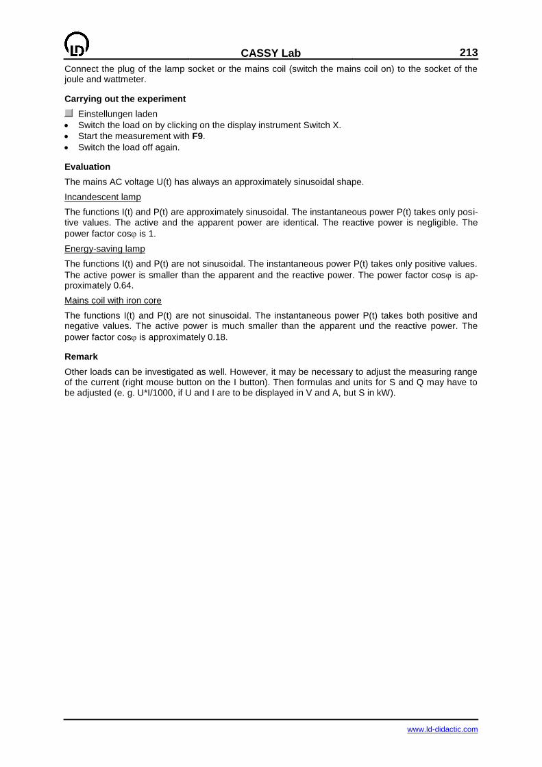
CASSY Lab

213

www.ld-didactic.com

Connect the plug of the lamp socket or the mains coil (switch the mains coil on) to the socket of the joule and wattmeter.


Einstellungen laden

Switch the load on by clicking on the display instrument Switch X.


Switch the load off again.

Evaluation

The mains AC voltage U(t) has always an approximately sinusoidal shape.

Incandescent lamp

The functions I(t) and P(t) are approximately sinusoidal. The instantaneous power P(t) takes only posi-tive values. The active and the apparent power are identical. The reactive power is negligible. The

power factor cos is 1.

Energy-saving lamp

The functions I(t) and P(t) are not sinusoidal. The instantaneous power P(t) takes only positive values.

The active power is smaller than the apparent and the reactive power. The power factor cos is ap-proximately 0.64.

Mains coil with iron core

The functions I(t) and P(t) are not sinusoidal. The instantaneous power P(t) takes both positive and negative values. The active power is much smaller than the apparent und the reactive power. The

power factor cos is approximately 0.18.

Remark

Other loads can be investigated as well. However, it may be necessary to adjust the measuring range of the current (right mouse button on the I button). Then formulas and units for S and Q may have to be adjusted (e. g. U*I/1000, if U and I are to be displayed in V and A, but S in kW).

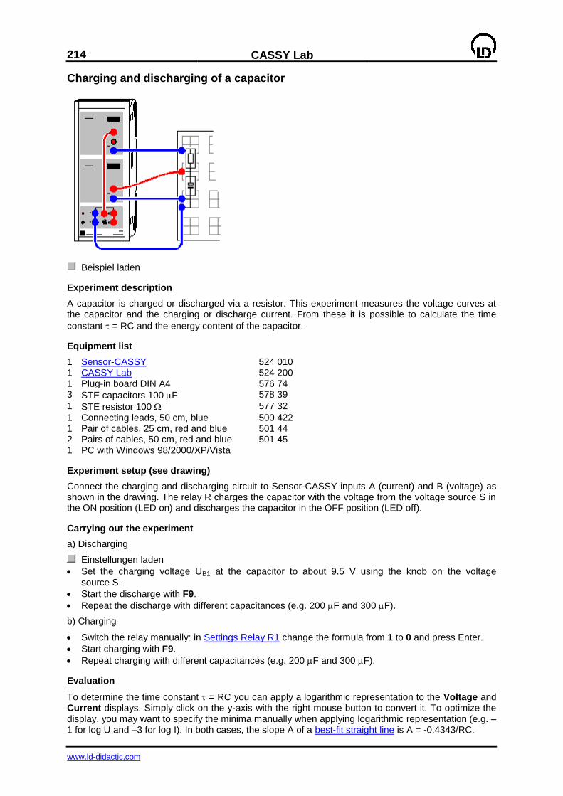
214

CASSY Lab

www.ld-didactic.com

Charging and discharging of a capacitor

Beispiel laden


A capacitor is charged or discharged via a resistor. This experiment measures the voltage curves at the capacitor and the charging or discharge current. From these it is possible to calculate the time

constant = RC and the energy content of the capacitor.

Equipment list

1 Sensor-CASSY 524 010 1 CASSY Lab 524 200 1 Plug-in board DIN A4 576 74 3 STE capacitors 100 F 578 39

1 STE resistor 100 577 32

1 Connecting leads, 50 cm, blue 500 422 1 Pair of cables, 25 cm, red and blue 501 44 2 Pairs of cables, 50 cm, red and blue 501 45 1 PC with Windows 98/2000/XP/Vista


Connect the charging and discharging circuit to Sensor-CASSY inputs A (current) and B (voltage) as shown in the drawing. The relay R charges the capacitor with the voltage from the voltage source S in the ON position (LED on) and discharges the capacitor in the OFF position (LED off).


a) Discharging

Einstellungen laden

Set the charging voltage UB1 at the capacitor to about 9.5 V using the knob on the voltage

source S.

Start the discharge with F9.

Repeat the discharge with different capacitances (e.g. 200 F and 300 F).

b) Charging

Switch the relay manually: in Settings Relay R1 change the formula from 1 to 0 and press Enter.

Start charging with F9.

Repeat charging with different capacitances (e.g. 200 F and 300 F).

Evaluation

To determine the time constant = RC you can apply a logarithmic representation to the Voltage and Current displays. Simply click on the y-axis with the right mouse button to convert it. To optimize the display, you may want to specify the minima manually when applying logarithmic representation (e.g. –1 for log U and –3 for log I). In both cases, the slope A of a best-fit straight line is A = -0.4343/RC.

CASSY Lab

215

www.ld-didactic.com

The time constant is obtained either from a fit to an exponential function or a free fit of the function A*exp(-x/B) or A*(1-exp(-x/B)) with suitable starting values for the charging voltage A and the time

constant B = RC = .

However, you can also determine the capacitances C from the applied or discharged charges Q. The charge Q is determined from the integral of the I(t) diagrams, and Q = CU (where U is the charging voltage).

The stored energy E = ½CU2 is the integral of the P(t) diagrams in the display Power.

Hint

The easiest way to define a time zero point is by setting a trigger. The most suitable quantity is the

current IA1 (when charging e.g. 0.001 A, rising edge, when discharging e.g. –0.001 A, falling edge). When the trigger is switched on, an external changeover switch can be used instead of the relay for more clarity of the circuit.

216

CASSY Lab

www.ld-didactic.com

Charging and discharging of a capacitor (with modelling)

Beispiel laden


A capacitor is charged and discharged via a resistor. The voltage curve at the capacitor is measured.

As a supplement to the previous experiment, the measured voltage curve is now compared with the

voltage curve UC(t) which is obtained from energy conservation. The power UI(t) supplied by an ex-

ternal source has to be equal to the sum of the power at the capacitor d(1/2CUC(t)2)/dt and the power

at the resistor RI(t)2, i.e.

UI(t) = UQ'(t) = d(1/2Q(t)2/C)/dt + RI(t)

2 = Q(t)/CQ'(t) + RQ'(t)

2

and, after solving for Q'(t),

Q'(t) = I(t) = –Q(t)/RC+U/R.

U is the voltage supplied by an external source and is equal to the voltage at the end of the charging or discharging process. The constants R and C correspond to the resistor and to the capacitor used.

The voltage UC(t) at the capacitor is Q(t)/C.

Equipment list

1 Sensor-CASSY 524 010 1 CASSY Lab 524 200 1 Plug-in board DIN A4 576 74 3 STE capacitors 100 µF 578 39 1 STE resistor 100 577 32

1 Connecting lead, 50 cm, blue 500 422 1 Pair of cables, 25 cm, red and blue 501 44 2 Pairs of cables, 50 cm, red and blue 501 45 1 PC with Windows 98/2000/XP/Vista


Connect the charging and discharging circuit to Sensor-CASSY inputs A (current) and B (voltage) as shown in the drawing. The relay R charges the capacitor with the voltage from the voltage source S in the ON position (LED on) and discharges the capacitor in the OFF position (LED off).


a) Discharging

Einstellungen laden

Set the charging voltage UB1 at the capacitor to about 9.5 V using the knob at the voltage source S.


Repeat the discharge with different capacitances (e.g. 200 F and 300 F).

CASSY Lab

217

www.ld-didactic.com

b) Charging

Einstellungen laden


Repeat charging with different capacitances (e.g. 200 F and 300 F).

Modelling

When the capacitor is charged, the initial condition is Q(t=0)=0. The constants R (resistance) and C (capacitance) and the voltage U supplied by an external source can be altered by dragging the pointer of the corresponding display instrument (or by clicking to the left or to the right of the pointer) until the model agrees with the measurement.

When the capacitor is discharged, the initial condition is Q(t=0)=CU0. The constants R (resistance)

and C (capacitance) and the initial voltage U0 of the capacitor can be altered by dragging the pointer

of the corresponding display instrument (or by clicking to the left or to the right of the pointer) until the model agrees with the measurement.

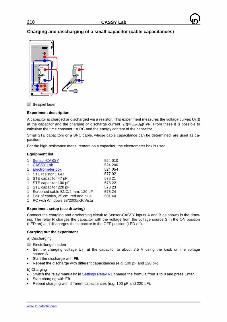
218

CASSY Lab

www.ld-didactic.com

Charging and discharging of a small capacitor (cable capacitances)

Beispiel laden


A capacitor is charged or discharged via a resistor. This experiment measures the voltage curves UB(t)

at the capacitor and the charging or discharge current IA(t)=(UA-UB(t))/R. From these it is possible to

calculate the time constant = RC and the energy content of the capacitor.

Small STE capacitors or a BNC cable, whose cable capacitance can be determined, are used as ca-pacitors.

For the high-resistance measurement on a capacitor, the electrometer box is used.

Equipment list

1 Sensor-CASSY 524 010 1 CASSY Lab 524 200 1 Electrometer box 524 054 1 STE resistor 1 G 577 02

1 STE capacitor 47 pF 578 21 1 STE capacitor 100 pF 578 22 1 STE capacitor 220 pF 578 23 1 Screened cable BNC/4 mm, 120 pF 575 24 3 Pair of cables, 25 cm, red and blue 501 44 1 PC with Windows 98/2000/XP/Vista


Connect the charging and discharging circuit to Sensor-CASSY inputs A and B as shown in the draw-ing. The relay R charges the capacitor with the voltage from the voltage source S in the ON position (LED on) and discharges the capacitor in the OFF position (LED off).


a) Discharging

Einstellungen laden

Set the charging voltage UB1 at the capacitor to about 7.5 V using the knob on the voltage source S.


Repeat the discharge with different capacitances (e.g. 100 pF and 220 pF).

b) Charging

Switch the relay manually: in Settings Relay R1 change the formula from 1 to 0 and press Enter.


Repeat charging with different capacitances (e.g. 100 pF and 220 pF).

CASSY Lab

219

www.ld-didactic.com

Evaluation

To determine the time constant = RC you can apply a logarithmic representation to the Voltage and Current displays. Simply click on the y-axis with the right mouse button to convert it. To optimize the display, you may want to specify the minima manually when applying logarithmic representation (e.g. –1 for log U and –3 for log I). In both cases, the slope A of a best-fit straight line is A = -0.4343/RC.

The time constant is obtained either from a fit to an exponential function or a free fit of the function A*exp(-x/B) or A*(1-exp(-x/B)) with suitable starting values for the charging voltage A and the time

constant B = RC = . For R = 1 G, the time constant in s corresponds to the capacitance in nF.

However, you can also determine the capacitances C from the applied or discharged charges Q. The charge Q is determined from the integral of the I(t) diagrams, and Q = CU (where U is the charging voltage).

The stored energy E = ½CU2 is the integral of the P(t) diagrams in the display Power.

Hint

The easiest way to define a time zero point is by setting a trigger. The must suitable quantity is the

voltage UA1 (when charging e.g. 0.5 V, rising edge, when discharging e.g. 0.5 V, falling edge). When the trigger is switched on, an external changeover switch can be used instead of the relay for more clarity of the circuit.

220

CASSY Lab

www.ld-didactic.com

Damped oscillator circuit

Beispiel laden


An electrical oscillator is excited and the free oscillation is recorded. The damping and the phase dif-

ference between U(t) and I(t) become apparent. In the evaluation the calculated frequency and

damping coefficient of the oscillation are compared with theory.

Equipment list

1 Sensor-CASSY 524 010 1 CASSY Lab 524 200 1 Plug-in board DIN A4 576 74 1 STE coil, 1000 turns 590 84 1 STE capacitor 1 F, 5 % 578 15

1 STE key switch (n.o.) 579 10 1 Set of bridging plugs 501 48 3 Pairs of cables, 50 cm, red and blue 501 45 1 PC with Windows 98/2000/XP/Vista


Set up the oscillator circuit on the plug-in board as shown in the drawing. The current flows via input A of Sensor-CASSY and the capacitor voltage is measured at input B. At the start of the experiment the capacitor is charged from voltage source S. The oscillation is started with the key switch, which shorts the voltage source S.

Note

You can also use relay R instead of the key switch. However, this can bounce so hard when switching that the oscillation is disturbed in the first few milliseconds.


Einstellungen laden

Set the charging voltage UB1 at the capacitor to about 9.5 V using the knob at voltage source S.


Close the oscillator circuit with the key switch (generates trigger signal).

Evaluation

The easiest way to determine the frequency f is in the Frequency Spectrum display (click on this tab and calculate the peak center). The initial amplitude and time constant of the damping can be deter-mined from parameters A and B by fitting an envelope.

CASSY Lab

221

www.ld-didactic.com

These parameters can demonstrate impressive agreement of U(t) with y(t) = A*exp(-t/B)*sin(f*t*360). To realize this, change parameters A, B and f in the formula settings and select the display tab Match-ing.

Example

From the U(t) envelope the experiment example gives us the initial amplitude A = 6.64 V and the time constant B = 1.77 ms. The oscillation frequency is determined to be 1235 Hz. The function of the oscil-lation is thus

y(t) = 6.64*exp(-t/0.00177)*sin(1235*t*360)

and is entered as the function for matching to U(t). The same time constant and frequency apply for I(t), but with a different initial amplitude and phase relation.

The calculated parameters also enable conclusions regarding the parameters R, L and C of the oscil-lator circuit, as in a damped oscillator the following applies:

U(t) = U0 exp(-t) sin(t) where

(1) 2 = 0

2 -

2,

(2) 02 = 1/LC and

(3) = R/2L (= 1/B of envelope).

When we insert the determined values we obtain:

= 2f = 7760 /s

= 565 /s

0 = 7781 /s from (1).

(2) now allows us to calculate the inductance L of the coil when the capacitance C is known. In this

example we obtain L = 0.0165 H (with C = 1 F). (3) gives us the damping resistance R = 18.6 . This

agrees well with the specification of the coil used here (R = 18 ).

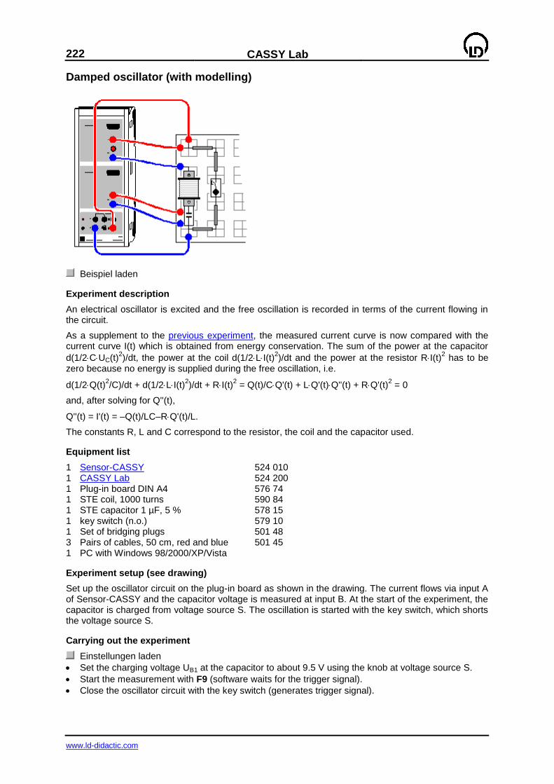
222

CASSY Lab

www.ld-didactic.com

Damped oscillator (with modelling)

Beispiel laden


An electrical oscillator is excited and the free oscillation is recorded in terms of the current flowing in the circuit.

As a supplement to the previous experiment, the measured current curve is now compared with the current curve I(t) which is obtained from energy conservation. The sum of the power at the capacitor

d(1/2CUC(t)2)/dt, the power at the coil d(1/2LI(t)

2)/dt and the power at the resistor RI(t)

2 has to be

zero because no energy is supplied during the free oscillation, i.e.

d(1/2Q(t)2/C)/dt + d(1/2LI(t)

2)/dt + RI(t)

2 = Q(t)/CQ'(t) + LQ'(t)Q''(t) + RQ'(t)

2 = 0

and, after solving for Q''(t),

Q''(t) = I'(t) = –Q(t)/LC–RQ'(t)/L.

The constants R, L and C correspond to the resistor, the coil and the capacitor used.

Equipment list

1 Sensor-CASSY 524 010 1 CASSY Lab 524 200 1 Plug-in board DIN A4 576 74 1 STE coil, 1000 turns 590 84 1 STE capacitor 1 µF, 5 % 578 15 1 key switch (n.o.) 579 10 1 Set of bridging plugs 501 48 3 Pairs of cables, 50 cm, red and blue 501 45 1 PC with Windows 98/2000/XP/Vista


Set up the oscillator circuit on the plug-in board as shown in the drawing. The current flows via input A of Sensor-CASSY and the capacitor voltage is measured at input B. At the start of the experiment, the capacitor is charged from voltage source S. The oscillation is started with the key switch, which shorts the voltage source S.


Einstellungen laden




CASSY Lab

223

www.ld-didactic.com

Modelling

The initial condition for the charge Q of the capacitor is Q(t=0)=-U0C with the initial voltage U0. This

voltage U0 is not exactly the charging voltage of the capacitor because the measurement is only trig-

gered somewhat later. Therefore the second initial condition is simply I(t=0)=0. The constants R (resis-

tance), C (capacitance) and L (inductance) and the initial voltage U0 can be altered by dragging the pointer of the corresponding display instrument (or by clicking to the left or to the right of the pointer)

until the model agrees with the measurement. The ohmic resistance of the coil (approx. 20 ) has to be taken into account when the attenuation resistance R is determined.

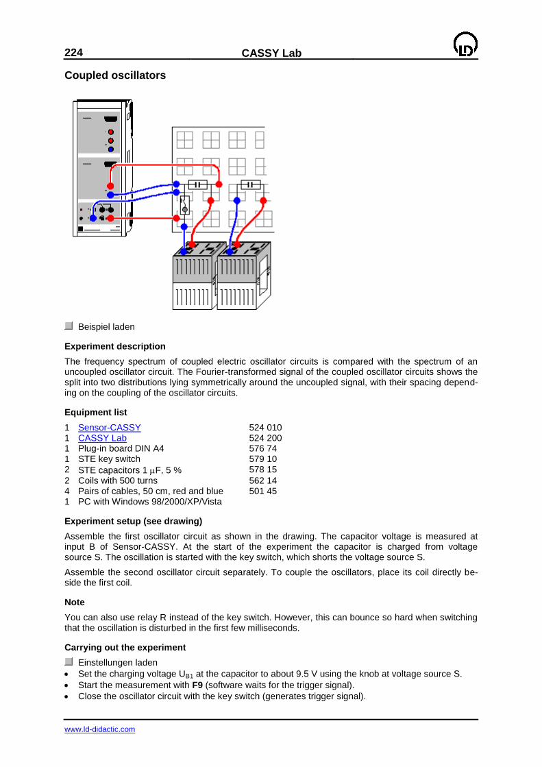
224

CASSY Lab

www.ld-didactic.com

Coupled oscillators

Beispiel laden


The frequency spectrum of coupled electric oscillator circuits is compared with the spectrum of an uncoupled oscillator circuit. The Fourier-transformed signal of the coupled oscillator circuits shows the split into two distributions lying symmetrically around the uncoupled signal, with their spacing depend-ing on the coupling of the oscillator circuits.

Equipment list

1 Sensor-CASSY 524 010 1 CASSY Lab 524 200 1 Plug-in board DIN A4 576 74 1 STE key switch 579 10 2 STE capacitors 1 F, 5 % 578 15

2 Coils with 500 turns 562 14 4 Pairs of cables, 50 cm, red and blue 501 45 1 PC with Windows 98/2000/XP/Vista


Assemble the first oscillator circuit as shown in the drawing. The capacitor voltage is measured at input B of Sensor-CASSY. At the start of the experiment the capacitor is charged from voltage source S. The oscillation is started with the key switch, which shorts the voltage source S.

Assemble the second oscillator circuit separately. To couple the oscillators, place its coil directly be-side the first coil.

Note

You can also use relay R instead of the key switch. However, this can bounce so hard when switching that the oscillation is disturbed in the first few milliseconds.


Einstellungen laden




CASSY Lab

225

www.ld-didactic.com

Place the coil of the second oscillator directly beside that of the first to couple the oscillators.



Evaluation

The uncoupled case produces a damped harmonic oscillation. The coupled oscillation is a beat with the same envelope and the same oscillation frequency.

In the uncoupled case, the Frequency Spectrum display shows only one peak, for which the fre-quency can be calculated as the peak center.

In the coupled case the frequency splits symmetrically into two frequencies. The amplitudes are just half as great as in the uncoupled case, and the interval depends on the coupling.

Given the differential equations of the coupled oscillation circuits

with coupling k (0 ≤ k < 1), we can calculate the two natural frequencies 1 and 2 as

In particular, the oscillation frequency of the coupled system is equal to

and is thus practically unchanged with respect to the uncoupled system (for small k values).

Note

The split into two peaks of precisely the same size is only possible with completely identical oscillators. This is not always precisely the case due to the tolerances of the inductances L and capacitances C.

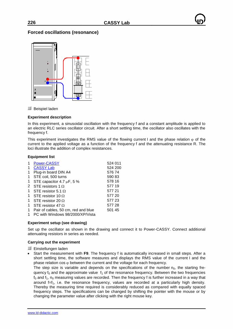
226

CASSY Lab

www.ld-didactic.com

Forced oscillations (resonance)

Beispiel laden


In this experiment, a sinusoidal oscillation with the frequency f and a constant amplitude is applied to an electric RLC series oscillator circuit. After a short settling time, the oscillator also oscillates with the frequency f.

This experiment investigates the RMS value of the flowing current I and the phase relation of the current to the applied voltage as a function of the frequency f and the attenuating resistance R. The loci illustrate the addition of complex resistances.

Equipment list

1 Power-CASSY 524 011 1 CASSY Lab 524 200 1 Plug-in board DIN A4 576 74 1 STE coil, 500 turns 590 83 1 STE capacitor 4.7 F, 5 % 578 16

2 STE resistors 1 577 19

1 STE resistor 5.1 577 21




1 Pair of cables, 50 cm, red and blue 501 45 1 PC with Windows 98/2000/XP/Vista


Set up the oscillator as shown in the drawing and connect it to Power-CASSY. Connect additional attenuating resistors in series as needed.


Einstellungen laden

Start the measurement with F9. The frequency f is automatically increased in small steps. After a short settling time, the software measures and displays the RMS value of the current I and the

phase relation cos between the current and the voltage for each frequency.

The step size is variable and depends on the specifications of the number n0, the starting fre-

quency f0 and the approximate value f1 of the resonance frequency. Between the two frequencies

f0 and f1, n0 measuring values are recorded. Then the frequency f is further increased in a way that

around f=f1, i.e. the resonance frequency, values are recorded at a particularly high density. Thereby the measuring time required is considerably reduced as compared with equally spaced frequency steps. The specifications can be changed by shifting the pointer with the mouse or by changing the parameter value after clicking with the right mouse key.

CASSY Lab

227

www.ld-didactic.com

The measuring condition f < 5*f1 and f < 5000 and delta t > 2/f+2 allows measured values to be recorded up to 5 kHz (or 5 times the resonance frequency), but not before 2/f+2 s after a frequency increase (transient time).

Stop the measurement with F9 when the desired frequency is reached.

Repeat the measurement with other attenuation resistances as necessary.

Evaluation

The resonance frequency can be exactly determined, for example, by determining the peak center in the display Resonance.

In other displays, also the Power and the Phase are shown as functions of the frequency.

The last two displays show the Loci for the complex resistance Z of the oscillating circuit and the complex conductance Y. In the Z representation, the addition of complex resistances in series connec-

tion is nicely displayed: Z = R + iL + 1/iC. As in the example only the frequency , that is the imagi-nary part of Z, is varied for each damping resistance, the real ohmic part remains constant. Thus verti-cal lines are generated in the complex plane whose distance from the imaginary axis is equal to the

ohmic resistance R. The coil in the example has an ohmic internal resistance of approximately 4 . Therefore the distance from the imaginary axis is larger than the individual damping resistances by

approximately 4 .

Remark

For an AC circuit we can write

U = |U| * eit

and I = |I| * ei(t+)

where the complex resistance Z = U/I no longer depends on t

Z = |U|/|I| * e-i

= |Z| * e-i

(Z locus)

On the other hand we have

Y = 1/Z = 1/|Z| * ei

(Y locus)

The Y locus corresponds to the complex inversion of the Z locus (r -> -r, -> -). This transformation

turns the straight lines Z = R + iL + 1/iC of the Z loci into circles in the Y representation (inversion with respect to the unit circle).

Hints

With F7 the measuring instruments can be hidden and unhidden at the same time.

You can logarithmically scale the frequency axis or the current axis easily by clicking on the corre-sponding axis with the right mouse button.

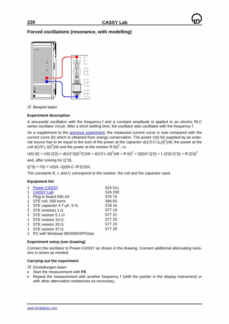
228

CASSY Lab

www.ld-didactic.com

Forced oscillations (resonance, with modelling)

Beispiel laden


A sinusoidal oscillation with the frequency f and a constant amplitude is applied to an electric RLC series oscillator circuit. After a short settling time, the oscillator also oscillates with the frequency f.

As a supplement to the previous experiment, the measured current curve is now compared with the

current curve I(t) which is obtained from energy conservation. The power U(t)I(t) supplied by an exter-

nal source has to be equal to the sum of the power at the capacitor d(1/2CUC(t)2)/dt, the power at the

coil d(1/2LI(t)2)/dt and the power at the resistor RI(t)

2, i.e.

U(t)I(t) = U(t)Q'(t) = d(1/2Q(t)2/C)/dt + d(1/2LI(t)

2)/dt + RI(t)

2 = Q(t)/CQ'(t) + LQ'(t)Q''(t) + RQ'(t)

2

and, after solving for Q''(t),

Q''(t) = I'(t) = U(t)/L–Q(t)/LC–RQ'(t)/L.

The constants R, L and C correspond to the resistor, the coil and the capacitor used.

Equipment list

1 Power-CASSY 524 011 1 CASSY Lab 524 200 1 Plug-in board DIN A4 576 74 1 STE coil, 500 turns 590 83 1 STE capacitor 4.7 µF, 5 % 578 16 2 STE resistors 1 577 19

1 STE resistor 5.1 577 21






Connect the oscillator to Power-CASSY as shown in the drawing. Connect additional attenuating resis-tors in series as needed.


Einstellungen laden


Repeat the measurement with another frequency f (shift the pointer in the display instrument) or with other attenuation resistances as necessary.

CASSY Lab

229

www.ld-didactic.com

Modelling

The initial conditions for the charge Q and the current I are both zero as there is no voltage and no current in the oscillator circuit before the measurement. The constants R (resistance), C (capacitance) and L (inductance) can be altered by dragging the pointer of the corresponding display instrument (or by clicking to the left or to the right of the pointer) until the model agrees with the measurement. The

ohmic resistance of the coil (approx. 4 ) has to be taken into account when the attenuation resis-tance R is determined.

The Power-CASSY only switches the exciting frequency on when the measurement is started. There-fore the transient oscillation process of the oscillator circuit is seen. Depending on the attenuation and the frequency, you see that the oscillator circuit first oscillates at its natural frequency (resonance fre-quency) before it is forced to oscillate at the exciting frequency.

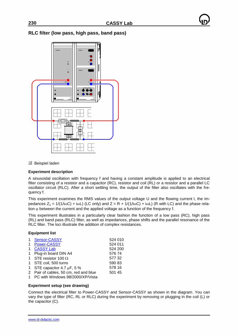
230

CASSY Lab

www.ld-didactic.com

RLC filter (low pass, high pass, band pass)

Beispiel laden


A sinusoidal oscillation with frequency f and having a constant amplitude is applied to an electrical filter consisting of a resistor and a capacitor (RC), resistor and coil (RL) or a resistor and a parallel LC oscillator circuit (RLC). After a short settling time, the output of the filter also oscillates with the fre-quency f.

This experiment examines the RMS values of the output voltage U and the flowing current I, the im-

pedances Z1 = 1/(1/iC) + iL) (LC only) and Z = R + 1/(1/iC) + iL) (R with LC) and the phase rela-

tion between the current and the applied voltage as a function of the frequency f.

This experiment illustrates in a particularly clear fashion the function of a low pass (RC), high pass (RL) and band pass (RLC) filter, as well as impedances, phase shifts and the parallel resonance of the RLC filter. The loci illustrate the addition of complex resistances.

Equipment list

1 Sensor-CASSY 524 010 1 Power-CASSY 524 011 1 CASSY Lab 524 200 1 Plug-in board DIN A4 576 74 1 STE resistor 100 577 32

1 STE coil, 500 turns 590 83 1 STE capacitor 4.7 F, 5 % 578 16

2 Pair of cables, 50 cm, red and blue 501 45 1 PC with Windows 98/2000/XP/Vista


Connect the electrical filter to Power-CASSY and Sensor-CASSY as shown in the diagram. You can vary the type of filter (RC, RL or RLC) during the experiment by removing or plugging in the coil (L) or the capacitor (C).

CASSY Lab

231

www.ld-didactic.com


Einstellungen laden

Realize the RC filter by removing the coil. Start the measurement with F9. The frequency f is automatically increased in small steps. After a short setting time, the software measures and displays the respective RMS value of the output voltage U and the current I.

The step size is variable and depends on the specifications of the number n0, the starting fre-

quency f0 and the approximate value f1 of the resonance frequency. Between the two frequencies

f0 and f1, n0 measuring values are recorded. Then the frequency f is further increased in a way that

around f=f1, i.e. the resonance frequency, values are recorded at a particularly high density. Thereby the measuring time required is considerably reduced as compared with equally spaced frequency steps. The specifications can be changed by shifting the pointer with the mouse or by changing the parameter value after clicking with the right mouse key. The measuring condition f < 5*f1 and f < 5000 and delta t > 2/f+3 allows measured values to be recorded up to 5 kHz (or 5 times the resonance frequency), but not before 2/f+3 s after a frequency increase (transient time).

Stop the measurement with F9 when the desired frequency is reached.

Repeat the measurement with the RL filter and the RLC filter.

Evaluation

The Output Voltage and Input Current displays (accessible with the mouse) show the curves of the output voltage and the current as function of the frequency. The RC filter attenuates the output voltage at high frequencies by about half (low pass) for each octave (doubling of frequency). The RL filter, on the other hand, attenuates the lower frequencies by about half (high pass) for each octave (half fre-quency). The RLC filter attenuates frequencies outside of the resonance frequency of the parallel LC oscillator corresponding to the individual filters. However, the output voltage shows a visible maximum in the resonance range (band pass). The resonance frequency is independent of R.

The two impedances Z1 (LC only) and Z (R with LC) are also calculated and displayed. The resistance of the parallel LC oscillator reaches its maximum at its resonance frequency (in an ideal circuit this would be infinite). The flowing current is thus minimal, as is the voltage drop at the resistor. Conse-quently, the output voltage reaches its maximum where resonance occurs.

The Phase view shows the phase shift between the applied voltage and the flowing current.

The last two displays show the Loci for the complex resistance Z of the filter and the complex conduc-tance Y. In the Z representation, the addition of complex resistances in series connection is nicely

displayed. For a low pass we have Z = R + 1/iC and for a high pass Z = R + iL. As only the fre-

quency , that is the imaginary part of Z, is varied, the real ohmic part remains constant. Thus vertical lines are generated in the complex plane whose distance from the imaginary axis is equal to the ohmic

resistance R. The coil in the example has an ohmic internal resistance of approximately 4 . In the

case of the high pass, the distance from the imaginary axis is therefore larger by approximately 4 than in the case of the low pass.

Remark

For an AC circuit we can write

U = |U| * eit

and I = |I| * ei(t+)

where the complex resistance Z = U/I no longer depends on t

Z = |U|/|I| * e-i

= |Z| * e-i

(Z locus)

On the other hand we have

Y = 1/Z = 1/|Z| * ei

(Y locus)

The Y locus corresponds to the complex inversion of the Z locus (r -> -r, -> -). This transformation

turns the straight lines Z = R + 1/iC and Z = R + iL of the Z loci into semicircles in the Y representa-tion (inversion with respect to the unit circle).

Hints

With F7 the measuring instruments can be hidden and unhidden at the same time.

232

CASSY Lab

www.ld-didactic.com

You can logarithmically scale the coordinate axes easily by clicking on the corresponding axis with the right mouse button.

The attenuations of 6 dB/octave (resp. 20 dB/decade) can be read off easily in a log-log display as the slope ±1.

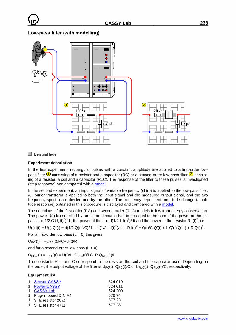
CASSY Lab

233

www.ld-didactic.com

Low-pass filter (with modelling)

Beispiel laden


In the first experiment, rectangular pulses with a constant amplitude are applied to a first-order low-

pass filter consisting of a resistor and a capacitor (RC) or a second-order low-pass filter consist-ing of a resistor, a coil and a capacitor (RLC). The response of the filter to these pulses is investigated (step response) and compared with a model.

In the second experiment, an input signal of variable frequency (chirp) is applied to the low-pass filter. A Fourier transform is applied to both the input signal and the measured output signal, and the two frequency spectra are divided one by the other. The frequency-dependent amplitude change (ampli-tude response) obtained in this procedure is displayed and compared with a model.

The equations of the first-order (RC) and second-order (RLC) models follow from energy conservation.

The power U(t)I(t) supplied by an external source has to be equal to the sum of the power at the ca-

pacitor d(1/2CUC(t)2)/dt, the power at the coil d(1/2LI(t)


2, i.e.


2)/dt + RI(t)

2 = Q(t)/CQ'(t) + LQ'(t)Q''(t) + RQ'(t)

2.

For a first-order low pass (L = 0) this gives

QRC'(t) = –QRC(t)/RC+U(t)/R

and for a second-order low pass (L > 0)

QRLC''(t) = IRLC'(t) = U(t)/L–QRLC(t)/LC–RQRLC'(t)/L.

The constants R, L and C correspond to the resistor, the coil and the capacitor used. Depending on

the order, the output voltage of the filter is URC(t)=QRC(t)/C or URLC(t)=QRLC(t)/C, respectively.

Equipment list



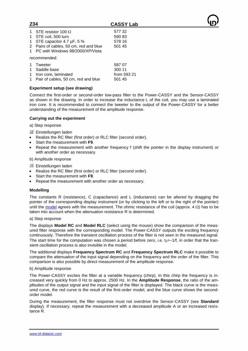
234

CASSY Lab

www.ld-didactic.com


1 STE coil, 500 turn 590 83 1 STE capacitor 4.7 µF, 5 % 578 16 2 Pairs of cables, 50 cm, red and blue 501 45 1 PC with Windows 98/2000/XP/Vista

recommended:

1 Tweeter 587 07 1 Saddle base 300 11 1 Iron core, laminated from 593 21 1 Pair of cables, 50 cm, red and blue 501 45


Connect the first-order or second-order low-pass filter to the Power-CASSY and the Sensor-CASSY as shown in the drawing. In order to increase the inductance L of the coil, you may use a laminated iron core. It is recommended to connect the tweeter to the output of the Power-CASSY for a better understanding of the measurement of the amplitude response.


a) Step response

Einstellungen laden

Realize the RC filter (first order) or RLC filter (second order).


Repeat the measurement with another frequency f (shift the pointer in the display instrument) or with another order as necessary.

b) Amplitude response

Einstellungen laden



Repeat the measurement with another order as necessary.

Modelling

The constants R (resistance), C (capacitance) and L (inductance) can be altered by dragging the pointer of the corresponding display instrument (or by clicking to the left or to the right of the pointer)


a) Step response

The displays Model RC and Model RLC (select using the mouse) show the comparison of the meas-ured filter response with the corresponding model. The Power-CASSY outputs the exciting frequency continuously. Therefore the transient oscillation process of the filter is not seen in the measured signal.

The start time for the computation was chosen a period before zero, i.e. t0=–1/f, in order that the tran-sient oscillation process is also invisible in the model.

The additional displays Frequency Spectrum RC and Frequency Spectrum RLC make it possible to compare the attenuation of the input signal depending on the frequency and the order of the filter. This comparison is also possible by direct measurement of the amplitude response.


The Power-CASSY excites the filter at a variable frequency (chirp). In this chirp the frequency is in-creased very quickly from 0 Hz to approx. 2500 Hz. In the Amplitude Response, the ratio of the am-plitudes of the output signal and the input signal of the filter is displayed. The black curve is the meas-ured curve, the red curve is the result of the first-order model, and the blue curve shows the second-order model.

During the measurement, the filter response must not overdrive the Sensor-CASSY (see Standard display). If necessary, repeat the measurement with a decreased amplitude A or an increased resis-tance R.

CASSY Lab

235

www.ld-didactic.com

Remark concerning the measurement of the amplitude response

When the basic frequency f of the chirp (f = 2.5 Hz in the example) is changed, the measuring interval has to be changed, too, so that the measuring time T corresponds to the chirp period again (T= 400 ms in the example).

Moreover, the range of the amplitudes AB, ARC and ARLC has to be adjusted. In the example, the ampli-tude ratios are only defined if the amplitude of the FFT in the denominator is at least 1.5 % of the input amplitude A.

The computation time of the models is limited to 5 s. If this is not sufficient in the case of slow com-puters, the subsequent Fourier analysis is only computed for the incomplete solution. In this case, please increase the maximum computation time of the models.

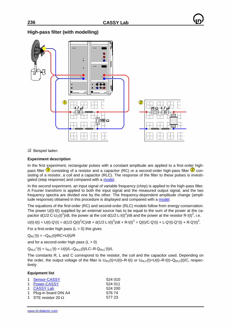
236

CASSY Lab

www.ld-didactic.com

High-pass filter (with modelling)

Beispiel laden


In the first experiment, rectangular pulses with a constant amplitude are applied to a first-order high-

pass filter consisting of a resistor and a capacitor (RC) or a second-order high-pass filter con-sisting of a resistor, a coil and a capacitor (RLC). The response of the filter to these pulses is investi-gated (step response) and compared with a model.

In the second experiment, an input signal of variable frequency (chirp) is applied to the high-pass filter. A Fourier transform is applied to both the input signal and the measured output signal, and the two frequency spectra are divided one by the other. The frequency-dependent amplitude change (ampli-tude response) obtained in this procedure is displayed and compared with a model.

The equations of the first-order (RC) and second-order (RLC) models follow from energy conservation.

The power U(t)I(t) supplied by an external source has to be equal to the sum of the power at the ca-

pacitor d(1/2CUC(t)2)/dt, the power at the coil d(1/2LI(t)


2, i.e.


2)/dt + RI(t)

2 = Q(t)/CQ'(t) + LQ'(t)Q''(t) + RQ'(t)

2.

For a first-order high pass (L = 0) this gives

QRC'(t) = –QRC(t)/RC+U(t)/R

and for a second-order high pass (L > 0)

QRLC''(t) = IRLC'(t) = U(t)/L–QRLC(t)/LC–RQRLC'(t)/L

The constants R, L and C correspond to the resistor, the coil and the capacitor used. Depending on

the order, the output voltage of the filter is URC(t)=U(t)–RI(t) or URLC(t)=U(t)–RI(t)–QRLC(t)/C, respec-tively.

Equipment list


CASSY Lab

237

www.ld-didactic.com



1 STE coil, 500 turns 590 83 1 STE capacitor 4.7 µF, 5 % 578 16 2 pairs of cables, 50 cm, red and blue 501 45 1 PC with Windows 98/2000/XP/Vista

recommended:

1 Tweeter 587 07 1 Saddle base 300 11 1 Iron core, laminated from 593 21 1 Pair of cables, 50 cm, red and blue 501 45


Connect the first-order or second-order high-pass filter to the Power-CASSY and the Sensor-CASSY as shown in the drawing. In order to increase the inductance L of the coil, you may use a laminated iron core. It is recommended to connect the tweeter to the output of the Power-CASSY for a better understanding of the measurement of the amplitude response.


a) Step response

Einstellungen laden



Repeat the measurement with another frequency f (shift the pointer in the display instrument) or with another order as necessary.


Einstellungen laden



Repeat the measurement with another order as necessary.

Modelling

The constants R (resistance), C (capacitance) and L (inductance) can be altered by dragging the pointer of the corresponding display instrument (or by clicking to the left or to the right of the pointer)


a) Step response

The displays Model RC and Model RLC (select using the mouse) show the comparison of the meas-ured filter response with the corresponding model. The Power-CASSY outputs the exciting frequency continuously. Therefore the transient oscillation process of the filter is not seen in the measured signal.

The start time for the computation was chosen a period before zero, i.e. t0=–1/f, in order that the tran-

sient oscillation process is also invisible in the model.

The additional displays Frequency Spectrum RC and Frequency Spectrum RLC make it possible to compare the attenuation of the input signal depending on the frequency and the order of the filter. This comparison is also possible by direct measurement of the amplitude response.


The Power-CASSY excites the filter at a variable frequency (chirp). In this chirp the frequency is de-creased very quickly from approx. 2500 Hz to 0 Hz. In the Amplitude Response, the ratio of the am-plitudes of the output signal and the input signal of the filter is displayed. The black curve is the meas-ured curve, the red curve is the result of the first-order model, and the blue curve shows the second-order model.

During the measurement, the filter response must not overdrive the Sensor-CASSY (see Standard display). If necessary, repeat the measurement with a decreased amplitude A or an increased resis-tance R.

238

CASSY Lab

www.ld-didactic.com

Remark concerning the measurement of the amplitude response

When the basic frequency f of the chirp (f = 2.5 Hz in the example) is changed, the measuring interval has to be changed, too, so that the measuring time T corresponds to the chirp period again (T= 400 ms in the example).

Moreover, the range of the amplitudes AB, ARC and ARLC has to be adjusted. In the example, the ampli-tude ratios are only defined if the amplitude of the FFT in the denominator is at least 1.5 % of the input amplitude A.

The computation time of the models is limited to 5 s. If this is not sufficient in the case of slow com-puters, the subsequent Fourier analysis is only computed for the incomplete solution. In this case, please increase the maximum computation time of the models.

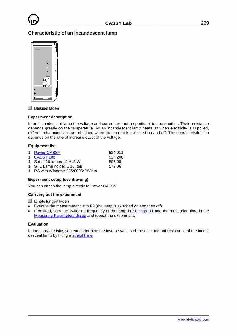
CASSY Lab

239

www.ld-didactic.com

Characteristic of an incandescent lamp

Beispiel laden


In an incandescent lamp the voltage and current are not proportional to one another. Their resistance depends greatly on the temperature. As an incandescent lamp heats up when electricity is supplied, different characteristics are obtained when the current is switched on and off. The characteristic also depends on the rate of increase dU/dt of the voltage.

Equipment list

1 Power-CASSY 524 011 1 CASSY Lab 524 200 1 Set of 10 lamps 12 V /3 W 505 08 1 STE Lamp holder E 10, top 579 06 1 PC with Windows 98/2000/XP/Vista


You can attach the lamp directly to Power-CASSY.


Einstellungen laden

Execute the measurement with F9 (the lamp is switched on and then off).

If desired, vary the switching frequency of the lamp in Settings U1 and the measuring time in the Measuring Parameters dialog and repeat the experiment.

Evaluation

In the characteristic, you can determine the inverse values of the cold and hot resistance of the incan-descent lamp by fitting a straight line.

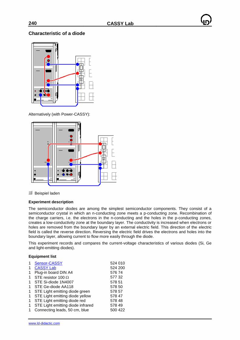
240

CASSY Lab

www.ld-didactic.com

Characteristic of a diode

Alternatively (with Power-CASSY):

Beispiel laden


The semiconductor diodes are among the simplest semiconductor components. They consist of a semiconductor crystal in which an n-conducting zone meets a p-conducting zone. Recombination of the charge carriers, i.e. the electrons in the n-conducting and the holes in the p-conducting zones, creates a low-conductivity zone at the boundary layer. The conductivity is increased when electrons or holes are removed from the boundary layer by an external electric field. This direction of the electric field is called the reverse direction. Reversing the electric field drives the electrons and holes into the boundary layer, allowing current to flow more easily through the diode.

This experiment records and compares the current-voltage characteristics of various diodes (Si, Ge and light-emitting diodes).

Equipment list

1 Sensor-CASSY 524 010 1 CASSY Lab 524 200 1 Plug-in board DIN A4 576 74 1 STE resistor 100 577 32

1 STE Si-diode 1N4007 578 51 1 STE Ge-diode AA118 578 50 1 STE Light emitting diode green 578 57 1 STE Light emitting diode yellow 578 47 1 STE Light emitting diode red 578 48 1 STE Light emitting diode infrared 578 49 1 Connecting leads, 50 cm, blue 500 422

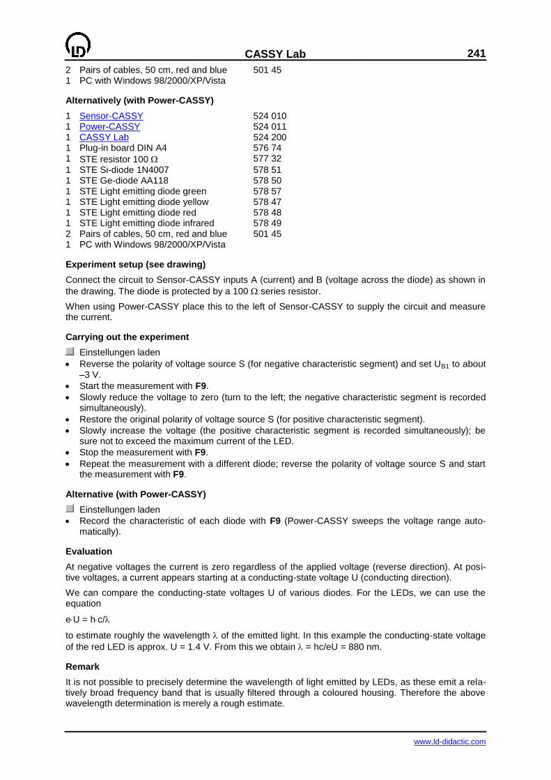
CASSY Lab

241

www.ld-didactic.com

2 Pairs of cables, 50 cm, red and blue 501 45 1 PC with Windows 98/2000/XP/Vista

Alternatively (with Power-CASSY)


1 STE Si-diode 1N4007 578 51 1 STE Ge-diode AA118 578 50 1 STE Light emitting diode green 578 57 1 STE Light emitting diode yellow 578 47 1 STE Light emitting diode red 578 48 1 STE Light emitting diode infrared 578 49 2 Pairs of cables, 50 cm, red and blue 501 45 1 PC with Windows 98/2000/XP/Vista


Connect the circuit to Sensor-CASSY inputs A (current) and B (voltage across the diode) as shown in

the drawing. The diode is protected by a 100 series resistor.

When using Power-CASSY place this to the left of Sensor-CASSY to supply the circuit and measure the current.


Einstellungen laden

Reverse the polarity of voltage source S (for negative characteristic segment) and set UB1 to about –3 V.


Slowly reduce the voltage to zero (turn to the left; the negative characteristic segment is recorded simultaneously).

Restore the original polarity of voltage source S (for positive characteristic segment).

Slowly increase the voltage (the positive characteristic segment is recorded simultaneously); be sure not to exceed the maximum current of the LED.


Repeat the measurement with a different diode; reverse the polarity of voltage source S and start the measurement with F9.

Alternative (with Power-CASSY)

Einstellungen laden

Record the characteristic of each diode with F9 (Power-CASSY sweeps the voltage range auto-matically).

Evaluation

At negative voltages the current is zero regardless of the applied voltage (reverse direction). At posi-tive voltages, a current appears starting at a conducting-state voltage U (conducting direction).

We can compare the conducting-state voltages U of various diodes. For the LEDs, we can use the equation

eU = hc/

to estimate roughly the wavelength of the emitted light. In this example the conducting-state voltage

of the red LED is approx. U = 1.4 V. From this we obtain = hc/eU = 880 nm.

Remark

It is not possible to precisely determine the wavelength of light emitted by LEDs, as these emit a rela-tively broad frequency band that is usually filtered through a coloured housing. Therefore the above wavelength determination is merely a rough estimate.

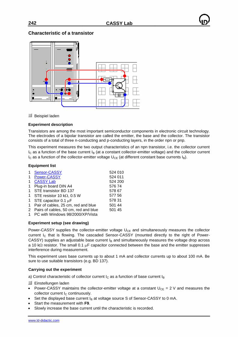
242

CASSY Lab

www.ld-didactic.com

Characteristic of a transistor

Beispiel laden


Transistors are among the most important semiconductor components in electronic circuit technology. The electrodes of a bipolar transistor are called the emitter, the base and the collector. The transistor consists of a total of three n-conducting and p-conducting layers, in the order npn or pnp.

This experiment measures the two output characteristics of an npn transistor, i.e. the collector current

IC as a function of the base current IB (at a constant collector-emitter voltage) and the collector current

IC as a function of the collector-emitter voltage UCE (at different constant base currents IB).

Equipment list

1 Sensor-CASSY 524 010 1 Power-CASSY 524 011 1 CASSY Lab 524 200 1 Plug-in board DIN A4 576 74 1 STE transistor BD 137 578 67 1 STE resistor 10 k, 0.5 W 577 56

1 STE capacitor 0.1 F 578 31

1 Pair of cables, 25 cm, red and blue 501 44 2 Pairs of cables, 50 cm, red and blue 501 45 1 PC with Windows 98/2000/XP/Vista


Power-CASSY supplies the collector-emitter voltage UCE and simultaneously measures the collector

current IC that is flowing. The cascaded Sensor-CASSY (mounted directly to the right of Power-

CASSY) supplies an adjustable base current IB and simultaneously measures the voltage drop across

a 10 k resistor. The small 0.1 F capacitor connected between the base and the emitter suppresses interference during measurement.

This experiment uses base currents up to about 1 mA and collector currents up to about 100 mA. Be sure to use suitable transistors (e.g. BD 137).


a) Control characteristic of collector current IC as a function of base current IB

Einstellungen laden

Power-CASSY maintains the collector-emitter voltage at a constant UCE = 2 V and measures the

collector current IC continuously.

Set the displayed base current IB at voltage source S of Sensor-CASSY to 0 mA.


Slowly increase the base current until the characteristic is recorded.

CASSY Lab

243

www.ld-didactic.com


b) Characteristic of collector current IC as a function of collector-emitter voltage UCE

Einstellungen laden

Power-CASSY increases the collector-emitter voltage to UCE = 2 V during the measurement and

measures the collector current IC.

Set the displayed base current IB at voltage source S of Sensor-CASSY to 0.1 mA.

Start the measurement with F9 (the characteristic is recorded automatically).

Increase the base current IB in steps of 0.1 mA and record additional characteristics with F9.

Evaluation

The current gain can be determined easily from control characteristic a) by fitting a straight line. In the

example, we obtain a current gain factor of IC/IB = 149.6.

Characteristic b) also shows the current gain of a transistor in an impressive manner. Starting from a

relatively low collector-emitter voltage UCE, the output current IC remains virtually constant, depending

only on the base current IB.

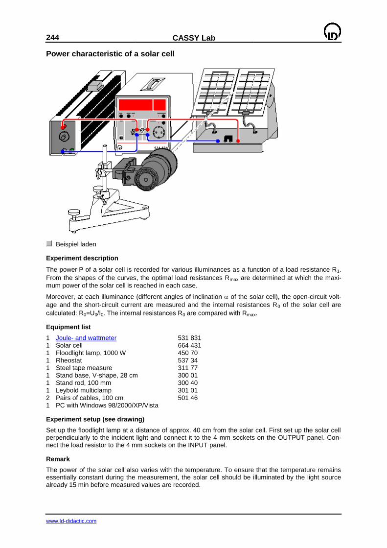
244

CASSY Lab

www.ld-didactic.com

Power characteristic of a solar cell

Beispiel laden


The power P of a solar cell is recorded for various illuminances as a function of a load resistance R1.

From the shapes of the curves, the optimal load resistances Rmax are determined at which the maxi-

mum power of the solar cell is reached in each case.

Moreover, at each illuminance (different angles of inclination of the solar cell), the open-circuit volt-

age and the short-circuit current are measured and the internal resistances R0 of the solar cell are

calculated: R0=U0/I0. The internal resistances R0 are compared with Rmax.

Equipment list

1 Joule- and wattmeter 531 831 1 Solar cell 664 431 1 Floodlight lamp, 1000 W 450 70 1 Rheostat 537 34 1 Steel tape measure 311 77 1 Stand base, V-shape, 28 cm 300 01 1 Stand rod, 100 mm 300 40 1 Leybold multiclamp 301 01 2 Pairs of cables, 100 cm 501 46 1 PC with Windows 98/2000/XP/Vista


Set up the floodlight lamp at a distance of approx. 40 cm from the solar cell. First set up the solar cell perpendicularly to the incident light and connect it to the 4 mm sockets on the OUTPUT panel. Con-nect the load resistor to the 4 mm sockets on the INPUT panel.

Remark

The power of the solar cell also varies with the temperature. To ensure that the temperature remains essentially constant during the measurement, the solar cell should be illuminated by the light source already 15 min before measured values are recorded.

CASSY Lab

245

www.ld-didactic.com


Einstellungen laden

a) Recording the characteristic

Adjust the rheostat so that a resistance of 2 is displayed in the display instrument Load Resis-

tance R1.

Take the measured value into the table manually with F9.

Increase the load resistance in steps of 2 , and record further measured values.

In order to vary the illuminance, incline the solar cell by an angle of 45° or 30°, respectively, rela-tive to the incident light. Repeat the experiment for each angle.

For each illuminance, determine the load resistance Rmax at which the maximum power of the solar cell is reached.

b) Measuring the open-circuit voltage and the short-circuit current

Open the display instruments U, I, U0, I0 and R0 by clicking on .

Connect the solar cell to the 4 mm sockets of the joule and wattmeter marked with U.

Using the mouse, take the value measured in the display instrument U to the display instrument

Open-Circuit Voltage U0 (drag & drop).

Connect the solar cell to the socket of the joule and wattmeter marked with I.

Using the mouse, take the value measured in the display instrument I to the display instrument

Short-Circuit Current I0 (drag & drop). Read the internal resistance R0 of the solar cell.

Evaluation

The power supplied by a solar cell depends on the load resistance and on the illuminance.

The maximum power of the solar cell is reached if the load resistance is approximately equal to the internal resistance of the solar cell.

The maximum power of the solar cell is the larger, the larger the illuminance is (at constant tempera-ture).

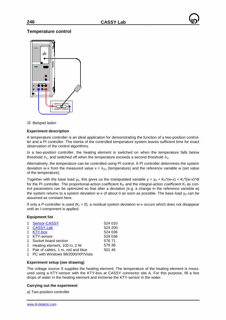
246

CASSY Lab

www.ld-didactic.com

Temperature control

Beispiel laden


A temperature controller is an ideal application for demonstrating the function of a two-position control-ler and a PI controller. The inertia of the controlled temperature system leaves sufficient time for exact observation of the control algorithms.

In a two-position controller, the heating element is switched on when the temperature falls below

threshold 1, and switched off when the temperature exceeds a second threshold 2.

Alternatively, the temperature can be controlled using PI control. A PI controller determines the system

deviation w-x from the measured value x = A1 (temperature) and the reference variable w (set value of the temperature).

Together with the base load y0, this gives us the manipulated variable y = y0 + KP*(w-x) + KI*(w-x)*dt

for the PI controller. The proportional-action coefficient KP and the integral-action coefficient KI as con-trol parameters can be optimized so that after a deviation (e.g. a change in the reference variable w)

the system returns to a system deviation w-x of about 0 as soon as possible. The base load y0 can be

assumed as constant here.

If only a P-controller is used (KI = 0), a residual system deviation w-x occurs which does not disappear

until an I-component is applied.

Equipment list

1 Sensor-CASSY 524 010 1 CASSY Lab 524 200 1 KTY-box 524 036 1 KTY-sensor 529 036 1 Socket board section 576 71 1 Heating element, 100 , 2 W 579 38

1 Pair of cables, 1 m, red and blue 501 46 1 PC with Windows 98/2000/XP/Vista


The voltage source S supplies the heating element. The temperature of the heating element is meas-ured using a KTY-sensor with the KTY-box at CASSY connector site A. For this purpose, fill a few drops of water in the heating element and immerse the KTY-sensor in the water.


a) Two-position controller

CASSY Lab

247

www.ld-didactic.com

Einstellungen laden

Turn the potentiometer of the voltage source S all the way to the right.

Replace switching thresholds 1 and 2 with individual values by moving the pointer of the display

instrument with the mouse or changing the value of the parameter in the Settings 1 or 2 (right mouse button).

If desired, you can record the temperature curve during control, and stop recording, with F9.

b) PI controller

Einstellungen laden


Set the reference variable w about 5 °C above the current temperature A1 by moving the pointer of the display instrument with the mouse or changing the value of the reference variable in the Set-tings w (right mouse button).

Replace the proportional-action (KP) and integral-action (KI) coefficients using individual values of the parameter in the Settings KP or KI (right mouse button).

Start (and stop) temperature control with F9.

Evaluation

For the two-position controller, we can set horizontal lines to mark the two switching thresholds and

2.

The quality of the PI controller depends significantly on the choice of the proportional-action coefficient

KP and the integral-action coefficient KI. The black line represents the reference variable w (set value).

The red curve represents the controlled variable x (measured value) and should converge with the black curve quickly following a deviation. The blue curve represents the manipulated variable y and thus corresponds to the heating voltage.

Empirically optimizing the PI temperature controller

The controlled temperature system is very slow. This is why the effects of changes in KP and KI can only be seen with a large delay. Empirical optimization will thus take a certain amount of time.

Set KI to 0, and increase KP in moderate steps (e.g. by 1) until the control loop oscillates.

Reduce KP again until the oscillations die out. A residual system deviation is created.

Increase KI in moderate steps (e.g. by KP/200) until the system oscillates again.

Reduce KI again until the oscillations die out. Note that the controller becomes slower, the lower KI becomes.

In this example, we have used KP=5 and KI=0.05 /s.

Automatically varying the reference variable

The reference variable w (set value) can be varied not only manually, but automatically as well. We can do this, for example, by entering the formula 30+sin(360*t/1000) in the Settings w. This controls a sinusoidal temperature curve between 29 °C and 31 °C with a period of 1000 s.

Using the temperature box (524 045)

The temperature box (524 045) with NiCr-Ni sensor or NTC can also be used in place of the KTY box.

To do this, first delete the temperature in the Settings A1; then in the CASSY Settings (F5) click on the temperature box at input A and additionally activate Averaged Values and Zero Point Left. Then, just set the measuring range from 0 °C to 120 °C in the Settings w and modify the formula to (w-&JA11)/50 in Settings w-x.

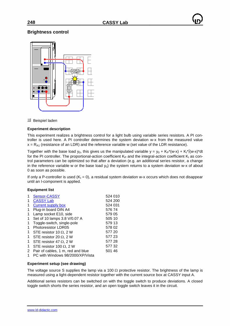
248

CASSY Lab

www.ld-didactic.com

Brightness control

Beispiel laden


This experiment realizes a brightness control for a light bulb using variable series resistors. A PI con-troller is used here. A PI controller determines the system deviation w-x from the measured value

x = RA1 (resistance of an LDR) and the reference variable w (set value of the LDR resistance).


for the PI controller. The proportional-action coefficient KP and the integral-action coefficient KI as con-trol parameters can be optimized so that after a deviation (e.g. an additional series resistor, a change

in the reference variable w or the base load y0) the system returns to a system deviation w-x of about

0 as soon as possible.

If only a P-controller is used (KI = 0), a residual system deviation w-x occurs which does not disappear until an I-component is applied.

Equipment list

1 Sensor-CASSY 524 010 1 CASSY Lab 524 200 1 Current supply box 524 031 1 Plug-in board DIN A4 576 74 1 Lamp socket E10, side 579 05 1 Set of 10 lamps 3.8 V/0.07 A 505 10 1 Toggle-switch, single-pole 579 13 1 Photoresistor LDR05 578 02 1 STE resistor 10 , 2 W 577 20

1 STE resistor 20 , 2 W 577 23

1 STE resistor 47 , 2 W 577 28

1 STE resistor 100 , 2 W 577 32



The voltage source S supplies the lamp via a 100 protective resistor. The brightness of the lamp is measured using a light-dependent resistor together with the current source box at CASSY input A.

Additional series resistors can be switched on with the toggle switch to produce deviations. A closed toggle switch shorts the series resistor, and an open toggle switch leaves it in the circuit.

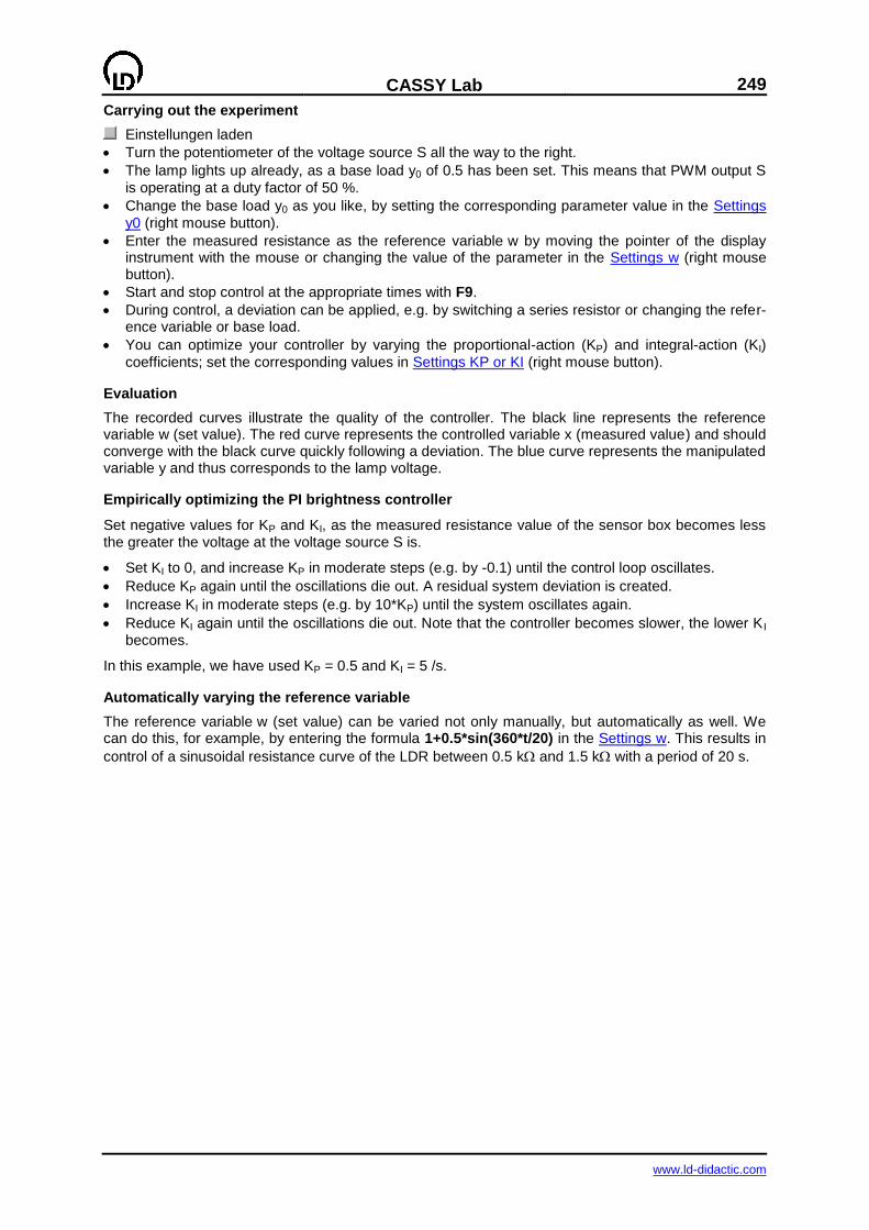
CASSY Lab

249

www.ld-didactic.com


Einstellungen laden


The lamp lights up already, as a base load y0 of 0.5 has been set. This means that PWM output S

is operating at a duty factor of 50 %.

Change the base load y0 as you like, by setting the corresponding parameter value in the Settings

y0 (right mouse button).

Enter the measured resistance as the reference variable w by moving the pointer of the display instrument with the mouse or changing the value of the parameter in the Settings w (right mouse button).

Start and stop control at the appropriate times with F9.

During control, a deviation can be applied, e.g. by switching a series resistor or changing the refer-ence variable or base load.

You can optimize your controller by varying the proportional-action (KP) and integral-action (KI)

coefficients; set the corresponding values in Settings KP or KI (right mouse button).

Evaluation

The recorded curves illustrate the quality of the controller. The black line represents the reference variable w (set value). The red curve represents the controlled variable x (measured value) and should converge with the black curve quickly following a deviation. The blue curve represents the manipulated variable y and thus corresponds to the lamp voltage.

Empirically optimizing the PI brightness controller

Set negative values for KP and KI, as the measured resistance value of the sensor box becomes less the greater the voltage at the voltage source S is.

Set KI to 0, and increase KP in moderate steps (e.g. by -0.1) until the control loop oscillates.


Increase KI in moderate steps (e.g. by 10*KP) until the system oscillates again.

Reduce KI again until the oscillations die out. Note that the controller becomes slower, the lower K I becomes.

In this example, we have used KP = 0.5 and KI = 5 /s.


The reference variable w (set value) can be varied not only manually, but automatically as well. We can do this, for example, by entering the formula 1+0.5*sin(360*t/20) in the Settings w. This results in

control of a sinusoidal resistance curve of the LDR between 0.5 k and 1.5 k with a period of 20 s.

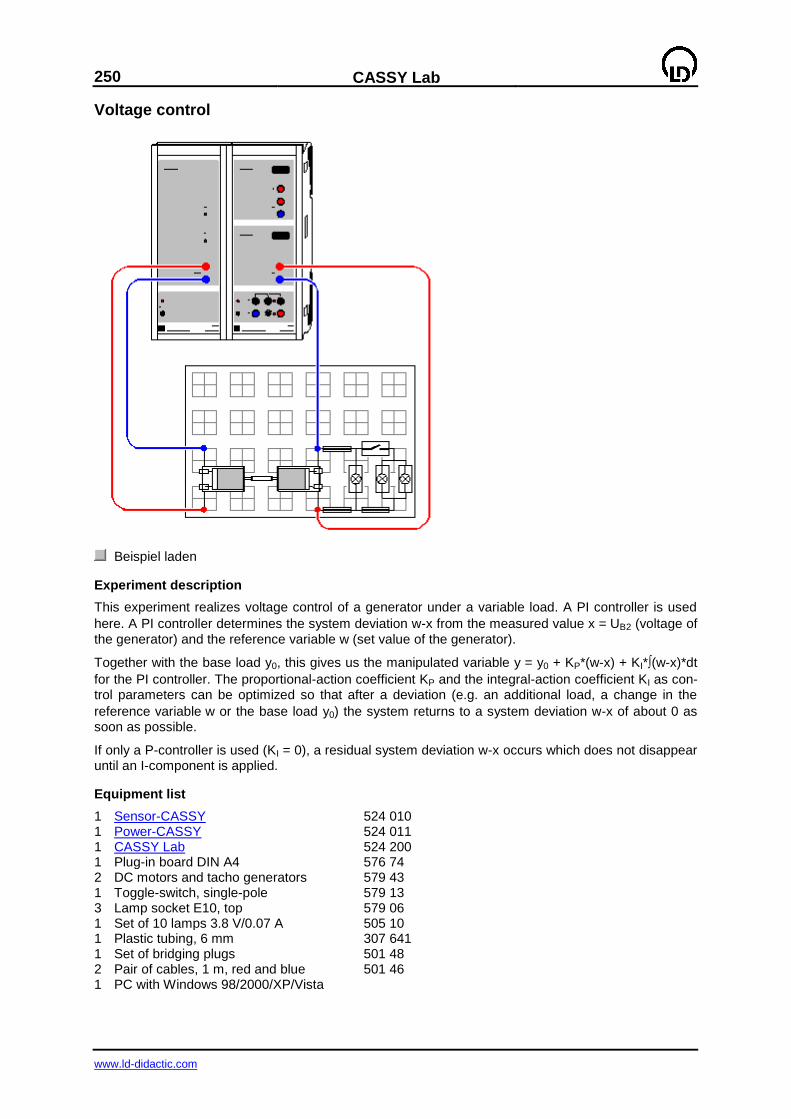
250

CASSY Lab

www.ld-didactic.com

Voltage control

Beispiel laden


This experiment realizes voltage control of a generator under a variable load. A PI controller is used

here. A PI controller determines the system deviation w-x from the measured value x = UB2 (voltage of

the generator) and the reference variable w (set value of the generator).


for the PI controller. The proportional-action coefficient KP and the integral-action coefficient KI as con-trol parameters can be optimized so that after a deviation (e.g. an additional load, a change in the

reference variable w or the base load y0) the system returns to a system deviation w-x of about 0 as soon as possible.

If only a P-controller is used (KI = 0), a residual system deviation w-x occurs which does not disappear until an I-component is applied.

Equipment list

1 Sensor-CASSY 524 010 1 Power-CASSY 524 011 1 CASSY Lab 524 200 1 Plug-in board DIN A4 576 74 2 DC motors and tacho generators 579 43 1 Toggle-switch, single-pole 579 13 3 Lamp socket E10, top 579 06 1 Set of 10 lamps 3.8 V/0.07 A 505 10 1 Plastic tubing, 6 mm 307 641 1 Set of bridging plugs 501 48 2 Pair of cables, 1 m, red and blue 501 46 1 PC with Windows 98/2000/XP/Vista

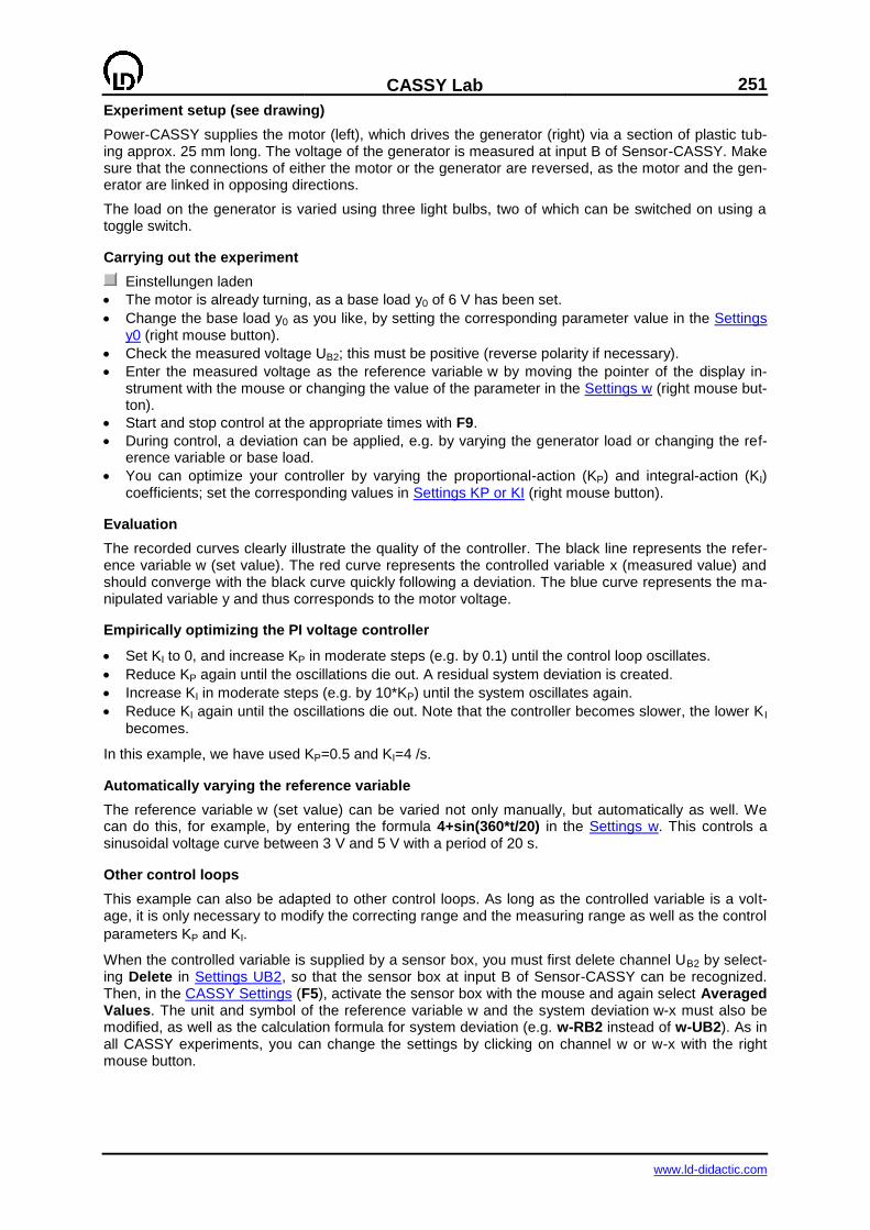
CASSY Lab

251

www.ld-didactic.com


Power-CASSY supplies the motor (left), which drives the generator (right) via a section of plastic tub-ing approx. 25 mm long. The voltage of the generator is measured at input B of Sensor-CASSY. Make sure that the connections of either the motor or the generator are reversed, as the motor and the gen-erator are linked in opposing directions.

The load on the generator is varied using three light bulbs, two of which can be switched on using a toggle switch.


Einstellungen laden

The motor is already turning, as a base load y0 of 6 V has been set.

Change the base load y0 as you like, by setting the corresponding parameter value in the Settings y0 (right mouse button).

Check the measured voltage UB2; this must be positive (reverse polarity if necessary).

Enter the measured voltage as the reference variable w by moving the pointer of the display in-strument with the mouse or changing the value of the parameter in the Settings w (right mouse but-ton).

Start and stop control at the appropriate times with F9.

During control, a deviation can be applied, e.g. by varying the generator load or changing the ref-erence variable or base load.

You can optimize your controller by varying the proportional-action (KP) and integral-action (KI) coefficients; set the corresponding values in Settings KP or KI (right mouse button).

Evaluation

The recorded curves clearly illustrate the quality of the controller. The black line represents the refer-ence variable w (set value). The red curve represents the controlled variable x (measured value) and should converge with the black curve quickly following a deviation. The blue curve represents the ma-nipulated variable y and thus corresponds to the motor voltage.

Empirically optimizing the PI voltage controller

Set KI to 0, and increase KP in moderate steps (e.g. by 0.1) until the control loop oscillates.


Increase KI in moderate steps (e.g. by 10*KP) until the system oscillates again.

Reduce KI again until the oscillations die out. Note that the controller becomes slower, the lower K I

becomes.

In this example, we have used KP=0.5 and KI=4 /s.


The reference variable w (set value) can be varied not only manually, but automatically as well. We can do this, for example, by entering the formula 4+sin(360*t/20) in the Settings w. This controls a sinusoidal voltage curve between 3 V and 5 V with a period of 20 s.

Other control loops

This example can also be adapted to other control loops. As long as the controlled variable is a volt-age, it is only necessary to modify the correcting range and the measuring range as well as the control

parameters KP and KI.

When the controlled variable is supplied by a sensor box, you must first delete channel UB2 by select-ing Delete in Settings UB2, so that the sensor box at input B of Sensor-CASSY can be recognized. Then, in the CASSY Settings (F5), activate the sensor box with the mouse and again select Averaged Values. The unit and symbol of the reference variable w and the system deviation w-x must also be modified, as well as the calculation formula for system deviation (e.g. w-RB2 instead of w-UB2). As in all CASSY experiments, you can change the settings by clicking on channel w or w-x with the right mouse button.

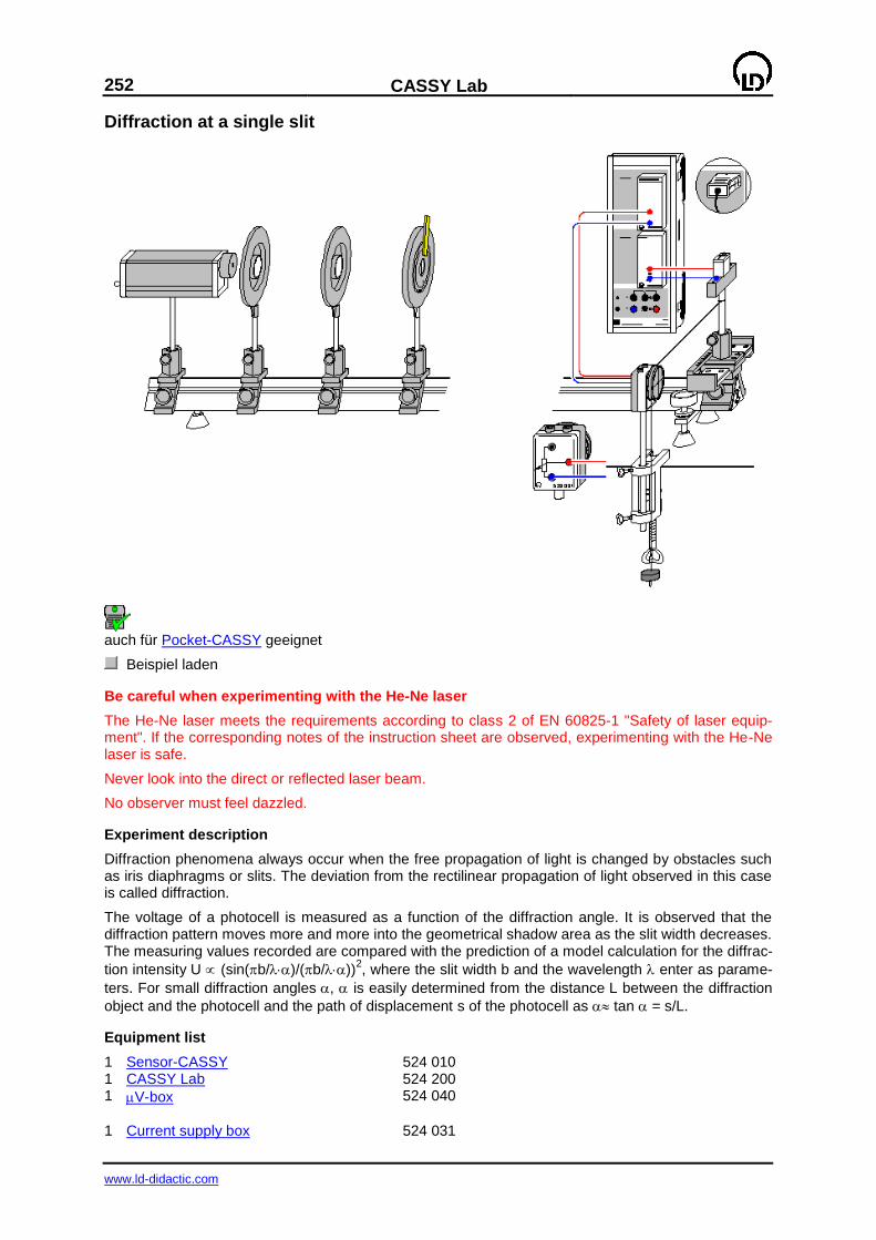
252

CASSY Lab

www.ld-didactic.com

Diffraction at a single slit


Beispiel laden

Be careful when experimenting with the He-Ne laser

The He-Ne laser meets the requirements according to class 2 of EN 60825-1 "Safety of laser equip-ment". If the corresponding notes of the instruction sheet are observed, experimenting with the He-Ne laser is safe.

Never look into the direct or reflected laser beam.

No observer must feel dazzled.


Diffraction phenomena always occur when the free propagation of light is changed by obstacles such as iris diaphragms or slits. The deviation from the rectilinear propagation of light observed in this case is called diffraction.

The voltage of a photocell is measured as a function of the diffraction angle. It is observed that the diffraction pattern moves more and more into the geometrical shadow area as the slit width decreases. The measuring values recorded are compared with the prediction of a model calculation for the diffrac-

tion intensity U (sin(b/)/(b/))2, where the slit width b and the wavelength enter as parame-

ters. For small diffraction angles , is easily determined from the distance L between the diffraction

object and the photocell and the path of displacement s of the photocell as tan = s/L.

Equipment list

1 Sensor-CASSY 524 010 1 CASSY Lab 524 200 1 V-box 524 040

1 Current supply box 524 031

CASSY Lab

253

www.ld-didactic.com

with Displacement transducer and 529 031 Pair of cables, 100 cm, red and blue 501 46 or 1 Rotary motion sensor S 524 082 1 He-Ne laser, linearly polarized 471 840 1 Precision optical bench, 2 m 460 33 4 Riders, H=90 mm/B=60 mm 460 374 1 Sliding rider 460 383 1 Lens in frame, f = +5 mm 460 01 1 Lens in frame, f = +50 mm 460 02 1 Adjustable slit 460 14 1 Holder for plug-in elements 460 21 1 Photocell STE 2/19 578 62 1 Simple bench clamp 301 07 1 Fishing line, 10 m 309 48 1 Set of 12 weights, each 50 g 342 61 1 Pair of cables, 100 cm, red and blue 501 46 1 PC with Windows 98/2000/XP/Vista


Remark: the adjustment should be carried out in a slightly darkened room.

Using a rider, mount the He-Ne laser to the optical bench as shown in the drawing.

Set up the photocell at a distance of approx. 1.90 m from the laser by means of the sliding rider and the holder for plug-in elements. The photocell should be located in the middle of the sliding rider. Stick two strips of dark paper on the photocell so that an entrance slit of approx. 1 mm is left.

Direct the laser towards the photocell, and switch it on.

Adjust the height of the laser so that the laser beam impinges on the centre of the photocell.

Place the spherical lens with the focal length f = +5 mm in front of the laser at a distance of approx. 1 cm. The laser beam has to cover the photocell.

Position the converging lens with the focal length f = +50 mm in front of the spherical lens at a dis-tance of approx. 55 mm and displace it on the optical bench towards the spherical lens until the la-ser beam is sharply imaged on the photocell.

Displace the converging lens on the optical bench somewhat further towards the spherical lens until the diameter of the laser beam on the photocell is approx. 6 mm. Now the laser beam should have a circular profile of constant diameter along the optical axis.

Put the adjustable slit on the optical bench, and displace it until the distance L between the photo-cell and the slit diaphragm is 1.50 m.

Fix the bench clamp with the displacement sensor to the table as shown in the drawing.

The path of displacement sA1 perpendicular to the optical axis is measured via the displacement sensor at the current supply box on input A of the Sensor-CASSY.

In order to measure the voltage, the photocell is connected to input B of the Sensor-CASSY via the

V-box.


Einstellungen laden

Set the photocell to the position -6.0 cm opposite the displacement sensor.

Turn the wheel of the displacement sensor to the stop so that the display of the path sA1 is ap-proximately -6.0 cm. If it turns out that the path measurement will lead to a wrong sign, connect the current supply box to the other arm of the displacement sensor.

Tie a piece of fishing line to the holder for plug-in elements, wind it once around the wheel of the displacement sensor, and suspend a weight from it.

Calibrate the zero of the path – for this place the photocell in the middle of the sliding rider (= zero of the scale or of the position of the principal intensity maxima, respectively).

Enter the target value 0 cm in Settings sA1 Correct, and then select Correct Offset.

Slide the photocell back to the position opposite the displacement sensor, and keep it there.

If necessary, Correct the background brightness in the Settings UB1. For this enter the target value 0 mV, and then select Correct Offset.

Start the measurement with F9 (the message No Trigger Signal appears).

254

CASSY Lab

www.ld-didactic.com

Displace the photocell very slowly by hand towards the displacement sensor. As soon as you pass the starting point at -5.5 cm, recording of measured values begins.


Evaluation

The intensity distribution of the diffraction pattern appears already during the measurement. The measured intensity distribution can now be compared with the result of the model calculation for small

diffraction angles tan = sA1/L by performing a Free fit (Alt+F). Use the following formula:

A*(sin(180*B/0.633*(x-C)/150)/(180*B/0.633*(x-C)/150))^2

with

x: displacement sA1 perpendicular to the optical axis

A: intensity I0

B: slit width b in m C: correction of the position of the principal maximum L: distance between the diaphragm and the photocell (here: L = 150 cm)

: wavelength of the He-Ne laser (here: = 0.633 m)

In this fit, the wavelength = 0.633 m of the He-Ne laser has been assumed to be known and the slit

width b has been determined. The other way round, the wavelength of the laser can be determined if the slit width b is known. For this, the formula can be modified, e.g., in the following way:

A*(sin(180*240/B*(x-C)/150)/(180*240/B*(x-C)/150))^2

For the Free fit, always a reasonable starting value for the slit width should be chosen, e. g.,

B=240 (m) for b=0.24 mm.

Remark

In this experiment on diffraction of light at a single slit, the intensity distribution is recorded manually. The measuring values can be recorded automatically with the aid of VideoCom (experiment P5.3.1.6).

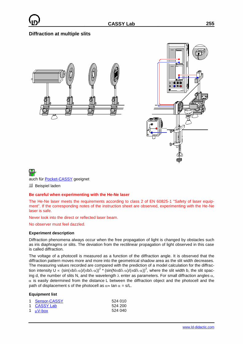
CASSY Lab

255

www.ld-didactic.com

Diffraction at multiple slits


Beispiel laden

Be careful when experimenting with the He-Ne laser

The He-Ne laser meets the requirements according to class 2 of EN 60825-1 "Safety of laser equip-ment". If the corresponding notes of the instruction sheet are observed, experimenting with the He-Ne laser is safe.

Never look into the direct or reflected laser beam.

No observer must feel dazzled.


Diffraction phenomena always occur when the free propagation of light is changed by obstacles such as iris diaphragms or slits. The deviation from the rectilinear propagation of light observed in this case is called diffraction.

The voltage of a photocell is measured as a function of the diffraction angle. It is observed that the diffraction pattern moves more and more into the geometrical shadow area as the slit width decreases. The measuring values recorded are compared with the prediction of a model calculation for the diffrac-

tion intensity U (sin(b/)/(b/))2 * (sin(Nd/)/(d/))

2, where the slit width b, the slit spac-

ing d, the number of slits N, and the wavelength enter as parameters. For small diffraction angles ,

is easily determined from the distance L between the diffraction object and the photocell and the

path of displacement s of the photocell as tan = s/L.

Equipment list

1 Sensor-CASSY 524 010 1 CASSY Lab 524 200 1 V-box 524 040

256

CASSY Lab

www.ld-didactic.com

1 Current supply box 524 031 with Displacement transducer and 529 031 Pair of cables, 100 cm, red and blue 501 46 or 1 Rotary motion sensor S 524 082 1 He-Ne laser, linearly polarized 471 840 1 Precision optical bench, 2 m 460 33 4 Riders, H=90 mm/B=60 mm 460 374 1 Sliding rider 460 383 1 Lens in frame, f = +5 mm 460 01 1 Lens in frame, f = +50 mm 460 02 1 Diaphragm with 3 double slits 469 84 1 Diaphragm with 4 double slits 469 85 1 Diaphragm with 5 multiple slits 469 86 1 Holder with spring clips 460 22 1 Photocell STE 2/19 578 62 1 Holder for plug-in elements 460 21 1 Simple bench clamp 301 07 1 Fishing line, 10 m 309 48 1 Set of 12 weights, each 50 g 342 61 1 Pair of cables, 100 cm, red and blue 501 46 1 PC with Windows 98/2000/XP/Vista


Remark: the adjustment should be carried out in a slightly darkened room.

Using a rider, mount the He-Ne laser to the optical bench as shown in the drawing.

Set up the photocell at a distance of approx. 1.90 m from the laser by means of the sliding rider and the holder for plug-in elements. The photocell should be located in the middle of the sliding rider. Stick two strips of dark paper on the photocell so that an entrance slit of approx. 1 mm is left.

Direct the laser towards the photocell, and switch it on.

Adjust the height of the laser so that the laser beam impinges on the centre of the photocell.

Place the spherical lens with the focal length f = +5 mm in front of the laser at a distance of approx. 1 cm. The laser beam has to cover the photocell.

Position the converging lens with the focal length f = +50 mm in front of the spherical lens at a dis-tance of approx. 55 mm and displace it on the optical bench towards the spherical lens until the la-ser beam is sharply imaged on the photocell.

Displace the converging lens on the optical bench somewhat further towards the spherical lens until the diameter of the laser beam on the photocell is approx. 6 mm. Now the laser beam should have a circular profile of constant diameter along the optical axis.

Put the holder with spring clips on the optical bench with the diaphragm being clamped, and dis-place it until the distance L between the photocell and the slit diaphragm is 1.50 m.

Fix the bench clamp with the displacement sensor to the table as shown in the drawing.

The path of displacement sA1 perpendicular to the optical axis is measured via the displacement

sensor at the current supply box on input A of the Sensor-CASSY.

In order to measure the voltage, the photocell is connected to input B of the Sensor-CASSY via the

V-box.


Einstellungen laden

Set the photocell to the position -6.0 cm opposite the displacement sensor.

Turn the wheel of the displacement sensor to the stop so that the display of the path sA1 is ap-

proximately -6.0 cm. If it turns out that the path measurement will lead to a wrong sign, connect the current supply box to the other arm of the displacement sensor.

Tie a piece of fishing line to the holder for plug-in elements, wind it once around the wheel of the displacement sensor, and suspend a weight from it.

Calibrate the zero of the path – for this place the photocell in the middle of the sliding rider (= zero of the scale or of the position of the principal intensity maxima, respectively).

Enter the target value 0 cm in Settings sA1 Correct, and then select Correct Offset.

CASSY Lab

257

www.ld-didactic.com

Slide the photocell back to the position opposite the displacement sensor, and keep it there.

If necessary, Correct the background brightness in the Settings UB1. For this enter the target value 0 mV, and then select Correct Offset.

Start the measurement with F9 (the message No Trigger Signal appears).

Displace the photocell very slowly by hand towards the displacement sensor. As soon as you pass the starting point at -5.5 cm, recording of measured values begins.


Evaluation

The intensity distribution of the diffraction pattern appears already during the measurement. The measured intensity distribution can now be compared with the result of the model calculation for small

diffraction angles tan = sA1/L by performing a Free fit (Alt+F). Use the following formula:

A*(sin(180*B/0.633*(x-C)/150)/(180*B/0.633*(x-C)/150))^2 * (sin(2*180*D/0.633*(x-C)/150)/sin(180*D/0.633*(x-C)/150))^2

with

x: displacement sA1 perpendicular to the optical axis

A: intensity I0

B: slit width b in m C: correction of the position of the principal maximum

D: slit spacing d in m N: number of slits (here double slit: N = 2) L: distance between the diaphragm and the photocell (here: L = 150 cm)

: wavelength of the He-Ne laser (here: = 0.633 m)

In this fit, the wavelength = 0.633 m of the He-Ne laser has been assumed to be known and the slit

width b and the slit spacing d have been determined. The other way round, the wavelength of the laser can be determined if the slit width b and the slit spacing d are known.

For the Free fit, always reasonable starting values for the slit width and the slit spacing should be cho-

sen, e. g., B=200 (m) for b=0.2 mm and D=250 (m) for d=0.25 mm.

If the secondary maxima are not clearly seen for N > 2, the slit spacing d cannot be determined by the

Free fit. In this case, the correct slit spacing d should be entered in m as a starting value for the fit and then be kept constant (e. g. 250 for 0.25 mm).

Remark

In this experiment on diffraction of light at multiple slits, the intensity distribution is recorded manually. The measuring values can be recorded automatically with the aid of VideoCom (experiment P5.3.1.7).

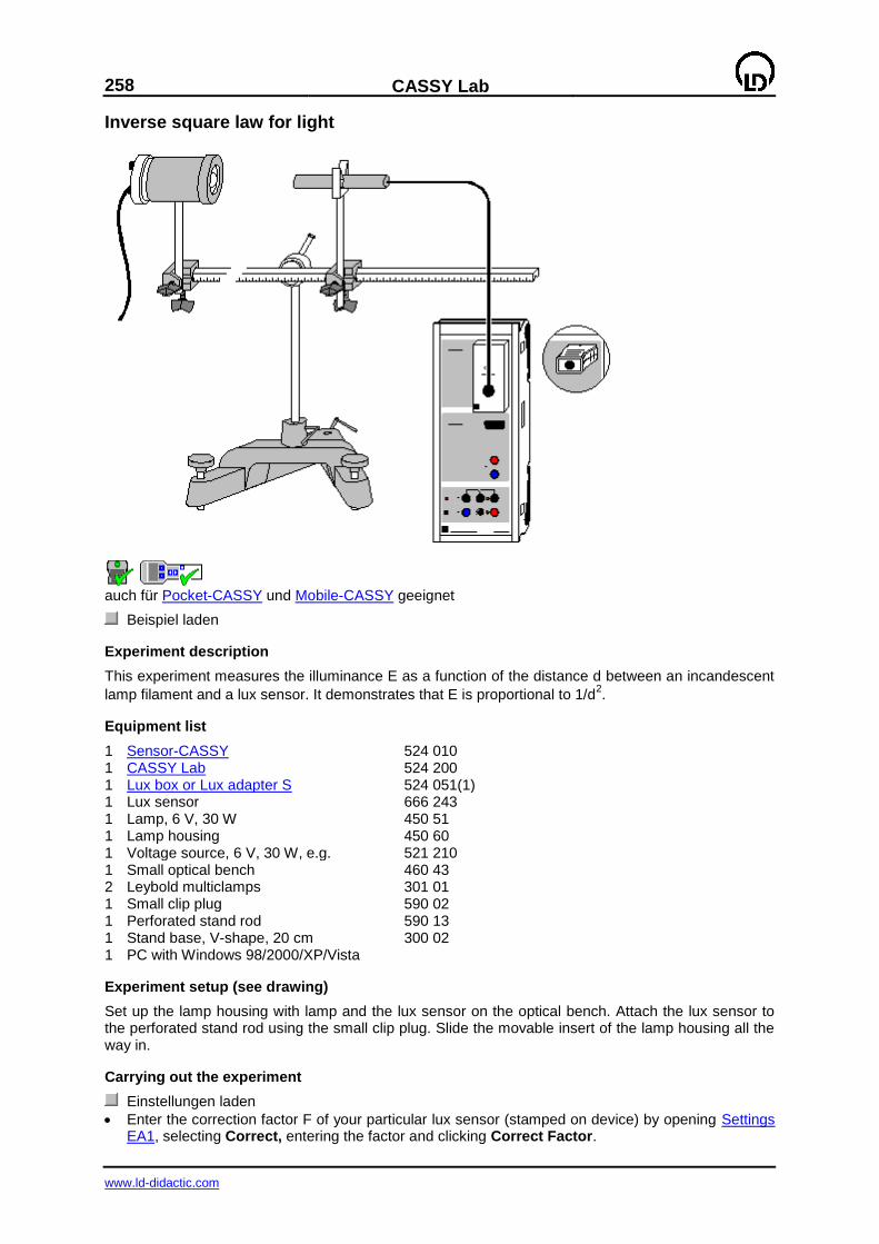
258

CASSY Lab

www.ld-didactic.com

Inverse square law for light


Beispiel laden


This experiment measures the illuminance E as a function of the distance d between an incandescent

lamp filament and a lux sensor. It demonstrates that E is proportional to 1/d2.

Equipment list

1 Sensor-CASSY 524 010 1 CASSY Lab 524 200 1 Lux box or Lux adapter S 524 051(1) 1 Lux sensor 666 243 1 Lamp, 6 V, 30 W 450 51 1 Lamp housing 450 60 1 Voltage source, 6 V, 30 W, e.g. 521 210 1 Small optical bench 460 43 2 Leybold multiclamps 301 01 1 Small clip plug 590 02 1 Perforated stand rod 590 13 1 Stand base, V-shape, 20 cm 300 02 1 PC with Windows 98/2000/XP/Vista


Set up the lamp housing with lamp and the lux sensor on the optical bench. Attach the lux sensor to the perforated stand rod using the small clip plug. Slide the movable insert of the lamp housing all the way in.


Einstellungen laden

Enter the correction factor F of your particular lux sensor (stamped on device) by opening Settings EA1, selecting Correct, entering the factor and clicking Correct Factor.

CASSY Lab

259

www.ld-didactic.com

Correct the background brightness with Settings EA1, Correct, Correct Offset.

Switch on the lamp and set a distance of 10 cm between the lamp filament and the lux sensor.

Enter this value in the table (click on the column d in the first table row and type in the value).

Transfer the illuminance value to the table with F9.

Increase the distance in steps, write the distances in the table and accept each new illuminance value with F9.

Evaluation

The measurements are displayed in the diagram while the measurement is running. To confirm the

inverse square law for light, you can fit a hyperbola 1/x2 to the diagram, or alternatively convert the x-

axis to 1/x2 (click on the axis with the mouse) and fit a straight line.

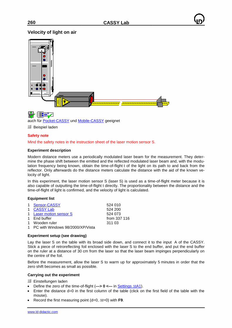
260

CASSY Lab

www.ld-didactic.com

Velocity of light on air


Beispiel laden

Safety note



Modern distance meters use a periodically modulated laser beam for the measurement. They deter-mine the phase shift between the emitted and the reflected modulated laser beam and, with the modu-lation frequency being known, obtain the time-of-flight t of the light on its path to and back from the reflector. Only afterwards do the distance meters calculate the distance with the aid of the known ve-locity of light.

In this experiment, the laser motion sensor S (laser S) is used as a time-of-flight meter because it is also capable of outputting the time-of-flight t directly. The proportionality between the distance and the time-of-flight of light is confirmed, and the velocity of light is calculated.

Equipment list

1 Sensor-CASSY 524 010 1 CASSY Lab 524 200 1 Laser motion sensor S 524 073 1 End buffer from 337 116 1 Wooden ruler 311 03 1 PC with Windows 98/2000/XP/Vista


Lay the laser S on the table with its broad side down, and connect it to the input A of the CASSY. Stick a piece of retroreflecting foil enclosed with the laser S to the end buffer, and put the end buffer on the ruler at a distance of 30 cm from the laser so that the laser beam impinges perpendicularly on the centre of the foil.

Before the measurement, allow the laser S to warm up for approximately 5 minutes in order that the zero shift becomes as small as possible.


Einstellungen laden

Define the zero of the time-of-flight (—> 0 <— in Settings tA1).

Enter the distance d=0 in the first column of the table (click on the first field of the table with the mouse).

Record the first measuring point (d=0, t=0) with F9.

CASSY Lab

261

www.ld-didactic.com

Displace the end buffer away from the laser by 10 cm, and enter the distance 0.1 m in the first column of the table (click on the second field of the table with the mouse).

Record the second measuring point (d=0.1 m, t) with F9.

Repeat the measurement for greater distances up to approximately 50 cm.

Evaluation

The optical path s of the laser beam is equal to twice the distance d. This is already taken into account

in the s(t) diagram in the Velocity of Light display. The proportionality between s and t, i.e. s = ct, is confirmed by the s(t) diagram. Fitting a straight line through the origin leads to the proportionality con-stant c = 0.3 m/ns = 300,000 km/s.

262

CASSY Lab

www.ld-didactic.com

Velocity of light in various materials


Beispiel laden

Safety note



Modern distance meters use a periodically modulated laser beam for the measurement. They deter-mine the phase shift between the emitted and the reflected modulated laser beam and, with the modu-lation frequency being known, obtain the time-of-flight t of the light on its path to and back from the reflector. Only afterwards do the distance meters calculate the distance with the aid of the known ve-locity of light.

In this experiment, the laser motion sensor S (laser S) is used as a time-of-flight meter because it is also capable of outputting the time-of-flight t directly. Water and acrylic glass of thickness d are held

into the path of the beam, and then the resulting increase of the time-of-flight t is measured. With the

velocity of light c in air measured in the previous experiment, the velocity of light cM in matter can now be determined:

cM = 2d/(2d/c+t) = 1/(1/c+t/2d).

Finally, the refractive index n is determined according to

n = c/cM = c(1/c+t/2d) = 1 + c/2dt.

Equipment list

1 Sensor-CASSY 524 010 1 CASSY Lab 524 200 1 Laser motion sensor S 524 073 1 End buffer from 337 116 1 Plate glass cell, 50 mm × 50 mm × 50 mm 477 03 1 Acrylic glass block 476 34 1 PC with Windows 98/2000/XP/Vista


Lay the laser S on the table with its broad side down, and connect it to the input A of the CASSY. Stick a piece of retroreflecting foil enclosed with the laser S to the end buffer, and put the end buffer on the ruler at a distance of approximately 50 cm from the laser so that the laser beam impinges per-pendicularly on the centre of the foil.

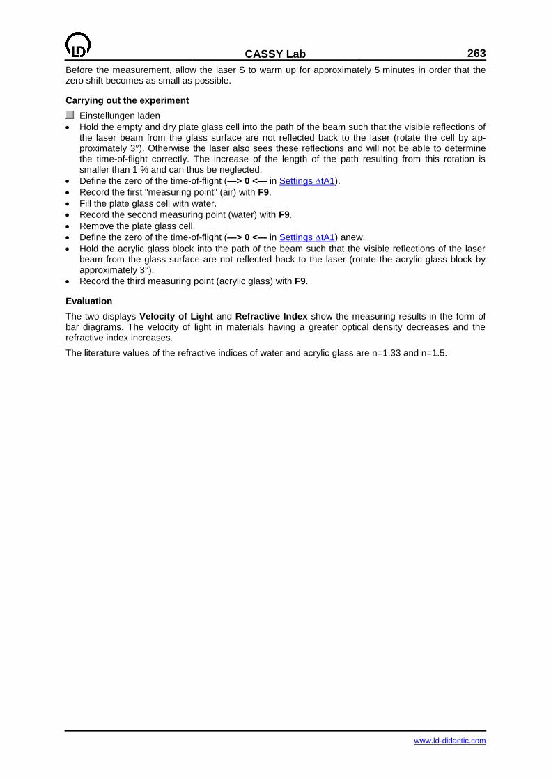
CASSY Lab

263

www.ld-didactic.com

Before the measurement, allow the laser S to warm up for approximately 5 minutes in order that the zero shift becomes as small as possible.


Einstellungen laden

Hold the empty and dry plate glass cell into the path of the beam such that the visible reflections of the laser beam from the glass surface are not reflected back to the laser (rotate the cell by ap-proximately 3°). Otherwise the laser also sees these reflections and will not be able to determine the time-of-flight correctly. The increase of the length of the path resulting from this rotation is smaller than 1 % and can thus be neglected.

Define the zero of the time-of-flight (—> 0 <— in Settings tA1).

Record the first "measuring point" (air) with F9.

Fill the plate glass cell with water.

Record the second measuring point (water) with F9.

Remove the plate glass cell.

Define the zero of the time-of-flight (—> 0 <— in Settings tA1) anew.

Hold the acrylic glass block into the path of the beam such that the visible reflections of the laser beam from the glass surface are not reflected back to the laser (rotate the acrylic glass block by approximately 3°).

Record the third measuring point (acrylic glass) with F9.

Evaluation

The two displays Velocity of Light and Refractive Index show the measuring results in the form of bar diagrams. The velocity of light in materials having a greater optical density decreases and the refractive index increases.

The literature values of the refractive indices of water and acrylic glass are n=1.33 and n=1.5.

264

CASSY Lab

www.ld-didactic.com

Millikan's experiment


Beispiel laden


In 1910, R. A. Millikan succeeded in demonstrating the quantized occurrence of smallest amounts of electrical charge using his famous oil droplet method. He observed charged oil droplets in a vertical electrical field of a plate capacitor with the plate distance d and determined the charge q of a floating droplet from its radius r and the electrical field E=U/d. In his experiment, he found that q only occurs as

integral multiples of an elementary charge e, i.e. q = ne.

Theory

When an oil droplet with radius r0 falls with the velocity –v1, this droplet is subject to Stokes friction,

which leads to the upward directed force F1 = 6r0v1 ( = viscosity of air). When the oil droplet rises

with the velocity v2 in an external electrical field E, the downward directed force due to Stokes friction

is F2 = –6r0v2. The difference between these two forces is exactly the force q0E exerted by the

applied electrical field E, i.e.

q0E = q0U/d = F1–F2 = 6r0(v1+v2) or

q0 = 6r0d(v1+v2) / U.

In order to determine the charge q0, only the radius r0 of the oil droplet under consideration is required, which, however, is easily obtained from the equilibrium of forces between its resultant gravitational

force F = –Vg and the Stokes frictional force F1 in the case of the falling droplet, where is the

difference between the densities of oil and air.

Thus we have:

0 = F+F1 = –4/3 r03g + 6r0v1 or

CASSY Lab

265

www.ld-didactic.com

r0 = 9v1 / 2g).

For a more precise determination of the charge q, it has to be taken into account that Stokes friction has to be corrected for very small radii r because these are of the order of magnitude of the mean free path of the air molecules. The corrected formula for the frictional force, which depends on the air pres-sure p, reads

F = 6rv / (1+b/rp)

with b = 80 µmhPa (constant).

With the abbreviation A = b/p, the corrected radius r is

r = (r02 + A

2/4) – A/2

and the corrected charge q is

q = q0 / (1+A/r)1.5

.

Floating method

In this version of the experiment, the voltage U at the plate capacitor is adjusted such that a particular

oil droplet floats, i.e. the rising velocity is v2=0. The falling velocity v1 is measured after switching off

the voltage U at the capacitor. Because of v2=0, the above formulas are slightly simplified.

However, v2=0 cannot be adjusted very precisely for fundamental reasons. Therefore the floating method leads to larger measurement errors and broader scattering in the frequency distribution than in the case of the following method.

Falling/rising method

In the second version, the two velocities v1 and v2 the voltage U are measured. This method makes

possible more precise measured values than the floating method because the velocity v2 is really measured.

Equipment list

1 Sensor-CASSY 524 010 1 CASSY Lab 524 200 1 Timer box 524 034 1 Millikan apparatus 559 411 1 Millikan supply unit 559 421 1 Connecting lead, 50 cm, red 500 421 3 Pairs of cables, 50 cm, red and blue 501 45 1 Pair of cables, 50 cm, black 501 451 1 PC with Windows 98/2000/XP/Vista


Set up the Millikan apparatus as described in the instruction sheet, fill in oil, and set up the circuit as shown in the drawing. Connect the stopwatch output 1 to the input E and the stopwatch output 2 to the input F of the timer box. Connect the voltage output of the supply unit to the input B of the Sensor-CASSY.

Attention: the microscope creates an inverted image. Therefore all directions of motions are inverted. In the following, however, the real motion is described.

For a better demonstration of the oil droplets, it is recommended to record the image of the micro-scope by means of a video camera (e. g. VideoFlex from ken-a-vision). In this case, the camera can record upside down so that the visible direction of motion corresponds to the real direction of motion.


a) Floating method

Einstellungen laden

Orient the eyepiece micrometer vertically and turn the lens holder of the eyepiece until you can clearly see the micrometer scale.

First set the switches U and t in the down position.

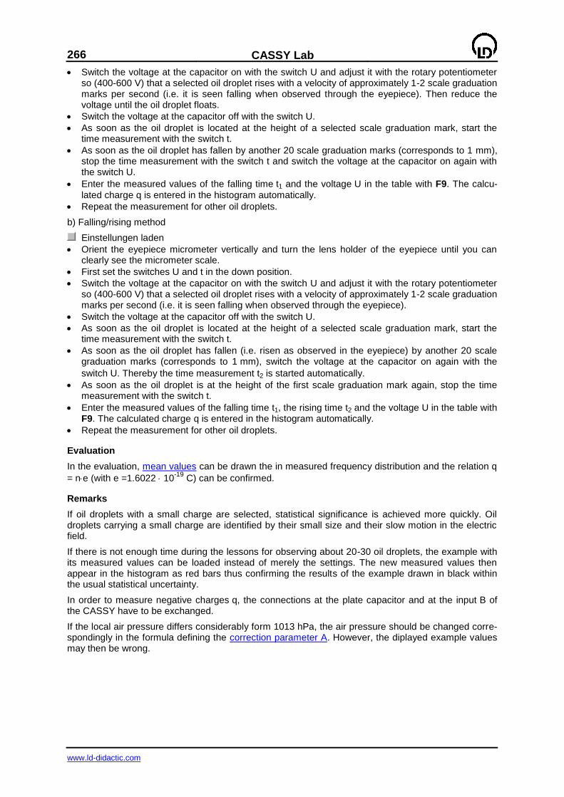
266

CASSY Lab

www.ld-didactic.com

Switch the voltage at the capacitor on with the switch U and adjust it with the rotary potentiometer so (400-600 V) that a selected oil droplet rises with a velocity of approximately 1-2 scale graduation marks per second (i.e. it is seen falling when observed through the eyepiece). Then reduce the voltage until the oil droplet floats.

Switch the voltage at the capacitor off with the switch U.

As soon as the oil droplet is located at the height of a selected scale graduation mark, start the time measurement with the switch t.

As soon as the oil droplet has fallen by another 20 scale graduation marks (corresponds to 1 mm), stop the time measurement with the switch t and switch the voltage at the capacitor on again with the switch U.

Enter the measured values of the falling time t1 and the voltage U in the table with F9. The calcu-

lated charge q is entered in the histogram automatically.

Repeat the measurement for other oil droplets.

b) Falling/rising method

Einstellungen laden

Orient the eyepiece micrometer vertically and turn the lens holder of the eyepiece until you can clearly see the micrometer scale.

First set the switches U and t in the down position.

Switch the voltage at the capacitor on with the switch U and adjust it with the rotary potentiometer so (400-600 V) that a selected oil droplet rises with a velocity of approximately 1-2 scale graduation marks per second (i.e. it is seen falling when observed through the eyepiece).

Switch the voltage at the capacitor off with the switch U.

As soon as the oil droplet is located at the height of a selected scale graduation mark, start the time measurement with the switch t.

As soon as the oil droplet has fallen (i.e. risen as observed in the eyepiece) by another 20 scale graduation marks (corresponds to 1 mm), switch the voltage at the capacitor on again with the

switch U. Thereby the time measurement t2 is started automatically.

As soon as the oil droplet is at the height of the first scale graduation mark again, stop the time measurement with the switch t.

Enter the measured values of the falling time t1, the rising time t2 and the voltage U in the table with F9. The calculated charge q is entered in the histogram automatically.

Repeat the measurement for other oil droplets.

Evaluation

In the evaluation, mean values can be drawn the in measured frequency distribution and the relation q

= ne (with e =1.6022 10-19

C) can be confirmed.

Remarks

If oil droplets with a small charge are selected, statistical significance is achieved more quickly. Oil droplets carrying a small charge are identified by their small size and their slow motion in the electric field.

If there is not enough time during the lessons for observing about 20-30 oil droplets, the example with its measured values can be loaded instead of merely the settings. The new measured values then appear in the histogram as red bars thus confirming the results of the example drawn in black within the usual statistical uncertainty.

In order to measure negative charges q, the connections at the plate capacitor and at the input B of the CASSY have to be exchanged.

If the local air pressure differs considerably form 1013 hPa, the air pressure should be changed corre-spondingly in the formula defining the correction parameter A. However, the diplayed example values may then be wrong.

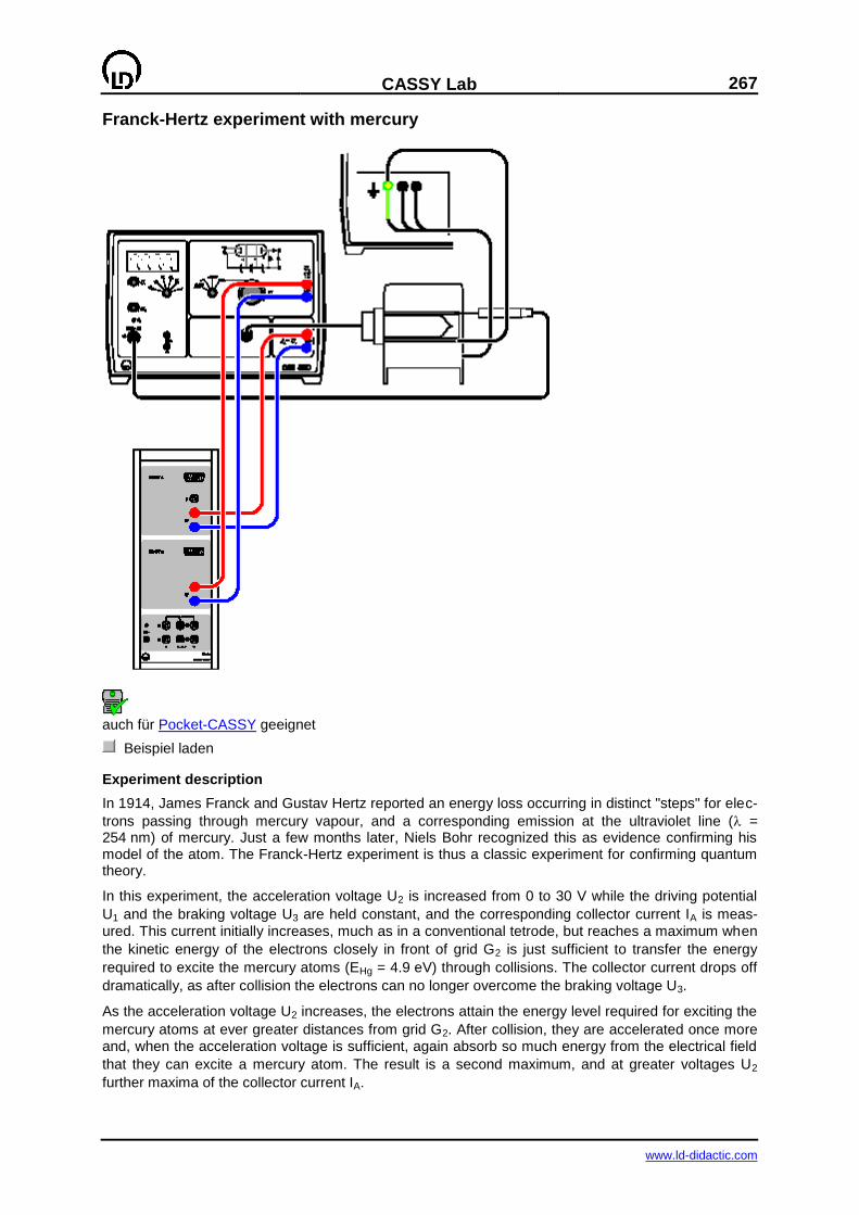
CASSY Lab

267

www.ld-didactic.com

Franck-Hertz experiment with mercury


Beispiel laden


In 1914, James Franck and Gustav Hertz reported an energy loss occurring in distinct "steps" for elec-

trons passing through mercury vapour, and a corresponding emission at the ultraviolet line ( = 254 nm) of mercury. Just a few months later, Niels Bohr recognized this as evidence confirming his model of the atom. The Franck-Hertz experiment is thus a classic experiment for confirming quantum theory.

In this experiment, the acceleration voltage U2 is increased from 0 to 30 V while the driving potential

U1 and the braking voltage U3 are held constant, and the corresponding collector current IA is meas-

ured. This current initially increases, much as in a conventional tetrode, but reaches a maximum when

the kinetic energy of the electrons closely in front of grid G2 is just sufficient to transfer the energy

required to excite the mercury atoms (EHg = 4.9 eV) through collisions. The collector current drops off

dramatically, as after collision the electrons can no longer overcome the braking voltage U3.

As the acceleration voltage U2 increases, the electrons attain the energy level required for exciting the

mercury atoms at ever greater distances from grid G2. After collision, they are accelerated once more and, when the acceleration voltage is sufficient, again absorb so much energy from the electrical field

that they can excite a mercury atom. The result is a second maximum, and at greater voltages U2

further maxima of the collector current IA.

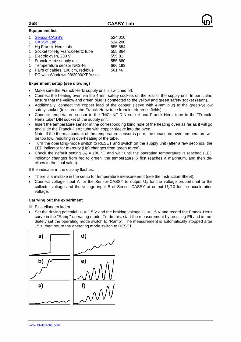
268

CASSY Lab

www.ld-didactic.com

Equipment list

1 Sensor-CASSY 524 010 1 CASSY Lab 524 200 1 Hg Franck-Hertz tube 555 854 1 Socket for Hg Franck-Hertz tube 555 864 1 Electric oven, 230 V 555 81 1 Franck-Hertz supply unit 555 880 1 Temperature sensor NiCr-Ni 666 193 2 Pairs of cables, 100 cm, red/blue 501 46 1 PC with Windows 98/2000/XP/Vista


Make sure the Franck-Hertz supply unit is switched off.

Connect the heating oven via the 4-mm safety sockets on the rear of the supply unit. In particular, ensure that the yellow and green plug is connected to the yellow and green safety socket (earth).

Additionally, connect the copper lead of the copper sleeve with 4-mm plug to the green-yellow safety socket (to screen the Franck-Hertz tube from interference fields).

Connect temperature sensor to the "NiCr-Ni" DIN socket and Franck-Hertz tube to the "Franck-Hertz tube" DIN socket of the supply unit.

Insert the temperature sensor in the corresponding blind hole of the heating oven as far as it will go and slide the Franck-Hertz tube with copper sleeve into the oven. Note: If the thermal contact of the temperature sensor is poor, the measured oven temperature will be too low, resulting in overheating of the tube.

Turn the operating-mode switch to RESET and switch on the supply unit (after a few seconds, the LED indicator for mercury (Hg) changes from green to red).

Check the default setting S = 180 °C and wait until the operating temperature is reached (LED

indicator changes from red to green; the temperature first reaches a maximum, and then de-clines to the final value).

If the indicator in the display flashes:

There is a mistake in the setup for temperature measurement (see the Instruction Sheet).

Connect voltage input A for the Sensor-CASSY to output UA for the voltage proportional to the

collector voltage and the voltage input B of Sensor-CASSY at output U2/10 for the acceleration voltage.


Einstellungen laden

Set the driving potential U1 = 1.5 V and the braking voltage U3 = 1.5 V and record the Franck-Hertz curve in the "Ramp" operating mode. To do this, start the measurement by pressing F9 and imme-diately set the operating mode switch to "Ramp". The measurement is automatically stopped after 15 s, then return the operating mode switch to RESET.

CASSY Lab

269

www.ld-didactic.com

1) Optimizing

If the Franck-Hertz curve rises abruptly (a) and you can see a gas discharge in the Franck-Hertz tube through the insertion opening of the oven (blue glow):

Immediately turn the operating-mode switch to RESET and wait until the setup reaches the operat-ing temperature.

If necessary, raise the set value S using the screwdriver potentiometer (e.g. by 5 °C) and wait a

few minutes until the system settles into the new thermal equilibrium.

2) Optimizing U1

A higher driving potential U1 results in a greater electron emission current.

If the Franck-Hertz curve rises too steeply, i.e. the overdrive limit of the current measuring amplifier is

reached at values below U2 = 30 V and the top of the Franck-Hertz curve is cut off (b):

Reduce U1 until the curve steepness corresponds to (d).

If the Franck-Hertz curve is too flat, i.e. the collector current IA remains below 5 nA in all areas (c):

Increase U1 until the curve steepness corresponds to (d).

If the Franck-Hertz curve is flat even after increasing U1:

Reduce the set value S for the oven temperature using the screwdriver potentiometer.

3) Optimizing U3

A greater braking voltage U3 causes better-defined maxima and minima of the Franck-Hertz curve; at the same time, however, the total collector current is reduced.

If the maxima and minima of the Franck-Hertz curve are insufficiently defined (d):

Alternately increase first the braking voltage U3 and then the driving potential U1 until you obtain

the curve form shown in (f).

If the minima of the Franck-Hertz curve are cut off at the bottom (e):

Alternately reduce first the braking voltage U3 and then the driving potential U1 until you obtain the curve form shown in (f).

The Hg Franck-Hertz tube in the experimental example was measured using the parameters U1 =

2.58 V, U3 = 1.95 V und S = 180 °C.

Evaluation

The recorded curve is evaluated by drawing vertical lines or peak centers to find the distance between

the subsequent maxima. In the experimental example, an average value of U2 = 5.07 V is found. This

corresponds to an energy transfer E = 5.07 eV.

The value found in the literature for the transfer energy of the mercury atoms from the basic state 1S0

to the first 3P1 state is EHg = 4.9 eV.

The position of the first maximum is determined through the contact voltage of the electrode materials

used and the driving potential U1. The larger distance between the maxima of higher order is caused by superposition of the Franck-Hertz curve by the characteristic tube line.

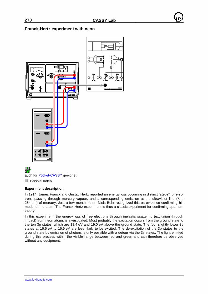
270

CASSY Lab

www.ld-didactic.com

Franck-Hertz experiment with neon


Beispiel laden


In 1914, James Franck and Gustav Hertz reported an energy loss occurring in distinct "steps" for elec-

trons passing through mercury vapour, and a corresponding emission at the ultraviolet line ( = 254 nm) of mercury. Just a few months later, Niels Bohr recognized this as evidence confirming his model of the atom. The Franck-Hertz experiment is thus a classic experiment for confirming quantum theory.

In this experiment, the energy loss of free electrons through inelastic scattering (excitation through impact) from neon atoms is investigated. Most probably the excitation occurs from the ground state to the ten 3p states, which are 18.4 eV and 19.0 eV above the ground state. The four slightly lower 3s states at 16.6 eV to 16.9 eV are less likely to be excited. The de-excitation of the 3p states to the ground state by emission of photons is only possible with a detour via the 3s states. The light emitted during this process within the visible range between red and green and can therefore be observed without any equipment.

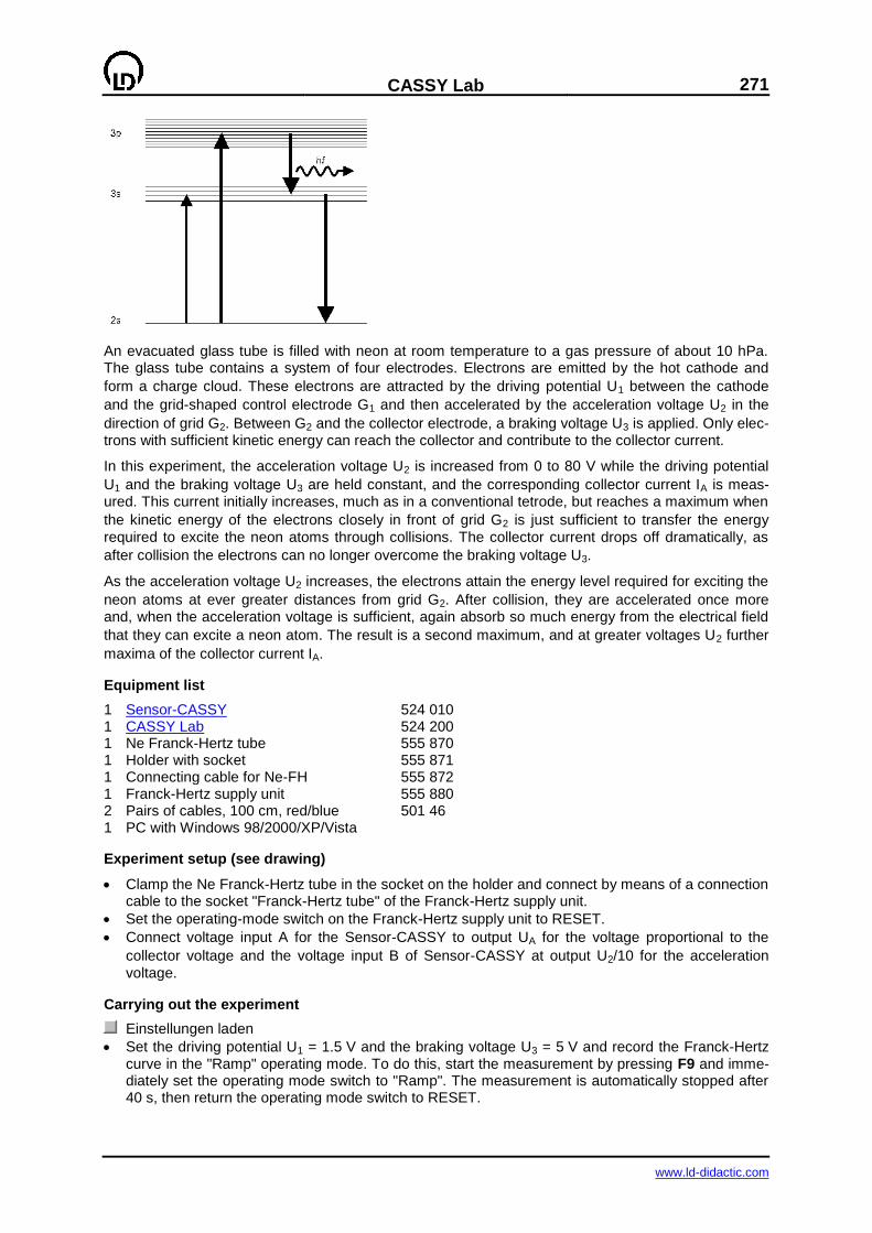
CASSY Lab

271

www.ld-didactic.com

An evacuated glass tube is filled with neon at room temperature to a gas pressure of about 10 hPa. The glass tube contains a system of four electrodes. Electrons are emitted by the hot cathode and

form a charge cloud. These electrons are attracted by the driving potential U1 between the cathode

and the grid-shaped control electrode G1 and then accelerated by the acceleration voltage U2 in the

direction of grid G2. Between G2 and the collector electrode, a braking voltage U3 is applied. Only elec-trons with sufficient kinetic energy can reach the collector and contribute to the collector current.

In this experiment, the acceleration voltage U2 is increased from 0 to 80 V while the driving potential

U1 and the braking voltage U3 are held constant, and the corresponding collector current IA is meas-ured. This current initially increases, much as in a conventional tetrode, but reaches a maximum when

the kinetic energy of the electrons closely in front of grid G2 is just sufficient to transfer the energy

required to excite the neon atoms through collisions. The collector current drops off dramatically, as

after collision the electrons can no longer overcome the braking voltage U3.

As the acceleration voltage U2 increases, the electrons attain the energy level required for exciting the

neon atoms at ever greater distances from grid G2. After collision, they are accelerated once more and, when the acceleration voltage is sufficient, again absorb so much energy from the electrical field

that they can excite a neon atom. The result is a second maximum, and at greater voltages U2 further

maxima of the collector current IA.

Equipment list

1 Sensor-CASSY 524 010 1 CASSY Lab 524 200 1 Ne Franck-Hertz tube 555 870 1 Holder with socket 555 871 1 Connecting cable for Ne-FH 555 872 1 Franck-Hertz supply unit 555 880 2 Pairs of cables, 100 cm, red/blue 501 46 1 PC with Windows 98/2000/XP/Vista


Clamp the Ne Franck-Hertz tube in the socket on the holder and connect by means of a connection cable to the socket "Franck-Hertz tube" of the Franck-Hertz supply unit.

Set the operating-mode switch on the Franck-Hertz supply unit to RESET.

Connect voltage input A for the Sensor-CASSY to output UA for the voltage proportional to the

collector voltage and the voltage input B of Sensor-CASSY at output U2/10 for the acceleration

voltage.


Einstellungen laden

Set the driving potential U1 = 1.5 V and the braking voltage U3 = 5 V and record the Franck-Hertz curve in the "Ramp" operating mode. To do this, start the measurement by pressing F9 and imme-diately set the operating mode switch to "Ramp". The measurement is automatically stopped after 40 s, then return the operating mode switch to RESET.

272

CASSY Lab

www.ld-didactic.com

1) Optimizing U1

A higher driving potential U1 results in a greater electron emission current.

If the Franck-Hertz curve rises too steeply, i.e. the overdrive limit of the current measuring amplifier is

reached at values below U2 = 80 V and the top of the Franck-Hertz curve is cut off (a):

Reduce U1 until the curve steepness corresponds to (c).

If the Franck-Hertz curve is too flat, i.e. the collector current IA remains below 5 nA in all areas (b):

Increase U1 until the curve steepness corresponds to (c).

If necessary, optimize the cathode heating as described in the Instruction Sheet for the Franck-Hertz supply unit.

2) Optimizing U3

A greater braking voltage U3 causes better-defined maxima and minima of the Franck-Hertz curve; at the same time, however, the total collector current is reduced.

If the maxima and minima of the Franck-Hertz curve are insufficiently defined (c):

Alternately increase first the braking voltage U3 and then the driving potential U1 until you obtain

the curve form shown in (e).

If the minima of the Franck-Hertz curve are cut off at the bottom (d):

Alternately reduce first the braking voltage U3 and then the driving potential U1 until you obtain the curve form shown in (e).

The Ne Franck-Hertz tube in the experimental example was measured using the parameters U1 =

1.5 V and U3 = 7.9 V.

Evaluation

The recorded curve is evaluated by drawing vertical lines (by eye) to find the distance between the

subsequent maxima. In the experimental example, an average value of U2 = 18.2 V is found. This value is much closer to the excitation energies for the 3p-levels of neon (18.4-19.0 eV) than to the energies of the 3s-levels (16.6–16.9 eV). Thus, the probability of excitation to the latter due to inelastic electron collision is significantly less.

The substructure in the measured curve shows that the excitation of the 3s-levels cannot be ignored altogether. Note that for double and multiple collisions, each combination of excitation of a 3s-level and a 3p-level occurs.

In the Ne Franck-Hertz tube, luminous zones can be observed which depend on the acceleration volt-age. They directly correlate with the minima of the Franck-Hertz curve.

CASSY Lab

273

www.ld-didactic.com

Moseley's law (K-line x-ray fluorescence)


Beispiel laden

Safety notes

The X-ray apparatus fulfils all regulations on the design of an X-ray apparatus and fully protected de-vice for instructional use and is type approved for school use in Germany (BfS 05/07 V/Sch RöV or NW 807 / 97 Rö).

The built-in protective and shielding fixtures reduce the dose rate outside the X-ray apparatus to less than 1 µSv/h, which is of the order of magnitude of the natural background radiation.

Before putting the X-ray apparatus into operation, inspect it for damage and check whether the voltage is switched off when the sliding doors are opened (See instruction sheet of the X-ray appa-ratus).

Protect the X-ray apparatus against access by unauthorized persons.

Avoid overheating of the anode in the X-ray tube.

When switching the X-ray apparatus on, check whether the ventilator in the tube chamber starts rotating.

The goniometer is positioned solely by means of electric stepper motors.

Do not block the target arm and the sensor arm of the goniometer and do not use force to move them.

When handling heavy metals or allergen substances from the target set, observe their operating in-structions.

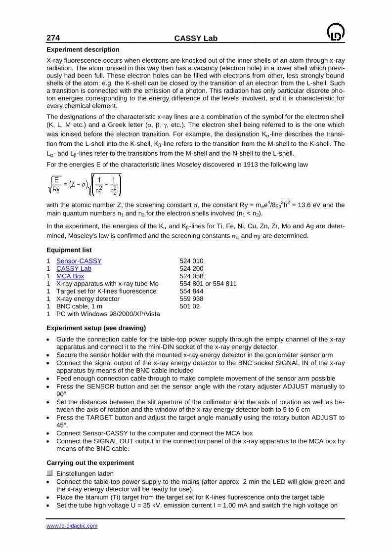
274

CASSY Lab

www.ld-didactic.com


X-ray fluorescence occurs when electrons are knocked out of the inner shells of an atom through x-ray radiation. The atom ionised in this way then has a vacancy (electron hole) in a lower shell which previ-ously had been full. These electron holes can be filled with electrons from other, less strongly bound shells of the atom: e.g. the K-shell can be closed by the transition of an electron from the L-shell. Such a transition is connected with the emission of a photon. This radiation has only particular discrete pho-ton energies corresponding to the energy difference of the levels involved, and it is characteristic for every chemical element.

The designations of the characteristic x-ray lines are a combination of the symbol for the electron shell

(K, L, M etc.) and a Greek letter (, , , etc.). The electron shell being referred to is the one which

was ionised before the electron transition. For example, the designation K-line describes the transi-

tion from the L-shell into the K-shell, K-line refers to the transition from the M-shell to the K-shell. The

L- and L-lines refer to the transitions from the M-shell and the N-shell to the L-shell.

For the energies E of the characteristic lines Moseley discovered in 1913 the following law

with the atomic number Z, the screening constant , the constant Ry = mee4/80

2h

2 = 13.6 eV and the

main quantum numbers n1 and n2 for the electron shells involved (n1 < n2).

In the experiment, the energies of the K and K-lines for Ti, Fe, Ni, Cu, Zn, Zr, Mo and Ag are deter-

mined, Moseley's law is confirmed and the screening constants and are determined.

Equipment list

1 Sensor-CASSY 524 010 1 CASSY Lab 524 200 1 MCA Box 524 058 1 X-ray apparatus with x-ray tube Mo 554 801 or 554 811 1 Target set for K-lines fluorescence 554 844 1 X-ray energy detector 559 938 1 BNC cable, 1 m 501 02 1 PC with Windows 98/2000/XP/Vista


Guide the connection cable for the table-top power supply through the empty channel of the x-ray apparatus and connect it to the mini-DIN socket of the x-ray energy detector.

Secure the sensor holder with the mounted x-ray energy detector in the goniometer sensor arm

Connect the signal output of the x-ray energy detector to the BNC socket SIGNAL IN of the x-ray apparatus by means of the BNC cable included

Feed enough connection cable through to make complete movement of the sensor arm possible

Press the SENSOR button and set the sensor angle with the rotary adjuster ADJUST manually to 90°

Set the distances between the slit aperture of the collimator and the axis of rotation as well as be-tween the axis of rotation and the window of the x-ray energy detector both to 5 to 6 cm

Press the TARGET button and adjust the target angle manually using the rotary button ADJUST to 45°.

Connect Sensor-CASSY to the computer and connect the MCA box

Connect the SIGNAL OUT output in the connection panel of the x-ray apparatus to the MCA box by means of the BNC cable.


Einstellungen laden

Connect the table-top power supply to the mains (after approx. 2 min the LED will glow green and the x-ray energy detector will be ready for use).

Place the titanium (Ti) target from the target set for K-lines fluorescence onto the target table

Set the tube high voltage U = 35 kV, emission current I = 1.00 mA and switch the high voltage on

CASSY Lab

275

www.ld-didactic.com

Start the measurement by pressing F9

Then record the spectra for the other targets (Fe, Ni, Cu, Zn, Zr, Mo and Ag) in the target set for K-lines fluorescence

Energy calibration

The energy calibration of the spectra is made using the K-lines of iron (Fe) and molybdenum (Mo).

Open in the context menu of the diagram (right mouse button) or select with Alt+E the Energy cali-bration, select global energy calibration and enter on the right-hand side the energies of the Fe

K-line (6.40 keV) and of the Mo K-line (17.48 keV). Do not yet close the Energy calibration

window.

In the context menu of the diagram select under Other evaluations Calculate peak center, mark the

Fe K-line (2nd spectrum) and enter the result in the left-hand side of the energy calibration (e.g.

with drag & drop from the status line)

Then determine the centre of the Mo K-line (7th

spectrum) and also enter the result on the left-

hand side

Close the Energy calibration window

Evaluation

As the atomic number Z increases the energy of the characteristic lines also increases and so does

the separation between the - and the -component in the K spectral series. For a quantitative analy-sis, the energies of the individual lines can be determined.

Select a spectrum in the diagram

In the context menu of the diagram (right mouse button) or with Alt+V choose Vertical line and

mark approximately the positions of the K and K-line.

In the context menu of the diagram select under Other evaluations Gaussians of equal width and mark the area of the desired peak (also mark sufficient background!)

Read the determined peak positions from the status line and enter them together with the atomic numbers Z of Ti (Z=22), Fe (Z=26), Ni (Z=28), Cu (Z=29), Zn (Z=30), Zr (Z=40), Mo (Z=42) and Ag (Z=47) into the Energy diagram (click with mouse) (e.g. by drag & drop from the status line)

For each line, the expression E/Ry is automatically calculated and plotted in the Moseley diagram as

a function of the atomic number Z. The same applies to the screening constants and and the

Screening diagram.

In the Moseley diagram, by a free fit with the formula (x-1)*sqr(3/4), the theoretical line for the K-line

can be entered, which corresponds well to the measured values.

The Screening diagram shows for the K-line that the deviation from the theoretically expected =1

grows with increasing atomic number Z. This is explained by the fact that the influence of the external electrons increases as the number of electrons increases.

The screening constants for the K-lines have a value 2 which indicates, as expected, a

stronger effective screening of the nucleus charge for the electron transitions from the higher level

n2=3.

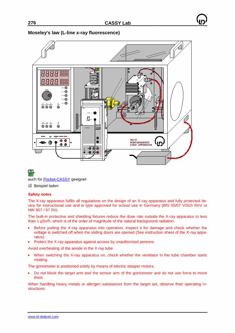
276

CASSY Lab

www.ld-didactic.com

Moseley's law (L-line x-ray fluorescence)


Beispiel laden

Safety notes










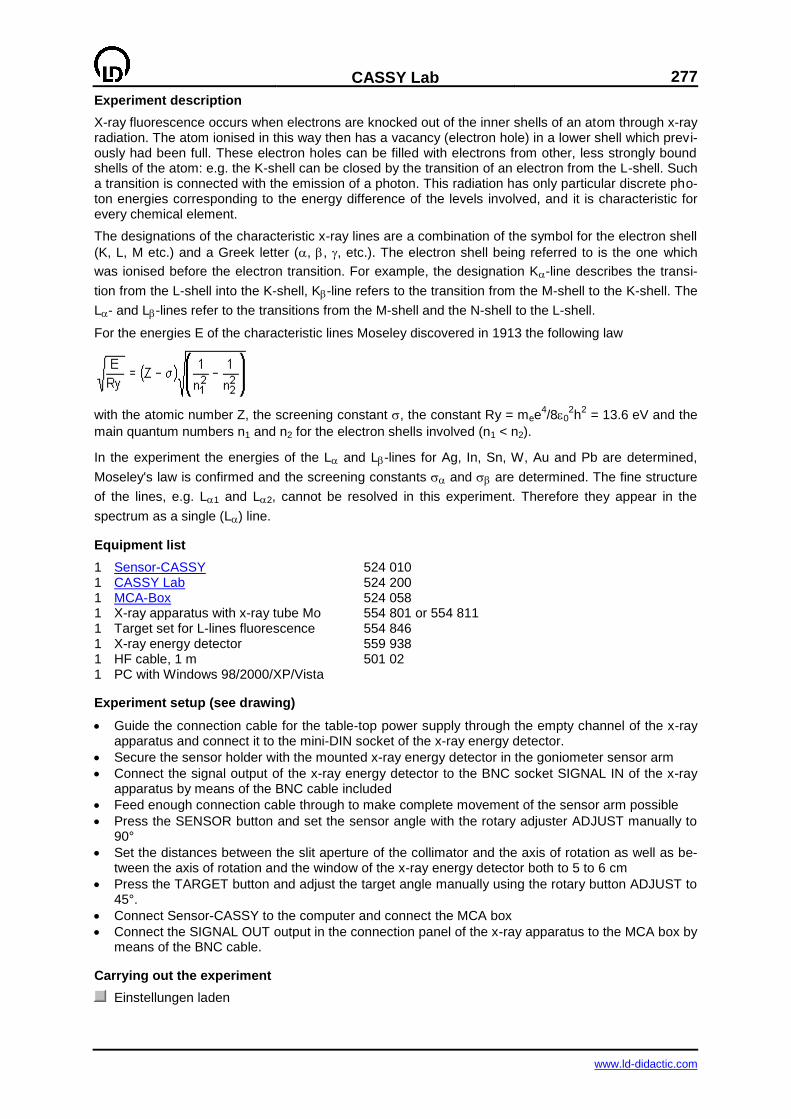
CASSY Lab

277

www.ld-didactic.com


X-ray fluorescence occurs when electrons are knocked out of the inner shells of an atom through x-ray radiation. The atom ionised in this way then has a vacancy (electron hole) in a lower shell which previ-ously had been full. These electron holes can be filled with electrons from other, less strongly bound shells of the atom: e.g. the K-shell can be closed by the transition of an electron from the L-shell. Such a transition is connected with the emission of a photon. This radiation has only particular discrete pho-ton energies corresponding to the energy difference of the levels involved, and it is characteristic for every chemical element.

The designations of the characteristic x-ray lines are a combination of the symbol for the electron shell

(K, L, M etc.) and a Greek letter (, , , etc.). The electron shell being referred to is the one which

was ionised before the electron transition. For example, the designation K-line describes the transi-

tion from the L-shell into the K-shell, K-line refers to the transition from the M-shell to the K-shell. The

L- and L-lines refer to the transitions from the M-shell and the N-shell to the L-shell.

For the energies E of the characteristic lines Moseley discovered in 1913 the following law

with the atomic number Z, the screening constant , the constant Ry = mee4/80

2h

2 = 13.6 eV and the

main quantum numbers n1 and n2 for the electron shells involved (n1 < n2).

In the experiment the energies of the L and L-lines for Ag, In, Sn, W, Au and Pb are determined,

Moseley's law is confirmed and the screening constants and are determined. The fine structure

of the lines, e.g. L1 and L2, cannot be resolved in this experiment. Therefore they appear in the

spectrum as a single (L) line.

Equipment list

1 Sensor-CASSY 524 010 1 CASSY Lab 524 200 1 MCA-Box 524 058 1 X-ray apparatus with x-ray tube Mo 554 801 or 554 811 1 Target set for L-lines fluorescence 554 846 1 X-ray energy detector 559 938 1 HF cable, 1 m 501 02 1 PC with Windows 98/2000/XP/Vista












Einstellungen laden

278

CASSY Lab

www.ld-didactic.com

Connect the table-top power supply to the mains (after approx. 2 min the LED will glow green and the x-ray energy detector will be ready for use)

Place the first target (Ag) from the target set for L-lines fluorescence onto the target table



Then record spectra for the other targets (In, Sn, W, Au and Pb) in the target set for L-lines fluores-cence.

Energy calibration

The energy calibration of the spectra is made using the L-line of tungsten (W) and the K-line of sil-

ver (Ag).

Open in the context menu of the diagram (right mouse button) or select with Alt+E the Energy cali-bration, select global energy calibration and enter on the right-hand side the energies of the W

L-line (8.40 keV) and of the Ag K-line (22.17 keV). Do not yet close the Energy calibration win-

dow.


W L-line (4th

spectrum) and enter the result on the left-hand side of the Energy calibration (e.g.

with drag & drop from the status line)

Then determine the centre of the Ag K line (1st spectrum) and also enter it on the left-hand side


Evaluation

As the atomic number Z increases, the energy of the characteristic lines also increases and so does

the separation between the - and the -components in the L spectral series. For the heavier ele-

ments, in addition to the L and L-components, the relatively small Ll and L-components can also be

demonstrated with the x-ray energy detector. For a quantitative analysis, the energies of the individual lines can be determined:

Select spectrum in the diagram

In the context menu of the diagram (right-hand mouse button) or with Alt+V choose Vertical line

and mark the approximate positions of the L and L-line. Because for the elements silver, indium

and tin the L-line and L-line are not resolved, they will be treated in the evaluation as a single

line.

In the context menu of the diagram select under Other evaluations Gaussians of equal width and mark the area of the desired peak (also mark sufficient background!)

Read the determined peak positions from the status line and enter them together with the atomic numbers Z of Ag (Z=47), In (Z=49), Sn (Z=50), W (Z=74), Au (Z=79) and Pb (Z=82) into the En-ergy diagram (click with mouse) (e.g. by drag & drop from the status line)

For each line, the expression E/Ry is automatically calculated and plotted in the Moseley diagram as

a function of the atomic number Z. The same applies to the screening constants and and the

Screening diagram.

In the Moseley diagram, by means of a Best-fit straight line for L and L, the linear relationship in

Moseley's law can be confirmed.

In the Screening diagram, the very different dependence of the atomic screening constants for the L-

lines and L-lines of the atomic number Z indicates the differences in structure of the sublevels in the

M-shell and the L-shell. It is remarkable that the atomic screening constant for the L-lines has a value

of 7. This means that the screening is provided by the seven electrons remaining in the L-shell after ionisation. This again indicates that the p-orbitals and s-orbitals (L-shell or K-shell respectively) have

such a form that the two electrons in the K-shell are ineffective at screening the L-transition.

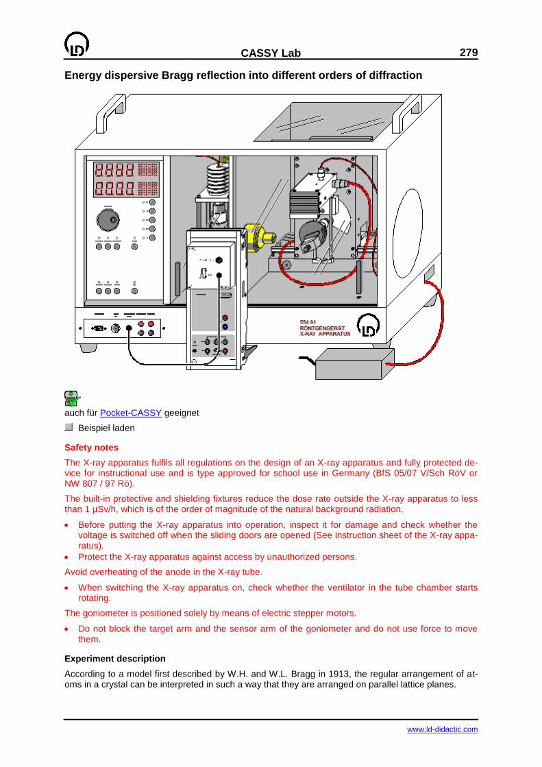
CASSY Lab

279

www.ld-didactic.com

Energy dispersive Bragg reflection into different orders of diffraction


Beispiel laden

Safety notes










According to a model first described by W.H. and W.L. Bragg in 1913, the regular arrangement of at-oms in a crystal can be interpreted in such a way that they are arranged on parallel lattice planes.

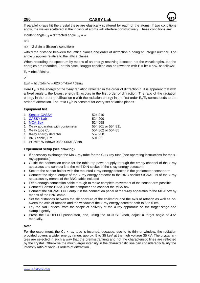
280

CASSY Lab

www.ld-didactic.com

If parallel x-rays hit the crystal these are elastically scattered by each of the atoms. If two conditions apply, the waves scattered at the individual atoms will interfere constructively. These conditions are:

Incident angle 1 = diffracted angle 2 =

and

n = 2dsin (Bragg's condition)

with d the distance between the lattice planes and order of diffraction n being an integer number. The

angle applies relative to the lattice planes.

When recording the spectrum by means of an energy resolving detector, not the wavelengths, but the

energies are recorded. For this case, Bragg's condition can be rewritten with E = h = hc/ as follows:

En = nhc / 2dsin

or

En/n = hc / 2dsin 620 pmkeV / dsin

Here En is the energy of the x-ray radiation reflected in the order of diffraction n. It is apparent that with

a fixed angle the lowest energy E1 occurs in the first order of diffraction. The ratio of the radiation

energy in the order of diffraction n with the radiation energy in the first order En/E1 corresponds to the

order of diffraction. The ratio En/n is constant for every set of lattice planes.

Equipment list

1 Sensor-CASSY 524 010 1 CASSY Lab 524 200 1 MCA-Box 524 058 1 X-ray apparatus with goniometer 554 801 or 554 811 1 X-ray tube Cu 554 862 or 554 85 1 X-ray energy detector 559 938 1 BNC cable, 1 m 501 02 1 PC with Windows 98/2000/XP/Vista


If necessary exchange the Mo x-ray tube for the Cu x-ray tube (see operating instructions for the x-ray apparatus)








Lay the NaCl crystal from the scope of delivery of the X-ray apparatus on the target stage and clamp it gently.

Press the COUPLED pushbutton, and, using the ADJUST knob, adjust a target angle of 4.5° manually.

Note

For the experiment, the Cu x-ray tube is inserted, because, due to its thinner window, the radiation provided covers a wider energy range: approx. 5 to 35 keV at the high voltage 35 kV. The crystal an-gles are selected in such a way that the bremsstrahlung and not the characteristic lines are reflected by the crystal. Otherwise the much larger intensity in the characteristic line can considerably falsify the intensity ratio of various orders of diffraction.

CASSY Lab

281

www.ld-didactic.com


Einstellungen laden



Record the calibration spectrum (start the spectrum recording by pressing F9)

Set the emission current to I = 0.40 mA

Record the spectra for the target angles 5°, 10°, 15° and 20°

Energy calibration

In the housing of the Si-PIN photodiode of the x-ray energy detector the x-ray radiation produces addi-tional x-ray fluorescence radiation which will also be recorded. In the primary spectrum therefore, in addition to the peaks of the reflected radiation, the gold (Au) and the silver (Ag) lines are also to be expected. With the help of these lines the energy calibration of the spectra can be carried out.

Through the scatter of the Cu K-line of the primary spectrum of the x-ray tube, on the left-hand side a

peak occurs at E=8.1 keV. The subsequent smaller peaks at E=9.7 keV, 11.4 keV and 22.2 keV have

been caused by the fluorescence of the housing (Au L, L and Ag K) and the large peak on the

right-hand side is the reflected radiation (Bragg's condition).

Select spectrum N1 (4.5°)

Open in the context menu of the diagram (right mouse button) or select with Alt+E the Energy cali-bration, select global energy calibration and enter on the right-hand side the energies of the Au

L-line (9.71 keV) and of the Ag K-line (22.16 keV). Do not yet close the Energy calibration win-

dow.


Au L-line and enter the result in the left-hand side of the Energy calibration (e.g. with drag & drop

from the status line)

Then determine the centre for the Ag K-line and also enter it on the left-hand side.


Note

In order to excite the silver K-lines in the housing material, the energy of the reflected radiation must exceed the K-edge of silver (25.52 keV). For this reason the energy calibration is carried out on the

spectrum for =4.5°.

Evaluation

For confirmation that the remaining peaks associated with the various orders of diffraction belong to the same set of lattice planes, the ratios of the peak energies must be analysed.

For the determination of the peak energies as a function of the scatter angle

Select energy spectrum (5°, 10°, 15° and 20°).

In the context menu of the diagram select under Other evaluations Calculate peak centre and mark the desired peak

Read the determined peak positions from the status line and enter as En=1, En=2, En=3 or En=4

together with the angle into the Energy diagram (click with mouse) (e.g. by drag & drop from the status line)

In the Order diagram a table is formed in which the ratios En/E1 of the radiation energy in the order of diffraction n with the first order radiation energy are given. They have approximately integer values which confirms the assumption that they belong to different orders of diffraction from the same set of lattice planes.

In the Lattice plane spacing diagram the lattice plane spacing d was calculated for each crystal angle

from the determined values En/n. It becomes apparent that the diffraction for all angles was observed

from the same set of lattice planes with a spacing of d 280 pm. By comparing with the data given in the literature for NaCl (grid constant 564 pm) it becomes apparent that this is the diffraction from the (200) lattice planes (d = 282 pm).

282

CASSY Lab

www.ld-didactic.com

Additional information

For a Bragg spectrum recorded using a Geiger-Müller counter as the detector, the photons which are reflected in the various orders of diffraction are counted together. A spectrum recorded in this way is therefore a combination of several components which cannot easily be separated. In the 20° spectrum it is particularly clear how incorrect the statement about the intensity of radiation would be if only the first order of diffraction were taken into account and the existence of higher orders of diffraction were ignored.

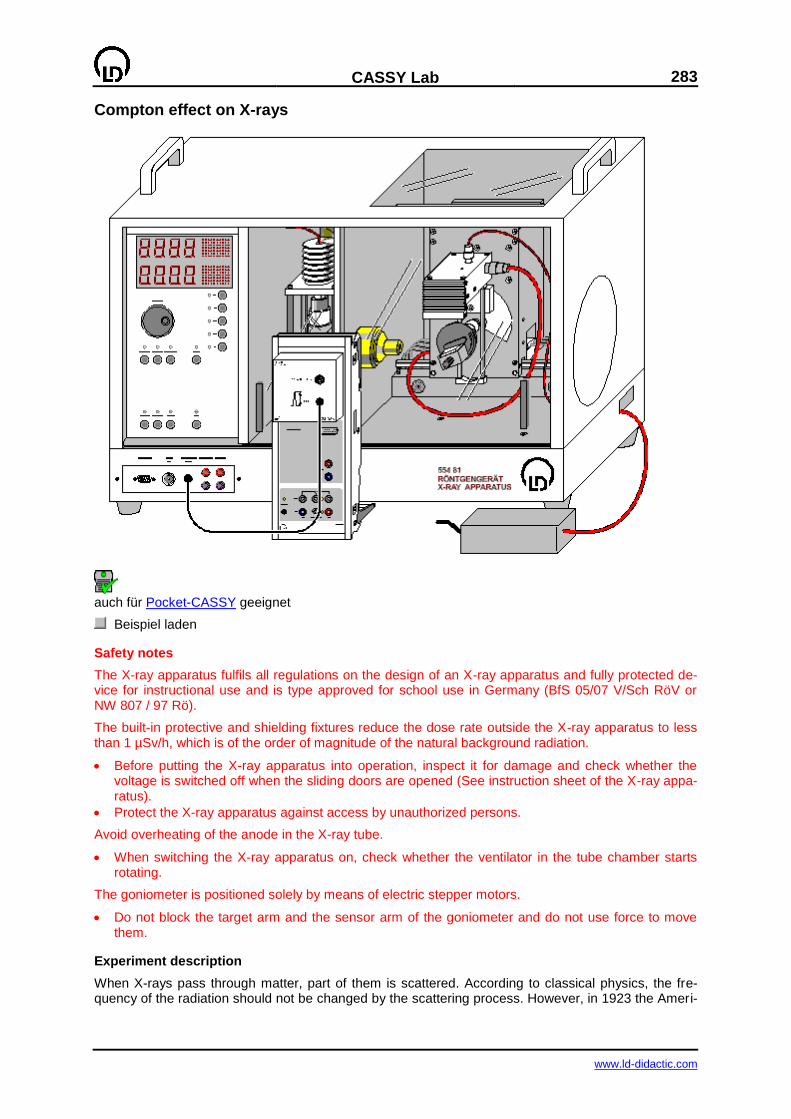
CASSY Lab

283

www.ld-didactic.com

Compton effect on X-rays


Beispiel laden

Safety notes










When X-rays pass through matter, part of them is scattered. According to classical physics, the fre-quency of the radiation should not be changed by the scattering process. However, in 1923 the Ameri-

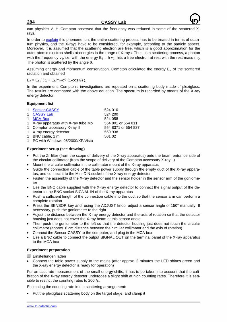
284

CASSY Lab

www.ld-didactic.com

can physicist A. H. Compton observed that the frequency was reduced in some of the scattered X-rays.

In order to explain this phenomenon, the entire scattering process has to be treated in terms of quan-tum physics, and the X-rays have to be considered, for example, according to the particle aspect. Moreover, it is assumed that the scattering electron are free, which is a good approximation for the outer atomic electron shells at energies in the range of X-rays. Thus, in a scattering process, a photon

with the frequency 1, i.e. with the energy E1 = h1, hits a free electron at rest with the rest mass m0.

The photon is scattered by the angle .

Assuming energy and momentum conservation, Compton calculated the energy E2 of the scattered radiation and obtained

E2 = E1 / ( 1 + E1/m0c2 (1-cos ) ).

In the experiment, Compton's investigations are repeated on a scattering body made of plexiglass. The results are compared with the above equation. The spectrum is recorded by means of the X-ray energy detector.

Equipment list

1 Sensor-CASSY 524 010 1 CASSY Lab 524 200 1 MCA-Box 524 058 1 X-ray apparatus with X-ray tube Mo 554 801 or 554 811 1 Compton accessory X-ray II 554 8371 or 554 837 1 X-ray energy detector 559 938 1 BNC cable, 1 m 501 02 1 PC with Windows 98/2000/XP/Vista


Put the Zr filter (from the scope of delivery of the X-ray apparatus) onto the beam entrance side of the circular collimator (from the scope of delivery of the Compton accessory X-ray II)

Mount the circular collimator in the collimator mount of the X-ray apparatus

Guide the connection cable of the table power supply through the empty duct of the X-ray appara-tus, and connect it to the Mini-DIN socket of the X-ray energy detector

Fasten the assembly of the X-ray detector and the sensor holder in the sensor arm of the goniome-ter

Use the BNC cable supplied with the X-ray energy detector to connect the signal output of the de-tector to the BNC socket SIGNAL IN of the X-ray apparatus

Push a sufficient length of the connection cable into the duct so that the sensor arm can perform a complete rotation

Press the SENSOR key and, using the ADJUST knob, adjust a sensor angle of 150° manually. If necessary, push the goniometer to the right

Adjust the distance between the X-ray energy detector and the axis of rotation so that the detector housing just does not cover the X-ray beam at this sensor angle

Then push the goniometer to the left so that the detector housing just does not touch the circular collimator (approx. 8 cm distance between the circular collimator and the axis of rotation)

Connect the Sensor-CASSY to the computer, and plug in the MCA box

Use a BNC cable to connect the output SIGNAL OUT on the terminal panel of the X-ray apparatus to the MCA box

Experiment preparation

Einstellungen laden

Connect the table power supply to the mains (after approx. 2 minutes the LED shines green and the X-ray energy detector is ready for operation)

For an accurate measurement of the small energy shifts, it has to be taken into account that the cali-bration of the X-ray energy detector undergoes a slight shift at high counting rates. Therefore it is sen-sible to restrict the counting rates to 200 /s.

Estimating the counting rate in the scattering arrangement:

Put the plexiglass scattering body on the target stage, and clamp it

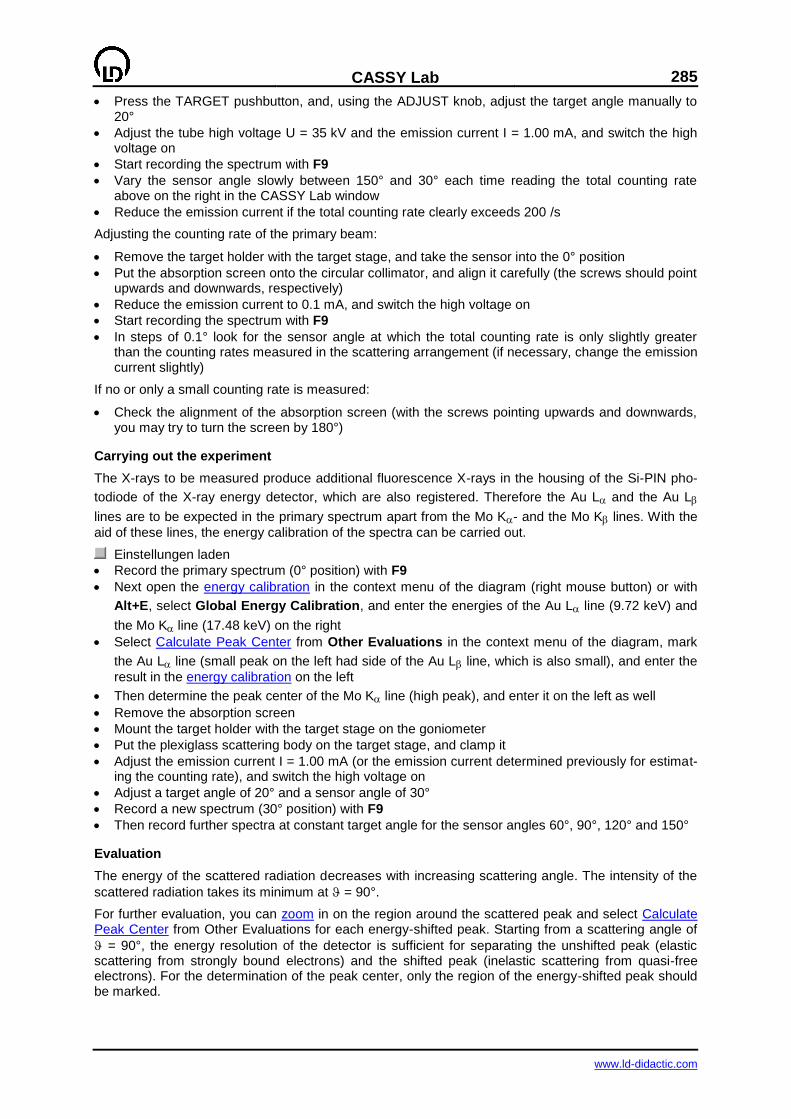
CASSY Lab

285

www.ld-didactic.com

Press the TARGET pushbutton, and, using the ADJUST knob, adjust the target angle manually to 20°

Adjust the tube high voltage U = 35 kV and the emission current I = 1.00 mA, and switch the high voltage on

Start recording the spectrum with F9

Vary the sensor angle slowly between 150° and 30° each time reading the total counting rate above on the right in the CASSY Lab window

Reduce the emission current if the total counting rate clearly exceeds 200 /s

Adjusting the counting rate of the primary beam:

Remove the target holder with the target stage, and take the sensor into the 0° position

Put the absorption screen onto the circular collimator, and align it carefully (the screws should point upwards and downwards, respectively)

Reduce the emission current to 0.1 mA, and switch the high voltage on

Start recording the spectrum with F9

In steps of 0.1° look for the sensor angle at which the total counting rate is only slightly greater than the counting rates measured in the scattering arrangement (if necessary, change the emission current slightly)

If no or only a small counting rate is measured:

Check the alignment of the absorption screen (with the screws pointing upwards and downwards, you may try to turn the screen by 180°)


The X-rays to be measured produce additional fluorescence X-rays in the housing of the Si-PIN pho-

todiode of the X-ray energy detector, which are also registered. Therefore the Au L and the Au L

lines are to be expected in the primary spectrum apart from the Mo K- and the Mo K lines. With the

aid of these lines, the energy calibration of the spectra can be carried out.

Einstellungen laden

Record the primary spectrum (0° position) with F9

Next open the energy calibration in the context menu of the diagram (right mouse button) or with

Alt+E, select Global Energy Calibration, and enter the energies of the Au L line (9.72 keV) and

the Mo K line (17.48 keV) on the right

Select Calculate Peak Center from Other Evaluations in the context menu of the diagram, mark

the Au L line (small peak on the left had side of the Au L line, which is also small), and enter the

result in the energy calibration on the left

Then determine the peak center of the Mo K line (high peak), and enter it on the left as well

Remove the absorption screen

Mount the target holder with the target stage on the goniometer

Put the plexiglass scattering body on the target stage, and clamp it

Adjust the emission current I = 1.00 mA (or the emission current determined previously for estimat-ing the counting rate), and switch the high voltage on

Adjust a target angle of 20° and a sensor angle of 30°

Record a new spectrum (30° position) with F9

Then record further spectra at constant target angle for the sensor angles 60°, 90°, 120° and 150°

Evaluation

The energy of the scattered radiation decreases with increasing scattering angle. The intensity of the

scattered radiation takes its minimum at = 90°.

For further evaluation, you can zoom in on the region around the scattered peak and select Calculate Peak Center from Other Evaluations for each energy-shifted peak. Starting from a scattering angle of

= 90°, the energy resolution of the detector is sufficient for separating the unshifted peak (elastic scattering from strongly bound electrons) and the shifted peak (inelastic scattering from quasi-free electrons). For the determination of the peak center, only the region of the energy-shifted peak should be marked.

286

CASSY Lab

www.ld-didactic.com

For each peak center, the energy is entered in the Evaluation display together with the corresponding scattering angle. The energy can be taken from the status line into the table using the mouse (drag & drop). The angle has to be entered manually in the table.

For a comparison of the measured energies with the energies calculated from energy and momentum conservation, a free fit of the equation

17.48/(1+17.48*(1-cos(x))/A)

can be selected in the Evaluation display with the starting value A = 511 (=constant).

The result corresponds to the theoretical curve with the parameters E1 = 17.48 keV and m0c2 =

511 keV, which is in good agreement with the measured values.

When X-rays pass through matter, part of them is scattered and experiences an energy shift (Compton effect). The energy shift can be calculated by describing the scattering process as a collision between an X-ray photon and a free electron at rest and by postulating the conservation of energy and momen-tum in this process.

Remark

Alternatively, the comparison between measurement and theory can be carried out as a free fit with the free fit parameter A (the rest mass of the collision partner of the X-ray photon). As a result a value

for the parameter A is obtained, which agrees with the "rest mass" of an electron (m0c2 = 511 keV) to

a good approximation.

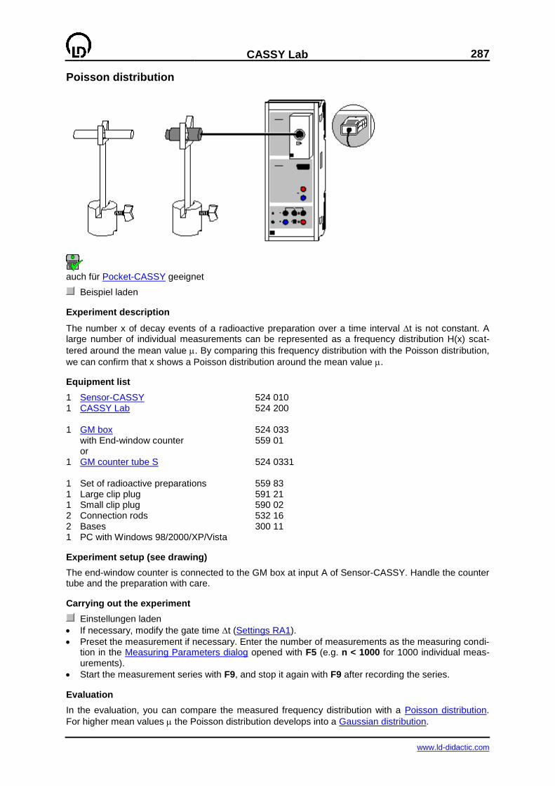
CASSY Lab

287

www.ld-didactic.com

Poisson distribution


Beispiel laden


The number x of decay events of a radioactive preparation over a time interval t is not constant. A large number of individual measurements can be represented as a frequency distribution H(x) scat-

tered around the mean value . By comparing this frequency distribution with the Poisson distribution,

we can confirm that x shows a Poisson distribution around the mean value .

Equipment list

1 Sensor-CASSY 524 010 1 CASSY Lab 524 200 1 GM box 524 033 with End-window counter 559 01 or 1 GM counter tube S 524 0331 1 Set of radioactive preparations 559 83 1 Large clip plug 591 21 1 Small clip plug 590 02 2 Connection rods 532 16 2 Bases 300 11 1 PC with Windows 98/2000/XP/Vista


The end-window counter is connected to the GM box at input A of Sensor-CASSY. Handle the counter tube and the preparation with care.


Einstellungen laden

If necessary, modify the gate time t (Settings RA1).

Preset the measurement if necessary. Enter the number of measurements as the measuring condi-tion in the Measuring Parameters dialog opened with F5 (e.g. n < 1000 for 1000 individual meas-urements).

Start the measurement series with F9, and stop it again with F9 after recording the series.

Evaluation

In the evaluation, you can compare the measured frequency distribution with a Poisson distribution.

For higher mean values the Poisson distribution develops into a Gaussian distribution.

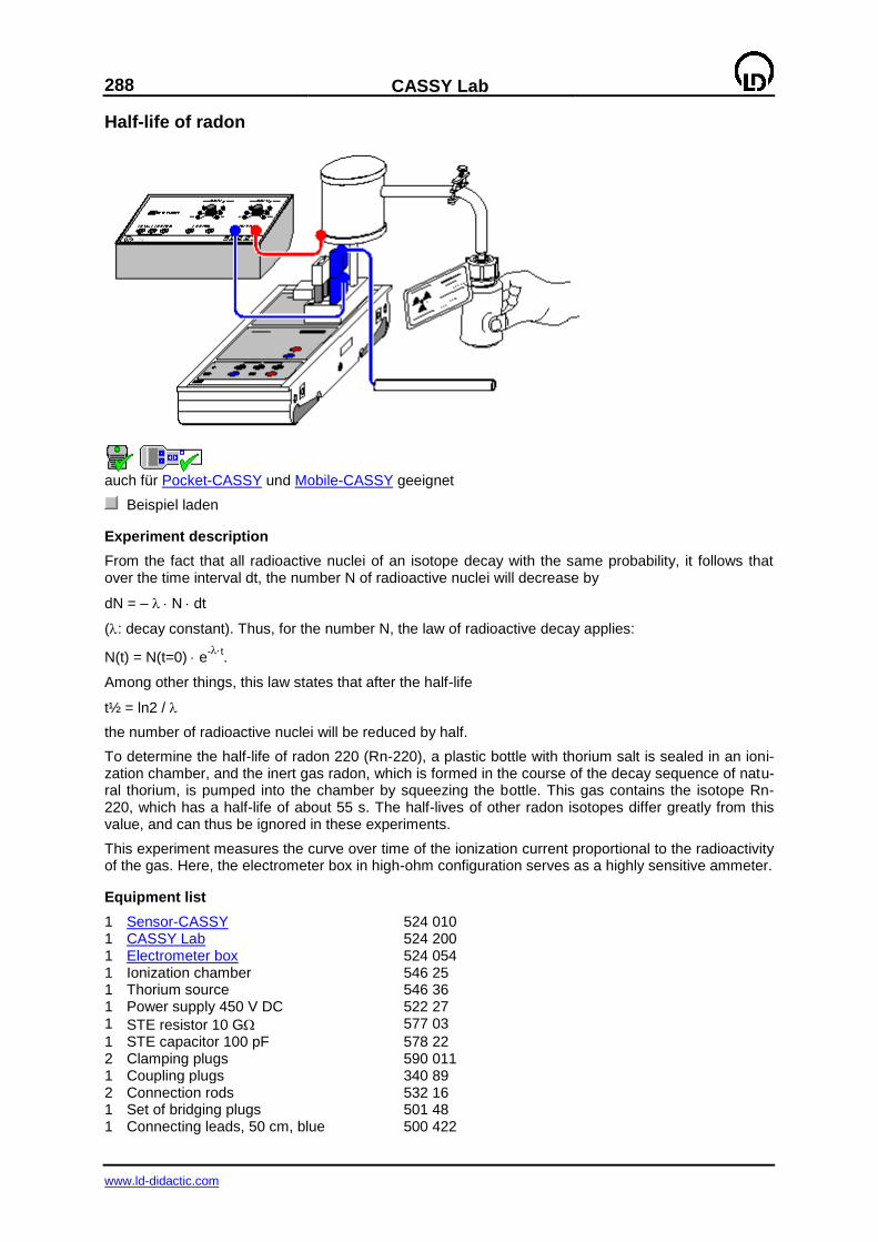
288

CASSY Lab

www.ld-didactic.com

Half-life of radon


Beispiel laden


From the fact that all radioactive nuclei of an isotope decay with the same probability, it follows that over the time interval dt, the number N of radioactive nuclei will decrease by

dN = – N dt

(: decay constant). Thus, for the number N, the law of radioactive decay applies:

N(t) = N(t=0) e-t

.

Among other things, this law states that after the half-life

t½ = ln2 /

the number of radioactive nuclei will be reduced by half.

To determine the half-life of radon 220 (Rn-220), a plastic bottle with thorium salt is sealed in an ioni-zation chamber, and the inert gas radon, which is formed in the course of the decay sequence of natu-ral thorium, is pumped into the chamber by squeezing the bottle. This gas contains the isotope Rn-220, which has a half-life of about 55 s. The half-lives of other radon isotopes differ greatly from this value, and can thus be ignored in these experiments.

This experiment measures the curve over time of the ionization current proportional to the radioactivity of the gas. Here, the electrometer box in high-ohm configuration serves as a highly sensitive ammeter.

Equipment list

1 Sensor-CASSY 524 010 1 CASSY Lab 524 200 1 Electrometer box 524 054 1 Ionization chamber 546 25 1 Thorium source 546 36 1 Power supply 450 V DC 522 27 1 STE resistor 10 G 577 03

1 STE capacitor 100 pF 578 22 2 Clamping plugs 590 011 1 Coupling plugs 340 89 2 Connection rods 532 16 1 Set of bridging plugs 501 48 1 Connecting leads, 50 cm, blue 500 422

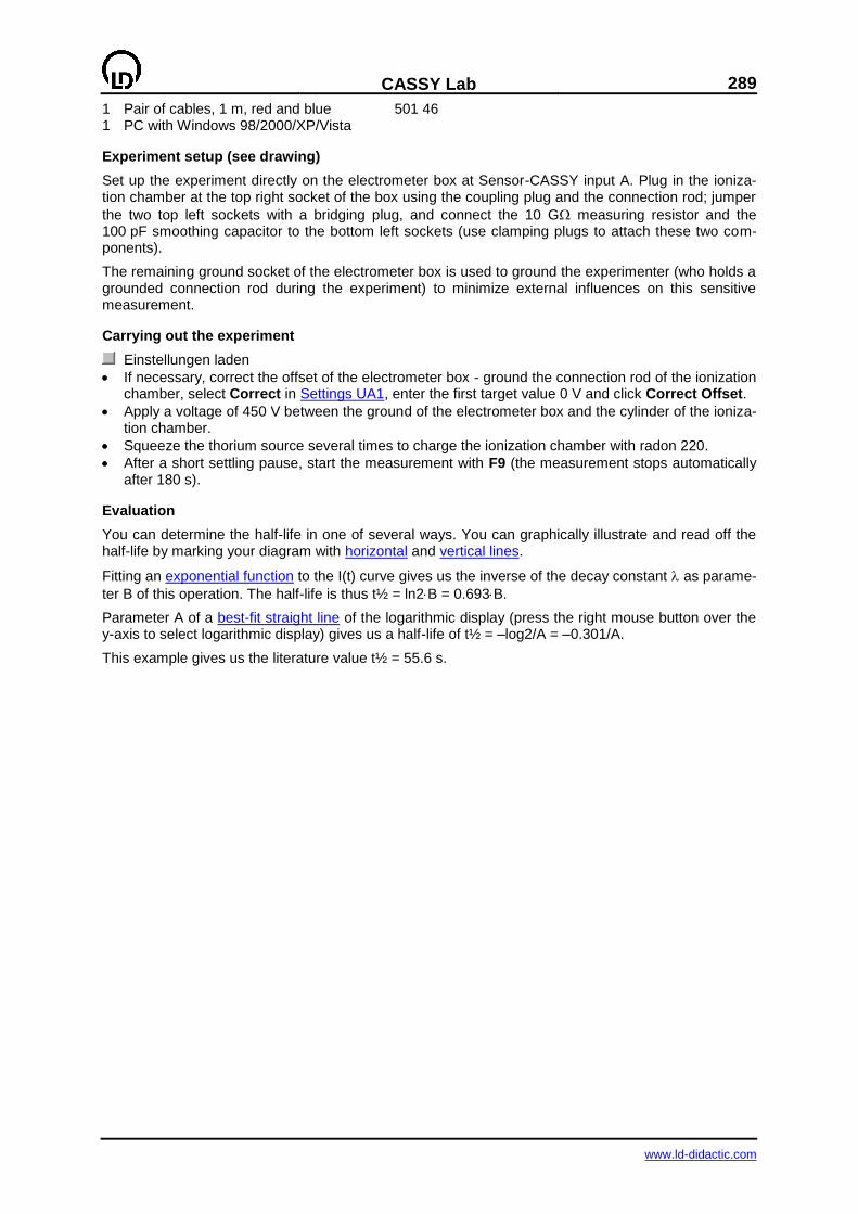
CASSY Lab

289

www.ld-didactic.com



Set up the experiment directly on the electrometer box at Sensor-CASSY input A. Plug in the ioniza-tion chamber at the top right socket of the box using the coupling plug and the connection rod; jumper

the two top left sockets with a bridging plug, and connect the 10 G measuring resistor and the 100 pF smoothing capacitor to the bottom left sockets (use clamping plugs to attach these two com-ponents).

The remaining ground socket of the electrometer box is used to ground the experimenter (who holds a grounded connection rod during the experiment) to minimize external influences on this sensitive measurement.


Einstellungen laden

If necessary, correct the offset of the electrometer box - ground the connection rod of the ionization chamber, select Correct in Settings UA1, enter the first target value 0 V and click Correct Offset.

Apply a voltage of 450 V between the ground of the electrometer box and the cylinder of the ioniza-tion chamber.

Squeeze the thorium source several times to charge the ionization chamber with radon 220.

After a short settling pause, start the measurement with F9 (the measurement stops automatically after 180 s).

Evaluation

You can determine the half-life in one of several ways. You can graphically illustrate and read off the half-life by marking your diagram with horizontal and vertical lines.

Fitting an exponential function to the I(t) curve gives us the inverse of the decay constant as parame-

ter B of this operation. The half-life is thus t½ = ln2B = 0.693B.

Parameter A of a best-fit straight line of the logarithmic display (press the right mouse button over the y-axis to select logarithmic display) gives us a half-life of t½ = –log2/A = –0.301/A.

This example gives us the literature value t½ = 55.6 s.

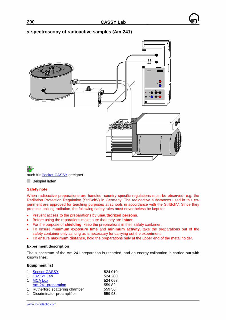
290

CASSY Lab

www.ld-didactic.com

spectroscopy of radioactive samples (Am-241)


Beispiel laden

Safety note

When radioactive preparations are handled, country specific regulations must be observed, e.g. the Radiation Protection Regulation (StrlSchV) in Germany. The radioactive substances used in this ex-periment are approved for teaching purposes at schools in accordance with the StrlSchV. Since they produce ionizing radiation, the following safety rules must nevertheless be kept to:

Prevent access to the preparations by unauthorized persons.

Before using the reparations make sure that they are intact.

For the purpose of shielding, keep the preparations in their safety container.

To ensure minimum exposure time and minimum activity, take the preparations out of the safety container only as long as is necessary for carrying out the experiment.

To ensure maximum distance, hold the preparations only at the upper end of the metal holder.


The spectrum of the Am-241 preparation is recorded, and an energy calibration is carried out with known lines.

Equipment list

1 Sensor CASSY 524 010 1 CASSY Lab 524 200 1 MCA box 524 058 1 Am-241 preparation 559 82 1 Rutherford scattering chamber 559 56 1 Discriminator-preamplifier 559 93

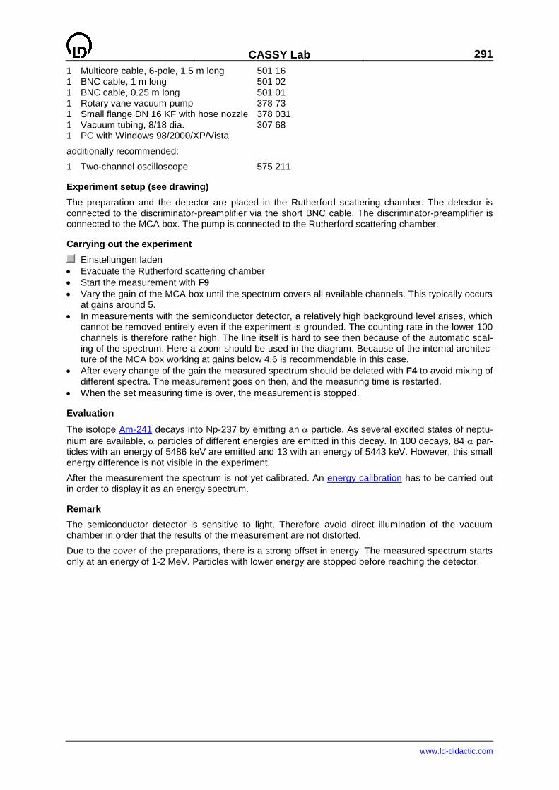
CASSY Lab

291

www.ld-didactic.com

1 Multicore cable, 6-pole, 1.5 m long 501 16 1 BNC cable, 1 m long 501 02 1 BNC cable, 0.25 m long 501 01 1 Rotary vane vacuum pump 378 73 1 Small flange DN 16 KF with hose nozzle 378 031 1 Vacuum tubing, 8/18 dia. 307 68 1 PC with Windows 98/2000/XP/Vista

additionally recommended:

1 Two-channel oscilloscope 575 211


The preparation and the detector are placed in the Rutherford scattering chamber. The detector is connected to the discriminator-preamplifier via the short BNC cable. The discriminator-preamplifier is connected to the MCA box. The pump is connected to the Rutherford scattering chamber.


Einstellungen laden

Evacuate the Rutherford scattering chamber

Start the measurement with F9

Vary the gain of the MCA box until the spectrum covers all available channels. This typically occurs at gains around 5.

In measurements with the semiconductor detector, a relatively high background level arises, which cannot be removed entirely even if the experiment is grounded. The counting rate in the lower 100 channels is therefore rather high. The line itself is hard to see then because of the automatic scal-ing of the spectrum. Here a zoom should be used in the diagram. Because of the internal architec-ture of the MCA box working at gains below 4.6 is recommendable in this case.

After every change of the gain the measured spectrum should be deleted with F4 to avoid mixing of different spectra. The measurement goes on then, and the measuring time is restarted.

When the set measuring time is over, the measurement is stopped.

Evaluation

The isotope Am-241 decays into Np-237 by emitting an particle. As several excited states of neptu-

nium are available, particles of different energies are emitted in this decay. In 100 decays, 84 par-ticles with an energy of 5486 keV are emitted and 13 with an energy of 5443 keV. However, this small energy difference is not visible in the experiment.

After the measurement the spectrum is not yet calibrated. An energy calibration has to be carried out in order to display it as an energy spectrum.

Remark

The semiconductor detector is sensitive to light. Therefore avoid direct illumination of the vacuum chamber in order that the results of the measurement are not distorted.

Due to the cover of the preparations, there is a strong offset in energy. The measured spectrum starts only at an energy of 1-2 MeV. Particles with lower energy are stopped before reaching the detector.

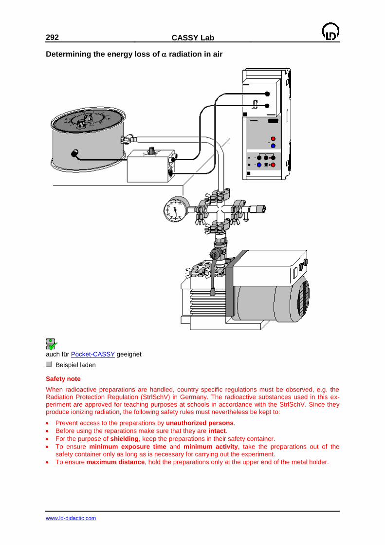
292

CASSY Lab

www.ld-didactic.com

Determining the energy loss of radiation in air


Beispiel laden

Safety note







CASSY Lab

293

www.ld-didactic.com


The energy loss of the radiation from the Am-241 sample is measured in the scattering chamber in dependence on the air pressure. From this the energy loss at normal pressure is calculated as a func-

tion of the distance. The range of the radiation in air is obtained.

Equipment list

1 Sensor CASSY 524 010 1 CASSY Lab 524 200 1 MCA Box 524 058 1 Am-241 preparation 559 82 1 Rutherford scattering chamber 559 56 1 Discriminator-preamplifier 559 93 1 Multicore cable, 6-pole, 1.5 m 501 16 1 BNC cable, 1 m long 501 02 1 BNC cable, 0.25 m long 501 01 1 Rotary-vane vacuum pump 378 73 1 Small flange DN 16 KF 378 031 1 Vacuum tubing, 8/18 mm dia. 307 68 1 Cross DN 16 KF 378 015 1 Variable leak valve DN 16 KF 378 776 1 Pointer manometer 378 510 4 Centering ring DN 16 KF 378 045 4 Clamping ring DN 10/16 KF 378 050 1 PC with Windows 98/2000/XP/Vista


The preparation and the detector are placed in the Rutherford scattering chamber. The detector is connected to the discriminator-preamplifier via the short BNC cable. The discriminator-preamplifier is connected to the MCA box. The pump and the vacuum meter are connected to the Rutherford scatter-ing chamber.


Einstellungen laden

After inserting the preparation and the detector, cautiously evacuate the Rutherford scattering chamber.

When the vacuum is established, record the spectrum (F9) varying the gain until the Am-241 line is approximately in the middle of the spectrum.

Make an energy calibration, see remark.

Open the variable leak valve until the pressure in the vacuum chamber is approx. 300 mbar. Re-cord another spectrum.

Increase the pressure in the vacuum chamber, first in steps of about 100 mbar, from 800 mbar on

in smaller steps. Record an spectrum at each pressure (F9).

Evaluation

The energy of the line is determined from the individual spectra. The air pressure is converted into an effective path in air at normal pressure. From the representation of the energy as a function of the

effective path in air the range of the radiation in air is read.

Remarks

The range in air can, of course, also be measured directly without using the scattering chamber. It can be determined by varying the distance. In this case, however, the setup requires some improvisation with respect to fixing the preparation. The detector can be attached to the discriminator-preamplifier directly. In this case, it provides stronger pulses as the load of the capacitance of the BNC cable is missing.


In measurements with the semiconductor detector, a relatively high background level arises, which cannot be removed entirely even if the experiment is grounded. The counting rate in the lower 100

294

CASSY Lab

www.ld-didactic.com

channels is therefore rather high. The line itself is hard to see then because of the automatic scaling of the spectrum. Here a zoom should be used in the diagram. Because of the internal architecture of the MCA box working at gains below 4.6 is recommendable in this case.

Due to the cover of the preparations, there is a strong offset in energy. The measured spectrum starts only at an energy of 1-2 MeV. Particles with lower energy are stopped before reaching the detector.

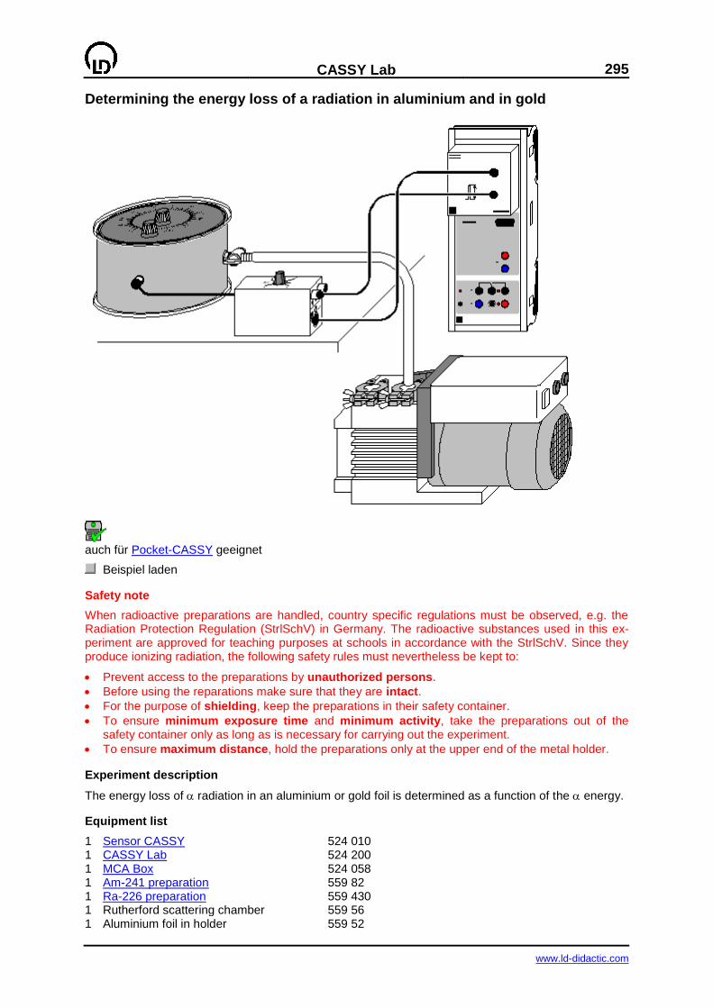
CASSY Lab

295

www.ld-didactic.com

Determining the energy loss of a radiation in aluminium and in gold


Beispiel laden

Safety note








The energy loss of radiation in an aluminium or gold foil is determined as a function of the energy.

Equipment list

1 Sensor CASSY 524 010 1 CASSY Lab 524 200 1 MCA Box 524 058 1 Am-241 preparation 559 82 1 Ra-226 preparation 559 430 1 Rutherford scattering chamber 559 56 1 Aluminium foil in holder 559 52

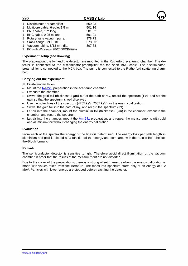
296

CASSY Lab

www.ld-didactic.com

1 Discriminator-preamplifier 559 93 1 Multicore cable, 6-pole, 1.5 m 501 16 1 BNC cable, 1 m long 501 02 1 BNC cable, 0.25 m long 501 01 1 Rotary-vane vacuum pump 378 73 1 Small flange DN 16 KF 378 031 1 Vacuum tubing, 8/18 mm dia. 307 68 1 PC with Windows 98/2000/XP/Vista


The preparation, the foil and the detector are mounted in the Rutherford scattering chamber. The de-tector is connected to the discriminator-preamplifier via the short BNC cable. The discriminator-preamplifier is connected to the MCA box. The pump is connected to the Rutherford scattering cham-ber.


Einstellungen laden

Mount the Ra-226 preparation in the scattering chamber

Evacuate the chamber

Swivel the gold foil (thickness 2 m) out of the path of ray, record the spectrum (F9), and set the gain so that the spectrum is well displayed

Use the outer lines of the spectrum (4785 keV, 7687 keV) for the energy calibration

Swivel the gold foil into the path of ray, and record the spectrum (F9)

Let air into the chamber, mount the aluminium foil (thickness 8 m) in the chamber, evacuate the chamber, and record the spectrum

Let air into the chamber, mount the Am-241 preparation, and repeat the measurements with gold and aluminium foil without changing the energy calibration

Evaluation

From each of the spectra the energy of the lines is determined. The energy loss per path length in aluminium and gold is plotted as a function of the energy and compared with the results from the Be-the-Bloch formula.

Remark


Due to the cover of the preparations, there is a strong offset in energy when the energy calibration is made with values taken from the literature. The measured spectrum starts only at an energy of 1-2 MeV. Particles with lower energy are stopped before reaching the detector.

CASSY Lab

297

www.ld-didactic.com

Determining the age of a Ra-226 sample


Beispiel laden

Safety note








The relative activity of the nuclides Ra-226 and Pb-210 in a Ra-226 sample is determined and used to determine the age of the sample.

Equipment list

1 Sensor CASSY 524 010 1 CASSY Lab 524 200 1 MCA Box 524 058 1 Ra-226 preparation 559 430 1 Rutherford scattering chamber 559 56 1 Discriminator preamplifier 559 93

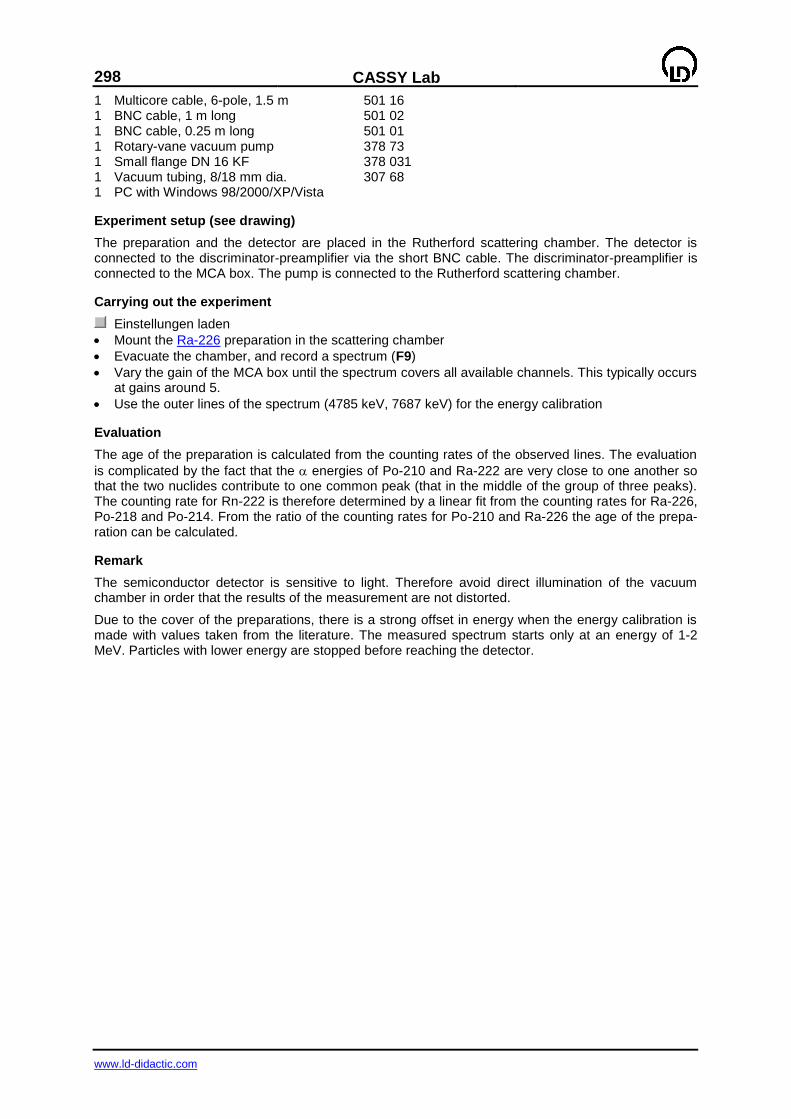
298

CASSY Lab

www.ld-didactic.com

1 Multicore cable, 6-pole, 1.5 m 501 16 1 BNC cable, 1 m long 501 02 1 BNC cable, 0.25 m long 501 01 1 Rotary-vane vacuum pump 378 73 1 Small flange DN 16 KF 378 031 1 Vacuum tubing, 8/18 mm dia. 307 68 1 PC with Windows 98/2000/XP/Vista


The preparation and the detector are placed in the Rutherford scattering chamber. The detector is connected to the discriminator-preamplifier via the short BNC cable. The discriminator-preamplifier is connected to the MCA box. The pump is connected to the Rutherford scattering chamber.


Einstellungen laden

Mount the Ra-226 preparation in the scattering chamber

Evacuate the chamber, and record a spectrum (F9)

Vary the gain of the MCA box until the spectrum covers all available channels. This typically occurs at gains around 5.

Use the outer lines of the spectrum (4785 keV, 7687 keV) for the energy calibration

Evaluation

The age of the preparation is calculated from the counting rates of the observed lines. The evaluation

is complicated by the fact that the energies of Po-210 and Ra-222 are very close to one another so that the two nuclides contribute to one common peak (that in the middle of the group of three peaks). The counting rate for Rn-222 is therefore determined by a linear fit from the counting rates for Ra-226, Po-218 and Po-214. From the ratio of the counting rates for Po-210 and Ra-226 the age of the prepa-ration can be calculated.

Remark


Due to the cover of the preparations, there is a strong offset in energy when the energy calibration is made with values taken from the literature. The measured spectrum starts only at an energy of 1-2 MeV. Particles with lower energy are stopped before reaching the detector.

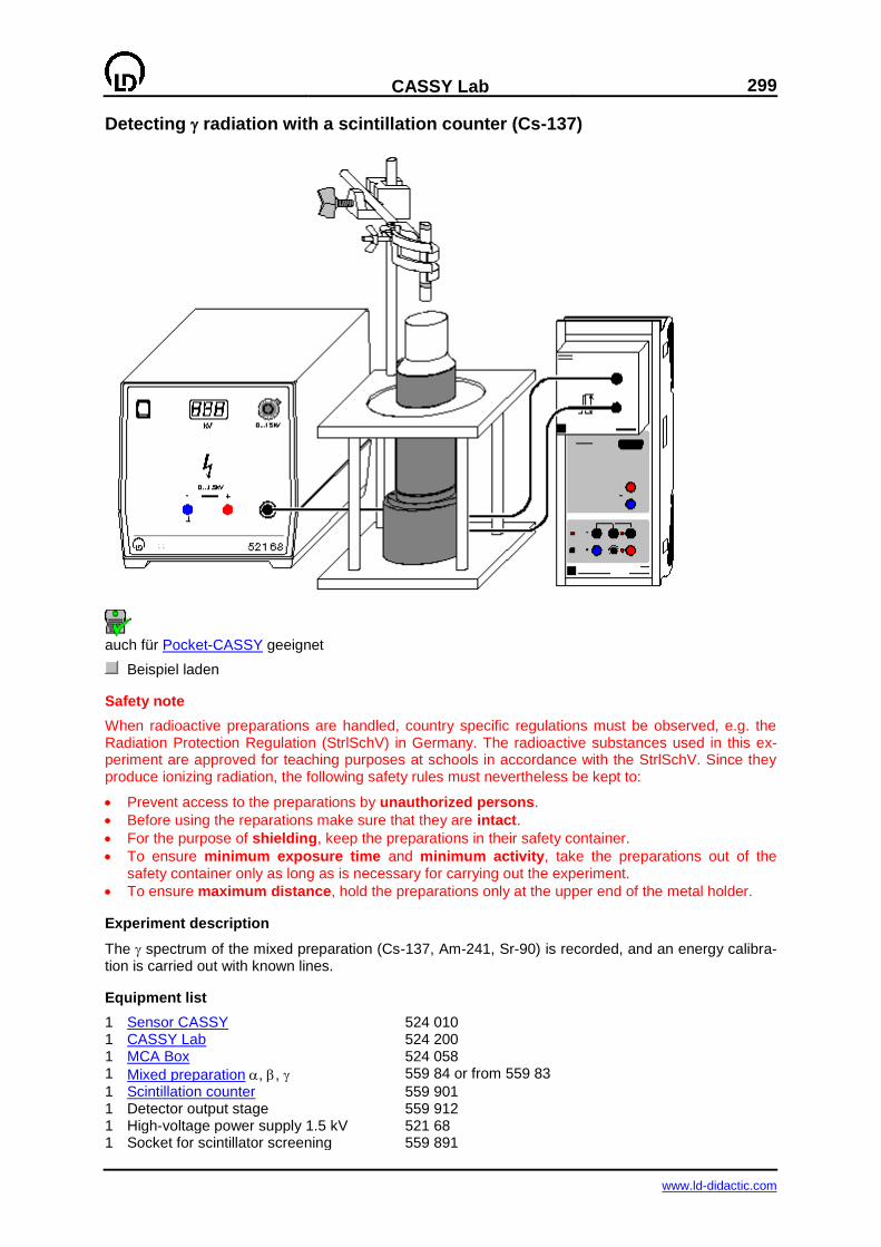
CASSY Lab

299

www.ld-didactic.com

Detecting radiation with a scintillation counter (Cs-137)


Beispiel laden

Safety note








The spectrum of the mixed preparation (Cs-137, Am-241, Sr-90) is recorded, and an energy calibra-tion is carried out with known lines.

Equipment list

1 Sensor CASSY 524 010 1 CASSY Lab 524 200 1 MCA Box 524 058 1 Mixed preparation, , 559 84 or from 559 83

1 Scintillation counter 559 901 1 Detector output stage 559 912 1 High-voltage power supply 1.5 kV 521 68 1 Socket for scintillator screening 559 891

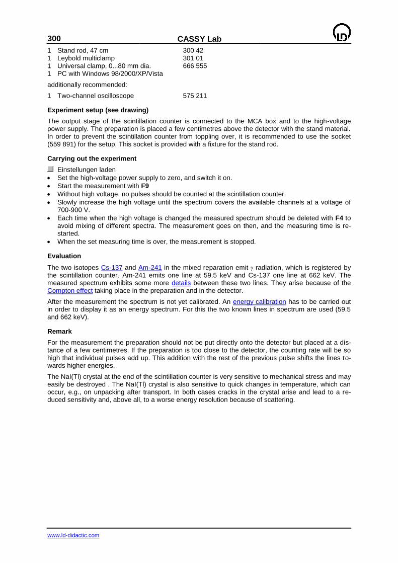
300

CASSY Lab

www.ld-didactic.com

1 Stand rod, 47 cm 300 42 1 Leybold multiclamp 301 01 1 Universal clamp, 0...80 mm dia. 666 555 1 PC with Windows 98/2000/XP/Vista

additionally recommended:

1 Two-channel oscilloscope 575 211


The output stage of the scintillation counter is connected to the MCA box and to the high-voltage power supply. The preparation is placed a few centimetres above the detector with the stand material. In order to prevent the scintillation counter from toppling over, it is recommended to use the socket (559 891) for the setup. This socket is provided with a fixture for the stand rod.


Einstellungen laden

Set the high-voltage power supply to zero, and switch it on.


Without high voltage, no pulses should be counted at the scintillation counter.

Slowly increase the high voltage until the spectrum covers the available channels at a voltage of 700-900 V.

Each time when the high voltage is changed the measured spectrum should be deleted with F4 to avoid mixing of different spectra. The measurement goes on then, and the measuring time is re-started.

When the set measuring time is over, the measurement is stopped.

Evaluation

The two isotopes Cs-137 and Am-241 in the mixed reparation emit radiation, which is registered by the scintillation counter. Am-241 emits one line at 59.5 keV and Cs-137 one line at 662 keV. The measured spectrum exhibits some more details between these two lines. They arise because of the Compton effect taking place in the preparation and in the detector.

After the measurement the spectrum is not yet calibrated. An energy calibration has to be carried out in order to display it as an energy spectrum. For this the two known lines in spectrum are used (59.5 and 662 keV).

Remark

For the measurement the preparation should not be put directly onto the detector but placed at a dis-tance of a few centimetres. If the preparation is too close to the detector, the counting rate will be so high that individual pulses add up. This addition with the rest of the previous pulse shifts the lines to-wards higher energies.

The NaI(Tl) crystal at the end of the scintillation counter is very sensitive to mechanical stress and may easily be destroyed . The NaI(Tl) crystal is also sensitive to quick changes in temperature, which can occur, e.g., on unpacking after transport. In both cases cracks in the crystal arise and lead to a re-duced sensitivity and, above all, to a worse energy resolution because of scattering.

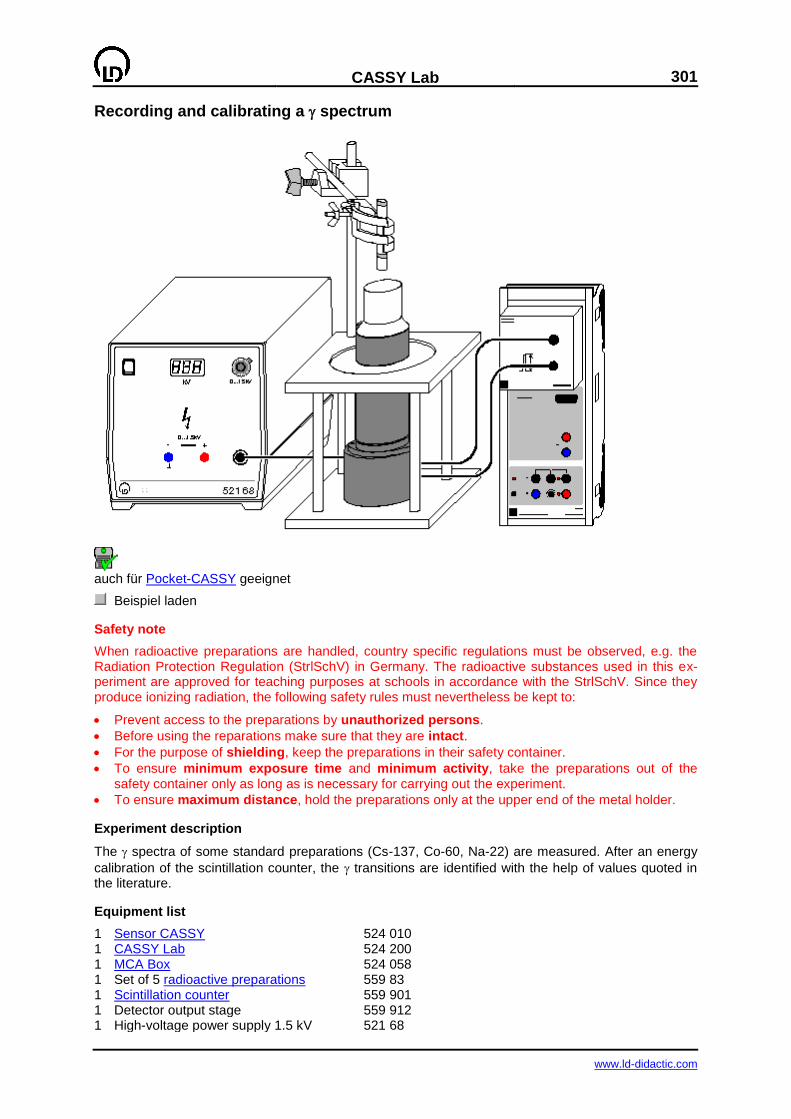
CASSY Lab

301

www.ld-didactic.com

Recording and calibrating a spectrum


Beispiel laden

Safety note








The spectra of some standard preparations (Cs-137, Co-60, Na-22) are measured. After an energy

calibration of the scintillation counter, the transitions are identified with the help of values quoted in the literature.

Equipment list

1 Sensor CASSY 524 010 1 CASSY Lab 524 200 1 MCA Box 524 058 1 Set of 5 radioactive preparations 559 83 1 Scintillation counter 559 901 1 Detector output stage 559 912 1 High-voltage power supply 1.5 kV 521 68

302

CASSY Lab

www.ld-didactic.com

1 Socket for scintillator screening 559 891 1 Stand rod, 47 cm 300 42 1 Leybold multiclamp 301 01 1 Universal clamp, 0...80 mm dia. 666 555 1 PC with Windows 98/2000/XP/Vista


The output stage of the scintillation counter is connected to the MCA box and the high-voltage power supply. The preparation to be studied is placed a few centimetres above the scintillation counter with stand material. In order to prevent the scintillation counter from toppling over, it is recommended to use the socket (559 891) for the setup.


Einstellungen laden

Record the spectra of Co-60, Na-22 and Cs-137 (F9) one after another. It is recommendable to begin with the Co-60 preparation because the radiation it emits has the highest energy so that the high voltage and the gain can be adjusted appropriately from the very beginning.

In order to get an energy spectrum, an energy calibration has to be carried out. For this e.g. the lines of Na-22 at 511 keV and 1275 keV can be used.

Evaluation

The energies of the individual lines are determined. For this the function Fit Gaussian curves can be used. The radiating isotopes are identified by comparison with values from the literature.

Remarks

There are several databases available in the internet where the known energies of all radioactive sub-stances are listed, e.g. under http://nucleardata.nuclear.lu.se/nucleardata/toi/. These may be used for identifying the radioactive nuclides.

For the measurement the preparation should not be put directly onto the detector but placed at a dis-tance of a few centimetres. If the preparation is too close to the detector, the counting rate will be so high that individual pulses add up. This addition with the rest of the previous pulse shifts the lines to-wards higher energies.

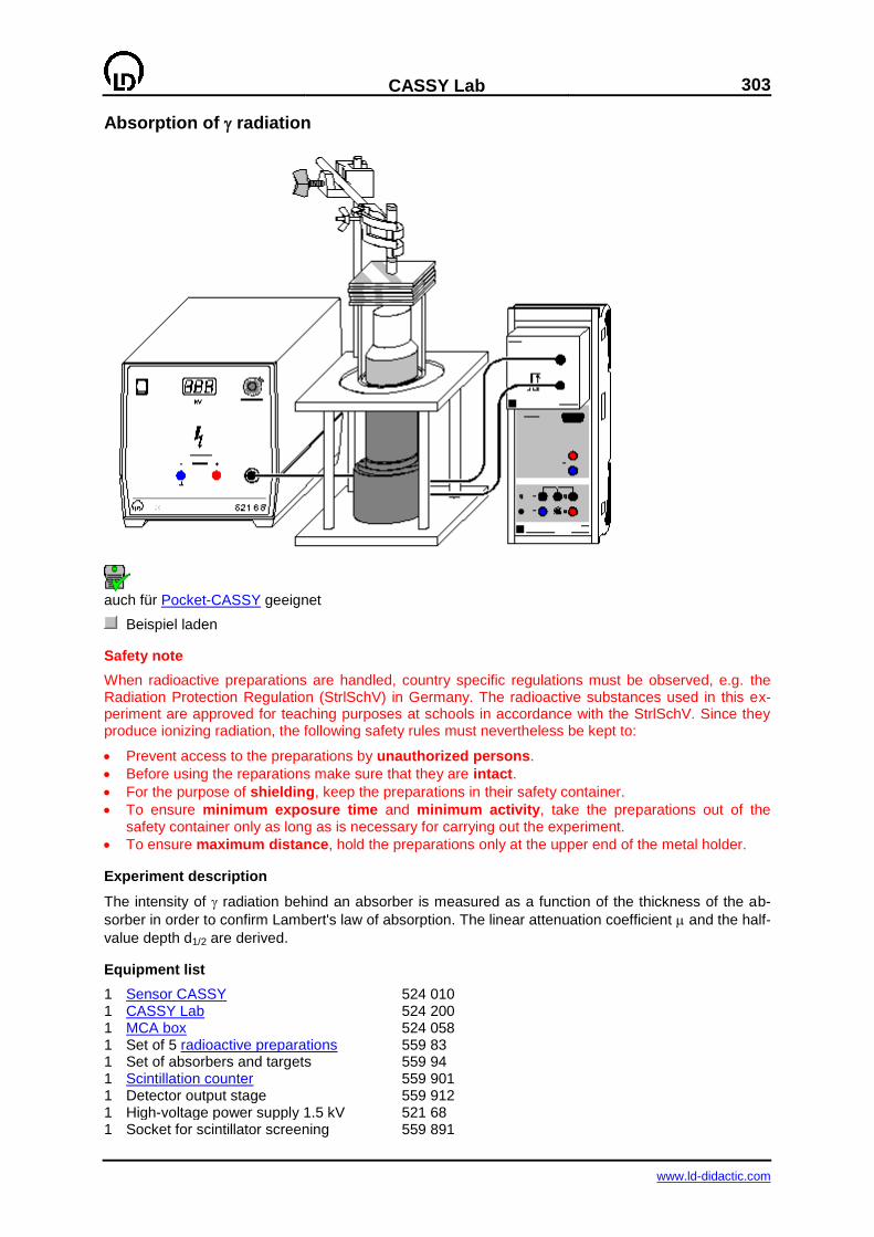
http://nucleardata.nuclear.lu.se/nucleardata/toi

CASSY Lab

303

www.ld-didactic.com

Absorption of radiation


Beispiel laden

Safety note








The intensity of radiation behind an absorber is measured as a function of the thickness of the ab-

sorber in order to confirm Lambert's law of absorption. The linear attenuation coefficient and the half-

value depth d1/2 are derived.

Equipment list

1 Sensor CASSY 524 010 1 CASSY Lab 524 200 1 MCA box 524 058 1 Set of 5 radioactive preparations 559 83 1 Set of absorbers and targets 559 94 1 Scintillation counter 559 901 1 Detector output stage 559 912 1 High-voltage power supply 1.5 kV 521 68 1 Socket for scintillator screening 559 891

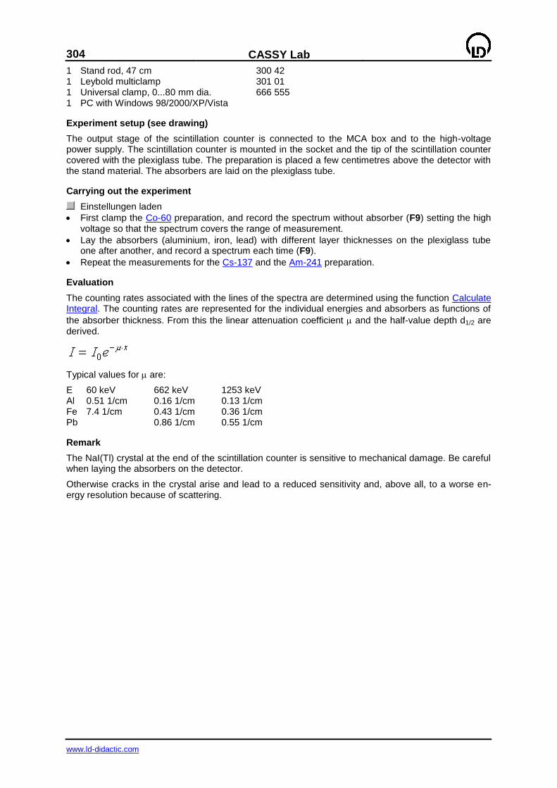
304

CASSY Lab

www.ld-didactic.com



The output stage of the scintillation counter is connected to the MCA box and to the high-voltage power supply. The scintillation counter is mounted in the socket and the tip of the scintillation counter covered with the plexiglass tube. The preparation is placed a few centimetres above the detector with the stand material. The absorbers are laid on the plexiglass tube.


Einstellungen laden

First clamp the Co-60 preparation, and record the spectrum without absorber (F9) setting the high voltage so that the spectrum covers the range of measurement.

Lay the absorbers (aluminium, iron, lead) with different layer thicknesses on the plexiglass tube one after another, and record a spectrum each time (F9).

Repeat the measurements for the Cs-137 and the Am-241 preparation.

Evaluation

The counting rates associated with the lines of the spectra are determined using the function Calculate Integral. The counting rates are represented for the individual energies and absorbers as functions of

the absorber thickness. From this the linear attenuation coefficient and the half-value depth d1/2 are derived.

Typical values for are:

E 60 keV 662 keV 1253 keV Al 0.51 1/cm 0.16 1/cm 0.13 1/cm Fe 7.4 1/cm 0.43 1/cm 0.36 1/cm Pb 0.86 1/cm 0.55 1/cm

Remark

The NaI(Tl) crystal at the end of the scintillation counter is sensitive to mechanical damage. Be careful when laying the absorbers on the detector.

Otherwise cracks in the crystal arise and lead to a reduced sensitivity and, above all, to a worse en-ergy resolution because of scattering.

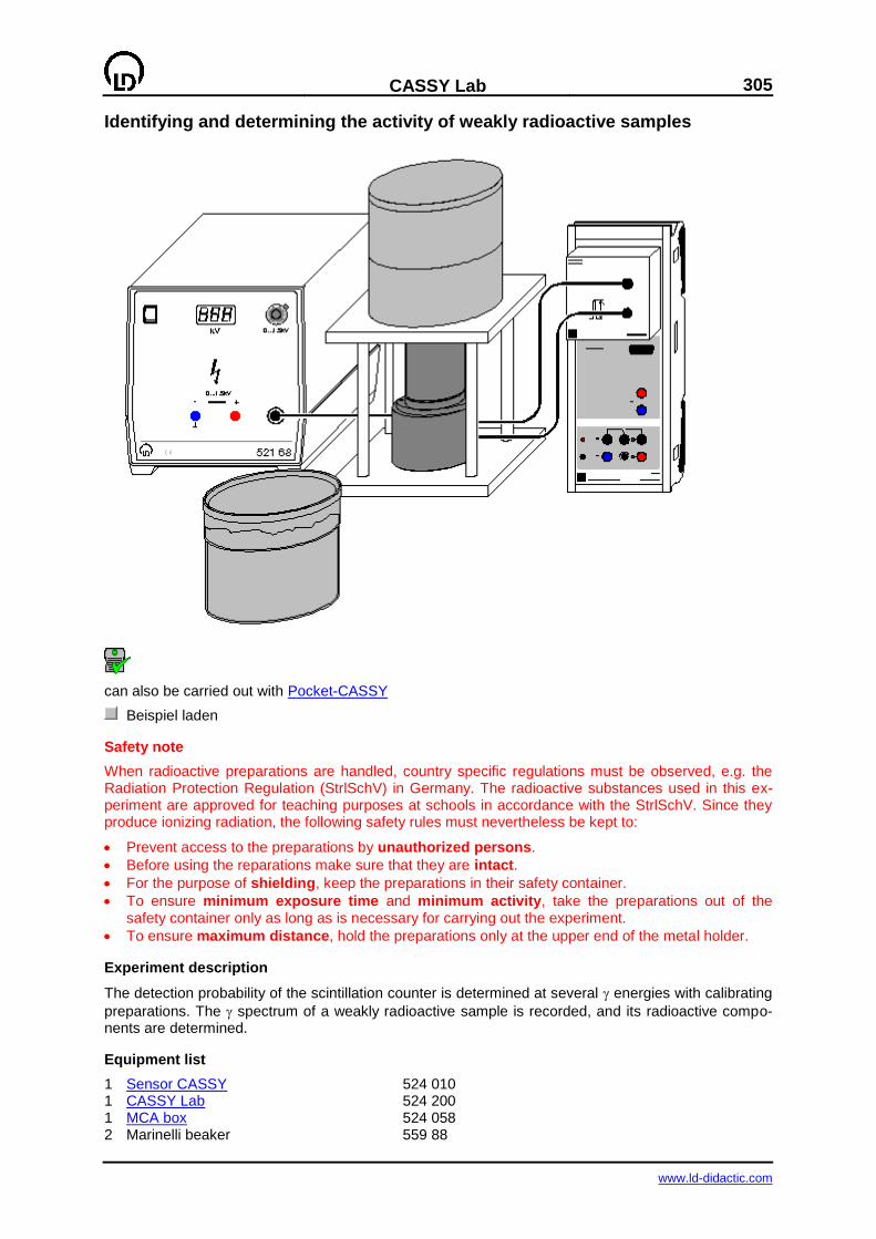
CASSY Lab

305

www.ld-didactic.com

Identifying and determining the activity of weakly radioactive samples

can also be carried out with Pocket-CASSY

Beispiel laden

Safety note








The detection probability of the scintillation counter is determined at several energies with calibrating

preparations. The spectrum of a weakly radioactive sample is recorded, and its radioactive compo-nents are determined.

Equipment list

1 Sensor CASSY 524 010 1 CASSY Lab 524 200 1 MCA box 524 058 2 Marinelli beaker 559 88

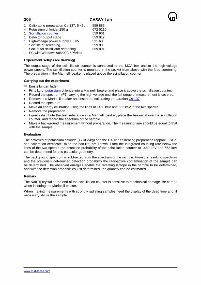
306

CASSY Lab

www.ld-didactic.com

1 Calibrating preparation Cs-137, 5 kBq 559 885 4 Potassium chloride, 250 g 672 5210 1 Scintillation counter 559 901 1 Detector output stage 559 912 1 High-voltage power supply 1.5 kV 521 68 1 Scintillator screening 559 89 1 Socket for scintillator screening 559 891 1 PC with Windows 98/2000/XP/Vista


The output stage of the scintillation counter is connected to the MCA box and to the high-voltage power supply. The scintillation counter is mounted in the socket from above with the lead screening. The preparation in the Marinelli beaker is placed above the scintillation counter.


Einstellungen laden

Fill 1 kg of potassium chloride into a Marinelli beaker and place it above the scintillation counter.

Record the spectrum (F9) varying the high voltage until the full range of measurement is covered.

Remove the Marinelli beaker and insert the calibrating preparation Cs-137

Record the spectrum

Make an energy calibration using the lines at 1460 keV and 662 keV in the two spectra.

Remove the preparation

Equally distribute the test substance in a Marinelli beaker, place the beaker above the scintillation counter, and record the spectrum of the sample.

Make a background measurement without preparation. The measuring time should be equal to that with the sample.

Evaluation

The activities of potassium chloride (17 kBq/kg) and the Cs-137 calibrating preparation (approx. 5 kBq, see calibration certificate, mind the half-life) are known. From the integrated counting rate below the lines of the two spectra the detection probability of the scintillation counter at 1460 keV and 662 keV can be determined for this particular geometry.

The background spectrum is subtracted from the spectrum of the sample. From the resulting spectrum and the previously determined detection probability the radioactive contamination of the sample can be determined. The observed energies enable the radiating isotope in the sample to be determined, and with the detection probabilities just determined, the quantity can be estimated.

Remark

The NaI(Tl) crystal at the end of the scintillation counter is sensitive to mechanical damage. Be careful when inserting the Marinelli beaker.

When making measurements with strongly radiating samples heed the display of the dead time and, if necessary, dilute the sample.

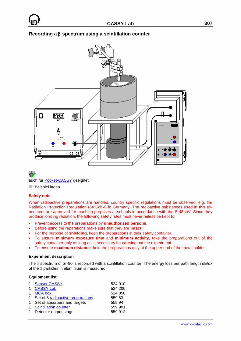
CASSY Lab

307

www.ld-didactic.com

Recording a spectrum using a scintillation counter


Beispiel laden

Safety note








The spectrum of Sr-90 is recorded with a scintillation counter. The energy loss per path length dE/dx

of the particles in aluminium is measured.

Equipment list

1 Sensor CASSY 524 010 1 CASSY Lab 524 200 1 MCA box 524 058 1 Set of 5 radioactive preparations 559 83 1 Set of absorbers and targets 559 94 1 Scintillation counter 559 901 1 Detector output stage 559 912

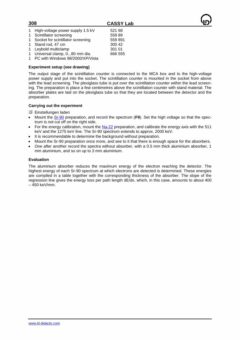
308

CASSY Lab

www.ld-didactic.com

1 High-voltage power supply 1.5 kV 521 68 1 Scintillator screening 559 89 1 Socket for scintillator screening 559 891 1 Stand rod, 47 cm 300 42 1 Leybold multiclamp 301 01 1 Universal clamp, 0...80 mm dia. 666 555 1 PC with Windows 98/2000/XP/Vista


The output stage of the scintillation counter is connected to the MCA box and to the high-voltage power supply and put into the socket. The scintillation counter is mounted in the socket from above with the lead screening. The plexiglass tube is put over the scintillation counter within the lead screen-ing. The preparation is place a few centimetres above the scintillation counter with stand material. The absorber plates are laid on the plexiglass tube so that they are located between the detector and the preparation.


Einstellungen laden

Mount the Sr-90 preparation, and record the spectrum (F9). Set the high voltage so that the spec-trum is not cut off on the right side.

For the energy calibration, mount the Na-22 preparation, and calibrate the energy axis with the 511 keV and the 1275 keV line. The Sr-90 spectrum extends to approx. 2000 keV.

It is recommendable to determine the background without preparation.

Mount the Sr-90 preparation once more, and see to it that there is enough space for the absorbers.

One after another record the spectra without absorber, with a 0.5 mm thick aluminium absorber, 1 mm aluminium, and so on up to 3 mm aluminium.

Evaluation

The aluminium absorber reduces the maximum energy of the electron reaching the detector. The highest energy of each Sr-90 spectrum at which electrons are detected is determined. These energies are compiled in a table together with the corresponding thickness of the absorber. The slope of the regression line gives the energy loss per path length dE/dx, which, in this case, amounts to about 400 – 450 keV/mm.

CASSY Lab

309

www.ld-didactic.com

Quantitative observation of the Compton effect


Beispiel laden

Safety note








An energy calibration of the scintillation counter is made. The energy distribution of quanta scattered in an aluminium scatterer is recorded for several angles between the source and the detector. From this the quantitative confirmation of the Compton effect is obtained.

Equipment list

1 Sensor CASSY 524 010 1 CASSY Lab 524 200 1 MCA box 524 058 1 Mixed preparation, , 559 84 or from 559 83

1 Equipment set Compton 559 800 1 Cs-137 preparation, 3.7 MBq 559 809 1 Scintillation counter 559 901 1 Detector output stage 559 912 1 High-voltage power supply 1.5 kV 521 68 1 PC with Windows 98/2000/XP/Vista

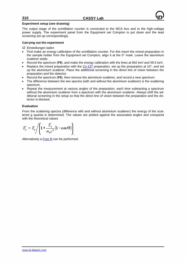
310

CASSY Lab

www.ld-didactic.com


The output stage of the scintillation counter is connected to the MCA box and to the high-voltage power supply. The experiment panel from the Equipment set Compton is put down and the lead screening set up correspondingly.


Einstellungen laden

First make an energy calibration of the scintillation counter. For this insert the mixed preparation in the sample holder from the Equipment set Compton, align it at the 0° mark. Leave the aluminium scatterer aside.

Record the spectrum (F9), and make the energy calibration with the lines at 662 keV and 59.5 keV.

Replace the mixed preparation with the Cs-137 preparation, set up the preparation at 10°, and set up the aluminium scatterer. Place the additional screening in the direct line of vision between the preparation and the detector.

Record the spectrum (F9), then remove the aluminium scatterer, and record a new spectrum.

The difference between the two spectra (with and without the aluminium scatterer) is the scattering spectrum.

Repeat the measurement at various angles of the preparation, each time subtracting a spectrum without the aluminium scatterer from a spectrum with the aluminium scatterer. Always shift the ad-ditional screening in the setup so that the direct line of vision between the preparation and the de-tector is blocked.

Evaluation

From the scattering spectra (difference with and without aluminium scatterer) the energy of the scat-tered g quanta is determined. The values are plotted against the associated angles and compared with the theoretical values

.

Alternatively a Free fit can be performed.

CASSY Lab

311

www.ld-didactic.com

Recording the complex spectrum of Ra-226 and its decay products


Beispiel laden

Safety note








The complex spectrum of Ra-226 and its decay products is recorded.

Equipment list


1 Ra-226 preparation 559 430 1 Scintillation counter 559 901 1 Detector output stage 559 912 1 High-voltage power supply 1.5 kV 521 68 1 Scintillator screening 559 89

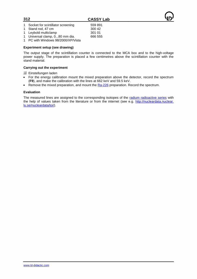
312

CASSY Lab

www.ld-didactic.com

1 Socket for scintillator screening 559 891 1 Stand rod, 47 cm 300 42 1 Leybold multiclamp 301 01 1 Universal clamp, 0...80 mm dia. 666 555 1 PC with Windows 98/2000/XP/Vista


The output stage of the scintillation counter is connected to the MCA box and to the high-voltage power supply. The preparation is placed a few centimetres above the scintillation counter with the stand material.


Einstellungen laden

For the energy calibration mount the mixed preparation above the detector, record the spectrum (F9), and make the calibration with the lines at 662 keV and 59.5 keV.

Remove the mixed preparation, and mount the Ra-226 preparation. Record the spectrum.

Evaluation

The measured lines are assigned to the corresponding isotopes of the radium radioactive series with the help of values taken from the literature or from the internet (see e.g. http://nucleardata.nuclear. lu.se/nucleardata/toi/).




CASSY Lab

313

www.ld-didactic.com

Recording the complex spectrum of an incandescent gas hood


Beispiel laden

Safety note








The complex spectrum of Th-232 and its decay products is recorded. The use of radioactive sub-stances in household articles in the past is demonstrated.

Equipment list


1 Incandescent gas hood from 588 855 1 Scintillation counter 559 901 1 Detector output stage 559 912 1 High-voltage power supply 1.5 kV 521 68 1 Scintillator screening 559 89 1 Socket for scintillator screening 559 891 1 Stand rod, 47 cm 300 42 1 Leybold multiclamp 301 01 1 Universal clamp, 0...80 mm dia. 666 555 1 PC with Windows 98/2000/XP/Vista

314

CASSY Lab

www.ld-didactic.com


The output stage of the scintillation counter is connected to the MCA box and to the high-voltage power supply. The preparation is placed above the scintillation counter with the stand material or sim-ply laid on the detector.


Einstellungen laden

For the energy calibration mount the mixed preparation above the detector, record the spectrum (F9), and make the calibration with the lines at 662 keV and 59.5 keV.

Remove the mixed preparation, and mount the incandescent gas hood (Th-232). Record the spec-trum.

Evaluation

The measured lines are assigned to the corresponding isotopes of the thorium radioactive series with the help of values taken from the literature or from the internet (see e.g. http://nucleardata.nuclear. lu.se/nucleardata/toi/).

Remark

Incandescent gas hoods manufactured in recent time no longer contain thorium but yttrium.

During the first years after manufacture the intensity of some lines changes until a new radioactive equilibrium has been reached. In particular the intensity of the lines at 338 and 911 keV (decay of Ac-

228 into Th-228) behaves in another manner than the other lines. This also influences the K lines.

Incandescent gas hoods which have already been used in a lamp should not be used for the experi-ment because of the dust released by them.




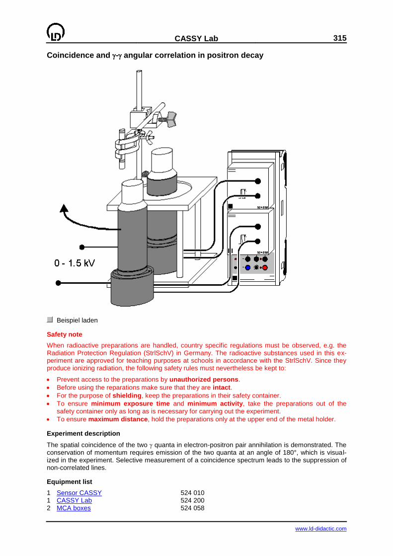
CASSY Lab

315

www.ld-didactic.com

Coincidence and - angular correlation in positron decay

Beispiel laden

Safety note








The spatial coincidence of the two quanta in electron-positron pair annihilation is demonstrated. The conservation of momentum requires emission of the two quanta at an angle of 180°, which is visual-ized in the experiment. Selective measurement of a coincidence spectrum leads to the suppression of non-correlated lines.

Equipment list

1 Sensor CASSY 524 010 1 CASSY Lab 524 200 2 MCA boxes 524 058

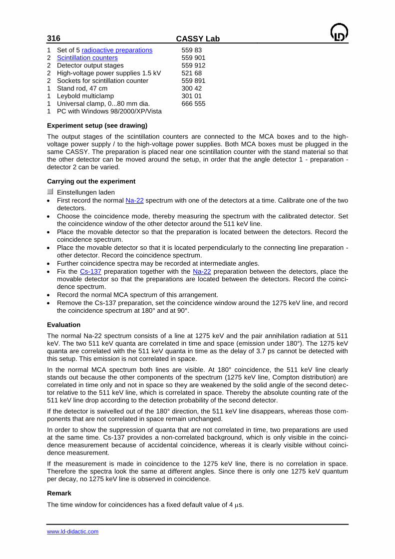
316

CASSY Lab

www.ld-didactic.com

1 Set of 5 radioactive preparations 559 83 2 Scintillation counters 559 901 2 Detector output stages 559 912 2 High-voltage power supplies 1.5 kV 521 68 2 Sockets for scintillation counter 559 891 1 Stand rod, 47 cm 300 42 1 Leybold multiclamp 301 01 1 Universal clamp, 0...80 mm dia. 666 555 1 PC with Windows 98/2000/XP/Vista


The output stages of the scintillation counters are connected to the MCA boxes and to the high-voltage power supply / to the high-voltage power supplies. Both MCA boxes must be plugged in the same CASSY. The preparation is placed near one scintillation counter with the stand material so that the other detector can be moved around the setup, in order that the angle detector 1 - preparation - detector 2 can be varied.


Einstellungen laden

First record the normal Na-22 spectrum with one of the detectors at a time. Calibrate one of the two detectors.

Choose the coincidence mode, thereby measuring the spectrum with the calibrated detector. Set the coincidence window of the other detector around the 511 keV line.

Place the movable detector so that the preparation is located between the detectors. Record the coincidence spectrum.

Place the movable detector so that it is located perpendicularly to the connecting line preparation - other detector. Record the coincidence spectrum.

Further coincidence spectra may be recorded at intermediate angles.

Fix the Cs-137 preparation together with the Na-22 preparation between the detectors, place the movable detector so that the preparations are located between the detectors. Record the coinci-dence spectrum.

Record the normal MCA spectrum of this arrangement.

Remove the Cs-137 preparation, set the coincidence window around the 1275 keV line, and record the coincidence spectrum at 180° and at 90°.

Evaluation

The normal Na-22 spectrum consists of a line at 1275 keV and the pair annihilation radiation at 511 keV. The two 511 keV quanta are correlated in time and space (emission under 180°). The 1275 keV quanta are correlated with the 511 keV quanta in time as the delay of 3.7 ps cannot be detected with this setup. This emission is not correlated in space.

In the normal MCA spectrum both lines are visible. At 180° coincidence, the 511 keV line clearly stands out because the other components of the spectrum (1275 keV line, Compton distribution) are correlated in time only and not in space so they are weakened by the solid angle of the second detec-tor relative to the 511 keV line, which is correlated in space. Thereby the absolute counting rate of the 511 keV line drop according to the detection probability of the second detector.

If the detector is swivelled out of the 180° direction, the 511 keV line disappears, whereas those com-ponents that are not correlated in space remain unchanged.

In order to show the suppression of quanta that are not correlated in time, two preparations are used at the same time. Cs-137 provides a non-correlated background, which is only visible in the coinci-dence measurement because of accidental coincidence, whereas it is clearly visible without coinci-dence measurement.

If the measurement is made in coincidence to the 1275 keV line, there is no correlation in space. Therefore the spectra look the same at different angles. Since there is only one 1275 keV quantum per decay, no 1275 keV line is observed in coincidence.

Remark

The time window for coincidences has a fixed default value of 4 s.

CASSY Lab

317

www.ld-didactic.com

Measurements with the single-channel analyzer


Beispiel laden

Safety note








To demonstrate the time advantage with a multichannel analyzer, a measurement in the MCA mode is carried out and then compared with a measurement in the single-channel mode.

Equipment list


1 Scintillation counter 559 901 1 Detector output stage 559 912 1 High-voltage power supply 1.5 kV 521 68 1 Socket for scintillator screening 559 891

318

CASSY Lab

www.ld-didactic.com



The output stage of the scintillation counter is connected to the MCA box and to the high-voltage power supply. The preparation is placed a few centimetres above the scintillation counter with the stand material.


Einstellungen laden

Start the measurement in the MCA mode (F9).

Start the measurement in the single-channel mode, e.g. with an equal total measuring time or with the same measuring time per point.

Evaluation

The parallel measurement of all channels has an obvious time advantage in comparison with the se-quential measurement of individual channels. With equal measuring times, this time advantage is con-verted into a gain in resolution or in the signal-to-noise ratio.

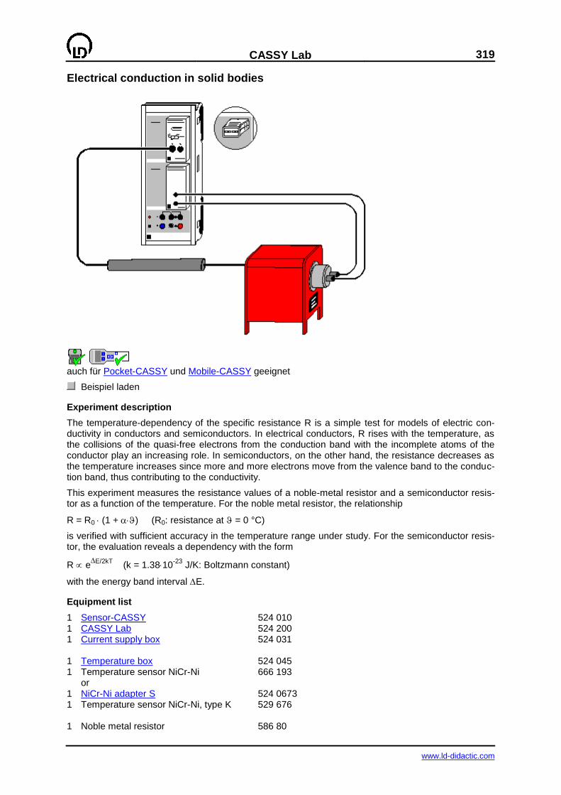
CASSY Lab

319

www.ld-didactic.com

Electrical conduction in solid bodies


Beispiel laden


The temperature-dependency of the specific resistance R is a simple test for models of electric con-ductivity in conductors and semiconductors. In electrical conductors, R rises with the temperature, as the collisions of the quasi-free electrons from the conduction band with the incomplete atoms of the conductor play an increasing role. In semiconductors, on the other hand, the resistance decreases as the temperature increases since more and more electrons move from the valence band to the conduc-tion band, thus contributing to the conductivity.

This experiment measures the resistance values of a noble-metal resistor and a semiconductor resis-tor as a function of the temperature. For the noble metal resistor, the relationship

R = R0(1 + ) (R0: resistance at = 0 °C)

is verified with sufficient accuracy in the temperature range under study. For the semiconductor resis-tor, the evaluation reveals a dependency with the form

R eE/2kT

(k = 1.3810-23

J/K: Boltzmann constant)

with the energy band interval E.

Equipment list

1 Sensor-CASSY 524 010 1 CASSY Lab 524 200 1 Current supply box 524 031 1 Temperature box 524 045 1 Temperature sensor NiCr-Ni 666 193 or 1 NiCr-Ni adapter S 524 0673 1 Temperature sensor NiCr-Ni, type K 529 676 1 Noble metal resistor 586 80

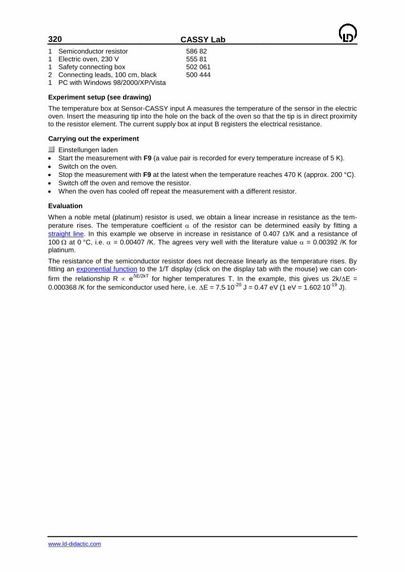
320

CASSY Lab

www.ld-didactic.com

1 Semiconductor resistor 586 82 1 Electric oven, 230 V 555 81 1 Safety connecting box 502 061 2 Connecting leads, 100 cm, black 500 444 1 PC with Windows 98/2000/XP/Vista


The temperature box at Sensor-CASSY input A measures the temperature of the sensor in the electric oven. Insert the measuring tip into the hole on the back of the oven so that the tip is in direct proximity to the resistor element. The current supply box at input B registers the electrical resistance.


Einstellungen laden

Start the measurement with F9 (a value pair is recorded for every temperature increase of 5 K).

Switch on the oven.

Stop the measurement with F9 at the latest when the temperature reaches 470 K (approx. 200 °C).

Switch off the oven and remove the resistor.

When the oven has cooled off repeat the measurement with a different resistor.

Evaluation

When a noble metal (platinum) resistor is used, we obtain a linear increase in resistance as the tem-

perature rises. The temperature coefficient of the resistor can be determined easily by fitting a

straight line. In this example we observe in increase in resistance of 0.407 /K and a resistance of

100 at 0 °C, i.e. = 0.00407 /K. The agrees very well with the literature value = 0.00392 /K for platinum.

The resistance of the semiconductor resistor does not decrease linearly as the temperature rises. By fitting an exponential function to the 1/T display (click on the display tab with the mouse) we can con-

firm the relationship R eE/2kT

for higher temperatures T. In the example, this gives us 2k/E =

0.000368 /K for the semiconductor used here, i.e. E = 7.510-20

J = 0.47 eV (1 eV = 1.60210-19

J).

CASSY Lab

321

www.ld-didactic.com

Hysteresis of a transformer core


Beispiel laden

322

CASSY Lab

www.ld-didactic.com


In a transformer core (ferromagnet) the magnetic field

H = N1/L I

is proportional to the coil current I and the effective turns density N1/L of the primary coil. However, the generated magnetic flux density or magnetic induction

B = r0H (where 0 = 410-7

Vs/Am)

is not proportional to H. Rather, it reaches a saturation value Bs as the magnetic field H increases. The

relative permeability r of the ferromagnet depends on the magnetic field strength H, and also on the

previous magnetic treatment of the ferromagnet. In a demagnetized ferromagnet, the magnetic field strength is B = 0 T at H = 0 A/m. Normally however, a ferromagnet still retains a residual magnetic flux density B not equal to 0 T when H = 0 A/m (remanence).

Thus, it is common to represent the magnetic induction B in the form of a hysteresis curve as a func-tion of the rising and falling field strength H. The hysteresis curve differs from the magnetization curve, which begins at the origin of the coordinate system and can only be measured for completely demag-netized material (H = 0 A/m, B = 0 T).

In this example H and B are not measured directly; rather, the quantities proportional to these, i.e. the

primary current I = L/N1H and magnetic flux = N2AB through the secondary coil are used (N2:

number of turns of secondary coil; A: cross-section of ferromagnet). The magnetic flux is calculated as the integral of the voltage U induced in the secondary coil.

Equipment list

1 Power-CASSY 524 011 1 Sensor-CASSY 524 010 1 CASSY Lab 524 200 1 U-core with yoke 562 11 1 Clamping device 562 12 2 Coils with 500 turns 562 14 4 Connecting leads, 100 cm, black 500 444 1 PC with Windows 98/2000/XP/Vista


1 Sensor-CASSY 524 010 1 CASSY Lab 524 200 1 U-core with yoke 562 11 1 Clamping device 562 12 2 Coils with 500 turns 562 14 1 Function generator S12 522 621 1 STE resistor 1 , 2 W 577 19

1 Socket board section 576 71 1 Connecting lead, 50 cm, black 500 424 7 Connecting leads, 100 cm, black 500 444 1 PC with Windows 98/2000/XP/Vista


Power-CASSY supplies the current for the primary coil of the transformer. The magnetic flux is cal-culated from the induction voltage U of the secondary coil, which is measured at Sensor-CASSY in-put B.

Alternatively, you can perform the experiment without Power-CASSY, using the function generator S12. This apparatus must be set to sawtooth signal, frequency around 0.1 Hz and amplitude about 2 V. Recording of the magnetization curve is triggered at I = 0 A. To hit this point exactly, the current is

shunted past the transformer by the relay and flows through a 1 resistor prior to recording of the curve.

CASSY Lab

323

www.ld-didactic.com


Einstellungen laden

Correct the offset if necessary: open Settings UB, select Correct, set the first target value 0 V and click on Correct Offset.

Demagnetize the transformer core, e.g. by striking the end face of the yoke against the end faces of the U-core several times.


Stop the measurement with F9 after one period of the hysteresis curve or at = 0 Vs (in this case the core does not have to be demagnetized again).

If the hysteresis curve lies in the second and fourth quadrants, reverse the connections on one of the two coils.

If the display instrument UB is overdriven during measurement (display flashes), extend the meas-

uring range in Settings UB.

Evaluation

As the area of a hysteresis loop B(H)

just corresponds to the energy loss in remagnetization per volume V of the demagnetized material, the

enclosed area in the diagram (I)

gives us precisely the energy loss E of the remagnetization for N1=N2.

In the diagram, you can calculate this energy loss using "peak integration" of a hysteresis loop.

324

CASSY Lab

www.ld-didactic.com

Non-destructive analysis of the chemical composition (x-ray fluorescence)


Beispiel laden

Safety notes










When a sample is irradiated with high energy x-ray photons it will emit characteristic x-ray lines whose energy depends on the atomic number of the element of the sample material. This dependency is the topic of the experimental examples of Moseley's law (K-line and L-line x-ray fluorescence)

CASSY Lab

325

www.ld-didactic.com

If a sample consists of a chemical compound or mixture, its fluorescence spectrum will also be com-plex. Because the inner electron shells between which the x-ray transitions occur are not involved in the chemical bonds, the characteristic lines are largely independent of the chemical bonds in the ele-ment. This means that the x-ray fluorescence spectra of a chemical compound are, to a first approxi-mation, a superposition of the spectra of its components.

For the qualitative analysis of the chemical composition of a sample, initially all the peaks found in the fluorescence spectrum are correlated to the elements. This is done by means of the values for the energies of the characteristic lines found in the table. For the correlation, the "pattern" of each of the

spectral series is also considered: for example, together with the K-line there must also be the K-line

with a lesser (approx. one fifth to one tenth) intensity in the spectrum. The L-line appears accompa-

nied by the L-line of a similar intensity and the L-line of a lesser intensity.

Information about the relative concentrations of individual elements in the compound can be gained from the relative intensities of their fluorescence lines.

Equipment list

1 Sensor-CASSY 524 010 1 CASSY Lab 524 200 1 MCA-Box 524 058 1 X-ray apparatus with x-ray tube Mo 554 801 or 554 811 1 Target set of alloys 554 848 1 X-ray energy detector 559 938 1 HF cable, 1 m 501 02 1 PC with Windows 98/2000/XP/Vista












Einstellungen laden


Place the calibration target (galvanised steel plate) from the scope of delivery for the x-ray energy detector onto the table



Then record spectra for the four targets in the target set of alloys

Energy calibration

The energy calibration of the spectra is made using the spectrum of the calibration target (Fe+Zn).

Open in the context menu of the diagram (right mouse button) or select with Alt+E the Energy cali-bration, select global energy calibration and enter on the right-hand side the energies of the Fe

K-line (6.40 keV) and of the Zn K-line (8.64 keV). Do not yet close the Energy calibration win-

dow.

326

CASSY Lab

www.ld-didactic.com

In the context menu of the diagram select under other evaluations Calculate peak center, mark the

Fe K-line and enter the result in the left-hand side of the Energy calibration (e.g. with drag & drop


Then determine the centre for the Zn K-line and also enter it on the left-hand side


Call the X-ray energies for identification and labelling of the lines in the context menu of the dia-gram or by using Alt+X and click on the Fe element symbol, select Adopt, click on Zn and close the window by clicking on OK.

It becomes apparent that four of the measured peaks have been caused by the fluorescence of the main components Fe and Zn of the galvanised steel plate.

Evaluation

For the identification of the components of the alloys:

Select spectrum and mark a suitable section

In the context menu of the diagram window or by using Alt+X select the window X-ray energies and click on the element symbols and determine a suitable element by means of the displayed markers for the energies in the table.

Place the marker by clicking Adopt and determine further components of the alloy

The results of the qualitative investigation of the alloys by means of their x-ray fluorescence spectra correspond to the known chemical composition:

Target 1: Stainless steel X5CrNi18-10 – contains 72 % Fe, 18 % Cr, 10 % Ni.

Target 2: Brass CuZn36 – contains 64 % Cu, 36 % Zn.

Target 3: Brass CuZn39Pb3 – contains 58 % Cu, 39 % Zn, 3% Pb.

Target 4: Praseodymium-samarium-cobalt magnet. These magnets can, in addition to Co, Sm, Pr, also contain Fe, Cu and Zr. Also the K-lines of bromium can be found, which originate from the fire-retardant in the plastic support.

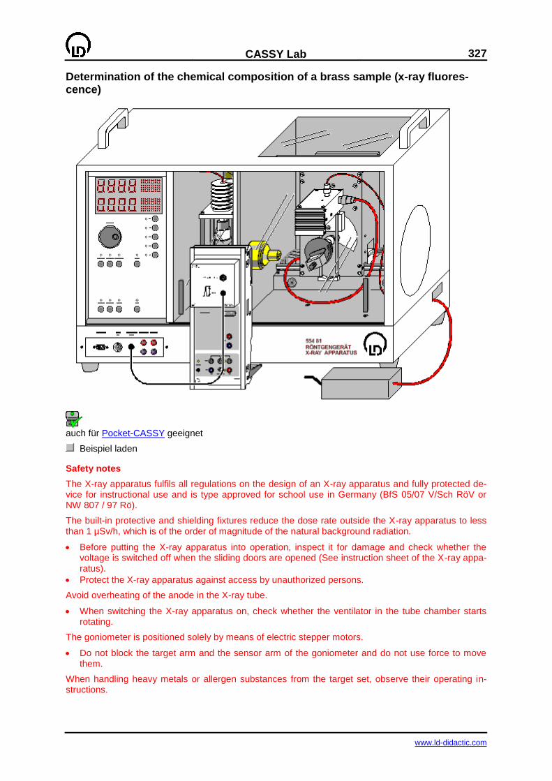
CASSY Lab

327

www.ld-didactic.com

Determination of the chemical composition of a brass sample (x-ray fluores-cence)


Beispiel laden

Safety notes










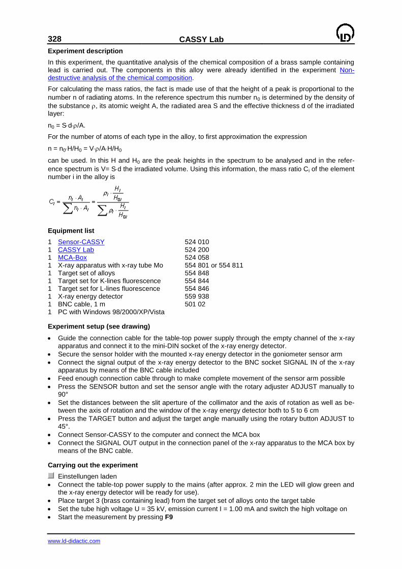
328

CASSY Lab

www.ld-didactic.com


In this experiment, the quantitative analysis of the chemical composition of a brass sample containing lead is carried out. The components in this alloy were already identified in the experiment Non-destructive analysis of the chemical composition.

For calculating the mass ratios, the fact is made use of that the height of a peak is proportional to the

number n of radiating atoms. In the reference spectrum this number n0 is determined by the density of

the substance , its atomic weight A, the radiated area S and the effective thickness d of the irradiated layer:

n0 = Sd/A.

For the number of atoms of each type in the alloy, to first approximation the expression

n = n0H/H0 = V/AH/H0

can be used. In this H and H0 are the peak heights in the spectrum to be analysed and in the refer-

ence spectrum is V= Sd the irradiated volume. Using this information, the mass ratio Ci of the element number i in the alloy is

Equipment list

1 Sensor-CASSY 524 010 1 CASSY Lab 524 200 1 MCA-Box 524 058 1 X-ray apparatus with x-ray tube Mo 554 801 or 554 811 1 Target set of alloys 554 848 1 Target set for K-lines fluorescence 554 844 1 Target set for L-lines fluorescence 554 846 1 X-ray energy detector 559 938 1 BNC cable, 1 m 501 02 1 PC with Windows 98/2000/XP/Vista












Einstellungen laden


Place target 3 (brass containing lead) from the target set of alloys onto the target table



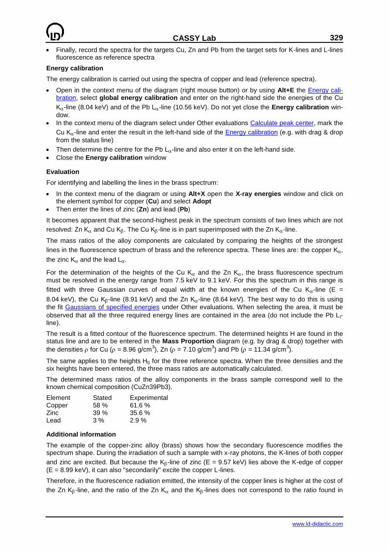
CASSY Lab

329

www.ld-didactic.com

Finally, record the spectra for the targets Cu, Zn and Pb from the target sets for K-lines and L-lines fluorescence as reference spectra

Energy calibration

The energy calibration is carried out using the spectra of copper and lead (reference spectra).

Open in the context menu of the diagram (right mouse button) or by using Alt+E the Energy cali-bration, select global energy calibration and enter on the right-hand side the energies of the Cu

K-line (8.04 keV) and of the Pb L-line (10.56 keV). Do not yet close the Energy calibration win-

dow.


Cu K-line and enter the result in the left-hand side of the Energy calibration (e.g. with drag & drop


Then determine the centre for the Pb L-line and also enter it on the left-hand side.


Evaluation

For identifying and labelling the lines in the brass spectrum:

In the context menu of the diagram or using Alt+X open the X-ray energies window and click on the element symbol for copper (Cu) and select Adopt

Then enter the lines of zinc (Zn) and lead (Pb)

It becomes apparent that the second-highest peak in the spectrum consists of two lines which are not

resolved: Zn K and Cu K. The Cu K-line is in part superimposed with the Zn K-line.

The mass ratios of the alloy components are calculated by comparing the heights of the strongest

lines in the fluorescence spectrum of brass and the reference spectra. These lines are: the copper K,

the zinc K and the lead L.

For the determination of the heights of the Cu K and the Zn K, the brass fluorescence spectrum

must be resolved in the energy range from 7.5 keV to 9.1 keV. For this the spectrum in this range is

fitted with three Gaussian curves of equal width at the known energies of the Cu K-line (E =

8.04 keV), the Cu K-line (8.91 keV) and the Zn K-line (8.64 keV). The best way to do this is using

the fit Gaussians of specified energies under Other evaluations. When selecting the area, it must be

observed that all the three required energy lines are contained in the area (do not include the Pb L l-line).

The result is a fitted contour of the fluorescence spectrum. The determined heights H are found in the status line and are to be entered in the Mass Proportion diagram (e.g. by drag & drop) together with

the densities for Cu ( = 8.96 g/cm3), Zn ( = 7.10 g/cm

3) and Pb ( = 11.34 g/cm

3).

The same applies to the heights H0 for the three reference spectra. When the three densities and the six heights have been entered, the three mass ratios are automatically calculated.

The determined mass ratios of the alloy components in the brass sample correspond well to the known chemical composition (CuZn39Pb3).

Element Stated Experimental Copper 58 % 61.6 % Zinc 39 % 35.6 % Lead 3 % 2.9 %

Additional information

The example of the copper-zinc alloy (brass) shows how the secondary fluorescence modifies the spectrum shape. During the irradiation of such a sample with x-ray photons, the K-lines of both copper

and zinc are excited. But because the K-line of zinc (E = 9.57 keV) lies above the K-edge of copper

(E = 8.99 keV), it can also "secondarily" excite the copper L-lines.

Therefore, in the fluorescence radiation emitted, the intensity of the copper lines is higher at the cost of

the Zn K-line, and the ratio of the Zn K and the K-lines does not correspond to the ratio found in

330

CASSY Lab

www.ld-didactic.com

pure zinc. For this reason, the mass ratio of the alloy components determined from the K-lines indi-

cates a slightly too high proportion of copper.

CASSY Lab

331

www.ld-didactic.com

Experiment examples chemistry

These experiment examples support you in using CASSY Lab. Where applicable, the corresponding experiment number is also given. The measurement data or settings for the examples can be loaded directly into CASSY Lab. Simply click in the buttons in the descriptions. New examples are labelled

with a red .

Inorganic Chemistry

The Bunsen burner

C1.3.1.6a pH measurement on foodstuffs

C1.3.1.6b pH measurement on cleaning agents

C1.3.1.7 Determining the pKa value of acetic acid

C1.3.1.8 Titration of phosphoric acid

Analytical Chemistry

Melting and solidification point of palmitic acid

Supercooling a sodium thiosulphate melt

C3.1.4.5 Determining the molar mass byway of freezing-point depression

Titration of hydrochloric acid with caustic soda solution (pH and conductivity)

C3.3.7.2 Titration of household vinegar

Titration of acetic acid with caustic soda solution (pH and conductivity)

Automatic titration of NH3 with NaH2PO4 (piston burette)

Automatic titration (drop counter)

C3.4.4.1 Gas chromatography (separation of alkanes from lighter gas)

C3.4.4.2 Gas chromatography (separation of alcohols)

C3.4.4.3 Gas chromatography (separation of air)

Recording the spectrum of a solution of crude chlorophyll (with the spectrophotome-ter 667 3491)

Physical Chemistry

Reaction of marble with hydrochloric acid (determining the carbonate content)

Splitting of urea by urease (zero-order reaction)

C4.3.2.3 Hydrolysis of tertiary butyl chloride (determining the reaction order)

Reaction of marble with hydrochloric acid (determining the reaction order)

C4.3.2.4 Alkaline hydrolysis of ethyl acetate (determining the reaction order)

Alkaline hydrolysis of ethyl acetate (determining the activation parameters)

C4.4.3.5 Differential thermal analysis of copper sulphate

Preparing a freezing mixture

C4.4.4.5 Determining the melting enthalpy of ice

Gas laws

C4.6.1.1 Determining the conductivity of different solutions

C4.6.1.4 Determining the limiting equivalent conductivity of sodium chloride

C4.6.1.5 Determining the dissociation constant of acetic acid

Technical Chemistry

Separation of a two-component mixture using the rectification apparatus CE2

Environmental Technology

Absorption of UV radiation

C6.1.4.3 Simulation of the ozone hole

C6.1.4.4 Greenhouse effect of CO2

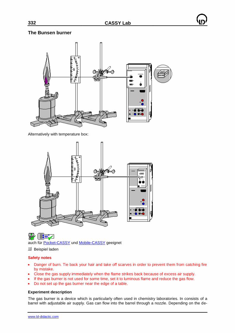
332

CASSY Lab

www.ld-didactic.com

The Bunsen burner

Alternatively with temperature box:


Beispiel laden

Safety notes

Danger of burn. Tie back your hair and take off scarves in order to prevent them from catching fire by mistake.

Close the gas supply immediately when the flame strikes back because of excess air supply.

If the gas burner is not used for some time, set it to luminous flame and reduce the gas flow.

Do not set up the gas burner near the edge of a table.


The gas burner is a device which is particularly often used in chemistry laboratories. In consists of a barrel with adjustable air supply. Gas can flow into the barrel through a nozzle. Depending on the de-

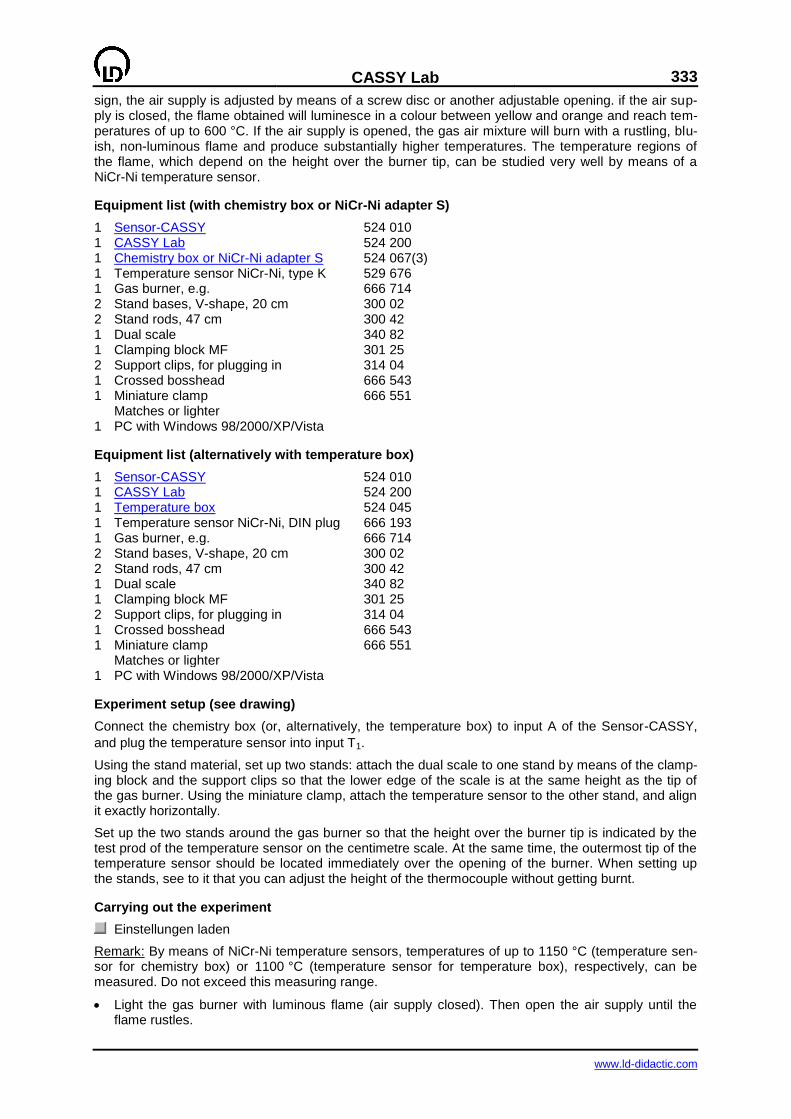
CASSY Lab

333

www.ld-didactic.com

sign, the air supply is adjusted by means of a screw disc or another adjustable opening. if the air sup-ply is closed, the flame obtained will luminesce in a colour between yellow and orange and reach tem-peratures of up to 600 °C. If the air supply is opened, the gas air mixture will burn with a rustling, blu-ish, non-luminous flame and produce substantially higher temperatures. The temperature regions of the flame, which depend on the height over the burner tip, can be studied very well by means of a NiCr-Ni temperature sensor.

Equipment list (with chemistry box or NiCr-Ni adapter S)

1 Sensor-CASSY 524 010 1 CASSY Lab 524 200 1 Chemistry box or NiCr-Ni adapter S 524 067(3) 1 Temperature sensor NiCr-Ni, type K 529 676 1 Gas burner, e.g. 666 714 2 Stand bases, V-shape, 20 cm 300 02 2 Stand rods, 47 cm 300 42 1 Dual scale 340 82 1 Clamping block MF 301 25 2 Support clips, for plugging in 314 04 1 Crossed bosshead 666 543 1 Miniature clamp 666 551 Matches or lighter 1 PC with Windows 98/2000/XP/Vista

Equipment list (alternatively with temperature box)

1 Sensor-CASSY 524 010 1 CASSY Lab 524 200 1 Temperature box 524 045 1 Temperature sensor NiCr-Ni, DIN plug 666 193 1 Gas burner, e.g. 666 714 2 Stand bases, V-shape, 20 cm 300 02 2 Stand rods, 47 cm 300 42 1 Dual scale 340 82 1 Clamping block MF 301 25 2 Support clips, for plugging in 314 04 1 Crossed bosshead 666 543 1 Miniature clamp 666 551 Matches or lighter 1 PC with Windows 98/2000/XP/Vista


Connect the chemistry box (or, alternatively, the temperature box) to input A of the Sensor-CASSY,

and plug the temperature sensor into input T1.

Using the stand material, set up two stands: attach the dual scale to one stand by means of the clamp-ing block and the support clips so that the lower edge of the scale is at the same height as the tip of the gas burner. Using the miniature clamp, attach the temperature sensor to the other stand, and align it exactly horizontally.

Set up the two stands around the gas burner so that the height over the burner tip is indicated by the test prod of the temperature sensor on the centimetre scale. At the same time, the outermost tip of the temperature sensor should be located immediately over the opening of the burner. When setting up the stands, see to it that you can adjust the height of the thermocouple without getting burnt.


Einstellungen laden

Remark: By means of NiCr-Ni temperature sensors, temperatures of up to 1150 °C (temperature sen-sor for chemistry box) or 1100 °C (temperature sensor for temperature box), respectively, can be measured. Do not exceed this measuring range.

Light the gas burner with luminous flame (air supply closed). Then open the air supply until the flame rustles.

334

CASSY Lab

www.ld-didactic.com

Fix the temperature sensor at the upper end of the measuring scale. See to it that the tip is exactly in the centre of the flame.

Wait until the displayed measured value is almost stable (±5 °C). Record the measured value by

pressing F9 or the button. Via the display instrument, which is accessed via the A11 button at

the upper edge of the screen, the instantaneous value of the temperature can be displayed on the full screen so that persons who are sitting at a distance are able to read the temperature.

Click the corresponding cell of the table, and enter the height over the burner tip associated with the measured value via the key board.

Access another colour region of the flame (outer cone: weakly bluish, inner cone: light blue) in the diagram by pressing the combination Alt+V, and, using the mouse, mark the subsequent position by a vertical line. With Alt+T text related to the mark can be added.

When reaching the light blue region of the flame, make the measurements in steps of 0.5 cm.

Evaluation

As expected, the temperature in the central region of the burner flame is higher than at a certain height above the flame. However, the temperatures generated by the light blue flame just above the outlet opening is much lower than the temperature generated by the weakly bluish flame a few centi-metres above. From this it can be concluded that the gas used is only completely burnt above the light blue region of the flame.

When chemical experiments are carried out, the different temperatures of the regions of the burner flame can be taken advantage of. If particularly high temperatures are desired, the region immediately above the light blue flame is used for heating. If the heating temperature should be lower, a greater distance from the burner tip is chosen.

CASSY Lab

335

www.ld-didactic.com

pH measurement on foodstuffs

Alternatively with pH box:


Beispiel laden


In this experiment, the pH values of foodstuffs, particularly of drinks, are investigated.

The pH value is a measure for the acidic strength or basic strength, respectively, of a solution. It is

defined as the negative decimal logarithm of the concentration of H3O+ ions in an aqueous solution:

pH = - lg c(H3O+)

The concentration of H3O+ ions depends on the autoprotolysis equilibrium of water:

H2O + H2O H3O+ + OH

-

In dilute solutions, the equilibrium is independent of the concentration of water molecules; at 25 °C, the equilibrium constant is:

K = c(H3O+) c(OH

-) = 10

-14 mol

2/l

2

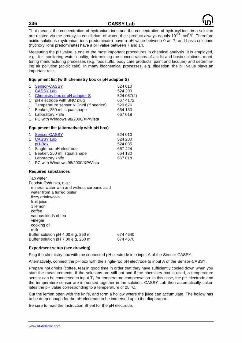
336

CASSY Lab

www.ld-didactic.com

That means, the concentration of hydronium ions and the concentration of hydroxyl ions in a solution

are related via the protolysis equilibrium of water; their product always equals 10-14

mol2/l

2. Therefore

acidic solutions (hydronium ions predominate) have a pH value between 0 an 7, and basic solutions (hydroxyl ions predominate) have a pH value between 7 and 14.

Measuring the pH value is one of the most important procedures in chemical analysis. It is employed, e.g., for monitoring water quality, determining the concentrations of acidic and basic solutions, moni-toring manufacturing processes (e.g. foodstuffs, body care products, paint and lacquer) and determin-ing air pollution (acidic rain). In many biochemical processes, e.g. digestion, the pH value plays an important role.

Equipment list (with chemistry box or pH adapter S)

1 Sensor-CASSY 524 010 1 CASSY Lab 524 200 1 Chemistry box or pH adapter S 524 067(2) 1 pH electrode with BNC plug 667 4172 1 Temperature sensor NiCr-Ni (if needed) 529 676 1 Beaker, 250 ml, squat shape 664 130 1 Laboratory knife 667 018 1 PC with Windows 98/2000/XP/Vista

Equipment list (alternatively with pH box)

1 Sensor-CASSY 524 010 1 CASSY Lab 524 200 1 pH-Box 524 035 1 Single-rod pH electrode 667 424 1 Beaker, 250 ml, squat shape 664 130 1 Laboratory knife 667 018 1 PC with Windows 98/2000/XP/Vista

Required substances

Tap water Foodstuffs/drinks, e.g.: mineral water with and without carbonic acid water from a furred boiler fizzy drinks/cola fruit juice 1 lemon coffee various kinds of tea vinegar cooking oil milk Buffer solution pH 4.00 e.g. 250 ml 674 4640 Buffer solution pH 7.00 e.g. 250 ml 674 4670


Plug the chemistry box with the connected pH electrode into input A of the Sensor-CASSY.

Alternatively, connect the pH box with the single-rod pH electrode to input A of the Sensor-CASSY.

Prepare hot drinks (coffee, tea) in good time in order that they have sufficiently cooled down when you start the measurements. If the solutions are still hot and if the chemistry box is used, a temperature

sensor can be connected to input T1 for temperature compensation. In this case, the pH electrode and the temperature sensor are immersed together in the solution. CASSY Lab then automatically calcu-lates the pH value corresponding to a temperature of 25 °C.

Cut the lemon open with the knife, and form a hollow where the juice can accumulate. The hollow has to be deep enough for the pH electrode to be immersed up to the diaphragm.

Be sure to read the Instruction Sheet for the pH electrode.

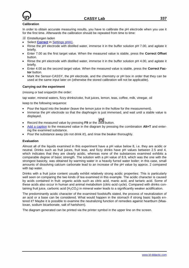
CASSY Lab

337

www.ld-didactic.com

Calibration

In order to obtain accurate measuring results, you have to calibrate the pH electrode when you use it for the first time. Afterwards the calibration should be repeated from time to time:

Einstellungen laden

Select Correct in Settings pHA1.

Rinse the pH electrode with distilled water, immerse it in the buffer solution pH 7.00, and agitate it briefly.

Enter 7.00 as the first target value. When the measured value is stable, press the Correct Offset button.


Enter 4.00 as the second target value. When the measured value is stable, press the Correct Fac-tor button.

Mark the Sensor-CASSY, the pH electrode, and the chemistry or pH box in order that they can be used at the same input later on (otherwise the stored calibration will not be applicable).


(missing or bad snippet)In the order:

tap water, mineral waters, fizzy drinks/coke, fruit juices, lemon, teas, coffee, milk, vinegar, oil

keep to the following sequence:

Pour the liquid into the beaker (leave the lemon juice in the hollow for the measurement).

Immerse the pH electrode so that the diaphragm is just immersed, and wait until a stable value is displayed.

Record the measured value by pressing F9 or the button.

Add a caption to the measured value in the diagram by pressing the combination Alt+T and enter-ing the examined substance.

Pour the substance away (do not drink it!), and rinse the beaker thoroughly.

Evaluation

Almost all of the liquids examined in this experiment have a pH value below 8, i.e. they are acidic or neutral. Drinks such as fruit juices, fruit teas, and fizzy drinks have pH values between 2.5 and 4, which indicates that they are clearly acidic, whereas none of the substances examined exhibits a comparable degree of basic strength. The solution with a pH value of 8.9, which was the one with the strongest basicity, was obtained by warming water in a heavily furred water boiler; in this case, small amounts of dissolving calcium carbonate lead to an increase of the pH value by approx. 2 compared with tap water.

Drinks with a fruit juice content usually exhibit relatively strong acidic properties: This is particularly well seen on comparing the two kinds of tea examined in this example. The acidic character is caused by acids contained in fruit: organic acids such as citric acid, manic acid, and tartaric acid. Some of these acids also occur in human and animal metabolism (citric-acid cycle). Compared with drinks con-

taining fruit juice, carbonic acid (H2CO3) in mineral water leads to a significantly weaker acidification.

The predominantly acidic character of the examined foodstuffs stated, the process of neutralization of an acid or a base can be considered. What would happen in the stomach if strong basic liquids en-tered it? Maybe it is possible to examine the neutralizing function of remedies against heartburn (Maa-loxan, sodium bicarbonate, salt of hartshorn).

The diagram generated can be printed via the printer symbol in the upper line on the screen.

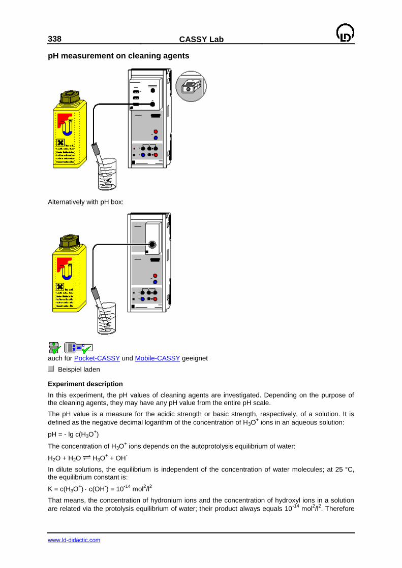
338

CASSY Lab

www.ld-didactic.com

pH measurement on cleaning agents



Beispiel laden


In this experiment, the pH values of cleaning agents are investigated. Depending on the purpose of the cleaning agents, they may have any pH value from the entire pH scale.

The pH value is a measure for the acidic strength or basic strength, respectively, of a solution. It is

defined as the negative decimal logarithm of the concentration of H3O+ ions in an aqueous solution:

pH = - lg c(H3O+)

The concentration of H3O+ ions depends on the autoprotolysis equilibrium of water:

H2O + H2O H3O+ + OH

-

In dilute solutions, the equilibrium is independent of the concentration of water molecules; at 25 °C, the equilibrium constant is:

K = c(H3O+) c(OH

-) = 10

-14 mol

2/l

2

That means, the concentration of hydronium ions and the concentration of hydroxyl ions in a solution

are related via the protolysis equilibrium of water; their product always equals 10-14

mol2/l

2. Therefore

CASSY Lab

339

www.ld-didactic.com

acidic solutions (hydronium ions predominate) have a pH value between 0 an 7, and basic solutions (hydroxyl ions predominate) have a pH value between 7 and 14.

Measuring the pH value is one of the most important procedures in chemical analysis. It is employed, e.g., for monitoring water quality, determining the concentrations of acidic and basic solutions, moni-toring manufacturing processes (e.g. foodstuffs, body care products, paint and lacquer) and determin-ing air pollution (acidic rain). In many biochemical processes, e.g. digestion, the pH value plays an important role.


1 Sensor-CASSY 524 010 1 CASSY Lab 524 200 1 Chemistry box or pH adapter S 524 067(2) 1 pH electrode with BNC plug 667 4172 1 Beaker, 100 ml, tall shape 664 137 1 Laboratory knife 667 018 1 PC with Windows 98/2000/XP/Vista


1 Sensor-CASSY 524 010 1 CASSY Lab 524 200 1 pH-Box 524 035 1 Single-rod pH electrode 667 424 1 Beaker, 100 ml, tall shape 664 137 1 Laboratory knife 667 018 1 PC with Windows 98/2000/XP/Vista

Required substances

Tap water Cleaning agents, e.g.: washing-up liquid detergents containing acetic acid tube cleaner cleaning agents that are ecologically friendly For comparison: vinegar 1 lemon Buffer solution pH 4.00 e.g. 250 ml 674 4640 Buffer solution pH 7.00 e.g. 250 ml 674 4670


Plug the chemistry box with the connected pH electrode into input A of the Sensor-CASSY.

Alternatively, connect the pH box with the single-rod pH electrode to input A of the Sensor-CASSY.

Cut the lemon open with the knife, and form a hollow where the juice can accumulate. The hollow has to be deep enough for the pH electrode to be immersed up to the diaphragm.

Be sure to read the Instruction Sheet for the pH electrode.

Calibration


Einstellungen laden





340

CASSY Lab

www.ld-didactic.com




(missing or bad snippet)

For all cleaning agents examined in the experiment keep to the following sequence:

Keeping to safety notes and dosage instructions (calculate the dosage for the volume of the beaker, which is 100 ml) that may be written on the package, prepare the solution to be examined in the beaker. If a cleaning agent is to be used undiluted, pour as little as possible (approx. 30 ml) into the beaker.

Leave the lemon juice in the hollow for the measurement.

Immerse the pH electrode in the solution so that the diaphragm is just immersed, and wait until a stable value is displayed.

Record the measured value by pressing F9 or the button.

Add a caption to the measured value in the diagram by pressing the combination Alt+T and enter-ing the examined substance.

Pour the substance away, and rinse the beaker thoroughly with tap water.

Evaluation

Depending on the purpose, cleaning agents can have any pH value from strongly acidic to strongly basic.

Particularly agents for removing lime deposits and for cleaning bathrooms have relatively low pH val-ues, which may even correspond to hydrochloric acid of approx. 0.3 mol/l concentration. This is due to

the lime dissolving reaction of CaCO3 with acids, which is used for removing lime deposits:

As the acidity of these cleaning agents is sometimes quite strong, the instruction saying that protective gloves should be worn is right in place on the package.

The ecologically friendly agent containing citric acid does not dissolve CaCO3 through the acidic char-acter of citric acid, but through formation of a water soluble complex of citric acid and calcium ions. In this way the low pH value of other cleaning agents can be avoided.

As basic soap solution also damages the skin, nowadays washing-up liquids for dissolving fat and oil mainly contain neutral surfactants instead of basic soaps. This shows up in the pH value of the exam-ined washing-up liquid, which indicates approximate neutrality. However, as the surface of human skin is slightly acidic (around pH 5.5), this washing-up liquid will also mean stress to the skin although to a lesser extent.

Among strongly basic cleaning agents there are, above all, tube cleaners, which have to dissolve fat deposits and hair at places where mechanical cleaning is impossible. These tube cleaners contain high concentrations of sodium hydroxide (NaOH) and often, in addition, hypochlorites, e.g. NaOCl, as oxidizing agents. Tube cleaners that contain hypochlorites must not get into contact with other clean-ing agents as corrosive chlorine gas is generated when acids are added to NaOCl and common salt, which is also contained in tube cleaners:

If usual pH electrodes are used, the pH value measured on the strongly basic tube cleaner is distorted by the so-called alkali error. Starting from pH values of approx. 12, glass electrodes display a value below the real one; therefore you can assume that the examined tube cleaner is even more basic.

As an alternative, economically friendly tube cleaners are supplied today, which are based on en-zymes and are almost neutral. The cleaning agent examined in the example is supposed to decom-pose fat enzymatically. This is achieved under almost neutral conditions, which means that sewage is much less contaminated.


CASSY Lab

341

www.ld-didactic.com

Further experiment options

The pH values of other substances that occur in everyday life can be examined as well.

An insertion electrode with a conical diaphragm enables solid pieces of soap and creams to be examined.

Determining the pH value of human skin by means of an electrode with flat diaphragm before and after washing the skin with soaps may be interesting with regard to the question of whether these substances are well-tolerated by the skin.

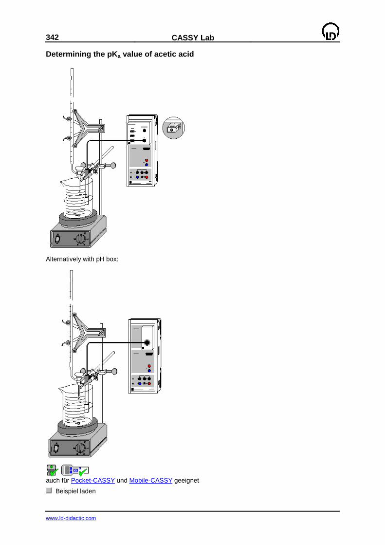
342

CASSY Lab

www.ld-didactic.com

Determining the pKa value of acetic acid



Beispiel laden

CASSY Lab

343

www.ld-didactic.com

Danger

Acids and bases are caustic. Wear protective goggles and acid-resistant gloves.


A measure for the strength of moderately strong or weak acids called the pKa value is determined from its titration curve with a strong base. Starting from the dissociation equation for the acid,

,

we obtain

[A-] = [HA].

for the point of half equivalence (where half of the acid has reacted with the base).

From the equilibrium equation

it therefore follows that

in this case.

Thus the pKa value can easily be read after the equivalence point and the point of half equivalence of the titration have been determined.


1 Sensor-CASSY 524 010 1 CASSY Lab 524 200 1 Chemistry box or pH adapter S 524 067(2) 1 pH electrode with BNC plug 667 4172 1 Magnetic stirrer 666 845 1 Beaker, 250 ml, squat shape 664 103 1 Stand rod, 450 mm, M10 thread 666 523 1 Graduated pipette, 10 ml 665 997 1 Pipetting ball 666 003 1 Burette, 25 ml 665 845 1 Burette filling funnel 665 816 1 Burette clamp simple 666 559 1 Crossed bosshead 666 543 1 Small universal clamp 666 551 1 PC with Windows 98/2000/XP/Vista


1 Sensor-CASSY 524 010 1 CASSY Lab 524 200 1 pH box 524 035 1 Single-rod pH electrode 667 424 1 Magnetic stirrer 666 845 1 Beaker, 250 ml, squat shape 664 103 1 Stand rod, 450 mm, M10 thread 666 523 1 Graduated pipette, 10 ml 665 997 1 Pipetting ball 666 003 1 Burette, 25 ml 665 845 1 Burette filling funnel 665 816 1 Burette clamp simple 666 559 1 Crossed bosshead 666 543 1 Small universal clamp 666 551 1 PC with Windows 98/2000/XP/Vista

344

CASSY Lab

www.ld-didactic.com

Chemicals

Acetic acid, c = 0.1 mol/l e.g. 500 ml: 671 9560 Caustic soda solution, c = 0.1 mol/l e.g. 500 ml: 673 8410 Buffer solution pH 4.00 e.g. 250 ml: 674 4640 Buffer solution pH 7.00 e.g. 250 ml: 674 4670 Distilled water


Plug the pH box with the single rod pH electrode into input A of the Sensor-CASSY, which is con-nected to the PC.

Set up the titration assembly using the stand material, the magnetic stirrer, the beaker and the burette. Put about 100 ml of distilled water into the beaker and add exactly 10 ml of 0.1 M acetic acid by means of the pipette. Fill 0.1 M caustic soda solution into the burette through the funnel up to the zero mark.

Attach the pH electrode so that on the one hand the measuring diaphragm is completely immersed and on the other hand the glass membrane cannot be damaged by the rotating stirrer bar. In order to mark the equivalence point, you may add some drops of phenolphthalein solution as an indicator.

Calibration


Einstellungen laden






Mark the Sensor-CASSY, the pH electrode, and the pH box in order that they can be used at the same input later on (otherwise the stored calibration will not be applicable).



If you want to apply other volume steps than 0.2 ml, the entry can be changed in Settings V in the field Formula, e.g. by entering "0.5*n-0.5" for steps of 0.5 ml.

Determine the first measured value by pressing the key F9 or the button.

Continuously add drops of caustic soda solution at a slow rate, and record the pH value in steps of 0.2 ml by pressing F9.

Evaluation

At the equivalence point (V = Veq), all the acetic acid has reacted with the caustic soda solution:

HAc + NaOH —> Na+ + Ac

- + H2O

In order to exactly determine the equivalence point with CASSY-Lab, press the right mouse button in the diagram, select Find Equivalence Point in the menu Other Evaluations. After marking the curve

range, you will obtain a graphical display of the equivalence point and the pKa value as determined via

the point of half equivalence (V = Vheq). The associated values are written below in the status line and can be inserted as text at an arbitrary place in the diagram.


By neutralizing a hydrochloric acid solution of the same pH value as the present acetic acid solution (approx. 10 ml of 0.01 M HCl) and comparing the two titration curves, the concept of a buffer solution can be introduced. The strongly diluted hydrochloric acid is already neutralized after 1 ml of NaOH has

CASSY Lab

345

www.ld-didactic.com

been added, whereas for neutralizing the acetic acid of similar acidity approx. 10 ml of NaOH are re-

quired. Determining the pKa value of the hydrochloric acid would not be meaningful.

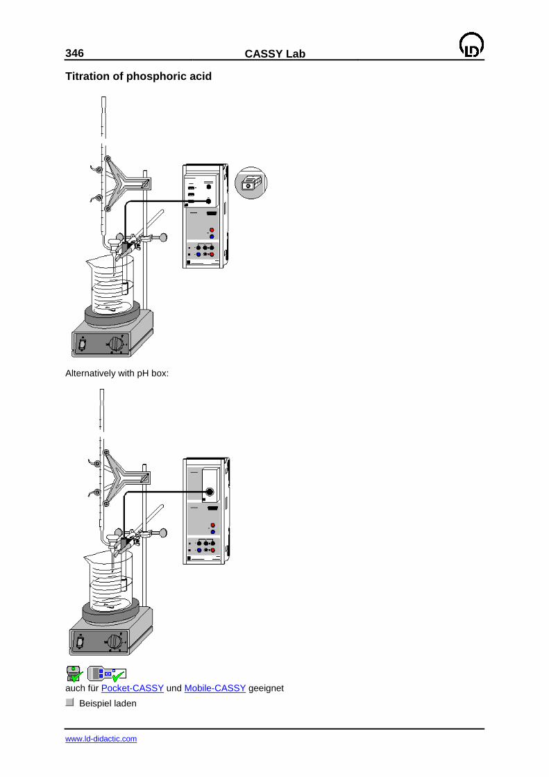
346

CASSY Lab

www.ld-didactic.com

Titration of phosphoric acid



Beispiel laden

CASSY Lab

347

www.ld-didactic.com

Danger

Acids and bases are caustic. Wear protective goggles, gloves and clothing.


Polybasic acids exhibit characteristic titration curves, which enable the pKa values of individual stages of protolysis to be determined following sections of the curve that have similar shapes.

In aqueous solution, phosphoric acid forms the following equilibria:

As the differences between the pKa values amount to approx. 5 in each case, the equilibria can be considered independently of each other.

By titration with caustic potash solution, the equivalence points of the first and the second stage of protolysis can be determined. However, since KOH is not a substantially stronger base than the phos-phate ion, the equilibrium 3 does not sufficiently tend to the right-hand side for the third equivalence point to be determined. In aqueous solution, the latter is only accessible in the opposite direction by titrating potassium phosphate, e.g., with hydrochloric acid.

In the pH range of the titration considered here (approx. pH 2 to pH 12), the hydrogenphosphates act as ampholytes, on the right-hand side of an equilibrium they represent the base of the respective acid-base pair, whereas on the left-hand side they have the function of the base.


1 Sensor-CASSY 524 010 1 CASSY Lab 524 200 1 Chemistry box or pH adapter S 524 067(2) 1 pH electrode with BNC plug 667 4172 1 Temperature sensor NiCr-Ni (if needed) 529 676 1 Magnetic stirrer 666 845 1 Beaker, 250 ml, squat shape 664 103 1 Stand rod, 450 mm, M10 thread 666 523 1 Graduated pipette, 10 ml 665 997 1 Pipetting ball 666 003 1 Burette, 50 ml 665 847 1 Burette filling funnel 665 816 1 Burette clamp simple 666 559 2 Crossed bossheads 666 543 2 Small universal clamps 666 551 1 PC with Windows 98/2000/XP/Vista


1 Sensor-CASSY 524 010 1 CASSY Lab 524 200 1 pH box 524 035 1 Single-rod pH electrode 667 424 1 Magnetic stirrer 666 845 1 Beaker, 250 ml, squat shape 664 103 1 Stand rod, 450 mm, M10 thread 666 523 1 Graduated pipette, 10 ml 665 997 1 Pipetting ball 666 003 1 Burette, 50 ml 665 847 1 Burette filling funnel 665 816 1 Burette clamp simple 666 559 1 Crossed bosshead 666 543 1 Small universal clamp 666 551

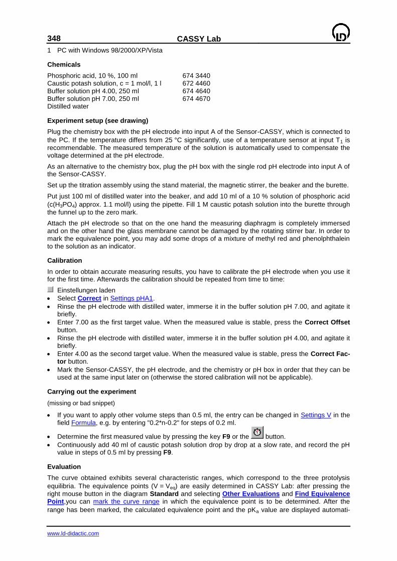
348

CASSY Lab

www.ld-didactic.com


Chemicals

Phosphoric acid, 10 %, 100 ml 674 3440 Caustic potash solution, c = 1 mol/l, 1 l 672 4460 Buffer solution pH 4.00, 250 ml 674 4640 Buffer solution pH 7.00, 250 ml 674 4670 Distilled water


Plug the chemistry box with the pH electrode into input A of the Sensor-CASSY, which is connected to

the PC. If the temperature differs from 25 °C significantly, use of a temperature sensor at input T1 is recommendable. The measured temperature of the solution is automatically used to compensate the voltage determined at the pH electrode.

As an alternative to the chemistry box, plug the pH box with the single rod pH electrode into input A of the Sensor-CASSY.

Set up the titration assembly using the stand material, the magnetic stirrer, the beaker and the burette.

Put just 100 ml of distilled water into the beaker, and add 10 ml of a 10 % solution of phosphoric acid

(c(H3PO4) approx. 1.1 mol/l) using the pipette. Fill 1 M caustic potash solution into the burette through

the funnel up to the zero mark.

Attach the pH electrode so that on the one hand the measuring diaphragm is completely immersed and on the other hand the glass membrane cannot be damaged by the rotating stirrer bar. In order to mark the equivalence point, you may add some drops of a mixture of methyl red and phenolphthalein to the solution as an indicator.

Calibration


Einstellungen laden











Continuously add 40 ml of caustic potash solution drop by drop at a slow rate, and record the pH value in steps of 0.5 ml by pressing F9.

Evaluation

The curve obtained exhibits several characteristic ranges, which correspond to the three protolysis

equilibria. The equivalence points (V = Veq) are easily determined in CASSY Lab: after pressing the right mouse button in the diagram Standard and selecting Other Evaluations and Find Equivalence Point,you can mark the curve range in which the equivalence point is to be determined. After the

range has been marked, the calculated equivalence point and the pKa value are displayed automati-

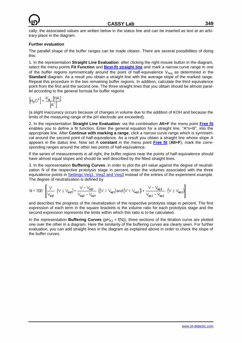
CASSY Lab

349

www.ld-didactic.com

cally; the associated values are written below in the status line and can be inserted as text at an arbi-trary place in the diagram.

Further evaluation

The parallel shape of the buffer ranges can be made clearer. There are several possibilities of doing this:

1. In the representation Straight Line Evaluation: after clicking the right mouse button in the diagram, select the menu points Fit Function and Best-fit straight line and mark a narrow curve range in one

of the buffer regions symmetrically around the point of half-equivalence Vheq as determined in the Standard diagram. As a result you obtain a straight line with the average slope of the marked range. Repeat this procedure in the two remaining buffer regions. In addition, calculate the third equivalence point from the first and the second one. The three straight lines that you obtain should be almost paral-lel according to the general formula for buffer regions

(a slight inaccuracy occurs because of changes in volume due to the addition of KOH and because the limits of the measuring range of the pH electrode are exceeded).

2. In the representation Straight Line Evaluation: via the combination Alt+F the menu point Free fit enables you to define a fit function. Enter the general equation for a straight line, "A*x+B", into the appropriate line. After Continue with marking a range, click a narrow curve range which is symmetri-cal around the second point of half-equivalence. As a result you obtain a straight line whose slope A appears in the status line. Now set A constant in the menu point Free fit (Alt+F), mark the corre-sponding ranges around the other two points of half-equivalence.

If the series of measurements is all right, the buffer regions near the points of half-equivalence should have almost equal slopes and should be well described by the fitted straight lines.

3. In the representation Buffering Curves: in order to plot the pH value against the degree of neutrali-zation N of the respective protolysis stage in percent, enter the volumes associated with the three equivalence points in Settings Veq1, Veq2 and Veq3 instead of the entries of the experiment example. The degree of neutralization is defined by

and describes the progress of the neutralization of the respective protolysis stage in percent. The first expression of each term in the square brackets is the volume ratio for each protolysis stage and the second expression represents the limits within which this ratio is to be calculated.

In the representation Buffering Curves (pHA1 = f(N)), three sections of the titration curve are plotted one over the other in a diagram. Here the similarity of the buffering curves are clearly seen. For further evaluation, you can add straight lines in the diagram as explained above in order to check the slope of the buffer curves.

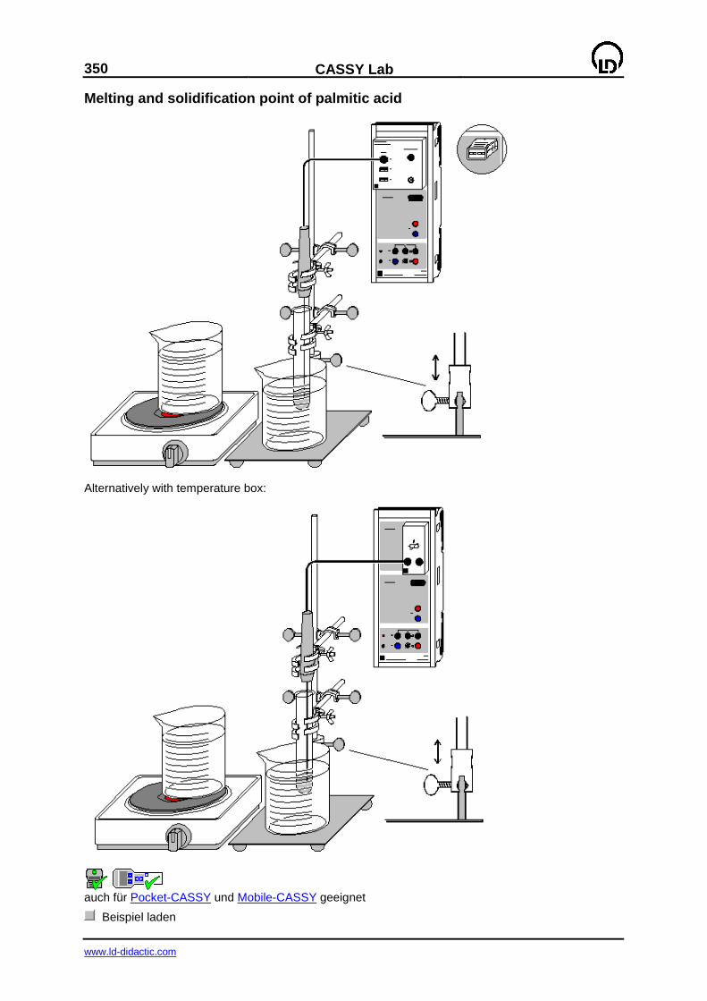
350

CASSY Lab

www.ld-didactic.com

Melting and solidification point of palmitic acid

Alternatively with temperature box:


Beispiel laden

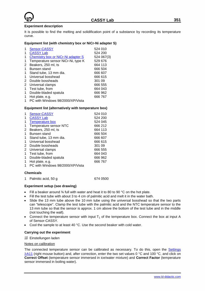
CASSY Lab

351

www.ld-didactic.com


It is possible to find the melting and solidification point of a substance by recording its temperature curve.

Equipment list (with chemistry box or NiCr-Ni adapter S)

1 Sensor-CASSY 524 010 1 CASSY Lab 524 200 1 Chemistry box or NiCr-Ni adapter S 524 067(3) 1 Temperature sensor NiCr-Ni, type K 529 676 2 Beakers, 250 ml, ts 664 113 1 Bunsen stand 666 504 1 Stand tube, 13 mm dia. 666 607 1 Universal bosshead 666 615 2 Double bossheads 301 09 2 Universal clamps 666 555 1 Test tube, from 664 043 1 Double-bladed spatula 666 962 1 Hot plate, e.g. 666 767 1 PC with Windows 98/2000/XP/Vista

Equipment list (alternatively with temperature box)

1 Sensor-CASSY 524 010 1 CASSY Lab 524 200 1 Temperature box 524 045 1 Temperature sensor NTC 666 212 2 Beakers, 250 ml, ts 664 113 1 Bunsen stand 666 504 1 Stand tube, 13 mm dia. 666 607 1 Universal bosshead 666 615 2 Double bossheads 301 09 2 Universal clamps 666 555 1 Test tube, from 664 043 1 Double-bladed spatula 666 962 1 Hot plate, e.g. 666 767 1 PC with Windows 98/2000/XP/Vista

Chemicals

1 Palmitic acid, 50 g 674 0500


Fill a beaker around ¾ full with water and heat it to 80 to 90 °C on the hot plate.

Fill the test tube with about 3 to 4 cm of palmitic acid and melt it in the water bath.

Slide the 13 mm tube above the 10 mm tube using the universal bosshead so that the two parts can "telescope". Clamp the test tube with the palmitic acid and the NTC temperature sensor to the 13 mm tube so that the sensor is approx. 1 cm above the bottom of the test tube and in the middle (not touching the wall).

Connect the temperature sensor with input T1 of the temperature box. Connect the box at input A of Sensor-CASSY.

Cool the sample to at least 40 °C. Use the second beaker with cold water.


Einstellungen laden

Notes on calibration

The connected temperature sensor can be calibrated as necessary. To do this, open the Settings

A11 (right mouse button) and, after correction, enter the two set values 0 °C and 100 °C, and click on Correct Offset (temperature sensor immersed in ice/water mixture) and Correct Factor (temperature sensor immersed in boiling water).

352

CASSY Lab

www.ld-didactic.com

Using your telescopic stand, place the test tube with the solidified palmitic acid and the embedded temperature sensor in the water bath at approx. 80 °C.

In the program, start the measurement by clicking on the clock button (or press F9).

When the temperature starts to climb steadily again above about 60 °C, lift the sample with the sensor out of the hot water bath using the stand and place in a beaker of cold water to cool it down more quickly (you can also let the sample cool in air, but this takes longer).

When the temperature has fallen significantly below the solidification point (approx. 60 °C), stop the measurement by pressing F9 or clicking the clock button.

Evaluation

You can vary areas of the windows for optimum diagram display. To do this, click on the respective axis with the right mouse button or zoom the graph.

To determine and mark the melting and solidification point, draw a horizontal line (click on the graph with the right mouse button and set a horizontal line as a marker) and position this line so that it runs through the constant solidification range.

You can insert the value shown in the status line (bottom left) in the diagram as text (click on the graphic with the right mouse button, set the marker and select text). You can also edit this text if desired.


Recording the temperature curve of other substances, e.g. sodium thiosulfate-5-hydrate

Comparing the temperature curves of different substances by superimposing

Comparing the temperature curves for a single substance in differing purities

Investigating the melting and solidification behaviour of mixtures with different compositions, de-termining the eutectic mixture, preparing a phase diagram

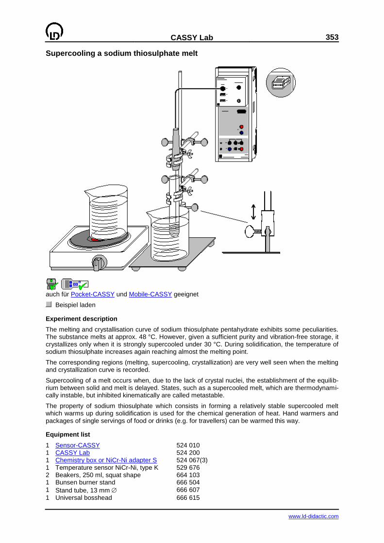
CASSY Lab

353

www.ld-didactic.com

Supercooling a sodium thiosulphate melt


Beispiel laden


The melting and crystallisation curve of sodium thiosulphate pentahydrate exhibits some peculiarities. The substance melts at approx. 48 °C. However, given a sufficient purity and vibration-free storage, it crystallizes only when it is strongly supercooled under 30 °C. During solidification, the temperature of sodium thiosulphate increases again reaching almost the melting point.

The corresponding regions (melting, supercooling, crystallization) are very well seen when the melting and crystallization curve is recorded.

Supercooling of a melt occurs when, due to the lack of crystal nuclei, the establishment of the equilib-rium between solid and melt is delayed. States, such as a supercooled melt, which are thermodynami-cally instable, but inhibited kinematically are called metastable.

The property of sodium thiosulphate which consists in forming a relatively stable supercooled melt which warms up during solidification is used for the chemical generation of heat. Hand warmers and packages of single servings of food or drinks (e.g. for travellers) can be warmed this way.

Equipment list

1 Sensor-CASSY 524 010 1 CASSY Lab 524 200 1 Chemistry box or NiCr-Ni adapter S 524 067(3) 1 Temperature sensor NiCr-Ni, type K 529 676 2 Beakers, 250 ml, squat shape 664 103 1 Bunsen burner stand 666 504 1 Stand tube, 13 mm 666 607

1 Universal bosshead 666 615

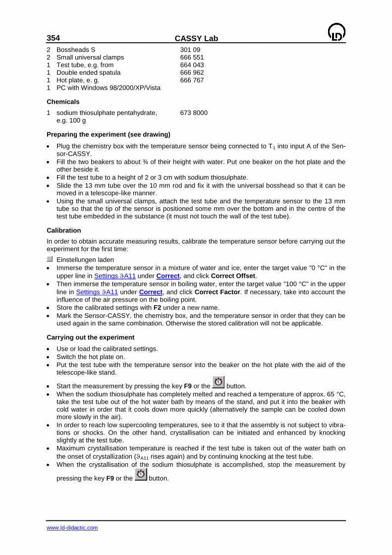
354

CASSY Lab

www.ld-didactic.com

2 Bossheads S 301 09 2 Small universal clamps 666 551 1 Test tube, e.g. from 664 043 1 Double ended spatula 666 962 1 Hot plate, e. g. 666 767 1 PC with Windows 98/2000/XP/Vista

Chemicals

1 sodium thiosulphate pentahydrate, e.g. 100 g

673 8000

Preparing the experiment (see drawing)

Plug the chemistry box with the temperature sensor being connected to T1 into input A of the Sen-sor-CASSY.

Fill the two beakers to about ¾ of their height with water. Put one beaker on the hot plate and the other beside it.

Fill the test tube to a height of 2 or 3 cm with sodium thiosulphate.

Slide the 13 mm tube over the 10 mm rod and fix it with the universal bosshead so that it can be moved in a telescope-like manner.

Using the small universal clamps, attach the test tube and the temperature sensor to the 13 mm tube so that the tip of the sensor is positioned some mm over the bottom and in the centre of the test tube embedded in the substance (it must not touch the wall of the test tube).

Calibration

In order to obtain accurate measuring results, calibrate the temperature sensor before carrying out the experiment for the first time:

Einstellungen laden

Immerse the temperature sensor in a mixture of water and ice, enter the target value "0 °C" in the

upper line in Settings A11 under Correct, and click Correct Offset.

Then immerse the temperature sensor in boiling water, enter the target value "100 °C" in the upper

line in Settings A11 under Correct, and click Correct Factor. If necessary, take into account the influence of the air pressure on the boiling point.

Store the calibrated settings with F2 under a new name.

Mark the Sensor-CASSY, the chemistry box, and the temperature sensor in order that they can be used again in the same combination. Otherwise the stored calibration will not be applicable.


Use or load the calibrated settings.

Switch the hot plate on.

Put the test tube with the temperature sensor into the beaker on the hot plate with the aid of the telescope-like stand.

Start the measurement by pressing the key F9 or the button.

When the sodium thiosulphate has completely melted and reached a temperature of approx. 65 °C, take the test tube out of the hot water bath by means of the stand, and put it into the beaker with cold water in order that it cools down more quickly (alternatively the sample can be cooled down more slowly in the air).

In order to reach low supercooling temperatures, see to it that the assembly is not subject to vibra-tions or shocks. On the other hand, crystallisation can be initiated and enhanced by knocking slightly at the test tube.

Maximum crystallisation temperature is reached if the test tube is taken out of the water bath on

the onset of crystallization (A11 rises again) and by continuing knocking at the test tube.

When the crystallisation of the sodium thiosulphate is accomplished, stop the measurement by

pressing the key F9 or the button.

CASSY Lab

355

www.ld-didactic.com

Evaluation

Several regions are discernible in the curve:

a) Warming of the solid substance.

b) Melting range of sodium thiosulphate pentahydrate. As the warming takes place more quickly than the establishment of the thermodynamic equilibrium, only a melting range, but not an exact melting point is seen.

c) Warming of the melt.

d) Cooling of the melt. It is clearly seen that the temperature falls below the melting range without a plateau showing up, which would be typical of a phase transition.

e) The minimum of the temperature curve marks the onset of the crystallization of sodium thiosulphate pentahydrate, which, in turn, leads to a rise in temperature up to the crystallization temperature. The latter can be determined by clicking the diagram with the right mouse button, selecting Draw Mean Value and marking the approximately horizontal range in the temperature maximum of the crystalliza-tion region. The average crystallization temperature is displayed in the status line and can be dragged into the diagram by means of the mouse pointer or via Alt+T.

f) Cooling of the completely solidified substance.

The different regions of the measured curve can be marked by vertical lines for better separation.

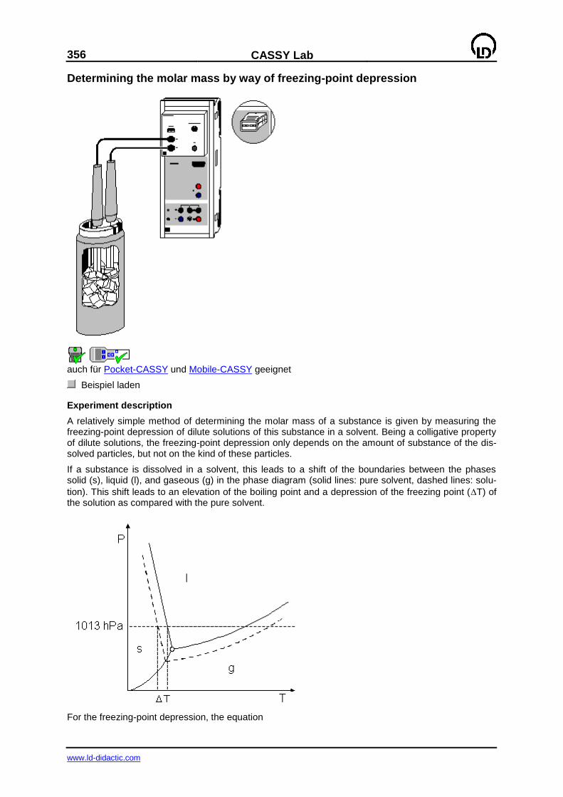
356

CASSY Lab

www.ld-didactic.com

Determining the molar mass by way of freezing-point depression


Beispiel laden


A relatively simple method of determining the molar mass of a substance is given by measuring the freezing-point depression of dilute solutions of this substance in a solvent. Being a colligative property of dilute solutions, the freezing-point depression only depends on the amount of substance of the dis-solved particles, but not on the kind of these particles.

If a substance is dissolved in a solvent, this leads to a shift of the boundaries between the phases solid (s), liquid (l), and gaseous (g) in the phase diagram (solid lines: pure solvent, dashed lines: solu-

tion). This shift leads to an elevation of the boiling point and a depression of the freezing point (T) of the solution as compared with the pure solvent.

For the freezing-point depression, the equation

CASSY Lab

357

www.ld-didactic.com

can be derived, where R is the general gas constant, T* and M2 are the freezing point and molar mass

of the pure solvent, and Hf is its molar enthalpy of fusion. The term in brackets is defined as the cry-

oscopic constant Kk, which is characteristic of every solvent. For water Kk is 1853 K*g/mol; in chemical analysis, however, often camphor is preferred as a solvent because of its high constant

Kk = 40000 K*g/mol. The second fraction in the above equation is called the molality (amount of sub-

stance n1 / mass m2 of solvent) of the dissolved substance.

From the freezing-point depression the molar mass of the dissolved substance is easily determined:

(m1: mass of the dissolved substance in g, m2: mass of the solvent in g, M1: molar mass of the dis-solved substance in g/mol)

Solving for M1 gives:

This equation does not only apply to dissociating substances. In the case of salts, acids, and bases,

the number of dissolved particles and the degree of dissociation have to be taken into account.

In the experiment example, an approximately 1.0-M solution of ethylene glycol (HO-CH2-CH2-OH) in water is examined. Ethylene glycol is found, e.g., in cars as an antifreeze agent for the cooling water and the windscreen wiper system.

For the purpose of cooling, a freezing mixture of common salt and water in a Dewar flask is used (see Preparing a freezing mixture).

Equipment list

1 Sensor-CASSY 524 010 1 CASSY Lab 524 200 1 Chemistry box or NiCr-Ni adapter S 524 067(3) 2 Temperature sensor NiCr-Ni, type K 529 676 1 Dewar flask, 0.5 l 667 320 2 Test tubes, 16x160 mm e.g. from 664 043 1 Pasteur pipette e.g. from 665 950 1 Bulb for the Pasteur pipette e.g. from 665 954 1 Rubber stopper, 14-18 mm 667 253

1 Beaker, 250 ml, tall shape 664 138 1 Laboratory balance, resolution ≤ 0.01 g, Range ≥ 300 g 1 PC with Windows 98/2000/XP/Vista

Required substances

Sodium chloride, e.g. 250 g 673 5700 Ethylene glycol, e.g. 250 ml 671 9800 Ice, approx. 200 g Distilled water

Calibration

In order to obtain accurate measuring results, calibrate the temperature sensors when using it for the first time. Afterwards the calibration should be repeated from time to time.

Einstellungen laden

Immerse the two temperature sensors in ice water (mixture of ice and water), stir with the tempera-ture sensors, and wait until the displays show measured values that are stable up to ± 0.1 °C.

358

CASSY Lab

www.ld-didactic.com

For each of the sensors, enter the target value "0" in the first line in Settings A12, A13 and TA1 under Correct, and press the Correct Offset button.


Mark the Sensor-CASSY, the chemistry box, and the temperature sensors in order that they can be used again in the same combination (otherwise the stored calibration will not be applicable).


Plug the chemistry box with the temperature sensors being connected to T2 and T3 into input A of the Sensor-CASSY.

For preparing the freezing mixture, crush the ice as fine as possible, and put it into the Dewar flask.

Using the balance, weigh in approx. 40-50 g of NaCl into the beaker.

Step by step add the salt to the ice in the Dewar flask and stir with a temperature sensor. If the ice is difficult to stir, add some distilled water.

Stir until a uniform temperature distribution is achieved in the Dewar flask. A temperature of approx. -18 to -20 °C is to be expected. This can be checked by means of the display instrument associated with the temperature sensor.

Put two dry test tubes into the beaker on the balance, and set the balance to 0.

Use the Pasteur pipette to put approx. 0.5-0.7 g of ethylene glycol into one of the test tubes and determine the exact mass. Set the balance to 0, add 10-12 g of distilled water to the ethylene gly-col, and determine the exact mass. In Settings Comment (accessible via F5), the values can be en-tered and stored along with the measurement.

Close the test tube with the rubber stopper, and dissolve the ethylene glycol by shaking.

Put approx. 9-10 g of distilled water into the second test tube.

Immerse the clean temperature sensor which is connected to T2 in the ethylene glycol solution and the other sensor, which should be clean as well, in the distilled water.



The temperature sensors being immersed, put the two test tubes into the freezing mixture at the same time and to the same depth. The liquid levels in the test tubes should be below the level of the freezing mixture. See to it that no salt solution from the freezing mixture comes into the test tubes.


Permanently stir the content of the test tubes with the two temperature sensors until the liquids are completely frozen.

Continue the measurement until TA1 is almost back to 0 and the temperatures are virtually con-

stant.

Stop the measurement by pressing the key F9 or the button.

Evaluation

During the measurement, three curves were recorded at the same time: the two freezing curves (A12

and A13) - one for the sample and a reference curve of distilled water - and the difference curve

(TA1).

The freezing curves exhibit several regions:

a) At the beginning of the measurement, the temperatures A12 and A13 drop sharply as long as the two liquids are cooled quickly.

b) The steep drop in temperature ends - above all in the case of A12 - in a local minimum, the so-called supercooling of the liquids.

c) This temperature minimum is followed by the solidification region of the curve, which is the relevant part for determining the freezing-point depression. In the case of pure solvents, the temperature re-mains exactly constant during solidification giving rise to a plateau region in the freezing curve (see

the curve A13 in the example).

In the case of solutions, the solidification region has another shape: as here almost pure solvent crys-tallizes and the dissolved substance remains in the liquid phase, the concentration of the dissolved substance increases steadily. For this reason, the freezing point of the solution drops even more (see

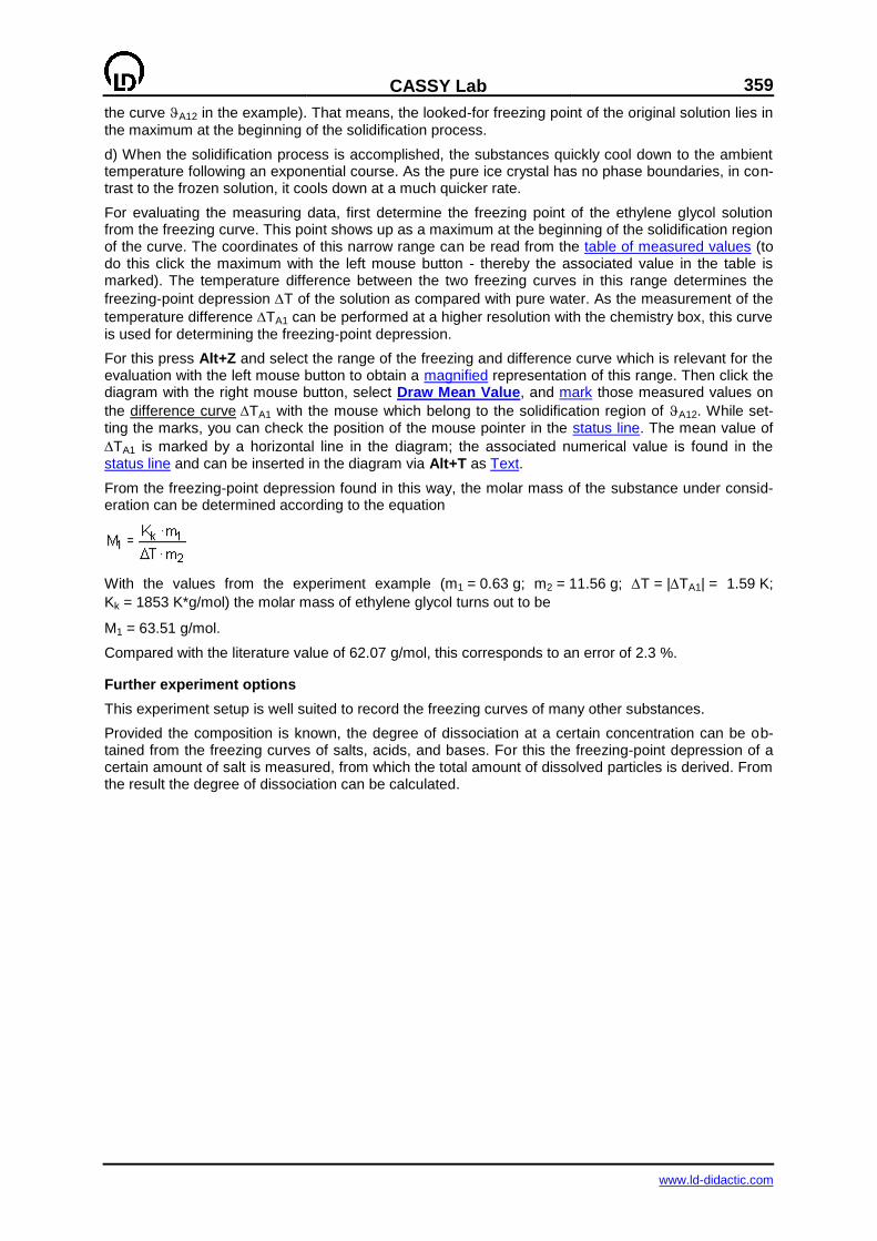
CASSY Lab

359

www.ld-didactic.com

the curve A12 in the example). That means, the looked-for freezing point of the original solution lies in

the maximum at the beginning of the solidification process.

d) When the solidification process is accomplished, the substances quickly cool down to the ambient temperature following an exponential course. As the pure ice crystal has no phase boundaries, in con-trast to the frozen solution, it cools down at a much quicker rate.

For evaluating the measuring data, first determine the freezing point of the ethylene glycol solution from the freezing curve. This point shows up as a maximum at the beginning of the solidification region of the curve. The coordinates of this narrow range can be read from the table of measured values (to do this click the maximum with the left mouse button - thereby the associated value in the table is marked). The temperature difference between the two freezing curves in this range determines the

freezing-point depression T of the solution as compared with pure water. As the measurement of the

temperature difference TA1 can be performed at a higher resolution with the chemistry box, this curve is used for determining the freezing-point depression.

For this press Alt+Z and select the range of the freezing and difference curve which is relevant for the evaluation with the left mouse button to obtain a magnified representation of this range. Then click the diagram with the right mouse button, select Draw Mean Value, and mark those measured values on

the difference curve TA1 with the mouse which belong to the solidification region of A12. While set-ting the marks, you can check the position of the mouse pointer in the status line. The mean value of

TA1 is marked by a horizontal line in the diagram; the associated numerical value is found in the status line and can be inserted in the diagram via Alt+T as Text.

From the freezing-point depression found in this way, the molar mass of the substance under consid-eration can be determined according to the equation

With the values from the experiment example (m1 = 0.63 g; m2 = 11.56 g; T = |TA1| = 1.59 K;

Kk = 1853 K*g/mol) the molar mass of ethylene glycol turns out to be

M1 = 63.51 g/mol.

Compared with the literature value of 62.07 g/mol, this corresponds to an error of 2.3 %.


This experiment setup is well suited to record the freezing curves of many other substances.

Provided the composition is known, the degree of dissociation at a certain concentration can be ob-tained from the freezing curves of salts, acids, and bases. For this the freezing-point depression of a certain amount of salt is measured, from which the total amount of dissolved particles is derived. From the result the degree of dissociation can be calculated.

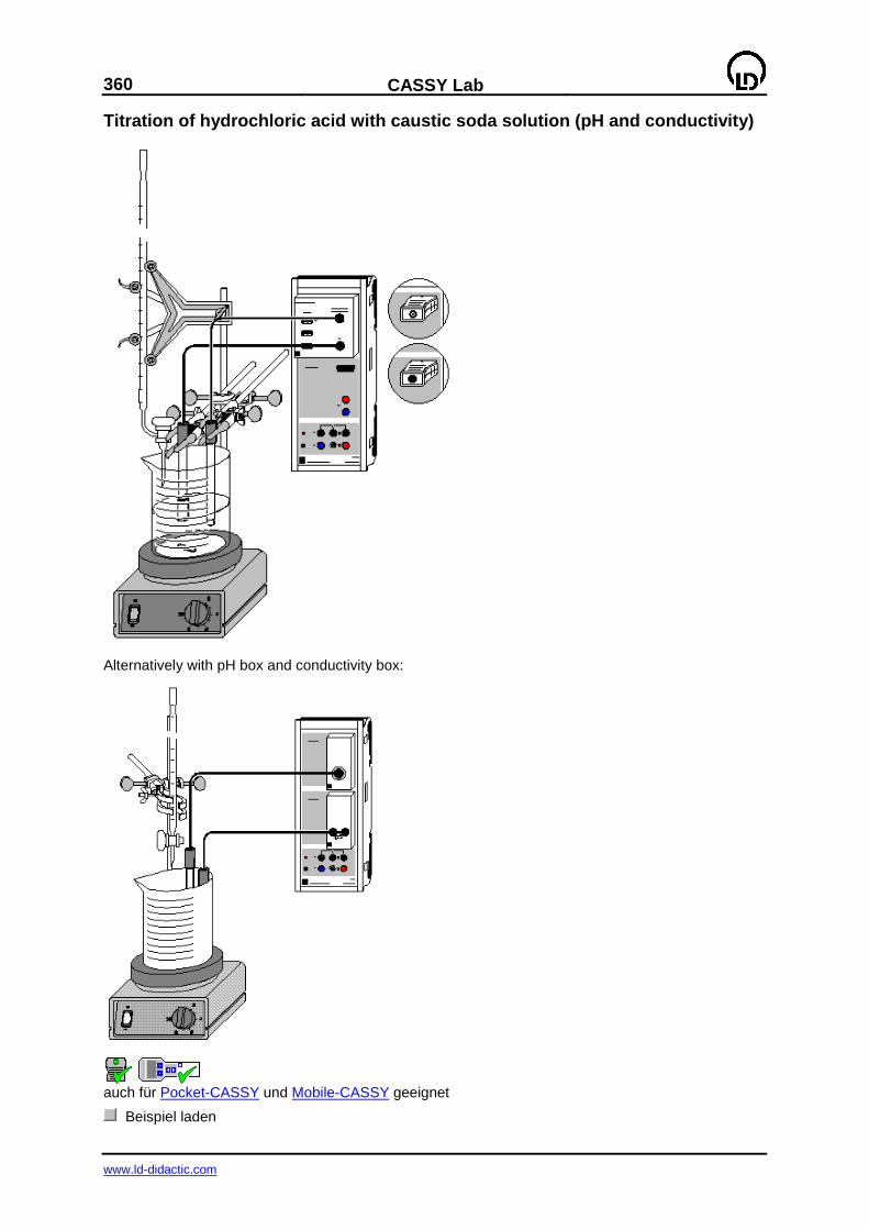
360

CASSY Lab

www.ld-didactic.com

Titration of hydrochloric acid with caustic soda solution (pH and conductivity)

Alternatively with pH box and conductivity box:


Beispiel laden

CASSY Lab

361

www.ld-didactic.com

Danger

Acids and bases are caustic. Wear protective goggles.


During titration the pH value and the conductivity are measured simultaneously, and the equivalence

point and the pKa value of the titration are determined in the evaluation.

Equipment list (with chemistry box or pH/conductivity adapter S)

1 Sensor-CASSY 524 010 1 CASSY Lab 524 200 1 Chemistry box or pH/conductivity adapter S 524 067(2+1) 1 Conductivity sensor 529 670 1 pH electrode with BNC plug 667 4172 1 Magnetic stirrer 666 845 1 Beaker, 250 ml, ts 664 113 1 Stand rod, 450 mm, M10 thread 666 523 3 Crossed bossheads 666 543 3 Universal clamps 666 555 1 Burette, 50 ml 665 847 1 Burette funnel 665 816 1 Pipette, 10 ml 665 975 1 Pipetting ball 666 003 1 PC with Windows 98/2000/XP/Vista

Equipment list (alternatively with pH box and conductivity box)

1 Sensor-CASSY 524 010 1 CASSY Lab 524 200 1 pH box 524 035 1 pH single-rod electrode 667 424 1 Conductivity box 524 037 1 Conductivity measuring cell 667 426 1 Magnetic stirrer 666 845 1 Beaker, 250 ml, ts 664 113 1 Stand rod, 450 mm, M10 thread 666 523 3 Crossed bossheads 666 543 3 Universal clamps 666 555 1 Burette, 50 ml 665 847 1 Burette funnel 665 816 1 Pipette, 10 ml 665 975 1 Pipetting ball 666 003 1 PC with Windows 98/2000/XP/Vista

Chemicals

Hydrochloric acid, c = 0.1 mol/l, 500 ml 674 6950 Caustic soda solution, c = 0.1 mol/l, 500 ml 673 8410 Distilled water


The pH and conductivity are measured by Sensor-CASSY via the pH box at input A and the conductiv-ity box at input B.

Set up the titration assembly using the magnetic stirrer, the beaker, the stand material and the burette. Put approx. 100 ml water in the beaker and add 10 ml hydrochloric acid with the pipette.

Attach the electrodes so that they are immersed to a sufficient depth but cannot be struck by the rotat-ing stirrer bars.

Calibration

For precise measurements, you should calibrate the electrodes before first use as well as later at longer intervals.

362

CASSY Lab

www.ld-didactic.com

Einstellungen laden

In Settings pH pHA1 select Correct.

Rinse the electrode with distilled water, immerse it in a pH 7.00 buffer solution and agitate it briefly.

Enter 7.00 as the first target value and click Correct Offset.

Rinse the electrode with distilled water, immerse it in a pH 4.00 buffer solution and agitate it briefly.

Enter 4.00 as the second target value and click Correct Factor.

In Settings Conductivity CB1 select Correct.

Enter the factor engraved on the electrode shaft in place of the factor 1.00 and click on Correct Factor.

Mark Sensor-CASSY, the electrodes and sensor boxes so that they can be used subsequently in the same configuration (this is the only way that the stored calibration will remain applicable).



Use or load the appropriate calibrated settings.

Record the inital values with F9.

Allow the caustic soda solution to drip continuously and register the corresponding pH and conduc-tivity values every 0.5 ml with F9.

Evaluation

There are two ways to determine the equivalence point:

pH

Click on the diagram with the right mouse button, select in the other evaluations Find Equivalence Point and mark the desired curve range. The value (if desired with pK value) appears in the status line at the bottom left and can be inserted anywhere in the diagram as text.

Conductivity

Click on the diagram with the right mouse button, fit a straight line and mark the left branch of the con-ductivity curve. Do the same with the right branch. You can place a vertical line to mark the intersec-tion of the two lines. It is also possible to display the coordinates.


Recording of a single measurement quantity (e.g. pH) Click on the conductivity window with the right mouse button and select Delete. The display win-dow disappears, along with all other data relating to conductivity. The experiment now only meas-ures pH.

Using a synchronous burette or motor piston burette (automatic titration) In the measuring parameter window (press F5 twice) select Automatic Recording and set an in-terval of e.g. 1 s. In the Settings V for the volume, enter the formula t/20 (this assumes that 1 ml is metered every 20 s. You may need to match this value as well as the maximum volume).

Registering volume using a balance (automatic titration) In the CASSY General Settings (press F5), select the option Balance for the serial interface to which the balance is connected (e.g. set COM2 to Balance if the balance is connected to this port). Match the settings of the balance (transmission rate, mode, etc.) to the balance program (refer to the manual for that balance if necessary). In the Settings V for the volume, enter the formula m/1.05 (this assumes a density of the titrant of 1.05 g/ml. You may need to match this value as well as the maximum volume).

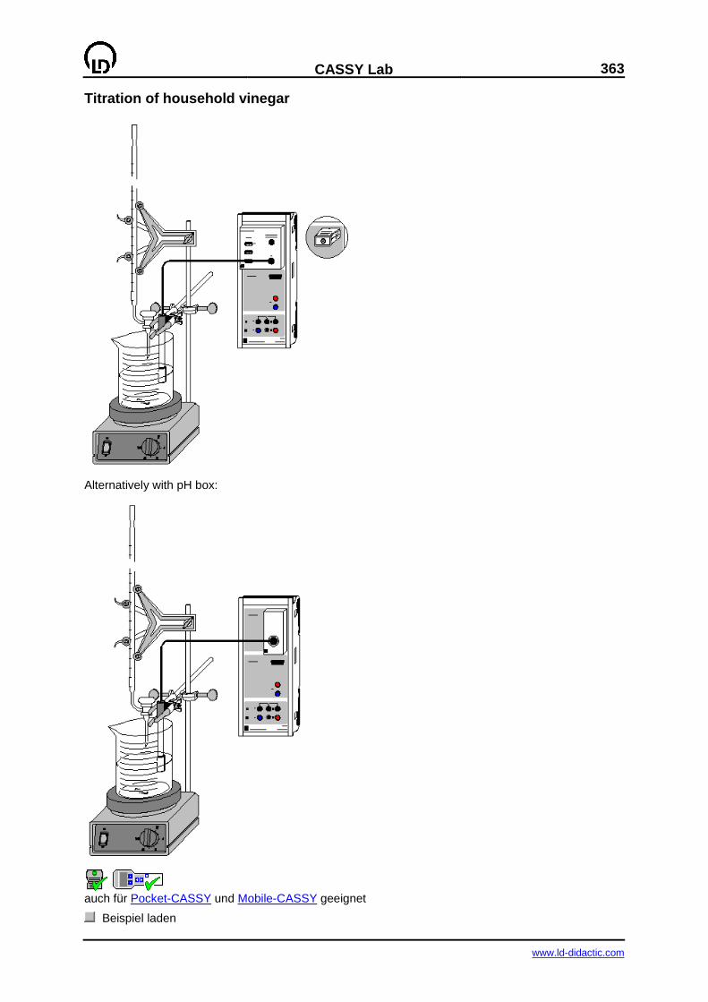
CASSY Lab

363

www.ld-didactic.com

Titration of household vinegar



Beispiel laden

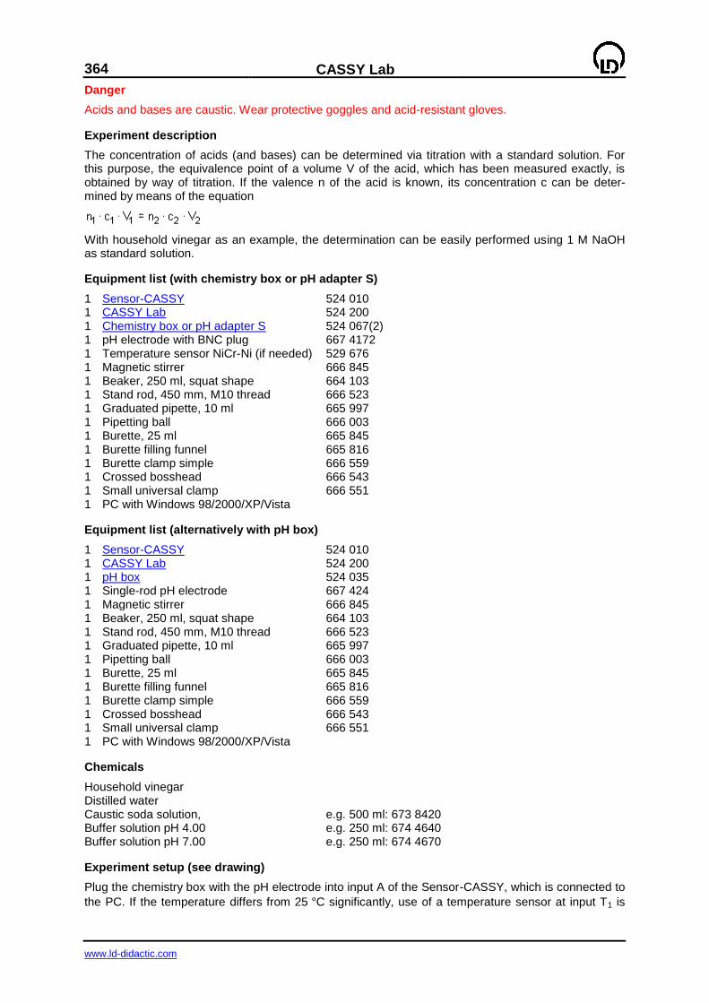
364

CASSY Lab

www.ld-didactic.com

Danger



The concentration of acids (and bases) can be determined via titration with a standard solution. For this purpose, the equivalence point of a volume V of the acid, which has been measured exactly, is obtained by way of titration. If the valence n of the acid is known, its concentration c can be deter-mined by means of the equation

With household vinegar as an example, the determination can be easily performed using 1 M NaOH as standard solution.


1 Sensor-CASSY 524 010 1 CASSY Lab 524 200 1 Chemistry box or pH adapter S 524 067(2) 1 pH electrode with BNC plug 667 4172 1 Temperature sensor NiCr-Ni (if needed) 529 676 1 Magnetic stirrer 666 845 1 Beaker, 250 ml, squat shape 664 103 1 Stand rod, 450 mm, M10 thread 666 523 1 Graduated pipette, 10 ml 665 997 1 Pipetting ball 666 003 1 Burette, 25 ml 665 845 1 Burette filling funnel 665 816 1 Burette clamp simple 666 559 1 Crossed bosshead 666 543 1 Small universal clamp 666 551 1 PC with Windows 98/2000/XP/Vista


1 Sensor-CASSY 524 010 1 CASSY Lab 524 200 1 pH box 524 035 1 Single-rod pH electrode 667 424 1 Magnetic stirrer 666 845 1 Beaker, 250 ml, squat shape 664 103 1 Stand rod, 450 mm, M10 thread 666 523 1 Graduated pipette, 10 ml 665 997 1 Pipetting ball 666 003 1 Burette, 25 ml 665 845 1 Burette filling funnel 665 816 1 Burette clamp simple 666 559 1 Crossed bosshead 666 543 1 Small universal clamp 666 551 1 PC with Windows 98/2000/XP/Vista

Chemicals

Household vinegar Distilled water Caustic soda solution, e.g. 500 ml: 673 8420 Buffer solution pH 4.00 e.g. 250 ml: 674 4640 Buffer solution pH 7.00 e.g. 250 ml: 674 4670



the PC. If the temperature differs from 25 °C significantly, use of a temperature sensor at input T1 is

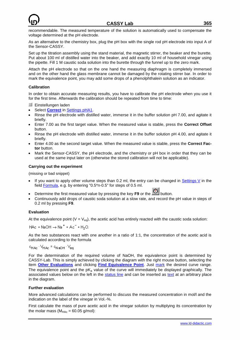
CASSY Lab

365

www.ld-didactic.com

recommendable. The measured temperature of the solution is automatically used to compensate the voltage determined at the pH electrode.


Set up the titration assembly using the stand material, the magnetic stirrer, the beaker and the burette. Put about 100 ml of distilled water into the beaker, and add exactly 10 ml of household vinegar using the pipette. Fill 1 M caustic soda solution into the burette through the funnel up to the zero mark.

Attach the pH electrode so that on the one hand the measuring diaphragm is completely immersed and on the other hand the glass membrane cannot be damaged by the rotating stirrer bar. In order to mark the equivalence point, you may add some drops of a phenolphthalein solution as an indicator.

Calibration


Einstellungen laden











Continuously add drops of caustic soda solution at a slow rate, and record the pH value in steps of 0.2 ml by pressing F9.

Evaluation

At the equivalence point (V = Veq), the acetic acid has entirely reacted with the caustic soda solution:

As the two substances react with one another in a ratio of 1:1, the concentration of the acetic acid is calculated according to the formula

For the determination of the required volume of NaOH, the equivalence point is determined by CASSY-Lab. This is simply achieved by clicking the diagram with the right mouse button, selecting the item Other Evaluations and clicking Find Equivalence Point. Just mark the desired curve range.

The equivalence point and the pKa value of the curve will immediately be displayed graphically. The associated values below on the left in the status line and can be inserted as text at an arbitrary place in the diagram.

Further evaluation

More advanced calculations can be performed to discuss the measured concentration in mol/l and the indication on the label of the vinegar in Vol.-%.

First calculate the mass of pure acetic acid in the vinegar solution by multiplying its concentration by

the molar mass (MHAc = 60.05 g/mol):

366

CASSY Lab

www.ld-didactic.com

Divide the value obtained by the density of pure acetic acid (Hac = 1050 g/l) to obtain the proportion per volume of pure acetic acid in the titrated household vinegar. The percentage is then calculated by multiplying by a factor of 100:

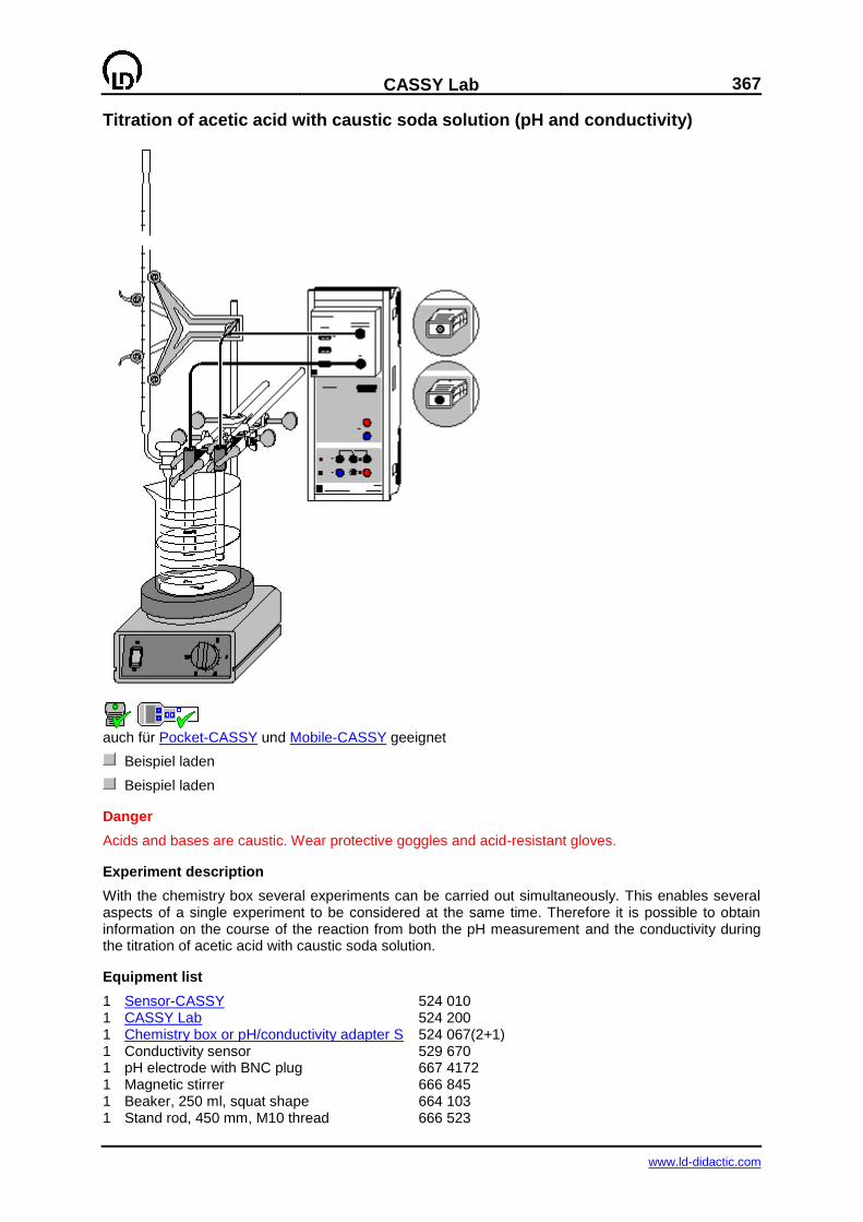
CASSY Lab

367

www.ld-didactic.com

Titration of acetic acid with caustic soda solution (pH and conductivity)


Beispiel laden

Beispiel laden

Danger



With the chemistry box several experiments can be carried out simultaneously. This enables several aspects of a single experiment to be considered at the same time. Therefore it is possible to obtain information on the course of the reaction from both the pH measurement and the conductivity during the titration of acetic acid with caustic soda solution.

Equipment list

1 Sensor-CASSY 524 010 1 CASSY Lab 524 200 1 Chemistry box or pH/conductivity adapter S 524 067(2+1) 1 Conductivity sensor 529 670 1 pH electrode with BNC plug 667 4172 1 Magnetic stirrer 666 845 1 Beaker, 250 ml, squat shape 664 103 1 Stand rod, 450 mm, M10 thread 666 523

368

CASSY Lab

www.ld-didactic.com

1 Graduated pipette, 10 ml 665 997 1 Pipetting ball 666 003 1 Burette, 25 ml 665 845 1 Burette filling funnel 665 816 1 Burette clamp simple 666 559 2 Crossed bossheads 666 543 2 Small universal clamps 666 551 1 PC with Windows 98/2000/XP/Vista

Chemicals

Acetic acid, c = 0.1 mol/l e.g. 500 ml: 671 9560 Caustic soda solution, c = 0.1 mol/l e.g. 500 ml: 673 8410 Distilled water Buffer solution pH 4.00 e.g. 250 ml: 674 4640 Buffer solution pH 7.00 e.g. 250 ml: 674 4670


Plug the chemistry box with the conductivity sensor and the pH electrode into input A of the Sensor-CASSY, which is connected to the PC.


Put about 120 ml of distilled water into the beaker, and add exactly 10 ml of acetic acid using the pi-pette; fill caustic soda solution into the burette through the funnel up to the zero mark.

In order to prevent distortion of the conductivity measurement by contamination of reference electro-lyte from the pH electrode, rinse the pH electrode thoroughly with distilled water before using it in the experiment. In addition, the upper opening of the electrode should be laid open for the purpose of pressure compensation. When attaching the pH electrode, see to it that on the one hand the measur-ing diaphragm is completely immersed and on the other hand the glass membrane cannot be dam-aged by the rotating stirrer bar.

Because of its stray field, the conductivity sensor has to be immersed to a depth of at least 2 cm in way that its distance from the wall of the vessel and from other material in the liquid (pH sensor, stirrer bar) is at least 1 cm.

Calibration


Einstellungen laden






The cell constant of the conductivity sensor for the chemistry box has already been set to 0.58 in CASSY Lab. If another conductivity sensor is used, its cell constant has to be entered as a factor in Settings CA1 under Correct. Then the Correct Factor button has to be pressed.

For a more precise determination of the cell constant, calibration solutions can be used: rinse the beaker and the conductivity sensor first with distilled water and then with approx. 30-40 ml of cali-bration solution. Immerse the conductivity sensor in another 50 ml of calibration solution as if it was for a conductivity measurement (pay attention to the distances from the walls of the beaker), enter the target value in the second line in Settings CA1 under Correct, and press the Correct Factor button when a stable measured value is reached.

Mark the Sensor-CASSY, the electrodes, and the chemistry box in order that they can be used at the same input later on (otherwise the stored calibration will not be applicable).

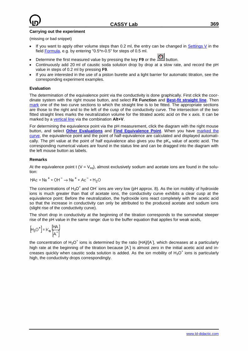
CASSY Lab

369

www.ld-didactic.com





Continuously add 20 ml of caustic soda solution drop by drop at a slow rate, and record the pH value in steps of 0.2 ml by pressing F9.

If you are interested in the use of a piston burette and a light barrier for automatic titration, see the corresponding experiment examples.

Evaluation

The determination of the equivalence point via the conductivity is done graphically. First click the coor-dinate system with the right mouse button, and select Fit Function and Best-fit straight line. Then mark one of the two curve sections to which the straight line is to be fitted. The appropriate sections are those to the right and to the left of the cusp of the conductivity curve. The intersection of the two fitted straight lines marks the neutralization volume for the titrated acetic acid on the x axis. It can be marked by a vertical line via the combination Alt+V.

For determining the equivalence point via the pH measurement, click the diagram with the right mouse button, and select Other Evaluations and Find Equivalence Point. When you have marked the curve, the equivalence point and the point of half-equivalence are calculated and displayed automati-

cally. The pH value at the point of half equivalence also gives you the pKa value of acetic acid. The corresponding numerical values are found in the status line and can be dragged into the diagram with the left mouse button as labels.

Remarks

At the equivalence point t (V = Veq), almost exclusively sodium and acetate ions are found in the solu-tion:

The concentrations of H3O+ and OH

- ions are very low (pH approx. 8). As the ion mobility of hydroxide

ions is much greater than that of acetate ions, the conductivity curve exhibits a clear cusp at the equivalence point: Before the neutralization, the hydroxide ions react completely with the acetic acid so that the increase in conductivity can only be attributed to the produced acetate and sodium ions (slight rise of the conductivity curve).

The short drop in conductivity at the beginning of the titration corresponds to the somewhat steeper rise of the pH value in the same range: due to the buffer equation that applies for weak acids,

the concentration of H3O+ ions is determined by the ratio [HA]/[A

-], which decreases at a particularly

high rate at the beginning of the titration because [A-] is almost zero in the initial acetic acid and in-

creases quickly when caustic soda solution is added. As the ion mobility of H3O+ ions is particularly

high, the conductivity drops correspondingly.

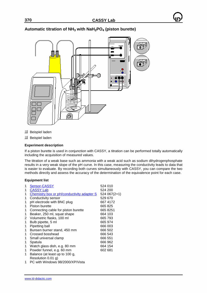
370

CASSY Lab

www.ld-didactic.com

Automatic titration of NH3 with NaH2PO4 (piston burette)

Beispiel laden

Beispiel laden


If a piston burette is used in conjunction with CASSY, a titration can be performed totally automatically including the acquisition of measured values.

The titration of a weak base such as ammonia with a weak acid such as sodium dihydrogenphosphate results in a very weak slope of the pH curve. In this case, measuring the conductivity leads to data that is easier to evaluate. By recording both curves simultaneously with CASSY, you can compare the two methods directly and assess the accuracy of the determination of the equivalence point for each case.

Equipment list

1 Sensor-CASSY 524 010 1 CASSY Lab 524 200 1 Chemistry box or pH/conductivity adapter S 524 067(2+1) 1 Conductivity sensor 529 670 1 pH electrode with BNC plug 667 4172 1 Piston burette 665 825 1 Connecting cable for piston burette 665 8251 1 Beaker, 250 ml, squat shape 664 103 2 Volumetric flasks, 100 ml 665 793 1 Bulb pipette, 5 ml 665 974 1 Pipetting ball 666 003 1 Bunsen burner stand, 450 mm 666 502 1 Crossed bosshead 666 543 1 Small universal clamp 666 551 1 Spatula 666 962 1 Watch glass dish, e.g. 80 mm 664 154 1 Powder funnel, e.g. 60 mm 602 681 1 Balance (at least up to 100 g,

Resolution 0.01 g)


CASSY Lab

371

www.ld-didactic.com

Chemicals

Distilled water Ammonia solution, dilute e.g. 500 ml: 670 3650

NaH2PO4 * 2 H2O e.g. 50 g: 673 6000

Buffer solution pH 4.00 e.g. 250 ml: 674 4640 Buffer solution pH 7.00 e.g. 250 ml: 674 4670

Preparing the solutions

Weigh in exactly 1.56 g of sodium dihydrogenphosphate (0.01 mol) on a watch glass dish on the bal-ance, rinse it via a funnel into a 100 ml volumetric flask with distilled water and fill up to 100 ml. Using the bulb pipette, put 5 ml of ammonia into the other volumetric flask and fill up to the mark with distilled water. As a result you have a 0.1 M solution of each of the two substances.


Plug the chemistry box with the pH electrode into input A of the Sensor-CASSY, which is connected to the PC.

Rinse and fill the piston burette (read the instruction sheet) with the NaH2PO4 solution just prepared, and put the beaker with 10 ml of ammonia solution, 100 ml of distilled water, and a stirrer bar on the magnetic stirrer of the piston burette. In the menu "Dosing" of the burette, set the target volume to 20 ml and the feed rate to 2.0 ml/min.

Plug one end of the connecting cable into the two inputs on the right of the relay R of the Sensor CASSY and the other end into the push-button input of the piston burette.

In order to prevent distortion of the conductivity measurement by contamination of reference electro-lyte from the pH electrode, rinse the pH electrode thoroughly with distilled water before using it in the experiment. In addition, the upper opening of the electrode should be laid open for the purpose of pressure compensation. When attaching the pH electrode (to the stand of the piston burette), see to it that on the one hand the measuring diaphragm is completely immersed and on the other hand the glass membrane cannot be damaged by the rotating stirrer bar.

Because of its stray field, the conductivity sensor has to be immersed to a depth of at least 2 cm so that its distance from the wall of the vessel and from other material in the liquid (pH sensor, stirrer bar) is at least 1 cm. Therefore it is recommendable to attach the conductivity sensor to a separate Bunsen burner stand.

Calibration


Einstellungen laden







For a more precise determination of the cell constant, calibration solutions can be used: rinse the beaker and the conductivity sensor first with distilled water and then with approx. 30-40 ml of cali-bration solution. Immerse the conductivity sensor in another 50 ml of calibration solution as if it was for a conductivity measurement (pay attention to the distances from the walls of the beaker), enter the target value in the second line in Settings CA1 under Correct, and press the Correct Factor button when a stable measured value is reached.

Mark the Sensor-CASSY, the pH electrode, and the chemistry box in order that they can be used at the same input later on (otherwise the stored calibration will not be applicable).

372

CASSY Lab

www.ld-didactic.com



If you wish another dosage than the target volume of 20 ml and the feed rate of 2.0 ml/min at the piston burette, the default values in CASSY Lab have to be changed, namely the quantity n (table index) in the Measuring parameters and in Settings Relay/Voltage Source and the formula in Set-tings Volume V.

Start the titration by pressing the key F9 or the button. The measured values and the dosage of the titrator from 0 to 20 ml are recorded automatically.

Evaluation

NH3 and NaH2PO4 react according to the following equation:

As ammonia is only a weak base, very few OH- ions are in the solution at the beginning of the reac-

tion. For this reason, the initial conductivity is very small and increases in the course of the titration due to the formation of the reaction products. When the equivalence point has been reached, i.e., when the ammonia has entirely reacted, the conductivity only increases by the amount of sodium and dihydrogenphosphate ions, which leads to a marked cusp of the conductivity curve at the equivalence point.

In order to determine the equivalence point from the conductivity graphically, first click the coordinate system with the right mouse button, and select Fit Function and Best-fit straight line. Then mark one of the two curve sections to which the straight line is to be fitted. The appropriate sections are those to the right and to the left of the cusp of the conductivity curve. The intersection of the two fitted straight lines marks the neutralization volume for the titrated acetic acid on the x axis. It can be marked by a vertical line via the combination Alt+V.

For determining the equivalence point via the pH measurement, click the diagram with the right mouse button, and select Other Evaluations and Find Equivalence Point. When you have marked the curve, the equivalence point and the point of half-equivalence are usually calculated and displayed automatically. The corresponding numerical values are found in the status line and can be dragged into the diagram with the left mouse button as labels.

In this example, however, the slope of the pH curve is so weak that no meaningful results are obtained when the equivalence point is determined. The determination of the equivalence point via the conduc-tivity turns out to be more reliable in this case.

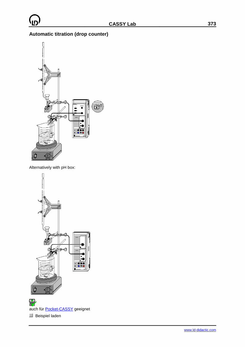
CASSY Lab

373

www.ld-didactic.com

Automatic titration (drop counter)



Beispiel laden

374

CASSY Lab

www.ld-didactic.com

Danger

Acids and bases are caustic. Wear protective goggles, gloves and clothing.


A titration experiment can be simplified significantly by using a light barrier as a drop counter. From the number of drops CASSY Lab calculates the dosage automatically. As the pH measurement and the plot in the pH (V) diagram are done automatically as well, you only need to read the exact total volume of the added titrator in order to be able to evaluate the measuring results.

Here the procedure of employing a drop counter is described with the titration of phosphoric acid with caustic potash solution as an example.

In aqueous solution, phosphoric acid forms the following equilibria:

As the differences between the pKa values amount to approx. 5, the three equilibria can be considered independently of each other.

By titration with caustic potash solution, the equivalence points of the first and the second stage of protolysis can be determined. However, since KOH is not a substantially stronger base than the phos-phate ion, the equilibrium 3 does not sufficiently tend to the right-hand side for the third equivalence point to be determined.


1 Sensor-CASSY 524 010 1 CASSY Lab 524 200 1 Chemistry box or pH adapter S 524 067(2) 1 pH electrode with BNC plug 667 4172 1 Temperature sensor NiCr-Ni (if needed) 529 676 1 Timer box 524 034 1 Combination light barrier 337 462 1 Multi-core cable, 6-pole, 1.5 m 501 16 1 Magnetic stirrer 666 845 2 Beakers, 250 ml, squat shape 664 103 1 Stand rod, 450 mm, M10 thread 666 523 1 Graduated pipette, 10 ml 665 997 1 Pipetting ball 666 003 1 Burette, 50 ml 665 847 1 Burette filling funnel 665 816 1 Burette clamp simple 666 559 2 Crossed bossheads 666 543 1 Small universal clamp 666 551 1 PC with Windows 98/2000/XP/Vista


1 Sensor-CASSY 524 010 1 CASSY Lab 524 200 1 pH box 524 035 1 Single-rod pH electrode 667 424 1 Timer box 524 034 1 Combination light barrier 337 462 1 Multi-core cable, 6-pole, 1.5 m 501 16 1 Magnetic stirrer 666 845 2 Beakers, 250 ml, squat shape 664 103 1 Stand rod, 450 mm, M10 thread 666 523 1 Graduated pipette, 10 ml 665 997

CASSY Lab

375

www.ld-didactic.com

1 Pipetting ball 666 003 1 Burette, 50 ml 665 847 1 Burette filling funnel 665 816 1 Burette clamp simple 666 559 2 Crossed bossheads 666 543 1 Small universal clamp 666 551 1 PC with Windows 98/2000/XP/Vista

Chemicals

Phosphoric acid, 10 %, 100 ml 674 3440 Caustic potash solution, c = 1 mol/l, 1 l 672 4460 Buffer solution pH 4.00, 250 ml 674 4640 Buffer solution pH 7.00, 250 ml 674 4670 Distilled water



the PC. If the temperature differs from 25 °C significantly, use of a temperature sensor at input T1 is recommendable. The measured temperature of the solution is automatically used to compensate the voltage determined at the pH electrode.


Plug the timer box into input B with the light barrier being connected to connector E via the 6-pole cable.


Put just 100 ml of distilled water into the beaker, and add 10 ml of a 10 % solution of phosphoric acid

(c(H3PO4) approx. 1.1 mol/l) using the pipette; fill 1 M caustic potash solution into the burette through

the funnel up to the zero mark.

Attach the pH electrode so that on the one hand the measuring diaphragm is completely immersed and on the other hand the glass membrane cannot be damaged by the rotating stirrer bar.

With the aid of the enclosed stand rod, mount the combination light barrier below the outlet of the bu-rette so that the drops escaping from the burette fall through the slit of the light barrier into the beaker and trigger a signal in the sensor of the light barrier. The sensor is located by approx. 1 cm behind the

opening of the light barrier. Triggering of a signal is indicated by the display instrument NB1 and by the

red LED at the light barrier. To check the function, allow some drops to fall through the light barrier into an empty beaker. Then reset the counter to zero in Settings Events NB1.

Calibration


Einstellungen laden









376

CASSY Lab

www.ld-didactic.com

Start the measurement series by pressing the key F9 or the button.

Carefully open the cock of the burette, and add drops of caustic potash solution at a slow rate.

Every five seconds a measured value (volume and pH value) is recorded automatically. See to it that the drops are added at a constant rate.

When approx. 40 ml of KOH have been added, close the cock, stop the measurement (F9 or ),

and read the total number of drops (N0) and the exact volume of added KOH (V0).

Evaluation

At first the average volume of a drop of KOH is calculated. The general formula to be applied reads

"NB1 * V0 / N0", where NB1 is the number of drops, V0 the total volume added, and N0 the total number

of drops at the end of the titration. Enter the read values for N0 and V0 in the field Formula of the Set-

tings Volume V instead of "754" and "40".

The titration curve, which is determined automatically, exhibits several characteristic ranges, which can be assigned to the three protolysis equilibria of phosphoric acid.

The equivalence points (V = Veq) are easily determined in CASSY Lab: after pressing the right mouse button in the diagram and selecting Other Evaluations and Find equivalence point,you can mark the curve range in which the equivalence point is to be determined. After the range has been marked, the calculated equivalence point and the pKa value are displayed automatically; the associated values are written below in the status line and can be inserted as text at an arbitrary place in the diagram using the mouse.

For further evaluation options in CASSY Lab see experiment example Titration of phosphoric acid.

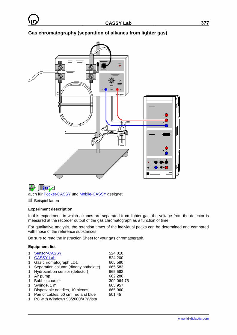
CASSY Lab

377

www.ld-didactic.com

Gas chromatography (separation of alkanes from lighter gas)


Beispiel laden


In this experiment, in which alkanes are separated from lighter gas, the voltage from the detector is measured at the recorder output of the gas chromatograph as a function of time.

For qualitative analysis, the retention times of the individual peaks can be determined and compared with those of the reference substances.

Be sure to read the Instruction Sheet for your gas chromatograph.

Equipment list

1 Sensor-CASSY 524 010 1 CASSY Lab 524 200 1 Gas chromatograph LD1 665 580 1 Separation column (dinonylphthalate) 665 583 1 Hydrocarbon sensor (detector) 665 582 1 Air pump 662 286 1 Bubble counter 309 064 75 1 Syringe, 1 ml 665 957 1 Disposable needles, 10 pieces 665 960 1 Pair of cables, 50 cm, red and blue 501 45 1 PC with Windows 98/2000/XP/Vista

378

CASSY Lab

www.ld-didactic.com

Chemicals

Lighter gas (sample) n butane, Minican gas can (reference) 660 989 Fine regulating valve 660 980


Set up the gas chromatograph (GC) with the separation column (dinonylphthalate) and the hydro-carbon sensor (detector).

Connect the input of the GC to the air pump and the output to the bubble counter.

Switch the air pump on.

Connect the GC to the plug-in unit. The LED at the GC lights up.


Einstellungen laden

Use the zero point controllers on the GC to set the zero line at approx. UA1=0.05 V.

Start the test measurement with F9.

As soon as a stable zero line is recorded, stop the test measurement, again with F9.

Draw approx. 1 ml of gas from the lighter into the syringe without needle. Do this several times. Then put a needle on the syringe and push the gas out except 0.05 ml. Inject the remaining 0.05 ml of gas into the injection head of the GC.

Restart the recording of the voltage with F9, and continue measuring until all peaks to be expected have appeared; then stop the measurement with F9. Store the measurement series.

For identifying individual components, repeat the experiment with a reference substance, e. g. n butane. Store this measurement series, too.

Evaluation

You can zoom in on the relevant curve section so that it covers the diagram (open the Evaluations menu by clicking on the diagram with the right mouse button).

To determine the retention times you can insert a vertical line through the maximum value of a peak or calculate the peak center. You can also insert the retention time in the diagram as text. By comparing the retention time of the reference peak (n butane) with the retention times of the sample, it turns out that the fourth substance is n butane.

Alternatively the curves of the sample and the reference substance can be superimposed. For this load the curves one after another and answer yes to the question "Do you want to load the new meas-urement series in addition to the present one?".

Remark: discrepancies between the retention times can arise because of changes in the room tem-perature.


As described for the example of n butane, other components of the lighter gas can be identified with the corresponding reference substances (ethane, propane, i butane).

By recording the chromatograms of the gases from different lighters, differences in composition can be detected.

CASSY Lab

379

www.ld-didactic.com

Gas chromatography (separation of alcohols)


Beispiel laden


In this experiment, in which different alcohols are separated, the voltage from the detector at the re-corder output of the gas chromatograph is measured as a function of time.

For qualitative analysis, the retention times of the individual peaks can be determined. A determination of the peak areas by integration enables quantitative investigation of the sample.


Equipment list

1 Sensor-CASSY 524 010 1 CASSY Lab 524 200 1 Gas chromatograph LD1 665 580 1 Separation column (Porapak P) 665 584 1 Hydrocarbon sensor (detector) 665 582 1 Air pump 662 286 1 Bubble counter 309 064 75 1 Microliter syringe, 1 l 665 617

1 Replacement cannulas, set of 3665 616 1 Pair of cables, 50 cm, red and blue 501 45 1 PC with Windows 98/2000/XP/Vista

380

CASSY Lab

www.ld-didactic.com

Chemicals

Methanol, 250 ml 673 2700 Ethanol, abs., 250 ml 671 9700 Propanol-1, 250 ml 674 4310 Propanol-2, 250 ml 674 4400


Prepare the sample, e. g. a mixture of different alcohols such as: methanol, ethanol and propanol.

Set up the gas chromatograph with the separation column (Porapak P) and the hydrocarbon sen-sor (detector).

Connect the input of the gas chromatograph to the air pump and the output to the bubble counter.

Switch the air pump on.

Connect the gas chromatograph to the plug-in unit. The LED at the gas chromatograph lights up.


Einstellungen laden

Use the zero point controller on the gas chromatograph to set the zero line at approx. UA1=0.05 V.

Start the test measurement with F9


Using the microliter syringe, inject 0.5 l of the alcohol mixture into the injection head of the gas chromatograph.

Restart recording of the voltage with F9, and continue measuring until all peaks to be expected have appeared; then stop the measurement with F9

Evaluation


To determine the retention times you can insert a vertical line through the maximum value of a peak or calculate the peak center. You can also insert the retention time in the diagram as text.

For quantitative analysis of the mixture, the peak areas are determined by integration. Then the frac-tion of the peak area relative to the total area of all peaks is determined. In this example, the total area of all peaks is 950 Vs. The fractional area of ethanol is thus 206 Vs / 950 Vs = 22 %. The concentra-tion can be determined precisely through calibration with the individual substances or by using the addition method.


After recording a calibration series with known alcohol concentrations, you can determine the alcohol content of several alcoholic drinks.

By heating the column in a water bath, you can also separate alcohols of greater chain length.

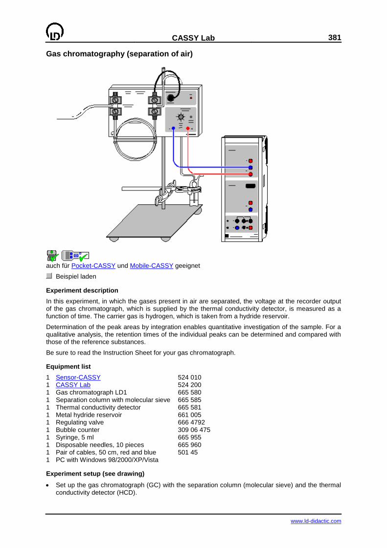
CASSY Lab

381

www.ld-didactic.com

Gas chromatography (separation of air)


Beispiel laden


In this experiment, in which the gases present in air are separated, the voltage at the recorder output of the gas chromatograph, which is supplied by the thermal conductivity detector, is measured as a function of time. The carrier gas is hydrogen, which is taken from a hydride reservoir.

Determination of the peak areas by integration enables quantitative investigation of the sample. For a qualitative analysis, the retention times of the individual peaks can be determined and compared with those of the reference substances.


Equipment list

1 Sensor-CASSY 524 010 1 CASSY Lab 524 200 1 Gas chromatograph LD1 665 580 1 Separation column with molecular sieve 665 585 1 Thermal conductivity detector 665 581 1 Metal hydride reservoir 661 005 1 Regulating valve 666 4792 1 Bubble counter 309 06 475 1 Syringe, 5 ml 665 955 1 Disposable needles, 10 pieces 665 960 1 Pair of cables, 50 cm, red and blue 501 45 1 PC with Windows 98/2000/XP/Vista


Set up the gas chromatograph (GC) with the separation column (molecular sieve) and the thermal conductivity detector (HCD).

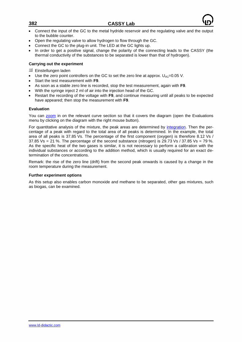
382

CASSY Lab

www.ld-didactic.com

Connect the input of the GC to the metal hydride reservoir and the regulating valve and the output to the bubble counter.

Open the regulating valve to allow hydrogen to flow through the GC.

Connect the GC to the plug-in unit. The LED at the GC lights up.

In order to get a positive signal, change the polarity of the connecting leads to the CASSY (the thermal conductivity of the substances to be separated is lower than that of hydrogen).


Einstellungen laden

Use the zero point controllers on the GC to set the zero line at approx. UA1=0.05 V.

Start the test measurement with F9.


With the syringe inject 2 ml of air into the injection head of the GC.

Restart the recording of the voltage with F9, and continue measuring until all peaks to be expected have appeared; then stop the measurement with F9.

Evaluation


For quantitative analysis of the mixture, the peak areas are determined by integration. Then the per-centage of a peak with regard to the total area of all peaks is determined. In the example, the total area of all peaks is 37.85 Vs. The percentage of the first component (oxygen) is therefore 8.12 Vs / 37.85 Vs = 21 %. The percentage of the second substance (nitrogen) is 29.73 Vs / 37.85 Vs = 79 %. As the specific heat of the two gases is similar, it is not necessary to perform a calibration with the individual substances or according to the addition method, which is usually required for an exact de-termination of the concentrations.

Remark: the rise of the zero line (drift) from the second peak onwards is caused by a change in the room temperature during the measurement.


As this setup also enables carbon monoxide and methane to be separated, other gas mixtures, such as biogas, can be examined.

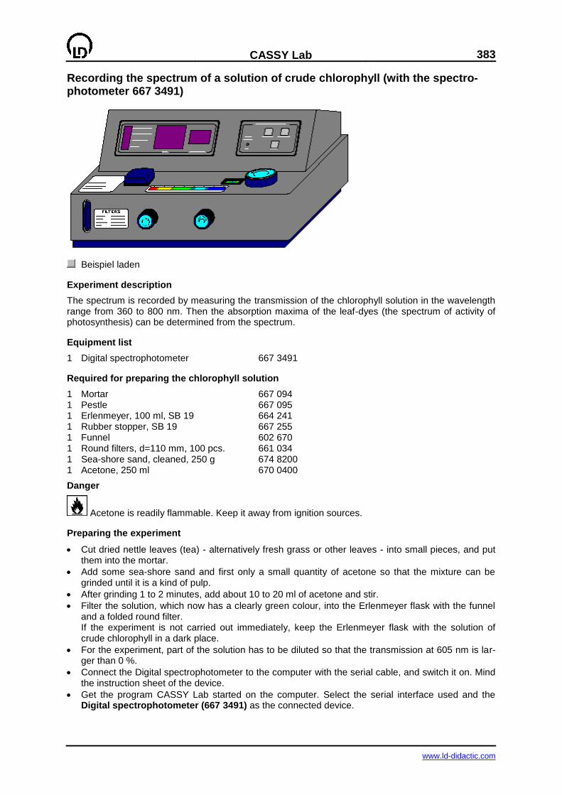
CASSY Lab

383

www.ld-didactic.com

Recording the spectrum of a solution of crude chlorophyll (with the spectro-photometer 667 3491)

Beispiel laden


The spectrum is recorded by measuring the transmission of the chlorophyll solution in the wavelength range from 360 to 800 nm. Then the absorption maxima of the leaf-dyes (the spectrum of activity of photosynthesis) can be determined from the spectrum.

Equipment list

1 Digital spectrophotometer 667 3491

Required for preparing the chlorophyll solution

1 Mortar 667 094 1 Pestle 667 095 1 Erlenmeyer, 100 ml, SB 19 664 241 1 Rubber stopper, SB 19 667 255 1 Funnel 602 670 1 Round filters, d=110 mm, 100 pcs. 661 034 1 Sea-shore sand, cleaned, 250 g 674 8200 1 Acetone, 250 ml 670 0400

Danger

Acetone is readily flammable. Keep it away from ignition sources.

Preparing the experiment

Cut dried nettle leaves (tea) - alternatively fresh grass or other leaves - into small pieces, and put them into the mortar.

Add some sea-shore sand and first only a small quantity of acetone so that the mixture can be grinded until it is a kind of pulp.

After grinding 1 to 2 minutes, add about 10 to 20 ml of acetone and stir.

Filter the solution, which now has a clearly green colour, into the Erlenmeyer flask with the funnel and a folded round filter. If the experiment is not carried out immediately, keep the Erlenmeyer flask with the solution of crude chlorophyll in a dark place.

For the experiment, part of the solution has to be diluted so that the transmission at 605 nm is lar-ger than 0 %.

Connect the Digital spectrophotometer to the computer with the serial cable, and switch it on. Mind the instruction sheet of the device.

Get the program CASSY Lab started on the computer. Select the serial interface used and the Digital spectrophotometer (667 3491) as the connected device.

384

CASSY Lab

www.ld-didactic.com


Einstellungen laden

Fill one round cell with the solution of crude chlorophyll (sample solution) and another one with the reference solution (the pure solvent, here: acetone) each to approximately ¾ height.

Set the starting wavelength to 340 nm at the spectrophotometer. (For general explanations on using the device see instruction sheet.)

Make the 100 %T calibration with the reference cell, then insert the sample cell.

Take over the displayed measured value and the associated wavelength by pressing F9 (or by clicking the clock button). This value is now displayed in the table and in the plot.

Increase the measuring wavelength by 5 nm, and repeat the calibration and the measurement.

The measurement is finished when the measuring wavelength 800 nm has been reached.

Remark

Recording the measured values as described here takes about one hour. A shorter measuring time can be achieved by measuring in steps of 10 nm and/or by stopping the measurement already at 730 nm.

Evaluation

The spectrum can be displayed as transmission T, absorption A = 100-T or as extinction E = -log(T/100).

The strong absorption (lower transmission) around 405 nm (blue light) and 660 nm (red-orange) is clearly discernible. The evaluation menu (click Graphics with the right mouse key) enables individual wavelengths to be marked with a vertical line. With Text the marked wavelength is written near the line or curve.

Due to absorption in these parts of the visible light spectrum the rest of the spectrum stands out more conspicuously when light is reflected (leaf surface) or passes through (solution). This latter part around 550 nm corresponds to the green component of light, and this is the reason why a solution of chloro-phyll and leaves appear to be green.

By irradiating with light at wavelengths around the absorption maxima, maximum photosynthetic per-formance is obtained, i. e. the absorption or extinction curve represents the spectrum of activity of photosynthesis.

If considered more precisely, this spectrum turns out to be the superposition of three individual spec-

tra, namely those of chlorophyll a, chlorophyll b, and -carotene. The individual leaf-dyes can be sepa-rated, e. g. by thin-layer chromatography.

Further experiment proposals

Apart from chlorophyll, the spectra of arbitrary other coloured solutions can be studied.

For carrying out the experiment in a shorter time a rougher resolution (e. g. in steps of 10 nm) and another wavelength range may be chosen.

The Diode-array Photometer (667 347) makes recording spectra considerably quicker and more comfortable (667 347).

The dependence of the transmission and the extinction on the concentration can be demonstrated by measuring a series of concentrations, e. g. of a copper-sulphate solution, at the absorption maximum.

For kinetic investigations (e. g. decolourization of crystal violet) the absorption maximum is meas-ured as a function of time. The opportunities provided by specifying a formula and the correspond-ing displays and evaluations enable the reaction order and the rate constant of the reaction to be determined.

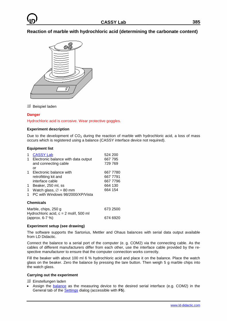
CASSY Lab

385

www.ld-didactic.com

Reaction of marble with hydrochloric acid (determining the carbonate content)

Beispiel laden

Danger

Hydrochloric acid is corrosive. Wear protective goggles.


Due to the development of CO2 during the reaction of marble with hydrochloric acid, a loss of mass occurs which is registered using a balance (CASSY interface device not required).

Equipment list

1 CASSY Lab 524 200 1 Electronic balance with data output 667 795 and connecting cable 729 769 or 1 Electronic balance with 667 7780 retrofitting kit and 667 7791 interface cable 667 7796 1 Beaker, 250 ml, ss 664 130 1 Watch glass, = 80 mm 664 154


Chemicals

Marble, chips, 250 g 673 2500 Hydrochloric acid, c = 2 mol/l, 500 ml (approx. 6-7 %) 674 6920


The software supports the Sartorius, Mettler and Ohaus balances with serial data output available from LD Didactic.

Connect the balance to a serial port of the computer (e. g. COM2) via the connecting cable. As the cables of different manufacturers differ from each other, use the interface cable provided by the re-spective manufacturer to ensure that the computer connection works correctly.

Fill the beaker with about 100 ml 6 % hydrochloric acid and place it on the balance. Place the watch glass on the beaker. Zero the balance by pressing the tare button. Then weigh 5 g marble chips into the watch glass.


Einstellungen laden

Assign the balance as the measuring device to the desired serial interface (e.g. COM2) in the General tab of the Settings dialog (accessible with F5).

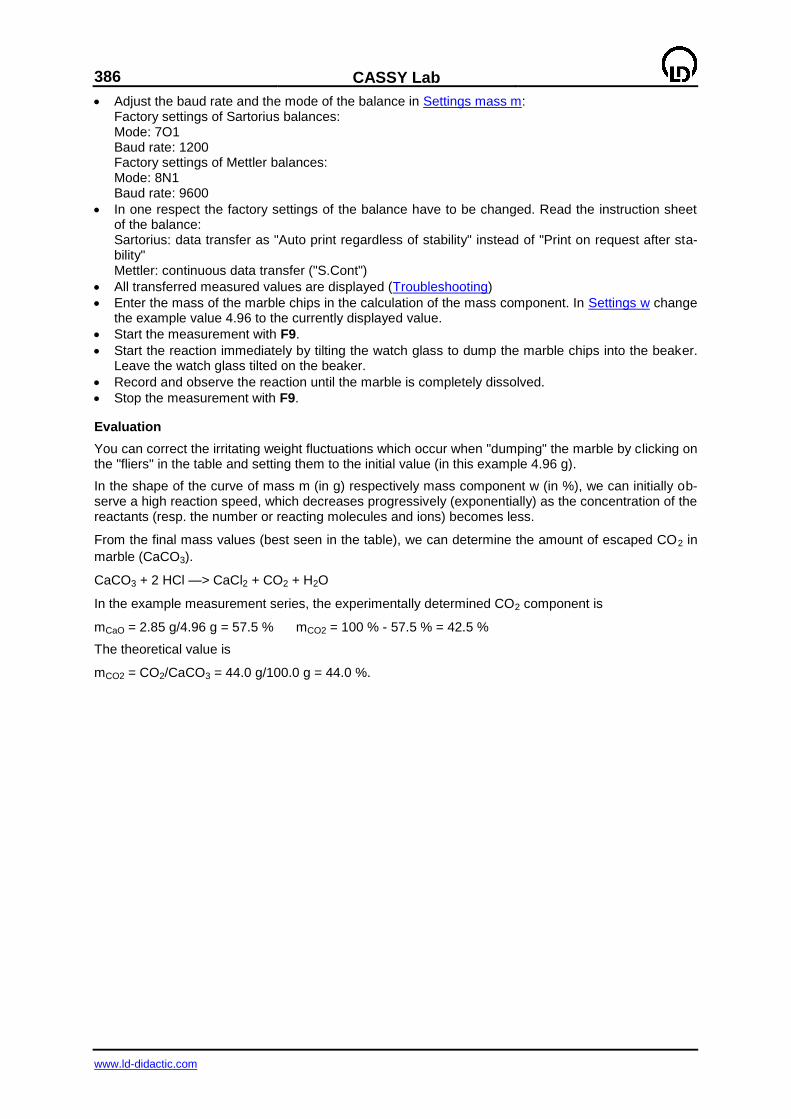
386

CASSY Lab

www.ld-didactic.com

Adjust the baud rate and the mode of the balance in Settings mass m: Factory settings of Sartorius balances: Mode: 7O1 Baud rate: 1200 Factory settings of Mettler balances: Mode: 8N1 Baud rate: 9600

In one respect the factory settings of the balance have to be changed. Read the instruction sheet of the balance: Sartorius: data transfer as "Auto print regardless of stability" instead of "Print on request after sta-bility" Mettler: continuous data transfer ("S.Cont")

All transferred measured values are displayed (Troubleshooting)

Enter the mass of the marble chips in the calculation of the mass component. In Settings w change the example value 4.96 to the currently displayed value.


Start the reaction immediately by tilting the watch glass to dump the marble chips into the beaker. Leave the watch glass tilted on the beaker.

Record and observe the reaction until the marble is completely dissolved.


Evaluation

You can correct the irritating weight fluctuations which occur when "dumping" the marble by clicking on the "fliers" in the table and setting them to the initial value (in this example 4.96 g).

In the shape of the curve of mass m (in g) respectively mass component w (in %), we can initially ob-serve a high reaction speed, which decreases progressively (exponentially) as the concentration of the reactants (resp. the number or reacting molecules and ions) becomes less.

From the final mass values (best seen in the table), we can determine the amount of escaped CO2 in

marble (CaCO3).

CaCO3 + 2 HCl —> CaCl2 + CO2 + H2O

In the example measurement series, the experimentally determined CO2 component is

mCaO = 2.85 g/4.96 g = 57.5 % mCO2 = 100 % - 57.5 % = 42.5 %

The theoretical value is

mCO2 = CO2/CaCO3 = 44.0 g/100.0 g = 44.0 %.

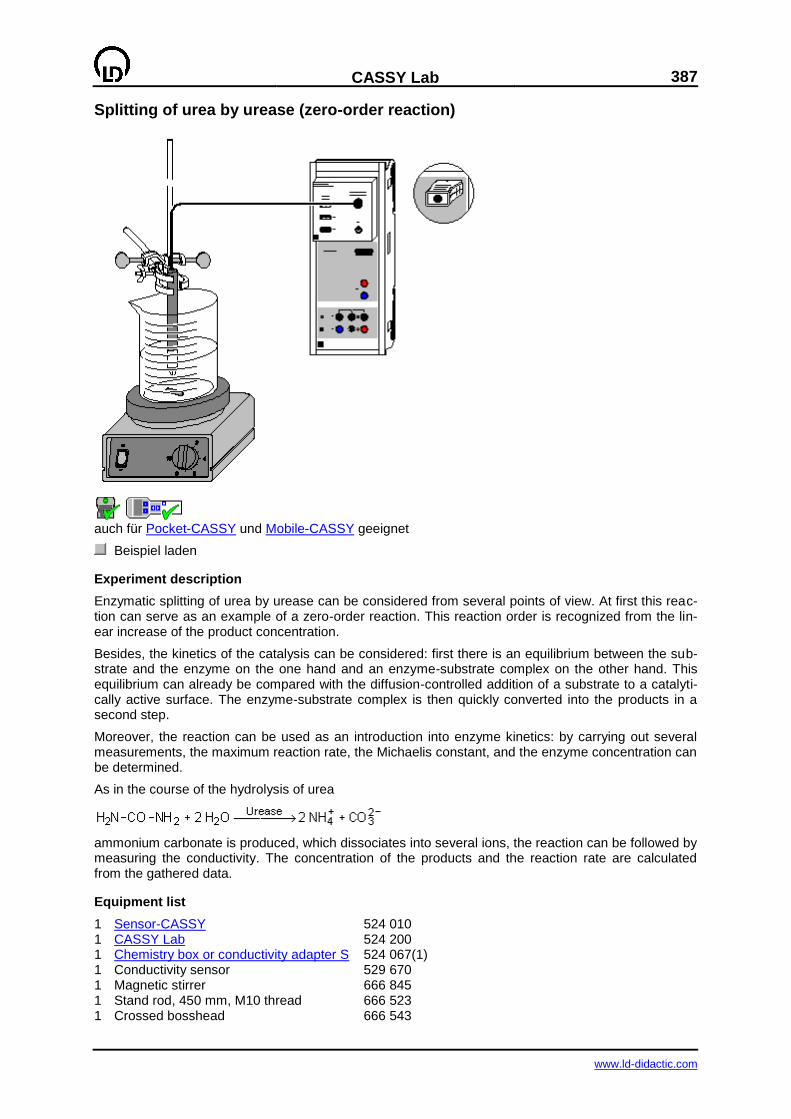
CASSY Lab

387

www.ld-didactic.com

Splitting of urea by urease (zero-order reaction)


Beispiel laden


Enzymatic splitting of urea by urease can be considered from several points of view. At first this reac-tion can serve as an example of a zero-order reaction. This reaction order is recognized from the lin-ear increase of the product concentration.

Besides, the kinetics of the catalysis can be considered: first there is an equilibrium between the sub-strate and the enzyme on the one hand and an enzyme-substrate complex on the other hand. This equilibrium can already be compared with the diffusion-controlled addition of a substrate to a catalyti-cally active surface. The enzyme-substrate complex is then quickly converted into the products in a second step.

Moreover, the reaction can be used as an introduction into enzyme kinetics: by carrying out several measurements, the maximum reaction rate, the Michaelis constant, and the enzyme concentration can be determined.

As in the course of the hydrolysis of urea

ammonium carbonate is produced, which dissociates into several ions, the reaction can be followed by measuring the conductivity. The concentration of the products and the reaction rate are calculated from the gathered data.

Equipment list

1 Sensor-CASSY 524 010 1 CASSY Lab 524 200 1 Chemistry box or conductivity adapter S 524 067(1) 1 Conductivity sensor 529 670 1 Magnetic stirrer 666 845 1 Stand rod, 450 mm, M10 thread 666 523 1 Crossed bosshead 666 543

388

CASSY Lab

www.ld-didactic.com

1 Beaker, 100 ml, tall shape 664 137 1 Beaker, 150 ml, tall shape 602 010 2 Weighing scoops 602 763 1 Graduated pipette, 10 ml 665 997 1 Pipetting ball 666 003 1 Volumetric flask, 100 ml 665 793 1 Watch glass dish, e.g. 80 mm 664 154 1 Powder funnel, e.g. 60 mm 602 681 2 Test tubes from 664 043 2 Rubber stoppers, 14...18 mm 667 253

1 Spatula 666 961 1 Balance, resolution 0.01 g 1 PC with Windows 98/2000/XP/Vista

Chemicals

Ammonium carbonate, e.g. 100 g 670 3900 Urea, e.g. 100 g 672 1700 Urease (1 U/mg), e.g. 5 g 675 2810 Copper(II) sulphate pentahydrate, e.g. 100 g 672 9600 Distilled water

Note concerning the chemicals

At room temperature, urease degenerates within a few hours. Therefore urease may only stay outside the refrigeration for a few minutes.

In air, ammonium carbonate slowly reacts to ammonium bicarbonate. As this would distort the conduc-tivity measurement, do not use old stocks.


Weigh in 0.96 g of ammonium carbonate on the watch glass dish, and rinse it via the funnel into the 100 ml volumetric flask. Fill the volumetric flask up to the mark, and dissolve the ammonium carbonate completely.

Weigh in 0.10 g of urease and 0.60 g of urea each in a weighing scoop. Put the substances into the two test tubes, and rinse residues that may have remained in the weighing scoops into the test tubes with the aid of the pipette, in each case using exactly 10 ml of distilled water.

Close the test tubes with the rubber stoppers, and dissolve the substances by shaking. As a result you obtain 10 ml of a 1 M urea solution and 10 ml of a urease solution with an enzyme activity of 10000 U/l - i.e., given the activity of the urease of 1U/mg, 10 mmol of the substrate can be converted per minute and litre.

Calibration

Einstellungen laden

The cell constant of the conductivity sensor for the chemistry box has already been set to 0.58 in CASSY Lab.

If another conductivity sensor is used, its cell constant has to be entered as a factor in Settings CA1 under Correct. Then the Correct Factor button has to be pressed.

For a more precise determination of the cell constant, calibration solutions can be used:

Rinse the 100 ml beaker and the conductivity sensor first with distilled water and then with approx. 30-40 ml of calibration solution.

Immerse the conductivity sensor in another 50 ml of calibration solution as if it was for a conductiv-ity measurement (pay attention to the distances from the walls of the beaker), enter the target value in the second line in Settings CA1 under Correct, and press the Correct Factor button when a stable measured value is reached.

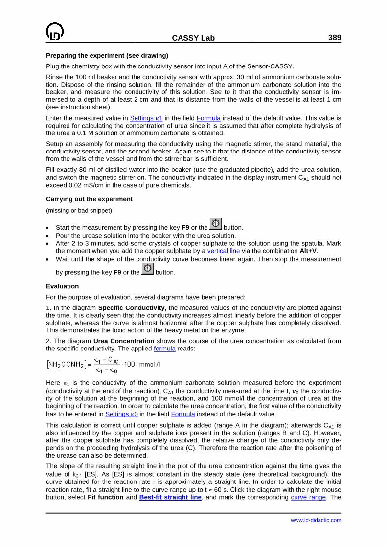
CASSY Lab

389

www.ld-didactic.com


Plug the chemistry box with the conductivity sensor into input A of the Sensor-CASSY.

Rinse the 100 ml beaker and the conductivity sensor with approx. 30 ml of ammonium carbonate solu-tion. Dispose of the rinsing solution, fill the remainder of the ammonium carbonate solution into the beaker, and measure the conductivity of this solution. See to it that the conductivity sensor is im-mersed to a depth of at least 2 cm and that its distance from the walls of the vessel is at least 1 cm (see instruction sheet).

Enter the measured value in Settings 1 in the field Formula instead of the default value. This value is required for calculating the concentration of urea since it is assumed that after complete hydrolysis of the urea a 0.1 M solution of ammonium carbonate is obtained.

Setup an assembly for measuring the conductivity using the magnetic stirrer, the stand material, the conductivity sensor, and the second beaker. Again see to it that the distance of the conductivity sensor from the walls of the vessel and from the stirrer bar is sufficient.

Fill exactly 80 ml of distilled water into the beaker (use the graduated pipette), add the urea solution,

and switch the magnetic stirrer on. The conductivity indicated in the display instrument CA1 should not exceed 0.02 mS/cm in the case of pure chemicals.




Pour the urease solution into the beaker with the urea solution.

After 2 to 3 minutes, add some crystals of copper sulphate to the solution using the spatula. Mark the moment when you add the copper sulphate by a vertical line via the combination Alt+V.

Wait until the shape of the conductivity curve becomes linear again. Then stop the measurement

by pressing the key F9 or the button.

Evaluation

For the purpose of evaluation, several diagrams have been prepared:

1. In the diagram Specific Conductivity, the measured values of the conductivity are plotted against the time. It is clearly seen that the conductivity increases almost linearly before the addition of copper sulphate, whereas the curve is almost horizontal after the copper sulphate has completely dissolved. This demonstrates the toxic action of the heavy metal on the enzyme.

2. The diagram Urea Concentration shows the course of the urea concentration as calculated from the specific conductivity. The applied formula reads:

Here 1 is the conductivity of the ammonium carbonate solution measured before the experiment

(conductivity at the end of the reaction), CA1 the conductivity measured at the time t, 0 the conductiv-ity of the solution at the beginning of the reaction, and 100 mmol/l the concentration of urea at the beginning of the reaction. In order to calculate the urea concentration, the first value of the conductivity

has to be entered in Settings 0 in the field Formula instead of the default value.

This calculation is correct until copper sulphate is added (range A in the diagram); afterwards CA1 is also influenced by the copper and sulphate ions present in the solution (ranges B and C). However, after the copper sulphate has completely dissolved, the relative change of the conductivity only de-pends on the proceeding hydrolysis of the urea (C). Therefore the reaction rate after the poisoning of the urease can also be determined.

The slope of the resulting straight line in the plot of the urea concentration against the time gives the

value of k2 [ES]. As [ES] is almost constant in the steady state (see theoretical background), the curve obtained for the reaction rate r is approximately a straight line. In order to calculate the initial

reaction rate, fit a straight line to the curve range up to t 60 s. Click the diagram with the right mouse button, select Fit function and Best-fit straight line, and mark the corresponding curve range. The

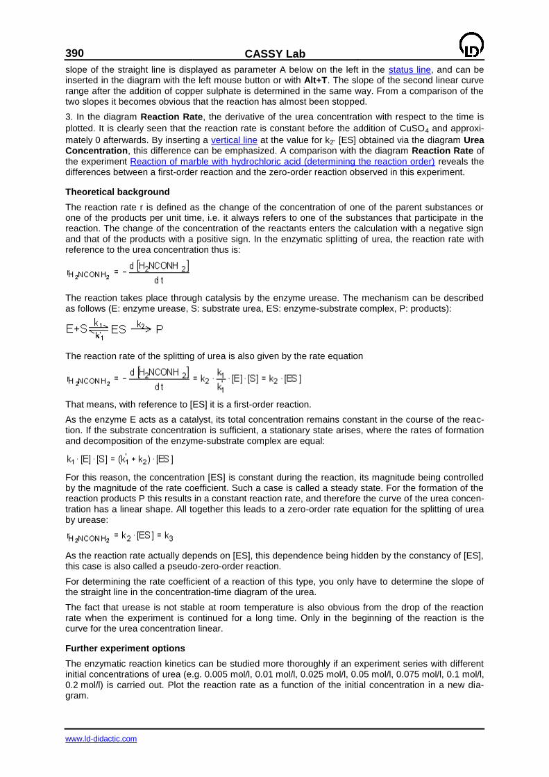
390

CASSY Lab

www.ld-didactic.com

slope of the straight line is displayed as parameter A below on the left in the status line, and can be inserted in the diagram with the left mouse button or with Alt+T. The slope of the second linear curve range after the addition of copper sulphate is determined in the same way. From a comparison of the two slopes it becomes obvious that the reaction has almost been stopped.

3. In the diagram Reaction Rate, the derivative of the urea concentration with respect to the time is

plotted. It is clearly seen that the reaction rate is constant before the addition of CuSO4 and approxi-

mately 0 afterwards. By inserting a vertical line at the value for k2 [ES] obtained via the diagram Urea Concentration, this difference can be emphasized. A comparison with the diagram Reaction Rate of the experiment Reaction of marble with hydrochloric acid (determining the reaction order) reveals the differences between a first-order reaction and the zero-order reaction observed in this experiment.

Theoretical background

The reaction rate r is defined as the change of the concentration of one of the parent substances or one of the products per unit time, i.e. it always refers to one of the substances that participate in the reaction. The change of the concentration of the reactants enters the calculation with a negative sign and that of the products with a positive sign. In the enzymatic splitting of urea, the reaction rate with reference to the urea concentration thus is:

The reaction takes place through catalysis by the enzyme urease. The mechanism can be described as follows (E: enzyme urease, S: substrate urea, ES: enzyme-substrate complex, P: products):

The reaction rate of the splitting of urea is also given by the rate equation

That means, with reference to [ES] it is a first-order reaction.

As the enzyme E acts as a catalyst, its total concentration remains constant in the course of the reac-tion. If the substrate concentration is sufficient, a stationary state arises, where the rates of formation and decomposition of the enzyme-substrate complex are equal:

For this reason, the concentration [ES] is constant during the reaction, its magnitude being controlled by the magnitude of the rate coefficient. Such a case is called a steady state. For the formation of the reaction products P this results in a constant reaction rate, and therefore the curve of the urea concen-tration has a linear shape. All together this leads to a zero-order rate equation for the splitting of urea by urease:

As the reaction rate actually depends on [ES], this dependence being hidden by the constancy of [ES], this case is also called a pseudo-zero-order reaction.

For determining the rate coefficient of a reaction of this type, you only have to determine the slope of the straight line in the concentration-time diagram of the urea.

The fact that urease is not stable at room temperature is also obvious from the drop of the reaction rate when the experiment is continued for a long time. Only in the beginning of the reaction is the curve for the urea concentration linear.


The enzymatic reaction kinetics can be studied more thoroughly if an experiment series with different initial concentrations of urea (e.g. 0.005 mol/l, 0.01 mol/l, 0.025 mol/l, 0.05 mol/l, 0.075 mol/l, 0.1 mol/l, 0.2 mol/l) is carried out. Plot the reaction rate as a function of the initial concentration in a new dia-gram.

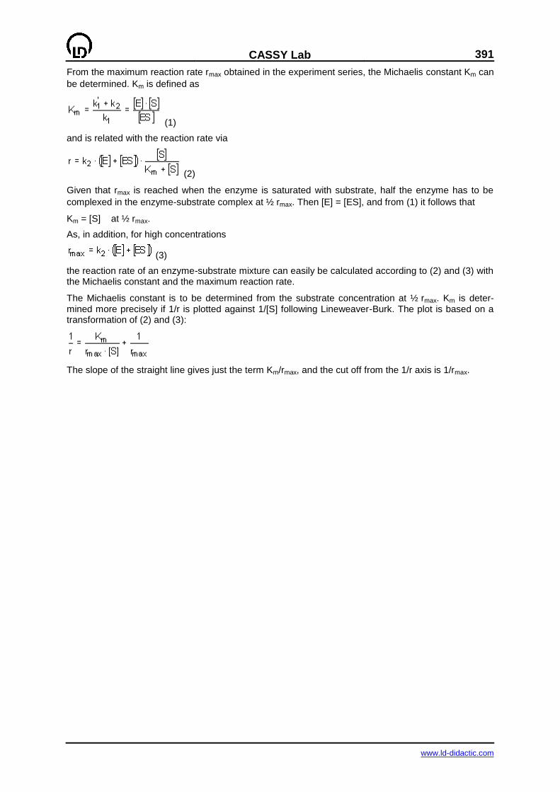
CASSY Lab

391

www.ld-didactic.com

From the maximum reaction rate rmax obtained in the experiment series, the Michaelis constant Km can

be determined. Km is defined as

(1)

and is related with the reaction rate via

(2)

Given that rmax is reached when the enzyme is saturated with substrate, half the enzyme has to be

complexed in the enzyme-substrate complex at ½ rmax. Then [E] = [ES], and from (1) it follows that

Km = [S] at ½ rmax.

As, in addition, for high concentrations

(3)

the reaction rate of an enzyme-substrate mixture can easily be calculated according to (2) and (3) with the Michaelis constant and the maximum reaction rate.

The Michaelis constant is to be determined from the substrate concentration at ½ rmax. Km is deter-mined more precisely if 1/r is plotted against 1/[S] following Lineweaver-Burk. The plot is based on a transformation of (2) and (3):

The slope of the straight line gives just the term Km/rmax, and the cut off from the 1/r axis is 1/rmax.

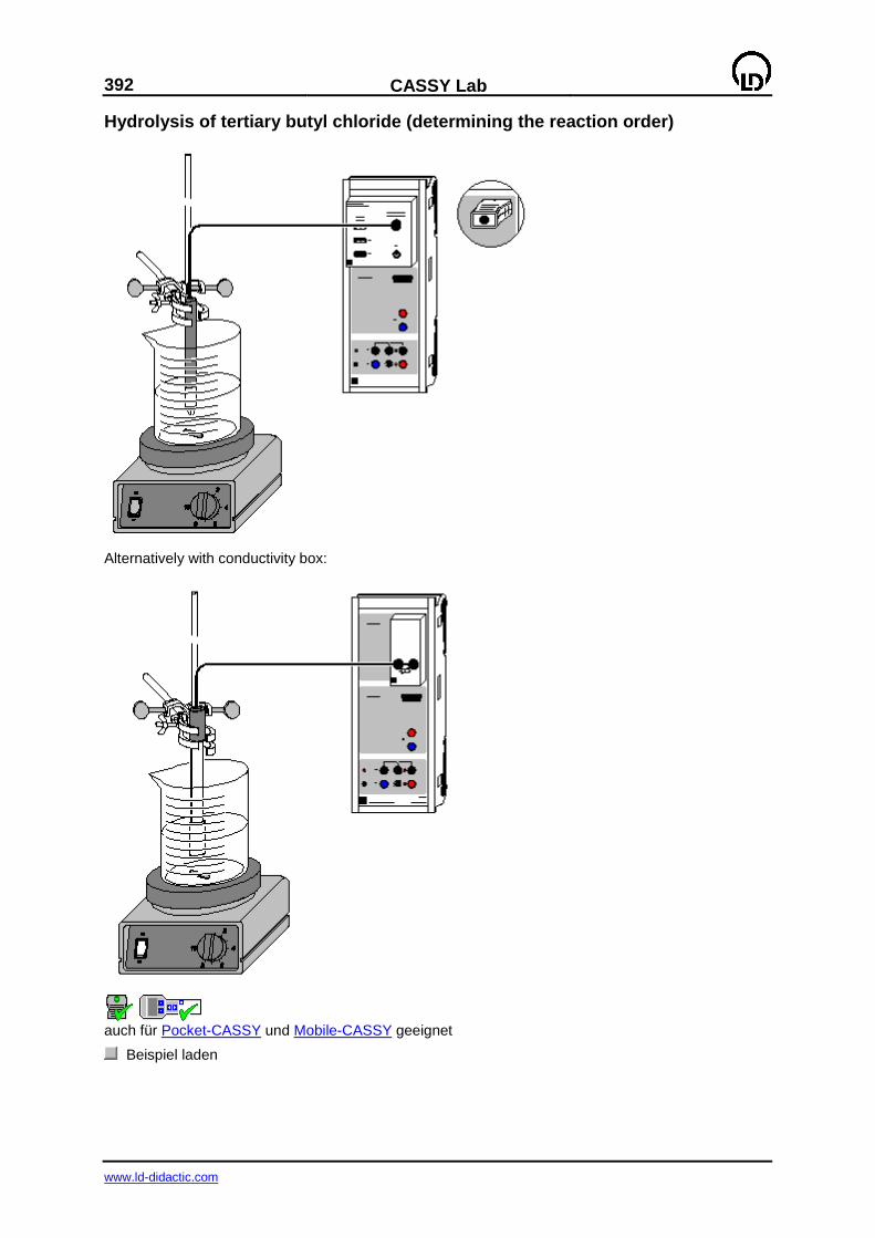
392

CASSY Lab

www.ld-didactic.com

Hydrolysis of tertiary butyl chloride (determining the reaction order)

Alternatively with conductivity box:


Beispiel laden

CASSY Lab

393

www.ld-didactic.com


Hydrolysis of tertiary butyl chloride (2-chloro-2-methylpropane) results in the formation of tertiary bu-tanol and hydrogen chloride (through protolysis of oxonium and chloride ions), which lead to a sharp increase in conductivity:

(CH3)3C – Cl + 2 H2O ——> (CH3)3C – OH + H3O+ + Cl

-

Equipment list (with chemistry box or conductivity adapter S)

1 Sensor-CASSY 524 010 1 CASSY Lab 524 200 1 Chemistry box or conductivity adapter S 524 067(1) 1 Conductivity sensor 529 670 1 Magnetic stirrer 666 845 1 Beaker, 250 ml, ts 664 113 1 Stand tube 666 607 1 Double bosshead 301 09 1 Small clamp 666 551 1 Graduated cylinder, 100 ml 665 754 1 Measuring pipette, 1 ml 665 994 1 Pipetting ball 666 003 1 PC with Windows 98/2000/XP/Vista

Equipment list (alternatively with conductivity box)

1 Sensor-CASSY 524 010 1 CASSY Lab 524 200 1 Conductivity box 524 037 1 Conductivity measuring cell 667 426 1 Magnetic stirrer 666 845 1 Beaker, 250 ml, ts 664 113 1 Stand tube 666 607 1 Double bosshead 301 09 1 Small clamp 666 551 1 Graduated cylinder, 100 ml 665 754 1 Measuring pipette, 1 ml 665 994 1 Pipetting ball 666 003 1 PC with Windows 98/2000/XP/Vista

Chemicals

0.8 ml solution of tertiary butyl chloride (c=0.1 mol/l) in acetone

Danger

Acetone is highly flammable. Keep away from ignition sources.


Set up the magnetic stirrer on the stand.

In the graduated cylinder, measure off 90 ml distilled water and 10 ml acetone and pour these into the beaker.

Add a magnetic stirrer bar and place the beaker on the magnetic stirrer. Mount the conductivity measuring cell on the stand so that it is immersed to a level just below the air opening. Switch on the magnetic stirrer.

Plug in the conductivity box at input A of Sensor-CASSY and connect the conductivity measuring cell to the conductivity box using the banana plug.

394

CASSY Lab

www.ld-didactic.com


Einstellungen laden

Notes on the displayed conductivity value

The initial conductivity value should not exceed 10 S/cm for this experiment. If this occurs, clean the measuring cell thoroughly with distilled water.

Alternatively, you can Correct the offset in Settings Conductivity (click on the display with the right mouse button) to set the initial value to zero.

Calibrate the measuring cell. To do this, open Settings Conductivity (click on the display with the right mouse button), enter the factor stamped on the cell and select Correct Factor.

Measure off 0.8 ml of the tertiary butyl chloride solution (c = 0.1 mol/l) with the measuring pipette.

In the program, start the measurement by clicking on the clock button (or press F9).

Quickly dissolve the measured quantity of tertiary butyl chloride in the beaker. Mark the time of injection by a vertical line in the diagram by pressing the combination Alt+V.

After about 8 minutes, terminate the measurement by clicking the clock button again (or with F9); at this point the conductivity should scarcely change. If necessary, you can increase the measuring range in Settings CA1.

Evaluation

This experiment is provided with four evaluation procedures already prepared:

Display of change in concentration

Click the Concentration tab. You can now follow the change in the concentration c of tertiary butyl chloride. The calculation of the concentration in mmol/l is performed using the amount of the sub-

stance (0.8 ml 0.1 mol solution), the present conductivity CA1 and the final conductivity (here: 198.9

S/cm; this value can be changed in accordance with the conductivity value read from the table).

You can view the conversion formula (1-CA1/198.9)*0.8, and alter it if desired, in the Settings c; the same is true for the display range.

Test for 1st-order reaction

Select the tab Test for 1st Order. This shows ln(cA/c) as a function of t (cA = initial concentration, c

quantity of tertiary butyl chloride used). To determine the velocity constant k of the reaction, apply a best-fit straight line to the beginning linear section of the curve (click the right mouse button to fit the line in the diagram) and determine the slope. Using Set Marker, you can label the line with the value for the slope (A).

Test for 2nd-order reaction

Select the tab Test for 2nd

Order. This shows 1/c - 1/cA as a function of t (cA = initial concentration, c quantity of tertiary butyl chloride used). This diagram does not show a linear relationship. Thus, no second-order reaction occurs here.

Method of half-times

In the diagram Half-time: as this is a first-order reaction, the rate constant can also be determined via the method of half-times. Insert horizontal lines with Alt+H at 0.4 mmol, 0.2 mmol, and 0.1 mmol; mark the points of intersection of these lines with the concentration curve by vertical lines (Alt+V). The av-

erage time difference between all vertical lines is thehalf-time t1/2, which in this example is 63 s.

Enter the half-time determined in the experiment in Settings k in the formula ln 2/63 as denominator. The result is displayed in the display instrument k.


Performance and recording of hydrolysis at different temperatures. The curves are superimposed for comparison when the measurement is repeated. The effect on the progress and speed of the reaction can be clearly seen. The activation energy of the reaction can be calculated from the dif-ferent velocity constants and the corresponding temperatures.

Use of different solvents to investigate how the solvent affects the order and speed of the reaction.

Investigation of enzymatic reactions, e.g. breakdown of urea by urease.

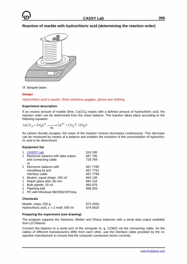
CASSY Lab

395

www.ld-didactic.com

Reaction of marble with hydrochloric acid (determining the reaction order)

Beispiel laden

Danger

Hydrochloric acid is caustic. Wear protective goggles, gloves and clothing.


If an excess amount of marble (lime, CaCO3) reacts with a defined amount of hydrochloric acid, the reaction order can be determined from the mass balance. The reaction takes place according to the following equation:

As carbon dioxide escapes, the mass of the reaction mixture decreases continuously. This decrease can be measured by means of a balance and enables the evolution of the concentration of hydrochlo-ric acid to be determined.

Equipment list

1 CASSY Lab 524 200 1 Electronic balance with data output 667 795 and connecting cable 729 769 or 1 Electronic balance with 667 7780 retrofitting kit and 667 7791 interface cable 667 7796 1 Beaker, squat shape, 250 ml 664 130 1 Watch glass dish, 80 mm 664 154 1 Bulb pipette, 25 ml 665 976 1 Pipetting ball 666 003 1 PC with Windows 98/2000/XP/Vista

Chemicals

Marble, chips, 250 g 673 2500 Hydrochloric acid, c = 2 mol/l, 500 ml 674 6920


The program supports the Sartorius, Mettler and Ohaus balances with a serial data output available from LD Didactic.

Connect the balance to a serial port of the computer (e. g. COM2) via the connecting cable. As the cables of different manufacturers differ from each other, use the interface cable provided by the re-spective manufacturer to ensure that the computer connection works correctly.

396

CASSY Lab

www.ld-didactic.com

Use the pipette to put exactly 75 ml of hydrochloric acid into the beaker. Put the watch glass dish on the beaker, set the balance to 0, and weigh in exactly 30 g of marble chips on the watch glass dish. Reset the balance to 0.


Einstellungen laden

Assign the balance as a measuring device to the desired interface in the General settings (acces-sible, e. g., via F5).

Adjust the baud rate and the mode of the balance in Settings mass m: Factory settings of Sartorius balances: Mode: 7O1 Baud rate: 1200 Factory settings of Mettler balances: Mode: 8N1 Baud rate: 9600

In one respect the factory settings of the balance have to be changed. Read the instruction sheet of the balance: Sartorius: data transfer as "Auto print regardless of stability" instead of "Print on request after sta-bility" Mettler: continuous data transfer ("S.Cont")

All transferred measured values are displayed (Troubleshooting)


Initiate the reaction by pouring the marble chips from the watch glass dish into the beaker. Leave the watch glass dish on the beaker.

When the reaction has almost come to a standstill (approx. 10 minutes), stop the data logging by

pressing the key F9 or the button.

Evaluation

The fluctuations at the beginning of the measurement, which are caused by moving the watch glass dish, can be corrected by clicking the respective value with the mouse and entering "0".

1. In the diagram Standard: the measuring data give the mass m of the carbon dioxide that has es-

caped during the reaction (see reaction equation). Calculate the amount n(CO2) that has escaped from

these data points and from this the concentration of the remaining acid [H3O+]:

.

In the second equation, the numerator corresponds to the overall balance with respect to the amount of acid and the denominator to the overall volume balance.

2. In the diagram 1st order: as a test for a first-order reaction with respect to the hydrochloric acid, the natural logarithm of the concentration of hydrochloric acid is plotted against the time t. In the case of a first order reaction, this plot leads to a straight line with the slope -k.

In order to determine the rate coefficient k, click the diagram with the right mouse button, select Fit function and Best-fit straight line, and mark the linear curve range, where a linear fit is reasonable. The slope of the straight line obtained in the fit is displayed in the status line below on the left and can be dragged into the diagram using the mouse. In the present experiment example, a rate coefficient of 0.01541/s is obtained.

In the experiment example, the plot for the first-order rate equation does not result in a straight line over the whole range because, after part of the hydrochloric acid has reacted, the rate is governed by diffusion: when the concentration of hydrochloric acid decreases, the acid reacts at a faster rate than

new H3O+ ions are transported to the surface of the marble. Therefore the rate coefficient drops, and a

deviation from the rate equation is observed. However, the reaction is well described by the first-order rate equation until 80 % of the acid are consumed in the reaction.

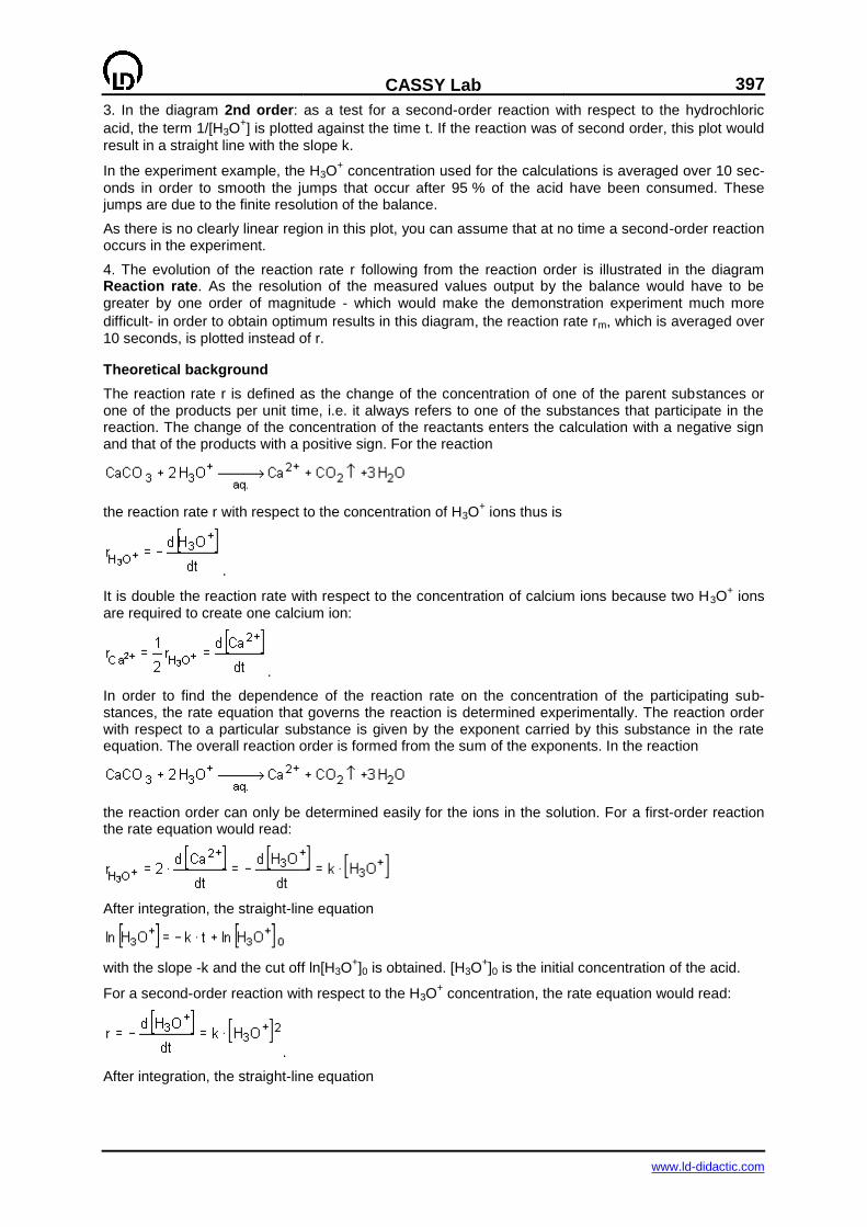
CASSY Lab

397

www.ld-didactic.com

3. In the diagram 2nd order: as a test for a second-order reaction with respect to the hydrochloric

acid, the term 1/[H3O+] is plotted against the time t. If the reaction was of second order, this plot would

result in a straight line with the slope k.

In the experiment example, the H3O+ concentration used for the calculations is averaged over 10 sec-

onds in order to smooth the jumps that occur after 95 % of the acid have been consumed. These jumps are due to the finite resolution of the balance.

As there is no clearly linear region in this plot, you can assume that at no time a second-order reaction occurs in the experiment.

4. The evolution of the reaction rate r following from the reaction order is illustrated in the diagram Reaction rate. As the resolution of the measured values output by the balance would have to be greater by one order of magnitude - which would make the demonstration experiment much more

difficult- in order to obtain optimum results in this diagram, the reaction rate rm, which is averaged over 10 seconds, is plotted instead of r.


The reaction rate r is defined as the change of the concentration of one of the parent substances or one of the products per unit time, i.e. it always refers to one of the substances that participate in the reaction. The change of the concentration of the reactants enters the calculation with a negative sign and that of the products with a positive sign. For the reaction

the reaction rate r with respect to the concentration of H3O+ ions thus is

.

It is double the reaction rate with respect to the concentration of calcium ions because two H3O+ ions

are required to create one calcium ion:

.

In order to find the dependence of the reaction rate on the concentration of the participating sub-stances, the rate equation that governs the reaction is determined experimentally. The reaction order with respect to a particular substance is given by the exponent carried by this substance in the rate equation. The overall reaction order is formed from the sum of the exponents. In the reaction

the reaction order can only be determined easily for the ions in the solution. For a first-order reaction the rate equation would read:

After integration, the straight-line equation

with the slope -k and the cut off ln[H3O+]0 is obtained. [H3O

+]0 is the initial concentration of the acid.

For a second-order reaction with respect to the H3O+ concentration, the rate equation would read:

.

After integration, the straight-line equation

398

CASSY Lab

www.ld-didactic.com

with the slope k and the cut off 1/[H3O+]0 is obtained.

By plotting these two straight lines, it can be examined to what extent a reaction obeys the rate equa-tions of first order or second order, respectively.

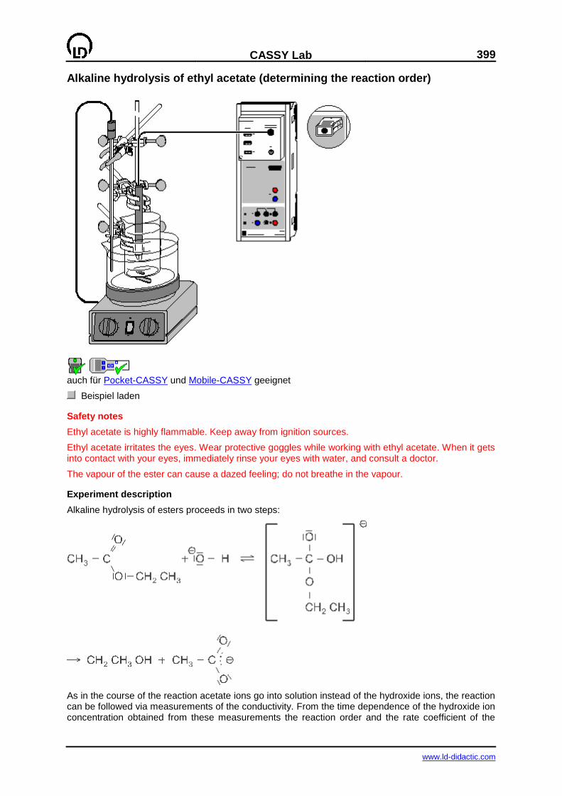
CASSY Lab

399

www.ld-didactic.com

Alkaline hydrolysis of ethyl acetate (determining the reaction order)


Beispiel laden

Safety notes

Ethyl acetate is highly flammable. Keep away from ignition sources.

Ethyl acetate irritates the eyes. Wear protective goggles while working with ethyl acetate. When it gets into contact with your eyes, immediately rinse your eyes with water, and consult a doctor.

The vapour of the ester can cause a dazed feeling; do not breathe in the vapour.


Alkaline hydrolysis of esters proceeds in two steps:

As in the course of the reaction acetate ions go into solution instead of the hydroxide ions, the reaction can be followed via measurements of the conductivity. From the time dependence of the hydroxide ion concentration obtained from these measurements the reaction order and the rate coefficient of the

400

CASSY Lab

www.ld-didactic.com

alkaline ester hydrolysis can be determined. As the rate coefficient depends on the temperature, it is recommendable to carry out the experiment in a thermostated water bath.

Equipment list

1 Sensor-CASSY 524 010 1 CASSY Lab 524 200 1 Chemistry box or conductivity adapter S 524 067(1) 1 Conductivity sensor 529 670 1 Magnetic stirrer with hot plate 666 839 1 KT4 contact rod thermometer 666 8401 1 Stirrer bar, 50 mm 666 854 1 Stirrer bar, 15 mm 666 850 1 Stand rod, 500 mm, = 10 mm 301 27

3 Crossed bossheads 666 543 2 Small universal clamps 666 551 1 Universal clamp 666 555 1 Beaker 100 ml, tall shape 664 137 1 Crystallization dish, 900 ml 664 177 1 Syringe, 2 ml 665 963 1 Disposable needle, 40 mm 665 960 1 Bulb pipette, 25 ml 665 976 1 Pipetting ball 666 003 1 Balance, resolution 0.01 g 1 PC with Windows 98/2000/XP/Vista

Chemicals

Ethyl acetate, e.g. 250 ml 671 9630 Caustic soda solution, c = 0.1 mol/l, e.g. 500 ml

673 8410

f necessary: calibration solution, 12.88 mS/cm

667 4640

Calibration

Einstellungen laden


For a more precise determination of the cell constant, calibration solutions can be used: rinse the beaker and the conductivity sensor first with distilled water and then with approx. 30-40 ml of cali-bration solution. Immerse the conductivity sensor in another 50 ml of calibration solution as if it was for a conductivity measurement (see to it that the distance from the walls of the beaker is at least 1 cm), enter the target value in the second line in Settings CA1 under Correct, and press the Cor-rect Factor button when a stable measured value is reached.

Mark the sensor used, the chemistry box, and the Sensor-CASSY as the calibration is only valid for this combination.


Fill tap water into the crystallization dish almost up to the brim, and put the dish with the bigger stirrer bar onto the magnetic stirrer. Attach the beaker with the other stirrer bar to the stand rod with the aid of the universal clamp so that the beaker hangs in the crystallization dish. The beaker should be im-mersed as deeply as possible in the centre of the water bath over the stirring magnet. Use the pipette to put exactly 75 ml of caustic soda solution (0.0075 mol) into the beaker.

Immerse the contact thermometer in the water bath and the conductivity sensor in the beaker, each with one of the small universal clamps. See to it that the distance between the conductivity sensor and both the glass wall and the stirrer bar is at least 1 cm. Set the heat controller of the magnetic stirrer to 80 °C at maximum. Set the contact thermometer, which has to be connected to the magnetic stirrer, to approx. 40 to 45 °C. Set the speed of the stirrer so that vortex formation is just avoided.

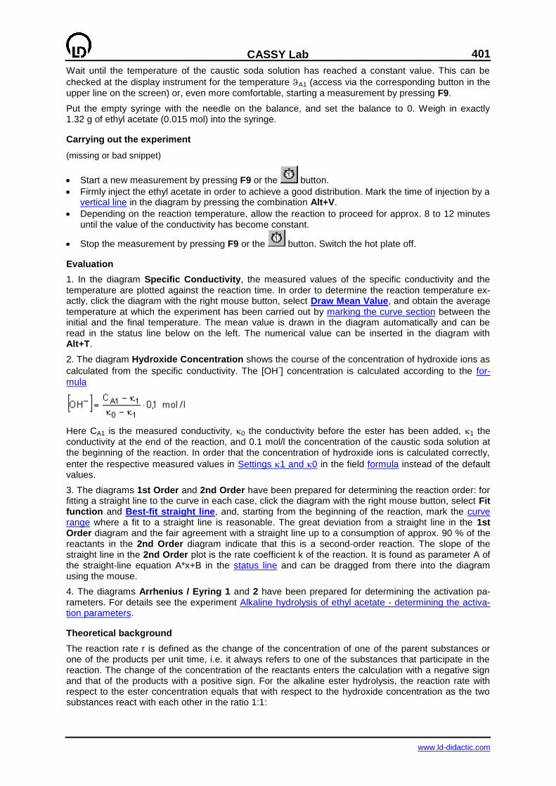
CASSY Lab

401

www.ld-didactic.com

Wait until the temperature of the caustic soda solution has reached a constant value. This can be

checked at the display instrument for the temperature A1 (access via the corresponding button in the upper line on the screen) or, even more comfortable, starting a measurement by pressing F9.

Put the empty syringe with the needle on the balance, and set the balance to 0. Weigh in exactly 1.32 g of ethyl acetate (0.015 mol) into the syringe.



Start a new measurement by pressing F9 or the button.

Firmly inject the ethyl acetate in order to achieve a good distribution. Mark the time of injection by a vertical line in the diagram by pressing the combination Alt+V.

Depending on the reaction temperature, allow the reaction to proceed for approx. 8 to 12 minutes until the value of the conductivity has become constant.

Stop the measurement by pressing F9 or the button. Switch the hot plate off.

Evaluation

1. In the diagram Specific Conductivity, the measured values of the specific conductivity and the temperature are plotted against the reaction time. In order to determine the reaction temperature ex-actly, click the diagram with the right mouse button, select Draw Mean Value, and obtain the average temperature at which the experiment has been carried out by marking the curve section between the initial and the final temperature. The mean value is drawn in the diagram automatically and can be read in the status line below on the left. The numerical value can be inserted in the diagram with Alt+T.

2. The diagram Hydroxide Concentration shows the course of the concentration of hydroxide ions as

calculated from the specific conductivity. The [OH-] concentration is calculated according to the for-

mula

Here CA1 is the measured conductivity, 0 the conductivity before the ester has been added, 1 the conductivity at the end of the reaction, and 0.1 mol/l the concentration of the caustic soda solution at the beginning of the reaction. In order that the concentration of hydroxide ions is calculated correctly,

enter the respective measured values in Settings 1 and 0 in the field formula instead of the default values.

3. The diagrams 1st Order and 2nd Order have been prepared for determining the reaction order: for fitting a straight line to the curve in each case, click the diagram with the right mouse button, select Fit function and Best-fit straight line, and, starting from the beginning of the reaction, mark the curve range where a fit to a straight line is reasonable. The great deviation from a straight line in the 1st Order diagram and the fair agreement with a straight line up to a consumption of approx. 90 % of the reactants in the 2nd Order diagram indicate that this is a second-order reaction. The slope of the straight line in the 2nd Order plot is the rate coefficient k of the reaction. It is found as parameter A of the straight-line equation A*x+B in the status line and can be dragged from there into the diagram using the mouse.

4. The diagrams Arrhenius / Eyring 1 and 2 have been prepared for determining the activation pa-rameters. For details see the experiment Alkaline hydrolysis of ethyl acetate - determining the activa-tion parameters.


The reaction rate r is defined as the change of the concentration of one of the parent substances or one of the products per unit time, i.e. it always refers to one of the substances that participate in the reaction. The change of the concentration of the reactants enters the calculation with a negative sign and that of the products with a positive sign. For the alkaline ester hydrolysis, the reaction rate with respect to the ester concentration equals that with respect to the hydroxide concentration as the two substances react with each other in the ratio 1:1:

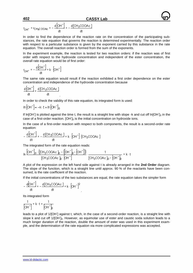
402

CASSY Lab

www.ld-didactic.com

In order to find the dependence of the reaction rate on the concentration of the participating sub-stances, the rate equation that governs the reaction is determined experimentally. The reaction order with respect to a particular substance is given by the exponent carried by this substance in the rate equation. The overall reaction order is formed from the sum of the exponents.

In the experiment example, the reaction is tested for two reaction orders: if the reaction was of first order with respect to the hydroxide concentration and independent of the ester concentration, the overall rate equation would be of first order:

The same rate equation would result if the reaction exhibited a first order dependence on the ester concentration and independence of the hydroxide concentration because

.

In order to check the validity of this rate equation, its integrated form is used:

If ln[OH-] is plotted against the time t, the result is a straight line with slope -k and cut off ln[OH

-]0 in the

case of a first-order reaction. [OH-]0 is the initial concentration on hydroxide ions.

In the case of a first-order reaction with respect to both components, the result is a second-order rate equation:

The integrated form of the rate equation reads:

A plot of the expression on the left hand side against t is already arranged in the 2nd Order diagram. The slope of the function, which is a straight line until approx. 90 % of the reactants have been con-sumed, is the rate coefficient of the reaction.

If the initial concentrations of the two substances are equal, the rate equation takes the simpler form

.

Its integrated form

leads to a plot of 1/[OH-] against t, which, in the case of a second-order reaction, is a straight line with

slope k and cut off 1/[OH-]0. However, as equimolar use of ester and caustic soda solution leads to a

much longer duration of the reaction, double the amount of ester was used in this experiment exam-ple, and the determination of the rate equation via more complicated expressions was accepted.

CASSY Lab

403

www.ld-didactic.com

Alkaline hydrolysis of ethyl acetate (determining the activation parameters)


Beispiel laden

Safety notes

Ethyl acetate is highly flammable. Keep away from ignition sources.

Ethyl acetate irritates the eyes. Wear protective goggles while working with ethyl acetate. When it gets into contact with your eyes, immediately rinse your eyes with water, and consult a doctor.

The vapour of the ester can cause a dazed feeling; do not breathe in the vapour.


Alkaline hydrolysis of esters proceeds in two steps:

As in the course of the reaction acetate ions go into solution instead of the hydroxide ions, the reaction can be followed via measurements of the conductivity. From the time dependence of the hydroxide ion concentration obtained from these measurements the reaction order and the rate coefficient k of the alkaline ester hydrolysis can be determined.

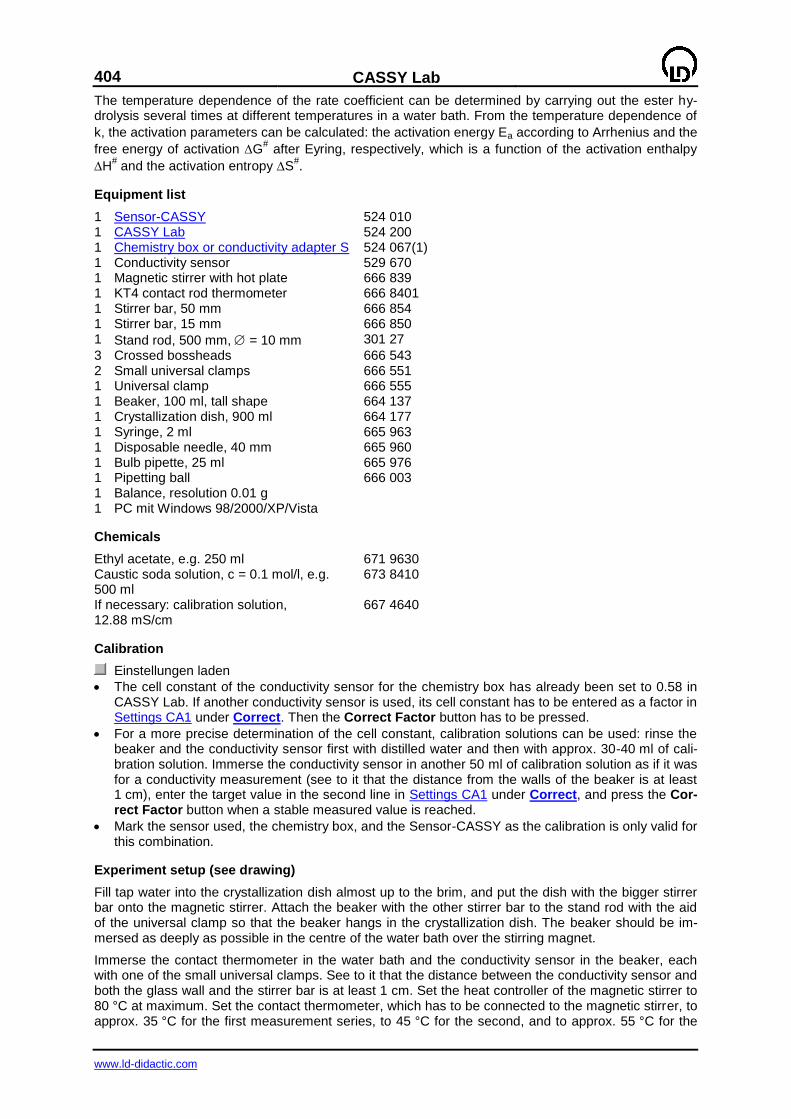
404

CASSY Lab

www.ld-didactic.com

The temperature dependence of the rate coefficient can be determined by carrying out the ester hy-drolysis several times at different temperatures in a water bath. From the temperature dependence of

k, the activation parameters can be calculated: the activation energy Ea according to Arrhenius and the

free energy of activation G# after Eyring, respectively, which is a function of the activation enthalpy

H# and the activation entropy S

#.

Equipment list

1 Sensor-CASSY 524 010 1 CASSY Lab 524 200 1 Chemistry box or conductivity adapter S 524 067(1) 1 Conductivity sensor 529 670 1 Magnetic stirrer with hot plate 666 839 1 KT4 contact rod thermometer 666 8401 1 Stirrer bar, 50 mm 666 854 1 Stirrer bar, 15 mm 666 850 1 Stand rod, 500 mm, = 10 mm 301 27

3 Crossed bossheads 666 543 2 Small universal clamps 666 551 1 Universal clamp 666 555 1 Beaker, 100 ml, tall shape 664 137 1 Crystallization dish, 900 ml 664 177 1 Syringe, 2 ml 665 963 1 Disposable needle, 40 mm 665 960 1 Bulb pipette, 25 ml 665 976 1 Pipetting ball 666 003 1 Balance, resolution 0.01 g 1 PC mit Windows 98/2000/XP/Vista

Chemicals

Ethyl acetate, e.g. 250 ml 671 9630 Caustic soda solution, c = 0.1 mol/l, e.g. 500 ml

673 8410

If necessary: calibration solution, 12.88 mS/cm

667 4640

Calibration

Einstellungen laden


For a more precise determination of the cell constant, calibration solutions can be used: rinse the beaker and the conductivity sensor first with distilled water and then with approx. 30-40 ml of cali-bration solution. Immerse the conductivity sensor in another 50 ml of calibration solution as if it was for a conductivity measurement (see to it that the distance from the walls of the beaker is at least 1 cm), enter the target value in the second line in Settings CA1 under Correct, and press the Cor-rect Factor button when a stable measured value is reached.

Mark the sensor used, the chemistry box, and the Sensor-CASSY as the calibration is only valid for this combination.


Fill tap water into the crystallization dish almost up to the brim, and put the dish with the bigger stirrer bar onto the magnetic stirrer. Attach the beaker with the other stirrer bar to the stand rod with the aid of the universal clamp so that the beaker hangs in the crystallization dish. The beaker should be im-mersed as deeply as possible in the centre of the water bath over the stirring magnet.

Immerse the contact thermometer in the water bath and the conductivity sensor in the beaker, each with one of the small universal clamps. See to it that the distance between the conductivity sensor and both the glass wall and the stirrer bar is at least 1 cm. Set the heat controller of the magnetic stirrer to 80 °C at maximum. Set the contact thermometer, which has to be connected to the magnetic stirrer, to approx. 35 °C for the first measurement series, to 45 °C for the second, and to approx. 55 °C for the

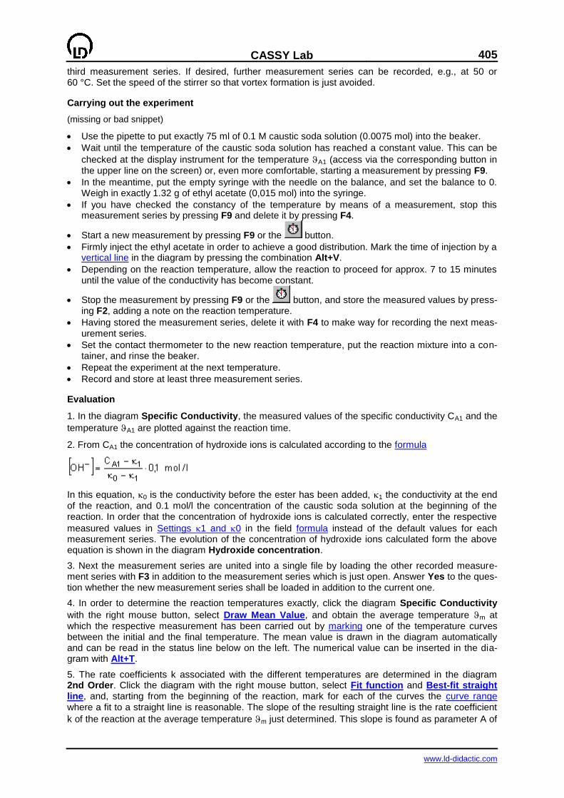
CASSY Lab

405

www.ld-didactic.com

third measurement series. If desired, further measurement series can be recorded, e.g., at 50 or 60 °C. Set the speed of the stirrer so that vortex formation is just avoided.



Use the pipette to put exactly 75 ml of 0.1 M caustic soda solution (0.0075 mol) into the beaker.

Wait until the temperature of the caustic soda solution has reached a constant value. This can be

checked at the display instrument for the temperature A1 (access via the corresponding button in the upper line on the screen) or, even more comfortable, starting a measurement by pressing F9.

In the meantime, put the empty syringe with the needle on the balance, and set the balance to 0. Weigh in exactly 1.32 g of ethyl acetate (0,015 mol) into the syringe.

If you have checked the constancy of the temperature by means of a measurement, stop this measurement series by pressing F9 and delete it by pressing F4.

Start a new measurement by pressing F9 or the button.

Firmly inject the ethyl acetate in order to achieve a good distribution. Mark the time of injection by a vertical line in the diagram by pressing the combination Alt+V.

Depending on the reaction temperature, allow the reaction to proceed for approx. 7 to 15 minutes until the value of the conductivity has become constant.

Stop the measurement by pressing F9 or the button, and store the measured values by press-ing F2, adding a note on the reaction temperature.

Having stored the measurement series, delete it with F4 to make way for recording the next meas-urement series.

Set the contact thermometer to the new reaction temperature, put the reaction mixture into a con-tainer, and rinse the beaker.

Repeat the experiment at the next temperature.

Record and store at least three measurement series.

Evaluation

1. In the diagram Specific Conductivity, the measured values of the specific conductivity CA1 and the

temperature A1 are plotted against the reaction time.

2. From CA1 the concentration of hydroxide ions is calculated according to the formula

In this equation, 0 is the conductivity before the ester has been added, 1 the conductivity at the end of the reaction, and 0.1 mol/l the concentration of the caustic soda solution at the beginning of the reaction. In order that the concentration of hydroxide ions is calculated correctly, enter the respective

measured values in Settings 1 and 0 in the field formula instead of the default values for each measurement series. The evolution of the concentration of hydroxide ions calculated form the above equation is shown in the diagram Hydroxide concentration.

3. Next the measurement series are united into a single file by loading the other recorded measure-ment series with F3 in addition to the measurement series which is just open. Answer Yes to the ques-tion whether the new measurement series shall be loaded in addition to the current one.

4. In order to determine the reaction temperatures exactly, click the diagram Specific Conductivity

with the right mouse button, select Draw Mean Value, and obtain the average temperature m at which the respective measurement has been carried out by marking one of the temperature curves between the initial and the final temperature. The mean value is drawn in the diagram automatically and can be read in the status line below on the left. The numerical value can be inserted in the dia-gram with Alt+T.

5. The rate coefficients k associated with the different temperatures are determined in the diagram 2nd Order. Click the diagram with the right mouse button, select Fit function and Best-fit straight line, and, starting from the beginning of the reaction, mark for each of the curves the curve range where a fit to a straight line is reasonable. The slope of the resulting straight line is the rate coefficient

k of the reaction at the average temperature m just determined. This slope is found as parameter A of

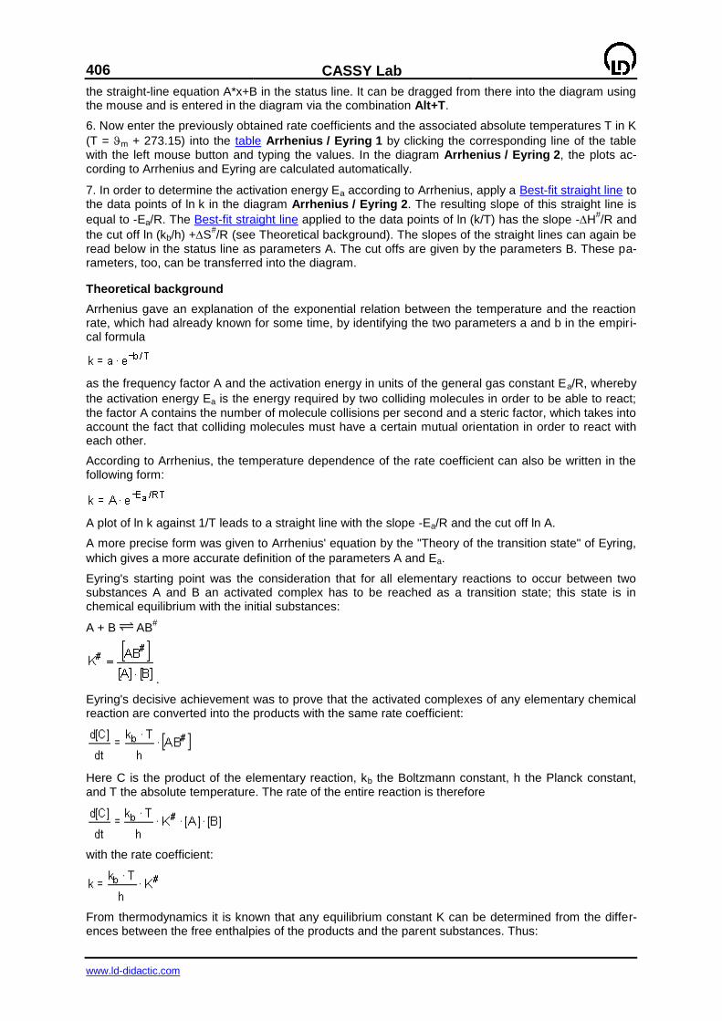
406

CASSY Lab

www.ld-didactic.com

the straight-line equation A*x+B in the status line. It can be dragged from there into the diagram using the mouse and is entered in the diagram via the combination Alt+T.

6. Now enter the previously obtained rate coefficients and the associated absolute temperatures T in K

(T = m + 273.15) into the table Arrhenius / Eyring 1 by clicking the corresponding line of the table with the left mouse button and typing the values. In the diagram Arrhenius / Eyring 2, the plots ac-cording to Arrhenius and Eyring are calculated automatically.

7. In order to determine the activation energy Ea according to Arrhenius, apply a Best-fit straight line to the data points of ln k in the diagram Arrhenius / Eyring 2. The resulting slope of this straight line is

equal to -Ea/R. The Best-fit straight line applied to the data points of ln (k/T) has the slope -H#/R and

the cut off ln (kb/h) +S#/R (see Theoretical background). The slopes of the straight lines can again be

read below in the status line as parameters A. The cut offs are given by the parameters B. These pa-rameters, too, can be transferred into the diagram.


Arrhenius gave an explanation of the exponential relation between the temperature and the reaction rate, which had already known for some time, by identifying the two parameters a and b in the empiri-cal formula

as the frequency factor A and the activation energy in units of the general gas constant Ea/R, whereby

the activation energy Ea is the energy required by two colliding molecules in order to be able to react;

the factor A contains the number of molecule collisions per second and a steric factor, which takes into account the fact that colliding molecules must have a certain mutual orientation in order to react with each other.

According to Arrhenius, the temperature dependence of the rate coefficient can also be written in the following form:

A plot of ln k against 1/T leads to a straight line with the slope -Ea/R and the cut off ln A.

A more precise form was given to Arrhenius' equation by the "Theory of the transition state" of Eyring,

which gives a more accurate definition of the parameters A and Ea.

Eyring's starting point was the consideration that for all elementary reactions to occur between two substances A and B an activated complex has to be reached as a transition state; this state is in chemical equilibrium with the initial substances:

A + B AB#

.

Eyring's decisive achievement was to prove that the activated complexes of any elementary chemical reaction are converted into the products with the same rate coefficient:

Here C is the product of the elementary reaction, kb the Boltzmann constant, h the Planck constant, and T the absolute temperature. The rate of the entire reaction is therefore

with the rate coefficient:

From thermodynamics it is known that any equilibrium constant K can be determined from the differ-ences between the free enthalpies of the products and the parent substances. Thus:

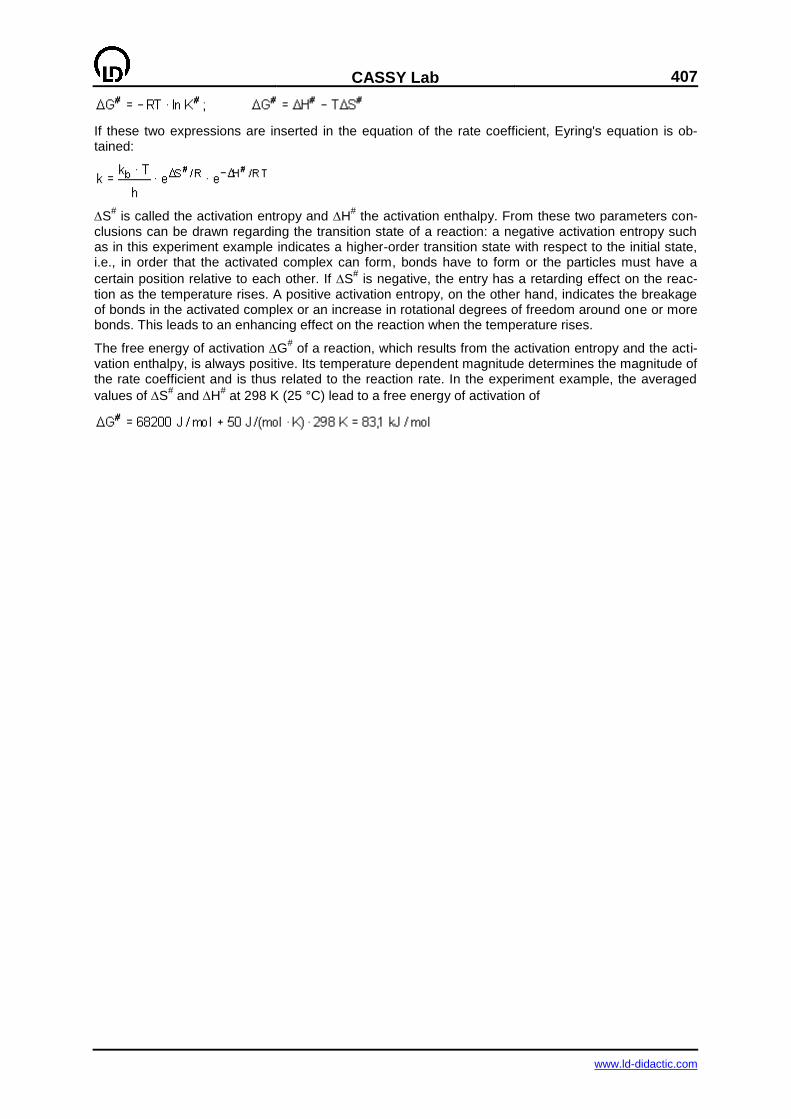
CASSY Lab

407

www.ld-didactic.com

If these two expressions are inserted in the equation of the rate coefficient, Eyring's equation is ob-tained:

S# is called the activation entropy and H

# the activation enthalpy. From these two parameters con-

clusions can be drawn regarding the transition state of a reaction: a negative activation entropy such as in this experiment example indicates a higher-order transition state with respect to the initial state, i.e., in order that the activated complex can form, bonds have to form or the particles must have a

certain position relative to each other. If S# is negative, the entry has a retarding effect on the reac-

tion as the temperature rises. A positive activation entropy, on the other hand, indicates the breakage of bonds in the activated complex or an increase in rotational degrees of freedom around one or more bonds. This leads to an enhancing effect on the reaction when the temperature rises.

The free energy of activation G# of a reaction, which results from the activation entropy and the acti-

vation enthalpy, is always positive. Its temperature dependent magnitude determines the magnitude of the rate coefficient and is thus related to the reaction rate. In the experiment example, the averaged

values of S# and H

# at 298 K (25 °C) lead to a free energy of activation of

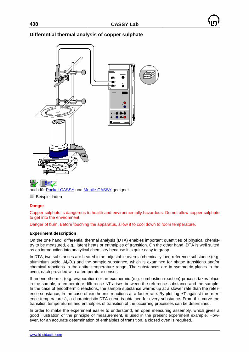
408

CASSY Lab

www.ld-didactic.com

Differential thermal analysis of copper sulphate


Beispiel laden

Danger

Copper sulphate is dangerous to health and environmentally hazardous. Do not allow copper sulphate to get into the environment.

Danger of burn. Before touching the apparatus, allow it to cool down to room temperature.


On the one hand, differential thermal analysis (DTA) enables important quantities of physical chemis-try to be measured, e.g., latent heats or enthalpies of transition. On the other hand, DTA is well suited as an introduction into analytical chemistry because it is quite easy to grasp.

In DTA, two substances are heated in an adjustable oven: a chemically inert reference substance (e.g.

aluminium oxide, Al2O3) and the sample substance, which is examined for phase transitions and/or chemical reactions in the entire temperature range. The substances are in symmetric places in the oven, each provided with a temperature sensor.

If an endothermic (e.g. evaporation) or an exothermic (e.g. combustion reaction) process takes place

in the sample, a temperature difference T arises between the reference substance and the sample. In the case of endothermic reactions, the sample substance warms up at a slower rate than the refer-

ence substance, in the case of exothermic reactions at a faster rate. By plotting T against the refer-

ence temperature , a characteristic DTA curve is obtained for every substance. From this curve the transition temperatures and enthalpies of transition of the occurring processes can be determined.

In order to make the experiment easier to understand, an open measuring assembly, which gives a good illustration of the principle of measurement, is used in the present experiment example. How-ever, for an accurate determination of enthalpies of transition, a closed oven is required.

CASSY Lab

409

www.ld-didactic.com

In this example, the temperatures at which water of crystallization bonded in copper sulphate is split off are determined up to 150 °C. For this the opportunity of directly measuring the differential tempera-ture provided by the chemistry box is taken advantage of as it is more precise than computing the difference between two individual temperatures.

Equipment list

1 Sensor-CASSY 524 010 1 CASSY Lab 524 200 1 Chemistry box or NiCr-Ni adapter S 524 067(3) 2 Temperature sensor NiCr-Ni, type K,

1.5 mm

529 676

1 Heating block with two holes 666 202 1 Set of 20 glass tubes 666 203 1 Electric burner 666 776 1 Stand base, V-shape, 20 cm 300 02 1 Stand rod, 47 cm 300 42 2 Crossed bossheads 666 543 1 Miniature clamp 666 551 1 Stand ring with stem, 100 mm 666 573

1 Wire gauze, 160*160 mm 666 685 1 Laboratory stand 3 666 583 2 Mortars, 50 ml 608 350 2 Pestles 608 360 1 PC with Windows 98/2000/XP/Vista

Chemicals

Aluminium oxide (Al2O3), e.g. 250 g 670 2900

Copper(II) sulphate pentahydrate, e.g. 100 g 672 9600


Connect the chemistry box to input A of the Sensor-CASSY with the temperature sensors being con-

nected to inputs T2 and T3.

Set up an assembly for heating the heating block using the stand material, the wire gauze, the electric burner, and the laboratory stand 3. Put the heating block onto the wire gauze exactly over the heating aperture of the electric burner. At the beginning of the measurement, the distance between the heating aperture of the burner and the wire gauze should be approx. 5 cm.

Triturate a spatula-tipfull of copper sulphate in one of the mortars, and fill it into one of the glass tubes up to approx. two-thirds of its height. Do the same with another glass tube and a spatula-tipfull of alu-minium oxide.

Turn the temperature sensor connected to T2 as deeply as possible into the aluminium oxide and that

connected to T3 into the copper sulphate.

Fix both temperature sensors together with a miniature clamp below the handle so that the glass tubes rest on the bottom of the two holes of the heating block. See to it that the entire base of the heating block has contact with the wire gauze.


Einstellungen laden

Switch the electric burner on.

Wait about one minute. Then start the measurement by pressing F9 or the button.

When the temperature curve becomes horizontal, enhance the height of the laboratory stand 3 somewhat to reduce the distance between the burner and the wire gauze.

Stop the measurement by pressing F9 or the button when the temperature is approx. 150°C. Switch the electric burner off.

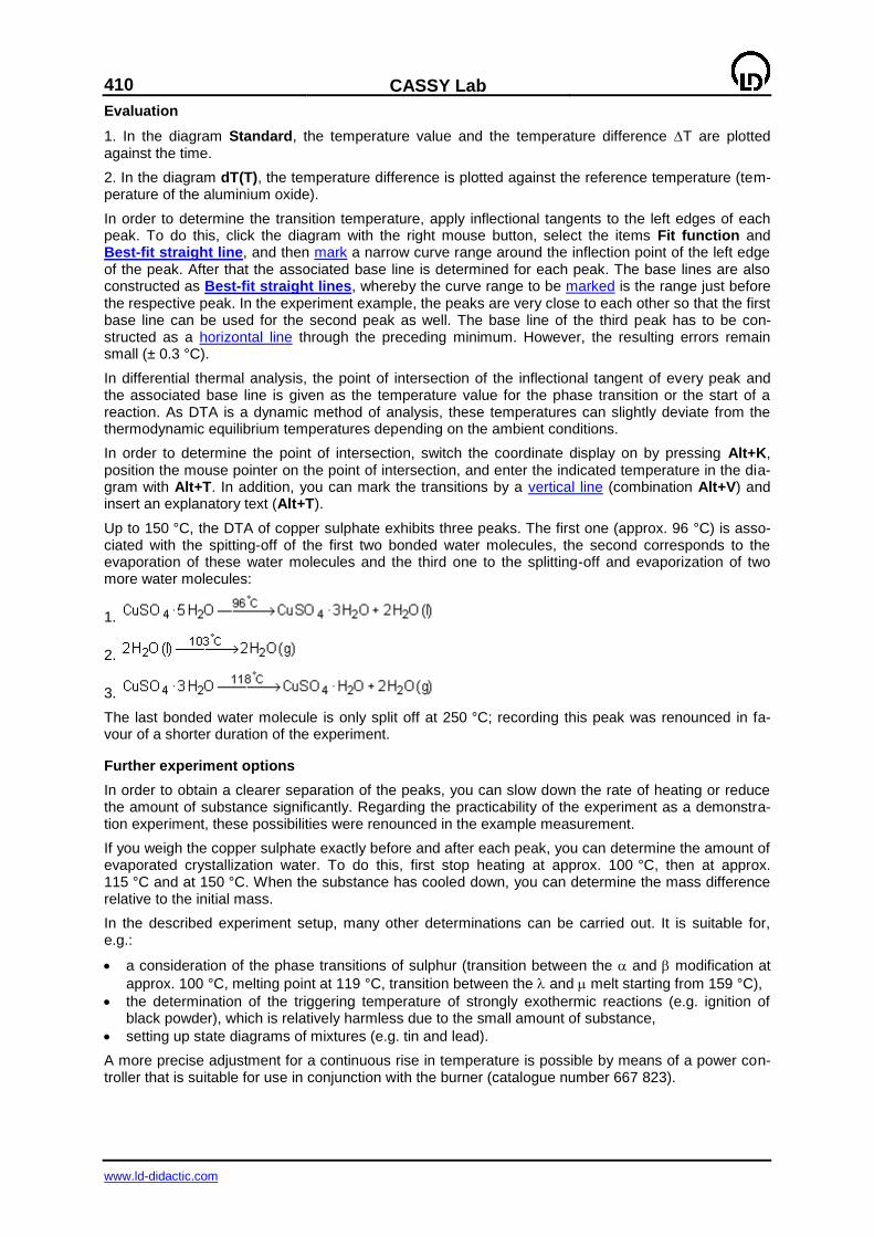
410

CASSY Lab

www.ld-didactic.com

Evaluation

1. In the diagram Standard, the temperature value and the temperature difference T are plotted against the time.

2. In the diagram dT(T), the temperature difference is plotted against the reference temperature (tem-perature of the aluminium oxide).

In order to determine the transition temperature, apply inflectional tangents to the left edges of each peak. To do this, click the diagram with the right mouse button, select the items Fit function and Best-fit straight line, and then mark a narrow curve range around the inflection point of the left edge of the peak. After that the associated base line is determined for each peak. The base lines are also constructed as Best-fit straight lines, whereby the curve range to be marked is the range just before the respective peak. In the experiment example, the peaks are very close to each other so that the first base line can be used for the second peak as well. The base line of the third peak has to be con-structed as a horizontal line through the preceding minimum. However, the resulting errors remain small (± 0.3 °C).

In differential thermal analysis, the point of intersection of the inflectional tangent of every peak and the associated base line is given as the temperature value for the phase transition or the start of a reaction. As DTA is a dynamic method of analysis, these temperatures can slightly deviate from the thermodynamic equilibrium temperatures depending on the ambient conditions.

In order to determine the point of intersection, switch the coordinate display on by pressing Alt+K, position the mouse pointer on the point of intersection, and enter the indicated temperature in the dia-gram with Alt+T. In addition, you can mark the transitions by a vertical line (combination Alt+V) and insert an explanatory text (Alt+T).

Up to 150 °C, the DTA of copper sulphate exhibits three peaks. The first one (approx. 96 °C) is asso-ciated with the spitting-off of the first two bonded water molecules, the second corresponds to the evaporation of these water molecules and the third one to the splitting-off and evaporization of two more water molecules:

1.

2.

3.

The last bonded water molecule is only split off at 250 °C; recording this peak was renounced in fa-vour of a shorter duration of the experiment.


In order to obtain a clearer separation of the peaks, you can slow down the rate of heating or reduce the amount of substance significantly. Regarding the practicability of the experiment as a demonstra-tion experiment, these possibilities were renounced in the example measurement.

If you weigh the copper sulphate exactly before and after each peak, you can determine the amount of evaporated crystallization water. To do this, first stop heating at approx. 100 °C, then at approx. 115 °C and at 150 °C. When the substance has cooled down, you can determine the mass difference relative to the initial mass.

In the described experiment setup, many other determinations can be carried out. It is suitable for, e.g.:

a consideration of the phase transitions of sulphur (transition between the and modification at

approx. 100 °C, melting point at 119 °C, transition between the and melt starting from 159 °C),

the determination of the triggering temperature of strongly exothermic reactions (e.g. ignition of black powder), which is relatively harmless due to the small amount of substance,

setting up state diagrams of mixtures (e.g. tin and lead).

A more precise adjustment for a continuous rise in temperature is possible by means of a power con-troller that is suitable for use in conjunction with the burner (catalogue number 667 823).

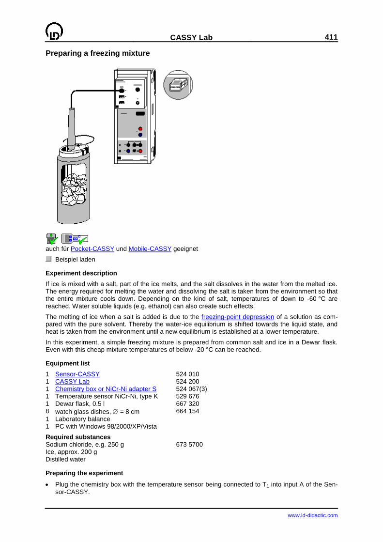
CASSY Lab

411

www.ld-didactic.com

Preparing a freezing mixture


Beispiel laden


If ice is mixed with a salt, part of the ice melts, and the salt dissolves in the water from the melted ice. The energy required for melting the water and dissolving the salt is taken from the environment so that the entire mixture cools down. Depending on the kind of salt, temperatures of down to -60 °C are reached. Water soluble liquids (e.g. ethanol) can also create such effects.

The melting of ice when a salt is added is due to the freezing-point depression of a solution as com-pared with the pure solvent. Thereby the water-ice equilibrium is shifted towards the liquid state, and heat is taken from the environment until a new equilibrium is established at a lower temperature.

In this experiment, a simple freezing mixture is prepared from common salt and ice in a Dewar flask. Even with this cheap mixture temperatures of below -20 °C can be reached.

Equipment list

1 Sensor-CASSY 524 010 1 CASSY Lab 524 200 1 Chemistry box or NiCr-Ni adapter S 524 067(3) 1 Temperature sensor NiCr-Ni, type K 529 676 1 Dewar flask, 0.5 l 667 320 8 watch glass dishes, = 8 cm 664 154

1 Laboratory balance 1 PC with Windows 98/2000/XP/Vista

Required substances Sodium chloride, e.g. 250 g 673 5700 Ice, approx. 200 g Distilled water

Preparing the experiment

Plug the chemistry box with the temperature sensor being connected to T1 into input A of the Sen-sor-CASSY.

412

CASSY Lab

www.ld-didactic.com

Weigh in 10 g of sodium chloride on each of the watch glass dishes.

Crush the ice as fine as possible in order that it can well be mixed with the salt.

Calibration

In order to ensure a sufficient accuracy, calibrate the temperature sensor when using it for the first time. Afterwards the calibration should be repeated from time to time.

Einstellungen laden

Immerse the temperature sensor in ice water (mixture of ice and a small amount of water), stir with the temperature sensor, and wait until the display instrument shows a measured value that is sta-ble up to ± 0.1 °C.

Enter the target value "0" in the first line in Settings A11 under Correct, and press the Correct Offset button.


Mark the Sensor-CASSY, the chemistry box, and the temperature sensor in order that they can be used again in the same combination (otherwise the stored calibration will not be applicable).



Fill crushed ice into the Dewar flask, and add a small amount of water.

Immerse the temperature sensor in the ice and stir.

Record the first measured value by pressing the key F9 or the button, and enter "0" as the first

value in the table column mNaCl, by clicking the table line with the left mouse button and typing the number.

Keep to the following procedure until all of the salt has been added to the ice:

Put 10 g of common salt into the Dewar flask.

Thoroughly stir with the temperature sensor until a uniform temperature is measured everywhere in

the freezing mixture (check with the aid of the display instrument A11).

Record the measured value by pressing the key F9 or the button.

Enter the total mass of common salt added up to that moment into the appropriate table cell for

mNaCl.

Evaluation

The measuring curve shows the temperature in the freezing mixture as a function of the mass of so-dium chloride added. It is clearly seen that addition of 10 g of NaCl to pure ice leads to a significantly stronger decrease in temperature than addition to a freezing mixture that already contains a great amount of salt. After 60 g of NaCl has been added, saturation is reached. Further addition of common salt does not lower the temperature of the mixture as the limit of the solubility of common salt in water is reached.

The saturation temperature can be marked by a horizontal line through the temperature minimum by pressing Alt+H. The temperature value is displayed in the status line and can be inserted in the dia-gram with the mouse or by pressing Alt+T.

If desired, the temperatures can be displayed as a bar chart by clicking the diagram with the right mouse button and selecting Select Value Display and Show bars.


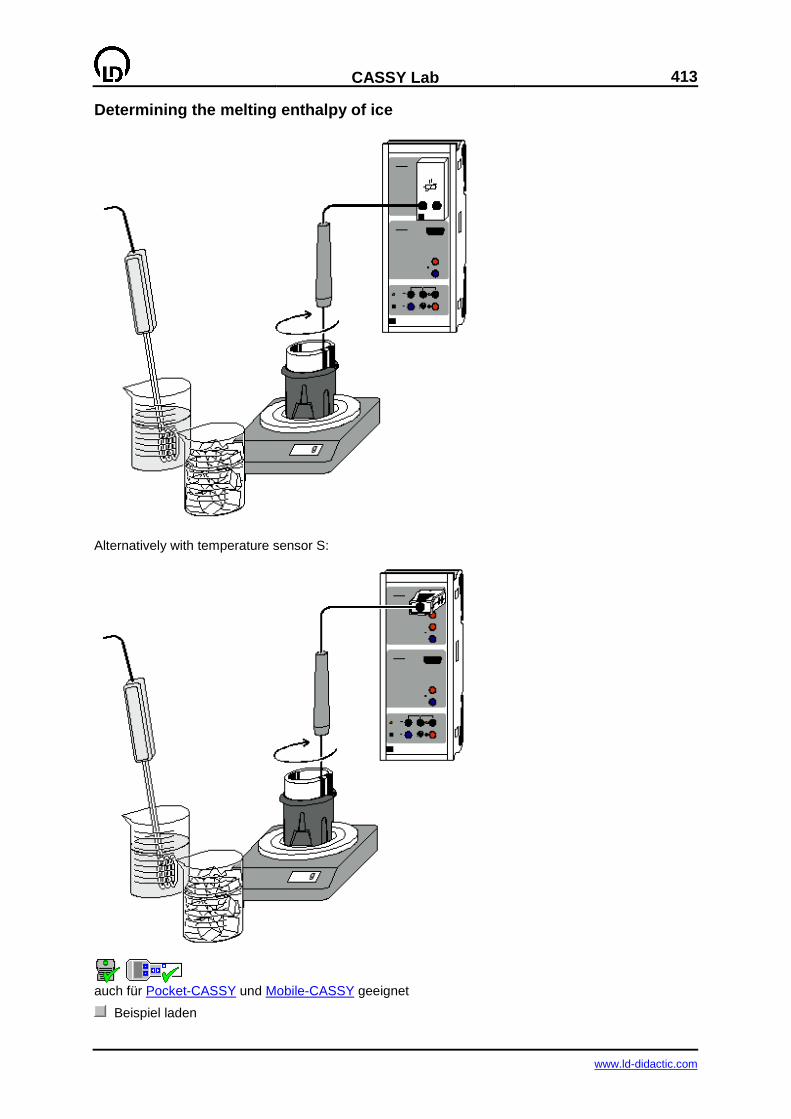
CASSY Lab

413

www.ld-didactic.com

Determining the melting enthalpy of ice

Alternatively with temperature sensor S:


Beispiel laden

414

CASSY Lab

www.ld-didactic.com


If a certain amount of ice is put into the warm water contained in a calorimeter, a mixing temperature

m can be determined after the ice has melted and completely mixed with the water. The mixing tem-

perature depends on the masses of the water (m1) and the ice (m2) as well as on the corresponding

temperatures 1 and 2. In order to simplify the evaluation, ice of 2 = 0 °C is used for the measure-ment.

Quick recording of the measured values with CASSY Lab enables a temperature curve to be deter-mined, which can be used to calculate the melting enthalpy of ice. With the same setup other calo-rimetric measurements can be carried out as well, e.g., mixing experiments or the determination of heat capacities.

Equipment list (temperature box)

1 Sensor-CASSY 524 010 1 CASSY Lab 524 200 1 Temperature box 524 045 1 Temperature sensor NTC 666 212 1 Dewar flask 386 48 1 Safety immersion heater 303 25 1 Beaker, squat shape, 250 ml 664 130 1 Beaker, squat shape, 600 ml 664 132 1 Balance, measuring range up to 500 g, resolution 0.01 g 1 Absorbent cloth 1 PC with Windows 98/2000/XP/Vista

Equipment list (temperature sensor S)

1 Sensor-CASSY 524 010 1 CASSY Lab 524 200 1 Temperature sensor S 524 044 1 Dewar flask 386 48 1 Safety immersion heater 303 25 1 Beaker, squat shape, 250 ml 664 130 1 Beaker, squat shape, 600 ml 664 132 1 Balance, measuring range up to 500 g, resolution 0.01 g 1 Absorbent cloth 1 PC with Windows 98/2000/XP/Vista

Required substances

Ice, approx. 100 g Distilled water


Plug the temperature box with the temperature sensor being connected into input A of the Sensor-CASSY. Alternatively, connect the temperature sensor S to input A.

Heat distilled water in the bigger beaker up to a temperature of about 80 °C. Put the dry Dewar flask on the balance and set the display of the balance to 0.

Calibration

Calibrate the temperature sensor while the water is heated:

Einstellungen laden

Crush the ice, and put it into the other beaker.

Add a small amount of water. After a short time, the ice-water equilibrium with a temperature of 0 °C should be established.

Immerse the temperature sensor in the ice water mixture and stir.

Enter the target value "0" in the first line in Settings A11 under Correct, and press the Correct Offset button.

CASSY Lab

415

www.ld-didactic.com


Pour about 120 g of hot water into the Dewar flask.

Pour the water from the ice water mixture away, pour the ice on the cloth, and dry it thoroughly.

Read the mass of the hot water, and take it down.

Immerse the temperature sensor in the flask.


Having waited for approx. 30 to 60 seconds, pour the ice from the cloth into the Dewar flask. While doing so, permanently stir with the temperature sensor.

After another 30 to 60 seconds, stop the measurement by pressing the key F9 or the button.

Remove the temperature sensor from the Dewar flask, and drain it well over the flask. Read the total mass at the balance, and take it down.

Evaluation

In the diagram, the measured values of the temperature are plotted against the time t.

1. In order to determine the calorimeter and the mixing temperature, first fit straight lines to the linear curve ranges at the beginning and at the end of the measurement (click the diagram with the right mouse button, select, Fit function and Best-fit straight line, and mark the respective curve section).

2. Next generate a vertical line with Alt+V, and position it so that the two (almost triangular) areas each formed by one of the fitted straight lines, the vertical line and the measuring curve have equal sizes. The point of intersection of the vertical line with the upper best-fit straight line corresponds to the

initial temperature 1 of the calorimeter, whereas the lower point of intersection corresponds to the

mixing temperature m. As the straight lines are almost horizontal, only a small error has to be ex-pected (± 0.1 °C).

3. For a precise determination of the coordinates, press Alt+C, and position the mouse pointer exactly in the points of intersection. The coordinates are displayed in the status line below on the left and can be inserted as text in the diagram via Alt+T.

The calculation of the melting enthalpy Hf can be derived in the following way:

I) Quantity of heat given off by the calorimeter and the hot water:

II) Quantity of heat taken up by the ice (2 = 0 °C) from the calorimeter:

Here cw is the heat capacity of water, m1 the mass of the hot water, m2 the mass of the ice and mo the water equivalent of the calorimeter. As there is almost no heat exchanged with the environment, we have

.

Consequently the melting enthalpy Hf is calculated according to

.

With the water equivalent m0 = 24 g of the Dewar flask used, the measured values of the experiment example lead to the following calculation:

This result is very close to the value of 334 J/g quoted in the literature.

Hf is significantly greater than the heat capacity of 1 g of water:

416

CASSY Lab

www.ld-didactic.com

That means: with the energy required to melt 1 g of ice having a temperature of 0 °C, 1 g of water can be heated from 0 °C to approx. 80 °C.

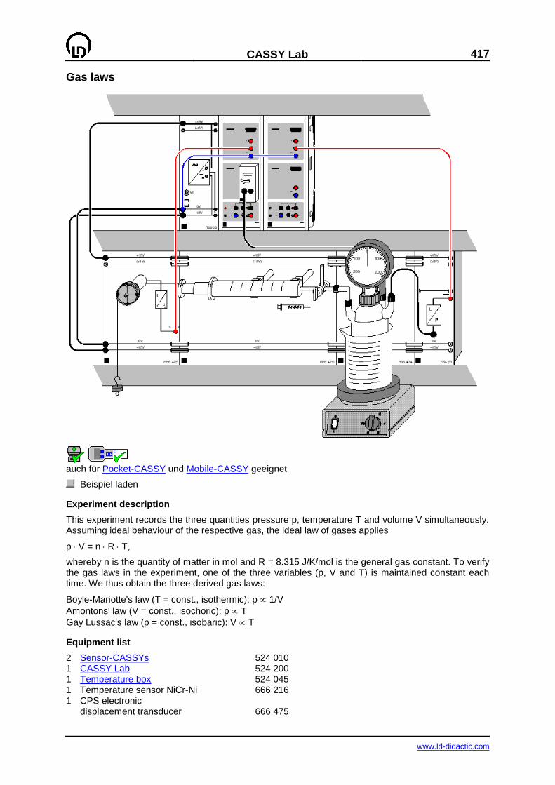
CASSY Lab

417

www.ld-didactic.com

Gas laws


Beispiel laden


This experiment records the three quantities pressure p, temperature T and volume V simultaneously. Assuming ideal behaviour of the respective gas, the ideal law of gases applies

p V = n R T,

whereby n is the quantity of matter in mol and R = 8.315 J/K/mol is the general gas constant. To verify the gas laws in the experiment, one of the three variables (p, V and T) is maintained constant each time. We thus obtain the three derived gas laws:

Boyle-Mariotte's law (T = const., isothermic): p 1/V

Amontons' law (V = const., isochoric): p T

Gay Lussac's law (p = const., isobaric): V T

Equipment list

2 Sensor-CASSYs 524 010 1 CASSY Lab 524 200 1 Temperature box 524 045 1 Temperature sensor NiCr-Ni 666 216 1 CPS electronic displacement transducer 666 475

418

CASSY Lab

www.ld-didactic.com

1 CPS-P/U converter 734 83 1 CPS-basic unit for gas laws 666 474 1 Gas syringe for gas laws 666 473 1 Stabilized power supply ±15 V 726 86 1 Magnetic stirrer, heatable 666 847 1 Stirrer bar 666 854 1 Laboratory stand 300 76 1 Beaker, 1000 ml, ss 664 107 1 GL-18 screw cap 667 305 1 Set of 10 silicone seals 667 306 1 Set of 10 bridging plugs 501 511 1 Panel frame C100, two-level 666 428 3 Connecting leads, 100 cm, black 500 444 2 Pairs of cables, 1 m, red and blue 501 46 1 PC with Windows 98/2000/XP/Vista


Place the displacement transducer, the gas syringe for gas laws, the basic unit for gas laws and the power supply in the bottom level of the panel frame and connect the individual panels together using the bridging plugs. Attach the gas syringe, the thermocouple and the pressure sensor to the basic unit using the GL 18 screw connectors. Seal the GL 45 connector with the enclosed screw cap. Attach the weight to the clamp for the gas syringe using a thread. Push the clamp onto the end of the plunger and wind the thread two times around the pulley of the displacement transducer. When the plunger is pushed in, the weight should be around 30 to 40 cm above the benchtop. Shorten the thread as nec-essary.

Place the two Sensor-CASSY units in the top level of the CPS panel frame and cascade them (con-nect them together). Allocate the Sensor-CASSY analog outputs as follows:

Connect sensor input A1 to the voltage output of the CPS displacement transducer using connect-

ing leads.

Connect sensor output B1 to the NiCr-Ni temperature sensor via the temperature box.

Connect sensor output A2 to the voltage output of the CPS-P/U converter using connecting leads.


a) Boyle-Mariotte's law (T = const., p 1/V)

Einstellungen laden

Open the three-way stopcock.

Pull out the plunger of the gas syringe to the 100 ml mark and turn the deflection pulley to the left until just before full stop.

Check the volume V = 725 ml, if necessary adjust the adjusting screw on the CPS displacement transducer.

Close the stopcock so that there is only one connection between the syringe and the bottle, and no more air can enter the system.

Record the first measured values with F9.

Carefully depress the plunger in increments of 10 ml and wait until the previously measured tem-perature (ambient temperature) is restored.

Record additional measured values each time with F9.

b) Amontons' law (V = const., p T)

Einstellungen laden

Open the three-way stopcock to vent the Woulff's bottle.

Close the stopcock so that there is no connection to the bottle.

Switch on the hot plate and the magnetic stirrer.

Start automatic measurement with F9.

Switch off the hot plate before the water in the beaker begins to boil and stop the measurement with F9.

CASSY Lab

419

www.ld-didactic.com

c) Gay Lussac's law (p = const., V T)

Einstellungen laden

Switch on the hot plate and the magnetic stirrer.

Switch off the hot plate before the water in the beaker begins to boil.

Open the three-way stopcock.

Pull out the plunger of the gas syringe to the 100 ml mark and turn the deflection pulley to the left until just before full stop.

Check the volume V = 725 ml, if necessary adjust the adjusting screw on the CPS displacement transducer.

Close the stopcock so that there is only one connection between the syringe and the bottle, and no more air can enter the system.

Record the first measured values with F9.

Carefully depress the plunger in increments of 5 ml and wait until the previously measured pres-sure (ambient pressure) is restored.

Record additional measured values each time with F9.

Stop the measurement as soon as the temperatures approach the ambient temperature.

Evaluation

The following diagrams are used to evaluate the respective experiment parts:

a) Isothermic experiment part (T = const.): p(V) diagram b) Isochoric experiment part (V = const.): p(T) diagram c) Isobaric experiment part (p = const.): T(V) diagram

In the display Regression (click on this tab) these diagrams area already pre-scaled so that the zero point of the coordinate system is visible; you can fit the following functions in the diagram:

a) Isothermic experiment part (p 1/V): hyperbola 1/x

b) Isochoric experiment part (p T): best-fit line or line through origin

c) Isobaric experiment part (T V): best-fit line or line through origin

Remark

The scaling in Regression begins with the zero point and covers a broad range. This enables signifi-cant curve sections and intersections to be recognized and explained better.

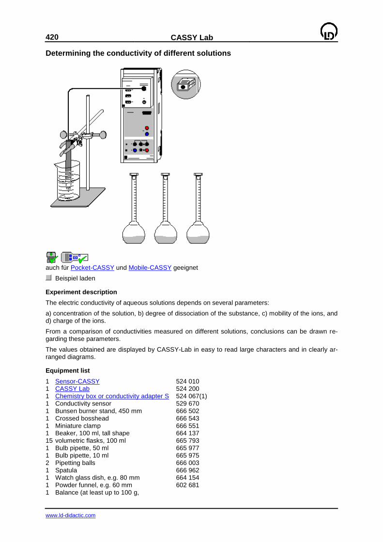
420

CASSY Lab

www.ld-didactic.com

Determining the conductivity of different solutions


Beispiel laden


The electric conductivity of aqueous solutions depends on several parameters:

a) concentration of the solution, b) degree of dissociation of the substance, c) mobility of the ions, and d) charge of the ions.

From a comparison of conductivities measured on different solutions, conclusions can be drawn re-garding these parameters.

The values obtained are displayed by CASSY-Lab in easy to read large characters and in clearly ar-ranged diagrams.

Equipment list

1 Sensor-CASSY 524 010 1 CASSY Lab 524 200 1 Chemistry box or conductivity adapter S 524 067(1) 1 Conductivity sensor 529 670 1 Bunsen burner stand, 450 mm 666 502 1 Crossed bosshead 666 543 1 Miniature clamp 666 551 1 Beaker, 100 ml, tall shape 664 137 15 volumetric flasks, 100 ml 665 793 1 Bulb pipette, 50 ml 665 977 1 Bulb pipette, 10 ml 665 975 2 Pipetting balls 666 003 1 Spatula 666 962 1 Watch glass dish, e.g. 80 mm 664 154 1 Powder funnel, e.g. 60 mm 602 681 1 Balance (at least up to 100 g,

CASSY Lab

421

www.ld-didactic.com

resolution 0.01 g) 1 PC with Windows 98/2000/XP/Vista

Chemicals

D(+)-glucose, e.g. 100 g 672 1100 Acetic acid, c = 1 mol/l, e.g. 1000 ml 671 9590 Magnesium sulphate 7-hydrate, e.g. 100 g 673 1600 Sodium chloride, e.g. 250 g 673 5700 Hydrochloric acid, c = 1 mol/l, 500 ml 674 6900 Distilled water If necessary: Calibration solution, 111.8 mS/cm 667 4644 Calibration solution, 12.88 mS/cm 667 4640


For preparing the solutions, the balance, the pipettes, the volumetric flasks, the spatula, the watch glass dish, and the funnel are required. From each substance three solutions of different concentra-tions are prepared. Of course, other concentrations can be used in addition or some of the measuring values can be omitted.

1) Glucose solutions (1 mol/l, 0.5 mol/l, 0.1 mol/l)

One after another weigh in exactly 19.82 g (1 mol/l), 9.91 g (0.5 mol/l) and 1.98 g (0.1 mol/l) of glucose on the watch glass dish, which is lying on the balance, and rinse it with distilled water through the fun-nel into a 100 ml flask. Then clean the watch glass dish, the spatula and the funnel.

2) Acetic acid solutions (0.5 mol/l, 0.1 mol/l, 0.01 mol/l)

Using the pipette, put 50 ml (0.5 mol/l) and 10 ml (0.1 mol/l) of 1 M acetic acid in a 100 ml volumetric flask each, and fill the flasks with distilled water up to the calibration mark. Prepare the 0.01 M acetic acid from 10 ml of 0.1 M solution in a new flask.

3) Magnesium sulphate solutions (0.5 mol/l, 0.1 mol/l. 0.01 mol/l)

One after another weigh in exactly 12.32 g (0.5 mol/l) and 2.46 g (0.1 mol/l) of magnesium sulphate on the watch glass dish, which is lying on the balance, and rinse it with distilled water through the funnel into a 100 ml flask. Using the cleaned pipette, prepare the 0.01 M solution from 10 ml of 0.1 M magne-sium sulphate solution in a new flask. Then clean the watch glass dish, the spatula, the funnel and the pipette.

4) NaCl solutions (0.5 mol/l, 0.1 mol/l, 0.01 mol/l)

Weigh in exactly 2.92 g (0.5 mol/l) of sodium chloride on the watch glass dish, which is lying on the balance, and rinse it with distilled water through the funnel into a 100 ml flask. Using the pipette, pre-pare the 0.1 M solution from 20 ml of 0.5 M solution in a new volumetric flask and the 0.01 M solution from 10 ml of the 0.1 M solution.

5) Hydrochloric acid solution (0.5 mol/l, 0.1 mol/l, 0.01 mol/l)

Using cleaned pipettes, put 50 ml (0.5 mol/l) and 10 ml (0.1 mol/l) of 1 M hydrochloric acid into a 100 ml volumetric flask each, and fill the flask with distilled water up to the calibration mark. Prepare the 0.01 M acetic acid from 10 ml of 0.1 M solution in a new flask.


Plug the chemistry box with the conductivity sensor being connected into input A of the Sensor-CASSY. After thoroughly rinsing the conductivity sensor with distilled water, fix it in the clamp, so that its height can be adjusted with the crossed bosshead according to the requirements.

Calibration

Einstellungen laden

The cell constant of the conductivity sensor for the chemistry box has already been set to 0.58 in CASSY Lab. If another conductivity sensor is used, its cell constant has to be entered as a factor in Settings Conductivity CA1 under Correct. Then the Correct Factor button has to be pressed.

For a more precise determination of the cell constant, calibration solutions can be used: rinse the beaker and the conductivity sensor first with distilled water and then with approx. 30-40 ml of calibra-

422

CASSY Lab

www.ld-didactic.com

tion solution. Immerse the conductivity sensor in another 50 ml of calibration solution as if it was for a conductivity measurement (pay attention to the distances from the walls of the beaker), enter the tar-get value in the second line in Settings CA1 under Correct, and press the Correct Factor button when a stable measured value is reached.


(missing or bad snippet)One after another measure the conductivity of distilled water, the solutions of glucose, acetic acid, magnesium sulphate, sodium chloride, and hydrochloric acid, starting with the lowest concentration and keeping to the following order:

Rinse the electrode and the beaker thoroughly with 30-40 ml of the solution.

Fill another 60 ml of the solution into the beaker.

Adjust the height of the conductivity sensor so that its immersion depth in the liquid is 2 cm and its distance from every wall at least 1 cm.

If necessary, change the measuring range in Settings Conductivity CA1. Always select the lowest possible measuring range.

When the displayed value is stable, record the measured value by pressing F9 or the button.

Enter the concentration and the substance associated with the measured value in the diagram. To do this, press Alt+T, type the substance and the value of the concentration and position the text at the desired place in the diagram with the mouse.

In order to simplify the evaluation, select Append New Meas. Series in Measuring Parameters before measuring the conductivity of a new substance.

Before measuring the conductivity of a new substance, thoroughly rinse the beaker and the con-ductivity sensor with distilled water.

Evaluation

When the large representation of the display instrument is selected, the measured values can also be read by persons who are at some distance from the screen. The values are automatically entered in the diagrams as bars so that the differences between the conductivities are visualized.

The diagram Specific Conductivity has been prepared as an overview for this purpose. The other diagrams allow direct comparison of two particular substances with each other. In order to get a clear separation between the different substances, vertical lines can be inserted in the diagram between the measurement series.

This experiment demonstrates clearly that the conductivity depends strongly on the concentration. Moreover it can be seen from the measuring results that strong electrolytes having a high degree of dissociation conduct much better than substances that do not or only to a small proportion dissociate. From the higher conductivity of hydrochloric acid as compared with the common salt solutions it can be concluded that the mobility of hydronium ions is greater than that of sodium ions.

Despite the higher ion charge, the magnesium sulphate solutions of higher concentration do not ex-hibit a greater conductivity than the corresponding NaCl solutions because the ions exert strong elec-trostatic forces on each other due to their charges, which are twice the charges of the ions of sodium and chloride ions. However, at lower concentrations (great distances between the ions), e.g. 0.01 mol/l, the conductivity is higher as compared with NaCl.

The diagrams generated can be printed via the printer symbol in the upper line on the screen.

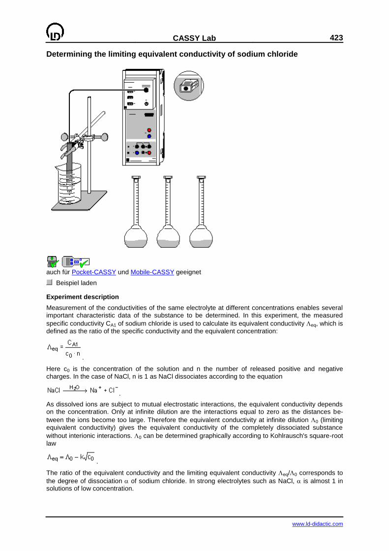
CASSY Lab

423

www.ld-didactic.com

Determining the limiting equivalent conductivity of sodium chloride


Beispiel laden


Measurement of the conductivities of the same electrolyte at different concentrations enables several important characteristic data of the substance to be determined. In this experiment, the measured

specific conductivity CA1 of sodium chloride is used to calculate its equivalent conductivity eq, which is defined as the ratio of the specific conductivity and the equivalent concentration:

.

Here c0 is the concentration of the solution and n the number of released positive and negative charges. In the case of NaCl, n is 1 as NaCl dissociates according to the equation

.

As dissolved ions are subject to mutual electrostatic interactions, the equivalent conductivity depends on the concentration. Only at infinite dilution are the interactions equal to zero as the distances be-

tween the ions become too large. Therefore the equivalent conductivity at infinite dilution 0 (limiting equivalent conductivity) gives the equivalent conductivity of the completely dissociated substance

without interionic interactions. 0 can be determined graphically according to Kohlrausch's square-root

law

.

The ratio of the equivalent conductivity and the limiting equivalent conductivity eq/0 corresponds to

the degree of dissociation of sodium chloride. In strong electrolytes such as NaCl, is almost 1 in solutions of low concentration.

424

CASSY Lab

www.ld-didactic.com

Equipment list

1 Sensor-CASSY 524 010 1 CASSY Lab 524 200 1 Chemistry box or conductivity adapter S 524 067(1) 1 Conductivity sensor 529 670 1 Bunsen burner stand, 450 mm 666 502 1 Crossed bosshead 666 543 1 Miniature clamp 666 551 1 Beaker, 100 ml, tall shape 664 137 1 Volumetric flask, 250 ml 665 794 6 Volumetric flask, 100 ml 665 793 1 Bulb pipette, 10 ml 665 975 1 Bulb pipette, 25 ml 665 976 2 Pipetting balls 666 003 1 Spatula 666 962 1 Watch glass dish, e.g. 80 mm 664 154 1 Powder funnel, e.g. 60 mm 602 681 1 Balance (at least up to 100 g, resolution 0.01 g) 1 PC with Windows 98/2000/XP/Vista or higher version

Chemicals

Sodium chloride, e.g. 250 g 673 5700 Distilled water If necessary: Calibration solution, 111.8 mS/cm 667 4644 Calibration solution, 12.88 mS/cm 667 4640


For preparing the solutions, the balance, the pipettes, the volumetric flasks, the spatula, the watch glass dish, and the funnel are required.

Weigh in exactly 29.22 g of sodium chloride (0.5 mol) on the watch glass dish, which is lying on the balance, and rinse the salt through the funnel into the 250 ml flask with distilled water. After dissolving the salt completely and filling the flask up to the calibration mark, use the 2 M NaCl solution for prepar-ing the other solutions. For 100 ml of the respective solution you need:

for 1 mol/l: 50 ml for 0.8 mol/l: 40 ml for 0.5 mol/l: 25 ml for 0.2 mol/l: 10 ml for 0.1 mol/l: of the solution with c = 1 mol/l: 10 ml for 0.01 mol/l: of the solution with c = 0.1 mol/l: 10 ml

If you intend to investigate the specific conductivity of NaCl over the total range of concentrations, it is recommendable to prepare some additional solutions of higher concentration, e.g. 1.5 mol/l, 3 mol/l, 4 mol/l, 5 mol/l, and 6 mol/l.


Plug the chemistry box with the conductivity sensor being connected into input A of the Sensor-CASSY. After thoroughly rinsing the conductivity sensor with distilled water, fix it in the clamp, so that its height can be adjusted with the crossed bosshead according to the requirements.

Calibration

Einstellungen laden


CASSY Lab

425

www.ld-didactic.com

For a more precise determination of the cell constant, calibration solutions can be used: rinse the beaker and the conductivity sensor first with distilled water and then with approx. 30-40 ml of calibra-tion solution. Immerse the conductivity sensor in another 50 ml of calibration solution as if it was for a conductivity measurement (pay attention to the distances from the walls of the beaker), enter the tar-get value in the second line in Settings CA1 under Correct, and press the Correct Factor button when a stable measured value is reached.

Such a correction with calibration solutions is also necessary for the conductivity sensor used in this experiment if you intend measurements on highly concentrated NaCl solutions whose specific conduc-tivity exceeds 100 mS/cm. This is the case for concentrations over 1.5 mol/l.


(missing or bad snippet)Starting with the solution of the lowest concentration (0.01 mol/l) and following the order up to the 2 M solution, keep to the following procedure:

Rinse the electrode and the beaker thoroughly with 30-40 ml of the solution.

Pour this portion of the solution away.

Fill the remaining solution (approx. 60 ml) into the beaker.

Adjust the height of the conductivity sensor so that its immersion depth in the liquid is 2 cm and its distance from every wall at least 1 cm.

If necessary, change the measuring range in Settings Conductivity CA1. Always select the lowest possible measuring range.


Enter the concentration associated with the measured value into the table. To do this, click the corresponding line of the table with the left mouse button, and type the value of the concentration.

Pour the solution away.

Evaluation

The values obtained for CA1 give the specific conductivity of the solution. This quantity is not sub-stance specific, but depends on the concentration and the temperature. The temperature compensa-tion for the sensor programmed in CASSY Lab determines the data automatically with respect to the standard temperature of 25 °C.

For the evaluation of the data, 4 diagrams have been prepared in CASSY-Lab:

1. In the first diagram, the specific conductivity CA1 is plotted against the concentration c0.

2. The second diagram displays the concentration dependence of the equivalent conductivityeq.

3. According to Kohlrausch's square-root law, the plot of the equivalent conductivity against the square root of the molar concentration is approximately a straight line in the range of low concentrations, the cut off being the limiting equivalent conductivity. This behaviour can be seen in the diagram Kohl-rausch plot. The slope k depends on the number of ions that result form dissociation (i.e., this slope is

smaller in the case of NaCl than, e.g., in the case of H2SO4).

For fitting a straight line, click the diagram with the right mouse button, select Fit function, and Best-fit straight line. After marking the curve range between 0 and 0.5 mol/l you obtain a straight line whose slope A and cut off B are displayed in the status line below on the left. These values can be dragged in to the diagram with the mouse or inserted as text via Alt+T. The parameter A corresponds to -k in the

Kohlrausch law, and B is the value of the limiting equivalent conductivity 0. Enter this value in Set-

tings 0 in the field Formula to calculate .

4. Finally, the diagram Degree of dissociation shows the calculated data for . It is clearly seen that even in the case of strong electrolytes the degree of dissociation is only approximately 1 for very low concentrations. This deviation from the ideal behaviour of a strong electrolyte can be explained by the interactions between the ions (ionic association due to Coulomb forces, impediment to the migration of ions in the solution).

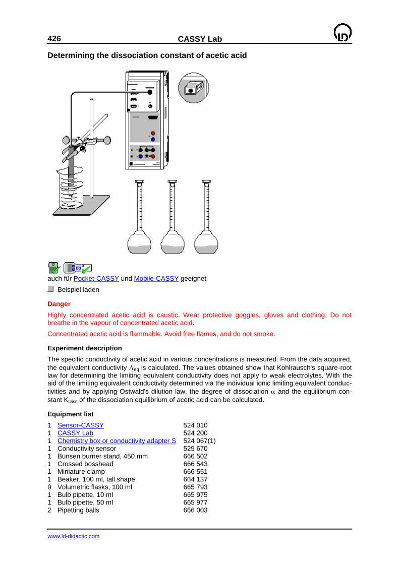
426

CASSY Lab

www.ld-didactic.com

Determining the dissociation constant of acetic acid


Beispiel laden

Danger

Highly concentrated acetic acid is caustic. Wear protective goggles, gloves and clothing. Do not breathe in the vapour of concentrated acetic acid.

Concentrated acetic acid is flammable. Avoid free flames, and do not smoke.


The specific conductivity of acetic acid in various concentrations is measured. From the data acquired,

the equivalent conductivity eq is calculated. The values obtained show that Kohlrausch's square-root law for determining the limiting equivalent conductivity does not apply to weak electrolytes. With the aid of the limiting equivalent conductivity determined via the individual ionic limiting equivalent conduc-

tivities and by applying Ostwald's dilution law, the degree of dissociation and the equilibrium con-

stant KDiss of the dissociation equilibrium of acetic acid can be calculated.

Equipment list

1 Sensor-CASSY 524 010 1 CASSY Lab 524 200 1 Chemistry box or conductivity adapter S 524 067(1) 1 Conductivity sensor 529 670 1 Bunsen burner stand, 450 mm 666 502 1 Crossed bosshead 666 543 1 Miniature clamp 666 551 1 Beaker, 100 ml, tall shape 664 137 9 Volumetric flasks, 100 ml 665 793 1 Bulb pipette, 10 ml 665 975 1 Bulb pipette, 50 ml 665 977 2 Pipetting balls 666 003

CASSY Lab

427

www.ld-didactic.com

1 Collection container, approx. 1.5 l capacity 1 PC with Windows 98/2000/XP/Vista

Chemicals

Acetic acid, 99-100 % (approx. 17.5 mol/l), 500 ml

671 9510

Acetic acid, c = 1 mol/l, 1000 ml 671 9590 Distilled water


For preparing the acetic acid solutions, the pipettes and the volumetric flasks are required.

Quantities of pure acetic acid required for 100 ml of solution:

for HAc 50 % (8.75 mol/l): 50 ml

for HAc 20 % (3.5 mol/l) and 10 % (1.75 mol/l), respectively: 20 ml and 10 ml, respectively

For preparing other solutions, use 1 M acetic acid:

for HAc, c = 0.5 mol/l: 50 ml

for HAc, c = 0.1 mol/l: 10 ml

Fill distilled water into the volumetric flasks containing the above mentioned amounts of acetic acid up to the calibration mark. Now use the acetic acid solutions just prepared to prepare further solutions. For this purpose put 10 ml of the HAc solution that has ten times the concentration of the solution to be prepared into a new flask, and add distilled water up to the calibration mark. In this way you obtain the following concentrations:

c = 0.05 mol/l, c = 0.01 mol/l, c = 0.005 mol/l, c = 0.001 mol/l

Now you have eleven acetic acid solutions available for measuring the conductivity at different con-centrations. If you intend to perform detailed investigations of the total range of the specific conductiv-ity, it is recommendable to prepare additional solutions of higher concentration (e.g. 30 %, 40 %, 60 %, 70 %, 80 %, 90 %).


Plug the chemistry box with the conductivity sensor being connected into input A of the Sensor-CASSY. After thoroughly rinsing the conductivity sensor with distilled water, fix it in the clamp, so that its height can be adjusted by loosening and fastening the screw of the crossed bosshead at the stand.

Calibration

Einstellungen laden


For a more precise determination of the cell constant, calibration solutions can be used: rinse the beaker and the conductivity sensor first with distilled water and then with approx. 30-40 ml of calibra-tion solution. Immerse the conductivity sensor in another 50 ml of calibration solution as if it was for a conductivity measurement (pay attention to the distances from the walls of the beaker), enter the tar-get value in the second line in Settings CA1 under Correct, and press the Correct Factor button when a stable measured value is reached.


(missing or bad snippet)Starting with the solution of the lowest concentration (0.001 mol/l) and follow-ing the order up to concentrated acetic acid, keep to the following procedure:

Rinse the electrode and the 100 ml beaker thoroughly with 30-40 ml of the solution.

Pour this portion of the solution into a collection container.

Fill the remaining solution (approx. 60 ml) into the 100 ml beaker.

Fix the conductivity sensor at the stand so that its immersion depth in the liquid is 2 cm and its distance from every wall at least 1 cm.

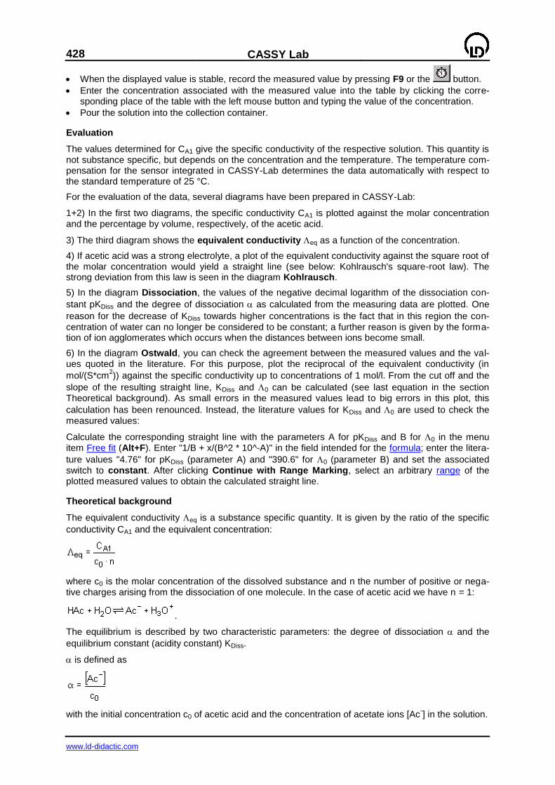
428

CASSY Lab

www.ld-didactic.com


Enter the concentration associated with the measured value into the table by clicking the corre-sponding place of the table with the left mouse button and typing the value of the concentration.

Pour the solution into the collection container.

Evaluation

The values determined for CA1 give the specific conductivity of the respective solution. This quantity is not substance specific, but depends on the concentration and the temperature. The temperature com-pensation for the sensor integrated in CASSY-Lab determines the data automatically with respect to the standard temperature of 25 °C.

For the evaluation of the data, several diagrams have been prepared in CASSY-Lab:

1+2) In the first two diagrams, the specific conductivity CA1 is plotted against the molar concentration and the percentage by volume, respectively, of the acetic acid.

3) The third diagram shows the equivalent conductivity eq as a function of the concentration.

4) If acetic acid was a strong electrolyte, a plot of the equivalent conductivity against the square root of the molar concentration would yield a straight line (see below: Kohlrausch's square-root law). The strong deviation from this law is seen in the diagram Kohlrausch.

5) In the diagram Dissociation, the values of the negative decimal logarithm of the dissociation con-

stant pKDiss and the degree of dissociation as calculated from the measuring data are plotted. One

reason for the decrease of KDiss towards higher concentrations is the fact that in this region the con-

centration of water can no longer be considered to be constant; a further reason is given by the forma-tion of ion agglomerates which occurs when the distances between ions become small.

6) In the diagram Ostwald, you can check the agreement between the measured values and the val-ues quoted in the literature. For this purpose, plot the reciprocal of the equivalent conductivity (in

mol/(S*cm2)) against the specific conductivity up to concentrations of 1 mol/l. From the cut off and the

slope of the resulting straight line, KDiss and 0 can be calculated (see last equation in the section Theoretical background). As small errors in the measured values lead to big errors in this plot, this

calculation has been renounced. Instead, the literature values for KDiss and 0 are used to check the

measured values:

Calculate the corresponding straight line with the parameters A for pKDiss and B for 0 in the menu item Free fit (Alt+F). Enter "1/B + x/(B^2 * 10^-A)" in the field intended for the formula; enter the litera-

ture values "4.76" for pKDiss (parameter A) and "390.6" for 0 (parameter B) and set the associated switch to constant. After clicking Continue with Range Marking, select an arbitrary range of the plotted measured values to obtain the calculated straight line.


The equivalent conductivity eq is a substance specific quantity. It is given by the ratio of the specific

conductivity CA1 and the equivalent concentration:

where c0 is the molar concentration of the dissolved substance and n the number of positive or nega-tive charges arising from the dissociation of one molecule. In the case of acetic acid we have n = 1:

.

The equilibrium is described by two characteristic parameters: the degree of dissociation and the

equilibrium constant (acidity constant) KDiss.

is defined as

with the initial concentration c0 of acetic acid and the concentration of acetate ions [Ac-] in the solution.

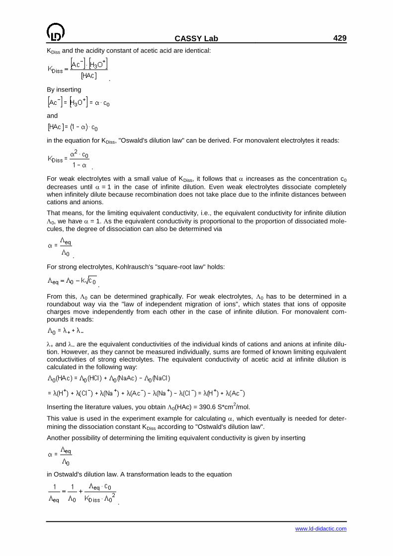
CASSY Lab

429

www.ld-didactic.com

KDiss and the acidity constant of acetic acid are identical:

.

By inserting

and

in the equation for KDiss, "Oswald's dilution law" can be derived. For monovalent electrolytes it reads:

.

For weak electrolytes with a small value of KDiss, it follows that increases as the concentration c0

decreases until = 1 in the case of infinite dilution. Even weak electrolytes dissociate completely when infinitely dilute because recombination does not take place due to the infinite distances between cations and anions.

That means, for the limiting equivalent conductivity, i.e., the equivalent conductivity for infinite dilution

0, we have = 1. s the equivalent conductivity is proportional to the proportion of dissociated mole-cules, the degree of dissociation can also be determined via

.

For strong electrolytes, Kohlrausch's "square-root law" holds:

.

From this, 0 can be determined graphically. For weak electrolytes, 0 has to be determined in a roundabout way via the "law of independent migration of ions", which states that ions of opposite charges move independently from each other in the case of infinite dilution. For monovalent com-pounds it reads:

+ and – are the equivalent conductivities of the individual kinds of cations and anions at infinite dilu-tion. However, as they cannot be measured individually, sums are formed of known limiting equivalent conductivities of strong electrolytes. The equivalent conductivity of acetic acid at infinite dilution is calculated in the following way:

Inserting the literature values, you obtain 0(HAc) = 390.6 S*cm2/mol.

This value is used in the experiment example for calculating , which eventually is needed for deter-

mining the dissociation constant KDiss according to "Ostwald's dilution law".

Another possibility of determining the limiting equivalent conductivity is given by inserting

in Ostwald's dilution law. A transformation leads to the equation

.

430

CASSY Lab

www.ld-didactic.com

If you plot 1/eq against eq*c0, you obtain a straight line with the cut off 1/0 and the slope

1/(KDiss*0), whereby eq*c0 = CA1 for acetic acid. However, as even very small inaccuracies of the measurement lead to big errors, this method it only suited for high-precision measurements. Here the equation is used to check the accuracy of the measurement in the low concentration range.

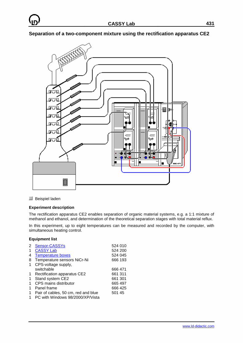
CASSY Lab

431

www.ld-didactic.com

Separation of a two-component mixture using the rectification apparatus CE2

Beispiel laden


The rectification apparatus CE2 enables separation of organic material systems, e.g. a 1:1 mixture of methanol and ethanol, and determination of the theoretical separation stages with total material reflux.

In this experiment, up to eight temperatures can be measured and recorded by the computer, with simultaneous heating control.

Equipment list

2 Sensor-CASSYs 524 010 1 CASSY Lab 524 200 4 Temperature boxes 524 045 8 Temperature sensors NiCr-Ni 666 193 1 CPS-voltage supply, switchable 666 471 1 Rectification apparatus CE2 661 311 1 Stand system CE2 661 301 1 CPS mains distributor 665 497 1 Panel frame 666 425 1 Pair of cables, 50 cm, red and blue 501 45 1 PC with Windows 98/2000/XP/Vista

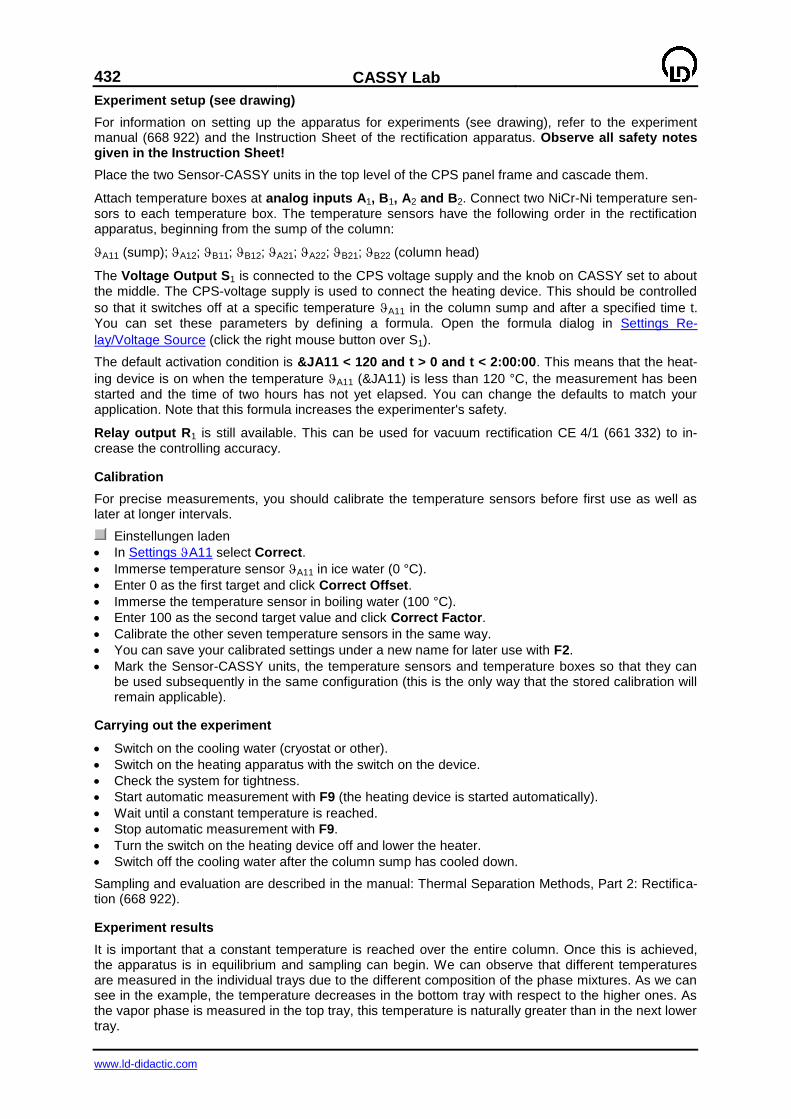
432

CASSY Lab

www.ld-didactic.com


For information on setting up the apparatus for experiments (see drawing), refer to the experiment manual (668 922) and the Instruction Sheet of the rectification apparatus. Observe all safety notes given in the Instruction Sheet!

Place the two Sensor-CASSY units in the top level of the CPS panel frame and cascade them.

Attach temperature boxes at analog inputs A1, B1, A2 and B2. Connect two NiCr-Ni temperature sen-sors to each temperature box. The temperature sensors have the following order in the rectification apparatus, beginning from the sump of the column:

A11 (sump); A12; B11; B12; A21; A22; B21; B22 (column head)

The Voltage Output S1 is connected to the CPS voltage supply and the knob on CASSY set to about the middle. The CPS-voltage supply is used to connect the heating device. This should be controlled

so that it switches off at a specific temperature A11 in the column sump and after a specified time t. You can set these parameters by defining a formula. Open the formula dialog in Settings Re-

lay/Voltage Source (click the right mouse button over S1).

The default activation condition is &JA11 < 120 and t > 0 and t < 2:00:00. This means that the heat-

ing device is on when the temperature A11 (&JA11) is less than 120 °C, the measurement has been started and the time of two hours has not yet elapsed. You can change the defaults to match your application. Note that this formula increases the experimenter's safety.

Relay output R1 is still available. This can be used for vacuum rectification CE 4/1 (661 332) to in-crease the controlling accuracy.

Calibration

For precise measurements, you should calibrate the temperature sensors before first use as well as later at longer intervals.

Einstellungen laden

In Settings A11 select Correct.

Immerse temperature sensor A11 in ice water (0 °C).

Enter 0 as the first target and click Correct Offset.

Immerse the temperature sensor in boiling water (100 °C).

Enter 100 as the second target value and click Correct Factor.

Calibrate the other seven temperature sensors in the same way.

You can save your calibrated settings under a new name for later use with F2.

Mark the Sensor-CASSY units, the temperature sensors and temperature boxes so that they can be used subsequently in the same configuration (this is the only way that the stored calibration will remain applicable).


Switch on the cooling water (cryostat or other).

Switch on the heating apparatus with the switch on the device.

Check the system for tightness.

Start automatic measurement with F9 (the heating device is started automatically).

Wait until a constant temperature is reached.

Stop automatic measurement with F9.

Turn the switch on the heating device off and lower the heater.

Switch off the cooling water after the column sump has cooled down.

Sampling and evaluation are described in the manual: Thermal Separation Methods, Part 2: Rectifica-tion (668 922).

Experiment results

It is important that a constant temperature is reached over the entire column. Once this is achieved, the apparatus is in equilibrium and sampling can begin. We can observe that different temperatures are measured in the individual trays due to the different composition of the phase mixtures. As we can see in the example, the temperature decreases in the bottom tray with respect to the higher ones. As the vapor phase is measured in the top tray, this temperature is naturally greater than in the next lower tray.

CASSY Lab

433

www.ld-didactic.com

Absorption of UV radiation


Beispiel laden

Safety note

Do not look directly into the ray.


The transmission of several materials for UV-A, UV-B, and UV-C radiation is determined and the effect of sunscreens is tested by measuring the transmitted illuminance.

Equipment list

1 Sensor-CASSY 524 010 1 CASSY Lab 524 200 1 Lux box 524 051 1 UV-A sensor 666 244 and/or 1 UV-B sensor 666 245 and/or 1 UV-C sensor 666 246 1 UV-IR-VIS experiment kit 666 265 1 PC with Windows 98/2000/XP/Vista


Connect the lux box together with the selected UV sensor (A, B, or C) to the Sensor-CASSY. Using a clamp, fix the UV sensor as close as possible to the appropriate exit aperture of the UV-IR-VIS ex-periment kit. However, see to it that the holding rail remains free for material samples to be inserted. Connect the experiment kit via the plug-in power supply.

Read the instruction sheets of the UV-IR-VIS experiment kit and the sensors carefully.

434

CASSY Lab

www.ld-didactic.com

Calibration

Before using a UV sensor for the first time, you have to calibrate it.

Einstellungen laden

Select the Correct button in Settings Illuminance EA1, enter the factor printed on the sensor, and click Correct Factor.

The calibration is only valid for the particular corrected sensor.



Switch the desired UV lamp on, and wait approx. 5 minutes until a stable final value has been

reached in the display window for the Illuminance EA1. You may have to select another measuring range in Settings Illuminance EA1, if the preset range is exceeded.

Record the first measured value (without absorber) by pressing the key F9 or the button.

One after another insert the following absorbers in the holding rail between the UV lamp and the sensor: - quartz glass, - window glass, - plexiglass, - PVC, - quartz glass with a thin film of sunscreen filter (Parsol), - optionally: quartz glass with a thin film of cooking oil, spectacle lens and record a further measured value for each item.

Evaluation

The values are displayed in two diagrams: in the bar chart Illuminance, the absolute measured values are shown. With Alt+T explanatory text can be assigned to the bars.

The second diagram, Transmission, shows the percentage of the examined radiation that has passed through the respective material.

The specific filtering effect of some materials on UV-B and UV-C radiation and their transmission of UV-A radiation is of particular interest with regard to danger to humans:

In the case of the quartz glass which has been covered with sunscreen filter, the transmission of UV-A radiation, which gives rise to the suntan, is significantly higher than the transmission of the dangerous UV-B and UV-C radiation. In the past decades, the UV-B irradiation on the surface of the earth has increased because the ozone layer has continuously become thinner and thinner. This effect is con-sidered to be the cause of damage of hereditary substance, skin cancer, and blindness. The agent Parsol protects the skin with its UV-B and UV-C filtering effect and passes a great proportion of the tanning UV-A radiation.

As UV-C radiation is even more aggressive than UV-B radiation, the UV-C filtering effect of many ma-terials and particularly of the atmosphere is a prerequisite for life on earth to be possible.

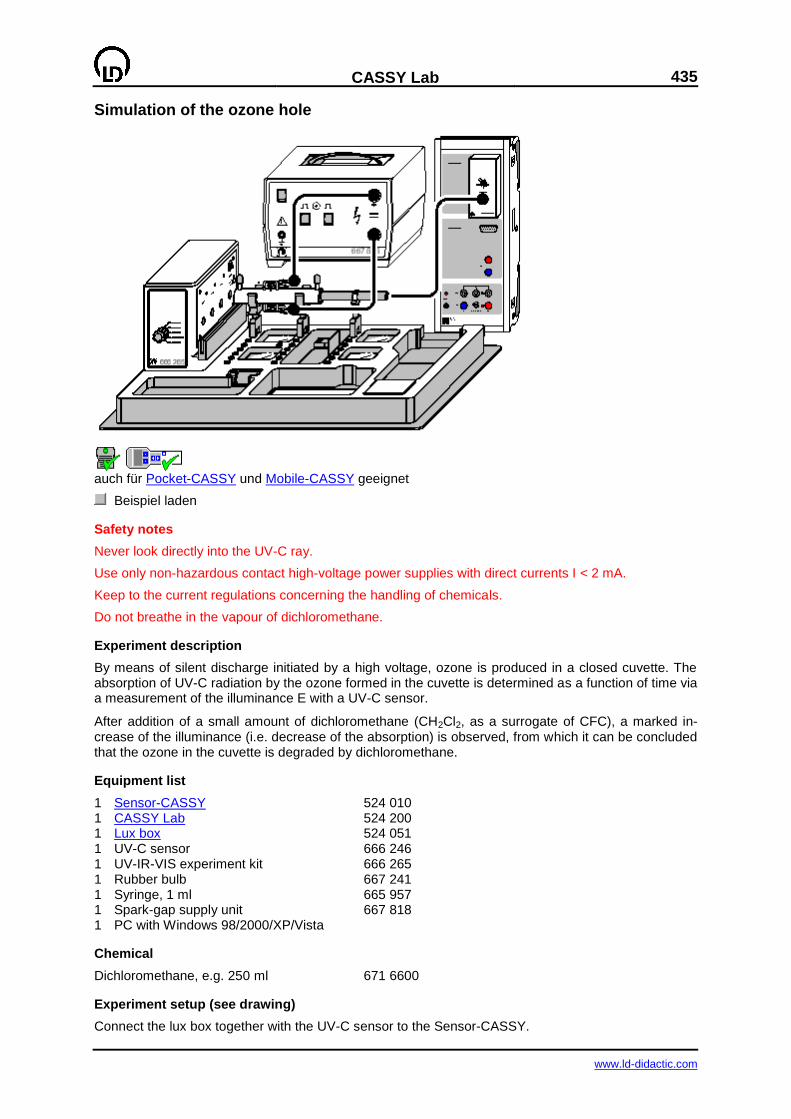
CASSY Lab

435

www.ld-didactic.com

Simulation of the ozone hole


Beispiel laden

Safety notes

Never look directly into the UV-C ray.

Use only non-hazardous contact high-voltage power supplies with direct currents I < 2 mA.

Keep to the current regulations concerning the handling of chemicals.

Do not breathe in the vapour of dichloromethane.


By means of silent discharge initiated by a high voltage, ozone is produced in a closed cuvette. The absorption of UV-C radiation by the ozone formed in the cuvette is determined as a function of time via a measurement of the illuminance E with a UV-C sensor.

After addition of a small amount of dichloromethane (CH2Cl2, as a surrogate of CFC), a marked in-crease of the illuminance (i.e. decrease of the absorption) is observed, from which it can be concluded that the ozone in the cuvette is degraded by dichloromethane.

Equipment list

1 Sensor-CASSY 524 010 1 CASSY Lab 524 200 1 Lux box 524 051 1 UV-C sensor 666 246 1 UV-IR-VIS experiment kit 666 265 1 Rubber bulb 667 241 1 Syringe, 1 ml 665 957 1 Spark-gap supply unit 667 818 1 PC with Windows 98/2000/XP/Vista

Chemical

Dichloromethane, e.g. 250 ml 671 6600


Connect the lux box together with the UV-C sensor to the Sensor-CASSY.

436

CASSY Lab

www.ld-didactic.com

Set up the UV-IR-VIS experiment kit so that nobody can be blinded by the UV-C radiation. Mount the round cuvette from the UV-IR-VIS experiment kit with two holders immediately in front of the exit aper-ture of the UV-C radiation, and connect the metal contacts to the spark-gap supply unit via two tapping clamps and the connecting leads. As the electric field is very strong, see to it that the connecting leads do not lie one on top of the other or too close to the sensor, the Sensor-CASSY or their cabling. Using a holder, insert the UV sensor immediately in front of the cuvette window. Connect the UV-IR-VIS experiment kit via the plug-in power supply.

Read the instruction sheets of the UV-IR-VIS experiment kit and of the spark-gap supply unit carefully.

Calibration

Before using the UV sensor, you have to calibrate it.

Einstellungen laden





Using the rubber bulb, remove residual gas that may be left in the round cuvette, and close the openings of the cuvette with the two black caps.

Switch the UV-C lamp on, and wait approx. 5 minutes until a stable final value has been reached in

the display window for the Illuminance EA1.

You may have to select another measuring range in Settings Illuminance EA1, if the preset range is exceeded.

Switch the spark-gap supply unit on, and set it to the mode "continuous operation" (red LED shines).

Immediately start recording the measuring data by pressing the key F9 or the button.

During the entire measurement do not move the cuvette and the sensor as this would distort the measurement.

Switch the spark-gap supply unit off after 5 to 10 minutes and mark this moment in the diagram by a vertical line with Alt+V.

Switch the supply unit on again after approx. 3 to 5 minutes, and set another mark with Alt+V at the corresponding position in the diagram.

After another 3 to 5 minutes, shake the closed bottle containing dichloromethane briefly, and, using the syringe, take 1 ml of the vapour from the gas space over the liquid. Close the bottle. Do not breathe in the vapour.

Open one of the caps of the round cuvette, inject the content of the syringe, and, having closed the cuvette, set another mark with Alt+V at the moment of injection.

Stop the data logging by pressing the key F9 or the button after another 3 to 5 minutes has elapsed, and switch the high voltage off.

Remarks

The formation and degradation of ozone in the stratosphere (10 to 35 km altitude) is governed by sev-eral reactions:

These reactions keep the ozone concentration in a stationary equilibrium.

If UV-C radiation with wavelengths below 240 nm acts on oxygen, this leads to ozone formation (reac-tions 1 and 2) because the oxygen radicals formed in this process react with other oxygen molecules

CASSY Lab

437

www.ld-didactic.com

to ozone giving off their kinetic energy to a third inert reactant M (e.g. a nitrogen molecule). As the mercury lamp used in the UV-IR-VIS experiment kit generates UV-C radiation of 254 nm wavelength, which is not able to split oxygen molecules, the reaction 1 is initiated by a high voltage of 10 kV in this experiment.

The degradation of ozone, too, takes place with the aid of UV radiation: however, for the splitting (re-action 3), radiation with wavelengths below 310 nm is sufficient. This UV dependence of the ozone formation and degradation leads to a complete absorption of UV-C radiation (220-280 nm, initiation of the reactions 1 and 3) and to a partial absorption of UV-B radiation (280-320 nm, initiation of the reac-tion 3) by the ozone layer in the stratosphere.

The degradation of ozone by CFC is also initiated by UV-C radiation:

The chlorine radical created in reaction 5 by absorption of UV-C radiation is set free again and again in a continuous repetition of the reactions 6 and 7, whereby the oxygen radical in reaction 7 comes from the natural degeneration of ozone (reaction 3) or from the natural splitting of oxygen (reaction 1). Therefore a few chlorine radicals suffice to initiate a ozone degenerating chain reaction.

In contrast to completely halogenated CFC, dichloromethane, which is used in this experiment, is al-ready degenerated in the troposhere and does not damage the ozone layer.

Evaluation

In order to get a clearer display, you can remove the values corresponding to short-term fluctuations in the illuminance caused by switching on and off the high voltage by double-clicking these values in the table and pressing the blank key.

To start the evaluation, enter the first value of the measurements series for the illuminance EA1 instead of the default value of "0.290" in the field Formula of Settings Absorption A. An explanatory text can be inserted with Alt+T to label the sections separated by the vertical lines.

After switching the high voltage on, the reactions 1 and 2 (ozone formation) predominate over the degeneration reactions 3 and 4. This is seen from the decrease in illuminance or from the increasing absorption of UV-C radiation (range A in the diagrams), respectively. When the high voltage is switched off, the ozone concentration is reduced as oxygen radicals from reaction 1 are no longer available for ozone formation, and therefore the degeneration reactions 3 and 4 predominate. As a consequence, the illuminance rises quickly and the absorption of UV-C radiation is reduced (range B) indicating a drop of the ozone concentration.

In range C, the illuminance decreases again due to another production of ozone by the high voltage. Addition of a small amount of dichloromethane again results in an increasing illuminance despite the

high voltage, which is still applied (range D in the diagrams). Even a very small amount of CH2Cl2 vapour leads to a strong decrease in ozone concentration accompanied by a reduction of the UV-C absorption.

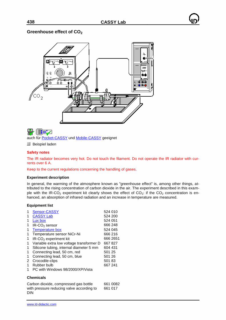
438

CASSY Lab

www.ld-didactic.com

Greenhouse effect of CO2


Beispiel laden

Safety notes

The IR radiator becomes very hot. Do not touch the filament. Do not operate the IR radiator with cur-rents over 6 A.

Keep to the current regulations concerning the handling of gases.


In general, the warming of the atmosphere known as "greenhouse effect" is, among other things, at-tributed to the rising concentration of carbon dioxide in the air. The experiment described in this exam-

ple with the IR-CO2 experiment kit clearly shows the effect of CO2: if the CO2 concentration is en-

hanced, an absorption of infrared radiation and an increase in temperature are measured.

Equipment list

1 Sensor-CASSY 524 010 1 CASSY Lab 524 200 1 Lux box 524 051 1 IR-CO2 sensor 666 248

1 Temperature box 524 045 1 Temperature sensor NiCr-Ni 666 216 1 IR-CO2 experiment kit 666 2651

1 Variable extra low voltage transformer D 667 827 1 Silicone tubing, internal diameter 5 mm 604 431 1 Connecting lead, 50 cm, red 501 25 1 Connecting lead, 50 cm, blue 501 26 2 Crocodile-clips 501 83 1 Rubber bulb 667 241 1 PC with Windows 98/2000/XP/Vista

Chemicals

Carbon dioxide, compressed gas bottle 661 0082 with pressure reducing valve according to DIN

661 017

CASSY Lab

439

www.ld-didactic.com


Read the instruction sheets of the IR-CO2 experiment kit, the variable extra low voltage transformer

and the IR-CO2 sensor carefully.

Connect the lux box with the IR-CO2 sensor to input A and the temperature box with the temperature

sensor being plugged in T1 to input B of the Sensor-CASSY.

Insert the IR radiator in the holding clamp on the tray, clamp the measuring cuvette which is covered with two plastic foils in the holders on the tray so that its distance from the radiator is at least 5 mm, and insert the temperature sensor in the GL14 thread so that the tip of the sensing element in posi-tioned in the centre of the cuvette.

Using the holding clamp, mount the IR-CO2 sensor immediately behind the measuring cuvette, and connect the direct current output of the variable extra low voltage transformer (0...20 V) to the contacts of the radiator via the connecting leads.

Connect one of the inlets of the cuvette to the compressed gas bottle via the tubing. Close the other inlet with a black plastic cap.

Calibration

Before using the IR-CO2 sensor, you have to calibrate it.

Einstellungen laden





Adjust a current of at most 6 A so that the filament only glows very weakly. The measured tem-perature should not exceed 80 °C.

When the temperature and the illuminance are virtually constant (observe the display windows in

CASSY Lab), start the measurement by pressing the key F9 or the button.

After approx. one minute, remove the black cover cap and allow carbon dioxide to flow through the cuvette for about one minute. Mark the moment when you switch the carbon dioxide flow on by a vertical line by pressing Alt+V and positioning the line with the mouse.

Set another vertical line (Alt+V) when you switch the carbon dioxide current off, and close the cu-vette with the black cap.

Wait another 3 to 5 minutes until the temperature is constant again. Then stop the measurement by

pressing the key F9 or the button, and switch the variable extra low voltage transformer off.

Evaluation

In the two diagrams, the relation between the temperature (first diagram) / illuminance (second dia-gram) and the absorption by carbon dioxide is illustrated.

For the evaluation, the stationary states before and after the introduction of carbon dioxide are rele-vant.

1. A comparison of the temperatures and the illuminances before and after the cuvette was filled with carbon dioxide shows a marked rise in temperature accompanied by a reduction of the illuminance.

For comparing the initial values with the values at the end of the measurement, first enter the mean values in the diagram. To do this, click the diagram with the right mouse button, select Draw Mean Value, and mark the respective stationary curve range at the beginning and at the end of the meas-urement series. The mean value calculated by CASSY Lab is displayed by a horizontal line. The cor-responding value can be dragged with the mouse from the status line into the diagram.

Hint: if the scale of the Y axis relevant for the respective measured values is activated via the diagram

buttons EA1 and B11, the mean values and labels are displayed in the same colour as the correspond-ing curve.

440

CASSY Lab

www.ld-didactic.com

The exact difference between the two mean values of the temperature and the illuminance is output in the status line when Alt+D is pressed and subsequently the two mean value straight lines are clicked. This value, too, can be dragged into the diagram with the mouse.

2. For determining the absorption, enter the first mean value E0 (initial value) in Settings illuminance E0 in the field formula. For the calculation of the absorption A, the formula

is preset. Mean values and differences are entered in the same way as in the case of the first diagram.

The results make it clear that carbon dioxide absorbs a great proportion of the infrared radiation. The rise of the temperature in the cuvette can be attributed to this absorption.

CASSY Lab

441

www.ld-didactic.com

Experiment examples biology

These experiment examples support you in using CASSY Lab. The measurement data or settings for the examples can be loaded directly into CASSY Lab. Simply click in the buttons in the descriptions.

New examples are labelled with a red .

Pulse

Skin resistance

Electrocardiogram

Electromyogram

Blood pressure

Reaction time

Lung volume (spirometry)

Long-term measurement of climate data

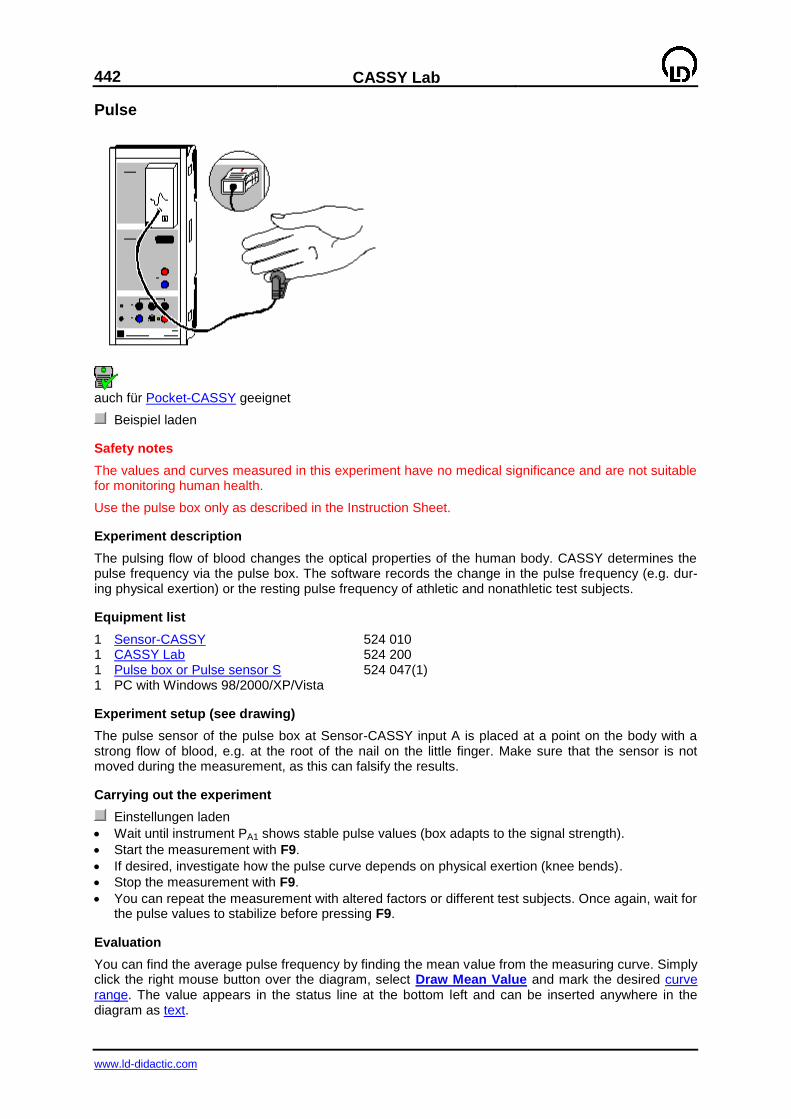
442

CASSY Lab

www.ld-didactic.com

Pulse


Beispiel laden

Safety notes

The values and curves measured in this experiment have no medical significance and are not suitable for monitoring human health.

Use the pulse box only as described in the Instruction Sheet.


The pulsing flow of blood changes the optical properties of the human body. CASSY determines the pulse frequency via the pulse box. The software records the change in the pulse frequency (e.g. dur-ing physical exertion) or the resting pulse frequency of athletic and nonathletic test subjects.

Equipment list

1 Sensor-CASSY 524 010 1 CASSY Lab 524 200 1 Pulse box or Pulse sensor S 524 047(1) 1 PC with Windows 98/2000/XP/Vista


The pulse sensor of the pulse box at Sensor-CASSY input A is placed at a point on the body with a strong flow of blood, e.g. at the root of the nail on the little finger. Make sure that the sensor is not moved during the measurement, as this can falsify the results.


Einstellungen laden

Wait until instrument PA1 shows stable pulse values (box adapts to the signal strength).


If desired, investigate how the pulse curve depends on physical exertion (knee bends).


You can repeat the measurement with altered factors or different test subjects. Once again, wait for the pulse values to stabilize before pressing F9.

Evaluation

You can find the average pulse frequency by finding the mean value from the measuring curve. Simply click the right mouse button over the diagram, select Draw Mean Value and mark the desired curve range. The value appears in the status line at the bottom left and can be inserted anywhere in the diagram as text.

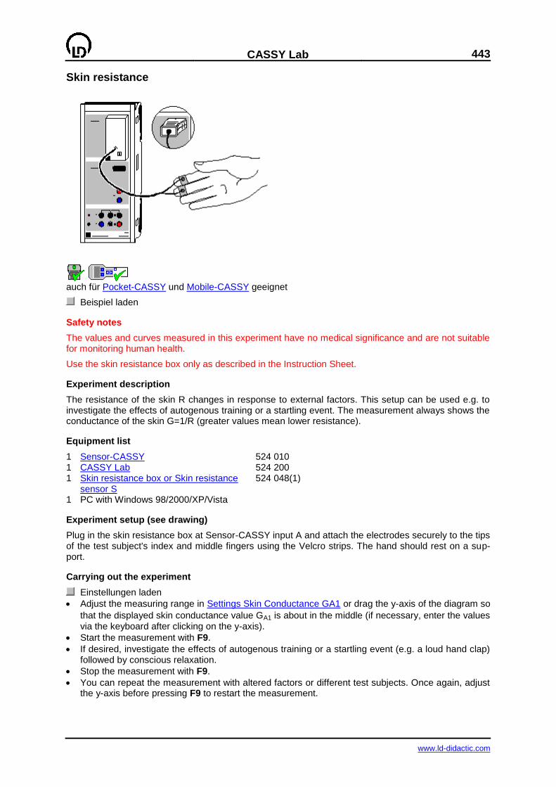
CASSY Lab

443

www.ld-didactic.com

Skin resistance


Beispiel laden

Safety notes


Use the skin resistance box only as described in the Instruction Sheet.


The resistance of the skin R changes in response to external factors. This setup can be used e.g. to investigate the effects of autogenous training or a startling event. The measurement always shows the conductance of the skin G=1/R (greater values mean lower resistance).

Equipment list

1 Sensor-CASSY 524 010 1 CASSY Lab 524 200 1 Skin resistance box or Skin resistance

sensor S 524 048(1)



Plug in the skin resistance box at Sensor-CASSY input A and attach the electrodes securely to the tips of the test subject's index and middle fingers using the Velcro strips. The hand should rest on a sup-port.


Einstellungen laden

Adjust the measuring range in Settings Skin Conductance GA1 or drag the y-axis of the diagram so

that the displayed skin conductance value GA1 is about in the middle (if necessary, enter the values via the keyboard after clicking on the y-axis).


If desired, investigate the effects of autogenous training or a startling event (e.g. a loud hand clap) followed by conscious relaxation.


You can repeat the measurement with altered factors or different test subjects. Once again, adjust the y-axis before pressing F9 to restart the measurement.

444

CASSY Lab

www.ld-didactic.com

Evaluation

The diagram reveals how the skin conductance changes in response to external factors.

You can determine the average skin conductance by finding the mean value from the measuring curve. Simply click the right mouse button over the diagram, select Draw Mean Value and mark the desired curve range. The value appears in the status line at the bottom left and can be inserted any-where in the diagram as text.

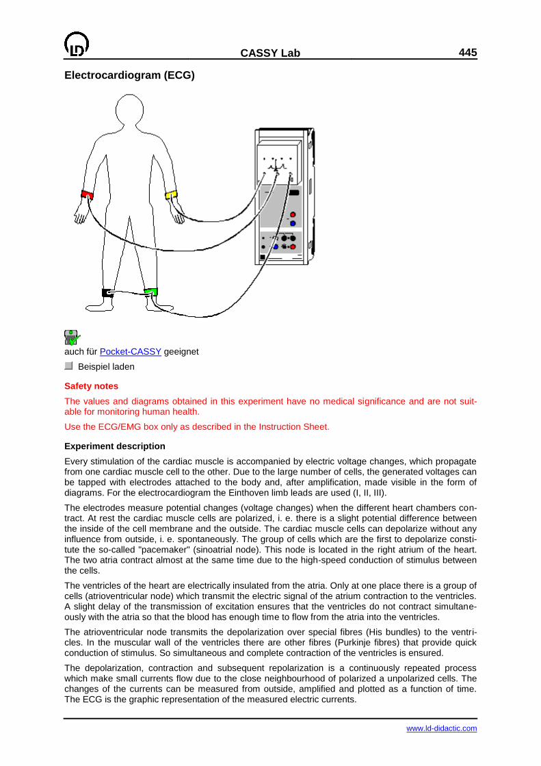
CASSY Lab

445

www.ld-didactic.com

Electrocardiogram (ECG)


Beispiel laden

Safety notes

The values and diagrams obtained in this experiment have no medical significance and are not suit-able for monitoring human health.

Use the ECG/EMG box only as described in the Instruction Sheet.


Every stimulation of the cardiac muscle is accompanied by electric voltage changes, which propagate from one cardiac muscle cell to the other. Due to the large number of cells, the generated voltages can be tapped with electrodes attached to the body and, after amplification, made visible in the form of diagrams. For the electrocardiogram the Einthoven limb leads are used (I, II, III).

The electrodes measure potential changes (voltage changes) when the different heart chambers con-tract. At rest the cardiac muscle cells are polarized, i. e. there is a slight potential difference between the inside of the cell membrane and the outside. The cardiac muscle cells can depolarize without any influence from outside, i. e. spontaneously. The group of cells which are the first to depolarize consti-tute the so-called "pacemaker" (sinoatrial node). This node is located in the right atrium of the heart. The two atria contract almost at the same time due to the high-speed conduction of stimulus between the cells.

The ventricles of the heart are electrically insulated from the atria. Only at one place there is a group of cells (atrioventricular node) which transmit the electric signal of the atrium contraction to the ventricles. A slight delay of the transmission of excitation ensures that the ventricles do not contract simultane-ously with the atria so that the blood has enough time to flow from the atria into the ventricles.

The atrioventricular node transmits the depolarization over special fibres (His bundles) to the ventri-cles. In the muscular wall of the ventricles there are other fibres (Purkinje fibres) that provide quick conduction of stimulus. So simultaneous and complete contraction of the ventricles is ensured.

The depolarization, contraction and subsequent repolarization is a continuously repeated process which make small currents flow due to the close neighbourhood of polarized a unpolarized cells. The changes of the currents can be measured from outside, amplified and plotted as a function of time. The ECG is the graphic representation of the measured electric currents.

446

CASSY Lab

www.ld-didactic.com

Equipment list

1 Sensor-CASSY 524 010 1 CASSY Lab 524 200 1 ECG/EMG box 524 049 1 Electrode gel 662 112 1 Disinfectant spray 662 113 1 PC with Windows 98/2000/XP/Vista


The test subject should be relaxed and in a resting posture, as otherwise the ECG signal can be over-laid by the electrical potentials of the skeletal musculature, falsifying the measurement. To reduce the skin resistance, spread electrode gel (662 112) on the electrodes and attach them to the appropriate points in the body using the rubber straps. Then attach the leads to the electrodes as follows:

red right arm yellow left arm green left calf black right calf

Important

Clean the electrodes after each use with a paper towel or similar to prevent a salt layer from forming when the gel dries. Then spray the electrodes and the corresponding skin sites with disinfectant (662 113) to ensure maximum hygiene.


Einstellungen laden


The three leads according to Einthoven are recorded simultaneously.


Evaluation

For the sake of clarity, part of the display should be enlarged with the Zoom function before evaluation

A typical part of an ECG is given by a flat line, the isoelectric line. Deviations from this line are due to the electric activity of the cardiac muscle.

In a typical ECG, the first deviation from this line is a small upward deflection. The P-wave last approx. 0.05 seconds. For the evaluation a vertical line can be set at the beginning and the end of the P-wave. The duration can be determined by a differential measurement between the two lines. The P-wave is based on the depolarization and contraction of the atria.

Next the ECG returns to the isoelectric line. During this time, the atrioventricular node transmits the excitation via the His bundle and the Purkinje fibres to the ventricles. The depolarization of the AV node leads to a slight downward pulse, the Q-wave. Immediately afterwards a quick rise (R-wave) and a subsequent drop below the isoelectric line (S-wave) occur. Then the ECG returns to the initial value. These three waves are called the QRS complex, which is brought about by the depolarization and contraction of the ventricles.

After a further break the cell repolarize. The corresponding current causes an upward wave, the T-wave.

The sequence from P over QRS to T is one cycle of the heart. The number of cycles per minute corre-sponds to the pulse beat.

Further experiment proposals

Recording an ECG before and after exertion (e. g. knee-bends)

Statistics of the duration of the individual sections for all students in the class

Differences between women and men

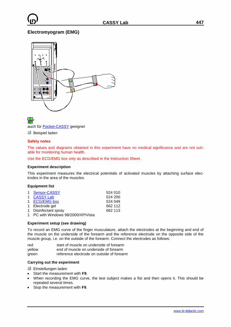
CASSY Lab

447

www.ld-didactic.com

Electromyogram (EMG)


Beispiel laden

Safety notes

The values and diagrams obtained in this experiment have no medical significance and are not suit-able for monitoring human health.

Use the ECG/EMG box only as described in the Instruction Sheet.


This experiment measures the electrical potentials of activated muscles by attaching surface elec-trodes in the area of the muscles.

Equipment list

1 Sensor-CASSY 524 010 1 CASSY Lab 524 200 1 ECG/EMG box 524 049 1 Electrode gel 662 112 1 Disinfectant spray 662 113 1 PC with Windows 98/2000/XP/Vista


To record an EMG curve of the finger musculature, attach the electrodes at the beginning and end of the muscle on the underside of the forearm and the reference electrode on the opposite side of the muscle group, i.e. on the outside of the forearm. Connect the electrodes as follows:

red start of muscle on underside of forearm yellow end of muscle on underside of forearm green reference electrode on outside of forearm


Einstellungen laden


When recording the EMG curve, the test subject makes a fist and then opens it. This should be repeated several times.


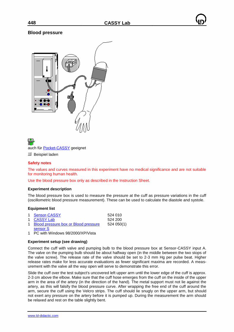
448

CASSY Lab

www.ld-didactic.com

Blood pressure


Beispiel laden

Safety notes


Use the blood pressure box only as described in the Instruction Sheet.


The blood pressure box is used to measure the pressure at the cuff as pressure variations in the cuff (oscillometric blood pressure measurement). These can be used to calculate the diastole and systole.

Equipment list

1 Sensor-CASSY 524 010 1 CASSY Lab 524 200 1 Blood pressure box or Blood pressure

sensor S 524 050(1)



Connect the cuff with valve and pumping bulb to the blood pressure box at Sensor-CASSY input A. The valve on the pumping bulb should be about halfway open (in the middle between the two stops of the valve screw). The release rate of the valve should be set to 2-3 mm Hg per pulse beat. Higher release rates make for less accurate evaluations as fewer significant maxima are recorded. A meas-urement with the valve all the way open will serve to demonstrate this error.

Slide the cuff over the test subject's uncovered left upper arm until the lower edge of the cuff is approx. 2-3 cm above the elbow. Make sure that the cuff hose emerges from the cuff on the inside of the upper arm in the area of the artery (in the direction of the hand). The metal support must not lie against the artery, as this will falsify the blood pressure curve. After wrapping the free end of the cuff around the arm, secure the cuff using the Velcro strips. The cuff should lie snugly on the upper arm, but should not exert any pressure on the artery before it is pumped up. During the measurement the arm should be relaxed and rest on the table slightly bent.

CASSY Lab

449

www.ld-didactic.com


Einstellungen laden

Correct the zero point of the pressure display if necessary. To do this, open Settings Blood Pres-sure pA1 and select —> 0 <—.

Using the bulb, pump up the cuff to about 180 mmHg (depending on the expected systolic pres-sure). The display shows how the cuff pressure increases.


The arm must not move during the experiment. The amplitude of the oscillations increases during the measurement (once the pressure drops below the systolic threshold) and then decreases (once the pressure drops below the diastolic threshold).

When the amplitude of the oscillations remains constant several times in a row, stop the measure-ment with F9.

Vent the cuff completely by pressing the red button on the hand valve.

Wait at least two minutes before repeating measurements on the same test subject.

Evaluation

The pressure varies only slightly at supersystolic cuff pressures, due to pulse beats in the compressed arterial section. At the moment in which the cuff pressure falls below the systolic pressure and a brief systolic opening occurs in the artery, the oscillations increase and reach a maximum at the mean arte-rial blood pressure (which corresponds to the arithmetic mean of the pressure). The diastolic blood pressure corresponds to the point at which the oscillations stop decreasing, i.e. when the blood ves-sels are open during the entire diastole. The remaining pressure variations are caused by pulse beats transmitted to the cuff.

To calculate the systole and diastole, press the right mouse button in the diagram, select in the other evaluations Determine Systole and Diastole and mark the entire curve range. The systole and dias-tole values appear in the status line at the bottom left and can be inserted anywhere in the diagram as text.

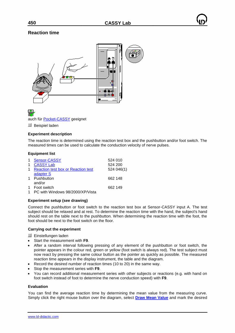
450

CASSY Lab

www.ld-didactic.com

Reaction time


Beispiel laden


The reaction time is determined using the reaction test box and the pushbutton and/or foot switch. The measured times can be used to calculate the conduction velocity of nerve pulses.

Equipment list

1 Sensor-CASSY 524 010 1 CASSY Lab 524 200 1 Reaction test box or Reaction test

adapter S 524 046(1)

1 Pushbutton 662 148 and/or 1 Foot switch 662 149 1 PC with Windows 98/2000/XP/Vista


Connect the pushbutton or foot switch to the reaction test box at Sensor-CASSY input A. The test subject should be relaxed and at rest. To determine the reaction time with the hand, the subject's hand should rest on the table next to the pushbutton. When determining the reaction time with the foot, the foot should be next to the foot switch on the floor.


Einstellungen laden


After a random interval following pressing of any element of the pushbutton or foot switch, the pointer appears in the colour red, green or yellow (foot switch is always red). The test subject must now react by pressing the same colour button as the pointer as quickly as possible. The measured reaction time appears in the display instrument, the table and the diagram.

Record the desired number of reaction times (10 to 20) in the same way.

Stop the measurement series with F9.

You can record additional measurement series with other subjects or reactions (e.g. with hand on foot switch instead of foot to determine the nerve conduction speed) with F9.

Evaluation

You can find the average reaction time by determining the mean value from the measuring curve. Simply click the right mouse button over the diagram, select Draw Mean Value and mark the desired

CASSY Lab

451

www.ld-didactic.com

curve range. The value appears in the status line at the bottom left and can be inserted anywhere in the diagram as text.

To determine the nerve conduction velocity you need to determine the difference in the lengths of the conducting nerve paths by first measuring the length from the spine at the level of the shoulder joint to the middle of the upper arm. Then measure from the same point to the middle of the thigh.

The mean nerve conduction velocity v is calculated as the quotient of the length difference (foot – hand) and the time difference (reaction time foot – reaction time hand) as

v = ( l(foot) – l/(hand) ) / ( t(foot) – t(hand) ).

452

CASSY Lab

www.ld-didactic.com

Lung volume (spirometry)


Beispiel laden

Safety notes

Never use the spirometer without a bacteria filter.


Use the spirometer box only as described in the Instruction Sheet.


The spirometer is used to determine the respiratory volume. The device operates according to the pneumotachographic principle and measures the volume flux. CASSY Lab then determines the respi-ratory volume through integration.

Equipment list

1 Sensor-CASSY 524 010 1 CASSY Lab 524 200 1 Spirometer box 524 056 1 Mouthpiece for the spirometer, 30 items 662 3812 1 Bacteria filter for spirometer, 30 items 662 3813 1 PC with Windows 98/2000/XP/Vista


Connect the spirometer box to Sensor-CASSY input A about 10 seconds before the measurement (warm-up phase). Use a new mouthpiece and a new bacteria filter for every test person, and disinfect the sieves regularly with a disinfectant.


Einstellungen laden

Compensate the zero point off the displayed volume flux dVA1. Open the window Settings Volume Flux dVA1, select —> 0 <— and make sure that no air is flowing through the spirometer during this procedure.

Start the measurement as soon as possible afterwards with F9 (as long as the thermal error in

volume flux dVA1 is still negligible).

Breathe evenly through the spirometer three or four times. Then inhale and exhale as much air as possible through the spirometer. Then breathe evenly again.

CASSY Lab

453

www.ld-didactic.com


Evaluation

The tidal volume V1 is the difference between the maximum and minimum for normal breathing. You can determine this e.g. by setting horizontal lines or directly by measuring the difference. You can insert this value at any point in the diagram as text.

The vital capacity V2 is calculated as the sum of the inspiratory and expiratory reserve volume and the tidal volume. It can be determined from the minimum and maximum at maximum inspiration and expi-ration analogously to the tidal volume.

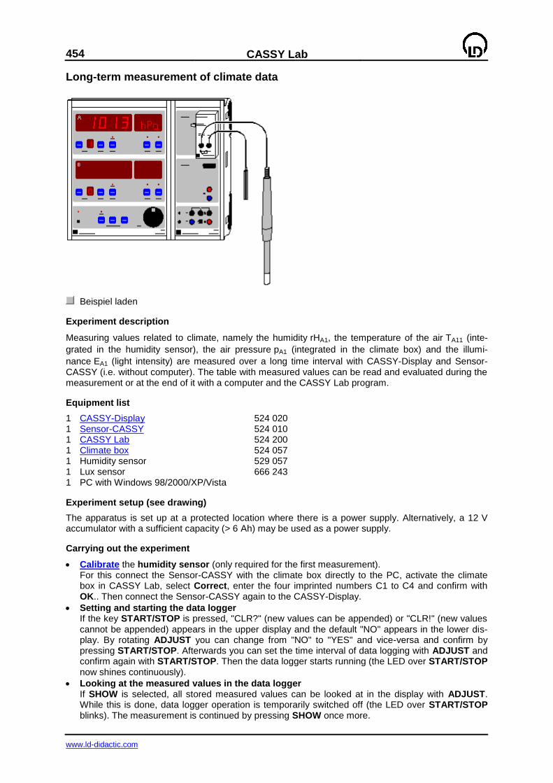
454

CASSY Lab

www.ld-didactic.com

Long-term measurement of climate data

Beispiel laden


Measuring values related to climate, namely the humidity rHA1, the temperature of the air TA11 (inte-

grated in the humidity sensor), the air pressure pA1 (integrated in the climate box) and the illumi-

nance EA1 (light intensity) are measured over a long time interval with CASSY-Display and Sensor-CASSY (i.e. without computer). The table with measured values can be read and evaluated during the measurement or at the end of it with a computer and the CASSY Lab program.

Equipment list

1 CASSY-Display 524 020 1 Sensor-CASSY 524 010 1 CASSY Lab 524 200 1 Climate box 524 057 1 Humidity sensor 529 057 1 Lux sensor 666 243 1 PC with Windows 98/2000/XP/Vista


The apparatus is set up at a protected location where there is a power supply. Alternatively, a 12 V accumulator with a sufficient capacity (> 6 Ah) may be used as a power supply.


Calibrate the humidity sensor (only required for the first measurement). For this connect the Sensor-CASSY with the climate box directly to the PC, activate the climate box in CASSY Lab, select Correct, enter the four imprinted numbers C1 to C4 and confirm with OK.. Then connect the Sensor-CASSY again to the CASSY-Display.

Setting and starting the data logger If the key START/STOP is pressed, "CLR?" (new values can be appended) or "CLR!" (new values cannot be appended) appears in the upper display and the default "NO" appears in the lower dis-play. By rotating ADJUST you can change from "NO" to "YES" and vice-versa and confirm by pressing START/STOP. Afterwards you can set the time interval of data logging with ADJUST and confirm again with START/STOP. Then the data logger starts running (the LED over START/STOP now shines continuously).

Looking at the measured values in the data logger If SHOW is selected, all stored measured values can be looked at in the display with ADJUST. While this is done, data logger operation is temporarily switched off (the LED over START/STOP blinks). The measurement is continued by pressing SHOW once more.

CASSY Lab

455

www.ld-didactic.com

Activating economy operation of the CASSY-Display It is possible to activate economy operation during the measurement by switching off the display of the CASSY-Display for long measuring times. For this the CASSY with number 0 is selected in both displays with the key NEXT. The displays go out and the Sensor-CASSY is switched off. For every new measurement the instruments are switched on for a short time interval.

Evaluation

For the data readout connect the CASSY-Display to a computer with CASSY Lab. The CASSY-Display can be transported to the computer without power supply (the measured values remain stored). The start of the measurement is entered in the comment field automatically.

In the example, a measurement series of the climate at Hanover from December 15, 2000 to February 23, 2001 is shown. The measuring interval was half an hour.

The maximum number of measured values depends on the number of measured quantities. In this example a total of approx. 5000 lines of measured values is possible. This corresponds to a maximum measuring period of 100 days.

Remark

In order that faultless operation of the CASSY-Display is ensured, the version of its firmware should be 1.08 or higher. If necessary, the CASSY-Display can be updated by CASSY Lab. When this is done, all measured data that might be stored in the CASSY-Display are deleted.

456

CASSY Lab

www.ld-didactic.com

Experiment examples technology

These experiment examples support you in using CASSY Lab. If available, the corresponding label is given. The measurement data or settings for the examples can be loaded directly into CASSY Lab.

Simply click the buttons in the descriptions. New examples are labelled with a red .

T 3.2.4 Motor vehicle – ignition systems

T 3.2.5 Motor vehicle – mixture formation systems

T 3.2.7.1 Motor vehicle – on-board computer with radio

T 3.2.7.5 Motor vehicle – comfort system with CAN bus

T 3.2.7.5 Motor vehicle – investigating CAN data bus signals

T 7.2.2.1 Pulse code modulation (quantization)

T 7.4.1 Physical principles of microwave technology (characteristics of the Gunn oscillator)

T 7.4.2 Parallel plate line (TEM and TE modes)

T 7.4.3 Microwave propagation in waveguides (measurement of the standing wave ratio)

T 7.6 Antenna technology

T 12.5.3 Drive engineering

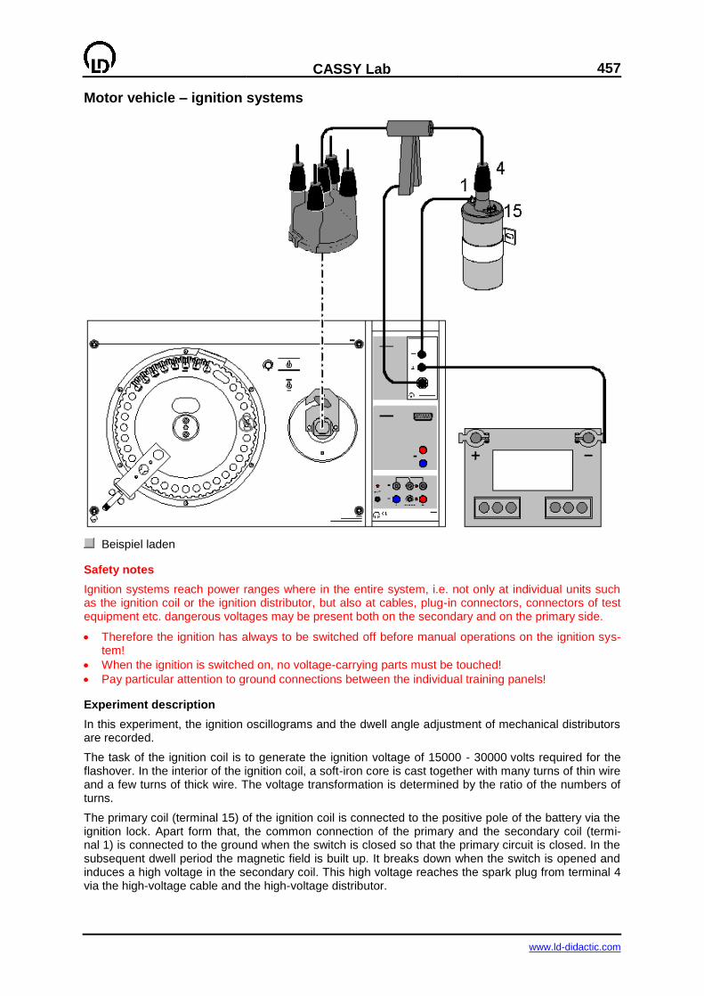
CASSY Lab

457

www.ld-didactic.com

Motor vehicle – ignition systems

Beispiel laden

Safety notes

Ignition systems reach power ranges where in the entire system, i.e. not only at individual units such as the ignition coil or the ignition distributor, but also at cables, plug-in connectors, connectors of test equipment etc. dangerous voltages may be present both on the secondary and on the primary side.

Therefore the ignition has always to be switched off before manual operations on the ignition sys-tem!

When the ignition is switched on, no voltage-carrying parts must be touched!

Pay particular attention to ground connections between the individual training panels!


In this experiment, the ignition oscillograms and the dwell angle adjustment of mechanical distributors are recorded.

The task of the ignition coil is to generate the ignition voltage of 15000 - 30000 volts required for the flashover. In the interior of the ignition coil, a soft-iron core is cast together with many turns of thin wire and a few turns of thick wire. The voltage transformation is determined by the ratio of the numbers of turns.

The primary coil (terminal 15) of the ignition coil is connected to the positive pole of the battery via the ignition lock. Apart form that, the common connection of the primary and the secondary coil (termi-nal 1) is connected to the ground when the switch is closed so that the primary circuit is closed. In the subsequent dwell period the magnetic field is built up. It breaks down when the switch is opened and induces a high voltage in the secondary coil. This high voltage reaches the spark plug from terminal 4 via the high-voltage cable and the high-voltage distributor.

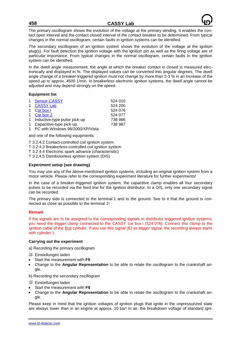
458

CASSY Lab

www.ld-didactic.com

The primary oscillogram shows the evolution of the voltage at the primary winding. It enables the con-tact open interval and the contact closed interval of the contact breaker to be determined. From typical changes in the normal oscillogram, certain faults in ignition systems can be identified.

The secondary oscillogram of an ignition system shows the evolution of the voltage at the ignition plug(s). For fault detection the ignition voltage with the ignition pin as well as the firing voltage are of particular importance. From typical changes in the normal oscillogram, certain faults in the ignition system can be identified.

In the dwell angle measurement, the angle at which the breaker contact is closed is measured elec-tronically and displayed in %. The displayed values can be converted into angular degrees. The dwell angle change of a breaker-triggered ignition must not change by more than 2-3 % in an increase of the speed up to approx. 4500 1/min. In breakerless electronic ignition systems, the dwell angle cannot be adjusted and may depend strongly on the speed.

Equipment list

1 Sensor-CASSY 524 010 1 CASSY Lab 524 200 1 Car box i 524 076 1 Car box Z 524 077 1 Inductive-type pulse pick-up 738 986 1 Capacitive-type pick-up 738 987 1 PC with Windows 98/2000/XP/Vista

and one of the following equipments:

T 3.2.4.2 Contact-controlled coil ignition system T 3.2.4.3 Breakerless-controlled coil ignition system T 3.2.4.4 Electronic spark advance (characteristic) T 3.2.4.5 Distributorless ignition system (DIS)


You may use any of the above-mentioned ignition systems, including an original ignition system from a motor vehicle. Please refer to the corresponding experiment literature for further experiments!

In the case of a breaker-triggered ignition system, the capacitive clamp enables all four secondary pulses to be recorded via the feed line for the ignition distributor. In a DIS, only one secondary signal can be recorded.

The primary side is connected to the terminal 1 and to the ground. See to it that the ground is con-nected as close as possible to the terminal 1!

Remark

If the signals are to be assigned to the corresponding signals in distributor-triggered ignition systems, you need the trigger clamp connected to the CASSY car box i (524 076). Connect this clamp to the ignition cable of the first cylinder. If you use this signal (E) as trigger signal, the recording always starts with cylinder 1.


a) Recording the primary oscillogram

Einstellungen laden


Change to the Angular Representation to be able to relate the oscillogram to the crankshaft an-gle.

b) Recording the secondary oscillogram

Einstellungen laden


Change to the Angular Representation to be able to relate the oscillogram to the crankshaft an-gle.

Please keep in mind that the ignition voltages of ignition plugs that ignite in the unpressurized state are always lower than in an engine at approx. 10 bar! In air, the breakdown voltage of standard igni-

CASSY Lab

459

www.ld-didactic.com

tion plugs is only approx. 3.5 kV. For this reason, the height of the ignition pin can vary from cycle to cycle.

c) Recording the contact closed interval

Einstellungen laden


Increase the speed form 800 to 5000 1/min

Evaluation

In the example files, the measurements have been evaluated by way of example. Load the example files, and change to the Evaluation display. The contact closed interval was measured for a distributor with centrifugal advance. Up to approx. 4500 1/min, the contact closed interval does not change. Only at higher values of the speed does it decrease.

Remark

Please refer to the corresponding experiment literature for further experiments!

Further example files

Beispiel laden

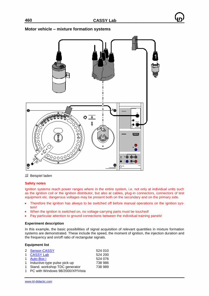
460

CASSY Lab

www.ld-didactic.com

Motor vehicle – mixture formation systems

Beispiel laden

Safety notes

Ignition systems reach power ranges where in the entire system, i.e. not only at individual units such as the ignition coil or the ignition distributor, but also at cables, plug-in connectors, connectors of test equipment etc. dangerous voltages may be present both on the secondary and on the primary side.

Therefore the ignition has always to be switched off before manual operations on the ignition sys-tem!

When the ignition is switched on, no voltage-carrying parts must be touched!

Pay particular attention to ground connections between the individual training panels!


In this example, the basic possibilities of signal acquisition of relevant quantities in mixture formation systems are demonstrated. These include the speed, the moment of ignition, the injection duration and the frequency and on/off ratio of rectangular signals.

Equipment list

2 Sensor-CASSY 524 010 1 CASSY Lab 524 200 1 Auto-Box i 524 076 1 Inductive-type pulse pick-up 738 986 1 Stand. workshop TDC generator 738 989 1 PC with Windows 98/2000/XP/Vista

CASSY Lab

461

www.ld-didactic.com

optionally for adjusting the vacuum: 1 Pressure sensor S, ±2000 hPa 524 064 1 Vacuum pump 738 996

and one of the following equipments:

T 3.2.5.6 LU-Jetronic T 3.2.5.7 Motronic T 3.2.5.10 LH-Motronic M 1.5.4 or 1.5.2 T 3.2.5.11 MONO-Motronic


You can use one of the above-mentioned systems or a mixture formation system in a motor vehicle.

The ignition signal of cylinder 1 is detected by means of the trigger clamp. The TDC generator detects the upper dead centre of the cylinder. Apart from the speed, the moment of ignition is determined from these signals.

At the two 4 mm sockets, an arbitrary rectangular signal can be applied. The quantities that can be evaluated are the frequency, the on/off ratio and the operating time or shut-off time. If the signal of an injection valve is applied, the injection duration ti is displayed in ms.

For the measurement of the ignition angle, the crankshaft mark of the TDC and the ignition signal of cylinder 1 are recorded. The time between the ignition pulse and the TDC generator pulse is related to the time required by the flywheel for one revolution. The result is displayed as advance angle in de-grees crankshaft angle. The mark for the TDC generator is not located in the upper dead centre of cylinder 1, but 20 degrees crankshaft angle later! This angle is taken into account automatically.


a) Centrifugal advance

The centrifugal advance mechanism of a rotating distribution adjusts the moment of ignition depending on the speed of the engine. With increasing speed, the cam is moved in the direction of rotation of the ignition-distributor shaft, whereby the breaker contact is opened earlier. This leads to an earlier igni-tion. The centrifugal advance can only be determined, if the vacuum tubings are removed!

Einstellungen laden


Pass through the speed range from 600 to 6000 1/min

The centrifugal advance causes an adjustment of the ignition angle towards earlier ignition, which increases linearly up to approx. 3000 1/min. At higher speeds, there is no further advance as the cen-trifugal advance is limited mechanically. If vacuum advance is to be investigated subsequently, the corresponding centrifugal components can be determined from the diagram, which have to be sub-tracted from the vacuum advance.

b) Vacuum advance, advance unit

The vacuum advance mechanism adjusts the moment of ignition depending on the load of the engine. The vacuum unit is connected to the intake manifold above the throttle valve and adjusts the moment of ignition in the part-load range by turning the breaker contact in the direction opposite to the rota-tion of the ignition distributor shaft. This leads to an earlier ignition. This type of vacuum unit is called "advance unit".

The contribution of the vacuum advance to the total advance can be determined by first determining the pure centrifugal component and then subtracting it from the value measured in the vacuum ex-periment!

Einstellungen laden


Generate a vacuum of 0 to –600 hPa (-600 mbar) at 1000 1/min

Repeat the measurement for 2000 and 4000 1/min

Regardless of the speed, the adjustment of the advance unit causes an advance of approx. 13 de-grees crankshaft angle. For 1000 and 2000 1/min, the advance ranges are equal after subtraction of the centrifugal component!

c) Vacuum retard, retard unit

462

CASSY Lab

www.ld-didactic.com

The vacuum unit for ignition retard is connected to the intake manifold below the throttle valve be-cause in this position there is a high vacuum during idle and overrun. The retard unit adjusts the mo-ment of ignition by turning the breaker contact in the direction of rotation of the ignition distributor shaft. This leads to a later ignition. This type of vacuum unit is called "retard unit".

The ignition retard is subordinate to ignition advance.

The contribution of the vacuum retard to the total advance can be determined by first determining the pure centrifugal component and then subtracting it from the value measured in the vacuum experi-ment!

Einstellungen laden


Generate a vacuum of 0 to –600 hPa (-600 mbar) at 1000 1/min

Repeat the measurement for 2000 and 4000 1/min

Regardless of the speed, the adjustment of the retard unit causes an ignition retard of approx. –8 degrees crankshaft angle in the pressure range from –200 to –400 hPa. For 1000 and 2000 1/min, the retard ranges are equal after subtraction of the centrifugal component!

d) Injection valve

The function of the injection valves is to supply all cylinders (single-point injection) or individual cylin-ders (multipoint injection) with gasoline depending on the signal from the control unit. Usually they are triggered with 12 V via the ground cable. The injected fuel quantity depends solely on the injection duration as the opening cross-section and the pressure difference between the fuel-injection tubing and the intake manifold are kept constant. A typical effect of DC solenoid valves (injection valves) is the high induction voltage in the opposite direction when the voltage is switched off.

Einstellungen laden


Increase the speed of the engine at operating temperature and 50 % load from idle to approx. 5000 1/min

Repeat the measurement for several load conditions (17 %, 33 %, 67 %, 83 %)

As the speed of the engine increases at constant air throughput, the absolute pressure behind the throttle valve decreases, and the cylinders can induce less mixture per lift. Therefore less fuel is re-quired, which is achieved by a shorter injection duration. If the engine power increases at constant speed, the cylinder charge is greater. This leads to a greater fuel quantity and thus to longer injection times.

e) Lambda closed-loop control

If the exhaust-gas oxygen content is 3 % (lean mixture), the difference relative to the oxygen content of the ambient air leads to a voltage of 0.1 V. If the exhaust-gas oxygen content is less than 3% (rich mixture), the voltage of the lambda sensor increases relative to the increased difference to 0.9 V. Hence there is a control loop for each cylinder bank, which enables the mixture composition to be controlled. Depending on the sensor voltage, the injection duration is changed

Einstellungen laden

Activate the periodic change of the lambda voltage

Start the measurement with F9 at 2000 1/min with the engine at operating temperature

Repeat the measurement for a very cold engine and for full load, respectively

The lambda closed-loop control works such that the injection duration rises in the case of a lean mix-ture, which leads to a richer mixture. In the case of a rich mixture, the injection duration drops, which leads to a leaner mixture. The control does not work if the engine is cold because the fuel-air mixture has to be enriched to compensate for condensation losses at cold components. The mixture cannot be

operated with = 1.

At full load, the control is also shut off as the engine has to be operated with a rich mixture to achieve maximum engine power.

f) Rotary idle actuator

During the fuel injection, the function of the rotary idle actuator is to open a bypass air channel around the throttle valve more or less thus controlling the idle operation. The percentage of the time within an interval of 100 ms, during which the electric motor receives a current pulse for opening, is called on/off ratio. It is, e. g., 50 % if the motor receives 12 V for 50 ms and then 0 V for another 50 ms. In this

CASSY Lab

463

www.ld-didactic.com

case, the inertia of the armature should lead to the bypass channel being opened for about 50 % of the time.

Einstellungen laden


Reduce the speed of the engine at operating temperature from 850 to 400 1/min

Repeat the measurement for a cold engine and with the air conditioner being switched on

When the speed is decreased, the on/off ratio increases, as the engine tries to increase the speed. If the engine is cold, the on/off ratio is increased as well, as the higher engine friction has to be over-come. If the air conditioner is switched on, the engine also tries to increase the air throughput of the rotary idle actuator by increasing the on/off ratio in order to compensate for the drop in speed caused by the increased load.

g) Knocking sensor

"Knocking", an uncontrolled form of combustion, can lead to damage in the engine. However, as knock limits depend on many variable quantities such as fuel quality, engine condition and ambient condi-tions, a sufficient distance from the knock limit has to be kept in ignition systems with electronic ad-justment, which leads to a deterioration of the fuel consumption. The distance of the program map from the knock limit, which has been indispensable up to now, may be cancelled if a knock during operation, e. g. caused by poor fuel quality, is detected and if the ignition angle is reduced accordingly. The knock control enables the engine to be operated in the limit range without damage.

Einstellungen laden


With the engine at operating temperature and running at a speed of 2500 1/min almost at full load, slightly hit the knock sensor against a metal block

In the case of combustion knock, the control circuit delays the moment of ignition of the knocking cyl-inder. Subsequently the moment of ignition is taken back to its original value slowly according to a particular scheme.

Remark

Please refer to the corresponding experiment literature for further experiments!

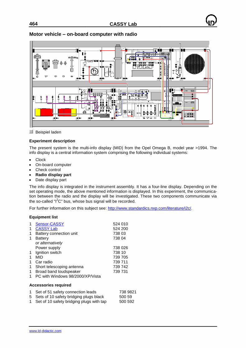
464

CASSY Lab

www.ld-didactic.com

Motor vehicle – on-board computer with radio

Beispiel laden


The present system is the multi-info display (MID) from the Opel Omega B, model year >1994. The info display is a central information system comprising the following individual systems:

Clock

On-board computer

Check control

Radio display part

Date display part

The info display is integrated in the instrument assembly. It has a four-line display. Depending on the set operating mode, the above mentioned information is displayed. In this experiment, the communica-tion between the radio and the display will be investigated. These two components communicate via

the so-called "I2C" bus, whose bus signal will be recorded.

For further information on this subject see: http://www.standardics.nxp.com/literature/i2c/.

Equipment list

1 Sensor-CASSY 524 010 1 CASSY Lab 524 200 1 Battery connection unit 738 03 1 Battery 738 04 or alternatively Power supply 738 026 1 Ignition switch 738 10 1 MID 739 705 1 Car radio 739 711 1 Short telescoping antenna 739 742 1 Broad band loudspeaker 739 731 1 PC with Windows 98/2000/XP/Vista

Accessories required

1 Set of 51 safety connection leads 738 9821 5 Sets of 10 safety bridging plugs black 500 59 1 Set of 10 safety bridging plugs with tap 500 592

http://www.standardics.nxp.com/literature/i2c

CASSY Lab

465

www.ld-didactic.com


Set up the experiment as shown in the drawing. Some devices are optional and are not required for carrying out the experiment! Connect the Sensor-CASSY to a serial RS232 port or a USB port of the computer. Connect the measurement inputs to the experiment setup as shown in the drawing.


Einstellungen laden

Switch the system on, first using the battery connection unit and then the ignition switch.

Switch the radio on by pressing the volume key.

Start the measurement by pressing F9 or .

Now switch over a station key of the radio to create a data flow.

Evaluation of the experiment

The following findings can be obtained from the diagrams:

The address of the display is: 1 0 0 1 0 1 0

A write access from the display to the radio takes place (RW bit)

Further variations of the experiment and their evaluation are found in the associated experiment litera-ture.

Further measurement examples

Beispiel laden

466

CASSY Lab

www.ld-didactic.com

Motor vehicle – comfort system with CAN bus

Beispiel laden


The new comfort system was first used in the VW Passat in the model year 1997 and has been avail-able in the VW Golf since the model year 1998. The individual functionalities that belong to the comfort system such as the central locking system, the mirror adjusting system and the theft-deterrent system have not changed essentially. What is new, however, is the structure and the organisation of the com-fort system. In contrast to conventional systems, it has a decentralized structure. That means tasks are shared by several control units.

The control units of the comfort system are connected to one another via two lines, the CAN data bus. A permanent data exchange between the control units takes place via these lines.

For this a control unit has to:

provide data of its own,

send these data to other control units,

receive data from other control units,

check these data and, if required, accept them.

The system consists of a central control unit and two door control units. The central control unit has no higher-level function. There is no hierarchy among the control units. Apart from its functionalities within the comfort system, the central control unit establishes the connection between the remaining vehicle electrical system and the diagnosis cables.

Functionalities of the central control unit:

Mirror adjustment,

Interior light control,

Remote release of the luggage compartment lid,

Radio remote control,

Theft-deterrent system.

The door control units monitor and control the functionalities of the comfort system carried out in the doors.

CASSY Lab

467

www.ld-didactic.com

Equipment list

1 Sensor-CASSY 524 010 1 CASSY Lab 524 200 1 Battery connection unit 738 03 1 Battery 738 04 or alternatively Power supply 738 026 1 Ignition switch 738 10 1 Comfort system 739 58 1 PC with Windows 98/2000/XP/Vista

Accessories required

1 Set of 51 safety connection leads 738 9821 5 Sets of 10 safety bridging plugs black 500 92 1 Set of 10 safety bridging plugs with tap 500 592


Set up the experiment as shown in the drawing. Connect the Sensor-CASSY to a serial RS232 port or a USB port of the computer. Connect the measurement inputs to the experiment setup as shown in the drawing.


Einstellungen laden

First switch the system on using the battery connection unit.

Now open one of the two doors by turning the corresponding key switch in the "OPEN" direction.

Switch the ignition on using the ignition switch.

Start the measurement by pressing F9 or .

Evaluation of the experiment

The following findings can be obtained from the diagrams:

The signals on the lines CANH and CANL are mutually inverted.

The messages are set in three frames with a repeat time of 20 ms.

Two messages have equal lengths (approx. 1.34 ms) and one message in shorter (approx. 1 ms). The latter obviously concerns the door control unit of the co-driver side.

In addition to CANH and CANL, the Difference display also shows their difference CAN=CANH-CANL, which is defined as a formula.

Further variations of the experiment and their evaluation are found in the associated experiment litera-ture 566 1481.

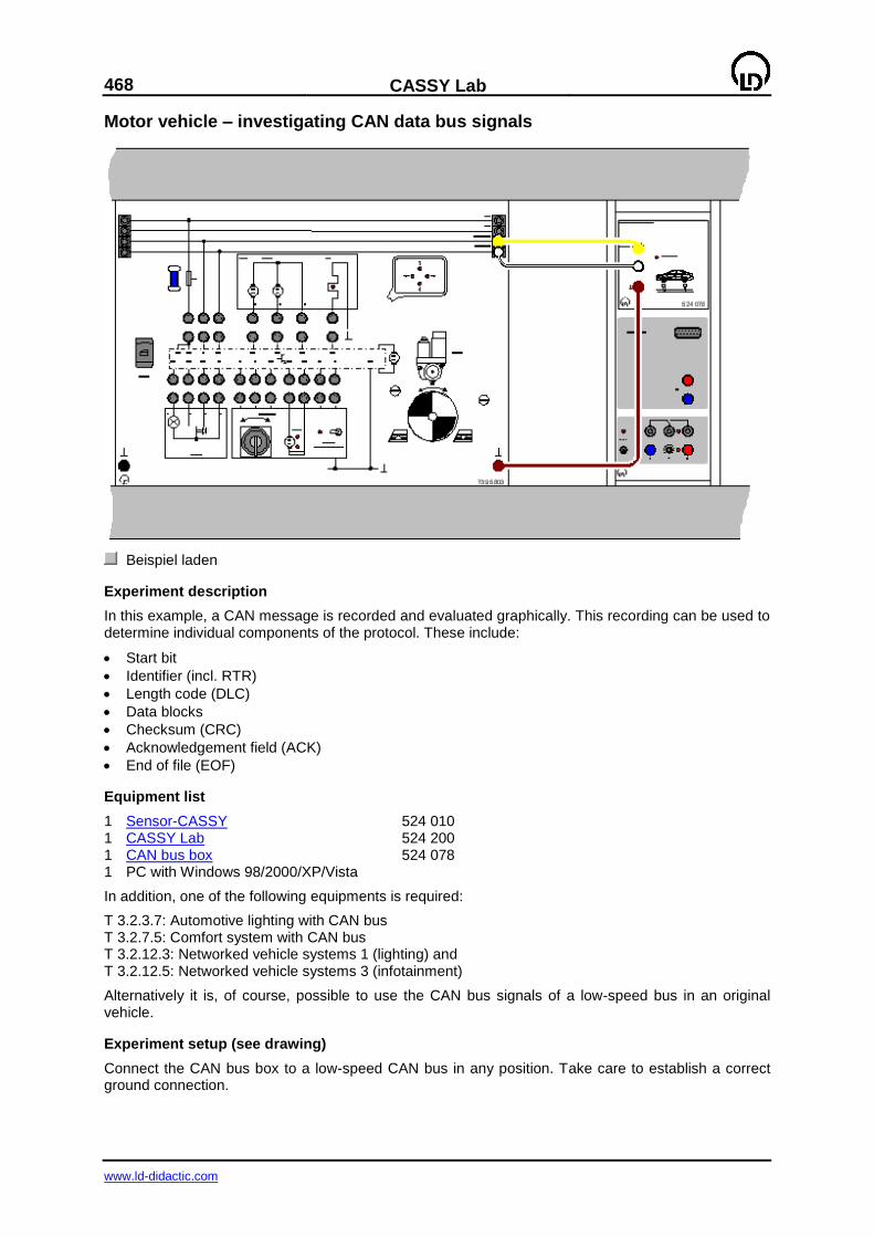
468

CASSY Lab

www.ld-didactic.com

Motor vehicle – investigating CAN data bus signals

Beispiel laden


In this example, a CAN message is recorded and evaluated graphically. This recording can be used to determine individual components of the protocol. These include:

Start bit

Identifier (incl. RTR)

Length code (DLC)

Data blocks

Checksum (CRC)

Acknowledgement field (ACK)

End of file (EOF)

Equipment list

1 Sensor-CASSY 524 010 1 CASSY Lab 524 200 1 CAN bus box 524 078 1 PC with Windows 98/2000/XP/Vista

In addition, one of the following equipments is required:

T 3.2.3.7: Automotive lighting with CAN bus T 3.2.7.5: Comfort system with CAN bus T 3.2.12.3: Networked vehicle systems 1 (lighting) and T 3.2.12.5: Networked vehicle systems 3 (infotainment)

Alternatively it is, of course, possible to use the CAN bus signals of a low-speed bus in an original vehicle.


Connect the CAN bus box to a low-speed CAN bus in any position. Take care to establish a correct ground connection.

CASSY Lab

469

www.ld-didactic.com

To gain workshop practice you may also connect the CAN bus of an available vehicle as long as it is a low-speed bus. Follow the manufacturer's circuit diagrams to get access to the two bus cables, and additionally connect the ground socket to the ground of the vehicle's body.

Hint: in modern vehicles, the CAN bus signals may be available at the 16-pole OBD socket!


Einstellungen laden


The measurement is stopped automatically after the first received message has been recorded.

The measurement can be repeated for other data to be transmitted. To do this, first select the cor-

responding identifier in the ID filter in the Settings CANA1 (right mouse button on CANA1) and re-start with F9.

Evaluation

In the display all recorded messages are first shown as hexadecimal numbers. If there are more than two messages in the system which are repeated cyclically, the display shows these messages one after another. From the left to the right the following components are displayed:

Identifier

Data length code

Data blocks

Checksum

Status of the acknowledgement

The displays are separated from one another by a blank character. In Settings CANA1 two different binary modes can also be selected:

Raw data, i. e. all stuff bits are contained

Binary data, i. e. all stuff bits are filtered out

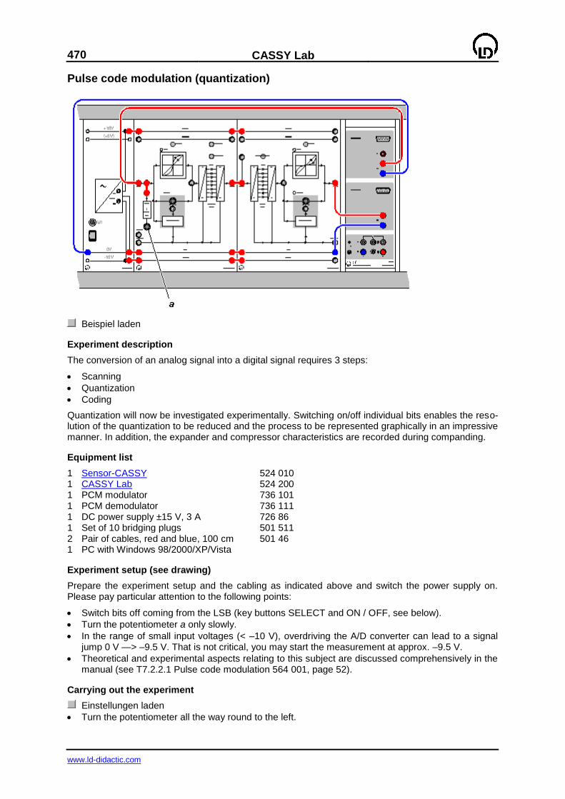
470

CASSY Lab

www.ld-didactic.com

Pulse code modulation (quantization)

Beispiel laden


The conversion of an analog signal into a digital signal requires 3 steps:

Scanning

Quantization

Coding

Quantization will now be investigated experimentally. Switching on/off individual bits enables the reso-lution of the quantization to be reduced and the process to be represented graphically in an impressive manner. In addition, the expander and compressor characteristics are recorded during companding.

Equipment list

1 Sensor-CASSY 524 010 1 CASSY Lab 524 200 1 PCM modulator 736 101 1 PCM demodulator 736 111 1 DC power supply ±15 V, 3 A 726 86 1 Set of 10 bridging plugs 501 511 2 Pair of cables, red and blue, 100 cm 501 46 1 PC with Windows 98/2000/XP/Vista


Prepare the experiment setup and the cabling as indicated above and switch the power supply on. Please pay particular attention to the following points:

Switch bits off coming from the LSB (key buttons SELECT and ON / OFF, see below).

Turn the potentiometer a only slowly.

In the range of small input voltages (< –10 V), overdriving the A/D converter can lead to a signal jump 0 V —> –9.5 V. That is not critical, you may start the measurement at approx. –9.5 V.

Theoretical and experimental aspects relating to this subject are discussed comprehensively in the manual (see T7.2.2.1 Pulse code modulation 564 001, page 52).


Einstellungen laden

Turn the potentiometer all the way round to the left.

CASSY Lab

471

www.ld-didactic.com

Start the measurement with F9 or .

Turn the potentiometer a to the right. Now there is a voltage at the input of the PCM modulator (736 101), which increases slowly from –10 V up to +10 V. This input voltage is displayed as the

voltage UA1. The output voltage (after quantization) at the PCM demodulator (736 111) is displayed

as the voltage UB1.

After recording the quantization characteristic, stop the measurement with F9.

Variations

Reduction of the resolution from 8 to 5 bits. Deactivate the 3 least significant bits (LSB) of the PCM modulator by pressing SELECT and ON/OFF. The position of the desired bit is reached by pressing SELECT repeatedly. ON/OFF changes between active/inactive. Turn the potentiometer a back to the left (minimum input voltage: approx. –10 V) and record the quantization characteristic again. The 32 steps of equal height re-sulting from the 5 bits are clearly seen.

Non-linear quantization Press the MODE key buttons of the PCM modulator and of the PCM demodulator once each. Now both devices work in the non-linear quantization mode (in each case each indicated by an LED in the 13 segment characteristics). Then record the characteristic again.

Compressor/expander characteristic For recording the compressor/expander characteristic, only one of the two devices is operated in the non-linear mode, whereas the other one works in the linear mode.

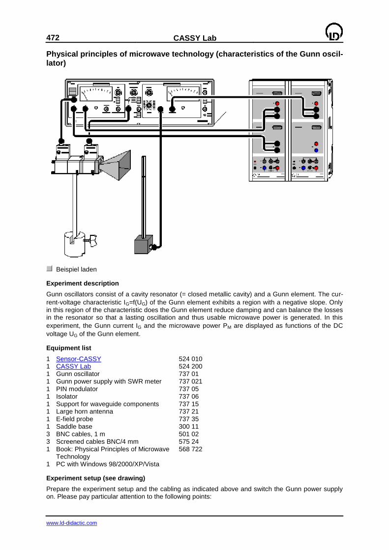
472

CASSY Lab

www.ld-didactic.com

Physical principles of microwave technology (characteristics of the Gunn oscil-lator)

Beispiel laden


Gunn oscillators consist of a cavity resonator (= closed metallic cavity) and a Gunn element. The cur-

rent-voltage characteristic IG=f(UG) of the Gunn element exhibits a region with a negative slope. Only in this region of the characteristic does the Gunn element reduce damping and can balance the losses in the resonator so that a lasting oscillation and thus usable microwave power is generated. In this

experiment, the Gunn current IG and the microwave power PM are displayed as functions of the DC

voltage UG of the Gunn element.

Equipment list

1 Sensor-CASSY 524 010 1 CASSY Lab 524 200 1 Gunn oscillator 737 01 1 Gunn power supply with SWR meter 737 021 1 PIN modulator 737 05 1 Isolator 737 06 1 Support for waveguide components 737 15 1 Large horn antenna 737 21 1 E-field probe 737 35 1 Saddle base 300 11 3 BNC cables, 1 m 501 02 3 Screened cables BNC/4 mm 575 24 1 Book: Physical Principles of Microwave

Technology 568 722



Prepare the experiment setup and the cabling as indicated above and switch the Gunn power supply on. Please pay particular attention to the following points:

CASSY Lab

473

www.ld-didactic.com

Connections between the power supply and the Gunn oscillator and between the PIN modulator and the E-field probe with BNC cables male/male.

Connections between the power supply (AMP OUT and RECORDER X,Y, respectively) and the Sensor-CASSY with screened cables BNC/4 mm.

Power supply, MODULATION: select PIN INT.

Select a suitable gain at the SWR meter (v/dB and ZERO).

Theoretical and experimental aspects relating to this subject are discussed comprehensively in the manual (see pages 11ff).

Remark

The illustration shows an experiment setup with a cascade arrangement of 2 Sensor-CASSYs. With

this arrangement the characteristics IG=f(UG) and PM=f(UG) are recorded simultaneously. The second characteristic represents the microwave power of the Gunn oscillator as a function of the DC voltage UG of the Gunn element.

If only one Sensor-CASSY is available, the experiment is carried out in two steps.

Carrying out the experiment with 2 Sensor-CASSYs

Einstellungen laden

Turn the potentiometer UG all the way round to the left (UG = 0 V).


Turn the potentiometer UG to the right. The Gunn voltage, the Gunn current and the microwave power are displayed on dedicated display instruments.

After recording the two characteristics IG=f(UG) and PM=f(UG), stop the measurement with F9.

Carrying out the experiment with 1 Sensor-CASSY

Einstellungen laden

Turn the potentiometer UG all the way round to the left (UG = 0 V).


Turn the potentiometer UG to the right. The Gunn voltage and the Gunn current are displayed on dedicated display instruments.

After recording the characteristic IG=f(UG), stop the measurement with F9.

The second characteristic PM=f(UG) is recorded subsequently with the same Sensor-CASSY and the same settings. Therefore the relative microwave power is displayed in the Gunn current display in-strument. For this:

Disconnect the Sensor-CASSY from the Gunn power supply (RECORDER Y) and change to AMP OUT.

Select a suitable gain at the SWR meter (v/dB and ZERO).

Record the characteristic again.

Remarks

Characteristics of active elements in microwave experiments exhibit wide scattering. Therefore the characteristics shown in the examples should only be considered as examples. The important thing is the connection between the falling region of the current-voltage characteristic and the generation of microwave power. The absolute values or the shape of the curves can vary considerably, depending on the Gunn element used.

The measurement of the microwave power PM is made with an uncalibrated detector. Therefore its numerical value is arbitrary.

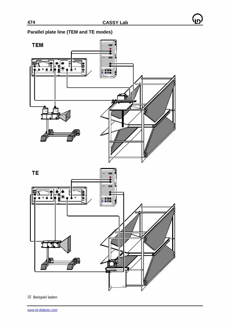
474

CASSY Lab

www.ld-didactic.com

Parallel plate line (TEM and TE modes)

Beispiel laden

CASSY Lab

475

www.ld-didactic.com


TEM or TE waves can be excited on the parallel plate line by rotating the direction of polarization of the exciting microwave field (pay attention to this in the experiment!). TE waves exhibit a cut-off phe-nomenon, i. e. for a given frequency of the exciting field, TE waves can only propagate if the plate distance exceeds a certain minimum value. In the case of an excitation with a variable frequency and a fixed plate distance, TE waves cannot propagate if the frequency is below the so-called cut-off fre-quency. As microwave experiments in free space are only permitted at certain, fixed frequencies, this experiment is carried out with a variable plate distance.

Equipment list

1 Sensor-CASSY 524 010 1 CASSY Lab 524 200 1 Gunn oscillator 737 01 1 Gunn power supply with SWR meter 737 021 1 PIN modulator 737 05 1 Isolator 737 06 1 Two-plate waveguide 737 07 1 Measuring carriage for parallel plate line 737 071 1 Support for waveguide components 737 15 1 Large horn antenna 737 21 1 E-field probe 737 35 2 BNC cables, 1 m 501 02 2 BNC cables, 2 m 501 022 2 Screened cables BNC/4 mm 575 24 2 Stand bases MF 301 21 1 Book: Parallel Plate Line 568 661 1 PC with Windows 98/2000/XP/Vista

Experiment setup TEM or TE (see drawing TEM or TE)


Connections form the power supply to the Gunn oscillator, to the PIN modulator and to the measur-ing carriage for parallel plate line (input IN 8-24 V) with BNC cables male/male.

Connections from the power supply (AMP OUT) and from the measuring carriage for parallel plate line (output X) to the Sensor-CASSY with screened cables BNC/4 mm.

Set the Gunn voltage to UG = 10 V at the power supply.


Place the measuring carriage for parallel plate line on the props of the parallel plate line such that the E-field probe just reaches into the parallel part of the two-plate waveguide when it is at the left stop.

The E-field probe should always be in mechanical contact with the edge of the plate when it is moved because this helps to avoid variations in position.

One after another terminate the two-plate waveguides with the termination profiles 13 mm and 22 mm.

For additional notes see the instruction sheets 737 07 and 737 071.

Theoretical and experimental aspects relating to this subject are discussed comprehensively in the manual (see page 27).


Einstellungen laden

Slide the calliper gauge of the measuring carriage (737 071) to the right (x = 75 mm).

Use the mouse to take the numerical value of the displayed voltage UB1 into the display instrument

voltage U75 (drag & drop, right calibration point for position measurement).

Slide the calliper gauge of the measuring carriage (737 071) to the left (x = 25 mm).


voltage U25 (drag & drop, left calibration point for position measurement).

Slide the calliper gauge to the left (x = 0 mm).


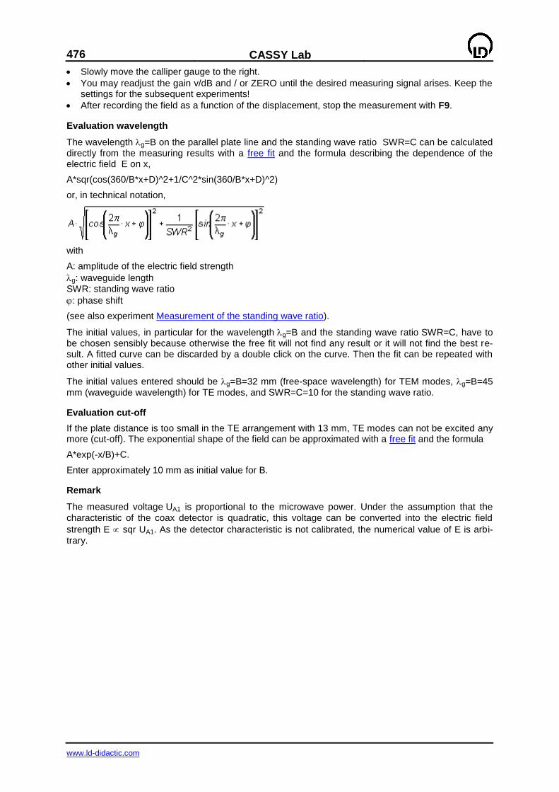
476

CASSY Lab

www.ld-didactic.com

Slowly move the calliper gauge to the right.

You may readjust the gain v/dB and / or ZERO until the desired measuring signal arises. Keep the settings for the subsequent experiments!

After recording the field as a function of the displacement, stop the measurement with F9.

Evaluation wavelength

The wavelength g=B on the parallel plate line and the standing wave ratio SWR=C can be calculated directly from the measuring results with a free fit and the formula describing the dependence of the electric field E on x,

A*sqr(cos(360/B*x+D)^2+1/C^2*sin(360/B*x+D)^2)

or, in technical notation,

with

A: amplitude of the electric field strength

g: waveguide length SWR: standing wave ratio

: phase shift

(see also experiment Measurement of the standing wave ratio).

The initial values, in particular for the wavelength g=B and the standing wave ratio SWR=C, have to be chosen sensibly because otherwise the free fit will not find any result or it will not find the best re-sult. A fitted curve can be discarded by a double click on the curve. Then the fit can be repeated with other initial values.

The initial values entered should be g=B=32 mm (free-space wavelength) for TEM modes, g=B=45 mm (waveguide wavelength) for TE modes, and SWR=C=10 for the standing wave ratio.

Evaluation cut-off

If the plate distance is too small in the TE arrangement with 13 mm, TE modes can not be excited any more (cut-off). The exponential shape of the field can be approximated with a free fit and the formula

A*exp(-x/B)+C.

Enter approximately 10 mm as initial value for B.

Remark

The measured voltage UA1 is proportional to the microwave power. Under the assumption that the

characteristic of the coax detector is quadratic, this voltage can be converted into the electric field

strength E sqr UA1. As the detector characteristic is not calibrated, the numerical value of E is arbi-

trary.

CASSY Lab

477

www.ld-didactic.com

Microwave propagation in waveguides (measurement of the standing wave ra-tio)

Beispiel laden


The standing wave ratio (SWR) is a scalar measure of the match. In experiments with microwaves, it determines the power transfer from the source to the load and the magnitude of the field strength in the components of the circuit. Therefore an SWR of approximately 1 is desired in most cases. In this experiment, the standing wave ratios of various waveguide terminations are compared. A variable attenuator (alters the magnitude of reflections) and an adjustable movable short (alters the phase of reflections) in series connection are used as a complex microwave load. For the case of an average standing wave ratio (SWR approximately 3), the match is improved by means of a slide screw trans-former.

Equipment list

1 Sensor-CASSY 524 010 1 CASSY Lab 524 200 1 Gunn oscillator 737 01 1 Coax detector 737 03 1 Transition waveguide / coax 737 035 1 Gunn power supply with SWR meter 737 021 1 PIN modulator 737 05 1 Isolator 737 06 1 Variable attenuator 737 09 1 Movable short 737 10 1 Slotted measuring line 737 111 1 Slide screw transformer 737 13 1 Waveguide terminaton 737 14

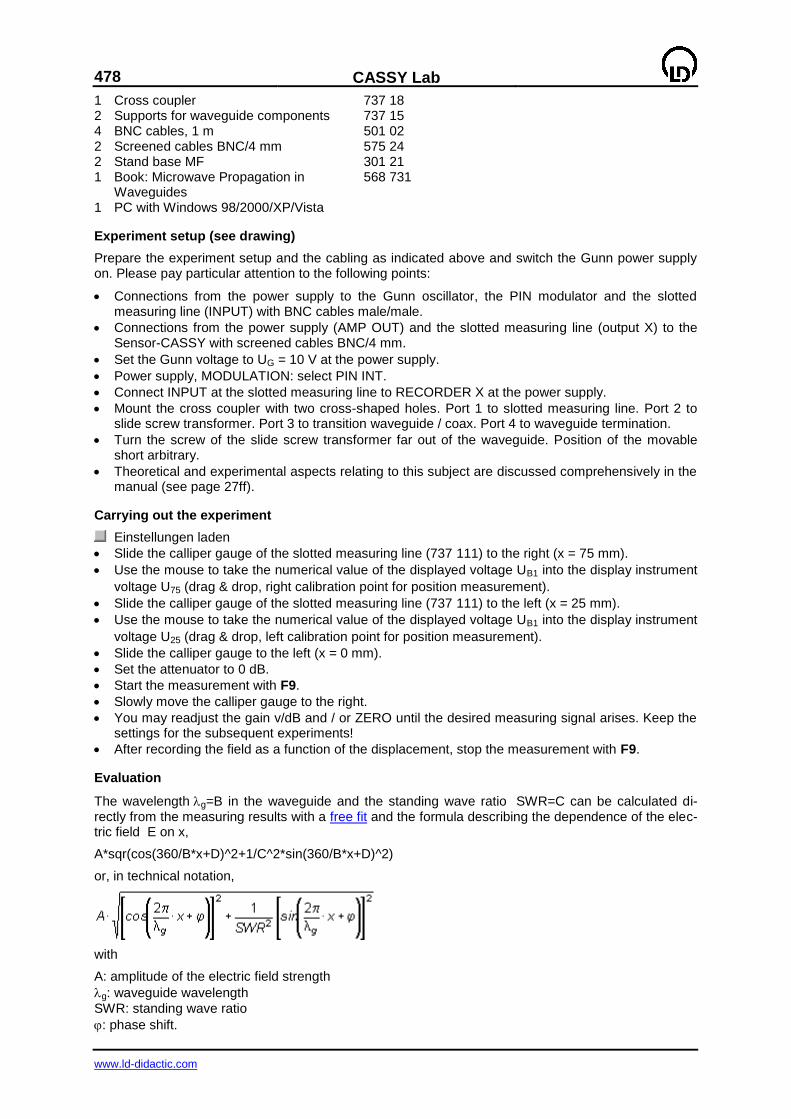
478

CASSY Lab

www.ld-didactic.com

1 Cross coupler 737 18 2 Supports for waveguide components 737 15 4 BNC cables, 1 m 501 02 2 Screened cables BNC/4 mm 575 24 2 Stand base MF 301 21 1 Book: Microwave Propagation in

Waveguides 568 731




Connections from the power supply to the Gunn oscillator, the PIN modulator and the slotted measuring line (INPUT) with BNC cables male/male.

Connections from the power supply (AMP OUT) and the slotted measuring line (output X) to the Sensor-CASSY with screened cables BNC/4 mm.

Set the Gunn voltage to UG = 10 V at the power supply.


Connect INPUT at the slotted measuring line to RECORDER X at the power supply.

Mount the cross coupler with two cross-shaped holes. Port 1 to slotted measuring line. Port 2 to slide screw transformer. Port 3 to transition waveguide / coax. Port 4 to waveguide termination.

Turn the screw of the slide screw transformer far out of the waveguide. Position of the movable short arbitrary.

Theoretical and experimental aspects relating to this subject are discussed comprehensively in the manual (see page 27ff).


Einstellungen laden

Slide the calliper gauge of the slotted measuring line (737 111) to the right (x = 75 mm).


voltage U75 (drag & drop, right calibration point for position measurement).

Slide the calliper gauge of the slotted measuring line (737 111) to the left (x = 25 mm).


voltage U25 (drag & drop, left calibration point for position measurement).

Slide the calliper gauge to the left (x = 0 mm).

Set the attenuator to 0 dB.


Slowly move the calliper gauge to the right.

You may readjust the gain v/dB and / or ZERO until the desired measuring signal arises. Keep the settings for the subsequent experiments!

After recording the field as a function of the displacement, stop the measurement with F9.

Evaluation

The wavelength g=B in the waveguide and the standing wave ratio SWR=C can be calculated di-rectly from the measuring results with a free fit and the formula describing the dependence of the elec-tric field E on x,

A*sqr(cos(360/B*x+D)^2+1/C^2*sin(360/B*x+D)^2)

or, in technical notation,

with

A: amplitude of the electric field strength

g: waveguide wavelength

SWR: standing wave ratio

: phase shift.

CASSY Lab

479

www.ld-didactic.com

The initial values, in particular for the wavelength g=B and the standing wave ratio SWR=C, have to be chosen sensibly (in this case B=45 mm and C=10) because otherwise the free fit will not find any result or it will not find the best result. A fitted curve can be discarded by a double click on the curve. Then the fit can be repeated with other initial values.

Variations

Recording the standing wave ratio for reduced reflection. The SWR is decreased by adjusting the attenuator (a > 0 dB).

Improving the match with the aid of the slide screw transformer.

Set a=3 dB at the attenuator. Now only 25 % of the incoming microwave power is reflected. The reflection coefficient is r=0.5 and the SWR is 3.

Make a new measurement to verify what has changed.

Screw the coax detector on the transition waveguide / coax. Now only the reflected signal is meas-ured.

Change the penetration depth and the position of the adjusting screw of the slide screw trans-former, and reduce the reflected signal to its minimum.

Screw the coax detector on the slotted measuring line again, and measure the SWR curve anew.

Remark

The measured voltage UA1 is proportional to the microwave power. Under the assumption that the characteristic of the coax detector is quadratic, this voltage can be converted into the electric field

strength E sqr UA1. As the detector characteristic is not calibrated, the numerical value of E is arbi-trary.

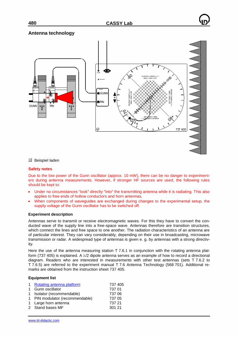
480

CASSY Lab

www.ld-didactic.com

Antenna technology

Beispiel laden

Safety notes

Due to the low power of the Gunn oscillator (approx. 10 mW), there can be no danger to experiment-ers during antenna measurements. However, if stronger HF sources are used, the following rules should be kept to:

Under no circumstances "look" directly "into" the transmitting antenna while it is radiating. This also applies to free ends of hollow conductors and horn antennas.

When components of waveguides are exchanged during changes to the experimental setup, the supply voltage of the Gunn oscillator has to be switched off.


Antennas serve to transmit or receive electromagnetic waves. For this they have to convert the con-ducted wave of the supply line into a free-space wave. Antennas therefore are transition structures, which connect the lines and free space to one another. The radiation characteristics of an antenna are of particular interest. They can vary considerably, depending on their use in broadcasting, microwave transmission or radar. A widespread type of antennas is given e. g. by antennas with a strong directiv-ity.

Here the use of the antenna measuring station T 7.6.1 in conjunction with the rotating antenna plat-

form (737 405) is explained. A /2 dipole antenna serves as an example of how to record a directional diagram. Readers who are interested in measurements with other test antennas (sets T 7.6.2 to T 7.6.5) are referred to the experiment manual T 7.6 Antenna Technology (568 701). Additional re-marks are obtained from the instruction sheet 737 405.

Equipment list

1 Rotating antenna platform 737 405 1 Gunn oscillator 737 01 1 Isolator (recommendable) 737 06 1 PIN modulator (recommendable) 737 05 1 Large horn antenna 737 21 2 Stand bases MF 301 21

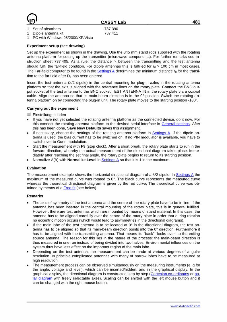
CASSY Lab

481

www.ld-didactic.com

1 Set of absorbers 737 390 1 Dipole antenna kit 737 411 1 PC with Windows 98/2000/XP/Vista


Set up the experiment as shown in the drawing. Use the 345 mm stand rods supplied with the rotating antenna platform for setting up the transmitter (microwave components). For further remarks see in-

struction sheet 737 405. As a rule, the distance r0 between the transmitting and the test antenna

should fulfil the far-field condition. For dipole antennas this is fulfilled for r0 > 100 cm in most cases.

The Far-field computer to be found in the Settings A determines the minimum distance r0 for the transi-

tion to the far field after DT has been entered.

Insert the test antenna (/2 dipole) in the central mounting for plug-in axles in the rotating antenna platform so that the axis is aligned with the reference lines on the rotary plate. Connect the BNC out-put socket of the test antenna to the BNC socket TEST ANTENNA IN in the rotary plate via a coaxial cable. Align the antenna so that its main-beam direction is in the 0° position. Switch the rotating an-tenna platform on by connecting the plug-in unit. The rotary plate moves to the starting position -180°.


Einstellungen laden

If you have not yet selected the rotating antenna platform as the connected device, do it now. For this connect the rotating antenna platform to the desired serial interface in General settings. After this has been done, Save New Defaults saves this assignment.

If necessary, change the settings of the rotating antenna platform in Settings A. If the dipole an-tenna is used, the bias current has to be switched on. If no PIN modulator is available, you have to switch over to Gunn modulation.

Start the measurement with F9 (stop clock). After a short break, the rotary plate starts to run in the forward direction, whereby the actual measurement of the directional diagram takes place. Imme-diately after reaching the set final angle, the rotary plate begins to return to its starting position.

Normalize A() with Normalize Level in Settings A so that it is 1 in the maximum.

Evaluation

The measurement example shows the horizontal directional diagram of a /2 dipole. In Settings A the maximum of the measured curve was rotated to 0°. The black curve represents the measured curve whereas the theoretical directional diagram is given by the red curve. The theoretical curve was ob-tained by means of a Free fit (see below).

Remarks

The axis of symmetry of the test antenna and the centre of the rotary plate have to be in line. If the antenna has been inserted in the central mounting of the rotary plate, this is in general fulfilled. However, there are test antennas which are mounted by means of stand material. In this case, the antenna has to be aligned carefully over the centre of the rotary plate in order that during rotation no eccentric motion occurs (which would lead to asymmetries in the directional diagrams).

If the main lobe of the test antenna is to be located at 0° in the directional diagram, the test an-tenna has to be aligned so that its main-beam direction points into the 0° direction. Furthermore it has to be aligned with the transmitting antenna. That means its "back" "looks over" to the exiting source antenna. The reason for this lies in the nature of the process: the main-beam direction is thus measured in one run instead of being divided into two halves. Environmental influences on the system thus have less effect on the important region of the main lobe.

Depending on the test antenna, the measurement can be made at various degrees of angular resolution. In principle complicated antennas with many or narrow lobes have to be measured at high resolution.

The measurement process can be observed simultaneously on the measuring instruments (e. g for the angle, voltage and level), which can be inserted/hidden, and in the graphical display. In the graphical display, the directional diagram is constructed step by step (Cartesian co-ordinates or po-lar diagram with freely selectable axes). Scaling can be shifted with the left mouse button and it can be changed with the right mouse button.

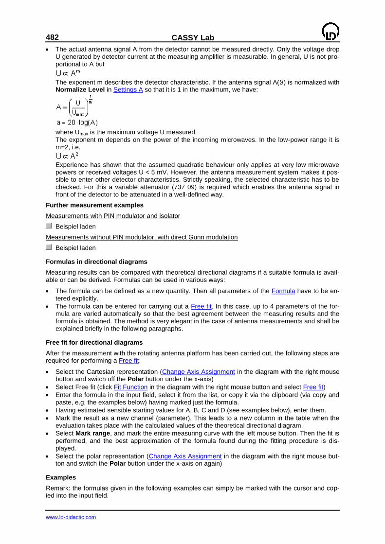
482

CASSY Lab

www.ld-didactic.com

The actual antenna signal A from the detector cannot be measured directly. Only the voltage drop U generated by detector current at the measuring amplifier is measurable. In general, U is not pro-portional to A but

The exponent m describes the detector characteristic. If the antenna signal A() is normalized with Normalize Level in Settings A so that it is 1 in the maximum, we have:

where Umax is the maximum voltage U measured.

The exponent m depends on the power of the incoming microwaves. In the low-power range it is m=2, i.e.

Experience has shown that the assumed quadratic behaviour only applies at very low microwave powers or received voltages U < 5 mV. However, the antenna measurement system makes it pos-sible to enter other detector characteristics. Strictly speaking, the selected characteristic has to be checked. For this a variable attenuator (737 09) is required which enables the antenna signal in front of the detector to be attenuated in a well-defined way.

Further measurement examples

Measurements with PIN modulator and isolator

Beispiel laden

Measurements without PIN modulator, with direct Gunn modulation

Beispiel laden

Formulas in directional diagrams

Measuring results can be compared with theoretical directional diagrams if a suitable formula is avail-able or can be derived. Formulas can be used in various ways:

The formula can be defined as a new quantity. Then all parameters of the Formula have to be en-tered explicitly.

The formula can be entered for carrying out a Free fit. In this case, up to 4 parameters of the for-mula are varied automatically so that the best agreement between the measuring results and the formula is obtained. The method is very elegant in the case of antenna measurements and shall be explained briefly in the following paragraphs.

Free fit for directional diagrams

After the measurement with the rotating antenna platform has been carried out, the following steps are required for performing a Free fit:

Select the Cartesian representation (Change Axis Assignment in the diagram with the right mouse button and switch off the Polar button under the x-axis)

Select Free fit (click Fit Function in the diagram with the right mouse button and select Free fit)

Enter the formula in the input field, select it from the list, or copy it via the clipboard (via copy and paste, e.g. the examples below) having marked just the formula.

Having estimated sensible starting values for A, B, C and D (see examples below), enter them.

Mark the result as a new channel (parameter). This leads to a new column in the table when the evaluation takes place with the calculated values of the theoretical directional diagram.

Select Mark range, and mark the entire measuring curve with the left mouse button. Then the fit is performed, and the best approximation of the formula found during the fitting procedure is dis-played.

Select the polar representation (Change Axis Assignment in the diagram with the right mouse but-ton and switch the Polar button under the x-axis on again)

Examples

Remark: the formulas given in the following examples can simply be marked with the cursor and cop-ied into the input field.

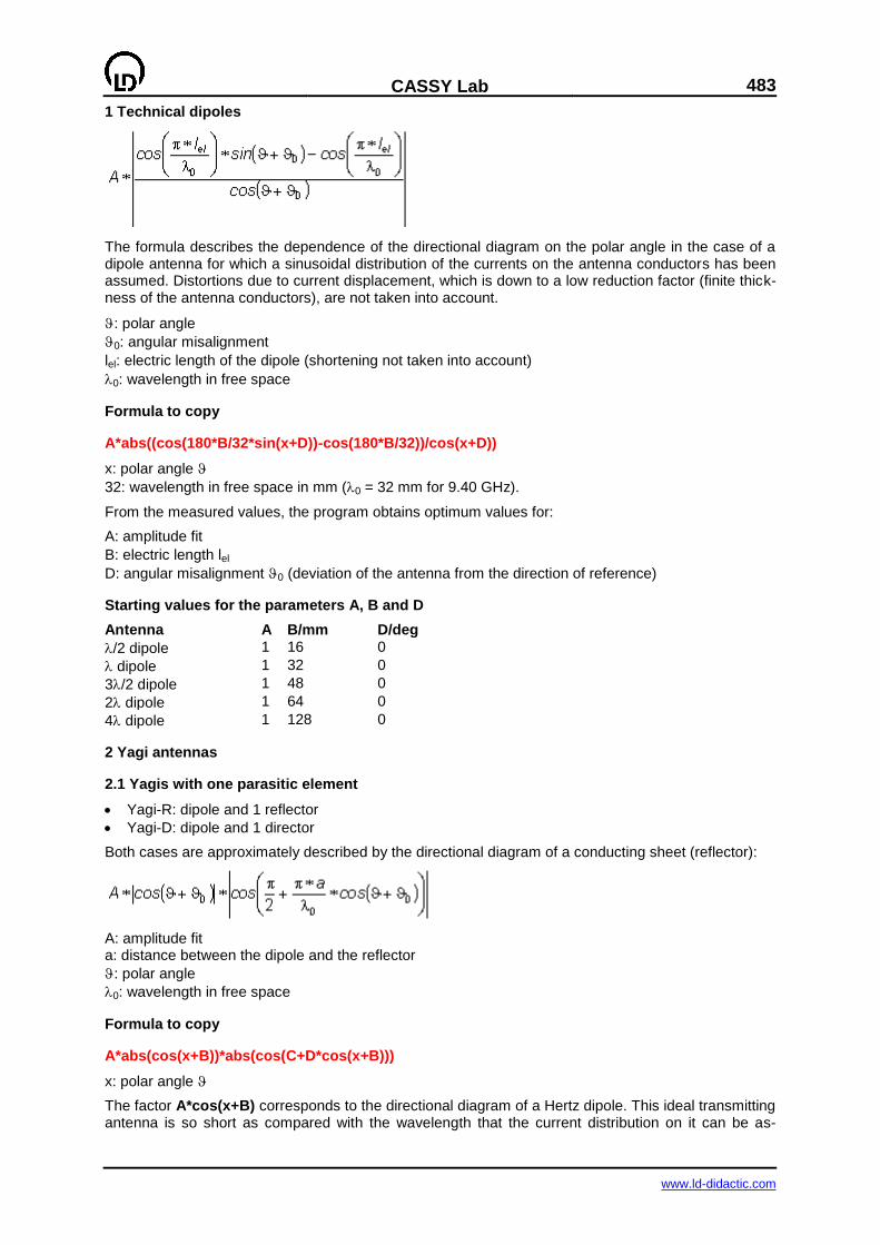
CASSY Lab

483

www.ld-didactic.com

1 Technical dipoles

The formula describes the dependence of the directional diagram on the polar angle in the case of a dipole antenna for which a sinusoidal distribution of the currents on the antenna conductors has been assumed. Distortions due to current displacement, which is down to a low reduction factor (finite thick-ness of the antenna conductors), are not taken into account.

: polar angle

0: angular misalignment

lel: electric length of the dipole (shortening not taken into account)

0: wavelength in free space

Formula to copy

A*abs((cos(180*B/32*sin(x+D))-cos(180*B/32))/cos(x+D))

x: polar angle

32: wavelength in free space in mm (0 = 32 mm for 9.40 GHz).

From the measured values, the program obtains optimum values for:

A: amplitude fit

B: electric length lel

D: angular misalignment 0 (deviation of the antenna from the direction of reference)

Starting values for the parameters A, B and D

Antenna A B/mm D/deg

/2 dipole 1 16 0

dipole 1 32 0

3/2 dipole 1 48 0

2 dipole 1 64 0

4 dipole 1 128 0

2 Yagi antennas

2.1 Yagis with one parasitic element

Yagi-R: dipole and 1 reflector

Yagi-D: dipole and 1 director

Both cases are approximately described by the directional diagram of a conducting sheet (reflector):

A: amplitude fit a: distance between the dipole and the reflector

: polar angle


Formula to copy

A*abs(cos(x+B))*abs(cos(C+D*cos(x+B)))

x: polar angle

The factor A*cos(x+B) corresponds to the directional diagram of a Hertz dipole. This ideal transmitting antenna is so short as compared with the wavelength that the current distribution on it can be as-

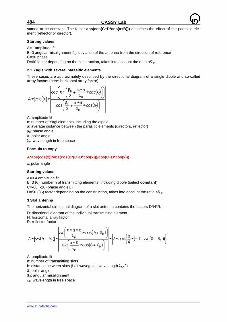
484

CASSY Lab

www.ld-didactic.com

sumed to be constant. The factor abs(cos(C+D*cos(x+B))) describes the effect of the parasitic ele-ment (reflector or director).

Starting values

A=1 amplitude fit

B=0 angular misalignment 0, deviation of the antenna from the direction of reference C=90 phase

D=60 factor depending on the construction, takes into account the ratio a/0

2.2 Yagis with several parasitic elements

These cases are approximately described by the directional diagram of a single dipole and so-called array factors (here: horizontal array factor):

A: amplitude fit n: number of Yagi elements, including the dipole a: average distance between the parasitic elements (directors, reflector)

0: phase angle

: polar angle


Formula to copy

A*abs(cos(x))*abs(cos(B*(C+D*cos(x)))/cos(C+D*cos(x)))

x: polar angle

Starting values

A=0.4 amplitude fit B=3 (6) number n of transmitting elements, including dipole (select constant)

C=-60 (-20) phase angle 0

D=50 (36) factor depending on the construction, takes into account the ratio a/0

3 Slot antenna

The horizontal directional diagram of a slot antenna contains the factors D*H*R:

D: directional diagram of the individual transmitting element H: horizontal array factor R: reflector factor

A: amplitude fit n: number of transmitting slots

b: distance between slots (half waveguide wavelength G/2)

: polar angle

0: angular misalignment


CASSY Lab

485

www.ld-didactic.com

Formula to copy

A*abs(sin(x+B))*abs((sin(D*180*C/32*cos(x+B))/sin(180*C/32*cos(x+B)))*cos(45*(-1+sin(x+B))))

x: polar angle

Starting values

A=1 amplitude fit

B=0 angle fit 0 C=23 distance b between slots D=7 number n of slots (select constant)

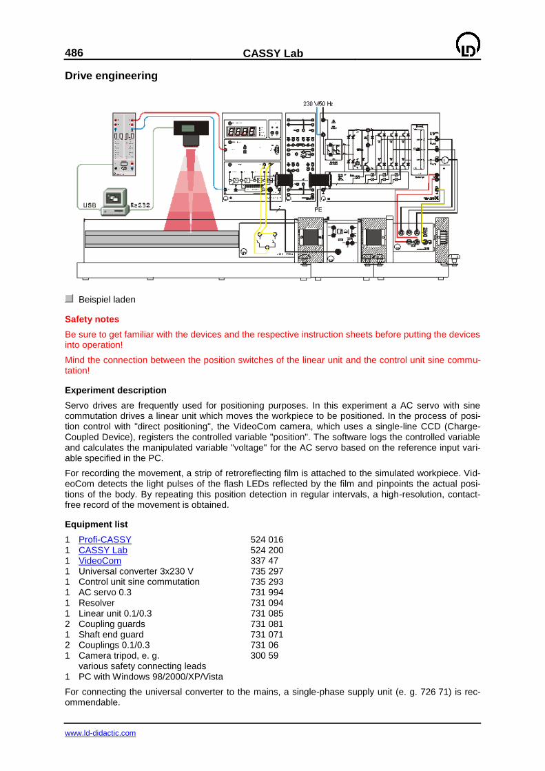
486

CASSY Lab

www.ld-didactic.com

Drive engineering

Beispiel laden

Safety notes

Be sure to get familiar with the devices and the respective instruction sheets before putting the devices into operation!

Mind the connection between the position switches of the linear unit and the control unit sine commu-tation!


Servo drives are frequently used for positioning purposes. In this experiment a AC servo with sine commutation drives a linear unit which moves the workpiece to be positioned. In the process of posi-tion control with "direct positioning", the VideoCom camera, which uses a single-line CCD (Charge-Coupled Device), registers the controlled variable "position". The software logs the controlled variable and calculates the manipulated variable "voltage" for the AC servo based on the reference input vari-able specified in the PC.

For recording the movement, a strip of retroreflecting film is attached to the simulated workpiece. Vid-eoCom detects the light pulses of the flash LEDs reflected by the film and pinpoints the actual posi-tions of the body. By repeating this position detection in regular intervals, a high-resolution, contact-free record of the movement is obtained.

Equipment list

1 Profi-CASSY 524 016 1 CASSY Lab 524 200 1 VideoCom 337 47 1 Universal converter 3x230 V 735 297 1 Control unit sine commutation 735 293 1 AC servo 0.3 731 994 1 Resolver 731 094 1 Linear unit 0.1/0.3 731 085 2 Coupling guards 731 081 1 Shaft end guard 731 071 2 Couplings 0.1/0.3 731 06 1 Camera tripod, e. g. 300 59 various safety connecting leads 1 PC with Windows 98/2000/XP/Vista

For connecting the universal converter to the mains, a single-phase supply unit (e. g. 726 71) is rec-ommendable.

CASSY Lab

487

www.ld-didactic.com

Experiment setup

Set up the experiment according to the drawing. Connect the Profi-CASSY to a USB port and the Vid-eoCom to a serial RS232 port of the PC. Do NOT yet couple the linear unit to the drive line! Couple the AC servo and the resolver as described in the instruction sheet, and put the system into operation. Turn the slide of the linear unit approximately into the centre. Attach the camera to a stand at a height of approximately 1 m over the centre of the linear unit. Switch the control unit sine commutation into the mode "Closed-loop Speed Control".


Einstellungen laden

If you have not yet selected VideoCom as the connected device, do it now. For this assign Video-Com to the desired port in the General Settings. Then save this assignment with Save New De-faults.

If no value is displayed in the window for the controlled variable path s, adjust the camera so that the position is displayed.

Set the reference input variable w to a value of 0.5 m.

Start the measurement with F9 (stop clock). The motor starts up. Turn the positioning unit manually until the motor stops.

Now couple the positioning unit and the drive line together. By changing the reference input vari-able w you can specify positions, which then are approached.

Now you can change the control parameters Kp and Tn and observe the effect of these changes on the control. in the same way you can set the limits for the speed and the current at the control unit sine commutation (see instruction sheet).

488

CASSY Lab

www.ld-didactic.com

Appendix

Scintillation counter

With a scintillation counter (559 901) the energy of radiation can be determined. By interaction with the scintillation crystal the radiation gives rise to light flashes, which are converted into a voltage pulse by a photomultiplier. The number of emitted photons, and therefore the pulse height is proportional to

the energy. The pulse-height analysis in made with a multichannel analyzer (MCA), e.g. with the MCA box (524 058) in conjunction with the Sensor CASSY (524 010).

The energy of radiation can be determined with a semiconductor detector.

NaI(Tl) scintillators

A common material for the construction of scintillation counters is NaI(Tl). Doping with thallium (Tl) generates luminescent centres. The iodine content (Z=53) leads to a very high detection probability for

radiation. Detection of quanta emitted from a source takes place via energy transfer to electrons of NaI, which are slowed down in the scintillation crystal. Thereby pairs of populated states in the con-duction band and unpopulated states in the valence band are released. The number of these electron-hole pairs is proportional to the absorbed energy as the energy required to produce an electron-hole pair is always the same. The thallium atoms bonded in the crystal are ionized by interaction with the holes which arise while the primary electron is slowed down. After subsequent recombination with an electron, they emit photons with an energy between 2.9 and 3.1 eV. The number of photons is thus proportional to the absorbed energy.

The NaI crystal is transparent for the emitted photons. The absorption of these photons by other thal-lium atoms is very unlikely because of the low thallium concentration. As the scintillation crystal is a crystal, there is no scattering from grain boundaries in the crystal. Moreover, the crystal has a light-tight encapsulation and is coated with a highly reflecting material. So a great part of the emitted pho-tons reaches the attached photocathode of the photomultiplier. In the photocathode the emitted pho-tons knock out electrons. Next the electron current is avalanche-like amplified through generation of secondary electrons in a series of dynodes that follow one another. The gain for one dynode stage depends, among other things, on the potential difference between the dynodes and on the dynode material. The dynode potentials are tapped at a voltage divider where a thermally and long-term stable high voltage is applied. A charge that is proportional to the number of photons reaches the anode and causes a current, which leads to a voltage signal at a load resistor. This signal is proportional to the charge if the decay time of the output pulse is considerably larger than the time constant for the emis-

sion of light by the excited thallium atoms (t = 0.23 s). Altogether the pulse amplitude is thus propor-tional to the energy of the absorbed radiation.

This voltage pulse is then evaluated, e.g. with a system consisting of the MCA box, the Sensor CASSY and the CASSY Lab software on a PC.

The energy of the radiation entering the detector is not always completely converted in the scintillation crystal, but part of it can escape, e.g. via the Compton effect.

Caution

The NaI(Tl) crystal at the end of the scintillation counter is very sensitive to mechanical stress and may easily be destroyed.

The NaI(Tl) crystal is also sensitive to quick changes in temperature, which can occur, e.g., on unpacking after transport.

In both cases cracks in the crystal arise and lead to a reduced sensitivity and, above all, to a worse energy resolution because of scattering.

CASSY Lab

489

www.ld-didactic.com

Semiconductor counters

For the detection of radiation, semiconductor barrier layer detectors are preferred. Ionizing radia-tion generates a charge in the barrier layer of a semiconductor diode (559 92). This charge, which is

proportional to the energy, is measured electronically and can be made available at the output of a suitable preamplifier (559 93). The pulse can be further processed with a multichannel analyzer, e.g. with the MCA box in conjunction with the Sensor-CASSY.

The preparations used in this experiment emit particles with an energy around 6 MeV. In silicon

these particles have a penetration depth of approx. 50 m. The width of the barrier layer of the semi-

conductor diode depends on the applied reverse voltage and is of the order of 70 m at a reverse voltage of 10 V.

Multichannel pulse-height analysis

The detector signals are further processed in a multichannel analyzer whose central components are a peak detector and an analog-to-digital converter. The peak detector stores the maximum value of the input pulse U, and the analog-to-digital converter converts the measured value into a proportional digital value k. More precisely, k corresponds to an interval of pulse heights, whose width depends on the resolution of the analog-to-digital converter. The computer assigns a storage location to each digi-tal value and counts the events in each storage location. The result is a histogram which represents the frequency distribution of the pulse heights. For a quantitative evaluation an energy calibration is required as the proportionality factors between the energy and the pulse height are unknown at first.

For the energy calibration a spectrum of a known source is recorded. Then the channel numbers can be assigned to the corresponding energies. This calibration is then valid for other spectra recorded under the same conditions.

The MCA box (524 058) is such a multichannel analyzer for the Sensor CASSY (524 010), which is supported by CASSY Lab (524 200).

490

CASSY Lab

www.ld-didactic.com

Interaction of radiation with matter

In the energy range between 50 and 2000 keV, two interaction processes of radiation with the scin-tillation crystal play the major role.

In the photoelectric effect, the quantum transfers its total energy E to an atom in the crystal and

releases a bound electron. Apart from the amount of the binding energy, the energy is converted into kinetic energy of the electron. This kinetic energy is transferred to the crystal through inelastic scatter-ing. The ionized atom emits X-ray quanta or Auger electrons, whose energy is completely absorbed in the detector in most cases. Then the total amount of absorbed energy corresponds to the energy of

the quantum. The radiation is registered in the peak of total absorption of the pulse-height distribu-tion in this case.

In the Compton effect, part of the energy is converted into kinetic energy of a quasi-free electron in

an elastic collision. The rest of the original energy is left with the scattered quantum, which escapes from the scintillation crystal with a certain probability certain probability. The energy of the electron

absorbed in the detector then lies between 0 keV (forward scattering of the quantum) and a maxi-

mum value EC (backward scattering of the quantum). This leads to a Compton distribution with a

Compton edge at the energy EC.

Internal conversion

After a radioactive decay ( or decay), the daughter nucleus may be in an excited state. In the tran-sition to the energetically more favourable ground state energy is released, which can be given off in different ways.

Apart from giving off the energy by direct emission of a quantum, the nucleus may as well transfer the energy to an electron of its atomic shell. The probability of finding shell electrons in the nucleus is not zero. The energy is preferably transferred to electrons of the inner shells. These carry the energy of the excited state away as kinetic energy and leave behind a singly ionized atom. The hole left in the inner atomic shell is replenished by electrons from higher shells. The energy that is released in this process can be transferred to outer electrons of the same nucleus (Auger process) or emitted in the form of characteristic X radiation.

As the de-excitation of the nucleus via internal conversion competes with emission, emitting iso-

topes are favourable candidates for the observation of K emissions.

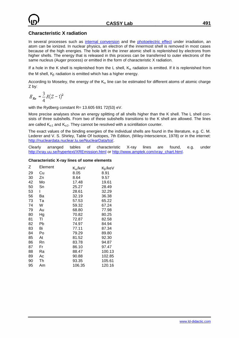
CASSY Lab

491

www.ld-didactic.com

Characteristic X radiation

In several processes such as internal conversion and the photoelectric effect under irradiation, an atom can be ionized. In nuclear physics, an electron of the innermost shell is removed in most cases because of the high energies. The hole left in the inner atomic shell is replenished by electrons from higher shells. The energy that is released in this process can be transferred to outer electrons of the same nucleus (Auger process) or emitted in the form of characteristic X radiation.

If a hole in the K shell is replenished from the L shell, K radiation is emitted. If it is replenished from

the M shell, K radiation is emitted which has a higher energy.

According to Moseley, the energy of the K line can be estimated for different atoms of atomic charge

Z by:

with the Rydberg constant R= 13.605 691 72(53) eV.

More precise analyses show an energy splitting of all shells higher than the K shell. The L shell con-sists of three subshells. From two of these subshells transitions to the K shell are allowed. The lines

are called K1 and K2. They cannot be resolved with a scintillation counter.

The exact values of the binding energies of the individual shells are found in the literature, e.g. C. M. Lederer and V. S. Shirley, Table Of Isotopes, 7th Edition, (Wiley-Interscience, 1978) or in the internet: http://nucleardata.nuclear.lu.se/NuclearData/toi/.

Clearly arranged tables of characteristic X-ray lines are found, e.g. under http://xray.uu.se/hypertext/XREmission.html or http://www.amptek.com/xray_chart.html.

Characteristic X-ray lines of some elements

Z Element K/keV K/keV

29 Cu 8.05 8.91 30 Zn 8.64 9.57 42 Mo 17.48 19.61 50 Sn 25.27 28.49 53 I 28.61 32.29 56 Ba 32.19 36.38 73 Ta 57.53 65.22 74 W 59.32 67.24 79 Au 68.80 77.98 80 Hg 70.82 80.25 81 Tl 72.87 82.58 82 Pb 74.97 84.94 83 Bi 77.11 87.34 84 Po 79.29 89.80 85 At 81.52 92.30 86 Rn 83.78 94.87 87 Fr 86.10 97.47 88 Ra 88.47 100.13 89 Ac 90.88 102.85 90 Th 93.35 105.61 95 Am 106.35 120.16

http://nucleardata.nuclear.lu.se/NuclearData/toi

http://xray.uu.se/hypertext/XREmission.html

http://www.amptek.com/xray_chart.html

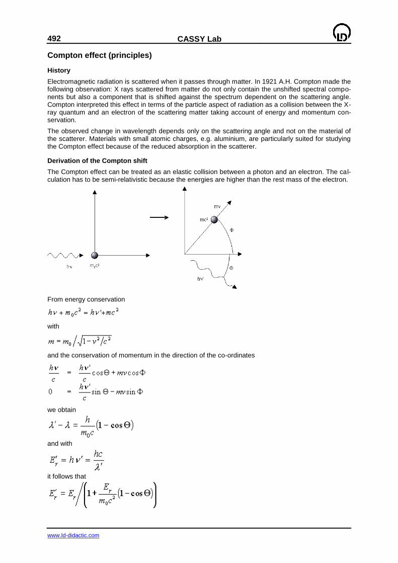
492

CASSY Lab

www.ld-didactic.com

Compton effect (principles)

History

Electromagnetic radiation is scattered when it passes through matter. In 1921 A.H. Compton made the following observation: X rays scattered from matter do not only contain the unshifted spectral compo-nents but also a component that is shifted against the spectrum dependent on the scattering angle. Compton interpreted this effect in terms of the particle aspect of radiation as a collision between the X-ray quantum and an electron of the scattering matter taking account of energy and momentum con-servation.

The observed change in wavelength depends only on the scattering angle and not on the material of the scatterer. Materials with small atomic charges, e.g. aluminium, are particularly suited for studying the Compton effect because of the reduced absorption in the scatterer.

Derivation of the Compton shift

The Compton effect can be treated as an elastic collision between a photon and an electron. The cal-culation has to be semi-relativistic because the energies are higher than the rest mass of the electron.

From energy conservation

with

and the conservation of momentum in the direction of the co-ordinates

we obtain

and with

it follows that

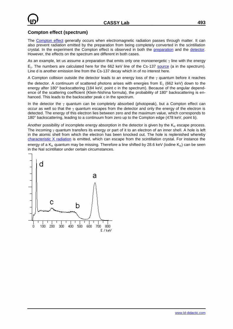
CASSY Lab

493

www.ld-didactic.com

Compton effect (spectrum)

The Compton effect generally occurs when electromagnetic radiation passes through matter. It can also prevent radiation emitted by the preparation from being completely converted in the scintillation crystal. In the experiment the Compton effect is observed in both the preparation and the detector. However, the effects on the spectrum are different in both cases.

As an example, let us assume a preparation that emits only one monoenergetic line with the energy

E. The numbers are calculated here for the 662 keV line of the Cs-137 source (a in the spectrum).

Line d is another emission line from the Cs-137 decay which in of no interest here.

A Compton collision outside the detector leads to an energy loss of the quantum before it reaches

the detector. A continuum of scattered photons arises with energies from E (662 keV) down to the

energy after 180° backscattering (184 keV, point c in the spectrum). Because of the angular depend-ence of the scattering coefficient (Klein-Nishina formula), the probability of 180° backscattering is en-hanced. This leads to the backscatter peak c in the spectrum.

In the detector the quantum can be completely absorbed (photopeak), but a Compton effect can

occur as well so that the quantum escapes from the detector and only the energy of the electron is detected. The energy of this electron lies between zero and the maximum value, which corresponds to 180° backscattering, leading to a continuum from zero up to the Compton edge (478 keV, point b).

Another possibility of incomplete energy absorption in the detector is given by the K escape process.

The incoming quantum transfers its energy or part of it to an electron of an inner shell. A hole is left in the atomic shell from which the electron has been knocked out. The hole is replenished whereby characteristic X radiation is emitted, which can escape from the scintillation crystal. For instance the

energy of a K quantum may be missing. Therefore a line shifted by 28.6 keV (iodine K) can be seen

in the NaI scintillator under certain circumstances.

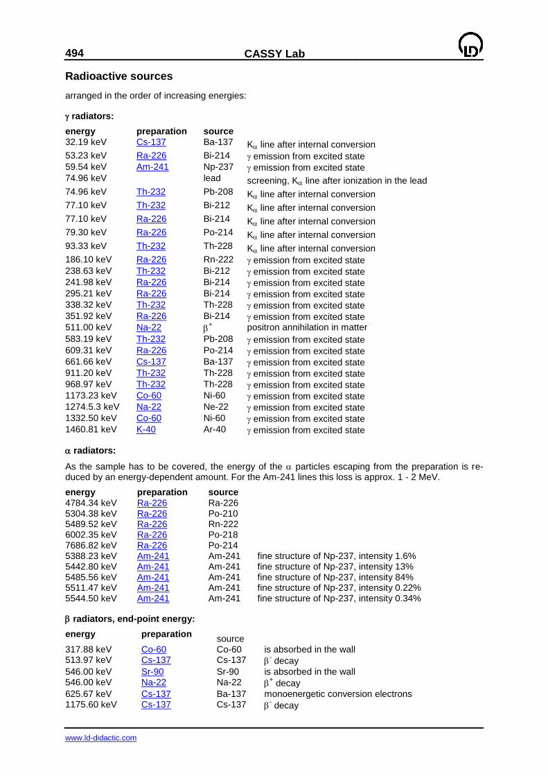
494

CASSY Lab

www.ld-didactic.com

Radioactive sources

arranged in the order of increasing energies:

radiators:

energy preparation source 32.19 keV Cs-137 Ba-137 K line after internal conversion

53.23 keV Ra-226 Bi-214 emission from excited state 59.54 keV Am-241 Np-237 emission from excited state 74.96 keV lead screening, K line after ionization in the lead

74.96 keV Th-232 Pb-208 K line after internal conversion

77.10 keV Th-232 Bi-212 K line after internal conversion

77.10 keV Ra-226 Bi-214 K line after internal conversion

79.30 keV Ra-226 Po-214 K line after internal conversion

93.33 keV Th-232 Th-228 K line after internal conversion

186.10 keV Ra-226 Rn-222 emission from excited state 238.63 keV Th-232 Bi-212 emission from excited state 241.98 keV Ra-226 Bi-214 emission from excited state 295.21 keV Ra-226 Bi-214 emission from excited state 338.32 keV Th-232 Th-228 emission from excited state 351.92 keV Ra-226 Bi-214 emission from excited state 511.00 keV Na-22

+ positron annihilation in matter

583.19 keV Th-232 Pb-208 emission from excited state 609.31 keV Ra-226 Po-214 emission from excited state 661.66 keV Cs-137 Ba-137 emission from excited state 911.20 keV Th-232 Th-228 emission from excited state 968.97 keV Th-232 Th-228 emission from excited state 1173.23 keV Co-60 Ni-60 emission from excited state 1274.5.3 keV Na-22 Ne-22 emission from excited state 1332.50 keV Co-60 Ni-60 emission from excited state 1460.81 keV K-40 Ar-40 emission from excited state

radiators:

As the sample has to be covered, the energy of the particles escaping from the preparation is re-duced by an energy-dependent amount. For the Am-241 lines this loss is approx. 1 - 2 MeV.

energy preparation source 4784.34 keV Ra-226 Ra-226 5304.38 keV Ra-226 Po-210 5489.52 keV Ra-226 Rn-222 6002.35 keV Ra-226 Po-218 7686.82 keV Ra-226 Po-214 5388.23 keV Am-241 Am-241 fine structure of Np-237, intensity 1.6% 5442.80 keV Am-241 Am-241 fine structure of Np-237, intensity 13% 5485.56 keV Am-241 Am-241 fine structure of Np-237, intensity 84% 5511.47 keV Am-241 Am-241 fine structure of Np-237, intensity 0.22% 5544.50 keV Am-241 Am-241 fine structure of Np-237, intensity 0.34%

radiators, end-point energy:

energy preparation source

317.88 keV Co-60 Co-60 is absorbed in the wall 513.97 keV Cs-137 Cs-137

- decay

546.00 keV Sr-90 Sr-90 is absorbed in the wall 546.00 keV Na-22 Na-22

+ decay

625.67 keV Cs-137 Ba-137 monoenergetic conversion electrons 1175.60 keV Cs-137 Cs-137

- decay

CASSY Lab

495

www.ld-didactic.com

1820.20 keV Na-22 Na-22 + decay

2280.10 keV Sr-90 Y-90 - decay

The data are taken from: The Lund/LBNL Nuclear Data Search Version 2.0, February 1999 S.Y.F. Chu 1, L.P. Ekstroem 1,2 and R.B. Firestone 1 1 LBNL, Berkeley, USA 2 Department of Physics, Lund University, Sweden and are also available under http://nucleardata.nuclear.lu.se/nucleardata/toi/index.asp.

The following preparations are currently available from LD Didactic:

Cat. No. designation 588 855 STM equipment set RAD 1 containing among other things:

Brazil nut ash 060 26 002 (Ra-226) potassium sulphate 200 67 322 (K-40)

559 430 Ra-226 preparation, 3.3 kBq 559 82 Am-241 preparation, 330 kBq 559 87 Sr-90 preparation, 110 kBq 559 809 Cs-137 preparation, 3.7 MBq 559 815 Cs-137 preparation, 370 kBq, for extracting Ba-137 m 559 885 Cs-137 preparation, 5 kBq, for Marinelli beaker 559 83 set of radioactive preparations

Am-241 preparation 74 kBq Co-60 preparation 74 kBq Na-22 preparation 74 kBq Sr-90 preparation 74 kBq

mixed preparation , , as 559 84, see below 559 84 559 84 mixed preparation , , , containing

Cs-137, 330 kBq Am-241, 4.4 kBq Sr-90, 4.4 kBq

To Table of experiments

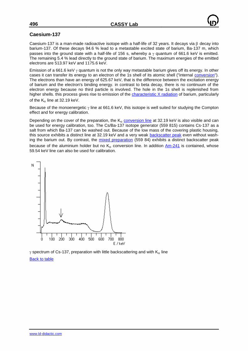
http://nucleardata.nuclear.lu.se/nucleardata/toi/index.asp

496

CASSY Lab

www.ld-didactic.com

Caesium-137

Caesium-137 is a man-made radioactive isotope with a half-life of 32 years. It decays via decay into barium-137. Of these decays 94.6 % lead to a metastable excited state of barium, Ba-137 m, which

passes into the ground state with a half-life of 156 s, whereby a quantum of 661.6 keV is emitted. The remaining 5.4 % lead directly to the ground state of barium. The maximum energies of the emitted electrons are 513.97 keV and 1175.6 keV.

Emission of a 661.6 keV quantum is not the only way metastable barium gives off its energy. In other cases it can transfer its energy to an electron of the 1s shell of its atomic shell ("internal conversion"). The electrons than have an energy of 625.67 keV, that is the difference between the excitation energy of barium and the electron's binding energy. in contrast to beta decay, there is no continuum of the electron energy because no third particle is involved. The hole in the 1s shell is replenished from higher shells. this process gives rise to emission of the characteristic X radiation of barium, particularly

of the K line at 32.19 keV.

Because of the monoenergetic line at 661.6 keV, this isotope is well suited for studying the Compton effect and for energy calibration.

Depending on the cover of the preparation, the K conversion line at 32.19 keV is also visible and can

be used for energy calibration, too. The Cs/Ba-137 isotope generator (559 815) contains Cs-137 as a salt from which Ba-137 can be washed out. Because of the low mass of the covering plastic housing, this source exhibits a distinct line at 32.19 keV and a very weak backscatter peak even without wash-ing the barium out. By contrast, the mixed preparation (559 84) exhibits a distinct backscatter peak

because of the aluminium holder but no K conversion line. In addition Am-241 is contained, whose

59.54 keV line can also be used for calibration.

spectrum of Cs-137, preparation with little backscattering and with K line

Back to table

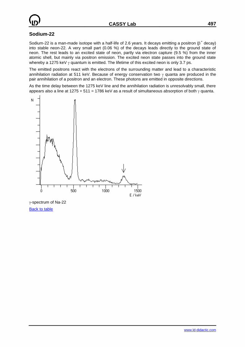
CASSY Lab

497

www.ld-didactic.com

Sodium-22

Sodium-22 is a man-made isotope with a half-life of 2.6 years. It decays emitting a positron (+ decay)

into stable neon-22. A very small part (0.06 %) of the decays leads directly to the ground state of neon. The rest leads to an excited state of neon, partly via electron capture (9.5 %) from the inner atomic shell, but mainly via positron emission. The excited neon state passes into the ground state

whereby a 1275 keV quantum is emitted. The lifetime of this excited neon is only 3.7 ps.

The emitted positrons react with the electrons of the surrounding matter and lead to a characteristic

annihilation radiation at 511 keV. Because of energy conservation two quanta are produced in the pair annihilation of a positron and an electron. These photons are emitted in opposite directions.

As the time delay between the 1275 keV line and the annihilation radiation is unresolvably small, there

appears also a line at 1275 + 511 = 1786 keV as a result of simultaneous absorption of both quanta.

-spectrum of Na-22

Back to table

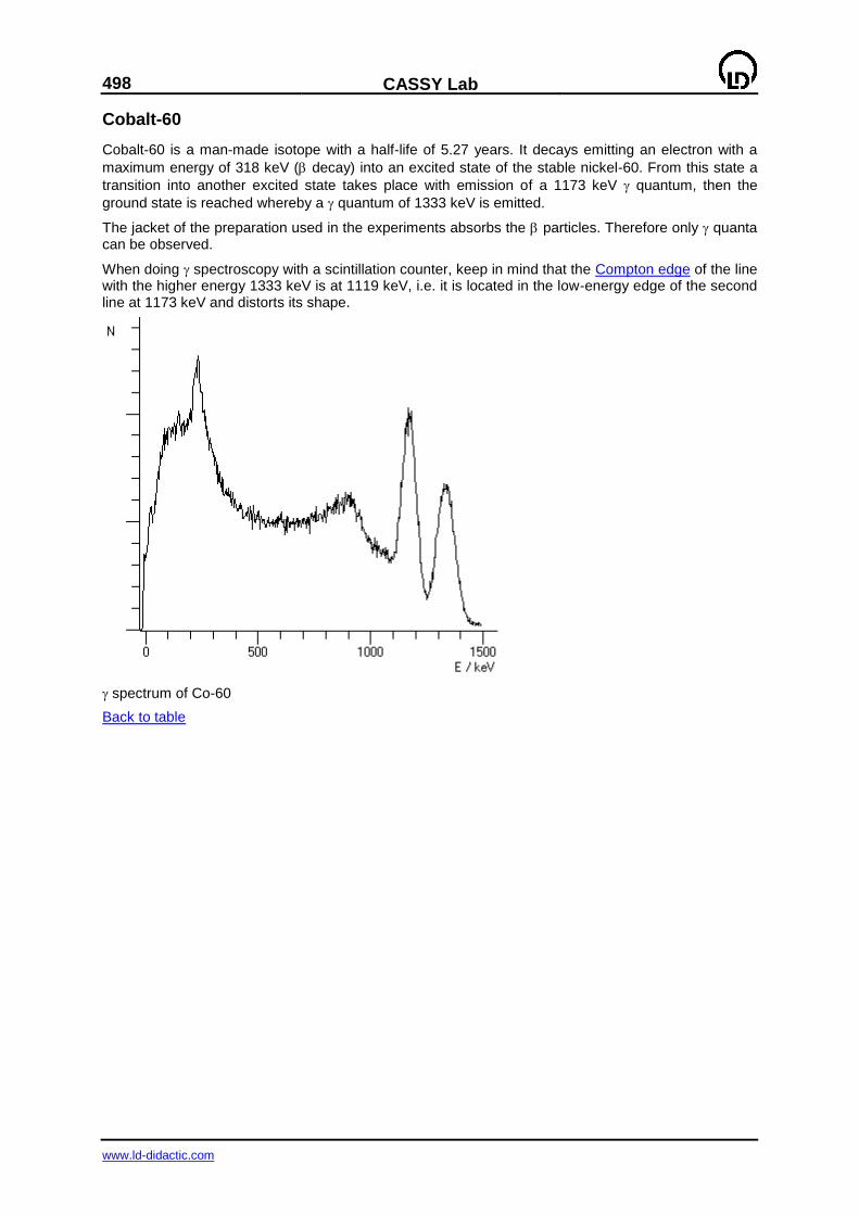
498

CASSY Lab

www.ld-didactic.com

Cobalt-60

Cobalt-60 is a man-made isotope with a half-life of 5.27 years. It decays emitting an electron with a

maximum energy of 318 keV ( decay) into an excited state of the stable nickel-60. From this state a

transition into another excited state takes place with emission of a 1173 keV quantum, then the

ground state is reached whereby a quantum of 1333 keV is emitted.

The jacket of the preparation used in the experiments absorbs the particles. Therefore only quanta can be observed.

When doing spectroscopy with a scintillation counter, keep in mind that the Compton edge of the line with the higher energy 1333 keV is at 1119 keV, i.e. it is located in the low-energy edge of the second line at 1173 keV and distorts its shape.

spectrum of Co-60

Back to table

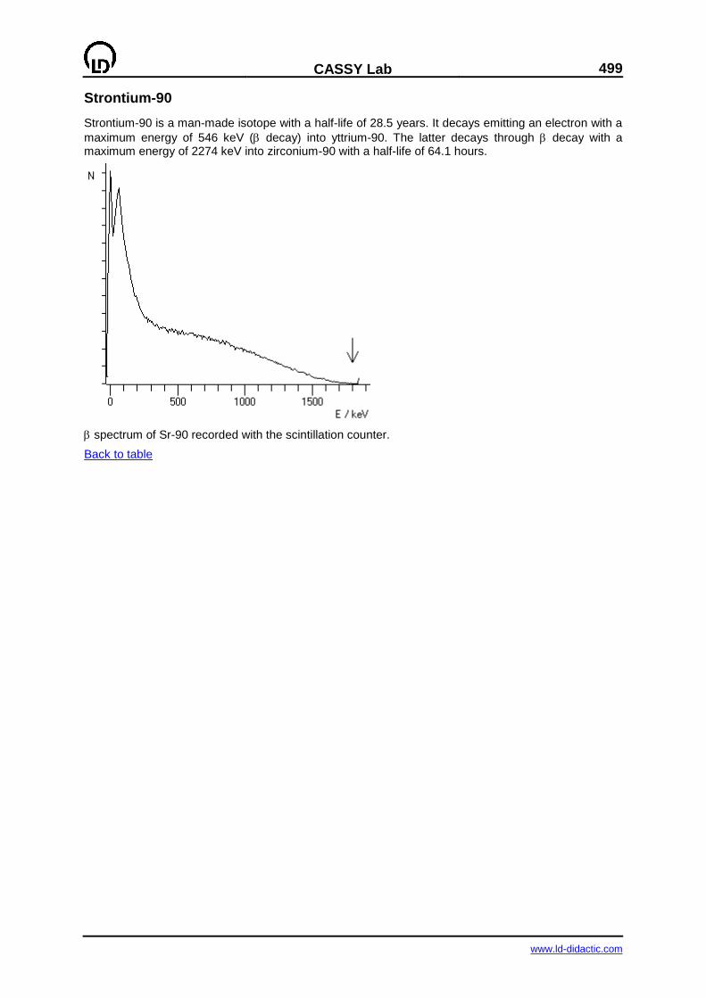
CASSY Lab

499

www.ld-didactic.com

Strontium-90

Strontium-90 is a man-made isotope with a half-life of 28.5 years. It decays emitting an electron with a

maximum energy of 546 keV ( decay) into yttrium-90. The latter decays through decay with a maximum energy of 2274 keV into zirconium-90 with a half-life of 64.1 hours.

spectrum of Sr-90 recorded with the scintillation counter.

Back to table

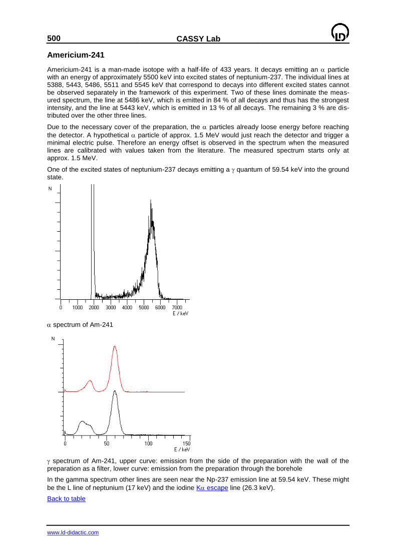
500

CASSY Lab

www.ld-didactic.com

Americium-241

Americium-241 is a man-made isotope with a half-life of 433 years. It decays emitting an particle with an energy of approximately 5500 keV into excited states of neptunium-237. The individual lines at 5388, 5443, 5486, 5511 and 5545 keV that correspond to decays into different excited states cannot be observed separately in the framework of this experiment. Two of these lines dominate the meas-ured spectrum, the line at 5486 keV, which is emitted in 84 % of all decays and thus has the strongest intensity, and the line at 5443 keV, which is emitted in 13 % of all decays. The remaining 3 % are dis-tributed over the other three lines.

Due to the necessary cover of the preparation, the particles already loose energy before reaching

the detector. A hypothetical particle of approx. 1.5 MeV would just reach the detector and trigger a minimal electric pulse. Therefore an energy offset is observed in the spectrum when the measured lines are calibrated with values taken from the literature. The measured spectrum starts only at approx. 1.5 MeV.

One of the excited states of neptunium-237 decays emitting a quantum of 59.54 keV into the ground state.

spectrum of Am-241

spectrum of Am-241, upper curve: emission from the side of the preparation with the wall of the preparation as a filter, lower curve: emission from the preparation through the borehole

In the gamma spectrum other lines are seen near the Np-237 emission line at 59.54 keV. These might

be the L line of neptunium (17 keV) and the iodine K escape line (26.3 keV).

Back to table

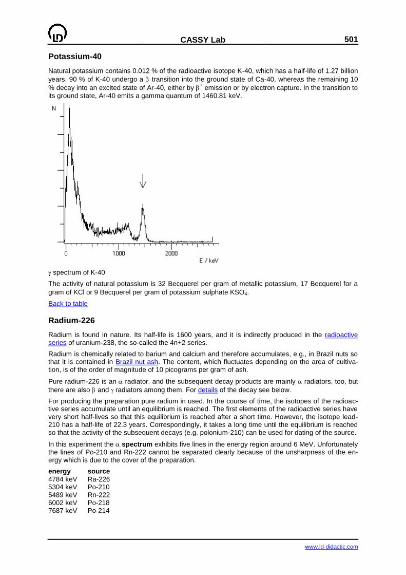
CASSY Lab

501

www.ld-didactic.com

Potassium-40

Natural potassium contains 0.012 % of the radioactive isotope K-40, which has a half-life of 1.27 billion

years. 90 % of K-40 undergo a transition into the ground state of Ca-40, whereas the remaining 10

% decay into an excited state of Ar-40, either by + emission or by electron capture. In the transition to

its ground state, Ar-40 emits a gamma quantum of 1460.81 keV.

spectrum of K-40

The activity of natural potassium is 32 Becquerel per gram of metallic potassium, 17 Becquerel for a

gram of KCl or 9 Becquerel per gram of potassium sulphate KSO4.

Back to table

Radium-226

Radium is found in nature. Its half-life is 1600 years, and it is indirectly produced in the radioactive series of uranium-238, the so-called the 4n+2 series.

Radium is chemically related to barium and calcium and therefore accumulates, e.g., in Brazil nuts so that it is contained in Brazil nut ash. The content, which fluctuates depending on the area of cultiva-tion, is of the order of magnitude of 10 picograms per gram of ash.

Pure radium-226 is an radiator, and the subsequent decay products are mainly radiators, too, but

there are also and radiators among them. For details of the decay see below.

For producing the preparation pure radium in used. In the course of time, the isotopes of the radioac-tive series accumulate until an equilibrium is reached. The first elements of the radioactive series have very short half-lives so that this equilibrium is reached after a short time. However, the isotope lead-210 has a half-life of 22.3 years. Correspondingly, it takes a long time until the equilibrium is reached so that the activity of the subsequent decays (e.g. polonium-210) can be used for dating of the source.

In this experiment the spectrum exhibits five lines in the energy region around 6 MeV. Unfortunately the lines of Po-210 and Rn-222 cannot be separated clearly because of the unsharpness of the en-ergy which is due to the cover of the preparation.

energy source 4784 keV Ra-226 5304 keV Po-210 5489 keV Rn-222 6002 keV Po-218 7687 keV Po-214

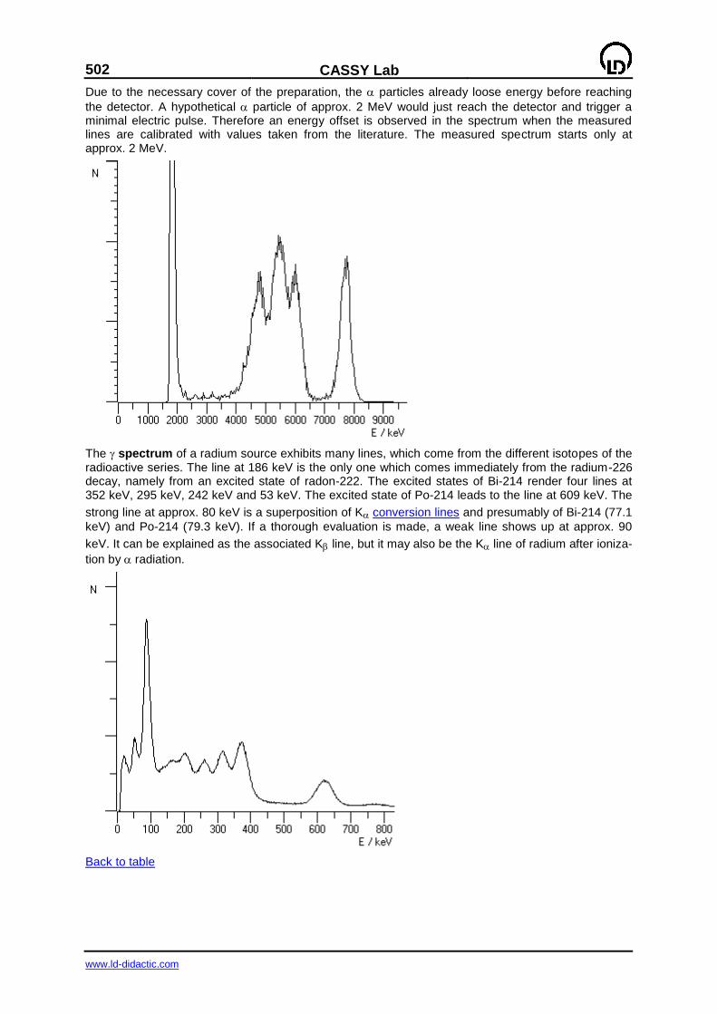
502

CASSY Lab

www.ld-didactic.com

Due to the necessary cover of the preparation, the particles already loose energy before reaching

the detector. A hypothetical particle of approx. 2 MeV would just reach the detector and trigger a minimal electric pulse. Therefore an energy offset is observed in the spectrum when the measured lines are calibrated with values taken from the literature. The measured spectrum starts only at approx. 2 MeV.

The spectrum of a radium source exhibits many lines, which come from the different isotopes of the radioactive series. The line at 186 keV is the only one which comes immediately from the radium-226 decay, namely from an excited state of radon-222. The excited states of Bi-214 render four lines at 352 keV, 295 keV, 242 keV and 53 keV. The excited state of Po-214 leads to the line at 609 keV. The

strong line at approx. 80 keV is a superposition of K conversion lines and presumably of Bi-214 (77.1

keV) and Po-214 (79.3 keV). If a thorough evaluation is made, a weak line shows up at approx. 90

keV. It can be explained as the associated K line, but it may also be the K line of radium after ioniza-

tion by radiation.

Back to table

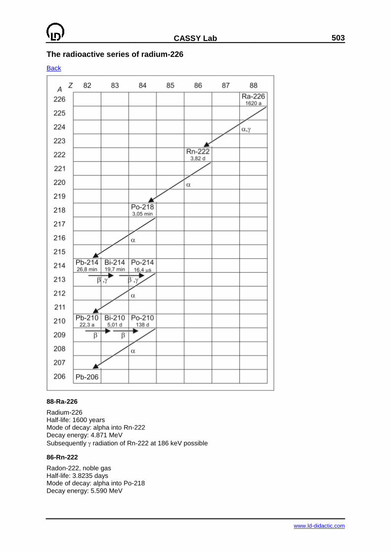
CASSY Lab

503

www.ld-didactic.com

The radioactive series of radium-226

Back

88-Ra-226

Radium-226 Half-life: 1600 years Mode of decay: alpha into Rn-222 Decay energy: 4.871 MeV

Subsequently radiation of Rn-222 at 186 keV possible

86-Rn-222

Radon-222, noble gas Half-life: 3.8235 days Mode of decay: alpha into Po-218 Decay energy: 5.590 MeV

504

CASSY Lab

www.ld-didactic.com

84-Po-218

Polonium-218 (Historically Po-218 is also called radium A) Half-life: 3.10 minutes Mode of decay: alpha into Pb-214 Probability: 99.98 % Decay energy: 6.115 MeV

Mode of decay: beta into At-218 Probability: 0.02 % Decay energy: 0.265 MeV

85-At-218

Astatine-218 Half-life: 1.5 seconds Mode of decay: alpha into Bi-214 Probability: 99.90 % Decay energy: 6.874 MeV

Mode of decay: beta into Rn-218 Probability: 0.1 % Decay energy: 2.883 MeV

86-Rn-218

Radon-218 Half-life: 35 milliseconds Mode of decay: alpha into Po-214 Decay energy: 7.263 MeV

82-Pb-214

Lead-214 (Historically Pb-214 is also called radium B) Half-life: 26.8 minutes Mode of decay: beta into Bi-214 Decay energy: 1.024 MeV

Subsequently radiation of Bi-214 at 352 keV, 295 keV, 242 keV, 53 keV possible

83-Bi-214

Bismuth-214 (Historically Bi-214 is also called radium C) Half-life: 19.9 minutes Mode of decay: beta into Po-214 Probability: 99.98 % Decay energy: 3.272 MeV

Subsequently radiation of Po-214 at 609 keV possible Mode of decay: alpha into Tl-210 Probability: 0.02 % Decay energy: 5.617 MeV

84-Po-214

Polonium-214 (Historically Po-214 is also called radium C')

Half-life: 164.3 s Mode of decay: alpha into Pb-210 Decay energy: 7.833 MeV

CASSY Lab

505

www.ld-didactic.com

81-Tl-210

Thallium-210 (Historically Tl-210 is also called radium C") Half-life: 1.3 Minutes Mode of decay: beta into Pb-210 Decay energy: 5.484 MeV

82-Pb-210

Lead-210 (Historically Pb-210 is also called radium D) Half-life: 22.3 years Mode of decay: beta into Bi-210 Decay energy: 0.064 MeV Mode of decay: alpha into Hg-206

Probability: 1.9-6

%

Decay energy: 3.792 MeV

83-Bi-210

Bismuth-210 (Historically Bi-210 is also called radium E) Half-life: 5.013 days Mode of decay: beta into Po-210 Decay energy: 1.163 MeV

Mode of decay: alpha into Tl-206 Probability: 0.00013 % Decay energy: 5.037 MeV

84-Po-210

Polonium-210 (Historically Po-210 is also called radium F) Half-life: 138.376 days Mode of decay: alpha into Pb-206 Decay energy: 5.407 MeV

82-Pb-206

Lead-206 (Historically Pb-206 is also called Radium G) Pb-206 is the final product of the U-238 radioactive series. It is stable.

The entries are taken from the NUDAT database, see:

R.R.Kinsey, et al., The NUDAT/PCNUDAT Program for Nuclear Data, paper submitted to the 9 th International Symposium of Capture-Gamma_ray Spectroscopy and Related Topics, Budapest, Hun-gary, Octover 1996. Data extracted from NUDAT database (Dec.18, 1997).

Back

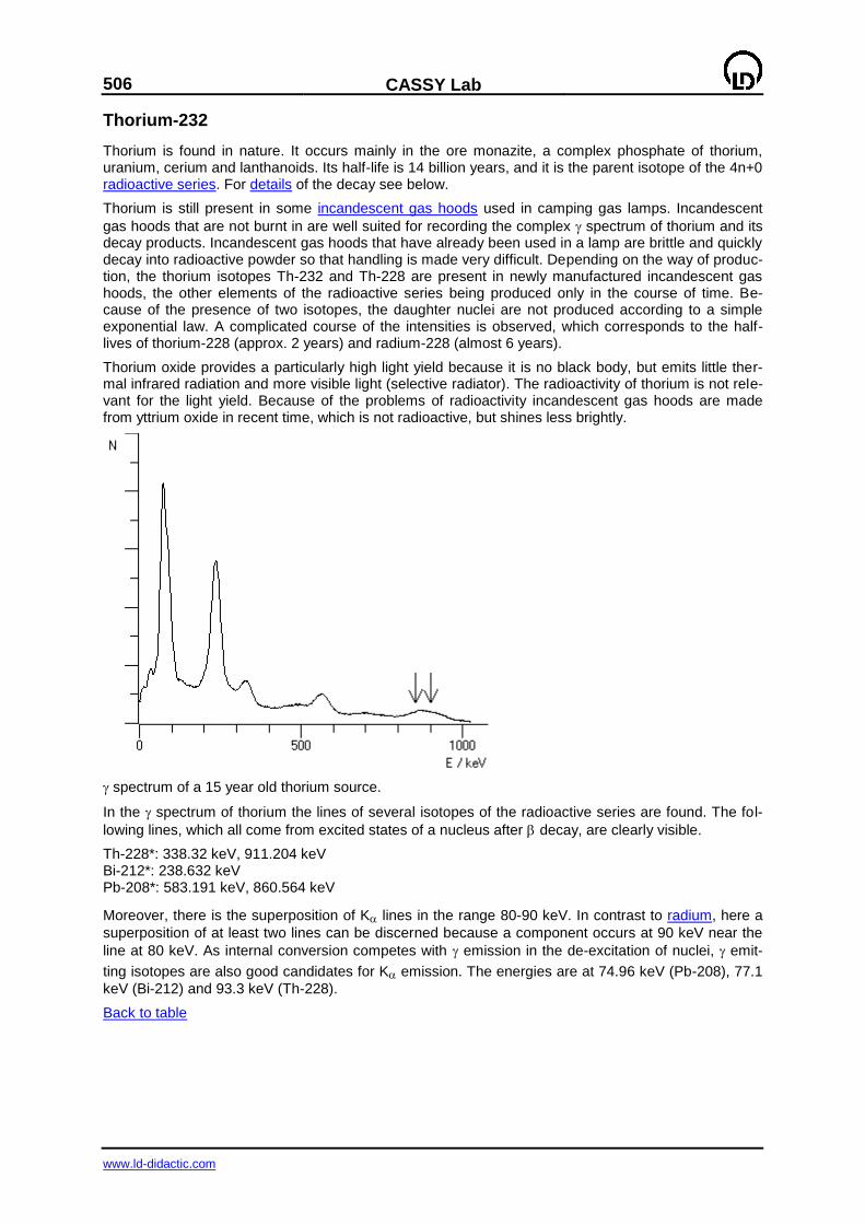
506

CASSY Lab

www.ld-didactic.com

Thorium-232

Thorium is found in nature. It occurs mainly in the ore monazite, a complex phosphate of thorium, uranium, cerium and lanthanoids. Its half-life is 14 billion years, and it is the parent isotope of the 4n+0 radioactive series. For details of the decay see below.

Thorium is still present in some incandescent gas hoods used in camping gas lamps. Incandescent

gas hoods that are not burnt in are well suited for recording the complex spectrum of thorium and its decay products. Incandescent gas hoods that have already been used in a lamp are brittle and quickly decay into radioactive powder so that handling is made very difficult. Depending on the way of produc-tion, the thorium isotopes Th-232 and Th-228 are present in newly manufactured incandescent gas hoods, the other elements of the radioactive series being produced only in the course of time. Be-cause of the presence of two isotopes, the daughter nuclei are not produced according to a simple exponential law. A complicated course of the intensities is observed, which corresponds to the half-lives of thorium-228 (approx. 2 years) and radium-228 (almost 6 years).

Thorium oxide provides a particularly high light yield because it is no black body, but emits little ther-mal infrared radiation and more visible light (selective radiator). The radioactivity of thorium is not rele-vant for the light yield. Because of the problems of radioactivity incandescent gas hoods are made from yttrium oxide in recent time, which is not radioactive, but shines less brightly.

spectrum of a 15 year old thorium source.

In the spectrum of thorium the lines of several isotopes of the radioactive series are found. The fol-

lowing lines, which all come from excited states of a nucleus after decay, are clearly visible.

Th-228*: 338.32 keV, 911.204 keV Bi-212*: 238.632 keV Pb-208*: 583.191 keV, 860.564 keV

Moreover, there is the superposition of K lines in the range 80-90 keV. In contrast to radium, here a

superposition of at least two lines can be discerned because a component occurs at 90 keV near the

line at 80 keV. As internal conversion competes with emission in the de-excitation of nuclei, emit-

ting isotopes are also good candidates for K emission. The energies are at 74.96 keV (Pb-208), 77.1

keV (Bi-212) and 93.3 keV (Th-228).

Back to table

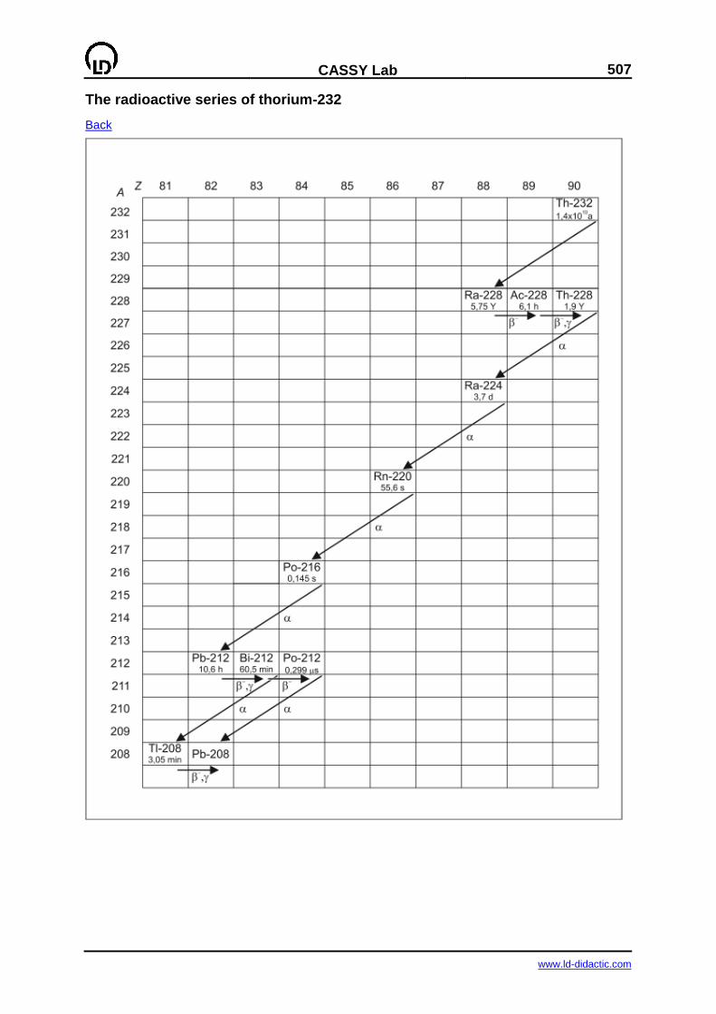
CASSY Lab

507

www.ld-didactic.com

The radioactive series of thorium-232

Back

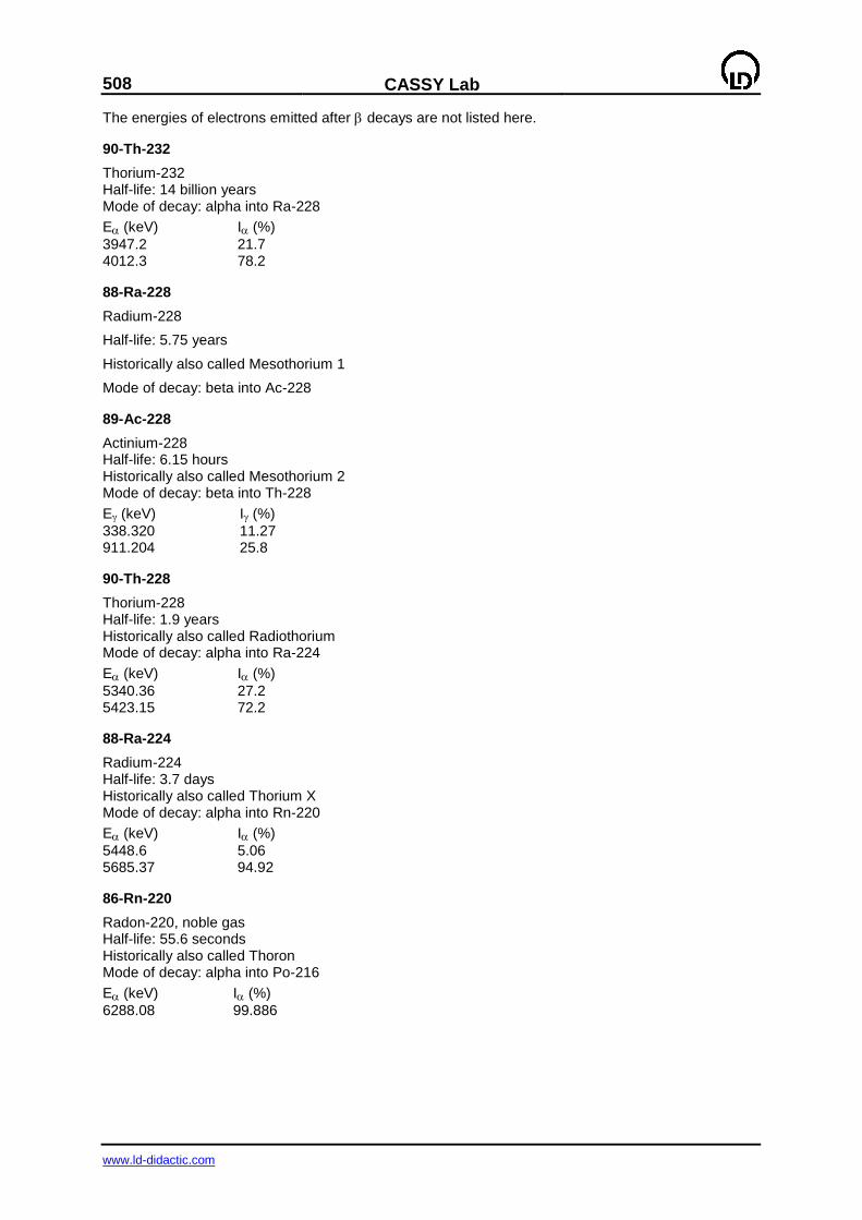
508

CASSY Lab

www.ld-didactic.com

The energies of electrons emitted after decays are not listed here.

90-Th-232

Thorium-232 Half-life: 14 billion years Mode of decay: alpha into Ra-228

E (keV) I (%)

3947.2 21.7 4012.3 78.2

88-Ra-228

Radium-228

Half-life: 5.75 years

Historically also called Mesothorium 1

Mode of decay: beta into Ac-228

89-Ac-228

Actinium-228 Half-life: 6.15 hours Historically also called Mesothorium 2 Mode of decay: beta into Th-228

E (keV) I (%)

338.320 11.27 911.204 25.8

90-Th-228

Thorium-228 Half-life: 1.9 years Historically also called Radiothorium Mode of decay: alpha into Ra-224

E (keV) I (%)

5340.36 27.2 5423.15 72.2

88-Ra-224

Radium-224 Half-life: 3.7 days Historically also called Thorium X Mode of decay: alpha into Rn-220

E (keV) I (%)

5448.6 5.06 5685.37 94.92

86-Rn-220

Radon-220, noble gas Half-life: 55.6 seconds Historically also called Thoron Mode of decay: alpha into Po-216

E (keV) I (%)

6288.08 99.886

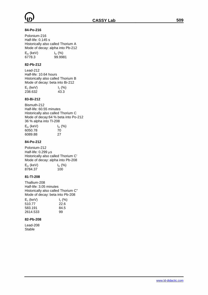
CASSY Lab

509

www.ld-didactic.com

84-Po-216

Polonium-216 Half-life: 0.145 s Historically also called Thorium A Mode of decay: alpha into Pb-212

E (keV) I (%)

6778.3 99.9981

82-Pb-212

Lead-212 Half-life: 10.64 hours Historically also called Thorium B Mode of decay: beta into Bi-212

E (keV) I (%)

238.632 43.3

83-Bi-212

Bismuth-212 Half-life: 60.55 minutes Historically also called Thorium C Mode of decay:64 % beta into Po-212 36 % alpha into Tl-208

E (keV) I (%)

6050.78 70 6089.88 27

84-Po-212

Polonium-212

Half-life: 0.299 s Historically also called Thorium C' Mode of decay: alpha into Pb-208

E (keV) I (%)

8784.37 100

81-Tl-208

Thallium-208 Half-life: 3.05 minutes Historically also called Thorium C'' Mode of decay: beta into Pb-208

E (keV) I (%)

510.77 22.6 583.191 84.5 2614.533 99

82-Pb-208

Lead-208 Stable

510

CASSY Lab

www.ld-didactic.com

Radioactive series

The decay of natural radioactive elements mainly occurs through and decay. Excited nuclear

states that arise occasionally also emit radiation. In decay, the masses of nuclei change by four

nucleon masses, whereas the mass change in and decay is negligible. Thus a nucleus can change its mass only by multiples of 4 nucleon masses in these modes of decay. Therefore all natural radioac-tive nuclei can be assigned to one of four radioactive series according to their mass number. These series contain the nuclei with the mass numbers 4n, 4n+1, 4n+2 or 4n+3 respectively. Each of the series has a long-lived starting isotope. When the parent nucleus undergoes its first decay, the subse-quent decays follow at a relative quick rate until the stable final nucleus is reached.

Mass Examples 4n+0 Th-232, Ra-228, Ra-224, Pb-208 4n+1 Np-237, U-233, Bi-209 4n+2 U-238, Ra-226, Pb-206 4n+3 U-235, Ra-223, Pb-207

The 4n+1 series is very rare in nature because the isotope Np-237 has a half-life of only 2 million years. Since the earth came into being, it has almost entirely decayed. The parent isotopes of the other three series have half-lives of the order of magnitude of billion years.

There are other ways for atomic nuclei than and decay to decay, e.g. by evaporating neutrons or spontaneous fission so that a transition between the 4n+x groups is possible. However, in natural nu-clei these decay channels are rather seldom. For instance, in uranium-235 one nucleus out of 14 bil-

lion decays in a spontaneous fission, all others through decay.

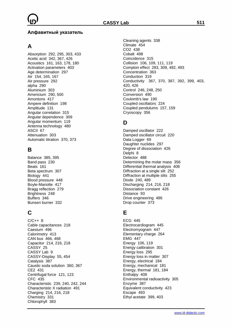
CASSY Lab

511

www.ld-didactic.com

Алфавитный указатель

A

Absorption 292, 295, 303, 433 Acetic acid 342, 367, 426 Acoustics 161, 163, 178, 180 Activation parameters 403 Age determination 297 Air 154, 165, 167 Air pressure 292 alpha 290 Aluminium 303 Americium 290, 500 Amontons 417 Ampere definition 198 Amplitude 131 Angular correlation 315 Angular dependence 309 Angular momentum 119 Antenna technology 480 ASCII 67 Attenuation 303 Automatic titration 370, 373

B

Balance 385, 395 Band pass 230 Beats 161 Beta spectrum 307 Biology 441 Blood pressure 448 Boyle-Mariotte 417 Bragg reflection 279 Brightness 248 Buffers 346 Bunsen burner 332

C

C/C++ 8 Cable capacitances 218 Caesium 496 Calorimetry 413 CAN bus 466, 468 Capacitor 214, 216, 218 CASSY 25 CASSY Lab 9 CASSY-Display 55, 454 Catalysis 387 Caustic soda solution 360, 367 CE2 431 Centrifugal force 121, 123 CFC 435 Characteristic 239, 240, 242, 244 Characteristic X radiation 491 Charging 214, 216, 218 Chemistry 331 Chlorophyll 383

Cleaning agents 338 Climate 454 CO2 438 Cobalt 498 Coincidence 315 Collision 106, 109, 111, 119 Compton effect 283, 309, 492, 493 Concentration 363 Conduction 319 Conductivity 367, 370, 387, 392, 399, 403, 420, 426 Control 246, 248, 250 Conversion 490 Coulomb's law 190 Coupled oscillators 224 Coupled pendulums 157, 159 Cryoscopy 356

D

Damped oscillator 222 Damped oscillator circuit 220 Data Logger 69 Daughter nuclides 297 Degree of dissociation 426 Delphi 8 Detector 488 Determining the molar mass 356 Differential thermal analysis 408 Diffraction at a single slit 252 Diffraction at multiple slits 255 Diode 240, 489 Discharging 214, 216, 218 Dissociation constant 426 Distance 93 Drive engineering 486 Drop counter 373

E

ECG 445 Electrocardiogram 445 Electromyogram 447 Elementary charge 264 EMG 447 Energy 106, 119 Energy calibration 301 Energy loss 295 Energy loss in matter 307 Energy, electrical 184 Energy, mechanical 181 Energy, thermal 181, 184 Enthalpy 408 Environmental radioactivity 305 Enzyme 387 Equivalent conductivity 423 Escape 493 Ethyl acetate 399, 403

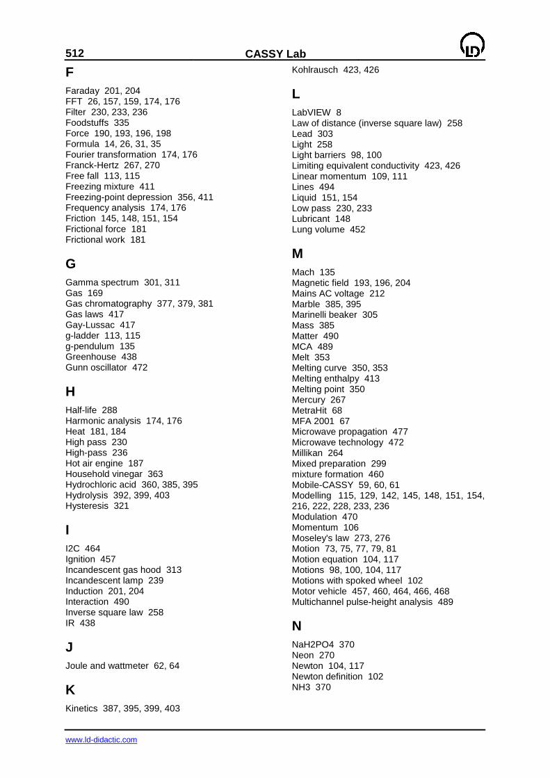
512

CASSY Lab

www.ld-didactic.com

F

Faraday 201, 204 FFT 26, 157, 159, 174, 176 Filter 230, 233, 236 Foodstuffs 335 Force 190, 193, 196, 198 Formula 14, 26, 31, 35 Fourier transformation 174, 176 Franck-Hertz 267, 270 Free fall 113, 115 Freezing mixture 411 Freezing-point depression 356, 411 Frequency analysis 174, 176 Friction 145, 148, 151, 154 Frictional force 181 Frictional work 181

G

Gamma spectrum 301, 311 Gas 169 Gas chromatography 377, 379, 381 Gas laws 417 Gay-Lussac 417 g-ladder 113, 115 g-pendulum 135 Greenhouse 438 Gunn oscillator 472

H

Half-life 288 Harmonic analysis 174, 176 Heat 181, 184 High pass 230 High-pass 236 Hot air engine 187 Household vinegar 363 Hydrochloric acid 360, 385, 395 Hydrolysis 392, 399, 403 Hysteresis 321

I

I2C 464 Ignition 457 Incandescent gas hood 313 Incandescent lamp 239 Induction 201, 204 Interaction 490 Inverse square law 258 IR 438

J

Joule and wattmeter 62, 64

K

Kinetics 387, 395, 399, 403

Kohlrausch 423, 426

L

LabVIEW 8 Law of distance (inverse square law) 258 Lead 303 Light 258 Light barriers 98, 100 Limiting equivalent conductivity 423, 426 Linear momentum 109, 111 Lines 494 Liquid 151, 154 Low pass 230, 233 Lubricant 148 Lung volume 452

M

Mach 135 Magnetic field 193, 196, 204 Mains AC voltage 212 Marble 385, 395 Marinelli beaker 305 Mass 385 Matter 490 MCA 489 Melt 353 Melting curve 350, 353 Melting enthalpy 413 Melting point 350 Mercury 267 MetraHit 68 MFA 2001 67 Microwave propagation 477 Microwave technology 472 Millikan 264 Mixed preparation 299 mixture formation 460 Mobile-CASSY 59, 60, 61 Modelling 115, 129, 142, 145, 148, 151, 154, 216, 222, 228, 233, 236 Modulation 470 Momentum 106 Moseley's law 273, 276 Motion 73, 75, 77, 79, 81 Motion equation 104, 117 Motions 98, 100, 104, 117 Motions with spoked wheel 102 Motor vehicle 457, 460, 464, 466, 468 Multichannel pulse-height analysis 489

N

NaH2PO4 370 Neon 270 Newton 104, 117 Newton definition 102 NH3 370

CASSY Lab

513

www.ld-didactic.com

O

Ohm's law 83, 85, 87 On-board computer 464 Oscillation 125, 127, 129, 131, 133, 135, 138, 142, 145, 148, 151, 154, 157, 159, 220, 222, 224, 226, 228 Ostwald 426 Ozone 435

P

Parallel connection of resistors 87 PCM 470 Pendulum 125, 127, 129, 131, 133, 135, 138, 140, 142, 145, 148, 151, 154, 157, 159 Period of oscillation 140 pH 363, 367, 370 pH measurement 335, 338 Phosporic acid 346 Photometer 383 Physics 95 PI controller 246, 248, 250 Piston burette 370 pKa value 342 Pocket-CASSY 56, 57, 58 Poisson distribution 287 Polybasic acid 347 Potassium 501 Potassium-40 305 Potentiometer 89, 91 Power 210, 212, 244 Power-CASSY 47, 48, 49 Pressure 417 Profi-CASSY 50, 51, 52, 53, 54 Pulse 442 pV diagram 187

Q

Quantization 470

R

Radio 464 Radioactive series 297, 507, 510 Radium 311, 501 Radium decay 503 Radon 288 Range 292 Reaction kinetics 392 Reaction order 387, 392, 395, 399 Reaction time 450 Rectification 431 Resistance 319 Resonance 226, 228 Reversible pendulum 133

S

Scintillation counter 488

Semiconductor counter 489 Sensor-CASSY 36, 37, 38, 39, 45, 46 Separation of air 381 Separation of alcohols 379 Separation of alkanes from lighter gas 377 Separation of substances 431 Serial Devices 67, 68, 69 Series 510 Series connection of resistors 85 Servo technology 486 Single-channel analyzer 317 Skin resistance 443 Sodium 497 Sodium chloride 423 Solar cell 244 Solid 145 Solid bodies 172, 319 Solidification point 350, 353 Sonic synthesis 180 Sound analysis 178 Sources 494 Spectrum 299, 383 Spirometry 452 Splitting of urea 387 Standing wave ratio 477 STM 72 String vibrations 163 Strong acid 360 Strong base 360, 367 Strontium 499 Sun screen 433 Supercooling 353

T

TE modes 474 Technology 456 TEM modes 474 Temperature 246, 332, 350, 417 Tensile force 163 Thermal separation procedures 431 Thorium 313, 506, 507 Titration 360, 363, 367, 370, 373 Transformer 208, 210 Transformer core 321 Transistor 242 Two-plate waveguide 474 Two-position controller 246

U

Universal measuring instrument 65, 66 Urease 387 UV 433, 435

V

Velocity of light 260, 262 Velocity of sound 165, 167, 169, 172 Vibrational frequency of a string 163 VideoCom 67

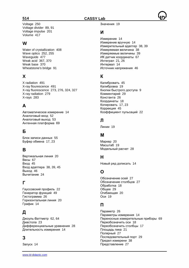
514

CASSY Lab

www.ld-didactic.com

Voltage 250 Voltage divider 89, 91 Voltage impulse 201 Volume 417

W

Water of crystallization 408 Wave optics 252, 255 Waveguide 477 Weak acid 367, 370 Weak base 370 Wheatstone's bridge 91

X

X radiation 491 X-ray flourescence 491 X-ray fluorescence 273, 276, 324, 327 X-ray radiation 279 X-rays 283

А

Автоматическое измерение 14 Аналоговый вход 52 Аналоговый выход 53 Антенная платформа 69

Б

Блок записи данных 55 Буфер обмена 17, 23

В

Вертикальная линия 20 Весы 67 Вход 45 Вход адаптера 38, 39, 45 Выход 46 Вычитание 24

Г

Гауссовский профиль 22 Генератор функций 49 Гистограмма 26 Горизонтальная линия 20 График 14

Д

Джоуль-Ваттметр 62, 64 Диастола 23 Дифференциальные уравнения 28 Длительность измерения 14

З

Запуск 14

Значения 19

И

Измерение 14 Измерение вручную 14 Измерительный адаптер 38, 39 Измеряемая величина 38 Измеряемые величины 39 ИК датчик координаты 67 Интеграл 21, 26 Интервал 14 Источник напряжения 46

К

Калибровать 45 Калибровка 19 Кнопки быстрого доступа 9 Комментарий 29 Константа 26 Координаты 18 Копировать 17, 23 Коррекция 45 Коэффициент пульсаций 22

Л

Линии 19

М

Маркер 20 Масштаб 19 Модельный расчет 28

Н

Новый ряд дописать 14

О

Обозначение осей 27 Обозначение столбцов 27 Обработка 18 Общее 29 Огибающая 20 Оси 19

П

Параметр 26 Параметры измерения 14 Переносные измерительные приборы 69 Переобозначить оси 18 Переобозначить столбцы 17 Площадь пика 21 Полярный 27 Последовательный порт 29 Предел измерени 38 Представление 27

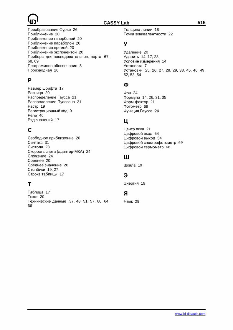
CASSY Lab

515

www.ld-didactic.com

Преобразование Фурье 26 Приближение 20 Приближение гиперболой 20 Приближение параболой 20 Приближение прямой 20 Приближение экспонентой 20 Приборы для последовательного порта 67, 68, 69 Программное обеспечение 8 Производная 26

Р

Размер шрифта 17 Разница 20 Распределение Гаусса 21 Распределение Пуассона 21 Растр 19 Регистрационный код 9 Реле 46 Ряд значений 17

С

Свободное приближение 20 Синтакс 31 Систола 23 Скорость счета (адаптер-МКА) 24 Сложение 24 Среднее 20 Среднее значение 26 Столбики 19, 27 Строка таблицы 17

Т

Таблица 17 Текст 20 Технические данные 37, 48, 51, 57, 60, 64, 66

Толщина линии 18 Точка эквивалентности 22

У

Удаление 20 Удалить 14, 17, 23 Условие измерения 14 Установка 7 Установки 25, 26, 27, 28, 29, 38, 45, 46, 49, 52, 53, 54

Ф

Фон 24 Формула 14, 26, 31, 35 Форм-фактор 21 Фотометр 69 Функция Гаусса 24

Ц

Центр пика 21 Цифровой вход 54 Цифровой выход 54 Цифровой спектрофотометр 69 Цифровой термометр 68

Ш

Шкала 19

Э

Энергия 19

Я

Язык 29

cassy lab - ld didactic

Documents