Università degli Studi di Napoli “Federico II”

Scuola Politecnica e delle Scienze di Base

Area Didattica di Scienze Matematiche Fisiche e Naturali

Dipartimento di Fisica “Ettore Pancini”

Laurea Magistrale in Fisica

Geometry and Physics:

A Didactic Proposal

Relatori: Prof. Emilio Balzano

Prof. Rodolfo Figari

Candidato: Ivano Vettigli

Matricola N94000342

A.A. 2017/2018

Contents

Introduction and Acknowledgements iv

1 Time and Relative Dimension in Space 11.1 Distance and reference systems . . . . . . . . . . . . . . . . . . . . . . . . 21.2 Plane geometry and optics . . . . . . . . . . . . . . . . . . . . . . . . . . . 91.3 How time was understood in different times . . . . . . . . . . . . . . . . . 141.4 Galilean transformation . . . . . . . . . . . . . . . . . . . . . . . . . . . . 181.5 Non relativistic mechanics . . . . . . . . . . . . . . . . . . . . . . . . . . . 23

2 Special theory of relativity 322.1 Derivation of wave equation from Maxwell’s equations . . . . . . . . . . . 332.2 Comparing mechanical waves with electromagnetic waves and Michelson

interferometer. . . . . . . . . . . . . . . . . . . . . . . . . . . . . . . . . . 362.3 Lorentz transformations, thought experiments, four-vectors and relativis-

tic mechanics . . . . . . . . . . . . . . . . . . . . . . . . . . . . . . . . . . 43

3 Approach to general relativity 483.1 Geometry on a sphere, metric and curvature . . . . . . . . . . . . . . . . . 493.2 Tensors and Einstein field equation . . . . . . . . . . . . . . . . . . . . . . 583.3 Schwarzschild metric . . . . . . . . . . . . . . . . . . . . . . . . . . . . . . 65

Conclusions 70

A Students commentary to the space-time and velocity time diagrams 72

B Python and Jupyter Notebook 77

Bibliography 80

ii

“The scientist does not study nature because it is useful to do so. He studies it because

he takes pleasure in it, and he takes pleasure in it because it is beautiful. If nature were

not beautiful it would not be worth knowing, and life would not be worth living. I am not

speaking, of course, of the beauty which strikes the senses, of the beauty of qualities and

appearances. I am far from despising this, but it has nothing to do with science. What I

mean is that more intimate beauty which comes from the harmonious order of its parts,

and which a pure intelligence can grasp.”

Henri Poincaré - The selection of facts

Introduction and Acknowledgements

The aim of the present work is to help teachers who plan to introduce the theory of

relativity to their students. Indeed, nowadays teachers are asked to update the school

curriculum and treat topics of modern physics like quantum mechanics and general rela-

tivity [1]. This is indispensable since the school has to give students the tools to under-

stand the society in which they live and the technology they use, as is argued in [2]. On

the other hand, without a daring attempt to revise physics and mathematics curricula,

these topics run the risk to be conveyed only as a popular subject with no true insight.

Indeed, while Newtonian mechanics, thermodynamics and electromagnetism, together

with other classical topics of physics, are meaningfully treated with elementary math-

ematics. It is matter of recent educational physics research how to teach more recent

theories of physics.

Many works in literature focus on the students difficulties and misconceptions, this work

focuses on how to help students overcome their difficulties.

We want to preliminarly stress that, in our opinion, it should be avoided to introduce

features of modern physics starting from popular aphorisms of great scientists or from

often obscure epistemelogical debates among them. This is especially true when we think

of quantum mechanics, where the original disputes among scientists like Bohr, Einstein

and Heisenberg cannot be understood without a basic understanding of the physical the-

ory.

Searching a way to introduce in a meaningful way the theory of relativity to students of

high school, I participated to training meeting for teachers and I designed laboratorial

activities experimented in classrooms. These activities are described in the present work.

I have presented just a few ideas, centred on special relativity and non-Euclidean geom-

etry, but during the meeting the discussion was centered on how to revise mathematics

and physics curriculum. On one side the need for experimental activity, which should

form the core of the physics curriculum, has been coped taking advantage of the wide

material produced in the LES Project (Laboratori per l’Educazione alla Scienza) that

can be found on http://www.les.unina.it/. Teachers have tried some of the experience

described, adapting it to the needs of their classrooms. The activities were documented

and they were discussed in the subsequent meetings.

On the other side there is need for a formalization of the advanced concepts. The idea

is to start from computations and calculations that students can perform through and

through. A starting point is the discretization of differential equations. The wave equa-

tion, or even Schrödinger equation, can be solved numerically in one dimension also

iv

Contents v

with elementary mathematics, as shown in [3]. With the help of modern computers

and instruments like the spreadsheets, students can gain astonishing insight into physi-

cal systems through numerical methods. In this work we also propose to approach the

three-body problems, computing the trajectory of two planets that turns around the Sun,

with numerical methods. Anyway, I have chosen to use Python programming language

(see appendix B) to implement the algorithms. I believe it is important for students to

approach coding technologies like Python useful for teachers and students to illustrate

physics concepts and develop a sense of physical intuition through simulations and mod-

elling.

The pedagogical framework in which the activities are designed are the ones of Vygotskij

and Sfard. The expert must put himself in the zone of proximal development, propos-

ing things that students does not know, but can actually understand. Furthermore, the

class work is a collective study where the interactions between pairs and with the ex-

pert are the true propelling factor [4]. On the other hand, mathematical concepts are

fist introduced as operation to perform on concrete objects. A paradigmatic example

is the division of natural numbers, where the activities aims to catalyze the cycle of

internalization, condensation and reification, until students perceives the operation as a

mathematical object, the positive rational numbers [5].

The methodologies we propose are also based ...on a rich and growing body of research

on teaching and learning in science, as well as on nearly two decades of efforts to define

foundational knowledge and skills for K-12 science and engineering ... We focus on a

limited number of disciplinary core ideas and crosscutting concepts, designed so that stu-

dents continually build on and revise their knowledge and abilities over multiple years,

and support the integration of such knowledge and abilities with the practices needed to

engage in scientific inquiry ... [6].

The thesis is structured miming a textbook. Topics are presented starting from the

simplest ones, where only the knowledge of physics and mathematics generally owned

by students in high-school is assumed and later proceeding to more complex topics like

general relativity. Every topic is introduced with exercises and laboratorial activity but

most of the interesting aspect of rigorous mathematics are not discussed for the sake of

brevity. Nevertheless, the work has been carried out having in mind modularity criteria

so that a teacher may chose any set of topics, if any, to propose in classroom.

In the first chapter a way to introduce Galilean transformations is proposed. Distance

and angles are defined and particular relevance is given to the operations of translation

and rotation of the system of reference. Successively, it follows a description of the penta-

laser, a didactic tools that allows various experiments to be performed in classrooms. In

Contents vi

the last section, time and motion are introduced and the concept of relative motion is

discussed with the aid of a motion sensor.

In the second chapter a way to introduce special relativity is proposed. In the first section

Maxwell equations are presented and the wave equation is derived. Afterward, it follows

a description of the microwave optics bench and the Michelson interferometer with an

account of classroom activity in which various experiment have been presented. Later,

the Lorentz transformation is presented as a rotation in space-time and the special theory

of relativity is introduced with geometric concepts and thought experiments. In the last

section, relativistic mechanics is discussed with the introduction of the four-vectors.

In the third chapter, a way to approach the general theory of relativity is introduced.

In the first section, non-Euclidean geometry is presented trough measurement of an-

gles, lengths and areas on a sphere. After that, tensors are introduced and the Einstein

equation is discussed with some solutions. In the last section numerical simulations are

implemented to show how astronomical predictions differs in the different theories.

This work would not have been possible without the teachers that hosted me in their

classrooms, trusting my ideas. I want to thank Maria Rosaria Camarda, Annette Lu-

ongo and Maria Loffredo from the "Liceo Scientifico Statale Carlo Urbani", Margherita

D’Urzo and Ilaria Limoncelli from the "Liceo Scientifico Statale Filippo Silvestri" and

Marina De Cesare and Chiara Tarallo from the "Liceo Scientifico Statale Calamandrei".

It seems that no student has been phisically or psychologically harmed as a consequence

of this thesis work.

I want to thank my teachers, who never gave up on me, because they were not only

transmitters of knowledge, but life-examples to follow. Among them Giorgio Montalto,

who inspired my passion for theoretical aspects of physics and Orietta Laurenza, who

inspired the habit of inquiry, Marina Cerza, who never stopped feeding my curiosity and

Rosalba Cerbone, who believed in me even in the hardest times. I also want to thank my

supervisors, Emilio Balzano, Rodolfo Figari and Ofelia Pisanti for their patience and

their guidance. Also, I want to thank doctor Cosimo Stornaiolo for his time and his

contributions. Furthermore, I want to thank professor Antonio Sasso, whose experience

in teaching optics has been a beacon to follow for me.

I also wish to thank Giuseppe Bausilio and the Ing. Gaetano Mascetta for their uncon-

ditioned friendship among all these years.

And I want to thank my family, who always supported and "sopported" me (sorry for

the italian slang).

And above all, I want to thank Sara~ for loving and caring about me.

Chapter 1

Time and Relative Dimension in

Space

The task of the educator is to makethe child’s spirit pass again where itsforefathers have gone, moving rapidlythrough certain stages butsuppressing none of them. In thisregard, the history of science must beour guide.

Henri Poincaré - L’enseignementmathématique

The goal of this chapter is to present Galilean transformations and classical mechanics

in a way easily generalizable to Lorentz transformation and relativistic mechanics. In

the first two sections distance, angles and reference system are introduced with the

help of exercises, drawings and laboratorial activities with the pentalaser. After that

time is introduced first as an astronomical measure, then more recent definitions of the

unit of measure are discussed. The concept of relative motion is introduced through a

laboratorial activity with the motion sensors and Galilean transformations are finally

discussed trough exercises. In the last section, classical mechanics is presented with its

symmetries with respect to the Galilean transformation and numerical simulations are

performed to show the predictive power of the theory.

1

Contents 2

1.1 Distance and reference systems

It is by logic that we prove, but byintuition that we discover. To knowhow to criticize is good, to know howto create is better.

Henri Poincaré - MathematicalDefinitions and Education

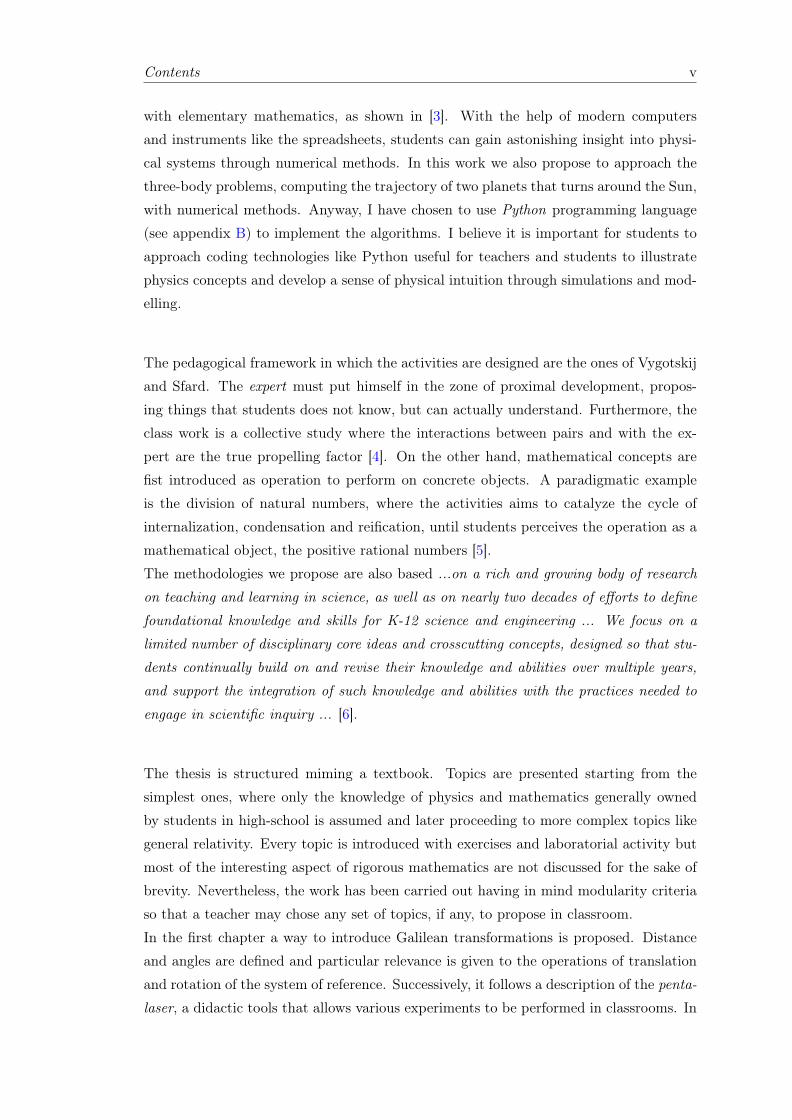
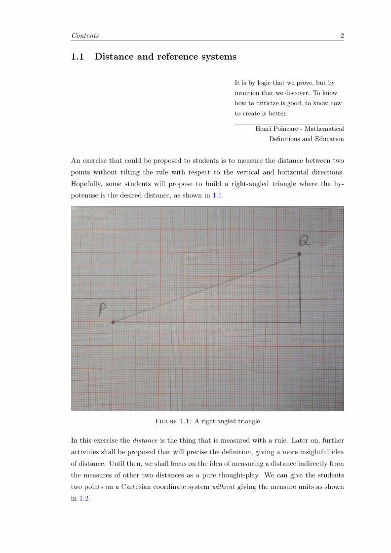
An exercise that could be proposed to students is to measure the distance between two

points without tilting the rule with respect to the vertical and horizontal directions.

Hopefully, some students will propose to build a right-angled triangle where the hy-

potenuse is the desired distance, as shown in 1.1.

Figure 1.1: A right-angled triangle

In this exercise the distance is the thing that is measured with a rule. Later on, further

activities shall be proposed that will precise the definition, giving a more insightful idea

of distance. Until then, we shall focus on the idea of measuring a distance indirectly from

the measures of other two distances as a pure thought-play. We can give the students

two points on a Cartesian coordinate system without giving the measure units as shown

in 1.2.

Contents 3

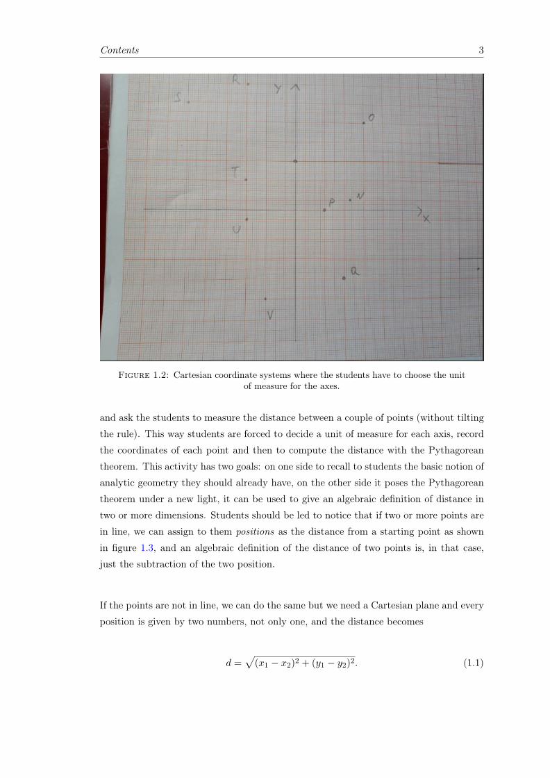
Figure 1.2: Cartesian coordinate systems where the students have to choose the unitof measure for the axes.

and ask the students to measure the distance between a couple of points (without tilting

the rule). This way students are forced to decide a unit of measure for each axis, record

the coordinates of each point and then to compute the distance with the Pythagorean

theorem. This activity has two goals: on one side to recall to students the basic notion of

analytic geometry they should already have, on the other side it poses the Pythagorean

theorem under a new light, it can be used to give an algebraic definition of distance in

two or more dimensions. Students should be led to notice that if two or more points are

in line, we can assign to them positions as the distance from a starting point as shown

in figure 1.3, and an algebraic definition of the distance of two points is, in that case,

just the subtraction of the two position.

If the points are not in line, we can do the same but we need a Cartesian plane and every

position is given by two numbers, not only one, and the distance becomes

d =√

(x1 − x2)2 + (y1 − y2)2. (1.1)

Contents 4

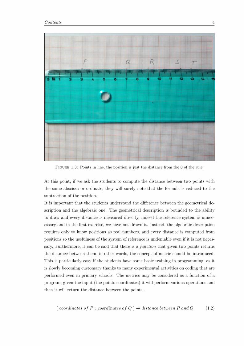
Figure 1.3: Points in line, the position is just the distance from the 0 of the rule.

At this point, if we ask the students to compute the distance between two points with

the same abscissa or ordinate, they will surely note that the formula is reduced to the

subtraction of the position.

It is important that the students understand the difference between the geometrical de-

scription and the algebraic one. The geometrical description is bounded to the ability

to draw and every distance is measured directly, indeed the reference system is unnec-

essary and in the first exercise, we have not drawn it. Instead, the algebraic description

requires only to know positions as real numbers, and every distance is computed from

positions so the usefulness of the system of reference is undeniable even if it is not neces-

sary. Furthermore, it can be said that there is a function that given two points returns

the distance between them, in other words, the concept of metric should be introduced.

This is particularly easy if the students have some basic training in programming, as it

is slowly becoming customary thanks to many experimental activities on coding that are

performed even in primary schools. The metrics may be considered as a function of a

program, given the input (the points coordinates) it will perform various operations and

then it will return the distance between the points.

( coordinates of P ; coordinates of Q ) −→ distance between P and Q (1.2)

Contents 5

It is important to note that we can think and talk about points in space without referring

to any reference systems, but that they are really convenient. A more complete treatment

of this topics, with the metrics fist presented as I did, can be found in [7].

A great advantage of the algebraic description is how well it leads to generalization. It

is easy to generalize the formula for the distance to any number of dimensions

d2(P ;Q) =∑i

(qi − pi)2 (1.3)

with obvious symbol meaning.

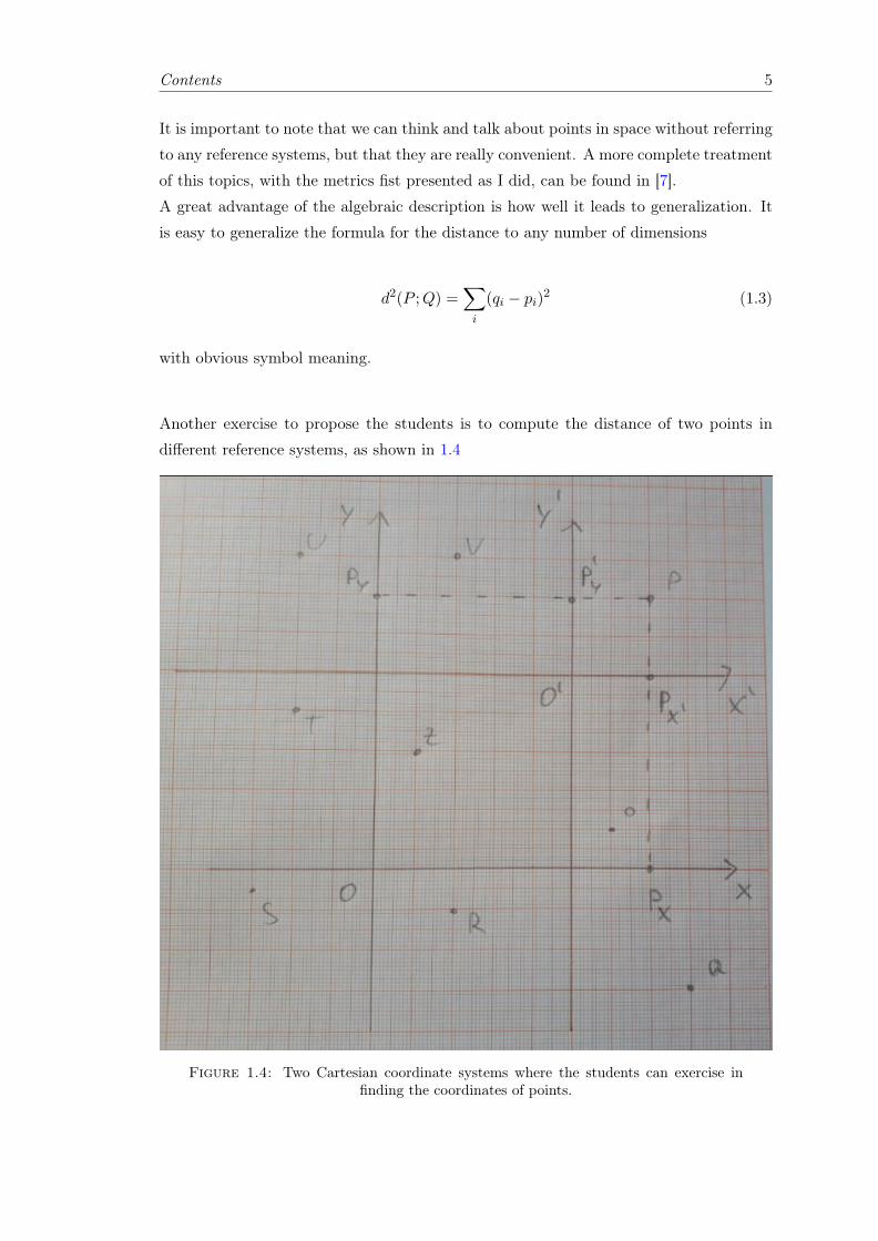
Another exercise to propose the students is to compute the distance of two points in

different reference systems, as shown in 1.4

Figure 1.4: Two Cartesian coordinate systems where the students can exercise infinding the coordinates of points.

Contents 6

In the geometric description is intuitive to assume that the distance between points does

not depend on the reference systems, but in the algebraic version this is not obvious. A

few trials will persuade the students that this is the case, giving the opportunity to show

how something can be proved with a calculation. The first thing to do is to understand

how the coordinates of a point change when we pass from a reference system to another,

as in the example before were the reference systems are shifted with respect to one

another. In this case, ones just have to add or subtract a quantity to the coordinate of

every point to change reference systems, in other words

x′ = x+ a

y′ = y + b

and this leads to the distance in the second frame as

d(Q;P ) =√x′21 + y′22 =

√[x1 + a− (x2 + a)]2 + [y1 + b− (y2 + b)]2 =

√x2

1 + y22.

(1.4)

Then the independence of the distance from the frame of reference in the algebraic

descriptions follows from the fact that c− c = 0.

It is slightly more complicated to repeat the computation when the reference system is

tilted, as shown in 1.5

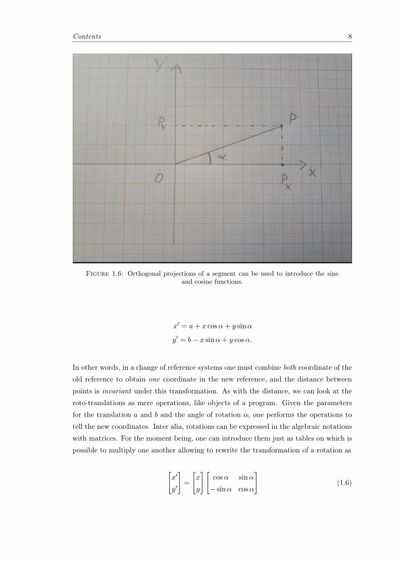
If the students have no familiarity with the trigonometric functions, this is a good time

to introduce them. Nowadays this topic is frequently proposed in the first year of high

schools as an operation that given an angle returns a real number and as a way to project

segments. In figure 1.6 the cosine is the number one has to multiply the OP length to

obtain the length of OPx while the sine is the number by which one has to multiply OP

length to obtain the length of OPy.

Of course this number depends on α and some numerical example to show the value of

sine and cosine at particular angles would help students understand them. Of course this

is not a rigorous and satisfactory definition of the trigonometric functions, nevertheless to

give first an incomplete but intuitive definitions and to refine it when the needs arise is a

technique used even in university textbook like [8]. For a discussion on the importance of

definitions in mathematical teaching, we recommend [9]. For a laboratorial experience on

the Snell-Descartes law that can be used to introduce the sine and cosine we recommend

the Project LES (Laboratori per l’Educazione alla Scienza) on http://www.les.unina.it/.

Contents 7

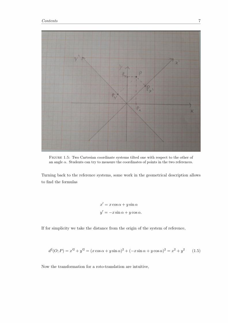
Figure 1.5: Two Cartesian coordinate systems tilted one with respect to the other ofan angle α. Students can try to measure the coordinates of points in the two references.

Turning back to the reference systems, some work in the geometrical description allows

to find the formulas

x′ = x cosα+ y sinα

y′ = −x sinα+ y cosα.

If for simplicity we take the distance from the origin of the system of reference,

d2(O;P ) = x′2 + y′2 = (x cosα+ y sinα)2 + (−x sinα+ y cosα)2 = x2 + y2 (1.5)

Now the transformation for a roto-translation are intuitive,

Contents 8

Figure 1.6: Orthogonal projections of a segment can be used to introduce the sineand cosine functions.

x′ = a+ x cosα+ y sinα

y′ = b− x sinα+ y cosα.

In other words, in a change of reference systems one must combine both coordinate of the

old reference to obtain one coordinate in the new reference, and the distance between

points is invariant under this transformation. As with the distance, we can look at the

roto-translations as mere operations, like objects of a program. Given the parameters

for the translation a and b and the angle of rotation α, one performs the operations to

tell the new coordinates. Inter alia, rotations can be expressed in the algebraic notations

with matrices. For the moment being, one can introduce them just as tables on which is

possible to multiply one another allowing to rewrite the transformation of a rotation as

[x′

y′

]=

[x

y

][cosα sinα

− sinα cosα

](1.6)

Contents 9

The discussions on how matrix behave under change of frames or the definition of de-

terminant may wait for the moment, but it could be useful to ask students to represent

translation in this new formalism. An exercise like this could help students understand

how to work with formalism and investigate its power and its weakness, in the specific

that a matrix assoiciated to a transformation must have the origin fixed. In this way

mathematics is not presented as results, but as a structure that can be built which has

a great impact on the proficiency of students, like shows the works like [10] and [11].

We stress out the importance of this approach to the new concept since is often argued

that it is not possible to teach modern physics without the mathematical preparatory

concepts and that is not possible to teach mathematics if the students are not ready to

grasp the definition and the rigorous thought needed. We think that the opposite is true,

it is not possible to teach mathematics without an intuitive description while intuition

and physics help to build a more rigorous thought-pattern until abstraction is recognized

as the most efficient way by the students.

1.2 Plane geometry and optics

Doc: REACH!Engineer : IS THIS A HOLD-UP?Doc: IT IS A SCIENCEEXPERIMENT!

Back to the future

The pentalaser, shown in the figures below, is simply made of five lasers whose rays are

parallel with good accuracy. For good we mean that even if the rays are projected on a

screen several meters away, the light dots remain at the same distance with the precision

of the millimetre. In this particular tool, made by Kvanta we can choose to light up only

the mid laser, all five lasers, the central laser and two on the sides. The pentalaser can

be combined with printed sheets and big lenses made with Poly(methyl methacrylate),

also known as Plexiglas, to illustrate the functioning of optical systems. I have utilized

this instrument with different audiences, from middle school to university. For students

of the first year of the degree course in Ottica e Optometria provided by the Department

of Physics Ettore Pancini, the activity was suggested by their professor Antonio Sasso

during my work as a tutor. It has been a way to visualize in a crystal-clear way Snell

Descartes law, fostering their interest in the subject. For middle-class students, it has

been a way to understand how lenses and mirrors works.

For now and for our purpose, an angle will be the thing we measure with the goniometer.

Then we can add a prism to the configuration, to measure the angle by which the ray is

Contents 10

deflected as shown in 1.7.

Figure 1.7: The prism refraction of light

The great power of this methods is that it visually connect everyday phenomena with

their description in the frame of optical geometry. As in the already cited laboratorial

experience of the L.E.S., it is possible to mount the prism on a rotating plate in order

to measure the dependence of the diffraction angles from the incident angle, the Snell-

Descartes law.

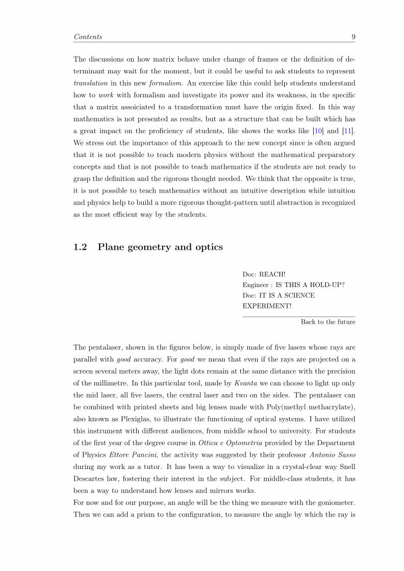
Another experiment that could be done collaborating with the biology teacher is shown

in 1.8.

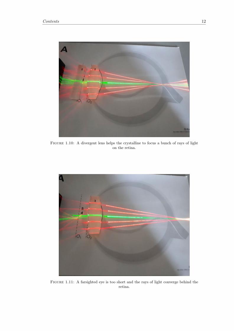
The light emitted by an object far away, is schematized as a bunch of parallel rays of

light. The crystalline is schematized as a lens that converges the ray on the retina. This

is the case of a perfect eye, but we can study what happens when the eye is too long or

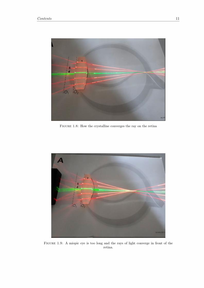
too short, as shown in the figures 1.9, 1.10, 1.11, 1.12.

If the eye is too long the rays converge in a point placed before the retina (in the exper-

iment apparatus we have used a different lens as crystalline). To correct this defect, we

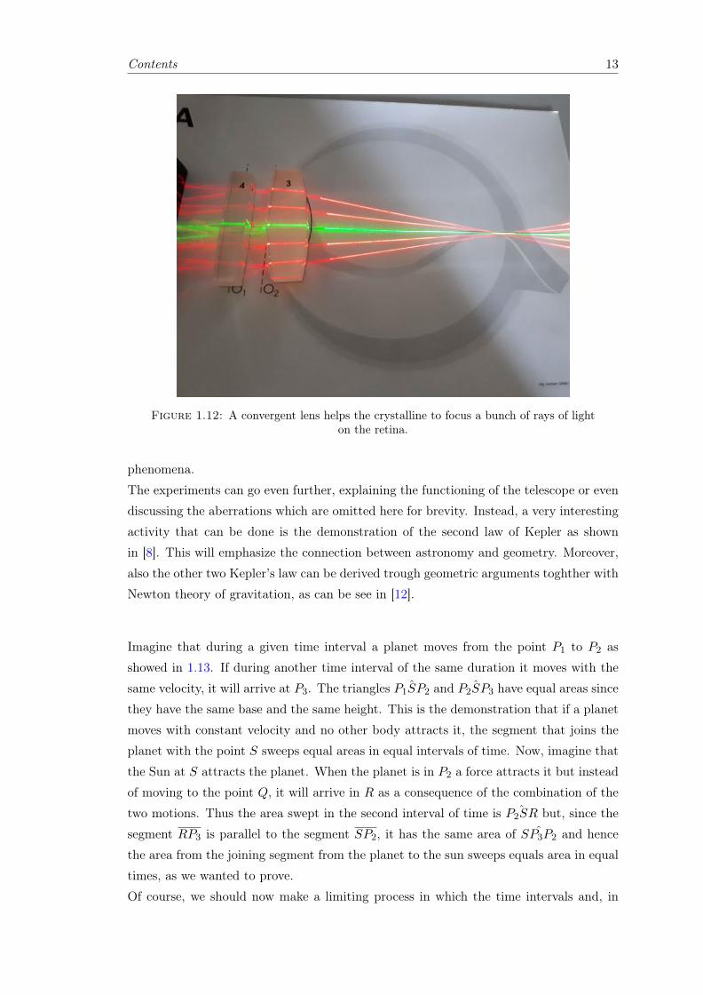
add a divergent lens. If the eye is too short, the rays converge in a point placed after the

retina. To correct this defect, we add a convergent lens.

Showing how the physical models describe actual problems and can be used to solve it

is very powerful. It worked both with middle school students that with university stu-

dents, fostering the comprehension of a symbolic language and its translation in actual

Contents 11

Figure 1.8: How the crystalline converges the ray on the retina

Figure 1.9: A miopic eye is too long and the rays of light converge in front of theretina.

Contents 12

Figure 1.10: A divergent lens helps the crystalline to focus a bunch of rays of lighton the retina.

Figure 1.11: A farsighted eye is too short and the rays of light converge behind theretina.

Contents 13

Figure 1.12: A convergent lens helps the crystalline to focus a bunch of rays of lighton the retina.

phenomena.

The experiments can go even further, explaining the functioning of the telescope or even

discussing the aberrations which are omitted here for brevity. Instead, a very interesting

activity that can be done is the demonstration of the second law of Kepler as shown

in [8]. This will emphasize the connection between astronomy and geometry. Moreover,

also the other two Kepler’s law can be derived trough geometric arguments toghther with

Newton theory of gravitation, as can be see in [12].

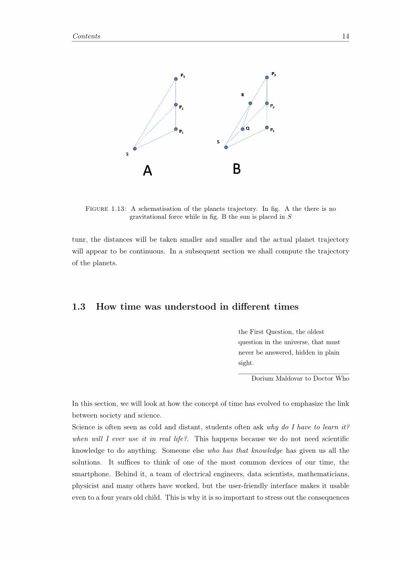
Imagine that during a given time interval a planet moves from the point P1 to P2 as

showed in 1.13. If during another time interval of the same duration it moves with the

same velocity, it will arrive at P3. The triangles ˆP1SP2 and ˆP2SP3 have equal areas since

they have the same base and the same height. This is the demonstration that if a planet

moves with constant velocity and no other body attracts it, the segment that joins the

planet with the point S sweeps equal areas in equal intervals of time. Now, imagine that

the Sun at S attracts the planet. When the planet is in P2 a force attracts it but instead

of moving to the point Q, it will arrive in R as a consequence of the combination of the

two motions. Thus the area swept in the second interval of time is ˆP2SR but, since the

segment RP3 is parallel to the segment SP2, it has the same area of ˆSP3P2 and hence

the area from the joining segment from the planet to the sun sweeps equals area in equal

times, as we wanted to prove.

Of course, we should now make a limiting process in which the time intervals and, in

Contents 14

Figure 1.13: A schematisation of the planets trajectory. In fig. A the there is nogravitational force while in fig. B the sun is placed in S

tunr, the distances will be taken smaller and smaller and the actual planet trajectory

will appear to be continuous. In a subsequent section we shall compute the trajectory

of the planets.

1.3 How time was understood in different times

the First Question, the oldestquestion in the universe, that mustnever be answered, hidden in plainsight.

Dorium Maldovar to Doctor Who

In this section, we will look at how the concept of time has evolved to emphasize the link

between society and science.

Science is often seen as cold and distant, students often ask why do I have to learn it?

when will I ever use it in real life?. This happens because we do not need scientific

knowledge to do anything. Someone else who has that knowledge has given us all the

solutions. It suffices to think of one of the most common devices of our time, the

smartphone. Behind it, a team of electrical engineers, data scientists, mathematicians,

physicist and many others have worked, but the user-friendly interface makes it usable

even to a four years old child. This is why it is so important to stress out the consequences

Contents 15

of the scientific knowledge upon society and how society needs to drive scientific research.

Indeed many textbooks like [13] and [14] start with a description of the most advanced

techniques to measure physical quantities. As stated in [15] there is a very pragmatic

reason if men started measuring times longer than days and lunar months, they needed

to know when to sow and when to harvest. For example, the priests of ancient Egypt,

probably the custodians of the more advanced scientific knowledge of their time, had the

life or death task of looking out for the heliacal rising of the star Sirius. The heliacal

rising occurs annually when the star becomes visible above the eastern horizon for a

brief moment before sunrise, after a period of less than a year in which it had not been

visible. In the same period of the year, a combination of favourable circumstances causes

the Nile’s floods. The Egyptians probably thought that stars influence actually modified

earth phenomena, but this is a good example of how correlation did not imply causation.

Anyway, if the floods where foretold they could have been used to fertilize the fields,

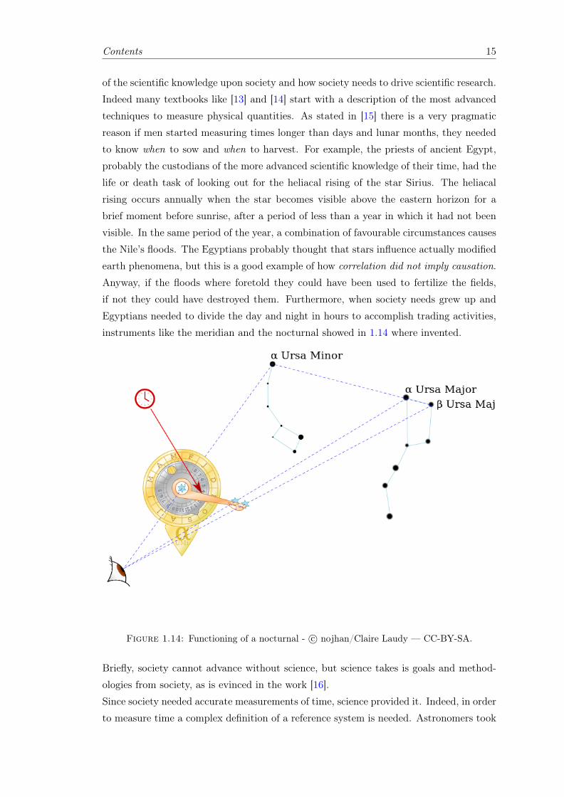
if not they could have destroyed them. Furthermore, when society needs grew up and

Egyptians needed to divide the day and night in hours to accomplish trading activities,

instruments like the meridian and the nocturnal showed in 1.14 where invented.

Figure 1.14: Functioning of a nocturnal - c© nojhan/Claire Laudy — CC-BY-SA.

Briefly, society cannot advance without science, but science takes is goals and method-

ologies from society, as is evinced in the work [16].

Since society needed accurate measurements of time, science provided it. Indeed, in order

to measure time a complex definition of a reference system is needed. Astronomers took

Contents 16

advantage of the great uniformity in Earth rotation. A point is chosen on the celestial

sphere, like the centre of the sun or the point on the ecliptic where the Sun crosses from

the southern celestial hemisphere to the northern, which occurs at the (northern) vernal

equinox, called vernal point. A measure of time was actually a measure of the degree by

which one of this points had moved since in a day they perform a rotation of 360 degrees

is easy to define the sidereal time and the solar time. For a more detailed discussion on

astronomical systems of reference and time measurement, we suggest [17] or any astron-

omy textbook.

Anyway, this is why time and angles share so many common features like the term sec-

onds which indicate both a time than a division of the grade.

Going on with the years, let us analyze the following problems taken from a medieval

textbook with their solutions as translated in the work [18]. It will be evident that time

was not thought of as a parameter and were not used while solving problems.

There is a field 150 feet long. At one end is a dog and at the other a hare. The dog

chases when the hare runs. The dog travels 9 feet in a jump, while the hare travels 7

feet. How many feet will be travelled by the pursuing dog and the fleeing hare before

the hare is seized? (Alcuin, 2005, p. 68)

The length of the field is 150 feet. Take half of 150, which is 75. The dog goes 9 feet in a

jump. 75 times 9 is 675; this is the number of feet the pursuing dog runs before he seizes

the hare in his grasping teeth. Because in a jump the hare goes 7 feet, multiply 75 by

7, obtaining 525. This is the number of feet the fleeing hare travels before it is caught.

(Alcuin, 2005, p. 68)

This problem can easily be solved with kinematic, but in the middle ages, they solved it

without never explicitly considering time. Another example is this:

A fox is 40 paces ahead of a dog, and three paces of the latter are 5 paces of the former. I

ask in how many paces the dog will reach the fox. (dell’Abacco as translated by Arrighi,

1964, p. 78)

The medieval solution to this problem starts considering that three-step of the dog are

equals to five steps of the fox, 3D = 5F . Then applying the proportion 5D = (8 + 13F

and the dog regains 3 + 13 fox paces at every step. Applying again a proportion, the

number of steps the dog have to take are 60.

Of course, both problems and the last one, in particular, can be solved more easily intro-

ducing the time as a variable. But apparently, in the middle age, people did not think

time as a variable. The jump or the steps are the measures of time since they happen at

the same time.

This suggests that the more intuitive quantity is not time, but the movement. Indeed

a good clock can be assumed to be something that appear to move with uniform speed.

Following this line of reasoning, in the next section, we will study the proprieties of mo-

tions with the aid of the motion detector.

Contents 17

A good idea would be to repropose these problems with students in the classroom. One

could tell students to make paces of given length, so that the idea that the steps are

simultaneus and that they define the time can emerge spontaneously.

Going on with the years, times emerge as a a-priori intuitions. has described in [19],

we distinguish two way of measuring time. One is, following the tradition of the astro-

nomical definition, the search for systems that appears periodic, like pendulums. For

example, we can compare two or more pendulum counting their oscillations. If the ratios

of this number are constant, we recognize periodicity in the oscillations of the pendulums.

Then, we can use pendulums as clocks, defining the oscillation of a particular pendulum

as the unit of measure of time. Furthermore, this system is easy to reproduce and, for

what we know, there are no variations in the oscillations frequencies, while the motion

of the celestial bodies is subjected to secular variations. The other approach is to find

systems that appear to vary uniformly, for example, a bottle full of a liquid with a hole

in it on a weight scale. If the bottle is large enough so that for small times the water

level does not vary too much, the water flows away uniformly. The variation in weight

reported on the scale can be used as time. We cannot say that the amount of water that

flows away in a given interval of time is always the same since we are trying to define

time. The only way to test our approximation, that the water flows away uniformly, is

to check our clock with others. In this picture, we assume that time exists and flows

independently of our attempts to measure it.

In everyday life, we still use this naive understanding of time. Even when we use in-

struments like the GPS, where the computation on our position must be corrected with

general relativity, we still think the time as something that passes uniformly and peri-

odically. As we will see in the next chapters, this ideas must be rethinking if we want to

understand the theory of relativity.

As for now, the more recent definition of second is:

The second is the duration of 9192631770 periods of the radiation corresponding to the

transition between the two hyperfine levels of the ground state of the caesium 133 atom."

13th CGPM (1967/68, Resolution 1; CR, 103)

"This definition refers to a caesium atom at rest at a temperature of 0 K."

(Added by CIPM in 1997)

Contents 18

1.4 Galilean transformation

You know that in nine hundred yearsof time and space and I’ve never metanybody who wasn’t importantbefore.

Doctor who

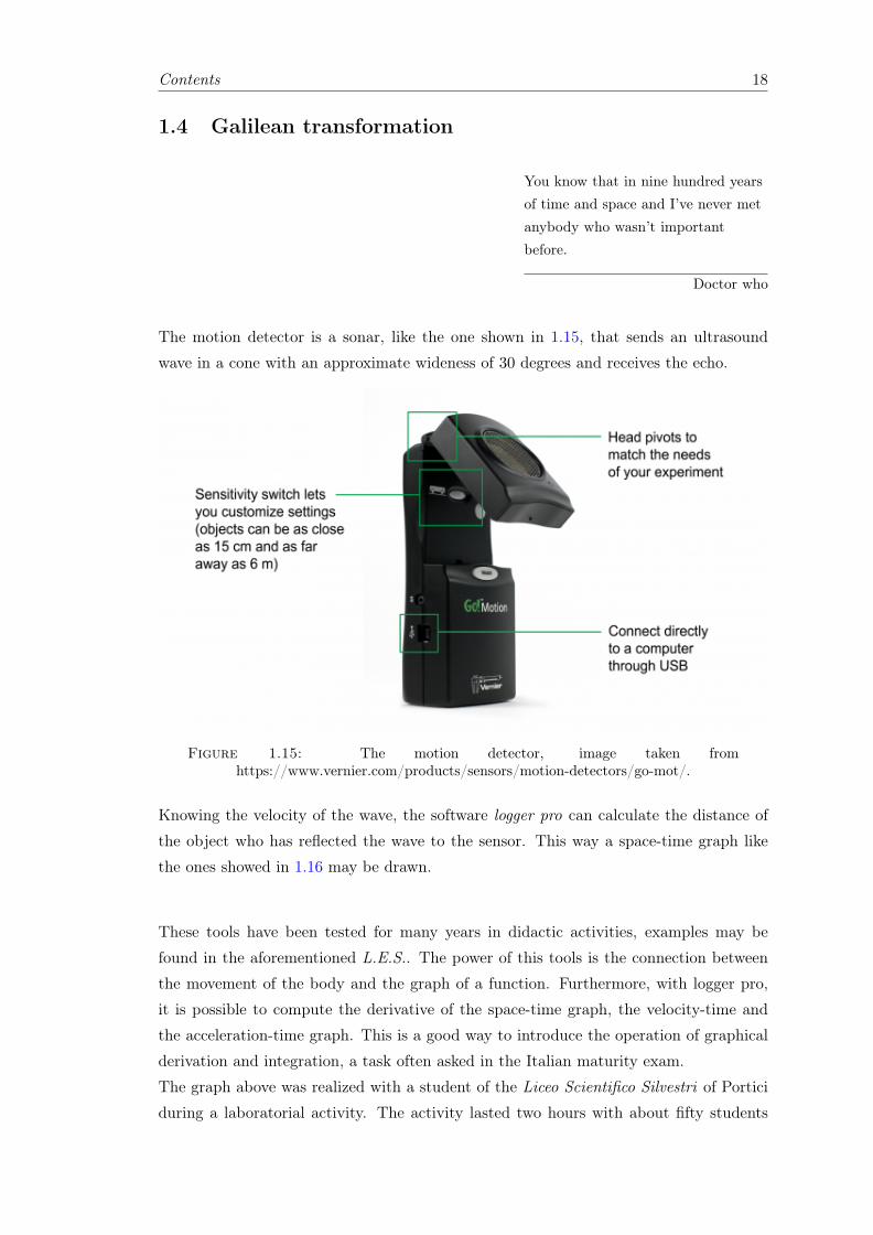
The motion detector is a sonar, like the one shown in 1.15, that sends an ultrasound

wave in a cone with an approximate wideness of 30 degrees and receives the echo.

Figure 1.15: The motion detector, image taken fromhttps://www.vernier.com/products/sensors/motion-detectors/go-mot/.

Knowing the velocity of the wave, the software logger pro can calculate the distance of

the object who has reflected the wave to the sensor. This way a space-time graph like

the ones showed in 1.16 may be drawn.

These tools have been tested for many years in didactic activities, examples may be

found in the aforementioned L.E.S.. The power of this tools is the connection between

the movement of the body and the graph of a function. Furthermore, with logger pro,

it is possible to compute the derivative of the space-time graph, the velocity-time and

the acceleration-time graph. This is a good way to introduce the operation of graphical

derivation and integration, a task often asked in the Italian maturity exam.

The graph above was realized with a student of the Liceo Scientifico Silvestri of Portici

during a laboratorial activity. The activity lasted two hours with about fifty students

Contents 19

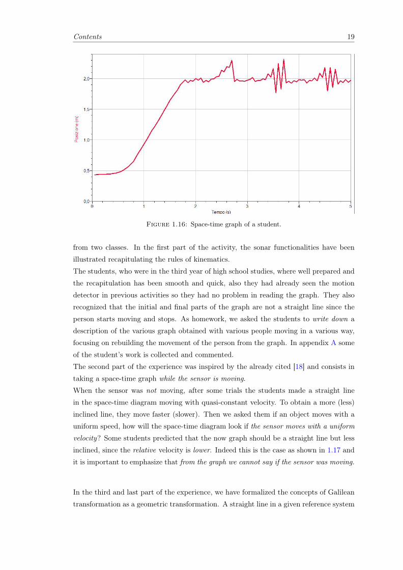
Figure 1.16: Space-time graph of a student.

from two classes. In the first part of the activity, the sonar functionalities have been

illustrated recapitulating the rules of kinematics.

The students, who were in the third year of high school studies, where well prepared and

the recapitulation has been smooth and quick, also they had already seen the motion

detector in previous activities so they had no problem in reading the graph. They also

recognized that the initial and final parts of the graph are not a straight line since the

person starts moving and stops. As homework, we asked the students to write down a

description of the various graph obtained with various people moving in a various way,

focusing on rebuilding the movement of the person from the graph. In appendix A some

of the student’s work is collected and commented.

The second part of the experience was inspired by the already cited [18] and consists in

taking a space-time graph while the sensor is moving.

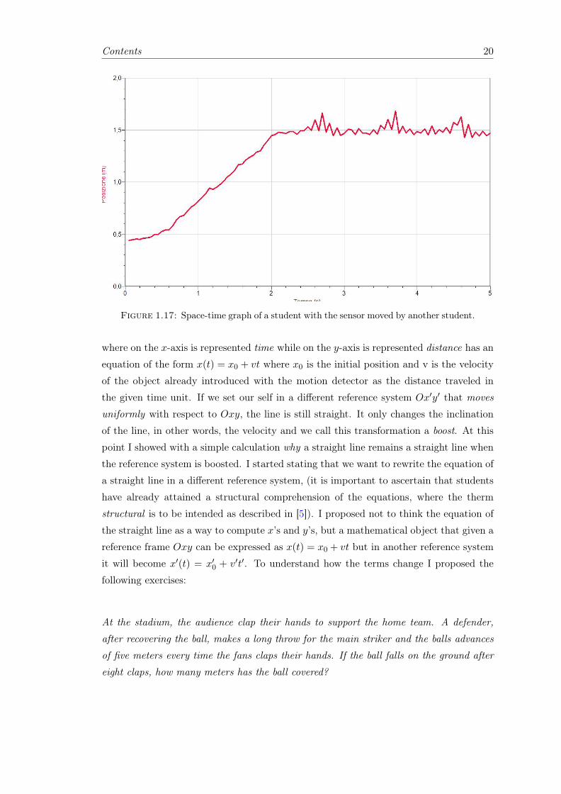
When the sensor was not moving, after some trials the students made a straight line

in the space-time diagram moving with quasi-constant velocity. To obtain a more (less)

inclined line, they move faster (slower). Then we asked them if an object moves with a

uniform speed, how will the space-time diagram look if the sensor moves with a uniform

velocity? Some students predicted that the now graph should be a straight line but less

inclined, since the relative velocity is lower. Indeed this is the case as shown in 1.17 and

it is important to emphasize that from the graph we cannot say if the sensor was moving.

In the third and last part of the experience, we have formalized the concepts of Galilean

transformation as a geometric transformation. A straight line in a given reference system

Contents 20

Figure 1.17: Space-time graph of a student with the sensor moved by another student.

where on the x-axis is represented time while on the y-axis is represented distance has an

equation of the form x(t) = x0 + vt where x0 is the initial position and v is the velocity

of the object already introduced with the motion detector as the distance traveled in

the given time unit. If we set our self in a different reference system Ox′y′ that moves

uniformly with respect to Oxy, the line is still straight. It only changes the inclination

of the line, in other words, the velocity and we call this transformation a boost. At this

point I showed with a simple calculation why a straight line remains a straight line when

the reference system is boosted. I started stating that we want to rewrite the equation of

a straight line in a different reference system, (it is important to ascertain that students

have already attained a structural comprehension of the equations, where the therm

structural is to be intended as described in [5]). I proposed not to think the equation of

the straight line as a way to compute x’s and y’s, but a mathematical object that given a

reference frame Oxy can be expressed as x(t) = x0 + vt but in another reference system

it will become x′(t) = x′0 + v′t′. To understand how the terms change I proposed the

following exercises:

At the stadium, the audience clap their hands to support the home team. A defender,

after recovering the ball, makes a long throw for the main striker and the balls advances

of five meters every time the fans claps their hands. If the ball falls on the ground after

eight claps, how many meters has the ball covered?

Contents 21

In this exercise, the students need to recognize the claps of the hands of the audience as

the unit of measure for the time. Furthermore, they have to confine themselves in one

dimension to avoid cumbersome computations.

At the stadium, the audience clap their hands to support the home team. A defender,

after recovering the ball, makes a long throw for the main striker and the ball advances of

fifteen meters. If the fans have clasped their hands eight times while the ball flew, what

was the speed of the ball?

A midfielder makes a long throw forward. If the balls travel at a speed of thirteen meters

per second and stay in the air for five seconds, at what distance from the midfielder the

ball will fall?

With this two exercises, one can ascertain that the students have understood the concept

of velocity.

Near the midfielder of the previous exercise there is a wing half who starts running to

support the offensive scheme when the long throw is kicked. After how many seconds did

he sees that the balls fall on the ground?

With this exercise, we want to emphasize that the time in which things happens does

not change for people that move one with respect to the other. Both soccer players see

that the ball falls in five seconds.

If the wing half of the previous exercise runs at a speed of six meters per second he will

not get to the point on which the ball falls, how far from him will the ball fall?

Finally, this exercise shows that the position of points does change from a player to

another. If we call x the point in which the midfielder sees the balls fall down on the

ground, for the wing half the point in which the ball falls will be x′ = x− V t, where Vis the velocity of the half wing.

We have then obtained the Galilean transformation

Contents 22

x′ = x− V t

t′ = t

It is easy to generalize this transformation for the other spatial dimensions, it suffices to

remember that the x direction is arbitrary. It is more interesting to show what happens

to the equations x′ = x′0 +v′t′ when change applies the Galilean transformation. In doing

so one must remember that the initial position x′0 turns into x0 − V t0, where t0 is the

initial time that we can put to zero so that x′0 = x0 and the new velocity of an object

is given by the velocity in the old reference system v minus the velocity of the reference

frame V . We then obtain:

x′ = x′0 + v′t′

(x− V t) = (x0 − V t0) + (v − V )t

x = x0 + vt− V t+ V t

x = x0 + vt.

We have achieved a great deal that should be welcomed with much rejoicing. We have,

by experience, found a symmetry that we think nature posses and we know how to write

it in a mathematical form. In the next chapter, we will use this symmetry to build

up mechanics, a theory used to build building, cars, aeroplanes, ships and many other

things.

Contents 23

1.5 Non relativistic mechanics

If all the parts of the universe areinterchained in a certain measure, anyone phenomenon will not be the effectof a single cause, but the resultant ofcauses infinitely numerous; it is, oneoften says, the consequence of thestate of the universe the momentbefore.

Henri Poincaré - The Value of Science

In the previous section we have seen how the space-time diagram of a object changes if

we change the reference system with a Galilean transformation. The lines, not only the

straight ones, are just rotated. We have not analyzed what happens if the new reference

system is accelerating and we will not discuss this case now. So far the experience has

told us that in a different reference systems moving with a velocity V the time-space

diagram is the same, just rotated. In other words the numerical values of the quantities

are changed, but the form of the equation (polynomial of degree n, exponential ecc..)

are the same. This means that if we want to foretell the motion of an object with mass

m, our prediction must respect this symmetry. The best way to do that is to use vectors.

At school level vectors are introduced as arrows with magnitude, direction and point of

application. But they can also be treated as an n-tuple of numbers which transform in a

specific way in a change of coordinate system. For a more detailed treatment, we suggest

[14], where it showed that in a change of reference system the coordinates of a vector

change in specific ways so that the proprieties of the object as a whole are preserved. By

the way, this is also a good reason to distinguish physical vector from arrays in coding,

and by analogy table of numbers, matrix and tensors.

This suggests to use vector to express how object moves, so that our model will be invari-

ant for Galilean transformation. With this in mind, lets start discussing the movement

of an object of mass m. It is common sense that the greater the mass, the more diffi-

cult is to move the object and to sustain its movement. Usually at this point the three

laws of dynamics are introduced, but we shall follow another route proposed by the The

Karlsruhe Physics Course. The following line of reasoning has also been proposed in the

ending comments of the activity in the Liceo Silvestri with good results, as teachers said

it has connected various topics of physics which are often seen disconnected due to the

asphyxiating rhythm of lessons.

We introduce the momentum as the product of the mass and the velocity of an object

~p = m~v. Instead of the velocity we could have thought of position or acceleration, but

Contents 24

in this way this quantity would not preserve in time. If it was the product of the mass

for the acceleration to be conserved, objects should always be accelerating. It was the

product of the mass for the position, objects should stop, but unless a force like friction

is applied on the objects they preserve their motion. Only the product of the mass for

the velocity is preserved. Since the mass is an intrinsic propriety of the body, this is

equivalent to the law of inertia. Moreover, if the momentum changes something must be

changing it, and we give this something the name of force and write

~F =d

dt~p (1.7)

or ~F = ∆~p∆t if students did not know the operation of derivation. This is the second law

of dynamics, and it is also very clear that the variation in momentum is equal to the

impulse. Lastly, the third law of dynamics is also a simple consequence of the principle

of conservation of the momentum. If a body gives momentum to another body, its own

momentum must decrease, getting negative if necessary.

The power of this equations is that it allows us to predict the actual evolution of a

motion, and there is no need to actually solve the differential equation at all. As shown

in [14], given the initial conditions one can compute the position and velocity after a

short time interval of ∆t. This action can be repeated to obtain the orbit of the planet.

Of course, the gravitation force

|~F | = −Gm1m2

r2(1.8)

must be known. Furthermore, this force has to be projected on the axes, and as shown

in [14] this can be done easily if one of the masses is in the centre of the reference system:

Fx = −Gm1m2

r3x

Fy = −Gm1m2

r3y

where x and y are just the coordinates of the planets. Always on Feynmann textbook,

the generalization to the object in any points is found as:

Contents 25

Fx = −Gm1m2

r3(x1 − x2)

Fy = −Gm1m2

r3(y1 − y2).

In the Feynman lectures on physics, this algorithm is carried on by hand reporting the

values on a table. Nowadays, it can be fastened using a excel sheet or a similar program,

which is really intuitive and powerful. Nevertheless, the culture of coding is spreading

from elementary schools. In Italy, a particularly successful project is described on the

website platform.europeanmoocs.eu/course_coding_in_your_classroom_now. To chil-

dren, coding is presented as a game, often a video game, but cycle and conditional struc-

ture are learned at a very early age. Furthermore, the modern programming languages

like Python or Mathematica are intuitive, to know how to code is a powerful tool. From

my personal experience, to know how to code since the high school helped me in the

study of physics just as much as calculus and linear algebra, the one who finds the

numerical approach difficult often have never seen a program in their previous studies.

To learn a programming language is like learning a mathematical notation, it is like a

lens that puts a problem in a completely different light. Since coding is becoming more

popular and since I believe that is an irreplaceable instrument, the following numerical

studies are not carried out with an excel data sheet, but with the Python programming

language and the Jupyter notebook. More information about Python and the Jupyter

notebook can be found in appendix B, here it suffices to say that the language is so high

level to resemble pseudo-code and the notebook allows to interact with it intuitively and

effectively. Furthermore, we suggest [20] to the reader who wants others, more detailed

examples of numerical methods in didactic. Differently from us, the cited work goes into

the detail of the stability of the algorithms. We have used a variant of the Velocity-Verlet

algorithm, which is just a little more complex than the Euler methods but it is more

stable.

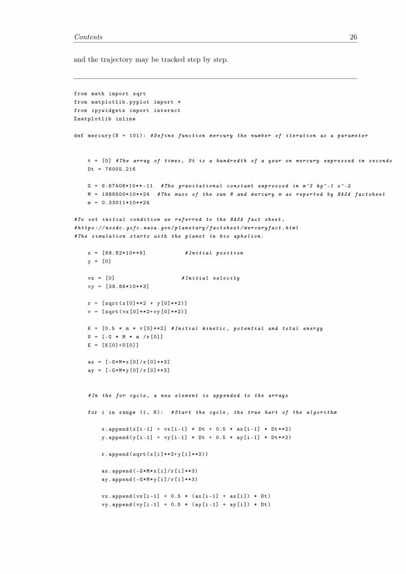
The following code plots the trajectory of Mercury around the Sun and the energy trend.

The Sun is at the centre of the reference system and the action of the planet on him is

neglected since the force is the same but the mass of the sun is seven orders of magnitude

bigger. The algorithm starts with the initial position and velocity of the planets as taken

from the N.A.S.A. fact sheet. To compute the position and velocity at the subsequent

step, differently on how this was implemented by Feynmann textbook, the acceleration is

computed from the gravitational force and the motion is supposed uniformly accelerated

with that acceleration, which is a good approximation for small intervals of time. Fur-

thermore, if the program is executed in the textitJupiter notebook a widget is launched

Contents 26

and the trajectory may be tracked step by step.

from math import sqrt

from matplotlib.pyplot import *

from ipywidgets import interact

%matplotlib inline

def mercury(N = 101): #Define function mercury the number of iteration as a parameter

t = [0] #The array of times , Dt is a hundredth of a year on mercury expressed in seconds

Dt = 76005.216

G = 6.67408*10** -11 #The gravitational constant expressed in m^3 kg^-1 s^-2

M = 1988500*10**24 #The mass of the sun M and mercury m as reported by NASA factsheet

m = 0.33011*10**24

#To set initial condition we referred to the NASA fact sheet ,

#https :// nssdc.gsfc.nasa.gov/planetary/factsheet/mercuryfact.html

#The simulation starts with the planet in his aphelion.

x = [69.82*10**9] #Initial position

y = [0]

vx = [0] #Initial velocity

vy = [38.86*10**3]

r = [sqrt(x[0]**2 + y[0]**2)]

v = [sqrt(vx [0]**2+ vy [0]**2)]

K = [0.5 * m * v[0]**2] #Initial kinetic , potential and total energy

U = [-G * M * m /r[0]]

E = [K[0]+U[0]]

ax = [-G*M*x[0]/r[0]**3]

ay = [-G*M*y[0]/r[0]**3]

#In the for cycle , a new element is appended to the arrays

for i in range (1, N): #Start the cycle , the true hart of the algorithm

x.append(x[i-1] + vx[i-1] * Dt + 0.5 * ax[i-1] * Dt**2)

y.append(y[i-1] + vy[i-1] * Dt + 0.5 * ay[i-1] * Dt**2)

r.append(sqrt(x[i]**2+y[i]**2))

ax.append(-G*M*x[i]/r[i]**3)

ay.append(-G*M*y[i]/r[i]**3)

vx.append(vx[i-1] + 0.5 * (ax[i-1] + ax[i]) * Dt)

vy.append(vy[i-1] + 0.5 * (ay[i-1] + ay[i]) * Dt)

Contents 27

v.append(sqrt(vx[i]**2+vy[i]**2))

K.append (0.5 * m * v[i]**2)

U.append(-G*M*m/r[i])

E.append(U[i] + K[i])

t.append(t[i-1] + Dt) #Advance time

#Plot the results

figure () #Plots the trajectory of the planets

plot(x, y)

title("Trajectory , both axes have meters as units")

grid()

figure () #Plots energy as a function of time

plot(t, E)

plot(t, K)

plot(t, U)

title("Kinetic , potential and total energy")

xlabel("Time[s]")

ylabel("Energy [J]")

grid()

show()

interact (mercury , N = (1 ,100000 ,1))

#The program is interactive so the trajectory can be followed step by step

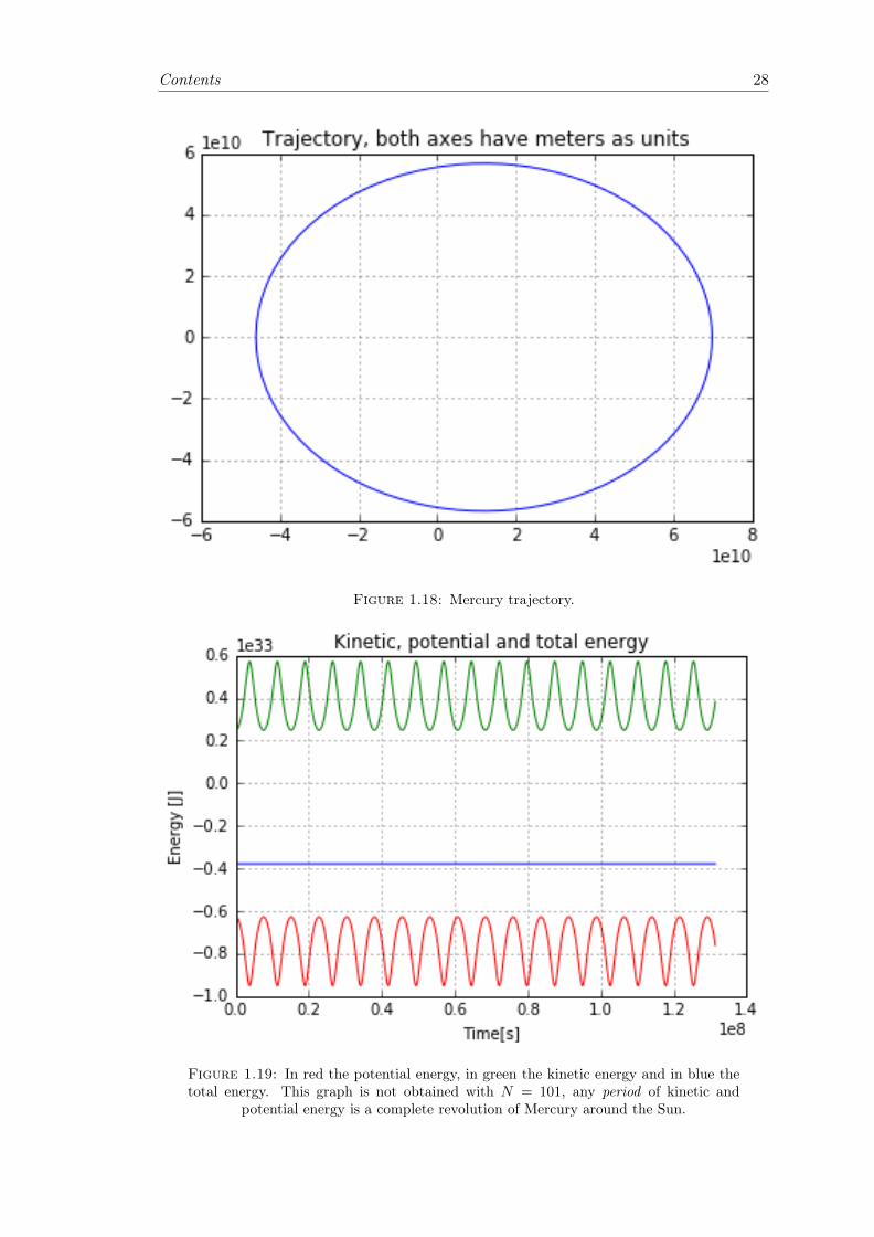
The output of the program is showed in 1.18 and 1.19

This shows that the trajectory of Mercury is an ellipse with the Sun in one of the focuses.

This means that Kepler laws follow from Newtonian laws, which are more general, more

useful and more powerful. It is interesting to note that certain quantity can be introduced

whose sum is constant during all the motion, kinetic and potential energy. This quantity

gives much information about the system that would be hard to retrieve in a different

way. To show the power of the concept of energy as a tool to model natural phenomena,

let’s examine for a moment a simple system. On an inclined plane, two bottles are rolling

down, one is empty and the other one is half full of sands. From cinematic proprieties,

all object should fall with the same velocity, but the sand inside the second bottle slows

it down. This is easily explained if we think that the gravitational potential energy is

divided into two channels: rolling down the bottle and shaking the sand.

Turning back to numerical methods, they are so powerful that allow us to study systems

that cannot be solved analytically. In the following code, the trajectories of both Mercury

and Jupyter are tracked taking into account their mutual interaction.

Contents 28

Figure 1.18: Mercury trajectory.

Figure 1.19: In red the potential energy, in green the kinetic energy and in blue thetotal energy. This graph is not obtained with N = 101, any period of kinetic and

potential energy is a complete revolution of Mercury around the Sun.

Contents 29

from math import sqrt

from numpy import size

from matplotlib.pyplot import *

from ipywidgets import interact

%matplotlib inline

def mercury(N = 3000):

t = [0]

Dt = 76005.216

G = 6.67408*10** -11

M = 1988500*10**24

m = 0.33011*10**24

J = 1898.19*10**24

#To set initial condition we referred to the NASA fact sheet ,

#https :// nssdc.gsfc.nasa.gov/planetary/factsheet/mercuryfact.html

#The simulation starts with both planets aligned in the aphelion.

#That is a simplification since the orbits of the planets are inclined

#one with respect to the other.

xm = [69.82*10**9]

ym = [0]

vxm = [0]

vym = [38.86*10**3]

xJ = [816.62*10**9]

yJ = [0]

vxJ = [0]

vyJ = [12.44*10**3]

rm = [sqrt(xm [0]**2 + ym [0]**2)]

rJm = [sqrt((xJ[0]-xm [0])**2+( yJ[0]-ym [0])**2)]

rJ = [sqrt(xJ [0]**2 + yJ [0]**2)]

axm = [-G*M*xm[0]/rm [0]**3 - G*J*(xm[0]-xJ [0])/( rJm [0]**3)]

aym = [-G*M*ym[0]/rm [0]**3 - G*J*(ym[0]-yJ [0])/( rJm [0]**3)]

axJ = [-G*M*xJ[0]/rJ [0]**3 - G*m*(xJ[0]-xm [0])/( rJm [0]**3)]

ayJ = [-G*M*yJ[0]/rJ [0]**3 - G*m*(yJ[0]-ym [0])/( rJm [0]**3)]

for i in range (1, N):

xm.append(xm[i-1] + vxm[i-1] * Dt + 0.5 * axm[i-1] * Dt**2)

ym.append(ym[i-1] + vym[i-1] * Dt + 0.5 * aym[i-1] * Dt**2)

rm.append(sqrt(xm[i]**2+ym[i]**2))

xJ.append(xJ[i-1] + vxJ[i-1] * Dt + 0.5 * axJ[i-1] * Dt**2)

Contents 30

yJ.append(yJ[i-1] + vyJ[i-1] * Dt + 0.5 * ayJ[i-1] * Dt**2)

rJ.append(sqrt(xJ[i]**2+yJ[i]**2))

rJm.append(sqrt((xJ[i]-xm[i])**2+( yJ[i]-ym[i])**2))

axm.append(-G*M*xm[i]/rm[i]**3 - G*J*(xm[0]-xJ [0])/( rJm [0]**3))

aym.append(-G*M*ym[i]/rm[i]**3 - G*J*(ym[0]-yJ [0])/( rJm [0]**3))

axJ.append(-G*M*xJ[i]/rJ[i]**3 - G*m*(xm[0]-xJ [0])/( rJm [0]**3))

ayJ.append(-G*M*yJ[i]/rJ[i]**3 - G*m*(ym[0]-yJ [0])/( rJm [0]**3))

vxm.append(vxm[i-1] + 0.5 * (axm[i-1] + axm[i]) * Dt)

vym.append(vym[i-1] + 0.5 * (aym[i-1] + aym[i]) * Dt)

vxJ.append(vxJ[i-1] + 0.5 * (axJ[i-1] + axJ[i]) * Dt)

vyJ.append(vyJ[i-1] + 0.5 * (ayJ[i-1] + ayJ[i]) * Dt)

t.append(t[i-1] + Dt)

#Plot the relusts

figure ()

plot(xm, ym)

plot(xJ, yJ)

title("Motion")

grid()

show()

interact (mercury , N = (1 ,100000 ,1))

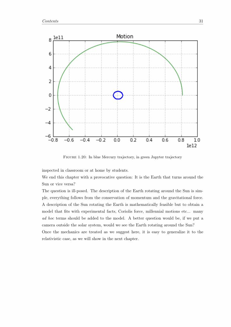
The output of the code is shown in figure 1.20

This can be generalized to any number of interacting objects, it suffices to generalize the

formula for the decomposition of the gravitational force as

Fx = −N∑i

Gmimj(xi − xj)

r3

Fy = −N∑i

Gmimj(yi − yj)

r3.

We can even include the third spatial dimension or the effects of the planets on the Sun

that causes the star to move, a movement that in others stars allow us to detect planets

orbiting them!

Other formidable tools to study the interaction between many bodies can be found on

the site https://phet.colorado.edu/en/simulations which is full of applets that can be

Contents 31

Figure 1.20: In blue Mercury trajectory, in green Jupyter trajectory

inspected in classroom or at home by students.

We end this chapter with a provocative question: It is the Earth that turns around the

Sun or vice versa?

The question is ill-posed. The description of the Earth rotating around the Sun is sim-

ple, everything follows from the conservation of momentum and the gravitational force.

A description of the Sun rotating the Earth is mathematically feasible but to obtain a

model that fits with experimental facts, Coriolis force, millennial motions etc... many

ad hoc terms should be added to the model. A better question would be, if we put a

camera outside the solar system, would we see the Earth rotating around the Sun?

Once the mechanics are treated as we suggest here, it is easy to generalize it to the

relativistic case, as we will show in the next chapter.

Chapter 2

Special theory of relativity

You’re just not thinking fourthdimensionally!

Doctor Emmett Brown - Back to thefuture

In this chapter, we will generalize the Newtonian mechanics to relativistic mechanics.

The first section is a semi-quantitative derivation of the wave equation for the electro-

magnetic fields from the Maxwell’s equations in integral form. The second section is a

recapitulation of the mechanical waves and a comparison with the electromagnetic ones.

In the third section, we propose a laboratorial activity with the Michelson interferometer,

followed by a description of the Michelson and Morley experiment, followed by an intro-

duction to the Lorentz transformation as a generalization of the Galilean transformation.

In the last part of this section, non-relativistic mechanics is presented in an analogous

way as the Newtonian mechanics was introduced in the last chapter.

32

Contents 33

2.1 Derivation of wave equation from Maxwell’s equations

The Scientist must set in order.Science is built up with facts, as ahouse is with stones. But a collectionof facts is no more a science than aheap of stones is a house.

Henri Poincaré - Science andHypothesis

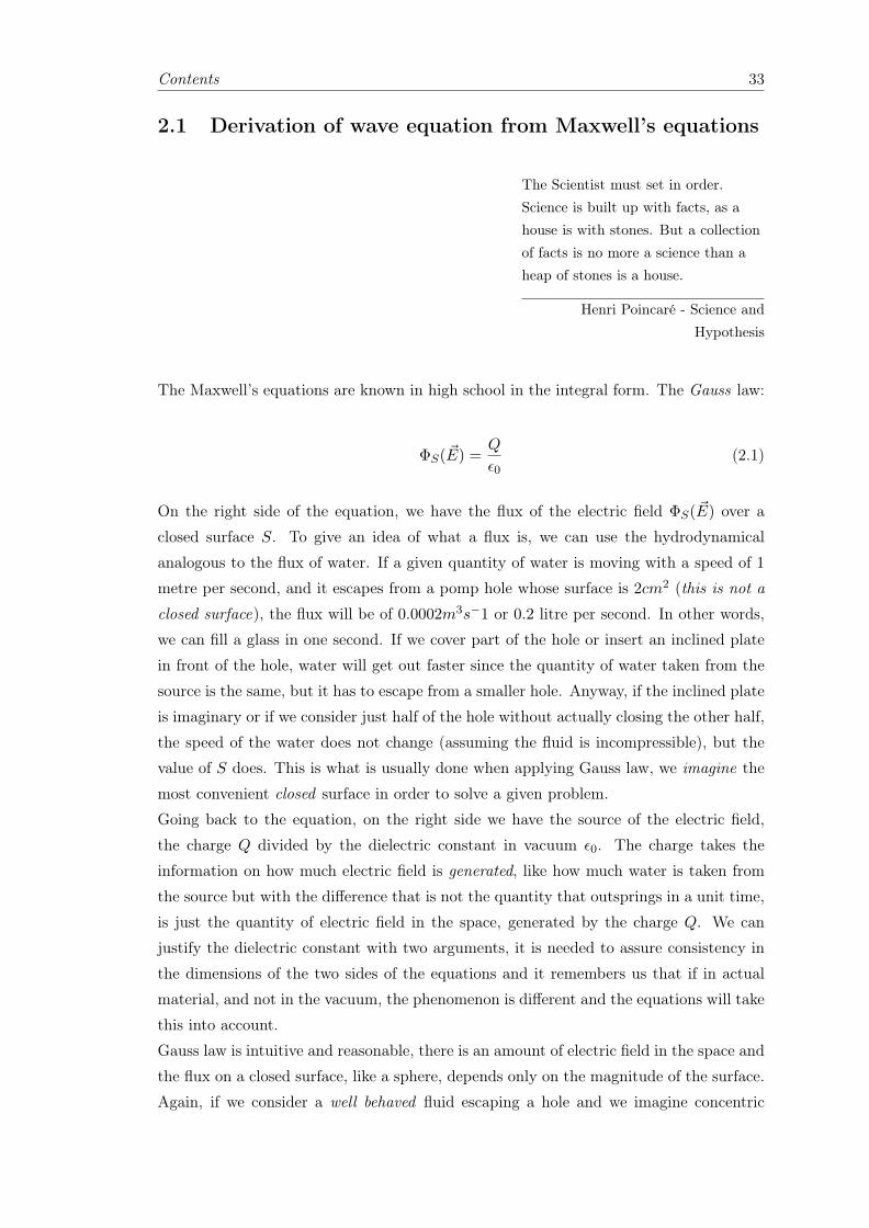
The Maxwell’s equations are known in high school in the integral form. The Gauss law:

ΦS( ~E) =Q

ε0(2.1)

On the right side of the equation, we have the flux of the electric field ΦS( ~E) over a

closed surface S. To give an idea of what a flux is, we can use the hydrodynamical

analogous to the flux of water. If a given quantity of water is moving with a speed of 1

metre per second, and it escapes from a pomp hole whose surface is 2cm2 (this is not a

closed surface), the flux will be of 0.0002m3s−1 or 0.2 litre per second. In other words,

we can fill a glass in one second. If we cover part of the hole or insert an inclined plate

in front of the hole, water will get out faster since the quantity of water taken from the

source is the same, but it has to escape from a smaller hole. Anyway, if the inclined plate

is imaginary or if we consider just half of the hole without actually closing the other half,

the speed of the water does not change (assuming the fluid is incompressible), but the

value of S does. This is what is usually done when applying Gauss law, we imagine the

most convenient closed surface in order to solve a given problem.

Going back to the equation, on the right side we have the source of the electric field,

the charge Q divided by the dielectric constant in vacuum ε0. The charge takes the

information on how much electric field is generated, like how much water is taken from

the source but with the difference that is not the quantity that outsprings in a unit time,

is just the quantity of electric field in the space, generated by the charge Q. We can

justify the dielectric constant with two arguments, it is needed to assure consistency in

the dimensions of the two sides of the equations and it remembers us that if in actual

material, and not in the vacuum, the phenomenon is different and the equations will take

this into account.

Gauss law is intuitive and reasonable, there is an amount of electric field in the space and

the flux on a closed surface, like a sphere, depends only on the magnitude of the surface.

Again, if we consider a well behaved fluid escaping a hole and we imagine concentric

Contents 34

spheres of different radius surrounding it, the flux of water for the different surface is

the same. The quantity of water that goes out any sphere, in a given amount of time,

is the same but as the surface of the spheres through which water passes gets bigger,

the speed of the water diminishes. In an analogous way, as the sphere around a charge

gets bigger, the intensity of the electric field diminishes. Furthermore, the flux and the

field intensity must be in a proportional relation. Since the surface of the sphere gets

bigger in proportion with the square of the distance from the charge, the intensity of the

flux must decrease in the same way. We have assumed that the reader is a teacher with

a basic or advanced knowledge in physics, so the reader knows that the electric field is

defined as the force that acted on a unit charge, hence the Coulomb force must satisfy

a relation with the square of the distance at the denominator. This is another way to

emphasize how all pieces of a scientific theory fits together, science is true even if no one

believes in it, but people (and researcher are people) must be convinced of the theory

they are working on.

The second of Maxwell’s equations states that the flux of the magnetic field on a closed

surface is always zero, this can be explained assuming that magnetic charges (north and

south pole) are always in pairs and the field line is closed, the equation is

ΦS( ~B) = 0. (2.2)

The third equations, also known as Faraday-Lenz law, connects the variation in time of

the flux with the work needed to move a unit charge on a closed circuit Γ

Γ( ~E) = −∆ΦS( ~B)

∆t. (2.3)

In this case, the flux is to be considered on the surface that has as boundaries the

circulation path and it is not closed.

The left-hand side of this equations is also known as circulation of the electric field. In

the case of a flux that varies in a spire, the circulation is equal to the electromotive force

generated in the spire and can be measured. This is the first of Maxwell’s equation in

which ~E and ~B are connected. Indeed, the first two equations give information on the

fields but can be obtained from the other equations [14].

The last (but not least) of the Maxwell’s equations, also known as the Ampère circuital

law, connects the circulation of the magnetic field with the sum of all the electric currents

I trough the path of circulation and the variation in time of the electric flux on the surface

whose boundaries are the circulation path, in formula

Contents 35

Γ( ~B) = µ0

(Itot + ε0

∆ΦS( ~E)

∆t

). (2.4)

The term on which we will focus is the displacement current ε0µ0∆ΦS( ~E)

∆t . This was

adjunct by Maxwell to adapt the equations in cases, like a capacitor, where there is no

conduction current but the field is not zero. With this two equations, that connect the

electric and the magnetic fields, it is possible to explain how many everyday objects

works like electric engine or electromagnets, but we will focus on a different topic.

With this two equations, we can see that there is the chance to create a self-sustaining

propagating electromagnetic field. The derivation that we proposed can is a sum up of

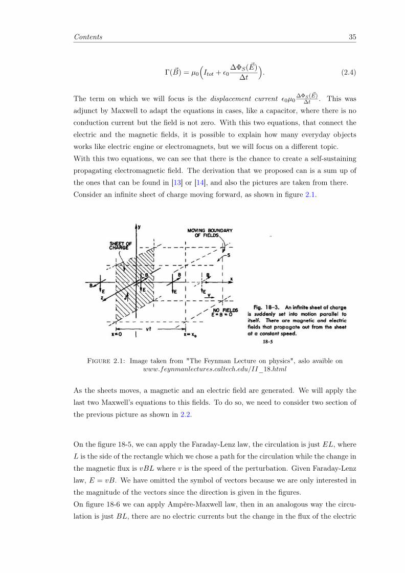
the ones that can be found in [13] or [14], and also the pictures are taken from there.

Consider an infinite sheet of charge moving forward, as shown in figure 2.1.

Figure 2.1: Image taken from "The Feynman Lecture on physics", aslo avaible onwww.feynmanlectures.caltech.edu/II_18.html

As the sheets moves, a magnetic and an electric field are generated. We will apply the

last two Maxwell’s equations to this fields. To do so, we need to consider two section of

the previous picture as shown in 2.2.

On the figure 18-5, we can apply the Faraday-Lenz law, the circulation is just EL, where

L is the side of the rectangle which we chose a path for the circulation while the change in

the magnetic flux is vBL where v is the speed of the perturbation. Given Faraday-Lenz

law, E = vB. We have omitted the symbol of vectors because we are only interested in

the magnitude of the vectors since the direction is given in the figures.

On figure 18-6 we can apply Ampère-Maxwell law, then in an analogous way the circu-

lation is just BL, there are no electric currents but the change in the flux of the electric

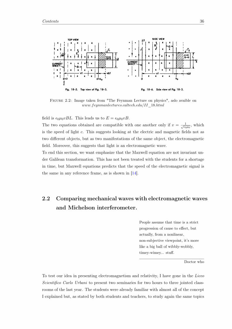
Contents 36

Figure 2.2: Image taken from "The Feynman Lecture on physics", aslo avaible onwww.feynmanlectures.caltech.edu/II_18.html

field is ε0µ0vBL. This leads us to E = ε0µ0vB.

The two equations obtained are compatible with one another only if v = 1√ε0µ0

, which

is the speed of light c. This suggests looking at the electric and magnetic fields not as

two different objects, but as two manifestations of the same object, the electromagnetic

field. Moreover, this suggests that light is an electromagnetic wave.

To end this section, we want emphasize that the Maxwell equation are not invariant un-

der Galilean transformation. This has not been treated with the students for a shortage

in time, but Maxwell equations predicts that the speed of the electromagnetic signal is

the same in any reference frame, as is shown in [14].

2.2 Comparing mechanical waves with electromagnetic waves

and Michelson interferometer.

People assume that time is a strictprogression of cause to effect, butactually, from a nonlinear,non-subjective viewpoint, it’s morelike a big ball of wibbly-wobbly,timey-wimey... stuff.

Doctor who

To test our idea in presenting electromagnetism and relativity, I have gone in the Liceo

Scientifico Carlo Urbani to present two seminaries for two hours to three jointed class-

rooms of the last year. The students were already familiar with almost all of the concept

I explained but, as stated by both students and teachers, to study again the same topics

Contents 37

but in a different light, connecting arguments that were previously discussed in a differ-

ent month or even different years has been a great stimulus.

In the first activity, I have presented a recapitulation of mechanical waves and a com-

parison with electromagnetic fields. The first object I have used is a slinky (see 2.6),

with the help of this toy mechanical waves can be actually seen. Both longitudinal and

transverse waves can be discussed and some laboratorial activity can be found on the

L.E.S. My goal was to show that a wave is usually described in two ways, as

x(t) = A cosωt+ φ (2.5)

or

y(x) = A cos kx+ φ. (2.6)

What many students had not grasp was the meaning of φ, and some numerical example

was helpful in clearing up the meaning of this term.

So in a mechanical wave something oscillates, and the direction of the oscillation is called

polarization. For the wave on the slinky, we have found three possible directions of polar-

ization, two for the transverse waves and one for the longitudinal. Of course, the various

polarizations can be combined, but at this point with the help of a laser, two Polaroids

and a slit, the wave nature of light has been shown (see 2.7). The proposed experiments

are all well know and well described in the literature, and the students had already seen

them in videos proposed during the mandatory lessons.

At this point, to trigger their speculations, I asked: "if the electromagnetic radiation, as

we have seen, is a wave, what is oscillating?".

After a brainstorm, following the line of thought of the previous chapter, we arrived at

the conclusion that are the electric and magnetic fields that oscillate. With this, the first

lessons has ended.

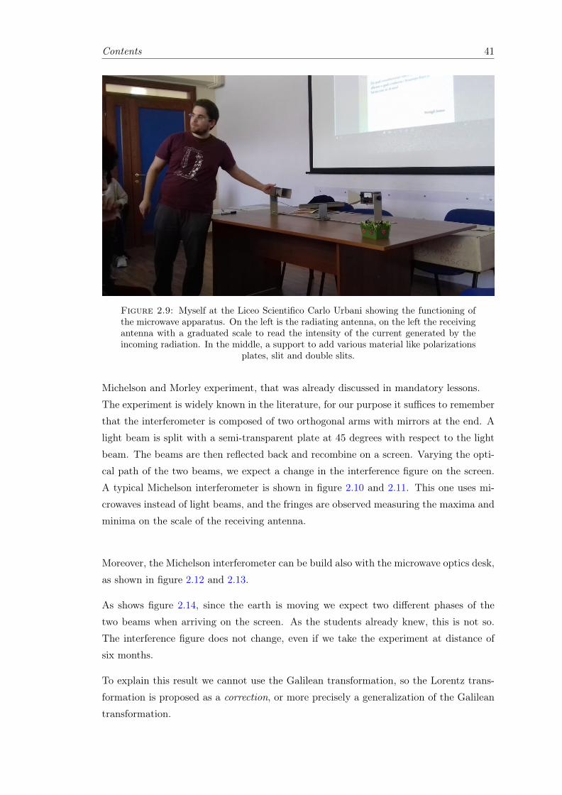
After a month, I returned to the school and meet the same student, taking from where

we left. I bought the microwave apparatus showed in 2.9, where On the left there is an

antenna that radiates in the frequency of microwaves, on the left the receiving antenna

with a graduated scale to read the intensity of the current generated by the incoming

radiation. In the middle, a support to add various material like polarizations plates, slit

and double slits.

I have briefly proposed again the polarization and the double slit experiment, so to recap

the previous lesson. After that it was really easy to explain the basic features of the

Contents 38

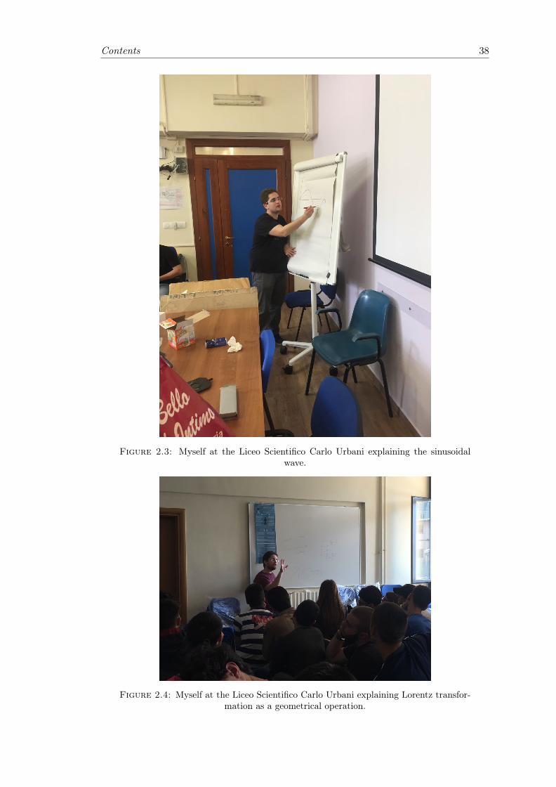
Figure 2.3: Myself at the Liceo Scientifico Carlo Urbani explaining the sinusoidalwave.

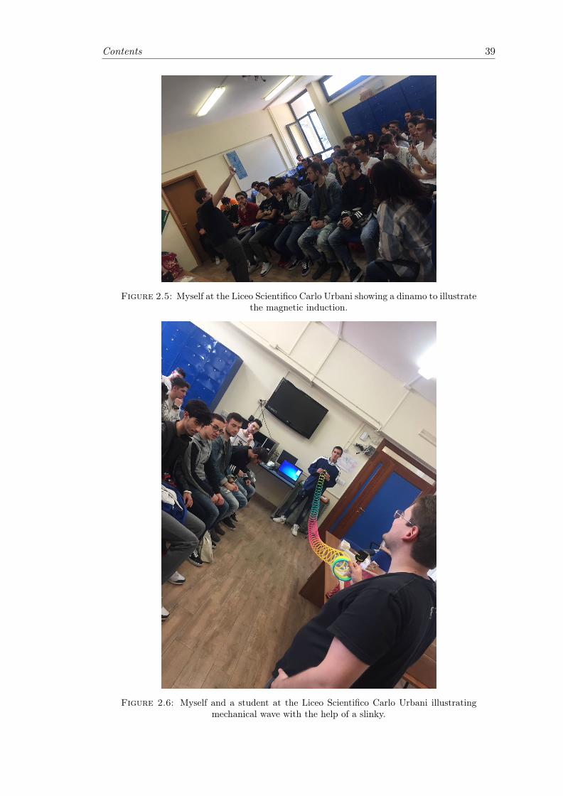
Figure 2.4: Myself at the Liceo Scientifico Carlo Urbani explaining Lorentz transfor-mation as a geometrical operation.

Contents 39

Figure 2.5: Myself at the Liceo Scientifico Carlo Urbani showing a dinamo to illustratethe magnetic induction.

Figure 2.6: Myself and a student at the Liceo Scientifico Carlo Urbani illustratingmechanical wave with the help of a slinky.

Contents 40

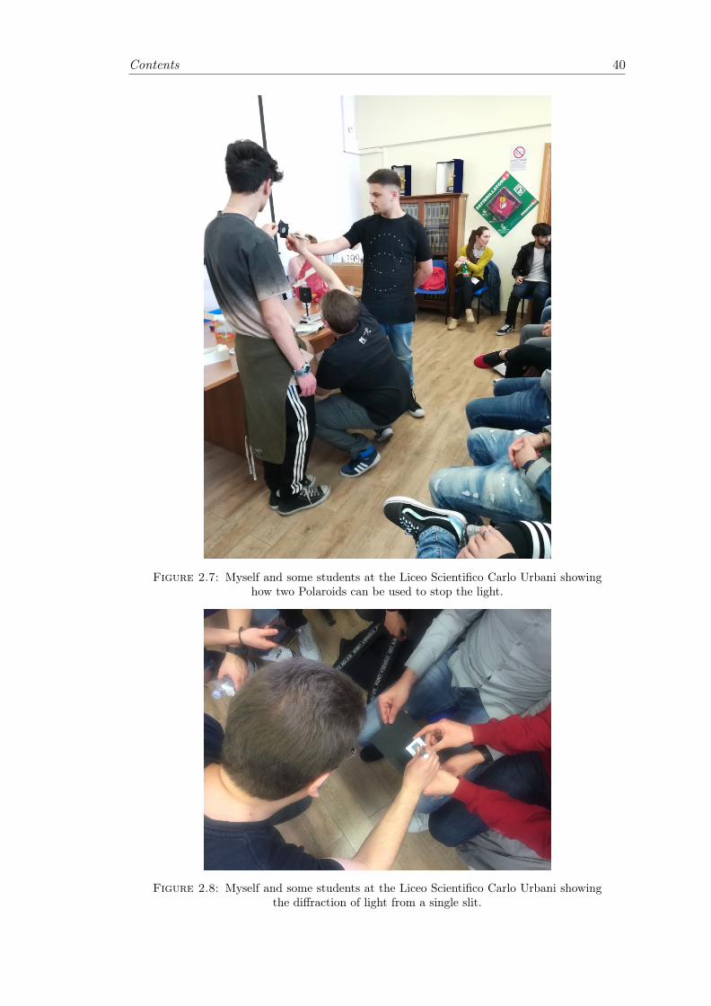
Figure 2.7: Myself and some students at the Liceo Scientifico Carlo Urbani showinghow two Polaroids can be used to stop the light.

Figure 2.8: Myself and some students at the Liceo Scientifico Carlo Urbani showingthe diffraction of light from a single slit.

Contents 41

Figure 2.9: Myself at the Liceo Scientifico Carlo Urbani showing the functioning ofthe microwave apparatus. On the left is the radiating antenna, on the left the receivingantenna with a graduated scale to read the intensity of the current generated by theincoming radiation. In the middle, a support to add various material like polarizations

plates, slit and double slits.

Michelson and Morley experiment, that was already discussed in mandatory lessons.

The experiment is widely known in the literature, for our purpose it suffices to remember

that the interferometer is composed of two orthogonal arms with mirrors at the end. A

light beam is split with a semi-transparent plate at 45 degrees with respect to the light

beam. The beams are then reflected back and recombine on a screen. Varying the opti-

cal path of the two beams, we expect a change in the interference figure on the screen.

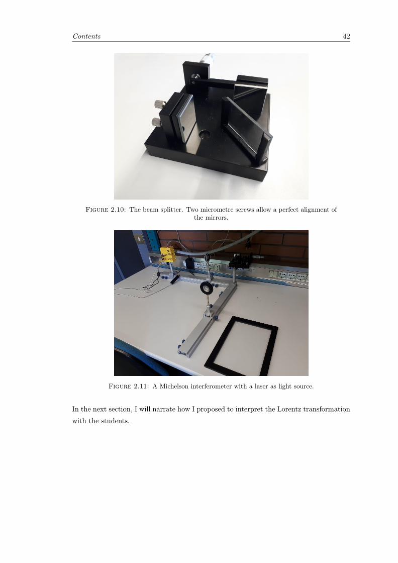
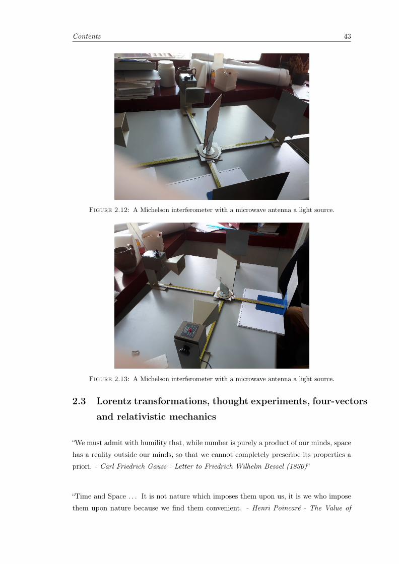
A typical Michelson interferometer is shown in figure 2.10 and 2.11. This one uses mi-

crowaves instead of light beams, and the fringes are observed measuring the maxima and

minima on the scale of the receiving antenna.

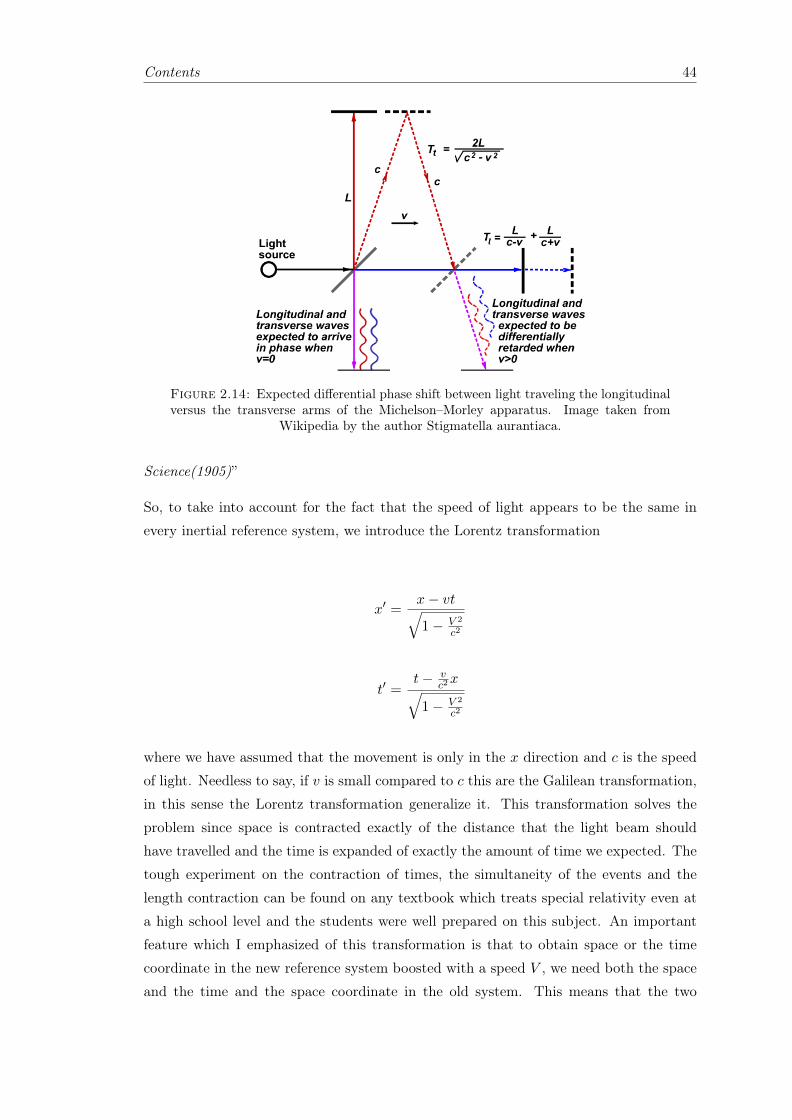
Moreover, the Michelson interferometer can be build also with the microwave optics desk,

as shown in figure 2.12 and 2.13.

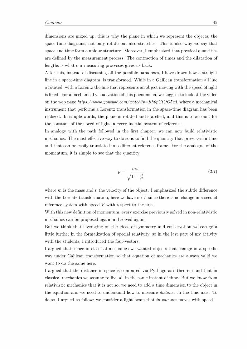
As shows figure 2.14, since the earth is moving we expect two different phases of the

two beams when arriving on the screen. As the students already knew, this is not so.

The interference figure does not change, even if we take the experiment at distance of

six months.

To explain this result we cannot use the Galilean transformation, so the Lorentz trans-

formation is proposed as a correction, or more precisely a generalization of the Galilean

transformation.

Contents 42

Figure 2.10: The beam splitter. Two micrometre screws allow a perfect alignment ofthe mirrors.

Figure 2.11: A Michelson interferometer with a laser as light source.

In the next section, I will narrate how I proposed to interpret the Lorentz transformation

with the students.

Contents 43

Figure 2.12: A Michelson interferometer with a microwave antenna a light source.

Figure 2.13: A Michelson interferometer with a microwave antenna a light source.

2.3 Lorentz transformations, thought experiments, four-vectors

and relativistic mechanics

“We must admit with humility that, while number is purely a product of our minds, space

has a reality outside our minds, so that we cannot completely prescribe its properties a

priori. - Carl Friedrich Gauss - Letter to Friedrich Wilhelm Bessel (1830)”

“Time and Space . . . It is not nature which imposes them upon us, it is we who impose

them upon nature because we find them convenient. - Henri Poincaré - The Value of

Contents 44

Figure 2.14: Expected differential phase shift between light traveling the longitudinalversus the transverse arms of the Michelson–Morley apparatus. Image taken from

Wikipedia by the author Stigmatella aurantiaca.

Science(1905)”

So, to take into account for the fact that the speed of light appears to be the same in

every inertial reference system, we introduce the Lorentz transformation

x′ =x− vt√1− V 2

c2

t′ =t− v

c2x√

1− V 2

c2

where we have assumed that the movement is only in the x direction and c is the speed

of light. Needless to say, if v is small compared to c this are the Galilean transformation,

in this sense the Lorentz transformation generalize it. This transformation solves the

problem since space is contracted exactly of the distance that the light beam should

have travelled and the time is expanded of exactly the amount of time we expected. The

tough experiment on the contraction of times, the simultaneity of the events and the

length contraction can be found on any textbook which treats special relativity even at

a high school level and the students were well prepared on this subject. An important

feature which I emphasized of this transformation is that to obtain space or the time

coordinate in the new reference system boosted with a speed V , we need both the space

and the time and the space coordinate in the old system. This means that the two

Contents 45

dimensions are mixed up, this is why the plane in which we represent the objects, the

space-time diagrams, not only rotate but also stretches. This is also why we say that

space and time form a unique structure. Moreover, I emphasized that physical quantities

are defined by the measurement process. The contraction of times and the dilatation of

lengths is what our measuring processes gives us back.

After this, instead of discussing all the possible paradoxes, I have drawn how a straight

line in a space-time diagram, is transformed. While in a Galilean transformation all line

a rotated, with a Lorentz the line that represents an object moving with the speed of light

is fixed. For a mechanical visualization of this phenomena, we suggest to look at the video

on the web page https://www.youtube.com/watch?v=Rh0pYtQG5wI, where a mechanical

instrument that performs a Lorentz transformation in the space-time diagram has been

realized. In simple words, the plane is rotated and starched, and this is to account for

the constant of the speed of light in every inertial system of reference.

In analogy with the path followed in the first chapter, we can now build relativistic

mechanics. The most effective way to do so is to find the quantity that preserves in time

and that can be easily translated in a different reference frame. For the analogue of the

momentum, it is simple to see that the quantity

p =mv√1− v2

c2

(2.7)

where m is the mass and v the velocity of the object. I emphasized the subtle difference

with the Lorentz transformation, here we have no V since there is no change in a second

reference system with speed V with respect to the first.

With this new definition of momentum, every exercise previously solved in non-relativistic

mechanics can be proposed again and solved again.

But we think that leveraging on the ideas of symmetry and conservation we can go a

little further in the formalization of special relativity, so in the last part of my activity

with the students, I introduced the four-vectors.

I argued that, since in classical mechanics we wanted objects that change in a specific

way under Galilean transformation so that equation of mechanics are always valid we

want to do the same here.

I argued that the distance in space is computed via Pythagoras’s theorem and that in

classical mechanics we assume to live all in the same instant of time. But we know from

relativistic mechanics that it is not so, we need to add a time dimension to the object in

the equation and we need to understand how to measure distance in the time axis. To

do so, I argued as follow: we consider a light beam that in vacuum moves with speed

Contents 46

c =ds

dt. (2.8)

In a different inertial reference system, times will be dilatated and lengths will be con-

tracted, but the speed of light remains c

c′ =ds′

dt′= c =

ds

dt. (2.9)

From the above equations follows that

cdt′ − ds′ = cdt− ds. (2.10)

This means that the difference between the spatial distance ds and the time duration dt

multiplied by the speed of light, is the same in every inertial reference system and we

use this as the distance in space-time.

This little computation justifies the definition of vectors with four coordinates instead

of three, one represents the time dimension and the other the spatial dimensions. When

computing the modulus of this four-vector, we need to make the difference between the

spatial and the time distance. This is the Minkowski metric, and we have defined the

Minkowski space. If I had more time with the students I would have liked to emphasize

that differently than in the usual Euclidean space, the modulus of a vector can be imag-

inary, and this leads to the definition of the light cone (which the students had already

seen), the distinction of time-like and space-like four-vector and assures the validity of

the causation principle. Instead, to trigger students thought for the last time in the

activity, I asked them how to complete the momentum with a fourth time representative

element. Arguing that we needed something that under transformation changes as the

modulus of the momentum, since the difference with the modulus of the spatial and

time coordinates must be unchanged. Remembering that the kinetic energy can also be

written as E = p2/2m, we arrived at the conclusion that this time element must have

the dimension of an energy divided by c. With the definition of the four-momentum the

circle is closed, we have built the relativistic mechanics in a way that allows students

to solve problems. To end the activity, we tried to interpret the modulus of the four-

moment as a physical quantity. Since it is always positive and it has the dimension of

the square of a mass multiplied by the square of a distance, we assumed that

|E|2

c2− |p| = m2c2 (2.11)

Contents 47

and this leads to

|E|2 = m2c4 + |p|c2 (2.12)

which, for an object with no momentum reduces to

E = mc2 (2.13)

This equation is used in many application like the production of nuclear energy and since

the time was finished the lesson ended.

After this, I would have done two things. The first is the paradox of the rotation wheel.

Since in a moving object only the lengths which are parallel to the motion contracts, the

circumference and the radius should change their ratio. This means that the rigid body

cannot be used as an approximation for any body in the framework of special relativity.

The last thing that I would have emphasized is the fact that the electromagnetism, as

described by Maxwell equation, takes already into account special relativity.

If we have a moving particle, this will generate an electric and a magnetic field. But if we

place ourselves in the reference system in which the charge is fixed, we will only measure

an electric field. Anyway, the paradox is fixed if we think the electric and magnetic fields

as a single electromagnetic field, where the magnetic and the electric components of the

fields adjust under a Lorentz transformation so that the description remains coherent.

To arrive at the transformation of the fields would be the satisfactory justification for

the union of the two different fields.

With this, the circle is closed and the relativistic mechanics is developed as a gener-

alization of the classical mechanics. From the Galilean transformation and the Eu-

clidean space, we have built classical mechanics, from the Lorentz transformation and

the Minkowski space the relativistic mechanics. Anyway, this is already done in schools

with different strategies. In the next chapter, we will see how a physical theory can

use an even more general geometry to build more general mechanics and an attempt to

introduce General Relativity in high school is pursued.

Chapter 3

Approach to general relativity

I foresee two possibilities. 1: comingface to face with herself 30 years olderwould put her into shock and she’dsimply pass out. Or 2: the encountercould create a time paradox, theresult of which could cause a chainreaction that would unravel the veryfabric of the spacetime continuumand destroy the entire universe!Granted, that’s a worst-case scenario.The destruction might in fact be verylocalised, limited to merely our owngalaxy.

Doctor Emmet Brown - Back to thefuture

In this chapter, an approach to general relativity for students of the high school is

presented. In the first section, a laboratorial activity in school is described in which

the basic features of spherical geometry are presented and Girard’s theorem is proved.

Continuing the description of the laboratorial activity, the second section documents my

attempt to introduce tensors and to interpret Einstein field equation. The last section

starts with a discussion of the Schwarzschild and the simulation of the motion of Mercury

is revised taking into account correction from general relativity. The last pages have a

more speculative imprint, discussing black holes and the cosmological constant without

going into mathematical details.

48

Contents 49

3.1 Geometry on a sphere, metric and curvature

Experience guides us in this choicewithout forcing it upon us; it tells usnot which is the truest geometry, butwhich is the most convenient.

Henri Poincaré - Science andHypothesis

Though the goal of this chapter is to introduce general relativity, we start with a section

on spherical geometry, which is also the focus of my laboratorial activity with a class

of the last year of the Liceo Scientifico Calamandrei. We have done so because, even if

general relativity uses hyperbolic geometry, it is fundamental that students understand

that we can do geometry on any kind of surface. The globe is a perfect example to

connect non-Euclidean geometry with personal experiences. This topic is usually treated

in mathematics lectures so, in literature, the approach starts from the discussion on the

axioms and postulates of the Euclidean geometry, as is done in [21] and [22], but we

will not follow that path. We will adopt a more experimental approach, starting from

the things that can be measured. Of course, this is a great opportunity to take and

a discussion on the foundation of geometry should be performed, but our goal in the

present work is to introduce the concept of curvature and metrics.

Differently than other two experience, this time there was only one classroom of sixteen

students and we were in the laboratory of the school. I have taken six world globe as

the one showed in 3.1 and 3.2 and the experience lasted 2 hours. Students had already

studied General relativity in ordinary lessons from the book [23], so the aim of the preset

laboratorial experience is to probe, recapitulate and strengthen the knowledge on non-

Euclidean geometry and general relativity.

To every group was given a survey, for the first hour they where let free to do it by

themselves, I had just a function of support for the inevitable questions and doubts on

how to proceed. The first three questions were:

1) Measure the length at the equator on the world globe and transcribe it

Circumference = . . . . . . . . . . . . . . . cm

2) Did the measure of the circumference has errors? would you know how to estimate it?

would it have any sense to make an average of the measure of all group to get a better

estimation?

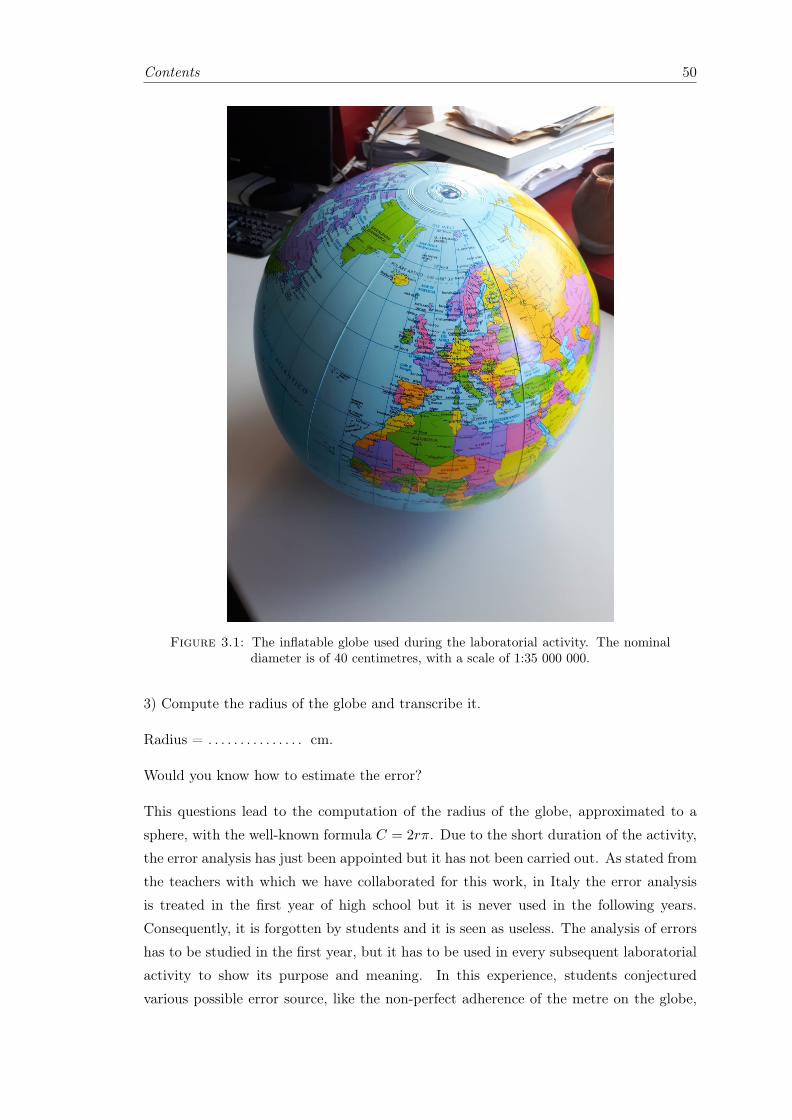
Contents 50

Figure 3.1: The inflatable globe used during the laboratorial activity. The nominaldiameter is of 40 centimetres, with a scale of 1:35 000 000.

3) Compute the radius of the globe and transcribe it.

Radius = . . . . . . . . . . . . . . . cm.

Would you know how to estimate the error?

This questions lead to the computation of the radius of the globe, approximated to a

sphere, with the well-known formula C = 2rπ. Due to the short duration of the activity,

the error analysis has just been appointed but it has not been carried out. As stated from

the teachers with which we have collaborated for this work, in Italy the error analysis

is treated in the first year of high school but it is never used in the following years.

Consequently, it is forgotten by students and it is seen as useless. The analysis of errors

has to be studied in the first year, but it has to be used in every subsequent laboratorial

activity to show its purpose and meaning. In this experience, students conjectured

various possible error source, like the non-perfect adherence of the metre on the globe,

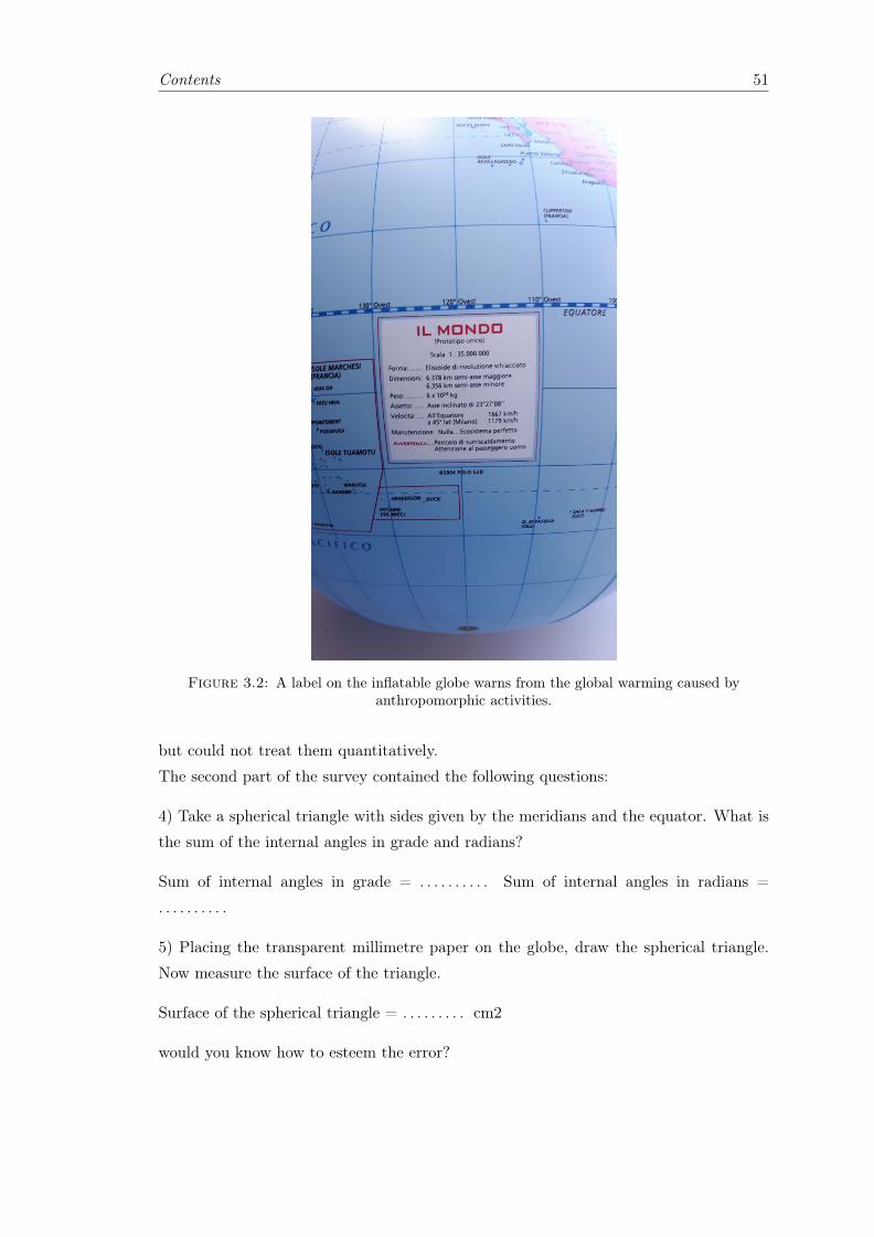
Contents 51

Figure 3.2: A label on the inflatable globe warns from the global warming caused byanthropomorphic activities.

but could not treat them quantitatively.

The second part of the survey contained the following questions:

4) Take a spherical triangle with sides given by the meridians and the equator. What is

the sum of the internal angles in grade and radians?

Sum of internal angles in grade = . . . . . . . . . . Sum of internal angles in radians =

. . . . . . . . . .

5) Placing the transparent millimetre paper on the globe, draw the spherical triangle.

Now measure the surface of the triangle.

Surface of the spherical triangle = . . . . . . . . . cm2

would you know how to esteem the error?

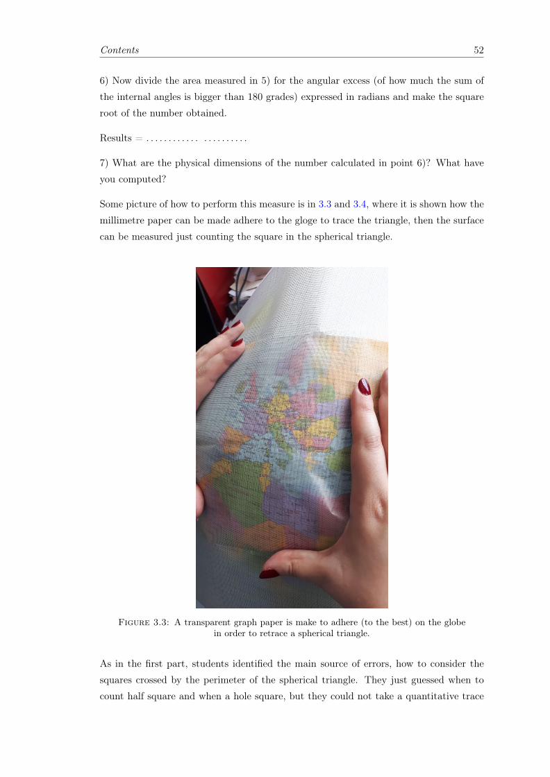
Contents 52

6) Now divide the area measured in 5) for the angular excess (of how much the sum of

the internal angles is bigger than 180 grades) expressed in radians and make the square

root of the number obtained.

Results = . . . . . . . . . . . . . . . . . . . . . .

7) What are the physical dimensions of the number calculated in point 6)? What have

you computed?

Some picture of how to perform this measure is in 3.3 and 3.4, where it is shown how the

millimetre paper can be made adhere to the gloge to trace the triangle, then the surface

can be measured just counting the square in the spherical triangle.

Figure 3.3: A transparent graph paper is make to adhere (to the best) on the globein order to retrace a spherical triangle.

As in the first part, students identified the main source of errors, how to consider the

squares crossed by the perimeter of the spherical triangle. They just guessed when to

count half square and when a hole square, but they could not take a quantitative trace

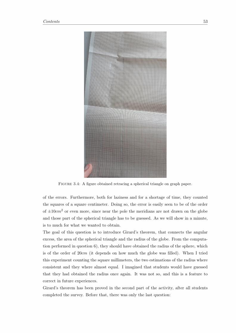
Contents 53

Figure 3.4: A figure obtained retracing a spherical triangle on graph paper.

of the errors. Furthermore, both for laziness and for a shortage of time, they counted

the squares of a square centimeter. Doing so, the error is easily seen to be of the order

of ±10cm2 or even more, since near the pole the meridians are not drawn on the globe

and those part of the spherical triangle has to be guessed. As we will show in a minute,

is to much for what we wanted to obtain.

The goal of this question is to introduce Girard’s theorem, that connects the angular

excess, the area of the spherical triangle and the radius of the globe. From the computa-

tion performed in question 6), they should have obtained the radius of the sphere, which

is of the order of 20cm (it depends on how much the globe was filled). When I tried

this experiment counting the square millimeters, the two estimations of the radius where

consistent and they where almost equal. I imagined that students would have guessed

that they had obtained the radius once again. It was not so, and this is a feature to

correct in future experiences.

Girard’s theorem has been proved in the second part of the activity, after all students

completed the survey. Before that, there was only the last question:

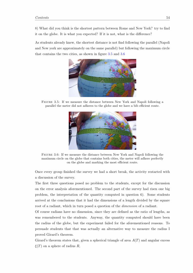
Contents 54

8) What did you think is the shortest pattern between Rome and New York? try to find

it on the globe. It is what you expected? If it is not, what is the difference?

As students already knew, the shortest distance is not find following the parallel (Napoli

and New york are approximately on the same parallel) but following the maximum circle

that contains the two cities, as shown in figure 3.5 and 3.6

Figure 3.5: If we measure the distance between New York and Napoli following aparallel the meter did not adheres to the globe and we have a bib efficient route.

Figure 3.6: If we measure the distance between New York and Napoli following themaximum circle on the globe that contains both cities, the meter will adhere perfectly

on the globe and marking the most efficient route.

Once every group finished the survey we had a short break, the activity restarted with

a discussion of the survey.

The first three questions posed no problem to the students, except for the discussion

on the error analysis aforementioned. The second part of the survey had risen one big

problem, the interpretation of the quantity computed in question 6). Some students

arrived at the conclusions that it had the dimensions of a length divided by the square

root of a radiant, which in turn posed a question of the dimension of a radiant.

Of course radians have no dimension, since they are defined as the ratio of lengths, as

was remembered to the students. Anyway, the quantity computed should have been

the radius of the globe, but the experiment failed for the aforementioned reasons. To

persuade students that that was actually an alternative way to measure the radius I

proved Girard’s theorem.

Girard’s theorem states that, given a spherical triangle of area A(T ) and angular excess

ξ(T ) on a sphere of radius R,

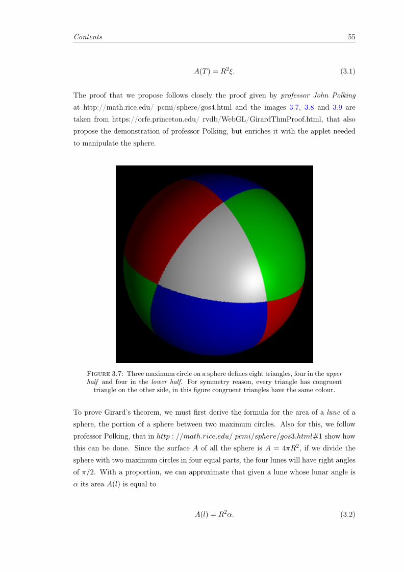
Contents 55

A(T ) = R2ξ. (3.1)

The proof that we propose follows closely the proof given by professor John Polking

at http://math.rice.edu/ pcmi/sphere/gos4.html and the images 3.7, 3.8 and 3.9 are

taken from https://orfe.princeton.edu/ rvdb/WebGL/GirardThmProof.html, that also

propose the demonstration of professor Polking, but enriches it with the applet needed

to manipulate the sphere.

Figure 3.7: Three maximum circle on a sphere defines eight triangles, four in the upperhalf and four in the lower half. For symmetry reason, every triangle has congruenttriangle on the other side, in this figure congruent triangles have the same colour.

To prove Girard’s theorem, we must first derive the formula for the area of a lune of a

sphere, the portion of a sphere between two maximum circles. Also for this, we follow

professor Polking, that in http : //math.rice.edu/ pcmi/sphere/gos3.html#1 show how

this can be done. Since the surface A of all the sphere is A = 4πR2, if we divide the

sphere with two maximum circles in four equal parts, the four lunes will have right angles

of π/2. With a proportion, we can approximate that given a lune whose lunar angle is

α its area A(l) is equal to

A(l) = R2α. (3.2)

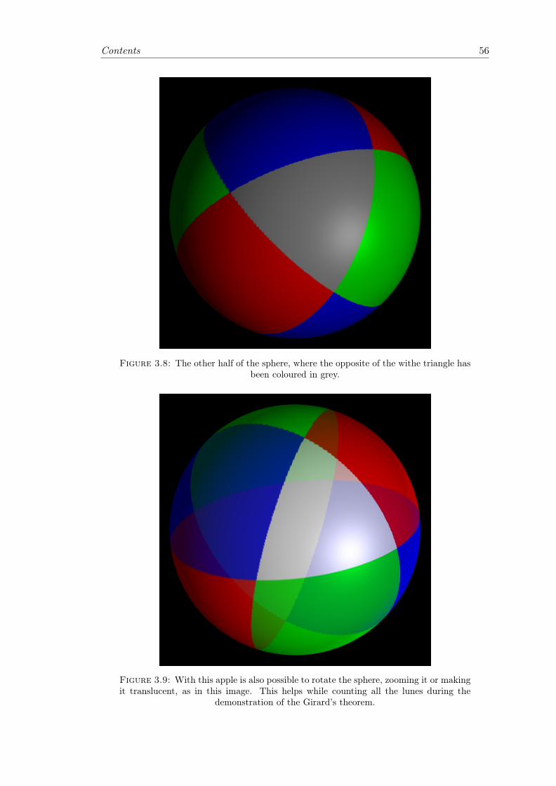
Contents 56

Figure 3.8: The other half of the sphere, where the opposite of the withe triangle hasbeen coloured in grey.

Figure 3.9: With this apple is also possible to rotate the sphere, zooming it or makingit translucent, as in this image. This helps while counting all the lunes during the

demonstration of the Girard’s theorem.

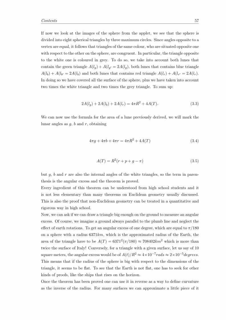
Contents 57

If now we look at the images of the sphere from the applet, we see that the sphere is

divided into eight spherical triangles by three maximum circles. Since angles opposite to a

vertex are equal, it follows that triangles of the same colour, who are situated opposite one

with respect to the other on the sphere, are congruent. In particular, the triangle opposite

to the white one is coloured in grey. To do so, we take into account both lunes that

contain the green triangle A(lg) +A(lg′ = 2A(lg), both lunes that contains blue triangle

A(lb) + A(lb′ = 2A(lb) and both lunes that contains red triangle A(lr) + A(lr′ = 2A(lr).

In doing so we have covered all the surface of the sphere, plus we have taken into account

two times the white triangle and two times the grey triangle. To sum up:

2A(lg) + 2A(lb) + 2A(lr) = 4πR2 + 4A(T ). (3.3)

We can now use the formula for the area of a lune previously derived, we will mark the

lunar angles as g, b and r, obtaining

4πg + 4πb+ 4πr = 4πR2 + 4A(T ) (3.4)

A(T ) = R2(r + p+ g − π) (3.5)

but g, b and r are also the internal angles of the white triangles, so the term in paren-

thesis is the angular excess and the theorem is proved.

Every ingredient of this theorem can be understood from high school students and it

is not less elementary than many theorems on Euclidean geometry usually discussed.

This is also the proof that non-Euclidean geometry can be treated in a quantitative and

rigorous way in high school.

Now, we can ask if we can draw a triangle big enough on the ground to measure an angular

excess. Of course, we imagine a ground always parallel to the plumb line and neglect the

effect of earth rotations. To get an angular excess of one degree, which are equal to π/180

on a sphere with a radius 6371km, which is the approximated radius of the Earth, the

area of the triangle have to be A(T ) = 63712(π/180) ≈ 708402km2 which is more than

twice the surface of Italy! Conversely, for a triangle with a given surface, let us say of 10

square meters, the angular excess would be of A(t)/R2 ≈ 4×10−7rads ≈ 2×10−5degrees.

This means that if the radius of the sphere is big with respect to the dimensions of the

triangle, it seems to be flat. To see that the Earth is not flat, one has to seek for other

kinds of proofs, like the ships that rises on the horizon.

Once the theorem has been proved one can use it in reverse as a way to define curvature

as the inverse of the radius. For many surfaces we can approximate a little piece of it

Contents 58

with a sphere of radius R, but for different little pieces, who are actually points, we need

a sphere of different radius, moreover it could change side and we can have positive or

negative curvature. To be more rigorous, a surface has a negative curvature at a point if

the surface curves away from the tangent plane in two different directions and the classic

example is a saddle.

Before going into discussing how to apply non-Euclidean geometry to physics, we dis-

cussed the last question of the survey and how it is related the previous questions.

I used question 8) to emphasize that we need to introduce a way to measure a distance.

We agree that the distance is the shortest path between two points. Of course, we can get

from one point to another following infinite paths, but the distance is only the shortest

one (or ones if there are two or more path with the same shortest length).

On the globe, if one goes from Napoli to New York following the maximum circle instead

than the parallel, the route is shortest of approximately a centimetre. Anyway, the map

on the globe is in scale 1 : 35000000, so an aeroplane would save approximately 350km!

Anyway, on a globe with a different radius, the distance is measured differently. And if

the surface has a variable curvature, the distance must be measured differently in every

little piece approximated by a sphere.

The connection between the curvature and the way in which we measure distance is

investigated in the next section.

3.2 Tensors and Einstein field equation

Dare un calcio alla ragione e fareposto all’impossibile: è la nostrafilosofia, no? È così che siamo arrivatiin superficie. E allora perché nondovremmo riuscire ad andare sullaLuna?

Kamina - Gurren Lagann

In the previous section we ha ve introduced non-Euclidean geometry. But the goal is to

discuss general relativity, so I focused students attention on another question: How do

we measure distance in the space?

Gauss and Riemann, two great mathematicians and physician of the nineteen century,

approached this problem trying to measure the angular excess of big triangles. They tried

with a triangle whose vertex were approximated with the position of three mountains

tops, but the angular excess was consistent with zero within the experimental errors.

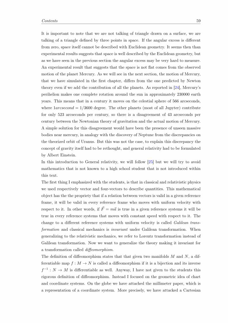
Contents 59

It is important to note that we are not talking of triangle drawn on a surface, we are

talking of a triangle defined by three points in space. If the angular excess is different

from zero, space itself cannot be described with Euclidean geometry. It seems then than

experimental results suggests that space is well described by the Euclidean geometry, but

as we have seen in the previous section the angular excess may be very hard to measure.

An experimental result that suggests that the space is not flat comes from the observed

motion of the planet Mercury. As we will see in the next section, the motion of Mercury,

that we have simulated in the first chapter, differs from the one predicted by Newton

theory even if we add the contribution of all the planets. As reported in [24], Mercury’s

perihelion makes one complete rotation around the sun in approximately 230000 earth

years. This means that in a century it moves on the celestial sphere of 566 arcseconds,

where 1arcsecond = 1/3600 degree. The other planets (most of all Jupyter) contribute

for only 523 arcseconds per century, so there is a disagreement of 43 arcseconds per

century between the Newtonian theory of gravitation and the actual motion of Mercury.

A simple solution for this disagreement would have been the presence of unseen massive

bodies near mercury, in analogy with the discovery of Neptune from the discrepancies on

the theorized orbit of Uranus. But this was not the case, to explain this discrepancy the

concept of gravity itself had to be rethought, and general relativity had to be formulated

by Albert Einstein.

In this introduction to General relativity, we will follow [25] but we will try to avoid

mathematics that is not known to a high school student that is not introduced within

this text.

The first thing I emphasized with the students, is that in classical and relativistic physics

we used respectively vector and four-vectors to describe quantities. This mathematical

object has the the propriety that if a relation between vectors is valid in a given reference

frame, it will be valid in every reference frame who moves with uniform velocity with

respect to it. In other words, if ~F = m~a is true in a given reference systems it will be

true in every reference systems that moves with constant speed with respect to it. The

change to a different reference systems with uniform velocity is called Galilean trans-

formation and classical mechanics is invariant under Galilean transformation. When

generalizing to the relativistic mechanics, we refer to Lorentz transformation instead of

Galilean transformation. Now we want to generalize the theory making it invariant for

a transformation called diffeomorphism.

The definition of diffeomorphism states that that given two manifolds M and N , a dif-

ferentiable map f : M → N is called a diffeomorphism if it is a bijection and its inverse

f−1 : N → M is differentiable as well. Anyway, I have not given to the students this

rigorous definition of diffeomorphism. Instead I focused on the geometric idea of chart

and coordinate systems. On the globe we have attached the millimeter paper, which is

a representation of a coordinate system. More precisely, we have attacked a Cartesian

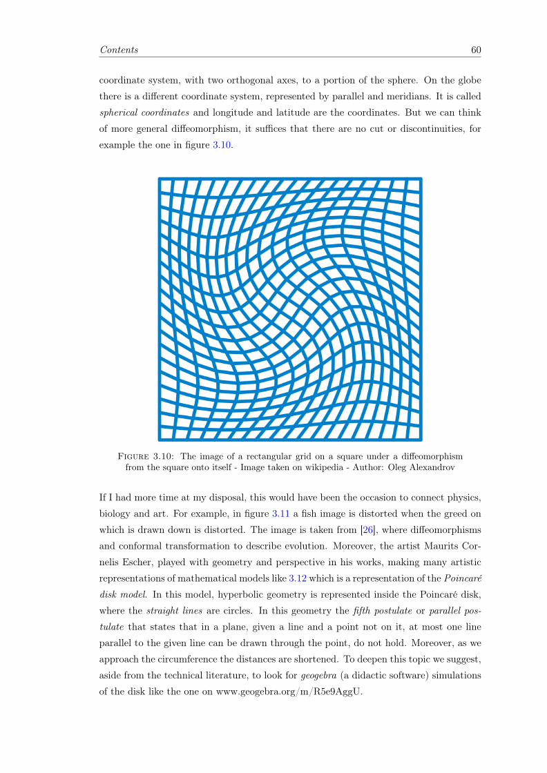
Contents 60

coordinate system, with two orthogonal axes, to a portion of the sphere. On the globe

there is a different coordinate system, represented by parallel and meridians. It is called

spherical coordinates and longitude and latitude are the coordinates. But we can think

of more general diffeomorphism, it suffices that there are no cut or discontinuities, for

example the one in figure 3.10.

Figure 3.10: The image of a rectangular grid on a square under a diffeomorphismfrom the square onto itself - Image taken on wikipedia - Author: Oleg Alexandrov

If I had more time at my disposal, this would have been the occasion to connect physics,

biology and art. For example, in figure 3.11 a fish image is distorted when the greed on

which is drawn down is distorted. The image is taken from [26], where diffeomorphisms

and conformal transformation to describe evolution. Moreover, the artist Maurits Cor-

nelis Escher, played with geometry and perspective in his works, making many artistic

representations of mathematical models like 3.12 which is a representation of the Poincaré

disk model. In this model, hyperbolic geometry is represented inside the Poincaré disk,

where the straight lines are circles. In this geometry the fifth postulate or parallel pos-

tulate that states that in a plane, given a line and a point not on it, at most one line

parallel to the given line can be drawn through the point, do not hold. Moreover, as we

approach the circumference the distances are shortened. To deepen this topic we suggest,

aside from the technical literature, to look for geogebra (a didactic software) simulations

of the disk like the one on www.geogebra.org/m/R5e9AggU.

Contents 61

Also, to deepen the connection between science and art we suggest [27], where the con-

nection between geometry, painting and informatics is enlightened.

Figure 3.11: How the image of a fish is distorted when a diffeomorphism is appliedto the rectangular grid in which is drawn down.

Anyway, I had not the time to go into this detail. Instead I discussed the interpretation

of the Einstein field equation. As I stated before, these equations need to relate object

that, during a diffeomorphism, change in a way that the relation still holds. Since a

diffeomorphism may deform the space in a different way along different directions, this

objects and the way it is transformed must take this into account. Of course, we are

talking about tensors which I introduced just a table of numbers, like sometimes is done

with matrices.

A good way yo introduce tensors is shown in the video at

www.youtube.com/watch?v=f5liqUk0ZTw, where it is introduced with children toys as

a generalization of the three-dimensional vectors. In simple and elementary words, it

describes the stress tensor, we have three components (the diagonal of the table) which

represent the stress along three spatial directions. The other components are spurious

and takes into account how the stress is projected into different directions. Of course,

this has to be generalized to tensors in Minkowski space. Moreover, the video does not

shows quantitatively how a tensors transform under a change in coordinates. An attempt

in doing so can be found on the video on www.youtube.com/watch?v=CliW7kSxxWU,

where a reasonable definition of contravariant and covariant components (if the given

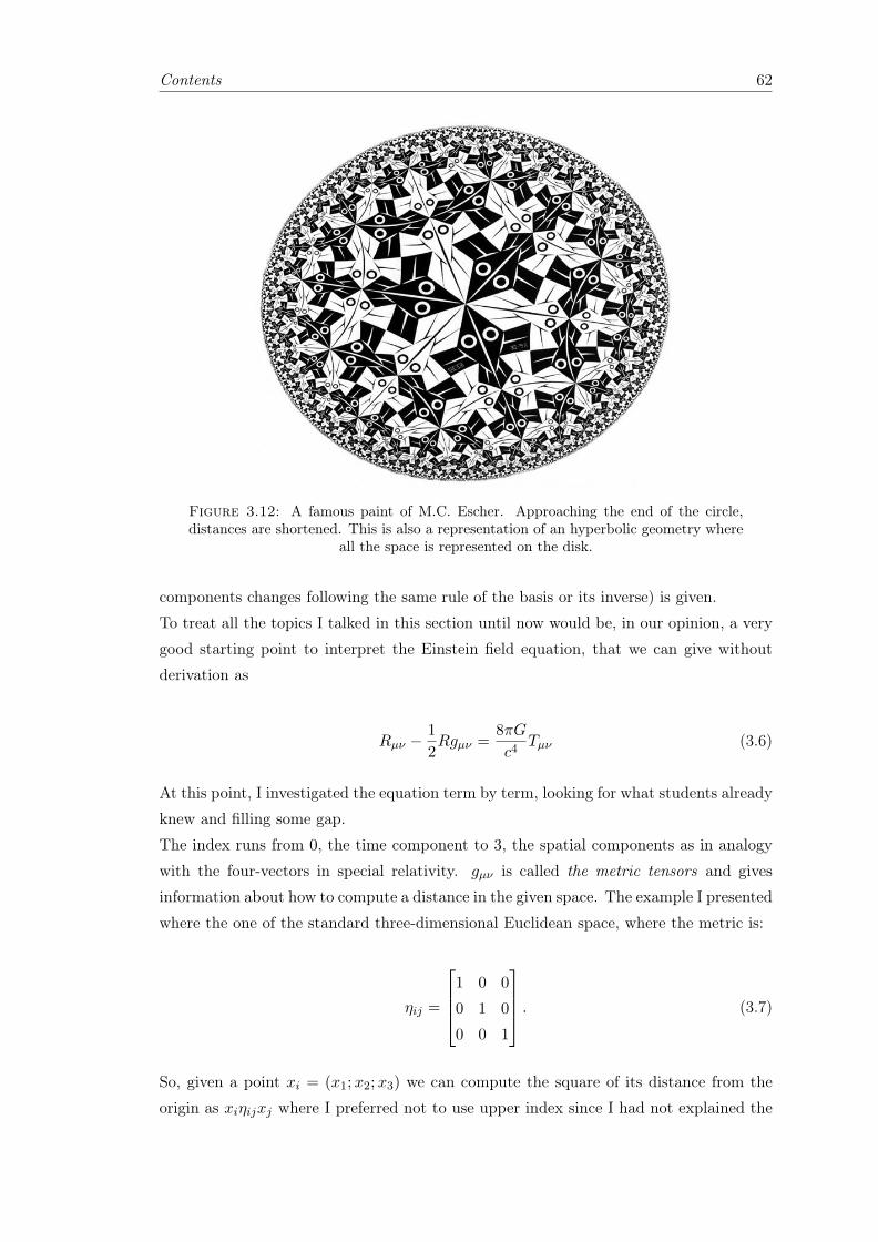
Contents 62

Figure 3.12: A famous paint of M.C. Escher. Approaching the end of the circle,distances are shortened. This is also a representation of an hyperbolic geometry where

all the space is represented on the disk.

components changes following the same rule of the basis or its inverse) is given.

To treat all the topics I talked in this section until now would be, in our opinion, a very

good starting point to interpret the Einstein field equation, that we can give without

derivation as

Rµν −1

2Rgµν =

8πG

c4Tµν (3.6)

At this point, I investigated the equation term by term, looking for what students already

knew and filling some gap.

The index runs from 0, the time component to 3, the spatial components as in analogy

with the four-vectors in special relativity. gµν is called the metric tensors and gives

information about how to compute a distance in the given space. The example I presented

where the one of the standard three-dimensional Euclidean space, where the metric is:

ηij =

1 0 0

0 1 0

0 0 1

. (3.7)

So, given a point xi = (x1;x2;x3) we can compute the square of its distance from the

origin as xiηijxj where I preferred not to use upper index since I had not explained the

Contents 63

difference between covariant and contravariant components. Students also did not know

the algorithm for the multiplication of matrices, so I just make them note that they

already knew the results as the sum of the square of the components:

d2 = x21 + x2

2 + x23 (3.8)

As a second example, I proposed the Minkowski metric:

gµν =

1 0 0 0

0 −1 0 0

0 0 −1 0

0 0 0 −1

(3.9)

and pointed out that the square of the distance is computed as:

d2 = +x20 − x2

1 − x22 − x2

3 (3.10)

In other words, the metric tensor codifies the way to measure distances in the space,

and by consequence its geometry. As we have seen in the previous section, this must be

connected to the curvature. The tensors that codify the information about the curvature

is Rµν , and R is the sum of the elements of the diagonal of Rµν .

On the other side of the equation, G is Newton gravitational constant, c is the speed of

light and Tµν is the generalization of the stress-energy tensor that codifies the information

about the mass and energy in the space-time region we are considering.

At this point, my time was over, and I ended the lesson stating that we can interpret this

formula seeing the gravitation not as a force, like in Newton theory, but as a geometry

in space-time. Mass cures space-time and the straight line is not the shortest distance

anymore, so object follows the geodesic (line of shortest distance) which now is a curve.

In General relativity, we don’t seek for the forces that act upon the objects changing

their state of motion, it is the geometry of the space-time changes that changes. So to

find how an object moves we need to know how to compute the geodesic in a geometry

where the metric and the curvature are given.

To talk about the geodesic equation I would have needed two more ingredients, the four

velocity and the Christoffel symbols. The four-velocity can be seen as a generalization of

velocity in three-dimensional space to the space-time. We start from the four position of

a point, X = (cx0;x1;x2;x3) We note that the first coordinate cx0 is the time coordinate,

but this time we cannot divide the space travelled by the time lapsed, or else we would

not obtain a four-vector. Anyway, the trajectory of the object in the space-time, also

Contents 64

called world-line, will have a tangent in every point, and that is the four-velocity. From

an algebraic point of view, we need to find a parameter that has the function of the time

in the classical theories. For now, we shall use the proper time τ . In this notation, the

four-velocity Uµ is defined as:

Uµ =dX

dτ. (3.11)

Unfortunately, an introduction of the Christoffel symbols without making use of differ-

ential geometry is less simple. I would just say that we need to define the concept of

derivative on spaces that are not Euclidean. The derivative is indeed connected to how

we measure distances and how we make limits. If the coordinate systems are not the

usual one, the operation of derivation needs to be revised. To do so, we introduce the

Christoffel symbol Γµαβ .

We can now write the geodesic equation as:

Uµ

dτ= ΓµαβU

αUβ (3.12)

The connection from the Einstein field equation and the geodesic equation is in the

Christoffel symbol, the Einstein equations tell us the geometry of the space and the

geodesic equation tells us the trajectory of the bodies. Unfortunately, the Einstein field

equation is hard to solve due to the non-linearity of the equations. This is a problem

that can arise also in classical physics. For example, if a particle with charge q is moving

in an electric field E, we have to neglect the field produced by the charge if we want to

avoid the non-linearity in solving the equation of motion. In the Einstein field equation,

the geometry tells the mass how to distribute in the space while the mass and energy

distribution tells the space-time how to curve so to define the geometry.

There are two strategies that are used to solve the Einstein field equation. One is to

use numerical methods. In particular, we would like to cite Regge Calculus [28] where

the manifold is replaced with a polyhedron with an appropriate number of dimensions.

This approach also has the advantage of not needing any coordinate systems to work,

indeed if the theory is invariant under diffeomorphism it means that is only helpful but

not needful to introduce one!

The other approach consists in studying particular cases in which the equation is simple.

For example, if the space-time is flat and we consider a particle whose mass is negligible,

the Christoffel symbols are all zeroes. This means that the variation in the proper time

of the four-velocity is zero, in other words, the four-velocity is constant. So a free particle

in a flat space moves with uniform four-velocity.

In the next section, we will see another situation in which the Einstein equation can be

Contents 65

solved, obtaining the Schwarzschild metric.

3.3 Schwarzschild metric

Doc: Marty, you gotta came backwith me!Marty: Where?Doc: Back to the future!

Back to the future

One significant solution of the Einstein field equations can be obtained assuming a spher-

ical symmetry for the systems. This is a good approximation for the solar systems, but

also for more exotic systems like the black holes.

We remember that, in space-time, the spherical coordinates are:

t = t

x = r sin θ cosφ

y = r sin θ sinφ

z = r cos θ.

Given this coordinates, if we try to solve the Einstein equation in the vacuum, with zero

on the right hand, we obtain the Schwarzschild metric:

d2s = +(

1− 2Gm

r

)dt2 −

(1− 2Gm

r

)dr2 − dr2 + r2(dθ2 + sin2 θdφ2). (3.13)

We have assumed at this point that the notion of the differential is known to students

and I would not suggest an actual derivation of the metrics, but to verify that it is a

solution plugging it into the Einstein field equation. We can use the Schwarzschild to

find the trajectory of a particle that moves in a radial field and this is a good model for

a planet spinning around the Sun. Unfortunately, we have not found a way to derive,

from Schwarzschild metrics and the geodesic equation, the equation of motion without

mathematics that is not usually treated in high school, but the formula ca be presented

as a correction to Newton’s law of universal gravitation:

Contents 66

F ≈ Gm1m2

r2

(1 +

α

r2

). (3.14)

The ≈ is necessary since we have omitted a few terms in the complete equation that

takes into account also the chance of massless particles and the contribution of angular

momentum.

For a derivation of this formula, we suggest to look at [29], [30] and [31]. In particular,

the last one derives it with only algebraic calculations.

For our goals, the only difference from the classical formula is the the new term propor-

tional to αr2. In [24] a way to numerically measure α for the planet Mercury based on the

astronomical data is presented, and it is of the order of 2, 4×1014)m2. The idea is not to

simulate 230000 earth years of motion but to measure on a more suitable interval on time

and then to apply a linear regression. We propose something more simple, modifing the

program of chapter one to see what happens to the planet trajectory when the new term

is added to the classical formula. To make the effect visible, we have assumed α = 10(31)

as can be checked on the code:

from math import sqrt ,atan , pi

from matplotlib.pyplot import *

from ipywidgets import interact

from scipy import stats

%matplotlib inline

def mercury_GR(N = 170):

t = [0]

Dt = 76005.216

G = 6.67408*10** -11

M = 1988500*10**24

m = 0.33011*10**24

#To set initial condition we referred to the NASA fact sheet ,

#https :// nssdc.gsfc.nasa.gov/planetary/factsheet/mercuryfact.html

#The simulation starts with the plant in his aphelion.

alpha = 10**31

x = [69.82*10**9]

y = [0]

vx = [0]

vy = [38.86*10**3]

r = [sqrt(x[0]**2 + y[0]**2)]

v = [sqrt(vx [0]**2 + vy [0]**2)]

Contents 67

ax = [-G*M*x[0]/r[0]**3 - G*M*x[0]* alpha/(r[0]**6)]

ay = [-G*M*y[0]/r[0]**3 - G *M*y[0]* alpha /(r[0]**6)]

for i in range (1, N):

x.append(x[i-1] + vx[i-1] * Dt + 0.5 * ax[i-1] * Dt**2)

y.append(y[i-1] + vy[i-1] * Dt + 0.5 * ay[i-1] * Dt**2)

r.append(sqrt(x[i]**2+y[i]**2))

ax.append(-G*M*x[i]/r[i]**3 - G*M*x[i]* alpha/(r[i]**6))

ay.append(-G*M*y[i]/r[i]**3 - G *M*y[i]*alpha /(r[i]**6))

vx.append(vx[i-1] + 0.5 * (ax[i-1] + ax[i]) * Dt)

vy.append(vy[i-1] + 0.5 * (ay[i-1] + ay[i]) * Dt)

v.append(sqrt(vx[i]**2+vy[i]**2))

t.append(t[i-1] + Dt)

#Plot the results

figure ()

plot(x, y)

title("Trajectory , both axes have meters as units")

grid()

perihelion_x = []

perihelion_y = []

for i in range (1,N-1):

if r[i] < r[i-1] and r[i] < r[i+1]:

perihelion_x.append(x[i])

perihelion_y.append(y[i])

figure ()

scatter(perihelion_x , perihelion_y)

title("Mercury perihelion motion , both axes have meters as units")

grid()

show()

interact (mercury_GR , N = (1 ,100000 ,1))

The codes produces two graphs, 3.13 shows how the trajectory is not an ellipse anymore.

At any revolution around the sun, the perihelion moves, and in 3.14 is shown the position

of it at any revolution.

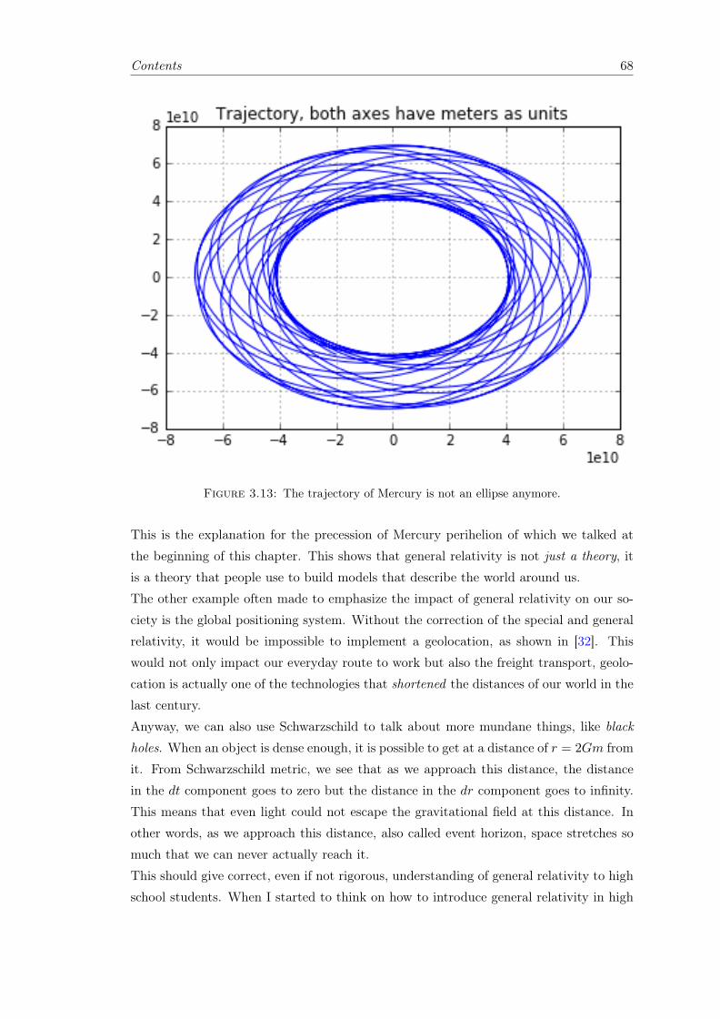
Contents 68

Figure 3.13: The trajectory of Mercury is not an ellipse anymore.

This is the explanation for the precession of Mercury perihelion of which we talked at

the beginning of this chapter. This shows that general relativity is not just a theory, it

is a theory that people use to build models that describe the world around us.

The other example often made to emphasize the impact of general relativity on our so-

ciety is the global positioning system. Without the correction of the special and general

relativity, it would be impossible to implement a geolocation, as shown in [32]. This

would not only impact our everyday route to work but also the freight transport, geolo-

cation is actually one of the technologies that shortened the distances of our world in the

last century.

Anyway, we can also use Schwarzschild to talk about more mundane things, like black

holes. When an object is dense enough, it is possible to get at a distance of r = 2Gm from

it. From Schwarzschild metric, we see that as we approach this distance, the distance

in the dt component goes to zero but the distance in the dr component goes to infinity.

This means that even light could not escape the gravitational field at this distance. In

other words, as we approach this distance, also called event horizon, space stretches so

much that we can never actually reach it.

This should give correct, even if not rigorous, understanding of general relativity to high

school students. When I started to think on how to introduce general relativity in high

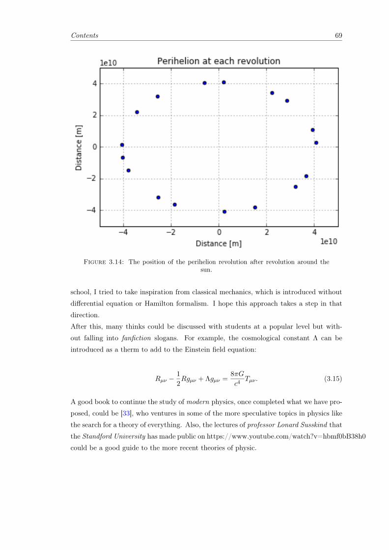
Contents 69

Figure 3.14: The position of the perihelion revolution after revolution around thesun.

school, I tried to take inspiration from classical mechanics, which is introduced without

differential equation or Hamilton formalism. I hope this approach takes a step in that

direction.

After this, many thinks could be discussed with students at a popular level but with-

out falling into fanfiction slogans. For example, the cosmological constant Λ can be

introduced as a therm to add to the Einstein field equation:

Rµν −1

2Rgµν + Λgµν =

8πG

c4Tµν . (3.15)

A good book to continue the study of modern physics, once completed what we have pro-

posed, could be [33], who ventures in some of the more speculative topics in physics like

the search for a theory of everything. Also, the lectures of professor Lonard Susskind that

the Standford University has made public on https://www.youtube.com/watch?v=hbmf0bB38h0

could be a good guide to the more recent theories of physic.

Conclusions

Both teachers and students have enjoyed the laboratorial activities. As teachers pointed

out, the most fruitful aspects was the enlightenment of new connections between top-

ics. The focus on the crosscutting concepts like conservation rules, transformations and

symmetries allows a bridge between classical and modern physics. This is essential to

promote a sound and profound understanding of physical theories, integrating different

physics topics without renouncing to point out the alterations of meanings as we move

from one context to another.

I have presented four laboratorial activities to test a new approach in the building of

the mathematics and physics curriculum in high-school. One activity was on classi-

cal mechanics. Starting from experiments with a motion detector I discussed Galilean

transformations as rotation in the space-time diagram and the momentum conservation.

Emphasizing momentum conservation I connected topics that are usually treated apart,

like Newton’s laws and impulse. This approach leads to an easy generalization to rela-

tivistic mechanics where Lorentz transformations can be presented geometrically. This

activity was proposed to two classes joined, more than forty students, in the laboratory

of the Liceo Scientifico Statale Filippo Silvestri with the collaboration of the teachers

Ilaria Limoncelli and Margherita D’Urzo.

The second and third activities were presented to three classes joined, more than fifty

students, of the Liceo Scientifico Statale Carlo Urbani with the collaboration of the teach-

ers Maria Rosaria Camarda, Maria Loffredo and Annette Luongo. In these activities I

discussed electromagnetic waves, comparing them with mechanical waves, and special

relativity. Students were particularly pleased to see, with instruments like the slinky and

the microwave optic bench, phenomena they only discussed theoretically.

In the fourth activity, I presented non-Euclidean geometry in a class, less than twenty stu-

dents, of the Liceo Scientifico Statale Calamandrei with the collaboration of the teachers

Marina De Cesare and Chiara Tarallo. With the help of globes and an applet, I proved

Girard’s theorem with the students and then we discussed the basic features of the Ein-

stein field equation. The discussion of the Einstein field equation is already proposed in

high-school textbooks, but we think that is not satisfactory. In this work, we propose

activities to enlighten the connection between the theory and actual physical models,

like the simulation of Mercury motions around the Sun.

More works has to be done on the presentation of the theory of general relativity if we

want to present it in a non-rigorous, but yet correct, way. We think that a great aid may

come from numerical methods. It is true that numerical analysis and optimization theory

are complicated and we suggest [20] for a more detailed introduction to them focused on

didactic purposes. Yet their implementation is simple and powerful. They can be used

to simulate classical, relativistic and quantistic systems, and nowadays instrument like

70

Contents 71

electronics spreadsheet and high level programming language allow a simple implemen-

tation of the algorithm that can be done by students. Moreover, in nowadays society

electronics, with products like Arduino and Raspberry Pi, and coding, with programming

languages like Python and Java have a great grip on young students for the pratical ap-

plication that they allow. We hope that, in the near future, the comprehension of a

physical phenomena, its mathematical model and of technological implementations may

integrate to form a homogeneous educational path.

It is desirable that in future works more activities are dedicated to a single classroom,

with no more than twenty students. This would allow more experiments to be performed

by the students. It is often argued that an experimental approach is too slow for the

time schedule of schools. From the experiences shared in the various meetings with the

teachers the opposite emerged. This approach is slow in the beginning. Once students

masters basic concepts acquired in laboratorial activities, teachers found a speed-up in

their lessons. We hope that in near future, more teachers will try didactics methodologies

focused on experimentation performed by the students.

Appendix A

Students commentary to the

space-time and velocity time

diagrams

On Wednesday, May 9th I have gone to the "Liceo Scientifico Statale Carlo Urbani"

hosted by professors Margherita D’Urzo and Ilaria Limoncelli. As described in chapter

one, I proposed two hours of laboratorial activity to introduce classical mechanics from

the Galilean transformation. As stated by the professors, one of the main merits of this

lessons was that it connected many topics generally not seen as one. As Ilaria Limoncelli

said, this has been a great recapitulation of the work done during the year, and if it was

done at the beginning of the year it could have been served as a good introduction for

the subsequent work.

To test the efficacy of my activity, I gave (under the suggestion of my supervisors) to the

students the assignment to describe the graphs we produced in a written relation.

We think that this is a very important activity, very often students did not know how to

express their thoughts because they are not trained in describing something with written

words. In the following, some of the work produced by the students is proposed.

Mercoledì 9 Maggio 2018, i ragazzi della classe III sez. H e G hanno seguito una lezione

della durata di due ore con un docente universitario. Nella parte iniziale della lezione

sono stati svolti vari esperimenti dai ragazzi stessi per studiare il moto rettilineo uni-

forme e uniformemente accelerato. L’esperimento seguente è stato svolto utilizzando un

sensore di movimento e l’aiuto di un ragazzo che ha effettuato degli spostamenti davanti

al sensore. Il grafico è il seguente:

72

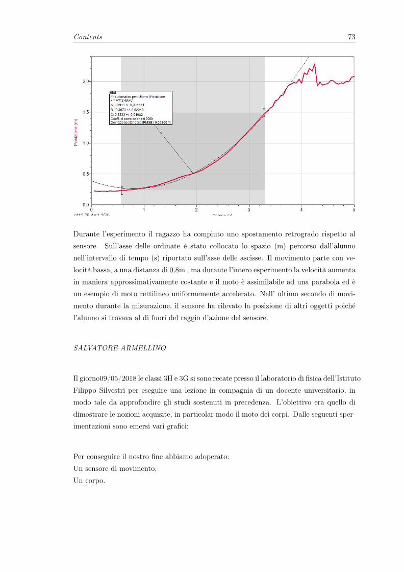
Contents 73

Durante l’esperimento il ragazzo ha compiuto uno spostamento retrogrado rispetto al

sensore. Sull’asse delle ordinate è stato collocato lo spazio (m) percorso dall’alunno

nell’intervallo di tempo (s) riportato sull’asse delle ascisse. Il movimento parte con ve-

locità bassa, a una distanza di 0,8m , ma durante l’intero esperimento la velocità aumenta

in maniera approssimativamente costante e il moto è assimilabile ad una parabola ed è

un esempio di moto rettilineo uniformemente accelerato. Nell’ ultimo secondo di movi-

mento durante la misurazione, il sensore ha rilevato la posizione di altri oggetti poiché

l’alunno si trovava al di fuori del raggio d’azione del sensore.

SALVATORE ARMELLINO

Il giorno09/05/2018 le classi 3H e 3G si sono recate presso il laboratorio di fisica dell’Istituto

Filippo Silvestri per eseguire una lezione in compagnia di un docente universitario, in

modo tale da approfondire gli studi sostenuti in precedenza. L’obiettivo era quello di

dimostrare le nozioni acquisite, in particolar modo il moto dei corpi. Dalle seguenti sper-

imentazioni sono emersi vari grafici:

Per conseguire il nostro fine abbiamo adoperato:

Un sensore di movimento;

Un corpo.

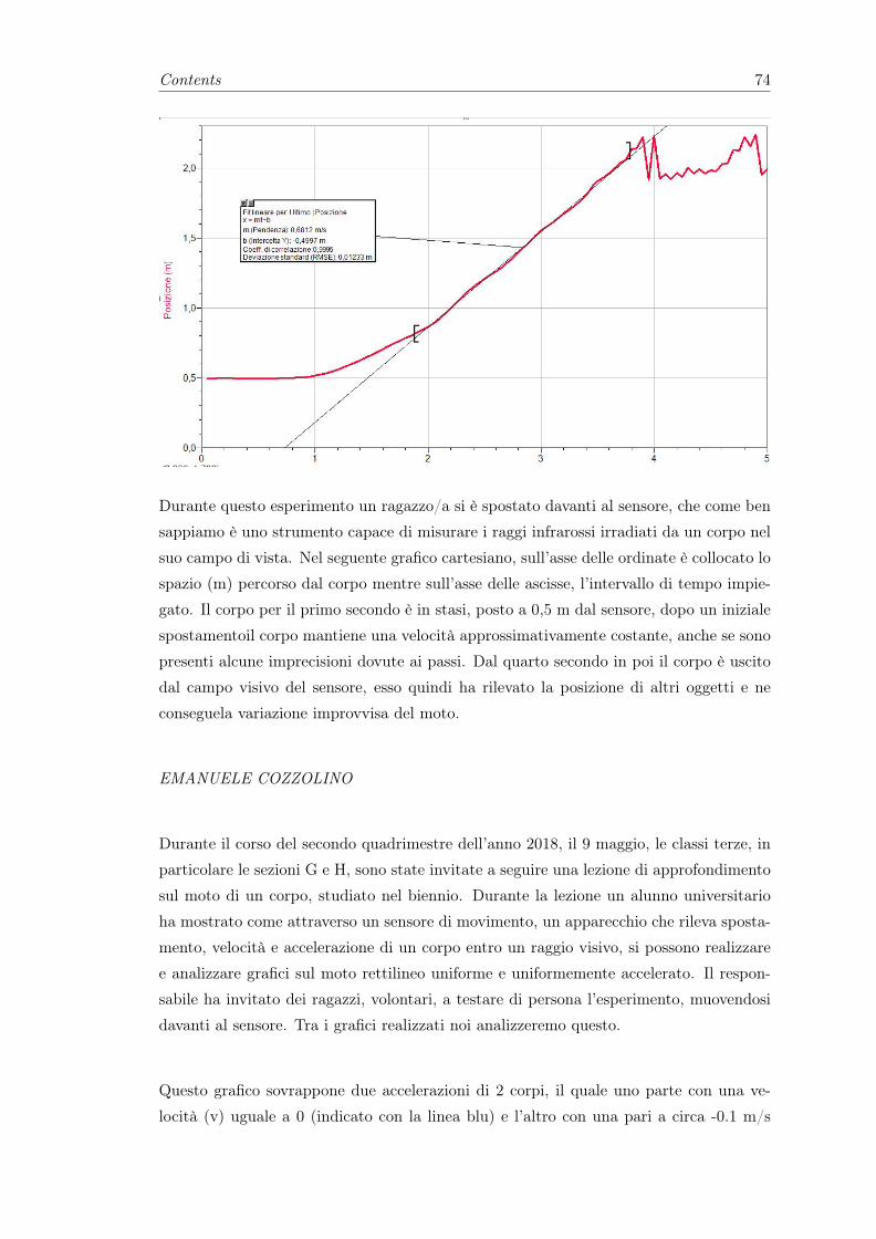
Contents 74

Durante questo esperimento un ragazzo/a si è spostato davanti al sensore, che come ben

sappiamo è uno strumento capace di misurare i raggi infrarossi irradiati da un corpo nel

suo campo di vista. Nel seguente grafico cartesiano, sull’asse delle ordinate è collocato lo

spazio (m) percorso dal corpo mentre sull’asse delle ascisse, l’intervallo di tempo impie-

gato. Il corpo per il primo secondo è in stasi, posto a 0,5 m dal sensore, dopo un iniziale

spostamentoil corpo mantiene una velocità approssimativamente costante, anche se sono

presenti alcune imprecisioni dovute ai passi. Dal quarto secondo in poi il corpo è uscito

dal campo visivo del sensore, esso quindi ha rilevato la posizione di altri oggetti e ne

conseguela variazione improvvisa del moto.

EMANUELE COZZOLINO

Durante il corso del secondo quadrimestre dell’anno 2018, il 9 maggio, le classi terze, in

particolare le sezioni G e H, sono state invitate a seguire una lezione di approfondimento

sul moto di un corpo, studiato nel biennio. Durante la lezione un alunno universitario

ha mostrato come attraverso un sensore di movimento, un apparecchio che rileva sposta-

mento, velocità e accelerazione di un corpo entro un raggio visivo, si possono realizzare

e analizzare grafici sul moto rettilineo uniforme e uniformemente accelerato. Il respon-

sabile ha invitato dei ragazzi, volontari, a testare di persona l’esperimento, muovendosi

davanti al sensore. Tra i grafici realizzati noi analizzeremo questo.

Questo grafico sovrappone due accelerazioni di 2 corpi, il quale uno parte con una ve-

locità (v) uguale a 0 (indicato con la linea blu) e l’altro con una pari a circa -0.1 m/s

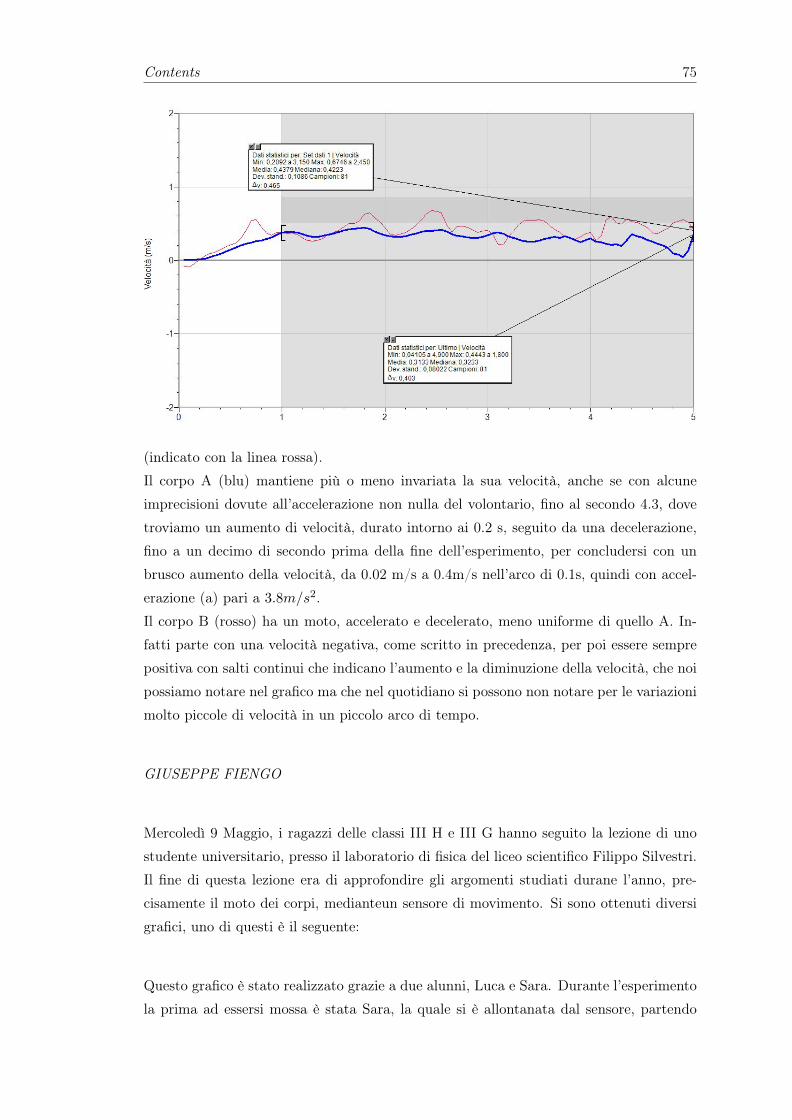
Contents 75

(indicato con la linea rossa).

Il corpo A (blu) mantiene più o meno invariata la sua velocità, anche se con alcune

imprecisioni dovute all’accelerazione non nulla del volontario, fino al secondo 4.3, dove

troviamo un aumento di velocità, durato intorno ai 0.2 s, seguito da una decelerazione,

fino a un decimo di secondo prima della fine dell’esperimento, per concludersi con un

brusco aumento della velocità, da 0.02 m/s a 0.4m/s nell’arco di 0.1s, quindi con accel-

erazione (a) pari a 3.8m/s2.

Il corpo B (rosso) ha un moto, accelerato e decelerato, meno uniforme di quello A. In-

fatti parte con una velocità negativa, come scritto in precedenza, per poi essere sempre

positiva con salti continui che indicano l’aumento e la diminuzione della velocità, che noi

possiamo notare nel grafico ma che nel quotidiano si possono non notare per le variazioni

molto piccole di velocità in un piccolo arco di tempo.

GIUSEPPE FIENGO

Mercoledì 9 Maggio, i ragazzi delle classi III H e III G hanno seguito la lezione di uno

studente universitario, presso il laboratorio di fisica del liceo scientifico Filippo Silvestri.

Il fine di questa lezione era di approfondire gli argomenti studiati durane l’anno, pre-

cisamente il moto dei corpi, medianteun sensore di movimento. Si sono ottenuti diversi

grafici, uno di questi è il seguente:

Questo grafico è stato realizzato grazie a due alunni, Luca e Sara. Durante l’esperimento

la prima ad essersi mossa è stata Sara, la quale si è allontanata dal sensore, partendo

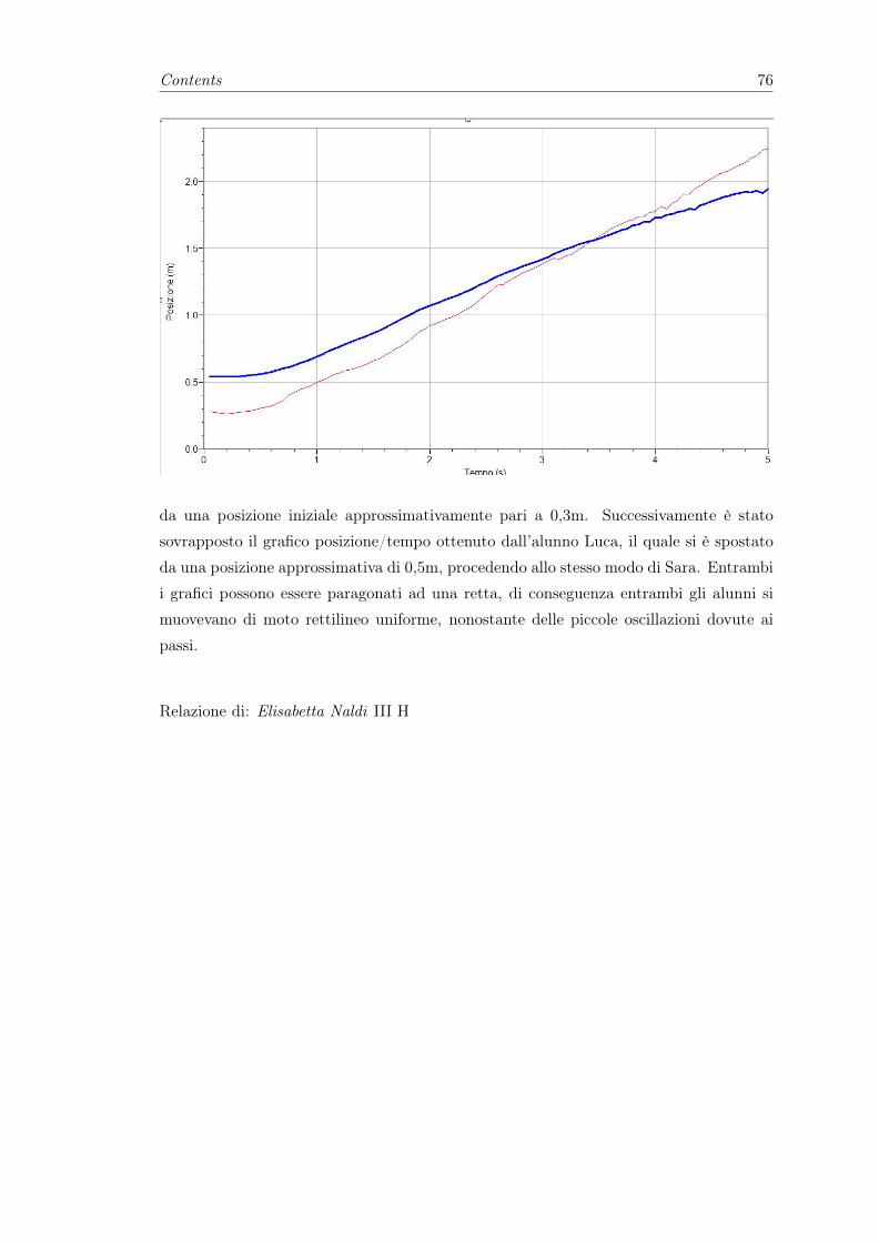
Contents 76

da una posizione iniziale approssimativamente pari a 0,3m. Successivamente è stato

sovrapposto il grafico posizione/tempo ottenuto dall’alunno Luca, il quale si è spostato

da una posizione approssimativa di 0,5m, procedendo allo stesso modo di Sara. Entrambi

i grafici possono essere paragonati ad una retta, di conseguenza entrambi gli alunni si

muovevano di moto rettilineo uniforme, nonostante delle piccole oscillazioni dovute ai

passi.

Relazione di: Elisabetta Naldi III H

Appendix B

Python and Jupyter Notebook

As may be found on https://www.python.org/, python is a great object-oriented, inter-

preted, and interactive programming language. It is often compared (favorably of course

:-) ) to Lisp, Tcl, Perl, Ruby, C#, Visual Basic, Visual Fox Pro, Scheme or Java... and

it’s much more fun.

Python combines remarkable power with very clear syntax. It has modules, classes, ex-

ceptions, very high level dynamic data types, and dynamic typing. There are interfaces to

many system calls and libraries, as well as to various windowing systems. New built-in

modules are easily written in C or C++ (or other languages, depending on the chosen

implementation). Python is also usable as an extension language for applications written

in other languages that need easy-to-use scripting or automation interfaces.

Python can be downloaded from the aforementioned website, and in this work it is used

together with the jupyter notebook. With this tools students can build, in a simple and

intuitive way, interactive graphs and simulations of physical systems. Indeed the numer-

ical approach allows to study systems that could not be solved with analytic methods

both because it is not possible or because students have not the tools. Solution of the

equation of motion with the Euler methods are a valid example, and python has well

tested libraries for visualizing data and create interactive graphs.

Teachers should not be afraid in requiring coding skill from their students, projects like

Coding in your Classroom, Now! as described on the web page

https://platform.europeanmoocs.eu/course_coding_in_your_classroom_now

introduce programming already in elementary schools (also in Italy).

Hopefully, in some years the coding abilities will be considered at the same level of alge-

braic and geometric ones, since they form a semantic register powerful and intuitive in

which thinking and solving problems.

A powerful tools for programming in python (or other programming languages) is the

jupyter notebook.

77

Contents 78

As may be found on https://www.python.org/, python is a great object-oriented, inter-

preted, and interactive programming language. It is often compared (favorably of course

:-) ) to Lisp, Tcl, Perl, Ruby, C#, Visual Basic, Visual Fox Pro, Scheme or Java... and

it’s much more fun.

Python combines remarkable power with very clear syntax. It has modules, classes, ex-

ceptions, very high level dynamic data types, and dynamic typing. There are interfaces to

many system calls and libraries, as well as to various windowing systems. New built-in

modules are easily written in C or C++ (or other languages, depending on the chosen

implementation). Python is also usable as an extension language for applications written

in other languages that need easy-to-use scripting or automation interfaces.

Python can be downloaded from the aforementioned website, and in this work it is used

together with the jupyter notebook. With this tools students can build, in a simple and

intuitive way, interactive graphs and simulations of physical systems. Indeed the numer-

ical approach allows to study systems that could not be solved with analytic methods

both because it is not possible or because students have not the tools. Solution of the

equation of motion with the Euler methods are a valid example, and python has well

tested libraries for visualizing data and create interactive graphs.

Teachers should not be afraid in requiring coding skill from their students, projects like

Coding in your Classroom, Now! as described on the web page

https://platform.europeanmoocs.eu/course_coding_in_your_classroom_now

introduce programming already in elementary schools (also in Italy).

Hopefully, in some years the coding abilities will be considered at the same level of alge-

braic and geometric ones, since they form a semantic register powerful and intuitive in

which thinking and solving problems.

A powerful tools for programming in python (or other programming languages) is the

jupyter notebook

Contents 79

“But it is true that if we look at a glass of wine closely enough we see the entire universe.

There are the things of physics: the twisting liquid which evaporates depending on the

wind and weather, the reflection in the glass; and our imagination adds atoms. The

glass is a distillation of the earth’s rocks, and in its composition we see the secrets of

the universe’s age, and the evolution of stars. What strange array of chemicals are

in the wine? How did they come to be? There are the ferments, the enzymes, the

substrates, and the products. There in wine is found the great generalization; all life

is fermentation. Nobody can discover the chemistry of wine without discovering, as

did Louis Pasteur, the cause of much disease. How vivid is the claret, pressing its

existence into the consciousness that watches it! If our small minds, for some convenience,

divide this glass of wine, this universe, into parts – physics, biology, geology, astronomy,

psychology, and so on – remember that nature does not know it! So let us put it all back

together, not forgetting ultimately what it is for. Let it give us one more final pleasure;

drink it and forget it all! - The Feynman lectures on physics”

Richard Philips Feynmann - The Feynmann lectures on physics

Bibliography

[1] http: // www.indire.it/lucabas/lkmw _file/licei2010/indicazioni_nuovo7 _imagi-

nato_decreto _indicazioni _nazionali.pdf.

[2] H.R.W. Benjamin and A.J. Peddiwell. The Saber-Tooth Curriculum, Classic Edi-

tion. The classic edition. McGraw-Hill Education, 2004. ISBN 9780071422888. URL

https://books.google.it/books?id=NaCQ-PLoLxUC.

[3] Emilio Balzano, Eliana D’Ambrosio, and Rodolfo Figari. An algorithm-based intro-

duction to the evolution of physical systems. 05 2017.

[4] L.S. Vygotskij. Pensiero e linguaggio. I fondamenti della psicologia moderna. Giunti

Editore, 1966. ISBN 9788809200630. URL https://books.google.it/books?id=

CP7uAQAACAAJ.

[5] Anna Sfard. On the dual nature of mathematical conceptions: Reflections on pro-

cesses and objects as different sides of the same coin. Educational Studies in Math-

ematics., 22:1–36, 1991.

[6] National research council. (2012). a framework for k-12 science education: Practices,

crosscutting concepts, and core ideas. committee on a conceptual framework for new

k-12 science education standards. board on science education, division of behavioral

and social sciences and education. washington, dc: The national academies press.

[7] C.W. Misner, K.S. Thorne, and J.A. Wheeler. Gravitation. Number pt. 3 in Gravi-

tation. W. H. Freeman, 1973. ISBN 9780716703440. URL https://books.google.

it/books?id=w4Gigq3tY1kC.

[8] M. Spivak. Calculus. Calculus. Cambridge University Press, 2006. ISBN

9780521867443. URL https://books.google.it/books?id=7JKVu_9InRUC.

[9] Shlomo Vinner. The role of definitions in the teaching and learning of mathematics.

Advanced Mathematical Thinking., pages 1–36, 1991.

80

Bibliography 81

[10] R. Borasi. Reconceiving Mathematics Instruction: A Focus on Errors. Issues in

curriculum theory, policy, and research. Ablex Pub., 1996. ISBN 9781567501674.

URL https://books.google.it/books?id=jKCA3leU3hMC.

[11] Anne Watson. John Mason, Max Stephens. Appreciating mathematical structure

for all. Mathematics Education Research Journal., 21:10–32, 2009.

[12] D.L. Goodstein and J.R. Goodstein. Feynman’s Lost Lecture: The Motion of Planets

Around the Sun. Norton, 1999. ISBN 9780393319958. URL https://books.google.

it/books?id=ysZI5NcksUcC.

[13] U. Haber-Schaim. PSSC Physics. Kendall/Hunt, 1991. ISBN 9780840360250. URL

https://books.google.it/books?id=VxHPPwAACAAJ.

[14] R.P. Feynman, R.B. Leighton, and M.L. Sands. The Feynman Lectures on Physics.

Number v. 1 in The Feynman Lectures on Physics. Addison-Wesley, 1963. ISBN

9780201021165. URL https://books.google.it/books?id=UtJEAAAAIAAJ.

[15] M. Hoskin. Storia dell’astronomia di Cambridge. Superbur scienza. Rizzoli, 2001.

ISBN 9788817125901. URL https://books.google.it/books?id=yrXGAAAACAAJ.

[16] A. Koestler. The Sleepwalkers: A History of Man’s Changing Vision of the Universe.

Penguin Group (USA) Incorporated, 2002. ISBN 9780141007175. URL https:

//books.google.it/books?id=jv5AkgEACAAJ.

[17] Agatino Rifatto. Lezioni ed esercizi di astronomia. ., 2002.

[18] L. Radford. Signifying relative motion: Time, space and the semiotics of cartesian

graphs. Mathematical Representations at the Interface of the Body and Culture.,

pages 45–69, 2009.

[19] M. Jammer and Johns Hopkins University Press. Concepts of Simultaneity: From

Antiquity to Einstein and Beyond. Concepts of Simultaneity. Johns Hopkins Univer-

sity Press, 2006. ISBN 9780801884221. URL https://books.google.it/books?

id=vuTXBPvswOwC.

[20] Eleonora Messina (co-supervisor) Carmen Cusitore, Emilio Balzano (supervisor).

Il problema dei due corpi: didattica interattiva e simulazione numerica. Master’s

thesis, Università degli studi di Napoli, 2016/2017.

[21] R.J. Trudeau. The non-Euclidean revolution. Birkhäuser, 1987. ISBN

9780817633110. URL https://books.google.it/books?id=kU3vAAAAMAAJ.

[22] E. Agazzi and D. Palladino. Le geometrie non euclidee. Biblioteca della EST.

Mondadori, 1977. ISBN 9788804151531. URL https://books.google.it/books?

id=g0zrAQAACAAJ.

Bibliography 82

[23] Ugo Amaldi. L’Amaldi per licei scientifici.blu. Zanichelli, 2015.

[24] N.J. Giordano and H. Nakanishi. Computational Physics: 2nd edition. Dorling

Kindersley, 2012. ISBN 9788131766279. URL https://books.google.it/books?

id=RCCVN2A_1tQC.

[25] Sean M. Carrol. A no-nonsense introduction to general relativity, 2001.

[26] Arthur Wallace. Arcy thompson and the theory of transformations. Nature Reviews

Genetics., 7:401–406, 2006. URL http://dx.doi.org/10.1038/nrg1891.

[27] D.R. Hofstadter. Gödel, Escher, Bach: An Eternal Golden Braid. Winner of the

Pulitzer prize. Vintage Books, 1979. ISBN 9780394756820. URL https://books.

google.it/books?id=8cgtAAAAYAAJ.

[28] T. Regge. General relativity without coordinates. Il Nuovo Cimento (1955-1965),

19(3):558–571, Feb 1961. ISSN 1827-6121. doi: 10.1007/BF02733251. URL https:

//doi.org/10.1007/BF02733251.

[29] Daniel R. Stump. Precession of the perihelion of mercury. American Journal of

Physics, 1991.

[30] M. G. Stewart. Precession of the perihelion of mercury’s orbit. American Journal

of Physics, 2005.

[31] C. Magnan. Complete calculations of the perihelion precession of mercury and the

deflection of light by the sun in general relativity. ArXiv, 2007.

[32] Neil Ashby. Relativity in the global positioning system. Living Reviews in Relativity,

2003. URL https://doi.org/10.12942/lrr-2003-1.

[33] R. Penrose. The Road to Reality: A Complete Guide to the Laws of the Universe.

Vintage Series. Vintage Books, 2007. ISBN 9780679776314. URL https://books.

google.it/books?id=coahAAAACAAJ.