candidates for asteroid dust trails

CANDIDATES FOR ASTEROID DUST TRAILS

David Nesvorny,1Mark Sykes,

2David J. Lien,

2John Stansberry,

3William T. Reach,

4David Vokrouhlicky,

1

William F. Bottke,1Daniel D. Durda,

1Sumita Jayaraman,

2and Russell G. Walker

5

Received 2006 March 16; accepted 2006 April 25

ABSTRACT

The contribution of different sources to the circumsolar dust cloud (known as the zodiacal cloud) can be deducedfrom diagnostic observations. We used the Spitzer Space Telescope to observe the diffuse thermal emission of thezodiacal cloud near the ecliptic. Several structures were identified in these observations, including previously knownasteroid dust bands, which are thought to have been produced by recent asteroid collisions, and cometary trails. Inter-estingly, two of the detected dust trails, denoted t1 and t2 here, cannot be linked to any known comet. Trails t1 and t2represent a much larger integrated brightness than all known cometary trails combined and may therefore be majorcontributors to the circumsolar dust cloud.We used our Spitzer observations to determine the orbits of these trails andwere able to link them to two (‘‘orphan’’ or type II) trails that were discovered by the Infrared Astronomical Satellite(IRAS ) in 1983. The orbits of trails t1 and t2 that we determined by combining the Spitzer and IRAS data have semi-major axes, eccentricities, and inclinations like those of themain-belt asteroids.We therefore propose that trails t1 andt2 were produced by very recent (P100 kyr old) collisional breakups of small,P10 km diameter main-belt asteroids.

Key words: comets: general — interplanetary medium — minor planets, asteroids

1. INTRODUCTION

The circumsolar dust cloud (known as the zodiacal cloud [ZC])is an excellent laboratory for the study of debris disks and theirinteraction with planets. Over the past two decades, NASA’sspace-borne facilities, such as the Infrared Astronomical Satellite(IRAS ), theCosmic Background Explorer, and the Long-DurationExposure Facility, have probed the spatial distribution of the ZC,accretion rates of dust particles on the Earth, the origin of in-terplanetary dust particles, etc. The analysis of data from theseinstruments provides a baseline for interpreting features of thedebris disks that were discovered around many stars (e.g., seeGreaves et al. [2004, 2005] for recent examples).

It is believed that cometary activity and asteroid collisions arethe two major contributors to the ZC. The proportions in whichthese two sources contribute to the ZC, however, have yet to beprecisely determined. Observed cometary trails and asteroid dustbands provide important constraints on this problem.

Cometary dust trails were first observed by IRAS (Sykes 1986)and consist of large refractory particles ejected from Jupiter-familycomets (JFCs) at low speeds. Consequently, they tend to be foundnear the orbital paths of their parent bodies. The infrared (IR)brightness and length of a trail can be used to determine the cometmass loss (Sykes & Walker 1992). For example, the total masslost from comet 2P/Encke during its 1997 apparition is estimatedto be 2�6ð Þ ;1013 g (Reach et al. 2000).

Asteroid dust bands were also discovered by IRAS as extendedsources of IR emission roughly parallel to the ecliptic (Low et al.1984). These structures were produced by disruptive collisions

of large, k10 km diameter main-belt asteroids (Dermott et al.1984; Sykes&Greenberg 1986). Precisemodeling of these obser-vations has been used to determine the contribution of disruptedlarge asteroids to the ZC (e.g., Grogan et al. 2001 and referencestherein).The results indicate that the two prominent IRAS dust bands

at inclinations6 �2N1 and �9N3 are by-products of two recentasteroid disruption events. The former is associated with a dis-ruption of an�30 km diameter asteroid occurring 5.8 Myr ago;this event gave birth to the Karin cluster (Nesvorny et al. 2002).The latter came from a breakup of a large, >100 km diameter as-teroid �8.3 Myr ago that produced the Veritas family (Nesvornyet al. 2003). Together, particles from theKarin andVeritas familiescontribute by�5% of the ZC brightness in the wavelength range10–60 �m and for �50

� < b < 50�, where b is the ecliptic lati-

tude (Nesvorny et al. 2006b).Using the Spitzer Space Telescope, we observed the diffuse

thermal emission of the ZC near the ecliptic and found candi-dates for the asteroid dust trails, which may have been producedby much more recent (P100 kyr old) asteroid collisions thanthose that produced the asteroid dust bands. If indeed asteroidalby origin, these trails may help us to determine the collective con-tribution of disrupted small asteroids to the ZC. This contributionis likely to be important because the two identified trails representa much larger integrated brightness than all known cometary trailscombined.Here we describe our new Spitzer observations of trails (x 2),

show how source orbits of observed trails can be determined(x 3), link them to IRAS observations (x 4), and determine theorbits by combining the Spitzer and IRAS data sets (x 5). Implica-tions of this work are discussed in x 6.

2. OBSERVATIONS

We used the 24 �mMIPS array of Spitzer to obtain four sets(A, B, C, D) of four parallel scans (1, 2, 3, 4). The scans are5A4 wide and go from +10� down to�10� in ecliptic latitude, b,

1 Department of Space Studies, Southwest Research Institute, 1050 WalnutStreet, Suite 400, Boulder, CO 80302.

2 Planetary Science Institute, 1700 East Fort Lowell, Suite 106, Tucson, AZ85719.

3 Steward Observatory, University of Arizona, 933 North Cherry Avenue,Tucson, AZ 85721-0065.

4 California Institute of Technology, Spitzer Science Center, 1200 East Cal-ifornia Boulevard, Pasadena, CA 91125.

5 Monterey Institute for Research in Astronomy, 200 Eighth Street, Marina,CA 93933.

6 Inclinations are defined here with respect to the invariant plane of the planets.

582

The Astronomical Journal, 132:582–595, 2006 August

# 2006. The American Astronomical Society. All rights reserved. Printed in U.S.A.

except for scans C1 and D1, which reach down to b ¼ �13N5and�14N4, respectively. Individual scans in each set run roughlyparallel to each other across the ecliptic and are separated by 1N5in ecliptic longitude, l.

By co-adding all 128 pixels cross-scan, the MIPS imageswere used to generate ‘‘noodles’’ (M. V. Sykes et al. 2006, inpreparation) with 2B5 in scan resolution that show profiles of thediffuse IR flux in 24 �m as a function of b. These profiles pro-vide much better sensitivity (about 10 times) and spatial resolu-tion (2B5; about 20 times) than IRAS observations. Table 1 listsgeneral information for our 16 noodles. Figure 1 shows the ob-served IR fluxes.

As expected, the observed emission peaks near the ecliptic. Itshows broad shoulders, several degrees apart in ecliptic latitude,corresponding to the inner dust bands (denoted � and � in Sykes1986). Sets B and C show stronger signals than sets A and Dbecause of differences in solar elongation. In sets B and C, wherethe elongation is smaller, the shoulders are narrower becausethe source of the emission is seen from a larger distance. Severaladditional humps in the flux profiles are also apparent (e.g., forb � �7� and b � 5N5 in set D).

We used a Fourier filter to enhance small-scale structures inthe noodles (see Reach et al. [1997] and Nesvorny et al. [2006b]for a description of the filter). The filter suppressed structures inthe signal with latitudinal spreads<0N1 and >4�. Figure 2 showsthe filtered profiles. Structures corresponding to the asteroiddust bands and trails clearly appear and are denoted in the figure.

The inner dust bands � and � (Sykes 1986) are nicely re-solved, especially in set D. The �-band pair appears to be�50%brighter than the �-band pair. The southern component of the� band shows b � �9� in noodle C1 (Fig. 2c, bottom line) as apyramidal peak rising about 0.2 MJy sr�1 above the background.Noodle C1 had a favorable geometry and was extended past�10�, which allowed us to determine the filtered signal down tob � �10�. In other, shorter legs of set C, the southern compo-nent of the � band produces an increasing flux intensitydownward to b � �9�. The same feature can be seen at positivelatitudes in set B.

Three major trails are denoted in Figure 2:

1. Trail 1, denoted t1, can be seen at b � 4N3 in set C andb � 5N5 in set D. It shows up as peaks that are �1� wide and0.2 MJy sr�1 high. These peaks in two different sets of scanscorrespond to the same trail because the observing longitude forsets C and D was similar (Table 1). In set D the hump corre-sponding to this trail is clearly split, showing two (or perhapseven three) peaks separated by about 0N3–0N4 in latitude (Fig. 3).We denote these peaks t1a (the one at larger b) and t1b (the oneat smaller b); t1b appears as a shoulder of t1 in set C.

2. Trail 2, denoted t2, appears at b � �6� in set C and atb � �7N5 in set D as humps in the signal approximately 1

�wide

and 0.1–0.2MJy sr�1 high. The humps have a broad and concavestructure (Fig. 3).

3. Trail 3, denoted t3, is a sharp peak at b � 7N5�8� in allscans of sets A and B. With increasing longitude (following scansequence 1, 2, 3, 4 in both sets), the exact location of the peakshifts to larger latitudes.

It is important to determine the sources of these trails becausethese sources apparently supply large quantities of dust to the ZC.For example, the peak surface brightness of t2 in our Spitzer datais 0.22MJy sr�1, and its FWHM is 0N72. Therefore, the integratedflux is �0N18 MJy sr�1 or about 910 MJy arcmin�1. For a com-parison, typical comet trails have one-dimensional integrated fluxesof 2–20 MJy arcmin�1. Therefore, trail t2 is about 2 orders ofmagnitude stronger in one-dimensional flux than a bright comettrail. The integrated flux of trail t1 is similar to that of trail t2. To-gether, trails t1 and t2 probably represent a much larger surfacearea than all observed cometary trails combined.

To identify the source of these trails we first tried to link themwith known comets. We used a large number of JFCs and long-periodic comets with present perihelion distance q < 5:5 AU(i.e., inside Jupiter’s orbit) from Y. Fernandez’s list.7 The orbitof each comet at the epoch of our Spitzer observationswas obtained

TABLE 1

Basic Information for Our 16 Noodles

ID

(1)

Day (mm/dd/yy)

(2)

Scan Dir.

(3)

No. Pixels

(4)

t (JD � 2,453,300)

(5)

lSpitzer(deg)

(6)

bSpitzer(deg)

(7)

RSpitzer–Sun

(AU)

(8)

Obs. l

(deg)

(9)

Elong.

(deg)

(10)

24 �m

(MJy sr�1)

(11)

A1............ 12/01/04 Trail 29123 41.00739 61.7377 1.0954 1.012608 354.0061 112.26 46.52

A2............ 12/03/04 Trail 28974 42.60715 63.2857 1.0868 1.012305 355.5061 112.22 46.59

A3............ 12/04/04 Trail 28974 44.08755 64.7190 1.0783 1.012024 357.0061 112.28 46.63

A4............ 12/06/04 Trail 28974 45.62665 66.2101 1.0686 1.011733 358.5061 112.29 46.60

B1............ 12/27/04 Trail 28974 66.73215 86.7415 0.8658 1.007876 354.0061 87.26 66.22

B2............ 12/28/04 Trail 28974 68.16565 88.1413 0.8477 1.007630 355.5061 87.26 66.19

B3............ 12/30/04 Trail 28974 69.69305 89.6340 0.8277 1.007372 357.0061 87.37 66.14

B4............ 12/31/04 Trail 28974 71.33755 91.2417 0.8055 1.007098 358.5061 87.26 66.31

C1............ 12/27/04 Lead 34047 67.23748 87.2348 0.8595 1.007789 178.9928 88.24 61.87

C2............ 12/29/04 Lead 28974 68.84678 88.8069 0.8388 1.007515 180.4928 88.31 61.85

C3............ 12/30/04 Lead 28974 70.42108 90.3456 0.8179 1.007250 181.9928 88.35 61.77

C4............ 01/01/05 Lead 28974 71.99917 91.8887 0.7964 1.006989 183.4928 88.39 61.80

D1............ 01/24/05 Lead 32356 94.84678 114.3112 0.4272 1.003759 178.9928 115.31 44.27

D2............ 01/25/05 Lead 28974 96.19448 115.6379 0.4027 1.003606 180.4928 115.14 44.40

D3............ 01/27/05 Lead 28974 97.62028 117.0420 0.3766 1.003451 181.9928 115.04 44.46

D4............ 01/28/05 Lead 28974 99.32338 118.7197 0.3451 1.003272 183.4928 115.22 44.34

Notes.—The columns are: (1) noodle identification; (2) observation date; (3) scanning direction; (4) total number of pixels obtained; (5) exact time when each scancrossed the ecliptic; (6)–(8) ecliptic longitude and latitude of Spitzer’s position and its distance from the Sun at the time shown in col. (5); (9) and (10) Spitzer-centricecliptic longitude and solar elongation of the observing direction; and (11) measured 24 �m flux at the ecliptic.

7 See http://www.physics.ucf.edu/~yfernandez/cometlist.html.

CANDIDATES FOR ASTEROID DUST TRAILS 583

from the JPL’s Horizons Web site.8 We then determined thelatitudes of orbits at longitudes corresponding to the individualscans. Finally, we compared those latitude values with the ob-served b of trails t1, t2, and t3.

Based on this method we determined that the source of trailt3 is comet 29P/Schwassmann-Wachmann 1. A short trail be-hind 29P/Schwassmann-Wachmann 1 (about 10� long) was foundby Sykes & Walker (1992) in the IRAS data and was studied byStansberry et al. (2004) using Spitzer. This object has irregularoutbursts due to sublimation of carbon dioxide ice. By chance,our Spitzer scans intersect this short trail between 3N85 and 8N75in mean anomaly behind the location of 29P/Schwassmann-Wachmann 1, producing t3.

Interestingly, none of the known comets provided a satisfac-tory match to trails t1 and t2. Similarly, none of the meteoroidstreams listed in Jopek et al. (2002) matches the location of t1 or

t2 in our Spitzer observations. Therefore, the origin of trails t1and t2 has to be established by a different method.

3. ORBITAL FITS

One way to identify the source location of a trail is to deter-mine its heliocentric orbit and compare it with the orbits of vari-ous populations of bodies in the solar system. For example, themain-belt asteroids have small eccentricities and inclinationsand semimajor axes between 2 and 3.3 AU. The comets, on theother hand, tend to have large eccentricities and Jupiter-crossingorbits. Therefore, once the orbit of the trail is determined with areasonable precision, it should be relatively easy to tell whetherits source is asteroidal or cometary.We used our Spitzer observations to solve for the orbits of trails

t1, t2, and t3. We include trail t3 in this work, despite the factthat its orbit is known (it is that of comet 29P/Schwassmann-Wachmann 1), as a test case for our method. In the first step, weselected eight values of ecliptic latitude and longitude that best

Fig. 1.—The 24 �mfluxes for our four sets (A, B, C, D) of four scans (1, 2, 3, 4). Scans 2, 3, and 4 in each set were offset by 2, 4, and 6MJy sr�1, respectively, relativeto scan 1 to appear clearly in the plots. Individual segments in each scan, each about 1� in length, were joined smoothly by multiplying observed fluxes in each segmentby a factor f, where 0:9 < f < 1:1. This procedure removes from the signal the discontinuities between individual segments produced by the observation delays up to 6 hr.The value of the flux shown here can differ from the observed flux by up to 10%.

8 See http://ssd.jpl.nasa.gov/?horizons.

NESVORNY ET AL.584 Vol. 132

correspond to t1, t2, and t3 in our Spitzer scans (each of these trailsis seen in eight scans). The noodles were filtered to remove spa-tial features >4�. The high-frequency component was left in thesignal. We fitted a polynomial to this filtered signal near the lo-cation of t1, t2, and t3 and determined the 1 � error of the mea-surements. The mean derived value is 0.009 MJy sr�1, a valueexpected from the sensitivity of the Spitzer instrument (recall that128 pixels were co-added cross-scan).

Next, we selected an approximate value for the observed b ofeach peak. Using an interval of length � around this value, wefitted a second-order polynomial, a0 þ a1bþ a2b

2, to the signaland determined the latitude of themaximum, bmax ¼ �a1 /2a2. Theuncertainties in a0, a1, and a2 were used to determine 1 � errors ofbmax. This estimation of error is valid only if the parabolic profilecan be satisfactorily fitted by a parabola, like in cases in which� is small. For large�, we assumed that the error of bmax is 1

0.We used � ¼ 0N01 and 0N1 for t1a, � � 0N7 for t1, � ¼ 1�

for t2, and� ¼ 0N01 and 0N1 for t3. For small�, bmax falls closeto latitudes corresponding to the maximum of peaks shown inFigure 3. Fits with the� values that are more comparable to thelatitudinal widths of peaks produce somewhat smaller jbmaxj dueto a slightly asymmetrical shape of the peaks (Fig. 3). Tables 2, 3,and 4 show the position of Spitzer and its pointing geometry at the

exact moment when it scanned over bmax corresponding to t1, t2,and t3, respectively.

In the second step, we sampled over 109 heliocentric orbitsfor each trail with each orbit being defined by its semimajor axis,a, eccentricity, e, inclination, i, perihelion argument, !, and nodallongitude, �. The orbits were then projected9 onto the sky asthey would be observed by Spitzer on the specific observationdates listed in Table 1. The Spitzer-centric latitude of an orbit,borb, was determined at the intersection of each orbit with theSpitzer scans. We defined

�2 ¼XNj¼1

b( j)orb � b( j)max

� �2

�2j

; ð1Þ

where index j denotes individual scans, N ¼ 8, and �j is the 1 �error of b( j)max. Table 5 lists the orbital fits that produced thesmallest �2.

Fig. 2.—Filtered profiles. The original profiles shown in Fig. 1 were filtered to remove spatial features in ecliptic latitude<0N1 and >4�. Inner asteroid dust bands (�and �; Sykes 1986) and trails (t1, t2, and t3) are denoted. The artifacts at extreme latitudes were produced by the filter.

9 The orbits and orbital elements used here, as well as the coordinates of thespacecraft, are heliocentric. Observing latitudes and longitudes are spacecraft-centric. We make rigorous transformations between these two reference systemsin the fitting code.

CANDIDATES FOR ASTEROID DUST TRAILS 585No. 2, 2006

Figure 4 shows the best-fit orbits for t1a. The best-fit value of�2 is 30.1 in this case (� ¼ 0N1; Table 5), which is larger thanthe number of observations used to determine the orbit (N ¼ 8).Apparently, the maxima of the brightness cannot be fitted by anorbit with formal precision �j determined by the polynomial fit.

This is an expected result, because the maxima of broad peaksin the filtered scans (Fig. 3) do not necessarily correspond to asingle heliocentric orbit. Instead, the peaks are produced by a col-lection of particles moving in various, slightly different helio-centric orbits.

Fig. 3.—Part of the filtered profiles near trails t1 (left) and t2 (right). Trail t1 is split into two peaks, which we denote t1a and t1b. Trail t2 shows a complicatedstructure that changes with observing longitude l.

TABLE 2

Spitzer Data Used to Determine the Orbit for t1

ID

(1)

t

(JD)

(2)

lSpitzer(deg)

(3)

bSpitzer(deg)

(4)

RSpitzer

(AU)

(5)

l

(deg)

(6)

bmax

(deg)

(7)

�

(deg)

(8)

C1................... 2,453,367.15235 87.15172 0.86064 1.0078036 178.99037 4.17780 0.0167

C2................... 2,453,368.56178 88.52848 0.84259 1.0075637 180.49064 4.22084 0.0167

C3................... 2,453,370.33052 90.25708 0.81920 1.0072656 181.99115 4.26353 0.0167

C4................... 2,453,371.68517 91.58171 0.80074 1.0070410 183.49137 4.31087 0.0167

D1................... 2,453,394.67231 114.13950 0.43038 1.0037796 179.00868 5.53633 0.0167

D2................... 2,453,396.07735 115.52257 0.40493 1.0036190 180.50499 5.60700 0.0167

D3................... 2,453,397.49888 116.92249 0.37892 1.0034641 182.00393 5.62779 0.0167

D4................... 2,453,398.97856 118.38008 0.35149 1.0033082 183.50184 5.66783 0.0167

Notes.—We used� ¼ 0N6 for scans in set C and� ¼ 0N8 for scans in set D. The columns are: (1) scan identification label; (2) time of theobservation; (3)–(5) ecliptic longitude, latitude, and heliocentric distance of Spitzer at the time shown in col. (2); (6) and (7) Spitzer-centricecliptic longitude and latitude of t1 in each scan; and (8) error in bmax (assumed to be 10 here).

NESVORNY ET AL.586

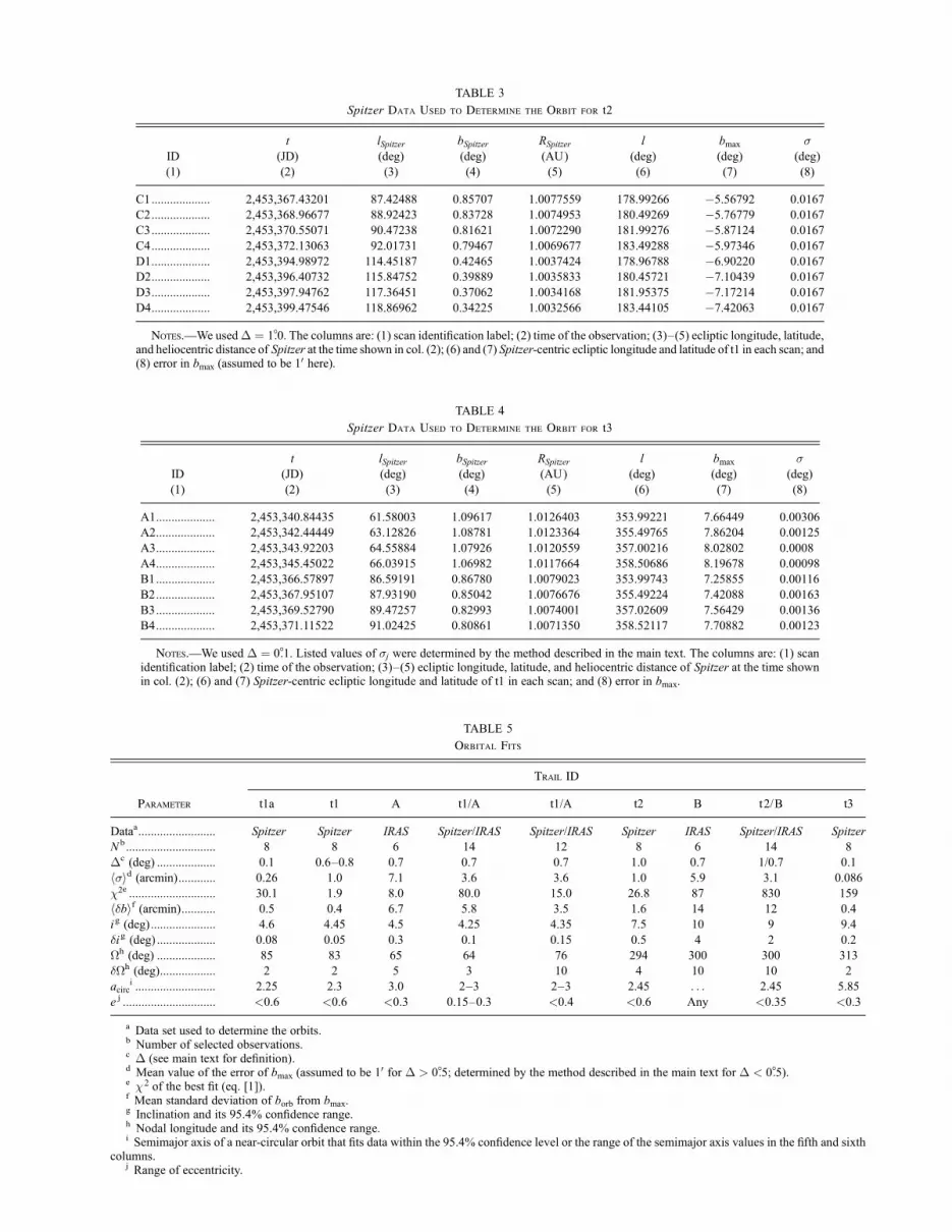
TABLE 3


ID

(1)

t

(JD)

(2)

lSpitzer(deg)

(3)

bSpitzer(deg)

(4)

RSpitzer

(AU)

(5)

l

(deg)

(6)

bmax

(deg)

(7)

�

(deg)

(8)

C1................... 2,453,367.43201 87.42488 0.85707 1.0077559 178.99266 �5.56792 0.0167

C2................... 2,453,368.96677 88.92423 0.83728 1.0074953 180.49269 �5.76779 0.0167

C3................... 2,453,370.55071 90.47238 0.81621 1.0072290 181.99276 �5.87124 0.0167

C4................... 2,453,372.13063 92.01731 0.79467 1.0069677 183.49288 �5.97346 0.0167

D1................... 2,453,394.98972 114.45187 0.42465 1.0037424 178.96788 �6.90220 0.0167

D2................... 2,453,396.40732 115.84752 0.39889 1.0035833 180.45721 �7.10439 0.0167

D3................... 2,453,397.94762 117.36451 0.37062 1.0034168 181.95375 �7.17214 0.0167

D4................... 2,453,399.47546 118.86962 0.34225 1.0032566 183.44105 �7.42063 0.0167

Notes.—We used� ¼ 1N0. The columns are: (1) scan identification label; (2) time of the observation; (3)–(5) ecliptic longitude, latitude,and heliocentric distance of Spitzer at the time shown in col. (2); (6) and (7) Spitzer-centric ecliptic longitude and latitude of t1 in each scan; and(8) error in bmax (assumed to be 10 here).

TABLE 4


ID

(1)

t

(JD)

(2)

lSpitzer(deg)

(3)

bSpitzer(deg)

(4)

RSpitzer

(AU)

(5)

l

(deg)

(6)

bmax

(deg)

(7)

�

(deg)

(8)

A1................... 2,453,340.84435 61.58003 1.09617 1.0126403 353.99221 7.66449 0.00306

A2................... 2,453,342.44449 63.12826 1.08781 1.0123364 355.49765 7.86204 0.00125

A3................... 2,453,343.92203 64.55884 1.07926 1.0120559 357.00216 8.02802 0.0008

A4................... 2,453,345.45022 66.03915 1.06982 1.0117664 358.50686 8.19678 0.00098

B1................... 2,453,366.57897 86.59191 0.86780 1.0079023 353.99743 7.25855 0.00116

B2................... 2,453,367.95107 87.93190 0.85042 1.0076676 355.49224 7.42088 0.00163

B3................... 2,453,369.52790 89.47257 0.82993 1.0074001 357.02609 7.56429 0.00136

B4................... 2,453,371.11522 91.02425 0.80861 1.0071350 358.52117 7.70882 0.00123

Notes.—We used � ¼ 0N1. Listed values of �j were determined by the method described in the main text. The columns are: (1) scanidentification label; (2) time of the observation; (3)–(5) ecliptic longitude, latitude, and heliocentric distance of Spitzer at the time shownin col. (2); (6) and (7) Spitzer-centric ecliptic longitude and latitude of t1 in each scan; and (8) error in bmax.

TABLE 5

Orbital Fits

Trail ID

Parameter t1a t1 A t1/A t1/A t2 B t2/B t3

Dataa......................... Spitzer Spitzer IRAS Spitzer/IRAS Spitzer/IRAS Spitzer IRAS Spitzer/IRAS Spitzer

N b............................. 8 8 6 14 12 8 6 14 8

�c (deg) ................... 0.1 0.6–0.8 0.7 0.7 0.7 1.0 0.7 1/0.7 0.1

h�id (arcmin)............ 0.26 1.0 7.1 3.6 3.6 1.0 5.9 3.1 0.086

�2e ............................ 30.1 1.9 8.0 80.0 15.0 26.8 87 830 159

h�bif (arcmin)........... 0.5 0.4 6.7 5.8 3.5 1.6 14 12 0.4

ig (deg)..................... 4.6 4.45 4.5 4.25 4.35 7.5 10 9 9.4

�ig (deg) ................... 0.08 0.05 0.3 0.1 0.15 0.5 4 2 0.2

�h (deg) ................... 85 83 65 64 76 294 300 300 313

��h (deg).................. 2 2 5 3 10 4 10 10 2

acirci .......................... 2.25 2.3 3.0 2–3 2–3 2.45 . . . 2.45 5.85

e j .............................. <0.6 <0.6 <0.3 0.15–0.3 <0.4 <0.6 Any <0.35 <0.3

a Data set used to determine the orbits.b Number of selected observations.c � (see main text for definition).d Mean value of the error of bmax (assumed to be 10 for � > 0N5; determined by the method described in the main text for � < 0N5).e �2 of the best fit (eq. [1]).f Mean standard deviation of borb from bmax.g Inclination and its 95.4% confidence range.h Nodal longitude and its 95.4% confidence range.i Semimajor axis of a near-circular orbit that fits data within the 95.4% confidence level or the range of the semimajor axis values in the fifth and sixth

columns.j Range of eccentricity.

With� ¼ 0N1, the best-fit orbit matches observed latitudes oft1a in scans C and D to within 3000 in b; we consider this to be asatisfactory precision. The precision is lower with � ¼ 0N01,for which the latitudes agree only to �8000. This comparisonsuggests that the orbits of dust particles do not follow the exactlocations of maxima in Figure 3 but rather intersect (on average)the approximate ‘‘centers’’ of each peak that can only be de-fined from a larger range of latitudes (i.e., from larger �).

We used the following method to define a 95.4% confidenceregion around the best-fit orbit. We normalized �2 to �2

norm ¼�2N /�2

min, where �2min is the best-fit value of �2. The 95.4%

confidence region is then a five-dimensional domain in the spaceof a, e, i, !,� in which�2

norm < N þ 11:3 (e.g., Press et al. 1992).Figure 4 shows that the inclination and nodal longitude of

t1a are particularly well defined. The best fits have i � 4N6and � � 85�. Most orbital solutions also show e P 0:3 and

Fig. 4.—The 95.4% confidence region for the orbit of t1a. Colored squares show orbits in the 95.4% confidence region that we sampled in our orbit-fitting program.Different colors correspond to different levels of confidence: 68.3% (blue), 90% (green), and 95.4% (red ). The orbital fits were determined from our Spitzer data with� ¼ 0N1. The gray polygon in (b) schematically denotes the region of the main asteroid belt. Symbols� in (b) denote orbits of all known JFCs with 4�< i < 5�. Whilemost low-e solutions correspond to asteroidal orbits, the tail of the 95.4% confidence region at large a and e extends to the orbital domain populated by cometary orbits.Two known JFCs, 137P/Shoemaker-Levy 2 (a ¼ 4:432 AU, e ¼ 0:579, and i ¼ 4N6) and 143P/Kowal-Mrkos (a ¼ 4:306 AU, e ¼ 0:409, and i ¼ 4N6), that appearclosest to the 95.4% confidence region in (b) have incompatible � with (a).

Fig. 5.—The 95.4% confidence region for the orbit of t1. The color code and symbols are the same as in Fig. 4. The orbital fits were determined from our Spitzer datawith � ¼ 0N6 for set C and � ¼ 0N8 for set D.


1 AU P aP 3 AU. Perihelion longitudes ! are not well de-termined from our observations for the low-e orbits. There aretwo high-e tails extending to small and large a. These tails havea(1þ e) � acirc and a(1� e) � acirc, respectively, where acirc ¼2:25 AU. The best-fit values of! for these high-e orbital solutionsare clustered within�20�–270� (for low-a orbits) and to 40� (forlarge-a orbits).

Figure 5 shows our best-fit orbits for t1 determined withlarger �. These fits show values of i that are about 0N15 lowerthan those obtained for t1a and values of � that are about 2�

lower. The difference in the best-fit i between t1a and t1 is larger

than the formal errors determined in each case (i.e., 95.4%confidence regions of t1a and t1 in the i, � projection do notoverlap). This difference probably stems from the fact that wecannot resolve individual orbits in the trail and measure onlytheir collective contribution. Consequently, a larger uncertaintyof i and � should be allowed than the formal uncertainty of ourorbital fits listed in Table 5.

The 95.4% confidence region in Figure 5a is shaped similarlyto that in Figure 4a showing larger i for larger �. This correlationbetween i and� can be readily explained by the way these orbitalelements must adjust to match the Spitzer observations. The quality

Fig. 6.—The 95.4% confidence region for the orbit of t2. The color code and symbols are the same as in Fig. 4. All known JFCs with 5� < i < 10� are plotted in (b).The orbital fits were determined from our Spitzer data with � ¼ 1�.

Fig. 7.—The 95.4% confidence region for the orbit of t3. The color code and symbols are the same as in Fig. 4. The orbital fits were determined from our Spitzer datawith � ¼ 0N1. JFCs with 5� < i < 15� are plotted in (b). ‘‘SW1’’ denotes the orbital elements of comet 29P/Schwassmann-Wachmann 1 on 2005 January 1.


of the best fits for t1’s orbit is comparable to those obtained for t1a(i.e., �2500 precision in b). The value of ! for the high-e or-bits is confined in ways similar to those discussed for t1a above.

Figure 6 shows the best-fit orbits for t2. These fits show largervalues of �2 than those obtained for t1 (Table 5). The orbitalelements of t2 are also not constrained that well. Inclinations arefound to be between 7

�and 8

�, and nodal longitudes range

between 290� and 298�. Figure 6b shows that the source of t2may be asteroidal (if e < 0:3) or cometary (if e > 0:3). None ofthe existing comets currently has i and � in (or close to) the95.4% confidence region shown in Figure 6a. Additional ob-servation data are needed to better determine the orbit of t2.

Figure 7 shows the best-fit orbits for t3. We obtained theseorbit solutions by the same method used for trails t1 and t2. Thefit constrains the orbital elements in important ways: 9N2 P i P9N6 and � ¼ 313� � 2�. The predicted orbit has a semimajoraxis slightly larger than that of Jupiter and e P 0:3.

For comparison, comet 29P/Schwassmann-Wachmann 1 hadthe following orbital elements on 2005 January 1: a ¼ 5:987AU, e ¼ 0:04407, i ¼ 9N391, � ¼ 312N708, ! ¼ 48N752, andmean anomalyM ¼ 11N911. The location of this orbit is shownin Figure 7. The similarity of a, e, i, and� between the predictedorbit of t3 and that of comet 29P/Schwassmann-Wachmann 1reinforces our previous identification of trail t3 with the trail ofthis comet. It also validates our method of orbit determinationfor trails from Spitzer’s observations.

4. RELATION OF t1 AND t2 TO TYPE II TRAILS

Sykes (1988) and Sykes & Walker (1992) identified a num-ber of trails in the IRAS data that do not correspond to anyknown comet. They call them type II, or ‘‘orphan,’’ trails. Thesetrails may have detached from their parent comets by Jupiter’sorbital perturbations. Alternatively, some type II trails mayhave been produced by comet or asteroid disruptions. Sykes

Fig. 8.—Top:Expected locations of Spitzer trails t1 (red ), t2 (green), and t3 (blue) in IRAS’s HCONs 1 and 2. For t3 we used the orbit of 29P/Schwassmann-Wachmann1. For t1 and t2 we used the best-fit orbits from Figs. 5 and 6 with e ¼ 0. Projections into HCONs 1 and 2 of the best-fit orbits with larger e show only minor differencescompared to those with e ¼ 0. Bottom:Map constructed from IRAS’s 25 �mHCONs 1 and 2.We have filtered individual scans to remove spatial structures extending >4�

and <0N1 in ecliptic latitudes. IRAS’s type II trails A and B are denoted. Several comet trails that appear in this plot have been identified by Sykes & Walker (1992) andcorrespond to comets Tempel 1 and 2, Encke, Kopff, andGunn. The trail of comet 29P/Schwassmann-Wachmann, which is difficult to see in the bottom plot, has b � �10

�

and l � 200� (Sykes & Walker 1992). The close correspondence between the expected locations of Spitzer’s trails t1 and t2 in the IRAS data and the locations of IRAS’strails A and B, respectively, suggests that t1 is A and t2 is B.

NESVORNY ET AL.590

Fig. 9.—Top:Expected locations of Spitzer trails t1 (red), t2 (green), and t3 (blue) in IRAS’s HCON3. Bottom:Map constructed from IRAS’s 25 �mHCON3. See Fig.8 for further details. The arrow denotes the location of trail A (Sykes 1990).

TABLE 6

IRAS Data Used to Determine the Orbit for Trail A

Scan ID

(1)

t

(JD)

(2)

lIRAS(deg)

(3)

bIRAS(deg)

(4)

RIRAS

(AU)

(5)

l

(deg)

(6)

bmax

(deg)

(7)

�

(deg)

(8)

029_12........................ 2,445,374.84861 140.25779 0.00128 0.9866445 61.04 0.60867 0.49848

122_30........................ 2,445,421.59349 187.08281 �0.00061 0.9980069 101.53 4.03678 0.02533

146_22........................ 2,445,433.62227 198.94082 �0.00075 1.0015088 111.31 4.48414 0.03221

183_05........................ 2,445,451.73489 216.64899 �0.00159 1.0064676 128.20 4.79011 0.04814

574_20........................ 2,445,647.45744 46.20277 0.00163 0.9906180 140.09 3.82940 0.04080

587_47........................ 2,445,654.11148 52.89600 0.00189 0.9890415 150.54 4.03159 0.06496

Notes.—We used� ¼ 0N7 here. The columns are: (1) scan identification label; (2) time of the observation; (3)–(5) ecliptic longitude, latitude,and heliocentric distance of IRAS at the time shown in col. (2); (6) and (7) IRAS-centric ecliptic longitude and latitude of A in each scan; and(8) error of bmax. Listed values of �j were determined by the method described in the main text.

(1990, Fig. 2) lists the main type II trails as A, B, C, and D. Weuse the same notation here.

Figure 8 (bottom) shows filtered IRAS data corresponding toHCONs 1 and 2.10 We used the same filter parameters here asfor the Spitzer data. Trail A extends over about 80� in ecliptic lon-gitude, between l � 60� and 140�. Its latitude varies from b � 0�

for l ¼ 60�to b � 5

�for l ¼ 140

�. Trail B extends over at least

60� in l, from�100� to�160� (it is not clear whether it continuesbeyond l ¼ 100�, because there is strong Galactic emission atl < 100

�). Trail B starts at b � 0

�for l ¼ 100

�and goes down to

b � �7�for l ¼ 160

�. Trails C and D are more dispersed struc-

tures that were not detected in HCONs 1 and 2.We have taken one of the best orbital fits for our Spitzer trails

t1 and t2 and projected these orbits onto sky locations where

they would be observed by IRAS. Figure 8 (top) shows thisprojection. It is apparent from the comparison of the panels inFigure 8 that the predicted locations of trails t1 and t2 in theIRAS data correspond well to the locations of IRAS trails A andB, respectively. In addition, the brightness and latitudinal spreadsof t1 and t2 seen in the Spitzer data are comparable to those of IRAStrails A and B. We therefore identify t1 with A and t2 with B.Figure 9 shows the projection of our best-fit orbit into IRAS’s

HCON 3. Trail B was not found in HCON 3. Trail A appears inHCON 3 as a short line segment about 40

�long in l, near l ¼

140�and b ¼ 4

�. The predicted path of t1 in HCON 3 passes

near the observed segment (Fig. 9, top) but is slightly more in-clined to the ecliptic than the observed trail A and has a bit smallerb. In x 5 we compensate for this slight difference by adjusting thebest-fit orbits to better match these IRAS observations.

5. ORBIT FITS FOR t1/a AND t2/b FROM SpitzerAND IRAS DATA

Having identified trails t1 and t2 with trails A and B in theIRAS data, we may now use the location of these trails as deter-mined by IRAS observations to improve the orbit determination.Trails A and B are best visible in the 25 �m IRAS filter. We

TABLE 7

IRAS Data Used to Determine the Orbit for Trail B

Scan ID

(1)

t

(JD)

(2)

lIRAS(deg)

(3)

bIRAS(deg)

(4)

RIRAS

(AU)

(5)

l

(deg)

(6)

bmax

(deg)

(7)

�

(deg)

(8)

181_07........................ 2,445,450.80743 215.74690 �0.00158 1.0062237 126.31 �5.3089 0.3757

181_11........................ 2,445,450.87879 215.81632 �0.00158 1.0062425 126.54 �5.1049 0.0565

211_18........................ 2,445,465.98310 230.45968 �0.00169 1.0100433 143.22 �6.9045 0.0276

219_02........................ 2,445,469.70495 234.05355 �0.00189 1.0108669 135.39 �5.6094 0.0483

221_06........................ 2,445,470.77907 235.08959 �0.00195 1.0110929 137.76 �5.8484 0.0434

241_01........................ 2,445,480.73291 244.66522 �0.00214 1.0129924 152.49 �8.8289 0.0397

Notes.—We used� ¼ 0N7. The columns are: (1) scan identification label; (2) time of the observation; (3)–(5) ecliptic longitude, latitude, andheliocentric distance of IRAS at the time shown in col. (2); (6) and (7) IRAS-centric ecliptic longitude and latitude of B in each scan; and(8) error of bmax.

Fig. 10.—The 95.4% confidence region for the orbit of t1/A. The color code and symbols are the same as in Fig. 4. JFCswith 4�< i < 5� are plotted in (b). The orbitalelements of t1/A have been determined by combining Spitzer and IRAS observations of this trail.

10 Each IRAS scan had a width of 0N5 and was shifted in ecliptic longitude by0N25 on the subsequent orbit, allowing a fixed source to be scanned twice in the103 minute orbital period. This was referred to as an ‘‘hours-confirmed obser-vation,’’ or HCON. During the initial portion of its mission, IRASwould map outa section of sky (HCON 1) and after about a week remap the same section(HCON 2). During the last 3 months of the mission, a third map (HCON 3) wasattempted using a larger range of solar elongations. It covered 72% of the skybefore the satellite terminated operations.


selected several 25 �m IRAS scans in which these trails can bereadily identified. Information about these scans is listed inTables 6 and 7. To identify the exact latitudinal locations oftrails A and B in each scan, we used the polynomial fit methoddescribed in x 3. The IRAS data are significantly noisier than theSpitzer data. Therefore, the formal errors of bmax determined bythe polynomial fit are relatively large.

We first attempted to fit for the orbits of trails A and B usingthe IRAS data alone. These orbital fits are listed in Table 5. Thequality of the orbital fits is significantly lower than those ob-tained for t1 and t2 from Spitzer ; the best-fit orbits match theIRAS observations of trails A and B to within 90 and 300, respec-tively (compared to about an order of magnitude better precisionwith Spitzer).

For trail A, the best-fit orbits have 60� P � P 70�, 4N2 P i P4N8, e P 0:3, and 2 AU P a P 4 AU. This range of orbital ele-ments is comparable to those obtained for t1 from Spitzer. In-terestingly, most orbits of trail A as determined from the IRASdata have low eccentricities and a in the range of themain asteroidbelt.

Nodal longitude � determined for trail A from IRAS is smallerby 10�–20� than values of � determined for t1 from Spitzer. It isunlikely that this difference was produced by the secular pre-cession of � between 1983.5 (epoch of IRAS observations) and2005 (epoch of Spitzer observations), because planetary pertur-bations cause � < 0 and small j�j, while large and positive �would be needed to shift � by 10

�–20

�in 21.5 yr.

Assuming that the orbit of t1/A has not changed in the interimperiod, we searched for the best-fit orbits of t1/A fromboth Spitzerand IRAS observations. These orbits match bmax in the Spitzer datato about 20 (compared to 0A4when only Spitzer data were used) andthe bmax in the IRAS data to �100. The combined fit requires that2 AU < a < 3 AU and 0:15 < e < 0:3 (Fig. 10). This range ofa and e, and small values of i that we consistently obtain fort1 from all data sets, suggests that the source of t1/A maybe asteroidal. The combined fit requires that 4N15 < i < 4N35,61

� < � < 67�, and 140

� < ! < 220�.

We performed a number of tests to see how the orbital fitsdetermined from the combined Spitzer and IRAS data depend on theselection of scans used in the orbit-fitting program. For example,we combined the Spitzer datawith IRAS’s HCONs 1 and 2 only andfitted for orbits from 12 data points (eight Spitzer data points fromTable 2 and four IRAS data points corresponding to HCONs 1 and2; Table 6, first four rows). The best-fit orbits determined in this testhave a slightly larger range of i and� than that in Figure 10. Like inFigure 10, however, most of the best-fit orbits are located in themain asteroid belt. This result shows that our conclusion aboutthe asteroidal origin of trail t1/A does not rely on the input fromIRAS’s HCON 3.

The orbital fits for trail B from the IRAS data show a largespread in a and e. This is due to the fact that trail B has beenobserved in HCONs 1 and 2 only where the solar elongation ofthe telescope’s pointing direction did not vary much. It is there-fore difficult to determine the orbit from IRAS data only. WhenSpitzer and IRAS data are used together, however, we find thatmost best-fit orbits for t2/B are asteroidal (Fig. 11). Despite this,there exists a tail of solutions with large a and e that correspond tocometary orbits. Additional data will be needed to better con-strain the orbit of t2/B.

6. DISCUSSION

Our orbital fits suggest that the source of trail t1 may beasteroidal. This conclusion relies on the combined fits in whichSpitzer and IRAS observationswere used together.While useful, itis not ideal to combine these data sets, because (1) IRAS data arerelatively noisy, making it more difficult to determine the exactlatitudinal locations of trails, and (2) we must assume that orbitsdid not changemuch in the period between IRAS and Spitzer obser-vations. Assumption (2) is likely to be correct if the source has astable orbit in the main asteroid belt. If, however, the orbit wasJupiter-crossing (e.g., a JFC’s orbit), encounters with Jupiter mayhave modified it, and assumption (2) may be incorrect.

A recent collisional breakup of a main-belt asteroid would notonly produce a strong dust trail, but the large fragments released

Fig. 11.—The 95.4% confidence region for the orbit of t2/B. The color code and symbols are the same as in Fig. 4. JFCs with 6�< i < 12� are plotted in (b). Theorbital elements have been determined by combining Spitzer and IRAS observations of this trail.


Fig. 12.—Expected locations of trails t1/A (left panels) and t2/B (right panels) as seen by Spitzer during Cycle 1 from 2004 June 1 to 2005 May 31. To make theseplots, we assumed four different observing solar elongations, 112N25, 87N25, 88N3, and 115N2, corresponding to our noodles A, B, C, and D, respectively (top to bottom).The individual four scans in each set are shown by vertical line segments separated by 1N5 in ecliptic longitude. The sinusoidal lines show projections of orbits for trailst1/A and t2/B that were determined from our Spitzer Cycle 1 and the IRAS data. Gray areas show locations of the inner and outer asteroid dust bands and the Galacticemission.

during the breakup could also potentially create an observableasteroid family. We searched for asteroid families that wouldhave orbital elements near those predicted for t1 and t2. We usedthe hierarchical clustering method (Zappala et al. 1990) with ageneralized metric in the five-dimensional space of osculatingorbital elements: a, e, i, !, and � (see Nesvorny et al. 2006a;Nesvorny &Vokrouhlicky 2006).We found no obvious clustersthat could be linked with t1 or t2. This result probably impliesthat the disrupted body was small, perhaps only several kilo-meters across, such that the largest fragments produced by thebreakup have sizes below the current detection limit. Accordingto Bottke et al. (2005), a 1 km diameter asteroid disrupts in themain belt every �100 yr and a 10 km diameter asteroid every�100 kyr.

If the ejection speeds of fragments, �V , from these disruptionswere of the order of 10 m s�1, we estimate that the fragmentswere spread in semimajor axis by �a ¼ 4a�V /V � 5 ; 10�3 AU,where V � 20 kms�1 is the orbital speed for a ¼ 2:3AU.Havingdifferent semimajor axes, the fragments then started to differ-entially spread in mean anomaly M, !, and �.

Particles in trails t1 and t2 must have narrow spreads in � atthe current epoch (we would not otherwise obtain good orbitalfits). This sets a firm upper limit on the age of these trails. Usingthe results of Sykes & Greenberg (1986), we estimate that trailst1 and t2 cannot be older than�100 kyr. A detailed model of thedifferential precession of nodes could be used to better constrainthe age of trails t1 and t2. This model will have to include effectsof radiation forces such as Poynting-Robertson drag and ac-count for collisional disruptions of migrating small particles.Such a model could also be useful to explain the double-peakedstructure of trail t1 (Fig. 3).

The lengths of observed trails A and B in the IRAS data mayprovide additional constraints on the age. There are two pos-sibilities: (1) due to favorable observing conditions, IRAS de-tected only parts of trails A and B, which are actually spread over360� inM (i.e., trails are tubes); or (2) the lengths of the observedarcs directly correspond to the spread of particles inM (i.e., trailsare arcs). As for (1), we estimate that the variation of 24 �mbrightness of trails t1/A and t2/B from perihelion to aphelion oftheir asteroidal orbits should be a factor of a few. It is not ob-vious whether this variation is large enough to favor (1).

Unfortunately, it is also difficult to determine whether Spitzerand IRAS could have observed the same arc of trails t1 and t2.

This is due to the fact that the uncertainty in the semimajor axisof trails is large, so M cannot be reliably tracked over the timeperiod that separates the IRAS and Spitzer observations (about21.5 yr). Conversely, the nondetection of trails t1 and t2 innoodles A and B could provide a better constraint on the exten-sion of trails because of the sensitivity of Spitzer observations andbecause all our observations were taken within a period of only2 months (so that particles did not move much along their orbits).

To help address this issue we determined the expected eclipticcoordinates of trails t1/A and t2/B that correspond to the observinggeometry of Spitzer during Cycle 1. Figure 12 shows that scans Aand B were not sufficiently extended above the ecliptic plane tocross over the expected location of trail t2/B (b � 10��12�). It istherefore not surprising that this trail was not detected in our setsAand B. Conversely, the expected location of trail t1/A in scans Aand B is b ��4

�, well within the scanned interval of ecliptic

latitudes. It is unfortunate, however, that the strong south com-ponent of the inner dust band is also located at b � �4�. Aweakersignal of trail t1/A may then be hidden and easily overlooked atthis latitude. The nondetection of trails in scans A and B cannot,therefore, be used to favor (2). The question of whether trails t1/Aand t2/B are arcs or tubes remains open.

The cometary origin of trail t2/B cannot be strictly excludedwith the present data because our orbital fits allow for someorbit solutions with comet-like large e. Additional observationsare needed to resolve this issue. Ideally, we would plan the ob-servations to obtain scans with Spitzer at several different eclipticlongitudes, at least two different solar elongations, and acrossthe latitude values predicted for the orbits determined here. Suchobservationswould be extremely useful to determine (1) the orbitsof t1/A and t2/B precisely and (2) whether the trails are arcs ortubes. The results would have major implications for our under-standing of the age of the observed trails and the overall con-tribution of small asteroid breakups to the zodiacal cloud.

This paper is based on work supported by the Spitzer Cycle 1grant entitled ‘‘The Production of Zodiacal Dust by Asteroidsand Comets.’’ Work by D. N. was funded by NASA under PGGgrant NAG513038. Research funds for W. F. B. were providedby NASA’s OSS program (grant NAG510658). We thank T.Spahr for his inspiring comments on the submitted manuscript.

REFERENCES

Bottke, W. F., Durda, D. D., Nesvorny, D., Jedicke, R., Morbidelli, A.,Vokrouhlicky, D., & Levison, H. F. 2005, Icarus, 179, 63

Dermott, S. F., Nicholson, P. D., Burns, J. A., & Houck, J. R. 1984, Nature,312, 505

Greaves, J. S., Wyatt, M. C., Holland, W. S., & Dent, W. R. F. 2004, MNRAS,351, L54

Greaves, J. S., et al. 2005, ApJ, 619, L187Grogan, K., Dermott, S. F., & Durda, D. D. 2001, Icarus, 152, 251Jopek, T. J., Valsecchi, G. B., & Froeschle, C. 2002, in Asteroids III, ed. W. F.Bottke et al. (Tucson: Univ. Arizona Press), 645

Low, F. J., et al. 1984, ApJ, 278, L19Nesvorny, D., Bottke, W. F., Levison, H., & Dones, L. 2002, Nature, 417, 720———. 2003, ApJ, 591, 486Nesvorny, D., & Vokrouhlicky, D. 2006, AJ, submittedNesvorny, D., Vokrouhlicky, D., & Bottke, W. F. 2006a, Science, in press

Nesvorny, D., Vokrouhlicky, D., Bottke, W. F., & Sykes, M. 2006b, Icarus,181, 107

Press, W. H., Teukolsky, S. A., Vetterling, W. T., & Flannery, B. P. 1992,Numerical Recipes in C (2nd ed.; Cambridge: Cambridge Univ. Press)

Reach, W. T., Franz, B. A., & Weiland, J. L. 1997, Icarus, 127, 461Reach, W. T., Sykes, M. V., Lien, D., & Davies, J. K. 2000, Icarus, 148, 80Stansberry, J. A., et al. 2004, ApJS, 154, 463Sykes, M. V. 1986, Ph.D. thesis, Univ. Arizona———. 1988, ApJ, 334, L55———. 1990, Icarus, 85, 267Sykes, M. V., & Greenberg, R. 1986, Icarus, 65, 51Sykes, M. V., & Walker, R. G. 1992, Icarus, 95, 180Zappala, V., Cellino, A., Farinella, P., & Knezevic, Z. 1990, AJ, 100, 2030

CANDIDATES FOR ASTEROID DUST TRAILS 595

candidates for asteroid dust trails

Documents