formation of asteroid pairs by rotational fission
TRANSCRIPT

1
Formation of asteroid pairs by rotational fission
P. Pravec1, D. Vokrouhlický2, D. Polishook3, D. J. Scheeres4, A. W. Harris5, A.
Galád6,1, O. Vaduvescu7,8, F. Pozo7, A. Barr7, P. Longa7, F. Vachier9, F. Colas9, D. P.
Pray10, J. Pollock11, D. Reichart12, K. Ivarsen12, J. Haislip12, A. LaCluyze12, P.
Kušnirák1, T. Henych1, F. Marchis13,14, B. Macomber13,14, S.A. Jacobson15, Yu. N.
Krugly16, A.V. Sergeev16 & A. Leroy17
1Astronomical Institute AS CR, Fričova 1, CZ-25165 Ondřejov, Czech Republic.
2Institute of Astronomy, Charles University, V Holešovičkách 2, CZ-18000 Prague,
Czech Republic. 3Wise Observatory and Department of Geophysics and Planetary
Sciences, Tel-Aviv University, Israel. 4Department of Aerospace Engineering Sciences,
University of Colorado, Boulder, CO, USA. 5Space Science Institute, 4603 Orange
Knoll Ave., La Canada, CA 91011, USA. 6Modra Observatory, Comenius University,
Bratislava SK-84248, Slovakia. 7Instituto de Astronomia, Universidad Catolica del
Norte, Avenida Angamos 0610, Antofagasta, Chile. 8Isaac Newton Group of Telescopes,
E-38700 Santa Cruz de la Palma, Canary Islands, Spain. 9IMCCE-CNRS-Observatoire
de Paris, 77 avenue Denfert Rochereau, 75014, Paris, France. 10Carbuncle Hill
Observatory, W. Brookfield, MA, USA. 11Physics and Astronomy Dept., Appalachian
State University, Boone, NC, USA. 12Physics and Astronomy Department, University of
North Carolina, Chapel Hill, NC, USA. 13University of California at Berkeley, Berkeley
CA, USA. 14SETI Institute, Mountain View CA, USA. 15Department of Astrophysical and
Planetary Sciences, University of Colorado, Boulder, CO, USA. 16Institute of Astronomy
of Kharkiv National University, Sumska Str. 35, Kharkiv 61022, Ukraine.
17Observatoire Midi Pyrénées and Association T60, Pic du Midi, France.
Asteroid pairs sharing similar heliocentric orbits were found recently1–3.
Backward integrations of their orbits indicated that they separated gently with low
relative velocities, but did not provide additional insight into their formation

2
mechanism. A previously hypothesized rotational fission process4 may explain
their formation – critical predictions are that the mass ratios are less than about
0.2 and, as the mass ratio approaches this upper limit, the spin period of the larger
body becomes long. Here we report photometric observations of a sample of
asteroid pairs revealing that primaries of pairs with mass ratios much less than 0.2
rotate rapidly, near their critical fission frequency. As the mass ratio approaches
0.2, the primary period grows long. This occurs as the total energy of the system
approaches zero requiring the asteroid pair to extract an increasing fraction of
energy from the primary's spin in order to escape. We do not find asteroid pairs
with mass ratios larger than 0.2. Rotationally fissioned systems beyond this limit
have insufficient energy to disrupt. We conclude that asteroid pairs are formed by
the rotational fission of a parent asteroid into a proto-binary system which
subsequently disrupts under its own internal system dynamics soon after
formation.
Analyses of the orbits of asteroid pairs reveal some common properties. Asteroid
pairs are ubiquitous, found throughout the main belt and Hungarias5. Pair members are
separated with low relative velocities on the order of metres per second in the space of
proper elements (dprop), and with the best studied asteroid pair (6070)-(54827) having a
speed after escape of only 0.17 m/s (ref. 3). They are young with most pairs separated
less than 1 Myr ago (Supplementary Information). The existence of a population of
bound binary systems at a similar range of sizes suggests that related processes may
account for both binary and pair formation. Previous investigations have indicated that
binaries form from parent bodies spinning at a critical rate by some sort of fission or
mass shedding process4,6,7 and that binaries formed by fission will initially have chaotic
orbit and spin evolution8. The free energy of a binary system formed by fission, defined
as the total energy (kinetic and potential) minus the self-potentials of each component9,
is found here to play a fundamental role in the evolution of a binary. Systems with mass

3
ratios less than ~0.2 have a positive free energy and can escape under internal dynamics,
while systems with greater mass ratios have a negative free energy and cannot. As the
system mass ratio approaches this limit, kinetic energy for escape is drawn from the
primary rotation leaving it rotating at a slower rate. This predicts that primaries of pairs
with small mass ratios rotate nearer to their critical fission period, as the mass ratio
approaches 0.2 the primary period grows long, and beyond this limit disruption of the
binary is not possible. (See Supplementary Information.)
We studied the relative sizes, spin rates, and shapes between pairs and binaries via
a photometric observational program. Our sample consists of 35 asteroid pairs, listed in
Table 1. Thirty two of them were taken from ref. 2, the pair (6070)-(54827) was from
ref. 3, and the pairs (48652)-(139156) and (229401)-2005 UY97 were identified with
backward orbit integrations of the pair's components. The only selection criterion, other
than the pair identification procedures used in the above works, was that the pairs
occurred in favorable conditions for photometric observations with available telescopes
(brightness, position in the sky). Our sample covers a range of sizes 1.9-7.0 km for
primaries and 1.2-4.5 km for secondaries, with the median of 3.2 and 1.9 km,
respectively, as estimated from the asteroids’ absolute magnitudes6, assuming geometric
albedos according to their orbital group membership12.
We integrated orbits of the asteroid pairs backward to 1 Myr before the present
using techniques developed in refs 1–3 and achieved convergence for 31 of the 35
asteroid pairs in our sample. That strengthened their identification as real, genetically
related pairs, and also provided estimates of ages of the pairs (T). The four pairs for
which convergence was not achieved may be older than 1 Myr (see Supplementary
Information).

4
We estimate the size ratio (X) and mass ratio (q) between the components of an
asteroid pair from the difference between their absolute magnitudes (∆H ≡ H2 – H1)
using the relation between an asteroid's absolute magnitude (H), effective diameter (D),
and geometric albedo6. Assuming that the components have the same albedo and bulk
density, the size ratio is X ≡ D2/D1 = 10-∆H/5 and the mass ratio q ≡ M2/M1 = X3, where
M1, M2 is the mass of the primary and secondary (see Discussion 2 in Supplementary
Information). A dominating uncertainty source in the size and mass ratio estimate are
uncertainties of the estimated absolute magnitudes of the components. For all asteroids
in this work, we have used absolute magnitude estimates obtained as a by-product of
asteroid astrometric observations published in the AstDyS catalog (also used in ref. 2).
We estimated a mean uncertainty of the catalog absolute magnitudes for our studied
paired asteroids to be δH ∼ 0.3 mag. This propagates to a relative uncertainty of the
estimated size ratio of 20%.
Figure 1 presents the observed primary period P1 vs ∆H data for the 32 primaries.
The primary spin rates show a correlation with the mass ratio q between members of the
asteroid pairs. Specifically, primaries of pairs with small secondaries (∆H > 2.0,
q < 0.06) rotate rapidly and their spin periods have a narrow distribution from 2.53 to
4.42 hr with a median of 3.41 hr, near the critical fission rotational period. As the mass
ratio approaches the predicted approximate cutoff limit of 0.2, the primary period grows
long. The correlation coefficient between ω12 = (2π/P1)
2 and q is -0.73 and the
Student’s t statistic is -5.94 for the degrees of freedom of 30 of the sample that shows
that the correlation is significant at a level higher than 99.9% (see Supplementary
Information).
It is notable that the distribution of primary rotations of pairs with small
secondaries is similar to rotations of primaries of orbiting binaries with similar sizes and
size ratios. From a database of binary system parameters6, main belt and Hungaria

5
binaries with primary diameters D1 = 2–10 km and size ratios D2/D1 < 0.4 (q < 0.06)
have primary rotation periods from 2.21 to 4.41 hr, with a median of 2.92 hr.
The observed primary spin rate distribution is consistent with pair formation via
the mutual escape of a transient proto-binary system formed from the rotational fission
of a critically spinning parent body. In Fig. 1 we show theoretical curves that
incorporate constraints on the expected spin period of a primary assuming a system that
is initially fissioned and later undergoes escape. For these computations, systems are
given an initial angular momentum consistent with a critical rotation rate as observed in
orbiting binary systems6. Then, assuming conservation of energy and angular
momentum we evaluate the spin period of the larger body if the binary orbit undergoes
escape. For simplicity we assume planar systems. Shape ratios of the primary and
secondary are incorporated into the energy and angular momentum budget6 and in
conjunction with a range of initial angular momentum values lead to the envelopes
shown in the figure. (The mathematical formulation of the model is given in
Supplementary Information.)
The observed data for paired asteroids show consistency with the theoretical
curves from the simple model of the post-fission system of two components starting in
close proximity, as explained above. This starting condition and subsequent process is
consistent with the rotational fission model4,8,13 which models the parent asteroid as a
contact binary-like asteroid with components resting on each other. A mechanism to
spin the asteroid up to its critical rotation frequency is provided by the Yarkovsky–
O'Keefe–Radzievskii–Paddack (YORP) effect14. When the angular momentum of the
system is increased sufficiently the components can enter orbit about each other, what
we term rotational fission. The fission spin rate is a function of the mass ratio between
the components, for large mass ratios or highly ellipsoidal shapes the spin period can be
significantly longer than the surface disruption limit of a rapidly spinning sphere4. The

6
free energy of the proto-binary system is also a strong function of the mass ratio
between the components and is relatively independent of the mutual shapes of the pairs
that enter fission, with the theory predicting that systems with q less than about 0.20
will have a positive free energy and systems with greater mass ratios a negative free
energy. Taking shapes into account, there is some variability about this mass ratio value
with the dividing mass ratio ranging up to 0.28 for more distended shapes8.
Further evidence indicates that asteroid fission as described here may not be the
only process at work forming multi-component asteroid systems. There is a disparity
between the lightcurve amplitudes of the primary components in asteroid pairs and
binary systems (Fig. 2). This cannot be explained with the mechanism of rotational
fission only, as all asteroid systems that undergo rotational fission are initially unstable,
regardless of the degree of elongation8. Though a more elongated primary may be more
efficient at ejecting a secondary, numerical simulations show that ejection can occur
even for systems with moderate elongation (Supplementary Information). It suggests
that either some process occurs during the formation process of a stable binary asteroid
to form a nearly symmetric shape of the primary or that a different formation
mechanism is at work7. Further observational and theoretical studies must be carried
out to discover a cause for this pattern.
The fission mechanism that describes our observations is independent of
mineralogical properties and only depends on mechanical/gravitational interactions
between two mass components. Given this and the ubiquity of asteroid pairs as well as
binary asteroids, and the occurrence of binaries among the major taxonomic types, S
and C, we can speculate that the formation of asteroid binaries is driven by mechanical
and not mineralogical properties.

7
1. Vokrouhlický, D. & Nesvorný, D. Pairs of asteroids probably of a common origin.
Astron. J. 136, 280–290 (2008).
2. Pravec, P. & Vokrouhlický, D. Significance analysis of asteroid pairs. Icarus 204,
580–588 (2009).
3. Vokrouhlický, D. & Nesvorný, D. The common roots of asteroids (6070) Rheinland
and (54827) 2001 NQ8. Astron. J. 137, 111–117 (2009).
4. Scheeres, D. J. Rotational fission of contact binary asteroids. Icarus 189, 370–385
(2007).
5. Milani, A., Knežević, Z., Novaković, B. & Cellino, A. Dynamics of the Hungaria
asteroids. Icarus 207, 769-794 (2010).
6. Pravec, P. & Harris, A. W. Binary asteroid population. 1. Angular momentum
content. Icarus 190, 250–259 (2007).
7. Walsh, K. J., Richardson, D. C. & Michel, P. Rotational breakup as the origin of
small binary asteroids. Nature 454, 188–191 (2008).
8. Scheeres, D. J. Stability of the planar full 2-body problem. Celest. Mech. Dyn. Astr.
104, 103–128 (2009).
9. Scheeres, D. J. Stability in the Full Two-Body Problem. Celest. Mech. Dyn. Astr. 83,
155–169 (2002).
10. Warner, B. D. Asteroid lightcurve analysis at the Palmer Divide Observatory: 2008
May – September. Minor Planet Bull. 36, 7–13 (2009).
11. Galád, A., Kornoš, L. & Világi, J. An ensemble of lightcurves from Modra. Minor
Planet Bull. 37, 9–15 (2009).
12. Warner, B. D., Harris, A. W. & Pravec, P. The asteroid lightcurve database. Icarus
202, 134–146 (2009).
13. Scheeres, D. J. Minimum energy asteroid reconfigurations and catastrophic
disruptions. Planetary and Space Science 57, 154–164 (2009).
14. Bottke, W. F. Jr, Vokrouhlický, D., Rubincam, D. P. & Nesvorný, D. The
Yarkovsky and Yorp Effects: Implications for asteroid dynamics. Annu. Rev. Earth
Planet. Sci. 34, 157–191 (2006).

8
Supplementary Information is linked to the online version of the paper at
http://www.nature.com/nature/journal/v466/n7310/extref/nature09315-s1.pdf.
Acknowledgements Research at Ondřejov was supported by the Grant Agency of the Czech Republic.
D.V. was supported by the Czech Ministry of Education. D.P. was supported by an Ilan Ramon grant
from the Israeli Ministry of Science, and is grateful for the guidance of N. Brosch and D. Prialnik. D.J.S.
and S.A.J. acknowledge support by NASA's PG&G and OPR research programs. A.W.H. was supported
by NASA and NSF. Work at Modra Observatory was supported by the Slovak Grant Agency for Science.
The observations at Cerro Tololo were performed with the support of CTIO and Joselino Vasquez, using
telescopes operated by SMARTS Consortium. Work at Pic du Midi Observatory was supported by CNRS
– Programme de Planétologie. Operations at Carbuncle Hill Observatory were supported by the Planetary
Society’s Gene Shoemaker NEO Grant. Support for PROMPT has been provided by the NSF. F.M. and
B.M. were supported by the NSF. We thank to O. Bautista, T. Moulinier and P. Eclancher for assistance
with observations with the T60 on Pic du Midi.
Author Contributions All named authors made significant contributions to this work, often to more than
just one task, thus this work is a result of the team and individual contributions cannot always be isolated.
In following we only specify the most significant contributions by individual authors. P.P. led the project
and worked on most of its parts, except SI sections 1 and 4. D.V. performed the backward orbit
integrations and contributed to interpretations of the results. D.P. ran the observations and data
reductions and contributed to interpretations. D.J.S. developed the fission theory and worked out its
implications for the observation data A.W.H. contributed to interpretations and implications of the data.
A.G., O.V., F.P., A.B., P.L. F.V., F.C., D.P.P., J.P., D.R., K.I., J.H., A.L., O.K., T.H., F.M., B.M.,
Yu.N.K., A.V.S. and A.L. carried out the observations, data reductions and analyses. S.A.J. ran
simulations of the satellite ejection process in a proto-binary after fission.
Author Information Correspondence and requests for materials should be addressed to P.P.

9
Table 1: Parameters of asteroid pairs
Asteroid pair dprop T ∆H P1 δP1 U1 A1 P2 δP2 U2 A2
(m s–1) (kyr) (h) (h) (mag) (h) (h) (mag)
1979-13732 9.02 >1,000 0.7 8.2987 0.0004 3 0.28
2110-44612 3.36 >1,000 2.2 3.34474 0.00002 3 0.38 4.9070 0.0002 3 0.44
4765-2001XO105 3.49 >90 3.8 3.6260 0.0002 3 0.56
5026-2005WW113 13.99 17 ± 2 4.1 4.4243 0.0003 3 0.49
6070-54827 8.09 17.2 ± 0.3 1.5 4.2733 0.0004 3 0.42 5.8764 0.0005 3 0.25
7343-154634 19.91v >800 2.9 3.7547 0.0004 3 0.20
9068-2002OP28 34.15v ~32 4.1 3.406 0.004 3 0.20
10484-44645 0.43 >130 0.9 5.508 0.002 3 0.21
11842-228747 0.71 >150 2.6 3.68578 0.00009 3 0.13
15107-2006AL54 2.07 >300 2.6 2.530 0.002 3 0.14
17198-229056 0.93 >100 2.6 3.2430 0.0002 3 0.13
19289-2006YY40 6.31v 640 ± 50 2.3 2.85 0.01 3 0.16
21436-2003YK39 5.88 70 7035+
− 3.3 2.87 0.03 3 0.08
23998-205383 3.25 >300 1.2 13.526 0.004 3 1.0 5.554 0.004 3 0.30
38707-32957 1.01 >1,000 1.1 6.1509 0.0004 3 0.36
40366-78024 27.22v >350 1.2 >17 2 >0.12
48652-139156 1.38 >650 1.1 13.829 0.004 3 0.63
51609-1999TE221 1.49 >300 1.5 6.767 0.002 3 0.42
52773-2001HU24 2.07 >250 2.1 3.7083 0.0003 3 0.35
52852-2003SC7 1.51 >300 2.0 5.432 0.002 2 0.19
54041-220143 0.56 >125 1.8 18.86 5 2 0.23 3.502 0.004 3 0.10
56232-115978 40.31v >60 1.1 5.6 1 2 0.47 2.9 0.4 2 0.11
60744-218099 8.18 350 ± 50 1.1 5.03 0.04 2 0.27
63440-2004TV14 0.21 50 5520
+
− 2.3 3.2969 0.0002 3 0.17
69142-127502 4.81 >400 1.0 7.389 0.002 3 0.55
10
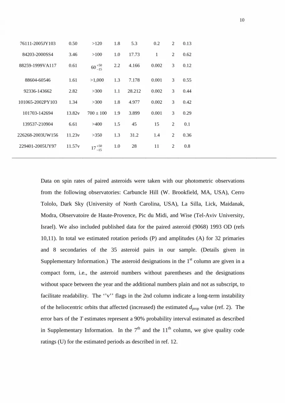
76111-2005JY103 0.50 >120 1.8 5.3 0.2 2 0.13
84203-2000SS4 3.46 >100 1.0 17.73 1 2 0.62
88259-1999VA117 0.61 60 5015+
− 2.2 4.166 0.002 3 0.12
88604-60546 1.61 >1,000 1.3 7.178 0.001 3 0.55
92336-143662 2.82 >300 1.1 28.212 0.002 3 0.44
101065-2002PY103 1.34 >300 1.8 4.977 0.002 3 0.42
101703-142694 13.82v 700 ± 100 1.9 3.899 0.001 3 0.29
139537-210904 6.61 >400 1.5 45 15 2 0.1
226268-2003UW156 11.23v >350 1.3 31.2 1.4 2 0.36
229401-2005UY97 11.57v 17 5015+
− 1.0 28 11 2 0.8
Data on spin rates of paired asteroids were taken with our photometric observations
from the following observatories: Carbuncle Hill (W. Brookfield, MA, USA), Cerro
Tololo, Dark Sky (University of North Carolina, USA), La Silla, Lick, Maidanak,
Modra, Observatoire de Haute-Provence, Pic du Midi, and Wise (Tel-Aviv University,
Israel). We also included published data for the paired asteroid (9068) 1993 OD (refs
10,11). In total we estimated rotation periods (P) and amplitudes (A) for 32 primaries
and 8 secondaries of the 35 asteroid pairs in our sample. (Details given in
Supplementary Information.) The asteroid designations in the 1st column are given in a
compact form, i.e., the asteroid numbers without parentheses and the designations
without space between the year and the additional numbers plain and not as subscript, to
facilitate readability. The ‘’v’’ flags in the 2nd column indicate a long-term instability
of the heliocentric orbits that affected (increased) the estimated dprop value (ref. 2). The
error bars of the T estimates represent a 90% probability interval estimated as described
in Supplementary Information. In the 7th and the 11th column, we give quality code
ratings (U) for the estimated periods as described in ref. 12.

11
Figure 1. Primary rotation periods P1 vs mass ratios q of asteroid pairs. The mass ratio values were
estimated from the differences between the absolute magnitudes of the pair components ∆H. Error bars
represent estimated standard errors of the values. The curves were generated with the model of pair
separation from the post-fission transient proto-binary. The dashed curve is for the set of parameters best
representing the pairs properties and the red and blue curves represent upper and lower limit cases. The
upper curves are for the system’s scaled angular momentum αL = 1.2, primary’s axial ratio a1/b1 = 1.2,
and initial orbit’s normalized semi-major axis Aini/b1 = 2 and 4. The lower curves are for αL = 0.7,
a1/b1 = 1.5, and Aini/b1 = 2 and 4. The choice of a1/b1 = 1.2 for the upper limit cases is because the four
primaries closest to the upper limit curve have low amplitudes A1 = 0.1–0.2 mag. Similarly, the choice of
a1/b1 = 1.5 for the lower limit cases is because the point closest to the lower limit curve has the amplitude
A1 = 0.49, suggesting the equatorial elongation ∼ 1.5.

12
Figure 2. A disparity between the lightcurve amplitudes of the primary components in asteroid pairs and
binary systems. The amplitudes of primaries of asteroid pairs (a) are distributed relatively randomly, and
achieve high values in general while primaries of binary asteroids (b) have more subdued amplitudes.
Either asteroids with shapes closer to rotational symmetry are more prone to form stable binaries, or some
process occurs during the formation process of a binary asteroid to create such a shape.

Supplementary Information
Supplementary Figure 1: A parent asteroid consisting of small component pieces that canbe pulled apart without tensile resistance is spun up to the critical fission frequency by theYarkovsky-O’Keefe-Radzievskii-Paddack (YORP) effect, forms a proto-binary system whichsubsequently disrupts under its own internal dynamics and becomes an asteroid pair. This is aconceptual sketch based on important model assumptions/limitations.
1

1 Pair ages estimation
1.1 Initial data and integrator used
The orbit integrations were nominally run back to the time 500 ky before present. For some
pairs though, the backward integrations showed a possibility for convergence of the orbits not
far beyond the nominal integration time, so we extended it to1 My for them.
As described in refs 1, 3, it is insufficient to perform backward integration of the nominal
solutions for the paired-asteroids as given by the orbit determination from observations. There
are at least two reasons: (i) observation uncertainties that directly project onto the uncertainty
of the orbit determination, and (ii) uncertainty in the force model that may not corrupt the
orbit determination procedure but may affect the orbit evolution on a long term (thousands of
years and more). The first topic is accounted for by considering statistically equivalent past
evolution of the integrated orbits that all reside inside the uncertainty hyper-ellipsoid at the
current epoch. This is typically a rather confined zone in theorbital elements space∗ but it
may quickly stretch to the past. For instance, just taking the typical uncertainty factorδa/a ∼
10−7−10−5 in the determination of the semimajor axis, the simple Keplerian shear would cause
lost of determinism in computing the mean longitude in orbitin ∼(
a3δa
)
Porb ∼ 0.1 − 10 My
(Porb is the orbital period). Things are, however, worse because the lost of determinism is
actually not dominated by the initial orbital uncertainty but more by the underlying chaoticity of
the dynamical problem of gravitational perturbations due to the planets. The relevant timescale
is typically expressed in terms of the Lyapunov time that ranges from∼ 10 ky to ∼ 1 My for
the orbits we are interested in, depending on whether they are close to some prominent orbital
resonances or not. To account for these effects, we have to consider a statistically equivalent
multitude of the past orbital evolutions of a given orbit randomly sampling the uncertainty
∗In our work we consider the best-fit orbital elements and their uncertainties as determined by theOrbFitsoftware and free-available through theAstDyS website athttp://hamilton.dm.unipi.it/astdys/
2

ellipsoid at the current epoch (taken into account as the initial data). In practice, we typically
take50 − 70 such initial data and call them “geometric clones”.
The problem of the propagation model uncertainty (ii) aboveis dominated by our lack of
information about the thermal (Yarkovsky) forces acting differentially on both components in
the pair14,15. These forces make primarily the semimajor axis of the orbitsecularly drift with
(da/dt) as large as∼ 10−4 AU/My ∼ 5 × 10⁻⁸ km/s for kilometer sized objects in the inner
main belt (the(da/dt) may be positive or negative within this range of amplitude).The effect
may be though smaller for larger objects and/or favorably oriented spin axis. Because we do not
know anything about the strength of the Yarkovsky effect on the asteroids in the pairs at this mo-
ment we have to consider different past orbital histories with different values of the Yarkovsky
drift in the semimajor axis. Since the Yarkovsky forces are likely to be dominated by the diurnal
variant14,15, for which(da/dt) ∝ cos γ (γ is the obliquity of the spin axis), we should consider
a uniform distribution of(da/dt) value within the limits set bycos γ = ±1 values. Differ-
ent variants of the past histories with different strength of the Yarkovsky forces, hereafter called
“Yarkovsky clones”, quickly diverge from each other. The effect is again fastest in the longitude
in orbit and the total lost of predictability occurs on a timescale∼(
vorb
3π (da/dt)
)1/2
Porb ∼ 20 ky
only for vorb ∼ 20 km/s and the maximum(da/dt) estimated above. Note that this value is
(i) very short, for most pairs shorter than the Lyapunov timescale, and (ii) is not affected by
improvements in the orbit determination by acquiring new astrometry observations, but only
can improve by observations that constrain the strength of the Yarkovsky effect (such as the
size and/or pole determination). For that reason the uncertainty due to dynamical model incom-
pleteness appears to be the prime reason for our inability toaccurately reconstruct the past fate
of the asteroid-pairs orbits.
In practice, we typically used40 − 70 Yarkovsky clonesfor each of the geometric clones,
uniformly sampling the interval of(da/dt) values between the minimum and maximum values
3

estimated for the asteroid’s size. This provided between2000 and5000 clones altogether for
each of the components in a given pair.
The past orbit of each of these clones was propagated using the SWIFT MVS integrator
(e.g.,http://www.boulder.swri.edu/∼hal/swift.html and ref. 16). All plane-
tary perturbations were included and planets’ positions, together with physical parameters such
as masses, taken from the JPL DE405 ephemeris file. The Yarkovsky acceleration was modeled
as an along-track acceleration with an amplitude12n na
vorb
(
dadt
)
, wheren is the mean motion and
vorb orbital velocity1,3. Integration timestep was5 days and we stored the state vectors of all
integrated clones every10 years (only in some cases of intense search for the age limit of the
pair we had a denser output every1 year).
1.2 How close do we want the components to converge?
Performing the integrations described above we end-up, foreach of the pairs we are interested
in, with a typically 10-30 GB output file that keeps track of the state vectors for each of the
clones for the two asteroids. In the analysis phase we want tojudge whether the possible past
orbits of the asteroids converged to each other and how well.For the latter we need some
quantitative criterion that would sift through our output data and suggest success or failure.
Obviously, most of the pairs have at the starting epoch quitedifferent values of the longi-
tude in orbit for the two asteroids. So the two clouds of clones (for each of the component in
the pair) initially start well separated in space, typically of the order of astronomical unit or
more. However, as the Keplerian shear, chaoticity effects and accumulated differential motion
in longitude of different Yarkovsky clones start to spread the clones along the whole Keplerian
ellipses some of the clones approach closer. Eventually, the two clouds of clones may overlap
(or near-overlap) in some parts of space bringing some of theclones very close each other. We
are primarily interested to know the minimum distance in space to which some clones of the
4

two asteroids in a pair can be brought. But, how close is closein quantitative terms?
For instance, given the fact that asteroids in pairs have frequently their initial semimajor axes
close to few times10−4 AU, it might not be surprising to get the closest clones at a distance of
∼ 50− 100 thousand kilometers which would be just the opposition distance if all other orbital
elements are equal. Obviously a factor of few may be expectedbecause of slight differences
in other orbital elements. It has been suggested in refs 1, 3 that the ultimate-goal criterion to
be met for the past convergence of the paired-asteroids orbits is to bring them closer in space
than the estimated Hill radius of the parent asteroid:† RHill ∼ aD 12
(
4π9
Gρµ
)−1/3
wherea is
the semimajor axis of the pair-components orbits,D the estimated size of the parent body
(roughly obtained to have a volume equal to sum of volumes of the two components),G is
the gravitational constant,ρ is the bulk density andµ is the gravitational parameter of the Sun.
Assuminga in AU andD in kilometers, we haveRHill ∼ 90 aD km. For a multikilometer parent
object in the inner zone of the asteroid belt we haveRHill of the order of several hundreds to a
thousand of kilometers.
However, bringing the two clones at theRHill distance is just part of the condition we want
to meet. The case of an incredible fluke might be recognized bychecking the relative velocity
of the two clones when their distance is smaller thanRHill. Having in mind the model of initially
gentle separation of the two asteroids in the pair, the relative velocity must be smaller (in fact a
fraction) of the escape velocity from the parent object:vesc ∼ D 12
(
8π3
Gρ)−1/2
. Again, plugging
in characteristic parameters we obtainvesc ∼ 0.6 D m/s, where the sizeD of the parent object is
in kilometers. ForD in the kilometer size range the expected relative velocities are of the order
of m/s. Assuming for simplicity again two nearby orbits witha semimajor axis separation of
∼ 10−3 AU we may expect their relative velocity at opposition∼ vorbδa2a
, about 10 m/s. So a few
tens of m/s relative velocities between two nearby orbits atopposition, hence close encounter, is
†This is where actually our model should fail to represent thetrue orbital history of the clones because weconsider them massless particles.
5

not that demanding condition. In reality, though, we shall see below that really good solutions
we shall reach will be characterized by relative velocitiesof decimeters per second or less, a
really small fraction of the estimated escape velocities.
1.3 Examples
Hereafter we give some examples of successful past-convergence simulations for orbits of as-
teroids in pairs and therefore constrains on their age.
The couple (21436) Chaoyichi and 2003 YK39 is a very tight pair residing in the inner part of
the main asteroid belt. Luckily the orbits happen to fall aside the nearby mean motion resonance
M7/12 with Mars and their past orbital reconstruction is notlargely troubled by this source
(the Lyapunov timescale for Chaoyichi’s orbit is∼ 22 ky; http://hamilton.dm.unipi.it/astdys/).
The orbits are reasonably well constrained such that the semimajor axis values have relative
uncertainties of∼ 2.5×10⁻⁸ and∼ 2.5×10⁻⁷, respectively. The larger component in the pair,
(21436) Chaoyichi, is estimated to have roughly∼ 2 km size (for0.2 albedo) and the smaller
component, 2003 YK39, is a sub-kilometer object with a size∼ 0.7 km (for 0.2 albedo). The
composite parent object thus might have a size of∼ 2.1 km and we roughly estimate the Hill
radius of its gravitational influence to beRHill ∼ 600 km and the escape velocityvesc ∼ 1.2 m/s.
Supplementary Figure 2 summarizes the principal information from our propagation of 2500
clones for each of the two asteroids. At each of the output instants, separated by10 y, we ran-
domly selected 5 million trial identifications between the clones of the primary and secondary
components and determined their minimum distance in space and the relative velocity of these
closest pair of clones. These data are shown in the middle andbottom parts of Suppl. Fig. 2. We
note the minimum distances reach about∼ 50 km, well inside the Hill sphere of influence of
either the parent object or the primary. Additionally, these very close clones move with a typical
relative velocity of few centimeters per second only, with minima reaching below a centimeter
6

per second. At the top panel of Suppl. Fig. 2 we show a distribution of successful pair matches
for which a relative distance was smaller thanRHill and their relative velocity was smaller than
vesc. We note this distribution is quasi-Maxwellian with a median value of70 ky. Constructing
a cumulative distribution of these successful matches we may estimate the characteristic range
of ages for this pair by neglecting the first and the last 5% cases in the distribution. With that
we obtain the best estimated age of this pair to be70+70−35 ky. The distribution is skewed toward
the younger ages, as also seen in Suppl. Fig. 2. This is a real effect in the simulation that has to
do with dilution of the clone clouds for the two components asthe time increases to the past.
We now turn to another example, namely a pair (88259) 2001 HJ7 and 1999 VA117 which
resides in the Hungaria zone. As in the previous case, the strongest near-by mean motion res-
onance M7/10 with Mars does not perturb these asteroid orbits and we can reliably reconstruct
their past evolution (the Lyapunov timescale for 2001 HJ7 is 1.3 Myr; ref. 5 and
http://hamilton.dm.unipi.it/astdys/). The orbits are well constrained with rel-
ative uncertainties of the semimajor axis value of∼ 2 × 10⁻⁸ and∼ 2.5 × 10⁻⁸, respec-
tively. The larger component in the pair, (88259) 2001 HJ7, is estimated to have roughly
∼ 2.4 km size (for0.3 albedo appropriate for the Hungaria population) and the smaller compo-
nent, 1999 VA117, has a size∼ 1 km (for 0.3 albedo). The composite parent object thus might
have a size of∼ 2.5 km and we roughly estimate the Hill radius of its gravitational influence to
beRHill ∼ 600 km and the escape velocityvesc ∼ 1 m/s.
The past orbital evolution of the two asteroids, and their clones, has been analysed using the
same approach as above and the result is shown in Suppl. Fig. 3. The situation is very similar
in the previous and this pair such that the minimum distancesreached between the trial-pairs
of different clones we near to∼ 50 km with relative velocities of a few centimeters per second
only. This is less then 10% of the estimated escape velocity from the parent body and this shows
that the smaller component, 1999 VA117, obtained just barely enough relative energy to escape
7

the gravitational well of the primary component separatingfrom it very gently. The analysis of
the distribution of successful clone identifications at different times, top panel in Suppl. Fig. 3,
indicates an age of60+50−15 ky for this pair. This age corresponds well to the result found in ref. 5,
where they obtained more distant close approaches of these two asteroids because their analysis
did not include the Yarkovsky forces.
Our last example is that of a pair (229401) 2005 SU152 and 2005 UY97 that resides in the
middle zone of the asteroid belt. Proper elements of the primary‡ indicate its location in the
asteroid Iannini family, that itself is very young17. Our analysis below indicates, that this pair
should be much younger than the family itself (with an estimated age between 2-5 My; ref. 17).
On a longer term, the past evolution of orbits in this pair is affected by the nearby J11/4 mean
motion resonance with Jupiter, but luckily this does not seen to greatly affect shorter-term prop-
agation. The orbit of the smaller component, 2005 UY97 has only been recovered at a second
opposition in September 2009 and thus is not very accurate. The same is actually true for the
primary. The relative uncertainties of the semimajor axis values are∼ 3×10⁻⁷ and∼ 9×10⁻⁷,
respectively, in this case. Henceforth, the possibilitiesof predicting/constraining the past orbital
evolution for this pair will improve after more astrometry observations are taken during the next
few years. The larger component in the pair, (229401) 2005 SU152, is estimated to have roughly
∼ 1.7 km size (for0.15 albedo) and the smaller component, 2005 UY97, has probably a size of
∼ 1.1 km (for 0.15 albedo). The composite parent object thus might have a size of ∼ 1.9 km
and we roughly estimate the Hill radius of its gravitationalinfluence to beRHill ∼ 500 km and
the escape velocityvesc ∼ 1 m/s.
We propagated about 5000 geometric and Yarkovsky clones forboth asteroids in this pair
over the past 100 ky time interval (the youth of this pair is suggested by very close corre-
spondence of the osculating orbital elements in this case).Using the same approach as in the
‡Seehttp://hamilton.dm.unipi.it/astdys/.
8

previous two cases we give our results in Suppl. Fig. 4 (because of larger number of clones
we now used 10 million of trial identifications of the clone pairs at each output time, sampled
by 1 y step). The minimum distances we could reach between the trial pairs of clones were as
small as∼ 10 km with a relative velocity of millimeters per second (note this is already com-
parable to the physical size of the two asteroids). Obviously the success here goes along with
the suggested young age of17+25−10 ky for this pair.
Unfortunately, in most of the other cases orbital uncertainties prevented us to reach such a
satisfactory result as above. Very often we are able to provepossible convergence of a subset
of clones to distances comparable to the Hill sphere of the parent object and comfortably small
relative speed (typically smaller than meter per second), but we set only the lower limit for the
pair’s age. The upper limits, such as seen of Suppl. Figs. 2 to 4, are in these other cases pushed
well beyond the500 ky limit of our integration. Future orbital constrains, more astrometry and
physical observations able to constrain the Yarkovsky forces, and using more orbital clones for
pairs with ages larger than∼ 100 ky could lead to improvements in the age determination for
these pairs.
1.4 Implications from the backward integrations
The fact that for nearly all of the pairs in our sample we foundthe convergence of a subset
of their clones to the level of (or close to, for some older ones) the estimated Hill radius of
the parent object at small relative velocity strengthens the case that they are real, genetically
related pairs. While in refs 1, 2 we made efforts to characterize the statistical significances of
the pairs and demonstrate they are real, some issues in the method remained debated5. The
ability to converge to the level that strongly distincts real pairs from coincidental associations
therefore increases credibility of most of the pairs in our sample. We note that we did not
reach a convergence during the past1 Myr (the maximum backward integration time in this
9

work) for four pairs: (1979) Sakharov and (13732) Woodall, (2110) Moore-Sitterly and (44612)
1999 RP27, (32957) 1996 HX20 and (38707) 2000 QK89, and (60546) 2000 EE85 and (88604)
2001 QH293. We consider two possible reasons for not reaching convergence for a pair: (i) it
is a random coincidental couple of asteroids from the background population, or (ii) its age is
greater than the integration interval of1 Myr. At this moment we cannot resolve between these
two alternatives with the backward integrations for the four pairs. Their lowdprop values in the
range 1 to 9 m/s as well as mostly low probabilities of chance coincidence of asteroids from the
background population suggest that they may be real pairs older than 1 Myr, but it needs to be
confirmed with future studies. In any case, we note that the data on primary spin rates and∆H
for all the four suspect old pairs fit with the model of pair separation presented in our paper.
An important implication from the pair age estimation effort is estimating or constraining
a magnitude of change of the primary spin rate by the YORP effect. The premise used when
comparing the data for the pairs with outcomes of the model inthis work is that the primary
spin rate did not change significantly since separation of the pair, so the current observedP1
value can be taken as representing a final rotation rate that the primary reached at the end of
the pair separation. If a magnitude of change of the spin ratedue to the YORP effect was not
much less than the spin rate itself, we would have to take thatadditional effect into account in
the comparison of the data with the model.
As an example, we present an estimation of the magnitude of the YORP effect on the pri-
mary of the pair (229401)-2005 UY97. The primary (229401) 2005 SU152 rotates slowly, with
P1 ∼ 28 hr, i.e.,ω1 ∼ 6.2 × 10⁻⁵ s−1. Rescaling the YORP spin evolution rate estimated in
ref. 18 to the size and heliocentric distance of (229401), weestimate the secular rate of change
of the angular velocity due to YORP of(dω/dt) ≃ 5×10⁻⁵ s−1 My−1. During the pair’s age of
∼ 17 kyr, the YORP effect might have changed the angular frequency of (229401) by no more
than∼ 10−6 s−1, i.e., by less than 2%. This change of the spin rate due to YORPis negligible
10

for the purpose of the comparison of the data with the model (and actually in this particular
case where there is present also a substantial uncertainty in theP1 estimate itself, the possible
change due to YORP is also much less than the observational uncertaintyδP1). We conclude
that YORP could not affect the rotation of the primary (229401) significantly and the observed
P1 value is a very good proxy for a final rotation rate that the primary reached at the end of the
pair separation. Similar results of the relative (in)significance of the YORP effect were obtained
also for the other pairs in our sample.
11
2 Photometric observations of paired asteroids
We carried out photometric observations using our standardasteroid lightcurve photometry
techniques and obtained estimates for rotation periods andamplitudes for 32 primaries (i.e.,
larger members) and 8 secondaries (smaller members) of the 35 asteroid pairs in our sample. In
Supplementary Table 1, there are listed participating observatories and instruments used. Sup-
plementary Table 2 gives observational circumstances of the observations. We give references
and descriptions of observational procedures on individual observatories in following.
CarbH0.35, 0.50- Observational and reduction procedure at Carbuncle Hill Observatory is
described in ref. 19.
CTIO0.9- General information about the system is available at
http://www.ctio.noao.edu/telescopes/36/0-9m.html. The telescope was op-
erated in service mode and we used the full chip setting with the FOV13′ × 13′, the readout
noise∼ 5 ADU = 3e− and V filter. Integration times were mostly 120 s.MaxImDLwas used to
process and reduce the observations.
CTIO1.0- General information about the system is available at
http://www.astronomy.ohio-state.edu/Y4KCam/detector.html. We used
the2 × 2 binning mode. Integration times were mostly 120 s.MaxImDLwas used to process
and reduce the observations.
Danish1.54- Technical information on the telescope is available at
http://www.eso.org/lasilla/telescopes/d1p5/. Most of the observations were
done in the Cousins R filter. Integration times were 60 to 180 s, depending on apparent sky mo-
tion of targeted asteroid so that to get an image streak not longer than 2 pixels (i.e., comparable
to a typical seeing at the site). The data were processed and reduced withMaxImDL and our
photometric reduction software packageAphot32, both using the aperture photometry tech-
12

nique. A part of the observations was calibrated in the Johnson-Cousins system using Landolt
standard stars20.
DarkSky and PROMPT- Appalachian State University’s Dark Sky Observatory is located
in the mountains of northwestern North Carolina at an elevation of 1000 meters. The 0.8-m
telescope is equipped a Photometrics CCD camera with a1024 × 1024 25-micron pixel Tek
chip. The field of view is8′ × 8′ with 0.50 arcsec/pixel.
The University of North Carolina at Chapel Hill’s PROMPT observatory (Panchromatic
Robotic Optical Monitoring and Polarimetry Telescopes) ison Cerro Tololo. PROMPT consists
of six 0.41-m outfitted with Alta U47+ cameras by Apogee, which make use of E2V CCDs. The
field of view is10′ × 10′ with 0.59 arcsec/pixel.
All raw image frames were processed (master dark, master flat, bad pixel correction) using
the software package MIRA. Aperture photometry was then performed on the asteroid and three
comparison stars. A master image frame was created to identify any faint stars in the path of
the asteroid. Data from images with background contamination stars in the asteroid’s path were
then eliminated.
Lick - Observations were collected using the Lick Observatory 1m-Nickel telescope and its
Direct Imaging Camera at the f/17 Cassegrain focus in R band.The detector is a thinned, Loral,
2048 × 2048 CCD with 15-micron pixels, corresponding to 0.184 arcsec/pixel, so a FOV of
6.3×6.3 arcmin. The observations were remotely conducted from a control room located at the
Department of Astronomy of the University of California at Berkeley. The relative photometry
measurements were made using an automatic software developed in Python 2.5. It detects and
reduces the asteroid and three selected nearby bright comparison stars on each processed frame
(after dark subtraction, badpixel removal, and flat-field correction). The flux is estimated with
an aperture photometry technique using a Gaussian fit function. A reducer checks the frames
for a possible contamination of the images of the asteroid and the comparison stars by a remnant
13

bad pixel, cosmic rays, or a background star and such affected data points are discarded.
Maidanak- Observations were carried out at Maidanak Astronomical Observatory (Uzbek-
istan) with 1.5-m telescope AZT-22 (Cassegrain f/7.7), equipped with back-illuminated Fairchild
486 CCD camera (4096 × 4096 CCD,15 × 15 µm pixels, 0.27 arcsec/pixel, FOV18.4 × 18.4
arcmin) and Bessell UBVRI standard filters. The observations were carried out in the R band
and were reduced in the standard way with master-bias subtracting and median flat-field di-
viding. The aperture photometry of the asteroid and comparison stars in the images was done
with the ASTPHOT package developed at DLR21. The effective radius of aperture was equal
to 1 − 1.5× the seeing that included more than 90% of the flux of a star or the asteroid. The
relative photometry of the asteroid was done with typical errors in a range of0.01 − 0.02 mag
using an ensemble of comparision stars.
Modra - Observational system, data analysis and reduction process are described in ref. 22.
PdM0.6- Details about the telescope are available athttp://astrosurf.com/t60.
Reduction was performed using the Prism V7 software.
T120-OHP- We used the 1.2-m Newton f/6 telescope equipped with a CCD TeK 1024 ×
1024 in the R band, with the field of view of 12 arcmin and 0.7 arcsec/pix. The standard
reduction (flat-field correction, dark substraction, badpixel and cosmic removal) was performed.
Relative photometry was performed with a custom software written in IDL, using a fiting of the
Gauss function. Images affected by close encounters with background stars were discarded by
the user.
Wise0.46+1.0- Observations were performed using the two telescopes of the Wise Obser-
vatory (Tel-Aviv University) in the Israeli desert (MPC code 097): A 1-m Ritchey-Chretien
telescope and a 0.46-m Centurion telescope (see ref. 23 for adescription of the telescope and
its performance). The 1-m telescope is equipped with a cryogenically-cooled Princeton Instru-
ments CCD. At the f/7 focus of the telescope this CCD covers a field of view of13′ × 13′ with
14

1340 × 1300 pixels (0.58 arcsec per pixel, unbinned). The 0.46-m telescope was used with an
SBIG STL-6303E CCD at the f/2.8 prime focus. This CCD covers afield of view of 75′ × 50′
with 3072×2048 pixels, with each pixel subtending 1.47 arcsec, unbinned. Rand V filters were
used on the 1-m telescope while observations with the 0.46-mtelescope were unfiltered. Inte-
gration times were 120-300 s, all with auto-guider. The reduction, measurements, calibration
and analysis methods of the photometric data are fully described in refs 24, 25.
We analysed the observations using the standard Fourier series method26,27,28.
Data for most of the asteroids given in Supplementary Table 2and presented in plots with
composite lightcurves (Suppl. Figs. 6 to 44) are self-explanatory, but comments on four of
them are given below. In a few cases where lightcurve amplitude changes were observed, we
give an amplitude at the lowest observed solar phase in Table1 as it was least affected by the
amplitude-phase effect29.
(6070) Rheinland was observed over a 4-month long interval during July-November 2009.
The observations showed variations of synodic period and amplitude of the asteroid that will be
useful data for future spin axis and shape modeling. In Suppl. Fig. 10, we plot the data and fit
with a constant synodic period.
(78024) 2002 JO70: A lower limit on its period of 17 hr was estimated from the data of
2009 Sept. 26 that showed a continuous increase of brightness during the 4.4-hr long observ-
ing interval. The data from the previous night of 2009 Sept. 25 showed no variation greater
than 0.02 mag and they are consistent with being taken aroundan extremum of long-period
lightcurve. See Suppl. Fig. 32.
(101703) 1999 CA150: A few first measurements taken on 2009 Sept. 20 showed an atten-
uation that resembles mutual events observed in orbiting binaries30. The possibility that this
primary is actually a bound orbiting binary needs to be confirmed with more observations in
future. See Suppl. Fig. 38.
15

(139537) 2001 QE25: A continuous brightness decrease by 0.10 mag observed during the
7.7-hr long observing interval on 2009 March 19 gives a lowerlimit on the asteroid’s period
of 30 hr. In Supplementary Table 1, we give a period of45 ± 15 hr, as periods longer by a
factor of 2 of the lower limit are less likely. The shorter session of 2009 March 18 showed no
brightness variation greater than 0.04 mag during the 5.4-hr long interval, consistent with being
taken around an extremum of long-period lightcurve. See Suppl. Fig. 40.
16

3 Correlation between primary spin rate and pair mass ratio
The primary spin rate is correlated with the mass ratio between components of the asteroid pair
(Fig. 1). Here we give a test of the statistical significance of the correlation between the two
variables.
The model of a proto-binary separation given in Sect. 5 predicts that there is a linear correla-
tion betweenω21 ≡ (2π/P1)
2 andq (Eq. 15). We computed the correlation coefficient for theω21
andq data of the sample of 32 asteroid pairs,r = −0.7349. This sample correlation coefficient
is a point estimate of the population parameterrpop, the correlation coefficient in the population
that was sampled. To investigate whether the observed correlation is statistically significant,
i.e., whether the sample correlation coefficient is different from0 at a high confidence level, we
test the null hypothesisrpop = 0 using Student’s t statistics,
t =r
sr
, where sr =
√
1 − r2
n − 2, (1)
and the degrees of freedomn − 2 = 30. We gett = −5.9351. Sincet0.001 = 3.646 for the
degrees of freedom of 30, we get that the correlation betweenthe primary spin rate and the pair
mass ratio is significant at a level higher than 99.9%.
17

4 Fission mechanics
Rotating bodies can be characterized by their total energy and rotational angular momentum.
When the body is a single entity, the rotational angular momentum vector is simply computed
as:
L = I · ω (2)
whereI is the rotational inertia dyad andω is the angular velocity of the body. The total energy
of a rotating body is also driven by its rotation rate, but is also a function of its mass distribution
through its self-potential (U):
E =1
2ω · I · ω + U (3)
The rotational inertia tensor and the self-potential are defined through the mass distribution of
the body:
I =
∫
β
[(ρ · ρ)U − ρρ] dm (4)
U = −G
2
∫
β
∫
β
dmdm′
|ρ − ρ′|(5)
whereβ represents the mass distribution,U is the identity dyad,ρ, ρ′ is the location in the body
of a mass elementdm, dm′, andG is the gravitational constant.
Due to the well-documented YORP effect the angular velocityof asteroids of size< 10km
in diameter can be changed in time spans short relative to their lifetime. As a rigid or rubble-
pile body undergoes changes in its rotation rate the mass distribution parameters can remain
constant over a relatively wide range of rates, unlike a fluidic body which will change its shape
incrementally with changes in total angular momentum. Despite this, if large enough changes
in the total angular momentum of the object occur, even collections of rigid components can
undergo shifts into configurations that have a lower total energy, with excess energy being
18

dissipated thermally or through seismic waves4,13,31. This occurs as the angular momentum
of a collection of rigid components resting on each other changes, and represents different
configurations of the mass that may have a lower energy at thatgiven angular momentum.
If the total system angular momentum increases sufficiently, the minimum energy config-
uration for the body will eventually involve components of the body entering orbit about each
other4,13. Once this occurs a different regime of physics takes over and the system can evolve
rapidly and dynamically with the components in orbit about each other. A detailed analysis of
the fission process shows that such systems will invariably enter a highly unstable dynamical
state, and the orbit and rotations of each component will vary chaotically as they interchange
energy and angular momentum between each other8. The transition from a collection of rigid
components resting on each other to one where two of the collections are in orbit liberates
energy that can drive the system dynamically.
The total angular momentum and energy are, in general, conserved across fission but be-
comes decomposed into multiple components:
I · ω = I1 · ω1 + I2 · ω2 +M1M2
M1 + M2r × v (6)
1
2ω · I · ω + U =
1
2ω1 · I1 · ω1 +
1
2ω2 · I2 · ω2 +
1
2
M1M2
M1 + M2v · v + U11 + U22 + U12 (7)
whereM1 andM2 are the masses of the two components,r andv are the relative position and
velocity vector between these two components,Uii is the self-potential of the new components
andU12 is the mutual potential between the components.
U12 = −G
∫
β1
∫
β2
dm1dm2
|ρ1 − ρ2|(8)
The mutual potential represents a conduit for energy being transferred from rotational to trans-
lational energy and vice-versa and can be surprisingly effective.
The fundamental characteristic of the system after it undergoes fission is its free energy,
defined as the total energy minus the self-potentials of eachcomponent. If the free energy is
19

positive, the two components can escape from each other and become an “asteroid pair”. If
the free energy is negative, then such a mutual escape is impossible, barring release of energy
from changes in the self-potentials of the components or an exogenous source of angular mo-
mentum and energy. A positive free energy does not necessarily dictate that the system disrupt.
Constancy of the free energy requires that the self-potentials of the system after fission will not
change, i.e., that the mass distribution is fixed after fission. This is a reasonable assumption as
the components are under lower stresses when in orbit than they were in when in close proxim-
ity to each other. However, even if changes in the self potentials occur, the free energy will still
provide a crucial parameter for this system.
The free energy can be represented as:
EFree =1
2ω1 · I1 · ω1 +
1
2ω2 · I2 · ω2 +
1
2
M1M2
M1 + M2v · v + U12 (9)
If the system undergoes disruption, we note that the mutual potential will decrease to0 and the
translational kinetic energy will approach hyperbolic escape speeds. Thus, if disruption occurs
we find:
EFree =1
2ω1 · I1 · ω1 +
1
2ω2 · I2 · ω2 +
1
2
M1M2
M1 + M2v2∞ (10)
We note that all of these terms are positive by definition, andthus if the free energy is negative,
a mutual disruption cannot occur. Further, escape speeds can be quite small, indicating that
EFree >1
2ω1 · I1 · ω1 +
1
2ω2 · I2 · ω2 (11)
Thus if the free energy is positive but small, escape is possible but requires that the rotational
kinetic energy of the components must be reduced, indicating that energy has been drawn from
these modes to enable escape. As the majority of the rotational kinetic energy will reside in
the larger component, a consequence is that the larger component will naturally be rotating at a
slower rate, with the resulting rotation rate approaching zero with the free energy. The rotation
20

rate of the smaller component can still remain relatively high, as its much lower mass allows it
to “hide” relative to the more massive body.
Being equipped with the results of the theory of fission mechanics, we constructed a simple
model of the post-fission system interpreting the observed spin rates of asteroid pairs primaries.
The model, its assumptions and mathematical formulation are given in the next section.
21

5 Model of a proto-binary separation
To quantify our asteroid pairs we model the post-fission system as a binary of two components
starting in close proximity and with the total angular momentum in the range of critical values
as observed in close binary systems6. Assuming the mass distribution in the components of
the system is fixed in this post-fission evolution phase, the free energy of the system is con-
stant. Energy is transferred between the rotational and orbital energy by a conduit of the mutual
potential between the components. The model is following:
• The initial state is a close binary.
• The end state is a barely escaping satellite (parabolic orbit).
• Both the free energy and the total angular momentum of the system are conserved.
• The total angular momentum is close to critical (αL ∼ 1), as we observe in small binary
systems6.
• The spin vectors of the components are coplanar with their mutual orbit, i.e., rotation and
orbit poles are aligned. The rotations are prograde and around the principal axes of the
bodies.
• We assume a constant secondary period, neglecting possiblechanges in the secondary’s
rotational angular momentum due to its small size, and we take it to beP2 = 6 hr (ap-
proximately a mean of the observed secondary rotation periods).
• Bulk density of both components isρ = 2 g/cm3.
The first five assumptions are fundamental, whereas the last two ones are less critical as out-
comes of the model are less sensitive to variations of the twoparameters within observed or
plausible ranges.
22

The mathematical formulation of our model follows. The freeenergy of the system is
EFree =1
2I1ω
21 +
1
2I2ω
22 − G
M1M2
2A, (12)
whereIi, ωi, Mi are the moment of inertia around the principal axis, the angular velocity and
the mass of thei-th body (1 for primary, 2 for secondary), respectively, andA is the system’s
orbit semimajor axis.
Since the free energy andω2 are constant, we get
1
2I1ω
21ini − G
M1M2
2Aini
=1
2I1ω
21final, (13)
where the subscripts “ini” and “final” denote initial and endstate values of the parameters. Note
that1/Afinal = 0 for the end state of a barely escaping satellite (parabolic orbit).
In Eq. 13, we substituteM2 ≡ qM1, the moment of inertia of the primary
I1 =M1
5(a2
1 + b21), (14)
andM1 = V1ρ, whereV1 is the volume of the primary. We assume thatV1 is equal to the
volume of the dynamically equivalent equal mass ellipsoid (DEEME) of the primary, i.e.,V1 =
a1b1c1π4/3. The parametersa1, b1, c1 are semiaxes of the DEEME of the primary. After the
substitutions, we get
ω21final = ω2
1ini −203πqGa1
b1c1b1
ρ[
1 +(
a1
b1
)2]
Aini
b1
. (15)
The initial angular velocity of the primaryω1ini is computed from the normalized total an-
gular momentum of the binary system. It was defined in ref. 6:
αL ≡L1 + L2 + Lorb
Leqsph
, (16)
23

whereL1 andL2 are rotational angular momentum of the primary and the secondary, respec-
tively, Lorb is the orbital angular momentum, andLeqsph is the angular momentum of the equiv-
alent sphere spinning at the critical spin rate. The quantities in the numerator in Eq. 16 are given
with following formulas:
L1 =M
5(1 + q)(a2
1 + b21)ω1, (17)
L2 =qM
5(1 + q)(a2
2 + b22)ω2, (18)
Lorb =qM
(1 + q)2
√
GMA(1 − e2), (19)
whereM ≡ M1 + M2 is the total mass of the system, andai, bi, ci are semiaxes of the DEEME
of the ith body. The quantity in the denominator in Eq. 16 is the angular momentum of the
equivalent sphere spinning at the critical spin rate. It is
Leqsph =2
5M
(
3
4πV1
)2/3
(1 + q)2/3ωcsph, (20)
whereωcsph is the critical spin rate for the sphere with the angle of friction of 90◦ and it is
ωcsph =
√
4
3πρG. (21)
We have evaluated this disruption scenario for a number of values of scaled angular momen-
tum (αL), normalized initial semi-major axis (Aini/b1), and ratios of the primary’s axes (a1/b1
andb1/c1), wherea1, b1, c1 are the long, intermediate, and short axis of the dynamically equiva-
lent equal mass ellipsoid of the primary. Forb1/c1, we assumed a value of 1.2, corresponding to
a low primary polar flattening (cf. with valuesb1/c1 between 1.1 and 1.2 estimated for primaries
of NEA binaries 1999 KW4 and 2002 CE26 (refs 32, 33).Values of the primary’s equatorial ratio
a1/b1 were varied between 1.1 and 2.0, i.e., in the range of primaryelongations suggested by
the observed primary amplitudes. We assumed a value of 1.3 for the equatorial axis ratio of
the secondary (a2/b2), corresponding to the observed low to moderate secondary amplitudes.
24

The normalized total angular momentumαL was varied over an interval 0.7 to 1.3, which is the
range observed for orbiting binaries withD1 < 10 km (ref. 6). The initial relative semi-major
axisAini/b1 values were taken in the range from 2 to 4. Values in the upper half of the range, 3
to 4, have been observed in known very close asteroid binaries, while values between 2 and 3
are extremely close initial orbits near or below the Roche’s limit for strengthless satellites.
For each set of parameters we generated a corresponding rotation period of the primary,
assuming a separated pair, as a function of mass ratioq between the pair components. Over the
varied ranges of parameters, this model shows the same general character as the asteroid pairs
data plotted in Fig. 1. The dashed line plotted there is forαL = 1.0, a1/b1 = 1.4 andAini/b1 =
3. This set of parameters can be considered as the best representation of pair parameters. In
particular, the total angular momentum content of 1.0 is about the mean of the distribution of
αL values in small binaries, and the axial ratio of 1.4 is about amean of equatorial elongations
of pair primaries suggested by their observed amplitudes. We have also plotted four additional
curves that represent limit cases.
25

Discussion 1Predictions and implications of the fission theory
The results of the fission theory4,8,13 predict the observational data presented in Fig. 1. The
primary rotation periods become long with increasing mass ratio, consistent with the free en-
ergy of a binary system formed by rotational fission approaching zero and the non-existence of
separated pairs with mass ratios appreciably larger than the predicted cutoff. The limit curves
of our model forαL = 1.2 go up toq = 0.4, i.e., a bit behind the upper limitq ∼ 0.2 estimated
in ref. 8. It is because the value ofαL = 1.2 is actually a super-critical amount of angular
momentum for a body with the low elongation of the upper limitcase and such system can form
from an original elongated body that is re-shaped during satellite’s formation with a resulted
low-elongation primary (see ref. 6, Fig. 1). The limit ofq ∼ 0.2 is valid if the components be-
have like rigid bodies during a fission of the original body. An alternative explanation is that the
few systems closest to the upper limit may have a higher bulk density than the assumed value of
2 g/cm3, with the total angular momentum not exceeding the criticalvalue for a low-elongation
body.
It is important to note that the theory predicts that fissioned binary asteroids are always
initially unstable, independent of the free energy and massratio, and thus undergo chaotic
variations immediately after fission8. The time scale for these systems to transition from their
initial fission proto-binary state to an orbitally disrupted, asteroid pair state (for those systems
with positive free energy) is not immediate but occurs aftera characteristic time span of tens to
hundreds of days, with a median time estimated to be 0.6 yr (see Suppl. Fig. 5).
It is important to note the existence of binary asteroids with mass ratios larger than this
threshold6. Thus, such objects exist but, if formed from the rotationalfission process described
here, these binary asteroids should not be able to disrupt bythemselves. The existence of this
26

population across the mass ratio threshold, and the fact that asteroid pairs are found consistent
with the disruption threshold§, shows a remarkable consistency with the rigid body rotational
fission model for the creation of binary asteroids and asteroid pairs.
However, this model may not cover all aspects of asteroid rotational fission. The effect of
adding angular momentum via YORP to a continuum model of ellipsoidal asteroids modeled
as a cohesionless soil was studied and it was found that, theoretically, these bodies should
reshape themselves as the angular momentum increases34. While the transition of such a body
to actual fission has not been studied in the work, they indicate that such fission could occur. In
their model the transition to a binary asteroid may be distinct from the rigid body fission model
discussed above, although no clear predictions on the initial configuration of such a system have
been made. The current results do provide a target state for such a fission process, however.
An alternate formation process for binary asteroids was proposed in ref. 7. This model
was motivated by simulations of asteroid fission using a numerical model of a parent body,
consisting of cohesionless, hard spheres resting on each other, with its spin rate increasing
(simulating YORP) until material left the surface. It is significant to note that the numerical
runs were only allowed for evolution over less than 10 orbitsfollowing the fission of material
before the spin rate of the primary was incremented again. From their computations they found
that the secondary satellite was formed in orbit following inter-particle collisions. However,
such a formation mechanism should dissipate excess energy in the system, and hence would
not lead to a system that can spontaneously undergo escape. Additionally, in this model the
satellites form at a distance where orbital ejection does not occur. Finally, we note that this
model of stable binary formation does not predict the observed correlation between the primary
period and mass ratio of asteroid pairs and thus is likely notthe source of these asteroid pairs.
§While most asteroid pairs identified as probably genetically related pairs in ref. 2 have∆H > 1, implyingq about or less than 0.2, a smaller fraction of pairs have low estimated∆H values. We suspect that the absolutemagnitude estimates of one or both members of the asteroid pairs with the anomalous low∆H values may be inerror. Accurate absolute magnitude estimates for the asteroids are needed to check the theoretical prediction.
27

Discussion 2Assumptions and uncertainties in the size and mass ratios es-timates
The assumption that the components of an asteroid pair have the same albedo and bulk density
is plausible for the bodies formed by a fission or breakup of the original parent asteroid of a pre-
sumably homogeneous composition. As a result of details of the pair formation mechanism, the
two components might differ in a size distribution of piecesof the regolith and its surface frac-
tion coverage, and cosmic ray exposure age of the surface material, but we have little knowledge
on these possible differences and how large albedo difference they could cause. Photometric
observations of orbiting binaries are consistent with the primary and secondary albedos being
same to within 20% (refs 30, 35). If it is valid also for components of asteroid pairs, then the
uncertainty of the albedo ratio less than 20% propagates to an uncertainty of the ratio of effec-
tive diameters between pair components of less than 10%. In this work we neglect this possible
uncertainty and assume that the components have the same albedo.
It was found that bulk densities of the secondary and primaryof 1999 KW4 differ by a factor
of 1.43, but with a relative uncertainty of about 30%, so it was only a marginally significant
difference32. Another, implicit assumption in the conversion between the size and mass ratios
is that the effective diameterD estimated from the absolute magnitude is proportional to a
mean diameterDmean that is related to the volume of the asteroidV = πD3mean/6. Deviations
from this assumption can cause some systematic errors in themass ratio estimates, because the
effective diameter is actually related to the cross-section rather than volume of an asteroid, and
the cross-section-to-volume ratio is a function of the asteroid’s shape and viewing aspect, but
we neglect this additional uncertainty source in this study.
28

15. Bottke, W. F., Jr., Vokrouhlicky, D., Rubincam, D. P. & Broz, M. inAsteroids III(eds Bottke
Jr., W. F., Cellino, A., Paolicchi, P. & Binzel, R. P.) 395–408 (Univ. Arizona Press, 2002).
16. Levison, H. F. & Duncan, M. J. The long-term dynamical behavior of short-period comets.
Icarus108, 18–36 (1994).
17. Nesvorny, D., Bottke, W. F., Levison, H. F. & Dones, L. Recent Origin of the Solar System
Dust Bands.Astrophys. J.591, 486–497 (2003).
18. Capek, D. & Vokrouhlicky, D. The YORP effect with finite thermal conductivity. Icarus
172, 526–536 (2004).
19. Warner, B. D. & Pray, D. P. Analysis of the Lightcurve of (6179) Brett.Minor Planet Bull.
36, 166–168 (2009).
20. Landolt, A. U. UBVRI photometric standard stars in the magnitude range11.5 < V < 16.0
around the celestial equator.Astron. J.104, 340–371 (1992).
21. Mottola, S.et al. The Near-Earth objects follow-up program: first results.Icarus 117,
62–70 (1995).
22. Galad, A., Pravec, P., Gajdos,S., Kornos, L. & Vilagi, J. Seven asteroids studied from
Modra observatory in the course of binary asteroid photometric campaign.Earth Moon Planets
101, 17–25 (2007).
23. Broschet al. The Centurion 18 telescope of the Wise Observatory.Astrophys. Space Sci.
314, 163–176 (2008).
24. Polishook, D. & Brosch, N. Photometry of Aten asteroids–More than a handful of binaries.
Icarus194, 111–124 (2008).
25. Polishook, D. & Brosch, N. Photometry and spin rate distribution of small main belt aster-
oids. Icarus199, 319–332 (2009).
26. Harris, A. W.et al. Photoelectric observations of asteroids 3, 24, 60, 261, and863. Icarus
77, 171–186 (1989).
29

27. Pravec, P.,Sarounova, L. & Wolf, M. Lightcurves of 7 near-Earth asteroids. Icarus 124,
471–482 (1996).
28. Pravec, P.et al. Fast rotating asteroids 1999 TY2, 1999 SF10, and 1998 WB2. Icarus147,
477–486 (2000).
29. Zappala, V., Cellino, A., Barucci, A. M., Fulchignoni,M. & Lupishko, D. F. An analysis of
the amplitude-phase relationship among asteroids.Astron. Astrophys.231, 548–560 (1990).
30. Pravec, P.et al. Photometric survey of binary near-Earth asteroids.Icarus 181, 63–93
(2006).
31. Guibout, V. & Scheeres, D. J. Stability of Surface Motionon a Rotating Ellipsoid.Celest.
Mech. Dyn. Astr.87, 263–290 (2003).
32. Ostro, S. J.et al. Radar imaging of binary near-Earth asteroid (66391) 1999 KW4. Science
314, 1276–1280 (2006).
33. Shepard, M. K.et al. Radar and infrared observations of binary near-Earth Asteroid
2002 CE26. Icarus184, 198–210 (2006).
34. Holsapple, K. A. On YORP-induced spin deformations of asteroids. Icarus205, 430–442
(2010).
35. Scheirich, P. & Pravec, P. Modeling of lightcurves of binary asteroids.Icarus200, 531–547
(2009).
AcknowledgementsResearch at Ondrejov was supported by the Grant Agency of the Czech
Republic, Grants 205/09/1107 and 205/08/H005. D.V. was supported by the Research Program
MSM0021620860 of the Czech Ministry of Education. D.P. was supported by anIlan Ra-
mondoctoral scholarship from the Israeli Ministry of Science,and he is grateful for guidance
and support provided by Dr. N. Brosch and Prof. D. Prialnik. D.J.S. acknowledges support by
NASA’s PG&G program grant NNX 08AL51G. A.W.H. was supported by NASA grant NNX
09AB48G and by National Science Foundation grant AST-0907650. Work at Modra Obser-
30
vatory was supported by the Slovak Grant Agency for Science VEGA, Grant 2/0016/09. The
observations on Cerro Tololo were performed with the support of CTIO and Joselino Vasquez,
using telescopes operated by SMARTS Consortium. Work at Picdu Midi Observatory has
been supported by CNRS – Programme de Planetologie. Operations at Carbuncle Hill Obser-
vatory were supported by a Gene Shoemaker NEO Grant from the Planetary Society. Support
for PROMPT has been provided by the National Science Foundation under awards CAREER-
0449001, AAG-0707634, and MRI-0836187. F.M. and B.M. were supported by the National
Science Foundation under award number AAG-0807468. We thank to O. Bautista, T. Moulinier
and P. Eclancher for assistance with observations with the T60 on Pic du Midi.
31

Supplementary Table 1: Observatories, Instruments, and ObserversObs/Tel Code Observatory Telescope Diameter (m) ObserversCarbH0.35, 0.50 Carbuncle Hill 0.35, 0.50 PrayCTIO0.9 CTIO 0.90 Longa, PozoCTIO1.0 CTIO 1.0 Pozo, BarrDarkSky Dark Sky DSO-32 0.81 PollockDanish1.54 La Silla Danish 1.54 Galad, Pravec, HenychLick Lick Nickel 1.0 Marchis, MacomberMaidanak Maidanak AZT-22 1.50 Krugly, SergeevModra Modra 0.60 GaladOHP OHP OHP-120 1.20 VachierPdM0.6 Pic du Midi 0.60 Leroy, Bautista, Moulinier, EclancherPdM1.0 Pic du Midi 1.0 Colas, MaquetPROMPT PROMPT Prompt5 0.41 PollockWise0.46, 1.0 Wise 0.46, 1.0 Polishook
32

Supplementary Table 2: Observational circumstances ofpaired asteroids. Given are the mid-time of observing in-terval rounded to the nearest tenth of a day, telescope codefrom Table 1, filter (C for clear or undefined), duration of theobserving interval, the helio– and geocentric distances andsolar phase of the asteroid at the mid-time.
Dates Obs/Tel Filter Int(hr) r(AU) ∆(AU) phase(◦)(2110) Moore-Sitterly
2008-11-26.3 PROMPT R 1.2 2.224 1.281 9.82008-11-28.3 PROMPT R 3.6 2.228 1.276 8.72008-12-06.3 PROMPT R 3.2 2.245 1.268 4.32008-12-07.2 PROMPT R 2.1 2.246 1.268 3.82008-12-07.3 PROMPT R 2.5 2.247 1.268 3.82008-12-08.2 PROMPT R 2.3 2.248 1.268 3.32008-12-09.2 PROMPT R 0.6 2.250 1.269 2.72008-12-09.3 PROMPT R 3.2 2.251 1.269 2.72008-12-10.2 PROMPT R 2.4 2.252 1.270 2.22008-12-10.3 PROMPT R 2.1 2.253 1.270 2.12008-12-20.0 Wise0.46 C 2.8 2.272 1.294 3.62008-12-23.8 Modra C 3.9 2.279 1.310 5.62008-12-24.0 Modra C 3.0 2.280 1.311 5.72008-12-25.8 Modra C 3.2 2.283 1.320 6.72008-12-27.9 Modra C 3.6 2.287 1.332 7.72009-01-02.9 Wise0.46 C 7.0 2.299 1.372 10.72009-01-03.9 Wise0.46 C 7.3 2.300 1.380 11.1
(4765) Wasserburg2008-08-23.2 CTIO0.9 V 3.2 2.008 1.229 23.72008-08-25.1 CTIO0.9 V 4.3 2.009 1.244 24.12008-08-26.1 CTIO0.9 V 4.1 2.010 1.252 24.3
(5026) Martes2008-02-13.2 PdM1.0 C 4.4 2.874 1.996 10.82008-02-14.2 PdM1.0 C 3.1 2.873 1.987 10.52009-07-15.9 Wise0.46 C 1.4 1.802 0.959 24.92009-07-17.0 Wise0.46 C 1.7 1.802 0.952 24.62009-07-18.0 Wise0.46 C 4.3 1.802 0.945 24.22009-08-13.9 Wise0.46 C 3.0 1.804 0.819 11.22009-08-14.9 Wise0.46 C 1.1 1.805 0.817 10.62009-08-24.0 PdM0.6 C 3.9 1.809 0.805 5.32009-09-17.9 OHP R 3.1 1.831 0.858 11.5
Continued on next page
33

Supplementary Table 2 – continued from previous page
Dates Obs/Tel Filter Int(hr) r(AU) ∆(AU) phase(◦)(6070) Rheinland
2009-07-22.0 Wise0.46 C 2.5 1.981 1.267 26.42009-07-24.0 Wise0.46 C 1.8 1.978 1.247 26.02009-07-25.0 Wise0.46 C 3.8 1.976 1.237 25.72009-07-26.0 Wise0.46 C 2.0 1.975 1.227 25.52009-08-16.3 CarbH0.35 C 2.9 1.943 1.043 18.82009-08-17.9 Wise0.46 C 1.6 1.941 1.032 18.12009-08-18.3 CarbH0.35 C 3.8 1.941 1.029 17.92009-09-20.9 Wise0.46 C 6.6 1.905 0.904 3.72009-10-20.8 Wise0.46 C 6.4 1.888 0.994 18.42009-10-23.8 Wise0.46 C 4.8 1.887 1.012 19.72009-11-20.8 Wise0.46 C 3.8 1.887 1.237 28.22009-11-22.7 Wise0.46 C 1.3 1.888 1.255 28.5
(7343) Ockeghem2009-07-18.9 Wise0.46 C 3.4 2.255 1.244 3.72009-07-23.9 Wise0.46 C 4.3 2.247 1.235 3.02009-07-24.9 Wise0.46 C 0.6 2.246 1.234 3.12009-07-25.9 Wise0.46 C 2.7 2.244 1.233 3.32009-07-28.9 Wise0.46 C 1.3 2.239 1.232 4.4
(10484) Hecht2008-11-29.1 Wise1.0 R 2.3 2.142 1.401 21.72008-11-30.0 Wise1.0 R 5.9 2.142 1.393 21.42008-12-01.0 Wise1.0 R 6.1 2.143 1.384 21.12008-12-02.0 Wise1.0 R 5.3 2.143 1.375 20.8
(11842) Kap’bos2009-08-20.0 OHP R 6.6 2.242 1.398 18.22009-08-21.0 OHP R 6.5 2.241 1.389 17.82009-08-28.0 Wise0.46 C 2.8 2.233 1.332 15.22009-09-02.1 Modra C 1.1 2.228 1.296 13.12009-09-17.8 Wise0.46 C 1.7 2.211 1.219 5.72009-09-22.8 Wise0.46 C 3.5 2.205 1.207 3.72009-09-23.0 OHP R 8.2 2.205 1.207 3.72009-09-26.1 CarbH0.35 C 3.5 2.202 1.203 3.1
(13732) Woodall2009-08-27.1 Wise1.0 C 1.4 2.258 1.387 16.62009-08-28.0 Wise1.0 C 5.2 2.257 1.380 16.32009-08-30.9 Wise0.46 C 3.6 2.254 1.357 15.22009-09-18.2 CarbH0.50 C 2.9 2.236 1.251 6.8
Continued on next page
34

Supplementary Table 2 – continued from previous page
Dates Obs/Tel Filter Int(hr) r(AU) ∆(AU) phase(◦)2009-09-19.2 CarbH0.50 C 4.8 2.235 1.248 6.32009-09-19.9 Wise0.46 C 8.7 2.235 1.245 5.92009-09-20.2 CarbH0.50 C 6.5 2.235 1.244 5.72009-09-21.2 CarbH0.50 C 5.5 2.234 1.241 5.22009-09-24.0 OHP C 7.5 2.231 1.234 3.8
(15107) Toepperwein2008-09-23.4 Lick R 8.3 2.230 1.282 11.12008-09-24.4 Lick R 7.8 2.232 1.279 10.72008-11-02.9 Wise1.0 V 2.8 2.311 1.381 11.12008-11-04.0 Wise1.0 V 1.7 2.314 1.390 11.5
(17198) Gorjup2008-07-27.9 Wise1.0 R 3.0 2.083 1.078 5.62008-07-28.9 Wise1.0 R 4.3 2.083 1.081 6.12008-08-01.9 Wise1.0 R 3.5 2.086 1.094 8.12008-08-02.9 Wise1.0 R 3.0 2.087 1.098 8.62008-08-22.1 CTIO0.9 V 4.2 2.102 1.212 17.32008-08-24.1 CTIO0.9 V 4.5 2.103 1.228 18.1
(19289) 1996 HY122009-11-12.1 Danish1.54 R 5.5 2.080 1.228 18.2
(21436) Chaoyichi2009-11-16.1 Danish1.54 R 5.0 2.233 1.390 16.9
(23998) 1999 RP292009-02-14.3 CTIO1.0 V 4.6 1.839 0.898 13.42009-02-15.3 CTIO1.0 V 2.7 1.839 0.894 12.92009-02-18.0 Wise0.46 C 7.1 1.838 0.885 11.72009-02-18.9 Wise0.46 C 3.8 1.838 0.882 11.3
(38707) 2000 QK892009-02-16.3 CTIO1.0 V 1.9 2.468 1.559 11.32009-02-17.3 CTIO1.0 V 3.8 2.469 1.553 10.92009-02-25.2 CarbH0.50 C 2.9 2.476 1.518 7.42009-03-02.2 PROMPT C 8.1 2.480 1.504 5.22009-03-04.0 Wise0.46 C 6.3 2.481 1.501 4.4
(44612) 1999 RP272009-10-09.3 Danish1.54 R 2.2 1.984 1.107 18.62009-10-11.3 Danish1.54 R 1.7 1.987 1.098 17.72009-10-12.3 Danish1.54 R 2.5 1.989 1.094 17.22009-10-23.0 Wise1.0 C 4.7 2.010 1.058 11.4
Continued on next page
35

Supplementary Table 2 – continued from previous page
Dates Obs/Tel Filter Int(hr) r(AU) ∆(AU) phase(◦)2009-10-25.0 Wise1.0 C 2.1 2.014 1.054 10.2
(48652) 1995 VB2009-11-12.3 Danish1.54 R 2.6 2.000 1.197 21.52009-11-13.1 OHP C 6.3 2.000 1.190 21.22009-11-13.3 Danish1.54 R 2.3 2.000 1.188 21.22009-11-14.3 Danish1.54 R 1.9 1.999 1.180 20.82009-11-15.3 Danish1.54 R 2.8 1.999 1.172 20.42009-11-16.0 Maidanak R 1.1 1.998 1.166 20.22009-11-16.3 PROMPT C 1.8 1.998 1.164 20.12009-11-16.4 DarkSky R 2.2 1.998 1.163 20.02009-11-17.1 OHP C 2.9 1.998 1.157 19.7
(51609) 2001 HZ322009-10-26.0 Wise1.0 C 5.8 2.152 1.185 8.32009-10-30.0 Modra C 6.5 2.159 1.180 6.02009-10-30.9 Modra C 4.7 2.161 1.180 5.52009-10-31.1 Modra C 2.1 2.161 1.180 5.4
(52773) 1998 QU122008-07-28.0 Wise1.0 V 2.0 1.794 0.949 25.02008-07-29.0 Wise1.0 V 2.2 1.793 0.942 24.62008-08-02.0 Wise1.0 V 2.7 1.789 0.913 23.12008-08-03.0 Wise1.0 V 3.3 1.788 0.906 22.72008-10-06.2 CTIO0.9 V 2.0 1.770 0.826 15.62008-10-07.1 CTIO0.9 V 3.5 1.770 0.830 16.1
(52852) 1998 RB752008-09-06.3 CTIO0.9 V 1.3 2.118 1.137 8.52008-09-07.1 CTIO0.9 V 3.9 2.117 1.139 8.92008-09-11.1 CTIO0.9 V 4.7 2.113 1.151 10.9
(54041) 2000 GQ1132008-10-08.1 CTIO0.9 V 3.8 2.034 1.183 19.42008-11-03.8 Wise0.46 C 4.7 2.052 1.438 26.22008-11-04.8 Wise1.0 R 4.8 2.052 1.449 26.42008-11-16.7 Wise0.46 C 2.5 2.062 1.585 27.7
(54827) 2001 NQ82009-11-14.3 Danish1.54 R 3.7 2.040 1.163 17.12009-11-16.3 Danish1.54 R 3.0 2.044 1.154 16.12009-11-17.3 Danish1.54 R 3.8 2.046 1.149 15.62009-11-18.8 Maidanak R 5.1 2.049 1.143 14.92009-11-22.0 Wise1.0 C 7.1 2.055 1.132 13.2
Continued on next page
36

Supplementary Table 2 – continued from previous page
Dates Obs/Tel Filter Int(hr) r(AU) ∆(AU) phase(◦)2009-11-25.9 Maidanak R 3.8 2.063 1.121 11.1
(56232) 1999 JM31
2009-06-27.9 Wise1.0 R 3.6 1.942 0.934 5.6(63440) 2001 MD30
2009-08-17.9 Wise1.0 C 3.5 1.988 1.092 18.52009-08-26.9 Wise1.0 C 7.1 1.978 1.095 19.22009-09-30.1 Danish1.54 R 3.5 1.942 1.223 26.22009-10-01.1 Danish1.54 R 3.9 1.941 1.229 26.42009-10-02.1 Danish1.54 R 3.5 1.940 1.235 26.6
(69142) 2003 FL1152009-05-25.9 Wise1.0 R 6.6 1.914 1.052 21.62009-05-28.0 PdM1.0 C 6.5 1.915 1.052 21.62009-05-29.0 PdM1.0 C 6.4 1.915 1.052 21.6
(76111) 2000 DK1062009-03-17.0 Wise1.0 R 2.6 2.686 1.701 3.82009-03-20.0 PdM1.0 C 9.7 2.687 1.706 4.52009-03-20.3 Lick R 7.5 2.688 1.706 4.6
(84203) 2002 RD1332009-01-19.8 Wise0.46 C 3.8 2.013 1.132 16.62009-01-25.9 Wise0.46 C 3.5 2.020 1.138 16.52009-01-26.8 Wise0.46 C 4.8 2.021 1.139 16.62009-02-01.9 Wise1.0 R 11.0 2.027 1.154 17.12009-02-03.0 Wise1.0 R 4.8 2.028 1.157 17.3
(88259) 2001 HJ72009-02-13.2 CTIO1.0 V 7.8 1.810 1.008 24.62009-02-14.1 CTIO1.0 V 2.9 1.810 1.002 24.32009-02-15.2 CTIO1.0 V 3.9 1.810 0.996 24.1
(88604) 2001 QH2932009-06-18.0 Wise1.0 R 3.4 2.949 1.989 7.82009-06-19.0 Wise1.0 R 3.2 2.950 1.983 7.52009-06-23.0 Wise1.0 R 4.9 2.950 1.965 6.0
(92336) 2000 GY812009-08-13.9 Wise1.0 R 2.8 1.943 1.031 17.92009-08-19.9 Modra C 6.1 1.936 1.020 17.62009-08-21.0 Modra C 6.8 1.935 1.018 17.62009-08-23.9 Modra C 6.1 1.932 1.016 17.62009-08-24.0 OHP R 6.7 1.932 1.016 17.6
Continued on next page
37

Supplementary Table 2 – continued from previous page
Dates Obs/Tel Filter Int(hr) r(AU) ∆(AU) phase(◦)2009-08-25.0 OHP R 5.5 1.931 1.016 17.72009-08-27.9 Wise1.0 R 7.5 1.928 1.016 17.92009-09-01.9 Modra C 4.8 1.922 1.020 18.62009-09-21.1 Danish1.54 R 3.9 1.902 1.079 23.22009-09-22.1 Danish1.54 R 5.1 1.901 1.084 23.52009-09-23.1 Danish1.54 R 3.5 1.900 1.089 23.72009-09-24.1 Danish1.54 R 4.8 1.899 1.095 24.02009-09-25.1 Danish1.54 R 4.9 1.898 1.100 24.32009-09-26.1 Danish1.54 R 4.4 1.897 1.105 24.62009-09-27.1 Danish1.54 R 4.3 1.896 1.111 24.8
(101065) 1998 RV112009-11-19.1 Danish1.54 R 4.5 2.274 1.524 19.92009-11-20.1 Danish1.54 R 3.8 2.276 1.537 20.22009-11-21.1 Danish1.54 R 2.4 2.279 1.549 20.4
(101703) 1999 CA1502009-09-20.2 Danish1.54 R 3.9 2.372 1.373 3.52009-09-21.3 Danish1.54 R 4.1 2.370 1.371 2.92009-09-22.3 Danish1.54 R 1.2 2.369 1.368 2.42009-09-24.3 Danish1.54 R 3.4 2.367 1.364 1.4
(115978) 2003 WQ562009-06-27.0 Wise1.0 R 3.0 1.860 0.888 13.32009-06-28.9 Wise1.0 R 1.5 1.857 0.878 12.3
(139537) 2001 QE252009-03-18.1 PdM1.0 C 5.4 2.454 1.482 6.52009-03-19.0 PdM1.0 C 7.7 2.451 1.476 6.0
(205383) 2001 BV472009-02-16.2 CTIO1.0 V 5.8 1.850 0.867 4.62009-02-16.9 Wise1.0 R 6.1 1.849 0.868 5.12009-02-17.1 CTIO1.0 V 4.1 1.849 0.868 5.22009-02-17.9 Wise1.0 R 9.6 1.849 0.869 5.8
(218099) 2002 MH32009-09-21.9 Wise1.0 C 4.9 1.776 0.795 10.42009-10-22.8 Wise1.0 C 5.7 1.812 0.965 22.82009-10-23.8 Wise1.0 C 4.8 1.813 0.973 23.1
(220143) 2002 TO1342009-09-22.2 Danish1.54 R 5.6 2.043 1.048 5.42009-09-23.2 Danish1.54 R 5.7 2.043 1.050 5.6
Continued on next page
38

Supplementary Table 2 – continued from previous page
Dates Obs/Tel Filter Int(hr) r(AU) ∆(AU) phase(◦)(226268) 2003 AN55
2009-11-18.3 Danish1.54 R 3.8 1.948 1.023 14.32009-11-19.3 Danish1.54 R 4.0 1.949 1.020 13.72009-11-20.3 Danish1.54 R 3.6 1.951 1.017 13.22009-12-17.1 PROMPT C 2.8 2.000 1.021 4.02009-12-17.2 DarkSky C 5.9 2.001 1.022 4.02009-12-18.9 Wise1.0 C 9.1 2.004 1.028 5.02009-12-19.2 PROMPT C 4.7 2.004 1.029 5.22009-12-19.8 Wise1.0 C 6.4 2.006 1.031 5.52009-12-20.2 PROMPT C 6.3 2.006 1.033 5.7
(229401) 2005 SU1522009-11-17.1 Danish1.54 R 4.3 1.820 1.343 32.22009-11-18.1 Danish1.54 R 4.0 1.821 1.352 32.22009-11-19.1 Danish1.54 R 3.9 1.822 1.362 32.32009-11-20.1 Danish1.54 R 3.7 1.823 1.372 32.32009-11-21.0 Danish1.54 R 1.2 1.824 1.381 32.3
39
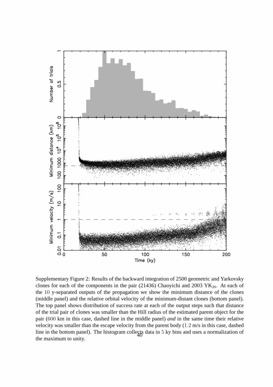
Supplementary Figure 2: Results of the backward integration of 2500 geometric and Yarkovskyclones for each of the components in the pair (21436) Chaoyichi and 2003 YK39. At each ofthe 10 y-separated outputs of the propagation we show the minimum distance of the clones(middle panel) and the relative orbital velocity of the minimum-distant clones (bottom panel).The top panel shows distribution of success rate at each of the output steps such that distanceof the trial pair of clones was smaller than the Hill radius ofthe estimated parent object for thepair (600 km in this case, dashed line in the middle panel)and in the same time their relativevelocity was smaller than the escape velocity from the parent body (1.2 m/s in this case, dashedline in the bottom panel). The histogram collects data in5 ky bins and uses a normalization ofthe maximum to unity.
40

Supplementary Figure 3: Results of the backward integration of 2500 geometric and Yarkovskyclones for each of the components in the pair (88259) 2001 HJ7 and 1999 VA117. At each ofthe 10 y-separated outputs of the propagation we show the minimum distance of the clones(middle panel) and the relative orbital velocity of the minimum-distant clones (bottom panel).The top panel shows distribution of success rate at each of the output steps such that distanceof the trial pair of clones was smaller than the Hill radius ofthe estimated parent object for thepair (600 km in this case, dashed line in the middle panel)and in the same time their relativevelocity was smaller than the escape velocity from the parent body (1 m/s in this case, dashedline in the bottom panel). The histogram collects data in5 ky bins and uses a normalization ofthe maximum to unity.
41

Supplementary Figure 4: Results of the backward integration of 5000 geometric and Yarkovskyclones for each of the components in the pair (229401) 2005 SU152 and 2005 UY97. At eachof the1 y-separated outputs of the propagation we show the minimum distance of the clones(middle panel) and the relative orbital velocity of the minimum-distant clones (bottom panel).The top panel shows distribution of success rate at each of the output steps such that distanceof the trial pair of clones was smaller than the Hill radius ofthe estimated parent object for thepair (500 km in this case, dashed line in the middle panel)and in the same time their relativevelocity was smaller than the escape velocity from the parent body (1 m/s in this case, dashedline in the bottom panel). The histogram collects data in2.5 ky bins and uses a normalizationof the maximum to unity.
42

Supplementary Figure 5: Timescale for disruption of rotationally fissioned asteroids. 121 sys-tems with mass ratios varying up to 0.3 and tri-axial ellipsoid shapes were evolved after arotational fission event. Each point represents either the time of disruption or the length of thesimulation (100 years marked by a red line). The blue line indicates the median escape time(0.6 years) for secondaries in systems with a mass ratio below 0.2.
43

Supplementary Figure 6: Composite lightcurve of (2110) Moore-Sitterly.
44

Supplementary Figure 7: Composite lightcurve of (4765) Wasserburg.
45

Supplementary Figure 8: Composite lightcurve of (5026) Martes in 2008.
46

Supplementary Figure 9: Composite lightcurve of (5026) Martes during July-September 2009.The amplitude was changing during the observing campaign, and we present separate fits forthree different observational intervals. They are plottedwith arbitrary vertical offsets for clarity.
47

Supplementary Figure 10: Composite lightcurve of (6070) Rheinland. The amplitude was loweron 2009 Sept. 20 than on the other observing nights, and we present the data with a separate fitand with an arbitrary vertical offset for clarity. See also comments in the text.
48

Supplementary Figure 11: Composite lightcurve of (7343) Ockeghem.
49

Supplementary Figure 12: Composite lightcurve of (10484) Hecht.
50

Supplementary Figure 13: Composite lightcurve of (11842) Kap’bos.
51

Supplementary Figure 14: Composite lightcurve of (13732) Woodall.
52

Supplementary Figure 15: Composite lightcurve of (15107) Toepperwein.
53

Supplementary Figure 16: Composite lightcurve of (17198) Gorjup.
54

Supplementary Figure 17: Lightcurve of (19289) 1996 HY12.
55

Supplementary Figure 18: Lightcurve of (21436) Chaoyichi.
56

Supplementary Figure 19: Composite lightcurve of (23998) 1999 RP29.
57

Supplementary Figure 20: Composite lightcurve of (38707) 2000 QK89.
58

Supplementary Figure 21: Composite lightcurve of (44612) 1999 RP27.
59

Supplementary Figure 22: Composite lightcurve of (48652) 1995 VB.
60

Supplementary Figure 23: Composite lightcurve of (51609) 2001 HZ32.
61

Supplementary Figure 24: Composite lightcurve of (52773) 1998 QU12.
62

Supplementary Figure 25: Composite lightcurve of (52852) 1998 RB75.
63

Supplementary Figure 26: Composite lightcurve of (54041) 2000 GQ113.
64

Supplementary Figure 27: Composite lightcurve of (54827) 2001 NQ8.
65

Supplementary Figure 28: Lightcurve of (56232) 1999 JM31.
66

Supplementary Figure 29: Composite lightcurve of (63440) 2001 MD30.
67

Supplementary Figure 30: Composite lightcurve of (69142) 2003 FL115.
68

Supplementary Figure 31: Composite lightcurve of (76111) 2000 DK106.
69

Supplementary Figure 32: Lightcurve of (78024) 2002 JO70. Only a lower limit on the asteroid’speriod was estimated, see text. The period and magnitude scale offset used in this plot of thetwo relative nightly sessions are arbitrary.
70

Supplementary Figure 33: Composite lightcurve of (84203) 2002 RD133.
71

Supplementary Figure 34: Composite lightcurve of (88259) 2001 HJ7.
72

Supplementary Figure 35: Composite lightcurve of (88604) 2001 QH293.
73

Supplementary Figure 36: Composite lightcurve of (92336) 2000 GY81.
74

Supplementary Figure 37: Composite lightcurve of (101065)1998 RV11.
75

Supplementary Figure 38: Composite lightcurve of (101703)1999 CA150.
76

Supplementary Figure 39: Composite lightcurve of (115978)2003 WQ56.
77

Supplementary Figure 40: Lightcurve data of (139537) 2001 QE25. The magnitude scale offsetbetween the two relative nightly sessions is arbitrary. Seetext for comments on the periodestimate.
78

Supplementary Figure 41: Composite lightcurve of (205383)2001 BV47.
79

Supplementary Figure 42: Composite lightcurve of (218099)2002 MH3.
80

Supplementary Figure 43: Composite lightcurve of (220143)2002 TO134.
81

Supplementary Figure 44: Composite lightcurve of (226268)2003 AN55.
82

Supplementary Figure 45: Composite lightcurve of (229401)2005 SU152.
83