calibration of the delphi de/dx for 1991 f and 1992 d data

DELPHI Collaboration <r DELPHI 95-48 TRACK 81 Qe 24 April, 1995

Calibration of the DELPHI dE/dx for 1991 F and 1992 D data

J. Dahm, M. Elsing, M. Reale

Bergische Universitat Wuppertal

Abstract

We describe the procedure used and the results achieved in the calibration of the DELPHI TPC dE/dz data relative to the processing 1991 F and 1992 D for hadronic (high multiplicity) events. These data correspond to the LEP fill numbers 563-866 and 894-1461 respectively, for a total of roughly 300,000 hadronic events for 1991 and 600,000 for 1992.

Calibration takes into account LEP fill number, track-theta, track-phi, module- gaps dependencies induced on systematics.

Relevant parameters like the resolution and the pull are reported before and after our fixing, to witness its effectiveness.

1 Introduction

The DELPHI TPC (Time Projection Chamber) data, like others, are affected by systematic measurement errors due to unwanted daily-life experimental prob- lems : fluctuations in the gas pressure of the chambers, different number of signal pick-up wires from track to track, effects due to the different track cur- vatures and many others. Among these it is worth to mention the effect of proximity of other tracks on a given track’s ionization measurement. A good calibration of the energy loss (dE/dz) should be able to restore the ideal operating condition for this measurement, and provide for all tracks a measurement independent of these unwanted side effects corrupting the data. It should eliminate all the differences between the ionization amount measured in the ideal case (all tracks crossing the detector orthogonal to the chamber plane direction, in the middle of the wire frame planes and with operating conditions always stable in time) and real experimental data. The most important part of the correction on the TPC data for systematics and above all distortions due to the effective electric potential configuration is done at the DELANA level in the data processing. Anyhow a given SHORT-DST taken data set shows fluctuations in the value of the average measured dE/dz for a given particle flavour (like pions, for example) at fixed momentum, according to the LEP fill number, the polar (6) and the azimuthal (®) angle of the track, the TPC module number, because of many systematic effetcts. After having read this information, these are the main effects we have taken into account and we corrected for. Our fixing is therefore running at the SHORT- DST level, easily available for all users. It will soon be implemented in the code and included therefore in the GETDEDX routine.

This calibration has been performed on the data 1991F and 1992D using (apart from the @ fixing) all tracks with momentum above 2 GeV/c .

2 The TPC and its identification

The TPC is the central tracking detector in DELPHI. Nevertheless it also pro- vides particle identification through a measurement of the energy loss of charged particles produced in the Z° decay. It consists of two halves (z > 0, z < 0) with six 60-degrees vassels sectors in @ each, for a total of 12 modules.

The active lenght of the detector is 2 * 1.34 m and the active radial range is between 0.325 and 1.16 m; the number of R¢ points per module is 16 for a total of 1680 pads per sector.

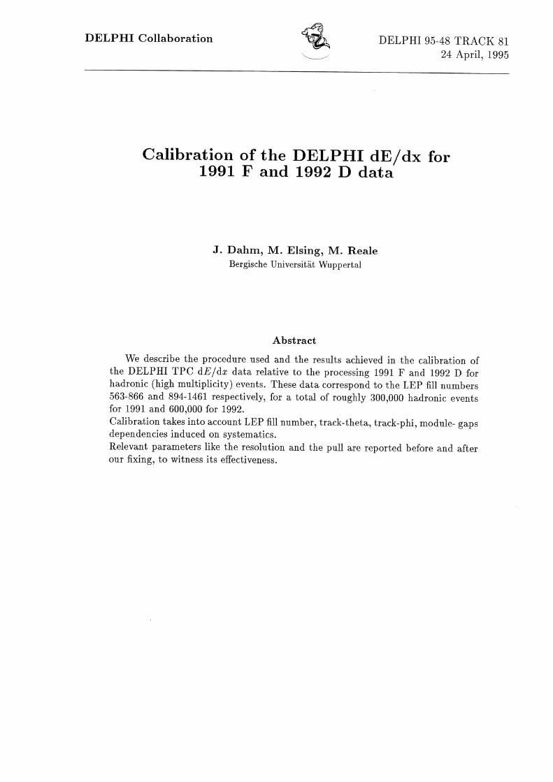
The three coordinates are reconstructed as follows : z and y are given by the single pad hits distributions at the end of the drift volume on the collector plane and z is reconstructed by the charge drift time. The detector is sketched in figure 1.

isation 4

lectrons d'ion dérive des é

trace d'une particule chargée

enceinfe en

er1aux composites a

mat 101 d'amplificat

See By

ecw

woe.

/

ESOT

plaque H.T.

ar ;

a Aeon

y Te

SSE

1 NE

PN ee

oS SEN

ay RT

mn /

~

axe

des faisceaux

chambre

proportionnelle

Sketch of the DELPHI TPC detector Figure 1

The whole detector is in the magnetic field of the DELPHI superconducting solenoid of 1.2 Tesla, parallel to the beam axis. It is out of the aims of this short note to describe in detail the detector, a description of which can be found in ref.[1]. At our purposes it is sufficient to say that the ionization electrons produced by charged tracks in the TPC gas (Ar 80% - CH, 20% ) drift with a veloc- ity of 6.67 cm/s, reaching the end-side Multi Wire Proportional Chambers (MWPC) because of a 20000 V very high tension (equivalent to an electric field of 150 V/cm), and their signal is measured by the MWPC wires (set to the High Voltage of 1385 V). Each MWPC is 1 cm thick and is made by three planes of wires: a gating grid to address the drift, a cathode (negative) wire plane to define the end of the drift volume, and a sense wire plane of 192 very thin (20 ym in diameter) anode wires to collect the ionization electrons. The charge signal collected by pads and wires is first translated into an electronic signal by preamplifiers, and then, in the FASTBUS crates, is shaped gaussian with a 250 ns width, keeping its integrated size, and digitized. The Proportional Chambers are called like this because of their proportionality in the total collected charge as a function of the applied voltage. By working in this linear regime are used to measure the energy loss of the charged particles produced in DELPHI. A charged track produces on average 70 electrons per centimeter while crossing the TPC. The energy loss of moderately relativistic charge particles (other than electrons) in matter is given by the Bethe — Bloch formula :

dE. 5Z1 1, 2m.c*B27*Tmaz Kz —In

é

dx A B?°2 [? - 8-5) (1)

In this formula 8 and y are the relativistic kinematical parameters of the particle, m, is the electron mass [“$"], A is the mass number of the mate- rial, { is its ionization potential in [MeV] ( According to the Thomas-Fermi model [[ey) ~ 12Z, Z = atomic number ), Tinaz is the maximum kinetic en-

ergy transfer from the particle of mass M to an electron in a single collision

(Tmar 2m,.c*B2y? for Ae << 1), K = 4nNyr2m,c? ( r, is the classical electron radius, 2.818 fm) and 6 is the density ef fect correction factor.

In the case of the DELPHI TPC, the final dE /dz measurement written on the

DST's comes from the averaging of the 80% lowest amplitudes associated to

a given track. This is done in order to avoid an excessive rise in the Landau

fluctuations for the highest amplitudes and to exclude the saturation region for

the chamber in which the dE’/dz measurement is wrong.

To this number many successive corrections are applied :

e A normalization (to 4 mm) to take into account different path lenghts due to

different incident track angles

e A correction for the bias induced by the truncation procedure

e A drift distance correction in the case the electronic shapers are not used, to

take into account the deformation of the electronic signal during the drift

e A track separation rejection of clusters separated by less then 2 cm in z

rs) a

~ DN

&

Fash *<

S PS 2.25

2

1.75

L5 — — " - ~

Ce Rey reset 1.25 Bee pee hee

PENS ae “

0.75

i_.f.§_f f { 2 i

1 10

xy, 2 Impuls [GeV/c’]

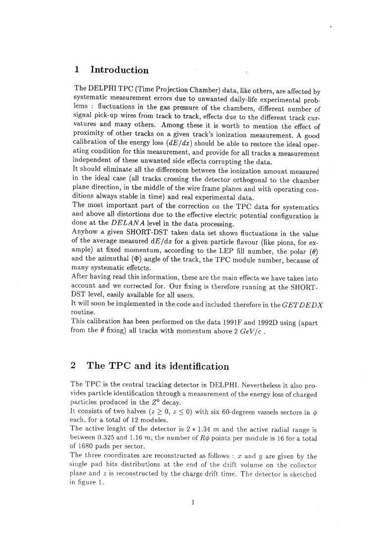
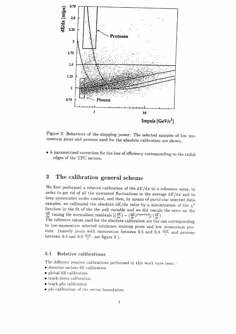
Figure 2: Behaviour of the stopping power. The selected samples, of low momentum pions and protons used for the absolute calibration are shown.

e A parametrised correction for the loss of efficiency corresponding to the radial edges of the TPC sectors.

3 The calibration general scheme

We first performed a relative calibration of the dE /dz to a reference value, in order to get rid of all the unwanted fluctuations in the average dF’ /dz and to keep systematics under control, and then, by means of particular selected data samples, we calibrated the absolute dE /dz value by a minimization of the y? function in the fit of the the pull variable and we did rescale the error on the <= tuning the normalised residuals [(S2) - (G2 )ewrected) / (aE) The reference values used for the absolute calibration are the one corresponding to low-momentum selected minimum ionizing pions and low momentum protons. (namely pions with momentum between 0.5 and 0.8 Sev and protons between 0.5 and 0.9 S¢". see figure 2 ).

3.1 Relative calibrations

The different relative calibrations performed in this work have been : e detector sectors fill calibration

e global fill calibration

e track-theta calibration

e track-phi calibration

e phi-calibration of the sector boundaries.

As a reference value, we normalized the dE /dz to the value of

dE (Tres =1.2 (DELPHI a.u., mips=1) (2)

The basic assumption is the factorization of this independent corrections:

dE dE (Gres = fin * fo * fo * (~~) (3)

Each one of these is described in detail in the incoming sections, where we define and describe the correction factors f used in the different fixings.

3.2 Absolute Calibration

The absolute calibration is based on the assumption that the systematics ef- fetcting the dE'/dz measurement can be corrected for with a linear rescaling of the dE/dx’ .

Minimizing the x? function in the fit of the residuals a — dg cmpected for low momentum pions and protons gave us the factor and the offset in the linear rescaling of the dE’/dz (see section 8). As a second step we did rescale the error on the dE'/dz tunining the pull variable

a,

(4) _ (52 )espected

pull = (4)

The pull variable should be normally distributed with mean value zero and standard deviation (c) 1. The selected data samples used have been minimum ionizing pions, low momentum protons and V® recontructed pions and protons.

To have a higher purity in the V° sample of pions, we used only very tight (i.e.V°-flag = 22 ) reconstructed pions from the K° decay. The purity of this sample is close to 100 % ( background max = 1.-2. % ).

The absolute calibration results are discussed in detail in section 8.

4 The global and sectorwise fill-number calibrations

TPC data show a dependency on the LEP fill number due essentially to fluc-

tuations in the gas preassure inside the vassel.

The average amount of collected ionization charge is effected by these fluctua-

tions through the ionization potential J in the Bethe-Block formula 1.

We performed fist an individual module fill-calibration and later a global TPC

calibration in order not to loose the interesting information on the individual

TPC-sector systematics in fill-number.

+ pi ond + bhi we H ont Ver

j Aah . 1 l cist pn np a Ly i

800 900 600 700 800 3900

1 pun il.3,

600 700

Modi +: dedx vs. fillHadr Mod! +: dedx vs. fillHadr

| 2 fps fed ¢¢ 2 aba hit

it . ao tp

600 700 800 900 600 700 800 900

Mod3+: dedx vs. fillHadr Mod3+: dedx vs. fillHadr

* Paget + fom 0

odin sochhe

parent. ,,, 3, . J tr, , fi. gg iy fa Brnmind.

600 70C 800 900 600 70C &GO 300

Mod5+.: dedx vs. fillHadr Mod5+: dedx vs. fillHadr

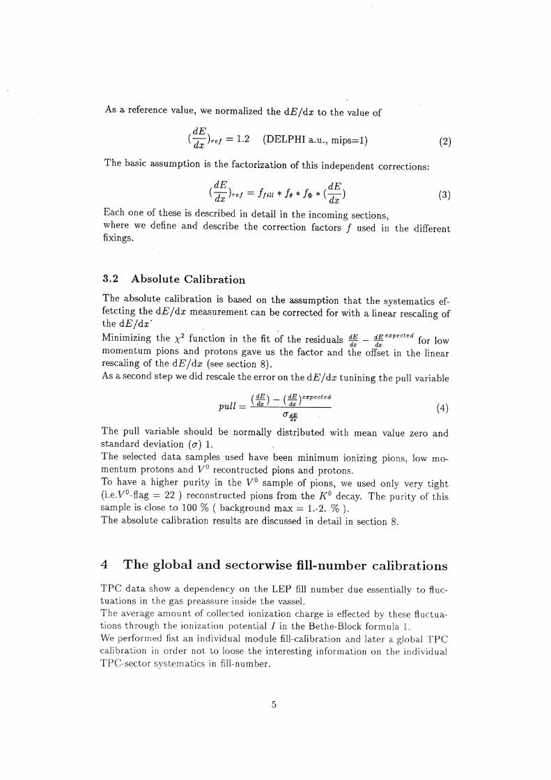
Figure 3: Sectorwise Fill-Number dependency for the dE/dz before (left) and after (right) the calibration for data 1991F, module number 1,3,5

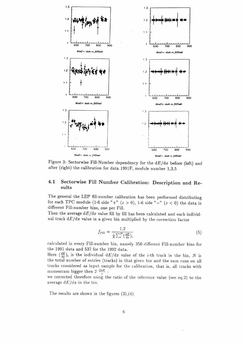
4.1 Sectorwise Fill Number Calibration: Description and Re- sults

The general the LEP fill-number calibration has been performed distributing for each TPC module (1-6 side ”+” (z > 0), 1-6 side ”—” (z < 0) the data in different Fill-number bins, one per Fill. | Then the average dE//dz value fill by fill has been calculated and each individual track dE/dz value in a given bin multiplied by the correction factor

1.2 iu = —— 5

frat a (2); 8) calculated in every Fill-number bin, namely 350 different Fill-number bins for the 1991 data and 537 for the 1992 data. Here (£2); is the individual dE/dz value of the i-th track in the bin, N is the total number of entries (tracks) in that given bin and the sum runs on all tracks considered as input sample for the calibration, that is, all tracks with momentum bigger then 2 cen

we corrected therefore using the ratio of the reference value (see eq.2) to the average dFE’/dz in the bin.

The results are shown in the figures (3),(4).

12 ba 2 He | ,e |

~ti.zrynt,z,,t

1000 1200 1400

1 od j owd. A 4 J A. Armee I A 1 A

1000 1200 1400

Mod] +: dedx vs. fillHadr

L

2 Ht Heiden g

11.

Mod! +: dedx vs. fillHadr

.

A all. j wh. A. A. J A. A ] A

1000 -1200-~—«1400

13 |

at $ I

| rb |

Mod3+: dedx vs. filtHadr

t ; . . , | es a

* SoC Zot 1<00

Se *Q0C 1z00 1<QC

Mod5< dedx vs. fillHad: Moad5< dedz vs. fillHadr

Figure 4: Sectorwise Fill- Number dependency for the dE’/dz before (left) and

after (right) the calibration for data 1992D, module number 1,3,5

_

” ND

mean(dEdx) vs Fill Daten 91F, all p2GEV mean(dEdx) vs Fill Daten 91F, all p2GEV

Vy

1.25 +

| ak wt ee 4 4% x As h 12 | ‘ tala i hhiteg ad ede Hh ws f 4 | | :

| | | L aL

1.05 -

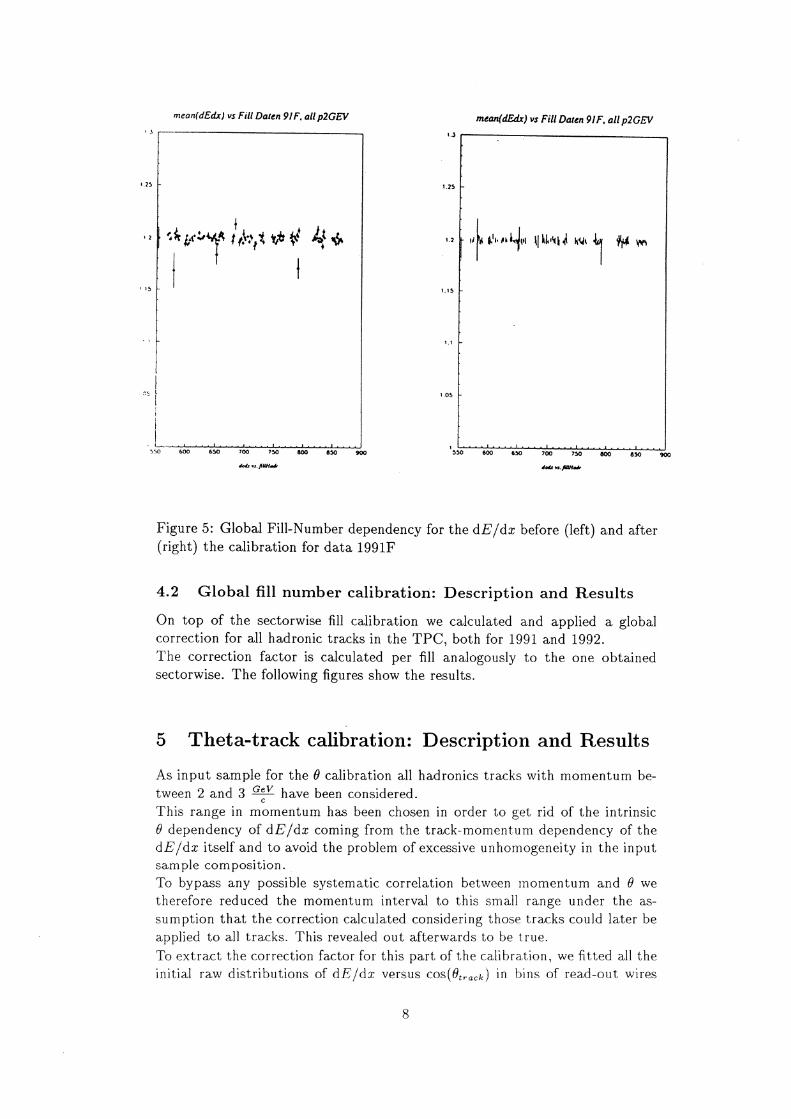
Figure 5: Global Fill-Number dependency for the dE’/dz before (left) and after (right) the calibration for data 1991F

4.2 Global fill number calibration: Description and Results

On top of the sectorwise fill calibration we calculated and applied a global

correction for all hadronic tracks in the TPC, both for 1991 and 1992.

The correction factor is calculated per fill analogously to the one obtained

sectorwise. The following figures show the results.

5 Theta-track calibration: Description and Results

As input sample for the @ calibration all hadronics tracks with momentum be- G tween 2 and 3 ev have been considered.

This range in momentum has been chosen in order to get rid of the intrinsic

6 dependency of dE‘/dz coming from the track-momentum dependency of the

di /dz itself and to avoid the problem of excessive unhomogeneity in the input

sample composition.

To bypass any possible systematic correlation between momentum and @ we

therefore reduced the momentum interval to this small range under the as-

sumption that the correction calculated considering those tracks could later be

applied to all tracks. This revealed out afterwards to be true.

To extract the correction factor for this part of the calibration, we fitted all the

initial raw distributions of dE/dx versus cos(6@,,a-.) in bins of read-out wires

dEdx vs. Fill Daten 92D, all p2GEV

1.25 -

‘

mi | 2 F Nt { rom lapse sbye

e nae o

>

.

1.158 pf

oe

10S

1 ee a $00 1006 1100 1200 1300 1400 1$0c

deds vs. fillHade

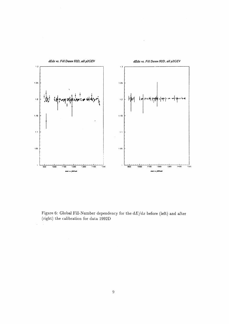
Figure 6: Global Fill-Number dependency for the dE//dz before (left) and after (right) the calibration for data 1992D

dEdx vs. Fill Daten 92D, all p2GEV

1.2 : r ki | fr teaht re hye rs “fh by otf

wis bf

>

P

t1

.

.

.

1.05 F

2

.

§

1 tl tt tt 900 1000 1100 1200 1300 1400

dedx vs. filltHade

1S0C

SCR27: DEDXANAzSHORTS 1F7.HBK

18) 40154

Entries 63789

L Meon 0.2917E-03

1.35 - RMS 0.5462

P x/ndf 1248 / 73

P1 1.088

r P2 . —0.2408

13 P3 0.1099 . P4 0.3004E-01

r P5 0.1795 1.25 P6 1.112

r P7 -0.5839

P8 ~ 1.045

F P9 -0.7801

V2 P10 -0.1651

pet te a a Pt tt

-0.25 0 0.25 0.5 0.75 1

> bose irtiinit,

-1 ~0.75 -0.5

dedx vs.cos(theta), 110nwir20ehadr

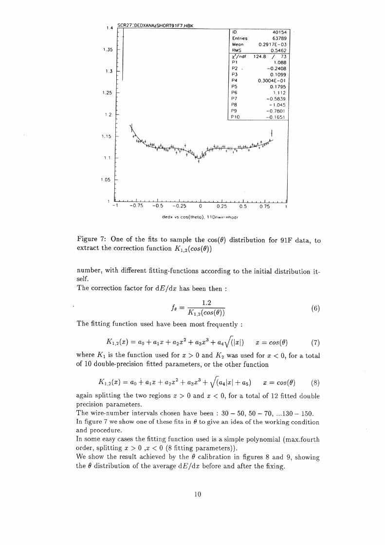
Figure 7: One of the fits to sample the cos(@) distribution for 91F data, to extract the correction function K, 2(cos(@))

number, with different fitting-functions according to the initial distribution itself.

The correction factor for dE'/dz has been then :

4-2 "Ky 2(cos(8))

The fitting function used have been most frequently :

(6)

Ky (x) = a9 +a, 2 + agz? + azz? + asy/((21) rz = cos(6) (7)

where K;, is the function used for z > 0 and Ky was used for x < 0, for a total

of 10 double-precision fitted parameters, or the other function

Ky o(z) = ap + a,z + az? + a32° 4+ V (asl +as) «= cos(@) (8)

again splitting the two regions z > 0 and z < 0, for a total of 12 fitted double precision parameters.

The wire-number intervals chosen have been : 30 — 50, 50 — 70, ...130 — 150.

In figure 7 we show one of these fits in 8 to give an idea of the working condition

and procedure.

In some easy cases the fitting function used is a simple polynomial (max.fourth

order, splitting z > 0 ,z < 0 (8 fitting parameters)).

We show the result achieved by the @ calibration in figures 8 and 9, showing

the @ distribution of the average dE’ /dz before and after the fixing.

10

1.4 1.4 i

1.35 & | } 1.35 tf

13 6

C 1.3 i 1.25 y |

12 125 fh | |! F

1.15 E ty . { a! ! ‘ . Ne, { ty ae 1.2 ta | } L tk titi dd fy att f bh, Hayetete 11 Eb a hy i Ha | “eral yf! rt t .

: a i

C PS or 1.05

] St | dtd i JS. ot if | if it 7 4 [ Ae | Jt : d dood | ijt iJ

~1 —~C5 0 0.5 1 - 3 -0.5 0 C.5 1

dedx vs.cos(theta), 1 30nwir]6Qhadr dedx vs.cos(theta), 1 30nwir1 6Qhadr

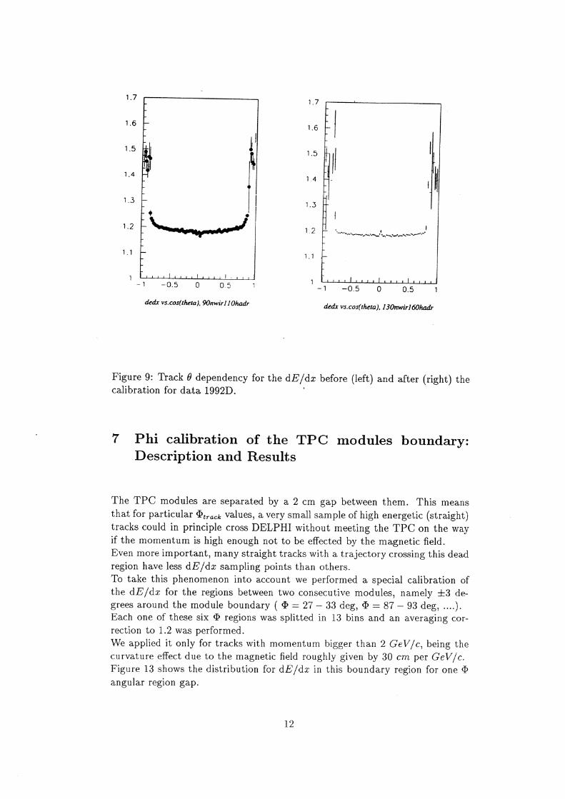
Figure 8: Track 6 dependency for the dE/dx before (left) and after (right) the calibration for data 1991F. |

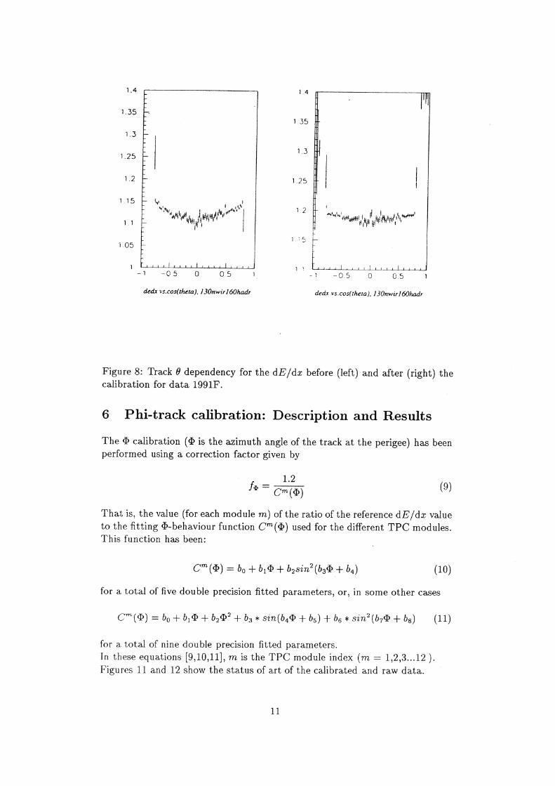
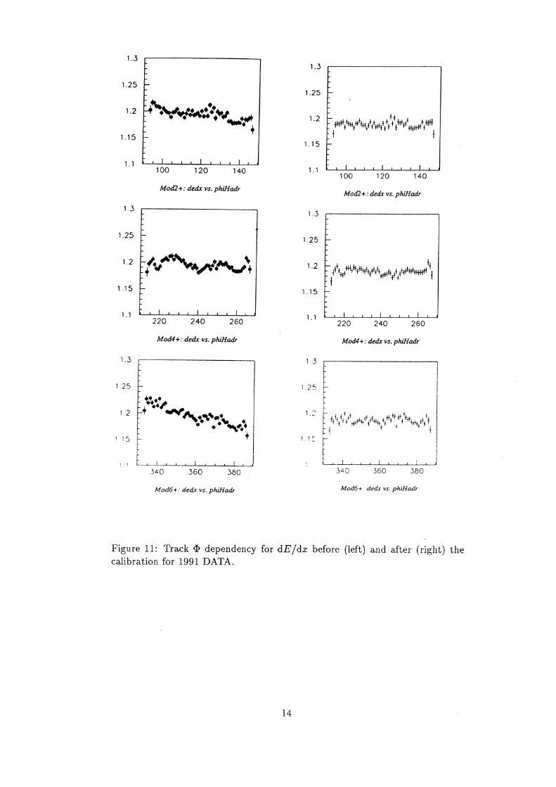
6 Phi-track calibration: Description and Results

The ® calibration (® is the azimuth angle of the track at the perigee) has been performed using a correction factor given by

1.2 fe = Cm(S) (9)

That is, the value (for each module m) of the ratio of the reference dE/dz value to the fitting 6-behaviour function C™(®) used for the different TPC modules. This function has been:

C™(®) = bo + 0, B + by sin? (b3® + b,) (10)

for a total of five double precision fitted parameters, or, in some other cases

C™(®D) = bo + 6: ® + b,B* + b3 * sin(b4® + ds) + bg * sin?(by@+ 6g) (11)

for a total of nine double precision fitted parameters.

In these equations [9,10,11], m is the TPC module index (m = 1,2,3...12).

Figures 11 and 12 show the status of art of the calibrated and raw data.

11

1.6

Pr

prr

nn

hae

1.1

1.4

Par

r ¢ °

'e > eetenygemennne

poutira il wt. I 1 dtd fj} ] sist tirrr tris, 4,55, -O0.5 0 0.5 j —1 —Q.5 0 ~—60.5 1

{ wed

dedx vs.cos(theta), 90nwir 1 1Ohadr dedx vs.cos(theta), 130nwir1 60hadr

Figure 9: Track @ dependency for the dE/dx before (left) and after (right) the calibration for data 1992D.

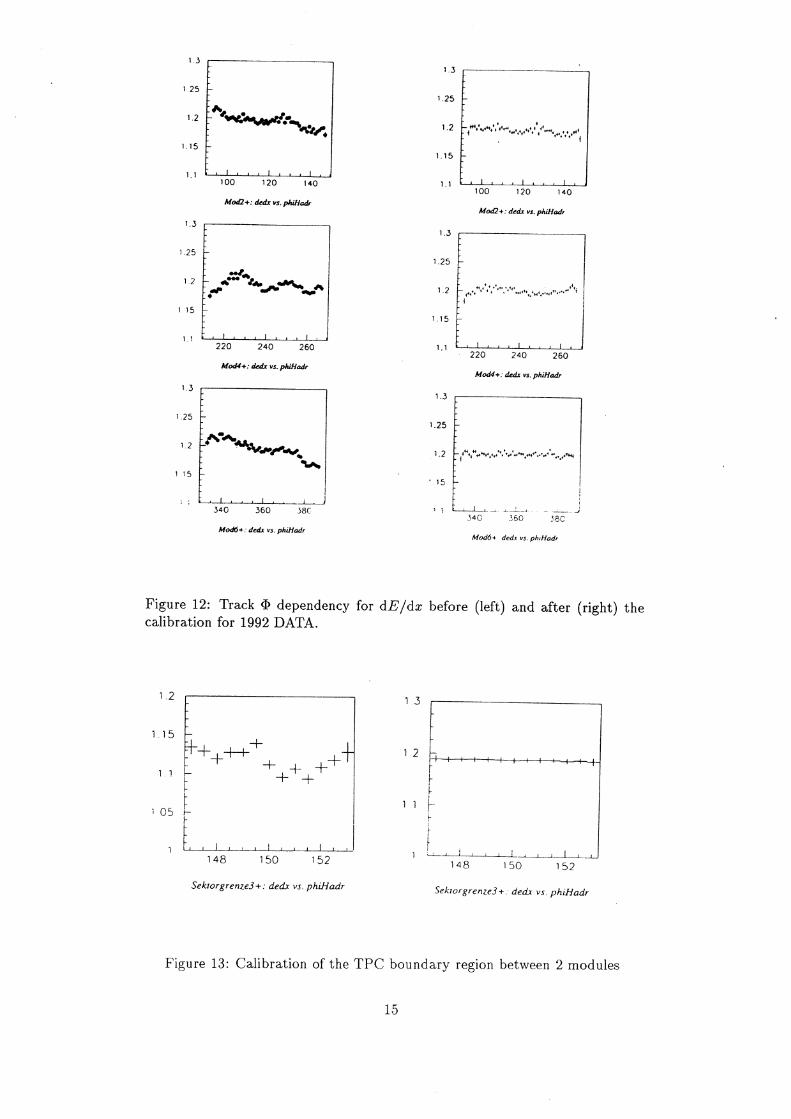
¢ Phi calibration of the TPC modules boundary: Description and Results

The TPC modules are separated by a 2 cm gap between them. This means that for particular ©,,,., values, a very small sample of high energetic (straight) tracks could in principle cross DELPHI without meeting the TPC on the way

if the momentum is high enough not to be effected by the magnetic field.

Even more important, many straight tracks with a trajectory crossing this dead

region have less df’/dz sampling points than others.

To take this phenomenon into account we performed a special calibration of

the d&/dz for the regions between two consecutive modules, namely +3 de-

grees around the module boundary ( ® = 27 — 33 deg, ® = 87 — 93 deg, ....). Each one of these six ® regions was splitted in 13 bins and an averaging cor-

rection to 1.2 was performed.

We applied it only for tracks with momentum bigger than 2 GeV/c, being the

curvature effect due to the magnetic field roughly given by 30 cm per GeV/c.

Figure 13 shows the distribution for dE’/dz in this boundary region for one ®

angular region gap.

12

1.3 ID 40123

P Entries 109621

1.28 Mean 240.0 - RMS. 15.86

f ¥/ndf 150.8 / 50 1.26 FF P 1.258

f P2 —0.1873E-03

. P3 —~0.1991E-01 1.24 - P4 0.1369

f P5 3.449

1.22 +4 fa

1.18 k&

1.146 -

1.14 -

1.12 -

1.4 i i 4 1 4 | j I 1 4 | 4 1 t i | i i i i | i i 1 1 ] i 1 1 i |

210 220 230 240 250 260 270

Mod4+z dedx vs. phiHadr

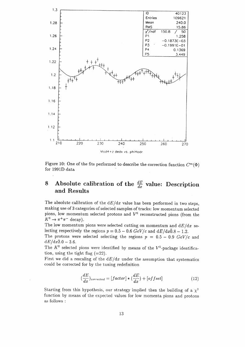
Figure 10: One of the fits performed to describe the correction function C™(®) for 1991D data /

8 Absolute calibration of the oe value: Description and Results |

The absolute calibration of the dE/dx value has been performed in two steps, making use of 3 categories of selected samples of tracks: low momentum selected pions, low momentum selected protons and V° reconstructed pions (from the K° - atn- decay). The low momentum pions were selected cutting on momentum and dE/dz selecting respectively the regions p = 0.5 — 0.6 GeV/c and dE/dz0.8 — 1.2. The protons were selected selecting the regions p = 0.5 — 0.9 GeV/c and dE /dx2.0 — 3.6. The K® selected pions were identified by means of the V°-package identification, using the tight flag (=22). First we did a rescaling of the dF’/dx under the assumption that systematics could be corrected for by the tuning redefinition

dE (= ecrrected = [factor] « (=) + [of fet] (12) Starting from this hypothesis, our strategy implied then the building of a y’

function by means of the expected values for low momenta pions and protons

as follows :

13

1.2

1.15

1.1

1.2

1.15

Figure 11: Track ® dependency for dE/dx before (left) and after (right) the

¢ os NAPE, ?

pe

Ss | i 1 i J i i J | i

100 120 140

Mod2+: dedx vs. phiHadr

Perr

purr

Pon pep’

PPreepe

A | J i i | i 4 i | i

220 240 260


eee Tere

J. i A 4 i J 4 AL A | i 340 560 380


calibration for 1991 DATA.

1.15

1.1

1.3

1.2

1.15

1.7

No nr i)

qn

14

EEE

Pere

ryp errr

rrr

Ht, HH, Ht tH tat atts i ‘i syitt Ht

| i J i | 1 i i i J Ln

100 120 140


Oe

a

t + uit t

Hy Ty Haat att ttt are Meet ttt ‘ i # i

i | i j 4 | i i i | i

220 240 260


af i L 44 t at H at i ro 14 Pathe (Pay a Me Paty ttt

lL A. i i i d i a. j i _i.

340 360 380


1.3 1.3

s L

Nob 1.25

1.2 Nenecan sagt r ‘ ‘ [ aes, 1.2 ree ath,’ Wet naetely! ots a

Vt P 1.15

] 1 . I | 1 1 i I i 14 | i

, ] i | me 20 40 " “7100. “120° 140 Mod2+: dedx vs. phiHHadr

, phil Mod2+: dedx vs. phiHadr

1.3 13

[ -

ee 1.25 f

1.2 L a “tae A... } +444 ‘ “ wv owe } 2 T ate ‘ . EE atte at eat 4

rT 4

V1 - 1.15

q Jj. ij A. A. a | 1 A i { : P

I 1 i i

#20 240 260 "320.40 260. Mod4+: dedx vs. phifladr Mod4+: dedx vs. phiHadr

1.3 13

1.25 6 15

1.2 LEN Mans | LL. , fog, AeA, 1 2 7 Mas titgate ‘ved ae SH ett tate ati

r wre r PIS ob is t

. vi j od. ab. i j i a . i f r .

: Ss. phi Modo+: dedx vs. phiHtadr Mod6+ dedx vs. phiHadr

Figure 12: Track ® dependency for dE/dz before (left) and after (right) the calibration for 1992 DATA.

4.

1205 hp pp pf

if tt tt FoF —- | z

[ 1. OS bk :

7 pa pi i ft 1 C pot os a se ot , Lo 148 150 152 148 150 152

Sektorgrenze3+: dedx vs. phiHadr Sektorgrenze3+. dedx vs. phiHadr

Figure 13: Calibration of the TPC boundary region between 2 modules

15

dE\ _(dE\n 2 dE dE 2 2 (ae )i — (GE) ea pecl (Se )i — (Se Bepecl = eee! yy Een? pions (4), protons (42):

We minimize this x? using the MI NUIT CERN-package. These two sample were used for the following reason : They have very similar momenta but a big separation in dE /dz so that they provided two good points to fit the flavour-independent scaling expressed by eq.(12).

The output of the minimization is :

factor offset |

1991F | 0.97+0.11 | 0.032+0.15

1992D | 0.96+ 0.04 | 0.043 + 0.15

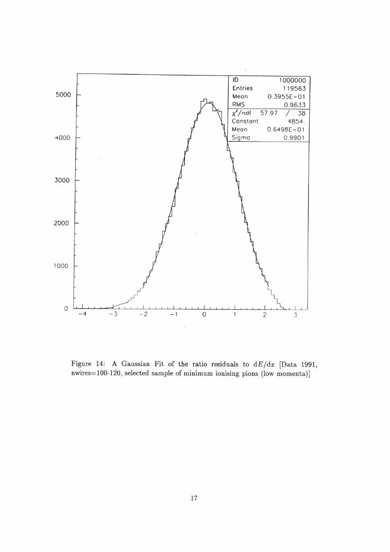
After this rescaling, we did retune the error on the dE/dz by plotting the natural scaling with the number of wires for the ratio of the o of the residuals to the dE/dx value itself. Technically speaking we did prefere to plot the Squared values :

2

° (42) } 4 = — 1 (By °° oy u)

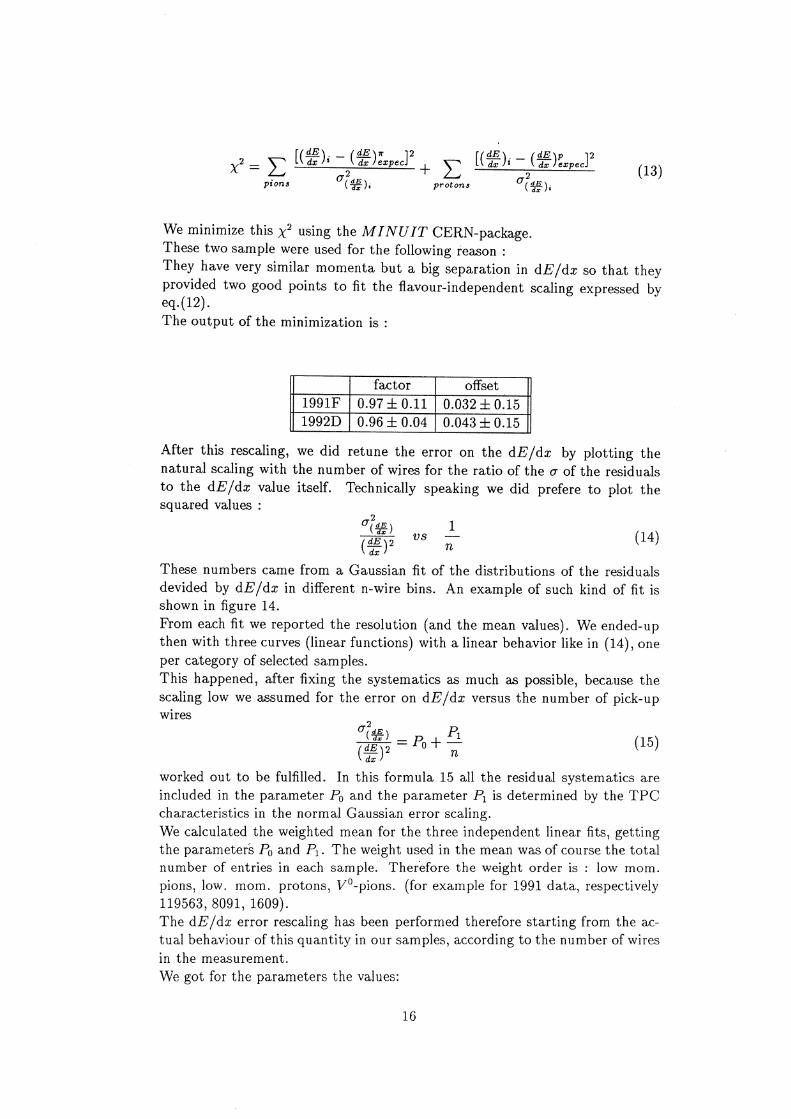
These numbers came from a Gaussian fit of the distributions of the residuals devided by dE/dz in different n-wire bins. An example of such kind of fit is shown in figure 14.

From each fit we reported the resolution (and the mean values). We ended-up then with three curves (linear functions) with a linear behavior like in (14), one per category of selected samples.

This happened, after fixing the systematics as much as possible, because the

scaling low we assumed for the error on dE’ /dz versus the number of pick-up wires

O? ap P (32) 1 dx — P. + 15 (42)? 0 n ( )

worked out to be fulfilled. In this formula 15 all the residual systematics are

included in the parameter P, and the parameter P, is determined by the TPC

characteristics in the normal Gaussian error scaling.

We calculated the weighted mean for the three independent linear fits, getting

the parameters Py and P,. The weight used in the mean was of course the total

number of entries in each sample. Therefore the weight order is : low mom.

pions, low. mom. protons, V°-pions. (for example for 1991 data, respectively

119563, 8091, 1609).

The dE//dz error rescaling has been performed therefore starting from the ac-

tual behaviour of this quantity in our samples, according to the number of wires

in the measurement.

We got for the parameters the values:

16

5000

4000

3000

2000

1000

ID 1000000

Entries 119563

— Mean 0.3955E-01

L RMS 0.9633

x’/ndf 57.97 / 38

: Constant 4854.

r Mean O0.6498E-01

Sigma 0.9901

a _ i

r - — _

L. | ] A pe i a _| i i t i { i ti i 1 i i i ld 1 | j _i 1 i | Jd j 1 d

—4 ~3 -2 ~] O 1 2 3

Figure 14: A Gaussian Fit of the ratio residuals to dE/dx [Data 1991,

nwires=100-120, selected sample of minimum ionising pions (low momenta)|

17

0.16 1991 DEOX ERROR RESCALING

0.14

0.12

0.08 0.06

20 40 60 80 100 120 140 160

SIQMO vs nwires 1993

Figure 15: Natural Scaling of the error on the dE/dx shown by the plot of the residuals versus the number of wires, for low momentum selected pions (1991F)

Po +3% | P+ 3%

1991F | 0.000513 | 0.484

1992D | 0.000798 | 0.460

9 Summary of the Results for 1991F and 1992D data

The relative calibrations show an easily understandable good behaviour in the

plots we showed.

The improvement on the natural width of the Pull variable can be quantified

by the following numbers : for the data 1991 F , before and after this fixing

DATA 1991 F before | after

Op. 1.086 | 0.994 opp" 1.168 | 1.019

Pull” | _0.138 | 0.056 Pull’? "™°"?"""* | _9 972 | 0.072

18

1991 DEDX ERROR RESCALING

0.16

VO pions 1991 F data

0.14 -

0.12 -

O.1 F-

0.08

0.06 - | A 2 Ss i i 1 4 { L Ai i i 4 ai. : j

2C 40 60 80 100 120 140 — 160

sigma vs awires 1991

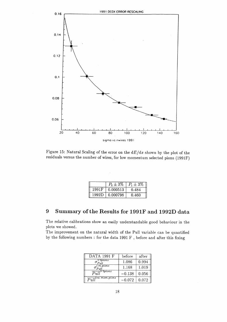
Figure 16: Natural Scaling of the error on the dE’/dz shown by the plot of the

residuals versus the number of wires, for V° (i°) reconstructed pions (1991F)

19

1992 DATA DEOX ERROR RESCALING

0.12 fit sqrt(atb/x)

0.09 -

0.08 +

0.07 + 0.06 + ] i A A. { 4 A. A. j 4.

29 £0 60 80 100 120 140 160 005 eet a

Sigmo vs nwires 1992

Figure 17: Natural Scaling of the error on the dE//dz shown by the plot of the

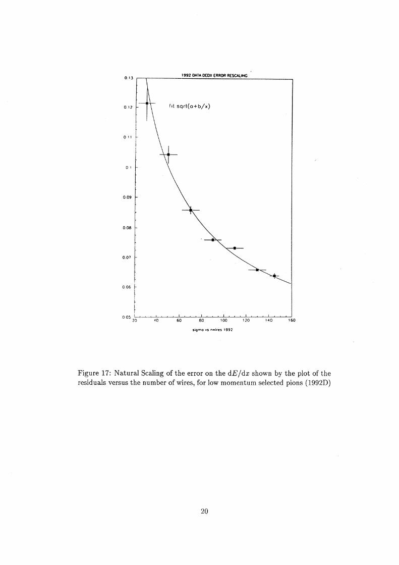
residuals versus the number of wires, for low momentum selected pions (1992D)

20

1992 DATA DEOX ERROR RESCALING

Gs

o sigmo

(o.u.),

fit sqrt(o+b/x) nN t

low momentum protons

0.11 -

0.09 F

0.08 -

0.07

0.06 - 0.05 A. 4. 4 i i 4 i. ] i. 4. i { 4. i. A 1 4. 4 Jb ] 4 i 4 l rt 4 d.

20 40 60 BO 100 120 140 160 co, Se number of wires

Sigmo vs nwires 1992 a

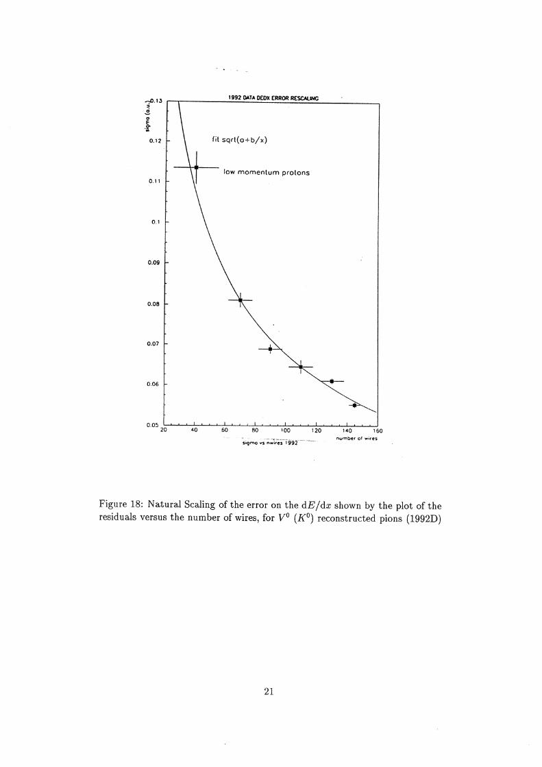
Figure 18: Natural Scaling of the error on the dE/dz shown by the plot of the residuals versus the number of wires, for V° (K°) reconstructed pions (1992D)

21

The numbers obtained for the data 1992D are perfectly analogous to these ones. The asymptotic resolution on the dE /dz has been estimated by the scaling of the sigma with the number of wires to be

. dk; oye) = 5.7%(—~) (DATA 1991 F) (16)

pions __ % dk;

10 Conclusions

The distributions of the Pull Variable after the calibration shows a remarkable improvement on both the natural width and the mean values, both for 1991 and 1992 data.

Fixing the uncontrolled fluctuations on dE /dz due to changes in the detector operating conditions and other systematics allowed a good increase in the per- formance of the dE’/dz identification. This has been checked carefully through the use of the D*t+ signal identified by the reconstructed decay D*t + D°nrt —+ K-atat. Using the calibrated dE/dz to identify the charged pions and kaons determined an increase on the signal to noise ratio of roughly 6%. Future work will concern the leptonics and the Monte Carlo tuning.

We would appreciate very much feedback from other users on other physics channels, in order to improve the detailed understanding of the actual calibration performances.

11 Written and Software references

Written references

e {1] Y.Sacquin ” The DELPHI Time Projection Chamber” D.N.92-41/TRACK70

e (2) DELPHI” The DELPHI Time Projection Chamber” D.N.88-79/TRACK50

e [3] F.Sauli” Principles of operation of Multiwire Proportional and Drift Chambers” CERN 77-09 }

e [4] P.Billoir, Y.Sacquin ”The Delphi TPC distorsions” D.N.92-16/TRACK 68 PROG 182

e [5] P.Antilogus - TPC DOC on the Delphi TPC on WWW-Delphi page.

e [6] Leo ” Techniques for Nuclear and Particle Physics experiments” pp. 141- 146 Springer-Verlag

22

Software references The code is already available at CERN in the form of the FORTRAN package called ”WUPDEDX CAR”, available by the HAD-IDENT task on the HADL DENT disk area of CERNVM. This code is using the normal PHDST (UX) standard package commons. Questions about the code or suggestions can be addressed to DAH MQW PV X7.PHYSIK.UNI—-WUPPERTAL.DE or REALEQW PVX7.PHYSIK.UNI —-WUPPERTAL.DE.

12 Aknowledgements

We would like to thank Pierre Antilogus and Yves Sacquin for the fruitful discussions concerning this work; Klaus Hamacher for the encouragement and useful suggestions during the daily work in Wuppertal, Thomas Brenke for his valuable help more then one time.

23

calibration of the delphi de/dx for 1991 f and 1992 d data

Documents