building the cosmic infrared background brick by brick with herschel /pep
TRANSCRIPT
arX
iv:1
106.
3070
v1 [
astr
o-ph
.CO
] 15
Jun
201
1Astronomy & Astrophysicsmanuscript no. berta˙PEP˙counts2 c© ESO 2011June 17, 2011
Building the cosmic infrared background brick by brick withHerschel/PEP. ⋆
S. Berta1, B. Magnelli1, R. Nordon1, D. Lutz1, S. Wuyts1, B. Altieri2, P. Andreani3,4, H. Aussel5, H. Castaneda6, J.Cepa6,7, A. Cimatti8, E. Daddi5, D. Elbaz5, N.M. Forster Schreiber1, R. Genzel1, E. Le Floc’h5, R. Maiolino9, I.
Perez-Fournon6, A. Poglitsch1, P. Popesso1, F. Pozzi8, L. Riguccini5, G. Rodighiero10, M. Sanchez-Portal2, E. Sturm1,L.J. Tacconi1, and I. Valtchanov2
1 Max-Planck-Institut fur Extraterrestrische Physik (MPE), Postfach 1312, 85741 Garching, Germany.2 Herschel Science Centre, ESAC, Villanueva de la Canada, 28691 Madrid, Spain.3 ESO, Karl-Schwarzschild-Str. 2, D-85748 Garching, Germany.4 INAF - Osservatorio Astronomico di Trieste, via Tiepolo 11,34143 Trieste, Italy.5 Laboratoire AIM, CEA/DSM-CNRS-Universite Paris Diderot, IRFU/Service d’Astrophysique, Bat.709, CEA-Saclay, 91191 Gif-
sur-Yvette Cedex, France.6 Instituto de Astrofısica de Canarias, 38205 La Laguna, Spain.7 Departamento de Astrofısica, Universidad de La Laguna, Spain.8 Dipartimento di Astronomia, Universita di Bologna, Via Ranzani 1, 40127 Bologna, Italy.9 INAF - Osservatorio Astronomico di Roma, via di Frascati 33,00040 Monte Porzio Catone, Italy.
10 Dipartimento di Astronomia, Universita di Padova, Vicolodell’Osservatorio 3, 35122 Padova, Italy.
Received ...; accepted ...
ABSTRACT
The cosmic infrared background (CIB) includes roughly halfof the energy radiated by all galaxies at all wavelengths across cosmictime, as observed at the present epoch. ThePACS Evolutionary Probe (PEP) survey is exploited here to study the CIB and its redshiftdifferential, at 70, 100 and 160µm, where the background peaks. Combining PACS observationsof the GOODS-S, GOODS-N,Lockman Hole and COSMOS areas, we define number counts spanning over more than two orders of magnitude in flux: from∼1mJy to few hundreds mJy. Stacking of 24µm sources andP(D) statistics extend the analysis down to∼0.2 mJy. Taking advantageof the wealth of ancillary data in PEP fields, differential number countsd 2N/dS/dz and CIB are studied up toz = 5. Based onthese counts, we discuss the effects of confusion on PACS blank field observations and provide confusion limits for the three bandsconsidered. While most of the available backward evolutionmodels predict the total PACS number counts with reasonablesuccess, theconsistency to redshift distributions and CIB derivativescan still be significantly improved. The new high-quality PEP data highlightthe need to include redshift-dependent constraints in future modeling. The total CIB surface brightness emitted abovePEP 3σ fluxlimits is νIν = 4.52± 1.18, 8.35± 0.95 and 9.49± 0.59 [nW m−2 sr−1] at 70, 100, and 160µm, respectively. These values correspondto 58± 7% and 74± 5% of the COBE/DIRBE CIB direct measurements at 100 and 160µm. Employing theP(D) analysis, thesefractions increase to∼65% and∼89%. More than half of the resolved CIB was emitted at redshift z ≤ 1. The 50%-light redshifts lieat z = 0.58, 0.67 and 0.73 at the three PACS wavelengths. The distribution moves towards earlier epochs at longer wavelengths: whilethe 70µm CIB is mainly produced byz ≤ 1.0 objects, the contribution ofz > 1.0 sources reaches 50% at 160µm. Most of the CIBresolved in the three PACS bands was emitted by galaxies withinfrared luminosities in the range 1011 − 1012 L⊙.
Key words. Infrared: diffuse background – Infrared: galaxies – Cosmology: cosmic background radiation – Galaxies: statistics –Galaxies: evolution
1. Introduction
With the exception of the cosmic microwave background, whichrepresents the relic of the Big Bang, emitted at the last scatter-ing surface, the extragalactic background light (EBL) is the inte-gral of the energy radiated by all galaxies, fromγ-rays to radiofrequencies, across all cosmic epochs. Its energy density distri-bution is characterized by two primary peaks: the first atλ ∼ 1µm produced by starlight, and a second peak at∼ 100− 200µm mainly due to starlight absorbed and reprocessed by dust ingalaxies (e.g. Hauser & Dwek 2001). Contribution from other
Send offprint requests to: Stefano Berta, e-mail:[email protected]⋆ Herschel is an ESA space observatory with science instruments pro-
vided by European-led Principal Investigator consortia and with impor-tant participation from NASA.
sources, such as active galactic nuclei, are expected to be only5-20% to the total EBL in the mid- and far-IR (e.g. Matute et al.2006; Jauzac et al. 2011; Draper & Ballantyne 2011). The opti-cal and infrared backgrounds dominate the EBL by several or-ders of magnitude with respect to all other spectral domains.
The cosmic infrared background (CIB) was detected andmeasured for the first time in the mid nineties, analyzing thedata obtained with the DIRBE and FIRAS instruments aboardtheCosmic Background Explorer (COBE) satellite (Puget et al.1996; Hauser et al. 1998; Fixsen et al. 1998; Lagache et al.1999, 2000). In the global budget, the CIB provides roughlyhalf of the total EBL (e.g. Dole et al. 2006; Hauser & Dwek2001). Since in the local Universe the infrared output of galax-ies is only a third of the emission at optical wavelengths (e.g.Soifer & Neugebauer 1991), this implies a strong evolution of
1

S. Berta et al.: Building the cosmic infrared background brick by brick with Herschel/PEP.
infrared galaxy populations, towards an enhanced far-IR outputin the past, in order to account for the total measured CIB.
The discovery of large numbers of distant sources emittinga substantial amount of their energy in the IR (e.g. Smail et al.1997; Aussel et al. 1999; Elbaz et al. 1999; Papovich et al. 2004,among many others) demonstrated that, although locally rare,powerful IR galaxies are indeed numerous at high redshift. Thedeep extragalactic campaigns carried out in the nineties and2000’s with theInfrared Space Observatory (ISO, see Genzel &Cesarsky 2000 for a summary), and theSpitzer Space Telescope(Werner et al. 2004; e.g. Papovich et al. 2004) were very effi-cient in identifying and characterizing large samples of mid-IRsources. In contrast, at wavelengths near the CIB peak (100-200µm), the performance of these telescopes was strongly limitedby their small apertures (≤ 85 cm diameter), the prohibitive con-fusion limits, and detectors’ sensitivity. Spitzer surveys at 70 and160µm produced limited samples of distant far-IR objects (e.g.Frayer et al. 2009): in the 160µm Spitzer/MIPS band only∼ 7%of the CIB was resolved into individually detected objects (Doleet al., 2004, see Lagache et al. 2005 for a review). Performingstacking of 24µm sources, Dole et al. (2006) retrieved more than70% of the far-IR background at 70 and 160µm. Bethermin et al.(2010a) extended this analysis by extrapolating to very faint fluxdensities using a power-law fit to stacked number counts, andproduced an estimate of the CIB surface brightness in agreementwith direct measurements.
Launched in May 2009, Herschel (Pilbratt et al. 2010) is pro-viding stunning results: its large 3.5 m mirror, and the highsensi-tivity Photodetector Array Camera & Spectrometer (PACS, per-forming imaging at 70, 100, 160µm; Poglitsch et al., 2010) aretailored to overtake the confusion and blending of sources thatwere hampering the detection of faint far-IR sources in previousspace missions. In Berta et al. (2010, hereafter called “Paper I”),we exploited data from thePACS Evolutionary Probe (PEP)survey, covering the GOODS-N, Lockman Hole and COSMOS(to partial depth only) fields, and we resolved into individualsources 45% and 52% of the CIB at 100 and 160µm. At longerwavelengths, in the spectral domain covered by theSpectraland Photometric Imaging Receiver (SPIRE, Griffin et al. 2010),Oliver et al. (2010) resolved 15%, 10% and 6% of the CIB at250, 350 and 500µm. These fractions increased to 64%, 60%and 43%, respectively, using aP(D) analysis (Glenn et al. 2010).Finally, Bethermin et al. (2010b) retrieved roughly 50% oftheCIB applying stacking of 24µm sources to BLAST 250, 350and 500µm maps.
The PACS Evolutionary Probe (PEP1) is one of the ma-jor Herschel Guaranteed Time (GT) extragalactic projects.It isstructured as a “wedding cake” survey, based on four differentlayers in order to cover wide shallow areas and deep pencil-beam fields. PEP includes the most popular and widely studiedextragalactic blank fields: COSMOS (2 deg2), Lockman Hole,EGS and ECDFS (450-700 arcmin2), GOODS-N and GOODS-S (∼200 arcmin2). In addition, the fourth tier of the “cake” con-sists of ten nearby lensing clusters, offering the chance to breakthe PACS confusion limit thanks to gravitational lensing. Anin depth description of PEP fields and survey properties is pre-sented by Lutz et al. (2011, in prep.).
Here we extend the analysis carried out in Paper I to thedeepest field observed by PEP, GOODS-S, reaching a 3σdepth of 1.2 mJy at 100µm, and including also the 70µmPACS bandpass. The surface brightness of the CIB and its spec-tral energy distribution (SED) has become known with increas-
1 http://www.mpe.mpg.de/ir/Research/PEP/
ing detail, from its initial discovery with COBE to the Spitzerera. The real conundrum is now represented by how the CIBevolves as a function of cosmic time. This information is notonly important to constrain models of galaxy evolution, butalsoto shed light on the intrinsic spectra of TeV sources, such asBLAZARs, whoseγ-ray photons interact with the CIB (e.g.Domınguez et al. 2011; Franceschini et al. 2008; Mazin & Raue2007). Thanks to Herschel capabilities, in Paper I we have ini-tiated the study of the redshift build-up of the local far-IRCIB,by associating to each object detected by PACS in GOODS-Na complete UV-to-FIR SED and splitting number counts andCIB into redshift slices. Jauzac et al. (2011) performed a similarstudy based on stacking on 70 and 160µm Spitzer/MIPS maps ofCOSMOS, and Le Floc’h et al. (2009) performed a similar anal-ysis at 24µm in the same field. Here we take advantage of deeperPACS observations in GOODS-S and full coverage in COSMOSto further explore the history of CIB, with the aim to understandwhen it was primarily emitted.
In this paper, the cosmic far-IR background is reconstructed“brick by brick” in three main “storeys”. In Section 2 the re-solved component of number counts is presented, including slic-ing in redshift and a comparison to available evolutionary mod-els. Section 3 deals with stacking of 24µm sources onto PACSmaps. The third step (Sect. 4) extends the analysis to even fainterfluxes using the “probability of deflection”,P(D), technique.After a brief digression about source confusion in Sect. 5, wediscuss the observed properties of CIB in Sect. 6. Finally, Sect.7 draws a summary of our findings.
2. Level 1: detected sources
In Paper I we studied number counts based onScienceDemonstration Phase (SDP) and early routine phase data, i.e.based on the GOODS-N, Lockman Hole and COSMOS fields.At the time of SDP, COSMOS was available only to 2/3 of itsnominal depth. Altieri et al. (2010) exploited gravitational lens-ing in the Abell 2218 cluster of galaxies to estimate the lensamplification of the fluxes of background galaxies. In this way,they were able to push the analysis down to 1 mJy at 100 and160µm, thus breaking the confusion limit for blank field obser-vations (see Sect. 5).
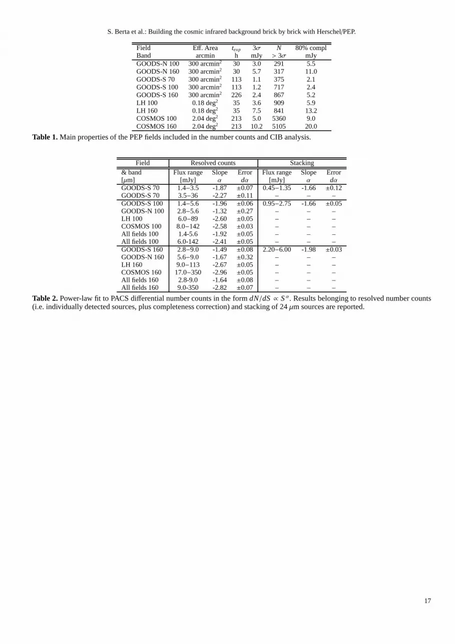
Here we complete the Herschel/PACS view of far-IR numbercounts and CIB, making use of the deepest PEP field, GOODS-S, and the full coverage of COSMOS, in addition to Paper Iresults. Data reduction, catalogs construction and simulations,aimed at deriving completeness, fraction of spurious sources andphotometric reliability, are described in Lutz et al. (in prep.) andBerta et al. (2010). Table 1 summarizes the main properties ofthe fields taken into account here.
We applied the method described by Chary et al. (2004) andSmail et al. (1995) to correct number counts for incompleteness,on the basis of simulations. The distribution of input and out-put fluxes in simulations is organized in a matrixPi j, so thatirepresents the input flux andj the output flux. In other words,thei j-th element of the matrix gives the number of sources withi-th input flux andj-th output flux. The wayPi j is built impliesthat
∑
j Pi j ≤ 1 represents the completeness correction factorat thei-th input flux in simulations. In order to correct the ob-served counts,Pi j is re-normalized such that the
∑
i Pi j equalsthe number of real sources detected in thej-th flux bin. Finally,the completeness-corrected counts in the giveni-th bin are givenby
∑
j P renormi j .
Figure 1 presents PACS number counts at 70, 100 and160 µm, normalized to the Euclidean slope (i.e. the slope ex-
2

S. Berta et al.: Building the cosmic infrared background brick by brick with Herschel/PEP.
Fig. 1. Differential number counts in the three PACS bands, normalized to the Euclidean slope (dN/dS ∝ S −2.5). Filled/opensymbols belong to flux bins above/below the 80% completeness limit. Models belong to Lagache et al. (2004), Franceschini et al.(2010), Rowan-Robinson (2009), Le Borgne et al. (2009), Valiante et al. (2009), Lacey et al. (2010), Bethermin et al. (2010c),Marsden et al. (2010), Gruppioni et al. (2011, in prep.), Niemi et al. (2011, in prep.). Shaded areas represent ISO and Spitzer data(Rodighiero & Franceschini 2004; Heraudeau et al. 2004; B´ethermin et al. 2010a); hatched areas belong to Spitzer 24µm stacking(Bethermin et al. 2010a).Left andright panels present individual fields and averaged counts, respectively.
pected for a uniform distribution of galaxies in Euclidean space,dN/dS ∝ S −2.5). Error bars include Poisson statistics, flux cal-ibration uncertainties, and photometric errors. The latter havebeen propagated into number counts via 104 realizations of ran-dom Gaussian flux errors applied to each PACS source, using adispersion equal to the local measured noise. It is worth to note
that in most cases the faint end of counts derived in shallow fieldsis consistent with results from deeper fields, thus confirming thevalidity of completeness corrections. Number counts, their cor-responding uncertainties and completeness values are reportedin Tabs. 3, 4, and 5.
3
S. Berta et al.: Building the cosmic infrared background brick by brick with Herschel/PEP.
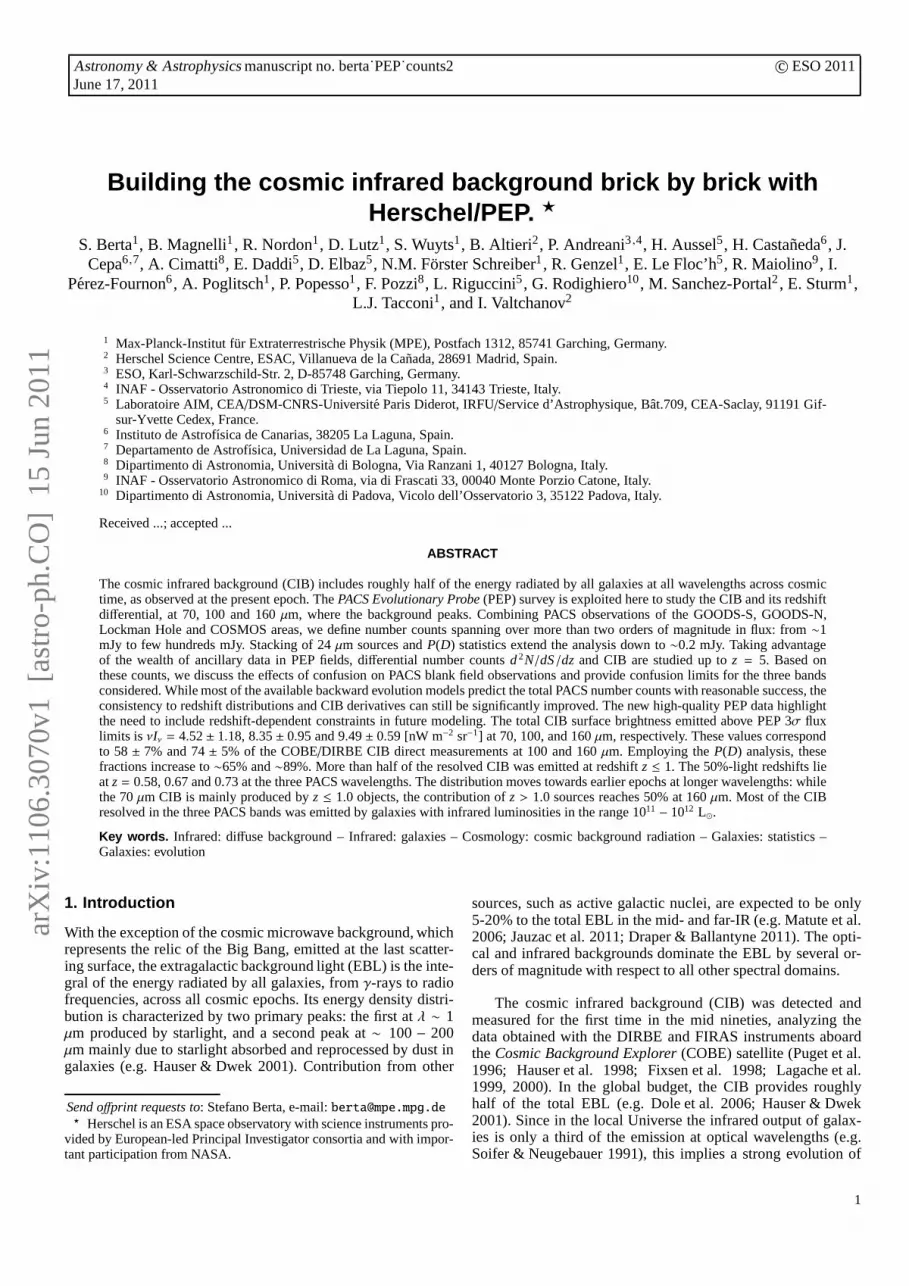
Fig. 2. Field-to-field variations of number counts in COSMOS.Top panels: number counts split into sub-areas (lines) comparedto full-field counts (black dots).Bottom diagram: standard deviation among the sub-fields (top), as a function of flux. In the verybottom panels, we show the comparison between the field-to-field σ(var) and the uncertaintyσP obtained combining Poissonstatistics, photometric errors and systematics. Shaded areas represent 1σ uncertainties onσ(var) andσ(var)/σP determinations.
The left panels in Fig. 1 show the counts for each field sep-arately. Filled symbols represent data above 80% completeness,while open symbols extend down to the 3σ detection threshold.The grey shaded areas in Fig. 1 belong to pre-Herschel num-ber counts. We include the Rodighiero & Franceschini (2004)and Heraudeau et al. (2004) 95µm ISO data, and the 70µmand 160µm Spitzer number counts by Bethermin et al. (2010a),based on GOODS/FIDEL, COSMOS and SWIRE fields. Bothindividual detection and stacked Spitzer counts (hatched areas)are shown. PACS counts and previous results are in good agree-ment, over the flux range in common. The PEP deepest field,GOODS-S, extends the knowledge on far-IR number counts oneorder of magnitude deeper in flux than Spitzer individual de-tections at 160µm and roughly 5 times deeper at 70µm. The3σ limit in GOODS-S (1.2 mJy and 2.4 mJy at 100 and 160µm, respectively) is very close to the effective depth reachedby Altieri et al. (2010) in the Abell 2218 cluster when studyinglensed background galaxies, but our improved source statisticsprovide much tighter uncertainties.
In order to provide a single reference counts description, thenumber counts belonging to the four PEP fields studied havebeen combined via a simple average, weighted by their respec-tive uncertainties in each flux bin. Results are included in Tabs.
3, 4, 5, and are shown in the right panels of Fig. 1, as comparedto a collection of model predictions (see Sect. 2.4).
The depth reached by PACS/PEP allows us to accuratelyprobe the faint-end of counts. The peak in the normalized countsis well sampled and turns out to lie at∼4 mJy at 70µm,∼10 mJyat 100µm, and∼20-30 mJy at 160µm. The differential countsare reproduced by a broken power law (dN/dS ∝ S α), charac-terized by a break at fluxS break and two distinct slopes at the atfaint/bright sides of the break. A weighted least squares fit wasperformed on the data, and the results are presented in Tab. 2, fordifferent fields and flux ranges. Breaks happen at∼3.5 mJy at 70µm, ∼5.0 mJy at 100µm, and∼9.0 at 160µm. Uncertainties atthe bright end are dominated by Poisson statistics, and nearly-Euclidean slopes are allowed.
2.1. Field to field variations
The large area probed by COSMOS (∼2 deg2) can be used totest the effect of field-to-field density variations on the bright-end of number counts. We adopt a fully empirical method, de-scribing the variance in number counts coming from the inferredvariations, while a full clustering quantification goes beyond thescope of this paper. To this aim, we split the COSMOS field intoa number of fully independent tiles, probing different angular
4

S. Berta et al.: Building the cosmic infrared background brick by brick with Herschel/PEP.
scales: 28 tiles with size∼200 arcmin2, similar to the size ofGOODS fields, 12 Lockman Hole like tiles (∼500 arcmin2), and4 tiles of∼1500 arcmin2 each.
Fig. 3. Comparison between photometric and available spectro-scopic redshifts in GOODS-S, GOODS-N and COSMOS, re-gardless of PACS detections. Dotted and dashed lines mark 10%and 20% uncertainty levels.
Number counts in each tile were computed as described be-fore and are plotted in Fig. 2 as thin solid lines. Black symbolsrepresent the average counts in each flux bin, and the associ-ated error bars are computed in the usual manner accounting forPoisson statistics, systematics and photometric uncertainties.
The properties of field-to-field standard deviation are stud-ied in the bottom diagrams of Fig. 2. As expected, theσ(var)in number counts increases as a function of flux (upper panels),both because more luminous sources are rarer in the sky andbecause lower-redshift objects are dominating at these fluxes,hence probing a smaller volume. Over the whole flux rangecovered by this analysis, the field-to-field deviation is compara-ble to the uncertaintyσP obtained combining Poisson statistics,photometric errors and systematics (bottom panels). Overall,σ(var)/σP is slightly larger than unity within the errors. This ef-fect can be explained considering that neighboring sub-tiles arenot fully independent: because of clustering, a non-negligiblecorrelation term contributes toσ(var). At larger scales (dottedgreen lines),σ(var)/σP is more noisy because of the limitednumber of tiles available.
2.2. Ancillary data and multi-wavelength catalogs
The fields observed with PACS as part of the PEP survey ben-efit from a plethora of ancillary data, spanning from the x-raysto radio frequencies. We took advantage of these data to buildreliable multi-wavelength catalogs and associate a full spectralenergy distribution (SED) and a redshift estimate to each PACS-detected object.
As described in Paper I, a PSF-matched catalog was createdin GOODS-N, including photometry from GALEX far-UV toSpitzer IRAC and MIPS 24µm. The Southern GOODS field isrich in coverage as well. Here we adopt the PSF-matched cat-alog built by Grazian et al. (2006), to which we add the 24µmphotometry by Magnelli et al. (2009) and a collection of spectro-scopic redshifts for more than 3000 sources (Balestra et al.2010;Popesso et al. 2009; Santini et al. 2009; Vanzella et al. 2008;Le Fevre et al. 2005; Mignoli et al. 2005; Doherty et al. 2005;Szokoly et al. 2004; Dickinson et al. 2004; van der Wel et al.2004; Stanway et al. 2004b,a; Strolger et al. 2004; Bunker etal.2003; Croom et al. 2001; Cristiani et al. 2000). Finally, webrowsed the COSMOS public database2 and combined the U-to-K broad- and intermediate-band photometry (Capak et al.2007; Ilbert et al. 2009, containing 2,017,800 sources), the pub-lic IRAC catalogs, the 24µm data (Le Floc’h et al. 2009) andthe available photometric (Ilbert et al. 2009) and spectroscopic(Lilly et al. 2009; Trump et al. 2009) redshifts. As far as theLockman Hole is concerned, an extensive ancillary catalog iscurrently on the make by Fotopoulou et al. (2011, in prep.), butis not available at the time of this analysis, hence this fieldwillnot be used in this piece of analysis.
PACS catalogs were matched to the ancillary source listsby means of a multi-band maximum likelihood procedure(Sutherland & Saunders 1992), starting from the longest wave-length available (160µm, PACS) and progressively matching100 µm (PACS), 70µm (PACS, GOODS-S only) and 24µm(Spitzer/MIPS) data.
When no spectroscopic redshift is available, a photometricestimate is necessary. In GOODS-S we make use of the avail-able photometric redshifts by Grazian et al. (2006), while newphoto-z’s were produced in GOODS-N, exploiting the wealthof multi-wavelength data collected, and adopting the EAZY(Brammer et al. 2008) code. Up to 14 photometric bands wereused, depending on the data available. The top panel in Fig. 3presents the comparison between photometric and the availablespectroscopic redshifts. The fraction of outliers, definedas ob-jects having∆(z)/(1+ zspec) ≥ 0.2, is∼6% over the whole sam-ple of spectroscopic redshifts, and decreases to∼2% for sourceswith a PACS detection. Most of these outliers are sources withfew photometric points available, or SEDs hardly reproduced bythe available templates. The median absolute deviation (MAD3)of the∆(z) distribution4 is 0.040 for the whole catalog, and 0.038for PACS-detected objects with spec-z available.
In the area covered by ancillary data, roughly 60-65% ofGOODS-N sources detected by PACS in either band have aspectroscopic redshift estimate. In the GOODS-S MUSIC area(Grazian et al. 2006) this fraction is as high as∼80%. Roughly95% of these spectroscopic redshifts in GOODS-S lie atz < 2.0,with an almost complete coverage. For the remaining PACSsources we adopt photometric redshifts, obtaining a 100% red-shift completeness above the 80% photometric completeness
2 http://irsa.ipac.caltech.edu/data/COSMOS/3 MAD(x) = median(|x −median(x)|)4 where here∆ denotes the difference between photometric and spec-
troscopic redshift.
5
S. Berta et al.: Building the cosmic infrared background brick by brick with Herschel/PEP.
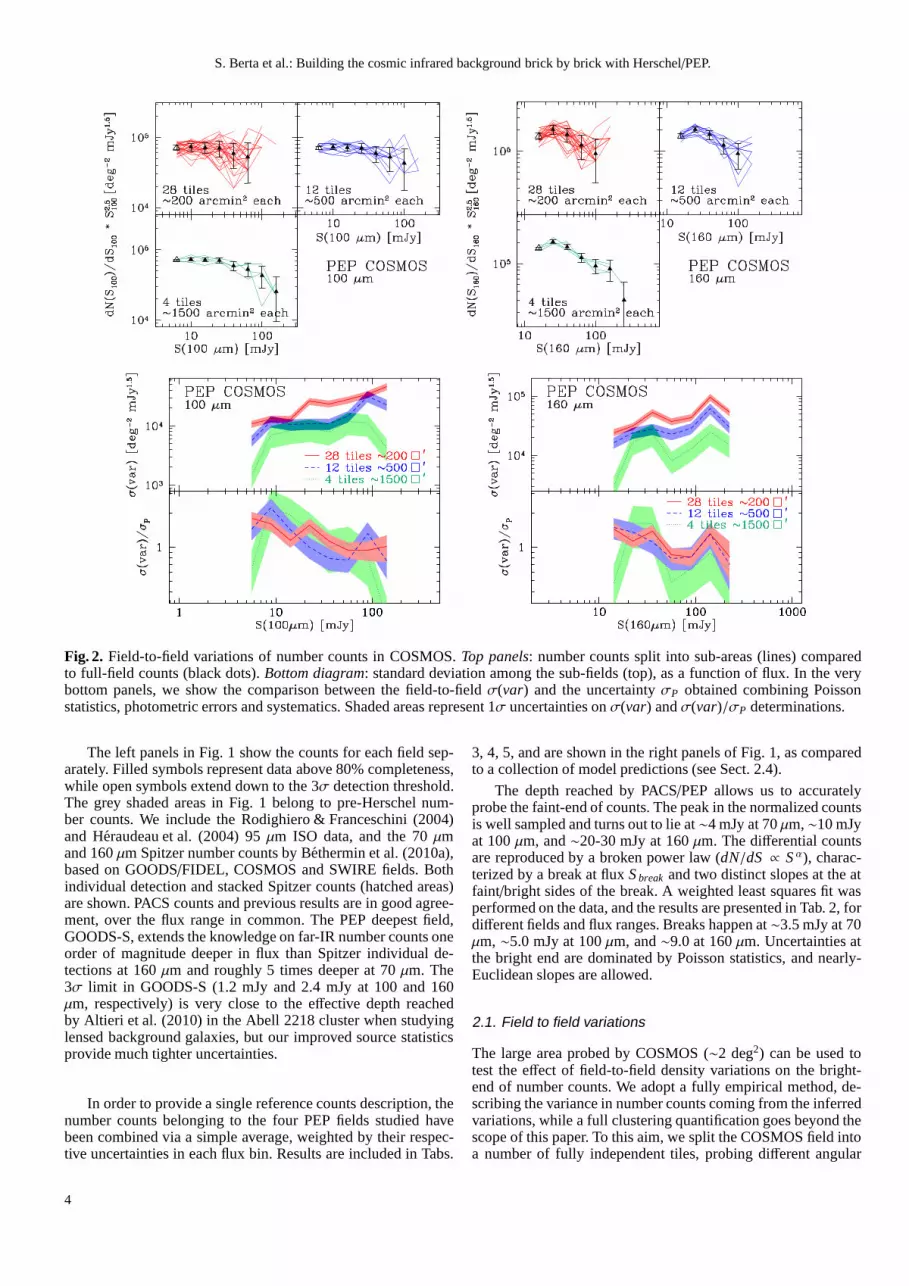
Fig. 4. Redshift derivativedN/dz for PACS-detected sources in COSMOS (left), GOODS-N (center) and GOODS-S (right), nor-malized to a 1 deg2 area, and above the 80% photometric completeness limit. Black lines refer to models and are reported only atthe GOODS-S and COSMOS depths for clarity sake.
threshold (see Tab. 1). As far as COSMOS is concerned, the pub-lic photometric redshift catalog (Ilbert et al. 2009) is limited toa magnitudeI ≤ 25, thus producing a redshift incompleteness inthe PACS-selected sample. Only∼75% of PACS sources have aphotometric redshift estimate in the Ilbert et al. (2009) catalog.This incompleteness is independent of PACS fluxes. We derivednew photometric redshifts using the EAZY code and exploitingthe public COSMOS datasets. The bottom panel of Fig. 3 showsthe results. The fraction of outliers is∼1% in this case, andMAD(∆(z)) ≃ 0.01. This result is similar to that by Ilbert et al.(2009) for the objects in common.
Given the non-null fractions of outliers in Fig. 3, it is possiblethat the number of sources at high redshift (e.g.z ≥ 2) in PEPcatalogs is in part contaminated by “catastrophic photometric-redshift failures”, mainly represented by low-z objects withwrong, high photo-z. Because of the paucity ofz ≥ 2 PACSsources benefiting from a spectroscopic follow-up, the onlyvi-able approach to test this effect is to assume that the distributionof ∆(z)/(1+ zspec) of PACS-detected objects is similar to that ofthe general galaxy population. For this reason, the resulting con-tamination fraction has to be considered as an upper limit only.
The fraction of potential contaminants atz ≥ 2 is computedin two steps. First the fraction ofz < 2 objects havingzspec < 2,but ∆(z)/(1 + zspec) ≥ 0.2 andzphot > 2 is derived; then thisis re-scaled to the ratio ofz ≷ 2 PACS sources. It turns outthat up to∼25% of GOODS-Sz ≥ 2 PACS objects might havean improperly attributed high redshift. Similar results were ob-tained in GOODS-N, while this effect cannot be properly testedin COSMOS, because publicz ≥ 2 spectroscopic redshifts arecurrently still lacking.
We also note that the opposite phenomenon — namely high-redshift sources with wrong photo-z potentially being shifted atlow-z — does not play a significant role here, because the vastmajority of z < 2 PEP/PACS objects benefits from a spectro-scopic redshift measurement.
2.3. Contribution to the counts from different epochs
We exploit the rich ancillary information described in the pre-vious Section to perform a detailed study of counts across cos-mic time. The redshift derivativedN/dz of PACS sources abovethe 80% photometric completeness limits, normalized to 1 deg2,is shown in Fig. 4 for the three fields and bands consideredhere. The covered flux ranges are quoted on each panel. In theCOSMOS area, we sample the bright end of PACS counts. Thedistribution in this field peaks atz ≤ 0.5 in both 100 and 160µmbands, with 70-80% of all sources lying belowz = 1 and∼20%betweenz = 1 andz = 2. For the deeper GOODS-N data, thepeak of the redshift distribution shifts toz ∼ 0.7. Although thesmall sampled area limits source statistics, objects at high red-shift (up toz ≃ 5) start to pop up. Our deepest field, GOODS-S,covered in all three PACS bands, displays some remarkable fea-tures. OveralldN/dz is now peaked aroundz ∼ 1. It is possibleto recognize two well known structures atz ≃ 0.7 andz ≃ 1.1(e.g. Gilli et al. 2003; Vanzella et al. 2005), which producenar-row and intense spikes in the distribution at 100 and 160µm.On the other hand, at 70µm these structures are barely seen. Athigher redshift, a broad “bump” is detected, betweenz = 2− 3.This peak cannot be identified in the shallower 70µm data, butis outstanding at the other two PACS wavelengths. Cutting theGOODS-S catalog at the depth reached by GOODS-N (5.5 mJyand 11.0 mJy at 100 and 160µm, respectively), the high-z fea-ture disappears and the redshift distribution resembles that ofGOODS-N, with only a few sources left abovez ≥ 2. Similarly,when cutting GOODS-S at the COSMOS 80% depth, we re-trieve a distribution peaked atz = 0− 0.5, obviously with muchpoorer statistics than in the COSMOS field itself. An extensiveanalysis of PACS GOODS-S large scale structure atz = 2 − 3and of az = 2.2 filamentary over density is being presented byMagliocchetti et al. (2011, sub.). Table 6 reportsdN/dz [deg−2],as derived in these three PEP fields. The median redshifts of thesources detected in GOODS-S arez ∼ 0.6, ∼ 0.7, ∼ 0.8 in thethree PACS bands, but would shift if the known spikes indN/dzwere not present.
6
S. Berta et al.: Building the cosmic infrared background brick by brick with Herschel/PEP.
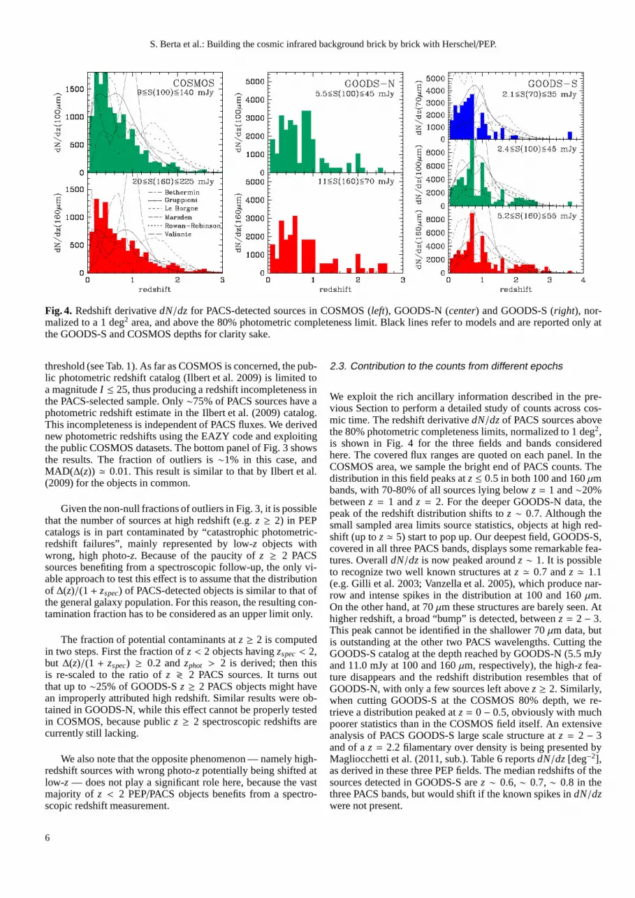
Finally, it is possible to split number counts in GOODS-S,GOODS-N and COSMOS into redshift bins, similarly to whatwas done in Paper I for GOODS-N. Counts are then constructedin four broad bins, in order to allow for a sufficient numberof sources in the small fields. In every redshift bin we applythe same completeness correction derived for the total numbercounts at the given flux. Similarly to what was done for the totalcounts, we build combined number counts through a weightedmean in each flux bin. The average number counts, sliced in red-shift intervals are reported in Tabs. 7, 8, and 9, and are shown inFig. 5. PACS observations in the three fields nicely complementeach other: the southern GOODS field reaches deep flux den-sities, not probed previously, and also traces the high redshiftpopulation that was missing in GOODS-N. The bright end ofcounts is sampled by observations in the COSMOS area, whichnot only contribute to the low-redshift counts, but also nicelytrace the bright component up toz = 2 and beyond.
2.4. Comparison to model predictions for counts across time
Number counts and redshift distributions encode the evolutionof galaxies: the upturn at intermediate fluxes and the over-Euclidean slope at the bright side of the peak are usually inter-preted as signatures of strong evolution in the properties of theunderlying galaxy populations, and have stimulated a plethoraof model interpretations.
We are comparing here our results to examples of twobasic classes of models attempting to reproduce these observ-ables.Backward evolutionary models transform the statisticalproperties of far-IR galaxies observed at known redshift (e.g.local luminosity functions) into observables at any redshift(e.g. galaxy counts, CIB brightness, etc.) assuming a library oftemplate SEDs and parametric laws of luminosity and/or densityevolution. These models do not implement fundamental physi-cal information but simply attempt to describe the evolution ofgalaxy populations (e.g. Lagache et al. 2004; Franceschiniet al.2010; Rowan-Robinson 2009; Le Borgne et al. 2009;Valiante et al. 2009; Bethermin et al. 2010c; Marsden et al.2010; Gruppioni, C., Pozzi, F., Zamorani, G., Vignali, C., et al.2011).
Very simple in their principles, backward models arethus parameterizations embedding the knowledge obtainedfrom previous observations. The different adopted recipeswere optimized to reproduce available observables such asmid-IR ISO and Spitzer number counts and far-IR Spitzercounts based on detections and — in some cases —stacking, sub-mm counts, as well as redshift distributions.A couple of models took advantage of early Herschelresults, namely SDP PACS and SPIRE number counts(Bethermin et al. 2010c) and PACS luminosity functions up toz ∼ 3 (Gruppioni, C., Pozzi, F., Zamorani, G., Vignali, C., et al.2011). Generally speaking, confronting backward models tothenew, detailed Herschel data is a test to their flexibility in produc-ing reliable predictions at far-IR wavelengths.
At the opposite side,forward evolution models simulate thephysics of galaxy formation and evolution forward in time, fromthe Big Bang to present days. Current implementations are basedon semi-analytic recipes (SAM) to describe the dissipativeandnon-dissipative processes influencing galaxy evolution, framedintoΛ-CDM dark matter numerical simulations (e.g. Lacey et al.2010, Niemi et al. in prep.). Galaxy radiation, including far-IRemission, is computed with spectrophotometric synthesis and ra-diation transfer dust reprocessing, given the fundamentalprop-erties of the galaxies in the model.
Fig. 5.Differential number counts in the three PACS bands, nor-malized to the Euclidean slope and split in redshift bins. The 70µm counts belong to the GOODS-S field, while those at 100 and160µm were obtained via a weighted average between GOODS-S, GOODS-N and COSMOS. See Fig. 1 for models references.
Figures 1 and 5 show a collection of models overlaid to theobserved PACS counts. Most of the models reproduce fairly wellthe observed 100 and 160µm normalized counts, on average the
7

S. Berta et al.: Building the cosmic infrared background brick by brick with Herschel/PEP.
most successful being Franceschini et al. (2010), Marsden et al.(2010), Rowan-Robinson (2009), Valiante et al. (2009) andGruppioni, C., Pozzi, F., Zamorani, G., Vignali, C., et al.(2011). Very different assumptions produce relatively similarnumber counts predictions. The Franceschini et al. (2010)model adopts four different galaxy populations, includingnormal galaxies, luminous infrared galaxies, AGNs and a classof strongly-evolving ULIRGs, which dominate abovez ≥ 1.5,but is negligible at later epochs, resembling high-z sub-mmgalaxies. Also Rowan-Robinson (2009) uses four galaxypopulations (cirrus-dominated quiescent galaxies, M82-likestarbursts, Arp220-like extreme starbursts, AGN dust torii), butemploys analytic evolutionary functions without discontinuities.Valiante et al. (2009) describe galaxy population taking intoaccount the observed local dispersion in dust temperature,thelocal observed distribution of AGN contribution toLT IR as afunction of luminosity, and an evolution of the local luminosity-temperature relation for IR galaxies. Marsden et al. (2010)base their SEDs on Draine & Li (2007) prescriptions and tunethem to reproduce the local color-dependent far-IR luminosityfunctions; they include luminosity, density and color evolutionsto fit sub-mm counts, redshift distributions and EBL. Finally,Gruppioni, C., Pozzi, F., Zamorani, G., Vignali, C., et al. (2011)include a significant Seyfert-2 population, based on a fit toHerschel LFs (see also Gruppioni et al. 2010).
Semi-analytical approaches surely represent a more com-plete view of galaxy evolution, including a wide variety ofphysics in a single coherent model. They cover a wide rangeof observational data: UV, optical, near-IR luminosity functions,galaxy sizes, metallicity, etc. Moreover, at far-IR wavelengths,even in the case that global properties such as star formationand AGN activity are correctly modeled, a further complicationarises from the assumptions about dust content and structure,which need to be invoked. As a result, the large number of pa-rameters involved goes at the expense of inference precision: theperformance of SAM models with respect to PACS observablesneeds still substantial tuning.
As described above, it seems that pre-Herschel models, withonly a few exceptions, are quite successful at reproducing totalnumber counts despite the range and diversity of the employedsolutions, thus showing that the discriminatory power of this ob-servable is rather limited.
The right answer comes from the redshift information avail-able in the selected PEP fields. Figure 4 presents the redshiftdistributiondN/dz of PACS galaxies, and Fig. 5 shows numbercounts split in redshift slices (d 2N/dS/dz). The combination ofthe two is a real discriminant: model predictions are now dra-matically different.
None of the available models provides a convincing coherentprediction of the whole new set of observables (bothdN/dz andd 2N/dS/dz), over the flux range covered. One common sourceof discrepancy seems to be the well-know degeneracy betweendust temperature (and hence luminosity and total dust mass)andredshift (e.g. Blain et al. 2003): red objects can be either coollocal galaxies or warmer distant galaxies. What is observedis amis-prediction of the redshift distribution, reflected forexamplein an overestimation of high redshift counts and an underesti-mation at later epochs — or vice versa. Several models seem tosystematically over predict the number of galaxies abovez ≃ 1in the deep regime. A variety of SED libraries are adopted inthese model recipes, based on different assumptions and tem-plates. These differences in SED shapes and their evolution —as well as the implementation of luminosity and density evolu-
tion for the adopted galaxy populations — indeed produce sig-nificantly different results.
Among all, the Bethermin et al. (2010c) distribution is prob-ably the closest to observations, although it presents a signifi-cant underestimation ofdN/dz at 70µm. This model was opti-mized taking into account differential number counts between 15µm and 1.1 mm, including PACS (Berta et al. 2010) and SPIRE(Oliver et al. 2010) early results, mid-IR luminosity functions(LF) up to z = 2, the far-IR local LF, and CIB measurements.This success demonstrates the need to include in model tuning(ideally by means of a proper automated fit) not only Herscheldata, but also the detailed redshift information (e.g. evolving LF,number counts split in redshift bins, redshift distributions, etc.).
In summary, while several pre-Herschel backward evolution-ary models already provide reasonable descriptions of the to-tal counts in at least some of the PACS bands, they tend to failin the synopsis of all counts and in particular redshift distribu-tions. The new Herschel dataset is a treasure box, allowing toexplore the evolution of counts and CIB with unprecedented de-tail and much deeper than previous data, on which models werecalibrated. Significant modifications on model assumptionsforSEDs and/or evolution will be needed for a satisfactory fit tothis new quality of data.
3. Level 2: stacking of 24 µm sources
Limiting the number counts analysis to individually-detectedsources only, we miss a significant fraction of the informa-tion stored in PACS maps. It is possible to recover part ofthis information by performing stacking of sources from deeperdata (typically at shorter wavelengths, e.g. Dole et al. 2006;Marsden et al. 2009; Bethermin et al. 2010a). The 24µm cat-alog in the GOODS-S field, extending down to∼20 µJy(Magnelli et al. 2009), provides the ideal priors to performstack-ing of faint sources on PACS maps.
The aim here is to transform 24µm faint number counts intoPACS counts, given the average PACS/24µm colors of galaxies.The overall procedure consists in building such colors as a func-tion of 24µm flux, including both sources detected by PACS andun-detected ones. Then the derived colors are used to transform24 µm counts into PACS counts, probing the faint end of thedistribution, below the PACS detection limit.
To reach this goal, we select 24µm sources not detectedin PACS maps, and bin them by their 24µm flux. Followingthe standard technique described by Dole et al. (2006) andBethermin et al. (2010a), in eachS (24µm) flux bin, we pile-up postage stamps at the position of these sources and pro-duce stacked frames at 70, 100 and 160µm. We measurethe flux density of the stacked sources by performing PSF-fitting in the same way as for the individually-detected ob-jects (see Berta et al. 2010). Uncertainties on the stacked fluxesare computed through a simple bootstrap procedure. Stackingwas performed on PACS residual images, i.e. after removal ofindividually-detected sources, and the fluxes of the latterwerethen added back to stacking results. Finally, we checked that nosignificant signal was detected when stacking at random posi-tions, and that stacks of PACS-detected sources retrieved theiractual total summed flux. Flux corrections due to losses duringthe high-pass filtering process were tested via simulationsandturned out to have a negligible effect on our results (see Lutz etal. 2011 for a description).
We derived average flux densities simply dividing by the to-tal number of sources in each 24µm flux bin, and then we builtPACS/24µm average colors. Figure 6 shows the results. Stacking
8
S. Berta et al.: Building the cosmic infrared background brick by brick with Herschel/PEP.
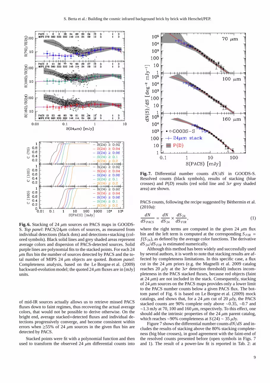
Fig. 6. Stacking of 24µm sources on PACS maps in GOODS-S. Top panel: PACS/24µm colors of sources, as measured fromindividual detections (black dots) and detections+stacking (col-ored symbols). Black solid lines and grey shaded areas representaverage colors and dispersion of PACS-detected sources. Solidpurple lines are polynomial fits to the stacked points. For each 24µm flux bin the number of sources detected by PACS and the to-tal number of MIPS 24µm objects are quoted.Bottom panel:Completeness analysis, based on the Le Borgne et al. (2009)backward-evolution model; the quoted 24µm fluxes are in [mJy]units.
of mid-IR sources actually allows us to retrieve missed PACSfluxes down to faint regimes, thus recovering the actual averagecolors, that would not be possible to derive otherwise. On thebright end, average stacked+detected fluxes and individual de-tections progressively converge, and become consistent withinerrors when≥55% of 24µm sources in the given flux bin aredetected by PACS.
Stacked points were fit with a polynomial function and thenused to transform the observed 24µm differential counts into
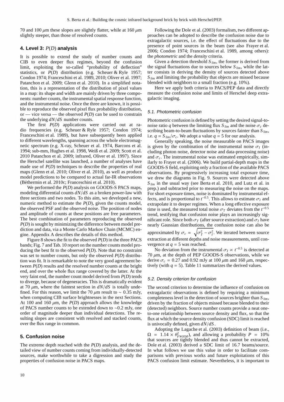
Fig. 7. Differential number countsdN/dS in GOODS-S.Resolved counts (black symbols), results of stacking (bluecrosses) andP(D) results (red solid line and 3σ grey shadedarea) are shown.
PACS counts, following the recipe suggested by Bethermin et al.(2010a):
dNdS PACS
=dN
dS 24×
dS 24
dS FIR, (1)
where the right terms are computed in the given 24µm fluxbin and the left term is computed at the correspondingS FIR =
f (S 24), as defined by the average color functions. The derivativedS 24/dS FIR is estimated numerically.
Although this method has been widely and successfully usedby several authors, it is worth to note that stacking resultsare af-fected by completeness limitations. In this specific case, afluxcut in the 24µm priors (e.g. the Magnelli et al. 2009 catalogreaches 20µJy at the 3σ detection threshold) induces incom-pleteness in the PACS stacked fluxes, because red objects (faintat 24µm) are not included in the stack. Consequently, stackingof 24µm sources on the PACS maps provides only a lower limitto the PACS number counts below a given PACS flux. The bot-tom panel of Fig. 6 is based on Le Borgne et al. (2009) mockcatalogs, and shows that, for a 24µm cut of 20µJy, the PACSstacked counts are 90% complete only above∼0.35,∼0.7 and∼1.3 mJy at 70, 100 and 160µm, respectively. To this effect, oneshould add the intrinsic properties of the 24µm parent catalog,which reaches∼90% completeness atS (24)∼ 35µJy.
Figure 7 shows the differential number countsdN/dS and in-cludes the results of stacking above the 80% stacking complete-ness (big blue crosses), in good agreement with the faint-end ofthe resolved counts presented before (open symbols in Figs.7and 1). The result of a power-law fit is reported in Tab. 2: at
9
S. Berta et al.: Building the cosmic infrared background brick by brick with Herschel/PEP.
70 and 100µm these slopes are slightly flatter, while at 160µmslightly steeper, than those of resolved counts.
4. Level 3: P(D) analysis
It is possible to extend the study of number counts andCIB to even deeper flux regimes, beyond the confusionlimit, exploiting the so-called “probability of deflection”statistics, or P(D) distribution (e.g. Scheuer & Ryle 1957;Condon 1974; Franceschini et al. 1989, 2010; Oliver et al. 1997;Patanchon et al. 2009; Glenn et al. 2010). In a simplified nota-tion, this is a representation of the distribution of pixel valuesin a map: its shape and width are mainly driven by three compo-nents: number counts, the instrumental spatial response function,and the instrumental noise. Once the three are known, it is possi-ble to reproduce the observed pixel flux probability distribution,or — vice versa — the observedP(D) can be used to constrainthe underlyingdN/dS number counts.
The first P(D) applications were carried out at ra-dio frequencies (e.g. Scheuer & Ryle 1957; Condon 1974;Franceschini et al. 1989), but have subsequently been appliedto different wavelengths, spanning across the whole electromag-netic spectrum (e.g. X-ray, Scheuer et al. 1974, Barcons et al.1994; sub-mm, Hughes et al. 1998, Weiß et al. 2009; Scott et al.2010 Patanchon et al. 2009; infrared, Oliver et al. 1997). Sincethe Herschel satellite was launched, a number of analyses havemade use ofP(D) techniques to describe the properties of realmaps (Glenn et al. 2010; Oliver et al. 2010), as well as producemodel predictions to be compared to actual far-IR observations(Bethermin et al. 2010c; Franceschini et al. 2010).
We performed theP(D) analysis on GOODS-S PACS maps,modeling differential countsdN/dS as a broken power-law withthree sections and two nodes. To this aim, we developed a new,numeric method to estimate theP(D), given the counts model,the observed PSF and the observed noise. The position of nodesand amplitude of counts at these positions are free parameters.The best combination of parameters reproducing the observedP(D) is sought by minimizing the difference between model pre-diction and data, via a Monte Carlo Markov Chain (MCMC) en-gine. Appendix A describes the details of this method.
Figure 8 shows the fit to the observedP(D) in the three PACSbands; Fig. 7 and Tab. 10 report on the number counts model pro-ducing the best fit to the observedP(D). Note that no constraintwas set to number counts, but only the observedP(D) distribu-tion was fit. It is remarkable to note the very good agreement be-tweenP(D) results and the resolved number counts at the brightend, and over the whole flux range covered by the latter. At thevery faint end, the number count model derived fromP(D) tendsto diverge, because of degeneracies. This is dramatically evidentat 70µm, where the faintest section indN/dS is totally unde-fined. For this reason, we limit the 70µm result to∼ 0.35 mJy,when computing CIB surface brightnesses in the next Sections.At 100 and 160µm, theP(D) approach allows the knowledgeof PACS number counts to be extended down to∼0.2 mJy, oneorder of magnitude deeper than individual detections. The re-sulting slopes are consistent with resolved and stacked counts,over the flux range in common.
5. Confusion noise
The extreme depth reached with theP(D) analysis, and the de-tailed view of number counts coming from individually-detectedsources, make worthwhile to take a digression and study theproperties of confusion noise in PACS maps.
Following the Dole et al. (2003) formalism, two different ap-proaches can be adopted to describe the confusion noise due toextragalactic sources, i.e. the effect of fluctuations due to thepresence of point sources in the beam (see also Frayer et al.2006; Condon 1974; Franceschini et al. 1989, among others):thephotometric and thedensity criteria.
Given a detection thresholdS lim, the former is derived fromthe signal fluctuations due to sources belowS lim, while the lat-ter consists in deriving the density of sources detected aboveS lim and limiting the probability that objects are missed becauseblended with neighbors to a small fraction (e.g. 10%).
Here we apply both criteria to PACS/PEP data and directlymeasure the confusion noise and limits of Herschel deep extra-galactic imaging.
5.1. Photometric confusion
Photometric confusion is defined by setting the desired signal-to-noise ratioq between the limiting fluxS lim and the noiseσc de-scribing beam-to-beam fluctuations by sources fainter thanS lim,i.e.q = S lim/σc. We adopt a valueq = 5 for our analysis.
Generally speaking, the noise measurable on PACS imagesis given by the combination of the instrumental noiseσI (in-cluding photon noise, detector noise and data-processing noise)andσc. The instrumental noise was estimated empirically, sim-ilarly to Frayer et al. (2006). We build partial-depth maps in theGOODS-S field, exploiting only a fraction of the available PACSobservations. By progressively increasing total exposuretime,we drew the diagrams in Fig. 9. Sources were detected aboveS lim in the usual way (see Berta et al. 2010, and Lutz et al. inprep.) and subtracted prior to measuring the noise on the maps.For short exposure times, noise is dominated by instrumental ef-fects, and is proportional tot−0.5. This allows to estimateσI andextrapolate it to deeper regimes. When a long effective exposuretime is used, the measured total noiseσT deviates from thet−0.5
trend, testifying that confusion noise plays an increasingly sig-nificant role. Since bothσT (after source extraction) andσI havenearly Gaussian distributions, the confusion noise can also be
approximated byσc =
√
σ2T − σ
2I . We iterated between source
extraction at different depths and noise measurements, until con-vergence atq = 5 was reached.
No deviation from the instrumentalσI ∝ t−0.5 is detected at70 µm, at the depth of PEP GOODS-S observations, while wederiveσc = 0.27 and 0.92 mJy at 100µm and 160µm, respec-tively (with q = 5). Table 11 summarizes the derived values.
5.2. Density criterion for confusion
The second criterion to determine the influence of confusiononextragalactic observations is defined by requiring a minimumcompleteness level in the detection of sources brighter than S lim,driven by the fraction of objects missed because blended to their(detected) neighbors. Source number counts provide a neat one-to-one relationship between source density and flux, so thattheflux at which the source density confusion (SDC) limit is reachedis univocally defined, givendN/dS .
Adopting the Lagache et al. (2003) definition of beam (i.e.,Ω = 1.14 × θ2FWHM ), and allowing a probabilityP = 10%that sources are tightly blended and thus cannot be extracted,Dole et al. (2003) derived a SDC limit of 16.7 beams/source.In what follows we use this value in order to facilitate com-parisons with previous works and future exploitations of thisPACS confusion limit estimate. Nevertheless, it is important to
10
S. Berta et al.: Building the cosmic infrared background brick by brick with Herschel/PEP.
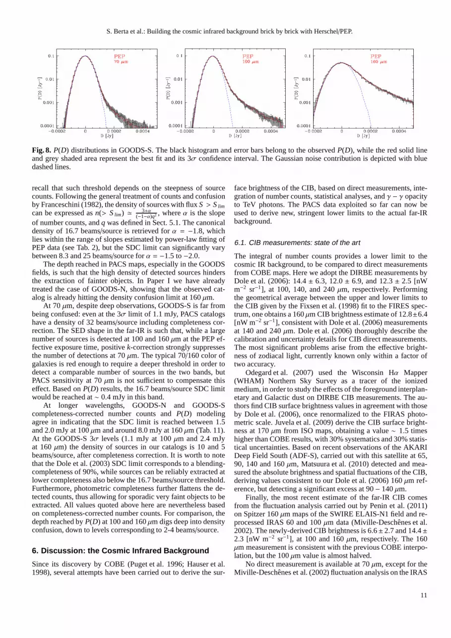
Fig. 8. P(D) distributions in GOODS-S. The black histogram and error bars belong to the observedP(D), while the red solid lineand grey shaded area represent the best fit and its 3σ confidence interval. The Gaussian noise contribution is depicted with bluedashed lines.
recall that such threshold depends on the steepness of sourcecounts. Following the general treatment of counts and confusionby Franceschini (1982), the density of sources with fluxS > S lim
can be expressed asn(> S lim) ≃ 3+α(−1−α)q2 , whereα is the slope
of number counts, andq was defined in Sect. 5.1. The canonicaldensity of 16.7 beams/source is retrieved forα = −1.8, whichlies within the range of slopes estimated by power-law fitting ofPEP data (see Tab. 2), but the SDC limit can significantly varybetween 8.3 and 25 beams/source forα = −1.5 to−2.0.
The depth reached in PACS maps, especially in the GOODSfields, is such that the high density of detected sources hindersthe extraction of fainter objects. In Paper I we have alreadytreated the case of GOODS-N, showing that the observed cat-alog is already hitting the density confusion limit at 160µm.
At 70 µm, despite deep observations, GOODS-S is far frombeing confused: even at the 3σ limit of 1.1 mJy, PACS catalogshave a density of 32 beams/source including completeness cor-rection. The SED shape in the far-IR is such that, while a largenumber of sources is detected at 100 and 160µm at the PEP ef-fective exposure time, positivek-correction strongly suppressesthe number of detections at 70µm. The typical 70/160 color ofgalaxies is red enough to require a deeper threshold in ordertodetect a comparable number of sources in the two bands, butPACS sensitivity at 70µm is not sufficient to compensate thiseffect. Based onP(D) results, the 16.7 beams/source SDC limitwould be reached at∼ 0.4 mJy in this band.
At longer wavelengths, GOODS-N and GOODS-Scompleteness-corrected number counts andP(D) modelingagree in indicating that the SDC limit is reached between 1.5and 2.0 mJy at 100µm and around 8.0 mJy at 160µm (Tab. 11).At the GOODS-S 3σ levels (1.1 mJy at 100µm and 2.4 mJyat 160µm) the density of sources in our catalogs is 10 and 5beams/source, after completeness correction. It is worth to notethat the Dole et al. (2003) SDC limit corresponds to a blending-completeness of 90%, while sources can be reliably extracted atlower completeness also below the 16.7 beams/source threshold.Furthermore, photometric completeness further flattens the de-tected counts, thus allowing for sporadic very faint objects to beextracted. All values quoted above here are nevertheless basedon completeness-corrected number counts. For comparison,thedepth reached byP(D) at 100 and 160µm digs deep into densityconfusion, down to levels corresponding to 2-4 beams/source.
6. Discussion: the Cosmic Infrared Background
Since its discovery by COBE (Puget et al. 1996; Hauser et al.1998), several attempts have been carried out to derive the sur-
face brightness of the CIB, based on direct measurements, inte-gration of number counts, statistical analyses, andγ − γ opacityto TeV photons. The PACS data exploited so far can now beused to derive new, stringent lower limits to the actual far-IRbackground.
6.1. CIB measurements: state of the art
The integral of number counts provides a lower limit to thecosmic IR background, to be compared to direct measurementsfrom COBE maps. Here we adopt the DIRBE measurements byDole et al. (2006): 14.4 ± 6.3, 12.0 ± 6.9, and 12.3 ± 2.5 [nWm−2 sr−1], at 100, 140, and 240µm, respectively. Performingthe geometrical average between the upper and lower limits tothe CIB given by the Fixsen et al. (1998) fit to the FIRES spec-trum, one obtains a 160µm CIB brightness estimate of 12.8±6.4[nW m−2 sr−1], consistent with Dole et al. (2006) measurementsat 140 and 240µm. Dole et al. (2006) thoroughly describe thecalibration and uncertainty details for CIB direct measurements.The most significant problems arise from the effective bright-ness of zodiacal light, currently known only within a factoroftwo accuracy.
Odegard et al. (2007) used the Wisconsin Hα Mapper(WHAM) Northern Sky Survey as a tracer of the ionizedmedium, in order to study the effects of the foreground interplan-etary and Galactic dust on DIRBE CIB measurements. The au-thors find CIB surface brightness values in agreement with thoseby Dole et al. (2006), once renormalized to the FIRAS photo-metric scale. Juvela et al. (2009) derive the CIB surface bright-ness at 170µm from ISO maps, obtaining a value∼ 1.5 timeshigher than COBE results, with 30% systematics and 30% statis-tical uncertainties. Based on recent observations of the AKARIDeep Field South (ADF-S), carried out with this satellite at65,90, 140 and 160µm, Matsuura et al. (2010) detected and mea-sured the absolute brightness and spatial fluctuations of the CIB,deriving values consistent to our Dole et al. (2006) 160µm ref-erence, but detecting a significant excess at 90− 140µm.
Finally, the most recent estimate of the far-IR CIB comesfrom the fluctuation analysis carried out by Penin et al. (2011)on Spitzer 160µm maps of the SWIRE ELAIS-N1 field and re-processed IRAS 60 and 100µm data (Miville-Deschenes et al.2002). The newly-derived CIB brightness is 6.6±2.7 and 14.4±2.3 [nW m−2 sr−1], at 100 and 160µm, respectively. The 160µm measurement is consistent with the previous COBE interpo-lation, but the 100µm value is almost halved.
No direct measurement is available at 70µm, except for theMiville-Deschenes et al. (2002) fluctuation analysis on the IRAS
11

S. Berta et al.: Building the cosmic infrared background brick by brick with Herschel/PEP.
Fig. 9.Noise in PACS GOODS-S maps at 70, 100, 160µm (top,middle, bottom panels), as a function of exposure time. Thedashed line represent the trendσI ∝ t−0.5 followed by instru-mental noise; while the dotted line isσT obtained by summingσI and the confusion noiseσc in quadrature. Squares mark theexpected pure-instrumental noise at the exposure times consid-ered, while circles denote the measuredσT .
60µm map (νIν = 9.0 [nW m−2 sr−1]) and the AKARI estimateat 65µm (νIν = 12.4± 1.4± 9.2 [nW m−2 sr−1], including statis-tical and zodiacal-light uncertainties, Matsuura et al. 2010).
Further constraints on the actual value of the CIB come fromthe cosmic photon-photo opacity: very high-energy photonssuf-fer opacity effects byγ−γ interactions with local radiation back-grounds, producing particle pairs (e.g. Franceschini et al. 2008;Nikishov 1962). Because of the large photon density of the cos-
mic microwave background (CMB), any photon with energyǫ > 100 TeV has a very short free path, and extragalactic sourcesare undetectable above this energy. Less energetic photonssuf-fer from the opacity induced by extragalactic backgrounds,otherthan the CMB, including the CIB. Observations of absorptionfeatures and cut-offs in the high-energy spectra of BLAZARshave been successfully used to pose upper limits to the intensityof the EBL. Mazin & Raue (2007), among many others, assem-bled a compilation of 11 TeV BLAZARs (all those known at thetime of their analysis) and combined them obtaining constraintsto the EBL over the whole 0.44-80µm wavelength range.
6.2. The total CIB in PEP
Integration of number counts was performed over as wide aflux range as possible, i.e. using the combined counts pre-sented in Sect. 2, including all the four fields analyzed so far:GOODS-S, GOODS-N, Lockman Hole and COSMOS. To thisaim, GOODS-S data were extended down to the 3σ detectionthreshold, thus reaching 1.2 mJy at 70 and 100µm and 2.0 mJyat 160µm. At the bright side, COSMOS allows the integrationto be carried out to 140 mJy at 100µm and 360 mJy at 160µm.Including completeness corrections, the derived CIB locked inresolved number counts isνIν = 7.82±0.94 and 9.17±0.59 [nWm−2 sr−1], corresponding to 54±7% and 72±5% of the COBE di-rect measurements at 100 and 160µm, respectively. If the Peninet al. (2011) 100µm value were taken as reference, then PACSsources would produce∼100% of the CIB. The resolved CIB at70µm is νIν = 3.61± 1.12 [nW m−2 sr−1].
The PEP fields are missing the very bright end of num-ber counts, that can be probed only over areas even larger thanCOSMOS. This lack of information is particularly relevant at70 µm, because this band was employed only for GOODS-S observations. We therefore add previous bright counts mea-surements to our data, in order to derive the CIB brightnessemittedabove PEP flux limits, integrated all the way to+∞.The available data taken into account here are the 70 and160 µm Spitzer counts by Bethermin et al. (2010a), built overa more than of∼50 deg2 and extending to∼1 Jy, and 100µm ISO and IRAS number counts (Rodighiero & Franceschini2004; Heraudeau et al. 2004; Rowan-Robinson et al. 2004;Efstathiou et al. 2000; Oliver et al. 1992; Bertin et al. 1997), ex-tending to∼60 Jy. Beyond the flux range covered by these pastsurveys, we extrapolate the number counts with an Euclideanlaw, dN/dS ∝ S −2.5, normalized so to match the very bright endof observed counts, and extended to infinity.
Figure 10 shows the cumulative CIB surface brightness asa function of flux, as derived from the combination of PACS,Spitzer, ISO and IRAS data. The curve describing the resolvedCIB (red circles) rapidly converges to the COBE measurementsat 100 and 160µm, over the flux range covered by PACS/PEP.Our data extend the knowledge of counts and CIB by over anorder of magnitude in flux, with respect to previous estimatesbased on individual detections. The depth reached in GOODS-Sis similar to the one obtained in Abell 2218 through gravitationallensing, and the corresponding CIB surface brightnesses are con-sistent within the uncertainties. The total CIB emitted above PEP3σ flux limits (1.1 mJy at 70µm, 1.2 mJy at 100µm, 2.0 mJy at160µm), isνIν = 4.52± 1.18, 8.35± 0.95 and 9.49± 0.59 [nWm−2 sr−1] at 70, 100 and 160µm, respectively. Table 12 lists allthe values obtained.
Roughly 10% of the CIB down to the 70µm adopted thresh-old is emitted by bright galaxies, out of reach for our survey,due to the limited volume sampled. On the other hand, only a
12

S. Berta et al.: Building the cosmic infrared background brick by brick with Herschel/PEP.
Fig. 10.Cumulative CIB as a function of flux. Red circles, bluecrosses and the yellow square belong to completeness-correctedcounts, stacking andP(D) analysis, respectively. The black linesolid and grey shaded area are based on power-law fit to theresolved number counts. The star symbol indicates the CIBderived from gravitational lensing in Abell 2218 (Altieri et al.2010). The horizontal lines and shades mark the reference di-rect measurements of the CIB by Dole et al. (2006, at 100 and160µm, including 1σ uncertainty) and Miville-Deschenes et al.(2002, at 70µm). The green shaded area belongs to previous sur-veys carried out with IRAS, ISO and Spitzer (Oliver et al. 1992;Bertin et al. 1997; Efstathiou et al. 2000; Rowan-Robinson et al.2004; Rodighiero & Franceschini 2004; Heraudeau et al. 2004).At the very bright end, an Euclidean extrapolation is used (dottedlines).
few percent is produced at fluxes brighter than PEP COSMOSupper limit at 100 and 160µm. Including 100µm ELAIS and
IRAS data (up to 60 Jy), only a negligible fraction (< 0.05%) ismissed at the bright end, while beyond Spitzer counts (reaching∼1 Jy at 70 and 160µm) the Euclidean extrapolation providesroughly 1-2% of the total CIB.
The power-law fit to resolved counts (see Sect. 2 and Tab.2) provides a new estimate of the total expected CIB. We ex-trapolate power laws down to 1.0µJy and obtainνIν ≥ 11.09,νIν = 12.61+8.31
−1.74 andνIν = 13.63+3.53−0.85 [nW m−2 sr−1] in the three
PACS bands. At 70µm our data provide only a lower limit, be-cause the curve obtained from our power-law fit is not fully con-verging at 1µJy (see Fig. 10). The uncertainty on the 100µmCIB is still large because discordant slopes were found at thefaint end in the different PEP fields. The results are fully consis-tent with COBE data, but PEP and PACS pinpoint the total CIBvalues with unprecedented precision, thanks to the high qualityof observations, survey strategy, maps, and — last but not least— thanks to Herschel capabilities (grey shaded areas in Fig.10denote the 3σ uncertainty on power-law fits).
Stacking results are fully consistent with resolved numbercounts, and theP(D) analysis extends down by another decadein flux with the exception of 70µm, for which we truncatedthe computation of CIB because of a strong divergence inP(D)uncertainties (see Sect. 4). Consequently, the lower limitset tothe CIB by PACS data is further improved: above the flux levelreached byP(D) statistics, the contributions to the CIB are 4.98,9.32 and 11.31 [nW m−2 sr−1] in the three bands, thus recover-ing ∼65% and 89% of the total Dole et al. (2006) CIB at 100and 160µm, respectively. When referred to the total values ob-tained through power-law extrapolations, theP(D) analysis re-covers 45%, 74% and 83% of the total background at 70, 100and 160µm.
6.3. CIB contributions from different cosmic epochs
Thanks to the rich ancillary datasets available in PEP fields, itis possible to estimate the amount of CIB emitted at differentepochs. In order to reach this goal, we integrate the numbercounts split into redshift bins. The same completeness correctionwas applied in each redshift bin, as derived from total counts.Table 13 reports the results for GOODS-S and for the combina-tion of GOODS-S, GOODS-N and COSMOS.
Figure 11 shows the fraction of resolved CIB emitted at dif-ferent cosmic epochs in the GOODS-S and COSMOS fields. Inthis case, we keep the two fields separate, in order to study thedetails of different flux regimes and aid the comparison to modelpredictions. As stated above, deep observations resolve most ofthe CIB at 100 and 160µm, and thus give a fairly complete cen-sus of the redshift dependence of the background. At the PEP3σ detection threshold, more than half of the resolved CIB isemitted by objects lying atz ≤ 1. The new results are in linewith our Paper I analysis, based on shallower GOODS-N detec-tions and stacking of 24µm sources. As expected, at the depthof GOODS-S, galaxies in the highest redshift bin come into playand provide a non negligible contribution to the CIB, as highas∼15% of the resolved amount in GOODS-S.
For comparison, based on SED template extrapolations from15µm, Elbaz et al. (2002) estimated that the contribution of ISO15 µm sources to the 140µm CIB was of the order of 65%,with a median redshift ofz = 0.6, and mostly emitted belowz = 1. Exploiting Spitzer 24µm observations in the COSMOSfield, Le Floc’h et al. (2009) showed that∼50% of the 24µmbackground intensity originates atz ≃ 1.
The comoving (IR) luminosity (or SFR) density dependenceon redshift (Madau, Pozzetti & Dickinson 1998, see Gruppioni
13

S. Berta et al.: Building the cosmic infrared background brick by brick with Herschel/PEP.
Fig. 11.Redshift distribution of CIB surface brightness, in GOODS-S (left) and COSMOS (right). Top panels depict the resolvedfraction of CIB emitted at different epochs. The horizontal black lines (solid and dashed)represent the total value and its uncer-tainty (Dole et al. 2006; Miville-Deschenes et al. 2002). The red horizontal lines and shaded areas belong to the fraction resolvedinto individual sources (plus completeness correction) byPEP.Bottom panels: Redshift derivative, compared to available models(Marsden et al. 2010; Bethermin et al. 2010c; Valiante et al. 2009; Le Borgne et al. 2009). See Fig 5 for model lines notation.
et al. 2010 for a recent determination based on Herschel data) isknown to peak between redshiftz = 1.5 and 3.0. Harwit (1999)showed that when transforming the resulting energy generationrate into unit redshift interval, the high redshift component isstrongly suppressed, by a factor (1+ z)5/2 in a q0 = 0.5 cosmol-ogy. Moreover, the effective energy reception rate, thus the back-ground observed locally, is further suppressed by a factor (1+ z),because bandwidths are reduced. Based on these and other sim-ple considerations, it is easy to demonstrate that the distributionof the integrated CIB should be dominated byz < 1 galaxies(Harwit 1999).
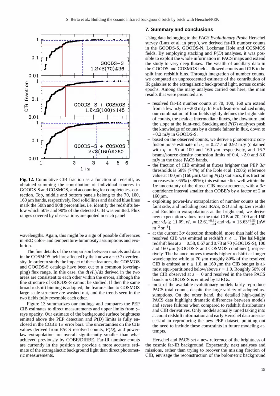
The relative fraction among the four bins moves from lowto high redshift, as wavelength increases: Fig. 12 shows thecumulative CIB fraction as a function of redshift, computedon the combination of GOODS-S and COSMOS, and includ-ing completeness correction. Half of the CIB detected over theflux ranges quoted on each panel was emitted below redshiftz = 0.58, 0.67 and 0.73 at 70, 100, 160µm, respectively.
While at 70µm ∼80% of the resolved CIB was emitted atz ≤ 1.0, at 160µm this fraction decreases to∼55%. This trendis mainly due to the positivek-correction of far-IR SEDs shortward of their peak, and will become even more relevant in SPIREand sub-mm bands, where negativek-correction comes into play(Oliver et al. 2010; Marsden et al. 2009). Note also that includ-ing the contribution from 70µm unresolved galaxies would shiftthe distribution to slightly higher redshifts (see also discussionabout 70µm depth and confusion in Sect. 5.2). On the otherhand, adding the bright end of number counts, sampled by theobservations in the COSMOS field, does not significantly in-fluence the high redshift bins in the CIB, because most of thecontribution goes into filling the lower redshift slices (see Tab.13). The 90th percentiles of the redshift-cumulative CIB fall atz = 1.38, 2.03 and 2.20. Excluding the bright end covered byCOSMOS (only at 100 and 160µm), we witness only a marginalshift of the 90%-light redshift by∆(z) ≤ 0.05.
Performing SED fitting of each individual object detected inGOODS-S in the PACS bands, Rodighiero et al. (2010) derivedIR luminosities (8-1000µm) of the sources contributing to far-IR counts and CIB. Combining the CIB distribution found above
and the notion of Malmquist bias, it is no surprise that the re-solved background is dominated by normal galaxies (L < 1011
L⊙) at low redshift and more luminous sources dominate the highredshift bins. Quantitatively, 95% of the resolved 160µm CIB atz ≤ 0.5 is produced by normal galaxies,>90% of the contri-bution at 0.5 < z ≤ 1.0 arises from luminous infrared galax-ies (LIRGs, 1011 ≤ L < 1012 L⊙) and ultra-luminous infraredgalaxies (ULIRGs, 1012 ≤ L < 1013 L⊙) provide 50% of thebackground at 1.0 < z ≤ 2.0 and 88% above. Globally, roughly50% of the CIB resolved in the three PACS bands in GOODS-Swas produced by LIRGs. At 160µm, the remainder is equallydistributed between normal IR galaxies and ULIRGs, while atshorter wavelengths the former prevail.
COSMOS shallow observations probe the bright end ofPACS number counts, and hence are limited to lower redshifts,but the large area grants a greater detail in the distribution ofCIB, allowing a much finer binning. At the COSMOS 80%completeness limits (9.0 and 20.0 mJy at 100 and 160µm, re-spectively), the resolved CIB peaks atz ≃ 0.3 and exhibits aweak secondary “bump” atz ≃ 0.7 in both bands. Recently,Jauzac et al. (2011) obtained similar results based on stackingof 24 µm sources on Spitzer MIPS 70 and 160µm. These au-thors find a dip atz ≃ 0.5 in the differential CIB brightness inCOSMOS, i.e. the same secondary peak az ≃ 0.7 found in PACSdata. This features are certainly due to thez = 0.73 structureknown in the COSMOS field. Only a small fraction (≤10%) ofthe total CIB is locked inz < 0.5 bright objects, which are domi-nated by the non-evolutionary component of number counts (seefor example Franceschini et al. 2010; Berta et al. 2010).
The bottom panels in Fig. 11 present the redshift deriva-tive of the background surface brightness, and compare it toa set of model predictions. The derivatived(νIν)/dz peaks inthe 0.5 < z ≤ 1.0 bin and then drops at higher redshifts.Le Floc’h et al. (2009) find a similar behavior at 24µm, basedon deep COSMOS data. The decrement is very steep at 70µm,while it becomes milder at longer wavelengths. While over broadredshift binning the five models considered are overall consistentto the data, at the low redshift bright-end, where detailed infor-mation is available, they significantly differ, especially at longer
14
S. Berta et al.: Building the cosmic infrared background brick by brick with Herschel/PEP.
Fig. 12. Cumulative CIB fraction as a function of redshift, asobtained summing the contribution of individual sources inGOODS-S and COSMOS, and accounting for completeness cor-rection. Top, middle and bottom panels belong to the 70, 100,160µm bands, respectively. Red solid lines and dashed blue linesmark the 50th and 90th percentiles, i.e. identify the redshifts be-low which 50% and 90% of the detected CIB was emitted. Fluxranges covered by observations are quoted in each panel.
wavelengths. Again, this might be a sign of possible differencesin SED color- and temperature-luminosity assumptions and evo-lution.
The fine details of the comparison between models and datain the COSMOS field are affected by the knownz ∼ 0.7 overden-sity. In order to study the impact of these features, the COSMOSand GOODS-S catalogs have been cut to a common (overlap-ping) flux range. In this case, thed(νIν)/dz derived in the twoareas are consistent to each other within the errors, although thefine structure of GOODS-S cannot be studied. If then the samebroad redshift binning is adopted, the features due to COSMOSlarge scale structure are washed out, and the trends seen in thetwo fields fully resemble each other.
Figure 13 summarizes our findings and compares the PEPCIB estimates to direct measurements and upper limits fromγ-rays opacity. Our estimate of the background surface brightnessemitted above the PEP detection andP(D) limits is fully en-closed in the COBE 1σ error bars. The uncertainties on the CIBvalues derived from PACS resolved counts,P(D), and power-law extrapolation are overall significantly smaller than whatachieved previously by COBE/DIRBE. Far-IR number countsare currently in the position to provide a more accurate esti-mate of the extragalactic background light than direct photomet-ric measurements.
7. Summary and conclusions
Using data belonging to thePACS Evolutionary Probe Herschelsurvey (Lutz et al. in prep.), we derived far-IR number countsin the GOODS-S, GOODS-N, Lockman Hole and COSMOSfields. By employing stacking andP(D) analyses, it was pos-sible to exploit the whole information in PACS maps and extendthe study to very deep fluxes. The wealth of ancillary data inthe GOODS and COSMOS fields allowed counts and CIB to besplit into redshift bins. Through integration of number counts,we computed an unprecedented estimate of the contribution ofIR galaxies to the extragalactic background light, across cosmicepochs. Among the many analyses carried out here, the mainresults that were presented are:
– resolved far-IR number counts at 70, 100, 160µm extendfrom a few mJy to∼200 mJy. In Euclidean-normalized units,our combination of four fields tightly defines the bright sideof counts, the peak at intermediate fluxes, the downturn andthe slope at the faint-end. Stacking andP(D) analyses pushthe knowledge of counts by a decade fainter in flux, down to∼0.2 mJy in GOODS-S.
– based on the observed counts, we derive a photometric con-fusion noise estimate ofσc = 0.27 and 0.92 mJy (obtainedwith q = 5) at 100 and 160µm respectively, and 16.7beams/source density confusion limits of 0.4,∼2.0 and 8.0mJy in the three PACS bands.
– the fraction of CIB emitted at fluxes brighter that PEP 3σthresholds is 58% (74%) of the Dole et al. (2006) referencevalue at 100µm (160µm). UsingP(D) statistics, this fractionincreases to∼65% (∼89%); this estimate lies well within the1σ uncertainty of the direct CIB measurements, with a 3σconfidence interval smaller than COBE’s by a factor of 2 at160µm.
– exploiting power-law extrapolation of number counts at thefaint side, and including past IRAS, ISO and Spitzer resultsand Euclidean extrapolations at the bright end, we derivenew expectation values for the total CIB at 70, 100 and 160µm: νIν ≥ 11.09,νIν = 12.61+8.31
−1.74 andνIν = 13.63+3.53−0.85 [nW
m−2 sr−1].– at the current 3σ detection threshold, more than half of the
resolved CIB was emitted at redshiftz ≤ 1. The half-lightredshift lies atz = 0.58, 0.67 and 0.73 at 70 (GOODS-S), 100and 160µm (GOODS-S and COSMOS combined), respec-tively. The balance moves towards higher redshift at longerwavelengths: while at 70µm roughly 80% of the resolvedCIB is emitted atz ≤ 1.0, at 160µm the CIB budget is al-most equi-partitioned below/abovez = 1.0. Roughly 50% ofthe CIB observed atz = 0 and resolved in the three PACSbands in GOODS-S is emitted by LIRGs.
– most of the available evolutionary models fairly reproducePACS total counts, despite the large variety of adopted as-sumptions. On the other hand, the detailed high-qualityPACS data highlight dramatic differences between modelsand severe failures when compared to redshift distributionsand CIB derivatives. Only models actually tuned taking intoaccount redshift information and early Herschel data are suc-cessful in reproducing the new PEP dataset, pointing outthe need to include these constraints in future modeling at-tempts.
Herschel and PACS set a new reference of the brightness ofthe cosmic far-IR background. Expectantly, next analyses andmissions, rather than trying to recover the missing fraction ofCIB, envisage the reconstruction of the bolometric background
15

S. Berta et al.: Building the cosmic infrared background brick by brick with Herschel/PEP.
Fig. 13. The cosmic infrared background. Black filled triangles represent the total CIB emitted above the PEP flux limits, basedon resolved number counts in GOODS-S, GOODS-N, Lockman Holeand COSMOS, evaluated as described in Sect. 6.2. Yellowsquares belong to theP(D) analysis in GOODS-S. Histograms denote the contribution of different redshift bins to the CIB, overthe flux range covered by GOODS-S. Literature data include: DIRBE measurements (filled circles, 1σ errors, Dole et al. 2006),FIRAS spectrum (solid lines above 200µm, Lagache et al. 1999, 2000), Fixsen et al. (1998) modified Black Body (shaded area),60 µm IRAS fluctuation analysis (cross, Miville-Deschenes et al. 2002), andγ-ray upper limits (green hatched line below 80µmMazin & Raue 2007).
from the mid-IR to sub-mm frequencies. The contribution ofgalaxies at different redshift to the CIB is being investigated toan increasing details by current surveys. A further study oftheredshift-dependent CIB, e.g. based on luminosity functions andproperly including the effects ofk-correction, goes beyond thepurpose of this paper and is deferred to future works. This infor-mation is not only important in the fine tuning of galaxy evolu-tion models, but is also of fundamental importance to constrainthe intrinsic spectra of distant TeV sources, such as BLAZARs,whoseγ-ray photons interact with the CIB. So far, such con-straints have been based solely on model predictions, to be con-firmed with direct estimates of the CIB as observedfrom dif-ferent epochs. Herschel source statistics have demonstrated toprovide a precise estimate of the total CIB. Future studies willnecessitate to improve direct measurements and thus the study offoreground contaminants, in order to complete the understandingof the total background and pinpoint its measurement.
GOODS-SS center Counts Err. Compl.[mJy] [104 deg−2 mJy1.5]
1.13 0.86 0.11 0.361.42 1.17 0.14 0.541.79 1.43 0.17 0.772.25 1.61 0.22 0.802.84 1.81 0.27 0.853.57 2.05 0.36 0.924.50 1.88 0.42 0.955.66 1.70 0.48 0.977.13 1.81 0.60 0.988.97 1.65 0.69 1.00
11.30 2.22 0.93 1.0014.22 2.51 1.18 1.0017.91 1.66 1.27 1.0022.54 4.83 2.22 1.0028.38 2.53 1.94 1.0035.73 2.41 2.28 1.00
Table 3.PEP 70µm number counts, normalized to the Euclideanslope.
16
S. Berta et al.: Building the cosmic infrared background brick by brick with Herschel/PEP.
Field Eff. Area texp 3σ N 80% complBand arcmin h mJy > 3σ mJyGOODS-N 100 300 arcmin2 30 3.0 291 5.5GOODS-N 160 300 arcmin2 30 5.7 317 11.0GOODS-S 70 300 arcmin2 113 1.1 375 2.1GOODS-S 100 300 arcmin2 113 1.2 717 2.4GOODS-S 160 300 arcmin2 226 2.4 867 5.2LH 100 0.18 deg2 35 3.6 909 5.9LH 160 0.18 deg2 35 7.5 841 13.2COSMOS 100 2.04 deg2 213 5.0 5360 9.0COSMOS 160 2.04 deg2 213 10.2 5105 20.0
Table 1.Main properties of the PEP fields included in the number counts and CIB analysis.
Field Resolved counts Stacking& band Flux range Slope Error Flux range Slope Error[µm] [mJy] α dα [mJy] α dαGOODS-S 70 1.4−3.5 -1.87 ±0.07 0.45−1.35 -1.66 ±0.12GOODS-S 70 3.5−36 -2.27 ±0.11 – – –GOODS-S 100 1.4−5.6 -1.96 ±0.06 0.95−2.75 -1.66 ±0.05GOODS-N 100 2.8−5.6 -1.32 ±0.27 – – –LH 100 6.0−89 -2.60 ±0.05 – – –COSMOS 100 8.0−142 -2.58 ±0.03 – – –All fields 100 1.4-5.6 -1.92 ±0.05 – – –All fields 100 6.0-142 -2.41 ±0.05 – – –GOODS-S 160 2.8−9.0 -1.49 ±0.08 2.20−6.00 -1.98 ±0.03GOODS-N 160 5.6−9.0 -1.67 ±0.32 – – –LH 160 9.0−113 -2.67 ±0.05 – – –COSMOS 160 17.0−350 -2.96 ±0.05 – – –All fields 160 2.8-9.0 -1.64 ±0.08 – – –All fields 160 9.0-350 -2.82 ±0.07 – – –
Table 2.Power-law fit to PACS differential number counts in the formdN/dS ∝ S α. Results belonging to resolved number counts(i.e. individually detected sources, plus completeness correction) and stacking of 24µm sources are reported.
17

S.B
ertaetal.:B
uildingthe
cosmic
infraredbackground
brick
bybrick
with
Herschel/P
EP
.Table 4.PEP 100µm number counts, normalized to the Euclidean slope.
GOODS-S GOODS-N Lockman Hole COSMOS All FieldsS center Counts Err. σ(var) Compl. Counts Err. σ(var) Compl. Counts Err. σ(var) Compl. Counts Err. Compl. Counts Err.[mJy] [104 deg−2 mJy1.5] [104 deg−2 mJy1.5] [104 deg−2 mJy1.5] [104 deg−2 mJy1.5] [104 deg−2 mJy1.5]
1.42 2.58 0.22 – 0.24 – – – – – – – – – – – 2.58 0.221.79 3.13 0.26 – 0.62 – – – – – – – – – – – 3.13 0.262.25 3.72 0.33 – 0.64 – – – – – – – – – – – 3.72 0.332.84 4.15 0.41 – 0.81 3.19 0.67 – 0.10 – – – – – – – 4.15 0.413.57 4.44 0.52 – 0.92 4.67 0.68 – 0.49 – – – – – – – 4.52 0.164.50 4.74 0.65 1.85 0.95 5.57 0.83 1.85 0.54 – – 0.96 – – – – 5.06 0.585.66 5.52 0.84 1.41 0.97 6.37 1.03 1.41 0.77 7.00 0.60 0.74 0.65 6.02 0.15 0.27 6.07 0.567.13 5.65 1.03 1.36 0.99 6.90 1.28 1.36 0.84 7.22 0.72 1.06 0.78 6.67 0.18 0.48 6.67 0.508.97 4.31 1.10 1.80 1.00 6.43 1.51 1.80 0.90 6.58 0.84 1.65 0.86 7.23 0.22 0.70 7.08 1.22
11.30 5.47 1.45 2.14 1.00 6.29 1.81 2.14 0.97 7.24 1.06 1.42 0.93 7.55 0.27 0.83 7.45 0.8914.22 4.67 1.66 1.86 1.00 6.81 2.27 1.86 0.99 8.13 1.36 1.54 0.96 7.42 0.32 0.95 7.35 1.2217.91 5.61 2.13 1.98 1.00 11.10 3.35 1.98 1.00 7.00 1.52 1.23 0.98 7.79 0.40 0.99 7.72 1.2822.54 7.48 2.90 3.50 1.00 8.13 3.60 3.50 1.00 6.66 1.79 1.72 0.99 8.08 0.49 1.00 7.97 0.8128.38 5.99 3.14 3.12 1.00 11.12 4.85 3.12 1.00 6.70 2.13 1.52 1.00 6.97 0.55 1.00 6.97 1.1135.73 5.34 3.50 3.83 1.00 6.63 4.65 3.83 1.00 4.01 2.12 1.44 1.00 6.50 0.64 1.00 6.27 1.4544.98 8.97 5.35 3.21 1.00 6.68 5.43 3.21 1.00 5.97 2.89 1.88 1.00 6.37 0.76 1.00 6.40 0.8656.62 – – 4.13 – – – 4.13 – ≤3.63 – 2.25 1.00 5.83 0.88 1.00 5.83 0.8871.29 – – 4.22 – – – 4.22 – ≤4.80 – 3.10 1.00 5.91 1.05 1.00 5.91 1.0589.74 – – 5.30 – – – 5.30 – 8.46 5.55 5.14 1.00 4.22 1.10 1.00 4.38 1.08
112.98 – – 8.01 – – – 8.01 – – – 4.86 – 4.96 1.34 1.00 4.96 1.34142.23 – – 6.91 – – – 6.91 – – – 5.20 – 4.03 1.47 1.00 4.03 1.47
18
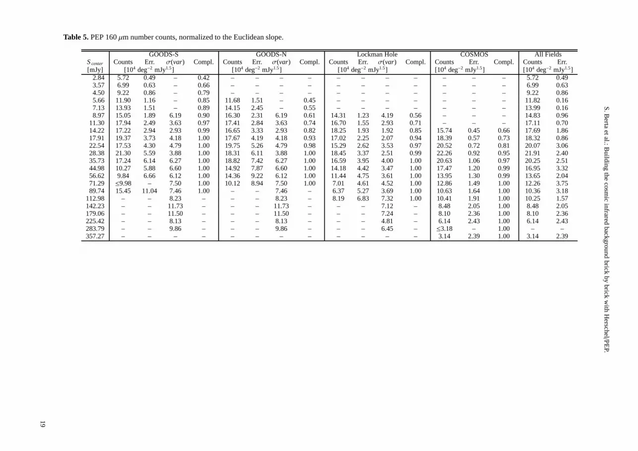
S.B
ertaetal.:B
uildingthe
cosmic
infraredbackground
brick
bybrick
with
Herschel/P
EP
.Table 5.PEP 160µm number counts, normalized to the Euclidean slope.
GOODS-S GOODS-N Lockman Hole COSMOS All FieldsS center Counts Err. σ(var) Compl. Counts Err. σ(var) Compl. Counts Err. σ(var) Compl. Counts Err. Compl. Counts Err.[mJy] [104 deg−2 mJy1.5] [104 deg−2 mJy1.5] [104 deg−2 mJy1.5] [104 deg−2 mJy1.5] [104 deg−2 mJy1.5]
2.84 5.72 0.49 – 0.42 – – – – – – – – – – – 5.72 0.493.57 6.99 0.63 – 0.66 – – – – – – – – – – – 6.99 0.634.50 9.22 0.86 – 0.79 – – – – – – – – – – – 9.22 0.865.66 11.90 1.16 – 0.85 11.68 1.51 – 0.45 – – – – – – – 11.82 0.167.13 13.93 1.51 – 0.89 14.15 2.45 – 0.55 – – – – – – – 13.99 0.168.97 15.05 1.89 6.19 0.90 16.30 2.31 6.19 0.61 14.31 1.23 4.19 0.56 – – – 14.83 0.96
11.30 17.94 2.49 3.63 0.97 17.41 2.84 3.63 0.74 16.70 1.55 2.93 0.71 – – – 17.11 0.7014.22 17.22 2.94 2.93 0.99 16.65 3.33 2.93 0.82 18.25 1.93 1.92 0.85 15.74 0.45 0.66 17.69 1.8617.91 19.37 3.73 4.18 1.00 17.67 4.19 4.18 0.93 17.02 2.25 2.07 0.94 18.39 0.57 0.73 18.32 0.8622.54 17.53 4.30 4.79 1.00 19.75 5.26 4.79 0.98 15.29 2.62 3.53 0.97 20.52 0.72 0.81 20.07 3.0628.38 21.30 5.59 3.88 1.00 18.31 6.11 3.88 1.00 18.45 3.37 2.51 0.99 22.26 0.92 0.95 21.91 2.4035.73 17.24 6.14 6.27 1.00 18.82 7.42 6.27 1.00 16.59 3.95 4.00 1.00 20.63 1.06 0.97 20.25 2.5144.98 10.27 5.88 6.60 1.00 14.92 7.87 6.60 1.00 14.18 4.42 3.47 1.00 17.47 1.20 0.99 16.95 3.3256.62 9.84 6.66 6.12 1.00 14.36 9.22 6.12 1.00 11.44 4.75 3.61 1.00 13.95 1.30 0.99 13.65 2.0471.29 ≤9.98 – 7.50 1.00 10.12 8.94 7.50 1.00 7.01 4.61 4.52 1.00 12.86 1.49 1.00 12.26 3.7589.74 15.45 11.04 7.46 1.00 – – 7.46 – 6.37 5.27 3.69 1.00 10.63 1.64 1.00 10.36 3.18
112.98 – – 8.23 – – – 8.23 – 8.19 6.83 7.32 1.00 10.41 1.91 1.00 10.25 1.57142.23 – – 11.73 – – – 11.73 – – – 7.12 – 8.48 2.05 1.00 8.48 2.05179.06 – – 11.50 – – – 11.50 – – – 7.24 – 8.10 2.36 1.00 8.10 2.36225.42 – – 8.13 – – – 8.13 – – – 4.81 – 6.14 2.43 1.00 6.14 2.43283.79 – – 9.86 – – – 9.86 – – – 6.45 – ≤3.18 – 1.00 – –357.27 – – – – – – – – – – – – 3.14 2.39 1.00 3.14 2.39
19
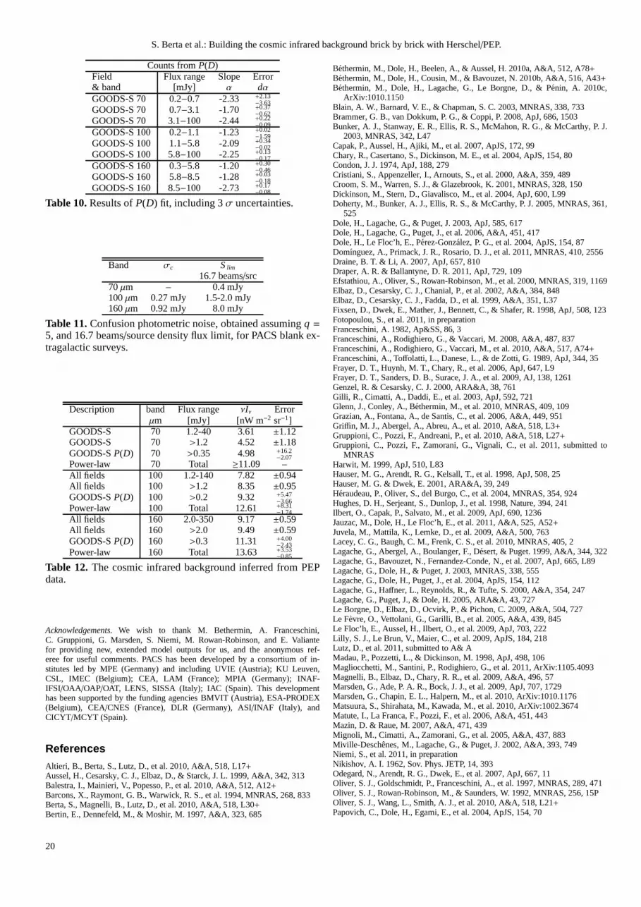
S. Berta et al.: Building the cosmic infrared background brick by brick with Herschel/PEP.
Counts fromP(D)Field Flux range Slope Error& band [mJy] α dαGOODS-S 70 0.2−0.7 -2.33 +2.13
−3.63GOODS-S 70 0.7−3.1 -1.70 +0.37
−0.62GOODS-S 70 3.1−100 -2.44 +0.22
−0.09GOODS-S 100 0.2−1.1 -1.23 +0.02
−1.59GOODS-S 100 1.1−5.8 -2.09 +0.34
−0.02GOODS-S 100 5.8−100 -2.25 +0.13
−0.17GOODS-S 160 0.3−5.8 -1.20 +0.30
−0.46GOODS-S 160 5.8−8.5 -1.28 +0.03
−0.18GOODS-S 160 8.5−100 -2.73 +0.17
−0.08
Table 10.Results ofP(D) fit, including 3σ uncertainties.
Band σc S lim
16.7 beams/src70µm – 0.4 mJy100µm 0.27 mJy 1.5-2.0 mJy160µm 0.92 mJy 8.0 mJy
Table 11.Confusion photometric noise, obtained assumingq =5, and 16.7 beams/source density flux limit, for PACS blank ex-tragalactic surveys.
Description band Flux range νIν Errorµm [mJy] [nW m−2 sr−1]
GOODS-S 70 1.2-40 3.61 ±1.12GOODS-S 70 >1.2 4.52 ±1.18GOODS-SP(D) 70 >0.35 4.98 +16.2
−2.07Power-law 70 Total ≥11.09 –All fields 100 1.2-140 7.82 ±0.94All fields 100 >1.2 8.35 ±0.95GOODS-SP(D) 100 >0.2 9.32 +5.47
−3.66Power-law 100 Total 12.61 +8.31
−1.74All fields 160 2.0-350 9.17 ±0.59All fields 160 >2.0 9.49 ±0.59GOODS-SP(D) 160 >0.3 11.31 +4.00
−2.43Power-law 160 Total 13.63 +3.53
−0.85
Table 12. The cosmic infrared background inferred from PEPdata.
Acknowledgements. We wish to thank M. Bethermin, A. Franceschini,C. Gruppioni, G. Marsden, S. Niemi, M. Rowan-Robinson, and E. Valiantefor providing new, extended model outputs for us, and the anonymous ref-eree for useful comments. PACS has been developed by a consortium of in-stitutes led by MPE (Germany) and including UVIE (Austria);KU Leuven,CSL, IMEC (Belgium); CEA, LAM (France); MPIA (Germany); INAF-IFSI/OAA/OAP/OAT, LENS, SISSA (Italy); IAC (Spain). This developmenthas been supported by the funding agencies BMVIT (Austria),ESA-PRODEX(Belgium), CEA/CNES (France), DLR (Germany), ASI/INAF (Italy), andCICYT/MCYT (Spain).
ReferencesAltieri, B., Berta, S., Lutz, D., et al. 2010, A&A, 518, L17+Aussel, H., Cesarsky, C. J., Elbaz, D., & Starck, J. L. 1999, A&A, 342, 313Balestra, I., Mainieri, V., Popesso, P., et al. 2010, A&A, 512, A12+Barcons, X., Raymont, G. B., Warwick, R. S., et al. 1994, MNRAS, 268, 833Berta, S., Magnelli, B., Lutz, D., et al. 2010, A&A, 518, L30+Bertin, E., Dennefeld, M., & Moshir, M. 1997, A&A, 323, 685
Bethermin, M., Dole, H., Beelen, A., & Aussel, H. 2010a, A&A, 512, A78+Bethermin, M., Dole, H., Cousin, M., & Bavouzet, N. 2010b, A&A, 516, A43+Bethermin, M., Dole, H., Lagache, G., Le Borgne, D., & Penin, A. 2010c,
ArXiv:1010.1150Blain, A. W., Barnard, V. E., & Chapman, S. C. 2003, MNRAS, 338, 733Brammer, G. B., van Dokkum, P. G., & Coppi, P. 2008, ApJ, 686, 1503Bunker, A. J., Stanway, E. R., Ellis, R. S., McMahon, R. G., & McCarthy, P. J.
2003, MNRAS, 342, L47Capak, P., Aussel, H., Ajiki, M., et al. 2007, ApJS, 172, 99Chary, R., Casertano, S., Dickinson, M. E., et al. 2004, ApJS, 154, 80Condon, J. J. 1974, ApJ, 188, 279Cristiani, S., Appenzeller, I., Arnouts, S., et al. 2000, A&A, 359, 489Croom, S. M., Warren, S. J., & Glazebrook, K. 2001, MNRAS, 328, 150Dickinson, M., Stern, D., Giavalisco, M., et al. 2004, ApJ, 600, L99Doherty, M., Bunker, A. J., Ellis, R. S., & McCarthy, P. J. 2005, MNRAS, 361,
525Dole, H., Lagache, G., & Puget, J. 2003, ApJ, 585, 617Dole, H., Lagache, G., Puget, J., et al. 2006, A&A, 451, 417Dole, H., Le Floc’h, E., Perez-Gonzalez, P. G., et al. 2004, ApJS, 154, 87Domınguez, A., Primack, J. R., Rosario, D. J., et al. 2011, MNRAS, 410, 2556Draine, B. T. & Li, A. 2007, ApJ, 657, 810Draper, A. R. & Ballantyne, D. R. 2011, ApJ, 729, 109Efstathiou, A., Oliver, S., Rowan-Robinson, M., et al. 2000, MNRAS, 319, 1169Elbaz, D., Cesarsky, C. J., Chanial, P., et al. 2002, A&A, 384, 848Elbaz, D., Cesarsky, C. J., Fadda, D., et al. 1999, A&A, 351, L37Fixsen, D., Dwek, E., Mather, J., Bennett, C., & Shafer, R. 1998, ApJ, 508, 123Fotopoulou, S., et al. 2011, in preparationFranceschini, A. 1982, Ap&SS, 86, 3Franceschini, A., Rodighiero, G., & Vaccari, M. 2008, A&A, 487, 837Franceschini, A., Rodighiero, G., Vaccari, M., et al. 2010,A&A, 517, A74+Franceschini, A., Toffolatti, L., Danese, L., & de Zotti, G. 1989, ApJ, 344, 35Frayer, D. T., Huynh, M. T., Chary, R., et al. 2006, ApJ, 647, L9Frayer, D. T., Sanders, D. B., Surace, J. A., et al. 2009, AJ, 138, 1261Genzel, R. & Cesarsky, C. J. 2000, ARA&A, 38, 761Gilli, R., Cimatti, A., Daddi, E., et al. 2003, ApJ, 592, 721Glenn, J., Conley, A., Bethermin, M., et al. 2010, MNRAS, 409, 109Grazian, A., Fontana, A., de Santis, C., et al. 2006, A&A, 449, 951Griffin, M. J., Abergel, A., Abreu, A., et al. 2010, A&A, 518, L3+Gruppioni, C., Pozzi, F., Andreani, P., et al. 2010, A&A, 518, L27+Gruppioni, C., Pozzi, F., Zamorani, G., Vignali, C., et al. 2011, submitted to
MNRASHarwit, M. 1999, ApJ, 510, L83Hauser, M. G., Arendt, R. G., Kelsall, T., et al. 1998, ApJ, 508, 25Hauser, M. G. & Dwek, E. 2001, ARA&A, 39, 249Heraudeau, P., Oliver, S., del Burgo, C., et al. 2004, MNRAS, 354, 924Hughes, D. H., Serjeant, S., Dunlop, J., et al. 1998, Nature,394, 241Ilbert, O., Capak, P., Salvato, M., et al. 2009, ApJ, 690, 1236Jauzac, M., Dole, H., Le Floc’h, E., et al. 2011, A&A, 525, A52+Juvela, M., Mattila, K., Lemke, D., et al. 2009, A&A, 500, 763Lacey, C. G., Baugh, C. M., Frenk, C. S., et al. 2010, MNRAS, 405, 2Lagache, G., Abergel, A., Boulanger, F., Desert, & Puget. 1999, A&A, 344, 322Lagache, G., Bavouzet, N., Fernandez-Conde, N., et al. 2007, ApJ, 665, L89Lagache, G., Dole, H., & Puget, J. 2003, MNRAS, 338, 555Lagache, G., Dole, H., Puget, J., et al. 2004, ApJS, 154, 112Lagache, G., Haffner, L., Reynolds, R., & Tufte, S. 2000, A&A, 354, 247Lagache, G., Puget, J., & Dole, H. 2005, ARA&A, 43, 727Le Borgne, D., Elbaz, D., Ocvirk, P., & Pichon, C. 2009, A&A, 504, 727Le Fevre, O., Vettolani, G., Garilli, B., et al. 2005, A&A, 439, 845Le Floc’h, E., Aussel, H., Ilbert, O., et al. 2009, ApJ, 703, 222Lilly, S. J., Le Brun, V., Maier, C., et al. 2009, ApJS, 184, 218Lutz, D., et al. 2011, submitted to A& AMadau, P., Pozzetti, L., & Dickinson, M. 1998, ApJ, 498, 106Magliocchetti, M., Santini, P., Rodighiero, G., et al. 2011, ArXiv:1105.4093Magnelli, B., Elbaz, D., Chary, R. R., et al. 2009, A&A, 496, 57Marsden, G., Ade, P. A. R., Bock, J. J., et al. 2009, ApJ, 707, 1729Marsden, G., Chapin, E. L., Halpern, M., et al. 2010, ArXiv:1010.1176Matsuura, S., Shirahata, M., Kawada, M., et al. 2010, ArXiv:1002.3674Matute, I., La Franca, F., Pozzi, F., et al. 2006, A&A, 451, 443Mazin, D. & Raue, M. 2007, A&A, 471, 439Mignoli, M., Cimatti, A., Zamorani, G., et al. 2005, A&A, 437, 883Miville-Deschenes, M., Lagache, G., & Puget, J. 2002, A&A,393, 749Niemi, S., et al. 2011, in preparationNikishov, A. I. 1962, Sov. Phys. JETP, 14, 393Odegard, N., Arendt, R. G., Dwek, E., et al. 2007, ApJ, 667, 11Oliver, S. J., Goldschmidt, P., Franceschini, A., et al. 1997, MNRAS, 289, 471Oliver, S. J., Rowan-Robinson, M., & Saunders, W. 1992, MNRAS, 256, 15POliver, S. J., Wang, L., Smith, A. J., et al. 2010, A&A, 518, L21+Papovich, C., Dole, H., Egami, E., et al. 2004, ApJS, 154, 70
20

S. Berta et al.: Building the cosmic infrared background brick by brick with Herschel/PEP.
zcen COSMOS GOODS-N GOODS-S100µm 160µm 100µm 160µm 70µm 100µm 160µm
0.1 1.01e+03 7.37e+02 1.82e+03 1.56e+03 1.54e+03 2.77e+03 2.16e+030.2 1.89e+03 1.33e+03 1.04e+03 7.81e+02 2.77e+03 3.08e+03 2.77e+030.3 1.59e+03 9.83e+02 3.12e+03 2.86e+03 2.16e+03 4.01e+03 3.39e+030.4 2.01e+03 1.26e+03 2.34e+03 1.82e+03 2.77e+03 4.31e+03 2.77e+030.5 1.17e+03 7.91e+02 2.86e+03 2.08e+03 3.08e+03 3.08e+03 3.39e+030.6 1.07e+03 7.07e+02 2.60e+03 3.12e+03 3.39e+03 5.55e+03 4.62e+030.7 8.93e+02 5.87e+02 5.20e+02 – 3.70e+03 1.11e+04 8.94e+030.8 1.04e+03 6.23e+02 3.38e+03 1.82e+03 – 1.54e+03 1.54e+030.9 5.99e+02 3.96e+02 3.38e+03 1.82e+03 9.24e+02 1.54e+03 1.54e+031.0 7.79e+02 5.81e+02 1.82e+03 1.82e+03 2.16e+03 6.47e+03 5.55e+031.1 4.85e+02 4.32e+02 – – 1.23e+03 2.77e+03 3.08e+031.2 3.36e+02 2.88e+02 7.81e+02 5.20e+02 3.08e+02 2.16e+03 1.54e+031.3 3.96e+02 3.72e+02 5.20e+02 5.20e+02 – 3.08e+02 6.16e+021.4 1.86e+02 1.92e+02 2.60e+02 5.20e+02 6.16e+02 6.16e+02 1.23e+031.5 1.98e+02 1.68e+02 2.60e+02 7.81e+02 – 9.24e+02 3.08e+021.6 1.80e+02 1.20e+02 2.60e+02 – 9.24e+02 2.47e+03 2.16e+031.7 1.02e+02 8.99e+01 – – – – –1.8 1.50e+02 1.38e+02 5.20e+02 2.60e+02 – 3.08e+02 6.16e+021.9 1.80e+02 1.74e+02 – – 3.08e+02 6.16e+02 6.16e+022.0 1.02e+02 1.26e+02 1.04e+03 1.04e+03 3.08e+02 1.23e+03 1.23e+032.1 3.60e+01 7.79e+01 2.60e+02 2.60e+02 – 1.23e+03 9.24e+022.2 1.20e+01 2.40e+01 – – – 1.23e+03 1.23e+032.3 2.40e+01 2.40e+01 – 2.60e+02 – 9.24e+02 1.23e+032.4 2.40e+01 3.60e+01 – – – 9.24e+02 1.23e+032.5 3.60e+01 5.39e+01 2.60e+02 5.20e+02 – 9.24e+02 1.23e+032.6 5.39e+01 7.19e+01 – 5.20e+02 – 6.16e+02 6.16e+022.7 – 2.40e+01 – – – – –2.8 5.99e+00 1.80e+01 – – – – 3.08e+022.9 1.20e+01 1.20e+01 – – – – 9.24e+023.0 5.99e+00 1.20e+01 – – – – 3.08e+023.1 1.20e+01 1.20e+01 – – – – –3.2 – 1.20e+01 – – – – –3.3 1.20e+01 1.80e+01 2.60e+02 – – – –3.4 – – – – – – –3.5 – 5.99e+00 – – – – –3.6 – – – – 6.16e+02 6.16e+02 3.08e+023.7 – – – – – – –3.8 5.99e+00 5.99e+00 – – – – –3.9 – – – – – – –4.0 – – – – – – –4.1 – – – – – – –4.2 5.99e+00 – – – – – 3.08e+024.3 – – – – 3.08e+02 3.08e+02 3.08e+024.4 – – 2.60e+02 – – – –
Table 6.Redshift derivativedN/dz [deg−2] for PACS detected source in COSMOS, GOODS-N and GOODS-S. Catalogs are cut at80% photometric completeness, see Fig. 4 for actual flux ranges covered.
Patanchon, G., Ade, P. A. R., Bock, J. J., et al. 2009, ApJ, 707, 1750Penin, A., Lagache, G., Noriega-Crepo, A., et al. 2011, ArXiv:1105.1463Pilbratt, G. L., Riedinger, J. R., Passvogel, T., et al. 2010, A&A, 518, L1+Poglitsch, A., Waelkens, C., Geis, N., et al. 2010, A&A, 518,L2+Popesso, P., Dickinson, M., Nonino, M., et al. 2009, A&A, 494, 443Popesso, P., et al. 2011, in preparationPuget, J., Abergel, A., Bernard, J., et al. 1996, A&A, 308, L5+Rodighiero, G., Cimatti, A., Gruppioni, C., et al. 2010, A&A, 518, L25+Rodighiero, G. & Franceschini, A. 2004, A&A, 419, L55Rowan-Robinson, M. 2009, MNRAS, 394, 117Rowan-Robinson, M., Lari, C., Perez-Fournon, I., et al. 2004, MNRAS, 351,
1290Santini, P., Fontana, A., Grazian, A., et al. 2009, A&A, 504,751Scheuer, P. A. G. 1974, MNRAS, 166, 329Scheuer, P. A. G. & Ryle, M. 1957, in Proceedings of the Cambridge
Philosophical Society, Vol. 53, Proceedings of the Cambridge PhilosophicalSociety, 764–+
Scott, K. S., Yun, M. S., Wilson, G. W., et al. 2010, MNRAS, 405, 2260Smail, I., Hogg, D. W., Yan, L., & Cohen, J. G. 1995, ApJ, 449, L105+Smail, I., Ivison, R. J., & Blain, A. W. 1997, ApJ, 490, L5+
Soifer, B. T. & Neugebauer, G. 1991, AJ, 101, 354Stanway, E. R., Bunker, A. J., McMahon, R. G., et al. 2004a, ApJ, 607, 704Stanway, E. R., Glazebrook, K., Bunker, A. J., et al. 2004b, ApJ, 604, L13Strolger, L., Riess, A. G., Dahlen, T., et al. 2004, ApJ, 613,200Sutherland, W. & Saunders, W. 1992, MNRAS, 259, 413Szokoly, G. P., Bergeron, J., Hasinger, G., et al. 2004, ApJS, 155, 271Trump, J. R., Impey, C. D., Elvis, M., et al. 2009, ApJ, 696, 1195Valiante, E., Lutz, D., Sturm, E., Genzel, R., & Chapin, E. 2009, ApJ, 701, 1814van der Wel, A., Franx, M., van Dokkum, P. G., & Rix, H. 2004, ApJ, 601, L5Vanzella, E., Cristiani, S., Dickinson, M., et al. 2008, A&A, 478, 83Vanzella, E., Cristiani, S., Dickinson, M., et al. 2005, A&A, 434, 53Viero, M. P., Ade, P. A. R., Bock, J. J., et al. 2009, ApJ, 707, 1766Weiß, A., Kovacs, A., Coppin, K., et al. 2009, ApJ, 707, 1201Werner, M. W., Roellig, T. L., Low, F. J., et al. 2004, ApJS, 154, 1
Appendix A: A cheap P(D) estimator
In addition to directly detected sources and to stacking of 24µm dense catalogs, further information about the shape of PACS
21
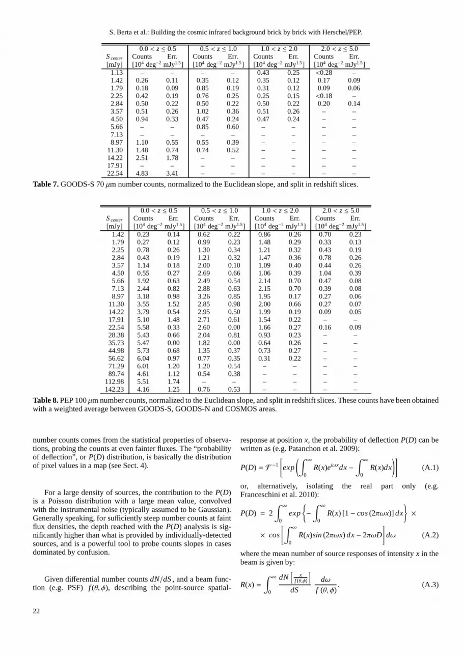
S. Berta et al.: Building the cosmic infrared background brick by brick with Herschel/PEP.
0.0 < z ≤ 0.5 0.5 < z ≤ 1.0 1.0 < z ≤ 2.0 2.0 < z ≤ 5.0S center Counts Err. Counts Err. Counts Err. Counts Err.[mJy] [104 deg−2 mJy1.5] [104 deg−2 mJy1.5] [104 deg−2 mJy1.5] [104 deg−2 mJy1.5]
1.13 – – – – 0.43 0.25 <0.28 –1.42 0.26 0.11 0.35 0.12 0.35 0.12 0.17 0.091.79 0.18 0.09 0.85 0.19 0.31 0.12 0.09 0.062.25 0.42 0.19 0.76 0.25 0.25 0.15 <0.18 –2.84 0.50 0.22 0.50 0.22 0.50 0.22 0.20 0.143.57 0.51 0.26 1.02 0.36 0.51 0.26 – –4.50 0.94 0.33 0.47 0.24 0.47 0.24 – –5.66 – – 0.85 0.60 – – – –7.13 – – – – – – – –8.97 1.10 0.55 0.55 0.39 – – – –
11.30 1.48 0.74 0.74 0.52 – – – –14.22 2.51 1.78 – – – – – –17.91 – – – – – – – –22.54 4.83 3.41 – – – – – –
Table 7.GOODS-S 70µm number counts, normalized to the Euclidean slope, and split in redshift slices.
0.0 < z ≤ 0.5 0.5 < z ≤ 1.0 1.0 < z ≤ 2.0 2.0 < z ≤ 5.0S center Counts Err. Counts Err. Counts Err. Counts Err.[mJy] [104 deg−2 mJy1.5] [104 deg−2 mJy1.5] [104 deg−2 mJy1.5] [104 deg−2 mJy1.5]
1.42 0.23 0.14 0.62 0.22 0.86 0.26 0.70 0.231.79 0.27 0.12 0.99 0.23 1.48 0.29 0.33 0.132.25 0.78 0.26 1.30 0.34 1.21 0.32 0.43 0.192.84 0.43 0.19 1.21 0.32 1.47 0.36 0.78 0.263.57 1.14 0.18 2.00 0.10 1.09 0.40 0.44 0.264.50 0.55 0.27 2.69 0.66 1.06 0.39 1.04 0.395.66 1.92 0.63 2.49 0.54 2.14 0.70 0.47 0.087.13 2.44 0.82 2.88 0.63 2.15 0.70 0.39 0.088.97 3.18 0.98 3.26 0.85 1.95 0.17 0.27 0.06
11.30 3.55 1.52 2.85 0.98 2.00 0.66 0.27 0.0714.22 3.79 0.54 2.95 0.50 1.99 0.19 0.09 0.0517.91 5.10 1.48 2.71 0.61 1.54 0.22 – –22.54 5.58 0.33 2.60 0.00 1.66 0.27 0.16 0.0928.38 5.43 0.66 2.04 0.81 0.93 0.23 – –35.73 5.47 0.00 1.82 0.00 0.64 0.26 – –44.98 5.73 0.68 1.35 0.37 0.73 0.27 – –56.62 6.04 0.97 0.77 0.35 0.31 0.22 – –71.29 6.01 1.20 1.20 0.54 – – – –89.74 4.61 1.12 0.54 0.38 – – – –
112.98 5.51 1.74 – – – – – –142.23 4.16 1.25 0.76 0.53 – – – –
Table 8.PEP 100µm number counts, normalized to the Euclidean slope, and split in redshift slices. These counts have been obtainedwith a weighted average between GOODS-S, GOODS-N and COSMOSareas.
number counts comes from the statistical properties of observa-tions, probing the counts at even fainter fluxes. The “probabilityof deflection”, orP(D) distribution, is basically the distributionof pixel values in a map (see Sect. 4).
For a large density of sources, the contribution to theP(D)is a Poisson distribution with a large mean value, convolvedwith the instrumental noise (typically assumed to be Gaussian).Generally speaking, for sufficiently steep number counts at faintflux densities, the depth reached with theP(D) analysis is sig-nificantly higher than what is provided by individually-detectedsources, and is a powerful tool to probe counts slopes in casesdominated by confusion.
Given differential number countsdN/dS , and a beam func-tion (e.g. PSF) f (θ, φ), describing the point-source spatial-
response at positionx, the probability of deflectionP(D) can bewritten as (e.g. Patanchon et al. 2009):
P(D) = F −1
[
exp
(∫ ∞
0R(x)eiωxdx −
∫ ∞
0R(x)dx
)]
(A.1)
or, alternatively, isolating the real part only (e.g.Franceschini et al. 2010):
P(D) = 2∫ ∞
0exp
−
∫ ∞
0R(x) [1 − cos (2πωx)] dx
×
× cos
[∫ ∞
0R(x)sin (2πωx) dx − 2πωD
]
dω (A.2)
where the mean number of source responses of intensityx in thebeam is given by:
R(x) =∫ ∞
0
dN[
xf (θ,φ)
]
dSdω
f (θ, φ). (A.3)
22

S. Berta et al.: Building the cosmic infrared background brick by brick with Herschel/PEP.
0.0 < z ≤ 0.5 0.5 < z ≤ 1.0 1.0 < z ≤ 2.0 2.0 < z ≤ 5.0S center Counts Err. Counts Err. Counts Err. Counts Err.[mJy] [104 deg−2 mJy1.5] [104 deg−2 mJy1.5] [104 deg−2 mJy1.5] [104 deg−2 mJy1.5]
2.84 1.11 0.21 1.48 0.52 1.29 0.49 1.48 0.523.57 0.93 0.45 2.02 0.56 2.02 0.56 2.02 0.564.50 0.60 0.38 3.41 0.83 4.01 0.90 1.20 0.495.66 2.13 0.35 3.14 0.60 3.94 1.13 2.08 0.797.13 3.62 0.56 3.73 3.62 3.85 0.83 2.71 1.028.97 1.41 0.81 7.20 7.09 2.78 1.36 3.29 1.24
11.30 3.87 1.98 6.38 0.65 4.88 1.10 2.47 1.2414.22 4.39 1.80 8.35 0.34 2.72 1.57 1.81 1.2817.91 6.83 2.69 6.82 1.70 6.18 3.07 1.81 0.9022.54 9.04 1.93 7.64 2.23 6.47 0.50 1.49 0.2628.38 11.20 2.48 8.05 0.22 6.21 1.74 – –35.73 11.57 3.21 6.90 2.49 6.08 0.78 0.50 0.2244.98 10.65 0.23 6.10 0.92 4.16 0.76 0.42 0.2456.62 10.49 2.62 3.07 0.72 3.41 0.76 – –71.29 11.56 1.59 2.18 0.69 1.96 0.65 – –89.74 8.91 1.82 2.97 1.05 1.11 0.64 – –
112.98 11.50 2.64 1.21 0.86 – – – –142.23 9.67 2.58 – – – – – –179.06 9.24 2.47 – – – – – –225.42 5.00 3.53 – – – – – –283.79 1.94 1.12 – – – – – –
Table 9.PEP 160µm number counts, normalized to the Euclidean slope, and split in redshift slices. These counts have been obtainedwith a weighted average between GOODS-S, GOODS-N and COSMOSareas.
Description band Flux range 0.0 < z ≤ 0.5 0.5 < z ≤ 1.0 1.0 < z ≤ 2.0 2.0 < z ≤ 5.0µm [mJy] νIν Error νIν Error νIν Error νIν Error
[nW m−2 sr−1] [nW m−2 sr−1] [nW m−2 sr−1] [nW m−2 sr−1]GOODS-S 70 1.2-36 1.57 0.97 1.70 1.10 0.47 0.23 0.08 0.06GOODS-S 100 1.2-45 2.02 1.19 2.38 1.14 1.44 0.46 0.51 0.22All fields 100 1.2-142 3.35 0.77 2.80 0.63 2.03 0.37 0.61 0.22GOODS-S 160 2.0-55 1.64 0.85 2.59 0.94 1.91 0.70 1.16 0.50All fields 160 2.0-357 3.21 0.75 3.02 0.71 2.43 0.62 1.16 0.45
Table 13.The contribution of galaxies at different epochs to the cosmic infrared background.
We defer to Patanchon et al. (2009), Franceschini et al.(2010), Glenn et al. (2010) for a full treatment and descriptionof the P(D) formalism. Only in the case of very simpledN/dSfunctional forms and trivial beams (e.g. Gaussian), the aboveequations can be solved analytically. For an effective beam thatis not strictly positive, or is not azimuthally symmetric, it is nec-essary to use the full 2-D beam map.
For example, the Herschel/PACS beam is characterized by3 prominent lobes, which cannot be described analytically.Insuch a case, if one likes to account for the real beam function, anumerical treatment ofR(x), and possiblyP(D) is necessary.
Finally, in case of real observations, the instrumental noisecontribution to pixel flux densities must be included.
A.1. The numerical P(D) approach
Given an instrumental PSFf (θ, φ) and a number counts modeldN/dS , it is possible to predict the pixel flux density distributionof a map withM pixels, simply rolling random numbers. Wedescribe here the principles of the method we developed in theframe of the PEP survey. This approach turns out to be of simpleimplementation, avoiding integrations of oscillating functions orFourier Transforms, and it is accessible to any user with a basicknowledge of random number generators. Furthermore, it avoidsany analytic simplification of the beam function, thus allowing
to employ the real instrumental PSF, regardless of how complexits bi-dimensional profile is.
For a givendN/dS , we describe how a syntheticP(D) iscomputed. The adopted form of number counts and fitting tech-nique are described in the next Section. Parameters are varied bymeans of a MCMC engine and for each realization a newP(D)is computed and compared to the observed data.
The input information needed by theP(D) numerical algo-rithm are:
– description of number counts,dN/dS ;– beam function, e.g. in form of an observed PSF 2-D map;– value of instrumental noise.
Further secondary inputs, derived from the three primariesabove, are:
– the maximum radiusrmax in pixels from a given sourcewithin which a pixel is affected by the source itself, e.g. theradius at which 99% of the observed PSF flux is enclosed; ifthe pixel scale of the map isα arcsec/pix, the correspondingangular radius isαrmax;
– the total expected number,N0, of sources within the solid an-gleΩ defined byrmax, simply given by the integral of numbercounts:N0 = Ω
∫ S max
S min
dNdS dS
– the cumulative probability that a random source has a flux
lower thanS , given by:P(S ) = ΩN0
∫ S
S min
dNdS ′ dS ′.
23

S. Berta et al.: Building the cosmic infrared background brick by brick with Herschel/PEP.
As mentioned above, the procedure relies on several dicerolls, using random numbers to determine the actual number ofsources expected to contribute to each pixel of the map, the dis-tance of the given source to the pixel, the fluxes of sources.
Step 1. We assume that the distribution of sources in the skyis randomly uniform, i.e. we ignore the clustering proper-ties of sources in the sky. Clustering would mainly affect theP(D) over scales larger than the size of the GOODS-S fieldunder exam here (e.g. Glenn et al. 2010; Viero et al. 2009;Lagache et al. 2007).GivenN0, the number of sources affecting the given pixel inthe current realization is a random Poisson deviate for ex-pectedN0. This number is recomputed for each pixel andeachdN/dS realization.
Step 2. For each source affecting the given pixel, it is necessaryto determine the fractionfi of flux affecting the pixel. RollNrandom, uniformly distributed positions, insidermax (definedeither byr, φ or by x, y coordinates). Based on the position ofthe given source, and the beam function, derive the fractionof flux affecting the pixel for each source.
Step 3. Finally assign a random fluxS i to each of theN sourcesaffecting the given pixel, according to the inputdN/dS . Tothis aim, the probabilityP(S ) (defined above) is used totransform a flat random number distribution in the neededflux values.
Assuming that any further background has been subtractedfrom the map, the flux of the given pixel is finally given byD = D0 +
∑Ni=1 fiS i, whereD0 is the term describing pure noise
(i.e. random flux, in case of no sources at all) and is given by aGaussian deviate as wide as the noise measured on actual PEPr.m.s. maps (see Tab. 1).
A.2. Number counts model and minimization
Number counts are modeled similarly to Patanchon et al. (2009)and Glenn et al. (2010). We adopt a simple, parametric model,defined by the differential countsdN/dS at a set of flux densityknots, or nodes. The model is defined within aS min andS maxlower and upper flux boundaries; outside of this flux range, wesimply setdN/dS to zero. Between nodes, number counts aredescribed as power-laws, connecting at knots.
We used a Markov-Chain Monte Carlo (MCMC) samplingof the parameter space, to explore the likelihood function of themodel to reproduce the observedP(D). We use a Metropolis-Hastings algorithm as our MCMC sampler. In order for thissampler to converge efficiently, we draw new steps from univari-ate Gaussian distributions, whose widths were given by dummyMCMC runs.
The position of knots and the corresponding amplitude ofcounts are free parameters, and are varied at each MCMC maprealization. The upper boundary of the covered flux range isfixed to 100 mJy, a value driven by the limits of observed, re-solved counts in GOODS-S. In order to minimize the numberof free parameters, and further degeneracies, we limit the de-scription of number counts to a broken power-law with threesections, for a total of seven free parameters (3 positions and 4amplitudes).
In the past, a standard approach was to subtract bright indi-vidually detected sources from theP(D) analysis, and work onlyat the faint side, but it has been shown that a more robust estimateof the source counts is obtained if theP(D) is fitted across thewhole available flux density range (e.g. Patanchon et al. 2009).
Therefore, to derive the observedP(D) to be reproduced, we usethe observed science maps without subtracting any object.
Section 4, Figs. 8, 7 and Tab. 10 describe the results of thewholeP(D) analysis.
A.3. Effects of map-making high-pass filtering
It is necessary to recall that PEP maps have been obtained by ap-plying a high-pass filtering process along the data time-line, inorder to get rid of 1/ f noise. This procedure consist in a running-box median filter, and induces two different side effects ontoPACS maps:1) the background is naturally removed from themaps;2) the PSF profile is eroded and wings are suppressed.
At very faint fluxes, and high source densities, close toand beyond the confusion limit, the contribution of sourcestothe modelP(D) basically generates a “background” sheet ofsources, which shifts theP(D) histogram to a non-zero peak andmedian. In principle, the source component of theP(D) is al-ways positive, and the addition of noise generates the negativenearly-Gaussian behaviors at the faint side ofP(D). The adoptedhigh-pass filtering shifts the whole flux pixel distributionfunc-tion to a zero peak/median. In order to take this into account,with the current form of PEP maps, we shift the modelP(D) tothe same zero peak, prior of fitting.
The second consequence of applying an high-pass filter isa modification of object profiles. Detected objects are maskedand excluded from the median filter derivation. Tests were doneadding simulated sources to the time-lines before masking andbefore high-pass filtering (see Popesso et al. 2011 and Lutz etal. 2011). The result is that the filtering modifies the fluxes ofmasked sources by less than 5%, and those of unmasked pointsources — below the detection limit — by a factor≤ 16%. Inorder to understand the impact of this on theP(D) analysis,we built simulated maps 20 times deeper than the GOODS-S3σ threshold, once using an un-filtered (i.e. masked) PSF at allfluxes, and once using an un-filtered PSF above 3σ, but a filtered(unmasked) PSF below. TheP(D) obtained in the two cases arewell consistent to each other, with unit median ratio and a<5%scatter across all fluxes; no systematic shift, nor skewnessareobserved.
24