branch-and-price-and-cut algorithms for solving the reliable h-paths problem

Branch-and-Price-and-Cut Algorithms for Solving the Reliable

h-Paths Problem∗

April K. Andreas

Department of Systems and Industrial Engineering

The University of Arizona, PO Box 210020

Tucson, AZ 85721

[email protected]

J. Cole Smith

Department of Industrial and Systems Engineering

The University of Florida, PO Box 116595

Gainesville, FL 32611

[email protected]

Simge Kucukyavuz

Department of Systems and Industrial Engineering

The University of Arizona, PO Box 210020

Tucson, AZ 85721

[email protected]

July 14, 2007

Abstract

We examine a routing problem in which network arcs fail according to independent failure probabil-

ities. The reliable h-path routing problem seeks to find a minimum-cost set of h ≥ 2 arc-independent

paths from a common origin to a common destination, such that the probability that at least one path

remains operational is sufficiently large. For the formulation in which variables are used to represent

the amount of flow on each arc, the reliability constraint induces a nonconvex feasible region, even when

the integer variable restrictions are relaxed. Prior arc-based models and algorithms tailored for the case

∗The authors are grateful for the remarks made by two anonymous referees, which helped improve the presentation andcontribution of the paper. The authors also gratefully acknowledge the support of the Office of Naval Research under GrantNumber N00014-03-1-0510 and the Air Force Office of Scientific Research under Grant Number F49620-03-1-0377.

1

in which h = 2 do not extend well to the general h-path problem. Thus, we propose two alternative

integer programming formulations for the h-path problem in which the variables correspond to origin-

destination paths. Accordingly, we develop two branch-and-price-and-cut algorithms for solving these

new formulations, and provide computational results to demonstrate the efficiency of these algorithms.

Keywords: Nonconvex Optimization; Branch-and-Price-and-Cut; Network Optimization; Reliability

1 Problem Setup

Real-world applications of routing problems often call for a diverse routing strategy to protect against the

failure of network infrastructure. For example, consider a communications company that has determined

that its customers will tolerate having a fraction of up to (1− τ) of their data dropped. The company can

send the information over one highly reliable path, or it can send the same information along less-reliable

paths, requiring that at least one signal reaches the destination with a probability of at least τ . It might be

cheaper for the company to establish multiple relatively unreliable paths than to construct one highly-reliable

path. Another application arises in achieving military missions, such as destroying a particular target that

can be accessed via any number of paths, where each path assumes its own set of risks. A commander can

choose to deploy several groups along different paths such that at least one of the groups will complete its

mission within some acceptable level of reliability.

In this paper, we consider a directed graph G(N,A), where N = {1, . . . , n} is the set of nodes and A is

the set of arcs. Each arc (i, j) ∈ A has a usage cost cij ∈ R+ and a reliability 0 < pij ≤ 1, which denotes the

probability that arc (i, j) is successfully traversed. These probabilities are assumed to be independent. The

problem considered here is that of finding h ≥ 2 arc-independent paths from an origin node to a destination

node such that the total cost is minimized and the probability that at least one entire path of arcs does not

fail, called the joint reliability, is greater than or equal to some threshold value τ . We call this the Reliable

h-Path Problem with disjoint arcs, or RhP-D. A special case of this problem that we shall also briefly discuss

is the Reliable Two-Path Problem with disjoint arcs, or R2P-D.

In the example in Figure 1, each arc is labeled with its usage cost and reliability. Given τ = 0.65 and

h = 2, the optimal solution uses paths ABFH and ADGH, with a cost of 31 and a joint reliability of 72.6%.

Given instead τ = 0.80 and h = 3, the optimal solution uses paths ACEH, ABFH, and ADGH, with a cost

of 48 and a joint reliability of 81.5%. (The fact that the same arcs from the two-path solution appear in the

three-path solution is coincidental.)

Reliable single shortest path problems (h = 1) have received much attention in the literature, both in their

methodological development and in their applications. Desrochers and Soumis [7] develop a pseudopolynomial-

time label-setting algorithm for a version of this problem where time windows exist during which certain

nodes can be visited. Their algorithms generalizes the best-first selection strategy of Dijkstra’s algorithm

[9] for the shortest path problem, and uses a data structure called a generalized bucket in order to reduce

the time- and space-complexity required to solve these instances. For more details on the foundational al-

2

Av

Bv

��

��

��

��*

(1, 0.8)

Cv-(5, 0.6)

Dv

HHHHH

HHHHHHHj

(7, 0.7)

Ev-(9, 0.7)

��

��

��

��*

(8, 0.6)

Fv

HHHHH

HHHHHHHj

(7, 0.8)

-(8, 0.8)

��

��

��

��*

(4, 0.6)

Gv

HHHHH

HHHHHHHj

(4, 0.5)

-(4, 0.9)

Hv

HHHHH

HHHHHHHj

(4, 0.9)

-(5, 0.7)

��

��

��

��*

(7, 0.8)

Figure 1: Reliable h-Path Problem Example.

gorithms for these reliable single shortest path problems, we refer the reader to the comprehensive work of

Desrosiers et al. [8]. More recently, Chen and Powell [6] show that a label-correcting algorithm based on the

work of Glover et al. [15] often executes faster than the algorithm of Desrosiers et al., despite its inferior

worst-case complexity. Dumitrescu and Boland [10, 11] present refinements to label-setting algorithms for

this class of problems. In particular, they perform preprocessing steps to reduce the size of test instances,

demonstrating that four out of six problem classes tested can largely be solved within their preprocessing

phase. For problems that cannot be solved by preprocessing, the authors prescribe a weight-scaling method

used in conjunction with a label-setting algorithm, where the weights can be obtained from a preliminary

Lagrangian dual phase.

Applications of single shortest path problems vary widely. Bard and Miller [3] address a research and

development project selection problem, in which spending additional money on projects could increase their

probability of success. Their approach employs a dynamic programming-based heuristic technique embedded

within Monte Carlo simulation to handle the probabilistic aspect of their problem. Zabarankin, Uryasev, and

Pardalos [24] consider a related problem in optimizing path risk in the context of aircraft flight trajectory

through a threat environment. Elimam and Kohler [12] describe some unique applications of the resource-

constrained shortest-path problem, such as the determination of optimal wastewater treatment processes

and thermal resistance of building structures.

Related to the class of multiple-path problems that we study in this paper, Fortune, Hopcroft, and Wyllie

[14] provide a characterization of NP-complete vertex-independent routing problems on directed graphs via

the graph homeomorphism problem. Suurballe [19] presents a polynomial-time labeling algorithm to find k

node-disjoint paths between two given nodes. Andreas and Smith [2] examine two versions of the reliable

two-path problem, one where the two paths must be arc-disjoint (R2P-D), and one where arc sharing is

3

allowed, and prove both these problems to be strongly NP-hard [1]. Therefore, we can state that RhP-D is

strongly NP-hard as well.

In this paper we investigate the use of a branch-and-price-and-cut strategy for solving RhP-D. Column

generation often allows us to solve linear programs with a huge number of variables, in which the vast

majority of variables will equal to zero in a basic solution. (For a detailed overview of column generation, see

[16] and [23].) The branching step can be more difficult in column generation algorithms than in traditional

branch-and-bound procedures, because it must prevent the regeneration of any columns previously fixed to

zero in the branch-and-bound process. Another major challenge in implementing these algorithms lies in

ensuring that the pricing algorithm used in the root is unchanged in the child nodes of the branch-and-

bound tree. Further computational difficulties arise when the master problem exhibits symmetry, or when

symmetry is induced by the column generation procedure. Vanderbeck [21] proposes a generic routine to

address the difficulties of maintaining an invariant column generation routine and of combatting symmetry

in solving Dantzig-Wolfe reformulations of an integer program. Also, Vanderbeck and Wolsey [22] propose a

method to resolve integrality issues in specific column generation problems by modifying the subproblems as

non-integer solutions are found, and extend their logic to the special case of 0-1 column generation problems.

The multi-commodity flow problem (MCFP) shares some characteristics with the reliable h-path problem,

and is particularly amenable to solution via column generation. Barnhart, Hane, and Vance [5] describe the

implementation of a branch-and-price-and-cut algorithm for a version of the multi-commodity flow problem

in which each commodity’s flows must take place on a single path. In a separate paper, Barnhart et al. [4]

also investigate using a so-called keypath to help find optimal solutions using column generation.

We make the following contributions in this paper. One, we present two alternative reformulations of

RhP-D that are at least as tight as a compact model for solving the problem. Two, we compare the efficiency

of branch-and-price-and-cut on a concise model whose column generation phase is computationally difficult,

as opposed to a larger model in which columns are generated in pseudopolynomial time. Three, we give

models for handling the presence of symmetry-breaking constraints and dynamically-generated cutting planes

within the column generation phase.

The rest of this paper is organized as follows. We begin in Section 2 by introducing some relevant theory

developed in [2] for R2P-D, and discuss the implications of extending this logic to include instances where

h ≥ 3. In Sections 3 and 4, we develop two column generation-based approaches for RhP-D. Section 5

discusses the results of a computational comparison of these strategies. We conclude in Section 6 with a

summary of our work and areas for future research.

2 Compact Model Formulation

We begin by presenting a polynomial-size formulation of RhP-D. For all i ∈ N , define FS(i) and RS(i)

as the forward and reverse stars of node i, respectively. (That is, FS(i) = {j ∈ N : (i, j) ∈ A} and

4

RS(i) = {j ∈ N : (j, i) ∈ A}, ∀i ∈ N .) Let τ be the minimum permissible probability that at least

one path from the origin node 1 to the destination node n survives, where 0 < τ < 1. We define ykij ,

∀(i, j) ∈ A, k = 1, . . . , h, to be a binary variable equal to one if path number k utilizes arc (i, j) and zero

otherwise. Also, let variables ski represent the probability that path k = 1, . . . , h successfully reaches node

i ∈ N from node 1, given that path k visits node i. RhP-D can be modeled as the following nonlinear

mixed-integer program.

Minimize∑

(i,j)∈A

cij

(h∑k=1

ykij

)(1a)

subject to∑

j∈FS(1)

yk1j = 1 ∀k = 1, . . . , h (1b)

∑j∈FS(i)

ykij =∑

`∈RS(i)

yk`i ∀i ∈ {2, . . . , n− 1}, k = 1, . . . , h (1c)

h∑k=1

ykij ≤ 1 ∀(i, j) ∈ A (1d)

skj ≤ pijski + (1− ykij) ∀k = 1, . . . , h, (i, j) ∈ A (1e)

sk1 = 1 ∀k = 1, . . . , h (1f)

1−h∏k=1

(1− skn

)≥ τ (1g)

skn ≤ sk+1n ∀k = 1, . . . , h− 1 (1h)

0 ≤ ski ≤ 1 ∀i ∈ N, k = 1, . . . , h (1i)

ykij ∈ {0, 1} ∀k = 1, . . . , h, (i, j) ∈ A. (1j)

The objective (1a) minimizes the total cost of the chosen paths, while (1b) and (1c) are standard flow

balance constraints and constraint (1d) enforces arc-disjointness. Our strategy in (1e) and (1f) enforces the

reduction of path k’s reliability along each arc (i, j) ∈ A for which ykij = 1, ∀k = 1, . . . , h. The nonlinear

constraint (1g) enforces the condition that at least one path remains survivable with sufficiently large prob-

ability. Constraint (1h) removes some problem symmetry by requiring that s1n, . . . , skn be a nondecreasing

sequence.

Andreas and Smith [2] handle the single nonlinear constraint (1g) for the case in which h = 2 by

constructing a convex hull relaxation of problem (1) without the integrality constraints (1j). This relaxation

is accomplished noting that (1g) intersects (1h) at (s1n, s2n) = (1 −

√1− τ , 1 −

√1− τ), and s2n ≥ 0 at

(s1n, s2n) = (τ, 0). A convex underestimation of (1g) that passes through these points is given by

(1−√

1− τ)s1n + (√

1− τ − 1 + τ)s2n ≥ τ(1−√

1− τ). (2)

The approach in [2] then reinstates the integrality constraints and solves the resulting problem by replacing

5

(1g) with the relaxed constraint (2). If the resulting solution obtained from this relaxation is feasible to

the original problem in which (2) is replaced by (1g), then an optimal solution has been identified. Else, a

disjunction is created over the continuous space of s1n and s2n, and a branch-and-bound algorithm is executed

in which each subproblem is an integer program over some particular interval of s1n and s2n. One general rule

divides the feasible region into rectangular partitions of the(s1n, s

2n

)space. This technique is equivalent to

the Reformulation-Linearization Technique (RLT) [18] for continuous-variables optimization problems, in a

strategy similar to that employed by [13].

The previous approach would suffer for RhP-D, h ≥ 3, due to the increasing difficulties of relaxing

multiple nonlinear terms as h increases. For h = 3, for example, (1g) now includes the nonlinear terms s1ns2n,

s1ns3n, s2ns

3n, and s1ns

2ns

3n. We can handle these terms by an RLT approach related to the one employed for

h = 2, but the number of such terms will increase exponentially as h increases. Moreover, for the case in

which h = 2, the optimization process will tend to minimize the sole nonlinear term s1ns2n in order to achieve

feasibility to (1g). However, this behavior does not necessarily persist for h ≥ 3, and hence more effort would

be required to converge to the optimal solution.

As an alternative, recalling our assumption that τ < 1, observe that by rearranging the terms of (1g)

and taking the logarithm of both sides, we can rewrite this constraint as

h∑k=1

log(1− skn

)≤ log(1− τ),

which can be tightened as

h∑k=1

max{

log(1− skn

), log (1− τ)

}≤ log(1− τ). (3)

Now, this problem can be approached as in [2] by approximating each term log(1 − skn) with a relaxed

linear function, and executing a continuous branch-and-bound search as before. More specifically, we replace

the left-hand-side of (3) with a piecewise-linear function u(skn), which has one segment that intersects the

points (skn, u(skn)) = (0,0) and (τ, log(1 − τ)), and a horizontal segment passing through (τ, log(1 − τ)) and

(1, log(1− τ)). We represent this function using the following constraints:

Uk ≥ (log(1− τ)/τ)skn (4)

Uk ≥ log(1− τ), (5)

where Uk, ∀k = 1, . . . , h, is a nonpositive value function variable associated with each piecewise-linear

function. We claim that replacing (3) with the constraint

h∑k=1

Uk ≤ log(1− τ), (6)

6

)1log( kns−

1 τ kns

)1log( τ−

Original piecewise-linear underestimation

Linear underestimations after branching on kns

kns

Figure 2: Example Continuous Branching Scheme.

along with (4) and (5), yields a valid relaxation to RhP-D. This claim is justified by noting that log(1−skn) is

concave on the interval [0, 1), and so Uk ≤ log(1− skn) for 0 ≤ skn ≤ τ . Hence, if skn ≤ τ for each k = 1, . . . , h,

(6) must be valid. Else, if skn > τ for any k = 1, . . . , h, we have that Uk = log(1 − τ) and (6) is satisfied,

which ensures the validity of (6).

Denote the relaxation of (1) in which (1g) is replaced with (4), (5), and (6) as LRhP-D. An analogous

approach as taken in [2] would solve LRhP-D and tighten the constraints (1g) via a continuous branch-and-

bound process according to the following procedure.

Suppose that a solution with values skn, ∀k = 1, . . . , h, optimizes LRhP-D, but is infeasible to (1g). (Note

that the skn-values can be set artificially low if, for instance, (6) is not binding. However, for efficiency in this

algorithm, we consider a solution to LRhP-D in which skn is equal to the true reliability of path k, for each

k = 1, . . . , h.) At the current step of the algorithm, assume that skn has been restricted to lie in the interval

[`k, uk], and that u(skn) = log(1− skn) at the points skn = `k and skn = min{τ, uk}, for each k = 1, . . . , h. Since

the current solution is infeasible to (1g), we must have that Uk < log(1− skn) for some k = 1, . . . , h. Choose

k? ∈ argmaxk=1,...,h{log(1− skn)− Uk}, and create two new problems: one in which sk?

n ∈ [`k, sk?

] with (4)

modified so that it intersects log(1 − `k) and log(1 − sk?), and the other in which sk?

n ∈ [sk?

, uk] with (4)

modified so that it intersects log(1− sk?) and log(1−min{τ, uk}). In this manner, we have branched on the

continuous s-solution while preserving the validity of (6) over each new interval, and we recursively solve

both new problems in this fashion. Observe that the previous solution can no longer be feasible in either of

the two new branches, and will not be regenerated. This process continues just as in branch-and-bound for

integer programs, and terminates when each subproblem is fathomed due to feasibility to (1g), infeasibility

to the relaxed problem, or by bound. An illustration of this process is given in Figure 2.

Note that by contrast to the method presented in [2], this process must branch on h nonlinear terms.

Anticipating that the convergence of this method can potentially be slow if the reliability constraint is

difficult to meet, we instead turn to a branch-and-price-and-cut approach that circumvents the need for a

continuous branch-and-bound search.

7

3 Aggregated Column Generation Model

In this section, we introduce an alternative path-based formulation for RhP-D in which decision variable xp

equals to one if path p ∈ P is selected, and zero otherwise, where P is the entire set of origin-destination paths

in the network. Since there are exponentially many such paths to generate, we instead consider a subset

of paths P ⊆ P and employ column generation, using a branch-and-price-and-cut algorithm to solve the

problem. After relaxing integrality, we have the following Restricted Master Problem (RMP) formulation:

Minimize∑p∈P

Cpxp (7a)

subject to∑p∈P

xp = h (7b)

∑p∈P

δpijxp ≤ 1 ∀(i, j) ∈ A (7c)

1−∏p∈P

(1−Rp)xp ≥ τ (7d)

xp ≥ 0 ∀p ∈ P , (7e)

where Cp is the total cost of path p (sum of its arc costs), Rp is the reliability of path p (product of its

arc reliabilities), and δpij is a constant that equals to 1 if arc (i, j) is used in path p, and zero otherwise,

∀p ∈ P , (i, j) ∈ A. We convert (7d) to the linear constraint

∑p∈P

log (1−Rp)xp ≤ log (1− τ) , (8)

by the same logic used to transform (1g) into (3).

Remark 1. Note that we could choose to tighten (8) by tightening the left-hand-side coefficients as

∑p∈P

max{log (1−Rp) , log (1− τ)}xp ≤ log (1− τ) . (9)

Except where noted otherwise, we develop the column generation procedure using the simpler (but weaker)

constraint (8). We demonstrate in Section 5 that the use of the stronger inequalities above do not significantly

affect the efficiency of our proposed algorithm. 2

Denote RMP? as formulation (7) in which (9) is used in lieu of (7d) and in which all columns in the set

P have been generated. Proposition 1 demonstrates that RMP? is at least as tight as the linear relaxation

of LRhP-D.

8

Proposition 1. Let zL equal the linear programming relaxation objective function value of LRhP-D, and

let zA equal the objective function value of RMP? (where each z-value is taken to equal∞ if its corresponding

problem is infeasible). Then zA ≤ zL.

Proof. We prove this proposition by demonstrating that any solution x′ to RMP? corresponds to a solution

to the linear relaxation of LRhP-D having an identical objective function value. First, we transform the

solution x′p, ∀p ∈ P , to an equivalent intermediate solution xkp, ∀p ∈ P , k = 1, . . . , h, as follows:

h∑k=1

xkp = x′p ∀p ∈ P∑p∈P

xkp = 1 ∀k = 1, . . . , h.

This (nonunique) transformation decomposes the x′-solution into individual collections of fractional paths

(as will be done in Section 4). This allows us to obtain a solution (y, s) to the linear relaxation of LRhP-D

as follows.

ykij =∑

p∈P :(i,j)∈p

xkp ∀(i, j) ∈ A, k = 1, . . . , h

sk1 = 1 ∀k = 1, . . . , h

skj = min{

1,mini∈RS(j)

{pij s

ki + (1− ykij)

}}∀j ∈ N \ {1}, k = 1, . . . , h,

where the s-variables are determined recursively starting from node 1. It is easy to see that the objective

function of the linear relaxation of LRhP-D given by this choice of (y, s) is equal to the objective function

of RMP? given by x′. After reindexing the indices k = 1, . . . , h if necessary to satisfy the anti-symmetry

constraint, the solution (y, s) clearly obeys all constraints of (1) except for the reliability constraint. Setting

Uk = max{skn log(1− τ)/τ, log(1− τ)} (10)

guarantees feasibility to (4) and (5). We now show that (6) holds true.

The key step in our proof shows that∑p∈P Rpx

kp ≤ skn, ∀k = 1, . . . , h, which we will accomplish by

demonstrating that Rpxkp is no more than a unique term comprising skn, for each p ∈ P . For each k, consider

an origin-destination “critical path” having arcs (i1 = 1, j1), (i2 = j1, j2), . . . , (iW = jW−1, jW = n) such

that skjw = min{1, piwjw siw +(1− ykiwjw)} for each w = 1, . . . ,W . First, suppose that skjw < 1, ∀w = 1, . . . ,W .

To show that Rpxkp is no more than some term of skn for some path p ∈ P , let (iµ, jµ) be the last arc on

the critical path that does not belong to path p. If (iµ, jµ) does not exist, then path p is equivalent to the

critical path, and so contains exactly the arcs (i1, j1), . . . , (iW , jW ). Hence, Rp =∏Ww=1 piwjw . Observe that

skn = ((((pi1j1 + 1− yki1j1)pi2j2 + 1− yki2j2) . . .)piW jW + 1− ykiW jW )

9

=W∏w=1

piwjw +W∑w=1

[(1− ykiwjw

) W∏a=w+1

piaja

], (11)

where∏Wa=W+1 piaja is taken to be 1. Because the first term of (11) is given by

∏Ww=1 piwjw = Rp, and since

xkp ≤ 1, we have that

Rpxkp ≤

W∏w=1

piwjw . (12)

Now, suppose that (iµ, jµ) exists for some µ ∈ {1, . . . ,W}. Noting that 1−ykiµjµ is equal to∑v∈P :(iµ,jµ)/∈v x

kv ,

we can write skn as:

skn =

skiµpiµjµ +∑

v∈P :(iµ,jµ)/∈v

xkv

W∏w=µ+1

piwjw +W∑

w=µ+1

[(1− ykiwjw

) W∏a=w+1

piaja

]. (13)

Since the path p under consideration belongs to the set {v ∈ P : (iµ, jµ) /∈ v}, one term of skn is equal

to xkp∏Ww=µ+1 piwjw . Furthermore, path p intersects arcs (iµ+1, jµ+1), . . . , (iW , jW ), and so we have that

Rpxkp ≤ xkp

∏Ww=µ+1 piwjw .

Therefore, every nonzero term of∑p∈P Rpx

kp is less than or equal to a term of skn. Furthermore, for the

unique path p ∈ P in which (iµ, jµ) does not exist, the first term of (11) is no less than Rpxkp, and for all

other paths, a separate term in the summation term of (11) is no less than (11), and so unique terms of (11)

are no less than each term of∑p∈P Rpx

kp. Since all terms of (11) are nonnegative, we have

∑p∈P

Rpxkp ≤ skn. (14)

Now, suppose that ski = 1 for at least one node on the critical path other than node 1, and let node iν

be the last critical path node for which skiν = 1. The same argument as above can be used to demonstrate

that unique terms of skn are greater than or equal to Rpxkp for each path p ∈ P for which µ exists, and µ ≥ ν.

Else, for the unique path p ∈ P such that µ does not exist, or for paths p ∈ P such that µ < ν, we can

rewrite skn as

skn =∑v∈P

xkv

W∏w=ν

piwjw +W∑w=ν

[(1− ykiwjw

) W∏a=w+1

piaja

], (15)

because∑v∈P x

kv = 1. Note that (15) contains the term xkp

∏Ww=ν piwjw , and that

∏Ww=ν piwjw ≤ Rp, since

path p uses each of the arcs (iν , jν), . . . , (iW , jW ) in its path. Thus, once again, we obtain (14) for the case

in which ski = 1 for node i on the critical path, i 6= 1.

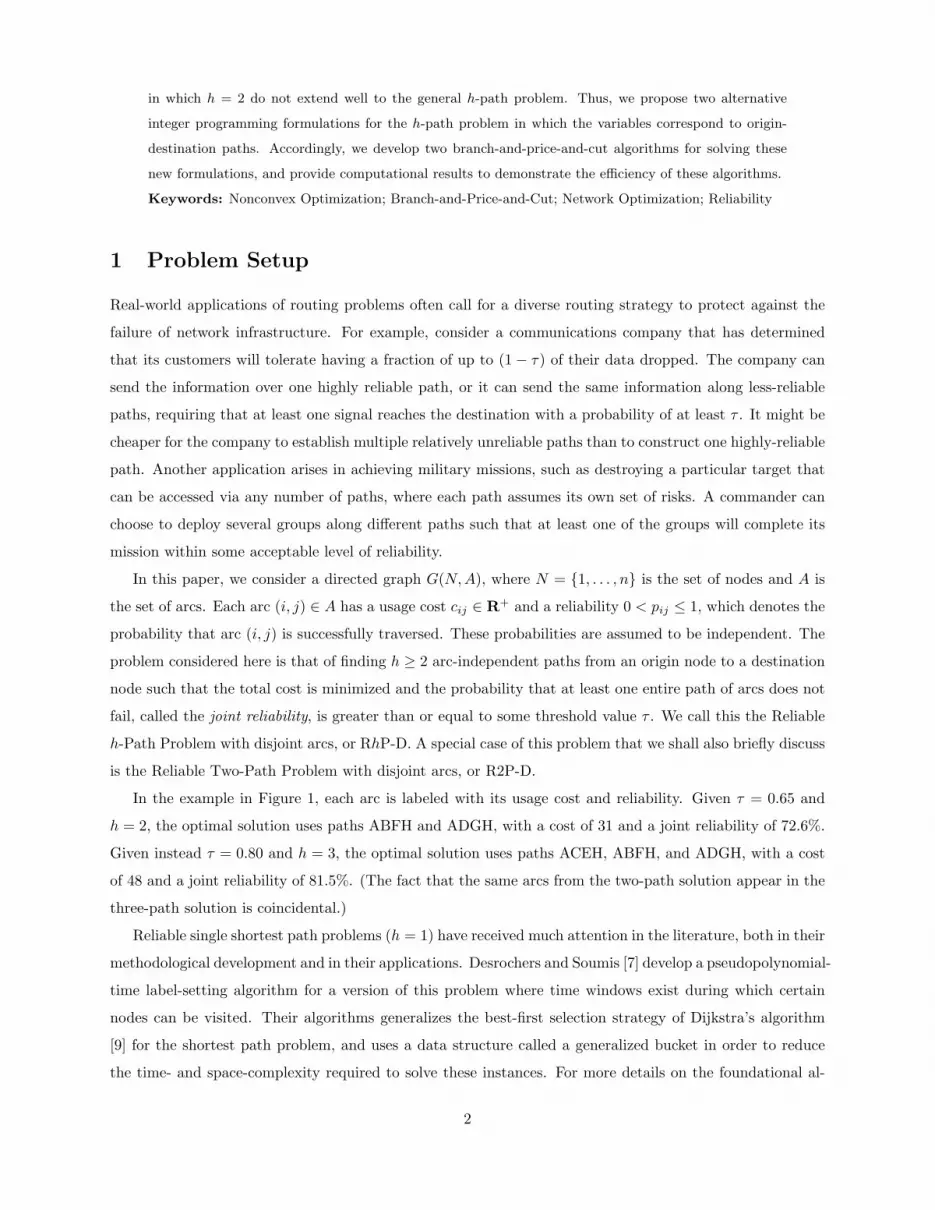
Recalling that u is the piecewise-linear function represented by (4) and (5), since (14) holds true for all

10

k = 1, . . . , h, we have

Uk = u(skn) ≤ u

∑p∈P

Rpxkp

≤

∑p∈P

u (Rp) xkp

≤∑p∈P

max{log(1−Rp), log(1− τ)}xkp. (16)

The first inequality is due to the fact that u is nonincreasing, and due to (14). The second inequality is due

to the convexity of u, and the third inequality is due to the fact that max{log(1−Rp), log(1− τ)} ≥ u (Rp).

Thus, the feasibility of x to (9) implies that U as computed by (10) must represent a feasible solution to

LRhP-D. Therefore, any feasible solution to RMP? is also feasible to LRhP-D, and this completes the proof.

2

Remark 2. Note that zA < zL in many instances, due to the presence of strict inequalities in the derivation

of (16). First, we often have that∑p∈P Rpx

kp < skn. This is due to the fact that in showing (14), we can

often state that each term Rpxkp is strictly less than a corresponding (and unique) term of skn. Furthermore,

there usually exist many additional positive terms of skn that do not correspond to terms of∑p∈P Rpx

kp,

which further increase the gap in the first inequality. Second, because log(1 − Rp) is strictly concave,

u(Rp) < max{log(1−Rp), log(1− τ)} for Rp < τ in the third inequality. 2

The tightness of (7) is primarily due to the fact that the reliability of each path is not approximated in (8)

(or (9)). This formulation does, however, require the dynamic generation of new columns whose values must

be binary at optimality. We thus propose a branch-and-price-and-cut strategy as described in the following

subsections. Section 3.1 describes the pricing problem and algorithm used to generate columns. Section 3.2

discusses strategies for generating cutting planes to eliminate fractional solutions, and for generating initial

columns to ensure the existence of feasible solutions. We discuss our branching strategy in Section 3.3.

3.1 Pricing

Let α, −πij , and −λ represent the duals associated with (7b), (7c), and (8), respectively. Given these dual

values, the reduced cost cp of any variable xp, p ∈ P , is given by

cp = −α+∑

(i,j)∈A

(cij + πij) δpij + λ log (1−Rp) . (17)

We seek a variable corresponding to a path p ∈ P that has a negative reduced cost with respect to the

current dual variable values. Since the −α term in (17) is constant, we minimize∑

(i,j)∈A (cij + πij) δpij +

λ log (1−Rp). The smallest value of the first term is easy to find by simply adjusting the arc lengths

to cij + πij , and solving a shortest-path problem. However, in order to incorporate the values of Rp, we

11

enumerate each Pareto-optimal path with respect to minimizing adjusted cost and maximizing reliability

(retaining one such path in case of a tie). We employ a node-labeling scheme such that at the completion

of the algorithm, we have ` such Pareto-optimal paths, labeled p1, . . . , p`, such that Rpi > Rpi+1 and

C ′pi > C ′pi+1, ∀i = 1, . . . , `− 1, where C ′p is the cost of path p with the adjusted arc costs. If all arc costs are

nonnegative, we can use a version of Dijkstra’s algorithm to accomplish this; however, if any arc costs are

negative, we must use a modified Bellman-Ford algorithm. The details of these modified path algorithms

are given in the Appendix. They are variants of the label setting method of Desrochers and Soumis [7] for

solving weight constrained shortest path problems.

After all such Pareto-optimal paths have been found, we then compute the reduced cost of each path

according to (17), and select one path p∗ having the minimum reduced cost. If cp∗ = 0, then we have

optimized the RMP, and we proceed to the branching portion of the algorithm. Else, we have that cp∗ < 0,

and thus we add the path p∗ to P and resolve the RMP.

3.2 Enhancements

One option to accelerate the convergence of this algorithm is to complement the reliability constraint with

a set of valid inequalities that prohibit the selection of paths whose reliabilities are too small to be used in a

feasible solution. Given a solution x to our RMP at an active node of the branch-and-bound tree, we define

P (x) as a set of paths associated with the h-largest xp-variables in our current solution, and let A(x) be the

set of arcs used by those paths.

Note that if∑p∈P (x) xp > h− 1, then the paths in P (x) will be arc-disjoint. To see this, note that even

the two smallest x-values would sum to more than 1, since otherwise, we would have paths p1 and p2 in

P (x) such that xp1 + xp2 ≤ 1, and thus∑p∈P (x)\{p1,p2} xp > h− 2. But since |P (x) \ {p1, p2}| = h− 2, the

latter inequality would require at least one x-variable to exceed 1, which is impossible. Hence, xp1 + xp2 > 1

for any distinct pair of pi and pj in P (x), and so by (7c), the paths cannot share any arcs. Therefore, if

1−∏p∈P (x) (1−Rp) ≥ τ , then the solution using the paths in P (x) is a feasible solution. We calculate the

cost of this solution and, if it is less than our current incumbent solution objective, use this new solution to

prune our branch-and-bound tree. This check will be done automatically and will serve as our baseline to

compare to the enhancement methods described below.

On the other hand, if 1 −∏p∈P (x) (1−Rp) < τ and

∑p∈P (x) xp > h − 1, then we can seek a feasible

solution by using an implicit enumeration algorithm, described below, to see if a feasible solution exists using

only the arcs in A(x). If so, then we update our incumbent upper bound, if possible, and attempt to further

prune our branch-and-bound tree. We refer to this process as “probing.”

The implicit enumeration algorithm that we use as a subroutine identifies a feasible set of h paths (with

respect to the joint reliability constraint) from node 1 to node n in a subgraph, which contains a set of arcs

from which exactly h arc-disjoint paths must be created. Our algorithm builds an enumeration tree that

contains all possible sets of h paths, pruning a particular branch of the tree if the partial paths established

12

on the branch are infeasible due to sufficiently low joint reliabilities of the paths already constructed.

If no feasible solution exists using only arcs in A(x), then we can add a cutting plane to the model (our

“cutting plane” scheme). We index these inequalities q = 1, . . . , Q, where Q is the current number of valid

inequalities added. If∑

(i,j)∈A(x)

∑p∈P δ

pij xp > |A(x)| − 1, then we set Q = Q + 1 and AQ = A(xp), and

add inequality Q to the formulation as follows:

∑p∈P

∑(i,j)∈AQ

δpij

xp ≤ |AQ| − 1. (18)

Formulating RhP-D as (7a) − (7c), (7e), (8), and inequalities (18), ∀q = 1, . . . , Q, the reduced cost of

the variable corresponding to path p is now given by

cp = −α+∑

(i,j)∈A

(cij + πij) δpij +

Q∑q=1

∑(i,j)∈Aq

σqδpij

+ λ log (1−Rp) , (19)

where −σq is the dual variable associated with constraints (18), ∀q = 1, . . . , Q. During the pricing portion

of the algorithm, the adjusted cost for an arc (i, j) now becomes cij + πij +∑Qq=1 ∆q

ijσq, where ∆qij equals

to 1 if (i, j) ∈ Aq and 0 otherwise.

The branch-and-price-and-cut approach assumes the existence of an initial feasible solution to the RMP

which may in fact become infeasible after cut generation and branching steps are applied. For the aggregated

model, we will create a single initialization column having a big-M cost, such that its selection maintains

RMP feasibility regardless of what columns have already been added, or what branching restrictions have

been applied. Hence, we create a column having a coefficient of h for (7b), zero for all the constraints (7c)

(and later for all the constraints (18)), and log (1− τ) for the constraint (8). This initialization column must

be included after each branching step, due to the modifications to the RMP that take place after branching,

as described in the following subsection.

In addition to the single-initialization column method, we may also opt to initialize the RMP by seeding

P with several paths, which may lead to a feasible solution. One such procedure uses Dijkstra’s algorithm

to find a most reliable path in the graph, and adds that column to P . We then delete the arcs used in that

column from the graph, and find a most reliable path on the remaining arcs, if one exists. We continue to

add paths in this greedy manner until P contains at most h arc-disjoint paths, or until no more paths exist

in the reduced network. The goal of this procedure is to seek a set of high-reliability paths that are likely to

satisfy the joint-reliability constraint.

An alternative idea is to generate h arc-disjoint paths of minimum costs. This goal can be accomplished

by solving a minimum-cost flow problem in which a supply of h units exists at node 1, a demand of h units

at node n, and in which all arc-capacities are equal to 1. A preliminary investigation revealed that the

greedy reliability-based initialization method is slightly more effective than the other methods, although the

13

advantage is not significant. This is consistent with the work of Vanderbeck [20], who showed empirically

that the inclusion of initialization columns corresponding to good integer solutions do not necessarily improve

the computational efficiency of branch-and-price-and-cut algorithms.

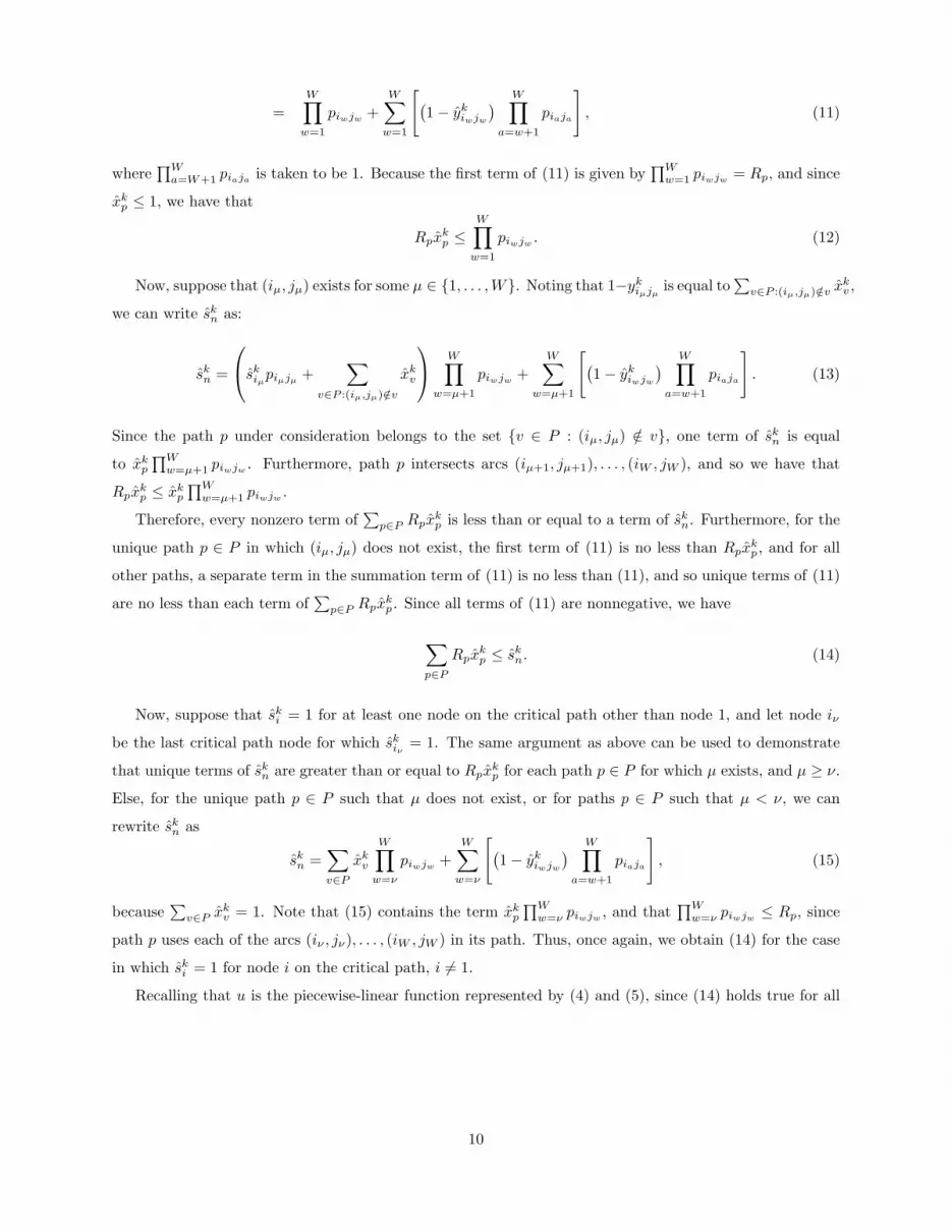
3.3 Branching

Following the column generation phase, the branching phase must occur in a manner that forces the algorithm

to converge. Simply branching on an xp-variable is problematic, because a variable that is forced to equal

to zero will reappear under a different index in the column generation subroutine that follows the branching

step. Instead, we examine the sum of flows on each arc in our solution. If there exists an arc (i, j) such that

0 <∑p∈P δ

pij xp < 1, we branch by insisting that this arc contains a total flow of either zero or one. In the

former case, we simply delete (i, j) from the graph, as well as any paths in P that use that arc, for future

iterations along that branch. In the latter case, we adjust the constraint corresponding to (i, j) in (7c) to be

an equality.

When we require the sum of flows to equal one, the dual variable πij becomes unrestricted and there

now exists a risk of encountering negative-cost cycles in our network during the column generation phase.

The column generation phase becomes strongly NP-hard in this case, and so we cannot reasonably solve

the pricing portion of the algorithm if these cycles exist in our graph. Indeed, a preliminary computational

analysis revealed that this behavior is persistent in cyclic graphs, and that the foregoing algorithm fails to

converge within reasonable computational limits. Therefore, we limit our examination of the aggregated

model to directed, acyclic graphs.

If the sum of flows on each arc in a solution is binary but the xp-variables are not integer, then this

branching scheme fails since there are no fractional flows on which we may branch. In this case, we need to

determine if any feasible integer solution can be found using only the arcs in our solution by employing an

implicit enumeration algorithm in which we examine viable permutations of the arcs used in our solution.

(For the special case in which h = 2, the two paths with the highest joint reliability will use the most reliable

path available; however, this greedy approach does not necessarily maximize joint reliability when h ≥ 3.)

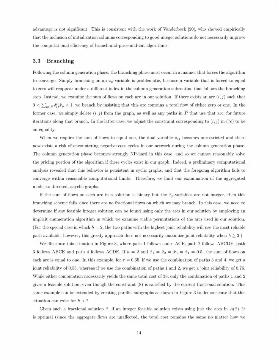
We illustrate this situation in Figure 3, where path 1 follows nodes ACE, path 2 follows ABCDE, path

3 follows ABCE and path 4 follows ACDE. If h = 2 and x1 = x2 = x3 = x4 = 0.5, the sum of flows on

each arc is equal to one. In this example, for τ = 0.65, if we use the combination of paths 3 and 4, we get a

joint reliability of 0.55, whereas if we use the combination of paths 1 and 2, we get a joint reliability of 0.76.

While either combination necessarily yields the same total cost of 38, only the combination of paths 1 and 2

gives a feasible solution, even though the constraint (8) is satisfied by the current fractional solution. This

same example can be extended by creating parallel subgraphs as shown in Figure 3 to demonstrate that this

situation can exist for h > 2.

Given such a fractional solution x, if an integer feasible solution exists using just the arcs in A(x), it

is optimal (since the aggregate flows are unaffected, the total cost remains the same no matter how we

14

Av

Bv

Cv

Dv

Ev��(9 0.5)

-(3, 0.9)

@@@@@@R

(7, 0.7)

��(6, 0.7)

-(5, 0.8)

@@@@@@R

(8, 0.6)

Figure 3: Example of Fractional Paths and Integer Flows.

distribute the individual paths). On the other hand, if no solution exists, we cut off the solution by adding

a cutting plane of the form (18). This check uses the same implicit enumeration algorithm described earlier.

As expected, our preliminary investigation confirms that the introduction of possible negative-cost cycles

in the course of the foregoing branching strategy causes the column generation approach to become much

less efficient, because the shortest path problem solved in the pricing phase becomes strongly NP-hard in

the presence of negative cost cycles. We address this difficulty in the following section by reformulating the

Restricted Master Problem.

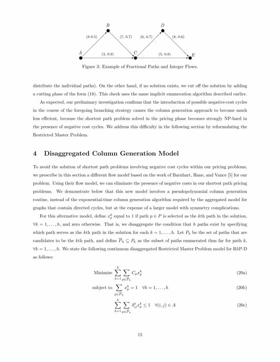
4 Disaggregated Column Generation Model

To avoid the solution of shortest path problems involving negative cost cycles within our pricing problems,

we prescribe in this section a different flow model based on the work of Barnhart, Hane, and Vance [5] for our

problem. Using their flow model, we can eliminate the presence of negative costs in our shortest path pricing

problems. We demonstrate below that this new model involves a pseudopolynomial column generation

routine, instead of the exponential-time column generation algorithm required by the aggregated model for

graphs that contain directed cycles, but at the expense of a larger model with symmetry complications.

For this alternative model, define xkp equal to 1 if path p ∈ P is selected as the kth path in the solution,

∀k = 1, . . . , h, and zero otherwise. That is, we disaggregate the condition that h paths exist by specifying

which path serves as the kth path in the solution for each k = 1, . . . , h. Let Pk be the set of paths that are

candidates to be the kth path, and define P k ⊆ Pk as the subset of paths enumerated thus far for path k,

∀k = 1, . . . , h. We state the following continuous disaggregated Restricted Master Problem model for RhP-D

as follows:

Minimizeh∑k=1

∑p∈Pk

Cpxkp (20a)

subject to∑p∈Pk

xkp = 1 ∀k = 1, . . . , h (20b)

h∑k=1

∑p∈Pk

δpijxkp ≤ 1 ∀(i, j) ∈ A (20c)

15

h∑k=1

∑p∈Pk

log (1−Rp)xkp ≤ log (1− τ) (20d)

xkp ≥ 0 ∀p ∈ P k, k = 1, . . . , h. (20e)

Note again that (20d) can be tightened by adjusting the left-hand-side coefficients to max{log(1−Rp), log(1−

τ)} as mentioned in Remark 1. Moreover, using this tightened constraint in lieu of (20d), the proof of

Proposition 1 can be directly applied (without need for transforming x′ to x) to show that the linear

relaxation of (20), using all columns, is at least as strong as that of LRhP-D.

Aside from the increase in model size from using the disaggregated model instead of the aggregated model

discussed in Section 3, the formulation given by (20) also exhibits problem symmetry that is known to induce

substantial computational complications in integer programming problems [17]. In this particular case, the

designation of paths as the first path, second path, and so on, is artificial, and guarantees the existence of

at least h! alternative optimal solutions. Rather than burden the branch-and-bound process with the task

of identifying and fathoming all branches that contain these solutions, we state a set of symmetry-breaking

constraints to eliminate the existence of these solutions. Since each path must be arc-disjoint, the second

node visited in each path must be distinct. Hence, we require that the index of the second node visited in

path 1 is strictly less (by at least one) than the second node visited in path 2, which is strictly less than the

second node visited in path 3, and so on. The following constraints establish this hierarchy.

∑p∈Pk+1

∑j∈FS(1)

jδp1jxk+1p −

∑p∈Pk

∑j∈FS(1)

jδp1jxkp ≥ 1 k = 1, . . . , h− 1. (21)

Remark 3. We may also attempt to break symmetry by enforcing some restriction such as Rp1 ≥ Rp2 ≥

· · · ≥ Rph . Breaking symmetry in this fashion allows us to use information about the reliability of specific

paths to limit the search area and prune the graph. However, if we attempt to break symmetry based on

reliability or cost (Cp1 ≥ Cp2 ≥ · · · ≥ Cph), not only will these rules fail to uniquely break symmetry, but

they can create situations in which less-reliable, higher-cost paths will have a lower reduced cost than highly-

reliable, low-cost paths due to the values of the duals associated with these constraints. Worse, this could

make the pricing algorithm enumerate almost every possible path from 1 to n. Hence, we do not consider

the use of cost- or reliability-based symmetry-breaking rules in this paper. 2

Once again, we divide the discussion of our branch-and-cut into three subsections. We discuss the pricing

algorithm in Section 4.1, cutting plane and initial feasible solutions in Section 4.2, and the branching scheme

in Section 4.3.

16

4.1 Pricing

Let αk, −πij , −λ, and φk represent the duals associated with (20b) − (20d) and (21), respectively. Define

φ0 = 0 and φh = 0. We can write the reduced cost of any k path p ∈ Pk as

ckp = −αk +∑

(i,j)∈A

(cij + πij) δpij +

∑j∈FS(1)

j (φk − φk−1) δp1j + λ log (1−Rp) ∀k = 1, . . . , h. (22)

For each path p generated by the procedure, we add p only to P k for which p has the lowest reduced

cost. That is, we add at most one path to each set P k each time we solve the RMP. Note that the term

φk − φk−1 of (22) could be negative, with the result that the adjusted costs of the arcs leaving node 1 may

be negative for the pricing portion of the algorithm. However, since we can assume without loss of generality

that RS(1) = ∅, we can proceed with our modified Dijkstra’s algorithm as before.

Due to our symmetry-breaking constraints, we note that if some path p∗ uses arc (1, 2), for example,

then p∗ must be the first path, if it is used. That is, we must require x2p∗ + · · · + xhp∗ = 0. In general, this

constraint is as follows ∑p∈P j

δp1j

h∑k=j

xkp

= 0 ∀j = 2, . . . , h. (23)

Similarly, we also state that

∑p∈P j

δp1,n−j+1

(h−j∑k=1

xkp

)= 0 ∀j = 1, . . . , h− 1. (24)

Rather than formally adding these constraints (and handling their associated dual values in the pricing

phase), we can simply remove the arcs (1, 2), . . . , (1, j) in the pricing problem for j = 2, . . . , h, as well as the

arcs (1, n− (h− j) + 1), . . . , (1, n) in the pricing problem for j = 1, . . . , h− 1.

4.2 Enhancements

We can use the enhancements discussed in Section 3.2 without significant adjustment. In the disaggregated

model, given a solution x to our RMP at an active node of the branch-and-bound tree, we define P (x) as a

set of paths associated with the h-largest xkp-variables in our current solution, and again let A(x) be the set

of arcs used by those paths.

As for the initialization of this model, we create h initialization columns, each having a coefficient of 1 for

(20b), zero for all the constraints (20c), and log (1− τ) for the constraint (20d). We also use a coefficient of

k+ n for the (k− 1)st constraint of (21), ∀k = 2, . . . , h, and a coefficient of −k− n for the kth constraint of

(21), ∀k = 1, . . . , h− 1. Again, each of these h columns will have some big-M cost. Additionally, we employ

the greedy reliability-based initialization column routine as described in Section 3.2.

17

4.3 Branching

We adopt the divergent path rule of Barnhart, Hane, and Vance [5] for this model. If there is any fractional

flow on the kth path, we trace the flow from node 1 on path k until we find the first arc (dk, f1) on which the

total flow in our solution is fractional (such an arc must exist, because a flow of 1 reaches node dk). Next,

we identify another arc, (dk, f2), on which a fractional flow leaves node dk. Then we designate two sets of

arcs Dk1 and Dk2 such that (dk, f1) ∈ Dk1, (dk, f2) ∈ Dk2, Dk1 ∩Dk2 = ∅, and Dk1 ∪Dk2 = FS(dk). We

now branch from our current solution such that on one branch we have

∑p∈Pk

δpijxkp = 0 ∀(i, j) ∈ Dk1, (25)

and on the other branch we have ∑p∈Pk

δpijxkp = 0 ∀(i, j) ∈ Dk2. (26)

Instead of adding these constraints formally, we remove the arcs in Dk1 from the graph on one branch and

the arcs in Dk2 from the graph in the other branch for path k. Additionally, we remove all paths in P k that

use the arcs deleted in each of the newly-created branches when we resolve the RMP. This technique reduces

the size of the graph on which the pricing problem is executed over the course of the branch-and-price-and-

cut algorithm. Since we cannot encounter negative-cost cycles during the pricing portion of the algorithm,

the branch-and-price-and-cut approach can be executed on acyclic or cyclic graphs without encountering a

strongly NP-hard column generation problem.

5 Computational Results

In this section, we evaluate the computational advantages of each of the strategies presented here for various

values of h. We will first compare the enhancement methods discussed in Section 3.2 for both models, and

will then compare the two models’ overall efficiency. We will also make a comparison of these models to

the problem formulation presented in [2] on acyclic graphs. All computations were done on a 500 MHz Sun

Blade 100 running Solaris version 5.8 with 1.5 GB of installed memory. All computational times are listed

in CPU seconds. Linear and integer programming problems were solved using CPLEX 8.1.

Problem Set Generation. For comparison purposes, we tested the aggregated and disaggregated models

on directed, acyclic graphs. For Problem Set 1, we generated 20 directed, acyclic graphs for each combination

of total nodes and arc densities, where a graph could have 25, 50, 75, or 100 nodes, and could have an arc

density of 20%, 50%, or 80%, for a total of 240 instances. To generate a graph with roughly d% arc density,

for each possible (i, j) node pair, i < j, a random number was generated with a uniform distribution between

0 and 1, and arc (i, j) was generated if and only if this number was not more than d%. Since no arcs (j, i),

18

Size Method 20% Density 50% Density 80% Density

Standard Standard StandardAverage Deviation Average Deviation Average Deviation

25 Base 0.06 0.05 0.33 0.40 1.09 1.4225 Probing 0.06 0.05 0.34 0.41 1.08 1.4325 CG 0.05 0.05 0.34 0.36 1.15 1.49

50 Base 0.45 0.68 3.61 5.30 21.04 32.2350 Probing 0.46 0.69 3.61 5.28 21.01 32.1950 CG 0.43 0.59 3.25 3.98 21.76 35.50

75 Base 2.92 3.63 42.31 50.94 69.67 94.1475 Probing 2.93 3.65 42.36 50.97 69.71 94.1975 CG 2.52 2.71 37.45 48.07 45.13 58.34

100 Base 11.65 15.70 77.94 81.17 757.20 1539.74100 Probing 11.66 15.65 77.90 81.15 757.89 1541.56100 CG 11.71 15.83 56.65 68.50 385.00 797.38

Table 1: Computational times for enhancement methods on aggregated model for h = 3

j > i, were generated, no directed cycles exist. We prohibited the generation of an arc connecting node 1

directly to node n and required that at least five arcs left node 1 and at least five arcs entered node n. Arc

costs were assigned by generating a random number with a uniform distribution between 0 and 100. The

joint reliability threshold τ was generated using a uniform distribution between 0.5 and 1.0. Problem Set 2

was generated in a similar fashion except that we required that at least ten arcs left node 1 and that at least

ten arcs entered node n.

In our first experiment, we analyzed the effectiveness of the enhancement methods discussed in Section

3.2 by comparing the impact of probing and cut generation (CG) to the baseline for both the aggregated

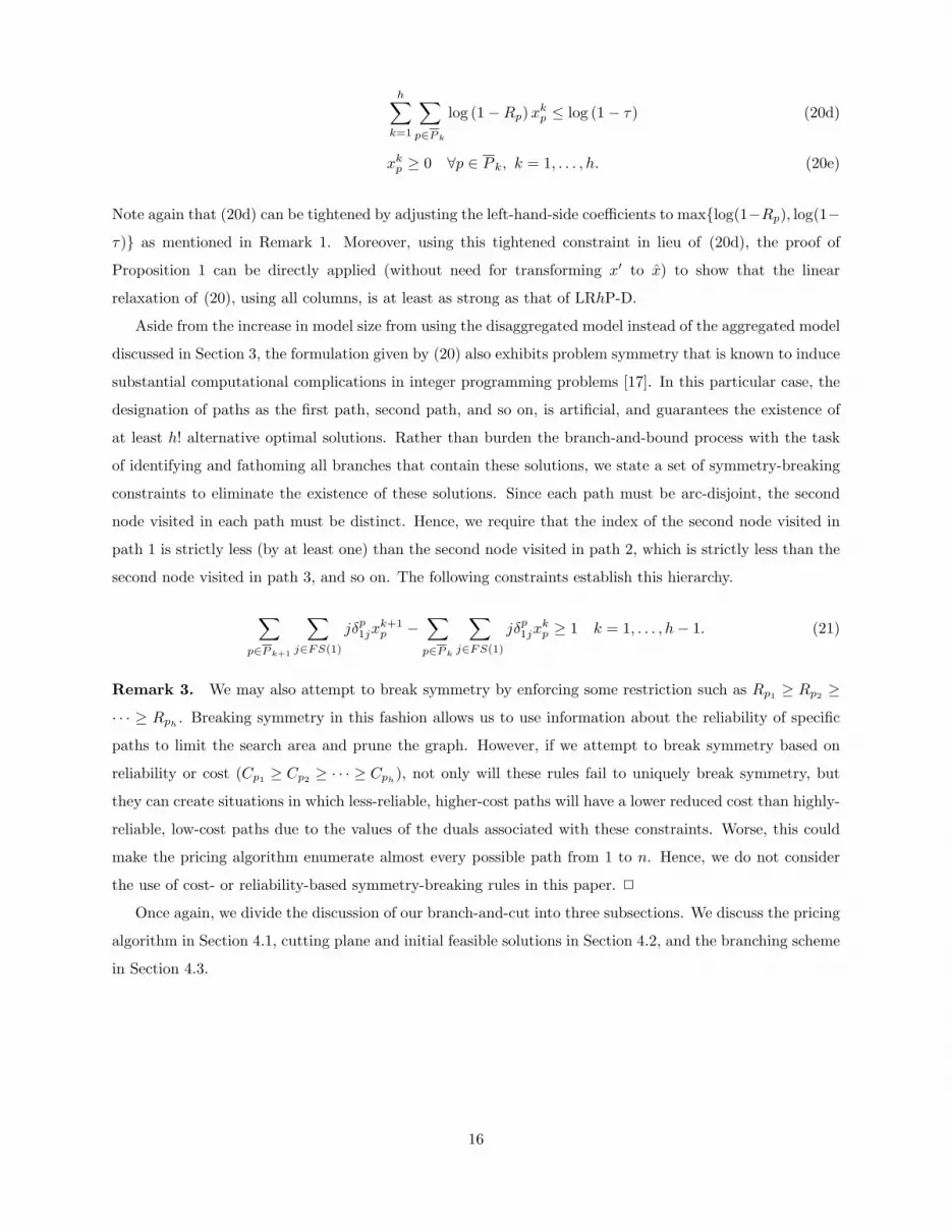
and disaggregated models using Problem Set 1. The results of these experiments for h = 3, 4, and 5 are

shown in Tables 1 − 6 for the aggregated and disaggregated models.

For the aggregated model, the cut generation strategy improved solution times for 75- and 100-node

instances with 50% and 80% densities, and this improvement becomes more pronounced as h increases.

The number of cuts generated for a problem instance varied from 4 to 160. We observed that the implicit

enumeration algorithm necessary for branching in the aggregated model was rarely invoked. For example,

for Problem Set 1 and h = 5, only three out of the 240 instances required the implicit enumeration algorithm

to resolve a branching problem and this happened only once throughout the course of the algorithm in each

of these three instances.

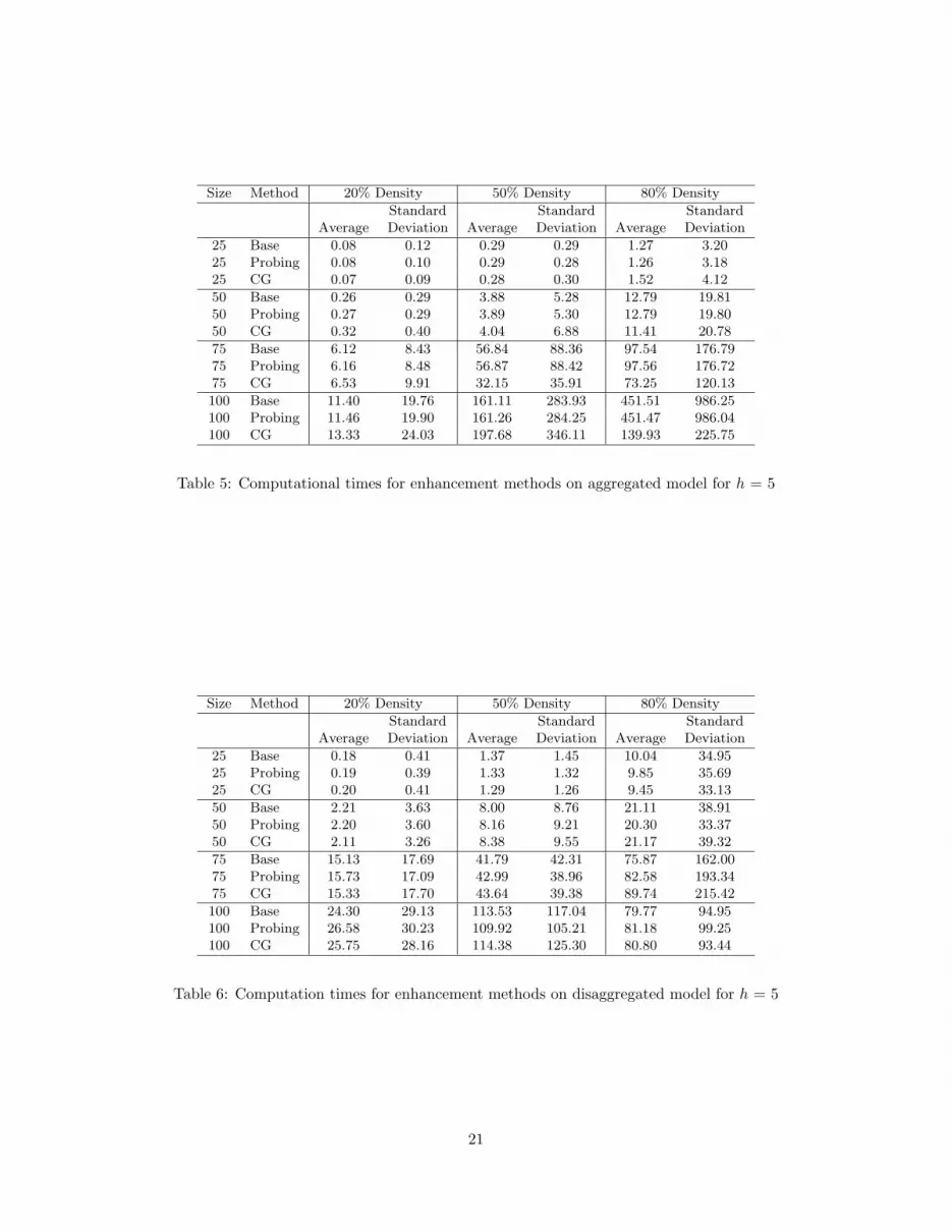
For the disaggregated case, neither of the enhancements consistently provided any computational advan-

tage. In fact, the probing and cut generation methods increased the average computational time to solve the

problem. This behavior appears to be due to the fact that the branching phase eliminates many of the arcs

that would otherwise be included in the valid inequalities, thereby nullifying the effectiveness of any cutting

plane strategy. Probing failed to improve computation times over the baseline for either model, and failed

to provide an improved upper bound for the problem instances examined.

The results from Tables 1 − 6 seem to indicate that the disaggregated model is easier to solve than

19



25 Base 0.09 0.12 0.58 0.55 1.24 1.9625 Probing 0.09 0.11 0.57 0.55 1.23 1.9025 CG 0.09 0.12 0.55 0.53 1.36 2.26

50 Base 0.81 1.10 2.20 1.84 11.59 26.8850 Probing 0.80 0.97 2.56 2.32 9.97 19.3550 CG 0.79 0.97 2.60 2.30 10.51 21.76

75 Base 3.27 3.27 15.32 20.29 10.04 8.1075 Probing 3.14 2.68 14.29 17.47 11.18 9.4675 CG 3.17 2.76 16.53 24.16 10.79 8.94

100 Base 8.63 10.48 14.53 12.19 35.15 48.99100 Probing 7.90 8.30 13.71 10.44 39.38 63.15100 CG 8.00 8.64 13.89 11.60 50.59 99.97

Table 2: Computational times for enhancement methods on disaggregated model for h = 3



25 Base 0.07 0.08 0.29 0.24 0.84 1.4725 Probing 0.07 0.08 0.29 0.24 0.86 1.5025 CG 0.08 0.11 0.29 0.24 0.88 1.50

50 Base 0.37 0.44 3.38 3.80 10.41 13.5950 Probing 0.38 0.46 3.37 3.79 10.41 13.5950 CG 0.39 0.50 3.51 4.30 10.44 13.76

75 Base 3.47 4.25 47.75 66.31 66.18 117.6675 Probing 3.50 4.27 47.83 66.46 66.15 117.6275 CG 3.49 4.50 37.45 47.09 46.88 52.77

100 Base 13.09 17.76 74.65 108.86 749.28 2213.40100 Probing 13.14 17.85 74.67 108.76 749.07 2212.88100 CG 12.52 16.94 72.82 118.81 357.63 939.28




25 Base 0.15 0.31 0.79 0.72 2.72 6.5925 Probing 0.14 0.23 0.74 0.62 3.69 10.9125 CG 0.15 0.30 0.74 0.70 3.16 8.43

50 Base 1.15 1.51 4.80 4.75 9.03 11.8250 Probing 1.17 1.63 5.16 5.50 9.10 11.7550 CG 1.33 1.90 5.01 5.34 8.02 9.70

75 Base 6.35 7.18 27.44 27.06 26.77 38.5175 Probing 6.10 6.38 31.56 46.58 24.32 36.6475 CG 7.10 8.40 28.41 30.96 27.15 43.47

100 Base 17.27 16.71 30.61 30.53 56.09 92.05100 Probing 17.70 17.47 33.09 35.49 58.45 96.73100 CG 20.14 22.19 32.62 35.19 55.10 79.09

Table 4: Computational times for enhancement methods on disaggregated model for h = 4

20



25 Base 0.08 0.12 0.29 0.29 1.27 3.2025 Probing 0.08 0.10 0.29 0.28 1.26 3.1825 CG 0.07 0.09 0.28 0.30 1.52 4.12

50 Base 0.26 0.29 3.88 5.28 12.79 19.8150 Probing 0.27 0.29 3.89 5.30 12.79 19.8050 CG 0.32 0.40 4.04 6.88 11.41 20.78

75 Base 6.12 8.43 56.84 88.36 97.54 176.7975 Probing 6.16 8.48 56.87 88.42 97.56 176.7275 CG 6.53 9.91 32.15 35.91 73.25 120.13

100 Base 11.40 19.76 161.11 283.93 451.51 986.25100 Probing 11.46 19.90 161.26 284.25 451.47 986.04100 CG 13.33 24.03 197.68 346.11 139.93 225.75




25 Base 0.18 0.41 1.37 1.45 10.04 34.9525 Probing 0.19 0.39 1.33 1.32 9.85 35.6925 CG 0.20 0.41 1.29 1.26 9.45 33.13

50 Base 2.21 3.63 8.00 8.76 21.11 38.9150 Probing 2.20 3.60 8.16 9.21 20.30 33.3750 CG 2.11 3.26 8.38 9.55 21.17 39.32

75 Base 15.13 17.69 41.79 42.31 75.87 162.0075 Probing 15.73 17.09 42.99 38.96 82.58 193.3475 CG 15.33 17.70 43.64 39.38 89.74 215.42

100 Base 24.30 29.13 113.53 117.04 79.77 94.95100 Probing 26.58 30.23 109.92 105.21 81.18 99.25100 CG 25.75 28.16 114.38 125.30 80.80 93.44

Table 6: Computation times for enhancement methods on disaggregated model for h = 5

21

h Size Density Aggregated Disaggregated

Standard StandardAverage Deviation Average Deviation

6 75 50% 25.98 59.28 69.51 142.066 75 80% 81.04 109.99 108.55 112.81

6 100 50% 118.20 188.33 282.99 480.906 100 80% 130.53 480.47 150.99 385.72

8 75 50% 30.60 61.18 435.85∗ 990.98∗

8 75 80% 34.22 80.61 163.30 168.18

8 100 50% 55.81 106.61 630.56 1276.338 100 80% 155.07 409.67 735.81∗ 1369.52∗

10 75 50% 75.78 280.94 677.63∗ 1330.00∗

10 75 80% 74.78 124.87 749.72 1179.99

10 100 50% 123.61 345.68 1283.64∗ 1926.68∗

10 100 80% 183.76 460.71 1236.09∗ 1927.82∗

Table 7: Computational times for “best” aggregated and disaggregated models

the aggregated model for h = 3, 4, and 5. For these instances, the computational advantage afforded by

the disaggregated model may be attributed to its branching strategy, which removes approximately half of

the arcs leaving a particular node from consideration for path k. This technique shrinks the search region

considerably after a few branches, and allows us to conduct a more specific search to find the best path to

add for a particular k. This property, however, appears to become less of an advantage as h increases.

To test the hypothesis that the aggregated model becomes more effective as h increases, we test the

performance of both models for h = 6, 8, and 10. We compare the two models using their most promising

strategies (namely cut generation for the aggregated model and the baseline for the disaggregated model)

on the most challenging test instances (i.e., 75- and 100-node instances having 50% and 80% density) using

Problem Set 2, and display the results in Table 7. In our computations, we halted the algorithm before

solving the master problem if the total time elapsed exceeds 90 minutes (5400 seconds). The values in Table

7 marked with an asterisk include at least one such instance, where the average computational times include

the time elapsed before the algorithm terminates (prematurely). For h = 8, the disaggregated model failed

to solve one instance out of the 75-node, 50% density set and one instance out of the 100-node, 80%-density

set. For h = 10, the disaggregated model failed to solve one instance out of the 75-node, 50% density set,

two instances out of the 100-node, 50% density set, and one instance out of the 100-node, 80% density

set. The aggregated implementation solves all instances within the allotted time limit. Table 7 conclusively

demonstrates that as h increases beyond 6, the best implementation of the aggregated model outperforms

the best implementation of the disaggregated model due to its reduced model size.

Next, we compared the column generation-based algorithm of the disaggregated model with the arc-

based model developed in [2], and the continuous branch-and-bound procedure for solving LhP-D, for h = 2.

The results from this experiment are displayed in Table 8, where the average computational times over

twenty instances using the recommended method from [2] are denoted as Arc-Based, the results from the

disaggregated model are denoted as Disagg, and the results from solving LhP-D are denoted as LhP-D. We

22



25 Arc-Based 0.03 0.02 0.17 0.14 0.24 0.2025 Disagg 0.09 0.02 0.44 0.34 0.83 0.6525 LhP-D 0.18 0.21 5.06 6.47 9.49 8.83

50 Arc-Based 0.12 0.06 0.63 0.90 2.31 2.6950 Disagg 0.47 0.47 1.65 2.21 3.62 4.5050 LhP-D 19.27 77.05 260.13 523.31 740.38? 1620.78?

75 Arc-Based 0.46 0.46 2.56 2.54 7.95 12.1175 Disagg 1.45 1.34 4.48 4.75 8.88 6.1975 LhP-D 152.30 388.33 1297.91? 1965.59? 1468.92? 1736.05?

100 Arc-Based 0.95 1.06 9.20 17.55 100.52 145.66100 Disagg 3.25 3.01 10.16 9.12 24.34 29.07100 LhP-D 653.64? 1339.76? 1721.58? 2054.09? 2930.77? 2486.39?

?: Instances exceeding the 5400-second time limit are assigned a 5400s CPU time.

Table 8: Comparison of prior methods to disaggregated model for h = 2

conclude that using the disaggregated model is in fact a more effective method for the 100-node, 80% density

instances than solving these acyclic problems via the branch-and-bound method prescribed in [2], although

the specialized Arc-Based procedure of [2] is more effective than Disagg on the other 11 problem classes.

The compact formulation LhP-D is not competitive on any of these problem classes, even for the case of

h = 2. Indeed, we examined LhP-D for the case of h = 3 as well, but the performance of the continuous

branch-and-bound algorithm seems to deteriorate as h increases. For instance, even on the 50-node, 50%-

density instances (which the aggregated model solves in an average of 3.25 seconds, and the disaggregated

model solves in an average of 2.6 seconds) the LhP-D fails to solve four of the twenty instances within the

5400-second time limit, and requires an average of 297.6 seconds on the other sixteen instances. (The details

of this experiment are omitted for brevity.)

Finally, we executed a comparison of the proposed aggregated and disaggregated branch-and-price-and-

cut algorithms with and without the constraint tightening mentioned in Remark 1. The algorithms are

implemented in the same fashion with this tightened modification, with the exception that the pricing

problem only recognizes a maximum reliability of τ in generating paths. (Paths with reliabilities larger than

τ can indeed be generated, but only λ log(1 − τ) is contributed to the reduced cost function in (17) and

(22).) Table 9 displays the results of this experiment, in which the columns labeled “No Tightening” display

the results reported previously in which no coefficient tightening was performed, and the columns labeled

“With Tightening” display the results reported in which coefficient tightening was peformed. These results

demonstrate that there is no evidence to suggest that coefficient tightening reduces the computational effort

to solve the most challenging (100 nodes, 80% density) instances. The lack of effectiveness of this technique

is perhaps due to the rarity with which paths having reliabilities greater than τ were encountered in our test

instances.

23

Average CPU Time Standard Deviation

Method h No Tightening With Tightening No Tightening With Tightening

Aggregated 3 385.00 387.59 797.38 803.03Aggregated 4 357.63 364.84 939.28 957.49Aggregated 5 139.93 142.51 225.75 230.01

Disaggregated 3 50.59 39.19 99.97 62.07Disaggregated 4 55.10 65.81 79.09 114.51Disaggregated 5 80.80 84.70 93.44 102.84

Table 9: Comparison of methods with and without coefficient tightening.

6 Conclusions

In this paper, we examined the solution of the h-path routing problem with reliability considerations via

branch-and-price-and-cut. We investigated two different formulations for this problem: one smaller “aggre-

gated” model in which each origin-destination flow was represented by a common set of variables, and a

larger “disaggregated” model in which a separate set of variables was dedicated to each of the h paths. The

latter formulation was created to avoid having to solve a resource-constrained shortest-path problem in the

presence of negative-cost cycles during the column generation phase, and affords a more effective branching

procedure. We analyzed the use of model and algorithmic enhancements to improve computational per-

formance, and while our cut generation method was effective for the aggregated model, no enhancements

tested seemed helpful for the disaggregated model. When h ≤ 5, the disaggregated model is preferable

to the aggregated model. However, the more compact aggregated formulation is more effective than the

disaggregated model formulation when h ≥ 6.

Future studies for this problem may include the examination of the reliable h-path problem where either

limited or unlimited arc sharing is permitted. Other considerations may include how to revise this formulation

when arc reliabilities or costs are stochastic. For very large problems, it may serve well to develop strong

heuristics and determine when a good stopping point may be reached, instead of requiring a globally optimal

solution.

Appendix

Our pricing strategy requires modified versions of both Dijkstra’s shortest path algorithm and the Bellman-

Ford algorithm.

Dijkstra’s Algorithm and Modifications. Dijkstra’s algorithm computes the shortest path from the

origin node to each node in a graph when all arc costs are nonnegative. For our purposes, we must adjust

the algorithm to include multiple records at each node containing labels for both cost and reliability. We

need to keep a list of records for each node such that if we have ` records for a particular node, the list is

sorted such that C ′p1 > C ′p2 > · · · > C ′p` and Rp1 > Rp2 > · · · > Rp` > 0. Each record will now have four

24

attributes: cost, reliability (rel), predecessor (pred), and visited.

We shall refer to the process to enter a (cost, reliability) pair into the list of records for node j, called

records[j], as enterItem(cost, rel, pred, j). The function enterItem performs two checks. First,

if −α + cost + λ log(1 − rel) ≥ 0, then since all arc costs are nonnegative, any path resulting from this

record will have a nonnegative reduced cost and hence the function will not add the (cost, reliability) pair

to the list of records for j. (In the disaggregated model, even though arc (1, j) may have a negative cost,

as long as we label the graph forward as shown in the algorithm, we can still discard these records.) Next,

the function examines the records listed in records[j] and adds the (cost, reliability) pair only if it is not

dominated by, or identical to, any other (cost, reliability) pair in the list of records. If a record needs to be

added, the function adds the record in records[j] and sets its attributes appropriately, with an automatic

initialization of the “visited” field to zero. The modified Dijkstra’s algorithm is shown in Algorithm 1.

Algorithm 1: Modified Dijkstra’s AlgorithmCreate an initial record partial for records[1]partial.cost = 0partial.rel = 1partial.pred =NULLpartial.visited = 0i = 1minrecord = minNotVisited(i)Comment: minNotVisited(i) returns a pointer to the record in i with the minimum costnot yet marked as visited. It returns a NULL if all records have been visited in i.while minrecord 6= NULL do

minrecord.visited = 1foreach (i, j) ∈ A do

enterItem(minrecord.cost + cij ,minrecord.rel× pij , i, j)endmincost =∞minrecord = NULLfor j = 1 to n do

if minNotVisited(j) 6= NULL thenif minNotVisited(j).cost < mincost then

minrecord = minNotVisited(j)mincost = minNotVisited(j).costi = j

endend

endend

The Bellman-Ford Algorithm and Modifications. The Bellman-Ford algorithm computes the shortest

path from the origin node to each node in a graph, and permits the existence of negative-cost arcs, as long

as no negative-cost cycles exist. If there are no negative-cost cycles, then at the end of the algorithm each

record contains the length of the shortest path from that node to the origin.

The labeling process will be similar to that of the one used in the modified Dijkstra’s algorithm. However,

25

due to the existence of negative-cost arcs, the function enterItem will add records regardless of the value of

−α+ cost+ λ log (1− rel).

In a traditional Bellman-Ford algorithm, a simple test is performed to see if negative cost cycles exist.

Although we prohibited the creation of cycles in our test instances, we keep the check here for completeness.

The modified Bellman-Ford algorithm with logic to identify negative cost cycles is shown in Algorithm 2.

Algorithm 2: Modified Bellman-Ford AlgorithmCreate an initial record partial for records[1]partial.cost = 0partial.rel = 1partial.pred = NULLpartial.visited = 0for k = 1 to n do

foreach (i, j) ∈ A doforeach record partial in records[i] do

if partial.visited == 0 thenenterItem(partial.cost + cij , partial.rel× pij , i, j)partial.visited = 1

endend

endendforeach (i, j) ∈ A do

Comment: minCost(i) returns a pointer to the record in records[i] with the lowestcost value.if minCost(j).cost > minCost(i).cost + cij then

Terminate: Graph contains a negative cost cycle.end

end

References

[1] A. K. Andreas. Mathematical Programming Algorithms For Robust Routing and Evacuation Problems.

PhD thesis, Department of Systems and Industrial Engineering, The University of Arizona, Tucson,

Arizona, 2006.

[2] A. K. Andreas and J. C. Smith. Mathematical programming algorithms for two-path routing problems

with reliability considerations. Working Paper, Department of Systems and Industrial Engineering, The

University of Arizona, Tucson, Arizona, 2006.

[3] J. F. Bard and J. L. Miller. Probabilistic shortest path problems with budgetary constraints. Computers

and Operations Research, 16(2):145–159, 1989.

[4] C. Barnhart, C. A. Hane, E. L. Johnson, and G. Sigismondi. A column generation and partitioning

approach for multi-commodity flow problems. Telecommunication Systems, 3:239–258, 1995.

26

[5] C. Barnhart, C. A. Hane, and P. H. Vance. Using branch-and-price-and-cut to solve origin-destination

integer multicommodity flow problems. Operations Research, 48(2):318–326, 2000.

[6] Z. L. Chen and W. B. Powell. A generalized threshold algorithm for the shortest path problem with time

windows. In P. M. Pardalos and D.-Z. Du, editors, Network Design: Connectivity and Facilities Loca-

tion, Discrete Mathematics and Theoretical Computer Science, pages 303–318. American Mathematical

Society, Providence, RI, 1998.

[7] M. Desrochers and F. Soumis. A generalized permanent labelling algorithm for the shortest path problem

with time windows. Information Systems and Operational Research, 26(3):191–211, 1988.

[8] J. Desrosiers, Y. Dumas, M. M. Solomon, and F. Soumis. Time constrained routing and scheduling. In

M. O. Ball, T. L. Magnanti, C. L. Monma, and G. L. Nemhauser, editors, Network Routing, volume 8 of

Handbooks in Operations Research and Management Science, pages 35–139. Elsevier, Amsterdam, The

Netherlands, 1995.

[9] E. W. Dijkstra. A note on two problems in connexion with graphs. Numerische Mathematik, 1:269–271,

1959.

[10] I. Dumitrescu and N. Boland. Algorithms for the weight constrained shortest path problem. Interna-

tional Transactions in Operational Research, 8:15–29, 2001.

[11] I. Dumitrescu and N. Boland. Improved preprocessing, labeling and scaling algorithms for the weight-

constrained shortest path problem. Networks, 42(3):135–153, 2003.

[12] A. A. Elimam and D. Kohler. Case study: Two engineering applications of a constrained shortest-path

model. European Journal of Operational Research, 103:426–438, 1997.

[13] J. E. Falk and R. M. Soland. An algorithm for separable nonconvex programming problems. Management

Science, 15:550–569, 1969.

[14] S. Fortune, J. Hopcroft, and J. Wyllie. The directed subgraph homeomorphism problem. Theoretical

Computer Science, 10:111–121, 1980.

[15] F. Glover, R. Glover, and D. Klingman. The threshold shortest path problem. Networks, 14:25–36,

1984.

[16] M. E. Lubbecke and J. Desrosiers. Selected topics in column generation. Operations Research,

53(6):1007–1023, 2005.

[17] H. D. Sherali and J. C. Smith. Improving discrete model representations via symmetry considerations.

Management Science, 47(10):1396–1407, 2001.

27

[18] H. D. Sherali and C. H. Tuncbilek. A global optimization algorithm for polynomial programming

problems using a Reformulation-Linearization Technique. Journal of Global Optimization, 2:101–112,

1992.

[19] J. W. Suurballe. Disjoint paths in a network. Networks, 4:125–145, 1974.

[20] F. Vanderbeck. Decomposition and Column Generation for Integer Programs. PhD thesis, Universite

Catholique de Louvain, Belgium, 1994.

[21] F. Vanderbeck. Branching in branch-and-price: a generic scheme. Working Paper, Applied Mathematics,

University Bordeaux 1, F-33405 Talence Cedex, France, 2006.

[22] F. Vanderbeck and L. A. Wolsey. An exact algorithm for IP column generation. Operations Research

Letters, 19:151–159, 1996.

[23] W. E. Wilhelm. A technical review of column generation in integer programming. Optimization and

Engineering, 2:159–200, 2001.

[24] M. Zabarankin, S. Uryasev, and P. M. Pardalos. Optimal risk path algorithms. In R. Murphey and P. M.

Pardalos, editors, Cooperative Control and Optimization, pages 273–303. Kluwer Academic Publishers,

Boston, MA, 2002.

28

branch-and-price-and-cut algorithms for solving the reliable h-paths problem

Documents