brain-computer interfaces: towards practical
TRANSCRIPT
Computational Intelligence & Neuroscience
Brain-Computer Interfaces: Towards Practical Implementations and Potential Applications
Guest Editors: Fabio Babiloni, Andrzej Cichocki, and Shangkai Gao

Brain-Computer Interfaces: TowardsPractical Implementations andPotential Applications

Computational Intelligence and Neuroscience
Brain-Computer Interfaces: TowardsPractical Implementations andPotential Applications
Guest Editors: Fabio Babiloni,Andrzej Cichocki, and Shangkai Gao

Copyright © 2007 Hindawi Publishing Corporation. All rights reserved.
This is a special issue published in volume 2007 of “Computational Intelligence and Neuroscience.” All articles are open access articlesdistributed under the Creative Commons Attribution License, which permits unrestricted use, distribution, and reproduction in anymedium, provided the original work is properly cited.

Editor-in-ChiefAndrzej Cichocki, Riken, Brain Science Institute, Japan
Advisory Editors
Georg Adler, GermanyShun-ichi Amari, Japan
Remi Gervais, France Johannes Pantel, Germany
Associate Editors
Fabio Babiloni, ItalySylvain Baillet, FranceTheodore W. Berger, USAVince D Calhoun, USASeungjin Choi, KoreaS. Antonio Cruces-Alvarez, SpainDeniz Erdogmus, USASimone G. O. Fiori, Italy
Shangkai Gao, ChinaLars Kai Hansen, DenmarkShiro Ikeda, JapanPasi A. Karjalainen, FinlandYuanqing Li, SingaporeHiroyuki Nakahara, JapanKarim G. Oweiss, USARodrigo Quian Quiroga, UK
Saied Sanei, UKHiroshige Takeichi, JapanAkaysha Tang, USAFabian Joachim Theis, JapanShiro Usui, JapanMarc Van Hulle, BelgiumYoko Yamaguchi, JapanLiqing Zhang, China

Contents
Brain-Computer Interfaces: Towards Practical Implementations and Potential Applications,F. Babiloni, A. Cichocki, and S. GaoVolume 2007, Article ID 62637, 2 pages
Fully Online Multicommand Brain-Computer Interface with Visual Neurofeedback Using SSVEPParadigm, Pablo Martinez, Hovagim Bakardjian, and Andrzej CichockiVolume 2007, Article ID 94561, 9 pages
The Estimation of Cortical Activity for Brain-Computer Interface: Applications in a DomoticContext, F. Babiloni, F. Cincotti, M. Marciani, S. Salinari, L. Astolfi, A. Tocci, F. Aloise,F. De Vico Fallani, S. Bufalari, and D. MattiaVolume 2007, Article ID 91651, 7 pages
An Algorithm for Idle-State Detection in Motor-Imagery-Based Brain-Computer Interface,Dan Zhang, Yijun Wang, Xiaorong Gao, Bo Hong, and Shangkai GaoVolume 2007, Article ID 39714, 9 pages
Vibrotactile Feedback for Brain-Computer Interface Operation, Febo Cincotti, Laura Kauhanen,Fabio Aloise, Tapio Palomaki, Nicholas Caporusso, Pasi Jylanki, Donatella Mattia, Fabio Babiloni,Gerolf Vanacker, Marnix Nuttin, Maria Grazia Marciani, and Jose del R. MillanVolume 2007, Article ID 48937, 12 pages
A Semisupervised Support Vector Machines Algorithm for BCI Systems, Jianzhao Qin,Yuanqing Li, and Wei SunVolume 2007, Article ID 94397, 9 pages
Context-Based Filtering for Assisted Brain-Actuated Wheelchair Driving, Gerolf Vanacker,Jose del R. Millan, Eileen Lew, Pierre W. Ferrez, Ferran Galan Moles, Johan Philips,Hendrik Van Brussel, and Marnix NuttinVolume 2007, Article ID 25130, 12 pages
Connecting Neurons to a Mobile Robot: An In Vitro Bidirectional Neural Interface, A. Novellino,P. D’Angelo, L. Cozzi, M. Chiappalone, V. Sanguineti, and S. MartinoiaVolume 2007, Article ID 12725, 13 pages
Novel Features for Brain-Computer Interfaces, W. L. Woon and A. CichockiVolume 2007, Article ID 82827, 7 pages
Channel Selection and Feature Projection for Cognitive Load Estimation Using Ambulatory EEG,Tian Lan, Deniz Erdogmus, Andre Adami, Santosh Mathan, and Misha PavelVolume 2007, Article ID 74895, 12 pages
Extracting Rhythmic Brain Activity for Brain-Computer Interfacing through ConstrainedIndependent Component Analysis, Suogang Wang and Christopher J. JamesVolume 2007, Article ID 41468, 9 pages
The Self-Paced Graz Brain-Computer Interface: Methods and Applications, Reinhold Scherer,Alois Schloegl, Felix Lee, Horst Bischof, Janez Jansa, and Gert PfurtschellerVolume 2007, Article ID 79826, 9 pages

Temporal and Spatial Features of Single-Trial EEG for Brain-Computer Interface,Qibin Zhao and Liqing ZhangVolume 2007, Article ID 37695, 14 pages
Nessi: An EEG-Controlled Web Browser for Severely Paralyzed Patients, Michael Bensch,Ahmed A. Karim, Jurgen Mellinger, Thilo Hinterberger, Michael Tangermann, Martin Bogdan,Wolfgang Rosenstiel, and Niels BirbaumerVolume 2007, Article ID 71863, 5 pages
Self-Paced (Asynchronous) BCI Control of a Wheelchair in Virtual Environments: A Case Studywith a Tetraplegic, Robert Leeb, Doron Friedman, Gernot R. Muller-Putz, Reinhold Scherer,Mel Slater, and Gert PfurtschellerVolume 2007, Article ID 79642, 8 pages
Enhanced Detection of Visual-Evoked Potentials in Brain-Computer Interface Using GeneticAlgorithm and Cyclostationary Analysis, Cota Navin Gupta and Ramaswamy PalaniappanVolume 2007, Article ID 28692, 12 pages
EEG-Based Brain-Computer Interface for Tetraplegics, Laura Kauhanen, Pasi Jylanki, Janne Lehtonen,Pekka Rantanen, Hannu Alaranta, and Mikko SamsVolume 2007, Article ID 23864, 11 pages
A Concept for Extending the Applicability of Constraint-Induced Movement Therapy throughMotor Cortex Activity Feedback Using a Neural Prosthesis, Tomas E. Ward, Christopher J. Soraghan,Fiachra Matthews, and Charles MarkhamVolume 2007, Article ID 51363, 9 pages
Towards Development of a 3-State Self-Paced Brain-Computer Interface, Ali Bashashati,Rabab K. Ward, and Gary E. BirchVolume 2007, Article ID 84386, 8 pages
Online Artifact Removal for Brain-Computer Interfaces Using Support Vector Machines andBlind Source Separation, Sebastian Halder, Michael Bensch, Jurgen Mellinger, Martin Bogdan,Andrea Kubler, Niels Birbaumer, and Wolfgang RosenstielVolume 2007, Article ID 82069, 10 pages
fMRI Brain-Computer Interface: A Tool for Neuroscientific Research and Treatment, RanganathaSitaram, Andrea Caria, Ralf Veit, Tilman Gaber, Giuseppina Rota, Andrea Kuebler, and Niels BirbaumerVolume 2007, Article ID 25487, 10 pages
Modern Electrophysiological Methods for Brain-Computer Interfaces,Rolando Grave de Peralta Menendez, Quentin Noirhomme, Febo Cincotti, Donatella Mattia,Fabio Aloise, and Sara Gonzalez AndinoVolume 2007, Article ID 56986, 8 pages
Classifying EEG for Brain-Computer Interface: Learning Optimal Filters for DynamicalSystem Features, Le Song and Julien EppsVolume 2007, Article ID 57180, 11 pages
High-Resolution Movement EEG Classification, Jakub Stastny and Pavel SovkaVolume 2007, Article ID 54925, 12 pages
Hindawi Publishing CorporationComputational Intelligence and NeuroscienceVolume 2007, Article ID 62637, 2 pagesdoi:10.1155/2007/62637
EditorialBrain-Computer Interfaces: Towards PracticalImplementations and Potential Applications
F. Babiloni,1 A. Cichocki,2 and S. Gao3
1 Dipartimento di Fisiologia Umana e Farmacologia “Vittorio Erspamer”, Universita delgi Studi di Roma “La Sapienza”,Piazzale Aldo Moro 5, 00185 Roma, Italy
2 Laboratory for Advanced Brain Signal Processing (ABSP), RIKEN Brain Science Institute, 2-1 Hirosawa, Wako-shi,Saitama 351-0198, Japan
3 Department of Biomedical Engineering, Tsinghua University, Beijing 100084, China
Correspondence should be addressed to A. Cichocki, [email protected]
Received 3 December 2007; Accepted 3 December 2007
Copyright © 2007 F. Babiloni et al. This is an open access article distributed under the Creative Commons Attribution License,which permits unrestricted use, distribution, and reproduction in any medium, provided the original work is properly cited.
Brain-computer interfaces (BCIs) are systems that use brainsignals (electric, magnetic, metabolic) to control external de-vices such as computers, switches, wheelchairs, or neuro-prosthesis. While BCI research hopes to create new commu-nication channels for disabled or elderly persons using theirbrain signals, recently efforts have been focused on develop-ing potential applications in rehabilitation, multimedia com-munication, and relaxation (such as immersive virtual realitycontrol). The various BCI systems use different methods toextract the user’s intentions from her/his brain activity. Manyresearchers world wide are actually investigating and testingseveral promising BCI paradigms, including (i) measuringthe brain activities over the primary motor cortex that resultsfrom imaginary limbs and tongue movements, (ii) detect-ing the presence of EEG periodic waveforms, called steady-state visual evoked potentials (SSVEPs), elicited by flashinglight sources (e.g., LEDs or phase-reversing checkerboards),and (iii) identifying event-related potentials (ERPs) in EEGthat follow an event noticed by the user (or his/her inten-tion), for example, P300 peak waveforms after a target/rare(oddball) stimulus among a sequence the user pay atten-tion to. One promising extension of BCI is to incorporatevarious neurofeedbacks to train subjects to modulate EEGbrain patterns and parameters such as event-related poten-tials (ERPs), event-related desynchronization (ERD), senso-rimotor rhythm (SMR), or slow cortical potentials (SCPs)to meet a specific criterion or to learn self-regulation skills.The subject then changes their brain patterns in response tosome feedbacks. Such integration of neurofeedback in BCIis an emerging technology for rehabilitation, but we believe
it is also a new paradigm in neuroscience that might revealpreviously unknown brain activities associated with behav-ior or self-regulated mental states. The possibility of auto-matic context-awareness as a new interface goes far beyondthe standard BCI with simple feedback control. BCI relies in-creasingly on findings from other disciplines, especially, neu-roscience, information technology, biomedical engineering,machine learning, and clinical rehabilitation.
This special issue covers the following topics:
(i) noninvasive BCI systems (EEG, MEG, fMRI) for de-coding and classification neural activity in humans;
(ii) comparisons of linear versus nonlinear signal process-ing for decoding and classifying neural activity;
(iii) multimodal neural imaging methods for BCI;(iv) systems for monitoring brain mental states to enable
cognitive user interfaces;(v) online and offline algorithms for decoding brain activ-
ity;(vi) signal processing and machine learning methods for
handling artifacts and noise in BCI systems;(vii) neurofeedback and BCI;
(viii) applications of BCI, especially, in therapy and rehabil-itation;
(ix) new technologies for BCI, especially, multielectrodetechnologies interfacing, telemetry, wireless commu-nication for BCI.
This special issue includes 23 contributions which cover awide range of techniques and approaches for BCI and relatedproblems.

2 Computational Intelligence and Neuroscience
ACKNOWLEDGMENTS
The guest editors of this special issue are much indebted totheir authors and reviewers who put a tremendous amountof effort and dedication to make this issue a reality.
F. BabiloniA. Cichocki
S. Gao

Hindawi Publishing CorporationComputational Intelligence and NeuroscienceVolume 2007, Article ID 94561, 9 pagesdoi:10.1155/2007/94561
Research ArticleFully Online Multicommand Brain-Computer Interface withVisual Neurofeedback Using SSVEP Paradigm
Pablo Martinez, Hovagim Bakardjian, and Andrzej Cichocki
Laboratory for Advanced Brain Signal Processing, Brain Science Institute RIKEN, Wako-Shi, Saitama 351-0198, Japan
Correspondence should be addressed to Pablo Martinez, [email protected]
Received 22 December 2006; Accepted 22 May 2007
Recommended by Fabio Babiloni
We propose a new multistage procedure for a real-time brain-machine/computer interface (BCI). The developed system allows aBCI user to navigate a small car (or any other object) on the computer screen in real time, in any of the four directions, and to stopit if necessary. Extensive experiments with five young healthy subjects confirmed the high performance of the proposed online BCIsystem. The modular structure, high speed, and the optimal frequency band characteristics of the BCI platform are features whichallow an extension to a substantially higher number of commands in the near future.
Copyright © 2007 Pablo Martinez et al. This is an open access article distributed under the Creative Commons AttributionLicense, which permits unrestricted use, distribution, and reproduction in any medium, provided the original work is properlycited.
1. INTRODUCTION
A brain-computer interface (BCI), or a brain-machine inter-face (BMI), is a system that acquires and analyzes brain sig-nals to create a high-bandwidth communication channel inreal time between the human brain and the computer or ma-chine [1–5]. In other words, brain-computer interfaces (BCI)are systems that use brain activity (as reflected by electric,magnetic, or metabolic signals) to control external devicessuch as computers, switches, wheelchairs, or neuroprostheticextensions [6–12]. While BCI research hopes to create newcommunication channels for disabled or elderly persons us-ing their brain signals [1, 2], recent efforts have been focusedon developing potential applications in rehabilitation, mul-timedia communication, and relaxation (such as immersivevirtual reality control) [13, 14]. Today, BCI research is aninterdisciplinary endeavor involving neuroscience, engineer-ing, signal processing, and clinical rehabilitation, and lies atthe intersection of several emerging technologies such as ma-chine learning (ML) and artificial intelligence (AI). BCI isconsidered as a new frontier in science and technology, espe-cially in multimedia communication [1–18].
The various BCI systems use different methods to extractthe user’s intentions from her/his brain-electrical activity, forexample:
(i) measuring the brain activity over the primary motorcortex that results from imaginary limbs and tonguemovements [3, 5],
(ii) detecting the presence of EEG periodic waveforms,called steady-state visual evoked potentials (SSVEP),elicited by multiple flashing light sources (e.g., LEDsor phase-reversing checkerboards) [6–18],
(iii) identifying characteristic event-related potentials(ERP) in EEG that follow an event noticed by theuser (or his/her intention), for example, P300 peakwaveforms after a flash of a character the user focusedattention on [1–3].
In the first approach, the usually exploited features of thebrain signals are their temporal/spatial changes and/or thespectral characteristics of the SMR (sensorimotor rhythm)oscillations, or the mu-rhythm (8–12 Hz), and the betarhythm (18–25 Hz). These oscillations typically decreaseduring movement or when preparing for movement (event-related desynchronization, ERD) and increase after move-ment and in relaxation (event-related synchronization, ERS).ERD and ERS help identify those EEG features associatedwith the task of motor imagery EEG classification [3, 5].
While the first example (i) relies on imaginary actionsto activate the corresponding parts of the motor cortex, the
2 Computational Intelligence and Neuroscience
second (ii) and third (iii) examples involve actual selectivestimulation in order to increase the information transfer bitrates [3].
Steady-state visual evoked potentials are the elicited ex-ogenous responses of the brain under visual stimulations atspecific frequencies. Repetitive stimulation evokes responsesof constant amplitude and frequency. Each potential overlapsanother so that no individual response can be related to anyparticular stimulus cycle. It is presumed therefore that thebrain has achieved a steady state of excitability [19].
Applications of SSVEP on BCI were proposed by Mid-dendorf et al. [6] and applied later by other groups [7–18, 20]. Previously cited BCI systems, except the approachdone by Materka and Byczuk [10], have in common that theyare based on spectrum techniques for feature extraction in-stead of time domain techniques. And all of them use sourcesof the stimuli (flickering patterns, LED. . . ) in a fixed spatialposition.
Comparing to previous SSVEP BCI, our system is basedmainly on the temporal domain combining of a blind sourceseparation (BSS) algorithm for artifact rejection and tunedmicrobatch filtering to estimate the features to be used witha classifier, in our case a fuzzy neural network classifier.
Also, in our design, the sources of stimulus are moving(adding extra complexity), and we have shown that it is pos-sible to perform also a robust BCI for moving flickering tar-gets.
In general, the SSVEP-BCI paradigm has the followingpotential advantages and perspectives.
(1) It offers the possibility of high performance (informa-tion rate) with minimal training time and low requirementsfrom the subject.
(2) The carefully designed SSVEP-BCI system can be rel-atively robust in respect to noise and artifacts. Artifacts maycause performance degradation; however they can be re-moved or reduced using advanced signal processing tech-niques like BSS. Also, blink movement and electrocardio-graphic artifacts are confined to much lower frequencies anddo not make serious problem to accurate feature extraction.
(3) SSVEP-BCI systems are relatively easy to extend tomore commands.
(4) Usually BCI systems have higher information transferrates.
(5) Short training phase is required and application al-most does not require special training.
However, SSVEP-BCI may have also some disadvantages.(1) The flickering visual stimuli may cause some fatigue
or tiredness if subjects use it for a long time. This fatigue iscaused from the stimulation, while other BCI systems as P300can cause fatigue due to the required concentration, whileSSVEP does not.
(2) The flickering stimuli at some frequencies, patterns,colors, and so forth may not be appropriate for subjects withphotosensitive neurological disorders
(3) SSVEP-based BCIs depend on muscular control ofgaze direction for their operation, whereas other kinds of BCIsystems do not depend on the brain’s normal output path-ways of peripheral nerves and muscles. Due to this reason,
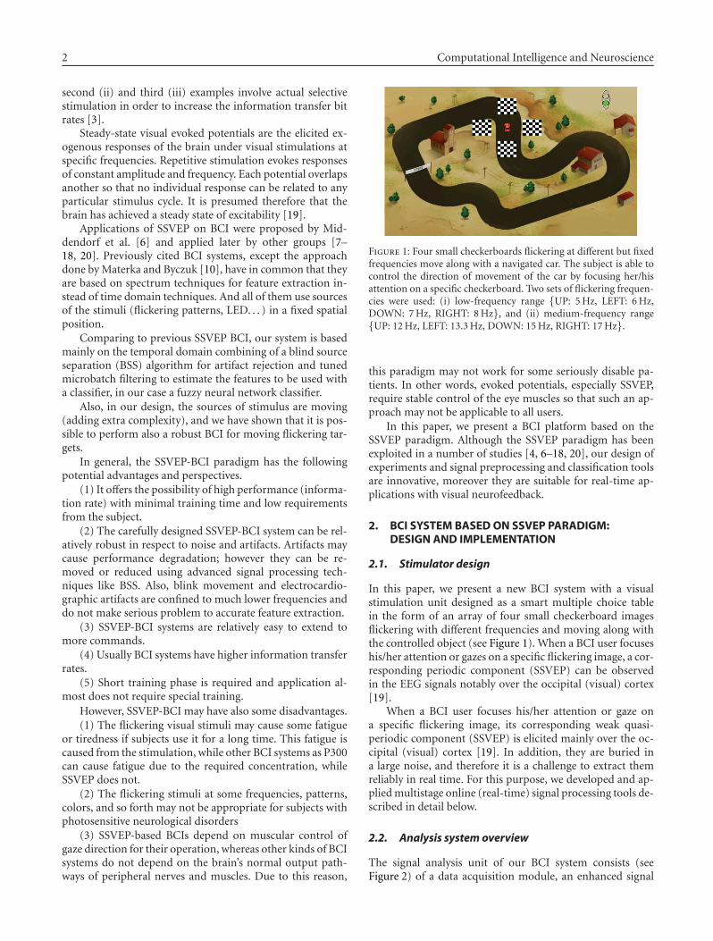
Figure 1: Four small checkerboards flickering at different but fixedfrequencies move along with a navigated car. The subject is able tocontrol the direction of movement of the car by focusing her/hisattention on a specific checkerboard. Two sets of flickering frequen-cies were used: (i) low-frequency range {UP: 5 Hz, LEFT: 6 Hz,DOWN: 7 Hz, RIGHT: 8 Hz}, and (ii) medium-frequency range{UP: 12 Hz, LEFT: 13.3 Hz, DOWN: 15 Hz, RIGHT: 17 Hz}.
this paradigm may not work for some seriously disable pa-tients. In other words, evoked potentials, especially SSVEP,require stable control of the eye muscles so that such an ap-proach may not be applicable to all users.
In this paper, we present a BCI platform based on theSSVEP paradigm. Although the SSVEP paradigm has beenexploited in a number of studies [4, 6–18, 20], our design ofexperiments and signal preprocessing and classification toolsare innovative, moreover they are suitable for real-time ap-plications with visual neurofeedback.
2. BCI SYSTEM BASED ON SSVEP PARADIGM:DESIGN AND IMPLEMENTATION
2.1. Stimulator design
In this paper, we present a new BCI system with a visualstimulation unit designed as a smart multiple choice tablein the form of an array of four small checkerboard imagesflickering with different frequencies and moving along withthe controlled object (see Figure 1). When a BCI user focuseshis/her attention or gazes on a specific flickering image, a cor-responding periodic component (SSVEP) can be observedin the EEG signals notably over the occipital (visual) cortex[19].
When a BCI user focuses his/her attention or gaze ona specific flickering image, its corresponding weak quasi-periodic component (SSVEP) is elicited mainly over the oc-cipital (visual) cortex [19]. In addition, they are buried ina large noise, and therefore it is a challenge to extract themreliably in real time. For this purpose, we developed and ap-plied multistage online (real-time) signal processing tools de-scribed in detail below.
2.2. Analysis system overview
The signal analysis unit of our BCI system consists (seeFigure 2) of a data acquisition module, an enhanced signal
Pablo Martinez et al. 3
EEG BSS ANFISFeature
extraction(energy)
Commandoutput
Bank of filters
· · ·
m m m× n m× n nX
‖X‖
S-G
m: number of electrodes (6)n: number of bands (4)
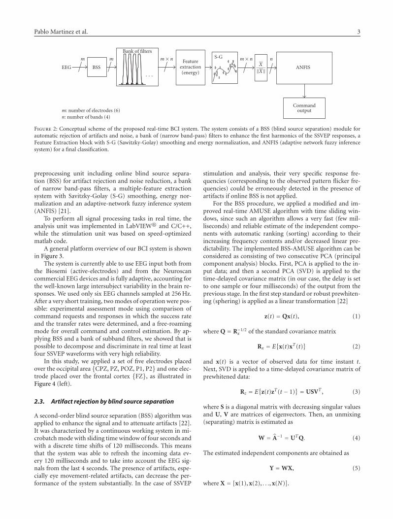
Figure 2: Conceptual scheme of the proposed real-time BCI system. The system consists of a BSS (blind source separation) module forautomatic rejection of artifacts and noise, a bank of (narrow band-pass) filters to enhance the first harmonics of the SSVEP responses, aFeature Extraction block with S-G (Sawitzky-Golay) smoothing and energy normalization, and ANFIS (adaptive network fuzzy inferencesystem) for a final classification.
preprocessing unit including online blind source separa-tion (BSS) for artifact rejection and noise reduction, a bankof narrow band-pass filters, a multiple-feature extractionsystem with Savitzky-Golay (S-G) smoothing, energy nor-malization and an adaptive-network fuzzy inference system(ANFIS) [21].
To perform all signal processing tasks in real time, theanalysis unit was implemented in LabVIEW� and C/C++,while the stimulation unit was based on speed-optimizedmatlab code.
A general platform overview of our BCI system is shownin Figure 3.
The system is currently able to use EEG input both fromthe Biosemi (active-electrodes) and from the Neuroscancommercial EEG devices and is fully adaptive, accounting forthe well-known large intersubject variability in the brain re-sponses. We used only six EEG channels sampled at 256 Hz.After a very short training, two modes of operation were pos-sible: experimental assessment mode using comparison ofcommand requests and responses in which the success rateand the transfer rates were determined, and a free-roamingmode for overall command and control estimation. By ap-plying BSS and a bank of subband filters, we showed that ispossible to decompose and discriminate in real time at leastfour SSVEP waveforms with very high reliability.
In this study, we applied a set of five electrodes placedover the occipital area {CPZ, PZ, POZ, P1, P2} and one elec-trode placed over the frontal cortex {FZ}, as illustrated inFigure 4 (left).
2.3. Artifact rejection by blind source separation
A second-order blind source separation (BSS) algorithm wasapplied to enhance the signal and to attenuate artifacts [22].It was characterized by a continuous working system in mi-crobatch mode with sliding time window of four seconds andwith a discrete time shifts of 120 milliseconds. This meansthat the system was able to refresh the incoming data ev-ery 120 milliseconds and to take into account the EEG sig-nals from the last 4 seconds. The presence of artifacts, espe-cially eye movement-related artifacts, can decrease the per-formance of the system substantially. In the case of SSVEP
stimulation and analysis, their very specific response fre-quencies (corresponding to the observed pattern flicker fre-quencies) could be erroneously detected in the presence ofartifacts if online BSS is not applied.
For the BSS procedure, we applied a modified and im-proved real-time AMUSE algorithm with time sliding win-dows, since such an algorithm allows a very fast (few mil-liseconds) and reliable estimate of the independent compo-nents with automatic ranking (sorting) according to theirincreasing frequency contents and/or decreased linear pre-dictability. The implemented BSS-AMUSE algorithm can beconsidered as consisting of two consecutive PCA (principalcomponent analysis) blocks. First, PCA is applied to the in-put data; and then a second PCA (SVD) is applied to thetime-delayed covariance matrix (in our case, the delay is setto one sample or four milliseconds) of the output from theprevious stage. In the first step standard or robust prewhiten-ing (sphering) is applied as a linear transformation [22]
z(t) = Qx(t), (1)
where Q = R−1/2x of the standard covariance matrix
Rx = E{
x(t)xT(t)}
(2)
and x(t) is a vector of observed data for time instant t.Next, SVD is applied to a time-delayed covariance matrix ofprewhitened data:
Rz = E{
z(t)zT(t − 1)} = USVT , (3)
where S is a diagonal matrix with decreasing singular valuesand U, V are matrices of eigenvectors. Then, an unmixing(separating) matrix is estimated as
W = A−1 = UTQ. (4)
The estimated independent components are obtained as
Y = WX, (5)
where X = [x(1), x(2), . . ., x(N)].

4 Computational Intelligence and Neuroscience
EEGBCI computer
EEG data acquisition(Neuroscan/Biosemi)
Analysis and visualization platform
SSVEP stimulation CP
(Subject’s station)
Commands &neurofeedback
Figure 3: Our BCI platform consists of two PC computers. One for EEG data acquisition, stimuli generation, and a second machine foronline processing of data in microbatch mode.
Occipital electrodeconfiguration
(a)
(b)
Figure 4: Electrode configuration. Five electrodes placed over theoccipital area {CPZ, PZ, POZ, P1, P2} and one over the frontal cor-tex {FZ}.
The AMUSE BSS algorithm allowed us to automaticallyrank the EEG components. The undesired components cor-responding to artifacts were removed and the rest of the use-ful (significant) components were projected back to scalplevel using the pseudo inverse of W, see Figure 5
X = W+X. (6)
Sensorsignals
Demixingsystem
BSS/ICA
Hardswitches
0 or 1
Inversesystem
Reconstructedsensorssignals
x1
x2
xm
...
y1
y2
yn
...
W W+
x1
x2
xm
...
Expertdecision
Figure 5: Enhancement of EEG via BSS. First, the raw EEG data(sensor signals) is decomposed and ranked as independent or spa-tially decorrelated components; in the next step, only the usefulcomponents are projected back to the scalp level, while undesir-able components containing artifacts and noise are removed fromthe signal. The main advantage of our approach is that we do notneed any expert decision to select significant components, sincethe AMUSE algorithm automatically ranks the components as il-lustrated in Figure 6.
The six EEG channels were high-pass-filtered with a cutofffrequency of 2 Hz before the AMUSE algorithm was applied.
The rejection of the first and the last components had twoimplications: (1) the EEG signal was enhanced as some oscil-lations were removed which were due to ocular and otherartifacts but included frequencies similar to the target flickerresponses. Without this procedure, the performance of thesystem would have deteriorated substantially since blinkingcould not be avoided by the experimental subjects; (2) at the
Pablo Martinez et al. 5
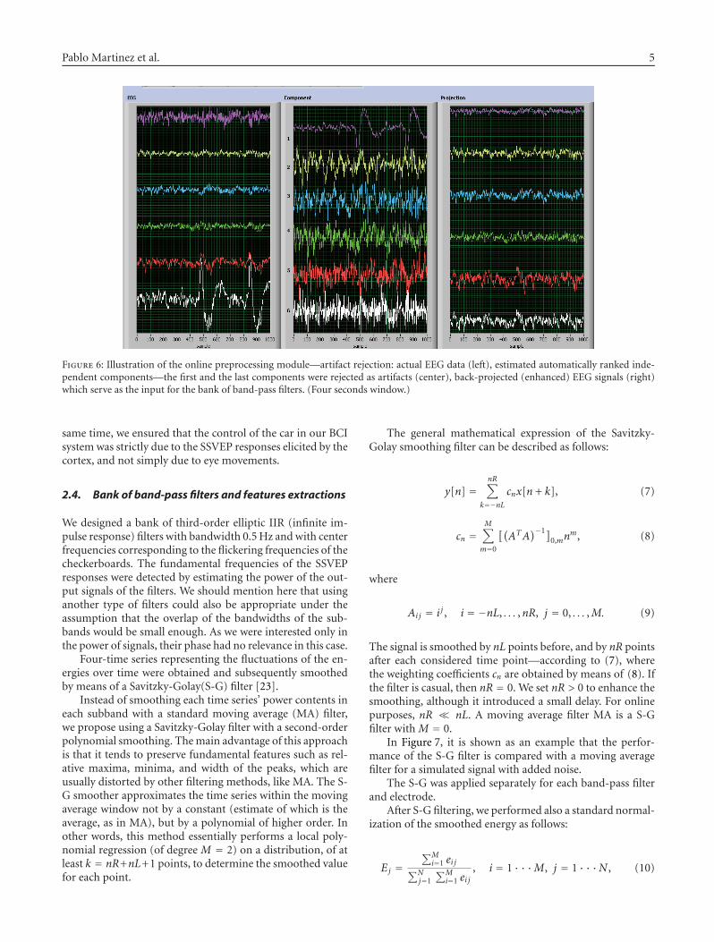
Figure 6: Illustration of the online preprocessing module—artifact rejection: actual EEG data (left), estimated automatically ranked inde-pendent components—the first and the last components were rejected as artifacts (center), back-projected (enhanced) EEG signals (right)which serve as the input for the bank of band-pass filters. (Four seconds window.)
same time, we ensured that the control of the car in our BCIsystem was strictly due to the SSVEP responses elicited by thecortex, and not simply due to eye movements.
2.4. Bank of band-pass filters and features extractions
We designed a bank of third-order elliptic IIR (infinite im-pulse response) filters with bandwidth 0.5 Hz and with centerfrequencies corresponding to the flickering frequencies of thecheckerboards. The fundamental frequencies of the SSVEPresponses were detected by estimating the power of the out-put signals of the filters. We should mention here that usinganother type of filters could also be appropriate under theassumption that the overlap of the bandwidths of the sub-bands would be small enough. As we were interested only inthe power of signals, their phase had no relevance in this case.
Four-time series representing the fluctuations of the en-ergies over time were obtained and subsequently smoothedby means of a Savitzky-Golay(S-G) filter [23].
Instead of smoothing each time series’ power contents ineach subband with a standard moving average (MA) filter,we propose using a Savitzky-Golay filter with a second-orderpolynomial smoothing. The main advantage of this approachis that it tends to preserve fundamental features such as rel-ative maxima, minima, and width of the peaks, which areusually distorted by other filtering methods, like MA. The S-G smoother approximates the time series within the movingaverage window not by a constant (estimate of which is theaverage, as in MA), but by a polynomial of higher order. Inother words, this method essentially performs a local poly-nomial regression (of degree M = 2) on a distribution, of atleast k = nR+nL+1 points, to determine the smoothed valuefor each point.
The general mathematical expression of the Savitzky-Golay smoothing filter can be described as follows:
y[n] =nR∑
k=−nLcnx[n + k], (7)
cn =M∑
m=0
[(ATA
)−1]0,mn
m, (8)
where
Aij = i j , i = −nL, . . . ,nR, j = 0, . . . ,M. (9)
The signal is smoothed by nL points before, and by nR pointsafter each considered time point—according to (7), wherethe weighting coefficients cn are obtained by means of (8). Ifthe filter is casual, then nR = 0. We set nR > 0 to enhance thesmoothing, although it introduced a small delay. For onlinepurposes, nR � nL. A moving average filter MA is a S-Gfilter with M = 0.
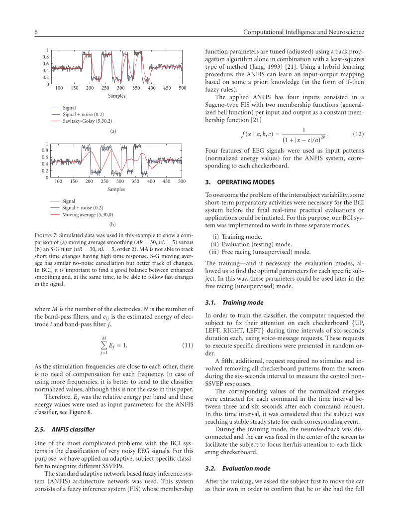
In Figure 7, it is shown as an example that the perfor-mance of the S-G filter is compared with a moving averagefilter for a simulated signal with added noise.
The S-G was applied separately for each band-pass filterand electrode.
After S-G filtering, we performed also a standard normal-ization of the smoothed energy as follows:
Ej =∑M
i=1 ei j∑N
j=1
∑Mi=1 ei j
, i = 1 · · ·M, j = 1 · · ·N , (10)
6 Computational Intelligence and Neuroscience
00.20.40.60.8
1
100 150 200 250 300 350 400 450 500
Samples
SignalSignal + noise (0.2)Savitzky-Golay (5,30,2)
(a)
00.20.40.60.8
1
100 150 200 250 300 350 400 450 500
Samples
SignalSignal + noise (0.2)Moving average (5,30,0)
(b)
Figure 7: Simulated data was used in this example to show a com-parison of (a) moving average smoothing (nR = 30, nL = 5) versus(b) an S-G filter (nR = 30, nL = 5, order 2). MA is not able to trackshort time changes having high time response. S-G moving aver-age has similar no-noise cancellation but better track of changes.In BCI, it is important to find a good balance between enhancedsmoothing and, at the same time, to be able to follow fast changesin the signal.
where M is the number of the electrodes, N is the number ofthe band-pass filters, and ei j is the estimated energy of elec-trode i and band-pass filter j,
M∑
j=1
Ej = 1. (11)
As the stimulation frequencies are close to each other, thereis no need of compensation for each frequency. In case ofusing more frequencies, it is better to send to the classifiernormalized values, although this is not the case in this paper.
Therefore, Ej was the relative energy per band and theseenergy values were used as input parameters for the ANFISclassifier, see Figure 8.
2.5. ANFIS classifier
One of the most complicated problems with the BCI sys-tems is the classification of very noisy EEG signals. For thispurpose, we have applied an adaptive, subject-specific classi-fier to recognize different SSVEPs.
The standard adaptive network based fuzzy inference sys-tem (ANFIS) architecture network was used. This systemconsists of a fuzzy inference system (FIS) whose membership
function parameters are tuned (adjusted) using a back prop-agation algorithm alone in combination with a least-squarestype of method (Jang, 1993) [21]. Using a hybrid learningprocedure, the ANFIS can learn an input-output mappingbased on some a priori knowledge (in the form of if-thenfuzzy rules).
The applied ANFIS has four inputs consisted in aSugeno-type FIS with two membership functions (general-ized bell function) per input and output as a constant mem-bership function [21]
f (x | a, b, c) = 1(1 + |x − c|/a)2b . (12)
Four features of EEG signals were used as input patterns(normalized energy values) for the ANFIS system, corre-sponding to each checkerboard.
3. OPERATING MODES
To overcome the problem of the intersubject variability, someshort-term preparatory activities were necessary for the BCIsystem before the final real-time practical evaluations orapplications could be initiated. For this purpose, our BCI sys-tem was implemented to work in three separate modes.
(i) Training mode.(ii) Evaluation (testing) mode.
(iii) Free racing (unsupervised) mode.
The training—and if necessary the evaluation modes, al-lowed us to find the optimal parameters for each specific sub-ject. In this way, these parameters could be used later in thefree racing (unsupervised) mode.
3.1. Training mode
In order to train the classifier, the computer requested thesubject to fix their attention on each checkerboard {UP,LEFT, RIGHT, LEFT} during time intervals of six-secondsduration each, using voice-message requests. These requeststo execute specific directions were presented in random or-der.
A fifth, additional, request required no stimulus and in-volved removing all checkerboard patterns from the screenduring the six-seconds interval to measure the control non-SSVEP responses.
The corresponding values of the normalized energieswere extracted for each command in the time interval be-tween three and six seconds after each command request.In this time interval, it was considered that the subject wasreaching a stable steady state for each corresponding event.
During the training mode, the neurofeedback was dis-connected and the car was fixed in the center of the screen tofacilitate the subject to focus her/his attention to each flick-ering checkerboard.
3.2. Evaluation mode
After the training, we asked the subject first to move the caras their own in order to confirm that he or she had the full

Pablo Martinez et al. 7
Table 1: Experimental results for occipital configuration (mean val-ues).
Subject #1 #2 #3 #4 #5
LF (5–8 Hz)
Success (%) 100 77.5 94.8 92.3 100
Delay Time [s] 3.6 ± 0.4 3.8 ± 1.7 3.3 ± 1 3.3 ± 1.1 4.8 ± 1
MF (12–17 Hz)
Success (%) 100 100 100 100 82.3
Delay Time [s] 3.6 ± 0.3 3.9 ± 0.8 3.2 ± 0.4 3.1 ± 1.1 3.7 ± 1.3
ability to control the car in any direction. Then, to evalu-ate the BCI performance for this subject, including time re-sponses and percentage of success (see results bellow), thecomputer generated in random order requests for movementin each direction using voice messages, similarly to the train-ing mode. The subject was asked to move the car in one ofthe four directions at intervals of nine seconds in 32 trials(eight trials per direction). It was assumed that the subjectsuccessfully performed a task if she/he moved the car prop-erly in a time window between one second and up to a maxi-mum of six seconds after the onset of the voice-request com-mand. During the evaluation mode, the neurofeedback wasfully enabled and the car was able to move freely, respondingto the subject’s commands.
3.3. Free race (unsupervised) mode
In this mode, the user could move the car freely within theracing course (Figure 1), and we asked all the subjects tocomplete at least one lap to evaluate their overall control ofthe car by performing this task without any external voicecommands. This typically took from each subject between 90to 150 seconds to achieve this complex goal, also dependingon the flicker frequency range.
4. EXPERIMENTAL SETTING AND RESULTS
We tested our SSVEP-based BCI system with five subjects(two females and three males) and for two different ranges offlicker frequencies: low-frequency (LF) range—5, 6, 7, 8 Hzand medium-frequency (MF) range—12, 13.3, 15, 17 Hz.
The subjects sat on a chair approximately 90 cm from thecenter of a 21-inch cathode-ray tube (CRT) monitor screenusing a refresh rate of 120 Hz.
Six electrodes were used: five placed over the occipitalcortex {CPZ, PZ, POZ, P1, P2} and one over the frontal cor-tex {Fz}, see Figure 2.
The performance of the BCI system was measured duringthe evaluation mode, as described in the previous section.
The results are shown in Table 1 (subject-specific results)and Table 2 (mean results). The data obtained in this studyindicated that the performance for the medium-frequencyrange flicker was slightly higher when compared to the low-frequency range flicker responses, in terms of controllabilityof the car and execution-time delay.
Table 2: Experimental results for occipital configuration (mean val-ues and mean bit rate).
Flicker range LF MF
(Frequency) (5–8 Hz) (12–17 Hz)
Success rate 93% 96.5%
Execution delay 3.7± 1.0 s 3.5± 0.8 s
Bit rate 26 bits/min 30 bits/min
Only one of the subjects was more comfortable with,and felt that his car control was better when using the low-frequency range flicker.
The subjects performed the BCI experiments just a sin-gle time for each frequency range (LF, MF), including classi-fier training and evaluation (results) modes. After the exper-iment, each subject was asked to demonstrate her/his overallcontrol of the car for each frequency range by completing afull lap as quickly as possible in free racing mode.
5. CONCLUSION AND DISCUSSIONS
Although the SSVEP paradigm is well known in the BCIcommunity since the studies performed by several re-search groups [6–18, 20], especially Shangkai Gao group atTshinghua University [8–10, 18] and NASA research groupof Trejo et al. [7], we believe that our system offers severalnovel points for improved usability and efficiency, such asthe integrated moving checkerboard patterns to maximizeselective attention and to minimize eye movements in respectto the controlled target, as well as an online BSS module toreduce automatically artifacts and noise, improved featureselection algorithm with efficient smoothing and filteringand an adaptive fuzzy neural network classifier ANFIS. All ofour EEG signal processing modules and algorithms are care-fully optimized to work online in real time. This proposedmethod and BCI platform could be easily extended for vari-ous BCI paradigms, as well as for other types of brain anal-ysis in which real-time processing and dynamic visualizationof features are crucial.
Paradigms based on steady-state visual and other evokedpotentials are among the most reliable modes of commu-nication for implementation of a fast noninvasive EEG-BCIsystem that can discriminate in near real time a very highnumber of unique commands or symbols. The capability ofa BCI system to issue more commands in a more reliableway has significant advantages such as allowing better controlof semiautonomous remote navigation devices in hazardousenvironments, or navigating precisely a cursor on a computerscreen (or the realization of a virtual joystick). However, inour experimental design, we have incorporated a number oforiginal elements and ideas as compared to the typical SSVEPparadigm. In addition to our new dynamic visual stimula-tion approach, we have developed and implemented noveland efficient real-time signal preprocessing tools and featureextraction algorithms. Although using our dynamic patternmovement design may require some eye movement controlby the subjects, as well as sustained short-term attention, the
8 Computational Intelligence and Neuroscience
Eval. mode: request L U L D U R L D U R
U = upL = leftD = downR = right
(a)
Eval. mode: request L R U R D U L D U R L
U = upL = leftD = downR = right
(b)
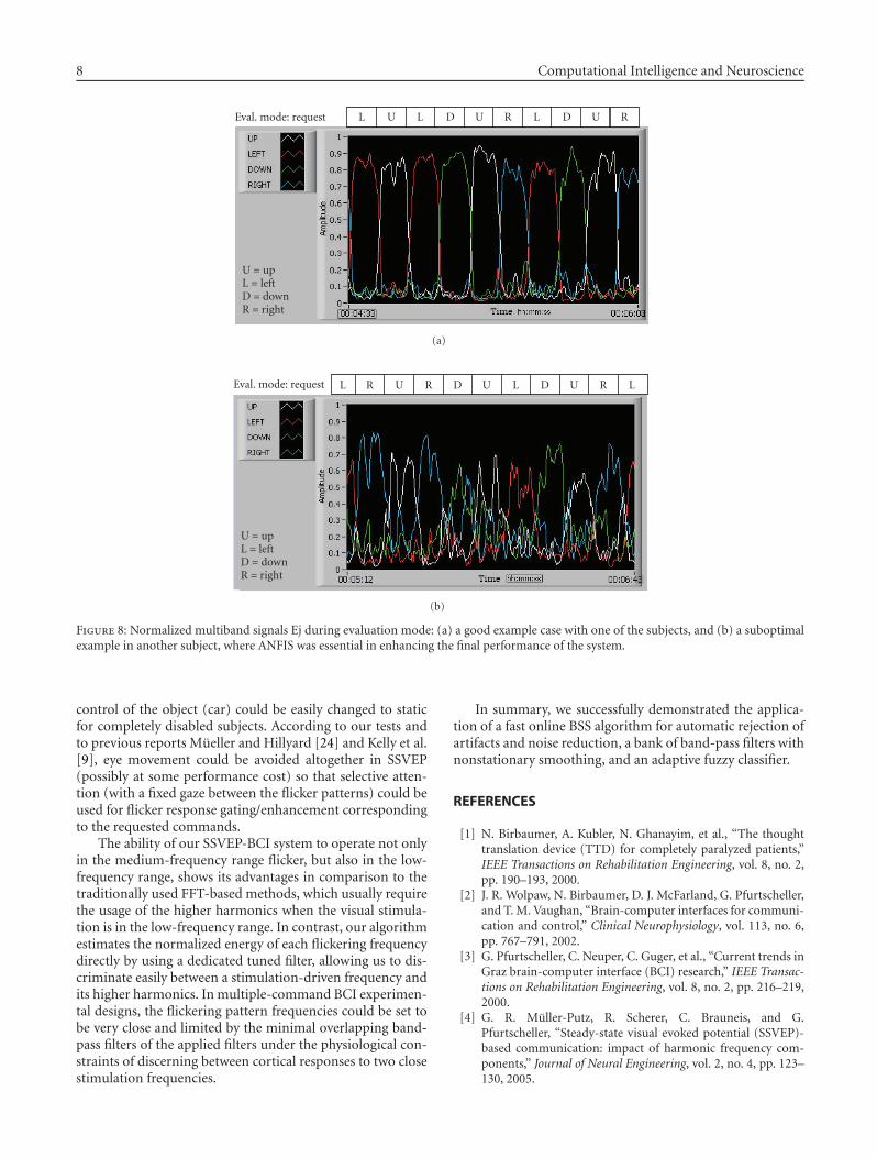
Figure 8: Normalized multiband signals Ej during evaluation mode: (a) a good example case with one of the subjects, and (b) a suboptimalexample in another subject, where ANFIS was essential in enhancing the final performance of the system.
control of the object (car) could be easily changed to staticfor completely disabled subjects. According to our tests andto previous reports Mueller and Hillyard [24] and Kelly et al.[9], eye movement could be avoided altogether in SSVEP(possibly at some performance cost) so that selective atten-tion (with a fixed gaze between the flicker patterns) could beused for flicker response gating/enhancement correspondingto the requested commands.
The ability of our SSVEP-BCI system to operate not onlyin the medium-frequency range flicker, but also in the low-frequency range, shows its advantages in comparison to thetraditionally used FFT-based methods, which usually requirethe usage of the higher harmonics when the visual stimula-tion is in the low-frequency range. In contrast, our algorithmestimates the normalized energy of each flickering frequencydirectly by using a dedicated tuned filter, allowing us to dis-criminate easily between a stimulation-driven frequency andits higher harmonics. In multiple-command BCI experimen-tal designs, the flickering pattern frequencies could be set tobe very close and limited by the minimal overlapping band-pass filters of the applied filters under the physiological con-straints of discerning between cortical responses to two closestimulation frequencies.
In summary, we successfully demonstrated the applica-tion of a fast online BSS algorithm for automatic rejection ofartifacts and noise reduction, a bank of band-pass filters withnonstationary smoothing, and an adaptive fuzzy classifier.
REFERENCES
[1] N. Birbaumer, A. Kubler, N. Ghanayim, et al., “The thoughttranslation device (TTD) for completely paralyzed patients,”IEEE Transactions on Rehabilitation Engineering, vol. 8, no. 2,pp. 190–193, 2000.
[2] J. R. Wolpaw, N. Birbaumer, D. J. McFarland, G. Pfurtscheller,and T. M. Vaughan, “Brain-computer interfaces for communi-cation and control,” Clinical Neurophysiology, vol. 113, no. 6,pp. 767–791, 2002.
[3] G. Pfurtscheller, C. Neuper, C. Guger, et al., “Current trends inGraz brain-computer interface (BCI) research,” IEEE Transac-tions on Rehabilitation Engineering, vol. 8, no. 2, pp. 216–219,2000.
[4] G. R. Muller-Putz, R. Scherer, C. Brauneis, and G.Pfurtscheller, “Steady-state visual evoked potential (SSVEP)-based communication: impact of harmonic frequency com-ponents,” Journal of Neural Engineering, vol. 2, no. 4, pp. 123–130, 2005.
Pablo Martinez et al. 9
[5] H. Lee, A. Cichocki, and S. Choi, “Nonnegative matrix factor-ization for motor imagery EEG classification,” in Proceedings ofthe 16th International Conference on Artificial Neural Networks(ICANN ’06), vol. 4132 of Lecture Notes in Computer Science,pp. 250–259, Springer, Athens, Greece, September 2006.
[6] M. Middendorf, G. McMillan, G. Calhoun, and K. S. Jones,“Brain-computer interfaces based on the steady-state visual-evoked response,” IEEE Transactions on Rehabilitation Engi-neering, vol. 8, no. 2, pp. 211–214, 2000.
[7] L. J. Trejo, R. Rosipal, and B. Matthews, “Brain-computer in-terfaces for 1-D and 2-D cursor control: designs using vo-litional control of the EEG spectrum or steady-state visualevoked potentials,” IEEE Transactions on Neural Systems andRehabilitation Engineering, vol. 14, no. 2, pp. 225–229, 2006.
[8] M. Cheng, X. Gao, S. Gao, and D. Xu, “Design and implemen-tation of a brain-computer interface with high transfer rates,”IEEE Transactions on Biomedical Engineering, vol. 49, no. 10,pp. 1181–1186, 2002.
[9] S. P. Kelly, E. C. Lalor, R. B. Reilly, and J. J. Foxe, “Visual spatialattention tracking using high-density SSVEP data for indepen-dent brain-computer communication,” IEEE Transactions onNeural Systems and Rehabilitation Engineering, vol. 13, no. 2,pp. 172–178, 2005.
[10] A. Materka and M. Byczuk, “Using comb filter to enhanceSSVEP for BCI applications,” in Proceedings of the 3rd Interna-tional Conference on Advances in Medical, Signal and Informa-tion Processing (MEDSIP ’06), p. 33, Glasgow, UK, July 2006.
[11] Z. Lin, C. Zhang, W. Wu, and X. Gao, “Frequency recogni-tion based on canonical correlation analysis for SSVEP-basedBCIs,” IEEE Transactions on Biomedical Engineering, vol. 53,no. 12, part 2, pp. 2610–2614, 2006.
[12] O. Friman, I. Volosyak, and A. Graser, “Multiple channeldetection of steady-state visual evoked potentials for brain-computer interfaces,” IEEE Transactions on Biomedical Engi-neering, vol. 54, no. 4, pp. 742–750, 2007.
[13] E. C. Lalor, S. P. Kelly, C. Finucane, et al., “Steady-state VEP-based brain-computer interface control in an immersive 3Dgaming environment,” EURASIP Journal on Applied SignalProcessing, vol. 2005, no. 19, pp. 3156–3164, 2005.
[14] L. Piccini, S. Parini, L. Maggi, and G. Andreoni, “A wear-able home BCI system: preliminary results with SSVEP pro-tocol,” in Proceedings of the 27th Annual International Con-ference of the IEEE Engineering in Medicine and Biology Soci-ety (EMBS ’05), pp. 5384–5387, Shanghai, China, September2005.
[15] Y. Wang, R. Wang, X. Gao, B. Hong, and S. Gao, “A practicalVEP-based brain-computer interface,” IEEE Transactions onNeural Systems and Rehabilitation Engineering, vol. 14, no. 2,pp. 234–240, 2006.
[16] K. D. Nielsen, A. F. Cabrera, and O. F. do Nascimento, “EEGbased BCI-towards a better control. Brain-computer interfaceresearch at Aalborg university,” IEEE Transactions on NeuralSystems and Rehabilitation Engineering, vol. 14, no. 2, pp. 202–204, 2006.
[17] V. Jaganathan, T. M. S. Mukesh, and M. R. Reddy, “Designand implementation of high performance visual stimulator forbrain computer interfaces,” in Proceedings of the 27th AnnualInternational Conference of the IEEE Engineering in Medicineand Biology Society (EMBS ’05), pp. 5381–5383, Shanghai,China, September 2005.
[18] X. Gao, D. Xu, M. Cheng, and S. Gao, “A BCI-based envi-ronmental controller for the motion-disabled,” IEEE Transac-tions on Neural Systems and Rehabilitation Engineering, vol. 11,no. 2, pp. 137–140, 2003.
[19] E. Niedermeyer and F. L. Lopes da Silva, Electroencephalogra-phy: Basic Principles, Clinical Applications and Related Fields,chapter 54, Lippincott Williams & Wilkins, Philadelphia, Pa,USA, 1982.
[20] F. Beverina, G. Palmas, S. Silvoni, F. Piccione, and S. Giove,“User adaptive BCIs: SSVEP and P300 based interfaces,” Psy-chNology Journal, vol. 1, no. 4, pp. 331–354, 2003.
[21] J.-S. R. Jang, “ANFIS: adaptive-network-based fuzzy inferencesystem,” IEEE Transactions on Systems, Man and Cybernetics,vol. 23, no. 3, pp. 665–685, 1993.
[22] A. Cichocki and S. Amari, Adaptive Blind Signal and ImageProcessing: Learning Algorithms and Applications, John Wiley& Sons, Chichester, UK, 2003.
[23] A. Savitzky and M. J. E. Golay, “Smoothing and differentia-tion of data by simplified least squares procedures,” AnalyticalChemistry, vol. 36, no. 8, pp. 1627–1639, 1964.
[24] M. M. Muller and S. Hillyard, “Concurrent recording ofsteady-state and transient event-related potentials as indicesof visual-spatial selective attention,” Clinical Neurophysiology,vol. 111, no. 9, pp. 1544–1552, 2000.
Hindawi Publishing CorporationComputational Intelligence and NeuroscienceVolume 2007, Article ID 91651, 7 pagesdoi:10.1155/2007/91651
Research ArticleThe Estimation of Cortical Activity for Brain-ComputerInterface: Applications in a Domotic Context
F. Babiloni,1, 2 F. Cincotti,1 M. Marciani,1 S. Salinari,3 L. Astolfi,1, 2 A. Tocci,1 F. Aloise,1
F. De Vico Fallani,1 S. Bufalari,1 and D. Mattia1
1 Istituto di Ricovero e Cura a Carattere Scientifico, Fondazione Santa Lucia, Via Ardeatina, 306-00179 Rome, Italy2 Dipartimento di Fisiologia Umana e Farmacologia, Universita di Roma “La Sapienza”, Piazzale Aldo Moro 5, 00185 Rome, Italy
3 Dipartimento di Informatica e Sistemistica, Universita di Roma “La Sapienza”, Piazzale Aldo Moro 5, 00185 Rome, Italy
Correspondence should be addressed to D. Mattia, [email protected]
Received 18 February 2007; Revised 8 June 2007; Accepted 4 July 2007
Recommended by Andrzej Cichocki
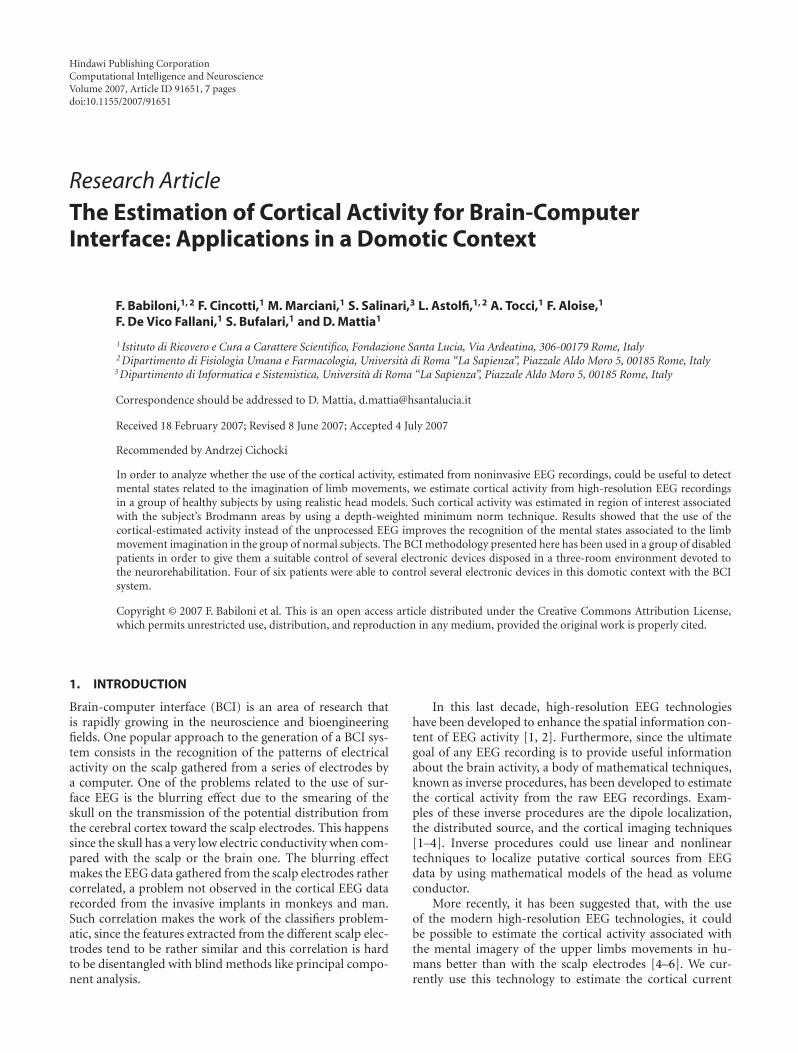
In order to analyze whether the use of the cortical activity, estimated from noninvasive EEG recordings, could be useful to detectmental states related to the imagination of limb movements, we estimate cortical activity from high-resolution EEG recordingsin a group of healthy subjects by using realistic head models. Such cortical activity was estimated in region of interest associatedwith the subject’s Brodmann areas by using a depth-weighted minimum norm technique. Results showed that the use of thecortical-estimated activity instead of the unprocessed EEG improves the recognition of the mental states associated to the limbmovement imagination in the group of normal subjects. The BCI methodology presented here has been used in a group of disabledpatients in order to give them a suitable control of several electronic devices disposed in a three-room environment devoted tothe neurorehabilitation. Four of six patients were able to control several electronic devices in this domotic context with the BCIsystem.
Copyright © 2007 F. Babiloni et al. This is an open access article distributed under the Creative Commons Attribution License,which permits unrestricted use, distribution, and reproduction in any medium, provided the original work is properly cited.
1. INTRODUCTION
Brain-computer interface (BCI) is an area of research thatis rapidly growing in the neuroscience and bioengineeringfields. One popular approach to the generation of a BCI sys-tem consists in the recognition of the patterns of electricalactivity on the scalp gathered from a series of electrodes bya computer. One of the problems related to the use of sur-face EEG is the blurring effect due to the smearing of theskull on the transmission of the potential distribution fromthe cerebral cortex toward the scalp electrodes. This happenssince the skull has a very low electric conductivity when com-pared with the scalp or the brain one. The blurring effectmakes the EEG data gathered from the scalp electrodes rathercorrelated, a problem not observed in the cortical EEG datarecorded from the invasive implants in monkeys and man.Such correlation makes the work of the classifiers problem-atic, since the features extracted from the different scalp elec-trodes tend to be rather similar and this correlation is hardto be disentangled with blind methods like principal compo-nent analysis.
In this last decade, high-resolution EEG technologieshave been developed to enhance the spatial information con-tent of EEG activity [1, 2]. Furthermore, since the ultimategoal of any EEG recording is to provide useful informationabout the brain activity, a body of mathematical techniques,known as inverse procedures, has been developed to estimatethe cortical activity from the raw EEG recordings. Exam-ples of these inverse procedures are the dipole localization,the distributed source, and the cortical imaging techniques[1–4]. Inverse procedures could use linear and nonlineartechniques to localize putative cortical sources from EEGdata by using mathematical models of the head as volumeconductor.
More recently, it has been suggested that, with the useof the modern high-resolution EEG technologies, it couldbe possible to estimate the cortical activity associated withthe mental imagery of the upper limbs movements in hu-mans better than with the scalp electrodes [4–6]. We cur-rently use this technology to estimate the cortical current
2 Computational Intelligence and Neuroscience
density in particular region of interest (ROI) on the mod-eled brain structures from high-resolution EEG recordings toprovide high-quality signals for the extraction of the featuresuseful to be employed in a BCI system.
In this paper, we would like to illustrate how, with the useof such advanced high-resolution EEG methods for the esti-mation of the cortical activity, it is possible to run a BCI sys-tem able to drive and control several devices in a domotic en-vironment. In particular, we first describe a BCI system usedon a group of normal subjects in which the technology ofthe estimation of the cortical activity is illustrated. Then, weused the BCI system for the command of several electronicdevices within a three-room environment employed for theneurorehabilitation. The BCI system was tested by a group ofsix patients.
2. METHODOLOGY
Subjects
Two groups of subjects have been involved in the trainingwith the BCI system. One was composed of normal healthysubjects while the second one was composed of disabled per-sons who used the BCI system in attempt to drive electronicdevices in a three-room facility at the laboratory of the foun-dation of Santa Lucia in Rome. The first group was composedby fourteen healthy subjects that voluntarily participated tothe study. The second group of subjects were formed by sixpatients affected by Duchenne muscular dystrophy. Accord-ing to the Barthel index (BI) score for their daily activity, allpatients depended almost completely on caregivers, having aBI score lower than 35. In general, all patients were unable towalk since they were adolescent, and their mobility was possi-ble only by a wheelchair which was electric in all (except two)patients and it was driven by a modified joystick which couldbe manipulated by either the residual “fine” movements ofthe first and second fingers or the residual movements ofthe wrist. As for the upper limbs, all patients had a residualmuscular strength either of proximal or distal arm musclesthat was insufficient for carrying on any everyday life activ-ity. The neck muscles were as weak as to require a mechan-ical support to maintain the posture in all of them. Finally,eye movements were substantially preserved in all of them.At the moment of the study, none of the patients was usingtechnologically advanced aids.
2.1. Patient’s preparation and training
Patients were admitted for a neurorehabilitation programthat includes also the use of BCI system on a voluntary base.Caregivers and patients gave the informed consent for therecordings in agreement with the ethical committee rulesadopted for this study. The rehabilitation programs aimedto allow to the patients the use of a versatile system for thecontrol of several domestic devices by using different inputdevices, tailored on the disability level of the final user. Oneof the possible inputs for this system was the BCI by usingthe modulation of the EEG.
The first step of the clinical procedure consisted of an in-terview and a physical examination performed by the clini-cians, wherein several levels of the variables of interest (andpossible combinations) were addressed as follows: the degreeof motor impairment and of reliance on the caregivers foreveryday activities as assessed by current standardized scale,that is, the Barthel Index (BI) for ability to perform daily ac-tivities; the familiarity with transducers and aids (sip/puff,switches, speech recognition, joysticks) that could be used asthe input to the system; the ability to speak or communi-cate, being understandable to an unfamiliar person; the levelof informatics alphabetization measured by the number ofhours per week spent in front of a computer. Informationwas structured in a questionnaire administered to the pa-tients at the beginning and the end of the training. A levelof system acceptance by the users was schematized by askingthe users to indicate, with a number ranging from 0 (not sat-isfactory) to 5 (very satisfactory), their degree of acceptancerelative to each of the controlled output devices. The train-ing consisted of weekly sessions; for a period of time rangingfrom 3 to 4 weeks, the patient and (when required) her/hiscaregivers were practicing with the system. During the wholeperiod, patients had the assistance of an engineer and a ther-apist in their interaction with the system.
2.2. Experimental task
Both normals and patients were trained by using the BCI sys-tem in order to control the movement of a cursor on thescreen on the base of the modulation of their EEG activity.In particular, the description of the experimental task per-formed by all of them during the training follows. Each trialconsisted of four phases.
(1) Target appearance: a rectangular target appeared onthe right side of the screen, covering either the upperor the lower half of the side.
(2) Feedback phase: one second after the target, a cursorappeared in the middle of the left side of the screenand moved at a constant horizontal speed to the right.Vertical speed was determined by the amplitude of sen-sorimotor rhythms (see Section 2.6). A cursor sweeplasted about three seconds.
(3) Reward phase: if the cursor succesfully hit the target,the latter flashed for about one second. Otherwise, itjust disappeared.
(4) Intertrial interval: the screen stayed blank for abouttwo seconds, in which the subject was allowed to blinkand swallow.
Subjects were aware that the increase or decrease of a spe-cific rhythm in their EEG produces a movement of the cur-sor towards the top or the bottom of the screen. They weresuggested to concentrate on kinesthetic imagination of upperlimb movements (e.g., fist clenching) to produce a desyn-chronization of the μ rhythm on relevant channels (cursorup), and to concentrate on kinesthetic imagination of lowerlimb movements (e.g., repeated dorsiflexion of ankle joint) toproduce a contrasting pattern (with possible desynchroniza-tion of μ/β rhythm over the mesial channels, cursor down).
F. Babiloni et al. 3
Using this simple binary task as performance measure, train-ing is meant to improve performances from 50–70% to 80–100% of correct hits.
2.3. Experimental training
The BCI training was performed using the BCI2000 softwaresystem [7]. An initial screening session was used to define theideal locations and frequencies of each subject’s spontaneousμ- and β-rhythm activity. During this session, the subject wasprovided with any feedback (any representation of her/his μrhythm), and she/he had to perform motor tasks just in anopen loop. The screening session consisted in the alternateand random presentation of cues on opposite sides of thescreen (either up/down -vertical- or left/right -horizontal).In two subsequent runs, the subject was asked to execute(first run) or to image (second run) movements of her/hishands or feet upon the appearance of top or bottom target,respectively. This sequence was repeated three times. Fromthe seventh run on, the targets appeared on the left or rightside of the screen, and the subject was asked to move (oddtrials) or to image (even trials) her/his hands for a total of 12trials. The offline analysis based on pairs of contrasts for eachtask aimed at detecting two, possibly independent, groups offeatures which will be used to train the subject to control twoindependent dimensions in the BCI. Analysis was carried onby replicating the same signal conditioning and feature ex-traction that was also used in the online processing (trainingsession). Datasets are divided into epochs (usually 1-secondlong) and spectral analysis is performed by means of a maxi-mum entropy algorithm, with a resolution of 2 Hz.
Different from the online processing, when the systemonly computes the few features relevant for BCI control,all possible features in a reasonable range are extracted andanalyzed simultaneously. A feature vector is extracted fromeach epoch composed by the spectral value at each frequencybin between 0 and 60 Hz for each spatially filtered channel.When all features in the two datasets under contrast havebeen extracted, a statistical analysis is performed to assesssignificant differences in the values (epochs) of each featurein the two conditions. Usually an r2 analysis is performed,but in the case of 2-level-independent variables (such in casetasks = {T1,T2}, t-test, ANOVA, etc.) would provide theanalogous results. At the end of this process, the results wereavailable (channel-frequency matrix and head topography ofr2 values) and evaluated to identify the most promising set offeatures to be enhanced with training.
Using information gathered from the offline analysis, theexperimenter set the online feature extractor so that a “con-trol signal” was generated from the linear combination oftime-varying value of these features, and then passed to a lin-ear classifier. The latter’s output controls how the position ofthe feedback cursor was updated. During the following train-ing sessions, the subjects were thus fed back with a represen-tation of their μ-rhythm activity, so that they could learn howto improve its modulation.
Each session lasted about 40 minutes and consisted ofeight 3-minute runs of 30 trials. The task was increased in
difficulty during the training, so mainly two different taskclasses can be defined.
During the training sessions, subjects were asked to per-form the same kinaesthetic imagination movement they wereasked during the screening session. An upward movementof the cursor was associated to the bilateral decrease of μrhythm over the hand area (which usually occurs duringimagination of upper limb movement). Consequently, the(de)synchroinization pattern correlated to imagination oflower limb movements made the cursor move downwards.With the same principle, the horizontal movement of thecursor to the left (right) was linked to the lateralization of μrhythm due to imagination of movement of the left (right).
To do so, two different control signals were defined. Thevertical control signal was obtained as the sum of the μ-rhythm amplitude over both hand motor areas; the valueof μ-rhythm amplitude over the foot area was possibly sub-tracted (depending on the individual subject’s pattern). Thehorizontal control channel was obtained as the difference be-tween the μ-rhythm amplitudes over each hand motor areas.
During the first 5–10 training sessions, the user is trainedto optimize modulation of one control signal at a time,that is, overall amplitude (“vertical control”) or lateralization(“horizontal control”) of the μ rhythm. Either control chan-nel was associated with vertical or horizontal movement of acursor on the screen, respectively.
For the training of “vertical” control, the cursor movedhorizontally across the screen from left to right at a fixedrate, while the user controlled vertical movements towardsappearing targets, justified to the right side of the screen.Analogously, for the training of “horizontal” control, the cur-sor moved vertically across the screen from top to bottom ata fixed rate, while the user controlled horizontal movementstowards appearing targets justified to the bottom side of thescreen.
This phase was considered complete when the healthysubjects reached a performance of 70–80% correct hits (60–65% for patients) on both monodimensional tasks. In caseof bidimensional task that was performed only by the nor-mal subjects, the cursor appeared in the center, and its move-ment was entirely controlled by the subject, using both con-trol channels (“horizontal” and “vertical”) simultaneously.
2.4. Domotic system prototype features
The system core that disabled patients attempted to use inorder to drive electronic devices in a three-room laboratorywas implemented as follows. It received the logical signalsfrom several input devices (including the BCI system) andconverted them into commands that could be used to drivethe output devices. Its operation was organized as a hierar-chical structure of possible actions, whose relationship couldbe static or dynamic. In the static configuration, it behavedas a “cascaded menu” choice system and was used to feed thefeedback module only with the options available at the mo-ment (i.e., current menu). In the dynamic configuration, anintelligent agent tried to learn from the use which would havebeen the most probable choice the user will make. The usercould select the commands and monitor the system behavior
4 Computational Intelligence and Neuroscience
Figure 1: A realistic head model employed for the estimation ofthe cortical activity. Three layers are displayed, namely, representingdura mater, skull, and scalp. Also the electrode positions are visibleon the scalp surface.
through a graphic interface. The prototype system allowedthe user to operate remotely electric devices (e.g., TV, tele-phone, lights, motorized bed, alarm, and front door opener)as well as monitoring the environment with remotely con-trolled video cameras. While input and feedback signals werecarried over a wireless communication, so that mobility ofthe patient was minimally affected, most of the actuationcommands were carried via a powerline-based control sys-tem. As described above, the generated system admits theBCI as one possible way to communicate with it, being opento accept command by other signals related to the residualability of the patient. However, in this study we report onlythe performance of these patients with the BCI system in thedomotic applications.
2.5. Estimation of the cortical activity fromthe EEG recordings
For all normal subjects analyzed in this study, sequential MRimages were acquired and realistic head models were gener-ated. For all the patients involved in this study, due to thelack of their MR images, we used the Montreal average headmodel. Figure 1 shows realistic head models generated for aparticular experimental subjects, together with the employedhigh-resolution electrode array. Scalp, skull, dura mater, andcortical surfaces of the realistic and averaged head modelswere obtained. The surfaces of the realistic head models werethen used to build the boundary element model of the headas volume conductor employed in the present study. Con-ductivities values for scalp, skull, and dura mater were thosereported in Oostendorp et al. [8]. A cortical surface recon-struction was accomplished for each subject’s head with atessellation of about 5000 triangles on average, while the av-erage head model has about 3000 triangles.
The estimation of cortical activity during the mental im-agery task was performed in each subject by using the depth-weighted minimum norm algorithm [9, 10]. Such estima-tion returns a current density estimate for each one of the
thousand dipoles constituting the modeled cortical sourcespace. Each dipole returns a time-varying amplitude repre-senting the brain activity of a restricted patch of cerebralcortex during the entire task time course. This rather largeamount of data can be synthesized by computing the en-semble average of all the dipoles magnitudes belonging tothe same cortical region of interest (ROI). Each ROI was de-fined on each subject’s cortical model adopted in accordancewith its Brodmann areas (BAs). Such areas are regions of thecerebral cortex whose neurons sharing the same anatomical(and often also functional) properties. Actually, such areasare largely used in neuroscience as a coordinate system forsharing cortical activation patterns found with different neu-roimaging techniques. In the present study, the activity in thefollowing ROI was taken into account: the primary left andright motor areas, related to the BA 4, the left and right pri-mary somatosensory and supplementary motor areas.
2.6. Online processing
Digitized EEG data were transmitted in real time to theBCI2000 software system [7] which performed all necessarysignal processing and displayed feedback to the user. Theprocessing pipe can be considered of several stages, whichprocess the signal in sequence. Only the main ones will bementioned below: spatial filter, spectral feature extraction,feature combination, and normalization.
Spatial filter
A general linear combination of data channels is imple-mented by defining a matrix of weights that is multipliedto each time sample of potentials (vector). This allowed im-plementation of different spatial filters, such for instance theestimation of cortical current density waveforms on the cor-tical ROIs.
Spectral feature extraction
It was performed every 40 milliseconds, using the latest300 milliseconds of data. An autoregressive spectral estima-tor based on the maximum entropy algorithm yielded anamplitude spectrum with resolution of 2 Hz. Maximum fre-quency was limited to 60 Hz
Feature selection and combination
A small subset of those spectral features (frequency bins ×EEG channels or ROIs) that were significantly modulated bythe motor imagery tasks was linearly combined to form a sin-gle control signal. Selection of responsive channels and fre-quency bins and determination of combination weights wereoperated before each online session (see Section 2.7). In gen-eral, only two or three spectral amplitude values (depend-ing on individual patterns) were generally used to obtain thecontrol signal.
F. Babiloni et al. 5
(a) (b)
(c) (d)
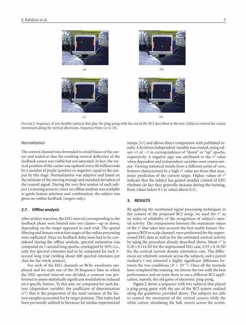
Figure 2: Sequence of two healthy subjects that play the ping-pong with the use of the BCI described in the text. Subjects control the cursormovement along the vertical directions. Sequence from (a) to (d).
Normalization
The control channel was detrended to avoid biases of the cur-sor and scaled so that the resulting vertical deflection of thefeedback cursor was visible but not saturated. In fact, the ver-tical position of the cursor was updated every 40 millisecondsby a number of pixels (positive or negative) equal to the out-put by this stage. Normalization was adaptive and based onthe estimate of the moving average and standard deviation ofthe control signal. During the very first session of each sub-ject (screening session), since no offline analysis was availableto guide feature selection and combination, the subject wasgiven no online feedback (targets only).
2.7. Offline analysis
After artifact rejection, the EEG interval corresponding to thefeedback phase were binned into two classes—up or down,depending on the target appeared in each trial. The spatialfiltering and feature extraction stages of the online processingwere replicated. Since no feedback delay issue had to be con-sidered during the offline analysis, spectral estimation wascomputed on 1-second long epochs, overlapped by 50% (i.e.,only five spectral estimates had to be computed for each 3-second long trial yielding about 600 spectral estimates perclass for the whole session).
For each of the EEG channels or ROIs waveforms em-ployed and for each one of the 30 frequency bins in whichthe EEG spectral interval was divided, a contrast was per-formed to assess statistically significant modulations inducedon a specific feature. To this aim, we computed for each fea-ture (dependent variable) the coefficient of determination(r2) that is the proportion of the total variance of the fea-ture samples accounted for by target position. This index hadbeen previously utilized in literature for similar experimental
setups [11] and allows direct comparison with published re-sults. A fictitious independent variable was created, using val-ues +1 or −1 in correspondence of “down” or “up” epochs,respectively. A negative sign was attributed to the r2 valuewhen dependent and independent variables were controvari-ant. Viewing statistical results from a different point of view,features characterized by a high r2 value are those that max-imize prediction of the current target. Higher values of r2
indicate that the subject has gained steadier control of EEGrhythms (in fact they generally increase during the training,from values below 0.1 to values above 0.3).
3. RESULTS
By applying the mentioned signal processing techniques inthe context of the proposed BCI setup, we used the r2 asan index of reliability of the recognition of subject’s men-tal activity. The comparisons between the maximum valuesof the r2 that takes into account the best usable feature (fre-quency/ROI or scalp channel) were performed for the unpro-cessed EEG data as well as for the estimated cortical activityby using the procedure already described above. Mean r2 is0.20±0.114 SD for the unprocessed EEG case, 0.55±0.16 SDfor the cortical current density estimation case. The differ-ences are relatively constant across the subjects, and a pairedstudent’s t test returned a highly significant difference be-tween the two conditions (P < 10−5). Once all the normalshave completed the training, we choose the two with the bestperformance and we train them to use a different BCI appli-cation, namely, the old game of electronic ping-pong.
Figure 2 shows a sequence with two subjects that playeda ping-pong game with the use of the BCI system realizedalong the guidelines provided above. The subjects are ableto control the movement of the vertical cursors while thewhite cursor, simulating the ball, moves across the screen.
6 Computational Intelligence and Neuroscience
(a) (b)
(c) (d)
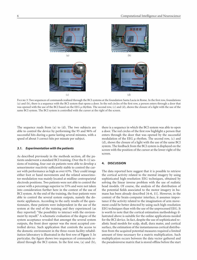
Figure 3: Two sequences of commands realized through the BCI systems at the foundation Santa Lucia in Rome. In the first row, foundations(a) and (b), there is a sequence with the BCI system that opens a door. In the red circles of the first row, a person enters through a door thatwas opened with the use of the BCI based on the EEG μ rhythm. The second row, (c) and (d), shows the closure of a light with the use of thesame BCI system. The BCI system is controlled with the cursor at the right of the screen.
The sequence reads from (a) to (d). The two subjects areable to control the device by performing the 95 and 96% ofsuccessful hits during a game lasting several minutes, with aspeed of about 5 correct hits per minute per subject.
3.1. Experimentation with the patients
As described previously in the methods section, all the pa-tients underwent a standard BCI training. Over the 8–12 ses-sions of training, four out six patients were able to develop asensorimotor reactivity sufficiently stable to control the cur-sor with performance as high as over 63%. They could imageeither foot or hand movements and the related sensorimo-tor modulation was mainly located at midline centroparietalelectrode positions. Two patients were not able to control thecursor with a percentage superior to 55% and were not takeninto consideration further here in the context of the use ofBCI system. At the end of the training, the four patients wereable to control the several system outputs, namely the do-motic appliances. According to the early results of the ques-tionnaire, these patients were independent in the use of thesystem at the end of the training and they experienced (asthey reported) “the possibility to interact with the environ-ment by myself.” A schematic evaluation of the degree of thesystem acceptance revealed that amongst the several systemoutputs, the front door opener was the most accepted con-trolled device. Such application that controls the access tothe domotic environment in the three-room facility rehabil-itation laboratory is illustrated in the first row of Figure 3. Inparticular, the figure shows two sequences of commands re-alized through the BCI system. In the first row, (a) and (b),
there is a sequence in which the BCI system was able to opena door. The red circles of the first row highlight a person thatenters through the door that was opened by the successfulmodulation of the EEG μ rhythm. The second row, (c) and(d), shows the closure of a light with the use of the same BCIsystem. The feedback from the BCI system is displayed on thescreen with the position of the cursor at the lower right of thescreen.
4. DISCUSSION
The data reported here suggest that it is possible to retrievethe cortical activity related to the mental imagery by usingsophisticated high-resolution EEG techniques, obtained bysolving the linear inverse problem with the use of realistichead models. Of course, the analysis of the distribution ofthe potential fields associated to the motor imagery in hu-mans has been already described [4–6, 11]. However, in thecontext of the brain-computer interface, it assumes impor-tance if the activity related to the imagination of arm move-ment could be better detected by using such high-resolutionEEG techniques than with the use of the unprocessed EEG. Itis worth to note that the cortical estimation methodology il-lustrated above is suitable for the online applications neededfor the BCI device. In fact, despite the use of sophisticated re-alistic head models for scalp, skull, dura mater, and corticalsurface, the estimation of the instantaneous cortical distribu-tion from the acquired potential measures required a limitedamount of time necessary for a matrix multiplication. Suchmultiplication occurs between the data vector gathered andthe pseudoinverse matrix that is stored offline before the start
F. Babiloni et al. 7
of the EEG acquisition process. In the pseudoinverse matrixis enclosed with the complexity of the geometrical head mod-eling with the boundary element or with the finite elementmodeling techniques, as well as the priori constraints usedfor the minimum norm solutions.
The described methodologies were applied in the contextof the neurorehabilitation in a group of six patients affectedby the Duchenne muscular dystrophy. Four out of six werealso able to control with the BCI system several electronicdevices disposed in a three-room facility, we described previ-ously. The devices guided by them with an average percent-age score of 63% are as follows: (i) a simple TV remote com-mander, with the capabilities to switch on and off the deviceas well as the capability to change a TV channel; (ii) the open-ing and closing of the light in a room; (iii) the switch on andoff of a mechanical engine for opening a door of the room.These devices can be, of course, also controlled with differ-ent inputs signals that eventually uses the residual degree ofmuscular control of such patients. This experiment was herereported because it demonstrates the capability for the pa-tient to accept and adapt themselves to the use of the newtechnology for the control of their domestic environment.
There is a large trend in the modern neuroscience field tomove toward invasive electrodes implants for the recordingof cortical activity in both animals and humans for the real-ization of an efficient BCI device [12–14]. In this paper, wehave presented evidences that suggest an alternative method-ology for the estimation of such cortical activity in a non-invasive way, by using the possibilities offered by an accu-rate modeling of the principal head structures involved in thetransmission of the cortical potential from the brain surfaceto the scalp electrodes.
ACKNOWLEDGMENTS
This work has been partially supported by the ItalianTelethon Foundation (Grant GUP03562); Division for theScientific and Technologic Development, the Minister forForeign Affairs, in the framework of a bilateral project be-tween Italy and China (Tsinghua University); the EuropeanUnion through the MAIA project (IST Programme FETProject FP6-003758) and the COST granting scheme throughthe Action BM0601 NEUROMATH. It was also supported inpart by a grant from NIH (EB006356) in the USA. This pa-per only reflects the authors’ views, and funding agencies arenot liable for any use that may be made of the informationcontained herein.
REFERENCES
[1] P. L. Nunez, Neocortical Dynamics and Human EEG Rhythms,Oxford University Press, New York, NY, USA, 1995.
[2] A. Gevins, P. Brickett, B. Costales, J. Le, and B. Reutter, “Be-yond topographic mapping: towards functional-anatomicalimaging with 124-channel EEGs and 3-D MRIs,” Brain Topog-raphy, vol. 3, no. 1, pp. 53–64, 1990.
[3] A. M. Dale and M. I. Sereno, “Improved localization of cor-tical activity by combining EEG and MEG with MRI corticalsurface reconstruction: a linear approach,” Journal of CognitiveNeuroscience, vol. 5, no. 2, pp. 162–176, 1993.
[4] F. Babiloni, F. Cincotti, F. Carducci, P. M. Rossini, and C. Ba-biloni, “Spatial enhancement of EEG data by surface Laplacianestimation: the use of magnetic resonance imaging-based headmodels,” Clinical Neurophysiology, vol. 112, no. 5, pp. 724–727,2001.
[5] F. Cincotti, D. Mattia, C. Babiloni, et al., “Classification ofEEG mental patterns by using two scalp electrodes and Ma-halanobis distance-based classifiers,” Methods of Informationin Medicine, vol. 41, no. 4, pp. 337–341, 2002.
[6] R. Grave de Peralta, S. L Gonzalez Andino, J. Millan, T. Pun,and C. M. Michel, “Direct non invasive brain computer inter-face (BCIS),” in Proceedings of the 9th International Conferenceon Functional Mapping of the Human Brain, New York, NY,USA, June 2003, CD-Rom in NeuroImage, vol. 19, no. 2, poster1027.
[7] G. Schalk, D. J. McFarland, T. Hinterberger, N. Birbaumer, andJ. R. Wolpaw, “BCI2000: a general-purpose brain-computerinterface (BCI) system,” IEEE Transactions on Biomedical En-gineering, vol. 51, no. 6, pp. 1034–1043, 2004.
[8] T. F. Oostendorp, J. Delbeke, and D. F. Stegeman, “The con-ductivity of the human skull: results of in vivo and in vitromeasurements,” IEEE Transactions on Biomedical Engineering,vol. 47, no. 11, pp. 1487–1492, 2000.
[9] F. Babiloni, C. Babiloni, L. Locche, F. Cincotti, P. M. Rossini,and F. Carducci, “High-resolution electro-encephalogram:source estimates of Laplacian-transformed somatosensory-evoked potentials using a realistic subject head model con-structed from magnetic resonance images,” Medical and Bio-logical Engineering and Computing, vol. 38, no. 5, pp. 512–519,2000.
[10] F. Babiloni, C. Babiloni, F. Carducci, et al., “Multimodal inte-gration of high-resolution EEG and functional magnetic reso-nance imaging data: a simulation study,” NeuroImage, vol. 19,no. 1, pp. 1–15, 2003.
[11] J. R. Wolpaw, N. Birbaumer, D. J. McFarland, G. Pfurtscheller,and T. M. Vaughan, “Brain-computer interfaces for communi-cation and control,” Clinical Neurophysiology, vol. 113, no. 6,pp. 767–791, 2002.
[12] P. R. Kennedy, R. A. E. Bakay, M. M. Moore, K. Adams, andJ. Goldwaithe, “Direct control of a computer from the humancentral nervous system,” IEEE Transactions on RehabilitationEngineering, vol. 8, no. 2, pp. 198–202, 2000.
[13] D. M. Taylor, S. I. H. Tillery, and A. B. Schwartz, “Direct cor-tical control of 3D neuroprosthetic devices,” Science, vol. 296,no. 5574, pp. 1829–1832, 2002.
[14] J. P. Donoghue, “Connecting cortex to machines: recent ad-vances in brain interfaces,” Nature Neuroscience, vol. 5, sup-plement, pp. 1085–1088, 2002.
Hindawi Publishing CorporationComputational Intelligence and NeuroscienceVolume 2007, Article ID 39714, 9 pagesdoi:10.1155/2007/39714
Research ArticleAn Algorithm for Idle-State Detection inMotor-Imagery-Based Brain-Computer Interface
Dan Zhang, Yijun Wang, Xiaorong Gao, Bo Hong, and Shangkai Gao
Department of Biomedical Engineering, School of Medicine, Tsinghua University, Beijing 100084, China
Correspondence should be addressed to Yijun Wang, [email protected]
Received 28 February 2007; Accepted 27 May 2007
Recommended by Andrzej Cichocki
For a robust brain-computer interface (BCI) system based on motor imagery (MI), it should be able to tell when the subject is notconcentrating on MI tasks (the “idle state”) so that real MI tasks could be extracted accurately. Moreover, because of the diversityof idle state, detecting idle state without training samples is as important as classifying MI tasks. In this paper, we propose analgorithm for solving this problem. A three-class classifier was constructed by combining two two-class classifiers, one specifiedfor idle-state detection and the other for these two MI tasks. Common spatial subspace decomposition (CSSD) was used to extractthe features of event-related desynchronization (ERD) in two motor imagery tasks. Then Fisher discriminant analysis (FDA) wasemployed in the design of two two-class classifiers for completion of detecting each task, respectively. The algorithm successfullyprovided a way to solve the problem of “idle-state detection without training samples.” The algorithm was applied to the datasetIVc from BCI competition III. A final result with mean square error of 0.30 was obtained on the testing set. This is the winningalgorithm in BCI competition III. In addition, the algorithm was also validated by applying to the EEG data of an MI experimentincluding “idle” task.
Copyright © 2007 Dan Zhang et al. This is an open access article distributed under the Creative Commons Attribution License,which permits unrestricted use, distribution, and reproduction in any medium, provided the original work is properly cited.
1. INTRODUCTION
People who suffer from severe motor disabilities but arestill cognitively intact, need an alternative method to inter-act with the environment. Over the past decades, the de-velopment of the technology called brain-computer inter-face (BCI) has provided a novel and promising communi-cation channel for these patients. A BCI is a communicationsystem in which messages or commands that an individualwishes to convey to the external world do not pass throughthe brain’s normal motor output pathways [1]. A BCI systemcan “read out” the intention of the patients and translates itinto physical commands which control devices that serve thepatients.
There are various BCI systems using different methodsto extract the subjects’ intentions from their EEG signals.One of the practical BCI systems is based on motor im-agery (MI) [2, 3]. The advantage of this type of BCI sys-tems is that no external stimulation is needed. Current de-velopment of MI-based BCI is focused on how to discrim-inate different MI tasks and many algorithms could be ap-
plied to get satisfied results. However, during practical useof BCI system, users may stay free of MI tasks (i.e., “idlestate”) at all. In order to make the system robust, the BCIsystem should be able to effectively detect the “idle state”and act properly. Moreover, because idle state may refer tovarious brain activities except the specific MI tasks, so itis not possible to acquire representative training samplesfor classifier designing. Therefore, to develop a new algo-rithm which cannot only discriminate different MI tasksbut also effectively detect the idle state without any train-ing samples is critical for improving present MI-based BCIsystem.
In this paper, an algorithm which integrates two two-class classifiers with different parameters into one three-classclassifier is proposed to overcome the difficulties mentionedabove. The algorithm was applied to dataset IVc of BCI com-petition III. A final result with mean square error of 0.30 wasobtained. In addition, an EEG experiment was carried outwith similar setting as the one for the dataset of BCI compe-tition III; the results showed the effectiveness of the proposedalgorithm.
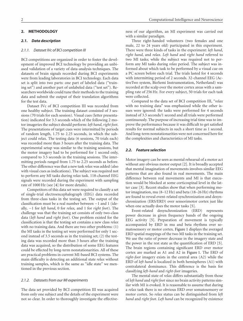
2 Computational Intelligence and Neuroscience
2. METHODOLOGY
2.1. Data description
2.1.1. Dataset IVc of BCI competition III
BCI competitions are organized in order to foster the devel-opment of improved BCI technology by providing an unbi-ased validation of a variety of data-analysis techniques. Thedatasets of brain signals recorded during BCI experimentswere from leading laboratories in BCI technology. Each dataset is split into two parts: one part of labeled data (“train-ing set”) and another part of unlabeled data (“test set”). Re-searchers worldwide could tune their methods to the trainingdata and submit the output of their translation algorithmsfor the test data.
Dataset IVc of BCI competition III was recorded fromone healthy subject. The training dataset consisted of 3 ses-sions (70 trials for each session). Visual cues (letter presenta-tion) indicated for 3.5 seconds which of the following 2 mo-tor imageries the subject should perform: left hand, right foot.The presentations of target cues were intermitted by periodsof random length, 1.75 to 2.25 seconds, in which the sub-ject could relax. The testing data (6 sessions, 70 trials each)was recorded more than 3 hours after the training data. Theexperimental setup was similar to the training sessions, butthe motor imagery had to be performed for 1 second only,compared to 3.5 seconds in the training sessions. The inter-mitting periods ranged from 1.75 to 2.25 seconds as before.The other difference was that a new task relax was added (alsowith visual cues as indications). The subject was required notto perform any MI tasks during relax task. 118-channel EEGsignals were recorded during the experiment with samplingrate of 1000 Hz (see [4] for more details).
Competitors of this data set were required to classify a setof single-trial electroencephalograph (EEG) data recordedfrom three-class tasks in the testing set. The output of theclassification must be a real number between −1 and 1 (ide-ally, −1 for left hand, 0 for relax, and 1 for right foot). Thechallenge was that the training set consists of only two-classdata (left hand and right foot). One problem existed for theclassification is that the testing set contains a new class relaxwith no training data. And there are two other problems: (1)the MI tasks in the testing set were performed for only 1 sec-ond instead of 3.5 seconds as in the training set; (2) the test-ing data was recorded more than 3 hours after the trainingdata was acquired, so the distribution of some EEG featurescould be effected by long-term nonstationarities. All of theseare practical problems in current MI-based BCI systems. Themain difficulty is detecting an additional state relax withouttraining samples, which is the same as “idle state” we men-tioned in the previous section.
2.1.2. Datasets from our MI experiments
The data set provided by BCI competition III was acquiredfrom only one subject and the details of the experiment werenot so clear. In order to thoroughly investigate the effective-
ness of our algorithm, an MI experiment was carried outwith a similar paradigm.
Three right-handed volunteers (two females and onemale, 22 to 24 years old) participated in this experiment.There were three kinds of tasks in the experiment: left hand,right hand, and relax. Left hand and right hand referred totwo MI tasks; while the subject was required not to per-form any MI tasks during relax period. The subject was in-formed about which task to be performed by a visual cue ona PC screen before each trial. The trials lasted for 4 secondswith intermitting period of 2 seconds. 32-channel EEG (Ac-tiveTwo system, BioSemi Instrumentation, Netherland) wasrecorded at the scalp over the motor cortex areas with a sam-pling rate of 256 Hz. For every subject, 50 trials for each taskwere collected.
Compared to the data set of BCI competition III, “relaxwith no training data” was emphasized while the other is-sues were ignored: the tasks were performed for 4 secondsinstead of 3.5 seconds/1 second and all trials were performedcontinuously. The purpose of increasing trial time was to im-prove the performance because it was difficult to get satisfiedresults for normal subjects in such a short time as 1 second.And long-term nonstationarities were not concerned here forthe complexities and characteristics of MI tasks.
2.2. Feature selection
Motor imagery can be seen as mental rehearsal of a motor actwithout any obvious motor output [2]. It is broadly acceptedthat mental imagination of movements involves similar EEGpatterns that are also found in real movements. The maindifference between real movements and MI is that execu-tion would be blocked at some corticospinal level in the lat-ter case [3]. Recent studies show that when performing mo-tor imagination, mu (8–12 Hz) and beta (18–26 Hz) rhythmsare found to reveal event-related synchronization and desyn-chronization (ERS/ERD) over sensorimotor cortex just likewhen one actually does the motor tasks [5].
Event-related desynchronization (ERD) representspower decrease in given frequency bands of the ongoingEEG activity [5]. Preparation of movement is typicallyaccompanied by ERD in mu and beta rhythms over so-matosensory or motor cortex. Figure 1 displays the averagedERD spatial mappings of the two MI tasks in the training set.We use the ratio of power decrease in the imagery state andthe power in the rest state as the quantification of ERD [5].The brain regions containing significant ERD over motorcortex are marked as A1 and A2 in Figure 1. The ERD ofright-foot imagery exists in the central area (A2) while theERD of left hand is localized in both hemispheres (A1) withcontralateral dominance. This difference is the basis forclassifying left-hand and right-foot imageries.
The mental state of relax differs substantially from thoseof left hand and right foot since no brain activity patterns sim-ilar with MI is evoked. It is reasonable to assume that duringa relax task there is no obvious ERD over somatosensory ormotor cortex. So relax status can be distinguished from lefthand and right foot. Left hand can be recognized by existence
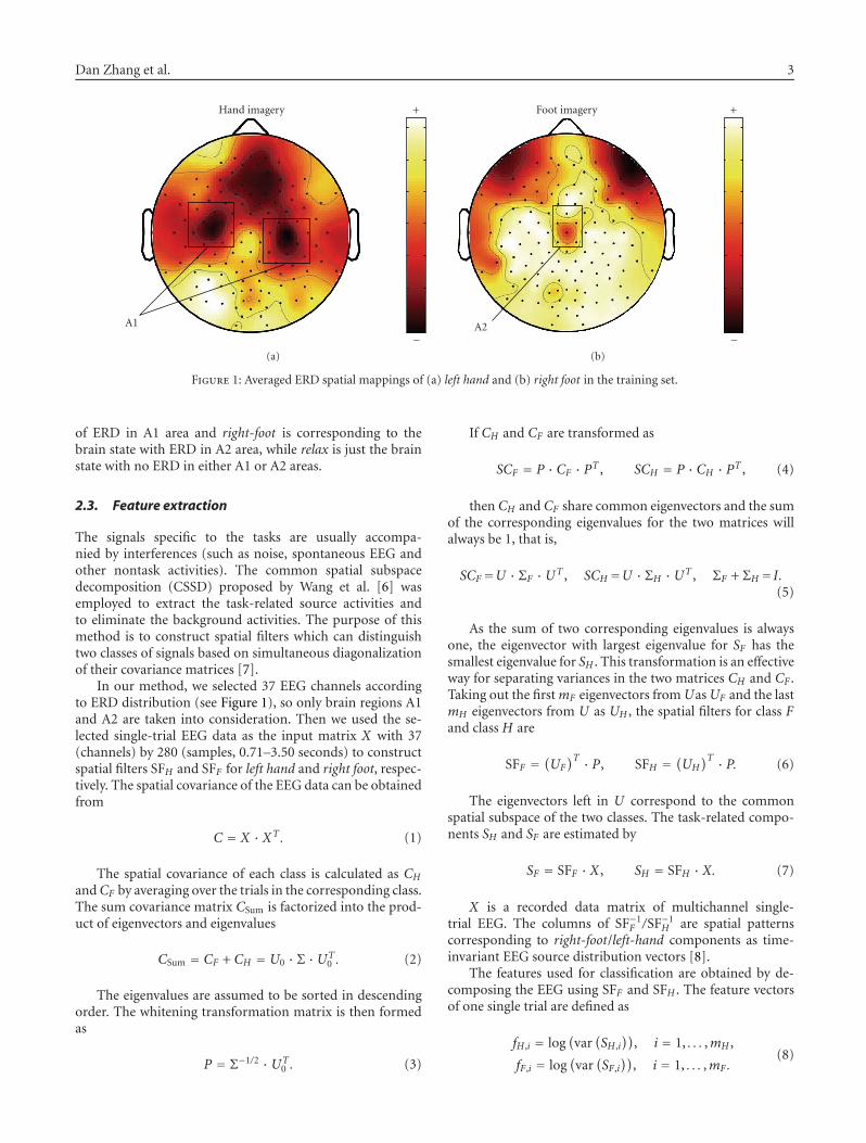
Dan Zhang et al. 3
A1
Hand imagery +
−(a)
A2
Foot imagery +
−(b)
Figure 1: Averaged ERD spatial mappings of (a) left hand and (b) right foot in the training set.
of ERD in A1 area and right-foot is corresponding to thebrain state with ERD in A2 area, while relax is just the brainstate with no ERD in either A1 or A2 areas.
2.3. Feature extraction
The signals specific to the tasks are usually accompa-nied by interferences (such as noise, spontaneous EEG andother nontask activities). The common spatial subspacedecomposition (CSSD) proposed by Wang et al. [6] wasemployed to extract the task-related source activities andto eliminate the background activities. The purpose of thismethod is to construct spatial filters which can distinguishtwo classes of signals based on simultaneous diagonalizationof their covariance matrices [7].
In our method, we selected 37 EEG channels accordingto ERD distribution (see Figure 1), so only brain regions A1and A2 are taken into consideration. Then we used the se-lected single-trial EEG data as the input matrix X with 37(channels) by 280 (samples, 0.71–3.50 seconds) to constructspatial filters SFH and SFF for left hand and right foot, respec-tively. The spatial covariance of the EEG data can be obtainedfrom
C = X · XT. (1)
The spatial covariance of each class is calculated as CH
andCF by averaging over the trials in the corresponding class.The sum covariance matrix CSum is factorized into the prod-uct of eigenvectors and eigenvalues
CSum = CF + CH = U0 · Σ ·UT0 . (2)
The eigenvalues are assumed to be sorted in descendingorder. The whitening transformation matrix is then formedas
P = Σ−1/2 ·UT0 . (3)
If CH and CF are transformed as
SCF = P · CF · PT , SCH = P · CH · PT , (4)
then CH and CF share common eigenvectors and the sumof the corresponding eigenvalues for the two matrices willalways be 1, that is,
SCF=U · ΣF ·UT , SCH=U · ΣH ·UT , ΣF + ΣH=I.(5)
As the sum of two corresponding eigenvalues is alwaysone, the eigenvector with largest eigenvalue for SF has thesmallest eigenvalue for SH . This transformation is an effectiveway for separating variances in the two matrices CH and CF .Taking out the first mF eigenvectors from Uas UF and the lastmH eigenvectors from U as UH , the spatial filters for class Fand class H are
SFF =(UF)T · P, SFH =
(UH)T · P. (6)
The eigenvectors left in U correspond to the commonspatial subspace of the two classes. The task-related compo-nents SH and SF are estimated by
SF = SFF · X , SH = SFH · X. (7)
X is a recorded data matrix of multichannel single-trial EEG. The columns of SF−1
F /SF−1H are spatial patterns
corresponding to right-foot/left-hand components as time-invariant EEG source distribution vectors [8].
The features used for classification are obtained by de-composing the EEG using SFF and SFH . The feature vectorsof one single trial are defined as
fH ,i = log(var(SH ,i
)), i = 1, . . . ,mH ,
fF,i = log(var(SF,i))
, i = 1, . . . ,mF.(8)

4 Computational Intelligence and Neuroscience
SH ,i/SF,i represents the ith row vector of SH/SF . The log-transformation serves to approximate normal distribution ofthe data. Our experiences on the training set indicated thatsetting mF = 3 and mH = 3 was enough to get a fairly goodperformance.
During left-hand imagery, ERD occurs in region A1, lead-ing to a relatively decreased EEG variance in this area. There-fore, right foot has a higher EEG variance than left hand inregion A1. This behavior is reflected by large coefficientsfor channels covering region A1 in the spatial pattern cor-responding to right-foot imagery. Figure 2 displays the mostimportant spatial pattern of the two tasks. As shown inFigure 2(b), the most important spatial pattern of right footaccords with the ERD distribution of left hand. The spatial fil-ter SFF serves as extracting the component with a source dis-tribution like the corresponding spatial pattern. Therefore,the component extracted by SFF can be considered as thesource activity concerning left-hand ERD, which has a sig-nificant distribution over region A1. A weak source activityleads to a small variance of relative scalp EEG, which is cor-responding to significant ERD. Due to no ERD in region A1,the component of right foot has a larger variance than that ofleft hand when filtered by SFF , that is,
var(SFF · XF
)> var
(SFF · XH
), (9)
where XH and XF are single-trial EEG corresponding to lefthand and right foot, respectively. We can also get another in-equality as follows:
var(SFH · XH
)> var
(SFH · XF
). (10)
Note that according to the above definitions, left-hand MIcauses a relatively increased EEG variance over area A2 (cor-responding to right-foot task) because event-related desyn-chronization of EEG takes place on area A1. This behavior isreflected in large coefficients for electrodes on area A2 in thespatial filter of left-hand (SFH) [8], and vice versa for rightfoot.
2.4. Classification method
The paper of Garrett et al. [9] showed that if features wereproperly extracted, the performance of linear classifiers canbehave as well as that of complex nonlinear classifiers, sowe simply used Fisher discriminant analysis (FDA) in ourmethod.
After using CSSD to extract ERD feature out of the train-ing set, FDA was applied for classification and an accuracy of(99.1±1.2)% was obtained on the training set using a 10×10-fold cross-validation. The result of FDA proves that there isno need to use other complicated methods.
2.5. Classification on the testing set
Denote XR as a single-trial EEG of relax, as no ERD occursin both regions A1 and A2 during relax tasks, the following
inequalities come into existence:
var(SFF · XR
)> var
(SFF · XH
), (11)
var(SFH · XR
)> var
(SFH · XF
). (12)
Both components of relax and right foot are larger thanthat of left hand when filtered by SFF , so left-hand motor im-ageries can be discriminated from right-foot/relax. Similarly,right foot can be discriminated from left-hand/relax when fil-tered by SFH .
The required classification outputs of left hand and rightfoot are defined as −1 and +1. If we do a two-class classifi-cation based on the feature vectors fH extracted by SFH andset the classification outputs of left hand and right foot to −1and +1 as required, then samples of relax are also classifiedto −1 as it is the same as left hand according to (9) and (11).Samples of relax are classified to +1 according to (10) and(12). Table 1 shows the different outputs of the three tasksin ideal conditions. Column “ fF” and “ fH” shows the twotwo-class classification results. Column “( fF + fH)/2” repre-sents the mean value of two outputs corresponding to fF andfH in the same row. Ideally, the two classifiers correspond-ing to “ fF” and “ fH” will result in opposite outputs for relax(+1/−1) and the final classification result of relax can be setto 0 easily by “( fF+ fH)/2.” Therefore, it is possible to separatethe three classes.
Our strategy goes as following: at first, a two-class clas-sifier was used to classify samples of relax to output 0 (seeTable 1). Then the second two-class classifier was defined toclassify the remaining samples into either right foot or lefthand. The whole procedure of the classification algorithm isshown in Figure 3.
Step 1 (Discriminating the relax trials). The classificationprocess of this step is showed in Figure 4. A subject-specificbandpass filter of 12–14 Hz (with most significant ERD fea-ture for the subject of dataset IVc) and a time window of0.71–3.50 seconds (eliminating the first 0.7 seconds as reac-tion time) were set for CSSD algorithm to calculate two spa-tial filters SFF1 and SFH1 from the training data. Because theduration of each trial in the testing set is much shorter thanthat of the training set, CSSD filter cannot get enough in-formation with such a short time window to keep a high ac-curacy. Here we bring forward another assumption that thespatial pattern in the intermitted time (1.75–2.25 seconds)after a relax trial is similar to that of the relax trial (however,the intermitted time after an MI task cannot be simply con-sidered as relax because the subject might keep on doing MIfor a certain period even after he saw the cue for stop). Withthis assumption, a time window of 2.75 seconds (1 secondfor the task and at least 1.75 seconds for intermitted time)was selected as the input of the CSSD filters for the testingset. The effective duration of relax can thus be prolonged,making the classification results more reliable than those ob-tained by only using a short-time window.
Bagging strategy [10] was used here for reducing varianceof classification accuracy. 160 trials were randomly selected
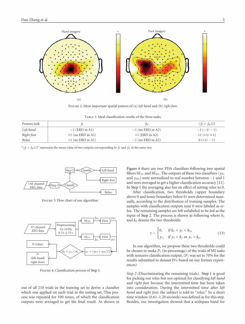
Dan Zhang et al. 5
Hand imagery +
−(a)
Foot imagery +
−(b)
Figure 2: Most important spatial pattern of (a) left hand and (b) right foot.
Table 1: Ideal classification results of the three tasks.
Feature task fF fH ( fF + fH)/2
Left hand −1 (ERD in A1) −1 (no ERD in A2) −1 (−1/ − 1)
Right foot +1 (no ERD in A1) +1 (ERD in A2) +1 (+1/ + 1)
Relax +1 (no ERD in A1) −1 (no ERD in A2) 0 (+1/ − 1)
“( fF + fH )/2” represents the mean value of two outputs corresponding to fF and fH in the same row.
118-channelEEG data
Step 1
Step 2
Classify
Classify Left hand
Right foot
Relax
Figure 3: Flow chart of our algorithm.
37-channelEEG data
0 (relax)
y1
(left-hand/right-foot)
Preprocessing12–14 Hz
0.71–2.75 s
k1 < y1 < k2 y1 = (yF1 + yH1)/2
SFH1
SFF1
fH1
fF1
FDA
FDA
yH1
yF1
Figure 4: Classification process of Step 1.
out of all 210 trials in the training set to derive a classifierwhich was applied on each trial in the testing set. This pro-cess was repeated for 100 times, of which the classificationoutputs were averaged to get the final result. As shown in
Figure 4 there are two FDA classifiers following two spatialfilters SFF1 and SFH1. The outputs of these two classifiers (yF1
and yH1) were normalized to real number between −1 and 1and were averaged to get a higher classification accuracy [11].In Step 1 the averaging also has an effect of setting relax to 0.
After classification, two thresholds (upper boundaryabove 0 and lower boundary below 0) were determined man-ually, according to the distribution of training samples. Thesamples with classification outputs near 0 were labeled as re-lax. The remaining samples are left unlabeled to be fed as theinput of Step 2. The process is shown as following where k1
and k2 denote the two thresholds:
z =⎧⎨
⎩0, if k1 < y1 < k2,
y1, if y1 < k1 or y1 > k2.(13)
In our algorithm, we propose these two thresholds couldbe chosen to make P1 (in percentage) of the trials of MI taskswith nonzero classification output. (P1 was set to 70% for theresults submitted to dataset IVc based on our former experi-ences)
Step 2 (Discriminating the remaining trials). Step 1 is goodfor picking out relax but not optimal for classifying left handand right foot because the intermitted time has been takeninto consideration. During the intermitted time after lefthand and right foot, the subject is told to “relax.” So a shorttime window (0.61–1.20 seconds) was defined as for this step.Besides, our investigation showed that a widepass band for
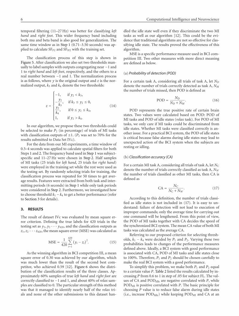
6 Computational Intelligence and Neuroscience
temporal filtering (11–27 Hz) was better for classifying lefthand and right foot. This wider frequency band includingboth mu and beta band is also good for generalization. Thesame time window as in Step 1 (0.71–3.50 seconds) was ap-plied to calculate SFF2 and SFH2 with the training set.
The classification process of this step is shown inFigure 5. After classification we also set two thresholds man-ually to label samples with outputs congregating near−1 and1 to right hand and left foot, respectively, and the others to areal number between −1 and 1. The normalization processis as follows, where y is the original output and z is the nor-malized output, k3 and k4 denote the two thresholds:
z =
⎧⎪⎪⎪⎪⎪⎪⎪⎪⎪⎨
⎪⎪⎪⎪⎪⎪⎪⎪⎪⎩
−1, if y2 < k3,
− y2
k3, if k3 ≤ y2 ≤ 0,
y2
k4, if 0 ≤ y2 ≤ k4,
1, if y2 > k4.
(14)
In our algorithm, we propose these two thresholds couldbe selected to make P2 (in percentage) of trials of MI taskswith classification outputs of ±1. (P2 was set to 70% for theresults submitted to Data Set IVc).
For the data from our MI experiments, a time window of0.5–4 seconds was applied to calculate spatial filters for bothSteps 1 and 2. The frequency band used in Step 1 was subject-specific and 11–27 Hz were chosen in Step 2. Half samplesof MI tasks (25 trials for left hand, 25 trials for right hand)were employed in the training set while the rest were used asthe testing set. By randomly selecting trials for training, theclassification process was repeated for 50 times to get aver-age results. Features were extracted from both task and inter-mitting periods (6 seconds) in Step 1 while only task periodswere considered in Step 2. Furthermore, we investigated howto choose threshold k1−k4 to get a better performance (referto Section 3 for details).
3. RESULTS
The result of dataset IVc was evaluated by mean square er-ror criterion. Defining the true labels for 420 trials in thetesting set as y1, y2 · · · y420, and the classification outputs asz1, z2 · · · z420, the mean square error (MSE) was calculated as
MSE = 1420
420∑
i=1
(yi − zi
)2. (15)
As the winning algorithm in BCI competition III, a meansquare error of 0.30 was achieved by our algorithm, whichwas much lower than the result of the second best com-petitor, who achieved 0.59 [12]. Figure 6 shows the distri-bution of the classification results of the three classes. Ap-proximately 60% samples of true left hand and right foot arecorrectly classified to −1 and 1, and about 40% of relax sam-ples are classified to 0. The particular strength of this methodwas that it managed to identify nearly half of the relax tri-als and none of the other submissions to this dataset han-
dled the idle state well even if they discriminate the two MItasks as well as our algorithm [12]. This could be the evi-dence that traditional algorithms are not so effective for clas-sifying idle state. The results proved the effectiveness of thisalgorithm.
MSE is a specific performance measure used in BCI com-petition III. Two other measures with more direct meaningare defined as below.
(a) Probability of detection (POD)
For a certain task A, considering all trials of task A, let ND
denote the number of trials correctly detected as task A, NM
the number of trials missed, then POD is defined as
POD = ND
ND + NM. (16)
POD represents the true positive rate of certain brainstates. Two values were calculated based on POD: POD ofMI tasks and POD of idle states (relax task). For POD of MItasks, we only care if MI tasks could be discriminated fromidle states. Whether MI tasks were classified correctly is an-other issue. For a practical BCI system, the POD of idle statesis critical because false alarms during idle states may lead tounexpected action of the BCI system when the subjects areresting or idling.
(b) Classification accuracy (CA)
For a certain MI task A, considering all trials of task A, let NC
denote the number of trials correctly classified as task A, NW
the number of trials classified as other MI tasks, then CA isdefined as
CA = NC
NC + NW. (17)
According to this definition, the number of trials classi-fied as idle states is not included in (17). It is easy to un-derstand: failure of detection will not lead to execution ofimproper commands; only the average time for carrying outone command will be lengthened. From this point of view,the POD of MI tasks together with CA decides the speed ofthe synchronized BCI system. The mean CA value of both MItasks was calculated as the average CA.
Referring to our proposed criterion for selecting thresh-olds, k1 − k4 were decided by P1 and P2. Varying these twoprobabilities leads to changes of the performance measuresdefined above. Ideally, a BCI system with good performanceis associated with CA, POD of MI tasks and idle states closeto 100%. Therefore, P1 and P2 should be chosen carefully tomake the real BCI system with a good performance.
To simplify this problem, we make both P1 and P2 equalto a certain value P. Table 2 listed the results calculated by in-creasing P from 0.6 to 1 in step of .05 for subject FL. The val-ues of CA and PODIdle are negative correlated with P, whilePODMI is positive correlated with P. The basic principle forchoosing P value is to reduce false alarm during idle states(i.e., increase PODIdle) while keeping PODMI and CA at an
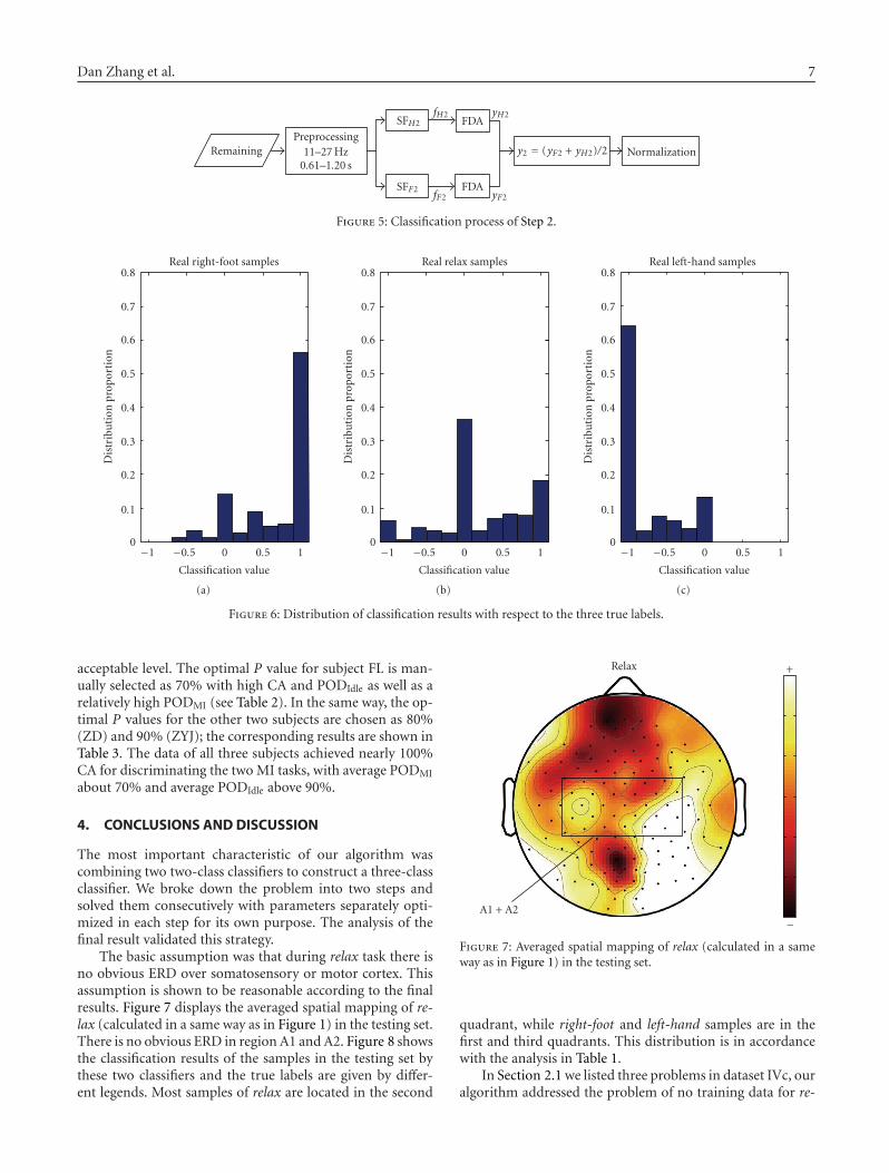
Dan Zhang et al. 7
Remaining NormalizationPreprocessing
11–27 Hz0.61–1.20 s
y2 = (yF2 + yH2)/2
SFH2
SFF2
fH2
fF2
FDA
FDA
yH2
yF2
Figure 5: Classification process of Step 2.
0
0.1
0.2
0.3
0.4
0.5
0.6
0.7
0.8
Dis
trib
uti
onpr
opor
tion
−1 −0.5 0 0.5 1
Classification value
Real right-foot samples
(a)
0
0.1
0.2
0.3
0.4
0.5
0.6
0.7
0.8
Dis
trib
uti
onpr
opor
tion
−1 −0.5 0 0.5 1
Classification value
Real relax samples
(b)
0
0.1
0.2
0.3
0.4
0.5
0.6
0.7
0.8
Dis
trib
uti
onpr
opor
tion
−1 −0.5 0 0.5 1
Classification value
Real left-hand samples
(c)
Figure 6: Distribution of classification results with respect to the three true labels.
acceptable level. The optimal P value for subject FL is man-ually selected as 70% with high CA and PODIdle as well as arelatively high PODMI (see Table 2). In the same way, the op-timal P values for the other two subjects are chosen as 80%(ZD) and 90% (ZYJ); the corresponding results are shown inTable 3. The data of all three subjects achieved nearly 100%CA for discriminating the two MI tasks, with average PODMI
about 70% and average PODIdle above 90%.
4. CONCLUSIONS AND DISCUSSION
The most important characteristic of our algorithm wascombining two two-class classifiers to construct a three-classclassifier. We broke down the problem into two steps andsolved them consecutively with parameters separately opti-mized in each step for its own purpose. The analysis of thefinal result validated this strategy.
The basic assumption was that during relax task there isno obvious ERD over somatosensory or motor cortex. Thisassumption is shown to be reasonable according to the finalresults. Figure 7 displays the averaged spatial mapping of re-lax (calculated in a same way as in Figure 1) in the testing set.There is no obvious ERD in region A1 and A2. Figure 8 showsthe classification results of the samples in the testing set bythese two classifiers and the true labels are given by differ-ent legends. Most samples of relax are located in the second
A1 + A2
Relax +
−Figure 7: Averaged spatial mapping of relax (calculated in a sameway as in Figure 1) in the testing set.
quadrant, while right-foot and left-hand samples are in thefirst and third quadrants. This distribution is in accordancewith the analysis in Table 1.
In Section 2.1 we listed three problems in dataset IVc, ouralgorithm addressed the problem of no training data for re-
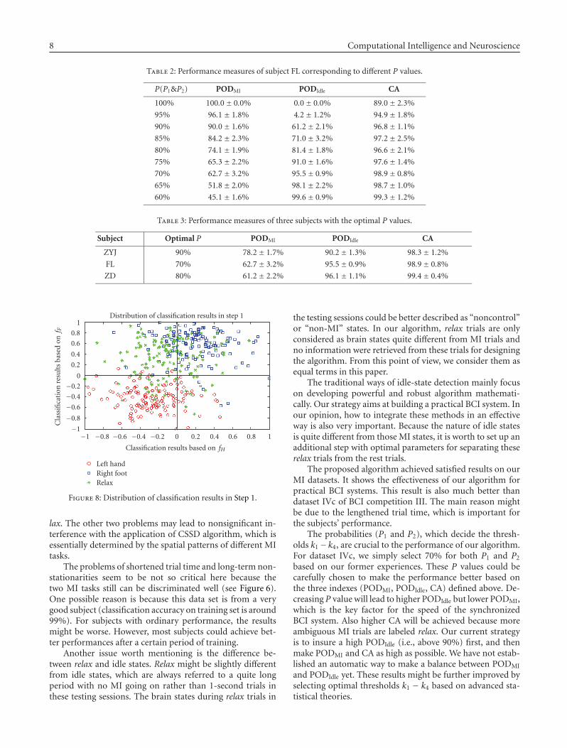
8 Computational Intelligence and Neuroscience
Table 2: Performance measures of subject FL corresponding to different P values.
P(P1&P2) PODMI PODIdle CA
100% 100.0± 0.0% 0.0± 0.0% 89.0± 2.3%
95% 96.1± 1.8% 4.2± 1.2% 94.9± 1.8%
90% 90.0± 1.6% 61.2± 2.1% 96.8± 1.1%
85% 84.2± 2.3% 71.0± 3.2% 97.2± 2.5%
80% 74.1± 1.9% 81.4± 1.8% 96.6± 2.1%
75% 65.3± 2.2% 91.0± 1.6% 97.6± 1.4%
70% 62.7± 3.2% 95.5± 0.9% 98.9± 0.8%
65% 51.8± 2.0% 98.1± 2.2% 98.7± 1.0%
60% 45.1± 1.6% 99.6± 0.9% 99.3± 1.2%
Table 3: Performance measures of three subjects with the optimal P values.
Subject Optimal P PODMI PODIdle CA
ZYJ 90% 78.2± 1.7% 90.2± 1.3% 98.3± 1.2%
FL 70% 62.7± 3.2% 95.5± 0.9% 98.9± 0.8%
ZD 80% 61.2± 2.2% 96.1± 1.1% 99.4± 0.4%
−1
−0.8
−0.6
−0.4
−0.2
0
0.2
0.4
0.6
0.8
1
Cla
ssifi
cati
onre
sult
sba
sed
onf F
−1 −0.8 −0.6 −0.4 −0.2 0 0.2 0.4 0.6 0.8 1
Classification results based on fH
Distribution of classification results in step 1
Left handRight footRelax
Figure 8: Distribution of classification results in Step 1.
lax. The other two problems may lead to nonsignificant in-terference with the application of CSSD algorithm, which isessentially determined by the spatial patterns of different MItasks.
The problems of shortened trial time and long-term non-stationarities seem to be not so critical here because thetwo MI tasks still can be discriminated well (see Figure 6).One possible reason is because this data set is from a verygood subject (classification accuracy on training set is around99%). For subjects with ordinary performance, the resultsmight be worse. However, most subjects could achieve bet-ter performances after a certain period of training.
Another issue worth mentioning is the difference be-tween relax and idle states. Relax might be slightly differentfrom idle states, which are always referred to a quite longperiod with no MI going on rather than 1-second trials inthese testing sessions. The brain states during relax trials in
the testing sessions could be better described as “noncontrol”or “non-MI” states. In our algorithm, relax trials are onlyconsidered as brain states quite different from MI trials andno information were retrieved from these trials for designingthe algorithm. From this point of view, we consider them asequal terms in this paper.
The traditional ways of idle-state detection mainly focuson developing powerful and robust algorithm mathemati-cally. Our strategy aims at building a practical BCI system. Inour opinion, how to integrate these methods in an effectiveway is also very important. Because the nature of idle statesis quite different from those MI states, it is worth to set up anadditional step with optimal parameters for separating theserelax trials from the rest trials.
The proposed algorithm achieved satisfied results on ourMI datasets. It shows the effectiveness of our algorithm forpractical BCI systems. This result is also much better thandataset IVc of BCI competition III. The main reason mightbe due to the lengthened trial time, which is important forthe subjects’ performance.
The probabilities (P1 and P2), which decide the thresh-olds k1− k4, are crucial to the performance of our algorithm.For dataset IVc, we simply select 70% for both P1 and P2
based on our former experiences. These P values could becarefully chosen to make the performance better based onthe three indexes (PODMI, PODIdle, CA) defined above. De-creasing P value will lead to higher PODIdle but lower PODMI,which is the key factor for the speed of the synchronizedBCI system. Also higher CA will be achieved because moreambiguous MI trials are labeled relax. Our current strategyis to insure a high PODIdle (i.e., above 90%) first, and thenmake PODMI and CA as high as possible. We have not estab-lished an automatic way to make a balance between PODMI
and PODIdle yet. These results might be further improved byselecting optimal thresholds k1 − k4 based on advanced sta-tistical theories.

Dan Zhang et al. 9
A BCI system that can distinguish patterns not includedin training data is very attractive. Solving the problem ofdataset IVc is a good step towards this target. The proposedalgorithm is especially useful to reduce the false alarms incurrent BCI system based on MI when the subjects are notperforming MI tasks. Although we perform offline anal-ysis here, this algorithm could be easily moved to onlinesystem.
ACKNOWLEDGMENTS
This project is supported by National Natural Science Foun-dation of China (no. 60318001, 30630022), and Tsinghua-Yuyuan Medicine Research fund. We are grateful to Klaus-Robert Muller, Benjamin Blankertz, and Gabriel Curio forproviding the dataset. Also, we would like to extend our spe-cial thanks to Prof. Fusheng Yang for a very informative dis-cussion and his valuable comments.
REFERENCES
[1] J. R. Wolpaw, N. Birbaumer, D. J. McFarland, G. Pfurtscheller,and T. M. Vaughan, “Brain-computer interfaces for communi-cation and control,” Clinical Neurophysiology, vol. 113, no. 6,pp. 767–791, 2002.
[2] G. Pfurtscheller and C. Neuper, “Motor imagery and di-rect brain-computer communication,” Proceedings of the IEEE,vol. 89, no. 7, pp. 1123–1134, 2001.
[3] M. Jeannerod, “Mental imagery in the motor context,” Neu-ropsychologia, vol. 33, no. 11, pp. 1419–1432, 1995.
[4] http://ida.first.fraunhofer.de/projects/bci/competition iii/desc IVc.html.
[5] G. Pfurtscheller and F. H. Lopes da Silva, “Event-relatedEEG/MEG synchronization and desynchronization: basicprinciples,” Clinical Neurophysiology, vol. 110, no. 11, pp.1842–1857, 1999.
[6] Y. Wang, P. Berg, and M. Scherg, “Common spatial subspacedecomposition applied to analysis of brain responses undermultiple task conditions: a simulation study,” Clinical Neuro-physiology, vol. 110, no. 4, pp. 604–614, 1999.
[7] Y. Wang, Z. Zhang, Y. Li, X. Gao, S. Gao, and F. Yang, “BCIcompetition 2003—data set IV: an algorithm based on CSSDand FDA for classifying single-trial EEG,” IEEE Transactions onBiomedical Engineering, vol. 51, no. 6, pp. 1081–1086, 2004.
[8] H. Ramoser, J. Muller-Gerking, and G. Pfurtscheller, “Opti-mal spatial filtering of single trial EEG during imagined handmovement,” IEEE Transactions on Rehabilitation Engineering,vol. 8, no. 4, pp. 441–446, 2000.
[9] D. Garrett, D. A. Peterson, C. W. Anderson, and M. H. Thaut,“Comparison of linear, nonlinear, and feature selection meth-ods for EEG signal classification,” IEEE Transactions on NeuralSystems and Rehabilitation Engineering, vol. 11, no. 2, pp. 141–144, 2003.
[10] L. Breiman, “Bagging predictors,” Machine Learning, vol. 24,no. 2, pp. 123–140, 1996.
[11] G. Dornhege, B. Blankertz, G. Curio, and K.-R. Muller,“Boosting bit rates in noninvasive EEG single-trial classifica-tions by feature combination and multiclass paradigms,” IEEETransactions on Biomedical Engineering, vol. 51, no. 6, pp. 993–1002, 2004.
[12] B. Blankertz, K.-R. Muller, D. J. Krusienski, et al., “The BCIcompetition III: validating alternative approaches to actualBCI problems,” IEEE Transactions on Neural Systems and Re-habilitation Engineering, vol. 14, no. 2, pp. 153–159, 2006.
Hindawi Publishing CorporationComputational Intelligence and NeuroscienceVolume 2007, Article ID 48937, 12 pagesdoi:10.1155/2007/48937
Research ArticleVibrotactile Feedback for Brain-Computer Interface Operation
Febo Cincotti,1 Laura Kauhanen,2 Fabio Aloise,1 Tapio Palomaki,2 Nicholas Caporusso,1, 3
Pasi Jylanki,2 Donatella Mattia,1 Fabio Babiloni,1, 4 Gerolf Vanacker,5 Marnix Nuttin,5
Maria Grazia Marciani,1, 6 and Jose del R. Millan7, 8
1 Laboratory of Neuroelectrical Imaging and Brain Computer Interface, Fondazione Santa Lucia IRCCS,Via Ardeatina 306, 00179 Roma, Italy
2 Laboratory of Computational Engineering, Helsinki University of Technology, P.O. Box 9203, 02015 TKK, Finland3 Department of Computer Science, University of Bari, Via Orabona 4, 70125 Bari, Italy4 Dipartimento di Fisiologia Umana e Farmacologia, Universita degli Studi di Roma “La Sapienza”, Piazzale Aldo Moro 5,00185 Roma, Italy
5 Department of Mechanical Engineering, Katholieke Universiteit Leuven, Celestijnenlaan 300 B, 3000 Leuven, Belgium6 Dipartimento di Neuroscienze, Universita degli Studi di Roma “Tor Vergata”, Via Montpellier 1, 00173 Roma, Italy7 IDIAP Research Institute, 1920 Martigny, Switzerland
8 Ecole Polytechnique Federale de Lausanne (EPFL), 1015 Lausanne, Switzerland
Correspondence should be addressed to Febo Cincotti, [email protected]
Received 18 February 2007; Accepted 26 June 2007
Recommended by Andrzej Cichocki
To be correctly mastered, brain-computer interfaces (BCIs) need an uninterrupted flow of feedback to the user. This feedback isusually delivered through the visual channel. Our aim was to explore the benefits of vibrotactile feedback during users’ training andcontrol of EEG-based BCI applications. A protocol for delivering vibrotactile feedback, including specific hardware and softwarearrangements, was specified. In three studies with 33 subjects (including 3 with spinal cord injury), we compared vibrotactile andvisual feedback, addressing: (I) the feasibility of subjects’ training to master their EEG rhythms using tactile feedback; (II) thecompatibility of this form of feedback in presence of a visual distracter; (III) the performance in presence of a complex visual taskon the same (visual) or different (tactile) sensory channel. The stimulation protocol we developed supports a general usage ofthe tactors; preliminary experimentations. All studies indicated that the vibrotactile channel can function as a valuable feedbackmodality with reliability comparable to the classical visual feedback. Advantages of using a vibrotactile feedback emerged whenthe visual channel was highly loaded by a complex task. In all experiments, vibrotactile feedback felt, after some training, morenatural for both controls and SCI users.
Copyright © 2007 Febo Cincotti et al. This is an open access article distributed under the Creative Commons Attribution License,which permits unrestricted use, distribution, and reproduction in any medium, provided the original work is properly cited.
1. INTRODUCTION
The human brain relies on inputs from different senses toform percepts of objects and events, during everyday life.These pieces of information usually complement and con-firm each other, thereby enhancing the reliability of percept[1]. Somatosensory feedback is a vital component of motorplanning, control, and adaptation, and there is a growing ef-fort to include this feedback modality in neural prostheticsystems [2].
Visual presentation of stimuli is the most common feed-back modality in neurofeedback paradigms for self-regula-
tion of the brain’s electrical activity. Thus, it is comprehen-sible that current brain-computer communication systemsmainly operate with visual stimuli [3]. However, compo-nents of the visual system such as vision, visual attention,and focusing gaze are physiologically engaged during the dy-namic contact between the body and environment. Further-more, the visual sense may be compromised in some patientswho are in need of BCI support. Thus, towards more effi-cient brain-computer communication, it seems important toalso obtain evidence of how the extravision somatosensorymodality performs during self-regulation of the brain’s elec-trical activity.
2 Computational Intelligence and Neuroscience
Only few studies have tested other feedback modalitiesfor brain-computer interfaces (BCIs). Hinterberger et al. [4]and Pham et al. [5, 6] tested auditory feedback, but, to ourknowledge, no one has trained subjects with tactile feedback.Vibrotactile stimuli have been previously used [7, 8] for BCIoperation in a different context, that is, as an external drivingstimulus to elicit exogenous EEG rhythms.
In addition to freeing visual and auditory attention, tac-tile stimuli are more natural in a manipulation task than, forexample, visual stimuli. Even though BCI training is stronglydependent on feedback, surprisingly, only two studies haveexplored how feedback affects the learning process. McFar-land et al. [9] investigated what happens when feedback isremoved from well-trained subjects and Neuper et al. [10]compared continuous and discrete feedback. No guidelinesexist regarding somatosensory stimulation for BCIs.
This study aims to explore the benefits of vibrotactilefeedback for user training and accurate control of an EEG-based brain-computer interface.
2. VIBROTACTILE STIMULATION
2.1. Physiological perception
Several receptors for the transduction of mechanical solicita-tion on the skin into neuronal signals are available in man:Merkel’s receptors, which are slow adapting receptors withhigh spatial resolution; the Meissner’s corpuscles, present inthe glabrous skin (lips, finger), with characteristic of rapidadaptation and high spatial resolution; the Pacini’s corpus-cles which detect very rapid vibration and are quickly adapt-ing. The somesthetic information travels from the receptorsto the central nervous system using the fastest communica-tion lines in the human body; the so-called dorsal-lateral col-umn way, delivering information at a speed of over 100 m/s.This somesthetic system delivers very precise information ofwhich two neighboring points on the human skin can be per-ceived as distinct. The spatial resolution of the skin has beentested since 1826 [11] using static pressure stimuli showingthat it varies along the body, ranging from few millimeters(fingers) to more than four centimeters (trunk).
Vibrotactile devices delivering variable pressure on theskin have been employed as an alternative sensitive channelfor blind or deaf individuals [12, 13]. The sensitivity for vi-brotactile stimulation depends on body position and age ofthe subjects [14]. Frequency of vibration is a second param-eter that influences the quality and intensity of perception,being modulated by factors like body position, skin temper-ature, and underlying tissue (bone, fat, muscle, or a com-bination). Values between 50 and 300 Hz should generallybe chosen. The use of oscillating pressure also adds new de-grees of freedom to the design of vibrotactile stimuli, such aswaveform shape, for example, sinusoidal or square and am-plitude modulations (at different modulation frequencies) ofthe carrier frequency.
In summary, several features of vibrotactile stimuli can bemodulated to convey information over this sensory channel.The list can be divided into two subsets. The first includesfeatures related to physical perception:
(1) frequency, the main spectral component of the peri-odic stimulus;
(2) intensity, the strength of stimulation (measured eitheras force applied or as displacement produced);
(3) timbre, the complexity of the stimulation waveform(i.e., the content of harmonics in the spectral repre-sentation);
(4) duration, the time length of the “on” time or an ele-mentary stimulation;
(5) spatial location, the single body part or the pattern ofparts that are stimulated.
Features in the second subset are clearly perceived by an indi-vidual, but do not rely on any property of the receptors (e.g.,need to be interpreted on a cognitive level):
(1) rhythm, the sequences of stimulation and pauses, withspecific durations, that compose the current message,that is, a triplet of stimuli, a Morse coded SOS, and soforth;
(2) tempo, the fastness, due to longer or shorter durationof the whole message, given at fixed rhythm;
(3) flutter, an amplitude modulation of the stimulationcarrier frequency that can either be perceived as in-crease and decrease of the intensity (if modulation isslower than 5 Hz) or as “roughness” (if modulation isfaster than 10 Hz).
Given the hardware at our disposal (described below), we de-signed an appropriate software framework to test the effec-tiveness of all the features mentioned above, as to maximizethe capacity of the vibrotactile channel.
2.2. Generation and delivery of stimuli
We used C-2 tactors (Engineering Acoustics, Inc, WinterPark, FL, USA) (see Figure 1) that are magnetic actuators,similar in principle to audio speakers; the current flowing intheir coil pushes a central structure named contactor againstthe skin and back. Different from acoustic transducers, thestructure is tuned on a narrow band around 250 Hz, so onlysignals at these frequencies can be effectively transduced.
By driving a tactor with two mixed sine waves, complexwaveforms can be obtained. Moreover, a third auxiliary in-put can be fed at the amplification stage. Even if efficiencyissues suggest not to deviate from the resonance frequency of250 Hz, the frequency of stimulation can be selected by theuser. The output intensity can be set to four different values(amplification gains). A peripheral interface controller (PIC)included on the control board takes care of serial commu-nication with the PC, and sets in the generation and ampli-fication subsystems the appropriate values of frequency andgain. By using a battery as power supply and a serial port toa Bluetooth (BT) adapter, the host PC can send commandsover the air to the vibrotactile device. Since both the controlboard and the BT adapter are battery powered, the users canwear a wireless system during the experiments.
The tactors are relatively lightweight and small (∼4 cmdiameter). The skin contactor is 7.5 mm diameter, raisedto 0.6 mm from the surface of the case, so that it can be
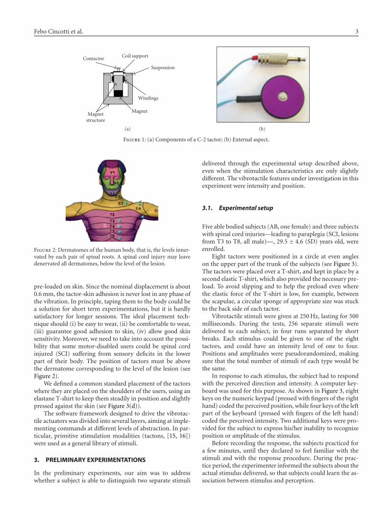
Febo Cincotti et al. 3
Contactor Coil support
Suspension
Windings
MagnetMagnet
structure
(a) (b)
Figure 1: (a) Components of a C-2 tactor; (b) External aspect.
Figure 2: Dermatomes of the human body, that is, the levels inner-vated by each pair of spinal roots. A spinal cord injury may leavedenervated all dermatomes, below the level of the lesion.
pre-loaded on skin. Since the nominal displacement is about0.6 mm, the tactor-skin adhesion is never lost in any phase ofthe vibration. In principle, taping them to the body could bea solution for short term experimentations, but it is hardlysatisfactory for longer sessions. The ideal placement tech-nique should (i) be easy to wear, (ii) be comfortable to wear,(iii) guarantee good adhesion to skin, (iv) allow good skinsensitivity. Moreover, we need to take into account the possi-bility that some motor-disabled users could be spinal cordinjured (SCI) suffering from sensory deficits in the lowerpart of their body. The position of tactors must be abovethe dermatome corresponding to the level of the lesion (seeFigure 2).
We defined a common standard placement of the tactorswhere they are placed on the shoulders of the users, using anelastane T-shirt to keep them steadily in position and slightlypressed against the skin (see Figure 3(d)).
The software framework designed to drive the vibrotac-tile actuators was divided into several layers, aiming at imple-menting commands at different levels of abstraction. In par-ticular, primitive stimulation modalities (tactons, [15, 16])were used as a general library of stimuli.
3. PRELIMINARY EXPERIMENTATIONS
In the preliminary experiments, our aim was to addresswhether a subject is able to distinguish two separate stimuli
delivered through the experimental setup described above,even when the stimulation characteristics are only slightlydifferent. The vibrotactile features under investigation in thisexperiment were intensity and position.
3.1. Experimental setup
Five able bodied subjects (AB, one female) and three subjectswith spinal cord injuries—leading to paraplegia (SCI, lesionsfrom T3 to T8, all male)—, 29.5 ± 4.6 (SD) years old, wereenrolled.
Eight tactors were positioned in a circle at even angleson the upper part of the trunk of the subjects (see Figure 3).The tactors were placed over a T-shirt, and kept in place by asecond elastic T-shirt, which also provided the necessary pre-load. To avoid slipping and to help the preload even wherethe elastic force of the T-shirt is low, for example, betweenthe scapulae, a circular sponge of appropriate size was stuckto the back side of each tactor.
Vibrotactile stimuli were given at 250 Hz, lasting for 500milliseconds. During the tests, 256 separate stimuli weredelivered to each subject, in four runs separated by shortbreaks. Each stimulus could be given to one of the eighttactors, and could have an intensity level of one to four.Positions and amplitudes were pseudorandomized, makingsure that the total number of stimuli of each type would bethe same.
In response to each stimulus, the subject had to respondwith the perceived direction and intensity. A computer key-board was used for this purpose. As shown in Figure 3, eightkeys on the numeric keypad (pressed with fingers of the righthand) coded the perceived position, while four keys of the leftpart of the keyboard (pressed with fingers of the left hand)coded the perceived intensity. Two additional keys were pro-vided for the subject to express his/her inability to recognizeposition or amplitude of the stimulus.
Before recording the response, the subjects practiced fora few minutes, until they declared to feel familiar with thestimuli and with the response procedure. During the prac-tice period, the experimenter informed the subjects about theactual stimulus delivered, so that subjects could learn the as-sociation between stimulus and perception.
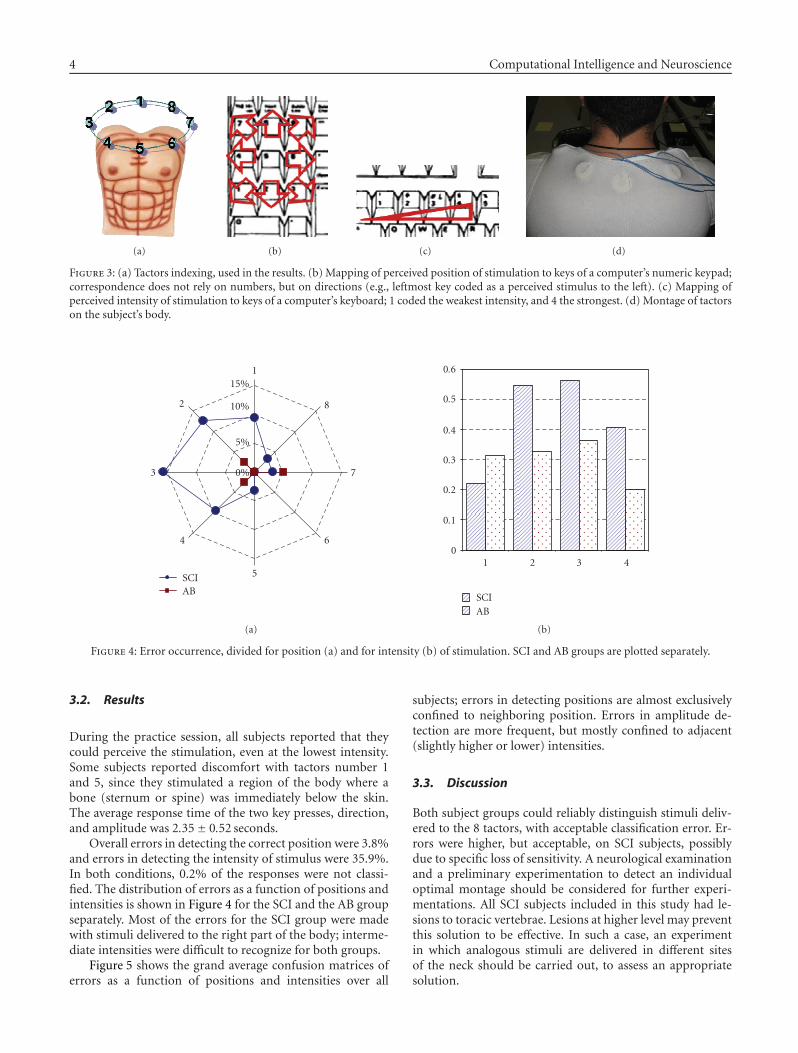
4 Computational Intelligence and Neuroscience
(a) (b) (c) (d)
Figure 3: (a) Tactors indexing, used in the results. (b) Mapping of perceived position of stimulation to keys of a computer’s numeric keypad;correspondence does not rely on numbers, but on directions (e.g., leftmost key coded as a perceived stimulus to the left). (c) Mapping ofperceived intensity of stimulation to keys of a computer’s keyboard; 1 coded the weakest intensity, and 4 the strongest. (d) Montage of tactorson the subject’s body.
1
2
3
4
5
6
7
8
0%
5%
10%
15%
SCIAB
(a)
0
0.1
0.2
0.3
0.4
0.5
0.6
SCIAB
1 2 3 4
(b)
Figure 4: Error occurrence, divided for position (a) and for intensity (b) of stimulation. SCI and AB groups are plotted separately.
3.2. Results
During the practice session, all subjects reported that theycould perceive the stimulation, even at the lowest intensity.Some subjects reported discomfort with tactors number 1and 5, since they stimulated a region of the body where abone (sternum or spine) was immediately below the skin.The average response time of the two key presses, direction,and amplitude was 2.35± 0.52 seconds.
Overall errors in detecting the correct position were 3.8%and errors in detecting the intensity of stimulus were 35.9%.In both conditions, 0.2% of the responses were not classi-fied. The distribution of errors as a function of positions andintensities is shown in Figure 4 for the SCI and the AB groupseparately. Most of the errors for the SCI group were madewith stimuli delivered to the right part of the body; interme-diate intensities were difficult to recognize for both groups.
Figure 5 shows the grand average confusion matrices oferrors as a function of positions and intensities over all
subjects; errors in detecting positions are almost exclusivelyconfined to neighboring position. Errors in amplitude de-tection are more frequent, but mostly confined to adjacent(slightly higher or lower) intensities.
3.3. Discussion
Both subject groups could reliably distinguish stimuli deliv-ered to the 8 tactors, with acceptable classification error. Er-rors were higher, but acceptable, on SCI subjects, possiblydue to specific loss of sensitivity. A neurological examinationand a preliminary experimentation to detect an individualoptimal montage should be considered for further experi-mentations. All SCI subjects included in this study had le-sions to toracic vertebrae. Lesions at higher level may preventthis solution to be effective. In such a case, an experimentin which analogous stimuli are delivered in different sitesof the neck should be carried out, to assess an appropriatesolution.
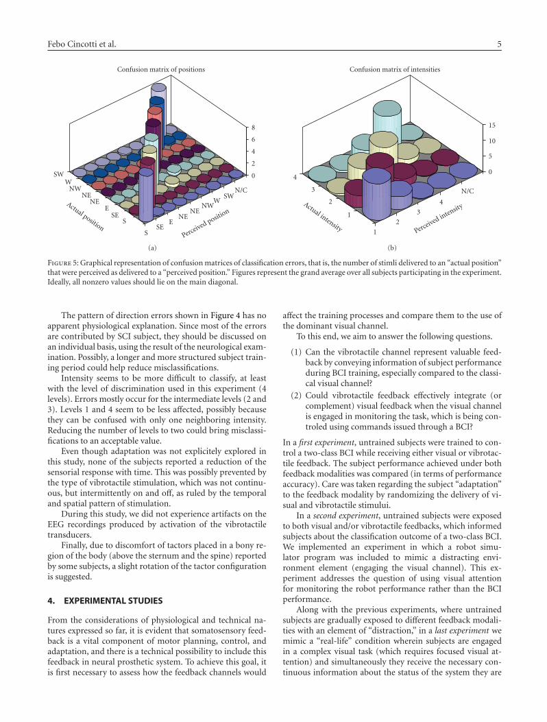
Febo Cincotti et al. 5
0
2
4
6
8
SWW
NWNE
NEE
SES
Actual positionS
SEE
NENE
NWW
SWN/C
Perceived position
Confusion matrix of positions
(a)
0
5
10
15
4
3
2
1
Actual intensity1
2
3
4
N/C
Perceived intensity
Confusion matrix of intensities
(b)
Figure 5: Graphical representation of confusion matrices of classification errors, that is, the number of stimli delivered to an “actual position”that were perceived as delivered to a “perceived position.” Figures represent the grand average over all subjects participating in the experiment.Ideally, all nonzero values should lie on the main diagonal.
The pattern of direction errors shown in Figure 4 has noapparent physiological explanation. Since most of the errorsare contributed by SCI subject, they should be discussed onan individual basis, using the result of the neurological exam-ination. Possibly, a longer and more structured subject train-ing period could help reduce misclassifications.
Intensity seems to be more difficult to classify, at leastwith the level of discrimination used in this experiment (4levels). Errors mostly occur for the intermediate levels (2 and3). Levels 1 and 4 seem to be less affected, possibly becausethey can be confused with only one neighboring intensity.Reducing the number of levels to two could bring misclassi-fications to an acceptable value.
Even though adaptation was not explicitely explored inthis study, none of the subjects reported a reduction of thesensorial response with time. This was possibly prevented bythe type of vibrotactile stimulation, which was not continu-ous, but intermittently on and off, as ruled by the temporaland spatial pattern of stimulation.
During this study, we did not experience artifacts on theEEG recordings produced by activation of the vibrotactiletransducers.
Finally, due to discomfort of tactors placed in a bony re-gion of the body (above the sternum and the spine) reportedby some subjects, a slight rotation of the tactor configurationis suggested.
4. EXPERIMENTAL STUDIES
From the considerations of physiological and technical na-tures expressed so far, it is evident that somatosensory feed-back is a vital component of motor planning, control, andadaptation, and there is a technical possibility to include thisfeedback in neural prosthetic system. To achieve this goal, itis first necessary to assess how the feedback channels would
affect the training processes and compare them to the use ofthe dominant visual channel.
To this end, we aim to answer the following questions.
(1) Can the vibrotactile channel represent valuable feed-back by conveying information of subject performanceduring BCI training, especially compared to the classi-cal visual channel?
(2) Could vibrotactile feedback effectively integrate (orcomplement) visual feedback when the visual channelis engaged in monitoring the task, which is being con-troled using commands issued through a BCI?
In a first experiment, untrained subjects were trained to con-trol a two-class BCI while receiving either visual or vibrotac-tile feedback. The subject performance achieved under bothfeedback modalities was compared (in terms of performanceaccuracy). Care was taken regarding the subject “adaptation”to the feedback modality by randomizing the delivery of vi-sual and vibrotactile stimului.
In a second experiment, untrained subjects were exposedto both visual and/or vibrotactile feedbacks, which informedsubjects about the classification outcome of a two-class BCI.We implemented an experiment in which a robot simu-lator program was included to mimic a distracting envi-ronment element (engaging the visual channel). This ex-periment addresses the question of using visual attentionfor monitoring the robot performance rather than the BCIperformance.
Along with the previous experiments, where untrainedsubjects are gradually exposed to different feedback modali-ties with an element of “distraction,” in a last experiment wemimic a “real-life” condition wherein subjects are engagedin a complex visual task (which requires focused visual at-tention) and simultaneously they receive the necessary con-tinuous information about the status of the system they are
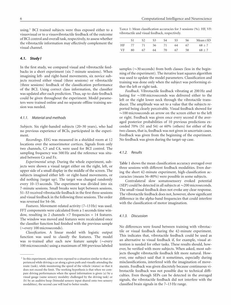
6 Computational Intelligence and Neuroscience
using.1 BCI trained subjects were thus exposed either to avisuovisual or to a visuovibrotactile feedback of the outcomeof BCI control and overall task, respectively, to assess whetherthe vibrotactile information may effectively complement thevisual channel.
4.1. Study I
In the first study, we compared visual and vibrotactile feed-backs in a short experiment (six 7-minute sessions). Whenimagining left- and right-hand movements, six novice sub-jects received either visual (three sessions) or vibrotactile(three sessions) feedback of the classification performanceof the BCI. Using correct class information, the classifierwas updated after each prediction. Thus, up-to-date feedbackcould be given throughout the experiment. Model parame-ters were trained online and no separate offline training ses-sion was needed.
4.1.1. Material and methods
Subjects. Six right-handed subjects (20–30 years), who hadno previous experience of BCIs, participated in the experi-ment.
Recordings. EEG was measured in a shielded room at 12locations over the sensorimotor cortices. Signals from onlytwo channels, C3 and C4, were used for BCI control. Thesampling frequency was 500 Hz and the reference was situ-ated between Cz and Fz.
Experimental setup. During the whole experiment, sub-jects were shown a visual target either on the right, left, orupper side of a small display in the middle of the screen. Thesubjects imagined either left- or right-hand movements, ordid nothing (target up). The target was changed randomlyevery 10–15 seconds. The experiment was divided into six7-minute sessions. Small breaks were kept between sessions.S1–S3 received vibrotactile feedback in the first three sessionsand visual feedback in the following three sessions. The orderwas reversed for S4–S6.
Features. Movement-related activity (7–13 Hz) was used.FFT components were calculated from a 1 seconds time win-dow, resulting in 2 channels ×7 frequencies = 14 features.The window was moved and features were recalculated oncethe classifier function had finished with the previous sample(∼every 100 microseconds).
Classification. A linear model with logistic outputfunction was used to classify the features. The modelwas re-trained after each new feature sample (∼every100 microseconds) using a maximum of 300 previous labeled
1 In this experiment, subjects were exposed to a situation similar to that ex-perienced while driving a car along a given path and visually attending theroute (task), while monitoring the speed of the vehicle (status) so that itdoes not exceed the limit. The working hypothesis is that when we com-pare driving performances when the speed information is given (a) by avisual gauge (same sensory modality challenged by the driving task) or(b) by an auditive beep (bimodal sensory input shared onto two sensorymodalities), the second case will lead to better results.
Table 1: Mean classification accuracies for 3 sessions (%). HF, VF:vibrotactile and visual feedback, respectively.
S1 S2 S3 S4 S5 S6 Mean±SD
HF 77 71 56 71 64 67 68± 7
VF 80 67 64 70 67 58 68± 7
samples (∼30 seconds) from both classes (less in the begin-ning of the experiment). The iterative least squares algorithmwas used to update the model parameters. Classification andtraining was done only when the subject was performing ei-ther the left or right task.
Feedback. Vibrotactile feedback vibrating at 200 Hz andlasting for ∼100 microseconds was delivered either to theleft or the right lower neck through the vibrotactile trans-ducer. The amplitude was set to a value that the subjects re-ported being clearly perceivable. Visual feedback showed for∼100 microseconds an arrow on the screen either to the leftor right. Feedback was given once every second if the aver-aged posterior probabilities of 10 previous predictions ex-ceeded 70% (S1 and S4) or 60% (others) for either of thetwo classes, that is, feedback was not given in uncertain cases.Feedback was given from the beginning of the experiment.No feedback was given during the target-up case.
4.1.2. Results
Table 1 shows the mean classification accuracy averaged overthree sessions with different feedback modalities. Even dur-ing the short 42-minute experiment, high-classification ac-curacies (means 56–80%) were possible in some subjects.
Contralateral slow somatosensory evoked potential(SEP) could be detected in all subjects at ∼200 microseconds.The small visual feedback does not evoke any clear response.The vibrotactile feedback does not, however, show significantdifference in the alpha-band frequencies that could interferewith the classification of motor imagination.
4.1.3. Discussion
No differences were found between training with vibrotac-tile or visual feedback during the 42-minute experiment.This indicates that, vibrotactile feedback could be used asan alternative to visual feedback if, for example, visual at-tention is needed for other tasks. These results should, how-ever, be verified with more subjects. When asked, most sub-jects thought vibrotactile feedback felt more natural. How-ever, one subject said that it sometimes, especially duringmisclassifications, interfered with the imagination of move-ments. Feedback was given discretely because continuous vi-brotactile feedback was not possible due to technical diffi-culties. Even though SEPs can be detected in the averagedsignals, the vibrotactile feedback did not interfere with theclassified brain signals in the 7–13 Hz range.
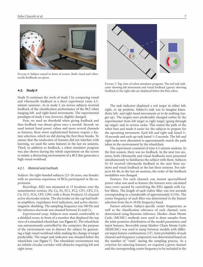
Febo Cincotti et al. 7
Figure 6: Subject seated in front of screen. Both visual and vibro-tactile feedbacks are given.
4.2. Study II
Study II continues the work of study I by comparing visualand vibrotactile feedback in a short experiment (nine 4.5-minute sessions). As in study I, six novice subjects receivedfeedback of the classification performance of the BCI whenimaging left- and right-hand movements. The experimentalparadigm of study I was, however, slightly changed.
First, we used no threshold when giving feedback andthus feedback was always given once a second. Second, weused instant band power values and more several channelsas features; these more sophisticated features require a fea-ture selection, which we did during the first three breaks. Toensure that the reselection of features did not interfere withlearning, we used the same features in the last six sessions.Third, in addition to feedback, a robot simulator programwas also shown during the whole experiment on the screento mimic a distracting environment of a BCI that generates ahigh visual workload.
4.2.1. Material and methods
Subjects. Six right-handed subjects (22–26 years, one female)with no previous experience of BCIs participated in the ex-periment.
Recordings. EEG was measured at 13 locations over thesensorimotor cortices (Fz, Cz, Pz, FC1, FC2, CP1, CP2, C3,C4, FC5, FC6, CP5, CP6) with a Brain Products 32-channelactive electrodes system. The electrodes on the cap had built-in amplifiers, impedance level indicators, and active electro-magnetic shielding. The sampling frequency was 500 Hz andthe reference electrode was situated between Fz and Cz.
Experimental setup. Subjects were seated comfortably ina shielded room, in front of a monitor that displayed the topview of a simulated wheelchair (see Figure 6). The wheelchairwas autonomously controlled by the computer; the purposeof the environment was to distract the subject by generat-ing a high visual workload while making the change of targetpredictable. The target task indicator was situated below thewheelchair (see Figure 7). The wheelchair environment wasan infinite circular corridor with obstacles requiring left andright turns.
Figure 7: Top view of robot simulator program. The red task indi-cator showing left movement and visual feedback (green) showingfeedback to the right side are displayed below the blue robot.
The task indicator displayed a red target in either left,right, or up position. Subject’s task was to imagine kines-thetic left- and right-hand movements or to do nothing (tar-get up). The targets were predictably changed online by theexperimenter from left target to right target (going throughup target) and in reverse order. This suited the path of therobot best and made it easier for the subjects to prepare forthe upcoming movement. Each left and right task lasted 5–10 seconds and each up-task lasted 1–2 seconds. The left andright tasks were alternated to approximately match the pathtaken in the environment by the wheelchair.
The experiment consisted of nine 4.5 minute sessions. Inthe first session, there was no feedback. In the next two ses-sions, both vibrotactile and visual feedbacks were presentedsimultaneously to familiarize the subject with them. SubjectsS1–S3 received vibrotactile feedback in the next three ses-sions and visual feedback in the last three sessions. For sub-jects S4–S6, in the last six sessions, the order of the feedbackmodalities was changed.
Features. For each channel, one instant spectral/bandpower value was used as feature; the features were calculatedonce every second by convolving the EEG signals with Ga-bor filters. The length of each Gabor filter was two secondscorresponding to a bandwidth of approximately 0.5 Hz. Thecenter frequency of each filter was determined in the featureselection from the 6–30 Hz frequency band.
Feature selection. Subject-specific center frequencies, aswell as the classification relevance of each channel, weredetermined using Bayesian inference. Markov chain MonteCarlo (MCMC) methods were used to draw samples fromthe joint posterior distribution of the model parameters andinput features. Reversible jump Markov Chain Monte Carlo(RJMCMC) was used to jump between models with differ-ent input feature combinations [17]. Joint probability of eachchannel and frequency component was determined based onthe number of “visits” during the sampling process. As acriterion for selecting features, we required a given channeland the corresponding centre frequency to be included in the

8 Computational Intelligence and Neuroscience
Table 2: The average subject performance in the training sessions2-3 (TS), vibrotactile feedback sessions (HF), and visual feedbacksessions (VF). S1–S3 were given vibrotactile feedback in sessions 4–6; conversely S4–S6 were shown visual feedback in sessions 4–6.
S1 S2 S3 S4 S5 S6 Mean±SD
TS 62 56 65 68 67 50 61± 7
HF 79 70 70 68 59 54 67± 9
VF 79 65 65 79 64 53 68± 10
model with sufficiently high posterior probability; we chosesix or more of the most probable features for which the jointprobability exceeded 0.25.
Feature selection was done during the breaks after ses-sions 1, 2, and 3. After sessions 1 and 2, the best Gabor fre-quency for each channel was determined using the data fromthe previous session. This Gabor frequency from all 13 chan-nels was included in the model used in the following sessions,2 and 3 correspondingly. After the third session, using datafrom sessions 2 and 3, RJMCMC sampling of input channelswas combined with the sampling of the Gabor frequencies todetermine the final channels and Gabor filters as features.
Classification. The classifier parameters were updated on-line once every second with the iterative least squares algo-rithm [18]. A prediction of the current class was made onceevery second for the newest sample before retraining of themodel; a maximum of 300 most recent samples (5 minutesof data) with correct class labels was used as training data foreach class.
In sessions 2–5 and 7-8, the model was trained onlineonce every second. In the beginning of sessions 2 and 3, amodel was used that was trained with the selected featuresusing the data from the previous session. During the thirdbreak, the final features were used to initialize a model whichwas then used in sessions 4 and 7; the resulting models werethen continued to be trained in sessions 5 and 8. The ob-tained models were tested, without training them, in sessionssix and nine.
Feedback. The subject was given visual and/or vibrotac-tile feedback once every second. The visual feedback was dis-played as a rose in the middle of the simulator screen with agreen segment to each of the four directions. The left and theright segments were lit for 200 microseconds correspondingto the output of the classifier (see Figure 7). The vibrotactilefeedback was given for 200 microseconds at 200 Hz with vi-brating elements attached with tape to the subject’s left- andright-side of the lower neck.
4.2.2. Results
Five subjects achieved high overall classification accuracies,on average as good as 59–79%, in the vibrotactile (HF), andvisual feedback (VF) sessions (see Table 2). The subjects per-formed between 160 and 247 trials per session. S6 did notgain control over chance level (50–54%). S1 obtained an av-erage accuracy of 79% for both feedback modalities and S4reached 79% for the visual feedback modality. The averageaccuracies in the training sessions (TS) were 6-7% lower than
the average accuracies in HF and VF sessions. We found nodifferences between average accuracies of the VF and HF ses-sions.
A response to the vibrotactile stimulation appears in the0–8 Hz and 30–40 Hz bands in synchrony with the onset andend of the vibrotactile stimulation. In the event-related po-tentials (ERP) to the vibrotactile stimulation, low-pass fil-tered below 10 Hz, an N200 peak can be seen in both hemi-spheres during left- and right-side vibrotactile stimulation.However, both these responses have no role in real-time clas-sification using time-frequency transformations in the 8–30 Hz frequency range.
4.2.3. Discussion
This study confirmed the results of study I; no differenceswere found between training with either vibrotactile or vi-sual feedback, during the short 41-minute experiment. Theseresults show that vibrotactile feedback could be used as analternative to visual feedback when starting to learn to usea BCI. The choice of feedback modality is therefore largelydependent on subjects’ preferences, indented environmentof use, and the application. The use of the robot simulatorprogram as a distracter did not disturb the subjects train-ing. As in study I, when asked, most of the subjects felt thatvibrotactile feedback was more natural. S1, S2, and S4 in-dicated that in the case of conflicting feedback, vibrotactilefeedback was more disturbing than visual feedback. Eventhough vibrotactile responses could be detected in the av-eraged signals, the vibrotactile feedback did not interferewith the classification of the brain signals in the 6–30 Hzrange.
S2–S5 performed better during the first feedback sessionscompared to the second ones, independently of the type offeedback. This can partly be explained by the fact that thesame model was used. Because the model was initialized af-ter session 3 it was not as much up-to-date as during the sec-ond feedback modality. The model was not updated duringthe testing sessions explaning why the results of the trainingsessions are better.
From study I and II, we conclude that short-term learn-ing is possible also with vibrotactile feedback. New experi-ments with more subjects are needed to evaluate the longer-term benefits of vibrotactile feedback. It should also be testedwhether vibrotactile feedback is useful to patients with re-duced sensing capabilities.
4.3. Study III
In study III, subjects were exposed to a joint visual and vi-brotactile feedback, to assess whether the vibrotactile infor-mation could complement the visual channel for feedback,when the visual channel is intensively used as a carrier oftask-related information. This experimental condition mim-icked a “real-life” condition where the subject, engaged ina given task (spatial navigation), could simultaneously re-ceive continuous information of his control strategy (feed-back). Continuous state of the control signal, rather than a
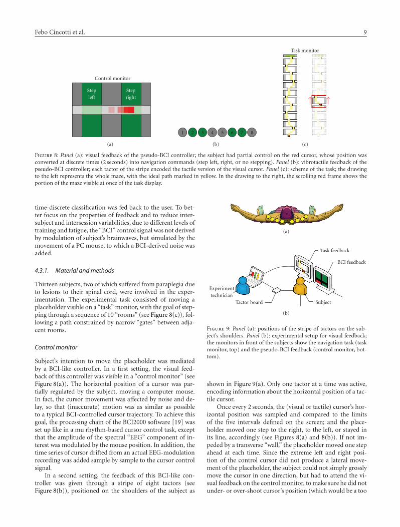
Febo Cincotti et al. 9
Control monitor
Stepleft
Stepright
(a)
1 2 3 4 5 6 7 8
(b)
Task monitor
(c)
Figure 8: Panel (a): visual feedback of the pseudo-BCI controller; the subject had partial control on the red cursor, whose position wasconverted at discrete times (2 seconds) into navigation commands (step left, right, or no stepping). Panel (b): vibrotactile feedback of thepseudo-BCI controller; each tactor of the stripe encoded the tactile version of the visual cursor. Panel (c): scheme of the task; the drawingto the left represents the whole maze, with the ideal path marked in yellow. In the drawing to the right, the scrolling red frame shows theportion of the maze visible at once of the task display.
time-discrete classification was fed back to the user. To bet-ter focus on the properties of feedback and to reduce inter-subject and intersession variabilities, due to different levels oftraining and fatigue, the “BCI” control signal was not derivedby modulation of subject’s brainwaves, but simulated by themovement of a PC mouse, to which a BCI-derived noise wasadded.
4.3.1. Material and methods
Thirteen subjects, two of which suffered from paraplegia dueto lesions to their spinal cord, were involved in the exper-imentation. The experimental task consisted of moving aplaceholder visible on a “task” monitor, with the goal of step-ping through a sequence of 10 “rooms” (see Figure 8(c)), fol-lowing a path constrained by narrow “gates” between adja-cent rooms.
Control monitor
Subject’s intention to move the placeholder was mediatedby a BCI-like controller. In a first setting, the visual feed-back of this controller was visible in a “control monitor” (seeFigure 8(a)). The horizontal position of a cursor was par-tially regulated by the subject, moving a computer mouse.In fact, the cursor movement was affected by noise and de-lay, so that (inaccurate) motion was as similar as possibleto a typical BCI-controlled cursor trajectory. To achieve thisgoal, the processing chain of the BCI2000 software [19] wasset up like in a mu rhythm-based cursor control task, exceptthat the amplitude of the spectral “EEG” component of in-terest was modulated by the mouse position. In addition, thetime series of cursor drifted from an actual EEG-modulationrecording was added sample by sample to the cursor controlsignal.
In a second setting, the feedback of this BCI-like con-troller was given through a stripe of eight tactors (seeFigure 8(b)), positioned on the shoulders of the subject as
(a)
Task feedback
BCI feedback
SubjectTactor board
Experimenttechnician
(b)
Figure 9: Panel (a): positions of the stripe of tactors on the sub-ject’s shoulders. Panel (b): experimental setup for visual feedback;the monitors in front of the subjects show the navigation task (taskmonitor, top) and the pseudo-BCI feedback (control monitor, bot-tom).
shown in Figure 9(a). Only one tactor at a time was active,encoding information about the horizontal position of a tac-tile cursor.
Once every 2 seconds, the (visual or tactile) cursor’s hor-izontal position was sampled and compared to the limitsof the five intervals defined on the screen; and the place-holder moved one step to the right, to the left, or stayed inits line, accordingly (see Figures 8(a) and 8(b)). If not im-peded by a transverse “wall,” the placeholder moved one stepahead at each time. Since the extreme left and right posi-tion of the control cursor did not produce a lateral move-ment of the placeholder, the subject could not simply grosslymove the cursor in one direction, but had to attend the vi-sual feedback on the control monitor, to make sure he did notunder- or over-shoot cursor’s position (which would be a too
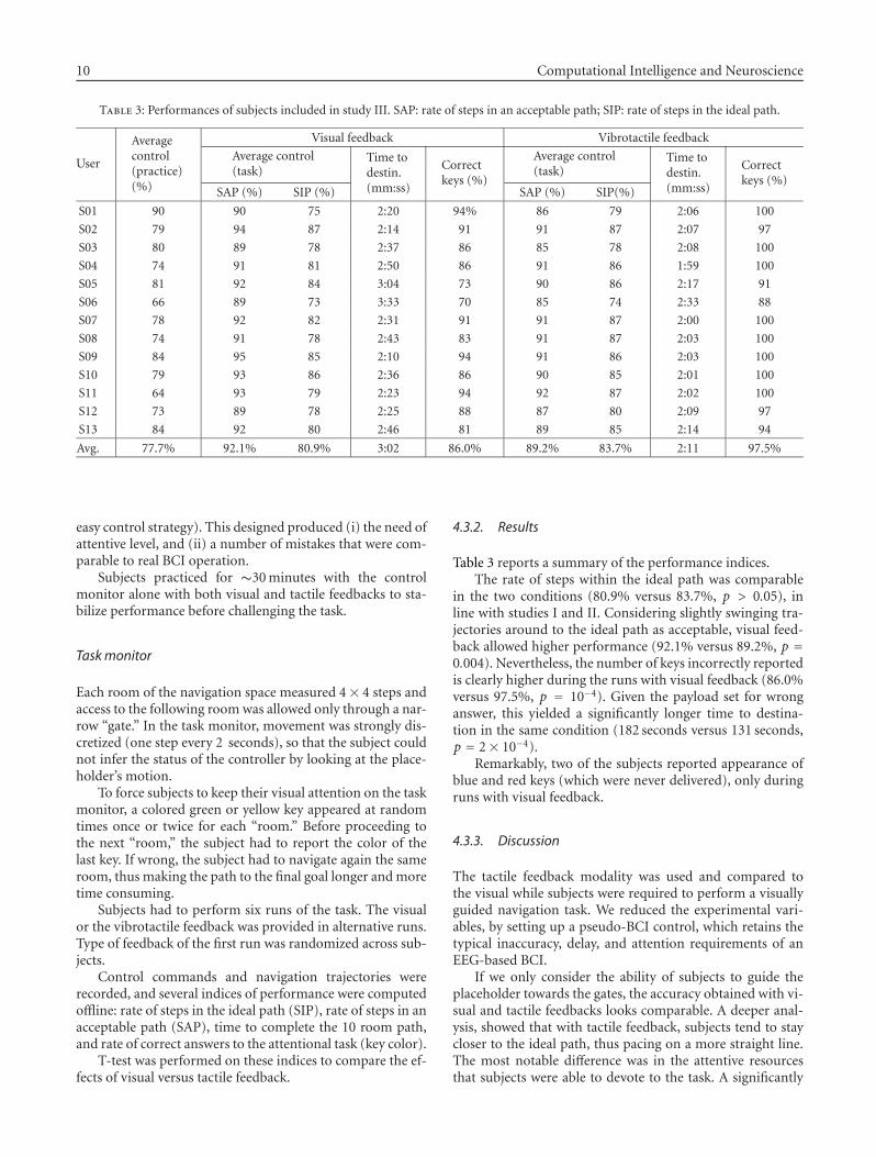
10 Computational Intelligence and Neuroscience
Table 3: Performances of subjects included in study III. SAP: rate of steps in an acceptable path; SIP: rate of steps in the ideal path.
User
Averagecontrol(practice)(%)
Visual feedback Vibrotactile feedback
Average control(task)
Time todestin.(mm:ss)
Correctkeys (%)
Average control(task)
Time todestin.(mm:ss)
Correctkeys (%)
SAP (%) SIP (%) SAP (%) SIP(%)
S01 90 90 75 2:20 94% 86 79 2:06 100
S02 79 94 87 2:14 91 91 87 2:07 97
S03 80 89 78 2:37 86 85 78 2:08 100
S04 74 91 81 2:50 86 91 86 1:59 100
S05 81 92 84 3:04 73 90 86 2:17 91
S06 66 89 73 3:33 70 85 74 2:33 88
S07 78 92 82 2:31 91 91 87 2:00 100
S08 74 91 78 2:43 83 91 87 2:03 100
S09 84 95 85 2:10 94 91 86 2:03 100
S10 79 93 86 2:36 86 90 85 2:01 100
S11 64 93 79 2:23 94 92 87 2:02 100
S12 73 89 78 2:25 88 87 80 2:09 97
S13 84 92 80 2:46 81 89 85 2:14 94
Avg. 77.7% 92.1% 80.9% 3:02 86.0% 89.2% 83.7% 2:11 97.5%
easy control strategy). This designed produced (i) the need ofattentive level, and (ii) a number of mistakes that were com-parable to real BCI operation.
Subjects practiced for ∼30 minutes with the controlmonitor alone with both visual and tactile feedbacks to sta-bilize performance before challenging the task.
Task monitor
Each room of the navigation space measured 4× 4 steps andaccess to the following room was allowed only through a nar-row “gate.” In the task monitor, movement was strongly dis-cretized (one step every 2 seconds), so that the subject couldnot infer the status of the controller by looking at the place-holder’s motion.
To force subjects to keep their visual attention on the taskmonitor, a colored green or yellow key appeared at randomtimes once or twice for each “room.” Before proceeding tothe next “room,” the subject had to report the color of thelast key. If wrong, the subject had to navigate again the sameroom, thus making the path to the final goal longer and moretime consuming.
Subjects had to perform six runs of the task. The visualor the vibrotactile feedback was provided in alternative runs.Type of feedback of the first run was randomized across sub-jects.
Control commands and navigation trajectories wererecorded, and several indices of performance were computedoffline: rate of steps in the ideal path (SIP), rate of steps in anacceptable path (SAP), time to complete the 10 room path,and rate of correct answers to the attentional task (key color).
T-test was performed on these indices to compare the ef-fects of visual versus tactile feedback.
4.3.2. Results
Table 3 reports a summary of the performance indices.The rate of steps within the ideal path was comparable
in the two conditions (80.9% versus 83.7%, p > 0.05), inline with studies I and II. Considering slightly swinging tra-jectories around to the ideal path as acceptable, visual feed-back allowed higher performance (92.1% versus 89.2%, p =0.004). Nevertheless, the number of keys incorrectly reportedis clearly higher during the runs with visual feedback (86.0%versus 97.5%, p = 10−4). Given the payload set for wronganswer, this yielded a significantly longer time to destina-tion in the same condition (182 seconds versus 131 seconds,p = 2× 10⁻⁴).
Remarkably, two of the subjects reported appearance ofblue and red keys (which were never delivered), only duringruns with visual feedback.
4.3.3. Discussion
The tactile feedback modality was used and compared tothe visual while subjects were required to perform a visuallyguided navigation task. We reduced the experimental vari-ables, by setting up a pseudo-BCI control, which retains thetypical inaccuracy, delay, and attention requirements of anEEG-based BCI.
If we only consider the ability of subjects to guide theplaceholder towards the gates, the accuracy obtained with vi-sual and tactile feedbacks looks comparable. A deeper anal-ysis, showed that with tactile feedback, subjects tend to staycloser to the ideal path, thus pacing on a more straight line.The most notable difference was in the attentive resourcesthat subjects were able to devote to the task. A significantly
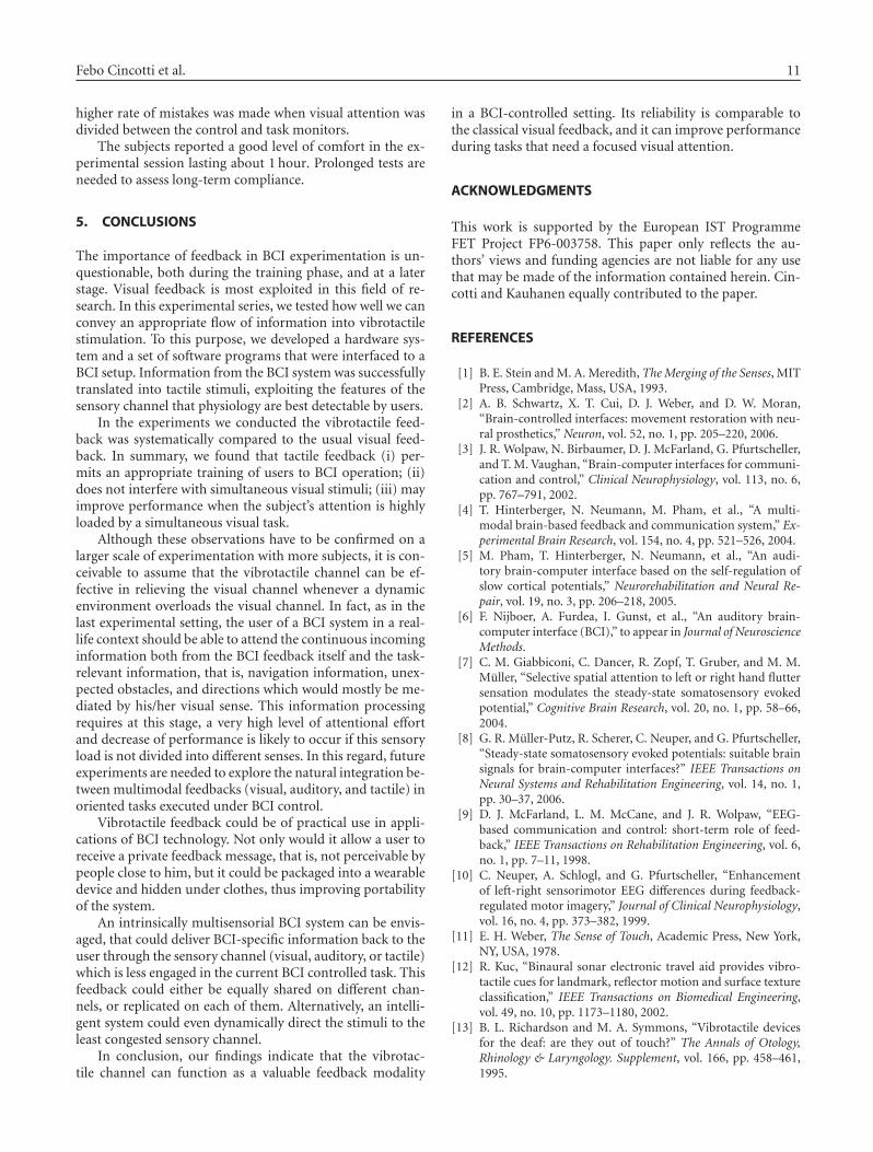
Febo Cincotti et al. 11
higher rate of mistakes was made when visual attention wasdivided between the control and task monitors.
The subjects reported a good level of comfort in the ex-perimental session lasting about 1 hour. Prolonged tests areneeded to assess long-term compliance.
5. CONCLUSIONS
The importance of feedback in BCI experimentation is un-questionable, both during the training phase, and at a laterstage. Visual feedback is most exploited in this field of re-search. In this experimental series, we tested how well we canconvey an appropriate flow of information into vibrotactilestimulation. To this purpose, we developed a hardware sys-tem and a set of software programs that were interfaced to aBCI setup. Information from the BCI system was successfullytranslated into tactile stimuli, exploiting the features of thesensory channel that physiology are best detectable by users.
In the experiments we conducted the vibrotactile feed-back was systematically compared to the usual visual feed-back. In summary, we found that tactile feedback (i) per-mits an appropriate training of users to BCI operation; (ii)does not interfere with simultaneous visual stimuli; (iii) mayimprove performance when the subject’s attention is highlyloaded by a simultaneous visual task.
Although these observations have to be confirmed on alarger scale of experimentation with more subjects, it is con-ceivable to assume that the vibrotactile channel can be ef-fective in relieving the visual channel whenever a dynamicenvironment overloads the visual channel. In fact, as in thelast experimental setting, the user of a BCI system in a real-life context should be able to attend the continuous incominginformation both from the BCI feedback itself and the task-relevant information, that is, navigation information, unex-pected obstacles, and directions which would mostly be me-diated by his/her visual sense. This information processingrequires at this stage, a very high level of attentional effortand decrease of performance is likely to occur if this sensoryload is not divided into different senses. In this regard, futureexperiments are needed to explore the natural integration be-tween multimodal feedbacks (visual, auditory, and tactile) inoriented tasks executed under BCI control.
Vibrotactile feedback could be of practical use in appli-cations of BCI technology. Not only would it allow a user toreceive a private feedback message, that is, not perceivable bypeople close to him, but it could be packaged into a wearabledevice and hidden under clothes, thus improving portabilityof the system.
An intrinsically multisensorial BCI system can be envis-aged, that could deliver BCI-specific information back to theuser through the sensory channel (visual, auditory, or tactile)which is less engaged in the current BCI controlled task. Thisfeedback could either be equally shared on different chan-nels, or replicated on each of them. Alternatively, an intelli-gent system could even dynamically direct the stimuli to theleast congested sensory channel.
In conclusion, our findings indicate that the vibrotac-tile channel can function as a valuable feedback modality
in a BCI-controlled setting. Its reliability is comparable tothe classical visual feedback, and it can improve performanceduring tasks that need a focused visual attention.
ACKNOWLEDGMENTS
This work is supported by the European IST ProgrammeFET Project FP6-003758. This paper only reflects the au-thors’ views and funding agencies are not liable for any usethat may be made of the information contained herein. Cin-cotti and Kauhanen equally contributed to the paper.
REFERENCES
[1] B. E. Stein and M. A. Meredith, The Merging of the Senses, MITPress, Cambridge, Mass, USA, 1993.
[2] A. B. Schwartz, X. T. Cui, D. J. Weber, and D. W. Moran,“Brain-controlled interfaces: movement restoration with neu-ral prosthetics,” Neuron, vol. 52, no. 1, pp. 205–220, 2006.
[3] J. R. Wolpaw, N. Birbaumer, D. J. McFarland, G. Pfurtscheller,and T. M. Vaughan, “Brain-computer interfaces for communi-cation and control,” Clinical Neurophysiology, vol. 113, no. 6,pp. 767–791, 2002.
[4] T. Hinterberger, N. Neumann, M. Pham, et al., “A multi-modal brain-based feedback and communication system,” Ex-perimental Brain Research, vol. 154, no. 4, pp. 521–526, 2004.
[5] M. Pham, T. Hinterberger, N. Neumann, et al., “An audi-tory brain-computer interface based on the self-regulation ofslow cortical potentials,” Neurorehabilitation and Neural Re-pair, vol. 19, no. 3, pp. 206–218, 2005.
[6] F. Nijboer, A. Furdea, I. Gunst, et al., “An auditory brain-computer interface (BCI),” to appear in Journal of NeuroscienceMethods.
[7] C. M. Giabbiconi, C. Dancer, R. Zopf, T. Gruber, and M. M.Muller, “Selective spatial attention to left or right hand fluttersensation modulates the steady-state somatosensory evokedpotential,” Cognitive Brain Research, vol. 20, no. 1, pp. 58–66,2004.
[8] G. R. Muller-Putz, R. Scherer, C. Neuper, and G. Pfurtscheller,“Steady-state somatosensory evoked potentials: suitable brainsignals for brain-computer interfaces?” IEEE Transactions onNeural Systems and Rehabilitation Engineering, vol. 14, no. 1,pp. 30–37, 2006.
[9] D. J. McFarland, L. M. McCane, and J. R. Wolpaw, “EEG-based communication and control: short-term role of feed-back,” IEEE Transactions on Rehabilitation Engineering, vol. 6,no. 1, pp. 7–11, 1998.
[10] C. Neuper, A. Schlogl, and G. Pfurtscheller, “Enhancementof left-right sensorimotor EEG differences during feedback-regulated motor imagery,” Journal of Clinical Neurophysiology,vol. 16, no. 4, pp. 373–382, 1999.
[11] E. H. Weber, The Sense of Touch, Academic Press, New York,NY, USA, 1978.
[12] R. Kuc, “Binaural sonar electronic travel aid provides vibro-tactile cues for landmark, reflector motion and surface textureclassification,” IEEE Transactions on Biomedical Engineering,vol. 49, no. 10, pp. 1173–1180, 2002.
[13] B. L. Richardson and M. A. Symmons, “Vibrotactile devicesfor the deaf: are they out of touch?” The Annals of Otology,Rhinology & Laryngology. Supplement, vol. 166, pp. 458–461,1995.
12 Computational Intelligence and Neuroscience
[14] R. W. Cholewiak and A. A. Collins, “Vibrotactile localizationon the arm: effects of place, space, and age,” Perception andPsychophysics, vol. 65, no. 7, pp. 1058–1077, 2003.
[15] S. A. Brewster and L. M. Brown, “Non-visual information dis-play using tactons,” in Proceedings of the Conference on HumanFactors in Computing Systems (CHI ’04), pp. 787–788, Vienna,Austria, April 2004.
[16] L. M. Brown, S. A. Brewster, and H. C. Purchase, “A first in-vestigation into the effectiveness of tactons,” in Proceedings ofthe 1st Joint Eurohaptics Conference and Symposium on Hap-tic Interfaces for Virtual Environment and Teleoperator Systems(WHC ’05), vol. 00, pp. 167–176, Pisa, Italy, March 2005.
[17] P. J. Green, “Reversible jump Markov chain Monte Carlocomputation and Bayesian model determination,” Biometrika,vol. 82, no. 4, pp. 711–732, 1995.
[18] P. McCullaghJ and A. Nelder, Generalized Linear Models,Chapman and Hall, London, UK, 1989.
[19] G. Schalk, D. J. McFarland, T. Hinterberger, N. Birbaumer, andJ. R. Wolpaw, “BCI2000: a general-purpose brain-computerinterface (BCI) system,” IEEE Transactions on Biomedical En-gineering, vol. 51, no. 6, pp. 1034–1043, 2004.
Hindawi Publishing CorporationComputational Intelligence and NeuroscienceVolume 2007, Article ID 94397, 9 pagesdoi:10.1155/2007/94397
Research ArticleA Semisupervised Support Vector Machines Algorithmfor BCI Systems
Jianzhao Qin,1, 2 Yuanqing Li,1 and Wei Sun3
1 Institute of Automation Science and Engineering, South China University of Technology, Guangzhou 510640, China2 Shenzhen Institute of Advanced Integration Technology, Chinese Academy of Sciences,The Chinese University of Hong Kong, Hong Kong
3 School of Maths, Central-South University, Changsha 410008, China
Correspondence should be addressed to Jianzhao Qin, [email protected]
Received 30 January 2007; Accepted 18 June 2007
Recommended by Andrzej Cichocki
As an emerging technology, brain-computer interfaces (BCIs) bring us new communication interfaces which translate brain activ-ities into control signals for devices like computers, robots, and so forth. In this study, we propose a semisupervised support vectormachine (SVM) algorithm for brain-computer interface (BCI) systems, aiming at reducing the time-consuming training process.In this algorithm, we apply a semisupervised SVM for translating the features extracted from the electrical recordings of brain intocontrol signals. This SVM classifier is built from a small labeled data set and a large unlabeled data set. Meanwhile, to reduce thetime for training semisupervised SVM, we propose a batch-mode incremental learning method, which can also be easily appliedto the online BCI systems. Additionally, it is suggested in many studies that common spatial pattern (CSP) is very effective indiscriminating two different brain states. However, CSP needs a sufficient labeled data set. In order to overcome the drawback ofCSP, we suggest a two-stage feature extraction method for the semisupervised learning algorithm. We apply our algorithm to twoBCI experimental data sets. The offline data analysis results demonstrate the effectiveness of our algorithm.
Copyright © 2007 Jianzhao Qin et al. This is an open access article distributed under the Creative Commons Attribution License,which permits unrestricted use, distribution, and reproduction in any medium, provided the original work is properly cited.
1. INTRODUCTION
A brain-computer interface is a communication system thatdoes not depend on brain’s normal output pathways of pe-ripheral nerves and muscles. It provides a new augmenta-tive communication technology to those who are paralyzedor have other severe movement deficits [1].
For many BCI systems, a tedious and time-consumingtraining process is needed to train the user and system pa-rameters, for example, the parameters of the translation algo-rithm. In BCI competition III, reducing the training processhas been explicitly proposed as a task by Schalk et al. [2].
In this paper, we resort to semisupervised learning totrain an SVM classifier. Compared with the case of super-vised learning, semisupervised learning can build better clas-sifiers by using large amounts of unlabeled data, when the la-beled data are expensive or time consuming to obtain [3, 4](in BCI systems, the training process can be taken as thelabeling process). Thus, the performance of semisupervisedlearning can still be satisfactory. The semisupervised learning
algorithms that have been developed so far include EM algo-rithm [5], self-training algorithm [6], cotraining algorithm[7], graph-based methods [8, 9], and so forth. A survey ofsemisupervised learning can be found in [3, 4].
In [10], Bennett and Demiriz proposed a semisupervisedSVM. Given a set of labeled data and a set of unlabeled data, asemisupervised SVM was trained using both the labeled dataand unlabeled data. This algorithm can be implemented us-ing mixed integer programming. However, since the compu-tational burden of mixed integer programming will increasegreatly with the number of integer variables (i.e., the num-ber of unlabeled samples), it is unacceptable when the sizeof the unlabeled data set is large, especially when we applythis algorithm to the online BCI system. Thus, we propose abatch-mode incremental training method for the semisuper-vised SVM.
There are two basic ideas in this method: (1) we assumethat the users’ electroencephalography (EEG) change grad-ually during the use of BCI systems. Therefore we can de-compose the unlabeled data set into several subsets; then we
2 Computational Intelligence and Neuroscience
use mixed integer programming to adjust the parameters ofthe semisupervised SVM incrementally with the entering ofeach subset, that is, we do mixed integer programming onlybased on a small-scale unlabeled data set each time. (2) Foreach unlabeled subset, we first select and label the most reli-able data; then do the mixed integer programming based onthe remaining unlabeled data set. This can further reduce thenumber of integer variables (i.e., the number of unlabeleddata) for each running of the mixed integer programming.
Additionally, in BCI systems, the common spatial pat-terns (CSP) method is very effective for extracting featuresfrom the EEG recordings [11–13] (we refer to the feature ex-tracted by CSP method as “CSP feature” in this paper). Theextraction of the CSP feature is label dependent, that is, theCSP feature should be extracted from the labeled data set. Ifthe number of labeled samples is too small, the transforma-tion matrix for CSP feature extraction cannot be estimatedaccurately. This will result in an ineffective CSP feature. Inorder to overcome the drawback of CSP feature, we suggesta two-stage feature extraction method, that is, we first ex-tract a dynamic power feature and perform an initial clas-sification on a part of the unlabeled data at the first stage(the first several loops) of our semisupervised learning algo-rithm. Next, we extend the small labeled data set by includingthe most confidently classified unlabeled data with the pre-dicted labels. Based on the extended labeled data set, some-what reliable CSP features and better classification result canbe obtained at the second stage (the remaining loops) of oursemisupervised learning algorithm.
We evaluate the semisupervised SVM algorithm using adata set from an EEG-based cursor control experiment car-ried out in Wadsworth Center [14] and a data set from amovement imagination experiment provided by Departmentof Computer Engineering University of Tubingen, Germany,and Institute of Medical Psychology and Behavioral Neuro-biology [15]. Data analysis results demonstrate the validity ofour algorithm.
The organization of this paper is as follows. In Section 2,we introduce the proposed methods, including feature ex-traction, semisupervised SVM, and batch-mode incremen-tal training. Section 3 presents the data analysis results. InSection 4, we discuss our algorithm in detail.
2. METHODS
In this section, we first present the dynamic CSP feature ex-traction and the dynamic power feature extraction method;then we combine them to form a two-stage feature extractionmethod. Next, we introduce the semisupervised SVM algo-rithm. Finally we present the batch-mode incremental learn-ing method for training the semisupervised SVM.
2.1. Dynamic CSP feature extraction
The common spatial patterns (CSP) is a method that hasbeen applied to EEG analysis to classify the normal versus ab-normal EEGs [16] and find spatial structures of event-related(de-)synchronization [12]. We define two CSP feature in this
paper: (1) nonnormalized CSP feature, (2) normalized CSPfeature. The nonnormalized CSP feature is extracted directlyfrom the covariance matrix of the raw or filtered EEG sig-nal. The normalized CSP feature is extracted from the nor-malized covariance matrix of the raw or filtered EEG signal.The advantages of the nonnormalized CSP feature are: (1) itkeeps the amplitude information of the EEG signal; (2) itsdimension is usually half of the normalized CSP feature. Thenormalized CSP feature also has its advantages. It can reducethe influence of the scaling (due to the change of the elec-trode impedances or other causes) of the amplitude of therecorded EEG.
Now, we present the extraction of the dynamic nonnor-malized CSP feature, which is similar to the method de-scribed in [11]. First, we filter the raw EEG in μ rhythm fre-quency band. The following CSP feature extraction is basedon the filtered signals. In order to reflect the change of brainsignals during a trial, we extract a dynamic CSP feature, thatis, we separate the time interval of each trial into f over-lapped time segments. For each time segment, we calculatea CSP feature vector as follows. The CSP analysis in the ith(i = 1, . . . , f ) time segment involves calculating a matrixWi and diagonal matrix Di through a joint diagonalizationmethod as (1):
WiZni WT
i = Di, WiZmi WT
i = 1−Di, (1)
where Zni and Zm
i are covariance matrices of EEG data matri-ces En
i and Emi (one row of the EEG data matrices corresponds
to one channel EEG signal). n and m denote two differentclasses (for the cursor control experiment, n and m repre-sent two different targets; for the movement imagination ex-periment, n and m denote two different movement imagi-nations). Using all trials with class n, we construct the matrixEni by trial-concatenating the filtered EEG data in the ith time
segments of every trial. Emi is obtained similarly except that it
corresponds to the trials with class m. The diagonal elementsof Di are sorted with a decreasing order.
After obtaining the transformation matrix Wi, we nowextract CSP feature in the ith time segment of a trial (i =1, . . . , f ). We first calculate a covariance matrix using the fil-tered EEG signals in the ith time segment; then we take thefirst p or the last p main diagonal elements of the trans-formed (by Wi) covariance matrix. Note that the first p diag-onal elements correspond to p largest eigenvalues in the di-agonal matrix Di above, the last p correspond to its p small-est eigenvalues. Thus we obtain a p-dimensional CSP fea-ture for each time segment. We concatenate the CSP featuresof f time segments to construct the p · f -dimensional dy-namic CSP feature of each trial, which is denoted as CF =[CF1, CF2, . . . , CF f ].
The normalized CSP feature [12] is almost the same asthe above CSP feature, except that: (1) the correlation matrixis normalized by dividing the trace of the correlation ma-trix; (2) the first p and the last p main diagonal elementsof the transformed covariance matrix are taken, then nor-malized by dividing the sum of the 2p elements followed bya log-transformation. The log transformation serves to ap-proximate normal distribution of the data [12]. Thus the
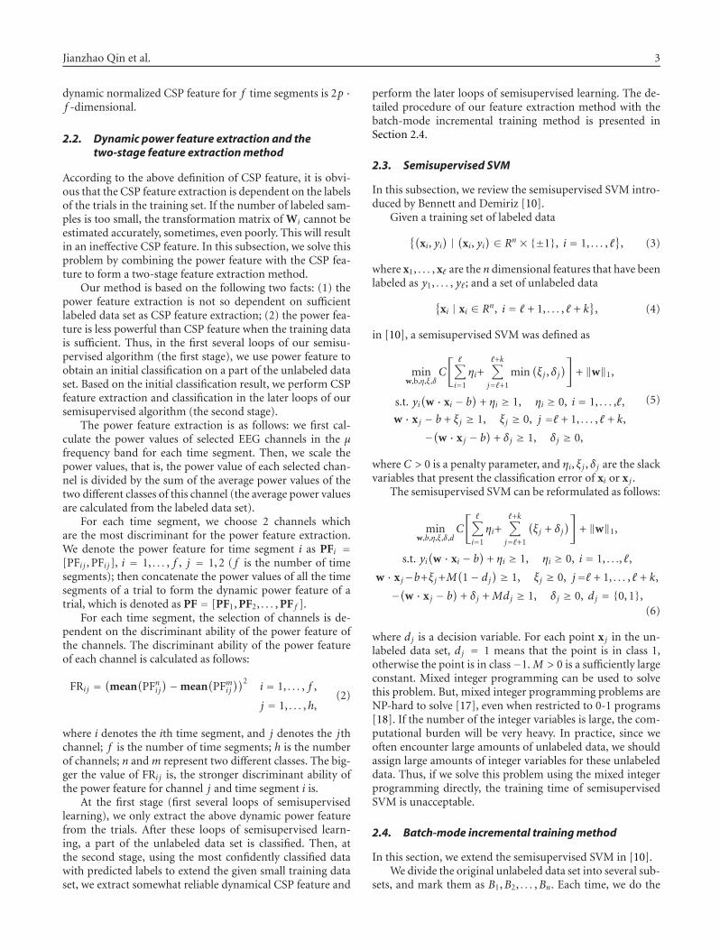
Jianzhao Qin et al. 3
dynamic normalized CSP feature for f time segments is 2p ·f -dimensional.
2.2. Dynamic power feature extraction and thetwo-stage feature extraction method
According to the above definition of CSP feature, it is obvi-ous that the CSP feature extraction is dependent on the labelsof the trials in the training set. If the number of labeled sam-ples is too small, the transformation matrix of Wi cannot beestimated accurately, sometimes, even poorly. This will resultin an ineffective CSP feature. In this subsection, we solve thisproblem by combining the power feature with the CSP fea-ture to form a two-stage feature extraction method.
Our method is based on the following two facts: (1) thepower feature extraction is not so dependent on sufficientlabeled data set as CSP feature extraction; (2) the power fea-ture is less powerful than CSP feature when the training datais sufficient. Thus, in the first several loops of our semisu-pervised algorithm (the first stage), we use power feature toobtain an initial classification on a part of the unlabeled dataset. Based on the initial classification result, we perform CSPfeature extraction and classification in the later loops of oursemisupervised algorithm (the second stage).
The power feature extraction is as follows: we first cal-culate the power values of selected EEG channels in the μfrequency band for each time segment. Then, we scale thepower values, that is, the power value of each selected chan-nel is divided by the sum of the average power values of thetwo different classes of this channel (the average power valuesare calculated from the labeled data set).
For each time segment, we choose 2 channels whichare the most discriminant for the power feature extraction.We denote the power feature for time segment i as PFi =[PFi j , PFi j], i = 1, . . . , f , j = 1, 2 ( f is the number of timesegments); then concatenate the power values of all the timesegments of a trial to form the dynamic power feature of atrial, which is denoted as PF = [PF1, PF2, . . . , PF f ].
For each time segment, the selection of channels is de-pendent on the discriminant ability of the power feature ofthe channels. The discriminant ability of the power featureof each channel is calculated as follows:
FRi j =(
mean(PFn
i j
)−mean(PFm
i j
))2i = 1, . . . , f ,
j = 1, . . . ,h,(2)
where i denotes the ith time segment, and j denotes the jthchannel; f is the number of time segments; h is the numberof channels; n and m represent two different classes. The big-ger the value of FRi j is, the stronger discriminant ability ofthe power feature for channel j and time segment i is.
At the first stage (first several loops of semisupervisedlearning), we only extract the above dynamic power featurefrom the trials. After these loops of semisupervised learn-ing, a part of the unlabeled data set is classified. Then, atthe second stage, using the most confidently classified datawith predicted labels to extend the given small training dataset, we extract somewhat reliable dynamical CSP feature and
perform the later loops of semisupervised learning. The de-tailed procedure of our feature extraction method with thebatch-mode incremental training method is presented inSection 2.4.
2.3. Semisupervised SVM
In this subsection, we review the semisupervised SVM intro-duced by Bennett and Demiriz [10].
Given a training set of labeled data
{(xi, yi
) | (xi, yi) ∈ Rn × {±1}, i = 1, . . . , �
}, (3)
where x1, . . . , x� are the n dimensional features that have beenlabeled as y1, . . . , y� ; and a set of unlabeled data
{xi | xi ∈ Rn, i = � + 1, . . . , � + k
}, (4)
in [10], a semisupervised SVM was defined as
minw,b,η,ξ,δ
C
[ �∑
i=1
ηi+�+k∑
j=�+1
min(ξj , δj
)]
+ ‖w‖1,
s.t. yi(
w · xi − b)
+ ηi ≥ 1, ηi ≥ 0, i = 1, . . . ,�,
w · x j − b + ξj ≥ 1, ξj ≥ 0, j =� + 1, . . . , � + k,
−(w · x j − b)
+ δj ≥ 1, δj ≥ 0,
(5)
where C > 0 is a penalty parameter, and ηi, ξj , δj are the slackvariables that present the classification error of xi or x j .
The semisupervised SVM can be reformulated as follows:
minw,b,η,ξ,δ,d
C
[ �∑
i=1
ηi+�+k∑
j=�+1
(ξj + δj
)]
+ ‖w‖1,
s.t. yi(
w · xi − b)
+ ηi ≥ 1, ηi ≥ 0, i = 1, . . ., �,
w · x j−b+ξj+M(1− dj
) ≥ 1, ξj ≥ 0, j=� + 1, . . . , � + k,
−(w · x j − b)
+ δj + Mdj ≥ 1, δj ≥ 0, dj = {0, 1},(6)
where dj is a decision variable. For each point x j in the un-labeled data set, dj = 1 means that the point is in class 1,otherwise the point is in class−1. M > 0 is a sufficiently largeconstant. Mixed integer programming can be used to solvethis problem. But, mixed integer programming problems areNP-hard to solve [17], even when restricted to 0-1 programs[18]. If the number of the integer variables is large, the com-putational burden will be very heavy. In practice, since weoften encounter large amounts of unlabeled data, we shouldassign large amounts of integer variables for these unlabeleddata. Thus, if we solve this problem using the mixed integerprogramming directly, the training time of semisupervisedSVM is unacceptable.
2.4. Batch-mode incremental training method
In this section, we extend the semisupervised SVM in [10].We divide the original unlabeled data set into several sub-
sets, and mark them as B1,B2, . . . ,Bn. Each time, we do the
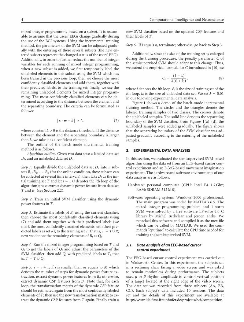
4 Computational Intelligence and Neuroscience
mixed integer programming based on a subset. It is reason-able to assume that the users’ EEGs change gradually duringthe use of the BCI systems. Using the incremental trainingmethod, the parameters of the SVM can be adjusted gradu-ally with the entering of these several subsets (the new en-tered subsets represent the changed status of the users’ EEG).Additionally, in order to further reduce the number of integervariables for each running of mixed integer programming,when a new subset is added, we first temporarily label theunlabeled elements in this subset using the SVM which hasbeen trained in the previous loop; then we choose the mostconfidently classified elements and add them, together withtheir predicted labels, to the training set; finally, we use theremaining unlabeled elements for mixed integer program-ming. The most confidently classified elements can be de-termined according to the distance between the element andthe separating boundary. The criteria can be formulated asfollows:
∣∣x ·w − b
∣∣ ≥ L, (7)
where constant L > 0 is the distance threshold. If the distancebetween the element and the separating boundary is largerthan L, we take it as a confident element.
The outline of the batch-mode incremental trainingmethod is as follows.
Algorithm outline. Given two data sets: a labeled data setDl, and an unlabeled data set Du.
Step 1. Equally divide the unlabeled data set Du into n sub-sets B1,B2, . . . ,Bn (for the online condition, these subsets canbe collected at several time intervals); then take Dl as the ini-tial training set T and let i = 1 (i denotes the ith loop of thealgorithm); next extract dynamic power feature from data setT and B1 (see Section 2.2).
Step 2. Train an initial SVM classifier using the dynamicpower features in T .
Step 3. Estimate the labels of Bi using the current classifier,then choose the most confidently classified elements using(7) and add them together with their predicted labels (wemark the most confidently classified elements with their pre-dicted labels as set R), to the training set T , that is, T = T∪R;next we denote the remaining elements of Bi as Qi.
Step 4. Run the mixed integer programming based on T andQi to get the labels of Qi and adjust the parameters of theSVM classifier; then add Qi with predicted labels to T , thatis, T = T ∪Qi.
Step 5. i = i + 1, if i is smaller than or equals to M whichdenotes the number of steps for dynamic power feature ex-traction, extract dynamic power features from Bi; otherwise,extract dynamic CSP features from Bi. Note that, for eachloop, the transformation matrix of the dynamic CSP featureshould be estimated again from the most confidently labeledelements of T ; then use the new transformation matrix to ex-tract the dynamic CSP features from T again. Finally train a
new SVM classifier based on the updated CSP features andtheir labels of T .
Step 6. If i equals n, terminate; otherwise, go back to Step 3.
Additionally, since the size of the training set is enlargedduring the training procedure, the penalty parameter C ofthe semisupervised SVM should adapt to this change. Thus,we extend the empirical formula for C introduced in [10] as:
Ci = (1− λ)λ(�i + ki
) , (8)
where i denotes the ith loop. �i is the size of training set of theith loop. ki is the size of unlabeled data set. We set λ = 0.01in our following experimental data analysis.
Figure 1 shows a demo of the batch-mode incrementaltraining method. The circles and the triangles denote thelabeled training samples of two classes. The crosses denotethe unlabeled samples. The solid line denotes the separatingboundary of the SVM classifier. From Figures 1(a)–(d), theunlabeled samples were added gradually. The figure showsthat the separating boundary of the SVM classifier was ad-justed gradually according to the entering of the unlabeledsamples.
3. EXPERIMENTAL DATA ANALYSIS
In this section, we evaluated the semisupervised SVM-basedalgorithm using the data set from an EEG-based cursor con-trol experiment and an ECoG-based movement imaginationexperiment. The hardware and software environments of ourdata analysis are as follows.
Hardware: personal computer (CPU: Intel P4 1.7 Ghz;RAM: SDRAM 512 MB).
Software: operating system: Windows 2000 professional.The main program was coded by MATLAB 6.5. Themixed integer programming problem and 1-normSVM were solved by a free software LP-solve 2.0 Clibrary by Michel Berkelaar and Jeroen Dirks. Werepacked this software and compiled it as the mex filewhich can be called by MATLAB. We used the com-mands “cputime” to calculate the CPU time needed fortraining the semisupervised SVM.
3.1. Data analysis of an EEG-based cursorcontrol experiment
The EEG-based cursor control experiment was carried outin Wadsworth Center. In this experiment, the subjects satin a reclining chair facing a video screen and was askedto remain motionless during performance. The subjectsused μ or β rhythm amplitude to control vertical positionof a target located at the right edge of the video screen.The data set was recorded from three subjects (AA, BB,CC). Each subject’s data included 10 sessions. The dataset and the details of this experiment are available athttp://www.ida.first.fraunhofer.de/projects/bci/competition.
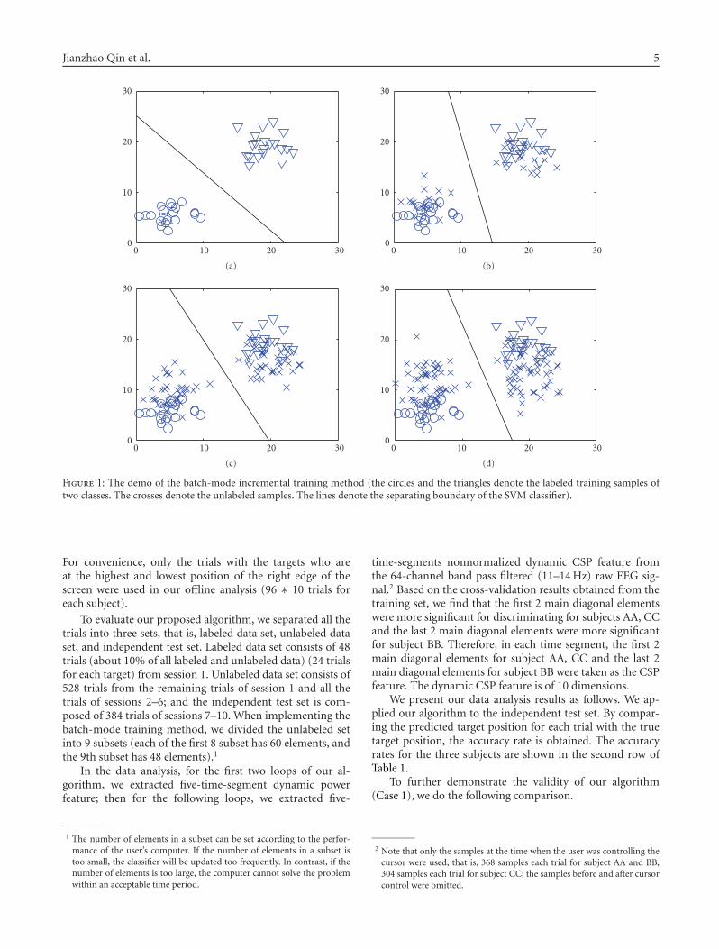
Jianzhao Qin et al. 5
0
10
20
30
0 10 20 30
(a)
0
10
20
30
0 10 20 30
(b)
0
10
20
30
0 10 20 30
(c)
0
10
20
30
0 10 20 30
(d)
Figure 1: The demo of the batch-mode incremental training method (the circles and the triangles denote the labeled training samples oftwo classes. The crosses denote the unlabeled samples. The lines denote the separating boundary of the SVM classifier).
For convenience, only the trials with the targets who areat the highest and lowest position of the right edge of thescreen were used in our offline analysis (96 ∗ 10 trials foreach subject).
To evaluate our proposed algorithm, we separated all thetrials into three sets, that is, labeled data set, unlabeled dataset, and independent test set. Labeled data set consists of 48trials (about 10% of all labeled and unlabeled data) (24 trialsfor each target) from session 1. Unlabeled data set consists of528 trials from the remaining trials of session 1 and all thetrials of sessions 2–6; and the independent test set is com-posed of 384 trials of sessions 7–10. When implementing thebatch-mode training method, we divided the unlabeled setinto 9 subsets (each of the first 8 subset has 60 elements, andthe 9th subset has 48 elements).1
In the data analysis, for the first two loops of our al-gorithm, we extracted five-time-segment dynamic powerfeature; then for the following loops, we extracted five-
1 The number of elements in a subset can be set according to the perfor-mance of the user’s computer. If the number of elements in a subset istoo small, the classifier will be updated too frequently. In contrast, if thenumber of elements is too large, the computer cannot solve the problemwithin an acceptable time period.
time-segments nonnormalized dynamic CSP feature fromthe 64-channel band pass filtered (11–14 Hz) raw EEG sig-nal.2 Based on the cross-validation results obtained from thetraining set, we find that the first 2 main diagonal elementswere more significant for discriminating for subjects AA, CCand the last 2 main diagonal elements were more significantfor subject BB. Therefore, in each time segment, the first 2main diagonal elements for subject AA, CC and the last 2main diagonal elements for subject BB were taken as the CSPfeature. The dynamic CSP feature is of 10 dimensions.
We present our data analysis results as follows. We ap-plied our algorithm to the independent test set. By compar-ing the predicted target position for each trial with the truetarget position, the accuracy rate is obtained. The accuracyrates for the three subjects are shown in the second row ofTable 1.
To further demonstrate the validity of our algorithm(Case 1), we do the following comparison.
2 Note that only the samples at the time when the user was controlling thecursor were used, that is, 368 samples each trial for subject AA and BB,304 samples each trial for subject CC; the samples before and after cursorcontrol were omitted.
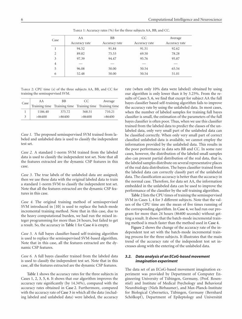
6 Computational Intelligence and Neuroscience
Table 1: Accuracy rates (%) for the three subjects AA, BB, and CC.
CaseAA BB CC Average
Accuracy rate Accuracy rate Accuracy rate Accuracy rate
1 94.52 91.84 91.51 92.62
2 89.82 75.53 69.50 78.28
3 97.39 94.47 95.76 95.87
4 — — — —
5 96.08 50.00 50.54 65.54
6 52.48 50.00 50.54 51.01
Table 2: CPU time (s) of the three subjects AA, BB, and CC fortraining the semisupervised SVM.
CaseAA BB CC Average
Training time Training time Training time Training time
1 1186.40 375.72 568.51 710.21
3 >86400 >86400 >86400 >86400
Case 1. The proposed semisupervised SVM trained from la-beled and unlabeled data is used to classify the independenttest set.
Case 2. A standard 1-norm SVM trained from the labeleddata is used to classify the independent test set. Note that allthe features extracted are the dynamic CSP features in thiscase.
Case 3. The true labels of the unlabeled data are assigned;then we use these data with the original labeled data to traina standard 1-norm SVM to classify the independent test set.Note that all the features extracted are the dynamic CSP fea-tures in this case.
Case 4. The original training method of semisupervisedSVM introduced in [10] is used to replace the batch-modeincremental training method. Note that in this case, due tothe heavy computational burden, we had run the mixed in-teger programming for more than 24 hours, but failed to geta result. So, the accuracy in Table 1 for Case 4 is empty.
Case 5. A full bayes classifier-based self-training algorithmis used to replace the semisupervised SVM-based algorithm.Note that in this case, all the features extracted are the dy-namic CSP features.
Case 6. A full bayes classifier trained from the labeled datais used to classify the independent test set. Note that in thiscase, all the features extracted are the dynamic CSP features.
Table 1 shows the accuracy rates for the three subjects inCases 1, 2, 3, 5, 6. It shows that our algorithm improves theaccuracy rate significantly (by 14.34%), compared with theaccuracy rates obtained in Case 2. Furthermore, comparedwith the accuracy rate of Case 3 in which all the data (includ-ing labeled and unlabeled data) were labeled, the accuracy
rate (when only 10% data were labeled) obtained by usingour algorithm is only lower than it by 3.25%. From the re-sults of Cases 5, 6, we find that except for subject AA the fullbayes classifier based self-training algorithm fails to improvethe accuracy rate by using the unlabeled data. In most cases,when the number of labeled samples for training full bayesclassifier is small, the estimation of the parameters of the fullbayes classifier is often poor. Thus, when we use this classifiertrained from the labeled data to predict the classes of the un-labeled data, only very small part of the unlabeled data canbe classified correctly. When only very small part of correctclassified unlabeled data is available, we cannot employ theinformation provided by the unlabeled data. This results inthe poor performance in data sets BB and CC. In some rarecases, however, the distribution of the labeled small samplesalso can present partial distribution of the real data, that is,the labeled samples distribute on several representative placesof the real data distribution. The bayes classifier trained fromthe labeled data can correctly classify part of the unlabeleddata. The classification accuracy is better than the accuracy inthe normal case. Therefore, for data set AA, the informationembedded in the unlabeled data can be used to improve theperformance of the classifier by the self-training algorithm.
Table 2 lists the CPU times of training the semisupervisedSVM in Cases 1, 4 for 3 different subjects. Note that the val-ues of the CPU time are the mean of five times running ofthe corresponding algorithm. In Case 4, we had run our pro-gram for more than 24 hours (86400 seconds) without get-ting a result. It shows that the batch-mode incremental train-ing method is much faster than the method used in Case 4.
Figure 2 shows the change of the accuracy rate of the in-dependent test set with the batch-mode incremental train-ing process for the three subjects. It illustrates that the maintrend of the accuracy rate of the independent test set in-creases along with the entering of the unlabeled data.
3.2. Data analysis of an ECoG-based movementimagination experiment
The data set of an ECoG-based movement imagination ex-periment was provided by Department of Computer En-gineering University of Tubingen, Germany, (Prof. Rosen-stiel) and Institute of Medical Psychology and BehavioralNeurobiology (Niels Birbaumer), and Max-Planck-Institutefor Biological Cybernetics, Tubingen, Germany (BernhardScholkopf), Department of Epileptology and Universitat
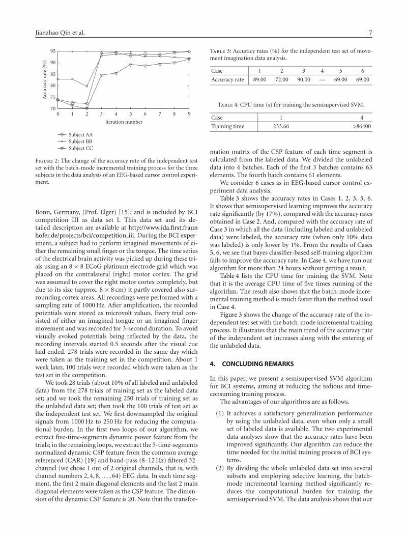
Jianzhao Qin et al. 7
70
75
80
85
90
95
0 1 2 3 4 5 6 7 8 9
Iteration number
Acc
ura
cyra
te(%
)
Subject AASubject BBSubject CC
Figure 2: The change of the accuracy rate of the independent testset with the batch-mode incremental training process for the threesubjects in the data analysis of an EEG-based cursor control experi-ment.
Bonn, Germany, (Prof. Elger) [15]; and is included by BCIcompetition III as data set I. This data set and its de-tailed description are available at http://www.ida.first.fraunhofer.de/projects/bci/competition iii. During the BCI exper-iment, a subject had to perform imagined movements of ei-ther the remaining small finger or the tongue. The time seriesof the electrical brain activity was picked up during these tri-als using an 8 × 8 ECoG platinum electrode grid which wasplaced on the contralateral (right) motor cortex. The gridwas assumed to cover the right motor cortex completely, butdue to its size (approx. 8 × 8 cm) it partly covered also sur-rounding cortex areas. All recordings were performed with asampling rate of 1000 Hz. After amplification, the recordedpotentials were stored as microvolt values. Every trial con-sisted of either an imagined tongue or an imagined fingermovement and was recorded for 3-second duration. To avoidvisually evoked potentials being reflected by the data, therecording intervals started 0.5 seconds after the visual cuehad ended. 278 trials were recorded in the same day whichwere taken as the training set in the competition. About 1week later, 100 trials were recorded which were taken as thetest set in the competition.
We took 28 trials (about 10% of all labeled and unlabeleddata) from the 278 trials of training set as the labeled dataset; and we took the remaining 250 trials of training set asthe unlabeled data set; then took the 100 trials of test set asthe independent test set. We first downsampled the originalsignals from 1000 Hz to 250 Hz for reducing the computa-tional burden. In the first two loops of our algorithm, weextract five-time-segments dynamic power feature from thetrials; in the remaining loops, we extract the 5-time-segmentsnormalized dynamic CSP feature from the common averagereferenced (CAR) [19] and band-pass (8–12 Hz) filtered 32-channel (we chose 1 out of 2 original channels, that is, withchannel numbers 2, 4, 8, . . . , 64) EEG data. In each time seg-ment, the first 2 main diagonal elements and the last 2 maindiagonal elements were taken as the CSP feature. The dimen-sion of the dynamic CSP feature is 20. Note that the transfor-
Table 3: Accuracy rates (%) for the independent test set of move-ment imagination data analysis.
Case 1 2 3 4 5 6
Accuracy rate 89.00 72.00 90.00 — 69.00 69.00
Table 4: CPU time (s) for training the semisupervised SVM.
Case 1 4
Training time 233.66 >86400
mation matrix of the CSP feature of each time segment iscalculated from the labeled data. We divided the unlabeleddata into 4 batches. Each of the first 3 batches contains 63elements. The fourth batch contains 61 elements.
We consider 6 cases as in EEG-based cursor control ex-periment data analysis.
Table 3 shows the accuracy rates in Cases 1, 2, 3, 5, 6.It shows that semisupervised learning improves the accuracyrate significantly (by 17%), compared with the accuracy ratesobtained in Case 2. And, compared with the accuracy rate ofCase 3 in which all the data (including labeled and unlabeleddata) were labeled, the accuracy rate (when only 10% datawas labeled) is only lower by 1%. From the results of Cases5, 6, we see that bayes classifier-based self-training algorithmfails to improve the accuracy rate. In Case 4, we have run ouralgorithm for more than 24 hours without getting a result.
Table 4 lists the CPU time for training the SVM. Notethat it is the average CPU time of five times running of thealgorithm. The result also shows that the batch-mode incre-mental training method is much faster than the method usedin Case 4.
Figure 3 shows the change of the accuracy rate of the in-dependent test set with the batch-mode incremental trainingprocess. It illustrates that the main trend of the accuracy rateof the independent set increases along with the entering ofthe unlabeled data.
4. CONCLUDING REMARKS
In this paper, we present a semisupervised SVM algorithmfor BCI systems, aiming at reducing the tedious and time-consuming training process.
The advantages of our algorithms are as follows.
(1) It achieves a satisfactory generalization performanceby using the unlabeled data, even when only a smallset of labeled data is available. The two experimentaldata analyses show that the accuracy rates have beenimproved significantly. Our algorithm can reduce thetime needed for the initial training process of BCI sys-tems.
(2) By dividing the whole unlabeled data set into severalsubsets and employing selective learning, the batch-mode incremental learning method significantly re-duces the computational burden for training thesemisupervised SVM. The data analysis shows that our
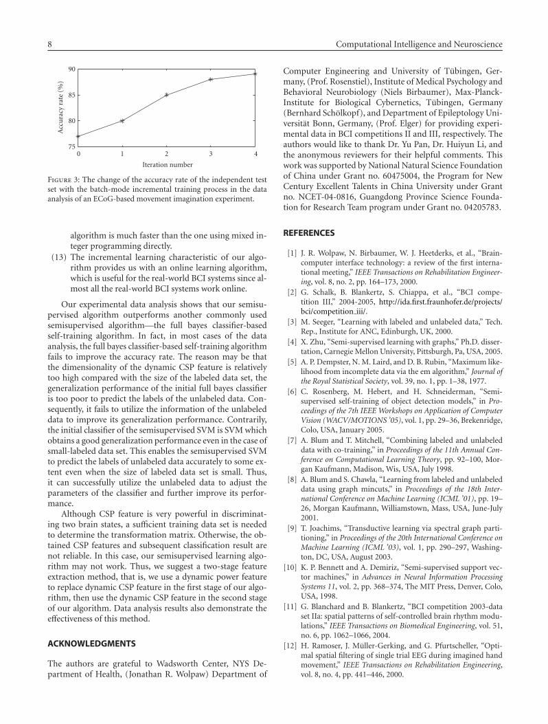
8 Computational Intelligence and Neuroscience
75
80
85
90
0 1 2 3 4
Iteration number
Acc
ura
cyra
te(%
)
Figure 3: The change of the accuracy rate of the independent testset with the batch-mode incremental training process in the dataanalysis of an ECoG-based movement imagination experiment.
algorithm is much faster than the one using mixed in-teger programming directly.
(13) The incremental learning characteristic of our algo-rithm provides us with an online learning algorithm,which is useful for the real-world BCI systems since al-most all the real-world BCI systems work online.
Our experimental data analysis shows that our semisu-pervised algorithm outperforms another commonly usedsemisupervised algorithm—the full bayes classifier-basedself-training algorithm. In fact, in most cases of the dataanalysis, the full bayes classifier-based self-training algorithmfails to improve the accuracy rate. The reason may be thatthe dimensionality of the dynamic CSP feature is relativelytoo high compared with the size of the labeled data set, thegeneralization performance of the initial full bayes classifieris too poor to predict the labels of the unlabeled data. Con-sequently, it fails to utilize the information of the unlabeleddata to improve its generalization performance. Contrarily,the initial classifier of the semisupervised SVM is SVM whichobtains a good generalization performance even in the case ofsmall-labeled data set. This enables the semisupervised SVMto predict the labels of unlabeled data accurately to some ex-tent even when the size of labeled data set is small. Thus,it can successfully utilize the unlabeled data to adjust theparameters of the classifier and further improve its perfor-mance.
Although CSP feature is very powerful in discriminat-ing two brain states, a sufficient training data set is neededto determine the transformation matrix. Otherwise, the ob-tained CSP features and subsequent classification result arenot reliable. In this case, our semisupervised learning algo-rithm may not work. Thus, we suggest a two-stage featureextraction method, that is, we use a dynamic power featureto replace dynamic CSP feature in the first stage of our algo-rithm, then use the dynamic CSP feature in the second stageof our algorithm. Data analysis results also demonstrate theeffectiveness of this method.
ACKNOWLEDGMENTS
The authors are grateful to Wadsworth Center, NYS De-partment of Health, (Jonathan R. Wolpaw) Department of
Computer Engineering and University of Tubingen, Ger-many, (Prof. Rosenstiel), Institute of Medical Psychology andBehavioral Neurobiology (Niels Birbaumer), Max-Planck-Institute for Biological Cybernetics, Tubingen, Germany(Bernhard Scholkopf), and Department of Epileptology Uni-versitat Bonn, Germany, (Prof. Elger) for providing experi-mental data in BCI competitions II and III, respectively. Theauthors would like to thank Dr. Yu Pan, Dr. Huiyun Li, andthe anonymous reviewers for their helpful comments. Thiswork was supported by National Natural Science Foundationof China under Grant no. 60475004, the Program for NewCentury Excellent Talents in China University under Grantno. NCET-04-0816, Guangdong Province Science Founda-tion for Research Team program under Grant no. 04205783.
REFERENCES
[1] J. R. Wolpaw, N. Birbaumer, W. J. Heetderks, et al., “Brain-computer interface technology: a review of the first interna-tional meeting,” IEEE Transactions on Rehabilitation Engineer-ing, vol. 8, no. 2, pp. 164–173, 2000.
[2] G. Schalk, B. Blankertz, S. Chiappa, et al., “BCI compe-tition III,” 2004-2005, http://ida.first.fraunhofer.de/projects/bci/competition iii/.
[3] M. Seeger, “Learning with labeled and unlabeled data,” Tech.Rep., Institute for ANC, Edinburgh, UK, 2000.
[4] X. Zhu, “Semi-supervised learning with graphs,” Ph.D. disser-tation, Carnegie Mellon University, Pittsburgh, Pa, USA, 2005.
[5] A. P. Dempster, N. M. Laird, and D. B. Rubin, “Maximum like-lihood from incomplete data via the em algorithm,” Journal ofthe Royal Statistical Society, vol. 39, no. 1, pp. 1–38, 1977.
[6] C. Rosenberg, M. Hebert, and H. Schneiderman, “Semi-supervised self-training of object detection models,” in Pro-ceedings of the 7th IEEE Workshops on Application of ComputerVision (WACV/MOTIONS ’05), vol. 1, pp. 29–36, Brekenridge,Colo, USA, January 2005.
[7] A. Blum and T. Mitchell, “Combining labeled and unlabeleddata with co-training,” in Proceedings of the 11th Annual Con-ference on Computational Learning Theory, pp. 92–100, Mor-gan Kaufmann, Madison, Wis, USA, July 1998.
[8] A. Blum and S. Chawla, “Learning from labeled and unlabeleddata using graph mincuts,” in Proceedings of the 18th Inter-national Conference on Machine Learning (ICML ’01), pp. 19–26, Morgan Kaufmann, Williamstown, Mass, USA, June-July2001.
[9] T. Joachims, “Transductive learning via spectral graph parti-tioning,” in Proceedings of the 20th International Conference onMachine Learning (ICML ’03), vol. 1, pp. 290–297, Washing-ton, DC, USA, August 2003.
[10] K. P. Bennett and A. Demiriz, “Semi-supervised support vec-tor machines,” in Advances in Neural Information ProcessingSystems 11, vol. 2, pp. 368–374, The MIT Press, Denver, Colo,USA, 1998.
[11] G. Blanchard and B. Blankertz, “BCI competition 2003-dataset IIa: spatial patterns of self-controlled brain rhythm modu-lations,” IEEE Transactions on Biomedical Engineering, vol. 51,no. 6, pp. 1062–1066, 2004.
[12] H. Ramoser, J. Muller-Gerking, and G. Pfurtscheller, “Opti-mal spatial filtering of single trial EEG during imagined handmovement,” IEEE Transactions on Rehabilitation Engineering,vol. 8, no. 4, pp. 441–446, 2000.
Jianzhao Qin et al. 9
[13] Y. Li, C. Guan, and J. Qin, “Enhancing feature extraction withsparse component analysis for brain-computer interface,” inProceedings of the 27th IEEE Annual International Conferenceof Engineering in Medicine and Biology (EMBS ’05), vol. 7, pp.5335–5338, Shanghai, China, September 2005.
[14] J. R. Wolpaw, D. J. McFarland, G. W. Neat, and C. A. Forneris,“An EEG-based brain-computer interface for cursor control,”Electroencephalography and Clinical Neurophysiology, vol. 78,no. 3, pp. 252–259, 1991.
[15] T. N. Lal, T. Hinterberger, G. Widman, et al., “Methods to-wards invasive human brain computer interfaces,” in Advancesin Neural Information Processing Systems 17, L. K. Saul, Y.Weiss, and L. Bottou, Eds., pp. 737–744, The MIT Press, Van-couver, Canada, 2004.
[16] Z. J. Koles, M. S. Lazar, and S. Z. Zhou, “Spatial patternsunderlying population differences in the background EEG,”Brain Topography, vol. 2, no. 4, pp. 275–284, 1990.
[17] R. M. Karp, “Reducibility among combinatorial problems,” inComplexity of Computer Computations, R. E. Miller and J. W.Thatcher, Eds., pp. 85–103, Plenum Press, New York, NY, USA,1972.
[18] S. Sahni, “Computationally related problems,” SIAM Journalon Computing, vol. 3, no. 4, pp. 262–279, 1974.
[19] O. Bertrand, F. Perrin, and J. Pernier, “A theoretical justifica-tion of the average reference in topographic evoked potentialstudies,” Electroencephalography and Clinical Neurophysiology,vol. 62, no. 6, pp. 462–464, 1985.
Hindawi Publishing CorporationComputational Intelligence and NeuroscienceVolume 2007, Article ID 25130, 12 pagesdoi:10.1155/2007/25130
Research ArticleContext-Based Filtering for Assisted Brain-ActuatedWheelchair Driving
Gerolf Vanacker,1 Jose del R. Millan,2 Eileen Lew,2 Pierre W. Ferrez,2 Ferran Galan Moles,2
Johan Philips,1 Hendrik Van Brussel,1 and Marnix Nuttin1
1 The Department of Mechanical Engineering, Katholieke Universiteit, 3001 Leuven, Belgium2 The IDIAP Research Institute, 1920 Martigny, Switzerland
Correspondence should be addressed to Gerolf Vanacker, [email protected]
Received 18 February 2007; Accepted 23 May 2007
Recommended by Fabio Babiloni
Controlling a robotic device by using human brain signals is an interesting and challenging task. The device may be complicated tocontrol and the nonstationary nature of the brain signals provides for a rather unstable input. With the use of intelligent processingalgorithms adapted to the task at hand, however, the performance can be increased. This paper introduces a shared control systemthat helps the subject in driving an intelligent wheelchair with a noninvasive brain interface. The subject’s steering intentions areestimated from electroencephalogram (EEG) signals and passed through to the shared control system before being sent to thewheelchair motors. Experimental results show a possibility for significant improvement in the overall driving performance whenusing the shared control system compared to driving without it. These results have been obtained with 2 healthy subjects duringtheir first day of training with the brain-actuated wheelchair.
Copyright © 2007 Gerolf Vanacker et al. This is an open access article distributed under the Creative Commons AttributionLicense, which permits unrestricted use, distribution, and reproduction in any medium, provided the original work is properlycited.
1. INTRODUCTION
The continuing progress in the research for noninvasiveBCI classification systems gives rise to a wealth of po-tential practical applications. The prospect of humans in-terfacing the mechanical world through brain-coupled de-vices and thereby controlling everyday machines throughthe process of mere thought is certainly an appealing oneas discussed in [1–3]. A promising class of applicationsare those concerning assistive devices for people with seri-ous impairments. The classical interfaces that disabled peo-ple commonly used to control or manipulate an assistivedevice typically require the patient to have adequate con-trol over one or more physical components of his or herbody. Typically, that would be one of the limbs: an arm,hand, or finger. Bioprosthetic systems that are controlled di-rectly through brain signals on the other hand could providefor a more natural extention of human capabilities. Espe-cially in the case where the patient is completely paralysed,this technology may provide for the only possible way forhim/her to gain control over basic aspects of his/her dailylife.
Amongst these, the ability to control the personal mobil-ity is generally considered an important one. The reductionin mobility that many people experience, due to various im-pairments or simply due to the effects of ageing, often has aprofound impact on the person’s independence, social activ-ity, and self-esteem. For many people suffering from a diverserange of impairments, the primary device that could providefor that mobility is the electrical wheelchair. It is worth not-ing, however, that in case of locked-in patients their highestpriority is not mobility. Still, learning how to make it pos-sible to drive complex devices such a wheelchair will alsolead to better communication and domotic tools. Many pa-tients, however, do not have the ability to exercise the de-manding fine control that wheelchair steering requires, evenwith an input device capable of communicating a high levelof detail, such as the classical joystick. Problems regardingnot only the physical inability to accurately manipulate thejoystick, but also a reduced kinematical and dynamical in-sight in the wheelchair motion regularly occur, as was seenin earlier work [4]. Therefore, the prospect of wheelchaircontrol through a brain-coupled control interface, which isin general less reliable than a classical interface, may seem a
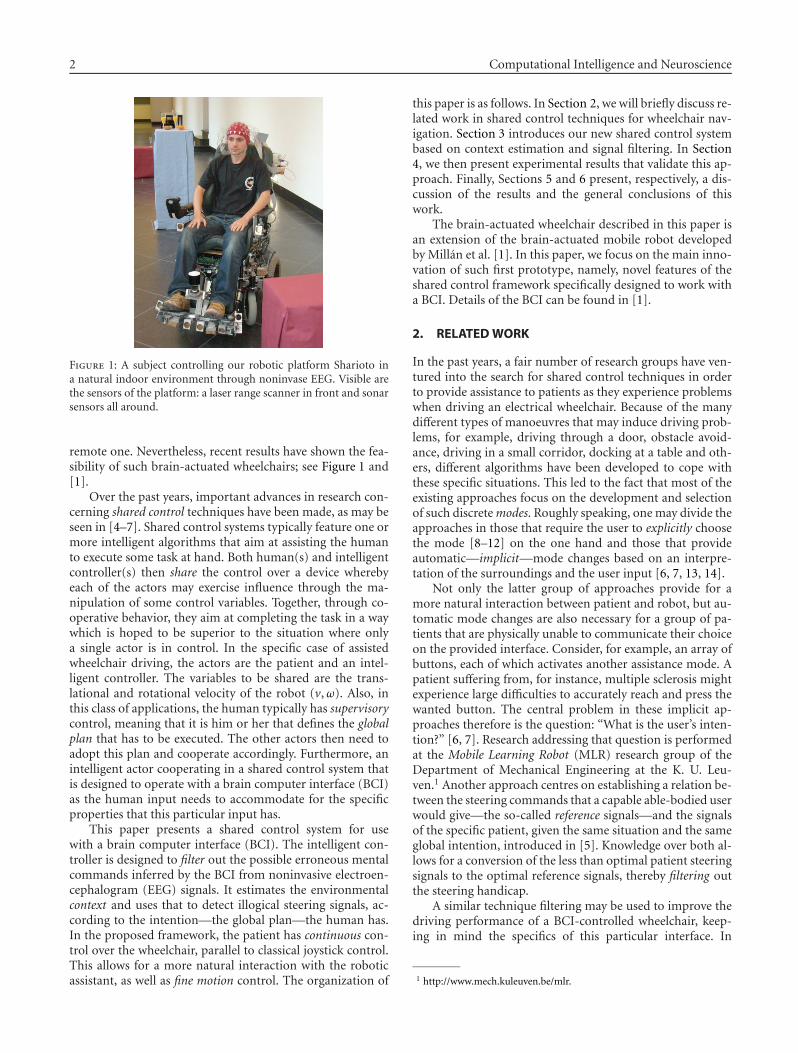
2 Computational Intelligence and Neuroscience
Figure 1: A subject controlling our robotic platform Sharioto ina natural indoor environment through noninvase EEG. Visible arethe sensors of the platform: a laser range scanner in front and sonarsensors all around.
remote one. Nevertheless, recent results have shown the fea-sibility of such brain-actuated wheelchairs; see Figure 1 and[1].
Over the past years, important advances in research con-cerning shared control techniques have been made, as may beseen in [4–7]. Shared control systems typically feature one ormore intelligent algorithms that aim at assisting the humanto execute some task at hand. Both human(s) and intelligentcontroller(s) then share the control over a device wherebyeach of the actors may exercise influence through the ma-nipulation of some control variables. Together, through co-operative behavior, they aim at completing the task in a waywhich is hoped to be superior to the situation where onlya single actor is in control. In the specific case of assistedwheelchair driving, the actors are the patient and an intel-ligent controller. The variables to be shared are the trans-lational and rotational velocity of the robot (v,ω). Also, inthis class of applications, the human typically has supervisorycontrol, meaning that it is him or her that defines the globalplan that has to be executed. The other actors then need toadopt this plan and cooperate accordingly. Furthermore, anintelligent actor cooperating in a shared control system thatis designed to operate with a brain computer interface (BCI)as the human input needs to accommodate for the specificproperties that this particular input has.
This paper presents a shared control system for usewith a brain computer interface (BCI). The intelligent con-troller is designed to filter out the possible erroneous mentalcommands inferred by the BCI from noninvasive electroen-cephalogram (EEG) signals. It estimates the environmentalcontext and uses that to detect illogical steering signals, ac-cording to the intention—the global plan—the human has.In the proposed framework, the patient has continuous con-trol over the wheelchair, parallel to classical joystick control.This allows for a more natural interaction with the roboticassistant, as well as fine motion control. The organization of
this paper is as follows. In Section 2, we will briefly discuss re-lated work in shared control techniques for wheelchair nav-igation. Section 3 introduces our new shared control systembased on context estimation and signal filtering. In Section4, we then present experimental results that validate this ap-proach. Finally, Sections 5 and 6 present, respectively, a dis-cussion of the results and the general conclusions of thiswork.
The brain-actuated wheelchair described in this paper isan extension of the brain-actuated mobile robot developedby Millan et al. [1]. In this paper, we focus on the main inno-vation of such first prototype, namely, novel features of theshared control framework specifically designed to work witha BCI. Details of the BCI can be found in [1].
2. RELATED WORK
In the past years, a fair number of research groups have ven-tured into the search for shared control techniques in orderto provide assistance to patients as they experience problemswhen driving an electrical wheelchair. Because of the manydifferent types of manoeuvres that may induce driving prob-lems, for example, driving through a door, obstacle avoid-ance, driving in a small corridor, docking at a table and oth-ers, different algorithms have been developed to cope withthese specific situations. This led to the fact that most of theexisting approaches focus on the development and selectionof such discrete modes. Roughly speaking, one may divide theapproaches in those that require the user to explicitly choosethe mode [8–12] on the one hand and those that provideautomatic—implicit—mode changes based on an interpre-tation of the surroundings and the user input [6, 7, 13, 14].
Not only the latter group of approaches provide for amore natural interaction between patient and robot, but au-tomatic mode changes are also necessary for a group of pa-tients that are physically unable to communicate their choiceon the provided interface. Consider, for example, an array ofbuttons, each of which activates another assistance mode. Apatient suffering from, for instance, multiple sclerosis mightexperience large difficulties to accurately reach and press thewanted button. The central problem in these implicit ap-proaches therefore is the question: “What is the user’s inten-tion?” [6, 7]. Research addressing that question is performedat the Mobile Learning Robot (MLR) research group of theDepartment of Mechanical Engineering at the K. U. Leu-ven.1 Another approach centres on establishing a relation be-tween the steering commands that a capable able-bodied userwould give—the so-called reference signals—and the signalsof the specific patient, given the same situation and the sameglobal intention, introduced in [5]. Knowledge over both al-lows for a conversion of the less than optimal patient steeringsignals to the optimal reference signals, thereby filtering outthe steering handicap.
A similar technique filtering may be used to improve thedriving performance of a BCI-controlled wheelchair, keep-ing in mind the specifics of this particular interface. In
1 http://www.mech.kuleuven.be/mlr.
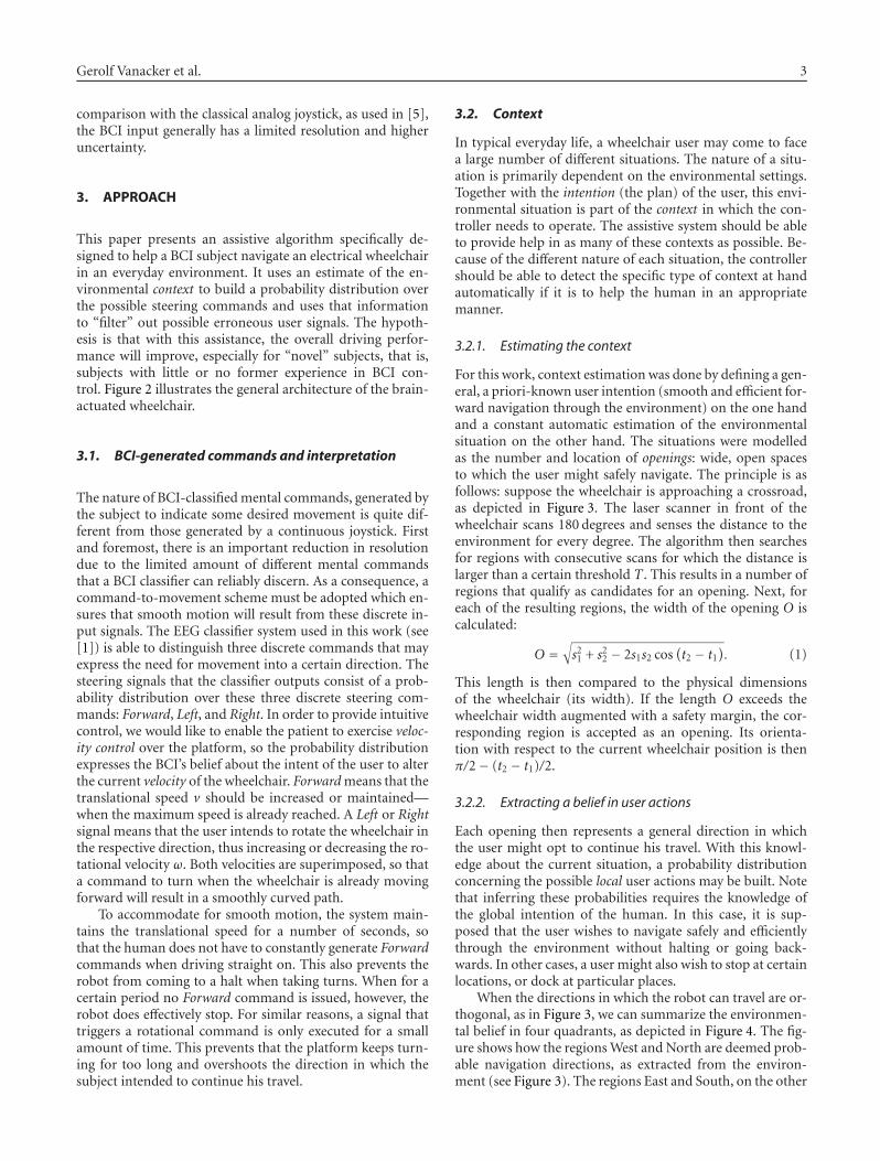
Gerolf Vanacker et al. 3
comparison with the classical analog joystick, as used in [5],the BCI input generally has a limited resolution and higheruncertainty.
3. APPROACH
This paper presents an assistive algorithm specifically de-signed to help a BCI subject navigate an electrical wheelchairin an everyday environment. It uses an estimate of the en-vironmental context to build a probability distribution overthe possible steering commands and uses that informationto “filter” out possible erroneous user signals. The hypoth-esis is that with this assistance, the overall driving perfor-mance will improve, especially for “novel” subjects, that is,subjects with little or no former experience in BCI con-trol. Figure 2 illustrates the general architecture of the brain-actuated wheelchair.
3.1. BCI-generated commands and interpretation
The nature of BCI-classified mental commands, generated bythe subject to indicate some desired movement is quite dif-ferent from those generated by a continuous joystick. Firstand foremost, there is an important reduction in resolutiondue to the limited amount of different mental commandsthat a BCI classifier can reliably discern. As a consequence, acommand-to-movement scheme must be adopted which en-sures that smooth motion will result from these discrete in-put signals. The EEG classifier system used in this work (see[1]) is able to distinguish three discrete commands that mayexpress the need for movement into a certain direction. Thesteering signals that the classifier outputs consist of a prob-ability distribution over these three discrete steering com-mands: Forward, Left, and Right. In order to provide intuitivecontrol, we would like to enable the patient to exercise veloc-ity control over the platform, so the probability distributionexpresses the BCI’s belief about the intent of the user to alterthe current velocity of the wheelchair. Forward means that thetranslational speed v should be increased or maintained—when the maximum speed is already reached. A Left or Rightsignal means that the user intends to rotate the wheelchair inthe respective direction, thus increasing or decreasing the ro-tational velocity ω. Both velocities are superimposed, so thata command to turn when the wheelchair is already movingforward will result in a smoothly curved path.
To accommodate for smooth motion, the system main-tains the translational speed for a number of seconds, sothat the human does not have to constantly generate Forwardcommands when driving straight on. This also prevents therobot from coming to a halt when taking turns. When for acertain period no Forward command is issued, however, therobot does effectively stop. For similar reasons, a signal thattriggers a rotational command is only executed for a smallamount of time. This prevents that the platform keeps turn-ing for too long and overshoots the direction in which thesubject intended to continue his travel.
3.2. Context
In typical everyday life, a wheelchair user may come to facea large number of different situations. The nature of a situ-ation is primarily dependent on the environmental settings.Together with the intention (the plan) of the user, this envi-ronmental situation is part of the context in which the con-troller needs to operate. The assistive system should be ableto provide help in as many of these contexts as possible. Be-cause of the different nature of each situation, the controllershould be able to detect the specific type of context at handautomatically if it is to help the human in an appropriatemanner.
3.2.1. Estimating the context
For this work, context estimation was done by defining a gen-eral, a priori-known user intention (smooth and efficient for-ward navigation through the environment) on the one handand a constant automatic estimation of the environmentalsituation on the other hand. The situations were modelledas the number and location of openings: wide, open spacesto which the user might safely navigate. The principle is asfollows: suppose the wheelchair is approaching a crossroad,as depicted in Figure 3. The laser scanner in front of thewheelchair scans 180 degrees and senses the distance to theenvironment for every degree. The algorithm then searchesfor regions with consecutive scans for which the distance islarger than a certain threshold T . This results in a number ofregions that qualify as candidates for an opening. Next, foreach of the resulting regions, the width of the opening O iscalculated:
O =√s2
1 + s22 − 2s1s2 cos
(t2 − t1
). (1)
This length is then compared to the physical dimensionsof the wheelchair (its width). If the length O exceeds thewheelchair width augmented with a safety margin, the cor-responding region is accepted as an opening. Its orienta-tion with respect to the current wheelchair position is thenπ/2− (t2 − t1)/2.
3.2.2. Extracting a belief in user actions
Each opening then represents a general direction in whichthe user might opt to continue his travel. With this knowl-edge about the current situation, a probability distributionconcerning the possible local user actions may be built. Notethat inferring these probabilities requires the knowledge ofthe global intention of the human. In this case, it is sup-posed that the user wishes to navigate safely and efficientlythrough the environment without halting or going back-wards. In other cases, a user might also wish to stop at certainlocations, or dock at particular places.
When the directions in which the robot can travel are or-thogonal, as in Figure 3, we can summarize the environmen-tal belief in four quadrants, as depicted in Figure 4. The fig-ure shows how the regions West and North are deemed prob-able navigation directions, as extracted from the environ-ment (see Figure 3). The regions East and South, on the other
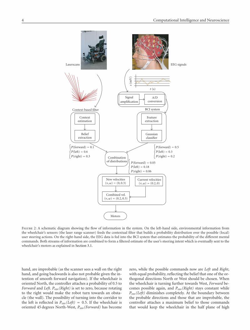
4 Computational Intelligence and Neuroscience
Laserscans EEG signals
t (s)
s(m
V)
Signalamplification
A/Dconversion
BCI systemContext-based filter
Contextestimation
Beliefextraction
Featureextraction
Gaussianclassifier
P(forward) = 0.1
P(left) = 0.6
P(right) = 0.3
P(forward) = 0.5
P(left) = 0.3
P(right) = 0.2Combinationof distributions P(forward) = 0.05
P(left) = 0.18P(right) = 0.06
New velocities(v,ω) = (0, 0.3)
Current velocities(v,ω) = (0.2, 0)
Combined vel.(v,ω) = (0.2, 0.3)
Motors
Figure 2: A schematic diagram showing the flow of information in the system. On the left-hand side, environmental information fromthe wheelchair’s sensors (the laser range scanner) feeds the contextual filter that builds a probability distribution over the possible (local)user steering actions. On the right-hand side, the EEG data is fed into the BCI system that estimates the probability of the different mentalcommands. Both streams of information are combined to form a filtered estimate of the user’s steering intent which is eventually sent to thewheelchair’s motors as explained in Section 3.1.
hand, are improbable (as the scanner sees a wall on the righthand, and going backwards is also not probable given the in-tention of smooth forward navigation). If the wheelchair isoriented North, the controller attaches a probability of 0.5 toForward and Left. Penv(Right) is set to zero, because rotatingto the right would make the robot turn towards an obsta-cle (the wall). The possibility of turning into the corridor tothe left is reflected in Penv(Left) = 0.5. If the wheelchair isoriented 45 degrees North-West, Penv(Forward) has become
zero, while the possible commands now are Left and Right,with equal probability, reflecting the belief that one of the or-thogonal directions North or West should be chosen. Whenthe wheelchair is turning further towards West, Forward be-comes possible again, and Penv(Right) stays constant whilePenv(Left) diminishes completely. At the boundary betweenthe probable directions and those that are improbable, thecontroller attaches a maximum belief to those commandsthat would keep the wheelchair in the half plane of high
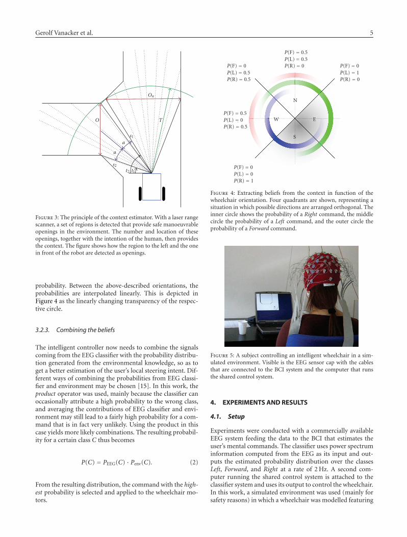
Gerolf Vanacker et al. 5
O T
On
s1
s2t2 t1
a
a
Figure 3: The principle of the context estimator. With a laser rangescanner, a set of regions is detected that provide safe manoeuvrableopenings in the environment. The number and location of theseopenings, together with the intention of the human, then providesthe context. The figure shows how the region to the left and the onein front of the robot are detected as openings.
probability. Between the above-described orientations, theprobabilities are interpolated linearly. This is depicted inFigure 4 as the linearly changing transparency of the respec-tive circle.
3.2.3. Combining the beliefs
The intelligent controller now needs to combine the signalscoming from the EEG classifier with the probability distribu-tion generated from the environmental knowledge, so as toget a better estimation of the user’s local steering intent. Dif-ferent ways of combining the probabilities from EEG classi-fier and environment may be chosen [15]. In this work, theproduct operator was used, mainly because the classifier canoccasionally attribute a high probability to the wrong class,and averaging the contributions of EEG classifier and envi-ronment may still lead to a fairly high probability for a com-mand that is in fact very unlikely. Using the product in thiscase yields more likely combinations. The resulting probabil-ity for a certain class C thus becomes
P(C) = PEEG(C) · Penv(C). (2)
From the resulting distribution, the command with the high-est probability is selected and applied to the wheelchair mo-tors.
N
S
EW
P(F) = 0P(L) = 0P(R) = 1
P(F) = 0.5P(L) = 0P(R) = 0.5
P(F) = 0P(L) = 0.5P(R) = 0.5
P(F) = 0.5P(L) = 0.5P(R) = 0 P(F) = 0
P(L) = 1P(R) = 0
Figure 4: Extracting beliefs from the context in function of thewheelchair orientation. Four quadrants are shown, representing asituation in which possible directions are arranged orthogonal. Theinner circle shows the probability of a Right command, the middlecircle the probability of a Left command, and the outer circle theprobability of a Forward command.
Figure 5: A subject controlling an intelligent wheelchair in a sim-ulated environment. Visible is the EEG sensor cap with the cablesthat are connected to the BCI system and the computer that runsthe shared control system.
4. EXPERIMENTS AND RESULTS
4.1. Setup
Experiments were conducted with a commercially availableEEG system feeding the data to the BCI that estimates theuser’s mental commands. The classifier uses power spectruminformation computed from the EEG as its input and out-puts the estimated probability distribution over the classesLeft, Forward, and Right at a rate of 2 Hz. A second com-puter running the shared control system is attached to theclassifier system and uses its output to control the wheelchair.In this work, a simulated environment was used (mainly forsafety reasons) in which a wheelchair was modelled featuring
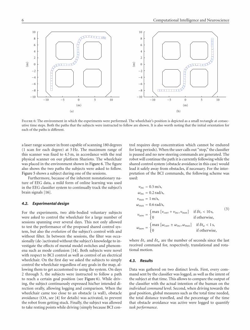
6 Computational Intelligence and Neuroscience
−10
−8
−6
−4
−2
0
2
4
6
8
10
(m)
−10 −5 0 5 10
(m)
(a)
−10
−8
−6
−4
−2
0
2
4
6
8
10
(m)
−10 −5 0 5 10
(m)
(b)
Figure 6: The environment in which the experiments were performed. The wheelchair’s position is depicted as a small rectangle at consec-utive time steps. Both the paths that the subjects were instructed to follow are shown. It is also worth noting that the initial orientation foreach of the paths is different.
a laser range scanner in front capable of scanning 180 degrees(1 scan for each degree) at 5 Hz. The maximum range ofthis scanner was fixed to 4.5 m, in accordance with the realphysical scanner on our platform Sharioto. The wheelchairwas placed in the environment shown in Figure 6. The figurealso shows the two paths the subjects were asked to follow.Figure 5 shows a subject during one of the sessions.
Furthermore, because of the inherent nonstationary na-ture of EEG data, a mild form of online learning was usedin the EEG classifier system to continually track the subject’sbrain signals [16].
4.2. Experimental design
For the experiments, two able-bodied voluntary subjectswere asked to control the wheelchair for a large number ofsessions spanning over several days. This not only allowedto test the performance of the proposed shared control sys-tem, but also the evolution of the subject’s control with andwithout filter. In between the sessions, the filter was occa-sionally (de-)activated without the subject’s knowledge to in-vestigate the effects of mental model switches and phenom-ena such as mode confusion [14]. Both subjects were novelwith respect to BCI control as well as control of an electricalwheelchair. On the first day we asked the subjects to simplycontrol the wheelchair regardless of any goals in the map, al-lowing them to get accustomed to using the system. On days2 through 5, the subjects were instructed to follow a pathto reach a certain goal position (see Figure 6). While driv-ing, the subject continuously expressed his/her intended di-rection orally, allowing logging and comparison. When thewheelchair came too close to an obstacle (a wall), obstacleavoidance (OA, see [4] for details) was activated, to preventthe robot from getting stuck. Finally, the subject was allowedto take resting points while driving (simply because BCI con-
trol requires deep concentration which cannot be enduredfor long periods). When the user calls out “stop,” the classifieris paused and no new steering commands are generated. Therobot will continue the path it is currently following while theshared control system (obstacle avoidance in this case) wouldlead it safely away from obstacles, if necessary. For the inter-pretation of the BCI commands, the following scheme wasused:
vinc = 0.5 m/s,
ωinc = 0.2 rad/s,
vmax = 1 m/s,
ωmax = 0.6 rad/s,
vnew ={
max{vcurr + vinc, vmax
}if δtv < 10 s,
0 if otherwise,
ωnew ={
max{ωcurr ± ωinc,ωmax
}if δtω < 1 s,
0 if otherwise,
(3)
where δtv and δtω are the number of seconds since the lastreceived command for, respectively, translational and rota-tional motion.
4.3. Results
Data was gathered on two distinct levels. First, every com-mand sent by the classifier was logged, as well as the intent ofthe subject at that time. This allows to compare the output ofthe classifier with the actual intention of the human on theindividual command level. Second, when driving towards thegoal position, global measures such as the total time needed,the total distance travelled, and the percentage of the timethat obstacle avoidance was active were logged to quantifytask performance.
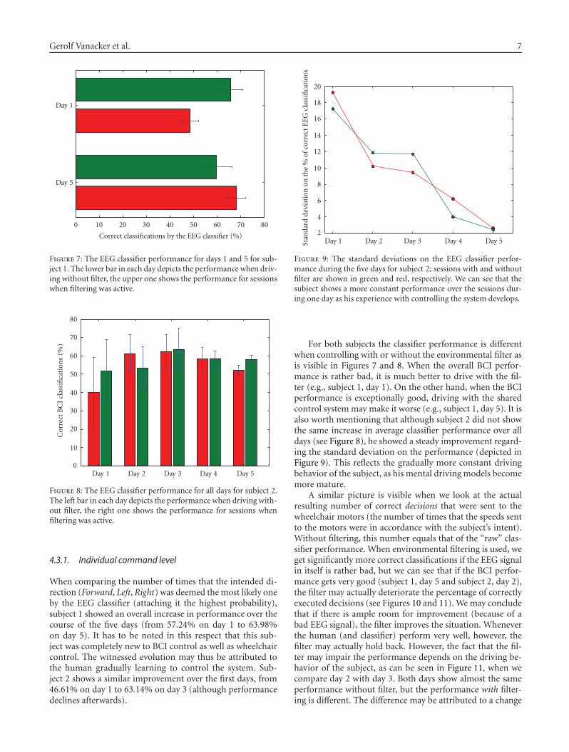
Gerolf Vanacker et al. 7
Day 5
Day 1
0 10 20 30 40 50 60 70 80
Correct classifications by the EEG classifier (%)
Figure 7: The EEG classifier performance for days 1 and 5 for sub-ject 1. The lower bar in each day depicts the performance when driv-ing without filter, the upper one shows the performance for sessionswhen filtering was active.
0
10
20
30
40
50
60
70
80
Day 1 Day 2 Day 3 Day 4 Day 5
Cor
rect
BC
Icl
assi
fica
tion
s(%
)
Figure 8: The EEG classifier performance for all days for subject 2.The left bar in each day depicts the performance when driving with-out filter, the right one shows the performance for sessions whenfiltering was active.
4.3.1. Individual command level
When comparing the number of times that the intended di-rection (Forward, Left, Right) was deemed the most likely oneby the EEG classifier (attaching it the highest probability),subject 1 showed an overall increase in performance over thecourse of the five days (from 57.24% on day 1 to 63.98%on day 5). It has to be noted in this respect that this sub-ject was completely new to BCI control as well as wheelchaircontrol. The witnessed evolution may thus be attributed tothe human gradually learning to control the system. Sub-ject 2 shows a similar improvement over the first days, from46.61% on day 1 to 63.14% on day 3 (although performancedeclines afterwards).
2
4
6
8
10
12
14
16
18
20
Day 1 Day 2 Day 3 Day 4 Day 5Stan
dar
dd
evia
tion
onth
e%
ofco
rrec
tE
EG
clas
sifi
cati
ons
Figure 9: The standard deviations on the EEG classifier perfor-mance during the five days for subject 2; sessions with and withoutfilter are shown in green and red, respectively. We can see that thesubject shows a more constant performance over the sessions dur-ing one day as his experience with controlling the system develops.
For both subjects the classifier performance is differentwhen controlling with or without the environmental filter asis visible in Figures 7 and 8. When the overall BCI perfor-mance is rather bad, it is much better to drive with the fil-ter (e.g., subject 1, day 1). On the other hand, when the BCIperformance is exceptionally good, driving with the sharedcontrol system may make it worse (e.g., subject 1, day 5). It isalso worth mentioning that although subject 2 did not showthe same increase in average classifier performance over alldays (see Figure 8), he showed a steady improvement regard-ing the standard deviation on the performance (depicted inFigure 9). This reflects the gradually more constant drivingbehavior of the subject, as his mental driving models becomemore mature.
A similar picture is visible when we look at the actualresulting number of correct decisions that were sent to thewheelchair motors (the number of times that the speeds sentto the motors were in accordance with the subject’s intent).Without filtering, this number equals that of the “raw” clas-sifier performance. When environmental filtering is used, weget significantly more correct classifications if the EEG signalin itself is rather bad, but we can see that if the BCI perfor-mance gets very good (subject 1, day 5 and subject 2, day 2),the filter may actually deteriorate the percentage of correctlyexecuted decisions (see Figures 10 and 11). We may concludethat if there is ample room for improvement (because of abad EEG signal), the filter improves the situation. Wheneverthe human (and classifier) perform very well, however, thefilter may actually hold back. However, the fact that the fil-ter may impair the performance depends on the driving be-havior of the subject, as can be seen in Figure 11, when wecompare day 2 with day 3. Both days show almost the sameperformance without filter, but the performance with filter-ing is different. The difference may be attributed to a change
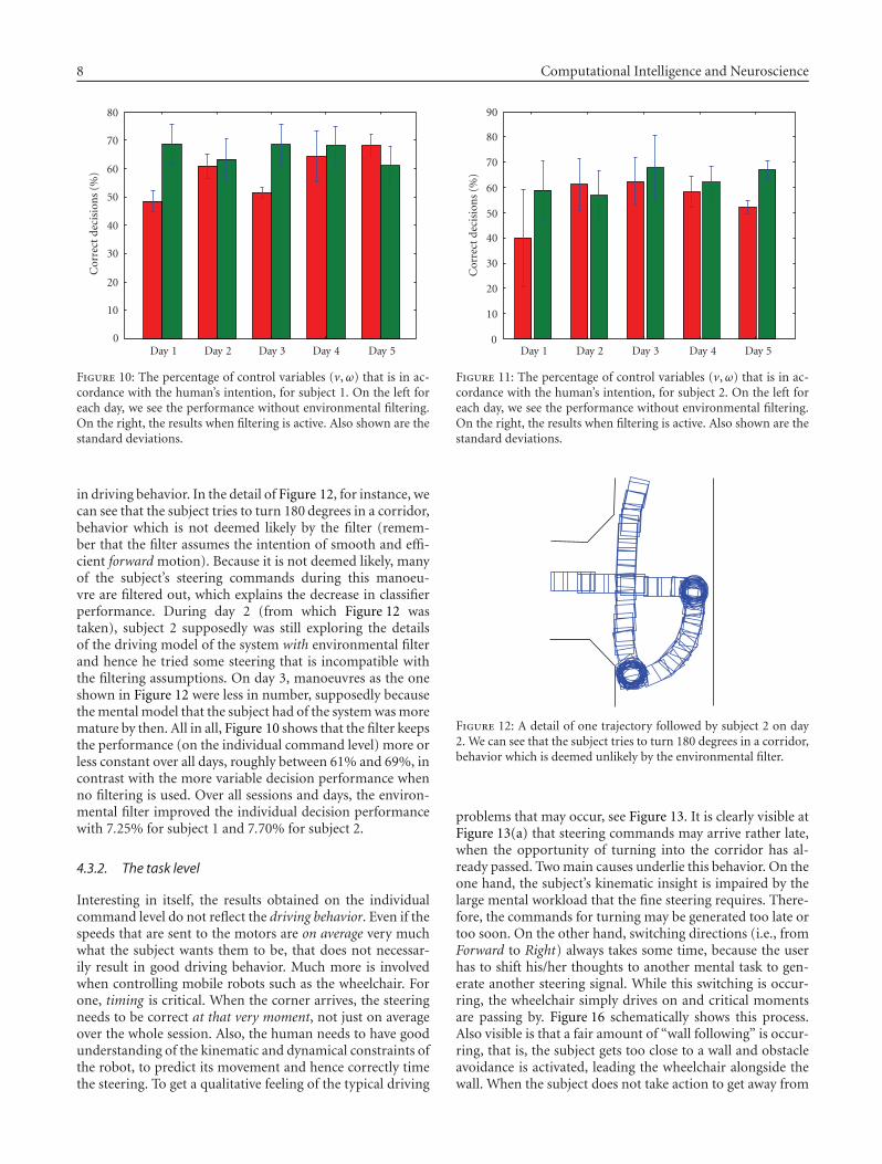
8 Computational Intelligence and Neuroscience
0
10
20
30
40
50
60
70
80
Day 1 Day 2 Day 3 Day 4 Day 5
Cor
rect
dec
isio
ns
(%)
Figure 10: The percentage of control variables (v,ω) that is in ac-cordance with the human’s intention, for subject 1. On the left foreach day, we see the performance without environmental filtering.On the right, the results when filtering is active. Also shown are thestandard deviations.
in driving behavior. In the detail of Figure 12, for instance, wecan see that the subject tries to turn 180 degrees in a corridor,behavior which is not deemed likely by the filter (remem-ber that the filter assumes the intention of smooth and effi-cient forward motion). Because it is not deemed likely, manyof the subject’s steering commands during this manoeu-vre are filtered out, which explains the decrease in classifierperformance. During day 2 (from which Figure 12 wastaken), subject 2 supposedly was still exploring the detailsof the driving model of the system with environmental filterand hence he tried some steering that is incompatible withthe filtering assumptions. On day 3, manoeuvres as the oneshown in Figure 12 were less in number, supposedly becausethe mental model that the subject had of the system was moremature by then. All in all, Figure 10 shows that the filter keepsthe performance (on the individual command level) more orless constant over all days, roughly between 61% and 69%, incontrast with the more variable decision performance whenno filtering is used. Over all sessions and days, the environ-mental filter improved the individual decision performancewith 7.25% for subject 1 and 7.70% for subject 2.
4.3.2. The task level
Interesting in itself, the results obtained on the individualcommand level do not reflect the driving behavior. Even if thespeeds that are sent to the motors are on average very muchwhat the subject wants them to be, that does not necessar-ily result in good driving behavior. Much more is involvedwhen controlling mobile robots such as the wheelchair. Forone, timing is critical. When the corner arrives, the steeringneeds to be correct at that very moment, not just on averageover the whole session. Also, the human needs to have goodunderstanding of the kinematic and dynamical constraints ofthe robot, to predict its movement and hence correctly timethe steering. To get a qualitative feeling of the typical driving
0
10
20
30
40
50
60
70
80
90
Day 1 Day 2 Day 3 Day 4 Day 5
Cor
rect
dec
isio
ns
(%)
Figure 11: The percentage of control variables (v,ω) that is in ac-cordance with the human’s intention, for subject 2. On the left foreach day, we see the performance without environmental filtering.On the right, the results when filtering is active. Also shown are thestandard deviations.
Figure 12: A detail of one trajectory followed by subject 2 on day2. We can see that the subject tries to turn 180 degrees in a corridor,behavior which is deemed unlikely by the environmental filter.
problems that may occur, see Figure 13. It is clearly visible atFigure 13(a) that steering commands may arrive rather late,when the opportunity of turning into the corridor has al-ready passed. Two main causes underlie this behavior. On theone hand, the subject’s kinematic insight is impaired by thelarge mental workload that the fine steering requires. There-fore, the commands for turning may be generated too late ortoo soon. On the other hand, switching directions (i.e., fromForward to Right) always takes some time, because the userhas to shift his/her thoughts to another mental task to gen-erate another steering signal. While this switching is occur-ring, the wheelchair simply drives on and critical momentsare passing by. Figure 16 schematically shows this process.Also visible is that a fair amount of “wall following” is occur-ring, that is, the subject gets too close to a wall and obstacleavoidance is activated, leading the wheelchair alongside thewall. When the subject does not take action to get away from
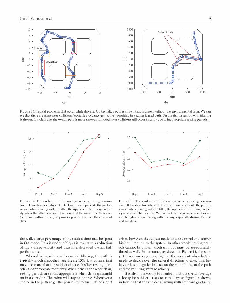
Gerolf Vanacker et al. 9
−10
−8
−6
−4
−2
0
2
4
6
8
10
(m)
Late turn
OA active
−10 −5 0 5 10
(m)
(a)
−1000
−800
−600
−400
−200
0
200
400
600
800
1000
(m)
Subject rests
−1000 −500 0 500 1000
(m)
(b)
Figure 13: Typical problems that occur while driving. On the left, a path is shown that is driven without the environmental filter. We cansee that there are many near collisions (obstacle avoidance gets active), resulting in a rather jagged path. On the right a session with filteringis shown. It is clear that the overall path is more smooth, although near collisions still occur (mainly due to inappropriate resting periods).
0.1
0.2
0.3
0.4
0.5
Day 1 Day 2 Day 3 Day 4 Day 5
Ave
rage
velo
city
(m/s
)
Figure 14: The evolution of the average velocity during sessionsover all five days for subject 1. The lower line represents the perfor-mance when driving without filter, the upper one the average veloc-ity when the filter is active. It is clear that the overall performance(with and without filter) improves significantly over the course ofdays.
the wall, a large percentage of the session time may be spentin OA mode. This is undesirable, as it results in a reductionof the average velocity and thus in a degraded overall taskperformance.
When driving with environmental filtering, the path istypically much smoother (see Figure 13(b)). Problems thatmay occur are that the subject chooses his/her resting peri-ods at inappropriate moments. When driving the wheelchair,resting periods are most appropriate when driving straighton in a corridor. The robot will stay on course. Whenever achoice in the path (e.g., the possibility to turn left or right)
0
0.1
0.2
0.3
0.4
0.5
Day 1 Day 2 Day 3 Day 4 Day 5
Ave
rage
velo
city
(m/s
)
Figure 15: The evolution of the average velocity during sessionsover all five days for subject 2. The lower line represents the perfor-mance when driving without filter, the upper one the average veloc-ity when the filter is active. We can see that the average velocities aremuch higher when driving with filtering, especially during the firstand last days.
arises, however, the subject needs to take control and conveyhis/her intention to the system. In other words, resting peri-ods cannot be chosen arbitrarily but must be appropriatelytimed as well. For instance, as shown in Figure 13, the sub-ject takes two long rests, right at the moment when he/sheneeds to decide over the general direction to take. This be-havior has a negative impact on the smoothness of the pathand the resulting average velocity.
It is also noteworthy to mention that the overall averagevelocity for subject 1 rises over the days as Figure 14 shows,indicating that the subject’s driving skills improve gradually.

10 Computational Intelligence and Neuroscience
Penv (R)
Intent(R)
PEEG(R)
ΔTk ΔTm
Figure 16: The timing problem. The upper row of figures shows a few frames in the path a subject may follow when the task is to turn southinto the T-shaped corridor. We can see the evolution of the probabilities for Right commands as seen from the environmental filter and theBCI. Also visible is the moment at which the user decides to start turning, shown as intention(R). The timing issue has 2 components. First,there is a delay δTk that denotes the suboptimal kinematic prediction by the subject; the turn should have started earlier for the currentspeed of the platform. Secondly, a mental task switching delay Tm occurs which increases the total time delay even more. Eventually, theopportunity has passed by and the wheelchair crashes into the wall.
Table 1: The percentage of sessions in which subject 1 reached thegoal position within 4 minutes.
Day Overall (all sessions)Sessionswithout filtering
Sessionswith filtering
Day 2 60% 40% 80%
Day 3 80% 66.67% 85.71%
Day 4 70% 60% 80%
Day 5 80% 100% 60%
Table 2: The time subject 2 needed to reach the goal position (in s).
Day Overall (all sessions)Sessionswithout filtering
Sessionswith filtering
Day 2 151.32 164.25 138.4
Day 3 120.37 144.6 115.52
Day 4 138.7 145.6 127.2
Day 5 110.26 126.01 84.01
Subject 2 does not show a similar evolution (see Figure 15),but in both cases we can see that the average velocities aremuch higher when filtering is active. For subject 1, the aver-age improvement the filter offers regarding the average veloc-ity is 17.58%. For subject 2 the gain is even higher: 22.72%.
Another interesting factor is the time the user spent inobstacle avoidance mode, as this reflects an undesirable as-pect: namely that the subject is controlling the robot to alesser extent when in this mode. Furthermore, OA is designedas a safety measure, not to provide continuous navigationalassistance. All in all, spending much time in OA does notconstitute what we regard as “good driving behavior” and itslows the navigation down significantly. When we comparethe average amount of time spent in OA mode when drivingwithout filter to the amount when driving with environmen-tal filtering, we see an overall 13.3% (subject 1) and 17.44%
(subject 2) decrease for the latter case. This is reflected in themore efficient (centre of corridor) driving behavior.
Now, if we consider the task that the subjects had to per-form (driving to a certain goal pose, if possible via a prede-termined path, as shown in Figure 6) we get the results forsubject 1 listed in Table 1. This table shows the figures forday 2 through 5 (there was no goal-directed task in day 1). Itis clear that for the majority of days, the environmental fil-ter significantly increases the probability of reaching the goalposition within 4 minutes. Only during the last day, the sub-ject had better control without the filter and could reach thegoal 100% of the time. All sessions together, the filter provesto increase the task performance by about 10%. Consideringonly days 2 through 4, we see an increase of more than 26%.Subject 2 on the other hand, did not show a large differencein probability of reaching the goal with or without filtering(+7.5% when filtering is active). However, the time neededto reach the goal is significantly lower when using the envi-ronmental filter, as Table 2 shows. In total, subject 2 reachedthe goal 19.87% more rapidly when driving with filter com-pared to driving without.
5. DISCUSSION
The experiments were conducted with two subjects that hadno previous experience in BCI control nor control of differ-entially driven robots such as the electrical wheelchair. Fromthe data collected over all five days, we can clearly see howthe subjects have gradually learned to improve this control.Yet, the problem of predicting the kinematic behavior of thewheelchair accurately remains a mentally demanding task.This may cause erroneous timing when initiating a turn intoa corridor, leading to a worse overall driving behavior; referto Figure 16 for a graphical overview of this problem.
During the course of the first days, when the subjectswere still performing rather bad, the filter acts as a correc-tional tool that rectifies much of the misclassifications com-ing from the EEG classifier. This is visible in Figures 10,11,14,15 and Table 1. As a result, filtering enables a novel subject
Gerolf Vanacker et al. 11
to achieve good levels of performance even on the first dayof usage. It is clear from Figures 10 and 11 that the filterkeeps the performance on the level of the individual com-mands more or less stable over all days. The environmentalfilter may thus be seen as a learning tool that keeps the sub-jects performance on a workable level even if that subject isjust taking the first steps in learning to use BCI control fordriving a wheelchair. Later on, when the subject shows animproved control, the filter corrects less, up to the point thatthe control is so good that the filter actually holds back. It isremarkable that on the first day, when the subjects still werecompletely new to the task, for some (filtered) sessions verygood performance could be noted.
However, the collected data and the performance figuresextracted from the experiments are to a large extent depen-dent on the driving strategy the subject employs. As the sub-jects gradually learned to control the system, different strate-gies were explored. One example is visible in Figure 13(a),where the subject exploited the behavior provided by the ob-stacle avoidance algorithm to lead the robot without muchcontrol effort alongside a wall. Similarly, the subject occa-sionally exploited the OA safety behavior to let the robot rideuntil it approaches a wall. At that point, OA slows the robotdown and the subject has more time to choose the direc-tion he/she wants to go into. This is, for instance, visible inFigure 13(b). Now, while exploring alternative strategies, theperformance measures naturally change as well.
A further source of “noise” on the collected data iscaused by inappropriate usage of the resting possibility, asalready discussed before. Figure 13-right shows an example.Of course, this strategy also has a negative influence on theresulting performance.
Furthermore, the filter was regularly switched on and offin between sessions, without the subject’s knowledge. Be-cause of the fact that the driving system is different when thefiltering is applied, the subject needs to use another mentalmodel (or at least adapt his/her existing one) when the filteris switched on or off. Also, the subjects were not told how theenvironmental filter internally works, so that they needed tolearn an appropriate mental model from scratch while driv-ing. The result is that when the subject’s acquired strategiesbuilt up using the one driving system (i.e., without filtering)were applied to the other situation, performance was seri-ously weakened. This effect is sometimes referred to as modeconfusion [14] and it is a common problem in shared controlsystems. An illustrative example is that when driving with-out filtering, the subjects learned at a certain moment to turn180 degrees in a corridor, whenever they got orientated in thewrong direction (see Figure 12). When the filter was switchedon, he/she tried to use that same strategy. Because the filterassumes smooth and efficient forward motion, such behav-ior was deemed unlikely and the filter made it a difficult ma-noeuvre. This leads to a situation in which the environmentalfilter is actually working against the user’s intention.
6. CONCLUSIONS AND FURTHER WORK
We have shown that the usage of an environmental filter-ing technique, which uses knowledge about the current con-
text to filter out erroneous steering commands, can improvethe overall driving behavior. Especially when the subject isnot already trained for the task, the filter provides significantbenefits. However, when the subject is performing really welland employs driving behavior that is not compatible with thelogic of the filter, performance may be weakened. All in all,the subjects declared that driving with filtering was more easyto do, especially during the first days. As such, the systemproves most useful as a learning tool, when the subject is inthe learning phase of BCI control.
Probably the most notable weakness of the filter in itscurrent form is the fixed user model. The system assumes acertain driving behavior that would lead to smooth and effi-cient forward motion. Whenever strategies are employed thatcontradict with this assumption, the performance gets worse(i.e., 180-degree turning in a corridor). Therefore, we needan adaptive model that constantly adapts to whatever strate-gies the user might employ. Besides that, we could also ben-efit from a detection mechanism that simply switches off thefilter if user performance gets high, or more generally somemechanism to regulate the amount of influence the filter has.Also, a user model incorporating the specific BCI profile theparticular subject has (how likely it is that he/she generatesthe correct steering commands) might lead to a better filter-ing of the individual commands.
ACKNOWLEDGMENTS
This research was funded by a Ph.D. grant of the Institute forthe Promotion of Innovation through Science and Technol-ogy in Flanders (IWT-Vlaanderen). This work is supportedby the Swiss National Science Foundation NCCR “IM2” andby the European IST Programme FET Project FP6-003758.This paper only reflects the authors’ views and funding agen-cies are not liable for any use that may be made of the infor-mation contained herein.
REFERENCES
[1] J. d. R. Millan, F. Renkens, J. Mourino, and W. Gerstner, “Non-invasive brain-actuated control of a mobile robot by humanEEG,” IEEE Transactions on Biomedical Engineering, vol. 51,no. 6, pp. 1026–1033, 2004.
[2] J. d. R. Millan, “Brain-computer interfaces,” in Handbook ofBrain Theory and Neural Networks, M. A. Arbib, Ed., pp. 178–181, MIT Press, Cambridge, Mass,USA, 2002.
[3] J. d. R. Millan, F. Renkens, J. Mourino, and W. Gerstner,“Brain-actuated interaction,” Artificial Intelligence, vol. 159,no. 1-2, pp. 241–259, 2004.
[4] M. Nuttin, D. Vanhooydonck, E. Demeester, and H. Van Brus-sel, “Selection of suitable human-robot interaction techniquesfor intelligent wheelchairs,” in Proceedings of the 11th IEEE In-ternational Workshop on Robot and Human Interactive Com-munication (ROMAN ’02), pp. 146–151, Berlin, Germany,September 2002.
[5] G. Vanacker, D. Vanhooydonck, E. Demeester, et al., “Adap-tive filtering approach to improve wheelchair driving perfor-mance,” in Proceedings of the 15th IEEE International Sympo-sium on Robot and Human Interactive Communication (RO-MAN ’06), pp. 527–532, Hatfield, UK, September 2006.

12 Computational Intelligence and Neuroscience
[6] D. Vanhooydonck, E. Demeester, M. Nuttin, and H. Van Brus-sel, “Shared control for intelligent wheelchairs: an implicit es-timation of the user intention,” in Proceedings of the 1st Inter-national Workshop on Advances in Service Robotics (ASER ’03),pp. 176–182, Bardolino, Italy, March 2003.
[7] E. Demeester, M. Nuttin, D. Vanhooydonck, and H. Van Brus-sel, “A model-based, probabilistic framework for plan recog-nition in shared wheelchair control: experiments and evalua-tion,” in Proceedings of IEEE/RSJ International Conference onIntelligent Robots and Systems (IROS ’03), vol. 2, pp. 1456–1461, Las Vegas, Nev, USA, October 2003.
[8] N. I. Katevas, N. M. Sgours, S. G. Tzafestas, et al., “The au-tonomous mobile robot SENARIO: a sensor-aided intelligentnavigation system for powered wheelchairs,” IEEE Robotics &Automation Magazine, vol. 4, no. 4, pp. 60–70, 1997.
[9] E. Prassler, J. Scholz, and M. Strobel, “MAid: mobility assis-tance for elderly and disabled people,” in Proceedings of the24th Annual Conference of the IEEE Industrial Electronics So-ciety (IECON ’98), vol. 4, pp. 2493–2498, Aachen, Germany,August-September 1998.
[10] H. Yanco, Shared user-computer control of a robotic wheelchairsystem, Ph.D. thesis, Massachusetts Institute of Technology,Cambridge, Mass, USA, September 2000.
[11] G. Bourhis, O. Horn, O. Habert, and A. Pruski, “An au-tonomous vehicle for people with motor disabilities,” IEEERobotics & Automation Magazine, vol. 8, no. 1, pp. 20–28,2001.
[12] R. S. Rao, K. Conn, S. H. Jung, et al., “Human robot in-teraction: application to smart wheelchairs,” in Proceedingsof IEEE International Conference on Robotics and Automation(ICRA ’02), vol. 4, pp. 3583–3588, Washington, DC, USA, May2002.
[13] R. C. Simpson, S. P. Levine, D. A. Bell, L. A. Jaros, Y. Ko-ren, and J. Borenstein, “NavChair: an assistive wheelchair nav-igation system with automatic adaptation,” in Proceedings ofthe Assistive Technology and Artificial Intelligence, Applicationsin Robotics, User Interfaces and Natural Language Processing,vol. 1458 of Lecture Notes in Computer Science, pp. 235–255,1998.
[14] T. Rofer and A. Lankenau, “Architecture and applications ofthe Bremen autonomous wheelchair,” in Proceedings of the 4thJoint Conference on Information Systems, vol. 1, pp. 365–368,Association for Intelligent Machinery, October 1998.
[15] L. I. Kuncheva, Combining Pattern Classifiers: Methods and Al-gorithms, John Wiley & Sons, New York, NY, USA, 2004.
[16] A. Buttfield, P. W. Ferrez, and J. d. R. Millan, “Towards a ro-bust BCI: error potentials and online learning,” IEEE Transac-tions on Neural Systems and Rehabilitation Engineering, vol. 14,no. 2, pp. 164–168, 2006.
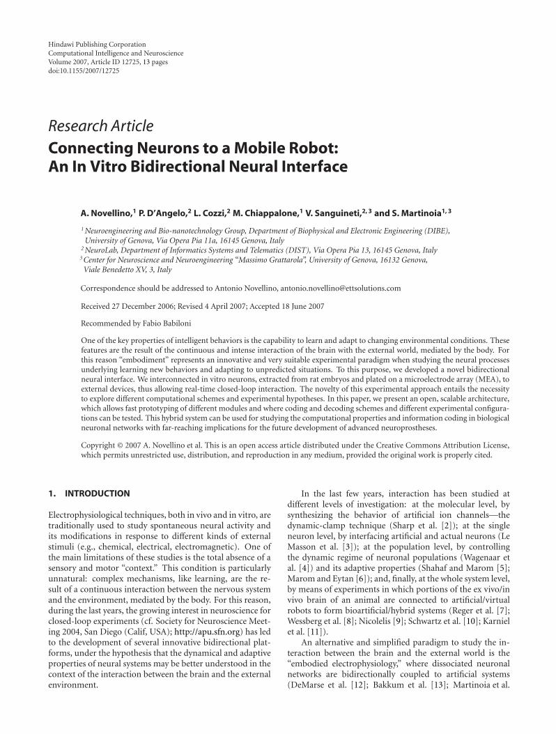
Hindawi Publishing CorporationComputational Intelligence and NeuroscienceVolume 2007, Article ID 12725, 13 pagesdoi:10.1155/2007/12725
Research ArticleConnecting Neurons to a Mobile Robot:An In Vitro Bidirectional Neural Interface
A. Novellino,1 P. D’Angelo,2 L. Cozzi,2 M. Chiappalone,1 V. Sanguineti,2, 3 and S. Martinoia1, 3
1 Neuroengineering and Bio-nanotechnology Group, Department of Biophysical and Electronic Engineering (DIBE),University of Genova, Via Opera Pia 11a, 16145 Genova, Italy
2 NeuroLab, Department of Informatics Systems and Telematics (DIST), Via Opera Pia 13, 16145 Genova, Italy3 Center for Neuroscience and Neuroengineering “Massimo Grattarola”, University of Genova, 16132 Genova,Viale Benedetto XV, 3, Italy
Correspondence should be addressed to Antonio Novellino, [email protected]
Received 27 December 2006; Revised 4 April 2007; Accepted 18 June 2007
Recommended by Fabio Babiloni
One of the key properties of intelligent behaviors is the capability to learn and adapt to changing environmental conditions. Thesefeatures are the result of the continuous and intense interaction of the brain with the external world, mediated by the body. Forthis reason “embodiment” represents an innovative and very suitable experimental paradigm when studying the neural processesunderlying learning new behaviors and adapting to unpredicted situations. To this purpose, we developed a novel bidirectionalneural interface. We interconnected in vitro neurons, extracted from rat embryos and plated on a microelectrode array (MEA), toexternal devices, thus allowing real-time closed-loop interaction. The novelty of this experimental approach entails the necessityto explore different computational schemes and experimental hypotheses. In this paper, we present an open, scalable architecture,which allows fast prototyping of different modules and where coding and decoding schemes and different experimental configura-tions can be tested. This hybrid system can be used for studying the computational properties and information coding in biologicalneuronal networks with far-reaching implications for the future development of advanced neuroprostheses.
Copyright © 2007 A. Novellino et al. This is an open access article distributed under the Creative Commons Attribution License,which permits unrestricted use, distribution, and reproduction in any medium, provided the original work is properly cited.
1. INTRODUCTION
Electrophysiological techniques, both in vivo and in vitro, aretraditionally used to study spontaneous neural activity andits modifications in response to different kinds of externalstimuli (e.g., chemical, electrical, electromagnetic). One ofthe main limitations of these studies is the total absence of asensory and motor “context.” This condition is particularlyunnatural: complex mechanisms, like learning, are the re-sult of a continuous interaction between the nervous systemand the environment, mediated by the body. For this reason,during the last years, the growing interest in neuroscience forclosed-loop experiments (cf. Society for Neuroscience Meet-ing 2004, San Diego (Calif, USA); http://apu.sfn.org) has ledto the development of several innovative bidirectional plat-forms, under the hypothesis that the dynamical and adaptiveproperties of neural systems may be better understood in thecontext of the interaction between the brain and the externalenvironment.
In the last few years, interaction has been studied atdifferent levels of investigation: at the molecular level, bysynthesizing the behavior of artificial ion channels—thedynamic-clamp technique (Sharp et al. [2]); at the singleneuron level, by interfacing artificial and actual neurons (LeMasson et al. [3]); at the population level, by controllingthe dynamic regime of neuronal populations (Wagenaar etal. [4]) and its adaptive properties (Shahaf and Marom [5];Marom and Eytan [6]); and, finally, at the whole system level,by means of experiments in which portions of the ex vivo/invivo brain of an animal are connected to artificial/virtualrobots to form bioartificial/hybrid systems (Reger et al. [7];Wessberg et al. [8]; Nicolelis [9]; Schwartz et al. [10]; Karnielet al. [11]).
An alternative and simplified paradigm to study the in-teraction between the brain and the external world is the“embodied electrophysiology,” where dissociated neuronalnetworks are bidirectionally coupled to artificial systems(DeMarse et al. [12]; Bakkum et al. [13]; Martinoia et al.
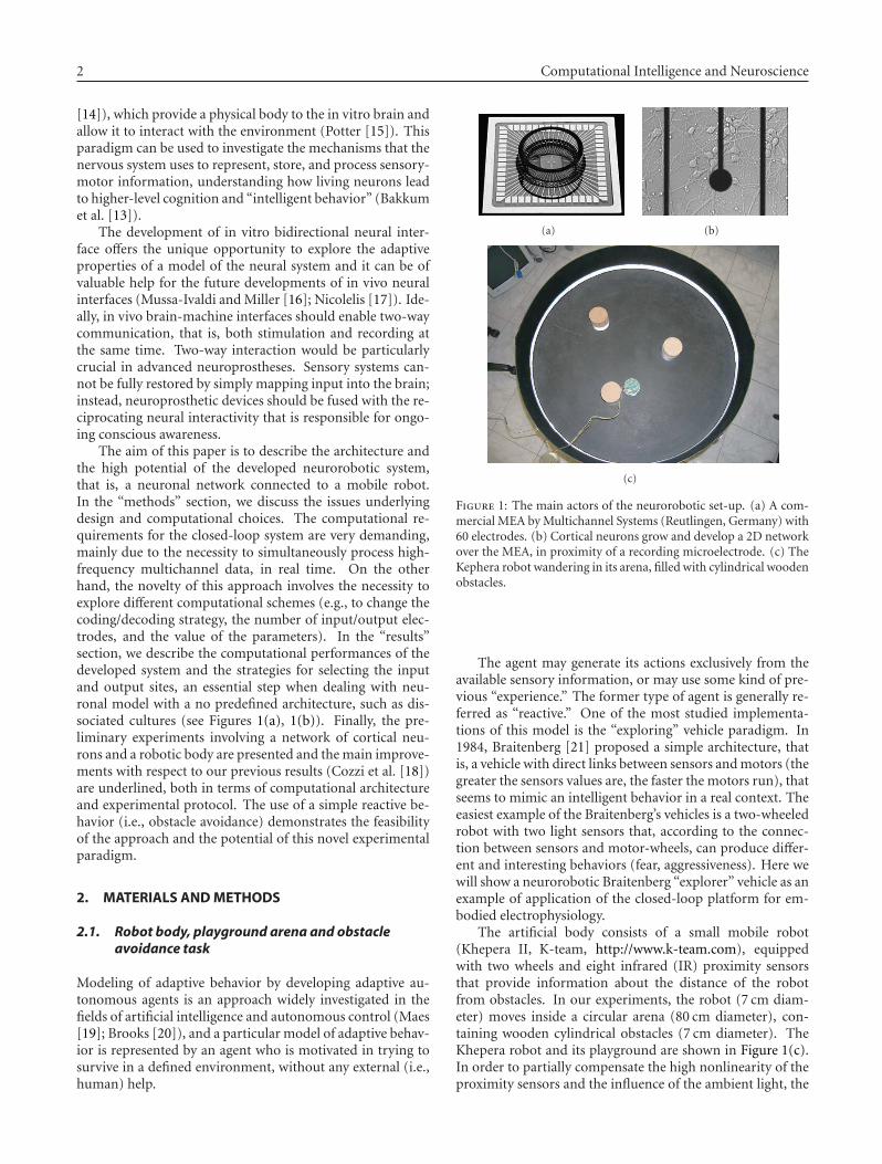
2 Computational Intelligence and Neuroscience
[14]), which provide a physical body to the in vitro brain andallow it to interact with the environment (Potter [15]). Thisparadigm can be used to investigate the mechanisms that thenervous system uses to represent, store, and process sensory-motor information, understanding how living neurons leadto higher-level cognition and “intelligent behavior” (Bakkumet al. [13]).
The development of in vitro bidirectional neural inter-face offers the unique opportunity to explore the adaptiveproperties of a model of the neural system and it can be ofvaluable help for the future developments of in vivo neuralinterfaces (Mussa-Ivaldi and Miller [16]; Nicolelis [17]). Ide-ally, in vivo brain-machine interfaces should enable two-waycommunication, that is, both stimulation and recording atthe same time. Two-way interaction would be particularlycrucial in advanced neuroprostheses. Sensory systems can-not be fully restored by simply mapping input into the brain;instead, neuroprosthetic devices should be fused with the re-ciprocating neural interactivity that is responsible for ongo-ing conscious awareness.
The aim of this paper is to describe the architecture andthe high potential of the developed neurorobotic system,that is, a neuronal network connected to a mobile robot.In the “methods” section, we discuss the issues underlyingdesign and computational choices. The computational re-quirements for the closed-loop system are very demanding,mainly due to the necessity to simultaneously process high-frequency multichannel data, in real time. On the otherhand, the novelty of this approach involves the necessity toexplore different computational schemes (e.g., to change thecoding/decoding strategy, the number of input/output elec-trodes, and the value of the parameters). In the “results”section, we describe the computational performances of thedeveloped system and the strategies for selecting the inputand output sites, an essential step when dealing with neu-ronal model with a no predefined architecture, such as dis-sociated cultures (see Figures 1(a), 1(b)). Finally, the pre-liminary experiments involving a network of cortical neu-rons and a robotic body are presented and the main improve-ments with respect to our previous results (Cozzi et al. [18])are underlined, both in terms of computational architectureand experimental protocol. The use of a simple reactive be-havior (i.e., obstacle avoidance) demonstrates the feasibilityof the approach and the potential of this novel experimentalparadigm.
2. MATERIALS AND METHODS
2.1. Robot body, playground arena and obstacleavoidance task
Modeling of adaptive behavior by developing adaptive au-tonomous agents is an approach widely investigated in thefields of artificial intelligence and autonomous control (Maes[19]; Brooks [20]), and a particular model of adaptive behav-ior is represented by an agent who is motivated in trying tosurvive in a defined environment, without any external (i.e.,human) help.
(a) (b)
(c)
Figure 1: The main actors of the neurorobotic set-up. (a) A com-mercial MEA by Multichannel Systems (Reutlingen, Germany) with60 electrodes. (b) Cortical neurons grow and develop a 2D networkover the MEA, in proximity of a recording microelectrode. (c) TheKephera robot wandering in its arena, filled with cylindrical woodenobstacles.
The agent may generate its actions exclusively from theavailable sensory information, or may use some kind of pre-vious “experience.” The former type of agent is generally re-ferred as “reactive.” One of the most studied implementa-tions of this model is the “exploring” vehicle paradigm. In1984, Braitenberg [21] proposed a simple architecture, thatis, a vehicle with direct links between sensors and motors (thegreater the sensors values are, the faster the motors run), thatseems to mimic an intelligent behavior in a real context. Theeasiest example of the Braitenberg’s vehicles is a two-wheeledrobot with two light sensors that, according to the connec-tion between sensors and motor-wheels, can produce differ-ent and interesting behaviors (fear, aggressiveness). Here wewill show a neurorobotic Braitenberg “explorer” vehicle as anexample of application of the closed-loop platform for em-bodied electrophysiology.
The artificial body consists of a small mobile robot(Khepera II, K-team, http://www.k-team.com), equippedwith two wheels and eight infrared (IR) proximity sensorsthat provide information about the distance of the robotfrom obstacles. In our experiments, the robot (7 cm diam-eter) moves inside a circular arena (80 cm diameter), con-taining wooden cylindrical obstacles (7 cm diameter). TheKhepera robot and its playground are shown in Figure 1(c).In order to partially compensate the high nonlinearity of theproximity sensors and the influence of the ambient light, the
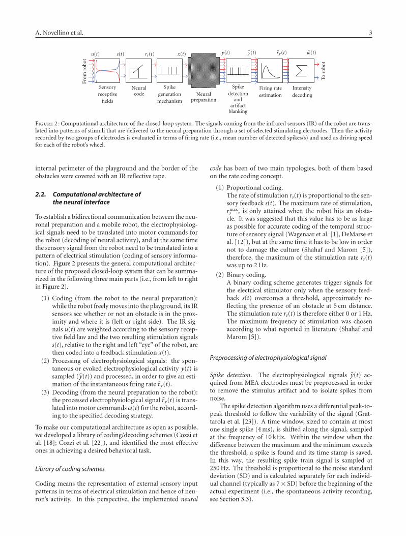
A. Novellino et al. 3
From
robo
t
Toro
bot
u(t) s(t) rs(t) x(t) y(t) y(t) ry(t) ω(t)
Sensoryreceptive
fields
Neuralcode
Spikegenerationmechanism
Neuralpreparation
Spikedetection
andartifact
blanking
Firing rateestimation
Intensitydecoding
Figure 2: Computational architecture of the closed-loop system. The signals coming from the infrared sensors (IR) of the robot are trans-lated into patterns of stimuli that are delivered to the neural preparation through a set of selected stimulating electrodes. Then the activityrecorded by two groups of electrodes is evaluated in terms of firing rate (i.e., mean number of detected spikes/s) and used as driving speedfor each of the robot’s wheel.
internal perimeter of the playground and the border of theobstacles were covered with an IR reflective tape.
2.2. Computational architecture ofthe neural interface
To establish a bidirectional communication between the neu-ronal preparation and a mobile robot, the electrophysiolog-ical signals need to be translated into motor commands forthe robot (decoding of neural activity), and at the same timethe sensory signal from the robot need to be translated into apattern of electrical stimulation (coding of sensory informa-tion). Figure 2 presents the general computational architec-ture of the proposed closed-loop system that can be summa-rized in the following three main parts (i.e., from left to rightin Figure 2).
(1) Coding (from the robot to the neural preparation):while the robot freely moves into the playground, its IRsensors see whether or not an obstacle is in the prox-imity and where it is (left or right side). The IR sig-nals u(t) are weighted according to the sensory recep-tive field law and the two resulting stimulation signalss(t), relative to the right and left “eye” of the robot, arethen coded into a feedback stimulation x(t).
(2) Processing of electrophysiological signals: the spon-taneous or evoked electrophysiological activity y(t) issampled ( y(t)) and processed, in order to give an esti-mation of the instantaneous firing rate ry(t).
(3) Decoding (from the neural preparation to the robot):the processed electrophysiological signal ry(t) is trans-lated into motor commandsω(t) for the robot, accord-ing to the specified decoding strategy.
To make our computational architecture as open as possible,we developed a library of coding/decoding schemes (Cozzi etal. [18]; Cozzi et al. [22]), and identified the most effectiveones in achieving a desired behavioral task.
Library of coding schemes
Coding means the representation of external sensory inputpatterns in terms of electrical stimulation and hence of neu-ron’s activity. In this perspective, the implemented neural
code has been of two main typologies, both of them basedon the rate coding concept.
(1) Proportional coding.The rate of stimulation rs(t) is proportional to the sen-sory feedback s(t). The maximum rate of stimulation,rmaxs , is only attained when the robot hits an obsta-
cle. It was suggested that this value has to be as largeas possible for accurate coding of the temporal struc-ture of sensory signal (Wagenaar et al. [1], DeMarse etal. [12]), but at the same time it has to be low in ordernot to damage the culture (Shahaf and Marom [5]),therefore, the maximum of the stimulation rate rs(t)was up to 2 Hz.
(2) Binary coding.A binary coding scheme generates trigger signals forthe electrical stimulator only when the sensory feed-back s(t) overcomes a threshold, approximately re-flecting the presence of an obstacle at 5 cm distance.The stimulation rate rs(t) is therefore either 0 or 1 Hz.The maximum frequency of stimulation was chosenaccording to what reported in literature (Shahaf andMarom [5]).
Preprocessing of electrophysiological signal
Spike detection. The electrophysiological signals y(t) ac-quired from MEA electrodes must be preprocessed in orderto remove the stimulus artifact and to isolate spikes fromnoise.
The spike detection algorithm uses a differential peak-to-peak threshold to follow the variability of the signal (Grat-tarola et al. [23]). A time window, sized to contain at mostone single spike (4 ms), is shifted along the signal, sampledat the frequency of 10 kHz. Within the window when thedifference between the maximum and the minimum exceedsthe threshold, a spike is found and its time stamp is saved.In this way, the resulting spike train signal is sampled at250 Hz. The threshold is proportional to the noise standarddeviation (SD) and is calculated separately for each individ-ual channel (typically as 7× SD) before the beginning of theactual experiment (i.e., the spontaneous activity recording,see Section 3.3).
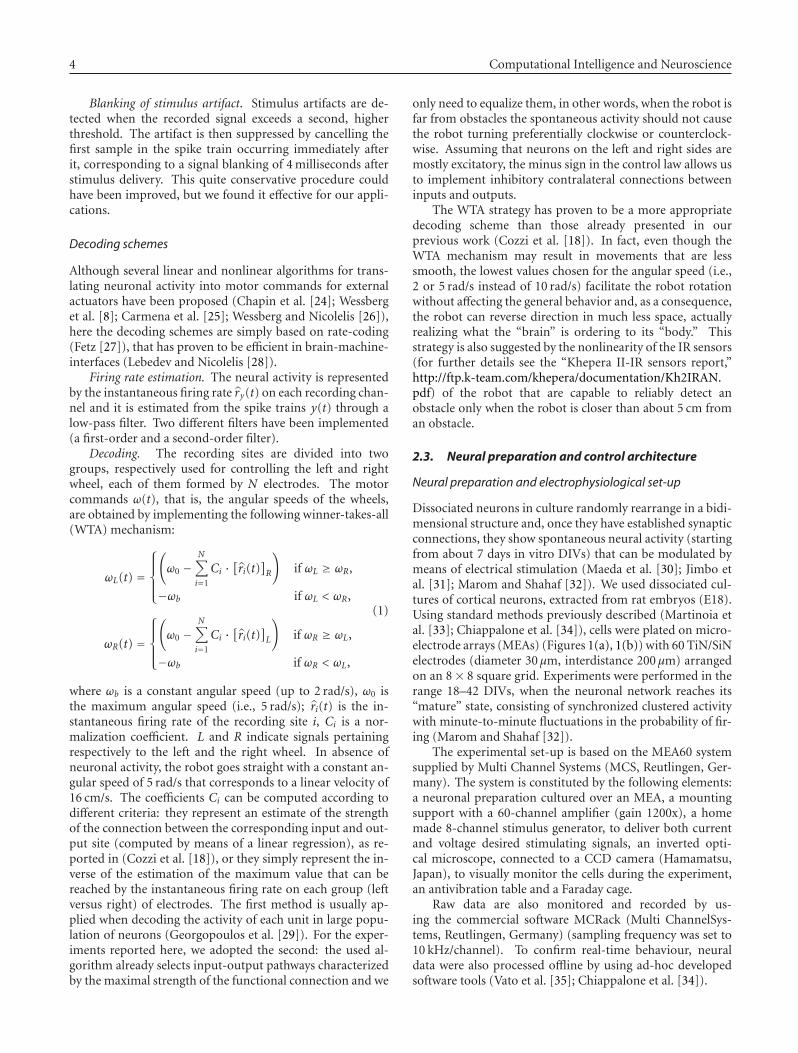
4 Computational Intelligence and Neuroscience
Blanking of stimulus artifact. Stimulus artifacts are de-tected when the recorded signal exceeds a second, higherthreshold. The artifact is then suppressed by cancelling thefirst sample in the spike train occurring immediately afterit, corresponding to a signal blanking of 4 milliseconds afterstimulus delivery. This quite conservative procedure couldhave been improved, but we found it effective for our appli-cations.
Decoding schemes
Although several linear and nonlinear algorithms for trans-lating neuronal activity into motor commands for externalactuators have been proposed (Chapin et al. [24]; Wessberget al. [8]; Carmena et al. [25]; Wessberg and Nicolelis [26]),here the decoding schemes are simply based on rate-coding(Fetz [27]), that has proven to be efficient in brain-machine-interfaces (Lebedev and Nicolelis [28]).
Firing rate estimation. The neural activity is representedby the instantaneous firing rate ry(t) on each recording chan-nel and it is estimated from the spike trains y(t) through alow-pass filter. Two different filters have been implemented(a first-order and a second-order filter).
Decoding. The recording sites are divided into twogroups, respectively used for controlling the left and rightwheel, each of them formed by N electrodes. The motorcommands ω(t), that is, the angular speeds of the wheels,are obtained by implementing the following winner-takes-all(WTA) mechanism:
ωL(t) =
⎧⎪⎪⎨⎪⎪⎩(ω0 −
N∑i=1
Ci ·[ri(t)
]R
)if ωL ≥ ωR,
−ωb if ωL < ωR,
ωR(t) =
⎧⎪⎪⎨⎪⎪⎩(ω0 −
N∑i=1
Ci ·[ri(t)
]L
)if ωR ≥ ωL,
−ωb if ωR < ωL,
(1)
where ωb is a constant angular speed (up to 2 rad/s), ω0 isthe maximum angular speed (i.e., 5 rad/s); ri(t) is the in-stantaneous firing rate of the recording site i, Ci is a nor-malization coefficient. L and R indicate signals pertainingrespectively to the left and the right wheel. In absence ofneuronal activity, the robot goes straight with a constant an-gular speed of 5 rad/s that corresponds to a linear velocity of16 cm/s. The coefficients Ci can be computed according todifferent criteria: they represent an estimate of the strengthof the connection between the corresponding input and out-put site (computed by means of a linear regression), as re-ported in (Cozzi et al. [18]), or they simply represent the in-verse of the estimation of the maximum value that can bereached by the instantaneous firing rate on each group (leftversus right) of electrodes. The first method is usually ap-plied when decoding the activity of each unit in large popu-lation of neurons (Georgopoulos et al. [29]). For the exper-iments reported here, we adopted the second: the used al-gorithm already selects input-output pathways characterizedby the maximal strength of the functional connection and we
only need to equalize them, in other words, when the robot isfar from obstacles the spontaneous activity should not causethe robot turning preferentially clockwise or counterclock-wise. Assuming that neurons on the left and right sides aremostly excitatory, the minus sign in the control law allows usto implement inhibitory contralateral connections betweeninputs and outputs.
The WTA strategy has proven to be a more appropriatedecoding scheme than those already presented in ourprevious work (Cozzi et al. [18]). In fact, even though theWTA mechanism may result in movements that are lesssmooth, the lowest values chosen for the angular speed (i.e.,2 or 5 rad/s instead of 10 rad/s) facilitate the robot rotationwithout affecting the general behavior and, as a consequence,the robot can reverse direction in much less space, actuallyrealizing what the “brain” is ordering to its “body.” Thisstrategy is also suggested by the nonlinearity of the IR sensors(for further details see the “Khepera II-IR sensors report,”http://ftp.k-team.com/khepera/documentation/Kh2IRAN.pdf) of the robot that are capable to reliably detect anobstacle only when the robot is closer than about 5 cm froman obstacle.
2.3. Neural preparation and control architecture
Neural preparation and electrophysiological set-up
Dissociated neurons in culture randomly rearrange in a bidi-mensional structure and, once they have established synapticconnections, they show spontaneous neural activity (startingfrom about 7 days in vitro DIVs) that can be modulated bymeans of electrical stimulation (Maeda et al. [30]; Jimbo etal. [31]; Marom and Shahaf [32]). We used dissociated cul-tures of cortical neurons, extracted from rat embryos (E18).Using standard methods previously described (Martinoia etal. [33]; Chiappalone et al. [34]), cells were plated on micro-electrode arrays (MEAs) (Figures 1(a), 1(b)) with 60 TiN/SiNelectrodes (diameter 30 μm, interdistance 200 μm) arrangedon an 8× 8 square grid. Experiments were performed in therange 18–42 DIVs, when the neuronal network reaches its“mature” state, consisting of synchronized clustered activitywith minute-to-minute fluctuations in the probability of fir-ing (Marom and Shahaf [32]).
The experimental set-up is based on the MEA60 systemsupplied by Multi Channel Systems (MCS, Reutlingen, Ger-many). The system is constituted by the following elements:a neuronal preparation cultured over an MEA, a mountingsupport with a 60-channel amplifier (gain 1200x), a homemade 8-channel stimulus generator, to deliver both currentand voltage desired stimulating signals, an inverted opti-cal microscope, connected to a CCD camera (Hamamatsu,Japan), to visually monitor the cells during the experiment,an antivibration table and a Faraday cage.
Raw data are also monitored and recorded by us-ing the commercial software MCRack (Multi ChannelSys-tems, Reutlingen, Germany) (sampling frequency was set to10 kHz/channel). To confirm real-time behaviour, neuraldata were also processed offline by using ad-hoc developedsoftware tools (Vato et al. [35]; Chiappalone et al. [34]).

A. Novellino et al. 5
Control architecture
The control architecture presented in our previous work(Cozzi et al. [18]) has partially changed and some feature hasbeen added. In particular, we have moved from xPC-Target(http://www.mathworks.com/products/xpctarget) that wasnot able to handle and log the very large amount of data com-ing from neuronal network, to the QNX 6.1 (QNX softwaresystems), a POSIX-compatible operating system specific forhard real-time applications.
The present architecture involves three PCs. PC1 (P4,2.8 GHz, 512 MB RAM), that is, the one that runs QNX, isequipped with an A/D board PCI-6071E (National Instru-ments, Texas, USA) and it is responsible for (a) electrophys-iological signals acquisition, (b) online spike detection andartifact blanking, (c) decoding of the spike trains, (d) han-dling the serial communication with the robot and PC3, (e)coding of robot’s proximity sensors signals, (f) productionof the pattern of stimuli that trigger the electrical stimulator,and (g) experimental data logging (spikes, sensors activity,wheel speeds, stimuli, robot trajectory). These tasks are pro-cessed by different threads at different sampling rates, in par-ticular tasks (a)-(b) are at 10 Khz, tasks (c)–(e)-(f)-(g) are at250 Hz, and task (d) is at 10 Hz.
A second computer, PC2 (P4, 2.8 GHz, 512 MB RAM,Win2000), connected to PC1 through an Ethernet link, isthe experimental front-end. We used Simulink/Real-TimeWorkshop (the MathWorks) and the RT-Lab package (Opal-RT) as development environments. This package generatestwo processes that are executed in real-time on the targetnode, that is, PC1. This system allows simultaneous acqui-sition of neural signals from up to 32 recording sites.
PC3 (P4 2.8 GHz 512 MB RAM, QNX 6.1) is in chargeof real-time tracking of the robot movement and it is con-nected through a serial cable to the main computational nodeof the architecture (PC1). A CCD camera (DSE TCC5 with1/3 CCD SONY SuperHAD) is placed 1.5 m above the centralposition of the arena. This physical arrangement of the cam-era allows a good resolution while minimizing distortion atthe boundaries of the arena. A frame-grabber (Arvoo PicassoPCI-2SQ) acquires samples at 5 Hz from the camera with aresolution of 640× 480 pixels. One pixel on the CCD sensorcorresponds to ∼ 2 mm, so that the arena is contained in a400× 400 subwindow at the center of the image. The detec-tion phase is performed in a small square portion (50 × 50pixels) of the global field of the CCD camera (the detectionin such small area is low demanding in computing perfor-mance and thus the process can be performed in real-time).This square area represents the predicted robot location. Ared round marker placed onto the top of the robot and thedetection of its position is based on a local evaluation of theintensity of the RGB values of every pixel belonging to thedetection window.
2.4. Data analysis
Processing of electrophysiological signals
Poststimulus Time Histogram. To investigate the neural ac-tivity evoked by stimulation, we computed the poststimulus
time histogram (i.e., PSTH), which represents the impulseresponse of each site of the neural preparation to electricalstimulation. The PSTHs were calculated by taking 400 mstime windows from the recordings that follow each stimu-lus. We then counted the number of spikes occurring in a 2–4 msec bin and divided this measure by the number of stimuli(Rieke et al. [36]). For our cultures, typical PSTHs show an“early” (less than 50 msec) and a “late” (50–250 milliseconds)component (Shahaf and Marom [5]; Marom and Shahaf[32]; Cozzi et al. [22]).
Stimulus-Triggered Speed. The stimulus-triggered speed(STS) is constructed by averaging the speed waveform dueto each stimulus. The robot has two independent wheels,whose speeds are proportional to the neuronal activity of two“brain” regions (i.e., the two set of electrodes selected as mo-tor areas within the network). These regions receive sensoryfeedback by two independent stimulating sites. It is possibleto construct two STSs for each input-output, that is, sensory-motor pathways, for a total of 4 curves (i.e., the variations ofthe speed of the left and the right wheels in response to theleft stimulus are the first two curves and constitute the firstSTS, and the variation of the speed of the left and the rightwheels in response to the right stimulus constitute the sec-ond STS with the latter two curves), and it is also possibleto study the performance of the robot behavior by studyingthe side-selectivity of the relationship between stimuli andspeeds.
Indicators of robot performance
The behavior of the neurorobotic system can be evaluated bymeans of the stimulus-triggered speed (STS), that is, the aver-age motor commands elicited by a single electrical stimulus:
STS(τ) = ⟨ω(τ − ti)⟩
i, (2)
where ti is the time instant of delivery of the ith stimulus andτ is the time coordinate.
In order to have a more general evaluation of the robotperformance during each trail (5′), we also used the follow-ing three parameters:
(i) number of hits,(ii) trajectory length,
(iii) space covered. The percentage of the arena area coveredby the robot path:
SC = NP · c f 2
Aarena − nAobstacle· 100%, (3)
where NP is the number of pixels covered by the robot,c f 2 is the area of one pixel, n is the number of obstaclesin the playground, Aarena and Aobstacle are, respectively,the areas of the playground and of each obstacle.
The software tools for of-line signal processing aimed at theanalysis of the behavior of the neurorobotic system were de-veloped using Matlab 6.5 (the MathWorks).
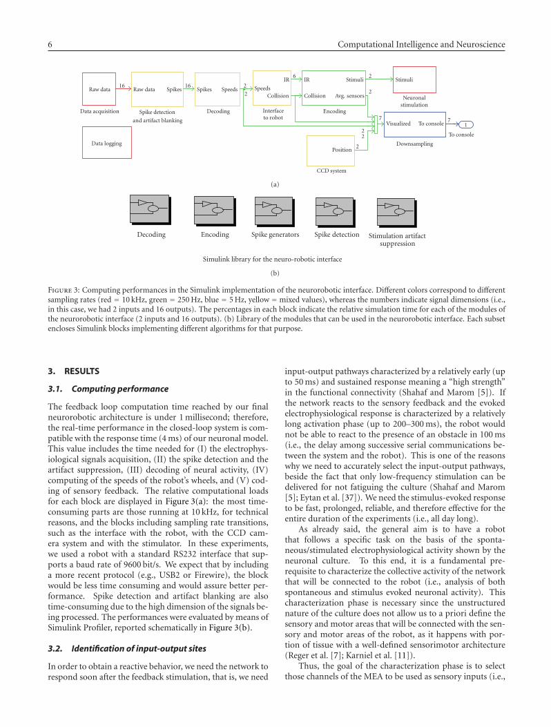
6 Computational Intelligence and Neuroscience
Spikes16
Spikes Speeds2
2Speeds
Collision
IR6
IR Stimuli
Collision Avg. sensors
2
2
22
2Position
Encoding7
Stimuli
Visualized To console
To console
71
Downsampling
Neuronalstimulation
Raw data Raw data
Data logging
Data acquisition
16
Spike detection
and artifact blanking
Decoding Interfaceto robot
CCD system
(a)
Decoding Encoding Spike generators Spike detection Stimulation artifactsuppression
Simulink library for the neuro-robotic interface
(b)
Figure 3: Computing performances in the Simulink implementation of the neurorobotic interface. Different colors correspond to differentsampling rates (red = 10 kHz, green = 250 Hz, blue = 5 Hz, yellow = mixed values), whereas the numbers indicate signal dimensions (i.e.,in this case, we had 2 inputs and 16 outputs). The percentages in each block indicate the relative simulation time for each of the modules ofthe neurorobotic interface (2 inputs and 16 outputs). (b) Library of the modules that can be used in the neurorobotic interface. Each subsetencloses Simulink blocks implementing different algorithms for that purpose.
3. RESULTS
3.1. Computing performance
The feedback loop computation time reached by our finalneurorobotic architecture is under 1 millisecond; therefore,the real-time performance in the closed-loop system is com-patible with the response time (4 ms) of our neuronal model.This value includes the time needed for (I) the electrophys-iological signals acquisition, (II) the spike detection and theartifact suppression, (III) decoding of neural activity, (IV)computing of the speeds of the robot’s wheels, and (V) cod-ing of sensory feedback. The relative computational loadsfor each block are displayed in Figure 3(a): the most time-consuming parts are those running at 10 kHz, for technicalreasons, and the blocks including sampling rate transitions,such as the interface with the robot, with the CCD cam-era system and with the stimulator. In these experiments,we used a robot with a standard RS232 interface that sup-ports a baud rate of 9600 bit/s. We expect that by includinga more recent protocol (e.g., USB2 or Firewire), the blockwould be less time consuming and would assure better per-formance. Spike detection and artifact blanking are alsotime-consuming due to the high dimension of the signals be-ing processed. The performances were evaluated by means ofSimulink Profiler, reported schematically in Figure 3(b).
3.2. Identification of input-output sites
In order to obtain a reactive behavior, we need the network torespond soon after the feedback stimulation, that is, we need
input-output pathways characterized by a relatively early (upto 50 ms) and sustained response meaning a “high strength”in the functional connectivity (Shahaf and Marom [5]). Ifthe network reacts to the sensory feedback and the evokedelectrophysiological response is characterized by a relativelylong activation phase (up to 200–300 ms), the robot wouldnot be able to react to the presence of an obstacle in 100 ms(i.e., the delay among successive serial communications be-tween the system and the robot). This is one of the reasonswhy we need to accurately select the input-output pathways,beside the fact that only low-frequency stimulation can bedelivered for not fatiguing the culture (Shahaf and Marom[5]; Eytan et al. [37]). We need the stimulus-evoked responseto be fast, prolonged, reliable, and therefore effective for theentire duration of the experiments (i.e., all day long).
As already said, the general aim is to have a robotthat follows a specific task on the basis of the sponta-neous/stimulated electrophysiological activity shown by theneuronal culture. To this end, it is a fundamental pre-requisite to characterize the collective activity of the networkthat will be connected to the robot (i.e., analysis of bothspontaneous and stimulus evoked neuronal activity). Thischaracterization phase is necessary since the unstructurednature of the culture does not allow us to a priori define thesensory and motor areas that will be connected with the sen-sory and motor areas of the robot, as it happens with por-tion of tissue with a well-defined sensorimotor architecture(Reger et al. [7]; Karniel et al. [11]).
Thus, the goal of the characterization phase is to selectthose channels of the MEA to be used as sensory inputs (i.e.,
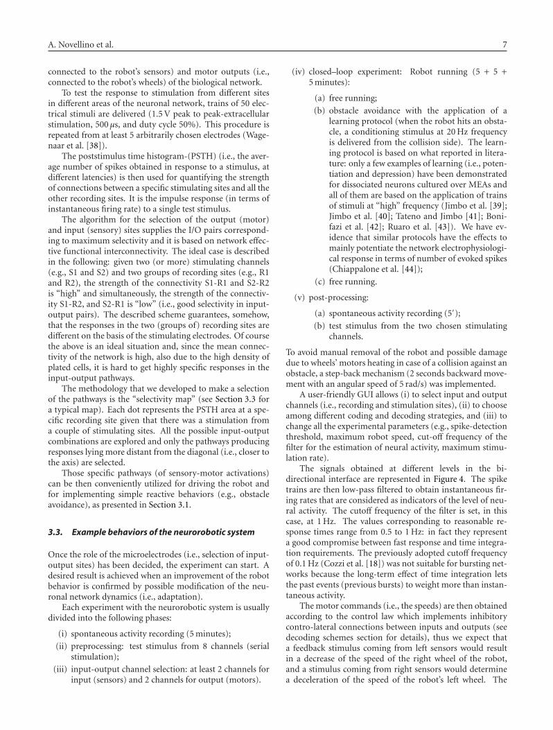
A. Novellino et al. 7
connected to the robot’s sensors) and motor outputs (i.e.,connected to the robot’s wheels) of the biological network.
To test the response to stimulation from different sitesin different areas of the neuronal network, trains of 50 elec-trical stimuli are delivered (1.5 V peak to peak-extracellularstimulation, 500 μs, and duty cycle 50%). This procedure isrepeated from at least 5 arbitrarily chosen electrodes (Wage-naar et al. [38]).
The poststimulus time histogram-(PSTH) (i.e., the aver-age number of spikes obtained in response to a stimulus, atdifferent latencies) is then used for quantifying the strengthof connections between a specific stimulating sites and all theother recording sites. It is the impulse response (in terms ofinstantaneous firing rate) to a single test stimulus.
The algorithm for the selection of the output (motor)and input (sensory) sites supplies the I/O pairs correspond-ing to maximum selectivity and it is based on network effec-tive functional interconnectivity. The ideal case is describedin the following: given two (or more) stimulating channels(e.g., S1 and S2) and two groups of recording sites (e.g., R1and R2), the strength of the connectivity S1-R1 and S2-R2is “high” and simultaneously, the strength of the connectiv-ity S1-R2, and S2-R1 is “low” (i.e., good selectivity in input-output pairs). The described scheme guarantees, somehow,that the responses in the two (groups of) recording sites aredifferent on the basis of the stimulating electrodes. Of coursethe above is an ideal situation and, since the mean connec-tivity of the network is high, also due to the high density ofplated cells, it is hard to get highly specific responses in theinput-output pathways.
The methodology that we developed to make a selectionof the pathways is the “selectivity map” (see Section 3.3 fora typical map). Each dot represents the PSTH area at a spe-cific recording site given that there was a stimulation froma couple of stimulating sites. All the possible input-outputcombinations are explored and only the pathways producingresponses lying more distant from the diagonal (i.e., closer tothe axis) are selected.
Those specific pathways (of sensory-motor activations)can be then conveniently utilized for driving the robot andfor implementing simple reactive behaviors (e.g., obstacleavoidance), as presented in Section 3.1.
3.3. Example behaviors of the neurorobotic system
Once the role of the microelectrodes (i.e., selection of input-output sites) has been decided, the experiment can start. Adesired result is achieved when an improvement of the robotbehavior is confirmed by possible modification of the neu-ronal network dynamics (i.e., adaptation).
Each experiment with the neurorobotic system is usuallydivided into the following phases:
(i) spontaneous activity recording (5 minutes);
(ii) preprocessing: test stimulus from 8 channels (serialstimulation);
(iii) input-output channel selection: at least 2 channels forinput (sensors) and 2 channels for output (motors).
(iv) closed–loop experiment: Robot running (5 + 5 +5 minutes):
(a) free running;
(b) obstacle avoidance with the application of alearning protocol (when the robot hits an obsta-cle, a conditioning stimulus at 20 Hz frequencyis delivered from the collision side). The learn-ing protocol is based on what reported in litera-ture: only a few examples of learning (i.e., poten-tiation and depression) have been demonstratedfor dissociated neurons cultured over MEAs andall of them are based on the application of trainsof stimuli at “high” frequency (Jimbo et al. [39];Jimbo et al. [40]; Tateno and Jimbo [41]; Boni-fazi et al. [42]; Ruaro et al. [43]). We have ev-idence that similar protocols have the effects tomainly potentiate the network electrophysiologi-cal response in terms of number of evoked spikes(Chiappalone et al. [44]);
(c) free running.
(v) post-processing:
(a) spontaneous activity recording (5′);
(b) test stimulus from the two chosen stimulatingchannels.
To avoid manual removal of the robot and possible damagedue to wheels’ motors heating in case of a collision against anobstacle, a step-back mechanism (2 seconds backward move-ment with an angular speed of 5 rad/s) was implemented.
A user-friendly GUI allows (i) to select input and outputchannels (i.e., recording and stimulation sites), (ii) to chooseamong different coding and decoding strategies, and (iii) tochange all the experimental parameters (e.g., spike-detectionthreshold, maximum robot speed, cut-off frequency of thefilter for the estimation of neural activity, maximum stimu-lation rate).
The signals obtained at different levels in the bi-directional interface are represented in Figure 4. The spiketrains are then low-pass filtered to obtain instantaneous fir-ing rates that are considered as indicators of the level of neu-ral activity. The cutoff frequency of the filter is set, in thiscase, at 1 Hz. The values corresponding to reasonable re-sponse times range from 0.5 to 1 Hz: in fact they representa good compromise between fast response and time integra-tion requirements. The previously adopted cutoff frequencyof 0.1 Hz (Cozzi et al. [18]) was not suitable for bursting net-works because the long-term effect of time integration letsthe past events (previous bursts) to weight more than instan-taneous activity.
The motor commands (i.e., the speeds) are then obtainedaccording to the control law which implements inhibitorycontro-lateral connections between inputs and outputs (seedecoding schemes section for details), thus we expect thata feedback stimulus coming from left sensors would resultin a decrease of the speed of the right wheel of the robot,and a stimulus coming from right sensors would determinea deceleration of the speed of the robot’s left wheel. The

8 Computational Intelligence and Neuroscience
20 s
Right wheel speed
Left wheel speed
Right detected spikes
Left detected spikes
Right stimuli
Left stimuli
Right sensors
Left sensors
Thumbs
(a)
1
2
2
Detected spikes
Mean wheel speed
Left Right
Left Right
(b)
Figure 4: Signals obtained at different levels of the neurorobotic interface during 20 seconds of a free running session (c.f. Results, for adetailed description of the experimental protocol). In this particular experiment we used 2 stimulation sites and 2 recording sites. Whenthe robot is approaching an obstacle, the value of sensors increases and when it overcomes a threshold (i.e., 500 levels) a feedback stimulusis delivered (max frequency 1 Hz). The left and right detected spike trains are then processed into motor commands, that is, left and rightwheel speeds (the line corresponds to 0 rad/s). The network was spontaneously active and during this phase we recorded 2046 spikes fromleft and 1057 from the right one, resulting in a mean wheel speed of 1.4 rad/s (left) and 1.6 rad/s (right).
proximity signals coming from the sensors placed on the twosides of the robot are averaged in order to obtain two feed-back signals, each of them related to one side of the robot.Figure 4 shows the patterns of stimuli obtained from thefeedback signals, according to the binary coding scheme.
A number of preliminary experiments were performedusing, respectively, 2 stimulation and 2 recording sites. Inthe following, the results of two example experiments are re-ported to let the reader better understand the experimentalprocedure and appreciate the performances of the developedclosed-loop system.
Figure 5 shows the PSTHs obtained during the charac-terization phase of one example experiment. The responsesevoked from different stimulation sites are similar (i.e., Fig-ures 5(a) and 5(b)), thus revealing a low degree of selectiv-ity and a high degree of connectivity. In a case like the onepresented in Figure 5, the preparation can hardly be used tocontrol the robot and it is discarded.
Figure 6 presents an example of good connectivity mapsobtained during the characterization phase (Figure 6(a))and after the robotic experiment (Figure 6(b)): the elec-trodes 15 and 45, that will be further chosen as recordingelectrodes, are positioned close to the axis, indicating thattheir responses to the stimulating channel are selective (seeSection 3.2 for further details).
Figures 7(a) and 7(b) show the PSTHs corresponding tothe inputs/outputs chosen after the characterization phase;during an experimental session with the robot (i.e., experi-ment is different from the previous one). In this example,the recording electrode 15 is very sensitive to the stimulationdelivered from electrode 16 (top left) while it is quite unaf-
fected by stimuli delivered form electrode 48 (top right). Atthe same time, the recording site 45 is not sensitive to stim-uli coming from electrode 16 (bottom left) while it is veryaffected by stimulation from electrode 48. In this case, dif-ferent stimulation sites evoke very different response, thusrevealing a high degree of selectivity that is also confirmedby the connectivity maps presented in Figure 6.
The shapes of the PSTHs must be similar to those of thePSTHs obtained during the characterization phase in orderto ensure the stability of the response of the neuronal cul-ture. If the area of the PSTHs drastically decreases at the endof the closed loop phases it means that the neuronal networkhas been fatigued by excessive repeated stimulations (Sha-haf and Marom [5]). The wellness and stability of the cul-ture are “sine qua non” conditions to be verified before de-scribing the neurorobotic behavior by means of the robot’sperformance indicators. Under these conditions, the per-formance of the neural preparation in controlling the robotcan be represented by the STSs, depicted in Figures 7(c) and7(d).
Examples of the robot trajectories are presented in Fig-ures 8(a) and 8(b). Figure 8(c) shows the indicators generallyused for quantifying the robot performance. The first indi-cator alone, that is, the number of hits, is not sufficient fordescribing the performances of an obstacle avoidance task.In fact, a low number of hits could result from limited robotmovements or from the repetition of the same trajectory.For this reason, it is necessary to consider also the fractionof space covered by the robot and the length of its trajec-tory. Together, these simple indicators evaluate the robotperformances inside the arena, even if they are not related
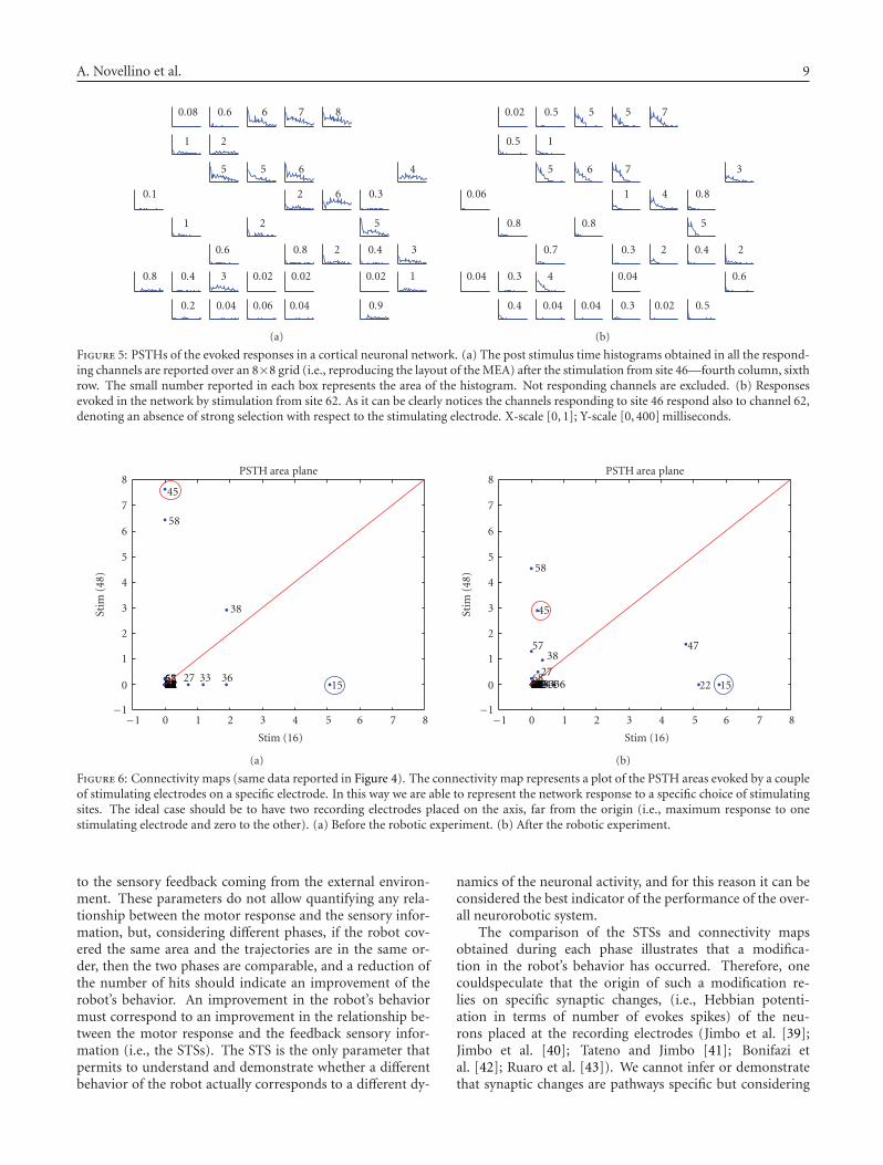
A. Novellino et al. 9
0.08 0.6 6 7 8
1 2
5 5 6 4
0.1 2 6 0.3
1 2 5
0.6 0.8 2 0.4 3
0.8 0.4 3 0.02 0.02 0.02 1
0.2 0.04 0.06 0.04 0.9
(a)
0.02 0.5 5 5 7
0.5 1
5 6 7 3
0.06 1 4 0.8
0.8 0.8 5
0.7 0.3 2 0.4 2
0.04 0.3 4 0.04 0.6
0.4 0.04 0.04 0.3 0.02 0.5
(b)
Figure 5: PSTHs of the evoked responses in a cortical neuronal network. (a) The post stimulus time histograms obtained in all the respond-ing channels are reported over an 8×8 grid (i.e., reproducing the layout of the MEA) after the stimulation from site 46—fourth column, sixthrow. The small number reported in each box represents the area of the histogram. Not responding channels are excluded. (b) Responsesevoked in the network by stimulation from site 62. As it can be clearly notices the channels responding to site 46 respond also to channel 62,denoting an absence of strong selection with respect to the stimulating electrode. X-scale [0, 1]; Y-scale [0, 400] milliseconds.
1213141617212425262831323435374142434446485152535455565761626364656667687172737475767778828384858687
−1 0 1 2 3 4 5 6 7 8
Stim (16)
PSTH area plane
Stim
(48)
−1
0
1
2
3
4
5
6
7
845
58
38
27 33 3615
(a)
121314161721242526283132333435 3637414243 444648515253545556616263646566677172737475767778828384858687
−1 0 1 2 3 4 5 6 7 8
Stim (16)
PSTH area planeSt
im(4
8)
−1
0
1
2
3
4
5
6
7
8
58
45
5738
2768
47
22 15
(b)
Figure 6: Connectivity maps (same data reported in Figure 4). The connectivity map represents a plot of the PSTH areas evoked by a coupleof stimulating electrodes on a specific electrode. In this way we are able to represent the network response to a specific choice of stimulatingsites. The ideal case should be to have two recording electrodes placed on the axis, far from the origin (i.e., maximum response to onestimulating electrode and zero to the other). (a) Before the robotic experiment. (b) After the robotic experiment.
to the sensory feedback coming from the external environ-ment. These parameters do not allow quantifying any rela-tionship between the motor response and the sensory infor-mation, but, considering different phases, if the robot cov-ered the same area and the trajectories are in the same or-der, then the two phases are comparable, and a reduction ofthe number of hits should indicate an improvement of therobot’s behavior. An improvement in the robot’s behaviormust correspond to an improvement in the relationship be-tween the motor response and the feedback sensory infor-mation (i.e., the STSs). The STS is the only parameter thatpermits to understand and demonstrate whether a differentbehavior of the robot actually corresponds to a different dy-
namics of the neuronal activity, and for this reason it can beconsidered the best indicator of the performance of the over-all neurorobotic system.
The comparison of the STSs and connectivity mapsobtained during each phase illustrates that a modifica-tion in the robot’s behavior has occurred. Therefore, onecouldspeculate that the origin of such a modification re-lies on specific synaptic changes, (i.e., Hebbian potenti-ation in terms of number of evokes spikes) of the neu-rons placed at the recording electrodes (Jimbo et al. [39];Jimbo et al. [40]; Tateno and Jimbo [41]; Bonifazi etal. [42]; Ruaro et al. [43]). We cannot infer or demonstratethat synaptic changes are pathways specific but considering
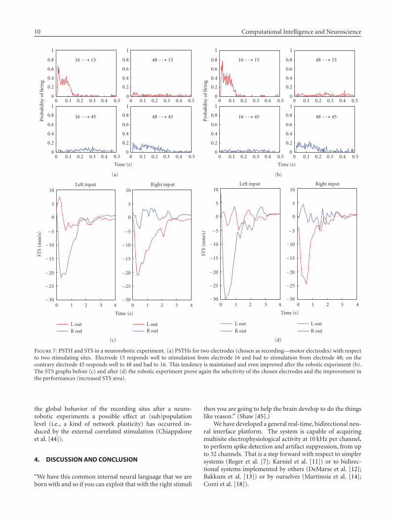
10 Computational Intelligence and Neuroscience
0 0.1 0.2 0.3 0.4 0.5
0 0.1 0.2 0.3 0.4 0.5 0 0.1 0.2 0.3 0.4 0.5
0 0.1 0.2 0.3 0.4 0.5
Time (s)
Pro
babi
lity
offi
rin
g
0
0.2
0.4
0.6
0.8
1
0
0.2
0.4
0.6
0.8
1
0
0.2
0.4
0.6
0.8
1
0
0.2
0.4
0.6
0.8
1
16 ��� 15 48 ��� 15
16 ��� 45 48 ��� 45
(a)
0 0.1 0.2 0.3 0.4 0.5
0 0.1 0.2 0.3 0.4 0.5
0
0.2
0.4
0.6
0.8
1
0
0.2
0.4
0.6
0.8
1
0 0.1 0.2 0.3 0.4 0.5
0 0.1 0.2 0.3 0.4 0.5
Time (s)
Pro
babi
lity
offi
rin
g
0
0.2
0.4
0.6
0.8
1
0
0.2
0.4
0.6
0.8
1
16 ��� 15 48 ��� 15
16 ��� 45 48 ��� 45
(b)
0 1 2 3 4 0 1 2 3 4
Time (s)
Left input Right input
L outR out
L outR out
−30
−25
−20
−15
−10
−5
0
5
10
STS
(mm
/s)
−30
−25
−20
−15
−10
−5
0
5
10
(c)
0 1 2 3 4 0 1 2 3 4
Time (s)
Left input Right input
L out
R out
L out
R out
STS
(mm
/s)
−30
−25
−20
−15
−10
−5
0
5
10
−30
−25
−20
−15
−10
−5
0
5
10
(d)
Figure 7: PSTH and STS in a neurorobotic experiment. (a) PSTHs for two electrodes (chosen as recording—motor electrodes) with respectto two stimulating sites. Electrode 15 responds well to stimulation from electrode 16 and bad to stimulation from electrode 48; on thecontrary electrode 45 responds well to 48 and bad to 16. This tendency is maintained and even improved after the robotic experiment (b).The STS graphs before (c) and after (d) the robotic experiment prove again the selectivity of the chosen electrodes and the improvement inthe performances (increased STS area).
the global behavior of the recording sites after a neuro-robotic experiments a possible effect at (sub)populationlevel (i.e., a kind of network plasticity) has occurred in-duced by the external correlated stimulation (Chiappaloneet al. [44]).
4. DISCUSSION AND CONCLUSION
“We have this common internal neural language that we areborn with and so if you can exploit that with the right stimuli
then you are going to help the brain develop to do the thingslike reason.” (Shaw [45].)
We have developed a general real-time, bidirectional neu-ral interface platform. The system is capable of acquiringmultisite electrophysiological activity at 10 kHz per channel,to perform spike detection and artifact suppression, from upto 32 channels. That is a step forward with respect to simplersystems (Reger et al. [7]; Karniel et al. [11]) or to bidirec-tional systems implemented by others (DeMarse et al. [12];Bakkum et al. [13]) or by ourselves (Martinoia et al. [14];Cozzi et al. [18]).
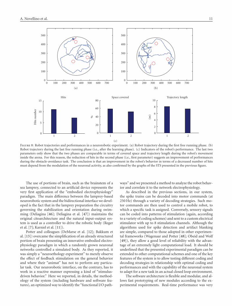
A. Novellino et al. 11
0 100 200 300 400 500 600 7000
100
200
300
400
500
(a)
0 100 200 300 400 500 600 7000
100
200
300
400
500
(b)
0
5
10
15Hits
Hit
sn
um
ber
1 20
20
40
60
80Space covered
%
1 20
2
4
6
8
10Trajectory length
(m)
1 2
(c)
Figure 8: Robot trajectories and performances in a neurorobotic experiment. (a) Robot trajectory during the first free running phase. (b)Robot trajectory during the last free running phase (i.e., after the learning phase). (c) Indicators of the robot’s performance. The last twoparameters only show that the two phases are comparable in terms of covered space and trajectory length during the robot’s movementinside the arena. For this reason, the reduction of hits in the second phase (i.e., first parameter) suggests an improvement of performancesduring the obstacle-avoidance task. The conclusion is that an improvement in the robot’s behavior in terms of a decreased number of hitsmust depend from the modulation of the neuronal activity, as also confirmed by the graphs of the STS presented in the previous figure.
The use of portions of brain, such as the brainstem of asea lamprey, connected to an artificial device represents thevery first application of the “embodied electrophysiology”paradigm. The main difference between the lamprey-basedneurorobotic system and the bidirectional interface we devel-oped is the fact that in the lamprey preparation the circuitrygoverning the stabilization and orientation during swim-ming (Deliagina [46]; Deliagina et al. [47]) maintains theoriginal citoarchitecture and the natural input-output sys-tem is used as a controller to drive the robotic body (Regeret al. [7]; Karniel et al. [11]).
Potter and colleagues (DeMarse et al. [12]; Bakkum etal. [13]) overcame the simplification of an already structuredportion of brain presenting an innovative embodied electro-physiology paradigm in which a randomly grown neuronalnetworks controlled a simulated body. As they reported, itwas simply a “neuroethology experiment” to merely observethe effect of feedback stimulation on the general behaviorand where their “animat” has not to perform any particu-lar task. Our neurorobotic interface, on the contrary, has towork in a reactive manner expressing a kind of “stimulus-driven behavior.” Here we reported, in details, the method-ology of the system (including hardware and software fea-tures), an optimized way to identify the “functional I/O path-
ways” and we presented a method to analyze the robot behav-ior and correlate it to the network electrophysiology.
As described in the previous sections, in our system,the spike trains can be decoded into motor commands (at250 Hz) through a variety of decoding strategies. Such mo-tor commands are then used to control a mobile robot, towhich a specific task is assigned. Conversely, sensory signalscan be coded into patterns of stimulation (again, accordingto a variety of coding schemes) and sent to a custom electricalstimulator with up to 8 stimulation channels. Although thealgorithms used for spike detection and artifact blankingare simple, compared to those adopted in other experimen-tal frameworks (Wagenaar and Potter [48]; Obeid and Wolf[49]), they allow a good level of reliability with the advan-tage of an extremely light computational load. It should beunderlined that the presented experimental paradigm can beextended to other computational schemes and one of the keyfeatures of the system is to allow testing different coding anddecoding strategies in relationship with optimal coding andperformances and with the capability of the neuronal systemto adapt for a new task in an actual closed loop environment.
The software architecture is flexible and modular, and al-lows fast prototyping of new modules according to the ex-perimental requirements. Real-time performance was very
12 Computational Intelligence and Neuroscience
good and it is comparable to other simpler systems (in termsof recording/stimulating channels), previously described inthe literature (Reger et al. [7]; Martinoia et al. [14]; Wage-naar and Potter [38]; Cozzi et al. [18]; Karniel et al. [11];Wagenaar et al. [50]). We developed a library of coding anddecoding modules, which, as mentioned, could be easily ex-tended. This is a key point with respect to possible impli-cation for the development of novel brain-machine interfacewith enhanced capabilities and bidirectional interactivity.
Concerning our particular application, we also developedthe tools for studying the ability of a culture of cortical neu-rons to process information in order to drive a robot ac-cording to a defined motor task (with a particular empha-sis on the method for input-output pathways selection), andat the same time it allows to supervise the population activ-ity changes in response to external feedbacks. It should bestressed that this is the first time that a closed-loop neuro-robotic system (with in vitro neuronal populations) is uti-lized for performing specific behavioral oriented tasks.
The proposed experimental framework creates new pos-sibility for investigating basic mechanisms of learning andadaptation (e.g., distributed synaptic plasticity, long termpotentiation (LTP) and long term depression (LTD)) by di-rectly studying how behavior arises from the emerging col-lective dynamics of a neuronal ensemble. Additionally, theexperimental system could be also conveniently utilized andadapted to other in vitro models such as acute, organotypicslices, and patterned neurons, where the network architec-ture is partly preserved or can be designed.
Finally, on a long term perspective, this approach couldhave a relevant impact in the field of bio-inspired compu-tational systems and for the development of novel brain-computer interfaces and of advanced neuroprosthetic de-vices.
ACKNOWLEDGMENTS
The authors wish to thank Dr. M. Tedesco (Brunella) forcell culture preparation. This work is partly supported bythe EU Grant IST-2001-33564 (Neurobit), and by a grantfrom the Italian Ministry of University, Education and Re-search. Novellino’s Ph.D. fellowship was supported by etts.r.l. (http://www.ettsolutions.com).
REFERENCES
[1] D. A. Wagenaar, J. Pine, and S. M. Potter, “Effective parametersfor stimulation of dissociated cultures using multi-electrodearrays,” Journal of Neuroscience Methods, vol. 138, no. 1-2, pp.27–37, 2004.
[2] A. A. Sharp, M. B. O’Neil, L. F. Abbott, and E. Marder, “Thedynamic clamp: artificial conductances in biological neurons,”Trends in Neurosciences, vol. 16, no. 10, pp. 389–394, 1993.
[3] G. Le Masson, S. Renaud-Le Masson, D. Debay, and T. Bal,“Feedback inhibition controls spike transfer in hybrid thala-mic circuits,” Nature, vol. 417, no. 6891, pp. 854–858, 2002.
[4] D. A. Wagenaar, R. Madhavan, J. Pine, and S. M. Potter, “Con-trolling bursting in cortical cultures with closed-loop multi-electrode stimulation,” Journal of Neuroscience, vol. 25, no. 3,pp. 680–688, 2005.
[5] G. Shahaf and S. Marom, “Learning in networks of corticalneurons,” Journal of Neuroscience, vol. 21, no. 22, pp. 8782–8788, 2001.
[6] S. Marom and D. Eytan, “Learning in ex-vivo developing net-works of cortical neurons,” Progress in Brain Research, vol. 147,pp. 189–199, 2005.
[7] B. D. Reger, K. M. Fleming, V. Sanguineti, S. Alford, and F. A.Mussa-Ivaldi, “Connecting brains to robots: an artificial bodyfor studying the computational properties of neural tissues,”Artificial Life, vol. 6, no. 4, pp. 307–324, 2000.
[8] J. Wessberg, C. R. Stambaugh, J. D. Kralik, et al., “Real-timeprediction of hand trajectory by ensembles of cortical neuronsin primates,” Nature, vol. 408, no. 6810, pp. 361–365, 2000.
[9] M. A. L. Nicolelis, “Actions from thoughts,” Nature, vol. 409,no. 6818, pp. 403–407, 2001.
[10] A. B. Schwartz, D. M. Taylor, and S. I. H. Tillery, “Extractionalgorithms for cortical control of arm prosthetics,” CurrentOpinion in Neurobiology, vol. 11, no. 6, pp. 701–708, 2001.
[11] A. Karniel, M. Kositsky, K. M. Fleming, et al., “Computationalanalysis in vitro: dynamics and plasticity of a neuro-roboticsystem,” Journal of Neural Engineering, vol. 2, no. 3, pp. S250–S265, 2005.
[12] T. B. DeMarse, D. A. Wagenaar, A. W. Blau, and S. M. Potter,“The neurally controlled animat: biological brains acting withsimulated bodies,” Autonomous Robots, vol. 11, no. 3, pp. 305–310, 2001.
[13] D. J. Bakkum, A. C. Shkolnik, G. Ben-Ary, P. Gamblen, T. B.DeMarse, and S. M. Potter, “Removing some ‘A’ from AI: em-bodied cultured networks,” in International Seminar on Em-bodied Artificial Intelligence, vol. 3139 of Lecture Notes in Arti-ficial Intelligence, pp. 130–145, Dagstuhl Castle, Germany, July2004.
[14] S. Martinoia, V. Sanguineti, L. Cozzi, et al., “Towards an em-bodied in vitro electrophysiology:the NeuroBIT project,” Neu-rocomputing, vol. 58–60, pp. 1065–1072, 2004.
[15] S. M. Potter, “Chapter 4 distributed processing in culturedneuronal networks,” Progress in Brain Research, vol. 130, pp.49–62, 2001.
[16] F. A. Mussa-Ivaldi and L. E. Miller, “Brain-machine interfaces:computational demands and clinical needs meet basic neuro-science,” Trends in Neurosciences, vol. 26, no. 6, pp. 329–334,2003.
[17] M. A. L. Nicolelis, “Brain-machine interfaces to restore mo-tor function and probe neural circuits,” Nature Reviews Neu-roscience, vol. 4, no. 5, pp. 417–422, 2003.
[18] L. Cozzi, P. D’Angelo, M. Chiappalone, et al., “Coding anddecoding of information in a bi-directional neural interface,”Neurocomputing, vol. 65-66, pp. 783–792, 2005.
[19] P. Maes, “Modeling adaptive autonomous agents,” ArtificialLife, vol. 1, no. 1-2, pp. 135–162, 1994.
[20] R. A. Brooks, Robot: The Future of Flesh and Machines, AllenLane, The Penguin Press, London, UK, 2002.
[21] V. Braitenberg, Vehicles: Experiments in Synthetic Psychology,The MIT Press, Cambridge, Mass, USA, 1984.
[22] L. Cozzi, P. D’Angelo, and V. Sanguineti, “Encoding of time-varying stimuli in populations of cultured neurons,” BiologicalCybernetics, vol. 94, no. 5, pp. 335–349, 2006.
[23] M. Grattarola, M. Chiappalone, F. Davide, et al., “Burst anal-ysis of chemically stimulated spinal cord neuronal networkscultured on microelectrode arrays,” in Proceedings of the 23rdAnnual International Conference of the IEEE Engineering inMedicine and Biology Society, vol. 1, pp. 729–732, Istanbul,Turkey, October 2001.
A. Novellino et al. 13
[24] J. K. Chapin, K. A. Moxon, R. S. Markowitz, and M. A. L.Nicolelis, “Real-time control of a robot arm using simultane-ously recorded neurons in the motor cortex,” Nature Neuro-science, vol. 2, no. 7, pp. 664–670, 1999.
[25] J. M. Carmena, M. A. Lebedev, R. E. Crist, et al., “Learning tocontrol a brain-machine interface for reaching and graspingby primates,” PLoS Biology, vol. 1, no. 2, pp. 193–208, 2003.
[26] J. Wessberg and M. A. L. Nicolelis, “Optimizing a linear al-gorithm for real-time robotic control using chronic corticalensemble recordings in monkeys,” Journal of Cognitive Neuro-science, vol. 16, no. 6, pp. 1022–1035, 2004.
[27] E. E. Fetz, “Real-time control of a robotic arm by neuronalensembles,” Nature Neuroscience, vol. 2, no. 7, pp. 583–584,1999.
[28] M. A. Lebedev and M. A. L. Nicolelis, “Brain-machine in-terfaces: past, present and future,” Trends in Neurosciences,vol. 29, no. 9, pp. 536–546, 2006.
[29] A. P. Georgopoulos, A. B. Schwartz, and R. E. Kettner, “Neu-ronal population coding on movement direction,” Science,vol. 233, no. 4771, pp. 1416–1419, 1986.
[30] E. Maeda, Y. Kuroda, H. P. C. Robinson, and A. Kawana,“Modification of parallel activity elicited by propagatingbursts in developing networks of rat cortical neurones,” Euro-pean Journal of Neuroscience, vol. 10, no. 2, pp. 488–496, 1998.
[31] Y. Jimbo, A. Kawana, P. Parodi, and V. Torre, “The dynamics ofa neuronal culture of dissociated cortical neurons of neonatalrats,” Biological Cybernetics, vol. 83, no. 1, pp. 1–20, 2000.
[32] S. Marom and G. Shahaf, “Development, learning and mem-ory in large random networks of cortical neurons: lessons be-yond anatomy,” Quarterly Reviews of Biophysics, vol. 35, no. 1,pp. 63–87, 2002.
[33] S. Martinoia, L. Bonzano, M. Chiappalone, M. Tedesco, M.Marcoli, and G. Maura, “In vitro cortical neuronal networksas a new high-sensitive system for biosensing applications,”Biosensors and Bioelectronics, vol. 20, no. 10, pp. 2071–2078,2005.
[34] M. Chiappalone, M. Bove, A. Vato, M. Tedesco, and S. Marti-noia, “Dissociated cortical networks show spontaneously cor-related activity patterns during in vitro development,” BrainResearch, vol. 1093, no. 1, pp. 41–53, 2006.
[35] A. Vato, L. Bonzano, M. Chiappalone, et al., “Spike manager:a new tool for spontaneous and evoked neuronal networksactivity characterization,” Neurocomputing, vol. 58–60, pp.1153–1161, 2004.
[36] F. Rieke, D. Warland, R. de Ruyter van Steveninck, and W.Bialek, Spikes: Exploring the Neural Code, The MIT Press,Cambridge, Mass, USA, 1997.
[37] D. Eytan, N. Brenner, and S. Marom, “Selective adaptation innetworks of cortical neurons,” Journal of Neuroscience, vol. 23,no. 28, pp. 9349–9356, 2003.
[38] D. A. Wagenaar and S. M. Potter, “A versatile all-channel stim-ulator for electrode arrays, with real-time control,” Journal ofNeural Engineering, vol. 1, no. 1, pp. 39–45, 2004.
[39] Y. Jimbo, H. P. C. Robinson, and A. Kawana, “Strengtheningof synchronized activity by tetanic stimulation in cortical cul-tures: application of planar electrode arrays,” IEEE Transac-tions on Biomedical Engineering, vol. 45, no. 11, pp. 1297–1304,1998.
[40] Y. Jimbo, T. Tateno, and H. P. C. Robinson, “Simultaneousinduction of pathway-specific potentiation and depression innetworks of cortical neurons,” Biophysical Journal, vol. 76,no. 2, pp. 670–678, 1999.
[41] T. Tateno and Y. Jimbo, “Activity-dependent enhancement inthe reliability of correlated spike timings in cultured corti-cal neurons,” Biological Cybernetics, vol. 80, no. 1, pp. 45–55,1999.
[42] P. Bonifazi, M. E. Ruaro, and V. Torre, “Statistical properties ofinformation processing in neuronal networks,” European Jour-nal of Neuroscience, vol. 22, no. 11, pp. 2953–2964, 2005.
[43] M. E. Ruaro, P. Bonifazi, and V. Torre, “Toward the neurocom-puter: image processing and pattern recognition with neu-ronal cultures,” IEEE Transactions on Biomedical Engineering,vol. 52, no. 3, pp. 371–383, 2005.
[44] M. Chiappalone, P. Massobrio, M. Tedesco, and S. Marti-noia, “Stimulus-induced synaptic changes in networks of cor-tical neurons,” in Proceedings of the 5th International Meetingon Substrate-Integrated Micro Electrode Arrays (SIMEA ’06),pp. 32–33, BIOPRO Baden-Wurttemberg GmbH, Reutlingen,Germany, 2006.
[45] G. L. Shaw, Keeping Mozart in Mind, Academic Press, SanDiego, Calif, USA, 2nd edition, 2003.
[46] T. G. Deliagina, “Vestibular compensation in lampreys: im-pairment and recovery of equilibrium control during locomo-tion,” The Journal of Experimental Biology, vol. 200, no. 10, pp.1459–1471, 1997.
[47] T. G. Deliagina, P. V. Zelenin, P. Fagerstedt, S. Grillner, and G.N. Orlovsky, “Activity of reticulospinal neurons during loco-motion in the freely behaving lamprey,” Journal of Neurophys-iology, vol. 83, no. 2, pp. 853–863, 2000.
[48] D. A. Wagenaar and S. M. Potter, “Real-time multi-channelstimulus artifact suppression by local curve fitting,” Journal ofNeuroscience Methods, vol. 120, no. 2, pp. 113–120, 2002.
[49] I. Obeid and P. D. Wolf, “Evaluation of spike-detection algo-rithms for a brain-machine interface application,” IEEE Trans-actions on Biomedical Engineering, vol. 51, no. 6, pp. 905–911,2004.
[50] D. Wagenaar, T. B. DeMarse, and S. M. Potter, “MeaBench: atoolset for multi-electrode data acquisition and on-line analy-sis,” in Proceedings of the 2nd International IEEE EMBS Confer-ence on Neural Engineering, pp. 518–521, Arlington, Va, USA,March 2005.
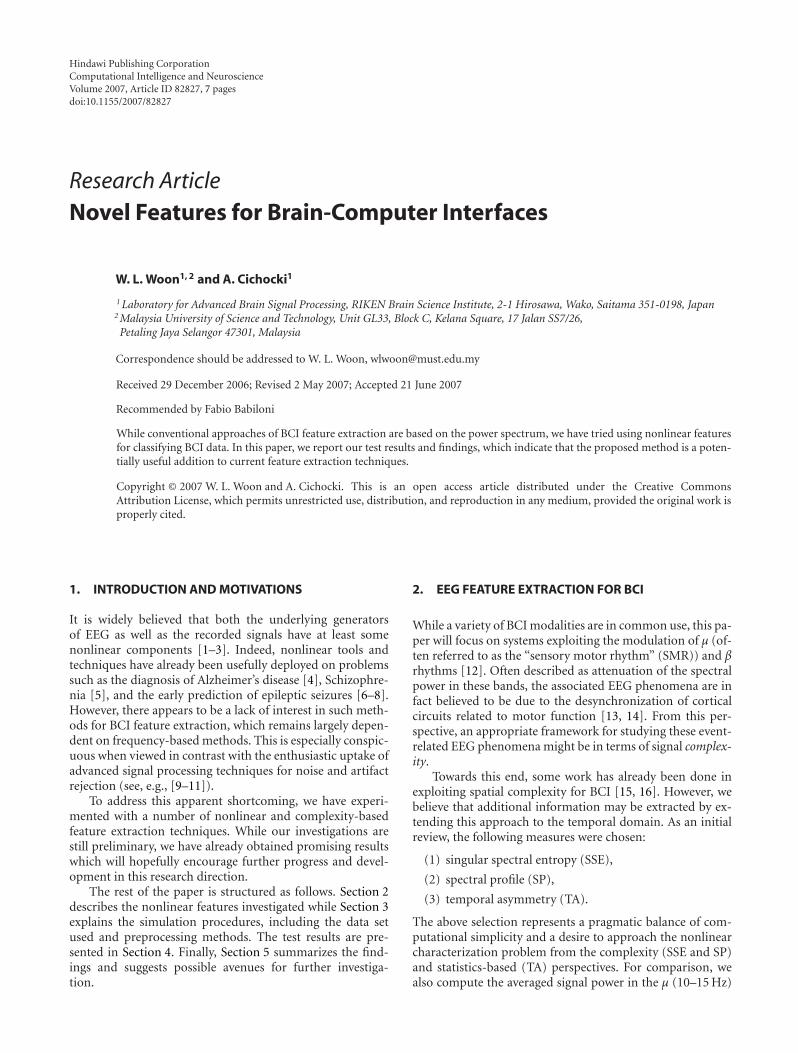
Hindawi Publishing CorporationComputational Intelligence and NeuroscienceVolume 2007, Article ID 82827, 7 pagesdoi:10.1155/2007/82827
Research ArticleNovel Features for Brain-Computer Interfaces
W. L. Woon1, 2 and A. Cichocki1
1 Laboratory for Advanced Brain Signal Processing, RIKEN Brain Science Institute, 2-1 Hirosawa, Wako, Saitama 351-0198, Japan2 Malaysia University of Science and Technology, Unit GL33, Block C, Kelana Square, 17 Jalan SS7/26,Petaling Jaya Selangor 47301, Malaysia
Correspondence should be addressed to W. L. Woon, [email protected]
Received 29 December 2006; Revised 2 May 2007; Accepted 21 June 2007
Recommended by Fabio Babiloni
While conventional approaches of BCI feature extraction are based on the power spectrum, we have tried using nonlinear featuresfor classifying BCI data. In this paper, we report our test results and findings, which indicate that the proposed method is a poten-tially useful addition to current feature extraction techniques.
Copyright © 2007 W. L. Woon and A. Cichocki. This is an open access article distributed under the Creative CommonsAttribution License, which permits unrestricted use, distribution, and reproduction in any medium, provided the original work isproperly cited.
1. INTRODUCTION AND MOTIVATIONS
It is widely believed that both the underlying generatorsof EEG as well as the recorded signals have at least somenonlinear components [1–3]. Indeed, nonlinear tools andtechniques have already been usefully deployed on problemssuch as the diagnosis of Alzheimer’s disease [4], Schizophre-nia [5], and the early prediction of epileptic seizures [6–8].However, there appears to be a lack of interest in such meth-ods for BCI feature extraction, which remains largely depen-dent on frequency-based methods. This is especially conspic-uous when viewed in contrast with the enthusiastic uptake ofadvanced signal processing techniques for noise and artifactrejection (see, e.g., [9–11]).
To address this apparent shortcoming, we have experi-mented with a number of nonlinear and complexity-basedfeature extraction techniques. While our investigations arestill preliminary, we have already obtained promising resultswhich will hopefully encourage further progress and devel-opment in this research direction.
The rest of the paper is structured as follows. Section 2describes the nonlinear features investigated while Section 3explains the simulation procedures, including the data setused and preprocessing methods. The test results are pre-sented in Section 4. Finally, Section 5 summarizes the find-ings and suggests possible avenues for further investiga-tion.
2. EEG FEATURE EXTRACTION FOR BCI
While a variety of BCI modalities are in common use, this pa-per will focus on systems exploiting the modulation of μ (of-ten referred to as the “sensory motor rhythm” (SMR)) and βrhythms [12]. Often described as attenuation of the spectralpower in these bands, the associated EEG phenomena are infact believed to be due to the desynchronization of corticalcircuits related to motor function [13, 14]. From this per-spective, an appropriate framework for studying these event-related EEG phenomena might be in terms of signal complex-ity.
Towards this end, some work has already been done inexploiting spatial complexity for BCI [15, 16]. However, webelieve that additional information may be extracted by ex-tending this approach to the temporal domain. As an initialreview, the following measures were chosen:
(1) singular spectral entropy (SSE),
(2) spectral profile (SP),
(3) temporal asymmetry (TA).
The above selection represents a pragmatic balance of com-putational simplicity and a desire to approach the nonlinearcharacterization problem from the complexity (SSE and SP)and statistics-based (TA) perspectives. For comparison, wealso compute the averaged signal power in the μ (10–15 Hz)

2 Computational Intelligence and Neuroscience
and β2 (23–28 Hz) bands, which will be referred to as the“power feature” or PF. Note that at present we only considerthe high beta range (β2), as is done in a number of otherstudies on this data set, for example [10, 17, 18]. The exactfrequency ranges mentioned above are based on the work de-scribed in [17].
These features will now be briefly described.
2.1. Singular spectral entropy (SSE)
If we define complexity as the number of independentthough possibly interacting components which are active ina signal or system at a particular time, then one way by whichcomplexity may be characterized is through the notion of en-tropy. While a variety of power distributions might be suit-able candidates for this purpose, the shape of the singularspectrum provides an efficient representation of the con-stituent components of a time series. The approach chosenhere is to obtain the singular spectrum of the delay embed-ding of a time series (described in further detail below), thento model this spectrum as a probability distribution beforecalculating the entropy of the singular values; the resultingmeasure will henceforth be termed the singular spectral en-tropy (SSE). An initial study was conducted in [19], whereit was noted that imagined movements correlated with fluc-tuations of the SSE. Unfortunately, there was no attempt tofurther characterize these fluctuations or to build a classifierbased on this approach. Since then, however, SSE has beenapplied to other aspects of EEG such as sleep [20] and ictal(seizure) EEG [6]. Hence, while its use is not widespread, SSEis a promising candidate for BCI feature extraction, motivat-ing its use in this study.
For a time series x(t), SSE is calculated by first construct-ing a delay embedding matrix, X, of dimension m:
X = [x(t), x(t + 1), . . . , x(t + n)] ∈Rm×(n+1), (1)
where x(t) = [x(t), x(t−1), . . . , x(t−m)]T . Next, X is decom-posed using singular value decomposition (SVD) to obtain
X = USVT , (2)
where U and V are orthogonal matrices, and S is a diago-nal matrix containing the singular values of the embeddingmatrix, si. These are then normalized to one and used to cal-culate SSE as follows:
SSEm = −m∑
i=1
si log si. (3)
2.2. Spectral profile (SP)
The intuition behind the SSE feature can equally be appliedto the frequency spectrum (in fact, an additional complex-ity measure proposed in [21] used the entropy of the powerspectral density). However, experimentally we have foundthis measure to be extremely noisy and unsuitable for usewith BCI.
However, as an alternative to SSE, we wish to define afurther feature based on the shape of the power spectra; itwas decided to evaluate the effectiveness of directly using theordinates of the frequency spectra as a feature vector. To pre-vent the power of the signal from dominating or even affect-ing the classification process in any way, the extracted spec-tral components were first normalized to one before incor-poration into the feature set. For convenience, we will referto this feature as the spectral profile (SP) of the trial.
To obtain the SP vector, the elements of the spectra cor-responding to the μ and β bands were extracted then normal-ized as follows:
μ ={
θi∑j∈Σμ
θ j: i ∈ Σμ
}
,
β ={
θi∑i∈Σβ
θ j: j ∈ Σβ
}
,
(4)
where θi is the ith ordinate of the power spectrum, and Σμ
and Σβ are the sets of frequency ordinates falling within thetwo bands, respectively. μ and β are the sets containing thenormalized spectral ordinates and if we define μi and βj asthe enumerated elements of these sets, the SP feature vectoris then written as follows:
SPΣμ,Σβ =[μi, . . . ,μNμ ,βj , . . . ,βNβ
], (5)
where Nμ and Nβ are the sizes of sets μ and β.
2.3. Temporal asymmetry (TA)
If we assume that the desynchronization process accompany-ing motor visualization reflects the activation of previouslydormant neuronal circuits, then this might also be accompa-nied by a detectable increase in signatures of nonlinear dy-namics.
One property of linear time series is that the associatedstatistics remain constant under time reversal, since a lin-ear process is essentially a combination of sinusoids whichare symmetric in time. This fact can be exploited to providea particularly powerful indicator of nonlinearity, temporalasymmetry (TA); this is frequently defined as [22]
TAτ =∑N
n=τ+1
(x(n)− x(n− τ)
)3
[∑Nn=τ+1
(x(n)− x(n− τ)
)2]3/2 , (6)
where τ is the time delay. To restrict the analysis to compo-nents of the signal which exhibit the highest variability withrespect to the classes of interest, a pair of bandpass filters wasused to extract signal components in the μ and β bands (de-tails provided later in Section 4), from which the TA was cal-culated and used to create a feature vector based on temporalasymmetry.
2.4. Power feature (PF)
In addition to the features mentioned above, the power fea-ture (PF) was included for comparison. This represents the

W. L. Woon and A. Cichocki 3
conventional approach to BCI feature extraction (variationsof which are used in [10, 17, 18], e.g.) and is defined as thespectral power contained in the μ and β bands. PF is calcu-lated, thus
PF =[
∑
f∈[10,15]
θ f ,∑
f∈[23,28]
θ f
]
, (7)
where θ f is the power spectrum at frequency f .Finally, for the calculation of the SSE and TA features,
we use bandpass filters to restrict the analysis to the μ and βbands of the signal, as these are known a priori to be activeduring motor imagery. As the actual magnitudes of the sig-nals in these two bands are removed via normalization, wehope to focus on the overall shape of the spectrum ratherthan on particular peaks, as nonlinear phenomena are likelyto have broader spectra compared to oscillatory generators.
3. PROCEDURES
3.1. Data
To test the proposed approach, we used dataset IIA fromBCI competition 2003 [23, 24], which was provided by theWadsworth Center, New York State Department of Health .The data consists of 64-channel recordings from three sub-jects (AA, BB, and CC) for ten 30-minute sessions. Each ses-sion consists of 192 trials in which the subject is requiredto use motor imagery to guide a cursor to one of four pos-sible target positions. As was done during the competition,we use data from the first six sessions as the training set,while recordings of the last four sessions were used to testthe trained classifiers.
3.2. Preprocessing and channel selections
As an initial preprocessing step, we evaluated two methodscommonly used for EEG analysis: the common average refer-ence (CAR) and the Laplacian spatial filtering methods. TheCAR filter was found to significantly improve classificationperformance and was subsequently retained as a basic firststage in the classification process, (e.g., of its use in BCI, see[10, 18]). The CAR filter is applied as follows:
vCARi = vRaw
i − 1N
N∑
j=1
vRawj , (8)
where N is the number of channels in the data set, vRawi is the
unprocessed signal from channel number i, and vCARi is the
same channel after CAR filtering.As CAR filtering is primarily for noise rejection, projec-
tion onto CSP (common spatial patterns) features is used tofurther emphasize information relevant to the BCI classifi-cation task. CSP is widely used in EEG analysis [17, 25] tofind spatial filters that maximize the variance of trials corre-sponding to one particular class at the expense of another.
Briefly, the CSP filters are found as follows.
(1) Partition the full data matrix X into the two class-specific matrices XA and Xb corresponding to the twoclasses to be discriminated.
(2) Calculate the corresponding covariance matrices CA
and CB as well as the sum C = CA + CB.(3) Find the whitening matrix W such that WTCW = I,
where W may be found via the eigenvector decompo-sition
C = UTΣU, (9)
then W = UΣ−1/2. Hence,
WTCW = I =⇒ WTCAW + WTCBW = I. (10)
(4) Apply a rotation matrix Y to both sides of (10),
YT(
WTCAW + WTCBW)
Y = I. (11)
(5) Choose Y such that it diagonalizes WTCAW, that is,
YT[
WTCAW]
Y =
⎡
⎢⎢⎢⎢⎣
σ1A 0 · · · 00 σ2
A · · · 0
0 0. . . 0
0 · · · 0 σnA
⎤
⎥⎥⎥⎥⎦. (12)
(6) From (10)–(12), it follows that YT[WTCBW]Y willalso be diagonal, and the sum of corresponding diago-nal elements will be 1.
(7) Hence, to create a spatial filter that maximizes the vari-ance of class A trials while minimizing the variance ofclass B trials, set Y to be the eigenvectors of WTCAW.Then, the columns of the matrix WY provide the CSPspatial filters and may be sorted based on the eigenval-ues.
For both of the data sets presented above, a bandpass filterwith the following passbands: 10–15 Hz (μ) and 23–26 Hz(β) was applied. This creates two filtered signals which arethen added together. As was done in [17, 18], only classes 1and 4 are considered at this stage. Trials belonging to thesetwo classes are extracted and combined to form XA and XB,respectively. These are then used to obtain the CSP filters asdescribed above.
For operations requiring the power spectra, the Welchmethod was used to estimate the power spectral density. Thismethod has been used in a number of other BCI related stud-ies (e.g., [9], in which it was noted for producing superiorperformance). A 128-point window with 50% overlap wasused. For bandpass filtering operations, we used third orderButterworth filters as they provided frequency responses withmaximal flatness, (and hence minimal distortion of the am-plitude spectra). The use of FIR filters was also considered fortheir linear phase property. However, subsequent inspectionsof the frequency responses revealed that a similar amplituderesponse would have required an FIR with around 50 taps; incomparison, the trials for subject CC are 304 samples long.
In the actual experimental setting, two CSP channelswere used at any time (the actual choice of channels usedvaried with the subject, as will be described later). In addi-tion, it was discovered that submitting the entire set of 64channels to CSP processing resulted in problems with matrixsingularity, as many channels are highly correlated. As such,only a subset consisting of 18 channels situated over the mo-tor cortex was used. These were 8–10, 12–17, 19–21, 48–50,and 52–54 [18].

4 Computational Intelligence and Neuroscience
3.3. Feature translation
For feature classification, we adopt a probabilistic approachsimilar to that used in [26]. However, because the presentdata set is a lot larger, Gaussian mixture models (GMM) wereused in place of the single Gaussians used in [26]. Prelimi-nary experimentations were conducted with the case of 1 and2 Gaussians.
To train the models, the selected features were first ex-tracted from the training data and grouped according to tar-get classes. For each class c ∈ {1, 2, 3, 4}, we train a two-Gaussian GMM using the expectation-maximization (EM)algorithm.
To classify a test vector f into one of the four classes, themaximum a posteriori (MAP) decision rule is used:
cMAP(f) = argmaxc P(c | f). (13)
P(c|f) can be found via Bayes’ theorem. Also, in this case, wehave uniform prior and constant evidence terms, hence
P(c | f) = P(f | c)p(c)P(f)
= kP(f | c)
∝∑
i∈{1,2}πi,c exp
[− (f − μi,c
)TC−1i,c
(f − μi,c
)],
(14)
where μi,c and Ci,c are the mean and covariance of Gaussiansi in class mixture c, and πi,c are the mixing coefficients deter-mined during training.
The effectiveness of the features can now be evaluated interms of the classification rates, which are calculated as fol-lows:
Accuracy (%) = 100×[∑n
i=1 δ(cMAP
(fi)− c(i)
)]
n, (15)
where i is the trial index and n is the number of trials. fi andc(i) denote the feature vector and class labels for trial i, re-spectively, and δ(·) is Dirac’s delta function.
4. RESULTS AND OBSERVATIONS
The procedures and features described in the preceding sec-tions were applied to the BCI data and classification accuracyevaluated according to (15). For SSE, an embedding dimen-sion of m = 15 was used, while for the delay parameter inTA, τ = 2 was used. These values were selected based on anevaluation of a range of potential combinations. The perfor-mances of all four features are compared in Tables 1 and 2 forthe 1 and 2 Gaussian cases, respectively.
As can be seen, the classification performance obtainedusing both SSE and SP is encouraging when compared tothe performance of PF. SSE in particular is more accuratethan both SP and PF. SP also produced higher classificationrates compared to PF though the disparity was a lot narrower.However, PF has better classification rates in the case of sub-ject CC when compared with SP.
On the negative side, the TA feature performed verypoorly. However, while disappointing, this result is not sur-prising considering that measures based on high-order statis-tics are notoriously sensitive to noise. In most cases, TA is
Table 1: Feature-wise classification accuracy using 1 Gaussian (%).
FeaturesSubjects
AA BB CC Mean
SSE 68.5 52.3 68.6 63.2
SP 61.3 54.7 62.5 59.5
TA 36.8 27.9 35.0 33.2
PF 57.7 49.9 64.6 57.4
Table 2: Feature-wise mean classification accuracy using 2 Gaus-sians (%).
FeaturesSubjects
AA BB CC Mean
SSE 68.4 52.3 68.7 63.1
SP 62.5 54.7 62.1 59.8
TA 36.3 29.9 35.5 33.9
PF 55.2 52.1 67.4 58.2
used only in combination with surrogate data and then onlyto establish the presence of nonlinearity, not to characterizeit.
Finally, in terms of the classification algorithm, the per-formance of the 1 and 2 gaussian models did not appear todiffer very much. Henceforth, for brevity, we only presentresults produced by the two Gaussian models, which per-formed slightly better. However, it must be noted that thechoice of either of these two models does not appear to becritical.
4.1. Detailed comparisons of SSE, SP, and PF
Given the disappointing classification rates obtained usingTA, we exclude it from further discussions and focus now onthe relative performances of SSE, SP, and PF. To better under-stand the performance characteristics of these three features,the per-session classification accuracies for each of the threefeatures are presented in Table 3. For comparison, the aver-age online accuracies (this is the success rate of the subjectin hitting the target) obtained during the actual recording atthe Wadsworth centre have also been included.
Some observations were as follows.
(1) As mentioned before, SSE was the best all-round per-former, producing the best classification rates in 7 outof 12 sessions. SP was superior to PF in 9 sessions.
(2) However, SP emerged as the best feature in only 2 ses-sions, compared to 3 sessions in the case of PF. PF per-formed particularly well with subject CC, especially insession 7 where it had by far the best results. For sub-ject BB, PF had the best classification rate for session 7while its accuracy for session 8 was clearly better thanSSE and comparable to SP.
(3) Similarly, though the overall results obtained usingSSE were the best, SP produced the highest averageclassification rate for subject BB.
(4) This variability in the results implies that SSE, SP, andPF are monitoring independent aspects of the signal
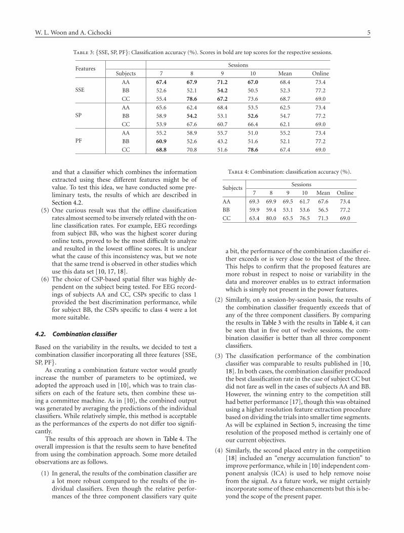
W. L. Woon and A. Cichocki 5
Table 3: {SSE, SP, PF}: Classification accuracy (%). Scores in bold are top scores for the respective sessions.
FeaturesSessions
Subjects 7 8 9 10 Mean Online
SSEAA 67.4 67.9 71.2 67.0 68.4 73.4
BB 52.6 52.1 54.2 50.5 52.3 77.2
CC 55.4 78.6 67.2 73.6 68.7 69.0
SPAA 65.6 62.4 68.4 53.5 62.5 73.4
BB 58.9 54.2 53.1 52.6 54.7 77.2
CC 53.9 67.6 60.7 66.4 62.1 69.0
PFAA 55.2 58.9 55.7 51.0 55.2 73.4
BB 60.9 52.6 43.2 51.6 52.1 77.2
CC 68.8 70.8 51.6 78.6 67.4 69.0
and that a classifier which combines the informationextracted using these different features might be ofvalue. To test this idea, we have conducted some pre-liminary tests, the results of which are described inSection 4.2.
(5) One curious result was that the offline classificationrates almost seemed to be inversely related with the on-line classification rates. For example, EEG recordingsfrom subject BB, who was the highest scorer duringonline tests, proved to be the most difficult to analyzeand resulted in the lowest offline scores. It is unclearwhat the cause of this inconsistency was, but we notethat the same trend is observed in other studies whichuse this data set [10, 17, 18].
(6) The choice of CSP-based spatial filter was highly de-pendent on the subject being tested. For EEG record-ings of subjects AA and CC, CSPs specific to class 1provided the best discrimination performance, whilefor subject BB, the CSPs specific to class 4 were a lotmore suitable.
4.2. Combination classifier
Based on the variability in the results, we decided to test acombination classifier incorporating all three features {SSE,SP, PF}.
As creating a combination feature vector would greatlyincrease the number of parameters to be optimized, weadopted the approach used in [10], which was to train clas-sifiers on each of the feature sets, then combine these us-ing a committee machine. As in [10], the combined outputwas generated by averaging the predictions of the individualclassifiers. While relatively simple, this method is acceptableas the performances of the experts do not differ too signifi-cantly.
The results of this approach are shown in Table 4. Theoverall impression is that the results seem to have benefitedfrom using the combination approach. Some more detailedobservations are as follows.
(1) In general, the results of the combination classifier area lot more robust compared to the results of the in-dividual classifiers. Even though the relative perfor-mances of the three component classifiers vary quite
Table 4: Combination: classification accuracy (%).
SubjectsSessions
7 8 9 10 Mean Online
AA 69.3 69.9 69.5 61.7 67.6 73.4
BB 59.9 59.4 53.1 53.6 56.5 77.2
CC 63.4 80.0 65.5 76.5 71.3 69.0
a bit, the performance of the combination classifier ei-ther exceeds or is very close to the best of the three.This helps to confirm that the proposed features aremore robust in respect to noise or variability in thedata and moreover enables us to extract informationwhich is simply not present in the power features.
(2) Similarly, on a session-by-session basis, the results ofthe combination classifier frequently exceeds that ofany of the three component classifiers. By comparingthe results in Table 3 with the results in Table 4, it canbe seen that in five out of twelve sessions, the com-bination classifier is better than all three componentclassifiers.
(3) The classification performance of the combinationclassifier was comparable to results published in [10,18]. In both cases, the combination classifier producedthe best classification rate in the case of subject CC butdid not fare as well in the cases of subjects AA and BB.However, the winning entry to the competition stillhad better performance [17], though this was obtainedusing a higher resolution feature extraction procedurebased on dividing the trials into smaller time segments.As will be explained in Section 5, increasing the timeresolution of the proposed method is certainly one ofour current objectives.
(4) Similarly, the second placed entry in the competition[18] included an “energy accumulation function” toimprove performance, while in [10] independent com-ponent analysis (ICA) is used to help remove noisefrom the signal. As a future work, we might certainlyincorporate some of these enhancements but this is be-yond the scope of the present paper.
6 Computational Intelligence and Neuroscience
5. DISCUSSIONS
While preliminary, the results presented here suggest thatfeatures which allow for nonlinear dynamics are promisingand potentially useful in the development of BCI systems.
As the tests were conducted using offline recordings,our initial objective was not to directly compare the pro-posed features with existing frequency-based techniques. Be-cause these were used as the online control signals, sub-jects might have been conditioned to directly modulate thepower spectrum, thus biasing the results in favour of tradi-tional approaches. As such, we did not perform extensive op-timization of the feature extraction parameters; in any case,though this might have produced slight improvements tothe results, it could also have resulted in overfitting or over-customization to a particular subject and was thus avoided.
Rather than obsessing with the final classification figures,our main aim was to demonstrate the general feasibility ofcomplexity-based feature extraction. On this count, it ap-pears that the proposed method is potentially useful for BCI.As far as we know, this is the first publication which seriouslystudies the performance of a temporal complexity measureon a BCI problem. If the results presented in this paper canbe supported by further studies, it will provide an efficientnew set of features for use with motor-imagery-based BCIsystems. However, many issues need to be investigated beforethe practical utility of the method can be established. In par-ticular, it should be noted that the experiments decribed inthis paper process entire trials at a time to produce the clas-sifications. While this is consistent with the approach takenin [18], a shorter-time window needs to be considered beforethe method can be tested for online (real-time) scenarios.
At present, we are either actively investigating or seriouslyconsidering a number of avenues for further investigation. Inparticular, we are interested in extracting SSE features fromshorter-time windows (e.g., in the BCI experiments for thisdata, time windows of 200 ms were used to control the cur-sor motion). A separate but important issue is to find andtest other practical measures of system complexity, for exam-ple, approximate entropy. If found to be promising, findingsand results of these ongoing investigations will be describedin a further publication in the hope of stimulating broaderinterest and development in this area.
REFERENCES
[1] G. Nolte, T. Sander, A. Lueschow, and B. A. Pearlmutter, “Non-linear time series analysis of human alpha rhythm,” in The In-ternational Conference on Biomagnetism (BIOMAG ’03), Jena,Germany, August 2003.
[2] C. J. Stam, “Nonlinear dynamical analysis of EEG andMEG: review of an emerging field,” Clinical Neurophysiology,vol. 116, no. 10, pp. 2266–2301, 2005.
[3] M. Breakspear and J. R. Terry, “Nonlinear interdependence inneural systems: motivation, theory, and relevance,” Interna-tional Journal of Neuroscience, vol. 112, no. 10, pp. 1263–1284,2002.
[4] B. Jelles, J. H. van Birgelen, J. P. J. Slaets, R. E. M. Hekster, E. J.Jonkman, and C. J. Stam, “Decrease of non-linear structure in
the EEG of Alzheimer patients compared to healthy controls,”Clinical Neurophysiology, vol. 110, no. 7, pp. 1159–1167, 1999.
[5] M. S. Keshavan, J. D. Cashmere, J. Miewald, and V. K. Yeragani,“Decreased nonlinear complexity and chaos during sleep infirst episode schizophrenia: a preliminary report,” Schizophre-nia Research, vol. 71, no. 2–3, pp. 263–272, 2004.
[6] C. J. James and D. Lowe, “Extracting multisource brain activityfrom a single electromagnetic channel,” Artificial Intelligence inMedicine, vol. 28, no. 1, pp. 89–104, 2003.
[7] M. Palus, V. Komarek, Z. Hrncir, and T. Prochazka, “Is nonlin-earity relevant for detecting changes in EEG?” Theory in Bio-sciences, vol. 118, no. 3–4, pp. 179–188, 1999.
[8] K. Lehnertz and C. E. Elger, “Can epileptic seizures be pre-dicted? evidence from nonlinear time series analysis of brainelectrical activity,” Physical Review Letters, vol. 80, no. 22, pp.5019–5022, 1998.
[9] S. Chiappa and D. Barber, “EEG classification using generativeindependent component analysis,” Neurocomputing, vol. 69,no. 7–9, pp. 769–777, 2006.
[10] J. Qin, Y. Li, and A. Cichocki, “ICA and committee machine-based algorithm for cursor control in a BCI system,” in Pro-ceedings of the 2nd International Symposium on Neural Net-works (ISNN ’05), vol. 3496 of Lecture Notes in Computer Sci-ence, pp. 973–978, Chongqing, China, May-June 2005.
[11] H. Lee, A. Cichocki, and S. Choi, “Nonnegative matrix factor-ization for motor imagery EEG classification,” in Proceedingsof the International Conference on Artificial Neural Networks(ICANN ’06), vol. 4132 of Lecture Notes in Computer Science,pp. 250–259, Athens, Greece, September 2006.
[12] J. R. Wolpaw, N. Birbaumer, D. J. McFarland, G. Pfurtscheller,and T. M. Vaughan, “Brain-computer interfaces for communi-cation and control,” Clinical Neurophysiology, vol. 113, no. 6,pp. 767–791, 2002.
[13] G. Pfurtscheller and F. H. Lopes da Silva, “Event-relatedEEG/MEG synchronization and desynchronization: basicprinciples,” Clinical Neurophysiology, vol. 110, no. 11, pp.1842–1857, 1999.
[14] G. Pfurtscheller, C. Brunner, A. Schlogl, and F. H. Lopes daSilva, “Mu rhythm (de)synchronization and EEG single-trialclassification of different motor imagery tasks,” NeuroImage,vol. 31, no. 1, pp. 153–159, 2006.
[15] L. Song and J. Epps, “Classifying EEG for brain-computerinterfaces: learning optimal filters for dynamical system fea-tures,” in Proceedings of the 23rd International Conference onMachine Learning (ICML ’06), pp. 857–864, Pittsburgh, Pa,USA, June 2006.
[16] X.-M. Pei, C.-X. Zheng, J. Xu, G.-Y. Bin, and H.-W. Wang,“Multi-channel linear descriptors for event-related EEG col-lected in brain computer interface,” Journal of Neural Engineer-ing, vol. 3, no. 1, pp. 52–58, 2006.
[17] G. Blanchard and B. Blankertz, “BCI competition 2003: dataset IIa: spatial patterns of self-controlled brain rhythm modu-lations,” IEEE Transactions on Biomedical Engineering, vol. 51,no. 6, pp. 1062–1066, 2004.
[18] M. Cheng, W. Jia, X. Gao, S. Gao, and F. Yang, “Mu rhythm-based cursor control: an offline analysis,” Clinical Neurophysi-ology, vol. 115, no. 4, pp. 745–751, 2004.
[19] S. J. Roberts, W. Penny, and I. Rezek, “Temporal and spatialcomplexity measures for electroencephalogram based brain-computer interfacing,” Medical and Biological Engineering andComputing, vol. 37, no. 1, pp. 93–98, 1999.
[20] I. Rezek, S. Roberts, and P. Sykacek, “Complexity features forsleep stage analysis,” in Proceedings of the European Medical
W. L. Woon and A. Cichocki 7
and Biological Engineering Conference (EMBEC ’99), pp. 1650–1651, Vienna, Austria, November 1999.
[21] I. A. Rezek and S. J. Roberts, “Stochastic complexity mea-sures for physiological signal analysis,” IEEE Transactions onBiomedical Engineering, vol. 45, no. 9, pp. 1186–1191, 1998.
[22] T. Schreiber, “Interdisciplinary application of nonlinear timeseries methods,” Physics Reports, vol. 308, no. 1, pp. 1–64,1999.
[23] D. J. McFarland, A. T. Lefkowicz, and J. R. Wolpaw, “Designand operation of an EEG-based brain-computer interface withdigital signal processing technology,” Behavior Research Meth-ods, Instruments, and Computers, vol. 29, no. 3, pp. 337–345,1997.
[24] B. Blankertz, K.-R. Muller, G. Curio, et al., “The BCI competi-tion 2003: progress and perspectives in detection and discrim-ination of EEG single trials,” IEEE Transactions on BiomedicalEngineering, vol. 51, no. 6, pp. 1044–1051, 2004.
[25] P. Shenoy, M. Krauledat, B. Blankertz, R. P. N. Rao, and K.-R. Muller, “Towards adaptive classification for BCI,” Journal ofNeural Engineering, vol. 3, no. 1, pp. R13–R23, 2006.
[26] S. Lemm, C. Schafer, and G. Curio, “BCI competition 2003-data set III: probabilistic modeling of sensorimotor μ rhythmsfor classification of imaginary hand movements,” IEEE Trans-actions on Biomedical Engineering, vol. 51, no. 6, pp. 1077–1080, 2004.
Hindawi Publishing CorporationComputational Intelligence and NeuroscienceVolume 2007, Article ID 74895, 12 pagesdoi:10.1155/2007/74895
Research ArticleChannel Selection and Feature Projection for Cognitive LoadEstimation Using Ambulatory EEG
Tian Lan,1 Deniz Erdogmus,1 Andre Adami,2 Santosh Mathan,3 and Misha Pavel1
1 Department of Biomedical Engineering, Oregon Health and Science University, Portland, OR 97239, USA2 Department of Computer Science, University of Caxias do Sul, 95070-560 Caxias do Sul, RS, Brazil
3 Human Centered Systems, Honeywell Laboratories, Minneapolis, MN 55401, USA
Correspondence should be addressed to Deniz Erdogmus, [email protected]
Received 14 February 2007; Accepted 18 June 2007
Recommended by Andrzej Cichocki
We present an ambulatory cognitive state classification system to assess the subject’s mental load based on EEG measurements.The ambulatory cognitive state estimator is utilized in the context of a real-time augmented cognition (AugCog) system that aimsto enhance the cognitive performance of a human user through computer-mediated assistance based on assessments of cognitivestates using physiological signals including, but not limited to, EEG. This paper focuses particularly on the offline channel selectionand feature projection phases of the design and aims to present mutual-information-based techniques that use a simple sampleestimator for this quantity. Analyses conducted on data collected from 3 subjects performing 2 tasks (n-back/Larson) at 2 difficultylevels (low/high) demonstrate that the proposed mutual-information-based dimensionality reduction scheme can achieve up to94% cognitive load estimation accuracy.
Copyright © 2007 Tian Lan et al. This is an open access article distributed under the Creative Commons Attribution License,which permits unrestricted use, distribution, and reproduction in any medium, provided the original work is properly cited.
1. INTRODUCTION
Following the successful demonstration of a P300 oddballdetector [1], many brain computer interfaces (BCIs) aredesigned on similar concepts [2]—evoked response poten-tial (ERP) detection or sliding window classification. Arti-fact removal using adaptive filtering source separation tech-niques have been proposed [3, 4], wavelet coefficients [5],short-term power spectrum [6–8], and chaos/fractal struc-ture [9, 10] have been investigated as potential features. Var-ious standard classifiers including linear discriminants, neu-ral networks, and support vector machines are employed[11–16], parametric and nonparametric approximate Bayesclassifiers and boosting techniques have been evaluated [17–22]. Some benchmark datasets for BCI design evaluationshave been proposed [23] and have met reasonable accep-tance.
Accurate assessment of cognitive load from ambulatoryelectroencephalogram (EEG) could lead to a wide variety ofapplications for brain interface systems [24]. Of specific in-terest to us is the concept of augmented cognition (AugCog),which is applicable where the cognitive load of human op-erators needs to be monitored to design optimal informa-
tion flow protocols from the computer to the human in or-der to maximize task performance [25]. These applicationsinclude, but are not limited to, vehicle drivers, machineryoperators, air traffic controllers, and robotic surgery oper-ators. Optimizing the information flow for seamless human-computer interaction requires the real-time assessments ofcognitive states during the execution of certain tasks leadingto a prescribed goal. An accurate cognitive load estimator isessential for the successful implementation of assistive sys-tems that are aware of the user’s status and environment. In-stantaneous estimates of mental state and workload can beused to control the rate and the modality of the informationpresented to the operator, which in turn helps the operatorallocate mental resources to maximize performance [26]. Asthe envisioned applications require ambulatory EEG record-ings, special care must be given to proper signal condition-ing, noise and artifact reduction.
The use of EEG, as the basis of assessment in brain-computer interface (BCI) and AugCog systems, is predicatedon characteristics such as good temporal resolution, non-invasiveness, low cost, and portability [27]. However, thefollowing factors make it particularly difficult to deal with
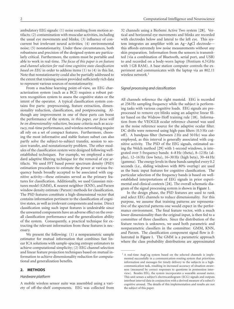
2 Computational Intelligence and Neuroscience
ambulatory EEG signals: (1) noise resulting from motion ar-tifacts; (2) contamination with muscular activities, includingthe usual eye movements and blinks; (3) influence of con-current but irrelevant neural activities; (4) environmentalnoise; (5) nonstationarity. Under these circumstances, bothrobustness and precision of the designed system are particu-larly critical. Furthermore, the system must be portable andable to work in real-time. The focus of this paper is on featureand channel selection for real-time cognitive state classificationbased on EEG in order to address items (1) to (4) in this list.Note that nonstationarity could also be partially addressed tothe extent that training session provided sufficiently rich datato represent various sources of nonstationarity.
From a machine learning point-of-view, an EEG char-acterization system (such as a BCI) requires a robust pat-tern recognition system to assess the cognitive states or theintent of the operator. A typical classification system con-tains five parts: preprocessing, feature extraction, dimen-sionality reduction, classification, and postprocessing. Al-though any improvement in one of these parts can boostthe performance of the system, in this paper, our focus willbe on dimensionality reduction, because criteria such as accu-racy, real-time performance, and wireless networking requireall rely on a set of compact features. Furthermore, choos-ing the most informative and stable feature subset can alsopartly solve the subject-to-subject transfer, session to ses-sion transfer, and nonstationarity problem. The other mod-ules of the classification system were designed following well-established techniques. For example, we employed a stan-dard adaptive filtering technique for the removal of eye ar-tifacts. We used FFT based power spectrum density (PSD)estimation procedures to estimate the power at various fre-quency bands broadly accepted to be associated with cog-nitive activity—these estimates served as the primary fea-tures for classification. Additionally, we used Gaussian mix-tures model (GMM), K nearest neighbor (KNN), and Parzenwindow density estimate (Parzen) methods for classification.The PSD features constitute a high-dimensional vector thatcontains information pertinent to the classification of cogni-tive states, as well as irrelevant components and noise. Directclassification using such input features is undesirable sincethe unwanted components have an adverse effect on the over-all classification performance and the generalization abilityof the system. Consequently, a practical technique for ex-tracting the relevant information from these features is nec-essary.
We present the following: (1) a nonparametric sampleestimator for mutual information that combines fast lin-ear ICA solutions with sample-spacing entropy estimators toachieve computational simplicity; (2) EEG channel selectionand linear feature projection techniques based on mutual in-formation to achieve dimensionality reduction for computa-tional and generalization benefits.
2. METHODS
Hardware platform
A mobile wireless sensor suite was assembled using a vari-ety of off-the-shelf components. EEG was collected from
32 channels using a BioSemi Active Two system [28]. Ver-tical and horizontal eye movements and blinks are recordedwith electrodes below and lateral to the left eye. This sys-tem integrates an amplifier with an Ag−AgCl electrode—this affords extremely low noise measurements without anyskin preparation. Information from the sensors is transmit-ted (via a combination of Bluetooth, serial port, and USB)to and recorded on a body-worn laptop (Pentium 4.3 GHzwith 1 GB RAM). A base station computer controls the ex-periment and communicates with the laptop via an 802.11wireless network.1
Signal processing and classification
All channels reference the right mastoid. EEG is recordedat 256 Hz sampling frequency while the subject is perform-ing tasks with various cognitive loads. EEG signals are pre-processed to remove eye blinks using an adaptive linear fil-ter based on the Widrow-Hoff training rule [18]. Informa-tion from the VEOGLB ocular reference channel was usedas the noise reference source for the adaptive ocular filter.DC drifts were removed using high-pass filters (0.5 Hz cut-off). A bandpass filter (between 2 Hz and 50 Hz) was alsoemployed, as this interval is generally associated with cog-nitive activity. The PSD of the EEG signals, estimated us-ing the Welch method [29] with 1-second windows, is inte-grated over 5 frequency bands: 4–8 Hz (theta), 8–12 Hz (al-pha), 12–16 Hz (low beta), 16–30 Hz (high beta), 30–44 Hz(gamma). The energy levels in these bands sampled every 0.2seconds (i.e., sliding windows with 80% overlap) are usedas the basic input features for cognitive classification. Theparticular selection of the frequency bands is based on well-established interpretations of EEG signals in prior experi-mental and clinical contexts [24]. The overall schematic dia-gram of the signal processing system is shown in Figure 1.
In the design phase, the PSD features are used to rankand select EEG channels to reduce dimensionality. For thispurpose, we assume that training patterns are representa-tive of the spectral patterns one would expect in the perfor-mance environment. The final feature vector, with a muchlower dimensionality than the original input, is then fed to acommittee of three classifiers. Since the distribution of thefeature vectors is unknown, we used both parametric andnonparametric classifiers in the committee: GMM, KNN,and Parzen. The classification component signal flow is il-lustrated in Figure 1. The GMM is a parametric approachwhere the class probability distributions are approximated
1 A real-time AugCog system based on the selected channels is imple-mented successfully in a communication-routing system that prioritizesinformation and messages for timely delivery to the subjects in a high-communication task, resulting in increased accuracy of situation aware-ness (measured by correct responses to questions in postsession inter-view). Besides EEG, the system incorporates a wearable arousal meter.This unit senses a subject’s electrocardiogram (ECG) signals and outputsinterbeat interval data in conjunction with a derived measure of a subect’scognitive arousal. The details of this implementation and results are notthe subject of this paper.
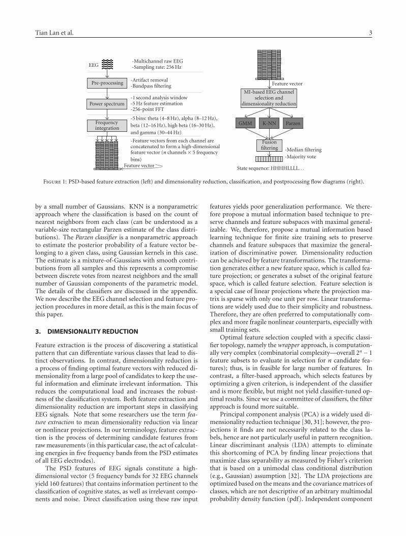
Tian Lan et al. 3
-Multichannel raw EEG-Sampling rate: 256 Hz
-Artifact removal-Bandpass filtering
-1 second analysis window-5 Hz feature estimation-256-point FFT
-5 bins: theta (4–8 Hz), alpha (8–12 Hz),beta (12–16 Hz), high beta (16–30 Hz),and gamma (30–44 Hz)
-Feature vectors from each channel areconcatenated to form a high-dimensionalfeature vector (n channels × 5 frequencybins)
Feature vector
Frequencyintegration
Power spectrum
Pre-processing
EEG
Feature vector
Fusionfiltering
GMM K-NN Parzen
MI-based EEG channelselection and
dimensionality reduction
-Median filtering-Majority vote
State sequence: HHHHLLLL. . .
Figure 1: PSD-based feature extraction (left) and dimensionality reduction, classification, and postprocessing flow diagrams (right).
by a small number of Gaussians. KNN is a nonparametricapproach where the classification is based on the count ofnearest neighbors from each class (can be understood as avariable-size rectangular Parzen estimate of the class distri-butions). The Parzen classifier is a nonparametric approachto estimate the posterior probability of a feature vector be-longing to a given class, using Gaussian kernels in this case.The estimate is a mixture-of-Gaussians with smooth contri-butions from all samples and this represents a compromisebetween discrete votes from nearest neighbors and the smallnumber of Gaussian components of the parametric model.The details of the classifiers are discussed in the appendix.We now describe the EEG channel selection and feature pro-jection procedures in more detail, as this is the main focus ofthis paper.
3. DIMENSIONALITY REDUCTION
Feature extraction is the process of discovering a statisticalpattern that can differentiate various classes that lead to dis-tinct observations. In contrast, dimensionality reduction isa process of finding optimal feature vectors with reduced di-mensionality from a large pool of candidates to keep the use-ful information and eliminate irrelevant information. Thisreduces the computational load and increases the robust-ness of the classification system. Both feature extraction anddimensionality reduction are important steps in classifyingEEG signals. Note that some researchers use the term fea-ture extraction to mean dimensionality reduction via linearor nonlinear projections. In our terminology, feature extrac-tion is the process of determining candidate features fromraw measurements (in this particular case, the act of calculat-ing energies in five frequency bands from the PSD estimatesof all EEG electrodes).
The PSD features of EEG signals constitute a high-dimensional vector (5 frequency bands for 32 EEG channelsyield 160 features) that contains information pertinent to theclassification of cognitive states, as well as irrelevant compo-nents and noise. Direct classification using these raw input
features yields poor generalization performance. We there-fore propose a mutual information based technique to pre-serve channels and feature subspaces with maximal general-izable. We, therefore, propose a mutual information basedlearning technique for finite size training sets to preservechannels and feature subspaces that maximize the general-ization of discriminative power. Dimensionality reductioncan be achieved by feature transformations. The transforma-tion generates either a new feature space, which is called fea-ture projection; or generates a subset of the original featurespace, which is called feature selection. Feature selection isa special case of linear projections where the projection ma-trix is sparse with only one unit per row. Linear transforma-tions are widely used due to their simplicity and robustness.Therefore, they are often preferred to computationally com-plex and more fragile nonlinear counterparts, especially withsmall training sets.
Optimal feature selection coupled with a specific classi-fier topology, namely the wrapper approach, is computation-ally very complex (combinatorial complexity—overall 2n− 1feature subsets to evaluate in selection for n candidate fea-tures); thus, is in feasible for large number of features. Incontrast, a filter-based approach, which selects features byoptimizing a given criterion, is independent of the classifierand is more flexible, but might not yield classifier-tuned op-timal results. Since we use a committee of classifiers, the filterapproach is found more suitable.
Principal component analysis (PCA) is a widely used di-mensionality reduction technique [30, 31]; however, the pro-jections it finds are not necessarily related to the class la-bels, hence are not particularly useful in pattern recognition.Linear discriminant analysis (LDA) attempts to eliminatethis shortcoming of PCA by finding linear projections thatmaximize class separability as measured by Fisher’s criterionthat is based on a unimodal class conditional distribution(e.g., Gaussian) assumption [32]. The LDA projections areoptimized based on the means and the covariance matrices ofclasses, which are not descriptive of an arbitrary multimodalprobability density function (pdf). Independent component
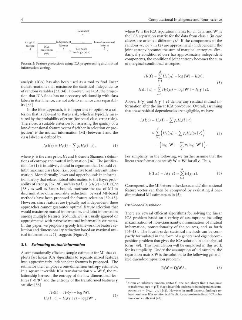
4 Computational Intelligence and Neuroscience
Originalfeature
xICA
projection
(W)
Independentfeatures
y MI-basedsorting I(yi; c)
Low-dimensionalfeatures
f
Class labelc
Figure 2: Feature projections using ICA preprocessing and mutualinformation sorting.
analysis (ICA) has also been used as a tool to find lineartransformations that maximize the statistical independenceof random variables [33, 34]. However, like PCA, the projec-tion that ICA finds has no necessary relationship with classlabels in itself, hence, are not able to enhance class separabil-ity [35].
In the filter approach, it is important to optimize a cri-terion that is relevant to Bayes risk, which is typically mea-sured by the probability of error (for equal class-error risks).Therefore, a suitable criterion for assessing the quality of alow-dimensional feature vector f (either in selection or pro-jection) is the mutual information (MI) between f and theclass label c as defined by
IS(f ; c) = HS(f)−∑
c
pcHS(f | c), (1)
where pc is the class prior, HS and IS denote Shannon’s defini-tions of entropy and mutual information [36]. The justifica-tion for (1) is intuitively found in argument that f should ex-hibit maximal class label (i.e., cognitive load) relevant infor-mation. More formally, lower and upper bounds in informa-tion theory that relate mutual information to the Bayes prob-ability of error pe [37, 38], such as pe(f) ≤ (HS(c)−IS(f ; c))/2[38], as well as Fano’s bound, motivate the use of MI indiscriminative dimensionality reduction. Several MI-basedmethods have been proposed for feature selection [39–43].However, since features are typically not independent, theseapproaches cannot guarantee optimal feature selection thatwould maximize mutual information, and joint informationamong multiple features (redundancy) is usually ignored orapproximated with pairwise mutual information estimates.In this paper, we propose a greedy framework for feature se-lection and dimensionality reduction based on maximal mu-tual information as (1) suggests (Figure 2).
3.1. Estimating mutual information
A computationally efficient sample estimator for MI that ex-ploits fast linear ICA algorithms to separate mixed featuresinto approximately independent features is proposed. Theestimator then employs a one-dimension entropy estimator.In a square invertible ICA transformation y = WT f , the re-lationship between the entropy of the low-dimensional fea-tures f ∈ �d and the entropy of the transformed features ysatisfies [36]
HS(f) = HS(y)− log |W|,HS(f | c) = HS(y | c)− log |Wc|, (2)
where W is the ICA separation matrix for all data, and Wc isthe ICA separation matrix for the data from class c (in caseclasses are oriented differently).2 If the components of therandom vector y in (2) are approximately independent, thejoint entropy becomes the sum of marginal entropies. Sim-ilarly, if y conditioned on c has approximately independentcomponents, the conditional joint entropy becomes the sumof marginal-conditional entropies:
HS(f) =d∑
l=1
HS(yl)− log |W| − IS(y),
HS(f | c) =d∑
l=1
HS(yl)− log |Wc| − IS(y | c).
(3)
Above, IS(y) and IS(y | c) denote any residual mutual in-formation after the linear ICA procedure. Overall, assumingthat these residual dependencies are negligible, we have
IS(f ; c) = HS(f)−∑
c
pcHS(f | c)
≈d∑
l=1
(HS(yl)−
∑
c
pcHS(yl | c
))
−(
log∣∣W
∣∣−∑
c
pc log∣∣W
c∣∣).
(4)
For simplicity, in the following, we further assume that thelinear transformations satisfy W = Wc for all c. Thus,
IS(f ; c) = IS(y; c) ≈d∑
l=1
IS(yl; c
). (5)
Consequently, the MI between the classes and d-dimensionalfeature vector can then be computed by evaluating d one-dimensional MI estimates as in (5).
Fast linear ICA solution
There are several efficient algorithms for solving the linearICA problem based on a variety of assumptions includingmaximization of non-Gaussianity, minimization of mutualinformation, nonstationarity of the sources, and so forth[46–48]. The fourth-order statistical methods can be com-pactly formulated in the form of a generalized eigendecom-position problem that gives the ICA solution in an analyticalform [49]. This formulation will be employed in this workfor its simplicity. Under the assumption of iid samples, theseparation matrix W is the solution to the following general-ized eigendecomposition problem:
Rf W = Qf WΛ, (6)
2 Given an arbitrary random vector f , one can always find a nonlineartransformation y = g(f) that is invertible and results in independent com-ponents y = {y1, . . . , yn} [44]. However, in small datasets, finding a ro-bust nonlinear ICA solution is difficult. An approximate linear ICA solu-tion can be sufficient [45].
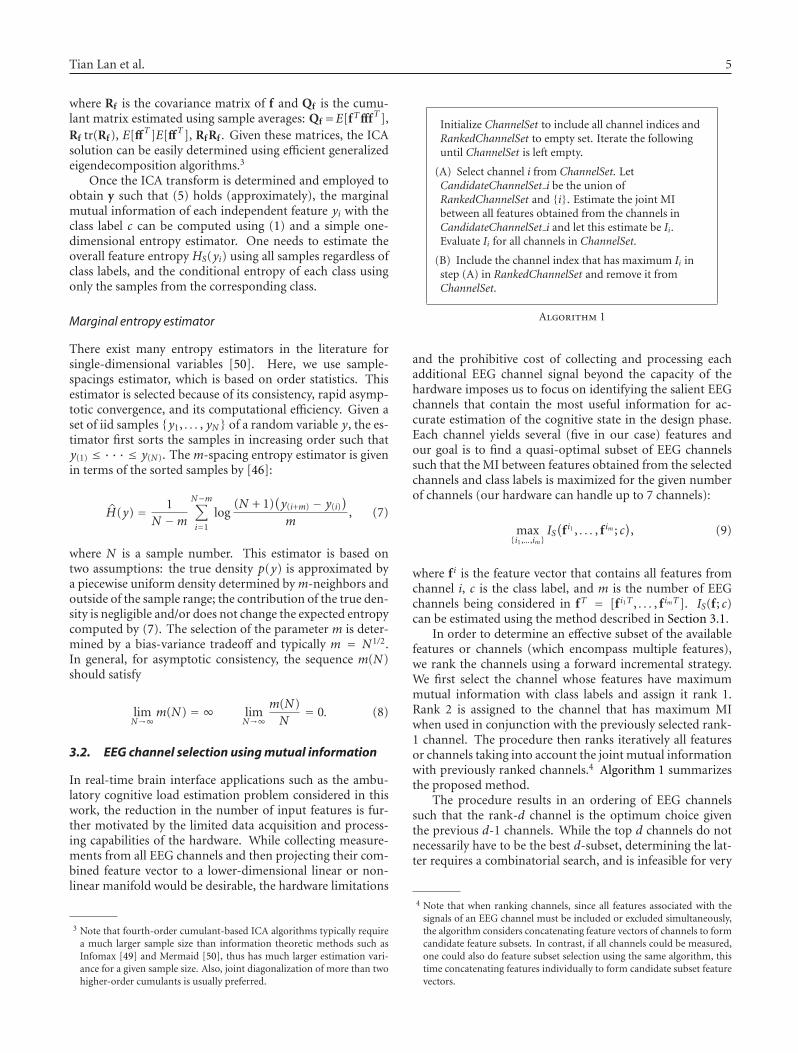
Tian Lan et al. 5
where Rf is the covariance matrix of f and Qf is the cumu-lant matrix estimated using sample averages: Qf=E[fTfffT],Rf tr(Rf ), E[ffT]E[ffT], Rf Rf . Given these matrices, the ICAsolution can be easily determined using efficient generalizedeigendecomposition algorithms.3
Once the ICA transform is determined and employed toobtain y such that (5) holds (approximately), the marginalmutual information of each independent feature yi with theclass label c can be computed using (1) and a simple one-dimensional entropy estimator. One needs to estimate theoverall feature entropy HS(yi) using all samples regardless ofclass labels, and the conditional entropy of each class usingonly the samples from the corresponding class.
Marginal entropy estimator
There exist many entropy estimators in the literature forsingle-dimensional variables [50]. Here, we use sample-spacings estimator, which is based on order statistics. Thisestimator is selected because of its consistency, rapid asymp-totic convergence, and its computational efficiency. Given aset of iid samples {y1, . . . , yN} of a random variable y, the es-timator first sorts the samples in increasing order such thaty(1) ≤ · · · ≤ y(N). The m-spacing entropy estimator is givenin terms of the sorted samples by [46]:
H(y) = 1N −m
N−m∑
i=1
log(N + 1)
(y(i+m) − y(i)
)
m, (7)
where N is a sample number. This estimator is based ontwo assumptions: the true density p(y) is approximated bya piecewise uniform density determined by m-neighbors andoutside of the sample range; the contribution of the true den-sity is negligible and/or does not change the expected entropycomputed by (7). The selection of the parameter m is deter-mined by a bias-variance tradeoff and typically m = N1/2.In general, for asymptotic consistency, the sequence m(N)should satisfy
limN→∞
m(N) = ∞ limN→∞
m(N)N
= 0. (8)
3.2. EEG channel selection using mutual information
In real-time brain interface applications such as the ambu-latory cognitive load estimation problem considered in thiswork, the reduction in the number of input features is fur-ther motivated by the limited data acquisition and process-ing capabilities of the hardware. While collecting measure-ments from all EEG channels and then projecting their com-bined feature vector to a lower-dimensional linear or non-linear manifold would be desirable, the hardware limitations
3 Note that fourth-order cumulant-based ICA algorithms typically requirea much larger sample size than information theoretic methods such asInfomax [49] and Mermaid [50], thus has much larger estimation vari-ance for a given sample size. Also, joint diagonalization of more than twohigher-order cumulants is usually preferred.
Initialize ChannelSet to include all channel indices andRankedChannelSet to empty set. Iterate the followinguntil ChannelSet is left empty.
(A) Select channel i from ChannelSet. LetCandidateChannelSet i be the union ofRankedChannelSet and {i}. Estimate the joint MIbetween all features obtained from the channels inCandidateChannelSet i and let this estimate be Ii.Evaluate Ii for all channels in ChannelSet.
(B) Include the channel index that has maximum Ii instep (A) in RankedChannelSet and remove it fromChannelSet.
Algorithm 1
and the prohibitive cost of collecting and processing eachadditional EEG channel signal beyond the capacity of thehardware imposes us to focus on identifying the salient EEGchannels that contain the most useful information for ac-curate estimation of the cognitive state in the design phase.Each channel yields several (five in our case) features andour goal is to find a quasi-optimal subset of EEG channelssuch that the MI between features obtained from the selectedchannels and class labels is maximized for the given numberof channels (our hardware can handle up to 7 channels):
max{i1,...,im}
IS(
f i1 , . . . , f im ; c), (9)
where f i is the feature vector that contains all features fromchannel i, c is the class label, and m is the number of EEGchannels being considered in fT = [f i1T , . . . , f imT]. IS(f ; c)can be estimated using the method described in Section 3.1.
In order to determine an effective subset of the availablefeatures or channels (which encompass multiple features),we rank the channels using a forward incremental strategy.We first select the channel whose features have maximummutual information with class labels and assign it rank 1.Rank 2 is assigned to the channel that has maximum MIwhen used in conjunction with the previously selected rank-1 channel. The procedure then ranks iteratively all featuresor channels taking into account the joint mutual informationwith previously ranked channels.4 Algorithm 1 summarizesthe proposed method.
The procedure results in an ordering of EEG channelssuch that the rank-d channel is the optimum choice giventhe previous d-1 channels. While the top d channels do notnecessarily have to be the best d-subset, determining the lat-ter requires a combinatorial search, and is infeasible for very
4 Note that when ranking channels, since all features associated with thesignals of an EEG channel must be included or excluded simultaneously,the algorithm considers concatenating feature vectors of channels to formcandidate feature subsets. In contrast, if all channels could be measured,one could also do feature subset selection using the same algorithm, thistime concatenating features individually to form candidate subset featurevectors.
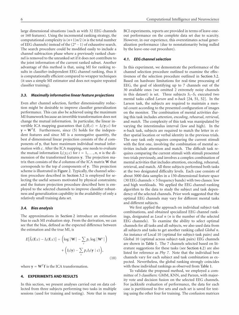
6 Computational Intelligence and Neuroscience
large dimensional situations (such as with 32 EEG channelsor 160 features). Using the incremental ranking strategy, thecomputational complexity is (n+1)n/2 (n is the total numberof EEG channels) instead of the (2n−1) of exhaustive search.The search procedure could be modified easily to include achannel subtraction phase where a previously ranked chan-nel is removed to the unranked set if it does not contribute tothe joint information of the current ranked subset. Anotheradvantage of this method is that, using MI for ranking re-sults in classifier-independent EEG channel ranking, thus itis computationally efficient compared to wrapper techniques(it uses a simple MI estimator and does not require repeatedclassifier training).
3.3. Maximally informative linear feature projections
Even after channel selection, further dimensionality reduc-tion might be desirable to improve classifier generalizationperformance. This can also be achieved using the maximumMI framework because an invertible transformation does notchange the mutual information. In particular, the linear in-vertible ICA mapping guarantees that IS(f ; c) = IS(y; c) fory = WT f . Furthermore, since (5) holds for the indepen-dent features and since MI is a nonnegative quantity, thebest d-dimensional linear projection consists of the d com-ponents of y, that have maximum individual mutual infor-mation with c. After the ICA mapping, one needs to evaluatethe mutual information IS(yi; c) for i = 1, . . . ,n, n is the di-mension of the transformed features y. The projection ma-trix then consists of the d columns of the ICA matrix W thatcorresponds to the top d components of y. This projectionscheme is illustrated in Figure 2. Typically, the channel selec-tion procedure described in Section 3.2 is employed for se-lecting the useful sensors motivated by physical constraints;and the feature projection procedure described here is em-ployed to the selected channels to improve classifier robust-ness and generalization capability in the availability of only arelatively small training data set.
3.4. Bias analysis
The approximations in Section 2 introduce an estimationbias to each MI evaluation step. From the derivation, we cansee that the bias, defined as the expected difference betweenthe estimation and the true MI, is
E[IS(f ; c)− IS(f ; c)
] =(
log∣∣W
∣∣−∑
c
pc log∣∣Wc
∣∣)
+(IS(y)−
∑
c
pcIS(y | c))
,
(10)
where y = WT f is the ICA transformation.
4. EXPERIMENTS AND RESULTS
In this section, we present analyses carried out on data col-lected from three subjects performing two tasks in multiplesessions (used for training and testing). Note that in many
BCI experiments, reports are provided in terms of leave-one-out performance on the complete data set due to scarcity.However, in our experience, this overestimates actual gener-alization performance (due to nonstationarity being nulledby the leave-one-out procedure).
4.1. EEG channel selection
In this experiment, we demonstrate the performance of thechannel selection procedure outlined to examine the effec-tiveness of the selection procedure outlined in Section 3.2.Based on hardware limitations for real-time processing ofEEG, the goal of identifying up to 7 channels out of the30 available ones (we omitted 2 extremely noisy channelsin this dataset) is set. Three subjects S1–S3 executed twomental tasks called Larson and n-back [24, 51, 52]. In theLarson task, the subjects are required to maintain a men-tal count according to the presented configuration of imageson the monitor. The combination of mental activities dur-ing this task includes attention, encoding, rehearsal, retrieval,and match. The complexity of this task was manipulated byvarying the interstimulus interval (low and high). In then-back task, subjects are required to match the letter in ei-ther spatial location or verbal identity in the previous trials.The easy task only requires comparing the current stimuliwith the first one, involving the combination of mental ac-tivities include attention and match. The difficult task re-quires comparing the current stimuli with stimuli presentedtwo trials previously, and involves a complex combination ofmental activities that includes attention, encoding, rehearsal,retrieval, and match. All three subjects performed both tasksat the two designated difficulty levels. Each case consists ofabout 3000 data samples in a 150-dimensional feature space(30 EEG channels× 5 frequency bands) with two classes: lowand high workloads. We applied the EEG channel-rankingalgorithm to the data to study the subject and task depen-dency of the selected channels. Prior work suggested that theoptimal EEG channels may vary for different mental tasksand different subjects.
We first applied the approach on individual subject-taskcombinations, and obtained specialized EEG channel rank-ings, designated as Local n (n is the number of the selectedEEG channels). To examine the ability to select optimalchannels for all tasks and all subjects, we also used data fromall subjects and tasks to get another ranking called Global n.An instance of Local 10 (optimal for subject-task pairs) andGlobal 10 (optimal across subject-task pairs) EEG channelsare shown in Table 1. The 7 channels selected based on lit-erature suggestions for these tasks (see Section 4.2) are alsolisted for reference as Phy 7. Note that the individual bestchannels vary for each subject and task combination as ex-pected. Nevertheless, the global ranking strongly coincideswith these individual rankings as observed from Table 1.
To validate the proposed method, we employed a com-mittee of 3 classifiers: GMM, KNN, and Parzen, with major-ity vote and decision fusion on the selected EEG channels.For jackknife evaluation of performance, the data for eachcase is partitioned to five sets and each set is saved for test-ing using the other four for training. The confusion matrices
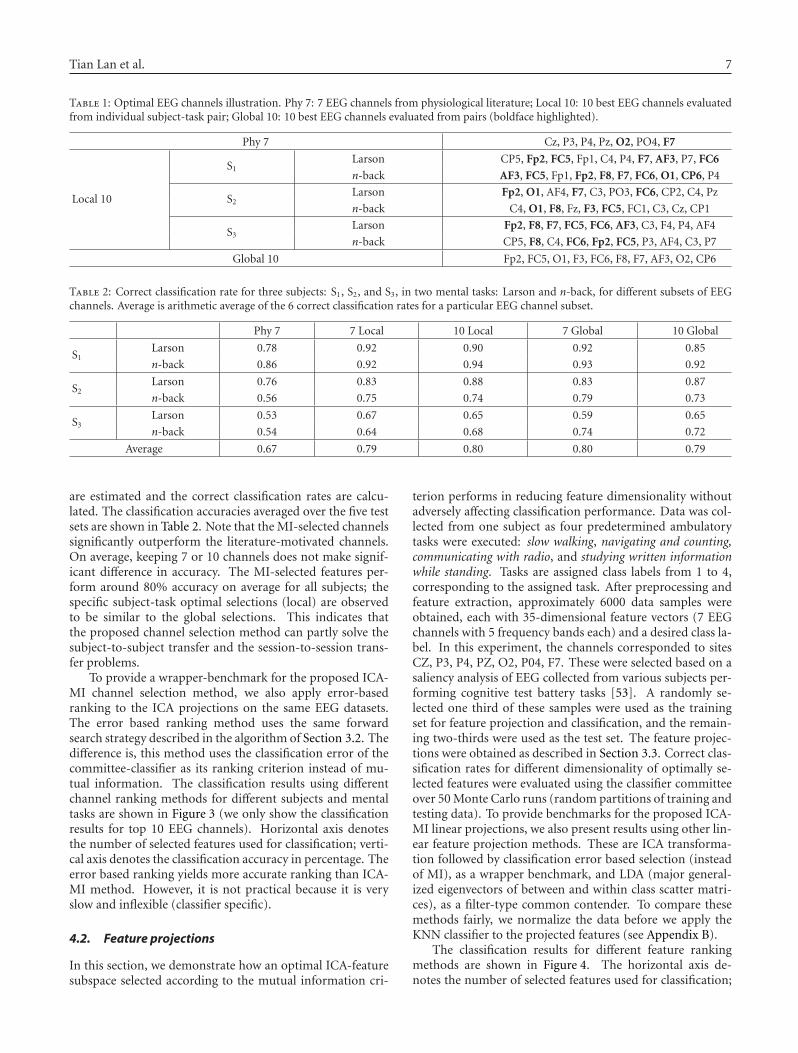
Tian Lan et al. 7
Table 1: Optimal EEG channels illustration. Phy 7: 7 EEG channels from physiological literature; Local 10: 10 best EEG channels evaluatedfrom individual subject-task pair; Global 10: 10 best EEG channels evaluated from pairs (boldface highlighted).
Phy 7 Cz, P3, P4, Pz, O2, PO4, F7
Local 10
S1Larson CP5, Fp2, FC5, Fp1, C4, P4, F7, AF3, P7, FC6
n-back AF3, FC5, Fp1, Fp2, F8, F7, FC6, O1, CP6, P4
S2Larson Fp2, O1, AF4, F7, C3, PO3, FC6, CP2, C4, Pz
n-back C4, O1, F8, Fz, F3, FC5, FC1, C3, Cz, CP1
S3Larson Fp2, F8, F7, FC5, FC6, AF3, C3, F4, P4, AF4
n-back CP5, F8, C4, FC6, Fp2, FC5, P3, AF4, C3, P7
Global 10 Fp2, FC5, O1, F3, FC6, F8, F7, AF3, O2, CP6
Table 2: Correct classification rate for three subjects: S1, S2, and S3, in two mental tasks: Larson and n-back, for different subsets of EEGchannels. Average is arithmetic average of the 6 correct classification rates for a particular EEG channel subset.
Phy 7 7 Local 10 Local 7 Global 10 Global
S1Larson 0.78 0.92 0.90 0.92 0.85
n-back 0.86 0.92 0.94 0.93 0.92
S2Larson 0.76 0.83 0.88 0.83 0.87
n-back 0.56 0.75 0.74 0.79 0.73
S3Larson 0.53 0.67 0.65 0.59 0.65
n-back 0.54 0.64 0.68 0.74 0.72
Average 0.67 0.79 0.80 0.80 0.79
are estimated and the correct classification rates are calcu-lated. The classification accuracies averaged over the five testsets are shown in Table 2. Note that the MI-selected channelssignificantly outperform the literature-motivated channels.On average, keeping 7 or 10 channels does not make signif-icant difference in accuracy. The MI-selected features per-form around 80% accuracy on average for all subjects; thespecific subject-task optimal selections (local) are observedto be similar to the global selections. This indicates thatthe proposed channel selection method can partly solve thesubject-to-subject transfer and the session-to-session trans-fer problems.
To provide a wrapper-benchmark for the proposed ICA-MI channel selection method, we also apply error-basedranking to the ICA projections on the same EEG datasets.The error based ranking method uses the same forwardsearch strategy described in the algorithm of Section 3.2. Thedifference is, this method uses the classification error of thecommittee-classifier as its ranking criterion instead of mu-tual information. The classification results using differentchannel ranking methods for different subjects and mentaltasks are shown in Figure 3 (we only show the classificationresults for top 10 EEG channels). Horizontal axis denotesthe number of selected features used for classification; verti-cal axis denotes the classification accuracy in percentage. Theerror based ranking yields more accurate ranking than ICA-MI method. However, it is not practical because it is veryslow and inflexible (classifier specific).
4.2. Feature projections
In this section, we demonstrate how an optimal ICA-featuresubspace selected according to the mutual information cri-
terion performs in reducing feature dimensionality withoutadversely affecting classification performance. Data was col-lected from one subject as four predetermined ambulatorytasks were executed: slow walking, navigating and counting,communicating with radio, and studying written informationwhile standing. Tasks are assigned class labels from 1 to 4,corresponding to the assigned task. After preprocessing andfeature extraction, approximately 6000 data samples wereobtained, each with 35-dimensional feature vectors (7 EEGchannels with 5 frequency bands each) and a desired class la-bel. In this experiment, the channels corresponded to sitesCZ, P3, P4, PZ, O2, P04, F7. These were selected based on asaliency analysis of EEG collected from various subjects per-forming cognitive test battery tasks [53]. A randomly se-lected one third of these samples were used as the trainingset for feature projection and classification, and the remain-ing two-thirds were used as the test set. The feature projec-tions were obtained as described in Section 3.3. Correct clas-sification rates for different dimensionality of optimally se-lected features were evaluated using the classifier committeeover 50 Monte Carlo runs (random partitions of training andtesting data). To provide benchmarks for the proposed ICA-MI linear projections, we also present results using other lin-ear feature projection methods. These are ICA transforma-tion followed by classification error based selection (insteadof MI), as a wrapper benchmark, and LDA (major general-ized eigenvectors of between and within class scatter matri-ces), as a filter-type common contender. To compare thesemethods fairly, we normalize the data before we apply theKNN classifier to the projected features (see Appendix B).
The classification results for different feature rankingmethods are shown in Figure 4. The horizontal axis de-notes the number of selected features used for classification;
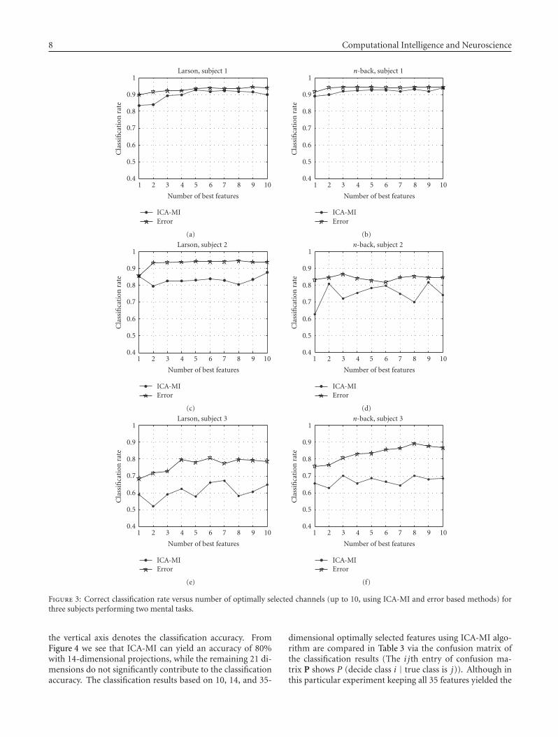
8 Computational Intelligence and Neuroscience
1 2 3 4 5 6 7 8 9 10
Number of best features
0.4
0.5
0.6
0.7
0.8
0.9
1
Cla
ssifi
cati
onra
te
Larson, subject 1
ICA-MIError
(a)
1 2 3 4 5 6 7 8 9 10
Number of best features
0.4
0.5
0.6
0.7
0.8
0.9
1
Cla
ssifi
cati
onra
te
n-back, subject 1
ICA-MIError
(b)
1 2 3 4 5 6 7 8 9 10
Number of best features
0.4
0.5
0.6
0.7
0.8
0.9
1
Cla
ssifi
cati
onra
te
Larson, subject 2
ICA-MIError
(c)
1 2 3 4 5 6 7 8 9 10
Number of best features
0.4
0.5
0.6
0.7
0.8
0.9
1
Cla
ssifi
cati
onra
te
n-back, subject 2
ICA-MIError
(d)
1 2 3 4 5 6 7 8 9 10
Number of best features
0.4
0.5
0.6
0.7
0.8
0.9
1
Cla
ssifi
cati
onra
te
Larson, subject 3
ICA-MIError
(e)
1 2 3 4 5 6 7 8 9 10
Number of best features
0.4
0.5
0.6
0.7
0.8
0.9
1
Cla
ssifi
cati
onra
te
n-back, subject 3
ICA-MIError
(f)
Figure 3: Correct classification rate versus number of optimally selected channels (up to 10, using ICA-MI and error based methods) forthree subjects performing two mental tasks.
the vertical axis denotes the classification accuracy. FromFigure 4 we see that ICA-MI can yield an accuracy of 80%with 14-dimensional projections, while the remaining 21 di-mensions do not significantly contribute to the classificationaccuracy. The classification results based on 10, 14, and 35-
dimensional optimally selected features using ICA-MI algo-rithm are compared in Table 3 via the confusion matrix ofthe classification results (The i jth entry of confusion ma-trix P shows P (decide class i | true class is j)). Although inthis particular experiment keeping all 35 features yielded the
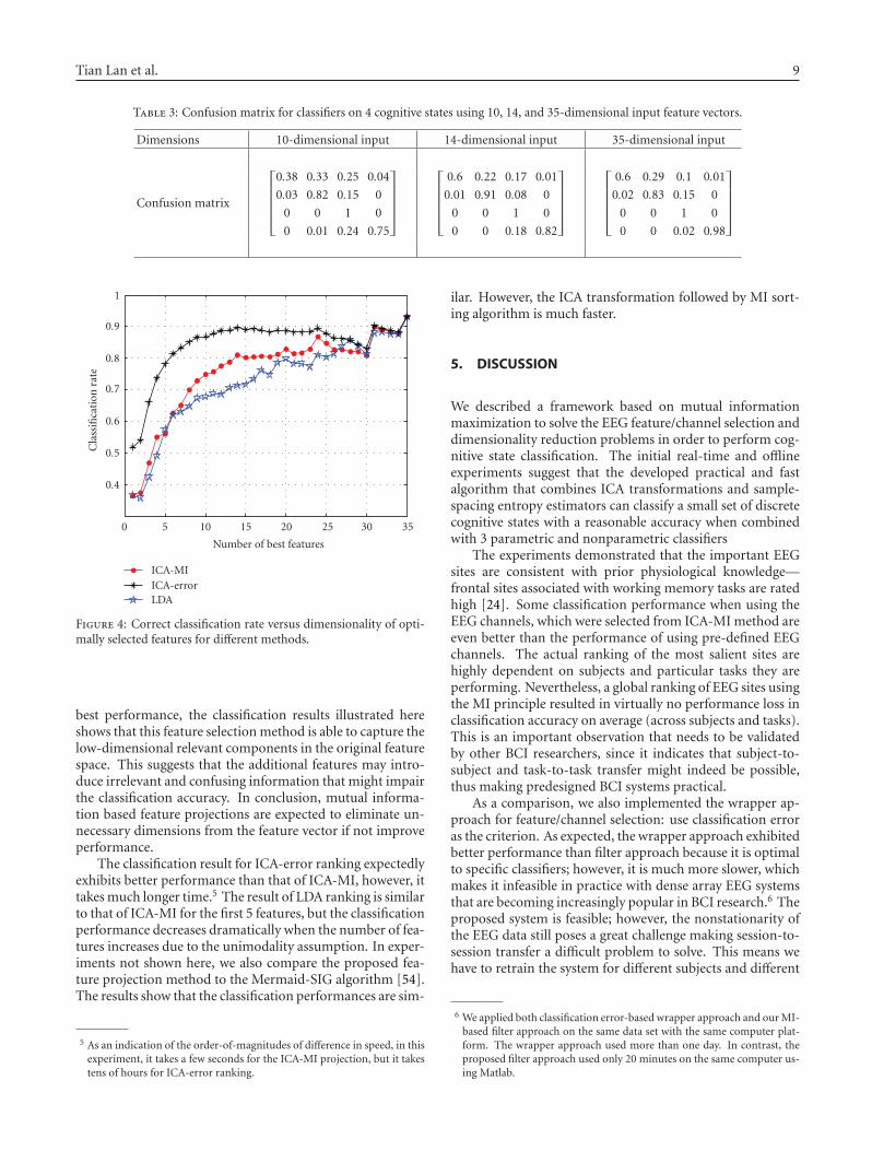
Tian Lan et al. 9
Table 3: Confusion matrix for classifiers on 4 cognitive states using 10, 14, and 35-dimensional input feature vectors.
Dimensions 10-dimensional input 14-dimensional input 35-dimensional input
Confusion matrix
⎡⎢⎢⎢⎢⎣
0.38 0.33 0.25 0.04
0.03 0.82 0.15 0
0 0 1 0
0 0.01 0.24 0.75
⎤⎥⎥⎥⎥⎦
⎡⎢⎢⎢⎢⎣
0.6 0.22 0.17 0.01
0.01 0.91 0.08 0
0 0 1 0
0 0 0.18 0.82
⎤⎥⎥⎥⎥⎦
⎡⎢⎢⎢⎢⎣
0.6 0.29 0.1 0.01
0.02 0.83 0.15 0
0 0 1 0
0 0 0.02 0.98
⎤⎥⎥⎥⎥⎦
0 5 10 15 20 25 30 35
Number of best features
0.4
0.5
0.6
0.7
0.8
0.9
1
Cla
ssifi
cati
onra
te
ICA-MIICA-errorLDA
Figure 4: Correct classification rate versus dimensionality of opti-mally selected features for different methods.
best performance, the classification results illustrated hereshows that this feature selection method is able to capture thelow-dimensional relevant components in the original featurespace. This suggests that the additional features may intro-duce irrelevant and confusing information that might impairthe classification accuracy. In conclusion, mutual informa-tion based feature projections are expected to eliminate un-necessary dimensions from the feature vector if not improveperformance.
The classification result for ICA-error ranking expectedlyexhibits better performance than that of ICA-MI, however, ittakes much longer time.5 The result of LDA ranking is similarto that of ICA-MI for the first 5 features, but the classificationperformance decreases dramatically when the number of fea-tures increases due to the unimodality assumption. In exper-iments not shown here, we also compare the proposed fea-ture projection method to the Mermaid-SIG algorithm [54].The results show that the classification performances are sim-
5 As an indication of the order-of-magnitudes of difference in speed, in thisexperiment, it takes a few seconds for the ICA-MI projection, but it takestens of hours for ICA-error ranking.
ilar. However, the ICA transformation followed by MI sort-ing algorithm is much faster.
5. DISCUSSION
We described a framework based on mutual informationmaximization to solve the EEG feature/channel selection anddimensionality reduction problems in order to perform cog-nitive state classification. The initial real-time and offlineexperiments suggest that the developed practical and fastalgorithm that combines ICA transformations and sample-spacing entropy estimators can classify a small set of discretecognitive states with a reasonable accuracy when combinedwith 3 parametric and nonparametric classifiers
The experiments demonstrated that the important EEGsites are consistent with prior physiological knowledge—frontal sites associated with working memory tasks are ratedhigh [24]. Some classification performance when using theEEG channels, which were selected from ICA-MI method areeven better than the performance of using pre-defined EEGchannels. The actual ranking of the most salient sites arehighly dependent on subjects and particular tasks they areperforming. Nevertheless, a global ranking of EEG sites usingthe MI principle resulted in virtually no performance loss inclassification accuracy on average (across subjects and tasks).This is an important observation that needs to be validatedby other BCI researchers, since it indicates that subject-to-subject and task-to-task transfer might indeed be possible,thus making predesigned BCI systems practical.
As a comparison, we also implemented the wrapper ap-proach for feature/channel selection: use classification erroras the criterion. As expected, the wrapper approach exhibitedbetter performance than filter approach because it is optimalto specific classifiers; however, it is much more slower, whichmakes it infeasible in practice with dense array EEG systemsthat are becoming increasingly popular in BCI research.6 Theproposed system is feasible; however, the nonstationarity ofthe EEG data still poses a great challenge making session-to-session transfer a difficult problem to solve. This means wehave to retrain the system for different subjects and different
6 We applied both classification error-based wrapper approach and our MI-based filter approach on the same data set with the same computer plat-form. The wrapper approach used more than one day. In contrast, theproposed filter approach used only 20 minutes on the same computer us-ing Matlab.
10 Computational Intelligence and Neuroscience
sessions, unless a very large training set encompassing a va-riety of operating conditions, numerous subjects, and tasksis available. We have utilized PSD-based features, and per-haps higher-order statistics or wavelet-based time-frequencyfeatures are more stationary and could lead to more robustdesigns. Future work will focus on determining better fea-tures.
APPENDICES
A. CLASSIFIERS
Gaussian mixture model (GMM) classifier
Gaussian mixture models are widely used to model the prob-ability density functions. In this paper, they are employedto approximate class-conditional distributions. It is assumedthat each class distribution consists of four Gaussian mod-els and the parameters of the mixture is optimized using theexpectation-maximization (EM) algorithm [55]. The esti-mated distributions are then utilized to form an approximateBayes classifier.
K nearest neighbor (KNN) classifier
The KNN classification approach is a nonparametric tech-nique that makes no assumptions about the form of theprobability densities underlying a particular set of data.Given a particular test sample, the K nearest training samples(usually in an Euclidean sense) are determined and the testsample is assigned to the class which lends the most neigh-bors to this set. It can be shown that if K is large, this classi-fier will approach the best possible classification performancegiven by the true Bayes classifier [56].
Parzen window classifier
Parzen windowing [57] is a nonparametric density estima-tion technique. It is employed to estimate the class distri-butions and to form a nonparametric approximation to theBayes classifier. In this context, it serves as a bridge betweenthe KNN where each sample contributes discretely to the de-cision (depending on whether they are in the neighborhoodor not) and the GMM classifier where each sample indirectlycontributes to the Gaussian models. In our implementation,we used Gaussian window functions, thus the Parzen classi-fiers is essentially a KNN classifier with decreasing influenceby distance, and at the same time it is a GMM itself, where aGaussian is placed on each sample.
Fusion
The classifiers output a decision at 10 Hz and the majorityvote determines the final cognitive state estimate. The Parzenclassifier decision was accepted when there was no agree-ment. It is also assumed that this state will not change over aperiod of 2 seconds, thus a median filter applied to the mostrecent 10 decisions is utilized to smoothen the classificationoutput. This postprocessing step significantly improves per-formance and reduces flickering.
B. SCALE NORMALIZATION ACROSS LINEARPROJECTIONS
When comparing different linear projection propositions us-ing a classifier whose training and performance depends onEuclidean sample distances and angles for the purpose ofhaving a controlled environment, it is important to guaran-tee that the classifier performances are not affected by Eu-clidean transformations of data across projection method-ologies. Data normalization to satisfy this desirable propertyis essential to conclude with certainty that differences in per-formances of classifiers due to various linear projections areinvariant to affine transformations.
Suppose that a linear projection matrix W ∈ �m×n,where m < n, is proposed as the optimal projection ac-cording to the criterion of that particular technique (e.g.,PCA, LDA, ICA, MI would yield different propositions). LetW = UDVT be the singular value decomposition of this ma-trix, where D is the diagonal matrix of eigenvalues, and U andV are orthonormal left and right eigenvector matrices. De-fine the multiplicative group inverse W+ = VD+UT , whereD+
ii = D−1ii if Dii �= 0 and D+
ii = 0 if Dii = 0 (i.e., D+ is thegroup inverse for diagonal matrices under multiplication).
In the comparison of linear projections using a particu-lar classifier (e.g., KNN, SVM, etc.), instead of utilizing thesamples obtained by y = Wx, where y ∈ �m, utilize thesamples generated with z = W+Wx. Note that, althoughz ∈ �n, since rank(W+W) = rank(VImVT) = m—whereIm = diag(1, . . . , 1, 0, . . . , 0) is n× n diagonal with m ones onits diagonal—the samples of the random vector z lie on anm-dimensional hyperplane determined by the rows of W. Thevariable z is a scale-normalized version of the desired projec-tion y, and its use eliminates the problems that might arisefrom the scale dependency of particular classifier topologiesand improper training procedures that might not take theseinto account.
ACKNOWLEDGMENTS
This research was supported by DARPA under ContractDAAD-16-03-C-0054 and NSF under Grants ECS-0524835and ECS-0622239.
REFERENCES
[1] L. A. Farwell and E. Donchin, “Talking off the top of yourhead: toward a mental prosthesis utilizing event-related brainpotentials,” Electroencephalography and Clinical Neurophysiol-ogy, vol. 70, no. 6, pp. 510–523, 1988.
[2] S. G. Mason and G. E. Birch, “A general framework for brain-computer interface design,” IEEE Transactions on Neural Sys-tems and Rehabilitation Engineering, vol. 11, no. 1, pp. 70–85,2003.
[3] P. He, M. Kahle, G. Wilson, and C. Russell, “Removal of ocularartifacts from EEG: a comparison of adaptive filtering methodand regression method using simulated data,” in Proceedings ofthe 27th IEEE Annual International Conference of the Engineer-ing in Medicine and Biology (EMBS ’05), vol. 7, pp. 1110–1113,Shanghai, China, September 2005.
Tian Lan et al. 11
[4] Y. Li, Z. Ma, W. Lu, and Y. Li, “Automatic removal of the eyeblink artifact from EEG using an ICA-based template match-ing approach,” Physiological Measurement, vol. 27, no. 4, pp.425–436, 2006.
[5] R. Fazel-Rezai and J. F. Peters, “P300 wave feature extrac-tion: preliminary results,” in Proceedings of the 18th AnnualCanadian Conference on Electrical and Computer Engineering(CCECE ’05), pp. 390–393, Saskatoon, Saskatchewan, Canada,May 2005.
[6] A. Subasi, “Application of classical and model-based spectralmethods to describe the state of alertness in EEG,” Journal ofMedical Systems, vol. 29, no. 5, pp. 473–486, 2005.
[7] D. J. McFarland, L. A. Miner, T. M. Vaughan, and J. R. Wol-paw, “Mu and beta rhythm topographies during motor im-agery and actual movements,” Brain Topography, vol. 12, no. 3,pp. 177–186, 2000.
[8] T. Wang, J. Deng, and B. He, “Classifying EEG-based motorimagery tasks by means of time-frequency synthesized spatialpatterns,” Clinical Neurophysiology, vol. 115, no. 12, pp. 2744–2753, 2004.
[9] G. Perea, S. Marquez-Gamino, S. Rodrıguez, and G. Moreno,“EEG-like signals generated by a simple chaotic model basedon the logistic equation,” Journal of Neural Engineering, vol. 3,no. 3, pp. 245–249, 2006.
[10] X. Li, J. Polygiannakis, P. Kapiris, A. Peratzakis, K. Eftaxias,and X. Yao, “Fractal spectral analysis of pre-epileptic seizuresin the terms of criticality,” Journal of Neural Engineering, vol. 2,no. 2, pp. 11–16, 2005.
[11] V. Bostanov, “BCI competition 2003-data sets Ib and IIb:feature extraction from event-related brain potentials withthe continuous wavelet transform and the t-value scalogram,”IEEE Transactions on Biomedical Engineering, vol. 51, no. 6, pp.1057–1061, 2004.
[12] D. Garrett, D. A. Peterson, C. W. Anderson, and M. H. Thaut,“Comparison of linear, nonlinear, and feature selection meth-ods for EEG signal classification,” IEEE Transactions on NeuralSystems and Rehabilitation Engineering, vol. 11, no. 2, pp. 141–144, 2003.
[13] R. Scherer, G. R. Muller, C. Neuper, B. Graimann, and G.Pfurtscheller, “An asynchronously controlled EEG-based vir-tual keyboard: improvement of the spelling rate,” IEEE Trans-actions on Biomedical Engineering, vol. 51, no. 6, pp. 979–984,2004.
[14] A. Rakotomamonjy, V. Guigue, G. Mallet, and V. Alvarado,“Ensemble of SVMs for improving brain computer interfaceP300 speller performances,” in Proceedings of the 15th Interna-tional Conference on Artificial Neural Networks (ICANN ’05),vol. 3696, pp. 45–50, Warsaw, Poland, September 2005.
[15] C. W. Anderson and Z. Sijercic, “Classification of EEG sig-nals from four subjects during five mental tasks,” in Interna-tional Conference on Engineering Applications of Neural Net-works (EANN ’96), pp. 407–414, London, UK, June 1996.
[16] R. Palaniappan, “Brain computer interface design using bandpowers extracted during mental tasks,” in Proceedings of the2nd International IEEE EMBS Conference on Neural Engineer-ing, pp. 321–324, Arlington, Va, USA, March 2005.
[17] X. Zhu, J. Wu, Y. Cheng, and Y. Wang, “GMM-based classifica-tion method for continuous prediction in brain-computer in-terface,” in Proceedings of the 18th International Conference onPattern Recognition (ICPR ’06), vol. 1, pp. 1171–1174, HongKong, August 2006.
[18] B. Widrow and M. Hoff, “Adaptive switching circuits,” inIRE Western Electronic Show and Convention (WESCON ’60),vol. 4, pp. 96–104, Los Angeles, Calif, USA, August 1960.
[19] J. F. Borisoff, S. G. Mason, A. Bashashati, and G. E. Birch,“Brain-computer interface design for asynchronous controlapplications: improvements to the LF-ASD asynchronousbrain switch,” IEEE Transactions on Biomedical Engineering,vol. 51, no. 6, pp. 985–992, 2004.
[20] R. Boostani and M. H. Moradi, “A new approach in the BCIresearch based on fractal dimension as feature and Adaboostas classifier,” Journal of Neural Engineering, vol. 1, no. 4, pp.212–217, 2004.
[21] U. Hoffmann, G. Garcia, J.-M. Vesin, K. Diserenst, and T.Ebrahimi, “A boosting approach to P300 detection with ap-plication to brain-computer interfaces,” in Proceedings of the2nd International IEEE EMBS Conference on Neural Engineer-ing, pp. 97–100, Arlington, Va, USA, March 2005.
[22] J. Qin, Y. Li, and A. Cichocki, “ICA and committee machine-based algorithm for cursor control in a BCI system,” in Pro-ceedings of the 2nd International Symposium on Neural Net-works (ISNN ’05), vol. 3496, pp. 973–978, Chongqing, China,May 2005.
[23] M. M. Jackson, S. G. Mason, and G. E. Birch, “Analyzing trendsin brain interface technology: a method to compare studies,”Annals of Biomedical Engineering, vol. 34, no. 5, pp. 859–878,2006.
[24] A. Gevins, M. E. Smith, L. McEvoy, and D. Yu, “High-resolution EEG mapping of cortical activation related to work-ing memory: effects of task difficulty, type of processing, andpractice,” Cerebral Cortex, vol. 7, no. 4, pp. 374–385, 1997.
[25] A. Kruse and D. Schmorrow, “Foundations of augmented cog-nition,” in Proceedings of the 1st International Conference onHuman-Computer Interaction (HCI ’05), Las Vegas, Nev, USA,July 2005.
[26] M. Pavel, G. Wang, and K. Li, “Augmented cognition: allo-cation of attention,” in Proceedings of the 36th Annual HawaiiInternational Conference on System Sciences (HICSS ’03), p. 6,Big Island, Hawaii, USA, January 2003.
[27] J. R. Wolpaw, N. Birbaumer, D. J. McFarland, G. Pfurtscheller,and T. M. Vaughan, “Brain-computer interfaces for communi-cation and control,” Clinical Neurophysiology, vol. 113, no. 6,pp. 767–791, 2002.
[28] http://www.biosemi.com/.
[29] P. Welch, “The use of fast Fourier transform for the estima-tion of power spectra: a method based on time averaging overshort, modified periodograms,” IEEE Transactions on Audioand Electroacoustics, vol. 15, no. 2, pp. 70–73, 1967.
[30] E Oja, Subspace Methods of Pattern Recognition, Wiley, NewYork, NY, USA, 1983.
[31] P. A. Devijver and J. Kittler, Pattern Recognition: A SatisticalApproach, Prentice Hall, London, UK, 1982.
[32] K. Fukunaga, Introduction to Statistical Pattern Recognition,Academic Press, New York, NY, USA, 2nd edition, 1990.
[33] R. Everson and S. Roberts, “Independent component analysis:a flexible nonlinearity and decorrelating manifold approach,”Neural Computation, vol. 11, no. 8, pp. 1957–1983, 1999.
[34] A. Hyvarinen, E. Oja, P. Hoyer, and J. Hurri, “Image feature ex-traction by sparse coding and independent component analy-sis,” in Proceedings of the 14th International Conference on Pat-tern Recognition (ICPR ’98), vol. 2, pp. 1268–1273, Brisbane,Australia, August 1998.
[35] K. Torkkola, “Feature extraction by non parametric mutualinformation maximization,” Journal of Machine Learning Re-search, vol. 3, pp. 1415–1438, 2003.
12 Computational Intelligence and Neuroscience
[36] T. M. Cover and J. A. Thomas, Elements of Information Theory,Wiley-Interscience, New York, NY, USA, 1991.
[37] R. M. Fano, Transmission of Information: A Statistical Theoryof Communications, Wiley, New York, NY, USA, 1961.
[38] M. Hellman and J. Raviv, “Probability of error, equivocation,and the Chernoff bound,” IEEE Transactions on InformationTheory, vol. 16, no. 4, pp. 368–372, 1970.
[39] R. Battiti, “Using mutual information for selecting features insupervised neural net learning,” IEEE Transactions on NeuralNetworks, vol. 5, no. 4, pp. 537–550, 1994.
[40] A. Ai-Ani and M. Deriche, “An optimal feature selection tech-nique using the concept of mutual information,” in Proceed-ings of the 6th International Symposium on Signal Processingand Its Applications (ISSPA ’01), vol. 2, pp. 477–480, KualaLumpur, Malaysia, August 2001.
[41] N. Kwak and C.-H. Choi, “Input feature selection for clas-sification problems,” IEEE Transactions on Neural Networks,vol. 13, no. 1, pp. 143–159, 2002.
[42] H. H. Yang and J. E. Moody, “Feature selection based on jointmutual information,” in Advances in Intelligent Data Analy-sis (AIDA), Computational Intelligence Methods and Applica-tions (CIMA), International Computer Science Conventions,Rochester, NY, USA, June 1999.
[43] H. H. Yang and J. E. Moody, “Data visualization and feature se-lection: new algorithms for nongaussian data,” in Advances inNeural Information Processing Systems 12 (NIPS ’99), pp. 687–702, Denver, Colo, USA, November-December 2000.
[44] A. Hyvarinen and P. Pajunen, “Nonlinear independent com-ponent analysis: existence and uniqueness results,” NeuralNetworks, vol. 12, no. 3, pp. 429–439, 1999.
[45] T. Lan and D. Erdogmus, “Maximally informative feature andsensor selection in pattern recognition using local and globalindependent component analysis,” Journal of VLSI Signal Pro-cessing Systems, vol. 48, no. 1-2, pp. 39–52, 2007.
[46] E. G. Learned-Miller and J. W. Fisher III, “ICA using spacingsestimates of entropy,” Journal of Machine Learning Research,vol. 4, no. 7-8, pp. 1271–1295, 2004.
[47] K. E. Hild II, D. Erdogmus, and J. Prıncipe, “Blind source sep-aration using Renyi’s mutual information,” IEEE Signal Pro-cessing Letters, vol. 8, no. 6, pp. 174–176, 2001.
[48] A. Hyvarinen and E. Oja, “A fast fixed-point algorithm for in-dependent component analysis,” Neural Computation, vol. 9,no. 7, pp. 1483–1492, 1997.
[49] L. Parra and P. Sajda, “Blind source separation via generalizedeigenvalue decomposition,” Journal of Machine Learning Re-search, vol. 4, no. 7-8, pp. 1261–1269, 2004.
[50] J. Beirlant, E. J. Dudewicz, L. Gyorfi, and E. C. van der Meulen,“Nonparametric entropy estimation: an overview,” Interna-tional Journal of Mathematical and Statistical Sciences, vol. 6,no. 1, pp. 17–39, 1997.
[51] E. Halgren, C. Boujon, J. Clarke, C. Wang, and P. Chauvel,“Rapid distributed fronto-parieto-occipital processing stagesduring working memory in humans,” Cerebral Cortex, vol. 12,no. 7, pp. 710–728, 2002.
[52] A. Gevins and M. E. Smith, “Neurophysiological measures ofworking memory and individual differences in cognitive abil-ity and cognitive style,” Cerebral Cortex, vol. 10, no. 9, pp. 829–839, 2000.
[53] C. A. Russell and S. G. Gustafson, “Selecting salient features ofpsychophysiological measures,” Tech. Rep. AFRL-HE-WP-TR-2001-0136, Air Force Research Laboratory, Rome, NY, USA,2001.
[54] K. E. Hild II, Blind source separation of convolutive mixturesusing Renyi’s divergence, Ph.D. thesis, University of Florida,Gainesville, Fla, USA, 2003.
[55] A. P. Dempster, N. M. Laird, and D. B. Rubin, “Maximum like-lihood from incomplete data via the EM algorithm,” Journal ofthe Royal Statistical Society, vol. 39, no. 1, pp. 1–38, 1977.
[56] R. O. Duda, P. E. Hart, and D. G. Stork, Pattern Classification,Wiley, New York, NY, USA, 2nd edition, 2000.
[57] E. Parzen, “On estimation of a probability density functionand mode,” in Time Series Analysis Papers, Holden-Day, SanDiego, Calif, USA, 1967.
Hindawi Publishing CorporationComputational Intelligence and NeuroscienceVolume 2007, Article ID 41468, 9 pagesdoi:10.1155/2007/41468
Research ArticleExtracting Rhythmic Brain Activity forBrain-Computer Interfacing through ConstrainedIndependent Component Analysis
Suogang Wang and Christopher J. James
Signal Processing and Control Group, ISVR, University of Southampton, Southampton SO17 1BJ, UK
Correspondence should be addressed to Suogang Wang, [email protected]
Received 31 December 2006; Accepted 18 June 2007
Recommended by Andrzej Cichocki
We propose a technique based on independent component analysis (ICA) with constraints, applied to the rhythmic electroen-cephalographic (EEG) data recorded from a brain-computer interfacing (BCI) system. ICA is a technique that can decompose therecorded EEG into its underlying independent components and in BCI involving motor imagery, the aim is to isolate rhythmicactivity over the sensorimotor cortex. We demonstrate that, through the technique of spectrally constrained ICA, we can learn aspatial filter suited to each individual EEG recording. This can effectively extract discriminatory information from two types ofsingle-trial EEG data. Through the use of the ICA algorithm, the classification accuracy is improved by about 25%, on average,compared to the performance on the unpreprocessed data. This implies that this ICA technique can be reliably used to identifyand extract BCI-related rhythmic activity underlying the recordings where a particular filter is learned for each subject. The highclassification rate and low computational cost make it a promising algorithm for application to an online BCI system.
Copyright © 2007 S. Wang and C. J. James. This is an open access article distributed under the Creative Commons AttributionLicense, which permits unrestricted use, distribution, and reproduction in any medium, provided the original work is properlycited.
1. INTRODUCTION
The electroencephalogram (EEG) is a recording of the brain’selectrical activity and is one of the most important mea-surements used to evaluate neurological disorders in theclinic and to investigate brain function in the laboratory. Therecording is obtained by placing electrodes on the scalp, gen-erally according to the 10/20 electrode placement system [1].
A brain-computer interface (BCI) is a communicationsystem in which messages or commands that an individualsends to the external world do not pass through the brain’snormal output pathways of peripheral nerves and muscles[2]. In an EEG-based BCI, the messages are carried throughEEG activity. The primary aim is to provide people with anew channel for communication with the outside environ-ment. Many different disorders, such as amyotrophic lateralsclerosis (ALS), brainstem stroke, brain or spinal cord injury,and numerous other diseases can disrupt the neuromuscu-lar channels through which the brain communicates with itsenvironment and exerts control. These kinds of severe dis-eases may cause people to lose voluntary muscle control and
to be unable to communicate in any way (this is known as be-ing “locked in”). As current knowledge about these disordersis rather limited, there are no effective treatments which canprovide a cure or even a significant recovery. In the absence ofmethods for repairing the damage caused by these diseases,a BCI system provides an option that conveys messages andcommands to use some devices such as assistive applicationsand computers. This type of direct brain interface would in-crease an individual’s independence and improve quality oflife and also reduce the costs on society.
Historically, EEG activity is divided into four types ofcontinuous rhythmic sinusoidal waves known as δ, θ, α, andβ frequency bands. In this study, it is the function that al-lows users to control the amplitude of their μ (8–12 Hz) orβ (18–22 Hz) brain rhythmic activity over the sensorimotorcortices caused by motor imagery (MI) [3, 4] (i.e., hand orfoot movement imagination), that is of interest. For MI, theusers are instructed to imagine a specific motor action with-out any related motor output. The imagination of the move-ment is accompanied by an effect known as event-related(desynchronization/synchronization) (ERD/ERS) [5]. When
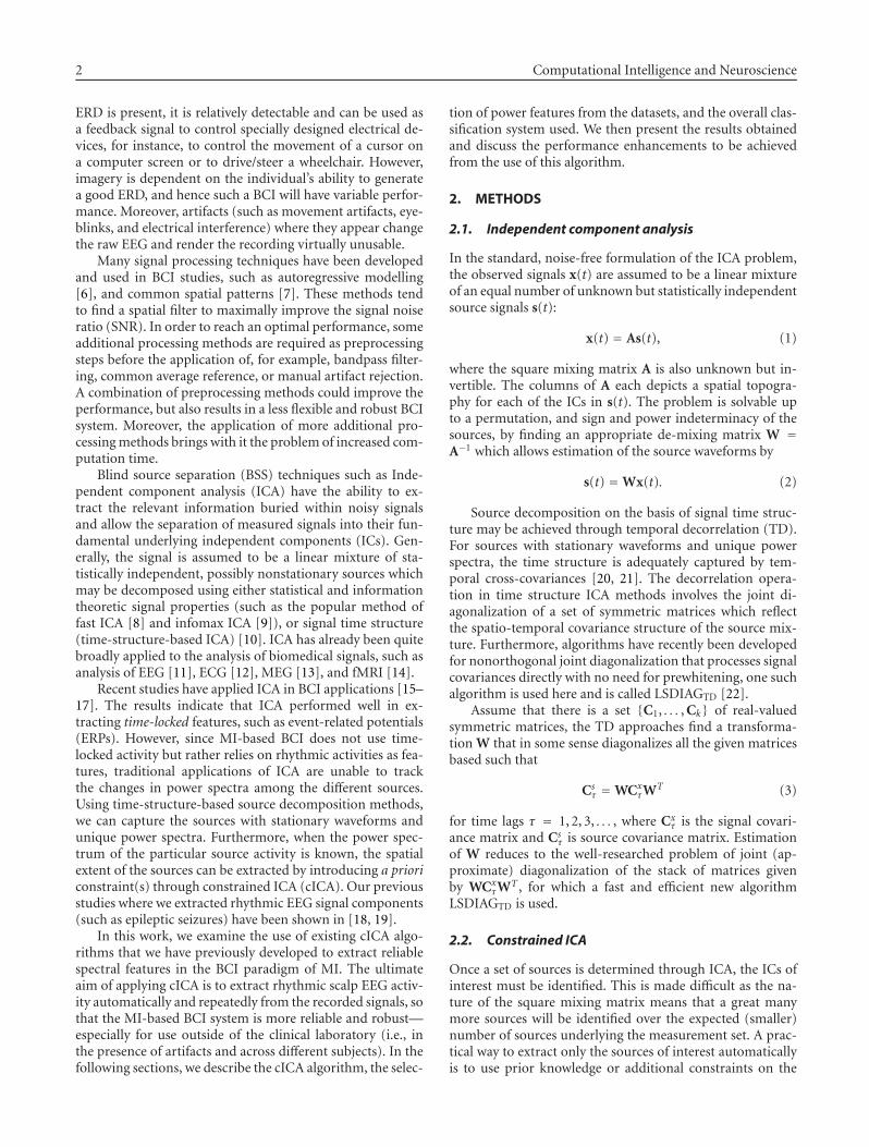
2 Computational Intelligence and Neuroscience
ERD is present, it is relatively detectable and can be used asa feedback signal to control specially designed electrical de-vices, for instance, to control the movement of a cursor ona computer screen or to drive/steer a wheelchair. However,imagery is dependent on the individual’s ability to generatea good ERD, and hence such a BCI will have variable perfor-mance. Moreover, artifacts (such as movement artifacts, eye-blinks, and electrical interference) where they appear changethe raw EEG and render the recording virtually unusable.
Many signal processing techniques have been developedand used in BCI studies, such as autoregressive modelling[6], and common spatial patterns [7]. These methods tendto find a spatial filter to maximally improve the signal noiseratio (SNR). In order to reach an optimal performance, someadditional processing methods are required as preprocessingsteps before the application of, for example, bandpass filter-ing, common average reference, or manual artifact rejection.A combination of preprocessing methods could improve theperformance, but also results in a less flexible and robust BCIsystem. Moreover, the application of more additional pro-cessing methods brings with it the problem of increased com-putation time.
Blind source separation (BSS) techniques such as Inde-pendent component analysis (ICA) have the ability to ex-tract the relevant information buried within noisy signalsand allow the separation of measured signals into their fun-damental underlying independent components (ICs). Gen-erally, the signal is assumed to be a linear mixture of sta-tistically independent, possibly nonstationary sources whichmay be decomposed using either statistical and informationtheoretic signal properties (such as the popular method offast ICA [8] and infomax ICA [9]), or signal time structure(time-structure-based ICA) [10]. ICA has already been quitebroadly applied to the analysis of biomedical signals, such asanalysis of EEG [11], ECG [12], MEG [13], and fMRI [14].
Recent studies have applied ICA in BCI applications [15–17]. The results indicate that ICA performed well in ex-tracting time-locked features, such as event-related potentials(ERPs). However, since MI-based BCI does not use time-locked activity but rather relies on rhythmic activities as fea-tures, traditional applications of ICA are unable to trackthe changes in power spectra among the different sources.Using time-structure-based source decomposition methods,we can capture the sources with stationary waveforms andunique power spectra. Furthermore, when the power spec-trum of the particular source activity is known, the spatialextent of the sources can be extracted by introducing a prioriconstraint(s) through constrained ICA (cICA). Our previousstudies where we extracted rhythmic EEG signal components(such as epileptic seizures) have been shown in [18, 19].
In this work, we examine the use of existing cICA algo-rithms that we have previously developed to extract reliablespectral features in the BCI paradigm of MI. The ultimateaim of applying cICA is to extract rhythmic scalp EEG activ-ity automatically and repeatedly from the recorded signals, sothat the MI-based BCI system is more reliable and robust—especially for use outside of the clinical laboratory (i.e., inthe presence of artifacts and across different subjects). In thefollowing sections, we describe the cICA algorithm, the selec-
tion of power features from the datasets, and the overall clas-sification system used. We then present the results obtainedand discuss the performance enhancements to be achievedfrom the use of this algorithm.
2. METHODS
2.1. Independent component analysis
In the standard, noise-free formulation of the ICA problem,the observed signals x(t) are assumed to be a linear mixtureof an equal number of unknown but statistically independentsource signals s(t):
x(t) = As(t), (1)
where the square mixing matrix A is also unknown but in-vertible. The columns of A each depicts a spatial topogra-phy for each of the ICs in s(t). The problem is solvable upto a permutation, and sign and power indeterminacy of thesources, by finding an appropriate de-mixing matrix W =A−1 which allows estimation of the source waveforms by
s(t) = Wx(t). (2)
Source decomposition on the basis of signal time struc-ture may be achieved through temporal decorrelation (TD).For sources with stationary waveforms and unique powerspectra, the time structure is adequately captured by tem-poral cross-covariances [20, 21]. The decorrelation opera-tion in time structure ICA methods involves the joint di-agonalization of a set of symmetric matrices which reflectthe spatio-temporal covariance structure of the source mix-ture. Furthermore, algorithms have recently been developedfor nonorthogonal joint diagonalization that processes signalcovariances directly with no need for prewhitening, one suchalgorithm is used here and is called LSDIAGTD [22].
Assume that there is a set {C1, . . . , Ck} of real-valuedsymmetric matrices, the TD approaches find a transforma-tion W that in some sense diagonalizes all the given matricesbased such that
Csτ = WCx
τWT (3)
for time lags τ = 1, 2, 3, . . . , where Cxτ is the signal covari-
ance matrix and Csτ is source covariance matrix. Estimation
of W reduces to the well-researched problem of joint (ap-proximate) diagonalization of the stack of matrices givenby WCx
τWT , for which a fast and efficient new algorithmLSDIAGTD is used.
2.2. Constrained ICA
Once a set of sources is determined through ICA, the ICs ofinterest must be identified. This is made difficult as the na-ture of the square mixing matrix means that a great manymore sources will be identified over the expected (smaller)number of sources underlying the measurement set. A prac-tical way to extract only the sources of interest automaticallyis to use prior knowledge or additional constraints on the
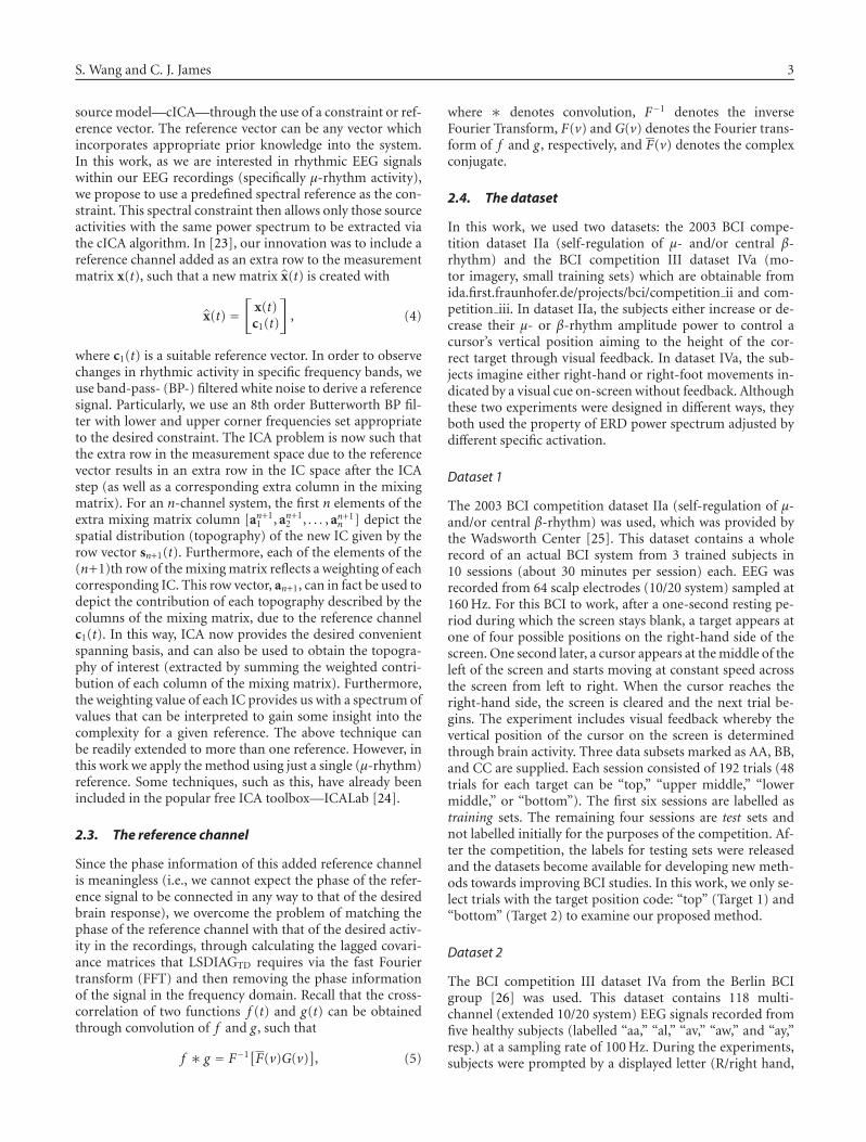
S. Wang and C. J. James 3
source model—cICA—through the use of a constraint or ref-erence vector. The reference vector can be any vector whichincorporates appropriate prior knowledge into the system.In this work, as we are interested in rhythmic EEG signalswithin our EEG recordings (specifically μ-rhythm activity),we propose to use a predefined spectral reference as the con-straint. This spectral constraint then allows only those sourceactivities with the same power spectrum to be extracted viathe cICA algorithm. In [23], our innovation was to include areference channel added as an extra row to the measurementmatrix x(t), such that a new matrix x(t) is created with
x(t) =[
x(t)c1(t)
]
, (4)
where c1(t) is a suitable reference vector. In order to observechanges in rhythmic activity in specific frequency bands, weuse band-pass- (BP-) filtered white noise to derive a referencesignal. Particularly, we use an 8th order Butterworth BP fil-ter with lower and upper corner frequencies set appropriateto the desired constraint. The ICA problem is now such thatthe extra row in the measurement space due to the referencevector results in an extra row in the IC space after the ICAstep (as well as a corresponding extra column in the mixingmatrix). For an n-channel system, the first n elements of theextra mixing matrix column [an+1
1 , an+12 , . . . , an+1
n ] depict thespatial distribution (topography) of the new IC given by therow vector sn+1(t). Furthermore, each of the elements of the(n+1)th row of the mixing matrix reflects a weighting of eachcorresponding IC. This row vector, an+1, can in fact be used todepict the contribution of each topography described by thecolumns of the mixing matrix, due to the reference channelc1(t). In this way, ICA now provides the desired convenientspanning basis, and can also be used to obtain the topogra-phy of interest (extracted by summing the weighted contri-bution of each column of the mixing matrix). Furthermore,the weighting value of each IC provides us with a spectrum ofvalues that can be interpreted to gain some insight into thecomplexity for a given reference. The above technique canbe readily extended to more than one reference. However, inthis work we apply the method using just a single (μ-rhythm)reference. Some techniques, such as this, have already beenincluded in the popular free ICA toolbox—ICALab [24].
2.3. The reference channel
Since the phase information of this added reference channelis meaningless (i.e., we cannot expect the phase of the refer-ence signal to be connected in any way to that of the desiredbrain response), we overcome the problem of matching thephase of the reference channel with that of the desired activ-ity in the recordings, through calculating the lagged covari-ance matrices that LSDIAGTD requires via the fast Fouriertransform (FFT) and then removing the phase informationof the signal in the frequency domain. Recall that the cross-correlation of two functions f (t) and g(t) can be obtainedthrough convolution of f and g, such that
f ∗ g = F−1[F(v)G(v)]
, (5)
where ∗ denotes convolution, F−1 denotes the inverseFourier Transform, F(v) and G(v) denotes the Fourier trans-form of f and g, respectively, and F(v) denotes the complexconjugate.
2.4. The dataset
In this work, we used two datasets: the 2003 BCI compe-tition dataset IIa (self-regulation of μ- and/or central β-rhythm) and the BCI competition III dataset IVa (mo-tor imagery, small training sets) which are obtainable fromida.first.fraunhofer.de/projects/bci/competition ii and com-petition iii. In dataset IIa, the subjects either increase or de-crease their μ- or β-rhythm amplitude power to control acursor’s vertical position aiming to the height of the cor-rect target through visual feedback. In dataset IVa, the sub-jects imagine either right-hand or right-foot movements in-dicated by a visual cue on-screen without feedback. Althoughthese two experiments were designed in different ways, theyboth used the property of ERD power spectrum adjusted bydifferent specific activation.
Dataset 1
The 2003 BCI competition dataset IIa (self-regulation of μ-and/or central β-rhythm) was used, which was provided bythe Wadsworth Center [25]. This dataset contains a wholerecord of an actual BCI system from 3 trained subjects in10 sessions (about 30 minutes per session) each. EEG wasrecorded from 64 scalp electrodes (10/20 system) sampled at160 Hz. For this BCI to work, after a one-second resting pe-riod during which the screen stays blank, a target appears atone of four possible positions on the right-hand side of thescreen. One second later, a cursor appears at the middle of theleft of the screen and starts moving at constant speed acrossthe screen from left to right. When the cursor reaches theright-hand side, the screen is cleared and the next trial be-gins. The experiment includes visual feedback whereby thevertical position of the cursor on the screen is determinedthrough brain activity. Three data subsets marked as AA, BB,and CC are supplied. Each session consisted of 192 trials (48trials for each target can be “top,” “upper middle,” “lowermiddle,” or “bottom”). The first six sessions are labelled astraining sets. The remaining four sessions are test sets andnot labelled initially for the purposes of the competition. Af-ter the competition, the labels for testing sets were releasedand the datasets become available for developing new meth-ods towards improving BCI studies. In this work, we only se-lect trials with the target position code: “top” (Target 1) and“bottom” (Target 2) to examine our proposed method.
Dataset 2
The BCI competition III dataset IVa from the Berlin BCIgroup [26] was used. This dataset contains 118 multi-channel (extended 10/20 system) EEG signals recorded fromfive healthy subjects (labelled “aa,” “al,” “av,” “aw,” and “ay,”resp.) at a sampling rate of 100 Hz. During the experiments,subjects were prompted by a displayed letter (R/right hand,
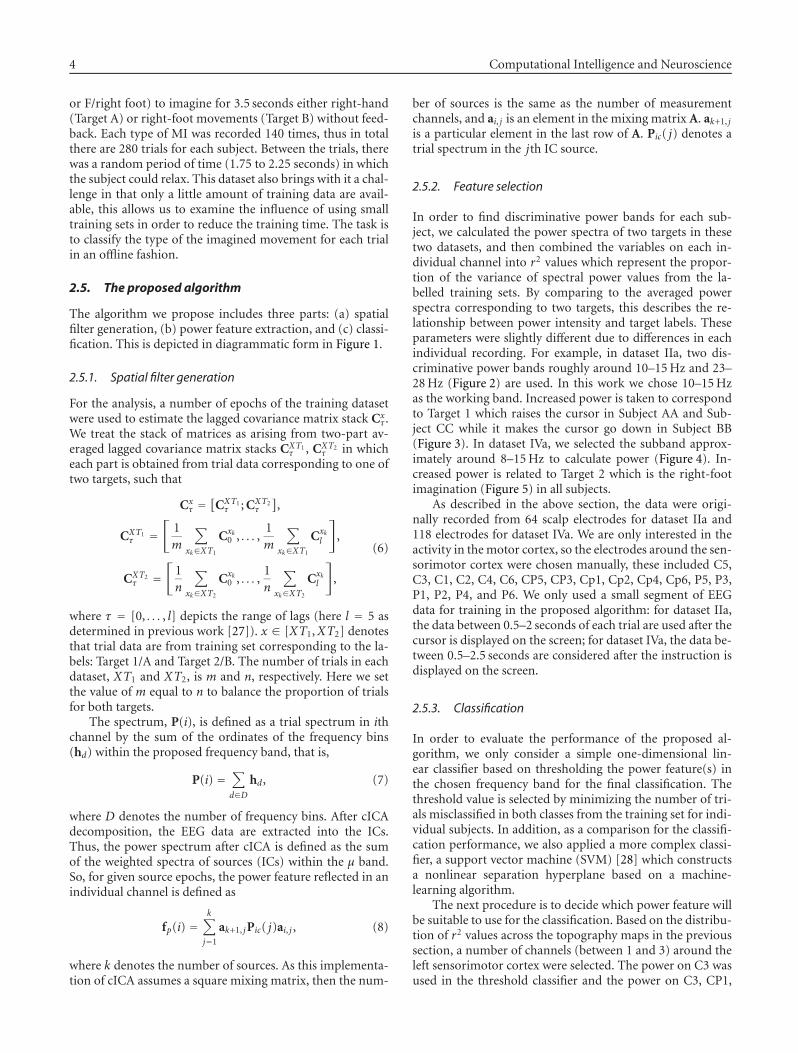
4 Computational Intelligence and Neuroscience
or F/right foot) to imagine for 3.5 seconds either right-hand(Target A) or right-foot movements (Target B) without feed-back. Each type of MI was recorded 140 times, thus in totalthere are 280 trials for each subject. Between the trials, therewas a random period of time (1.75 to 2.25 seconds) in whichthe subject could relax. This dataset also brings with it a chal-lenge in that only a little amount of training data are avail-able, this allows us to examine the influence of using smalltraining sets in order to reduce the training time. The task isto classify the type of the imagined movement for each trialin an offline fashion.
2.5. The proposed algorithm
The algorithm we propose includes three parts: (a) spatialfilter generation, (b) power feature extraction, and (c) classi-fication. This is depicted in diagrammatic form in Figure 1.
2.5.1. Spatial filter generation
For the analysis, a number of epochs of the training datasetwere used to estimate the lagged covariance matrix stack Cx
τ .We treat the stack of matrices as arising from two-part av-eraged lagged covariance matrix stacks CXT1
τ , CXT2τ in which
each part is obtained from trial data corresponding to one oftwo targets, such that
Cxτ =
[
CXT1τ ; CXT2
τ
]
,
CXT1τ =
[
1m
∑
xk∈XT1
Cxk0 , . . . ,
1m
∑
xk∈XT1
Cxkl
]
,
CXT2τ =
[
1n
∑
xk∈XT2
Cxk0 , . . . ,
1n
∑
xk∈XT2
Cxkl
]
,
(6)
where τ = [0, . . . , l] depicts the range of lags (here l = 5 asdetermined in previous work [27]). x ∈ [XT1,XT2] denotesthat trial data are from training set corresponding to the la-bels: Target 1/A and Target 2/B. The number of trials in eachdataset, XT1 and XT2, is m and n, respectively. Here we setthe value of m equal to n to balance the proportion of trialsfor both targets.
The spectrum, P(i), is defined as a trial spectrum in ithchannel by the sum of the ordinates of the frequency bins(hd) within the proposed frequency band, that is,
P(i) =∑
d∈Dhd, (7)
where D denotes the number of frequency bins. After cICAdecomposition, the EEG data are extracted into the ICs.Thus, the power spectrum after cICA is defined as the sumof the weighted spectra of sources (ICs) within the μ band.So, for given source epochs, the power feature reflected in anindividual channel is defined as
fp(i) =k∑
j=1
ak+1, jPic( j)ai, j , (8)
where k denotes the number of sources. As this implementa-tion of cICA assumes a square mixing matrix, then the num-
ber of sources is the same as the number of measurementchannels, and ai, j is an element in the mixing matrix A. ak+1, j
is a particular element in the last row of A. Pic( j) denotes atrial spectrum in the jth IC source.
2.5.2. Feature selection
In order to find discriminative power bands for each sub-ject, we calculated the power spectra of two targets in thesetwo datasets, and then combined the variables on each in-dividual channel into r2 values which represent the propor-tion of the variance of spectral power values from the la-belled training sets. By comparing to the averaged powerspectra corresponding to two targets, this describes the re-lationship between power intensity and target labels. Theseparameters were slightly different due to differences in eachindividual recording. For example, in dataset IIa, two dis-criminative power bands roughly around 10–15 Hz and 23–28 Hz (Figure 2) are used. In this work we chose 10–15 Hzas the working band. Increased power is taken to correspondto Target 1 which raises the cursor in Subject AA and Sub-ject CC while it makes the cursor go down in Subject BB(Figure 3). In dataset IVa, we selected the subband approx-imately around 8–15 Hz to calculate power (Figure 4). In-creased power is related to Target 2 which is the right-footimagination (Figure 5) in all subjects.
As described in the above section, the data were origi-nally recorded from 64 scalp electrodes for dataset IIa and118 electrodes for dataset IVa. We are only interested in theactivity in the motor cortex, so the electrodes around the sen-sorimotor cortex were chosen manually, these included C5,C3, C1, C2, C4, C6, CP5, CP3, Cp1, Cp2, Cp4, Cp6, P5, P3,P1, P2, P4, and P6. We only used a small segment of EEGdata for training in the proposed algorithm: for dataset IIa,the data between 0.5–2 seconds of each trial are used after thecursor is displayed on the screen; for dataset IVa, the data be-tween 0.5–2.5 seconds are considered after the instruction isdisplayed on the screen.
2.5.3. Classification
In order to evaluate the performance of the proposed al-gorithm, we only consider a simple one-dimensional lin-ear classifier based on thresholding the power feature(s) inthe chosen frequency band for the final classification. Thethreshold value is selected by minimizing the number of tri-als misclassified in both classes from the training set for indi-vidual subjects. In addition, as a comparison for the classifi-cation performance, we also applied a more complex classi-fier, a support vector machine (SVM) [28] which constructsa nonlinear separation hyperplane based on a machine-learning algorithm.
The next procedure is to decide which power feature willbe suitable to use for the classification. Based on the distribu-tion of r2 values across the topography maps in the previoussection, a number of channels (between 1 and 3) around theleft sensorimotor cortex were selected. The power on C3 wasused in the threshold classifier and the power on C3, CP1,
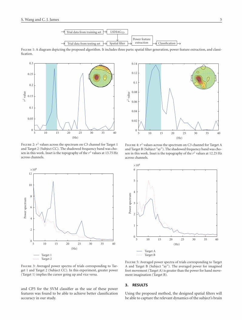
S. Wang and C. J. James 5
Trial data from training set LSDIAGTD
Trial data from testing set Spatial filterPower feature
extraction Classification
Figure 1: A diagram depicting the proposed algorithm. It includes three parts: spatial filter generation, power feature extraction, and classi-fication.
5 10 15 20 25 30 35 40
(Hz)
0
0.05
0.1
0.15
0.2
0.25
0.3
r2va
lue
Figure 2: r2 values across the spectrum on C3 channel for Target 1and Target 2 (Subject CC). The shadowed frequency band was cho-sen in this work. Inset is the topography of the r2 values at 13.75 Hzacross channels.
5 10 15 20 25 30 35 40
(Hz)
0
2
4
6
8
10
12×108
Pow
ersp
ectr
um
Target 1Target 2
Figure 3: Averaged power spectra of trials corresponding to Tar-get 1 and Target 2 (Subject CC). In this experiment, greater power(Target 1) implies the cursor going up and vice versa.
and CP5 for the SVM classifier as the use of these powerfeatures was found to be able to achieve better classificationaccuracy in our study.
5 10 15 20 25 30 35 40
(Hz)
0
0.02
0.04
0.06
0.08
0.1
0.12
0.14
r2va
lue
Figure 4: r2 values across the spectrum on C3 channel for Target Aand Target B (Subject “ay”). The shadowed frequency band was cho-sen in this work. Inset is the topography of the r2 values at 12.25 Hzacross channels.
5 10 15 20 25 30 35 40
(Hz)
0
1
2
3
4
5
6×10⁴
Pow
ersp
ectr
um
Target ATarget B
Figure 5: Averaged power spectra of trials corresponding to TargetA and Target B (Subject “ay”). The averaged power for imaginedfoot movement (Target A) is greater than the power for hand move-ment imagination (Target B).
3. RESULTS
Using the proposed method, the designed spatial filters willbe able to capture the relevant dynamics of the subject’s brain
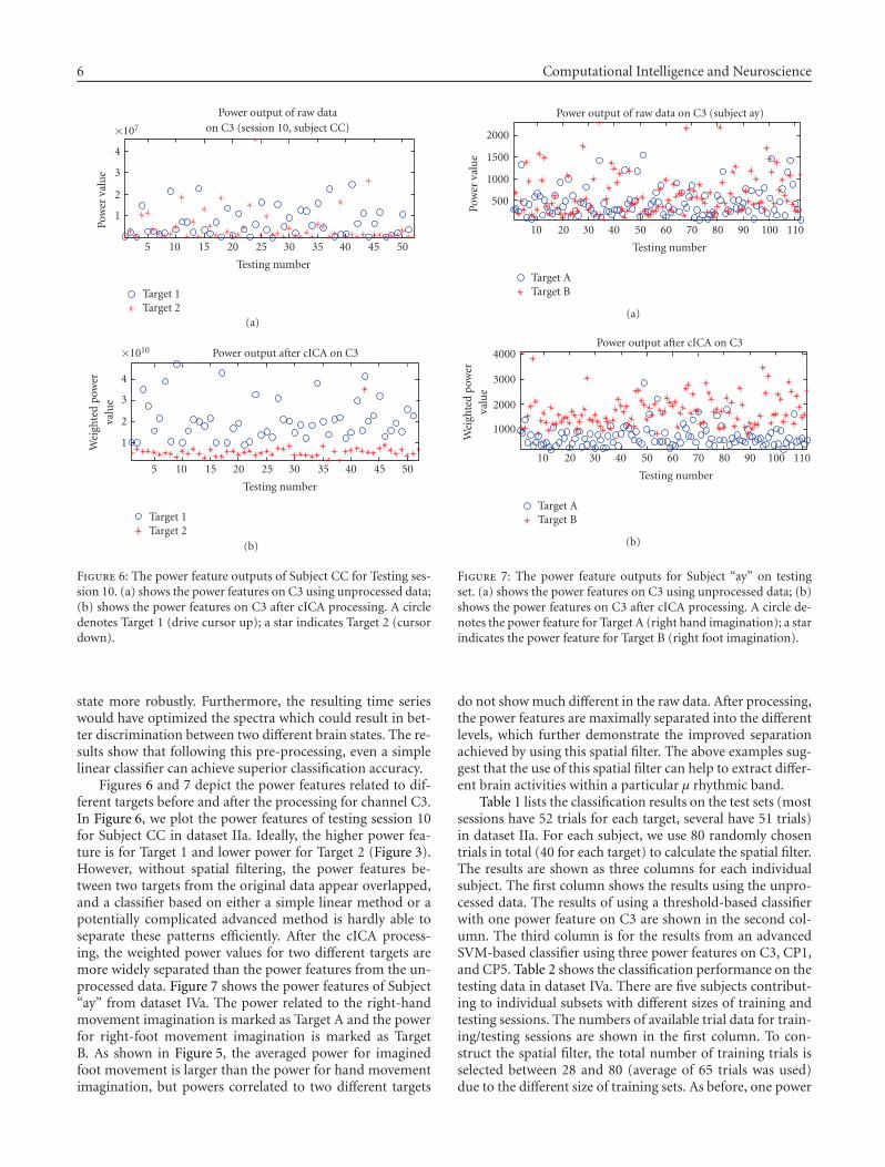
6 Computational Intelligence and Neuroscience
5 10 15 20 25 30 35 40 45 50
Testing number
1
2
3
4
×107
Pow
erva
lue
Target 1Target 2
Power output of raw dataon C3 (session 10, subject CC)
(a)
5 10 15 20 25 30 35 40 45 50
Testing number
1
2
3
4
×1010
Wei
ghte
dpo
wer
valu
e
Target 1Target 2
Power output after cICA on C3
(b)
Figure 6: The power feature outputs of Subject CC for Testing ses-sion 10. (a) shows the power features on C3 using unprocessed data;(b) shows the power features on C3 after cICA processing. A circledenotes Target 1 (drive cursor up); a star indicates Target 2 (cursordown).
state more robustly. Furthermore, the resulting time serieswould have optimized the spectra which could result in bet-ter discrimination between two different brain states. The re-sults show that following this pre-processing, even a simplelinear classifier can achieve superior classification accuracy.
Figures 6 and 7 depict the power features related to dif-ferent targets before and after the processing for channel C3.In Figure 6, we plot the power features of testing session 10for Subject CC in dataset IIa. Ideally, the higher power fea-ture is for Target 1 and lower power for Target 2 (Figure 3).However, without spatial filtering, the power features be-tween two targets from the original data appear overlapped,and a classifier based on either a simple linear method or apotentially complicated advanced method is hardly able toseparate these patterns efficiently. After the cICA process-ing, the weighted power values for two different targets aremore widely separated than the power features from the un-processed data. Figure 7 shows the power features of Subject“ay” from dataset IVa. The power related to the right-handmovement imagination is marked as Target A and the powerfor right-foot movement imagination is marked as TargetB. As shown in Figure 5, the averaged power for imaginedfoot movement is larger than the power for hand movementimagination, but powers correlated to two different targets
10 20 30 40 50 60 70 80 90 100 110
Testing number
500
1000
1500
2000
Pow
erva
lue
Target ATarget B
Power output of raw data on C3 (subject ay)
(a)
10 20 30 40 50 60 70 80 90 100 110
Testing number
1000
2000
3000
4000
Wei
ghte
dpo
wer
valu
e
Target ATarget B
Power output after cICA on C3
(b)
Figure 7: The power feature outputs for Subject “ay” on testingset. (a) shows the power features on C3 using unprocessed data; (b)shows the power features on C3 after cICA processing. A circle de-notes the power feature for Target A (right hand imagination); a starindicates the power feature for Target B (right foot imagination).
do not show much different in the raw data. After processing,the power features are maximally separated into the differentlevels, which further demonstrate the improved separationachieved by using this spatial filter. The above examples sug-gest that the use of this spatial filter can help to extract differ-ent brain activities within a particular μ rhythmic band.
Table 1 lists the classification results on the test sets (mostsessions have 52 trials for each target, several have 51 trials)in dataset IIa. For each subject, we use 80 randomly chosentrials in total (40 for each target) to calculate the spatial filter.The results are shown as three columns for each individualsubject. The first column shows the results using the unpro-cessed data. The results of using a threshold-based classifierwith one power feature on C3 are shown in the second col-umn. The third column is for the results from an advancedSVM-based classifier using three power features on C3, CP1,and CP5. Table 2 shows the classification performance on thetesting data in dataset IVa. There are five subjects contribut-ing to individual subsets with different sizes of training andtesting sessions. The numbers of available trial data for train-ing/testing sessions are shown in the first column. To con-struct the spatial filter, the total number of training trials isselected between 28 and 80 (average of 65 trials was used)due to the different size of training sets. As before, one power
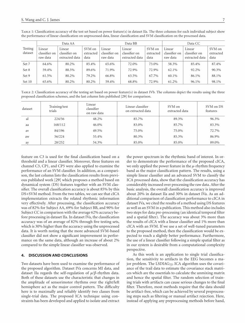
S. Wang and C. J. James 7
Table 1: Classification accuracy of the test set based on power feature(s) in dataset IIa. The three columns for each individual subject showthe performance of linear classification on unprocessed data, linear classification and SVM classification on the processed data.
Testingdataset
Data AA Data BB Data CC
Linearclassifier onraw data
Linearclassifier onextracted data
SVM onextracteddata
Linearclassifier onraw data
Linearclassifier onextracted data
SVM onextracteddata
Linearclassifier onraw data
Linearclassifier onextracted data
SVM onextracteddata
Set 7 64.6% 80.2% 85.4% 65.6% 72.0% 73.0% 58.3% 85.4% 87.4%
Set 8 59.4% 88.5% 89.6% 71.9% 72.9% 72.9% 62.1% 92.2% 90.3%
Set 9 61.5% 80.2% 79.2% 66.8% 63.5% 67.7% 60.1% 86.1% 88.1%
Set 10 65.6% 80.2% 80.2% 59.4% 68.8% 72.9% 61.2% 96.1% 98.1%
Table 2: Classification accuracy of the testing set based on power feature(s) in dataset IVb. The columns depict the results using the threeproposed classification schemes, and the last column lists published [29] for comparison.
datasetTraining/testtrials
Linearclassifieron raw data
Linear classifieron extracted data
SVM onextracted data
SVM on DSfeatures
al 224/56 48.2% 85.7% 89.3% 96.3%
aa 168/112 46.0% 83.0% 85.7% 83.3%
av 84/196 49.5% 75.0% 75.0% 72.7%
aw 56/224 55.4% 80.3% 85.3% 86.9%
ay 28/252 54.3% 85.0% 85.0% 89.0%
feature on C3 is used for the final classification based on athreshold and a linear classifier. Moreover, three features onchannel C3, CP1, and CP5 were also applied to examine theperformance of an SVM classifier. In addition, as a compari-son, the last column lists the classification results from previ-ous published work [29] which proposes a method based ondynamical system (DS) features together with an SVM clas-sifier. The overall classification accuracy is about 85% by thisDS+SVM method. From the two tables, we can see that cICAimplementation extracts the related rhythmic informationvery effectively. After processing, the classification accuracywas of 82% for Subject AA, 69% for Subject BB, and 90% forSubject CC in comparison with the average 62% accuracy be-fore processing in dataset IIa. In dataset IVa, the classificationaccuracy was of an average of 82% through five testing sets,which is 30% higher than the accuracy using the unprocesseddata. It is worth noting that the more advanced SVM-basedclassifier did not show a significant improvement in perfor-mance on the same data, although an increase of about 2%compared to the simple linear classifier was observed.
4. DISCUSSION AND CONCLUSIONS
Two datasets have been used to examine the performance ofthe proposed algorithm. Dataset IVa concerns MI data, anddataset IIa regards the self-regulation of μ/β-rhythm data.Both of these datasets use the characteristic that changes inthe amplitude of sensorimotor rhythms over the right/lefthemisphere act as the major control pattern. The difficultyhere is to maximally and reliably identify two classes fromsingle-trial data. The proposed ICA technique using con-straints has been developed and applied to isolate and extract
the power spectrum in the rhythmic band of interest. In or-der to demonstrate the performance of the proposed cICA,we only applied the power feature in the μ-rhythm frequencyband as the major classification pattern. The results, using asimple linear classifier and an advanced SVM to classify theICA processed data, show that the classification accuracy hasconsiderably increased over processing the raw data. After thebasic analysis, the overall classification accuracy is improvedabout 20% in dataset IIa and 30% in dataset IVa. As an ad-ditional comparison of classification performance to cICA indataset IVa, we cited the results of a method using DS featuresas well as an SVM in a publication. This method also includestwo steps for data pre-processing (an identical temporal filterand a spatial filter). The accuracy was about 3% more thanthe results of cICA with a linear classifier and 1% more thancICA with an SVM. If we use a set of well-tuned parametersto the proposed method, then the classification would be ex-pected to reach a slightly better performance. Furthermore,the use of a linear classifier following a simple spatial filter asin our system is desirable from a computational complexityperspective.
As this work is an application to single trial classifica-tion, the sensitivity to artifacts in the EEG becomes a ma-jor problem. The LSDIAGTD ICA algorithm uses the covari-ance of the trail data to estimate the covariance stack matri-ces which are the essentials to calculate the unmixing matrixand hence the spatial filter. The random selection of train-ing trials with artifacts can cause serious changes to the finalfilter. Therefore, most methods require that the data shouldbe artifact-free, which can be achieved by several preprocess-ing steps such as filtering or manual artifact rejection. Here,instead of applying any preprocessing methods before hand,
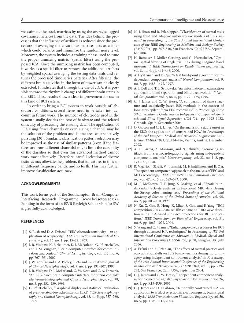
8 Computational Intelligence and Neuroscience
we estimate the stack matrices by using the averaged laggedcovariance matrices from the data. The idea behind the pro-cess is that the influence of artifacts is reduced since the pro-cedure of averaging the covariance matrices acts as a filterwhich could balance and minimize the random noise level.Moreover, the system includes a training phase used to tunethe proper unmixing matrix (spatial filter) using the pro-posed ICA. Once the unmixing matrix has been computed,it works as a spatial filter to remove the additional artifactsby weighted spatial averaging the testing data trials and re-turns the processed time series patterns. After filtering, thedifferent brain activities in the form of power can be clearlyextracted. It indicates that through the use of cICA, it is pos-sible to track the rhythmic changes of different brain states inthe EEG. These results show a clear improvement for use inthis kind of BCI system.
In order to bring a BCI system to work outside of lab-oratory conditions, several items need to be taken into ac-count in future work. The number of electrodes used in thesystem usually decides the cost of hardware and the relateddifficulty of processing the ensuing data. The application ofICA using fewer channels or even a single channel may bethe solution of the problem and is one area we are activelypursuing [30]. Similarly, classification pattern selection maybe improved as the use of similar patterns (even if the fea-tures are from different channels) might limit the capabilityof the classifier so that even this advanced method cannotwork most effectively. Therefore, careful selection of diversefeatures may alleviate the problem, that is, features in time orin different frequency bands, and so forth. This may furtherimprove classification accuracy.
ACKNOWLEDGMENTS
This work forms part of the Southampton Brain-ComputerInterfacing Research Programme (www.bci.soton.ac.uk).Funding in the form of an ISVR Rayleigh Scholarship for SWis greatfully acknowledged.
REFERENCES
[1] S. Rush and D. A. Driscoll, “EEG electrode sensitivity—an ap-plication of reciprocity,” IEEE Transactions on Biomedical En-gineering, vol. 16, no. 1, pp. 15–22, 1969.
[2] J. R. Wolpaw, N. Birbaumer, D. J. McFarland, G. Pfurtscheller,and T. M. Vaughan, “Brain-computer interfaces for communi-cation and control,” Clinical Neurophysiology, vol. 113, no. 6,pp. 767–791, 2002.
[3] J. W. Kozelka and T. A. Pedley, “Beta and mu rhythms,” Journalof Clinical Neurophysiology, vol. 7, no. 2, pp. 191–207, 1990.
[4] J. R. Wolpaw, D. J. McFarland, G. W. Neat, and C. A. Forneris,“An EEG-based brain-computer interface for cursor control,”Electroencephalography and Clinical Neurophysiology, vol. 78,no. 3, pp. 252–259, 1991.
[5] G. Pfurtscheller, “Graphical display and statistical evaluationof event-related desynchronization (ERD),” Electroencephalog-raphy and Clinical Neurophysiology, vol. 43, no. 5, pp. 757–760,1977.
[6] N.-J. Huan and R. Palaniappan, “Classification of mental tasksusing fixed and adaptive autoregressive models of EEG sig-nals,” in Proceedings of the 26th Annual International Confer-ence of the IEEE Engineering in Medicine and Biology Society(EMBC ’04), pp. 507–510, San Francisco, Calif, USA, Septem-ber 2004.
[7] H. Ramoser, J. Muller-Gerking, and G. Pfurtscheller, “Opti-mal spatial filtering of single trial EEG during imagined handmovement,” IEEE Transactions on Rehabilitation Engineering,vol. 8, no. 4, pp. 441–446, 2000.
[8] A. Hyvarinen and E. Oja, “A fast fixed-point algorithm for in-dependent component analysis,” Neural Computation, vol. 9,no. 7, pp. 1483–1492, 1997.
[9] A. J. Bell and T. J. Sejnowski, “An information-maximizationapproach to blind separation and blind deconvolution,” Neu-ral Computation, vol. 7, no. 6, pp. 1129–1159, 1995.
[10] C. J. James and C. W. Hesse, “A comparison of time struc-ture and statistically based BSS methods in the context oflong-term epileptiform EEG recordings,” in Proceedings of the5th International Conference on Independent Component Anal-ysis and Blind Signal Separation (ICA ’04), pp. 1025–1032,Granada, Spain, September 2004.
[11] O. Gibson and C. J. James, “On the analysis of seizure onset inthe EEG: the application of constrained ICA,” in Proceedingsof the 2nd European Medical and Biological Engineering Con-ference (EMBEC ’02), pp. 424–426, Vienna, Austria, December2002.
[12] A. K. Barros, A. Mansour, and N. Ohnishi, “Removing ar-tifacts from electrocardiographic signals using independentcomponents analysis,” Neurocomputing, vol. 22, no. 1–3, pp.173–186, 1998.
[13] R. Vigario, J. Sarela, V. Jousmaki, M. Hamalainen, and E. Oja,“Independent component approach to the analysis of EEG andMEG recordings,” IEEE Transactions on Biomedical Engineer-ing, vol. 47, no. 5, pp. 589–593, 2000.
[14] M. J. McKeown, T.-P. Jung, S. Makeig, et al., “Spatially in-dependent activity patterns in functional MRI data duringthe Stroop color-naming task,” Proceedings of the NationalAcademy of Sciences of the United States of America, vol. 95,no. 3, pp. 803–810, 1998.
[15] N. Xu, X. Gao, B. Hong, X. Miao, S. Gao, and F. Yang, “BCIcompetition 2003—data set IIb: enhancing P300 wave detec-tion using ICA-based subspace projections for BCI applica-tions,” IEEE Transactions on Biomedical Engineering, vol. 51,no. 6, pp. 1067–1072, 2004.
[16] S. Wang and C. J. James, “Enhancing evoked responses for BCIthrough advanced ICA techniques,” in Proceeding of IET 3rdInternational Conference on Advances in Medical, Signal andInformation Processing (MEDSIP ’06), p. 38, Glasgow, UK, July2006.
[17] A. Erfani and A. Erfanian, “The effects of mental practice andconcentration skills on EEG brain dynamics during motor im-agery using independent component analysis,” in Proceedingsof the 26th Annual International Conference of the Engineeringin Medicine and Biology Society (EMBC ’04), vol. 1, pp. 239–242, San Francisco, Calif, USA, September 2004.
[18] C. J. James and C. W. Hesse, “Independent component analy-sis for biomedical signals,” Physiological Measurement, vol. 26,no. 1, pp. R15–R39, 2005.
[19] C. J. James and O. J. Gibson, “Temporally constrained ICA: anapplication to artifact rejection in electromagnetic brain signalanalysis,” IEEE Transactions on Biomedical Engineering, vol. 50,no. 9, pp. 1108–1116, 2003.
S. Wang and C. J. James 9
[20] A. Ziehe and K.-R. Muller, “TDSEP—an efficient algorithmfor blind separation using time structure,” in Proceedings ofthe 8th International Conference on Artificial Neural Networks(ICANN ’98), pp. 675–680, Skovde, Sweden, September 1998.
[21] A. Belouchrani and M. G. Amin, “Blind source separationbased on time-frequency signal representations,” IEEE Trans-actions on Signal Processing, vol. 46, no. 11, pp. 2888–2897,1998.
[22] A. Ziehe, P. Laskov, K.-R. Mueller, and G. Nolte, “A linearleast-squares algorithm for joint diagonalization,” in Proceed-ings of the 4th International Symposium on Independent Com-ponent Analysis and Blind Signal Separation, pp. 469–474,Nara, Japan, April 2003.
[23] C. J. James and C. W. Hesse, “Mapping scalp topographiesof rhythmic EEG activity using temporal decorrelation basedconstrained ICA,” in Proceedings of the 26th Annual Interna-tional Conference of the IEEE Engineering in Medicine and Bi-ology Society (EMBC ’04), vol. 2, pp. 994–997, San Francisco,Calif, USA, September 2004.
[24] A. Cichocki, S. Amari, and K. Siwek, “ICALAB toolbox for sig-nal processing,” http://www.bsp.brain.riken.jp/ICALAB/.
[25] B. Blankertz, K.-R. Muller, G. Curio, et al., “The BCI competi-tion 2003: progress and perspectives in detection and discrim-ination of EEG single trials,” IEEE Transactions on BiomedicalEngineering, vol. 51, no. 6, pp. 1044–1051, 2004.
[26] G. Dornhege, B. Blankertz, G. Curio, and K.-R. Muller,“Boosting bit rates in noninvasive EEG single-trial classifica-tions by feature combination and multiclass paradigms,” IEEETransactions on Biomedical Engineering, vol. 51, no. 6, pp. 993–1002, 2004.
[27] C. J. James and C. W. Hesse, “Observing and tracking brain dy-namics in electromagnetic brain signals through blind sourceseparation,” in Proceedings of the IEE Medical Signal and In-formation Processing Conference (MEDSIP ’04), pp. 145–152,Malta, September 2004.
[28] S. R. Gunn and J. S. Kandola, “Structural modelling withsparse kernels,” Machine Learning, vol. 48, no. 1–3, pp. 137–163, 2002.
[29] L. Song and J. Epps, “Classifying EEG for brain-computerinterfaces: learning optimal filters for dynamical system fea-tures,” in Proceedings of the 23rd International Conference onMachine Learning (ICML ’06), pp. 857–864, Pittsburgh, Pa,USA, June 2006.
[30] C. J. James and S. Wang, “Blind source separation in single-channel EEG analysis: an application to BCI,” in Proceedingsof the 28th Annual International Conference of the IEEE Engi-neering in Medicine and Biology Society (EMBS ’06), pp. 6544–6547, New York, NY, USA, August-September 2006.
Hindawi Publishing CorporationComputational Intelligence and NeuroscienceVolume 2007, Article ID 79826, 9 pagesdoi:10.1155/2007/79826
Research ArticleThe Self-Paced Graz Brain-Computer Interface:Methods and Applications
Reinhold Scherer,1, 2 Alois Schloegl,3 Felix Lee,4 Horst Bischof,4 Janez Jansa,5 and Gert Pfurtscheller1, 2
1 Laboratory of Brain-Computer Interfaces, Institute for Knowledge Discovery, Graz University of Technology, Krenngasse 37,8010 Graz, Austria
2 NeuroCenter Styria, Krenngasse 37/I, 8010 Graz, Austria3 Intelligent Data Analysis Group, Fraunhofer-Institut fur Rechnerarchitektur und Softwaretechnik, FIRST, Kekulestrasse 7,12489 Berlin, Germany
4 Institute for Computer Graphics and Vision, Graz University of Technology, Inffeldgasse 16, 8010 Graz, Austria5 Aksioma - Institute for Contemporary Art, Neubergerjeva 25, 1000 Ljubljana, Slovenia
Correspondence should be addressed to Reinhold Scherer, [email protected]
Received 25 February 2007; Revised 13 June 2007; Accepted 19 July 2007
Recommended by Fabio Babiloni
We present the self-paced 3-class Graz brain-computer interface (BCI) which is based on the detection of sensorimotor electroen-cephalogram (EEG) rhythms induced by motor imagery. Self-paced operation means that the BCI is able to determine whether theongoing brain activity is intended as control signal (intentional control) or not (non-control state). The presented system is able toautomatically reduce electrooculogram (EOG) artifacts, to detect electromyographic (EMG) activity, and uses only three bipolarEEG channels. Two applications are presented: the freeSpace virtual environment (VE) and the Brainloop interface. The freeSpaceis a computer-game-like application where subjects have to navigate through the environment and collect coins by autonomouslyselecting navigation commands. Three subjects participated in these feedback experiments and each learned to navigate throughthe VE and collect coins. Two out of the three succeeded in collecting all three coins. The Brainloop interface provides an interfacebetween the Graz-BCI and Google Earth.
Copyright © 2007 Reinhold Scherer et al. This is an open access article distributed under the Creative Commons AttributionLicense, which permits unrestricted use, distribution, and reproduction in any medium, provided the original work is properlycited.
1. INTRODUCTION
A brain-computer interface (BCI) transforms electrophysi-ological or metabolic brain activity into control signals forapplications and devices (e.g., spelling system or neuropros-thesis). Instead of muscle activity, a specific type of mentalactivity is used to operate such a system. For a review on BCItechnologies see [1–4].
After years of basic research, modern BCIs have beenmoving out of the laboratory and are under evaluation inhospitals and at patients’ homes (e.g., [5–11]). However,BCIs have to meet several technical requirements before theyare practical alternatives to motor controlled communicationdevices. The most important requirements are high informa-tion transfer rates, ease-of-use, robustness, on-demand op-erability, and safety [12]. In summary, for the end-user, BCIsystems have to carry information as quickly and accuratelyas needed for individual applications, have to work in most
environments, and should be available without the assistanceof other people (self-initiation). To fulfill these issues, theGraz group focused on the development of small and robustsystems which are operated by using one or two bipolar elec-troencephalogram (EEG) channels only [13]. Motor imagery(MI), that is, the imagination of movements, is used as theexperimental strategy.
In this work, we aim at two important issues for practi-cal BCI systems. The first is detection of electromyographic(EMG) and reduction of electrooculographic (EOG) arti-facts and the second is the self-paced operation mode. Ar-tifacts are undesirable signals that can interfere and maychange the characteristics of the brain signal used to con-trol the BCI [14]. Especially in early training sessions, EMGartifacts are present in BCI training [15]. It is therefore cru-cial to ensure that (i) brain activity and not muscle activityis used as source of control and that (ii) artifacts are notproducing undesired BCI output. Self-paced BCIs are able
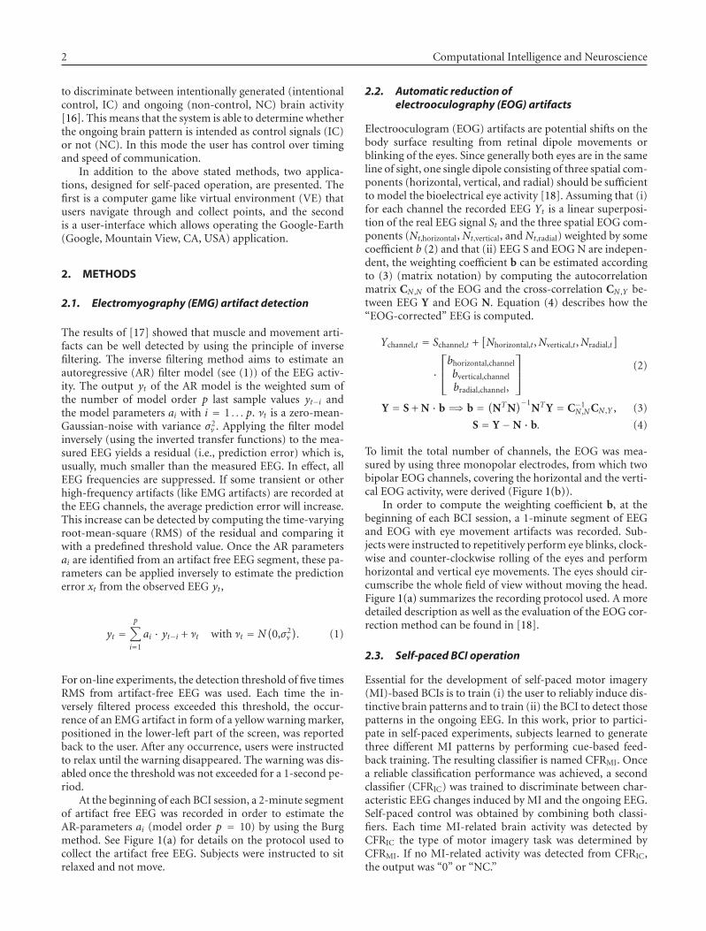
2 Computational Intelligence and Neuroscience
to discriminate between intentionally generated (intentionalcontrol, IC) and ongoing (non-control, NC) brain activity[16]. This means that the system is able to determine whetherthe ongoing brain pattern is intended as control signals (IC)or not (NC). In this mode the user has control over timingand speed of communication.
In addition to the above stated methods, two applica-tions, designed for self-paced operation, are presented. Thefirst is a computer game like virtual environment (VE) thatusers navigate through and collect points, and the secondis a user-interface which allows operating the Google-Earth(Google, Mountain View, CA, USA) application.
2. METHODS
2.1. Electromyography (EMG) artifact detection
The results of [17] showed that muscle and movement arti-facts can be well detected by using the principle of inversefiltering. The inverse filtering method aims to estimate anautoregressive (AR) filter model (see (1)) of the EEG activ-ity. The output yt of the AR model is the weighted sum ofthe number of model order p last sample values yt−i andthe model parameters ai with i = 1 . . . p. νt is a zero-mean-Gaussian-noise with variance σ2
ν . Applying the filter modelinversely (using the inverted transfer functions) to the mea-sured EEG yields a residual (i.e., prediction error) which is,usually, much smaller than the measured EEG. In effect, allEEG frequencies are suppressed. If some transient or otherhigh-frequency artifacts (like EMG artifacts) are recorded atthe EEG channels, the average prediction error will increase.This increase can be detected by computing the time-varyingroot-mean-square (RMS) of the residual and comparing itwith a predefined threshold value. Once the AR parametersai are identified from an artifact free EEG segment, these pa-rameters can be applied inversely to estimate the predictionerror xt from the observed EEG yt,
yt =p∑
i=1
ai · yt−i + νt with νt = N(0,σ2
ν
). (1)
For on-line experiments, the detection threshold of five timesRMS from artifact-free EEG was used. Each time the in-versely filtered process exceeded this threshold, the occur-rence of an EMG artifact in form of a yellow warning marker,positioned in the lower-left part of the screen, was reportedback to the user. After any occurrence, users were instructedto relax until the warning disappeared. The warning was dis-abled once the threshold was not exceeded for a 1-second pe-riod.
At the beginning of each BCI session, a 2-minute segmentof artifact free EEG was recorded in order to estimate theAR-parameters ai (model order p = 10) by using the Burgmethod. See Figure 1(a) for details on the protocol used tocollect the artifact free EEG. Subjects were instructed to sitrelaxed and not move.
2.2. Automatic reduction ofelectrooculography (EOG) artifacts
Electrooculogram (EOG) artifacts are potential shifts on thebody surface resulting from retinal dipole movements orblinking of the eyes. Since generally both eyes are in the sameline of sight, one single dipole consisting of three spatial com-ponents (horizontal, vertical, and radial) should be sufficientto model the bioelectrical eye activity [18]. Assuming that (i)for each channel the recorded EEG Yt is a linear superposi-tion of the real EEG signal St and the three spatial EOG com-ponents (Nt,horizontal, Nt,vertical, and Nt,radial) weighted by somecoefficient b (2) and that (ii) EEG S and EOG N are indepen-dent, the weighting coefficient b can be estimated accordingto (3) (matrix notation) by computing the autocorrelationmatrix CN ,N of the EOG and the cross-correlation CN ,Y be-tween EEG Y and EOG N. Equation (4) describes how the“EOG-corrected” EEG is computed.
Ychannel,t = Schannel,t +[Nhorizontal,t,Nvertical,t,Nradial,t
]
·
⎡⎢⎣bhorizontal,channel
bvertical,channel
bradial,channel,
⎤⎥⎦
(2)
Y = S + N · b =⇒ b = (NTN)−1
NTY = C−1N ,NCN ,Y , (3)
S = Y−N · b. (4)
To limit the total number of channels, the EOG was mea-sured by using three monopolar electrodes, from which twobipolar EOG channels, covering the horizontal and the verti-cal EOG activity, were derived (Figure 1(b)).
In order to compute the weighting coefficient b, at thebeginning of each BCI session, a 1-minute segment of EEGand EOG with eye movement artifacts was recorded. Sub-jects were instructed to repetitively perform eye blinks, clock-wise and counter-clockwise rolling of the eyes and performhorizontal and vertical eye movements. The eyes should cir-cumscribe the whole field of view without moving the head.Figure 1(a) summarizes the recording protocol used. A moredetailed description as well as the evaluation of the EOG cor-rection method can be found in [18].
2.3. Self-paced BCI operation
Essential for the development of self-paced motor imagery(MI)-based BCIs is to train (i) the user to reliably induce dis-tinctive brain patterns and to train (ii) the BCI to detect thosepatterns in the ongoing EEG. In this work, prior to partici-pate in self-paced experiments, subjects learned to generatethree different MI patterns by performing cue-based feed-back training. The resulting classifier is named CFRMI. Oncea reliable classification performance was achieved, a secondclassifier (CFRIC) was trained to discriminate between char-acteristic EEG changes induced by MI and the ongoing EEG.Self-paced control was obtained by combining both classi-fiers. Each time MI-related brain activity was detected byCFRIC the type of motor imagery task was determined byCFRMI. If no MI-related activity was detected from CFRIC,the output was “0” or “NC.”
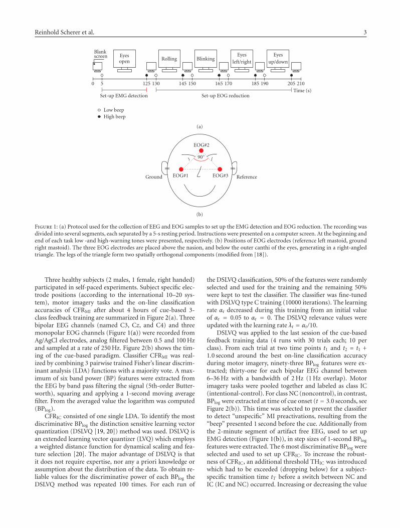
Reinhold Scherer et al. 3
Blankscreen Eyes
open Rolling BlinkingEyes
left/rightEyes
up/down
0 5 125 130 145 150 165 170 185 190 205 210Time (s)
Set-up EMG detection Set-up EOG reduction
Low beepHigh beep
(a)
EOG#2
EOG#1 EOG#3
90◦
Ground Reference
(b)
Figure 1: (a) Protocol used for the collection of EEG and EOG samples to set up the EMG detection and EOG reduction. The recording wasdivided into several segments, each separated by a 5-s resting period. Instructions were presented on a computer screen. At the beginning andend of each task low -and high-warning tones were presented, respectively. (b) Positions of EOG electrodes (reference left mastoid, groundright mastoid). The three EOG electrodes are placed above the nasion, and below the outer canthi of the eyes, generating in a right-angledtriangle. The legs of the triangle form two spatially orthogonal components (modified from [18]).
Three healthy subjects (2 males, 1 female, right handed)participated in self-paced experiments. Subject specific elec-trode positions (according to the international 10–20 sys-tem), motor imagery tasks and the on-line classificationaccuracies of CFRMI after about 4 hours of cue-based 3-class feedback training are summarized in Figure 2(a). Threebipolar EEG channels (named C3, Cz, and C4) and threemonopolar EOG channels (Figure 1(a)) were recorded fromAg/AgCl electrodes, analog filtered between 0.5 and 100 Hzand sampled at a rate of 250 Hz. Figure 2(b) shows the tim-ing of the cue-based paradigm. Classifier CFRMI was real-ized by combining 3 pairwise trained Fisher’s linear discrim-inant analysis (LDA) functions with a majority vote. A max-imum of six band power (BP) features were extracted fromthe EEG by band pass filtering the signal (5th-order Butter-worth), squaring and applying a 1-second moving averagefilter. From the averaged value the logarithm was computed(BPlog).
CFRIC consisted of one single LDA. To identify the mostdiscriminative BPlog the distinction sensitive learning vectorquantization (DSLVQ [19, 20]) method was used. DSLVQ isan extended learning vector quantizer (LVQ) which employsa weighted distance function for dynamical scaling and fea-ture selection [20]. The major advantage of DSLVQ is thatit does not require expertise, nor any a priori knowledge orassumption about the distribution of the data. To obtain re-liable values for the discriminative power of each BPlog theDSLVQ method was repeated 100 times. For each run of
the DSLVQ classification, 50% of the features were randomlyselected and used for the training and the remaining 50%were kept to test the classifier. The classifier was fine-tunedwith DSLVQ type C training (10000 iterations). The learningrate αt decreased during this training from an initial valueof αt = 0.05 to αt = 0. The DSLVQ relevance values wereupdated with the learning rate λt = αt/10.
DSLVQ was applied to the last session of the cue-basedfeedback training data (4 runs with 30 trials each; 10 perclass). From each trial at two time points t1 and t2 = t1 +1.0 second around the best on-line classification accuracyduring motor imagery, ninety-three BPlog features were ex-tracted; thirty-one for each bipolar EEG channel between6–36 Hz with a bandwidth of 2 Hz (1 Hz overlap). Motorimagery tasks were pooled together and labeled as class IC(intentional-control). For class NC (noncontrol), in contrast,BPlog were extracted at time of cue onset (t = 3.0 seconds, seeFigure 2(b)). This time was selected to prevent the classifierto detect “unspecific” MI preactivations, resulting from the“beep” presented 1 second before the cue. Additionally fromthe 2-minute segment of artifact free EEG, used to set upEMG detection (Figure 1(b)), in step sizes of 1-second BPlog
features were extracted. The 6 most discriminative BPlog wereselected and used to set up CFRIC. To increase the robust-ness of CFRIC, an additional threshold THIC was introducedwhich had to be exceeded (dropping below) for a subject-specific transition time tT before a switch between NC andIC (IC and NC) occurred. Increasing or decreasing the value
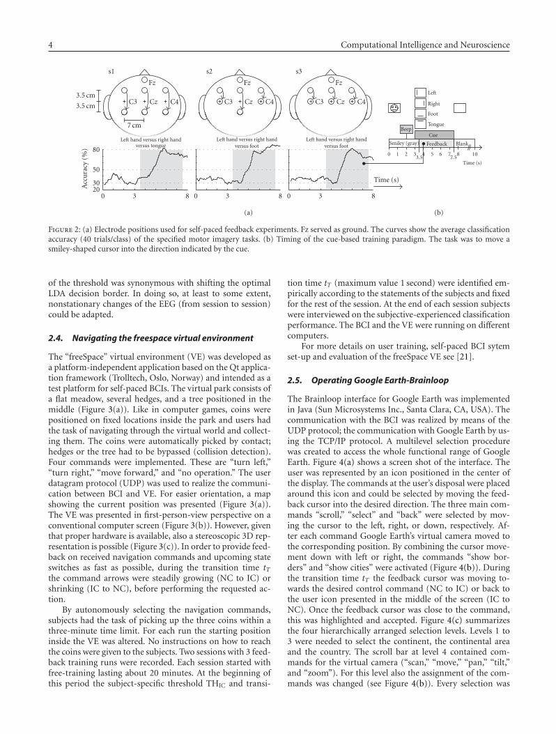
4 Computational Intelligence and Neuroscience
s1
3.5 cm
3.5 cm
7 cm
Fz
C3 Cz C4
s2
Fz
C3 Cz C4
s3
Fz
C3 Cz C4
Left hand versus right handversus foot
Left hand versus right handversus foot
Left hand versus right handversus tongue
Left
Right
Foot
TongueBeep
Cue
Smiley (gray) Feedback Blank
0 1 2 33.5
4 5 6 77.5
8 10
Time (s)
0 3 8 0 3 8 0 3 8
Time (s)2030
50
80
Acc
ura
cy(%
)
(a) (b)
Figure 2: (a) Electrode positions used for self-paced feedback experiments. Fz served as ground. The curves show the average classificationaccuracy (40 trials/class) of the specified motor imagery tasks. (b) Timing of the cue-based training paradigm. The task was to move asmiley-shaped cursor into the direction indicated by the cue.
of the threshold was synonymous with shifting the optimalLDA decision border. In doing so, at least to some extent,nonstationary changes of the EEG (from session to session)could be adapted.
2.4. Navigating the freespace virtual environment
The “freeSpace” virtual environment (VE) was developed asa platform-independent application based on the Qt applica-tion framework (Trolltech, Oslo, Norway) and intended as atest platform for self-paced BCIs. The virtual park consists ofa flat meadow, several hedges, and a tree positioned in themiddle (Figure 3(a)). Like in computer games, coins werepositioned on fixed locations inside the park and users hadthe task of navigating through the virtual world and collect-ing them. The coins were automatically picked by contact;hedges or the tree had to be bypassed (collision detection).Four commands were implemented. These are “turn left,”“turn right,” “move forward,” and “no operation.” The userdatagram protocol (UDP) was used to realize the communi-cation between BCI and VE. For easier orientation, a mapshowing the current position was presented (Figure 3(a)).The VE was presented in first-person-view perspective on aconventional computer screen (Figure 3(b)). However, giventhat proper hardware is available, also a stereoscopic 3D rep-resentation is possible (Figure 3(c)). In order to provide feed-back on received navigation commands and upcoming stateswitches as fast as possible, during the transition time tTthe command arrows were steadily growing (NC to IC) orshrinking (IC to NC), before performing the requested ac-tion.
By autonomously selecting the navigation commands,subjects had the task of picking up the three coins within athree-minute time limit. For each run the starting positioninside the VE was altered. No instructions on how to reachthe coins were given to the subjects. Two sessions with 3 feed-back training runs were recorded. Each session started withfree-training lasting about 20 minutes. At the beginning ofthis period the subject-specific threshold THIC and transi-
tion time tT (maximum value 1 second) were identified em-pirically according to the statements of the subjects and fixedfor the rest of the session. At the end of each session subjectswere interviewed on the subjective-experienced classificationperformance. The BCI and the VE were running on differentcomputers.
For more details on user training, self-paced BCI sytemset-up and evaluation of the freeSpace VE see [21].
2.5. Operating Google Earth-Brainloop
The Brainloop interface for Google Earth was implementedin Java (Sun Microsystems Inc., Santa Clara, CA, USA). Thecommunication with the BCI was realized by means of theUDP protocol; the communication with Google Earth by us-ing the TCP/IP protocol. A multilevel selection procedurewas created to access the whole functional range of GoogleEarth. Figure 4(a) shows a screen shot of the interface. Theuser was represented by an icon positioned in the center ofthe display. The commands at the user’s disposal were placedaround this icon and could be selected by moving the feed-back cursor into the desired direction. The three main com-mands “scroll,” “select” and “back” were selected by mov-ing the cursor to the left, right, or down, respectively. Af-ter each command Google Earth’s virtual camera moved tothe corresponding position. By combining the cursor move-ment down with left or right, the commands “show bor-ders” and “show cities” were activated (Figure 4(b)). Duringthe transition time tT the feedback cursor was moving to-wards the desired control command (NC to IC) or back tothe user icon presented in the middle of the screen (IC toNC). Once the feedback cursor was close to the command,this was highlighted and accepted. Figure 4(c) summarizesthe four hierarchically arranged selection levels. Levels 1 to3 were needed to select the continent, the continental areaand the country. The scroll bar at level 4 contained com-mands for the virtual camera (“scan,” “move,” “pan,” “tilt,”and “zoom”). For this level also the assignment of the com-mands was changed (see Figure 4(b)). Every selection was
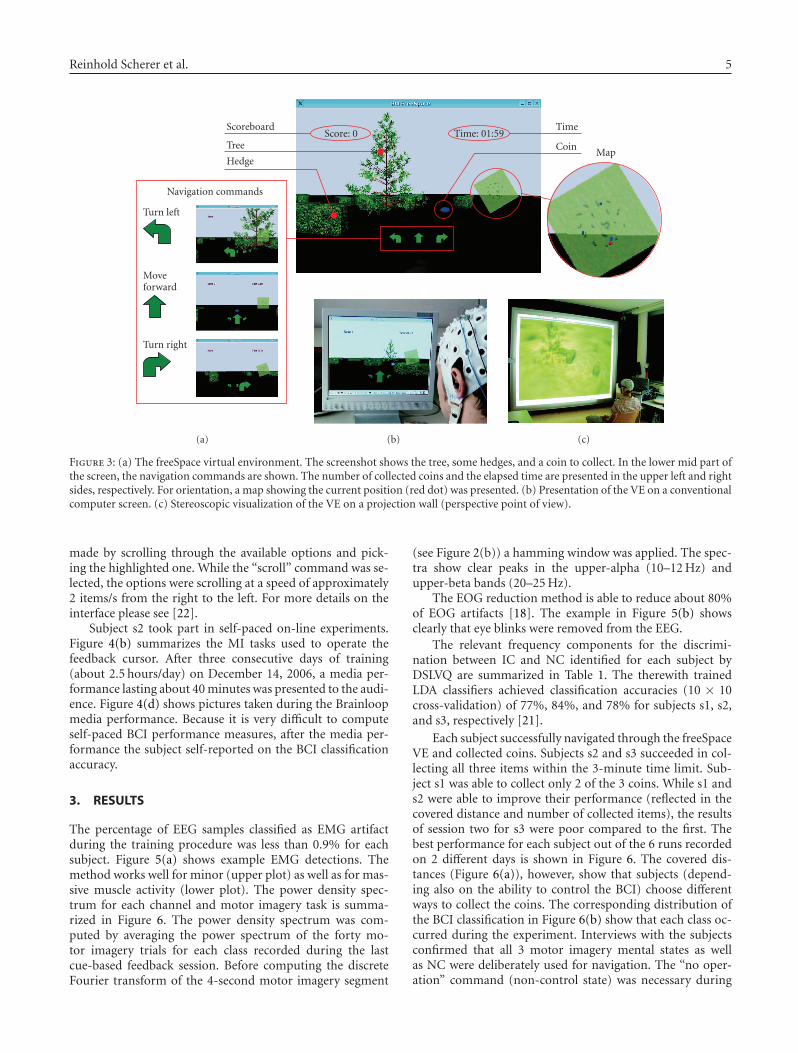
Reinhold Scherer et al. 5
Scoreboard
Tree
Hedge
Time
CoinMap
Score: 0 Time: 01:59
Navigation commands
Turn left
Moveforward
Turn right
(a) (b) (c)
Figure 3: (a) The freeSpace virtual environment. The screenshot shows the tree, some hedges, and a coin to collect. In the lower mid part ofthe screen, the navigation commands are shown. The number of collected coins and the elapsed time are presented in the upper left and rightsides, respectively. For orientation, a map showing the current position (red dot) was presented. (b) Presentation of the VE on a conventionalcomputer screen. (c) Stereoscopic visualization of the VE on a projection wall (perspective point of view).
made by scrolling through the available options and pick-ing the highlighted one. While the “scroll” command was se-lected, the options were scrolling at a speed of approximately2 items/s from the right to the left. For more details on theinterface please see [22].
Subject s2 took part in self-paced on-line experiments.Figure 4(b) summarizes the MI tasks used to operate thefeedback cursor. After three consecutive days of training(about 2.5 hours/day) on December 14, 2006, a media per-formance lasting about 40 minutes was presented to the audi-ence. Figure 4(d) shows pictures taken during the Brainloopmedia performance. Because it is very difficult to computeself-paced BCI performance measures, after the media per-formance the subject self-reported on the BCI classificationaccuracy.
3. RESULTS
The percentage of EEG samples classified as EMG artifactduring the training procedure was less than 0.9% for eachsubject. Figure 5(a) shows example EMG detections. Themethod works well for minor (upper plot) as well as for mas-sive muscle activity (lower plot). The power density spec-trum for each channel and motor imagery task is summa-rized in Figure 6. The power density spectrum was com-puted by averaging the power spectrum of the forty mo-tor imagery trials for each class recorded during the lastcue-based feedback session. Before computing the discreteFourier transform of the 4-second motor imagery segment
(see Figure 2(b)) a hamming window was applied. The spec-tra show clear peaks in the upper-alpha (10–12 Hz) andupper-beta bands (20–25 Hz).
The EOG reduction method is able to reduce about 80%of EOG artifacts [18]. The example in Figure 5(b) showsclearly that eye blinks were removed from the EEG.
The relevant frequency components for the discrimi-nation between IC and NC identified for each subject byDSLVQ are summarized in Table 1. The therewith trainedLDA classifiers achieved classification accuracies (10 × 10cross-validation) of 77%, 84%, and 78% for subjects s1, s2,and s3, respectively [21].
Each subject successfully navigated through the freeSpaceVE and collected coins. Subjects s2 and s3 succeeded in col-lecting all three items within the 3-minute time limit. Sub-ject s1 was able to collect only 2 of the 3 coins. While s1 ands2 were able to improve their performance (reflected in thecovered distance and number of collected items), the resultsof session two for s3 were poor compared to the first. Thebest performance for each subject out of the 6 runs recordedon 2 different days is shown in Figure 6. The covered dis-tances (Figure 6(a)), however, show that subjects (depend-ing also on the ability to control the BCI) choose differentways to collect the coins. The corresponding distribution ofthe BCI classification in Figure 6(b) show that each class oc-curred during the experiment. Interviews with the subjectsconfirmed that all 3 motor imagery mental states as wellas NC were deliberately used for navigation. The “no oper-ation” command (non-control state) was necessary during
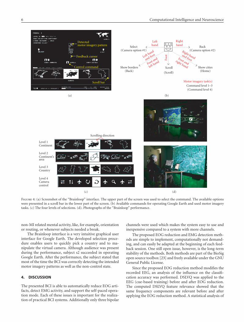
6 Computational Intelligence and Neuroscience
Detectedmotor imagery pattern
Feedback cursor
Control command
Scroll bar
(a)
Lefthand
Righthand
Select(Camera option #1)
Back(Camera option #2)
Left hand
and footRight handand footFo
ot
Foot and
left handFoot and
right handShow borders(Back)
Scroll
(Scroll)
Show cities(Home)
Motor imagery task(s)Command level 1–3(Command level 4)
(b)
Scrolling direction
Level 1Continent
Level 2Continent’sarea
Level 3Country
Level 4Cameracontrol
(c) (d)
Figure 4: (a) Screenshot of the “Brainloop” interface. The upper part of the screen was used to select the command. The available optionswere presented in a scroll bar in the lower part of the screen. (b) Available commands for operating Google Earth and used motor imagerytasks. (c) The four levels of selections. (d). Photographs of the “Brainloop” performance.
non-MI related mental activity, like, for example, orientationor routing, or whenever subjects needed a break.
The Brainloop interface is a very intuitive graphical userinterface for Google Earth. The developed selection proce-dure enables users to quickly pick a country and to ma-nipulate the virtual camera. Although audience was presentduring the performance, subject s2 succeeded in operatingGoogle Earth. After the performance, the subject stated thatmost of the time the BCI was correctly detecting the intendedmotor imagery patterns as well as the non-control state.
4. DISCUSSION
The presented BCI is able to automatically reduce EOG arti-facts, detect EMG activity, and support the self-paced opera-tion mode. Each of these issues is important for the realiza-tion of practical BCI systems. Additionally only three bipolar
channels were used which makes the system easy to use andinexpensive compared to a system with more channels.
The proposed EOG reduction and EMG detection meth-ods are simple to implement, computationally not demand-ing, and can easily be adapted at the beginning of each feed-back session. One still open issue, however, is the long-termstability of the methods. Both methods are part of the BioSigopen source toolbox [23] and freely available under the GNUGeneral Public License.
Since the proposed EOG reduction method modifies therecorded EEG, an analysis of the influence on the classifi-cation accuracy was performed. DSLVQ was applied to theEEG (cue-based training) before and after EOG reduction.The computed DSLVQ feature relevance showed that thesame frequency components are relevant before and afterapplying the EOG reduction method. A statistical analysis of
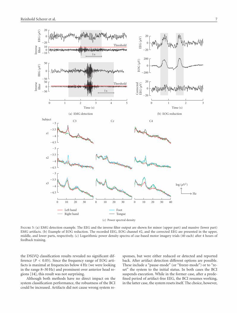
Reinhold Scherer et al. 7
543210
Time (s)
1 s
1 s
Threshold
Threshold
−50
0
50
Inve
rse
filt
er
−50
0
50
EE
G(μ
V)
−100
10
Inve
rse
filt
er−20
0
20
EE
G(μ
V)
(a) EMG detection
3210
Time (s)
−20
0
20
Cor
rect
edE
EG
(μV
)
−200
0
200
EO
G(μ
V)
−20
0
20
EE
G(μ
V)
(b) EOG reduction
40302010030201003020100
−4.5
−4
−3.5
−3
s3
−4.5
−4
−3.5
−3
s2
−4.5
−4
−3.5
−3
s1
Subject C3 Cz C4
log (μV2)
Hz
Left handRight hand
FootTongue
(c) Power spectral density
Figure 5: (a) EMG detection example. The EEG and the inverse filter output are shown for minor (upper part) and massive (lower part)EMG artifacts. (b) Example of EOG reduction. The recorded EEG, EOG channel #2, and the corrected EEG are presented in the upper,middle, and lower parts, respectively. (c) Logarithmic power density spectra of cue-based motor imagery trials (40 each) after 4 hours offeedback training.
the DSLVQ classification results revealed no significant dif-ference (P < 0.05). Since the frequency range of EOG arti-facts is maximal at frequencies below 4 Hz (we were lookingin the range 8–30 Hz) and prominent over anterior head re-gions [14], this result was not surprising.
Although both methods have no direct impact on thesystem classification performance, the robustness of the BCIcould be increased. Artifacts did not cause wrong system re-
sponses, but were either reduced or detected and reportedback. After artifact detection different options are possible.These include a “pause-mode” (or “freeze-mode”) or to “re-set” the system to the initial status. In both cases the BCIsuspends execution. While in the former case, after a prede-fined period of artifact-free EEG, the BCI resumes working,in the latter case, the system resets itself. The choice, however,
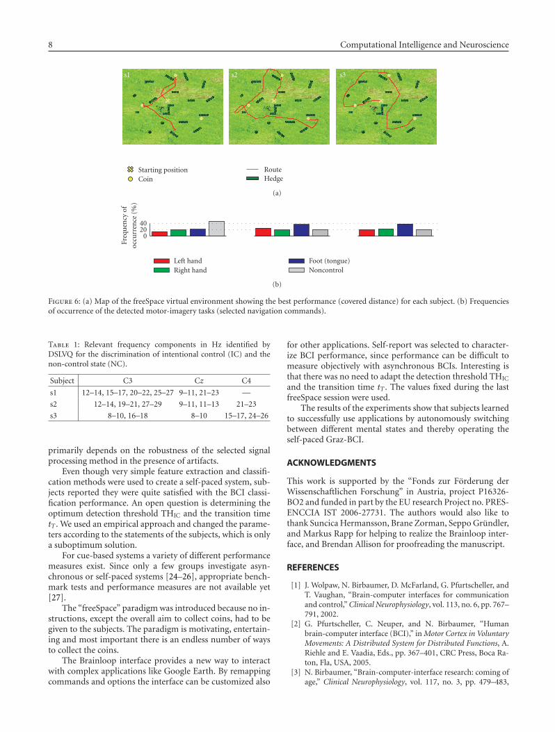
8 Computational Intelligence and Neuroscience
s1 s2 s3
Starting positionCoin
RouteHedge
(a)
02040
Freq
uen
cyof
occu
rren
ce(%
)
Left handRight hand
Foot (tongue)Noncontrol
(b)
Figure 6: (a) Map of the freeSpace virtual environment showing the best performance (covered distance) for each subject. (b) Frequenciesof occurrence of the detected motor-imagery tasks (selected navigation commands).
Table 1: Relevant frequency components in Hz identified byDSLVQ for the discrimination of intentional control (IC) and thenon-control state (NC).
Subject C3 Cz C4
s1 12–14, 15–17, 20–22, 25–27 9–11, 21–23 —
s2 12–14, 19–21, 27–29 9–11, 11–13 21–23
s3 8–10, 16–18 8–10 15–17, 24–26
primarily depends on the robustness of the selected signalprocessing method in the presence of artifacts.
Even though very simple feature extraction and classifi-cation methods were used to create a self-paced system, sub-jects reported they were quite satisfied with the BCI classi-fication performance. An open question is determining theoptimum detection threshold THIC and the transition timetT . We used an empirical approach and changed the parame-ters according to the statements of the subjects, which is onlya suboptimum solution.
For cue-based systems a variety of different performancemeasures exist. Since only a few groups investigate asyn-chronous or self-paced systems [24–26], appropriate bench-mark tests and performance measures are not available yet[27].
The “freeSpace” paradigm was introduced because no in-structions, except the overall aim to collect coins, had to begiven to the subjects. The paradigm is motivating, entertain-ing and most important there is an endless number of waysto collect the coins.
The Brainloop interface provides a new way to interactwith complex applications like Google Earth. By remappingcommands and options the interface can be customized also
for other applications. Self-report was selected to character-ize BCI performance, since performance can be difficult tomeasure objectively with asynchronous BCIs. Interesting isthat there was no need to adapt the detection threshold THIC
and the transition time tT . The values fixed during the lastfreeSpace session were used.
The results of the experiments show that subjects learnedto successfully use applications by autonomously switchingbetween different mental states and thereby operating theself-paced Graz-BCI.
ACKNOWLEDGMENTS
This work is supported by the “Fonds zur Forderung derWissenschaftlichen Forschung” in Austria, project P16326-BO2 and funded in part by the EU research Project no. PRES-ENCCIA IST 2006-27731. The authors would also like tothank Suncica Hermansson, Brane Zorman, Seppo Grundler,and Markus Rapp for helping to realize the Brainloop inter-face, and Brendan Allison for proofreading the manuscript.
REFERENCES
[1] J. Wolpaw, N. Birbaumer, D. McFarland, G. Pfurtscheller, andT. Vaughan, “Brain-computer interfaces for communicationand control,” Clinical Neurophysiology, vol. 113, no. 6, pp. 767–791, 2002.
[2] G. Pfurtscheller, C. Neuper, and N. Birbaumer, “Humanbrain-computer interface (BCI),” in Motor Cortex in VoluntaryMovements: A Distributed System for Distributed Functions, A.Riehle and E. Vaadia, Eds., pp. 367–401, CRC Press, Boca Ra-ton, Fla, USA, 2005.
[3] N. Birbaumer, “Brain-computer-interface research: coming ofage,” Clinical Neurophysiology, vol. 117, no. 3, pp. 479–483,
Reinhold Scherer et al. 9
2006.[4] B. Z. Allison, E. W. Wolpaw, and J. R. Wolpaw, “Brain-
computer interface systems: progress and prospects,” ExpertReview of Medical Devices, vol. 4, no. 4, pp. 463–474, 2007.
[5] E. W. Sellers and E. Donchin, “A P300-based brain-computerinterface: initial tests by ALS patients,” Clinical Neurophysiol-ogy, vol. 117, no. 3, pp. 538–548, 2006.
[6] F. Piccione, F. Giorgi, P. Tonin, et al., “P300-based braincomputer interface: reliability and performance in healthyand paralysed participants,” Clinical Neurophysiology, vol. 117,no. 3, pp. 531–537, 2006.
[7] N. Birbaumer, A. Kubler, N. Ghanayim, et al., “The thoughttranslation device (TTD) for completely paralyzed patients,”IEEE Transactions on Rehabilitation Engineering, vol. 8, no. 2,pp. 190–193, 2000.
[8] G. Pfurtscheller, G. R. Muller-Putz, J. Pfurtscheller, H. J.Gerner, and R. Rupp, “‘Thought’—control of functional elec-trical stimulation to restore hand grasp in a patient withtetraplegia,” Neuroscience Letters, vol. 351, no. 1, pp. 33–36,2003.
[9] G. R. Muller-Putz, R. Scherer, G. Pfurtscheller, and R. Rupp,“EEG-based neuroprosthesis control: a step towards clinicalpractice,” Neuroscience Letters, vol. 382, no. 1-2, pp. 169–174,2005.
[10] C. Neuper, G. R. Muller-Putz, A. Kubler, N. Birbaumer, andG. Pfurtscheller, “Clinical application of an EEG-based brain-computer interface: a case study in a patient with severe mo-tor impairment,” Clinical Neurophysiology, vol. 114, no. 3, pp.399–409, 2003.
[11] C. Neuper, G. R. Muller-Putz, R. Scherer, and G. Pfurtscheller,“Motor imagery and EEG-based control of spelling devicesand neuroprostheses,” Progress in Brain Research, vol. 159, pp.393–409, 2006.
[12] F. Cincotti, L. Bianchi, G. Birch, et al., “BCI Meeting 2005-Workshop on technology: hardware and software,” IEEETransactions on Neural Systems and Rehabilitation Engineering,vol. 14, no. 2, pp. 128–131, 2006.
[13] G. Pfurtscheller, G. R. Muller-Putz, A. Schlogl, et al., “15years of BCI research at Graz university of technology: currentprojects,” IEEE Transactions on Neural Systems and Rehabilita-tion Engineering, vol. 14, no. 2, pp. 205–210, 2006.
[14] M. Fatourechi, A. Bashashati, R. K. Ward, and G. E. Birch,“EMG and EOG artifacts in brain computer interface systems:a survey,” Clinical Neurophysiology, vol. 118, no. 3, pp. 480–494, 2007.
[15] D. J. McFarland, W. A. Sarnacki, T. M. Vaughan, and J. R. Wol-paw, “Brain-computer interface (BCI) operation: signal andnoise during early training sessions,” Clinical Neurophysiology,vol. 116, no. 1, pp. 56–62, 2005.
[16] S. G. Mason, A. Bashashati, M. Fatourechi, K. F. Navarro,and G. E. Birch, “A comprehensive survey of brain interfacetechnology designs,” Annals of Biomedical Engineering, vol. 35,no. 2, pp. 137–169, 2007.
[17] A. Schlogl, The Electroencephalogram and the Adaptive Autore-gressive Model: Theory and Applications, Shaker, Aachen, Ger-many, 2000.
[18] A. Schlogl, C. Keinrath, D. Zimmermann, R. Scherer, R. Leeb,and G. Pfurtscheller, “A fully automated correction methodof EOG artifacts in EEG recordings,” Clinical Neurophysiology,vol. 118, no. 1, pp. 98–104, 2007.
[19] M. Pregenzer and G. Pfurtscheller, “Frequency component se-lection for an EEG-based brain to computer interface,” IEEETransactions on Rehabilitation Engineering, vol. 7, no. 4, pp.413–419, 1999.
[20] M. Pregenzer, DSLVQ, Ph.D. thesis, Graz University of Tech-nology, Graz, Austria, 1998.
[21] R. Scherer, F. Lee, A. Schlogl, R. Leeb, H. Bischof, and G.Pfurtscheller, “Towards self-paced brain computer communi-cation: navigation through virtual worlds,” to appear in IEEETransactions on Biomedical Engineering.
[22] D. Grassi, “Brainloop media performance,” June 2007,http://www.aksioma.org/brainloop/index.html.
[23] A. Schlogl, “BioSig—an open source software package forbiomedical signal processing,” http://biosig.sourceforge.net/.
[24] R. Scherer, G. R. Muller-Putz, C. Neuper, B. Graimann, and G.Pfurtscheller, “An asynchronously controlled EEG-based vir-tual keyboard: improvement of the spelling rate,” IEEE Trans-actions on Biomedical Engineering, vol. 51, no. 6, pp. 979–984,2004.
[25] J. D. R. Millan and J. Mourino, “Asynchronous BCI and localneural classifiers: an overview of the adaptive brain interfaceproject,” IEEE Transactions on Neural Systems and Rehabilita-tion Engineering, vol. 11, no. 2, pp. 159–161, 2003.
[26] J. Borisoff, S. Mason, A. Bashashati, and G. Birch, “Brain-computer interface design for asynchronous control appli-cations: improvements to the LF-ASD asynchronous brainswitch,” IEEE Transactions on Biomedical Engineering, vol. 51,no. 6, pp. 985–992, 2004.
[27] S. Mason, J. Kronegg, J. Huggins, M. Fatourechi, and A.Schlogl, “Evaluating the performance of self-paced brain com-puter interface technology,” Tech. Rep., Neil Squire Soci-ety, Vancouver, Canada, 2006. http://www.bci-info.tugraz.at/Research Info/documents/articles/.
Hindawi Publishing CorporationComputational Intelligence and NeuroscienceVolume 2007, Article ID 37695, 14 pagesdoi:10.1155/2007/37695
Research ArticleTemporal and Spatial Features of Single-Trial EEG forBrain-Computer Interface
Qibin Zhao and Liqing Zhang
Department of Computer Science and Engineering, Shanghai Jiao Tong University, Shanghai 200240, China
Correspondence should be addressed to Qibin Zhao, [email protected]
Received 31 December 2006; Revised 23 February 2007; Accepted 18 June 2007
Recommended by Fabio Babiloni
Brain-computer interface (BCI) systems create a novel communication channel from the brain to an output device bypassingconventional motor output pathways of nerves and muscles. Modern BCI technology is essentially based on techniques for theclassification of single-trial brain signals. With respect to the topographic patterns of brain rhythm modulations, the commonspatial patterns (CSPs) algorithm has been proven to be very useful to produce subject-specific and discriminative spatial filters;but it didn’t consider temporal structures of event-related potentials which may be very important for single-trial EEG classifica-tion. In this paper, we propose a new framework of feature extraction for classification of hand movement imagery EEG. Computersimulations on real experimental data indicate that independent residual analysis (IRA) method can provide efficient temporal fea-tures. Combining IRA features with the CSP method, we obtain the optimal spatial and temporal features with which we achievethe best classification rate. The high classification rate indicates that the proposed method is promising for an EEG-based brain-computer interface.
Copyright © 2007 Q. Zhao and L. Zhang. This is an open access article distributed under the Creative Commons AttributionLicense, which permits unrestricted use, distribution, and reproduction in any medium, provided the original work is properlycited.
1. INTRODUCTION
Brain-computer interfaces (BCIs) provide new communica-tion and control channels that do not depend on the brain’snormal output channels of peripheral nerves and muscles[1]. The BCI research aims at the development of a sys-tem that allows direct control of a computer application ora neuroprosthesis, solely by human intentions reflected bycertain brain signals [2]. We mainly focus on noninvasive,electroencephalogram- (EEG-) based BCI systems which canbe used as tools of communication for the disabled or forhealthy subjects who might be interested in exploring a newpath of human-machine interfacing.
EEG-based BCI has received increasing attention recently[3–5]. The EEG allows the observation of gross electricalfields of the brain and reflects changes in neural mass ac-tivity associated with various mental processes. A physicallydisabled person with controlling his thoughts has potentialto use the mental processes for communication. The feasi-bility of this communication depends on the extent to whichthe EEGs associated with these mental processes can be reli-
ably recognized automatically. The electrophysiological phe-nomena investigated most in the quest for an automatic dis-crimination of mental states are event-related potential (EP)[3], and localized changes in spectral power of spontaneousEEG related to sensorimotor processes [4, 5]. For noninva-sive BCI systems that based on discrimination of voluntarilyinduced brain states, some approaches have been proposed.The Tubingen thought translation device (TTD) [6] enablessubjects to learn self-regulation of slow cortical potentials(SCP), that is, electro cortical positivity and negativity. Af-ter training in experiments with vertical cursor movement asfeedback navigated by the SCP from central scalp position,patients are able to generate binary decisions in a 4–6 secondspace with an accuracy of up to 85%. Users of the Albany BCIsystem [7] are able to control a cursor movement by their os-cillatory brain activity into one of two or four possible targetson the computer screen and achieve over 90% hit rates afteradapting to the system during many feedback sessions with aselection rate of 4-5 seconds in the binary decision problem.Based on event-related modulations of the pericentral μ- orβ-rhythms of sensorimotor cortices (with a focus on motor
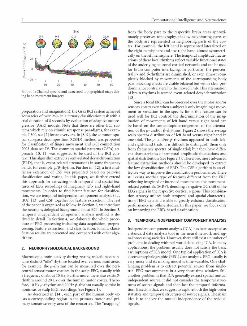
2 Computational Intelligence and Neuroscience
−20
0
20
Pow
er10×
log 10
(μV
2/H
z)
10 20 30 40 50 60
5.9 9.8 12.2 22 26.9
(Hz)
+
−
Figure 1: Channel spectra and associated topographical maps dur-ing hand movement imagery.
preparation and imagination), the Graz BCI system achievedaccuracies of over 96% in a ternary classification task with atrial duration of 8 seconds by evaluation of adaptive autore-gressive (AAR) models. Note that there are other BCI sys-tems which rely on stimulus/response paradigms, for exam-ple, P300, see [2] for an overview. In [8, 9], the common spa-tial subspace decomposition (CSSD) method was proposedfor classification of finger movement and BCI competition2003-data set IV. The common spatial patterns (CSPs) ap-proach [10, 11] was suggested to be used in the BCI con-text. This algorithm extracts event-related desynchronization(ERD), that is, event-related attenuations in some frequencybands, for example, μ/β-rhythm. Further in [12], a first mul-ticlass extension of CSP was presented based on pairwiseclassification and voting. In this paper, we further extendthis approach for extracting both temporal and spatial fea-tures of EEG recordings of imaginary left- and right-handmovements. In order to find better features for classifica-tion, we use temporal independent component analysis (i.e.,IRA) [13] and CSP together for feature extraction. The restof the paper is organized as follow. In Section 2, we introducethe neurophysiological background about BCI. In Section 3,temporal independent component analysis method is de-rived in detail. In Section 4, we elaborate the whole proce-dure of EEG processing including data acquisition, prepro-cessing, feature extraction, and classification. Finally, classi-fication results are presented and compared with other algo-rithms.
2. NEUROPHYSIOLOGICAL BACKGROUND
Macroscopic brain activity during resting wakefulness con-tains distinct “idle” rhythms located over various brain areas,for example, the μ-rhythm can be measured over the peri-central sensorimotor cortices in the scalp EEG, usually witha frequency of about 10 Hz. Furthermore, there also exists β-rhythm around 20 Hz over the human motor cortex. There-fore, 10 Hz μ-rhythm and 20 Hz β-rhythm usually coexist innoninvasive scalp EEG recordings (see Figure 1).
As described in [14], each part of the human body ex-ists a corresponding region in the primary motor and pri-mary somatosensory area of the neocortex. The “mapping”
from the body part to the respective brain areas approxi-mately preserves topography, that is, neighboring parts ofthe body are represented in neighboring parts of the cor-tex. For example, the left hand is represented lateralized onthe right hemisphere and the right hand almost symmetri-cally on the left hemisphere. The temporal amplitude fluctu-ations of these local rhythms reflect variable functional statesof the underlying neuronal cortical networks and can be usedfor brain-computer interfacing. In particular, the pericen-tral μ- and β-rhythms are diminished, or even almost com-pletely blocked by movements of the corresponding bodypart. Blocking effects are visible bilateral but with a clear pre-dominance contralateral to the moved limb. This attenuationof brain rhythms is termed event-related desynchronization[15].
Since a focal ERD can be observed over the motor and/orsensory cortex even when a subject is only imagining a move-ment or sensation in the specific limb, this feature can beused well for BCI control: the discrimination of the imag-ination of movements of left hand versus right hand canbe based on the somatotopic arrangement of the attenua-tion of the μ- and/or β-rhythms. Figure 2 shows the averagescalp spectra distribution of left hand versus right hand inone trial. The μ- and/or β-rhythms appeared in both left-and right-hand trials, it is difficult to distinguish them onlyfrom frequency spectra of single trial; but they have differ-ent characteristics of temporal amplitude fluctuations andspatial distribution (see Figure 3). Therefore, more advancedfeature extraction methods should be developed to extractthe low diversification of ERD. The CSP algorithm is an ef-fective way to improve the classification performance. Therestill exists another type of features different from the ERDreflecting imagined or intended movements, the movement-related potentials (MRP), denoting a negative DC shift of theEEG signals in the respective cortical regions. This combina-tion strategy utilizes both temporal and spatial characteris-tics of EEG data and is able to greatly enhance classificationperformance in offline studies. In this paper, we focus onlyon improving the ERD-based classification.
3. TEMPORAL INDEPENDENT COMPONENT ANALYSIS
Independent component analysis (ICA) has been accepted asa standard data analysis tool in the neural network and sig-nal processing societies. However, there still exist a number ofproblems in dealing with real world data using ICA. In manyapplications, the problem usually does not satisfy the basicassumptions of ICA model. One typical application of ICA iselectroencephalographic (EEG) data analysis. EEG usually isvery noisy and its mixing model is time-variable. One chal-lenging problem is to extract potential source from single-trial EEG measurements in a very short time window. Stillanother problem is that ICA generally extract spatial mutualindependent source, it did not consider the temporal struc-tures of source signals and then lost the temporal informa-tion. Based on that, we suggest to explore both the high-orderstatistics and temporal structures of source signals. The mainidea is to analyze the mutual independence of the residualsignals.
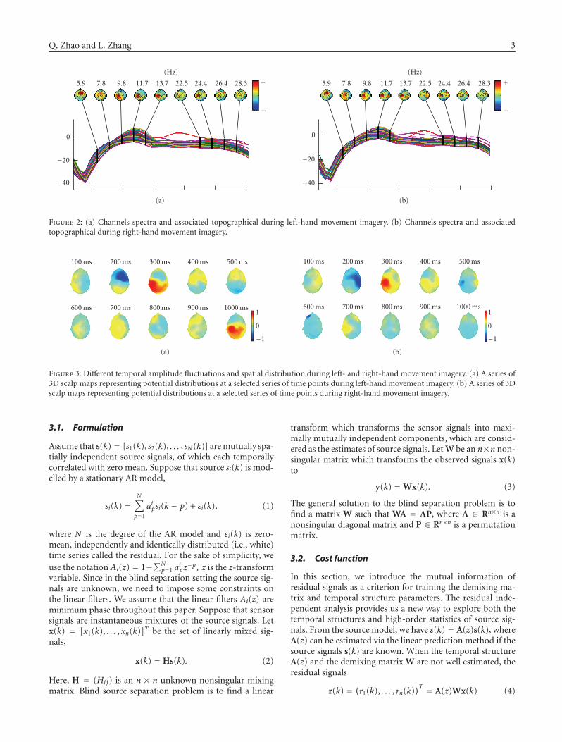
Q. Zhao and L. Zhang 3
−40
−20
0
5.9 7.8 9.8 11.7 13.7 22.5 24.4 26.4 28.3
(Hz)
+
−
(a)
−40
−20
0
5.9 7.8 9.8 11.7 13.7 22.5 24.4 26.4 28.3
(Hz)
+
−
(b)
Figure 2: (a) Channels spectra and associated topographical during left-hand movement imagery. (b) Channels spectra and associatedtopographical during right-hand movement imagery.
−1
0
1
100 ms 200 ms 300 ms 400 ms 500 ms
600 ms 700 ms 800 ms 900 ms 1000 ms
(a)
−1
0
1
100 ms 200 ms 300 ms 400 ms 500 ms
600 ms 700 ms 800 ms 900 ms 1000 ms
(b)
Figure 3: Different temporal amplitude fluctuations and spatial distribution during left- and right-hand movement imagery. (a) A series of3D scalp maps representing potential distributions at a selected series of time points during left-hand movement imagery. (b) A series of 3Dscalp maps representing potential distributions at a selected series of time points during right-hand movement imagery.
3.1. Formulation
Assume that s(k) = [s1(k), s2(k), . . . , sN (k)] are mutually spa-tially independent source signals, of which each temporallycorrelated with zero mean. Suppose that source si(k) is mod-elled by a stationary AR model,
si(k) =N∑
p=1
aipsi(k − p) + εi(k), (1)
where N is the degree of the AR model and εi(k) is zero-mean, independently and identically distributed (i.e., white)time series called the residual. For the sake of simplicity, weuse the notation Ai(z) = 1−∑N
p=1 aipz−p, z is the z-transform
variable. Since in the blind separation setting the source sig-nals are unknown, we need to impose some constraints onthe linear filters. We assume that the linear filters Ai(z) areminimum phase throughout this paper. Suppose that sensorsignals are instantaneous mixtures of the source signals. Letx(k) = [x1(k), . . . , xn(k)]T be the set of linearly mixed sig-nals,
x(k) = Hs(k). (2)
Here, H = (Hij) is an n × n unknown nonsingular mixingmatrix. Blind source separation problem is to find a linear
transform which transforms the sensor signals into maxi-mally mutually independent components, which are consid-ered as the estimates of source signals. Let W be an n×n non-singular matrix which transforms the observed signals x(k)to
y(k) = Wx(k). (3)
The general solution to the blind separation problem is tofind a matrix W such that WA = ΛP, where Λ ∈ Rn×n is anonsingular diagonal matrix and P ∈ Rn×n is a permutationmatrix.
3.2. Cost function
In this section, we introduce the mutual information ofresidual signals as a criterion for training the demixing ma-trix and temporal structure parameters. The residual inde-pendent analysis provides us a new way to explore both thetemporal structures and high-order statistics of source sig-nals. From the source model, we have ε(k) = A(z)s(k), whereA(z) can be estimated via the linear prediction method if thesource signals s(k) are known. When the temporal structureA(z) and the demixing matrix W are not well estimated, theresidual signals
r(k) = (r1(k), . . . , rn(k))T = A(z)Wx(k) (4)

4 Computational Intelligence and Neuroscience
are not mutually independent. Therefore, it provides us anew criterion for training the demixing model and tempo-ral structures to make the residuals r(k) spatially mutuallyindependent and temporally identically independently dis-tributed.
Assume q(r) is the probability density function of r andqi(ri) is the marginal probability density function of ri, i =1, . . . ,n. Now we introduce the mutual information rate I(r)between a set of stochastic processes r1, . . . , rn as
I(r) = −H(r) +n∑
i=1
H(ri), (5)
where H(ri) and H(r) are the entropies of random vari-ables ri and r, respectively. For blind deconvolution problem,Amari et al. [16] and Pham [17] simplify the first term of costfunction (5) and derive a cost function as follows:
l(
W, A(z)) = − 1
2π j
∮
rlog∣∣det
(A(z)W
)∣∣z−1dz
− 1L
L∑
k=1
n∑
i=1
log qi(ri(k)
),
(6)
where j is the imaginary unit of complex numbers, and thepath integral is over the unit circle γ of the complex plane.The first term of right side of (6) is introduced to prevent thefilter W from being singular. To simplify the cost function,we calculate the first term of the right side of (6) as follows:
log∣∣det
(A(z)W
)∣∣ = log∣∣det(W)
∣∣ + log∣∣det
(A(z)
)∣∣.(7)
Because the temporal filters A(z) is causal and minimumphase, we can easily verify
12π j
∮
γlog∣∣det
(A(z)
)∣∣z−1dz = 0. (8)
Now combining equations (7), (8) with (6), we obtain a sim-plified cost function for independent residual analysis
l(
W, A(z)) = − log
(∣∣det(W)∣∣)− 1
L
L∑
k=1
n∑
i=1
log qi(ri(k)
).
(9)
Independent residual analysis can be formulated into thesemiparametric model [18]. The probability density functionq and the temporal filter A(z) are seen as the nuisance pa-rameters in the semiparametric model. The demixing matrixW is called as the parameters of interest. The semiparametricapproach suggests using an estimating function to estimatethe parameter of interest, regardless of the nuisance parame-ters. We suggest to estimate the nuisance parameters in orderto have better separating performance of the algorithm.
3.3. Conjugate gradient algorithm
In this section, we derive a learning algorithm based on theconjugate gradient descent approach for the demixing ma-trix. We assume that the probability density functions and
the temporal filters are known for a moment during thederivation of a learning algorithm for the demixing matrix.To describe the conjugate gradient method for minimizingcost function, we need first to calculate the natural gradient
∇l(W, A(z)) =
(− I +
1L
L∑
k=1
N∑
p=0
Ap[ϕ(
r(k))
yT(k − p)])
W,
(10)
where ϕ(r) = (ϕ1(r1), . . . ,ϕn(rn))T is the vector of activationfunctions, defined by ϕi(ri) = −q′i (ri)/qi(ri).
Given an initial value W0 and k = 1, the conjugate gradi-ent algorithm starts out by searching in the steepest descentdirection (negative of the gradient) on the first iteration.
H0 = −∇l(
W0, A(z)). (11)
Now we perform one-dimensional search algorithm to findthe minimum point of the cost function l(W, A(z))
Wk = exp(t∗Hk−1W−1
k−1
)Wk−1, t∗ = arg min
tl(
Wk−1(t)),
(12)
along the geodesic: Wk−1(t) = exp(t∗Hk−1W−1k−1)Wk−1. The
new search direction Hk is defined by the following equation:
Hk = −∇l(
Wk)
+ γkτHk−1, (13)
where τHk−1 is the parallel translation from Wk−1 to Wk, thatis,
τHk−1 = Hk−1W−1k−1Wk. (14)
The value γk in (13) is evaluated by
τk =⟨
Gk − τGk−1, τGk⟩
⟨τGk−1, τGk−1
⟩ . (15)
For the geometrical structures, such as the geodesic andRiemannian metric of nonsingular matrices, refer to [19].The conjugate gradient algorithm search the minimum pointalong the geodesic which produces generally faster conver-gence than steepest descent directions. Both theoretical anal-ysis and computer stimulations show that the conjugate gra-dient algorithm has much better learning performance thanthe natural gradient does. Here we briefly introduce learn-ing algorithms for adapting the nuisance parameters in thesemiparametric ICA model. By using the gradient descentapproach, we obtain the learning algorithm for the filter co-efficients aik
Δaip(k) = −η′k1L
L∑
k=1
ϕi{ri(k)
}yi(k − p), (16)
where η′k is the learning rate. For the detailed informationabout activation function adaptation, refer to [20].
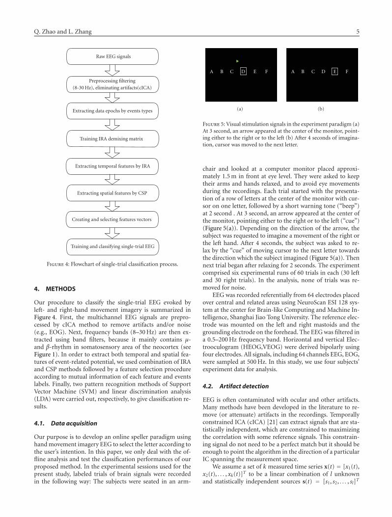
Q. Zhao and L. Zhang 5
Raw EEG signals
Preprocessing filtering(8-30 Hz), eliminating artifacts(cICA)
Extracting data epochs by events types
Training IRA demixing matrix
Extracting temporal features by IRA
Extracting spatial features by CSP
Creating and selecting features vectors
Training and classifying single-trial EEG
Figure 4: Flowchart of single-trial classification process.
4. METHODS
Our procedure to classify the single-trial EEG evoked byleft- and right-hand movement imagery is summarized inFigure 4. First, the multichannel EEG signals are prepro-cessed by cICA method to remove artifacts and/or noise(e.g., EOG). Next, frequency bands (8–30 Hz) are then ex-tracted using band filters, because it mainly contains μ-and β-rhythm in somatosensory area of the neocortex (seeFigure 1). In order to extract both temporal and spatial fea-tures of event-related potential, we used combination of IRAand CSP methods followed by a feature selection procedureaccording to mutual information of each feature and eventslabels. Finally, two pattern recognition methods of SupportVector Machine (SVM) and linear discrimination analysis(LDA) were carried out, respectively, to give classification re-sults.
4.1. Data acquisition
Our purpose is to develop an online speller paradigm usinghand movement imagery EEG to select the letter according tothe user’s intention. In this paper, we only deal with the of-fline analysis and test the classification performances of ourproposed method. In the experimental sessions used for thepresent study, labeled trials of brain signals were recordedin the following way: The subjects were seated in an arm-
A B C D E F
(a)
A B C D E F
(b)
Figure 5: Visual stimulation signals in the experiment paradigm (a)At 3 second, an arrow appeared at the center of the monitor, point-ing either to the right or to the left (b) After 4 seconds of imagina-tion, cursor was moved to the next letter.
chair and looked at a computer monitor placed approxi-mately 1.5 m in front at eye level. They were asked to keeptheir arms and hands relaxed, and to avoid eye movementsduring the recordings. Each trial started with the presenta-tion of a row of letters at the center of the monitor with cur-sor on one letter, followed by a short warning tone (“beep”)at 2 second . At 3 second, an arrow appeared at the center ofthe monitor, pointing either to the right or to the left (“cue”)(Figure 5(a)). Depending on the direction of the arrow, thesubject was requested to imagine a movement of the right orthe left hand. After 4 seconds, the subject was asked to re-lax by the “cue” of moving cursor to the next letter towardsthe direction which the subject imagined (Figure 5(a)). Thennext trial began after relaxing for 2 seconds. The experimentcomprised six experimental runs of 60 trials in each (30 leftand 30 right trials). In the analysis, none of trials was re-moved for noise.
EEG was recorded referentially from 64 electrodes placedover central and related areas using NeuroScan ESI 128 sys-tem at the center for Brain-like Computing and Machine In-telligence, Shanghai Jiao Tong University. The reference elec-trode was mounted on the left and right mastoids and thegrounding electrode on the forehead. The EEG was filtered ina 0.5–200 Hz frequency band. Horizontal and vertical Elec-trooculogram (HEOG,VEOG) were derived bipolarly usingfour electrodes. All signals, including 64 channels EEG, EOG,were sampled at 500 Hz. In this study, we use four subjects’experiment data for analysis.
4.2. Artifact detection
EEG is often contaminated with ocular and other artifacts.Many methods have been developed in the literature to re-move (or attenuate) artifacts in the recordings. Temporallyconstrained ICA (cICA) [21] can extract signals that are sta-tistically independent, which are constrained to maximizingthe correlation with some reference signals. This constrain-ing signal do not need to be a perfect match but it should beenough to point the algorithm in the direction of a particularIC spanning the measurement space.
We assume a set of k measured time series x(t) = [x1(t),x2(t), . . . , xk(t)]T to be a linear combination of l unknownand statistically independent sources s(t) = [s1, s2, . . . , sl]T
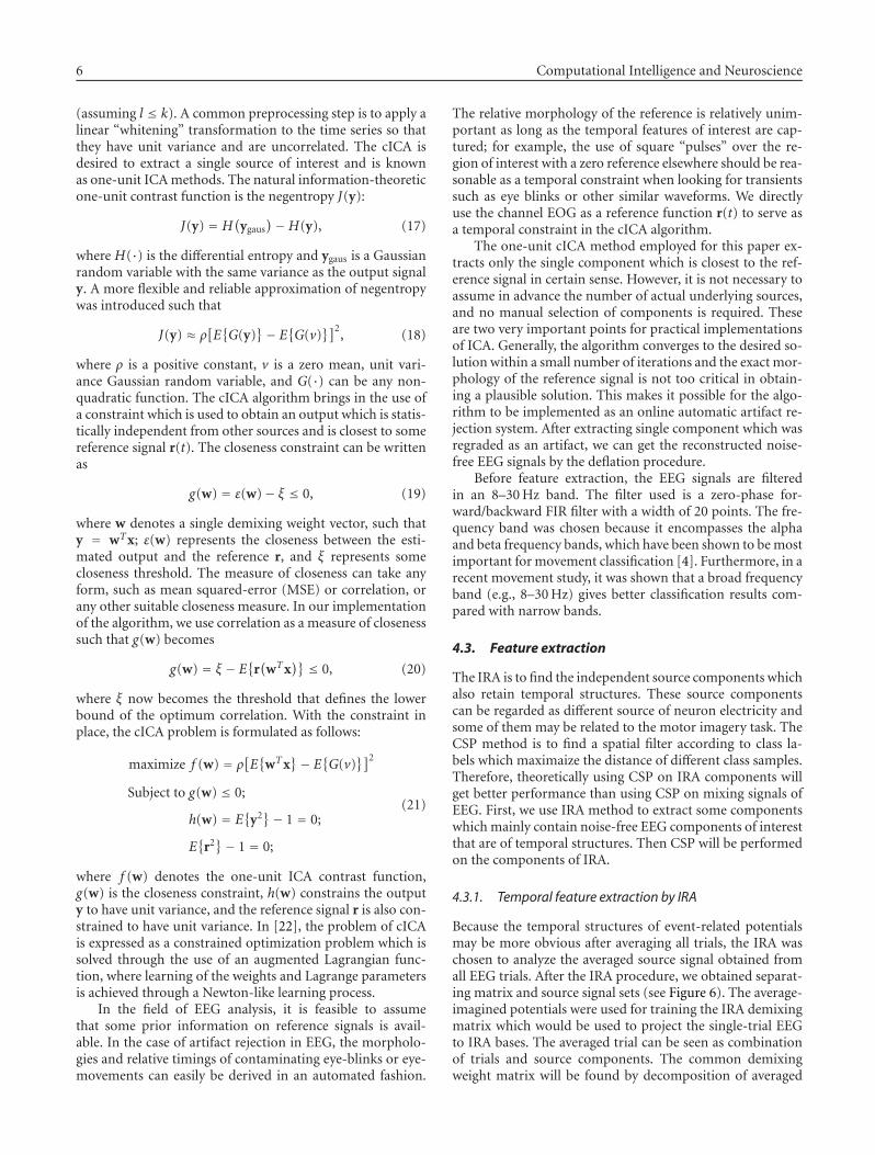
6 Computational Intelligence and Neuroscience
(assuming l ≤ k). A common preprocessing step is to apply alinear “whitening” transformation to the time series so thatthey have unit variance and are uncorrelated. The cICA isdesired to extract a single source of interest and is knownas one-unit ICA methods. The natural information-theoreticone-unit contrast function is the negentropy J(y):
J(y) = H(
ygaus)−H(y), (17)
where H(·) is the differential entropy and ygaus is a Gaussianrandom variable with the same variance as the output signaly. A more flexible and reliable approximation of negentropywas introduced such that
J(y) ≈ ρ[E{G(y)
}− E{G(v)
}]2, (18)
where ρ is a positive constant, v is a zero mean, unit vari-ance Gaussian random variable, and G(·) can be any non-quadratic function. The cICA algorithm brings in the use ofa constraint which is used to obtain an output which is statis-tically independent from other sources and is closest to somereference signal r(t). The closeness constraint can be writtenas
g(w) = ε(w)− ξ ≤ 0, (19)
where w denotes a single demixing weight vector, such thaty = wTx; ε(w) represents the closeness between the esti-mated output and the reference r, and ξ represents somecloseness threshold. The measure of closeness can take anyform, such as mean squared-error (MSE) or correlation, orany other suitable closeness measure. In our implementationof the algorithm, we use correlation as a measure of closenesssuch that g(w) becomes
g(w) = ξ − E{
r(
wTx)} ≤ 0, (20)
where ξ now becomes the threshold that defines the lowerbound of the optimum correlation. With the constraint inplace, the cICA problem is formulated as follows:
maximize f (w) = ρ[E{
wTx}− E
{G(v)
}]2
Subject to g(w) ≤ 0;
h(w) = E{
y2}− 1 = 0;
E{
r2}− 1 = 0;
(21)
where f (w) denotes the one-unit ICA contrast function,g(w) is the closeness constraint, h(w) constrains the outputy to have unit variance, and the reference signal r is also con-strained to have unit variance. In [22], the problem of cICAis expressed as a constrained optimization problem which issolved through the use of an augmented Lagrangian func-tion, where learning of the weights and Lagrange parametersis achieved through a Newton-like learning process.
In the field of EEG analysis, it is feasible to assumethat some prior information on reference signals is avail-able. In the case of artifact rejection in EEG, the morpholo-gies and relative timings of contaminating eye-blinks or eye-movements can easily be derived in an automated fashion.
The relative morphology of the reference is relatively unim-portant as long as the temporal features of interest are cap-tured; for example, the use of square “pulses” over the re-gion of interest with a zero reference elsewhere should be rea-sonable as a temporal constraint when looking for transientssuch as eye blinks or other similar waveforms. We directlyuse the channel EOG as a reference function r(t) to serve asa temporal constraint in the cICA algorithm.
The one-unit cICA method employed for this paper ex-tracts only the single component which is closest to the ref-erence signal in certain sense. However, it is not necessary toassume in advance the number of actual underlying sources,and no manual selection of components is required. Theseare two very important points for practical implementationsof ICA. Generally, the algorithm converges to the desired so-lution within a small number of iterations and the exact mor-phology of the reference signal is not too critical in obtain-ing a plausible solution. This makes it possible for the algo-rithm to be implemented as an online automatic artifact re-jection system. After extracting single component which wasregraded as an artifact, we can get the reconstructed noise-free EEG signals by the deflation procedure.
Before feature extraction, the EEG signals are filteredin an 8–30 Hz band. The filter used is a zero-phase for-ward/backward FIR filter with a width of 20 points. The fre-quency band was chosen because it encompasses the alphaand beta frequency bands, which have been shown to be mostimportant for movement classification [4]. Furthermore, in arecent movement study, it was shown that a broad frequencyband (e.g., 8–30 Hz) gives better classification results com-pared with narrow bands.
4.3. Feature extraction
The IRA is to find the independent source components whichalso retain temporal structures. These source componentscan be regarded as different source of neuron electricity andsome of them may be related to the motor imagery task. TheCSP method is to find a spatial filter according to class la-bels which maximaize the distance of different class samples.Therefore, theoretically using CSP on IRA components willget better performance than using CSP on mixing signals ofEEG. First, we use IRA method to extract some componentswhich mainly contain noise-free EEG components of interestthat are of temporal structures. Then CSP will be performedon the components of IRA.
4.3.1. Temporal feature extraction by IRA
Because the temporal structures of event-related potentialsmay be more obvious after averaging all trials, the IRA waschosen to analyze the averaged source signal obtained fromall EEG trials. After the IRA procedure, we obtained separat-ing matrix and source signal sets (see Figure 6). The average-imagined potentials were used for training the IRA demixingmatrix which would be used to project the single-trial EEGto IRA bases. The averaged trial can be seen as combinationof trials and source components. The common demixingweight matrix will be found by decomposition of averaged
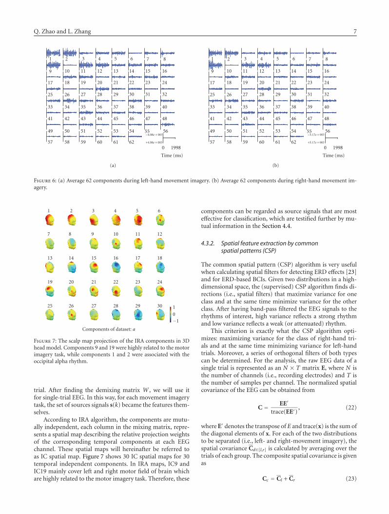
Q. Zhao and L. Zhang 7
1 2 3 4 5 6 7 8
9 10 11 12 13 14 15 16
17 18 19 20 21 22 23 24
25 26 27 28 29 30 31 32
33 34 35 36 37 38 39 40
41 42 43 44 45 46 47 48
49 50 51 52 53 54 55−4.08e + 003
56
57 58 59 60 61 62 +4.08e + 003
0 1998
Time (ms)
(a)
1 2 3 4 5 6 7 8
9 10 11 12 13 14 15 16
17 18 19 20 21 22 23 24
25 26 27 28 29 30 31 32
33 34 35 36 37 38 39 40
41 42 43 44 45 46 47 48
49 50 51 52 53 54 55−5.17e + 003
56
57 58 59 60 61 62 +5.17e + 003
0 1998
Time (ms)
(b)
Figure 6: (a) Average 62 components during left-hand movement imagery. (b) Average 62 components during right-hand movement im-agery.
−10
1
1 2 3 4 5 6
7 8 9 10 11 12
13 14 15 16 17 18
19 20 21 22 23 24
25 26 27 28 29 30
Components of dataset: a
Figure 7: The scalp map projection of the IRA components in 3Dhead model. Components 9 and 19 were highly related to the motorimagery task, while components 1 and 2 were associated with theoccipital alpha rhythm.
trial. After finding the demixing matrix W , we will use itfor single-trial EEG. In this way, for each movement imagerytask, the set of sources signals s(k) became the features them-selves.
According to IRA algorithm, the components are mutu-ally independent, each column in the mixing matrix, repre-sents a spatial map describing the relative projection weightsof the corresponding temporal components at each EEGchannel. These spatial maps will hereinafter be referred toas IC spatial map. Figure 7 shows 30 IC spatial maps for 30temporal independent components. In IRA maps, IC9 andIC19 mainly cover left and right motor field of brain whichare highly related to the motor imagery task. Therefore, these
components can be regarded as source signals that are mosteffective for classification, which are testified further by mu-tual information in the Section 4.4.
4.3.2. Spatial feature extraction by commonspatial patterns (CSP)
The common spatial pattern (CSP) algorithm is very usefulwhen calculating spatial filters for detecting ERD effects [23]and for ERD-based BCIs. Given two distributions in a high-dimensional space, the (supervised) CSP algorithm finds di-rections (i.e., spatial filters) that maximize variance for oneclass and at the same time minimize variance for the otherclass. After having band-pass filtered the EEG signals to therhythms of interest, high variance reflects a strong rhythmand low variance reflects a weak (or attenuated) rhythm.
This criterion is exactly what the CSP algorithm opti-mizes: maximizing variance for the class of right-hand tri-als and at the same time minimizing variance for left-handtrials. Moreover, a series of orthogonal filters of both typescan be determined. For the analysis, the raw EEG data of asingle trial is represented as an N × T matrix E, where N isthe number of channels (i.e., recording electrodes) and T isthe number of samples per channel. The normalized spatialcovariance of the EEG can be obtained from
C = EE′
trace(EE′), (22)
where E′ denotes the transpose of E and trace(x) is the sum ofthe diagonal elements of x. For each of the two distributionsto be separated (i.e., left- and right-movement imagery), thespatial covariance Cd∈[l,r] is calculated by averaging over thetrials of each group. The composite spatial covariance is givenas
Cc = Cl + Cr (23)
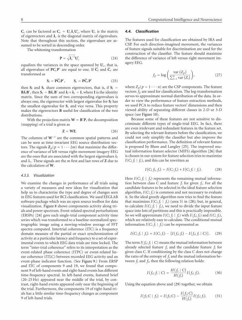
8 Computational Intelligence and Neuroscience
Cc can be factored as Cc = UcλcU′c, where Uc is the matrix
of eigenvectors and λc is the diagonal matrix of eigenvalues.Note that throughout this section, the eigenvalues are as-sumed to be sorted in descending order.
The whitening transformation
P =√λ−1c U′
c (24)
equalizes the variances in the space spanned by Uc, that is,all eigenvalues of PCcP′ are equal to one. If Cl and Cr aretransformed as
Sl = PClP′, Sr = PCrP′ (25)
then Sl and Sr share common eigenvectors, that is, if Sl =BλlB′, then Sr = BλrB′ and λl +λr = I, where I is the identitymatrix. Since the sum of two corresponding eigenvalues isalways one, the eigenvector with largest eigenvalue for Sl hasthe smallest eigenvalue for Sr and vice versa. This propertymakes the eigenvectors B useful for classification of the twodistributions.
With the projection matrix W = B′P, the decomposition(mapping) of a trial is given as
Z = WE. (26)
The columns of W−1 are the common spatial patterns andcan be seen as time-invariant EEG source distribution vec-tors. The signals Zp(p = 1 · · · 2m) that maximize the differ-ence of variance of left versus right-movement imagery EEGare the ones that are associated with the largest eigenvalues λland λr . These signals are the m first and last rows of Z due tothe calculation of W.
4.3.3. Visualization
We examine the changes in performance of all trials usinga variety of measures and new ideas for visualization thathelp us to characterize the type and degree of changes seenin EEG features used for BCI classification. We used EEGLABsoftware package which was an open source toolbox for datavisualization. Figure 8 shows components activity along tri-als and power spectrum. Event-related spectral perturbations(ERSPs) [24] gave each single-trial component activity timeseries which was transformed to a baseline-normalized spec-trographic image using a moving-window average of FFTspectra computed. Intertrial coherence (ITC) is a frequencydomain measure of the partial or exact synchronization ofactivity at a particular latency and frequency to a set of exper-imental events to which EEG data trials are time locked. Theterm “inter-trial coherence” refers to its interpretation as theevent-related phase coherence (ITPC) or event-related lin-ear coherence (ITLC) between recorded EEG activity and anevent-phase indicator function. (See Figure 9.) From ERSPand ITC of components 9 and 19, we found that compo-nent 9 of left-hand events and right-hand events has differenttime-frequency spectral. In left-hand events, featured brief(20–25 Hz) appeared near the middle of the trial, by con-trast, right-hand events appeared only near the beginning ofthe trial. Furthermore, the components 19 of right-hand tri-als has a little similar time-frequency changes as component9 of left-hand trials.
4.4. Classification
The features used for classification are obtained by IRA andCSP. For each direction-imagined movement, the variancesof feature signals suitable for discrimination are used for theconstruction of the classifier. The feature should maximizethe difference of variance of left versus right movement im-agery EEG.
fp = log
(var(Zp)
∑ni=1 var
(Zi))
, (27)
where Zp(p = 1 · · ·n) are the CSP components. The featurevectors fp are used for classification. The log-transformationserves to approximate normal distribution of the data. In or-der to view the performance of feature extraction methods,we used PCA to reduce feature vectors’ dimensions and thenviewed ability of separating different classes in 2-D or 3-Dspace (see Figure 10).
Because some of these features are not sensitive to dis-criminate different types of single-trial EEG. In fact, thereare even irrelevant and redundant features in the feature set.By selecting the relevant features before the classification, wecould not only simplify the classifier but also improve theclassification performance. The definition of relevant featureis proposed by Blum and Langley [25]. The improved mu-tual information feature selector (MIFS) algorithm [26] thatis chosen in our system for feature selection tries to maximizeI(C; fi | fs), and this can be rewritten as
I(C; fi, fs
) = I(C; fs
)+ I(C; fi | fs
). (28)
Here I(C; fi | fs) represents the remaining mutual informa-tion between class C and feature fi for given fs. For all thecandidate features to be selected in the ideal feature selectionalgorithm, I(C; fs) is common and not necessary to evaluateit. So the ideal greedy algorithm now tries to find the featurethat maximizes I(C; fi | fs) (area 3) in (28); but, in general,to calculate I(C; fi | fs), we need to divide the input featurespace into lots of partitions and this is practically impossible.So we will approximate I(C; fi | fs) with I( fs; fi) and I(C; fi),which are relatively easy to calculate. The conditional mutualinformation I(C; fi | fs) can be represented as
I(C; fi | fs
) = I(C; fi
)− {I( fs; fi)− I
(fs; fi | C
)}. (29)
The term I( fs; fi | C) means the mutual information betweenalready selected feature fs and the candidate feature fi forgiven class C. If conditioning by the class C does not changethe ratio of the entropy of fs and the mutual information be-tween fs and fi, then the following relation holds:
I(fs; fi | C
) = H(fs | C
)
H(fs) I
(fs; fi
). (30)
Using the equation above and (29) together, we obtain
I(fi;C | fs
) = I(fi;C
)− I(fs;C
)
H(fs) I(fs; fi
). (31)
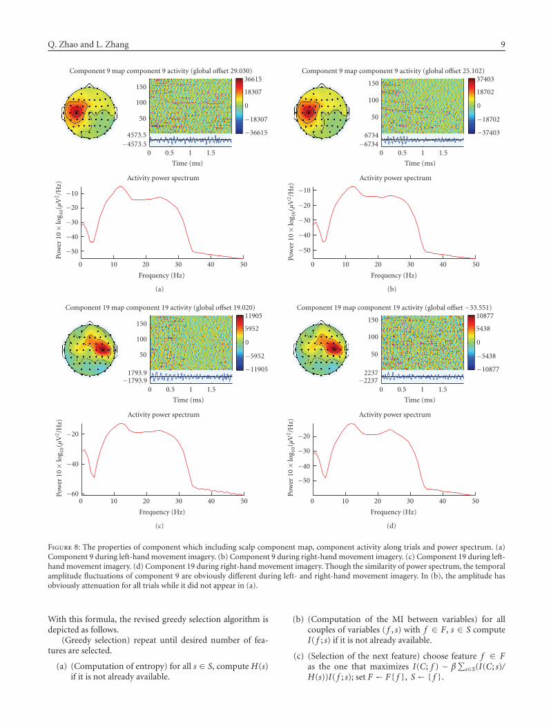
Q. Zhao and L. Zhang 9
−50
−40
−30
−20
−10
Pow
er10×
log 10
(μV
2/H
z)
0 10 20 30 40 50
Frequency (Hz)
Activity power spectrum
0 0.5 1 1.5
Time (ms)
−4573.54573.5
50
100
150
−36615
−18307
0
18307
36615Component 9 map component 9 activity (global offset 29.030)
(a)
−50
−40
−30
−20
−10
Pow
er10×
log 10
(μV
2/H
z)
0 10 20 30 40 50
Frequency (Hz)
Activity power spectrum
0 0.5 1 1.5
Time (ms)
−67346734
50
100
150
−37403
−18702
0
18702
37403Component 9 map component 9 activity (global offset 25.102)
(b)
−60
−40
−20
Pow
er10×
log 10
(μV
2/H
z)
0 10 20 30 40 50
Frequency (Hz)
Activity power spectrum
0 0.5 1 1.5
Time (ms)
−1793.91793.9
50
100
150
−11905
−5952
0
5952
11905Component 19 map component 19 activity (global offset 19.020)
(c)
−50
−40
−30
−20
Pow
er10×
log 10
(μV
2/H
z)
0 10 20 30 40 50
Frequency (Hz)
Activity power spectrum
0 0.5 1 1.5
Time (ms)
−22372237
50
100
150
−10877
−5438
0
5438
10877Component 19 map component 19 activity (global offset −33.551)
(d)
Figure 8: The properties of component which including scalp component map, component activity along trials and power spectrum. (a)Component 9 during left-hand movement imagery. (b) Component 9 during right-hand movement imagery. (c) Component 19 during left-hand movement imagery. (d) Component 19 during right-hand movement imagery. Though the similarity of power spectrum, the temporalamplitude fluctuations of component 9 are obviously different during left- and right-hand movement imagery. In (b), the amplitude hasobviously attenuation for all trials while it did not appear in (a).
With this formula, the revised greedy selection algorithm isdepicted as follows.
(Greedy selection) repeat until desired number of fea-tures are selected.
(a) (Computation of entropy) for all s ∈ S, compute H(s)if it is not already available.
(b) (Computation of the MI between variables) for allcouples of variables ( f , s) with f ∈ F, s ∈ S computeI( f ; s) if it is not already available.
(c) (Selection of the next feature) choose feature f ∈ Fas the one that maximizes I(C; f ) − β
∑s∈S(I(C; s)/
H(s))I( f ; s); set F ← F{ f }, S← { f }.
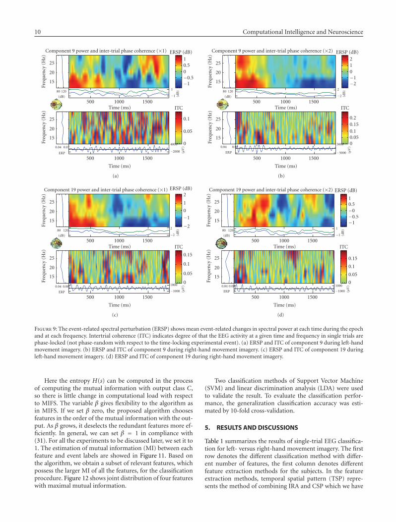
10 Computational Intelligence and Neuroscience
15
20
25
Freq
uen
cy(H
z)
500 1000 1500
Time (ms)
0.070.04
ERP −2000
4000
(μV
)
0
0.05
0.1
ITC500 1000 1500
Time (ms)
12080
(dB) −1
1
(dB
)
−1−0.500.51
ERSP (dB)
15
20
25
Freq
uen
cy(H
z)
Component 9 power and inter-trial phase coherence (×1)
(a)
15
20
25
Freq
uen
cy(H
z)
500 1000 1500
Time (ms)
0.070.04
ERP −5000
5000
(μV
)
00.050.10.150.2
ITC500 1000 1500
Time (ms)
12080
(dB) −2
2
(dB
)
15
20
25
Freq
uen
cy(H
z)
−2−1012
ERSP (dB)Component 9 power and inter-trial phase coherence (×2)
(b)
15
20
25
Freq
uen
cy(H
z)
500 1000 1500
Time (ms)
0.080.04
ERP −1000
1000
(μV
)
0
0.05
0.1
0.15
ITC500 1000 1500
Time (ms)
12080
(dB) −2
2
(dB
)
15
20
25
Freq
uen
cy(H
z)
−2
−1
0
1
2ERSP (dB)Component 19 power and inter-trial phase coherence (×1)
(c)
15
20
25
Freq
uen
cy(H
z)
500 1000 1500
Time (ms)
0.080.04
ERP −1000
1000
(μV
)
0
0.05
0.1
0.15
ITC500 1000 1500
Time (ms)
12080
(dB) −1
1
(dB
)
15
20
25Fr
equ
ency
(Hz)
−1−0.5−00.51
ERSP (dB)Component 19 power and inter-trial phase coherence (×2)
(d)
Figure 9: The event-related spectral perturbation (ERSP) shows mean event-related changes in spectral power at each time during the epochand at each frequency. Intertrial coherence (ITC) indicates degree of that the EEG activity at a given time and frequency in single trials arephase-locked (not phase-random with respect to the time-locking experimental event). (a) ERSP and ITC of component 9 during left-handmovement imagery. (b) ERSP and ITC of component 9 during right-hand movement imagery. (c) ERSP and ITC of component 19 duringleft-hand movement imagery. (d) ERSP and ITC of component 19 during right-hand movement imagery.
Here the entropy H(s) can be computed in the processof computing the mutual information with output class C,so there is little change in computational load with respectto MIFS. The variable β gives flexibility to the algorithm asin MIFS. If we set β zero, the proposed algorithm choosesfeatures in the order of the mutual information with the out-put. As β grows, it deselects the redundant features more ef-ficiently. In general, we can set β = 1 in compliance with(31). For all the experiments to be discussed later, we set it to1. The estimation of mutual information (MI) between eachfeature and event labels are showed in Figure 11. Based onthe algorithm, we obtain a subset of relevant features, whichpossess the larger MI of all the features, for the classificationprocedure. Figure 12 shows joint distribution of four featureswith maximal mutual information.
Two classification methods of Support Vector Machine(SVM) and linear discrimination analysis (LDA) were usedto validate the result. To evaluate the classification perfor-mance, the generalization classification accuracy was esti-mated by 10-fold cross-validation.
5. RESULTS AND DISCUSSIONS
Table 1 summarizes the results of single-trial EEG classifica-tion for left- versus right-hand movement imagery. The firstrow denotes the different classification method with differ-ent number of features, the first column denotes differentfeature extraction methods for the subjects. In the featureextraction methods, temporal spatial pattern (TSP) repre-sents the method of combining IRA and CSP which we have
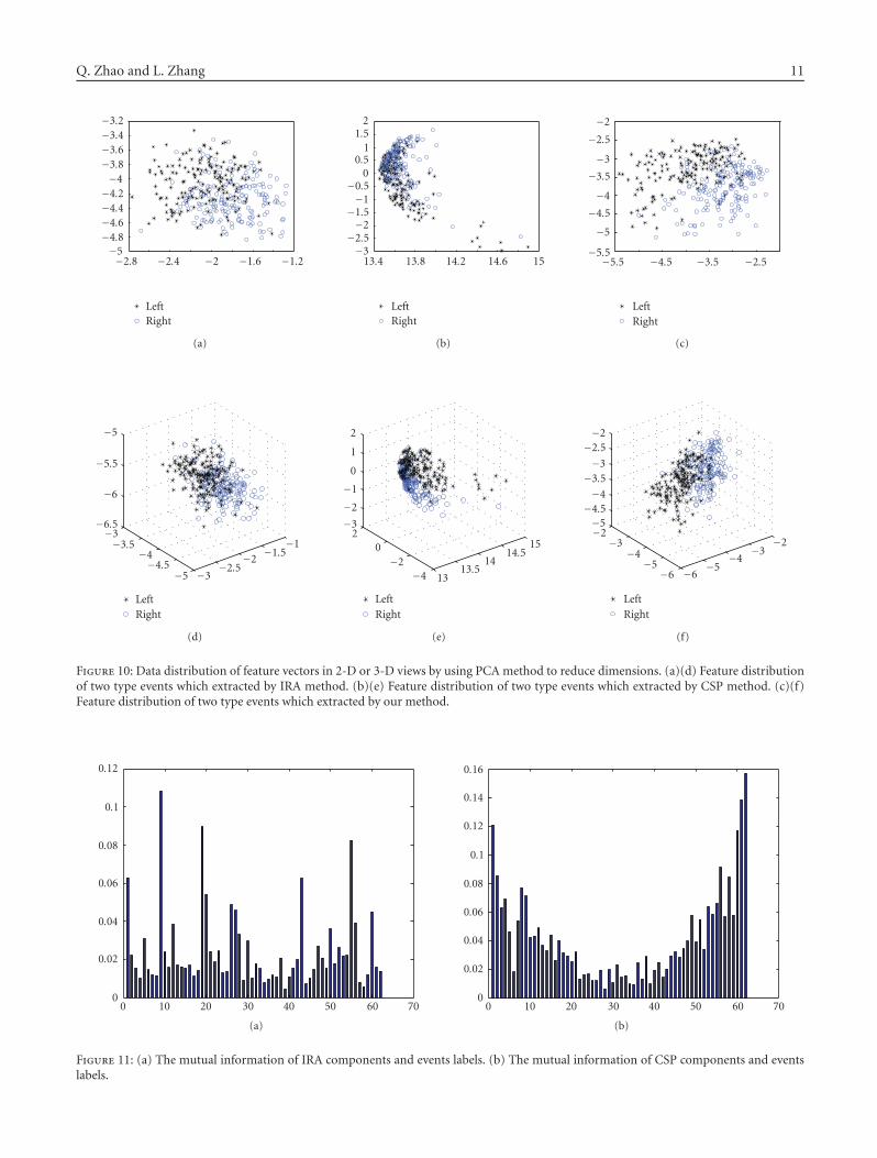
Q. Zhao and L. Zhang 11
−5−4.8−4.6−4.4−4.2−4−3.8−3.6−3.4−3.2
−2.8 −2.4 −2 −1.6 −1.2
LeftRight
(a)
−3−2.5−2−1.5−1−0.5
00.5
11.5
2
13.4 13.8 14.2 14.6 15
LeftRight
(b)
−5.5
−5
−4.5
−4
−3.5
−3
−2.5
−2
−5.5 −4.5 −3.5 −2.5
LeftRight
(c)
−3−3.5
−4−4.5
−5
−6.5
−6
−5.5
−5
−3−2.5
−2−1.5
−1
LeftRight
(d)
20−2
−4
−3
−2
−1
0
1
2
1313.5
1414.5
15
LeftRight
(e)
−2−3
−4−5
−6
−5−4.5−4
−3.5−3
−2.5−2
−6−5
−4−3
−2
LeftRight
(f)
Figure 10: Data distribution of feature vectors in 2-D or 3-D views by using PCA method to reduce dimensions. (a)(d) Feature distributionof two type events which extracted by IRA method. (b)(e) Feature distribution of two type events which extracted by CSP method. (c)(f)Feature distribution of two type events which extracted by our method.
0
0.02
0.04
0.06
0.08
0.1
0.12
0 10 20 30 40 50 60 70
(a)
0
0.02
0.04
0.06
0.08
0.1
0.12
0.14
0.16
0 10 20 30 40 50 60 70
(b)
Figure 11: (a) The mutual information of IRA components and events labels. (b) The mutual information of CSP components and eventslabels.
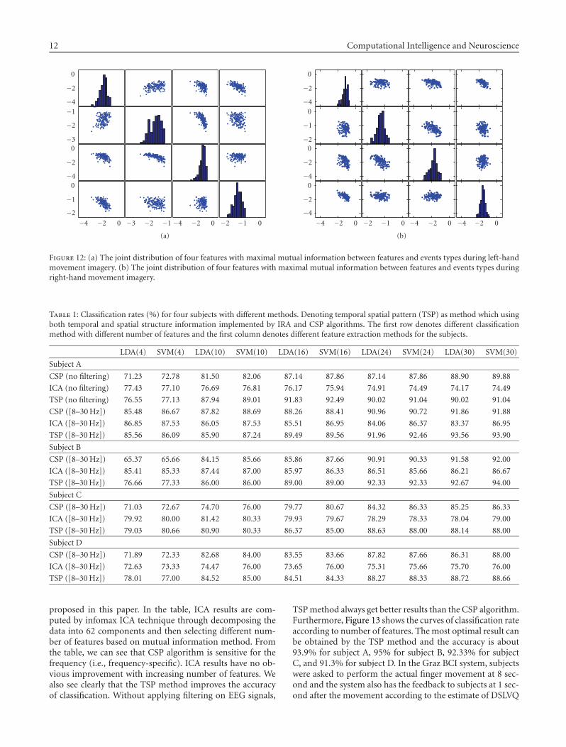
12 Computational Intelligence and Neuroscience
−2
−1
0−4
−2
0−3
−2
−1−4
−2
0
−4 −2 0 −3 −2 −1 −4 −2 0 −2 −1 0
(a)
−4
−2
0−4
−2
0−2
−1
0−4
−2
0
−4 −2 0 −2 −1 0 −4 −2 0 −4 −2 0
(b)
Figure 12: (a) The joint distribution of four features with maximal mutual information between features and events types during left-handmovement imagery. (b) The joint distribution of four features with maximal mutual information between features and events types duringright-hand movement imagery.
Table 1: Classification rates (%) for four subjects with different methods. Denoting temporal spatial pattern (TSP) as method which usingboth temporal and spatial structure information implemented by IRA and CSP algorithms. The first row denotes different classificationmethod with different number of features and the first column denotes different feature extraction methods for the subjects.
LDA(4) SVM(4) LDA(10) SVM(10) LDA(16) SVM(16) LDA(24) SVM(24) LDA(30) SVM(30)
Subject A
CSP (no filtering) 71.23 72.78 81.50 82.06 87.14 87.86 87.14 87.86 88.90 89.88
ICA (no filtering) 77.43 77.10 76.69 76.81 76.17 75.94 74.91 74.49 74.17 74.49
TSP (no filtering) 76.55 77.13 87.94 89.01 91.83 92.49 90.02 91.04 90.02 91.04
CSP ([8–30 Hz]) 85.48 86.67 87.82 88.69 88.26 88.41 90.96 90.72 91.86 91.88
ICA ([8–30 Hz]) 86.85 87.53 86.05 87.53 85.51 86.95 84.06 86.37 83.37 86.95
TSP ([8–30 Hz]) 85.56 86.09 85.90 87.24 89.49 89.56 91.96 92.46 93.56 93.90
Subject B
CSP ([8–30 Hz]) 65.37 65.66 84.15 85.66 85.86 87.66 90.91 90.33 91.58 92.00
ICA ([8–30 Hz]) 85.41 85.33 87.44 87.00 85.97 86.33 86.51 85.66 86.21 86.67
TSP ([8–30 Hz]) 76.66 77.33 86.00 86.00 89.00 89.00 92.33 92.33 92.67 94.00
Subject C
CSP ([8–30 Hz]) 71.03 72.67 74.70 76.00 79.77 80.67 84.32 86.33 85.25 86.33
ICA ([8–30 Hz]) 79.92 80.00 81.42 80.33 79.93 79.67 78.29 78.33 78.04 79.00
TSP ([8–30 Hz]) 79.03 80.66 80.90 80.33 86.37 85.00 88.63 88.00 88.14 88.00
Subject D
CSP ([8–30 Hz]) 71.89 72.33 82.68 84.00 83.55 83.66 87.82 87.66 86.31 88.00
ICA ([8–30 Hz]) 72.63 73.33 74.47 76.00 73.65 76.00 75.31 75.66 75.70 76.00
TSP ([8–30 Hz]) 78.01 77.00 84.52 85.00 84.51 84.33 88.27 88.33 88.72 88.66
proposed in this paper. In the table, ICA results are com-puted by infomax ICA technique through decomposing thedata into 62 components and then selecting different num-ber of features based on mutual information method. Fromthe table, we can see that CSP algorithm is sensitive for thefrequency (i.e., frequency-specific). ICA results have no ob-vious improvement with increasing number of features. Wealso see clearly that the TSP method improves the accuracyof classification. Without applying filtering on EEG signals,
TSP method always get better results than the CSP algorithm.Furthermore, Figure 13 shows the curves of classification rateaccording to number of features. The most optimal result canbe obtained by the TSP method and the accuracy is about93.9% for subject A, 95% for subject B, 92.33% for subjectC, and 91.3% for subject D. In the Graz BCI system, subjectswere asked to perform the actual finger movement at 8 sec-ond and the system also has the feedback to subjects at 1 sec-ond after the movement according to the estimate of DSLVQ
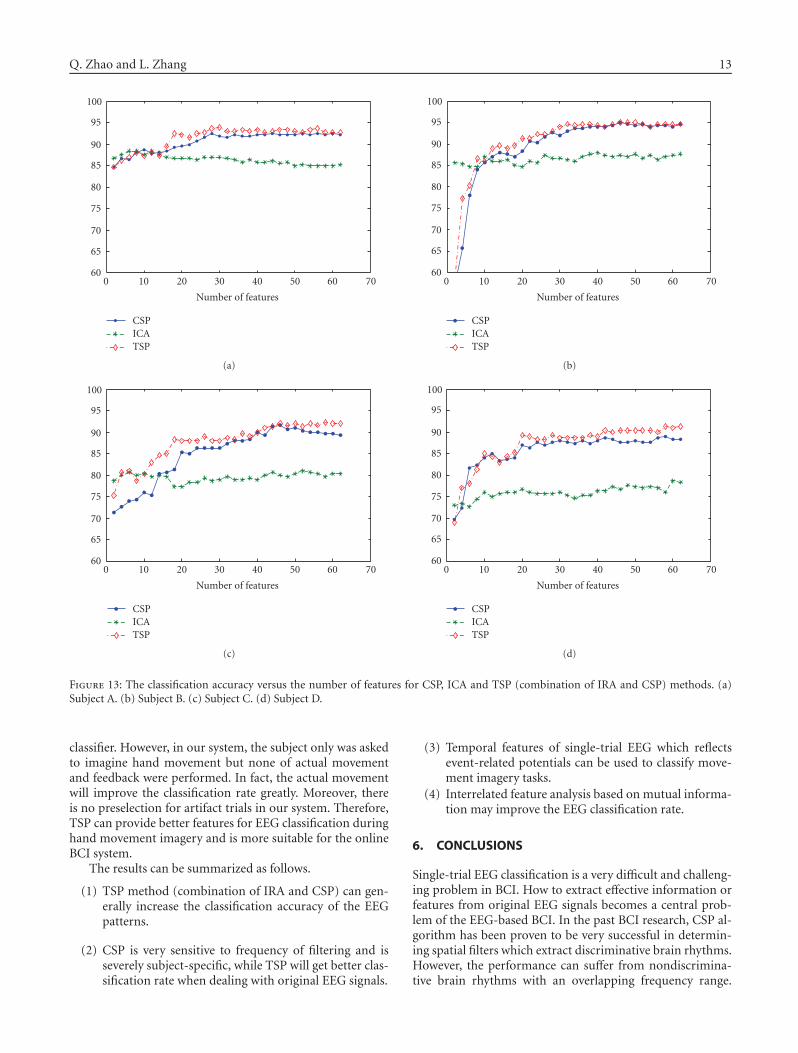
Q. Zhao and L. Zhang 13
60
65
70
75
80
85
90
95
100
0 10 20 30 40 50 60 70
Number of features
CSPICATSP
(a)
60
65
70
75
80
85
90
95
100
0 10 20 30 40 50 60 70
Number of features
CSPICATSP
(b)
60
65
70
75
80
85
90
95
100
0 10 20 30 40 50 60 70
Number of features
CSPICATSP
(c)
60
65
70
75
80
85
90
95
100
0 10 20 30 40 50 60 70
Number of features
CSPICATSP
(d)
Figure 13: The classification accuracy versus the number of features for CSP, ICA and TSP (combination of IRA and CSP) methods. (a)Subject A. (b) Subject B. (c) Subject C. (d) Subject D.
classifier. However, in our system, the subject only was askedto imagine hand movement but none of actual movementand feedback were performed. In fact, the actual movementwill improve the classification rate greatly. Moreover, thereis no preselection for artifact trials in our system. Therefore,TSP can provide better features for EEG classification duringhand movement imagery and is more suitable for the onlineBCI system.
The results can be summarized as follows.
(1) TSP method (combination of IRA and CSP) can gen-erally increase the classification accuracy of the EEGpatterns.
(2) CSP is very sensitive to frequency of filtering and isseverely subject-specific, while TSP will get better clas-sification rate when dealing with original EEG signals.
(3) Temporal features of single-trial EEG which reflectsevent-related potentials can be used to classify move-ment imagery tasks.
(4) Interrelated feature analysis based on mutual informa-tion may improve the EEG classification rate.
6. CONCLUSIONS
Single-trial EEG classification is a very difficult and challeng-ing problem in BCI. How to extract effective information orfeatures from original EEG signals becomes a central prob-lem of the EEG-based BCI. In the past BCI research, CSP al-gorithm has been proven to be very successful in determin-ing spatial filters which extract discriminative brain rhythms.However, the performance can suffer from nondiscrimina-tive brain rhythms with an overlapping frequency range.
14 Computational Intelligence and Neuroscience
Meanwhile, IRA algorithm successfully overcomes this prob-lem by finding the latency source related to events. ThroughIRA decomposition, we will separate useful source compo-nents with temporal structures from noise. Therefore, it willovercome the problem of losing temporal information that isvery useful for classification of event-related potential. Fur-thermore, through feature selection based on mutual infor-mation, most interrelated or effective features have been se-lected for classification. It allows to clearly reveal discrimi-nating parts in features set, thus contributes to a better un-derstanding of mechanism for an imagination task. Finally,it would be useful to explore configurations with more thantwo classes which are more natural and also more friendlyfrom the psychological perspective.
ACKNOWLEDGMENTS
This work was supported by the National Basic Research Pro-gram of China (Grant no. 2005CB724301) and National Nat-ural Science Foundation of China (Grant no. 60375015).
REFERENCES
[1] J. R. Wolpaw, N. Birbaumer, W. J. Heetderks, et al., “Brain-computer interface technology: a review of the first interna-tional meeting,” IEEE Transactions on Rehabilitation Engineer-ing, vol. 8, no. 2, pp. 164–173, 2000.
[2] J. R. Wolpaw, N. Birbaumer, D. J. McFarland, G. Pfurtscheller,and T. M. Vaughan, “Brain-computer interfaces for communi-cation and control,” Clinical Neurophysiology, vol. 113, no. 6,pp. 767–791, 2002.
[3] L. A. Farwell and E. Donchin, “Talking off the top of yourhead: toward a mental prosthesis utilizing event-related brainpotentials,” Electroencephalography and Clinical Neurophysiol-ogy, vol. 70, no. 6, pp. 510–523, 1988.
[4] G. Pfurtscheller, C. Neuper, D. Flotzinger, and M. Pregen-zer, “EEG-based discrimination between imagination of rightand left hand movement,” Electroencephalography and ClinicalNeurophysiology, vol. 103, no. 6, pp. 642–651, 1997.
[5] J. R. Wolpaw and D. J. McFarland, “Multichannel EEG-basedbrain-computer communication,” Electroencephalography andClinical Neurophysiology, vol. 90, no. 6, pp. 444–449, 1994.
[6] N. Birbaumer, N. Ghanayim, T. Hinterberger, et al., “A spellingdevice for the paralysed,” Nature, vol. 398, no. 6725, pp. 297–298, 1999.
[7] J. R. Wolpaw, D. J. McFarland, and T. M. Vaughan, “Brain-computer interface research at the Wadsworth Center,” IEEETransactions on Rehabilitation Engineering, vol. 8, no. 2, pp.222–226, 2000.
[8] Y. Li, X. Gao, H. Liu, and S. Gao, “Classification of single-trialelectroencephalogram during finger movement,” IEEE Trans-actions on Biomedical Engineering, vol. 51, no. 6, pp. 1019–1025, 2004.
[9] Y. Wang, Z. Zhang, Y. Li, X. Gao, S. Gao, and F. Yang, “BCIcompetition 2003-data set IV: an algorithm based on CSSDand FDA for classifying single-trial EEG,” IEEE Transactionson Biomedical Engineering, vol. 51, no. 6, pp. 1081–1086, 2004.
[10] H. Ramoser, J. Muller-Gerking, and G. Pfurtscheller, “Opti-mal spatial filtering of single trial EEG during imagined handmovement,” IEEE Transactions on Rehabilitation Engineering,vol. 8, no. 4, pp. 441–446, 2000.
[11] J. Muller-Gerking, G. Pfurtscheller, and H. Flyvbjerg, “Design-ing optimal spatial filters for single-trial EEG classification in amovement task,” Clinical Neurophysiology, vol. 110, no. 5, pp.787–798, 1999.
[12] G. Dornhege, B. Blankertz, G. Curio, and K.-R. Muller, “In-crease information transfer rates in BCI by CSP extension tomulti-class,” in Advances in Neural Information Processing Sys-tems 16 (NIPS ’03), vol. 3, Vancouver, BC, Canada, December2004.
[13] L. Zhang, “Temporal independent component analysis forseparating noisy signals,” in Proceedings of the 11th In-ternational Conference of Neural Information Processing(ICONIP ’04), vol. 3316 of Lecture Notes in Computer Science,pp. 1064–1069, Calcutta, India, November 2004.
[14] H. Jasper and W. Penfield, “Electrocorticograms in man: ef-fect of voluntary movement upon the electrical activity of theprecentral gyrus,” European Archives of Psychiatry and ClinicalNeuroscience, vol. 183, no. 1–2, pp. 163–174, 1949.
[15] G. Dornhege, B. Blankertz, M. Krauledat, F. Losch, G. Curio,and K.-R. Muller, “Combined optimization of spatial and tem-poral filters for improving brain-computer interfacing,” IEEETransactions on Biomedical Engineering, vol. 53, no. 11, pp.2274–2281, 2006.
[16] S. Amari and A. Cichocki, “Adaptive blind signal processing-neural network approaches,” Proceedings of the IEEE, vol. 86,no. 10, pp. 2026–2048, 1998.
[17] D. T. Pham, “Mutual information approach to blind separa-tion of stationary sources,” IEEE Transactions on InformationTheory, vol. 48, no. 7, pp. 1935–1946, 2002.
[18] S.-I. Amari and J.-F. Cardoso, “Blind source separation-semiparametric statistical approach,” IEEE Transactions onSignal Processing, vol. 45, no. 11, pp. 2692–2700, 1997.
[19] L.-Q. Zhang, A. Cichocki, and S. Amari, “Geometrical struc-tures of FIR manifold and multichannel blind deconvolution,”Journal of VLSI Signal Processing Systems, vol. 31, no. 1, pp.31–44, 2002.
[20] L. Zhang, A. Cichocki, and S. Amari, “Self-adaptive blindsource separation based on activation functions adaptation,”IEEE Transactions on Neural Networks, vol. 15, no. 2, pp. 233–244, 2004.
[21] C. J. James and O. J. Gibson, “Temporally constrained ICA: anapplication to artifact rejection in electromagnetic brain signalanalysis,” IEEE Transactions on Biomedical Engineering, vol. 50,no. 9, pp. 1108–1116, 2003.
[22] W. Lu and J. C. Rajapakse, “ICA with reference,” in Proceedingsof the 3rd International Conference on Independent ComponentAnalysis and Blind Source Separation (ICA ’01), pp. 120–125,San Diego, Calif, USA, December 2001.
[23] Z. J. Koles and A. C. K. Soong, “EEG source localization:implementing the spatio-temporal decomposition approach,”Electroencephalography and Clinical Neurophysiology, vol. 107,no. 5, pp. 343–352, 1998.
[24] A. Delorme and S. Makeig, “EEGLAB: an open source tool-box for analysis of single-trial EEG dynamics including inde-pendent component analysis,” Journal of Neuroscience Meth-ods, vol. 134, no. 1, pp. 9–21, 2004.
[25] A. L. Blum and P. Langley, “Selection of relevant features andexamples in machine learning,” Artificial Intelligence, vol. 97,no. 1–2, pp. 245–271, 1997.
[26] N. Kwak and C.-H. Choi, “Improved mutual information fea-ture selector for neural networks in supervised learning,” in In-ternational Joint Conference on Neural Networks (IJCNN ’99),vol. 2, pp. 1313–1318, Washington, DC, USA, July 1999.
Hindawi Publishing CorporationComputational Intelligence and NeuroscienceVolume 2007, Article ID 71863, 5 pagesdoi:10.1155/2007/71863
Research ArticleNessi: An EEG-Controlled Web Browser forSeverely Paralyzed Patients
Michael Bensch,1 Ahmed A. Karim,2, 3 Jurgen Mellinger,2 Thilo Hinterberger,2 Michael Tangermann,4
Martin Bogdan,1, 5 Wolfgang Rosenstiel,1 and Niels Birbaumer2, 6
1 Department of Computer Engineering, University of Tubingen, 72076 Tubingen, Germany2 Institute of Medical Psychology and Behavioral Neurobiology, University of Tubingen, Gartenstrasse 29, 72074 Tubingen, Germany3 Graduate School of Neural and Behavioral Sciences, International Max Planck Research School, University of Tubingen,72076 Tubingen, Germany
4 Fraunhofer FIRST, Intelligent Data Analysis Group, 12489 Berlin, Germany5 Department of Computer Engineering, University of Leipzig, 04103 Leipzig, Germany
6 Human Cortical Physiology Unit, National Institute of Neurological Disorders and Stroke (NINDS), National Institutes of Health(NIH), Bethesda, MD 20892, USA
Correspondence should be addressed to Ahmed A. Karim, [email protected]
Received 28 February 2007; Accepted 26 June 2007
Recommended by Shangkai Gao
We have previously demonstrated that an EEG-controlled web browser based on self-regulation of slow cortical potentials (SCPs)enables severely paralyzed patients to browse the internet independently of any voluntary muscle control. However, this system hadseveral shortcomings, among them that patients could only browse within a limited number of web pages and had to select linksfrom an alphabetical list, causing problems if the link names were identical or if they were unknown to the user (as in graphicallinks). Here we describe a new EEG-controlled web browser, called Nessi, which overcomes these shortcomings. In Nessi, the opensource browser, Mozilla, was extended by graphical in-place markers, whereby different brain responses correspond to differentframe colors placed around selectable items, enabling the user to select any link on a web page. Besides links, other interactiveelements are accessible to the user, such as e-mail and virtual keyboards, opening up a wide range of hypertext-based applications.
Copyright © 2007 Michael Bensch et al. This is an open access article distributed under the Creative Commons AttributionLicense, which permits unrestricted use, distribution, and reproduction in any medium, provided the original work is properlycited.
1. INTRODUCTION
Neurological diseases such as amyotrophic lateral sclerosis(ALS), Guillain-Barre syndrome, or brainstem stroke canlead to severe or total motor paralysis often referred to aslocked-in syndrome, where the intact intellect is locked intoa paralyzed body. One of the most terrifying aspects of this“locked-in syndrome” is that the loss of muscle control pre-vents the expression of even the most basic needs. Conven-tional augmentative communication devices, which dependon some rudimental muscle control, may not be feasible forpatients in the end stage of ALS if they have no remainingreliable muscle control. Thus, the final option for restoringcommunication to those patients is to provide the brain witha nonmuscular communication and control channel, a di-rect brain-computer interface (BCI) for conveying messages
and commands to the external world. In the late 1990s, Bir-baumer et al. [1, 2] were the first to provide ALS patientswith a BCI system, the so-called thought translation device(TTD). The TTD is a noninvasive, EEG-controlled BCI basedon regulation of slow cortical potentials (SCPs) which hu-mans can learn to control in an operant conditioning proce-dure [3]. Further studies have successfully applied sensory-motor EEG rhythms (SMR) [4, 5], P300 evoked potentials[6], and neuronal action potentials [7–9] for different BCIsystems. While letter spelling is a state-of-the-art applica-tion for BCI systems today, interactive access to the worldwide web (WWW) is one of the most promising BCI ap-plications, as it enables severely paralyzed patients to par-ticipate in the broad portion of life reflected by the WWW.Karim et al. [10] have recently shown that an EEG-controlledweb browser based on self-regulation of SCP can be reliably
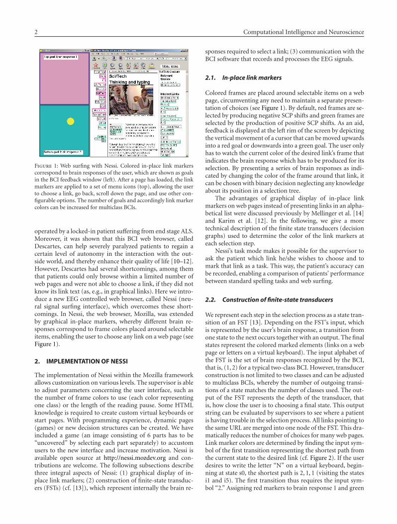
2 Computational Intelligence and Neuroscience
Figure 1: Web surfing with Nessi. Colored in-place link markerscorrespond to brain responses of the user, which are shown as goalsin the BCI feedback window (left). After a page has loaded, the linkmarkers are applied to a set of menu icons (top), allowing the userto choose a link, go back, scroll down the page, and use other con-figurable options. The number of goals and accordingly link markercolors can be increased for multiclass BCIs.
operated by a locked-in patient suffering from end stage ALS.Moreover, it was shown that this BCI web browser, calledDescartes, can help severely paralyzed patients to regain acertain level of autonomy in the interaction with the out-side world, and thereby enhance their quality of life [10–12].However, Descartes had several shortcomings, among themthat patients could only browse within a limited number ofweb pages and were not able to choose a link, if they did notknow its link text (as, e.g., in graphical links). Here we intro-duce a new EEG controlled web browser, called Nessi (neu-ral signal surfing interface), which overcomes these short-comings. In Nessi, the web browser, Mozilla, was extendedby graphical in-place markers, whereby different brain re-sponses correspond to frame colors placed around selectableitems, enabling the user to choose any link on a web page (seeFigure 1).
2. IMPLEMENTATION OF NESSI
The implementation of Nessi within the Mozilla frameworkallows customization on various levels. The supervisor is ableto adjust parameters concerning the user interface, such asthe number of frame colors to use (each color representingone class) or the length of the reading pause. Some HTMLknowledge is required to create custom virtual keyboards orstart pages. With programming experience, dynamic pages(games) or new decision structures can be created. We haveincluded a game (an image consisting of 6 parts has to be“uncovered” by selecting each part separately) to accustomusers to the new interface and increase motivation. Nessi isavailable open source at http://nessi.mozdev.org and con-tributions are welcome. The following subsections describethree integral aspects of Nessi: (1) graphical display of in-place link markers; (2) construction of finite-state transduc-ers (FSTs) (cf. [13]), which represent internally the brain re-
sponses required to select a link; (3) communication with theBCI software that records and processes the EEG signals.
2.1. In-place link markers
Colored frames are placed around selectable items on a webpage, circumventing any need to maintain a separate presen-tation of choices (see Figure 1). By default, red frames are se-lected by producing negative SCP shifts and green frames areselected by the production of positive SCP shifts. As an aid,feedback is displayed at the left rim of the screen by depictingthe vertical movement of a cursor that can be moved upwardsinto a red goal or downwards into a green goal. The user onlyhas to watch the current color of the desired link’s frame thatindicates the brain response which has to be produced for itsselection. By presenting a series of brain responses as indi-cated by changing the color of the frame around that link, itcan be chosen with binary decision neglecting any knowledgeabout its position in a selection tree.
The advantages of graphical display of in-place linkmarkers on web pages instead of presenting links in an alpha-betical list were discussed previously by Mellinger et al. [14]and Karim et al. [12]. In the following, we give a moretechnical description of the finite state transducers (decisiongraphs) used to determine the color of the link markers ateach selection step.
Nessi’s task mode makes it possible for the supervisor toask the patient which link he/she wishes to choose and tomark that link as a task. This way, the patient’s accuracy canbe recorded, enabling a comparison of patients’ performancebetween standard spelling tasks and web surfing.
2.2. Construction of finite-state transducers
We represent each step in the selection process as a state tran-sition of an FST [13]. Depending on the FST’s input, whichis represented by the user’s brain response, a transition fromone state to the next occurs together with an output. The finalstates represent the colored marked elements (links on a webpage or letters on a virtual keyboard). The input alphabet ofthe FST is the set of brain responses recognized by the BCI,that is, (1, 2) for a typical two-class BCI. However, transducerconstruction is not limited to two classes and can be adjustedto multiclass BCIs, whereby the number of outgoing transi-tions of a state matches the number of classes used. The out-put of the FST represents the depth of the transducer, thatis, how close the user is to choosing a final state. This outputstring can be evaluated by supervisors to see where a patientis having trouble in the selection process. All links pointing tothe same URL are merged into one node of the FST. This dra-matically reduces the number of choices for many web pages.Link marker colors are determined by finding the input sym-bol of the first transition representing the shortest path fromthe current state to the desired link (cf. Figure 2). If the userdesires to write the letter “N” on a virtual keyboard, begin-ning at state s0, the shortest path is 2, 1, 1 (visiting the statesi1 and i5). The first transition thus requires the input sym-bol “2.” Assigning red markers to brain response 1 and green
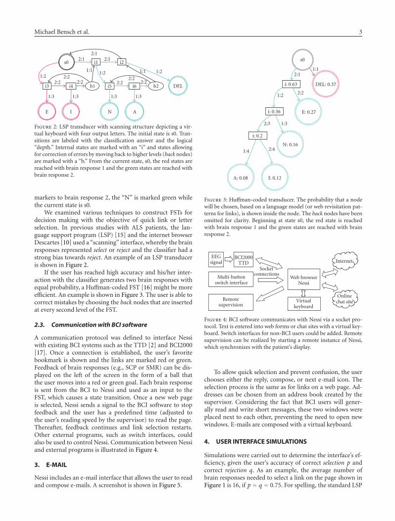
Michael Bensch et al. 3
s0 i1 i2
i3 i4 b1 i5 i6 b2 DEL
E I N A
2:12:1 2:1
1:2 2:21:1 1:2
2:22:2
2:2
1:1 1:2
2:2 2:2
1:3 1:3 1:3 1:3
Figure 2: LSP transducer with scanning structure depicting a vir-tual keyboard with four output letters. The initial state is s0. Tran-sitions are labeled with the classification answer and the logical“depth.” Internal states are marked with an “i” and states allowingfor correction of errors by moving back to higher levels (back nodes)are marked with a “b.” From the current state, s0, the red states arereached with brain response 1 and the green states are reached withbrain response 2.
markers to brain response 2, the “N” is marked green whilethe current state is s0.
We examined various techniques to construct FSTs fordecision making with the objective of quick link or letterselection. In previous studies with ALS patients, the lan-guage support program (LSP) [15] and the internet browserDescartes [10] used a “scanning” interface, whereby the brainresponses represented select or reject and the classifier had astrong bias towards reject. An example of an LSP transduceris shown in Figure 2.
If the user has reached high accuracy and his/her inter-action with the classifier generates two brain responses withequal probability, a Huffman-coded FST [16] might be moreefficient. An example is shown in Figure 3. The user is able tocorrect mistakes by choosing the back nodes that are insertedat every second level of the FST.
2.3. Communication with BCI software
A communication protocol was defined to interface Nessiwith existing BCI systems such as the TTD [2] and BCI2000[17]. Once a connection is established, the user’s favoritebookmark is shown and the links are marked red or green.Feedback of brain responses (e.g., SCP or SMR) can be dis-played on the left of the screen in the form of a ball thatthe user moves into a red or green goal. Each brain responseis sent from the BCI to Nessi and used as an input to theFST, which causes a state transition. Once a new web pageis selected, Nessi sends a signal to the BCI software to stopfeedback and the user has a predefined time (adjusted tothe user’s reading speed by the supervisor) to read the page.Thereafter, feedback continues and link selection restarts.Other external programs, such as switch interfaces, couldalso be used to control Nessi. Communication between Nessiand external programs is illustrated in Figure 4.
3. E-MAIL
Nessi includes an e-mail interface that allows the user to readand compose e-mails. A screenshot is shown in Figure 5.
s0
i: 0.63
i: 0.36
i: 0.2
DEL: 0.37
E: 0.27
N: 0.16
I: 0.12A: 0.08
1:12:1
1:2 2:2
2:3 1:3
1:4 2:4
Figure 3: Huffman-coded transducer. The probability that a nodewill be chosen, based on a language model (or web revisitation pat-terns for links), is shown inside the node. The back nodes have beenomitted for clarity. Beginning at state s0, the red state is reachedwith brain response 1 and the green states are reached with brainresponse 2.
EEGsignal
BCI2000TTD
Multi-buttonswitch interface
Remotesupervision
Socketconnections
Web browserNessi
Virtualkeyboard
Onlinechat site
Internet
Figure 4: BCI software communicates with Nessi via a socket pro-tocol. Text is entered into web forms or chat sites with a virtual key-board. Switch interfaces for non-BCI users could be added. Remotesupervision can be realized by starting a remote instance of Nessi,which synchronizes with the patient’s display.
To allow quick selection and prevent confusion, the userchooses either the reply, compose, or next e-mail icon. Theselection process is the same as for links on a web page. Ad-dresses can be chosen from an address book created by thesupervisor. Considering the fact that BCI users will gener-ally read and write short messages, these two windows wereplaced next to each other, preventing the need to open newwindows. E-mails are composed with a virtual keyboard.
4. USER INTERFACE SIMULATIONS
Simulations were carried out to determine the interface’s ef-ficiency, given the user’s accuracy of correct selection p andcorrect rejection q. As an example, the average number ofbrain responses needed to select a link on the page shown inFigure 1 is 16, if p = q = 0.75. For spelling, the standard LSP
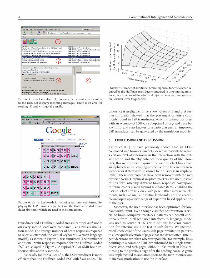
4 Computational Intelligence and Neuroscience
Figure 5: E-mail interface. (1) presents the current menu choicesto the user. (2) displays incoming messages. There is an area forreading (3) and writing (4) e-mails.
Figure 6: Virtual keyboards for entering text into web forms, dis-playing the LSP transducer (center) and the Huffman-coded trans-ducer (bottom), which are used in the simulations.
transducer and a Huffman-coded transducer with back nodeson every second level were compared using Nessi’s simula-tion mode. The average number of brain responses requiredto select a letter with the virtual keyboard (German languagemodel), as shown in Figure 6, was simulated. The number ofadditional brain responses required for the Huffman-codedFST is displayed in Figure 7. A typical SCP or SMR brain re-sponse takes about 5 seconds.
Especially for low values of p, the LSP transducer is moreefficient than the Huffman-coded FST with back nodes. The
10.95
0.90.85
0.80.75
0.7 Reject
accu
racyq
10.95
0.90.85
0.80.75
0.7
Select accuracy p
−5
0
5
10
15
Add
itio
nal
tria
lsre
quir
edfo
rH
uff
man
-tra
nsd
uce
r
Figure 7: Number of additional brain responses to write a letter, re-quired by the Huffman-transducer compared to the scanning trans-ducer, as a function of the select and reject accuracies p and q (basedon German letter frequencies).
difference is negligible for very low values of p and q. A fur-ther simulation showed that the placement of letters com-monly found in LSP transducers, which is optimal for userswith an accuracy of 100%, is suboptimal once p and q are be-low 1. If p and q are known for a particular user, an improvedLSP transducer can be generated by the simulation module.
5. CONCLUSION AND DISCUSSION
Karim et al. [10] have previously shown that an EEG-controlled web browser can help locked-in patients to regaina certain level of autonomy in the interaction with the out-side world and thereby enhance their quality of life. How-ever, this web browser required the user to select links froman alphabetical list, causing problems if the link names wereidentical or if they were unknown to the user (as in graphicallinks). These shortcomings have been resolved with the webbrowser Nessi. Graphical in-place markers are used insteadof link text, whereby different brain responses correspondto frame colors placed around selectable items, enabling theuser to select any link on a web page. Other interactive ele-ments, such as e-mail and virtual keyboards, are also accessi-ble and open up a wide range of hypertext-based applicationsto the user.
Moreover, the user interface has been optimized for low-bandwidth input. Even though classifier optimization is cru-cial to brain-computer interfaces, patients can benefit addi-tionally from intelligent user interfaces. A language modelwas used to construct FSTs with options for error correc-tion for entering URLs or text in web forms. We incorpo-rated knowledge of the user’s web page revisitation patternsto allow quick selection of pages that are visited often. Intelli-gent decisions are taken wherever possible, for example, linkspointing to a common URL are subsumed in a single trans-ducer state, and web pages without links result in Nessi re-turning to the previous page after the reading pause. A gamewas implemented to accustom users to the new interface andto increase motivation to use the interface.
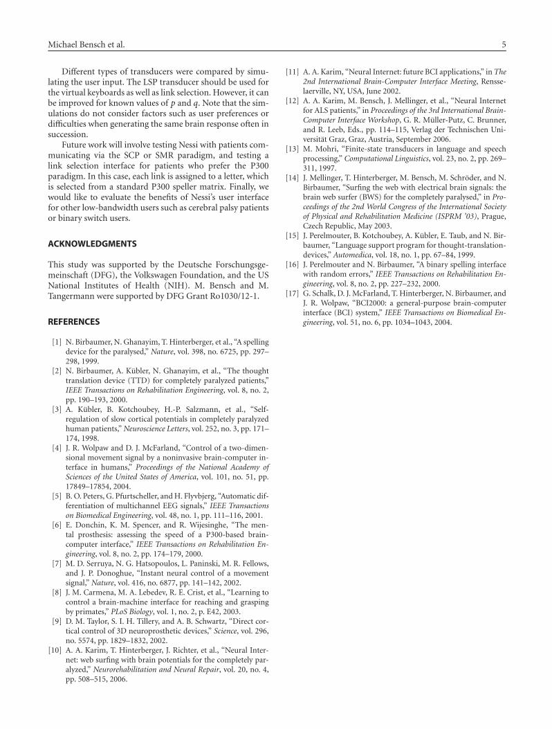
Michael Bensch et al. 5
Different types of transducers were compared by simu-lating the user input. The LSP transducer should be used forthe virtual keyboards as well as link selection. However, it canbe improved for known values of p and q. Note that the sim-ulations do not consider factors such as user preferences ordifficulties when generating the same brain response often insuccession.
Future work will involve testing Nessi with patients com-municating via the SCP or SMR paradigm, and testing alink selection interface for patients who prefer the P300paradigm. In this case, each link is assigned to a letter, whichis selected from a standard P300 speller matrix. Finally, wewould like to evaluate the benefits of Nessi’s user interfacefor other low-bandwidth users such as cerebral palsy patientsor binary switch users.
ACKNOWLEDGMENTS
This study was supported by the Deutsche Forschungsge-meinschaft (DFG), the Volkswagen Foundation, and the USNational Institutes of Health (NIH). M. Bensch and M.Tangermann were supported by DFG Grant Ro1030/12-1.
REFERENCES
[1] N. Birbaumer, N. Ghanayim, T. Hinterberger, et al., “A spellingdevice for the paralysed,” Nature, vol. 398, no. 6725, pp. 297–298, 1999.
[2] N. Birbaumer, A. Kubler, N. Ghanayim, et al., “The thoughttranslation device (TTD) for completely paralyzed patients,”IEEE Transactions on Rehabilitation Engineering, vol. 8, no. 2,pp. 190–193, 2000.
[3] A. Kubler, B. Kotchoubey, H.-P. Salzmann, et al., “Self-regulation of slow cortical potentials in completely paralyzedhuman patients,” Neuroscience Letters, vol. 252, no. 3, pp. 171–174, 1998.
[4] J. R. Wolpaw and D. J. McFarland, “Control of a two-dimen-sional movement signal by a noninvasive brain-computer in-terface in humans,” Proceedings of the National Academy ofSciences of the United States of America, vol. 101, no. 51, pp.17849–17854, 2004.
[5] B. O. Peters, G. Pfurtscheller, and H. Flyvbjerg, “Automatic dif-ferentiation of multichannel EEG signals,” IEEE Transactionson Biomedical Engineering, vol. 48, no. 1, pp. 111–116, 2001.
[6] E. Donchin, K. M. Spencer, and R. Wijesinghe, “The men-tal prosthesis: assessing the speed of a P300-based brain-computer interface,” IEEE Transactions on Rehabilitation En-gineering, vol. 8, no. 2, pp. 174–179, 2000.
[7] M. D. Serruya, N. G. Hatsopoulos, L. Paninski, M. R. Fellows,and J. P. Donoghue, “Instant neural control of a movementsignal,” Nature, vol. 416, no. 6877, pp. 141–142, 2002.
[8] J. M. Carmena, M. A. Lebedev, R. E. Crist, et al., “Learning tocontrol a brain-machine interface for reaching and graspingby primates,” PLoS Biology, vol. 1, no. 2, p. E42, 2003.
[9] D. M. Taylor, S. I. H. Tillery, and A. B. Schwartz, “Direct cor-tical control of 3D neuroprosthetic devices,” Science, vol. 296,no. 5574, pp. 1829–1832, 2002.
[10] A. A. Karim, T. Hinterberger, J. Richter, et al., “Neural Inter-net: web surfing with brain potentials for the completely par-alyzed,” Neurorehabilitation and Neural Repair, vol. 20, no. 4,pp. 508–515, 2006.
[11] A. A. Karim, “Neural Internet: future BCI applications,” in The2nd International Brain-Computer Interface Meeting, Rensse-laerville, NY, USA, June 2002.
[12] A. A. Karim, M. Bensch, J. Mellinger, et al., “Neural Internetfor ALS patients,” in Proceedings of the 3rd International Brain-Computer Interface Workshop, G. R. Muller-Putz, C. Brunner,and R. Leeb, Eds., pp. 114–115, Verlag der Technischen Uni-versitat Graz, Graz, Austria, September 2006.
[13] M. Mohri, “Finite-state transducers in language and speechprocessing,” Computational Linguistics, vol. 23, no. 2, pp. 269–311, 1997.
[14] J. Mellinger, T. Hinterberger, M. Bensch, M. Schroder, and N.Birbaumer, “Surfing the web with electrical brain signals: thebrain web surfer (BWS) for the completely paralysed,” in Pro-ceedings of the 2nd World Congress of the International Societyof Physical and Rehabilitation Medicine (ISPRM ’03), Prague,Czech Republic, May 2003.
[15] J. Perelmouter, B. Kotchoubey, A. Kubler, E. Taub, and N. Bir-baumer, “Language support program for thought-translation-devices,” Automedica, vol. 18, no. 1, pp. 67–84, 1999.
[16] J. Perelmouter and N. Birbaumer, “A binary spelling interfacewith random errors,” IEEE Transactions on Rehabilitation En-gineering, vol. 8, no. 2, pp. 227–232, 2000.
[17] G. Schalk, D. J. McFarland, T. Hinterberger, N. Birbaumer, andJ. R. Wolpaw, “BCI2000: a general-purpose brain-computerinterface (BCI) system,” IEEE Transactions on Biomedical En-gineering, vol. 51, no. 6, pp. 1034–1043, 2004.
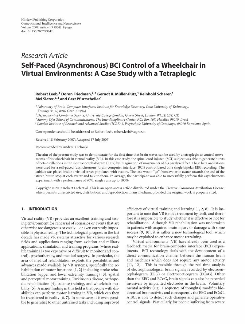
Hindawi Publishing CorporationComputational Intelligence and NeuroscienceVolume 2007, Article ID 79642, 8 pagesdoi:10.1155/2007/79642
Research ArticleSelf-Paced (Asynchronous) BCI Control of a Wheelchair inVirtual Environments: A Case Study with a Tetraplegic
Robert Leeb,1 Doron Friedman,2, 3 Gernot R. Muller-Putz,1 Reinhold Scherer,1
Mel Slater,2, 4 and Gert Pfurtscheller1
1 Laboratory of Brain-Computer Interfaces, Institute for Knowledge Discovery, Graz University of Technology,Krenngasse 37, 8010 Graz, Austria
2 Department of Computer Science, University College London, Gower Street, London WC1E 6BT, UK3 Sammy Ofer School of Communications, The Interdisciplinary Center, P.O. Box 167, Herzliya 08010, Israel
4 Catalan Institute of Research and Advanced Studies (ICREA), Polytechnic University of Catalunya, 08010 Barcelona, Spain
Correspondence should be addressed to Robert Leeb, [email protected]
Received 18 February 2007; Accepted 17 July 2007
Recommended by Andrzej Cichocki
The aim of the present study was to demonstrate for the first time that brain waves can be used by a tetraplegic to control move-ments of his wheelchair in virtual reality (VR). In this case study, the spinal cord injured (SCI) subject was able to generate burstsof beta oscillations in the electroencephalogram (EEG) by imagination of movements of his paralyzed feet. These beta oscillationswere used for a self-paced (asynchronous) brain-computer interface (BCI) control based on a single bipolar EEG recording. Thesubject was placed inside a virtual street populated with avatars. The task was to “go” from avatar to avatar towards the end of thestreet, but to stop at each avatar and talk to them. In average, the participant was able to successfully perform this asynchronousexperiment with a performance of 90%, single runs up to 100%.
Copyright © 2007 Robert Leeb et al. This is an open access article distributed under the Creative Commons Attribution License,which permits unrestricted use, distribution, and reproduction in any medium, provided the original work is properly cited.
1. INTRODUCTION
Virtual reality (VR) provides an excellent training and test-ing environment for rehearsal of scenarios or events that areotherwise too dangerous or costly—or even currently impos-sible in physical reality. The technological progress in the lastdecade has made VR systems attractive for various researchfields and applications ranging from aviation and militaryapplications, simulation and training programs (where real-life training is too expensive or difficult to monitor and con-trol), psychotherapy, and medical surgery. In particular, thearea of medical rehabilitation exploits the possibilities andadvances made available by VR systems, specifically the re-habilitation of motor functions [1, 2] including stroke reha-bilitation (upper and lower extremity training) [3], spatialand perceptual motor training, Parkinson’s disease, orthope-dic rehabilitation [4], balance training, and wheelchair mo-bility [5]. A major finding in this field is that people with dis-abilities can perform motor learning in VR, which can thenbe transferred to reality [6, 7]. In some cases it is even possi-ble to generalize to other untrained tasks including improved
efficiency of virtual training and learning [1, 2, 8]. It is im-portant to note that VR is not a treatment by itself, and there-fore it is impossible to study whether it is effective or not forrehabilitation. Although VR rehabilitation was undertakenin patients with acquired brain injury or damage with somesuccess [9, 10], it is rather a new technological tool, whichmay be exploited to enhance motor retraining.
Virtual environments (VE) have already been used as afeedback media for brain-computer interface (BCI) exper-iments. BCI technology deals with the development of adirect communication channel between the human brainand machines which does not require any motor activity[11, 12]. This is possible through the real-time analysisof electrophysiological brain signals recorded by electroen-cephalogram (EEG) or electrocorticogram (ECoG). Otherthan the EEG and ECoG, brain signals can also be recordedinvasively by implanted electrodes in the brain. Voluntarymental activity (e.g., a sequence of thoughts) modifies bio-electrical brain activity and consequently the EEG and ECoG.A BCI is able to detect such changes and generate operativecontrol signals. Particularly for people suffering from severe
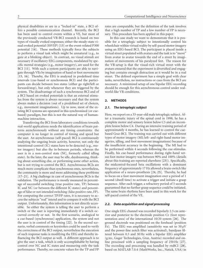
2 Computational Intelligence and Neuroscience
physical disabilities or are in a “locked-in” state, a BCI of-fers a possible communication channel. Recently, the BCIhas been used to control events within a VE, but most ofthe previously conducted VR-BCI research is based on twotypes of visually evoked responses; either the steady-state vi-sual evoked potential (SSVEP) [13] or the event-related P300potential [14]. These methods typically force the subjectsto perform a visual task which might be unnatural (e.g., togaze at a blinking object). In contrast, no visual stimuli arenecessary if oscillatory EEG components, modulated by spe-cific mental strategies (e.g., motor imagery), are used for theBCI [11]. With such a system participants are able to navi-gate through VEs by imagination of hand or foot movements[15, 16]. Thereby, the EEG is analyzed in predefined timeintervals (cue-based or synchronous BCI) and the partici-pants can decide between two states (either go right/left orforward/stop), but only whenever they are triggered by thesystem. The disadvantage of such a synchronous BCI and ofa BCI based on evoked potentials is that an external stimu-lus from the system is always necessary and that the systemalways makes a decision (out of a predefined set of choices,e.g., movement imaginations). Up to now, most of the ex-isting BCI systems are operated in this synchronized (or cue-based) paradigm, but this is not the natural way of human-machine interaction.
Transferring the BCI from laboratory conditions towardsreal-world applications needs the identification of brain pat-terns asynchronously without any timing constraints: thecomputer is no longer in control of timing and speed butthe user. An asynchronous (self-paced) BCI is continuouslyanalyzing the ongoing brain activity, however, not only theintentional-control (IC) states have to be detected (e.g., mo-tor imagery) but also the in-between periods, whereas theuser is in a non-control state (NC, formerly called idlingstate). In the later, the user may be idle, daydreaming, think-ing about something else, or performing some other action,but is not trying to control the BCI. Asynchronous BCIs aremuch more complicate than synchronous ones, nevertheless,the community is more and more addressing these problems[17–21]. A big challenge in case of asynchronous BCIs is thevalidation. The performance is mostly measured in percent-age of successful switching (true positive rate, TP) betweenIC and NC (or between the different IC states) and percent-age of false or not intended switching (false positive rate, FP).For computing the correct TP/FP rates, it is necessary to ac-cess the subjects “real” intend and to compare it with the BCIoutput. Unfortunately, this information is not directly acces-sible. So either the system is telling the user to perform aswitch or the user is reporting immediately if a switch oc-curred correctly or not. In the first scenario, analogical toa cue-based (synchronous) application, the system and notthe user is in control of the timing [22]. In the second sce-nario, verbal comments or keystrokes could be used to verifythe correctness of the BCI output, nevertheless the executionof such response tasks is modifying the EEG and thereby in-fluencing the BCI output as well. A different approach is togive the user a task, which is only accomplishable by havingcontrol over NC and IC states and measuring only the taskperformance. Thereby, no concrete values for the TP and FP
rates are computable, but the definition of the task involvesthat a high number of TP and a low number of FP is neces-sary. This procedure has been applied in this paper.
In this case study we want to demonstrate that it is pos-sible for a tetraplegic subject to intentionally control hiswheelchair within virtual reality by self-paced motor imageryusing an EEG-based BCI. The participant is placed inside avirtual street populated with avatars and the task is to “move”from avatar to avatar towards the end of a street by imagi-nation of movements of his paralyzed feet. The reason forthe VR-setup is that the visual-rich virtual street with theavatars ensured that the experiment is diversified and engag-ing but contains enough distraction as it would be in a realstreet. The defined experiment has a simple goal with cleartasks, nevertheless, no instructions or cues from the BCI arenecessary. A minimized setup of one bipolar EEG recordingshould be enough for this asynchronous control under real-world-like VR conditions.
2. METHODS
2.1. The tetraplegic subject
Here, we report on a 33-year-old male tetraplegic subject. Af-ter a traumatic injury of the spinal cord in 1998, he has acomplete motor and sensory lesion below C5 and an incom-plete lesion below C4. During an intensive training period ofapproximately 4 months, he has learned to control the cue-based Graz-BCI. The training was carried out with differenttypes of motor imagery (MI; left- and right-hand motor im-ageries, idling, and foot movement imaginations) because ofthe insufficient accuracy in the beginning. The MI had tobe performed within 4 seconds following the cue-stimulus.Finally, his cue-based performance during right-hand ver-sus foot motor imagery was between 90% and 100% (detailsabout this training are reported elsewhere [23]). Specifically,the midcentral-focused beta oscillations with a dominantfrequency of approximately 17 Hz allowed a brain-switch likeapplication of a neuro-prosthesis [24, 25]. Thereby, he hadto focus on a foot movement imagination over a period of 1second (dwell time) to activate a trigger and initiate a graspsequence. After each trigger, a refractory period of 5 secondsguaranteed that no further grasp sequence could be initiated.The same brain rhythms have been used in this work for theself-paced control of the VE.
2.2. Data acquisition and signal processing
One single EEG channel was recorded bipolarly 2.5 cm ante-rior and posterior to the electrode position Cz (foot repre-sentation area) of the international 10/20 system [26]. Theground electrode was positioned on the forehead (positionFz). The EEG was amplified (sensitivity was set to 50 μVand the power-line notch filter was activated), bandpass fil-tered between 0.5 and 30 Hz with a bipolar EEG amplifier(g.tec, Guger Technologies, Graz, Austria) recorded and on-line processed with a sampling frequency of 250 Hz [27].The recording and processing was handled by rtsBCI [28],based on MATLAB 7.0.4 (MathWorks, Inc., Natick, USA) in
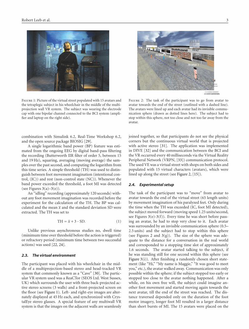
Robert Leeb et al. 3
Figure 1: Picture of the virtual street populated with 15 avatars andthe tetraplegic subject in his wheelchair in the middle of the multi-projection wall VR system. The subject was wearing the electrodecap with one bipolar channel connected to the BCI system (ampli-fier and laptop on the right side).
combination with Simulink 6.2, Real-Time Workshop 6.2,and the open source package BIOSIG [29].
A single logarithmic band power (BP) feature was esti-mated from the ongoing EEG by digital band-pass filteringthe recording (Butterworth IIR filter of order 5, between 15and 19 Hz), squaring, averaging (moving average) the sam-ples over the past second, and computing the logarithm fromthis time series. A simple threshold (TH) was used to distin-guish between foot movement imagination (intentional con-trol, (IC)) and rest (non-control state (NC)). Whenever theband power exceeded the threshold, a foot MI was detected(see Figures 3(a)–3(e)).
An “idling” recording (approximately 120 seconds) with-out any foot movement imagination was recorded before theexperiment for the calculation of the TH. The BP was cal-culated and the mean x and the standard deviation SD wereextracted. The TH was set to
TH = x + 3 · SD. (1)
Unlike previous asynchronous studies no, dwell time(minimum time over threshold before the action is triggered)or refractory period (minimum time between two successfulactions) was used [22, 24].
2.3. The virtual environment
The participant was placed with his wheelchair in the mid-dle of a multiprojection-based stereo and head-tracked VRsystem that commonly known as a “Cave” [30]. The partic-ular VR system used was a ReaCTor (SEOS Ltd. West Sussex,UK) which surrounds the user with three back-projected ac-tive stereo screens (3 walls) and a front-projected screen onthe floor (see Figure 1). Left- and right-eye images are alter-nately displayed at 45 Hz each, and synchronized with Crys-talEye stereo glasses. A special feature of any multiwall VRsystem is that the images on the adjacent walls are seamlessly
Avatar 1
Avatar 2Avatar 3
Figure 2: The task of the participant was to go from avatar toavatar towards the end of the street (outlined with a dashed line).The avatars were lined up and each avatar had its invisible commu-nication sphere (drawn as dotted lines here). The subject had tostop within this sphere, not too close and not too far away from theavatar.
joined together, so that participants do not see the physicalcorners but the continuous virtual world that is projectedwith active stereo [31]. The application was implementedin DIVE [32] and the communication between the BCI andthe VR occurred every 40 milliseconds via the Virtual RealityPeripheral Network (VRPN, [33]) communication protocol.The used VE was a virtual street with shops on both sides andpopulated with 15 virtual characters (avatars), which werelined up along the street (see Figure 2, [15]).
2.4. Experimental setup
The task of the participant was to “move” from avatar toavatar towards the end of the virtual street (65 length units)by movement imagination of his paralyzed feet. Only duringthe time when the TH was exceeded (IC, foot MI detected),the subject moved forward (moving speed 1.25 units/second,see Figures 3(e)-3(f)). Every time he was short before pass-ing an avatar, he had to stop very close to it. Each avatarwas surrounded by an invisible communication sphere (0.5–2.5 units) and the subject had to stop within this sphere(see Figures 2 and 3(g)). The size of the sphere was ade-quate to the distance for a conversation in the real worldand corresponded to a stopping time slot of approximately1.6 seconds. The avatar started talking to the subject, ifhe was standing still for one second within this sphere (seeFigure 3(i)). After finishing a randomly chosen short state-ment (like “Hi,” “My name is Maggie,” “It was good to meetyou,” etc.), the avatar walked away. Communication was onlypossible within the sphere; if the subject stopped too early orstopped too close to the avatar nothing happened. After awhile, on his own free will, the subject could imagine an-other foot movement and started moving again towards thenext avatar, till the end of the street was reached. The dis-tance traversed depended only on the duration of the footmotor imagery, longer foot MI resulted in a larger distancethan short bursts of MI. The 15 avatars were placed on the
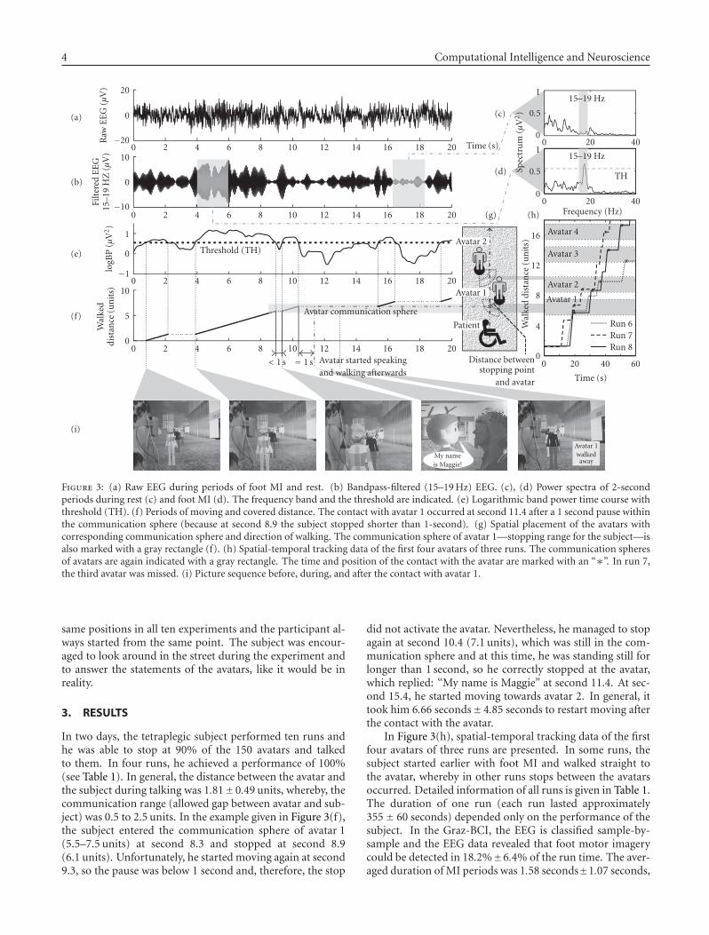
4 Computational Intelligence and Neuroscience
My nameis Maggie!
Avatar 1walkedaway
0 2 4 6 8 10 12 14 16 18 20Avatar started speakingand walking afterwards
< 1 s = 1 s
0
5
10
Wal
ked
dist
ance
(un
its)
Avatar communication sphere
0 2 4 6 8 10 12 14 16 18 20
Threshold (TH)
−1
0
1
logB
P(μ
V2)
0 2 4 6 8 10 12 14 16 18 20−10
0
10
Filt
ered
EE
G15
–19
HZ
(μV
)
0 2 4 6 8 10 12 14 16 18 20−20
0
20
Raw
EE
G(μ
V)
Distance betweenstopping point
and avatar
Patient
Avatar 1
Avatar 2
Time (s)
0 20 40 60
Time (s)
0
4
8
12
16
Wal
ked
dist
ance
(un
its)
Run 6Run 7Run 8
Avatar 1
Avatar 2
Avatar 3
Avatar 4
0 20 40Frequency (Hz)
0
0.5
115–19 Hz
TH
0 20 400
0.5
1
Spec
tru
m(μ
V2)
15–19 Hz
(a)
(b)
(c)
(d)
(e)
(f)
(g) (h)
(i)
∗
Figure 3: (a) Raw EEG during periods of foot MI and rest. (b) Bandpass-filtered (15–19 Hz) EEG. (c), (d) Power spectra of 2-secondperiods during rest (c) and foot MI (d). The frequency band and the threshold are indicated. (e) Logarithmic band power time course withthreshold (TH). (f) Periods of moving and covered distance. The contact with avatar 1 occurred at second 11.4 after a 1 second pause withinthe communication sphere (because at second 8.9 the subject stopped shorter than 1-second). (g) Spatial placement of the avatars withcorresponding communication sphere and direction of walking. The communication sphere of avatar 1—stopping range for the subject—isalso marked with a gray rectangle (f). (h) Spatial-temporal tracking data of the first four avatars of three runs. The communication spheresof avatars are again indicated with a gray rectangle. The time and position of the contact with the avatar are marked with an “∗”. In run 7,the third avatar was missed. (i) Picture sequence before, during, and after the contact with avatar 1.
same positions in all ten experiments and the participant al-ways started from the same point. The subject was encour-aged to look around in the street during the experiment andto answer the statements of the avatars, like it would be inreality.
3. RESULTS
In two days, the tetraplegic subject performed ten runs andhe was able to stop at 90% of the 150 avatars and talkedto them. In four runs, he achieved a performance of 100%(see Table 1). In general, the distance between the avatar andthe subject during talking was 1.81± 0.49 units, whereby, thecommunication range (allowed gap between avatar and sub-ject) was 0.5 to 2.5 units. In the example given in Figure 3(f),the subject entered the communication sphere of avatar 1(5.5–7.5 units) at second 8.3 and stopped at second 8.9(6.1 units). Unfortunately, he started moving again at second9.3, so the pause was below 1 second and, therefore, the stop
did not activate the avatar. Nevertheless, he managed to stopagain at second 10.4 (7.1 units), which was still in the com-munication sphere and at this time, he was standing still forlonger than 1 second, so he correctly stopped at the avatar,which replied: “My name is Maggie” at second 11.4. At sec-ond 15.4, he started moving towards avatar 2. In general, ittook him 6.66 seconds± 4.85 seconds to restart moving afterthe contact with the avatar.
In Figure 3(h), spatial-temporal tracking data of the firstfour avatars of three runs are presented. In some runs, thesubject started earlier with foot MI and walked straight tothe avatar, whereby in other runs stops between the avatarsoccurred. Detailed information of all runs is given in Table 1.The duration of one run (each run lasted approximately355± 60 seconds) depended only on the performance of thesubject. In the Graz-BCI, the EEG is classified sample-by-sample and the EEG data revealed that foot motor imagerycould be detected in 18.2%±6.4% of the run time. The aver-aged duration of MI periods was 1.58 seconds±1.07 seconds,
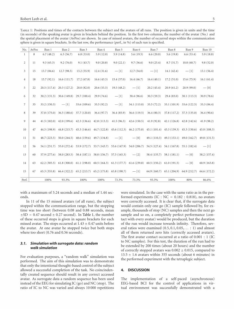
Robert Leeb et al. 5
Table 1: Positions and times of the contacts between the subject and the avatars of all runs. The position is given in units and the time(in seconds) of the speaking avatar is given in brackets behind the position. In the first two columns, the number of the avatar (No.) andthe spatial placement of the avatar (AvPos) are shown. In case of missed avatars, the number of occurred stops within the communicationsphere is given in square brackets. In the last row, the performance (perf., in %) of each run is specified.
No. AvPos Run 1 Run 2 Run 3 Run 4 Run 5 Run 6 Run 7 Run 8 Run 9 Run 10
1 8 6.7 (48.2) 6.3 (56.7) 6.8 (33.0) 5.9 (12.0) 5.9 (14.8) 5.6 (19.5) 6.6 (20.0) 5.6 (19.8) 6.6 (53.4) 5.9 (18.8)
2 11 9.3 (65.3) 9.2 (76.0) 9.1 (43.7) 9.0 (20.8) 9.0 (22.1) 9.7 (36.6) 9.0 (25.4) 8.7 (31.7) 10.0 (60.7) 9.8 (52.0)
3 15 13.7 (84.6) 12.7 (98.5) 13.2 (55.9) 12.4 (31.6) — [1] 12.7 (54.0) — [1] 14.1 (42.4) — [1] 13.1 (56.4)
4 18 15.7 (92.1) 16.6 (111.7) 17.2 (67.8) 16.6 (43.3) 15.4 (37.0) 16.4 (66.7) 16.4 (40.1) 17.2 (51.0) 15.6 (75.9) 16.1 (61.4)
5 22 20.5 (117.4) 20.3 (127.2) 20.0 (82.0) 20.6 (55.5) 19.5 (48.2) — [1] 20.2 (45.4) 20.9 (61.2) 20.9 (99.0) — [0]
6 32 30.2 (131.3) 30.6 (149.8) 29.7 (100.4) 29.9 (74.6) — [1] 30.4 (96.6) 30.3 (59.3) 29.4 (83.0) 30.1 (113.3) 30.9 (78.6)
7 35 33.2 (150.3) — [1] 33.6 (109.6) 33.5 (92.2) — [1] 34.1 (113.0) 33.5 (72.2) 33.1 (101.9) 33.6 (122.5) 33.3 (84.4)
8 39 37.8 (175.0) 36.5 (180.6) 37.7 (120.8) 36.4 (97.7) 36.4 (85.9) 36.6 (119.5) 36.4 (80.3) 37.8 (117.2) 37.3 (135.0) 36.4 (90.6)
9 44 41.5 (182.0) 42.0 (199.6) 42.3 (136.6) 42.8 (113.3) 41.5 (96.3) 42.6 (150.5) 41.9 (92.8) 42.1 (126.8) 42.8 (142.6) 41.9 (98.2)
10 47 44.5 (198.9) 44.8 (215.7) 45.3 (146.6) 44.7 (122.8) 45.6 (112.3) 46.2 (175.8) 45.1 (101.4) 45.3 (139.3) 45.3 (150.6) 45.0 (108.3)
11 51 48.7 (223.5) 50.0 (244.5) 48.6 (159.6) 49.7 (134.8) — [1] — [0] 49.1 (110.3) 49.3 (153.1) 49.0 (162.7) 49.8 (131.5)
12 56 54.1 (251.7) 55.0 (272.4) 53.9 (172.7) 53.7 (143.7) 53.6 (147.9) 54.0 (206.7) 54.5 (127.4) 54.1 (167.8) 55.1 (182.4) — [1]
13 60 57.9 (277.6) 58.0 (283.5) 58.4 (187.1) 58.0 (156.7) 57.5 (165.3) — [2] 58.4 (135.7) 58.1 (181.1) — [0] 58.2 (157.4)
14 63 62.2 (305.5) 61.8 (300.0) 61.1 (198.0) 60.5 (164.3) 61.3 (177.7) 61.6 (239.8) 60.5 (150.2) 61.0 (191.5) — [0] 60.9 (163.8)
15 67 65.3 (355.8) 66.4 (322.2) 65.2 (213.7) 65.2 (175.8) 65.8 (198.7) — [1] 64.9 (160.7) 65.1 (204.9) 64.9 (212.7) 64.6 (172.2)
Perf. 100% 93.3% 100% 100% 73.3% 73.3% 93.3% 100% 80% 86.6%
with a maximum of 5.24 seconds and a median of 1.44 sec-onds.
In 11 of the 15 missed avatars (of all runs), the subjectstopped within the communication range, but the stoppingtime was too short (between 0.08 and 0.88 seconds, mean±SD = 0.47 second ± 0.27 second). In Table 1, the numberof these occurred stops is given in square brackets for eachmissed avatar. The stops occurred at 1.43± 0.47 units beforethe avatar. At one avatar he stopped twice but both stopswhere too short (0.76 and 0.56 seconds).
3.1. Simulation with surrogate data: randomwalk simulation
For evaluation purposes, a “random walk” simulation wasperformed. The aim of this simulation was to demonstratethat only the intentional thought-based control of the subjectallowed a successful completion of the task. No coincinden-tally created sequence should result in any correct accessedavatar. As surrogate data a random sequence has been usedinstead of the EEG for simulating IC (go) and NC (stop). Theratio of IC to NC was varied and always 10 000 repetitions
were simulated. In the case with the same ratio as in the per-formed experiments (IC : NC = 0.182 : 0.818), no avatarswere correctly accessed. It is clear that, if the surrogate datawould contain only one go (IC) sample followed by, for ex-ample, thousands of stop (NC) samples and then the next gosample and so on, a completely perfect performance (con-tact with every avatar) would be produced, but the durationof the run would increase towards infinity. Therefore, sev-eral ratios were examined (0.5, 0.1, 0.05, . . . : 1) and almostall of them returned zero hits (correctly accessed avatars).The first avatar contact occurred at a ratio of 0.001 : 1 (ICto NC samples). For this test, the duration of the run had tobe extended by 200 times (about 20 hours) and the numberof correctly stopped avatars was 0.002 ± 0.015, compared to13.5 ± 1.6 avatars within 355 seconds (about 6 minutes) inthe performed experiment with the tetraplegic subject.
4. DISCUSSION
The implementation of a self-paced (asynchronous)EEG-based BCI for the control of applications in vir-tual environment was successfully demonstrated with a
6 Computational Intelligence and Neuroscience
tetraplegic subject. The patient was able to move forwardin the virtual street and to stop at each avatar with a singlebipolar EEG recording. The prominent induced centrallylocalized beta oscillations, allowed a very simple signal pro-cessing approach (compare Figure 3(c) with Figure 3(d)). Inan interview, the subject confirmed that moving occurredonly during periods of foot motor imagery, but he reportedthat it was hard to stop precisely. Specifically, when theavatars were placed more to the left or right, it was difficultto find the “correct distance” to the avatar. The instructionsgiven to the participant before the experiment did not implythe restriction to perform the experiment as fast as possible,but to take his time to look around, talk to the avatars orenjoy the VR world. Therefore, no statement about theduration of the runs can be given.
In four runs, the subject was able to reach a perfor-mance of 100%, in all other runs, in minimum one avatarwas missed. In most of the missed avatars (except two), thesubject stopped either too shortly within the communicationsphere or stopped close before (too early) or shortly afterthe sphere (too late). The reason for these missed avatarswas the invisible communication sphere around the avatars,which was reported by the subject as the biggest disadvan-tage of this VE. So it was not clear for the subject wherethe sphere started or ended, especially when the avatars wereplaced further away from the middle of the street and thesphere was, therefore, very small. Sometimes he thought tobe close enough, but maybe missed it by a hairbreadth, so anadditional very small “step” (very short foot MI) was neces-sary to come inside the sphere. Unfortunately, it could hap-pen that this step was too large (too long) and the spherealready passed by. Oscillatory EEG components need sometime to appear and stop, so very short bursts (necessary forsuch small steps) are very unlikely to be produced. Maybeit would have been better to visualize the communicationsphere or to change the appearance of the avatar (e.g., thecolor, the expression on the face, etc.) whenever the subjecthas entered the sphere. Nevertheless, the design of the ex-periment with necessary periods of IC (moving) and definedpositions of NC (stopping close to the avatars) guaranteedthat the performance during the asynchronous control couldbe verified. A drawback of the experimental design is that itforced the subject to be able in minimum to stop for 1 sec-ond (NC), but did not force the participant for shorter orlonger periods of IC (no impact on the performance, just in-fluencing the duration of a run). So good NC control wasmore crucial than IC control. Unfortunately, no values forTP and FP can be given for the experiment. Successful stops(90%) could be reported as TP and missed avatars (10%) asFN (false negative), but FP and TN (true negative) cannotbe evaluated. The experiment itself required only periods ofNC for stopping at the avatars and talking to them. There-fore, after reaching the last avatar, the BCI was not stoppedand the subject was instructed to stand still and wait till theVE was shut down. In this period of NC no movement hap-pened (duration between 8 and 93 seconds, mean = 44 sec-onds). The outcome of the simulation with surrogate datashowed that only the intentional control of the subject al-lowed a successful accomplishment of the given task, almost
all simulated data resulted in zero hits (no correct avatar con-tact).
The usage of a visually-rich VE with avatars, which weretalking to the subject, ensured that the experiment was di-verse and even distracting for the subject, somewhat like inthe real world. Nevertheless, the subject was able to suc-ceed with 90%. It is known that the development of skillsor knowledge that are obtained while someone is in a VEcan be transferred to real-world behavior and performance[6, 7]. Indeed, VEs have also been shown to reinforce thebuilding of new neural pathways through imaginations or in-tention to move a paralyzed limb [1, 2]. For a person who iswheelchair-bound, VEs are especially attractive. First, sim-ply using a VE that includes, for example, immersion in analmost all-surrounding stereo world [31] with the freedomto move at will can give such persons access to experiencesthat may be long forgotten (or which they have never had).Another advantage here is that the simulation power of VEscan be used to create virtual prototypes of new navigation orcontrol methods, and give potential users experience of themin a safe environment, before they are ever built physically.
The next step would be to extend the BCI to more thanone IC state, and thereby increase the degree of freedom andallow the subject to choose the direction of moving, for ex-ample, by imagining a left- or right-hand movement [34]. Inthe future, the final goal will be to control a real wheelchairin a real street. This could be supported by applying a sim-ilar procedure as Millan [35] reported during the control ofa miniaturized robot through an 80 × 60 cm representationof an empty flat. Thereby, the BCI was sending only high-level commands (forward, right, follow left wall, etc.) every0.5 second to a finite state automation. The robot was exe-cuting the high-level command (e.g., turn right at next oc-casion) autonomously using its on-board sensors (infraredproximity sensors for obstacles detection) and was continu-ing the command till the next high-level command was sent.Although the difficulties and challenges are more on the sideof the robot/wheelchair as on the side of the BCI, the feasibil-ity of a successful completion of such real-world navigationtask is increased.
5. CONCLUSION
For the first time, it was demonstrated that a tetraplegic sub-ject, sitting in a wheelchair, could control his movements ina VE by the usage of a self-paced (asynchronous) BCI basedon one single EEG recording. The usage of a visual-richVE with talking avatars ensured that the experiment is di-versified and engaging but contains enough distraction as itwould be in a real street. Controlling a VE (e.g., the virtualwheelchair) is the closest possible scenario for controlling thereal wheelchair in a real street, so virtual reality allows pa-tients to perform movements in a safe environment. So afurther step of transferring the BCI from laboratory condi-tions towards real-world applications could be performed.
ACKNOWLEDGMENTS
This work was carried out as part of the PRESENCCIAproject, an EU funded Integrated Project under the IST
Robert Leeb et al. 7
program (Project no. 27731) and supported by OctoberFilms, Hewlett-Packard and the EU COST B27 program. Theauthors would like to thank the subject for his participation.
REFERENCES
[1] M. K. Holden, “Virtual environments for motor rehabilita-tion: review,” Cyberpsychology & Behavior, vol. 8, no. 3, pp.187–211, 2005.
[2] J. Broeren and O. Scott, “Commentary on Holden, M. K., vir-tual environments for motor rehabilitation: review,” CyberPsy-chology & Behavior, vol. 8, no. 3, pp. 212–219, 2005.
[3] D. Jack, R. Boian, A. S. Merians, et al., “Virtual reality-enhanced stroke rehabilitation,” IEEE Transactions on NeuralSystems and Rehabilitation Engineering, vol. 9, no. 3, pp. 308–318, 2001.
[4] M. Girone, G. Burdea, M. Bouzit, V. Popescu, and J. E.Deutsch, “Orthopedic rehabilitation using the “rutgers an-kle” interface,” Studies in Health Technology and Informatics,vol. 70, pp. 89–95, 2000.
[5] J. S. Webster, P. T. McFarland, L. J. Rapport, B. Morrill, L.A. Roades, and P. S. Abadee, “Computer-assisted training forimproving wheelchair mobility in unilateral neglect patients,”Archives of Physical Medicine and Rehabilitation, vol. 82, no. 6,pp. 769–775, 2001.
[6] R. V. Kenyon and M. B. Afenya, “Training in virtual andreal environments,” Annals of Biomedical Engineering, vol. 23,no. 4, pp. 445–455, 1995.
[7] F. D. Rose, E. A. Attree, B. M. Brooks, et al., “Training in vir-tual environments: transfer to real world tasks and equivalenceto real task training,” Ergonomics, vol. 43, no. 4, pp. 494–511,2000.
[8] E. Todorov, R. Shadmehr, and E. Bizzi, “Augmented feedbackpresented in a virtual environment accelerates learning of adifficult motor task,” Journal of Motor Behavior, vol. 29, no. 2,pp. 147–158, 1997.
[9] F. D. Rose, B. M. Brooks, and A. A. Rizzo, “Virtual reality inbrain damage rehabilitation: review,” Cyberpsychology & Be-havior, vol. 8, no. 3, pp. 241–262, 2005.
[10] N. Foreman and J. Stirk, “Commentary on Rose, F. D., Brooks,B. M. & Rizzo, A. A., virtual reality in brain damage rehabili-tation: review,” CyberPsychology & Behavior, vol. 8, no. 3, pp.263–271, 2005.
[11] G. Pfurtscheller and C. Neuper, “Motor imagery and di-rect brain-computer communication,” Proceedings of the IEEE,vol. 89, no. 7, pp. 1123–1134, 2001.
[12] J. R. Wolpaw, N. Birbaumer, D. J. McFarland, G. Pfurtscheller,and T. M. Vaughan, “Brain-computer interfaces for communi-cation and control,” Clinical Neurophysiology, vol. 113, no. 6,pp. 767–791, 2002.
[13] E. C. Lalor, S. P. Kelly, C. Finucane, et al., “Steady-state VEP-based brain-computer interface control in an immersive 3Dgaming environment,” EURASIP Journal on Applied SignalProcessing, vol. 2005, no. 19, pp. 3156–3164, 2005.
[14] J. D. Bayliss, “Use of the evoked potential P3 component forcontrol in a virtual apartment,” IEEE Transactions on NeuralSystems and Rehabilitation Engineering, vol. 11, no. 2, pp. 113–116, 2003.
[15] R. Leeb, C. Keinrath, D. Friedman, et al., “Walking by think-ing: the brainwaves are crucial, not the muscles!,” Presence:Teleoperators and Virtual Environments, vol. 15, no. 5, pp. 500–514, 2006.
[16] G. Pfurtscheller, R. Leeb, C. Keinrath, et al., “Walking fromthought,” Brain Research, vol. 1071, no. 1, pp. 145–152, 2006.
[17] J. F. Borisoff, S. G. Mason, A. Bashashati, and G. E. Birch,“Brain-computer interface design for asynchronous controlapplications: improvements to the LF-ASD asynchronousbrain switch,” IEEE Transactions on Biomedical Engineering,vol. 51, no. 6, pp. 985–992, 2004.
[18] S. G. Mason, J. Kronegg, J. E. Huggins, M. Fatourechi, andA. Schlogl, “Evaluating the performance of self-paced brain-computer interface technology,” Tech. Rep., Brain-InterfaceLaboratory, Neil Squire Society, Vancouver, Canada, 2006.http://www.bci-info.org/.
[19] J. R. Millan and J. Mourino, “Asynchronous BCI and localneural classifiers: an overview of the adaptive brain interfaceproject,” IEEE Transactions on Neural Systems and Rehabilita-tion Engineering, vol. 11, no. 2, pp. 159–161, 2003.
[20] G. R. Muller-Putz, R. Scherer, G. Pfurtscheller, and R. Rupp,“EEG-based neuroprosthesis control: a step towards clinicalpractice,” Neuroscience Letters, vol. 382, no. 1-2, pp. 169–174,2005.
[21] R. Scherer, G. R. Muller-Putz, C. Neuper, B. Graimann, and G.Pfurtscheller, “An asynchronously controlled EEG-based vir-tual keyboard: improvement of the spelling rate,” IEEE Trans-actions on Biomedical Engineering, vol. 51, no. 6, pp. 979–984,2004.
[22] G. Townsend, B. Graimann, and G. Pfurtscheller, “Continu-ous EEG classification during motor imagery-simulation of anasynchronous BCI,” IEEE Transactions on Neural Systems andRehabilitation Engineering, vol. 12, no. 2, pp. 258–265, 2004.
[23] G. Pfurtscheller, C. Guger, G. R. Muller-Putz, G. Krausz,and C. Neuper, “Brain oscillations control hand orthosis in atetraplegic,” Neuroscience Letters, vol. 292, no. 3, pp. 211–214,2000.
[24] G. R. Muller-Putz, R. Scherer, G. Pfurtscheller, and R. Rupp,“Brain-computer interfaces for control of neuroprostheses:from synchronous to asynchronous mode of operation,”Biomedizinische Technik, vol. 51, no. 2, pp. 57–63, 2006.
[25] G. Pfurtscheller, G. R. Muller-Putz, J. Pfurtscheller, H. J.Gerner, and R. Rupp, “‘Thought’—control of functional elec-trical stimulation to restore hand grasp in a patient withtetraplegia,” Neuroscience Letters, vol. 351, no. 1, pp. 33–36,2003.
[26] H. H. Jasper, “The ten-twenty electrode system of the interna-tional federation,” Electroencephalography and Clinical Neuro-physiology, vol. 10, no. 2, pp. 370–375, 1958.
[27] G. Pfurtscheller, G. R. Muller-Putz, A. Schlogl, et al., “15years of BCI research at Graz university of technology: currentprojects,” IEEE Transactions on Neural Systems and Rehabilita-tion Engineering, vol. 14, no. 2, pp. 205–210, 2006.
[28] rtsBCI, “Graz brain-computer interface real-time open sourcepackage,” http://sourceforge.net/projects/biosig/, 2004-2007.
[29] BioSig, “An open source software package for biomedical sig-nal processing under matlab,” http://biosig.sf.net/, 2003-2007.
[30] C. Cruz-Neira, D. J. Sandin, and T. A. DeFanti, “Surround-screen projection-based virtual reality: the design and imple-mentation of the CAVE,” in Proceedings of the 20th AnnualConference on Computer Graphics and Interactive Techniques,pp. 135–142, Anaheim, Calif, USA, August 1993.
[31] M. Slater, A. Steed, and Y. Chrysanthou, Computer Graph-ics and Virtual Environments: From Realism to Real-Time,Addison-Wesley, Boston, Mass, USA, 2001.

8 Computational Intelligence and Neuroscience
[32] E. Frecon, G. Smith, A. Steed, M. Stenius, and O. Stahl, “Anoverview of the COVEN platform,” Presence: Teleoperators andVirtual Environments, vol. 10, no. 1, pp. 109–127, 2001.
[33] VRPN, “Virtual reality peripheral network,” http://www.cs.unc.edu/Research/vrpn/.
[34] R. Scherer, A. Schlogl, F. Lee, H. Bischof, D. Grassi, and G.Pfurtscheller, “The self-paced Graz brain-computer interface:methods and applications,” to appear in Computational Intel-ligence and Neuroscience, 2007.
[35] J. R. Millan, F. Renkens, J. Mourino, and W. Gerstner, “Non-invasive brain-actuated control of a mobile robot by humanEEG,” IEEE Transactions on Biomedical Engineering, vol. 51,no. 6, pp. 1026–1033, 2004.
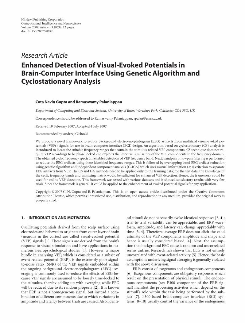
Hindawi Publishing CorporationComputational Intelligence and NeuroscienceVolume 2007, Article ID 28692, 12 pagesdoi:10.1155/2007/28692
Research ArticleEnhanced Detection of Visual-Evoked Potentials inBrain-Computer Interface Using Genetic Algorithm andCyclostationary Analysis
Cota Navin Gupta and Ramaswamy Palaniappan
Department of Computing and Electronic Systems, University of Essex, Wivenhoe Park, Colchester CO4 3SQ, UK
Correspondence should be addressed to Ramaswamy Palaniappan, [email protected]
Received 18 February 2007; Accepted 4 July 2007
Recommended by Andrzej Cichocki
We propose a novel framework to reduce background electroencephalogram (EEG) artifacts from multitrial visual-evoked po-tentials (VEPs) signals for use in brain-computer interface (BCI) design. An algorithm based on cyclostationary (CS) analysis isintroduced to locate the suitable frequency ranges that contain the stimulus-related VEP components. CS technique does not re-quire VEP recordings to be phase locked and exploits the intertrial similarities of the VEP components in the frequency domain.The obtained cyclic frequency spectrum enables detection of VEP frequency band. Next, bandpass or lowpass filtering is performedto reduce the EEG artifacts using these identified frequency ranges. This is followed by overlapping band EEG artifact reductionusing genetic algorithm and independent component analysis (G-ICA) which uses mutual information (MI) criterion to separateEEG artifacts from VEP. The CS and GA methods need to be applied only to the training data; for the test data, the knowledge ofthe cyclic frequency bands and unmixing matrix would be sufficient for enhanced VEP detection. Hence, the framework could beused for online VEP detection. This framework was tested with various datasets and it showed satisfactory results with very fewtrials. Since the framework is general, it could be applied to the enhancement of evoked potential signals for any application.
Copyright © 2007 C. N. Gupta and R. Palaniappan. This is an open access article distributed under the Creative CommonsAttribution License, which permits unrestricted use, distribution, and reproduction in any medium, provided the original work isproperly cited.
1. INTRODUCTION AND MOTIVATION
Oscillating potentials derived from the scalp surface usingelectrodes and believed to originate from outer layer of brain(neurons in the cortex) are called visual-evoked potential(VEP) signals [1]. These signals are derived from the brain’sresponse to visual stimulation and have applications in nu-merous neuropsychological studies [1]. However, a majorhurdle in analysing VEP, which is considered as a subset ofevent-related potential (ERP), is the extremely poor signal-to-noise ratio (SNR) of the VEP signals embedded withinthe ongoing background electroencephalogram (EEG). Av-eraging is commonly used to reduce the effects of EEG be-cause VEP signals are assumed to be loosely time-locked tothe stimulus, thereby adding up with averaging while EEGwill be reduced due to its random property [2]. It is knownthat ERP is not a homogeneous signal, but instead a com-bination of different components due to which variations inamplitude and latency between trials are caused. Also, identi-
cal stimuli do not necessarily evoke identical responses [3, 4];trial-to-trial variability can be appreciable, and ERP wave-form, amplitude, and latency can change appreciably withtime [3, 4]. Therefore, average ERP does not elicit the validestimate of the VEP components amplitude and shape andhence is usually considered biased [4]. Next, the assump-tion that background EEG noise is random and uncorrelatedseems untrue. Research has shown that EEG is not entirelyuncorrelated with event-related activity [5]. Hence, the basicassumptions underlying signal averaging is generally violatedwith the above discussion.
ERPs consist of exogenous and endogenous components[6]. Exogenous components are obligatory responses whichresult on the presentation of physical stimuli. The endoge-nous components (say P300 component of the ERP sig-nal) manifest the processing activities which depend on thestimuli’s role within the task being performed by the sub-ject [7]. P300-based brain-computer interface (BCI) sys-tems [8–10] usually control the variance of the endogenous
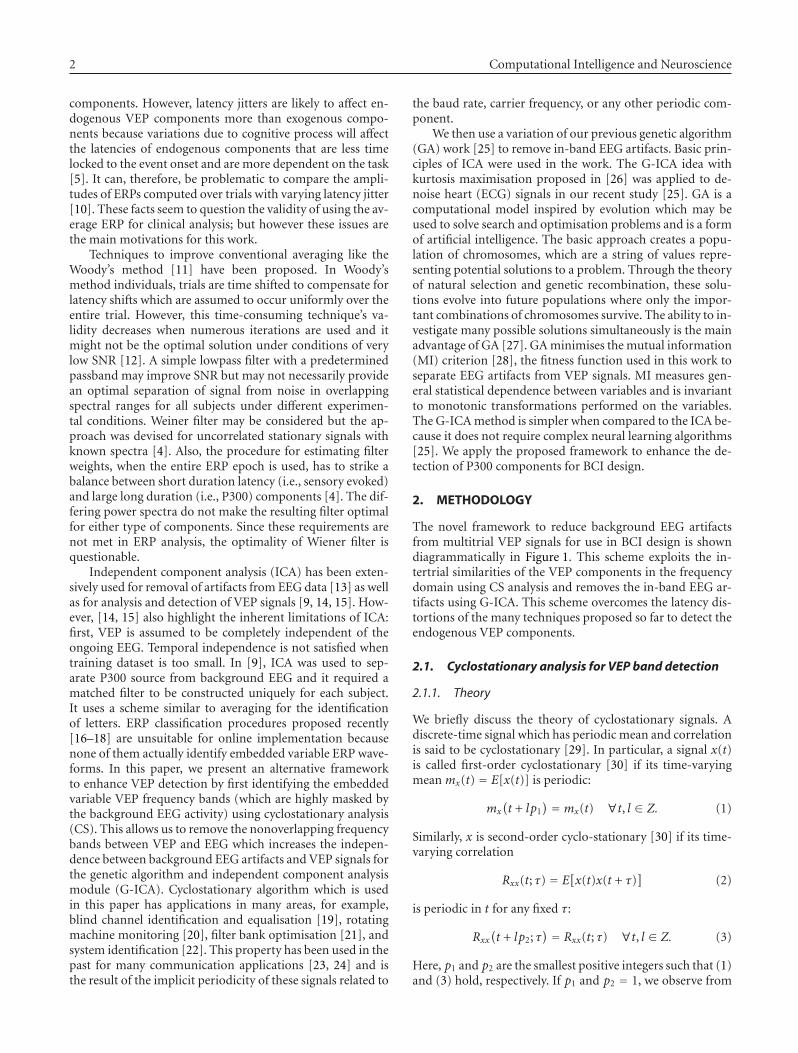
2 Computational Intelligence and Neuroscience
components. However, latency jitters are likely to affect en-dogenous VEP components more than exogenous compo-nents because variations due to cognitive process will affectthe latencies of endogenous components that are less timelocked to the event onset and are more dependent on the task[5]. It can, therefore, be problematic to compare the ampli-tudes of ERPs computed over trials with varying latency jitter[10]. These facts seem to question the validity of using the av-erage ERP for clinical analysis; but however these issues arethe main motivations for this work.
Techniques to improve conventional averaging like theWoody’s method [11] have been proposed. In Woody’smethod individuals, trials are time shifted to compensate forlatency shifts which are assumed to occur uniformly over theentire trial. However, this time-consuming technique’s va-lidity decreases when numerous iterations are used and itmight not be the optimal solution under conditions of verylow SNR [12]. A simple lowpass filter with a predeterminedpassband may improve SNR but may not necessarily providean optimal separation of signal from noise in overlappingspectral ranges for all subjects under different experimen-tal conditions. Weiner filter may be considered but the ap-proach was devised for uncorrelated stationary signals withknown spectra [4]. Also, the procedure for estimating filterweights, when the entire ERP epoch is used, has to strike abalance between short duration latency (i.e., sensory evoked)and large long duration (i.e., P300) components [4]. The dif-fering power spectra do not make the resulting filter optimalfor either type of components. Since these requirements arenot met in ERP analysis, the optimality of Wiener filter isquestionable.
Independent component analysis (ICA) has been exten-sively used for removal of artifacts from EEG data [13] as wellas for analysis and detection of VEP signals [9, 14, 15]. How-ever, [14, 15] also highlight the inherent limitations of ICA:first, VEP is assumed to be completely independent of theongoing EEG. Temporal independence is not satisfied whentraining dataset is too small. In [9], ICA was used to sep-arate P300 source from background EEG and it required amatched filter to be constructed uniquely for each subject.It uses a scheme similar to averaging for the identificationof letters. ERP classification procedures proposed recently[16–18] are unsuitable for online implementation becausenone of them actually identify embedded variable ERP wave-forms. In this paper, we present an alternative frameworkto enhance VEP detection by first identifying the embeddedvariable VEP frequency bands (which are highly masked bythe background EEG activity) using cyclostationary analysis(CS). This allows us to remove the nonoverlapping frequencybands between VEP and EEG which increases the indepen-dence between background EEG artifacts and VEP signals forthe genetic algorithm and independent component analysismodule (G-ICA). Cyclostationary algorithm which is usedin this paper has applications in many areas, for example,blind channel identification and equalisation [19], rotatingmachine monitoring [20], filter bank optimisation [21], andsystem identification [22]. This property has been used in thepast for many communication applications [23, 24] and isthe result of the implicit periodicity of these signals related to
the baud rate, carrier frequency, or any other periodic com-ponent.
We then use a variation of our previous genetic algorithm(GA) work [25] to remove in-band EEG artifacts. Basic prin-ciples of ICA were used in the work. The G-ICA idea withkurtosis maximisation proposed in [26] was applied to de-noise heart (ECG) signals in our recent study [25]. GA is acomputational model inspired by evolution which may beused to solve search and optimisation problems and is a formof artificial intelligence. The basic approach creates a popu-lation of chromosomes, which are a string of values repre-senting potential solutions to a problem. Through the theoryof natural selection and genetic recombination, these solu-tions evolve into future populations where only the impor-tant combinations of chromosomes survive. The ability to in-vestigate many possible solutions simultaneously is the mainadvantage of GA [27]. GA minimises the mutual information(MI) criterion [28], the fitness function used in this work toseparate EEG artifacts from VEP signals. MI measures gen-eral statistical dependence between variables and is invariantto monotonic transformations performed on the variables.The G-ICA method is simpler when compared to the ICA be-cause it does not require complex neural learning algorithms[25]. We apply the proposed framework to enhance the de-tection of P300 components for BCI design.
2. METHODOLOGY
The novel framework to reduce background EEG artifactsfrom multitrial VEP signals for use in BCI design is showndiagrammatically in Figure 1. This scheme exploits the in-tertrial similarities of the VEP components in the frequencydomain using CS analysis and removes the in-band EEG ar-tifacts using G-ICA. This scheme overcomes the latency dis-tortions of the many techniques proposed so far to detect theendogenous VEP components.
2.1. Cyclostationary analysis for VEP band detection
2.1.1. Theory
We briefly discuss the theory of cyclostationary signals. Adiscrete-time signal which has periodic mean and correlationis said to be cyclostationary [29]. In particular, a signal x(t)is called first-order cyclostationary [30] if its time-varyingmean mx(t) = E[x(t)] is periodic:
mx(t + lp1
) = mx(t) ∀t, l ∈ Z. (1)
Similarly, x is second-order cyclo-stationary [30] if its time-varying correlation
Rxx(t; τ) = E[x(t)x(t + τ)
](2)
is periodic in t for any fixed τ:
Rxx(t + lp2; τ
) = Rxx(t; τ) ∀t, l ∈ Z. (3)
Here, p1 and p2 are the smallest positive integers such that (1)and (3) hold, respectively. If p1 and p2 = 1, we observe from
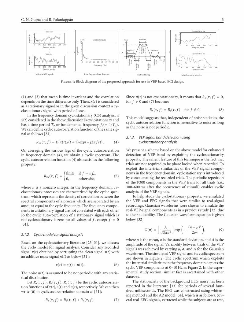
C. N. Gupta and R. Palaniappan 3
−3
−1
1
3
Am
plit
ude
0 50 100 150 200 250 300
Multitrial VEP signals
Sample number...
Trial one
−3
−1
1
3
Am
plit
ude
0 50 100 150 200 250 300Sample number
Trial five
0123456789
10×104
Mag
nit
ude
0 10 20 30 40 50 60 70 80 90
Frequency (Hz)
P300 frequency band detection
Cyclic spectrum Gain Passband
Bandpass filtering
Pass
ban
dri
pple
Stopband Stopband
Stop
ban
dri
pple
Tran
siti
onba
nd
Tran
siti
onba
nd St
opba
nd
ripp
le
Freq
.
1
fs1 fp1 fp2 fs2Fs/2
−2−1
0123
Am
plit
ude
0 50 100 150 200 250 300Sample number
Denoised-trial one
.
.
.
−2
−1
0
1
2
Am
plit
ude
0 50 100 150 200 250 300Sample number
Inband denoising using GA
Denoised-trial five
Figure 1: Block diagram of the proposed approach for use in VEP-based BCI design.
(1) and (3) that mean is time invariant and the correlationdepends on the time difference only. Then, x(t) is consideredas a stationary signal or in the given discussion context a cy-clostationary signal with period of one.
In the frequency domain cyclostationary (CS) analysis, ifx(t) considered in the above discussion is cyclostationary andhas a time period To or fundamental frequency fo(= 1/To).We can define cyclic autocorrelation function of the same sig-nal as follows [23]:
Rxx(τ, f ) = E{x(t)x(t + τ) exp(− j2π f t)}. (4)
On averaging the various lags of the cyclic autocorrelationin frequency domain (4), we obtain a cyclic spectrum. Thecyclic autocorrelation function (4) also satisfies the followingproperty:
Rxx(τ, f ) ={
finite if f = n fo,
0, otherwise,(5)
where n is a nonzero integer. In the frequency domain, cy-clostationary processes are characterized by the cyclic spec-trum, which represents the density of correlation between thespectral components of a process which are separated by anamount equal to the cycle frequency. The frequency compo-nents in a stationary signal are not correlated with each otherso the cyclic autocorrelation of a stationary signal which isnot cyclostationary is zero for all values of f , except f = 0[31].
2.1.2. Cyclo model for signal analysis
Based on the cyclostationary literature [23, 31], we discussthe cyclo model for signal analysis. Consider any recordedsignal x(t) obtained by corrupting the clean signal s(t) withan additive noise signal n(t) as below [31]:
x(t) = s(t) + n(t). (6)
The noise n(t) is assumed to be nonperiodic with any statis-tical distribution.
Let Rx(τ, f ), Rs(τ, f ), Rn(τ, f ) be the cyclic autocorrela-tion functions of x(t), s(t) and n(t), respectively. We can thenwrite (6) in cyclic autocorrelation domain as [31]:
Rx(τ, f ) = Rs(τ, f ) + Rn(τ, f ). (7)
Since n(t) is not cyclostationary, it means that Rn(τ, f ) = 0,for f �= 0 and (7) becomes
Rx(τ, f ) = Rs(τ, f ) for f �= 0. (8)
This model suggests that, independent of noise statistics, thecyclic autocorrelation function is insensitive to noise as longas the noise is not periodic.
2.1.3. VEP signal band detection usingcyclostationary analysis
We present a scheme based on the above model for enhanceddetection of VEP band by exploiting the cyclostationarityproperty. The salient feature of this technique is the fact thattrials are not required to be phase locked when recorded. Toexploit the intertrial similarities of the VEP signal compo-nents in the frequency domain, cyclostationary is introducedby concatenating the recorded trials. The periodic repetitionof the P300 components in the VEP trials for all trials (i.e.,300–600 ms after the occurrence of stimuli) enables cyclicanalysis of the VEP signals.
To help study the cyclostationary property, we emulatedthe VEP and EEG signals that were similar to real-signalrecordings. Gaussian waveforms were chosen to emulate thereal-VEP-signal components as in a previous study [32] dueto their suitability. The Gaussian waveform equation is givenbelow [32]:
G(n) =[
A√2πσ2
]exp
(− (n− μ)2
2σ2
), (9)
where μ is the mean, σ is the standard deviation, and A is theamplitude of the signal. Variability between trials of the VEPsignals was achieved by varying μ, σ , and A for the Gaussianwaveforms. The simulated VEP signal and its cyclic spectrumare shown in Figure 2. The cyclic spectrum which exploitsthe inter trial similarities in the frequency domain depicts thecyclic VEP components at 0–10 Hz as Figure 2. In the exper-imental study section, similar fact is ascertained with otherdatasets.
The stationarity of the background EEG noise has beenreported in the literature [33] for periods of several hun-dred milliseconds. The EEG was constructed using whiten-ing method and the AR model [34], which is as follows. Sev-eral real-EEG-signals, extracted while the subjects are at rest,
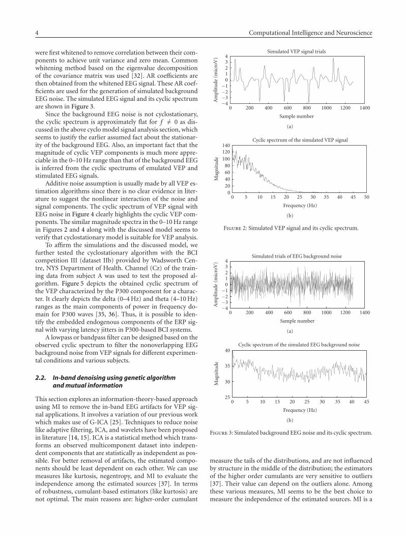
4 Computational Intelligence and Neuroscience
were first whitened to remove correlation between their com-ponents to achieve unit variance and zero mean. Commonwhitening method based on the eigenvalue decompositionof the covariance matrix was used [32]. AR coefficients arethen obtained from the whitened EEG signal. These AR coef-ficients are used for the generation of simulated backgroundEEG noise. The simulated EEG signal and its cyclic spectrumare shown in Figure 3.
Since the background EEG noise is not cyclostationary,the cyclic spectrum is approximately flat for f �= 0 as dis-cussed in the above cyclo model signal analysis section, whichseems to justify the earlier assumed fact about the stationar-ity of the background EEG. Also, an important fact that themagnitude of cyclic VEP components is much more appre-ciable in the 0–10 Hz range than that of the background EEGis inferred from the cyclic spectrums of emulated VEP andstimulated EEG signals.
Additive noise assumption is usually made by all VEP es-timation algorithms since there is no clear evidence in liter-ature to suggest the nonlinear interaction of the noise andsignal components. The cyclic spectrum of VEP signal withEEG noise in Figure 4 clearly highlights the cyclic VEP com-ponents. The similar magnitude spectra in the 0–10 Hz rangein Figures 2 and 4 along with the discussed model seems toverify that cyclostationary model is suitable for VEP analysis.
To affirm the simulations and the discussed model, wefurther tested the cyclostationary algorithm with the BCIcompetition III (dataset IIb) provided by Wadsworth Cen-tre, NYS Department of Health. Channel (Cz) of the train-ing data from subject A was used to test the proposed al-gorithm. Figure 5 depicts the obtained cyclic spectrum ofthe VEP characterized by the P300 component for a charac-ter. It clearly depicts the delta (0–4 Hz) and theta (4–10 Hz)ranges as the main components of power in frequency do-main for P300 waves [35, 36]. Thus, it is possible to iden-tify the embedded endogenous components of the ERP sig-nal with varying latency jitters in P300-based BCI systems.
A lowpass or bandpass filter can be designed based on theobserved cyclic spectrum to filter the nonoverlapping EEGbackground noise from VEP signals for different experimen-tal conditions and various subjects.
2.2. In-band denoising using genetic algorithmand mutual information
This section explores an information-theory-based approachusing MI to remove the in-band EEG artifacts for VEP sig-nal applications. It involves a variation of our previous workwhich makes use of G-ICA [25]. Techniques to reduce noiselike adaptive filtering, ICA, and wavelets have been proposedin literature [14, 15]. ICA is a statistical method which trans-forms an observed multicomponent dataset into indepen-dent components that are statistically as independent as pos-sible. For better removal of artifacts, the estimated compo-nents should be least dependent on each other. We can usemeasures like kurtosis, negentropy, and MI to evaluate theindependence among the estimated sources [37]. In termsof robustness, cumulant-based estimators (like kurtosis) arenot optimal. The main reasons are: higher-order cumulant
−4−3−2−1
01234
Am
plit
ude
(mic
roV
)
0 200 400 600 800 1000 1200 1400
Sample number
Simulated VEP signal trials
(a)
020406080
100120140
Mag
nit
ude
0 5 10 15 20 25 30 35 40 45 50
Frequency (Hz)
Cyclic spectrum of the simulated VEP signal
(b)
Figure 2: Simulated VEP signal and its cyclic spectrum.
−4−3−2−1
01234
Am
plit
ude
(mic
roV
)
0 200 400 600 800 1000 1200 1400
Sample number
Simulated trials of EEG background noise
(a)
25
30
35
40
Mag
nit
ude
0 5 10 15 20 25 30 35 40 45
Frequency (Hz)
Cyclic spectrum of the simulated EEG background noise
(b)
Figure 3: Simulated background EEG noise and its cyclic spectrum.
measure the tails of the distributions, and are not influencedby structure in the middle of the distribution; the estimatorsof the higher order cumulants are very sensitive to outliers[37]. Their value can depend on the outliers alone. Amongthese various measures, MI seems to be the best choice tomeasure the independence of the estimated sources. MI is a
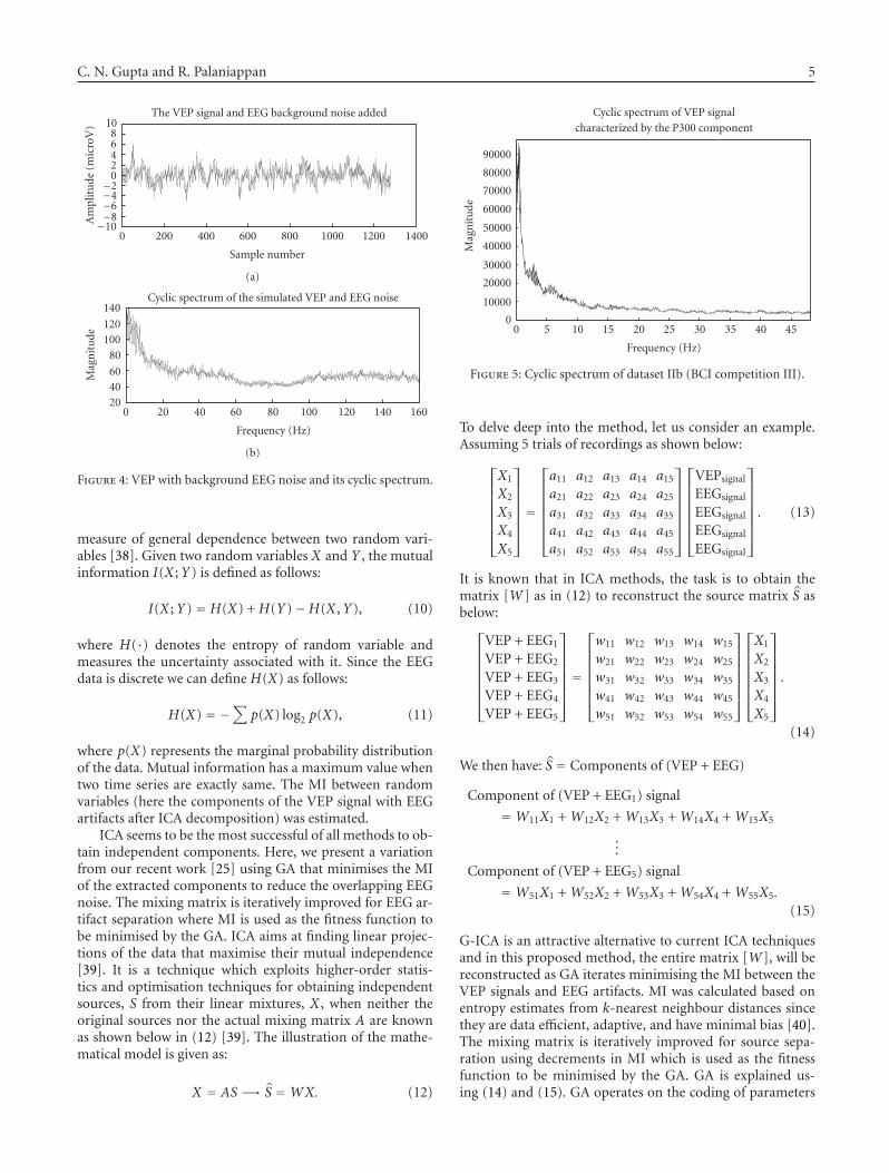
C. N. Gupta and R. Palaniappan 5
−10−8−6−4−2
02468
10
Am
plit
ude
(mic
roV
)
0 200 400 600 800 1000 1200 1400
Sample number
The VEP signal and EEG background noise added
(a)
204060
80100120
140
Mag
nit
ude
0 20 40 60 80 100 120 140 160
Frequency (Hz)
Cyclic spectrum of the simulated VEP and EEG noise
(b)
Figure 4: VEP with background EEG noise and its cyclic spectrum.
measure of general dependence between two random vari-ables [38]. Given two random variables X and Y , the mutualinformation I(X ;Y) is defined as follows:
I(X ;Y) = H(X) +H(Y)−H(X ,Y), (10)
where H(·) denotes the entropy of random variable andmeasures the uncertainty associated with it. Since the EEGdata is discrete we can define H(X) as follows:
H(X) = −∑
p(X) log2 p(X), (11)
where p(X) represents the marginal probability distributionof the data. Mutual information has a maximum value whentwo time series are exactly same. The MI between randomvariables (here the components of the VEP signal with EEGartifacts after ICA decomposition) was estimated.
ICA seems to be the most successful of all methods to ob-tain independent components. Here, we present a variationfrom our recent work [25] using GA that minimises the MIof the extracted components to reduce the overlapping EEGnoise. The mixing matrix is iteratively improved for EEG ar-tifact separation where MI is used as the fitness function tobe minimised by the GA. ICA aims at finding linear projec-tions of the data that maximise their mutual independence[39]. It is a technique which exploits higher-order statis-tics and optimisation techniques for obtaining independentsources, S from their linear mixtures, X , when neither theoriginal sources nor the actual mixing matrix A are knownas shown below in (12) [39]. The illustration of the mathe-matical model is given as:
X = AS −→ S =WX. (12)
0
10000
20000
30000
40000
50000
60000
70000
80000
90000
Mag
nit
ude
0 5 10 15 20 25 30 35 40 45
Frequency (Hz)
Cyclic spectrum of VEP signalcharacterized by the P300 component
Figure 5: Cyclic spectrum of dataset IIb (BCI competition III).
To delve deep into the method, let us consider an example.Assuming 5 trials of recordings as shown below:
⎡
⎢⎢⎢⎢⎢⎢⎣
X1
X2
X3
X4
X5
⎤
⎥⎥⎥⎥⎥⎥⎦
=
⎡
⎢⎢⎢⎢⎢⎢⎣
a11 a12 a13 a14 a15
a21 a22 a23 a24 a25
a31 a32 a33 a34 a35
a41 a42 a43 a44 a45
a51 a52 a53 a54 a55
⎤
⎥⎥⎥⎥⎥⎥⎦
⎡
⎢⎢⎢⎢⎢⎢⎣
VEPsignal
EEGsignal
EEGsignal
EEGsignal
EEGsignal
⎤
⎥⎥⎥⎥⎥⎥⎦
. (13)
It is known that in ICA methods, the task is to obtain thematrix [W] as in (12) to reconstruct the source matrix S asbelow:⎡
⎢⎢⎢⎢⎢⎢⎣
VEP + EEG1
VEP + EEG2
VEP + EEG3
VEP + EEG4
VEP + EEG5
⎤
⎥⎥⎥⎥⎥⎥⎦
=
⎡
⎢⎢⎢⎢⎢⎢⎣
w11 w12 w13 w14 w15
w21 w22 w23 w24 w25
w31 w32 w33 w34 w35
w41 w42 w43 w44 w45
w51 w52 w53 w54 w55
⎤
⎥⎥⎥⎥⎥⎥⎦
⎡
⎢⎢⎢⎢⎢⎢⎣
X1
X2
X3
X4
X5
⎤
⎥⎥⎥⎥⎥⎥⎦
.
(14)
We then have: S = Components of (VEP + EEG)
Component of (VEP + EEG1) signal
=W11X1 +W12X2 +W13X3 +W14X4 +W15X5
...
Component of (VEP + EEG5) signal
=W51X1 +W52X2 +W53X3 +W54X4 +W55X5.(15)
G-ICA is an attractive alternative to current ICA techniquesand in this proposed method, the entire matrix [W], will bereconstructed as GA iterates minimising the MI between theVEP signals and EEG artifacts. MI was calculated based onentropy estimates from k-nearest neighbour distances sincethey are data efficient, adaptive, and have minimal bias [40].The mixing matrix is iteratively improved for source sepa-ration using decrements in MI which is used as the fitnessfunction to be minimised by the GA. GA is explained us-ing (14) and (15). GA operates on the coding of parameters
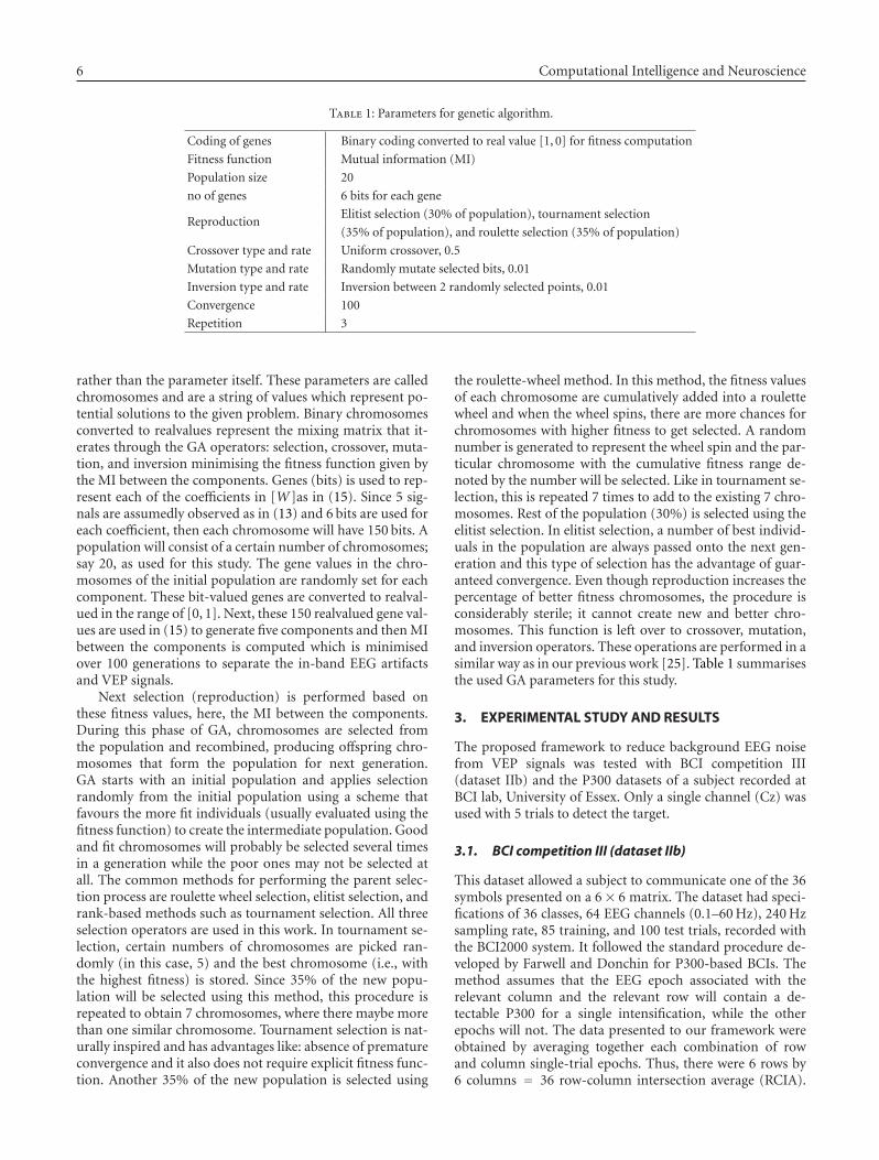
6 Computational Intelligence and Neuroscience
Table 1: Parameters for genetic algorithm.
Coding of genes Binary coding converted to real value [1, 0] for fitness computation
Fitness function Mutual information (MI)
Population size 20
no of genes 6 bits for each gene
ReproductionElitist selection (30% of population), tournament selection
(35% of population), and roulette selection (35% of population)
Crossover type and rate Uniform crossover, 0.5
Mutation type and rate Randomly mutate selected bits, 0.01
Inversion type and rate Inversion between 2 randomly selected points, 0.01
Convergence 100
Repetition 3
rather than the parameter itself. These parameters are calledchromosomes and are a string of values which represent po-tential solutions to the given problem. Binary chromosomesconverted to realvalues represent the mixing matrix that it-erates through the GA operators: selection, crossover, muta-tion, and inversion minimising the fitness function given bythe MI between the components. Genes (bits) is used to rep-resent each of the coefficients in [W]as in (15). Since 5 sig-nals are assumedly observed as in (13) and 6 bits are used foreach coefficient, then each chromosome will have 150 bits. Apopulation will consist of a certain number of chromosomes;say 20, as used for this study. The gene values in the chro-mosomes of the initial population are randomly set for eachcomponent. These bit-valued genes are converted to realval-ued in the range of [0, 1]. Next, these 150 realvalued gene val-ues are used in (15) to generate five components and then MIbetween the components is computed which is minimisedover 100 generations to separate the in-band EEG artifactsand VEP signals.
Next selection (reproduction) is performed based onthese fitness values, here, the MI between the components.During this phase of GA, chromosomes are selected fromthe population and recombined, producing offspring chro-mosomes that form the population for next generation.GA starts with an initial population and applies selectionrandomly from the initial population using a scheme thatfavours the more fit individuals (usually evaluated using thefitness function) to create the intermediate population. Goodand fit chromosomes will probably be selected several timesin a generation while the poor ones may not be selected atall. The common methods for performing the parent selec-tion process are roulette wheel selection, elitist selection, andrank-based methods such as tournament selection. All threeselection operators are used in this work. In tournament se-lection, certain numbers of chromosomes are picked ran-domly (in this case, 5) and the best chromosome (i.e., withthe highest fitness) is stored. Since 35% of the new popu-lation will be selected using this method, this procedure isrepeated to obtain 7 chromosomes, where there maybe morethan one similar chromosome. Tournament selection is nat-urally inspired and has advantages like: absence of prematureconvergence and it also does not require explicit fitness func-tion. Another 35% of the new population is selected using
the roulette-wheel method. In this method, the fitness valuesof each chromosome are cumulatively added into a roulettewheel and when the wheel spins, there are more chances forchromosomes with higher fitness to get selected. A randomnumber is generated to represent the wheel spin and the par-ticular chromosome with the cumulative fitness range de-noted by the number will be selected. Like in tournament se-lection, this is repeated 7 times to add to the existing 7 chro-mosomes. Rest of the population (30%) is selected using theelitist selection. In elitist selection, a number of best individ-uals in the population are always passed onto the next gen-eration and this type of selection has the advantage of guar-anteed convergence. Even though reproduction increases thepercentage of better fitness chromosomes, the procedure isconsiderably sterile; it cannot create new and better chro-mosomes. This function is left over to crossover, mutation,and inversion operators. These operations are performed in asimilar way as in our previous work [25]. Table 1 summarisesthe used GA parameters for this study.
3. EXPERIMENTAL STUDY AND RESULTS
The proposed framework to reduce background EEG noisefrom VEP signals was tested with BCI competition III(dataset IIb) and the P300 datasets of a subject recorded atBCI lab, University of Essex. Only a single channel (Cz) wasused with 5 trials to detect the target.
3.1. BCI competition III (dataset IIb)
This dataset allowed a subject to communicate one of the 36symbols presented on a 6× 6 matrix. The dataset had speci-fications of 36 classes, 64 EEG channels (0.1–60 Hz), 240 Hzsampling rate, 85 training, and 100 test trials, recorded withthe BCI2000 system. It followed the standard procedure de-veloped by Farwell and Donchin for P300-based BCIs. Themethod assumes that the EEG epoch associated with therelevant column and the relevant row will contain a de-tectable P300 for a single intensification, while the otherepochs will not. The data presented to our framework wereobtained by averaging together each combination of rowand column single-trial epochs. Thus, there were 6 rows by6 columns = 36 row-column intersection average (RCIA).
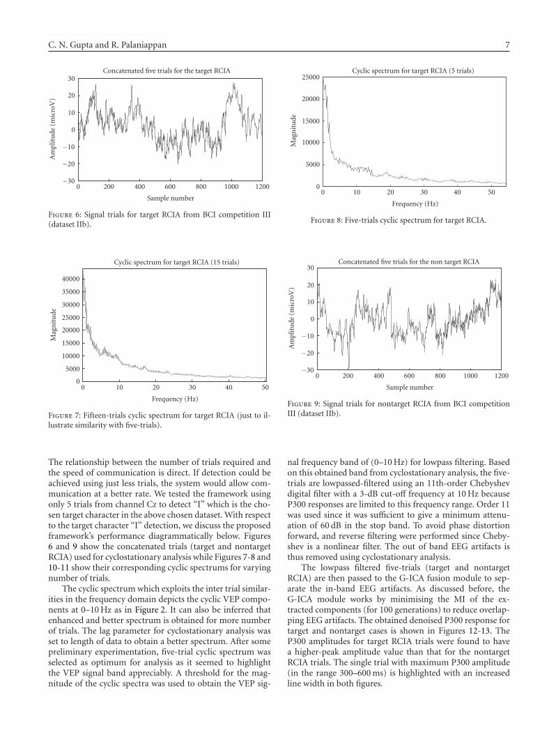
C. N. Gupta and R. Palaniappan 7
−30
−20
−10
0
10
20
30
Am
plit
ude
(mic
roV
)
0 200 400 600 800 1000 1200
Sample number
Concatenated five trials for the target RCIA
Figure 6: Signal trials for target RCIA from BCI competition III(dataset IIb).
0
5000
10000
15000
20000
25000
30000
35000
40000
Mag
nit
ude
0 10 20 30 40 50
Frequency (Hz)
Cyclic spectrum for target RCIA (15 trials)
Figure 7: Fifteen-trials cyclic spectrum for target RCIA (just to il-lustrate similarity with five-trials).
The relationship between the number of trials required andthe speed of communication is direct. If detection could beachieved using just less trials, the system would allow com-munication at a better rate. We tested the framework usingonly 5 trials from channel Cz to detect “I” which is the cho-sen target character in the above chosen dataset. With respectto the target character “I” detection, we discuss the proposedframework’s performance diagrammatically below. Figures6 and 9 show the concatenated trials (target and nontargetRCIA) used for cyclostationary analysis while Figures 7-8 and10-11 show their corresponding cyclic spectrums for varyingnumber of trials.
The cyclic spectrum which exploits the inter trial similar-ities in the frequency domain depicts the cyclic VEP compo-nents at 0–10 Hz as in Figure 2. It can also be inferred thatenhanced and better spectrum is obtained for more numberof trials. The lag parameter for cyclostationary analysis wasset to length of data to obtain a better spectrum. After somepreliminary experimentation, five-trial cyclic spectrum wasselected as optimum for analysis as it seemed to highlightthe VEP signal band appreciably. A threshold for the mag-nitude of the cyclic spectra was used to obtain the VEP sig-
0
5000
10000
15000
20000
25000
Mag
nit
ude
0 10 20 30 40 50
Frequency (Hz)
Cyclic spectrum for target RCIA (5 trials)
Figure 8: Five-trials cyclic spectrum for target RCIA.
−30
−20
−10
0
10
20
30
Am
plit
ude
(mic
roV
)
0 200 400 600 800 1000 1200
Sample number
Concatenated five trials for the non target RCIA
Figure 9: Signal trials for nontarget RCIA from BCI competitionIII (dataset IIb).
nal frequency band of (0–10 Hz) for lowpass filtering. Basedon this obtained band from cyclostationary analysis, the five-trials are lowpassed-filtered using an 11th-order Chebyshevdigital filter with a 3-dB cut-off frequency at 10 Hz becauseP300 responses are limited to this frequency range. Order 11was used since it was sufficient to give a minimum attenu-ation of 60 dB in the stop band. To avoid phase distortionforward, and reverse filtering were performed since Cheby-shev is a nonlinear filter. The out of band EEG artifacts isthus removed using cyclostationary analysis.
The lowpass filtered five-trials (target and nontargetRCIA) are then passed to the G-ICA fusion module to sep-arate the in-band EEG artifacts. As discussed before, theG-ICA module works by minimising the MI of the ex-tracted components (for 100 generations) to reduce overlap-ping EEG artifacts. The obtained denoised P300 response fortarget and nontarget cases is shown in Figures 12-13. TheP300 amplitudes for target RCIA trials were found to havea higher-peak amplitude value than that for the nontargetRCIA trials. The single trial with maximum P300 amplitude(in the range 300–600 ms) is highlighted with an increasedline width in both figures.

8 Computational Intelligence and Neuroscience
0
5000
10000
15000
20000
Mag
nit
ude
0 5 10 15 20 25 30 35 40 45
Frequency (Hz)
Cyclic spectrum for non target RCIA (15 trials)
Figure 10: Fifteen-trial cyclic spectrum for nontarget RCIA.
0
2000
4000
6000
8000
10000
12000
14000
16000
Mag
nit
ude
0 5 10 15 20 25 30 35 40 45
Frequency (Hz)
Cyclic spectrum for non target RCIA (5 trials)
Figure 11: Five-trials cyclic spectrum for nontarget RCIA.
−1.5
−1
−0.5
0
0.5
1
1.5
Am
plit
ude
(mic
roV
)
0 200 400 600 800 1000
Time (ms)
Five trials of target character obtained after G-ICA module
Figure 12: Detected P300 component for target RCIA showinghigher peak amplitude.
3.2. BCI labs, Essex dataset
The presented framework was also tested offline from adataset for a biometric application. Similar to the Donchinparadigm, the application had seven blocks of colours whichwere flashed to evoke P300 components. Sequences wereblock randomised, which means, after seven flashes each
−0.8
−0.6
−0.4
−0.20
0.20.4
0.6
0.8
11.2
Am
plit
ude
(mic
roV
)
0 200 400 600 800 1000
Time (ms)
Five trials of non target characterobtained after G-ICA module
Figure 13: Detected P300 component for nontarget RCIA showinglower peak amplitude.
−4
−3
−2
−1
0
1
2
3
4
Am
plit
ude
(mic
roV
)
0 200 400 600 800 1000 1200 1400
Sample number
Five trials of the target color block and its cyclic spectrum
(a)
0
50
100
150
200
250
Mag
nit
ude
0 10 20 30
Frequency (Hz)
(b)
Figure 14: Trials for target colour block and its cyclic spectrum.
colour was flashed once, after fourteen flashes each colourwas flashed twice. Forty trials were recorded (each trial had7 flashes of the colour block). The subject was asked to fo-cus on a single-colour block (say red) and also keep a countof the number of times it flashed, which enabled monitor-ing the performance of the subject. The colour blocks wereflashed for 100 millisecond with an interstimulus interval

C. N. Gupta and R. Palaniappan 9
−4
−3
−2
−1
0
1
2
3
4
Am
plit
ude
(mic
roV
)
0 200 400 600 800 1000 1200 1400
Sample number
Five trials of the non target color block and its cyclic spectrum
(a)
0
50
100
150
Mag
nit
ude
0 10 20 30 40 50 60 70
Frequency (Hz)
(b)
Figure 15: Trials for nontarget colour block and its cyclic spectrum.
of 300 millisecond. EEG recordings were carried out on aBiosemi Active Two system using 34 channels (32 on a scalpand 2 on either mastoids); however, only channel Cz wasused. Data was sampled at 256 Hz with no filtering. The sub-ject was a male aged 27 who had experience of using theBCIs before, with no known neurological disorders. The per-formance of the framework for target and nontarget colorblocks is discussed below diagrammatically. It can be seenfrom Figure 14 that the target-trial data is cyclic in time do-main and also that the magnitude of the cyclic spectrum ismuch higher than that of the nontarget data as in Figure 15.The lag parameter for cyclostationary analysis was set tolength of data. After some preliminary experimentation, five-trial cyclic spectrums were again found to be optimum foranalysis as it seemed to highlight the VEP signal band appre-ciably. A threshold for the magnitude of the cyclic spectra wasused to obtain the VEP signal frequency band of (0–10 Hz)for lowpass filtering. Based on this obtained band from cy-clostationary analysis, a lowpass filter for (target colour blockand nontarget colour block) was used as in Section 3.1 to re-move nonoverlapping EEG artifacts and the output is shownin Figures 16-17.
The five-trials (target colour block and nontarget colourblock) are then passed to G-ICA fusion module. InvestigatingFigures 18-19 clearly shows that the P300 component ampli-tude in the 300–600 millisecond range is higher for target-
−2
−1
0
1
2
3
4
Am
plit
ude
(mic
roV
)
0 200 400 600 800 1000
Time (ms)
Five trials of target signal after outof band cyclostationary denoising
Figure 16: Lowpassed-filtered trials for target colour block.
−3
−2
−1
0
1
2
3
Am
plit
ude
(mic
roV
)
0 200 400 600 800 1000
Time (ms)
Five trials of non target signal afterout of band cyclostationary denoising
Figure 17: Lowpassed-filtered trials for nontarget colour block.
−2
−1
0
1
2
3
4
Am
plit
ude
(mic
roV
)
0 200 400 600 800 1000
Time (ms)
Five trials of target color block obtained after G-ICA module
Figure 18: P300 components of the five-trials for target colourblock using G-ICA.
colour block than the nontarget colour block. The single trialwith maximum P300 amplitude is highlighted with an in-creased line width in both the figures. It was also observedthat the frequency band (CS analysis) and the unmixing ma-trix (G-ICA) do not change over trials.
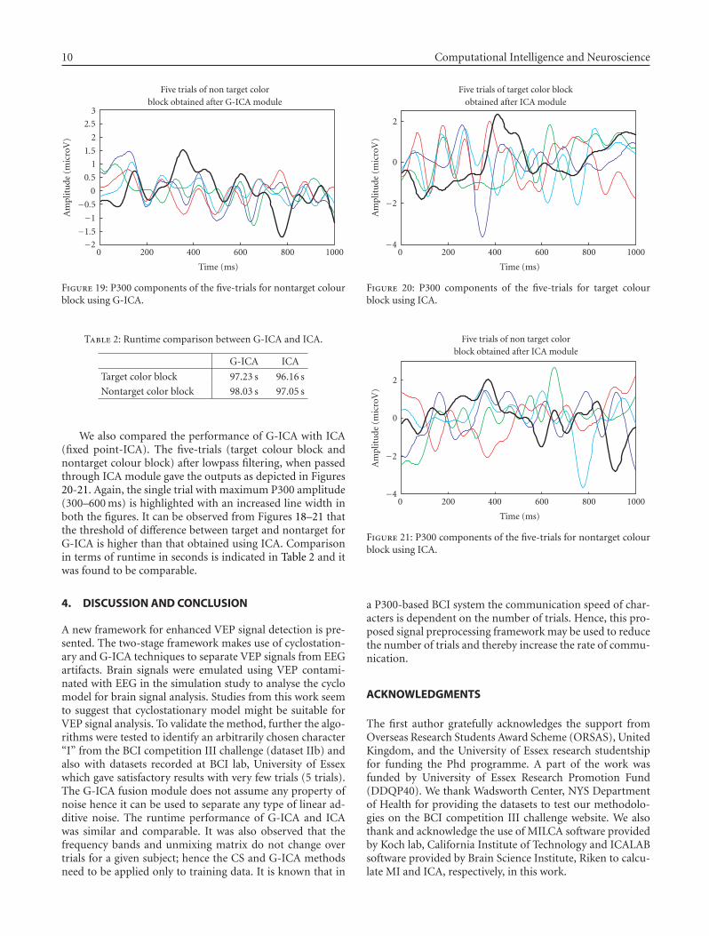
10 Computational Intelligence and Neuroscience
−2
−1.5
−1
−0.5
0
0.5
1
1.5
2
2.5
3
Am
plit
ude
(mic
roV
)
0 200 400 600 800 1000
Time (ms)
Five trials of non target colorblock obtained after G-ICA module
Figure 19: P300 components of the five-trials for nontarget colourblock using G-ICA.
Table 2: Runtime comparison between G-ICA and ICA.
G-ICA ICA
Target color block 97.23 s 96.16 s
Nontarget color block 98.03 s 97.05 s
We also compared the performance of G-ICA with ICA(fixed point-ICA). The five-trials (target colour block andnontarget colour block) after lowpass filtering, when passedthrough ICA module gave the outputs as depicted in Figures20-21. Again, the single trial with maximum P300 amplitude(300–600 ms) is highlighted with an increased line width inboth the figures. It can be observed from Figures 18–21 thatthe threshold of difference between target and nontarget forG-ICA is higher than that obtained using ICA. Comparisonin terms of runtime in seconds is indicated in Table 2 and itwas found to be comparable.
4. DISCUSSION AND CONCLUSION
A new framework for enhanced VEP signal detection is pre-sented. The two-stage framework makes use of cyclostation-ary and G-ICA techniques to separate VEP signals from EEGartifacts. Brain signals were emulated using VEP contami-nated with EEG in the simulation study to analyse the cyclomodel for brain signal analysis. Studies from this work seemto suggest that cyclostationary model might be suitable forVEP signal analysis. To validate the method, further the algo-rithms were tested to identify an arbitrarily chosen character“I” from the BCI competition III challenge (dataset IIb) andalso with datasets recorded at BCI lab, University of Essexwhich gave satisfactory results with very few trials (5 trials).The G-ICA fusion module does not assume any property ofnoise hence it can be used to separate any type of linear ad-ditive noise. The runtime performance of G-ICA and ICAwas similar and comparable. It was also observed that thefrequency bands and unmixing matrix do not change overtrials for a given subject; hence the CS and G-ICA methodsneed to be applied only to training data. It is known that in
−4
−2
0
2
Am
plit
ude
(mic
roV
)
0 200 400 600 800 1000
Time (ms)
Five trials of target color blockobtained after ICA module
Figure 20: P300 components of the five-trials for target colourblock using ICA.
−4
−2
0
2A
mpl
itu
de(m
icro
V)
0 200 400 600 800 1000
Time (ms)
Five trials of non target colorblock obtained after ICA module
Figure 21: P300 components of the five-trials for nontarget colourblock using ICA.
a P300-based BCI system the communication speed of char-acters is dependent on the number of trials. Hence, this pro-posed signal preprocessing framework may be used to reducethe number of trials and thereby increase the rate of commu-nication.
ACKNOWLEDGMENTS
The first author gratefully acknowledges the support fromOverseas Research Students Award Scheme (ORSAS), UnitedKingdom, and the University of Essex research studentshipfor funding the Phd programme. A part of the work wasfunded by University of Essex Research Promotion Fund(DDQP40). We thank Wadsworth Center, NYS Departmentof Health for providing the datasets to test our methodolo-gies on the BCI competition III challenge website. We alsothank and acknowledge the use of MILCA software providedby Koch lab, California Institute of Technology and ICALABsoftware provided by Brain Science Institute, Riken to calcu-late MI and ICA, respectively, in this work.
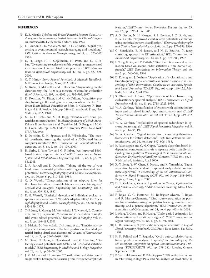
C. N. Gupta and R. Palaniappan 11
REFERENCES
[1] K. E. Misulis, Sphelmann’s Evoked Potential Primer: Visual, Au-ditory, and Somatosensory Evoked Potentials in Clinical Diagno-sis, Butterworth-Heinemann, Oxford, UK, 1994.
[2] J. I. Aunon, C. D. McGillem, and D. G. Childers, “Signal pro-cessing in event potential research: averaging and modelling,”CRC Critical Reviews in Bioengineering, vol. 5, pp. 323–367,1981.
[3] D. H. Lange, H. T. Siegelmann, H. Pratt, and G. F. In-bar, “Overcoming selective ensemble averaging: unsupervisedidentification of event-related brain potentials,” IEEE Transac-tions on Biomedical Engineering, vol. 47, no. 6, pp. 822–826,2000.
[4] C. T. Handy, Event-Related Potentials: A Methods Handbook,MIT Press, Cambridge, Mass, USA, 2005.
[5] M. Kutas, G. McCarthy, and E. Donchin, “Augmenting mentalchronometry: the P300 as a measure of stimulus evaluationtime,” Science, vol. 197, no. 4305, pp. 792–795, 1977.
[6] E. Donchin, W. Ritter, and C. McCallum, “Cognitive psy-chophysiology: the endogenous components of the ERP,” inBrain Event-Related Potentials in Man, E. Callaway, P. Tuet-ing, and S. H. Koslow, Eds., pp. 349–411, Academic Press, NewYork, NY, USA, 1978.
[7] M. G. H. Coles and M. D. Rugg, “Event-related brain po-tentials: an introduction,” in Electrophysiology of Mind: Event-Related Brain Potentials and Cognition, M. D. Rugg and M. G.H. Coles, Eds., pp. 1–26, Oxford University Press, New York,NY, USA, 1995.
[8] E. Donchin, K. M. Spencer, and R. Wijesinghe, “The men-tal prosthesis: assessing the speed of a P300-based brain-computer interface,” IEEE Transactions on Rehabilitation En-gineering, vol. 8, no. 2, pp. 174–179, 2000.
[9] H. Serby, E. Yom-Tov, and G. F. Inbar, “An improved P300-based brain-computer interface,” IEEE Transactions on NeuralSystems and Rehabilitation Engineering, vol. 13, no. 1, pp. 89–98, 2005.
[10] L. A. Farwell and E. Donchin, “Talking off the top of yourhead: toward a mental prosthesis utilizing event-related brainpotentials,” Electroencephalography and Clinical Neurophysiol-ogy, vol. 70, no. 6, pp. 510–523, 1988.
[11] C. D. Woody, “Characterization of an adaptive filter forthe characterization of variable latency neuroelectric signals,”Medical and Biological Engineering and Computing, vol. 5,no. 6, pp. 539–553, 1967.
[12] D. G. Wastell, “Statistical detection of individual evoked re-sponses: an evaluation of Woody’s adaptive filter,” Electroen-cephalography and Clinical Neurophysiology, vol. 42, no. 6, pp.835–839, 1977.
[13] T.-P. Jung, S. Makeig, M. Westerfield, J. Townsend, E. Courch-esne, and T. J. Sejnowski, “Analysis and visualization of single-trial event-related potentials,” Human Brain Mapping, vol. 14,no. 3, pp. 166–185, 2001.
[14] S. Makeig, M. Westerfield, T.-P. Jung, et al., “Functionally in-dependent components of the late positive event-related po-tential during visual spatial attention,” Journal of Neuroscience,vol. 19, no. 7, pp. 2665–2680, 1999.
[15] M. Drozd, P. Husar, A. Nowakowski, and G. Henning, “De-tecting evoked potentials with SVD- and ICA-based statisticalmodels,” IEEE Engineering in Medicine and Biology Magazine,vol. 24, no. 1, pp. 51–58, 2005.
[16] J. M. Moser and J. I. Aunon, “Classification and detection ofsingle evoked brain potentials using time-frequency amplitude
features,” IEEE Transactions on Biomedical Engineering, vol. 33,no. 12, pp. 1096–1106, 1986.
[17] A. S. Gevins, N. H. Morgan, S. L. Bressler, J. C. Doyle, andB. A. Cutillo, “Improved event-related potentials estimationusing statistical pattern classification,” Electroencephalographyand Clinical Neurophysiology, vol. 64, no. 2, pp. 177–186, 1986.
[18] G. Zouridakis, B. H. Jansen, and N. N. Boutros, “A fuzzyclustering approach to EP estimation,” IEEE Transactions onBiomedical Engineering, vol. 44, no. 8, pp. 673–680, 1997.
[19] L. Tong, G. Xu, and T. Kailath, “Blind identification and equal-ization based on second-order statistics: a time domain ap-proach,” IEEE Transactions on Information Theory, vol. 40,no. 2, pp. 340–349, 1994.
[20] D. Koenig and J. Boehme, “Application of cyclostationary andtime-frequency signal analysisto car engine diagnosis,” in Pro-ceedings of IEEE International Conference on Acoustics, Speech,and Signal Processing (ICASSP ’94), vol. 4, pp. 149–152, Ade-laide, Australia, April 1994.
[21] S. Ohno and H. Sakai, “Optimization of filter banks usingcyclostationary spectral analysis,” IEEE Transactions on SignalProcessing, vol. 44, no. 11, pp. 2718–2725, 1996.
[22] W. A. Gardner, “Identification of systems with cyclostationaryinput and correlated input/output measurement noise,” IEEETransactions on Automatic Control, vol. 35, no. 4, pp. 449–452,1990.
[23] W. A. Gardner, “Exploitation of spectral redundancy in cy-clostationary signals,” IEEE Signal Processing Magazine, vol. 8,no. 2, pp. 14–36, 1991.
[24] W. A. Gardner, “Signal interception: a unifying theoreticalframework for feature detection,” IEEE Transactions on Com-munications, vol. 36, no. 8, pp. 897–906, 1988.
[25] R. Palaniappan and C. N. Gupta, “Genetic algorithm based in-dependent component analysis to separate noise from Electro-cardiogram signals,” in Proceedings of IEEE International Con-ference on Engineering of Intelligent Systems (ICEIS ’06), pp. 1–5, Islamabad, Pakistan, April 2006.
[26] X.-Y. Zeng, Y.-W. Chen, Z. Nakao, and K. Yamashita, “Signalseparation by independent component analysis based on age-netic algorithm,” in Proceedings of the 5th International Con-ference on Signal Processing (ICSP ’00), vol. 3, pp. 1688–1694,Beijing, China, August 2000.
[27] D. E. Goldberg, Genetic Algorithms in Search, Optimizationand Machine Learning, Addison-Wesley, Reading, Mass, USA,1989.
[28] F. Rojas, C. G. Puntonet, M. Rodrıguez-Alvarez, I. Rojas,and R. Martın-Clemente, “Blind source separation in post-nonlinear mixtures using competitive learning, simulated an-nealing, and a genetic algorithm,” IEEE Transactions on Sys-tems, Man and Cybernetics, vol. 34, no. 4, pp. 407–416, 2004.
[29] J. Wang, T. Chen, and B. Huang, “Cyclo-period estimation fordiscrete-time cyclo-stationary signals,” IEEE Transactions onSignal Procesing, vol. 54, no. 1, pp. 83–94, 2006.
[30] G. B. Giannakis, “Cyclo-stationary signal analysis,” in DigitalSignal Processing Handbook, CRC Press, Boca Raton, Fla, USA,1999.
[31] K. K. Paliwal and Y. Sagisaka, “Cyclic autocorrelation-basedlinear prediction analysis of speech,” in Proceedings of the5th European Conference on Speech Communication and Tech-nology (EUROSPEECH ’97), pp. 279–282, Rhodes, Greece,September 1997.
[32] P. Sharmilakanna and R. Palaniappan, “EEG artifact reductionin VEP using 2-stage PCA and N4 analysis of alcoholics,” in
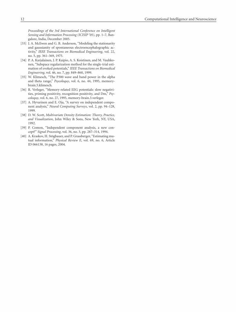
12 Computational Intelligence and Neuroscience
Proceedings of the 3rd International Conference on IntelligentSensing and Information Processing (ICISIP ’05), pp. 1–7, Ban-galore, India, December 2005.
[33] J. A. McEwen and G. B. Anderson, “Modeling the stationarityand gaussianity of spontaneous electroencephalographic ac-tivity,” IEEE Transactions on Biomedical Engineering, vol. 22,no. 5, pp. 361–369, 1975.
[34] P. A. Karjalainen, J. P. Kaipio, A. S. Koistinen, and M. Vauhko-nen, “Subspace regularization method for the single-trial esti-mation of evoked potentials,” IEEE Transactions on BiomedicalEngineering, vol. 46, no. 7, pp. 849–860, 1999.
[35] W. Klimesch, “The P300 wave and band power in the alphaand theta range,” Psycoloquy, vol. 6, no. 44, 1995, memory-brain.5.klimesch.
[36] R. Verleger, “Memory-related EEG potentials: slow negativi-ties, priming positivity, recognition positivity, and Dm,” Psy-coloquy, vol. 6, no. 27, 1995, memory-brain.3.verleger.
[37] A. Hyvarinen and E. Oja, “A survey on independent compo-nent analysis,” Neural Computing Surveys, vol. 2, pp. 94–128,1999.
[38] D. W. Scott, Multivariate Density Estimation: Theory, Practice,and Visualization, John Wiley & Sons, New York, NY, USA,1992.
[39] P. Comon, “Independent component analysis, a new con-cept?” Signal Processing, vol. 36, no. 3, pp. 287–314, 1994.
[40] A. Kraskov, H. Stogbauer, and P. Grassberger, “Estimating mu-tual information,” Physical Review E, vol. 69, no. 6, ArticleID 066138, 16 pages, 2004.
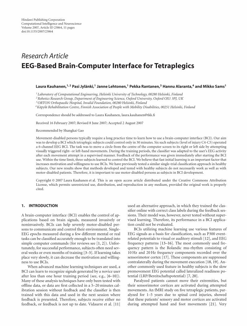
Hindawi Publishing CorporationComputational Intelligence and NeuroscienceVolume 2007, Article ID 23864, 11 pagesdoi:10.1155/2007/23864
Research ArticleEEG-Based Brain-Computer Interface for Tetraplegics
Laura Kauhanen,1, 2 Pasi Jylanki,1 Janne Lehtonen,1 Pekka Rantanen,3 Hannu Alaranta,4 and Mikko Sams1
1 Laboratory of Computational Engineering, Helsinki University of Technology, 00280 Helsinki, Finland2 Robotics Research Group, Department of Engineering Science, Oxford University, Oxford OX1 3PJ, UK3 ORTON Orthopaedic Hospital, Invalid Foundation, 00280 Helsinki, Finland
4 Kapyla Rehabilitation Centre, Finnish Association of People with Mobility Disabilities, 00251 Helsinki, Finland
Correspondence should be addressed to Laura Kauhanen, [email protected]
Received 16 February 2007; Revised 8 June 2007; Accepted 2 August 2007
Recommended by Shangkai Gao
Movement-disabled persons typically require a long practice time to learn how to use a brain-computer interface (BCI). Our aimwas to develop a BCI which tetraplegic subjects could control only in 30 minutes. Six such subjects (level of injury C4-C5) operateda 6-channel EEG BCI. The task was to move a circle from the centre of the computer screen to its right or left side by attemptingvisually triggered right- or left-hand movements. During the training periods, the classifier was adapted to the user’s EEG activityafter each movement attempt in a supervised manner. Feedback of the performance was given immediately after starting the BCIuse. Within the time limit, three subjects learned to control the BCI. We believe that fast initial learning is an important factor thatincreases motivation and willingness to use BCIs. We have previously tested a similar single-trial classification approach in healthysubjects. Our new results show that methods developed and tested with healthy subjects do not necessarily work as well as withmotor-disabled patients. Therefore, it is important to use motor-disabled persons as subjects in BCI development.
Copyright © 2007 Laura Kauhanen et al. This is an open access article distributed under the Creative Commons AttributionLicense, which permits unrestricted use, distribution, and reproduction in any medium, provided the original work is properlycited.
1. INTRODUCTION
A brain-computer interface (BCI) enables the control of ap-plications based on brain signals, measured invasively ornoninvasively. BCIs can help severely motor-disabled per-sons to communicate and control their environment. Single-EEG epochs measured during a few different mental or realtasks can be classified accurately enough to be translated intosimple computer commands (for reviews see [1, 2]). Unfor-tunately, for successful performance, subjects often need sev-eral weeks or even months of training [3–5]. If learning takesplace very slowly, it can decrease the motivation and willing-ness to use BCIs.
When advanced machine learning techniques are used, aBCI can learn to recognize signals generated by a novice userafter less than one hour training period (see, e.g., [6–10]).Many of these analysis techniques have only been tested withoffline data, or data are first collected in a 5–20 minutes cal-ibration session without feedback and the classifier is thentrained with this data and used in the next session wherefeedback is presented. Therefore, subjects receive either nofeedback, or feedback is not up to date. Vidaurre et al. [11]
used an alternative approach, in which they trained the clas-sifier online with correct class labels during the feedback ses-sions. Their model was, however, never tested without super-vised learning. Therefore, its performance in a BCI applica-tion could not be evaluated.
BCIs utilizing machine learning use various features ofEEG signals as a basis for classification, such as P300 event-related potentials to visual or auditory stimuli [12], and EEGfrequency patterns [13–16]. The most commonly used fre-quency pattern is the Rolandic mu-rhythm consisting of10 Hz and 20 Hz frequency components recorded over thesensorimotor cortex [17]. These components are suppressedcontralaterally during the movement execution [18, 19]. An-other commonly used feature in healthy subjects is the slowpremovement EEG potential called lateralized readiness po-tential (LRP/Bereitschaftspotential) [7, 20].
Paralyzed patients cannot move their extremities, buttheir sensorimotor cortices are activated during attemptedmovements. An fMRI study on five tetraplegic patients, par-alyzed for 1–5 years due to spinal cord injuries, showedthat these patients’ sensory and motor cortices are activatedduring attempted hand and foot movements [21]. Very
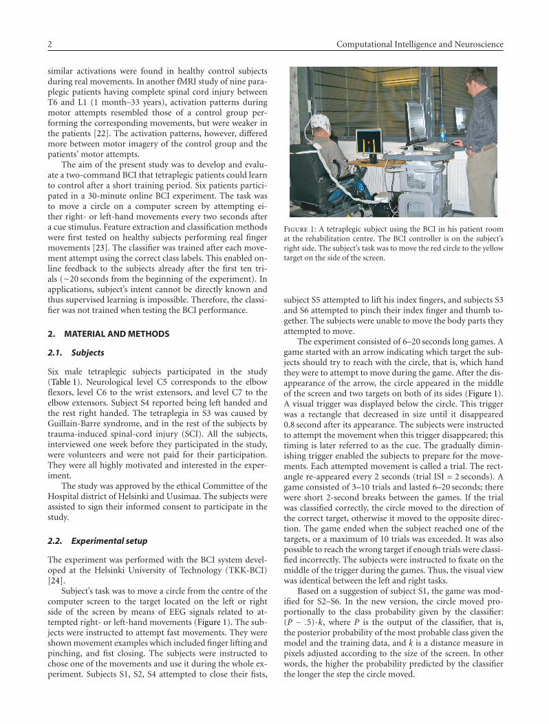
2 Computational Intelligence and Neuroscience
similar activations were found in healthy control subjectsduring real movements. In another fMRI study of nine para-plegic patients having complete spinal cord injury betweenT6 and L1 (1 month–33 years), activation patterns duringmotor attempts resembled those of a control group per-forming the corresponding movements, but were weaker inthe patients [22]. The activation patterns, however, differedmore between motor imagery of the control group and thepatients’ motor attempts.
The aim of the present study was to develop and evalu-ate a two-command BCI that tetraplegic patients could learnto control after a short training period. Six patients partici-pated in a 30-minute online BCI experiment. The task wasto move a circle on a computer screen by attempting ei-ther right- or left-hand movements every two seconds aftera cue stimulus. Feature extraction and classification methodswere first tested on healthy subjects performing real fingermovements [23]. The classifier was trained after each move-ment attempt using the correct class labels. This enabled on-line feedback to the subjects already after the first ten tri-als (∼20 seconds from the beginning of the experiment). Inapplications, subject’s intent cannot be directly known andthus supervised learning is impossible. Therefore, the classi-fier was not trained when testing the BCI performance.
2. MATERIAL AND METHODS
2.1. Subjects
Six male tetraplegic subjects participated in the study(Table 1). Neurological level C5 corresponds to the elbowflexors, level C6 to the wrist extensors, and level C7 to theelbow extensors. Subject S4 reported being left handed andthe rest right handed. The tetraplegia in S3 was caused byGuillain-Barre syndrome, and in the rest of the subjects bytrauma-induced spinal-cord injury (SCI). All the subjects,interviewed one week before they participated in the study,were volunteers and were not paid for their participation.They were all highly motivated and interested in the exper-iment.
The study was approved by the ethical Committee of theHospital district of Helsinki and Uusimaa. The subjects wereassisted to sign their informed consent to participate in thestudy.
2.2. Experimental setup
The experiment was performed with the BCI system devel-oped at the Helsinki University of Technology (TKK-BCI)[24].
Subject’s task was to move a circle from the centre of thecomputer screen to the target located on the left or rightside of the screen by means of EEG signals related to at-tempted right- or left-hand movements (Figure 1). The sub-jects were instructed to attempt fast movements. They wereshown movement examples which included finger lifting andpinching, and fist closing. The subjects were instructed tochose one of the movements and use it during the whole ex-periment. Subjects S1, S2, S4 attempted to close their fists,
Figure 1: A tetraplegic subject using the BCI in his patient roomat the rehabilitation centre. The BCI controller is on the subject’sright side. The subject’s task was to move the red circle to the yellowtarget on the side of the screen.
subject S5 attempted to lift his index fingers, and subjects S3and S6 attempted to pinch their index finger and thumb to-gether. The subjects were unable to move the body parts theyattempted to move.
The experiment consisted of 6–20 seconds long games. Agame started with an arrow indicating which target the sub-jects should try to reach with the circle, that is, which handthey were to attempt to move during the game. After the dis-appearance of the arrow, the circle appeared in the middleof the screen and two targets on both of its sides (Figure 1).A visual trigger was displayed below the circle. This triggerwas a rectangle that decreased in size until it disappeared0.8 second after its appearance. The subjects were instructedto attempt the movement when this trigger disappeared; thistiming is later referred to as the cue. The gradually dimin-ishing trigger enabled the subjects to prepare for the move-ments. Each attempted movement is called a trial. The rect-angle re-appeared every 2 seconds (trial ISI = 2 seconds). Agame consisted of 3–10 trials and lasted 6–20 seconds; therewere short 2-second breaks between the games. If the trialwas classified correctly, the circle moved to the direction ofthe correct target, otherwise it moved to the opposite direc-tion. The game ended when the subject reached one of thetargets, or a maximum of 10 trials was exceeded. It was alsopossible to reach the wrong target if enough trials were classi-fied incorrectly. The subjects were instructed to fixate on themiddle of the trigger during the games. Thus, the visual viewwas identical between the left and right tasks.
Based on a suggestion of subject S1, the game was mod-ified for S2–S6. In the new version, the circle moved pro-portionally to the class probability given by the classifier:(P − .5)·k, where P is the output of the classifier, that is,the posterior probability of the most probable class given themodel and the training data, and k is a distance measure inpixels adjusted according to the size of the screen. In otherwords, the higher the probability predicted by the classifierthe longer the step the circle moved.
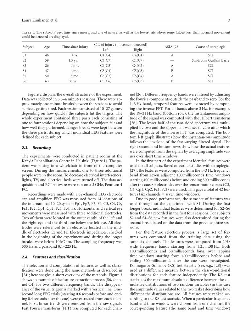
Laura Kauhanen et al. 3
Table 1: The subjects’ age, time since injury, and cite of injury, as well as the lowest site where some (albeit less than normal) movementcould be detected are displayed.
Subject Age Time since injuryCite of injury (movement detected)
ASIA [25] Cause of tetraplegiaLeft Right
S1 46 4 yr. C4(C4) C4(C4) A SCI
S2 59 1.5 yr. C4(C7) C4(C7) — Syndroma Guillain Barre
S3 26 4 mo. C4(C5) C4(C5) A SCI
S4 47 4 mo. C5(C4) C5(C5) B SCI
S5 50 3 mo. C5(C7) C5(C7) A SCI
S6 63 35 yr. C5(C6) C5(C6) B SCI
Figure 2 displays the overall structure of the experiment.Data was collected in 3.5–4 minutes sessions. There were ap-proximately one-minute breaks between the sessions to avoidsubjects getting tired. Each session consisted of 10–27 games,depending on how quickly the subjects hit the targets. Thewhole experiment contained three parts each consisting ofone to four sessions depending on how the subjects felt andhow well they performed. Longer breaks were kept betweenthe three parts, during which individual EEG features weredefined for each subject.
2.3. Recording
The experiments were conducted in patient rooms at theKapyla Rehabilitation Centre in Helsinki (Figure 1). The pa-tient was sitting in a wheelchair in front of the computerscreen. During the measurements, one to three additionalpeople were in the room. To decrease electrical interferences,lights, TV, and electrical beds were turned off. The data ac-quisition and BCI software were run on a 3 GHz, Pentium 4PC.
Recordings were made with a 32-channel EEG electrodecap and amplifier. EEG was measured from 14 locations ofthe international 10–20 system: Fp1, Fp2, F3, F4, C3, C4, Cz,Fc1, Fc2, Cp1, Cp2, Fc5, Fc6, Fz. Horizontal and vertical eyemovements were measured with three additional electrodes.Two of them were located at the outer canthi of the left andthe right eye and the third one below the left eye. All elec-trodes were referenced to an electrode located in the mid-dle of electrodes Cz and Fz. Electrode impedances, checkedin the beginning of the experiment and during the longerbreaks, were below 10 kOhm. The sampling frequency was500 Hz and passband 0.1–225 Hz.
2.4. Features and classification
The selection and computation of features as well as classi-fication were done using the same methods as described in[24]; here we give a short overview of the methods. Figure 3shows an example of the feature extraction process (S6, chan-nel C4) for two different frequency bands. The disappear-ance of the visual trigger is marked with a vertical line. One-second long EEG trials (starting 0.6 seconds before and end-ing 0.4 seconds after the cue) were extracted from each chan-nel. First, linear trends were removed from the raw signals.Fast Fourier transform (FFT) was computed for each chan-
nel [26]. Different frequency bands were filtered by adjustingthe Fourier components outside the passband to zero. For the1–3 Hz band, temporal features were extracted by comput-ing the inverse FFT. For all bands above 3 Hz, for example,the 19–21 Hz band (bottom row), the instantaneous ampli-tude of the signal was computed with the Hilbert transform[26]. The lower half of the two-sided spectrum was multi-plied by two and the upper half was set to zero after whichthe magnitude of the inverse FFT was computed. The bot-tom left graph illustrates how the instantaneous amplitudefollows the envelope of the fast varying filtered signal. Theright second and bottom rows show how the actual featureswere computed from the signals by averaging amplitude val-ues over short time windows.
In the first part of the experiment identical features wereused for all subjects. Based on earlier studies with tetraplegics[27], the features were computed from the 1–3 Hz frequencyband from seven adjacent 100 milliseconds time windowsstarting 400 milliseconds before and ending 300 millisecondsafter the cue. Six electrodes over the sensorimotor cortex (C3,C4, Cp1, Cp2, Fc1, Fc2) were used. This gave a total of 42 fea-tures (six channels × seven time windows).
Due to good performance, the same set of features wasused throughout the experiment with S1. During the firstlonger break, individual features were determined for S2–S6from the data recorded in the first four sessions. For subjectsS2 and S4–S6 new features were also determined during thesecond break based on the data from the previous three ses-sions.
For the feature selection process, a large set of fea-tures was computed from the training data using thesame six channels. The features were computed from 2 Hzwide frequency bands starting from 1,2,. . . ,38 Hz. Both100 milliseconds and 50 milliseconds long, over lappingtime windows starting from 400 milliseconds before andending 300 milliseconds after the cue were investigated.Kolmogorov-Smirnov (KS) test statistic (see, e.g., [28]) wasused as a difference measure between the class-conditionaldistributions for each feature independently. The KS teststatistic is the maximum absolute difference between the cu-mulative distributions of two random variables (in this casethe amplitude values related to the two tasks) describing howdifferent the distributions are. All features were ranked ac-cording to the KS test statistic. When a particular frequencyband and time window were chosen from one channel, thecorresponding feature (the same band and time window)
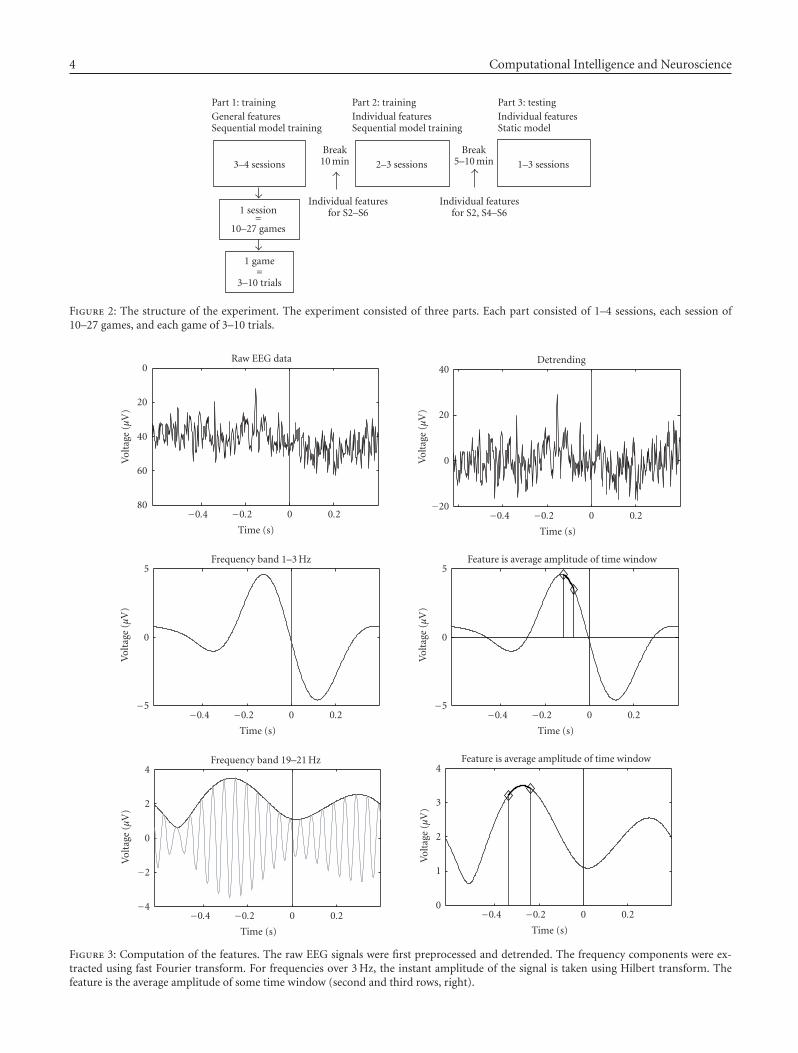
4 Computational Intelligence and Neuroscience
Part 1: trainingGeneral featuresSequential model training
Part 2: trainingIndividual featuresSequential model training
Part 3: testingIndividual featuresStatic model
3–4 sessions 2–3 sessions 1–3 sessions
1 session=
10–27 games
1 game=
3–10 trials
Break10 min
Break5–10 min
Individual featuresfor S2–S6
Individual featuresfor S2, S4–S6
Figure 2: The structure of the experiment. The experiment consisted of three parts. Each part consisted of 1–4 sessions, each session of10–27 games, and each game of 3–10 trials.
0.20−0.2−0.4
Time (s)
80
60
40
20
0
Vol
tage
(μV
)
Raw EEG data
0.20−0.2−0.4
Time (s)
−20
0
20
40
Vol
tage
(μV
)
Detrending
0.20−0.2−0.4
Time (s)
−5
0
5
Vol
tage
(μV
)
Frequency band 1–3 Hz
0.20−0.2−0.4
Time (s)
−5
0
5
Vol
tage
(μV
)
Feature is average amplitude of time window
0.20−0.2−0.4
Time (s)
−4
−2
0
2
4
Vol
tage
(μV
)
Frequency band 19–21 Hz
0.20−0.2−0.4
Time (s)
0
1
2
3
4
Vol
tage
(μV
)
Feature is average amplitude of time window
Figure 3: Computation of the features. The raw EEG signals were first preprocessed and detrended. The frequency components were ex-tracted using fast Fourier transform. For frequencies over 3 Hz, the instant amplitude of the signal is taken using Hilbert transform. Thefeature is the average amplitude of some time window (second and third rows, right).
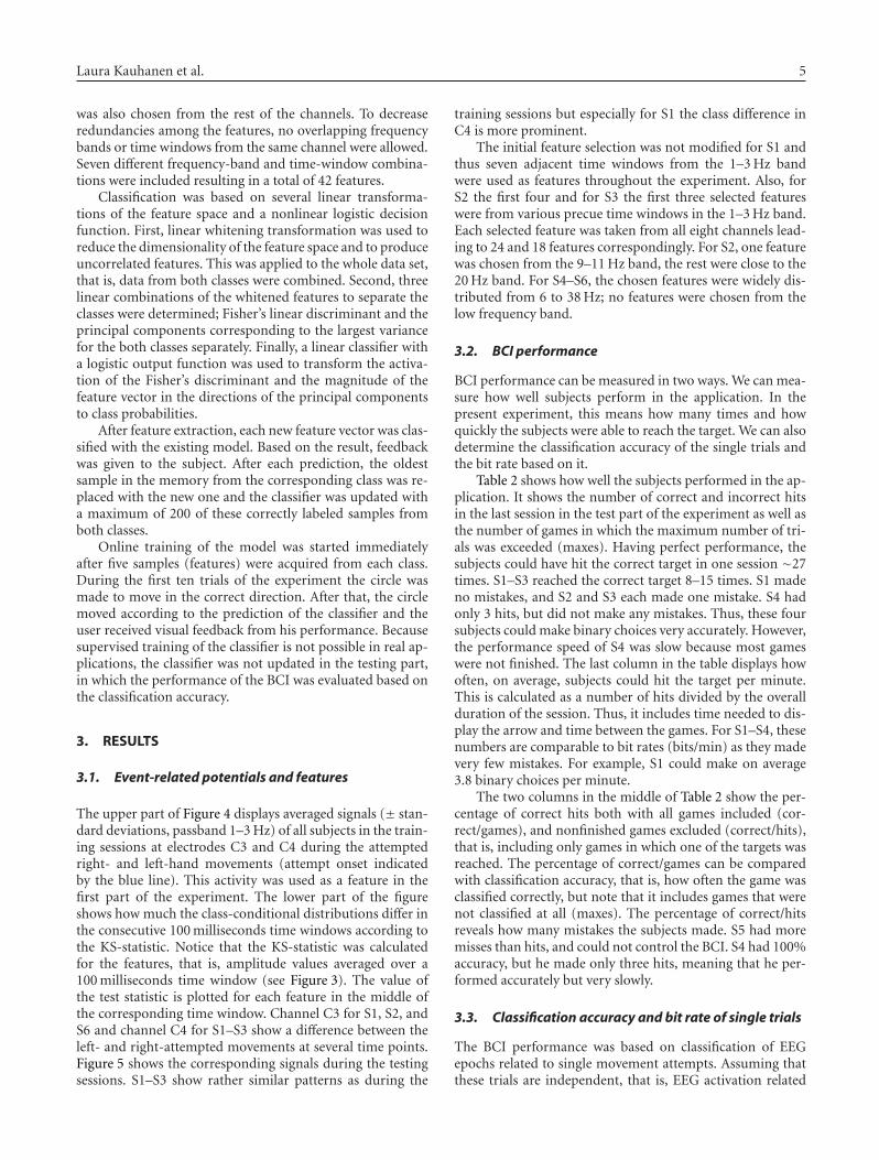
Laura Kauhanen et al. 5
was also chosen from the rest of the channels. To decreaseredundancies among the features, no overlapping frequencybands or time windows from the same channel were allowed.Seven different frequency-band and time-window combina-tions were included resulting in a total of 42 features.
Classification was based on several linear transforma-tions of the feature space and a nonlinear logistic decisionfunction. First, linear whitening transformation was used toreduce the dimensionality of the feature space and to produceuncorrelated features. This was applied to the whole data set,that is, data from both classes were combined. Second, threelinear combinations of the whitened features to separate theclasses were determined; Fisher’s linear discriminant and theprincipal components corresponding to the largest variancefor the both classes separately. Finally, a linear classifier witha logistic output function was used to transform the activa-tion of the Fisher’s discriminant and the magnitude of thefeature vector in the directions of the principal componentsto class probabilities.
After feature extraction, each new feature vector was clas-sified with the existing model. Based on the result, feedbackwas given to the subject. After each prediction, the oldestsample in the memory from the corresponding class was re-placed with the new one and the classifier was updated witha maximum of 200 of these correctly labeled samples fromboth classes.
Online training of the model was started immediatelyafter five samples (features) were acquired from each class.During the first ten trials of the experiment the circle wasmade to move in the correct direction. After that, the circlemoved according to the prediction of the classifier and theuser received visual feedback from his performance. Becausesupervised training of the classifier is not possible in real ap-plications, the classifier was not updated in the testing part,in which the performance of the BCI was evaluated based onthe classification accuracy.
3. RESULTS
3.1. Event-related potentials and features
The upper part of Figure 4 displays averaged signals (± stan-dard deviations, passband 1–3 Hz) of all subjects in the train-ing sessions at electrodes C3 and C4 during the attemptedright- and left-hand movements (attempt onset indicatedby the blue line). This activity was used as a feature in thefirst part of the experiment. The lower part of the figureshows how much the class-conditional distributions differ inthe consecutive 100 milliseconds time windows according tothe KS-statistic. Notice that the KS-statistic was calculatedfor the features, that is, amplitude values averaged over a100 milliseconds time window (see Figure 3). The value ofthe test statistic is plotted for each feature in the middle ofthe corresponding time window. Channel C3 for S1, S2, andS6 and channel C4 for S1–S3 show a difference between theleft- and right-attempted movements at several time points.Figure 5 shows the corresponding signals during the testingsessions. S1–S3 show rather similar patterns as during the
training sessions but especially for S1 the class difference inC4 is more prominent.
The initial feature selection was not modified for S1 andthus seven adjacent time windows from the 1–3 Hz bandwere used as features throughout the experiment. Also, forS2 the first four and for S3 the first three selected featureswere from various precue time windows in the 1–3 Hz band.Each selected feature was taken from all eight channels lead-ing to 24 and 18 features correspondingly. For S2, one featurewas chosen from the 9–11 Hz band, the rest were close to the20 Hz band. For S4–S6, the chosen features were widely dis-tributed from 6 to 38 Hz; no features were chosen from thelow frequency band.
3.2. BCI performance
BCI performance can be measured in two ways. We can mea-sure how well subjects perform in the application. In thepresent experiment, this means how many times and howquickly the subjects were able to reach the target. We can alsodetermine the classification accuracy of the single trials andthe bit rate based on it.
Table 2 shows how well the subjects performed in the ap-plication. It shows the number of correct and incorrect hitsin the last session in the test part of the experiment as well asthe number of games in which the maximum number of tri-als was exceeded (maxes). Having perfect performance, thesubjects could have hit the correct target in one session ∼27times. S1–S3 reached the correct target 8–15 times. S1 madeno mistakes, and S2 and S3 each made one mistake. S4 hadonly 3 hits, but did not make any mistakes. Thus, these foursubjects could make binary choices very accurately. However,the performance speed of S4 was slow because most gameswere not finished. The last column in the table displays howoften, on average, subjects could hit the target per minute.This is calculated as a number of hits divided by the overallduration of the session. Thus, it includes time needed to dis-play the arrow and time between the games. For S1–S4, thesenumbers are comparable to bit rates (bits/min) as they madevery few mistakes. For example, S1 could make on average3.8 binary choices per minute.
The two columns in the middle of Table 2 show the per-centage of correct hits both with all games included (cor-rect/games), and nonfinished games excluded (correct/hits),that is, including only games in which one of the targets wasreached. The percentage of correct/games can be comparedwith classification accuracy, that is, how often the game wasclassified correctly, but note that it includes games that werenot classified at all (maxes). The percentage of correct/hitsreveals how many mistakes the subjects made. S5 had moremisses than hits, and could not control the BCI. S4 had 100%accuracy, but he made only three hits, meaning that he per-formed accurately but very slowly.
3.3. Classification accuracy and bit rate of single trials
The BCI performance was based on classification of EEGepochs related to single movement attempts. Assuming thatthese trials are independent, that is, EEG activation related
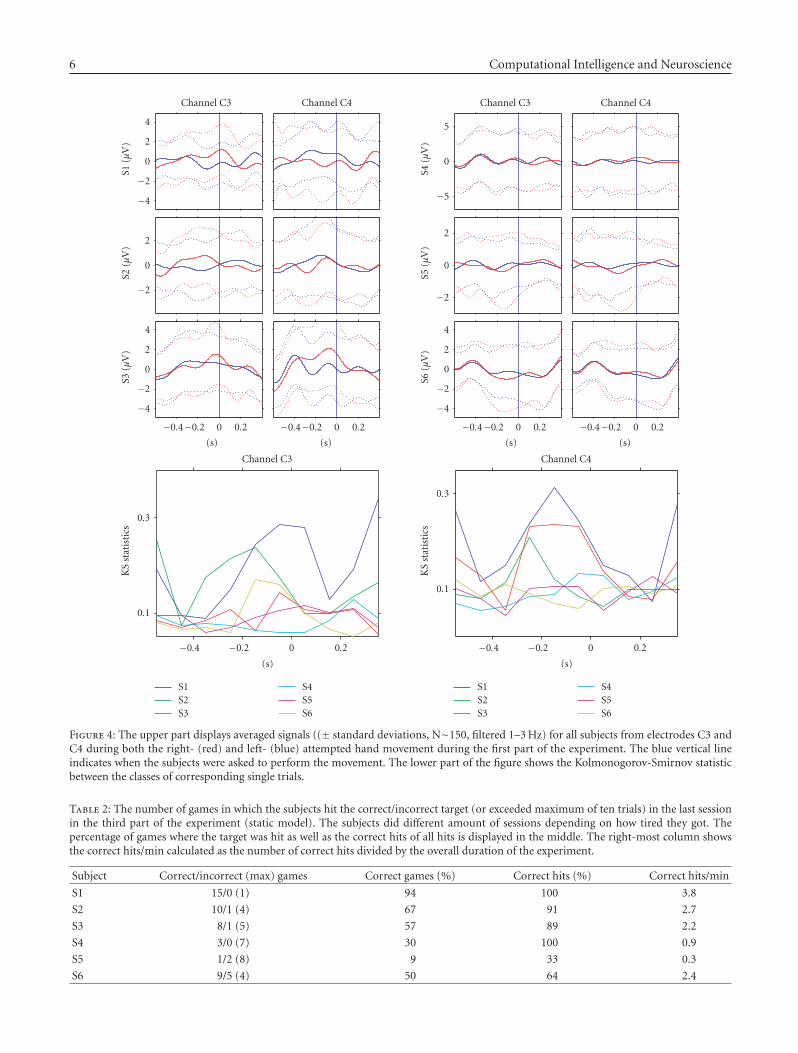
6 Computational Intelligence and Neuroscience
0.20−0.2−0.4
(s)
0.20−0.2−0.4
(s)
−4
−2
0
2
4
S3(μ
V)
−2
0
2
S2(μ
V)
−4
−2
0
2
4S1
(μV
)
Channel C3 Channel C4
0.20−0.2−0.4
(s)
0.20−0.2−0.4
(s)
−4
−2
0
2
4
S6(μ
V)
−2
0
2
S5(μ
V)
−5
0
5
S4(μ
V)
Channel C3 Channel C4
0.20−0.2−0.4
(s)
0.1
0.3
KS
stat
isti
cs
Channel C3
S1S2S3
S4S5S6
0.20−0.2−0.4
(s)
0.1
0.3
KS
stat
isti
cs
Channel C4
S1S2S3
S4S5S6
Figure 4: The upper part displays averaged signals ((± standard deviations, N∼150, filtered 1–3 Hz) for all subjects from electrodes C3 andC4 during both the right- (red) and left- (blue) attempted hand movement during the first part of the experiment. The blue vertical lineindicates when the subjects were asked to perform the movement. The lower part of the figure shows the Kolmonogorov-Smirnov statisticbetween the classes of corresponding single trials.
Table 2: The number of games in which the subjects hit the correct/incorrect target (or exceeded maximum of ten trials) in the last sessionin the third part of the experiment (static model). The subjects did different amount of sessions depending on how tired they got. Thepercentage of games where the target was hit as well as the correct hits of all hits is displayed in the middle. The right-most column showsthe correct hits/min calculated as the number of correct hits divided by the overall duration of the experiment.
Subject Correct/incorrect (max) games Correct games (%) Correct hits (%) Correct hits/min
S1 15/0 (1) 94 100 3.8
S2 10/1 (4) 67 91 2.7
S3 8/1 (5) 57 89 2.2
S4 3/0 (7) 30 100 0.9
S5 1/2 (8) 9 33 0.3
S6 9/5 (4) 50 64 2.4
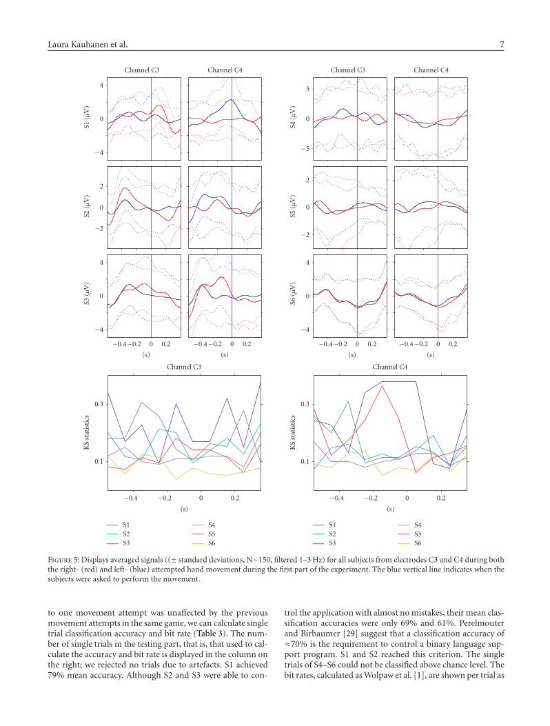
Laura Kauhanen et al. 7
0.20−0.2−0.4
(s)
0.20−0.2−0.4
(s)
−4
0
4
S3(μ
V)
−2
0
2
S2(μ
V)
−4
0
4S1
(μV
)
Channel C3 Channel C4
0.20−0.2−0.4
(s)
0.20−0.2−0.4
(s)
−4
0
4
S6(μ
V)
−2
0
2
S5(μ
V)
−5
0
5
S4(μ
V)
Channel C3 Channel C4
0.20−0.2−0.4
(s)
0.1
0.3
KS
stat
isti
cs
Channel C3
S1S2S3
S4S5S6
0.20−0.2−0.4
(s)
0.1
0.3
KS
stat
isti
cs
Channel C4
S1S2S3
S4S5S6
Figure 5: Displays averaged signals ((± standard deviations, N∼150, filtered 1–3 Hz) for all subjects from electrodes C3 and C4 during boththe right- (red) and left- (blue) attempted hand movement during the first part of the experiment. The blue vertical line indicates when thesubjects were asked to perform the movement.
to one movement attempt was unaffected by the previousmovement attempts in the same game, we can calculate singletrial classification accuracy and bit rate (Table 3). The num-ber of single trials in the testing part, that is, that used to cal-culate the accuracy and bit rate is displayed in the column onthe right; we rejected no trials due to artefacts. S1 achieved79% mean accuracy. Although S2 and S3 were able to con-
trol the application with almost no mistakes, their mean clas-sification accuracies were only 69% and 61%. Perelmouterand Birbaumer [29] suggest that a classification accuracy of≈70% is the requirement to control a binary language sup-port program. S1 and S2 reached this criterion. The singletrials of S4–S6 could not be classified above chance level. Thebit rates, calculated as Wolpaw et al. [1], are shown per trial as
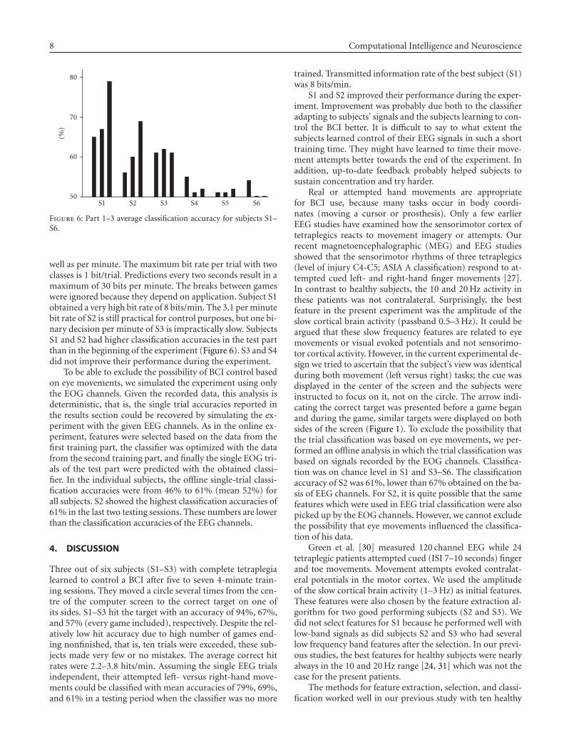
8 Computational Intelligence and Neuroscience
S6S5S4S3S2S150
60
70
80
(%)
Figure 6: Part 1–3 average classification accuracy for subjects S1–S6.
well as per minute. The maximum bit rate per trial with twoclasses is 1 bit/trial. Predictions every two seconds result in amaximum of 30 bits per minute. The breaks between gameswere ignored because they depend on application. Subject S1obtained a very high bit rate of 8 bits/min. The 3.1 per minutebit rate of S2 is still practical for control purposes, but one bi-nary decision per minute of S3 is impractically slow. SubjectsS1 and S2 had higher classification accuracies in the test partthan in the beginning of the experiment (Figure 6). S3 and S4did not improve their performance during the experiment.
To be able to exclude the possibility of BCI control basedon eye movements, we simulated the experiment using onlythe EOG channels. Given the recorded data, this analysis isdeterministic, that is, the single trial accuracies reported inthe results section could be recovered by simulating the ex-periment with the given EEG channels. As in the online ex-periment, features were selected based on the data from thefirst training part, the classifier was optimized with the datafrom the second training part, and finally the single EOG tri-als of the test part were predicted with the obtained classi-fier. In the individual subjects, the offline single-trial classi-fication accuracies were from 46% to 61% (mean 52%) forall subjects. S2 showed the highest classification accuracies of61% in the last two testing sessions. These numbers are lowerthan the classification accuracies of the EEG channels.
4. DISCUSSION
Three out of six subjects (S1–S3) with complete tetraplegialearned to control a BCI after five to seven 4-minute train-ing sessions. They moved a circle several times from the cen-tre of the computer screen to the correct target on one ofits sides. S1–S3 hit the target with an accuracy of 94%, 67%,and 57% (every game included), respectively. Despite the rel-atively low hit accuracy due to high number of games end-ing nonfinished, that is, ten trials were exceeded, these sub-jects made very few or no mistakes. The average correct hitrates were 2.2–3.8 hits/min. Assuming the single EEG trialsindependent, their attempted left- versus right-hand move-ments could be classified with mean accuracies of 79%, 69%,and 61% in a testing period when the classifier was no more
trained. Transmitted information rate of the best subject (S1)was 8 bits/min.
S1 and S2 improved their performance during the exper-iment. Improvement was probably due both to the classifieradapting to subjects’ signals and the subjects learning to con-trol the BCI better. It is difficult to say to what extent thesubjects learned control of their EEG signals in such a shorttraining time. They might have learned to time their move-ment attempts better towards the end of the experiment. Inaddition, up-to-date feedback probably helped subjects tosustain concentration and try harder.
Real or attempted hand movements are appropriatefor BCI use, because many tasks occur in body coordi-nates (moving a cursor or prosthesis). Only a few earlierEEG studies have examined how the sensorimotor cortex oftetraplegics reacts to movement imagery or attempts. Ourrecent magnetoencephalographic (MEG) and EEG studiesshowed that the sensorimotor rhythms of three tetraplegics(level of injury C4-C5; ASIA A classification) respond to at-tempted cued left- and right-hand finger movements [27].In contrast to healthy subjects, the 10 and 20 Hz activity inthese patients was not contralateral. Surprisingly, the bestfeature in the present experiment was the amplitude of theslow cortical brain activity (passband 0.5–3 Hz). It could beargued that these slow frequency features are related to eyemovements or visual evoked potentials and not sensorimo-tor cortical activity. However, in the current experimental de-sign we tried to ascertain that the subject’s view was identicalduring both movement (left versus right) tasks; the cue wasdisplayed in the center of the screen and the subjects wereinstructed to focus on it, not on the circle. The arrow indi-cating the correct target was presented before a game beganand during the game, similar targets were displayed on bothsides of the screen (Figure 1). To exclude the possibility thatthe trial classification was based on eye movements, we per-formed an offline analysis in which the trial classification wasbased on signals recorded by the EOG channels. Classifica-tion was on chance level in S1 and S3–S6. The classificationaccuracy of S2 was 61%, lower than 67% obtained on the ba-sis of EEG channels. For S2, it is quite possible that the samefeatures which were used in EEG trial classification were alsopicked up by the EOG channels. However, we cannot excludethe possibility that eye movements influenced the classifica-tion of his data.
Green et al. [30] measured 120 channel EEG while 24tetraplegic patients attempted cued (ISI 7–10 seconds) fingerand toe movements. Movement attempts evoked contralat-eral potentials in the motor cortex. We used the amplitudeof the slow cortical brain activity (1–3 Hz) as initial features.These features were also chosen by the feature extraction al-gorithm for two good performing subjects (S2 and S3). Wedid not select features for S1 because he performed well withlow-band signals as did subjects S2 and S3 who had severallow frequency band features after the selection. In our previ-ous studies, the best features for healthy subjects were nearlyalways in the 10 and 20 Hz range [24, 31] which was not thecase for the present patients.
The methods for feature extraction, selection, and classi-fication worked well in our previous study with ten healthy
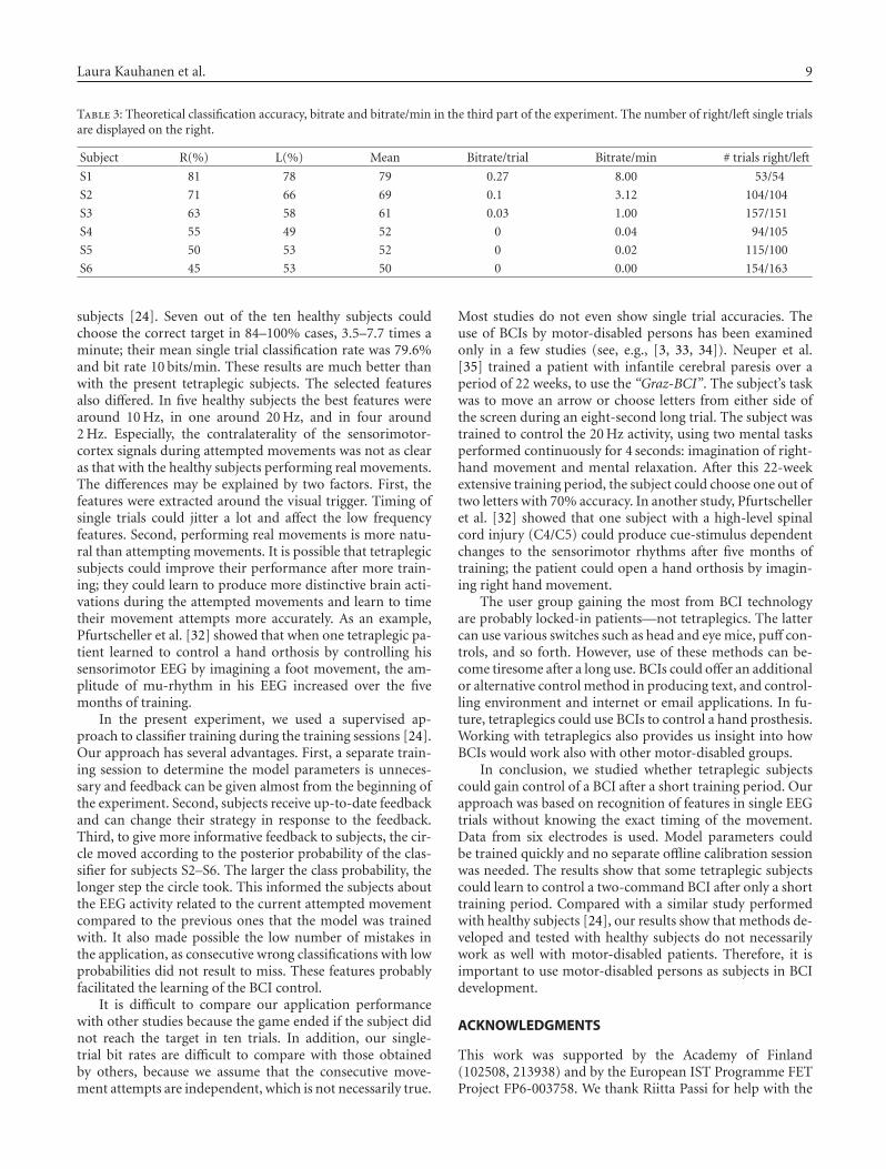
Laura Kauhanen et al. 9
Table 3: Theoretical classification accuracy, bitrate and bitrate/min in the third part of the experiment. The number of right/left single trialsare displayed on the right.
Subject R(%) L(%) Mean Bitrate/trial Bitrate/min # trials right/left
S1 81 78 79 0.27 8.00 53/54
S2 71 66 69 0.1 3.12 104/104
S3 63 58 61 0.03 1.00 157/151
S4 55 49 52 0 0.04 94/105
S5 50 53 52 0 0.02 115/100
S6 45 53 50 0 0.00 154/163
subjects [24]. Seven out of the ten healthy subjects couldchoose the correct target in 84–100% cases, 3.5–7.7 times aminute; their mean single trial classification rate was 79.6%and bit rate 10 bits/min. These results are much better thanwith the present tetraplegic subjects. The selected featuresalso differed. In five healthy subjects the best features werearound 10 Hz, in one around 20 Hz, and in four around2 Hz. Especially, the contralaterality of the sensorimotor-cortex signals during attempted movements was not as clearas that with the healthy subjects performing real movements.The differences may be explained by two factors. First, thefeatures were extracted around the visual trigger. Timing ofsingle trials could jitter a lot and affect the low frequencyfeatures. Second, performing real movements is more natu-ral than attempting movements. It is possible that tetraplegicsubjects could improve their performance after more train-ing; they could learn to produce more distinctive brain acti-vations during the attempted movements and learn to timetheir movement attempts more accurately. As an example,Pfurtscheller et al. [32] showed that when one tetraplegic pa-tient learned to control a hand orthosis by controlling hissensorimotor EEG by imagining a foot movement, the am-plitude of mu-rhythm in his EEG increased over the fivemonths of training.
In the present experiment, we used a supervised ap-proach to classifier training during the training sessions [24].Our approach has several advantages. First, a separate train-ing session to determine the model parameters is unneces-sary and feedback can be given almost from the beginning ofthe experiment. Second, subjects receive up-to-date feedbackand can change their strategy in response to the feedback.Third, to give more informative feedback to subjects, the cir-cle moved according to the posterior probability of the clas-sifier for subjects S2–S6. The larger the class probability, thelonger step the circle took. This informed the subjects aboutthe EEG activity related to the current attempted movementcompared to the previous ones that the model was trainedwith. It also made possible the low number of mistakes inthe application, as consecutive wrong classifications with lowprobabilities did not result to miss. These features probablyfacilitated the learning of the BCI control.
It is difficult to compare our application performancewith other studies because the game ended if the subject didnot reach the target in ten trials. In addition, our single-trial bit rates are difficult to compare with those obtainedby others, because we assume that the consecutive move-ment attempts are independent, which is not necessarily true.
Most studies do not even show single trial accuracies. Theuse of BCIs by motor-disabled persons has been examinedonly in a few studies (see, e.g., [3, 33, 34]). Neuper et al.[35] trained a patient with infantile cerebral paresis over aperiod of 22 weeks, to use the “Graz-BCI”. The subject’s taskwas to move an arrow or choose letters from either side ofthe screen during an eight-second long trial. The subject wastrained to control the 20 Hz activity, using two mental tasksperformed continuously for 4 seconds: imagination of right-hand movement and mental relaxation. After this 22-weekextensive training period, the subject could choose one out oftwo letters with 70% accuracy. In another study, Pfurtschelleret al. [32] showed that one subject with a high-level spinalcord injury (C4/C5) could produce cue-stimulus dependentchanges to the sensorimotor rhythms after five months oftraining; the patient could open a hand orthosis by imagin-ing right hand movement.
The user group gaining the most from BCI technologyare probably locked-in patients—not tetraplegics. The lattercan use various switches such as head and eye mice, puff con-trols, and so forth. However, use of these methods can be-come tiresome after a long use. BCIs could offer an additionalor alternative control method in producing text, and control-ling environment and internet or email applications. In fu-ture, tetraplegics could use BCIs to control a hand prosthesis.Working with tetraplegics also provides us insight into howBCIs would work also with other motor-disabled groups.
In conclusion, we studied whether tetraplegic subjectscould gain control of a BCI after a short training period. Ourapproach was based on recognition of features in single EEGtrials without knowing the exact timing of the movement.Data from six electrodes is used. Model parameters couldbe trained quickly and no separate offline calibration sessionwas needed. The results show that some tetraplegic subjectscould learn to control a two-command BCI after only a shorttraining period. Compared with a similar study performedwith healthy subjects [24], our results show that methods de-veloped and tested with healthy subjects do not necessarilywork as well with motor-disabled patients. Therefore, it isimportant to use motor-disabled persons as subjects in BCIdevelopment.
ACKNOWLEDGMENTS
This work was supported by the Academy of Finland(102508, 213938) and by the European IST Programme FETProject FP6-003758. We thank Riitta Passi for help with the
10 Computational Intelligence and Neuroscience
EEG measurements and Harri Valpola and Stephen Robertsfor useful comments.
REFERENCES
[1] J. R. Wolpaw, N. Birbaumer, D. J. McFarland, G. Pfurtscheller,and T. M. Vaughan, “Brain-computer interfaces for communi-cation and control,” Clinical Neurophysiology, vol. 113, no. 6,pp. 767–791, 2002.
[2] A. Kubler, B. Kotchoubey, J. Kaiser, J. R. Wolpaw, and N.Birbaumer, “Brain-computer communication: unlocking thelocked in,” Psychological Bulletin, vol. 127, no. 3, pp. 358–375,2001.
[3] J. R. Wolpaw and D. J. McFarland, “Control of a two-dimensional movement signal by a noninvasive brain-computer interface in humans,” Proceedings of the NationalAcademy of Sciences of the United States of America, vol. 101,no. 51, pp. 17849–17854, 2004.
[4] G. Pfurtscheller, C. Neuper, G. R. Muller, et al., “Graz-BCI:state of the art and clinical applications,” IEEE Transactions onNeural Systems and Rehabilitation Engineering, vol. 11, no. 2,pp. 177–180, 2003.
[5] N. Birbaumer, T. Hinterberger, A. Kubler, and N. Neu-mann, “The thought-translation device (TTD): neurobehav-ioral mechanisms and clinical outcome,” IEEE Transactions onNeural Systems and Rehabilitation Engineering, vol. 11, no. 2,pp. 120–123, 2003.
[6] S. Lemm, B. Blankertz, G. Curio, and K.-R. Muller, “Spatio-spectral filters for improving the classification of single trialEEG,” IEEE Transactions on Biomedical Engineering, vol. 52,no. 9, pp. 1541–1548, 2005.
[7] G. Dornhege, B. Blankertz, G. Curio, and K.-R. Muller,“Boosting bit rates in noninvasive EEG single-trial classifica-tions by feature combination and multiclass paradigms,” IEEETransactions on Biomedical Engineering, vol. 51, no. 6, pp. 993–1002, 2004.
[8] Y. Li, X. Gao, H. Liu, and S. Gao, “Classification of single-trialelectroencephalogram during finger movement,” IEEE Trans-actions on Biomedical Engineering, vol. 51, no. 6, pp. 1019–1025, 2004.
[9] P. Sykacek, S. J. Roberts, and M. Stokes, “Adaptive BCI basedon variational Bayesian Kalman filtering: an empirical evalu-ation,” IEEE Transactions on Biomedical Engineering, vol. 51,no. 5, pp. 719–727, 2004.
[10] J. D. R. Millan and J. Mourino, “Asynchronous BCI and localneural classifiers: an overview of the adaptive brain interfaceproject,” IEEE Transactions on Neural Systems and Rehabilita-tion Engineering, vol. 11, no. 2, pp. 159–161, 2003.
[11] C. Vidaurre, A. Schlogl, R. Cabeza, R. Scherer, and G.Pfurtscheller, “Adaptive on-line classification for EEG-basedbrain computer interfaces with ARR parameters and bandpower estimates,” Biomedizinische Technik, vol. 50, no. 11, pp.350–354, 2005.
[12] E. W. Sellers, A. Kubler, and E. Donchin, “Brain-computer in-terface research at the University of South Florida CognitivePsychophysiology Laboratory: the P300 speller,” IEEE Transac-tions on Neural Systems and Rehabilitation Engineering, vol. 14,no. 2, pp. 221–224, 2006.
[13] J. Muller-Gerking, G. Pfurtscheller, and H. Flyvbjerg, “Design-ing optimal spatial filters for single-trial EEG classification in amovement task,” Clinical Neurophysiology, vol. 110, no. 5, pp.787–798, 1999.
[14] E. Curran, P. Sykacek, M. Stokes, et al., “Cognitive tasks fordriving a brain-computer interfacing system: a pilot study,”IEEE Transactions on Neural Systems and Rehabilitation Engi-neering, vol. 12, no. 1, pp. 48–54, 2004.
[15] J. D. R. Millan, F. Renkens, J. Mourino, and W. Gerstner, “Non-invasive brain-actuated control of a mobile robot by humanEEG,” IEEE Transactions on Biomedical Engineering, vol. 51,no. 6, pp. 1026–1033, 2004.
[16] B. Obermaier, C. Neuper, C. Guger, and G. Pfurtscheller, “In-formation transfer rate in a five-classes brain-computer inter-face,” IEEE Transactions on Neural Systems and RehabilitationEngineering, vol. 9, no. 3, pp. 283–288, 2001.
[17] H. Gaustaut, “Etude electrocorticographique de la reactivitedes rhythmes rolandiques,” Revue Neurologique, vol. 87, no. 2,pp. 176–182, 1952.
[18] R. Salmelin and R. Hari, “Spatiotemporal characteristics ofsensorimotor neuromagnetic rhythms related to thumb move-ment,” Neuroscience, vol. 60, no. 2, pp. 537–550, 1994.
[19] G. Pfurtscheller, “Central beta rhythm during sensorimotoractivities in man,” Electroencephalography and Clinical Neuro-physiology, vol. 51, no. 3, pp. 253–264, 1981.
[20] B. Blankertz, K.-R. Muller, G. Curio, et al., “The BCI competi-tion 2003: progress and perspectives in detection and discrim-ination of EEG single trials,” IEEE Transactions on BiomedicalEngineering, vol. 51, no. 6, pp. 1044–1051, 2004.
[21] S. Shoham, E. Halgren, E. M. Maynard, and R. A. Normann,“Motor-cortical activity in tetraplegics,” Nature, vol. 413,no. 6858, p. 793, 2001.
[22] P. Sabbah, S. de Schonen, C. Leveque, et al., “Sensorimotorcortical activity in patients with complete spinal cord injury: afunctional magnetic resonance imaging study,” Journal of Neu-rotrauma, vol. 19, no. 1, pp. 53–60, 2002.
[23] P. Jylanki, L. Kauhanen, J. Lehtonen, J. Heikkonen, and M.Sams, “Use of feedback in classification of single EEG trialsduring finger movements,” in Proceedings of the 12th AnnualMeeting of the Organization for Human Brain Mapping, Flo-rence, Italy, June 2006.
[24] J. Lehtonen, P. Jylanki, L. Kauhanen, and M. Sams, “Onlineclassification of single EEG trials during finger movements,”in press.
[25] F. M. Maynard Jr., M. B. Bracken, G. Creasey, et al., “Interna-tional standards for neurological and functional classificationof spinal cord injury,” Spinal Cord, vol. 35, no. 5, pp. 266–274,1997.
[26] A. V. Oppenheim and R. V. Schafer, Discrete-Time Signal Pro-cessing, Prentice-Hall, Upper Saddle River, NJ, USA, 1989.
[27] L. Kauhanen, T. Nykopp, J. Lehtonen, et al., “EEG and MEGbrain-computer interface for tetraplegic patients,” IEEE Trans-actions on Neural Systems and Rehabilitation Engineering,vol. 14, no. 2, pp. 190–193, 2006.
[28] W. J. Conover, Practical Nonparametric Statistics, John Wiley ’Sons, New York, NY, USA, 3rd edition, 1999.
[29] J. Perelmouter and N. Birbaumer, “A binary spelling interfacewith random errors,” IEEE Transactions on Rehabilitation En-gineering, vol. 8, no. 2, pp. 227–232, 2000.
[30] J. B. Green, E. Sora, Y. Bialy, A. Ricamato, and R. W. Thatcher,“Cortical sensorimotor reorganization after spinal cord injury:an electroencephalographic study,” Neurology, vol. 50, no. 4,pp. 1115–1121, 1998.
[31] L. Kauhanen, T. Nykopp, and M. Sams, “Classification of sin-gle MEG trials related to left and right index finger move-ments,” Clinical Neurophysiology, vol. 117, no. 2, pp. 430–439,2006.

Laura Kauhanen et al. 11
[32] G. Pfurtscheller, C. Guger, G. Muller, G. Krausz, and C. Neu-per, “Brain oscillations control hand orthosis in a tetraplegic,”Neuroscience Letters, vol. 292, no. 3, pp. 211–214, 2000.
[33] A. Kubler, F. Nijboer, J. Mellinger, et al., “Patients with ALScan use sensorimotor rhythms to operate a brain-computerinterface,” Neurology, vol. 64, no. 10, pp. 1775–1777, 2005.
[34] N. Birbaumer, N. Ghanayim, T. Hinterberger, et al., “A spellingdevice for the paralysed,” Nature, vol. 398, no. 6725, pp. 297–298, 1999.
[35] C. Neuper, G. R. Muller, A. Kubler, N. Birbaumer, and G.Pfurtscheller, “Clinical application of an EEG-based brain-computer interface: a case study in a patient with severe mo-tor impairment,” Clinical Neurophysiology, vol. 114, no. 3, pp.399–409, 2003.
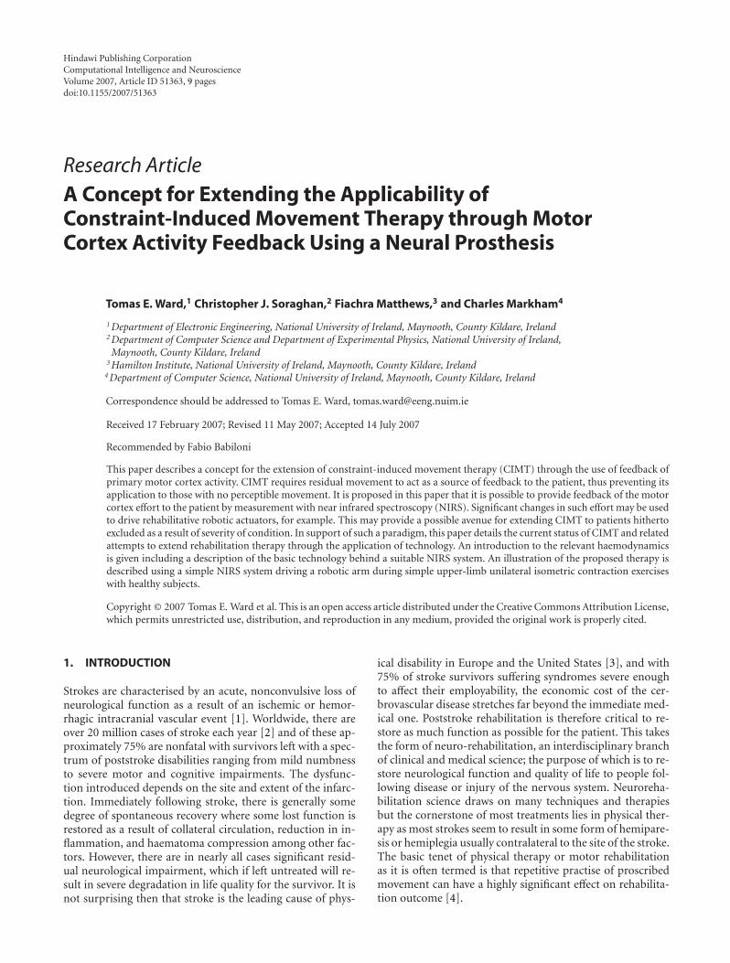
Hindawi Publishing CorporationComputational Intelligence and NeuroscienceVolume 2007, Article ID 51363, 9 pagesdoi:10.1155/2007/51363
Research ArticleA Concept for Extending the Applicability ofConstraint-Induced Movement Therapy through MotorCortex Activity Feedback Using a Neural Prosthesis
Tomas E. Ward,1 Christopher J. Soraghan,2 Fiachra Matthews,3 and Charles Markham4
1 Department of Electronic Engineering, National University of Ireland, Maynooth, County Kildare, Ireland2 Department of Computer Science and Department of Experimental Physics, National University of Ireland,Maynooth, County Kildare, Ireland
3 Hamilton Institute, National University of Ireland, Maynooth, County Kildare, Ireland4 Department of Computer Science, National University of Ireland, Maynooth, County Kildare, Ireland
Correspondence should be addressed to Tomas E. Ward, [email protected]
Received 17 February 2007; Revised 11 May 2007; Accepted 14 July 2007
Recommended by Fabio Babiloni
This paper describes a concept for the extension of constraint-induced movement therapy (CIMT) through the use of feedback ofprimary motor cortex activity. CIMT requires residual movement to act as a source of feedback to the patient, thus preventing itsapplication to those with no perceptible movement. It is proposed in this paper that it is possible to provide feedback of the motorcortex effort to the patient by measurement with near infrared spectroscopy (NIRS). Significant changes in such effort may be usedto drive rehabilitative robotic actuators, for example. This may provide a possible avenue for extending CIMT to patients hithertoexcluded as a result of severity of condition. In support of such a paradigm, this paper details the current status of CIMT and relatedattempts to extend rehabilitation therapy through the application of technology. An introduction to the relevant haemodynamicsis given including a description of the basic technology behind a suitable NIRS system. An illustration of the proposed therapy isdescribed using a simple NIRS system driving a robotic arm during simple upper-limb unilateral isometric contraction exerciseswith healthy subjects.
Copyright © 2007 Tomas E. Ward et al. This is an open access article distributed under the Creative Commons Attribution License,which permits unrestricted use, distribution, and reproduction in any medium, provided the original work is properly cited.
1. INTRODUCTION
Strokes are characterised by an acute, nonconvulsive loss ofneurological function as a result of an ischemic or hemor-rhagic intracranial vascular event [1]. Worldwide, there areover 20 million cases of stroke each year [2] and of these ap-proximately 75% are nonfatal with survivors left with a spec-trum of poststroke disabilities ranging from mild numbnessto severe motor and cognitive impairments. The dysfunc-tion introduced depends on the site and extent of the infarc-tion. Immediately following stroke, there is generally somedegree of spontaneous recovery where some lost function isrestored as a result of collateral circulation, reduction in in-flammation, and haematoma compression among other fac-tors. However, there are in nearly all cases significant resid-ual neurological impairment, which if left untreated will re-sult in severe degradation in life quality for the survivor. It isnot surprising then that stroke is the leading cause of phys-
ical disability in Europe and the United States [3], and with75% of stroke survivors suffering syndromes severe enoughto affect their employability, the economic cost of the cer-brovascular disease stretches far beyond the immediate med-ical one. Poststroke rehabilitation is therefore critical to re-store as much function as possible for the patient. This takesthe form of neuro-rehabilitation, an interdisciplinary branchof clinical and medical science; the purpose of which is to re-store neurological function and quality of life to people fol-lowing disease or injury of the nervous system. Neuroreha-bilitation science draws on many techniques and therapiesbut the cornerstone of most treatments lies in physical ther-apy as most strokes seem to result in some form of hemipare-sis or hemiplegia usually contralateral to the site of the stroke.The basic tenet of physical therapy or motor rehabilitationas it is often termed is that repetitive practise of proscribedmovement can have a highly significant effect on rehabilita-tion outcome [4].
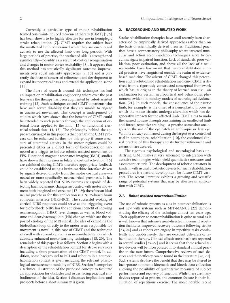
2 Computational Intelligence and Neuroscience
Currently, a particular type of motor rehabilitationtermed constraint-induced movement therapy (CIMT) [5, 6]has been shown to be highly effective for use in hemiplegicstroke rehabilitation [7]. CIMT requires the subject havethe unaffected limb constrained while they are encouragedactively to use the affected limb over long periods. Withlarge periods of practise, the weakened side is strengthenedsignificantly—possibly as a result of cortical reorganisationand changes in motor cortex excitability [8]. It appears thatthis method has statistically significant outcome improve-ments over equal intensity approaches [9, 10] and is cur-rently the focus of concerted refinement and development toexpand its theoretical basis and extend the application scope[11].
The flurry of research around this technique has hadan impact on rehabilitation engineering where over the pastfew years the therapy has been augmented by robot-assistedtraining [12]. Such techniques extend CIMT to patients whohave such severe disability that they are unable to engagein unassisted movement. This concept is underpinned bystudies which have shown that the benefits of CIMT couldbe extended to such patients through the application of ex-ternal forces applied to the limb [13] or functional elec-trical stimulation [14, 15]. The philosophy behind the ap-proach envisaged in this paper is that perhaps the CIMT pro-cess can be enhanced further for this group if some mea-sure of attempted activity in the motor regions could bepresented either as a direct form of biofeedback or har-nessed as a trigger to induce robotic-assisted movement orFES. Functional magnetic resonance imaging (fMRI) studieshave shown that increases in bilateral cortical activation [16]are exhibited during CIMT; therefore appropriate feedbackcould be established using a brain-machine interface drivenby signals derived directly from the motor cortical areas—aneural or more specifically, neurocortical prosthesis. It hasbeen widely reported that NIRS systems are capable of de-tecting haemodynamic changes associated with motor move-ment both imagined and executed [17–19]; therefore an idealneural prosthesis for this application is a NIRS-based braincomputer interface (NIRS-BCI). The successful evoking ofcortical NIRS responses could serve as the triggering eventfor biofeedback. NIRS has the additional benefit of showingoxyhaemoglobin (HbO) level changes as well as blood vol-ume and deoxyhaemoglobin (Hb) changes which are the re-ported etiology of the MRI signal. The idea of extending thebiofeedback loop directly to the motor areas responsible formovement is novel in this case of CIMT and the techniquesits well with current opinions in neurorehabilitation whichadvocate enhanced motor learning techniques [18, 20]. Theremainder of this paper is as follows. Section 2 begins with adescription of the rehabilitation context for stroke survivorsincluding a short presentation of the CIMT model. In ad-dition, some background to BCI and robotics in a neurore-habilitation context is given including the relevant physio-logical measurement modality of NIRS. Section 3 comprisesa technical illustration of the proposed concept to facilitatean appreciation for obstacles and issues facing practical em-bodiments of the idea. Section 4 discusses implications andprospects before a short summary is given.
2. BACKGROUND AND RELATED WORK
Stroke rehabilitation therapies have until recently been char-acterised by empirically derived approaches rather than onthe basis of scientifically derived theories. Traditional prac-tises have a compensatory philosophy where targeted mus-cular and action accommodation techniques serve to cir-cumnavigate impaired function. Lack of standards, poor val-idation, poor evaluation, and above all the lack of a neu-roscientific basis has meant that neurorehabilitation clini-cal practises have languished outside the realm of evidence-based medicine. The advent of CIMT changed this percep-tion and revolutionised rehabilitation medicine. CIMT is de-rived from a rigorously constructed conceptual frameworkwhich has its origins in the theory of learned non-use—anexplanation for certain neurocortical and behavioural phe-nomena evident in monkey models of neurological dysfunc-tion. [21]. In such models, the consequence of the pareticlimb, for example, is the onset of a neuroplastic process inwhich the motor circuits undergo alteration which has de-generative impacts for the affected limb. CIMT aims to undothe learned nonuse through constraining the unaffected limband forced repetitive training—a practise somewhat analo-gous to the use of the eye patch in amblyopia or lazy eye.With its efficacy confirmed during the largest ever controlledtrial in neurological rehabilitation [10], the continued clin-ical practise of this therapy and its further refinement andextension are assured.
The rigorous psychological and neurological basis un-derlying CIMT makes it very amenable to integration withassistive technologies which yield quantitative measures andassessment criteria. The development of robotic actuators intandem with neural prosthetic devices for such rehabilitationprocedures is a natural development for future CIMT vari-ants. The recent literature exhibits a growing and versatilerange of potential systems that may be effective in applica-tion with CIMT.
2.1. Robot-assisted neurorehabilitation
The use of robotic systems as aids in neurorehabilitation isnot new with systems such as MIT-MANUS [22] demon-strating the efficacy of the technique almost ten years ago.Their application to neurorehabilitation is quite natural as itis well known that intensive goal-directed movement repeti-tion facilitates improved recovery outcome following stroke[23, 24] and as robots can engage in repetitive tasks consis-tently and unobtrusively, they are excellent deliverers of re-habilitation therapy. Clinical effectiveness has been reportedin several studies [25–27] and it seems that these rehabilita-tive devices will be incorporated into standard clinical prac-tise in the near future. Comprehensive reviews of such de-vices and their efficacy can be found in the literature [28, 29].Such systems also have the benefit that they may be altered toincorporate automatic kinematic and kinetic data collectionallowing the possibility of quantitative measures of subjectperformance and recovery of function. While there are manydevices reported at present, the common feature is their fa-cilitation of repetitious exercise. The most notable recent
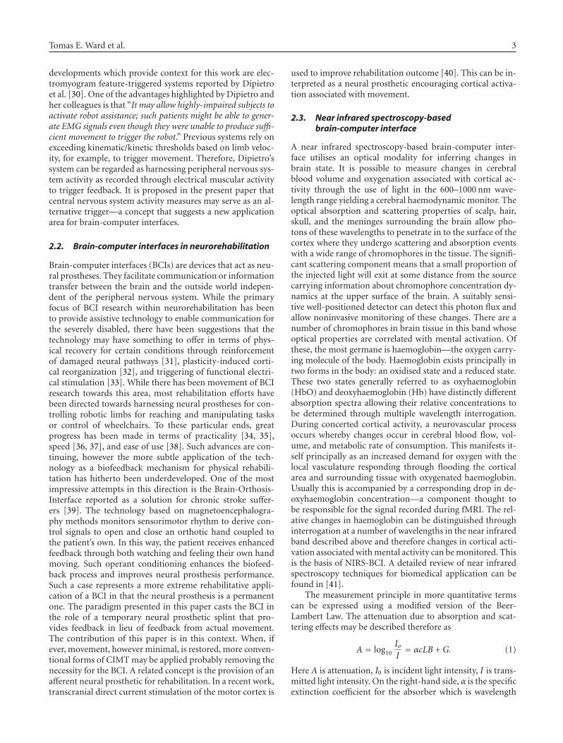
Tomas E. Ward et al. 3
developments which provide context for this work are elec-tromyogram feature-triggered systems reported by Dipietroet al. [30]. One of the advantages highlighted by Dipietro andher colleagues is that “It may allow highly-impaired subjects toactivate robot assistance; such patients might be able to gener-ate EMG signals even though they were unable to produce suffi-cient movement to trigger the robot.” Previous systems rely onexceeding kinematic/kinetic thresholds based on limb veloc-ity, for example, to trigger movement. Therefore, Dipietro’ssystem can be regarded as harnessing peripheral nervous sys-tem activity as recorded through electrical muscular activityto trigger feedback. It is proposed in the present paper thatcentral nervous system activity measures may serve as an al-ternative trigger—a concept that suggests a new applicationarea for brain-computer interfaces.
2.2. Brain-computer interfaces in neurorehabilitation
Brain-computer interfaces (BCIs) are devices that act as neu-ral prostheses. They facilitate communication or informationtransfer between the brain and the outside world indepen-dent of the peripheral nervous system. While the primaryfocus of BCI research within neurorehabilitation has beento provide assistive technology to enable communication forthe severely disabled, there have been suggestions that thetechnology may have something to offer in terms of phys-ical recovery for certain conditions through reinforcementof damaged neural pathways [31], plasticity-induced corti-cal reorganization [32], and triggering of functional electri-cal stimulation [33]. While there has been movement of BCIresearch towards this area, most rehabilitation efforts havebeen directed towards harnessing neural prostheses for con-trolling robotic limbs for reaching and manipulating tasksor control of wheelchairs. To these particular ends, greatprogress has been made in terms of practicality [34, 35],speed [36, 37], and ease of use [38]. Such advances are con-tinuing, however the more subtle application of the tech-nology as a biofeedback mechanism for physical rehabili-tation has hitherto been underdeveloped. One of the mostimpressive attempts in this direction is the Brain-Orthosis-Interface reported as a solution for chronic stroke suffer-ers [39]. The technology based on magnetoencephalogra-phy methods monitors sensorimotor rhythm to derive con-trol signals to open and close an orthotic hand coupled tothe patient’s own. In this way, the patient receives enhancedfeedback through both watching and feeling their own handmoving. Such operant conditioning enhances the biofeed-back process and improves neural prosthesis performance.Such a case represents a more extreme rehabilitative appli-cation of a BCI in that the neural prosthesis is a permanentone. The paradigm presented in this paper casts the BCI inthe role of a temporary neural prosthetic splint that pro-vides feedback in lieu of feedback from actual movement.The contribution of this paper is in this context. When, ifever, movement, however minimal, is restored, more conven-tional forms of CIMT may be applied probably removing thenecessity for the BCI. A related concept is the provision of anafferent neural prosthetic for rehabilitation. In a recent work,transcranial direct current stimulation of the motor cortex is
used to improve rehabilitation outcome [40]. This can be in-terpreted as a neural prosthetic encouraging cortical activa-tion associated with movement.
2.3. Near infrared spectroscopy-basedbrain-computer interface
A near infrared spectroscopy-based brain-computer inter-face utilises an optical modality for inferring changes inbrain state. It is possible to measure changes in cerebralblood volume and oxygenation associated with cortical ac-tivity through the use of light in the 600–1000 nm wave-length range yielding a cerebral haemodynamic monitor. Theoptical absorption and scattering properties of scalp, hair,skull, and the meninges surrounding the brain allow pho-tons of these wavelengths to penetrate in to the surface of thecortex where they undergo scattering and absorption eventswith a wide range of chromophores in the tissue. The signifi-cant scattering component means that a small proportion ofthe injected light will exit at some distance from the sourcecarrying information about chromophore concentration dy-namics at the upper surface of the brain. A suitably sensi-tive well-positioned detector can detect this photon flux andallow noninvasive monitoring of these changes. There are anumber of chromophores in brain tissue in this band whoseoptical properties are correlated with mental activation. Ofthese, the most germane is haemoglobin—the oxygen carry-ing molecule of the body. Haemoglobin exists principally intwo forms in the body: an oxidised state and a reduced state.These two states generally referred to as oxyhaemoglobin(HbO) and deoxyhaemoglobin (Hb) have distinctly differentabsorption spectra allowing their relative concentrations tobe determined through multiple wavelength interrogation.During concerted cortical activity, a neurovascular processoccurs whereby changes occur in cerebral blood flow, vol-ume, and metabolic rate of consumption. This manifests it-self principally as an increased demand for oxygen with thelocal vasculature responding through flooding the corticalarea and surrounding tissue with oxygenated haemoglobin.Usually this is accompanied by a corresponding drop in de-oxyhaemoglobin concentration—a component thought tobe responsible for the signal recorded during fMRI. The rel-ative changes in haemoglobin can be distinguished throughinterrogation at a number of wavelengths in the near infraredband described above and therefore changes in cortical acti-vation associated with mental activity can be monitored. Thisis the basis of NIRS-BCI. A detailed review of near infraredspectroscopy techniques for biomedical application can befound in [41].
The measurement principle in more quantitative termscan be expressed using a modified version of the Beer-Lambert Law. The attenuation due to absorption and scat-tering effects may be described therefore as
A = log10IoI= αcLB +G. (1)
Here A is attenuation, I0 is incident light intensity, I is trans-mitted light intensity. On the right-hand side, α is the specificextinction coefficient for the absorber which is wavelength
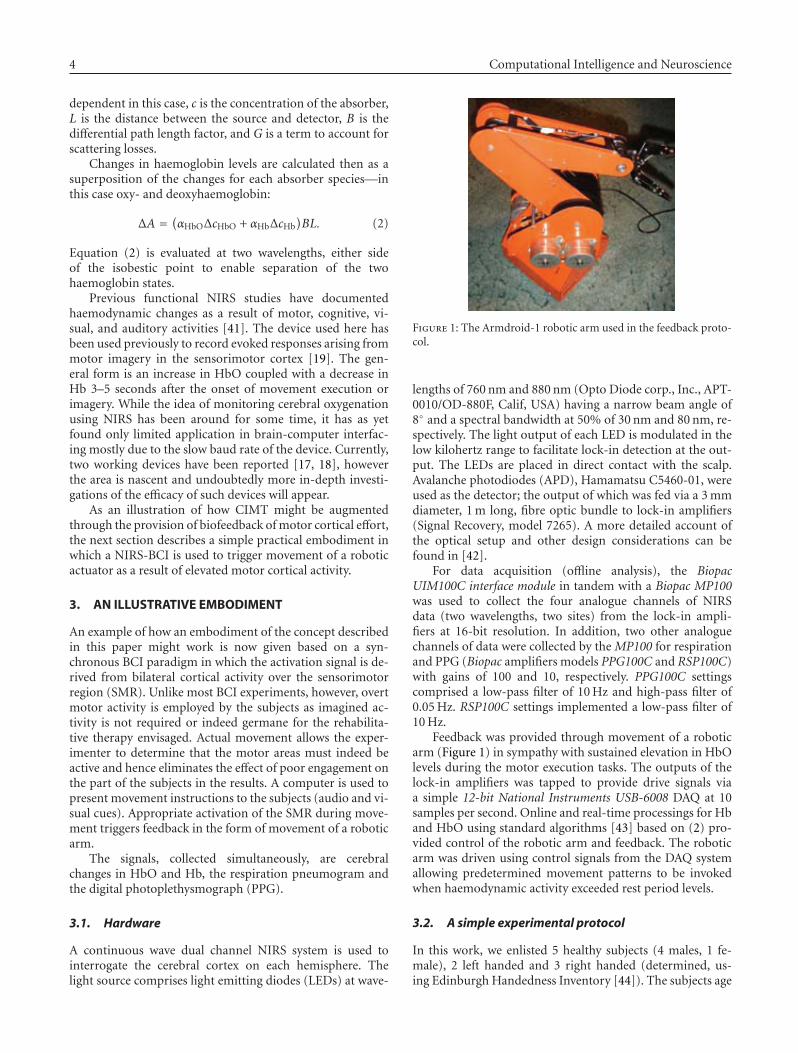
4 Computational Intelligence and Neuroscience
dependent in this case, c is the concentration of the absorber,L is the distance between the source and detector, B is thedifferential path length factor, and G is a term to account forscattering losses.
Changes in haemoglobin levels are calculated then as asuperposition of the changes for each absorber species—inthis case oxy- and deoxyhaemoglobin:
ΔA = (αHbOΔcHbO + αHbΔcHb)BL. (2)
Equation (2) is evaluated at two wavelengths, either sideof the isobestic point to enable separation of the twohaemoglobin states.
Previous functional NIRS studies have documentedhaemodynamic changes as a result of motor, cognitive, vi-sual, and auditory activities [41]. The device used here hasbeen used previously to record evoked responses arising frommotor imagery in the sensorimotor cortex [19]. The gen-eral form is an increase in HbO coupled with a decrease inHb 3–5 seconds after the onset of movement execution orimagery. While the idea of monitoring cerebral oxygenationusing NIRS has been around for some time, it has as yetfound only limited application in brain-computer interfac-ing mostly due to the slow baud rate of the device. Currently,two working devices have been reported [17, 18], howeverthe area is nascent and undoubtedly more in-depth investi-gations of the efficacy of such devices will appear.
As an illustration of how CIMT might be augmentedthrough the provision of biofeedback of motor cortical effort,the next section describes a simple practical embodiment inwhich a NIRS-BCI is used to trigger movement of a roboticactuator as a result of elevated motor cortical activity.
3. AN ILLUSTRATIVE EMBODIMENT
An example of how an embodiment of the concept describedin this paper might work is now given based on a syn-chronous BCI paradigm in which the activation signal is de-rived from bilateral cortical activity over the sensorimotorregion (SMR). Unlike most BCI experiments, however, overtmotor activity is employed by the subjects as imagined ac-tivity is not required or indeed germane for the rehabilita-tive therapy envisaged. Actual movement allows the exper-imenter to determine that the motor areas must indeed beactive and hence eliminates the effect of poor engagement onthe part of the subjects in the results. A computer is used topresent movement instructions to the subjects (audio and vi-sual cues). Appropriate activation of the SMR during move-ment triggers feedback in the form of movement of a roboticarm.
The signals, collected simultaneously, are cerebralchanges in HbO and Hb, the respiration pneumogram andthe digital photoplethysmograph (PPG).
3.1. Hardware
A continuous wave dual channel NIRS system is used tointerrogate the cerebral cortex on each hemisphere. Thelight source comprises light emitting diodes (LEDs) at wave-
Figure 1: The Armdroid-1 robotic arm used in the feedback proto-col.
lengths of 760 nm and 880 nm (Opto Diode corp., Inc., APT-0010/OD-880F, Calif, USA) having a narrow beam angle of8◦ and a spectral bandwidth at 50% of 30 nm and 80 nm, re-spectively. The light output of each LED is modulated in thelow kilohertz range to facilitate lock-in detection at the out-put. The LEDs are placed in direct contact with the scalp.Avalanche photodiodes (APD), Hamamatsu C5460-01, wereused as the detector; the output of which was fed via a 3 mmdiameter, 1 m long, fibre optic bundle to lock-in amplifiers(Signal Recovery, model 7265). A more detailed account ofthe optical setup and other design considerations can befound in [42].
For data acquisition (offline analysis), the BiopacUIM100C interface module in tandem with a Biopac MP100was used to collect the four analogue channels of NIRSdata (two wavelengths, two sites) from the lock-in ampli-fiers at 16-bit resolution. In addition, two other analoguechannels of data were collected by the MP100 for respirationand PPG (Biopac amplifiers models PPG100C and RSP100C)with gains of 100 and 10, respectively. PPG100C settingscomprised a low-pass filter of 10 Hz and high-pass filter of0.05 Hz. RSP100C settings implemented a low-pass filter of10 Hz.
Feedback was provided through movement of a roboticarm (Figure 1) in sympathy with sustained elevation in HbOlevels during the motor execution tasks. The outputs of thelock-in amplifiers was tapped to provide drive signals viaa simple 12-bit National Instruments USB-6008 DAQ at 10samples per second. Online and real-time processings for Hband HbO using standard algorithms [43] based on (2) pro-vided control of the robotic arm and feedback. The roboticarm was driven using control signals from the DAQ systemallowing predetermined movement patterns to be invokedwhen haemodynamic activity exceeded rest period levels.
3.2. A simple experimental protocol
In this work, we enlisted 5 healthy subjects (4 males, 1 fe-male), 2 left handed and 3 right handed (determined, us-ing Edinburgh Handedness Inventory [44]). The subjects age
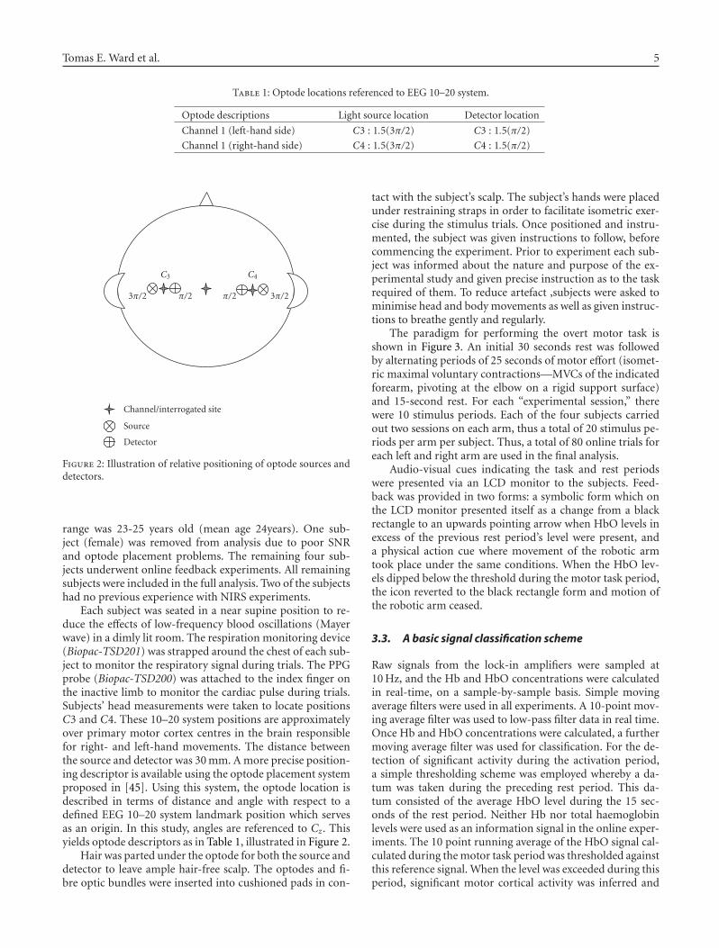
Tomas E. Ward et al. 5
Table 1: Optode locations referenced to EEG 10–20 system.
Optode descriptions Light source location Detector location
Channel 1 (left-hand side) C3 : 1.5(3π/2) C3 : 1.5(π/2)
Channel 1 (right-hand side) C4 : 1.5(3π/2) C4 : 1.5(π/2)
C3 C4
3π/2 π/2 π/2 3π/2
Channel/interrogated site
Source
Detector
Figure 2: Illustration of relative positioning of optode sources anddetectors.
range was 23-25 years old (mean age 24years). One sub-ject (female) was removed from analysis due to poor SNRand optode placement problems. The remaining four sub-jects underwent online feedback experiments. All remainingsubjects were included in the full analysis. Two of the subjectshad no previous experience with NIRS experiments.
Each subject was seated in a near supine position to re-duce the effects of low-frequency blood oscillations (Mayerwave) in a dimly lit room. The respiration monitoring device(Biopac-TSD201) was strapped around the chest of each sub-ject to monitor the respiratory signal during trials. The PPGprobe (Biopac-TSD200) was attached to the index finger onthe inactive limb to monitor the cardiac pulse during trials.Subjects’ head measurements were taken to locate positionsC3 and C4. These 10–20 system positions are approximatelyover primary motor cortex centres in the brain responsiblefor right- and left-hand movements. The distance betweenthe source and detector was 30 mm. A more precise position-ing descriptor is available using the optode placement systemproposed in [45]. Using this system, the optode location isdescribed in terms of distance and angle with respect to adefined EEG 10–20 system landmark position which servesas an origin. In this study, angles are referenced to Cz. Thisyields optode descriptors as in Table 1, illustrated in Figure 2.
Hair was parted under the optode for both the source anddetector to leave ample hair-free scalp. The optodes and fi-bre optic bundles were inserted into cushioned pads in con-
tact with the subject’s scalp. The subject’s hands were placedunder restraining straps in order to facilitate isometric exer-cise during the stimulus trials. Once positioned and instru-mented, the subject was given instructions to follow, beforecommencing the experiment. Prior to experiment each sub-ject was informed about the nature and purpose of the ex-perimental study and given precise instruction as to the taskrequired of them. To reduce artefact ,subjects were asked tominimise head and body movements as well as given instruc-tions to breathe gently and regularly.
The paradigm for performing the overt motor task isshown in Figure 3. An initial 30 seconds rest was followedby alternating periods of 25 seconds of motor effort (isomet-ric maximal voluntary contractions—MVCs of the indicatedforearm, pivoting at the elbow on a rigid support surface)and 15-second rest. For each “experimental session,” therewere 10 stimulus periods. Each of the four subjects carriedout two sessions on each arm, thus a total of 20 stimulus pe-riods per arm per subject. Thus, a total of 80 online trials foreach left and right arm are used in the final analysis.
Audio-visual cues indicating the task and rest periodswere presented via an LCD monitor to the subjects. Feed-back was provided in two forms: a symbolic form which onthe LCD monitor presented itself as a change from a blackrectangle to an upwards pointing arrow when HbO levels inexcess of the previous rest period’s level were present, anda physical action cue where movement of the robotic armtook place under the same conditions. When the HbO lev-els dipped below the threshold during the motor task period,the icon reverted to the black rectangle form and motion ofthe robotic arm ceased.
3.3. A basic signal classification scheme
Raw signals from the lock-in amplifiers were sampled at10 Hz, and the Hb and HbO concentrations were calculatedin real-time, on a sample-by-sample basis. Simple movingaverage filters were used in all experiments. A 10-point mov-ing average filter was used to low-pass filter data in real time.Once Hb and HbO concentrations were calculated, a furthermoving average filter was used for classification. For the de-tection of significant activity during the activation period,a simple thresholding scheme was employed whereby a da-tum was taken during the preceding rest period. This da-tum consisted of the average HbO level during the 15 sec-onds of the rest period. Neither Hb nor total haemoglobinlevels were used as an information signal in the online exper-iments. The 10 point running average of the HbO signal cal-culated during the motor task period was thresholded againstthis reference signal. When the level was exceeded during thisperiod, significant motor cortical activity was inferred and
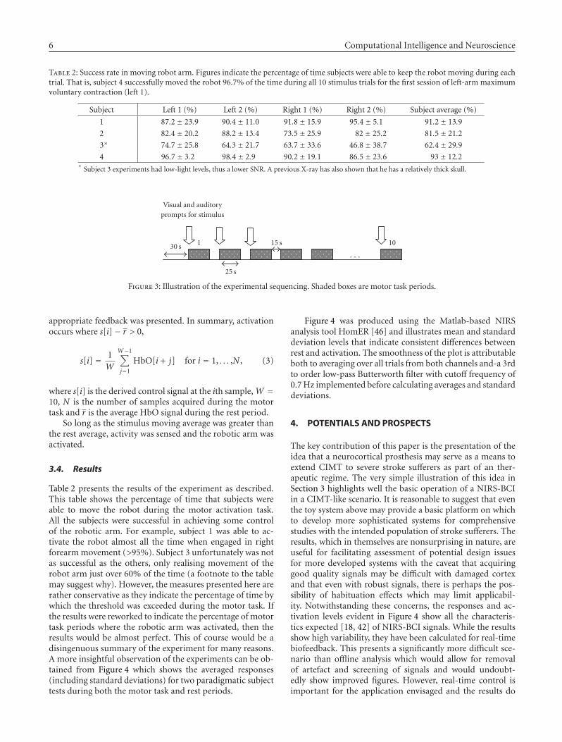
6 Computational Intelligence and Neuroscience
Table 2: Success rate in moving robot arm. Figures indicate the percentage of time subjects were able to keep the robot moving during eachtrial. That is, subject 4 successfully moved the robot 96.7% of the time during all 10 stimulus trials for the first session of left-arm maximumvoluntary contraction (left 1).
Subject Left 1 (%) Left 2 (%) Right 1 (%) Right 2 (%) Subject average (%)
1 87.2± 23.9 90.4± 11.0 91.8± 15.9 95.4± 5.1 91.2± 13.9
2 82.4± 20.2 88.2± 13.4 73.5± 25.9 82± 25.2 81.5± 21.2
3∗ 74.7± 25.8 64.3± 21.7 63.7± 33.6 46.8± 38.7 62.4± 29.9
4 96.7± 3.2 98.4± 2.9 90.2± 19.1 86.5± 23.6 93± 12.2∗
Subject 3 experiments had low-light levels, thus a lower SNR. A previous X-ray has also shown that he has a relatively thick skull.
Visual and auditoryprompts for stimulus
130 s 15 s 10
25 s
· · ·
Figure 3: Illustration of the experimental sequencing. Shaded boxes are motor task periods.
appropriate feedback was presented. In summary, activationoccurs where s[i]− r > 0,
s[i] = 1W
W−1∑
j=1
HbO[i + j] for i = 1, . . . ,N , (3)
where s[i] is the derived control signal at the ith sample,W =10, N is the number of samples acquired during the motortask and r is the average HbO signal during the rest period.
So long as the stimulus moving average was greater thanthe rest average, activity was sensed and the robotic arm wasactivated.
3.4. Results
Table 2 presents the results of the experiment as described.This table shows the percentage of time that subjects wereable to move the robot during the motor activation task.All the subjects were successful in achieving some controlof the robotic arm. For example, subject 1 was able to ac-tivate the robot almost all the time when engaged in rightforearm movement (>95%). Subject 3 unfortunately was notas successful as the others, only realising movement of therobot arm just over 60% of the time (a footnote to the tablemay suggest why). However, the measures presented here arerather conservative as they indicate the percentage of time bywhich the threshold was exceeded during the motor task. Ifthe results were reworked to indicate the percentage of motortask periods where the robotic arm was activated, then theresults would be almost perfect. This of course would be adisingenuous summary of the experiment for many reasons.A more insightful observation of the experiments can be ob-tained from Figure 4 which shows the averaged responses(including standard deviations) for two paradigmatic subjecttests during both the motor task and rest periods.
Figure 4 was produced using the Matlab-based NIRSanalysis tool HomER [46] and illustrates mean and standarddeviation levels that indicate consistent differences betweenrest and activation. The smoothness of the plot is attributableboth to averaging over all trials from both channels and-a 3rdto order low-pass Butterworth filter with cutoff frequency of0.7 Hz implemented before calculating averages and standarddeviations.
4. POTENTIALS AND PROSPECTS
The key contribution of this paper is the presentation of theidea that a neurocortical prosthesis may serve as a means toextend CIMT to severe stroke sufferers as part of an ther-apeutic regime. The very simple illustration of this idea inSection 3 highlights well the basic operation of a NIRS-BCIin a CIMT-like scenario. It is reasonable to suggest that eventhe toy system above may provide a basic platform on whichto develop more sophisticated systems for comprehensivestudies with the intended population of stroke sufferers. Theresults, which in themselves are nonsurprising in nature, areuseful for facilitating assessment of potential design issuesfor more developed systems with the caveat that acquiringgood quality signals may be difficult with damaged cortexand that even with robust signals, there is perhaps the pos-sibility of habituation effects which may limit applicabil-ity. Notwithstanding these concerns, the responses and ac-tivation levels evident in Figure 4 show all the characteris-tics expected [18, 42] of NIRS-BCI signals. While the resultsshow high variability, they have been calculated for real-timebiofeedback. This presents a significantly more difficult sce-nario than offline analysis which would allow for removalof artefact and screening of signals and would undoubt-edly show improved figures. However, real-time control isimportant for the application envisaged and the results do
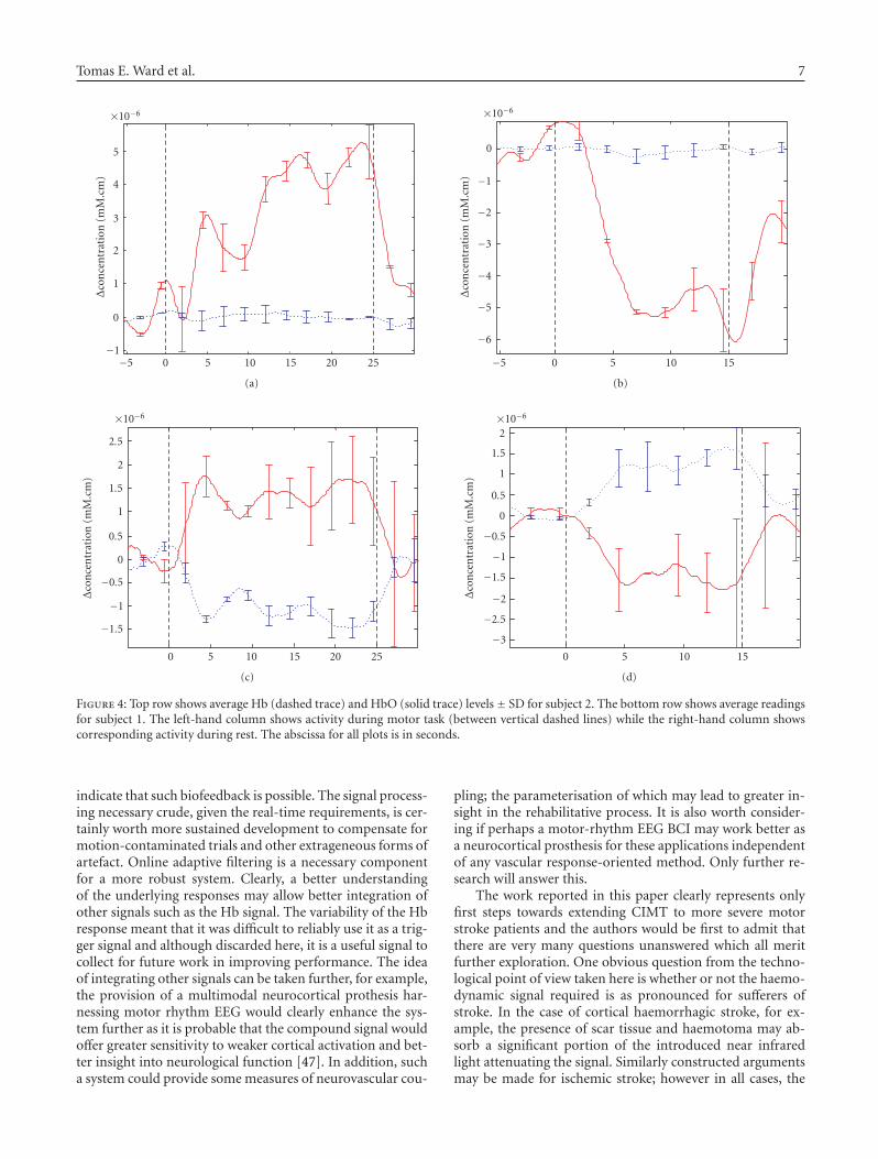
Tomas E. Ward et al. 7
−1
0
1
2
3
4
5
×10−6
Δco
nce
ntr
atio
n(m
M.c
m)
−5 0 5 10 15 20 25
(a)
−6
−5
−4
−3
−2
−1
0
×10−6
Δco
nce
ntr
atio
n(m
M.c
m)
−5 0 5 10 15
(b)
−1.5
−1
−0.5
0
0.5
1
1.5
2
2.5
×10−6
Δco
nce
ntr
atio
n(m
M.c
m)
0 5 10 15 20 25
(c)
−3
−2.5
−2
−1.5
−1
−0.5
0
0.5
1
1.5
2×10⁻⁶
Δco
nce
ntr
atio
n(m
M.c
m)
0 5 10 15
(d)
Figure 4: Top row shows average Hb (dashed trace) and HbO (solid trace) levels± SD for subject 2. The bottom row shows average readingsfor subject 1. The left-hand column shows activity during motor task (between vertical dashed lines) while the right-hand column showscorresponding activity during rest. The abscissa for all plots is in seconds.
indicate that such biofeedback is possible. The signal process-ing necessary crude, given the real-time requirements, is cer-tainly worth more sustained development to compensate formotion-contaminated trials and other extrageneous forms ofartefact. Online adaptive filtering is a necessary componentfor a more robust system. Clearly, a better understandingof the underlying responses may allow better integration ofother signals such as the Hb signal. The variability of the Hbresponse meant that it was difficult to reliably use it as a trig-ger signal and although discarded here, it is a useful signal tocollect for future work in improving performance. The ideaof integrating other signals can be taken further, for example,the provision of a multimodal neurocortical prothesis har-nessing motor rhythm EEG would clearly enhance the sys-tem further as it is probable that the compound signal wouldoffer greater sensitivity to weaker cortical activation and bet-ter insight into neurological function [47]. In addition, sucha system could provide some measures of neurovascular cou-
pling; the parameterisation of which may lead to greater in-sight in the rehabilitative process. It is also worth consider-ing if perhaps a motor-rhythm EEG BCI may work better asa neurocortical prosthesis for these applications independentof any vascular response-oriented method. Only further re-search will answer this.
The work reported in this paper clearly represents onlyfirst steps towards extending CIMT to more severe motorstroke patients and the authors would be first to admit thatthere are very many questions unanswered which all meritfurther exploration. One obvious question from the techno-logical point of view taken here is whether or not the haemo-dynamic signal required is as pronounced for sufferers ofstroke. In the case of cortical haemorrhagic stroke, for ex-ample, the presence of scar tissue and haemotoma may ab-sorb a significant portion of the introduced near infraredlight attenuating the signal. Similarly constructed argumentsmay be made for ischemic stroke; however in all cases, the
8 Computational Intelligence and Neuroscience
severity of such effects if they occur at al,l clearly dependson the site and extent of the injury. One might envisage thatinitial fMRI scans during attempted movement would facil-itate the deployment of the optode configurations requiredin such cases. To answer these concerns, clinical trials arerequired with appropriately selected stroke patients. An in-triguing possibility for controlled studies is the monitoring ofchanges in the haemodynamic signals themselves along withmotor movement efficacy. Additional quantitative measuressuch as those which might be provided through this methodwould surely prove useful in measuring rehabilitative out-come. The pioneers in this area have noted in a recent paperthat NIRS monitoring may provide a technological break-through in terms of developing and understanding CIMT[9]. Techniques such as the one espoused here may makesome contribution to the realisation of this suggestion. Thereare other concerns too. As mentioned during the backgroundsection, the neural prosthesis advocated here is not intendedas a permanent replacement for the patient’s own nervoussystem. It is envisaged that the device serve as a temporarychannel to convey some feedback for stroke sufferers whohave none. As soon as any other more conventional feedbackis available, then the prosthesis may be discarded. This phi-losophy is suggested in response to suggestions that repetitiveuse of stereotyped brain signals metabolic in origin or oth-erwise could within this disease context produce unwantedplasticity phenomena such as tics, obsessive thoughts, andother aberrant neurological functioning [32].
5. SUMMARY
This paper has highlighted the possibility of enhancing theapplication of CIMT for stroke sufferers through the addi-tion of a neuro-cortical prosthesis. Generally it is proposedthat a fruitful avenue for new research in the application ofbrain computer interfaces is in their measurement of voli-tional motor effort for biofeedback purposes in CIMT. Theintended target treatment group is severe stroke patients withlittle or no perceptible movement although the idea mayhave utility in the broader stroke population. More specifi-cally NIRS-based BCI are proposed as suitable candidates forsuch purposes. A simplified illustration of such a system ispresented which demonstrates the basic feasibility of the ap-proach. Testing with actual stroke sufferers is clearly the nextstep and will in itself undoubtedly introduce a number of sig-nificant challenges. Nevertheless we believe the concept de-scribed in this paper has merit as a specific extension of braincomputer interfaces into the neurorehabilitation domain.
ACKNOWLEDGMENTS
This work is supported by Science Foundation Ireland Grantno. SFI/05/RFP/ENG0089. The authors would like to ac-knowledge the contributions of Professor Barak P. Pearlmut-ter and Dr. Ray O’Neill in discussions concerning this work.Dr. Ward would also like to thank the reviewers and editorsfor their comments, advice, and suggestions during the re-viewing process.
REFERENCES
[1] R. Adams, M. Victor, and A. Ropper, Adam’s & Victor’s Princi-ples of Neurology, McGraw-Hill, New York, NY, USA, 6th edi-tion, 1997.
[2] World Health Organization Global Report 2002, “WorldHealth Organization,” http://www.who.int/whr/2002/en/index.html, January 2007.
[3] The Internet Stroke Centre, http://www.strokecenter.org/pat/stats.htm, January 2007.
[4] R. W. Bohannon, “Muscle strength and muscle training afterstroke,” Journal of Rehabilitation Medicine, vol. 39, no. 1, pp.14–20, 2007.
[5] E. Taub, N. E. Miller, T. A. Novack, et al., “Technique to im-prove chronic motor deficit after stroke,” Archives of PhysicalMedicine and Rehabilitation, vol. 74, no. 4, pp. 347–354, 1993.
[6] E. Taub, G. Uswatte, and R. Pidikiti, “Constraint-inducedmovement therapy: a new family of techniques with broad ap-plication to physical rehabilitation—a clinical review,” Journalof Rehabilitation Research and Development, vol. 36, no. 3, pp.237–251, 1999.
[7] W. H. Miltner, H. Bauder, M. Sommer, C. Dettmers, and E.Taub, “Effects of constraint-induced movement therapy onpatients with chronic motor deficits after stroke: a replication,”Stroke, vol. 30, no. 3, pp. 586–592, 1999.
[8] J. Liepert, “Motor cortex excitability in stroke before and afterconstraint-induced movement therapy,” Cognitive and Behav-ioral Neurology, vol. 19, no. 1, pp. 41–47, 2006.
[9] V. W. Mark, E. Taub, and D. M. Morris, “Neuroplasticity andconstraint-induced movement therapy,” Europa Medicophys-ica, vol. 42, no. 3, pp. 269–284, 2006.
[10] S. L. Wolf, C. J. Winstein, J. P. Miller, et al., “Effect ofconstraint-induced movement therapy on upper extremityfunction 3 to 9 months after stroke: the EXCITE random-ized clinical trial,” Journal of the American Medical Association,vol. 296, no. 17, pp. 2095–2104, 2006.
[11] V. W. Mark and E. Taub, “Constraint-induced movement ther-apy for chronic stroke hemiparesis and other disabilities,”Restorative Neurology and Neuroscience, vol. 22, no. 3-4, pp.317–336, 2004.
[12] P. S. Lum, C. G. Burgar, D. E. Kenney, and H. F. M. Van derLoos, “Quantification of force abnormalities during passiveand active-assisted upper-limb reaching movements in post-stroke hemiparesis,” IEEE Transactions on Biomedical Engi-neering, vol. 46, no. 6, pp. 652–662, 1999.
[13] J. H. van der Lee, R. C. Wagenaar, G. J. Lankhorst, T. W. Vo-gelaar, W. L. Deville, and L. M. Bouter, “Forced use of the up-per extremity in chronic stroke patients: results from a single-blind randomized clinical trial,” Stroke, vol. 30, no. 11, pp.2369–2375, 1999.
[14] J. Chae, F. Bethoux, T. Bohinc, L. Dobos, T. Davis, andA. Friedl, “Neuromuscular stimulation for upper extremitymotor and functional recovery in acute hemiplegia,” Stroke,vol. 29, no. 5, pp. 975–979, 1998.
[15] J. Powell, A. D. Pandyan, M. Granat, M. Cameron, and D. J.Stott, “Electrical stimulation of wrist extensors in poststrokehemiplegia,” Stroke, vol. 30, no. 7, pp. 1384–1389, 1999.
[16] A. J. Butler and S. J. Page, “Mental practice with motor im-agery: evidence for motor recovery and cortical reorganizationafter stroke,” Archives of Physical Medicine and Rehabilitation,vol. 87, no. 12, supplement, pp. 2–11, 2006.
Tomas E. Ward et al. 9
[17] S. Coyle, T. E. Ward, C. Markham, and G. McDarby, “Onthe suitability of near-infrared (NIR) systems for next-generation brain-computer interfaces,” Physiological Measure-ment, vol. 25, no. 4, pp. 815–822, 2004.
[18] R. Sitaram, H. Zhang, C. Guan, et al., “Temporal classificationof multichannel near-infrared spectroscopy signals of motorimagery for developing a brain-computer interface,” NeuroIm-age, vol. 34, no. 4, pp. 1416–1427, 2007.
[19] S. Coyle, T. E. Ward, and C. Markham, “An optical brain com-puter interface,” in Proceedings of the 2nd International Brain-Computer Interface Workshop and Training Course, vol. 49 ofBiomedizinische Technik, pp. 45–46, Graz, Austria, 2004.
[20] J. W. Krakauer, “Motor learning: its relevance to stroke recov-ery and neurorehabilitation,” Current Opinion in Neurology,vol. 19, no. 1, pp. 84–90, 2006.
[21] E. Taub and G. Uswatte, “Constraint-induced movement ther-apy: answers and questions after two decades of research,”NeuroRehabilitation, vol. 21, no. 2, pp. 93–95, 2006.
[22] H. I. Krebs, N. Hogan, M. L. Aisen, and B. T. Volpe, “Robot-aided neuro-rehabilitation,” IEEE Transactions on Rehabilita-tion Engineering, vol. 6, no. 1, pp. 75–87, 1998.
[23] E. J. Plautz, G. W. Milliken, and R. J. Nudo, “Effects of repet-itive motor training on movement representations in adultsquirrel monkeys: role of use versus learning,” Neurobiology ofLearning and Memory, vol. 74, no. 1, pp. 27–55, 2000.
[24] J. H. van der Lee, R. C. Wagenaar, G. J. Lankhorst, T. W. Vo-gelaar, W. L. Deville, and L. M. Bouter, “Forced use of the up-per extremity in chronic stroke patients: results from a single-blind randomized clinical trial,” Stroke, vol. 30, no. 11, pp.2369–2375, 1999.
[25] B. T. Volpe, H. I. Krebs, N. Hogan, L. Edelsteinn, C. M. Diels,and M. L. Aisen, “Robot training enhanced motor outcomein patients with stroke maintained over 3 years,” Neurology,vol. 53, no. 8, pp. 1874–1876, 1999.
[26] M. Ferraro, J. J. Palazzolo, J. Krol, H. I. Krebs, N. Hogan, and B.T. Volpe, “Robot-aided sensorimotor arm training improvesoutcome in patients with chronic stroke,” Neurology, vol. 61,no. 11, pp. 1604–1607, 2003.
[27] R. Colombo, F. Pisano, S. Micera, et al., “Robotic techniquesfor upper limb evaluation and rehabilitation of stroke pa-tients,” IEEE Transactions on Neural Systems and RehabilitationEngineering, vol. 13, no. 3, pp. 311–324, 2005.
[28] B. T. Volpe, M. Ferraro, D. Lynch, et al., “Robotics and otherdevices in the treatment of patients recovering from stroke,”Current Neurology and Neuroscience Reports, vol. 5, no. 6, pp.465–470, 2005.
[29] M. J. Johnson, “Recent trends in robot-assisted therapy en-vironments to improve real-life functional performance afterstroke,” Journal of NeuroEngineering and Rehabilitation, vol. 3,no. 1, p. 29, 2006.
[30] L. Dipietro, M. Ferraro, J. J. Palazzolo, H. I. Krebs, B. T. Volpe,and N. Hogan, “Customized interactive robotic treatment forstroke: EMG-triggered therapy,” IEEE Transactions on NeuralSystems and Rehabilitation Engineering, vol. 13, no. 3, pp. 325–334, 2005.
[31] A. Kubler, V. K. Mushahwar, L. R. Hochberg, and J. P.Donoghue, “BCI meeting 2005-workshop on clinical issuesand applications,” IEEE Transactions on Neural Systems andRehabilitation Engineering, vol. 14, no. 2, pp. 131–134, 2006.
[32] B. H. Dobkin, “Brain-computer interface technology as a toolto augment plasticity and outcomes for neurological rehabili-tation,” The Journal of Physiology, vol. 579, no. 3, pp. 637–642,2007.
[33] G. Pfurtscheller, G. R. Muller, J. Pfurtscheller, H. J. Gerner, andR. Rupp, “‘Thought’—control of functional electrical stimula-tion to restore hand grasp in a patient with tetraplegia,” Neu-roscience Letters, vol. 351, no. 1, pp. 33–36, 2003.
[34] A. Buttfield, P. W. Ferrez, and J. D. R. Millan, “Towards a ro-bust BCI: error potentials and online learning,” IEEE Transac-tions on Neural Systems and Rehabilitation Engineering, vol. 14,no. 2, pp. 164–168, 2006.
[35] Y. Wang, R. Wang, X. Gao, B. Hong, and S. Gao, “A practicalVEP-based brain-computer interface,” IEEE Transactions onNeural Systems and Rehabilitation Engineering, vol. 14, no. 2,pp. 234–240, 2006.
[36] D. J. McFarland, D. J. Krusienski, and J. R. Wolpaw, “Brain-computer interface signal processing at the Wadsworth Cen-ter: mu and sensorimotor beta rhythms,” Progress in Brain Re-search, vol. 159, pp. 411–419, 2006.
[37] E. W. Sellers, D. J. Krusienski, D. J. McFarland, T. M. Vaughan,and J. R. Wolpaw, “A P300 event-related potential brain-computer interface (BCI): the effects of matrix size and in-ter stimulus interval on performance,” Biological Psychology,vol. 73, no. 3, pp. 242–252, 2006.
[38] C. Vidaurre, A. Schlogl, R. Cabeza, R. Scherer, and G.Pfurtscheller, “A fully on-line adaptive BCI,” IEEE Transactionson Biomedical Engineering, vol. 53, no. 6, pp. 1214–1219, 2006.
[39] N. Birbaumer and L. G. Cohen, “Brain-computer interfaces:communication and restoration of movement in paralysis,”The Journal of Physiology, vol. 579, no. 3, pp. 621–636, 2007.
[40] F. Hummel, P. Celnik, P. Giraux, et al., “Effects of non-invasivecortical stimulation on skilled motor function in chronicstroke,” Brain, vol. 128, no. 3, pp. 490–499, 2005.
[41] P. Rolfe, “In vivo near-infrared spectroscopy,” Annual Reviewof Biomedical Engineering, vol. 2, pp. 715–754, 2000.
[42] S. Coyle, Near-infrared spectroscopy for brain computer inter-facing, Ph.D. thesis, National University of Ireland, Maynooth,Ireland, 2005.
[43] M. Cope and D. T. Delpy, “System for long-term measure-ment of cerebral blood and tissue oxygenation on newborninfants by near infra-red transillumination,” Medical and Bio-logical Engineering and Computing, vol. 26, no. 3, pp. 289–294,1988.
[44] R. C. Oldfield, “The assessment and analysis of handedness:the Edinburgh inventory,” Neuropsychologia, vol. 9, no. 1, pp.97–113, 1971.
[45] S. Coyle, C. Markham, W. Lanigan, and T. Ward, “A me-chanical mounting system for functional near-infrared spec-troscopy brain imaging studies,” in Opto-Ireland 2005: OpticalSensing and Spectroscopy, vol. 5826 of Proceedings of SPIE, pp.618–627, Dublin, Ireland, April 2005.
[46] HomER, http://www.nmr.mgh.harvard.edu/PMI/resources/homer/home.htm.
[47] F. Babiloni, D. Mattia, C. Babiloni, et al., “Multimodal integra-tion of EEG, MEG and fMRI data for the solution of the neu-roimage puzzle,” Magnetic Resonance Imaging, vol. 22, no. 10,pp. 1471–1476, 2004.
Hindawi Publishing CorporationComputational Intelligence and NeuroscienceVolume 2007, Article ID 84386, 8 pagesdoi:10.1155/2007/84386
Research ArticleTowards Development of a 3-State Self-PacedBrain-Computer Interface
Ali Bashashati,1, 2, 3 Rabab K. Ward,1, 4 and Gary E. Birch1, 3, 4
1 Electrical and Computer Engineering Department, University of British Columbia, Vancouver, BC, Canada V6T 1Z42 Terry Fox Laboratory, British Columbia Cancer Research Center, Vancouver, BC, Canada V5Z 1L33 Brain Interface Laboratory, Neil Squire Society, Suite 220, 2250 Boundary Road, Burnaby, BC, Canada V5M 3Z3
4 Institute for Computing, Information & Cognitive Systems, Vancouver, BC, Canada V6T 1Z4
Correspondence should be addressed to Ali Bashashati, [email protected]
Received 15 February 2007; Accepted 22 August 2007
Recommended by Andrzej Cichocki
Most existing brain-computer interfaces (BCIs) detect specific mental activity in a so-called synchronous paradigm. Unlike syn-chronous systems which are operational at specific system-defined periods, self-paced (asynchronous) interfaces have the advan-tage of being operational at all times. The low-frequency asynchronous switch design (LF-ASD) is a 2-state self-paced BCI thatdetects the presence of a specific finger movement in the ongoing EEG. Recent evaluations of the 2-state LF-ASD show an averagetrue positive rate of 41% at the fixed false positive rate of 1%. This paper proposes two designs for a 3-state self-paced BCI that iscapable of handling idle brain state. The two proposed designs aim at detecting right- and left-hand extensions from the ongoingEEG. They are formed of two consecutive detectors. The first detects the presence of a right- or a left-hand movement and thesecond classifies the detected movement as a right or a left one. In an offline analysis of the EEG data collected from four able-bodied individuals, the 3-state brain-computer interface shows a comparable performance with a 2-state system and significantperformance improvement if used as a 2-state BCI, that is, in detecting the presence of a right- or a left-hand movement (regard-less of the type of movement). It has an average true positive rate of 37.5% and 42.8% (at false positives rate of 1%) in detectingright- and left-hand extensions, respectively, in the context of a 3-state self-paced BCI and average detection rate of 58.1% (at falsepositive rate of 1%) in the context of a 2-state self-paced BCI.
Copyright © 2007 Ali Bashashati et al. This is an open access article distributed under the Creative Commons Attribution License,which permits unrestricted use, distribution, and reproduction in any medium, provided the original work is properly cited.
1. INTRODUCTION
Brain-computer interface (BCI) systems form a possible al-ternative communication and control solutions for individ-uals with severe disabilities. For a review of the field, see[1–3]. In BCI systems, the user’s cortical activity associatedwith an intentional control of a device (such as attemptedfinger movements) is directly mapped to an application-specific control signal. This allows the user to control var-ious devices such as a neural prosthetic by cognitive pro-cesses only, that is, by bypassing traditional interface path-ways (which cannot be used by individuals with severe dis-abilities).
In developing noninvasive BCI systems, the majority ofresearch has concentrated on developing synchronous sys-tems. These systems are only operational at specific periods.Asynchronous (self-paced) systems, on the other hand, have
the advantage of being operational at all times. The 2-statelow frequency-asynchronous switch design (LF-ASD) wasthe first BCI introduced for self-paced or asynchronous con-trol applications [4]. LF-ASD seeks to recognize the move-ment related potentials (MRPs) of a finger-flexion movementin the EEG signal. In a self-paced brain-computer interfacethe users affect the BCI transducer output whenever theywant by intentionally changing their brain states. Betweenperiods of intentional control (IC), users are said to be in ano-control (NC) state; they may be idle, daydreaming, think-ing about a problem or lunch, or performing any other actionother than trying to control the BCI transducer. These BCItransducers are thus designed to respond only when there isan intentional user control. The appropriate BCI responseto no-control (NC) would be a neutral or inactive output.We refer to this ability as NC support. NC support is neces-sary for most types of machine or device interactions where
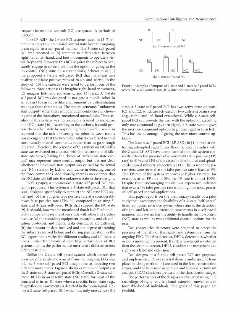
2 Computational Intelligence and Neuroscience
frequent intentional controls (IC) are spaced by periods ofinaction.
Like LF-ASD, the 2-state BCI systems tested in [5–7] at-tempt to detect an intentional control state from the ongoingbrain signal in a self-paced manner. The 3-state self-pacedBCI implemented in [8] attempts to differentiate betweenright-hand, left-hand, and foot movements to operate a vir-tual keyboard. However, this BCI requires the subject to con-stantly engage in control without the option of going to theno control (NC) state. In a recent work, Scherer et al. [9]has proposed a 4-state self-paced BCI that has mean truepositive and false positive rates of 28.4% and 16.9%. In thestudy of [10] the subjects were asked to perform one of thefollowing three actions: (1) imagine right-hand movement,(2) imagine left-hand movement, and (3) relax. A 3-stateself-paced BCI was designed to navigate a mobile robot inan 80 cm∗60 cm house-like environment by differentiatingamongst these three states. The system generates “unknownstate output” when there is not enough confidence in choos-ing one of the three above-mentioned mental tasks. The clas-sifier of this system was not explicitly trained to recognizeidle (NC) state [10]. According to the authors, it could pro-cess them adequately by responding “unknown”. It was alsoreported that the task of steering the robot between roomswas so engaging that the two tested subjects preferred to emitcontinuously mental commands rather than to go throughidle state. Therefore, the response of this system on NC (idle)state was evaluated on a dataset with limited amount of idle-state. Moreover, having the choice of “unknown state out-put” may represent some neutral output but it is not clearwhether the unknown state output was caused by the actualidle (NC) state or by lack of confidence in detecting one ofthe three commands. Additionally, there is no evidence thatthe NC state will fall into the unknown state in these designs.
In this paper, a noninvasive 3-state self-paced BCI sys-tem is proposed. This system is a 3-state self-paced BCI thatis (a) designed specifically to support the NC state EEG sig-nal, and (b) has a higher true positive rate at a considerablylower false positive rate (FP=1%) compared to existing 3-state and 4-state self-paced BCIs that support the NC state[9]. It should, however, be mentioned that it is difficult to di-rectly compare the results of our study with other BCI studiesbecause (a) the recording equipment, recording and classifi-cation protocols, and mental tasks considered are different,(b) the amount of data involved and the degree of trainingthe subjects received before and during participation in theBCI experiments varies for different studies, and (c) there isnot a unified framework of reporting performance of BCIsystems, that is, the performance metrics are different acrossdifferent studies.
Unlike the 2-state self-paced system which detects thepresence of a single movement from the ongoing EEG sig-nal, the 3-state self-paced BCI design aims at detecting twodifferent movements. Figure 1 shows examples of outputs ofthe 2-state and 3-state self-paced BCIs. Overall, a 2-state self-paced BCI is in an inactive state (NC state) for most of thetime and is in an IC state when a specific brain state (e.g.,finger-flexion movement) is detected in the brain signal. Un-like a 2-state self-paced BCI which has only one active (IC)
NC NC NC
IC IC
(a) 2-state self-paced BCI
NC NC NC NC NC
IC1
IC2 IC2
IC1
(b) 3-state self-paced BCI
Figure 1: Samples of outputs of 2-state and 3-state self-paced BCIs,where NC = no-control state, IC = intended control state.
state, a 3-state self-paced BCI has two active state outputs,IC1 and IC2, which are activated by two different brain states(e.g., right- and left-hand extensions). While a 2-state self-paced BCI can provide the user with the option of executingonly one command (e.g., turn right), a 3-state system givesthe user two command options (e.g., turn right or turn left).This has the advantage of giving the user more control op-tions.
The 2-state self-paced BCI (LF-ASD) in [4] aimed at de-tecting attempted right finger flexions. Recent studies withthe 2-state LF-ASD have demonstrated that this system cor-rectly detects the presence of a movement (true positive (TP)rate) in 41% and 42% of the cases for able-bodied and spinal-cord-injured subjects, respectively [11]. This is when the pa-rameters were set so that the false positive rate is fixed at 1%.The TP rate of the system improves at higher FP rates, forexample, at an FP rate of 5%, the TP rate is almost 100%.Despite these encouraging results, our experience indicatesthat even a 1% false positive rate is too high for most practi-cal self-paced control applications.
This paper reports on the preliminary results of a pilotstudy that investigates the feasibility of a 3-state “self-paced”brain-computer interface system whose aim is the detectionof right- and left-hand extension movements in a self-pacedmanner. This system has the ability to handle the no-control(NC) state as well as two additional control options for theuser.
Two consecutive detectors were designed to detect thepresence of the left- or the right-hand extensions from theongoing EEG. The first detector, DET1, determines whetheror not a movement is present. If such a movement is detectedthen the second detector, DET2, classifies the movement as aright- or a left-hand extension.
Two designs of a 3-state self-paced BCI are proposedand implemented. Power spectral density and a specific tem-plate matching method [4] are used in the feature extractionstages, and the k-nearest neighbour and linear discriminantanalysis (LDA) classifiers are used in the classification stages.
The performances of the designs are evaluated using EEGrecordings of right- and left-hand extension movements offour able-bodied individuals. The goals of this paper aretwofold.
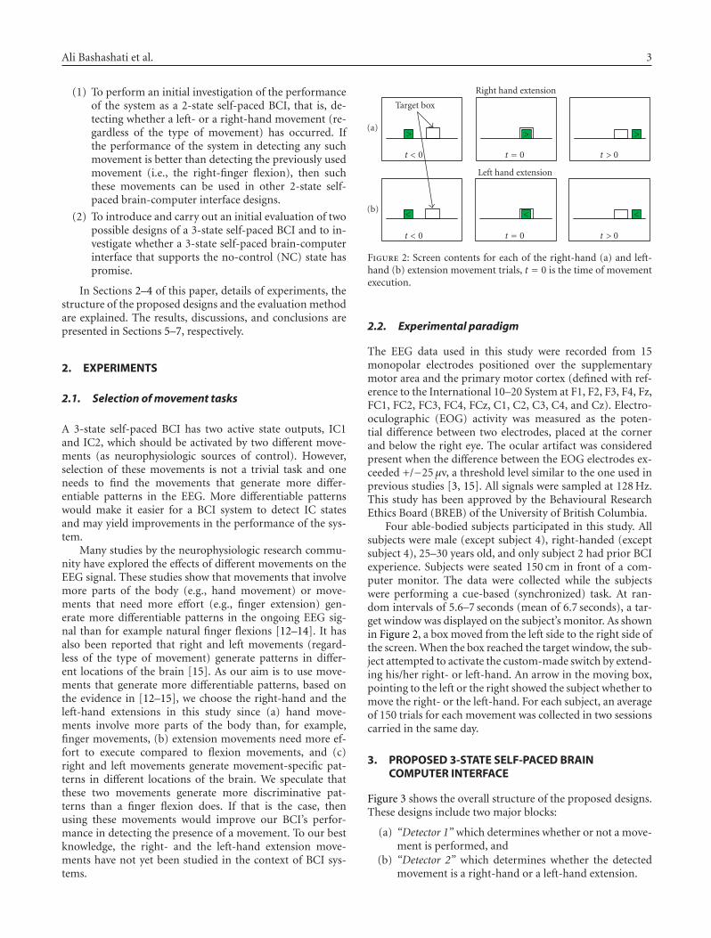
Ali Bashashati et al. 3
(1) To perform an initial investigation of the performanceof the system as a 2-state self-paced BCI, that is, de-tecting whether a left- or a right-hand movement (re-gardless of the type of movement) has occurred. Ifthe performance of the system in detecting any suchmovement is better than detecting the previously usedmovement (i.e., the right-finger flexion), then suchthese movements can be used in other 2-state self-paced brain-computer interface designs.
(2) To introduce and carry out an initial evaluation of twopossible designs of a 3-state self-paced BCI and to in-vestigate whether a 3-state self-paced brain-computerinterface that supports the no-control (NC) state haspromise.
In Sections 2–4 of this paper, details of experiments, thestructure of the proposed designs and the evaluation methodare explained. The results, discussions, and conclusions arepresented in Sections 5–7, respectively.
2. EXPERIMENTS
2.1. Selection of movement tasks
A 3-state self-paced BCI has two active state outputs, IC1and IC2, which should be activated by two different move-ments (as neurophysiologic sources of control). However,selection of these movements is not a trivial task and oneneeds to find the movements that generate more differ-entiable patterns in the EEG. More differentiable patternswould make it easier for a BCI system to detect IC statesand may yield improvements in the performance of the sys-tem.
Many studies by the neurophysiologic research commu-nity have explored the effects of different movements on theEEG signal. These studies show that movements that involvemore parts of the body (e.g., hand movement) or move-ments that need more effort (e.g., finger extension) gen-erate more differentiable patterns in the ongoing EEG sig-nal than for example natural finger flexions [12–14]. It hasalso been reported that right and left movements (regard-less of the type of movement) generate patterns in differ-ent locations of the brain [15]. As our aim is to use move-ments that generate more differentiable patterns, based onthe evidence in [12–15], we choose the right-hand and theleft-hand extensions in this study since (a) hand move-ments involve more parts of the body than, for example,finger movements, (b) extension movements need more ef-fort to execute compared to flexion movements, and (c)right and left movements generate movement-specific pat-terns in different locations of the brain. We speculate thatthese two movements generate more discriminative pat-terns than a finger flexion does. If that is the case, thenusing these movements would improve our BCI’s perfor-mance in detecting the presence of a movement. To our bestknowledge, the right- and the left-hand extension move-ments have not yet been studied in the context of BCI sys-tems.
t < 0 t = 0 t > 0
t < 0 t = 0 t > 0
Target box
>
<
Right hand extension
Left hand extension
>
<
>
<
(a)
(b)
Figure 2: Screen contents for each of the right-hand (a) and left-hand (b) extension movement trials, t = 0 is the time of movementexecution.
2.2. Experimental paradigm
The EEG data used in this study were recorded from 15monopolar electrodes positioned over the supplementarymotor area and the primary motor cortex (defined with ref-erence to the International 10–20 System at F1, F2, F3, F4, Fz,FC1, FC2, FC3, FC4, FCz, C1, C2, C3, C4, and Cz). Electro-oculographic (EOG) activity was measured as the poten-tial difference between two electrodes, placed at the cornerand below the right eye. The ocular artifact was consideredpresent when the difference between the EOG electrodes ex-ceeded +/−25 μv, a threshold level similar to the one used inprevious studies [3, 15]. All signals were sampled at 128 Hz.This study has been approved by the Behavioural ResearchEthics Board (BREB) of the University of British Columbia.
Four able-bodied subjects participated in this study. Allsubjects were male (except subject 4), right-handed (exceptsubject 4), 25–30 years old, and only subject 2 had prior BCIexperience. Subjects were seated 150 cm in front of a com-puter monitor. The data were collected while the subjectswere performing a cue-based (synchronized) task. At ran-dom intervals of 5.6–7 seconds (mean of 6.7 seconds), a tar-get window was displayed on the subject’s monitor. As shownin Figure 2, a box moved from the left side to the right side ofthe screen. When the box reached the target window, the sub-ject attempted to activate the custom-made switch by extend-ing his/her right- or left-hand. An arrow in the moving box,pointing to the left or the right showed the subject whether tomove the right- or the left-hand. For each subject, an averageof 150 trials for each movement was collected in two sessionscarried in the same day.
3. PROPOSED 3-STATE SELF-PACED BRAINCOMPUTER INTERFACE
Figure 3 shows the overall structure of the proposed designs.These designs include two major blocks:
(a) “Detector 1” which determines whether or not a move-ment is performed, and
(b) “Detector 2” which determines whether the detectedmovement is a right-hand or a left-hand extension.
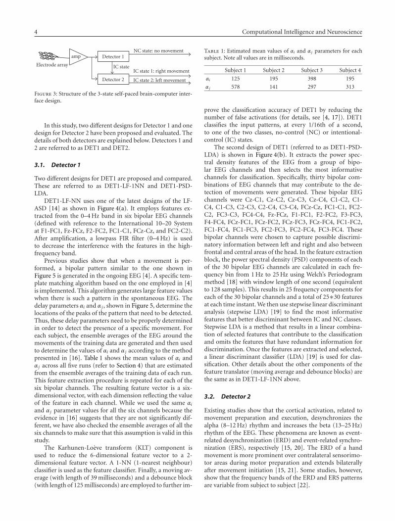
4 Computational Intelligence and Neuroscience
Electrode array
amp Detector 1
Detector 2
IC state
NC state: no movement
IC state 1: right movement
IC state 2: left movement
Figure 3: Structure of the 3-state self-paced brain-computer inter-face design.
In this study, two different designs for Detector 1 and onedesign for Detector 2 have been proposed and evaluated. Thedetails of both detectors are explained below. Detectors 1 and2 are referred to as DET1 and DET2.
3.1. Detector 1
Two different designs for DET1 are proposed and compared.These are referred to as DET1-LF-1NN and DET1-PSD-LDA.
DET1-LF-NN uses one of the latest designs of the LF-ASD [14] as shown in Figure 4(a). It employs features ex-tracted from the 0–4 Hz band in six bipolar EEG channels(defined with reference to the International 10–20 Systemat F1-FC1, Fz-FCz, F2-FC2, FC1-C1, FCz-Cz, and FC2-C2).After amplification, a lowpass FIR filter (0–4 Hz) is usedto decrease the interference with the features in the high-frequency band.
Previous studies show that when a movement is per-formed, a bipolar pattern similar to the one shown inFigure 5 is generated in the ongoing EEG [4]. A specific tem-plate matching algorithm based on the one employed in [4]is implemented. This algorithm generates large feature valueswhen there is such a pattern in the spontaneous EEG. Thedelay parameters αi and αj , shown in Figure 5, determine thelocations of the peaks of the pattern that need to be detected.Thus, these delay parameters need to be properly determinedin order to detect the presence of a specific movement. Foreach subject, the ensemble averages of the EEG around themovements of the training data are generated and then usedto determine the values of αi and αj according to the methodpresented in [16]. Table 1 shows the mean values of αi andαj across all five runs (refer to Section 4) that are estimatedfrom the ensemble averages of the training data of each run.This feature extraction procedure is repeated for each of thesix bipolar channels. The resulting feature vector is a six-dimensional vector, with each dimension reflecting the valueof the feature in each channel. While we used the same αiand αj parameter values for all the six channels because theevidence in [16] suggests that they are not significantly dif-ferent, we have also checked the ensemble averages of all thesix channels to make sure that this assumption is valid in thisstudy.
The Karhunen-Loeve transform (KLT) component isused to reduce the 6-dimensional feature vector to a 2-dimensional feature vector. A 1-NN (1-nearest neighbour)classifier is used as the feature classifier. Finally, a moving av-erage (with length of 39 milliseconds) and a debounce block(with length of 125 milliseconds) are employed to further im-
Table 1: Estimated mean values of αi and αj parameters for eachsubject. Note all values are in milliseconds.
Subject 1 Subject 2 Subject 3 Subject 4
αi 125 195 398 195
αj 578 141 297 313
prove the classification accuracy of DET1 by reducing thenumber of false activations (for details, see [4, 17]). DET1classifies the input patterns, at every 1/16th of a second,to one of the two classes, no-control (NC) or intentional-control (IC) states.
The second design of DET1 (referred to as DET1-PSD-LDA) is shown in Figure 4(b). It extracts the power spec-tral density features of the EEG from a group of bipo-lar EEG channels and then selects the most informativechannels for classification. Specifically, thirty bipolar com-binations of EEG channels that may contribute to the de-tection of movements were generated. These bipolar EEGchannels were Cz-C1, Cz-C2, Cz-C3, Cz-C4, C1-C2, C1-C4, C1-C3, C2-C3, C2-C4, C3-C4, FCz-Cz, FC1-C1, FC2-C2, FC3-C3, FC4-C4, Fz-FCz, F1-FC1, F2-FC2, F3-FC3,F4-FC4, FCz-FC1, FCz-FC2, FCz-FC3, FCz-FC4, FC1-FC2,FC1-FC4, FC1-FC3, FC2-FC3, FC2-FC4, FC3-FC4. Thesebipolar channels were chosen to capture possible discrimi-natory information between left and right and also betweenfrontal and central areas of the head. In the feature extractionblock, the power spectral density (PSD) components of eachof the 30 bipolar EEG channels are calculated in each fre-quency bin from 1 Hz to 25 Hz using Welch’s Periodogrammethod [18] with window length of one second (equivalentto 128 samples). This results in 25 frequency components foreach of the 30 bipolar channels and a total of 25∗30 featuresat each time instant. We then use stepwise linear discriminantanalysis (stepwise LDA) [19] to find the most informativefeatures that better discriminant between IC and NC classes.Stepwise LDA is a method that results in a linear combina-tion of selected features that contribute to the classificationand omits the features that have redundant information fordiscrimination. Once the features are extracted and selected,a linear discriminant classifier (LDA) [19] is used for clas-sification. Other details about the other components of thefeature translator (moving average and debounce blocks) arethe same as in DET1-LF-1NN above.
3.2. Detector 2
Existing studies show that the cortical activation, related tomovement preparation and execution, desynchronizes thealpha (8–12 Hz) rhythm and increases the beta (13–25 Hz)rhythm of the EEG. These phenomena are known as event-related desynchronization (ERD) and event-related synchro-nization (ERS), respectively [15, 20]. The ERD of a handmovement is more prominent over contralateral sensorimo-tor areas during motor preparation and extends bilaterallyafter movement initiation [15, 21]. Some studies, however,show that the frequency bands of the ERD and ERS patternsare variable from subject to subject [22].
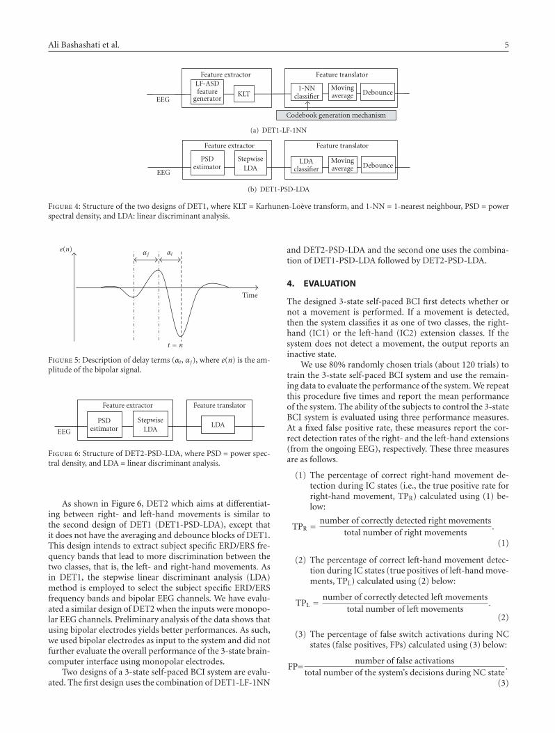
Ali Bashashati et al. 5
EEG
Feature extractorLF-ASDfeature
generatorKLT
Feature translator
1-NNclassifier
Movingaverage Debounce
Codebook generation mechanism
(a) DET1-LF-1NN
EEG
Feature extractor
PSDestimator
StepwiseLDA
Feature translator
LDAclassifier
Movingaverage Debounce
(b) DET1-PSD-LDA
Figure 4: Structure of the two designs of DET1, where KLT = Karhunen-Loeve transform, and 1-NN = 1-nearest neighbour, PSD = powerspectral density, and LDA: linear discriminant analysis.
e(n) αj αi
Time
t = n
Figure 5: Description of delay terms (αi, αj), where e(n) is the am-plitude of the bipolar signal.
EEG
Feature extractor
PSDestimator
StepwiseLDA
Feature translator
LDA
Figure 6: Structure of DET2-PSD-LDA, where PSD = power spec-tral density, and LDA = linear discriminant analysis.
As shown in Figure 6, DET2 which aims at differentiat-ing between right- and left-hand movements is similar tothe second design of DET1 (DET1-PSD-LDA), except thatit does not have the averaging and debounce blocks of DET1.This design intends to extract subject specific ERD/ERS fre-quency bands that lead to more discrimination between thetwo classes, that is, the left- and right-hand movements. Asin DET1, the stepwise linear discriminant analysis (LDA)method is employed to select the subject specific ERD/ERSfrequency bands and bipolar EEG channels. We have evalu-ated a similar design of DET2 when the inputs were monopo-lar EEG channels. Preliminary analysis of the data shows thatusing bipolar electrodes yields better performances. As such,we used bipolar electrodes as input to the system and did notfurther evaluate the overall performance of the 3-state brain-computer interface using monopolar electrodes.
Two designs of a 3-state self-paced BCI system are evalu-ated. The first design uses the combination of DET1-LF-1NN
and DET2-PSD-LDA and the second one uses the combina-tion of DET1-PSD-LDA followed by DET2-PSD-LDA.
4. EVALUATION
The designed 3-state self-paced BCI first detects whether ornot a movement is performed. If a movement is detected,then the system classifies it as one of two classes, the right-hand (IC1) or the left-hand (IC2) extension classes. If thesystem does not detect a movement, the output reports aninactive state.
We use 80% randomly chosen trials (about 120 trials) totrain the 3-state self-paced BCI system and use the remain-ing data to evaluate the performance of the system. We repeatthis procedure five times and report the mean performanceof the system. The ability of the subjects to control the 3-stateBCI system is evaluated using three performance measures.At a fixed false positive rate, these measures report the cor-rect detection rates of the right- and the left-hand extensions(from the ongoing EEG), respectively. These three measuresare as follows.
(1) The percentage of correct right-hand movement de-tection during IC states (i.e., the true positive rate forright-hand movement, TPR) calculated using (1) be-low:
TPR = number of correctly detected right movementstotal number of right movements
.
(1)
(2) The percentage of correct left-hand movement detec-tion during IC states (true positives of left-hand move-ments, TPL) calculated using (2) below:
TPL = number of correctly detected left movementstotal number of left movements
.
(2)
(3) The percentage of false switch activations during NCstates (false positives, FPs) calculated using (3) below:
FP= number of false activationstotal number of the system’s decisions during NC state
.
(3)
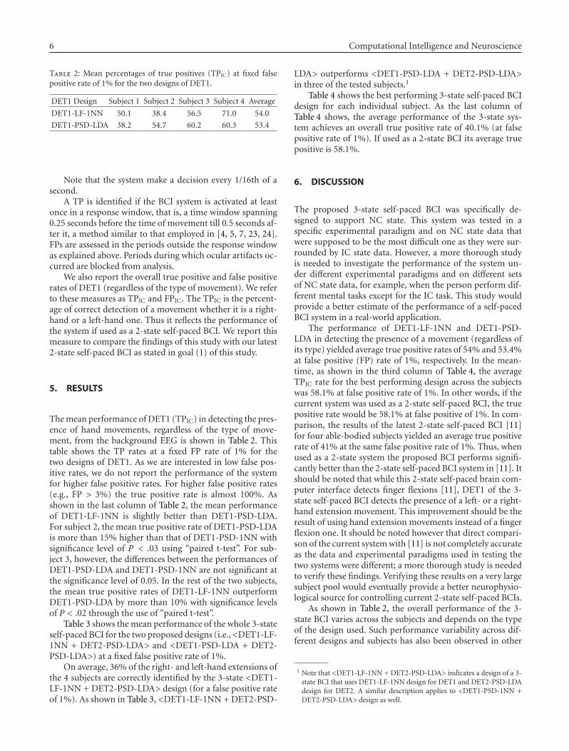
6 Computational Intelligence and Neuroscience
Table 2: Mean percentages of true positives (TPIC) at fixed falsepositive rate of 1% for the two designs of DET1.
DET1 Design Subject 1 Subject 2 Subject 3 Subject 4 Average
DET1-LF-1NN 50.1 38.4 56.5 71.0 54.0
DET1-PSD-LDA 38.2 54.7 60.2 60.3 53.4
Note that the system make a decision every 1/16th of asecond.
A TP is identified if the BCI system is activated at leastonce in a response window, that is, a time window spanning0.25 seconds before the time of movement till 0.5 seconds af-ter it, a method similar to that employed in [4, 5, 7, 23, 24].FPs are assessed in the periods outside the response windowas explained above. Periods during which ocular artifacts oc-curred are blocked from analysis.
We also report the overall true positive and false positiverates of DET1 (regardless of the type of movement). We referto these measures as TPIC and FPIC. The TPIC is the percent-age of correct detection of a movement whether it is a right-hand or a left-hand one. Thus it reflects the performance ofthe system if used as a 2-state self-paced BCI. We report thismeasure to compare the findings of this study with our latest2-state self-paced BCI as stated in goal (1) of this study.
5. RESULTS
The mean performance of DET1 (TPIC) in detecting the pres-ence of hand movements, regardless of the type of move-ment, from the background EEG is shown in Table 2. Thistable shows the TP rates at a fixed FP rate of 1% for thetwo designs of DET1. As we are interested in low false pos-itive rates, we do not report the performance of the systemfor higher false positive rates. For higher false positive rates(e.g., FP > 3%) the true positive rate is almost 100%. Asshown in the last column of Table 2, the mean performanceof DET1-LF-1NN is slightly better than DET1-PSD-LDA.For subject 2, the mean true positive rate of DET1-PSD-LDAis more than 15% higher than that of DET1-PSD-1NN withsignificance level of P < .03 using “paired t-test”. For sub-ject 3, however, the differences between the performances ofDET1-PSD-LDA and DET1-PSD-1NN are not significant atthe significance level of 0.05. In the rest of the two subjects,the mean true positive rates of DET1-LF-1NN outperformDET1-PSD-LDA by more than 10% with significance levelsof P < .02 through the use of “paired t-test”.
Table 3 shows the mean performance of the whole 3-stateself-paced BCI for the two proposed designs (i.e.,<DET1-LF-1NN + DET2-PSD-LDA> and <DET1-PSD-LDA + DET2-PSD-LDA>) at a fixed false positive rate of 1%.
On average, 36% of the right- and left-hand extensions ofthe 4 subjects are correctly identified by the 3-state <DET1-LF-1NN + DET2-PSD-LDA> design (for a false positive rateof 1%). As shown in Table 3, <DET1-LF-1NN + DET2-PSD-
LDA> outperforms <DET1-PSD-LDA + DET2-PSD-LDA>in three of the tested subjects.1
Table 4 shows the best performing 3-state self-paced BCIdesign for each individual subject. As the last column ofTable 4 shows, the average performance of the 3-state sys-tem achieves an overall true positive rate of 40.1% (at falsepositive rate of 1%). If used as a 2-state BCI its average truepositive is 58.1%.
6. DISCUSSION
The proposed 3-state self-paced BCI was specifically de-signed to support NC state. This system was tested in aspecific experimental paradigm and on NC state data thatwere supposed to be the most difficult one as they were sur-rounded by IC state data. However, a more thorough studyis needed to investigate the performance of the system un-der different experimental paradigms and on different setsof NC state data, for example, when the person perform dif-ferent mental tasks except for the IC task. This study wouldprovide a better estimate of the performance of a self-pacedBCI system in a real-world application.
The performance of DET1-LF-1NN and DET1-PSD-LDA in detecting the presence of a movement (regardless ofits type) yielded average true positive rates of 54% and 53.4%at false positive (FP) rate of 1%, respectively. In the mean-time, as shown in the third column of Table 4, the averageTPIC rate for the best performing design across the subjectswas 58.1% at false positive rate of 1%. In other words, if thecurrent system was used as a 2-state self-paced BCI, the truepositive rate would be 58.1% at false positive of 1%. In com-parison, the results of the latest 2-state self-paced BCI [11]for four able-bodied subjects yielded an average true positiverate of 41% at the same false positive rate of 1%. Thus, whenused as a 2-state system the proposed BCI performs signifi-cantly better than the 2-state self-paced BCI system in [11]. Itshould be noted that while this 2-state self-paced brain com-puter interface detects finger flexions [11], DET1 of the 3-state self-paced BCI detects the presence of a left- or a right-hand extension movement. This improvement should be theresult of using hand extension movements instead of a fingerflexion one. It should be noted however that direct compari-son of the current system with [11] is not completely accurateas the data and experimental paradigms used in testing thetwo systems were different; a more thorough study is neededto verify these findings. Verifying these results on a very largesubject pool would eventually provide a better neurophysio-logical source for controlling current 2-state self-paced BCIs.
As shown in Table 2, the overall performance of the 3-state BCI varies across the subjects and depends on the typeof the design used. Such performance variability across dif-ferent designs and subjects has also been observed in other
1 Note that <DET1-LF-1NN + DET2-PSD-LDA> indicates a design of a 3-state BCI that uses DET1-LF-1NN design for DET1 and DET2-PSD-LDAdesign for DET2. A similar description applies to <DET1-PSD-1NN +DET2-PSD-LDA> design as well.
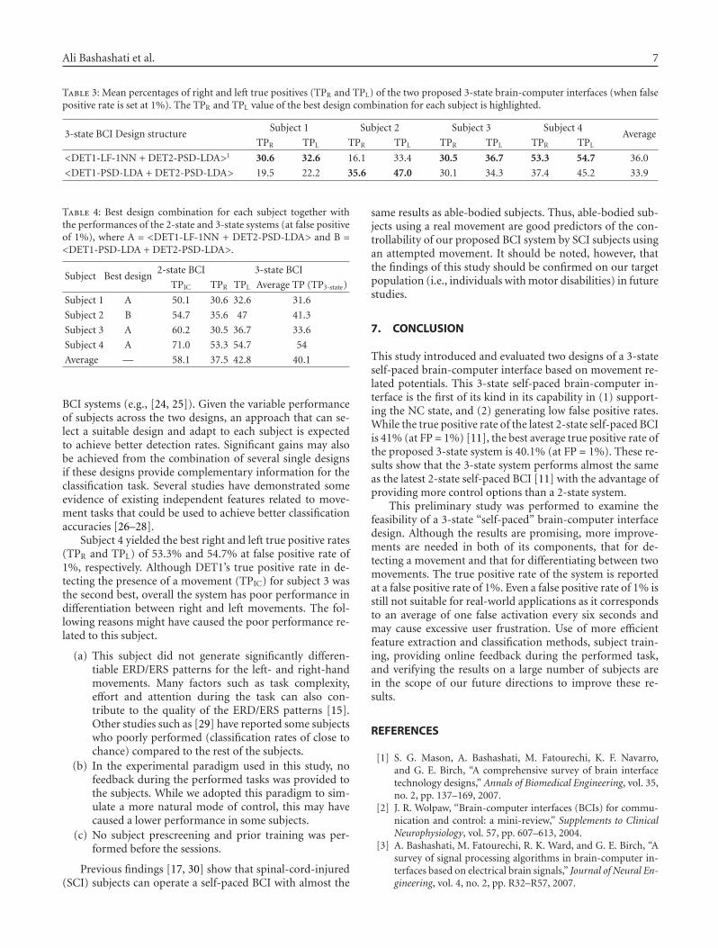
Ali Bashashati et al. 7
Table 3: Mean percentages of right and left true positives (TPR and TPL) of the two proposed 3-state brain-computer interfaces (when falsepositive rate is set at 1%). The TPR and TPL value of the best design combination for each subject is highlighted.
3-state BCI Design structureSubject 1 Subject 2 Subject 3 Subject 4
AverageTPR TPL TPR TPL TPR TPL TPR TPL
<DET1-LF-1NN + DET2-PSD-LDA>1 30.6 32.6 16.1 33.4 30.5 36.7 53.3 54.7 36.0
<DET1-PSD-LDA + DET2-PSD-LDA> 19.5 22.2 35.6 47.0 30.1 34.3 37.4 45.2 33.9
Table 4: Best design combination for each subject together withthe performances of the 2-state and 3-state systems (at false positiveof 1%), where A = <DET1-LF-1NN + DET2-PSD-LDA> and B =<DET1-PSD-LDA + DET2-PSD-LDA>.
Subject Best design2-state BCI 3-state BCI
TPIC TPR TPL Average TP (TP3-state)
Subject 1 A 50.1 30.6 32.6 31.6
Subject 2 B 54.7 35.6 47 41.3
Subject 3 A 60.2 30.5 36.7 33.6
Subject 4 A 71.0 53.3 54.7 54
Average — 58.1 37.5 42.8 40.1
BCI systems (e.g., [24, 25]). Given the variable performanceof subjects across the two designs, an approach that can se-lect a suitable design and adapt to each subject is expectedto achieve better detection rates. Significant gains may alsobe achieved from the combination of several single designsif these designs provide complementary information for theclassification task. Several studies have demonstrated someevidence of existing independent features related to move-ment tasks that could be used to achieve better classificationaccuracies [26–28].
Subject 4 yielded the best right and left true positive rates(TPR and TPL) of 53.3% and 54.7% at false positive rate of1%, respectively. Although DET1’s true positive rate in de-tecting the presence of a movement (TPIC) for subject 3 wasthe second best, overall the system has poor performance indifferentiation between right and left movements. The fol-lowing reasons might have caused the poor performance re-lated to this subject.
(a) This subject did not generate significantly differen-tiable ERD/ERS patterns for the left- and right-handmovements. Many factors such as task complexity,effort and attention during the task can also con-tribute to the quality of the ERD/ERS patterns [15].Other studies such as [29] have reported some subjectswho poorly performed (classification rates of close tochance) compared to the rest of the subjects.
(b) In the experimental paradigm used in this study, nofeedback during the performed tasks was provided tothe subjects. While we adopted this paradigm to sim-ulate a more natural mode of control, this may havecaused a lower performance in some subjects.
(c) No subject prescreening and prior training was per-formed before the sessions.
Previous findings [17, 30] show that spinal-cord-injured(SCI) subjects can operate a self-paced BCI with almost the
same results as able-bodied subjects. Thus, able-bodied sub-jects using a real movement are good predictors of the con-trollability of our proposed BCI system by SCI subjects usingan attempted movement. It should be noted, however, thatthe findings of this study should be confirmed on our targetpopulation (i.e., individuals with motor disabilities) in futurestudies.
7. CONCLUSION
This study introduced and evaluated two designs of a 3-stateself-paced brain-computer interface based on movement re-lated potentials. This 3-state self-paced brain-computer in-terface is the first of its kind in its capability in (1) support-ing the NC state, and (2) generating low false positive rates.While the true positive rate of the latest 2-state self-paced BCIis 41% (at FP = 1%) [11], the best average true positive rate ofthe proposed 3-state system is 40.1% (at FP = 1%). These re-sults show that the 3-state system performs almost the sameas the latest 2-state self-paced BCI [11] with the advantage ofproviding more control options than a 2-state system.
This preliminary study was performed to examine thefeasibility of a 3-state “self-paced” brain-computer interfacedesign. Although the results are promising, more improve-ments are needed in both of its components, that for de-tecting a movement and that for differentiating between twomovements. The true positive rate of the system is reportedat a false positive rate of 1%. Even a false positive rate of 1% isstill not suitable for real-world applications as it correspondsto an average of one false activation every six seconds andmay cause excessive user frustration. Use of more efficientfeature extraction and classification methods, subject train-ing, providing online feedback during the performed task,and verifying the results on a large number of subjects arein the scope of our future directions to improve these re-sults.
REFERENCES
[1] S. G. Mason, A. Bashashati, M. Fatourechi, K. F. Navarro,and G. E. Birch, “A comprehensive survey of brain interfacetechnology designs,” Annals of Biomedical Engineering, vol. 35,no. 2, pp. 137–169, 2007.
[2] J. R. Wolpaw, “Brain-computer interfaces (BCIs) for commu-nication and control: a mini-review,” Supplements to ClinicalNeurophysiology, vol. 57, pp. 607–613, 2004.
[3] A. Bashashati, M. Fatourechi, R. K. Ward, and G. E. Birch, “Asurvey of signal processing algorithms in brain-computer in-terfaces based on electrical brain signals,” Journal of Neural En-gineering, vol. 4, no. 2, pp. R32–R57, 2007.
8 Computational Intelligence and Neuroscience
[4] S. G. Mason and G. E. Birch, “A brain-controlled switchfor asynchronous control applications,” IEEE Transactions onBiomedical Engineering, vol. 47, no. 10, pp. 1297–1307, 2000.
[5] E. Yom-Tov and G. F. Inbar, “Detection of movement-relatedpotentials from the electro-encephalogram for possible use ina brain-computer interface,” Medical and Biological Engineer-ing and Computing, vol. 41, no. 1, pp. 85–93, 2003.
[6] S. P. Levine, J. E. Huggins, S. L. BeMent, et al., “A direct braininterface based on event-related potentials,” IEEE Transactionson Rehabilitation Engineering, vol. 8, no. 2, pp. 180–185, 2000.
[7] G. Townsend, B. Graimann, and G. Pfurtscheller, “Continu-ous EEG classification during motor imagery-simulation of anasynchronous BCI,” IEEE Transactions on Neural Systems andRehabilitation Engineering, vol. 12, no. 2, pp. 258–265, 2004.
[8] R. Scherer, G. R. Muller, C. Neuper, B. Graimann, and G.Pfurtscheller, “An asynchronously controlled EEG-based vir-tual keyboard: improvement of the spelling rate,” IEEE Trans-actions on Biomedical Engineering, vol. 51, no. 6, pp. 979–984,2004.
[9] R. Scherer, F. Lee, A. Schlogl, R. Leeb, H. Bischot, and G.Pfurtscheller, “Towards self-paced brain-computer communi-cation: navigation through virtual worlds,” to appear in IEEETransactions on Biomedical Engineering.
[10] J. D. R. Millan and J. Mourino, “Asynchronous BCI and localneural classifiers: an overview of the adaptive brain interfaceproject,” IEEE Transactions on Neural Systems and Rehabilita-tion Engineering, vol. 11, no. 2, pp. 159–161, 2003.
[11] A. Bashashati, S. Mason, R. K. Ward, and G. E. Birch, “An im-proved asynchronous brain interface: making use of the tem-poral history of the LF-ASD feature vectors,” Journal of NeuralEngineering, vol. 3, no. 2, pp. 87–94, 2006.
[12] A. Stancak Jr. and G. Pfurtscheller, “Event-related desyn-chronisation of central beta-rhythms during brisk and slowself-paced finger movements of dominant and nondominanthand,” Cognitive Brain Research, vol. 4, no. 3, pp. 171–183,1996.
[13] S. Slobounov, J. Johnston, H. Chiang, and W. Ray,“Movement-related EEG potentials are force or end-effectordependent: evidence from a multi-finger experiment,” Clini-cal Neurophysiology, vol. 113, no. 7, pp. 1125–1135, 2002.
[14] G. H. Yue, J. Z. Liu, V. Siemionow, V. K. Ranganathan, T.C. Ng, and V. Sahgal, “Brain activation during human fingerextension and flexion movements,” Brain Research, vol. 856,no. 1-2, pp. 291–300, 2000.
[15] G. Pfurtscheller and F. H. Lopes da Silva, “Event-relatedEEG/MEG synchronization and desynchronization: basicprinciples,” Clinical Neurophysiology, vol. 110, no. 11, pp.1842–1857, 1999.
[16] A. Bashashati, M. Fatourechi, R. K. Ward, and G. E. Birch,“User customization of the feature generator of an asyn-chronous brain interface,” Annals of Biomedical Engineering,vol. 34, no. 6, pp. 1051–1060, 2006.
[17] J. F. Borisoff, S. G. Mason, A. Bashashati, and G. E. Birch,“Brain-computer interface design for asynchronous controlapplications: improvements to the LF-ASD asynchronousbrain switch,” IEEE Transactions on Biomedical Engineering,vol. 51, no. 6, pp. 985–992, 2004.
[18] P. Welch, “The use of fast Fourier transform for the estima-tion of power spectra: a method based on time averaging overshort, modified periodograms,” IEEE Transactions on Audioand Electroacoustics, vol. 15, no. 2, pp. 70–73, 1967.
[19] P. A. Lachenbruch, Discriminant Analysis, Hafner Press, NewYork, NY, USA, 1975.
[20] G. Pfurtscheller and A. Aranibar, “Evaluation of event-relateddesynchronization (ERD) preceding and following voluntaryself-paced movement,” Electroencephalography and ClinicalNeurophysiology, vol. 46, no. 2, pp. 138–146, 1979.
[21] G. Pfurtscheller, C. Neuper, C. Andrew, and G. Edlinger, “Footand hand area mu rhythms,” International Journal of Psy-chophysiology, vol. 26, no. 1–3, pp. 121–135, 1997.
[22] M. Pregenzer and G. Pfurtscheller, “Frequency component se-lection for an EEG-based brain to computer interface,” IEEETransactions on Rehabilitation Engineering, vol. 7, no. 4, pp.413–419, 1999.
[23] G. E. Birch, P. D. Lawrence, and R. D. Hare, “Single-trial pro-cessing of event-related potentials using outlier information,”IEEE Transactions on Biomedical Engineering, vol. 40, no. 1, pp.59–73, 1993.
[24] B. Graimann, J. E. Huggins, S. P. Levine, and G. Pfurtscheller,“Toward a direct brain interface based on human subduralrecordings and wavelet-packet analysis,” IEEE Transactions onBiomedical Engineering, vol. 51, no. 6, pp. 954–962, 2004.
[25] G. R. Muller-Putz, R. Scherer, C. Brauneis, and G.Pfurtscheller, “Steady-state visual evoked potential (SSVEP)-based communication: impact of harmonic frequency com-ponents,” Journal of Neural Engineering, vol. 2, no. 4, pp. 123–130, 2005.
[26] G. Dornhege, B. Blankertz, G. Curio, and K.-R. Muller,“Boosting bit rates in non-invasive EEG single-trial classifi-cations by feature combination and multi-class paradigms,”IEEE Transactions on Biomedical Engineering, vol. 51, no. 6, pp.993–1002, 2004.
[27] G. Dornhege, B. Blankertz, G. Curio, and K.-R. Muller, “Com-bining features for BCI,” in Proceedings of the 6th Annual Neu-ral Information Processing Systems Conference (NIPS ’02), S.Becker, S. Thrun, and K. Obermayer, Eds., vol. 15 of Ad-vances in Neural Information Processing Systems, pp. 1115–1122, British Columbia, Canada, December 2003.
[28] C. Babiloni, F. Carducci, F. Cincotti, et al., “Humanmovement-related potentials vs desynchronization of EEGalpha rhythm: a high-resolution EEG study,” NeuroImage,vol. 10, no. 6, pp. 658–665, 1999.
[29] B. Blankertz, G. Dornhege, M. Krauledat, et al., “The Berlinbrain-computer interface: EEG-based communication with-out subject training,” IEEE Transactions on Neural Systems andRehabilitation Engineering, vol. 14, no. 2, pp. 147–152, 2006.
[30] G. E. Birch, Z. Bozorgzadeh, and S. G. Mason, “Initial on-line evaluations of the LF-ASD brain-computer interface withable-bodied and spinal-cord subjects using imagined volun-tary motor potentials,” IEEE Transactions on Neural Systemsand Rehabilitation Engineering, vol. 10, no. 4, pp. 219–224,2002.
Hindawi Publishing CorporationComputational Intelligence and NeuroscienceVolume 2007, Article ID 82069, 10 pagesdoi:10.1155/2007/82069
Research ArticleOnline Artifact Removal for Brain-Computer Interfaces UsingSupport Vector Machines and Blind Source Separation
Sebastian Halder,1 Michael Bensch,2 Jurgen Mellinger,1 Martin Bogdan,2, 3 Andrea Kubler,1
Niels Birbaumer,1, 4 and Wolfgang Rosenstiel2
1 Institute of Medical Psychology and Behavioral Neurobiology, University of Tubingen, Gartenstr. 29,72074 Tubingen, Germany
2 Wilhelm-Schickard Institute for Computer Engineering, University of Tubingen, Sand 13, 72076 Tubingen, Germany3 Computer Engineering, Institute of Computer Science, Faculty of Mathematics and Computer Science, University of Leipzig,Johannisgasse 26, 04103 Leipzig, Germany
4 National Institutes of Health (NIH), National Institute of Neurological Disorders and Stroke (NINDS),Human Cortical Physiology Section, Bethesda, MD 20892, USA
Correspondence should be addressed to Sebastian Halder, [email protected]
Received 16 February 2007; Revised 31 May 2007; Accepted 23 August 2007
Recommended by Andrzej Cichocki
We propose a combination of blind source separation (BSS) and independent component analysis (ICA) (signal decompositioninto artifacts and nonartifacts) with support vector machines (SVMs) (automatic classification) that are designed for online us-age. In order to select a suitable BSS/ICA method, three ICA algorithms (JADE, Infomax, and FastICA) and one BSS algorithm(AMUSE) are evaluated to determine their ability to isolate electromyographic (EMG) and electrooculographic (EOG) artifactsinto individual components. An implementation of the selected BSS/ICA method with SVMs trained to classify EMG and EOGartifacts, which enables the usage of the method as a filter in measurements with online feedback, is described. This filter is evalu-ated on three BCI datasets as a proof-of-concept of the method.
Copyright © 2007 Sebastian Halder et al. This is an open access article distributed under the Creative Commons AttributionLicense, which permits unrestricted use, distribution, and reproduction in any medium, provided the original work is properlycited.
1. INTRODUCTION
Since the discovery of the human electroencephalogram(EEG) activity in 1929 by Hans Berger [1], EEG measure-ments were mainly used for medical reasons or for researchin the area of brain function. In the past 15 years, applica-tions have been developed allowing the use of EEG activityas a nonmuscular communication channel or as an aid inmotor restoration after paralysis, so-called brain-computerinterfaces (BCIs) [2]. The idea is to provide completely par-alyzed patients with a rudimentary communication chan-nel by classifying the EEG signal (currently with informationtransfer rates between 10–25 bits/min [2]). Further progressof BCI systems depends on the development of new trainingmethods for patients, the identification of signals best suitedfor voluntary control, and the removal of noise interferingwith these signals.
Noise includes artifacts (we define any noncentral ner-vous system (CNS) signal recorded by the EEG to be an ar-tifact) introduced either by the subject himself or by an ex-ternal source. Artifacts in EEG recordings can be caused byeye blinks, eye movement, muscle and cardiac noise, as wellas nonbiological sources (e.g., power-line noise). A problemarises if the artifacts generated by the subject are used to con-trol the BCI system, because this violates the definition ofa BCI as a nonmuscular communication channel. Further-more, subjects with degenerative diseases would eventuallylose this ability. For instance, these artifacts could be a volun-tary or involuntary blinks or muscle contractions when thetask is presented. Additionally, involuntary muscle or ocu-lar activity might obscure the actual EEG signal, obstructingmeasurement of the features used to control the system. Elec-tromyographic (EMG) activity tends to overlap EEG from8 Hz upwards, whereas electrooculographic (EOG) activity
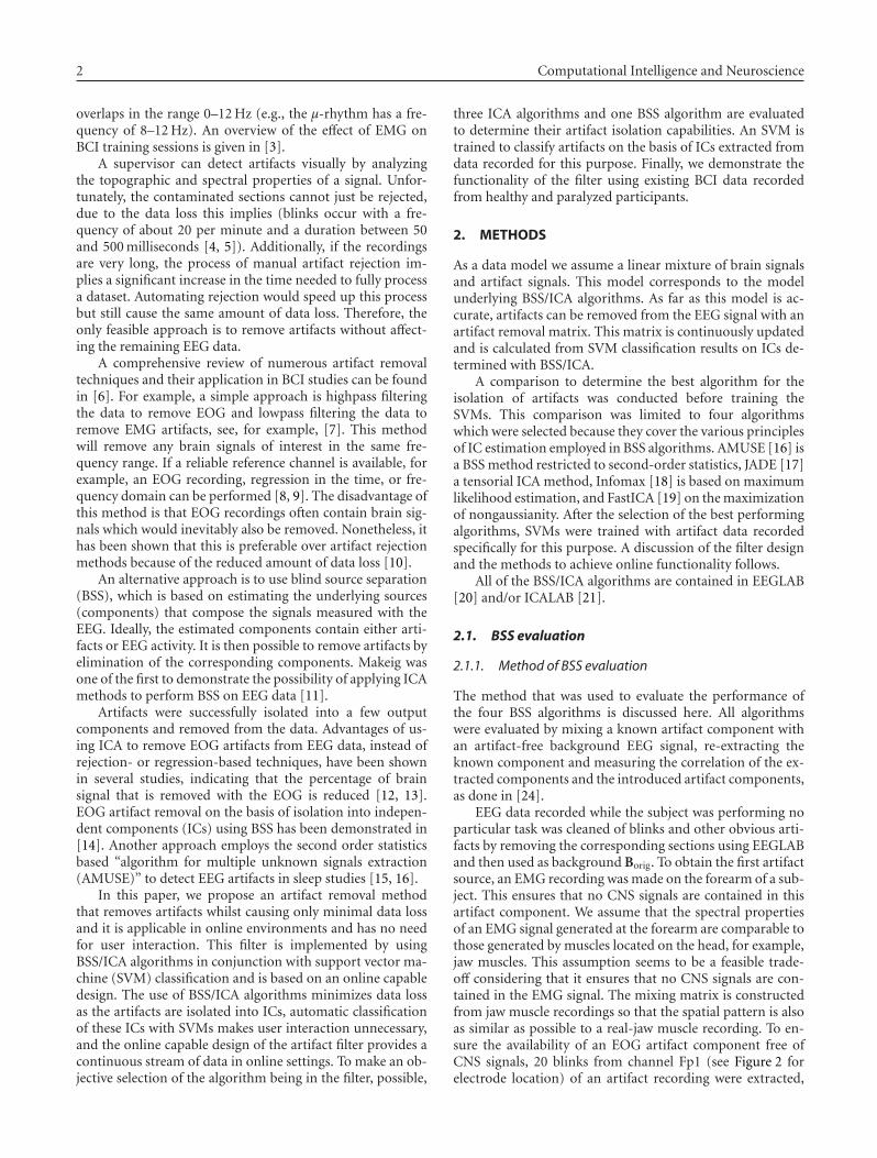
2 Computational Intelligence and Neuroscience
overlaps in the range 0–12 Hz (e.g., the μ-rhythm has a fre-quency of 8–12 Hz). An overview of the effect of EMG onBCI training sessions is given in [3].
A supervisor can detect artifacts visually by analyzingthe topographic and spectral properties of a signal. Unfor-tunately, the contaminated sections cannot just be rejected,due to the data loss this implies (blinks occur with a fre-quency of about 20 per minute and a duration between 50and 500 milliseconds [4, 5]). Additionally, if the recordingsare very long, the process of manual artifact rejection im-plies a significant increase in the time needed to fully processa dataset. Automating rejection would speed up this processbut still cause the same amount of data loss. Therefore, theonly feasible approach is to remove artifacts without affect-ing the remaining EEG data.
A comprehensive review of numerous artifact removaltechniques and their application in BCI studies can be foundin [6]. For example, a simple approach is highpass filteringthe data to remove EOG and lowpass filtering the data toremove EMG artifacts, see, for example, [7]. This methodwill remove any brain signals of interest in the same fre-quency range. If a reliable reference channel is available, forexample, an EOG recording, regression in the time, or fre-quency domain can be performed [8, 9]. The disadvantage ofthis method is that EOG recordings often contain brain sig-nals which would inevitably also be removed. Nonetheless, ithas been shown that this is preferable over artifact rejectionmethods because of the reduced amount of data loss [10].
An alternative approach is to use blind source separation(BSS), which is based on estimating the underlying sources(components) that compose the signals measured with theEEG. Ideally, the estimated components contain either arti-facts or EEG activity. It is then possible to remove artifacts byelimination of the corresponding components. Makeig wasone of the first to demonstrate the possibility of applying ICAmethods to perform BSS on EEG data [11].
Artifacts were successfully isolated into a few outputcomponents and removed from the data. Advantages of us-ing ICA to remove EOG artifacts from EEG data, instead ofrejection- or regression-based techniques, have been shownin several studies, indicating that the percentage of brainsignal that is removed with the EOG is reduced [12, 13].EOG artifact removal on the basis of isolation into indepen-dent components (ICs) using BSS has been demonstrated in[14]. Another approach employs the second order statisticsbased “algorithm for multiple unknown signals extraction(AMUSE)” to detect EEG artifacts in sleep studies [15, 16].
In this paper, we propose an artifact removal methodthat removes artifacts whilst causing only minimal data lossand it is applicable in online environments and has no needfor user interaction. This filter is implemented by usingBSS/ICA algorithms in conjunction with support vector ma-chine (SVM) classification and is based on an online capabledesign. The use of BSS/ICA algorithms minimizes data lossas the artifacts are isolated into ICs, automatic classificationof these ICs with SVMs makes user interaction unnecessary,and the online capable design of the artifact filter provides acontinuous stream of data in online settings. To make an ob-jective selection of the algorithm being in the filter, possible,
three ICA algorithms and one BSS algorithm are evaluatedto determine their artifact isolation capabilities. An SVM istrained to classify artifacts on the basis of ICs extracted fromdata recorded for this purpose. Finally, we demonstrate thefunctionality of the filter using existing BCI data recordedfrom healthy and paralyzed participants.
2. METHODS
As a data model we assume a linear mixture of brain signalsand artifact signals. This model corresponds to the modelunderlying BSS/ICA algorithms. As far as this model is ac-curate, artifacts can be removed from the EEG signal with anartifact removal matrix. This matrix is continuously updatedand is calculated from SVM classification results on ICs de-termined with BSS/ICA.
A comparison to determine the best algorithm for theisolation of artifacts was conducted before training theSVMs. This comparison was limited to four algorithmswhich were selected because they cover the various principlesof IC estimation employed in BSS algorithms. AMUSE [16] isa BSS method restricted to second-order statistics, JADE [17]a tensorial ICA method, Infomax [18] is based on maximumlikelihood estimation, and FastICA [19] on the maximizationof nongaussianity. After the selection of the best performingalgorithms, SVMs were trained with artifact data recordedspecifically for this purpose. A discussion of the filter designand the methods to achieve online functionality follows.
All of the BSS/ICA algorithms are contained in EEGLAB[20] and/or ICALAB [21].
2.1. BSS evaluation
2.1.1. Method of BSS evaluation
The method that was used to evaluate the performance ofthe four BSS algorithms is discussed here. All algorithmswere evaluated by mixing a known artifact component withan artifact-free background EEG signal, re-extracting theknown component and measuring the correlation of the ex-tracted components and the introduced artifact components,as done in [24].
EEG data recorded while the subject was performing noparticular task was cleaned of blinks and other obvious arti-facts by removing the corresponding sections using EEGLABand then used as background Borig. To obtain the first artifactsource, an EMG recording was made on the forearm of a sub-ject. This ensures that no CNS signals are contained in thisartifact component. We assume that the spectral propertiesof an EMG signal generated at the forearm are comparable tothose generated by muscles located on the head, for example,jaw muscles. This assumption seems to be a feasible trade-off considering that it ensures that no CNS signals are con-tained in the EMG signal. The mixing matrix is constructedfrom jaw muscle recordings so that the spatial pattern is alsoas similar as possible to a real-jaw muscle recording. To en-sure the availability of an EOG artifact component free ofCNS signals, 20 blinks from channel Fp1 (see Figure 2 forelectrode location) of an artifact recording were extracted,
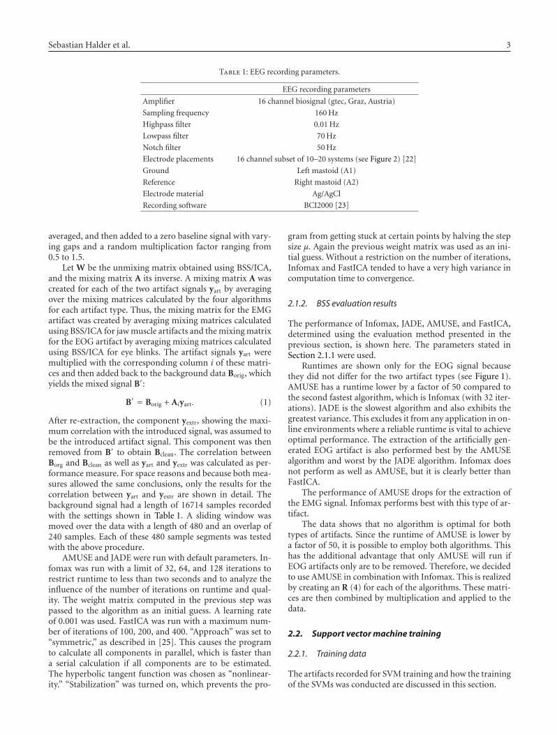
Sebastian Halder et al. 3
Table 1: EEG recording parameters.
EEG recording parameters
Amplifier 16 channel biosignal (gtec, Graz, Austria)
Sampling frequency 160 Hz
Highpass filter 0.01 Hz
Lowpass filter 70 Hz
Notch filter 50 Hz
Electrode placements 16 channel subset of 10–20 systems (see Figure 2) [22]
Ground Left mastoid (A1)
Reference Right mastoid (A2)
Electrode material Ag/AgCl
Recording software BCI2000 [23]
averaged, and then added to a zero baseline signal with vary-ing gaps and a random multiplication factor ranging from0.5 to 1.5.
Let W be the unmixing matrix obtained using BSS/ICA,and the mixing matrix A its inverse. A mixing matrix A wascreated for each of the two artifact signals yart by averagingover the mixing matrices calculated by the four algorithmsfor each artifact type. Thus, the mixing matrix for the EMGartifact was created by averaging mixing matrices calculatedusing BSS/ICA for jaw muscle artifacts and the mixing matrixfor the EOG artifact by averaging mixing matrices calculatedusing BSS/ICA for eye blinks. The artifact signals yart weremultiplied with the corresponding column i of these matri-ces and then added back to the background data Borig, whichyields the mixed signal B′:
B′ = Borig + Aiyart. (1)
After re-extraction, the component yextr, showing the maxi-mum correlation with the introduced signal, was assumed tobe the introduced artifact signal. This component was thenremoved from B′ to obtain Bclean. The correlation betweenBorg and Bclean as well as yart and yextr was calculated as per-formance measure. For space reasons and because both mea-sures allowed the same conclusions, only the results for thecorrelation between yart and yextr are shown in detail. Thebackground signal had a length of 16714 samples recordedwith the settings shown in Table 1. A sliding window wasmoved over the data with a length of 480 and an overlap of240 samples. Each of these 480 sample segments was testedwith the above procedure.
AMUSE and JADE were run with default parameters. In-fomax was run with a limit of 32, 64, and 128 iterations torestrict runtime to less than two seconds and to analyze theinfluence of the number of iterations on runtime and qual-ity. The weight matrix computed in the previous step waspassed to the algorithm as an initial guess. A learning rateof 0.001 was used. FastICA was run with a maximum num-ber of iterations of 100, 200, and 400. “Approach” was set to“symmetric,” as described in [25]. This causes the programto calculate all components in parallel, which is faster thana serial calculation if all components are to be estimated.The hyperbolic tangent function was chosen as “nonlinear-ity.” “Stabilization” was turned on, which prevents the pro-
gram from getting stuck at certain points by halving the stepsize μ. Again the previous weight matrix was used as an ini-tial guess. Without a restriction on the number of iterations,Infomax and FastICA tended to have a very high variance incomputation time to convergence.
2.1.2. BSS evaluation results
The performance of Infomax, JADE, AMUSE, and FastICA,determined using the evaluation method presented in theprevious section, is shown here. The parameters stated inSection 2.1.1 were used.
Runtimes are shown only for the EOG signal becausethey did not differ for the two artifact types (see Figure 1).AMUSE has a runtime lower by a factor of 50 compared tothe second fastest algorithm, which is Infomax (with 32 iter-ations). JADE is the slowest algorithm and also exhibits thegreatest variance. This excludes it from any application in on-line environments where a reliable runtime is vital to achieveoptimal performance. The extraction of the artificially gen-erated EOG artifact is also performed best by the AMUSEalgorithm and worst by the JADE algorithm. Infomax doesnot perform as well as AMUSE, but it is clearly better thanFastICA.
The performance of AMUSE drops for the extraction ofthe EMG signal. Infomax performs best with this type of ar-tifact.
The data shows that no algorithm is optimal for bothtypes of artifacts. Since the runtime of AMUSE is lower bya factor of 50, it is possible to employ both algorithms. Thishas the additional advantage that only AMUSE will run ifEOG artifacts only are to be removed. Therefore, we decidedto use AMUSE in combination with Infomax. This is realizedby creating an R (4) for each of the algorithms. These matri-ces are then combined by multiplication and applied to thedata.
2.2. Support vector machine training
2.2.1. Training data
The artifacts recorded for SVM training and how the trainingof the SVMs was conducted are discussed in this section.
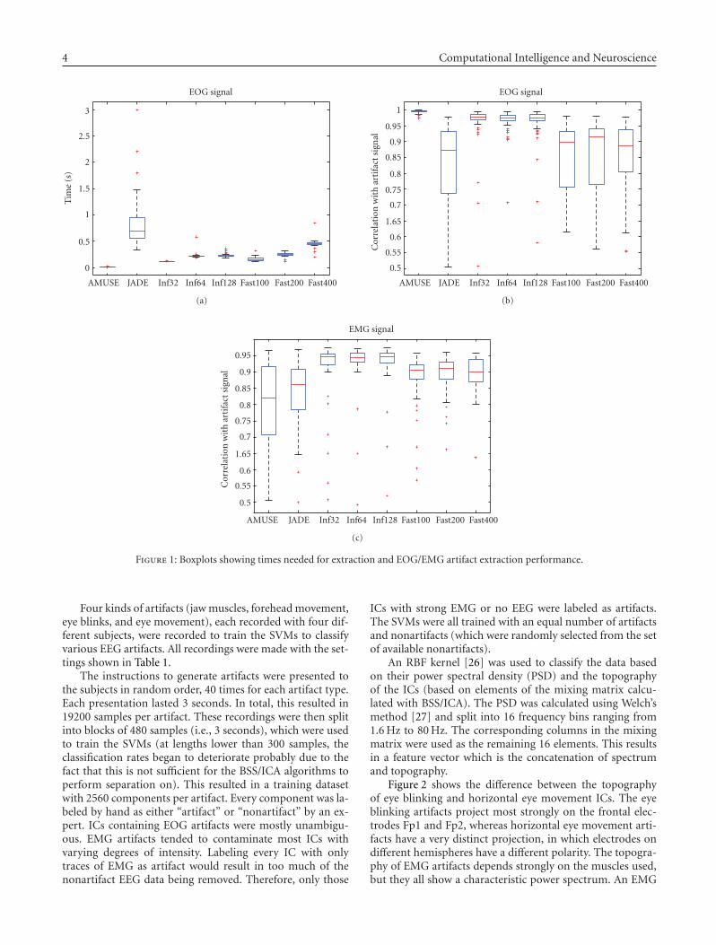
4 Computational Intelligence and Neuroscience
0
0.5
1
1.5
2
2.5
3
AMUSE JADE Inf32 Inf64 Inf128 Fast100 Fast200 Fast400
Tim
e(s
)
EOG signal
(a)
0.5
0.55
0.6
1.65
0.7
0.75
0.8
0.85
0.9
0.95
1
AMUSE JADE Inf32 Inf64 Inf128 Fast100 Fast200 Fast400
Cor
rela
tion
wit
har
tifa
ctsi
gnal
EOG signal
(b)
0.5
0.55
0.6
1.65
0.7
0.75
0.8
0.85
0.9
0.95
AMUSE JADE Inf32 Inf64 Inf128 Fast100 Fast200 Fast400
Cor
rela
tion
wit
har
tifa
ctsi
gnal
EMG signal
(c)
Figure 1: Boxplots showing times needed for extraction and EOG/EMG artifact extraction performance.
Four kinds of artifacts (jaw muscles, forehead movement,eye blinks, and eye movement), each recorded with four dif-ferent subjects, were recorded to train the SVMs to classifyvarious EEG artifacts. All recordings were made with the set-tings shown in Table 1.
The instructions to generate artifacts were presented tothe subjects in random order, 40 times for each artifact type.Each presentation lasted 3 seconds. In total, this resulted in19200 samples per artifact. These recordings were then splitinto blocks of 480 samples (i.e., 3 seconds), which were usedto train the SVMs (at lengths lower than 300 samples, theclassification rates began to deteriorate probably due to thefact that this is not sufficient for the BSS/ICA algorithms toperform separation on). This resulted in a training datasetwith 2560 components per artifact. Every component was la-beled by hand as either “artifact” or “nonartifact” by an ex-pert. ICs containing EOG artifacts were mostly unambigu-ous. EMG artifacts tended to contaminate most ICs withvarying degrees of intensity. Labeling every IC with onlytraces of EMG as artifact would result in too much of thenonartifact EEG data being removed. Therefore, only those
ICs with strong EMG or no EEG were labeled as artifacts.The SVMs were all trained with an equal number of artifactsand nonartifacts (which were randomly selected from the setof available nonartifacts).
An RBF kernel [26] was used to classify the data basedon their power spectral density (PSD) and the topographyof the ICs (based on elements of the mixing matrix calcu-lated with BSS/ICA). The PSD was calculated using Welch’smethod [27] and split into 16 frequency bins ranging from1.6 Hz to 80 Hz. The corresponding columns in the mixingmatrix were used as the remaining 16 elements. This resultsin a feature vector which is the concatenation of spectrumand topography.
Figure 2 shows the difference between the topographyof eye blinking and horizontal eye movement ICs. The eyeblinking artifacts project most strongly on the frontal elec-trodes Fp1 and Fp2, whereas horizontal eye movement arti-facts have a very distinct projection, in which electrodes ondifferent hemispheres have a different polarity. The topogra-phy of EMG artifacts depends strongly on the muscles used,but they all show a characteristic power spectrum. An EMG
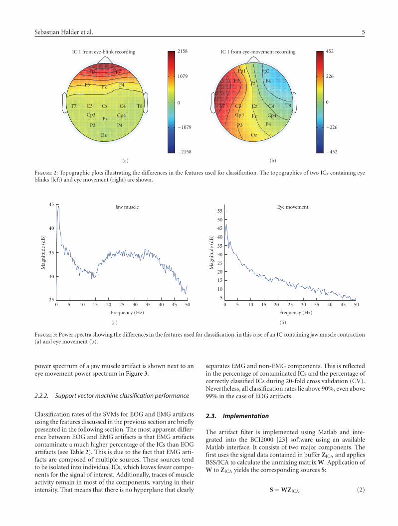
Sebastian Halder et al. 5
Fp1 Fp2
F3 Fz F4
T7 C3 Cz C4 T8
Cp3
P3Pz
Cp4
P4
Oz
2158
1079
0
−1079
−2158
IC 1 from eye-blink recording
(a)
Fp1 Fp2
F3 Fz F4
T7 C3 Cz C4 T8
Cp3
P3
Pz Cp4
P4
Oz
452
226
0
−226
−452
IC 1 from eye-movement recording
(b)
Figure 2: Topographic plots illustrating the differences in the features used for classification. The topographies of two ICs containing eyeblinks (left) and eye movement (right) are shown.
0 5 10 15 20 25 30 35 40 45 5025
30
35
40
45
Mag
nit
ude
(dB
)
Jaw muscle
Frequency (Hz)
(a)
0 5 10 15 20 25 30 35 40 45 505
10
15
20
25
30
35
40
45
50
55M
agn
itu
de(d
B)
Eye movement
Frequency (Hz)
(b)
Figure 3: Power spectra showing the differences in the features used for classification, in this case of an IC containing jaw muscle contraction(a) and eye movement (b).
power spectrum of a jaw muscle artifact is shown next to aneye movement power spectrum in Figure 3.
2.2.2. Support vector machine classification performance
Classification rates of the SVMs for EOG and EMG artifactsusing the features discussed in the previous section are brieflypresented in the following section. The most apparent differ-ence between EOG and EMG artifacts is that EMG artifactscontaminate a much higher percentage of the ICs than EOGartifacts (see Table 2). This is due to the fact that EMG arti-facts are composed of multiple sources. These sources tendto be isolated into individual ICs, which leaves fewer compo-nents for the signal of interest. Additionally, traces of muscleactivity remain in most of the components, varying in theirintensity. That means that there is no hyperplane that clearly
separates EMG and non-EMG components. This is reflectedin the percentage of contaminated ICs and the percentage ofcorrectly classified ICs during 20-fold cross validation (CV).Nevertheless, all classification rates lie above 90%, even above99% in the case of EOG artifacts.
2.3. Implementation
The artifact filter is implemented using Matlab and inte-grated into the BCI2000 [23] software using an availableMatlab interface. It consists of two major components. Thefirst uses the signal data contained in buffer ZICA and appliesBSS/ICA to calculate the unmixing matrix W. Application ofW to ZICA yields the corresponding sources S:
S = WZICA. (2)

6 Computational Intelligence and Neuroscience
Table 2: SVM training summary showing the percentage of independent components (ICs) that are contaminated by artifacts in the par-ticular artifact dataset and the percentage of ICs classified correctly as artifact and nonartifact when using 20-fold crossvalidation (CV).Additionally, channel capacity calculated using the Blahut-Arimoto algorithm [28, 29] and the parameters C (error penalty) and γ (kernelparameter of RBF kernel) used to train the SVMs are shown.
Artifact % ICs % correct (CV) Channel capacity C /γ
Eye blink 6.40 99.39 0.8141 2000/0.0005
Eye movement 5.15 99.62 0.9373 2/0.5
Jaw muscle 52.34 92.26 0.6308 8/0.5
Forehead 19.34 91.51 0.6043 2/0.5
Then the SVMs are used to classify the sources S. We use theprobability estimates p (values between zero and one, i.e., theprobability that a component is not an artifact) of the SVMinstead of classification results (zero or one) to construct a re-moval matrix. Probability estimates are calculated accordingto [30]. This avoids oscillation between removal and retain-ment in case of ambiguous components. Especially muscleartifacts are not cleanly isolated into single components, andthose which contain only weak contamination might sufferfrom this problem when binary classification is used. p isused to construct a diagonal matrix D using the output ofthe SVMs for each of the four artifact types:
Dii = pi, i = 1, . . . ,N ,
Dij = 0, ∀ i�= j, i = 1, ...,N , j = 1, . . . ,N ,(3)
with N being the number of ICs.D is combined with the unmixing matrix W and the mix-
ing matrix A, as shown in (4), to create the removal ma-trix R that is applied to the current output sample σi frombuffer Zsig in the second component of the artifact filter (5)which yields a sample σ ′i reconstructed out of BSS/ICA com-ponents weighted according to the probability estimates p ofthe SVM:
R = ADW, (4)
σ ′i = Rσi. (5)
The matrix R must be applied to every sample that passesthrough the filter. In a sequential approach in which the cal-culation of R takes tR > 0 this will prevent continuous out-put in online scenarios. Therefore the calculation of R andthe application of R to the current output sample σi must beperformed in separate threads.
R must include mixing and unmixing matrices fromAMUSE and Infomax. D must be calculated for each of thefour SVMs (eye movement, eye blinks, jaw muscle and fore-head muscle artifacts). All matrices are then combined bymultiplication as shown in (6) and applied to the data.
R = AAMUSEDEOG1DEOG2WAMUSE
× AInfomaxDEMG1DEMG2WInfomax.(6)
Additionally, it must be taken into account that the calcula-tion of the unmixing matrix W using the BSS/ICA algorithmis based on more than one sample. Therefore, the data thatare used for the calculation, that is, ZICA, must be represen-tative of the sample σi that the removal matrix R is applied
to. If simply the last n samples of the data are used, newly oc-curring artifacts might not have a strong enough impact onthe SVM to be classified as such, which would lead to the ar-tifact not being removed from σi. Conversely, artifacts in thebuffer which contaminate most of the samples, but not thenewest sample, will cause the SVM to classify a componentof σi as an artifact which is in fact artifact-free. Hence, theincoming samples have to be delayed by half of the numberof samples kZICA in buffer ZICA that contains the data for theBSS/ICA. This does not mean that a new sample arrives onlyevery kZICA /2 samples but that the whole recording is shiftedby this amount and the samples still arrive with the same in-terval.
It is inevitable that the same matrix is used for severalsamples as the time tR, needed for the calculation of R, isgreater than the time represented by one sample of the data.
3. RESULTS
The artifact filter is applied offline to three BCI datasets toevaluate the effect on determination coefficient plots andsubject performance. It is shown that application of the fil-ter increases performance in cases where artifacts randomlyinterfere with the control signal and decreases performancewhen artifacts are used to control the BCI. Additionally, theonline functionality of the filter is discussed.
3.1. Offline analysis of BCI data
The data analyzed originate from μ-rhythm (i.e., a BCI con-trolled using imagined movement/planning) training ses-sions recorded with the settings shown in Table 1 during aBCI evaluation project [31] (none of the datasets was usedduring the training of the SVMs). The control a user hasover the BCI can be evaluated with determination coeffi-cient (Pearson product-moment correlation coefficient, r2)values as those plotted in Figure 4. A higher value indicatesmodulation of the signal in a certain channel at a certainfrequency in correspondence with the required task. In thiscase, the modulation of the signal was used to control themovement of a cursor to either the top or the bottom of thescreen. Artifacts either increase or decrease the determina-tion coefficient value at certain frequency ranges. If the ar-tifact correlates with the task (mostly due to the attempt tocontrol the BCI with muscle activity or an involuntary mus-cle contraction while trying to perform the mental task), itwill increase the value, and if it does not (due to involuntary
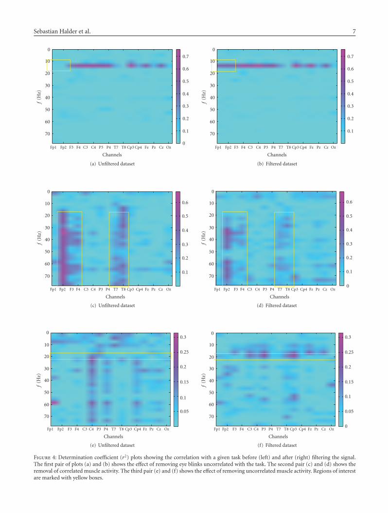
Sebastian Halder et al. 7
Fp1 Fp2 F3 F4 C3 C4 P3 P4 T7 T8 Cp3 Cp4 Fz Pz Cz Oz
f(H
z)
Channels
0
0.1
0.2
0.3
0.4
0.5
0.6
0.7
70
60
50
40
30
20
10
0
(a) Unfiltered dataset
Fp1 Fp2 F3 F4 C3 C4 P3 P4 T7 T8 Cp3 Cp4 Fz Pz Cz Oz
f(H
z)
Channels
0.1
0.2
0.3
0.4
0.5
0.6
0.7
70
60
50
40
30
20
10
0
(b) Filtered dataset
Fp1 Fp2 F3 F4 C3 C4 P3 P4 T7 T8 Cp3 Cp4 Fz Pz Cz Oz
f(H
z)
Channels
0.1
0.2
0.3
0.4
0.5
0.6
70
60
50
40
30
20
10
0
(c) Unfiltered dataset
Fp1 Fp2 F3 F4 C3 C4 P3 P4 T7 T8 Cp3 Cp4 Fz Pz Cz Oz
f(H
z)
Channels
0
0.1
0.2
0.3
0.4
0.5
0.6
70
60
50
40
30
20
10
0
(d) Filtered dataset
Fp1 Fp2 F3 F4 C3 C4 P3 P4 T7 T8 Cp3 Cp4 Fz Pz Cz Oz
f(H
z)
Channels
0.05
0.1
0.15
0.2
0.25
0.3
70
60
50
40
30
20
10
0
(e) Unfiltered dataset
Fp1 Fp2 F3 F4 C3 C4 P3 P4 T7 T8 Cp3 Cp4 Fz Pz Cz Oz
f(H
z)
Channels
0
0.05
0.1
0.15
0.2
0.25
0.3
70
60
50
40
30
20
10
0
(f) Filtered dataset
Figure 4: Determination coefficient (r2) plots showing the correlation with a given task before (left) and after (right) filtering the signal.The first pair of plots (a) and (b) shows the effect of removing eye blinks uncorrelated with the task. The second pair (c) and (d) shows theremoval of correlated muscle activity. The third pair (e) and (f) shows the effect of removing uncorrelated muscle activity. Regions of interestare marked with yellow boxes.
8 Computational Intelligence and Neuroscience
muscle spasms), it will decrease the determination coeffi-cient value. In the former case, removal can be expectedto decrease performance; in the latter, an increased or un-changed performance can be expected. This is what is in-tended since using artifacts to control a BCI violates the defi-nition of it as being a nonmuscular communication channel.Plots 4(a) and 4(b) in Figure 4 show the effect of EOG ar-tifact removal on data, which were recorded from a healthysubject presented 23 targets over 120 seconds, 22 of whichwere correctly chosen. Both of the frontal channels, Fp1 andFp2, were contaminated with eye blinks. Since the blinksare uncorrelated with target location, this will have a nega-tive influence on the determination coefficient value. As ex-pected, the right plot, which shows the determination coef-ficient plot of the filtered data, has a visibly increased de-termination coefficient value on the frontal channels. OnFp1 the r2 value increased from 0.0772 to 0.4539, and onFp2 from 0.0929 to 0.4775. The maximum r2 value increasesfrom 0.7006 to 0.7585. This increase occurs in the same fre-quency range as the horizontal band of high determinationcoefficient values which existed previously, which is an indi-cation of identical source (see box in 4(a) and 4(b)). Sucha horizontal pattern is typical of successful μ-rhythm mod-ulation. Because the control signal was not influenced sig-nificantly on the other electrodes, no increase in hit rate oc-curred.
In contrast to the top two plots, plots 4(c) and 4(d) showdata from a subject that used muscle artifacts to control theBCI. This is reflected in the plot by the vertical structures(which indicate signals with a broad spectrum) that correlatewith the task (which indicates that these signals were gener-ated intentionally). Such patterns are visible on channels 2,3, 4, 9, and 10 (see box in 4(c) and 4(d)). In total, 34 tar-gets were presented, 29 of which were hit (85%). The filterdoes not entirely remove the EMG artifacts due to the pre-viously described problem of muscle artifacts contaminatingtoo many ICs. Nevertheless, the effect of the artifacts is sig-nificantly reduced, in particular below 20 Hz. Additionally,the absolute amplitude of the correlation of the EMG sig-nals with the task was decreased visibly by the applicationof the filter (the maximum r2 value decreases from 0.6777to 0.5208). The removal led to a decrease of the simulatedhit rate from 85% to 73%. The final case that is presented(see Figures 4(e) and 4(f)) also shows some contaminationby EMG artifacts, even though not as strongly as the previ-ous data. The subject was presented 34 targets, 17 of whichwere hit resulting in a hit-rate of 50%. The interesting factabout this dataset is that the removal of the EMG artifact re-veals a horizontal structure in the range of 20 Hz (see box4(e) and 4(f)). This indicates that there was some brain ac-tivity that was superimposed by EMG and could thereforenot be used to control the BCI. The strongest increase ofthe determination coefficient value is based around electrodeCP3 (channel 11), supporting this claim. On this channel,the maximum r2 increases from 0.1204 to 0.2598. Addition-ally, this electrode was determined to be the most discrimi-native in initial screening sessions with the subject. The sim-ulated performance of the subject increased from 50% to74%.
3.2. Online functionality
The performance of the filter was tested by applying it to rawdata and classifying it again. The data obtained are identicalto the data that would have been obtained if the filter hadbeen used in an online recording with the same settings. Ofcourse, an arbitrary amount of time is available for the arti-fact filter in an offline setting. Therefore, the quality of arti-fact removal is potentially higher. Thus, the interval at whichthe removal matrix is updated was set to 5 sample blocks,which would be realistic in an online environment. Since thedata was recorded with 8 samples per block at 160 Hz, thisallows for 250 milliseconds per update.
The application of the removal matrix takes about2.6 milliseconds per sample block. The calculation of a newremoval matrix takes 145 milliseconds using both AMUSEand Infomax on the basis of 480 samples1. This is fast enoughto update the removal matrix every five sample blocks withthe above settings.
Using the BCI2000, several P300 recordings were madeto ensure that running the filter would not have a negativeimpact on performance.
4. DISCUSSION
A filter that removes artifacts from EEG signals used inBCI systems was described. The data presented in this pa-per shows that the implementation of an online artifact fil-ter using blind source separation and support vector ma-chines is possible. This is achieved by delaying output by aconstant amount between one and two seconds and by cal-culating and applying the removal matrix in two separatethreads. Infomax was found to be the best ICA method todecompose EEG signals contaminated with myographic ar-tifacts, but it had problems producing components whichwere completely free of contamination (especially if the myo-graphic artifacts were very strong, as jaw muscle contrac-tion). The second-order statistics-based algorithm AMUSEproduced a very clean decomposition of recordings contain-ing ocular artifacts, both eye movements and blinking. Inturn, it was possible to train SVMs to recognize these arti-facts with very high accuracy, because no contamination re-mained in the other components, making it easier to deter-mine a separating hyperplane. Correspondingly, muscle arti-facts could not be classified with such a high accuracy. Theapplication of our artifact filter to BCI data demonstratesthe usefulness of the technique. Performance increases wereachieved in the case of uncorrelated muscle and ocular ac-tivity task. Additionally, a decrease in performance was ap-parent if the filter was applied to data in which the subjectused muscle artifacts to control the BCI. Unfortunately, theremoval was not complete, allowing some control of mus-cles of the BCI to remain. In future experiments, this mightbe improved by using more EEG channels which increasethe number of ICs and therefore the chance that an EMG
1 Using an AMD Athlon X2 4400+ with 2 GB RAM.
Sebastian Halder et al. 9
subspace can be isolated from the EEG subspace. Addition-ally, the method could be adapted for use with alternativeBSS methods which are particularly suited to isolate EMG ar-tifacts, for example, the canonical correlation analysis (CCA)method demonstrated in [32]. The CCA would be used in-stead of one of the ICA algorithms employed in this paperand be automated by using the available SVMs.
The feasibility of using ICA as a preprocessing techniquefor artifact detection has been shown in [33]. Performanceincreased for all presented artifact detection types after ICApreprocessing. It was noted though, that no performance in-crease was found when applying ICA to data contaminatedwith muscle artifacts. This is another indication that an al-ternative BSS or ICA algorithm should be used before classi-fying the data with SVMs.
Automated artifact removal techniques have been pre-sented previously. For example, an automated regressionanalysis-based EOG removal method was presented in [34].While being easy to apply it still suffers from the drawbacksof EEG-contaminated EOG channels (even though this wasaddressed by mounting the EOG electrodes in the proxim-ity of the eyes and only calculating the regression coefficientsfrom large EOG artifacts). Moreover, it is not possible to ex-tend such a method to remove EMG artifacts.
Artifact isolation and removal using BSS/ICA algorithmsautomated by combination with SVMs or some other auto-matic classifier were already shown in [35]. While the ap-plicability of the method presented in [35] is also restrictedto ocular artifacts, we demonstrated a method based on thecombination of BSS/ICA algorithms and SVMs that uses ar-tifact features (topography and spectrum) that are availablefor all artifact types. Furthermore, we presented a design foronline settings. A comparable method suitable for online usepresented in [36], also not applied to EMG artifacts, dependson static models of artifact and brain signal topographies thatdo not adapt if the artifact changes, as the unmixing matrixcalculated with BSS/ICA does. The method presented in [36]offers the advantage of having no delay and a reduced com-putational complexity.
We demonstrated that it is possible to implement anonline-automated artifact removal technique on the basis ofBSS/ICA and SVMs and illustrated the ameliorating effect onBCI performance.
ACKNOWLEDGMENTS
This work was supported by the Deutsche Forschungsge-meinschaft SFB550/TB5 and Grant no. Ro1030/12-1 as wellas the National Institutes of Health, USA.
REFERENCES
[1] H. Berger, “Uber das Elektroenzephalogramm des Menschen,”Archiv fur Psychiatrie und Nervenkrankheiten, vol. 87, pp. 527–570, 1929.
[2] J. R. Wolpaw, N. Birbaumer, D. J. McFarland, G. Pfurtscheller,and T. M. Vaughan, “Brain-computer interfaces for communi-cation and control,” Clinical Neurophysiology, vol. 113, no. 6,pp. 767–791, 2002.
[3] D. J. McFarland, W. A. Sarnacki, T. M. Vaughan, and J. R. Wol-paw, “Brain-computer interface (BCI) operation: signal andnoise during early training sessions,” Clinical Neurophysiology,vol. 116, no. 1, pp. 56–62, 2005.
[4] M. Iwasaki, C. Kellinghaus, A. V. Alexopoulos, et al., “Effectsof eyelid closure, blinks, and eye movements on the electroen-cephalogram,” Clinical Neurophysiology, vol. 116, no. 4, pp.878–885, 2005.
[5] P. P. Caffier, U. Erdmann, and P. Ullsperger, “Experimentalevaluation of eye-blink parameters as a drowsiness measure,”European Journal of Applied Physiology, vol. 89, no. 3-4, pp.319–325, 2003.
[6] M. Fatourechi, A. Bashashati, R. K. Ward, and G. E. Birch,“EMG and EOG artifacts in brain-computer interface systems:a survey,” Clinical Neurophysiology, vol. 118, no. 3, pp. 480–494, 2007.
[7] J. S. Barlow, “EMG artifact minimization during clinic EEGrecordings by special analog filtering,” Electroencephalographyand Clinical Neurophysiology, vol. 58, no. 2, pp. 161–174, 1984.
[8] T. Elbert, W. Lutzenberger, B. Rockstroh, and N. Birbaumer,“Removal of ocular artifacts from the EEG—a biophysical ap-proach to the EOG,” Electroencephalography and Clinical Neu-rophysiology, vol. 60, no. 5, pp. 455–463, 1985.
[9] R. J. Croft and R. J. Barry, “Removal of ocular artifact fromthe EEG: a review,” Neurophysiologie Clinique, vol. 30, no. 1,pp. 5–19, 2000.
[10] R. J. Croft and R. J. Barry, “Issues relating to the subtractionphase in EOG artefact correction of the EEG,” InternationalJournal of Psychophysiology, vol. 44, no. 3, pp. 187–195, 2002.
[11] S. Makeig, A. J. Bell, T.-P. Jung, and T. J. Sejnowski, “Indepen-dent component analysis of electroencephalographic data,” inAdvances in Neural Information Processing Systems, vol. 8, pp.145–151, The MIT Press, Cambridge, Mass, USA, 1996.
[12] R. N. Vigario, “Extraction of ocular artefacts from EEG usingindependent component analysis,” Electroencephalography andClinical Neurophysiology, vol. 103, no. 3, pp. 395–404, 1997.
[13] T.-P. Jung, S. Makeig, M. Westerfield, J. Townsend, E. Courch-esne, and T. J. Sejnowski, “Removal of eye activity artifactsfrom visual event-related potentials in normal and clinicalsubjects,” Clinical Neurophysiology, vol. 111, no. 10, pp. 1745–1758, 2000.
[14] C. A. Joyce, I. F. Gorodnitsky, and M. Kutas, “Automatic re-moval of eye movement and blink artifacts from EEG datausing blind component separation,” Psychophysiology, vol. 41,no. 2, pp. 313–325, 2004.
[15] S. Romero, M. A. Mananas, S. Clos, S. Gimenez, and M. J. Bar-banoj, “Reduction of EEG artifacts by ICA in different sleepstages,” in Proceedings of the 25th Annual International Confer-ence of the IEEE Engineering in Medicine and Biology Society(EMBS ’03), vol. 3, pp. 2675–2678, Cancun, Mexico, Septem-ber 2003.
[16] L. Tong, R.-W. Liu, V. C. Soon, and Y.-F. Huang, “Indetermi-nacy and identifiability of blind identification,” IEEE Transac-tions on Circuits and Systems, vol. 38, no. 5, pp. 499–509, 1991.
[17] J.-F. Cardoso, “High-order contrasts for independent compo-nent analysis,” Neural Computation, vol. 11, no. 1, pp. 157–192, 1999.
[18] S. Makeig, T.-P. Jung, A. J. Bell, D. Ghahremani, and T. J.Sejnowski, “Blind separation of auditory event-related brain-responses into independent components,” Proceedings of theNational Academy of Sciences of the United States of America,vol. 94, no. 20, pp. 10979–10984, 1997.
10 Computational Intelligence and Neuroscience
[19] A. Hyvarinen and E. Oja, “A fast fixed-point algorithm for in-dependent component analysis,” Neural Computation, vol. 9,no. 7, pp. 1483–1492, 1997.
[20] A. Delorme and S. Makeig, “EEGLAB: an open source tool-box for analysis of single-trial EEG dynamics including inde-pendent component analysis,” Journal of Neuroscience Meth-ods, vol. 134, no. 1, pp. 9–21, 2004.
[21] A. Cichocki, S. Amari, K. Siwek, et al., “ICALAB Toolboxes,”http://www.bsp.brain.riken.jp/ICALAB.
[22] H. H. Jasper, “The 10-20 electrode system of the internationalfederation,” Electroencephalography and Clinical Neurophysiol-ogy, vol. 10, pp. 371–375, 1958.
[23] G. Schalk, D. J. McFarland, T. Hinterberger, N. Birbaumer, andJ. R. Wolpaw, “BCI2000: a general-purpose brain-computerinterface (BCI) system,” IEEE Transactions on Biomedical En-gineering, vol. 51, no. 6, pp. 1034–1043, 2004.
[24] N. J. Knight, “Signal fraction analysis and artifact re-moval in EEG,” M.S. thesis, Colorado State University, FortCollins, Colo, USA, 2004, http://www.cs.colostate.edu/eeg/publications/natethesis.pdf.
[25] A. Hyvarinen, “Fast and robust fixed-point algorithms for in-dependent component analysis,” IEEE Transactions on NeuralNetworks, vol. 10, no. 3, pp. 626–634, 1999.
[26] C.-C. Chang and C.-J. Lin, “LIBSVM: a library for supportvector machines,” http://www.csie.ntu.edu.tw/∼cjlin/libsvm,2001.
[27] P. D. Welch, “The use of fast Fourier transform for the esti-mation of power spectra: a method based on time averagingover short, modified periodograms,” IEEE Transactions on Au-dio and Electroacoustics, vol. 15, no. 2, pp. 70–73, 1967.
[28] S. Arimoto, “An algorithm for computing the capacity of ar-bitrary discrete memoryless channels,” IEEE Transactions onInformation Theory, vol. 18, no. 1, pp. 14–20, 1972.
[29] R. E. Blahut, “ Computation of channel capacity and rate-distortion functions,” IEEE Transactions on Information The-ory, vol. 18, no. 4, pp. 460–473, 1972.
[30] T.-F. Wu, C.-J. Lin, and R. C. Weng, “Probability estimates formulti-class classification by pairwise coupling,” Journal of Ma-chine Learning Research, vol. 5, pp. 975–1005, 2004.
[31] A. Kubler, F. Nijboer, J. Mellinger, et al., “Patients with ALScan use sensorimotor rhythms to operate a brain-computerinterface,” Neurology, vol. 64, no. 10, pp. 1775–1777, 2005.
[32] W. De Clercq, A. Vergult, B. Vanrumste, W. Van Paesschen,and S. Van Huffel, “Canonical correlation analysis appliedto remove muscle artifacts from the electroencephalogram,”IEEE Transactions on Biomedical Engineering, vol. 53, no. 12,part 1, pp. 2583–2587, 2006.
[33] A. Delorme, T. Sejnowski, and S. Makeig, “Enhanced detec-tion of artifacts in EEG data using higher-order statistics andindependent component analysis,” NeuroImage, vol. 34, no. 4,pp. 1443–1449, 2007.
[34] A. Schlogl, C. Keinrath, D. Zimmermann, R. Scherer, R. Leeb,and G. Pfurtscheller, “A fully automated correction methodof EOG artifacts in EEG recordings,” Clinical Neurophysiology,vol. 118, no. 1, pp. 98–104, 2007.
[35] L. Shoker, S. Sanei, and J. Chambers, “Artifact removal fromelectroencephalograms using a hybrid BSS-SVM algorithm,”IEEE Signal Processing Letters, vol. 12, no. 10, pp. 721–724,2005.
[36] N. Ille, P. Berg, and M. Scherg, “Artifact correction of the on-going EEG using spatial filters based on artifact and brain sig-nal topographies,” Journal of Clinical Neurophysiology, vol. 19,no. 2, pp. 113–124, 2002.
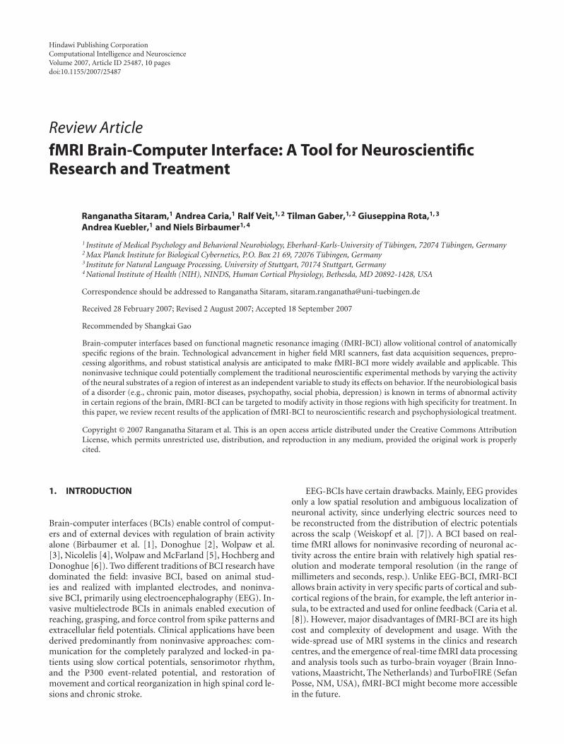
Hindawi Publishing CorporationComputational Intelligence and NeuroscienceVolume 2007, Article ID 25487, 10 pagesdoi:10.1155/2007/25487
Review ArticlefMRI Brain-Computer Interface: A Tool for NeuroscientificResearch and Treatment
Ranganatha Sitaram,1 Andrea Caria,1 Ralf Veit,1, 2 Tilman Gaber,1, 2 Giuseppina Rota,1, 3
Andrea Kuebler,1 and Niels Birbaumer1, 4
1 Institute of Medical Psychology and Behavioral Neurobiology, Eberhard-Karls-University of Tubingen, 72074 Tubingen, Germany2 Max Planck Institute for Biological Cybernetics, P.O. Box 21 69, 72076 Tubingen, Germany3 Institute for Natural Language Processing, University of Stuttgart, 70174 Stuttgart, Germany4 National Institute of Health (NIH), NINDS, Human Cortical Physiology, Bethesda, MD 20892-1428, USA
Correspondence should be addressed to Ranganatha Sitaram, [email protected]
Received 28 February 2007; Revised 2 August 2007; Accepted 18 September 2007
Recommended by Shangkai Gao
Brain-computer interfaces based on functional magnetic resonance imaging (fMRI-BCI) allow volitional control of anatomicallyspecific regions of the brain. Technological advancement in higher field MRI scanners, fast data acquisition sequences, prepro-cessing algorithms, and robust statistical analysis are anticipated to make fMRI-BCI more widely available and applicable. Thisnoninvasive technique could potentially complement the traditional neuroscientific experimental methods by varying the activityof the neural substrates of a region of interest as an independent variable to study its effects on behavior. If the neurobiological basisof a disorder (e.g., chronic pain, motor diseases, psychopathy, social phobia, depression) is known in terms of abnormal activityin certain regions of the brain, fMRI-BCI can be targeted to modify activity in those regions with high specificity for treatment. Inthis paper, we review recent results of the application of fMRI-BCI to neuroscientific research and psychophysiological treatment.
Copyright © 2007 Ranganatha Sitaram et al. This is an open access article distributed under the Creative Commons AttributionLicense, which permits unrestricted use, distribution, and reproduction in any medium, provided the original work is properlycited.
1. INTRODUCTION
Brain-computer interfaces (BCIs) enable control of comput-ers and of external devices with regulation of brain activityalone (Birbaumer et al. [1], Donoghue [2], Wolpaw et al.[3], Nicolelis [4], Wolpaw and McFarland [5], Hochberg andDonoghue [6]). Two different traditions of BCI research havedominated the field: invasive BCI, based on animal stud-ies and realized with implanted electrodes, and noninva-sive BCI, primarily using electroencephalography (EEG). In-vasive multielectrode BCIs in animals enabled execution ofreaching, grasping, and force control from spike patterns andextracellular field potentials. Clinical applications have beenderived predominantly from noninvasive approaches: com-munication for the completely paralyzed and locked-in pa-tients using slow cortical potentials, sensorimotor rhythm,and the P300 event-related potential, and restoration ofmovement and cortical reorganization in high spinal cord le-sions and chronic stroke.
EEG-BCIs have certain drawbacks. Mainly, EEG providesonly a low spatial resolution and ambiguous localization ofneuronal activity, since underlying electric sources need tobe reconstructed from the distribution of electric potentialsacross the scalp (Weiskopf et al. [7]). A BCI based on real-time fMRI allows for noninvasive recording of neuronal ac-tivity across the entire brain with relatively high spatial res-olution and moderate temporal resolution (in the range ofmillimeters and seconds, resp.). Unlike EEG-BCI, fMRI-BCIallows brain activity in very specific parts of cortical and sub-cortical regions of the brain, for example, the left anterior in-sula, to be extracted and used for online feedback (Caria et al.[8]). However, major disadvantages of fMRI-BCI are its highcost and complexity of development and usage. With thewide-spread use of MRI systems in the clinics and researchcentres, and the emergence of real-time fMRI data processingand analysis tools such as turbo-brain voyager (Brain Inno-vations, Maastricht, The Netherlands) and TurboFIRE (SefanPosse, NM, USA), fMRI-BCI might become more accessiblein the future.
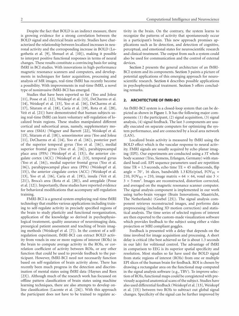
2 Computational Intelligence and Neuroscience
Despite the fact that BOLD is an indirect measure, thereis growing evidence for a strong correlation between theBOLD signal and electrical brain activity. Studies have char-acterized the relationship between localized increases in neu-ronal activity and the corresponding increase in BOLD (Lo-gothetis et al. [9], Shmuel et al. [10]), making it possibleto interpret positive functional responses in terms of neuralchanges. These results constitute a convincing basis for usingfMRI in BCI studies. With innovations in high-performancemagnetic resonance scanners and computers, and develop-ments in techniques for faster acquisition, processing andanalysis of MR images, real-time fMRI has recently becomea possibility. With improvements in real-time fMRI, a noveltype of noninvasive fMRI-BCI has emerged.
Studies that have been reported so far (Yoo and Jolesz[11], Posse et al. [12], Weiskopf et al. [13], DeCharms et al.[14], Weiskopf et al. [15], Yoo et al. [16], DeCharms et al.[17], Sitaram et al. [18], Caria et al. [19], Rota et al. [20],Veit et al. [21]) have demonstrated that human subjects us-ing real-time fMRI can learn voluntary self-regulation of lo-calized brain regions. These studies manipulated differentcortical and subcortical areas, namely, supplementary mo-tor area (SMA) (Wagner and Barrett [22], Weiskopf et al.[15], Sitaram et al. [18]), sensorimotor area (Yoo and Jolesz[11], DeCharms et al. [14], Yoo et al. [16]), posterior partof the superior temporal gyrus (Yoo et al. [16]), medialsuperior frontal gyrus (Yoo et al. [16]), parahippocampalplace area (PPA) (Weiskopf et al. [15]), the anterior cin-gulate cortex (ACC) (Weiskopf et al. [13], temporal gyrus(Yoo et al. [16]), medial superior frontal gyrus (Yoo et al.[16]), parahippocampal place area (PPA) (Weiskopf et al.[15]), the anterior cingulate cortex (ACC) (Weiskopf et al.[13], Yoo et al. [16], Caria et al. [19]), insula (Veit et al.[21]), Broca’s area (Rota et al. [20]), and amygdale (Posseet al. [12]). Importantly, these studies have reported evidencefor behavioral modifications that accompany self-regulationtraining.
FMRI-BCI is a general system employing real-time fMRItechnology that enables various applications including train-ing to self-regulate activity in precisely specified regions ofthe brain to study plasticity and functional reorganization,application of the knowledge so derived in psychophysio-logical treatement, quality assurance of neuroimaging data,presurgical patient assessment and teaching of brain imag-ing methods (Weiskopf et al. [7]). In the context of a self-regulation experiment, fMRI-BCI can extract BOLD activ-ity from voxels in one or more regions of interest (ROIs) inthe brain to compute average activity in the ROIs, or cor-relation coefficient of activity between ROIs, or any otherfunction that could be used to provide feedback to the par-ticipant. However, fMRI-BCI need not necessarily functionbased on self-regulation of brain activity alone. There hasrecently been much progress in the detection and discrim-ination of mental states using fMRI data (Haynes and Rees[23]). Although much of the research work has focussed onoffline pattern classification of brain states using machinelearning techniques, there are also attempts to develop on-line classification (Laconte et al. [24]). With this approachthe participant does not have to be trained to regulate ac-
tivity in the brain. On the contrary, the system learns torecognize the patterns of activity that spontaneously occurin a participant’s brain. This new approach promises ap-plications such as lie detection, and detection of cognitive,perceptual, and emotional states for neuroscientific researchand clinical treatment. The output from such a system couldalso be used for communication and the control of externaldevices.
Section 2 presents the general architecture of an fMRI-BCI system and its components. Section 3 paints a picture ofpotential applications of this emerging approach for neuro-scientific research. Section 4 describes possible applicationsin psychophysiological treatment. Section 5 offers conclud-ing remarks.
2. ARCHITECTURE OF fMRI-BCI
An fMRI-BCI system is a closed-loop system that can be de-picted as shown in Figure 1. It has the following major com-ponents: (1) the participant, (2) signal acquisition, (3) signalanalysis, (4) signal feedback. The last 3 components are usu-ally executed on separate computers for optimizing the sys-tem performance, and are connected by a local area network(LAN).
Localized brain activity is measured by fMRI using theBOLD effect which is the vascular response to neural activ-ity. FMRI signals are usually acquired by echo planar imag-ing (EPI). Our experiments are conducted using a 3T wholebody scanner (Trio, Siemens, Erlangen, Germany) with stan-dard head coil. EPI sequence parameters used are repetitiontime TR = 1.5 seconds, echo time TE = 45 milliseconds, flipangle = 70◦, 16 slices, bandwidth 1.3 KHz/pixel, FOVPE =210, FOVRO = 210, image matrix = 64 × 64, voxel size 3 ×3 × 5 mm3. Images are reconstructed, distortion corrected,and averaged on the magnetic resonance scanner computer.The signal analysis component is implemented in our workusing turbo-brain voyager (Brain Innovations, Maastricht,The Netherlands) (Goebel [25]). The signal analysis com-ponent retrieves reconstructed images, and performs datapreprocessing (including 3D motion correction) and statis-tical analysis. The time series of selected regions of interestare then exported to the custom-made visualization softwarewhich provides feedback to the subject using either a videoprojection or MRI compliant goggles.
Feedback is presented with a delay that depends on thetime involved for image acquisition and processing. A shortdelay is critical (the best achieved so far is about 1.3 secondsin our lab) for volitional control. The advantage of fMRIin comparison to EEG is its superior spatial specificity andresolution. Most studies so far have used the BOLD signalfrom static regions of interest (ROIs) from one or multipleEPI slices of the human brain for feedback. ROI is chosen bydrawing a rectangular area on the functional map computedin the signal analysis software (e.g., TBV). To improve selec-tion of ROIs, functional maps could be coregistered with pre-viously acquired anatomical scans of the subject. Studies havealso used differential feedback (Weiskopf et al. [13], Weiskopfet al. [15]) between two ROIs to subtract out global signalchanges. Specificity of the signal can be further improved by
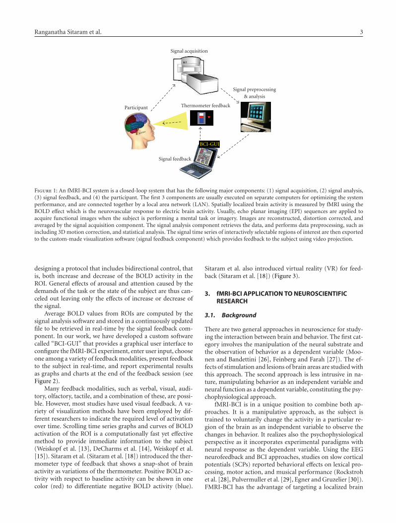
Ranganatha Sitaram et al. 3
Signal acquisition
Participant Thermometer feedback
Signal preprocessing& analysis
BCI-GUI
Signal feedback
Figure 1: An fMRI-BCI system is a closed-loop system that has the following major components: (1) signal acquisition, (2) signal analysis,(3) signal feedback, and (4) the participant. The first 3 components are usually executed on separate computers for optimizing the systemperformance, and are connected together by a local area network (LAN). Spatially localized brain activity is measured by fMRI using theBOLD effect which is the neurovascular response to electric brain activity. Usually, echo planar imaging (EPI) sequences are applied toacquire functional images when the subject is performing a mental task or imagery. Images are reconstructed, distortion corrected, andaveraged by the signal acquisition component. The signal analysis component retrieves the data, and performs data preprocessing, such asincluding 3D motion correction, and statistical analysis. The signal time series of interactively selectable regions of interest are then exportedto the custom-made visualization software (signal feedback component) which provides feedback to the subject using video projection.
designing a protocol that includes bidirectional control, thatis, both increase and decrease of the BOLD activity in theROI. General effects of arousal and attention caused by thedemands of the task or the state of the subject are thus can-celed out leaving only the effects of increase or decrease ofthe signal.
Average BOLD values from ROIs are computed by thesignal analysis software and stored in a continuously updatedfile to be retrieved in real-time by the signal feedback com-ponent. In our work, we have developed a custom softwarecalled “BCI-GUI” that provides a graphical user interface toconfigure the fMRI-BCI experiment, enter user input, chooseone among a variety of feedback modalities, present feedbackto the subject in real-time, and report experimental resultsas graphs and charts at the end of the feedback session (seeFigure 2).
Many feedback modalities, such as verbal, visual, audi-tory, olfactory, tactile, and a combination of these, are possi-ble. However, most studies have used visual feedback. A va-riety of visualization methods have been employed by dif-ferent researchers to indicate the required level of activationover time. Scrolling time series graphs and curves of BOLDactivation of the ROI is a computationally fast yet effectivemethod to provide immediate information to the subject(Weiskopf et al. [13], DeCharms et al. [14], Weiskopf et al.[15]). Sitaram et al. (Sitaram et al. [18]) introduced the ther-mometer type of feedback that shows a snap-shot of brainactivity as variations of the thermometer. Positive BOLD ac-tivity with respect to baseline activity can be shown in onecolor (red) to differentiate negative BOLD activity (blue).
Sitaram et al. also introduced virtual reality (VR) for feed-back (Sitaram et al. [18]) (Figure 3).
3. fMRI-BCI APPLICATION TO NEUROSCIENTIFICRESEARCH
3.1. Background
There are two general approaches in neuroscience for study-ing the interaction between brain and behavior. The first cat-egory involves the manipulation of the neural substrate andthe observation of behavior as a dependent variable (Moo-nen and Bandettini [26], Feinberg and Farah [27]). The ef-fects of stimulation and lesions of brain areas are studied withthis approach. The second approach is less intrusive in na-ture, manipulating behavior as an independent variable andneural function as a dependent variable, constituting the psy-chophysiological approach.
fMRI-BCI is in a unique position to combine both ap-proaches. It is a manipulative approach, as the subject istrained to voluntarily change the activity in a particular re-gion of the brain as an independent variable to observe thechanges in behavior. It realizes also the psychophysiologicalperspective as it incorporates experimental paradigms withneural response as the dependent variable. Using the EEGneurofeedback and BCI approaches, studies on slow corticalpotentials (SCPs) reported behavioral effects on lexical pro-cessing, motor action, and musical performance (Rockstrohet al. [28], Pulvermuller et al. [29], Egner and Gruzelier [30]).FMRI-BCI has the advantage of targeting a localized brain
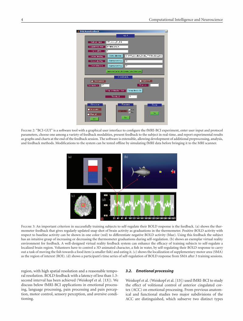
4 Computational Intelligence and Neuroscience
Figure 2: “BCI-GUI” is a software tool with a graphical user interface to configure the fMRI-BCI experiment, enter user input and protocolparameters, choose one among a variety of feedback modalities, present feedback to the subject in real-time, and report experimental resultsas graphs and charts at the end of the feedback session. The software is extensible, allowing development of additional preprocessing, analysis,and feedback methods. Modifications to the system can be tested offline by simulating fMRI data before bringing it to the MRI scanner.
(a) (b)
(c)(d)
Figure 3: An important criterion in successfully training subjects to self-regulate their BOLD response is the feedback. (a) shows the ther-mometer feedback that gives regularly updated snap shot of brain activity as graduations in the thermometer. Positive BOLD activity withrespect to baseline activity can be shown in one color (red) to differentiate negative BOLD activity (blue). Using this feedback the subjecthas an intuitive grasp of increasing or decreasing the thermometer graduations during self-regulation. (b) shows an exemplar virtual realityenvironment for feedback. A well-designed virtual reality feedback system can enhance the efficacy of training subjects to self-regulate alocalized brain region. Volunteers have to control a 3D animated character, a fish in water, by self-regulating their BOLD response to carryout a task of moving the fish towards a food item (a smaller fish) and eating it. (c) shows the localization of supplementary motor area (SMA)as the region of interest (ROI). (d) shows a participant’s time series of self-regulation of BOLD response from SMA after 3 training sessions.
region, with high spatial resolution and a reasonable tempo-ral resolution. BOLD feedback with a latency of less than 1.3-second interval has been achieved (Weiskopf et al. [13]). Wediscuss below fMRI-BCI applications in emotional process-ing, language processing, pain processing and pain percep-tion, motor control, sensory perception, and aversive condi-tioning.
3.2. Emotional processing
Weiskopf et al. (Weiskopf et al. [13]) used fMRI-BCI to studythe effect of volitional control of anterior cingulated cor-tex (ACC) on emotional processing. From previous anatom-ical and functional studies two major subdivisions of theACC are distinguished, which subserve two distinct types
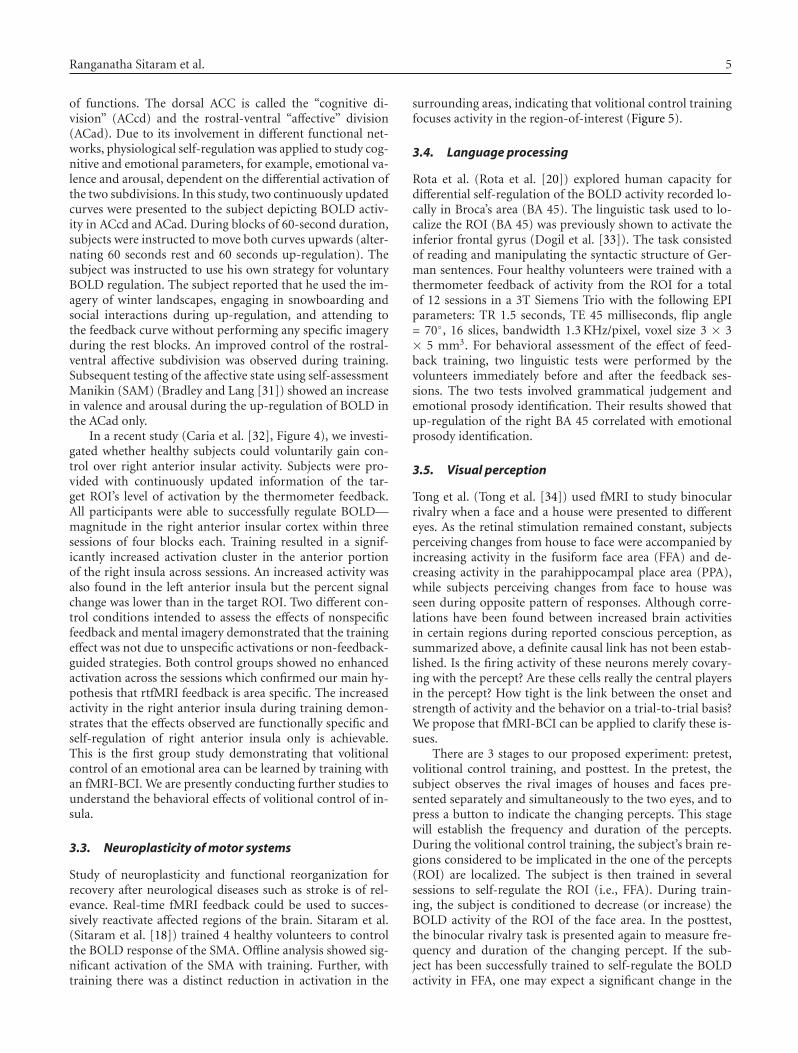
Ranganatha Sitaram et al. 5
of functions. The dorsal ACC is called the “cognitive di-vision” (ACcd) and the rostral-ventral “affective” division(ACad). Due to its involvement in different functional net-works, physiological self-regulation was applied to study cog-nitive and emotional parameters, for example, emotional va-lence and arousal, dependent on the differential activation ofthe two subdivisions. In this study, two continuously updatedcurves were presented to the subject depicting BOLD activ-ity in ACcd and ACad. During blocks of 60-second duration,subjects were instructed to move both curves upwards (alter-nating 60 seconds rest and 60 seconds up-regulation). Thesubject was instructed to use his own strategy for voluntaryBOLD regulation. The subject reported that he used the im-agery of winter landscapes, engaging in snowboarding andsocial interactions during up-regulation, and attending tothe feedback curve without performing any specific imageryduring the rest blocks. An improved control of the rostral-ventral affective subdivision was observed during training.Subsequent testing of the affective state using self-assessmentManikin (SAM) (Bradley and Lang [31]) showed an increasein valence and arousal during the up-regulation of BOLD inthe ACad only.
In a recent study (Caria et al. [32], Figure 4), we investi-gated whether healthy subjects could voluntarily gain con-trol over right anterior insular activity. Subjects were pro-vided with continuously updated information of the tar-get ROI’s level of activation by the thermometer feedback.All participants were able to successfully regulate BOLD—magnitude in the right anterior insular cortex within threesessions of four blocks each. Training resulted in a signif-icantly increased activation cluster in the anterior portionof the right insula across sessions. An increased activity wasalso found in the left anterior insula but the percent signalchange was lower than in the target ROI. Two different con-trol conditions intended to assess the effects of nonspecificfeedback and mental imagery demonstrated that the trainingeffect was not due to unspecific activations or non-feedback-guided strategies. Both control groups showed no enhancedactivation across the sessions which confirmed our main hy-pothesis that rtfMRI feedback is area specific. The increasedactivity in the right anterior insula during training demon-strates that the effects observed are functionally specific andself-regulation of right anterior insula only is achievable.This is the first group study demonstrating that volitionalcontrol of an emotional area can be learned by training withan fMRI-BCI. We are presently conducting further studies tounderstand the behavioral effects of volitional control of in-sula.
3.3. Neuroplasticity of motor systems
Study of neuroplasticity and functional reorganization forrecovery after neurological diseases such as stroke is of rel-evance. Real-time fMRI feedback could be used to succes-sively reactivate affected regions of the brain. Sitaram et al.(Sitaram et al. [18]) trained 4 healthy volunteers to controlthe BOLD response of the SMA. Offline analysis showed sig-nificant activation of the SMA with training. Further, withtraining there was a distinct reduction in activation in the
surrounding areas, indicating that volitional control trainingfocuses activity in the region-of-interest (Figure 5).
3.4. Language processing
Rota et al. (Rota et al. [20]) explored human capacity fordifferential self-regulation of the BOLD activity recorded lo-cally in Broca’s area (BA 45). The linguistic task used to lo-calize the ROI (BA 45) was previously shown to activate theinferior frontal gyrus (Dogil et al. [33]). The task consistedof reading and manipulating the syntactic structure of Ger-man sentences. Four healthy volunteers were trained with athermometer feedback of activity from the ROI for a totalof 12 sessions in a 3T Siemens Trio with the following EPIparameters: TR 1.5 seconds, TE 45 milliseconds, flip angle= 70◦, 16 slices, bandwidth 1.3 KHz/pixel, voxel size 3 × 3× 5 mm3. For behavioral assessment of the effect of feed-back training, two linguistic tests were performed by thevolunteers immediately before and after the feedback ses-sions. The two tests involved grammatical judgement andemotional prosody identification. Their results showed thatup-regulation of the right BA 45 correlated with emotionalprosody identification.
3.5. Visual perception
Tong et al. (Tong et al. [34]) used fMRI to study binocularrivalry when a face and a house were presented to differenteyes. As the retinal stimulation remained constant, subjectsperceiving changes from house to face were accompanied byincreasing activity in the fusiform face area (FFA) and de-creasing activity in the parahippocampal place area (PPA),while subjects perceiving changes from face to house wasseen during opposite pattern of responses. Although corre-lations have been found between increased brain activitiesin certain regions during reported conscious perception, assummarized above, a definite causal link has not been estab-lished. Is the firing activity of these neurons merely covary-ing with the percept? Are these cells really the central playersin the percept? How tight is the link between the onset andstrength of activity and the behavior on a trial-to-trial basis?We propose that fMRI-BCI can be applied to clarify these is-sues.
There are 3 stages to our proposed experiment: pretest,volitional control training, and posttest. In the pretest, thesubject observes the rival images of houses and faces pre-sented separately and simultaneously to the two eyes, and topress a button to indicate the changing percepts. This stagewill establish the frequency and duration of the percepts.During the volitional control training, the subject’s brain re-gions considered to be implicated in the one of the percepts(ROI) are localized. The subject is then trained in severalsessions to self-regulate the ROI (i.e., FFA). During train-ing, the subject is conditioned to decrease (or increase) theBOLD activity of the ROI of the face area. In the posttest,the binocular rivalry task is presented again to measure fre-quency and duration of the changing percept. If the sub-ject has been successfully trained to self-regulate the BOLDactivity in FFA, one may expect a significant change in the
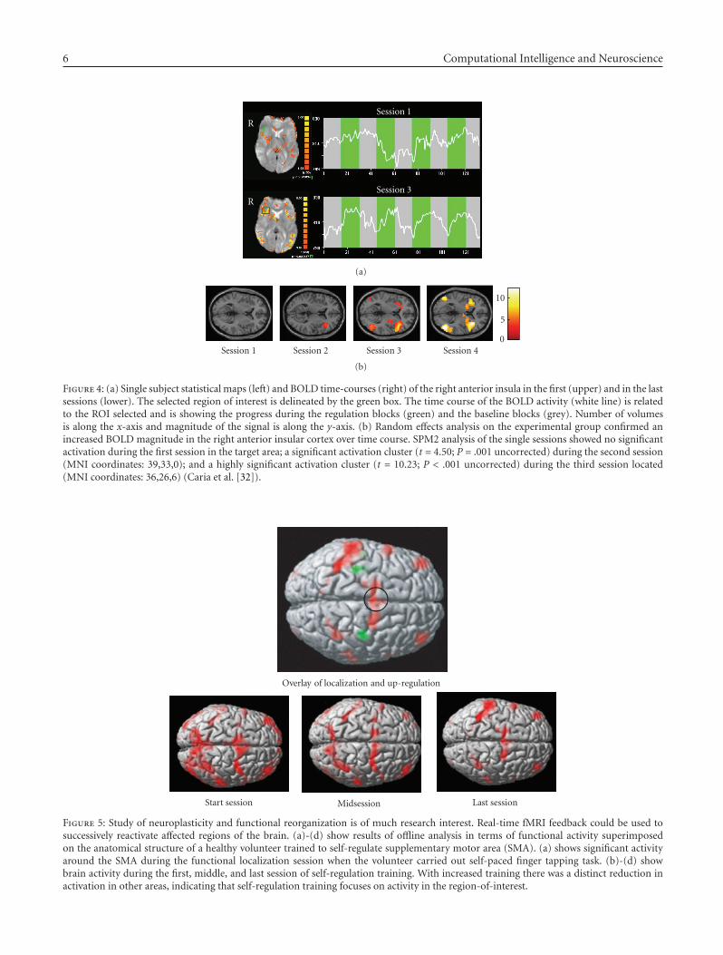
6 Computational Intelligence and Neuroscience
R
R
Session 1
Session 3
(a)
Session 1 Session 2 Session 3 Session 4
10
5
0
(b)
Figure 4: (a) Single subject statistical maps (left) and BOLD time-courses (right) of the right anterior insula in the first (upper) and in the lastsessions (lower). The selected region of interest is delineated by the green box. The time course of the BOLD activity (white line) is relatedto the ROI selected and is showing the progress during the regulation blocks (green) and the baseline blocks (grey). Number of volumesis along the x-axis and magnitude of the signal is along the y-axis. (b) Random effects analysis on the experimental group confirmed anincreased BOLD magnitude in the right anterior insular cortex over time course. SPM2 analysis of the single sessions showed no significantactivation during the first session in the target area; a significant activation cluster (t = 4.50; P = .001 uncorrected) during the second session(MNI coordinates: 39,33,0); and a highly significant activation cluster (t = 10.23; P < .001 uncorrected) during the third session located(MNI coordinates: 36,26,6) (Caria et al. [32]).
Overlay of localization and up-regulation
Start session Midsession Last session
Figure 5: Study of neuroplasticity and functional reorganization is of much research interest. Real-time fMRI feedback could be used tosuccessively reactivate affected regions of the brain. (a)-(d) show results of offline analysis in terms of functional activity superimposedon the anatomical structure of a healthy volunteer trained to self-regulate supplementary motor area (SMA). (a) shows significant activityaround the SMA during the functional localization session when the volunteer carried out self-paced finger tapping task. (b)-(d) showbrain activity during the first, middle, and last session of self-regulation training. With increased training there was a distinct reduction inactivation in other areas, indicating that self-regulation training focuses on activity in the region-of-interest.
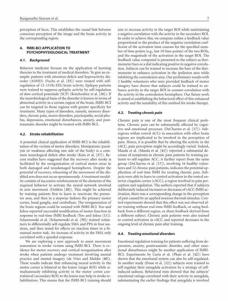
Ranganatha Sitaram et al. 7
perception of faces. This establishes the causal link betweenconscious perception of the image and the brain activity inthe corresponding region.
4. fMRI-BCI APPLICATION TOPSYCHOPHYSIOLOGICAL TREATMENT
4.1. Background
Behavior medicine focuses on the application of learningtheories to the treatment of medical disorders. To give an ex-ample: patients with attention-deficit and hyperactivity dis-order (ADHD) (Fuchs et al. [35]) were treated with self-regulation of 12–15 Hz EEG brain activity. Epilepsy patientswere trained to suppress epileptic activity by self-regulationof slow cortical potentials (SCP) (Kotchoubey et al. [36]). Ifthe neurobiological basis of the disorder is known in terms ofabnormal activity in a certain region of the brain, fMRI-BCIcan be targeted to those regions with greater specificity fortreatment. Many types of disorders, namely, memory disor-ders, chronic pain, motor disorders, psychopathy, social pho-bia, depression, emotional disturbances, anxiety, and post-traumatic disorder might be treated with fMRI-BCI.
4.2. Stroke rehabilitation
A potential clinical application of fMRI-BCI is the rehabili-tation of the victims of motor disorders. Hemiparesis (paral-ysis or weakness affecting one side of the body) is a com-mon neurological deficit after stroke (Kato et al. [37]). Re-cent studies have suggested that the recovery after stroke isfacilitated by the reorganization of cortical motor areas inboth damaged and nondamaged hemispheres. Despite thepotential of recovery, relearning of the movement of the dis-abled arm does not occur spontaneously. A treatment modal-ity consists of successive reinforcement of the elements of therequired behavior to activate the neural network involvedin arm movement (Dobkin [38]). This might be achievedby training patients first to learn to reactivate the premo-tor area, and then in a stepwise fashion the primary motorcortex, basal ganglia, and cerebellum. The reorganization ofthe brain regions could be assisted with fMRI-BCI. Yoo andJolesz reported successful modification of motor function inresponse to real-time fMRI feedback (Yoo and Jolesz [11]).Scharnowski et al. (Scharnowski et al. [39]) trained volun-teers to differentially self-regulate SMA and PPA in four ses-sions, and then tested for effects on reaction times in a bi-manual motor task. An increase of activity in the SMA onlycorrelated with a speeded response.
We are exploring a new approach to assist movementrestoration in stroke victims using fMRI-BCI. There is ev-idence for motor recovery and cortical reorganization afterstroke when patients undergo treatment involving mentalpractice and mental imagery (de Vries and Mulder [40]).These results indicate that enhancing neural activity in themotor cortex is bilateral to the lesion (target ROI) while si-multaneously inhibiting activity in the motor cortex con-tralateral (secondary ROI) to the lesion may help in stroke re-habilitation. This means that the fMRI-BCI training should
aim to increase activity in the target ROI while maintaininga negative correlation with the activity in the secondary ROI.In order to achieve this, we compute online a feedback valueproportional to the product of the negative correlation coef-ficient of the activation time courses for the specified num-ber of time points (e.g., last 10 time points) of the two ROIs,and the magnitude of the activation in the target ROI. Thefeedback value computed is presented to the subject as ther-mometer bars or a dial indicating positive to negative correla-tion. Subjects can be trained to increase the bars of the ther-mometer to enhance activation in the ipsilesion area whileinhibiting the contralesion area. Our preliminary results with2 healthy volunteers who were provided feedback of motorimagery have shown that subjects could be trained to en-hance activity in the target ROI in counter-correlation withthe activity in the contralesion hemisphere. Our future workis aimed at establishing the behavioral effect of this enhancedactivity and the suitability of this method for stroke therapy.
4.3. Treating chronic pain
Chronic pain is one of the most frequent clinical prob-lems. Chronic pain can be substantially affected by cogni-tive and emotional processes (DeCharms et al. [17]). Sub-regions within rostral ACCr in association with other brainregions are implicated to be involved in the perception ofpain. Hence, it is possible that by altering the activity in therACC, pain perception might be accordingly varied. Indeed,Maeda et al. (Maeda et al. [41]) reported a substantial de-crease of symptoms in chronic pain patients by training pa-tients to self-regulate ACC. A further report from the samegroup (DeCharms et al. [17]), involving 16 healthy volun-teers and 12 chronic pain patients, indicates the potential ap-plication of real-time fMRI for treating chronic pain. Sub-jects were able to learn to control activation in the rostral an-terior cingulate cortex (rACC), a region involved in pain per-ception and regulation. The authors reported that if subjectsdeliberately induced increases or decreases of rACC fMRI ac-tivation, there was a corresponding change in the perceptionof pain caused by an applied noxious thermal stimulus. Con-trol experiments showed that this effect was not observed af-ter training without real-time fMRI feedback, or using feed-back from a different region, or sham feedback derived froma different subject. Chronic pain patients were also trainedto control activation in rACC and reported decreases in theongoing level of chronic pain after training.
4.4. Treating emotional disorders
Emotional regulation training for patients suffering from de-pression, anxiety, posttraumatic disorder, and other emo-tional disturbances might be another application of fMRI-BCI. Experiments by Caria et al. (Phan et al. [42]) haveshown that the emotional system can also be self-regulated.In another study (Posse et al. [12]) subjects were trained toself-regulate their amygdala activation by a strategy of self-induced sadness. Behavioral tests showed that the subjects’emotional ratings correlated with their activity in amygdala,substantiating the earlier findings that amygdala is involved
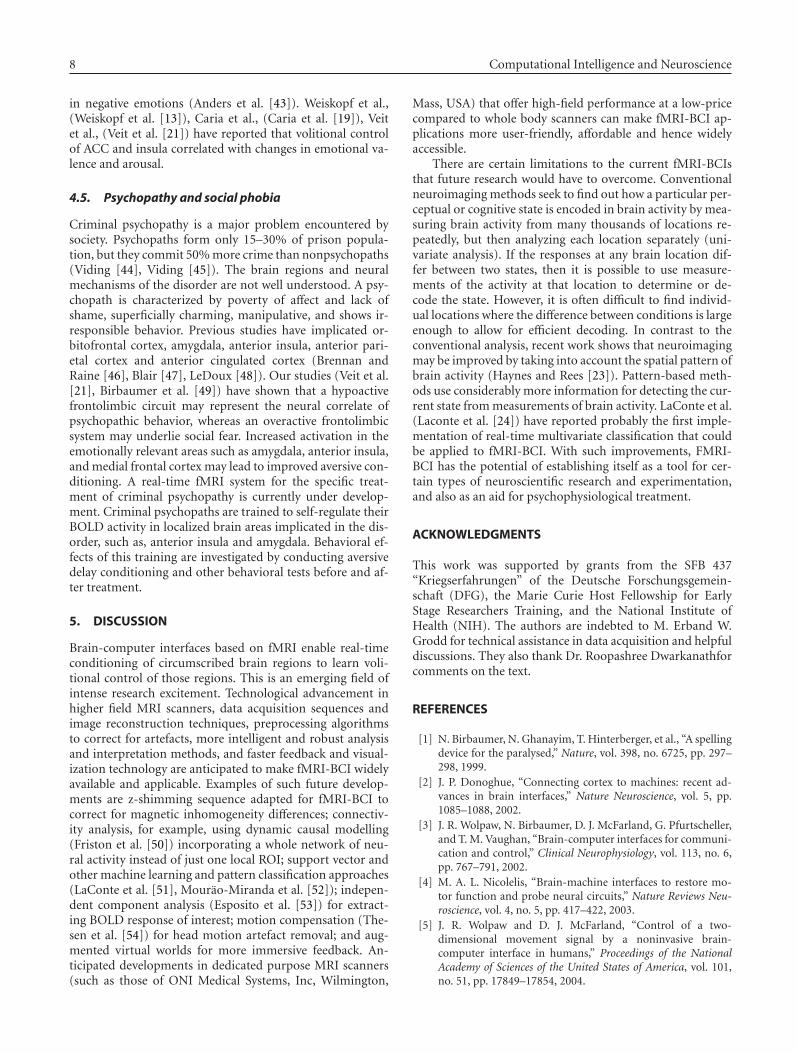
8 Computational Intelligence and Neuroscience
in negative emotions (Anders et al. [43]). Weiskopf et al.,(Weiskopf et al. [13]), Caria et al., (Caria et al. [19]), Veitet al., (Veit et al. [21]) have reported that volitional controlof ACC and insula correlated with changes in emotional va-lence and arousal.
4.5. Psychopathy and social phobia
Criminal psychopathy is a major problem encountered bysociety. Psychopaths form only 15–30% of prison popula-tion, but they commit 50% more crime than nonpsychopaths(Viding [44], Viding [45]). The brain regions and neuralmechanisms of the disorder are not well understood. A psy-chopath is characterized by poverty of affect and lack ofshame, superficially charming, manipulative, and shows ir-responsible behavior. Previous studies have implicated or-bitofrontal cortex, amygdala, anterior insula, anterior pari-etal cortex and anterior cingulated cortex (Brennan andRaine [46], Blair [47], LeDoux [48]). Our studies (Veit et al.[21], Birbaumer et al. [49]) have shown that a hypoactivefrontolimbic circuit may represent the neural correlate ofpsychopathic behavior, whereas an overactive frontolimbicsystem may underlie social fear. Increased activation in theemotionally relevant areas such as amygdala, anterior insula,and medial frontal cortex may lead to improved aversive con-ditioning. A real-time fMRI system for the specific treat-ment of criminal psychopathy is currently under develop-ment. Criminal psychopaths are trained to self-regulate theirBOLD activity in localized brain areas implicated in the dis-order, such as, anterior insula and amygdala. Behavioral ef-fects of this training are investigated by conducting aversivedelay conditioning and other behavioral tests before and af-ter treatment.
5. DISCUSSION
Brain-computer interfaces based on fMRI enable real-timeconditioning of circumscribed brain regions to learn voli-tional control of those regions. This is an emerging field ofintense research excitement. Technological advancement inhigher field MRI scanners, data acquisition sequences andimage reconstruction techniques, preprocessing algorithmsto correct for artefacts, more intelligent and robust analysisand interpretation methods, and faster feedback and visual-ization technology are anticipated to make fMRI-BCI widelyavailable and applicable. Examples of such future develop-ments are z-shimming sequence adapted for fMRI-BCI tocorrect for magnetic inhomogeneity differences; connectiv-ity analysis, for example, using dynamic causal modelling(Friston et al. [50]) incorporating a whole network of neu-ral activity instead of just one local ROI; support vector andother machine learning and pattern classification approaches(LaConte et al. [51], Mourao-Miranda et al. [52]); indepen-dent component analysis (Esposito et al. [53]) for extract-ing BOLD response of interest; motion compensation (The-sen et al. [54]) for head motion artefact removal; and aug-mented virtual worlds for more immersive feedback. An-ticipated developments in dedicated purpose MRI scanners(such as those of ONI Medical Systems, Inc, Wilmington,
Mass, USA) that offer high-field performance at a low-pricecompared to whole body scanners can make fMRI-BCI ap-plications more user-friendly, affordable and hence widelyaccessible.
There are certain limitations to the current fMRI-BCIsthat future research would have to overcome. Conventionalneuroimaging methods seek to find out how a particular per-ceptual or cognitive state is encoded in brain activity by mea-suring brain activity from many thousands of locations re-peatedly, but then analyzing each location separately (uni-variate analysis). If the responses at any brain location dif-fer between two states, then it is possible to use measure-ments of the activity at that location to determine or de-code the state. However, it is often difficult to find individ-ual locations where the difference between conditions is largeenough to allow for efficient decoding. In contrast to theconventional analysis, recent work shows that neuroimagingmay be improved by taking into account the spatial pattern ofbrain activity (Haynes and Rees [23]). Pattern-based meth-ods use considerably more information for detecting the cur-rent state from measurements of brain activity. LaConte et al.(Laconte et al. [24]) have reported probably the first imple-mentation of real-time multivariate classification that couldbe applied to fMRI-BCI. With such improvements, FMRI-BCI has the potential of establishing itself as a tool for cer-tain types of neuroscientific research and experimentation,and also as an aid for psychophysiological treatment.
ACKNOWLEDGMENTS
This work was supported by grants from the SFB 437“Kriegserfahrungen” of the Deutsche Forschungsgemein-schaft (DFG), the Marie Curie Host Fellowship for EarlyStage Researchers Training, and the National Institute ofHealth (NIH). The authors are indebted to M. Erband W.Grodd for technical assistance in data acquisition and helpfuldiscussions. They also thank Dr. Roopashree Dwarkanathforcomments on the text.
REFERENCES
[1] N. Birbaumer, N. Ghanayim, T. Hinterberger, et al., “A spellingdevice for the paralysed,” Nature, vol. 398, no. 6725, pp. 297–298, 1999.
[2] J. P. Donoghue, “Connecting cortex to machines: recent ad-vances in brain interfaces,” Nature Neuroscience, vol. 5, pp.1085–1088, 2002.
[3] J. R. Wolpaw, N. Birbaumer, D. J. McFarland, G. Pfurtscheller,and T. M. Vaughan, “Brain-computer interfaces for communi-cation and control,” Clinical Neurophysiology, vol. 113, no. 6,pp. 767–791, 2002.
[4] M. A. L. Nicolelis, “Brain-machine interfaces to restore mo-tor function and probe neural circuits,” Nature Reviews Neu-roscience, vol. 4, no. 5, pp. 417–422, 2003.
[5] J. R. Wolpaw and D. J. McFarland, “Control of a two-dimensional movement signal by a noninvasive brain-computer interface in humans,” Proceedings of the NationalAcademy of Sciences of the United States of America, vol. 101,no. 51, pp. 17849–17854, 2004.
Ranganatha Sitaram et al. 9
[6] L. R. Hochberg and J. P. Donoghue, “Sensors for brain-computer interfaces: options for turning thought into action,”IEEE Engineering in Medicine and Biology Magazine, vol. 25,no. 5, pp. 32–38, 2006.
[7] N. Weiskopf, R. Sitaram, O. Josephs, et al., “Real-time func-tional magnetic resonance imaging: methods and applica-tions,” Magnetic Resonance Imaging, vol. 25, no. 6, pp. 989–1003, 2007.
[8] A. Caria, R. Veit, R. Sitaram, et al., “Regulation of anteriorinsular cortex activity using real-time fMRI,” NeuroImage,vol. 35, no. 3, pp. 1238–1246, 2007.
[9] N. K. Logothetis, J. Pauls, M. Augath, T. Trinath, and A. Oel-termann, “Neurophysiological investigation of the basis of thefMRI signal,” Nature, vol. 412, no. 6843, pp. 150–157, 2001.
[10] A. Shmuel, M. Augath, A. Oeltermann, and N. K. Logothetis,“Negative functional MRI response correlates with decreasesin neuronal activity in monkey visual area V1,” Nature Neuro-science, vol. 9, no. 4, pp. 569–577, 2006.
[11] S.-S. Yoo and F. A. Jolesz, “Functional MRI for neurofeedback:feasibility study on a hand motor task,” NeuroReport, vol. 13,no. 11, pp. 1377–1381, 2002.
[12] S. Posse, D. Fitzgerald, K. Gao, et al., “Real-time fMRI of tem-porolimbic regions detects amygdala activation during single-trial self-induced sadness,” NeuroImage, vol. 18, no. 3, pp. 760–768, 2003.
[13] N. Weiskopf, R. Veit, M. Erb, et al., “Physiological self-regulation of regional brain activity using real-time functionalmagnetic resonance imaging (fMRI): methodology and exem-plary data,” NeuroImage, vol. 19, no. 3, pp. 577–586, 2003.
[14] R. C. DeCharms, K. Christoff, G. H. Glover, J. M. Pauly, S.Whitfield, and J. D. E. Gabrieli, “Learned regulation of spa-tially localized brain activation using real-time fMRI,” Neu-roImage, vol. 21, no. 1, pp. 436–443, 2004.
[15] N. Weiskopf, F. Scharnowski, R. Veit, R. Goebel, N. Birbaumer,and K. Mathiak, “Self-regulation of local brain activity us-ing real-time functional magnetic resonance imaging (fMRI),”Journal of Physiology, vol. 98, no. 4–6, pp. 357–373, 2004.
[16] S.-S. Yoo, T. Fairneny, N.-K. Chen, et al., “Brain-computer in-terface using fMRI: spatial navigation by thoughts,” NeuroRe-port, vol. 15, no. 10, pp. 1591–1595, 2004.
[17] R. C. DeCharms, F. Maeda, G. H. Glover, et al., “Control overbrain activation and pain learned by using real-time func-tional MRI,” Proceedings of the National Academy of Sciences ofthe United States of America, vol. 102, no. 51, pp. 18626–18631,2005.
[18] R. Sitaram, A. Caria, R. Veit, T. Gaber, A. Kuebler, and N. Bir-baumer, “Real-time fMRI based brain-computer interface en-hanced by interactive virtual worlds,” in Proceedings of the 45thAnnual Meeting Society for Psychophysiological Research, Lis-bon, Portugal, 2005.
[19] A. Caria, R. Veit, T. Gaber, R. Sitaram, A. Kuebler, and N.Birbaumer, “Can we learn to increase our emotional involve-ment? real-time fMRI of anterior cingulate cortex during emo-tional processing,” in Human Brain Mapping, Florence, Italy,June 2006.
[20] G. Rota, R. Sitaram, R. Veit, N. Weiskopf, N. Birbaumer, andG. Dogil, “ fMRI-neurofeedback for operant conditioning andneural plasticity investigation: a study on the physiologicalself-induced regulation of the BA 45,” in Proceedings of theCognitive Neuroscience Conference, San Francisco, Calif, USA,2006.
[21] R. Veit, H. Flor, M. Erb, et al., “Brain circuits involved in emo-tional learning in antisocial behavior and social phobia in hu-mans,” Neuroscience Letters, vol. 328, no. 3, pp. 233–236, 2002.
[22] C. H. Wagner and M. L. Barrett, Published online by PsycEx-tra, 2004.
[23] J.-D. Haynes and G. Rees, “Decoding mental states from brainactivity in humans,” Nature Reviews Neuroscience, vol. 7, no. 7,pp. 523–534, 2006.
[24] S. M. Laconte, S. J. Peltier, and X. P. Hu, “Real-time fMRI usingbrain-state classification,” in Human Brain Mapping, 2006.
[25] R. Goebel, “Cortex-based real-time fMRI,” NeuroImage,vol. 13, no. 6, p. 129, 2001.
[26] C. T. W. Moonen and P. A. Bandettini, Eds., Functional MRI,Springer, Berlin, Germany, 2000.
[27] T. E. Feinberg and M. J. Farah, Eds., Behavioral Neurology andNeuropsychology, McGraw-Hill, New York, NY, USA, 2nd edi-tion, 2003.
[28] B. Rockstroh, T. Elbert, N. Birbaumer, and W. Lutzenberger,“Biofeedback-produced hemispheric asymmetry of slow cor-tical potentials and its behavioural effects,” International Jour-nal of Psychophysiology, vol. 9, no. 2, pp. 151–165, 1990.
[29] F. Pulvermuller, B. Mohr, H. Schleichert, and R. Veit, “Operantconditioning of left-hemispheric slow cortical potentials andits effect on word processing,” Biological Psychology, vol. 53,no. 2-3, pp. 177–215, 2000.
[30] T. Egner and J. H. Gruzelier, “Ecological validity of neurofeed-back: modulation of slow wave EEG enhances musical perfor-mance,” NeuroReport, vol. 14, no. 9, pp. 1221–1224, 2003.
[31] M. M. Bradley and P. J. Lang, “Measuring emotion: the self-assessment manikin and the semantic differential,” Journal ofBehavior Therapy and Experimental Psychiatry, vol. 25, no. 1,pp. 49–59, 1994.
[32] A. Caria, R. Veit, R. Sitaram, M. Lotze, N. Weiskopf, W. Grodd,and N. Birbaumer, “Regulation of anterior insular cortex ac-tivity using real-time fMRI,” Neuroimage, vol. 35, no. 3, pp.1238–1246, 2007.
[33] G. Dogil, I. Frese, H. Haider, D. ROhm, and W. Wokurek,“Where and how does grammatically geared processing takeplace-and why is broca’s area often involved. A coordinatedfMRI/ERBP study of language processing,” Brain and Lan-guage, vol. 89, no. 2, pp. 337–345, 2004.
[34] F. Tong, K. Nakayama, J. T. Vaughan, and N. Kanwisher,“Binocular rivalry and visual awareness in human extrastriatecortex,” Neuron, vol. 21, no. 4, pp. 753–759, 1998.
[35] T. Fuchs, N. Birbaumer, W. Lutzenberger, J. H. Gruze-lier, and J. Kaiser, “Neurofeedback treatment for attention-deficit/hyperactivity disorder in children: a comparisonwith methylphenidate,” Applied Psychophysiology Biofeedback,vol. 28, no. 1, pp. 1–12, 2003.
[36] B. Kotchoubey, U. Strehl, C. Uhlmann, et al., “Modification ofslow cortical potentials in patients with refractory epilepsy: acontrolled outcome study,” Epilepsia, vol. 42, no. 3, pp. 406–416, 2001.
[37] H. Kato, M. Izumiyama, H. Koizumi, A. Takahashi, and Y.Itoyama, “Near-infrared spectroscopic topography as a toolto monitor motor reorganization after hemiparetic stroke: acomparison with functional MRI,” Stroke, vol. 33, no. 8, pp.2032–2036, 2002.
[38] B. H. Dobkin, “Functional MRI: a potential physiologic indi-cator for stroke rehabilitation interventions,” Stroke, vol. 34,no. 5, pp. e23–e28, 2003.
10 Computational Intelligence and Neuroscience
[39] F. Scharnowski, N. Weiskopf, K. Mathiak, et al., “Self-regulation of the BOLD signal of supplementary motorarea (SMA) and parahippocampal place area (PPA): fMRI-neurofeedbackand its behavioural consequences,” in Proceed-ings of 10th International Conference on Functional Mapping ofthe Human Brain, Budapest, Hungary, 2004.
[40] S. de Vries and T. Mulder, “Motor imagery and stroke re-habilitation: a critical discussion,” Journal of RehabilitationMedicine, vol. 39, no. 1, pp. 5–13, 2007.
[41] F. Maeda, “Learning to explicitly control activation in a lo-calized brain region through real-time fMRI feedback basedtraining, with result impact on pain perception,” in Proceed-ings of the Society for Neuroscience, pp. 601–604, Washington,DC, USA, 2004.
[42] K. L. Phan, D. A. Fitzgerald, K. Gao, G. J. Moore, M. E. Tancer,and S. Posse, “Real-time fMRI of cortico-limbic brain activityduring emotional processing,” NeuroReport, vol. 15, no. 3, pp.527–532, 2004.
[43] S. Anders, M. Lotze, M. Erb, W. Grodd, and N. Birbaumer,“Brain activity underlying emotional valence and arousal: aresponse-related fMRI study,” Human Brain Mapping, vol. 23,no. 4, pp. 200–209, 2004.
[44] E. Viding, “On the nature and nurture of antisocial behav-ior and violence,” Annals of the New York Academy of Sciences,vol. 1036, pp. 267–277, 2004.
[45] E. Viding, “Annotation: understanding the development ofpsychopathy,” Journal of Child Psychology and Psychiatry andAllied Disciplines, vol. 45, no. 8, pp. 1329–1337, 2004.
[46] P. A. Brennan and A. Raine, “Biosocial bases of antisocial be-havior: psychophysiological, neurological, and cognitive fac-tors,” Clinical Psychology Review, vol. 17, no. 6, pp. 589–604,1997.
[47] R. J. R. Blair, “Neurobiological basis of psychopathy,” BritishJournal of Psychiatry, vol. 182, pp. 5–7, 2003.
[48] J. LeDoux, “The emotional brain, fear, and the amygdala,” Cel-lular and Molecular Neurobiology, vol. 23, no. 4-5, pp. 727–738,2003.
[49] N. Birbaumer, R. Veit, M. Lotze, et al., “Deficient fear con-ditioning in psychopathy: a functional magnetic resonanceimaging study,” Archives of General Psychiatry, vol. 62, no. 7,pp. 799–805, 2005.
[50] K. J. Friston, L. Harrison, and W. Penny, “Dynamic causalmodelling,” NeuroImage, vol. 19, no. 4, pp. 1273–1302, 2003.
[51] S. LaConte, S. Strother, V. Cherkassky, J. Anderson, and X. Hu,“Support vector machines for temporal classification of blockdesign fMRI data,” NeuroImage, vol. 26, no. 2, pp. 317–329,2005.
[52] J. Mourao-Miranda, A. L. W. Bokde, C. Born, H. Hampel, andM. Stetter, “Classifying brain states and determining the dis-criminating activation patterns: support vector machine onfunctional MRI data,” NeuroImage, vol. 28, no. 4, pp. 980–995,2005.
[53] F. Esposito, E. Seifritz, E. Formisano, et al., “Real-time inde-pendent component analysis of fMRI time-series,” NeuroIm-age, vol. 20, no. 4, pp. 2209–2224, 2003.
[54] S. Thesen, O. Heid, E. Mueller, and L. R. Schad, “Prospec-tive acquisition correction for head motion with image-basedtracking for real-time fMRI,” Magnetic Resonance in Medicine,vol. 44, no. 3, pp. 457–465, 2000.
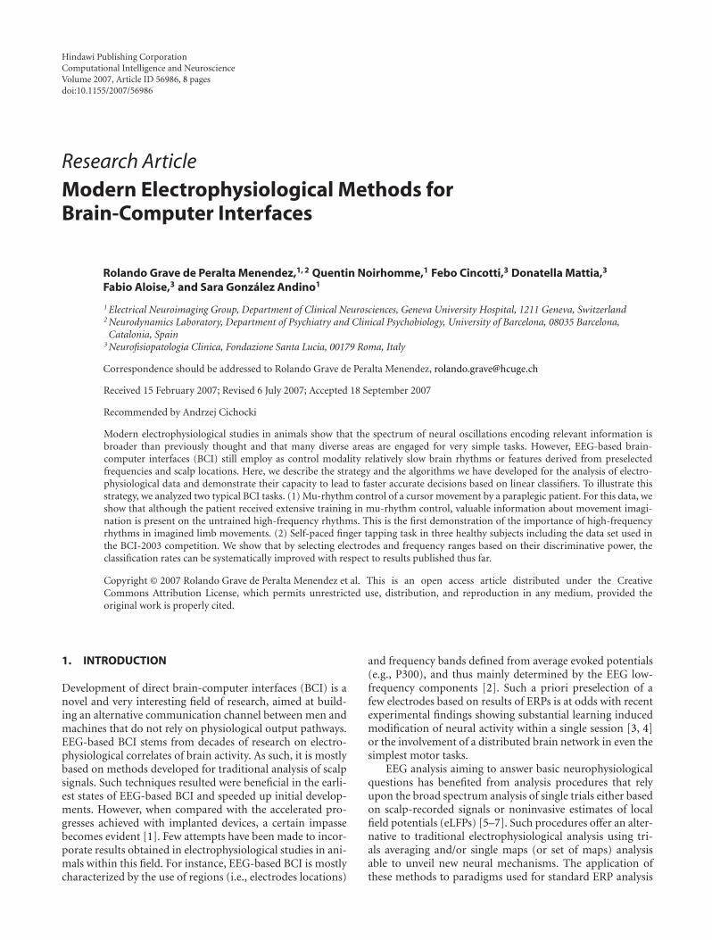
Hindawi Publishing CorporationComputational Intelligence and NeuroscienceVolume 2007, Article ID 56986, 8 pagesdoi:10.1155/2007/56986
Research ArticleModern Electrophysiological Methods forBrain-Computer Interfaces
Rolando Grave de Peralta Menendez,1, 2 Quentin Noirhomme,1 Febo Cincotti,3 Donatella Mattia,3
Fabio Aloise,3 and Sara Gonzalez Andino1
1 Electrical Neuroimaging Group, Department of Clinical Neurosciences, Geneva University Hospital, 1211 Geneva, Switzerland2 Neurodynamics Laboratory, Department of Psychiatry and Clinical Psychobiology, University of Barcelona, 08035 Barcelona,Catalonia, Spain
3 Neurofisiopatologia Clinica, Fondazione Santa Lucia, 00179 Roma, Italy
Correspondence should be addressed to Rolando Grave de Peralta Menendez, [email protected]
Received 15 February 2007; Revised 6 July 2007; Accepted 18 September 2007
Recommended by Andrzej Cichocki
Modern electrophysiological studies in animals show that the spectrum of neural oscillations encoding relevant information isbroader than previously thought and that many diverse areas are engaged for very simple tasks. However, EEG-based brain-computer interfaces (BCI) still employ as control modality relatively slow brain rhythms or features derived from preselectedfrequencies and scalp locations. Here, we describe the strategy and the algorithms we have developed for the analysis of electro-physiological data and demonstrate their capacity to lead to faster accurate decisions based on linear classifiers. To illustrate thisstrategy, we analyzed two typical BCI tasks. (1) Mu-rhythm control of a cursor movement by a paraplegic patient. For this data, weshow that although the patient received extensive training in mu-rhythm control, valuable information about movement imagi-nation is present on the untrained high-frequency rhythms. This is the first demonstration of the importance of high-frequencyrhythms in imagined limb movements. (2) Self-paced finger tapping task in three healthy subjects including the data set used inthe BCI-2003 competition. We show that by selecting electrodes and frequency ranges based on their discriminative power, theclassification rates can be systematically improved with respect to results published thus far.
Copyright © 2007 Rolando Grave de Peralta Menendez et al. This is an open access article distributed under the CreativeCommons Attribution License, which permits unrestricted use, distribution, and reproduction in any medium, provided theoriginal work is properly cited.
1. INTRODUCTION
Development of direct brain-computer interfaces (BCI) is anovel and very interesting field of research, aimed at build-ing an alternative communication channel between men andmachines that do not rely on physiological output pathways.EEG-based BCI stems from decades of research on electro-physiological correlates of brain activity. As such, it is mostlybased on methods developed for traditional analysis of scalpsignals. Such techniques resulted were beneficial in the earli-est states of EEG-based BCI and speeded up initial develop-ments. However, when compared with the accelerated pro-gresses achieved with implanted devices, a certain impassebecomes evident [1]. Few attempts have been made to incor-porate results obtained in electrophysiological studies in ani-mals within this field. For instance, EEG-based BCI is mostlycharacterized by the use of regions (i.e., electrodes locations)
and frequency bands defined from average evoked potentials(e.g., P300), and thus mainly determined by the EEG low-frequency components [2]. Such a priori preselection of afew electrodes based on results of ERPs is at odds with recentexperimental findings showing substantial learning inducedmodification of neural activity within a single session [3, 4]or the involvement of a distributed brain network in even thesimplest motor tasks.
EEG analysis aiming to answer basic neurophysiologicalquestions has benefited from analysis procedures that relyupon the broad spectrum analysis of single trials either basedon scalp-recorded signals or noninvasive estimates of localfield potentials (eLFPs) [5–7]. Such procedures offer an alter-native to traditional electrophysiological analysis using tri-als averaging and/or single maps (or set of maps) analysisable to unveil new neural mechanisms. The application ofthese methods to paradigms used for standard ERP analysis
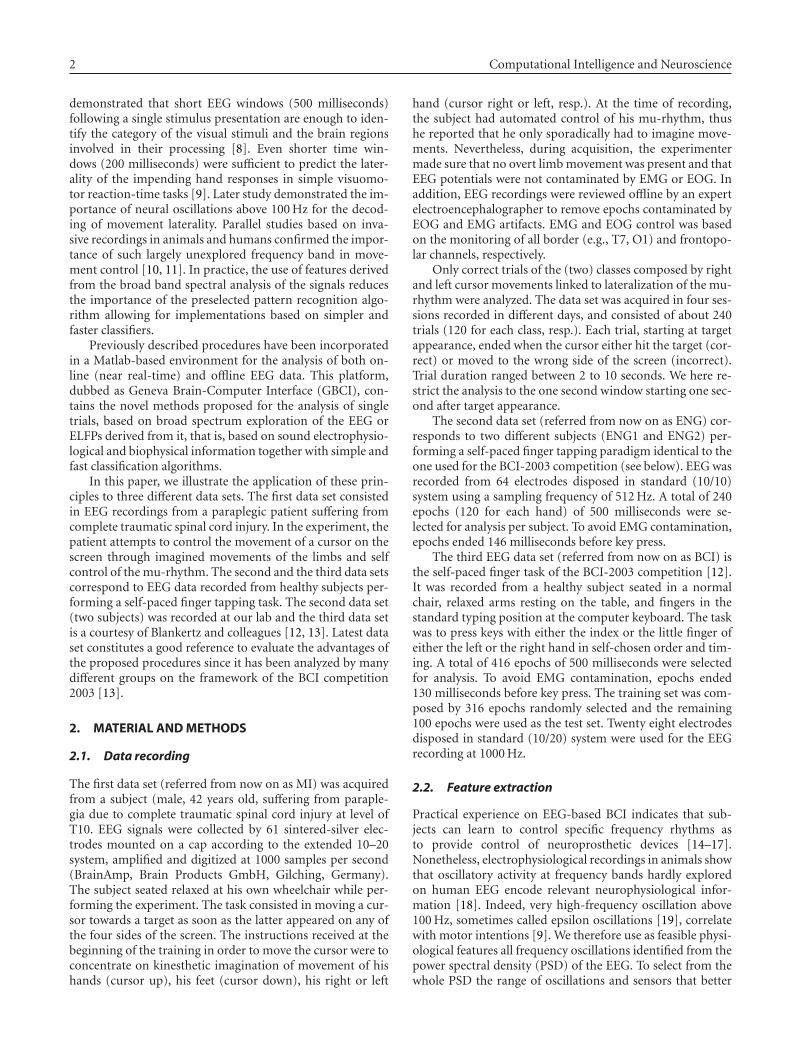
2 Computational Intelligence and Neuroscience
demonstrated that short EEG windows (500 milliseconds)following a single stimulus presentation are enough to iden-tify the category of the visual stimuli and the brain regionsinvolved in their processing [8]. Even shorter time win-dows (200 milliseconds) were sufficient to predict the later-ality of the impending hand responses in simple visuomo-tor reaction-time tasks [9]. Later study demonstrated the im-portance of neural oscillations above 100 Hz for the decod-ing of movement laterality. Parallel studies based on inva-sive recordings in animals and humans confirmed the impor-tance of such largely unexplored frequency band in move-ment control [10, 11]. In practice, the use of features derivedfrom the broad band spectral analysis of the signals reducesthe importance of the preselected pattern recognition algo-rithm allowing for implementations based on simpler andfaster classifiers.
Previously described procedures have been incorporatedin a Matlab-based environment for the analysis of both on-line (near real-time) and offline EEG data. This platform,dubbed as Geneva Brain-Computer Interface (GBCI), con-tains the novel methods proposed for the analysis of singletrials, based on broad spectrum exploration of the EEG orELFPs derived from it, that is, based on sound electrophysio-logical and biophysical information together with simple andfast classification algorithms.
In this paper, we illustrate the application of these prin-ciples to three different data sets. The first data set consistedin EEG recordings from a paraplegic patient suffering fromcomplete traumatic spinal cord injury. In the experiment, thepatient attempts to control the movement of a cursor on thescreen through imagined movements of the limbs and selfcontrol of the mu-rhythm. The second and the third data setscorrespond to EEG data recorded from healthy subjects per-forming a self-paced finger tapping task. The second data set(two subjects) was recorded at our lab and the third data setis a courtesy of Blankertz and colleagues [12, 13]. Latest dataset constitutes a good reference to evaluate the advantages ofthe proposed procedures since it has been analyzed by manydifferent groups on the framework of the BCI competition2003 [13].
2. MATERIAL AND METHODS
2.1. Data recording
The first data set (referred from now on as MI) was acquiredfrom a subject (male, 42 years old, suffering from paraple-gia due to complete traumatic spinal cord injury at level ofT10. EEG signals were collected by 61 sintered-silver elec-trodes mounted on a cap according to the extended 10–20system, amplified and digitized at 1000 samples per second(BrainAmp, Brain Products GmbH, Gilching, Germany).The subject seated relaxed at his own wheelchair while per-forming the experiment. The task consisted in moving a cur-sor towards a target as soon as the latter appeared on any ofthe four sides of the screen. The instructions received at thebeginning of the training in order to move the cursor were toconcentrate on kinesthetic imagination of movement of hishands (cursor up), his feet (cursor down), his right or left
hand (cursor right or left, resp.). At the time of recording,the subject had automated control of his mu-rhythm, thushe reported that he only sporadically had to imagine move-ments. Nevertheless, during acquisition, the experimentermade sure that no overt limb movement was present and thatEEG potentials were not contaminated by EMG or EOG. Inaddition, EEG recordings were reviewed offline by an expertelectroencephalographer to remove epochs contaminated byEOG and EMG artifacts. EMG and EOG control was basedon the monitoring of all border (e.g., T7, O1) and frontopo-lar channels, respectively.
Only correct trials of the (two) classes composed by rightand left cursor movements linked to lateralization of the mu-rhythm were analyzed. The data set was acquired in four ses-sions recorded in different days, and consisted of about 240trials (120 for each class, resp.). Each trial, starting at targetappearance, ended when the cursor either hit the target (cor-rect) or moved to the wrong side of the screen (incorrect).Trial duration ranged between 2 to 10 seconds. We here re-strict the analysis to the one second window starting one sec-ond after target appearance.
The second data set (referred from now on as ENG) cor-responds to two different subjects (ENG1 and ENG2) per-forming a self-paced finger tapping paradigm identical to theone used for the BCI-2003 competition (see below). EEG wasrecorded from 64 electrodes disposed in standard (10/10)system using a sampling frequency of 512 Hz. A total of 240epochs (120 for each hand) of 500 milliseconds were se-lected for analysis per subject. To avoid EMG contamination,epochs ended 146 milliseconds before key press.
The third EEG data set (referred from now on as BCI) isthe self-paced finger task of the BCI-2003 competition [12].It was recorded from a healthy subject seated in a normalchair, relaxed arms resting on the table, and fingers in thestandard typing position at the computer keyboard. The taskwas to press keys with either the index or the little finger ofeither the left or the right hand in self-chosen order and tim-ing. A total of 416 epochs of 500 milliseconds were selectedfor analysis. To avoid EMG contamination, epochs ended130 milliseconds before key press. The training set was com-posed by 316 epochs randomly selected and the remaining100 epochs were used as the test set. Twenty eight electrodesdisposed in standard (10/20) system were used for the EEGrecording at 1000 Hz.
2.2. Feature extraction
Practical experience on EEG-based BCI indicates that sub-jects can learn to control specific frequency rhythms asto provide control of neuroprosthetic devices [14–17].Nonetheless, electrophysiological recordings in animals showthat oscillatory activity at frequency bands hardly exploredon human EEG encode relevant neurophysiological infor-mation [18]. Indeed, very high-frequency oscillation above100 Hz, sometimes called epsilon oscillations [19], correlatewith motor intentions [9]. We therefore use as feasible physi-ological features all frequency oscillations identified from thepower spectral density (PSD) of the EEG. To select from thewhole PSD the range of oscillations and sensors that better
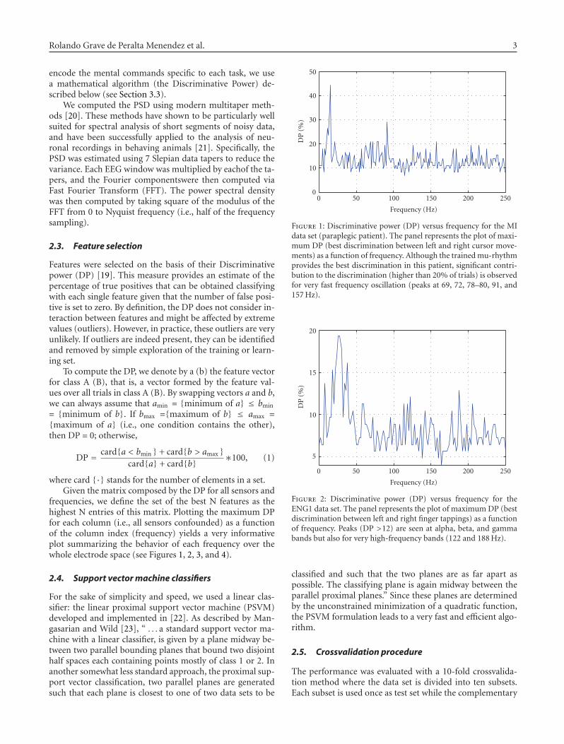
Rolando Grave de Peralta Menendez et al. 3
encode the mental commands specific to each task, we usea mathematical algorithm (the Discriminative Power) de-scribed below (see Section 3.3).
We computed the PSD using modern multitaper meth-ods [20]. These methods have shown to be particularly wellsuited for spectral analysis of short segments of noisy data,and have been successfully applied to the analysis of neu-ronal recordings in behaving animals [21]. Specifically, thePSD was estimated using 7 Slepian data tapers to reduce thevariance. Each EEG window was multiplied by eachof the ta-pers, and the Fourier componentswere then computed viaFast Fourier Transform (FFT). The power spectral densitywas then computed by taking square of the modulus of theFFT from 0 to Nyquist frequency (i.e., half of the frequencysampling).
2.3. Feature selection
Features were selected on the basis of their Discriminativepower (DP) [19]. This measure provides an estimate of thepercentage of true positives that can be obtained classifyingwith each single feature given that the number of false posi-tive is set to zero. By definition, the DP does not consider in-teraction between features and might be affected by extremevalues (outliers). However, in practice, these outliers are veryunlikely. If outliers are indeed present, they can be identifiedand removed by simple exploration of the training or learn-ing set.
To compute the DP, we denote by a (b) the feature vectorfor class A (B), that is, a vector formed by the feature val-ues over all trials in class A (B). By swapping vectors a and b,we can always assume that amin = {minimum of a} ≤ bmin
= {minimum of b}. If bmax ={maximum of b} ≤ amax ={maximum of a} (i.e., one condition contains the other),then DP = 0; otherwise,
DP = card{a < bmin } + card{b > amax }card{a} + card{b} ∗100, (1)
where card {·} stands for the number of elements in a set.Given the matrix composed by the DP for all sensors and
frequencies, we define the set of the best N features as thehighest N entries of this matrix. Plotting the maximum DPfor each column (i.e., all sensors confounded) as a functionof the column index (frequency) yields a very informativeplot summarizing the behavior of each frequency over thewhole electrode space (see Figures 1, 2, 3, and 4).
2.4. Support vector machine classifiers
For the sake of simplicity and speed, we used a linear clas-sifier: the linear proximal support vector machine (PSVM)developed and implemented in [22]. As described by Man-gasarian and Wild [23], “ . . . a standard support vector ma-chine with a linear classifier, is given by a plane midway be-tween two parallel bounding planes that bound two disjointhalf spaces each containing points mostly of class 1 or 2. Inanother somewhat less standard approach, the proximal sup-port vector classification, two parallel planes are generatedsuch that each plane is closest to one of two data sets to be
0 50 100 150 200 250
Frequency (Hz)
0
10
20
30
40
50
DP
(%)
Figure 1: Discriminative power (DP) versus frequency for the MIdata set (paraplegic patient). The panel represents the plot of maxi-mum DP (best discrimination between left and right cursor move-ments) as a function of frequency. Although the trained mu-rhythmprovides the best discrimination in this patient, significant contri-bution to the discrimination (higher than 20% of trials) is observedfor very fast frequency oscillation (peaks at 69, 72, 78–80, 91, and157 Hz).
0 50 100 150 200 250
Frequency (Hz)
5
10
15
20
DP
(%)
Figure 2: Discriminative power (DP) versus frequency for theENG1 data set. The panel represents the plot of maximum DP (bestdiscrimination between left and right finger tappings) as a functionof frequency. Peaks (DP >12) are seen at alpha, beta, and gammabands but also for very high-frequency bands (122 and 188 Hz).
classified and such that the two planes are as far apart aspossible. The classifying plane is again midway between theparallel proximal planes.” Since these planes are determinedby the unconstrained minimization of a quadratic function,the PSVM formulation leads to a very fast and efficient algo-rithm.
2.5. Crossvalidation procedure
The performance was evaluated with a 10-fold crossvalida-tion method where the data set is divided into ten subsets.Each subset is used once as test set while the complementary
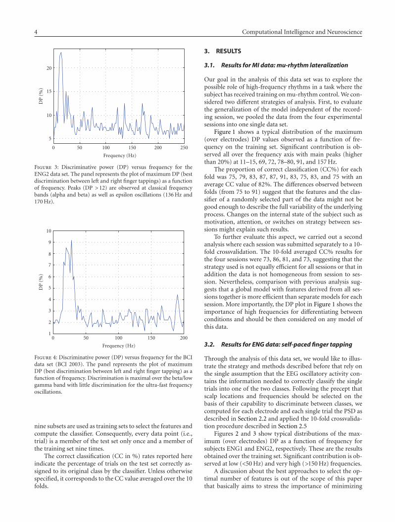
4 Computational Intelligence and Neuroscience
0 50 100 150 200 250
Frequency (Hz)
5
10
15
20
DP
(%)
Figure 3: Discriminative power (DP) versus frequency for theENG2 data set. The panel represents the plot of maximum DP (bestdiscrimination between left and right finger tappings) as a functionof frequency. Peaks (DP > 12) are observed at classical frequencybands (alpha and beta) as well as epsilon oscillations (136 Hz and170 Hz).
0 50 100 150 200
Frequency (Hz)
1
2
3
4
5
6
7
8
9
10
DP
(%)
Figure 4: Discriminative power (DP) versus frequency for the BCIdata set (BCI 2003). The panel represents the plot of maximumDP (best discrimination between left and right finger tapping) as afunction of frequency. Discrimination is maximal over the beta/lowgamma band with little discrimination for the ultra-fast frequencyoscillations.
nine subsets are used as training sets to select the features andcompute the classifier. Consequently, every data point (i.e.,trial) is a member of the test set only once and a member ofthe training set nine times.
The correct classification (CC in %) rates reported hereindicate the percentage of trials on the test set correctly as-signed to its original class by the classifier. Unless otherwisespecified, it corresponds to the CC value averaged over the 10folds.
3. RESULTS
3.1. Results for MI data: mu-rhythm lateralization
Our goal in the analysis of this data set was to explore thepossible role of high-frequency rhythms in a task where thesubject has received training on mu-rhythm control. We con-sidered two different strategies of analysis. First, to evaluatethe generalization of the model independent of the record-ing session, we pooled the data from the four experimentalsessions into one single data set.
Figure 1 shows a typical distribution of the maximum(over electrodes) DP values observed as a function of fre-quency on the training set. Significant contribution is ob-served all over the frequency axis with main peaks (higherthan 20%) at 11–15, 69, 72, 78–80, 91, and 157 Hz.
The proportion of correct classification (CC%) for eachfold was 75, 79, 83, 87, 87, 91, 83, 75, 83, and 75 with anaverage CC value of 82%. The differences observed betweenfolds (from 75 to 91) suggest that the features and the clas-sifier of a randomly selected part of the data might not begood enough to describe the full variability of the underlyingprocess. Changes on the internal state of the subject such asmotivation, attention, or switches on strategy between ses-sions might explain such results.
To further evaluate this aspect, we carried out a secondanalysis where each session was submitted separately to a 10-fold crossvalidation. The 10-fold averaged CC% results forthe four sessions were 73, 86, 81, and 73, suggesting that thestrategy used is not equally efficient for all sessions or that inaddition the data is not homogeneous from session to ses-sion. Nevertheless, comparison with previous analysis sug-gests that a global model with features derived from all ses-sions together is more efficient than separate models for eachsession. More importantly, the DP plot in Figure 1 shows theimportance of high frequencies for differentiating betweenconditions and should be then considered on any model ofthis data.
3.2. Results for ENG data: self-paced finger tapping
Through the analysis of this data set, we would like to illus-trate the strategy and methods described before that rely onthe single assumption that the EEG oscillatory activity con-tains the information needed to correctly classify the singletrials into one of the two classes. Following the precept thatscalp locations and frequencies should be selected on thebasis of their capability to discriminate between classes, wecomputed for each electrode and each single trial the PSD asdescribed in Section 2.2 and applied the 10-fold crossvalida-tion procedure described in Section 2.5
Figures 2 and 3 show typical distributions of the max-imum (over electrodes) DP as a function of frequency forsubjects ENG1 and ENG2, respectively. These are the resultsobtained over the training set. Significant contribution is ob-served at low (<50 Hz) and very high (>150 Hz) frequencies.
A discussion about the best approaches to select the op-timal number of features is out of the scope of this paperthat basically aims to stress the importance of minimizing
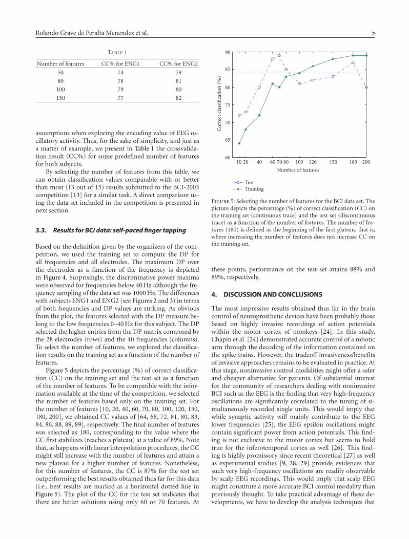
Rolando Grave de Peralta Menendez et al. 5
Table 1
Number of features CC% for ENG1 CC% for ENG2
50 74 79
80 78 81
100 79 80
150 77 82
assumptions when exploring the encoding value of EEG os-cillatory activity. Thus, for the sake of simplicity, and just asa matter of example, we present in Table 1 the crossvalida-tion result (CC%) for some predefined number of featuresfor both subjects.
By selecting the number of features from this table, wecan obtain classification values comparable with or betterthan most (13 out of 15) results submitted to the BCI-2003competition [13] for a similar task. A direct comparison us-ing the data set included in the competition is presented innext section.
3.3. Results for BCI data: self-paced finger tapping
Based on the definition given by the organizers of the com-petition, we used the training set to compute the DP forall frequencies and all electrodes. The maximum DP overthe electrodes as a function of the frequency is depictedin Figure 4. Surprisingly, the discriminative power maximawere observed for frequencies below 40 Hz although the fre-quency sampling of the data set was 1000 Hz. The differenceswith subjects ENG1 and ENG2 (see Figures 2 and 3) in termsof both frequencies and DP values are striking. As obviousfrom the plot, the features selected with the DP measure be-long to the low frequencies 0–40 Hz for this subject. The DPselected the higher entries from the DP matrix composed bythe 28 electrodes (rows) and the 40 frequencies (columns).To select the number of features, we explored the classifica-tion results on the training set as a function of the number offeatures.
Figure 5 depicts the percentage (%) of correct classifica-tion (CC) on the training set and the test set as a functionof the number of features. To be compatible with the infor-mation available at the time of the competition, we selectedthe number of features based only on the training set. Forthe number of features [10, 20, 40, 60, 70, 80, 100, 120, 150,180, 200], we obtained CC values of [64, 68, 72, 81, 80, 83,84, 86, 88, 89, 89], respectively. The final number of featureswas selected as 180, corresponding to the value where theCC first stabilizes (reaches a plateau) at a value of 89%. Notethat, as happens with linear interpolation procedures, the CCmight still increase with the number of features and attain anew plateau for a higher number of features. Nonetheless,for this number of features, the CC is 87% for the test setoutperforming the best results obtained thus far for this data(i.e., best results are marked as a horizontal dotted line inFigure 5). The plot of the CC for the test set indicates thatthere are better solutions using only 60 or 70 features. At
10 20 40 60 70 80 100 120 150 180 200
Number of features
60
65
70
75
80
85
90
Cor
rect
clas
sifi
cati
on(%
)
TestTraining
Figure 5: Selecting the number of features for the BCI data set. Thepicture depicts the percentage (%) of correct classification (CC) onthe training set (continuous trace) and the test set (discontinuoustrace) as a function of the number of features. The number of fea-tures (180) is defined as the beginning of the first plateau, that is,where increasing the number of features does not increase CC onthe training set.
these points, performance on the test set attains 88% and89%, respectively.
4. DISCUSSION AND CONCLUSIONS
The most impressive results obtained thus far in the braincontrol of neuroprosthetic devices have been probably thosebased on highly invasive recordings of action potentialswithin the motor cortex of monkeys [24]. In this study,Chapin et al. [24] demonstrated accurate control of a roboticarm through the decoding of the information contained onthe spike trains. However, the tradeoff invasiveness/benefitsof invasive approaches remains to be evaluated in practice. Atthis stage, noninvasive control modalities might offer a saferand cheaper alternative for patients. Of substantial interestfor the community of researchers dealing with noninvasiveBCI such as the EEG is the finding that very high-frequencyoscillations are significantly correlated to the tuning of si-multaneously recorded single units. This would imply thatwhile synaptic activity will mainly contribute to the EEGlower frequencies [25], the EEG epsilon oscillations mightcontain significant power from action potentials. This find-ing is not exclusive to the motor cortex but seems to holdtrue for the inferotemporal cortex as well [26]. This find-ing is highly promissory since recent theoretical [27] as wellas experimental studies [9, 28, 29] provide evidences thatsuch very high-frequency oscillations are readily observableby scalp EEG recordings. This would imply that scalp EEGmight constitute a more accurate BCI control modality thanpreviously thought. To take practical advantage of these de-velopments, we have to develop the analysis techniques that
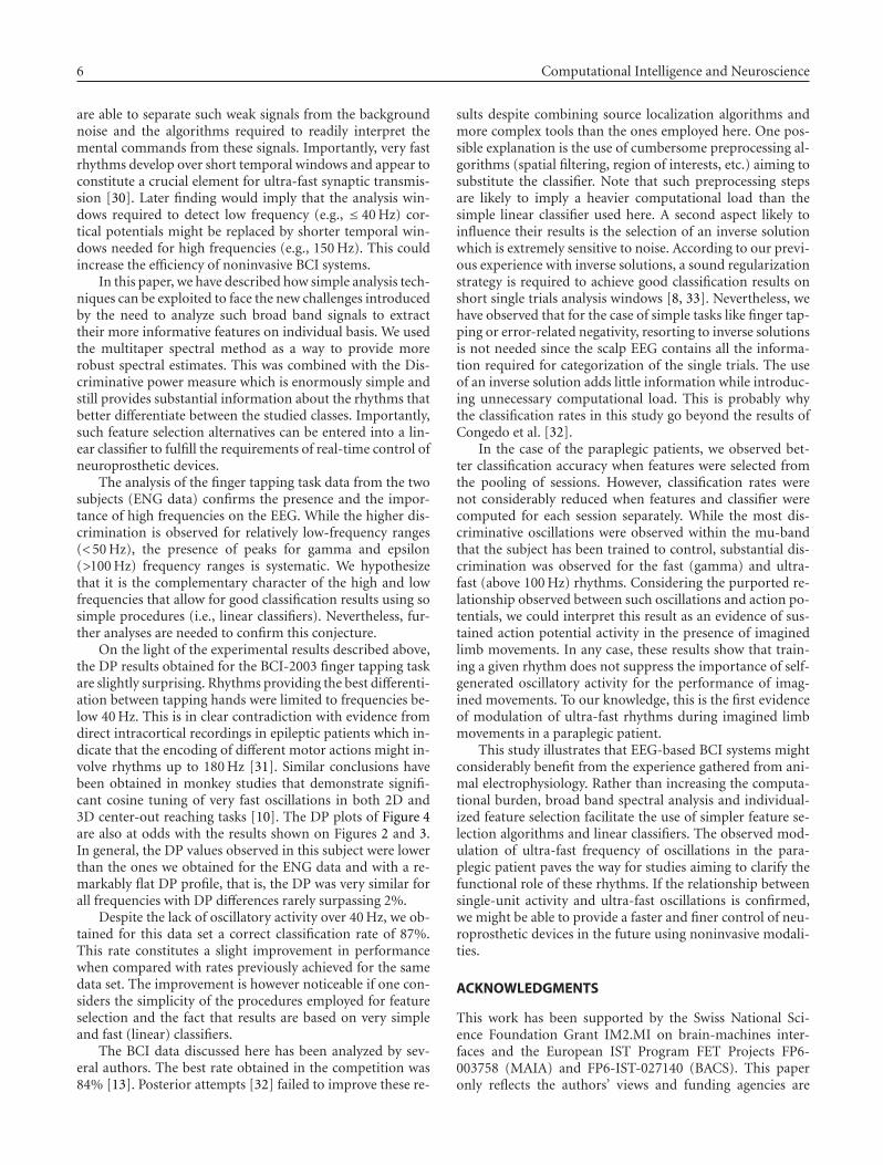
6 Computational Intelligence and Neuroscience
are able to separate such weak signals from the backgroundnoise and the algorithms required to readily interpret themental commands from these signals. Importantly, very fastrhythms develop over short temporal windows and appear toconstitute a crucial element for ultra-fast synaptic transmis-sion [30]. Later finding would imply that the analysis win-dows required to detect low frequency (e.g., ≤ 40 Hz) cor-tical potentials might be replaced by shorter temporal win-dows needed for high frequencies (e.g., 150 Hz). This couldincrease the efficiency of noninvasive BCI systems.
In this paper, we have described how simple analysis tech-niques can be exploited to face the new challenges introducedby the need to analyze such broad band signals to extracttheir more informative features on individual basis. We usedthe multitaper spectral method as a way to provide morerobust spectral estimates. This was combined with the Dis-criminative power measure which is enormously simple andstill provides substantial information about the rhythms thatbetter differentiate between the studied classes. Importantly,such feature selection alternatives can be entered into a lin-ear classifier to fulfill the requirements of real-time control ofneuroprosthetic devices.
The analysis of the finger tapping task data from the twosubjects (ENG data) confirms the presence and the impor-tance of high frequencies on the EEG. While the higher dis-crimination is observed for relatively low-frequency ranges(<50 Hz), the presence of peaks for gamma and epsilon(>100 Hz) frequency ranges is systematic. We hypothesizethat it is the complementary character of the high and lowfrequencies that allow for good classification results using sosimple procedures (i.e., linear classifiers). Nevertheless, fur-ther analyses are needed to confirm this conjecture.
On the light of the experimental results described above,the DP results obtained for the BCI-2003 finger tapping taskare slightly surprising. Rhythms providing the best differenti-ation between tapping hands were limited to frequencies be-low 40 Hz. This is in clear contradiction with evidence fromdirect intracortical recordings in epileptic patients which in-dicate that the encoding of different motor actions might in-volve rhythms up to 180 Hz [31]. Similar conclusions havebeen obtained in monkey studies that demonstrate signifi-cant cosine tuning of very fast oscillations in both 2D and3D center-out reaching tasks [10]. The DP plots of Figure 4are also at odds with the results shown on Figures 2 and 3.In general, the DP values observed in this subject were lowerthan the ones we obtained for the ENG data and with a re-markably flat DP profile, that is, the DP was very similar forall frequencies with DP differences rarely surpassing 2%.
Despite the lack of oscillatory activity over 40 Hz, we ob-tained for this data set a correct classification rate of 87%.This rate constitutes a slight improvement in performancewhen compared with rates previously achieved for the samedata set. The improvement is however noticeable if one con-siders the simplicity of the procedures employed for featureselection and the fact that results are based on very simpleand fast (linear) classifiers.
The BCI data discussed here has been analyzed by sev-eral authors. The best rate obtained in the competition was84% [13]. Posterior attempts [32] failed to improve these re-
sults despite combining source localization algorithms andmore complex tools than the ones employed here. One pos-sible explanation is the use of cumbersome preprocessing al-gorithms (spatial filtering, region of interests, etc.) aiming tosubstitute the classifier. Note that such preprocessing stepsare likely to imply a heavier computational load than thesimple linear classifier used here. A second aspect likely toinfluence their results is the selection of an inverse solutionwhich is extremely sensitive to noise. According to our previ-ous experience with inverse solutions, a sound regularizationstrategy is required to achieve good classification results onshort single trials analysis windows [8, 33]. Nevertheless, wehave observed that for the case of simple tasks like finger tap-ping or error-related negativity, resorting to inverse solutionsis not needed since the scalp EEG contains all the informa-tion required for categorization of the single trials. The useof an inverse solution adds little information while introduc-ing unnecessary computational load. This is probably whythe classification rates in this study go beyond the results ofCongedo et al. [32].
In the case of the paraplegic patients, we observed bet-ter classification accuracy when features were selected fromthe pooling of sessions. However, classification rates werenot considerably reduced when features and classifier werecomputed for each session separately. While the most dis-criminative oscillations were observed within the mu-bandthat the subject has been trained to control, substantial dis-crimination was observed for the fast (gamma) and ultra-fast (above 100 Hz) rhythms. Considering the purported re-lationship observed between such oscillations and action po-tentials, we could interpret this result as an evidence of sus-tained action potential activity in the presence of imaginedlimb movements. In any case, these results show that train-ing a given rhythm does not suppress the importance of self-generated oscillatory activity for the performance of imag-ined movements. To our knowledge, this is the first evidenceof modulation of ultra-fast rhythms during imagined limbmovements in a paraplegic patient.
This study illustrates that EEG-based BCI systems mightconsiderably benefit from the experience gathered from ani-mal electrophysiology. Rather than increasing the computa-tional burden, broad band spectral analysis and individual-ized feature selection facilitate the use of simpler feature se-lection algorithms and linear classifiers. The observed mod-ulation of ultra-fast frequency of oscillations in the para-plegic patient paves the way for studies aiming to clarify thefunctional role of these rhythms. If the relationship betweensingle-unit activity and ultra-fast oscillations is confirmed,we might be able to provide a faster and finer control of neu-roprosthetic devices in the future using noninvasive modali-ties.
ACKNOWLEDGMENTS
This work has been supported by the Swiss National Sci-ence Foundation Grant IM2.MI on brain-machines inter-faces and the European IST Program FET Projects FP6-003758 (MAIA) and FP6-IST-027140 (BACS). This paperonly reflects the authors’ views and funding agencies are
Rolando Grave de Peralta Menendez et al. 7
not liable for any use that may be made of the informationcontained herein. We acknowledge the contribution of twoanonymous reviewers for their constructive comments andsuggestions.
REFERENCES
[1] M. A. Lebedev and M. A. L. Nicolelis, “Brain-machine in-terfaces: past, present and future,” Trends in Neurosciences,vol. 29, no. 9, pp. 536–546, 2006.
[2] J. R. Wolpaw, N. Birbaumer, D. J. McFarland, G. Pfurtscheller,and T. M. Vaughan, “Brain-computer interfaces for communi-cation and control,” Clinical Neurophysiology, vol. 113, no. 6,pp. 767–791, 2002.
[3] J. N. Sanes and J. P. Donoghue, “Plasticity and primary motorcortex,” Annual Review of Neuroscience, vol. 23, pp. 393–415,2000.
[4] M. Graziano, “The organization of behavioral repertoire inmotor cortex,” Annual Review of Neuroscience, vol. 29, pp.105–134, 2006.
[5] S. L. Gonzalez Andino, M. M. Murray, J. J. Foxe, and R. Gravede Peralta Menendez, “How single-trial electrical neuroimag-ing contributes to multisensory research,” Experimental BrainResearch, vol. 166, no. 3-4, pp. 298–304, 2005.
[6] R. Grave de Peralta Menendez, S. Gonzalez Andino, L. Perez, P.W. Ferrez, and J. D. R. Millan, “Non-invasive estimation of lo-cal field potentials for neuroprosthesis control,” Cognitive Pro-cessing, vol. 6, no. 1, pp. 59–64, 2005.
[7] S. L. Gonzalez Andino, C. M. Michel, G. Thut, T. Landis, andR. Grave de Peralta Menendez, “Prediction of response speedby anticipatory high-frequency (gamma band) oscillations inthe human brain,” Human Brain Mapping, vol. 24, no. 1, pp.50–58, 2005.
[8] S. L. Gonzalez Andino, R. Grave de Peralta Menendez, A.Khateb, A. J. Pegna, G. Thut, and T. Landis, “A glimpse intoyour vision,” Human Brain Mapping, vol. 28, no. 7, pp. 614–624, 2006.
[9] S. L. Gonzalez, R. Grave de Peralta Menendez, G. Thut, J. D. R.Millan, P. Morier, and T. Landis, “Very high frequency oscil-lations (VHFO) as a predictor of movement intentions,” Neu-roImage, vol. 32, no. 1, pp. 170–179, 2006.
[10] J. Rickert, S. Cardoso de Oliveira, E. Vaadia, A. Aertsen, S.Rotter, and G. Mehring, “Encoding of movement direction indifferent frequency ranges of motor cortical local field poten-tials,” Journal of Neuroscience, vol. 25, no. 39, pp. 8815–8824,2005.
[11] E. C. Leuthardt, K. J. Miller, G. Schalk, R. P. N. Rao, andJ. G. Ojemann, “Electrocorticography-based brain computerinterface—the seattle experience,” IEEE Transactions on Neu-ral Systems and Rehabilitation Engineering, vol. 14, no. 2, pp.194–198, 2006.
[12] B. Blankertz, G. Dornhege, C. Schafer, et al., “Boosting bitrates and error detection for the classification of fast-pacedmotor commands based on single-trial EEG analysis,” IEEETransactions on Neural Systems and Rehabilitation Engineering,vol. 11, no. 2, pp. 127–131, 2003.
[13] B. Blankertz, K.-R. Muller, G. Curio, et al., “The BCI competi-tion 2003: progress and perspectives in detection and discrim-ination of EEG single trials,” IEEE Transactions on BiomedicalEngineering, vol. 51, no. 6, pp. 1044–1051, 2004.
[14] J. R. Wolpaw and D. J. McFarland, “Control of a two-dimensional movement signal by a noninvasive brain-computer interface in humans,” Proceedings of the National
Academy of Sciences of the United States of America, vol. 101,no. 51, pp. 17849–17854, 2004.
[15] J. D. R. Millan, M. Franze, J. Mourino, F. Cincotti, and F. Ba-biloni, “Relevant EEG features for the classification of spon-taneous motor-related tasks,” Biological Cybernetics, vol. 86,no. 2, pp. 89–95, 2002.
[16] J. D. R. Millan, F. Renkens, J. Mourino, and W. Gerstner, “Non-invasive brain-actuated control of a mobile robot by humanEEG,” IEEE Transactions on Biomedical Engineering, vol. 51,no. 6, pp. 1026–1033, 2004.
[17] N. Birbaumer, A. Kubler, N. Ghanayim, et al., “The thoughttranslation device (TTD) for completely paralyzed patients,”IEEE Transactions on Rehabilitation Engineering, vol. 8, no. 2,pp. 190–193, 2000.
[18] A. Bragin, J. Engel Jr., C. L. Wilson, I. Fried, and G. Buzsaki,“High-frequency oscillations in human brain,” Hippocampus,vol. 9, no. 2, pp. 137–142, 1999.
[19] W. J. Freeman, “Definitions of state variables and state spacefor brain-computer interface—part 1: multiple hierarchicallevels of brain function,” Cognitive Neurodynamics, vol. 1,no. 1, pp. 3–14, 2007.
[20] D. J. Thomson, “Spectrum estimation and harmonic analysis,”Proceedings of the IEEE, vol. 70, no. 9, pp. 1055–1096, 1982.
[21] B. Pesaran, J. S. Pezaris, M. Sahani, P. P. Mitra, and R. A. An-dersen, “Temporal structure in neuronal activity during work-ing memory in macaque parietal cortex,” Nature Neuroscience,vol. 5, no. 8, pp. 805–811, 2002.
[22] G. Fung and O. L. Mangasarian, “Proximal support vector ma-chine classifiers,” in Proceedings of the 7th ACM SIGKDD Inter-national Conference on Knowledge Discovery and Data Mining(KDD ’01), pp. 77–86, San Francisco, Calif, USA, August 2001.
[23] O. L. Mangasarian and E. W. Wild, “Multisurface proximalsupport vector machine classification via generalized eigenval-ues,” IEEE Transactions on Pattern Analysis and Machine Intel-ligence, vol. 28, no. 1, pp. 69–74, 2006.
[24] J. K. Chapin, K. A. Moxon, R. S. Markowitz, and M. A. L.Nicolelis, “Real-time control of a robot arm using simultane-ously recorded neurons in the motor cortex,” Nature Neuro-science, vol. 2, no. 7, pp. 664–670, 1999.
[25] A. B. Schwartz, X. T. Cui, D. J. Weber, and D. W. Moran,“Brain-controlled interfaces: movement restoration with neu-ral prosthetics,” Neuron, vol. 52, no. 1, pp. 205–220, 2006.
[26] G. Kreiman, C. P. Hung, A. Kraskov, R. Q. Quiroga, T. Poggio,and J. J. DiCarlo, “Object selectivity of local field potentialsand spikes in the macaque inferior temporal cortex,” Neuron,vol. 49, no. 3, pp. 433–445, 2006.
[27] S. Murakami and Y. Okada, “Contributions of principal neo-cortical neurons to magnetoencephalography and electroen-cephalography signals,” Journal of Physiology, vol. 575, no. 3,pp. 925–936, 2006.
[28] S. N. Baker, G. Curio, and R. N. Lemon, “EEG oscillationsat 600 Hz are macroscopic markers for cortical spike bursts,”Journal of Physiology, vol. 550, no. 2, pp. 529–534, 2003.
[29] G. Curio, “Linking 600 Hz “spikelike” EEG/MEG wavelets (‘σ-bursts’) to cellular substrates: concepts and caveats,” Journal ofClinical Neurophysiology, vol. 17, no. 4, pp. 377–396, 2000.
[30] D. Schmitz, S. Schuchmann, A. Fisahn, et al., “Axo-axonal cou-pling: a novel mechanism for ultrafast neuronal communica-tion,” Neuron, vol. 31, no. 5, pp. 831–840, 2001.
[31] E. C. Leuthardt, G. Schalk, J. R. Wolpaw, J. G. Ojemann, andD. W. Moran, “A brain-computer interface using electrocor-ticographic signals in humans,” Journal of Neural Engineering,vol. 1, no. 2, pp. 63–71, 2004.

8 Computational Intelligence and Neuroscience
[32] M. Congedo, F. Lotte, and A. Lecuyer, “Classification of move-ment intention by spatially filtered electromagnetic inverse so-lutions,” Physics in Medicine and Biology, vol. 51, no. 8, pp.1971–1989, 2006.
[33] R. G. Grave de Peralta Menendez, S. Gonzalez Andino, L.Perez, P. W. Ferrez, and J. D. R. Millan, “Non-invasive esti-mation of local field potentials for neuroprosthesis control,”Cognitive Processing, vol. 6, no. 1, pp. 59–64, 2005.
Hindawi Publishing CorporationComputational Intelligence and NeuroscienceVolume 2007, Article ID 57180, 11 pagesdoi:10.1155/2007/57180
Research ArticleClassifying EEG for Brain-Computer Interface:Learning Optimal Filters for Dynamical System Features
Le Song1 and Julien Epps2
1 School of Information Technologies, The University of Sydney, N.S.W. 2006, Australia2 National ICT Australia, Locked Bag 9013 Alexandria, N.S.W. 1435, Australia
Correspondence should be addressed to Le Song, [email protected]
Received 19 February 2007; Accepted 27 May 2007
Recommended by Andrzej Cichocki
Classification of multichannel EEG recordings during motor imagination has been exploited successfully for brain-computer in-terfaces (BCI). In this paper, we consider EEG signals as the outputs of a networked dynamical system (the cortex), and exploitsynchronization features from the dynamical system for classification. Herein, we also propose a new framework for learning op-timal filters automatically from the data, by employing a Fisher ratio criterion. Experimental evaluations comparing the proposeddynamical system features with the CSP and the AR features reveal their competitive performance during classification. Resultsalso show the benefits of employing the spatial and the temporal filters optimized using the proposed learning approach.
Copyright © 2007 L. Song and J. Epps. This is an open access article distributed under the Creative Commons Attribution License,which permits unrestricted use, distribution, and reproduction in any medium, provided the original work is properly cited.
1. INTRODUCTION
A brain-computer interface (BCI) is a communication sys-tem that relies on the brain rather than the body for controland feedback [1]. Ideally, it should run in a servo mode, al-lowing the subjects to initiate the communication anytimeand anywhere without resorting to external stimuli or trig-gers. Such an interface not only offers a promising prostheticdevice for those severely paralyzed, but also signifies a radi-cally new technology for the general public. Current BCI re-search is still in its early stage and the emphasis is placed onthe design of algorithms to decode a prespecified set of brainstates. This involves three main aspects.
Brain states
Only brain states consciously controllable by the subjectsare suitable for BCI. Besides, these states should generatedistinct, repeatable, and measurable patterns whenever ac-cessed. Among the most commonly used brain states areimaginations of body movements (motor imaginations).Motor imaginations can reliably change the neural activi-ties over sensorimotor cortices. Depending on the part of thebody imagined moving, these changes exhibit distinct spatialdistributions [2]. Recognition of these patterns can then betranslated into control signals, as is the case in this study.
Recording devices
Motor imaginations can be recorded by both electroen-cephalography (EEG) and magnetoencephalography (MEG).EEG remains the most popular way to record BCI signals andwill be the focus of this study. It measures scalp electricalactivities diffused from the cortex. Compared to MEG, it isportable and inexpensive. However, EEG can only measureblurred cortical activities due to the diffusion of the skull andthe skin. Thus, EEG is normally used for studying corticalpatches in the centimeter scale. Furthermore, EEG signals arecontaminated by noise from various sources, such as mus-cle activities and power line interference. Spatial and tempo-ral filters are commonly applied before any further analysis[3, 4].
Decoding algorithms
Prefiltered EEG signals still contain considerable noise, whichposes a challenge for its decoding. Statistical machine learn-ing (ML) techniques have been introduced into BCI to com-bat these variations. Techniques like artificial neural net-works, support vector machine (SVM) [5], and Linear Dis-criminant Analysis [4] have been employed to learn patternsfrom training EEG signals and then classify new EEG signals.This strategy often results in increased decoding success and
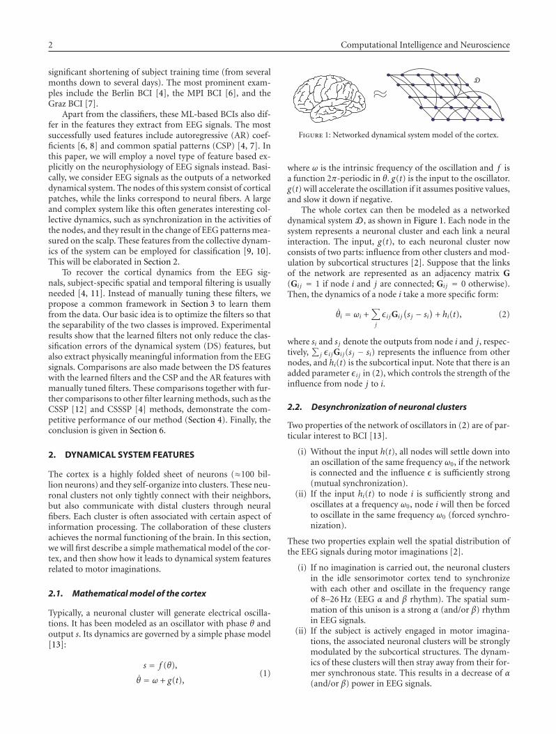
2 Computational Intelligence and Neuroscience
significant shortening of subject training time (from severalmonths down to several days). The most prominent exam-ples include the Berlin BCI [4], the MPI BCI [6], and theGraz BCI [7].
Apart from the classifiers, these ML-based BCIs also dif-fer in the features they extract from EEG signals. The mostsuccessfully used features include autoregressive (AR) coef-ficients [6, 8] and common spatial patterns (CSP) [4, 7]. Inthis paper, we will employ a novel type of feature based ex-plicitly on the neurophysiology of EEG signals instead. Basi-cally, we consider EEG signals as the outputs of a networkeddynamical system. The nodes of this system consist of corticalpatches, while the links correspond to neural fibers. A largeand complex system like this often generates interesting col-lective dynamics, such as synchronization in the activities ofthe nodes, and they result in the change of EEG patterns mea-sured on the scalp. These features from the collective dynam-ics of the system can be employed for classification [9, 10].This will be elaborated in Section 2.
To recover the cortical dynamics from the EEG sig-nals, subject-specific spatial and temporal filtering is usuallyneeded [4, 11]. Instead of manually tuning these filters, wepropose a common framework in Section 3 to learn themfrom the data. Our basic idea is to optimize the filters so thatthe separability of the two classes is improved. Experimentalresults show that the learned filters not only reduce the clas-sification errors of the dynamical system (DS) features, butalso extract physically meaningful information from the EEGsignals. Comparisons are also made between the DS featureswith the learned filters and the CSP and the AR features withmanually tuned filters. These comparisons together with fur-ther comparisons to other filter learning methods, such as theCSSP [12] and CSSSP [4] methods, demonstrate the com-petitive performance of our method (Section 4). Finally, theconclusion is given in Section 6.
2. DYNAMICAL SYSTEM FEATURES
The cortex is a highly folded sheet of neurons (≈100 bil-lion neurons) and they self-organize into clusters. These neu-ronal clusters not only tightly connect with their neighbors,but also communicate with distal clusters through neuralfibers. Each cluster is often associated with certain aspect ofinformation processing. The collaboration of these clustersachieves the normal functioning of the brain. In this section,we will first describe a simple mathematical model of the cor-tex, and then show how it leads to dynamical system featuresrelated to motor imaginations.
2.1. Mathematical model of the cortex
Typically, a neuronal cluster will generate electrical oscilla-tions. It has been modeled as an oscillator with phase θ andoutput s. Its dynamics are governed by a simple phase model[13]:
s = f (θ),
θ = ω + g(t),(1)
D
Figure 1: Networked dynamical system model of the cortex.
where ω is the intrinsic frequency of the oscillation and f isa function 2π-periodic in θ. g(t) is the input to the oscillator.g(t) will accelerate the oscillation if it assumes positive values,and slow it down if negative.
The whole cortex can then be modeled as a networkeddynamical system D , as shown in Figure 1. Each node in thesystem represents a neuronal cluster and each link a neuralinteraction. The input, g(t), to each neuronal cluster nowconsists of two parts: influence from other clusters and mod-ulation by subcortical structures [2]. Suppose that the linksof the network are represented as an adjacency matrix G(Gi j = 1 if node i and j are connected; Gi j = 0 otherwise).Then, the dynamics of a node i take a more specific form:
θi = ωi +∑
j
εi jGi j(s j − si
)+ hi(t), (2)
where si and s j denote the outputs from node i and j, respec-tively,
∑j εi jGi j(s j − si) represents the influence from other
nodes, and hi(t) is the subcortical input. Note that there is anadded parameter εi j in (2), which controls the strength of theinfluence from node j to i.
2.2. Desynchronization of neuronal clusters
Two properties of the network of oscillators in (2) are of par-ticular interest to BCI [13].
(i) Without the input h(t), all nodes will settle down intoan oscillation of the same frequency ω0, if the networkis connected and the influence ε is sufficiently strong(mutual synchronization).
(ii) If the input hi(t) to node i is sufficiently strong andoscillates at a frequency ω0, node i will then be forcedto oscillate in the same frequency ω0 (forced synchro-nization).
These two properties explain well the spatial distribution ofthe EEG signals during motor imaginations [2].
(i) If no imagination is carried out, the neuronal clustersin the idle sensorimotor cortex tend to synchronizewith each other and oscillate in the frequency rangeof 8–26 Hz (EEG α and β rhythm). The spatial sum-mation of this unison is a strong α (and/or β) rhythmin EEG signals.
(ii) If the subject is actively engaged in motor imagina-tions, the associated neuronal clusters will be stronglymodulated by the subcortical structures. The dynam-ics of these clusters will then stray away from their for-mer synchronous state. This results in a decrease of α(and/or β) power in EEG signals.
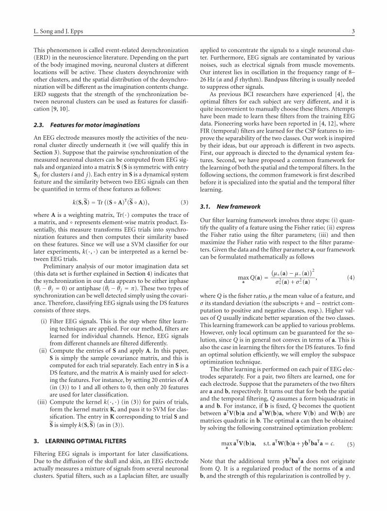
L. Song and J. Epps 3
This phenomenon is called event-related desynchronization(ERD) in the neuroscience literature. Depending on the partof the body imagined moving, neuronal clusters at differentlocations will be active. These clusters desynchronize withother clusters, and the spatial distribution of the desynchro-nization will be different as the imagination contents change.ERD suggests that the strength of the synchronization be-tween neuronal clusters can be used as features for classifi-cation [9, 10].
2.3. Features for motor imaginations
An EEG electrode measures mostly the activities of the neu-ronal cluster directly underneath it (we will qualify this inSection 3). Suppose that the pairwise synchronization of themeasured neuronal clusters can be computed from EEG sig-nals and organized into a matrix S (S is symmetric with entrySi j for clusters i and j). Each entry in S is a dynamical systemfeature and the similarity between two EEG signals can thenbe quantified in terms of these features as follows:
k(S, S) = Tr((S ◦ A)T(S ◦ A)
), (3)
where A is a weighting matrix, Tr(·) computes the trace ofa matrix, and ◦ represents element-wise matrix product. Es-sentially, this measure transforms EEG trials into synchro-nization features and then computes their similarity basedon these features. Since we will use a SVM classifier for ourlater experiments, k(·, ·) can be interpreted as a kernel be-tween EEG trials.
Preliminary analysis of our motor imagination data set(this data set is further explained in Section 4) indicates thatthe synchronization in our data appears to be either inphase(θi − θj = 0) or antiphase (θi − θj = π). These two types ofsynchronization can be well detected simply using the covari-ance. Therefore, classifying EEG signals using the DS featuresconsists of three steps.
(i) Filter EEG signals. This is the step where filter learn-ing techniques are applied. For our method, filters arelearned for individual channels. Hence, EEG signalsfrom different channels are filtered differently.
(ii) Compute the entries of S and apply A. In this paper,S is simply the sample covariance matrix, and this iscomputed for each trial separately. Each entry in S is aDS feature, and the matrix A is mainly used for select-ing the features. For instance, by setting 20 entries of A(in (3)) to 1 and all others to 0, then only 20 featuresare used for later classification.
(iii) Compute the kernel k(·, ·) (in (3)) for pairs of trials,form the kernel matrix K, and pass it to SVM for clas-sification. The entry in K corresponding to trial S andS is simply k(S, S) (as in (3)).
3. LEARNING OPTIMAL FILTERS
Filtering EEG signals is important for later classifications.Due to the diffusion of the skull and skin, an EEG electrodeactually measures a mixture of signals from several neuronalclusters. Spatial filters, such as a Laplacian filter, are usually
applied to concentrate the signals to a single neuronal clus-ter. Furthermore, EEG signals are contaminated by variousnoises, such as electrical signals from muscle movements.Our interest lies in oscillation in the frequency range of 8–26 Hz (α and β rhythm). Bandpass filtering is usually neededto suppress other signals.
As previous BCI researchers have experienced [4], theoptimal filters for each subject are very different, and it isquite inconvenient to manually choose these filters. Attemptshave been made to learn these filters from the training EEGdata. Pioneering works have been reported in [4, 12], whereFIR (temporal) filters are learned for the CSP features to im-prove the separability of the two classes. Our work is inspiredby their ideas, but our approach is different in two aspects.First, our approach is directed to the dynamical system fea-tures. Second, we have proposed a common framework forthe learning of both the spatial and the temporal filters. In thefollowing sections, the common framework is first describedbefore it is specialized into the spatial and the temporal filterlearning.
3.1. New framework
Our filter learning framework involves three steps: (i) quan-tify the quality of a feature using the Fisher ratio; (ii) expressthe Fisher ratio using the filter parameters; (iii) and thenmaximize the Fisher ratio with respect to the filter parame-ters. Given the data and the filter parameter a, our frameworkcan be formulated mathematically as follows
maxaQ(a) =
(μ+(a)− μ−(a)
)2
σ2+(a) + σ2−(a)
, (4)
where Q is the fisher ratio, μ the mean value of a feature, andσ its standard deviation (the subscripts + and− restrict com-putation to positive and negative classes, resp.). Higher val-ues of Q usually indicate better separation of the two classes.This learning framework can be applied to various problems.However, only local optimum can be guaranteed for the so-lution, since Q is in general not convex in terms of a. This isalso the case in learning the filters for the DS features. To findan optimal solution efficiently, we will employ the subspaceoptimization technique.
The filter learning is performed on each pair of EEG elec-trodes separately. For a pair, two filters are learned, one foreach electrode. Suppose that the parameters of the two filtersare a and b, respectively. It turns out that for both the spatialand the temporal filtering, Q assumes a form biquadratic ina and b. For instance, if b is fixed, Q becomes the quotientbetween aTV(b)a and aTW(b)a, where V(b) and W(b) arematrices quadratic in b. The optimal a can then be obtainedby solving the following constrained optimization problem:
maxa
aTV(b)a, s.t. aTW(b)a + γbTbaTa = c. (5)
Note that the additional term γbTbaTa does not originatefrom Q. It is a regularized product of the norms of a andb, and the strength of this regularization is controlled by γ.

4 Computational Intelligence and Neuroscience
Input: random initial values of a and bOutput: optimized value of a and b(1) repeat(2) a ← a(3) b ← b(4) compute V(a), W(a), V(a), and W(a)(5) b ← eigenvector of V(a)b = λW(a)b(6) compute V(b), W(b), V(b), and W(b)(7) a ← eigenvector of V(b)a = λW(b)a(8) until ‖a− a‖2 < ε and ‖b− b‖2 < ε
Algorithm 1: Learning optimal filter a and b.
Using the Lagrange multiplier method (let the multiplierbe λ), the optimal a can be derived from the following gener-alized eigenvector problem:
V(b)a = λW(b)a, (6)
where
V(b) = V(b) + V(b)T,
W(b) = W(b) + W(b)T + 2γbTbI.(7)
The optimal a is then the generalized eigenvector corre-sponding to the largest eigenvalue. Similarly, b can be opti-mized by fixing a. Local maxima can then be found by op-timizing a and b alternately (Algorithm 1). In our experi-ments, the solution usually changes very little after two iter-ations, and henceforth only two iterations are used. To spe-cialize this algorithm into the learning of the spatial and thetemporal filters, we only need to derive the exact forms ofV(a), W(a), V(b), and W(b) for these two cases, respectively.
3.2. Learning spatial filters
Studies show that the spherical spline Laplacian filter is usefulfor the study of cortical dynamics [14]. This method mod-els the shape of the head as a unit sphere and uses orthog-onal bases on the sphere to spatially interpolate EEG signals[3]. The filtering is then achieved by computing the analyt-ical Laplacian of the interpolation function. This filters onlyhigh-passes EEG signals, and is unable to emphasize inter-esting signals in the middle frequency range [11] (also seeFigure 2). This section will start with a reformulation of thespherical spline Laplacian filter, which leads to a class of spa-tial filters. The exact forms of V(a), W(a), V(b), and W(b)are then derived.
For square integrable functions on a sphere, the Legen-dre polynomials pn(·) evaluated at cos θ constitute a set oforthogonal bases. The parameter n is the degree of the poly-nomial and it controls the spatial frequency of a basis. A pnwith larger nwill generally represent higher spatial frequency.θ is the latitudinal (zonal) angle. In this study, a maximum ofn = 20 is used for the interpolation of EEG signals (due to thelow spatial variation of EEG signals).
Suppose that a position on the unit sphere is e, and theposition of the ith EEG electrode is ei. Let cos(e, ei) denote
the cosine of the angle between e and ei, we can construct amatrix P(e) with entries:
(P(e)
)in =
14π
2n + 1(n(n + 1)
)4 pn(
cos(
e, ei))
, (8)
where i ranges through the index of the electrodes, and n =1 · · · 20. Then, EEG signals at position e can be interpolatedas follows:
u(e) = c0 + CTP(e)1, (9)
where u(e) is a vector with each dimension correspondingto a time point. 1 is a vector of all ones. c0 (a vector of thesame size as u(e)) and CT (a matrix with 20 columns andthe same number of rows as u(e)) are the interpolation co-efficients estimated from actual EEG signals. The solution ofthese coefficients can be found using two constraints [3]: (i)the interpolated function has to pass the actual EEG mea-surements; (ii) CT · 1 = 0. Our formulation in (9) is equiva-lent to (1) in Perrin’s original formulation [3]. The differenceis that (9) describes the interpolation for each time point of atime series rather than that of a single time point. Our refor-mulation simply stacks separate interpolation for each timepoint into a matrix notation. This provides us with insight tohow spatial filtering is performed.
Spatial filtering of EEG signals can then be achieved bysimply removing the DC component c0 and reweightingother frequency components (the bases). Suppose that thefilter (weighting) is a. Thus, spatial filtering can be computedas follows:
u(
ei) = CTP
(ei)(1 ◦ a) = CTP
(ei)
a. (10)
The spherical spline Laplacian filter can be obtained by sim-ply setting entries of a to −n(n + 1) (equivalent to [3, equa-tion (5)]). With formula (10), other types of filtering can alsobe implemented by varying a. For example, a bell-shapedbandpass filter can be obtained by setting the entries of ato exp(−κn(n + 1))n(n + 1) (κ is a parameter controllingthe width and the peak). These two filters are illustrated inFigure 2. Note that the weights in the figures are normalizedinto the range between 0 and 1.
Suppose that filter a and b are applied to electrode ei ande j , respectively, the covariance between the two filtered EEGsignals can then be computed as
covi j = 1l
u(
ei)T
u(
e j) = 1
laTPT(ei
)CCTP
(e j)
b, (11)
where l is the number of time points. Further, denoteCi j = PT(ei)CCTP(e j). (Since the following derivations arethe same for each pair of electrodes, the superscripts i j aredropped henceforth for convenience.) Then, μ+ in (4) can becomputed as follows:
μ+ = 1m
∑
k∈+
covk = aT
(1ml
∑
k∈+
Ck
)b = aTD+b, (12)

L. Song and J. Epps 5
0 5 10 15 200
0.5
1
Wei
ght
n
(a)
0 5 10 15 200
0.5
1
Wei
ght
n
(b)
Figure 2: (a) Spherical spline Laplacian filter and (b) a bell-shaped filter.
where k ∈ + means that the index ranges through all m trialsin the positive class. (Suppose that the negative class also hasm trials). The variance σ+ can be computed as follows:
(σ+)2 = 1
m
∑
k∈+
(covk − μ+
)2 = aTE+(b)a, (13)
where
E+(b) = 1m2l2
((∑
k∈+
Ck
)b
)2
− 1ml2
∑
k∈+
(Ckb
)2. (14)
Similarly, μ− = aTD−b and (σ−)2 = aTE−(b)a. V(b) andW(b) can then be derived as follows:
(μ+ − μ−
)2 = aT(D+b−D−b)2
a = aTV(b)a,(σ+)2
+(σ−)2 = aT(E+(b) + E−(b)
)a = aTW(b)a.
(15)
Since a and b are symmetric, V(a) and W(a) can be de-rived analogously by exchanging the positions of a and b andtransposing Ck in (12)–(15). Substituting V(a), W(a), V(b),and W(b) into Algorithm 1 will then produce the optimalfilters.
3.3. Learning temporal filters
Unlike [4] that formulated the learning of the temporal fil-ters in the time domain (FIR filter), our formulation worksdirectly in the frequency domain. The basic idea of our ap-proach is to place weighting directly on the complex coeffi-cients of the discrete Fourier transformation (DFT).
Weighting the frequency components of an EEG signalu(ei) will transform it to
u(
ei) = F −1(F
(u(
ei)) ◦ a
), (16)
where a is the filter (weighting), and F represents the for-ward DFT (F −1, the inverse DFT). Suppose that filters a andb are applied to EEG electrodes ei and e j , respectively. Thecovariance of the filtered signals can then be computed asfollows:
cov = 1l
u(
ei)T
u(
e j)
= 1l
(F −1(F
(u(
ei)) ◦ a
))T(F −1(F
(u(
ei)) ◦ b
)).
(17)
(Note that the superscripts are dropped for convenience.)Computation (17) is inefficient, since two forward and in-verse DFTs are needed. The computation, however, can bereduced using the correlation theorem. This theorem statesthat the covariance between two signals u(ei) and u(e j) isequal to (F (u(ei)))∗F (u(e j)) (∗ denotes conjugate trans-pose). Thus, (17) can be simplified to:
cov = 1l
aTDiag((
F(
u(
ei)))∗ ◦F
(u(
e j)))
b, (18)
where Diag(·) transforms its vector argument into a diagonalmatrix. Formula (18) requires only two DFT computations,and hence it is more efficient.
The derivations for V(a), W(a), V(b), and W(b) becomestraightforward if we compare (18) with (11). By settingCi j = Diag((F (u(ei)))∗ ◦ F (u(e j))), they can be obtainedfrom (12)–(15). Substituting these matrices into Algorithm 1produces the optimal filters.
4. RESULTS AND COMPARISON
The dynamical system (DS) features and the filter learningapproach are evaluated using data set IVa from the BerlinBCI group [8]. This data set contains EEG signals (118 chan-nels, sampled at 100 Hz) for five healthy subjects (labeled“aa,” “al,” “av,” “aw” and “ay,” resp.). During the recordings,they were prompted by visual cues to imagine for 3.5 seconds
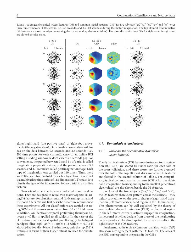
6 Computational Intelligence and Neuroscience
Table 1: Averaged dynamical system features (DS) and common spatial patterns (CSP) for five subjects (“aa,” “al,” “av,” “aw,” and “ay”) overthree-time windows (0–0.5 second, 0.5–2.5 seconds, and 3.5–4.0 seconds) during the motor imagination. The top 20 most discriminativeDS features are shown as edges connecting the corresponding electrodes (dots). The most discriminative CSPs for right-hand imaginationare plotted as color maps.
0–0.5 s 0.5–2.5 s 3.5–4 sDS DS DSCSP Filter
← Left ↑ Frontal ← Left ↑ Frontal ← Left ↑ Frontal
aa
al
av
aw
ay
either right-hand (the positive class) or right-foot move-ments (the negative class). Our classification analysis will fo-cus on the data between 0.5 seconds and 2.5 seconds (i.e.,200 time points for each channel), since in an online BCIsetting a sliding window seldom exceeds 2 seconds [4]. Forconvenience, the period between 0 s and 1 s of a trial is calledimagination preparation stage, and the period between 3.5seconds and 4.0 seconds is called postimagination stage. Eachtype of imagination was carried out 140 times. Thus, thereare 280 labeled trials in total for each subject (note: each trialis a multivariate time series of 118 dimensions). The task is toclassify the type of the imagination for each trial in an offlinefashion.
Two sets of experiments were conducted in our evalua-tions. They are designed to reveal two major aspects: (i) us-ing DS features for classification, and (ii) learning spatial andtemporal filters. We will first describe procedures common tothese experiments. All our classifications are carried out us-ing SVM and the errors are obtained from 10×10 fold cross-validation. An identical temporal prefiltering (bandpass be-tween 8–40 Hz) is applied to all subjects. In the case of theDS features, an identical spatial prefiltering (a bell-shapedbandpass filter exp(−κn(n + 1))n(n + 1) with κ = 0.01) isalso applied for all subjects. Furthermore, only the top 20 DSfeatures (in terms of their Fisher ratios) are used for classifi-cation.
4.1. Dynamical system features
4.1.1. Where are the discriminative dynamicalsystem features?
The dynamical system (DS) features during motor imagina-tion (0.5–2.5 s) are scored by Fisher ratio for each fold ofthe cross-validation, and these scores are further averagedover the folds. The top 20 most discriminative DS featuresare plotted in the second column of Table 1. For compari-son, typical common spatial patterns (CSPs) for the right-hand imagination (corresponding to the smallest generalizedeigenvalues) are also shown beside the DS features.
For four of the five subjects (“aa,” “al,” “av,” and “ay”),the DS features share clear pattern across the subjects—theytightly concentrate on the area in charge of right-hand imag-ination (left motor cortex, hand region in the Homunculus).This phenomenon can be well explained by the theory ofevent-related desynchronization (ERD): as the hand regionin the left motor cortex is actively engaged in imagination,its neuronal activities deviate from those of the neighboringcortices; and such localized spatial discordance results in thetight cluster of the DS features.
Furthermore, the typical common spatial patterns (CSP)also show nice agreement with the DS features. The areas ofthe ERD correspond to the peaks in the CSPs.
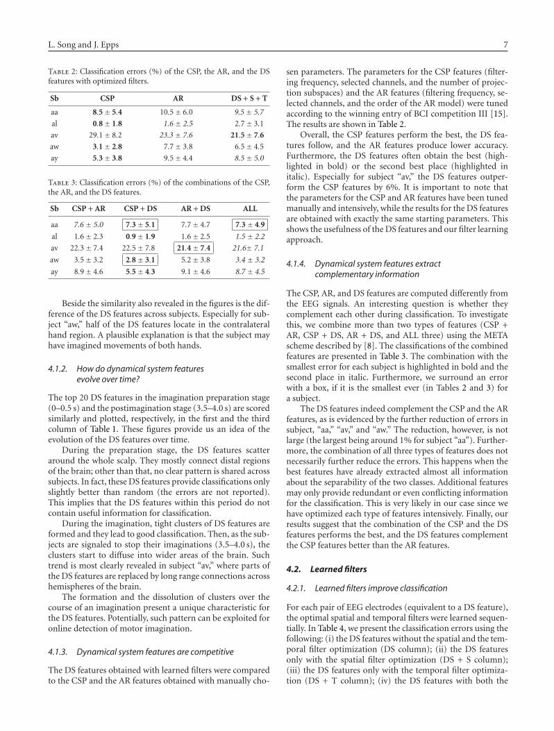
L. Song and J. Epps 7
Table 2: Classification errors (%) of the CSP, the AR, and the DSfeatures with optimized filters.
Sb CSP AR DS + S + T
aa 8.5± 5.4 10.5± 6.0 9.5 ± 5.7
al 0.8± 1.8 1.6 ± 2.5 2.7± 3.1
av 29.1± 8.2 23.3 ± 7.6 21.5± 7.6
aw 3.1± 2.8 7.7± 3.8 6.5± 4.5
ay 5.3± 3.8 9.5± 4.4 8.5 ± 5.0
Table 3: Classification errors (%) of the combinations of the CSP,the AR, and the DS features.
Sb CSP + AR CSP + DS AR + DS ALL
aa 7.6 ± 5.0 7.3± 5.1 7.7± 4.7 7.3± 4.9
al 1.6± 2.3 0.9± 1.9 1.6± 2.5 1.5 ± 2.2
av 22.3± 7.4 22.5± 7.8 21.4± 7.4 21.6± 7.1
aw 3.5± 3.2 2.8± 3.1 5.2± 3.8 3.4 ± 3.2
ay 8.9± 4.6 5.5± 4.3 9.1± 4.6 8.7 ± 4.5
Beside the similarity also revealed in the figures is the dif-ference of the DS features across subjects. Especially for sub-ject “aw,” half of the DS features locate in the contralateralhand region. A plausible explanation is that the subject mayhave imagined movements of both hands.
4.1.2. How do dynamical system featuresevolve over time?
The top 20 DS features in the imagination preparation stage(0–0.5 s) and the postimagination stage (3.5–4.0 s) are scoredsimilarly and plotted, respectively, in the first and the thirdcolumn of Table 1. These figures provide us an idea of theevolution of the DS features over time.
During the preparation stage, the DS features scatteraround the whole scalp. They mostly connect distal regionsof the brain; other than that, no clear pattern is shared acrosssubjects. In fact, these DS features provide classifications onlyslightly better than random (the errors are not reported).This implies that the DS features within this period do notcontain useful information for classification.
During the imagination, tight clusters of DS features areformed and they lead to good classification. Then, as the sub-jects are signaled to stop their imaginations (3.5–4.0 s), theclusters start to diffuse into wider areas of the brain. Suchtrend is most clearly revealed in subject “av,” where parts ofthe DS features are replaced by long range connections acrosshemispheres of the brain.
The formation and the dissolution of clusters over thecourse of an imagination present a unique characteristic forthe DS features. Potentially, such pattern can be exploited foronline detection of motor imagination.
4.1.3. Dynamical system features are competitive
The DS features obtained with learned filters were comparedto the CSP and the AR features obtained with manually cho-
sen parameters. The parameters for the CSP features (filter-ing frequency, selected channels, and the number of projec-tion subspaces) and the AR features (filtering frequency, se-lected channels, and the order of the AR model) were tunedaccording to the winning entry of BCI competition III [15].The results are shown in Table 2.
Overall, the CSP features perform the best, the DS fea-tures follow, and the AR features produce lower accuracy.Furthermore, the DS features often obtain the best (high-lighted in bold) or the second best place (highlighted initalic). Especially for subject “av,” the DS features outper-form the CSP features by 6%. It is important to note thatthe parameters for the CSP and AR features have been tunedmanually and intensively, while the results for the DS featuresare obtained with exactly the same starting parameters. Thisshows the usefulness of the DS features and our filter learningapproach.
4.1.4. Dynamical system features extractcomplementary information
The CSP, AR, and DS features are computed differently fromthe EEG signals. An interesting question is whether theycomplement each other during classification. To investigatethis, we combine more than two types of features (CSP +AR, CSP + DS, AR + DS, and ALL three) using the METAscheme described by [8]. The classifications of the combinedfeatures are presented in Table 3. The combination with thesmallest error for each subject is highlighted in bold and thesecond place in italic. Furthermore, we surround an errorwith a box, if it is the smallest ever (in Tables 2 and 3) fora subject.
The DS features indeed complement the CSP and the ARfeatures, as is evidenced by the further reduction of errors insubject, “aa,” “av,” and “aw.” The reduction, however, is notlarge (the largest being around 1% for subject “aa”). Further-more, the combination of all three types of features does notnecessarily further reduce the errors. This happens when thebest features have already extracted almost all informationabout the separability of the two classes. Additional featuresmay only provide redundant or even conflicting informationfor the classification. This is very likely in our case since wehave optimized each type of features intensively. Finally, ourresults suggest that the combination of the CSP and the DSfeatures performs the best, and the DS features complementthe CSP features better than the AR features.
4.2. Learned filters
4.2.1. Learned filters improve classification
For each pair of EEG electrodes (equivalent to a DS feature),the optimal spatial and temporal filters were learned sequen-tially. In Table 4, we present the classification errors using thefollowing: (i) the DS features without the spatial and the tem-poral filter optimization (DS column); (ii) the DS featuresonly with the spatial filter optimization (DS + S column);(iii) the DS features only with the temporal filter optimiza-tion (DS + T column); (iv) the DS features with both the
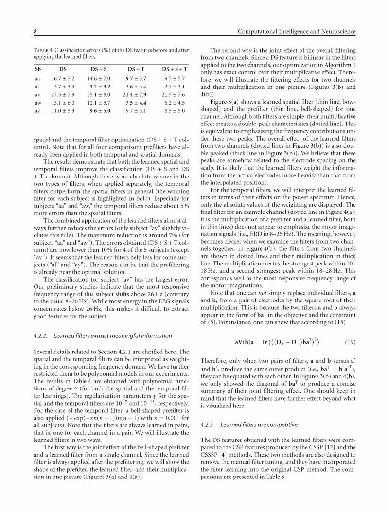
8 Computational Intelligence and Neuroscience
Table 4: Classification errors (%) of the DS features before and afterapplying the learned filters.
Sb DS DS + S DS + T DS + S + T
aa 16.7± 7.2 14.6± 7.0 9.7± 5.7 9.5± 5.7
al 3.7± 3.3 3.2± 3.2 3.6± 3.4 2.7± 3.1
av 27.3± 7.9 25.1± 8.0 21.4± 7.9 21.5± 7.6
aw 13.1± 6.0 12.1± 5.7 7.5± 4.4 6.2± 4.5
ay 11.0± 5.3 9.6± 5.0 9.7± 5.1 8.5± 5.0
spatial and the temporal filter optimization (DS + S + T col-umn). Note that for all four comparisons prefilters have al-ready been applied in both temporal and spatial domains.
The results demonstrate that both the learned spatial andtemporal filters improve the classification (DS + S and DS+ T columns). Although there is no absolute winner in thetwo types of filters, when applied separately, the temporalfilters outperform the spatial filters in general (the winningfilter for each subject is highlighted in bold). Especially forsubjects “aa” and “aw,” the temporal filters reduce about 5%more errors than the spatial filters.
The combined application of the learned filters almost al-ways further reduces the errors (only subject “av” slightly vi-olates this rule). The maximum reduction is around 7% (forsubject, “aa” and “aw”). The errors obtained (DS + S + T col-umn) are now lower than 10% for 4 of the 5 subjects (except“av”). It seems that the learned filters help less for some sub-jects (“al” and “ay”). The reason can be that the prefilteringis already near the optimal solution.
The classification for subject “av” has the largest error.Our preliminary studies indicate that the most responsivefrequency range of this subject shifts above 26 Hz (contraryto the usual 8–26 Hz). While most energy in the EEG signalsconcentrates below 26 Hz, this makes it difficult to extractgood features for the subject.
4.2.2. Learned filters extract meaningful information
Several details related to Section 4.2.1 are clarified here. Thespatial and the temporal filters can be interpreted as weight-ing in the corresponding frequency domain. We have furtherrestricted them to be polynomial models in our experiments.The results in Table 4 are obtained with polynomial func-tions of degree 6 (for both the spatial and the temporal fil-ter learnings). The regularization parameters γ for the spa-tial and the temporal filters are 10−7 and 10−13, respectively.For the case of the temporal filter, a bell-shaped prefilter isalso applied (− exp(−κn(n + 1))n(n + 1) with κ = 0.001 forall subjects). Note that the filters are always learned in pairs,that is, one for each channel in a pair. We will illustrate thelearned filters in two ways.
The first way is the joint effect of the bell-shaped prefilterand a learned filter from a single channel. Since the learnedfilter is always applied after the prefiltering, we will show theshape of the prefilter, the learned filter, and their multiplica-tion in one picture (Figures 3(a) and 4(a)).
The second way is the joint effect of the overall filteringfrom two channels. Since a DS feature is bilinear in the filtersapplied to the two channels, our optimization in Algorithm 1only has exact control over their multiplicative effect. There-fore, we will illustrate the filtering effects for two channelsand their multiplication in one picture (Figures 3(b) and4(b)).
Figure 3(a) shows a learned spatial filter (thin line, bow-shaped) and the prefilter (thin line, bell-shaped) for onechannel. Although both filters are simple, their multiplicativeeffect creates a double-peak characteristics (dotted line). Thisis equivalent to emphasizing the frequency contributions un-der these two peaks. The overall effect of the learned filtersfrom two channels (dotted lines in Figure 3(b)) is also dou-ble peaked (thick line in Figure 3(b)). We believe that thesepeaks are somehow related to the electrode spacing on thescalp. It is likely that the learned filters weight the informa-tion from the actual electrodes more heavily than that fromthe interpolated positions.
For the temporal filters, we will interpret the learned fil-ters in terms of their effects on the power spectrum. Hence,only the absolute values of the weighting are displayed. Thefinal filter for an example channel (dotted line in Figure 4(a);it is the multiplication of a prefilter and a learned filter, bothin thin lines) does not appear to emphasize the motor imagi-nation signals (i.e., ERD in 8–26 Hz). The meaning, however,becomes clearer when we examine the filters from two chan-nels together. In Figure 4(b), the filters from two channelsare shown in dotted lines and their multiplication in thickline. The multiplication creates the strongest peak within 10–18 Hz, and a second strongest peak within 18–28 Hz. Thiscorresponds well to the most responsive frequency range ofthe motor imaginations.
Note that one can not simply replace individual filters, aand b, from a pair of electrodes by the square root of theirmultiplication. This is because the two filters a and b alwaysappear in the form of baT in the objective and the constraintof (5). For instance, one can show that according to (15)
aV(b)a = Tr(((
D+ −D−)
baT)2). (19)
Therefore, only when two pairs of filters, a and b versus a′
and b′, produce the same outer product (i.e., baT = b′a′T),they can be equated with each other. In Figures 3(b) and 4(b),we only showed the diagonal of baT to produce a concisesummary of their joint filtering effect. One should keep inmind that the learned filters have further effect beyond whatis visualized here.
4.2.3. Learned filters are competitive
The DS features obtained with the learned filters were com-pared to the CSP features produced by the CSSP [12] and theCSSSP [4] methods. These two methods are also designed toremove the manual filter tuning, and they have incorporatedthe filter learning into the original CSP method. The com-parisons are presented in Table 5.
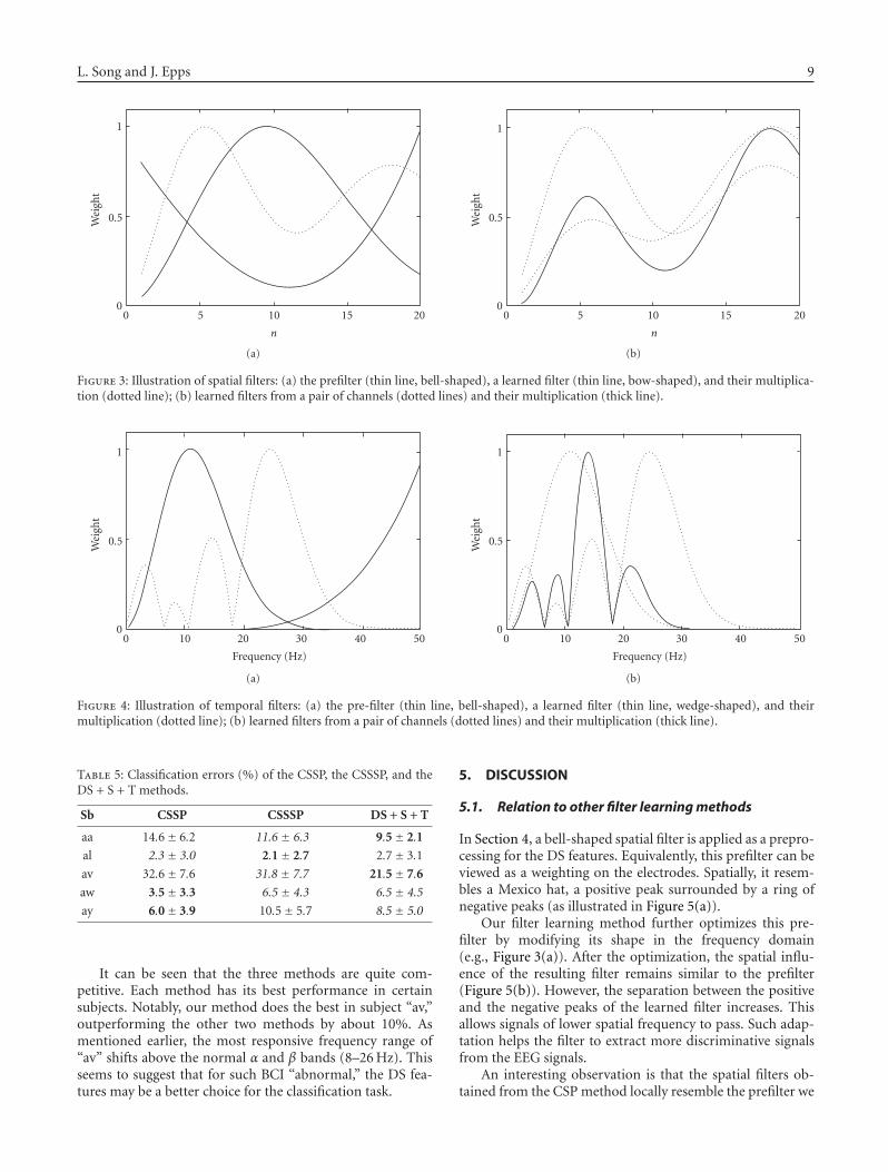
L. Song and J. Epps 9
0 5 10 15 200
0.5
1
Wei
ght
n
(a)
0 5 10 15 200
0.5
1
Wei
ght
n
(b)
Figure 3: Illustration of spatial filters: (a) the prefilter (thin line, bell-shaped), a learned filter (thin line, bow-shaped), and their multiplica-tion (dotted line); (b) learned filters from a pair of channels (dotted lines) and their multiplication (thick line).
0 10 20 30 50400
0.5
1
Wei
ght
Frequency (Hz)
(a)
0 10 20 30 50400
0.5
1
Wei
ght
Frequency (Hz)
(b)
Figure 4: Illustration of temporal filters: (a) the pre-filter (thin line, bell-shaped), a learned filter (thin line, wedge-shaped), and theirmultiplication (dotted line); (b) learned filters from a pair of channels (dotted lines) and their multiplication (thick line).
Table 5: Classification errors (%) of the CSSP, the CSSSP, and theDS + S + T methods.
Sb CSSP CSSSP DS + S + T
aa 14.6± 6.2 11.6 ± 6.3 9.5± 2.1
al 2.3 ± 3.0 2.1± 2.7 2.7± 3.1
av 32.6± 7.6 31.8 ± 7.7 21.5± 7.6
aw 3.5± 3.3 6.5 ± 4.3 6.5 ± 4.5
ay 6.0± 3.9 10.5± 5.7 8.5 ± 5.0
It can be seen that the three methods are quite com-petitive. Each method has its best performance in certainsubjects. Notably, our method does the best in subject “av,”outperforming the other two methods by about 10%. Asmentioned earlier, the most responsive frequency range of“av” shifts above the normal α and β bands (8–26 Hz). Thisseems to suggest that for such BCI “abnormal,” the DS fea-tures may be a better choice for the classification task.
5. DISCUSSION
5.1. Relation to other filter learning methods
In Section 4, a bell-shaped spatial filter is applied as a prepro-cessing for the DS features. Equivalently, this prefilter can beviewed as a weighting on the electrodes. Spatially, it resem-bles a Mexico hat, a positive peak surrounded by a ring ofnegative peaks (as illustrated in Figure 5(a)).
Our filter learning method further optimizes this pre-filter by modifying its shape in the frequency domain(e.g., Figure 3(a)). After the optimization, the spatial influ-ence of the resulting filter remains similar to the prefilter(Figure 5(b)). However, the separation between the positiveand the negative peaks of the learned filter increases. Thisallows signals of lower spatial frequency to pass. Such adap-tation helps the filter to extract more discriminative signalsfrom the EEG signals.
An interesting observation is that the spatial filters ob-tained from the CSP method locally resemble the prefilter we
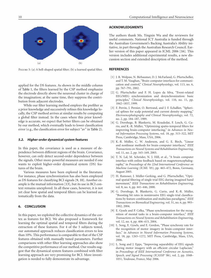
10 Computational Intelligence and Neuroscience
(a) (b)
Figure 5: (a) A bell-shaped spatial filter; (b) a learned spatial filter.
applied for the DS features. As shown in the middle columnof Table 1, the filters learned by the CSP method emphasizethe electrode directly above the neuronal cluster in charge ofthe imagination; at the same time, they suppress the contri-bution from adjacent electrodes.
While our filter learning method employs the prefilter asa prior knowledge and successively refines this knowledge lo-cally, the CSP method arrives at similar results by computinga global filter instead. In the cases where this prior knowl-edge is accurate, we expect that better filters can be obtainedby our method, which eventually leads to lower classificationerror (e.g., the classification error for subject “av” in Table 2).
5.2. Higher-order dynamical system features
In this paper, the covariance is used as a measure of de-pendence between different regions of the brain. Covariance,however, can only detect second-order dependence betweenthe signals. Other more-powerful measures are needed if onewants to exploit higher-order dynamical system (DS) fea-tures of the brain.
Various measures have been explored in the literature.For instance, phase synchronization has also been employedas DS features for classifying BCI signals [9, 10]. Another ex-ample is the mutual information [13], but its use in BCI con-text remains unexplored. In all these cases, however, it is notyet clear how spatial and temporal filters can be learned au-tomatically from the data.
6. CONCLUSION
In this paper, we exploited the collective dynamics of the cor-tex as features for BCI. We also proposed a framework forlearning the optimal spatial and temporal filters during theextraction of these features. For 4 of the 5 subjects tested,our automated approach reduces classification errors to lessthan 10%. This performance is comparable to that of the CSPfeatures obtained with manually tuned parameters. Furthercomparisons with other filter learning approaches also showthe competitive performance of our method. Our results sug-gest that the dynamical system features combined with filterlearning approach are very promising for BCI. More investi-gation is needed to fully demonstrate its advantage.
ACKNOWLEDGMENTS
The authors thank Ms. Yingxin Wu and the reviewers foruseful comments. National ICT Australia is funded throughthe Australian Government’s Backing Australia’s Ability ini-tiative, in part through the Australian Research Council. Ear-lier version of this paper appeared in ICML 2006 [16]. Thisversion includes additional experimental results, a new dis-cussion section and extended description of the method.
REFERENCES
[1] J. R. Wolpaw, N. Birbaumer, D. J. McFarland, G. Pfurtscheller,and T. M. Vaughan, “Brain-computer interfaces for communi-cation and control,” Clinical Neurophysiology, vol. 113, no. 6,pp. 767–791, 2002.
[2] G. Pfurtscheller and F. H. Lopes da Silva, “Event-relatedEEG/MEG synchronization and desynchronization: basicprinciples,” Clinical Neurophysiology, vol. 110, no. 11, pp.1842–1857, 1999.
[3] F. Perrin, J. Pernier, O. Bertrand, and J. F. Echallier, “Spheri-cal splines for scalp potential and current density mapping,”Electroencephalography and Clinical Neurophysiology, vol. 72,no. 2, pp. 184–187, 1989.
[4] G. Dornhege, B. Blankertz, M. Krauledat, F. Losch, G. Cu-rio, and K.-R. Muller, “Optimizing spatio-temporal filters forimproving brain-computer interfacing,” in Advances in Neu-ral Information Processing Systems, vol. 18, pp. 315–322, MITPress, Cambridge, Mass, USA, 2006.
[5] K.-R. Muller, C. W. Anderson, and G. E. Birch, “Linearand nonlinear methods for brain-computer interfaces,” IEEETransactions on Neural Systems and Rehabilitation Engineering,vol. 11, no. 2, pp. 165–169, 2003.
[6] T. N. Lal, M. Schroder, N. J. Hill, et al., “A brain computerinterface with online feedback based on magnetoencephalog-raphy,” in Proceedings of the 22nd International Conference onMachine Learning (ICML ’05), pp. 465–472, Bonn, Germany,August 2005.
[7] H. Ramoser, J. Muller-Gerking, and G. Pfurtscheller, “Opti-mal spatial filtering of single trial EEG during imagined handmovement,” IEEE Transactions on Rehabilitation Engineering,vol. 8, no. 4, pp. 441–446, 2000.
[8] G. Dornhege, B. Blankertz, G. Curio, and K.-R. Muller,“Boosting bit rates in noninvasive EEG single-trial classifica-tions by feature combination and multiclass paradigms,” IEEETransactions on Biomedical Engineering, vol. 51, no. 6, pp. 993–1002, 2004.
[9] E. Gysels and P. Celka, “Phase synchronization for the recog-nition of mental tasks in a brain-computer interface,” IEEETransactions on Neural Systems and Rehabilitation Engineering,vol. 12, no. 4, pp. 406–415, 2004.
[10] L. Song, E. Gysels, and E. Gordon, “Phase synchrony rate forthe recognition of motor imagery in brain-computer inter-face,” in Advances in Neural Information Processing Systems,vol. 18, pp. 1265–1272, MIT Press, Cambridge, Mass, USA,2006.
[11] L. Song and J. Epps, “Improving separability of EEG signalsduring motor imagery with an efficient circular Laplacian,”in Proceedings of IEEE International Conference on Acoustics,Speech, and Signal Processing (ICASSP ’06), vol. 2, pp. 1048–1051, Toulouse, France, May 2006.
L. Song and J. Epps 11
[12] S. Lemm, B. Blankertz, G. Curio, and K.-R. Muller, “Spatio-spectral filters for improving the classification of single trialEEG,” IEEE Transactions on Biomedical Engineering, vol. 52,no. 9, pp. 1541–1548, 2005.
[13] A. Pikovsky, M. Rosenblum, J. Kurths, and B. Chirikov, Syn-chronization: A Universal Concept in Nonlinear Sciences, Cam-bridge University Press, Cambridge, UK, 2003.
[14] R. Srinivasan, P. L. Nunez, and R. B. Silberstein, “Spatial fil-tering and neocortical dynamics: estimates of EEG coherence,”IEEE Transactions on Biomedical Engineering, vol. 45, no. 7, pp.814–826, 1998.
[15] X. Gao, Z. Zhang, B. Hong, and S. Gao, http://ida.first.fraunhofer.de/projects/bci/competition iii/results/berlin IVa/YijunWang desc.pdf
[16] L. Song and J. Epps, “Classifying EEG for brain-computerinterfaces: learning optimal filters for dynamical system fea-tures,” in Proceedings of the 23rd International Conference onMachine Learning (ICML ’06), pp. 857–864, Pittsburgh, Pa,USA, June 2006.
Hindawi Publishing CorporationComputational Intelligence and NeuroscienceVolume 2007, Article ID 54925, 12 pagesdoi:10.1155/2007/54925
Research ArticleHigh-Resolution Movement EEG Classification
Jakub Stastny and Pavel Sovka
Biosignal Laboratory, Department of Circuit Theory, Faculty of Electrotechnical Engineering,Czech Technical University in Prague, Technicka 2, 16627 Prague, Czech Republic
Correspondence should be addressed to Jakub Stastny, [email protected]
Received 17 February 2007; Accepted 23 September 2007
Recommended by Andrzej Cichocki
The aim of the contribution is to analyze possibilities of high-resolution movement classification using human EEG. For this pur-pose, a database of the EEG recorded during right-thumb and little-finger fast flexion movements of the experimental subjectswas created. The statistical analysis of the EEG was done on the subject’s basis instead of the commonly used grand averaging.Statistically significant differences between the EEG accompanying movements of both fingers were found, extending the resultsof other so far published works. The classifier based on hidden Markov models was able to distinguish between movement andresting states (classification score of 94–100%), but it was unable to recognize the type of the movement. This is caused by the largefraction of other (nonmovement related) EEG activities in the recorded signals. A classification method based on advanced EEGsignal denoising is being currently developed to overcome this problem.
Copyright © 2007 J. Stastny and P. Sovka. This is an open access article distributed under the Creative Commons AttributionLicense, which permits unrestricted use, distribution, and reproduction in any medium, provided the original work is properlycited.
1. INTRODUCTION
There are a great number of existing BCI prototypes allaround the world. However, all of them suffer from one ma-jor drawback; the communication channel between a humanbrain and a computer is usually very slow working at a speedlower than 100 bits per minute. If we compare this communi-cation channel with a standard keyboard computer interfaceallowing us to type texts at blazing speeds up to 1 kbit perminute, we can conclude that all these BCI devices are stillnot very suitable for the real computer control.
One possibility leading to higher data transfer lies in therecognition of more distinct brain states, which means trans-ferring more bits per state via the communication channel(high-resolution EEG recognition), while keeping the aver-age recognition score for the single states as high as possi-ble. However, the currently existing systems recognize onlyfew very different EEG phenomena (left/right- hand or fin-ger movement [1–5], mental activities such as mental arith-metic, mental rotation, visual imagination [3, 4, 6, 7], con-scious EEG rhythm control [8, 9], or event-related potentials[10–12], among others). Our research is targeted to the ex-ploration of possibilities of the high-resolution movement
recognition from the EEG signal. The movement-relatedEEG was selected because it is very natural to control any-thing with movement-related EEG as we usually control oursurroundings in this way. It is well known that only imagi-nation of the movement is sufficient [13, 14] to produce thedesired brain activity pattern and last, but not the least, itis possible to change quickly the movement-related states ofthe brain compared , for example, to mental activities furtherincreasing the interface transfer speed.
Our previous work showed that it is possible to distin-guish right-shoulder and right-index finger movements eas-ily from the EEG signal [15, 16] and classify the direction ofthe right-index finger movement on the basis of the EEG sig-nal [17]. Movements performed at only one side of the bodywere used. This task is more complicated compared to dif-ferentiating only the left/right-hand movement or types ofmental activities. The key requirement built into the classifi-cation system was to use changes in signal parameters ratherthan information stored in the difference of signal powersfrom different electrodes (extracted by means of appropri-ately defined spatial filters [18]), which lies in contrast withother existing systems. Encouraged by our previous result, wetargeted our research to the development of a classification

2 Computational Intelligence and Neuroscience
method which is able to recognize the single-finger move-ments from the EEG signal. Finger movements were chosenowing to the results of other works [19, 20].
The second important finding we learnt from our ex-periments is that the individualities of experimental subjectscause great differences between their recorded brain activi-ties. These differences nowadays obstruct the possibility ofthe BCI generalization (the usage of the system trained onone subject for the movement classification of another sub-ject). This led us to the conclusion that an individual ap-proach to the EEG statistical analysis will be selected insteadof the commonly used grand averaging (see, e.g., [20, 21]).
Last, but not least, the developed classification scheme[16] allows us to do a movement-related EEG classificationwithout any need of subject training, which is a great advan-tage compared to other systems.
Our current work deals with the right-index and little-finger flexion movement-related EEG analysis and classifi-cation. This contribution is organized as follows. The gen-eral properties of the movement-related EEG are introducedin Section 2. Further, the EEG recording experiment is de-scribed. Section 4 section is devoted to a simple prelimi-nary analysis of the recorded EEG proving the validity of ourdatabase. The core of our work is described in Sections 5 and6. First we analyze the EEG in an individual way to find subtledifferences between movements, then the classification sys-tem description and classification results are introduced. Fi-nally, several conclusions and future steps are drawn.
2. GENERAL PROPERTIES OFTHE MOVEMENT-RELATED EEG
We deal with movement-related changes of the EEG in thespectral domain in our work. The following characteristicphenomena are observed in the short-time EEG spectrumaround the time of a movement (see [20, 21]).
μ-rhythm event-related desynchronization (μERD) startsabout 1 second prior to the movement onset (see Figures 1and 4 with marked ERDs and interval II in Figure 2). μERDis usually localized to the C3/CP3 and C4/CP4 scalp ar-eas [14, 20, 22] and it exhibits a contralateral preponder-ance; usually we see two foci over both sensorimotor cortices.μERD allows to differentiate not only the side of the bodyperforming the movement but slow and fast movements aswell [23]. The desynchronization accompanies even the meremotor imagery and it is present in most normal adults’ EEG.
β-rhythm event-related desynchronization (βERD) has adiffuse character over the scalp central area, and it is morewidespread than βERS [14, 24]. βERD is at least partiallycoupled to the μERD showing the desynchronization at thefrequency of the second harmonic component of the μ-rhythm [25]. Although there might be some components re-lated to the βERS in the β-band during the ERD, there is noknown evidence that they somehow allow to distinguish be-tween different types of movement.
β-rhythm event-related synchronization (βERS) is dis-played by central β rhythms as a rebound in the form of aphasic synchronization [24] after the movement. βERS rep-resents a postmovement rise of power in the β-band; the
phenomenon is located about 1 second after the movementonset (see Figures 1 and 4 with marked ERSs, and Figure 2for interval III). βERS is larger over the contralateral hemi-sphere [24] and it is focused slightly anteriorly of the largestμERD. It is known that βERS allows to distinguish vari-ous types of movements such as wrist/finger flexion move-ments [20], index finger extension/flexion movements [26],or distal/proximal movements [21]. The βERS differencesbetween extension/flexion movements and distal/proximalmovements were successfully used for movement classifica-tion [16, 17].
3. EEG RECORDING
The following paragraphs describe the EEG recording andpostprocessing procedures and provide basic characteristicsof experimental subjects.
3.1. Experimental subjects
Eight subjects took part in the experiment—7 men and 1woman with average age of 24.5 years (σ = 3.59, see Table 1).None of them had a previous experience with such an ex-periment; all of them gave us an informed consent with theexperiment and stated that they were healthy, without anyknown neurological problems, and were not under influenceof any drug in the time of the experiment.
At first, we examined all the subjects on hand dominance.The [27] hand-dominance test consisting of three differenttapping and drawing tasks was used. According to this test,four out of eight subjects were found to be right-handed,three as nonright-handed, and one as left-handed. The sub-jects with no significantly dominant hand were selected in-tentionally as the proposed system will work independentlyof the subject’s handedness.
3.2. EEG recording setup
We used 41 unipolar scalp Ag/AgCl electrodes with 9 mm di-ameter placed symmetrically and equidistantly with 2.5 cmspacing [28] above both sensorimotor areas of the experi-mental subject (see Figure 3). Since the EEG changes in bothtime and space, the selection of appropriate EEG electroderepresenting movement is a crucial point for a successfulclassification of movements. As both movements are con-trolled primarily by the contralateral sensorimotor cortex,the most suitable electrodes are those overlying the contralat-eral sensorimotor hand area (electrode C3 and its surround-ings) [14, 20]. The ground electrode was mounted on thenose, and impedances of all the electrodes were kept be-low 10 kΩ. The real exact positions of the scalp electrodeswere measured with the help of the Isotrak II 3D scanner(manufactured by Polhemus, Colchester, Vermont, USA). Inaddition to the scalp electrodes, the following four bipo-lar channels were used: vertical and horizontal EOGs (elec-trodes placed horizontally and vertically along the subject’sright eye), thumb EMG electrode placed on thenar recordingthe EMG of musculus flexor pollicis brevis, m. opponens polli-cis, and m. adductor pollicis, and little-finger EMG electrode
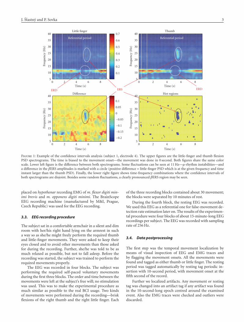
J. Stastny and P. Sovka 3
86420Time (s)
5
10
15
20
25
30
35
40
Freq
uen
cy(H
z)
0.1
0.2
0.3
0.4
0.5
0.6
0.7Little finger
Referential period
86420Time (s)
5
10
15
20
25
30
35
40
Freq
uen
cy(H
z)
Thumb
Referential period
86420
Time (s)
5
10
15
20
25
30
35
40
Freq
uen
cy(H
z)
−0.2
−0.15
−0.1
−0.05
0
0.05
0.1
Difference
86420
Time (s)
5
10
15
20
25
30
35
40
Freq
uen
cy(H
z)
Hot regions
ERDERD ERS
Figure 1: Example of the confidence intervals analysis (subject 1, electrode 4). The upper figures are the little-finger and thumb flexionPSD spectrograms. The time is biased to the movement onset—the movement was done in 0 second. Both figures share the same colorscale. Lower left figure is the difference between both spectrograms. Some fluctuations can be seen at 11 Hz—μ-rhythm instabilities—anda difference in the βERS amplitudes is marked with a circle (positive difference = little-finger PSD which is at the given frequency and timeinstant larger than the thumb PSD). Finally, the lower right figure shows time-frequency combinations where the confidence intervals ofboth spectrograms are disjoint. Besides some random fluctuations, a clearly pronounced βERS region may be seen.
placed on hypothenar recording EMG of m. flexor digiti min-imi brevis and m. opponens digiti minimi. The BrainScopeEEG recording machine (manufactured by M&I, Prague,Czech Republic) was used for the EEG recording.
3.3. EEG recording procedure
The subject sat in a comfortable armchair in a silent and dimroom with her/his right hand lying on the armrest in sucha way so as she/he might freely perform the required thumband little-finger movements. They were asked to keep theireyes closed and to avoid other movements than those askedfor during the recording. Further, she/he was told to be asmuch relaxed as possible, but not to fall asleep. Before therecording was started, the subject was trained to perform therequired movements properly.
The EEG was recorded in four blocks. The subject wasperforming the required self-paced voluntary movementsduring the first three blocks. The order and time between themovements were left at the subject’s free will; no stimulationwas used. This was to make the experimental procedure asmuch similar as possible to the real BCI usage. Two kindsof movements were performed during the recording—briskflexions of the right thumb and the right little finger. Each
of the three recording blocks contained about 30 movement;the blocks were separated by 10 minutes of rest.
During the fourth block, the resting EEG was recorded.We used this EEG as a referential one for false-movement de-tection rate estimation later on. The results of the experimen-tal procedure were four blocks of about 15-minute-long EEGrecordings per subject. The EEG was recorded with samplingrate of 256 Hz.
3.4. Data postprocessing
The first step was the temporal movement localization bymeans of visual inspection of EEG and EMG traces andby flagging the movement onsets. All the movements werefound and tagged as either thumb or little finger. The restingperiod was tagged automatically by resting tag periodic in-sertion with 10-second period, with movement onset at thefifth second of the record.
Further we localized artifacts. Any movement or restingtag was changed into an artifact tag if any artifact was foundin the 10-second-long epoch centred around the examinedevent. Also the EMG traces were checked and outliers werediscarded.
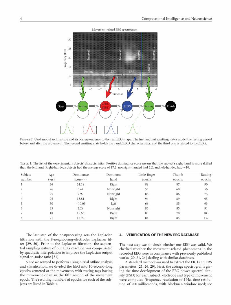
4 Computational Intelligence and Neuroscience
43210−1−2−3−4
Time (s)
5
10
15
20
25
30
Freq
uen
cy(H
z)
Movement-related EEG spectrogram
Inte
rval
I
Inte
rval
II
Inte
rval
III
Inte
rval
IV
Resting ERD ERS Res
tin
g
Mov
emen
t
Start RestingμERDβERD βERS Resting Finish
Figure 2: Used model architecture and its correspondence to the real EEG shape. The first and last emitting states model the resting periodbefore and after the movement. The second emitting state holds the μand βERD characteristics, and the third one is related to the βERS.
Table 1: The list of the experimental subjects’ characteristics. Positive dominance score means that the subject’s right hand is more skilledthan the lefthand. Right-handed subjects had the average score of 17.2, nonright-handed had 5.2, and left-handed had −10.
Subject Age Dominance Dominant Little-finger Thumb Resting
number (yrs) score (–) hand epochs epochs epochs
1 26 24.18 Right 88 87 90
2 26 5.44 Nonright 55 60 56
3 25 7.92 Nonright 86 86 75
4 25 13.81 Right 94 89 95
5 30 −10.03 Left 66 85 93
6 25 2.29 Nonright 86 85 91
7 18 15.63 Right 83 70 105
8 21 15.92 Right 84 85 132
The last step of the postprocessing was the Laplacianfiltration with the 8-neighboring-electrodes Laplacian fil-ter [29, 30]. Prior to the Laplacian filtration, the sequen-tial sampling nature of our EEG machine was compensatedby quadratic interpolation to improve the Laplacian outputsignal-to-noise ratio [31].
Since we wanted to perform a single-trial offline analysisand classification, we divided the EEG into 10-second-longepochs centered at the movement, with resting tags havingthe movement onset in the fifth second of the movementepoch. The resulting numbers of epochs for each of the sub-jects are listed in Table 1.
4. VERIFICATION OF THE NEW EEG DATABASE
The next step was to check whether our EEG was valid. Wechecked whether the movement-related phenomena in therecorded EEG were in compliance with previously publishedworks [20, 21, 26] dealing with similar databases.
A standard method was used to extract the ERD and ERSparameters [21, 26, 29]. First, the average spectrograms giv-ing the time development of the EEG power spectral den-sity (PSD) for each subject, electrode and type of movementwere computed (frequency resolution of 1 Hz, time resolu-tion of 200 milliseconds, with Blackman window used; see
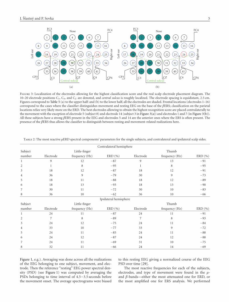
J. Stastny and P. Sovka 5
FC3Nose FC4
Rig
ht
ear
Left
ear
CP3 C3 CZ C4 CP4Central sulcus
1 2 3 4 5 6 7
8 9 10 11 12 13 14 15 16
17 18 19 20 21 22 23 24 25
26 27 28 29 30 31 32 33 34
35 36 37 38 39 40 41
(a)
FC3Nose FC4
Rig
ht
ear
Left
ear
CP3 C3 CZ C4 CP4Central sulcus
1 2 3 4 5 6 7
8 9 10 11 12 13 14 15 16
17 18 19 20 21 22 23 24 25
26 27 28 29 30 31 32 33 34
35 36 37 38 39 40 41
(b)
Figure 3: Localization of the electrodes allowing for the highest classification score and the real scalp electrode placement diagram. The10–20 electrode positions C3, C4, and CZ are denoted, and central sulcus is roughly localized. The electrode spacing is equidistant, 2.5 cm.Figures correspond to Table 5 (a) to the upper half: and (b) to the lower half; all the electrodes are shaded. Frontal locations (electrodes 1–16)correspond to the cases where the classifier distinguishes movement and resting EEG on the base of the βERS; classification on the parietallocations relies very likely more on the ERD. The best electrodes allowing to obtain the highest recognition score are placed contralaterally tothe movement with the exception of electrode 5 (subject 8) and electrode 14 (subject 3 in Figure 3(a)) and electrodes 1 and 7 (in Figure 3(b)).All these subjects have a strong βERS present in the EEG and electrodes 5 and 14 are the anterior ones where the ERS is often present. Thepresence of the βERS thus allows the classifier to distinguish between resting and movement-related realizations here.
Table 2: The most reactive μERD spectral components’ parameters for the single subjects, and contralateral and ipsilateral scalp sides.
Contralateral hemisphere
Subject Little-finger Thumb
number Electrode frequency (Hz) ERD (%) Electrode frequency (Hz) ERD (%)
1 9 12 −87 9 13 −91
2 1 8 −95 1 8 −95
3 18 12 −87 18 12 −91
4 36 9 −79 30 9 −73
5 18 11 −88 18 12 −89
6 18 13 −93 18 13 −90
7 30 11 −72 30 10 −83
8 36 10 −62 36 10 −66
Ipsilateral hemisphere
Subject Little-finger Thumb
number Electrode frequency (Hz) ERD (%) Electrode frequency (Hz) ERD (%)
1 24 11 −87 24 11 −91
2 7 8 −89 7 8 −93
3 24 12 −75 24 11 −84
4 33 10 −77 33 9 −72
5 24 11 −85 24 11 −88
6 24 12 −87 24 12 −88
7 24 11 −69 31 10 −75
8 32 11 −66 24 14 −69
Figure 1, e.g.). Averaging was done across all the realizationsof the EEG belonging to one subject, movement, and elec-trode. Then the reference “resting” EEG power spectral den-sity (PSD) (see Figure 1) was computed by averaging thePSDs belonging to time interval of 4.5−3.5 seconds beforethe movement onset. The average spectrograms were biased
to this resting EEG giving a normalized course of the EEGPSD over time [29].
The most reactive frequencies for each of the subjects,electrodes, and type of movement were found in the μ-and β-bands—either the most attenuated one for ERD, orthe most amplified one for ERS analysis. We performed
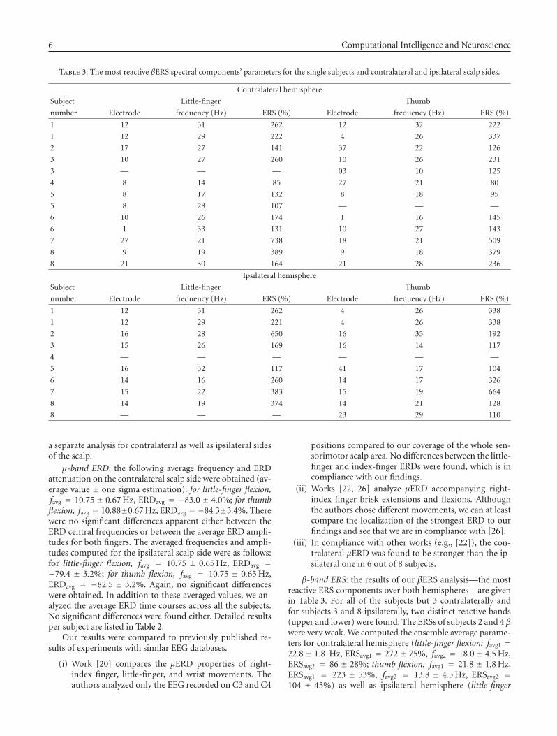
6 Computational Intelligence and Neuroscience
Table 3: The most reactive βERS spectral components’ parameters for the single subjects and contralateral and ipsilateral scalp sides.
Contralateral hemisphere
Subject Little-finger Thumb
number Electrode frequency (Hz) ERS (%) Electrode frequency (Hz) ERS (%)
1 12 31 262 12 32 222
1 12 29 222 4 26 337
2 17 27 141 37 22 126
3 10 27 260 10 26 231
3 — — — 03 10 125
4 8 14 85 27 21 80
5 8 17 132 8 18 95
5 8 28 107 — — —
6 10 26 174 1 16 145
6 1 33 131 10 27 143
7 27 21 738 18 21 509
8 9 19 389 9 18 379
8 21 30 164 21 28 236
Ipsilateral hemisphere
Subject Little-finger Thumb
number Electrode frequency (Hz) ERS (%) Electrode frequency (Hz) ERS (%)
1 12 31 262 4 26 338
1 12 29 221 4 26 338
2 16 28 650 16 35 192
3 15 26 169 16 14 117
4 — — — — — —
5 16 32 117 41 17 104
6 14 16 260 14 17 326
7 15 22 383 15 19 664
8 14 19 374 14 21 128
8 — — — 23 29 110
a separate analysis for contralateral as well as ipsilateral sidesof the scalp.
μ-band ERD: the following average frequency and ERDattenuation on the contralateral scalp side were obtained (av-erage value ± one sigma estimation): for little-finger flexion,favg = 10.75 ± 0.67 Hz, ERDavg = −83.0 ± 4.0%; for thumbflexion, favg = 10.88±0.67 Hz, ERDavg = −84.3±3.4%. Therewere no significant differences apparent either between theERD central frequencies or between the average ERD ampli-tudes for both fingers. The averaged frequencies and ampli-tudes computed for the ipsilateral scalp side were as follows:for little-finger flexion, favg = 10.75 ± 0.65 Hz, ERDavg =−79.4 ± 3.2%; for thumb flexion, favg = 10.75 ± 0.65 Hz,ERDavg = −82.5 ± 3.2%. Again, no significant differenceswere obtained. In addition to these averaged values, we an-alyzed the average ERD time courses across all the subjects.No significant differences were found either. Detailed resultsper subject are listed in Table 2.
Our results were compared to previously published re-sults of experiments with similar EEG databases.
(i) Work [20] compares the μERD properties of right-index finger, little-finger, and wrist movements. Theauthors analyzed only the EEG recorded on C3 and C4
positions compared to our coverage of the whole sen-sorimotor scalp area. No differences between the little-finger and index-finger ERDs were found, which is incompliance with our findings.
(ii) Works [22, 26] analyze μERD accompanying right-index finger brisk extensions and flexions. Althoughthe authors chose different movements, we can at leastcompare the localization of the strongest ERD to ourfindings and see that we are in compliance with [26].
(iii) In compliance with other works (e.g., [22]), the con-tralateral μERD was found to be stronger than the ip-silateral one in 6 out of 8 subjects.
β-band ERS: the results of our βERS analysis—the mostreactive ERS components over both hemispheres—are givenin Table 3. For all of the subjects but 3 contralaterally andfor subjects 3 and 8 ipsilaterally, two distinct reactive bands(upper and lower) were found. The ERSs of subjects 2 and 4 βwere very weak. We computed the ensemble average parame-ters for contralateral hemisphere (little-finger flexion: favg1 =22.8 ± 1.8 Hz, ERSavg1 = 272 ± 75%, favg2 = 18.0 ± 4.5 Hz,ERSavg2 = 86 ± 28%; thumb flexion: favg1 = 21.8 ± 1.8 Hz,ERSavg1 = 223 ± 53%, favg2 = 13.8 ± 4.5 Hz, ERSavg2 =104 ± 45%) as well as ipsilateral hemisphere (little-finger
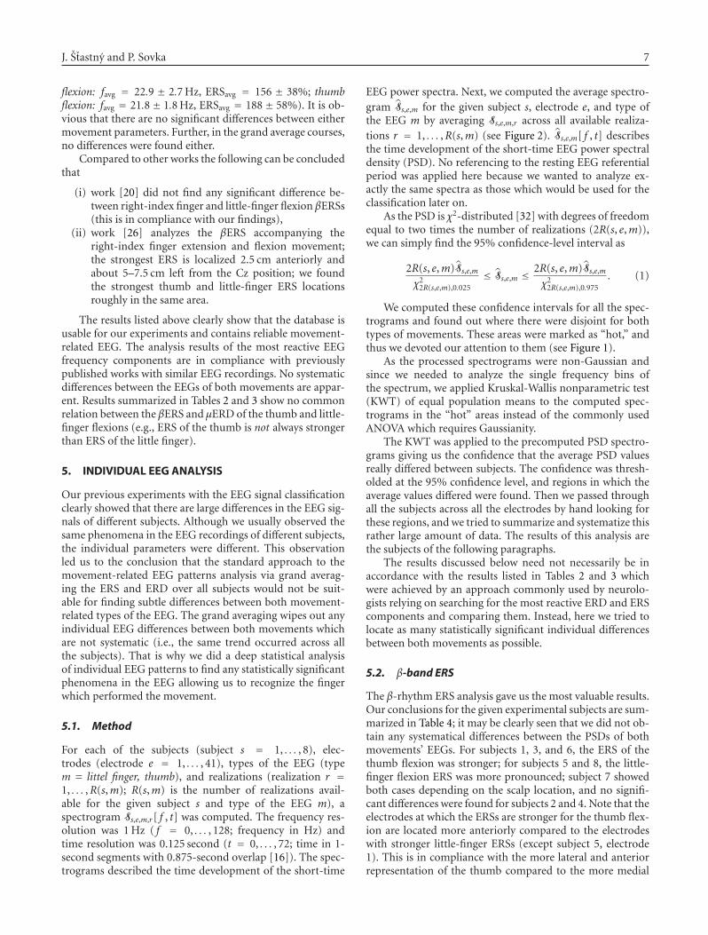
J. Stastny and P. Sovka 7
flexion: favg = 22.9 ± 2.7 Hz, ERSavg = 156 ± 38%; thumbflexion: favg = 21.8 ± 1.8 Hz, ERSavg = 188 ± 58%). It is ob-vious that there are no significant differences between eithermovement parameters. Further, in the grand average courses,no differences were found either.
Compared to other works the following can be concludedthat
(i) work [20] did not find any significant difference be-tween right-index finger and little-finger flexion βERSs(this is in compliance with our findings),
(ii) work [26] analyzes the βERS accompanying theright-index finger extension and flexion movement;the strongest ERS is localized 2.5 cm anteriorly andabout 5–7.5 cm left from the Cz position; we foundthe strongest thumb and little-finger ERS locationsroughly in the same area.
The results listed above clearly show that the database isusable for our experiments and contains reliable movement-related EEG. The analysis results of the most reactive EEGfrequency components are in compliance with previouslypublished works with similar EEG recordings. No systematicdifferences between the EEGs of both movements are appar-ent. Results summarized in Tables 2 and 3 show no commonrelation between the βERS and μERD of the thumb and little-finger flexions (e.g., ERS of the thumb is not always strongerthan ERS of the little finger).
5. INDIVIDUAL EEG ANALYSIS
Our previous experiments with the EEG signal classificationclearly showed that there are large differences in the EEG sig-nals of different subjects. Although we usually observed thesame phenomena in the EEG recordings of different subjects,the individual parameters were different. This observationled us to the conclusion that the standard approach to themovement-related EEG patterns analysis via grand averag-ing the ERS and ERD over all subjects would not be suit-able for finding subtle differences between both movement-related types of the EEG. The grand averaging wipes out anyindividual EEG differences between both movements whichare not systematic (i.e., the same trend occurred across allthe subjects). That is why we did a deep statistical analysisof individual EEG patterns to find any statistically significantphenomena in the EEG allowing us to recognize the fingerwhich performed the movement.
5.1. Method
For each of the subjects (subject s = 1, . . . , 8), elec-trodes (electrode e = 1, . . . , 41), types of the EEG (typem = littel finger, thumb), and realizations (realization r =1, . . . ,R(s,m); R(s,m) is the number of realizations avail-able for the given subject s and type of the EEG m), aspectrogram Ss,e,m,r[ f , t] was computed. The frequency res-olution was 1 Hz ( f = 0, . . . , 128; frequency in Hz) andtime resolution was 0.125 second (t = 0, . . . , 72; time in 1-second segments with 0.875-second overlap [16]). The spec-trograms described the time development of the short-time
EEG power spectra. Next, we computed the average spectro-gram Ss,e,m for the given subject s, electrode e, and type ofthe EEG m by averaging Ss,e,m,r across all available realiza-tions r = 1, . . . ,R(s,m) (see Figure 2). Ss,e,m[ f , t] describesthe time development of the short-time EEG power spectraldensity (PSD). No referencing to the resting EEG referentialperiod was applied here because we wanted to analyze ex-actly the same spectra as those which would be used for theclassification later on.
As the PSD is χ2-distributed [32] with degrees of freedomequal to two times the number of realizations (2R(s, e,m)),we can simply find the 95% confidence-level interval as
2R(s, e,m)Ss,e,mχ2
2R(s,e,m),0.025≤ Ss,e,m ≤ 2R(s, e,m)Ss,e,m
χ22R(s,e,m),0.975
. (1)
We computed these confidence intervals for all the spec-trograms and found out where there were disjoint for bothtypes of movements. These areas were marked as “hot,” andthus we devoted our attention to them (see Figure 1).
As the processed spectrograms were non-Gaussian andsince we needed to analyze the single frequency bins ofthe spectrum, we applied Kruskal-Wallis nonparametric test(KWT) of equal population means to the computed spec-trograms in the “hot” areas instead of the commonly usedANOVA which requires Gaussianity.
The KWT was applied to the precomputed PSD spectro-grams giving us the confidence that the average PSD valuesreally differed between subjects. The confidence was thresh-olded at the 95% confidence level, and regions in which theaverage values differed were found. Then we passed throughall the subjects across all the electrodes by hand looking forthese regions, and we tried to summarize and systematize thisrather large amount of data. The results of this analysis arethe subjects of the following paragraphs.
The results discussed below need not necessarily be inaccordance with the results listed in Tables 2 and 3 whichwere achieved by an approach commonly used by neurolo-gists relying on searching for the most reactive ERD and ERScomponents and comparing them. Instead, here we tried tolocate as many statistically significant individual differencesbetween both movements as possible.
5.2. β-band ERS
The β-rhythm ERS analysis gave us the most valuable results.Our conclusions for the given experimental subjects are sum-marized in Table 4; it may be clearly seen that we did not ob-tain any systematical differences between the PSDs of bothmovements’ EEGs. For subjects 1, 3, and 6, the ERS of thethumb flexion was stronger; for subjects 5 and 8, the little-finger flexion ERS was more pronounced; subject 7 showedboth cases depending on the scalp location, and no signifi-cant differences were found for subjects 2 and 4. Note that theelectrodes at which the ERSs are stronger for the thumb flex-ion are located more anteriorly compared to the electrodeswith stronger little-finger ERSs (except subject 5, electrode1). This is in compliance with the more lateral and anteriorrepresentation of the thumb compared to the more medial

8 Computational Intelligence and Neuroscience
Table 4: Statistically significant βERS spectral components for the single subjects, summary of the analysis. The location column gives thelocation of the found components in terms of our electrode numbers, see Figure 3.
Subject Movement with Parameters Location
number stronger βERS (time, frequency) (electrode)
1 Thumb 0.5–1 sec, 26-27 Hz 2, 3, 4, 5, 9, 10, 18, 19, 24
2 No significant differences
3 Thumb 0.375–0.875 s, 25–29 Hz 14
4 No significant differences
5 Little 1.250–1.625 s, 16–20 Hz 1, 29, 31
6 Thumb 0.25–1.125 s, 20–27 Hz 6, 23
7 Thumb 1–1.5 s, 17–23 Hz 5, 7, 15, 16, 24
Little 1–1.5 s, 17–23 Hz 36, 37, 38, 39
8 Little 1.5–2.0 s, 20–24 Hz 15
localization of the little finger in the M1 and S1 areas [19].Interestingly, this trend did not appear in the most reactiveERS analysis (see Table 3), where the strongest ERS coursesfor both fingers were often found at the same electrode.
In the later classification experiments, we reached a sig-nificant level of the movement-resting EEG discriminationon some of the electrodes mentioned in Table 4 (marked withboldface). This fact implies that there must be strong statis-tically significant differences between the resting EEGs andmovement-related EEG realizations as well. Our examina-tion here shows statistically significant differences betweenboth movements. All these findings imply that it should bepossible to discriminate the movements after some suitableEEG postprocessing.
Some more differences were found in addition to theselisted above, but they marked only changes in duration orbandwidth of the ERS between both movements. We did notlist them here because they are outside the scope of this pa-per.
5.3. μ-band ERD
Although the μERD parameters are believed not to be de-pendent on the type of the movements [20], we analyzed theμERD behavior with the test mentioned above. We discov-ered the following phenomena:
(i) for subject 4, the little-finger μERD around the move-ment onset was found to be stronger than the thumbμERD at some of the locations (electrodes 20, 21, 25,27, 29),
(ii) finally we found some differences in the length ofμERD of both movements.
5.4. β-band ERD
We also briefly examined ERD in β-band in order notto neglect anything which might be helpful or interest-ing. We found significant differences in the βERDs withone subject—subject no. 1, electrodes 9, 10, and 26, wherethe thumb-related βERD was significantly stronger than thelittle-finger flexion-related one. The frequency of the mostreactive βERD component was 25–26 Hz. The βERD was ob-
served in the same band as the βERS. The βERD frequencyband did not contain the frequency of the μERD second har-monic component, and thus it was not related to the ongoingμERD.
6. CLASSIFICATION
The next step was to test the possibility of a single-trial offlineclassification. The following paragraphs describe the classifi-cation paradigm, parameterization, and results.
We intentionally always used only one electrode for theEEG classification. Our target was to squeeze as much infor-mation as possible from only one signal source, without uti-lizing any information stored in differences between signalsfrom different electrodes.
6.1. Classifier
The used classification system is based on Hidden Markovmodels (HMM) [16, 33]. The HMMs —although nearly notused for EEG classification—have several advantages:
utilization of the context information: the system uses thetemporary context of the EEG to improve the classificationscore,
physiological compatibility: the selected model architec-ture matches the underlying physiological process, it is evenpossible to segment the EEG with the help of the HMM clas-sifier [16, 34],
ease of the interpretation: it is quite simple to interpret thecontents of the trained model. This is a big advantage com-pared to, for example, some kinds of neural networks, wherethe implementation of the trained system is not so straight-forward,
ability to model the EEG: we are able to generate syntheticrealizations of the EEG for testing of various algorithms.
The used models have the left-to-right, no skips architec-ture which captures the sequence of the movement-relatedEEG phases (see Figure 2) with 4 emitting states modellingthe four significant phases of movement-related EEG [16, 21](resting EEG, desynchronization, post-movement synchro-nization, resting EEG) generating p-dimensional Gaussianrandom processes (p is equal to the number of used EEG
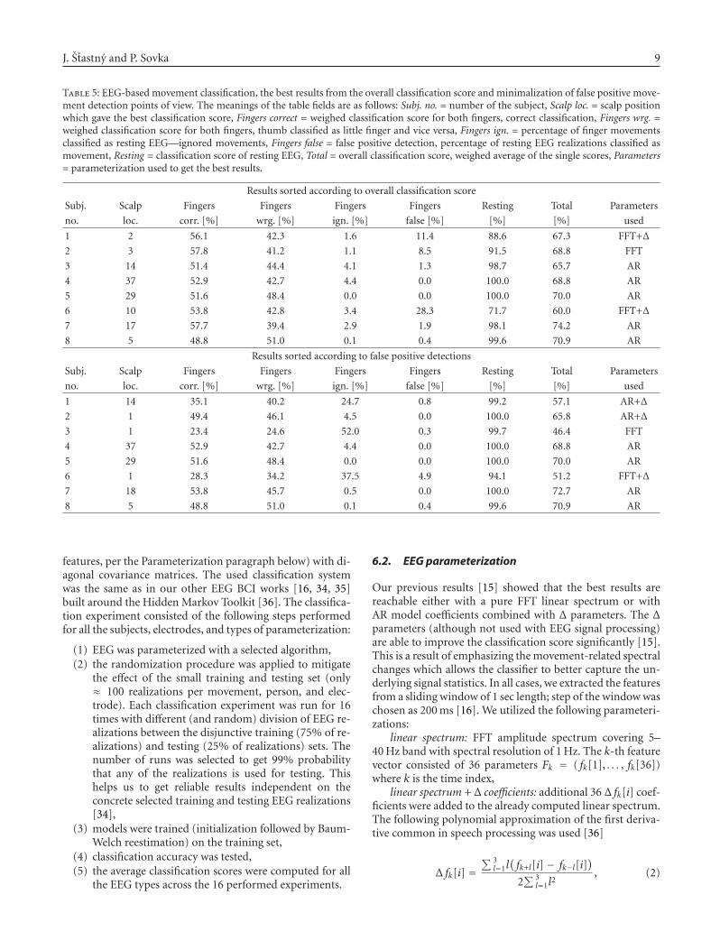
J. Stastny and P. Sovka 9
Table 5: EEG-based movement classification, the best results from the overall classification score and minimalization of false positive move-ment detection points of view. The meanings of the table fields are as follows: Subj. no. = number of the subject, Scalp loc. = scalp positionwhich gave the best classification score, Fingers correct = weighed classification score for both fingers, correct classification, Fingers wrg. =weighed classification score for both fingers, thumb classified as little finger and vice versa, Fingers ign. = percentage of finger movementsclassified as resting EEG—ignored movements, Fingers false = false positive detection, percentage of resting EEG realizations classified asmovement, Resting = classification score of resting EEG, Total = overall classification score, weighed average of the single scores, Parameters= parameterization used to get the best results.
Results sorted according to overall classification score
Subj. Scalp Fingers Fingers Fingers Fingers Resting Total Parameters
no. loc. corr. [%] wrg. [%] ign. [%] false [%] [%] [%] used
1 2 56.1 42.3 1.6 11.4 88.6 67.3 FFT+Δ
2 3 57.8 41.2 1.1 8.5 91.5 68.8 FFT
3 14 51.4 44.4 4.1 1.3 98.7 65.7 AR
4 37 52.9 42.7 4.4 0.0 100.0 68.8 AR
5 29 51.6 48.4 0.0 0.0 100.0 70.0 AR
6 10 53.8 42.8 3.4 28.3 71.7 60.0 FFT+Δ
7 17 57.7 39.4 2.9 1.9 98.1 74.2 AR
8 5 48.8 51.0 0.1 0.4 99.6 70.9 AR
Results sorted according to false positive detections
Subj. Scalp Fingers Fingers Fingers Fingers Resting Total Parameters
no. loc. corr. [%] wrg. [%] ign. [%] false [%] [%] [%] used
1 14 35.1 40.2 24.7 0.8 99.2 57.1 AR+Δ
2 1 49.4 46.1 4.5 0.0 100.0 65.8 AR+Δ
3 1 23.4 24.6 52.0 0.3 99.7 46.4 FFT
4 37 52.9 42.7 4.4 0.0 100.0 68.8 AR
5 29 51.6 48.4 0.0 0.0 100.0 70.0 AR
6 1 28.3 34.2 37.5 4.9 94.1 51.2 FFT+Δ
7 18 53.8 45.7 0.5 0.0 100.0 72.7 AR
8 5 48.8 51.0 0.1 0.4 99.6 70.9 AR
features, per the Parameterization paragraph below) with di-agonal covariance matrices. The used classification systemwas the same as in our other EEG BCI works [16, 34, 35]built around the Hidden Markov Toolkit [36]. The classifica-tion experiment consisted of the following steps performedfor all the subjects, electrodes, and types of parameterization:
(1) EEG was parameterized with a selected algorithm,(2) the randomization procedure was applied to mitigate
the effect of the small training and testing set (only≈ 100 realizations per movement, person, and elec-trode). Each classification experiment was run for 16times with different (and random) division of EEG re-alizations between the disjunctive training (75% of re-alizations) and testing (25% of realizations) sets. Thenumber of runs was selected to get 99% probabilitythat any of the realizations is used for testing. Thishelps us to get reliable results independent on theconcrete selected training and testing EEG realizations[34],
(3) models were trained (initialization followed by Baum-Welch reestimation) on the training set,
(4) classification accuracy was tested,(5) the average classification scores were computed for all
the EEG types across the 16 performed experiments.
6.2. EEG parameterization
Our previous results [15] showed that the best results arereachable either with a pure FFT linear spectrum or withAR model coefficients combined with Δ parameters. The Δparameters (although not used with EEG signal processing)are able to improve the classification score significantly [15].This is a result of emphasizing the movement-related spectralchanges which allows the classifier to better capture the un-derlying signal statistics. In all cases, we extracted the featuresfrom a sliding window of 1 sec length; step of the window waschosen as 200 ms [16]. We utilized the following parameteri-zations:
linear spectrum: FFT amplitude spectrum covering 5–40 Hz band with spectral resolution of 1 Hz. The k-th featurevector consisted of 36 parameters Fk = ( fk[1], . . . , fk[36])where k is the time index,
linear spectrum + Δ coefficients: additional 36 Δ fk[i] coef-ficients were added to the already computed linear spectrum.The following polynomial approximation of the first deriva-tive common in speech processing was used [36]
Δ fk[i] =∑ 3
l=1l(
fk+l[i]− fk−l[i])
2∑ 3
l=1l2, (2)
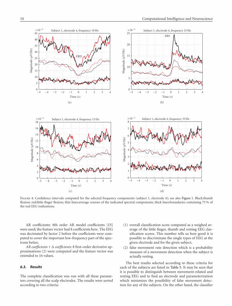
10 Computational Intelligence and Neuroscience
43210−1−2−3−4−5
Time (s)
0
5
10
15
20
25
30
35
40
45×10−3
Mag
nit
ude
(μV
/Hz)
Subject 1, electrode 4, frequency 10 Hz
ERD
(a)
43210−1−2−3−4−5
Time (s)
0
5
10
15
20
25×10−3
Mag
nit
ude
(μV
/Hz)
Subject 1, electrode 4, frequency 25 Hz
ERS
(b)
43210−1−2−3−4−5
Time (s)
0
2
4
6
8
10
12
14
16
18×10−3
Mag
nit
ude
(μV
/Hz)
Subject 1, electrode 4, frequency 15 Hz
(c)
43210−1−2−3−4−5
Time (s)
0
1
2
3
4
5
6
7
8×10⁻³
Mag
nit
ude
(μV
/Hz)
Subject 1, electrode 4, frequency 35 Hz
(d)
Figure 4: Confidence intervals computed for the selected frequency components (subject 1, electrode 4); see also Figure 1. Black:thumbflexion; red:little-finger flexion; thin lines:average courses of the indicated spectral components; thick lines:boundaries containing 75 % ofthe real EEG realizations.
AR coefficients: 8th order AR model coefficients [15]were used; the feature vector had 8 coefficients here. The EEGwas decimated by factor 2 before the coefficients were com-puted to cover the important low-frequency part of the spec-trum better,
AR coefficients + Δ coefficients: 8 first-order derivative ap-proximations (2) were computed and the feature vector wasextended to 16 values.
6.3. Results
The complete classification was run with all these parame-ters covering all the scalp electrodes. The results were sortedaccording to two criteria:
(1) overall classification score computed as a weighed av-erage of the little finger, thumb and resting EEG clas-sification scores. This number tells us how good it ispossible to discriminate the single types of EEG at thegiven electrode and for the given subject,
(2) false movement rate detection which is a probabilitymeasure of a movement detection when the subject isactually resting.
The best results selected according to these criteria foreach of the subjects are listed in Table 5. It may be seen thatit is possible to distinguish between movement-related andresting EEG and to find an electrode and parameterizationwhich minimizes the possibility of false movement detec-tion for any of the subjects. On the other hand, the classifier
J. Stastny and P. Sovka 11
was not able to distinguish between the thumb and little fin-ger EEG. Some of the movements are always ignored (lessthan 10%) recognizing them as resting EEG; however, thethumb—little finger discrimination—failed. Figure 3 withthe localization of the electrodes summarizes the best per-formances from the classification score point of view.
Subsequent analysis of the recognized movementsshowed that—although the mean values of the movement-related EEG spectra are significantly statistically different—the real time courses of the movement-related EEG are heav-ily buried in the non-movement related activity, see Figure 4.
7. CONCLUSIONS, NEXT STEPS
In this work, a detailed finger movement-related EEG sta-tistical analysis and result of classification experiment werepresented.
The movement-related EEG was analyzed in an indi-vidual way searching for as statistically significant phenom-ena as possible instead of the commonly used analysis ofthe strongest EEG component. This approach is in contrastwith the method used by [20, 21, 26] and others, where thestrongest ERDs and ERSs are found first and their statisticalsignificance is checked afterwards.
We found statistically significant differences betweenboth types of movement-related EEG signals. The differencesin the β and μERD parameters were present, although notvery important. More interestingly, we discovered signifi-cant differences in the βERS courses, their characters beinghighly individually dependent. These results are promisingfrom the classification point of view. No such results of fin-ger movement-related EEG analysis have been published yet.In addition to this, our analysis covered the whole EEG fre-quency band (5–30 Hz) and both sensorimotor areas extend-ing the results of [20], where only EEG recorded from C3/C4positions and only signal powers in 10–12 Hz, 16–20 Hz and20–24 Hz bands were examined.
Our classification paradigm was only partially succes-sful—we were able to distinguish the movement-related andresting EEG, but the movements were not distinguishedfrom each other. This was attributed to the fact that themovement-related spectral EEG courses are masked by otheron-going EEG activities not related to the movement. Thanksto the individual analysis results we believe it will be able toseparate and successfully classify both movements with thehelp of an advanced denoising approach.
In our recent work [37] we showed that it is possible toseparate movement-related EEG sources and non-movementrelated EEG activity with the help of the independent com-ponent analysis (ICA). Now we have been working on theintegration of an ICA-based denoising procedure into ourclassification system. This approach should help us to in-crease the classification score by means of EEG separationinto meaningful sources.
Next step will be to combine the developed method withthe left/right limb movement recognition to double the num-ber of recognized states—to increase the brain-computerchannel data rate.
ACKNOWLEDGMENTS
The authors thank Professor Andrej Stancak for his invalu-able comments and help. Further, they would like to thankJirı Vrana and Josef Mlynar for their help with data record-ing. In addition, grateful thanks go to all the experimentalsubjects. This work has been supported by the research pro-gram Transdisciplinary Research in Biomedical EngineeringII no. MSM6840770012 of the Czech Technical University inPrague.
REFERENCES
[1] L. Pickup, “Machine learning approaches for brain-computerinterfacing,” Tech. Rep. PARG-02-01, Pattern Analysis andMachine Leraning Group, Robotics Research Group, Depart-ment of engineering science, University of Oxford, Oxford,UK, May 2002.
[2] B. Blankertz, G. Dornhege, M. Krauledat, et al., “The Berlinbrain-computer interface: EEG-based communication with-out subject training,” IEEE Transactions on Neural Systems andRehabilitation Engineering, vol. 14, no. 2, pp. 147–152, 2006.
[3] W. D. Penny and S. J. Roberts, “Experiments with an EEG-based computer interface,” Tech. Rep., Department of Electri-cal Engineering, Imperial College, London, UK, July 1999.
[4] W. D. Penny, S. J. Roberts, and M. J. Stokes, “EEG-basedcommunication: a pattern recognition approach,” in Brain-Computer Interface Technology: Theory and Practice. First In-ternational Meeting, Rensselaerville, NY, USA, May 1999.
[5] A. Schlogl, K. Lugger, and G. Pfurtscheller, “Using adaptive au-toregressive parameters for a brain-computer interface equip-ment,” in Proceedings of the 19th International Conference of theIEEE Engineering in Medicine and Biology Society (EMBS ’97),pp. 1533–1535, Chicago, Ill, USA, October-Novermber 1997.
[6] C. W. Anderson, E. A. Stolz, and S. Shasunder, “Discrimi-nating mental tasks using EEG represented by AR model,” inProceedings of IEEE 17th Annual Conference on Engineering inMedicine and Biology Society (IEMBS ’95), vol. 2, pp. 875–876,Montreal, Quebec, Canada, September 1995.
[7] C. W. Anderson and Z. Sijercıc, “Classification of EEG sig-nals from four subjects during five mental tasks,” in Solv-ing Engineering Problems with Neural Networks: Proceedings ofthe Conference on Engineering Applications in Neural Networks(EANN ’96), pp. 407–414, Turku, Finland, June 1996.
[8] J. R. Wolpaw, N. Birbaumer, D. J. McFarland, G. Pfurtscheller,and T. M. Vaughan, “Brain-computer interfaces for communi-cation and control,” Clinical Neurophysiology, vol. 113, no. 6,pp. 767–791, 2002.
[9] J. R. Wolpaw, D. J. McFarland, and T. M. Vaughan, “Brain-computer interface research at the Wadsworth Center,” IEEETransactions on Rehabilitation Engineering, vol. 8, no. 2, pp.222–226, 2000.
[10] J. D. Bayllis and D. H. Ballard, “Recognizing evoked poten-tials in a virtual environment,” in Advances in Neural Informa-tion Processing Systems 12, vol. 12, pp. 3–9, Denver, Colo, USA,November-December 2000.
[11] G. Schalk, J. R. Wolpaw, D. J. McFarland, and G. Pfurtscheller,“EEG-based communication:presence of an error potential,”Clinical Neurophysiology, vol. 111, no. 12, pp. 2138–2144,2000.
12 Computational Intelligence and Neuroscience
[12] U. Hoffman, J.-M Versin, K. Deserens, and T. Ebrahimi, “Anefficient P300-based brain computer interface for disabledsubjects,” preprint, 2007, http://bci.epfl.ch/efficientp300bci.html.
[13] W. D. Penny, S. J. Roberts, and M. J. Stokes, “Imagined handmovements identified from the EEG μ-rhythm,” Tech. Rep.,Department of Electrical Engineering, Imperial College, Lon-don, UK, August 1998.
[14] D. J. McFarland, L. A. Miner, T. M. Vaughan, and J. R. Wolpaw,“μ and β rhythm topographies during motor imagery and ac-tual movements,” Brain Topography, vol. 12, no. 3, pp. 177–186, 2000.
[15] J. Stastny, J. Zejbrdlich, and P. Sovka, “Optimal parameteriza-tion selection for the brain-computer interface,” in Proceedingsof the 4th WSEAS International Conference of Applications ofElectrical Engineering , pp. 300–304, Prague, Czech Republic,March 2005.
[16] J. Stastny, P. Sovka, and A. Stancak, “EEG signal classification,”in Proceedings of the 23rd Annual International Conference ofthe IEEE Engineering in Medicine and Biology Society, vol. 2,pp. 2020–2023, Istanbul, Turkey, October 2001.
[17] J. Dolezal, J. Stastny, and P. Sovka, “Recognition of directionof finger movement from EEG signal using markov models,”in Proceedings of the 3rd European Medical&Biological Engi-neering Conference (EMBEC ’05), vol. 11, pp. 1492-1–1492-6,Prague, Czech Republic, November 2005.
[18] H. Ramoser, J. Muller-Gerking, and G. Pfurtscheller, “Opti-mal spatial filtering of single trial EEG during imagined handmovement,” IEEE Transactions on Rehabilitation Engineering,vol. 8, no. 4, pp. 441–446, 2000.
[19] P. Hlustık, A. Solodkin, R. P. Gullapalli, D. C. Noll, and S. L.Small, “Somatotopy in human primary motor and somatosen-sory hand representations revisited,” Cerebral Cortex, vol. 11,no. 4, pp. 312–321, 2001.
[20] G. Pfurtscheller, K. Zalaudek, and C. Neuper, “Event-relatedbeta synchronization after wrist, finger and thumb move-ment,” Electroencephalography and Clinical Neurophysiology -Electromyography and Motor Control, vol. 109, no. 2, pp. 154–160, 1998.
[21] A. Stancak, B. Feige, C. H. Lucking, and R. Kristeva-Feige,“Oscillatory cortical activity and movement-related potentialsin proximal and distal movements,” Clinical Neurophysiology,vol. 111, no. 4, pp. 636–650, 2000.
[22] A. Stancak and G. Pfurtscheller, “The effects of handednessand type of movement on the contralateral preponderanceof μ-rhythm desynchronisation,” Electroencephalography andClinical Neurophysiology, vol. 99, no. 2, pp. 174–182, 1996.
[23] A. Stancak, A. Riml, and G. Pfurtscheller, “The effects of ex-ternal load on movement-related changes of the senorimo-tor EEG rhythms,” Electroencephalography and Clinical Neu-rophysiology, vol. 102, no. 6, pp. 495–504, 1997.
[24] G. Pfurtscheller, A. Stancak, and C. Neuper, “Post-movementbeta synchronization: a correlate of an idling motor area?”Electroencephalography and Clinical Neurophysiology, vol. 98,no. 4, pp. 281–293, 1996.
[25] G. Pfurtscheller, A. Stancak, and G. Edlinger, “On the existenceof different types of central β rhythms below 30 Hz,” Electroen-cephalography and Clinical Neurophysiology, vol. 102, no. 4, pp.316–325, 1997.
[26] A. Stancak, “Event-related desynchronization of the μ-rhythmin extension and flexion finger movements,” in 11th Interna-tional Congress of Electromyography and Clinical Neurophysi-ology, Supplements to Clinical Neurophysiology, 53, pp. 636–650, Prague, Czech Republic, September 2000.
[27] H. J. Steingruber and G. A. Lieuert, Hand-Dominanztest,Hogrefe, 2nd edition, 1976.
[28] R. Srinivasan, “Methods to improve the spatial resolutionof EEG,” International Journal of Bioelectromagnetism, vol. 1,no. 1, pp. 102–111, 1999.
[29] G. Pfurtscheller, Digital Biosignal Processing, chapter 17, Else-vier Science, Amsterdam, The Netherlands, 2nd edition, 1991.
[30] B. Hjorth, “An on-line transformation of EEG scalp poten-tials into orhtogonal source derivations,” Electroencephalogra-phy and Clinical Neurophysiology, vol. 39, no. 5, pp. 526–530,1975.
[31] J. Stastny and P. Sovka, “The 3D surface Laplacian filtrationwith integrated sampling error compensation,” Signal Process-ing, vol. 87, no. 1, pp. 51–60, 2007.
[32] J. Uhlır and P. Sovka, Digital Signal Processing, Czech TechnicalUniversity, Prague, Czech Republic, 2nd edition, 2002.
[33] L. R. Rabiner, “A tutorial on hidden markov models and se-lected applications in speech recognition,” Proceedings of theIEEE, vol. 77, no. 2, pp. 257–286, 1989.
[34] J. Stastny, P. Sovka, and A. Stancak, “EEG signal classification:introduction to the problem,” Radioengineering, vol. 12, no. 3,pp. 51–55, 2003.
[35] J. Stastny, P. Sovka, and A. Stancak, “EEG signal classificationand segmentation by means of hidden markov models,” inProceedings of 16th Biennial International EURASIP Conferenceon Analysis of Biomedical Signals and Images (BIOSIGNAL ’02),pp. 415–417, Brno, Czech Republic, June 2002.
[36] S. J. Young, HTK Reference Manual, Cambridge University En-gineering Department, Cambridge, UK, 1993.
[37] O. Konopka, J. Stastny, and P. Sovka, “Movement-related EEGseparation using independent component analysis,” in Pro-ceedings of the 3rd European Medical & Biological EngineeringConference (EMBEC ’05) , vol. 11, pp. 1471-1–1471-6, Prague,Czech Republic, Novermber 2006.