bioluminescence estimation from ocean in situ irradiances

Bioluminescence estimation from ocean in situirradiances

H. C. Yi, R. Sanchez, and N. J. McCormick

An algorithm is developed for estimating the spatial location and magnitude of a bioluminescent radiationsource from measurements of the in situ irradiance and scalar irradiance at two depths. The algorithm isbased on the principle of photon conservation. The most direct application of the algorithm requires thatthe absorption coefficient be known, but the algorithm is useful even if that coefficient is unknown.Numerical tests and an error analysis have been done to test the algorithm numerically. In addition weshow that if the estimated source magnitude is nearly constant, that value can be used to estimate thevertical attenuation coefficient of the radiation field.

Key words: Ocean optics, bioluminescence, radiative transfer.

I. Introduction

One difficulty in estimating bioluminescence at agiven wavelength in seawater is that of separating outthe signal of interest from that of the inherent lightfield arising from moonlight, for example; both arepart of the radiance. A second difficulty is that thebioluminescence varies strongly with depth. Gor-don'2 has performed Monte Carlo calculations todetermine the upward irradiance at the surface causedby a single bioluminescent point source of unitstrength at some depth and horizontal distance awayfrom the detector. His calculations were done as afunction of different concentrations of phytoplanktonfor the idealized case of homogeneous seawater. Suchan approach can treat the problem of a localizedbioluminescent source but is not amenable to ageneralized distributed source, such as with a super-position of point sources of different magnitudes anddepths, without knowing a priori the position coordi-nates of the distributed sources (as is done fordepth-dependent atmospheric temperature estima-tions).

While schemes have been proposed for the measure-ment of individual marine particulates by an in situsampling technique,3 the approach here is to focus onthe assessment of bioluminescence by using in situirradiance and scalar irradiance measurements as a

The authors are with the Department of Nuclear Engineering,University of Washington, Seattle, Washington 98195.

Received 30 August 1990.0003-6935/92/060822-09$05.00/0.© 1992 Optical Society of America.

function of depth, which is more in the mannersuggested by Swift et al.4

The algorithm is based on the photon conservationequation that is formally exact, but its implementa-tion requires an approximation to estimate either thederivative of the irradiance or an integral involvingthe scalar irradiance. The algorithm can be applied indifferent ways depending on whether the absorptioncoefficient is known. Our purpose is to demonstratethat the algorithm is sensitive enough to consider forimplementation in a variety of simulated ocean condi-tions.

In certain conditions an estimate of the biolumines-cent source magnitude can also be used to estimatethe vertical attenuation coefficient of the radiation.This can be done if the source magnitude is relativelyconstant and if the radiance can be assumed to be inthe diffusion regime.

The algorithm for estimating the source is pre-sented in Section II, and the model of the seawaterproperties is presented in Section III. Results ofnumerical tests on the algorithm are in Section IV,and equations and numerical tests for estimating thevertical attenuation coefficient are in Section V.

Two models are considered for the bioluminescentsource for the numerical tests. When the source isproduced by mechanical agitation (such as eddies orcurrents), the optical properties of the source layersare not different from those for layers without sources.This enables the source magnitude to be estimatedwith only the source-free seawater properties. On theother hand, if the bioluminescence is produced by thedrift-in of additional particles that emit radiation, thenew particles alter the optical properties, and at least

822 APPLIED OPTICS / Vol. 31, No. 6 / 20 February 1992

two scans of the measured data must be made: thefirst to locate the presence of the source particles andthe second to estimate the source magnitude.

II. Algorithm

We consider seawater in a stratified plane geometryfor which L (z, ) is the azimuthally symmetric radi-ance at the wavelength of interest, z is the depthmeasured from the surface, and p. is the cosine of thepolar angle defined with respect to the nadir direc-tion. It is assumed that the bioluminescence is isotro-pic in all directions and that any external illumina-tion is uniform over the sea surface. Although thebioluminescent source is not constant in time, itsduration is much longer than the average photonlifetime in seawater. The azimuthally integrated radi-ance thus satisfies the steady-state radiative transferequation

pLaL(z, li) + cL(z, pl) = b fP(ii, i')L(z, p.')dp' + Q(z)/2, (1)

where Q (z) is the rate per unit volume at whichphotons at the implicit wavelength and depth z areisotropically produced by bioluminescence. The ab-sorption coefficient a and the scattering coefficient bare the probabilities per unit distance of travel that aphoton will be absorbed and scattered, respectively,and c = (a + b) is the beam attenuation coefficient.Also, the azimuthally integrated scattering phasefunction P (p, p.') is normalized so that its expansionin Legendre polynomials has the form

1N2 p W -o I 2 ) Unn ()Pn (u), fo = 1 (2)

The radiation at any depth consists of that from thebioluminescent source distribution LQ (z, ) plus thatfrom incident radiation at the atmosphere-sea sur-face interface yL(z, p.). Thus

L(z, ) = L'(z, p') + yL'(z, p2), (3)

where y is the dimensionless ratio of the magnitude ofthe sea surface illumination per unit area to thevertically integrated bioluminescent source strength.Thus when y > 0 there is nighttime illumination ofthe surface that can be simulated, for example, withthe boundary conditions

L'(0, pL) = V5(p - 0 )4ip,, 0 < p. < 1 (4a)

or

L'(0, 1i) = 2, < < 1 (4b)

which correspond to a monodirectional or isotropicillumination, respectively; here

= f Q (z)dz.

The integral of the radiative transfer equation overp., i.e., the photon conservation equation, gives

Q(z) = E(z) + aE0(z), (5)

where

E(z) = F_ L (z, p) pdp,

E,(z) = f , L (z, I.Odp,

are the irradiance and scalar irradiance, respectively,that depend on Q (z) and the external illuminationincident on the sea surface. It may be noted that ifQ(z) = 0, Eq. (5) reduces to the so-called Gershunrelation:

a = -azE(z)1E(z). (6)

The procedure for using Eq. (5) to estimate Q(z)depends on whether the absorption coefficient isknown.

A. Algorithm for a Known Absorption Coefficient

There are two ways in which Eq. (5) can be imple-mented with measurements of E (zn) and EO (zn) atdepths zn: by either a discrete point or an integralapproximation. For the simplest discrete-point ap-proach, the term a.E(z) can be approximated by atwo-point forward formula to give an estimate ofQ(zn) from

Q(zn) = [E(zn+1 ) -E(n)]I(zn+ -zn) + aEo(z). (7a)

In the integral approach, one integrates Eq. (5) fromzn to Zn1, and approximates the term

aEo (z)dz.

By assuming that a is constant within the region zn toZn1 , the simplest estimate of the average value of thesource Q (zn, Zn +) can be obtained from

Q(zn, Zn+1) = [E(zn+)- E(z)]/(zn+ - J)

+ (a/2)[Eo(zn+1 ) + Eo(z)]. (7b)

If a higher-order Lagrangian interpolate based onmore than two points is used to approximate eitherazE(z) or the integral of aE,(z), different forms forEqs. (7a) and (7b) are obtained. However, since suchhigher-order interpolates can lead to negative valuesor oscillations, we restrict ourselves to the case where(Zn+l - zn) is small enough that adjacent measure-ment points give a good approximation.

A discussion of the errors arising from the use ofthe algorithm is given in Appendix A.

20 February 1992 / Vol. 31, No. 6 / APPLIED OPTICS 823

B. Algorithm for an Unknown Absorption Coefficient

In this case one can still infer the presence of a sourceand estimate its minimum magnitude by using theconstraint that Q (z) 0. This is done by firstscanning the ratio of - aE(z)/E0(z) to estimate theminimum value of the absorption coefficient amin(z)corresponding to source-free seawater from

am,(z) = max[0, -E(z)1E,(z)], (8)

which can also be written as

amjn(z) = max[0, a(z) - Q(z)1E,(z)]. (9)

Hence amin(z) equals the actual absorption coefficientin regions where there is no source, while amin(z) <a(z) in the presence of a source. If the region locallyproduces more photons than are lost by absorption,amin(z) = 0 and azE(z) > 0, while if there is locally anetloss,a(z) > amin(z) > and E(z) < 0.

In practice Eq. (8) can be used to obtain an estimatedmin(z). If dmin(z) = 0, there must be a source present.When dmin(z) > 0, it is necessary to examine the globalbehavior of dmin(Z) to obtain the value to be used toestimate Q (z).

III. Model for the Seawater

A multilayer model for the bioluminescent source wasassumed in which the near-surface and deepest layerswere seawater and a layer between contained aspatially varying bioluminescent source. The seawa-ter was assumed to consist of pure water and one typeof particle of the type measured at 530 nm by Petzoldat station 2240 in the San Diego harbor.5 The beamattenuation coefficient was taken to be Cs = a, +bSD= c + cp, for which aD =0.125 m-' and bD =1.205 m. We assumed that the bioluminescentsource arises either from all particles in the seawateremitting radiation because they are stimulated bymechanical agitation or from the drift-in of newparticles that emit radiation. Both cases for thebioluminescence can be modeled with an equation forthe beam attenuation coefficient given by

c = c + (1 + k)cp,

= (1 + k)csD - kc,. (10)

When the particle parameter k = 0 the biolumines-cence comes from mechanical agitation of the parti-cles, and when k > 0 the source comes from thefraction k(l + k) of all particles that bioluminesce.The scattering coefficient b corresponding to Eq. (10)is

b = (1 + k)bS - kbw, (11)

where bSD= b + bp.For pure water at 530 nm, a = 0.0518 m-' and

b = 0.0023 m'1 and the Rayleigh phase function Pw

was used2 :

P(0) = P,(900 )(1 + 0.835 Cos2 0), (12)

for which the expansion coefficients in Eq. (2) arefw = 1, fw2 = 0.0871, and fw,, = 0 otherwise. For theSan Diego seawater, the phase function was repre-sented with a delta-Eddington model:

PSD(.IL, ) = (XSD8(4L - p.') + [(1 - %sD)/2 ]

x E (2n + 1) fSD.Pf(.)Pf(P.'), 0 < aSD < 1.n=0

(13)

The advantage of such a model is that the apparentdegree of scattering anisotropy N is considerably lessthan N; values of a-SD = 0.23 and SD, are given in Ref.6.

As a consequence of the use of the delta-Eddingtonmodel for the particles,

ba = (1 + k)bSDSD, I

b(1 - t)fn = (1 + k)bsD(1 - aSD)fsD - kbf

(14)

(15)

With these variables the radiative transfer equationcan be written as

pa.O,.L(z*, p.) + L(z*, p.) = (b*Ic*)

x fJ P* (p, p.')L(z*, p.')dp' + Q(z*)12c*, (16)

where z* = zc*, c* = c - ba, b* = b - ba, and

, N

P * (p W ) = I (2n + 1) fnPn (p])Pn (' )-2 =o

(17)

IV. Results of the Numerical TestsThe irradiances and scalar irradiances used to testthe algorithms of Eq. (7) were calculated with the FNmethod7'8 for simulated nighttime conditions withseveral values of y. It was assumed that the spacingbetween measurements (Az) could be either 1 m, 2 m,or a greater depth and that the incident illuminationat the sea surface was either zero or monodirectional,as in Eq. (4a), with p. = 0.866; in all cases theintegrated bioluminescent source strength was nor-malized so that q = 1 and Eq. (7b) was used for thealgorithm unless otherwise stated. We considered theseawater to be deep enough that the bottom effectswere negligible. Also, the value of the particle param-eter k was set equal to 0 (for mechanical agitation),0.05 (for intuitively what one can expect), or 3 (for anextreme change in the seawater properties). Com-pared with the case of k = 0, the percentage increasesin the absorption coefficients for k = 0.05 and 3 are2.9 and 176, respectively.

To test the algorithm two source distributions wereconsidered that consisted of a superposition of para-bolically shaped profiles that could be summed witharbitrary weights wi (which sum to unity) for the


fractional area underneath each parabola. The firstseries of numerical tests was performed for San Diegoseawater located at 0 m < z < 5 m and z 2 25 m witha uniform mixture of seawater and particles at 5 m <z < 25 m containing a nonuniformly shaped biolumi-nescent source: bioluminescent source 1 consisted ofsource parabola 1 at 9 m < z < 11 m with a weightW = 0.3, parabola 2 at 16 m < z < 18 m with w2 =-0.05, and parabola 3 at 5 m < z < 25 m with W 3 =

0.75. (A profile similar in shape to source 1 has beenobserved for daytime polychromatic biolumines-cence.9) The second series of tests was done for auniform mixture of seawater and particles between 9m < z < 11 m and 16 m < z < 18 m and San Diegoseawater everywhere else: bioluminescent source 2consisted of a superposition of source parabola 1 withW = 0.8 and parabola 2 with w2 = 0.2. (This sourcewas constructed to test whether the small sourcepeak could be detected beneath a big one.)

For the calculations it was assumed that the magni-tude of the source strength is sufficiently large thatthe bioluminescent signal itself is not noisy. Unlessthe bioluminescent source is strong, however, thereare fluctuations that can be simulated by assumingrandom variations in the measured signals. We willinvestigate later the effects of these fluctuations (andthose from the detectors themselves), but initially weconsider the case of noise-free measurements.

A. Mechanical Agitation (k = 0)

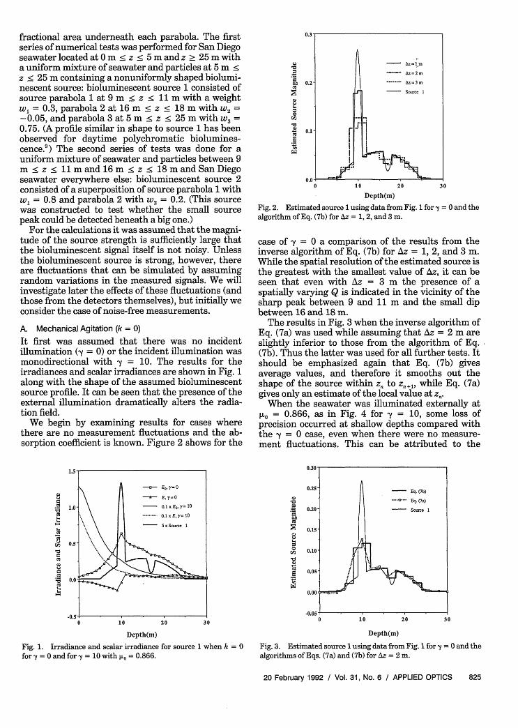
It first was assumed that there was no incidentillumination (y = 0) or the incident illumination wasmonodirectional with y = 10. The results for theirradiances and scalar irradiances are shown in Fig. 1along with the shape of the assumed bioluminescentsource profile. It can be seen that the presence of theexternal illumination dramatically alters the radia-tion field.

We begin by examining results for cases wherethere are no measurement fluctuations and the ab-sorption coefficient is known. Figure 2 shows for the

1.5-

10 - EO, = 10= \ I ^ ~~~~~.E,r1O.r 1.0 \ |~~~~~~...... 0.1 x E, Y= lo

5- S -~uc 1

-0.5-0 lo0 2 0 3 0

Depth(m)

Fig. 1. Irradiance and scalar irradiance for source 1 when k = 0for y = 0 and for y = 10 with p.0 = 0.866.

0.2 *- - Az= 3 m

0.00 lo 20 30

Depth(m)

Fig. 2. Estimated source using data from Fig. 1 for y = and thealgorithm of Eq. (7b) for Az = 1, 2, and 3 m.

case of y = a comparison of the results from theinverse algorithm of Eq. (7b) for Az = 1, 2, and 3 m.While the spatial resolution of the estimated source isthe greatest with the smallest value of z, it can beseen that even with Az = 3 m the presence of aspatially varying Q is indicated in the vicinity of thesharp peak between 9 and 11 m and the small dipbetween 16 and 18 m.

The results in Fig. 3 when the inverse algorithm ofEq. (7a) was used while assuming that Az = 2 m areslightly inferior to those from the algorithm of Eq.(7b). Thus the latter was used for all further tests. Itshould be emphasized again that Eq. (7b) givesaverage values, and therefore it smooths out theshape of the source within z to zn,,,, while Eq. (7a)gives only an estimate of the local value at z,

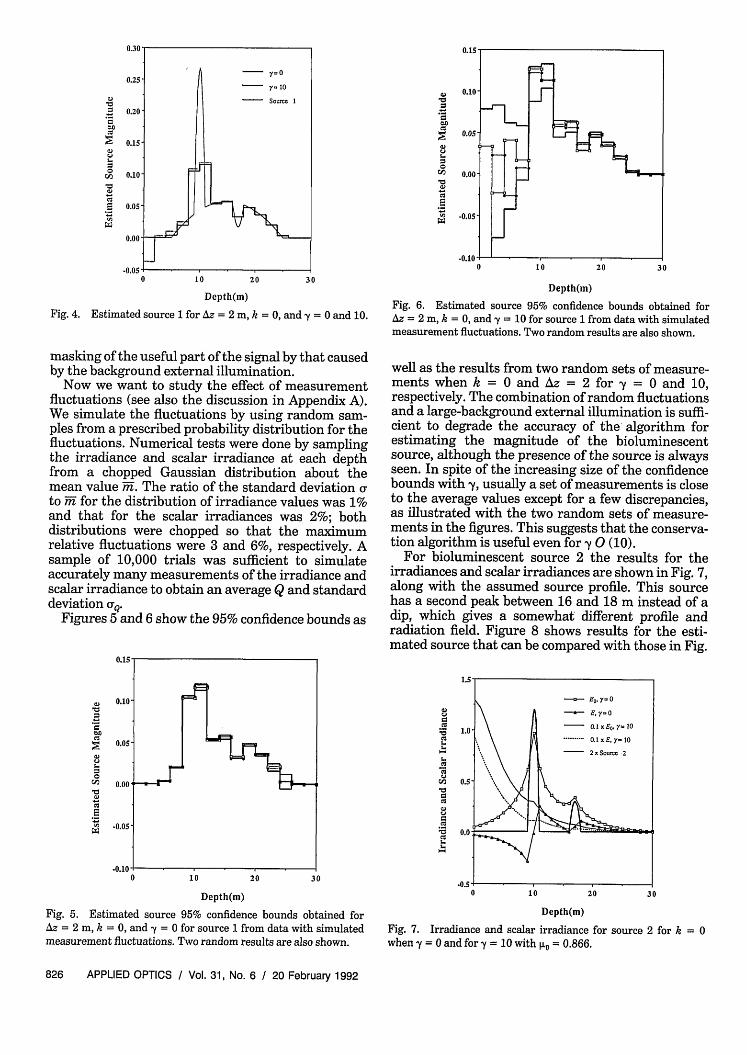
When the seawater was illuminated externally atVt = 0.866, as in Fig. 4 for y = 10, some loss ofprecision occurred at shallow depths compared withthe y = case, even when there were no measure-ment fluctuations. This can be attributed to the

0.30

0.2s- Eq. (7b)

20 l *--- - | ~~~Eq. (7a)

015S

-0.05'0 10 20 30

Depth(m)

Fig. 3. Estimated source 1 using data from Fig. 1 for y = 0 and thealgorithms of Eqs. (7a) and (7b) for Az = 2 m.


- Source I0.20

0.15

0.10

ci0.100 '0.05

0.00

0 10 20 30

Depth(m)

Fig. 4. Estimated source 1 for Az = 2 m, k = 0, andy = 0 and 10.

masking of the useful part of the signal by that causedby the background external illumination.

Now we want to study the effect of measurementfluctuations (see also the discussion in Appendix A).We simulate the fluctuations by using random sam-ples from a prescribed probability distribution for thefluctuations. Numerical tests were done by samplingthe irradiance and scalar irradiance at each depthfrom a chopped Gaussian distribution about themean value i. The ratio of the standard deviation uto m for the distribution of irradiance values was 1%and that for the scalar irradiances was 2%; bothdistributions were chopped so that the maximumrelative fluctuations were 3 and 6%, respectively. Asample of 10,000 trials was sufficient to simulateaccurately many measurements of the irradiance andscalar irradiance to obtain an average Q and standarddeviation Q.

Figures 5 and 6 show the 95% confidence bounds as

0.05

-0.100 1 0 2 0 3 0

Depth(m)

Fig. 5. Estimated source 95% confidence bounds obtained forAz = 2 m, k = O. and = for source from data with simulatedmeasurement fluctuations. Two random results are also shown.

.00'a,

-0.05

-0.10, _ . , -0 1 0 2 0 3 0

Depth(m)

Fig. 6. Estimated source 95% confidence bounds obtained forAz = 2 m, k = O. andy = 10 for source 1 from data with simulatedmeasurement fluctuations. Two random results are also shown.

well as the results from two random sets of measure-ments when k = and Az = 2 for y = and 1 0,respectively. The combination of random fluctuationsand a large-background external illumination is suffi-cient to degrade the accuracy of the'algorithm forestimating the magnitude of the bioluminescentsource, although the presence of the source is alwaysseen. In spite of the increasing size of the confidencebounds withya, usually a set of measurements is closeto the average values except for a few discrepancies,as illustrated with the two random sets of measure-ments in the figures. This suggests that the conserva-tion algorithm is useful even for y (10).

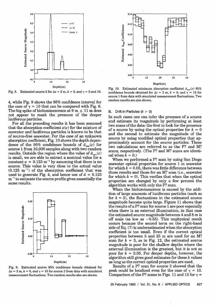
For bioluminescent source 2 the results for theirradiances and scalar irradiances are shown in Fig. 7,along with the assumed source profile. This sourcehas a second peak between 16 and 18 m instead of adip, which gives a somewhat different profile andradiation field. Figure 8 shows results for the esti-mated source that can be compared with those in Fig.

clcC)

It'I

._

C..

CSc2

'a

cuCS

C:

Cu

..

30

Depth(m)

Fig. 7. Irradiance and scalar irradiance for source 2 for k = 0when y = 0 and for y = 10 with I.L = 0.866.


'a

c:

so

c)

0

'a

C)

C's

.

ut

ln

0 10 20 30

Depth(m)

Fig. 8. Estimated source 2 for Az = 2 m, k = 0, and y = 0 and 10.

4, while Fig. 9 shows the 95% confidence interval forthe case of y = 10 that can be compared with Fig. 6.The big spike of bioluminescence at 9 m < 11 m doesnot appear to mask the presence of the deeperluciferous particles.

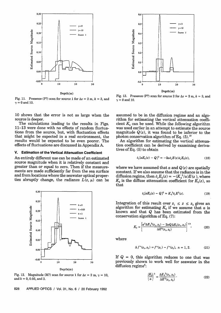
For all the preceding results it has been assumedthat the absorption coefficient a(z) for the mixture ofseawater and luciferous particles is known to be thatof source-free seawater. For the case of an unknownabsorption coefficient, Fig. 10 shows the depth depen-dence of the 95% confidence bounds of dmn(z) forsource 1 from 10,000 samples along with two randomresults. Outside the region where the value of dmin(Z)

is small, we are able to extract a nominal value for aconstant a = 0.123 m-l by assuming that there is nosource. This value is very close to the actual value(0.125 m-') of the absorption coefficient that wasused to generate Fig. 4, and hence use of d = 0.123m' to estimate the source profile gives essentially thesame results.

a

c)

*2

soE

._

0

CS

0.20 - C

0.10

0.00 I L

10 . 2

10 200 30

Depth(m)

Fig. 9. Estimated source 95% confidence bounds obtained forAz = 2 m, k = 0, andy = 10 for source 2 from data with simulatedmeasurement fluctuations. Two random results also are shown.

"IC)C)

E

<S

CS

2Cal

WE

Depth(m)

Fig. 10. Estimated minimum absorption coefficient dmi(z) 95%confidence bounds obtained for Az = 2 m, k = 0, and y = 10 forsource 1 from data with simulated measurement fluctuations. Tworandom results are also shown.

B. Drift-In Particles (k > 0)

In such cases one can infer the presence of a sourceand estimate its magnitude by performing at leasttwo scans of the data: the first to look for the presenceof a source by using the optical properties for k = 0and the second to estimate the magnitude of thesource by using modified optical properties that ap-proximately account for the source particles. Thesetwo calculations are referred to as the P? and M?scans, respectively. (The P? and M? scans are identi-cal when k = 0.)

When we performed a P? scan by using San Diegoseawater optical properties for source 1 in seawaterfor which k = 0.05, there was little difference betweenthose results and those for an M? scan (i.e., seawaterfor which k = 0). This verifies that when the opticalproperties are changed by only a few percent thealgorithm works with only the P? scan.

When the bioluminescence is caused by the addi-tion of large amounts of luciferous particles (such asfor k = 3), the fluctuations in the estimated sourcemagnitude become quite large. Figure 11 shows thatthe results of a P? scan for source 1 are poor especiallywhen there is an external illumination; in that casethe estimated source magnitude between 4 and 8 m isoff scale (as low as -0.55). This unphysical resultoccurs because the second term on the right-handside of Eq. (7) is underestimated when the absorptioncoefficient is too small. Even if the correct opticalproperties between 5 and 25 m are used for an M?scan for k = 3, as in Fig. 12, the estimated sourcemagnitude is poor for the shallow depths where theexternal illumination is the greatest, but it is not sopoor for k = 0.05. For deeper depths, however, thealgorithm still gives good estimates for these k valuesas long as the correct optical properties are used.

Results of a P? scan for source 2 showed that thepeak could be localized even for the case of y = 10.Comparison of the P? scans in Figs. 11 and 13 for y =


.

-u.u

- r100.20 - soure 1

CS ~ ~ ~ ~ ~ ~~O

0.15

.0

-0.050.1 20 30

Depth(m)

Fig. 1 1. Presence (P?) scan for source for z =2 m, k =3, and-y = and 10.

0.4- Soue

C

0.3-c)

0C2

0.1 _0.0

0 10 20

Depth(m)

Fig. 13. Presence (P?) scan for source 2 for Azy = O and 10.

10 shows that the error is not as large when thesource is deeper.

The calculations leading to the results in Figs.11-13 were done with no effects of random fluctua-tions from the source, but, with fluctuation effectsthat might be expected in a real environment, theresults would be expected to be even poorer. Theeffects of fluctuations are discussed in Appendix A.

V. Estimation of the Vertical Attenuation Coefficient

An entirely different use can be made of an estimatedsource magnitude when it is relatively constant andgreater than or equal to zero. Then if the measure-ments are made sufficiently far from the sea surfaceand from locations where the seawater optical proper-ties abruptly change, the radiance L (z, ji) can be

assumed to be in the diffusion regime and an algo-rithm for estimating the vertical attenuation coeffi-cient Ko can be used. While the following algorithmwas used earlier in an attempt to estimate the sourcemagnitude Q(z), it was found to be inferior to thephoton conservation algorithm of Eq. (5).1O

An algorithm for estimating the vertical attenua-tion coefficient can be derived by examining deriva-tives of Eq. (5) to obtain

a[aEo(z) - Q] = -2aO0 E(z)a0 EO(z), (18)

where we have assumed that a and Q (z) are spatiallyconstant. If we also assume that the radiance is in thediffusion regime, then Eo (z) = - (K0

2/a)E (z ), whereK0 is the diffuse attenuation coefficient for E,(z), sothat

10 20 30

Depth(m)

a [aE0 (z) - Q= - K, 2 E2(Z) (19)

Integration of this result over z1 < z < z gives analgorithm for estimating K0 if we assume that a isknown and that Q has been estimated from theconservation algorithm of Eq. (7):

ra2A2(zi, Z2 ) - 2aQAE((z), Z) 1/2Io = AE(z1, 2) ' (20)

where

A f(Z 1, Z2) = f(Z 1) -f (Z2), n = 1, 2. (21)

If Q = 0, this algorithm reduces to one that waspreviously shown to work well for seawater in thediffusion regimes:

Fig. 12. Magnitude (M?) scan for source 1 for Azand k = 0, 0.05, and 3.

= 2 m, y = 10,


30

= 2 m, k = 3, and

0C)

'a

so.

0

c:C1)

c2

Ko 2 AE 2(z Z2)

\a) AE2 (z1 , Z2) (22)

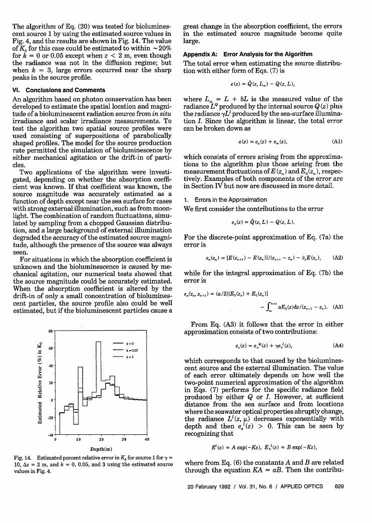
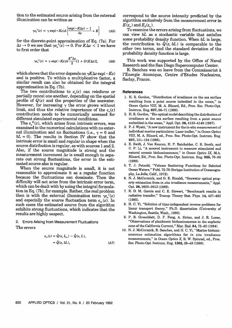
The algorithm of Eq. (20) was tested for biolumines-cent source 1 by using the estimated source values inFig. 4, and the results are shown in Fig. 14. The valueof K0 for this case could be estimated to within 20%for k = 0 or 0.05 except when z < 2 m, even thoughthe radiance was not in the diffusion regime; butwhen k = 3, large errors occurred near the sharppeaks in the source profile.

VI. Conclusions and Comments

An algorithm based on photon conservation has beendeveloped to estimate the spatial location and magni-tude of a bioluminescent radiation source from in situirradiance and scalar irradiance measurements. Totest the algorithm two spatial source profiles wereused consisting of superpositions of parabolicallyshaped profiles. The model for the source productionrate permitted the simulation of bioluminescence byeither mechanical agitation or the drift-in of parti-cles.

Two applications of the algorithm were investi-gated, depending on whether the absorption coeffi-cient was known. If that coefficient was known, thesource magnitude was accurately estimated as afunction of depth except near the sea surface for caseswith strong external illumination, such as from moon-light. The combination of random fluctuations, simu-lated by sampling from a chopped Gaussian distribu-tion, and a large background of external illuminationdegraded the accuracy of the estimated source magni-tude, although the presence of the source was alwaysseen.

For situations in which the absorption coefficient isunknown and the bioluminescence is caused by me-chanical agitation, our numerical tests showed thatthe source magnitude could be accurately estimated.When the absorption coefficient is altered by thedrift-in of only a small concentration of biolumines-cent particles, the source profile also could be wellestimated, but if the bioluminescent particles cause a

8'0 -.

CS ~~~~~~~~k=0.060' ----- k =00

k=3

~40

20

-;

-4

0 20 20 30 40

Depth(m)

Fig. 14. Estimated percent relative error in Kofor sourelfory =10, Az = 2 m, and k = O. 0.06, and 3 using the estimated sourcevalues in Fig. 4.

great change in the absorption coefficient, the errorsin the estimated source magnitude become quitelarge.

Appendix A: Error Analysis for the Algorithm

The total error when estimating the source distribu-tion with either form of Eqs. (7) is

e(z) = Q(z, Lm) - Q(z, L),

where Lm = L + L is the measured value of theradiance LQ produced by the internal source Q (z) plusthe radiance yL' produced by the sea-surface illumina-tion 1. Since the algorithm is linear, the total errorcan be broken down as

e (Z) = ea(z) + em(z), (Al)

which consists of errors arising from the approxima-tions to the algorithm plus those arising from themeasurement fluctuations of E (z0. ) and E0(zj), respec-tively. Examples of both components of the error arein Section IV but now are discussed in more detail.

1. Errors in the Approximation

We first consider the contributions to the error

e.(z) = Q(z,L) - Q(z,L).

For the discrete-point approximation of Eq. (7a) theerror is

ea(zn) = [E(zn+1) - E(zn)]I(zn+1 - z,) - OE(zA), (A2)

while for the integral approximation of Eq. (7b) theerror is

ea(zn, zn+i) = (aI2)[E0(z.) + E(zn)]

- f aE0(z)dz/(zn+1 - zn). (A3)

From Eq. (A3) it follows that the error in eitherapproximation consists of two contributions:

ea(Z) = eaQ(z) + yeaW(z), (A4)

which corresponds to that caused by the biolumines-cent source and the external illumination. The valueof each error ultimately depends on how well thetwo-point numerical approximation of the algorithmin Eqs. (7) performs for the specific radiance fieldproduced by either Q or I. However, at sufficientdistance from the sea surface and from locationswhere the seawater optical properties abruptly change,the radiance L'(z, p.) decreases exponentially withdepth and then ea(z) > 0. This can be seen byrecognizing that

E'(z) = A exp(-Kz), E,1 (z) B exp(-Kz),

where from Eq. (6) the constants A and B are relatedthrough the equation KA = aB. Then the contribu-


tion to the estimated source arising from the externalillumination can be written as

,yea'(z) exp(-Kz)A [ Az) + K] (AS)

for the discrete-point approximation of Eq. (7a). ForAz - 0 we see that yea'(z) -> 0. For KAz < 1 we haveto first order that

'(z) Sy exp(-Kz)A z2 [1 + O(KAz)], (A6)

which shows that the error depends on yKAz exp(-Kz)and is positive. To within a multiplicative factor, asimilar result can also be obtained for the integralapproximation in Eq. (7b).

The two contributions to e(z) can reinforce orpartially cancel one another, depending on the spatialprofile of Q (z) and the properties of the seawater.However, for increasing y the error grows withoutlimit, and thus the relative importance of the ea(z)contribution needs to be numerically assessed fordifferent simulated experimental conditions.

The eaQ (z), which arises from intrinsic errors, wasexamined in the numerical calculations with no exter-nal illumination and no fluctuations (i.e., y = 0 and6L = 0). The results in Section IV show that theintrinsic error is small and regular in shape when thesource distribution is regular, as with sources 1 and 2.Also, if the source magnitude is strong and themeasurement increment Az is small enough to sepa-rate out strong fluctuations, the error in the esti-mated source also is regular.

When the source magnitude is small, it is notreasonable to approximate it as a regular functionbecause the fluctuations can dominate. Then thedifficulty will not arise from the intrinsic error term,which can be dealt with by using the integral formula-tion in Eq. (7b), for example. Rather, the real problemthen is with the external illumination term yea'(z)and especially the source fluctuation term em (z). Insuch cases the estimated source from the algorithmexhibits strong fluctuations, which indicates that theresults are highly suspect.

2. Errors Arising from Measurement Fluctuations

The errors

em(z) = Q(zLm) -Q(z,L),

= Q(z, L), (A7)

correspond to the source intensity predicted by thealgorithm exclusively from the measurement error inE (zn ) and E0 (zn ).

To examine the errors arising from fluctuations, wecan view L as a stochastic variable that satisfiessome probability density function. When L is large,the contribution to Q(z, L) is comparable to theother two terms, and the standard deviation of theprobability density function is large.

This work was supported by the Office of NavalResearch and the San Diego Supercomputer Center.

R. Sanchez was on leave from the Commissariat al'Energie Atomique, Centre d'Etudes Nucleaires,Saclay, France.

References1. H. R. Gordon, "Distribution of irradiance on the sea surface

resulting from a point source imbedded in the ocean," inOcean Optics VIII, M. A. Blizard, Ed., Proc. Soc. Photo-Opt.Instrum. Eng. 637,66-71 (1986).

2. H. R. Gordon, "Bio-optical model describing the distribution ofirradiance at the sea surface resulting from a point sourceembedded in the ocean," Appl. Opt. 26, 4133-4148 (1987).

3. P. J. Wyatt, "A new instrument for the in-situ measurement ofindividual marine particulates: Laser troller," in Ocean OpticsVIII, M. A. Blizard, ed., Proc. Soc. Photo-Opt. Instrum. Eng.637, 131-134 (1986).

4. E. Swift, J. Van Keuren, H. P. Batchelder, C. R. Booth, andC. P. Li, "A moored instrument to measure stimulated andnatural oceanic bioluminescence," in Ocean Optics IX, M.A.Blizard, Ed., Proc. Soc. Photo-Opt. Instrum. Eng. 925, 76-86(1988).

5. T. J. Petzold, "Volume Scattering Functions for SelectedOcean Waters," Publ. 72-78 (Scripps Institution of Oceanogra-phy, La Jolla, Calif., 1972).

6. N. J. McCormick, and G. E. Rinaldi, "Seawater optical prop-erty estimation from in situ irradiance measurements," Appl.Opt. 28, 2605-2613 (1989).

7. R. D. M. Garcia and C. E. Siewert, "Benchmark results inradiative transfer," Transp. Theory Stat. Phys. 14, 437-483(1985).

8. H. C. Yi, "Solution of time-independent inverse problems forlinear transport theory," Ph.D. dissertation (University ofWashington, Seattle, Wash., 1990).

9. P. R. Greenblatt, D. F. Feng, A. Zirino, and J. R. Losee,"Observations of planktonic bioluminescence in the euphoticzone of the California Current," Mar. Biol. 84, 75-82 (1984).

10. N. J. McCormick, R. Sanchez, and H. C. Yi, "Marine biolumi-nescence estimation algorithms for in situ irradiancemeasurements," in Ocean Optics X, R. W. Spinrad, ed., Proc.Soc. Photo-Opt. Instrum. Eng 1302, 38-48 (1990).


bioluminescence estimation from ocean in situ irradiances

Documents