balanced ocean-data assimilation near the equator

SEPTEMBER 2002 2509B U R G E R S E T A L .

q 2002 American Meteorological Society

Balanced Ocean-Data Assimilation near the Equator

GERRIT BURGERS

Royal Netherlands Meteorological Institute, De Bilt, Netherlands

MAGDALENA A. BALMASEDA

European Centre for Medium-Range Weather Forecasts, Reading, Berkshire, United Kingdom

FEMKE C. VOSSEPOEL

Laboratoire d’Oceanographie Dynamique et de Climatologie, Paris, France

GEERT JAN VAN OLDENBORGH

Royal Netherlands Meteorological Institute, De Bilt, Netherlands

PETER JAN VAN LEEUWEN

Institute for Marine and Atmospheric Research Utrecht, Utrecht University, Utrecht, Netherlands

(Manuscript received 18 July 2001, in final form 3 January 2002)

ABSTRACT

The question is addressed whether using unbalanced updates in ocean-data assimilation schemes for seasonalforecasting systems can result in a relatively poor simulation of zonal currents. An assimilation scheme, wheretemperature observations are used for updating only the density field, is compared to a scheme where updatesof density field and zonal velocities are related by geostrophic balance. This is done for an equatorial linearshallow-water model. It is found that equatorial zonal velocities can be detoriated if velocity is not updated inthe assimilation procedure. Adding balanced updates to the zonal velocity is shown to be a simple remedy forthe shallow-water model. Next, optimal interpolation (OI) schemes with balanced updates of the zonal velocityare implemented in two ocean general circulation models. First tests indicate a beneficial impact on equatorialupper-ocean zonal currents.

1. Introduction

For seasonal forecasts with coupled general circula-tion models, a good analysis of the upper equatorialoceans is essential. Ocean-data assimilation has con-tributed significantly to the success of operational sys-tems (Stockdale et al. 1998; Ji et al. 1996). These sys-tems use optimal interpolation (OI) schemes and threedimensional variational (3D-VAR) schemes that assim-ilate in situ subsurface temperature observations for up-dating the 3D temperature field (Smith et al. 1991; Beh-ringer et al. 1998; Segschneider et al. 2000; Alves etal. 2001). Extended schemes are being developed andtested that in addition assimilate sea-level anomaliesobserved by satellite radar altimeters. These extended

Corresponding author address: Gerrit Burgers, Oceanographic Re-search Division, Royal Netherlands Meteorological Institute (KNMI),P.O. Box 201, 3730 AE De Bilt, Netherlands.E-mail: [email protected]

schemes also update the 3D temperature field (Ji et al.2000) and sometimes the 3D salinity field as well (Vos-sepoel and Behringer 2000; Segschneider et al. 2000;Alves et al. 2001).

In all these applications, observations are used forupdating variables that change the density field, notthe velocity field. This is in marked contrast to thesituation in meteorology, where initialization is a del-icate problem and updates of the density field and thevelocity field have to be related. Various methods exist,see, for example, the textbook of Daley (1991). Oneof the more direct, and simple, is OI with covariancesthat enforce a geostrophic balance of velocity andheight increments. Oceanographers are well aware ofthis, and also in oceanography often balances are ex-ploited in data assimilation. Examples are Oschlies andWillebrand (1996), who related sea-surface height in-crements from altimeter measurements through veloc-ity increments to density increments in a primitiveequation model of the North Atlantic, and Ishikawa et

2510 VOLUME 32J O U R N A L O F P H Y S I C A L O C E A N O G R A P H Y

al. (2001), who constructed a 3-D VAR assimilationscheme for a 1.5-layer model of the western part ofthe North Pacific. Bell et al. (2001) propose a schemefor making balanced corrections to compensate the biasin an ocean model near the equator. In some advancedtypes of assimilation schemes, the appropriate balanceis automatically ensured. This is, for instance, the casefor a Kalman filter, if both velocities and densities areupdated, and in 4D-VAR, if the driving fluxes of theocean are the control variables, as in the study of Bo-nekamp et al. (2001).

However, the question of balance usually is ignoredin optimal interpolation schemes for equatorial oceanmodels that simulate interannual variability. For this,there are two main reasons. The first is that, the largerthe scale, the more the height field and the less thevelocity field dominates the potential vorticity and de-termines the adjustment (Daley 1991). Although muchlarger than the Rossby radius in mid latitudes, the typicalbaroclinic equatorial Rossby radius is only of the orderof 300 km, which is small compared to the zonal scaleof ENSO variability. Consequently, not paying attentionto velocities is relatively harmless. The second reasonis that the very simplest form of balance, geostrophicbalance, breaks down at the equator where the Coriolisparameter vanishes. A posteriori, not paying attentionto geostrophic balance is justified since the results ofthe operational systems mentioned above show that dataassimilation in equatorial ocean models has a beneficialimpact.

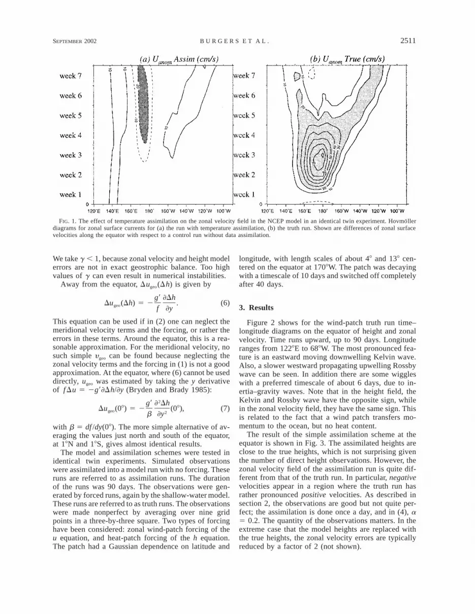
Nevertheless, the situation is not ideal. Velocities nearthe equator are relatively poorly simulated in oceaniccirculation models. The reason cannot be inadequateforcing data alone. For example, examining again thedata of an identical-twin assimilation experiment thathad resulted in much improved density and sea-levelestimates (Vossepoel and Behringer 2000), we foundthat velocities actually were degraded rather than im-proved by the data assimilation procedure (see Fig. 1).

Our hypothesis is that the poor performance of thistype of assimilation for velocities compared to densitiesis due to the lack of balance in the data assimilationupdates. We test this hypothesis in the controlled, muchsimplified, context of a 1.5-layer shallow-water modelthat reflects the main baroclinic mode of a general oce-anic circulation model. A simple assimilation schemethat nudges model height to observed height is the anal-ogy of an optimal interpolation scheme that assimilatestemperature and sea-level observations for improvingthe density structure. As a possible improvement, analternative assimilation scheme is considered, wherezonal velocity and height increments are related by geo-strophic balance. In spite of the vanishing Coriolis pa-rameter at the equator, this can be accomplished at theequator too, under rather general assumptions.

Model and methods are presented in section 2. Theresults of identical twin experiments with the schemesare reported in section 3. Both schemes have a good

performance for height, but the simple scheme has abad performance for zonal velocity while the alternativescheme has a good performance for zonal velocity. Insection 4, a brief discussion is given of a generalizationof the alternative scheme to 3D models. First tests indata assimilation experiments with two equatorial oceangeneral circulation models show a positive impact. Theimplications of the results are discussed in section 5.This is followed by a conclusion.

2. Model, assimilation procedure, andexperimental setup

The studies were performed with a linear shallow-water model for the upper tropical Pacific Ocean. Themodel can be forced by wind stress terms X and Y thatact on the zonal velocity u and the meridional velocityy, and by a heat source Q that acts on the height h (i.e.,the thermocline depth). The model equations are

]u ]h2 fy 1 g9 1 F (u) 5 X (1)M]t ]x

]y ]h1 fu 1 g9 1 F (y) 5 Y (2)M]t ]y

]h ]u ]y1 H 1 1 F (h) 5 Q, (3)H1 2]t ]x ]y

with f 5 by the Coriolis parameter in the beta-planeapproximation, and g9 reduced gravity; FM(u), FM(y),and FH(h) are frictional terms. The value of the shallowwater wave speed c0 5 (g9H)0.5 was 2 m s21 in the runsof this paper. More details can be found in the appendix.

Forcing the model with the Florida State Universitywind stress product (Stricherz et al. 1997) yields a depthanomaly over the Nino-3 region that has a correlationof about 0.8 with the observed Nino-3 temperature in-dex, which is an indication that the model is able tocapture the main characteristic of interannual variabilityin the eastern Pacific.

Assimilation of height observations was done bynudging schemes. Two such schemes have been used.The first is the simple scheme that just nudges modelheights hfg to observed heights hobs:

h 5 h 1 a(h 2 h ),ana fg obs fg (4)

with a a constant, and hana the height after assimilation.This was done once a day at every grid point, with a5 0.2. The quantity Dh 5 hana 2 hfg is called the heightincrement throughout this paper.

The second is the alternative scheme where in ad-dition increments are added to the zonal velocity thatare a function of Dh. They are proportional to changesDugeo, which are in geostrophic balance with the heightincrements Dh:

u 5 u 1 gDu (Dh).ana fg geo (5)


FIG. 1. The effect of temperature assimilation on the zonal velocity field in the NCEP model in an identical twin experiment. Hovmollerdiagrams for zonal surface currents for (a) the run with temperature assimilation, (b) the truth run. Shown are differences of zonal surfacevelocities along the equator with respect to a control run without data assimilation.

We take g , 1, because zonal velocity and height modelerrors are not in exact geostrophic balance. Too highvalues of g can even result in numerical instabilities.

Away from the equator, Dugeo(Dh) is given by

g9 ]DhDu (Dh) 5 2 . (6)geo f ]y

This equation can be used if in (2) one can neglect themeridional velocity terms and the forcing, or rather theerrors in these terms. Around the equator, this is a rea-sonable approximation. For the meridional velocity, nosuch simple ygeo can be found because neglecting thezonal velocity terms and the forcing in (1) is not a goodapproximation. At the equator, where (6) cannot be useddirectly, ugeo was estimated by taking the y derivativeof fDu 5 2g9]Dh/]y (Bryden and Brady 1985):

2g9 ] DhDu (08) 5 2 (08), (7)geo 2b ]y

with b 5 df /dy(08). The more simple alternative of av-eraging the values just north and south of the equator,at 18N and 18S, gives almost identical results.

The model and assimilation schemes were tested inidentical twin experiments. Simulated observationswere assimilated into a model run with no forcing. Theseruns are referred to as assimilation runs. The durationof the runs was 90 days. The observations were gen-erated by forced runs, again by the shallow-water model.These runs are referred to as truth runs. The observationswere made nonperfect by averaging over nine gridpoints in a three-by-three square. Two types of forcinghave been considered: zonal wind-patch forcing of theu equation, and heat-patch forcing of the h equation.The patch had a Gaussian dependence on latitude and

longitude, with length scales of about 48 and 138 cen-tered on the equator at 1708W. The patch was decayingwith a timescale of 10 days and switched off completelyafter 40 days.

3. Results

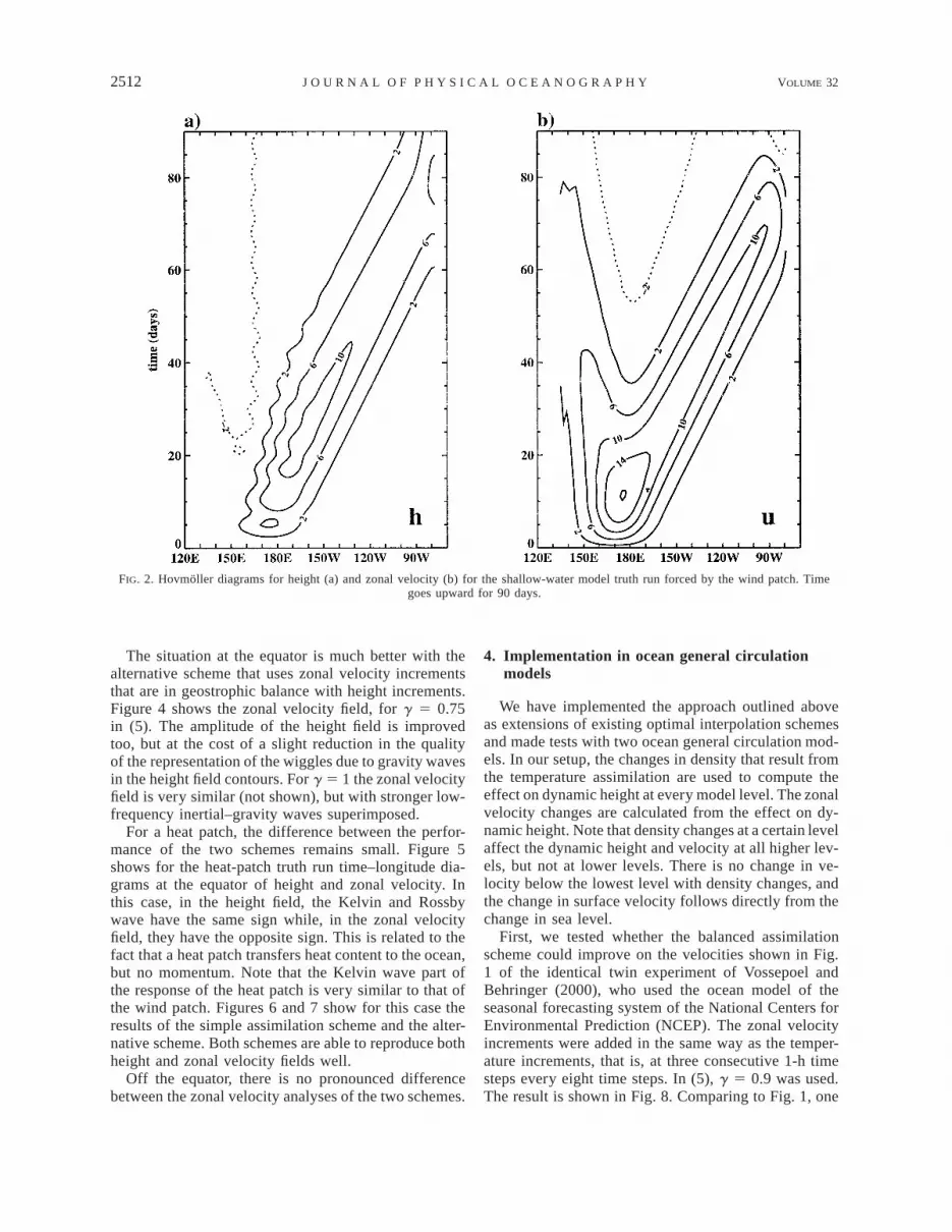
Figure 2 shows for the wind-patch truth run time–longitude diagrams on the equator of height and zonalvelocity. Time runs upward, up to 90 days. Longituderanges from 1228E to 688W. The most pronounced fea-ture is an eastward moving downwelling Kelvin wave.Also, a slower westward propagating upwelling Rossbywave can be seen. In addition there are some wiggleswith a preferred timescale of about 6 days, due to in-ertia–gravity waves. Note that in the height field, theKelvin and Rossby wave have the opposite sign, whilein the zonal velocity field, they have the same sign. Thisis related to the fact that a wind patch transfers mo-mentum to the ocean, but no heat content.

The result of the simple assimilation scheme at theequator is shown in Fig. 3. The assimilated heights areclose to the true heights, which is not surprising giventhe number of direct height observations. However, thezonal velocity field of the assimilation run is quite dif-ferent from that of the truth run. In particular, negativevelocities appear in a region where the truth run hasrather pronounced positive velocities. As described insection 2, the observations are good but not quite per-fect; the assimilation is done once a day, and in (4), a5 0.2. The quantity of the observations matters. In theextreme case that the model heights are replaced withthe true heights, the zonal velocity errors are typicallyreduced by a factor of 2 (not shown).


FIG. 2. Hovmoller diagrams for height (a) and zonal velocity (b) for the shallow-water model truth run forced by the wind patch. Timegoes upward for 90 days.

The situation at the equator is much better with thealternative scheme that uses zonal velocity incrementsthat are in geostrophic balance with height increments.Figure 4 shows the zonal velocity field, for g 5 0.75in (5). The amplitude of the height field is improvedtoo, but at the cost of a slight reduction in the qualityof the representation of the wiggles due to gravity wavesin the height field contours. For g 5 1 the zonal velocityfield is very similar (not shown), but with stronger low-frequency inertial–gravity waves superimposed.

For a heat patch, the difference between the perfor-mance of the two schemes remains small. Figure 5shows for the heat-patch truth run time–longitude dia-grams at the equator of height and zonal velocity. Inthis case, in the height field, the Kelvin and Rossbywave have the same sign while, in the zonal velocityfield, they have the opposite sign. This is related to thefact that a heat patch transfers heat content to the ocean,but no momentum. Note that the Kelvin wave part ofthe response of the heat patch is very similar to that ofthe wind patch. Figures 6 and 7 show for this case theresults of the simple assimilation scheme and the alter-native scheme. Both schemes are able to reproduce bothheight and zonal velocity fields well.

Off the equator, there is no pronounced differencebetween the zonal velocity analyses of the two schemes.

4. Implementation in ocean general circulationmodels

We have implemented the approach outlined aboveas extensions of existing optimal interpolation schemesand made tests with two ocean general circulation mod-els. In our setup, the changes in density that result fromthe temperature assimilation are used to compute theeffect on dynamic height at every model level. The zonalvelocity changes are calculated from the effect on dy-namic height. Note that density changes at a certain levelaffect the dynamic height and velocity at all higher lev-els, but not at lower levels. There is no change in ve-locity below the lowest level with density changes, andthe change in surface velocity follows directly from thechange in sea level.

First, we tested whether the balanced assimilationscheme could improve on the velocities shown in Fig.1 of the identical twin experiment of Vossepoel andBehringer (2000), who used the ocean model of theseasonal forecasting system of the National Centers forEnvironmental Prediction (NCEP). The zonal velocityincrements were added in the same way as the temper-ature increments, that is, at three consecutive 1-h timesteps every eight time steps. In (5), g 5 0.9 was used.The result is shown in Fig. 8. Comparing to Fig. 1, one


FIG. 3. As in Fig. 2 but for the run where the simple assimilation scheme is used for assimilating height observations from the wind-patch truth run.

can see that the surface velocities are markedly im-proved with respect to the original scheme.

Next we have performed a test of the scheme in areal ocean data assimilation context, in the system usedat European Centre for Medium-Range Weather Fore-casts to initialize seasonal forecasts (Stockdale et al.1998), which uses the Hamburg Ocean Primitive Equa-tion (HOPE) ocean model. In the original scheme, sub-surface temperature measurements are used for cor-recting temperature. The increments are not applied atonce, but spread over 10 days, to avoid the generationof gravity waves. In the new scheme, also zonal velocityincrements are added as in (5). For the results belowwe have used g 5 1.

In the original scheme, the assimilation stops themodel temperature from drifting away from climatol-ogy, but at the price of a relatively unrealistic zonalvelocity at the equator; see the section along the equatorin Fig. 9. There is no westward surface current in theeast, and between 1608 and 1108W there is little shoalingof the equatorial undercurrent from the east to the west,in contrast to observations (Johnson et al. 2001; Yu andMcPhaden 1999). In the new scheme, with the geo-strophic zonal velocity increments added, the represen-tation of zonal velocity is improved considerably, seeFig. 10, without degradation of the temperature field(not shown).

5. Discussion

At the equator for wind-forced situations, the simpleassimilation scheme for the shallow-water model thatuses height information for only updating the modelheight field can lead to a degradation of the zonal ve-locity field. This is not the case for the alternative as-similation scheme that has zonal velocity incrementsthat are related by geostrophic balance to the heightincrements. Off the equator, the problem does not arise.Clearly, the problem does not show up in filtered mod-els. An example is the ocean component of the Cane–Zebiak model (Zebiak and Cane 1987) where the long-wave approximation (Philander 1990) ensures that thezonal current is in geostrophic balance with the heightfield.

In shallow-water models and more complicated mod-els, density information alone is not sufficient to specifythe system completely. However, one can use the factthat the system tends to a state that is close to geo-strophic balance. From potential vorticity conservationit follows (Daley 1991) that for scales large comparedto the Rossby radius, the heights of the adjusted stateare less affected than the rotation of the velocities, whilefor the small scales it is the other way round. So assim-ilation schemes that assimilate density information onlygive reasonable estimates for the velocities for the large


FIG. 4. As in Fig. 2 but for the run where the balanced assimilation scheme is used for assimilating height observations from the wind-patch truth run.

FIG. 5. As in Fig. 2 but for the shallow-water model truth run forced by the heat patch.


FIG. 6. As in Fig. 2 but for the run where the simple assimilation scheme is used for assimilating height observations from the heat-patchtruth run.

scales, while the small scales are inherently problematic.Fortunately, in the ocean the Rossby radius is smallcompared to the scale of continents and ocean basins.So for many applications, density information can besufficient for an adequate estimate of the ocean state.Close to the equator, where the Rossby radius is rela-tively large and the separation between the timescalesof planetary waves and inertial–gravity waves is rela-tively small, this may require some extra care.

One can view a nudging or an OI type of scheme asa scheme where extra forcings are added in order to getthe ocean state closer to the observations. In case onlydensity is affected, only heat and possibly salt sourcesare added, while the mismatch between the ocean stateand the observations is also due to errors in the windforcing. This leads to the question of how well heatforcing can mimic the effect of wind forcing, a problemaddressed, for example, in the textbook of Gill (1982).If the forcing (X, Y, Q) in (1)–(3) gives rise to the fields(u, y, h), then there exists a forcing (0, 0, Q 1 wE) thatgives rise to the fields (u 1 uE, y 1 y E, h). In otherwords, there exists a forcing of the heat equation onlythat yields the same height field. The difference in thevelocities, uE and y E, satisfies the Ekman equations andis local in space, and approximately local in time (time-scale f 21 off the equator). The magnitude of the dif-ference scales with f 21, and for a typical wind stressand layer depth has a value of 25 cm s21 at 28N com-

pared to 1 cm s21 at 458N. Closer to the equator, scalingwith f 21 breaks down because friction starts to play arole. This explanation also applies when comparing thetwo data assimilation schemes, where the two differentexternal forcings give in first approximation the sameheight fields. So the difference in the velocity betweenthe schemes is expected to scale with f 21 as well. Notethat although the effect is local in time, if the data as-similation is to correct a model bias, this will result ina difference at all times between the schemes.

The difference between the zonal velocities in theassimilation schemes arises through gravity waves. Thiscan be seen in latitude–longitude pictures (not shown).If only the height is corrected in the data assimilationprocedure, attempting to reproduce the effect of thewind forcing by a heat forcing, then the change in pres-sure gradient does not correspond to a change in windforcing, and the change in pressure gradient will causevelocity tendencies, see (1) and (2), and create spuriousgravity waves. In the truth run, wind forcing causeszonal velocity changes and zonal velocity leads height.In the assimilation run, however, height leads zonal ve-locity, and the added water simply flows away in alldirections during the days before equatorial adjustmentsets in. Moreover, adjustment is not to the truth state,and around the equator the small differences lead to ageostrophic velocity that has the wrong sign in the wind-patch region compared to the truth run. Additional tests


FIG. 7. As in Fig. 2 but for the run where the balanced assimilation scheme is used for assimilating height observations from the heat-patch truth run.

FIG. 8. The effect of balanced assimilation of temperatures on thesurface zonal velocity field in the NCEP model in an identical twinexperiment. Hovmoller diagrams for zonal surface currents for therun with the balanced assimilation scheme, instead of the schemeused in Fig. 1a.

with the shallow-water model show that this even occursif the height increment is spread out in time and theamplitude of the gravity waves reduced. Nonperfect ob-servations make this even worse. In a run with balancedincrements, the increments cause no gravity waves di-rectly, as gravity waves are not in zonal geostrophicbalance.

A complication is that zonal velocity and height errorsare not in exact geostrophic balance. An extreme caseis when perfect height observations are assimilated inthe absence of forcing. Clearly, the assumption thatheight and zonal velocity errors are in geostrophic bal-ance does not apply here. Also, the homogeneous partof the equations is subtly changed by (5)–(6) in a waythat preferentially damps components that are in zonalgeostrophic balance, as the system wishes to replacethis component by observations. Thus inertial–gravitywaves may be damped less than in the system with nodata assimilation, or may even grow (e.g., for a 5 0.3,g 5 1). To remedy this situation, the zonal velocityincrements are multiplied with a factor g, see (5). Arule of thumb is that one should have g , 1, to accountfor the part of the error not in zonal geostrophic balance,and that the damping time of long waves should belonger than the Rossby period [2p(bc)20.5], in order tomake geostrophic adjustment of the flow possible.

One might wonder whether very close to the equator


FIG. 9. Mean zonal velocity (m s21) in a section along the equator of a HOPE model run with a subsurfacetemperature assimilation scheme that has temperature, but no zonal velocity increments.

FIG. 10. Mean zonal velocity (m s21) in a section along the equator of a HOPE model with a subsurface temperatureassimilation scheme that has both temperature and zonal velocity increments.

geostrophic balance does not pose a problem since (6)does not have a well-defined limit at the equator. How-ever, one should keep in mind that derivatives shouldalways be evaluated at an appropriate scale. In the caseat hand, an appropriate scale near the equator is a con-siderable fraction of the equatorial Rossby radius. Atthe equator, this leads to (7), where the second derivativeshould be evaluated at the same scale as used in (6).

The approach outlined above has been generalized totwo optimal interpolation schemes for general circula-tion models. First, in the identical twin experiment with

the NCEP model, the gross error in the surface velocityof the original scheme was eliminated. Second, in thereal data assimilation experiment using the HOPE mod-el, the mean current in the eastern Pacific was improved,especially in the surface layer. More tests will be nec-essary to determine whether currents are systematicallyimproved or not with the present generalization of thebalanced data assimilation scheme, and how to deter-mine the optimal choice for the factor g in (5). Perhapsa more sophisticated multivariate OI scheme would per-form significantly better than the present, more naive,


implementation. These questions, and the impact of thescheme on the forecasts, still need to be addressed.

In more advanced data assimilation methods, such asKalman filtering and 4D-VAR schemes, the need forbalanced updates has consequences for the proper for-mulation of background error covariance matrices. Thecontrol variables may already implicitly contain the geo-strophic balance [e.g., the wind updates in Bonekampet al. (2001)]. If they do not, the balance must be ensuredby a multivariate error covariance matrix that makesnongeostrophic updates unlikely.

Note, however, that using more advanced data assim-ilation methods can never compensate for an intrinsiclack of information about the currents. So if the forcingerrors cannot be neglected and the small-scale velocitystructures should be estimated as well, it is not sufficientto have density information only, irrespective of theassimilation method used.

6. Conclusions

Assimilation schemes of the type that is used for sea-sonal forecasts can have a problem in estimating zonalvelocities. This is the case for OI schemes that use den-sity information for updating only the model densityfield, which in some situations leads to a detoriation ofthe zonal velocity field around the equator. A possibleremedy has been tested and cures the problem in a sim-ple linear shallow-water model. It updates the zonalvelocity with increments that are related to the densityincrements by geostrophic balance. A straightforwardgeneralization of the method has been implemented intwo ocean circulation models, and first tests show apositive impact on surface currents.

Acknowledgments. Helpful discussions with DavidAnderson, Gerbrand Komen, and Jerome Vialard aregratefully acknowledged. We thank Ming Ji, Dick Reyn-olds, and Dave Behringer for making available and ex-plaining the NCEP model and analysis system. Com-puting resources for the computations with NCEP modelwere provided by the Center for High Performance ap-plied Computing (HPaC) of Delft University of Tech-nology. PJVL was supported by the National ResearchProgram, Grant 013001237.10.

APPENDIX

Linear Shallow-Water Model

The shallow-water model of the tropical Pacific is a1.5-layer linear model of a baroclinic mode on a betaplane. It describes the thermocline depth field h, thezonal velocity field u, and the meridional velocity y ofa shallow water layer of mean thickness H and densityr over a motionless bottom layer of density r 1 Dr.The model can be forced by wind stress terms X and Ythat act on u and y, and by a heat source Q that actson h. The model equations are

]u ]h2 byy 1 g9 1 F (u) 5 X (A1)M]t ]x

]y ]h1 byu 1 g9 1 F (y) 5 Y (A2)M]t ]y

]h ]u ]y1 H 1 1 F (h) 5 Q, (A3)H1 2]t ]x ]y

where, as usual, x denotes longitude and y latitude. Forthe Coriolis parameter f the beta-plane approximationf 5 by is used, g9 5 gr21Dr is the reduced gravity;FM(u), FM(y), and FH(h) are linear frictional terms. Thevalue of the shallow water wave speed c0 5 (g9H)0.5

was 2 m s21 in the runs of this paper, and the meandepth H was set to 150 m.

The frictional terms consist of several parts. The mainpart is the harmonic part, with an eddy viscosity of 23 104 m2 s22 in FM and an eddy diffusivity of 2 3 103

m2 s22 in FH. A linear damping term, which is onlysizable near the northern and southern boundary of thebasin, prevents waves propagating along these bound-aries. Small terms proportional to the fourth derivativein the x and y directions are used to damp short-wavelength instabilities near the equator. The coefficients ofthe fourth-order terms are of the order of 0.01, whenmade dimensionless with the model time step and modelgrid spacing.

The model equations (A1)–(A3) are implemented ona C grid in a standard way, see, for example, the text-book of Kantha and Clayson (2000), over a closed basin.The western boundary and eastern boundary follow ap-proximately the coastlines of Australasia and America,and the southern and northern boundary are at 308S and308N. The standard grid spacing is 28 in the zonal di-rection, and 18 in the meridional direction. With thisresolution, the main limit on the time step comes fromthe explicit treatment of the Coriolis terms near thenorthern and southern boundaries. The standard timestep is 8 h.

The time stepping scheme of the model is as follows.At each step, new values (h1, u1, y1) are obtained fromthe old values (h0, u0, y 0) as follows:

h 5 h (h , u , y )1 1 0 0 0

u 5 u (h , u , y )1 1 1 0 0

y 5 y (h , u , y ). (A4)1 1 1 1 0

This scheme allows for a relatively large time step withlittle need for storage compared to more standardschemes where u and y are evaluated at the same timelevel. In the assimilation runs, the increments are cal-culated and added right after the calculation of a newheight field.

A test to study the influence of the resolution hasbeen performed with a grid spacing of 0.58 lat by 18lon and a time step of 6 h for the wind patch run ofsection 3. Not only are the Kelvin and Rossby waves


the same, also the wiggles of the inertial–gravity wavesshowed no difference. In fact, there was hardly anydiscernible difference between the standard and the highresolution run.

REFERENCES

Alves, J. O. S., K. Haines, and D. L. T. Anderson, 2001: Sea levelassimilation experiments in the tropical Pacific. J. Phys. Ocean-ogr., 31, 305–323.

Behringer, D. W., M. Ji, and A. Leetmaa, 1998: An improved coupledmodel for ENSO prediction and implications for ocean initial-ization. Part I: The ocean data assimilation system. Mon. Wea.Rev., 126, 1013–1021.

Bell, M. J., M. J. Martin, and N. K. Nichols, 2001: Assimilation ofdata into an ocean model with systematic errors near the equator.Hadley Centre for Climate Prediction and Research, Met Office,Ocean Applications Tech. Note 27, Bracknell, United Kingdom,27 pp.

Bonekamp, H., G. J. van Oldenborgh, and G. Burgers, 2001: Vari-ational assimilation of Tropical Atmosphere–Ocean and ex-pendable bathythermograph data in the Hamburg Ocean Prim-itive Equation ocean general circulation model, adjusting thesurface fluxes in the tropical ocean. J. Geophys. Res., 106, 16693–16 709.

Bryden, H. L., and E. C. Brady, 1985: Diagnostic model of the three-dimensional circulation in the upper equatorial Pacific Ocean. J.Phys. Oceanogr., 15, 1255–1261.

Daley, R., 1991: Atmospheric Data Analysis. Cambridge UniversityPress, 457 pp.

Gill, A., 1982: Atmosphere–Ocean Dynamics. Academic Press, 662pp.

Ishikawa, Y., T. Awaji, and N. Komori, 2001: Dynamical initializationfor the numerical forecasting of ocean surface circulations using

a variational assimilation scheme. J. Phys. Oceanogr., 31, 75–93.

Ji, M., A. Leetmaa, and V. E. Kousky, 1996: Coupled model predic-tions of ENSO during the 1980s and 1990s at the National Cen-ters for Environmental Prediction. J. Climate, 9, 3105–3120.

——, R. W. Reynolds, and D. W. Behringer, 2000: Use of TOPEX/Poseidon sea level data for ocean analyses and ENSO prediction:Some early results. J. Climate, 13, 216–231.

Johnson, G. C., M. J. McPhaden, and E. Firing, 2001: EquatorialPacific Ocean horizontal velocity, divergence, and upwelling. J.Phys. Oceanogr., 31, 839–849.

Kantha, L. H., and C. A. Clayson, 2000: Numerical Models of Oceansand Oceanic Processes. Academic Press, 936 pp.

Oschlies, A., and J. Willebrand, 1996: Assimilation of Geosat altim-eter data into an eddy-resolving primitive equation model of theNorth Atlantic Ocean. J. Geophys. Res., 101, 14 175–14 190.

Philander, S. G. H., 1990: El-Nino, La Nina, and the Southern Os-cillation. Academic Press, 291 pp.

Segschneider, J., D. L. T. Anderson, and T. N. Stockdale, 2000: To-ward the use of altimetry for operational seasonal forecasting.J. Climate, 13, 3115–3138.

Smith, N., J. E. Blomley, and G. Meyers, 1991: A univariate statisticalinterpolation scheme for subsurface thermal analyses in the trop-ical oceans. Progress in Oceanography, Vol. 28, Pergamon,219–256.

Stockdale, T. N., D. L. T. Anderson, J. O. S. Alves, and M. A. Bal-maseda, 1998: Global seasonal rainfall forecasts using a coupledocean–atmosphere model. Nature, 392, 370–373.

Stricherz, J., D. Legler, and J. O’Brien, 1997: TOGA Pseudo-stressAtlas 1985–1994. Vol. II, Pacific Ocean. Florida State Univer-sity, 158 pp.

Vossepoel, F. C., and D. W. Behringer, 2000: Impact of sea levelassimilation on salinity variability in the western equatorial Pa-cific. J. Phys. Oceanogr., 30, 1706–1721.

Yu, X., and M. J. McPhaden, 1999: Seasonal variability in the equa-torial Pacific. J. Phys. Oceanogr., 29, 925–947.

Zebiak, S. E., and M. A. Cane, 1987: A model El Nino–SouthernOscillation. Mon. Wea. Rev., 115, 2262–2278.

balanced ocean-data assimilation near the equator

Documents