Optimal immigration, assimilation and trade

Istvan Konya 1

Boston College2

October, 2001

1I would like to thank Joseph Altonji, James Anderson, Gadi Barlevy andKiminori Matsuyama for helpful comments and suggestions.

2Correspondence: Economics Department, Boston College. Chestnut Hill, MA02467. Tel: (617) 552-3690. E-mail: konya@bc.edu

Abstract

The paper develops a model that examines the role of cultural conflict inimmigration and immigration policy. Cultural differences lead to frictions be-tween natives and immigrants, unless the latter make a costly investment toassimilate. Since rational agents will assess their assimilation abilities whencontemplating migration, the decisions to migrate and assimilate have to beanalyzed jointly. The paper’s key contribution is to endogenize the migrationdecision, which highlights the importance of self-selection in the migrationprocess. An important consequence of self-selection is that although thereare externalities in the assimilation decision, the equilibrium outcome is effi-cient for some parameter values. Because of the endogeneity of the migrationdecision, care must be taken to select the optimal policy instruments. Im-plementing the first best requires a policy that targets both the size andcomposition of the migration flow. Therefore, simple policies that only in-fluence one of these are not optimal. In particular, subsidizing assimilationor auctioning immigration permits do not achieve the first best. Instead,a tax scheme that differentiates between assimilating and non-assimilatingimmigrants can be used to promote efficiency.

Keywords: Culture, immigration policy, optimal immigration.JEL Classification: D62, F22, Z10

1 Immigration and culture

There has been a marked rise in immigration to the United States in thelast two decades, to levels that have not been seen since the beginning of the20th century. The foreign born proportion of the US population population isnow close to 5% and it is rising. Switzerland, Germany and Austria have farmore immigrants per capita than the US, while the foreign-born population ofFrance and Britain is roughly the same. Thus migration is clearly a pressingissue both in the traditional immigrant nations of the New World and inEurope.

The economic profession has been quick to analyze some of the conse-quences of the new migration wave. The emphasis has tended to be on theeconomic progress of immigrants and their impact on the host country econ-omy. In the labor literature, issues studied include the effect of migration onthe wages of low skilled workers and on the welfare state, and the economicassimilation of immigrants in the host country.1 Researchers in internationaltrade also looked at the economic impact of immigration, and they have ex-plored the connection between foreign trade and immigration.2 Given thesubstantial amount of work in this area, we now have a good understandingof these issues. But immigration also has important non-economic effects onimmigrants and natives. In practice discussion among non-economists cen-ters on issues that economists have largely ignored, such as cultural frictionsand clashes.

Sowell (1996) documents the experience of various immigrant groupsthroughout history. A recurring theme is that immigrants and natives withdifferent cultures and languages experience frictions in intergroup encoun-ters. Hostility between immigrants and natives can often be traced back toeconomic reasons, since (as Sowell points out) immigrants tend to hurt vo-cal native interest groups. But the fact that immigrants can be singled out,based on their different cultural and other characteristics and not on their

1Borjas (1999a) provides an overview of this literature. Altonji and Card (1991) andCard and DiNardo (2000) examine the effect of immigrants on local labor markets inthe US. The classic references on the economic assimilation of immigrants are Chiswick(1978) and Borjas (1987). Auerbach and Oreopoulos (1999) and Storesletten (2000) usemacro-economic models to look at the fiscal impact of immigration.

2Trefler (1997) and Venables (1999) look at the connection between migration andinternational trade in various trade models. Markusen and Zahniser (1997) examine theeffect of NAFTA on migration, while Hanson and Slaughter (1999) study the effect ofimmigration on US production patterns and factor prices.

1

economic effect, indicates that these cultural differences matter to people.3

In contemporary Europe, anti-immigrant sentiments are just as strong inlow- unemployment Switzerland as they are in high-unemployment Belgium.Clearly, to study the full impact of immigration one has to look beyond thetraditional economic factors.

This paper presents a model which examines the role of cultural con-flict in immigration and immigration policy. In the model individuals decidewhether to migrate into another country. In addition to the migration de-cision, immigrants can also decide to assimilate – acquire the culture of thehost country. In the model this eliminates cultural frictions between themand natives. The crucial feature of the model is the presence of externalitiesin the assimilation decision, which might lead to an inefficient equilibriumoutcome4, both in the size and composition of the migration flow. The latterarises because individuals are heterogenous both in their migration and as-similation costs. This emphasis on the composition of immigration is a novelfeature of the model. It leads to implications for immigration policy that aredifferent from what have been suggested in the previous literature.

One of the most important messages of the paper is that the welfare prop-erties of the equilibrium are not uniform across all parameter values. Thereare structural differences in immigration from developed, middle income andpoor countries, and these categories themselves depend on various parame-ters. A surprising conclusion is that cultural externalities do not necessarilymake the equilibrium inefficient. In particular, if the sending country is suf-ficiently rich, both the level and the composition of immigration are optimal.For less developed source countries this is not the case, so the paper presentsthe optimal policies that can implement the first best. Because the poli-cymaker has to select not just the size of migration but also those whoseassimilation and learning costs are the lowest, the optimal policy has to offerselective incentives to different people. This feature of the model impliesthat some popular tools of immigration policy do not implement the socialoptimum, and possibly make matters worse. I analyze the effects of two suchpolicies in detail: assimilation subsidies and restricting immigration levels.

3Chinese in Southeast Asia, Jews in medieval and modern Europe and Indians in EastAfrica suffered discrimination and worse, regardless of their individual economic status.Recurring persecution of Jews in medieval Europe often had no economic reasons, but werebased on religious differences and deeply rooted prejudices of the Christian population.

4I will look at the welfare properties of the equilibrium from the point of view of aplanner who wants to maximize world welfare.

2

An important special case of the second is selling immigration permits, whichis sometimes advocated by economists. I show that in the case of culturalexternalities this policy cannot achieve the first best.

The welfare measure used in the paper is the sum of world output. Inthe model this means that the social planner’s objective function includesthe welfare of immigrants in addition to the well-being of natives in thehost country. Since immigration policy is conducted in the host country,this might require some justification. First, a forward-looking governmentrecognizes that immigrants will be future voters, so it might cater to theirinterests, especially if they have relatives already in the country. Second,international cooperation on other issues might induce a country to followpolicies that take into account immigrant welfare. If, say, the US and Mexicoare interested in maintaining long-term cooperation on trade, law enforce-ment etc, then the US might offer concessions to Mexico in its immigrationpolicy. Finally, it is easy to find the optimal policy for the host country in themodel, and I show that in many cases it coincides with the world planner’soptimum. When it does not, it is interesting to look at the reasons for thedifference, and see if the interests of the social planner and the host countrynatives can be aligned. I will return to this issue later.

Apart from normative implications the model has interesting positivepredictions. It shows, for example, that immigration from culturally verydifferent source countries might have better welfare properties than immi-gration from similar countries. The model also allows for the possibility thatimmigrants are isolated from natives in the host country, which is often thecase. I show that segregation has ambiguous effects on welfare: it leads to adecrease in the frequency of inefficient encounters, but also hinders assimi-lation. Finally, the comparative statics results present testable implications,and I provide some preliminary evidence that the model’s predictions areborn out in US data.

One strand of the relevant literature is work on optimal migration, whereauthors looked at causes why migration levels might not be Pareto-efficientfrom the point of view of world welfare. In a book that discusses the possi-ble effects of Eastern European migration to Western Europe (Layard, Blan-chard, Dornbusch and Krugman 1992) the authors list many possibilities thatare of concern (wage compression, fiscal externalities, market size effects, in-formation and endogenous tastes, and cultural externalities), but they do notdevelop formal models to study them. Burda and Wyplosz (1992) explore therole of human capital externalities in the context of migration from Eastern

3

to Western Europe, using a Lucas-type growth model. The main differencebetween their model and the one in this paper is that the composition ofimmigration is crucial here, while in Burda and Wyplosz (1992) only the sizeof migration matters. This leads to very different policy implications, as wewill see later.

The literature on optimal migration has not explored the role of culturaldifferences. Two path-breaking articles (Lazear 1995, Lazear 1996), how-ever, look at cultural externalities and assimilation from a partial equilibriumpoint of view. Lazear models interaction between immigrants and natives asrandom matching. I depart from his model by explicitly considering the mi-gration decision. Lazear treats the size and composition of an immigrantgroup as exogenous, which might be the case for some specific groups (mostnotably, refugees). In general, however, immigrants are self- selected alongmany dimensions, among them the capability to assimilate. It is reasonableto expect that those who actually migrate are the ones who can learn thenew culture easier. Migration and assimilation decisions are not indepen-dent, but arise from the same fundamentals, and my model traces both backto these fundamentals. The importance of endogenizing migration is high-lighted when we look at policies such as assimilation subsidies to immigrants.In Lazear’s partial equilibrium framework assimilation subsidies can be usedto implement the first best. When migration is endogenous this is no longerthe case, because assimilation subsidies fail to select the immigrants whoshould come in the first place.

The rest of the paper is organized as follows. In Section 2 I describe theformal model of the migration and assimilation decisions in a two-countryframework. In Section 3 I derive the equilibrium conditions, explore theexistence and uniqueness of the equilibrium and look at some comparativestatics results. Section 4 solves the social planner’s problem, and Section 5discusses the policy implications of the model. In Section 6 I present someevidence in support of the model, using data from the United States. Finally,Section 7 concludes.

4

2 The model

2.1 Assumptions

In this section I develop a model of migration, assimilation and culturalexternalities. A simple and transparent way to model interaction betweenpeople is to use a random matching framework, which in this context was firstintroduced by Lazear (1995). In such a setting agents are paired togetheraccording to a random device, and generate some output that they shareaccording to a sharing rule.5 In contrast to assortative matching, peopledo not have the ability to search for good pairs, and might be stuck inan inefficient allocation. There is only one match for each agent, and agentsderive utility from the “income” (output share) they receive from this match.I assume the utility function is linear, and I normalize utility units such thatthey are equal to the output units. The qualitative conclusions would remainthe same with a more general concave utility function, but the linearityassumption simplifies the analysis greatly.

There are two countries, North and South, with initial populations of 1and L, respectively. Agents can change locations, but moving is costly. Ifa person decides to migrate, she has to pay c units of her income. Popula-tions are heterogenous with respect to c, and the initial distribution of themoving costs in each country is given by the c.d.f. F (c), with c ∈ (0, K).The two countries differ in their culture, which influences the outcome oftrades. When two people who have different cultures are matched together,the output they generate is only θ < 1 times the output they would receiveif they had the same culture. Also, the South is poorer than the North anda match in the South is worth only h < 1 times as much as the same tradewould be worth in the North. There are no international matches – all tradetakes place within the countries.6 Finally, I assume that the output from amatch is shared equally by the two parties, and I normalize the value of auni-cultural match in the North to 1 for each trader.

Because the South is poorer, in equilibrium migration will flow from theSouth to the North. When immigrants arrive at the North, their culture isdifferent from the native one. Thus matches between immigrants and natives

5In the rest of the paper I will also use the phrase “trade” to indicate a match.6Although it is possible to relax this assumption, there is no obvious way to incorporate

international trade into the model. Since the basic conclusions do not change with suchan extension, I use the closed economy model to avoid unnecessary complications.

5

would be less efficient than a trade within a group. It is possible, however,that an immigrant learns the native culture – that is, she assimilates. Anassimilated immigrant can trade efficiently with other immigrants and na-tives, because she knows both cultures. Thus in the North trades result in anoutput of 1 to the parties, unless a native and a non-assimilated immigrantmeet. In this case they only get θ each. Since non-assimilated immigrantshave a Southern culture, the parameter θ measures the cultural distinctive-ness between the North and the South. The more similar the two countriesare, the more efficient a bi-cultural match in the North is. Finally, note thatthe South remains homogenous (no immigrants there), but because it is lessdeveloped, trades yield h < 1 in any Southern match for the two traders.

Immigrants enjoy more efficient native matches when they assimilate.However, learning the native culture is costly, and immigrants have to forgoa fraction τ of their output in order to learn. Thus assimilation involves atime cost, the time required for learning. τ is different for each individual,and its distribution among the initial populations in the two countries isgiven by the c.d.f. G(τ), with τ ∈ [0, 1].7 It is important to note that thedistribution of τ among immigrants is different from the distribution in thegeneral population. This is because the capability to assimilate influencesthe migration decision, therefore immigrants will be self-selected in theircapacity to assimilate. To make inferences about optimal immigration andimmigration policy, we have to take this dependence into account.

Let us now turn to the matching technology. A stylized fact in immi-gration is that people tend to live with others who share their culture. In abook about Vietnamese refugees in the United States, Zhou and BankstonIII (1998) document that although the US government made a consciouseffort to scatter Vietnamese among natives, after a few years they tendedto move into areas with high concentration of their countrymen. In gen-eral, immigrants who do not (or only partially) assimilate live in their ownneighborhoods, and hence their contact with natives is limited. Assimilatedimmigrants, on the other hand, tend to move into native areas, because ofgenerally better amenities and job opportunities. To capture these stylizedfacts, I assume that the Northern population is geographically segregated intotwo segments. One consists of natives and assimilated immigrants, while the

7It would be reasonable to assume that the distribution function G also depends onθ, because it might be easier to learn for an immigrant if she comes from a more similarculture. I will use the simplest formulation that does not allow for such dependence, butmy results remain the same in the more general setting.

6

other includes non-assimilated immigrants. There is more interaction withineach group than between them, and the difference depends on the level ofsegregation in the society. At one extreme, all immigrants are scatteredrandomly among natives and all matches are equally likely. At the otherextreme, non-assimilated immigrants are completely isolated and there is nointer-group match.

Let p be the probability that two non-assimilated immigrants meet, andlet q be the probability that a native or an assimilated immigrant meetssomeone from their group. Also, let the equilibrium number of immigrantsbe m, and let the number of assimilated immigrants be a (thus the post-migration population of the North is 1 + m).8 I assume that p and q aregiven by the following expressions:

p = αm− a

1 + m+ 1− α (1)

q = α1 + a

1 + m+ 1− α. (2)

Thus α measures the level of interaction between the two groups: when α = 1intra- and inter-group matches occur with the same probability, when α = 0there are only intra-group trades. Note that trades must be balanced betweengroups, and it is easy to check that for the above specifications for p and q thisis indeed the case.9 Finally, I assume that non-assimilated immigrants witha match from the other group meet a native with probability 1/(1 + a) andan assimilated immigrant with probability a/(1 + a). Thus non-assimilatedimmigrants cannot search actively for assimilated ones.

To finish this section, I will maintain the following assumptions about thedistribution functions in the paper. First, both F and G are differentiableand have a continuous p.d.f. f and g, respectively. Second, both distributionfunctions have full support. Third, c and τ are independent. If we associatethe assimilation cost with ability, we can give examples suggesting both pos-itive and negative correlations. More able people might be more efficientmovers, leading to a positive correlation. But they might have more to loose

8It turns out that it is more convenient to work with the overall number of immigrantsthan with the number of non- assimilated ones.

9The number of natives and assimilated immigrants who are matched with the othergroup is (1− q)(1 + a)/(1 + m), while the number of non-assimilated immigrants who arematched outside is (1− p)(m− a)/(1 + m). One can easily check that the two quantitiesare the same.

7

from moving, which leads to a negative correlation. Given this ambiguity, itis natural to start with the assumption of independence, which also makesthe analysis much easier.

2.2 Individual decisions

Let us now examine how people choose to move and assimilate. In equilib-rium there are four different groups of people: Northern natives, assimilatedimmigrants and non-assimilated immigrants in the North, and Southernerswho do not migrate. In equilibrium the four group sizes are 1, a, m− a andL−m, respectively. The endogenous variables are m and a, and our goal is tofind these values. To start, let us write down the incomes or value functionsfor each group, given our assumptions on the matching technology and onthe efficiency of particular types of matches from the previous section:

VN = q + θ(1− q)

Va = (1− τ)(q + 1− q)− c

Vn = p + (1− p)a + θ

1 + a− c

VS = h,

where N, n, a and S stand for Northern natives, non-assimilated immigrants,assimilated immigrants and Southerners. Each term is the value of a partic-ular match type multiplied by the probability of such a match. Note that fornon-assimilated immigrants the second term is the expected value of an inter-group trade, since the partner can be a native or an assimilated immigrantin such cases.

Using the definitions of p and q from (1) and (2), we can rewrite the valuefunctions in the following forms:

VN = 1− α(1− θ)(m− a)

1 + m

Va = 1− τ − c

Vn = 1− α1− θ

1 + m− c

VS = h.

Notice that keeping the number of immigrants constant, Northern welfare isincreasing in a, the number of assimilated immigrants. This is the case be-

8

cause natives can trade more efficiently with assimilated immigrants, so theybenefit when immigrants learn their culture. Immigrants, however, do nottake into account this benefit for natives when they decide about learning.This external effect of the learning decision is what we called cultural exter-nalities in the introduction, and now we can start to examine their effect onthe migration and assimilation outcomes.

The difficulty to solve the model lies in the fact that the migration decisionis influenced by the assimilation choice. That is, individuals in the Southcan choose among three possibilities, and whether they migrate depends ontheir capability to assimilate. To overcome this barrier, I will proceed thefollowing way. First, it is evident that for any given m and a, the individualassimilation decisions involve a threshold. Immigrants will assimilate only iftheir benefit from doing so is greater than their cost. Equating Vn and Va

yields the threshold level for τ :

τa =α(1− θ)

1 + m. (3)

Thus any immigrant with a lower learning cost will assimilate, and otherswill not. This does not mean, however, that in a given immigrant groupsome people do not assimilate. As I stressed earlier, the distribution of τ isendogenous, and whether agents with high learning costs choose to leave theSouth depends on the underlying parameters. For this reason it is meaning-less to do comparative statics exercises with τa, since we do not know whatthe cutoff means if the distribution of τ changes with the parameters. Inorder to say more, we have to examine the migration decision.

We can start with those people who migrate but don’t assimilate. Let usindicate the threshold in c for them with cn. We get this value if we equateVS and Vn. That is, we have:

cn = 1− h− α(1− θ)

1 + m. (4)

For the people who assimilate, the relevant threshold can be calculated byequating VS and Va. If we rearrange this condition, we end up with thefollowing expression:

ca = 1− h− τ. (5)

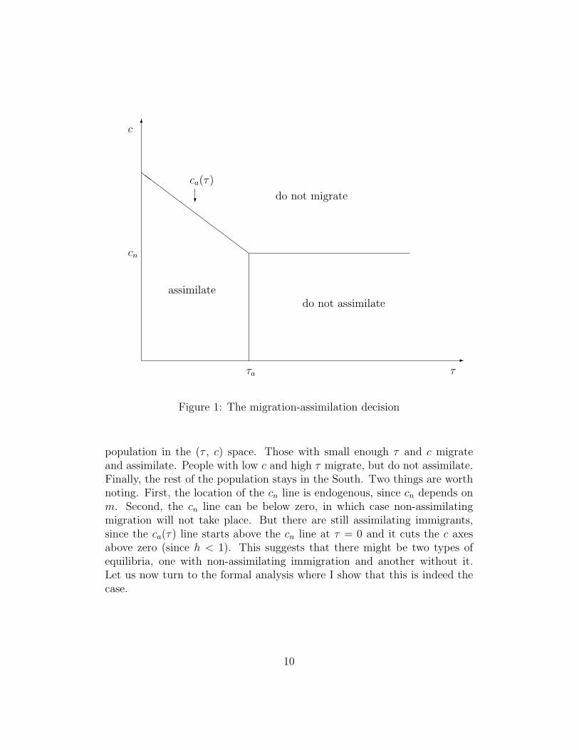
Thus we have three threshold levels that together determine the choiceof the Southern people. Figure 1 shows the break-down of the Southern

9

6

-

ZZ

ZZ

ZZ

ZZ

ZZ

ZZ

?

c

τ

cn

τa

ca(τ)

assimilatedo not assimilate

do not migrate

Figure 1: The migration-assimilation decision

population in the (τ , c) space. Those with small enough τ and c migrateand assimilate. People with low c and high τ migrate, but do not assimilate.Finally, the rest of the population stays in the South. Two things are worthnoting. First, the location of the cn line is endogenous, since cn depends onm. Second, the cn line can be below zero, in which case non-assimilatingmigration will not take place. But there are still assimilating immigrants,since the ca(τ) line starts above the cn line at τ = 0 and it cuts the c axesabove zero (since h < 1). This suggests that there might be two types ofequilibria, one with non-assimilating immigration and another without it.Let us now turn to the formal analysis where I show that this is indeed thecase.

10

3 Equilibrium

3.1 Existence and uniqueness

We can start by verifying the two observations from Figure 1. First, if thereare non-assimilating immigrants, there also must be assimilating ones. From(4) and (5) we can see that ca(τ) ≥ cn, because the last term in cn is justτa, which is the upper limit on learning costs for an assimilating immigrant.In other words, since assimilation is a profitable activity, its benefits can betraded off for higher migration costs. That is, low τ individuals will migrateeven if their c is above the distribution of c for those who do not assimilate.Second, it is easy to see that migration is always profitable for someone.Since the lower limit of τ and c is 0, for any h < 1 very low cost individualscan profit from assimilating migration.

These two results confirm our conjecture that two types of equilibriaare possible. Let us call the one with both types of immigrants interior(0 < a < m ≤ L) and the other with only assimilating immigrants corner(0 < a = m ≤ L). If the solution is interior, it has to satisfy the following:

m− a = LF (cn) [1−G(τa)] (6)

a = L

∫ τa

0

F [ca(τ)] dG(τ) (7)

The equations relate the expected and actual number of migrants of differenttypes and τa, cn and ca are as defined in (3), (4) and (5). In (6) the right-handside is the count of people who would not assimilate (τ > τa), but have lowenough moving cost to migrate (c < cn). Since c and τ are independent, themass of such people is just a product of the two probabilities times the totalmass of people in the South (L). In (7) we have a complication: ca dependson τ . Thus first we count people with low moving costs (c < ca) for a givenτ , and than “add” them together (integrate) for all τ < τa. Notice that wecan eliminate a because it does not enter the terms on the right-hand sidesof (6) and (7). This gives us the following condition for m:

m = LF (cn)[1−G(τa)] + L

∫ τa

0

F [ca(τ)] dG(τ). (8)

If a = m we need only one equation, since non-assimilating migrationis zero. This means that all immigrants have τ ≤ τa, possibly with the

11

inequality strict. In other words, we cannot just use (7) to determine a whena = m, since the upper limit on assimilation costs among immigrants mightbe lower than τa. To get the appropriate cutoff we have to solve ca(τ) = 0,which leads to the value of 1− h.10 Thus in the corner case the equilibriumcondition is:

m = L

∫ 1−h

0

F (1− h− τ) dG(τ), (9)

Since for any c ≤ 0 we have F (c) = 0, we can summarize the equilibriumconditions as follows:

m = LF (cn)[1−G(τa)] + L

∫ min {1−h,τa}

0

F (1− h− τ) dG(τ)

s.t. τa =α(1− θ)

1 + mand cn = 1− h− α(1− θ)

1 + m, (10)

where for convenience I repeated the equations for the cutoffs (and substi-tuted for ca). Thus we have to examine (10) to establish the properties ofequilibrium.

It is easy to see that an equilibrium exists, as the following propositionshows.

Proposition 1. For any parameter values 0 ≤ α ≤ 1, 0 < h < 1, 0 ≤ θ < 1and L > 0 there is an equilibrium level of migration 0 ≤ m ≤ L.

Proof. The proof is a straightforward application of Brouwer’s Fixed PointTheorem. Let us denote the right-hand side of (10) by Γ(m), thus the equi-librium condition is to find the fixed point of Γ(m) on the set [0, L]. This setis compact and convex, while the function Γ(m) is continuous (though notnecessarily differentiable) and maps [0, L] into itself. Thus the conditionsof Brouwer’s Theorem are satisfied, and there is an m ∈ [0, L] such thatm = Γ(m).

Thus the existence of an equilibrium is guaranteed, but uniqueness is not.The solution to (9) is unique (the right-hand side is independent of m), thusthere cannot be more than one corner equilibrium. Equation (8), however,can be satisfied by more than one m. It is easy to see the intuition behindthe possibility of multiple equilibria in this case. Looking at (3) and (4)reveals that τa decreases and cn increases with m. Thus there is a positive

10It is easy to check that cn < 0 implies 1− h < τa.

12

feedback in immigration: the more people move, the higher the incentivesfor non- assimilating immigration. Since those who do not assimilate tradeefficiently only with other immigrants, it is better if they are more numerous(and have a higher probability to meet). To see the problem mathematically,let us take the derivative of the right-hand side of (8), I(m):

∂I(m)

∂m= Lf(cn)[1−G(τa)]

α(1− θ)

(1 + m)2> 0.

This expression can take any values between zero and infinity, so the functionI(m) can cut the 450 line more than once. It is possible, however, to rule outsome of the possible equilibria on stability grounds. Although the model isstatic, we can talk about Walrasian or tatonment stability. In this context theequilibrium is locally stable if m− I(m) is increasing around the equilibriumpoint or I ′(m) < 1. If this condition holds independent of m the solution to(8) is unique, because 0− I(0) < 0, 1− I(1) > 0 and m− I(m) is monotonedecreasing.

In the rest of the paper I will restrict attention to the case where thesolution to (8) is unique. A sufficient condition for this is given by thefollowing restriction:

Assumption 1. The distribution of moving costs is not very concentrated.More precisely, for any values of c ∈ (0, K) the following inequality holds:

f(c) <1

α(1− θ)L. (11)

Note that Assumption 1 is likely to hold when α is small (North is verysegregated), θ is close to one (cultural differences are small) or when L issmall. Even in the polar case of α = 1 and θ = 0 (and L = 1), the conditionis satisfied when F is uniform on (0, K), where K > 1. Thus Assumption 1 isa fairly mild restriction, and is likely to be satisfied if people are heterogenousenough in their moving costs. Finally, even when multiplicity arises, manyresults below (e.g. comparative statics) continue to hold for stable equilibria.

Even if the solution to (8) is unique, it could still happen that there isan interior and a corner equilibrium for the same parameter values. As thenext proposition shows, however, such an outcome is not possible.

Proposition 2. Given Assumption 1, the solution (m∗, a∗) to the immigra-tion problem is unique. Moreover, ∃!h(α, θ, L) such that if h < h the equi-librium is interior and if h ≥ h, 0 < a∗ = m∗ < 1. Thus non-assimilatingmigration only occurs when the South is sufficiently poor.

13

Proof. We have already showed that there is a unique solution to both (8)and (9). The only question is whether there is a range of parameter valueswhen both of these m’s are equilibrium ones. It is clear that in any interiorsolution cn > 0. Let us define m by the equation cn = 0. That is,

m =α(1− θ)

1− h− 1.

We know that cn is increasing in m. This means that we have interior equi-libria if the solution to (8) is greater than m and a corner solution if m∗ < m.At the cutoff m the two types of equilibria should coincide. This defines himplicitly with the following equation:

α(1− θ)

1− h− 1 =

∫ 1−h

0

F (1− τ − h) dG(τ), (12)

which we get if we substitute m into either (8) or (9). We can easily seethat there is a unique h that satisfies (12): the left hand side is increasingand the right hand side is decreasing in h, moreover l.h.s<r.h.s at h = 0 andl.h.s>r.h.s at h = 1.

The final step is to show that if h < h then m∗ > m and if h > h thenm∗ < m. That is, the separation of the equilibria is consistent with thecondition on cn. But this is easy, since the right-hand sides of (8) and (9)are decreasing in h (see the Appendix), so a higher h means a smaller m inboth types of equilibria. Thus for h > h we have m < m and hence cn < 0,and the reverse is true for h < h.

Proposition 2 shows us that immigration has a different character formedium income and poor countries.11 Since the former are relatively welloff, migrating is attractive only for a few people. Thus immigrants frommiddle income countries tend to be those who are mobile and assimilateeasily. The situation is different for poorer sending countries (h < h). Whenh is small, gains from immigration are large even if no assimilation occurs.Therefore in this case many people move even if it is very costly for them tointegrate into the North.

11Notice that this statement is only true when α > 0. When isolation is complete thereare no incentives to assimilate, since there is no inefficient interaction with natives. Sincemy goal is to evaluate the effect of cultural externalities when they are present, I willignore the case of α = 0.

14

3.2 Comparative statics

We already saw that poorer countries (small h) send more immigrants, whichis a very intuitive result. At some point (h) there is a structural switch, as wemove from one equilibrium type to another. We know that non- assimilatingimmigration occurs if the South is sufficiently poor. We would also like toknow if the number of non- assimilating migrants (m− a) increases with h.The answer is affirmative, as the Appendix shows. In this sense, assimilationis a bigger problem when the sending country is poorer.

The second parameter of the model is θ, the cultural similarity of Northand South. It is easy to show (see the Appendix) that more cultural sim-ilarity (a higher θ) leads to higher immigration in both types of equilibria.Also, from (12) we can see that hθ > 0, so more cultural similarity makesnon-assimilating migration feasible for relatively richer countries. This re-sult is interesting because we would expect migration to cause more problemsfrom culturally very different sending countries. This is true if we only look atthe direct effect (less efficient matches between natives and non-assimilatingimmigrants). But there is also an indirect effect that works in the oppositedirection and follows from the endogeneity of the migration decision. Sinceculturally more distinct people are less likely to migrate, they are also lesslikely to come if they cannot assimilate. Thus when comparing two sourcecountries, North might want to prefer immigration from the less similar one,because all immigrants assimilate. This prediction of the model might explainwhy US immigrants from the Far East are so successful: they are self-selectedin their desire to assimilate. If cultural differences are too big, migration isonly profitable for those who can integrate into the host society.

The third parameter is L, the relative size of the source country. In-tuitively we expect that a bigger South sends more immigrants, since thedistribution of moving and assimilation costs does not depend on L. As theAppendix shows, this intuition is correct, and m depends positively on L.Moreover, the amount of non-assimilating immigration (m−a) also increaseswith the size of the South in any interior equilibria. These two results are verynatural, and arise because in a bigger South there are simply more people totake advantage of any gains from migration. What happens with the cutoff hwhen L changes? It is easy to see from (12) that the cutoff is increasing in L.This result is a consequence of the scale effects in non-assimilating immigra-tion. When more people migrate, assimilation is less attractive because thereis a bigger chance that immigrants are matched together. But an increase

15

in L leads to a higher m, which in turn raises the cutoff cn. Thus for somevalues of h where the equilibrium was previously a corner, non-assimilatingmigration now becomes profitable. That is, a larger country not only sendsmore non-assimilating immigrants in an interior equilibrium, but it is alsomore likely that such an equilibrium arises.

The last parameter to look at is the level of contact between the twosegments of Northern society, α. The Appendix proves that both the level ofmigration and the level of non-assimilating migration decrease with α, whilethe level of assimilating migration increases. That is, the more detachedthe two groups in the North are, the more likely that immigrants will comebut do not assimilate. Thus isolation has two effects on native welfare thatare of opposite signs. First, less contact between the two groups meansfewer inefficient encounters. On the other hand less contact also discouragesassimilation and encourages non-assimilating migration, which hurt natives.Moreover, h decreases with α (see [12]), thus non-assimilating migration ismore likely when the North is highly segregated. As long as there is somecontact between the two cultures, an increase in isolation might hurt natives,even in the absence of positive spillovers between groups. I will return tothis issue when I discuss possible policies for migration and assimilation.Before that, however, we have to compare the equilibrium with the planner’ssolution, and this is the task of the next section.

4 Global optimum

In this section I examine what the optimal size and composition of the migra-tion flow would be from the point of view of the social planner who wants tomaximize world welfare. I assume that the planner maximizes total output,which is the (population) weighted sum of the four value functions. Giventhe optimal values of m and a, the planner selects the lowest cost individualsfor the two migration types. Thus the optimal decision is still characterizedby cutoffs in τ and c. Let us indicate these cutoffs by Ta, Cn and Ca.

As in equilibrium, it is possible that the planner chooses a corner solution,that is m = a. Thus the formal maximization problem can be written as

16

follows:

maxm,a,Ta,Cn,Ca(τ)

{h(L−m) + L[1−G(Ta)]

∫ Cn

0

(1− α

1− θ

1 + m− c

)dF (c)

+ L

∫ Ta

0

∫ Ca(τ)

0

(1− τ − c) dF (c) dG(τ) + 1− α(1− θ)(m− a)

1 + m

}

s.t. a = L

∫ Ta

0

F [(Ca(τ)] dG(τ)

m− a = LF (Cn) [1−G(Ta)]

m− a ≥ 0. (13)

Notice that the cutoff level for assimilating immigration is defined as a func-tion, since it might (and will) be different for different values of the assimi-lation cost τ .

It is convenient to rewrite the maximand in a more suitable form. Usingthe first two constraints and denoting the multiplicators by λ, ν and η, theLagrangian for the problem can be simplified to:

L = (1− h)m− 2α(1− θ)(m− a)

1 + m− L[1−G(Ta)]

∫ Cn

0

c dF (c)

− L

∫ Tn

0

∫ Ca(τ)

0

(c + τ) dF (c) dG(τ) + λ[L

∫ Ta

0

F (ca(τ)) dG(τ)− a]

+ ν[LF (Cn)(1−G(Ta))−m + a] + η(m− a).

To characterize the optimum, let us take the first-order conditions with re-spect to m, a, Ta, Cn, Ca(τ). If the optimum is interior (m > a and η = 0),we can rearrange the FOC’s and the constraints and arrive at the followingsystem of equations:

a = L

∫ Ta

0

F (Ca(τ)) dG(τ)

m− a = LF (Cn)(1−G(Ta)), (14)

17

where

Ta =2α(1− θ)

1 + m

Cn = 1− h− 2α(1− θ)(1 + a)

(1 + m)2

Ca(τ) = 1− h +2α(1− θ)(m− a)

(1 + m)2− τ.

In a corner optimum, where m = a, the migration level is given by:

m = L

∫ 1−h

0

F (1− h− τ) dG(τ). (15)

Although the conditions above are suggestive of the pattern of the op-timal solution, there are some technical difficulties involved. The problemis that the system of equations that corresponds to the interior case doesnot necessarily give a unique solution, and there might be more than onelocal optima in that case. Fortunately, we can still tell a great deal aboutthe optimum when the solution to the planner’s problem is unique,12 andProposition 3 summarizes these results.

Proposition 3. Assume that the solution to the social planner’s problemis unique. Then there is an 0 ≤ h(α, θ, L) < 1 such that when h < h theoptimal solution is interior. Otherwise non-assimilating immigration shouldnot occur, that is m− a = 0.

Proof. We can substitute for a and m from the two consistency constraintsinto the planners problem (13). Instead of the inequality condition m −a ≥ 0, we can alternatively use the conditions Cn, Ca(τ) ∈ [0, K] andTa ∈ [0, 1]. Then the problem is to maximize a continuous function on acompact set, given the parameter values h, α, θ, L. For such problems theTheorem of the Maximum applies, and hence the optimal cutoff levels areupper hemi-continuous in the parameter values. Since by assumption the op-timal cutoffs are unique, they are continuous in h, α, θ and L. And becausea and m are continuous functions of the cutoffs, they are also continuous inthe parameters.

12This is a much weaker requirement than having a unique solution to the first orderconditions, because it allows for multiple local maxima.

18

It is easy to see from the first-order conditions that for h close enough to1, there cannot be an interior solution. This is because in the interior casethe cutoff Cn is strictly smaller than 1 − h (see (14)). Thus there must besome high values of h where the optimum is corner. Finally, there is a uniquevalue of h (not necessarily between zero and one) where m = a solves theequations in (14). Substituting a = m into Ca(τ) and Cn, solving Cn = 0 form and using this value in (14) leaves us with the following equation:

2α(1− θ)

1− h− 1 = L

∫ 1−h

0

F (1− h− τ) dG(τ). (16)

The left-hand side of (16) is increasing in h, the r.h.s is decreasing. Also, ath = 1 the l.h.s is bigger than the r.h.s. Thus there is non-negative solution ifthe l.h.s is smaller than the r.h.s when h = 0, so m = a solves (14) at some0 < h < 1 when:

2α(1− θ)

L<

∫ 1

0

F (1− τ) dG(τ). (17)

Let us define h as the solution of (16) when it exists, otherwise let itsvalue be zero. It is easy to see that in a corner solution m is decreasing in h,and that η ≥ 0 iff h > h. Thus the first-order condition for a corner optimumis satisfied only when h ≥ h. We only have to show that at these values of hthe corner solution is indeed the optimum. But we already know this whenh is close to h = 1, and we also know that m (and a) are continuous in h.This means that as h decreases and the solution switches to an interior type,there must be an h where the two types coincide, and thus m = a solves(14). But this can happen only at h = h, which is also the lower limit of thepossible corner optima. Thus for h ≥ h we have a corner optimum, otherwisethe optimum is interior.

Thus when the planner’s problem has a unique solution, it has the samestructure as the equilibrium outcome. The only difference is that non-assimilating immigration might not be optimal even for very poor countries ifthey are small, cultural differences are large and non-assimilating immigrantsare not very isolated in the North (see [17]). In fact it is easy to see thateven in the case of an interior cutoff, we have h < h. This follows from thefact that the right-hand sides of (12) and (16) are the same, but the l.h.s.of the latter is bigger. Thus there is a range of source country income levelswhere there is non-assimilating immigration in equilibrium, but not in theoptimal solution.

19

Comparing (9) and (15) reveals that the equilibrium outcome is globallyoptimal when h ≥ h. On the other hand, it is possible to show that aninterior equilibrium cannot be optimal. Assume that it is, thus we havem = m∗ and a = a∗. Looking at the equations of ca(τ) and Ca(τ) shows thatin an interior case the latter is bigger than the former for all τ . Thus a = a∗

only if Ta < τa, from (8) and (14). But in this case we also have Cn > cn,which together with Ta < τa implies that m − a > m∗ − h∗, which leads tom > m∗.

Thus an interior equilibrium is never optimal. We cannot say, in general,how the size and composition of equilibrium migration deviates from theoptimal values. However, the comparison is relatively easy when h ≤ h ≤ h.In this case there is too much non-assimilating migration (there should benone) and not enough assimilating migration (because τa < 1 − h). Thefollowing argument proves that overall migration is also too high:

m∗ − m = F (cn) [1−G(τa)]−∫ 1−h

τa

F (1− τ − h) dG(τ)

= F (cn)−∫ 1−h

τa

f(1− τ − h)G(τ) dτ

> F (cn)−∫ 1−h

τa

f(1− τ − h) dτ

= 0,

where integration by parts leads to the second equality, and the inequalityuses the fact that G(τ) < 1.

By the continuity of the optimal and equilibrium solutions these inequal-ities also hold when h is not much smaller than h. For lower values of h,however, much less can be said in general. It still “looks” likely that thereis too much non-assimilating migration and too little assimilating migration,but we can only be sure if L < 1. In this case it is easy to check that Cn < cn

and Ta > τa, which together with Ca(τ) > ca(τ) guarantees that a > a∗ andm − a < m∗ − a∗. But overall migration can be either too high or too loweven when L < 1.

Why do we have these ambiguities, given that we emphasized the neg-ative externality caused by non-assimilating immigration on natives? Theanswer is that there is also a positive externality involved, which the plannertakes into account when making her decision, and it arises in the migration

20

decision. When an additional Southerner decides to migrate, she comparesher costs to her benefits from living in the North. But when she moves, shealso benefits non-assimilating immigrants, because they are more likely toget an efficient match. Thus in optimum the planner must balance the nega-tive externality for natives with the positive externality for non-assimilatingimmigrants. This can lead to suboptimal migration levels for poor countries,and might even call for an increase in non-assimilating immigration when theSouth is poor and large.

To conclude this section, Proposition 4 summarizes the discussion onequilibrium and optimal migration. Equipped with these results, we can turnto the design of policies that can improve upon the equilibrium outcome.

Proposition 4. For fairly developed source countries (h ≥ h) the level andcomposition of migration are socially optimal. Countries with an incomerange of h < h < h send too many non-assimilating immigrants (insteadof none) and not enough assimilating immigrants, and the overall migrationlevel from such countries is too large. Finally, for poor countries it mightbe optimal to have non-assimilating immigrants, if the condition in (17) issatisfied. Even in this case, there are still too many non-assimilating im-migrants and too few assimilating immigrants when L < 1, but any patternmight arise when L > 1.

5 Policy evaluation

5.1 Implementing the first best

Having compared the optimal and equilibrium allocations, let us turn now tothe implementation of the social optimum. The first important message ofthe model is that the optimal policy has to be conditioned on the model pa-rameters. This is not just because the optimal and equilibrium solutions arefunctions of these parameters, but more importantly because the structureof the equilibrium and optimal outcomes changes at some parameter values.Because of these structural switches, it is best to talk about the differentpossibilities in turn.

The easiest case is when the source country is sufficiently rich13 so thath ≥ h(α, θ, L). In this case the equilibrium level and composition of migra-

13Although I do not always indicate, both h and h depend on the other parameters of

21

tion are globally optimal. There are no non- assimilating immigrants, andfrom (9) and (15) it is clear that the number of immigrants is the same inthe two allocations. Thus for developed source countries there is no needfor a policy intervention. Notice that this also holds from the point of viewof the North, since natives there are indifferent to the size of assimilatingmigration. Therefore the equilibrium allocation is also (weakly) optimal forthe North.

The next case is when the source country has a medium income level,h ≤ h < h. It is worth noting that this range might extend to poor countriesas well, because there is a set of parameter values with positive measure whereh = 0. In any case, for such source countries the policymaker needs to achievetwo objectives: limit the size of overall migration and change its compositionsuch that only people with low assimilation costs who will learn the culture ofthe North will migrate. Because of this latter goal, migration policy14 has totarget assimilating and non-assimilating immigrants differently. The optimalpolicy is a lump-sum tax on non-assimilating immigration, since from theplanner’s point of view their incentives to migrate are too high. The size ofthe tax D is given by the following equation:

D = 1− h− α(1− θ)

1 + m, (18)

where m is given by (15). The rational behind this policy can be seen from(4), since with the optimal tax D the cutoff for non-assimilating immigrationis zero at the optimal migration level. When there is no non-assimilatingimmigration, ca(τ) = 1 − h, since all people who have positive gains fromassimilating migration will move. Thus the selective tax both eliminatesnon-assimilating immigration and sets the migration level at its optimalvalue. As in the previous case, the outcome is also optimal from the North-ern point of view, since non-assimilating immigration is zero. Finally, noticethat the tax is actually never levied, and only serves as a deterrent. Thismeans that we don’t have to worry about allocating tax revenues, becausethere are none.

the model (α, θ and L). In the analysis, we keep parameters other than h constant whencomparing a “poor” and a “rich” country. Thus we have to be careful about real worldexamples, because countries usually differ along more than one dimensions.

14When no ambiguity arises, I will use the term “migration policy” also to refer toassimilation policy.

22

Apart from some practical problems (such as how to verify assimilationstatus), there is an additional caveat in administering the tax that stemsfrom the timing of the assimilation and migration decisions that is implicitin the model. To be more specific, the problem is that the policymaker mightnot credibly commit to the tax, since it is an out-of- equilibrium threat. Ifwe think of the planner and a non-assimilating immigrant as playing a two-period game, the optimal outcome is a Nash-equilibrium of this game, butit is not sub-game perfect. This is because if the immigrant decides to comeregardless of the tax, the planner has an incentive to revaluate her policy oncethe immigrant is in the country. At this point the composition of immigrationis given, so the policymaker’s decision is to select an optimal assimilationlevel. This second-stage problem is the same as in Lazear (1995), who showsthat because of the externality on natives an assimilation subsidy is required,given that they are already in the country. Therefore the tax penalty threatis not credible, and non-assimilating immigration occurs regardless of it.

This conclusion changes if the planner is concerned about reputation, be-cause of the game between her and immigrants is repeated over time. Inthis case it might be possible to commit to the optimal tax. Alternatively,legislation can tie the policymaker’s hand when credible commitment is notpossible. This line of argument closely resembles to the rules versus discre-tion debate in macroeconomics, so I will not pursue it further. But it isinteresting to point out that the analysis above sheds new light on the de-bate about bilingual education for immigrant children in the United States.Opponents of such programs question not its aim to help the assimilationprocess of immigrant children, but its effectiveness to achieve this goal. In abook about US immigration (Borjas 1999b), George Borjas argues that bilin-gual education in fact makes assimilation more difficult, and hence shouldbe abolished. But our argument points out that even if bilingual educationhelps children to assimilate by making their learning of English more grad-ual, it is an indication of the credibility problem faced by the policymaker.We can see that for each immigrant group already in the country there is anincentive for assimilation subsidies (such as bilingual education that is op-timally administered), but for future immigration they should not be used.Thus the debate can be understood as a clash between the short-term andlong-term interests of the country, without referring to the imperfections ofthe policy itself.

The final possibility is when the sending country is poor and the pa-rameters are such that 0 < h < h is a non-empty set. In this case some

23

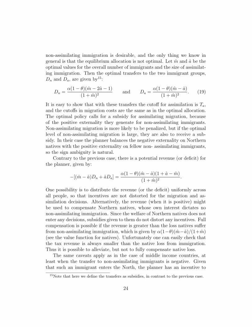
non-assimilating immigration is desirable, and the only thing we know ingeneral is that the equilibrium allocation is not optimal. Let m and a be theoptimal values for the overall number of immigrants and the size of assimilat-ing immigration. Then the optimal transfers to the two immigrant groups,Dn and Da, are given by15:

Dn =α(1− θ)(m− 2a− 1)

(1 + m)2and Da =

α(1− θ)(m− a)

(1 + m)2. (19)

It is easy to show that with these transfers the cutoff for assimilation is Ta,and the cutoffs in migration costs are the same as in the optimal allocation.The optimal policy calls for a subsidy for assimilating migration, becauseof the positive externality they generate for non-assimilating immigrants.Non-assimilating migration is more likely to be penalized, but if the optimallevel of non-assimilating migration is large, they are also to receive a sub-sidy. In their case the planner balances the negative externality on Northernnatives with the positive externality on fellow non- assimilating immigrants,so the sign ambiguity is natural.

Contrary to the previous case, there is a potential revenue (or deficit) forthe planner, given by:

−[(m− a)Dn + aDa] =α(1− θ)(m− a)(1 + a− m)

(1 + m)2.

One possibility is to distribute the revenue (or the deficit) uniformly acrossall people, so that incentives are not distorted for the migration and as-similation decisions. Alternatively, the revenue (when it is positive) mightbe used to compensate Northern natives, whose own interest dictates nonon-assimilating immigration. Since the welfare of Northern natives does notenter any decisions, subsidies given to them do not distort any incentives. Fullcompensation is possible if the revenue is greater than the loss natives sufferfrom non-assimilating immigration, which is given by α(1−θ)(m−a)/(1+m)(see the value function for natives). Unfortunately one can easily check thatthe tax revenue is always smaller than the native loss from immigration.Thus it is possible to alleviate, but not to fully compensate native loss.

The same caveats apply as in the case of middle income countries, atleast when the transfer to non-assimilating immigrants is negative. Giventhat such an immigrant enters the North, the planner has an incentive to

15Note that here we define the transfers as subsidies, in contrast to the previous case.

24

deviate from the ex ante optimal policy. The problem is even more serious,because the North has to commit to a policy that is not in its best interest.When some compensation of Northern natives is possible, this can be par-tially overcome. Also, the two countries might cooperate (perhaps because ofother shared goals) in immigration policy to approximate the social optimum.Otherwise, it is hard to see who enforces the first best, since policymaking isnaturally a Northern affair.

The following proposition summarizes the results of this section aboutthe optimal policies that achieve the first best. It is also interesting to lookat some other popular policy instruments and evaluate their effect in thepresent framework. This is the topic of the next section.

Proposition 5. The optimal policy for countries in the income range h ≤h < h is a tax on non-assimilating immigration that is a sufficient deterrentfor such migration. When some non-assimilating migration is desirable (h <h), assimilating immigrants should receive a subsidy and non-assimilatingimmigrants a transfer that can be either negative or positive, depending onthe model parameters. In both cases the problem of time inconsistency arisesfor the social planner. When there is non-assimilating migration in optimum,the likelihood of implementing the first best depends on the magnitude ofcompensation for Northern natives and on two-country cooperation.

5.2 The effect of some other policies

There are various policies that have been advocated by the immigrationliterature. Now that we have identified the optimal policies in the presentframework, it is instructive to see why some of these popular initiatives failto implement the first best. To keep matters simple, I will concentrate onthe case of middle income source countries (h ≤ h < h), where the socialoptimum and the Northern interest coincide. In this case we can safelyevaluate policies designed to maximize Northern welfare, which the literaturefocuses on.

The basic property of the optimal policy here is that it has to target thesize and composition of the immigrant group at the same time. This meansthat any policy that focuses on only one of the two is doomed to fail. Letus discuss some possibilities in turn. First, countries might simply limit theamount of immigrants they are willing to receive. Even allowing for differentquotas for different source countries (which is what optimality calls for), the

25

composition of immigration won’t be optimal. Assuming that those whobenefit most will migrate (either because immigration permits are sold orbecause of some other form of rationing takes place), it is easy to see thatat the optimal migration level some non- assimilating immigrants will come.This is because at this level of migration cn > 0 whenever h < h. Of course itis possible to set the migration limit so low that only assimilating migrationoccurs, but then their number will be suboptimal. Thus a policy that onlytargets the migration level cannot achieve the first best.16

The mirror image of setting the size of migration is influencing its com-position. In his model of cultural interactions Lazear (1995) concludes thatbecause assimilation is suboptimal, an assimilation subsidy is called for. Inour framework of endogenous migration it is easy to see why such a policyfails to achieve its goal. Let us assume that instead of τ the immigrant needsto spend only τ − s time to assimilate. This leads to the following cutoffs inthe equilibrium allocation:

τa =α(1− θ)

1 + m+ s

cn = 1− h− α(1− θ)

1 + m

ca(τ) = 1− h− τ + s.

We can immediately see that the first best cannot be implemented this way.The reason is that non-assimilating immigration is not penalized. Conse-quently, for any h < h we have cn > 0 at the optimal migration level m. Infact it is easy to show that for any positive subsidy the level of migrationincreases, so that cn will increase as well. By subsidizing assimilation it ispossible to push the assimilation cutoff to its optimal level of 1−h, but thatwill not eliminate non-assimilating immigration. Because of the positive ef-fect of m on cn, it is even possible that non-assimilating migration increasesas a result of the subsidy. Thus (as we discussed earlier) such a policy mightbe optimal for an immigrant group already in the host country, but it doesnot achieve the first best when rational immigrants take into account thesubsidy when they decide about moving.

16If we only care about Northern welfare this is not quite true, because the North isindifferent to the number of assimilating immigrants. But if immigration brings somegains for the North so that optimal immigration is strictly positive for the host countrythe same conflict between size and composition would arise.

26

So far we took the parameters as given and assumed that they cannot bechosen by the planner. It is interesting to relax this assumption and allowthe planner to influence these values. An interpretation of this is that theparameters represent variables that are fixed in the short run, but can bechanged in the long term. Thus we are interested in the design of a frame-work that allows for the best possible outcome in the migration problem.There is much scope for speculation here, and it is impossible to tackle allthe issues. Thus I will only look at α, the level of segregation in the hostcountry, and I will look at how the choice of this parameter influences thewelfare of Northern natives. One can carry out similar exercises for the otherparameters, but for lack of space I confine my attention here to α.

Some segmentation is inevitable, because people of different cultureschoose to live separately. Still, there is some scope for policy to influencethe amount of interaction between different groups. An example might beschooling. A government can encourage or discourage separation in schools,and there are examples to both in recent American history. Another exampleis Sweden, that has actively pursued a housing policy to spread immigrantsevenly in the country (Murdie and Borgegard 1998). The question we askhere is whether more or less isolation is optimal for natives. Of course a fullanalysis should take into account immigrants as well, but as we will see theanswer is not obvious even for natives and gives us some useful insights initself.

Let us rewrite the native value function from Section 2.2. It is a functionof the relative size of the non- assimilating immigrant group in the popula-tion, (m−a)/(1+m). Using the notation ρ for this ratio, the Northern valuefunction is:

VN

= 1− α(1− θ)ρ.

It is not obvious that a tradeoff arises, because the direct effect of α isnegative. There is, however, an indirect effect in equilibrium. In an optimalallocation this indirect effect could be ignored by the Envelope Theorem, buthere the equilibrium is not optimal in general. Thus we have to see how achange in α influences the equilibrium value of ρ. In the Appendix I showthat ρ is increasing in the level of segregation, so that native welfare dependson α in a non-trivial way.

The reason for this is easy to see. When the level of isolation increases,it is less likely that a native meets a non- assimilated immigrant, ceterisparibus. But more isolation also discourages assimilation, so that there are

27

more non-assimilating immigrants in the Northern population. These twoeffect work in the opposite direction, so in general it is not obvious whetherincreasing or decreasing segregation is what natives should prefer. Thus itis very well possible that natives are better off in a less segregated society,even if we don’t take into account ethical considerations.

6 Empirical evidence

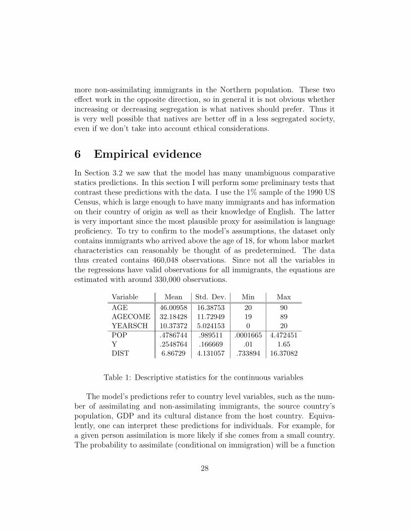
In Section 3.2 we saw that the model has many unambiguous comparativestatics predictions. In this section I will perform some preliminary tests thatcontrast these predictions with the data. I use the 1% sample of the 1990 USCensus, which is large enough to have many immigrants and has informationon their country of origin as well as their knowledge of English. The latteris very important since the most plausible proxy for assimilation is languageproficiency. To try to confirm to the model’s assumptions, the dataset onlycontains immigrants who arrived above the age of 18, for whom labor marketcharacteristics can reasonably be thought of as predetermined. The datathus created contains 460,048 observations. Since not all the variables inthe regressions have valid observations for all immigrants, the equations areestimated with around 330,000 observations.

Variable Mean Std. Dev. Min MaxAGE 46.00958 16.38753 20 90AGECOME 32.18428 11.72949 19 89YEARSCH 10.37372 5.024153 0 20POP .4786744 .989511 .0001665 4.472451Y .2548764 .166669 .01 1.65DIST 6.86729 4.131057 .733894 16.37082

Table 1: Descriptive statistics for the continuous variables

The model’s predictions refer to country level variables, such as the num-ber of assimilating and non-assimilating immigrants, the source country’spopulation, GDP and its cultural distance from the host country. Equiva-lently, one can interpret these predictions for individuals. For example, fora given person assimilation is more likely if she comes from a small country.The probability to assimilate (conditional on immigration) will be a function

28

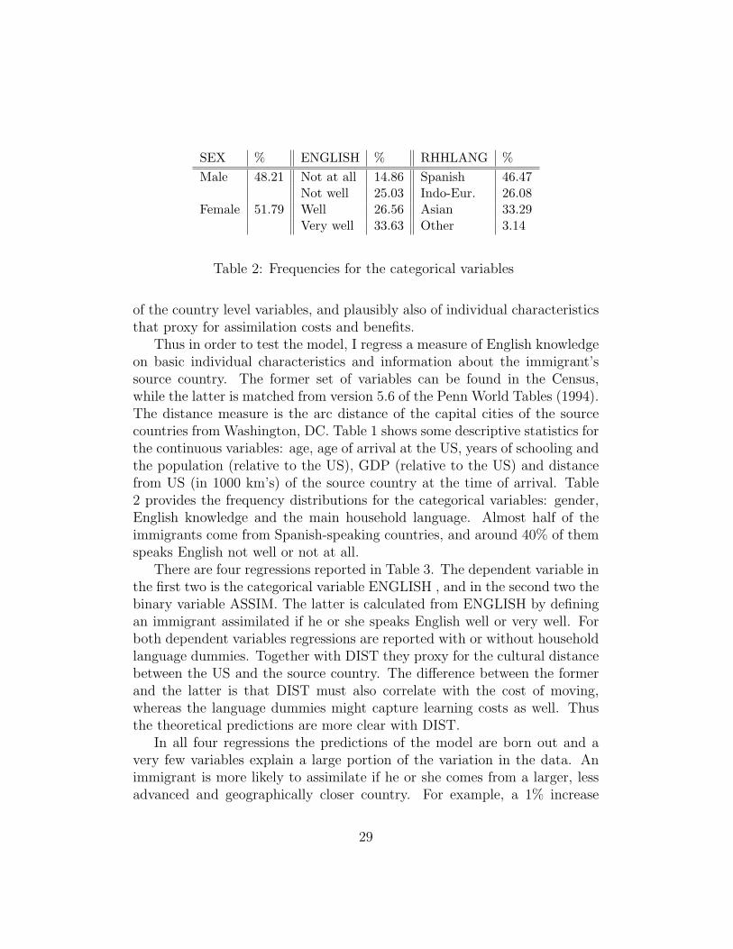
SEX % ENGLISH % RHHLANG %Male 48.21 Not at all 14.86 Spanish 46.47

Not well 25.03 Indo-Eur. 26.08Female 51.79 Well 26.56 Asian 33.29

Very well 33.63 Other 3.14

Table 2: Frequencies for the categorical variables

of the country level variables, and plausibly also of individual characteristicsthat proxy for assimilation costs and benefits.

Thus in order to test the model, I regress a measure of English knowledgeon basic individual characteristics and information about the immigrant’ssource country. The former set of variables can be found in the Census,while the latter is matched from version 5.6 of the Penn World Tables (1994).The distance measure is the arc distance of the capital cities of the sourcecountries from Washington, DC. Table 1 shows some descriptive statistics forthe continuous variables: age, age of arrival at the US, years of schooling andthe population (relative to the US), GDP (relative to the US) and distancefrom US (in 1000 km’s) of the source country at the time of arrival. Table2 provides the frequency distributions for the categorical variables: gender,English knowledge and the main household language. Almost half of theimmigrants come from Spanish-speaking countries, and around 40% of themspeaks English not well or not at all.

There are four regressions reported in Table 3. The dependent variable inthe first two is the categorical variable ENGLISH , and in the second two thebinary variable ASSIM. The latter is calculated from ENGLISH by definingan immigrant assimilated if he or she speaks English well or very well. Forboth dependent variables regressions are reported with or without householdlanguage dummies. Together with DIST they proxy for the cultural distancebetween the US and the source country. The difference between the formerand the latter is that DIST must also correlate with the cost of moving,whereas the language dummies might capture learning costs as well. Thusthe theoretical predictions are more clear with DIST.

In all four regressions the predictions of the model are born out and avery few variables explain a large portion of the variation in the data. Animmigrant is more likely to assimilate if he or she comes from a larger, lessadvanced and geographically closer country. For example, a 1% increase

29

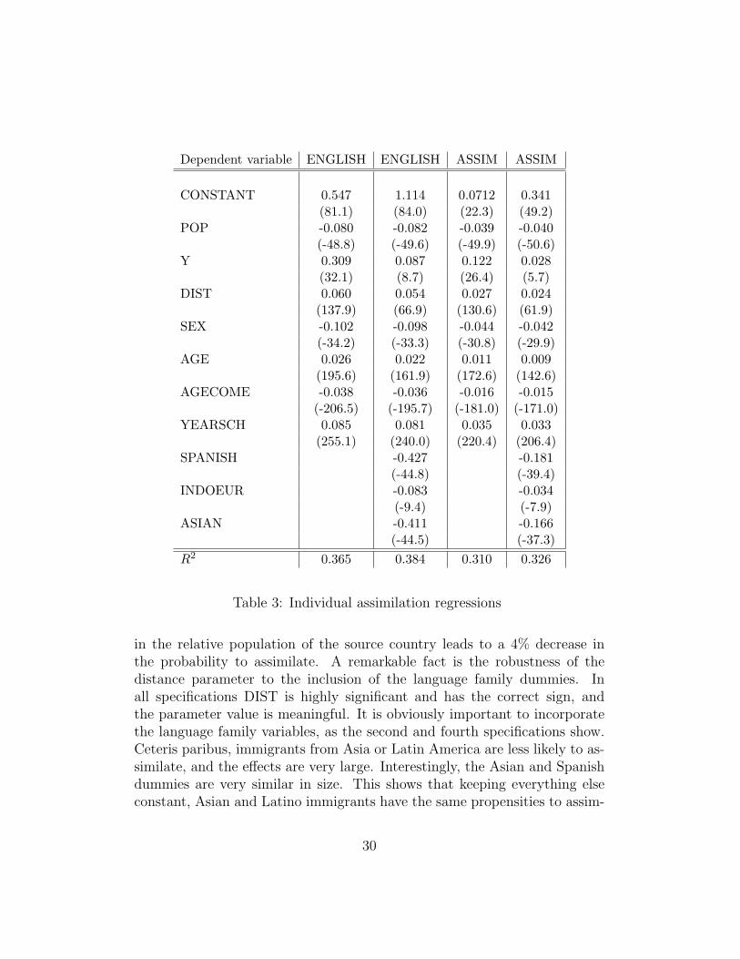
Dependent variable ENGLISH ENGLISH ASSIM ASSIM

CONSTANT 0.547 1.114 0.0712 0.341(81.1) (84.0) (22.3) (49.2)

POP -0.080 -0.082 -0.039 -0.040(-48.8) (-49.6) (-49.9) (-50.6)

Y 0.309 0.087 0.122 0.028(32.1) (8.7) (26.4) (5.7)

DIST 0.060 0.054 0.027 0.024(137.9) (66.9) (130.6) (61.9)

SEX -0.102 -0.098 -0.044 -0.042(-34.2) (-33.3) (-30.8) (-29.9)

AGE 0.026 0.022 0.011 0.009(195.6) (161.9) (172.6) (142.6)

AGECOME -0.038 -0.036 -0.016 -0.015(-206.5) (-195.7) (-181.0) (-171.0)

YEARSCH 0.085 0.081 0.035 0.033(255.1) (240.0) (220.4) (206.4)

SPANISH -0.427 -0.181(-44.8) (-39.4)

INDOEUR -0.083 -0.034(-9.4) (-7.9)

ASIAN -0.411 -0.166(-44.5) (-37.3)

R2 0.365 0.384 0.310 0.326

Table 3: Individual assimilation regressions

in the relative population of the source country leads to a 4% decrease inthe probability to assimilate. A remarkable fact is the robustness of thedistance parameter to the inclusion of the language family dummies. Inall specifications DIST is highly significant and has the correct sign, andthe parameter value is meaningful. It is obviously important to incorporatethe language family variables, as the second and fourth specifications show.Ceteris paribus, immigrants from Asia or Latin America are less likely to as-similate, and the effects are very large. Interestingly, the Asian and Spanishdummies are very similar in size. This shows that keeping everything elseconstant, Asian and Latino immigrants have the same propensities to assim-

30

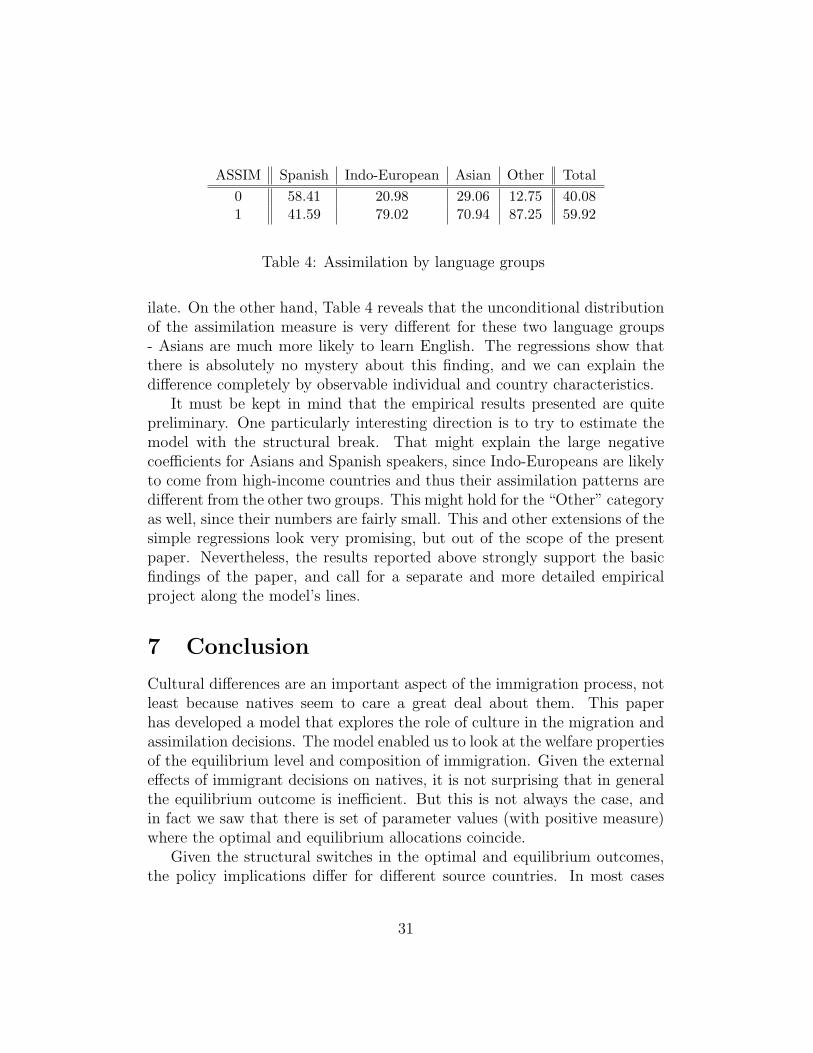
ASSIM Spanish Indo-European Asian Other Total0 58.41 20.98 29.06 12.75 40.081 41.59 79.02 70.94 87.25 59.92

Table 4: Assimilation by language groups

ilate. On the other hand, Table 4 reveals that the unconditional distributionof the assimilation measure is very different for these two language groups- Asians are much more likely to learn English. The regressions show thatthere is absolutely no mystery about this finding, and we can explain thedifference completely by observable individual and country characteristics.

It must be kept in mind that the empirical results presented are quitepreliminary. One particularly interesting direction is to try to estimate themodel with the structural break. That might explain the large negativecoefficients for Asians and Spanish speakers, since Indo-Europeans are likelyto come from high-income countries and thus their assimilation patterns aredifferent from the other two groups. This might hold for the “Other” categoryas well, since their numbers are fairly small. This and other extensions of thesimple regressions look very promising, but out of the scope of the presentpaper. Nevertheless, the results reported above strongly support the basicfindings of the paper, and call for a separate and more detailed empiricalproject along the model’s lines.

7 Conclusion

Cultural differences are an important aspect of the immigration process, notleast because natives seem to care a great deal about them. This paperhas developed a model that explores the role of culture in the migration andassimilation decisions. The model enabled us to look at the welfare propertiesof the equilibrium level and composition of immigration. Given the externaleffects of immigrant decisions on natives, it is not surprising that in generalthe equilibrium outcome is inefficient. But this is not always the case, andin fact we saw that there is set of parameter values (with positive measure)where the optimal and equilibrium allocations coincide.

Given the structural switches in the optimal and equilibrium outcomes,the policy implications differ for different source countries. In most cases

31

when the equilibrium is inefficient a tax on non-assimilating immigrants im-plements the first best, although it might be hard for the policymaker tocommit to such a policy. Also, for some parameter values natives in thehost country and the social planner (who cares about global welfare) havedifferent objectives. When the revenue from the optimal tax can be usedto compensate natives, this problem can be alleviated, if not completelyovercome. Otherwise, since policy decisions are made in the host country,implementing the social optimum might not be possible in practice.

To make the model tractable I abstracted away from many issues thattraditionally interest researchers of migration. Apart from assimilation skills,people do not differ in their labor market abilities. There is only one (ab-stract) sector of production, and there is no role for capital (physical orhuman) in the model. Also, the analysis is essentially static, although thereis an implicit dynamic element: the timing of the migration and the assimi-lation decisions. Still, we could make the model more explicitly dynamic byallowing for subsequent immigrant generations, and look at the evolution oftheir composition over time. Clearly, incorporating these would lead to addi-tional insights. But they would also make the model even more complicated,and I believe the main conclusions would not change substantially. Thus inmy view the present model is an acceptable compromise between tractabilityand usefulness.

Even so, there are several issues that would be interesting to look atin subsequent work. One of them concerns the benefits immigrants bringto the host country. An interesting issue is the possibility that immigrantscreate trade with their source country. Casella and Rauch (1998) developa model where ethnic networks facilitate trade between countries by havingaccess to information not available through the market. Ethic groups, suchas immigrants, can thus alleviate the market failure caused by incompleteinformation. There is also some empirical evidence that immigrants act ascatalysts for foreign trade. Helliwell (1997) documents that trade betweenUS states and Canadian provinces is larger if they have a larger share ofeach other’s citizens as immigrants. In another work, Head, Ries and Wag-ner (1997) examine the effect of immigration on trade between Canada andvarious East Asian countries, and they find a positive relationship.

The crucial question with this and other possible benefits is whether non-assimilating immigration generates positive externalities for natives. If not,we can safely abstract away from them, since the qualitative nature of theproblem remains the same, though the optimal levels might change. In the

32

trade creation context, this would require immigrants to appropriate all thebenefits from improved efficiency, or at least that they generate positiveexternality only for their source country. I think this is not unreasonableto assume, and it is possible to extend the present model to generate suchexternalities. Since this does not change the qualitative conclusions of thepaper much, I leave the extension for future research.

Another important issue is that the assimilation decision might involvestrategic considerations if natives can also learn the culture of immigrants.In this case learning by one group decreases the incentives for learning forthe other. In the present paper I avoided the strategic aspect of learningby not allowing natives to “reverse assimilate”. First, it would make theanalysis too complicated for analytical results. Second, I believe that inthe case of modest immigrant flows this is a fairly innocuous simplification.Culture in a country includes not just language, but habits, norms, and thelegal and political systems. Unless the immigrant group is large enoughto form its own self-governing society (in which case the simple randommatching framework is irrelevant anyway), a large chunk of culture has tobe acquired by immigrants regardless of native decisions. Furthermore, thestrategic view is important if the two groups are similar in size. Thus ifimmigration is modest, not allowing “reverse assimilation” can be viewed asa good approximation to reality. In other cases this need not be the case,for example when we look at the role of culture in inter-country relations.To address this issue, in a recent paper (Konya 2000) I incorporate strategiclearning decisions into the analysis in a model of international trade andculture.

Finally, further empirical investigations into the role of culture in the mi-gration process are desirable. The empirical findings reported in the paperare very encouraging, but more needs to be done. A very important (and verydifficult) task would be to quantify the extent of the cultural externalitiesbetween natives and immigrants. The qualitative conclusions of the presentmodel do not depend on this, but we need to understand the practical im-portance of the problem better. Historical evidence – such as the examplescited in Sowell (1996) – is available, but very hard to measure. It is not clearhow we can provide more quantitative measures, but it would clearly be veryimportant.

There are many ways to extend the model, and the possibilities I men-tioned above are some of them. Empirical research is clearly a priority, ifonly for the recent interest of politics in immigration and culture, especially

33

in Europe. Although there is scope for policy interventions, there is a cleardanger that in a heated political atmosphere they would be overdone. Mi-gration of poor people into rich countries is desirable for immigrants (andpossibly – in a more realistic setting – for the host country), and that makesthe implementation of right policies even more important. Some policies thatseem attractive might not have the desired effect, and they can even worsenthe problem instead of solving it. This paper hopefully provides a first stepin the direction of avoiding such costly mistakes.

References

Altonji, J. G. and Card, D. (1991). The effects of immigration on the la-bor market outcomes of less-skilled natives, in J. M. Abowd and R. B.Freeman (eds), Immigration, Trade and the Labor Market, University ofChicago Press.

Auerbach, A. J. and Oreopoulos, P. (1999). Generational accounting andimmigration in the United States, Working Paper 7041, NBER.

Borjas, G. J. (1987). Self-selection and the earnings of immigrants, AmericanEconomic Review 77(4): 531–552.

Borjas, G. J. (1999a). The economic analysis of immigration, in O. Ashenfel-ter and D. Card (eds), Handbook of Labor Economics, Vol. 3A, North-Holland.

Borjas, G. J. (1999b). Heaven’s Door, Princeton University Press.

Burda, M. and Wyplosz, C. (1992). Human capital, investment and migrationin an integrated Europe, European Economic Review 36: 677–684.

Card, D. and DiNardo, J. E. (2000). Do immigrant inflows lead to nativeoutflows?, Working Paper 7578, NBER.

Casella, A. and Rauch, J. E. (1998). Overcoming informational barriers tointernational resource allocation: prices and group ties, Working Paper6628, NBER.

Chiswick, B. R. (1978). The effect of Americanization on the earnings offoreign-born men, Journal of Political Economy 86: 897–921.

34

Hanson, G. H. and Slaughter, M. J. (1999). The Rybczynski theorem, factor-price equalization and immigration: evidence from U.S. states, WorkingPaper 7074, NBER.

Head, K., Ries, J. and Wagner, D. (1997). Immigrants as trade catalysts,in A. Safarian and W. Dobson (eds), The people link: Human resourcelinkages across the Pacific, University of Toronto Press.

Helliwell, J. F. (1997). National borders, trade and migration, Working Paper6027, NBER.

Konya, I. (2000). Modeling cultural barriers in international trade, Mimeo,Northwestern University.

Layard, R., Blanchard, O., Dornbusch, R. and Krugman, P. (1992). East-West Migration, The MIT Press, Cambridge, MA.

Lazear, E. P. (1995). Culture and language, Working Paper 5249, NBER.

Lazear, E. P. (1996). Culture wars in America, Essays in public policy, HooverInstitution, Stanford University.

Markusen, J. R. and Zahniser, S. (1997). Liberalization and incentives forlabour migration: theory with applications to NAFTA, Working Paper6232, NBER.

Murdie, R. A. and Borgegard, L.-E. (1998). Immigration, spatial segregationand housing segmentation of immigrants in metropolitan Stockholm,1960-95, Urban Studies 35(10): 1869–1888.

Sowell, T. (1996). Migrations and cultures: a world view, BasicBooks.

Storesletten, K. (2000). Sustaining fiscal policy through immigration, Journalof Political Economy 108(2): 300–323.

Trefler, D. (1997). Immigrants and natives in general equilibrium trade mod-els, Working Paper 6209, NBER.

Venables, A. J. (1999). Trade liberalisation and factor mobility: an overview,in R. Faini, J. D. Melo and K. F. Zimmermann (eds), Migration: thecontroversies and the evidence, Cambridge University Press.

35

Zhou, M. and Bankston III, C. L. (1998). Growing up American: HowVietnamese Children Adapt to Life in the United States, Russell SageFoundation, New York.

AppendixThe comparative statics analysis is straightforward in the case of a cornersolution, since the left-hand side of (9) does not depend on m. Thus themigration level in this case is increasing in L and it is decreasing in h.

For an interior equilibrium, let us define A and B with the followingequations:

A =

∫ τa

0

F (1− h− τ) dG(τ)

B = F (cn)[1−G(τa)],

where

τa =α(1− θ)

1 + m

cn = 1− h− α(1− θ)

1 + m.

Thus we have that m = A + B and m − a = B, and it is easy to see thatAm < 0 and Bm > 0. Assumption 1 also guarantees that 1− Am −Bm > 0.

The effect of parameters on m is given by the expression (Aj + Bj)/(1−Am − Bm), where j = α, θ, h, L. Since the denominator is positive, the signof the expression depends on the sign of the numerator. It is immediate thatAh, Bh < 0 and AL, BL > 0, hence m is increasing in L and it is decreasingin h. For α we have that:

∂(A + B)

∂α= f(cn)[1−G(τa)]

∂cn

∂α< 0,

so m is increasing in the level of segregation. Similarly for θ :

∂(A + B)

∂θ= f(cn)[1−G(τa)]

∂cn

∂θ> 0,

36

so m is increasing in the level of cultural similarity.For the other results we can use the following matrix equation:[

1− Am −Bm 0−Am 1

] [dmda

]=

[Aj + Bj

Aj

]d j,

where again j = α, θ, L, h. Then the derivatives of m− a are given by:

∂(m− a)

∂j=

Bj(1− Am) + AjBm

1− Am −Bm

.

This expression can be easily signed when Aj and Bj have the same sign, asin the case of L and h. For α it is easier to evaluate the derivative of a:

∂a

∂α=

Aα(1− Am −Bm) + Am(Aα + Bα)

1− Am −Bm

> 0.

Since the level of migration is decreasing in α and assimilating migration isincreasing in it, it is necessary that m − a decreases with α. Finally, in thepolicy section I claimed that ρ = (m−a)/(1+m) is decreasing in α. Now wecan see why this is the case, given that we can rewrite ρ as 1−(1+a)/(1+m).

37