b-spline channel smoothing for robust estimation

The B-Spline Channel Representation:Channel Algebra and

Channel Based Diffusion FilteringReport LiTH-ISY-R-2461

Michael Felsberg∗ Hanno Scharr† Per-Erik Forssen∗

[email protected] [email protected] [email protected]

∗Computer Vision Laboratory, Department of Electrical Engineering,

Linkoping University, SE-581 83 Linkoping, Sweden

†Intel Research, 3600 Juliette Lane, SC12-303, Santa Clara, CA 95054, USA

September 9, 2002

Abstract

In this paper we consider the channel representation based upon quadratic B-splines from a statistical point of view. Interpreting the channel representation as akernel method for estimating probability density functions, we establish a channelalgebra which allows to perform basic algebraic operations on measurements directlyin the channel representation. Furthermore, as a central point, we identify thesmoothing of channel values with a robust estimator, or equivalently, a diffusionprocess.

Keywords: channel representation, splines, kernel method, channel algebra, robustestimator, diffusion

1

2 M. Felsberg, H. Scharr, and P.-E. Forssen

Contents

1 Introduction 3

2 Channel Representation Based on B-Splines 42.1 The B-Spline Basis . . . . . . . . . . . . . . . . . . . . . . . . . . . . . . . 42.2 Encoding with B-Splines . . . . . . . . . . . . . . . . . . . . . . . . . . . . 52.3 Signal Reconstruction . . . . . . . . . . . . . . . . . . . . . . . . . . . . . . 62.4 Some Properties . . . . . . . . . . . . . . . . . . . . . . . . . . . . . . . . . 8

3 Computing with B-Spline Channels 113.1 Adding Channels . . . . . . . . . . . . . . . . . . . . . . . . . . . . . . . . 113.2 Affine Transforms of Channels . . . . . . . . . . . . . . . . . . . . . . . . . 123.3 Multiplying Channels . . . . . . . . . . . . . . . . . . . . . . . . . . . . . . 13

4 Channel Smoothing and Diffusion 144.1 Channel Smoothing . . . . . . . . . . . . . . . . . . . . . . . . . . . . . . . 144.2 Robust Estimation . . . . . . . . . . . . . . . . . . . . . . . . . . . . . . . 174.3 Outlier Processes . . . . . . . . . . . . . . . . . . . . . . . . . . . . . . . . 204.4 Relation to Diffusion . . . . . . . . . . . . . . . . . . . . . . . . . . . . . . 21

5 Future Work 25

B-Spline Channel Representation 3

1 Introduction

Since the channel representation has been introduced [13], it has proven to be a powerfulframework for several kinds of applications [9, 10, 11]. Although the underlying theory isformulated more generally, the channel representation has mostly been applied in form ofcos2-basis functions in the past. However, there are other possible local, smooth functionswhich can be used to encode a signal in channels, e.g., by B-splines. The encoding anddecoding based on quadratic B-splines is introduced in section 2.

From a viewpoint of classical statistics, the channel representation can be consideredas a kernel method for estimating the probability density function of a measurement [1].The requirements for a channel basis function imply the necessary conditions for being avalid kernel function, in particular the monopolarity1 constraint and the constant L1-normconstraint.

In practical applications it is often necessary to combine several measurements in orderto obtain the desired result. As long as there is an analytic description of the requiredcalculations, it would be quite advantageous to perform the calculations directly in thechannel domain in order to maintain the approximated probability density functions. Itturns out, that the spline-channels are well suited to transfer basic algebraic operations(addition, multiplication, field-multiplication, field addition2) to the channel representa-tion, see section 3.

A typical application of the channel representation motivated by the interpretation asa kernel method is the channel smoothing. The resulting reconstructions are similar toresults from diffusion processes (for an overview see [15]). Indeed, it is possible to showthat channel smoothing is related to a robust estimator, and therefore, to a line process[2]. It is then straightforward to relate the channel smoothing to a diffusion process [3].The relationship between channel smoothing and diffusion is worked out in section 4 as acentral topic of this paper.

1Monopolar means positive scalar.2For classical algebras there is no field-addition, because the algebra elements and the field elements

are either from different sets or are not to distinguish. In our case we can add a certain constant offsetto a measurement, such that we just perform a shift of the probability density function.


2 Channel Representation Based on B-Splines

In this section we describe how to represent a signal by means of B-spline channels.

2.1 The B-Spline Basis

B-splines are a well known technique for function approximation [6]. The basis functionsof the B-splines are obtained by successive convolutions of the unit rectangle with itself[12]. The resulting basis functions become smoother and wider with each iteration (seefigure 1).

0 0.5 1 1.5 2 2.5 3 3.5 40

0.2

0.4

0.6

0.8

1

f

Bk(f

)

degree 0degree 1degree 2degree 3

Figure 1: B-spline basis functions of degree zero to three.

The B-spline basis function (short: B-spline) of degree k is defined by convolving theunit rectangle3

rect(f) =

{1 if 0 ≤ f ≤ 1

0 else(1)

k times with itself and it is denoted by Bk(f). Alternatively to the definition above, onecan compute the B-splines by a recursive formula [6].

In order to obtain the full B-spline basis of degree k, the B-spline Bk(f) is shiftedby integers. The B-spline approximation of a function P (f) is then obtained by a linear

3Since we apply the B-splines to signals f(x) further below, we use f as the argument in this section.Furthermore, the spatial argument x is omitted if it is not relevant.


combination of the B-splines:

P (f) ≈∑n∈Z

αnBk(f − n) . (2)

Normally, the most interesting part of the spline approximation is the computation of thelinear coefficients αn. These coefficients are obtained from a large set of linear equations.In practice the sum in (2) is finite, i.e., n is an integer in [nmin − k, nmax − 1], where nmin

and nmax are the bounds of the approximation interval. Requiring

P (m) =nmax−1∑

n=nmin−k

αnBk(m− n) (3)

for all m ∈ {nmin, . . . , nmax} yields nmax − nmin + 1 equations. However, the number ofunknowns is nmax − nmin + k, and hence, we need k − 1 boundary conditions in order toobtain a unique solution.

2.2 Encoding with B-Splines

A signal f(x) is encoded with the B-splines by computing Bk(f(x) − n). If we considerthe B-splines of degree 0 − 2, we make the following observations:

1. The B-spline basis of degree 0 corresponds to an ordinary local histogram. A singlevalue cannot be reconstructed exactly.

2. The B-spline basis of degree 1 is the least degree basis which allows to reconstructa single value exactly. This is done by a linear interpolation scheme.

3. The B-spline basis of degree 2 is the least degree basis which is continuously dif-ferentiable, i.e., smooth. Single values can be exactly reconstructed by a linearinterpolation scheme (see below).

4. In order to have reconstructability, the B-spline basis of degree k > 0 requires tohave an overlap of k+1, i.e., at almost every point k+1 basis functions are non-zero.

We choose the basis function for the channel representation according to the obser-vations made above. Since we want to use a local smooth basis function, we have atleast to use a basis of degree 2. Since the overlap should be small in order to reduce thecomputational complexity, the degree should be as small as possible. Hence, we choosek = 2, i.e., piecewise quadratic functions, and the overlap is given to be 3. The explicitformulation of the 2nd degree B-spline is given by

B2(f) =

f2

2if f ∈ (0, 1]

−f 2 + 3f − 32

if f ∈ (1, 2](3−f)2

2if f ∈ (2, 3)

0 else

. (4)


Hence, the value for the nth channel is obtained as

cn(f) = B2(f − n) . (5)

These channel values cn(f) can be plugged into (2) in order to approximate any func-tion P (f). However, the common point of view to the channel representation implies thatP (f) = f . The computation of B2(f −n) corresponds to the encoding step and the linearcombination

∑αnB2(f − n) corresponds to the decoding step. Applying the decoding

directly after the encoding should give the identity. For certain applications however,P (f) is not necessarily given as the identity, it can also be some nonlinear mapping, e.g.,logarithm, arcus-tangent, etc.. Although the decoding to a non-linear function might yieldsophisticated methods for certain signal processing tasks, we only consider the linear casein this paper.

2.3 Signal Reconstruction

The question is now, which coefficients αn yield the identity? It is easily verified, that incase of a single value the reconstruction is obtained by the following linear interpolation:

f =nmax−1∑

n=nmin−2

(n+3

2)cn(f) . (6)

The linear coefficients are obtained by solving the linear system consisting of nmax−nmin+1equations and one boundary condition. If we use f ′(nmin) = 1 as a boundary condition,we obtain the system

1

2

−2 2 0 · · · 01 1 0 · · · 0

0. . . . . . . . .

......

. . . . . . . . . 00 · · · 0 1 1

αnmin−2

αnmin−1...

αnmax−2

αnmax−1

=

1nmin

...nmax

. (7)

The first two equations can be solved separately, which gives

αnmin−2 = nmin − 1

2and

αnmin−1 = nmin +1

2.

For nmax > n ≥ nmin we can apply induction, assuming that αn−1 = n+ 12. Selecting the

(n− nmin + 3)rd line in (7) gives

1

2

[1 1

](αn−1

αn

)=αn−1 + αn

2= n+ 1 .

Plugging in the induction assumption yields

n+ 12

+ αn

2= n+ 1


and hence

αn = 2(n+ 1) − n− 1

2= n+

3

2.

There are two remarks we want to make for applying (6) in practice:

1. We must take into account that in practice the channel representation is not singlevalued.

2. The linear interpolation assumes that the absolute scaling of the channel valuesremains unscaled, hence they must be normalized beforehand.

The consequence of the first remark is that we do not compute the full sum from (6),but we evaluate the sum between two different (a priori unknown) bounds, i.e., we applya window function, the reconstruction window. Although we use a rectangular (Parzen)window throughout this report, the reconstruction window can have different shapes.Using the a rectangular window, the reconstruction is obtained by

f =

nub∑n=nlb

(n+3

2)cn(f) , (8)

where nlb and nub are the lower bound and the upper bound of the reconstruction window,respectively.

According to the second remark, the channel values cn must be rescaled beforehand,in order to meet the requirement

nub∑n=nlb

cn(f) = 1 . (9)

The normalization is obtained by dividing the channel values by their sum in the recon-struction window.

This normalization of the channel values implies that any offset can be added to thereconstruction coefficients, being compensated by subtracting this offset from the finalresult. If w indicates the width of the reconstruction window and n0 its lower bound, (8)can be replaced with

f =3

2+ n0 +

w − 1

2+

w−1∑n=0

(n− w − 1

2)cn+n0(f) . (10)

If w = 3, the reconstruction is especially simple:

f =5

2+ n0 − cn0−1(f) + cn0+1(f) (11)

i.e., we just apply the discrete derivative operator of size three to the channel vector.Even if we assume that the reconstruction window is a rectangle, it is still unclear

how to choose the width w and the position n0 of the window. Ideal B-spline channelrepresentations which correspond to single values consist of only three adjacent non-zerovalues. Hence a window width of three seems to be a natural choice. However, there aretwo cases, where we have more than three adjacent non-zero values:


1. The channel representation corresponds to multiple values and the values are suffi-ciently close such that the non-zero channels overlap.

2. The channel representation is non-ideal since it is modified by some operation (e.g.channel smoothing, channel addition, see below).

Whereas for the second case a wider reconstruction window is the appropriate choice,the first case requires a narrow window with an exact positioning. Before we discuss theoptimal width of the reconstruction window, we turn to the positioning of the windowitself.

Our decoding algorithm selects the window position with the highest (weighted) L1-norm4 by by applying a (weighted) moving average filter and detecting its maximum. Thismethod assures that single values are reconstructed correctly if the channel representationis ideal. For non-ideal representations (i.e., more than three non-zero channels), thereconstruction error is minimized, at least for a certain window size. For overlappingrepresentations, the moving average method can either perform correctly or it leads tosome averaging of neighbored values, see figure 2. The behavior depends on the distancebetween the two values relative to the window width.

f f f

cn cn cn

Figure 2: Reconstruction errors with a rectangular window. Left: the channel representa-tion is too broad, the reconstructed value is too small. Center: the channels represent twovalues, they can be distinguished with the rectangular window. Right: the reconstructionaverages the two values, they are too close.

2.4 Some Properties

In the preceding sections the encoding and decoding for the channel representation basedon B-splines of degree two are defined. This section deals with some properties of the newapproach and compares it to the channel representation based on cos2-functions.

In the past, the cos2-functions were chosen as basis functions since they have thenice property of yielding channel vectors with constant L1- and L2-norm [8]. Whereas theconstant L1-norm is necessary to define an appropriate decoding procedure and for severalapplications (e.g. channel smoothing), a constant L2-norm is only necessary if channelvectors shall be compared by means of the scalar product [4]. It depends on the specific

4Notice that the channel values are monopolar, and hence, the L1-norm is simply the channel sum.In practice, we use a weighted norm, i.e., we apply a lowpass filter and search for the peak value.


application of the channel representation if scalar products of channel vectors occur ornot.

Hence, for many applications the missing L2-property does not matter. On the otherhand, the B-spline channel representation yields several advantages. The probably mostimportant is the decoding by means of a linear combination, in contrast to the quiteinvolved decoding of the cos2-channels. The linear decoding has several advantages:

1. The decoding is fast and accurate, even on machines without special numericalcapabilities.

2. The channel smoothing corresponds to a linear smoothing if the signal values havesmall variance.

3. The decoding can directly be integrated into a neural network.

4. Analytic derivations are simplified.

5. Certain computations can be performed directly in the channel representation.

The linear decoding is obviously faster than the cos2-decoding, since linear combina-tions are cheaper to compute than inverse trigonometric functions.

The second advantage is illustrated by figure 3. The examples show the results fromencoding three noisy 1D signals (linear function, sine, jump) with 6 channels, applyinga linear smoothing to each channel, and subsequent decoding with a window of widththree. Obviously, the continuous parts of all signals are quite well recovered, whereas thediscontinuity in the third signal is preserved. The recovered linear function is still a linearfunction, i.e., the channel smoothing had the same effect as a linear smoothing in thiscase. We will return to this topic in section 4.

Concerning the third advantage, we just mention here that each layer of an ordinary(i.e., not higher order) neural network consists of linear combinations. These can easilyrealize the decoding from the channel representation.

The argument that analytic derivations are simplified by linear approaches need nofurther comment. The last advantage is explained in detail in the following section.


x

f(x)

noisy datareconstruction

x

f(x)

noisy datareconstruction

x

f(x)

noisy datareconstructionreliability

Figure 3: Three 1D experiments. Left: a linear gradient is recovered. Center: a continuousfunction (sine) is recovered. Right: a discontinuity is preserved. The reconstructed curveshave an additional offset to improve the visualization.


3 Computing with B-Spline Channels

The aim of this section is to derive the operations on the channel representation whichcorrespond to basic algebraic operations in the original representation. In other words,we derive a channel algebra. A first attempt into this direction has been made in [7],but the non-linear decoding scheme of the cos2-channels did not allow to multiply in thechannel representation.

In order to describe that two channel vectors cn and c′m represent the same signal, i.e.,the representations are isomorphic, we introduce the notation

cn ' c′m which means∑

n

ncn =∑m

mc′m . (12)

3.1 Adding Channels

The channel representation can be interpreted as an estimate of the probability densityfunction of a certain measurement by means of a kernel-based method [1]. The B-splinesof any degree obviously fulfill the requirements for being a kernel function, since

Bk(f) > 0 (13)∫R

Bk(f) df = 1 . (14)

If two independent measurements are added, their probability density functions mustbe convolved in order to obtain the probability density function of the sum. Applying thisidea to two channel representations yields the interesting result that the reconstructionof their discrete convolution yields the sum of their reconstructions:

cn(f + g) ' cn(f) ∗ cn(g)∣∣n7→n+3/2

. (15)

This result is easily shown by resorting the addends in the discrete convolution andby using the fact that the channel vector is normalized (wrt. L1). First, the discreteconvolution reads

cn(f) ∗ cn(g) =∑m

cm(f)cn−m(g) .

Notice that cn(f)∗ cn(g) is also normalized (wrt. L1). Applying (6) to cn(f)∗ cn(g) yields

3

2+∑

n

n(cn(f) ∗ cn(g)) =3

2+∑

n

n∑m

cm(f)cn−m(g)

substitute l = n−m =3

2+∑

l

∑m

(l +m)cm(f)cl(g)

=3

2+∑

l

lcl(g)∑m

cm(f) +∑

l

cl(g)∑m

mcm(f)

=3

2+ (f − 3

2) · 1 + 1 · (g − 3

2)

= f + g − 3

2.


If we change the index n to n+ 32, cn(f)∗ cn(g) is decoded to the same signal as cn(f + g).

In this derivation channel indices are shifted. Actually, we can use index-shift andindex-scaling to simulate 1D affine transforms to the encoded signal.

3.2 Affine Transforms of Channels

Affine transforms correspond to field addition and field multiplication. Field multiplica-tion means a scaling of the channel positions and likewise a scaling of the approximatedprobability density function. Field addition means a shift of the channel positions.

First, we consider offsets, i.e., field addition. Adding a constant r ∈ R to the channelindex gives:

c′m(f) = cn(f)∣∣n7→n+r

' cn(f + r) . (16)

Inserting c′m(f) in (6) yields

∑m

(m+3

2)c′m(f) =

∑n

(n+ r +3

2)cn(f) = r +

∑n

(n+3

2)cn(f) = r + f .

More interesting is the scaling of the channel index (field multiplication), since thisallows to alter the dynamics of the decoded signal. Multiplying the index by a positiveconstant r ∈ R

+ results in

c′m(f) = cn(f)∣∣n7→rn

' cn(rf +3(1 − r)

2) . (17)


∑m

(m+3

2)c′m(f) =

3(1 − r)

2+∑

n

(rn+ r3

2)cn(f)

=3(1 − r)

2+ r

∑n

(n+3

2)cn(f) =

3(1 − r)

2+ rf .

The resulting implicit shift by 3(1−r)2

can easily be compensated by another shift operation.

Finally, a signal can be reflected by negating the index:

c′m(f) = cn(f)∣∣n7→−n

' cn(−f + 3) . (18)


∑m

(m+3

2)c′m(f) =

∑n

(−n+3

2)cn(f) = 3 −

∑n

(n+3

2)cn(f) = 3 − f .


3.3 Multiplying Channels

In order to multiply two measurements by means of their channel representations, itis necessary to introduce some new notations. Let cn(f) be the channel values of therepresentation of a measurement f . We define

cn/m =cbn/mc(dn/me − n/m) + cdn/me(n/m− bn/mc)

m, (19)

where b·c is the next smaller integer (floor operation), d·e is the next larger integer (ceilingoperation), and m is a positive integer.

The preceding definition is reasonable since the measurement f is recovered by

f =3

2+∑

n

n

mcn/m(f) . (20)

By some straightforward calculations, we obtain

3

2+∑

n

n

mcn/m(f) =

3

2+

1

m2

∑n

n(cbn/mc(dn/me − n/m) + cdn/me(n/m− bn/mc))

substitue n = mk + l

=3

2+

1

m2

∑k

m−1∑l=0

(mk + l)(ck(1 − l/m) + ck+1l/m)

=3

2+

1

m2

(m−1∑l=0

((l − l2/m)

∑k

ck + l2/m∑

k

ck+1

+(m− l)∑

k

kck + l∑

k

kck+1

))

=3

2+

1

m2

(m−1∑l=0

(l +m

∑k

kck − l∑

k

ck+1

))=

3

2+∑

k

kck .

Using the notation (19), we define the following, convolution-like operation:

cn � c′n =∑m

cmc′n/m . (21)

Using this definition, we can show the following central equation:

cn(fg +3

2) ' cn(f)

∣∣n7→n+3/2

� cn(g)∣∣n7→n+3/2

. (22)


Decoding the right side of (22) yields

3

2+∑

n

n∑m

cm−3/2(f)cn/m−3/2(g)

=3

2+∑

n

∑m

(m+3

2)cm(f)

n

mcn/m−3/2(g)

=3

2+∑m

∑n

(m+

3

2

)cm(f)

(n

m+

3

2

)cn/m(g)

=3

2+∑m

(3

2cm(f) +mcm(f)

)(3

2+∑

n

n

mcn/m(g)

)

=3

2+∑m

(3

2cm(f) +mcm(f)

)g =

3

2+ fg .

Hence, the product of two measurements can be computed by means of (22) with asubsequent shift by −3

2. This concludes the section about the channel algebra. Applying

the derived formulas, it is basically possible to compute all kinds of linear combinationsof arbitrary order products of measurements. In any of these operations, the probabilitydensity function is altered in the correct way.

4 Channel Smoothing and Diffusion

A straightforward application of the channel representation is image enhancement bymeans of channel smoothing. In order to denoise an image, it is encoded in channels andeach channel is smoothed by a linear filter. Depending on the applied filter, the decodedsignal is a denoised or even simplified version of the original image, see figure 4. In theseexamples the image was encoded in 24 channels and each channel was smoothed with abinomial filter of width 9. The reconstruction is calculated with a window size of three.

In the following sections, we relate the channel smoothing to the approach of non-lineardiffusion.

4.1 Channel Smoothing

Smoothing the channels with a linear filter is equivalent to smoothing the original signalif, and only if, the signal is smooth to a certain degree (see section 2.4). The smoothnessconstraint can be stated more precisely: the signal is smooth with respect to a certainfilter and to its channel representation, if all channel values in the filter support, which areneglected in the reconstruction, are zero. Equivalently, the signal is smooth if no non-zerovalues are neglected in the reconstruction of the filtered channels. These definitions ofsmoothness are illustrated in figure 5.


Figure 4: 2D experiments. Left column: original images. Center column: reconstruction.Right column: reliability of the reconstruction.

x x

chan

nels

chan

nels

Figure 5: Smoothness of channel representations. Left: a continuous gradient. Theblue frame indicates a smoothing filter of size 5 and a reconstruction window of size 3.Obviously, there are two non-zero channel values in the filter support which do not lieinside the frame, i.e., they do not effect the reconstruction. The signal is not smoothwith respect to the parameters indicated by the blue frame. According to the parametersindicated by the green frame (filter size 4 and reconstruction window size 4), the signal issmooth. Right: at the discontinuity the frame jumps from the blue position to the greenposition. Unless the reconstruction window covers the whole dynamic of the discontinuity,discontinuous signals are not smooth.


If a signal is smooth, filtering the channels and subsequent reconstruction is equivalentto directly filtering the signal. This result is easily obtained by linearity.

If the signal is smooth, the reconstruction formulae (6) and (8) are equivalent since nonon-zero channel values are neglected in (8). Hence, the reconstruction of the smoothedchannels reads

nmax−1∑n=nmin−2

(n+3

2)h(x) ∗ cn(f(x)) = h(x) ∗

nmax−1∑n=nmin−2

(n+3

2)cn(f(x)) = h(x) ∗ f(x) ,

where h(x) is a smoothing kernel.

If the signal violates the smoothness condition, the reconstruction from the smoothedchannels is no longer identical to the smoothed signal. However, if the deviation fromthe smoothness constraint is small, the difference between the reconstruction and thesmoothed signal is small as well. This difference is increasing with the deviation from thesmoothness condition until the signal contains a discontinuity. In this case, the channelsmoothing results in a totally different result than the smoothing of the signal. Thechannel smoothing does not smooth over discontinuities, i.e., instationary signal parts.This is a correct behavior since it is only admissible (from a stochastic point of view) tosmooth stationary signals.

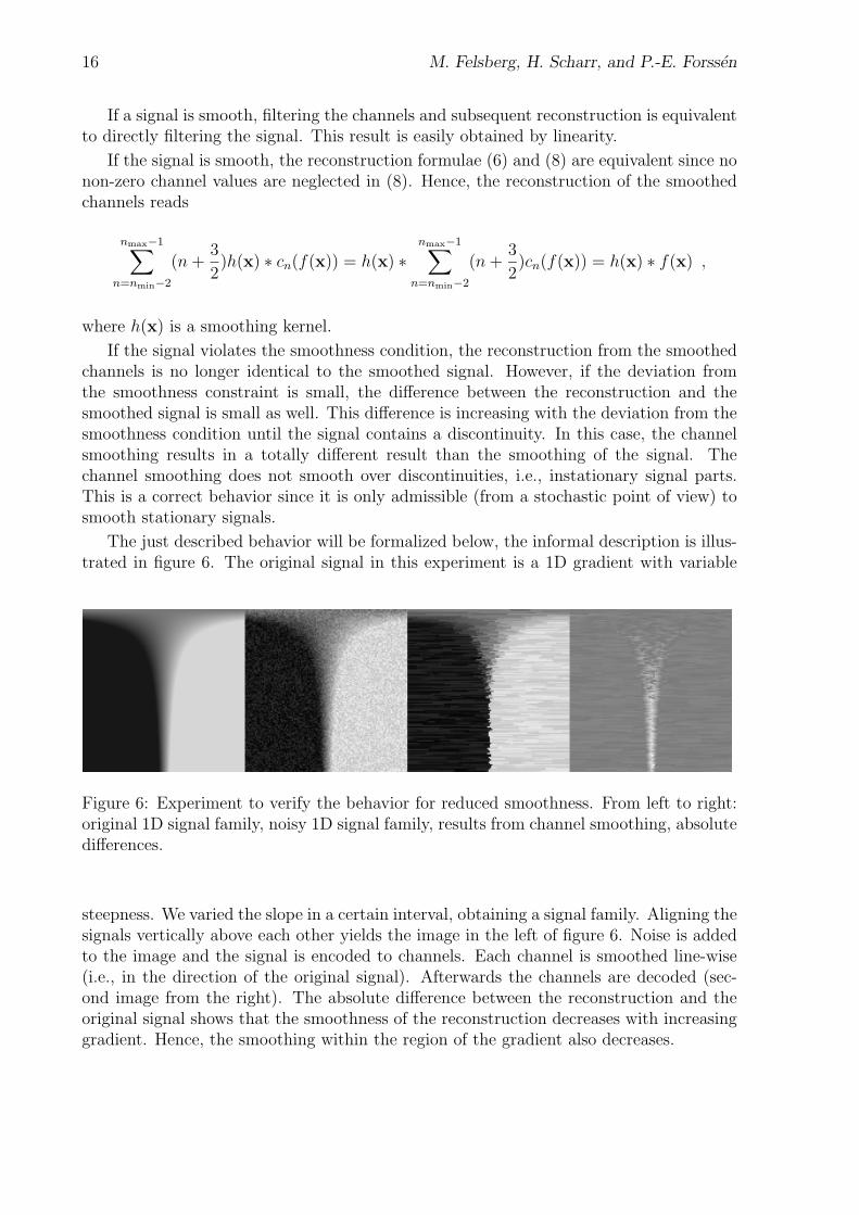
The just described behavior will be formalized below, the informal description is illus-trated in figure 6. The original signal in this experiment is a 1D gradient with variable

Figure 6: Experiment to verify the behavior for reduced smoothness. From left to right:original 1D signal family, noisy 1D signal family, results from channel smoothing, absolutedifferences.

steepness. We varied the slope in a certain interval, obtaining a signal family. Aligning thesignals vertically above each other yields the image in the left of figure 6. Noise is addedto the image and the signal is encoded to channels. Each channel is smoothed line-wise(i.e., in the direction of the original signal). Afterwards the channels are decoded (sec-ond image from the right). The absolute difference between the reconstruction and theoriginal signal shows that the smoothness of the reconstruction decreases with increasinggradient. Hence, the smoothing within the region of the gradient also decreases.


4.2 Robust Estimation

The behavior which is described in the previous section can be explained by means ofrobust statistics. Assume that in a certain region the mean value of the signal is given. Ifwe add another data sample, the mean value will change according to a certain influencefunction [2]. For ordinary L2-optimization, the influence function is simply the differencebetween sample and mean. In robust statistics however, we have a different behavior. Ifthe deviation from the mean is small, there is no difference to L2-optimized estimation.For large deviations however, the influence of the new sample is suppressed; it is consideredto be an outlier.

Smoothing with a Gaussian kernel directly corresponds to the solution of a least-squares problem, since a linear influence function implies the linear, isotropic heat equa-tion [2]. In case of channel smoothing with a Gaussian kernel, each channel is a solutionof the least-squares problem, but how about the reconstructed signal?

In order to understand the process acting on the whole signal, we consider the recon-struction (10) more in detail. Basically, the reconstruction is a discrete convolution of theB-splines with a finite symmetric ramp function R(n):

f = K +∑

n

R(n)B2(f − n) .

The resulting continuous function f(f) is plotted for different window widths in figure 7.

−4 −3 −2 −1 0 1 2 3 4−3

−2

−1

0

1

2

3

w=3w=4

w=5

w=6

w=7

Figure 7: Influence functions for different reconstruction window widths (3-7). The re-construction window is fixed symmetric to the origin.


This function is just the influence function mentioned above. Close to the origin, thisinfluence function is linear like in the least-squares case. For large |f | it is zero, i.e., f isconsidered as an outlier and it is neglected. The regions in between form continuous tran-sitions. Hence, channel smoothing can be considered as a solution of a robust estimationproblem.

The influence function of channel smoothing can be computed analytically. However,the formulation depends on the window width and a general description is quite involved.Thus, we calculate one special case for the window width three. The reconstructionformula is given by (11). With an appropriate shift of the origin, we obtain the followingresult:

ψ(f) = f(f) =

−B2(f + 52) = −f2

2− 5f

2− 25

8if f ∈ (−2.5,−1.5)

−B2(f + 52) = f 2 + 2f + 1

4if f ∈ [−1.5,−0.5)

−B2(f + 52) +B2(f + 1

2) = f if f ∈ [−0.5,−0.5]

B2(f + 12) = −f 2 + 2f − 1

4if f ∈ (0.5, 1.5]

B2(f + 12) = f2

2− 5f

2+ 25

8if f ∈ (1.5, 2.5)

0 else

. (23)

This function with its respective parts is plotted in figure 8.

−2.5 −2 −1.5 −1 −0.5 0 0.5 1 1.5 2 2.5−0.8

−0.6

−0.4

−0.2

0

0.2

0.4

0.6

0.8

f

ψ

Figure 8: The influence function for reconstruction window width three consists of fiveparts (see (23)).


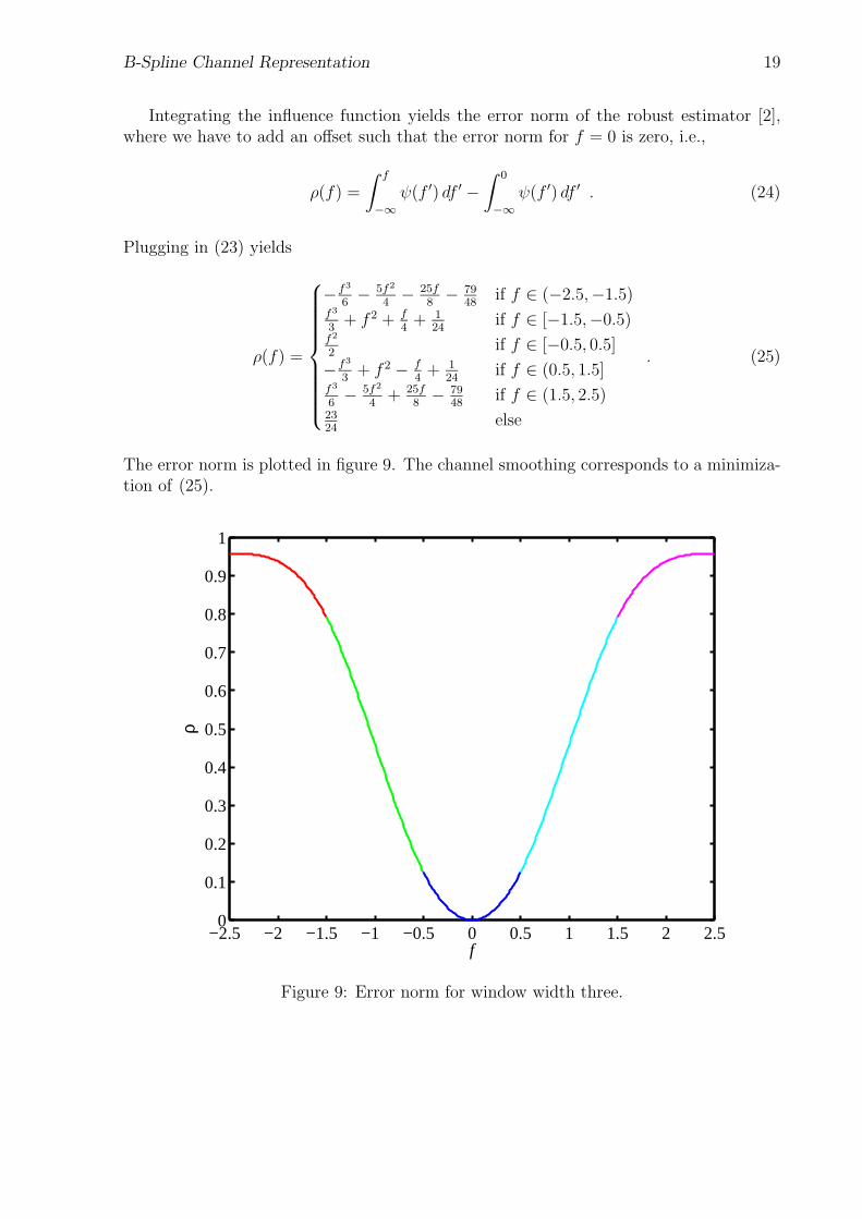
Integrating the influence function yields the error norm of the robust estimator [2],where we have to add an offset such that the error norm for f = 0 is zero, i.e.,

ρ(f) =

∫ f

−∞ψ(f ′) df ′ −

∫ 0

−∞ψ(f ′) df ′ . (24)

Plugging in (23) yields

ρ(f) =

−f3

6− 5f2

4− 25f

8− 79

48if f ∈ (−2.5,−1.5)

f3

3+ f 2 + f

4+ 1

24if f ∈ [−1.5,−0.5)

f2

2if f ∈ [−0.5, 0.5]

−f3

3+ f 2 − f

4+ 1

24if f ∈ (0.5, 1.5]

f3

6− 5f2

4+ 25f

8− 79

48if f ∈ (1.5, 2.5)

2324

else

. (25)

The error norm is plotted in figure 9. The channel smoothing corresponds to a minimiza-tion of (25).

−2.5 −2 −1.5 −1 −0.5 0 0.5 1 1.5 2 2.50

0.1

0.2

0.3

0.4

0.5

0.6

0.7

0.8

0.9

1

f

ρ

Figure 9: Error norm for window width three.


4.3 Outlier Processes

In [2] the authors present a method for converting a robust estimator into the objectivefunction of an outlier process. Applying this method to our robust estimator obtainedfrom the channel smoothing yields the following results.

In order to formulate an outlier process z, it is necessary to calculate the discontinuitypenalty function Ψ(z). The first step is to rewrite the error norm by plugging in x =

√2ω

for ω > 0:

φ(ω) = ρ(√

2ω) =

ω if ω ∈ [0, 1

8]

−2√

2ω3/2

3+ 2ω −

√2ω1/2

4+ 1

24if ω ∈ (1

8, 9

8]√

2ω3/2

3− 5ω

2+ 25

√2ω1/2

8− 79

48if ω ∈ (9

8, 25

8)

2324

if ω ≥ 258

.

In a second step, it is necessary to compute the first and second partial derivatives ofφ(ω) wrt. ω:

φ′(ω) =

1 if ω ∈ [0, 18]

−√2ω1/2 + 2 −

√2ω−1/2

8if ω ∈ (1

8, 9

8]√

2ω1/2

2− 5

2+ 25

√2ω−1/2

16if ω ∈ (9

8, 25

8)

0 if ω ≥ 258

,

φ′′(ω) =

0 if ω ∈ [0, 18]

−√

216

8ω−1ω3/2 if ω ∈ (1

8, 9

8]√

232

8ω−25ω3/2 if ω ∈ (9

8, 25

8)

0 if ω ≥ 258

.

In the third step, we have to check several requirements. In particular, we have φ′(0) = 1,limω→∞ φ′(ω) = 0, and φ′′(ω) < 0 for ω ∈ (1

8, 25

8).5 Defining z = φ′(ω) (fourth step), we

compute the inverse of φ′(ω) (step five):

(φ′)−1(z) =

{z2 + (5 − (z(5 + z))1/2)z + 25

8− 5

2(z(5 + z))1/2 if z ∈ [0, 1

3]

78− z + 1

2(3 − 4z + z2)1/2 + z2

4− z

4(3 − 4z + z2)1/2 if z ∈ (1

3, 1]

.

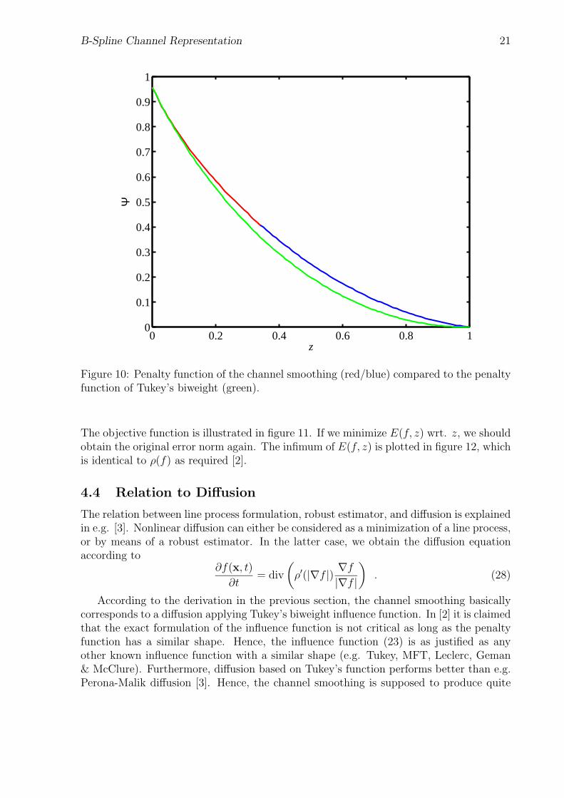
In step six, the penalty function Ψ(z) is defined by

Ψ(z) = φ((φ′)−1(z)) − z(φ′)−1(z) , (26)

which gives an analytic expression which is too long to be presented in a reasonable way.The graph of this expression is plotted in figure 10, together with the plot of the (scaled)penalty function of Tukey’s biweight (see [2]). Obviously, the penalty functions (andtherefore the robust estimators) do not differ essentially.

The seventh and last step in the method of [2] is to formulate the objective functionof the line process, which reads

E(f, z) =f 2z

2+ Ψ(z) . (27)

5In [2] the requirement reads φ′′(ω) < 0, i.e., for the whole interval, but in their examples the authorsfind φ′′(ω) < 0 on a smaller interval being sufficient.


0 0.2 0.4 0.6 0.8 10

0.1

0.2

0.3

0.4

0.5

0.6

0.7

0.8

0.9

1

z

Ψ

Figure 10: Penalty function of the channel smoothing (red/blue) compared to the penaltyfunction of Tukey’s biweight (green).

The objective function is illustrated in figure 11. If we minimize E(f, z) wrt. z, we shouldobtain the original error norm again. The infimum of E(f, z) is plotted in figure 12, whichis identical to ρ(f) as required [2].

4.4 Relation to Diffusion

The relation between line process formulation, robust estimator, and diffusion is explainedin e.g. [3]. Nonlinear diffusion can either be considered as a minimization of a line process,or by means of a robust estimator. In the latter case, we obtain the diffusion equationaccording to

∂f(x, t)

∂t= div

(ρ′(|∇f |) ∇f

|∇f |)

. (28)

According to the derivation in the previous section, the channel smoothing basicallycorresponds to a diffusion applying Tukey’s biweight influence function. In [2] it is claimedthat the exact formulation of the influence function is not critical as long as the penaltyfunction has a similar shape. Hence, the influence function (23) is as justified as anyother known influence function with a similar shape (e.g. Tukey, MFT, Leclerc, Geman& McClure). Furthermore, diffusion based on Tukey’s function performs better than e.g.Perona-Malik diffusion [3]. Hence, the channel smoothing is supposed to produce quite


Figure 11: Objective function of the channel smoothing as a 2D plot.

0 0.5 1 1.5 2 2.5 30

0.5

1

f

E

Figure 12: Infimum for 0 ≤ z ≤ 1 of the objective function. Compare to figure 9.


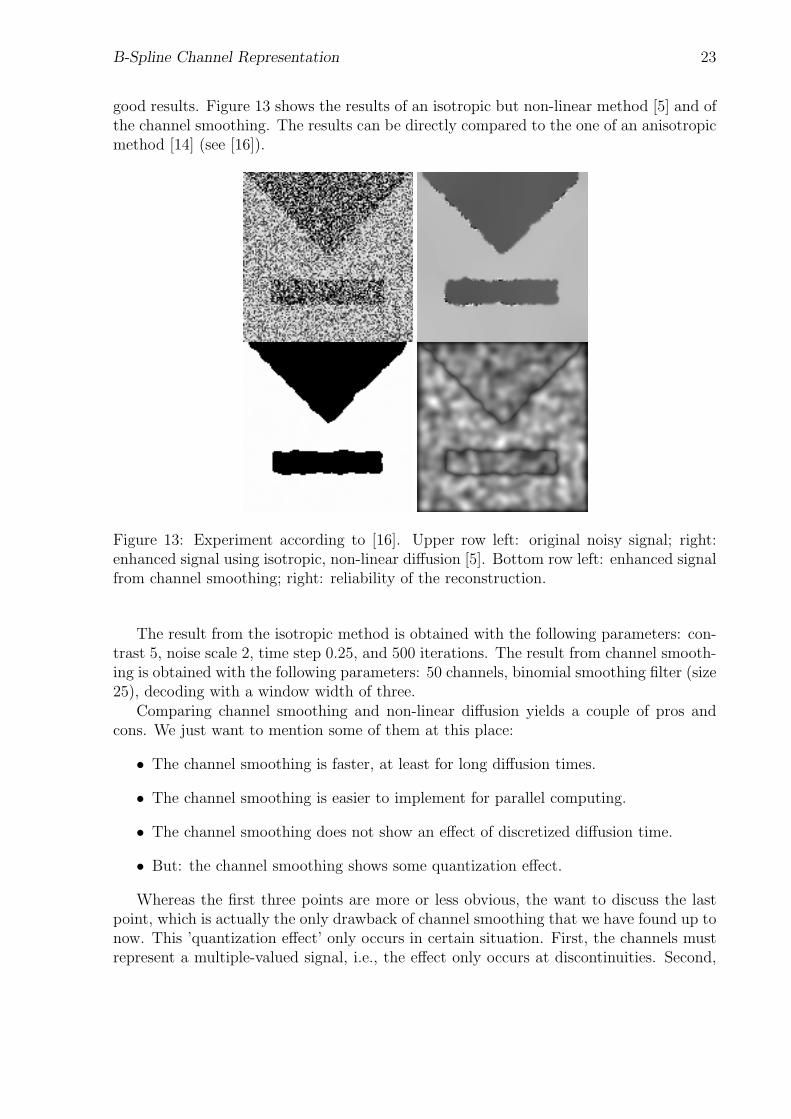
good results. Figure 13 shows the results of an isotropic but non-linear method [5] and ofthe channel smoothing. The results can be directly compared to the one of an anisotropicmethod [14] (see [16]).

Figure 13: Experiment according to [16]. Upper row left: original noisy signal; right:enhanced signal using isotropic, non-linear diffusion [5]. Bottom row left: enhanced signalfrom channel smoothing; right: reliability of the reconstruction.

The result from the isotropic method is obtained with the following parameters: con-trast 5, noise scale 2, time step 0.25, and 500 iterations. The result from channel smooth-ing is obtained with the following parameters: 50 channels, binomial smoothing filter (size25), decoding with a window width of three.

Comparing channel smoothing and non-linear diffusion yields a couple of pros andcons. We just want to mention some of them at this place:

• The channel smoothing is faster, at least for long diffusion times.

• The channel smoothing is easier to implement for parallel computing.

• The channel smoothing does not show an effect of discretized diffusion time.

• But: the channel smoothing shows some quantization effect.

Whereas the first three points are more or less obvious, the want to discuss the lastpoint, which is actually the only drawback of channel smoothing that we have found up tonow. This ’quantization effect’ only occurs in certain situation. First, the channels mustrepresent a multiple-valued signal, i.e., the effect only occurs at discontinuities. Second,


the difference between the signal values must lie in a certain (small) interval, such that itis neither so small that the values should be linearly interpolated, nor so big that one ofthe values is suppressed. Hence, we are in the non-linear, non-zero interval of the influencefunction.

Since the influence function is placed at discrete points (channel positions), the actualinfluence of an outlier depends on the positioning of the channels. This effect is visualizedin figure 14. In the experiment, two different linear functions are encoded in ten channels.

x

f(x)

reconstruction 1signal 1signal 2reconstruction 2

Figure 14: Quantization effect of the channel representation. The channels contain thechannel values of signal 1 and signal 2. The decoding yields a linear interpolation for smalldifferences and a selection of signal 1 for large distances. In between, the exact behaviordepends on the channel positions as it can be seen by the two different reconstructions.

The two representations are added component-wise, where the coefficients of the firstsignal are weighted with two. The subsequent reconstruction yields a linear average forsmall distances of the two functions. For large distances, the first signal is recovered.In between, there should be a continuous transition between the two cases, but somedistortions occur. These distortions depend on the channel positions, which can be seenin the two reconstructions based on two representations that only differ with respect totheir channel positions.

Although these distortions occur, they can mostly be neglected. First, they arebounded to be less than one half the channel width, i.e., for a gray-scale image with256 gray values and 32 channels, the maximal error is 4 gray values. Second, if thechannels of the two (or more) signals have different weights, the distortion is further re-


duced. This is typically the case for e.g. image enhancement (removing noise). Third,the distortion can only occur at places where multiple values exist which have a certaincritical distance. This distance depends on the reconstruction window width. Finally, thedistortion can be reduced by increasing the overlap between the basis functions, whichcorresponds to oversampling the channels [8].

5 Future Work

In some future work we are going to exploit the introduced methods from the channelalgebra. According to usability, the algorithm for addition and multiplication has to bedesigned such that the number of channels does not increase too much. In this context,it would be advantageous to have some kind of channel compression technique if theestimated probability functions become too broad. The compression of channels canbasically be achieved by subsampling, where the correct reconstruction must be assured.

The channel smoothing will also be applied in this context, yielding robust estimatesof certain measurements. According to the quantization effect, we will make furtherinvestigations in order to reduce the error. Furthermore, we will extend the theoreticconsiderations to higher dimensional feature spaces with certain topologies, e.g., orienta-tion vectors, color vectors, etc.. Quite unclear at this point is the relation of the channelsmoothing to anisotropic methods. Basically, it shows an anisotropic behavior. At edges,the channel representation blurs parallel to the edge but not perpendicular to the edge.

Acknowledgments

We appreciate the help of Joachim Weickert for providing the code for the isotropic,non-linear diffusion and the test image in figure 13.This work has been supported by DFG Grant FE 583/1-1 (M.Felsberg).


References

[1] Bishop, C. M. Neural Networks for Pattern Recognition. Oxford University Press, NewYork, 1995.

[2] Black, M. J., and Rangarajan, A. On the unification of line processes, outlier rejection,and robust statistics with applications in early vision. International Journal of ComputerVision 19, 1 (1996), 57–91.

[3] Black, M. J., Sapiro, G., Marimont, D. H., and Heeger, D. Robust anisotropicdiffusion. IEEE Transactions on Image Processing 7, 3 (1998), 421–432.

[4] Borga, M. Learning Multidimensional Signal Processing. PhD thesis, Linkoping Univer-sity, Sweden, 1998.

[5] Catte, F., Lions, P.-L., Morel, J.-M., and Coll, T. Image selective smoothing andedge detection by nonlinear diffusion. SIAM J. Numer. Analysis 32 (1992), 1895–1909.

[6] de Boor, C. Splinefunktionen. Birkhauser, 1990.

[7] Felsberg, M. Disparity from monogenic phase. In 24. DAGM Symposium Mustererken-nung, Zurich (2002), L. v. Gool, Ed., Lecture Notes in Computer Science, Springer-Verlag,Heidelberg. to appear.

[8] Forssen, P.-E. Sparse representations for medium level vision. Lic. Thesis LiU-Tek-Lic-2001:, Dept. EE, Linkoping University, February 2001.

[9] Forssen, P.-E., and Granlund, G. H. Sparse feature maps in a scale hierarchy. InProc. Int. Workshop on Algebraic Frames for the Perception-Action Cycle (Kiel, Germany,September 2000), G. Sommer and Y. Y. Zeevi, Eds., vol. 1888 of Lecture Notes in ComputerScience, Springer-Verlag, Heidelberg.

[10] Forssen, P.-E., Granlund, G. H., and Wiklund, J. Channel representation ofcolour images. Tech. Rep. LiTH-ISY-R-2418, Dept. EE, Linkoping University, SE-581 83Linkoping, Sweden, 2002.

[11] Granlund, G. H., Forssen, P.-E., and Johansson, B. HiperLearn: A High Perfor-mance Learning Architecture. Tech. Rep. LiTH-ISY-R-2409, Dept. EE, Linkoping Univer-sity, SE-581 83 Linkoping, Sweden, January 2002. Submitted to IEEE Trans. on NeuralNetworks.

[12] Jahne, B. Digitale Bildverarbeitung. Springer-Verlag, Berlin, 1997.

[13] Nordberg, K., Granlund, G. H., and Knutsson, H. Representation and Learning ofInvariance. In Proceedings of IEEE International Conference on Image Processing (Austin,Texas, 1994).

[14] Weickert, J. Theoretical foundations of anisotropic diffusion in image processing. InComputing, Suppl. 11. 1996, pp. 221–236.

[15] Weickert, J. A review of nonlinear diffusion filtering. In Scale-Space Theory in ComputerVision (1997), B. ter Haar Romeny, L. Florack, J. Koenderink, and M. Viergever, Eds.,vol. 1252 of LNCS, Springer, Berlin, pp. 260–271.

[16] Weickert, J. Examples of nonlinear diffusion filtering. http://www.mia.uni-saarland.de/weickert/demos.html, February 1998. (Accessed 4 Sep 2002).

b-spline channel smoothing for robust estimation

Documents