Adversarially Robust Kernel Smoothing

Jia-Jie Zhu∗, Christina Kouridi†, Yassine Nemmour, Bernhard SchölkopfEmpirical Inference Department

Max Planck Institute for Intelligent Systems, Tübingen, Germany{jia-jie.zhu,christina.kouridi,ynemmour,bs}@tuebingen.mpg.de

Abstract

We propose the adversarially robust kernel smoothing (ARKS) algorithm, com-bining kernel smoothing, robust optimization, and adversarial training for robustlearning. Our methods are motivated by the convex analysis perspective of distribu-tionally robust optimization based on probability metrics, such as the Wassersteindistance and the maximum mean discrepancy. We adapt the integral operator usingsupremal convolution in convex analysis to form a novel function majorant usedfor enforcing robustness. Our method is simple in form and applies to general lossfunctions and machine learning models. Furthermore, we report experiments withgeneral machine learning models, such as deep neural networks, to demonstratethat ARKS performs competitively with the state-of-the-art methods based on theWasserstein distance.

1 Introduction

When training models with finitely many samples, there is an inevitable distribution shift between thetraining distribution and the test one. Furthermore, adversaries may create large artificial distributionshifts to hamper the learners [27, 38, 67, 81]. Hence, learning under distribution shift presentssignificant challenges to current machine learning algorithms.

Distributionally robust optimization (DRO) [19, 61] seeks to robustify against unknown distributionshift explicitly. Given a loss function of interest l(θ, ·), it solves a minimax robust optimization [68,7] problem

minθ

supP∈C

Eξ∼P l(θ, ξ), (1)

where θ is the decision variable, ξ noise or randomness, C a set of distributions of the uncertainvariable ξ that the optimizer wishes to robustify against, often referred to as the ambiguity set.DRO is particularly relevant to statistical machine learning as one may construct the ambiguityset C as a metric ball centering at the empirical distribution PN that also contains the true data-generating distribution Ptrue. For example, the performance guarantees for Wasserstein DRO havebeen established by the authors of [48, 85]. The idea here is to use known convergence rate resultsfor empirical estimations of the underlying probability metrics, e.g., the Wasserstein metrics [35]and the more general integral probability metrics (IPM) [69, 49]. Such metrics (or topologies) oftencorrespond to smooth functions as their dual spaces, which characterize the empirical distribution’sconvergence to the true generating distribution [75, 10]. DRO is also related to a large body ofliterature in generative adversarial networks [26] and implicit generative models. Researchers haveproposed DRO algorithms with various statistically meaningful ambiguity sets in a large body ofliterature [19, 61, 23, 25, 5, 33, 52, 78, 21, 48, 85, 24, 11, 67, 71, 86]. While not the focus of thoseworks, convex analysis tools such as supremal convolution, Moreau-Yosida regularization play animportant role in enforcing distributional robustness. They are the main tools we employ in this paper.∗JZ is now with the Weierstrass Institute for Applied Analysis and Stochastics, Berlin.†CK is now with InstaDeep.

arX

iv:2

102.

0847

4v3

[cs

.LG

] 4

Jul

202

1

Hardness of DRO for general machine learning tasks. Certain simple problems, such as linearclassification with logistic regression losses, admit the tractable reformulation into convex problems,as studied by [5, 51, 48, 12, 63]. However, this only applies to a limited class of convex loss functionsand simple models, as also noted by, e.g., the authors of [67]. For general machine learning models,e.g., deep neural networks (DNNs), and common losses l in (1), there exists no tractable reformulationto solve DRO (1). This paper addresses general losses in machine learning tasks, which are lessexplored in terms of distributional robustness, save very few exceptions such as [67, 12, 86]. Wediscuss this topic further in Section 3.1.

Contribution. This paper takes a function approximation and majorization perspective of DRO,highlighting the critical role smoothness plays in distributional robustness. We summarize ourcontributions and sketch the main results.

1. We analyze the smooth function majorant perspective of distributional robustness, whichgeneralizes the existing practice of using the Moreau-Yosida regularization in WassersteinDRO to flexibly chosen general majorants surrogate losses. Specifically, we propose thek-transform (Definition 2) that adapts the convolution in the integral operator to the supremalconvolution in convex analysis to form a function majorant

lk(x) := supu{l(u)k(u, x)}.

where k is a kernel, e.g., Gaussian RBF kernel and, in general, the proposed c-exponentialkernel (Definition 3). Intuitively, u can be seen as an adversarial sample.

2. Using those tools, we propose a novel robust learning algorithm (Section 4), , the adver-sarially robust kernel smoothing (ARKS). It solves the minimax optimization problem

minθ

1

N

N∑i=1

{lkθ (ξi) := sup

u{l(θ, u)k(u, ξi)}

}. (2)

which possesses implicit regularization in contrast to the explicit regularization of existingDRO methods.

3. Treating general machine learning loss functions is a major limitation of the current DROapproaches. While ARKS is a tool derived from kernel methods, it can be easily appliedto large-scale machine learning with DNNs. For example, we report an experiment witha ResNet-20 model, where applying exact Wasserstein DRO reformulation techniques(e.g., [48, 63]) is out of the question. There, ARKS performs at least competitively with theWRM algorithm (5) proposed by [67].

4. We will make our ARKS implementation publicly available online.

Notation. In this paper, we refer to the uniform data distribution PN := 1N

∑Ni=1 ξi as the empirical

distribution. We use Ptrue to denote the (unknown) true data-generating distribution. For the lossfunctions of interest l(θ, ξ), we sometimes omit θ when there is no ambiguity. θ denotes thedecision variables, such as the weights of neural networks. ξ ∈ X denotes the random variable ofinterest, e.g., input data or features. Its samples of are denoted by ξi. For conciseness, we limitthe discussion to compact X ’s. We use H to denote a function space in the context, e.g., RKHSintroduced in the next section. Lip() denotes the Lipschitz semi-norm. ‖‖H is the RKHS norm in thecontext. ‖‖∞ denotes the infinity norm of a function. We will assume loss function l to be boundedcontinuous functions throughout the paper; extensions to upper semi-continuity in optimizationsettings is straightforward. See, e.g., [66]. Variables are in their vectorial representation, e.g.,x = [x1, . . . , xN ], and f(x) := [f(x1), . . . , f(xN )]. Throughout the paper, we will refer to DROusing the Wasserstein distance as Wasserstein DRO. We refer to the Moreau-Yosida regularizationly,p(x) := supu{l(u)− y · ‖u− x‖p} as the supremal convolution of a function l and the (scaled)norm function y‖ · ‖p. To avoid ambiguity, we refer to the maximization of a concave function as aconvex program. Finally, γ denotes some metric in the probability simplex.

2 Reproducing Kernel Hilbert Space

A learning task can be mathematically described as a function approximation problemminf∈H ‖f − l‖·, for some criterion ‖‖·, e.g., function norm. The target function of interest l

2

is not assumed to live in the space H of the approximating functions f . Furthermore, l is often onlyknown at certain data points [x1, ..., xN ]. One way to approach the function approximation problemis to consider a function approximator of the form

∑Nj=1 ajk(xi, xj) = l(xi), 1 ≤ i ≤ N, where aj

are the coefficients to be determined and k(xi, xj) some bi-variate function. It is in our interest thatthe matrix [k(xi, xj)]i,j should be positive definite. Motivated by this, we now define a symmetricreal-valued function k as a positive (semi-)definite kernel if

∑ni=1

∑nj=1 aiajk(xi, xj) ≥ 0 for any

n ∈ N, {xi}ni=1 ⊂ X , and {ai}ni=1 ⊂ R. It is known [e.g. 62, Chapter 2] that there is a one-to-onerelationship between every positive semi-definite kernel k and a Hilbert space H, whose featuremap φ : X → H satisfies k(x, y) = 〈φ(x), φ(y)〉H. This Hilbert space is reproducing, meaning thatf(x) = 〈f, φ(x)〉H for all f ∈ H, x ∈ X . We callH the reproducing kernel Hilbert space (RKHS),also termed the native space of the kernel k. RKHSs are widely used as function approximators basedon data due to their attractive properties.

Certain types of RKHSs, known as universal RKHSs, are dense in continuous functions on X [72,70]. In the context of this paper, we can view this property as a powerful analog of the Weierstrassapproximation theorem. That is, if we choose the function class in the function approximationproblem to be a universal RKHSH, one has inff∈H ‖f − l‖∞ = 0, i.e., kernel functions can be usedas universal function approximators.

In addition to the functional approximation aspect, the RKHS has also been prominently used tomanipulate and represent distributions, leveraging its statistical properties as the so-called Glivenko-Cantelli classes (intuitively, allowing the convergence of empirical expectations to true ones); cf. [75].Relevant to the robustness aspect, the maximum mean discrepancy (MMD, [28]) associated with anRKHSH is a metric in the probability simplex. γH(P,Q) = sup‖f‖H≤1

∫f d(P −Q). In particular,

a refined error rate for the MMD empirical estimation is proposed by [73, Proposition A.1], whichcan be used to set the ambiguity set level ε in the DRO problem (6). Notably, that rate is attractive inthat the constants are computable (if the RKHS is known) and the data dimension is absent, whilemeasure concentration rates (used for Wasserstein DRO in [48]) for the Wasserstein distance dependon dimensions. The MMD also has a closed-form estimator, while computing Wasserstein distanceis hard in general [57, 60]. MMD can be generalized to the integral probability metrics (IPM) [49]defined by some function class F , i.e., γF (P, P ) := supf∈F

∫fd(P − P ). The well-known choices

relevant to this paper include: F = {f : Lip(f) ≤ 1} recovers the type-1 Wasserstein metric(Kantorovich metric); the RKHS norm-ball F = {f : ‖f‖H ≤ 1} recovers the MMD

Given a kernel k and probability measure µ, recall that the integral operator T : L2µ → H is defined

asT l(x) :=

∫l(z)k(x, z)dµ(z). (3)

Integral operator maps L2µ to a dense subspace of the RKHS [80] and is used in the celebrated

Mercer’s theorem to characterize the eigendecomposition of RKHS functions. In the context of thispaper, we view the integral operator as a smoothing operation. We refer [17] for more details on thistopic and [80] for its use in approximating functions using RKHSs.

3 Distributionally Robust Optimization for Machine Learning Losses

We now continue our exposition on DRO. We limit our discussion to DRO using the Wassersteinmetrics [48, 85, 24, 13], the MMD [86, 71], and, more generally, DRO using IPM [86]. See [24,28, 1, 57, 79, Section 1.1] for the details of why those probability metrics are more advantageous inmany machine learning applications than, e.g., f -divergences. For convenience, we now restate thedata-driven DRO primal formulation in (1) with a discrepancy constraint.

(DRO-Primal) : minθ

supγ(P,PN )≤ε

EP l(θ, ξ), (4)

The discrepancy measure γ in (4) can be chosen to be an IPM.

In general, solving the minimax DRO problem (4) requires a reformulation via the duality ofoptimization, cf. [65, 6]. While Wasserstein distance has become the most popular choice for theDRO problem, it is important to understand that one cannot simply reformulate any WassersteinDRO problem as a convex program, except for very simple losses such as logistic regression [63].

3

For many practical machine learning models, there exists no exact tractable reformulation. We nowdiscuss this issue in detail.

3.1 Wasserstein DRO for General Machine Learning Losses

Unfortunately, popular Wasserstein DRO approaches such as those proposed in [48, 85] apply to alimited class of loss functions and models, such as logistic regression (linear classification). Moreover,it is also known that estimating the Lipschitz constant for general models is intractable; cf. [76, 9],making Lipschitz regularization in [64] difficult. This paper does not impose such restrictions onlosses or models. For commonly-used machine learning losses, it is well-known that one must resortto general approximate solution methods such as in [67, 12, 86]. For readers that are not familiarwith tractable reformulations and approximation techniques, we refer to [8] for an overview.

Most relevant to our work and in the context of adversarial robustness, the authors of [67] proposedto give up certifying the exact distributional robustness level ε and apply a convexification techniqueusing the Moreau-Yosida regularization, as approximate Wasserstein DRO. They solve the riskminimization problem, which they termed Wasserstein robust method (WRM),

(WRM) : minθ

1

N

N∑i=1

{fyθ (ξi) := sup

u{l(θ, u)− y · c(u, ξi)}

}, (5)

where c is called the ground cost or transport cost [60], e.g., squared Euclidean distance. WRMcan be straightforwardly applied with stochastic gradient based methods. When c is the squaredEuclidean distance, WRM overcomes the hurdle of the aforementioned hardness of DRO for generalmachine learning tasks by virtue of a convexification effect. Intuitively, subtracting a strongly convexfunction makes the inner objective more concave. This technique was also used in robust nonlinearoptimization [31], trust-region methods in numerical optimization (Chapter 4 of [54]), and the S-procedure in robust control [58, 84]. Later, we compare our novel kernel smoothing algorithm withWRM [67] in experiments with general machine learning models, e.g., DNNs, to demonstrate ouradvantages over classical reformulation techniques in practical machine learning settings.

On the other hand, if we choose the metric γ to be an IPM associated with the function class F ⊆ H,the authors of [86] proved the IPM-DRO duality. It states that the primal DRO problem (4) isequivalent to solving

(IPM-DRO) : minθ,f∈H

1

N

N∑i=1

f(ξi) + ε‖f‖H subject to l(θ, ξ) ≤ f(ξ), ∀ξ ∈ Xa.e. (6)

Those authors also proposed approximate solution methods when the IPM is chosen as the MMD(see Section 2 for the advantages of MMD), which generalized the results of [71] to general lossfunctions. Through the lens of this paper, (6) explicitly seeks an upper envelope f of the loss l assolutions to the variational dual program (6). Instead of the Moreau-Yosida regularization, the smoothmajorant role is played by a more general function f ∈ H. Note that program (6) is trivial if loss l isin anH and has a known RKHS norm. The authors of [86] then proposed Kernel DRO that makesit possible to use the MMD associated with any universal RKHSs for DRO and compute the ratefor general losses. To our knowledge, that is the only work aiming to exactly reformulate DRO forgeneral machine learning models. However, compared to their method, we provide an approach thatproduces a function that satisfies the (semi-)infinite constraint in (6), whereas [86]’s method can onlysatisfy that constraint approximately.

To motivate our method, we make two key observations into (5): (1) the absence of the robustnesslevel ε and (2) the fixed dual variable y. That insight is also equivalent to giving up the exactminimization w.r.t. f ∈ H and ‖f‖H in dual IPM-DRO (6), since fixing y in (5) is to not optimizew.r.t. the Moreau envelope fyθ .

4 A Kernel Smoothing Algorithm for Robust Learning

The so-called c-transform fyθ in WRM (5), also known as the Moreau-Yosida regularization, plays acrucial role in the robustness of WRM (5). Importantly, it is a majorant function.Definition 1 (Majorant). We say that f is a majorant of l if f(ξ) ≥ l(ξ) for ξ a.e. in the domain of l.

4

Notably examples of majorants relevant to DRO include the Moreau-Yosida regularization as well asthe kernel functions in (6). In this paper, we also refer to a majorant as an upper envelope function.To see that the role majorants play in robustness, it is an exercise in convex analysis to establish thefollowing. The derivations are provided in the appendix.

Suppose we choose transport cost c to be the Euclidian distance, then the c-transform fyθ is a supremalconvolution supu{l(θ, u)− y · ‖u− ·‖} , referred to as the y-Pasch-Hausdorff envelope in convexanalysis (see, e.g., [2]).Lemma 4.1. (Motivating example using type-1 Wasserstein DRO) Suppose the loss function l(θ, ·)is y−Lipschitz continuous. Let variable f in dual IPM-DRO (6) be the y-Pasch-Hausdorff envelopeof the loss l(θ, ·). Then, (6) is equivalent to the dual formulation of type-1 Wasserstein DRO; cf. [48,85, 40].

Unfortunately, estimating Lipschitz constants for general model classes is known to be difficult [76,9], resulting in the intractability of Wasserstein DRO when used with common machine learningmodels, e.g., neural networks, which our method can handle.

Our key insight from (6), (5), and Lemma 4.1 is that empirical risk minimization with the loss replacedby a majorant surrogate loss induces distributional robustness. Motivated by such relationshipbetween robustness and the use of majorants, e.g., c-transform (Moreau-Yosida regularization) in (5),kernel functions in (6), we now introduce our robust learning algorithm.

4.1 Adversarially Robust Kernel Smoothing (ARKS)

Our starting point is the minimax robust optimization (RO) problem [7, 68](RO) : min

θsupul(θ, u) (7)

where the learner assumes the uncertain variable u to take the worst-case value. It is easy to seethe pessimism of RO as we do not know the true support of u in machine learning. On the otherhand, empirical risk minimization (ERM; also referred to as the sample average approximation inthe optimization community) enjoys better performance but is more fragile to shift in distributionand uncertainty. It can be seen as a simple form of smoothing. Deviating from the typical DRO dualreformulation approaches, our key idea is to view smoothness as the opposite side of robustness bymanipulating the integral operator in RO. To that end, let us first establish some tools.

The image of the integral operator T l ∈ H (3) is a smooth function since it is in an RKHS, but doesnot directly enable robust learning. To achieve robustness, we notice the following inequality

T l(x) =

∫l(z)k(x, z)dµ(z) ≤ sup

u{l(u)k(u, x)}, ∀x ∈ X , (8)

which is a straightforward inequality between expectation and supremum. Using the right-hand-sideexpression, we construct the following majorant analogous to c-transform.Definition 2 (k-transform). The k-transform of a function l associated with kernel k is defined as

lk(x) := supu{l(u)k(u, x)}.

To the best of our knowledge, k-transform has not appeared in the existing literature. It is helpful tothink of the example where k(u, x) is the Gaussian RBF kernel or Laplacian kernel. To make ourdiscussion more general, we now propose the following family of kernels inspired by the transportcost c of Wasserstein distance.Definition 3 (c-exponential kernel). Suppose c is the transport cost (as in the Wasserstein distance).The c-exponential kernel with bandwidth σ > 0 is given by

k(x, x′) = e−c(x,x′)/σ.

Note that a relevant kernel on probability metrics was studied in [18]. It is beyond this paper’s scopeto study the properties of c-exponential kernel. For conciseness, we focus on the Gaussian RBFkernel and Laplacian kernel in the rest of the paper with no further specification. Many of our resultsstraightforwardly apply to the c-exponential kernel when c is nice in the sense that it is a metric.Other constructions of majorants are possible and discussed in the appendix. It is then straightforwardto verify the following:

5

Proposition 4.2. The k-transform of l is a majorant of l. Furthermore, we have lk → l as σ → 0.

Let us use the tools above to derive our robustification method. We mitigate the conservatism ofRO (7) by replacing the the original loss l with a smoothed version

minθ

supuT l(θ, u).

In reality, we can compute an empirical version of the integral operation based on empirical data ξi.We have the following

supu

{T l(θ, u) :=

1

N

N∑i=1

k(ξi, u)l(θ, u)}≤ 1

N

N∑i=1

supu{l(θ, u)k(u, ξi)} (9)

The inner objective on the right-hand-side is the k-transform. That objective is indeed less conservativethan RO and more robust than ERM since

(ERM) : supu

1

N

N∑i=1

l(θ, ξi) ≤1

N

N∑i=1

supu{l(θ, u)k(u, ξi)} ≤ sup

ul(θ, u) : (RO) (10)

for c-exponential kernels, e.g., Gaussian RBF kernels.

We are now ready to propose the following novel robust learning scheme based on the insight fromRO, (6), and (5). Our main idea is simple: we minimize the risk using a surrogate loss constructed bythe k-transform.

(ARKS) : minθ

1

N

N∑i=1

{lkθ (ξi) := sup

u{l(θ, u)k(u, ξi)}

}. (11)

ARKS resembles the risk minimization schemes using majorant surrogate losses in (6) and (5), butwith our newly proposed k-transform. Intuitively, one may view ARKS with Gaussian RBF kernelas the analog to WRM (5) with type-2 Wasserstein distance, Laplacian kernel type-1 WRM, andc-exponential kernel general WRM with transport cost c.

Program (11) also bears a clear resemblance to the Nadaraya-Watson model, and the vicinal riskminimization [16] in the literature. However, our approach differs in taking supremum to enforcerobustness. Different from the existing robust kernel density estimation methods such as [36], whichwas applied by [53] to learn uncertainty sets for robust optimization, ARKS considers specifically theworst-case risk of the loss l, rather than only performing general unsupervised density estimation.

Compared with existing DRO approaches, ARKS (11) does not use explicit regularization (e.g., [64]),but an implicit one. To see that, we establish the following.Proposition 4.3. Suppose the kernel bandwidth tends to infinity σ →∞, ARKS (11) is equivalent tothe worst-case robust optimization (RO) (7) [7, 68].

If kernel bandwidth tends to zero σ → 0, then ARKS (11) recovers the empirical risk minimization(ERM) 1

N

∑Ni=1 minθ l(θ, ξi).

If we choose a bandwidth σ between those cases, the robustness is between RO and ERM, whereDRO is. Therefore, just as the y parameter in WRM (5), kernel bandwidth parameter is an implicitregularization parameter for the robustness of ARKS.Remark (Robustness, kernel bandwidth, and size of the function space). It is known that thebandwidth of the Gaussian RBF kernels affects the size of the corresponding RKHSs; see, e.g.,justifications using Fourier transforms in [3] and [80, Chapter 10]. Intuitively, if the kernel bandwidthis large, the function space becomes small. In terms of robustness, this is also consistent with thecharacterization of dual function space sizes for DRO and RO in [86]: large dual function spacescorrespond to conservative but more robust optimization. In contrast, smaller ones have betterperformance but are less robust. We see those insights reflected in Proposition 4.3.Remark (Alternative interpretation of ARKS). The intuition of ARKS can also be viewed as usingsmooth kernels to model the distribution shift X ∼ Ptrue, U = X + shift, then minimize the shiftedrisk. We illustrate this in Figure 3 (right). Unlike f -divergence based DRO [5, 50, 41], our modelingdoes not require the shifted distribution to be absolute continuous (i.e., having the same support) w.r.t.the empirical distribution (similar to Wasserstein distance).

6

4.2 Robust Learning with ARKS

Our risk minimization scheme (11) can be straightforwardly used with stochastic gradient basedmethod for large-scale learning, e.g., with DNNs. We detail the training procedure in Algorithm 1.Note that Step 3 of Algorithm 1 can be seen as a proximal algorithm, cf. [55]. ARKS (11) can also

Algorithm 1: Adversarially robust kernel smoothing (ARKS)1: input: data sampler, initial iterate θ02: for k = 0, 1, 2, . . . , T do3: sample {ξk} and find u∗k by maximizing l(θk, u)k(u, ξk) w.r.t. u4: update θ by stochastic gradient descent using estimate∇θl(θk, u∗k)5: output: approximate solution θ∗ := θT

be interpreted as a form of adversarial training [38, 81, 27]: for each ξi, the inner maximizationproblem of (11) looks for an adversarial example u that hurts the learner the most. In the case ofGaussian RBF kernel, it is an exercise (we provide this proof in the appendix) to show that the innermaximization objective in (11) has favorable convexity structures for suitable choices of σ. The mainintuition is that, by multiplying the loss l(u) by the kernel function k(u, x) which is strongly concavenear its peak, the resulting function is consequently locally concave too. We illustrate this intuition inFigure 3 (right). A thorough analysis for various other kernels choices is out of our current scope.Next, we empirically demonstrate ARKS in Section 5 that ARKS can easily work with DNN models,which is a limitation of typical existing DRO reformulation techniques.

5 Numerical Experiments

5.1 Robust Learning under Adversarial Perturbations

In this section, we present empirical evaluations of our robust learning algorithm. We compare thefollowing algorithms when applicable: (A) ARKS Algorithm 1, (B) empirical risk minimization(ERM), (C) WRM [21], (D) (worst-case) robust optimization [7, 68] (in the appendix). Both ARKSand WRM have one hyper-parameter: bandwidth σ for ARKS and Lagrangian relaxation coefficienty for WRM. We do not test classical Wasserstein DRO algorithms, e.g., [48, 85, 64], since theycannot be applied to our test settings with general machine losses and DNN models. We further notethat ARKS (11) is a general robustification technique that can be applied to tasks beyond supervisedlearning and adversarial training.

0.0 0.1 0.2 0.3perturbation

0

20

40

60

80

100

test

erro

r (%

)

Test error on Fashion-MNIST, 5-layer CNN

ERMWRM y=1.0ARKS =0.5WRM y=0.5ARKS =0.9

0.0 0.1 0.2 0.3perturbation

0

20

40

60

80

100

test

erro

r (%

)

Test error on CIFAR-10, 20-layer ResNet

ERMWRM y=50ARKS =0.1WRM y=10ARKS =0.2

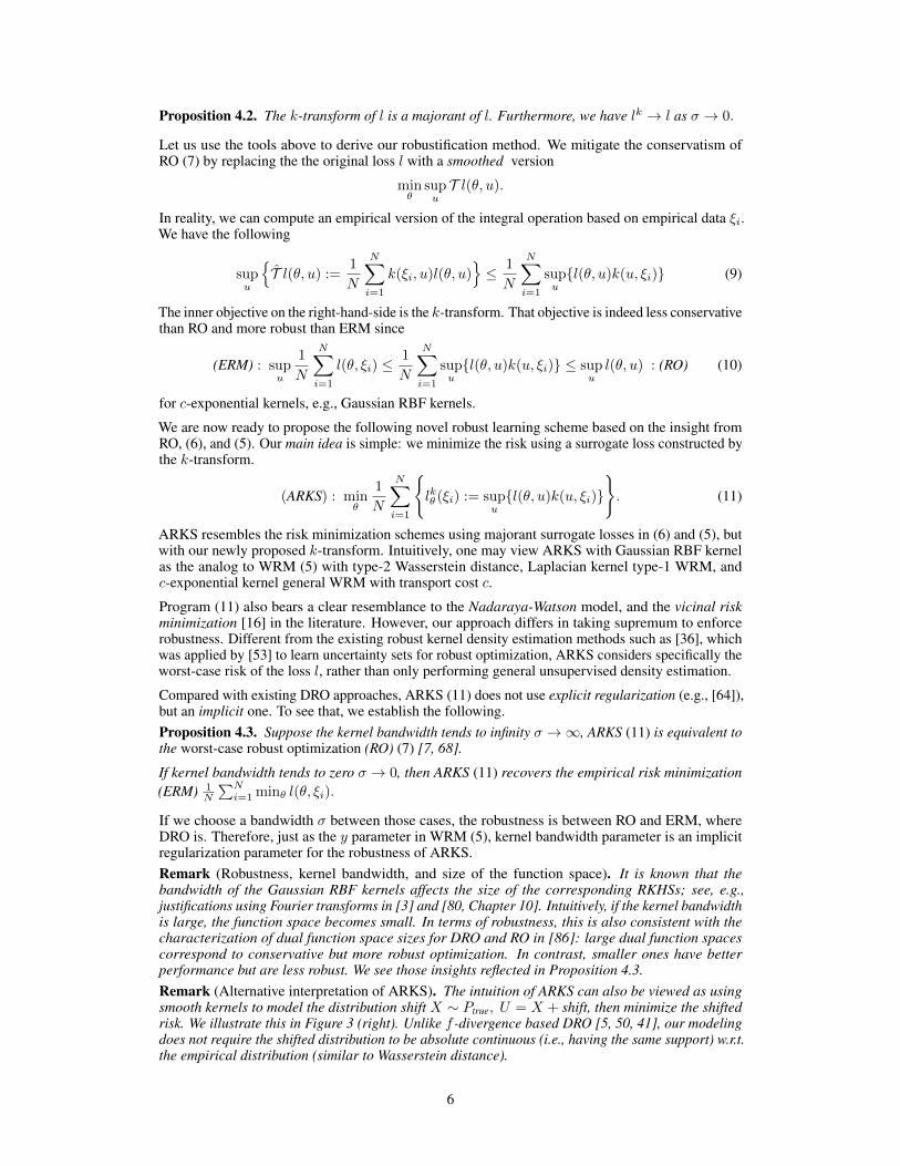
Figure 1: PGD attack with respect to ‖.‖∞ on the Fashion-MNIST (left) and CIFAR-10 (right)datasets. We show the classification error on perturbed test images versus the allowed magnitude ofthe adversarial perturbation ∆. AKRS and WRM exhibit similar adversarial performance profiles;AKRS becomes more robust as the kernel width σ increases, while WRM improves with a lowerLagrangian penalty y. For all algorithms, we report the mean and standard deviation across 10random seeds.

7

To start, we consider Fashion-MNIST [82] classification with a convolutional neural network. Weablate factors known to influence robustness, such as regularization and dropout. We then presenta more realistic large-scale classification scenario using the CIFAR-10 dataset [39]. Finally, weillustrate perturbed images generated by ARKS during training (u∗) via binary classification ofCelebFaces Attributes (CelebA) images [44].

In our evaluation, the test data is perturbed with worst-case disturbances δ within a box {δ : ‖δ‖∞ ≤∆}. δ is generated by attacking the model trained with ERM (for each random seed) using theprojected gradient descent (PGD) algorithm [45]. This experiment is repeated for fast-gradient signmethod (FGSM) [27] attacks with respect to ‖.‖∞; the results are included in the appendix. Note thatour focus is not on any specific attacks, since the key of our method is to enable the use of kernels todescribe a rich class of distribution shift. Details of our hyper-parameter setup, model architectures,and additional experimental results can be found in the appendix.

Fashion-MNIST with CNN. The Fashion-MNIST dataset contains greyscale images of garmentsfrom 10 categories. Each image x is represented by x ∈ [0, 1]28×28. The classifier consists of two3× 3 convolutional layers with ELU activations and max pooling, followed by two fully connectedlayers and a softmax layer.

The left panel of Figure 1 shows the classification error as we increase the magnitude of the perturba-tion ∆. We observe that ERM attains good performance when there is no perturbation but quicklyunderperforms as its magnitude increases. ARKS and WRM yield improved robustness while alsoachieving low test error under no perturbation. ARKS and WRM exhibit similar performance profiles;AKRS becomes more robust as the kernel width σ increases (cf. Proposition 4.3), while WRMimproves with a lower Lagrangian penalty y. To conclude, ARKS performs at least competitivelywith WRM.

CIFAR-10 with ResNet-20. The above experiment is repeated for the CIFAR-10 dataset, whichcontains colored images of different objects from 10 categories. Each image x is represented byx ∈ [0, 1]

32×32×3. We choose a deeper architecture, the ResNet-20 [29] with batch normalization[32] and ReLU activations. As is customary in such settings, we augment the training set withadditional samples by randomly cropping and flipping images. During training, we noticed thatWRM might require tuning y to be arbitrarily large for stable performance under highly non-smoothlosses, while σ can be easily tuned within a small range. The results are shown on the right panelof Figure 1: ARKS exhibits improved robustness under adversarial perturbations with little to notraining performance sacrifice, and is at least competitive with WRM.

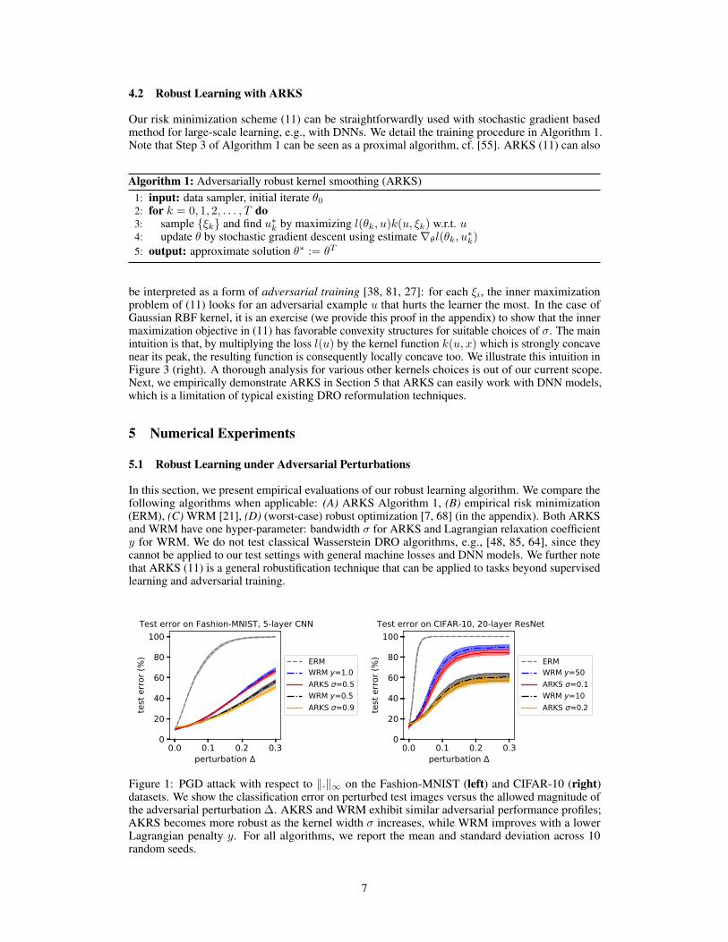
CelebA with CNN. The CelebA dataset is reduced to only contain colored images of celebritieswith eye-wear (class 1) or without (class 0). Each image x is represented by x ∈ [0, 1]64×48×3. Ourmodel architecture is borrowed from [30], comprised of four 5× 5 convolutional layers with LeakyReLU activations, followed by a fully connected and a softmax layer. Experimental results – similarto other datasets – can be found in the appendix, while Figure 2 illustrates examples of perturbedimages generated during training.

Figure 2: (top) Perturbed images (u∗) maximizing the inner optimization of ARKS in CelebA binaryclassification. (bottom) Unperturbed counterpart. We observe that ARKS generates worst-caseperturbations by creating interference around the eyes, reducing apparent separation between the twoclasses (with or without eye-wear).

8

5.2 Visualizing the Robustification of ARKS

0.5 0.0 0.5

1.0

1.2

1.4

1.6

1.8lo

ss sup l( )k( , )l( , )

0.00 0.25 0.50 0.75 1.000

1

2

3

4

losskernell( )k( , i)

i

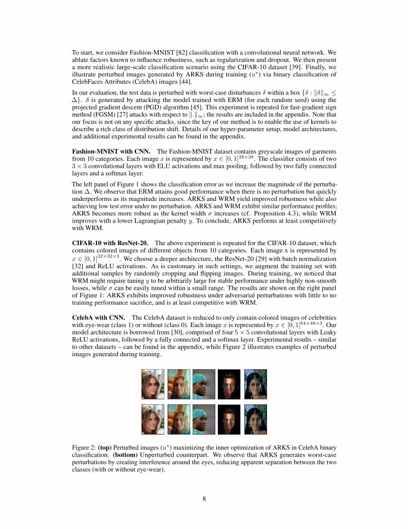
Figure 3: (left) Loss landscape of the kernel robust smoothed loss lk := supu{l(u)kσ(u, ·)}. Asanalyzed in the main text, as the width σ decreases, the ARKS surrogate loss tends towards theoriginal loss, i.e., lk → l as σ → 0. Note that, in our ARKS algorithm, the smoothed loss lk is amajorant of the original loss l. (right) Illustration of the inner maximization problem of ARKS. Thisfigure illustrates the mechanism that ARKS finds the adversarial example by kernel smoothing. Thefigure plots the original loss l in green. The inner objective (k-transform in Definition 2) is plotted inblue. The black cross is a sampled data point ξi. The red cross is the computed solution to the innermaximization problem of ARKS, i.e., adversarial example.

In this section, we use a toy problem to analyze the underlying mechanism of ARKS. Unlike thepreviously reported experiments, our aim here is not to benchmark competitively. We borrow therobust least-squares example from [86], which appeared in [22, 14]. It can be formulated as theoptimization problem minθ ‖A(ξ) · θ − b‖22, where A(ξ) is assumed to be uncertain and given byA(ξ) = A0 + ξA1, where −1 ≤ ξ ≤ 1 is an uncertain variable. Results and analyses are reportedin Figure 3. Figure 3 (left) shows that ARKS indeed produces a majorant of the loss function usingthe k-transform. In Figure 3 (right), we visualize the mechanism that ARKS finds the adversarialexample by kernel smoothing. See our analysis in Section 4.1, the appendix, and the caption for moredetails.

6 Discussion

In this paper, we propose the adversarially robust kernel smoothing (ARKS) algorithm using toolsfrom convex analysis, kernel smoothing, and adversarial robustness. Unlike classical kernel methods,ARKS does not require forming kernel Gram matrices and can be directly used with large-scalestochastic gradient methods. We have demonstrated state-of-the-art performance via ARKS inbenchmarks of learning with distribution shits, especially with DNN models that can not be treatedwith typical Wasserstein DRO convex reformulation techniques. ARKS is also easy to use and tune,which we believe can be a useful tool for robust learning in practice.

Our current presentation regarding kernel design is general and we proposed the c-exponential kernel.Hence a future direction is to design specific kernels for robust learning, especially for incorporatingrich descriptions of interventions in the real world beyond the typical norm-ball based adversarialperturbation. For example, we can similarly design the transportation cost c in our c-exponentialkernel (Definition 3) to be the data-dependent Mahalanobis distance to protect against distributionshift for causal inference as in, e.g., [30], as well as the metric learning aspect of robustness [46].Another direction is incorporating kernels defined on the probability measures, e.g., [18], into ourrobust learning framework.

9

References[1] Michael Arbel, Danica J. Sutherland, Mikołaj Binkowski, and Arthur Gretton. “On Gradient

Regularizers for MMD GANs”. In: arXiv:1805.11565 [cs, stat] (Jan. 2021). arXiv: 1805.11565 [cs, stat].

[2] Heinz H. Bauschke and Patrick L. Combettes. Convex Analysis and Monotone Operator Theoryin Hilbert Spaces. Vol. 408. Springer, 2011.

[3] Mikhail Belkin. “Approximation Beats Concentration? An Approximation View on Inferencewith Smooth Radial Kernels”. In: arXiv:1801.03437 [cs, stat] (Aug. 2018). arXiv: 1801.03437 [cs, stat].

[4] Mikhail Belkin, Daniel Hsu, Siyuan Ma, and Soumik Mandal. “Reconciling Modern MachineLearning Practice and the Bias-Variance Trade-Off”. In: arXiv:1812.11118 [cs, stat] (Sept.2019). arXiv: 1812.11118 [cs, stat].

[5] Aharon Ben-Tal, Dick den Hertog, Anja De Waegenaere, Bertrand Melenberg, and GijsRennen. “Robust Solutions of Optimization Problems Affected by Uncertain Probabilities”. en.In: Management Science 59.2 (Feb. 2013), pp. 341–357. ISSN: 0025-1909, 1526-5501. DOI:10.1287/mnsc.1120.1641.

[6] Aharon Ben-Tal, Dick den Hertog, and Jean-Philippe Vial. “Deriving Robust Counterpartsof Nonlinear Uncertain Inequalities”. en. In: Mathematical Programming 149.1 (Feb. 2015),pp. 265–299. ISSN: 1436-4646. DOI: 10.1007/s10107-014-0750-8.

[7] Aharon Ben-Tal, Laurent El Ghaoui, and Arkadi Nemirovski. Robust Optimization. Vol. 28.Princeton University Press, 2009.

[8] Dimitris Bertsimas, David B. Brown, and Constantine Caramanis. “Theory and Applicationsof Robust Optimization”. In: SIAM Review 53.3 (Jan. 2011), pp. 464–501. ISSN: 0036-1445.DOI: 10.1137/080734510.

[9] Alberto Bietti, Grégoire Mialon, Dexiong Chen, and Julien Mairal. “A Kernel Perspectivefor Regularizing Deep Neural Networks”. In: arXiv:1810.00363 [cs, stat] (May 2019). arXiv:1810.00363 [cs, stat].

[10] Patrick Billingsley. Weak Convergence of Measures: Applications in Probability. SIAM, 1971.[11] Jose Blanchet, Yang Kang, and Karthyek Murthy. “Robust Wasserstein Profile Inference and

Applications to Machine Learning”. In: Journal of Applied Probability 56.3 (Sept. 2019),pp. 830–857. ISSN: 0021-9002, 1475-6072. DOI: 10.1017/jpr.2019.49. arXiv: 1610.05627.

[12] Jose Blanchet, Karthyek Murthy, and Fan Zhang. “Optimal Transport Based Distribution-ally Robust Optimization: Structural Properties and Iterative Schemes”. In: arXiv preprintarXiv:1810.02403 (2018). arXiv: 1810.02403.

[13] Jose Blanchet and Karthyek R. A. Murthy. “Quantifying Distributional Model Risk viaOptimal Transport”. In: arXiv:1604.01446 [math, stat] (July 2017). arXiv: 1604.01446[math, stat].

[14] Stephen Boyd, Stephen P. Boyd, and Lieven Vandenberghe. Convex Optimization. en. Cam-bridge University Press, Mar. 2004. ISBN: 978-0-521-83378-3.

[15] Andrea Caponnetto and Ernesto De Vito. “Optimal Rates for the Regularized Least-SquaresAlgorithm”. In: Foundations of Computational Mathematics 7.3 (2007), pp. 331–368.

[16] Olivier Chapelle, Jason Weston, Léon Bottou, L Eon Bottou, and Vladimir Vapnik. “VicinalRisk Minimization”. In: Advances in Neural Information Processing Systems. MIT Press, 2001,pp. 416–422.

[17] John B. Conway. A Course in Functional Analysis. Vol. 96. Springer, 2019.[18] Henri De Plaen, Michaël Fanuel, and Johan A. K. Suykens. “Wasserstein Exponential Kernels”.

In: arXiv:2002.01878 [cs, stat] (Feb. 2020). arXiv: 2002.01878 [cs, stat].[19] Erick Delage and Yinyu Ye. “Distributionally Robust Optimization Under Moment Uncertainty

with Application to Data-Driven Problems”. en. In: Operations Research 58.3 (June 2010),pp. 595–612. ISSN: 0030-364X, 1526-5463. DOI: 10.1287/opre.1090.0741.

[20] Steven Diamond and Stephen Boyd. “CVXPY: A Python-embedded modeling language forconvex optimization”. In: Journal of Machine Learning Research 17.83 (2016), pp. 1–5.

[21] John Duchi, Peter Glynn, and Hongseok Namkoong. “Statistics of Robust Optimization: AGeneralized Empirical Likelihood Approach”. In: arXiv:1610.03425 [stat] (June 2018). arXiv:1610.03425 [stat].

10

[22] Laurent El Ghaoui and Hervé Lebret. “Robust Solutions to Least-Squares Problems withUncertain Data”. In: SIAM Journal on Matrix Analysis and Applications 18.4 (Oct. 1997),pp. 1035–1064. ISSN: 0895-4798. DOI: 10.1137/S0895479896298130.

[23] E. Erdogan and G. Iyengar. “Ambiguous Chance Constrained Problems and Robust Optimiza-tion”. en. In: Mathematical Programming 107.1 (June 2006), pp. 37–61. ISSN: 1436-4646.DOI: 10.1007/s10107-005-0678-0.

[24] Rui Gao and Anton J. Kleywegt. “Distributionally Robust Stochastic Optimization withWasserstein Distance”. In: arXiv:1604.02199 [math] (July 2016). arXiv: 1604.02199 [math].

[25] Joel Goh and Melvyn Sim. “Distributionally Robust Optimization and Its Tractable Approxima-tions”. en. In: Operations Research 58.4-part-1 (Aug. 2010), pp. 902–917. ISSN: 0030-364X,1526-5463. DOI: 10.1287/opre.1090.0795.

[26] Ian J. Goodfellow, Jean Pouget-Abadie, Mehdi Mirza, Bing Xu, David Warde-Farley, Sher-jil Ozair, Aaron Courville, and Yoshua Bengio. “Generative Adversarial Networks”. In:arXiv:1406.2661 [cs, stat] (June 2014). arXiv: 1406.2661 [cs, stat].

[27] Ian J. Goodfellow, Jonathon Shlens, and Christian Szegedy. “Explaining and HarnessingAdversarial Examples”. In: arXiv:1412.6572 [cs, stat] (Mar. 2015). arXiv: 1412.6572 [cs,stat].

[28] Arthur Gretton, Karsten M. Borgwardt, Malte J. Rasch, Bernhard Schölkopf, and AlexanderSmola. “A Kernel Two-Sample Test”. In: Journal of Machine Learning Research 13 (Mar.2012), pp. 723–773. ISSN: 1533-7928.

[29] Kaiming He, Xiangyu Zhang, Shaoqing Ren, and Jian Sun. Deep Residual Learning for ImageRecognition. 2015. arXiv: 1512.03385 [cs.CV].

[30] Christina Heinze-Deml and Nicolai Meinshausen. “Conditional Variance Penalties and DomainShift Robustness”. en. In: Machine Learning 110.2 (Feb. 2021), pp. 303–348. ISSN: 0885-6125,1573-0565. DOI: 10.1007/s10994-020-05924-1.

[31] Boris Houska and Moritz Diehl. “Nonlinear Robust Optimization via Sequential ConvexBilevel Programming”. en. In: Mathematical Programming 142.1-2 (Dec. 2013), pp. 539–577.ISSN: 0025-5610, 1436-4646. DOI: 10.1007/s10107-012-0591-2.

[32] Sergey Ioffe and Christian Szegedy. Batch Normalization: Accelerating Deep Network Trainingby Reducing Internal Covariate Shift. 2015. arXiv: 1502.03167 [cs.LG].

[33] Garud N. Iyengar. “Robust Dynamic Programming”. In: Mathematics of Operations Research30.2 (2005), pp. 257–280. ISSN: 0364-765X.

[34] Pavel Izmailov, Dmitrii Podoprikhin, Timur Garipov, Dmitry P. Vetrov, and Andrew GordonWilson. “Averaging Weights Leads to Wider Optima and Better Generalization”. In: CoRRabs/1803.05407 (2018). arXiv: 1803.05407. URL: http://arxiv.org/abs/1803.05407.

[35] Leonid Vasilevich Kantorovich and S. G. Rubinshtein. “On a Space of Totally AdditiveFunctions”. In: Vestnik of the St. Petersburg University: Mathematics 13.7 (1958), pp. 52–59.

[36] JooSeuk Kim and Clayton D. Scott. “Robust Kernel Density Estimation”. In: The Journal ofMachine Learning Research 13.1 (2012), pp. 2529–2565.

[37] Diederik P. Kingma and Jimmy Ba. Adam: A Method for Stochastic Optimization. 2017. arXiv:1412.6980 [cs.LG].

[38] Zico Kolter and Aleksander Madry. Adversarial Robustness - Theory and Practice. en.http://adversarial-ml-tutorial.org/. 2018.

[39] Alex Krizhevsky, Vinod Nair, and Geoffrey Hinton. “CIFAR-10 (Canadian Institute forAdvanced Research)”. In: (). URL: http://www.cs.toronto.edu/~kriz/cifar.html.

[40] Daniel Kuhn, Peyman Mohajerin Esfahani, Viet Anh Nguyen, and Soroosh Shafieezadeh-Abadeh. “Wasserstein Distributionally Robust Optimization: Theory and Applications inMachine Learning”. en. In: Operations Research & Management Science in the Age of Analyt-ics. Ed. by Serguei Netessine, Douglas Shier, and Harvey J. Greenberg. INFORMS, Oct. 2019,pp. 130–166. ISBN: 978-0-9906153-3-0. DOI: 10.1287/educ.2019.0198.

[41] Daniel Levy, Yair Carmon, John C. Duchi, and Aaron Sidford. “Large-Scale Methods forDistributionally Robust Optimization”. In: arXiv:2010.05893 [cs, math, stat] (Oct. 2020).arXiv: 2010.05893 [cs, math, stat].

[42] Tengyuan Liang and Alexander Rakhlin. “Just Interpolate: Kernel "Ridgeless" RegressionCan Generalize”. In: arXiv:1808.00387 [cs, math, stat] (Feb. 2019). arXiv: 1808.00387 [cs,math, stat].

11

[43] Fanghui Liu, Zhenyu Liao, and Johan A. K. Suykens. “Kernel Regression in High Dimension:Refined Analysis beyond Double Descent”. In: arXiv:2010.02681 [cs, stat] (Oct. 2020). arXiv:2010.02681 [cs, stat].

[44] Ziwei Liu, Ping Luo, Xiaogang Wang, and Xiaoou Tang. “Deep Learning Face Attributes inthe Wild”. In: Proceedings of International Conference on Computer Vision (ICCV). 2015.

[45] Aleksander Madry, Aleksandar Makelov, Ludwig Schmidt, Dimitris Tsipras, and Adrian Vladu.Towards Deep Learning Models Resistant to Adversarial Attacks. 2019. arXiv: 1706.06083[stat.ML].

[46] Chengzhi Mao, Ziyuan Zhong, Junfeng Yang, Carl Vondrick, and Baishakhi Ray. “MetricLearning for Adversarial Robustness”. In: arXiv:1909.00900 [cs, stat] (Oct. 2019). arXiv:1909.00900 [cs, stat].

[47] Song Mei and Andrea Montanari. “The Generalization Error of Random Features Regression:Precise Asymptotics and Double Descent Curve”. In: arXiv:1908.05355 [math, stat] (Dec.2020). arXiv: 1908.05355 [math, stat].

[48] Peyman Mohajerin Esfahani and Daniel Kuhn. “Data-Driven Distributionally Robust Optimiza-tion Using the Wasserstein Metric: Performance Guarantees and Tractable Reformulations”.en. In: Mathematical Programming 171.1 (Sept. 2018), pp. 115–166. ISSN: 1436-4646. DOI:10.1007/s10107-017-1172-1.

[49] Alfred Müller. “Integral Probability Metrics and Their Generating Classes of Functions”. In:Advances in Applied Probability 29.2 (1997), pp. 429–443.

[50] Hongseok Namkoong and John C Duchi. “Stochastic Gradient Methods for DistributionallyRobust Optimization with F-Divergences”. In: Advances in Neural Information ProcessingSystems 29. Ed. by D. D. Lee, M. Sugiyama, U. V. Luxburg, I. Guyon, and R. Garnett. CurranAssociates, Inc., 2016, pp. 2208–2216.

[51] Hongseok Namkoong and John C Duchi. “Variance-based Regularization with Convex Ob-jectives”. In: Advances in Neural Information Processing Systems. Ed. by I. Guyon, U. V.Luxburg, S. Bengio, H. Wallach, R. Fergus, S. Vishwanathan, and R. Garnett. Vol. 30. CurranAssociates, Inc., 2017. URL: https://proceedings.neurips.cc/paper/2017/file/5a142a55461d5fef016acfb927fee0bd-Paper.pdf.

[52] Arnab Nilim and Laurent El Ghaoui. “Robust Control of Markov Decision Processes withUncertain Transition Matrices”. en. In: Operations Research 53.5 (Oct. 2005), pp. 780–798.ISSN: 0030-364X, 1526-5463. DOI: 10.1287/opre.1050.0216.

[53] Chao Ning and Fengqi You. “Data-Driven Decision Making under Uncertainty IntegratingRobust Optimization with Principal Component Analysis and Kernel Smoothing Methods”. en.In: Computers & Chemical Engineering 112 (Apr. 2018), pp. 190–210. ISSN: 0098-1354. DOI:10.1016/j.compchemeng.2018.02.007.

[54] Jorge Nocedal and Stephen Wright. Numerical Optimization. Springer Science & BusinessMedia, 2006.

[55] Neal Parikh. “Proximal Algorithms”. en. In: Foundations and Trends in Optimization 1.3(2014), pp. 127–239. ISSN: 2167-3888, 2167-3918. DOI: 10.1561/2400000003.

[56] Adam Paszke et al. “PyTorch: An Imperative Style, High-Performance Deep Learning Li-brary”. In: Advances in Neural Information Processing Systems 32. Ed. by H. Wallach, H.Larochelle, A. Beygelzimer, F. d'Alché-Buc, E. Fox, and R. Garnett. Curran Associates, Inc.,2019, pp. 8024–8035. URL: http://papers.neurips.cc/paper/9015-pytorch-an-imperative-style-high-performance-deep-learning-library.pdf.

[57] Gabriel Peyré and Marco Cuturi. “Computational Optimal Transport: With Applications toData Science”. English. In: Foundations and Trends® in Machine Learning 11.5-6 (Feb. 2019),pp. 355–607. ISSN: 1935-8237, 1935-8245. DOI: 10.1561/2200000073.

[58] Imre Pólik and Tamás Terlaky. “A Survey of the S-Lemma”. en. In: SIAM Review 49.3 (Jan.2007), pp. 371–418. ISSN: 0036-1445, 1095-7200. DOI: 10.1137/S003614450444614X.

[59] Christian Rieger and Barbara Zwicknagl. “Sampling Inequalities for Infinitely Smooth Func-tions, with Applications to Interpolation and Machine Learning”. In: Advances in Computa-tional Mathematics 32.1 (2010), p. 103.

[60] Filippo Santambrogio. Optimal Transport for Applied Mathematicians: Calculus of Variations,PDEs, and Modeling. en. Progress in Nonlinear Differential Equations and Their Applications.Birkhäuser Basel, 2015. ISBN: 978-3-319-20827-5. DOI: 10.1007/978-3-319-20828-2.

12

[61] Herbert Scarf. “A Min-Max Solution of an Inventory Problem”. In: Studies in the mathematicaltheory of inventory and production (1958).

[62] B. Schölkopf and A. J. Smola. Learning with Kernels. Cambridge, MA, USA: MIT Press,2002.

[63] Soroosh Shafieezadeh-Abadeh, Peyman Mohajerin Esfahani, and Daniel Kuhn. “Distribu-tionally Robust Logistic Regression”. In: arXiv:1509.09259 [math, stat] (Dec. 2015). arXiv:1509.09259 [math, stat].

[64] Soroosh Shafieezadeh-Abadeh, Daniel Kuhn, and Peyman Mohajerin Esfahani. “Regularizationvia Mass Transportation.” In: Journal of Machine Learning Research 20.103 (2019), pp. 1–68.

[65] Alexander Shapiro. “On Duality Theory of Conic Linear Problems”. en. In: Semi-InfiniteProgramming. Ed. by Panos Pardalos, Miguel Á. Goberna, and Marco A. López. Vol. 57.Boston, MA: Springer US, 2001, pp. 135–165. ISBN: 978-1-4419-5204-2 978-1-4757-3403-4.DOI: 10.1007/978-1-4757-3403-4_7.

[66] Alexander Shapiro, Darinka Dentcheva, and Andrzej Ruszczynski. Lectures on StochasticProgramming: Modeling and Theory. SIAM, 2014.

[67] Aman Sinha, Hongseok Namkoong, Riccardo Volpi, and John Duchi. “Certifying SomeDistributional Robustness with Principled Adversarial Training”. In: arXiv preprintarXiv:1710.10571 (2017). arXiv: 1710.10571.

[68] A. L. Soyster. “Technical Note—Convex Programming with Set-Inclusive Constraints andApplications to Inexact Linear Programming”. en. In: Operations Research 21.5 (Oct. 1973),pp. 1154–1157. ISSN: 0030-364X, 1526-5463. DOI: 10.1287/opre.21.5.1154.

[69] Bharath K. Sriperumbudur, Kenji Fukumizu, Arthur Gretton, Bernhard Schölkopf, and Gert R.G. Lanckriet. “On the Empirical Estimation of Integral Probability Metrics”. EN. In: ElectronicJournal of Statistics 6 (2012), pp. 1550–1599. ISSN: 1935-7524. DOI: 10.1214/12-EJS722.

[70] Bharath K. Sriperumbudur, Kenji Fukumizu, and Gert R. G. Lanckriet. “Universality, Char-acteristic Kernels and RKHS Embedding of Measures”. In: Journal of Machine LearningResearch 12.Jul (2011), pp. 2389–2410. ISSN: ISSN 1533-7928.

[71] Matthew Staib and Stefanie Jegelka. “Distributionally Robust Optimization and Generalizationin Kernel Methods”. In: arXiv:1905.10943 [cs, stat] (May 2019). arXiv: 1905.10943 [cs,stat].

[72] Ingo Steinwart. “On the Influence of the Kernel on the Consistency of Support Vector Ma-chines”. In: Journal of Machine Learning Research 2.1 (), pp. 67–93. ISSN: 15324435. DOI:10.1162/153244302760185252.

[73] Ilya Tolstikhin, Bharath Sriperumbudur, and Krikamol Muandet. “Minimax Estimation ofKernel Mean Embeddings”. In: arXiv:1602.04361 [math, stat] (July 2017). arXiv: 1602.04361 [math, stat].

[74] Phuong Thi Tran and Le Trieu Phong. “On the Convergence Proof of AMSGrad and a NewVersion”. In: IEEE Access 7 (2019), 61706–61716. ISSN: 2169-3536. DOI: 10.1109/access.2019.2916341. URL: http://dx.doi.org/10.1109/ACCESS.2019.2916341.

[75] Aad van der Vaart and Jon Wellner. Weak Convergence and Empirical Processes: With Appli-cations to Statistics. en. Springer Science & Business Media, Mar. 2013. ISBN: 978-1-4757-2545-2.

[76] Aladin Virmaux and Kevin Scaman. “Lipschitz Regularity of Deep Neural Networks: Analysisand Efficient Estimation”. In: Advances in Neural Information Processing Systems 31. Ed. byS. Bengio, H. Wallach, H. Larochelle, K. Grauman, N. Cesa-Bianchi, and R. Garnett. CurranAssociates, Inc., 2018, pp. 3835–3844.

[77] Grace Wahba. Spline Models for Observational Data. SIAM, 1990.[78] Zizhuo Wang, Peter W. Glynn, and Yinyu Ye. “Likelihood Robust Optimization for Data-

Driven Problems”. en. In: Computational Management Science 13.2 (Apr. 2016), pp. 241–261.ISSN: 1619-697X, 1619-6988. DOI: 10.1007/s10287-015-0240-3.

[79] Jonathan Weed and Francis Bach. “Sharp Asymptotic and Finite-Sample Rates of Convergenceof Empirical Measures in Wasserstein Distance”. In: arXiv:1707.00087 [math, stat] (June2017). arXiv: 1707.00087 [math, stat].

[80] Holger Wendland. Scattered Data Approximation. Vol. 17. Cambridge university press, 2004.[81] Eric Wong and J Zico Kolter. “Provable Defenses against Adversarial Examples via the Convex

Outer Adversarial Polytope”. en. In: (), p. 10.

13

[82] Han Xiao, Kashif Rasul, and Roland Vollgraf. Fashion-MNIST: a Novel Image Dataset forBenchmarking Machine Learning Algorithms. 2017. arXiv: 1708.07747 [cs.LG].

[83] Huan Xu, Constantine Caramanis, and Shie Mannor. “Robustness and Regularization ofSupport Vector Machines.” In: Journal of machine learning research 10.7 (2009).

[84] Vladimir A. Yakubovich. “S-Procedure in Nonlinear Control Theory”. In: Vestnik Leninggrad-skogo Universiteta, Ser. Matematika (1971), pp. 62–77.

[85] Chaoyue Zhao and Yongpei Guan. “Data-Driven Risk-Averse Stochastic Optimization withWasserstein Metric”. en. In: Operations Research Letters 46.2 (Mar. 2018), pp. 262–267. ISSN:01676377. DOI: 10.1016/j.orl.2018.01.011.

[86] Jia-Jie Zhu, Wittawat Jitkrittum, Moritz Diehl, and Bernhard Schölkopf. Kernel Distribution-ally Robust Optimization. 2021. arXiv: 2006.06981 [math.OC].

14

Appendix: Adversarially Robust Kernel Smoothing

A Additional technical details

Notation and background. Throughout the appendix, we will consider the cases where the innersupremum is attained. Without further specifications, we consider the kernel choice to be the GaussianRBF kernel kσ(u, x) = e−‖u−x‖

22/2σ (or the Laplacian kernel) in the rest of the appendix. We leave

the generalization to the c-exponential kernel for future work. We suppress the kernel bandwidth σwhen there is no ambiguity in the context.

A.1 Proof of Lemma 4.1

We now prove Lemma 4.1. First, it is an exercise to show the following technical lemmas.

A.1.1 Technical lemma and proofs using convex analysis

Lemma A.1. A function’s y-Pasch-Hausdorff envelope dominates itself, i.e.,

ly,1(x) ≥ l(x),∀x ∈ X .

Furthermore, ly,1 is the smallest majorant of l with Lipschitz constant y.

Lemma A.2. If l is Lipschitz-continuous with constant y, then ly,1 coincides with l.

Similar results concerning the infimal convolution (instead of supremal) are well-known [2, Chapter12]. For completeness, we give self-contained proofs below. We assume the regularity conditionthat f(x) := ly,1(x) = supu{l(θ, u)− y · ‖u− x‖} <∞; we refer to [2, Proposition 12.14] for thedegenerative case when ly,1 =∞ and l has no y-Lipschitz majorant.

We now prove Lemma A.1.

Proof. By noting the special choice of u = x, the relationship f(x) ≥ l(x) is obvious. We nowprove the Lipschitz continuity.

For any x, z in the domain,

f(x) = supu{l(u)−y·‖u−x‖} ≥ sup

u{l(u)−y·‖u−z‖−y·‖z−x‖} = sup

u{l(u)−y·‖u−z‖}−y·‖z−x‖

= f(z)− y · ‖z − x‖. (12)

Therefore, f(z)− f(x) ≤ y · ‖z − x‖, f is y-Lipschitz.

To show that f is the smallest y-Lipschitz majorant, we let g be any y-Lipschitz majorant of l. Then,

g(x) ≥ g(z)− y · ‖z − x‖ ≥ l(z)− y · ‖z − x‖.

Take supremum on both sides,

g(x) ≥ supz{l(z)− y · ‖z − x‖} = f(x).

Hence, f is the smallest y-Lipschitz majorant.

Lemma A.2 follows directly from Lemma A.1. See, e.g., [2] Chapter 12 for more technical details onthe convolution operator.

By plugging in the expression for ly,1, we have

1

N

N∑i=1

supu{l(u)− y · ‖u− ξi‖}+ εy (13)

We have thus recovered the type-1 Wasserstein DRO dual in (??) as a special case of our analysis.

15

A.2 Proof of Proposition 4.2

We now verify the relationship lk(x) ≥ l(x),∀x ∈ X , and lk → l as σ → 0. The dominancerelationship lk(x) ≥ l(x) can be seen by taking the special case u = x in the supremum. Finally, theconvergence of lk → l as σ → 0 is obvious by examining the expression of the Gaussian RBF kerneland Laplacian kernel.

A.3 Proof of Proposition 4.3 (Robustness-performance trade-off using kernel width σ)

First, we note the continuity of the Gaussian RBF kernel and the loss function l; hence all limits areattained. If we let the kernel width be large σ →∞, then limσ→∞ k(u, x) = 1. Hence, the robustlearning algorithm recovers the worst-case robust optimization (RO)

minθ

supξl(θ, ξ).

Similarly, if kernel width is small σ → 0, then we recover the trivial Dirac function at limitlimσ→0 k(u, x) = δx(u). Hence ARKS becomes the empirical risk minimization (ERM),

minθ

1

N

N∑i=1

l(θ, ξi).

A.4 Convexity properties of the inner optimization problem

We are interested in the convexity properties of the objective function of the inner objective of ARKS,which we denote as f(u) := l(u)k(u, x). For ARKS, our intuition is that, by multiplying the loss l(u)by a function k(u, x) which is strongly concave near its peak, the resulting function is consequentlylocally concave too. This idea is illustrated in Figure 3. For conciseness, we assume that the lossfunction l is positive twice-differentiable (cf. [67] for why this is not restrictive), and x, u are scalars.We first show that the inner objective f(u) = l(u)k(u, x) is locally concave in a neighborhood of x.

Proof. We compute curvature d2

du2 f(u).

d2

du2f(u) =

d

du

(d

dul(u)k(u, x) + l(u)

d

duk(u, x)

),

=d2

du2l(u)k(u, x) + 2

d

dul(u)

d

duk(u, x) + l(u)

d2

du2k(u, x)

= e−(u−x)2/2σ

[d2

du2l(u) + 2

d

dul(u) (−(u− x)/σ) + l(u)

(−1/σ + (u− x)2/σ2

)]. (14)

Let us choose σ > 0 small enough such that the following holds.

d2

du2l(u)− l(u)/σ < 0. (15)

This can be done trivially if the curvature of the loss l is bounded (similar to the assumptions in [67,31]) and l(u) > 0. Then, there exists ∆ > 0 such that, for |u − x| ≤ ∆, curvature value (14) isnegative. Therefore, the objective f(u) = l(u)k(u, x) is concave in the ∆−neighborhood of x.

We now show that, for a suitable choice of σ, every stationary point of f is a local maximum, henceexplaining the good empirical performance in our experiments. A full convergence analysis is out ofthe scope of our current paper.

Let

σ∗ =2(u∗ − x)

2√1 + 4(u∗ − x)

2 · d2du2 l(u∗)/l(u∗)− 1,

which is a non-negative quantity if u∗ 6= x and d2

du2 l(u∗) > 0 by straightforward verification.

16

Lemma A.3. Suppose either the loss l is concave or the bandwidth satisfies σ < σ∗. Then, everystationary point of f is a maximum.

Proof. Suppose u∗ is a stationary point of f , which implies

d

duf(u) |u=u∗=

d

dul(u)k(u, x) + l(u)

d

duk(u, x) |u=u∗= 0.

Since k(u, x) 6= 0, that further implies

d

dul(u) + l(u) (−(u− x)/σ) |u=u∗= 0.

Plugging the above equality into the last line of (14),

d2

du2f(u) |u=u∗= e−(u−x)

2/2σ

[d2

du2l(u)− l(u)

(1/σ + (u− x)2/σ2

)]|u=u∗ .

Since either d2

du2 l(u∗) ≤ 0 or σ < σ∗, we have

d2

du2l(u∗)− l(u∗)

(1/σ + (u∗ − x)2/σ2

)< 0.

Then,d2

du2f(u) |u=u∗< 0,

Therefore, u∗ is a local maximum by the second derivative test of calculus.

Not that the condition σ < σ∗ can be easily satisfied when l has bounded curvature and is a weakercondition than (15). Therefore, the above lemma implies that a gradient based algorithm converges toa maximum. We leave the further analysis for future work.

A.5 Additional function approximator and majorant constructions

We now using smooth majorants, as well as interpolants, to construct robustification methods inaddition to the ARKS, e.g.,

1. Kernel distance envelope (KE)

fσ,y(x) := supu{l(θ, u)− y · (1− k(u, x))}. (16)

2. Kernel interpolant (KI; l denotes the vector of loss values at some interpolation points[l(θ, ξ1), . . . , l(θ, ξM )]> )

f(x) = l>k(X,X)−1k(X,x). (17)

While KI is not a strict majorant (since it only interpolates at data sites), we nonethelessshow below it can enforce robustness.

Once we take the function approximation perspective, the possibility is by no means limited to thosechoices. For example, for the inverse multi-quadratic kernels, the approximation supu{l(θ, u) −y[1/k2(u, x)− C2])} is equivalent to using the Moreau-Yosida regularization in type-2 WassersteinDRO. The authors of [86] used the RKHS basis expansion f(x) =

∑Mj=1 αjk(ζj , x), for some

discretization points ζj . Compared with their approach, our choices in (16) and ARKS are certifiedmajorants of loss function l. We now examine the specific approximation schemes.

Kernel distance envelope (KE). We adopt a similar insight as Wasserstein DRO in [67] andpropose the function approximator, which is a variant of the Moreau-Yosida regularization with thekernel distance (using the Gaussian RBF kernel)

fy,σ(x) = supu{l(θ, u) − y/2 · ‖φ(u)− φ(x)‖2H} = sup

u{l(θ, u) − y · (1− k(u, x))}. (18)

17

Similar to ARKS, one can verify

fy,σ(x) ≥ l(x),∀x ∈ X , and fy,σ → l as y → 0,

i.e., it is a function majorant of l. Furthermore, fy,σ can be viewed as a y−Lipschitz continuousmapping from the feature space (i.e., the RKHSH; see the appendix),

fy,σ(x)− fy,σ(z) ≤ y‖φ(x)− φ(z)‖H, ∀x, z ∈ X .

This further implies that, for fixed y, the second term in decomposition (??) is not affected by theoptimization variable θ. Analogous to ARKS, we can simply solve the optimization problem with afixed y,

minθ

1

N

N∑i=1

supu{l(θ, u)− y · (1− k(u, ξi))}. (19)

Similar to (11), for suitable choices of y, σ, the inner function of (19) is locally concave in aneighborhood of ξi, facilitating gradient based optimization. Note that KE can again be interpretedas adversarial training like ARKS. The empirical performance of KE is similar to ARKS in ourexperiments. We thus left it as a future work to examine the properties of KE in details.

Kernel interpolant (KI). We now turn to the kernel interpolant, an entirely different scheme fromARKS. Our main idea in this section is to find a map L2 → H such that we can perform robustlearning inH. For any given θ, we choose the approximation function f to be the well-known kernelinterpolant [77] of the loss function

f = l>k(X,X)−1k(X, ·).

where l is defined in (17). This is also referred to as the kernel “ridge-less” regression estimator. Werefer to [3, 42, 4, 47, 43, 59, 15] for the recent analysis. Plugging this interpolant back into the firsttwo terms of the risk bound (??) and nothing that f is an interpolant of l, we arrive at the regularizedrisk minimization

minθ

1

N

N∑i=1

l(θ, ξi) + ε√l>k(X,X)−1l. (20)

Intuitively, this can be seen as performing the following two steps simultaneously: 1) interpolatingthe optimization loss l using kernel regression; and 2) performing regularized risk minimization w.r.t.θ using the interpolant function’s RKHS norm.

Alternatively, using the least-squares loss as an example, l(θ, [X,Y ]) := (gθ(X)− Y )2, we may usef to interpolate the model gθ only, resulting in

minθ

1

N

N∑i=1

l(θ, [xi, yi]) + ε√

[(f(X)− Y )2]>k(X,X)−1[(f(X)− Y )2]. (21)

where f = gθ(X)>k(X,X)−1k(X, ·), an interpolant of the model g. In practice, we may alsochoose to use a regularizer motivated by kernel ridge regression,

minθ

1

N

N∑i=1

(gθ(Xi)− Yi)2 + λgθ(X)>k(X,X)−1gθ(X).

We refer to [9, 83, 71] for more interpretations of RKHS norm regularization.Remark. While the above formulations, such as (21), resemble the kernel ridge regression (KRR)estimator, they are not not the same. Our method can learn with either parametric or non-parametricmodels with loss l(θ, ·), while KRR only works with kernelized models. For example, we have reportexperiments with DNNs, which cannot be handled by KRR.

B Additional experimental set-up and results

In this Section, we provide additional information on the numerical experiments presented in Section 5.All of our experiments are conducted using the PyTorch [56] and the CVXPY [20] libraries.

18

B.1 Robust learning under Adversarial Perturbations

Datasets. The numerical experiments in Section 5.1 make use of the following publicly availabledatasets: Fashion-MNIST3 [82], CIFAR-104 [39], and CelebA5 [44]. Using the provided attributes,we reduce CelebA to face images with eye-wear (class 1) or without (class 0), and balance the classes.

Model architectures. For Fashion-MNIST, the model architecture consists of two 3× 3 convolu-tional layers with ELU activations and max pooling, followed by two fully connected layers and asoftmax layer. For CIFAR-10 we use the ResNet-20 model architecture [29], consisting of 18 convo-lutional layers with batch normalization [32] and ReLU activations, followed by a fully connectedand a softmax layer. For CelebA, the model architecture is borrowed from [30], comprised of four5× 5 convolutional layers with Leaky ReLU activations, followed by a fully connected and a softmaxlayer. The convolutions produce 16, 32, 64 and 128 channels respectively, using a stride of 2.

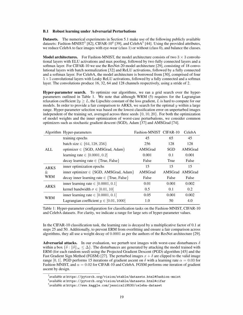
Hyper-parameter search. To optimize our algorithms, we ran a grid search over the hyper-parameters outlined in Table 1. We note that although WRM (5) requires for the Lagrangianrelaxation coefficient 2y ≥ L, the Lipschitz constant of the loss gradient, L is hard to compute for ourmodels. In order to provide a fair comparison to ARKS, we search for the optimal y within a largerange. Hyper-parameter selection was based on the lowest classification error on unperturbed imagesindependent of the training set, averaged across three seeds {0, 10, 20}. For both the optimizationof model weights and the inner optimization of worst-case perturbations, we consider commonoptimizers such as stochastic gradient descent (SGD), Adam [37] and AMSGrad [74].

Algorithm Hyper-parameters Fashion-MNIST CIFAR-10 CelebA

ALL

training epochs 45 65 45batch size ∈ {64, 128, 256} 256 128 128optimizer ∈ {SGD, AMSGrad, Adam} AMSGrad SGD AMSGradlearning rate ∈ [0.0001, 0.2] 0.001 0.1 0.001decay learning rate ∈ {True, False} False True False

ARKS&WRM

inner optimization epochs 15 15 15inner optimizer ∈ {SGD, AMSGrad, Adam} AMSGrad AMSGrad AMSGraddecay inner learning rate ∈ {True, False} False False False

ARKSinner learning rate ∈ [0.0001, 0.1] 0.01 0.001 0.002kernel bandwidth σ ∈ [0.01, 10] 0.5 0.1 0.2

WRMinner learning rate ∈ [0.0001, 0.1] 0.05 0.001 0.002Lagrangian coefficient y ∈ [0.01, 1000] 1.0 50 4.0

Table 1: Hyper-parameter configuration for classification tasks on the Fashion-MNIST, CIFAR-10and CelebA datasets. For clarity, we indicate a range for large sets of hyper-parameter values.

In the CIFAR-10 classification task, the learning rate is decayed by a multiplicative factor of 0.1 atsteps 25 and 50. Additionally, to prevent ERM from overfitting and ensure a fair comparison acrossalgorithms, they all use a weight decay of 0.0001 as per the authors of the ResNet architecture [29].

Adversarial attacks. In our evaluation, we perturb test images with worst-case disturbances δwithin a box {δ : ‖δ‖∞ ≤ ∆}. The disturbances are generated by attacking the model trained withERM (for each random seed) using the Projected Gradient Descent (PGD) algorithm [45] and theFast Gradient Sign Method (FGSM) [27]. The perturbed images x+ δ are clipped to the valid imagerange [0, 1]. PGD performs 15 iterations of gradient ascent on δ with a learning rate α = 0.03 forFashion-MNIST, and α = 0.02 for CIFAR-10 and CelebA. FGSM performs one iteration of gradientascent by design.

3available at https://pytorch.org/vision/stable/datasets.html#fashion-mnist4available at https://pytorch.org/vision/stable/datasets.html#cifar5available at https://www.kaggle.com/jessicali9530/celeba-dataset

19

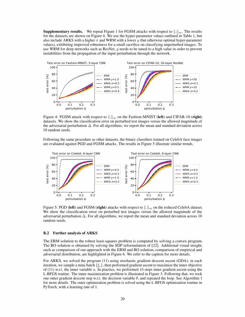
Supplementary results. We repeat Figure 1 for FGSM attacks with respect to ‖.‖∞. The resultsfor the datasets are shown on Figure 4. We use the hyper-parameter values outlined in Table 1, butalso include ARKS with a higher σ and WRM with a lower y (but otherwise optimal hyper-parametervalues), exhibiting improved robustness for a small sacrifice on classifying unperturbed images. Touse WRM for deep networks such as ResNet, y needs to be tuned to a high value in order to preventinstabilities from the propagation of the input perturbation through the network.

0.0 0.1 0.2 0.3perturbation

0

20

40

60

80

100

test

erro

r (%

)

Test error on Fashion-MNIST, 5-layer CNN

ERMWRM y=1.0ARKS =0.5WRM y=0.5ARKS =0.9

0.0 0.1 0.2 0.3perturbation

0

20

40

60

80

100

test

erro

r (%

)

Test error on CIFAR-10, 20-layer ResNet

ERMWRM y=50ARKS =0.1WRM y=10ARKS =0.2

Figure 4: FGSM attack with respect to ‖.‖∞ on the Fashion-MNIST (left) and CIFAR-10 (right)datasets. We show the classification error on perturbed test images versus the allowed magnitude ofthe adversarial perturbation ∆. For all algorithms, we report the mean and standard deviation across10 random seeds.

Following the same procedure as other datasets, the binary classifiers trained on CelebA face imagesare evaluated against PGD and FGSM attacks. The results in Figure 5 illustrate similar trends.

0.0 0.1 0.2 0.3perturbation

0

20

40

60

80

100

test

erro

r (%

)

Test error on CelebA, 6-layer CNN

ERMWRM y=4.0ARKS =0.2WRM y=1.0ARKS =0.5

0.0 0.1 0.2 0.3perturbation

0

20

40

60

80

100

test

erro

r (%

)

Test error on CelebA, 6-layer CNN

ERMWRM y=4.0ARKS =0.2WRM y=1.0ARKS =0.5

Figure 5: PGD (left) and FGSM (right) attacks with respect to ‖.‖∞ on the reduced CelebA dataset.We show the classification error on perturbed test images versus the allowed magnitude of theadversarial perturbation ∆. For all algorithms, we report the mean and standard deviation across 10random seeds.

B.2 Further analysis of ARKS

The ERM solution to the robust least-squares problem is computed by solving a convex program.The RO solution is obtained by solving the SDP reformulation of [22]. Additional visual insight,such as comparison of our approach with the ERM and RO solution, comparison of empirical andadversarial distribution, are highlighted in Figure 6. We refer to the caption for more details.

For ARKS, we solved the program (11) using stochastic gradient descent ascent (GDA): in eachiteration, we sample a mini-batch {ξi}, then performed gradient ascent to maximize the inner objectiveof (11) w.r.t. the inner variable u. In practice, we performed 10 steps inner gradient ascent using theL-BFGS routine. The inner maximization problem is illustrated in Figure 3. Following that, we tookone outer gradient descent step w.r.t. the decision variable θ, and repeated the loop. See Algorithm 1for more details. The outer optimization problem is solved using the L-BFGS optimization routine inPyTorch, with a learning rate of 1.

20

0 1 2 3perturbation

1.0

1.5

2.0

2.5

3.0

3.5

test

loss

KRS= 1.04

KRS= 0.4

KRS= 0.06

ERMRO

0.4 0.2 0.0 0.20

2

4

6

advemp

Figure 6: (left) We plot the performance-robustness trade-off of ARKS for various width settings(black, yellow, blue). We create settings of perturbed test distribution (different from the training datadistribution, with the random variables satisfying Xtest = (1 + δ) ·Xtrain), with increasing amountsof distribution shift parameter δ. We compare with ERM and the worst-case robust optimization (RO)solution of [22]. We see that ARKS with large width σ is more robust and conservative, tendingtowards RO. When width σ is small, ARKS achieves better performance but less robust under alarge distribution shift. Overall, ARKS performs as Proposition 4.3 indicates, achieving a balanceof moderate performance and robustness between ERM and RO. For every algorithm, we ran train10 independent models. The error bars are in standard errors. (right) Histogram density estimationwith σ = 0.41 (as used in ARKS) for both the empirical data (black) and the perturbed (adversarial)points (red). The closed-form MMD estimator [28] between the samples and the adversarial samplesevaluates to MMD = 0.167± 0.02, averaged over 10 independent runs.

B.3 Results for additional models and data sets

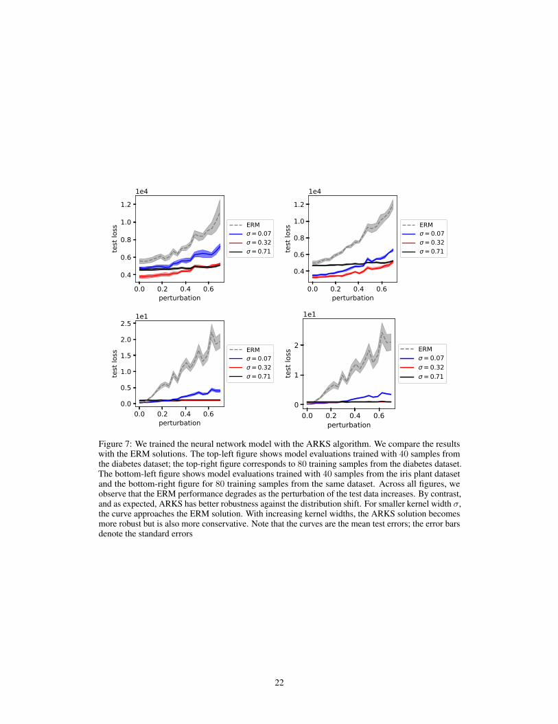
In addition to the linear model in the RLS example and the previously reported benchmarks onCIFAR-10, Fashion-MNIST, and CelebA datasets, we report other results using ARKS with a smallerneural network model. We used a multi-layer perceptron with two fully connected hidden layers, with32 hidden units for each layer. The multi-layer perceptron(MLP) uses the ELU activation because ofits smoothness property. We trained 5 independent models for every setting and use stochastic weightaveraging [34] for all neural network training. We report the results in Figure 7 and the captiontherein. For exact hyperparameter configurations of the MLP training, consult Table 2.

Algorithm Hyper-parameters Diabetes Iris

ERM &ARKS

batch size 256 128optimizer Adam SGDlearning rate 0.001 0.1epochs 2000 2000

ARKSinner optimizer L-BFGS L-BFGSinner learning rate 1 1inner epochs 10 10

Table 2: Hyperparameter configurations for experiments using a multi-layer perceptron as model

We report results on the diabetes regression dataset 6 and the iris plants classification dataset 6. Totest the robustness property of the methods, we add the perturbation to the test data samples using thefollowing rule

Xperturbed = Xtest + d · Uniform(−1, 1).

We increase the perturbation magnitude d from 0 to 1. The results are reported in Figure 7.

6available at https://scikit-learn.org/stable/datasets/toy_dataset.html

21

0.0 0.2 0.4 0.6perturbation

0.4

0.6

0.8

1.0

1.2

test

loss

1e4

ERM= 0.07= 0.32= 0.71

0.0 0.2 0.4 0.6perturbation

0.4

0.6

0.8

1.0

1.2

test

loss

1e4

ERM= 0.07= 0.32= 0.71

0.0 0.2 0.4 0.6perturbation

0.0

0.5

1.0

1.5

2.0

2.5

test

loss

1e1

ERM= 0.07= 0.32= 0.71

0.0 0.2 0.4 0.6perturbation

0

1

2

test

loss

1e1

ERM= 0.07= 0.32= 0.71

Figure 7: We trained the neural network model with the ARKS algorithm. We compare the resultswith the ERM solutions. The top-left figure shows model evaluations trained with 40 samples fromthe diabetes dataset; the top-right figure corresponds to 80 training samples from the diabetes dataset.The bottom-left figure shows model evaluations trained with 40 samples from the iris plant datasetand the bottom-right figure for 80 training samples from the same dataset. Across all figures, weobserve that the ERM performance degrades as the perturbation of the test data increases. By contrast,and as expected, ARKS has better robustness against the distribution shift. For smaller kernel width σ,the curve approaches the ERM solution. With increasing kernel widths, the ARKS solution becomesmore robust but is also more conservative. Note that the curves are the mean test errors; the error barsdenote the standard errors

22