INSTITUTE OF PHYSICS PUBLISHING MEASUREMENT SCIENCE AND TECHNOLOGY

Meas. Sci. Technol. 18 (2007) 907–927 doi:10.1088/0957-0233/18/3/046

Automatic drift elimination in probemicroscope images based on techniques ofcounter-scanning and topography featurerecognitionRostislav V Lapshin

Solid Nanotechnology Laboratory, Institute of Physical Problems, Zelenograd, Moscow,124460, Russian Federation

E-mail: rlapshin@yahoo.com

Received 7 August 2006, in final form 14 December 2006Published 13 February 2007Online at stacks.iop.org/MST/18/907

AbstractAn experimentally proved method for the automatic correction ofdrift-distorted surface topography obtained with a scanning probemicroscope (SPM) is suggested. Drift-produced distortions are described bylinear transformations valid for the case of rather slow changing of themicroscope drift velocity. One or two pairs of counter-scanned images(CSIs) of surface topography are used as initial data. To correct distortions,it is required to recognize the same surface feature within each CSI and todetermine the feature lateral coordinates. Solving a system of linearequations, the linear transformation coefficients suitable for CSI correctionin the lateral and the vertical planes are found. After matching the correctedCSIs, topography averaging is carried out in the overlap area.Recommendations are given that help both estimate the drift correction errorand obtain the corrected images where the error does not exceed somepreliminarily specified value. Two nonlinear correction approaches based onthe linear one are suggested that provide a greater precision of driftelimination. Depending on the scale and the measurement conditions aswell as the correction approach applied, the maximal error may be decreasedfrom 8–25% to 0.6–3%, typical mean error within the area of correctedimage is 0.07–1.5%. The method developed permits us to recoverdrift-distorted topography segments/apertures obtained by usingfeature-oriented scanning. The suggested method may be applied to anyinstrument of the SPM family.

Keywords: thermal drift, creep, counter-scanning, counter-scanned images,CSI, feature-oriented scanning, FOS, topography feature, recognition,scanner, manipulator, calibration, HOPG, porous alumina, STM, AFM,SPM, nanotechnology

1. Introduction

The precision of surface topography measurement, physicaldimensions of the elements varying in the range fromseveral angstroms to several tens of nanometres, is mostlydefined by the value of the drift of the scanning probemicroscope (SPM). As a rule, the instrument drift includes

0957-0233/07/030907+21$30.00 © 2007 IOP Publishing Ltd Print

two main components: one is caused by the thermaldeformation of mechanical units of the device, and the otherresults from the creep of piezomanipulators applied [1].Elimination of the drift can either be done by means of activecompensation [2] during the measurement or image correction[3, 4] after the measurement or a combination of bothmethods.

ed in the UK 907

R V Lapshin

Image-correcting methods, in particular the method [5]proposed in the given paper, as compared to compensatingmethods, have the advantage that no modifications arerequired to be done to the microscope in order to eliminatedistortions. Moreover, unlike the passive approaches,active drift compensation introduces additional noises, whichprevents it from being used for measurements at the highestmicroscope resolution.

The drift correction method developed is based on asimple linear system of equations composed for topographyfeatures found on each of the counter-scanned images of apair. A more complex version of the method, the linear driftcorrection being carried out by two simultaneously obtainedpairs of counter-scanned images, permits us to reach notablybetter results. Finally, transition to nonlinear methods builton the base of the found linear solutions ensures the greatestaccuracy of the drift correction. Application of the nonlinearmethods is especially effective in the case of a strong nonlinearcomponent of distortion produced by creep of microscopepiezomanipulators.

The principal concern in the work is devoted tousing the proposed methods in feature-oriented scanning(FOS) [6], namely for drift correction in segments and inapertures. FOS is a method intended for a high-accuracytopography measurement using surface features as referencepoints of the microscope probe. With this method, duringsuccessive passings from one surface feature to another onelocated nearby, what are being measured are the relativedistance between these features and the topography of theirneighbourhoods—segments (apertures). That permits us toscan the required area on the surface by parts and thenreconstruct the whole image by the obtained fragments.

The suggested drift correction methods have been testedso as to check the operation on different types of probeinstruments, different types of surfaces, in various scales,for several drift velocities and with different proportionsof thermal and creep drift components. Comparing theobtained results with the previously achieved ones [3] showsthat the distance between neighbouring carbon atoms on agraphite surface may now be measured with the error lyingin the interval 0.01–0.33% against 5%. Increase in driftcorrection accuracy is achieved due to the use of analyticalexpressions allowing for all components of linear rasterdistortion, transition to two pairs of counter-scanned images,application of nonlinear correction methods as well as methodsof automatic topography feature recognition.

2. Description of the method

2.1. Linear drift correction by one pair of counter-scannedimages

2.1.1. Building system of equations. Analysis of distortionscaused by drift of a microscope probe relative to a samplesurface proves that lateral-plane drift would lead to imagestretching/contraction along x and y raster axes as well as topicture skewness due to a shift of the image lines/columnsrelative to each other. The same is observed in the verticalplane with respect to the topography height. Here, the heightdifferences are imaged incorrectly and an additional spurioussurface tilt appears.

908

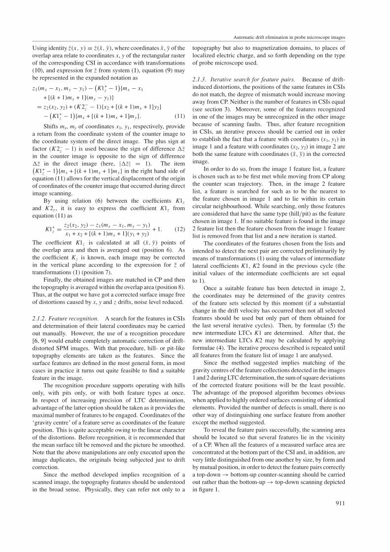
(a) (b)

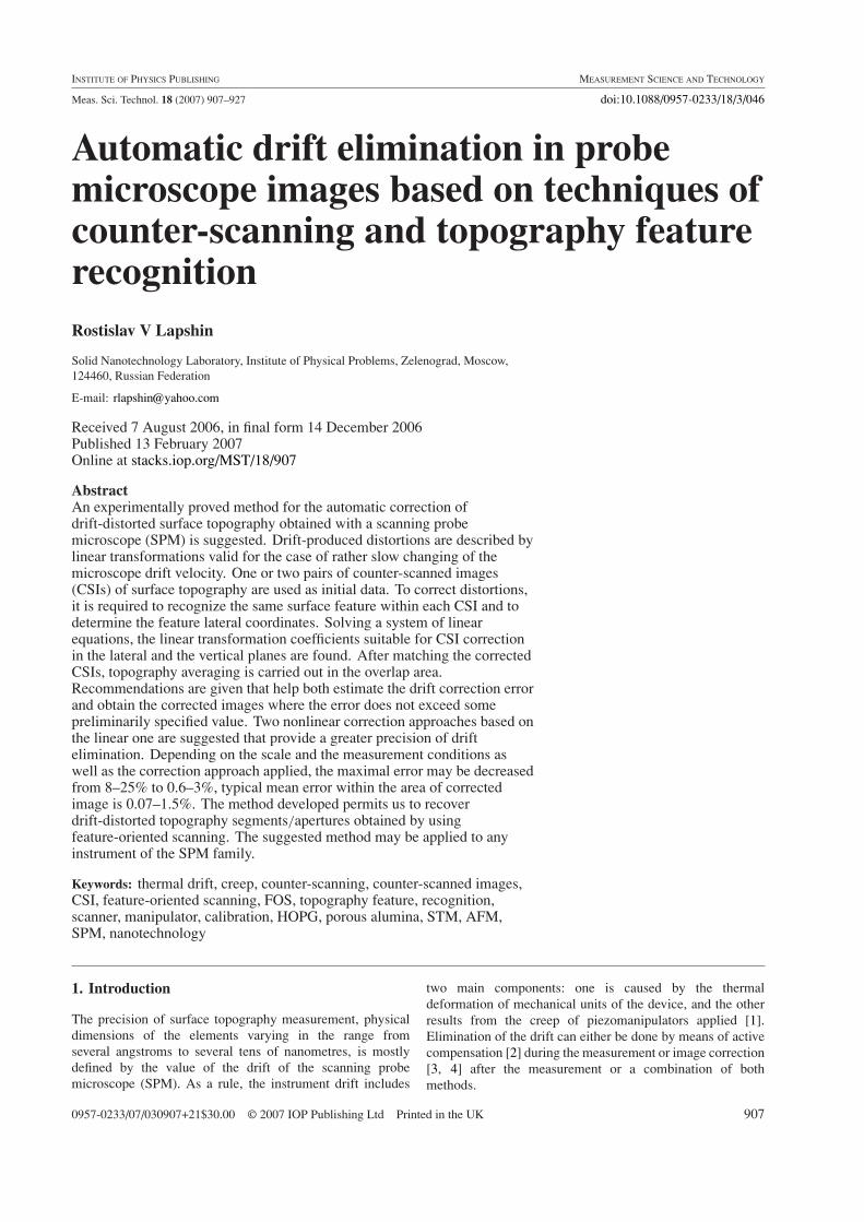
Figure 1. Sketch representation of a trajectory of probe movementwhile counter-scanning with (a) an idle line, (b) no idle line. Digits1–4 designate the numbers of the images obtained. CP is acoincidence point of the counter-scanned image pair. The raster(b) allows an additional reduction of noise level in the correctedimage to be achieved but requires double memory capacity andcalculation time.

Assuming the drift velocity to change slowly enoughwhile scanning a small-sized image [5, 6], the describeddistortions may be represented in the form of lineartransformations as follows:

x(x, y) = x + (Kx − 1){x + [(k + 1)mx + 1]y},y(x, y) = y + (Ky − 1){x + [(k + 1)mx + 1]y},z(x, y) = z(x, y) − (Kz − 1){x + [(k + 1)mx + 1]y},

(1)

where x, y, z are coordinates of points in the corrected image;x, y, z are coordinates of points in the drift-distorted image;Kx, Ky, Kz are linear transformation coefficients (LTCs); k isthe ratio of probe velocity vx in the forward scan line versusprobe velocity in the backward scan line; mx is the number (butone) of points in a line of the distorted image, which definesthe range of the variable x = 0, . . . , mx.

Besides the condition of an invariable drift velocity,equations (1) are written with the assumption that single stepsof the microscope in the lateral plane are equal �x = �y andso are the movement velocities vx = vy . The Kx − 1, Ky − 1,Kz − 1 factors of transformations (1) describe a displacementcaused by the drift along x, y, z, respectively, while moving theprobe by one step along x or y. The parameter k is to considerthe probe displacement along x, y, or z accumulated during theretrace sweep.

Thus, the (Kx − 1)x, (Ky − 1)x, (Kz − 1)x terms allow fordrift-induced probe displacement along x, y, z, respectively,that is occurring while moving the probe along the currentline. The (Kx − 1)(k + 1)mxy, (Ky − 1)(k + 1)mxy, (Kz − 1)× (k + 1)mxy terms represent probe displacement along x, y,z, respectively, that took place when moving the probe by theprevious lines. The (Kx − 1)y, (Ky − 1)y, (Kz − 1)y terms areresponsible for probe displacement along x, y, z, respectively,that occurred when moving the probe between the raster lines.

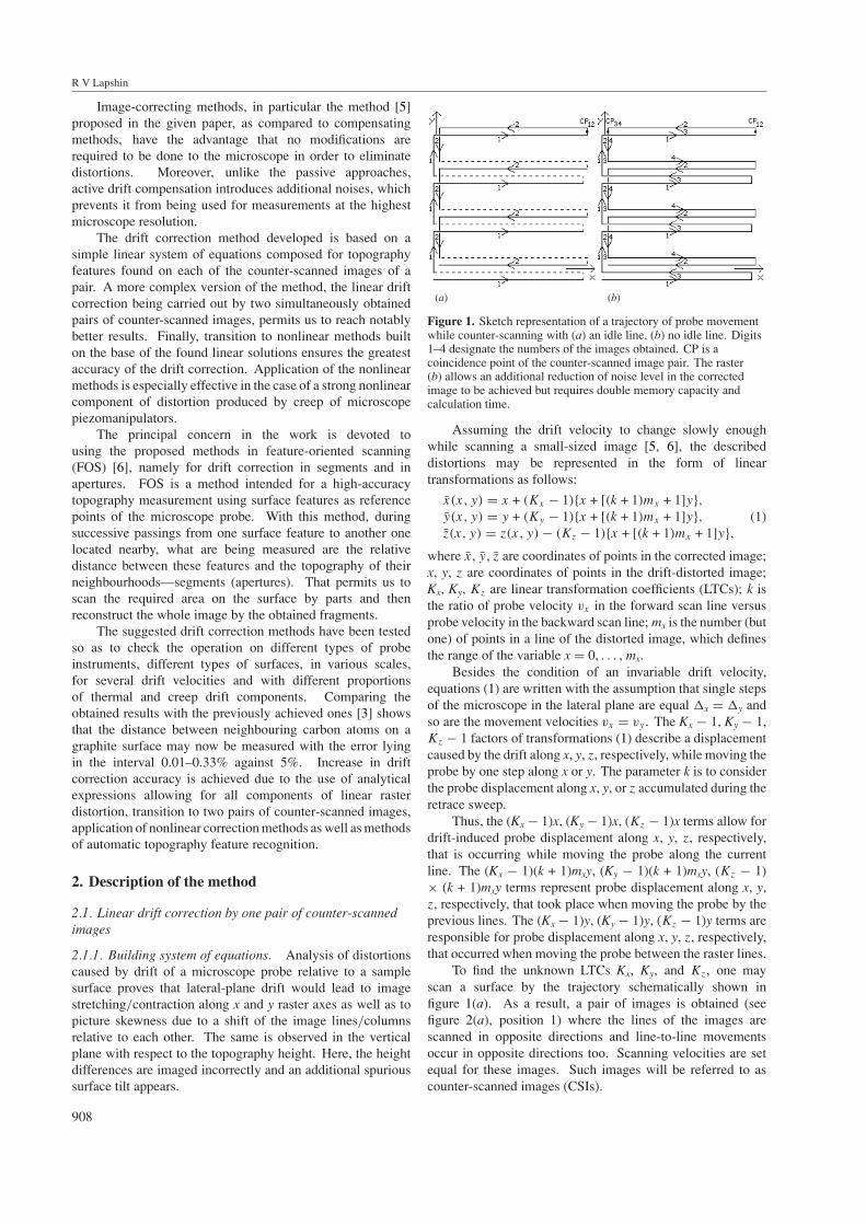
To find the unknown LTCs Kx, Ky, and Kz, one mayscan a surface by the trajectory schematically shown infigure 1(a). As a result, a pair of images is obtained (seefigure 2(a), position 1) where the lines of the images arescanned in opposite directions and line-to-line movementsoccur in opposite directions too. Scanning velocities are setequal for these images. Such images will be referred to ascounter-scanned images (CSIs).

Automatic drift elimination in probe microscope images

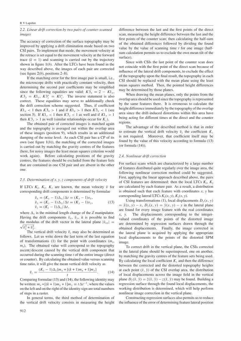
(b)

(a)

Figure 2. Sequence of operations eliminating the drift-induced distortions of surface scan. Correction by (a) one CSI pair, (b) two CSIpairs. GC designates the ‘gravity centre’ of a feature or a group of features. The symbol ‘∩’ designates overlapping for the correspondingCSIs, the bar means topography averaging.

Typical of CSIs is the existence of a point common forboth images (see figure 1). That point will be referred toas a coincidence point (CP). The CP is the end point of theraster trajectory of the first direct image and it is the startpoint of the raster trajectory of the second image counterto the first one. Moving away from the CP, because ofdrift the images become more different from each other,namely, the distinctions in positions of the same featuresbecome more noticeable and the features themselves undergomutually-opposite transformations (stretchings/contractionsand skewnesses).

Provided the same surface feature is present in each imageof the obtained pair (see figure 2(a), position 2), then thefollowing system of equations may be composed by using thelateral coordinates (x1, y1), (x2, y2) of the feature

x1(mx − x1,my − y1) = x2(x2, y2),

y1(mx − x1,my − y1) = y2(x2, y2),(2)

where digits 1 and 2 in the designations show that the quantityis attributed to the first (direct) or to the second (counter)image, respectively; my is the number (but one) of points in acolumn of the distorted image, which defines the range of the

909

R V Lapshin

variable y = 0, . . . , my. The items mx and my in equations (2)provide a transformation of the first image coordinate systemto the second image coordinate system (the origin of the secondimage coordinate system is CP).

Generally, to correct the drift-induced distortions, it issufficient to only reveal one feature on the CSIs and todetermine its lateral coordinates. Since real SPM images havea finite resolution, are noisy, and contain corrupted regions,for the correction parameters to be determined more precisely,it is desirable to use all the features available on the surfaceexcluding, may be, those located along edges of the images.

The fact is that the edges of SPM images are usuallydistorted nonlinearly by creep [7], by hysteresis [8], as wellas by motion dynamics of the piezomanipulators. As a rule,provided the edge distortions are quite distinct, the margins ofthe scanned image are just discarded after correction.

Those features more distant from CP provide a betterprecision while determining LTCs. On the other hand, theprobability of change in drift velocity is also increasingwhile moving away from CP. Therefore, selecting a particularfeature is each time a subject of compromise: on small-sizedscans, all the features are usable, while on large-sized scans,some of the features should be sometimes ‘sacrificed’ (seesection 3.1.1).

Thus, representing the totality of features by its ‘gravitycentre’ with coordinates (x1, y1) and (x2, y2) in the respectiveCSI and taking into consideration transformations (1),equations (2) may be rewritten as

mx − x1 + (K1x − 1){mx − x1 + [(k + 1)mx + 1](my − y1)}= x2 + (K2x − 1){x2 + [(k + 1)mx + 1]y2},

my − y1 + (K1y − 1){mx − x1 + [(k + 1)mx + 1](my − y1)}= y2 + (K2y − 1){x2 + [(k + 1)mx + 1]y2}. (3)

In the CSIs, the relation between coefficients K1 and K2is very simple:

K2x = 2 − K1x,

K2y = 2 − K1y,

K2z = 2 − K1z.

(4)

If one of the coefficients in a pair were to stretch the image,then the other one would contract it and vice versa. If eithercoefficient translates the image with no distortion, i.e., is equalto 1 (drift is absent), then the other one will also translate theimage with no distortion, i.e., will also be equal to 1.

By substituting the coefficients K2x and K2y from (4) inequation (3), the sought LTCs K1x , K1y for the first image arefound (position 3)

K1x = x1 + x2 − mx

x2 − x1 + mx + [(k + 1)mx + 1](y2 − y1 + my)+ 1,

K1y = y1 + y2 − my

x2 − x1 + mx + [(k + 1)mx + 1](y2 − y1 + my)+ 1.

(5)

Then, the LTCs K2x and K2y for the second image may bedetermined through the relationships (4). After that, using theobtained coefficients, the CSIs 1 and 2 are corrected in thelateral plane by means of transformations (1) (position 4).

Strictly speaking, one should distinguish the coefficientsKz for positive

(K+

z

)and for negative (K−

z ) topographydifferences �z. Therefore, the last expression from (4), which

910

shows the general connection between CSI coefficients Kz,should be represented as

K2−z = 2 − K1+

z ,

K2+z = 2 − K1−

z ,

K2−z = K1−

z ,

K2+z = K1+

z .

(6)

Whence the following relations may also be derived: K1−z =

2 − K1+z , K2−

z = 2 − K2+z .

In accordance with the definition of the Kz coefficient forheight differences at point (x, y) located inside the overlaparea of the laterally-corrected images 1 and 2 (position 5), thefollowing system of equations may be written:

�z1(x, y) = K1+z�z(x, y),

�z2(x, y) = K2−z �z(x, y),

(7)

where �z1, �z2 are distorted height differences in thelaterally-corrected images 1 and 2, respectively; �z is thetrue height difference of the topography.

By substituting coefficient K2−z from (6) in the obtained

linear system, the solutions could be found as follows:

K1+z (x, y) = 2�z1(x, y)

�z1(x, y) + �z2(x, y),

�z(x, y) = �z1(x, y) + �z2(x, y)

2.

(8)

The obtained solution for �z shows that the truetopography height difference is defined by a half-sum of thedistorted height differences. It should be noted that for variousheight differences �z various coefficients Kz will be obtained,since the vertical drift induces the same displacement duringtime �t of lateral step execution (coefficients Kz used informula (1) correspond to difference �z = 1).

It is convenient therefore to manipulate with the valueof vertical displacement (Kz − 1)�z, which is the same in allpoints of the overlap area, rather than with the height difference�z and corresponding coefficient Kz. Using formulae (8), itis easy to determine that the vertical displacement is equal toa half-difference of the height differences �z1 and �z2. Thevertical displacement is calculated at each point of the overlaparea and is then averaged.

Thus, the distortions in the vertical plane may be correctedapplying formula (1), where the obtained mean verticaldisplacement should be used instead of Kz − 1. However,this correction method is not accurate since the drift is unableto noticeably distort the height difference �z during time �tof lateral step execution.

For points belonging to the overlap area of laterally-corrected CSIs (position 5), the following equation may becomposed:

z1(x, y) = z2(x, y). (9)

In the lateral plane, transformations inverse to (1) are thefollowing:

x(x, y) = {(Ky − 1)[(k + 1)mx + 1] + 1}x − (Kx − 1)[(k + 1)mx + 1]y

Kx + (Ky − 1)[(k + 1)mx + 1],

y(x, y) = (1 − Ky)x + Kxy

Kx + (Ky − 1)[(k + 1)mx + 1].

(10)

Using identity z(x, y) ≡ z(x, y), where coordinates x, y of theoverlap area relate to coordinates x, y of the rectangular rasterof the corresponding CSI in accordance with transformations(10), and expression for z from system (1), equation (9) maybe represented in the expanded notation as

z1(mx − x1,my − y1) − (K1+

z − 1){mx − x1

+ [(k + 1)mx + 1](my − y1)}= z2(x2, y2) + (K2−

z − 1){x2 + [(k + 1)mx + 1]y2}− (

K1+z − 1

){mx + [(k + 1)mx + 1]my}. (11)

Shifts mx, my of coordinates x1, y1, respectively, providea return from the coordinate system of the counter image tothe coordinate system of the direct image. The plus sign atfactor (K2−

z − 1) is used because the sign of difference �z

in the counter image is opposite to the sign of difference�z in the direct image (here, |�z| = 1). The item(K1+

z − 1){mx + [(k + 1)mx + 1]my} in the right hand side of

equation (11) allows for the vertical displacement of the originof coordinates of the counter image that occurred during directimage scanning.

By using relation (6) between the coefficients K1z

and K2z, it is easy to express the coefficient K1z fromequation (11) as

K1+z = z2(x2, y2) − z1(mx − x1,my − y1)

x1 + x2 + [(k + 1)mx + 1](y1 + y2)+ 1. (12)

The coefficient K1z is calculated at all (x, y) points ofthe overlap area and then is averaged out (position 6). Asthe coefficient Kz is known, each image may be correctedin the vertical plane according to the expression for z oftransformations (1) (position 7).

Finally, the obtained images are matched in CP and thenthe topography is averaged within the overlap area (position 8).Thus, at the output we have got a corrected surface image freeof distortions caused by x, y and z drifts, noise level reduced.

2.1.2. Feature recognition. A search for the features in CSIsand determination of their lateral coordinates may be carriedout manually. However, the use of a recognition procedure[6, 9] would enable completely automatic correction of drift-distorted SPM images. With that procedure, hill- or pit-liketopography elements are taken as the features. Since thesurface features are defined in the most general form, in mostcases in practice it turns out quite feasible to find a suitablefeature in the image.

The recognition procedure supports operating with hillsonly, with pits only, or with both feature types at once.In respect of increasing precision of LTC determination,advantage of the latter option should be taken as it provides themaximal number of features to be engaged. Coordinates of the‘gravity centre’ of a feature serve as coordinates of the featureposition. This is quite acceptable owing to the linear characterof the distortions. Before recognition, it is recommended thatthe mean surface tilt be removed and the picture be smoothed.Note that the above manipulations are only executed upon theimage duplicates, the originals being subjected just to driftcorrection.

Since the method developed implies recognition of ascanned image, the topography features should be understoodin the broad sense. Physically, they can refer not only to a

Automatic drift elimination in probe microscope images

topography but also to magnetization domains, to places oflocalized electric charge, and so forth depending on the typeof probe microscope used.

2.1.3. Iterative search for feature pairs. Because of drift-induced distortions, the positions of the same features in CSIsdo not match, the degree of mismatch would increase movingaway from CP. Neither is the number of features in CSIs equal(see section 3). Moreover, some of the features recognizedin one of the images may be unrecognized in the other imagebecause of scanning faults. Thus, after feature recognitionin CSIs, an iterative process should be carried out in orderto establish the fact that a feature with coordinates (x1, y1) inimage 1 and a feature with coordinates (x2, y2) in image 2 areboth the same feature with coordinates (x, y) in the correctedimage.

In order to do so, from the image 1 feature list, a featureis chosen such as to be first met while moving from CP alongthe counter scan trajectory. Then, in the image 2 featurelist, a feature is searched for such as to be the nearest tothe feature chosen in image 1 and to lie within its certaincircular neighbourhood. While searching, only those featuresare considered that have the same type (hill/pit) as the featurechosen in image 1. If no suitable feature is found in the image2 feature list then the feature chosen from the image 1 featurelist is removed from that list and a new iteration is started.

The coordinates of the features chosen from the lists andintended to detect the next pair are corrected preliminarily bymeans of transformations (1) using the values of intermediatelateral coefficients K1, K2 found in the previous cycle (theinitial values of the intermediate coefficients are set equalto 1).

Once a suitable feature has been detected in image 2,the coordinates may be determined of the gravity centresof the feature sets selected by this moment (if a substantialchange in the drift velocity has occurred then not all selectedfeatures should be used but only part of them obtained forthe last several iterative cycles). Then, by formulae (5) thenew intermediate LTCs K1 are determined. After that, thenew intermediate LTCs K2 may be calculated by applyingformulae (4). The iterative process described is repeated untilall features from the feature list of image 1 are analysed.

Since the method suggested implies matching of thegravity centres of the feature collections detected in the images1 and 2 during LTC determination, the sum of square deviationsof the corrected feature positions will be the least possible.The advantage of the proposed algorithm becomes obviouswhen applied to highly ordered surfaces consisting of identicalelements. Provided the number of defects is small, there is noother way of distinguishing one surface feature from anotherexcept the method suggested.

To reveal the feature pairs successfully, the scanning areashould be located so that several features lie in the vicinityof a CP. When all the features of a measured surface area areconcentrated at the bottom part of the CSI and, in addition, arevery little distinguished from one another by size, by form andby mutual position, in order to detect the feature pairs correctlya top-down → bottom-up counter-scanning should be carriedout rather than the bottom-up → top-down scanning depictedin figure 1.

911

R V Lapshin

2.2. Linear drift correction by two pairs of counter-scannedimages

The accuracy of correction of the surface topography may beimproved by applying a drift elimination mode based on twoCSI pairs. To implement that mode, the movement velocity atthe retrace is set equal to the movement velocity at the forwardtrace (k = 1) and scanning is carried out by the trajectoryshown in figure 1(b). After the LTCs have been found in theway described above, the images of each pair are corrected(see figure 2(b), positions 2–8).

If the matching error for the first image pair is small, i.e.,the microscope drifts with practically constant velocity, thendetermining the second pair coefficients may be simplifiedsince the following equalities are valid: K3x = 2 − K1x ,K3y = K1y , K3+

z = K1+z . The inverse statement is also

correct. These equalities may serve to additionally checkthe drift correction scheme suggested. Thus, if coefficientK1x < 1 then K3x > 1 and if K1x > 1 then K3x < 1 (seesection 3). If K1y < 1 then K3y < 1 as well and if K1y > 1then K3y > 1 as well (similar relationships occur for Kz).

The obtained pair of corrected images is matched againand the topography is averaged out within the overlap areaof these images (position 9), which results in an additionaldamping of the noise level. As each CSI pair has a CP of itsown (see figure 1(b)), the matching of the corrected imagesis carried out by matching the gravity centres of the features(here, for noisy images the least mean squares criterion wouldwork again). Before calculating positions of the gravitycentres, the features should be excluded from the feature liststhat are contained in one CSI pair and are absent in the otherone.

2.3. Determination of x, y, z components of drift velocity

If LTCs Kx, Ky, Kz are known, the mean velocity v forcorresponding drift components is determined by formulae

vx = (Kx − 1)�x/�t = (Kx − 1)vx,

vy = (Ky − 1)�y/�t = (Ky − 1)vy,

vz = (Kz − 1)�z/�t,

(13)

where �z is the minimal length change of the Z manipulator.Having the drift components vx , vy , it is possible to findthe modulus of the drift vector in the lateral plane |vxy | =√

v2x + v2

y .The vertical drift velocity vz may also be determined as

follows. Let us write down the last term of the last equationof transformations (1) for the point with coordinates (mx,my). The obtained value will correspond to the topographyascent/descent caused by the vertical drift component thatoccurred during the scanning time t of the entire image (director counter). By calculating the obtained value versus scanningtime ratio, it will give the mean vertical drift velocity as

vz = (Kz − 1)�z{mx + [(k + 1)mx + 1]my}t

. (14)

Comparing formulae (13) and (14), the following identity maybe written: mx +[(k + 1)mx + 1]my ≡ t�t−1, where the valueson the left and on the right of the identity sign are total numbersof steps in a raster.

In general terms, the third method of determination ofthe vertical drift velocity consists in measuring the height

912

difference between the last and the first points of the directscan, measuring the height difference between the last and thefirst points of the counter scan; then calculating the half-sumof the obtained differences followed by dividing the foundvalue by the value of scanning time t for one image (half-sum calculation permits us to exclude the own mean tilt of thesurface).

Since with CSIs the last point of the counter scan doesnot coincide with the first point of the direct scan because ofinfluence of the lateral drift components, to exclude the effectof the topography upon the final result, the topography in eachCSI should be replaced with the mean plane using the leastmean squares method. Then, the pointed height differencesmay be determined by those planes.

When drawing the mean planes, only the points from theoverlap area should be used since the topography is representedby the same features there. It is erroneous to calculate theheight difference immediately by the topography of the overlaparea since the drift-induced distortions within this area havebeing acting for different times at the direct and the counterregions.

The advantage of the described method is that in orderto estimate the vertical drift velocity vz the coefficient Kz

is not required. Moreover, that coefficient itself may befound by the value of this velocity according to formula (13)(or formula (14)).

2.4. Nonlinear drift correction

For surface scans which are characterized by a large numberof features distributed quite regularly over the image area, thefollowing nonlinear correction method could be suggested.First, applying the linear approach described above, the pairsof CSI features are determined; then the local LTCs Kx, Ky

are calculated by each feature pair. As a result, a distributionis obtained such that each feature with coordinates x, y hascorresponding lateral LTCs Kx(x, y), Ky(x, y).

Using transformations (1), local displacements Dx(x, y)

= x(x, y) − x, Dy(x, y) = y(x, y) − y in the lateral planeare found for every image feature with the real coordinatesx, y. The displacements corresponding to the integer-valued coordinates of the points of the distorted imageare determined by regression surfaces drawn through theobtained displacements. Finally, the image corrected inthe lateral plane is acquired by applying the appropriatelocal displacements to the points of the distorted SPMimage.

To correct drift in the vertical plane, the CSIs correctedin the lateral plane should be superimposed, one on another,by matching the gravity centres of the feature sets being used.By calculating the local coefficient Kz and then the differencebetween the corrected and the distorted topography heightsat each point (x, y) of the CSI overlap area, the distributionof local displacements across the image field in the verticalplane Dz(x, y) = z(x, y) − z(x, y) may be found. Building aregression surface through the found local displacements, theworking distribution is determined, which will help performnonlinear image correction in the vertical plane.

Constructing regression surfaces also permits us to reducethe influence of the error of determining feature lateral position

and topography height on the results of nonlinear correction.The regression surface order is chosen by the residualmismatch of the feature positions (topography heights), sothat the mismatch is minimal. In the case of large nonlineardistortions, the regression surfaces may also be used duringiterative search for feature pairs.

Another nonlinear correction scheme may be suggested.First, some square neighbourhood (a segment) is cut outaround a feature in every corrected image. Then the cut-outtopography fragments are put in position, which is the meanof the corrected positions of this feature in the correspondingCSI. Correction of the images and the feature positionsmay be carried out by either linear or nonlinear methods asdescribed above. Finally, within the segment overlap areas,the topography is averaged. Thus, the corrected topography isgetting nearer to the actual one not only because of averagingin the vertical plane but also because of averaging of the featurepositions.

The basis of the described nonlinear correction methodsis that the true feature position lies somewhere in the segmentbetween the corrected feature positions, most probablygravitating to the middle.

2.5. Correction of drift-distorted topography segments in afeature-oriented scanning method

The described drift correction method yields the maximaleffect when used with the FOS approach [6], since in thatcase it would enable drift correction in images of an arbitrarylarge size. The point is that, beginning with a certain scan size,the main assumption of invariability of the drift velocity duringscanning time will necessarily cease to work (see section 3).Although the same assumption must be satisfied for scansobtained by the FOS method, the contradiction in that caseis eliminated because a large area is scanned by parts, i.e.,by small segments (square neighbourhoods of the surfacefeatures) and all movements occur within short distances fromone feature to another located nearby.

To make sure of the above, one should compare 1.5 minapproximately scanning time of (35 × 35) A2 atomic graphitesurface (see section 3.1) with 300 ms approximately scanning-recognition time of (4.5 × 4.5) A2 segments of the ‘Next’ andthe ‘Current’ carbon atoms in one skipping cycle [6]. Skippingis a basic measurement operation in FOS intended for accuratedetermination of relative coordinates of neighbouring featuresand acquisition of topography segments.

Passing from the atomic scale to surfaces with typicalfeature dimensions and distances between the features of tensand hundreds of nanometres, the visible evidence of the driftthermocomponent in the image would subside, though thenonlinear creep component of the drift, in contrast, wouldbecome more apparent (see section 4). Nevertheless, thenegative creep effect may be substantially reduced providedthat the topography is measured by parts using small segmentsand mutually opposite probe movements forming the entirehierarchy of counter movements are applied throughout theapertures (an aperture is an auxiliary scan of the current featuresurroundings containing several neighbouring features), inthe segments, between the neighbour features (the skipping)as well as in feature lines [6].

Automatic drift elimination in probe microscope images

Moreover, in the case that a noticeable change in driftvelocity occurred (the drift is being monitored continuouslyduring FOS) the measurement process is automaticallysuspended, the corrupted local data are discarded, and themicroscope waits for the drift velocity to become constant,at that executing periodical probe attachments to the currentsurface feature or inserting idle skipping cycles. Once thedrift velocity has become stable, the work is resumed and theinterrupted local measurement is executed over again. Thus,because of applying the pointed set of the methods, the totaldrift turns out to be a slowly changing process again and,therefore, it can be linearized as well.

It should be noted how simple it is to detect the samefeature in CSIs with the FOS approach. The fact is that asegment, as a rule, contains one feature only. When a segmentincludes several features (usually two or three), the featureslocated closer than the others to the CSI centres will correspondto the same current feature in the corrected segment since themain sign of the current feature in the segment is its proximityto the centre of the square raster [6].

Recognition of two/four CSIs may be carried outsimultaneously. Recognition of hill-like features and pit-like features in each image may also be processed inparallel [6]. Moreover, the process of direct imagerecognition and the process of counter image scanning may beimplemented concurrently. Thus, the calculation throughputmay be substantially increased by applying a two/fourprocessor computer. Maximal advantage can be taken of amultiprocessor computer when the counter-scanning methodis used within the FOS approach, where the recognition shouldbe carried out in real-time.

It should be noted in conclusion that, applying thedescribed drift correction method directly, the number ofimage averagings is restricted to 4 at most, whereas thereare no restrictions at all on the number of image (segment)averagings if the proposed method is used within the FOSapproach.

3. Experimental results

In order to verify the operation of the suggested driftcorrection method, a counter-scanning of an atomic surfaceof highly oriented pyrolytic graphite (HOPG) and a porousalumina surface was carried out. The graphite surface wasmeasured with a scanning tunnelling microscope (STM) andthe porous alumina surface was measured with an atomic-forcemicroscope (AFM). In both cases an SPM SolverTM P4 (NT-MDT Co.) was employed, the measurements were performedin ambient conditions, the sample was moved relative to a fixedprobe.

In order to provide a smoother transition of thepiezomanipulators from the quiescent state to the scanningstate, several tens of ‘training’ probe passages along the firstline of the raster were carried out just before the scanningsstarted. In this way, it allows us to substantially decreasethe creep-caused distortions at the beginning of the scan. Aswell, during the training, the actual scanning speed vx wasdetermined. Feature recognition in CSIs was executed in thecourse of virtual FOS [6].

913

R V Lapshin

(a) (b)

(c) (d )

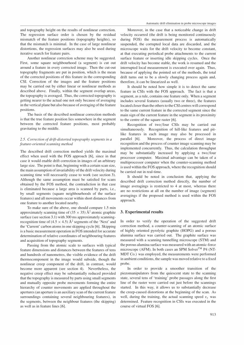
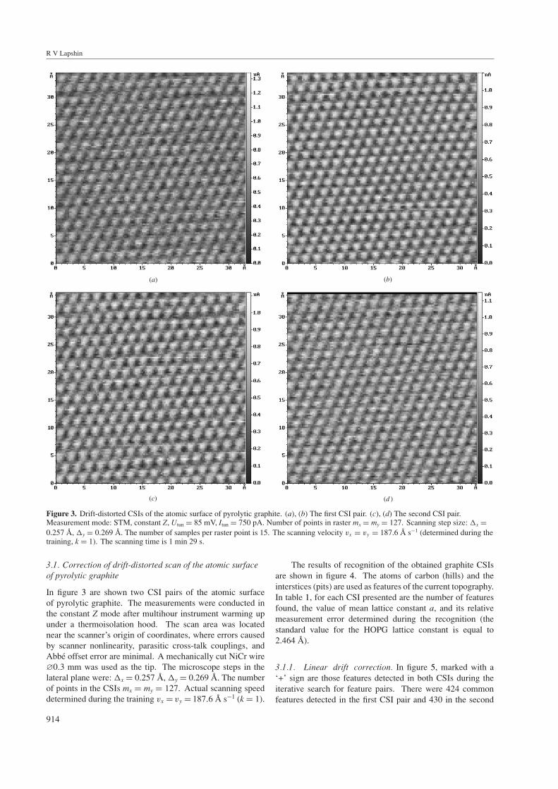
Figure 3. Drift-distorted CSIs of the atomic surface of pyrolytic graphite. (a), (b) The first CSI pair. (c), (d) The second CSI pair.Measurement mode: STM, constant Z, Utun = 85 mV, Itun = 750 pA. Number of points in raster mx = my = 127. Scanning step size: �x =0.257 A, �y = 0.269 A. The number of samples per raster point is 15. The scanning velocity vx = vy = 187.6 A s−1 (determined during thetraining, k = 1). The scanning time is 1 min 29 s.

3.1. Correction of drift-distorted scan of the atomic surfaceof pyrolytic graphite

In figure 3 are shown two CSI pairs of the atomic surfaceof pyrolytic graphite. The measurements were conducted inthe constant Z mode after multihour instrument warming upunder a thermoisolation hood. The scan area was locatednear the scanner’s origin of coordinates, where errors causedby scanner nonlinearity, parasitic cross-talk couplings, andAbbe offset error are minimal. A mechanically cut NiCr wire∅0.3 mm was used as the tip. The microscope steps in thelateral plane were: �x = 0.257 A, �y = 0.269 A. The numberof points in the CSIs mx = my = 127. Actual scanning speeddetermined during the training vx = vy = 187.6 A s−1 (k = 1).

914

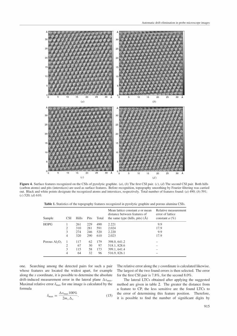
The results of recognition of the obtained graphite CSIsare shown in figure 4. The atoms of carbon (hills) and theinterstices (pits) are used as features of the current topography.In table 1, for each CSI presented are the number of featuresfound, the value of mean lattice constant a, and its relativemeasurement error determined during the recognition (thestandard value for the HOPG lattice constant is equal to2.464 A).

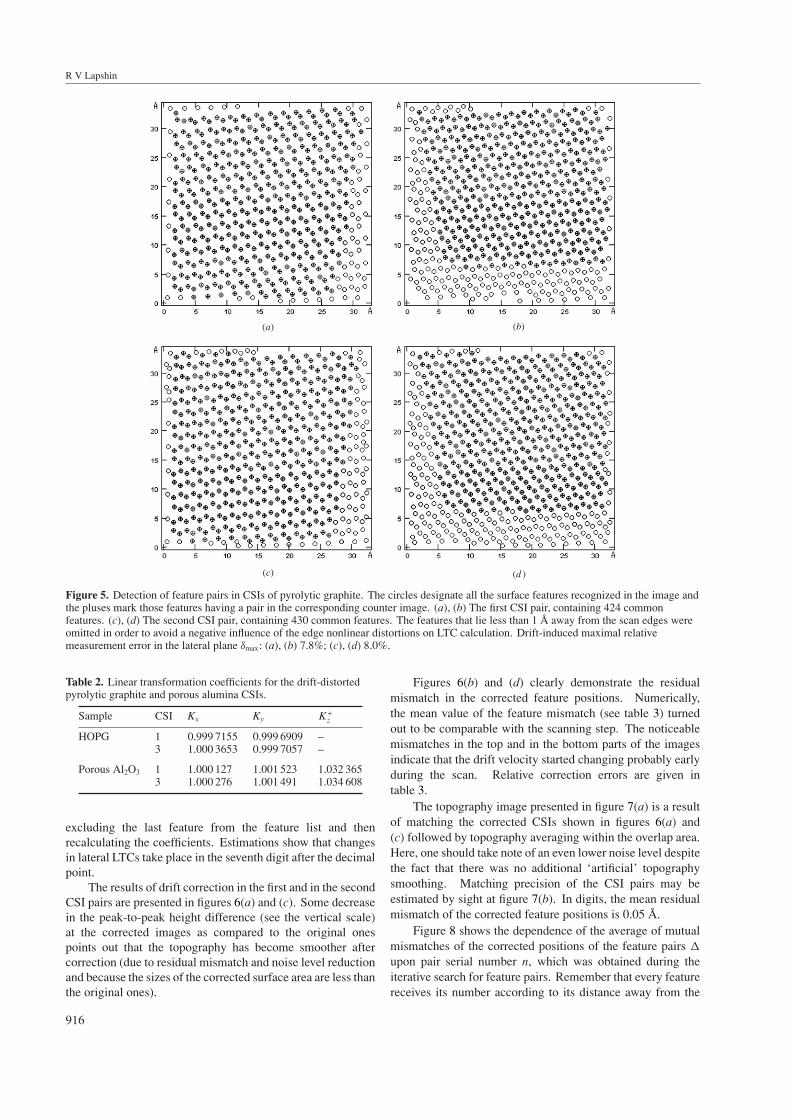
3.1.1. Linear drift correction. In figure 5, marked with a‘+’ sign are those features detected in both CSIs during theiterative search for feature pairs. There were 424 commonfeatures detected in the first CSI pair and 430 in the second

Automatic drift elimination in probe microscope images

(a) (b)

(c) (d )

Figure 4. Surface features recognized on the CSIs of pyrolytic graphite. (a), (b) The first CSI pair. (c), (d) The second CSI pair. Both hills(carbon atoms) and pits (interstices) are used as surface features. Before recognition, topography smoothing by Fourier filtering was carriedout. Black and white points designate the recognized atoms and interstices, respectively. Total number of features found: (a) 490; (b) 591;(c) 520; (d) 610.

Table 1. Statistics of the topography features recognized in pyrolytic graphite and porous alumina CSIs.

Mean lattice constant a or mean Relative measurementdistance between features of error of lattice

Sample CSI Hills Pits Total the same type (hills, pits) (A) constant a (%)

HOPG 1 261 229 490 2.221 9.92 310 281 591 2.024 17.93 274 246 520 2.220 9.94 320 290 610 2.023 17.9

Porous Al2O3 1 117 62 179 398.0, 641.2 –2 67 30 97 518.1, 828.6 –3 115 58 173 399.1, 641.4 –4 64 32 96 516.9, 826.1 –

one. Searching among the detected pairs for such a pairwhose features are located the widest apart, for examplealong the x coordinate, it is possible to determine the absolutedrift-induced measurement error in the lateral plane �xmax.Maximal relative error δmax for one image is calculated by theformula

δmax = �xmax100%

2mx�x

. (15)

The relative error along the y coordinate is calculated likewise.The largest of the two found errors is then selected. The errorfor the first CSI pair is 7.8%, for the second 8.0%.

The lateral LTCs obtained after applying the suggestedmethod are given in table 2. The greater the distance froma feature to CP, the less sensitive are the found LTCs tothe error of determining this feature position. Therefore,it is possible to find the number of significant digits by

915

R V Lapshin

(a) (b)

(c) (d )

Figure 5. Detection of feature pairs in CSIs of pyrolytic graphite. The circles designate all the surface features recognized in the image andthe pluses mark those features having a pair in the corresponding counter image. (a), (b) The first CSI pair, containing 424 commonfeatures. (c), (d) The second CSI pair, containing 430 common features. The features that lie less than 1 A away from the scan edges wereomitted in order to avoid a negative influence of the edge nonlinear distortions on LTC calculation. Drift-induced maximal relativemeasurement error in the lateral plane δmax: (a), (b) 7.8%; (c), (d) 8.0%.

Table 2. Linear transformation coefficients for the drift-distortedpyrolytic graphite and porous alumina CSIs.

Sample CSI Kx Ky K+z

HOPG 1 0.999 7155 0.999 6909 –3 1.000 3653 0.999 7057 –

Porous Al2O3 1 1.000 127 1.001 523 1.032 3653 1.000 276 1.001 491 1.034 608

excluding the last feature from the feature list and thenrecalculating the coefficients. Estimations show that changesin lateral LTCs take place in the seventh digit after the decimalpoint.

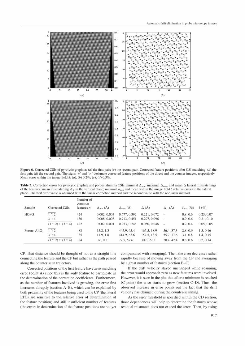
The results of drift correction in the first and in the secondCSI pairs are presented in figures 6(a) and (c). Some decreasein the peak-to-peak height difference (see the vertical scale)at the corrected images as compared to the original onespoints out that the topography has become smoother aftercorrection (due to residual mismatch and noise level reductionand because the sizes of the corrected surface area are less thanthe original ones).

916

Figures 6(b) and (d) clearly demonstrate the residualmismatch in the corrected feature positions. Numerically,the mean value of the feature mismatch (see table 3) turnedout to be comparable with the scanning step. The noticeablemismatches in the top and in the bottom parts of the imagesindicate that the drift velocity started changing probably earlyduring the scan. Relative correction errors are given intable 3.

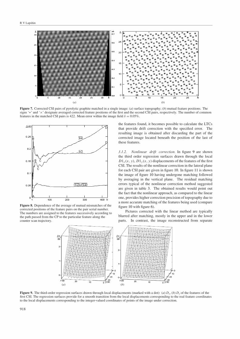
The topography image presented in figure 7(a) is a resultof matching the corrected CSIs shown in figures 6(a) and(c) followed by topography averaging within the overlap area.Here, one should take note of an even lower noise level despitethe fact that there was no additional ‘artificial’ topographysmoothing. Matching precision of the CSI pairs may beestimated by sight at figure 7(b). In digits, the mean residualmismatch of the corrected feature positions is 0.05 A.

Figure 8 shows the dependence of the average of mutualmismatches of the corrected positions of the feature pairs �

upon pair serial number n, which was obtained during theiterative search for feature pairs. Remember that every featurereceives its number according to its distance away from the

Automatic drift elimination in probe microscope images

(a) (b)

(c) (d )

Figure 6. Corrected CSIs of pyrolytic graphite: (a) the first pair; (c) the second pair. Corrected feature positions after CSI matching: (b) thefirst pair; (d) the second pair. The signs ‘+’ and ‘×’ designate corrected feature positions of the direct and the counter images, respectively.Mean error within the image field δ: (a), (b) 0.2%; (c), (d) 0.3%.

Table 3. Correction errors for pyrolytic graphite and porous alumina CSIs: minimal �min, maximal �max, and mean � lateral mismatchingsof the features; mean mismatching �⊥ in the vertical plane; maximal δmax and mean within the image field δ relative errors in the lateralplane. The first error value is obtained with the linear correction method and the second value with the nonlinear method.

Number ofcommon

Sample Corrected CSIs features n �min (A) �max (A) � (A) �⊥ (A) δmax (%) δ (%)

HOPG 1 ∩ 2 424 0.002, 0.003 0.677, 0.392 0.221, 0.072 – 0.8, 0.6 0.23, 0.073 ∩ 4 430 0.008, 0.008 0.713, 0.451 0.297, 0.096 – 0.9, 0.6 0.31, 0.10

(1 ∩ 2) ∩ (3 ∩ 4) 422 0.002, 0.001 0.253, 0.248 0.050, 0.048 – 0.2, 0.4 0.05, 0.05

Porous Al2O3 1 ∩ 2 88 15.2, 1.3 445.9, 65.4 165.5, 18.9 56.4, 37.3 2.8, 0.9 1.5, 0.163 ∩ 4 85 11.9, 1.8 414.9, 63.6 157.5, 18.5 55.7, 37.6 3.1, 0.8 1.4, 0.15

(1 ∩ 2) ∩ (3 ∩ 4) 84 0.6, 0.2 77.5, 57.6 30.6, 22.3 20.4, 42.4 0.8, 0.6 0.2, 0.14

CP. That distance should be thought of not as a straight lineconnecting the feature and the CP but rather as the path passedalong the counter scan trajectory.

Corrected positions of the first feature have zero matchingerror (point A) since this is the only feature to participate inthe determination of the correction coefficients. Furthermore,as the number of features involved is growing, the error firstincreases abruptly (section A–B), which can be explained byboth proximity of the features being used to the CP (the lateralLTCs are sensitive to the relative error of determination ofthe feature position) and still insufficient number of features(the errors in determination of the feature positions are not yet

compensated with averaging). Then, the error decreases ratherrapidly because of moving away from the CP and averagingby a great number of features (section B–C).

If the drift velocity stayed unchanged while scanning,the error would approach zero as new features were involved.However, it is seen in the plot that after a minimum is reached(C point) the error starts to grow (section C–D). Thus, theobserved increase in error points out the fact that the driftvelocity has changed during the counter-scanning.

As the error threshold is specified within the CD section,those dependences will help to determine the features whoseresidual mismatch does not exceed the error. Then, by using

917

R V Lapshin

(a) (b)

Figure 7. Corrected CSI pairs of pyrolytic graphite matched in a single image: (a) surface topography; (b) mutual feature positions. Thesigns ‘+’ and ‘×’ designate averaged corrected feature positions of the first and the second CSI pairs, respectively. The number of commonfeatures in the matched CSI pairs is 422. Mean error within the image field δ = 0.05%.

Figure 8. Dependence of the average of mutual mismatches of thecorrected positions of the feature pairs on the pair serial number.The numbers are assigned to the features successively according tothe path passed from the CP to the particular feature along thecounter scan trajectory.

918

the features found, it becomes possible to calculate the LTCsthat provide drift correction with the specified error. Theresulting image is obtained after discarding the part of thecorrected image located beneath the position of the last ofthese features.

3.1.2. Nonlinear drift correction. In figure 9 are shownthe third order regression surfaces drawn through the localD1x(x, y), D1y(x, y) displacements of the features of the firstCSI. The results of the nonlinear correction in the lateral planefor each CSI pair are given in figure 10. In figure 11 is shownthe image of figure 10 having undergone matching followedby averaging in the vertical plane. The residual matchingerrors typical of the nonlinear correction method suggestedare given in table 3. The obtained results would point outthe fact that the nonlinear approach, as compared to the linearone, provides higher correction precision of topography due toa more accurate matching of the features being used (comparefigure 10 with figure 6).

Pictures corrected with the linear method are typicallyblurred after matching, mostly in the upper and in the lowerparts. In contrast, the image reconstructed from separate

(a) (b)

Figure 9. The third-order regression surfaces drawn through local displacements (marked with a dot): (a) Dx, (b) Dy of the features of thefirst CSI. The regression surfaces provide for a smooth transition from the local displacements corresponding to the real feature coordinatesto the local displacements corresponding to the integer-valued coordinates of points of the image under correction.

Automatic drift elimination in probe microscope images

(a) (b)

(c) (d )

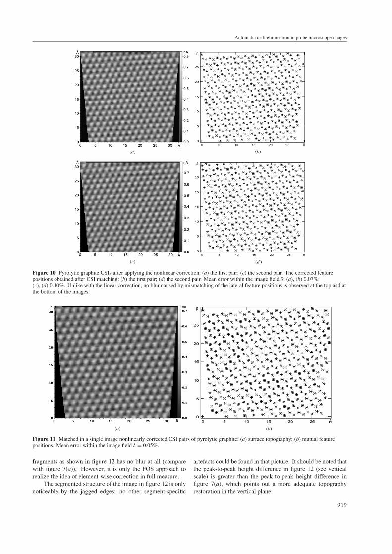
Figure 10. Pyrolytic graphite CSIs after applying the nonlinear correction: (a) the first pair; (c) the second pair. The corrected featurepositions obtained after CSI matching: (b) the first pair; (d) the second pair. Mean error within the image field δ: (a), (b) 0.07%;(c), (d) 0.10%. Unlike with the linear correction, no blur caused by mismatching of the lateral feature positions is observed at the top and atthe bottom of the images.

(a) (b)

Figure 11. Matched in a single image nonlinearly corrected CSI pairs of pyrolytic graphite: (a) surface topography; (b) mutual featurepositions. Mean error within the image field δ = 0.05%.

fragments as shown in figure 12 has no blur at all (comparewith figure 7(a)). However, it is only the FOS approach torealize the idea of element-wise correction in full measure.

The segmented structure of the image in figure 12 is onlynoticeable by the jagged edges; no other segment-specific

artefacts could be found in that picture. It should be noted thatthe peak-to-peak height difference in figure 12 (see verticalscale) is greater than the peak-to-peak height difference infigure 7(a), which points out a more adequate topographyrestoration in the vertical plane.

919

R V Lapshin

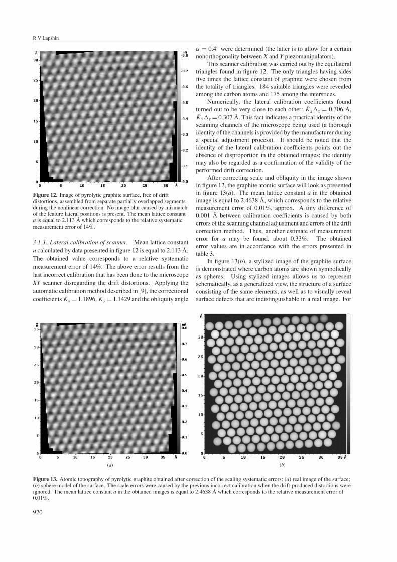
Figure 12. Image of pyrolytic graphite surface, free of driftdistortions, assembled from separate partially overlapped segmentsduring the nonlinear correction. No image blur caused by mismatchof the feature lateral positions is present. The mean lattice constanta is equal to 2.113 A which corresponds to the relative systematicmeasurement error of 14%.

3.1.3. Lateral calibration of scanner. Mean lattice constanta calculated by data presented in figure 12 is equal to 2.113 A.The obtained value corresponds to a relative systematicmeasurement error of 14%. The above error results from thelast incorrect calibration that has been done to the microscopeXY scanner disregarding the drift distortions. Applying theautomatic calibration method described in [9], the correctionalcoefficients Kx = 1.1896, Ky = 1.1429 and the obliquity angle

920

α = 0.4◦ were determined (the latter is to allow for a certainnonorthogonality between X and Y piezomanipulators).

This scanner calibration was carried out by the equilateraltriangles found in figure 12. The only triangles having sidesfive times the lattice constant of graphite were chosen fromthe totality of triangles. 184 suitable triangles were revealedamong the carbon atoms and 175 among the interstices.

Numerically, the lateral calibration coefficients foundturned out to be very close to each other: Kx�x = 0.306 A,Ky�y = 0.307 A. This fact indicates a practical identity of thescanning channels of the microscope being used (a thoroughidentity of the channels is provided by the manufacturer duringa special adjustment process). It should be noted that theidentity of the lateral calibration coefficients points out theabsence of disproportion in the obtained images; the identitymay also be regarded as a confirmation of the validity of theperformed drift correction.

After correcting scale and obliquity in the image shownin figure 12, the graphite atomic surface will look as presentedin figure 13(a). The mean lattice constant a in the obtainedimage is equal to 2.4638 A, which corresponds to the relativemeasurement error of 0.01%, approx. A tiny difference of0.001 A between calibration coefficients is caused by botherrors of the scanning channel adjustment and errors of the driftcorrection method. Thus, another estimate of measurementerror for a may be found, about 0.33%. The obtainederror values are in accordance with the errors presented intable 3.

In figure 13(b), a stylized image of the graphite surfaceis demonstrated where carbon atoms are shown symbolicallyas spheres. Using stylized images allows us to representschematically, as a generalized view, the structure of a surfaceconsisting of the same elements, as well as to visually revealsurface defects that are indistinguishable in a real image. For

(a) (b)

Figure 13. Atomic topography of pyrolytic graphite obtained after correction of the scaling systematic errors: (a) real image of the surface;(b) sphere model of the surface. The scale errors were caused by the previous incorrect calibration when the drift-produced distortions wereignored. The mean lattice constant a in the obtained images is equal to 2.4638 A which corresponds to the relative measurement error of0.01%.

Automatic drift elimination in probe microscope images

(a) (b)

(c) (d )

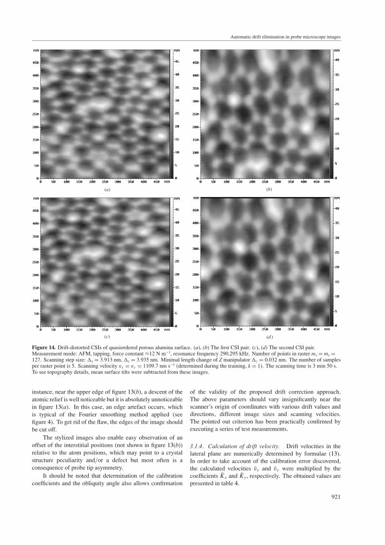
Figure 14. Drift-distorted CSIs of quasiordered porous alumina surface. (a), (b) The first CSI pair. (c), (d) The second CSI pair.Measurement mode: AFM, tapping, force constant ≈12 N m−1, resonance frequency 290.295 kHz. Number of points in raster mx = my =127. Scanning step size: �x = 3.913 nm, �y = 3.935 nm. Minimal length change of Z manipulator �z = 0.032 nm. The number of samplesper raster point is 5. Scanning velocity vx = vy = 1109.7 nm s−1 (determined during the training, k = 1). The scanning time is 3 min 50 s.To see topography details, mean surface tilts were subtracted from these images.

instance, near the upper edge of figure 13(b), a descent of theatomic relief is well noticeable but it is absolutely unnoticeablein figure 13(a). In this case, an edge artefact occurs, whichis typical of the Fourier smoothing method applied (seefigure 4). To get rid of the flaw, the edges of the image shouldbe cut off.

The stylized images also enable easy observation of anoffset of the interstitial positions (not shown in figure 13(b))relative to the atom positions, which may point to a crystalstructure peculiarity and/or a defect but most often is aconsequence of probe tip asymmetry.

It should be noted that determination of the calibrationcoefficients and the obliquity angle also allows confirmation

of the validity of the proposed drift correction approach.The above parameters should vary insignificantly near thescanner’s origin of coordinates with various drift values anddirections, different image sizes and scanning velocities.The pointed out criterion has been practically confirmed byexecuting a series of test measurements.

3.1.4. Calculation of drift velocity. Drift velocities in thelateral plane are numerically determined by formulae (13).In order to take account of the calibration error discovered,the calculated velocities vx and vy were multiplied by thecoefficients Kx and Ky , respectively. The obtained values arepresented in table 4.

921

R V Lapshin

(a) (b)

(c) (d )

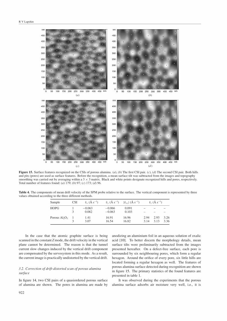
Figure 15. Surface features recognized on the CSIs of porous alumina. (a), (b) The first CSI pair. (c), (d) The second CSI pair. Both hillsand pits (pores) are used as surface features. Before the recognition, a mean surface tilt was subtracted from the images and topographysmoothing was carried out by averaging within a 3 × 3 matrix. Black and white points designate recognized hills and pores, respectively.Total number of features found: (a) 179; (b) 97; (c) 173; (d) 96.

Table 4. The components of mean drift velocity of the SPM probe relative to the surface. The vertical component is represented by threevalues obtained according to the three different methods.

Sample CSI vx (A s−1) vy (A s−1) |vxy | (A s−1) vz (A s−1)

HOPG 1 −0.063 −0.066 0.091 – – –3 0.082 −0.063 0.103 – – –

Porous Al2O3 1 1.41 16.91 16.96 2.94 2.93 3.263 3.07 16.54 16.82 3.14 3.13 3.36

In the case that the atomic graphite surface is beingscanned in the constant Z mode, the drift velocity in the verticalplane cannot be determined. The reason is that the tunnelcurrent slow changes induced by the vertical drift componentare compensated by the servosystem in this mode. As a result,the current image is practically undistorted by the vertical drift.

3.2. Correction of drift-distorted scan of porous aluminasurface

In figure 14, two CSI pairs of a quasiordered porous surfaceof alumina are shown. The pores in alumina are made by

922

anodizing an aluminium foil in an aqueous solution of oxalicacid [10]. To better discern the morphology details, meansurface tilts were preliminarily subtracted from the imagespresented hereafter. On a defect-free surface, each pore issurrounded by six neighbouring pores, which form a regularhexagon. Around the orifice of every pore, six little hills arelocated forming a regular hexagon as well. The features ofporous alumina surface detected during recognition are shownin figure 15. The primary statistics of the found features arepresented in table 1.

It was observed during the experiments that the porousalumina surface adsorbs air moisture very well, i.e., it is

Automatic drift elimination in probe microscope images

(a) (b)

(c) (d )

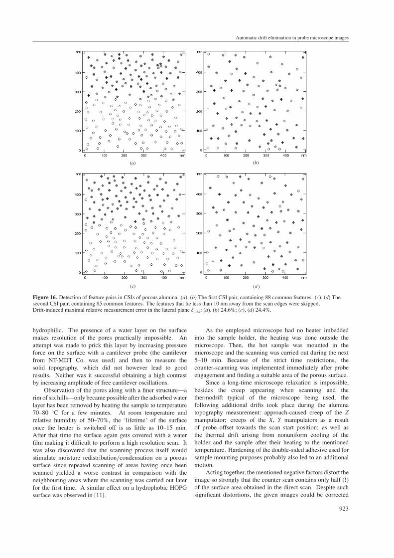
Figure 16. Detection of feature pairs in CSIs of porous alumina. (a), (b) The first CSI pair, containing 88 common features. (c), (d) Thesecond CSI pair, containing 85 common features. The features that lie less than 10 nm away from the scan edges were skipped.Drift-induced maximal relative measurement error in the lateral plane δmax: (a), (b) 24.6%; (c), (d) 24.4%.

hydrophilic. The presence of a water layer on the surfacemakes resolution of the pores practically impossible. Anattempt was made to prick this layer by increasing pressureforce on the surface with a cantilever probe (the cantileverfrom NT-MDT Co. was used) and then to measure thesolid topography, which did not however lead to goodresults. Neither was it successful obtaining a high contrastby increasing amplitude of free cantilever oscillations.

Observation of the pores along with a finer structure—arim of six hills—only became possible after the adsorbed waterlayer has been removed by heating the sample to temperature70–80 ◦C for a few minutes. At room temperature andrelative humidity of 50–70%, the ‘lifetime’ of the surfaceonce the heater is switched off is as little as 10–15 min.After that time the surface again gets covered with a waterfilm making it difficult to perform a high resolution scan. Itwas also discovered that the scanning process itself wouldstimulate moisture redistribution/condensation on a poroussurface since repeated scanning of areas having once beenscanned yielded a worse contrast in comparison with theneighbouring areas where the scanning was carried out laterfor the first time. A similar effect on a hydrophobic HOPGsurface was observed in [11].

As the employed microscope had no heater imbeddedinto the sample holder, the heating was done outside themicroscope. Then, the hot sample was mounted in themicroscope and the scanning was carried out during the next5–10 min. Because of the strict time restrictions, thecounter-scanning was implemented immediately after probeengagement and finding a suitable area of the porous surface.

Since a long-time microscope relaxation is impossible,besides the creep appearing when scanning and thethermodrift typical of the microscope being used, thefollowing additional drifts took place during the aluminatopography measurement: approach-caused creep of the Zmanipulator; creeps of the X, Y manipulators as a resultof probe offset towards the scan start position; as well asthe thermal drift arising from nonuniform cooling of theholder and the sample after their heating to the mentionedtemperature. Hardening of the double-sided adhesive used forsample mounting purposes probably also led to an additionalmotion.

Acting together, the mentioned negative factors distort theimage so strongly that the counter scan contains only half (!)of the surface area obtained in the direct scan. Despite suchsignificant distortions, the given images could be corrected

923

R V Lapshin

(a) (b)

(c) (d )

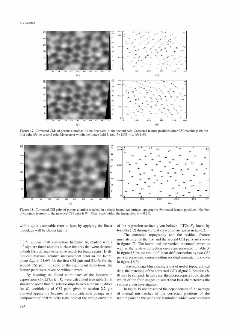
Figure 17. Corrected CSIs of porous alumina: (a) the first pair; (c) the second pair. Corrected feature positions after CSI matching: (b) thefirst pair; (d) the second pair. Mean error within the image field δ: (a), (b) 1.5%; (c), (d) 1.4%.

(a) (b)

Figure 18. Corrected CSI pairs of porous alumina matched in a single image: (a) surface topography; (b) mutual feature positions. Numberof common features in the matched CSI pairs is 84. Mean error within the image field δ = 0.2%.

with a quite acceptable error at least by applying the linearmodel, as will be shown later on.

3.2.1. Linear drift correction. In figure 16, marked with a‘+’ sign are those alumina surface features that were detectedin both CSIs during the iterative search for feature pairs. Drift-induced maximal relative measurement error in the lateralplane δmax is 24.6% for the first CSI pair and 24.4% for thesecond CSI pair. In spite of the significant distortions, thefeature pairs were revealed without errors.

By inserting the found coordinates of the features inexpressions (5), LTCs Kx, Ky were calculated (see table 2). Itshould be noted that the relationships between the inequalitiesfor Kx coefficients of CSI pairs given in section 2.2 gotviolated apparently because of a considerable change in xcomponent of drift velocity (take note of the strong curvature

924

of the regression surface given below). LTCs Kz found byformula (12) during vertical correction are given in table 2.

The corrected topography and the residual featuremismatching for the first and the second CSI pairs are shownin figure 17. The lateral and the vertical mismatch errors aswell as the relative correction errors are presented in table 3.In figure 18(a), the result of linear drift correction by two CSIpairs is presented; corresponding residual mismatch is shownin figure 18(b).

To avoid image blur causing a loss of useful topographicaldata, the matching of the corrected CSIs (figure 2, positions 8,9) may be skipped. In that case, the microscopist should decidewhich of the four images to select that best characterizes thesurface under investigation.

In figure 19 are presented the dependences of the averageof mutual mismatches of the corrected positions of thefeature pairs on the pair’s serial number, which were obtained

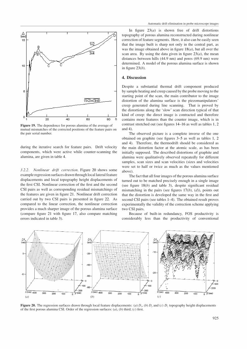
Figure 19. The dependence for porous alumina of the average ofmutual mismatches of the corrected positions of the feature pairs onthe pair serial number.

during the iterative search for feature pairs. Drift velocitycomponents, which were active while counter-scanning thealumina, are given in table 4.

3.2.2. Nonlinear drift correction. Figure 20 shows someexample regression surfaces drawn through local lateral featuredisplacements and local topography height displacements ofthe first CSI. Nonlinear correction of the first and the secondCSI pairs as well as corresponding residual mismatchings ofthe features are given in figure 21. Nonlinear drift correctioncarried out by two CSI pairs is presented in figure 22. Ascompared to the linear correction, the nonlinear correctionprovides a much sharper image of the porous alumina surface(compare figure 21 with figure 17, also compare matchingerrors indicated in table 3).

Automatic drift elimination in probe microscope images

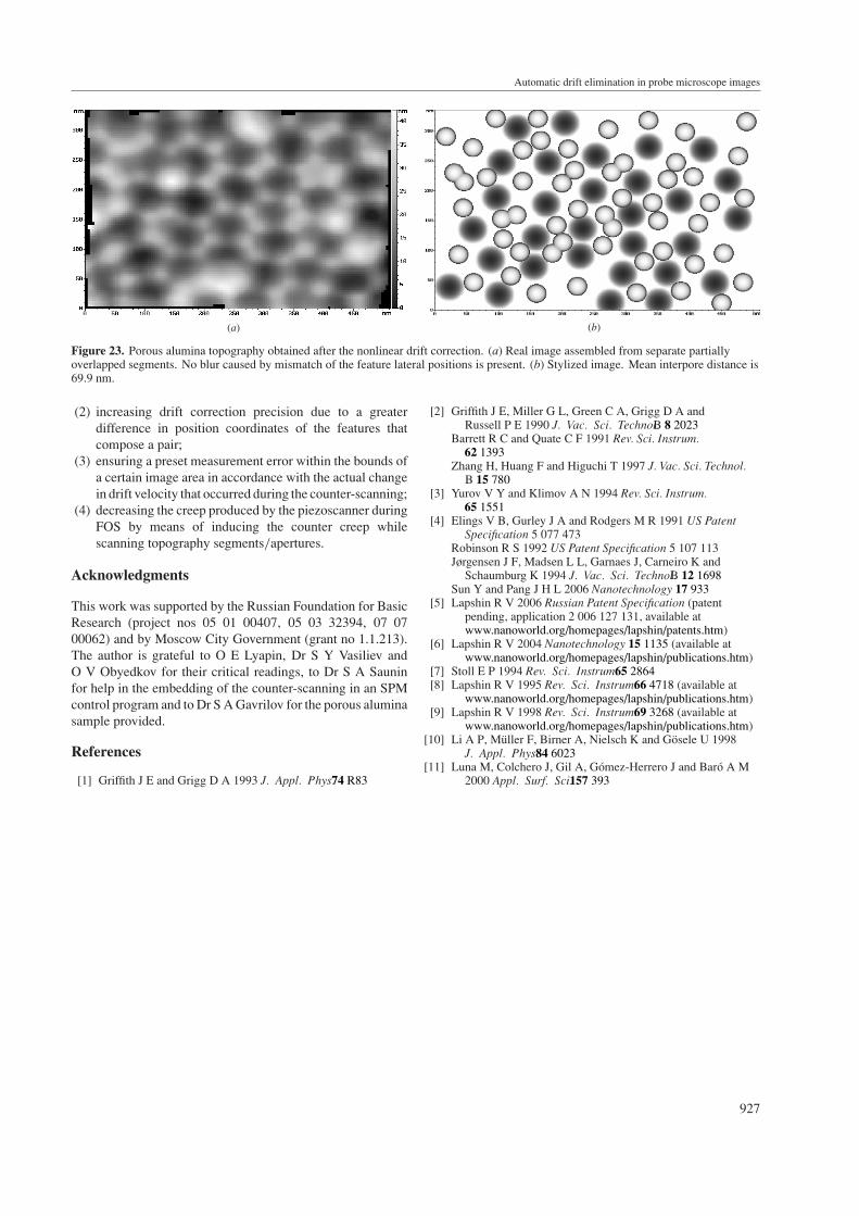
In figure 23(a) is shown free of drift distortionstopography of porous alumina reconstructed during nonlinearcorrection of feature segments. Here, it also can be easily seenthat the image built is sharp not only in the central part, aswas the image obtained above in figure 18(a), but all over thescan area. By using the data given in figure 23(a), the meandistances between hills (44.9 nm) and pores (69.9 nm) weredetermined. A model of the porous alumina surface is shownin figure 23(b).

4. Discussion

Despite a substantial thermal drift component producedby sample heating and creep caused by the probe moving to thestarting point of the scan, the main contributor to the imagedistortion of the alumina surface is the piezomanipulators’creep generated during line scanning. That is proved bythe distortions along the ‘slow’ scan direction typical of thatkind of creep: the direct image is contracted and thereforecontains more features than the counter image, which is incontrast stretched out (see figures 14–16 as well as tables 1, 2and 4).

The observed picture is a complete inverse of the oneobtained on graphite (see figures 3–5 as well as tables 1, 2and 4). Therefore, the thermodrift should be considered asthe main distortion factor at the atomic scale, as has beeninitially supposed. The described distortions of graphite andalumina were qualitatively observed repeatedly for differentsamples, scan sizes and scan velocities (sizes and velocitieswere set to half or twice as much as the values mentionedabove).

The fact that all four images of the porous alumina surfaceturned out to be matched precisely enough in a single image(see figure 18(b) and table 3), despite significant residualmismatching in the pairs (see figures 17(b), (d)), points outthat the distortion is developed the same way in the first andsecond CSI pairs (see tables 1–4). The obtained result provesexperimentally the validity of the correction scheme applyingtwo CSI pairs.

Because of built-in redundancy, FOS productivity isconsiderably less than the productivity of conventional

(a) (b) (c)

Figure 20. The regression surfaces drawn through local feature displacements: (a) Dx, (b) Dy and (c) Dz topography height displacementsof the first porous alumina CSI. Order of the regression surfaces: (a), (b) third; (c) first.

925

R V Lapshin

(a) (b)

(c) (d )

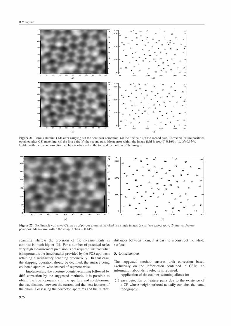
Figure 21. Porous alumina CSIs after carrying out the nonlinear correction: (a) the first pair; (c) the second pair. Corrected feature positionsobtained after CSI matching: (b) the first pair; (d) the second pair. Mean error within the image field δ: (a), (b) 0.16%; (c), (d) 0.15%.Unlike with the linear correction, no blur is observed at the top and the bottom of the images.

(a) (b)

Figure 22. Nonlinearly corrected CSI pairs of porous alumina matched in a single image: (a) surface topography; (b) mutual featurepositions. Mean error within the image field δ = 0.14%.

scanning whereas the precision of the measurements incontrast is much higher [6]. For a number of practical tasksvery high measurement precision is not required; instead whatis important is the functionality provided by the FOS approachretaining a satisfactory scanning productivity. In that case,the skipping operation should be declined, the surface beingcollected aperture-wise instead of segment-wise.

Implementing the aperture counter-scanning followed bydrift correction by the suggested methods, it is possible toobtain the true topography in the aperture and so determinethe true distance between the current and the next features ofthe chain. Possessing the corrected apertures and the relative

926

distances between them, it is easy to reconstruct the wholesurface.

5. Conclusions

The suggested method ensures drift correction basedexclusively on the information contained in CSIs; noinformation about drift velocity is required.

Application of the counter-scanning allows for

(1) easy detection of feature pairs due to the existence ofa CP whose neighbourhood actually contains the sametopography;

Automatic drift elimination in probe microscope images

(a) (b)

Figure 23. Porous alumina topography obtained after the nonlinear drift correction. (a) Real image assembled from separate partiallyoverlapped segments. No blur caused by mismatch of the feature lateral positions is present. (b) Stylized image. Mean interpore distance is69.9 nm.

(2) increasing drift correction precision due to a greaterdifference in position coordinates of the features thatcompose a pair;

(3) ensuring a preset measurement error within the bounds ofa certain image area in accordance with the actual changein drift velocity that occurred during the counter-scanning;

(4) decreasing the creep produced by the piezoscanner duringFOS by means of inducing the counter creep whilescanning topography segments/apertures.

Acknowledgments

This work was supported by the Russian Foundation for BasicResearch (project nos 05 01 00407, 05 03 32394, 07 0700062) and by Moscow City Government (grant no 1.1.213).The author is grateful to O E Lyapin, Dr S Y Vasiliev andO V Obyedkov for their critical readings, to Dr S A Sauninfor help in the embedding of the counter-scanning in an SPMcontrol program and to Dr S A Gavrilov for the porous aluminasample provided.

References

[1] Griffith J E and Grigg D A 1993 J. Appl. Phys. 74 R83

[2] Griffith J E, Miller G L, Green C A, Grigg D A andRussell P E 1990 J. Vac. Sci. Technol. B 8 2023

Barrett R C and Quate C F 1991 Rev. Sci. Instrum.62 1393

Zhang H, Huang F and Higuchi T 1997 J. Vac. Sci. Technol.B 15 780

[3] Yurov V Y and Klimov A N 1994 Rev. Sci. Instrum.65 1551

[4] Elings V B, Gurley J A and Rodgers M R 1991 US PatentSpecification 5 077 473

Robinson R S 1992 US Patent Specification 5 107 113Jørgensen J F, Madsen L L, Garnaes J, Carneiro K and

Schaumburg K 1994 J. Vac. Sci. Technol. B 12 1698Sun Y and Pang J H L 2006 Nanotechnology 17 933

[5] Lapshin R V 2006 Russian Patent Specification (patentpending, application 2 006 127 131, available atwww.nanoworld.org/homepages/lapshin/patents.htm)

[6] Lapshin R V 2004 Nanotechnology 15 1135 (available atwww.nanoworld.org/homepages/lapshin/publications.htm)

[7] Stoll E P 1994 Rev. Sci. Instrum. 65 2864[8] Lapshin R V 1995 Rev. Sci. Instrum. 66 4718 (available at

www.nanoworld.org/homepages/lapshin/publications.htm)[9] Lapshin R V 1998 Rev. Sci. Instrum. 69 3268 (available at

www.nanoworld.org/homepages/lapshin/publications.htm)[10] Li A P, Muller F, Birner A, Nielsch K and Gosele U 1998

J. Appl. Phys. 84 6023[11] Luna M, Colchero J, Gil A, Gomez-Herrero J and Baro A M

2000 Appl. Surf. Sci. 157 393

927