automatic differentiation of advanced cfd codes for

AUTOMATICDIFFERENTIATION OF

ADVANCED CFD CODES FORMULTIDISCIPLINARY DESIGN

C. Bischof1 andG. Corliss 2

Argonne National Laboratory, Argonne, Illinois

L. GreenNASA Langley Research Center, Hampton, Virginia

A. Griewank1

Argonne National Laboratory, Argonne, Illinois

K. Haigler and P. NewmanNASA Langley Research Center, Hampton, Virginia

Argonne Preprint MCS-P339-1192

Automated multidisciplinary design of aircraft andother ight vehicles requires the optimization of complexperformance objectives with respect to a number of designparameters and constraints. The e�ect of these indepen-dent design variables on the system performance criteriacan be quanti�ed in terms of sensitivity derivatives whichmust be calculated and propagated by the individual dis-cipline simulation codes. Typical advanced CFD analysiscodes do not provide such derivatives as part of a ow so-lution; these derivatives are very expensive to obtain bydivided (�nite) di�erences from perturbed solutions. Itis shown here that sensitivity derivatives can be obtainedaccurately and e�ciently by using the ADIFOR sourcetranslator for automatic di�erentiation. In particular, itis demonstrated that the 3-D, thin-layer Navier{Stokes,multigrid ow solver called TLNS3D is amenable to au-tomatic di�erentiation in the forward mode even with itsimplicit iterative solution algorithm and complex turbu-lence modeling. It is signi�cant that, using computationaldi�erentiation, consistent discrete nongeometric sensitiv-ity derivatives have been obtained from an aerodynamic3{D CFD code in a relatively short time, e.g. O(man-week) not O(man-year).

1This work was supported by the AppliedMathematical Sciencessubprogram of the O�ce of Energy Research, U. S. Department ofEnergy, under Contract W-31-109-Eng-38.

2This work was supported by the National Science Foundationunder Cooperative Agreement Number CCR-9120008.

1 Nomenclature

CD Wing drag coe�cientCL Wing lift coe�cientCM Wing pitching moment coe�cientD Generic sensitivity derivativeI Identity matrixJ Jacobian matrixM Free stream Mach numberP Preconditioner matrixR Residual vector for ow equationsRe Reynold's number (mean chord)S Seed matrixx Design variabley Discrete mesh coordinatesz Local ow (state) variable� Angle-of-attack� Spectral radius

Subscripts

AD Automatic di�erentiationDD Divided di�erencem Iteration indexx Partial derivative w.r.t. xy Partial derivative w.r.t. yz Partial derivative w.r.t. z� Root of R = 0 or iteration-�xed-point

Superscripts0 (prime) Total derivative w.r.t. x~ (tilde) Approximate operator

2 Introduction

In the past, design of ight vehicles typically requiredthe interaction of many technical disciplines over an ex-tended period of time in a more or less sequential manner.At present, computer-automated discipline analyses andinteractions o�er the possibility of signi�cantly shorten-ing the design-cycle time, while simultaneous multidisci-plinary design optimization (MDO) via formal sensitivityanalysis (SA) holds the possibility of improved designs.Recent topical conferences 3 [1{8], [10, 12, 34, 35, 54, 55]for example, attest to the interest in these possibilitiesfor improving aerospace vehicle design processes and pro-cedures. Advances in computer hardware and software,electronic communications, and discipline solution algo-rithms and codes will individually contribute; however,true synergisms may be required to make it all feasible.This paper addresses one such synergism for computa-

3Those without published proceedings include the 1992AIAA/AHS/ASEE Aerospace Design Conference, Feb. 1992, andthe AIAA Aircraft Design Systems Meeting, Aug. 1992.

1

tional science and computational uid dynamics (CFD)algorithm technologies.

Procedures for MDO of engineering systems have beenaddressed by Sobieski [65]. He proposes a uni�ed sys-tem SA guided by system sensitivity derivatives (SD);the optimizer code or algorithm that uses these SD is theoutermost loop of the entire design process. The objec-tive and constraint functions are now generally composedof output functions from several disciplines. Each single-discipline analysis code is then to supply not only theoutput functions required for the constrained optimiza-tion process and other discipline analysis inputs, but alsothe derivatives of all of these output functions with re-spect to its input variables. These variables include notonly the MDO variables, but also output functions fromother disciplines that implicitly depend on the MDO vari-ables.

Thus, a key technology required for MDO proceduresis the capability to calculate the SD of outputs from thevarious analysis codes with respect to a set of design vari-ables. However, a certain degree of exibility and au-tomation is needed, since the envisioned ight vehicle con-cept determines which objectives, constraint functions,MDO design variables, and discipline analysis codes arerequired to model the pertinent physical aspects through-out the ight regime (i.e., the particular MDO problem).Current technology cannot be counted on to deliver reli-able and fast derivatives for large computer codes such asadvanced 3-D CFD codes. Divided di�erences (DD) maynot be accurate and are obtained too slowly, symbolic ap-proaches do not appear to be feasible, and hand coding ofderivatives is impractical. This situation has dire conse-quences, in particular, for very large scale computer mod-els, as they are to be run on tera ops machines. Since DDerrors tend to grow with problem complexity, larger mod-els will have to deal with ever-more-inaccurate deriva-tives, even though a faithful modeling of their complexnonlinear behavior requires very accurate derivatives. Inaddition, the cost of DD will restrain the magnitude ofproblems that can be done in practice.

Automatic di�erentiation (AD) addresses this need byproviding a scalable technology that computes derivativesof large codes accurately, irrespective of the complexity ofthe model. This paper discusses and documents the initialapplication of an AD system to advanced CFD codes inorder to obtain SD typical of those required in an MDO.The general ideas and direction of this work, including asample result, have been outlined in [56] and [18]. As willbe seen, the initial results given here are both signi�cantand encouraging; but challenges remain.

The organization of this paper is as follows: �rst, brief

reviews of advanced CFD codes with SD calculations andAD of Fortran codes (ADIFOR); then, discussion of theapplication of ADIFOR to CFD codes; and �nally, com-ments on the future directions of this work.

The present interest and work have been stimulated bytwo research programs related to incorporating advancedCFD capabilities in MDO. The NASA Langley ResearchCenter High-Speed Airframe Integration Research (Hi-SAIR) project [32, 29, 28] is focused on the High-SpeedCivil Transport (HSCT) design activity in order to de-velop a methodology and computational environment formultidisciplinary analysis and design. The emphasis is onincluding most of the required disciplines and interactionsat a su�ciently advanced level of analysis to demonstrateimproved engineering design methodology. The secondstimulus is the NASA ComputationalAerosciences (CAS)grand challenge of the High Performance Computing andCommunications (HPCC) Program [45, 55], where oneof the applications is the HSCT. The two major thrustsin this latter program are enhanced simulations via mul-tidisciplinary formulations and improved computationale�ciency via massively parallel hardware. In both pro-grams, the primary NASA Langley approach being pur-sued is MDO via SA.

3 Advanced CFD with SD

The application of advanced CFD codes to provide aero-dynamic analyses within an MDO via SA is severely ham-pered by the sheer magnitude of the computational taskif these SD must be obtained by DD. Recent interestand progress have focused on quasi-analytical (QA) or\adjoint-related" techniques to get these SD. The mostrecent references [13, 22, 33, 37, 38, 39, 47, 50, 52, 56,62, 63, 66, 70] from several groups engaged in this re-search indicate the current status and cite many refer-ences to earlier works. A number of other aerodynamicdesign methods have been proposed, developed, and dis-cussed [23, 36, 48, 49, 53, 58, 60, 68, 73]. Typically thesemethods have been developed to solve \single-discipline"design problems, that is, problems in which the cost, orobjective and constraint functions, depend only upon theaerodynamic solution output. One then has the libertyto combine the optimization or iterative design variablesearch with the ow analysis solution(s) at several di�er-ent degrees of implicitness. Generally the computationale�ciency gets better with more implicitness, whereas the exibility to handle modi�ed problems gets worse. It ap-pears that use of these more e�cient implicit methods inMDO would require some suboptimization at the disci-

2

pline level or an implicit formulation of all the relevantdiscipline analyses. Note that one should be able to ob-tain the SD of the aerodynamic design from the \adjoint-related" methods. As can be seen from the cited ref-erences, there are only a handful of applications of anymethod to 3{D aerodynamic con�gurations.

Three major issues for obtaining SD from 3{D CFDcodes concern: (1) the form of the the linear sensitivityequations; (2) the means for di�erentiating the variousterms which appear; and (3) the method for solving theresulting large systems of sensitivity equations. Directmatrix solution methods have generally been used in 2{D problems; however, their use in 3{D problems appearshighly unlikely as a viable approach. In [52] and [56] anincremental iterative technique for e�ciently obtainingconsistent, discrete aerodynamic SD for advanced CFDcodes was proposed, demonstrated, and discussed. Thestudies concluded that: (1) the linear sensitivity equa-tions should be cast into an incremental (correction ordelta) form; (2) one should use AD or symbolic manipu-lation to obtain the needed derivatives; and (3) the result-ing large system of sensitivity equations should be solvediteratively, using the same operator form (i.e., code) asoriginally used to solve the nonlinear ow equations. Theincremental form allows for approximate operators of con-venience (stability, convergence acceleration, simplicity,parallel processing, etc., since only convergence is re-quired) while maintaining consistent discrete derivativesolutions. The iterative solution aspect allows for exten-sion to large 3{D problems, which presently cannot besolved by direct means because of storage and/or run-time limitations. A very brief discussion of the funda-mental equations from [52] and [56] is given in the nextparagraph.

The steady-state nonlinear uid- ow equations repre-senting conservation of mass, momentum, and energy canbe written symbolically as

R(z; y; x�) = 0 ; (1)

where R, the residual vector at each mesh point, is afunction of the local ow (state) variables z, the meshcoordinates y and the design parameters x�. Both y andz are implicit functions of x�. An iterative solution forthe ow variables z of (1) can be written symbolically as

�

�~Rz

�m� (zm+1 � zm) = R(zm; y; x�) ; (2)

where m is the iteration index, Rz denotes @R=@z and thetilde means some approximation of the operator. Sensi-tivity derivatives of various ow solutions with respect to

the design parameters x� are calculated in the QA meth-ods as functions of dy=dx� and dz=dx�, denoted respec-tively as y0 and z0. In order to remain on the solutionsurface, then

R0(z; y; x�) = Rzz0 + Ryy

0 +Rx = 0 : (3)

It is assumed that y0, the mesh sensitivity with respectto x, is obtained from the grid generation code or grid-movement algorithm [61, 64, 69]. Thus, (3) is a linearequation in z0; which has been called the standard form

�Rzz0 = Ryy

0 + Rx : (4)

Equation (4) can also be solved in an iterative fashion,written symbolically as

�

�~Rz

�m� (z0m+1 � z0m) = R0

m(z�; y; x�): (5)

The signi�cance of the incremental iterative solutionforms, (2) for z and (5) for z0, is that the LHS operatorscan be approximate; the RHS, a zero at convergence, isthe condition to be satis�ed. Consistent discretization forthe RHS of both produces consistent z and z0. Solutionof the standard form (4) for consistent z0 requires exactlyRz as the LHS operator. For many CFD codes, Rz is notvery well conditioned and cannot be directly inverted inpractice for large (i.e., 3{D) problems. In most advancedCFD codes, grid generation is not part of the code; anarray of mesh coordinates, denoted before as y, is readas input. For sensitivity analysis, the potentially muchlarger arrays of mesh sensitivities y0 also need to be ob-tained and given to the ow sensitivity code.The Jacobians Rz; Ry; and Rx are generally not com-

puted, much less identi�ed, in most CFD codes. To ob-tain them \by-hand", as has been done in the past for 2{Dproblems, is a very tedious, time-consuming, error-pronejob, hardly practical for complicated 3{D CFD codes.A more-or-less painless, automatic, and robust means togenerate them is highly desirable and appears to be real-izable in AD. In fact, the straightforward application ofAD to the entire iterative solution process (2) generatesz0, without having to identify and construct the terms in(4) or (5). The next section discusses AD in all of theseaspects.

4 AD of Large Programs

Automatic di�erentiation [59] is a chain-rule-based tech-nique for evaluating the derivatives of functions de�nedby computer programs with respect to their input vari-ables. In contrast to the approximation of derivatives

3

by DD, AD does not incur any truncation error so that,at least for noniterative and branch-free codes, the re-sulting derivative values are usually obtained with theworking accuracy of the original function evaluation. Incontrast to fully symbolic di�erentiation, both operationscount and storage requirement can be a priori boundedin terms of the complexity of the original function codefor all modes of AD. In many cases, the calculations initi-ated by an AD tool for the evaluation of derivatives mirrorthose of a carefully handwritten derivative code. A com-prehensive collection on the theory, implementation, andsome earlier applications can be found in the proceedings[43].

There are two basic modes of automatic di�erentia-tion, which are usually referred to as forward and re-verse, respectively. The results reported in this paperwere obtained with a variant of the forward mode. Asdiscussed in [41] the reverse mode is closely related toadjoint methods and has as intriguingly low operationscount for gradients. However, its potentially very largememory requirement has been a serious impediment toits application in large-scale scienti�c computing. Whenthere are several independent and dependent variablesthe operations count for evaluating the Jacobians maybe lowest for certain mixed strategies [44] rather thanthe forward or reverse mode. AD can also be extendedfor the accurate evaluation of second and higher deriva-tives [27, 42, 26, 17]. Second derivatives might eventuallybe useful for the application of higher order optimizationmethods in MDO. For a recent review of AD techniquesand tools in the context of engineering design see [11].An introduction to the Fortran tool ADIFOR and somepreliminary numerical results on a 2{D small-disturbancemodel of transonic ow are given in [18].

4.1 An Advanced FORTRAN Tool

ADIFOR (Automatic Di�erentiation of Fortran) [15, 19,16, 14] provides automatic di�erentiation for programswritten in Fortran 77. Given a Fortran subroutine (orcollection of subroutines) describing a \function," and anindication of which variables in parameter lists or com-mon blocks correspond to \independent" and \depen-dent" variables with respect to di�erentiation [20], AD-IFOR produces Fortran 77 code that allows the compu-tation of the derivatives of the dependent variables withrespect to the independent ones. ADIFOR employs a hy-brid of the forward and reverse modes of automatic dif-ferentiation [43]. That is, for each assignment statement,code is generated for computing the partial derivatives ofthe result with respect to the variables on the right-hand

side, and then employed in the forward mode to propagateoverall derivatives. The resulting decrease in complexitycompared to an entirely forward mode implementationusually is substantial.

In contrast to some earlier AD implementations [51]the source translator ADIFOR was designed from theoutset with large-scale codes in mind. It uses the fa-cilities of the ParaScope Fortran environment [24, 25]to parse the code and to extract control ow and de-pendence ow information. ADIFOR produces portableFortran 77 code and accepts almost all of Fortran 77|in particular, arbitrary calling sequences, nested subrou-tines, common blocks, and equivalences. The ADIFOR-generated code tries to preserve vectorization and paral-lelism in the original code, and employs a consistent sub-routine naming scheme that allows for code tuning, theuse of domain-speci�c knowledge, and the exploitationof vendor-supplied libraries. It should be stressed thatADIFOR uses the data ow analysis information fromParaScope to determine the set of variables that requirederivative information in addition to the dependent andindependent ones. This approach allows for an intuitiveinterface, and greatly reduces the storage requirements ofthe derivative code.

ADIFOR-generated code can be used in various ways.Instead of simply producing code to compute the Jaco-bian J , ADIFOR produces code to compute J � S, wherethe \seed matrix" S is initialized by the user. Therefore,if S is the identity, ADIFOR computes the full Jacobian;whereas if S is just a vector, ADIFOR computes the prod-uct of the Jacobian by a vector. \Compressed" versionsof sparse Jacobians can be computed by exploiting thesame graph coloring techniques [31, 30] that are used for

DD approximations of sparse Jacobians. The runtimeand storage requirements of the ADIFOR-generated codeare roughly proportional to the number of columns of S.Hence, the computation of Jacobian-vector products andcompressed Jacobians requires much less time and stor-age than does the generation of the full Jacobian matrix.For example, in a wing design optimization sketched be-low, typically only a relatively small number of geometricdesign variables determine the shape of the wing. Onthe other hand, hundreds to millions of mesh coordinatesenter into the aerodynamic or structural analysis code.Provided that the grid generation process is smooth, onecan determine for each mesh coordinate a comparativelyshort vector representing its gradient with respect to thedesign parameters. Declaring the mesh coordinates as theindependent variables of the analysis code and initializ-ing the rows of the seed matrix with the mesh coordinategradients, one can run the ADIFOR-generated code to

4

ANALYSIS

GRID

Shape

CFD

ANALYSIS + SD

GRID*

Shape

CFD*

Solution

Mesh

d Mesh

d Shaped Shape

d Solut.

d Stream

d Solut.

* = original code + AD added code

Solution

Stream

Stream

Mesh

compute the gradients of the resulting ow or displace-ment �eld with respect to the design parameters. Thisapproach is much cheaper than �rst performing a full SAon the analysis code and then multiplying the resultinglarge Jacobian J by the matrix S representing the gridsensitivities.

Currently ADIFOR does not provide for the automatic

transfer of derivative data via �les. Therefore, combin-ing the mesh-generation process and the CFD code in amultidisciplinary SA based on AD has not yet been done.When both programs are available as Fortran source, theexchange of derivative information is not very hard andwill be automated in future versions of ADIFOR. How-ever, in general the exchange of sensitivity informationbetween single discipline codes of di�erent origin and onvarious platforms will remain a di�cult challenge. An-other challenge stems from the tacit assumption thatthe outputs of all single disciplinary components dependsmoothly on their input parameters. For grid-generationalgorithms of eventual interest, such as adaptive unstruc-tured grids, that assumption is probably not satis�ed.

Advanced CFD codes pose several other principle chal-lenges and uncertainties regarding the automatic genera-tion of sensitivities. By far the most important di�cultyis that the ow equations for all nontrivial geometries and

stream conditions must be solved iteratively. The itera-tive ow solvers may take hundreds of steps and ofteninvolve discontinuous adjustments of solution operators,grids, shock waves, or free boundaries. The prospect ofobtaining accurate solution sensitivities by simply di�er-entiating the whole iterative process may appear dubiousfor multigrid methods. These are now the state of the artin 3-D CFD codes (for example [71]), despite the lack ofa convergence theory under realistic assumptions. In thefollowing section, some theoretical results from a forth-coming paper [21] are summarized; these theoretical con-siderations make the numerical observations of Section 5at least plausible, even though they do not apply directlyto multigrid methods in their current form.

4.2 Di�erentiating Implicit Functions

Large-scale codes in scienti�c computing frequently em-body iterative solution schemes. That is, for given x�, anonlinear system

R(z; x�) = 0 (6)

is solved to �nd the value z� = z(x�) of the functionimplicitly de�ned by R. The question is under whatcircumstances an AD version of the code implementingthis root�nding process computes the desired derivativesz0� = dz

dxjx=x� . Often, iterative schemes perform discon-

tinuous adjustments of step multipliers and precondition-ers, so that the iterates themselves are very unlikely tobe di�erentiable in the input parameters.For the sake of discussion, assume that our iteration

for solving (6) has the generic form

for m = 1; : : : doevaluate R(zm; x�) and stop if it is smallcompute a suitable preconditioner Pmupdate zm+1 = zm � PmR(zm; x�)

end for

This iteration must locally converge if one can ensure that

jjI � PmRz(zm; x�)jj � � < 1 (7)

The notation Rz (Rx) is shorthand for @R@z

(@R@x

). New-ton's method, for example, is a particular instance of thisscheme with Pm = (dR

dzjz=zm )

�1.The implicit function theorem tells us that at the �xed

point (z�; x�), one has

Rzz0� +Rx = 0: (8)

In fact, the so-called quasi-analytic (QA) approach for ob-taining z0 is to compute (or approximate by DD) Rz(x�)

5

and Rx(x�) and to solve the resulting linear system (8)for z0. However, the reliability of this approach dependsgreatly on the conditioning of Rz(x�), as well as the accu-racy of Rz and Rx. In the following discussion, a \prime"notation (such as z0) always denotes total di�erentiationwith respect to x. Applying AD to the generic iterationabove, we obtain the derivative iteration

for m = 1; : : : doevaluate Rm � R(zm; x�) andR0m � Rz(zm; x�)z

0m +Rx(zm; x�)

if (Rm and R0m are small enough) stop

compute Pm and its derivative P 0m

update zm+1 = zm � PmRm andz0m+1 =z

0m � P 0

mRm � PmR0m

end for

Given zm and z0m, one can obtain the derivative residualR0m at a cost roughly equal to that of evaluating R mul-

tiplied by the number of design parameters (i.e., compo-nents in x). In particular, this derivative evaluation doesnot require the calculation of the Jacobian Rz, which maycontain very many elements. Note that the stopping cri-terion based solely on Rm has been replaced by one thatalso requires R0

m to be small. While it is natural to do so,an automatic tool cannot be expected to spot the stop-ping criterion in a potentially complicated code withoutsome user intervention. Conceptually, one may removethe stopping criterion completely to obtain in�nite se-quences of iterates zm and derivative approximations z0m,which have been shown in [21] to converge R-linearly inthat

kzm � z�k+ kz0m � z0�k � �m ! 0 :

This result was originally obtained by Gilbert [40] andChristianson [26] for the case of Newton's method andsimilar smooth �xed point iterations.Recently, we have been able to extend these results

(see the forthcoming paper [21]) to quasi-Newton meth-ods, where the derivatives P 0

m may grow unbounded butP 0mRm still tends to zero, because of the superlinear rate

of convergence. Whenever the iterates themselves con-verge superlinearly there is the danger that the R-linearlyconvergent derivative approximations may lag behind.For such methods, it is particularly important that thestopping criterion enforce a signi�cant reduction of kR0

mk.In large scale applications, a reasonable linear rate is of-ten the best one can achieve, so that the asymptotic rateof convergence is likely to be the same.For even more general preconditioners Pm, it is shown

in [21] that the simple setting P 0m = 0 ensures conver-

gence to the desired derivative value z0� at the same R-linear rate, provided condition (7) is satis�ed. In con-trast to the previous black-box approach, the precondi-tioner Pm is treated here as a constant and hence the termP 0mR(zm; x�) is dropped in the update of z0m+1. This ap-

proach makes intuitive sense since in the end R(zm; x�)will converge to zero anyway, thereby annihilating anycontribution of P 0

m. Also, P 0m is likely to involve higher

derivatives that (according to the implicit function the-orem) play no role in the existence of z0�. This latterprocedure is the incremental iterative form of equation(5). The implications of this observation for the speedof derivative computations are noteworthy. For example,in a Newton iteration, one saves the work of di�erentiat-ing through the matrix factorization process, which is byfar the dominant work of the iteration process. Exploita-tion of this result does require some user intervention toindicate stopping criteria and variables containing pre-conditioners. Depending on code modularity, this may ormay not be easy to do. We are experimenting with \de-activation" concepts that would support the user in thistask. Techniques such as this one, which build on ADtechniques but require some understanding of the code,we call computational di�erentiation techniques.

Another point worth mentioning is that it does notmake sense to start the derivative iterations until the iter-ations for R(z; x�) = 0 have essentially converged. Obvi-ously, the derivatives z0� will not settle in until the \func-tion value" z� itself has. Again, this is not automatic andrequires user intervention, but the potential savings aresigni�cant. It is important to recognize that the cost ofevaluating R0

m for a given z0m is the same whether thezm have converged to z� or not. Since Rz(z; x�) is not

explicitly formed, one cannot exploit its constancy whenz = zm = z� for several iterations.

5 Application of AD to CFD

Numerical results reported here show that even the naiveapplication of ADIFOR to multigrid solvers viewed as ablack-box program can produce accurate sensitivity infor-mation at tolerable costs. In fact, all calculated deriva-tives could be reproduced with several digits agreementby carefully evaluated DD. Moreover, the implicit func-tion theorem yields a constructive test on the accuracyof the derivative approximation, which suggests that, inmost cases, at least six digits were correct. In the 2{Dquasi-analytical SD code [52], the turbulence model wasdeemed too complicated for di�erentiation by hand; itstreatment as constant led to sizable relative errors in some

6

resulting global sensitivities. Nevertheless, it was foundhere that for a Baldwin-Lomax model the results pro-duced by ADIFOR agree quite well with DD and there-fore convey meaningful sensitivity information even forthe turbulent case.

5.1 2-D Transonic Small Disturbance

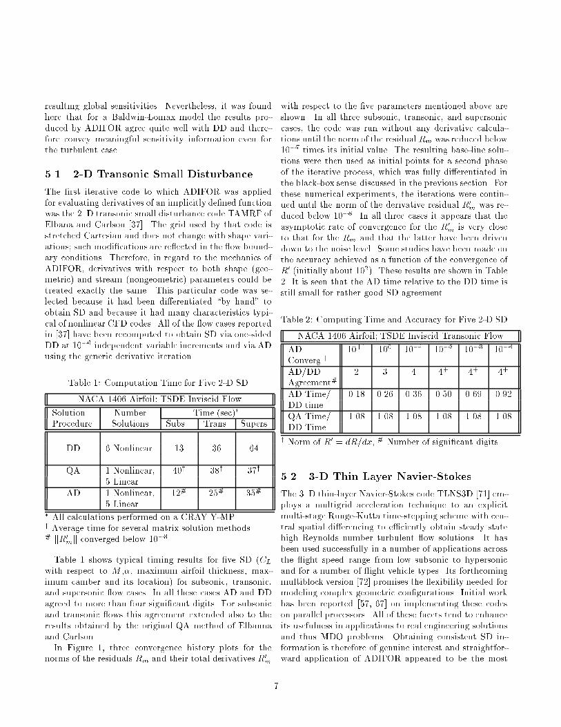
The �rst iterative code to which ADIFOR was appliedfor evaluating derivatives of an implicitly de�ned functionwas the 2{D transonic small disturbance code TAMRF ofElbana and Carlson [37]. The grid used by that code isstretched Cartesian and does not change with shape vari-ations; such modi�cations are re ected in the ow bound-ary conditions. Therefore, in regard to the mechanics ofADIFOR, derivatives with respect to both shape (geo-metric) and stream (nongeometric) parameters could betreated exactly the same. This particular code was se-lected because it had been di�erentiated \by hand" toobtain SD and because it had many characteristics typi-cal of nonlinear CFD codes. All of the ow cases reportedin [37] have been recomputed to obtain SD via one-sidedDD at 10�6 independent variable increments and via ADusing the generic derivative iteration.

Table 1: Computation Time for Five 2-D SD

NACA 1406 Airfoil; TSDE Inviscid Flow

Solution Number Time (sec)�

Procedure Solutions Subs. Trans. Supers.

DD 6 Nonlinear 13 36 64

QA 1 Nonlinear, 40y 38y 37y

5 Linear

AD 1 Nonlinear, 12# 25# 35#

5 Linear� All calculations performed on a CRAY Y-MP.y Average time for several matrix solution methods.# kR0

mk converged below 10�3.

Table 1 shows typical timing results for �ve SD (CLwith respect to M ,�, maximum airfoil thickness, max-imum camber and its location) for subsonic, transonic,and supersonic ow cases. In all these cases AD and DDagreed to more than four signi�cant digits. For subsonicand transonic ows this agreement extended also to theresults obtained by the original QA method of Elbannaand Carlson.In Figure 1, three convergence history plots for the

norms of the residuals Rm and their total derivatives R0m

with respect to the �ve parameters mentioned above areshown. In all three subsonic, transonic, and supersoniccases, the code was run without any derivative calcula-tions until the norm of the residual Rm was reduced below10�7 times its initial value. The resulting base-line solu-tions were then used as initial points for a second phaseof the iterative process, which was fully di�erentiated inthe black-box sense discussed in the previous section. Forthese numerical experiments, the iterations were contin-ued until the norm of the derivative residual R0

m was re-duced below 10�8. In all three cases it appears that theasymptotic rate of convergence for the R0

m is very closeto that for the Rm and that the latter have been drivendown to the noise level. Some studies have been made onthe accuracy achieved as a function of the convergence ofR0 (initially about 102). These results are shown in Table2. It is seen that the AD time relative to the DD time isstill small for rather good SD agreement.

Table 2: Computing Time and Accuracy for Five 2-D SD

NACA 1406 Airfoil; TSDE Inviscid Transonic Flow

ADConverg.y

10+1 100 10�1 10�2 10�3 10�4

AD/DDAgreement#

2 3 4 4+ 4+ 4+

AD Time/ 0.18 0.26 0.36 0.50 0.69 0.92DD time

QA Time/ 1.08 1.08 1.08 1.08 1.08 1.08DD Time

y Norm of R0 = dR=dx, # Number of signi�cant digits.

5.2 3-D Thin Layer Navier-Stokes

The 3{D thin-layer Navier-Stokes code TLNS3D [71] em-ploys a multigrid acceleration technique to an explicitmulti-stage Runge-Kutta time-stepping scheme with cen-tral spatial di�erencing to e�ciently obtain steady statehigh Reynolds number turbulent ow solutions. It hasbeen used successfully in a number of applications acrossthe ight speed range from low subsonic to hypersonicand for a number of ight vehicle types. Its forthcomingmultiblock version [72] promises the exibility needed formodeling complex geometric con�gurations. Initial workhas been reported [57, 67] on implementing these codeson parallel processors. All of these facets tend to enhanceits usefulness in applications to real engineering solutionsand thus MDO problems. Obtaining consistent SD in-formation is therefore of genuine interest and straightfor-ward application of ADIFOR appeared to be the most

7

direct route for obtaining it. Moreover, the multigrid al-gorithm operator, used to obtain the ow solution vari-ables z, is an incremental iterative form.

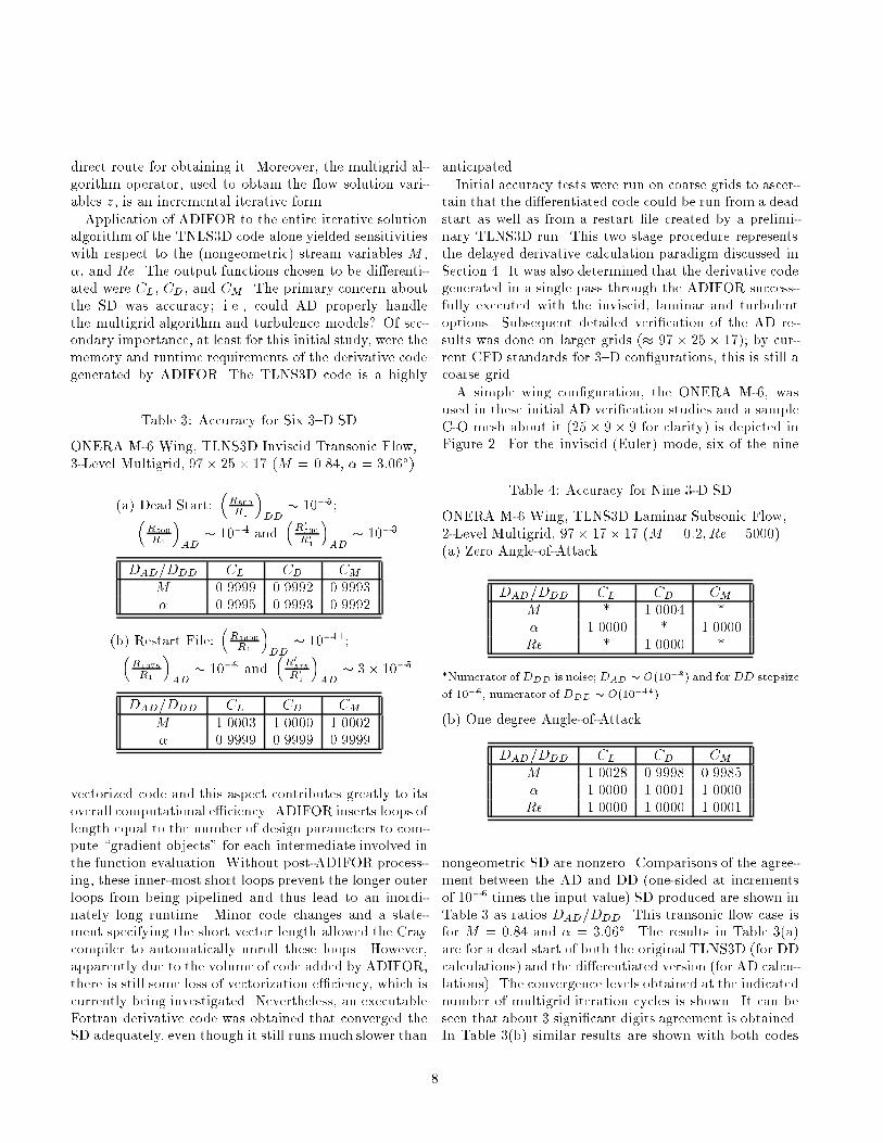
Application of ADIFOR to the entire iterative solutionalgorithm of the TNLS3D code alone yielded sensitivitieswith respect to the (nongeometric) stream variables M ,�, and Re. The output functions chosen to be di�erenti-ated were CL, CD, and CM . The primary concern aboutthe SD was accuracy; i.e., could AD properly handlethe multigrid algorithm and turbulence models? Of sec-ondary importance, at least for this initial study, were thememory and runtime requirements of the derivative codegenerated by ADIFOR. The TLNS3D code is a highly

Table 3: Accuracy for Six 3{D SD

ONERA M-6 Wing, TLNS3D Inviscid Transonic Flow,3-Level Multigrid, 97� 25� 17 (M = 0.84, � = 3:06�)

(a) Dead Start:�R800

R1

�DD

� 10�5;�R500

R1

�AD

� 10�4 and�R0

500

R0

1

�AD

� 10�3

DAD=DDD CL CD CMM 0.9999 0.9992 0.9993� 0.9995 0.9993 0.9992

(b) Restart File:�R1800

R1

�DD

� 10�11;�R1375

R1

�AD

� 10�9 and�R0

575

R0

1

�AD

� 3� 10�5

DAD=DDD CL CD CMM 1.0003 1.0000 1.0002� 0.9999 0.9999 0.9999

vectorized code and this aspect contributes greatly to itsoverall computational e�ciency. ADIFOR inserts loops oflength equal to the number of design parameters to com-pute \gradient objects" for each intermediate involved inthe function evaluation. Without post-ADIFOR process-ing, these inner-most short loops prevent the longer outerloops from being pipelined and thus lead to an inordi-nately long runtime. Minor code changes and a state-ment specifying the short vector length allowed the Craycompiler to automatically unroll these loops. However,apparently due to the volume of code added by ADIFOR,there is still some loss of vectorization e�ciency, which iscurrently being investigated. Nevertheless, an executableFortran derivative code was obtained that converged theSD adequately, even though it still runs much slower than

anticipated.

Initial accuracy tests were run on coarse grids to ascer-tain that the di�erentiated code could be run from a deadstart as well as from a restart �le created by a prelimi-nary TLNS3D run. This two stage procedure representsthe delayed derivative calculation paradigm discussed inSection 4. It was also determined that the derivative codegenerated in a single pass through the ADIFOR success-fully executed with the inviscid, laminar and turbulentoptions. Subsequent detailed veri�cation of the AD re-sults was done on larger grids (� 97� 25 � 17); by cur-rent CFD standards for 3{D con�gurations, this is still acoarse grid.

A simple wing con�guration, the ONERA M-6, wasused in these initial AD veri�cation studies and a sampleC-O mesh about it (25� 9� 9 for clarity) is depicted inFigure 2. For the inviscid (Euler) mode, six of the nine

Table 4: Accuracy for Nine 3-D SD

ONERA M-6 Wing, TLNS3D Laminar Subsonic Flow,2-Level Multigrid, 97� 17� 17 (M = 0:2; Re = 5000)(a) Zero Angle-of-Attack

DAD=DDD CL CD CMM * 1.0004 *� 1.0000 * 1.0000Re * 1.0000 *

�Numerator of DDD is noise; DAD � O(10�8) and forDD stepsize

of 10�6, numerator of DDD � O(10�14)

(b) One degree Angle-of-Attack

DAD=DDD CL CD CMM 1.0028 0.9998 0.9985� 1.0000 1.0001 1.0000Re 1.0000 1.0000 1.0001

nongeometric SD are nonzero. Comparisons of the agree-ment between the AD and DD (one-sided at incrementsof 10�6 times the input value) SD produced are shown inTable 3 as ratios DAD=DDD. This transonic ow case isfor M = 0:84 and � = 3:06�. The results in Table 3(a)are for a dead start of both the original TLNS3D (for DDcalculations) and the di�erentiated version (for AD calcu-lations). The convergence levels obtained at the indicatednumber of multigrid iteration cycles is shown. It can beseen that about 3 signi�cant digits agreement is obtained.In Table 3(b) similar results are shown with both codes

8

run from an original TLNS3D baseline restart �le. Againthe convergence levels obtained at the indicated numberof multigrid operations is shown. Agreement to essen-tially 4 signi�cant digits is obtained.The relative accuracy for all nine nongeometric SD at

subsonic laminar ow conditions, M = 0:2 and Re =5000, are shown in Table 4. For � = 0�, the resultingsymmetric ow produces some very small SD which forthe DD are only noise. However, the larger SD are seenfrom Table 4(a) to agree very well. The results for � = 1�

are shown in Table 4(b). Here again the agreement is verygood.


ONERA M-6 Wing, TLNS3D Turbulent Transonic Flow,3-Level Multigrid, 97� 25� 17(M = 0:84,� = 3:06�,Re = 11:7� 106)

(a) Mixing-length model


(b) Baldwin-Lomax model


(c) Convergence

�R1700

R1

�DD

� 10�12 ;

�R1300

R1

�AD

� 5� 10�12 and

�R0425

R01

�� 10�4

Similar relative accuracy results at transonic turbu-lent ow conditions, M = 0:84; � = 3:06�, and Re =11:7 � 106, are shown in Table 5. In Table 5(a) resultsare compared for the simple di�erentiable mixing-lengthturbulence model [46], whereas in Table 5(b), results forthe Baldwin-Lomax turbulence model [46] are compared.In both cases 3 to 4 signi�cant digits agreement betweenthe AD and DD results is obtained. The number of multi-grid iterations and convergence levels for both models isshown Table 5(c). An indication of the ow �eld resolu-

tion obtained on this (97 � 25 � 17) grid is displayed inFigure 3, which shows a wing upper surface pressure con-tour plot. It can be seen that both the swept leading-edgeshock and the almost normal wing-volume shock near themid chord are smeared out, as one would expect fromcentral-di�erence operators on such grids. It is not clearhow much e�ect such shock smearing has on these deriva-tive comparisons which have been presented; its e�ect issurely favorable though.

Table 6: Computing Time and Memory for Nine 3-D SD

ONERA M-6 Wing, TLNS3D Turbulent Transonic Flow,Baldwin-Lomax, 3-Level Multigrid, 97� 25� 17

Solution Number Time StorageProcedure Solutions (sec�) (MW)

DD one-sided 4 Nonlinear 3960 2.47DD central 6 Nonlinear 5940 2.47AD 1 Nonlinear, 10290 7.63

3 Linear

� All calculcations performed on CRAY Y-MP.

Convergence histories for the subsonic laminar ow (at� = 1�) and the transonic turbulent (Baldwin-Lomaxmodel) ow cases are presented in Figure 4. Here therelative residuals for both the original and di�erentiated(AD) TLNS3D codes are plotted versus work, which, for amultigrid algorithm, is taken as a unit roughly equivalentto the computational work of one iteration on the �nestgrid. As can be seen the subsonic laminar results are nottoo smooth; perhaps the ow would be seen to be un-steady on a �ner grid. The delayed derivative evaluationparadigm has been used and, as can be seen, the deriva-tive code solution (started from an original code restart�le) commences just beyond 1000 work units. These arethe residual histories for the accuracy results given in Ta-bles 4(b) and 5(b). An indication of the computationaltime and memory requirements for the derivative code inits current form compared with those for the original codecan be seen in Table 6. These are the runtime statisticsfor the results shown in Table 5(b) and Figure 4. TheAD-version code requires about 3 times the memory and2.5 times more runtime than that needed using the orig-inal code and DD for the problem considered. However,these are simply initial results and little has yet been doneto re�ne the iterative derivative paradigm with regard tojust what convergence levels are required. That is, whatis necessary for the residual R convergence level for theoriginal code baseline solution on the restart �le and also

9

that for R0 in the derivative code?

An indication of the derivative accuracy as a functionof the derivative residual R0 convergence level for the 3-D TLNS3D code is given in Table 7. As can be seen,for agreement to 2 signi�cant digits, the AD runtime isessentially equal to the DD runtime. The accuracy resultsgiven in Table 5(b) are the last column in Table 7. Itappears from comparing Tables 2 and 7 that the numberof signi�cant-digit agreement versus the convergence levelof R0 is essentially the same for the 2-D TSDE code andthe TLNS3D code.

Table 7: Computing Time and Accuracy for Nine 3-D SD


AD Convergencey 10+1 100 10�1 10�1:5

AD/DD Agreement# 2 3 4 4+

AD Time/DD Time 1.01 1.45 2.07 2.59


It appears that the newest version of ADIFOR is veryeasy to use. After a few examples, the NASA person-nel found that ADIFOR could be applied to a code in amatter of days. Veri�cation of the resulting derivativesby DD, however, was often much more time consuming.As the AD technology matures this extra e�ort will nolonger be necessary.

6 Conclusion and Challenges

Computational di�erentiation of an advanced CFD codeemploying ADIFOR in order to obtain SD of output owproperties with respect to nongeometric input variableshas been quantitatively demonstrated. This is a very sig-ni�cant and encouraging result for several reasons:

(a) The TLNS3D code is an e�cient, complex, state-of-the-art 3{D CFD code.

(b) The computational e�ciency of TLNS3D is basedupon the rather delicate multigrid acceleration al-gorithm and the successful application of ADIFORyielded similar convergence rates for the SD.

(c) ADIFOR also successfully di�erentiated theTLNS3D Baldwin-Lomax turbulence model.

(d) Accurate SD were obtained using AD in a relativelyshort lead time (O(man-week)), essentially treatingADIFOR and TLNS3D as black boxes.

While it has been shown that AD can be successfullyapplied to advanced CFD codes for nongeometric SD, theprocedures and results need to be improved before sensi-tivity information on high resolution meshes can be ob-tained. Also, the SD reported here were restricted to asingle discipline, namely the CFD calculation. However,experiments applying AD to the combination of the meshgeneration process and the ow analysis are under wayand preliminary results are encouraging. This interactionmust be achieved in order to perform the geometric SD,which is of primary interest to MDO.It should be stressed that, from a purely mathemati-

cal point of view, the di�erentiation of iterative processesdoes not seem to be a problem, despite the fact that theassumptions of known derivative convergence theoremshave not been veri�ed for the small disturbance code andare almost certainly not satis�ed by multigrid algorithms.Since, in the latter case, not even the convergence ofthe iterates themselves has been proven under reasonablygeneral assumptions, attempts to prove the convergenceof their derivatives seem premature. A comparativelysimple, but application and platform dependent, task isthe choice of criteria in the iterative paradigm for thetransition from the undi�erentiated iteration to the morecostly �nal stage, where derivative information is carriedalong. As our theoretical studies and numerical experi-ments indicate, one may assume that both solutions andderivatives converge at about the same rate once the it-eration has settled down. This is of signi�cance in designoptimization calculations since the objective function andits gradient need be obtained with high accuracy only inthe vicinity of the optimal design. Thus, great savingsare possible through less accurate evaluations in the ear-lier part of the optimization.A second goal is to avoid the unnecessary di�erentia-

tion of preconditioners and other intermediates that af-fect only the solution process but not the solution func-tion and its derivatives. Unless the original code is ap-propriately structured, \deactivating" such intermediates\by-hand" is a di�cult task. However, the resulting sim-pli�ed derivative calculation should be as e�cient as theincremental iterative form of the QA method. Therefore,an investigation will be made to determine if and howADIFOR can automatically perform deactivation with aminimum of directives from the user or programmer.A third goal is improved vectorization and parallelism

of the derivative code, so that their runtime is at worstequal to that of the original code multiplied by the num-

10

ber of design parameters. For standard test problems[9] ADIFOR achieves and undercuts this bound regularlyon scalar and super-scalar chips but, as in the case ofTLNS3D on a CRAY Y-MP, the situation is currentlymuch less favorable on vector machines.It may actually be simpler to maintain e�ciency for the

ADIFOR generated versions of parallel CFD codes. How-ever, as in the interdisciplinary case it becomes necessaryto pass derivative objects with intermediate data throughI/O statements and interprocessor messages. While thesize of the data transfers is multiplied by the number ofdesign variables, the data ow structure between varioustasks is preserved so that parallelism is essentially un-changed. The ADIFOR added code can interfere withthe inner loop vectorization whereas it is not seen in theouter loop parallelization.

Acknowledgements

We would like to thank Alan Carle of Rice Universityand Paul Hovland of Michigan State University for manystimulating discussions and their essential roles in theADIFOR development project. The authors are alsodeeply indebted to Veer Vatsa of NASA Langley for nu-merous useful and informative discussions concerning theTLNS3D code.

References

[1] H. M. Adelman and R. T. Haftka, editors. Proceed-ings of the Symposium on Sensitivity Analysis in En-gineering, NASA Langley Research Center, Hamp-ton, VA, Sept. 1986. NASA CP{2457, 1987.

[2] AGARD. Computational Methods for AerodynamicDesign (Inverse) and Optimization, Loen, Norway.AGARD{CP{463, May 1989.

[3] Twenty-Ninth AIAA/ASME/ASCE/AHS/ASCStructures, Structural Dynamics and Materials Con-ference, A Collection of Technical Papers. Williams-burg, VA. AIAA CP{882, Apr. 1988.

[4] Thirtieth AIAA/ASME/ASCE/AHS/ASC Struc-tures, Structural Dynamics and Materials Confer-ence, A Collection of Technical Papers. Mobile, AL.AIAA CP{891, Apr. 1989.

[5] Thirty-First AIAA/ASME/ASCE/AHS/ASCStructures, Structural Dynamics and Materials Con-ference, A Collection of Technical Papers. LongBeach, CA. AIAA CP{902, Apr. 1990.

[6] Thirty-Second AIAA/ASME/ASCE/AHS/ASCStructures, Structural Dynamics and Materials Con-ference, A Collection of Technical Papers. Baltimore,MD. AIAA CP{911, Apr. 1991.

[7] Fourth AIAA/USAF/NASA/OAI Symposium onMultidisciplinary Analysis and Optimization, A Col-lection of Technical Papers, Cleveland, OH. B B B kAIAA CP{9213, Sept. 1992.

[8] Thirty-Third AIAA/ASME/ASCE/AHS/ASCStructures, Structural Dynamics and Materials Con-ference, A Collection of Technical Papers. Dallas,TX. AIAA CP{922, Apr. 1992.

[9] B. Averick, R. G. Carter, and J. J. Mor�e.The MINPACK-2 test problem collection (prelim-inary version). Technical Report ANL/MCS{TM{150, Mathematics and Computer Science Division,Argonne National Laboratory, 1991.

[10] J. F. Barthelemy, editor. Second NASA/Air ForceSymposium on Recent Advances in MultidisciplinaryAnalysis and Optimization, Hampton, VA, Sept.1989. NASA CP{3031, 1989.

[11] J. F. Barthelemy, and L. Hall. Automatic di�eren-tiation as a tool in engineering design. In FourthAIAA/USAF/NASA/OAI Symposium on Multidis-ciplinary Analysis and Optimization, A Collectionof Technical Papers, Cleveland, OH, pages 424{432.AIAA 92{4743{CP, Sept. 1992.

[12] O. Baysal, editor. Symposium on MultidisciplinaryApplications of Computational Fluid Dynamics.FED{Vol. 129, ASME Winter Annual Meeting, Dec.1991.

[13] O. Baysal, M. E. Eleshaky, and G. W. Burgreen.Aerodynamic shape optimization using sensitivityanalysis on third-order Euler equations. In Proceed-ings of the AIAA Tenth Computational Fluid Dy-namics Conference, pages 573{583. AIAA 91-1577{CP, June 1991.

[14] C. H. Bischof, A. Carle, G. F. Corliss, and A.Griewank. ADIFOR: Automatic di�erentiation in asource translator environment. In Paul Wang, editor,International Symposium on Symbolic and AlgebraicComputing 92, pages 294{302. ACM, Washington,D.C., 1992.

[15] C. H. Bischof, A. Carle, G. F. Corliss, A. Griewank,and P. Hovland. ADIFOR: Generating derivative

11

codes from Fortran programs. Scienti�c Program-ming, 1(1):1{29, 1992.

[16] C. H. Bischof, G. F. Corliss, and A. Griewank. AD-IFOR exception handling. ADIFOR Working Note#3, MCS{TM{159, Mathematics and Computer Sci-ence Division, Argonne National Laboratory, 1991.

[17] C. H. Bischof, G. F. Corliss, and A. Griewank. Com-puting second- and higher-order derivatives throughunivariate Taylor series. ADIFORWorking Note #6,MCS{P296{0392, Mathematics and Computer Sci-ence Division, Argonne National Laboratory, 1992.

[18] C. H. Bischof and A. Griewank. ADIFOR: A For-tran system for portable automatic di�erentiation.In Fourth AIAA/USAF/NASA/OAI Symposium onMultidisciplinary Analysis and Optimization, A Col-lection of Technical Papers, Cleveland, OH, pages433{441. AIAA 92{4744{CP, Sept. 1992.

[19] C. H. Bischof and P. Hovland. Using ADIFORto compute dense and sparse Jacobians. ADIFORWorking Note #2, MCS{TM{158, Mathematics andComputer Science Division, Argonne National Lab-oratory, 1991.

[20] C. H. Bischof, A. Carle, G. Corliss, A. Griewank, andP. Hovland. Getting started with ADIFOR. ADI-FORWorking Note #9, ANL{MCS{TM{164, Math-ematics and Computer Science Division, ArgonneNational Laboratory, 1992.

[21] C. H. Bischof, A. Carle, G. F. Corliss, J. Dennis,A. Griewank, and K. Williamson. Derivative con-vergence for iterative equation solvers. ANL{MCS{P333{1192, Mathematics and Computer Science Di-vision, Argonne National Laboratory, 1992.

[22] G. Burgreen, O. Baysal, and M. Eleshaky. Improv-ing the e�ciency of aerodynamic shape optimizationprocedures. In Fourth AIAA/USAF/NASA/OAISymposium on Multidisciplinary Analysis and Opti-mization, A Collection of Technical Papers, Cleve-land, OH, pages 87{97. AIAA 92{4697{CP, Sept.1992.

[23] H. Cabuk, C.-H. Sung, and V. Modi. Adjoint opera-tor approach to shape design for internal incompress-ible ows. In Proceedings of Third International Con-ference on Inverse Design Concepts and Optimiza-tions in Engineering Sciences ICIDES{III, Washing-ton, DC, pages 391{404. Oct. 1991.

[24] D. Callahan, K. Cooper, R. T. Hood, K. Kennedy,and L. M. Torczon. ParaScope: A parallel program-ming environment. International Journal of Super-computer Applications, 2(4), Dec. 1988.

[25] A. Carle, K. D. Cooper, R. T. Hood, K. Kennedy,L. Torczon, and S. K. Warren. A practical environ-ment for scienti�c programming. IEEE Computer,20(11):75{89, Nov. 1987.

[26] B. D. Christianson. Reverse accumulation and accu-rate rounding error estimates for Taylor series coe�-cients. Optimization Methods and Software, 1(1):81{94, 1992.

[27] B. D. Christianson. Automatic Hessians by reverseaccumulation. Technical Report NOC TR228, TheNumerical Optimisation Center, Hat�eld Polytech-nic, Hat�eld, U.K., Apr. 1990.

[28] P. G. Coen. Recent results from the high-speed air-frame integration research project. AIAA Paper 92{4717, Sept. 1992.

[29] P. G. Coen, J. S-. Sobieski, and S. Dollyhigh. Prelim-inary results from the high-speed airframe integratedresearch project. AIAA Paper 92{1004, Feb. 1992.

[30] T. F. Coleman, B. S. Garbow, and J. J. Mor�e. Soft-ware for estimating sparse Jacobian matrices. ACMTrans. Math. Software, 10:329 { 345, 1984.

[31] T. F. Coleman and J. J. Mor�e. Estimation of sparseJacobian matrices and graph coloring problems.SIAM Journal on Numerical Analysis, 20:187 { 209,1984.

[32] S. Dollyhigh and J. S-. Sobieski. Recent experiencewith multidisciplinary analysis and optimization inadvanced aircraft design. In Third Air Force/NASASymposium on Recent Advances in MultidisciplinaryAnalysis and Optimization. A Collection of Techni-cal Papers, San Francisco, CA, pages 404{411. Sept.1990.

[33] M. Drela. Viscous and inviscid schemes using New-ton's method. In Special Course on Inverse Meth-ods for Airfoil Design for Aeronautical and Turbo-machinery Applications, pages 9-1 to 9-16. AGARDReport No. 780, May1990.

[34] G. S. Dulikravich, editor. Proceedings Second In-ternational Conference on Inverse Design Conceptsand Optimization in Engineering Sciences ICIDES{II, University Park, PA. Oct. 1987.

12

[35] G. S. Dulikravich, editor. Proceedings, Third Inter-national Conference on Inverse Design Concepts andOptimization in Engineering Sciences ICIDES{III,Washington, DC. Oct. 1991.

[36] G. S. Dulikravich. Aerodynamic shape design andoptimization. AIAA Paper No. 91{0476, Jan. 1991.

[37] H.M. Elbanna and L.A. Carlson. Determination ofaerodynamic sensitivity coe�cients based on thesmall perturbation formulation. J. Aircraft, 27(6):507{515, 1990. (Also appeared as AIAA Paper 89{0532.)

[38] H. M. Elbanna and L. A. Carlson. Determinationof aerodynamic sensitivity coe�cient based on thethree-dimensional full potential equation. In Proceed-ing of the AIAA 10th Applied Aerodynamics Confer-ence, pages 539{548. AIAA 92{2670{CP, June 1992.

[39] M. Eleshaky and O. Baysal. Aerodynamic shape op-timizationvia sensitivity analysis on decomposed computa-tional domains. In Fourth AIAA/USAF/NASA/OAISymposium on Multidisciplinary Analysis and Opti-mization, A Collection of Technical Papers, Cleve-land, OH, pages 98{109. AIAA 92{4698{CP, Sept.1992.

[40] Jean-Charles Gilbert. Automatic di�erentiation anditerative processes. Optimization Methods and Soft-ware, 1(1):13{22, 1992.

[41] A. Griewank. On automatic di�erentiation. In M. Iriand K. Tanabe, editors, Mathematical Programming:Recent Developments and Applications, pages 83{

108. Kluwer Academic Publishers, 1989.

[42] A. Griewank. Automatic evaluation of �rst- andhigher-derivative vectors. In R. Seydel, F. W. Schnei-der, T. K�upper, and H. Troger, editors, Proceedingsof the Conference at W�urzburg, Aug. 1990, Bifurca-tion and Chaos: Analysis, Algorithms, Applications,volume 97, pages 135{148. Birkh�auser Verlag, Basel,Switzerland, 1991.

[43] A. Griewank and G. F. Corliss, editors. AutomaticDi�erentiation of Algorithms: Theory, Implemen-tation, and Application. SIAM, Philadelphia, PA,1991.

[44] A. Griewank and S. Reese. On the calculation ofJacobian matrices by the Markowitz rule. In A.Griewank and G. F. Corliss, editors, Automatic Dif-ferentiation of Algorithms: Theory, Implementation,

and Application, pages 126{135. SIAM, Philadel-phia, PA, 1991.

[45] T. L. Holst, M. D. Salas, and R. W. Claus. TheNASA computational aerosciences program { towardtera op computing. AIAA Paper 92{0558, Jan. 1992.

[46] C. Hirsch. Numerical Computation of Internal andExternal Flows, Computational Methods for Inviscidand Viscous Flows, Vol. 2, Section 22.3.1, John Wi-ley & Sons, 1990.

[47] G. J-.W. Hou, A. C. Taylor III, and V. M. Korivi.Discrete shape sensitivity equations for aerodynamicproblems. AIAA Paper No. 91{2259, June 1991.

[48] A. Jameson. Aerodynamic design via control theory,Journal of Scienti�c Computing, 3:233{260, 1988.(Also NASA CR{181749 or ICASE Report No. 88{64, Nov. 1988).

[49] A. Jameson. Automatic design of transonic airfoilsto reduce the shock induced pressure drag. Prince-ton University MAE Report 1881, 1990. (Also ap-peared in 31st Israel Annual Conference in Aviationand Aeronautics, Feb. 1990).

[50] H. Jones, G. Hou, M. Korivi, A. Taylor III, andP. Newman. Multidisciplinary analysis and sensitiv-ity derivatives for isolated helicopter rotors in hover.In Fourth AIAA/USAF/NASA/OAI Symposium onMultidisciplinary Analysis and Optimization, A Col-lection of Technical Papers, Cleveland, OH, pages63{86. AIAA 92{4696{CP, Sept. 1992.

[51] D. Juedes. A taxonomy of automatic di�erentiationtools. In A. Griewank and G. F. Corliss, editors,Proceedings of the Workshop on Automatic Di�er-entiation of Algorithms: Theory, Implementation,and Application, pages 315{329. SIAM, Philadel-phia, PA, 1991.

[52] V. M. Korivi, A. C. Taylor III, P. A. Newman,G. J.-W. Hou, and H. E. Jones. An approximatelyfactored incremental strategy for calculating consis-tent discrete CFD sensitivity derivatives. In FourthAIAA/USAF/NASA/OAI Symposium on Multidis-ciplinary Analysis and Optimization, A Collectionof Technical Papers, Cleveland, OH, pages 465{478.AIAA 92{4746{CP, Sept. 1992.

[53] J. B. Malone and R. C. Swanson. Inverse airfoildesign procedure using a multigrid Navier-Stokes

13

method. In Proceedings, Third International Con-ference on Inverse Design Concepts and Optimiza-tion in Engineering Sciences ICIDES{III, Washing-ton, DC, pages 55{66. Oct. 1991.

[54] NASA. Third Air Force/NASA Symposium on Re-cent Advances in Multidisciplinary Analysis and Op-timization. A Collection of Technical Papers, SanFrancisco, CA. Sept. 1990.

[55] NASA. Computational Aerosciences Conference,Compendium of Abstracts. NASA Ames ResearchCenter, Mo�ett Field, CA, Aug. 1992.

[56] P. A. Newman, G. J.-W. Hou, H. E. Jones,A. C. Taylor, and V. M. Korivi. Observa-tions on computational methodologies for use inlarge-scale, gradient-based, multidisciplinary de-sign incorporating advanced CFD codes. In FourthAIAA/USAF/NASA/OAI Symposium on Multidis-ciplinary Analysis and Optimization, A Collectionof Technical Papers, Cleveland, OH, pages 531{542.AIAA 92{4753{CP, Sept. 1992.

[57] D. Olander and R. B. Schnabel. Preliminary experi-ence in developing a parallel thin-layer Navier Stokescode and implications for parallel language design. InProceedings, Scalable High Performance ComputingConference, SHPCC-92, pp. 276-283, Williamsburg,VA, Apr. 1992.

[58] C. Orozco and O. Ghattas. Optimal design of sys-tems governed by nonlinear partial di�erential equa-tions, In Fourth AIAA/USAF/NASA/OAI Sympo-sium on Multidisciplinary Analysis and Optimiza-tion, A Collection of Technical Papers, Cleveland,OH, pages 1126{1140. AIAA 92{4836{CP, Sept.1992.

[59] L. B. Rall. Automatic Di�erentiation: Techniquesand Applications, volume 120 of Lecture Notes inComputer Science. Springer Verlag, Berlin, Ger-many, 1981.

[60] M. H. Rizk. Optimization by updating design param-eters as CFD iterative ow solutions evolve. In O.Baysal, editor, Symposium on Multidisciplinary Ap-plications of Computational Fluid Dynamics, pages51{62. FED{Vol. 129, ASME Winter Annual Meet-ing, Dec. 1991.

[61] I. Sadrehaghighi, R. E. Smith Jr., and S. N. Tiwari.An analytical approach to grid sensitivity analysis.AIAA Paper 92{0660, Jan. 1992.

[62] G. R. Shubin. Obtaining \cheap" optimization gra-dients from computational aerodynamics codes. Ap-plied Mathematics and Statistics Technical ReportAMS{TR{164, Boeing Computer Services, June1991.

[63] G. R. Shubin and P. D. Frank. A comparison oftwo closely-related approaches to aerodynamic de-sign optimization, In Proceedings of the Third Inter-national Conference on Inverse Design Concepts andOptimizations in Engineering Sciences ICIDES-III,Washington. DC, pages 67{78. Oct. 1991. (Also ap-peared as Boeing Computer Services Technical Re-port AMS{TR{163, April, 1991).

[64] R. E. Smith Jr., and I. Sadrehaghighi. Grid sensitiv-ity in airplane design, In Proceedings of the 4th In-ternational Symposium of Computational Fluid Dy-namics, University of California-Davis, pages 1071{1077. Sept. 1991.

[65] J. S-. Sobieski. Multidisciplinary optimization forengineering systems: Achievements and potential.NASA TM 101566, NASA, Mar. 1989.

[66] T. Sorenson. Airfoil optimization with e�cient gra-dient calculations. In Proceedings of the Third Inter-national Conference on Inverse Design Concepts andOptimizations in Engineering Sciences ICIDES-III,Washington. DC, pages 433{444. Oct. 1991.

[67] A. Sussman, J. Saltz, R. Das, S. Gupta, D. Mavriplis,R. Ponnusamy, and K. Crowley. PARTI primitivesfor unstructured and block structured problems,NASA CR 189662, June 1992.

[68] S. T�aasan, G. Kuruvila, and M. D. Salas. Aerody-namic design and optimization in one shot. AIAAPaper No. 92{0025, Jan. 1992.

[69] A. C. Taylor III, G. J-.W. Hou, and V. M. Korivi. Amethodology for determining aerodynamic sensitiv-ity derivatives with respect to variation of geometricshape. AIAA Paper No. 91{1101, Apr. 1991.

[70] A. C. Taylor III, G.J-.W. Hou, and V. M. Korivi.Sensitivity analysis, approximate analysis, and de-sign optimization for internal and external ows.AIAA Paper No. 91{3083, Sept. 1991.

[71] V. N. Vatsa and B. W. Wedan. Development of amultigrid code for 3{D Navier-Stokes equations andits application to a grid-re�nement study, Computers& Fluids, 18(4):391-403, 1990.

14

[72] V. N. Vatsa, M. D. Sanetrik, and E. B. Parlette. De-velopment of a exible and e�cient multigrid-basedmultiblock ow solver, To be presented at AIAA 31stAerospace Sciences Meeting, Reno NV, AIAA 93-0677, Jan. 1993.

[73] N. J. Yu and R. C. Campbell. Transonic airfoil andwing design using Navier-Stokes codes, In Proceed-ings AIAA 10th Applied Aerodynamics Conference,pages 477-485, AIAA 92{2651{CP, June 1992.

15

Figure 1: Iteration convergence histories for subsonic, transonic, and supersonic inviscid ow solutions from the 2{Dtransonic small disturbance equation code TAMRF for an NACA 1406 airfoil at � = 1�.

Figure 2: Symmetry and back plane traces of the 3-D C-O mesh (25� 9� 9) produced by the grid generation codeWTCO about an ONERA M-6 wing.

Figure 3: Upper surface pressure contour plot on an ONERA M-6 wing for TLNS3D transonic turbulent ow solutionat M = 0:84; �= 3:06�; Re = 11:7� 106 with Baldwin-Lomax model on 97� 25� 17 computational mesh.

Figure 4: Iteration convergence histories for 3-D subsonic laminar and transonic turbulent ow solutions from theTLNS3D code for an ONERA M-6 wing.

16

ANALYSIS

GRID

Shape

CFD

ANALYSIS + SD

GRID*

Shape

CFD*

Solution

Mesh

d Mesh

d Shaped Shape

d Solut.

d Stream

d Solut.

* = original code + AD added code

Solution

Stream

Stream

Mesh

17

Table 1: Computation Time for Five 2-D SD

NACA 1406 Airfoil; TSDE Inviscid Flow

Solution Number Time (sec)�

Procedure Solutions Subs. Trans. Supers.

DD 6 Nonlinear 13 36 64

QA 1 Nonlinear, 40y 38y 37y

5 Linear

AD 1 Nonlinear, 12# 25# 35#

5 Linear� All calculations performed on a CRAY Y-MP.y Average time for several matrix solution methods.# kR0

mk converged below 10�3.

18

Table 2: Computing Time and Accuracy for Five 2-D SD

NACA 1406 Airfoil; TSDE Inviscid Transonic Flow

ADConverg.y

10+1 100 10�1 10�2 10�3 10�4

AD/DDAgreement#

2 3 4 4+ 4+ 4+

AD Time/ 0.18 0.26 0.36 0.50 0.69 0.92DD time

QA Time/ 1.08 1.08 1.08 1.08 1.08 1.08DD Time


19

Table 3: Accuracy for Six 3{D SD

ONERA M-6 Wing, TLNS3D Inviscid Transonic Flow,3-Level Multigrid, 97� 25� 17 (M = 0.84, � = 3:06�)

(a) Dead Start:�R800

R1

�DD

� 10�5;�R500

R1

�AD

� 10�4 and�R0

500

R0

1

�AD

� 10�3

DAD=DDD CL CD CMM 0.9999 0.9992 0.9993� 0.9995 0.9993 0.9992

(b) Restart File:�R1800

R1

�DD

� 10�11;�R1375

R1

�AD

� 10�9 and�R0

575

R0

1

�AD

� 3� 10�5

DAD=DDD CL CD CMM 1.0003 1.0000 1.0002� 0.9999 0.9999 0.9999

20


ONERA M-6 Wing, TLNS3D Laminar Subsonic Flow,2-Level Multigrid, 97� 17� 17 (M = 0:2; Re = 5000)(a) Zero Angle-of-Attack

DAD=DDD CL CD CMM * 1.0004 *� 1.0000 * 1.0000Re * 1.0000 *

�Numerator of DDD is noise;DAD � O(10�8) and for DD stepsize

of 10�6, numerator of DDD � O(10�14)

(b) One degree Angle-of-Attack


21


ONERA M-6 Wing, TLNS3D Turbulent Transonic Flow,3-Level Multigrid, 97� 25� 17(M = 0:84,� = 3:06�,Re = 11:7� 106)

(a) Mixing-length model


(b) Baldwin-Lomax model


(c) Convergence

�R1700

R1

�DD

� 10�12 ;

�R1300

R1

�AD

� 5� 10�12 and

�R0425

R01

�� 10�4

22

Table 6: Computing Time and Memory for Nine 3-D SD


Solution Number Time StorageProcedure Solutions (sec�) (MW)

DD one-sided 4 Nonlinear 3960 2.47DD central 6 Nonlinear 5940 2.47AD 1 Nonlinear, 10290 7.63

3 Linear

� All calculcations performed on CRAY Y-MP.

23

Table 7: Computing Time and Accuracy for Nine 3-D SD


AD Convergencey 10+1 100 10�1 10�1:5

AD/DD Agreement# 2 3 4 4+

AD Time/DD Time 1.01 1.45 2.07 2.59


24

automatic differentiation of advanced cfd codes for

Documents