Automatic Cell Planning

Dr Rupert Rawnsley

Originally submitted in June 2001 for the degree of Doctor of Philosophy to the Department of Computer Science, University of Wales, Cardiff, UK.

II

Abstract

An effective and efficient mobile telephone service relies, in part, on the deployment and configuration of network infrastructure. This thesis describes some of the problems faced by the network planners in providing such a service. Novel algorithmic methods are presented for designing networks that meet both the subscriber’s demand for a high quality of service and the operator’s requirement for low infrastructure overheads. Automatic Cell Planning (ACP) is the generic name for these network optimising techniques. Existing research into ACP is extended through the introduction of ‘interference surrogates’, which give the network designer greater control over interference in a wireless network. Interference management is the central theme of this thesis. The accurate simulation and control of interference leads to a more efficient use of the available radio spectrum (a limited and expensive commodity). Two approaches to ACP are developed: in the first, network performance (in terms of subscriber coverage) is given priority over the cost of network infrastructure; in the second, these priorities are reversed. These two distinct approaches typify a trade off that lies at the heart of the problem of network design − a trade off between spectral efficiency and the cost of network infrastructure.

Keywords: automatic cell planning, ACP, cellular mobile telephone network optimisation, cell plan optimisation, cell optimisation, cell dimensioning, base station placement, wireless networks, spectral efficiency, spectrum efficiency, channel assignment, CAP, frequency assignment, FAP, interference surrogates, signal freedom.

III

Contents

ABSTRACT II CONTENTS III LIST OF FIGURES V LIST OF TABLES VIII GLOSSARY OF TERMS IX GLOSSARY OF SYMBOLS X

CHAPTER 1 INTRODUCTION 1

1.1 OUTLINE OF PROBLEM 1 1.2 PREVIOUS WORK 7 1.3 THESIS AIMS AND OBJECTIVES 19 1.4 TEST PLATFORM 20 1.5 THESIS OUTLINE 21

CHAPTER 2 NETWORK MODEL 23

2.1 SIMULATION ISSUES 23 2.2 DESCRIPTION OF MODEL 31 2.3 PERFORMANCE EVALUATION 51 2.4 DATA SETS 56

CHAPTER 3 NETWORK DESIGN – PART 1 65

3.1 CHOICE OF OPTIMISATION ALGORITHMS 65 3.2 INITIALISATION ALGORITHMS 66 3.3 SEARCH ALGORITHMS 84 3.4 FACTORS LIMITING SEARCH PERFORMANCE 100

CHAPTER 4 CHANNEL ASSIGNMENT 103

4.1 PROBLEM DEFINITION 103 4.2 PERFORMANCE EVALUATION 109 4.3 DATA SETS 112 4.4 COMMON ALGORITHMIC CONCEPTS 114

IV

4.5 INITIALISATION ALGORITHMS 115 4.6 SEARCH ALGORITHMS 118 4.7 COMPARISON OF RESULTS 123

CHAPTER 5 INTERFERENCE SURROGATES 125

5.1 ROLE OF THE INTERFERENCE SURROGATE 126 5.2 INTERFERENCE SURROGATE DESCRIPTIONS 128 5.3 METHODOLOGY OF COMPARISON 133 5.4 RESULTS 136 5.5 CONCLUSION 146

CHAPTER 6 NETWORK DESIGN – PART 2 148

6.1 EVALUATION OF TWO-STAGE NETWORK DESIGN PROCESS 148 6.2 NETWORK DESIGNS WITH ‘HIGH’ COMPUTATIONAL INVESTMENT 152 6.3 NETWORK DESIGNS WITH MINIMAL INFRASTRUCTURE 156

CHAPTER 7 CONCLUSIONS AND FUTURE WORK 164

7.1 THESIS CONCLUSIONS 164 7.2 NETWORK MODEL ENHANCEMENTS 178 7.3 IMPROVEMENTS TO OPTIMISATION METHODOLOGY 182

ACKNOWLEDGMENTS 184

BIBLIOGRAPHY 185

V

List of Figures

Figure 1.1: The simplified path of a call between a wireless telephone and a wireline telephone.........................................2 Figure 1.2: An example of different switching technologies connecting both wireless and wireline telephones..................3 Figure 1.3: A pictorial illustration of radio signal propagation in wireless and wireline networks.......................................6 Figure 1.4: The relationship between re-use distance D and cell radius R in co-channel cells. ..........................................10 Figure 1.5: A channel re-use pattern for 7 different sets of channels.......................................................................................11 Figure 1.6: The translation of a political map into a colouring constraint graph..................................................................12 Figure 1.7: Some received power levels at a mobile station; this data may be measured or predicted. .............................13 Figure 2.1: An abstracted traffic cover problem using multiple servers..................................................................................28 Figure 2.2: Rasterisation of the network working area. ............................................................................................................32 Figure 2.3: The test point layout in NetworkA3..........................................................................................................................33 Figure 2.4: The test point traffic volumes in NetworkA3. ..........................................................................................................34 Figure 2.5: The test point service thresholds in NetworkB1......................................................................................................34 Figure 2.6: The site positions in NetworkB1. ..............................................................................................................................35 Figure 2.7: The geometry of the horizontal loss calculation for directional antennae...........................................................36 Figure 2.8: The geometry of the vertical loss calculation for antennae...................................................................................37 Figure 2.9: The angles-of-incidence for a site in NetworkA4....................................................................................................38 Figure 2.10: Two active base stations in NetworkA4.................................................................................................................42 Figure 2.11: The propagation gain from a site in NetworkA2..................................................................................................43 Figure 2.12: The signal strength due to an active base station in NetworkA4........................................................................45 Figure 2.13: An example of serviced test points in NetworkA4. ...............................................................................................46 Figure 2.14: An example CIR calculation for two active base stations in NetworkA4..........................................................49 Figure 2.15: An example of test point cover for two base stations in NetworkA4. .................................................................50 Figure 2.16: Comparison operator for network performance metrics....................................................................................55 Figure 2.17: NetworkA1 (a) test points, (b) traffic densities, and (c) candidate site positions. .............................................57 Figure 2.18: NetworkA2 (a) test points, (b) traffic densities, and (c) candidate site positions. .............................................59 Figure 2.19: NetworkA3 (a) test points, (b) traffic densities, and (c) candidate site positions. .............................................60 Figure 2.20: NetworkA4 (a) test points, (b) traffic densities, and (c) candidate site positions. .............................................61 Figure 2.21: NetworkB1 (a) test points, (b) traffic densities, (c) candidate site positions, and (d) service thresholds.......62 Figure 3.1: Algorithm InitBlank....................................................................................................................................................66 Figure 3.2: Algorithm InitRandomA............................................................................................................................................68 Figure 3.3: An example network design produced by InitRandomA. ......................................................................................69 Figure 3.4: The distribution of traffic cover for InitRandomA on NetworkA4........................................................................70 Figure 3.5: The distribution of test point cover for InitRandomA on NetworkA4...................................................................70 Figure 3.6: The distribution of site occupancy for InitRandomA on NetworkA4. ..................................................................71

VI

Figure 3.7: The distribution of number of base stations active for InitRandomA on NetworkA4.........................................71 Figure 3.8: Graph of traffic cover vs. base stations active for InitRandomA on NetworkA4................................................72 Figure 3.9: Graph of traffic cover vs. sites occupied for InitRandomA on NetworkA4.........................................................72 Figure 3.10: Graph of test point cover vs. base stations active for InitRandomA on NetworkA4. .......................................73 Figure 3.11: Graph of test point cover vs. sites occupied for InitRandomA on NetworkA4..................................................73 Figure 3.12: A subsection of the example network generated by InitRandomA.....................................................................74 Figure 3.13: Algorithm InitRandomB..........................................................................................................................................76 Figure 3.14: An example network design produced by InitRandomB.....................................................................................77 Figure 3.15: The distribution of traffic cover for InitRandomB on NetworkA4......................................................................78 Figure 3.16: The distribution of test point cover for InitRandomB on NetworkA4. ...............................................................78 Figure 3.17: Graph of traffic cover vs. base stations active for InitRandomB on NetworkA4..............................................79 Figure 3.18: Graph of traffic cover vs. sites occupied for InitRandomB on NetworkA4.......................................................79 Figure 3.19: Graph of test point cover vs. base stations active for InitRandomB on NetworkA4. .......................................80 Figure 3.20: Graph of test point cover vs. sites occupied for InitRandomB on NetworkA4..................................................80 Figure 3.21: Algorithm InitRandomC..........................................................................................................................................81 Figure 3.22: An example network design produced by InitRandomC.....................................................................................82 Figure 3.23: The distribution of traffic cover for InitRandomC on NetworkA4......................................................................83 Figure 3.24: The distribution of test point cover for InitRandomC on NetworkA4................................................................83 Figure 3.25: Algorithm SearchRandomB....................................................................................................................................85 Figure 3.26: The performance of the best design produced vs. time for SearchRandomB on NetworkA4.........................86 Figure 3.27: The performance of the best design produced vs. time for SearchRandomC on NetworkA4.........................87 Figure 3.28: Algorithm SearchHillClimbA.................................................................................................................................89 Figure 3.29: The performance of the best design produced vs. time for SearchHillClimbA on NetworkA4 (run 1). ........91 Figure 3.30: The performance of the best design produced vs. time for SearchHillClimbA on NetworkA4 (run 2). ........91 Figure 3.31: The performance of the best design produced vs. time for SearchHillClimbA on NetworkA4 (run 3). ........92 Figure 3.32: Algorithm SearchConstructA. ................................................................................................................................94 Figure 3.33: The performance of the best design produced vs. time for SearchConstructA on NetworkA1.......................95 Figure 3.34: The performance of the best design produced vs. time for SearchConstructB on NetworkA1.......................98 Figure 4.1: The comparison operator for assignment performance metrics. .......................................................................110 Figure 4.2: CAP problem CapA2−10 generated from NetworkA2. ......................................................................................113 Figure 4.3: Algorithm InitRandomD..........................................................................................................................................115 Figure 4.4: Algorithm InitConstructA........................................................................................................................................117 Figure 4.5: Algorithm SearchRandomD. ..................................................................................................................................119 Figure 4.6: The performance of the best assignment produced vs. time for SearchRandomD on CapA2−90.................120 Figure 4.7: Algorithm SearchHillClimbB. ................................................................................................................................122 Figure 4.8: The performance of the best assignment produced vs. time for SearchHillClimbB on CapA3−90...............123 Figure 5.1: The performance of an ideal (hypothetical) interference-surrogate.................................................................127 Figure 5.2: An illustration of the attenuation of interference by channel separation...........................................................130 Figure 5.3: The performance of an imperfect interference surrogate, in which one pair of designs violate the IS

Condition............................................................................................................................................................................134 Figure 5.4: The performance of an imperfect interference surrogate, in which three pairs of designs violate the IS

Condition............................................................................................................................................................................135 Figure 5.5: The normalised inaccuracy of three ISs vs. time for NetworkA1........................................................................137 Figure 5.6: Graph of overlap vs. test point cover for 10 designs in NetworkA1...................................................................138 Figure 5.7: Graph of non-dominance vs. test point cover for 10 designs in NetworkA1.....................................................138 Figure 5.8: Graph of signal freedom vs. test point cover for 10 designs in NetworkA1. .....................................................139 Figure 5.9: The normalised inaccuracy of three ISs vs. time for NetworkA2........................................................................140 Figure 5.10: Graph of overlap vs. test point cover for 10 designs in NetworkA2.................................................................140

VII

Figure 5.11: Graph of non-dominance vs. test point cover for 10 designs in NetworkA2...................................................141 Figure 5.12: Graph of signal freedom vs. test point cover for 10 designs in NetworkA2....................................................141 Figure 5.13: The normalised inaccuracy of three ISs vs. time for NetworkA3. ....................................................................142 Figure 5.14: Graph of overlap vs. test point cover for 10 designs in NetworkA3.................................................................142 Figure 5.15: Graph of non-dominance vs. test point cover for 10 designs in NetworkA3...................................................143 Figure 5.16: Graph of signal freedom vs. test point cover for 10 designs in NetworkA3....................................................143 Figure 5.17: The normalised inaccuracy of three ISs vs. time for NetworkA4. ....................................................................144 Figure 5.18: Graph of overlap vs. test point cover for 10 designs in NetworkA4.................................................................144 Figure 5.19: Graph of non-dominance vs. test point cover for 10 designs in NetworkA4...................................................145 Figure 5.20: Graph of signal freedom vs. test point cover for 10 designs in NetworkA4....................................................145 Figure 6.1: The performance of the best design produced vs. time for SearchRandomC on NetworkA4.........................150 Figure 6.2: The performance of the best design produced vs. time for SearchHillClimbA on NetworkA4.......................150 Figure 6.3: Algorithm SearchPruneA........................................................................................................................................153 Figure 6.4: The performance of the best BSCP solution vs. time for composite search on NetworkA2............................155 Figure 6.5: Algorithm SearchPruneB........................................................................................................................................158 Figure 6.6: Algorithm SearchHillClimbC.................................................................................................................................159 Figure 6.7: Graph of network infrastructure vs. time for algorithm SearchPruneB on NetworkA1..................................160 Figure 6.8: Algorithm SearchConstructC. ................................................................................................................................162 Figure 7.1: Graph of test point cover vs. base station activity for ten candidate designs in NetworkA1...........................167 Figure 7.2: Graph of test point cover vs. base station activity for ten candidate designs in NetworkA2...........................167 Figure 7.3: Graph of test point cover vs. base station activity for ten candidate designs in NetworkA3...........................168 Figure 7.4: Graph of test point cover vs. base station activity for ten candidate designs in NetworkA4...........................168 Figure 7.5: A pathological example of receiver cover for two transmitters..........................................................................170 Figure 7.6: A pathological example of receiver cover for three transmitters........................................................................170 Figure 7.7: Graph of subscriber cover vs. network infrastructure.........................................................................................171 Figure 7.8: Graph of the effect of computational investment on the pareto-optimal trade off between subscriber cover

and network infrastructure...............................................................................................................................................172 Figure 7.9: Target performance positions on the pareto-optimal graph...............................................................................173 Figure 7.10: Number of base stations vs. computational investment for a fixed subscriber cover.....................................176 Figure 7.11: Infrastructure cost vs. number of base stations...................................................................................................176 Figure 7.12: The determination of optimal computational investment by comparison of computational cost and network

infrastructure cost. ............................................................................................................................................................177

VIII

List of Tables

Table 1.1: Test platform specification. .........................................................................................................................................21 Table 2.1: Traffic capacity vs. number allocated base station channels..................................................................................39 Table 2.2: Summary of statistics for network data sets. .............................................................................................................56 Table 3.1: The statistical performance of algorithm InitRandomA..........................................................................................69 Table 3.2: The statistical performance of algorithm InitRandomB..........................................................................................77 Table 3.3: The statistical performance of algorithm InitRandomC..........................................................................................82 Table 3.4: A summary of results for initialisation algorithms. ..................................................................................................84 Table 3.5: The performance of the best network designs for SearchRandomB......................................................................86 Table 3.6: The performance of the best network designs for SearchRandomC......................................................................87 Table 3.7: Example moves for SearchHillClimbA......................................................................................................................88 Table 3.8: The performance of network designs for SearchHillClimbA..................................................................................90 Table 3.9: The initial and final traffic covers for multiple executions of SearchHillClimbA.................................................92 Table 3.10: The performance of the best network designs for SearchConstructA..................................................................95 Table 3.11: The performance of the best network designs for SearchConstructB..................................................................97 Table 3.12: A summary of results for all search algorithms on all networks..........................................................................99 Table 3.13: Computational complexity of network performance evaluation........................................................................100 Table 4.1: Summary statistics for CAP problem instances......................................................................................................113 Table 4.2: The performance of the best assignments produced by InitConstructA. .............................................................118 Table 4.3: The performance of the best assignments produced by SearchRandomD..........................................................120 Table 4.4: The performance of the best assignment produced by SearchHillClimbB. ........................................................122 Table 5.1: An example of IS performance vs. time....................................................................................................................136 Table 5.2: The final IS inaccuracy values for NetworkA1.......................................................................................................137 Table 5.3: The final IS inaccuracy values for NetworkA2.......................................................................................................139 Table 5.4: The final IS inaccuracy values for NetworkA3.......................................................................................................141 Table 5.5: The final IS inaccuracy values for NetworkA4.......................................................................................................143 Table 5.6: A summary of IS inaccuracy results.........................................................................................................................146 Table 6.1: The performance of the best BSCP solutions for SearchRandomC and SearchHillClimbA............................149 Table 6.2: The performance of the best network design (after channel assignment) for SearchRandomB.......................151 Table 6.3: The performance of the best BSCP solution for composite search......................................................................154 Table 6.4: The performance of the best network design for seven day optimisation............................................................155 Table 6.5: A comparison of actual network infrastructure with theoretic minimum............................................................156 Table 6.6: The performance of the final network designs produced by SearchPruneB.......................................................160 Table 6.7: The effect on network infrastructure of algorithm SearchPruneB. ......................................................................161 Table 6.8: The performance of the best network designs produced by the composite constructive search algorithm.....163

IX

Glossary of Terms

ACP Automatic Cell Planning

AI Angle of Incidence

BNDP Broadcast Network Design Problem

BSPP Base Station Placement Problem

CAP Channel Assignment Problem

CDMA Code Division Multiple Access

CIR Carrier to Interference Ratio

CNDP Capacitated Network Design Problem

FAP Frequency Assignment Problem

FDMA Frequency Division Multiple Access

FSP Fixed Span Problem

GCP Graph Colouring Problem

GOS Grade Of Service

GSM Global System for Mobile communications

ICR Interference to Carrier Ratio

QOS Quality Of Service

TDMA Time Division Multiple Access

VSP Variable Span Problem

WCNDP Wireless Capacitated Network Design Problem

X

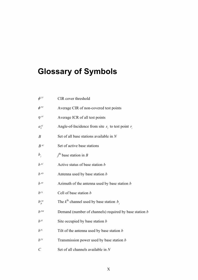
Glossary of Symbols

CVφ CIR cover threshold

NCφ Average CIR of non-covered test points

AVη Average ICR of all test points

AIila Angle-of-Incidence from site ls to test point ir

B Set of all base stations available in N

ACB Set of active base stations

jb jth base station in B

ACb Active status of base station b

ADb Antenna used by base station b

AZb Azimuth of the antenna used by base station b

CLb Cell of base station b

CHjkb The kth channel used by base station jb

DMb Demand (number of channels) required by base station b

STb Site occupied by base station b

TLb Tilt of the antenna used by base station b

TXb Transmission power used by base station b

C Set of all channels available in N

XI

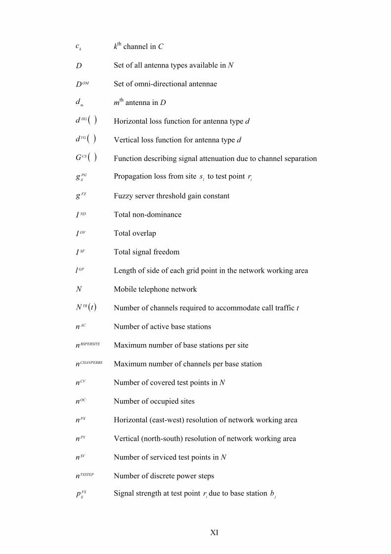
kc kth channel in C

D Set of all antenna types available in N

OMD Set of omni-directional antennae

md mth antenna in D

( )HGd Horizontal loss function for antenna type d

( )VGd Vertical loss function for antenna type d

( )CSG Function describing signal attenuation due to channel separation

PGilg Propagation loss from site ls to test point ir

FZg Fuzzy server threshold gain constant

NDI Total non-dominance

OVI Total overlap

SFI Total signal freedom

GPl Length of side of each grid point in the network working area

N Mobile telephone network

( )tN TR Number of channels required to accommodate call traffic t

ACn Number of active base stations

BSPERSITEn Maximum number of base stations per site

CHANPERBSn Maximum number of channels per base station

CVn Number of covered test points in N

OCn Number of occupied sites

PXn Horizontal (east-west) resolution of network working area

PYn Vertical (north-south) resolution of network working area

SVn Number of serviced test points in N

TXSTEPn Number of discrete power steps

FSijp Signal strength at test point ir due to base station jb

XII

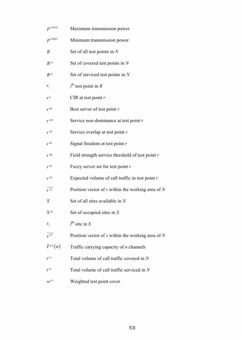
TXMAXp Maximum transmission power

TXMINp Minimum transmission power

R Set of all test points in N

CVR Set of covered test points in N

SVR Set of serviced test points in N

ir ith test point in R

φr CIR at test point r

BSr Best server of test point r

NDr Service non-dominance at test point r

OVr Service overlap at test point r

SFr Signal freedom at test point r

SQr Field strength service threshold of test point r

SSr Fuzzy server set for test point r

TRr Expected volume of call traffic in test point r

XYr Position vector of r within the working area of N

S Set of all sites available in N

OCS Set of occupied sites in S

ls lth site in S

XYs Position vector of s within the working area of N

( )nT CH Traffic carrying capacity of n channels

CVt Total volume of call traffic covered in N

SVt Total volume of call traffic serviced in N

CVw Weighted test point cover

1

Chapter 1 Introduction

An effective and efficient mobile telephone1 service relies, in part, on the deployment

and configuration of network infrastructure. This thesis tackles some of the problems

faced by the network planners in providing that service. Novel algorithmic methods are

presented for automatically designing networks that meet both the subscriber’s demand

for a high quality service and the operator’s requirement for low infrastructure

overheads. Automatic Cell Planning (ACP) is the generic name for these network

optimising techniques.

The structure of this chapter is as follows: Section 1.1 presents an outline of the problem

domain considered, Section 1.2 contains a review of resources and research related to

the problem domain, Section 1.3 sets out the aims and objectives of the thesis, and

Section 1.4 summarises the contents of each subsequent thesis chapter.

1.1 Outline of Problem

The growth of the mobile telephone industry has been enormous. In the early 1980’s

cellular2 mobile telephones were introduced; by the Year 1990 the number of

subscribers worldwide was 11 million, and by the Year 2000 that figure had risen to 500

1 A telephone with a wireless connection to its network. 2 A technology where services are provided in discrete geographical-regions, known as cells.

2

million. This growth shows no sign of slowing, and it is estimated that by 2010 the

number of mobile-telephone subscribers will be 2 billion − when it will exceed the

number of subscribers to wireline telephones1 [1]. In order to keep pace with the

enormous increase in demand, faster and more efficient methods are required for the

design of mobile telephone networks [2,3].

Wireless communication requires sophisticated technology. Consider GSM2 networks,

they employ advanced devices such as Very High Frequency (VHF) radio transceivers,

high-speed digital signal processors, optical fibre, microwave dishes, and data

compression. Until recently the cost of using mobile telephone networks has been too

high for the majority of consumers, however, advances in integrated-circuit design

(amongst other things) have reduced these costs sufficiently to make mass-market

wireless communications viable.

Base

Transceiver Station

Base Station

Controller

Mobile Switching

Centre

Public Land

Network

VHF Radio

Waves

Microwave Radio Link

Optical Fibre

Optical Fibre

Copper Wire

Wireline Telephone

Wireless Telephone

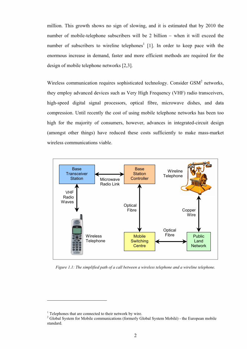
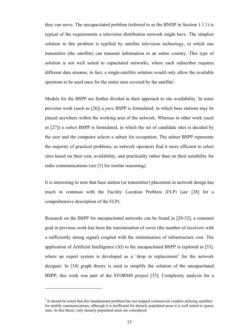
Figure 1.1: The simplified path of a call between a wireless telephone and a wireline telephone.

1 Telephones that are connected to their network by wire. 2 Global System for Mobile communications (formerly Global System Mobilé) - the European mobile standard.

3

Consider the simplified example, shown in Figure 1.1, of a call between a wireless

telephone and a wireline telephone (this example is adapted from [4]). The call passes

through a variety of network switches. Speech data leaving the wireline telephone

travels as electrical impulses through copper wire; these impulses are digitally encoded

by the Public Land Network (PLN)1 and transmitted, via optical fibre, to the wireless

subscriber’s Mobile Switching Centre (MSC). The MSC determines the destination of

the data2 and re-transmits it to the correct Base Station Controller (BSC), and then the

optically encoded data is decoded and transmitted via a microwave link to the Base

Transceiver Station (BTS) currently hosting the wireless telephone. The BTS identifies

which of the wireless telephones in its service area (known as a cell) is the intended

recipient, and forwards the data using a VHF radio link.

BTS

MSC

PLN

PLN

MSC

BSC

BSC

BSC

BTS

BTS

BTS

BTS

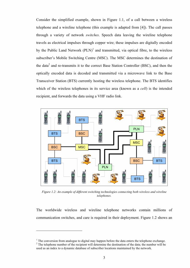
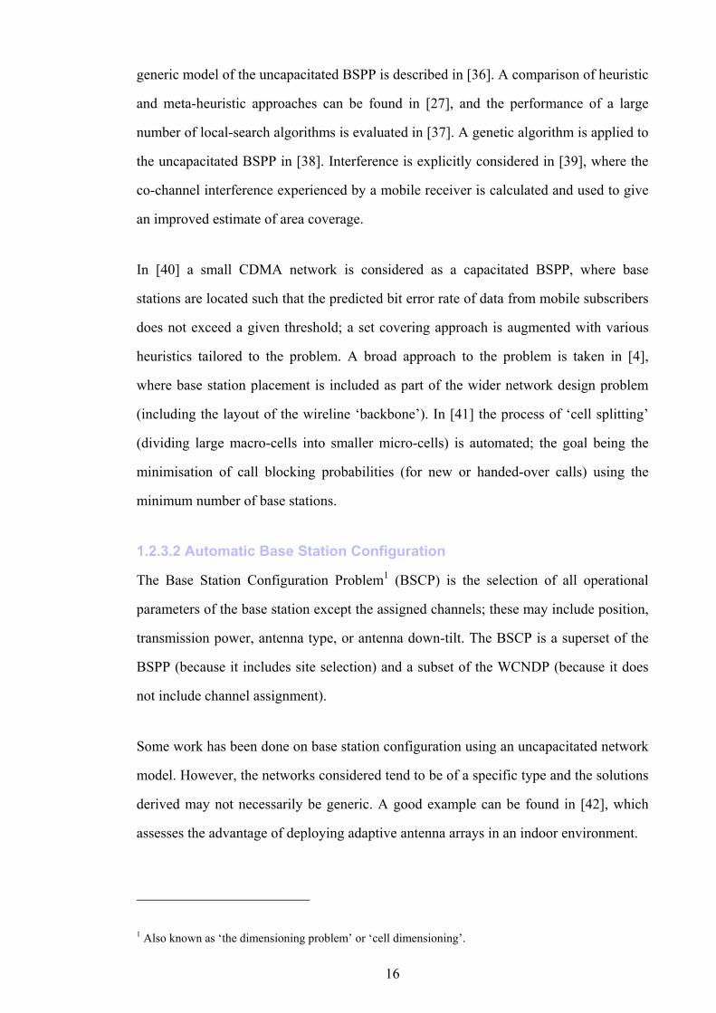
Figure 1.2: An example of different switching technologies connecting both wireless and wireline telephones.

The worldwide wireless and wireline telephone networks contain millions of

communication switches, and care is required in their deployment. Figure 1.2 shows an

1 The conversion from analogue to digital may happen before the data enters the telephone exchange. 2 The telephone number of the recipient will determine the destination of the data; the number will be used as an index to a dynamic database of subscriber locations maintained by the network.

4

example of the connectivity in a simplified communications network. Both wireless and

wireline equipment is connected together using switches, each of which has a maximum

call carrying capacity. In addition to creating an effective network (one which can

handle all the call traffic) the network designer must strive to minimise infrastructure

costs. Striking the correct balance between these competing goals takes skill and effort

− both of which are expensive commodities in themselves.

1.1.1 The Capacitated Network Design Problem

All communications switches have a limited call carrying capacity − at any one time

each switch may act as a conduit for only a finite number of telephone calls. Although

this maximum capacity varies widely for different technologies, it is a fundamental

limitation in the design of all communication systems (see [5] for a more detailed

explanation).

In abstraction, the Capacitated Network Design Problem1 (CNDP) involves the

provision of communication conduits between pairs of users2 (see [6] for a generic

problem formulation). A network with insufficient, or poorly deployed, switching

elements will not be able to transport all of the required call traffic, which will lead to

lost revenue and customer dissatisfaction. Conversely, a network that deployed too

many switches would have a high running cost and, hence, reduced profitability. A

network designer must also take account of many other issues including fault-tolerance

(by including ‘redundant’ switching elements), call delay from long wires, and switch

site availability. These problems tend to be technology specific (and hence, network

specific) so are often ignored in the study of ‘pure’ CNDPs.

Note that the CNDP is similar to the Broadcast Network Design Problem3 (BNDP), in

which a large number of users receive identical data. However, solutions for the BNDP

often exploit ‘economies of scale’ that are not present in the CNDP, and separate

1 Also known as the ‘point to point’ communication problem. 2 Communication may involve more than two users, but these ‘party calls’ are not common. 3 Also known as the ‘point to multi-point’ communication problem.

5

solutions must be sought for this problem (this is discussed in more detail in Section

1.2.3.1).

1.1.2 The Wireless Capacitated Network Design Problem

Wireless communication has two main advantages over wireline communication:

• Mobility: a wireless user is freer to move around than their wireline counterpart.

This is even more relevant in the case of multiple mobile-users, where wires would

soon get tangled.

• Economy: in a wireline network a significant portion of the wires are those that

terminate with the user. For example, from the switch on a telegraph pole to a

subscribers house (commonly known as the last mile problem). Using a wireless

connection for this portion of the network gives a significant saving in cable

installation1.

Conversely, wireless communication has two main disadvantages compared with

wireline communication:

• Poor signal propagation: a signal’s strength and quality will deteriorate more for

wireless transmission than for wireline transmission over the same distance. The

wire acts as a ‘wave guide’ for the signal, allowing precise propagation control.

• Poor noise immunity: wireline signals are shielded from noise sources, whereas

wireless signals may be easily contaminated by ‘stray’ radio waves.

1 It is worth noting that the cost of laying cable is usually significantly greater than the cost of the cable itself.

6

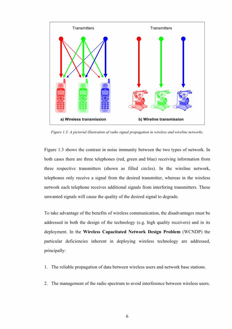
Transmitters Transmitters

a) Wireless transmission b) Wireline transmission

Figure 1.3: A pictorial illustration of radio signal propagation in wireless and wireline networks.

Figure 1.3 shows the contrast in noise immunity between the two types of network. In

both cases there are three telephones (red, green and blue) receiving information from

three respective transmitters (shown as filled circles). In the wireline network,

telephones only receive a signal from the desired transmitter, whereas in the wireless

network each telephone receives additional signals from interfering transmitters. These

unwanted signals will cause the quality of the desired signal to degrade.

To take advantage of the benefits of wireless communication, the disadvantages must be

addressed in both the design of the technology (e.g. high quality receivers) and in its

deployment. In the Wireless Capacitated Network Design Problem (WCNDP) the

particular deficiencies inherent in deploying wireless technology are addressed,

principally:

1. The reliable propagation of data between wireless users and network base stations.

2. The management of the radio spectrum to avoid interference between wireless users.

7

The solution of the WCNDP requires the location and configuration of network base

stations such that mobile subscriber demand is satisfied. This must be done in such a

way as to minimise the cost of deploying and running the network.

A key factor in creating high quality solutions to the WCNDP is the management of the

available radio spectrum. The restrictions imposed on base station deployment will vary

between different technologies, but limited spectrum availability remains a problem in

all wireless networks. The division of the spectrum (known as the multiple access

scheme) might be frequency based, as in Frequency Division Multiple Access (FDMA),

or it might be code based, as in Code Division Multiple Access (CDMA) (see [7] for

further information). Regardless of the multiple access scheme used, the same ‘piece’1

of radio spectrum cannot be re-used in the same place at the same time, as this would

result in interference.

1.2 Previous Work

This section contains an overview of previous approaches to solving the WCNDP, and

solutions to related problems are also included.

The exact formulation of the WCNDP is technology dependent and, as such, a variety of

models have arisen in which different aspects of the problem are emphasised. This has

led to the development of many different design techniques. The heterogeneity of

network models makes a quantitative comparison of design techniques impossible, and

therefore all comparisons must be made on a qualitative basis.

Some of the previous research (such as that on the problem of channel assignment)

relates only to a small part of the WCNDP. In this section these subproblems are

discussed and placed in the wider context of the WCNDP.

1 A channel in a FDMA scheme or a code in a CDMA scheme.

8

1.2.1 General Background Reading

A good introduction to radio communication can be found in [7]. More specific

information on mobile wireless communications can be found in [8-10], and a highly

accessible overview of the issues involved in designing wireless networks is given in

[11].

Information on the practical application of combinatorial optimisation can be found in

[12,13], and valuable insights into the theoretical aspects of combinatorial optimisation

can be found in [14,15]. An overview of the application of combinatorial optimisation

to problems in the field of telecommunications is given in [16].

1.2.2 Channel Assignment

The Channel Assignment Problem1 (CAP) is a well studied area of wireless network

design, and it is a sub-problem of the WCNDP (as described in Section 1.1.2). In the

CAP, only the channels assigned to base stations may vary, and all other network design

parameters (such as antenna selection or transmitter placement) are fixed. This section

contains a brief overview of the CAP, but a more complete taxonomy of problems and

solutions can be found in [17-19].

In the CAP a network is assumed to consist of a set of transmitters (TXs) and receivers

(RXs), where each RX requires an interference free signal from one or more TX. The

strength of the radio signal from each TX to each RX is known. The interference each

RX experiences is dependent on the separation between the channel used by the serving

TX and the channels used by interfering TXs – the greater the separation (in ‘channel

space’), the smaller the contribution of that signal to the total interference.

Given an unlimited radio spectrum, channel assignments could all be unique and

generously spaced, but unfortunately only a limited range of frequencies are suitable for

mobile communication, and it is smaller than the total number of channels required

1 Also known as the Frequency Assignment Problem (FAP).

9

worldwide. To maximise spectrum availability, portions of the spectrum must be reused.

This is only possible when RXs that share a common channel (or use channels that are

close enough to interfere) have sufficient electromagnetic isolation from one another.

As the range of wireless communication signals is small, typically line-of-site1, this is

not an insurmountable problem. Furthermore, in cities (where the demand for channels

is at its highest) the buildings provide RXs with extra shielding from interfering TXs,

and this allows the network designer more precise control over interference (an

observation made in [11]).

1.2.2.1 Fixed and Variable Spectrum

The CAP is usually stated in one of two forms: as a Variable Span Problem (VSP) or as

a Fixed Span Problem (FSP). The solution of the VSP requires all the RXs to have a

usable signal (i.e. to have acceptably low interference) whilst the difference between the

lowest and highest channels used (known as the span of the assignment) is minimised.

The solution of the FSP requires the maximum number of RXs to have a usable signal

given a fixed span of channels from which assignments may be made.

Network operators bidding for new spectrum licenses might adopt the VSP, as they

would need to know how much spectrum to buy. Another application might be in the

day-to-day allocation of spectrum in a theatre-of-war, as the reliance on radio

communications in modern warfare means that efficient spectrum management is

crucial.

Instances of the FSP are much more common than those of the VSP. The biggest users

of radio spectrum are commercial network operators (such as broadcasters, mobile

telephone companies, and taxi firms) and they usually have exclusive rights to a

particular portion of the radio spectrum2. Commercial networks typically have a

1 Some low-frequency radio signals have a much further range. However, high frequency signals (which are most useful for high bandwidth communications) have a short range. 2 This may vary with location, for instance two taxi firms might use the same part of the spectrum but in different cities.

10

consumer base of subscribers (or potential subscribers) who require interference free

radio-communication either one-way (e.g. TV broadcasts) or two-ways (e.g. mobile

telephone calls); they wish to maximise the number of subscribers covered (and hence

revenue) using the spectrum they have available. It will be assumed that all CAPs are

FSPs for the remainder of this thesis.

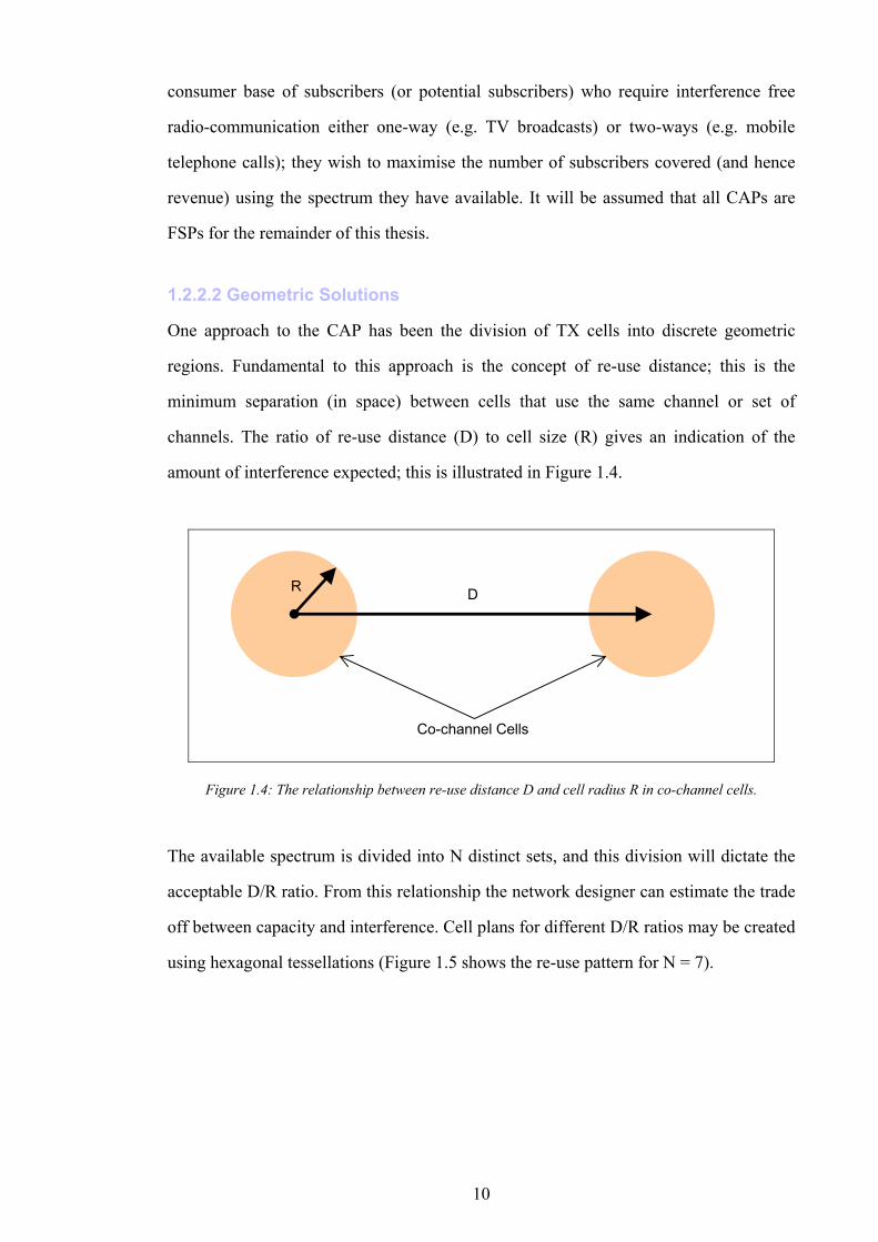
1.2.2.2 Geometric Solutions

One approach to the CAP has been the division of TX cells into discrete geometric

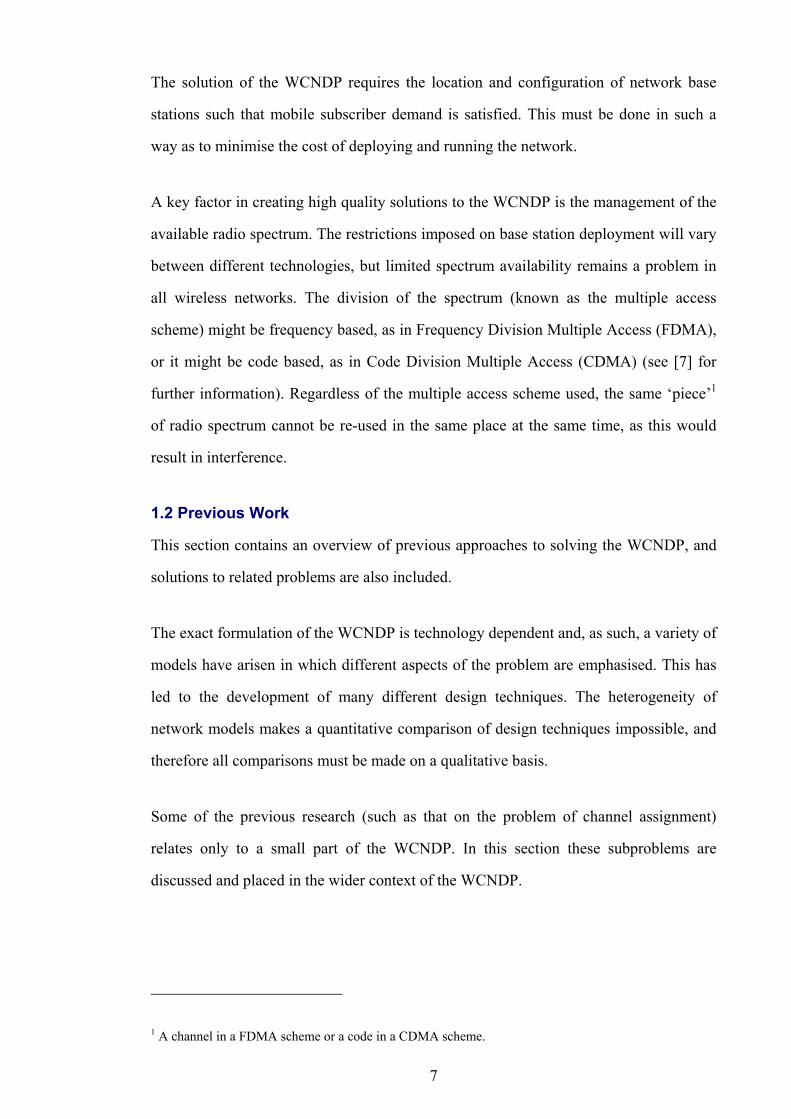
regions. Fundamental to this approach is the concept of re-use distance; this is the

minimum separation (in space) between cells that use the same channel or set of

channels. The ratio of re-use distance (D) to cell size (R) gives an indication of the

amount of interference expected; this is illustrated in Figure 1.4.

D R

Co-channel Cells

Figure 1.4: The relationship between re-use distance D and cell radius R in co-channel cells.

The available spectrum is divided into N distinct sets, and this division will dictate the

acceptable D/R ratio. From this relationship the network designer can estimate the trade

off between capacity and interference. Cell plans for different D/R ratios may be created

using hexagonal tessellations (Figure 1.5 shows the re-use pattern for N = 7).

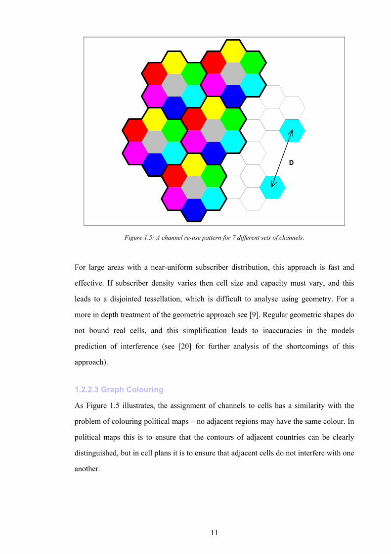
11

D

Figure 1.5: A channel re-use pattern for 7 different sets of channels.

For large areas with a near-uniform subscriber distribution, this approach is fast and

effective. If subscriber density varies then cell size and capacity must vary, and this

leads to a disjointed tessellation, which is difficult to analyse using geometry. For a

more in depth treatment of the geometric approach see [9]. Regular geometric shapes do

not bound real cells, and this simplification leads to inaccuracies in the models

prediction of interference (see [20] for further analysis of the shortcomings of this

approach).

1.2.2.3 Graph Colouring

As Figure 1.5 illustrates, the assignment of channels to cells has a similarity with the

problem of colouring political maps – no adjacent regions may have the same colour. In

political maps this is to ensure that the contours of adjacent countries can be clearly

distinguished, but in cell plans it is to ensure that adjacent cells do not interfere with one

another.

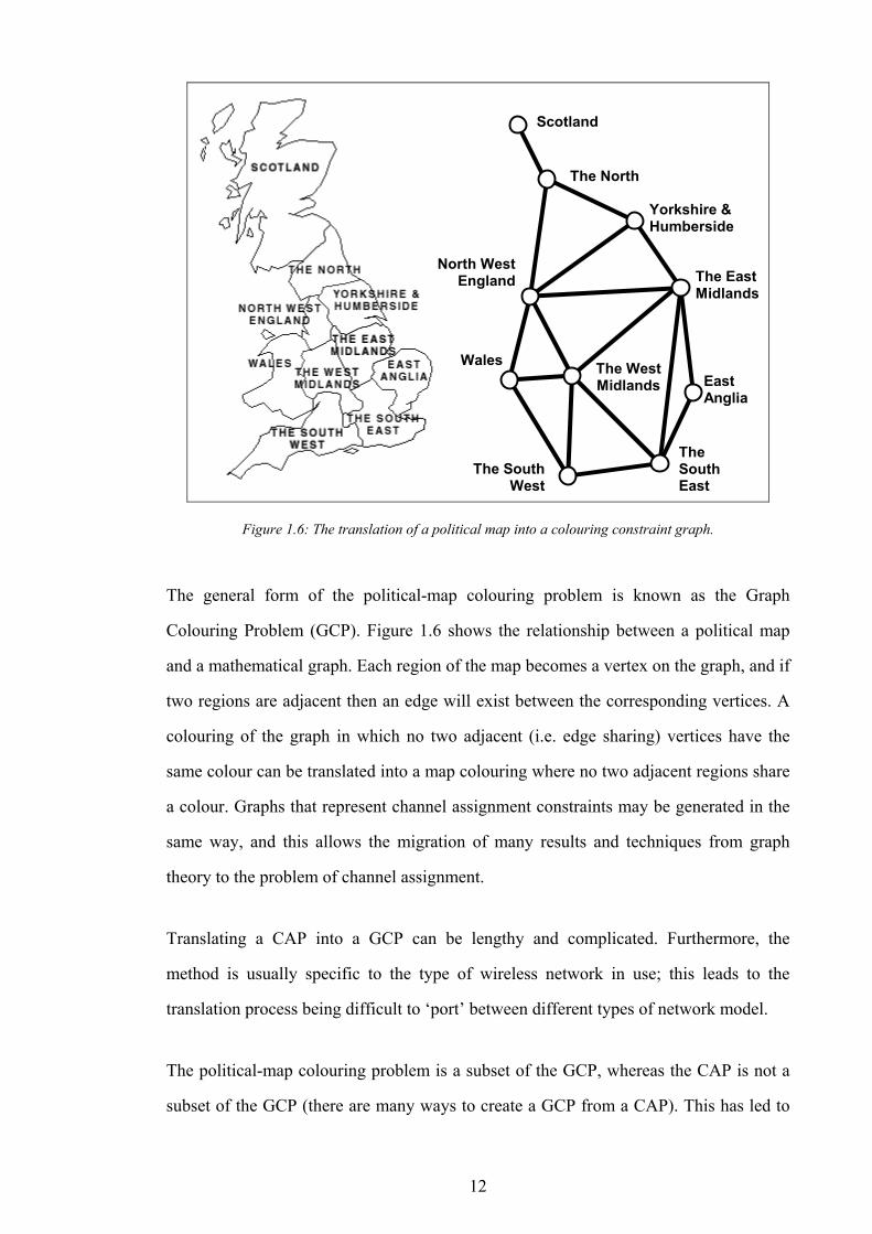
12

Scotland

The North

North West England

Wales

The SouthWest

The West Midlands

Yorkshire & Humberside

The East Midlands

The South East

East Anglia

Figure 1.6: The translation of a political map into a colouring constraint graph.

The general form of the political-map colouring problem is known as the Graph

Colouring Problem (GCP). Figure 1.6 shows the relationship between a political map

and a mathematical graph. Each region of the map becomes a vertex on the graph, and if

two regions are adjacent then an edge will exist between the corresponding vertices. A

colouring of the graph in which no two adjacent (i.e. edge sharing) vertices have the

same colour can be translated into a map colouring where no two adjacent regions share

a colour. Graphs that represent channel assignment constraints may be generated in the

same way, and this allows the migration of many results and techniques from graph

theory to the problem of channel assignment.

Translating a CAP into a GCP can be lengthy and complicated. Furthermore, the

method is usually specific to the type of wireless network in use; this leads to the

translation process being difficult to ‘port’ between different types of network model.

The political-map colouring problem is a subset of the GCP, whereas the CAP is not a

subset of the GCP (there are many ways to create a GCP from a CAP). This has led to

13

variants of the GCP being adopted that better approximate the CAP. Examples include

the addition of weighting to the graph edges, as described in [21], and the generalisation

from binary graphs (graphs with only two vertices per edge) to hyper graphs (graphs

with many vertices per edge), as described in [18].

The advantage of adopting a graph theoretic approach lies in the wealth of techniques

already derived for the GCP. A good example of this is lower-bounding [22], which can

provide an estimate of the minimum number of distinct colours required to satisfy a

given graph.

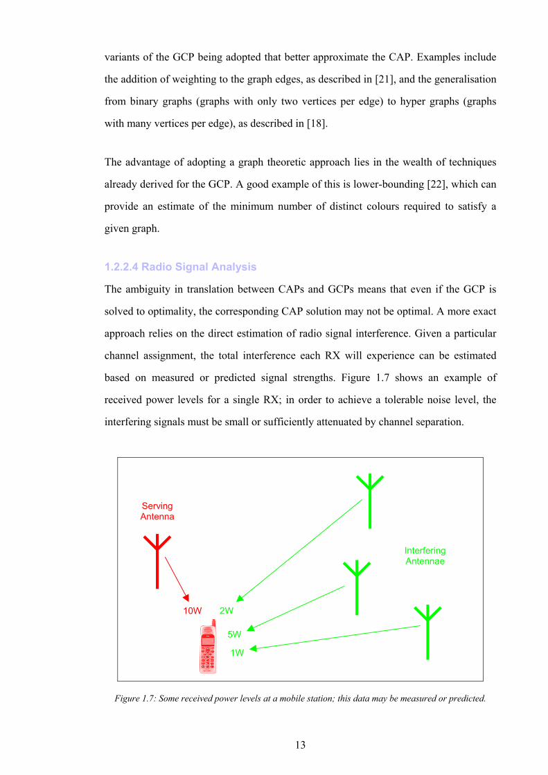
1.2.2.4 Radio Signal Analysis

The ambiguity in translation between CAPs and GCPs means that even if the GCP is

solved to optimality, the corresponding CAP solution may not be optimal. A more exact

approach relies on the direct estimation of radio signal interference. Given a particular

channel assignment, the total interference each RX will experience can be estimated

based on measured or predicted signal strengths. Figure 1.7 shows an example of

received power levels for a single RX; in order to achieve a tolerable noise level, the

interfering signals must be small or sufficiently attenuated by channel separation.

Serving Antenna

Interfering Antennae

10W 2W

5W

1W

Figure 1.7: Some received power levels at a mobile station; this data may be measured or predicted.

14

This approach gives the most accurate representation of the CAP, as it takes account of

everything that can be either measured or predicted. Some studies of the effectiveness of

this approach have been done (examples include [23]), and it has been shown to deliver

the highest quality solutions of any of the channel assignment methods. The

computational requirements of this approach are high, and this has meant that less exact

methods (such as graph colouring) have dominated the creation of channel assignments.

On-going improvements in areas such as microprocessor speed, compiler technology,

and software engineering have increased the size of problem for which this technique

can deliver superior solutions; some studies have been made of the scalability of this

approach versus less exact methods (see [24]) but the results remain inconclusive.

1.2.3 Cell Planning

At the time of writing, there are many commercial Computer Aided Design (CAD)

systems for cell planning available; examples include ATOLL (by FORSK), Wizard (by

Agilent Technologies), deciBell Planner (by Northwood), and Asset (by AIRCOM). An

introduction to the issues involved in CAD for mobile telephone networks can be found

in [20,25]. All current CAD systems require a user to decide base station locations and

configurations; feedback about network performance (information such as area

coverage and infrastructure costs) comes from a computer simulation.

The elimination of the user from the ‘design loop’ is a natural progression of the CAD

paradigm (as concluded in [20]). The user should be required to specify the desired

network performance, and not be required to specify the details of the network design

needed to achieve it. The following subsections describe research into the automation of

the network design process.

1.2.3.1 Automatic Base Station Placement

The Base Station Placement Problem (BSPP) is a subproblem of the WCNDP, and there

are two common formulations of this problem. In the first, known as uncapacitated, the

subscribers only require a usable (i.e. sufficiently strong) radio signal. In the second,

known as capacitated, base stations are limited by the maximum number of subscribers

15

they can serve. The uncapacitated problem (referred to as the BNDP in Section 1.1.1) is

typical of the requirements a television distribution network might have. The simplest

solution to this problem is typified by satellite television technology, in which one

transmitter (the satellite) can transmit information to an entire country. This type of

solution is not well suited to capacitated networks, where each subscriber requires

different data streams; in fact, a single-satellite solution would only allow the available

spectrum to be used once for the entire area covered by the satellite1.

Models for the BSPP are further divided in their approach to site availability. In some

previous work (such as [26]) a pure BSPP is formulated, in which base stations may be

placed anywhere within the working area of the network. Whereas in other work (such

as [27]) a subset BSPP is formulated, in which the set of candidate sites is decided by

the user and the computer selects a subset for occupation. The subset BSPP represents

the majority of practical problems, as network operators find it more efficient to select

sites based on their cost, availability, and practicality rather than on their suitability for

radio communications (see [3] for similar reasoning).

It is interesting to note that base station (or transmitter) placement in network design has

much in common with the Facility Location Problem (FLP) (see [28] for a

comprehensive description of the FLP).

Research on the BSPP for uncapacitated networks can be found in [29-32]; a common

goal in previous work has been the maximisation of cover (the number of receivers with

a sufficiently strong signal) coupled with the minimisation of infrastructure cost. The

application of Artificial Intelligence (AI) to the uncapacitated BSPP is explored in [33],

where an expert system is developed as a ‘drop in replacement’ for the network

designer. In [34] graph theory is used to simplify the solution of the uncapacitated

BSPP; this work was part of the STORMS project [35]. Complexity analysis for a

1 It should be noted that this fundamental problem has not stopped commercial vendors utilising satellites for mobile communications; although it is inefficient for densely populated areas it is well suited to sparse ones. In this thesis, only densely populated areas are considered.

16

generic model of the uncapacitated BSPP is described in [36]. A comparison of heuristic

and meta-heuristic approaches can be found in [27], and the performance of a large

number of local-search algorithms is evaluated in [37]. A genetic algorithm is applied to

the uncapacitated BSPP in [38]. Interference is explicitly considered in [39], where the

co-channel interference experienced by a mobile receiver is calculated and used to give

an improved estimate of area coverage.

In [40] a small CDMA network is considered as a capacitated BSPP, where base

stations are located such that the predicted bit error rate of data from mobile subscribers

does not exceed a given threshold; a set covering approach is augmented with various

heuristics tailored to the problem. A broad approach to the problem is taken in [4],

where base station placement is included as part of the wider network design problem

(including the layout of the wireline ‘backbone’). In [41] the process of ‘cell splitting’

(dividing large macro-cells into smaller micro-cells) is automated; the goal being the

minimisation of call blocking probabilities (for new or handed-over calls) using the

minimum number of base stations.

1.2.3.2 Automatic Base Station Configuration

The Base Station Configuration Problem1 (BSCP) is the selection of all operational

parameters of the base station except the assigned channels; these may include position,

transmission power, antenna type, or antenna down-tilt. The BSCP is a superset of the

BSPP (because it includes site selection) and a subset of the WCNDP (because it does

not include channel assignment).

Some work has been done on base station configuration using an uncapacitated network

model. However, the networks considered tend to be of a specific type and the solutions

derived may not necessarily be generic. A good example can be found in [42], which

assesses the advantage of deploying adaptive antenna arrays in an indoor environment.

1 Also known as ‘the dimensioning problem’ or ‘cell dimensioning’.

17

The majority of work relating to the BSCP is based on a capacitated network model, and

some solutions to the general problem of base station configuration can be found in

[43,44]. In [45] the evolution of a network over time is considered, which is an

important concern in commercial networks where subscriber demand is constantly

changing and generally increasing. The ‘connectivity’ of cell coverage is discussed in

[46]; cells that are irregular or fragmented have a detrimental effect on network

performance, specifically they make channel assignment more difficult and they

increase the probability of handover for mobile subscribers. In most of the network

models studied, only the transmission of a radio signal from the base station to the

mobile station (the downlink) is considered, and it is assumed that the uplink is either

easy to maintain or difficult to model. In [47] simulation of both the uplink and

downlink is considered, and its effect on the optimisation process discussed. The Pareto

optimality of the cell planning problem is discussed in [48]; this approach can provide

network designers with valuable insights into the intrinsic compromise’s that must be

made in solving a multi-objective problem such as cell planning.

Some work on the BSCP explicitly considers the channel assignment that follows the

completion of a cell plan. In [49] a simple network model is augmented with channel

assignment constraints. A novel approach to including channel assignment in the cell

planning process is used in [50], where lower bounding techniques (as described in

Section 1.2.2.3 and [22]) are used as an indicator of the ‘difficulty of channel

assignment’ without actually producing a complete assignment. The most

comprehensive treatment of the full WCNP is detailed in [72], in which channels are

assigned to optimised cell plans, but the relationship between the cell plan and the

channel plan is not explored in detail.

1.2.4 Shortcomings of Previous Work

This subsection describes some of the shortcomings of previous approaches to the

WCNDP. It is important to separate the underlying network model, by which all

candidate network designs must be judged, from the optimisation algorithms employed

to create candidate designs. Much effort has been expended on the application of

18

combinatorial algorithms to classical problems, which, by definition, have a standard

formulation (see [51] for example). Optimisation algorithms can be ‘tailored’1 to the

classical problems because the underlying evaluation function does not change, and this

allows assumptions to be made and shortcuts to be taken in the optimisation procedure.

However, the WCNDP has not reached a universally agreed formulation, and

assumptions may not be valid over the set of all formulations. This implies that the

tailoring of algorithms to a particular problem formulation may prove ‘wasted effort’

even if the formulation of the problem is altered only slightly. Worse still, the bias

introduced by a tailored algorithm could exclude sets of good solutions. In this thesis,

more attention is paid to the formulation of the problem than to the design of ‘clever’

optimisation techniques, and care has been taken to ensure that the optimisation

algorithms are generic; that is to say, they do not introduce bias by excluding possible

solutions and, hence, remain applicable to future formulations of the WCNDP. An

alternative approach would be to develop a simpler formulation of the WCNDP and

search for the ideal optimisation algorithm with which to solve it. This ideal algorithm

would be highly specific to the problem formulation and, hence, potentially inapplicable

to a wider set of problems, furthermore the particular WCNDP used may not be

sufficiently complex to be relevant to industry.

This thesis builds upon the model of a GSM network described in [2]. This model was

developed by industry, and is known to be used by at least two major European mobile

telephone network operators. The high availability of data (problem instances) for this

model also favoured its adoption. Other authors have extended this basic model to take

account of a variety of different problems (for example [45] describes a network ‘roll-

out’ scenario), and in this thesis an interference model was added, which considered

channel assignments. Channel assignment has been considered in the wider context of

cell planning (in work such as [49] and [50]) but only simple models were used; no

1 Usually manifest as embedded heuristics that can reject possible solutions as inferior without resorting to a (computationally intensive) full evaluation of the solutions performance.

19

work to date had explicitly considered the relationship between cell planning and

channel assignment. This significant omission was addressed in this thesis.

1.3 Thesis Aims and Objectives

The aim of this thesis was the development of techniques for solving the WCNDP, and

this general aim was divided into two objectives that were further divided into specific

tasks. The completion of tasks and objectives is explicitly mentioned in the thesis text,

and they are enumerated here to facilitate those references.

1.3.1 Objective O1: Statement of Problem

Previous formulations of the WCNDP do not completely represent the requirements of

the mobile telephone network designer, and an objective of this thesis was the

formulation of a more comprehensive WCNDP. The following tasks were completed in

order to meet this objective:

Task T1: Acquisition of industrial data for the simulation of mobile telephone

networks. The quality of the data obtained dictates the accuracy of the

simulations and, hence, the relevance of the network designs produced.

Task T2: Mathematical specification of the simulator. To communicate the details of

the network simulator concisely and without ambiguity a mathematical

description was derived. Without a clear description the model could not be

effectively criticised or accurately reproduced.

Task T3: Specification of network performance requirements. It was necessary to

identify a set of objectives that each network design must fulfil, as this is the

mechanism by which one candidate design may be judged against another.

Although such a specification of requirements is typical in the engineering

process, automatic design techniques require that it be expressed

algorithmically.

20

1.3.2 Objective O2: Development of Solutions

The formulation of the WCNDP derived to meet O1 provided a test-bed for the

development of optimisation algorithms. The effective application of automatic

optimisation to the WCNDP is broken down into the following stages:

Task T1: Simple optimisation algorithms were implemented and applied to the

WCNDP. The validity of this approach was demonstrated by the production

of high quality network designs in a reasonable time.

Task T2: Assessment of the advantages of separating the CAP from the rest of the

WCNDP. In Section 1.2.4 it was observed that the CAP is rarely considered

as part of the WCNDP, and channel assignment (if required) is only done

when all other parameters have been fixed.

Task T3: The optimisation procedures that produced the best network designs were

identified. Finding the ‘best’ optimisation algorithm was not the principal

goal of this thesis (as observed in Section 1.2.4), but it was still of interest.

Task T4: The specification of improvements that may be desirable to both the

network model and the optimisation methodology.

1.4 Test Platform

When assessing the performance of an optimisation algorithm, the best solution

produced must be placed in context by the amount of computer power that was required

to produce it. It is not easy to accurately describe computer power by any single figure

(such as the number of floating point operations performed) as it depends on many

factors (such as memory size and hard disk access speed). All of the results generated in

this thesis were done using the same computer operating under the same conditions, as

this approach eliminates (as far as possible) the distortion of results due to platform

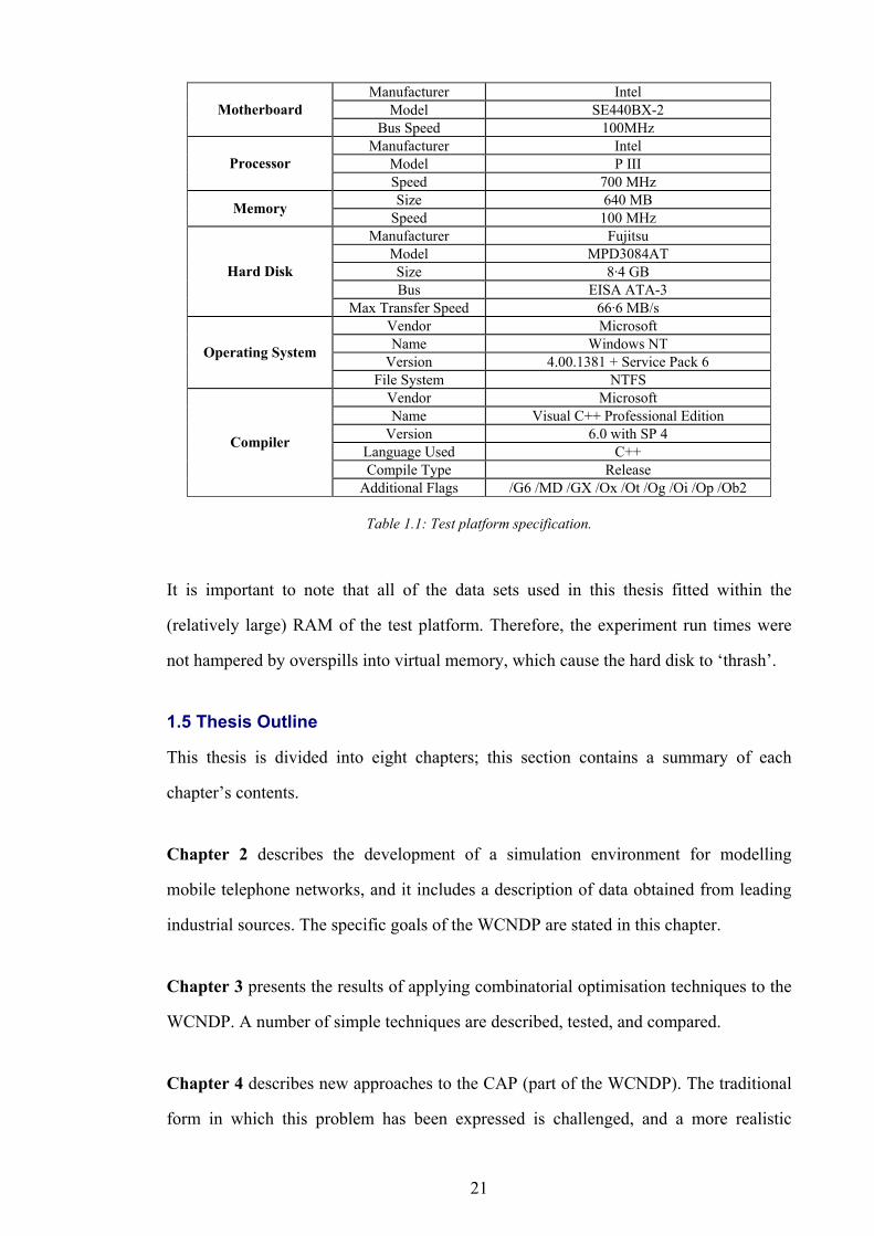
heterogeneity. Table 1.1 contains all of the defining characteristics of the test platform,

which corresponds to best practice as identified in [52].

21

Manufacturer Intel Model SE440BX-2 Motherboard

Bus Speed 100MHz Manufacturer Intel

Model P III Processor Speed 700 MHz Size 640 MB Memory Speed 100 MHz

Manufacturer Fujitsu Model MPD3084AT Size 8·4 GB Bus EISA ATA-3

Hard Disk

Max Transfer Speed 66·6 MB/s Vendor Microsoft Name Windows NT

Version 4.00.1381 + Service Pack 6 Operating System

File System NTFS Vendor Microsoft Name Visual C++ Professional Edition

Version 6.0 with SP 4 Language Used C++ Compile Type Release

Compiler

Additional Flags /G6 /MD /GX /Ox /Ot /Og /Oi /Op /Ob2

Table 1.1: Test platform specification.

It is important to note that all of the data sets used in this thesis fitted within the

(relatively large) RAM of the test platform. Therefore, the experiment run times were

not hampered by overspills into virtual memory, which cause the hard disk to ‘thrash’.

1.5 Thesis Outline

This thesis is divided into eight chapters; this section contains a summary of each

chapter’s contents.

Chapter 2 describes the development of a simulation environment for modelling

mobile telephone networks, and it includes a description of data obtained from leading

industrial sources. The specific goals of the WCNDP are stated in this chapter.

Chapter 3 presents the results of applying combinatorial optimisation techniques to the

WCNDP. A number of simple techniques are described, tested, and compared.

Chapter 4 describes new approaches to the CAP (part of the WCNDP). The traditional

form in which this problem has been expressed is challenged, and a more realistic

22

approach is described that aims to better represent the problem of spectrum

management.

Chapter 5 describes interference surrogates and evaluates them with respect to their

ability to predict subscriber cover.

Chapter 6 contains a comparison of the approach described in Chapter 3 to the two-

stage process discussed in Chapter 5.

Chapter 7 contains the conclusions that may be drawn from the thesis results, and

suggestions for future research on the WCNDP (including improvements to the design

process, and extensions of the underlying network model).

23

Chapter 2 Network Model

This chapter describes a mathematical model of a cellular mobile-telephone network. It

is based around, but not exclusive to, GSM. The model was developed for the purpose

of this thesis, and it is intended to represent industrial models currently in use. It takes

account of network coverage and capacity requirements, and it also considers the effect

that channel assignment has on interference. The Wireless Capacitated Network Design

Problem (WCNDP), as outlined in Section 1.1.2, is formulated in this chapter.

The structure of this chapter is as follows: Section 2.1 explains some of the issues raised

by the specification of the model, Section 2.2 contains a description of the actual model

used, and Section 2.3 contains details of the network data sets used in this thesis.

2.1 Simulation Issues

This section contains an explanation of the key design decisions made during the

specification of the network simulator. All the data sets used have been obtained from

companies that operate mobile telephone networks, and this has meant that some design

decisions are ‘inherited’ and, therefore, inflexible.

2.1.1 Limitations on Prediction Accuracy

Some aspects of mobile telephone networks are impossible to model exactly, for

example it is not possible to say at what times a particular subscriber will make or

24

receive calls. Quantities such as this may only be modelled on a probabilistic or

statistical basis, e.g. 80% of telephone calls will be made between the hours of 9am and

5pm. The prediction of network performance (the model’s output) is limited by the

accuracy of network data (the model’s inputs), but it is not easy to quantify the effect

that errors in the model’s input have on the model’s output.

2.1.2 Discretisation

For networks to be simulated using a computer, the data which defines them must be

discretised (or digitised). Some network data is inherently discrete, e.g. the number of

base stations, whereas other data is continuous (or analogue), e.g. the azimuth of a

directional antenna. Discretisation of an analogue quantity introduces inaccuracies (or

noise). All of the data used in this thesis had been prepared by network operators, and

most decisions regarding discretisation (such as the resolution of the terrain model)

cannot, therefore, be changed.

2.1.3 Rasterisation

A raster is a discrete, regular, and rectangular grid of data. Typically it is two-

dimensional (e.g. the picture elements, or pixels, in a television picture). A co-ordinate

vector can uniquely identify the data elements in the grid, and the datum at a particular

grid location may be digital or analogue. The process of converting data into a raster

format is known as rasterisation or, sometimes, rendering.

The model used for a mobile telephone network brings together data from a variety of

sources. This data does not necessarily conform to a common standard, which makes

interoperability difficult. Rasterisation facilitates interoperability between data sources

such as:

• The terrain databases derived from topographical relief maps.

• The vector based building models used for radio propagation prediction in urban

areas.

25

• The call traffic density information. This is sometimes derived from postcode

information, which describes discrete regions but is not constrained by a raster grid.

Not all data needs to be rasterised, for instance the location of base station sites can be

described as a free-vector within the network region without conflicting with other data

formats.

2.1.4 Spatial Dimensionality

The model used is essentially two-dimensional. Although some data, such as

propagation information, may have been derived from three-dimensional models, the

result is ultimately amalgamated into cells of a two-dimensional raster. The choice of a

two-dimensional model limits the accuracy of prediction, and this is especially true in

dense, urban areas where calls may occur in tall buildings. The advantage of two-

dimensional models is in the speed of evaluation.

2.1.5 Call Traffic Prediction

A statistical approach is used to assess the number of subscribers covered. The call

traffic (number of calls per hour) expected during the ‘busy hour’ is amalgamated into a

single figure (measured in Erlangs) for each geographic area. This is a typical,

conservative, approach to network capacity planning, i.e. it is implicitly assumed that a

network that can accommodate the peak traffic will be able to accommodate traffic for

all other times.

2.1.6 Uplink and Downlink

The network model only simulates the link from the base station to the mobile station

(known as the downlink or forward link), and the uplink is ignored. In general, the

quality of the circuitry in the base stations is higher than in the mobiles, and hence the

uplink signal can be more easily distinguished than that of the downlink (making the

downlink the limiting factor). The computational complexity of uplink simulation is

prohibitive, and the decision to ignore uplinks is inherited from the network operators

(i.e. they do not consider the uplink in the majority of their network simulations). In this

26

thesis, the simulation techniques used by operators have been adopted in order to

maximise the industrial relevance of the optimisation algorithms developed, but it is

worth noting that uplink is considered to be a limiting factor in CDMA networks and

may be explicitly considered during the optimisation process (see [40] for an example).

2.1.7 Fixed Base Station Sites

Base station site rental represents a significant portion of the cost of running a network,

typically the sites desired by network designers (based on their suitability for wireless

communications) are not always easy to obtain and may be subject to planning

regulations. A strategy popular with network operators has been to make site-acquisition

largely independent of the network design requirements, as this allows the identification

of a large number of potential sites that are easy to obtain (short lead-time) and

relatively cheap to occupy − in the network model these are known as candidate sites.

This approach increases the burden on the network design process, as undesirable sites

(such as electricity pylons) must be more intelligently utilised than those that are highly

desirable (such as the Eiffel Tower).

2.1.8 Radio-Propagation Prediction

The radio signal propagation in the network area was precalculated and provided as part

of the network data set. The prediction algorithms used in the network model are based

on the COST231 Walfish-Ikegami models (see [53] for further information), but these

propagation algorithms are computationally intensive. The fast simulation of a network

relies on the fact that (potentially slow) propagation predictions can be precomputed,

and this is possible for the following reasons:

• Only the downlink is simulated. This means that (potentially complex) uplink

propagation predictions can be avoided.

• Base station sites are fixed. Downlink propagation predictions are made from each

of the candidate sites to each of the possible mobile station locations.

27

• The propagation calculation can be performed independently of most base station

parameters. The relative (normalised) propagation gain can be included in the

calculation of signal strength as an independent factor.

Note, base station height does affect the relative propagation, however, the data sets

obtained for this thesis do not permit this parameter to vary. If height were desired to be

a variable then each different height could be treated as a different site, as this would

allow the pre-computation of propagation.

The frequency of a radio signal also affects its propagation, but across the range of

permitted frequencies the variation in propagation will be small, therefore the mean

frequency is used for the propagation calculation.

2.1.9 Best Server

When modelling the behaviour of base stations in a network it is necessary to know how

much call traffic they will be serving. This allows an estimate to be made of the number

of channels each base station will require (see Section 2.1.5). The ‘best server’ of a

mobile station is the base station from which it receives the strongest radio signal, and it

is assumed that a mobile station will always make a call through its best server. This

implies that the set of all the mobile stations for which a base station is ‘best server’

gives a prediction of that base station’s traffic-carrying requirement. The best server

model gives a conservative estimate of a network’s traffic capacity because each base

station can only accommodate a fixed amount of traffic, and any traffic above that limit

must be considered lost. In the best server model this ‘lost’ traffic is not allowed to be

covered by other base stations − even if they offer interference-free communication

channels. A more accurate estimate of traffic cover can be achieved with a more

sophisticated model, but its disadvantages make best server the most sensible model to

adopt. These disadvantages are summarised in the following subsection, but they are not

central to the thesis and may be skipped.

28

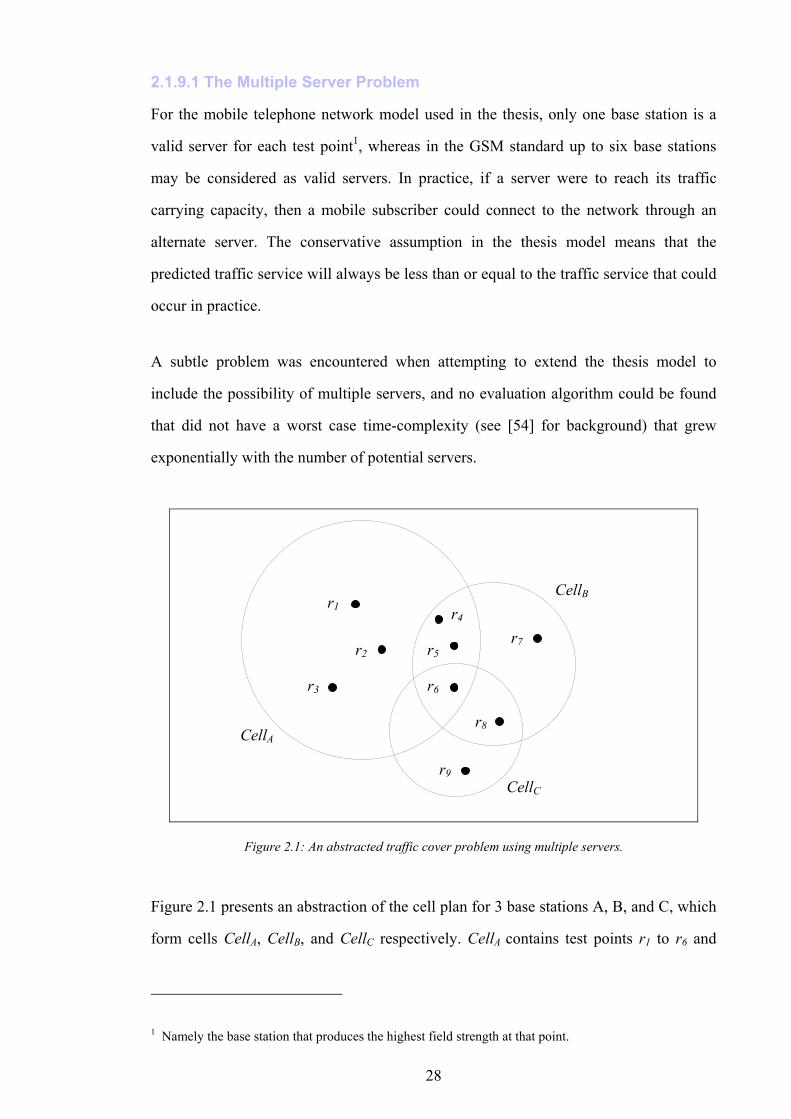
2.1.9.1 The Multiple Server Problem

For the mobile telephone network model used in the thesis, only one base station is a

valid server for each test point1, whereas in the GSM standard up to six base stations

may be considered as valid servers. In practice, if a server were to reach its traffic

carrying capacity, then a mobile subscriber could connect to the network through an

alternate server. The conservative assumption in the thesis model means that the

predicted traffic service will always be less than or equal to the traffic service that could

occur in practice.

A subtle problem was encountered when attempting to extend the thesis model to

include the possibility of multiple servers, and no evaluation algorithm could be found

that did not have a worst case time-complexity (see [54] for background) that grew

exponentially with the number of potential servers.

CellA

CellB

CellC

r6

r5 r7

r1

r3

r4

r2

r8

r9

Figure 2.1: An abstracted traffic cover problem using multiple servers.

Figure 2.1 presents an abstraction of the cell plan for 3 base stations A, B, and C, which

form cells CellA, CellB, and CellC respectively. CellA contains test points r1 to r6 and

1 Namely the base station that produces the highest field strength at that point.

29

CellB contains test points r4 to r8, in a multiple server model the points in the

intersection of CellA and CellB may be served by either base station A or base station B.

Assume that each test point represents 10 Er of traffic and that each base station may

serve up to 30 Er of traffic, therefore each base station may serve a maximum of 3 test

points. By inspection it can be seen that if base station A serves r1, r2, and r3, base

station B serves r4, r5, and r7, and base station C serves r6, r8, and r9 then full coverage

can be achieved (i.e. 3 test points per base station). The problem lies in identifying

which points to allocate to which base stations; consider the evaluation procedure below

that allocates points to base stations in the (arbitrary) order they have been defined:

1. Points r1, r2, and r3 are allocated to base station A.

2. Points r4, r5, and r6 are allocated to base station B.

3. Point r7 could only have gone to base station B, but B has already reached capacity

and hence it must be discarded

4. Points r8 and r9 are allocated to base station C.

Due to the discarding of test point r7, the total traffic coverage will be 10 Er less than

the potential maximum (found previously by inspection).

A variety of approaches were tried to overcome this problem but no suitable algorithm

was discovered, all heuristic based approaches tested (for example, ordering test points

by number of potential servers) were found to be defeated by pathological cases. An

algorithm based on hypergraphs was devised that guaranteed delivery of the correct

traffic coverage, however, analysis showed it to have a worst case time complexity that

increased exponentially with the number of potential servers, and testing proved this led

to long and unpredictable evaluation times. The performance of this algorithm was

compared to the simple algorithm employed in the thesis, and in no test case did the

traffic prediction from the best server model fall more than 5% below the actual

(multiple server model) value. This was felt to be an acceptable inaccuracy, especially

30

as the estimate was always conservative. Note that this problem can only occur in

situations where maximum base station capacity is reached by a base station, if all base

stations are operating below capacity then the best server prediction will be no less

accurate.

2.1.10 Fuzzy Servers

Although the ‘best server’ assumption is essential in determining a base stations channel

requirements, it is not safe to assume that mobile stations will communicate exclusively

through their best server. The best server of a mobile station may not be the one

predicted by the simulator, due, for example, to inaccuracies in the prediction of radio-

signal strength. To decrease the chance of these ‘server ambiguities’ creating unforeseen

interference, a set of potential servers is identified. This comprises base stations that

provide the mobile station with a sufficiently strong signal to ‘capture’ it from its

(predicted) best server. The set of potential servers is known as the fuzzy-server set, and

it includes all the base stations that provide the mobile station with a signal within a

fixed tolerance of the best-server signal. This tolerance corresponds, in part, to the

cumulative error expected in the predicted radio-signal strengths.

2.1.11 Fixed Spectrum

A network operator will typically lease the use of a fixed portion of the radio spectrum,

and once the spectrum is leased there is no benefit in not using all of it. The wider the

portion of spectrum available, the easier it is to minimise signal interference. In the

network model it is assumed that a fixed spectrum is available for communication.

Section 1.2.2.1 contains a summary of the fixed and variable approaches to spectrum

management.

2.1.12 Handover

Handover (or handoff) is the transition of a mobile from one server to another. This is

most usually between adjacent base stations in a network, and occurs as the user passes

out of one cell and into another – thus ensuring an uninterrupted service for mobile

31

users. Base stations have the ability to change communication channels mid-call, and

these changes may also be refered to as handover.

The network model takes no account of ‘handover’ performance. Handover models

have been proposed (examples include [2]) but their accuracy is not well defined.

Suggestions for the addition of handover performance models are included in Section

7.2.1.

2.2 Description of Model

The model used for the simulation of mobile-telephone networks is an extension of the

one used in [2]. Network data sets that complement this model have been obtained from

two network operators: four data sets from Operator A and one data set from Operator B

(this corresponds to Task T1 of Objective O1 in Section 1.3). In the original model,

interference was not explicitly calculated, but in the new model it was decided to

include the assignment of base station channels, thereby allowing the simulation of

signal interference. The following thesis subsections describe all the elements of the

network model (this corresponds to Task T2 of Objective O1 in Section 1.3).

2.2.1 Summary of Data Set

The data sets for the network model consist of the following elements:

• Network working area boundary.

• Subscriber service and demand requirement maps.

• Candidate sites for base station placement, including radio propagation information.

• Base station antenna types.

• Radio spectrum availabilty and characteristics.

The following subsections describe these elements in more detail.

32

2.2.2 Working Area

A network, N, contains a working area, and points in the working area may be described

by their x and y co-ordinates. Two types of point are located on the working area:

• Points at which a wireless service is required (known as test points)

• Candidate (or potential) sites where base stations may be positioned.

The test point data forms a two-dimensional raster, where the resolution of the raster

grid along the x-axis (east-west) and y-axis (north-south) is given by PXn and PYn

respectively. The size of each test point is the same for both the x and y axes, and is

denoted by GPl .

1

1

2

2

nPY

lGP

lGP

nPX

Figure 2.2: Rasterisation of the network working area.

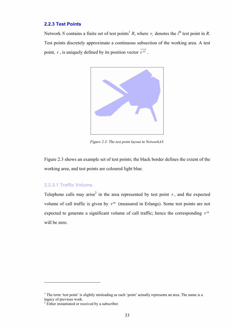
33

2.2.3 Test Points

Network N contains a finite set of test points1 R, where ir denotes the ith test point in R.

Test points discretely approximate a continuous subsection of the working area. A test

point, r , is uniquely defined by its position vector XYr .

Figure 2.3: The test point layout in NetworkA3.

Figure 2.3 shows an example set of test points; the black border defines the extent of the

working area, and test points are coloured light blue.

2.2.3.1 Traffic Volume

Telephone calls may arise2 in the area represented by test point r , and the expected

volume of call traffic is given by TRr (measured in Erlangs). Some test points are not

expected to generate a significant volume of call traffic; hence the corresponding TRr

will be zero.

1 The term ‘test point’ is slightly misleading as each ‘point’ actually represents an area. The name is a legacy of previous work. 2 Either instantiated or received by a subscriber.

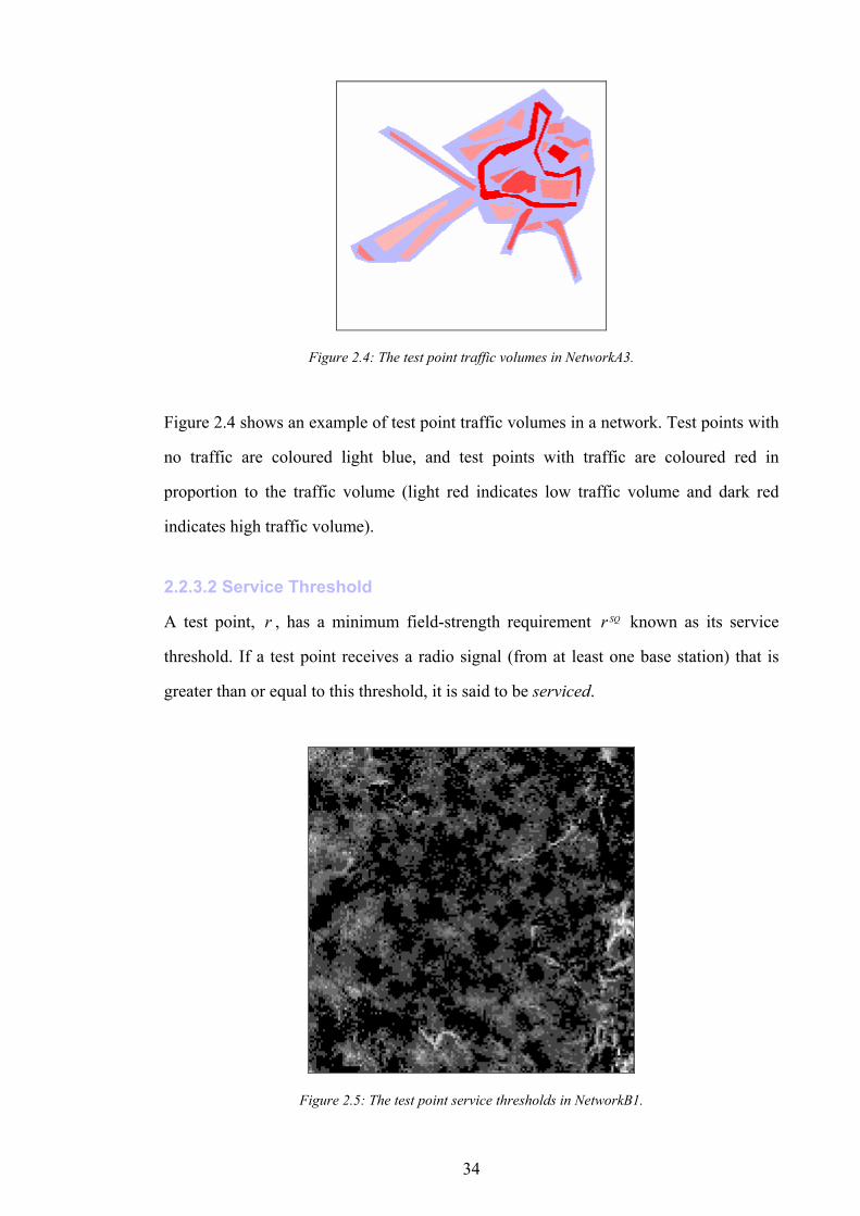
34

Figure 2.4: The test point traffic volumes in NetworkA3.

Figure 2.4 shows an example of test point traffic volumes in a network. Test points with

no traffic are coloured light blue, and test points with traffic are coloured red in

proportion to the traffic volume (light red indicates low traffic volume and dark red

indicates high traffic volume).

2.2.3.2 Service Threshold

A test point, r , has a minimum field-strength requirement SQr known as its service

threshold. If a test point receives a radio signal (from at least one base station) that is

greater than or equal to this threshold, it is said to be serviced.

Figure 2.5: The test point service thresholds in NetworkB1.

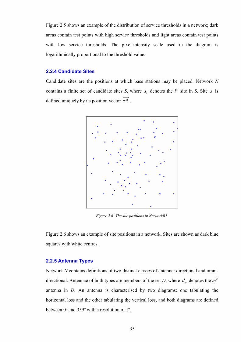
35

Figure 2.5 shows an example of the distribution of service thresholds in a network; dark

areas contain test points with high service thresholds and light areas contain test points

with low service thresholds. The pixel-intensity scale used in the diagram is

logarithmically proportional to the threshold value.

2.2.4 Candidate Sites

Candidate sites are the positions at which base stations may be placed. Network N

contains a finite set of candidate sites S, where ls denotes the lth site in S. Site s is

defined uniquely by its position vector XYs .

Figure 2.6: The site positions in NetworkB1.

Figure 2.6 shows an example of site positions in a network. Sites are shown as dark blue

squares with white centres.

2.2.5 Antenna Types

Network N contains definitions of two distinct classes of antenna: directional and omni-

directional. Antennae of both types are members of the set D, where md denotes the mth

antenna in D. An antenna is characterised by two diagrams: one tabulating the

horizontal loss and the other tabulating the vertical loss, and both diagrams are defined

between 0º and 359º with a resolution of 1º.

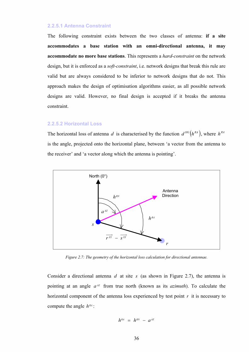
36

2.2.5.1 Antenna Constraint

The following constraint exists between the two classes of antenna: if a site

accommodates a base station with an omni-directional antenna, it may

accommodate no more base stations. This represents a hard-constraint on the network

design, but it is enforced as a soft-constraint, i.e. network designs that break this rule are

valid but are always considered to be inferior to network designs that do not. This

approach makes the design of optimisation algorithms easier, as all possible network

designs are valid. However, no final design is accepted if it breaks the antenna

constraint.

2.2.5.2 Horizontal Loss

The horizontal loss of antenna d is characterised by the function ( )RAHG hd , where RAh

is the angle, projected onto the horizontal plane, between ‘a vector from the antenna to

the receiver’ and ‘a vector along which the antenna is pointing’.

North (0°)

Antenna Direction

RAhs

RNh

XYXY sr −

AZa

r

Figure 2.7: The geometry of the horizontal loss calculation for directional antennae.

Consider a directional antenna d at site s (as shown in Figure 2.7), the antenna is

pointing at an angle AZa from true north (known as its azimuth). To calculate the

horizontal component of the antenna loss experienced by test point r it is necessary to

compute the angle RAh :

AZRNRA ahh −=

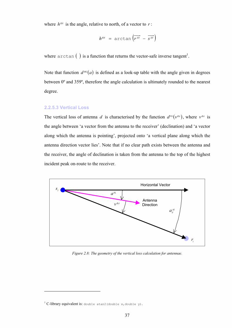
37

where RNh is the angle, relative to north, of a vector to r :

( )XYXYRN srh −= arctan

where ( )arctan is a function that returns the vector-safe inverse tangent1.

Note that function ( )ad HG is defined as a look-up table with the angle given in degrees

between 0º and 359º, therefore the angle calculation is ultimately rounded to the nearest

degree.

2.2.5.3 Vertical Loss

The vertical loss of antenna d is characterised by the function ( )RAVG vd , where RAv is

the angle between ‘a vector from the antenna to the receiver’ (declination) and ‘a vector

along which the antenna is pointing’, projected onto ‘a vertical plane along which the

antenna direction vector lies’. Note that if no clear path exists between the antenna and

the receiver, the angle of declination is taken from the antenna to the top of the highest

incident peak on-route to the receiver.

Horizontal Vector

Antenna Direction RAv

ls

AIila

ir

TLa

Figure 2.8: The geometry of the vertical loss calculation for antennae.

1 C-library equivalent is: double atan2(double x,double y).

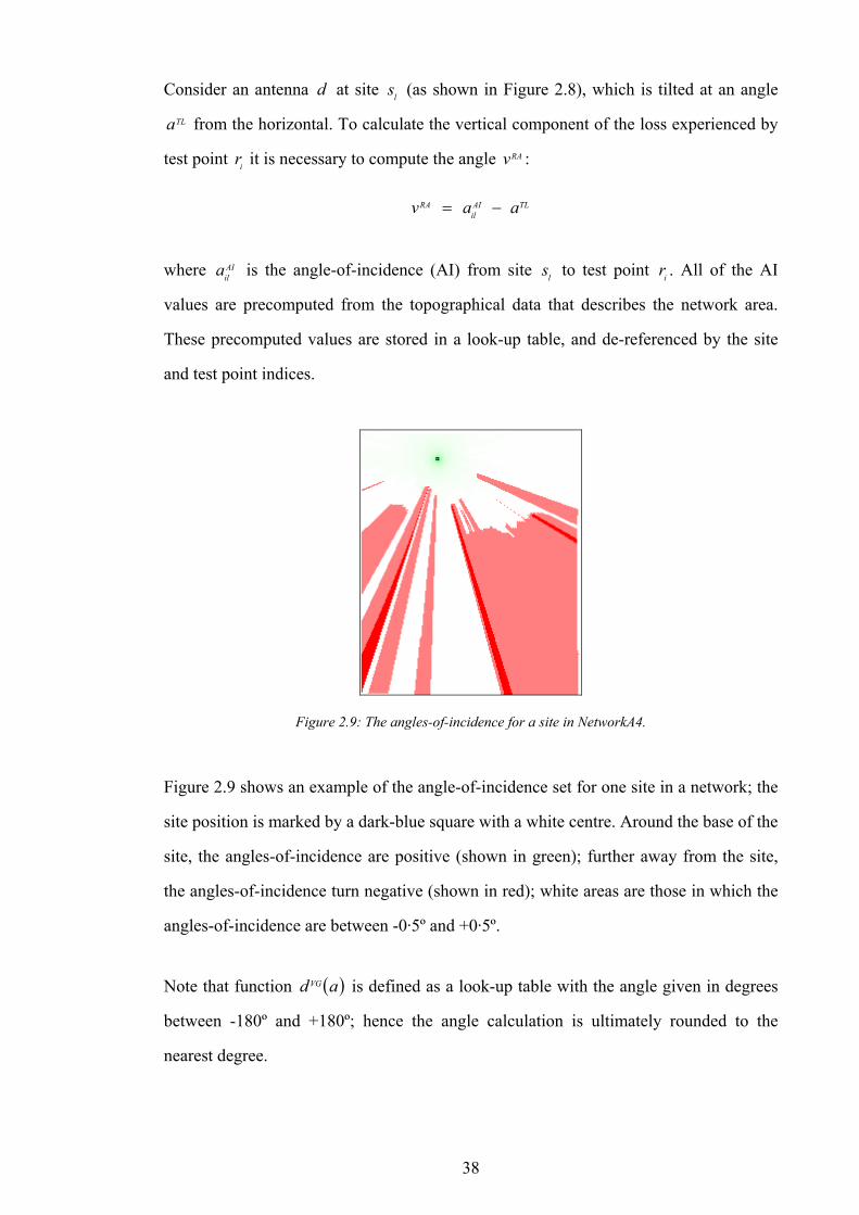
38

Consider an antenna d at site ls (as shown in Figure 2.8), which is tilted at an angle

TLa from the horizontal. To calculate the vertical component of the loss experienced by

test point ir it is necessary to compute the angle RAv :

TLAIil

RA aav −=

where AIila is the angle-of-incidence (AI) from site ls to test point ir . All of the AI

values are precomputed from the topographical data that describes the network area.

These precomputed values are stored in a look-up table, and de-referenced by the site

and test point indices.

Figure 2.9: The angles-of-incidence for a site in NetworkA4.

Figure 2.9 shows an example of the angle-of-incidence set for one site in a network; the

site position is marked by a dark-blue square with a white centre. Around the base of the

site, the angles-of-incidence are positive (shown in green); further away from the site,

the angles-of-incidence turn negative (shown in red); white areas are those in which the

angles-of-incidence are between -0·5º and +0·5º.

Note that function ( )adVG is defined as a look-up table with the angle given in degrees

between -180º and +180º; hence the angle calculation is ultimately rounded to the

nearest degree.

39

2.2.6 Channels

Network N contains the definition of a finite and ordered set of channels C, where kc

denotes the kth channel in C.

2.2.6.1 Channel Separation Gain

Receivers are tuned to receive signals on specific channels, and any received signal not

employing this channel will be attenuated – the greater the difference (between the

channel to which the receiver is tuned and the channel on which the received signal was

transmitted), the greater the attenuation.

If a receiver, tuned to channel Ccx ∈ , receives a signal, transmitted on channel

Ccy ∈ , the effective power of the received signal is attenuated. The effective gain

applied to the received signal is given by the function ( )yxCS ccG , . The range of the

function is given by:

( ) 10 ≤≤ yxCS ccG ,

2.2.6.2 Channel Traffic Capacity

The traffic carrying capacity of a given number of channels n is denoted ( )nT CH , and is

described in Table 2.1. Note that these figures are derived by the operators, and the

method used for their generation is based on a heuristically adjusted version of Erlangs

formula (as described in [9]).

Number of channels n 1 2 3 4 5 6 7 8 Traffic Capacity ( )nT CH in Erlangs 2.9 8.2 15 22 28 35.5 43 56

Table 2.1: Traffic capacity vs. number allocated base station channels.

The number of channels required by a base station is encapsulated in the function

( )tN TR , which returns the number of channels whose capacity is greater than or equal to

call volume t.

40

2.2.7 Base Stations

Network N contains the definition of a finite set of base stations B, where jb denotes the

jth base station in B. Base stations occupy the candidate sites defined by S. The

maximum number of base stations that can occupy one site is constant and denoted by

BSPERSITEn . Therefore the maximum number of base stations in a network is given by:

BSPERSITEnSB ⋅=

2.2.7.1 Activation

Boolean parameter ACb is true if base station b is active; if a base station is not active it

has no influence on the network. The set of active base stations BB AC ⊆ is given by:

{ }true=∈= ACAC bBbB :

and the number of active base stations is given by:

ACAB Bn =

2.2.7.2 Site Occupied

Base station b occupies site SbST ∈ , note that BSPERSITEn base stations may share each

site. The set of occupied sites SS OC ⊆ is given by:

{ }sbBbSsS STACOC =∈∃∈= :

and the number of occupied sites is given by:

OCOS Sn =

2.2.7.3 Antenna Type

The type of antenna used by base station b is given by DbAD ∈ .

The set of sites at which multiple base stations employ omni-directional antennae

(thereby breaking the antenna constraint described in Section 2.2.5.1) is given by:

41

( ) ( )

∧

∧=∧≠∈∃∈∃∈=

ADy

ADx

STy

STx

ACy

ACx

OC

OV

bbbbyxBbBbSs

SisOmniisOmni

:

where function ( )disOmni returns true if antenna Dd ∈ is omni-directional,

otherwise it returns false.

The number of sites on which multiple base stations employ omni-directional antennae

is given by:

OVOV Sn =

2.2.7.4 Transmission Power

The transmission power employed by base station b is given by TXb . The lower limit of

TXb is given by TXMINp and transmission power is divided into TXSTEPn discrete intervals,

each one being 2dB (a factor of ~1·58) higher than its predecessor. From this we can

calculate the maximum transmission power:

( ) 110

210−

⋅=TXSTEPn

TXMINTXMAX pp

2.2.7.5 Azimuth

The horizontal angle, or azimuth, of the antenna used by base station b is given by AZb ,

and it is stored in one-degree intervals in the range °≤≤° 3590 AZb .

2.2.7.6 Tilt

The vertical angle, or tilt, of the antenna used by base station b is given by TLb , and it is

stored in one-degree intervals in the range °≤≤° 150 TLb .

2.2.7.7 Channel Assignment

A set of channels is allocated to each base station, where the kth channel allocated to

base station jb is denoted by CHjkb . The maximum number of channels any base station

may use is given by CHANPERBSn .

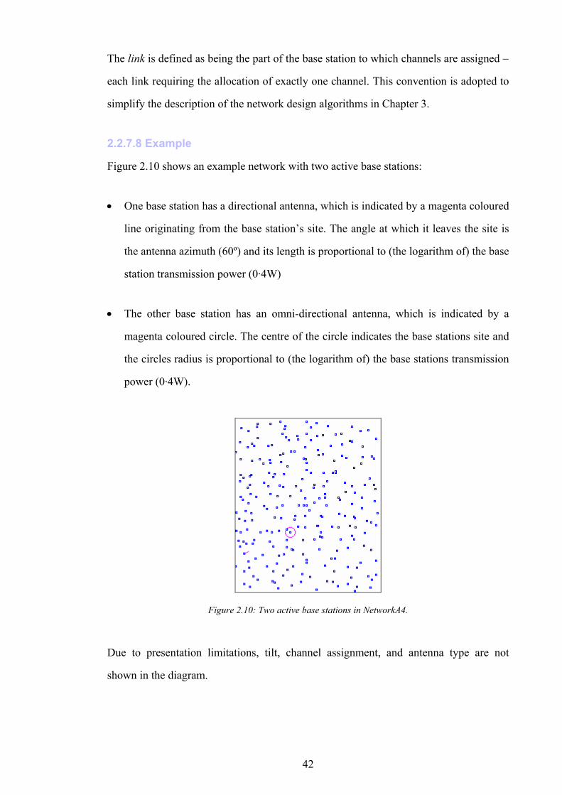
42

The link is defined as being the part of the base station to which channels are assigned −

each link requiring the allocation of exactly one channel. This convention is adopted to

simplify the description of the network design algorithms in Chapter 3.

2.2.7.8 Example

Figure 2.10 shows an example network with two active base stations:

• One base station has a directional antenna, which is indicated by a magenta coloured

line originating from the base station’s site. The angle at which it leaves the site is

the antenna azimuth (60º) and its length is proportional to (the logarithm of) the base

station transmission power (0·4W)

• The other base station has an omni-directional antenna, which is indicated by a

magenta coloured circle. The centre of the circle indicates the base stations site and

the circles radius is proportional to (the logarithm of) the base stations transmission

power (0·4W).

Figure 2.10: Two active base stations in NetworkA4.

Due to presentation limitations, tilt, channel assignment, and antenna type are not

shown in the diagram.

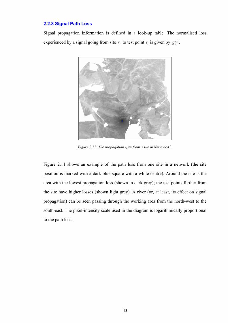
43

2.2.8 Signal Path Loss

Signal propagation information is defined in a look-up table. The normalised loss

experienced by a signal going from site ls to test point ir is given by PGilg .

Figure 2.11: The propagation gain from a site in NetworkA2.

Figure 2.11 shows an example of the path loss from one site in a network (the site

position is marked with a dark blue square with a white centre). Around the site is the

area with the lowest propagation loss (shown in dark grey); the test points further from

the site have higher losses (shown light grey). A river (or, at least, its effect on signal

propagation) can be seen passing through the working area from the north-west to the

south-east. The pixel-intensity scale used in the diagram is logarithmically proportional

to the path loss.

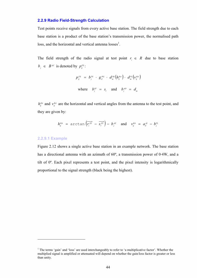
44

2.2.9 Radio Field-Strength Calculation

Test points receive signals from every active base station. The field strength due to each

base station is a product of the base station’s transmission power, the normalised path

loss, and the horizontal and vertical antenna losses1.

The field strength of the radio signal at test point Rri ∈ due to base station

ACj Bb ∈ is denoted by FS

ijp :

( ) ( )RAij

VLm

RAij

HLm

PGil

TXj

FSij vdhdgbp ⋅⋅⋅=

where lSTj sb = and m

ADj db =

RAijh and RA

ijv are the horizontal and vertical angles from the antenna to the test point, and

they are given by:

( ) AZj

XYl

XYi

RAij bsrh −−= arctan and TL

jAIil

RAij bav −=

2.2.9.1 Example

Figure 2.12 shows a single active base station in an example network. The base station

has a directional antenna with an azimuth of 60º, a transmission power of 0·4W, and a

tilt of 0º. Each pixel represents a test point, and the pixel intensity is logarithmically

proportional to the signal strength (black being the highest).

1 The terms ‘gain’ and ‘loss’ are used interchangeably to refer to ‘a multiplicative factor’. Whether the multiplied signal is amplified or attenuated will depend on whether the gain/loss factor is greater or less than unity.

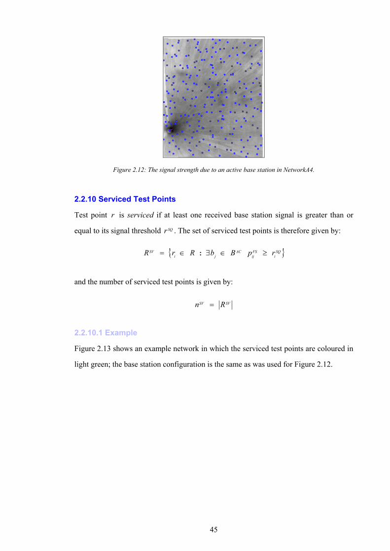
45

Figure 2.12: The signal strength due to an active base station in NetworkA4.

2.2.10 Serviced Test Points

Test point r is serviced if at least one received base station signal is greater than or

equal to its signal threshold SQr . The set of serviced test points is therefore given by:

{ }SQi

FSij

ACji

SV rpBbRrR ≥∈∃∈= :

and the number of serviced test points is given by:

SVSV Rn =

2.2.10.1 Example

Figure 2.13 shows an example network in which the serviced test points are coloured in

light green; the base station configuration is the same as was used for Figure 2.12.

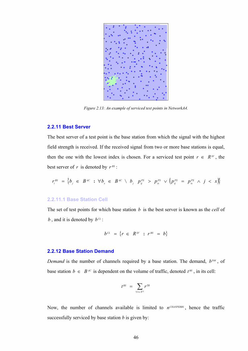
46

Figure 2.13: An example of serviced test points in NetworkA4.

2.2.11 Best Server

The best server of a test point is the base station from which the signal with the highest

field strength is received. If the received signal from two or more base stations is equal,

then the one with the lowest index is chosen. For a serviced test point SVRr ∈ , the

best server of r is denoted by BSr :

( ){ }xjppppbBbBbr FSix

FSij

FSix

FSijj

ACx

ACj

BSi <∧=∨>∈∀∈= \:

2.2.11.1 Base Station Cell

The set of test points for which base station b is the best server is known as the cell of

b , and it is denoted by CLb :

{ }brRrb BSSVCL =∈= :

2.2.12 Base Station Demand

Demand is the number of channels required by a base station. The demand, DMb , of

base station ACBb ∈ is dependent on the volume of traffic, denoted BSt , in its cell:

∑∈∀

=CLbr

TRBS rt

Now, the number of channels available is limited to CHANPERBSn , hence the traffic

successfully serviced by base station b is given by:

47

( ){ }CHANPERBSCHBSTS nTtb ,min=

The number of channels, n , required to accommodate traffic volume BSt is given by:

( )TSTR bNn =

Base stations that cover no traffic still require at least one channel if they are to

contribute to general area coverage. The demand of base station b is therefore given by:

{ }nb DM ,max 1=

2.2.13 Traffic Service

The total volume of traffic serviced by all the active base stations in the network is

given by:

∑∈∀

=ACBb

TSSV bt

This corresponds to the maximum potential traffic cover, or, in other words, the traffic

cover that would be achieved in the absence of interference.

2.2.14 Fuzzy-Server Set

For test point ir a set of servers SSir is defined to contain all base stations that provide a

signal within the fuzzy-server threshold (the fuzzy server model is discussed in Section

2.1.10). This threshold is the product of FZg (a gain constant) and the signal from the

best server of ir :

{ }FSix

FZFSij

ACj

SSi pgpBbr ⋅≥∈= :

where xBS

i br =

2.2.15 Carrier to Interference Ratio

The carrier-to-interference-ratio (CIR) φir for test point SV

i Rr ∈ is the worst-case CIR

from each of the servers in the fuzzy server set:

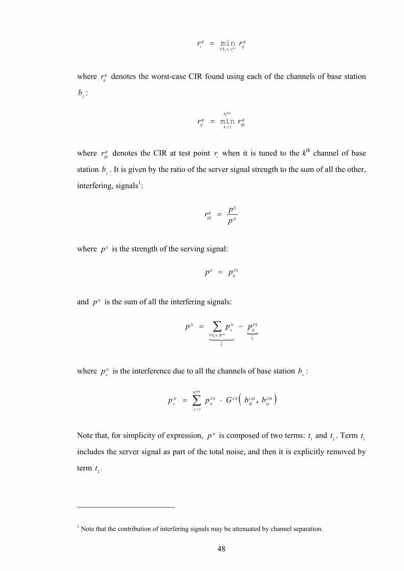
48

φφijrbi rr

SSij ∈∀

= min

where φijr denotes the worst-case CIR found using each of the channels of base station

jb :

φφijk

b

kij rrDMj

1== min

where φijkr denotes the CIR at test point ir when it is tuned to the kth channel of base

station jb . It is given by the ratio of the server signal strength to the sum of all the other,

interfering, signals1:

N

S

ijk ppr =φ

where Sp is the strength of the serving signal:

FSij

S pp =

and Np is the sum of all the interfering signals:

{2

1

t

FSij

t

Bb

Nx

N pppAC

x

−= ∑∈∀ 43421

where Nxp is the interference due to all the channels of base station xb :

( )∑=

⋅=DMxb

y

CHxy

CHjk

CSFSix

Nx bbGpp

1

,

Note that, for simplicity of expression, Np is composed of two terms: 1t and 2t . Term 1t

includes the server signal as part of the total noise, and then it is explicitly removed by

term 2t .

1 Note that the contribution of interfering signals may be attenuated by channel separation.

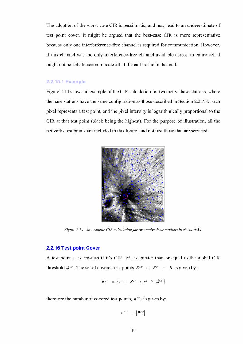
49

The adoption of the worst-case CIR is pessimistic, and may lead to an underestimate of

test point cover. It might be argued that the best-case CIR is more representative

because only one interferference-free channel is required for communication. However,

if this channel was the only interference-free channel available across an entire cell it

might not be able to accommodate all of the call traffic in that cell.

2.2.15.1 Example

Figure 2.14 shows an example of the CIR calculation for two active base stations, where

the base stations have the same configuration as those described in Section 2.2.7.8. Each

pixel represents a test point, and the pixel intensity is logarithmically proportional to the

CIR at that test point (black being the highest). For the purpose of illustration, all the

networks test points are included in this figure, and not just those that are serviced.

Figure 2.14: An example CIR calculation for two active base stations in NetworkA4.

2.2.16 Test point Cover

A test point r is covered if it’s CIR, φr , is greater than or equal to the global CIR

threshold CVφ . The set of covered test points RRR SVCV ⊆⊆ is given by:

{ }CVSVCV rRrR φφ ≥∈= :

therefore the number of covered test points, CVn , is given by:

CVCV Rn =

50

2.2.16.1 Example

Figure 2.15 shows an example network with two active base stations, where the base

stations have the same configuration as those described in Section 2.2.7.8. The non-

covered test points are coloured blue, the serviced test points are coloured light green,

and the covered test points are coloured dark green. It can be seen that cover is achieved

close to the base station sites, but cover becomes more difficult as the distance from the

base station increases.

Figure 2.15: An example of test point cover for two base stations in NetworkA4.

2.2.17 Traffic Cover

The traffic covered by base station ACj Bb ∈ is denoted TC

jb , it is calculated in the

same way as the traffic service (see Section 2.2.13) except that only covered test points

from the cell of jb may contribute:

( )

= ∑∩∈∀

CHANPERBSCH

Rbr

TRTCj nTrb

CVCLj

,min

The total volume of traffic successfully covered by the whole network of base stations is

given by:

∑∈∀

=ACBb

TCCV bt

51

2.2.18 Network Designs

Most network parameters (such as path loss and test point positions) are fixed, except

for the following base station configuration parameters:

• Activation, ACb

• Antenna Type, ADb

• Transmission Power, TXb

• Azimuth, AZb

• Tilt, TLb

• Channel Assignment, CHb

A complete and valid allocation of base station parameters is known as a network

design.

2.3 Performance Evaluation

To evaluate and compare design performances it is necessary to define what the design

goals are (this corresponds to Task T3 of Objective O1 in Section 1.3).

2.3.1 Design Goals

Like any business, the network operators wish to maximise profits. They must

maximise revenue and minimise overheads. For a network operator to succeed, the

network design goals must represent the economic goals as closely as possible.

2.3.1.1 Revenues and Overheads

Revenue is generated principally from telephone calls. The network model provides the

operator with a prediction of the volume of call traffic and, hence, the expected call

revenue. Examples of the overheads that contribute to the total cost of running the

network include:

52

• Base station equipment leasing.

• Base station site rental.

• Staff office rental.

• Personnel salaries.

• Radio spectrum rental.

The overheads can be divided into two categories:

• Dynamic costs, which grow with the size of the network (e.g. base station site rental,

equipment leasing).

• Static costs, which must be met regardless of the network size (e.g. office rental,

salaries, radio-spectrum rental).

No overhead component can be exclusively categorised in this way, but it is a

distinction that lends itself neatly to analysis.

2.3.1.2 Profit and Loss

Consider a network of size n (arbitrary units), and let network revenue be a function of

n and some constant T that represents the normalised value of providing telephony:

nT ⋅=Revenue

Let network overheads be a function of n and some constant DC that represents the

normalised cost of providing telephony. The overheads also include the static cost

component SC :

SD CnC +⋅=Overhead

Profit is given by Revenue − Overhead, therefore

53

( ) SDSD CCTnCnCnT −−⋅=−⋅−⋅=Profit

In order to turn a profit, the network operator must ensure that the revenue exceeds the

overhead. The equation above identifies two key-factors controlling a network’s

profitability: the network size, n, and the call-profit-per-unit-network, DCT − . These

expressions must both be maximised in order to maximise profits.

2.3.1.3 Translating Business Analysis into Engineering Requirements

The simple analysis in the previous section showed that high profitability is achieved in

a large network that provides efficient telephony. This must be translated into a network

design requirement. An ideal network design will:

• Be available for use by the maximum number of subscribers − every mobile station

in a network should be able to instantiate or receive telephone calls at any time.

• Minimise the cost of the network infrastructure.

2.3.1.4 Data Set Limitations

The available data for the network design problem does not include details of network

infrastructure costs, furthermore the subscriber information is only given in terms of call

volume which is, at best, a relative indicator of call revenue. Because of the omission of

absolute monetary-values in the network data sets, the design requirements were

simplified. The design requirements are listed below in order of significance:

1. Maximisation of subscriber coverage.

2. Maximisation of area coverage.

3. Minimisation of the number of sites used.

4. Minimisation of the number of base stations deployed.

54

If more information were available then this design specification could be improved, for

example it would be simple to include an ‘efficiency’ requirement such as the

maximisation of the ratio of call revenue to site rental. Note that site rental is assumed

to be considerably more expensive than the telephony equipment, hence the relative

significance of metrics 3 and 4; this assumption is based on the experience of network

operators.

2.3.2 Performance Comparison

Comparing the performance of different network designs is done by comparing network

performance metrics. Each performance metric has a relative significance, and the

networks are compared metric-by-metric. These metrics are listed below in order of

significance:

1. Number of co-sited omni-directional antennae, OVn

2. Volume of traffic covered, CVt

3. Volume of traffic serviced, SVt

4. Number of test points covered, CVn

5. Number of test points serviced, SVn

6. Number of occupied sites, OSn

7. Number of active base stations, ABn

Metrics 1,6 and 7 should be minimised and metrics 2,3,4 and 5 should be maximised.

The performance of a network design is expressed as a function ( )NDp . If network

designs aND and bND contain no co-sited omni-directional antennae and produce

traffic cover values CVat and CV

bt respectively then aND outperforms bND if CVb

CVa tt > .

However, if CVb

CVa tt = then a comparison of the next significant metrics, SV

at and SVbt ,

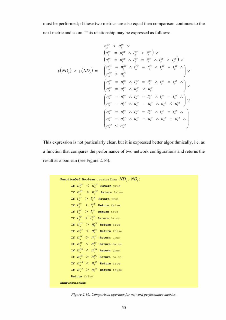
55

must be performed; if these two metrics are also equal then comparison continues to the

next metric and so on. This relationship may be expressed as follows:

( ) ( )

( )( )

<∧=∧=∧=

∧=∧=∧=

∨

<∧=∧=

∧=∧=∧=

∨

>∧=

∧=∧=∧=

∨

>

∧=∧=∧=

∨>∧=∧=∨>∧=

∨<

=>

ABb

ABa

OSb

OSa

SVb

SVa

CVb

CVa

SVb

SVa

CVb

CVa

OVb

OVa

OSb

OSa

SVb

SVa

CVb

CVa

SVb

SVa

CVb

CVa

OVb

OVa

SVb

SVa

CVb

CVa

SVb

SVa

CVb

CVa

OVb

OVa

CVb

CVa

SVb

SVa

CVb

CVa

OVb

OVa

SVb

SVa

CVb

CVa

OVb

OVa

CVb

CVa

OVb

OVa

OVb

OVa

ba

nnnnnnnn

ttttnn

nnnnnnttttnn

nnnnttttnn

nnttttnnttttnn

ttnnnn

NDND pp

This expression is not particularly clear, but it is expressed better algorithmically, i.e. as

a function that compares the performance of two network configurations and returns the

result as a boolean (see Figure 2.16).

FunctionDef Boolean greaterThan( aND , bND )

If OVb

OVa nn < Return true

If OVb

OVa nn > Return false

If CVb

CVa tt > Return true

If CVb

CVa tt < Return false

If SVb

SVa tt > Return true

If SVb

SVa tt < Return false

If CVb

CVa nn > Return true

If CVb

CVa nn < Return false

If SVb

SVa nn > Return true

If SVb

SVa nn < Return false

If OSb

OSa nn < Return true

If OSb

OSa nn > Return false

If ABb

ABa nn < Return true

If ABb

ABa nn > Return false

Return false EndFunctionDef

Figure 2.16: Comparison operator for network performance metrics.

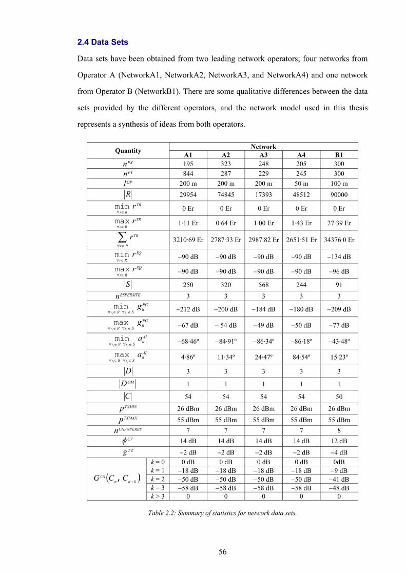
56

2.4 Data Sets

Data sets have been obtained from two leading network operators; four networks from

Operator A (NetworkA1, NetworkA2, NetworkA3, and NetworkA4) and one network

from Operator B (NetworkB1). There are some qualitative differences between the data

sets provided by the different operators, and the network model used in this thesis

represents a synthesis of ideas from both operators.

Network Quantity A1 A2 A3 A4 B1 PXn 195 323 248 205 300 PYn 844 287 229 245 300

GPl 200 m 200 m 200 m 50 m 100 m R 29954 74845 17393 48512 90000

TR

Rrr

∈∀min 0 Er 0 Er 0 Er 0 Er 0 Er

TR

Rrr

∈∀max 1·11 Er 0·64 Er 1·00 Er 1·43 Er 27·39 Er

∑∈∀ Rr

TRr 3210·69 Er 2787·33 Er 2987·82 Er 2651·51 Er 34376·0 Er

SQ

Rrr

∈∀min −90 dB −90 dB −90 dB −90 dB −134 dB

SQ

Rrr

∈∀max −90 dB −90 dB −90 dB −90 dB −96 dB

S 250 320 568 244 91 BSPERSITEn 3 3 3 3 3

PGilSsRr

gli ∈∀∈∀

min −212 dB −200 dB −184 dB −180 dB −209 dB PGilSsRr

gli ∈∀∈∀

max −67 dB − 54 dB −49 dB −50 dB −77 dB AIilSsRr

ali ∈∀∈∀

min −68·46º −84·91º −86·34º −86·18º −43·48º AIilSsRr

ali ∈∀∈∀

max 4·86º 11·34º 24·47º 84·54º 15·23º

D 3 3 3 3 3 OMD 1 1 1 1 1

C 54 54 54 54 50 TXMINp 26 dBm 26 dBm 26 dBm 26 dBm 26 dBm TXMAXp 55 dBm 55 dBm 55 dBm 55 dBm 55 dBm

CHANPERBSn 7 7 7 7 8 CVφ 14 dB 14 dB 14 dB 14 dB 12 dB FZg −2 dB −2 dB −2 dB −2 dB −4 dB

k = 0 0 dB 0 dB 0 dB 0 dB 0dB k = 1 −18 dB −18 dB −18 dB −18 dB −9 dB k = 2 −50 dB −50 dB −50 dB −50 dB −41 dB k = 3 −58 dB −58 dB −58 dB −58 dB −48 dB

( )knnCS CCG +,

k > 3 0 0 0 0 0

Table 2.2: Summary of statistics for network data sets.

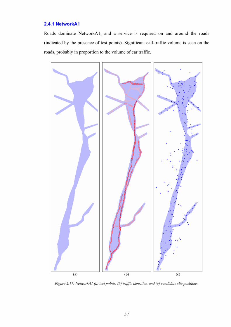
57

2.4.1 NetworkA1

Roads dominate NetworkA1, and a service is required on and around the roads

(indicated by the presence of test points). Significant call-traffic volume is seen on the

roads, probably in proportion to the volume of car traffic.

(a) (b) (c)

Figure 2.17: NetworkA1 (a) test points, (b) traffic densities, and (c) candidate site positions.

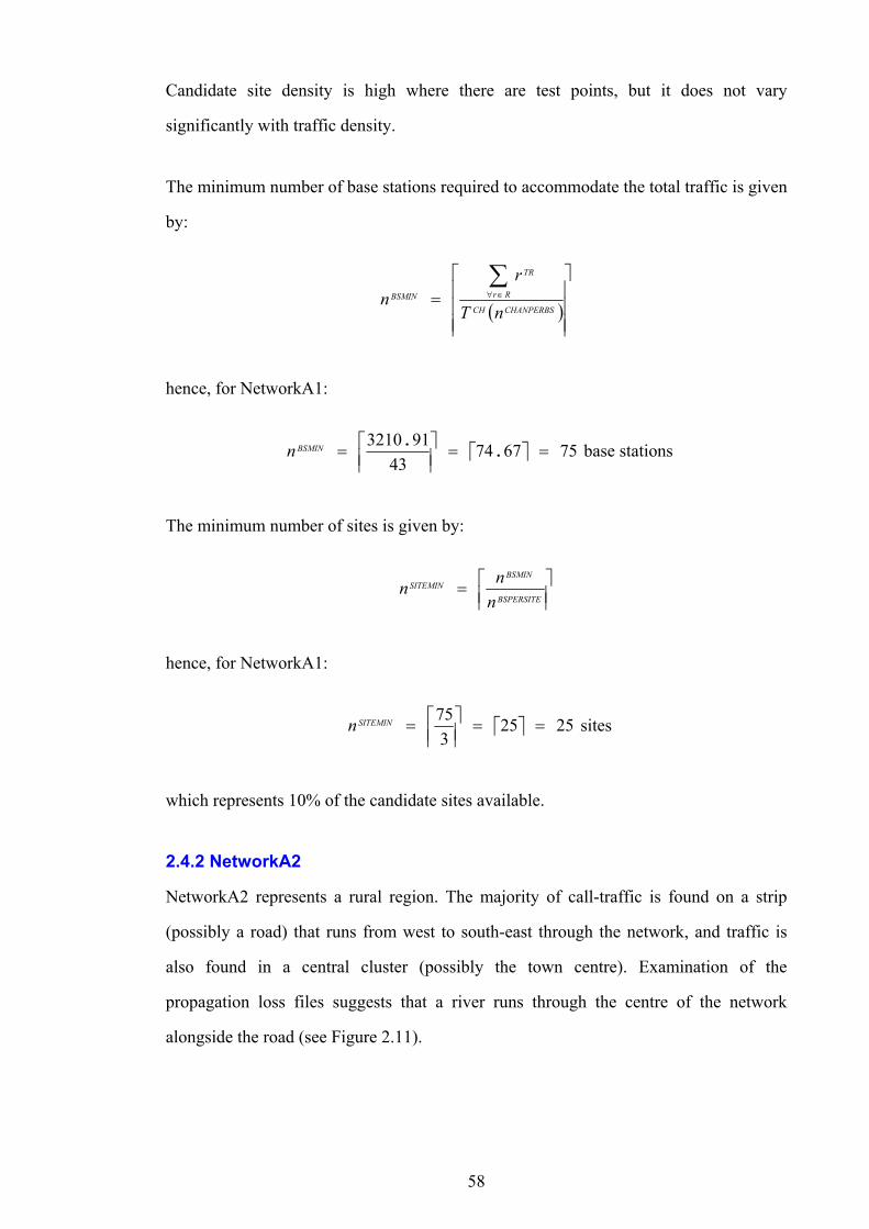
58

Candidate site density is high where there are test points, but it does not vary

significantly with traffic density.

The minimum number of base stations required to accommodate the total traffic is given

by:

( )

=

∑∈∀

CHANPERBSCH

Rr

TR

BSMIN

nT

rn

hence, for NetworkA1:

75677443

913210==

= .

.BSMINn base stations

The minimum number of sites is given by:

=

BSPERSITE

BSMINSITEMIN

nnn

hence, for NetworkA1:

2525375

==

=SITEMINn sites

which represents 10% of the candidate sites available.

2.4.2 NetworkA2

NetworkA2 represents a rural region. The majority of call-traffic is found on a strip

(possibly a road) that runs from west to south-east through the network, and traffic is

also found in a central cluster (possibly the town centre). Examination of the

propagation loss files suggests that a river runs through the centre of the network

alongside the road (see Figure 2.11).

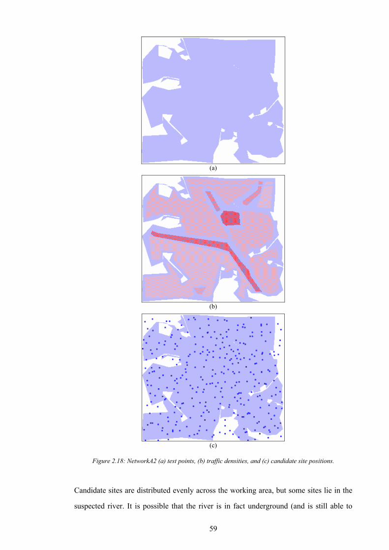
59

(a)

(b)

(c)

Figure 2.18: NetworkA2 (a) test points, (b) traffic densities, and (c) candidate site positions.

Candidate sites are distributed evenly across the working area, but some sites lie in the

suspected river. It is possible that the river is in fact underground (and is still able to

60

effect propagation) or that candidate sites have been placed randomly for the purpose of

creating test data. Candidate site density does not vary significantly with test point

density or call traffic density.

The minimum number of base stations required to accommodate the total traffic in

NetworkA2 is 65 and, hence, the minimum number of sites required is 22 - this

represents 6·9% of the candidate sites.

2.4.3 NetworkA3

NetworkA3 probably represents a small town. The centre of the network contains two

large clusters of call-traffic; the highest density of call-traffic is on a strip that circles the

centre (possibly a ring-road). Significant call-traffic is found on several ‘spokes’

(probably roads) radiating from the networks centre.

(a)

(b)

(c)

Figure 2.19: NetworkA3 (a) test points, (b) traffic densities, and (c) candidate site positions.

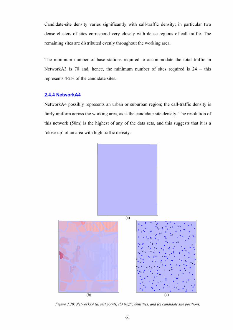
61

Candidate-site density varies significantly with call-traffic density; in particular two

dense clusters of sites correspond very closely with dense regions of call traffic. The

remaining sites are distributed evenly throughout the working area.

The minimum number of base stations required to accommodate the total traffic in

NetworkA3 is 70 and, hence, the minimum number of sites required is 24 − this

represents 4·2% of the candidate sites.

2.4.4 NetworkA4

NetworkA4 possibly represents an urban or suburban region; the call-traffic density is

fairly uniform across the working area, as is the candidate site density. The resolution of

this network (50m) is the highest of any of the data sets, and this suggests that it is a

‘close-up’ of an area with high traffic density.

(a)

(b)

(c)

Figure 2.20: NetworkA4 (a) test points, (b) traffic densities, and (c) candidate site positions.

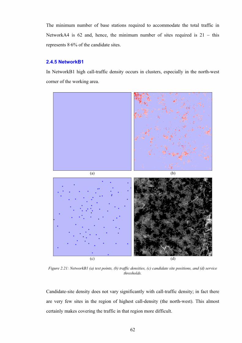
62

The minimum number of base stations required to accommodate the total traffic in

NetworkA4 is 62 and, hence, the minimum number of sites required is 21 − this

represents 8·6% of the candidate sites.

2.4.5 NetworkB1

In NetworkB1 high call-traffic density occurs in clusters, especially in the north-west

corner of the working area.

(a) (b)

(c)

(d)

Figure 2.21: NetworkB1 (a) test points, (b) traffic densities, (c) candidate site positions, and (d) service thresholds.

Candidate-site density does not vary significantly with call-traffic density; in fact there

are very few sites in the region of highest call-density (the north-west). This almost

certainly makes covering the traffic in that region more difficult.

63

There are some significant differences between this network and the networks obtained

from Operator A:

• The total traffic in this network is much higher – more than 10 times the total of

NetworkA1.

• The maximum traffic represented by one test point is 27·39 Er, whereas the highest

value for the other networks was 1·43 Er – almost 20 times smaller. This means that

some ‘well-dimensioned’ cells (i.e. cells which contain nearly the maximum traffic

they can hold without covering an un-necessarily large area) could be 2 or 3 test

points in size. This makes good network designs harder to find, and it also indicates

that the resolution of the test point grid is too low to enable the simulation of reliable

cell-plans.

• The number of candidate sites is much lower. This is possibly because the data is

derived from an existing network (i.e. candidate sites represent those currently

occupied) and not augmented with extra sites. In the other networks the addition of

extra sites increases the cell-planning options.

• In the previous networks, the service threshold was a constant −90dBm, whereas in

this network less than 2% of test points are that easy to cover. In fact the average

service threshold is approximately –70dBm (a factor of 100 larger than the average

for the other networks). This makes the test points harder to cover, or, at least,

necessitates the use of higher transmission powers, which reduces the scope of

relative power trade-offs for interference management.

• The channel separation gain is nearly 10 times as strict for this network as it is for

the other networks. This makes interference management by channel separation

more difficult.

The minimum number of base stations required to accommodate the total traffic in

NetworkB1 is 593 and, hence, the minimum number of sites required is 198. This is

64

more than twice as many sites as are defined for this network; therefore the total

network traffic is not coverable. The largest amount of traffic that may be covered

(assuming that each of the 91 sites accommodates 3 base stations, each of which can

handle 58 Er) is 91×3×58 = 15834 Er. This is 46·06% of the total network traffic.

65

Chapter 3 Network Design – Part 1

This chapter describes the application of simple combinatorial optimisation techniques

to the Wireless Capacitated Network Design Problem (WCNDP), the details of which

are described in the previous chapter. The goal of the work described in this chapter was

the identification of optimisation algorithms that produce high quality network designs

in a reasonable time (this corresponds to Task T1 of Objective O2 in Section 1.3).

The structure of this chapter is as follows: Section 3.2 describes algorithms for

initialising network designs, which are improved by the search algorithms described in

Section 3.3, finally Section 3.4 discusses the factors that limit search efficiency.

3.1 Choice of Optimisation Algorithms

For all of the different problems described in this thesis, a wide variety of optimisation

algorithms were trialed. An empirical approach was taken to development, in which

common heuristics such as hillclimbing, simulated annealing, and genetic algorithms

were compared using short run-times. Some poorly performing algorithms could be

quickly rejected, allowing more time for the remaining algorithms to evolve. The

algorithms detailed in this chapter (and in the thesis as a whole) are those that produced

the best network designs.

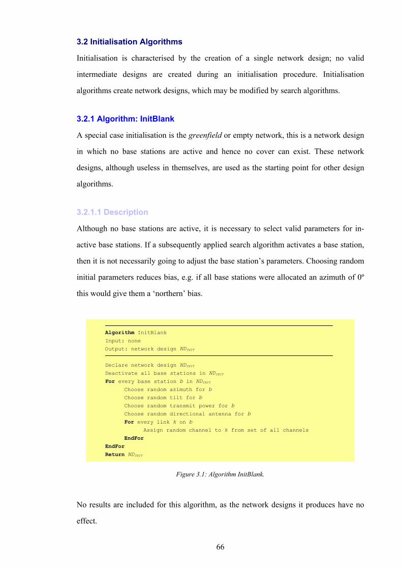
66

3.2 Initialisation Algorithms

Initialisation is characterised by the creation of a single network design; no valid

intermediate designs are created during an initialisation procedure. Initialisation

algorithms create network designs, which may be modified by search algorithms.

3.2.1 Algorithm: InitBlank

A special case initialisation is the greenfield or empty network, this is a network design

in which no base stations are active and hence no cover can exist. These network

designs, although useless in themselves, are used as the starting point for other design

algorithms.

3.2.1.1 Description

Although no base stations are active, it is necessary to select valid parameters for in-

active base stations. If a subsequently applied search algorithm activates a base station,

then it is not necessarily going to adjust the base station’s parameters. Choosing random

initial parameters reduces bias, e.g. if all base stations were allocated an azimuth of 0º

this would give them a ‘northern’ bias.

Algorithm InitBlank Input: none

Output: network design NDINIT

Declare network design NDINIT Deactivate all base stations in NDINIT

For every base station b in NDINIT Choose random azimuth for b

Choose random tilt for b

Choose random transmit power for b

Choose random directional antenna for b

For every link k on b Assign random channel to k from set of all channels

EndFor EndFor Return NDINIT

Figure 3.1: Algorithm InitBlank.

No results are included for this algorithm, as the network designs it produces have no

effect.

67

3.2.2 Algorithm InitRandomA

Network design parameters (such as azimuth or antenna type) uniquely define a

candidate network design, and Algorithm InitRandomA (outlined in Figure 3.2) does not

favour the production of any particular network design. Algorithm InitRandomA aims to

sample with equal probability from the set of all possible network designs.

The number of active base stations in each candidate design is between 1 and B (with

a uniform probability distribution). Note that this requirement forces the probability

distribution of the number of occupied sites to be non-uniform1.

3.2.2.1 Description

A set of n base stations is randomly activated. For each active base station, all

parameters (azimuth, tilt, transmit power, and channel assignment) are chosen

randomly, and the antenna used by each active base station is chosen at random from

the set of directional antennae. If only one base station is active at a site then there is a

probability, fixed at the beginning of the algorithm’s execution, that the base station will

be re-allocated an omni-directional antenna (selected at random from the set of

directional antennae).

1 It is possible for this to be made uniform; however, the probability distribution of the number of active base stations would then be non-uniform.

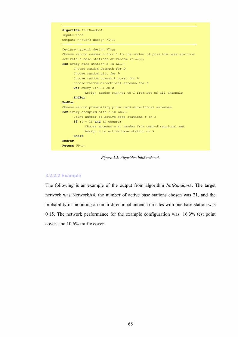
68

Algorithm InitRandomA Input: none

Output: network design NDINIT

Declare network design NDINIT Choose random number n from 1 to the number of possible base stations

Activate n base stations at random in NDINIT

For every base station b in NDINIT Choose random azimuth for b

Choose random tilt for b

Choose random transmit power for b

Choose random directional antenna for b

For every link l on b Assign random channel to l from set of all channels

EndFor EndFor Choose random probability p for omni-directional antennae

For every occupied site s in NDINIT Count number of active base stations t on s

If (t = 1) and (p occurs) Choose antenna a at random from omni-directional set

Assign a to active base station on s

EndIf EndFor Return NDINIT

Figure 3.2: Algorithm InitRandomA.

3.2.2.2 Example

The following is an example of the output from algorithm InitRandomA. The target

network was NetworkA4, the number of active base stations chosen was 21, and the

probability of mounting an omni-directional antenna on sites with one base station was

0·15. The network performance for the example configuration was: 16·3% test point

cover, and 10·6% traffic cover.

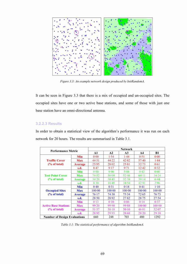
69

Figure 3.3: An example network design produced by InitRandomA.

It can be seen in Figure 3.3 that there is a mix of occupied and un-occupied sites. The

occupied sites have one or two active base stations, and some of those with just one

base station have an omni-directional antenna.

3.2.2.3 Results

In order to obtain a statistical view of the algorithm’s performance it was run on each

network for 20 hours. The results are summarised in Table 3.1.

Network Performance Metric A1 A2 A3 A4 B1 Min 0·00 1·54 1·44 0·51 0·00 Max 44·51 44·22 42·82 57·40 1·84

Average 25·95 28·02 25·81 32·73 0·61 Traffic Cover (% of total)

s.d. 8·47 9·17 9·71 12·42 0·32 Min 0·00 9·96 5·08 0·42 0·00 Max 74·52 56·09 52·46 64·11 16·24

Average 34·20 38·43 32·38 39·14 6·44 Test Point Cover

(% of total) s.d. 8·30 10·45 10·54 12·91 2·96 Min 0·40 0·31 0·18 0·41 1·10 Max 100·00 100·00 100·00 100·00 100·00

Average 76·17 74·30 75·34 72·65 76·73 Occupied Sites

(% of total) s.d. 28·50 28·92 27·82 28·75 27·54 Min 0·13 0·10 0·06 0·14 0·37 Max 99·20 99·90 99·88 100·00 100·00

Average 51·57 50·18 50·10 46·81 52·07 Active Base Stations

(% of total) s.d. 28·95 29·93 28·68 28·20 29·18

Number of Design Evaluations 660 248 703 480 1292

Table 3.1: The statistical performance of algorithm InitRandomA.

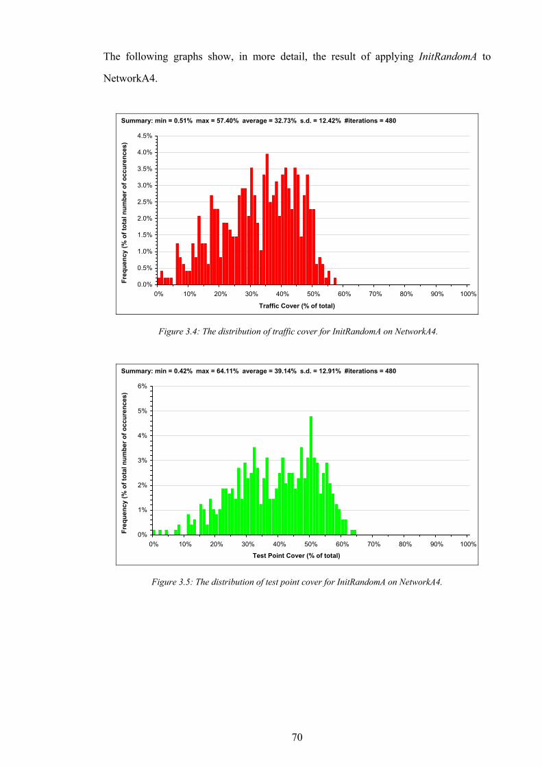
70

The following graphs show, in more detail, the result of applying InitRandomA to

NetworkA4.

0.0%

0.5%

1.0%

1.5%

2.0%

2.5%

3.0%

3.5%

4.0%

4.5%

0% 10% 20% 30% 40% 50% 60% 70% 80% 90% 100%

Traffic Cover (% of total)

Freq

uenc

y (%

of t

otal

num

ber o

f occ

uren

ces)

Summary: min = 0.51% max = 57.40% average = 32.73% s.d. = 12.42% #iterations = 480

Figure 3.4: The distribution of traffic cover for InitRandomA on NetworkA4.

0%

1%

2%

3%

4%

5%

6%

0% 10% 20% 30% 40% 50% 60% 70% 80% 90% 100%

Test Point Cover (% of total)

Freq

uenc

y (%

of t

otal

num

ber o

f occ

uren

ces)

Summary: min = 0.42% max = 64.11% average = 39.14% s.d. = 12.91% #iterations = 480

Figure 3.5: The distribution of test point cover for InitRandomA on NetworkA4.

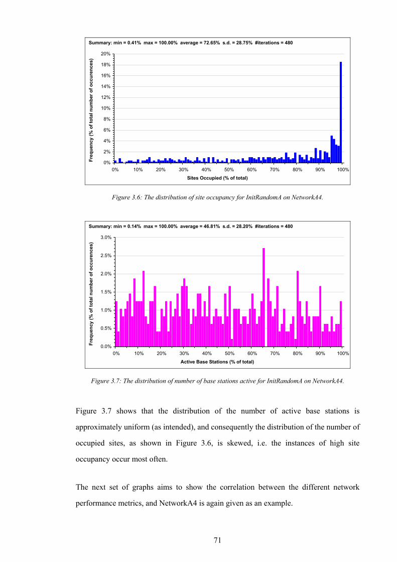
71

0%

2%

4%

6%

8%

10%

12%

14%

16%

18%

20%

0% 10% 20% 30% 40% 50% 60% 70% 80% 90% 100%

Sites Occupied (% of total)

Freq

uenc

y (%

of t

otal

num

ber o

f occ

uren

ces)

Summary: min = 0.41% max = 100.00% average = 72.65% s.d. = 28.75% #iterations = 480

Figure 3.6: The distribution of site occupancy for InitRandomA on NetworkA4.

0.0%

0.5%

1.0%

1.5%

2.0%

2.5%

3.0%

0% 10% 20% 30% 40% 50% 60% 70% 80% 90% 100%

Active Base Stations (% of total)

Freq

uenc

y (%

of t

otal

num

ber o

f occ

uren

ces)

Summary: min = 0.14% max = 100.00% average = 46.81% s.d. = 28.20% #iterations = 480

Figure 3.7: The distribution of number of base stations active for InitRandomA on NetworkA4.

Figure 3.7 shows that the distribution of the number of active base stations is

approximately uniform (as intended), and consequently the distribution of the number of

occupied sites, as shown in Figure 3.6, is skewed, i.e. the instances of high site

occupancy occur most often.

The next set of graphs aims to show the correlation between the different network

performance metrics, and NetworkA4 is again given as an example.

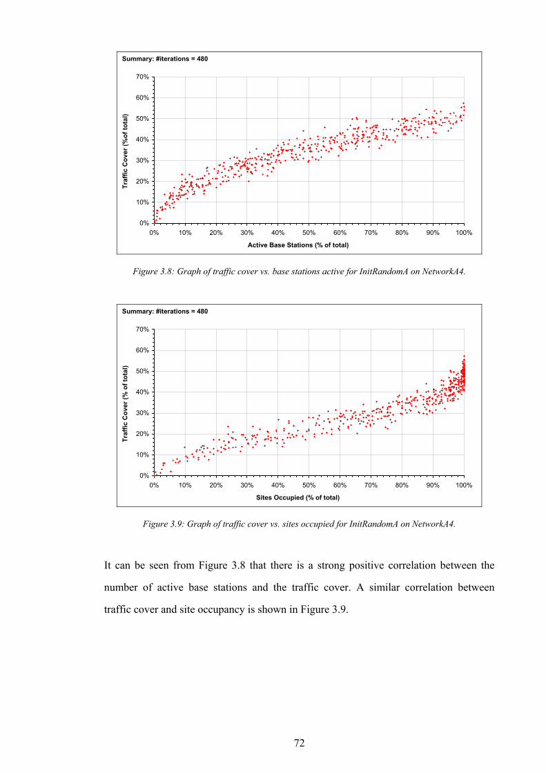
72

0%

10%

20%

30%

40%

50%

60%

70%

0% 10% 20% 30% 40% 50% 60% 70% 80% 90% 100%

Active Base Stations (% of total)

Traf

fic C

over

(%of

tota

l)

Summary: #iterations = 480

Figure 3.8: Graph of traffic cover vs. base stations active for InitRandomA on NetworkA4.

0%

10%

20%

30%

40%

50%

60%

70%

0% 10% 20% 30% 40% 50% 60% 70% 80% 90% 100%

Sites Occupied (% of total)

Traf

fic C

over

(% o

f tot

al)

Summary: #iterations = 480

Figure 3.9: Graph of traffic cover vs. sites occupied for InitRandomA on NetworkA4.

It can be seen from Figure 3.8 that there is a strong positive correlation between the

number of active base stations and the traffic cover. A similar correlation between

traffic cover and site occupancy is shown in Figure 3.9.

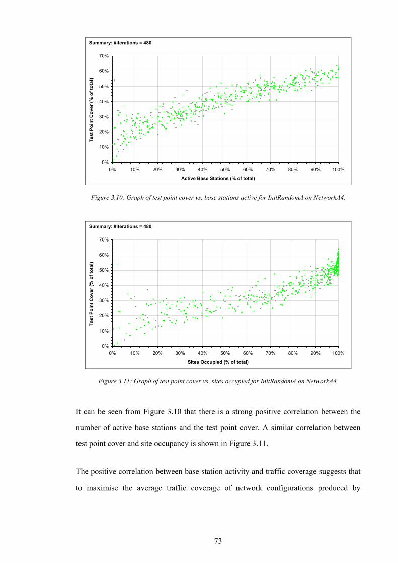
73

0%

10%

20%

30%

40%

50%

60%

70%

0% 10% 20% 30% 40% 50% 60% 70% 80% 90% 100%

Active Base Stations (% of total)

Test

Poi

nt C

over

(% o

f tot

al)

Summary: #iterations = 480

Figure 3.10: Graph of test point cover vs. base stations active for InitRandomA on NetworkA4.

0%

10%

20%

30%

40%

50%

60%

70%

0% 10% 20% 30% 40% 50% 60% 70% 80% 90% 100%

Sites Occupied (% of total)

Test

Poi

nt C

over

(% o

f tot

al)

Summary: #iterations = 480

Figure 3.11: Graph of test point cover vs. sites occupied for InitRandomA on NetworkA4.

It can be seen from Figure 3.10 that there is a strong positive correlation between the

number of active base stations and the test point cover. A similar correlation between

test point cover and site occupancy is shown in Figure 3.11.

The positive correlation between base station activity and traffic coverage suggests that

to maximise the average traffic coverage of network configurations produced by

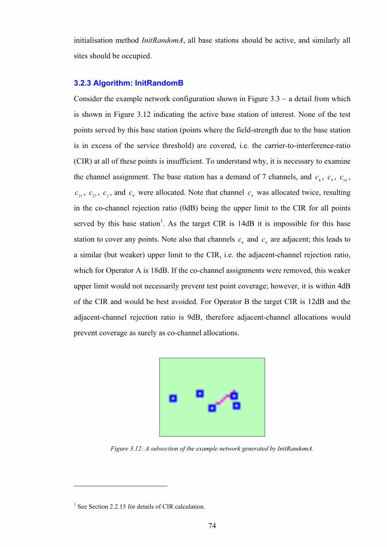
74

initialisation method InitRandomA, all base stations should be active, and similarly all

sites should be occupied.

3.2.3 Algorithm: InitRandomB

Consider the example network configuration shown in Figure 3.3 − a detail from which

is shown in Figure 3.12 indicating the active base station of interest. None of the test

points served by this base station (points where the field-strength due to the base station

is in excess of the service threshold) are covered, i.e. the carrier-to-interference-ratio

(CIR) at all of these points is insufficient. To understand why, it is necessary to examine

the channel assignment. The base station has a demand of 7 channels, and 8c , 9c , 18c ,

21c , 27c , 2c , and 9c were allocated. Note that channel 9c was allocated twice, resulting

in the co-channel rejection ratio (0dB) being the upper limit to the CIR for all points

served by this base station1. As the target CIR is 14dB it is impossible for this base

station to cover any points. Note also that channels 8c and 9c are adjacent; this leads to

a similar (but weaker) upper limit to the CIR, i.e. the adjacent-channel rejection ratio,

which for Operator A is 18dB. If the co-channel assignments were removed, this weaker

upper limit would not necessarily prevent test point coverage; however, it is within 4dB

of the CIR and would be best avoided. For Operator B the target CIR is 12dB and the

adjacent-channel rejection ratio is 9dB, therefore adjacent-channel allocations would

prevent coverage as surely as co-channel allocations.

Figure 3.12: A subsection of the example network generated by InitRandomA.

1 See Section 2.2.15 for details of CIR calculation.

75

Algorithm InitRandomB is a modified version of InitRandomA that employs an

improved channel selection process. It was shown above that a base station is

guaranteed to fail if any two allocated channels are equal, and likely to fail if any two

allocated channels are adjacent1. Algorithm InitRandomB selects channels at random

such that a two-channel separation is maintained between channels allocated to the same

base station − this is an example of an embedded heuristic (see [12]). Note that the

channel-selection bias is only designed to avoid channel ‘clashes’ in the same base

station, not between base stations (i.e. co-sector interference not co-site or far-site

interference).

3.2.3.1 Description

InitRandomB is identical to InitRandomA except for the channel selection process. For

each base station a list of all valid channels is constructed, and selections are made at

random from the channels in this list. Selected channels, and those adjacent to them, are

deleted from the list. This selection and deletion process is repeated until the base

station has received its full complement of channels.

1 Adjacent channel selection guarantees failure for Operator B networks.

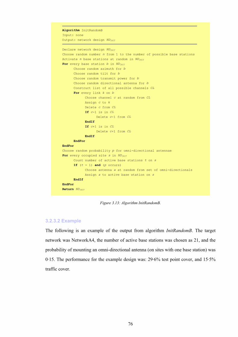
76

Algorithm InitRandomB Input: none

Output: network design NDINIT

Declare network design NDINIT Choose random number n from 1 to the number of possible base stations

Activate n base stations at random in NDINIT

For every base station b in NDINIT Choose random azimuth for b

Choose random tilt for b

Choose random transmit power for b

Choose random directional antenna for b

Construct list of all possible channels CL

For every link k on b Choose channel c at random from CL

Assign c to k

Delete c from CL

If c-1 is in CL Delete c-1 from CL

EndIf If c+1 is in CL Delete c+1 from CL

EndIf EndFor EndFor

Choose random probability p for omni-directional antennae

For every occupied site s in NDINIT Count number of active base stations t on s

If (t = 1) and (p occurs) Choose antenna a at random from set of omni-directionals

Assign a to active base station on s

EndIf EndFor Return NDINIT

Figure 3.13: Algorithm InitRandomB.

3.2.3.2 Example

The following is an example of the output from algorithm InitRandomB. The target

network was NetworkA4, the number of active base stations was chosen as 21, and the

probability of mounting an omni-directional antenna (on sites with one base station) was

0·15. The performance for the example design was: 29·6% test point cover, and 15·5%

traffic cover.

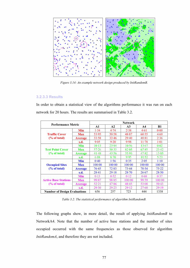
77

Figure 3.14: An example network design produced by InitRandomB.

3.2.3.3 Results

In order to obtain a statistical view of the algorithms performance it was run on each

network for 20 hours. The results are summarised in Table 3.2.

Network Performance Metric A1 A2 A3 A4 B1 Min 1·34 4·74 2·38 4·61 0·00 Max 53·95 50·58 48·87 60·55 4·69

Average 33·58 33·46 29·40 40·81 2·36 Traffic Cover (% of total)

s.d. 9·05 9·20 9·98 11·78 1·01 Min 10·13 23·94 10·56 13·67 0·02 Max 57·26 58·33 82·05 67·85 23·42

Average 41·48 43·56 35·93 47·82 13·05 Test Point Cover

(% of total) s.d. 6·88 8·70 9·95 10·52 5·23 Min 0·40 1·56 0·35 2·05 1·10 Max 100·00 100·00 100·00 100·00 100·00

Average 76·45 72·83 73·44 78·54 75·22 Occupied Sites

(% of total) s.d. 28·41 29·18 28·70 26·67 28·50 Min 0·13 0·52 0·12 0·68 0·37 Max 99·87 98·85 100·00 99·59 100·00

Average 52·21 47·86 48·45 53·08 50·43 Active Base Stations

(% of total) s.d. 29·30 29·23 29·12 27·60 29·19

Number of Design Evaluations 656 257 723 444 1338

Table 3.2: The statistical performance of algorithm InitRandomB.

The following graphs show, in more detail, the result of applying InitRandomB to

NetworkA4. Note that the number of active base stations and the number of sites

occupied occurred with the same frequencies as those observed for algorithm

InitRandomA, and therefore they are not included.

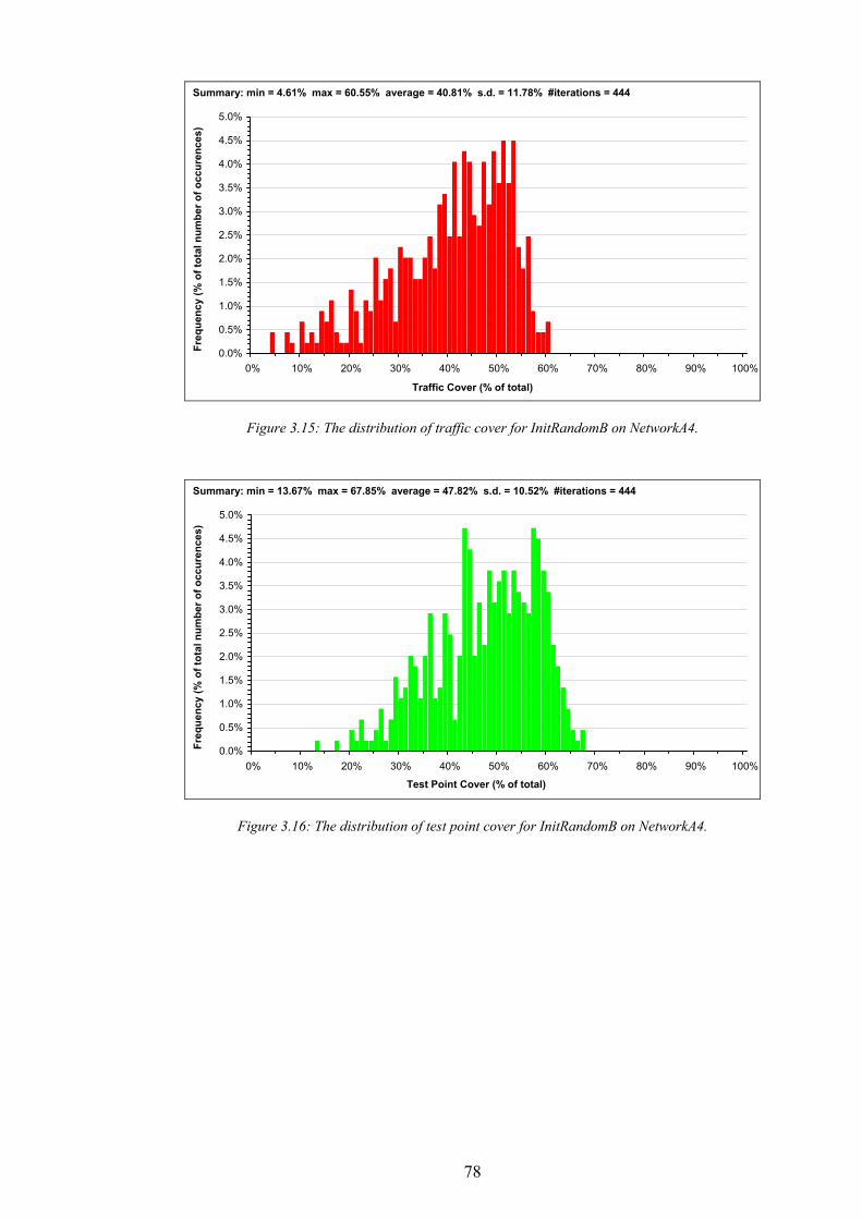
78

0.0%

0.5%

1.0%

1.5%

2.0%

2.5%

3.0%

3.5%

4.0%

4.5%

5.0%

0% 10% 20% 30% 40% 50% 60% 70% 80% 90% 100%

Traffic Cover (% of total)

Freq

uenc

y (%

of t

otal

num

ber o

f occ

uren

ces)

Summary: min = 4.61% max = 60.55% average = 40.81% s.d. = 11.78% #iterations = 444

Figure 3.15: The distribution of traffic cover for InitRandomB on NetworkA4.

0.0%

0.5%

1.0%

1.5%

2.0%

2.5%

3.0%

3.5%

4.0%

4.5%

5.0%

0% 10% 20% 30% 40% 50% 60% 70% 80% 90% 100%

Test Point Cover (% of total)

Freq

uenc

y (%

of t

otal

num

ber o

f occ

uren

ces)

Summary: min = 13.67% max = 67.85% average = 47.82% s.d. = 10.52% #iterations = 444

Figure 3.16: The distribution of test point cover for InitRandomB on NetworkA4.

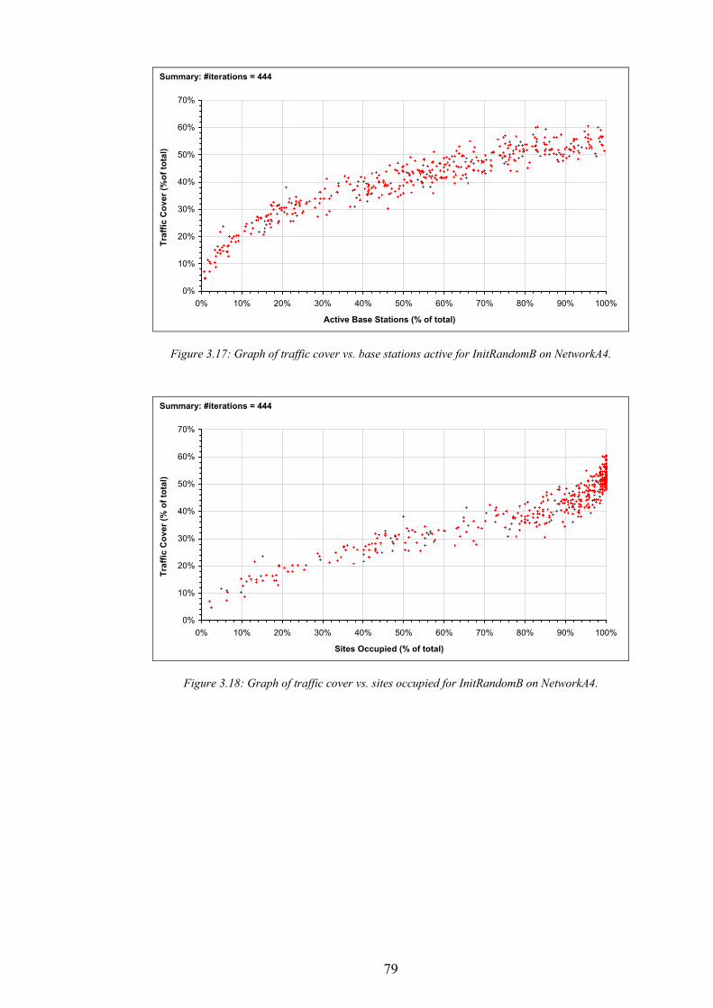
79

0%

10%

20%

30%

40%

50%

60%

70%

0% 10% 20% 30% 40% 50% 60% 70% 80% 90% 100%

Active Base Stations (% of total)

Traf

fic C

over

(%of

tota

l)

Summary: #iterations = 444

Figure 3.17: Graph of traffic cover vs. base stations active for InitRandomB on NetworkA4.

0%

10%

20%

30%

40%

50%

60%

70%

0% 10% 20% 30% 40% 50% 60% 70% 80% 90% 100%

Sites Occupied (% of total)

Traf

fic C

over

(% o

f tot

al)

Summary: #iterations = 444

Figure 3.18: Graph of traffic cover vs. sites occupied for InitRandomB on NetworkA4.

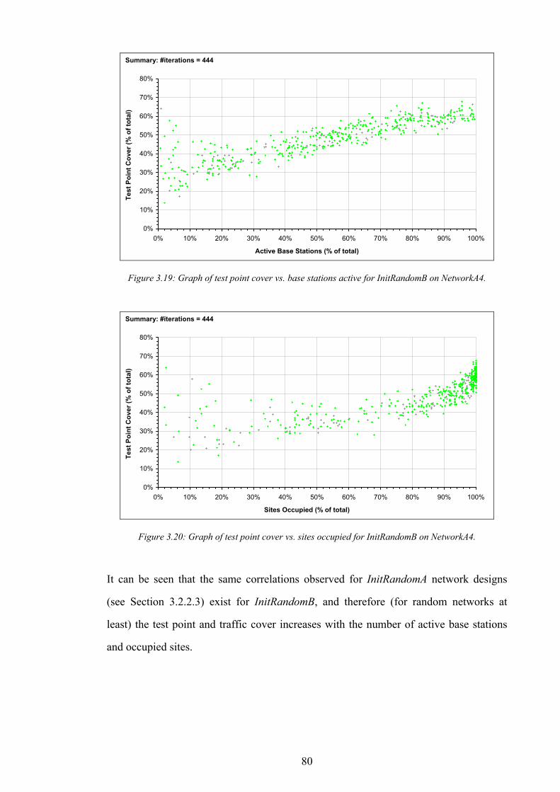
80

0%

10%

20%

30%

40%

50%

60%

70%

80%

0% 10% 20% 30% 40% 50% 60% 70% 80% 90% 100%

Active Base Stations (% of total)

Test

Poi

nt C

over

(% o

f tot

al)

Summary: #iterations = 444

Figure 3.19: Graph of test point cover vs. base stations active for InitRandomB on NetworkA4.

0%

10%

20%

30%

40%

50%

60%

70%

80%

0% 10% 20% 30% 40% 50% 60% 70% 80% 90% 100%

Sites Occupied (% of total)

Test

Poi

nt C

over

(% o

f tot

al)

Summary: #iterations = 444

Figure 3.20: Graph of test point cover vs. sites occupied for InitRandomB on NetworkA4.

It can be seen that the same correlations observed for InitRandomA network designs

(see Section 3.2.2.3) exist for InitRandomB, and therefore (for random networks at

least) the test point and traffic cover increases with the number of active base stations

and occupied sites.

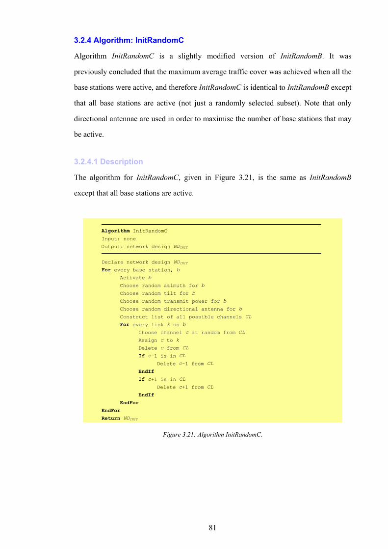
81

3.2.4 Algorithm: InitRandomC

Algorithm InitRandomC is a slightly modified version of InitRandomB. It was

previously concluded that the maximum average traffic cover was achieved when all the

base stations were active, and therefore InitRandomC is identical to InitRandomB except

that all base stations are active (not just a randomly selected subset). Note that only

directional antennae are used in order to maximise the number of base stations that may

be active.

3.2.4.1 Description

The algorithm for InitRandomC, given in Figure 3.21, is the same as InitRandomB

except that all base stations are active.

Algorithm InitRandomC Input: none

Output: network design NDINIT

Declare network design NDINIT For every base station, b Activate b

Choose random azimuth for b

Choose random tilt for b

Choose random transmit power for b

Choose random directional antenna for b

Construct list of all possible channels CL

For every link k on b Choose channel c at random from CL

Assign c to k

Delete c from CL

If c-1 is in CL Delete c-1 from CL

EndIf If c+1 is in CL Delete c+1 from CL

EndIf EndFor EndFor Return NDINIT

Figure 3.21: Algorithm InitRandomC.

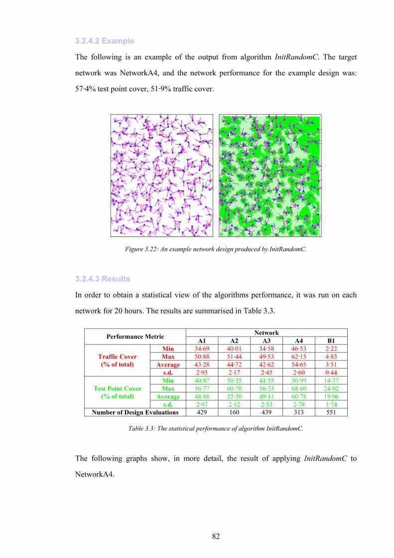
82

3.2.4.2 Example

The following is an example of the output from algorithm InitRandomC. The target

network was NetworkA4, and the network performance for the example design was:

57·4% test point cover, 51·9% traffic cover.

Figure 3.22: An example network design produced by InitRandomC.

3.2.4.3 Results

In order to obtain a statistical view of the algorithms performance, it was run on each

network for 20 hours. The results are summarised in Table 3.3.

Network Performance Metric A1 A2 A3 A4 B1 Min 34·69 40·01 34·58 46·53 2·22 Max 50·88 51·44 49·53 62·15 4·83

Average 43·28 44·72 42·62 54·65 3·51 Traffic Cover (% of total)

s.d. 2·95 2·17 2·45 2·60 0·44 Min 40·87 50·35 41·55 50·99 14·37 Max 56·77 60·70 56·33 68·60 24·02

Average 48·88 55·30 49·11 60·78 19·06 Test Point Cover

(% of total) s.d. 2·97 2·12 2·53 2·78 1·74

Number of Design Evaluations 429 160 439 313 551

Table 3.3: The statistical performance of algorithm InitRandomC.

The following graphs show, in more detail, the result of applying InitRandomC to

NetworkA4.

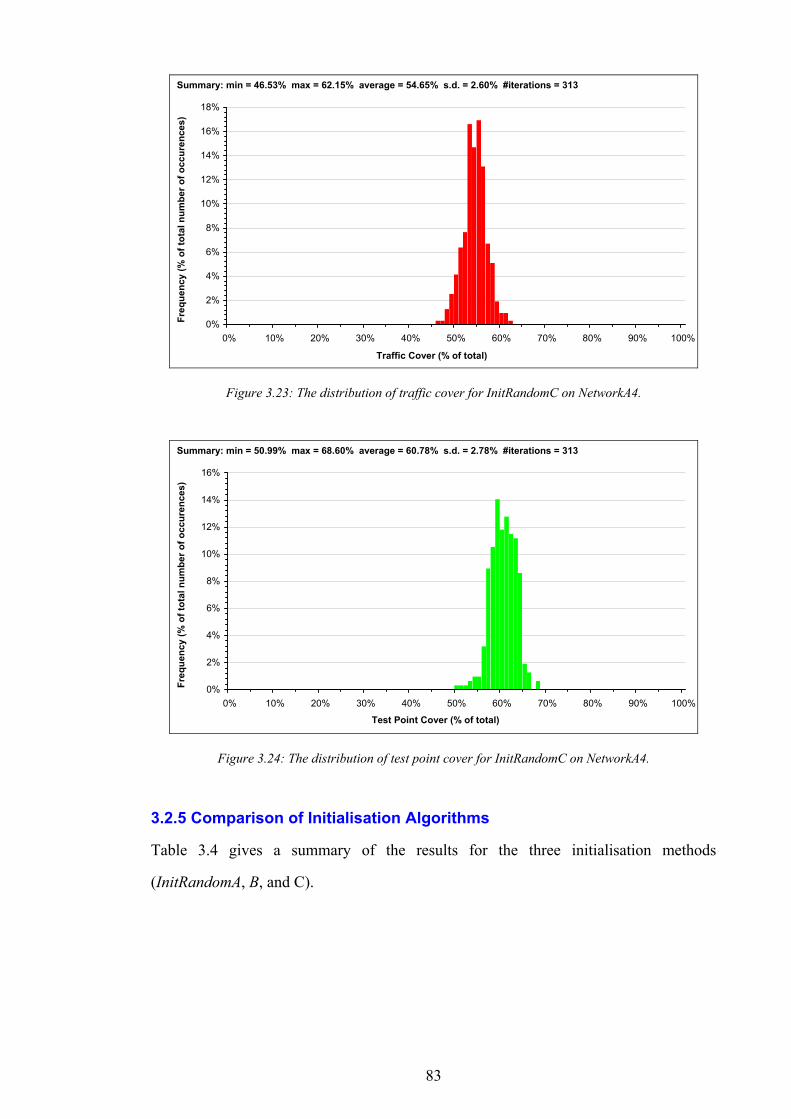
83

0%

2%

4%

6%

8%

10%

12%

14%

16%

18%

0% 10% 20% 30% 40% 50% 60% 70% 80% 90% 100%

Traffic Cover (% of total)

Freq

uenc

y (%

of t

otal

num

ber o

f occ

uren

ces)

Summary: min = 46.53% max = 62.15% average = 54.65% s.d. = 2.60% #iterations = 313

Figure 3.23: The distribution of traffic cover for InitRandomC on NetworkA4.

0%

2%

4%

6%

8%

10%

12%

14%

16%

0% 10% 20% 30% 40% 50% 60% 70% 80% 90% 100%

Test Point Cover (% of total)

Freq

uenc

y (%

of t

otal

num

ber o

f occ

uren

ces)

Summary: min = 50.99% max = 68.60% average = 60.78% s.d. = 2.78% #iterations = 313

Figure 3.24: The distribution of test point cover for InitRandomC on NetworkA4.

3.2.5 Comparison of Initialisation Algorithms

Table 3.4 gives a summary of the results for the three initialisation methods

(InitRandomA, B, and C).

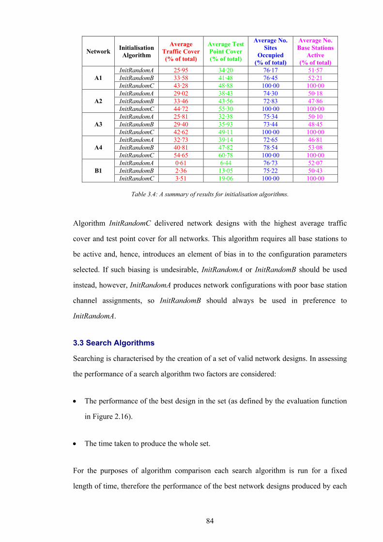
84

Network Initialisation Algorithm

Average Traffic Cover(% of total)

Average Test Point Cover (% of total)

Average No. Sites

Occupied (% of total)

Average No. Base Stations

Active (% of total)

InitRandomA 25·95 34·20 76·17 51·57 InitRandomB 33·58 41·48 76·45 52·21 A1 InitRandomC 43·28 48·88 100·00 100·00 InitRandomA 29·02 38·43 74·30 50·18 InitRandomB 33·46 43·56 72·83 47·86 A2 InitRandomC 44·72 55·30 100·00 100·00 InitRandomA 25·81 32·38 75·34 50·10 InitRandomB 29·40 35·93 73·44 48·45 A3 InitRandomC 42·62 49·11 100·00 100·00 InitRandomA 32·73 39·14 72·65 46·81 InitRandomB 40·81 47·82 78·54 53·08 A4 InitRandomC 54·65 60·78 100·00 100·00 InitRandomA 0·61 6·44 76·73 52·07 InitRandomB 2·36 13·05 75·22 50·43 B1 InitRandomC 3·51 19·06 100·00 100·00

Table 3.4: A summary of results for initialisation algorithms.

Algorithm InitRandomC delivered network designs with the highest average traffic

cover and test point cover for all networks. This algorithm requires all base stations to

be active and, hence, introduces an element of bias in to the configuration parameters

selected. If such biasing is undesirable, InitRandomA or InitRandomB should be used

instead, however, InitRandomA produces network configurations with poor base station

channel assignments, so InitRandomB should always be used in preference to

InitRandomA.

3.3 Search Algorithms

Searching is characterised by the creation of a set of valid network designs. In assessing

the performance of a search algorithm two factors are considered:

• The performance of the best design in the set (as defined by the evaluation function

in Figure 2.16).

• The time taken to produce the whole set.

For the purposes of algorithm comparison each search algorithm is run for a fixed

length of time, therefore the performance of the best network designs produced by each

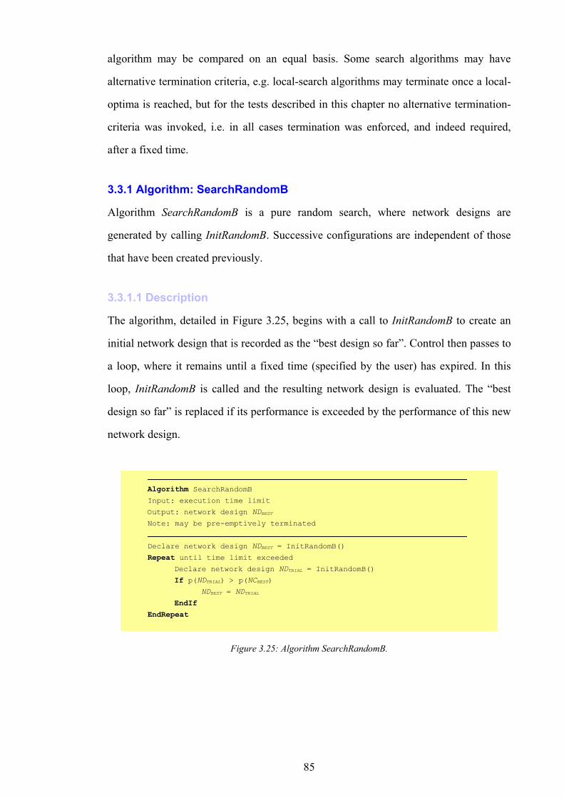
85

algorithm may be compared on an equal basis. Some search algorithms may have

alternative termination criteria, e.g. local-search algorithms may terminate once a local-

optima is reached, but for the tests described in this chapter no alternative termination-

criteria was invoked, i.e. in all cases termination was enforced, and indeed required,

after a fixed time.

3.3.1 Algorithm: SearchRandomB

Algorithm SearchRandomB is a pure random search, where network designs are

generated by calling InitRandomB. Successive configurations are independent of those

that have been created previously.

3.3.1.1 Description

The algorithm, detailed in Figure 3.25, begins with a call to InitRandomB to create an

initial network design that is recorded as the “best design so far”. Control then passes to

a loop, where it remains until a fixed time (specified by the user) has expired. In this

loop, InitRandomB is called and the resulting network design is evaluated. The “best

design so far” is replaced if its performance is exceeded by the performance of this new

network design.

Algorithm SearchRandomB Input: execution time limit

Output: network design NDBEST Note: may be pre-emptively terminated

Declare network design NDBEST = InitRandomB()

Repeat until time limit exceeded Declare network design NDTRIAL = InitRandomB()

If p(NDTRIAL) > p(NCBEST) NDBEST = NDTRIAL EndIf EndRepeat

Figure 3.25: Algorithm SearchRandomB.

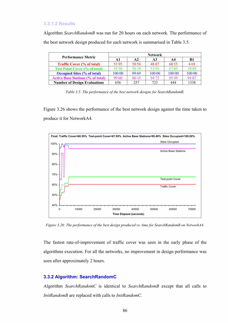
86

3.3.1.2 Results

Algorithm SearchRandomB was run for 20 hours on each network. The performance of

the best network design produced for each network is summarised in Table 3.5.

Network Performance Metric A1 A2 A3 A4 B1 Traffic Cover (% of total) 53·95 50·58 48·87 60·55 4·69

Test Point Cover (% of total) 55·50 58·19 53·91 67·85 19·89 Occupied Sites (% of total) 100·00 99·69 100·00 100·00 100·00

Active Base Stations (% of total) 99·60 86·15 94·72 95·49 94·87 Number of Design Evaluations 656 257 723 444 1338

Table 3.5: The performance of the best network designs for SearchRandomB.

Figure 3.26 shows the performance of the best network design against the time taken to

produce it for NetworkA4.

40%

50%

60%

70%

80%

90%

100%

0 10000 20000 30000 40000 50000 60000 70000

Time Elapsed (seconds)

Final: Traffic Cover=60.55% Test-point Cover=67.85% Active Base Stations=95.49% Sites Occupied=100.00%

Traffic Cover

Test-point Cover

Active Base Stations

Sites Occupied

Figure 3.26: The performance of the best design produced vs. time for SearchRandomB on NetworkA4.

The fastest rate-of-improvement of traffic cover was seen in the early phase of the

algorithms execution. For all the networks, no improvement in design performance was

seen after approximately 2 hours.

3.3.2 Algorithm: SearchRandomC

Algorithm SearchRandomC is identical to SearchRandomB except that all calls to

InitRandomB are replaced with calls to InitRandomC.

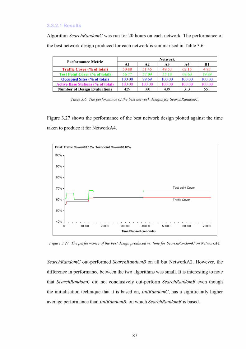
87

3.3.2.1 Results

Algorithm SearchRandomC was run for 20 hours on each network. The performance of

the best network design produced for each network is summarised in Table 3.6.

Network Performance Metric A1 A2 A3 A4 B1 Traffic Cover (% of total) 50·88 51·45 49·53 62·15 4·83

Test Point Cover (% of total) 56·77 57·09 55·18 68·60 19·89 Occupied Sites (% of total) 100·00 99·69 100·00 100·00 100·00

Active Base Stations (% of total) 100·00 100·00 100·00 100·00 100·00 Number of Design Evaluations 429 160 439 313 551

Table 3.6: The performance of the best network designs for SearchRandomC.

Figure 3.27 shows the performance of the best network design plotted against the time

taken to produce it for NetworkA4.

40%

50%

60%

70%

80%

90%

100%

0 10000 20000 30000 40000 50000 60000 70000

Time Elapsed (seconds)

Final: Traffic Cover=62.15% Test-point Cover=68.60%

Traffic Cover

Test-point Cover

Figure 3.27: The performance of the best design produced vs. time for SearchRandomC on NetworkA4.

SearchRandomC out-performed SearchRandomB on all but NetworkA2. However, the

difference in performance between the two algorithms was small. It is interesting to note

that SearchRandomC did not conclusively out-perform SearchRandomB even though

the initialisation technique that it is based on, InitRandomC, has a significantly higher

average performance than InitRandomB, on which SearchRandomB is based.

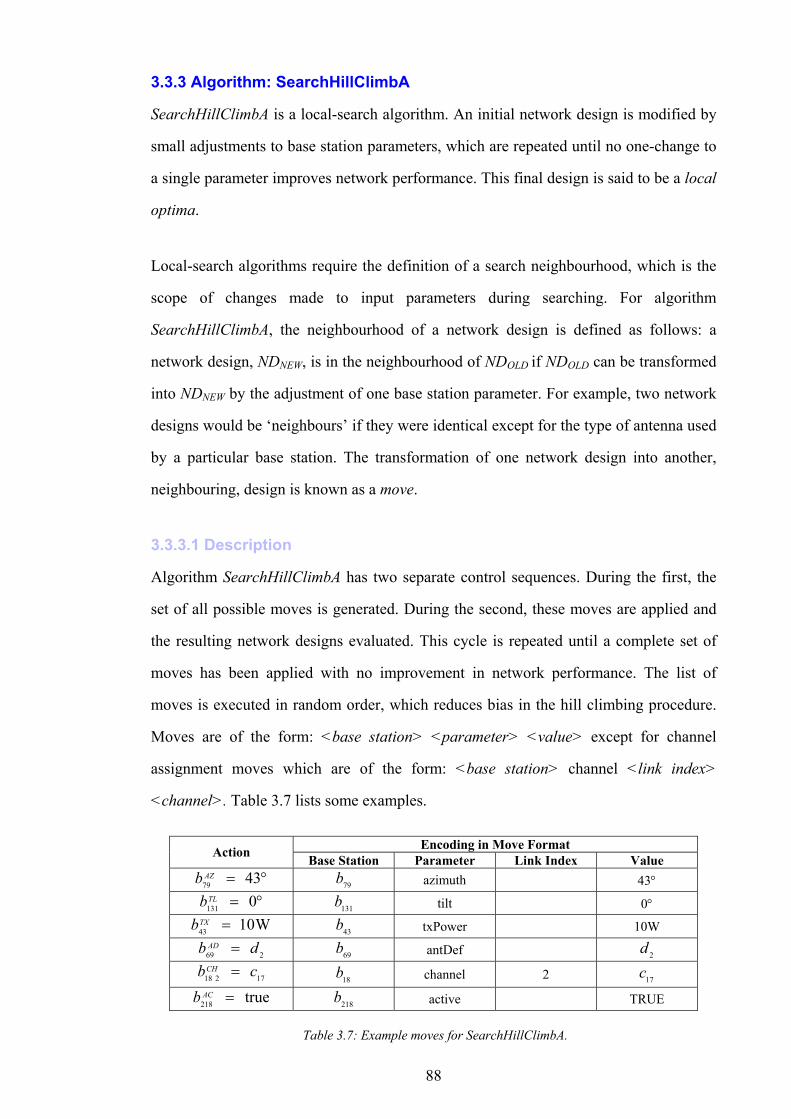
88

3.3.3 Algorithm: SearchHillClimbA

SearchHillClimbA is a local-search algorithm. An initial network design is modified by

small adjustments to base station parameters, which are repeated until no one-change to

a single parameter improves network performance. This final design is said to be a local

optima.

Local-search algorithms require the definition of a search neighbourhood, which is the

scope of changes made to input parameters during searching. For algorithm

SearchHillClimbA, the neighbourhood of a network design is defined as follows: a

network design, NDNEW, is in the neighbourhood of NDOLD if NDOLD can be transformed

into NDNEW by the adjustment of one base station parameter. For example, two network

designs would be ‘neighbours’ if they were identical except for the type of antenna used

by a particular base station. The transformation of one network design into another,

neighbouring, design is known as a move.

3.3.3.1 Description

Algorithm SearchHillClimbA has two separate control sequences. During the first, the

set of all possible moves is generated. During the second, these moves are applied and

the resulting network designs evaluated. This cycle is repeated until a complete set of

moves has been applied with no improvement in network performance. The list of

moves is executed in random order, which reduces bias in the hill climbing procedure.

Moves are of the form: <base station> <parameter> <value> except for channel

assignment moves which are of the form: <base station> channel <link index>

<channel>. Table 3.7 lists some examples.

Encoding in Move Format Action Base Station Parameter Link Index Value °= 4379

AZb 79b azimuth 43° °= 0131

TLb 131b tilt 0° W1043 =TXb 43b txPower 10W

269 db AD = 69b antDef 2d

17218 cbCH = 18b channel 2 17c

true218 =ACb 218b active TRUE

Table 3.7: Example moves for SearchHillClimbA.

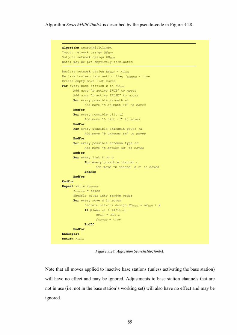
89

Algorithm SearchHillClimbA is described by the pseudo-code in Figure 3.28.

Algorithm SearchHillClimbA Input: network design NDINIT Output: network design NDBEST Note: may be pre-emptively terminated

Declare network design NDBEST = NDINIT Declare boolean termination flag fCONTINUE = true

Create empty move list moves

For every base station b in NDBEST Add move “b active TRUE” to moves

Add move “b active FALSE” to moves

For every possible azimuth az Add move “b azimuth az” to moves

EndFor For every possible tilt tl Add move “b tilt tl” to moves

EndFor For every possible transmit power tx Add move “b txPower tx” to moves

EndFor For every possible antenna type ad Add move “b antDef ad” to moves

EndFor For every link k on b For every possible channel c

Add move “b channel k c” to moves

EndFor EndFor EndFor Repeat while fCONTINUE fCONTINUE = false

Shuffle moves into random order

For every move m in moves Declare network design NDTRIAL = NDBEST + m

If p(NDTRIAL) > p(NDBEST) NDBEST = NDTRIAL

fCONTINUE = true

EndIf EndFor EndRepeat Return NDBEST

Figure 3.28: Algorithm SearchHillClimbA.

Note that all moves applied to inactive base stations (unless activating the base station)

will have no effect and may be ignored. Adjustments to base station channels that are

not in use (i.e. not in the base station’s working set) will also have no effect and may be

ignored.

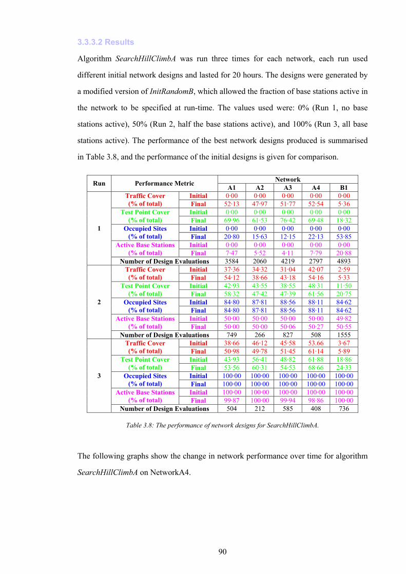
90

3.3.3.2 Results

Algorithm SearchHillClimbA was run three times for each network, each run used

different initial network designs and lasted for 20 hours. The designs were generated by

a modified version of InitRandomB, which allowed the fraction of base stations active in

the network to be specified at run-time. The values used were: 0% (Run 1, no base

stations active), 50% (Run 2, half the base stations active), and 100% (Run 3, all base

stations active). The performance of the best network designs produced is summarised

in Table 3.8, and the performance of the initial designs is given for comparison.

Network Run Performance Metric A1 A2 A3 A4 B1 Initial 0·00 0·00 0·00 0·00 0·00 Traffic Cover

(% of total) Final 52·13 47·97 51·77 52·54 5·36 Initial 0·00 0·00 0·00 0·00 0·00 Test Point Cover

(% of total) Final 69·96 61·53 76·42 69·48 18·32 Initial 0·00 0·00 0·00 0·00 0·00 Occupied Sites

(% of total) Final 20·80 15·63 12·15 22·13 53·85 Initial 0·00 0·00 0·00 0·00 0·00 Active Base Stations

(% of total) Final 7·47 5·52 4·11 7·79 20·88

1

Number of Design Evaluations 3584 2060 4219 2797 4893 Initial 37·36 34·32 31·04 42·07 2·59 Traffic Cover

(% of total) Final 54·12 38·66 43·18 54·16 5·33 Initial 42·93 43·55 38·55 48·31 11·50 Test Point Cover

(% of total) Final 58·32 47·42 47·39 61·56 20·75 Initial 84·80 87·81 88·56 88·11 84·62 Occupied Sites

(% of total) Final 84·80 87·81 88·56 88·11 84·62 Initial 50·00 50·00 50·00 50·00 49·82 Active Base Stations

(% of total) Final 50·00 50·00 50·06 50·27 50·55

2

Number of Design Evaluations 749 266 827 508 1555 Initial 38·66 46·12 45·58 53.66 3·67 Traffic Cover

(% of total) Final 50·98 49·78 51·45 61·14 5·89 Initial 43·93 56·41 48·82 61·88 18·86 Test Point Cover

(% of total) Final 53·56 60·31 54·53 68·66 24·33 Initial 100·00 100·00 100·00 100·00 100·00 Occupied Sites

(% of total) Final 100·00 100·00 100·00 100·00 100·00 Initial 100·00 100·00 100·00 100·00 100·00 Active Base Stations

(% of total) Final 99·87 100·00 99·94 98·86 100·00

3

Number of Design Evaluations 504 212 585 408 736

Table 3.8: The performance of network designs for SearchHillClimbA.

The following graphs show the change in network performance over time for algorithm

SearchHillClimbA on NetworkA4.

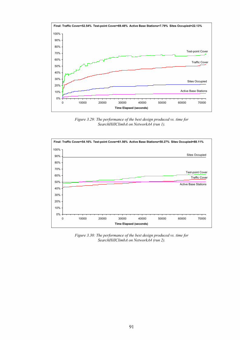
91

0%

10%

20%

30%

40%

50%

60%

70%

80%

90%

100%

0 10000 20000 30000 40000 50000 60000 70000

Time Elapsed (seconds)

Final: Traffic Cover=52.54% Test-point Cover=69.48% Active Base Stations=7.79% Sites Occupied=22.13%

Traffic Cover

Test-point Cover

Active Base Stations

Sites Occupied

Figure 3.29: The performance of the best design produced vs. time for SearchHillClimbA on NetworkA4 (run 1).

0%

10%

20%

30%

40%

50%

60%

70%

80%

90%

100%

0 10000 20000 30000 40000 50000 60000 70000

Time Elapsed (seconds)

Final: Traffic Cover=54.16% Test-point Cover=61.56% Active Base Stations=50.27% Sites Occupied=88.11%

Traffic Cover

Test-point Cover

Active Base Stations

Sites Occupied

Figure 3.30: The performance of the best design produced vs. time for SearchHillClimbA on NetworkA4 (run 2).

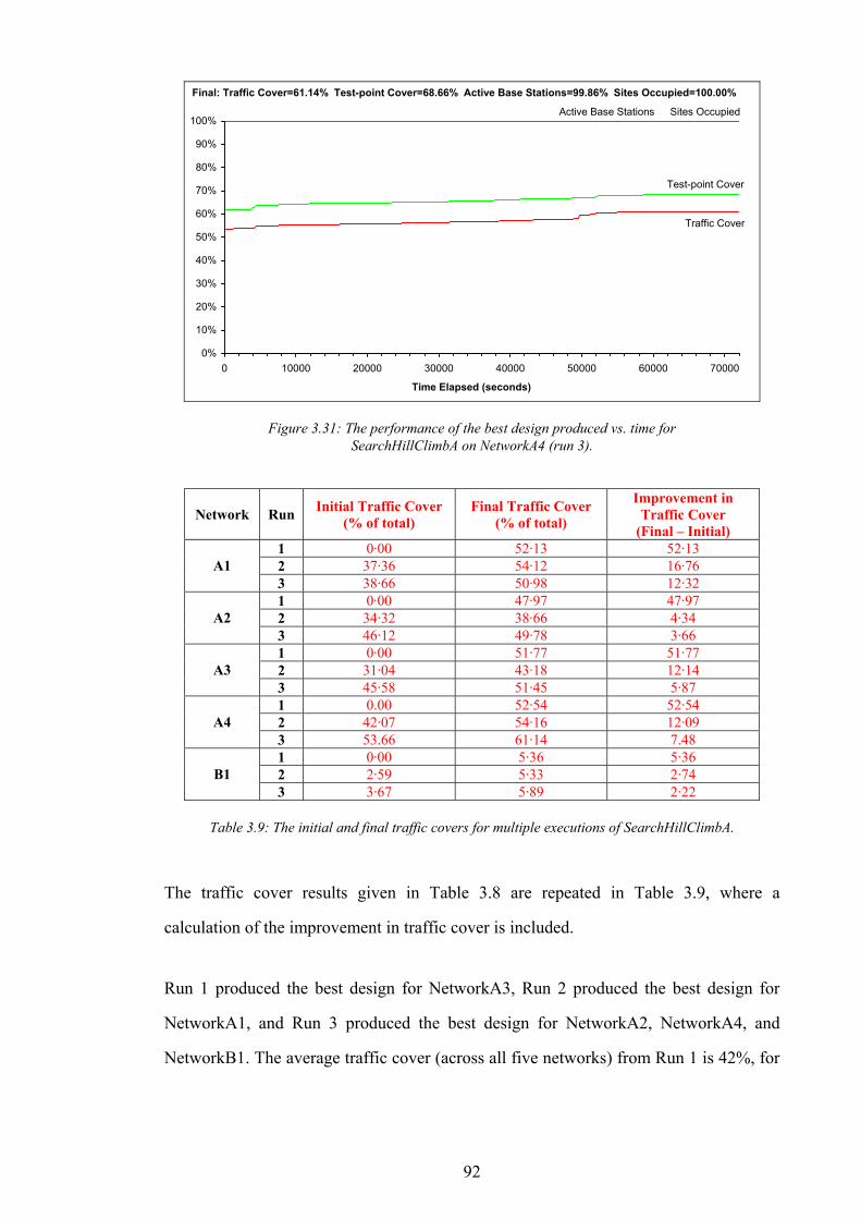
92

0%

10%

20%

30%

40%

50%

60%

70%

80%

90%

100%

0 10000 20000 30000 40000 50000 60000 70000

Time Elapsed (seconds)

Final: Traffic Cover=61.14% Test-point Cover=68.66% Active Base Stations=99.86% Sites Occupied=100.00%

Traffic Cover

Test-point Cover

Active Base Stations Sites Occupied

Figure 3.31: The performance of the best design produced vs. time for SearchHillClimbA on NetworkA4 (run 3).

Network Run Initial Traffic Cover (% of total)

Final Traffic Cover (% of total)

Improvement in Traffic Cover

(Final – Initial) 1 0·00 52·13 52·13 2 37·36 54·12 16·76 A1 3 38·66 50·98 12·32 1 0·00 47·97 47·97 2 34·32 38·66 4·34 A2 3 46·12 49·78 3·66 1 0·00 51·77 51·77 2 31·04 43·18 12·14 A3 3 45·58 51·45 5·87 1 0.00 52·54 52·54 2 42·07 54·16 12·09 A4 3 53.66 61·14 7.48 1 0·00 5·36 5·36 2 2·59 5·33 2·74 B1 3 3·67 5·89 2·22

Table 3.9: The initial and final traffic covers for multiple executions of SearchHillClimbA.

The traffic cover results given in Table 3.8 are repeated in Table 3.9, where a

calculation of the improvement in traffic cover is included.

Run 1 produced the best design for NetworkA3, Run 2 produced the best design for

NetworkA1, and Run 3 produced the best design for NetworkA2, NetworkA4, and

NetworkB1. The average traffic cover (across all five networks) from Run 1 is 42%, for

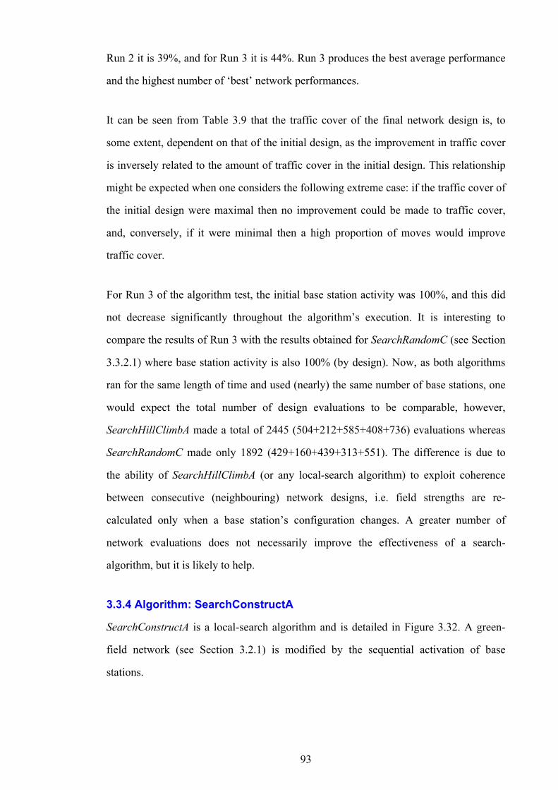
93

Run 2 it is 39%, and for Run 3 it is 44%. Run 3 produces the best average performance

and the highest number of ‘best’ network performances.

It can be seen from Table 3.9 that the traffic cover of the final network design is, to

some extent, dependent on that of the initial design, as the improvement in traffic cover

is inversely related to the amount of traffic cover in the initial design. This relationship

might be expected when one considers the following extreme case: if the traffic cover of

the initial design were maximal then no improvement could be made to traffic cover,

and, conversely, if it were minimal then a high proportion of moves would improve

traffic cover.

For Run 3 of the algorithm test, the initial base station activity was 100%, and this did

not decrease significantly throughout the algorithm’s execution. It is interesting to

compare the results of Run 3 with the results obtained for SearchRandomC (see Section

3.3.2.1) where base station activity is also 100% (by design). Now, as both algorithms

ran for the same length of time and used (nearly) the same number of base stations, one

would expect the total number of design evaluations to be comparable, however,

SearchHillClimbA made a total of 2445 (504+212+585+408+736) evaluations whereas

SearchRandomC made only 1892 (429+160+439+313+551). The difference is due to

the ability of SearchHillClimbA (or any local-search algorithm) to exploit coherence

between consecutive (neighbouring) network designs, i.e. field strengths are re-

calculated only when a base station’s configuration changes. A greater number of

network evaluations does not necessarily improve the effectiveness of a search-

algorithm, but it is likely to help.

3.3.4 Algorithm: SearchConstructA

SearchConstructA is a local-search algorithm and is detailed in Figure 3.32. A green-

field network (see Section 3.2.1) is modified by the sequential activation of base

stations.

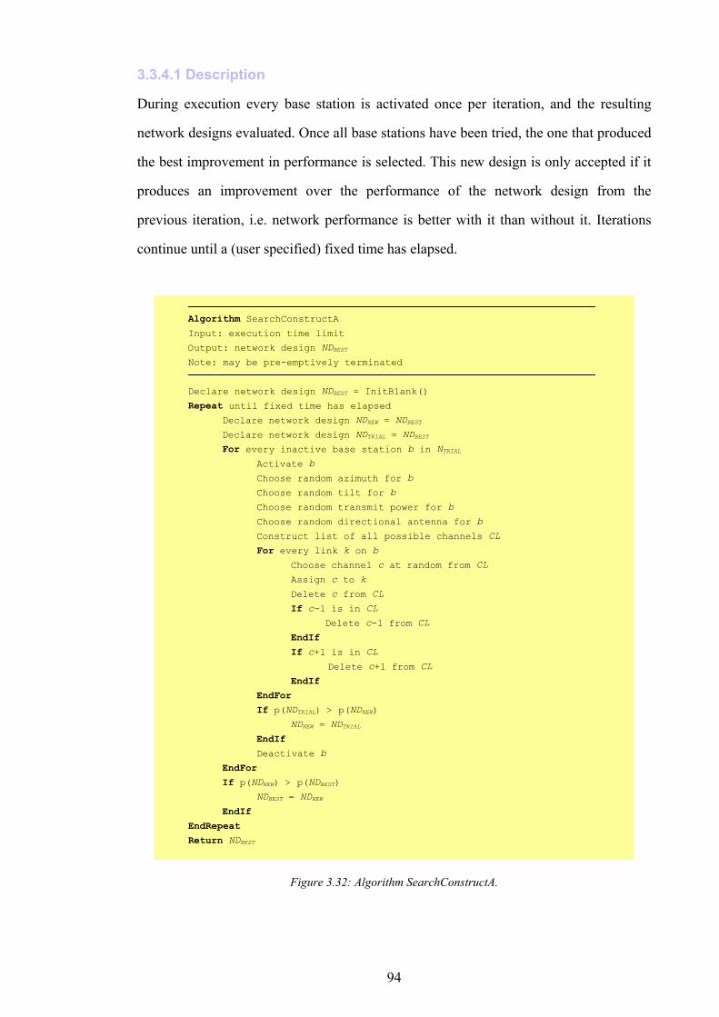
94

3.3.4.1 Description

During execution every base station is activated once per iteration, and the resulting

network designs evaluated. Once all base stations have been tried, the one that produced

the best improvement in performance is selected. This new design is only accepted if it

produces an improvement over the performance of the network design from the

previous iteration, i.e. network performance is better with it than without it. Iterations

continue until a (user specified) fixed time has elapsed.

Algorithm SearchConstructA Input: execution time limit

Output: network design NDBEST Note: may be pre-emptively terminated

Declare network design NDBEST = InitBlank()

Repeat until fixed time has elapsed Declare network design NDNEW = NDBEST Declare network design NDTRIAL = NDBEST For every inactive base station b in NTRIAL Activate b

Choose random azimuth for b

Choose random tilt for b

Choose random transmit power for b

Choose random directional antenna for b

Construct list of all possible channels CL

For every link k on b Choose channel c at random from CL

Assign c to k

Delete c from CL

If c-1 is in CL Delete c-1 from CL

EndIf If c+1 is in CL

Delete c+1 from CL

EndIf EndFor If p(NDTRIAL) > p(NDNEW) NDNEW = NDTRIAL EndIf Deactivate b

EndFor If p(NDNEW) > p(NDBEST) NDBEST = NDNEW EndIf

EndRepeat Return NDBEST

Figure 3.32: Algorithm SearchConstructA.

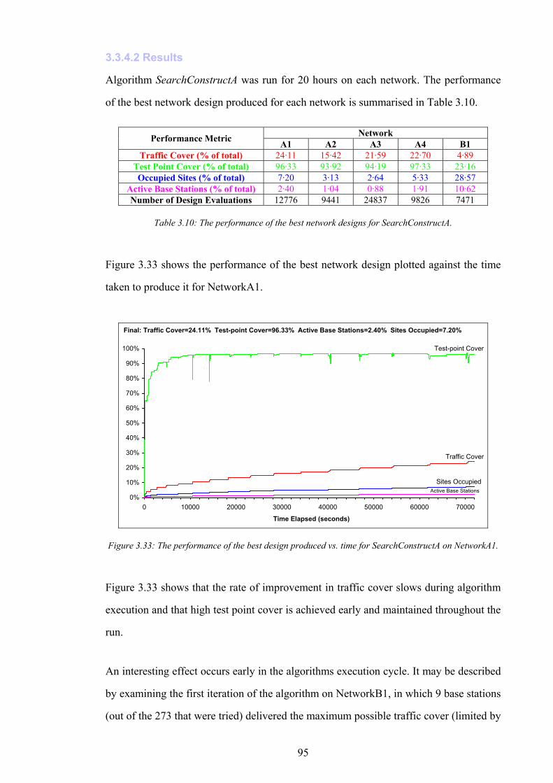
95

3.3.4.2 Results

Algorithm SearchConstructA was run for 20 hours on each network. The performance

of the best network design produced for each network is summarised in Table 3.10.

Network Performance Metric A1 A2 A3 A4 B1 Traffic Cover (% of total) 24·11 15·42 21·59 22·70 4·89

Test Point Cover (% of total) 96·33 93·92 94·19 97·33 23·16 Occupied Sites (% of total) 7·20 3·13 2·64 5·33 28·57

Active Base Stations (% of total) 2·40 1·04 0·88 1·91 10·62 Number of Design Evaluations 12776 9441 24837 9826 7471

Table 3.10: The performance of the best network designs for SearchConstructA.

Figure 3.33 shows the performance of the best network design plotted against the time

taken to produce it for NetworkA1.

0%

10%

20%

30%

40%

50%

60%

70%

80%

90%

100%

0 10000 20000 30000 40000 50000 60000 70000

Time Elapsed (seconds)

Final: Traffic Cover=24.11% Test-point Cover=96.33% Active Base Stations=2.40% Sites Occupied=7.20%

Traffic Cover

Test-point Cover

Active Base StationsSites Occupied

Figure 3.33: The performance of the best design produced vs. time for SearchConstructA on NetworkA1.

Figure 3.33 shows that the rate of improvement in traffic cover slows during algorithm

execution and that high test point cover is achieved early and maintained throughout the

run.

An interesting effect occurs early in the algorithms execution cycle. It may be described

by examining the first iteration of the algorithm on NetworkB1, in which 9 base stations

(out of the 273 that were tried) delivered the maximum possible traffic cover (limited by

96

the traffic capacity of a single base station, i.e. 58 Erlangs). The number of test points

covered by these base stations ranged between 74 and 1031, and, as the traffic cover for

each base station was equal, the base station with the highest test point cover was

accepted. If this was the final network design produced then this would be the best

choice, however, as the algorithm continues, the extra coverage achieved early on

becomes an obstacle to further coverage, i.e. it increases the likelihood of interference in

the network. Essentially, the ‘dimensions’ (i.e. the ratio of traffic cover to test point

cover) of the early cells are distorted by the requirements of the evaluation function.

3.3.5 Algorithm: SearchConstructB

In Section 3.3.4.2 it was postulated that during the initial stages of execution of

SearchConstructA, high test point cover was detrimental to the performance of the final

network design. Algorithm SearchConstructB attempts to avoid this problem by a

temporary adjustment of the evaluation function.

3.3.5.1 Description

The following list shows the default evaluation criteria in order of significance:

1. Higher traffic cover

2. Higher traffic service1

3. Higher test point cover

4. Higher test point service2

5. Lower site occupancy

6. Lower number of active base stations

1 The traffic that would be covered in the absence of interference. 2 The test points that would be covered in the absence of interference.

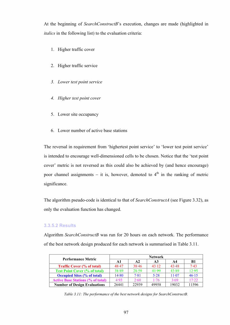
97

At the beginning of SearchConstructB’s execution, changes are made (highlighted in

italics in the following list) to the evaluation criteria:

1. Higher traffic cover

2. Higher traffic service

3. Lower test point service

4. Higher test point cover

5. Lower site occupancy

6. Lower number of active base stations

The reversal in requirement from ‘highertest point service’ to ‘lower test point service’

is intended to encourage well-dimensioned cells to be chosen. Notice that the ‘test point

cover’ metric is not reversed as this could also be achieved by (and hence encourage)

poor channel assignments − it is, however, demoted to 4th in the ranking of metric

significance.

The algorithm pseudo-code is identical to that of SearchConstructA (see Figure 3.32), as

only the evaluation function has changed.

3.3.5.2 Results

Algorithm SearchConstructB was run for 20 hours on each network. The performance

of the best network design produced for each network is summarised in Table 3.11.

Network Performance Metric A1 A2 A3 A4 B1 Traffic Cover (% of total) 48·47 38·46 43·12 43·48 7·43

Test Point Cover (% of total) 38·89 28·59 41·99 43·89 12·95 Occupied Sites (% of total) 14·80 7·81 5·28 11·07 46·15

Active Base Stations (% of total) 4·93 2·60 1·76 3·69 17·22 Number of Design Evaluations 26441 22939 49958 19032 11596

Table 3.11: The performance of the best network designs for SearchConstructB.

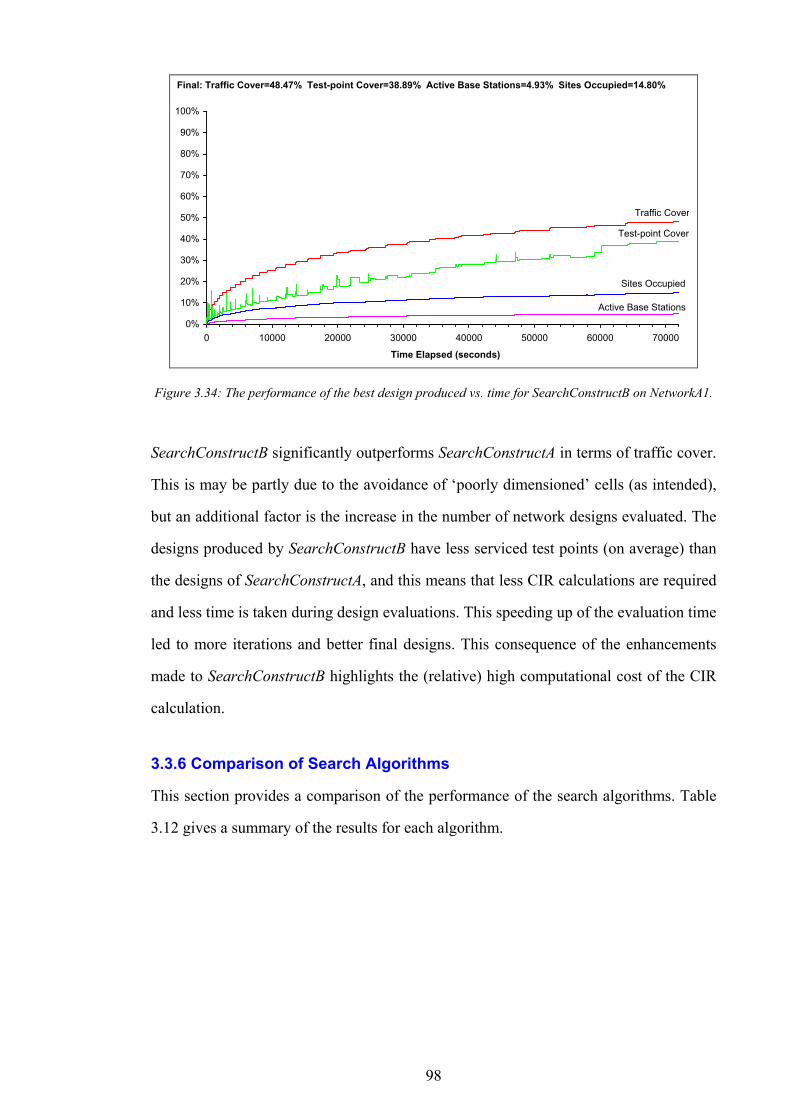
98

0%

10%

20%

30%

40%

50%

60%

70%

80%

90%

100%

0 10000 20000 30000 40000 50000 60000 70000

Time Elapsed (seconds)

Final: Traffic Cover=48.47% Test-point Cover=38.89% Active Base Stations=4.93% Sites Occupied=14.80%

Traffic Cover

Test-point Cover

Active Base Stations

Sites Occupied

Figure 3.34: The performance of the best design produced vs. time for SearchConstructB on NetworkA1.

SearchConstructB significantly outperforms SearchConstructA in terms of traffic cover.

This is may be partly due to the avoidance of ‘poorly dimensioned’ cells (as intended),

but an additional factor is the increase in the number of network designs evaluated. The

designs produced by SearchConstructB have less serviced test points (on average) than

the designs of SearchConstructA, and this means that less CIR calculations are required

and less time is taken during design evaluations. This speeding up of the evaluation time

led to more iterations and better final designs. This consequence of the enhancements

made to SearchConstructB highlights the (relative) high computational cost of the CIR

calculation.

3.3.6 Comparison of Search Algorithms

This section provides a comparison of the performance of the search algorithms. Table

3.12 gives a summary of the results for each algorithm.

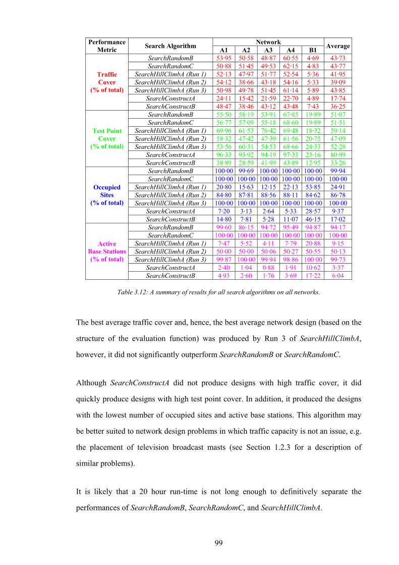
99

Network Performance Metric Search Algorithm A1 A2 A3 A4 B1 Average

SearchRandomB 53·95 50·58 48·87 60·55 4·69 43·73 SearchRandomC 50·88 51·45 49·53 62·15 4·83 43·77

SearchHillClimbA (Run 1) 52·13 47·97 51·77 52·54 5·36 41·95 SearchHillClimbA (Run 2) 54·12 38·66 43·18 54·16 5·33 39·09 SearchHillClimbA (Run 3) 50·98 49·78 51·45 61·14 5·89 43·85

SearchConstructA 24·11 15·42 21·59 22·70 4·89 17·74

Traffic Cover

(% of total)

SearchConstructB 48·47 38·46 43·12 43·48 7·43 36·25 SearchRandomB 55·50 58·19 53·91 67·85 19·89 51·07 SearchRandomC 56·77 57·09 55·18 68·60 19·89 51·51

SearchHillClimbA (Run 1) 69·96 61·53 76·42 69·48 18·32 59·14 SearchHillClimbA (Run 2) 58·32 47·42 47·39 61·56 20·75 47·09 SearchHillClimbA (Run 3) 53·56 60·31 54·53 68·66 24·33 52·28

SearchConstructA 96·33 93·92 94·19 97·33 23·16 80·99

Test Point Cover

(% of total)

SearchConstructB 38·89 28·59 41·99 43·89 12·95 33·26 SearchRandomB 100·00 99·69 100·00 100·00 100·00 99·94 SearchRandomC 100·00 100·00 100·00 100·00 100·00 100·00

SearchHillClimbA (Run 1) 20·80 15·63 12·15 22·13 53·85 24·91 SearchHillClimbA (Run 2) 84·80 87·81 88·56 88·11 84·62 86·78 SearchHillClimbA (Run 3) 100·00 100·00 100·00 100·00 100·00 100·00

SearchConstructA 7·20 3·13 2·64 5·33 28·57 9·37

Occupied Sites

(% of total)

SearchConstructB 14·80 7·81 5·28 11·07 46·15 17·02 SearchRandomB 99·60 86·15 94·72 95·49 94·87 94·17 SearchRandomC 100·00 100·00 100·00 100·00 100·00 100·00

SearchHillClimbA (Run 1) 7·47 5·52 4·11 7·79 20·88 9·15 SearchHillClimbA (Run 2) 50·00 50·00 50·06 50·27 50·55 50·13 SearchHillClimbA (Run 3) 99·87 100·00 99·94 98·86 100·00 99·73

SearchConstructA 2·40 1·04 0·88 1·91 10·62 3·37

Active Base Stations (% of total)

SearchConstructB 4·93 2·60 1·76 3·69 17·22 6·04

Table 3.12: A summary of results for all search algorithms on all networks.

The best average traffic cover and, hence, the best average network design (based on the

structure of the evaluation function) was produced by Run 3 of SearchHillClimbA,

however, it did not significantly outperform SearchRandomB or SearchRandomC.

Although SearchConstructA did not produce designs with high traffic cover, it did

quickly produce designs with high test point cover. In addition, it produced the designs

with the lowest number of occupied sites and active base stations. This algorithm may

be better suited to network design problems in which traffic capacity is not an issue, e.g.

the placement of television broadcast masts (see Section 1.2.3 for a description of

similar problems).

It is likely that a 20 hour run-time is not long enough to definitively separate the

performances of SearchRandomB, SearchRandomC, and SearchHillClimbA.

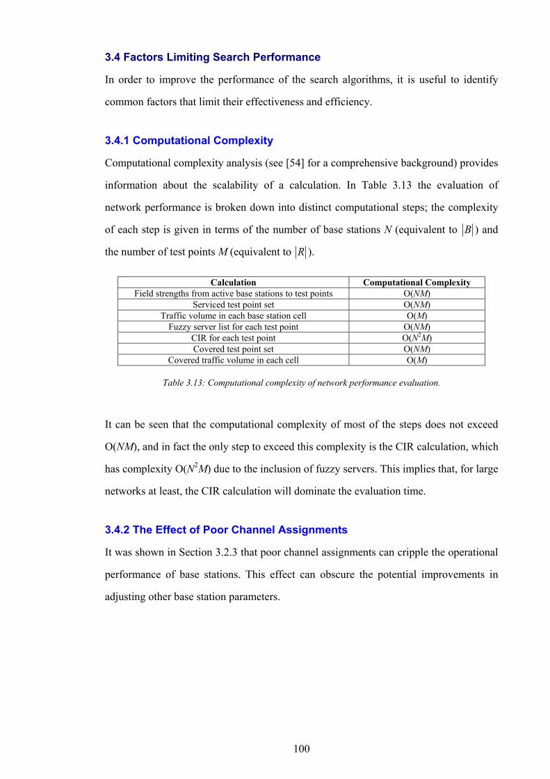
100

3.4 Factors Limiting Search Performance

In order to improve the performance of the search algorithms, it is useful to identify

common factors that limit their effectiveness and efficiency.

3.4.1 Computational Complexity

Computational complexity analysis (see [54] for a comprehensive background) provides

information about the scalability of a calculation. In Table 3.13 the evaluation of

network performance is broken down into distinct computational steps; the complexity

of each step is given in terms of the number of base stations N (equivalent to B ) and

the number of test points M (equivalent to R ).

Calculation Computational Complexity Field strengths from active base stations to test points O(NM)

Serviced test point set O(NM) Traffic volume in each base station cell O(M)

Fuzzy server list for each test point O(NM) CIR for each test point O(N2M) Covered test point set O(NM)

Covered traffic volume in each cell O(M)

Table 3.13: Computational complexity of network performance evaluation.

It can be seen that the computational complexity of most of the steps does not exceed

O(NM), and in fact the only step to exceed this complexity is the CIR calculation, which

has complexity O(N2M) due to the inclusion of fuzzy servers. This implies that, for large

networks at least, the CIR calculation will dominate the evaluation time.

3.4.2 The Effect of Poor Channel Assignments

It was shown in Section 3.2.3 that poor channel assignments can cripple the operational

performance of base stations. This effect can obscure the potential improvements in

adjusting other base station parameters.

101

3.4.3 Conclusion

To avoid the difficulties associated with the channel model (expensive CIR calculation

and bad channel assignments) it is desirable to split the problem into two stages:

1. Base station configuration without channel assignment (and its associated CIR

calculations), known as the Base Station Configuration Problem or BSCP (see

Section 1.2.3.2 for description).

2. Channel assignment for the network design produced by stage 1. This is known as

the Channel Assignment Problem or CAP (see Section 1.2.2 for description).

The division of the WCNDP into these two sub-problems is not novel, and in fact most

network design problems are explicitly formulated with this two-part approach (see

Section 1.2.4). The novelty lies in the opportunity to quantify the advantages this

approach may offer (Chapter 6 contains details of this comparison).

In the two-stage approach to the WCNDP, performance in the CAP phase depends

heavily on the design produced to solve the BSCP, because with high traffic and test

point service is useless unless it is relatively easy to create good channel assignments.

To do this, an estimate must be made (during the cell planning process) of how difficult

it will be to produce a good channel assignment. These ‘difficulty’ metrics shall be

referred to as interference surrogates. The interference surrogate must be included in

the definition of the BSCP, and the network design evaluation criteria must be as

follows (see Section 2.3.2 to compare this with the full WCNDP evaluation function):

1. High traffic service.

2. High test point service.

3. Low estimated interference.

4. Low site occupancy.

102

5. Low number of active base stations.

The interference surrogate is shown in italics, and the structure of the evaluation is such

that it would only become a deciding factor in networks that had identical traffic and

test point service. The interference surrogate function must have a computational

complexity that does not exceed O(NM), as this will ensure that it scales at least as well

as the other calculations.

103

Chapter 4 Channel Assignment

This chapter describes a novel formulation of the Channel Assignment Problem (CAP).

Channels represent a continuous portion of the radio spectrum, and channel assignment

is the allocation of channels to transmitters in a radio network such that the interference

between channels is minimised. The central frequency in a channel is sometimes used to

uniquely identify it, and for this reason the CAP is also know as the Frequency

Assignment Problem (FAP). An introduction to the CAP is given in Section 1.2.2.

The structure of this chapter is as follows: Section 4.1 gives a definition of the CAP as

formulated in this thesis, Section 4.2 describes how CAP solutions (i.e. assignments) are

compared, Section 4.3 summarises the problem instances studied in this chapter, Section

4.4 introduces some algorithmic concepts that prove useful in the definition of the

optimisation algorithms described in Sections 4.5 and 4.6, and the performance of these

algorithms is compared in Section 4.7.

4.1 Problem Definition

The definition of the CAP used in this thesis is not necessarily the same as the

definitions traditionally used in the literature. It is tailored to the cell planning problem

as described previously in this thesis and may not generalise to all CAP requirements.

The definition of the problem is such that: the solution of the CAP will maximise the

104

performance of the cell plan from which it was derived. It is hoped that this

definition has sufficient commonality with other CAPs to be applicable beyond the field

of mobile telephone networks.

This thesis introduces some novel additions to the basic CAP, including:

• A detailed calculation of the Carrier-to-Interference-Ratio (CIR) for each radio link.

• Consideration of the relative importance of receivers, i.e. it may be more important

to cover some receivers than others.

• An assessment of channel assignments based on two additional performance

metrics: average CIR of non-covered receivers, and average Interference-to-Carrier-

Ratio (ICR) of all receivers.

In the CAP it is assumed that transmitter locations and parameters (such as transmission

power) are fixed, and this accounts for all factors that affect the strength of the received

radio signal. Each transmitter requires the allocation of a fixed number of channels -

know as its demand. In cellular mobile telephone networks the demand of a transmitter

is related to the size (in terms of peak call-volume) of the transmitter’s cell (see Section

2.2.12).

The CAP is a subset of the Wireless Capacitated Network Design Problem or WCNDP

(see Section 1.1.2). Chapter 3 described a solution to the WCNDP in which channel

selection was regarded as one of many network configuration parameters, but in Section

3.4 it was postulated that there are advantages in separating the CAP from the rest of the

network design problem. Historically network design has been approached in this way −

transmitter configurations have been established and then channels have been allocated.

Instances of the CAP are generated from network designs that require a channel

assignment. All of the CAP data sets used in this chapter are derived from the cell-

planning data, as described in Section 2.4, obtained from Operators A and B.

105

The mathematical formulation of the CAP has much in common with the WCNDP (as

derived in Section 1.1.2), but the scope for ambiguity is sufficient to warrant the

repetition of common definitions. This also allows the chapter to stand on its own for

readers who are exclusively interested in channel assignment.

4.1.1 Service Region

A service region comprises:

• A set of receivers.

• A set of transmitters.

• A finite set of channels to allocate to transmitters.

4.1.2 Receivers

A service region contains a finite set of receivers R, where ir denotes the ith receiver in

R. Each receiver, r, has weight WTr , and this represents the importance of its received

signal’s freedom from interference. In the case of the mobile telephone data, the

receivers correspond to test points and the weights correspond to the amount of traffic at

those test points.

4.1.3 Channels

A service region includes the definition of a finite and ordered set of channels C, where

kc denotes the kth channel in C. For convenience, the first and last channels, 1c and C

c ,

are also denoted by MINC and MAXC respectively.

4.1.3.1 Channel Separation Gain

Receivers are tuned to receive signals on specific channels, so that any received signal

not employing this channel will be attenuated - the greater the difference (between the

channel to which the receiver is tuned and the channel on which the received signal was

transmitted), the greater the attenuation.

106

If a receiver tuned to channel Ccx ∈ receives a signal transmitted on channel

Ccy ∈ , the effective power of the received signal is attenuated. The effective gain

applied to the received signal is given by the function ( )yxCS ccG , . The range of the

function is given by:

( ) 10 ≤≤ yxCS ccG ,

4.1.4 Transmitters

The service region contains a finite set of transmitters B, where jb denotes the jth

transmitter in B. A set of channels is allocated to each transmitter. The kth channel

allocated to transmitter jb is denoted by CHjkb . The number of channels allocated to

transmitter b is the demand, and it is denoted by DMb .

4.1.5 Field-Strength

The field-strength of the radio signal at receiver ir due to transmitter jb is denoted by

FSijp . Note that this is a pre-calculated input of the CAP, and the method used to derive

these values is not important to the solution of the CAP.

4.1.6 Best Server

The best server of a receiver is the transmitter from which the signal with the highest

field-strength is received. If the received signal from two or more transmitters is equal,

then the one with the lowest index is chosen. For test point Rri ∈ , the best server is

denoted by BSir :

( ){ }xjppppbBbBbr FSix

FSij

FSix

FSijjxj

BSi <∧=∨>∈∀∈= \:

4.1.7 Fuzzy-Server Set

For test point ir a set of servers, SSir , is defined to contain all transmitters that provide a

signal within the fuzzy-server threshold (the fuzzy server model is discussed in Section

2.1.10). This threshold is the product of FZg (a gain constant) and the signal from the

best server of ir :

{ }FSix

FZFSijj

SSi pgpBbr ⋅≥∈= :

107

where xBS

i br =

4.1.8 Carrier-to-Interference Ratio

The CIR φir for receiver Rri ∈ is the worst case CIR from each of the servers in the

fuzzy server set SSir :

φφijrbi rr

SSij ∈∀

= min

where φijr denotes the worst case CIR found using each of the channels allocated to

transmitter jb :

φφijkbcij rr

CHjk ∈∀

= min

where φijkr denotes the CIR at receiver ir when it is tuned to the kth channel of transmitter

jb . It is given by the ratio of the server signal strength to the sum of all the other,

interfering, signals1:

N

S

ijk ppr =φ

where Sp is the strength of the serving signal:

FSij

S pp =

and Np is the sum of all the interfering signals:

{2

1

t

FSij

t

Bb

Nx

N pppx

−= ∑∈∀ 321

where Nxp is the interference due to all the channels of base station xb :

( )∑=

⋅=DMxb

y

CHxy

CHjk

CSFSix

Nx bbGpp

1

,

1 Note that the contribution of interfering signals may be attenuated by channel separation.

108

Note that, for simplicity of expression, Np is composed of two terms: 1t and 2t . Term

1t includes the server signal as part of the total noise; it is then explicitly removed by 2t .

4.1.9 Receiver Cover

Receiver r is covered if its CIR is greater than or equal to the global CIR threshold

CVφ . The set of covered receivers RRCV ⊆ is given by:

{ }CVCV rRrR φφ ≥∈= :

therefore the number of covered receivers, CVn , is given by:

CVCV Rn =

and the weighted receiver cover, CVw , is given by:

∑∈∀

=CVRr

WTCV rw

4.1.10 Average Non-Covered Carrier-to-Interference Ratio

The set of receivers not covered, NCR , is given by:

CVNC RRR −=

The average CIR of receivers that are not covered is denoted NCφ and given by:

∑∈∀

=NCRr

NCNC r

Rφφ 1

4.1.11 Average Interference-to-Carrier Ratio (ICR)

The ICR of receiver Rr ∈ is denoted ηr and given by:

φη

rr 1

=

The global average ICR, AVη , is given by:

∑∈∀

=Rr

AV rR

ηη 1

109

4.1.12 Assignment

All the service region parameters (such as field strengths and receiver weights) are

fixed, except for the allocation of transmitter channels. A complete and valid allocation

of channels is known as an assignment.

4.2 Performance Evaluation

Comparing the performance of different assignments is done by comparing their

respective network performance metrics. Each performance metric has a relative

significance, and networks are compared metric-by-metric. They are listed below in

order of significance:

1. weighted receiver cover, CVw

2. number of receivers covered, CVn

3. average non-covered CIR, NCφ

4. average ICR, AVη

Metrics 1, 2 and 3 should be maximised and metric 4 should be minimised.

The performance of an assignment, A , is expressed as a function ( )Ap . If network

configurations aA and bA produce weighted-cover-metrics CVaw and CV

bw respectively

then aA outperforms bA if CVb

CVa ww > . However, if CV

bCVa ww = then a comparison

of the next significant metrics, CVan and CV

bn , must be performed, and if these two metrics

are also equal then comparison progresses to the next metric and so on. This

relationship may be expressed as follows:

( ) ( )

( )( )( )( )AV

bAVa

NCb

NCa

CVb

CVa

CVb

CVa

NCb

NCa

CVb

CVa

CVb

CVa

CVb

CVa

CVb

CVa

CVb

CVa

ba

nnwwnnwwnnww

ww

AA

ηηφφφφ

<∧=∧=∧=∨>∧=∧=

∨>∧=∨>

=> pp

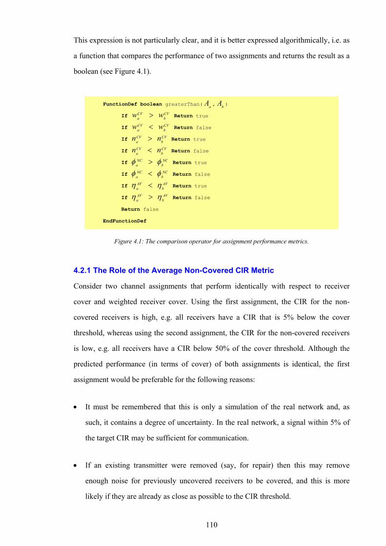
110

This expression is not particularly clear, and it is better expressed algorithmically, i.e. as

a function that compares the performance of two assignments and returns the result as a

boolean (see Figure 4.1).

FunctionDef boolean greaterThan( aA , bA )

If CVb

CVa ww > Return true

If CVb

CVa ww < Return false

If CVb

CVa nn > Return true

If CVb

CVa nn < Return false

If NCb

NCa φφ > Return true

If NCb

NCa φφ < Return false

If AVb

AVa ηη < Return true

If AVb

AVa ηη > Return false

Return false EndFunctionDef

Figure 4.1: The comparison operator for assignment performance metrics.

4.2.1 The Role of the Average Non-Covered CIR Metric

Consider two channel assignments that perform identically with respect to receiver

cover and weighted receiver cover. Using the first assignment, the CIR for the non-

covered receivers is high, e.g. all receivers have a CIR that is 5% below the cover

threshold, whereas using the second assignment, the CIR for the non-covered receivers

is low, e.g. all receivers have a CIR below 50% of the cover threshold. Although the

predicted performance (in terms of cover) of both assignments is identical, the first

assignment would be preferable for the following reasons:

• It must be remembered that this is only a simulation of the real network and, as

such, it contains a degree of uncertainty. In the real network, a signal within 5% of

the target CIR may be sufficient for communication.

• If an existing transmitter were removed (say, for repair) then this may remove

enough noise for previously uncovered receivers to be covered, and this is more

likely if they are already as close as possible to the CIR threshold.

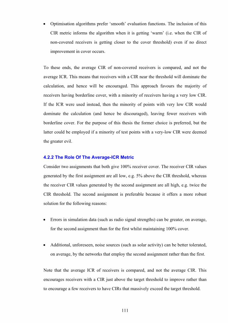
111

• Optimisation algorithms prefer ‘smooth’ evaluation functions. The inclusion of this

CIR metric informs the algorithm when it is getting ‘warm’ (i.e. when the CIR of

non-covered receivers is getting closer to the cover threshold) even if no direct

improvement in cover occurs.

To these ends, the average CIR of non-covered receivers is compared, and not the

average ICR. This means that receivers with a CIR near the threshold will dominate the

calculation, and hence will be encouraged. This approach favours the majority of

receivers having borderline cover, with a minority of receivers having a very low CIR.

If the ICR were used instead, then the minority of points with very low CIR would

dominate the calculation (and hence be discouraged), leaving fewer receivers with

borderline cover. For the purpose of this thesis the former choice is preferred, but the

latter could be employed if a minority of test points with a very-low CIR were deemed

the greater evil.

4.2.2 The Role Of The Average-ICR Metric

Consider two assignments that both give 100% receiver cover. The receiver CIR values

generated by the first assignment are all low, e.g. 5% above the CIR threshold, whereas

the receiver CIR values generated by the second assignment are all high, e.g. twice the

CIR threshold. The second assignment is preferable because it offers a more robust

solution for the following reasons:

• Errors in simulation data (such as radio signal strengths) can be greater, on average,

for the second assignment than for the first whilst maintaining 100% cover.

• Additional, unforeseen, noise sources (such as solar activity) can be better tolerated,

on average, by the networks that employ the second assignment rather than the first.

Note that the average ICR of receivers is compared, and not the average CIR. This

encourages receivers with a CIR just above the target threshold to improve rather than

to encourage a few receivers to have CIRs that massively exceed the target threshold.

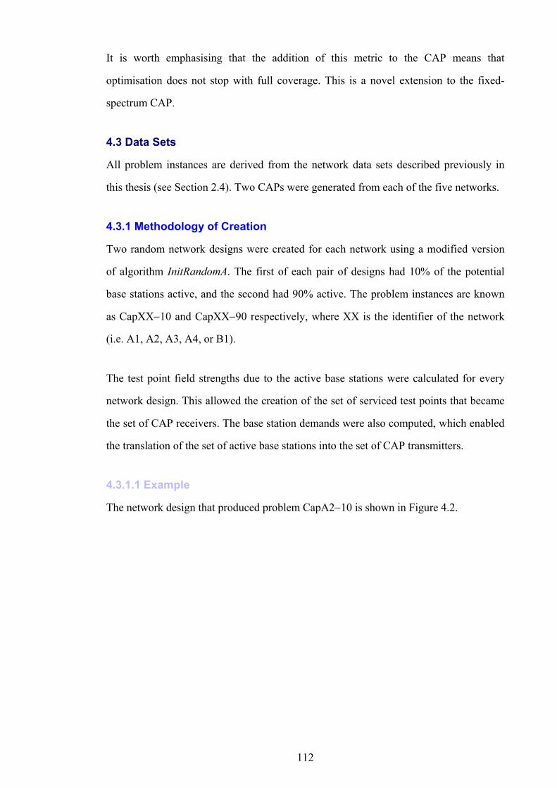
112

It is worth emphasising that the addition of this metric to the CAP means that

optimisation does not stop with full coverage. This is a novel extension to the fixed-

spectrum CAP.

4.3 Data Sets

All problem instances are derived from the network data sets described previously in

this thesis (see Section 2.4). Two CAPs were generated from each of the five networks.

4.3.1 Methodology of Creation

Two random network designs were created for each network using a modified version

of algorithm InitRandomA. The first of each pair of designs had 10% of the potential

base stations active, and the second had 90% active. The problem instances are known

as CapXX−10 and CapXX−90 respectively, where XX is the identifier of the network

(i.e. A1, A2, A3, A4, or B1).

The test point field strengths due to the active base stations were calculated for every

network design. This allowed the creation of the set of serviced test points that became

the set of CAP receivers. The base station demands were also computed, which enabled

the translation of the set of active base stations into the set of CAP transmitters.

4.3.1.1 Example

The network design that produced problem CapA2−10 is shown in Figure 4.2.

113

Figure 4.2: CAP problem CapA2−10 generated from NetworkA2.

4.3.2 Service Region Statistics

The ten problem instances used to test algorithms in this chapter are summarised in

Table 4.1.

Transmitter Statistics Receiver Statistics Data Set B ∑

∈∀ Bb

DMb R ∑∈∀ Rr

WTr

CapA1−10 75 259 29726 3196·23 CapA1−90 675 1019 29954 3210·91 CapA2−10 96 299 70777 2698·41 CapA2−90 864 1129 74845 2787·97 CapA3−10 170 372 17393 2988·11 CapA3−90 1533 1818 17393 2988·11 CapA4−10 73 225 48388 2649·22 CapA4−90 658 884 48512 2652·44 CapB1−10 27 74 4806 656·33 CapB1−90 245 523 32555 9346·62

Table 4.1: Summary statistics for CAP problem instances.

Problem instance data not listed in Table 4.1, such as the number of available channels,

is inherited from the networks (as summarised in Table 2.2) from which the CAP

problems were generated.

114

4.4 Common Algorithmic Concepts

The section contains a few definitions that help simplify the algorithm description of the

optimisation algorithms.

4.4.1 Cover Function

Some algorithm descriptions require the definition of a function, ( )Acover , which

returns the number of receivers covered by assignment A :

CVnA →:cover

4.4.2 Links

Links represent the connection from transmitter to receiver. Each link requires the

assignment of a single channel, so a transmitter has one link for every channel it

employs. The number of links in the network is given by:

∑∈∀

=Bb

DMLK bn

This convention means that instead of referring to the kth channel of the jth base station,

one may simply refer to the lth link in the network. The relationship between these

indices is given by:

∑−

=

+=1

1

j

x

DMxbkl

4.4.3 Magic Channels

A magic channel can cause no interference nor be interfered with. Magic channels

represent an intermediate step in the assignment process, and can be used to exclude the

influence of some transmitters from the evaluation of network performance. The final

assignment produced by an algorithm may not contain any magic channels if it is to be

realised in practice.

If a magic channel is denoted by m then:

( ) ( ) CcmcGcmG CSCS ∈∀== 0,,

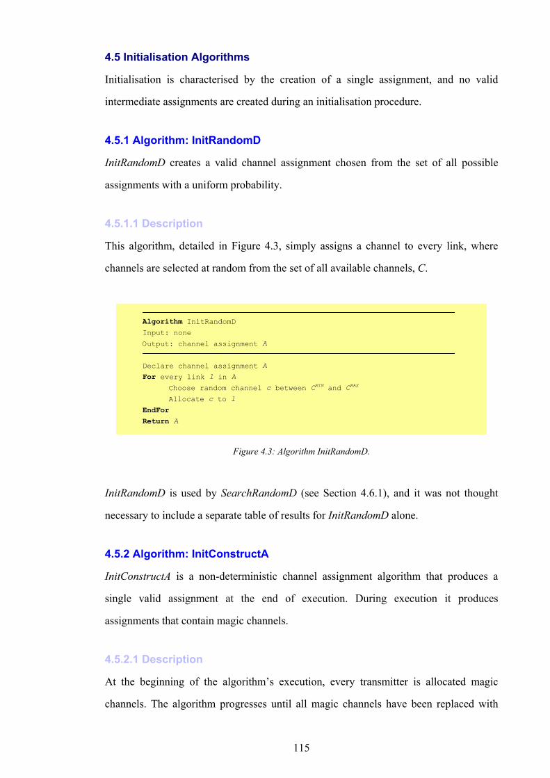
115

4.5 Initialisation Algorithms

Initialisation is characterised by the creation of a single assignment, and no valid

intermediate assignments are created during an initialisation procedure.

4.5.1 Algorithm: InitRandomD

InitRandomD creates a valid channel assignment chosen from the set of all possible

assignments with a uniform probability.

4.5.1.1 Description

This algorithm, detailed in Figure 4.3, simply assigns a channel to every link, where

channels are selected at random from the set of all available channels, C.

Algorithm InitRandomD Input: none

Output: channel assignment A

Declare channel assignment A

For every link l in A Choose random channel c between CMIN and CMAX

Allocate c to l

EndFor Return A

Figure 4.3: Algorithm InitRandomD.

InitRandomD is used by SearchRandomD (see Section 4.6.1), and it was not thought

necessary to include a separate table of results for InitRandomD alone.

4.5.2 Algorithm: InitConstructA

InitConstructA is a non-deterministic channel assignment algorithm that produces a

single valid assignment at the end of execution. During execution it produces

assignments that contain magic channels.

4.5.2.1 Description

At the beginning of the algorithm’s execution, every transmitter is allocated magic

channels. The algorithm progresses until all magic channels have been replaced with

116

real channels. Channel allocation occurs in two phases: the allocation of channels such

that no loss of cover occurs; and the allocation of channels such that the minimum loss

of cover occurs. In the first phase, channels are allocated in order from MINC to MAXC .

A channel is allocated to a link and the network performance is evaluated, if cover is

lost then the link is re-assigned a magic channel. This continues until the channel has

been tried for all the links, at which point testing moves to the next channel. The order

in which links are allocated channels is decided by the demand of the transmitter from

which they came, as this gives high demand transmitters a good opportunity to spread

across the available spectrum. In the second phase, all links that have not been allocated

a channel (i.e. still have magic channels) are given the channel that causes the least loss

in cover (the order in which links are allocated is the same as in the first phase). The

algorithm is detailed in Figure 4.4.

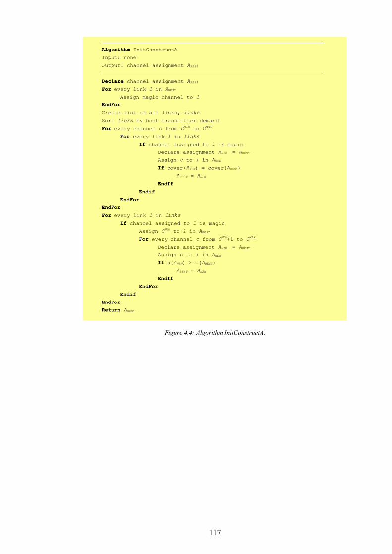
117

Algorithm InitConstructA Input: none

Output: channel assignment ABEST

Declare channel assignment ABEST For every link l in ABEST Assign magic channel to l

EndFor Create list of all links, links

Sort links by host transmitter demand

For every channel c from CMIN to CMAX For every link l in links If channel assigned to l is magic Declare assignment ANEW = ABEST

Assign c to l in ANEW

If cover(ANEW) = cover(ABEST) ABEST = ANEW

EndIf Endif EndFor EndFor For every link l in links If channel assigned to l is magic Assign CMIN to l in ABEST

For every channel c from CMIN+1 to CMAX Declare assignment ANEW = ABEST

Assign c to l in ANEW If p(ANEW) > p(ABEST) ABEST = ANEW

EndIf EndFor Endif EndFor Return ABEST

Figure 4.4: Algorithm InitConstructA.

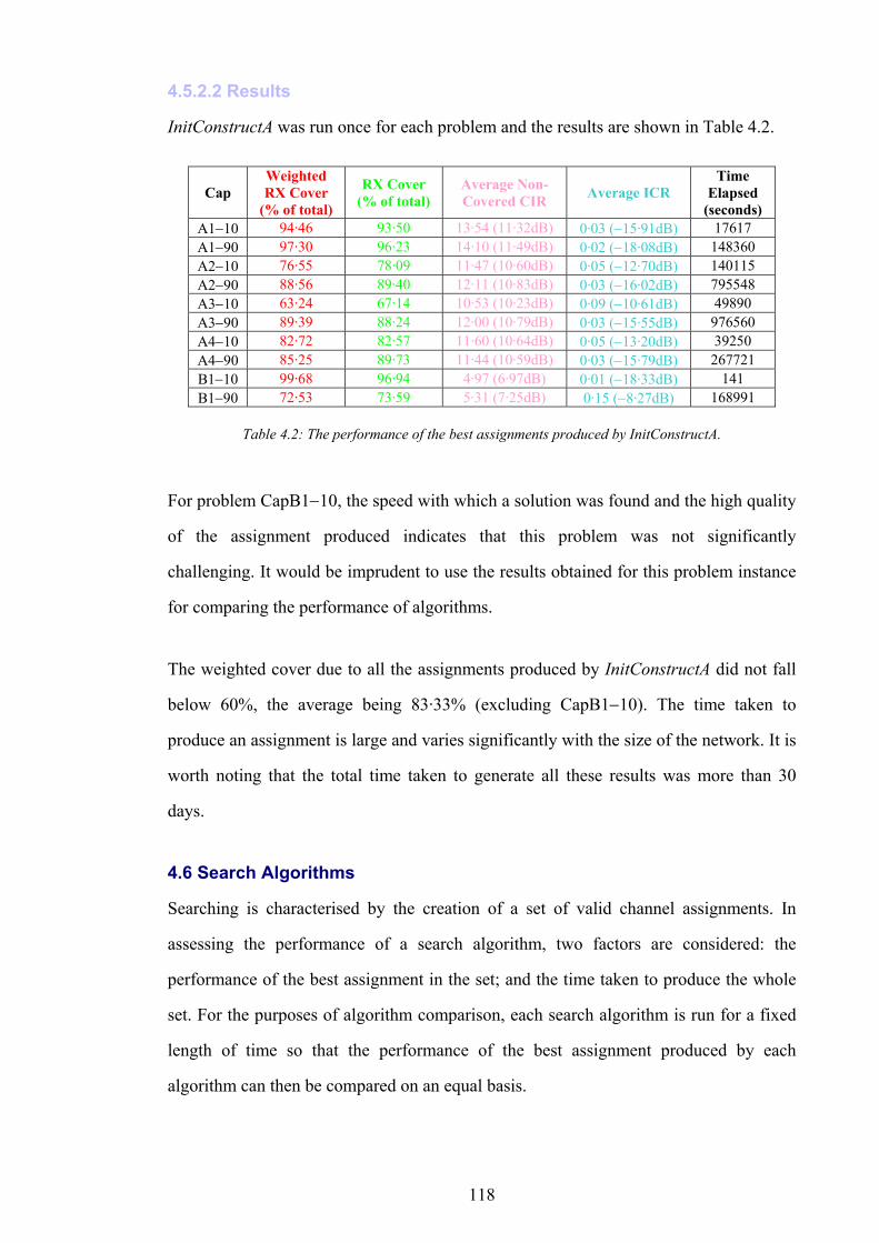
118

4.5.2.2 Results

InitConstructA was run once for each problem and the results are shown in Table 4.2.

Cap Weighted RX Cover

(% of total)

RX Cover (% of total)

Average Non-Covered CIR Average ICR

Time Elapsed

(seconds) A1−10 94·46 93·50 13·54 (11·32dB) 0·03 (−15·91dB) 17617 A1−90 97·30 96·23 14·10 (11·49dB) 0·02 (−18·08dB) 148360 A2−10 76·55 78·09 11·47 (10·60dB) 0·05 (−12·70dB) 140115 A2−90 88·56 89·40 12·11 (10·83dB) 0·03 (−16·02dB) 795548 A3−10 63·24 67·14 10·53 (10·23dB) 0·09 (−10·61dB) 49890 A3−90 89·39 88·24 12·00 (10·79dB) 0·03 (−15·55dB) 976560 A4−10 82·72 82·57 11·60 (10·64dB) 0·05 (−13·20dB) 39250 A4−90 85·25 89·73 11·44 (10·59dB) 0·03 (−15·79dB) 267721 B1−10 99·68 96·94 4·97 (6·97dB) 0·01 (−18·33dB) 141 B1−90 72·53 73·59 5·31 (7·25dB) 0·15 (−8·27dB) 168991

Table 4.2: The performance of the best assignments produced by InitConstructA.

For problem CapB1−10, the speed with which a solution was found and the high quality

of the assignment produced indicates that this problem was not significantly

challenging. It would be imprudent to use the results obtained for this problem instance

for comparing the performance of algorithms.

The weighted cover due to all the assignments produced by InitConstructA did not fall

below 60%, the average being 83·33% (excluding CapB1−10). The time taken to

produce an assignment is large and varies significantly with the size of the network. It is

worth noting that the total time taken to generate all these results was more than 30

days.

4.6 Search Algorithms

Searching is characterised by the creation of a set of valid channel assignments. In

assessing the performance of a search algorithm, two factors are considered: the

performance of the best assignment in the set; and the time taken to produce the whole

set. For the purposes of algorithm comparison, each search algorithm is run for a fixed

length of time so that the performance of the best assignment produced by each

algorithm can then be compared on an equal basis.

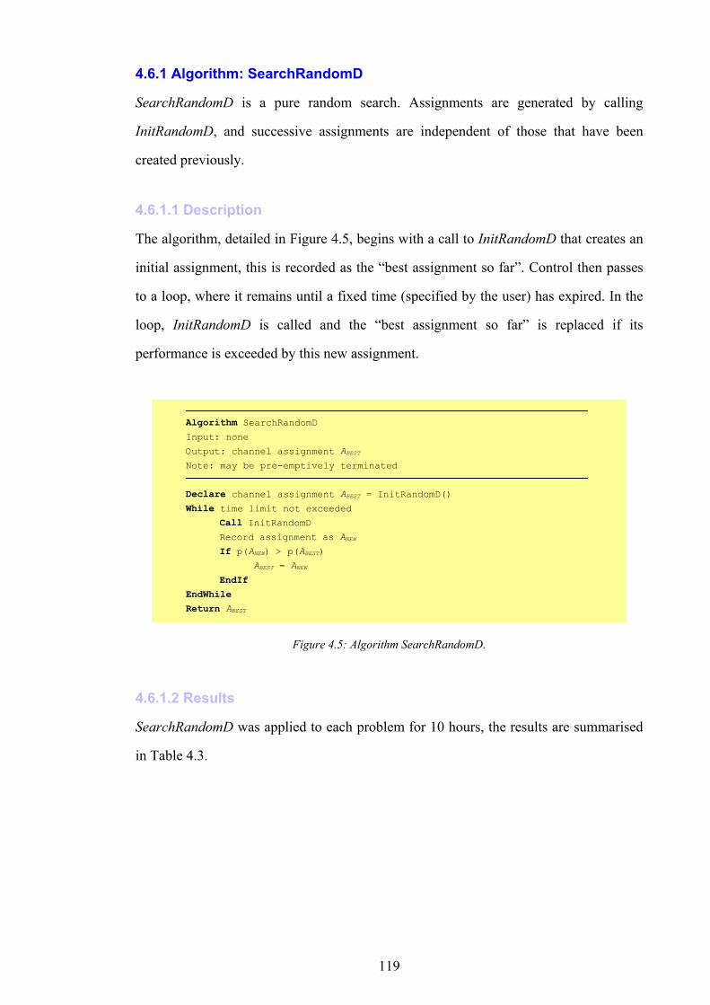
119

4.6.1 Algorithm: SearchRandomD

SearchRandomD is a pure random search. Assignments are generated by calling

InitRandomD, and successive assignments are independent of those that have been

created previously.

4.6.1.1 Description

The algorithm, detailed in Figure 4.5, begins with a call to InitRandomD that creates an

initial assignment, this is recorded as the “best assignment so far”. Control then passes

to a loop, where it remains until a fixed time (specified by the user) has expired. In the

loop, InitRandomD is called and the “best assignment so far” is replaced if its

performance is exceeded by this new assignment.

Algorithm SearchRandomD Input: none

Output: channel assignment ABEST Note: may be pre-emptively terminated

Declare channel assignment ABEST = InitRandomD() While time limit not exceeded Call InitRandomD Record assignment as ANEW If p(ANEW) > p(ABEST) ABEST = ANEW

EndIf EndWhile Return ABEST

Figure 4.5: Algorithm SearchRandomD.

4.6.1.2 Results

SearchRandomD was applied to each problem for 10 hours, the results are summarised

in Table 4.3.

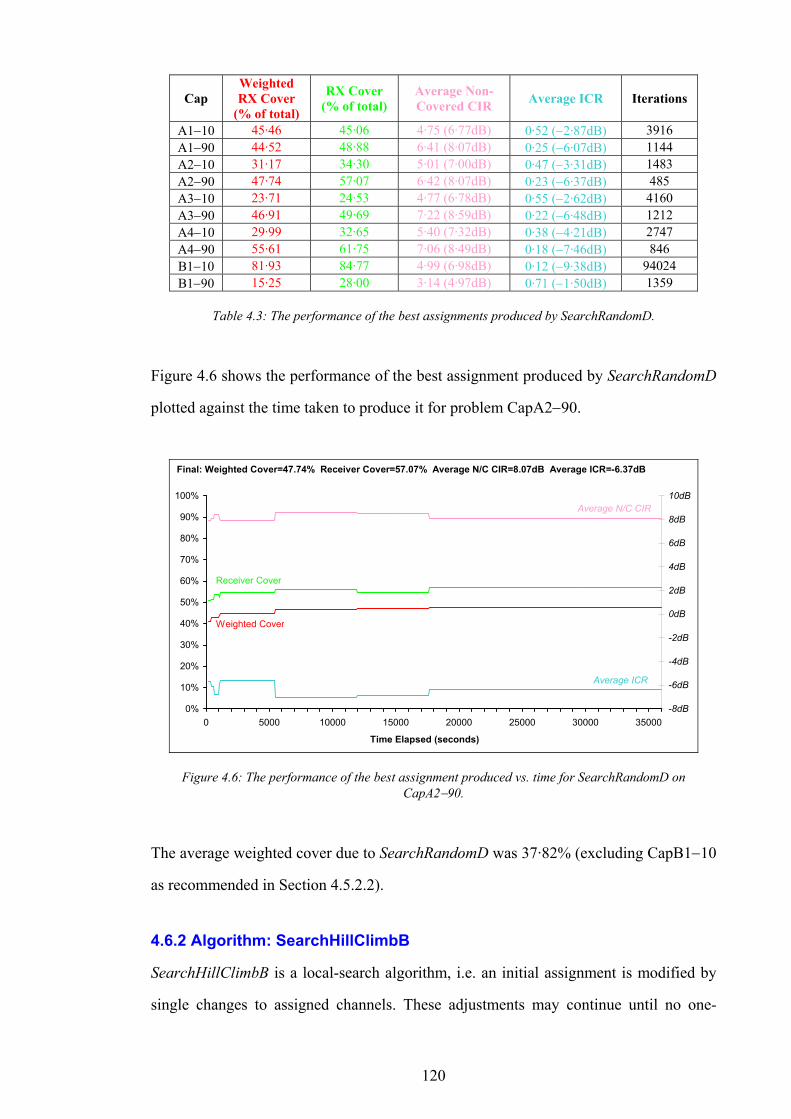
120

Cap Weighted RX Cover

(% of total)

RX Cover (% of total)

Average Non-Covered CIR Average ICR Iterations

A1−10 45·46 45·06 4·75 (6·77dB) 0·52 (−2·87dB) 3916 A1−90 44·52 48·88 6·41 (8·07dB) 0·25 (−6·07dB) 1144 A2−10 31·17 34·30 5·01 (7·00dB) 0·47 (−3·31dB) 1483 A2−90 47·74 57·07 6·42 (8·07dB) 0·23 (−6·37dB) 485 A3−10 23·71 24·53 4·77 (6·78dB) 0·55 (−2·62dB) 4160 A3−90 46·91 49·69 7·22 (8·59dB) 0·22 (−6·48dB) 1212 A4−10 29·99 32·65 5·40 (7·32dB) 0·38 (−4·21dB) 2747 A4−90 55·61 61·75 7·06 (8·49dB) 0·18 (−7·46dB) 846 B1−10 81·93 84·77 4·99 (6·98dB) 0·12 (−9·38dB) 94024 B1−90 15·25 28·00 3·14 (4·97dB) 0·71 (−1·50dB) 1359

Table 4.3: The performance of the best assignments produced by SearchRandomD.

Figure 4.6 shows the performance of the best assignment produced by SearchRandomD

plotted against the time taken to produce it for problem CapA2−90.

0%

10%

20%

30%

40%

50%

60%

70%

80%

90%

100%

0 5000 10000 15000 20000 25000 30000 35000

Time Elapsed (seconds)

-8dB

-6dB

-4dB

-2dB

0dB

2dB

4dB

6dB

8dB

10dB

Final: Weighted Cover=47.74% Receiver Cover=57.07% Average N/C CIR=8.07dB Average ICR=-6.37dB

Weighted Cover

Receiver Cover

Average N/C CIR

Average ICR

Figure 4.6: The performance of the best assignment produced vs. time for SearchRandomD on CapA2−90.

The average weighted cover due to SearchRandomD was 37·82% (excluding CapB1−10

as recommended in Section 4.5.2.2).

4.6.2 Algorithm: SearchHillClimbB

SearchHillClimbB is a local-search algorithm, i.e. an initial assignment is modified by

single changes to assigned channels. These adjustments may continue until no one-

121

change to an assigned channel produces an improvement in assignment performance.

This final assignment is said to be a local optima.

Local-search algorithms require the definition of a search neighbourhood, this is the

scope of changes made to input parameters during searching. For algorithm

SearchHillClimbB, the neighbourhood of an assignment is defined as follows:

Assignment ANEW is in the neighbourhood of AOLD if AOLD can be transformed into ANEW

by the re-assignment of only one transmitter channel. The transformation of one

assignment into another, neighbouring, assignment is known as a move.

4.6.2.1 Description

Algorithm SearchHillClimbB, as detailed in Figure 4.7, has two separate control

sequences:

1. The set of all possible moves is generated.

2. Each move is applied and the resulting assignment evaluated.

This cycle is repeated until a complete set of moves has been applied with no

improvement in assignment performance. The list of moves is executed in random

order, which reduces bias in the hill climbing procedure.

Moves are of the form: <link> <channel>

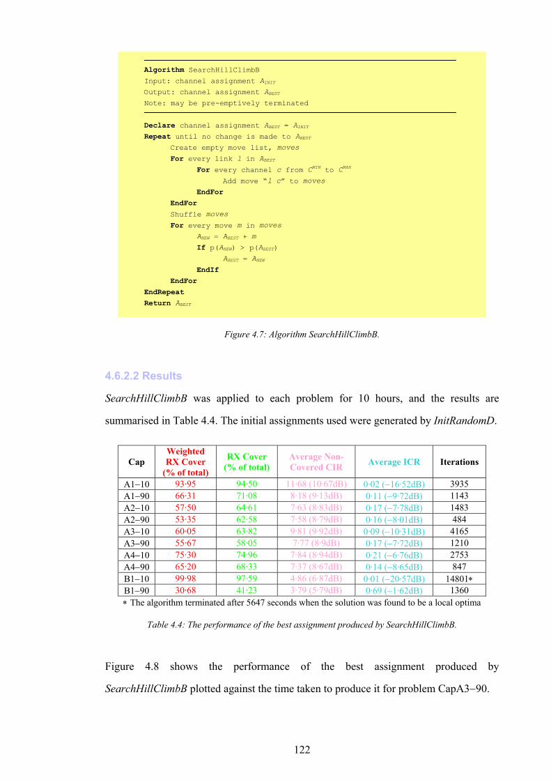
122

Algorithm SearchHillClimbB Input: channel assignment AINIT Output: channel assignment ABEST Note: may be pre-emptively terminated

Declare channel assignment ABEST = AINIT Repeat until no change is made to ABEST Create empty move list, moves

For every link l in ABEST For every channel c from CMIN to CMAX

Add move “l c” to moves

EndFor EndFor Shuffle moves

For every move m in moves ANEW = ABEST + m

If p(ANEW) > p(ABEST) ABEST = ANEW

EndIf EndFor EndRepeat Return ABEST

Figure 4.7: Algorithm SearchHillClimbB.

4.6.2.2 Results

SearchHillClimbB was applied to each problem for 10 hours, and the results are

summarised in Table 4.4. The initial assignments used were generated by InitRandomD.

Cap Weighted RX Cover

(% of total)

RX Cover (% of total)

Average Non-Covered CIR Average ICR Iterations

A1−10 93·95 94·50 11·68 (10·67dB) 0·02 (−16·52dB) 3935 A1−90 66·31 71·08 8·18 (9·13dB) 0·11 (−9·72dB) 1143 A2−10 57·50 64·61 7·63 (8·83dB) 0·17 (−7·78dB) 1483 A2−90 53·35 62·58 7·58 (8·79dB) 0·16 (−8·01dB) 484 A3−10 60·05 63·82 9·81 (9·92dB) 0·09 (−10·31dB) 4165 A3−90 55·67 58·05 7·77 (8·9dB) 0·17 (−7·72dB) 1210 A4−10 75·30 74·96 7·84 (8·94dB) 0·21 (−6·76dB) 2753 A4−90 65·20 68·33 7·37 (8·67dB) 0·14 (−8·65dB) 847 B1−10 99·98 97·59 4·86 (6·87dB) 0·01 (−20·57dB) 14801∗ B1−90 30·68 41·23 3·79 (5·79dB) 0·69 (−1·62dB) 1360 ∗ The algorithm terminated after 5647 seconds when the solution was found to be a local optima

Table 4.4: The performance of the best assignment produced by SearchHillClimbB.

Figure 4.8 shows the performance of the best assignment produced by

SearchHillClimbB plotted against the time taken to produce it for problem CapA3−90.

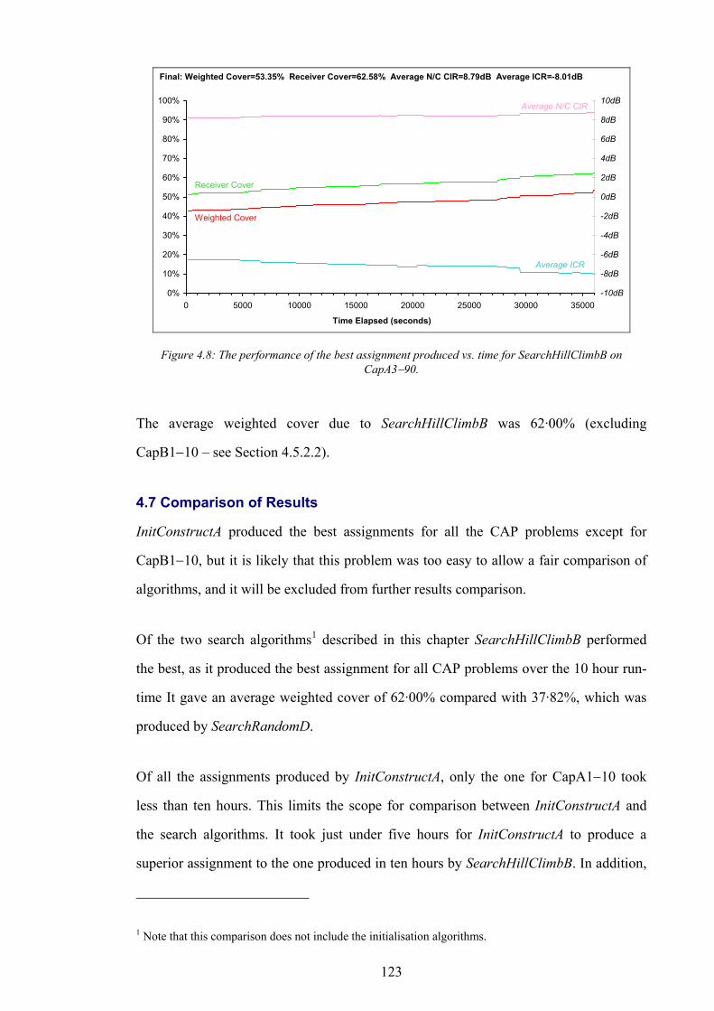
123

0%

10%

20%

30%

40%

50%

60%

70%

80%

90%

100%

0 5000 10000 15000 20000 25000 30000 35000

Time Elapsed (seconds)

-10dB

-8dB

-6dB

-4dB

-2dB

0dB

2dB

4dB

6dB

8dB

10dB

Final: Weighted Cover=53.35% Receiver Cover=62.58% Average N/C CIR=8.79dB Average ICR=-8.01dB

Weighted Cover

Receiver Cover

Average N/C CIR

Average ICR

Figure 4.8: The performance of the best assignment produced vs. time for SearchHillClimbB on CapA3−90.

The average weighted cover due to SearchHillClimbB was 62·00% (excluding

CapB1−10 – see Section 4.5.2.2).

4.7 Comparison of Results

InitConstructA produced the best assignments for all the CAP problems except for

CapB1−10, but it is likely that this problem was too easy to allow a fair comparison of

algorithms, and it will be excluded from further results comparison.

Of the two search algorithms1 described in this chapter SearchHillClimbB performed

the best, as it produced the best assignment for all CAP problems over the 10 hour run-

time It gave an average weighted cover of 62·00% compared with 37·82%, which was

produced by SearchRandomD.

Of all the assignments produced by InitConstructA, only the one for CapA1−10 took

less than ten hours. This limits the scope for comparison between InitConstructA and

the search algorithms. It took just under five hours for InitConstructA to produce a

superior assignment to the one produced in ten hours by SearchHillClimbB. In addition,

1 Note that this comparison does not include the initialisation algorithms.

124

it is likely that the assignment produced for CapA4−10 by InitConstructA would still

outperform the one produced by SearchHillClimbB, even if the search algorithm were

given the extra time taken by InitConstructA. It is likely that InitConstructA is the most

computationally efficient way of assigning channels for this type of CAP (a conclusion

supported by the results obtained for problem CapA1−10), but the disadvantage of

InitConstructA is that no valid assignment is produced until the algorithm finally

terminates. Furthermore, the time it will take to terminate is not easily predicted.

Given an unlimited time in which to produce assignments, the most efficient method (of

those tested) is likely to be the application of InitConstructA followed by

SearchHillClimbB. If assignments were required in a fixed time, then the best approach

would be to call InitRandomD followed by SearchHillClimbB.

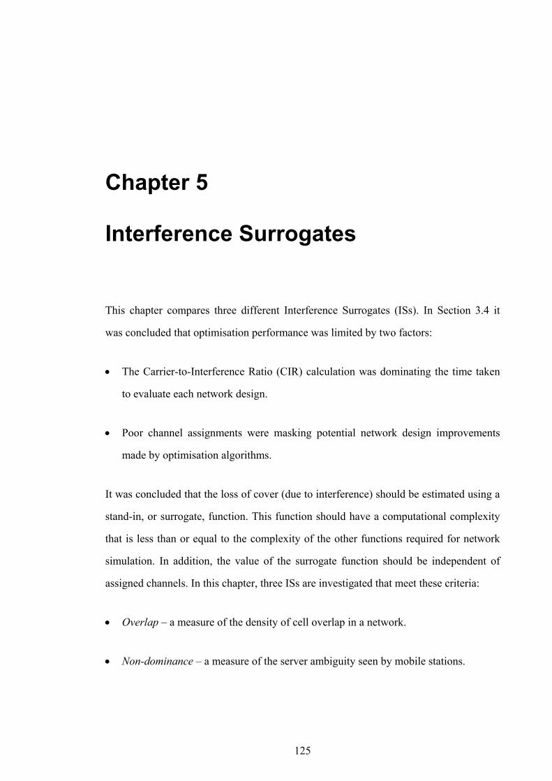
125

Chapter 5 Interference Surrogates

This chapter compares three different Interference Surrogates (ISs). In Section 3.4 it

was concluded that optimisation performance was limited by two factors:

• The Carrier-to-Interference Ratio (CIR) calculation was dominating the time taken

to evaluate each network design.

• Poor channel assignments were masking potential network design improvements

made by optimisation algorithms.

It was concluded that the loss of cover (due to interference) should be estimated using a

stand-in, or surrogate, function. This function should have a computational complexity

that is less than or equal to the complexity of the other functions required for network

simulation. In addition, the value of the surrogate function should be independent of

assigned channels. In this chapter, three ISs are investigated that meet these criteria:

• Overlap – a measure of the density of cell overlap in a network.

• Non-dominance – a measure of the server ambiguity seen by mobile stations.

126

• Signal Freedom – an estimate of the communication channels’ isolation from

interference.

The first two ISs are currently used in industry and they are employed by the operators

from whom the data for this thesis was acquired. The third surrogate is novel, and it was

derived from detailed analysis of the relationship between cell planning and channel

assignment.

5.1 Role of the Interference Surrogate

When comparing two candidate network designs, performance metrics are compared

one-at-a-time (see Section 2.3.2). When employing an IS during cell planning the order

of comparison is as follows:

1. Traffic service.

2. Test point service.

3. Interference surrogate performance.

4. Number of sites occupied.

5. Number of base stations active.

From this list it can be seen that the IS metric is only used when comparing network

designs with the same traffic and test point service. Suppose two such network designs

A and B have interference surrogate performances IA and IB respectively. A channel

assignment is produced for A that results in a test point cover CVA and a channel

assignment is produced for B that results in cover CVB. Now, if CVA > CVB then this

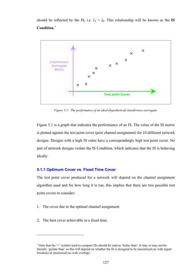
127

should be reflected by the IS, i.e. IA > IB. This relationship will be known as the IS

Condition.1

Interference Surrogate

Metric

Test point Cover

Figure 5.1: The performance of an ideal (hypothetical) interference-surrogate.

Figure 5.1 is a graph that indicates the performance of an IS. The value of the IS metric

is plotted against the test point cover (post channel-assignment) for 10 different network

designs. Designs with a high IS value have a correspondingly high test point cover. No

pair of network designs violate the IS Condition, which indicates that the IS is behaving

ideally.

5.1.1 Optimum Cover vs. Fixed Time Cover

The test point cover produced for a network will depend on the channel assignment

algorithm used and for how long it is run, this implies that there are two possible test

point covers to consider:

1. The cover due to the optimal channel assignment.

2. The best cover achievable in a fixed time.

1 Note that the ‘>’ symbol used to compare ISs should be read as ‘better than’. It may or may not be literally ‘greater than’ as this will depend on whether the IS is designed to be maximised (as with signal freedom) or minimised (as with overlap).

128

There is no known method that can deliver the first of these figures in a reasonable time.

To generate the second of these figures the best-known fixed time algorithm

(SearchHillClimbB) can be used. The longer the algorithm is run, the closer the result

will be to the optimum cover (although not guaranteed to ever equal it). The fixed time

performance is more realistic than the optimum performance because all real channel

assignments are produced in a fixed time.

5.2 Interference Surrogate Descriptions

The following section contains definitions of the three ISs investigated in this chapter.

The notation used for the mathematical descriptions is based on the definitions in

Chapter 2.

5.2.1 Overlap

Consider a subscriber served by a single base station, if that subscriber receives radio

signals from other base stations then the serving signal may be interfered with, i.e. the

CIR may fall below an acceptable threshold. The only way to attenuate the effective

power of the interfering signals is by channel separation, i.e. separation between those

channels used by interfering base stations and the channel on which the serving signal is

transmitted. The greater the number of interfering-signals that overlap serving signals,

the greater the number of channel separations required. The implicit assumption of the

overlap measure is that these increases in channel separation requirements will increase

the difficulty of channel assignment.

A non-serving signal is considered to overlap at a test point if it is above the test point’s

service threshold. The number of overlaps at each test point is summed to give the total

network overlap. If the set of base stations that overlap at test point SVi Rr ∈ is

denoted OVir and is given by:

{ }SQi

FSij

ACj

OVi rpBbr ≥∈= :

then the total network overlap is given by:

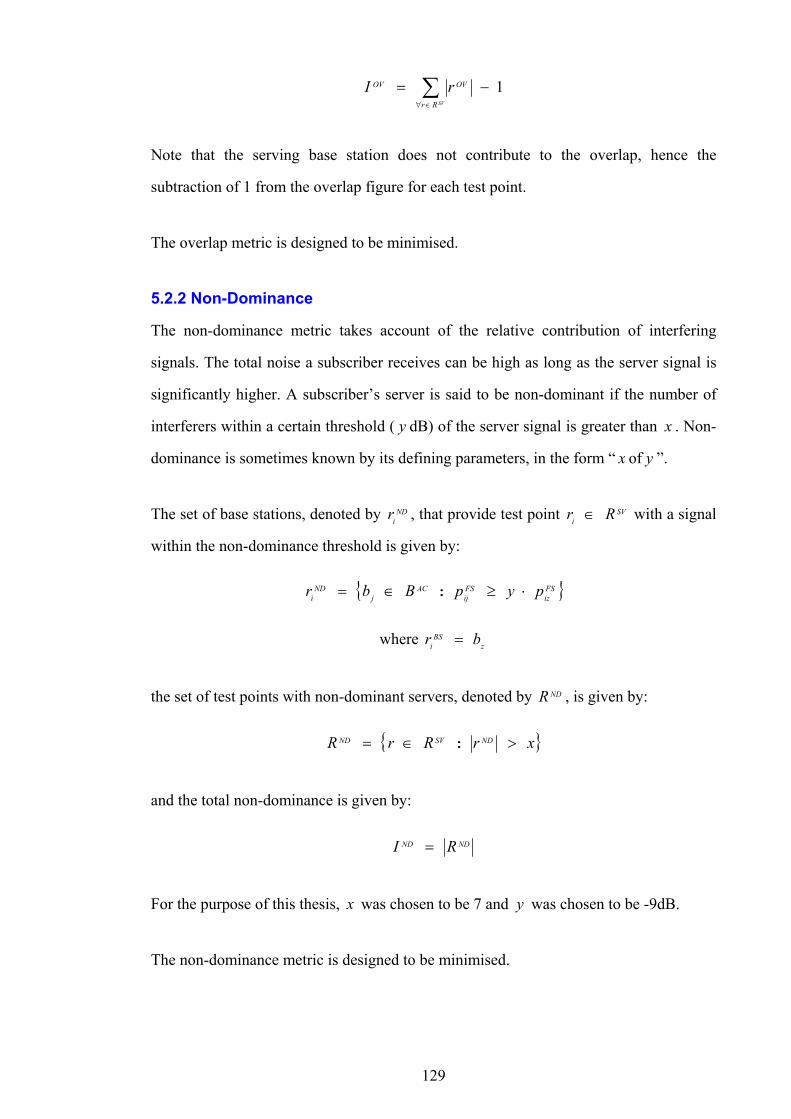
129

∑∈∀

−=SVRr

OVOV rI 1

Note that the serving base station does not contribute to the overlap, hence the

subtraction of 1 from the overlap figure for each test point.

The overlap metric is designed to be minimised.

5.2.2 Non-Dominance

The non-dominance metric takes account of the relative contribution of interfering

signals. The total noise a subscriber receives can be high as long as the server signal is

significantly higher. A subscriber’s server is said to be non-dominant if the number of

interferers within a certain threshold ( y dB) of the server signal is greater than x . Non-

dominance is sometimes known by its defining parameters, in the form “ x of y ”.

The set of base stations, denoted by NDir , that provide test point SV

i Rr ∈ with a signal

within the non-dominance threshold is given by:

{ }FSiz

FSij

ACj

NDi pypBbr ⋅≥∈= :

where zBS

i br =

the set of test points with non-dominant servers, denoted by NDR , is given by:

{ }xrRrR NDSVND >∈= :

and the total non-dominance is given by:

NDND RI =

For the purpose of this thesis, x was chosen to be 7 and y was chosen to be -9dB.

The non-dominance metric is designed to be minimised.

130

5.2.3 Signal Freedom

Signal freedom is a novel metric. In the signal freedom paradigm, networks are viewed

as a collection of links to which channels must be assigned1. The fact that links might

share base stations and that base stations might share sites is regarded as un-important.

Links simply represent conduits into the network.

5.2.3.1 A Single Test point with a Single Link

Consider a single test point r, a signal will be received by r for every active link2 in the

network. Figure 5.2 shows the strengths of four such signals received at r, they are the

serving signal S and the three interfering signals 0I , 1I , and 2I .

PO

WE

R

Server Signal Power

S Target Noise (with channel separation)

S / φ

Total Noise (no channel separation)

I0 + I1 + I2

I0

I1

I2

S

Figure 5.2: An illustration of the attenuation of interference by channel separation.

If the target CIR is φ then the total interference cannot exceed φS (known as the

target noise). The interfering signals must be attenuated such that the sum of all three is

less than the target noise. The greater the required attenuation, the greater the channel

separation will need to be. Therefore the ratio α of the target noise to the total

1 The concept of ‘links’ is the same as the one used to simplify the description of channel assignment algorithms in Section 4.4.2. 2 An active link represents a utilised channel of an active base station.

131

interference gives an estimate of the effort required in assigning channels. For the

example in Figure 5.2, α is given by:

( )210 III

S

++⋅=

φα

Note that α is the normalised CIR at r, therefore if 1≥α then no channel separation

would be required to cover r.

5.2.3.2 Normalised CIR Threshold

When calculating signal freedom, test point links for which 1>α are taken to have

1=α . This is to stop ‘easy’ links (i.e. those requiring no channel separation) from

‘swamping’ the α values of more demanding links in the final total.

5.2.3.3 Number of Links vs. Channel Separation

Signal freedom takes account of networks with different numbers of links by including

contributions from all possible links. Un-used links are considered perfect as they can

be assigned any channel. The two types of redundant links are:

• Links hosted by inactive base stations.

• Links that are not required to carry traffic but are hosted by an active base station.

A redundant link contributes a perfect α value of 1 to the signal freedom metric.

Two factors control the difficulty of a channel assignment: the number of links that

require channels; and the separation requirements between the links. Consider two

example network designs that are both equally difficult to assign channels for:

Design 1. A design requiring many links, in which the channel assigned to each

link has a small impact on the channels assigned to other links.

132

Design 2. A design requiring few links, in which the channel assigned to each link

has a large impact on the channels assigned to other links.

If the signal freedom metric was simply the average of the contributions from active

links (and not the average of all possible links) the first design would always be

favoured, even though the assignment of channels is equally difficult for both (as

postulated).

5.2.3.4 Mathematical Derivation

The total field-strength of radio signals received by test point SVi Rr ∈ is denoted TN

ip

and is given by:

∑∈∀

⋅=AC

x Bb

DMx

FSix

TNi bpp

therefore the normalised CIR, ijα , due to a channel of base station jb serving test point

ir is given by:

( )FSij

TNi

CV

FSij

ijpp

p

−⋅=

φα

To calculate the signal freedom metric, a threshold must be applied to α (see Section

5.2.3.2). In addition, an α value of 1 should be assumed for all in-active links (see

Section 5.2.3.3). Both these requirements are encapsulated in the calculation of ijkβ ,

which represents the signal freedom of the kth channel of base station jb serving test

point ir :

{ } ≤∧∈

=otherwise

if11 DM

jSS

ijijijk

bkrbαβ

,min

Hence, the signal freedom, SFir , for test point ir is given by the average of the signal

freedom due to every channel of every base station:

∑ ∑∈∀ =⋅

=Bb

M

kijk

SFi

jMB

r1

1β

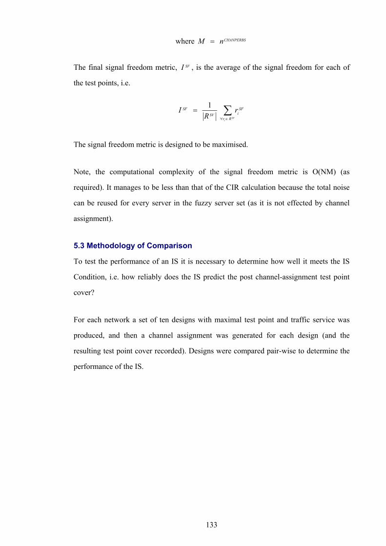
133

where CHANPERBSnM =

The final signal freedom metric, SFI , is the average of the signal freedom for each of

the test points, i.e.

∑∈∀

=SV

i Rr

SFiSV

SF rR

I 1

The signal freedom metric is designed to be maximised.

Note, the computational complexity of the signal freedom metric is O(NM) (as

required). It manages to be less than that of the CIR calculation because the total noise

can be reused for every server in the fuzzy server set (as it is not effected by channel

assignment).

5.3 Methodology of Comparison

To test the performance of an IS it is necessary to determine how well it meets the IS

Condition, i.e. how reliably does the IS predict the post channel-assignment test point

cover?

For each network a set of ten designs with maximal test point and traffic service was

produced, and then a channel assignment was generated for each design (and the

resulting test point cover recorded). Designs were compared pair-wise to determine the

performance of the IS.

134

Interference Surrogate

Metric

Test point Cover

e

d1 d2

Figure 5.3: The performance of an imperfect interference surrogate, in which one pair of designs violate the IS Condition.

The IS illustrated in Figure 5.1 behaves ideally (i.e. the IS Condition is never violated).

Figure 5.3 shows a similar scenario except with a different IS. The IS value for d1 is

below that of design d2 despite d1’s superior test point cover (i.e. a violation of the IS

Condition). This difference in cover (denoted by e in the diagram) shall be referred to as

an ‘inaccuracy’.

The difference in cover between all pairs of designs that violate the IS Condition shall

be referred to as the inaccuracy of the IS. Note that, for the purposes of calculating an

average, pairs of designs that do not violate the IS Condition are considered to have an

inaccuracy of zero.

135

Interference Surrogate

Metric

Test point Cover

e3

e2

e1

Figure 5.4: The performance of an imperfect interference surrogate, in which three pairs of designs violate the IS Condition.

Figure 5.4 shows the test point cover for ten network designs; three pairs of designs

violate the IS Condition giving inaccuracies of e1, e2, and e3. The total number of

possible (unique) pairs is given by:

452

10102

=− pairs

therefore the average inaccuracy of the IS is given by:

45321 eee ++

and the maximum inaccuracy is given by:

{ }321 eee ,,max

5.3.1 Generation of Network Designs

For each network, a set of ten random network designs was created, in which a fixed

fraction of the potential base stations were active: 201 for the first design, 203 for the

next design and so-on until the last design, which used the fraction 2019 . A high

variation in base station activity was chosen to give the widest range of final test point

covers, as this broadens the range of inaccuracies with which to compare ISs.

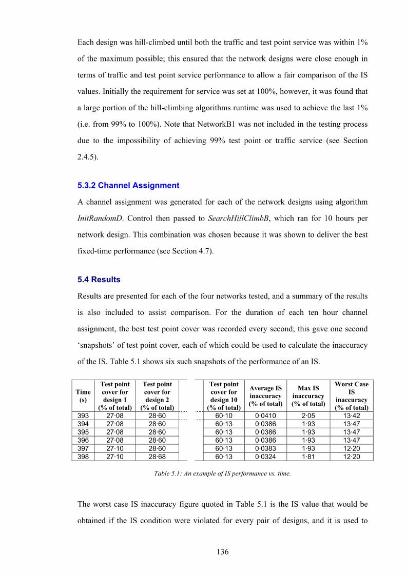
136

Each design was hill-climbed until both the traffic and test point service was within 1%

of the maximum possible; this ensured that the network designs were close enough in

terms of traffic and test point service performance to allow a fair comparison of the IS

values. Initially the requirement for service was set at 100%, however, it was found that

a large portion of the hill-climbing algorithms runtime was used to achieve the last 1%

(i.e. from 99% to 100%). Note that NetworkB1 was not included in the testing process

due to the impossibility of achieving 99% test point or traffic service (see Section

2.4.5).

5.3.2 Channel Assignment

A channel assignment was generated for each of the network designs using algorithm

InitRandomD. Control then passed to SearchHillClimbB, which ran for 10 hours per

network design. This combination was chosen because it was shown to deliver the best

fixed-time performance (see Section 4.7).

5.4 Results

Results are presented for each of the four networks tested, and a summary of the results

is also included to assist comparison. For the duration of each ten hour channel

assignment, the best test point cover was recorded every second; this gave one second

‘snapshots’ of test point cover, each of which could be used to calculate the inaccuracy

of the IS. Table 5.1 shows six such snapshots of the performance of an IS.

Time (s)

Test point cover for design 1

(% of total)

Test point cover for design 2

(% of total)

Test point cover for design 10

(% of total)

Average IS inaccuracy (% of total)

Max IS inaccuracy (% of total)

Worst Case IS

inaccuracy (% of total)

393 27·08 28·60 60·10 0·0410 2·05 13·42 394 27·08 28·60 60·13 0·0386 1·93 13·47 395 27·08 28·60 60·13 0·0386 1·93 13·47 396 27·08 28·60 60·13 0·0386 1·93 13·47 397 27·10 28·60 60·13 0·0383 1·93 12·20 398 27·10 28·68 60·13 0·0324 1·81 12·20

Table 5.1: An example of IS performance vs. time.

The worst case IS inaccuracy figure quoted in Table 5.1 is the IS value that would be

obtained if the IS condition were violated for every pair of designs, and it is used to

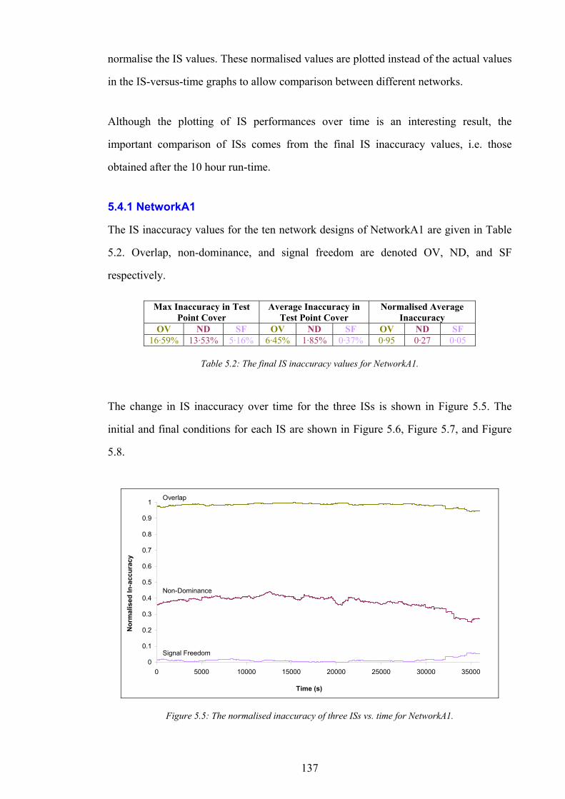
137

normalise the IS values. These normalised values are plotted instead of the actual values

in the IS-versus-time graphs to allow comparison between different networks.

Although the plotting of IS performances over time is an interesting result, the

important comparison of ISs comes from the final IS inaccuracy values, i.e. those

obtained after the 10 hour run-time.

5.4.1 NetworkA1

The IS inaccuracy values for the ten network designs of NetworkA1 are given in Table

5.2. Overlap, non-dominance, and signal freedom are denoted OV, ND, and SF

respectively.

Max Inaccuracy in Test Point Cover

Average Inaccuracy in Test Point Cover

Normalised Average Inaccuracy

OV ND SF OV ND SF OV ND SF 16·59% 13·53% 5·16% 6·45% 1·85% 0·37% 0·95 0·27 0·05

Table 5.2: The final IS inaccuracy values for NetworkA1.

The change in IS inaccuracy over time for the three ISs is shown in Figure 5.5. The

initial and final conditions for each IS are shown in Figure 5.6, Figure 5.7, and Figure

5.8.

0

0.1

0.2

0.3

0.4

0.5

0.6

0.7

0.8

0.9

1

0 5000 10000 15000 20000 25000 30000 35000

Time (s)

Nor

mal

ised

In-a

ccur

acy

Overlap

Signal Freedom

Non-Dominance

Figure 5.5: The normalised inaccuracy of three ISs vs. time for NetworkA1.

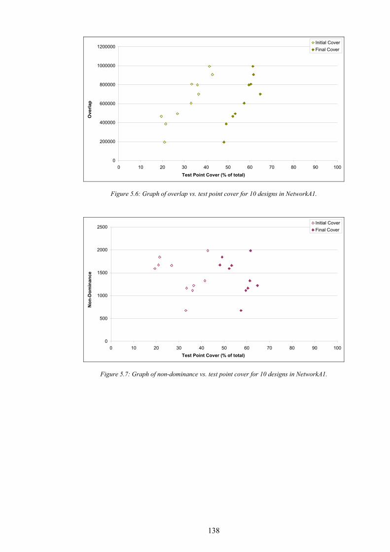
138

0

200000

400000

600000

800000

1000000

1200000

0 10 20 30 40 50 60 70 80 90 100Test Point Cover (% of total)

Ove

rlap

Initial CoverFinal Cover

Figure 5.6: Graph of overlap vs. test point cover for 10 designs in NetworkA1.

0

500

1000

1500

2000

2500

0 10 20 30 40 50 60 70 80 90 100Test Point Cover (% of total)

Non

-Dom

inan

ce

Initial CoverFinal Cover

Figure 5.7: Graph of non-dominance vs. test point cover for 10 designs in NetworkA1.

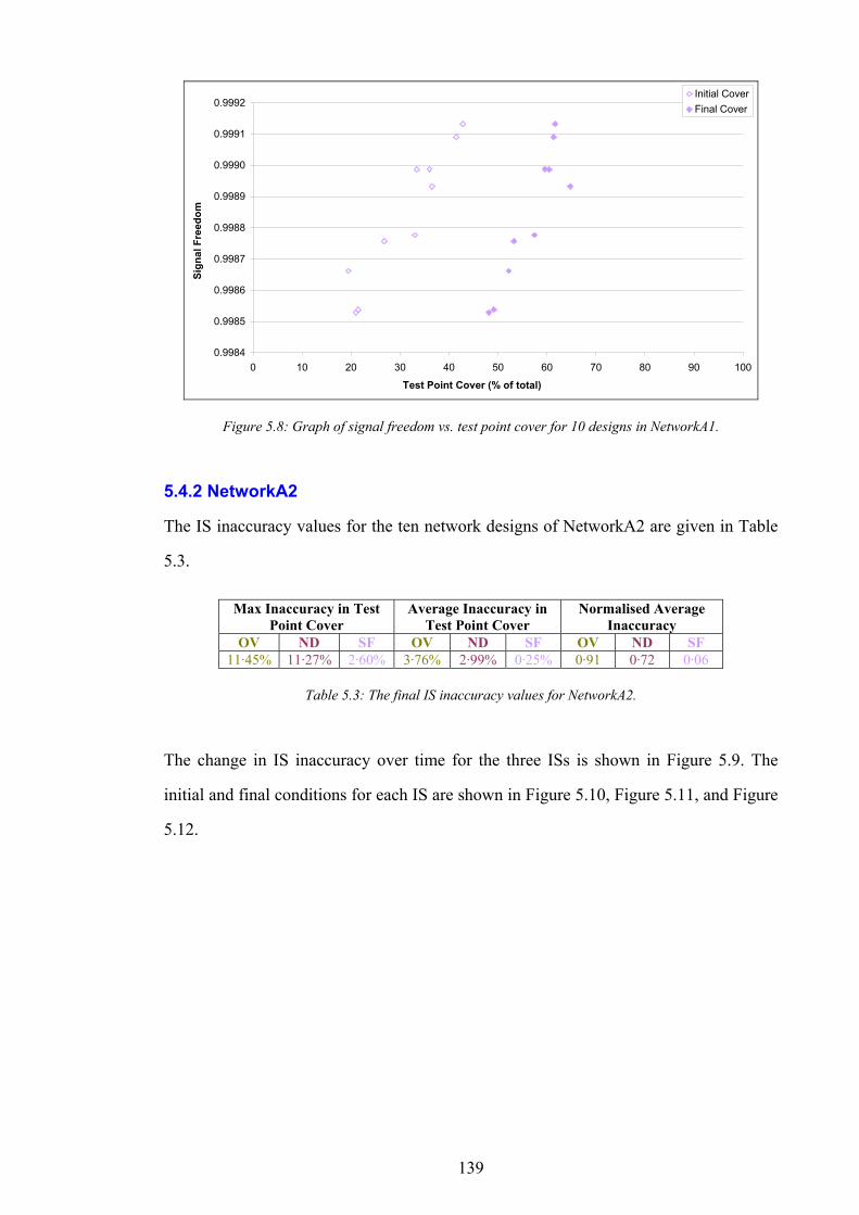
139

0.9984

0.9985

0.9986

0.9987

0.9988

0.9989

0.9990

0.9991

0.9992

0 10 20 30 40 50 60 70 80 90 100

Test Point Cover (% of total)

Sign

al F

reed

om

Initial CoverFinal Cover

Figure 5.8: Graph of signal freedom vs. test point cover for 10 designs in NetworkA1.

5.4.2 NetworkA2

The IS inaccuracy values for the ten network designs of NetworkA2 are given in Table

5.3.

Max Inaccuracy in Test Point Cover

Average Inaccuracy in Test Point Cover

Normalised Average Inaccuracy

OV ND SF OV ND SF OV ND SF 11·45% 11·27% 2·60% 3·76% 2·99% 0·25% 0·91 0·72 0·06

Table 5.3: The final IS inaccuracy values for NetworkA2.

The change in IS inaccuracy over time for the three ISs is shown in Figure 5.9. The

initial and final conditions for each IS are shown in Figure 5.10, Figure 5.11, and Figure

5.12.

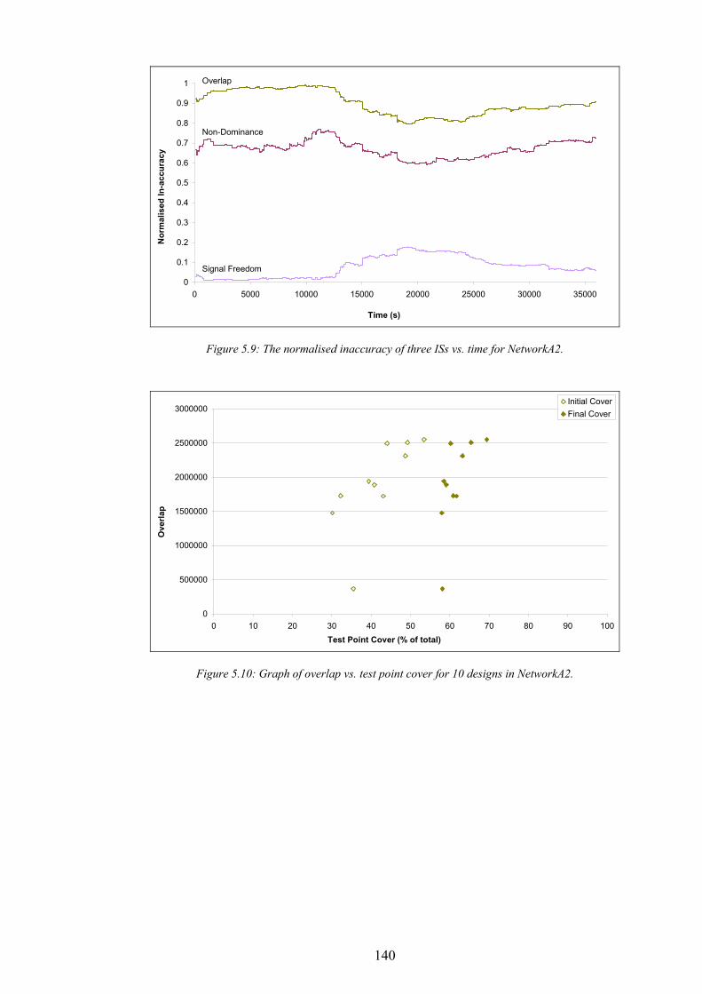
140

0

0.1

0.2

0.3

0.4

0.5

0.6

0.7

0.8

0.9

1

0 5000 10000 15000 20000 25000 30000 35000

Time (s)

Nor

mal

ised

In-a

ccur

acy

Overlap

Signal Freedom

Non-Dominance

Figure 5.9: The normalised inaccuracy of three ISs vs. time for NetworkA2.

0

500000

1000000

1500000

2000000

2500000

3000000

0 10 20 30 40 50 60 70 80 90 100Test Point Cover (% of total)

Ove

rlap

Initial CoverFinal Cover

Figure 5.10: Graph of overlap vs. test point cover for 10 designs in NetworkA2.

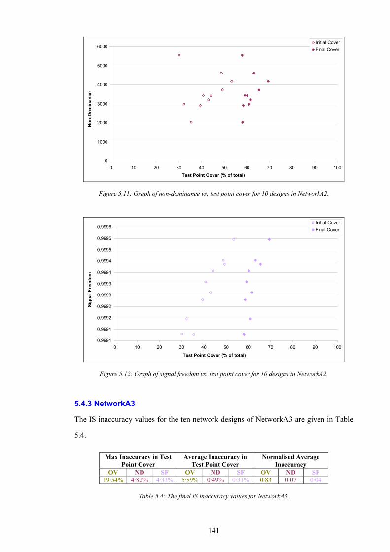
141

0

1000

2000

3000

4000

5000

6000

0 10 20 30 40 50 60 70 80 90 100Test Point Cover (% of total)

Non

-Dom

inan

ce

Initial CoverFinal Cover

Figure 5.11: Graph of non-dominance vs. test point cover for 10 designs in NetworkA2.

0.9991

0.9991

0.9992

0.9992

0.9993

0.9993

0.9994

0.9994

0.9995

0.9995

0.9996

0 10 20 30 40 50 60 70 80 90 100

Test Point Cover (% of total)

Sign

al F

reed

om

Initial CoverFinal Cover

Figure 5.12: Graph of signal freedom vs. test point cover for 10 designs in NetworkA2.

5.4.3 NetworkA3

The IS inaccuracy values for the ten network designs of NetworkA3 are given in Table

5.4.

Max Inaccuracy in Test Point Cover

Average Inaccuracy in Test Point Cover

Normalised Average Inaccuracy

OV ND SF OV ND SF OV ND SF 19·54% 4·82% 4·33% 5·89% 0·49% 0·31% 0·83 0·07 0·04

Table 5.4: The final IS inaccuracy values for NetworkA3.

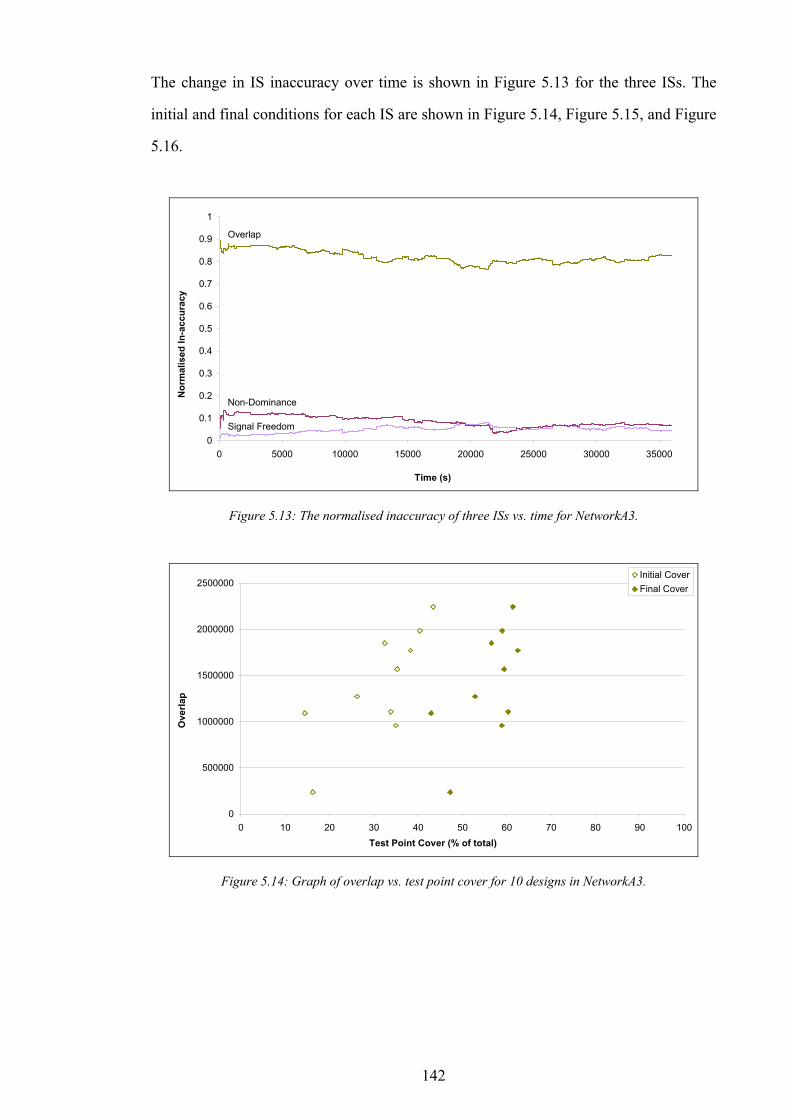
142

The change in IS inaccuracy over time is shown in Figure 5.13 for the three ISs. The

initial and final conditions for each IS are shown in Figure 5.14, Figure 5.15, and Figure

5.16.

0

0.1

0.2

0.3

0.4

0.5

0.6

0.7

0.8

0.9

1

0 5000 10000 15000 20000 25000 30000 35000

Time (s)

Nor

mal

ised

In-a

ccur

acy

Overlap

Signal Freedom

Non-Dominance

Figure 5.13: The normalised inaccuracy of three ISs vs. time for NetworkA3.

0

500000

1000000

1500000

2000000

2500000

0 10 20 30 40 50 60 70 80 90 100Test Point Cover (% of total)

Ove

rlap

Initial CoverFinal Cover

Figure 5.14: Graph of overlap vs. test point cover for 10 designs in NetworkA3.

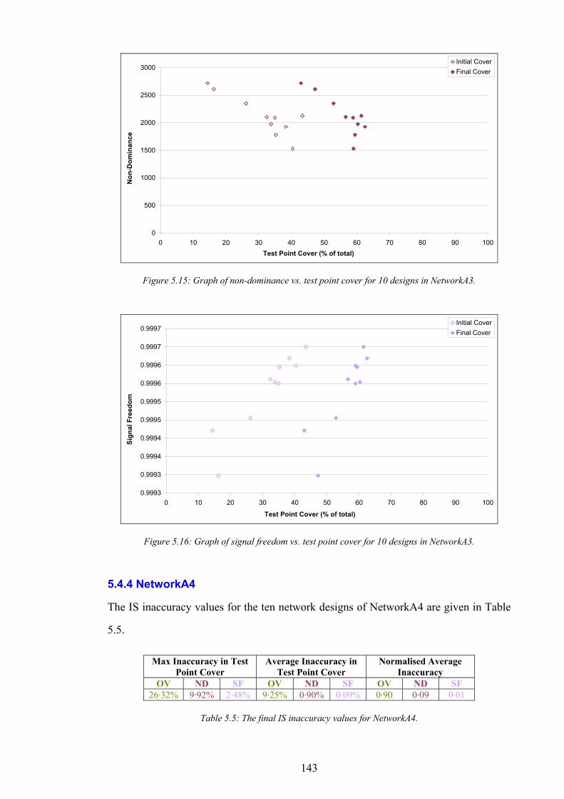
143

0

500

1000

1500

2000

2500

3000

0 10 20 30 40 50 60 70 80 90 100Test Point Cover (% of total)

Non

-Dom

inan

ce

Initial CoverFinal Cover

Figure 5.15: Graph of non-dominance vs. test point cover for 10 designs in NetworkA3.

0.9993

0.9993

0.9994

0.9994

0.9995

0.9995

0.9996

0.9996

0.9997

0.9997

0 10 20 30 40 50 60 70 80 90 100

Test Point Cover (% of total)

Sign

al F

reed

om

Initial CoverFinal Cover

Figure 5.16: Graph of signal freedom vs. test point cover for 10 designs in NetworkA3.

5.4.4 NetworkA4

The IS inaccuracy values for the ten network designs of NetworkA4 are given in Table

5.5.

Max Inaccuracy in Test Point Cover

Average Inaccuracy in Test Point Cover

Normalised Average Inaccuracy

OV ND SF OV ND SF OV ND SF 26·32% 9·92% 2·48% 9·25% 0·90% 0·09% 0·90 0·09 0·01

Table 5.5: The final IS inaccuracy values for NetworkA4.

144

The change in IS inaccuracy over time for the three ISs is shown in Figure 5.17. The

initial and final conditions for each IS are shown in Figure 5.18, Figure 5.19, and Figure

5.20.

0

0.1

0.2

0.3

0.4

0.5

0.6

0.7

0.8

0.9

1

0 5000 10000 15000 20000 25000 30000 35000

Time (s)

Nor

mal

ised

In-a

ccur

acy

Overlap

Signal Freedom

Non-Dominance

Figure 5.17: The normalised inaccuracy of three ISs vs. time for NetworkA4.

0

500000

1000000

1500000

2000000

2500000

0 10 20 30 40 50 60 70 80 90 100Test Point Cover (% of total)

Ove

rlap

Initial CoverFinal Cover

Figure 5.18: Graph of overlap vs. test point cover for 10 designs in NetworkA4.

145

0

500

1000

1500

2000

2500

3000

3500

4000

4500

0 10 20 30 40 50 60 70 80 90 100Test Point Cover (% of total)

Non

-Dom

inan

ce

Initial CoverFinal Cover

Figure 5.19: Graph of non-dominance vs. test point cover for 10 designs in NetworkA4.

0.9985

0.9986

0.9987

0.9988

0.9989

0.9990

0.9991

0.9992

0.9993

0.9994

0 10 20 30 40 50 60 70 80 90 100

Test Point Cover (% of total)

Sign

al F

reed

om

Initial CoverFinal Cover

Figure 5.20: Graph of signal freedom vs. test point cover for 10 designs in NetworkA4.

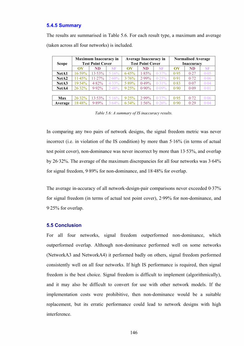
146

5.4.5 Summary

The results are summarised in Table 5.6. For each result type, a maximum and average

(taken across all four networks) is included.

Maximum Inaccuracy in Test Point Cover

Average Inaccuracy in Test Point Cover

Normalised Average Inaccuracy Scope

OV ND SF OV ND SF OV ND SF NetA1 16·59% 13·53% 5·16% 6·45% 1·85% 0·37% 0·95 0·27 0·05 NetA2 11·45% 11·27% 2·60% 3·76% 2·99% 0·25% 0·91 0·72 0·06 NetA3 19·54% 4·82% 4·33% 5·89% 0·49% 0·31% 0·83 0·07 0·04 NetA4 26·32% 9·92% 2·48% 9·25% 0·90% 0·09% 0·90 0·09 0·01

Max 26·32% 13·53% 5·16% 9·25% 2·99% 0·37% 0·95 0·72 0·06

Average 18·48% 9·89% 3·64% 6·34% 1·56% 0·26% 0·90 0·29 0·04

Table 5.6: A summary of IS inaccuracy results.

In comparing any two pairs of network designs, the signal freedom metric was never

incorrect (i.e. in violation of the IS condition) by more than 5·16% (in terms of actual

test point cover), non-dominance was never incorrect by more than 13·53%, and overlap

by 26·32%. The average of the maximum discrepancies for all four networks was 3·64%

for signal freedom, 9·89% for non-dominance, and 18·48% for overlap.

The average in-accuracy of all network-design-pair comparisons never exceeded 0·37%

for signal freedom (in terms of actual test point cover), 2·99% for non-dominance, and

9·25% for overlap.

5.5 Conclusion

For all four networks, signal freedom outperformed non-dominance, which

outperformed overlap. Although non-dominance performed well on some networks

(NetworkA3 and NetworkA4) it performed badly on others, signal freedom performed

consistently well on all four networks. If high IS performance is required, then signal

freedom is the best choice. Signal freedom is difficult to implement (algorithmically),

and it may also be difficult to convert for use with other network models. If the

implementation costs were prohibitive, then non-dominance would be a suitable

replacement, but its erratic performance could lead to network designs with high

interference.

147

Overlap performed badly on all networks, and it must be concluded that overlap is a

poor IS (under the conditions applied in this test). However, the IS requirement used in

this thesis is based on the particular formulation of the evaluation function, whereas a

different evaluation function (even if only slightly different) may lead to a very different

IS condition, to which overlap may be better suited. A fundamental problem with

overlap is it inability to take into account strong server signals, and the problem of

interfering signals is only relative to the strength of the serving signals.

It might be argued that overlap also functions as an indicator of a network's ability to

handover subscribers between cells. However, in practice it is better to have separate

metrics for each network performance characteristic, as this allows the network designer

to control the relative significance of each characteristic independently.

148

Chapter 6 Network Design – Part 2

The application of combinatorial optimisation to the Wireless Capacitated Network

Design Problem (WCNDP) is described in this chapter. In Chapter 3 the Base Station

Configuration Problem (BSCP) and the subsequent Channel Assignment Problem

(CAP) were solved as one problem (the WCNDP). In this chapter (following the

conclusion of Chapter 3) these two sub-problems are solved sequentially, and

comparisons drawn (this corresponds to Task T1 of Objective O2 in Section 1.3). The

evaluation function used throughout this chapter is the same as the one described in

Chapter 5.

The structure of this chapter is as follows: Section 6.1 evaluates the advantages of the

two-stage network design approach, Section 6.2 describes network designs that can be

produced with a ‘high’ computational investment, and Section 6.3 assesses the impact

that minimising network infrastructure has on network performance.

6.1 Evaluation of Two-Stage Network Design Process

In Chapter 3, optimisation algorithms were described for the network design problem,

and it was concluded (see Section 3.4) that the problem should be split into two stages

(BSCP and CAP). Signal freedom is the interference surrogate (see Chapter 5) used

during the BSCP phase of optimisation described in this chapter.

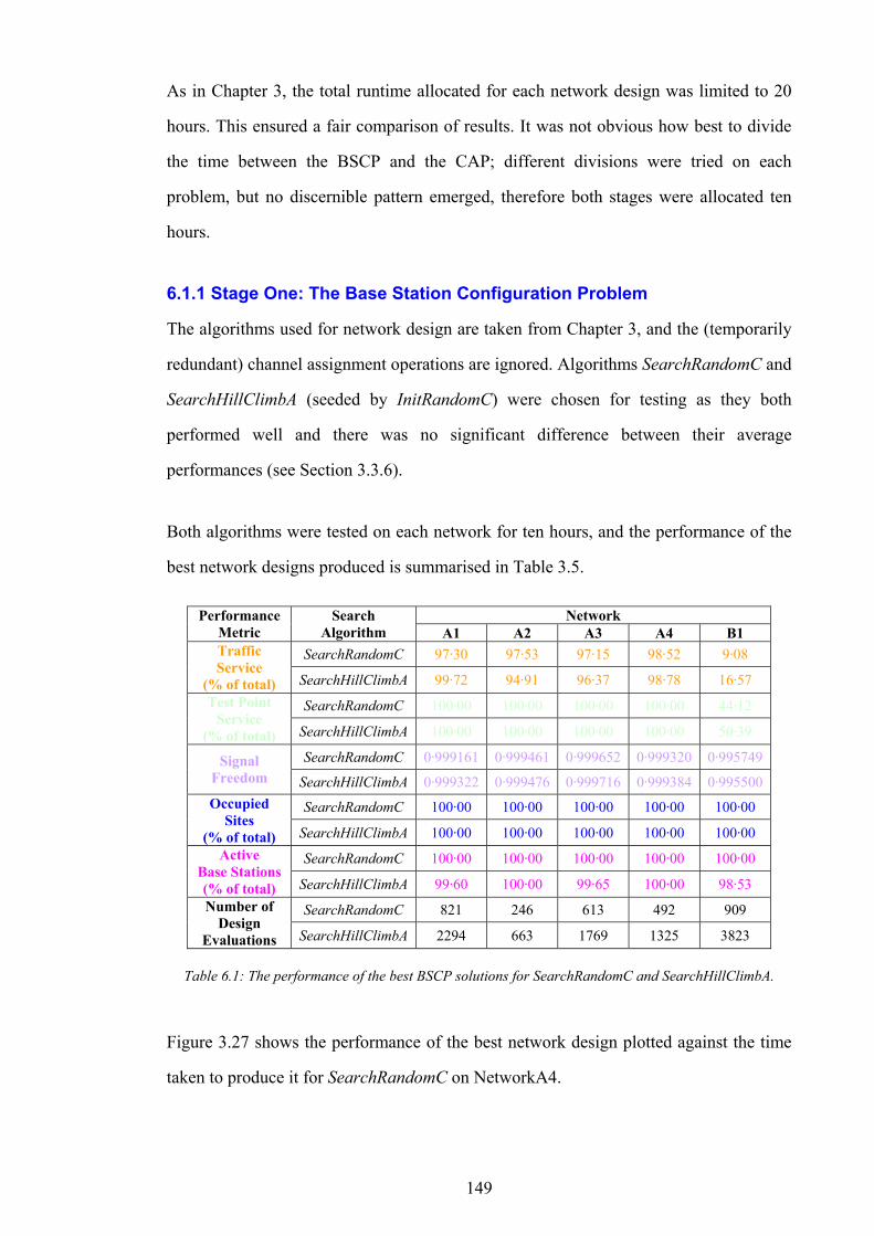
149

As in Chapter 3, the total runtime allocated for each network design was limited to 20

hours. This ensured a fair comparison of results. It was not obvious how best to divide

the time between the BSCP and the CAP; different divisions were tried on each

problem, but no discernible pattern emerged, therefore both stages were allocated ten

hours.

6.1.1 Stage One: The Base Station Configuration Problem

The algorithms used for network design are taken from Chapter 3, and the (temporarily

redundant) channel assignment operations are ignored. Algorithms SearchRandomC and

SearchHillClimbA (seeded by InitRandomC) were chosen for testing as they both

performed well and there was no significant difference between their average

performances (see Section 3.3.6).

Both algorithms were tested on each network for ten hours, and the performance of the

best network designs produced is summarised in Table 3.5.

Network Performance Metric

Search Algorithm A1 A2 A3 A4 B1

SearchRandomC 97·30 97·53 97·15 98·52 9·08 Traffic Service

(% of total) SearchHillClimbA 99·72 94·91 96·37 98·78 16·57

SearchRandomC 100·00 100·00 100·00 100·00 44·12 Test Point Service

(% of total) SearchHillClimbA 100·00 100·00 100·00 100·00 50·39

SearchRandomC 0·999161 0·999461 0·999652 0·999320 0·995749 Signal Freedom SearchHillClimbA 0·999322 0·999476 0·999716 0·999384 0·995500

SearchRandomC 100·00 100·00 100·00 100·00 100·00 Occupied Sites

(% of total) SearchHillClimbA 100·00 100·00 100·00 100·00 100·00

SearchRandomC 100·00 100·00 100·00 100·00 100·00 Active Base Stations (% of total) SearchHillClimbA 99·60 100·00 99·65 100·00 98·53

SearchRandomC 821 246 613 492 909 Number of Design

Evaluations SearchHillClimbA 2294 663 1769 1325 3823

Table 6.1: The performance of the best BSCP solutions for SearchRandomC and SearchHillClimbA.

Figure 3.27 shows the performance of the best network design plotted against the time

taken to produce it for SearchRandomC on NetworkA4.

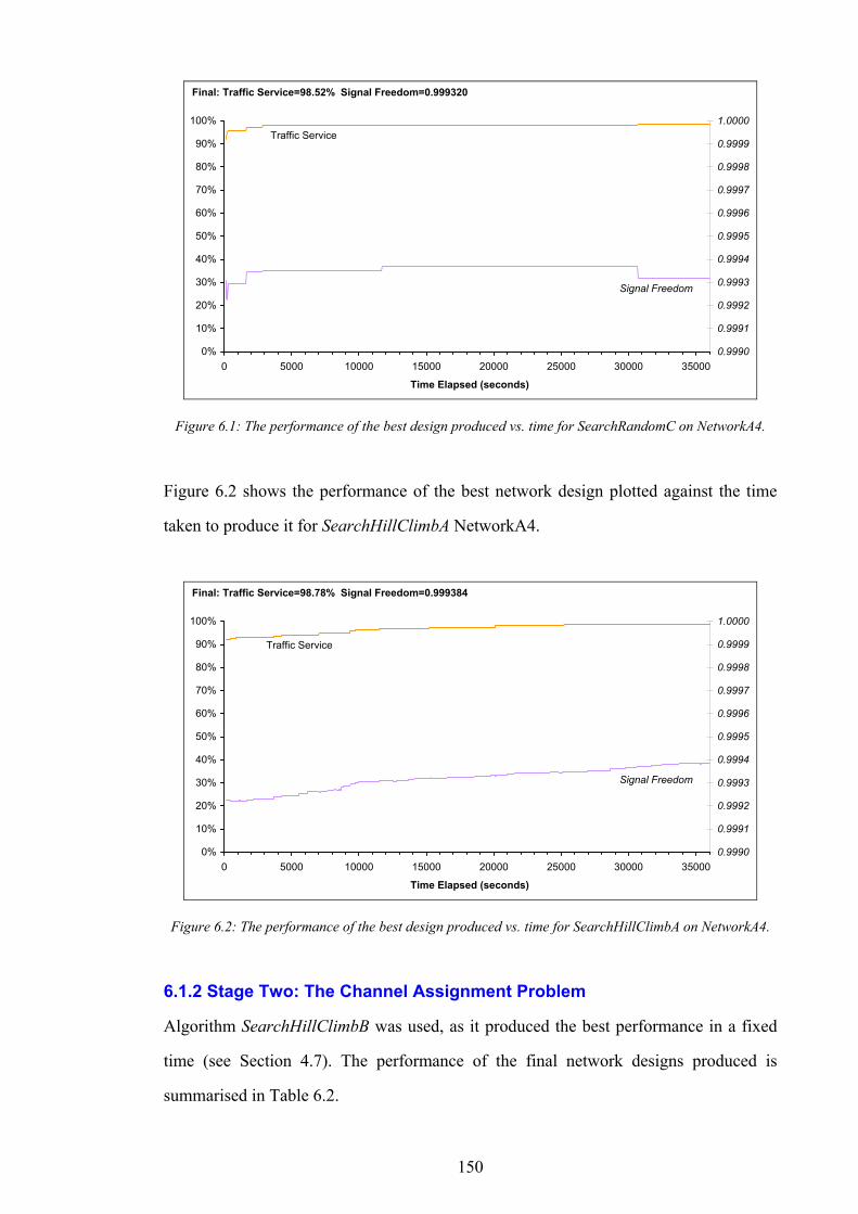
150

0%

10%

20%

30%

40%

50%

60%

70%

80%

90%

100%

0 5000 10000 15000 20000 25000 30000 35000

Time Elapsed (seconds)

0.9990

0.9991

0.9992

0.9993

0.9994

0.9995

0.9996

0.9997

0.9998

0.9999

1.0000

Final: Traffic Service=98.52% Signal Freedom=0.999320

Traffic Service

Signal Freedom

Figure 6.1: The performance of the best design produced vs. time for SearchRandomC on NetworkA4.

Figure 6.2 shows the performance of the best network design plotted against the time

taken to produce it for SearchHillClimbA NetworkA4.

0%

10%

20%

30%

40%

50%

60%

70%

80%

90%

100%

0 5000 10000 15000 20000 25000 30000 35000

Time Elapsed (seconds)

0.9990

0.9991

0.9992

0.9993

0.9994

0.9995

0.9996

0.9997

0.9998

0.9999

1.0000

Final: Traffic Service=98.78% Signal Freedom=0.999384

Traffic Service

Signal Freedom

Figure 6.2: The performance of the best design produced vs. time for SearchHillClimbA on NetworkA4.

6.1.2 Stage Two: The Channel Assignment Problem

Algorithm SearchHillClimbB was used, as it produced the best performance in a fixed

time (see Section 4.7). The performance of the final network designs produced is

summarised in Table 6.2.

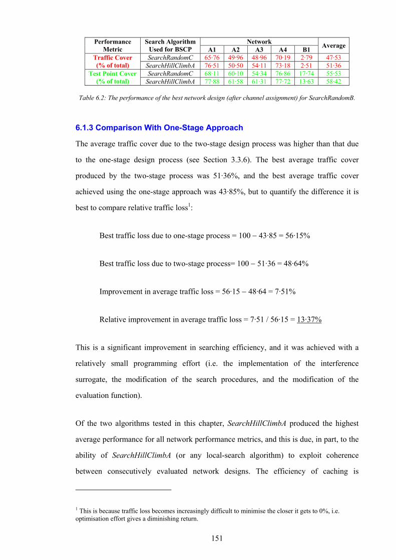
151

Network Performance Metric

Search Algorithm Used for BSCP A1 A2 A3 A4 B1 Average

SearchRandomC 65·76 49·96 48·96 70·19 2·79 47·53 Traffic Cover (% of total) SearchHillClimbA 76·51 50·50 54·11 73·18 2·51 51·36

SearchRandomC 68·11 60·10 54·34 76·86 17·74 55·53 Test Point Cover (% of total) SearchHillClimbA 77·88 61·58 61·31 77·72 13·63 58·42

Table 6.2: The performance of the best network design (after channel assignment) for SearchRandomB.

6.1.3 Comparison With One-Stage Approach

The average traffic cover due to the two-stage design process was higher than that due

to the one-stage design process (see Section 3.3.6). The best average traffic cover

produced by the two-stage process was 51·36%, and the best average traffic cover

achieved using the one-stage approach was 43·85%, but to quantify the difference it is

best to compare relative traffic loss1:

Best traffic loss due to one-stage process = 100 − 43·85 = 56·15%

Best traffic loss due to two-stage process= 100 − 51·36 = 48·64%

Improvement in average traffic loss = 56·15 − 48·64 = 7·51%

Relative improvement in average traffic loss = 7·51 / 56·15 = 13·37%

This is a significant improvement in searching efficiency, and it was achieved with a

relatively small programming effort (i.e. the implementation of the interference

surrogate, the modification of the search procedures, and the modification of the

evaluation function).

Of the two algorithms tested in this chapter, SearchHillClimbA produced the highest

average performance for all network performance metrics, and this is due, in part, to the

ability of SearchHillClimbA (or any local-search algorithm) to exploit coherence

between consecutively evaluated network designs. The efficiency of caching is

1 This is because traffic loss becomes increasingly difficult to minimise the closer it gets to 0%, i.e. optimisation effort gives a diminishing return.

152

demonstrated by the fact that approximately three times as many network evaluations

were made by SearchHillClimbA than were made by SearchRandomC. If the ‘caching’

of evaluation calculations were disabled it is certain that the performance of

SearchHillClimbA would decrease, and it is possible that it would fall below that of

SearchRandomC. Therefore, it should not be assumed that SearchHillClimbA would

always outperform SearchRandomC.

6.2 Network Designs with ‘High’ Computational Investment

All the network designs produced previously in this thesis have been limited to 20 hours

of runtime, but in this section the runtime is extended to seven days: five days for the

BSCP and two days for the CAP. This relative division of time between network design

and channel assignment was found to yield good network design performance, however,

no optimal division of time between the two stages has been determined.

An unlimited time would ideally be devoted to finding the best possible network, but

obviously this is not possible in practice. Therefore it was decided that 35 days (7 days

× 5 networks) was the maximum time available for the generation of results for this

section. The two-stage network design process was adopted because of its superior

searching efficiency (see Section 6.1.3).

6.2.1 Algorithms for the BSCP

A combination of search algorithms was used to produce a solution to the BSCP for

each of the five networks. Although SearchHillClimbA was found to produce the best

final network design performance, it was observed that SearchRandomC produced the

best improvement in network design in the early stages of optimisation (for example,

compare Figure 6.1 with Figure 6.2), but then stalled after about an hour. Therefore the

first hour of searching was done by SearchRandomC, after which the control was passed

to SearchHillClimbA.

Experience from previous runs of SearchHillClimbA showed that approximately 50% of

moves in which base stations were deactivated produced an improvement in design

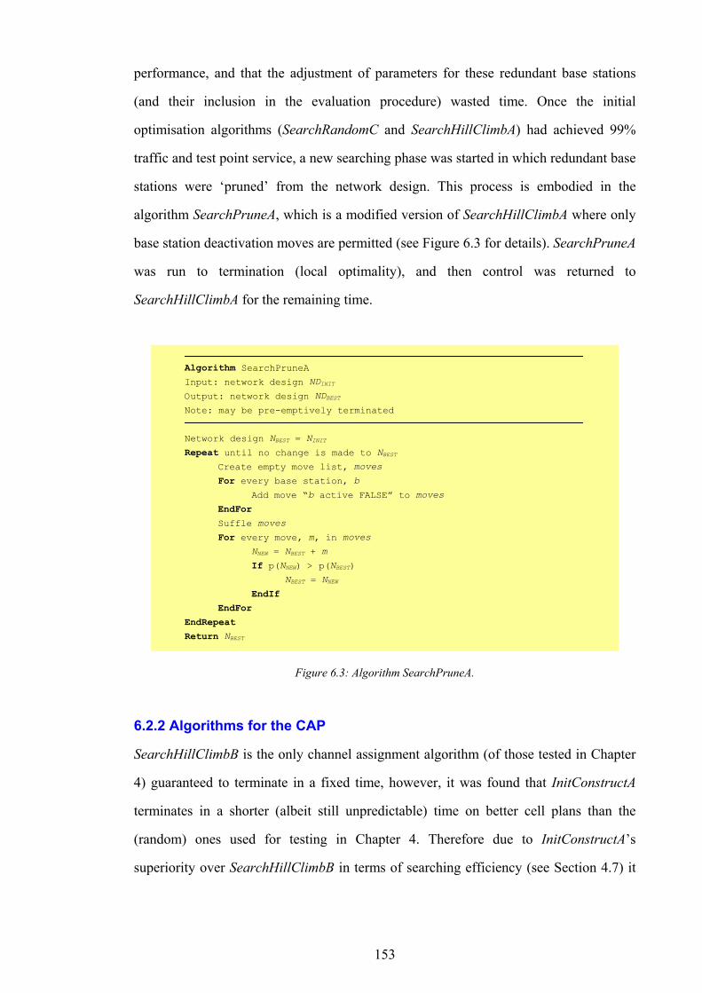
153

performance, and that the adjustment of parameters for these redundant base stations

(and their inclusion in the evaluation procedure) wasted time. Once the initial

optimisation algorithms (SearchRandomC and SearchHillClimbA) had achieved 99%

traffic and test point service, a new searching phase was started in which redundant base

stations were ‘pruned’ from the network design. This process is embodied in the

algorithm SearchPruneA, which is a modified version of SearchHillClimbA where only

base station deactivation moves are permitted (see Figure 6.3 for details). SearchPruneA

was run to termination (local optimality), and then control was returned to

SearchHillClimbA for the remaining time.

Algorithm SearchPruneA Input: network design NDINIT

Output: network design NDBEST

Note: may be pre-emptively terminated

Network design NBEST = NINIT Repeat until no change is made to NBEST Create empty move list, moves

For every base station, b Add move “b active FALSE” to moves

EndFor Suffle moves

For every move, m, in moves NNEW = NBEST + m

If p(NNEW) > p(NBEST) NBEST = NNEW

EndIf EndFor EndRepeat Return NBEST

Figure 6.3: Algorithm SearchPruneA.

6.2.2 Algorithms for the CAP

SearchHillClimbB is the only channel assignment algorithm (of those tested in Chapter

4) guaranteed to terminate in a fixed time, however, it was found that InitConstructA

terminates in a shorter (albeit still unpredictable) time on better cell plans than the

(random) ones used for testing in Chapter 4. Therefore due to InitConstructA’s

superiority over SearchHillClimbB in terms of searching efficiency (see Section 4.7) it

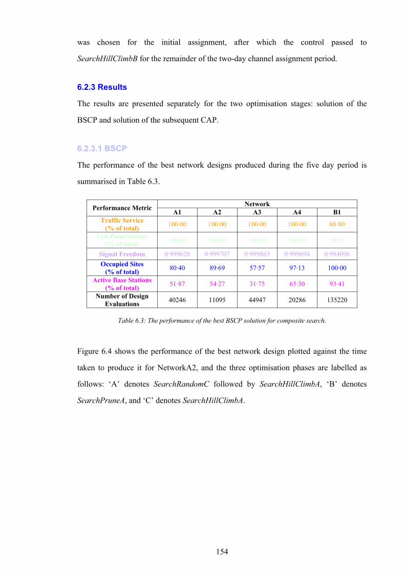
154

was chosen for the initial assignment, after which the control passed to

SearchHillClimbB for the remainder of the two-day channel assignment period.

6.2.3 Results

The results are presented separately for the two optimisation stages: solution of the

BSCP and solution of the subsequent CAP.

6.2.3.1 BSCP

The performance of the best network designs produced during the five day period is

summarised in Table 6.3.

Network Performance Metric A1 A2 A3 A4 B1 Traffic Service

(% of total) 100·00 100·00 100·00 100·00 68·80

Test Point Service (% of total) 100·00 100·00 100·00 100·00 38·53

Signal Freedom 0·999628 0·999707 0·999863 0·999694 0·994096 Occupied Sites

(% of total) 80·40 89·69 57·57 97·13 100·00

Active Base Stations (% of total) 51·87 54·27 31·75 65·30 93·41

Number of Design Evaluations 40246 11095 44947 20286 135220

Table 6.3: The performance of the best BSCP solution for composite search.

Figure 6.4 shows the performance of the best network design plotted against the time

taken to produce it for NetworkA2, and the three optimisation phases are labelled as

follows: ‘A’ denotes SearchRandomC followed by SearchHillClimbA, ‘B’ denotes

SearchPruneA, and ‘C’ denotes SearchHillClimbA.

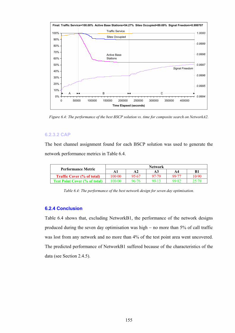
155

0%

10%

20%

30%

40%

50%

60%

70%

80%

90%

100%

0 50000 100000 150000 200000 250000 300000 350000 400000

Time Elapsed (seconds)

0.9994

0.9995

0.9996

0.9997

0.9998

0.9999

1.0000

Final: Traffic Service=100.00% Active Base Stations=54.27% Sites Occupied=89.69% Signal Freedom=0.999707

Traffic Service

Active Base Stations

Sites Occupied

Signal Freedom

A B C

Figure 6.4: The performance of the best BSCP solution vs. time for composite search on NetworkA2.

6.2.3.2 CAP

The best channel assignment found for each BSCP solution was used to generate the

network performance metrics in Table 6.4.

Network Performance Metric A1 A2 A3 A4 B1 Traffic Cover (% of total) 100·00 95·67 97·79 99·77 10·90

Test Point Cover (% of total) 100·00 96·76 99·13 99·82 25·78

Table 6.4: The performance of the best network design for seven day optimisation.

6.2.4 Conclusion

Table 6.4 shows that, excluding NetworkB1, the performance of the network designs

produced during the seven day optimisation was high − no more than 5% of call traffic

was lost from any network and no more than 4% of the test point area went uncovered.

The predicted performance of NetworkB1 suffered because of the characteristics of the

data (see Section 2.4.5).

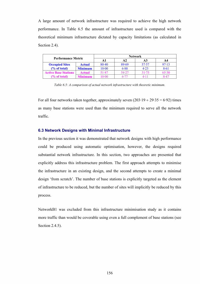
156

A large amount of network infrastructure was required to achieve the high network

performance. In Table 6.5 the amount of infrastructure used is compared with the

theoretical minimum infrastructure dictated by capacity limitations (as calculated in

Section 2.4).

Network Performance Metric A1 A2 A3 A4 Actual 80·40 89·69 57·57 97·13 Occupied Sites

(% of total) Minimum 10·00 6·88 4·23 8·61 Actual 51·87 54·27 31·75 65·30 Active Base Stations

(% of total) Minimum 10·00 6·77 4·11 8·47

Table 6.5: A comparison of actual network infrastructure with theoretic minimum.

For all four networks taken together, approximately seven (203·19 ÷ 29·35 = 6·92) times

as many base stations were used than the minimum required to serve all the network

traffic.

6.3 Network Designs with Minimal Infrastructure

In the previous section it was demonstrated that network designs with high performance

could be produced using automatic optimisation, however, the designs required

substantial network infrastructure. In this section, two approaches are presented that

explicitly address this infrastructure problem. The first approach attempts to minimise

the infrastructure in an existing design, and the second attempts to create a minimal

design ‘from scratch’. The number of base stations is explicitly targeted as the element

of infrastructure to be reduced, but the number of sites will implicitly be reduced by this

process.

NetworkB1 was excluded from this infrastructure minimisation study as it contains

more traffic than would be coverable using even a full complement of base stations (see

Section 2.4.5).

157

6.3.1 Algorithm: SearchPruneB

The goal of algorithm SearchPruneB, detailed in Figure 6.5, is the production of

network designs with minimal infrastructure. It is an extended version of

SearchPruneA.

SearchPruneB delivers a network design with a performance equal to (or greater than)

that of the initial network design used, and number of base stations in the new design

will be less than or equal to that of the initial design.

6.3.1.1 Description

A list of active base stations is made from the initial network design. The base stations

are then arranged in ascending order of the amount of traffic cover they provide, as the

removal of those covering the least traffic is likely to have the least impact on network

performance. The first base station in the list is deactivated and the resulting network

design evaluated. If network performance does not deteriorate (i.e. no loss of traffic or

test point cover), then this base station remains inactive, otherwise it is reactivated and

the next base station in the list is tested instead. If no superfluous base stations can be

found, the base station whose removal had the least impact (i.e. led to the least loss in

traffic cover) is deactivated, and the resulting network is then hill climbed until the

target network performance (that of the initial design) is restored. Whenever this target

performance is achieved (after the removal of a base station or after restoration by hill

climbing) the whole sequence is repeated on the new network design.

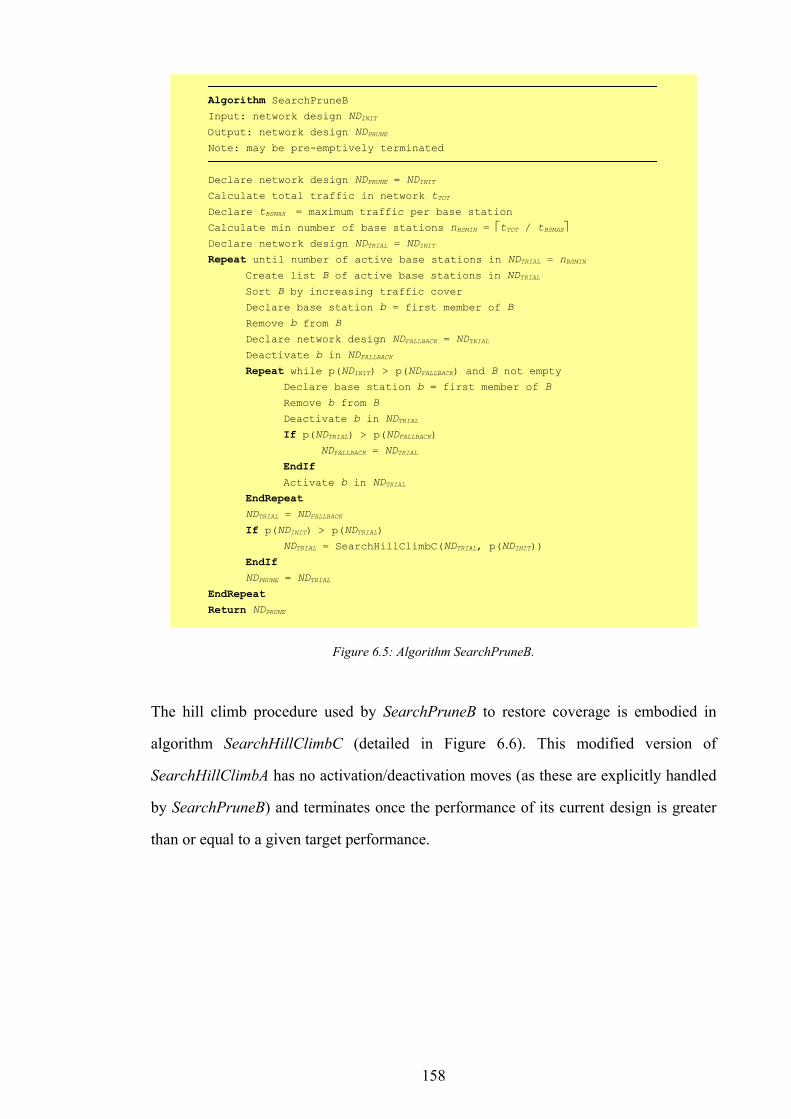
158

Algorithm SearchPruneB Input: network design NDINIT

Output: network design NDPRUNE

Note: may be pre-emptively terminated

Declare network design NDPRUNE = NDINIT

Calculate total traffic in network tTOT

Declare tBSMAX = maximum traffic per base station

Calculate min number of base stations nBSMIN = tTOT / tBSMAX Declare network design NDTRIAL = NDINIT

Repeat until number of active base stations in NDTRIAL = nBSMIN Create list B of active base stations in NDTRIAL Sort B by increasing traffic cover

Declare base station b = first member of B

Remove b from B

Declare network design NDFALLBACK = NDTRIAL Deactivate b in NDFALLBACK Repeat while p(NDINIT) > p(NDFALLBACK) and B not empty Declare base station b = first member of B

Remove b from B

Deactivate b in NDTRIAL If p(NDTRIAL) > p(NDFALLBACK) NDFALLBACK = NDTRIAL EndIf Activate b in NDTRIAL

EndRepeat NDTRIAL = NDFALLBACK

If p(NDINIT) > p(NDTRIAL) NDTRIAL = SearchHillClimbC(NDTRIAL, p(NDINIT))

EndIf NDPRUNE = NDTRIAL EndRepeat Return NDPRUNE

Figure 6.5: Algorithm SearchPruneB.

The hill climb procedure used by SearchPruneB to restore coverage is embodied in

algorithm SearchHillClimbC (detailed in Figure 6.6). This modified version of

SearchHillClimbA has no activation/deactivation moves (as these are explicitly handled

by SearchPruneB) and terminates once the performance of its current design is greater

than or equal to a given target performance.

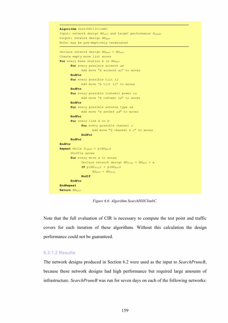
159

Algorithm SearchHillClimbC Input: network design NDINIT and target performance PTARGET

Output: network design NDBEST Note: may be pre-emptively terminated

Declare network design NDBEST = NDINIT Create empty move list moves

For every base station b in NDBEST For every possible azimuth az Add move “b azimuth az” to moves

EndFor For every possible tilt tl Add move “b tilt tl” to moves

EndFor For every possible transmit power tx Add move “b txPower tx” to moves

EndFor For every possible antenna type ad Add move “b antDef ad” to moves

EndFor For every link k on b For every possible channel c

Add move “b channel k c” to moves

EndFor EndFor EndFor Repeat while PTARGET > p(NDBEST) Shuffle moves

For every move m in moves Declare network design NDTRIAL = NDBEST + m

If p(NDTRIAL) > p(NDBEST) NDBEST = NDTRIAL

EndIf EndFor EndRepeat Return NDBEST

Figure 6.6: Algorithm SearchHillClimbC.

Note that the full evaluation of CIR is necessary to compute the test point and traffic

covers for each iteration of these algorithms. Without this calculation the design

performance could not be guaranteed.

6.3.1.2 Results

The network designs produced in Section 6.2 were used as the input to SearchPruneB,

because these network designs had high performance but required large amounts of

infrastructure. SearchPruneB was run for seven days on each of the following networks:

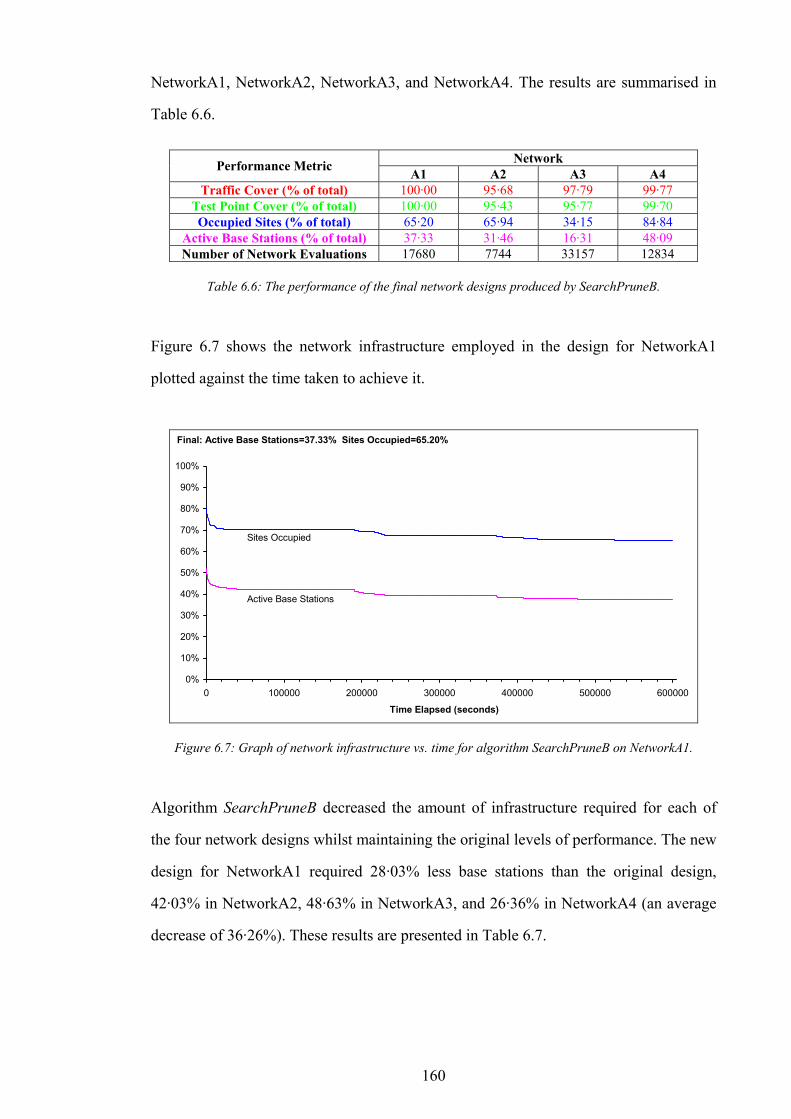
160

NetworkA1, NetworkA2, NetworkA3, and NetworkA4. The results are summarised in

Table 6.6.

Network Performance Metric A1 A2 A3 A4 Traffic Cover (% of total) 100·00 95·68 97·79 99·77

Test Point Cover (% of total) 100·00 95·43 95·77 99·70 Occupied Sites (% of total) 65·20 65·94 34·15 84·84

Active Base Stations (% of total) 37·33 31·46 16·31 48·09 Number of Network Evaluations 17680 7744 33157 12834

Table 6.6: The performance of the final network designs produced by SearchPruneB.

Figure 6.7 shows the network infrastructure employed in the design for NetworkA1

plotted against the time taken to achieve it.

0%

10%

20%

30%

40%

50%

60%

70%

80%

90%

100%

0 100000 200000 300000 400000 500000 600000

Time Elapsed (seconds)

Final: Active Base Stations=37.33% Sites Occupied=65.20%

Active Base Stations

Sites Occupied

Figure 6.7: Graph of network infrastructure vs. time for algorithm SearchPruneB on NetworkA1.

Algorithm SearchPruneB decreased the amount of infrastructure required for each of

the four network designs whilst maintaining the original levels of performance. The new

design for NetworkA1 required 28·03% less base stations than the original design,

42·03% in NetworkA2, 48·63% in NetworkA3, and 26·36% in NetworkA4 (an average

decrease of 36·26%). These results are presented in Table 6.7.

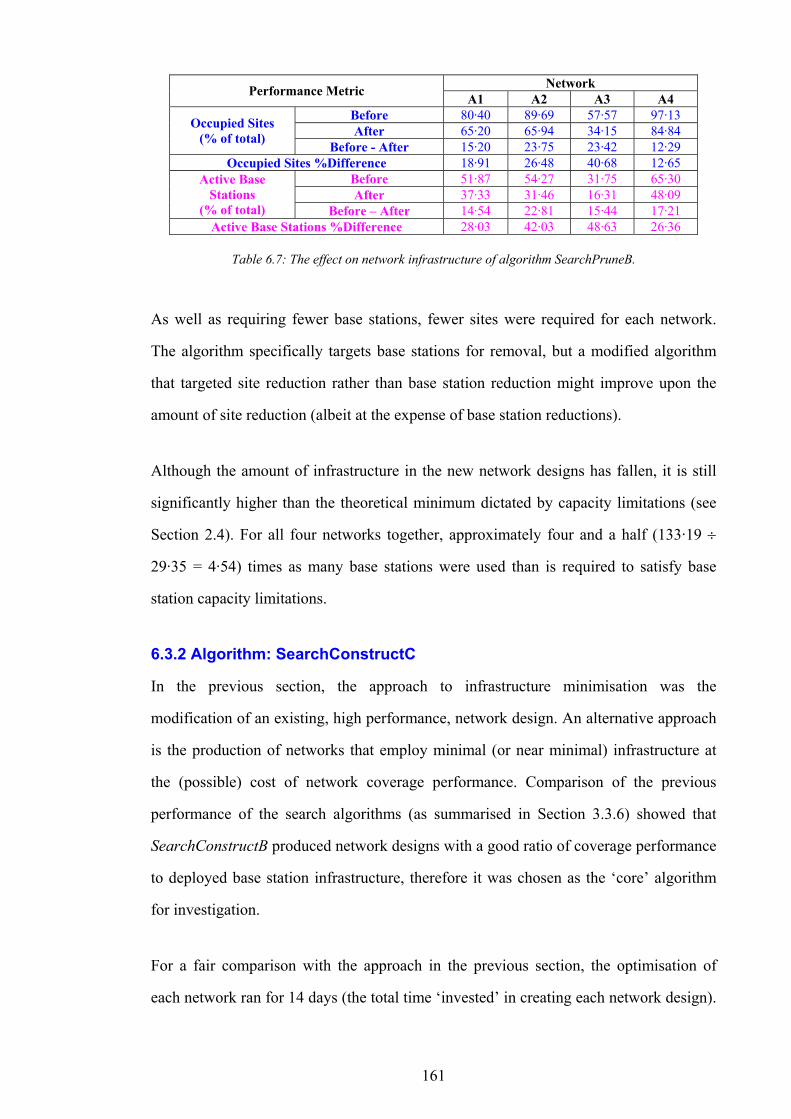
161

Network Performance Metric A1 A2 A3 A4 Before 80·40 89·69 57·57 97·13 After 65·20 65·94 34·15 84·84 Occupied Sites

(% of total) Before - After 15·20 23·75 23·42 12·29 Occupied Sites %Difference 18·91 26·48 40·68 12·65

Before 51·87 54·27 31·75 65·30 After 37·33 31·46 16·31 48·09

Active Base Stations

(% of total) Before – After 14·54 22·81 15·44 17·21 Active Base Stations %Difference 28·03 42·03 48·63 26·36

Table 6.7: The effect on network infrastructure of algorithm SearchPruneB.

As well as requiring fewer base stations, fewer sites were required for each network.

The algorithm specifically targets base stations for removal, but a modified algorithm

that targeted site reduction rather than base station reduction might improve upon the

amount of site reduction (albeit at the expense of base station reductions).

Although the amount of infrastructure in the new network designs has fallen, it is still

significantly higher than the theoretical minimum dictated by capacity limitations (see

Section 2.4). For all four networks together, approximately four and a half (133·19 ÷

29·35 = 4·54) times as many base stations were used than is required to satisfy base

station capacity limitations.

6.3.2 Algorithm: SearchConstructC

In the previous section, the approach to infrastructure minimisation was the

modification of an existing, high performance, network design. An alternative approach

is the production of networks that employ minimal (or near minimal) infrastructure at

the (possible) cost of network coverage performance. Comparison of the previous

performance of the search algorithms (as summarised in Section 3.3.6) showed that

SearchConstructB produced network designs with a good ratio of coverage performance

to deployed base station infrastructure, therefore it was chosen as the ‘core’ algorithm

for investigation.

For a fair comparison with the approach in the previous section, the optimisation of

each network ran for 14 days (the total time ‘invested’ in creating each network design).

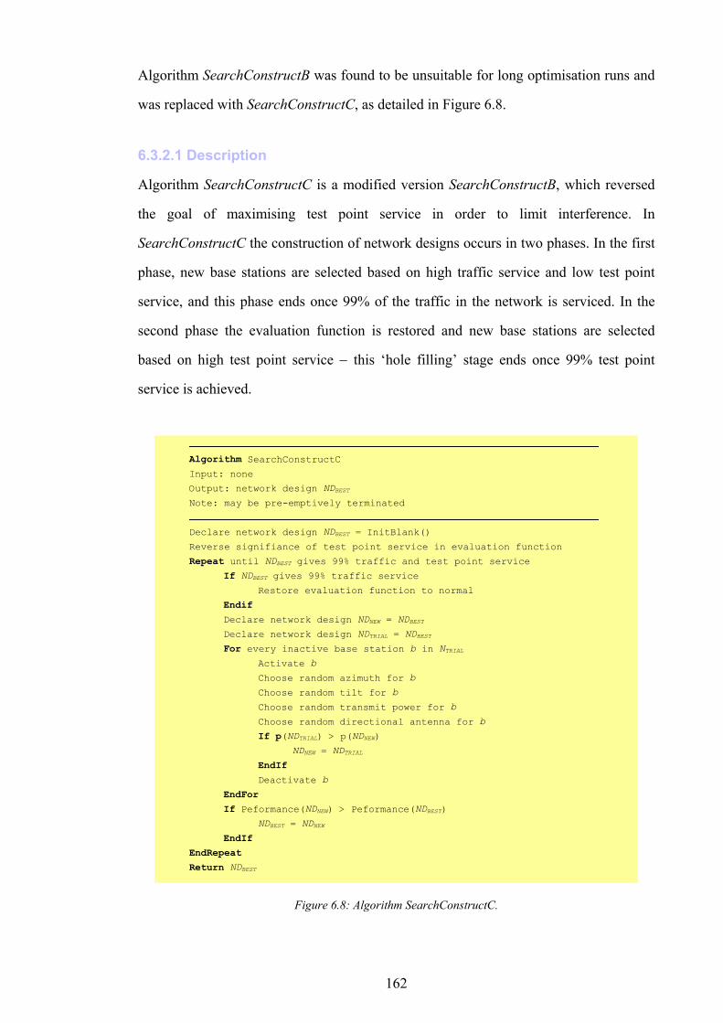
162

Algorithm SearchConstructB was found to be unsuitable for long optimisation runs and

was replaced with SearchConstructC, as detailed in Figure 6.8.

6.3.2.1 Description

Algorithm SearchConstructC is a modified version SearchConstructB, which reversed

the goal of maximising test point service in order to limit interference. In

SearchConstructC the construction of network designs occurs in two phases. In the first

phase, new base stations are selected based on high traffic service and low test point

service, and this phase ends once 99% of the traffic in the network is serviced. In the

second phase the evaluation function is restored and new base stations are selected

based on high test point service − this ‘hole filling’ stage ends once 99% test point

service is achieved.

Algorithm SearchConstructC Input: none

Output: network design NDBEST Note: may be pre-emptively terminated

Declare network design NDBEST = InitBlank()

Reverse signifiance of test point service in evaluation function

Repeat until NDBEST gives 99% traffic and test point service If NDBEST gives 99% traffic service Restore evaluation function to normal

Endif Declare network design NDNEW = NDBEST Declare network design NDTRIAL = NDBEST For every inactive base station b in NTRIAL Activate b

Choose random azimuth for b

Choose random tilt for b

Choose random transmit power for b

Choose random directional antenna for b

If p(NDTRIAL) > p(NDNEW) NDNEW = NDTRIAL EndIf Deactivate b

EndFor If Peformance(NDNEW) > Peformance(NDBEST) NDBEST = NDNEW EndIf

EndRepeat Return NDBEST

Figure 6.8: Algorithm SearchConstructC.

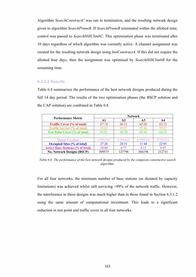
163

Algorithm SearchConstructC was run to termination, and the resulting network design

given to algorithm SearchPruneB. If SearchPruneB terminated within the allotted time,

control was passed to SearchHillClimbC. This optimisation phase was terminated after

10 days regardless of which algorithm was currently active. A channel assignment was

created for the resulting network design using InitConstructA. If this did not require the

allotted four days, then the assignment was optimised by SearchHillClimbB for the

remaining time.

6.3.2.2 Results

Table 6.8 summarises the performance of the best network designs produced during the

full 14 day period. The results of the two optimisation phases (the BSCP solution and

the CAP solution) are combined in Table 6.8.

Network Performance Metric A1 A2 A3 A4 Traffic Cover (% of total) 87·74 60·21 65·08 62·35 Traffic Service (% of total) 99·02 99·07 99·46 99·47

Test Point Cover (% of total) 81·01 60·20 65·66 64·12 Test Point Service (% of total) 100·00 99·94 100·00 100·00

Signal Freedom 0·998364 0·998645 0·999264 0·998216 Occupied Sites (% of total) 27·20 20·31 11·44 22·95

Active Base Stations (% of total) 10·00 6·77 4·11 8·47 No. Network Designs (BSCP) 309575 127796 366198 212731

Table 6.8: The performance of the best network designs produced by the composite constructive search algorithm.

For all four networks, the minimum number of base stations (as dictated by capacity

limitations) was achieved whilst still servicing >99% of the network traffic. However,

the interference in these designs was much higher than in those found in Section 6.3.1.2

using the same amount of computational investment. This leads to a significant

reduction in test point and traffic cover in all four networks.

164

Chapter 7 Conclusions and Future Work

The structure of this chapter is as follows: Section 7.1 contains the thesis conclusions,

Section 7.2 recommends enhancements to the network model, and Section 7.3 presents

possible improvements to the optimisation methodology.

7.1 Thesis Conclusions

In this section, the thesis results are examined and conclusions are drawn about the

applicability of optimisation to the problem of mobile telephone network design.

7.1.1 Spectral Efficiency and Network Infrastructure

Although this thesis was primarily a study of ACP techniques, an important principle to

emerge from the results was a trade off between spectral efficiency and the quantity of

network infrastructure. It is useful to discuss this relationship first so that the remaining

conclusions, more directly relevant to ACP, may be better placed in context. The

underlying principal will be referred to as the efficiency conjecture, and it may be stated

as follows: in general, spectral efficiency in a capacitated network may be

improved by the addition of more network infrastructure.

165

In a wireless network, spectral re-use is the amount of information transferred

(measured in bits) divided by the amount of spectrum used (measured in Hertz) to

transfer it1. There is a fundamental limit to the amount of information a radio channel

(or concatenation of channels) can convey to the same place at the same time [5], but

the same channels may be used multiple times in different places if the information

receivers are sufficiently electromagnetically isolated from one another. Hence, there is

no theoretical upper-limit to spectral re-use. However, in a real wireless network the

receivers may not be sufficiently spread-out to ensure EM isolation, and the spectral

efficiency per unit area is a more accurate indicator of network performance2. This is

the measure referred to by the efficiency conjecture.

Now, the information bandwidth (or data rate) available to a receiver is dictated by the

CIR of its serving signal [55], and a fixed data rate is required for telephony (in a GSM

system at least). Therefore, a corresponding (fixed) target CIR may be derived (as was

the case for the data sets used in this thesis) that ensures a successful telephone

connection. For the thesis results, only receivers for which a sufficient CIR was

available were considered covered (see Section 2.2.16), and it was found that: the

addition of more base stations often improved the CIR in the network, which in turn

improved the number of receivers covered. This is the basis for the efficiency

conjecture, and it is this relationship that the following subsection attempts to establish.

It is important to note that the improvement in spectral efficiency predicted by the

efficiency conjecture is not due simply to the addition of traffic carrying transceivers;

instead it refers to the reduction of interference in a network that already has sufficient

transceivers to serve all the subscribers.

There are limits on the range of situations for which the efficiency conjecture is valid,

and there exists a point at which the addition of infrastructure will give no appreciable

1 The units being bits/Hertz. 2 The units being bits/Hertz/m2.

166

improvement in spectral efficiency. One limiting factor is the background noise – even

if the interference due to other network elements where to disappear completely, the

CIR would be limited by unavoidable background noise.

7.1.1.1 Evidence

Figure 3.10 and Figure 3.19 show a positive correlation between test point cover and

base station activity for random network designs, but in the regions of the graph where

base station activity is low, a wide range of test point cover is seen. However,

comparison of designs in this region are (for the purposes of establishing a correlation)

invalid, because the subscriber capacity each design offers will vary widely. It is only

fair to compare network designs that have the same, or very similar, capacity

performance, i.e. the same traffic service. This is because interference, transceiver

allocations, and traffic are intimately linked.

To eliminate the effect (described in the previous example) that transceiver-based

capacity limitations have on the correlation graphs, it is necessary to compare network

designs in which the base station transceiver capacities have been matched to subscriber

demand (i.e. designs with the same traffic service). By chance, the network designs

produced for testing interference surrogates in Chapter 5 are ideally suited. Ten network

designs were produced (for each network data set), in which the number of active base

stations was widely varied (see Section 5.3) but the traffic service was the same. These

initial network designs were optimised until their traffic and test point service

performances both exceeded 99%. The correlations between base station activity and

test point cover are shown in Figure 7.1, Figure 7.2, Figure 7.3, and Figure 7.4. Clearly

a correlation does exist, but the stochastic nature of the process used to derive the

network designs means that some variance is present in the results, therefore the

correlation is not conclusive.

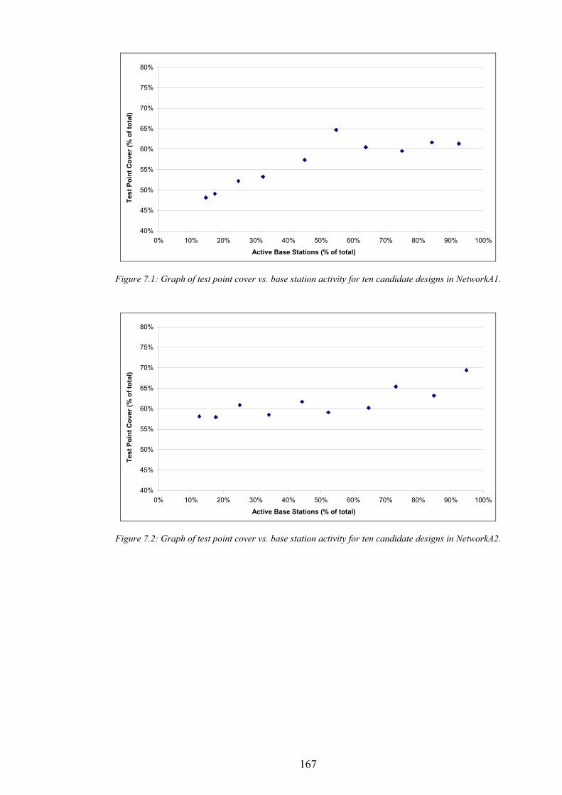
167

40%

45%

50%

55%

60%

65%

70%

75%

80%

0% 10% 20% 30% 40% 50% 60% 70% 80% 90% 100%

Active Base Stations (% of total)

Test

Poi

nt C

over

(% o

f tot

al)

Figure 7.1: Graph of test point cover vs. base station activity for ten candidate designs in NetworkA1.

40%

45%

50%

55%

60%

65%

70%

75%

80%

0% 10% 20% 30% 40% 50% 60% 70% 80% 90% 100%

Active Base Stations (% of total)

Test

Poi

nt C

over

(% o

f tot

al)

Figure 7.2: Graph of test point cover vs. base station activity for ten candidate designs in NetworkA2.

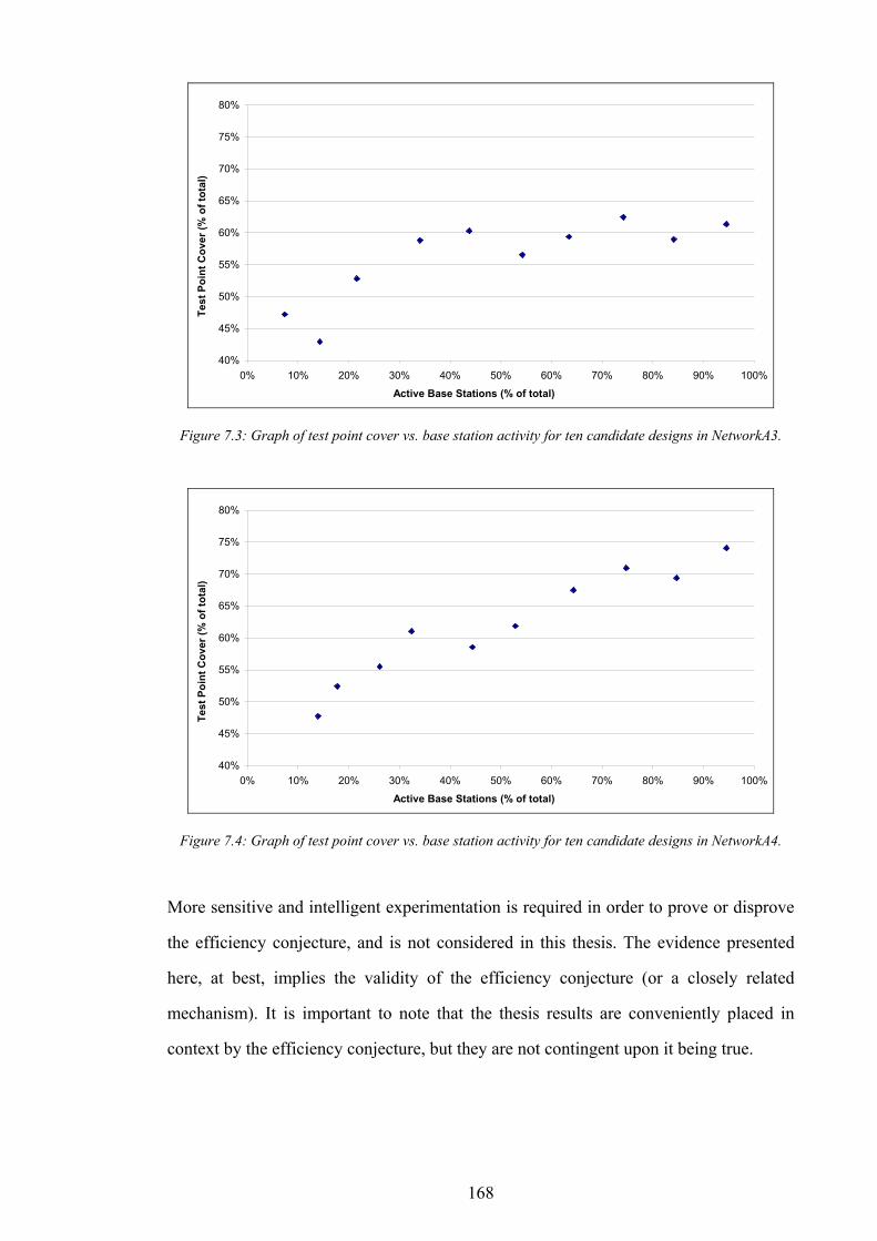
168

40%

45%

50%

55%

60%

65%

70%

75%

80%

0% 10% 20% 30% 40% 50% 60% 70% 80% 90% 100%

Active Base Stations (% of total)

Test

Poi

nt C

over

(% o

f tot

al)

Figure 7.3: Graph of test point cover vs. base station activity for ten candidate designs in NetworkA3.

40%

45%

50%

55%

60%

65%

70%

75%

80%

0% 10% 20% 30% 40% 50% 60% 70% 80% 90% 100%

Active Base Stations (% of total)

Test

Poi

nt C

over

(% o

f tot

al)

Figure 7.4: Graph of test point cover vs. base station activity for ten candidate designs in NetworkA4.

More sensitive and intelligent experimentation is required in order to prove or disprove

the efficiency conjecture, and is not considered in this thesis. The evidence presented

here, at best, implies the validity of the efficiency conjecture (or a closely related

mechanism). It is important to note that the thesis results are conveniently placed in

context by the efficiency conjecture, but they are not contingent upon it being true.

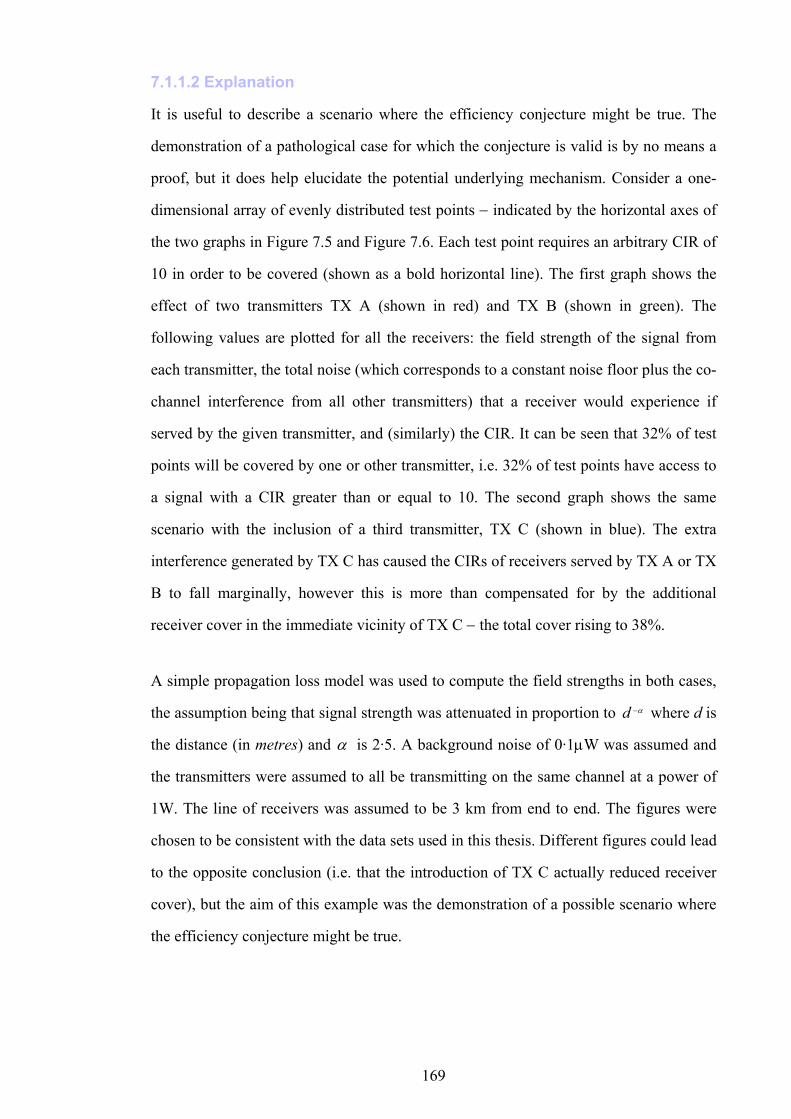
169

7.1.1.2 Explanation

It is useful to describe a scenario where the efficiency conjecture might be true. The

demonstration of a pathological case for which the conjecture is valid is by no means a

proof, but it does help elucidate the potential underlying mechanism. Consider a one-

dimensional array of evenly distributed test points − indicated by the horizontal axes of

the two graphs in Figure 7.5 and Figure 7.6. Each test point requires an arbitrary CIR of

10 in order to be covered (shown as a bold horizontal line). The first graph shows the

effect of two transmitters TX A (shown in red) and TX B (shown in green). The

following values are plotted for all the receivers: the field strength of the signal from

each transmitter, the total noise (which corresponds to a constant noise floor plus the co-

channel interference from all other transmitters) that a receiver would experience if

served by the given transmitter, and (similarly) the CIR. It can be seen that 32% of test

points will be covered by one or other transmitter, i.e. 32% of test points have access to

a signal with a CIR greater than or equal to 10. The second graph shows the same

scenario with the inclusion of a third transmitter, TX C (shown in blue). The extra

interference generated by TX C has caused the CIRs of receivers served by TX A or TX

B to fall marginally, however this is more than compensated for by the additional

receiver cover in the immediate vicinity of TX C − the total cover rising to 38%.

A simple propagation loss model was used to compute the field strengths in both cases,

the assumption being that signal strength was attenuated in proportion to α−d where d is

the distance (in metres) and α is 2·5. A background noise of 0·1µW was assumed and

the transmitters were assumed to all be transmitting on the same channel at a power of

1W. The line of receivers was assumed to be 3 km from end to end. The figures were

chosen to be consistent with the data sets used in this thesis. Different figures could lead

to the opposite conclusion (i.e. that the introduction of TX C actually reduced receiver

cover), but the aim of this example was the demonstration of a possible scenario where

the efficiency conjecture might be true.

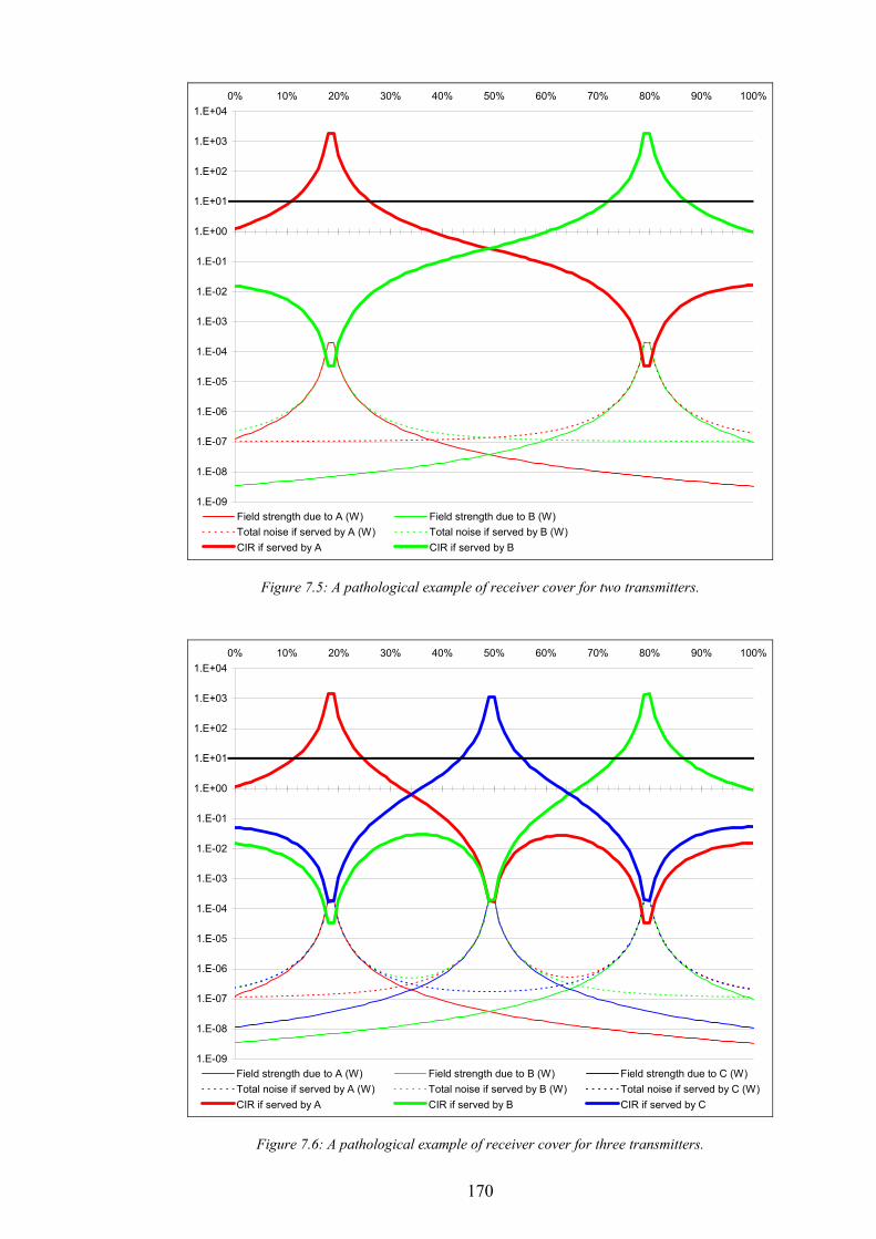
170

1.E-09

1.E-08

1.E-07

1.E-06

1.E-05

1.E-04

1.E-03

1.E-02

1.E-01

1.E+00

1.E+01

1.E+02

1.E+03

1.E+040% 10% 20% 30% 40% 50% 60% 70% 80% 90% 100%

Field strength due to A (W) Field strength due to B (W)Total noise if served by A (W) Total noise if served by B (W)CIR if served by A CIR if served by B

Figure 7.5: A pathological example of receiver cover for two transmitters.

1.E-09

1.E-08

1.E-07

1.E-06

1.E-05

1.E-04

1.E-03

1.E-02

1.E-01

1.E+00

1.E+01

1.E+02

1.E+03

1.E+040% 10% 20% 30% 40% 50% 60% 70% 80% 90% 100%

Field strength due to A (W) Field strength due to B (W) Field strength due to C (W)Total noise if served by A (W) Total noise if served by B (W) Total noise if served by C (W)CIR if served by A CIR if served by B CIR if served by C

Figure 7.6: A pathological example of receiver cover for three transmitters.

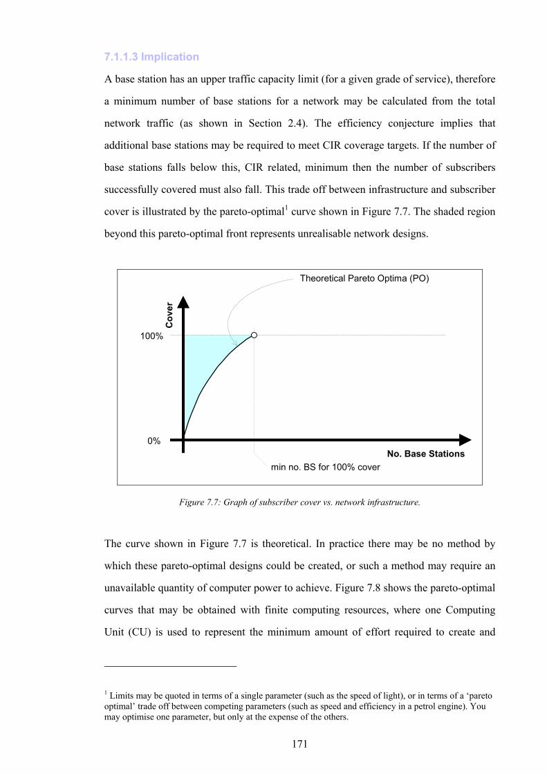
171

7.1.1.3 Implication

A base station has an upper traffic capacity limit (for a given grade of service), therefore

a minimum number of base stations for a network may be calculated from the total

network traffic (as shown in Section 2.4). The efficiency conjecture implies that

additional base stations may be required to meet CIR coverage targets. If the number of

base stations falls below this, CIR related, minimum then the number of subscribers

successfully covered must also fall. This trade off between infrastructure and subscriber

cover is illustrated by the pareto-optimal1 curve shown in Figure 7.7. The shaded region

beyond this pareto-optimal front represents unrealisable network designs.

0%

100%

Cov

er

No. Base Stationsmin no. BS for 100% cover

Theoretical Pareto Optima (PO)

Figure 7.7: Graph of subscriber cover vs. network infrastructure.

The curve shown in Figure 7.7 is theoretical. In practice there may be no method by

which these pareto-optimal designs could be created, or such a method may require an

unavailable quantity of computer power to achieve. Figure 7.8 shows the pareto-optimal

curves that may be obtained with finite computing resources, where one Computing

Unit (CU) is used to represent the minimum amount of effort required to create and

1 Limits may be quoted in terms of a single parameter (such as the speed of light), or in terms of a ‘pareto optimal’ trade off between competing parameters (such as speed and efficiency in a petrol engine). You may optimise one parameter, but only at the expense of the others.

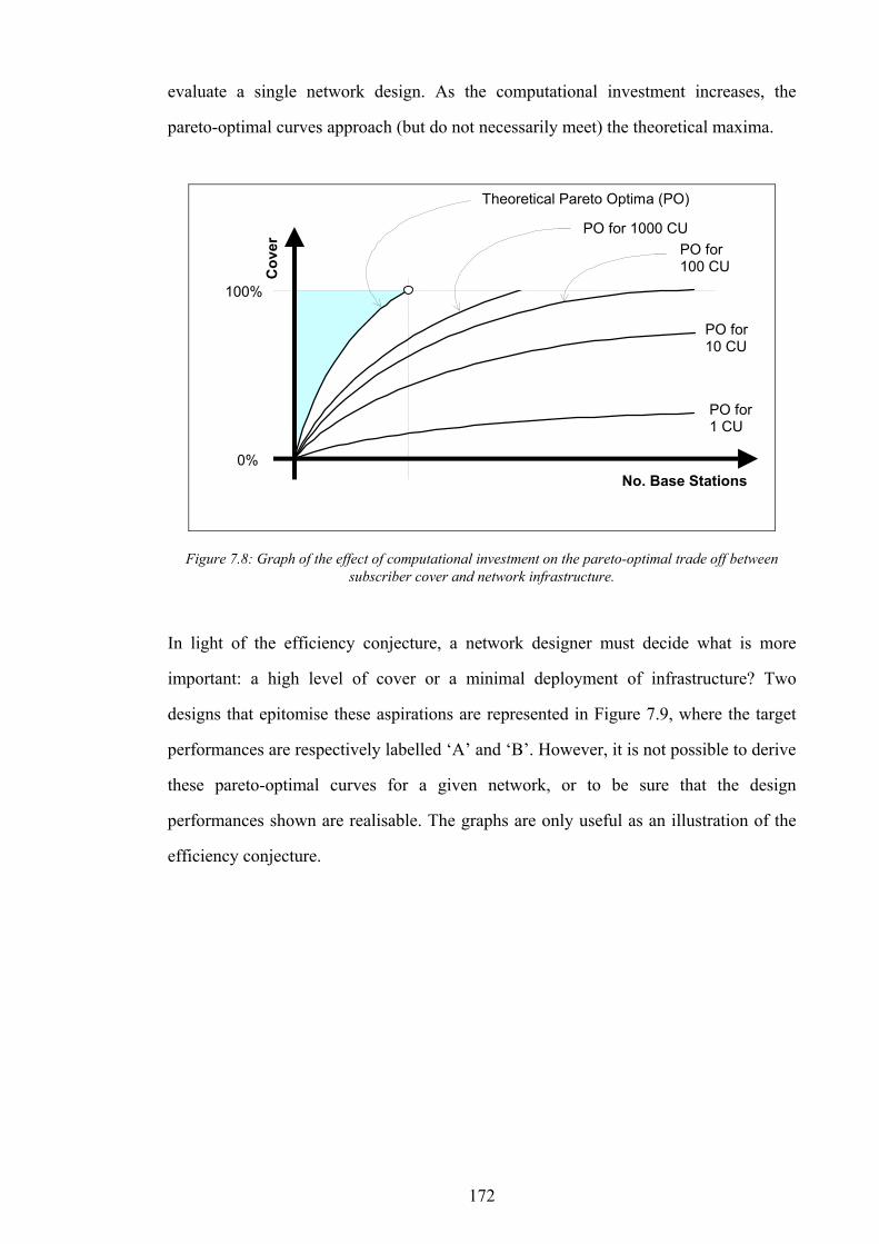
172

evaluate a single network design. As the computational investment increases, the

pareto-optimal curves approach (but do not necessarily meet) the theoretical maxima.

0%

100%C

over

No. Base Stations

Theoretical Pareto Optima (PO)

PO for 1 CU

PO for 10 CU

PO for 100 CU

PO for 1000 CU

Figure 7.8: Graph of the effect of computational investment on the pareto-optimal trade off between subscriber cover and network infrastructure.

In light of the efficiency conjecture, a network designer must decide what is more

important: a high level of cover or a minimal deployment of infrastructure? Two

designs that epitomise these aspirations are represented in Figure 7.9, where the target

performances are respectively labelled ‘A’ and ‘B’. However, it is not possible to derive

these pareto-optimal curves for a given network, or to be sure that the design

performances shown are realisable. The graphs are only useful as an illustration of the

efficiency conjecture.

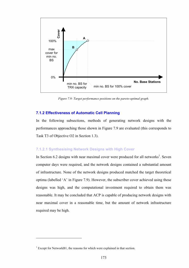
173

0%

100%

Cov

er

No. Base Stationsmin no. BS for TRX capacity min no. BS for 100% cover

max cover for min no.

BS

A

B

Figure 7.9: Target performance positions on the pareto-optimal graph.

7.1.2 Effectiveness of Automatic Cell Planning

In the following subsections, methods of generating network designs with the

performances approaching those shown in Figure 7.9 are evaluated (this corresponds to

Task T3 of Objective O2 in Section 1.3).

7.1.2.1 Synthesising Network Designs with High Cover

In Section 6.2 designs with near maximal cover were produced for all networks1. Seven

computer days were required, and the network designs contained a substantial amount

of infrastructure. None of the network designs produced matched the target theoretical

optima (labelled ‘A’ in Figure 7.9). However, the subscriber cover achieved using these

designs was high, and the computational investment required to obtain them was

reasonable. It may be concluded that ACP is capable of producing network designs with

near maximal cover in a reasonable time, but the amount of network infrastructure

required may be high.

1 Except for NetworkB1, the reasons for which were explained in that section.

174

7.1.2.2 Synthesising Networks with Minimal Infrastructure

The algorithms in Section 6.3 focused explicitly on the minimisation of network

infrastructure, and two distinct approaches were formulated. The first approach to

infrastructure minimisation (described in Section 6.3.1) relied on the modification of an

existing network design by the removal of redundant infrastructure. The average

reduction in the number of base stations was over 30% using seven computer days per

network. This approach is an extension of the previous design method (Section 7.1.2.1)

in so far as the target theoretical performance is that represented by ‘A’ in Figure 7.9.

The second approach to infrastructure minimisation (described in Section 6.3.2)

produced network designs with a minimal number of base stations (as dictated by base

station capacity and network traffic) at the potential expense of subscriber cover.

Minimal infrastructure was achieved for all networks, but the average loss in cover was

approximately 30%. This approach implicitly targets point ‘B’ in Figure 7.9.

It may be concluded that ACP is capable of significantly reducing network

infrastructure requirements, at least for synthetic network designs. Infrastructure

minimisation is most effective if the target subscriber cover does not need to be

guaranteed, however significant minimisation can be achieved regardless.

7.1.3 Separating the BSCP and the CAP

An important and novel feature of this thesis was the inclusion of channel assignment as

part of the whole wireless network design process, and a comparison was made with the

traditional two-stage approach. The network designs produced by the two-stage

approach had approximately 13% less traffic loss, and hence were superior. Note that

the efficiency of the two-stage approach is only available if a suitable interference

surrogate is used, as derived in this thesis.

Despite the superiority of the two-stage approach, the one-stage approach does have

certain advantages. Infrastructure minimisation algorithms, such as SearchPruneB, only

allow the removal of base stations if they do not effect subscriber cover, and this can

only be guaranteed if a full channel model is used to assess interference.

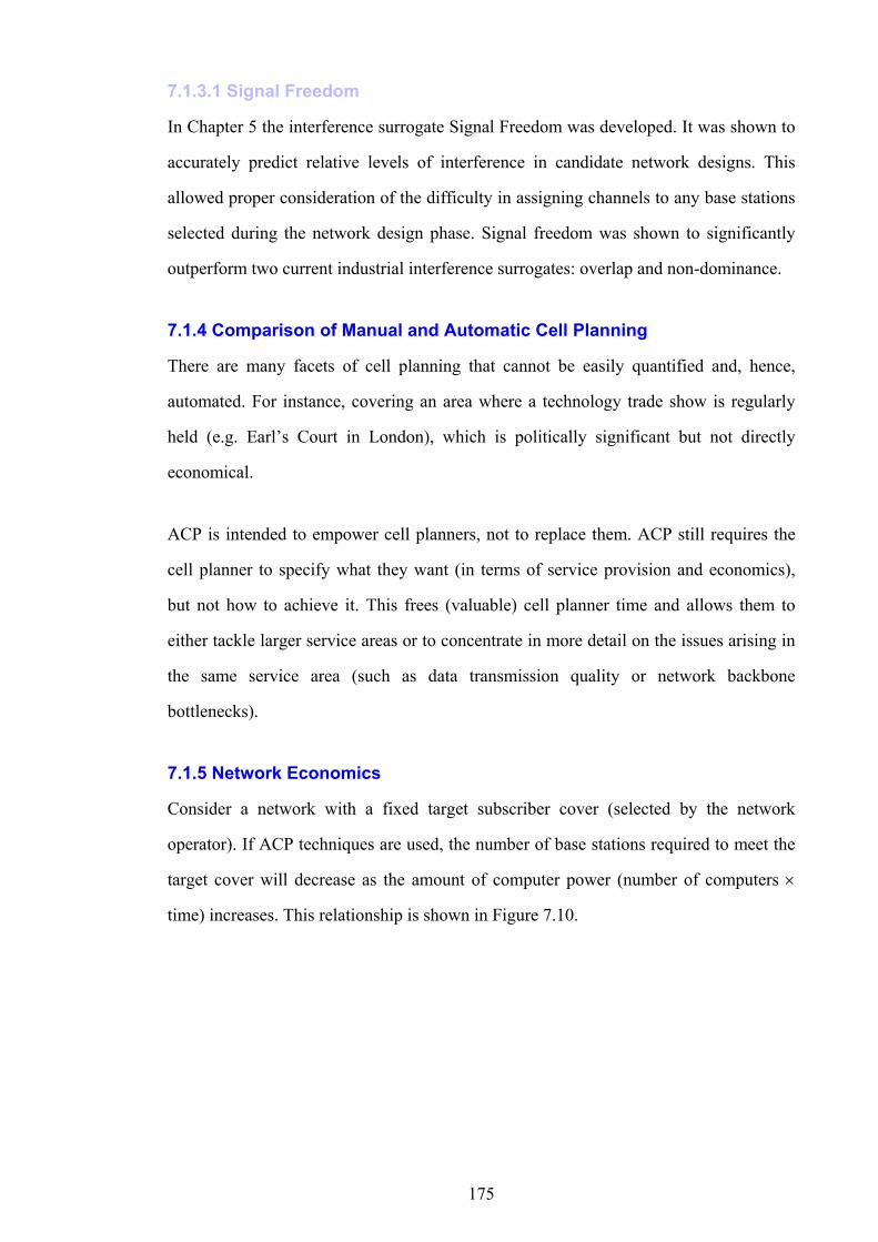
175

7.1.3.1 Signal Freedom

In Chapter 5 the interference surrogate Signal Freedom was developed. It was shown to

accurately predict relative levels of interference in candidate network designs. This

allowed proper consideration of the difficulty in assigning channels to any base stations

selected during the network design phase. Signal freedom was shown to significantly

outperform two current industrial interference surrogates: overlap and non-dominance.

7.1.4 Comparison of Manual and Automatic Cell Planning

There are many facets of cell planning that cannot be easily quantified and, hence,

automated. For instance, covering an area where a technology trade show is regularly

held (e.g. Earl’s Court in London), which is politically significant but not directly

economical.

ACP is intended to empower cell planners, not to replace them. ACP still requires the

cell planner to specify what they want (in terms of service provision and economics),

but not how to achieve it. This frees (valuable) cell planner time and allows them to

either tackle larger service areas or to concentrate in more detail on the issues arising in

the same service area (such as data transmission quality or network backbone

bottlenecks).

7.1.5 Network Economics

Consider a network with a fixed target subscriber cover (selected by the network

operator). If ACP techniques are used, the number of base stations required to meet the

target cover will decrease as the amount of computer power (number of computers ×

time) increases. This relationship is shown in Figure 7.10.

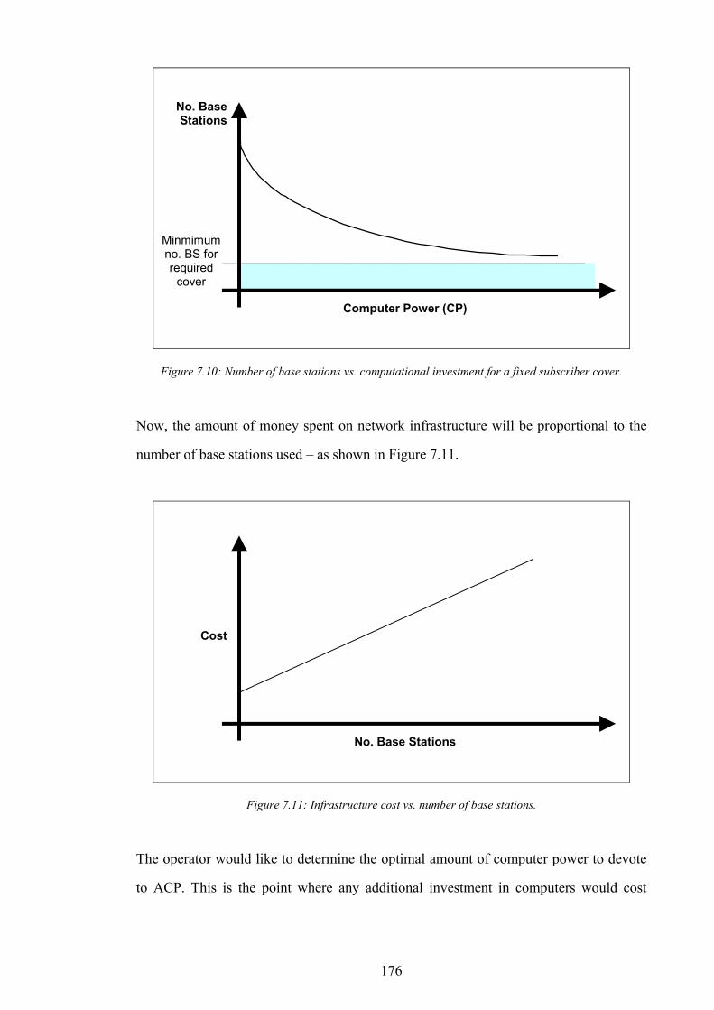
176

Computer Power (CP)

No. BaseStations

Minmimum no. BS for required

cover

Figure 7.10: Number of base stations vs. computational investment for a fixed subscriber cover.

Now, the amount of money spent on network infrastructure will be proportional to the

number of base stations used – as shown in Figure 7.11.

No. Base Stations

Cost

Figure 7.11: Infrastructure cost vs. number of base stations.

The operator would like to determine the optimal amount of computer power to devote

to ACP. This is the point where any additional investment in computers would cost

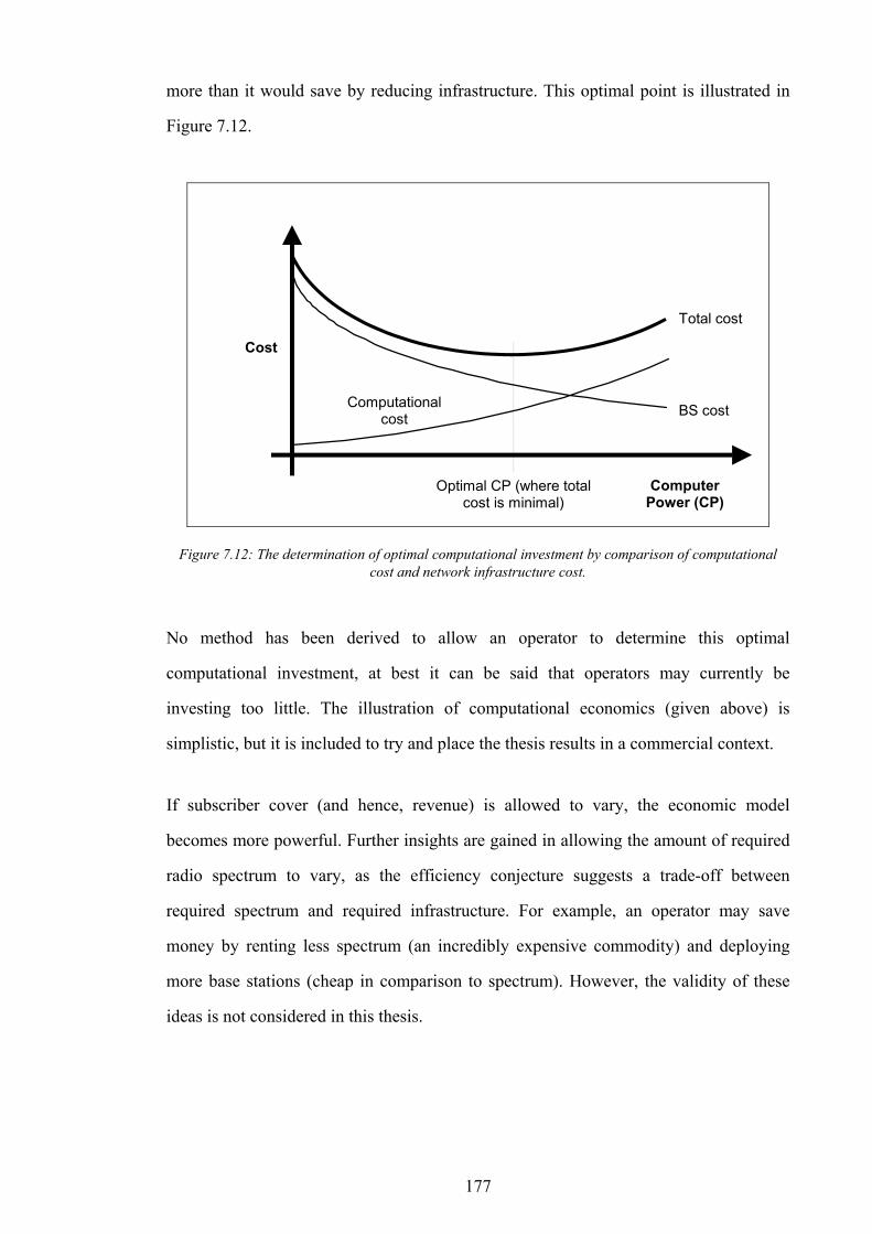
177

more than it would save by reducing infrastructure. This optimal point is illustrated in

Figure 7.12.

Computer Power (CP)

Cost

Optimal CP (where total cost is minimal)

Total cost

Computational cost BS cost

Figure 7.12: The determination of optimal computational investment by comparison of computational cost and network infrastructure cost.

No method has been derived to allow an operator to determine this optimal

computational investment, at best it can be said that operators may currently be

investing too little. The illustration of computational economics (given above) is

simplistic, but it is included to try and place the thesis results in a commercial context.

If subscriber cover (and hence, revenue) is allowed to vary, the economic model

becomes more powerful. Further insights are gained in allowing the amount of required

radio spectrum to vary, as the efficiency conjecture suggests a trade-off between

required spectrum and required infrastructure. For example, an operator may save

money by renting less spectrum (an incredibly expensive commodity) and deploying

more base stations (cheap in comparison to spectrum). However, the validity of these

ideas is not considered in this thesis.

178

7.2 Network Model Enhancements

This section presents extensions to the network model. All these proposals are intended

to improve the quality of the predictions made by the model.

7.2.1 Handover

The mechanism of subscriber handover from one cell to another has not been explicitly

considered in this thesis. True mobility relies on the support of handover between cells,

and this becomes more important as cell sizes decrease, which is an essential feature of

high capacity networks. The model presented in this thesis is static − it does not

consider the movement of subscribers. Some models, such as the ‘connectivity’ model

in [2], have relied on approximate measures of a network’s ‘handover performance’.

However, the quality of these approximations is unknown and, in pathological cases at

least, a predicted optimal performance would not guarantee handover support in a real

network.

A study of handover successes and failures in operational networks is required in order

to derive a complete model of handover behaviour. If the computational complexity of

this model prohibits its inclusion in an optimisation procedure, a surrogate function

should be derived (in a similar way to the interference surrogate derived in this thesis)

that has a known (or at least estimated) degree of accuracy.

7.2.2 Network Backbone Design

In this thesis no consideration is made of the network’s backbone infrastructure (such as

the trunking elements, PSTN entry points, and subscriber database services). These

considerations were omitted because of a lack of readily available data, but their

inclusion in the network model would greatly enhance the quality of information that

could be extracted from simulations (for example, the latency of communication

between two points in the network). The layout of the backbone infrastructure as a

separate optimisation problem has been well studied, and examples can be found in [56]

and [57].

179

7.2.3 Three-Dimensional Modelling

The thesis network model assumes that all subscriber traffic will originate on the

ground, and no consideration is made of the vertical distribution of traffic that might

occur (for instance, in a building). It has been informally estimated that in the City of

London, only 40% of mobile traffic occurs at ground level. This clearly implies that a

two-dimensional model will be less accurate than a three-dimensional one.

As subscriber densities and bandwidth requirements increase, cell sizes must decrease.

The only way to achieve efficient spectrum re-use in a built-up environment is to

sectorise the building vertically; this may be achieved by pico-cellular architectures

(each room of a building is given its own base station) or by mounting directional

antennae on adjacent buildings at different heights. To improve prediction accuracy,

consideration of the impact to users in vertically adjacent cells must be made.

The computational requirements of a full three-dimensional model are greater than that

of the model presented in this thesis, in which a trade off has been made between

prediction quality and simulation run-time. However, as the price/performance ratio of

computers continues to improve, this trade off must be periodically re-assessed.

7.2.4 Temporal Variance

The inclusion of temporal variance to the model could give an improvement in

simulation accuracy. The busy-hour traffic assumption used in the thesis model is only

able to give a worst-case prediction of network performance. Gross temporal variances

could be considered as individual static cases, for instance the traffic pattern during

working hour differs significantly from the traffic pattern outside of those hours. The

current model makes a conservative estimate of network coverage performance based

on the peak traffic expected at each test point throughout a typical day, but this leads to

an over-estimation of interference and an under-estimation of network capacity; a more

realistic prediction would allow the deployment of less infrastructure. Finer temporal

variance characteristics, such as mobility, could also be included to improve predictions

of handover support (see Section 7.2.1)

180

7.2.5 Delay Spread

Path loss is not the only characteristic of a radio signal that affects reception quality;

another important factor is delay spread. Delay spread occurs when a transmitted signal

travels by more than one path to its intended receiver. In the GSM system, adaptive

channel equalization is used to recover the intended signal, whereas in IS-95 [9] Rake

receiver techniques are used to overcome the problem of delay spread. The problem of

optimising wireless networks to meet delay spread constraints is explicitly considered in

[3].

7.2.6 Quality of Service

The central goal of the network design problem outlined in this thesis was the provision

of a signal with a sufficient Carrier-to-Interference-Ratio (CIR) for each user.

Expressing the design requirement in terms of Quality of Service (QOS) measures (such

as data throughput, latency, and blocking probability) instead of technology specific

measures, such as CIR, has two distinct advantages:

1. These measures are closer to a users experience of the network, and this makes the

relative prioritisation of these quantities easier for the network designer. In addition

to simplifying the specification of network requirements, the specification becomes

much more portable between different technologies (such as GSM and UMTS).

2. Actual QOS statistics can be directly compared with other communication systems.

A user (or a user’s application) will choose a transport medium (such as wireless

LAN, wireline ISDN, or GPRS) based on a comparison of the offered QOS, and the

network designer will be best placed to win that competition (and hence transport

the user’s data) if QOS is given explicit consideration during network design.

Mobile telephone network operators are increasingly interested in the provision of a

variety of services, each of which may have different QOS requirements. Although

telephony is set to continue as the core service, its QOS requirements (for instance, low

latency and low bandwidth) are not the same as those for other services. The explicit

181

calculation of QOS statistics allows a range of services to be mapped onto a wireless

network and not simply the one-size-fits-all mapping that results from designing solely

for telephony.

7.2.7 Error Management Through Interval Arithmetic

The accuracy of predictions made by the model is dependent on the accuracy of input

data such as terrain topography, subscriber positions, and equipment operating

characteristics. Additional inaccuracies are introduced by computational operations such

as propagation prediction. The calculation of the inaccuracy (or tolerance) of the results

is non-trivial and the usual practice is to quote a standard, conservative, estimate of the

expected tolerance for each type of simulation result (for example, 4dB for propagation

predictions).

Interval arithmetic is a computational approach that may prove useful in improving the

quality of the simulation results (see [58] for background). Instead of input variables

being quoted as single figures (as in single point arithmetic) they are quoted as two

figures (an interval), and the true value is said to be ‘contained within the interval’.

These intervals are propagated through the calculation until they emerge as outputs. The

output is guaranteed to contain the correct answer, and the ‘spread’ of the interval

indicates the certainty of the result. More conventional tolerance techniques usually

require an analytical analysis of the algorithms involved, but the numerical approach of

interval arithmetic delegates this ‘book-keeping’ to the computer instead of the

programmer. Several disadvantages must be addressed if interval analysis is to be

included in network simulation:

1. Propagation prediction algorithms must be modified to include the interval concept,

but this is cannot be achieved by a simple extension of the existing algorithms.

2. No optimisation techniques have been developed that are designed to deal with

interval based objective functions.

182

These disadvantages do not represent shortcomings in the interval approach to

computation but are in fact implicit problems the ‘single point’ approach ignores.

7.3 Improvements to Optimisation Methodology

A number of improvements to the optimisation methodology have been postulated, but

time constraints have prevented their implementation and testing. They are presented

here as a resource for future research on this problem as they represent an opportunity

for improving optimisation effectiveness and efficiency (this corresponds to Task T4 of

Objective O2 in Section 1.3).

7.3.1 Divide and Conquer

Divide and conquer is a classical approach to improving the efficiency of algorithms

that operate on large data sets (as exemplified in [51]). The underlying problem is

usually spacio-temporal in nature, or at least shares with these problems the following

property: adjacent data elements are more dependent on one another than non-

adjacent elements. It may be said, in general, that adjacent cells in a cellular network

have more influence on one another than non-adjacent cells (for instance, channel

selection), or that adjacent subscribers will affect each others quality of service more

than non-adjacent ones (for instance, base station availability).

When operators design networks manually (i.e. without automatic optimisation) they

invariably divide the network into manageable geographical regions. The automatic

division of the network area is non trivial, but it is easy to compare different approaches

by comparing the performance of the final network designs they produce.

7.3.2 Weighted Evaluation Function

Optimisation methods often rely on the use of a weighted evaluation function. This is

the combination of all the solution performance metrics into a single figure (by the

magnitude of which, each solution may be judged). In this thesis a novel approach was

taken based on the fact that the solutions are only ever compared with one another,

hence the evaluation function can be implemented as a binary comparison operator

183

(each network metric being compared in order of significance). This is the best one can

hope to achieve in the absence of a more complete network performance specification,

for instance, knowledge of the relative significance of traffic cover and test point cover.

This information could be obtained from network operators and embodied in a more

flexible evaluation function.

The ideal way to ‘weight’ the evaluation function is to relate all network statistics to a

monetary (or ‘dollar’) value. A single figure could then be produced that represents the

networks profitability, which must be the principal concern if a network is to remain

competitive. The inclusion of economics necessitates the inclusion of economists, and

this crossing of (typical) departmental boundaries (within a network operating

company) may impede the implementation of this approach. For instance, the economic

analysis given in Section 2.3.1 may be deemed too simplistic, whereas a comprehensive

economic model may be prohibitively complex to understand and implement.

184

Acknowledgments

I would like to thank my supervisor, Steve Hurley, for his constant support and

constructive criticism. I am also indebted to the many practicing engineers who have

freely discussed their work and ideas with me and helped to improve the industrial

relevance of my research. Thanks also to my colleagues in Cardiff for their ideas and

friendship, in particular Simon Chapman and Steve Margetts with whom I have

thrashed out many of the central themes of my work. I would particularly like to thank

my mother, Elinor Kapp, for her practical support and encouragement, without which

none of this would have been possible.

I would like to dedicate this thesis to my wife Erika with all my love.

[1-92]

185

Bibliography

[1] ITU, World Telecommunication Development Report (Executive Summary), International Telecommunication Union October 1999.

[2] A. Caminada and P. Reininger, Model for GSM Radio Network Optimisation, presented at the 2nd International Workshop on Discrete Algorithms and Methods for Mobile Computing and Communications, 1998.

[3] G. Athanasiadou, A. Molina, and A. Nix, The Effects of Control Node Density in Cellular Network Planning Using the Combination Algorithm for Total Optimisation (CAT), presented at the PIMRC2000, London, 2000.

[4] J. Button, K. Calderhead, I. Goetz, M. Hodges, R. Patient, R. Pilkington, R. Reeve, and P. Tattersall, Mobile network design and optimisation, BT Technology Journal, vol. 14, 1996.

[5] C. Shannon, A mathematical theory of communication, Bell System Technical Journal, vol. 27, 1948.

[6] K. Holmberg and D. Yuan, A Langrangean Heuristic Based Branch-and-Bound Approach for the Capacitated Network Design Problem, presented at the Symposium on Operations Research, 1996.

[7] W. Hershberger, Principles of Communication Systems, Prentice-Hall, 1960.

[8] R. Steele, Mobile Radio Communications, Pentech Press, 1992.

[9] R. Macario, Personal & Mobile Radio Systems, Peter Peregrinus Ltd., 1991.

[10] W. Lee, Mobile Cellular Telecommunications: Analogue and Digital Systems, McGraw-Hill, 1995.

[11] R. Steele, The Therapy of Percy Comms: A Dialogue on PCS Issues, International Journal of Wireless Information Networks, vol. 2, pp. 123-132, 1995.

[12] D. Fogel, How to Solve It: Modern Heuristics, Springer, 2000.

[13] C. Papadimitriou and K. Steiglitz, Combinatorial Optimization: Algorithms and Complexity, Dover Publications, 1998.

186

[14] W. Macready and D. Wolpert, No Free Lunch Theorems for Search, The Santa Fe Institute 1995.

[15] M. Garey and D. Johnson, Computers and Intractability: A Guide to the Theory of NP-Completeness, Bell Telephone Laboratories, 1979.

[16] D. Corne, M. Sinclair, and G. Smith, Evolutionary Telecommunications: Past, Present and Future, presented at the GECCO'99, USA, 1999.

[17] A. Koster, Frequency Assignment - Models and Algorithms, PhD Thesis, Maastricht University, Maastricht, 1999.

[18] J. Bater, Higher-order (non-binary) modelling and solution techniques for frequency assignment in mobile communications networks, PhD Thesis, Royal Holloway, University of London, 2000.

[19] R. Murphey, P. Pardalos, and M. Resende, Frequency Assignment Problems, Handbook of Combinatorial Optimiziation, vol. 16, 1999.

[20] R. Beck, A. Gamst, R. Simon, and E. Zinn, An Integrated Approach to Cellular Radio Network Planning, presented at the IEEE 35th Annual Vehicular Technology Conference, 1985.

[21] S. Hurley, J. Last, D. Smith, and B. Turhan, Algorithms for interference limited radiobeacon frequency assignment, presented at the Second International Conference on Information Communications and Signal Processing, Singapore, 1999.

[22] S. Allen, S. Hurley, and D. Smith, Lower bounding techniques for frequency assignment, Discrete Mathematics, vol. 197/198, 1999.

[23] R. Gower and R. Leese, The Sensitivity of Channel Assignments to Constraint Specification, presented at the EMC97 Symposium, Zurich, 1997.

[24] S. Hurley, D. Smith, and W. Watkins, Evaluation of Models for Area Coverage, Department of Computer Science, Cardiff University (Report No. 98003), 2 July 1998.

[25] P. Camarada, G. Schiraldi, F. Talucci, and R. Valla, Mobility and Performance Modeling in Cellular Communication Networks, Mobile Computing and Communications Review, vol. 1, 1997.

[26] L. Farkas and L. Nagy, Indoor Base Station Location Optimization using Genetic Algorithms, presented at the PIMRC2000, London, 2000.

[27] G. Athanasiadou, A. Molina, and A. Nix, The Automatic Location of Base-Stations for Optimised Cellular Coverage: A New Combinatorial Approach, presented at the IEEE Conference on Vehicular Technology, 1999.

[28] F. Hillier and G. Liberman, Introduction to Operations Research, McGraw-Hill, 1995.

187

[29] H. Anderson and J. McGeehan, Optimizing Microcell Base Station Locations Using Simulated Annealing Techniques, presented at the IEEE 44th Conference on Vehicular Technology, 1994.

[30] C. Pendyala, T. Rappaport, and H. Sherali, Optimal Location of Transmitters for Micro-Cellular Radio Communication System Design, IEEE Journal on Selected Areas in Communications, vol. 14, 1996.

[31] M. Wright, Optimization Methods for Base Station Placement in Wireless Applications, presented at the IEEE 48th Annual Vehicular Technology Conference, Ottawa, 1998.

[32] S. Fortune, D. Gay, B. Kernighan, O. Landron, R. Valenzuela, and M. Wright, WISE Design of Indoor Wireless Systems: Practical Computation and Optimization, IEEE Computational Science & Engineering, pp. 58-68, 1995.

[33] P. Brisset, T. Fruhwirth, and J. Molwitz, Planning Cordless Business Communication Systems, IEEE Expert/Intelligent Systems & Their Applications, vol. 11, 1996.

[34] D. Agner, P. Calegari, B. Chamaret, F. Guidec, S. Josselin, P. Kuonen, M. Pizarosso, and S. Ubeda, Radio Network Planning with Combinatorial Optimisation Algorithms, presented at the ACTS Mobile Summit, 1996.

[35] R. Menolascino and M. Pizarroso, STORMS Project Final Report, ACTS, Public A016/CSE/MRM/DR/P/091/a1, April 1999.

[36] C. Glaber, S. Reith, and H. Vollmer, The Complexity of Base Station Positioning in Cellular Networks, presented at the Workshop on Approximation and Randomized Algorithms in Communication Networks, Geneva, 2000.

[37] B. Krishnamachari and S. Wicker, Experimental Analysis of Local Search Algorithms for Optimal Base Station Location, presented at the International Conference on Evolutionary Computing for Computer, Communication, Control and Power (ECCAP 2000), Chennai, India, 2000.

[38] Y. Baggi, B. Chopard, P. Luthi, and J. Wagen, Wave Propagation and Optimal Antenna Layout using a Genetic Algorithm, SPEEDUP Journal, vol. 11, pp. 42-46, 1998.

[39] R. Mathar, T. Niessen, and K. Tutschku, Interference Minimization in Wireless Communication Systems by Optimal Cell Site Selection, presented at the 3rd European Personal Mobile Communications Conference, Paris, 1999.

[40] J. Kwon, Y. Myung, and D. Tcha, Base Station Location in a Cellular CDMA System, Telecommunication Systems, vol. 14, pp. 163-173, 2000.

[41] L. Correia, Traffic Modelling and its Influence in Planning Optimisation in Dense Urban Networks, presented at the COST 252/259 Joint Workshop, Bradford, 1998.

[42] A. Ephremides and D. Stamatelos, Spectral Efficiency and Optimal Base Placement for Indoor Wireless Networks, IEEE Journal on Selected Areas in Communications, vol. 14, 1996.

188

[43] C. Esposito, E. Olivetan, D. Wagner, and C. Willard, Forward cell planning networks, presented at the IEEE 44th Conference on Vehicular Technology, Stockholm, 1994.

[44] L. Correia, L. Ferreira, V. Garcia, and L. Santos, Cellular Planning Optimization for Non-Uniform Traffic Distributions in GSM, presented at the COST 259 TD(98), Bern,Switzerland, 1998.

[45] A. Caminada and P. Reininger, Genetic Algorithm for Multiperiod Optimisation of Cellular Network, presented at the 2000 International Conference on Artificial Intelligence, Las Vegas, 2000.

[46] A. Caminada and P. Reininger, Connectivity Management on Mobile Network Design, presented at the 10th Conference of the European Consortium for Mathematics in Industry, 1998.

[47] S. Sato and K. Takeo, Evaluation of a CDMA Cell Design Algorithm Considering Non-uniformity of Traffic and Base Station Locations, IEICE Transactions, vol. E81-A, pp. 1367-1377, 1998.

[48] H. Meunier, E. Talabi, and P. Reininer, A multiobjective genetic algorithm for radio network optimization, presented at the Congress on Evolutionary Computation, San Diego, USA, 2000.

[49] L. Floriani and G. Mateus, Optimization Models for Effective Cell Planning Design, presented at the Discrete Algorithms and Methods for Mobile Computing and Communications, Budapest, Hungary, 1997.

[50] U. Behr, X. Huang, and W. Wiesbeck, A New Approach to Automatic Base Station Placement in Mobile Network, presented at the International Zurich Seminar on Broadband Communications, Zurich, 2000.

[51] C. Valenzuela, Evolutionary Divide and Conquer: a novel genetic approach to the TSP, PhD Thesis, Imperial College of Science, Technology and Medicine, London, 1995.

[52] R. Barr, B. Golden, J. Kelly, M. Resende, and W. Stewart, Designing and Reporting on Computational Experiments with Heuristic Methods, Journal of Heuristics, vol. 1, pp. 33-42, 1995.

[53] E. Damosso (chairman), COST 231 Final Report 1997.

[54] N. Jones, Computability and Complexity : From a Programming Perspective, MIT Press, 1997.

[55] C. Shannon, Communication in the Presence of Noise, Proceedings of the Institute of Radio Engineers, vol. 37, pp. 10-21, 1949.

[56] R. Stanley, The Influence of MTSO Placement on Wireless Network Cost, presented at the PIMRC2000, London, 2000.

[57] I. Godor, J. Harmatos, and A. Szentesi, Planning of Tree-Topology UMTS Terrestrial Access Networks, presented at the PIMRC2000, London, 2000.

189

[58] G. Walster, Philosophy and Practicalities of Interval Arithmetic, in Reliability in Computing:The Role of Interval Methods in Scientific Computing, Moore (Editor), Academic Press Inc., 1988, pp. 309-323.

[59] S. Allen, S. Hurley, D. Smith, and W. Watkins, Frequency Assignment: Methods and Algorithms, presented at the NATA RTA SET/ISET Symposium on Frequency Assignment, Sharing and Conservation in Systems (Aerospace), Aalborg, Denmark, 1998.

[60] M. Alouini and A. Goldsmith, Area Spectral Efficiency of Cellular Mobile Radio Systems, IEEE Transactions on Vehicular Technology, vol. 48, pp. 1047, 1999.

[61] L. Ammeraal, STL for C++ Programmers, John Wiley & Sons, 1997.

[62] R. Battiti, A. Bertossi, and D. Cavallaro, A Randomized Saturation Degree Heuristic for Channel Assignment in Cellular Radio Networks, presented at the WSDAAL'99, Fonte Cerreto, l'Aquila, Italy, 1999.

[63] D. Beasley, D. Bull, and R. Martin, Reducing Epistasis in Combinatorial Problems by Expansive Coding, presented at the Fifth International Conference on Genetic Algorithms, University of Illinois, 1993.

[64] D. Beasley, D. Bull, and R. Martin, A Sequential Niche Technique for Multimodal Function Optimization, Evolutionary Computation, vol. 1, pp. 101-125, 1993.

[65] N. Blaustein, Radio Propagation in Cellular Networks, Artech House, 2000.

[66] D. Bull, N. Canagarajah, and A. Nix, Insights into Mobile Multimedia Communications, Academic Press, 1999.

[67] A. Caminada and D. Renaud, Evolutionary Methods and Operators for Frequency Assignment Problem, SPEEDUP Journal (Proceedings of 22nd Workshop), vol. 11, 1998.

[68] A. Capone and M. Trubian, Channel Assignment Problem in Cellular Systems: a new Model and a Tabu Search Algorithm, IEEE Transactions on Vehicular Technology, vol. 48, pp. 1252-1260, 1999.

[69] P. Cherriman, L. Hanzo, and F. Romiti, Channel Allocation for Third-generation Mobile Radio Systems, presented at the ACTS'98, Rhodes, Greece, 1998.

[70] D. Cox and D. Reudink, A Comparison of Some Channel Assignment Strategies in Large-Scale Mobile Communications Systems, IEEE Transactions on Communications, vol. COM-20, 1972.

[71] J. Doble, Introduction to Radio Propagation for Fixed and Mobile Communications, Artech House, 1996.

[72] R. Dorne, P. Galinier, and J. Hao, Tabu Search for Frequency Assignment in Mobile Radio Networks, Journal of Heuristics, vol. 4, pp. 47-62, 1998.

[73] A. Eisenblatter, A Frequency Assignment Problem in Cellular Phone Networks, DIMACS series in discrete mathematics for theoretical computer science, vol. 40, pp. 109-115, 1997.

190

[74] ESPRIT, ESPRIT0016: Algorithms for Radio Network Optimisation (ARNO), 1999.

[75] J. Flood, Telecommunication Networks, IEE, 1997.

[76] L. Floriani and G. Mateus, A Critic of the Graph Coloring Approach in the Solution of Channel Assignment Problems, presented at the Optimization Methods For Wireless Networks, Montreal, Canada, 1998.

[77] E. Gamma, R. Helm, R. Johnson, and J. Vlissides, Design Patterns: Elements of Reusable Object-Oriented Software, Addison-Wesley, 1995.

[78] S. Hurley, D. Smith, and S. Thiel, FASoft: A system for discrete channel frequency assignment, Radio Science, vol. 32, 1997.

[79] S. Hurley and D. Smith, Bounds for the Frequency Assignment Problem, Discrete Mathematics 167-168, pp. 571-582, 1997.

[80] S. Hurley, D. Smith, and C. Valenzuela, A Permutation Based Genetic Algorithm for Minimum Span Frequency Assignment, presented at the 5th International Conference on Parallel Problem Solving from Nature, Amsterdam, 1998.

[81] A. Kershenbaum, Telecommunications Network Design Algorithms, McGraw-Hill, 1993.

[82] T. Kurner, Analysis of Cell Assignment Probability Predictions, presented at the COST 259 TD (98) 05, Berne, 1998.

[83] M. Matsumoto and T. Nishimura, Mersenne Twister: A 623-dimensionally equidistributed uniform pseudorandom number generator, ACM Transactions on Modeling and Computer Simulation, vol. 8, pp. 3-30, 1998.

[84] S. Meyers, More Effective C++, Addison Wesley Longman, 1996.

[85] S. Meyers, Effective C++ (2nd edition), Addison Wesley Longman, 1998.

[86] M. Mouly and M. Pautet, The GSM System for Mobile Communications, published by the authors, 1992.

[87] Y. Myung, J. Kwon, and D. Tcha, Base Station Location in a Cellular CDMA System, Telecommunication Systems, vol. 14, pp. 163-173, 2000.

[88] H. Niederreiter, Random Number Generation and Quasi-Monte Carlo Methods, 1992.

[89] S. Ubeda and J. Zerovnik, A Randomized Algorithm for a Channel Assignment Problem, SPEEDUP Journal (Proceedings of 22nd Workshop), vol. 11, 1998.

[90] R. Wessaly, Dimensioning Survivable Capacitated Networks, Technische Universität Berlin, 2000.

[91] J. Zoellner, A Breakthrough in Spectrum Conserving Frequency Assignment Technology, IEEE Transactions on Electromagnetic Compatibility, vol. EMC-19, pp. 313-319, 1977.

191

[92] S. Zurbes, Frequency Assignment in Cellular Radio by Stochastic Optimization, presented at the 2nd European Personal Mobile Communications Conference, Bonn, 1997.