astudy to develop an electronics chassis compound cylinder

A STUDY TO DEVELOP AN ELECTRONICS CHASSIS

COMPOUND CYLINDER PRESSURE VESSEL USING

FINITE ELEMENT MODELING

GORDON RANDALL STRALEY, P.E.

Bachelor of Science in Mechanical Engineering

University of South Alabama, 1992

A thesis submitted to the College of Engineering at

FLORIDA INSTITUTE OF TECHNOLOGY

in partial fulfillment of the requirements

for the degree of

MASTER OF SCIENCE DEGREE in

MECHANICAL ENGINEERING

Melbourne, Florida

December, 2016

© Copyright 2016 G. Randall Straley

All Rights Reserved

The author grants permission to make single copies ______________________________

We the undersigned committee hereby approve the attached thesis,

“A Study to Develop an Electronics Chassis Compound Cylinder Pressure

Vessel Using Finite Element Modeling”

by Gordon Randall Straley, P.E.

_________________________________________________

David C. Fleming, Ph.D., Principal Advisor

Associate Professor

Department of Mechanical and Aerospace Engineering

_________________________________________________

Razvan Rusovici, Ph.D.

Associate Professor


_________________________________________________

Shengyuan Yang, Ph.D.

Associate Professor


_________________________________________________

Ronnal P. Reichard, Ph.D, Outside Member

Professor

Department of Marine and Environmental Systems

_________________________________________________

Hamid Hefazi, Ph.D.

Professor, Department Head


iii

Abstract

A Study to Develop an Electronics Chassis Compound Cylinder Pressure

Vessel Using Finite Element Modeling

by

Gordon Randall Straley, P.E.

Principal Advisor: David C. Fleming, Ph.D.

This thesis develops a process to design and analyze a two-layer compound cylinder pressure

vessel utilizing an inner insert to house electronic circuit card assemblies. The process begins

with sizing and analysis of a compound cylinder based on analytical formulas and progresses in

complexity to a 2-Dimensional plane stress finite element model of the chassis assembly and

ends with a computationally expensive 3-Dimensional finite element analysis of the pressure

vessel.

Comparing the results from the compound cylinder to the electronics chassis, it is observed that

the inner insert geometry has a strong influence on the interfacial pressure at the upper circuit

card assembly slot location. The values for the maximum contact pressure are approximately

125% higher when compared to a compound cylinder without an insert. However, the average

contact pressure between the outer shell and inner insert is only 2% to 6% higher than the

baseline compound cylinder. This difference is captured in a term deemed the Pressure Intensity

Factor (PIF). This high-pressure region affects the stress values in both components which is

captured in a Stress Concentration Factor (SCF) based on the equivalent stress values. The shell

SCF values range from 1.4 to 1.6 for the 3D compound cylinder and the 2D plane stress

electronics chassis models. The insert SCF values range from 5.6 to 6.8 for the same models.

Both component SCF values increase in the 3D electronics chassis models.

The thesis demonstrates that thin-walled cylindrical pressure vessels primary failure mode is

buckling and that the inclusion of the interference fit insert increases the depth rating of the

assembly by a factor of 8.0. The thesis employs the concept of margin of safety as the design

pass/fail criteria and illustrates that the margins decrease as the electronics chassis stress values

increase with the fidelity of the finite element models. The thesis illustrates that ending the

analysis with a computationally inexpensive 2-Dimensional plane stress finite element analysis

model may result in a failing pressure vessel design.

iv

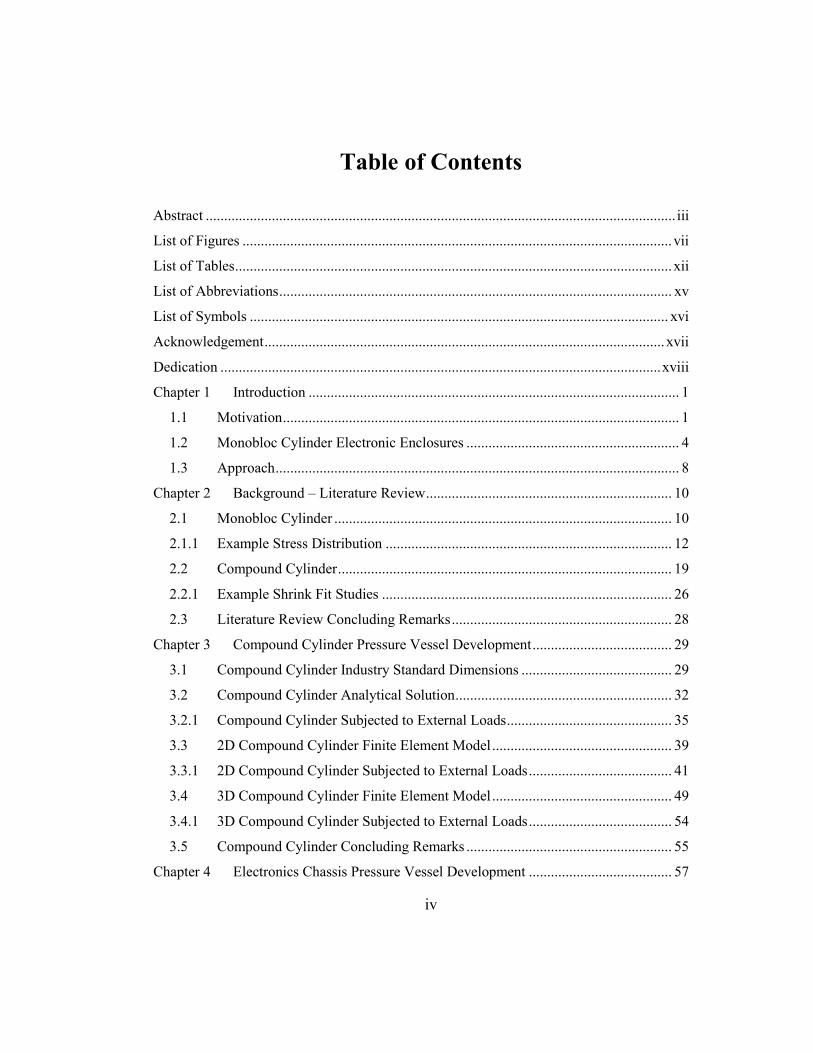
Table of Contents

Abstract ................................................................................................................................ iii

List of Figures ..................................................................................................................... vii

List of Tables ....................................................................................................................... xii

List of Abbreviations ........................................................................................................... xv

List of Symbols .................................................................................................................. xvi

Acknowledgement ............................................................................................................. xvii

Dedication ........................................................................................................................ xviii

Chapter 1 Introduction ..................................................................................................... 1

1.1 Motivation ............................................................................................................ 1

1.2 Monobloc Cylinder Electronic Enclosures .......................................................... 4

1.3 Approach .............................................................................................................. 8

Chapter 2 Background – Literature Review ................................................................... 10

2.1 Monobloc Cylinder ............................................................................................ 10

2.1.1 Example Stress Distribution .............................................................................. 12

2.2 Compound Cylinder ........................................................................................... 19

2.2.1 Example Shrink Fit Studies ............................................................................... 26

2.3 Literature Review Concluding Remarks ............................................................ 28

Chapter 3 Compound Cylinder Pressure Vessel Development ...................................... 29

3.1 Compound Cylinder Industry Standard Dimensions ......................................... 29

3.2 Compound Cylinder Analytical Solution ........................................................... 32

3.2.1 Compound Cylinder Subjected to External Loads ............................................. 35

3.3 2D Compound Cylinder Finite Element Model ................................................. 39

3.3.1 2D Compound Cylinder Subjected to External Loads ....................................... 41

3.4 3D Compound Cylinder Finite Element Model ................................................. 49

3.4.1 3D Compound Cylinder Subjected to External Loads ....................................... 54

3.5 Compound Cylinder Concluding Remarks ........................................................ 55

Chapter 4 Electronics Chassis Pressure Vessel Development ....................................... 57

v

4.1 Electronics Chassis Pressure Vessel Development Process............................... 59

4.2 2D Electronics Chassis Finite Element Model .................................................. 61

4.3 3D Electronics Chassis Finite Element Model .................................................. 66

4.3.1 Stress Distribution Away from Boundary Conditions ....................................... 70

4.3.2 Maximum Stress Value Results ......................................................................... 74

4.3.3 3D Electronics Chassis Deformation Study ....................................................... 79

4.3.3.1 Mid-Length Deformation .............................................................................. 79

4.3.3.2 Shell O-Ring Surface Deformation ............................................................... 81

4.4 3D Electronics Chassis Linear Buckling Analysis ............................................ 83

4.5 3D Electronics Chassis Modal Analysis ............................................................ 92

4.5.1 3D Electronics Chassis 1/8th Symmetry Model Modal Analysis ....................... 93

4.5.2 3D Electronics Chassis Full Model Modal Analysis ......................................... 94

Chapter 5 Manufacturing ............................................................................................... 97

5.1 Shell Manufacturing........................................................................................... 97

5.1.1 Shell Material ..................................................................................................... 97

5.1.2 Shell Machining ................................................................................................. 97

5.2 Insert Manufacturing .......................................................................................... 99

5.2.1 Insert Material .................................................................................................. 100

5.2.2 Insert Machining .............................................................................................. 103

5.3 Chassis Assembly ............................................................................................ 104

Chapter 6 Discussion and Conclusions ........................................................................ 108

6.1 Electronics Chassis Development Discussion ................................................. 108

6.2 Conclusions ...................................................................................................... 111

6.3 Recommendations ............................................................................................ 113

References ......................................................................................................................... 115

Appendix A Standard ANSI Sch 80 Pipe Dimensions ................................................ 117

Appendix B ANSI Standard Force and Shrink Fits ..................................................... 118

Appendix C Compound Cylinder FEA Results ........................................................... 119

Appendix D 3D Compound Cylinder Friction Study .................................................. 125

Appendix E Electronics Chassis FEA Results ............................................................ 129

Appendix F Pathfinder Chassis Analysis .................................................................... 144

vi

Pathfinder Chassis 2D Finite Element Model ............................................................... 145

Pathfinder Chassis 3D Finite Element Model ............................................................... 152

Pathfinder Chassis 3D FEA Deformation Study........................................................... 156

Pathfinder Chassis Mid-Length Deformation ............................................................... 156

Pathfinder Shell O-Ring Surface Deformation ............................................................. 157

vii

List of Figures

Figure 1.1: Closed-End Cylindrical Pressure Vessel. ................................................................ 1

Figure 1.2: Typical In-Water PV Electronics Chassis [1]. ......................................................... 2

Figure 1.3: CCA’s attached to inner wall of monobloc tube. ..................................................... 3

Figure 1.4: 4-CCA Slot Interference-Fit pressure vessel tube assembly. ................................... 4

Figure 1.5. US Patent 4,858,068 for electronic circuit housing [2]. ........................................... 5

Figure 1.6. US Patent 6,404,637 B2 for telecommunications equipment enclosure [3]. ........... 6

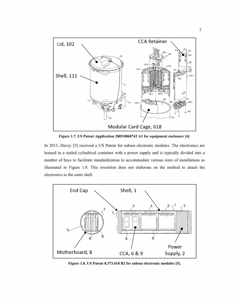
Figure 1.7. US Patent Application 2005/0068743 A1 for equipment enclosure [4]. ................. 7

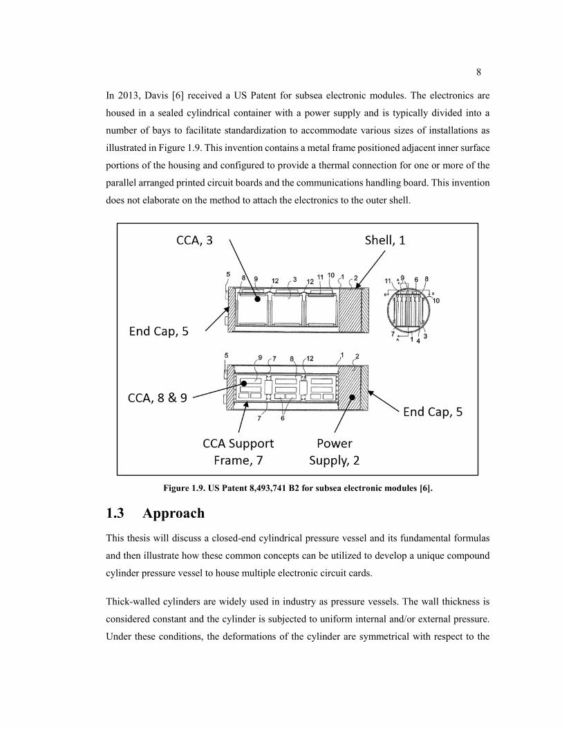
Figure 1.8. US Patent 8,373,418 B2 for subsea electronic modules [5]. .................................... 7

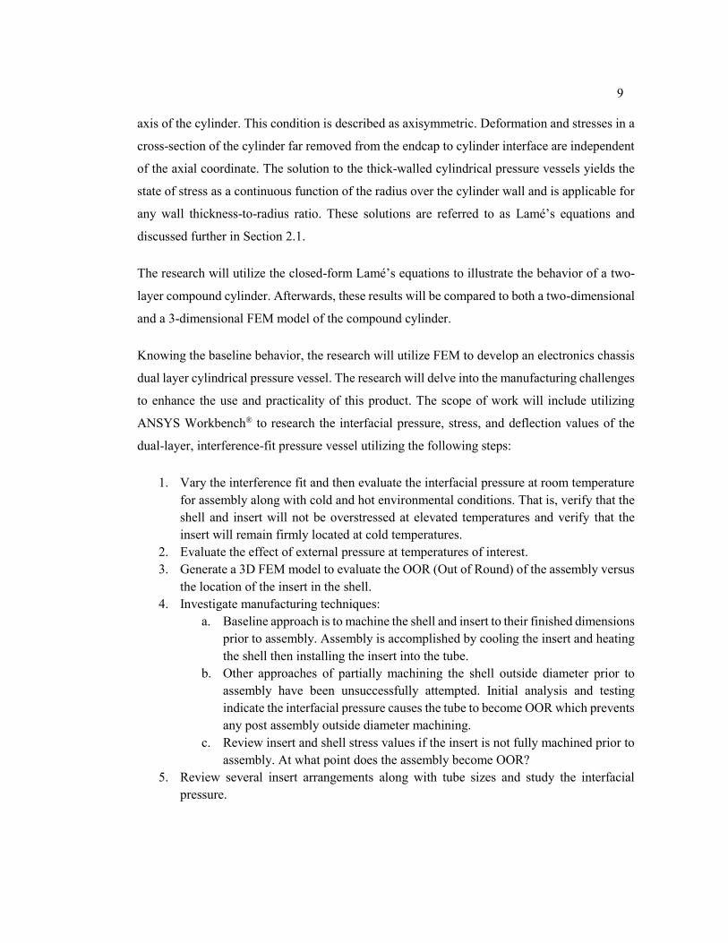
Figure 1.9. US Patent 8,493,741 B2 for subsea electronic modules [6]. .................................... 8

Figure 2.1. Thick-walled cylinder subjected to both uniform internal and external pressure. . 11

Figure 2.2: Stress distribution through a thick-walled cylinder – Internal Pressure Only. ...... 12

Figure 2.3: Stress distribution through a thick-walled cylinder - External Pressure Only. ...... 13

Figure 2.4. Monobloc cylinder failure plots for 300 series stainless steel. .............................. 15

Figure 2.5. Diagram of simply supported endcap. ................................................................... 16

Figure 2.6. Flat end cap failure plot for 300 series stainless steel. ........................................... 17

Figure 2.7. Critical buckling pressure for thin-walled tube. ..................................................... 18

Figure 2.8. Critical buckling pressure for a 0.065 wall stainless steel tube. ............................ 18

Figure 2.9: Two-Layer, Interference-Fit compound cylinder................................................... 20

Figure 2.10. Arrangement for induction heating of disk and shaft [17]. .................................. 26

Figure 2.11. FEA model of shrink fit interface joint [18]. ....................................................... 27

Figure 3.1. Interfacial pressure for ANSI Standard Force and Shrink Fits. ............................. 32

Figure 3.2. Compound cylinder change in interference diameter vs. temperature. .................. 32

Figure 3.3. Compound cylinder interfacial pressure illustration []. ......................................... 34

Figure 3.4. CREO® model of two-layer compound cylinder. .................................................. 39

Figure 3.5. ANSYS Workbench® ¼ symmetry 2D model of two-layer compound. ................ 40

Figure 3.6. 316 Stainless Steel Monobloc Cylinder Failure Modes ......................................... 43

Figure 3.7. Titanium Grade CP 2 Monobloc Cylinder Failure Modes ..................................... 43

Figure 3.8. Aluminum Alloy 6061-T6 Monobloc Cylinder Failure Modes ............................. 43

viii

Figure 3.9. Minimum wall thickness for an 8-inch diameter monobloc cylinder exposed to

hydrostatic pressure in accordance with Equation (2.13). ............................................... 44

Figure 3.10. Case 4: ANSYS Workbench® Pressure load analysis Step 2. .............................. 45

Figure 3.11. Case 4: ANSYS Workbench® Temperature load analysis Step 3. ....................... 45

Figure 3.12. Case 4: Interfacial pressure and equivalent stress plots. ...................................... 45

Figure 3.13. Workbench® 1/8 symmetry 3D model of two-layer compound cylinder. ............ 50

Figure 3.14. 3D ¼ symmetry analysis interfacial pressure plot for 10 mils diametrical

interference. ..................................................................................................................... 51

Figure 3.15. 3D compound cylinder ¼ symmetry analysis Shell hoop stress plot at ro for 10

mils diametrical interference. .......................................................................................... 51

Figure 3.16. 3D compound cylinder ¼ symmetry analysis Insert hoop stress plot at ro for 10

mils diametrical interference. .......................................................................................... 52

Figure 3.17. 3D compound cylinder ¼ symmetry analysis Shell axial stress plot for 10 mils

diametrical interference. .................................................................................................. 52

Figure 3.18. 3D compound cylinder ¼ symmetry analysis Insert axial stress plot for 10 mils

diametrical interference. .................................................................................................. 52

Figure 4.1. CREO® model of electronics chassis dual-layer cylinder. ..................................... 57

Figure 4.2. Overall dimensions of the electronics chassis pressure vessel cylinder. ............... 58

Figure 4.3. Mid-length cross-section of the electronics chassis pressure vessel cylinder. ....... 58

Figure 4.4. Electronics chassis pressure vessel development flow diagram. ........................... 60

Figure 4.5. ANSYS Workbench® 2D plane stress ¼ symmetry model geometry and mesh. .. 62

Figure 4.6. 2D Case 1, plane stress analysis interfacial contact pressure. ................................ 62

Figure 4.7. 2D Case 1, plane stress analysis Shell and Insert equivalent stress plots. ............. 63

Figure 4.8. 2D Case 1, Stress concentration at upper CCA slot location. ................................ 63

Figure 4.9. Case 1, 2D plane stress analysis Shell radial deformation. .................................... 64

Figure 4.10. Case 1, 2D plane stress analysis CCA slot radial deformation. ........................... 64

Figure 4.11. Examples of dished head end caps [21]. .............................................................. 67

Figure 4.12. Examples of flat head end caps [21]. ................................................................... 67

Figure 4.13. Electronics chassis flat end cap. ........................................................................... 67

Figure 4.14. Compound cylinder electronics chassis with end caps. ....................................... 68

Figure 4.15. Cross-section of Compound cylinder electronics chassis with end caps. ............ 68

ix

Figure 4.16. End cap to shell interface detail (O-rings are omitted for clarity). ...................... 68

Figure 4.17. Electronics Chassis ANSYS Workbench® 3D 1/4 symmetry model geometry. . 69

Figure 4.18. 3D 1/8th symmetry model parts A and B. ............................................................. 69

Figure 4.19. Case 1, Electronics Chassis 3D 1/8th symmetry model geometry Part A. ........... 70

Figure 4.20. Case 1, Electronics Chassis 3D 1/8th symmetry model geometry Part B. ............ 70

Figure 4.21. Case 1, 3D 1/8 symmetry analysis interfacial segment 2 pressure plots.............. 71

Figure 4.22. Case 1, 3D 1/8 symmetry analysis Shell segment 2 equivalent stress plots. ....... 71

Figure 4.23. Case 1, 3D 1/8 symmetry analysis Insert equivalent segment 2 stress plots. ...... 71

Figure 4.24. Case 1, 3D 1/8 symmetry analysis interfacial pressure plots. .............................. 74

Figure 4.25. Case 1, 3D 1/8 symmetry analysis Shell equivalent stress plots. ......................... 74

Figure 4.26. Case 1, 3D 1/8 symmetry analysis Insert equivalent stress plots. ........................ 75

Figure 4.27. Case 1, Insert Part A maximum equivalent stress location. ................................. 78

Figure 4.28. Case 1, Shell Parts A & B equivalent stress plots. ............................................... 78

Figure 4.29. Circularity or Out-Of-Round (OOR) definition. .................................................. 79

Figure 4.30. Case 1, 3D analysis radial deformation at the mid-length of the shell................. 81

Figure 4.31. Case 2, 3 and 4: 3D electronics chassis with end cap 1/8 symmetry FEA model.81

Figure 4.32. Case 1, 3D analysis radial deformation of the O-ring surface. ............................ 82

Figure 4.33. 2205 Duplex stainless steel monobloc cylinder failure mode plot. ..................... 84

Figure 4.34. Critical buckling pressure for thin-walled 2205 duplex stainless tube. ............... 85

Figure 4.35. Electronics Chassis 1/8 symmetry Part A model Eigenvalue Buckling results. .. 86

Figure 4.36. Shell Only 1/8 symmetry model Eigenvalue Buckling mode 1 plot. ................... 87

Figure 4.37. E-Chassis Part-A Shell Segment 2 axial and equivalent stress values at buckling

pressure of 955.6 psi. ....................................................................................................... 89

Figure 4.38. E-Chassis Part-A Shell axial and equivalent stress values at buckling pressure of

955.6 psi. .......................................................................................................................... 90

Figure 4.39. Four-Slot Electronics Chassis assembly. ............................................................. 92

Figure 4.40. ANSYS Workbench FEA model utilized for modal analysis. ............................. 93

Figure 4.41. ANSYS Workbench FEA model utilized for modal analysis. ............................. 95

Figure 4.42. Image of mode shape 1, 351 Hz, for an open-ended electronics chassis. ............ 95

Figure 4.43. Image of mode shape 11, 1,514 Hz, for an open-ended electronics chassis. ....... 96

Figure 5.1. Shell pre-Insert assembly fabrication drawing. ...................................................... 98

x

Figure 5.2. Shell fabrication open-end detail. .......................................................................... 99

Figure 5.3. Shell fabrication End Cap mounting holes clocking detail. ................................... 99

Figure 5.4. Illustration of transverse direction tensile test coupons. ...................................... 101

Figure 5.5. Porosity in 7075-T6 Insert. .................................................................................. 102

Figure 5.6. Case 1 and Case 3 Insert cross-section pre-assembly dimensions (10 mil

interference). .................................................................................................................. 104

Figure 5.7. Insert radial deformation at temperature of -320°F. ............................................ 105

Figure 5.8. Shell radial deformation at temperature of +450°F. ............................................ 106

Figure 5.9. Shell radial deformation at temperature of +450°F. ............................................ 106

Figure 5.10. E-Chassis post assembly machining details. ...................................................... 107

Figure 5.11. E-Chassis post assembly O-ring surface machining details. .............................. 107

Figure C-1. Case 1, 3D cpd cylinder ¼ symmetry analysis Insert axial stress plot. .............. 121

Figure C-2. Case 1, 3D cpd cylinder ¼ symmetry analysis Shell radial stress plot at ri. ....... 121

Figure C-3. Case 1, 3D cpd cylinder ¼ symmetry analysis Insert radial stress plot at ro. ...... 121

Figure C-4. Case 1, 3D cpd cylinder ¼ symmetry analysis Shell axial deformation plot. ..... 122

Figure C-5. Case 1, 3D cpd cylinder ¼ symmetry analysis Insert axial deformation plot. .... 122

Figure C-6. Case 1, 3D cpd cylinder ¼ symmetry analysis Shell equivalent stress plot. ...... 122

Figure C-7. Case 1, 3D cpd cylinder ¼ symmetry analysis Insert equivalent stress plot....... 123

Figure D-1. Interfacial pressure for cpd cylinder with 0.30 friction coefficient. ................... 126

Figure D-2. Axial stress plot of cpd cylinder Shell with 0.30 friction coefficient. ................ 126

Figure D-3. Axial stress plot of cpd cylinder Insert with 0.30 friction coefficient. ............... 127

Figure D-4. Interfacial pressure for cpd cylinder with 0.0001 friction coefficient. ............... 127

Figure D-5. Axial stress plot of cpd cylinder Shell with 0.0001 friction coefficient. ............ 128

Figure D-6. Axial stress plot of cpd cylinder Insert with 0.0001 friction coefficient. ........... 128

Figure E-1. Case 1, 3D E-Chassis 1/8 symmetry analysis Shell Part A hoop stress plot. ...... 134

Figure E-2. Case 1, 3D E-Chassis 1/8 symmetry analysis Shell Part A radial stress plot. ..... 135

Figure E-3. Case 1, 3D E-Chassis 1/8 symmetry analysis Shell Part A axial stress plot. ...... 135

Figure E-4. Case 1, 3D E-Chassis 1/8 symmetry analysis Shell Part A equivalent stress plot.

....................................................................................................................................... 135

Figure E-5. Case 1, 3D E-Chassis 1/8 symmetry analysis Insert Part A hoop stress plot. ..... 136

Figure E-6. Case 1, 3D E-Chassis 1/8 symmetry analysis Insert Part A radial stress plot. .... 136

xi

Figure E-7. Case 1, 3D E-Chassis analysis Insert Part A axial stress plot. ............................ 137

Figure E-8. Case 1, 3D E-Chassis analysis Insert Part A equivalent stress plot. ................... 137

Figure E-9. Case 1, 3D E-Chassis 1/8 symmetry analysis Shell Part B hoop stress plot. ...... 139

Figure E-10. Case 1, 3D E-Chassis 1/8 symmetry analysis Shell Part B radial stress plot. ... 140

Figure E-11. Case 1, 3D E-Chassis 1/8 symmetry analysis Shell Part B axial stress plot. .... 140

Figure E-12. Case 1, 3D E-Chassis 1/8 symmetry analysis Shell Part B equivalent stress plot.

....................................................................................................................................... 141

Figure E-13. Case 1, 3D E-Chassis 1/8 symmetry analysis Insert Part B hoop stress plot. ... 141

Figure E-14. Case 1, 3D E-Chassis 1/8 symmetry analysis Insert Part B radial stress plot. .. 142

Figure E-15. Case 1, 3D E-Chassis analysis Insert Part B axial stress plot. .......................... 142

Figure E-16. Case 1, 3D E-Chassis analysis Insert Part B equivalent stress plot. ................. 143

Figure F-1. CREO® model of Pathfinder electronics chassis. ................................................ 144

Figure F-2. Overall dimensions of the Pathfinder electronics chassis. .................................. 145

Figure F-3. Mid-length cross-section of the Pathfinder electronics chassis. .......................... 145

Figure F-4. Pathfinder 2D plane stress ¼ symmetry model geometry and mesh. .................. 147

Figure F-5. Pathfinder 2D Case 1, plane stress analysis interfacial contact pressure. ........... 148

Figure F-6. Pathfinder 2D Case 1, plane stress analysis Shell and Insert equivalent stress plots.

....................................................................................................................................... 148

Figure F-7. Pathfinder 2D Case 1, Stress concentration at upper CCA slot location. ............ 149

Figure F-8. Pathfinder Case 1, 2D plane stress analysis Shell radial deformation. ................ 149

Figure F-9. Pathfinder Case 1, 2D plane stress analysis CCA slot radial deformation. ......... 150

Figure F-10. Pathfinder Case 1, 3D 1/8 symmetry analysis interfacial pressure plots. .......... 152

Figure F-11. Pathfinder Case 1, 3D 1/8 symmetry analysis Shell equivalent stress plots. .... 153

Figure F-12. Case 1, 3D 1/8 symmetry analysis Insert equivalent stress plots. ..................... 153

Figure F-13. Case 1, Pathfinder Part A radial deformation at the mid-length of the shell. .... 157

Figure F-14. Case 2, 3 and 4: Pathfinder chassis with end cap 1/8 symmetry FEA model. ... 158

Figure F-15. Case 1, Pathfinder Part A radial deformation of the O-ring surface. ................ 159

xii

List of Tables

Table 1.1: Thermal conductivity of various metals. ................................................................... 3

Table 2.1. Two-layer compound cylinder dimensions and material properties. ...................... 21

Table 2.2. Comparison of interfacial pressure expression results. ........................................... 21

Table 2.3. Mechanical characteristics based on surface process. ............................................. 28

Table 3.1. Dimensions of 8-inch S80 stainless steel pipe. ....................................................... 30

Table 3.2. ANSI Standard Force and Shrink Fits. .................................................................... 31

Table 3.3. Example Two-layer compound cylinder dimensions and material properties. ....... 33

Table 3.4. Assembly residual stress analytical solutions of a two-layer closed-end compound

cylinder. ........................................................................................................................... 35

Table 3.5. Two-Layer compound cylinder load cases. ............................................................. 36

Table 3.6. Saltwater water column vs. pressure table1. ............................................................ 36

Table 3.7. Two-layer compound cylinder Case Study 4 analytical results. ............................. 38

Table 3.8. Two-layer compound cylinder dimensions and material properties. ...................... 39

Table 3.9: 2D FEM model Contact Pressure comparison. ....................................................... 40

Table 3.10: Assembly residual stress results of a 2D FEM Plane Stress Model Comparison to

the Analytical Solutions. .................................................................................................. 41

Table 3.11. Comparison of ANSI Shrink Fit results for nominal 8-inch compound cylinder. 42

Table 3.12. Two-Layer compound cylinder load cases. ........................................................... 42

Table 3.13. Margin Factors of Safety and Configuration Factors. ........................................... 46

Table 3.14. Design mechanical properties for 316 stainless steel and 6061-T651 aluminum

[25]................................................................................................................................... 47

Table 3.15. Mechanical properties for a two-layer compound cylinder. .................................. 48

Table 3.16. Summary of 316/6061 two-layer compound cylinder 2D case study, 0.065 shell. 48

Table 3.17. Margin summary of 316/6061 2D case study, 0.105 shell. ................................... 49

Table 3.18. Margin summary of 2205/6061 2D case study, 0.065 shell. ................................. 49

Table 3.19. Final dimensions and material selection from a 2D Plane Stress FEA case study of

a two-layer compound cylinder ....................................................................................... 49

Table 3.20: 3D FEM Compound Cylinder Model Comparison to Analytical Solution. .......... 50

xiii

Table 3.21. 3D open-end compound cylinder friction factor study (10 mil interference)........ 53

Table 3.22. Summary of 2205/6061 two-layer compound cylinder 3D case study. ................ 54

Table 3.23. Comparison of percent difference for 2D and 3D analysis results for compound

cylinder case study. .......................................................................................................... 55

Table 4.1. Two-Layer electronics chassis pressure vessel load cases. ..................................... 61

Table 4.2. Two-layer electronics chassis pressure vessel dimensions and materials. .............. 61

Table 4.3. Mechanical properties for two-layer electronics chassis pressure vessel. ............... 61

Table 4.4. Summary of 2205/6061 two-layer electronics chassis 2D analysis. ....................... 65

Table 4.5. Revised margin summary for 2D plane stress analysis upgrading to 7075-T651

insert. ............................................................................................................................... 65

Table 4.6. Percent difference 2D Compound Cylinder to the 2D Electronics Chassis. ........... 66

Table 4.7. Two-Layer electronics chassis pressure vessel load cases for 3D FEA. ................. 66

Table 4.8. 3D Compound Cylinder Electronics Chassis Part A segment 2 case study stress

results. .............................................................................................................................. 72

Table 4.9. 3D Compound Cylinder Electronics Chassis Part B segment 2 margin results. ..... 73

Table 4.10. Comparison of 3D Electronics Chassis Part A & B segment 2 case study results. 73

Table 4.11. 3D Electronics Chassis Part A 2205/7075 full model results. ............................... 75

Table 4.12. 3D Electronics Chassis 2205/7075 Part B full model results. ............................... 76

Table 4.13. Percent Difference Results Part A: Segment 2 to Non-segmented model. ........... 77

Table 4.14. Percent Difference Results Part B: Segment 2 to Non-segmented model. ............ 77

Table 4.15. Electronics Chassis mid-length deformation comparison. .................................... 80

Table 4.16. Electronics Chassis O-ring surface deformation comparison. .............................. 82

Table 4.17: Electronics Chassis Eigenvalue Buckling load multiplier. ................................... 86

Table 4.18: Electronics Chassis less Insert Eigenvalue Buckling load multiplier. .................. 87

Table 4.19. Monobloc Cylinder Failure Comparison of Under Pressure® to Workbench®. .... 88

Table 4.20. Under Pressure® Cylinder Comparison to Workbench® E-Chassis. ................... 91

Table 4.21. Two-Layer electronics chassis pressure vessel modal analysis case studies. ....... 93

Table 4.22. First six fundamental frequencies of E-Chassis Parts A and B using 1/8th

symmetry models. ............................................................................................................ 94

Table 4.23. First fourteen fundamental frequencies of the Electronics Chassis full model. .... 95

xiv

Table 5.1. Design mechanical properties for aluminum alloy extruded rod, bar and shapes

[25]................................................................................................................................. 100

Table 5.2. Design mechanical properties for aluminum alloy rolled, drawn or cold-finished

rod, bar and shapes [25]. ................................................................................................ 101

Table 5.3. Aluminum Alloy 7075-T6 tensile test results. ...................................................... 102

Table 5.4. Nominal 8-inch diameter Insert mechanical properties......................................... 102

Table 6.1. Margin Summary: 3D Compound Cylinder through 3D E-Chassis. ..................... 110

Table C-1. 316/6061 two-layer cpd cylinder 2D case study results. ...................................... 119

Table C-2. 2205/6061 cpd cylinder 3D FEA case study results. ............................................ 120

Table C-3. Summary of analytical, 2D and 3D FEA results for a cpd cylinder case study. .. 124

Table E-1. 2205/6061 Electronics Chassis 2D Plane Stress Results ...................................... 129

Table E-2. Comparison of 2D plane stress Compound Cylinder to Electronics Chassis. ...... 130

Table E-3. Case 1, 3D E-Chassis Parts A & B Segment 2 results comparison. ..................... 131

Table E-4. Case 1, 3D E-Chassis Parts A & B segment 2 results comparison con’t. ............ 132

Table E-5. Case 1, 3D E-Chassis Parts A all segments results comparison. .......................... 133

Table E-6. Case 1, 3D E-Chassis Parts A all segments results comparison con’t. ................. 134

Table E-7. Case 1, 3D E-Chassis Part B all segments results comparison. ............................ 138

Table E-8. Case 1, 3D E-Chassis Part B all segments results comparison con’t. .................. 139

Table F-1. Pathfinder electronics chassis pressure vessel load cases. .................................... 146

Table F-2. Mechanical properties for the Pathfinder electronics chassis pressure vessel. ..... 146

Table F-3. Summary of Pathfinder electronics chassis 2D analysis....................................... 151

Table F-4. Two-Layer electronics chassis pressure vessel load cases for 3D FEA. .............. 152

Table F-5. Pathfinder 3D Electronics Chassis Part A results. ................................................ 154

Table F-6. Pathfinder 3D Electronics Chassis Part B results. ................................................ 155

Table F-7. Pathfinder Chassis mid-length deformation comparison. ..................................... 156

Table F-8. Pathfinder chassis O-ring deformation comparison. ............................................. 158

xv

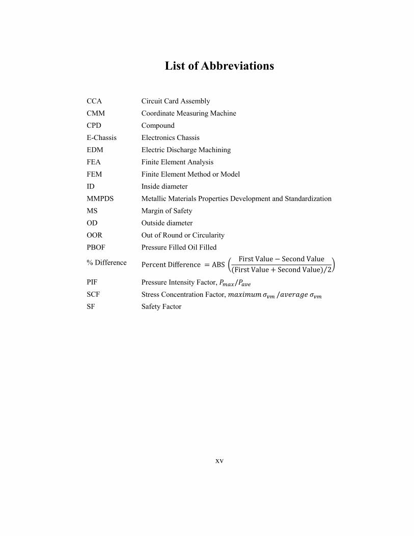
List of Abbreviations

CCA Circuit Card Assembly

CMM Coordinate Measuring Machine

CPD Compound

E-Chassis Electronics Chassis

EDM Electric Discharge Machining

FEA Finite Element Analysis

FEM Finite Element Method or Model

ID Inside diameter

MMPDS Metallic Materials Properties Development and Standardization

MS Margin of Safety

OD Outside diameter

OOR Out of Round or Circularity

PBOF Pressure Filled Oil Filled

% Difference Percent Difference = ABS (First Value − Second Value

(First Value + Second Value) 2⁄)

PIF Pressure Intensity Factor, 𝑃𝑚𝑎𝑥/𝑃𝑎𝑣𝑒

SCF Stress Concentration Factor, 𝑚𝑎𝑥𝑖𝑚𝑢𝑚𝜎𝑣𝑚 /𝑎𝑣𝑒𝑟𝑎𝑔𝑒 𝜎𝑣𝑚

SF Safety Factor

xvi

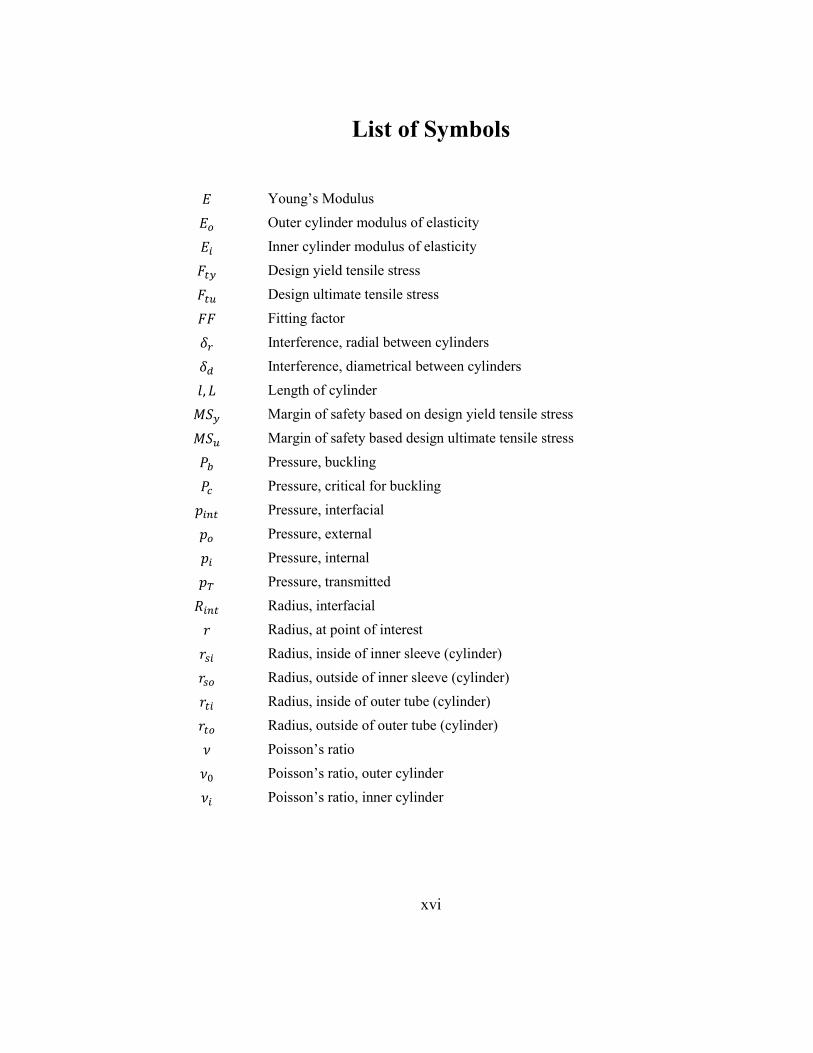
List of Symbols

𝐸 Young’s Modulus

𝐸𝑜 Outer cylinder modulus of elasticity

𝐸𝑖 Inner cylinder modulus of elasticity

𝐹𝑡𝑦 Design yield tensile stress

𝐹𝑡𝑢 Design ultimate tensile stress

𝐹𝐹 Fitting factor

𝛿𝑟 Interference, radial between cylinders

𝛿𝑑 Interference, diametrical between cylinders

𝑙, 𝐿 Length of cylinder

𝑀𝑆𝑦 Margin of safety based on design yield tensile stress

𝑀𝑆𝑢 Margin of safety based design ultimate tensile stress

𝑃𝑏 Pressure, buckling

𝑃𝑐 Pressure, critical for buckling

𝑝𝑖𝑛𝑡 Pressure, interfacial

𝑝𝑜 Pressure, external

𝑝𝑖 Pressure, internal

𝑝𝑇 Pressure, transmitted

𝑅𝑖𝑛𝑡 Radius, interfacial

𝑟 Radius, at point of interest

𝑟𝑠𝑖 Radius, inside of inner sleeve (cylinder)

𝑟𝑠𝑜 Radius, outside of inner sleeve (cylinder)

𝑟𝑡𝑖 Radius, inside of outer tube (cylinder)

𝑟𝑡𝑜 Radius, outside of outer tube (cylinder)

𝜈 Poisson’s ratio

𝜈0 Poisson’s ratio, outer cylinder

𝜈𝑖 Poisson’s ratio, inner cylinder

xvii

Acknowledgement

I would like to thank my advisor, Dr. David Fleming for his encouragement and guidance

throughout my academic career at the Florida Institute of Technology and this thesis. I also

would like to thank Dr. Razvan Rusovici, Dr. Shengyuan Yang and Dr. Ronnal Reichard for

serving on my Master’s thesis committee and providing valued insightful feedback. Finally, I

would also like to thank my employer for investing in my education and providing challenging

design tasks.

Remember:

There are no constraints on the human mind, no walls around the human spirit,

no barriers to our progress except those we ourselves erect.

President Ronald Reagan

xviii

Dedication

This thesis is dedicated first to my wife Sylvia, whose support, patience and understanding

during this endeavor have been unyielding. The thesis is also dedicated to my mother for her

lifelong encouragement in all matters. Finally, this work is dedicated to my friend and mentor

Mark D. Driscoll whose inspiration started me on this path so many years ago.

1

Chapter 1

Introduction

1.1 Motivation

The motivation of this thesis is to develop an enclosure for electronics equipment subjected to

different levels of external hydrostatic pressure along with varying external temperatures. The

enclosure will also be subjected to both fresh water and seawater environments along with

varying corrosive and thermal conductivity environments. Two additional design criteria are to

minimize the weight and maximize the thermal capacity of the enclosure. To ensure

manufacturability, the enclosure design should utilize commercially available materials and

fabrication standards.

A common approach for packaging electronics subjected to external hydrostatic pressure is to

house the components in a pressure vessel. The pressure vessel housings can be spherical,

cylindrical or even rectangular if a pressure balanced oil-filled (PBOF) approach is used. One

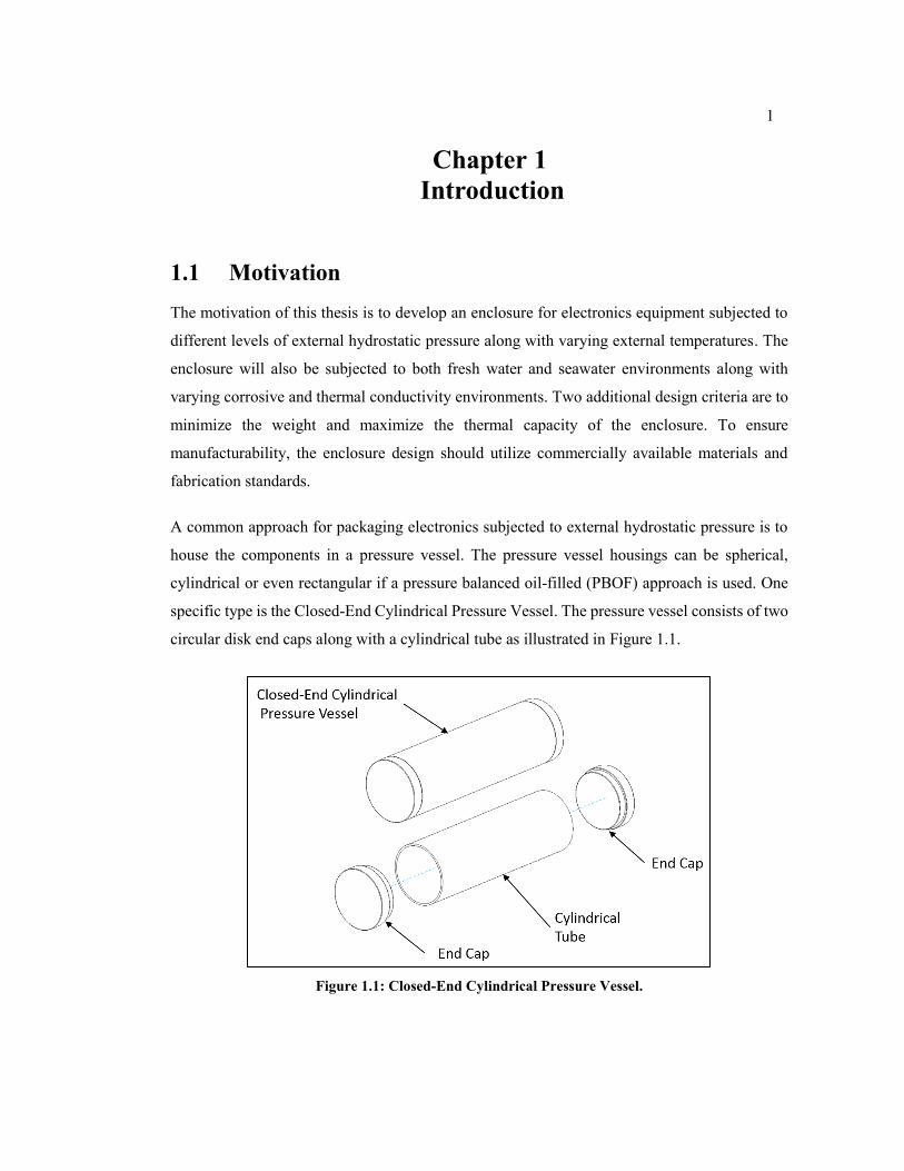
specific type is the Closed-End Cylindrical Pressure Vessel. The pressure vessel consists of two

circular disk end caps along with a cylindrical tube as illustrated in Figure 1.1.

Figure 1.1: Closed-End Cylindrical Pressure Vessel.

2

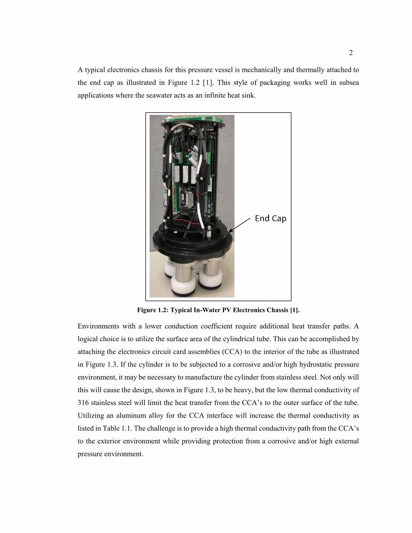
A typical electronics chassis for this pressure vessel is mechanically and thermally attached to

the end cap as illustrated in Figure 1.2 [1]. This style of packaging works well in subsea

applications where the seawater acts as an infinite heat sink.

Figure 1.2: Typical In-Water PV Electronics Chassis [1].

Environments with a lower conduction coefficient require additional heat transfer paths. A

logical choice is to utilize the surface area of the cylindrical tube. This can be accomplished by

attaching the electronics circuit card assemblies (CCA) to the interior of the tube as illustrated

in Figure 1.3. If the cylinder is to be subjected to a corrosive and/or high hydrostatic pressure

environment, it may be necessary to manufacture the cylinder from stainless steel. Not only will

this will cause the design, shown in Figure 1.3, to be heavy, but the low thermal conductivity of

316 stainless steel will limit the heat transfer from the CCA’s to the outer surface of the tube.

Utilizing an aluminum alloy for the CCA interface will increase the thermal conductivity as

listed in Table 1.1. The challenge is to provide a high thermal conductivity path from the CCA’s

to the exterior environment while providing protection from a corrosive and/or high external

pressure environment.

3

Figure 1.3: CCA’s attached to inner wall of monobloc tube.

Table 1.1: Thermal conductivity of various metals.

Material Thermal Conductivity

6061-T6 Aluminum 167.0 W/m-K

7075-T6 Aluminum 130.0 W/m-K

Grade 2 Titanium 16.4 W/m-K

316 Stainless Steel 16.3 W/m-K

2205 Duplex Stainless Steel 15.0 W/m-K

Grade 5 Titanium 6.7 W/m-K

The challenge can be met by utilizing a tube fabricated in two parts. The outer shell will be

made from a corrosion resistant steel while the inner insert will be made from a high thermal

conductivity aluminum alloy. The two components will be mechanically and thermally joined

using shrink-fit methods. The assembled interference-fit chassis will provide a longitudinal heat

transfer path from the rails of the insert to the perimeter of the outer shell instead of only to the

end cap. This approach gives the interference-fit pressure vessel a higher thermal load capacity

in both seawater and lower thermal conductivity environments. Figure 1.4 illustrates a four

circuit card chassis assembly.

4

Figure 1.4: 4-CCA Slot Interference-Fit pressure vessel tube assembly.

Even though one of the primary motivations for this pressure vessel is improving the heat

transfer capacity, the focus of this thesis is the mechanical design and manufacturing of the

pressure vessel with emphasis on the aspects of the interference fit.

1.2 Monobloc Cylinder Electronic Enclosures

This section introduces existing designs for subsea electronic equipment housings utilizing

monobloc cylindrical outer shells. The types of the inner sleeve and methods of attaching the

electronics to the housing shell vary from design to design. None of these assemblies utilize an

interference-fit inner sleeve.

In 1989, Bitller et al. [2] received a US Patent for an electronic circuit housing applicable to

undersea transmission-line repeater equipment. The housing consists of a cylindrical steel shell

provided with watertight end walls and a cylindrical assembly of frames to house the electronics

as shown in Figure 1.5. The cylindrical sector frames are fastened to the outer shell by a flange,

which is integral with the inner wall of the outer shell. The frames are attached to this flange at

one end and by an expandable collar at the opposite end. The frame is locked in position by

expansion within the shell. A low thermal resistance intercalary sleeve is placed between the

5

frames and the internal wall of the outer shell to provide good thermal conductivity and to absorb

elastic deformations of the outer shell produced by the high-pressure sea-bottom environment.

Figure 1.5. US Patent 4,858,068 for electronic circuit housing [2].

In 2002, Hutchison et al. [3] received a US Patent for a telecommunications equipment

enclosure that dissipates internally generated heat into the ambient environment. The cylindrical

enclosure utilized removable sleeves located concentrically about the interior and externally

mounted cooling fins as illustrated in Figure 1.6. Electronic cards generate heat that is

conducted to the removable sleeve. The sleeve transfers heat along two thermally conductive

heat pathways. Along the first pathway, heat is transferred from the removable sleeve portion

to the housing, through the housing wall and then to the fins where it is dissipated into the

ambient environment. Along a second pathway, heat is transferred from an inner sleeve portion

to a leaf spring and then to the cylindrical lid where it is dissipated into the ambient environment.

The sleeves are held against the interior of the housing by a circular spring assembly. The

springs function to bias the sleeves against the interior wall of the housing to improve

conduction of heat to the housing wall.

6

Figure 1.6. US Patent 6,404,637 B2 for telecommunications equipment enclosure [3].

In 2005, Ferris [4] et al. submitted a US Patent Application for heat dissipation in an electronics

enclosure. The enclosure includes a cylindrical body and one or more modular card cages

adapted to receive one or more electronic circuit cards as illustrated in Figure 1.7. The modular

card cages are in direct physical and thermal contact with the inner wall of the cylindrical body.

The detailed description includes a plethora of various embodiments of the invention. In one

particular embodiment, the cylindrical body encases up to four card cages with each card cage

being molded or extruded from a thermally conductive material such as aluminum. In alternate

embodiments, the card cage may be a single structure or multiple structures for form a

cylindrical shape. The enclosures include a spacer that attaches to each card cage to aid in

keeping the card cage in direct contact with the enclosure inner wall. In another embodiment,

each modular card cage is identical and they fit together to form a hollow cylindrical cage. In

one embodiment, the cylindrical body is made of a substantially thermally conductive material

and in another embodiment; the material is also substantially non-corrosive such as stainless

steel.

7

Figure 1.7. US Patent Application 2005/0068743 A1 for equipment enclosure [4].

In 2013, Davey [5] received a US Patent for subsea electronic modules. The electronics are

housed in a sealed cylindrical container with a power supply and is typically divided into a

number of bays to facilitate standardization to accommodate various sizes of installations as

illustrated in Figure 1.8. This invention does not elaborate on the method to attach the

electronics to the outer shell.

Figure 1.8. US Patent 8,373,418 B2 for subsea electronic modules [5].

8

In 2013, Davis [6] received a US Patent for subsea electronic modules. The electronics are

housed in a sealed cylindrical container with a power supply and is typically divided into a

number of bays to facilitate standardization to accommodate various sizes of installations as

illustrated in Figure 1.9. This invention contains a metal frame positioned adjacent inner surface

portions of the housing and configured to provide a thermal connection for one or more of the

parallel arranged printed circuit boards and the communications handling board. This invention

does not elaborate on the method to attach the electronics to the outer shell.

Figure 1.9. US Patent 8,493,741 B2 for subsea electronic modules [6].

1.3 Approach

This thesis will discuss a closed-end cylindrical pressure vessel and its fundamental formulas

and then illustrate how these common concepts can be utilized to develop a unique compound

cylinder pressure vessel to house multiple electronic circuit cards.

Thick-walled cylinders are widely used in industry as pressure vessels. The wall thickness is

considered constant and the cylinder is subjected to uniform internal and/or external pressure.

Under these conditions, the deformations of the cylinder are symmetrical with respect to the

9

axis of the cylinder. This condition is described as axisymmetric. Deformation and stresses in a

cross-section of the cylinder far removed from the endcap to cylinder interface are independent

of the axial coordinate. The solution to the thick-walled cylindrical pressure vessels yields the

state of stress as a continuous function of the radius over the cylinder wall and is applicable for

any wall thickness-to-radius ratio. These solutions are referred to as Lamé’s equations and

discussed further in Section 2.1.

The research will utilize the closed-form Lamé’s equations to illustrate the behavior of a two-

layer compound cylinder. Afterwards, these results will be compared to both a two-dimensional

and a 3-dimensional FEM model of the compound cylinder.

Knowing the baseline behavior, the research will utilize FEM to develop an electronics chassis

dual layer cylindrical pressure vessel. The research will delve into the manufacturing challenges

to enhance the use and practicality of this product. The scope of work will include utilizing

ANSYS Workbench® to research the interfacial pressure, stress, and deflection values of the

dual-layer, interference-fit pressure vessel utilizing the following steps:

1. Vary the interference fit and then evaluate the interfacial pressure at room temperature

for assembly along with cold and hot environmental conditions. That is, verify that the

shell and insert will not be overstressed at elevated temperatures and verify that the

insert will remain firmly located at cold temperatures.

2. Evaluate the effect of external pressure at temperatures of interest.

3. Generate a 3D FEM model to evaluate the OOR (Out of Round) of the assembly versus

the location of the insert in the shell.

4. Investigate manufacturing techniques:

a. Baseline approach is to machine the shell and insert to their finished dimensions

prior to assembly. Assembly is accomplished by cooling the insert and heating

the shell then installing the insert into the tube.

b. Other approaches of partially machining the shell outside diameter prior to

assembly have been unsuccessfully attempted. Initial analysis and testing

indicate the interfacial pressure causes the tube to become OOR which prevents

any post assembly outside diameter machining.

c. Review insert and shell stress values if the insert is not fully machined prior to

assembly. At what point does the assembly become OOR?

5. Review several insert arrangements along with tube sizes and study the interfacial

pressure.

10

Chapter 2

Background – Literature Review

This literature review will discuss the theory of thin-walled and thick-walled monobloc

cylinders and the application to cylindrical pressure vessels. Examples will be given to illustrate

the stress distribution in the thick-walled cylinder. Next, the theory of compound or multi-layer

cylinders will be discussed. Finally, a review of shrink-fit applications and studies utilizing these

theories will be reviewed.

2.1 Monobloc Cylinder

The simplest pressure vessel is a thin-walled monobloc cylinder. Mechanics of Materials

develops the approximate state of stress solution to this fundamental theory as an average value

over the cylinder wall thickness and thin-walled pressure vessel formulas are considered to be

accurate if the thickness-to-radius ratio is less than 1/20 [7]. The tangential stress, radial stress

and axial stress expressions are given by Equation (2.1) through Equation (2.3) as:

𝜎ℎ𝑜𝑜𝑝 = 𝜎𝜃 =𝑝𝑟

𝑡 (2.1)

𝜎𝑟𝑎𝑑𝑖𝑎𝑙 = 𝜎𝑟 = 𝑝 (2.2)

𝜎𝑎𝑥𝑖𝑎𝑙 = 𝜎𝑧 =𝑝𝑟

2𝑡 (2.3)

where: 𝜎ℎ𝑜𝑜𝑝 = tangential, circumferential or hoop stress,

𝜎𝑟𝑎𝑑𝑖𝑎𝑙 = radial stress,

𝜎𝑎𝑥𝑖𝑎𝑙 = axial stress,

𝑝 = internal pressure,

𝑟 = radius (because the wall is thin, the approximation makes no distinction

between inner, outer and mean radius),

𝑡 = wall thickness.

For cylinders of any significant wall thickness, the Theory of Elasticity is used to develop the

exact solution to thick-wall monobloc cylindrical pressure vessels. This advanced theory yields

the state of stress as a continuous function of the radius over the cylinder wall and is applicable

for any wall thickness-to-radius ratio at a distance far from open ends. Equations (2.4) through

11

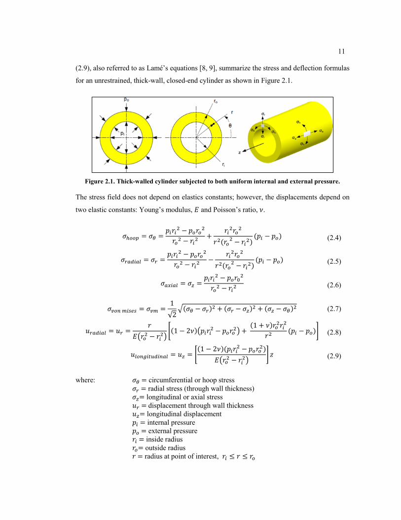
(2.9), also referred to as Lamé’s equations [8, 9], summarize the stress and deflection formulas

for an unrestrained, thick-wall, closed-end cylinder as shown in Figure 2.1.

Figure 2.1. Thick-walled cylinder subjected to both uniform internal and external pressure.

The stress field does not depend on elastics constants; however, the displacements depend on

two elastic constants: Young’s modulus, 𝐸 and Poisson’s ratio, 𝜈.

𝜎ℎ𝑜𝑜𝑝 = 𝜎𝜃 =𝑝𝑖𝑟𝑖

2 − 𝑝𝑜𝑟𝑜2

𝑟𝑜2 − 𝑟𝑖

2+

𝑟𝑖2𝑟𝑜

2

𝑟2(𝑟𝑜2 − 𝑟𝑖

2)(𝑝𝑖 − 𝑝𝑜) (2.4)

𝜎𝑟𝑎𝑑𝑖𝑎𝑙 = 𝜎𝑟 =𝑝𝑖𝑟𝑖



2−

𝑟𝑖2𝑟𝑜

2


2)(𝑝𝑖 − 𝑝𝑜) (2.5)

𝜎𝑎𝑥𝑖𝑎𝑙 = 𝜎𝑧 =𝑝𝑖𝑟𝑖

2 − 𝑝𝑜𝑟02


2 (2.6)

𝜎𝑣𝑜𝑛 𝑚𝑖𝑠𝑒𝑠 = 𝜎𝑣𝑚 =1

√2√(𝜎𝜃 − 𝜎𝑟)

2 + (𝜎𝑟 − 𝜎𝑧)2 + (𝜎𝑧 − 𝜎𝜃)

2 (2.7)

𝑢𝑟𝑎𝑑𝑖𝑎𝑙 = 𝑢𝑟 =𝑟

𝐸(𝑟𝑜2 − 𝑟𝑖

2)[(1 − 2𝜈)(𝑝𝑖𝑟𝑖

2 − 𝑝𝑜𝑟𝑜2) +

(1 + 𝜈)𝑟𝑜2𝑟𝑖2

𝑟2(𝑝𝑖 − 𝑝𝑜)] (2.8)

𝑢𝑙𝑜𝑛𝑔𝑖𝑡𝑢𝑑𝑖𝑛𝑎𝑙 = 𝑢𝑧 = [(1 − 2𝜈)(𝑝𝑖𝑟𝑖

2 − 𝑝𝑜𝑟𝑜2)

𝐸(𝑟𝑜2 − 𝑟𝑖

2)] 𝑧 (2.9)

where: 𝜎𝜃 = circumferential or hoop stress

𝜎𝑟 = radial stress (through wall thickness)

𝜎𝑧= longitudinal or axial stress

𝑢𝑟 = displacement through wall thickness

𝑢𝑧= longitudinal displacement

𝑝𝑖 = internal pressure

𝑝𝑜 = external pressure

𝑟𝑖 = inside radius

𝑟𝑜= outside radius

𝑟 = radius at point of interest, 𝑟𝑖 ≤ 𝑟 ≤ 𝑟𝑜

12

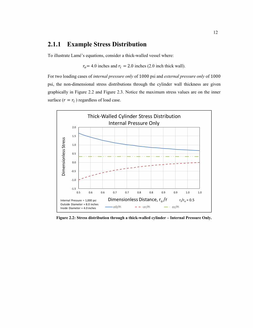
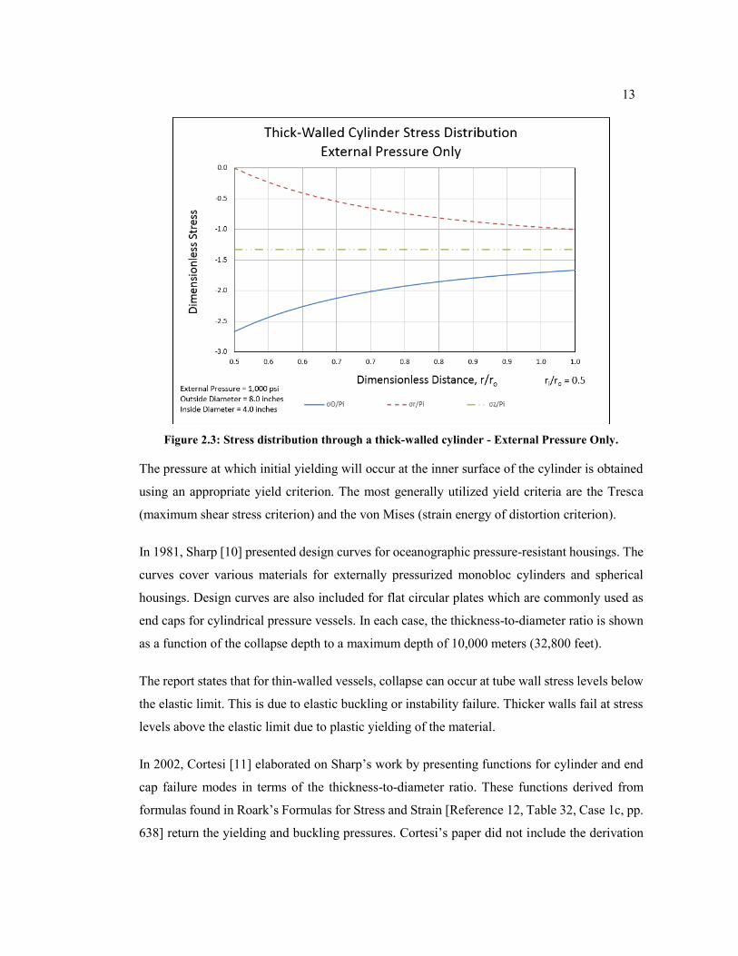
2.1.1 Example Stress Distribution

To illustrate Lamé’s equations, consider a thick-walled vessel where:

𝑟𝑜= 4.0 inches and 𝑟𝑖 = 2.0 inches (2.0 inch thick wall).

For two loading cases of internal pressure only of 1000 psi and external pressure only of 1000

psi, the non-dimensional stress distributions through the cylinder wall thickness are given

graphically in Figure 2.2 and Figure 2.3. Notice the maximum stress values are on the inner

surface (𝑟 = 𝑟𝑖 ) regardless of load case.

Figure 2.2: Stress distribution through a thick-walled cylinder – Internal Pressure Only.

-1.5

-1.0

-0.5

0.0

0.5

1.0

1.5

2.0

0.5 0.6 0.6 0.7 0.7 0.8 0.8 0.9 0.9 1.0 1.0

Dim

ensi

on

less

Str

ess

Dimensionless Distance, ro /r

Thick-Walled Cylinder Stress DistributionInternal Pressure Only

σΘ/Pi σr/Pi σz/Pi

Internal Pressure = 1,000 psi

Outside Diameter = 8.0 inchesInside Diameter = 4.0 inches

ri/ro = 0.5

13

Figure 2.3: Stress distribution through a thick-walled cylinder - External Pressure Only.

The pressure at which initial yielding will occur at the inner surface of the cylinder is obtained

using an appropriate yield criterion. The most generally utilized yield criteria are the Tresca

(maximum shear stress criterion) and the von Mises (strain energy of distortion criterion).

In 1981, Sharp [10] presented design curves for oceanographic pressure-resistant housings. The

curves cover various materials for externally pressurized monobloc cylinders and spherical

housings. Design curves are also included for flat circular plates which are commonly used as

end caps for cylindrical pressure vessels. In each case, the thickness-to-diameter ratio is shown

as a function of the collapse depth to a maximum depth of 10,000 meters (32,800 feet).

The report states that for thin-walled vessels, collapse can occur at tube wall stress levels below

the elastic limit. This is due to elastic buckling or instability failure. Thicker walls fail at stress

levels above the elastic limit due to plastic yielding of the material.

In 2002, Cortesi [11] elaborated on Sharp’s work by presenting functions for cylinder and end

cap failure modes in terms of the thickness-to-diameter ratio. These functions derived from

formulas found in Roark’s Formulas for Stress and Strain [Reference 12, Table 32, Case 1c, pp.

638] return the yielding and buckling pressures. Cortesi’s paper did not include the derivation

14

of the formulas. Because these functions are useful in understanding the behavior of the

cylinder, the derivations are included in this thesis.

Cylinder Yield Failure:

Recall the governing equations for stress in a thick-walled cylinder are:

𝜎ℎ𝑜𝑜𝑝 = 𝜎𝜃 =𝑝𝑖𝑟𝑖



2 −𝑟𝑖2𝑟𝑜2(𝑝𝑜 − 𝑝𝑖)


2) (2.4)

𝜎𝑟𝑎𝑑𝑖𝑎𝑙 = 𝜎𝑟 =𝑝𝑖𝑟𝑖



2 +𝑟𝑖2𝑟𝑜2(𝑝𝑜 − 𝑝𝑖)


2) (2.5)

𝜎𝑎𝑥𝑖𝑎𝑙 = 𝜎𝑎 =𝑝𝑖𝑟𝑖



2 (2.6)

where 𝜎𝜃 = circumferential or hoop stress

𝜎𝑟 = radial stress

𝜎𝑎 = axial or longitudinal stress


𝑝𝑖 = internal pressure

𝑟𝑜 = outer radius

𝑟𝑖 = inner radius

𝑟 = radius at point of interest, 𝑟𝑖 ≤ 𝑟 ≤ 𝑟𝑜

If the internal pressure 𝑝𝑖 = 0, then the maximum circumferential stress occurs at 𝑟 = 𝑟𝑖.

Substituting these values into Equation (2.4) yields Equation (2.10).

𝜎𝜃(𝑟 = 𝑟𝑖) =−2𝑝𝑜𝑟𝑜

2


2 (2.10)

Letting 𝜎𝜃 = 𝜎𝑦 and solving Equation (2.10) for the Thickness to Outer Diameter ratio of a

cylinder results in Equation (2.11). Equation (2.11) describes the relation that will cause yielding

at the inner surface for a given pressure. To prevent yielding, T/OD should be larger than this

value.

𝑇

𝑂𝐷= 1

2(1 − √1 −

2𝑝𝑜𝜎𝑦) (2.11)

where 𝜎𝑦 = yields strength of cylinder material

𝑇 = thickness of cylinder wall

𝑂𝐷 = outside diameter of cylinder

15

Cylinder Buckling Failure:

Equation (2.12) describes the pressure at which the cylinder will buckle.

𝑃 = 2𝐸

1 − 𝜈2(𝑇

𝑂𝐷)3

(2.12)

where 𝑃 = external buckling pressure

𝑇 = cylinder wall thickness


𝐸 = Young’s Modulus

𝜈 = Poisson’s ratio

Solving Equation (2.12) for T/OD yields Equation (2.13) which returns the Thickness to

Diameter (outer) ratio of a cylinder for buckling.

𝑇

𝑂𝐷= (

𝑃(1 − 𝜈2)

2𝐸)

1/3

(2.13)

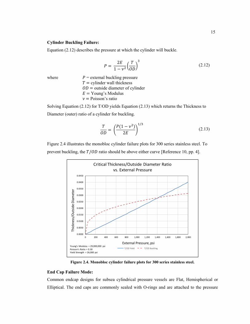
Figure 2.4 illustrates the monobloc cylinder failure plots for 300 series stainless steel. To

prevent buckling, the 𝑇/𝑂𝐷 ratio should be above either curve [Reference 10, pp. 4].

Figure 2.4. Monobloc cylinder failure plots for 300 series stainless steel.

End Cap Failure Mode:

Common endcap designs for subsea cylindrical pressure vessels are Flat, Hemispherical or

Elliptical. The end caps are commonly sealed with O-rings and are attached to the pressure

0.0000

0.0050

0.0100

0.0150

0.0200

0.0250

0.0300

0.0350

0.0400

0.0450

0 200 400 600 800 1,000 1,200 1,400 1,600 1,800 2,000

Thic

knes

s/O

uts

ide

Dia

met

er

External Pressure, psi

Critical Thickness/Outside Diameter Ratio vs. External Pressure

T/OD Yield T/OD BucklingYoung's Modulus = 29,000,000 psi

Poisson's Ratio = 0.30Yield Strength = 26,000 psi

16

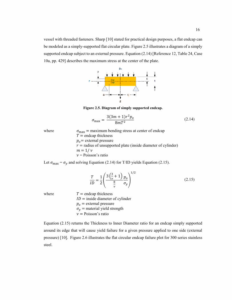
vessel with threaded fasteners. Sharp [10] stated for practical design purposes, a flat endcap can

be modeled as a simply-supported flat circular plate. Figure 2.5 illustrates a diagram of a simply

supported endcap subject to an external pressure. Equation (2.14) [Reference 12, Table 24, Case

10a, pp. 429] describes the maximum stress at the center of the plate.

Figure 2.5. Diagram of simply supported endcap.

𝜎max = 3(3𝑚 + 1)𝑟2𝑝𝑜

8𝑚𝑇2 (2.14)

where 𝜎max = maximum bending stress at center of endcap

𝑇 = endcap thickness

𝑝𝑜= external pressure

𝑟 = radius of unsupported plate (inside diameter of cylinder)

𝑚 = 1/ 𝜈 𝜈 = Poisson’s ratio

Let 𝜎max = 𝜎𝑦 and solving Equation (2.14) for T/ID yields Equation (2.15).

𝑇

𝐼𝐷=1

2(3(

3

𝜈+ 1)

8

𝜈

𝑝𝑜𝜎𝑦)

1/2

(2.15)

where 𝑇 = endcap thickness

𝐼𝐷 = inside diameter of cylinder


𝜎𝑦 = material yield strength


Equation (2.15) returns the Thickness to Inner Diameter ratio for an endcap simply supported

around its edge that will cause yield failure for a given pressure applied to one side (external

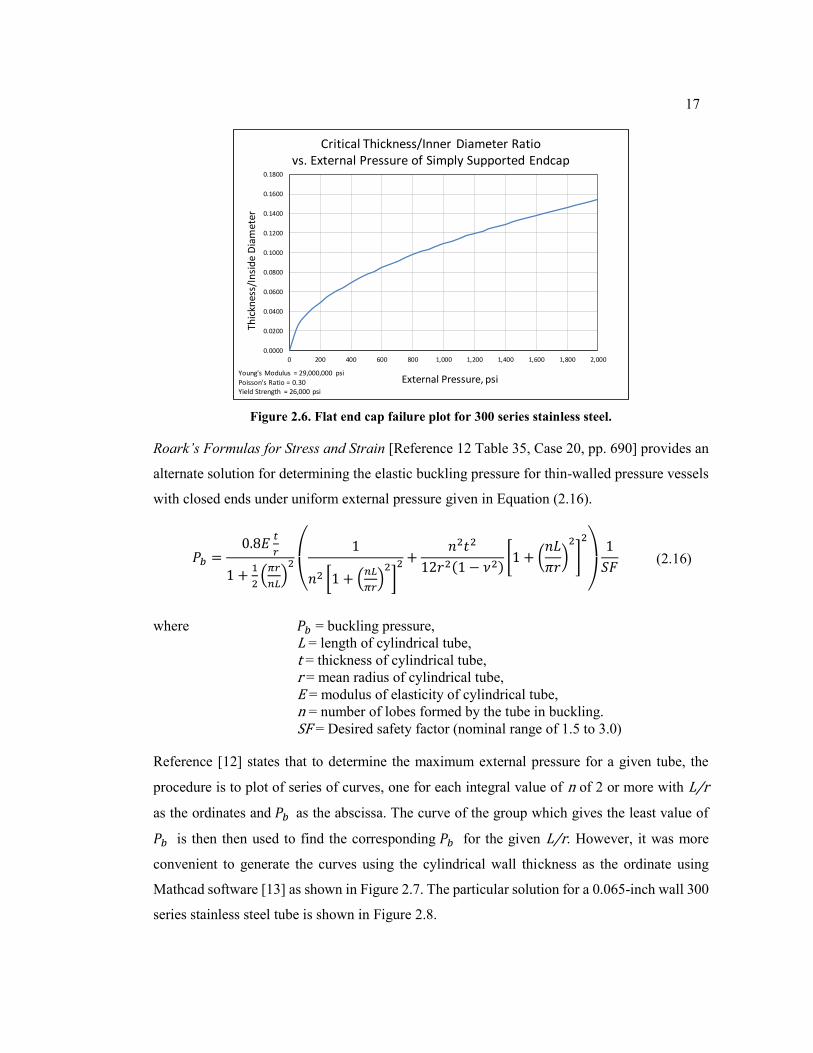
pressure) [10]. Figure 2.6 illustrates the flat circular endcap failure plot for 300 series stainless

steel.

17

Figure 2.6. Flat end cap failure plot for 300 series stainless steel.

Roark’s Formulas for Stress and Strain [Reference 12 Table 35, Case 20, pp. 690] provides an

alternate solution for determining the elastic buckling pressure for thin-walled pressure vessels

with closed ends under uniform external pressure given in Equation (2.16).

𝑃𝑏 =0.8𝐸

𝑡

𝑟

1 +1

2(𝜋𝑟

𝑛𝐿)2

(

1

𝑛2 [1 + (𝑛𝐿

𝜋𝑟)2]2 +

𝑛2𝑡2

12𝑟2(1 − 𝜈2)[1 + (

𝑛𝐿

𝜋𝑟)2

]

2

)

1

𝑆𝐹 (2.16)

where 𝑃𝑏 = buckling pressure,

L = length of cylindrical tube,

t = thickness of cylindrical tube,

r = mean radius of cylindrical tube,

E = modulus of elasticity of cylindrical tube,

n = number of lobes formed by the tube in buckling.

SF = Desired safety factor (nominal range of 1.5 to 3.0)

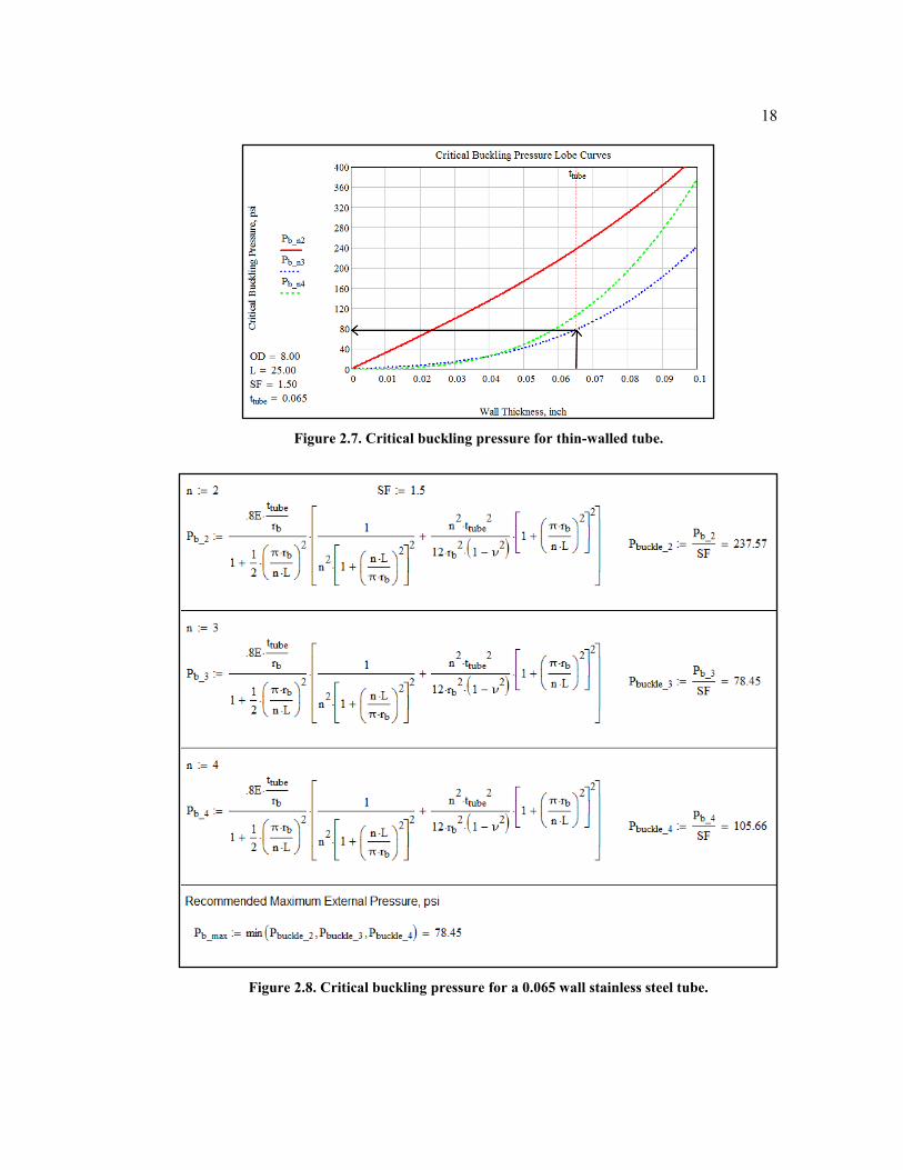
Reference [12] states that to determine the maximum external pressure for a given tube, the

procedure is to plot of series of curves, one for each integral value of n of 2 or more with L/r

as the ordinates and 𝑃𝑏 as the abscissa. The curve of the group which gives the least value of

𝑃𝑏 is then then used to find the corresponding 𝑃𝑏 for the given L/r. However, it was more

convenient to generate the curves using the cylindrical wall thickness as the ordinate using

Mathcad software [13] as shown in Figure 2.7. The particular solution for a 0.065-inch wall 300

series stainless steel tube is shown in Figure 2.8.

0.0000

0.0200

0.0400

0.0600

0.0800

0.1000

0.1200

0.1400

0.1600

0.1800

0 200 400 600 800 1,000 1,200 1,400 1,600 1,800 2,000

Thic

knes

s/In

sid

e D

iam

eter


Critical Thickness/Inner Diameter Ratio vs. External Pressure of Simply Supported Endcap

Young's Modulus = 29,000,000 psi


18

Figure 2.7. Critical buckling pressure for thin-walled tube.

Figure 2.8. Critical buckling pressure for a 0.065 wall stainless steel tube.

19

If 60 < (𝑙

𝑟)2(𝑟

𝑡) < (

𝑟

𝑡)2

, the critical pressure can be approximated by:

𝑃𝑐 = 0.92𝐸

(𝑙

𝑟) (

𝑟

𝑡)2.5 (2.17)

Values of experimentally determined critical pressures range 20% above and below the

theoretical values given by the expression above. A recommended probable minimum critical

pressure is 0.8Pc.

Solving Equation (2.17) for T/OD yields Equation (2.18).

𝑇

𝑂𝐷= (

𝑃𝑐3.7239𝐸

)1/3

(2.18)

where 𝑃𝑐 = Critical pressure for buckling

𝑇 = cylinder wall thickness


𝐸 = material modulus of elasticity

Equation (2.18) is valid for a maximum cylinder length of:

𝑙𝑚𝑎𝑥 = √0.3125𝑂𝐷3

𝑇 (2.19)

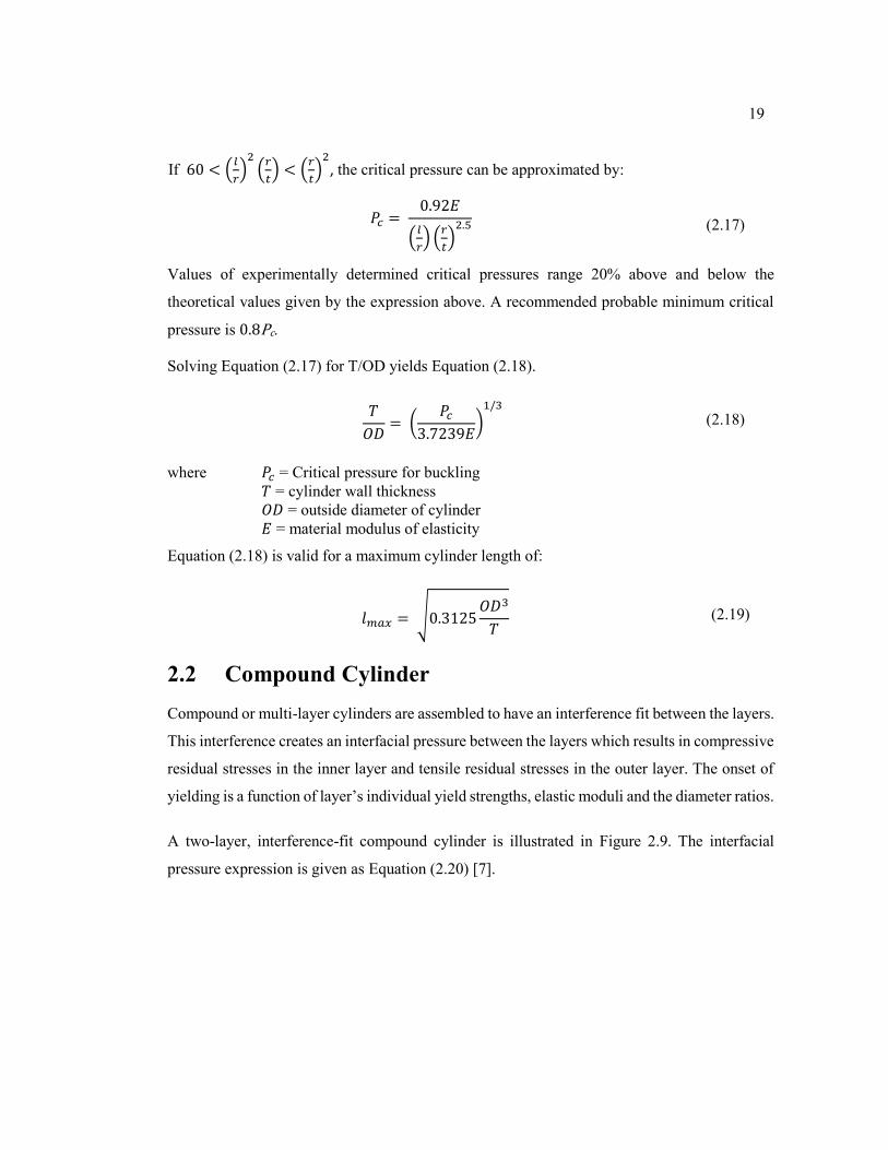
2.2 Compound Cylinder

Compound or multi-layer cylinders are assembled to have an interference fit between the layers.

This interference creates an interfacial pressure between the layers which results in compressive

residual stresses in the inner layer and tensile residual stresses in the outer layer. The onset of

yielding is a function of layer’s individual yield strengths, elastic moduli and the diameter ratios.

A two-layer, interference-fit compound cylinder is illustrated in Figure 2.9. The interfacial

pressure expression is given as Equation (2.20) [7].

20

Figure 2.9: Two-Layer, Interference-Fit compound cylinder.

𝑝𝑖𝑛𝑡 =𝛿𝑟

𝑅𝑖𝑛𝑡

𝐸𝑜(𝑟𝑜2+𝑅𝑖𝑛𝑡

2

𝑟𝑜2−𝑅𝑖𝑛𝑡

2 + 𝜈0) +𝑅𝑖𝑛𝑡

𝐸𝑜(𝑅𝑖𝑛𝑡

2+𝑟𝑖2

𝑅𝑖𝑛𝑡2−𝑟𝑖

2 − 𝜈𝑖) (2.20)

where: 𝑝𝑖𝑛𝑡 = interfacial pressure

𝛿𝑟 = radial interference between the tube and insert

𝑅𝑖𝑛𝑡 = interfacial radius

𝐸𝑜= outer tube modulus of elasticity

𝐸𝑖= inner insert modulus of elasticity

𝜈0 = outer tube Poisson’s ratio

𝜈𝑖 = inner insert tube Poisson’s ratio

Equation (2.20) is the most common expression for interfacial pressure. However, the definition

for the interfacial radius is not clearly defined. Published examples use the inside diameter of

the outer shell, the outside diameter of the inner insert and the average of the interference

diameters. The results are all similar but not exact.

Equation (2.21) is a less ambiguous expression [14]. This expression clearly distinguishes the

dimensions between the two components. Section 3.2.1 will illustrate that this expression

provides results within 0.08% of a 2D finite element analysis solution.

𝑝𝑖𝑛𝑡 =𝛿𝑑

𝐼𝐷𝑡𝑢𝑏𝑒

𝐸𝑡𝑢𝑏𝑒(𝑂𝐷𝑡𝑢𝑏𝑒

2+𝐼𝐷𝑡𝑢𝑏𝑒2

𝑂𝐷𝑡𝑢𝑏𝑒2−𝐼𝐷𝑡𝑢𝑏𝑒

2 + 𝜈𝑡𝑢𝑏𝑒) +𝑂𝐷𝑠𝑙𝑒𝑒𝑣𝑒

𝐸𝑠𝑙𝑒𝑒𝑣𝑒(𝑂𝐷𝑠𝑙𝑒𝑒𝑣𝑒

2+𝐼𝐷𝑠𝑙𝑒𝑒𝑣𝑒2

𝑂𝐷𝑠𝑙𝑒𝑒𝑣𝑒2−𝐼𝐷𝑠𝑙𝑒𝑒𝑣𝑒

2 − 𝜈𝑠𝑙𝑒𝑒𝑣𝑒) (2.21)

21

An example compound cylinder is used to illustrate the differences in the two equations. Table

2.1 lists the dimensions and material properties. Table 2.2 compares the interfacial pressure

results from Equation (2.20) and Equation (2.21).

Table 2.1. Two-layer compound cylinder dimensions and material properties.

Component

Inside

Diameter,

Inch

Wall

Thickness,

Inch

Young’s

Modulus,

psi

Poisson’s

Ratio

Outer Cylinder 7.850 0.065 29,000 ksi .30

Inner Cylinder varies 0.150 9,900 ksi .33

Table 2.2. Comparison of interfacial pressure expression results.

Interfacial Pressure Expression (2.20) and (2.21)

Comparison

Diametrical

Interference,

inch

Equation

(2.20)

psi

Equation

(2.21)

psi

%

Difference

0.001 27.277 27.273 0.01%

0.002 54.554 54.538 0.03%

0.003 81.831 81.769 0.04%

0.004 109.108 109.046 0.06%

0.005 136.384 136.288 0.07%

0.006 163.661 163.522 0.08%

0.007 190.938 190.749 0.10%

0.008 218.215 217.968 0.11%

0.009 245.492 245.179 0.13%

0.010 272.769 272.382 0.14%

0.011 300.046 299.578 0.16%

Equation (2.21) will be used throughout this thesis. Once the interfacial pressure has been

calculated, Lamé’s equations for the thick-wall cylinder can be utilized to compute the stress

values for the two-layer compound cylinder.

In 1969, Davidson et al. [15] provided a review of the theory and practice of pressure vessel

designs operating in the range of internal pressures from 1 to 55 kilo-bars (approximately 15,000

to 800,000 psi). They reported that if the materials for both layers are identical, the optimum

design of a dual-layer pressure vessel is accomplished when the diameter ratios of the inner and

outer cylinders (𝐾1 =𝑟2

𝑟1 and 𝐾2 =

𝑟3

𝑟2) are equal and the interfacial pressure results in the

simultaneous yielding at the bore of the layers at the maximum elastic operating pressure. Note:

subscript 1 refers to the bore of the inner cylinder, subscript 2 refers to the interface and subscript

22

3 refers to the outside of the outer cylinder. However, if layer materials have different yield

strengths and elastic constants, the optimum design is more complex as follows.

The Tresca yield criterion was used to determine the internal operating pressure for yielding an

optimum, two-layer cylinder as given in Equation (2.22).

𝑃𝑦

𝜎𝑦2=1

2(𝜎𝑦1

𝜎𝑦2+ 1) −

1

𝐾√𝜎𝑦1

𝜎𝑦2 (2.22)

where K and K1 are defined by Equations (2.23) and (2.24):

diameter ratio, 𝐾 = 𝑟2𝑟1

(2.23)

𝐾1 = (𝜎𝑦1

𝜎𝑦2)

1/4

√𝐾 (2.24)

𝐾2 = (𝜎𝑦1

𝜎𝑦2)

1/4

√𝑟3𝑟2

(2.25)

The initial radial interference for this two-layer optimum compound cylinder is given in

Equation (2.26):

𝛿𝑖𝑛𝑡𝑟2=1

2[𝜎𝑦2 −

1

𝐾√𝜎𝑦1𝜎𝑦2] [

1 − 𝜈12

𝐸1(𝐾12 + 1

𝐾12 − 1

) +1 − 𝜈2

2

𝐸2(𝐾22 + 1

𝐾22 − 1

) −𝜈1(1 + 𝜈1)

𝐸1

+𝜈2(1 + 𝜈2)

𝐸2] −

1 − 𝜈12

𝐸1[𝜎𝑦1 + 𝜎𝑦2 −

2

𝐾√𝜎𝑦1𝜎𝑦2

𝐾12 − 1

]

(2.26)

where 𝑃𝑦 = Internal pressure at initial yield

𝐸1 = Young’s elastic modulus of inner cylinder 1

𝐸2 = Young’s elastic modulus of outer cylinder 2

𝜎𝑦1 = Yield stress in tension of inner cylinder 1

𝜎𝑦2 = Yield stress in tension of outer cylinder 2

𝐾 = Diameter ratio defined in Equation (2.23)

𝐾1 = Condition for optimum inner cylinder defined in Equation (2.24)

𝐾2 = Condition for optimum outer cylinder defined in Equation (2.25)

𝑟1 = Bore radius of inner cylinder

𝑟2 = Radius of interface of two cylinders

𝑟3 = Outside radius of outer cylinder

23

Equation (2.26) illustrates that slight variations in the two elastic constants, Young’s modulus,

𝐸 and Poisson’s ratio, 𝜈, can have a significant effect on the design parameters for a compound

cylinder. Of course, variations in yield strength will also have a considerable effect. The

theoretical elastic pressure limit for a dual-layer compound cylinder is 100% of the material

yield strength. The theoretical elastic pressure limit is only 50% of the material yield for a single

wall cylinder [15].

In 2014, Majumder [16] researched the optimum design of compound cylindrical pressure

vessels subjected to internal pressure by finite element analysis. The thesis suggests that the

ideal value of contact pressure will produce equal maximum tensile stresses in both cylinders.

In other words, the main objective of an optimized multilayer cylinder is to achieve equivalent

maximum hoop stress at the inner surface of all cylinders. If the materials of the two cylinders

are identical, the ideal diametrical interference, 𝛿1 is defined by Equation (2.27).

𝛿1 = 𝑝𝑠 [2𝐷1𝑐1[(𝑐1𝑐2)

2 − 1]

𝐸(𝑐22 − 1)(𝑐1

2 − 1)] (2.27)

where 𝑐1 and 𝑐2 are defined by Equations (2.28) and (2.29):

𝑐1 = 𝐷2𝐷1

(2.28)

𝑐2 = 𝐷3𝐷2

(2.29)

and 𝑝𝑠 = Interfacial Pressure

𝐷1= Inner diameter of the insert

𝐷2= Outer diameter of the insert

𝐷3= Outer diameter of the shell

𝐸 = Modulus of elasticity for the insert and shell.

Slocum [14] states that the holding power of an interference fit depends on the coefficient of

friction and the amount by which the surface asperities (roughness) of the two parts dig into

each other forming a mechanical bond. Assuming the latter is the dominate holding power, it

should be maximized by cleaning and degreasing the parts prior to assembly. In addition, micro

slip occurs at small tangential levels. It is wrong to assume that the rougher the mating surfaces,

the better the chance that the peaks will interlock decreasing micro slip and increasing the

holding power of the interference joint. In fact, as the surface roughness increases, the stiffness

24

and dimensional location stability decreases. In general, the finer the surface finish (on the order

of 0.5 micro-meters 𝑅𝑎 or 16 micro-inches 𝑅𝑎) the more the joint appears to be solid. Slocum

suggests that clean, high surface finish parts actually cold weld together after they are press fit.

A 16 micro-inches 𝑅𝑎 finish is considered fine and is indicative of parts where the machining

marks direction is blurred i.e. not obvious. This finish can be applied by reaming, grinding

boring and rolling processes.

Slocum [14] explained that the interference joint should be designed to provide adequate

holding power when the minimum interference between parts exists. In addition, the stress

levels in the parts should not exceed the material yield strength when the maximum interference

exists even in the presence of other stresses in the system. A given system may be subjected to

the following stresses: axial, torsional, bending, pressure, thermal and inertial.

Axial Loads

The product of the minimum interfacial pressure, the coefficient of friction (𝜇) and the interface

area must be greater than the desired axial force. The minimum interfacial pressure to allow

transmission of the axial force without slipping is given in Equation (2.30).

𝑃𝑚𝑖𝑛 =𝐹𝑎𝑥𝑖𝑎𝑙𝜇𝜋𝐷𝐿

(2.30)

An axial force applied to the inner cylinder will cause the diameter to change. The change in

diameter can be approximated as given in Equation (2.31). After the required interference fit to

support the axial load has been determined, the absolute value of the change in diameter must

be added to the initial diametrical interference fit value.

∆𝐷 =−4𝜈𝐹𝑎𝑥𝑖𝑎𝑙𝜋𝐷𝐸

(2.31)

Torsional Loads

The product of the minimum interfacial pressure, the interface area, the coefficient of friction,

and the radius of the interface must be greater than the design torque. The minimum interfacial

pressure to allow transmission of the torque without slipping is given in Equation (2.32). Since

the torsional and axial motions are orthogonal, the interfacial pressure calculated must be able

to resist the resultant of the axial and tangential force vectors.

25

𝑃𝑚𝑖𝑛 =2𝑇𝑑𝑒𝑠𝑖𝑔𝑛

𝜇𝜋𝐷𝐿 (2.32)

Bending Loads

In general, when a beam bends, one surface is in tension and the other surface is in compression.

To prevent an interference fit joint from working loose, the product of the interface pressure and

the coefficient of friction must be greater than the maximum tensile or compressive stress in the

beam. In addition, to transfer the bending moment effectively across the joint, the area moment

of inertia of the outer cylinder must be greater than the area moment of inertial of the inner

cylinder.

𝑃𝑚𝑖𝑛𝜇 > 𝜎𝑏 (2.33)

𝐼𝑥−𝑥 𝑜𝑢𝑡𝑒𝑟 > 𝐼𝑥−𝑥 𝑖𝑛𝑛𝑒𝑟 (2.34)

Pressure Stresses

Application of external or internal hydrostatic pressure will cause the components to contract

or expand. This may cause tightening or loosening of the interference fit joint.

Thermal Loads

Temperature changes can cause the diameters of the interference fit assembly to contract or

expand which directly affects the allowable minimum and maximum interference fits. The

change in outside diameter relative to the inside diameter at the diameter 𝐷 of the interference

fit for a uniform temperature change ∆𝑇 from the assembly temperature is defined in Equation

(2.35).

∆𝐷 = 𝐷∆𝑇(𝛼𝐼 − 𝛼𝑂) (2.35)

Inertial Stresses

When a body spins, centrifugal forces tend to expand the body and cause internal radial and

circumferential stresses. The interference joint should be designed such that the parts do not

loosen or fly apart. This mainly applies to pulleys or disks on shafts and is not applicable to the

subject of this thesis. Consult reference [14] if additional information is desired.

26

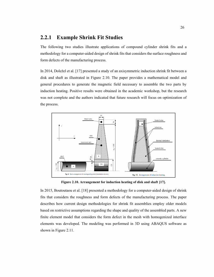
2.2.1 Example Shrink Fit Studies

The following two studies illustrate applications of compound cylinder shrink fits and a

methodology for a computer-aided design of shrink fits that considers the surface roughness and

form defects of the manufacturing process.

In 2014, Doležel et al. [17] presented a study of an axisymmetric induction shrink fit between a

disk and shaft as illustrated in Figure 2.10. The paper provides a mathematical model and

general procedures to generate the magnetic field necessary to assemble the two parts by

induction heating. Positive results were obtained in the academic workshop, but the research

was not complete and the authors indicated that future research will focus on optimization of

the process.

Figure 2.10. Arrangement for induction heating of disk and shaft [17].

In 2015, Boutoutaou et al. [18] presented a methodology for a computer-aided design of shrink

fits that considers the roughness and form defects of the manufacturing process. The paper

describes how current design methodologies for shrink fit assemblies employ older models

based on restrictive assumptions regarding the shape and quality of the assembled parts. A new

finite element model that considers the form defect in the mesh with homogenized interface

elements was developed. The modeling was performed in 3D using ABAQUS software as

shown in Figure 2.11.

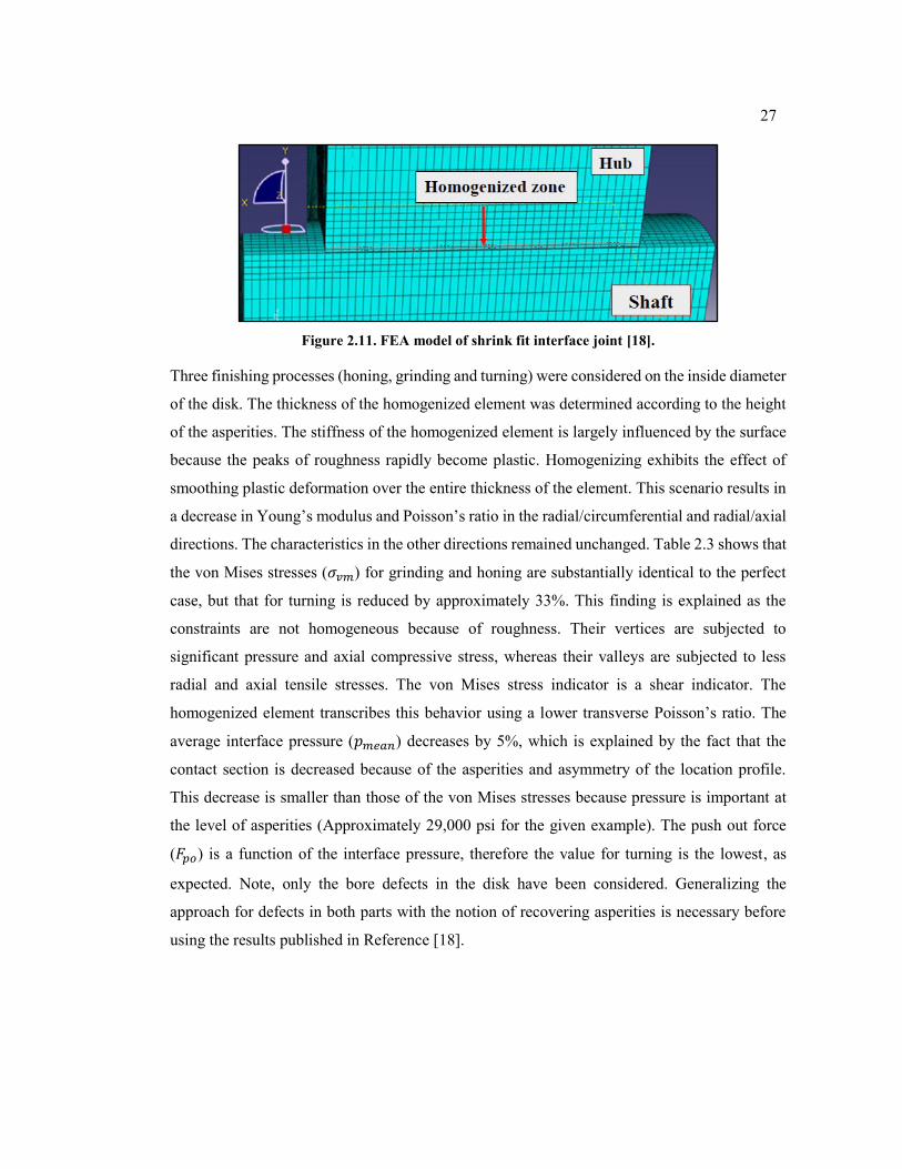
27

Figure 2.11. FEA model of shrink fit interface joint [18].

Three finishing processes (honing, grinding and turning) were considered on the inside diameter

of the disk. The thickness of the homogenized element was determined according to the height

of the asperities. The stiffness of the homogenized element is largely influenced by the surface

because the peaks of roughness rapidly become plastic. Homogenizing exhibits the effect of

smoothing plastic deformation over the entire thickness of the element. This scenario results in

a decrease in Young’s modulus and Poisson’s ratio in the radial/circumferential and radial/axial

directions. The characteristics in the other directions remained unchanged. Table 2.3 shows that

the von Mises stresses (𝜎𝑣𝑚) for grinding and honing are substantially identical to the perfect

case, but that for turning is reduced by approximately 33%. This finding is explained as the

constraints are not homogeneous because of roughness. Their vertices are subjected to

significant pressure and axial compressive stress, whereas their valleys are subjected to less

radial and axial tensile stresses. The von Mises stress indicator is a shear indicator. The

homogenized element transcribes this behavior using a lower transverse Poisson’s ratio. The

average interface pressure (𝑝𝑚𝑒𝑎𝑛) decreases by 5%, which is explained by the fact that the

contact section is decreased because of the asperities and asymmetry of the location profile.

This decrease is smaller than those of the von Mises stresses because pressure is important at

the level of asperities (Approximately 29,000 psi for the given example). The push out force

(𝐹𝑝𝑜) is a function of the interface pressure, therefore the value for turning is the lowest, as

expected. Note, only the bore defects in the disk have been considered. Generalizing the

approach for defects in both parts with the notion of recovering asperities is necessary before

using the results published in Reference [18].

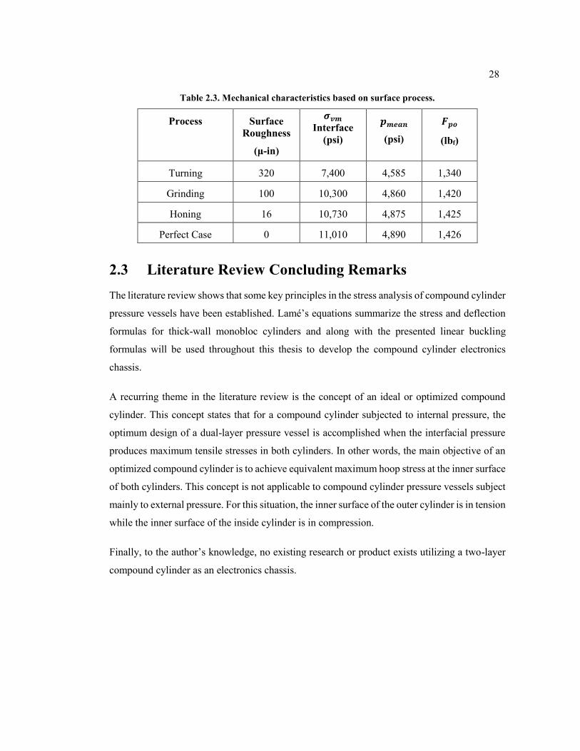
28

Table 2.3. Mechanical characteristics based on surface process.

Process Surface

Roughness

(μ-in)

𝝈𝒗𝒎 Interface

(psi)

𝒑𝒎𝒆𝒂𝒏

(psi)

𝑭𝒑𝒐

(lbf)

Turning 320 7,400 4,585 1,340

Grinding 100 10,300 4,860 1,420

Honing 16 10,730 4,875 1,425

Perfect Case 0 11,010 4,890 1,426

2.3 Literature Review Concluding Remarks

The literature review shows that some key principles in the stress analysis of compound cylinder

pressure vessels have been established. Lamé’s equations summarize the stress and deflection

formulas for thick-wall monobloc cylinders and along with the presented linear buckling

formulas will be used throughout this thesis to develop the compound cylinder electronics

chassis.

A recurring theme in the literature review is the concept of an ideal or optimized compound

cylinder. This concept states that for a compound cylinder subjected to internal pressure, the

optimum design of a dual-layer pressure vessel is accomplished when the interfacial pressure

produces maximum tensile stresses in both cylinders. In other words, the main objective of an

optimized compound cylinder is to achieve equivalent maximum hoop stress at the inner surface

of both cylinders. This concept is not applicable to compound cylinder pressure vessels subject

mainly to external pressure. For this situation, the inner surface of the outer cylinder is in tension

while the inner surface of the inside cylinder is in compression.

Finally, to the author’s knowledge, no existing research or product exists utilizing a two-layer

compound cylinder as an electronics chassis.

29

Chapter 3

Compound Cylinder Pressure Vessel Development

A primary goal of this thesis is to develop a methodology to design a compound cylinder

pressure vessel that can be manufactured using commercially available materials and industry

standards as guidelines for the interference fit and to demonstrate it through a representative

design. A secondary goal is to minimize the weight of the compound cylinder pressure vessel.

A tertiary goal is to minimize costs of the assembly. This goal may drive the material selection

once the first two goals have been met.

The development of the pressure vessel will begin with a discussion of a two-layer compound

cylinder. Chapter 4 will transition from this basic design to the development of the electronics

chassis pressure vessel based on the two-layer compound cylinder.

A discussion of the industry standard dimensions for the components and of the interference fit

will be presented first. Following this, the geometry driven Lamé’s equations along with

industry standards for margin of safety will be utilized to determine material based design

guidelines for a compound cylinder. Finally, both two-dimensional and three-dimensional finite

element models of the two-layer compound cylinder will be presented along with their results

and compared to the closed-form Lamé’s equations.

This thesis will primarily focus on the development of a nominal 8-inch diameter pressure vessel

but will present data for nominal sizes 10-inch and 12-inch diameter where applicable.

3.1 Compound Cylinder Industry Standard Dimensions

The outer shell of the pressure vessel will be typically fabricated from extruded thick-walled

aluminum tubing or seamless aluminum or stainless steel pipe. Dimensional tolerances on the

aluminum tubing are more exact than pipe but aluminum is not always the appropriate choice.

Consider an application where a nominal 8-inch diameter outer shell must be fabricated from

stainless steel. Seamless stainless steel pipe is commercially available in 0.500-inch wall

thickness but the large dimensional tolerances of pipe must be considered when determining the

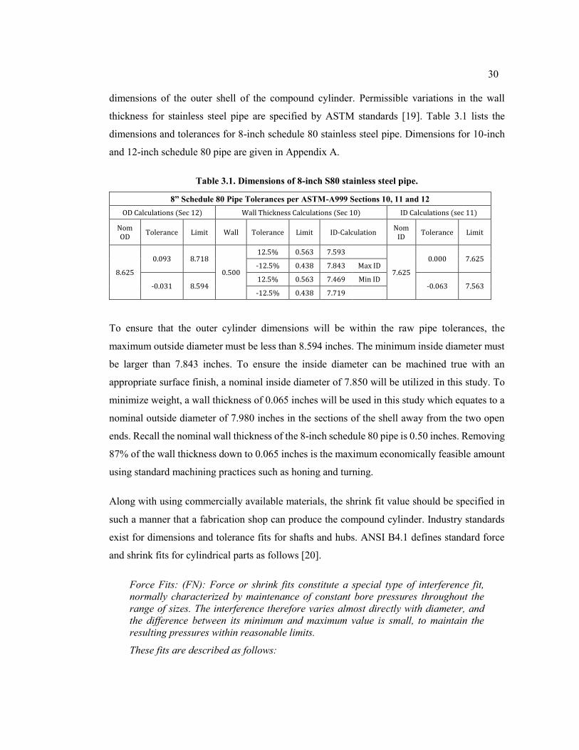
30

dimensions of the outer shell of the compound cylinder. Permissible variations in the wall

thickness for stainless steel pipe are specified by ASTM standards [19]. Table 3.1 lists the

dimensions and tolerances for 8-inch schedule 80 stainless steel pipe. Dimensions for 10-inch

and 12-inch schedule 80 pipe are given in Appendix A.

Table 3.1. Dimensions of 8-inch S80 stainless steel pipe.

8” Schedule 80 Pipe Tolerances per ASTM-A999 Sections 10, 11 and 12

OD Calculations (Sec 12) Wall Thickness Calculations (Sec 10) ID Calculations (sec 11)

Nom OD

Tolerance Limit Wall Tolerance Limit ID-Calculation Nom

ID Tolerance Limit

8.625

0.093 8.718

0.500

12.5% 0.563 7.593

7.625

0.000 7.625 -12.5% 0.438 7.843 Max ID

-0.031 8.594 12.5% 0.563 7.469 Min ID

-0.063 7.563 -12.5% 0.438 7.719

To ensure that the outer cylinder dimensions will be within the raw pipe tolerances, the

maximum outside diameter must be less than 8.594 inches. The minimum inside diameter must

be larger than 7.843 inches. To ensure the inside diameter can be machined true with an

appropriate surface finish, a nominal inside diameter of 7.850 will be utilized in this study. To

minimize weight, a wall thickness of 0.065 inches will be used in this study which equates to a

nominal outside diameter of 7.980 inches in the sections of the shell away from the two open

ends. Recall the nominal wall thickness of the 8-inch schedule 80 pipe is 0.50 inches. Removing

87% of the wall thickness down to 0.065 inches is the maximum economically feasible amount

using standard machining practices such as honing and turning.

Along with using commercially available materials, the shrink fit value should be specified in

such a manner that a fabrication shop can produce the compound cylinder. Industry standards

exist for dimensions and tolerance fits for shafts and hubs. ANSI B4.1 defines standard force

and shrink fits for cylindrical parts as follows [20].

Force Fits: (FN): Force or shrink fits constitute a special type of interference fit,

normally characterized by maintenance of constant bore pressures throughout the

range of sizes. The interference therefore varies almost directly with diameter, and

the difference between its minimum and maximum value is small, to maintain the

resulting pressures within reasonable limits.

These fits are described as follows:

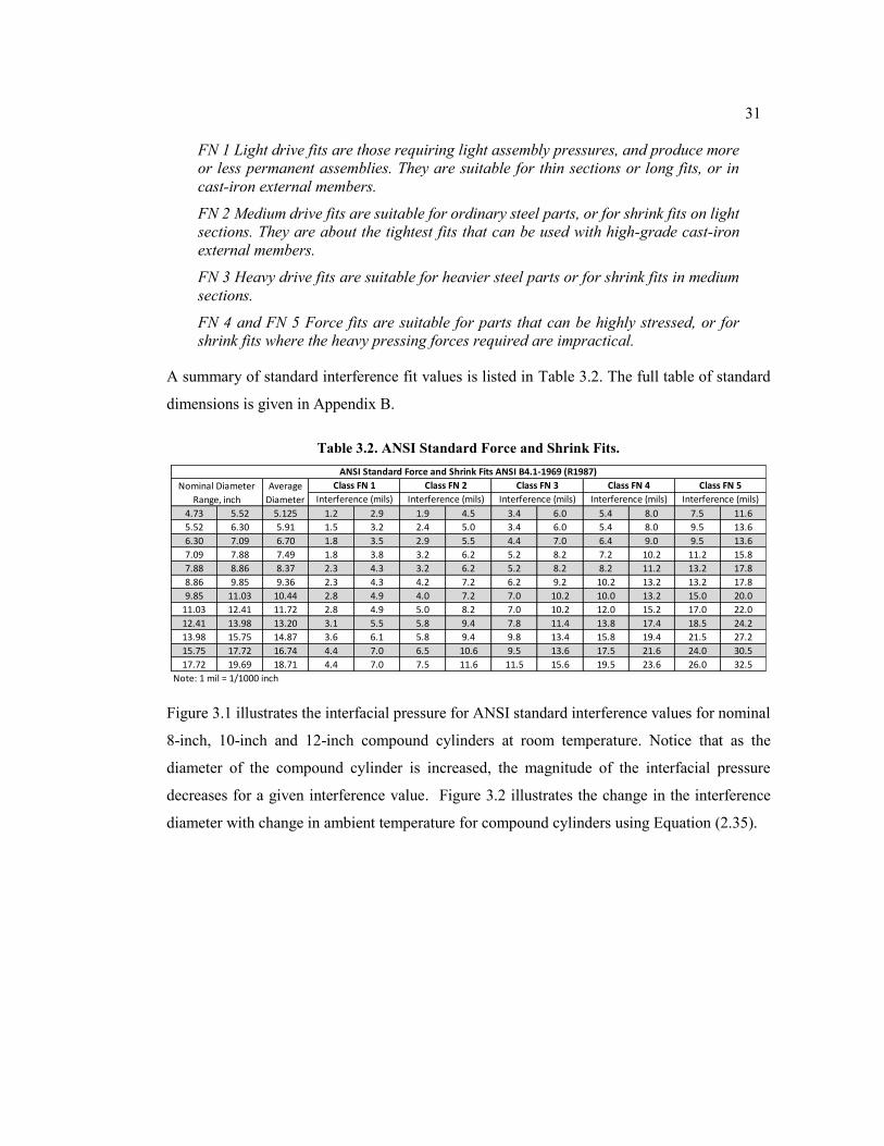
31

FN 1 Light drive fits are those requiring light assembly pressures, and produce more

or less permanent assemblies. They are suitable for thin sections or long fits, or in

cast-iron external members.

FN 2 Medium drive fits are suitable for ordinary steel parts, or for shrink fits on light

sections. They are about the tightest fits that can be used with high-grade cast-iron

external members.

FN 3 Heavy drive fits are suitable for heavier steel parts or for shrink fits in medium

sections.

FN 4 and FN 5 Force fits are suitable for parts that can be highly stressed, or for

shrink fits where the heavy pressing forces required are impractical.

A summary of standard interference fit values is listed in Table 3.2. The full table of standard

dimensions is given in Appendix B.

Table 3.2. ANSI Standard Force and Shrink Fits.

Figure 3.1 illustrates the interfacial pressure for ANSI standard interference values for nominal

8-inch, 10-inch and 12-inch compound cylinders at room temperature. Notice that as the

diameter of the compound cylinder is increased, the magnitude of the interfacial pressure

decreases for a given interference value. Figure 3.2 illustrates the change in the interference

diameter with change in ambient temperature for compound cylinders using Equation (2.35).

4.73 5.52 5.125 1.2 2.9 1.9 4.5 3.4 6.0 5.4 8.0 7.5 11.6

5.52 6.30 5.91 1.5 3.2 2.4 5.0 3.4 6.0 5.4 8.0 9.5 13.6

6.30 7.09 6.70 1.8 3.5 2.9 5.5 4.4 7.0 6.4 9.0 9.5 13.6

7.09 7.88 7.49 1.8 3.8 3.2 6.2 5.2 8.2 7.2 10.2 11.2 15.8

7.88 8.86 8.37 2.3 4.3 3.2 6.2 5.2 8.2 8.2 11.2 13.2 17.8

8.86 9.85 9.36 2.3 4.3 4.2 7.2 6.2 9.2 10.2 13.2 13.2 17.8

9.85 11.03 10.44 2.8 4.9 4.0 7.2 7.0 10.2 10.0 13.2 15.0 20.0

11.03 12.41 11.72 2.8 4.9 5.0 8.2 7.0 10.2 12.0 15.2 17.0 22.0

12.41 13.98 13.20 3.1 5.5 5.8 9.4 7.8 11.4 13.8 17.4 18.5 24.2

13.98 15.75 14.87 3.6 6.1 5.8 9.4 9.8 13.4 15.8 19.4 21.5 27.2

15.75 17.72 16.74 4.4 7.0 6.5 10.6 9.5 13.6 17.5 21.6 24.0 30.5

17.72 19.69 18.71 4.4 7.0 7.5 11.6 11.5 15.6 19.5 23.6 26.0 32.5

Note: 1 mil = 1/1000 inch

ANSI Standard Force and Shrink Fits ANSI B4.1-1969 (R1987)

Interference (mils)

Nominal Diameter

Range, inch

Average

Diameter Interference (mils) Interference (mils) Interference (mils) Interference (mils)

Class FN 1 Class FN 2 Class FN 3 Class FN 4 Class FN 5

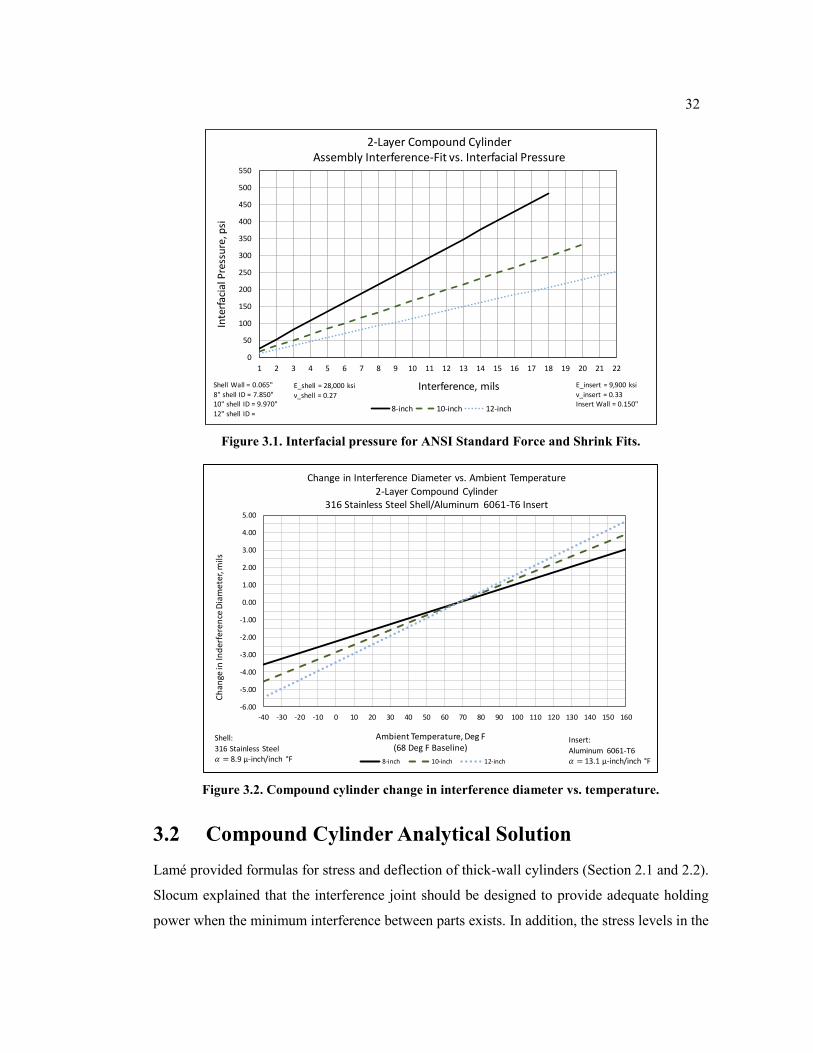
32

Figure 3.1. Interfacial pressure for ANSI Standard Force and Shrink Fits.

Figure 3.2. Compound cylinder change in interference diameter vs. temperature.

3.2 Compound Cylinder Analytical Solution

Lamé provided formulas for stress and deflection of thick-wall cylinders (Section 2.1 and 2.2).

Slocum explained that the interference joint should be designed to provide adequate holding

power when the minimum interference between parts exists. In addition, the stress levels in the

0

50

100

150

200

250

300

350

400

450

500

550

1 2 3 4 5 6 7 8 9 10 11 12 13 14 15 16 17 18 19 20 21 22

Inte

rfac

ial P

ress

ure

, psi

Interference, mils

2-Layer Compound CylinderAssembly Interference-Fit vs. Interfacial Pressure

8-inch 10-inch 12-inch

Shell Wall = 0.065"

8" shell ID = 7.850"10" shell ID = 9.970"

12" shell ID =

E_insert = 9,900 ksi

ν_insert = 0.33Insert Wall = 0.150"

E_shell = 28,000 ksi

ν_shell = 0.27

-6.00

-5.00

-4.00

-3.00

-2.00

-1.00

0.00

1.00

2.00

3.00

4.00

5.00

-40 -30 -20 -10 0 10 20 30 40 50 60 70 80 90 100 110 120 130 140 150 160

Ch

ange

in In

der

fere

nce

Dia

met

er, m

ils

Ambient Temperature, Deg F(68 Deg F Baseline)

Change in Interference Diameter vs. Ambient Temperature

2-Layer Compound Cylinder316 Stainless Steel Shell/Aluminum 6061-T6 Insert

8-inch 10-inch 12-inch

Shell:

316 Stainless Steel𝛼 = 8.9 µ-inch/inch °F

Insert:

Aluminum 6061-T6𝛼 = 13.1 µ-inch/inch °F

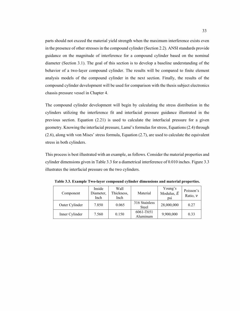
33

parts should not exceed the material yield strength when the maximum interference exists even

in the presence of other stresses in the compound cylinder (Section 2.2). ANSI standards provide

guidance on the magnitude of interference for a compound cylinder based on the nominal

diameter (Section 3.1). The goal of this section is to develop a baseline understanding of the

behavior of a two-layer compound cylinder. The results will be compared to finite element

analysis models of the compound cylinder in the next section. Finally, the results of the

compound cylinder development will be used for comparison with the thesis subject electronics

chassis pressure vessel in Chapter 4.

The compound cylinder development will begin by calculating the stress distribution in the

cylinders utilizing the interference fit and interfacial pressure guidance illustrated in the

previous section. Equation (2.21) is used to calculate the interfacial pressure for a given

geometry. Knowing the interfacial pressure, Lamé’s formulas for stress, Equations (2.4) through

(2.6), along with von Mises’ stress formula, Equation (2.7), are used to calculate the equivalent

stress in both cylinders.

This process is best illustrated with an example, as follows. Consider the material properties and

cylinder dimensions given in Table 3.3 for a diametrical interference of 0.010 inches. Figure 3.3

illustrates the interfacial pressure on the two cylinders.

Table 3.3. Example Two-layer compound cylinder dimensions and material properties.

Component

Inside

Diameter,

Inch

Wall

Thickness,

Inch

Material

Young’s

Modulus, 𝐸

psi

Poisson’s

Ratio, 𝜈

Outer Cylinder 7.850 0.065 316 Stainless

Steel 28,000,000 0.27

Inner Cylinder 7.560 0.150 6061-T651

Aluminum 9,900,000 0.33

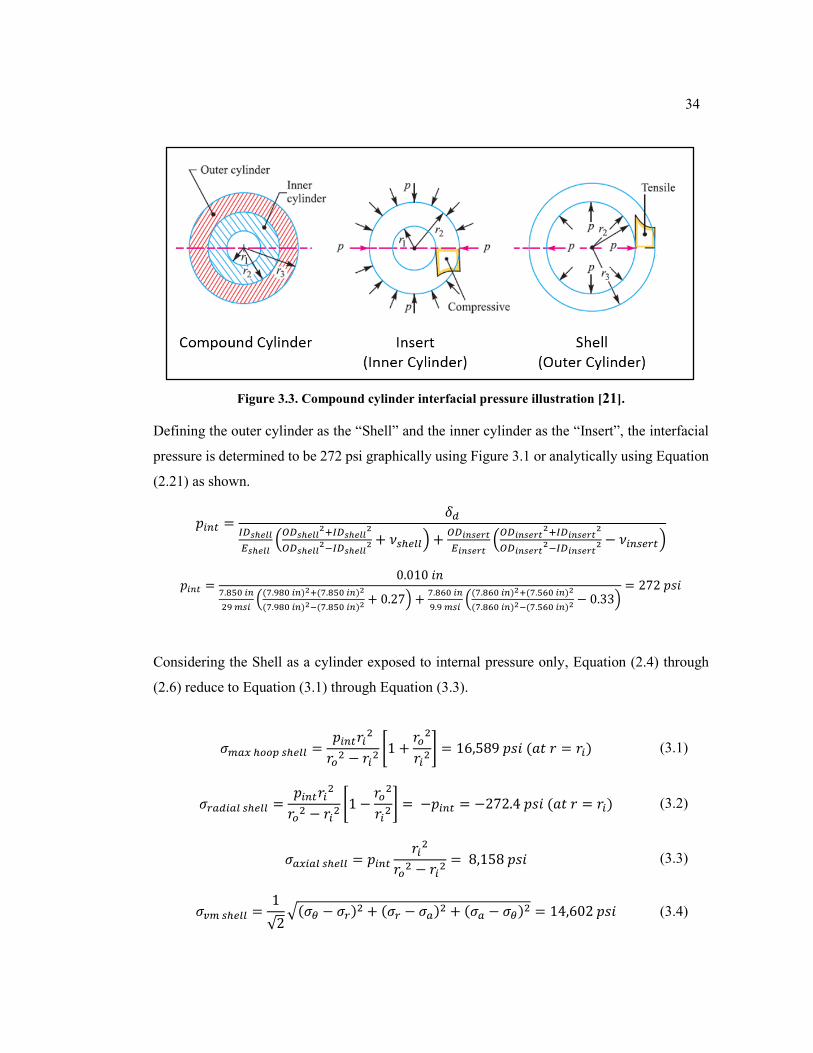
34

Figure 3.3. Compound cylinder interfacial pressure illustration [21].

Defining the outer cylinder as the “Shell” and the inner cylinder as the “Insert”, the interfacial

pressure is determined to be 272 psi graphically using Figure 3.1 or analytically using Equation

(2.21) as shown.

𝑝𝑖𝑛𝑡 =𝛿𝑑

𝐼𝐷𝑠ℎ𝑒𝑙𝑙

𝐸𝑠ℎ𝑒𝑙𝑙(𝑂𝐷𝑠ℎ𝑒𝑙𝑙

2+𝐼𝐷𝑠ℎ𝑒𝑙𝑙2

𝑂𝐷𝑠ℎ𝑒𝑙𝑙2−𝐼𝐷𝑠ℎ𝑒𝑙𝑙

2 + 𝜈𝑠ℎ𝑒𝑙𝑙) +𝑂𝐷𝑖𝑛𝑠𝑒𝑟𝑡

𝐸𝑖𝑛𝑠𝑒𝑟𝑡(𝑂𝐷𝑖𝑛𝑠𝑒𝑟𝑡

2+𝐼𝐷𝑖𝑛𝑠𝑒𝑟𝑡2

𝑂𝐷𝑖𝑛𝑠𝑒𝑟𝑡2−𝐼𝐷𝑖𝑛𝑠𝑒𝑟𝑡

2 − 𝜈𝑖𝑛𝑠𝑒𝑟𝑡)

𝑝𝑖𝑛𝑡 =0.010 𝑖𝑛

7.850 𝑖𝑛

29 𝑚𝑠𝑖((7.980 𝑖𝑛)2+(7.850 𝑖𝑛)2

(7.980 𝑖𝑛)2−(7.850 𝑖𝑛)2+ 0.27) +

7.860 𝑖𝑛

9.9 𝑚𝑠𝑖((7.860 𝑖𝑛)2+(7.560 𝑖𝑛)2

(7.860 𝑖𝑛)2−(7.560 𝑖𝑛)2− 0.33)

= 272 𝑝𝑠𝑖

Considering the Shell as a cylinder exposed to internal pressure only, Equation (2.4) through

(2.6) reduce to Equation (3.1) through Equation (3.3).

𝜎𝑚𝑎𝑥 ℎ𝑜𝑜𝑝 𝑠ℎ𝑒𝑙𝑙 =𝑝𝑖𝑛𝑡𝑟𝑖

2


2[1 +

𝑟𝑜2

𝑟𝑖2] = 16,589 𝑝𝑠𝑖 (𝑎𝑡 𝑟 = 𝑟𝑖) (3.1)

𝜎𝑟𝑎𝑑𝑖𝑎𝑙 𝑠ℎ𝑒𝑙𝑙 =𝑝𝑖𝑛𝑡𝑟𝑖

2


2[1 −

𝑟𝑜2

𝑟𝑖2] = −𝑝𝑖𝑛𝑡 = −272.4 𝑝𝑠𝑖 (𝑎𝑡 𝑟 = 𝑟𝑖) (3.2)

𝜎𝑎𝑥𝑖𝑎𝑙 𝑠ℎ𝑒𝑙𝑙 = 𝑝𝑖𝑛𝑡𝑟𝑖2


2= 8,158 𝑝𝑠𝑖 (3.3)

𝜎𝑣𝑚 𝑠ℎ𝑒𝑙𝑙 =1

√2√(𝜎𝜃 − 𝜎𝑟)

2 + (𝜎𝑟 − 𝜎𝑎)2 + (𝜎𝑎 − 𝜎𝜃)

2 = 14,602 𝑝𝑠𝑖 (3.4)

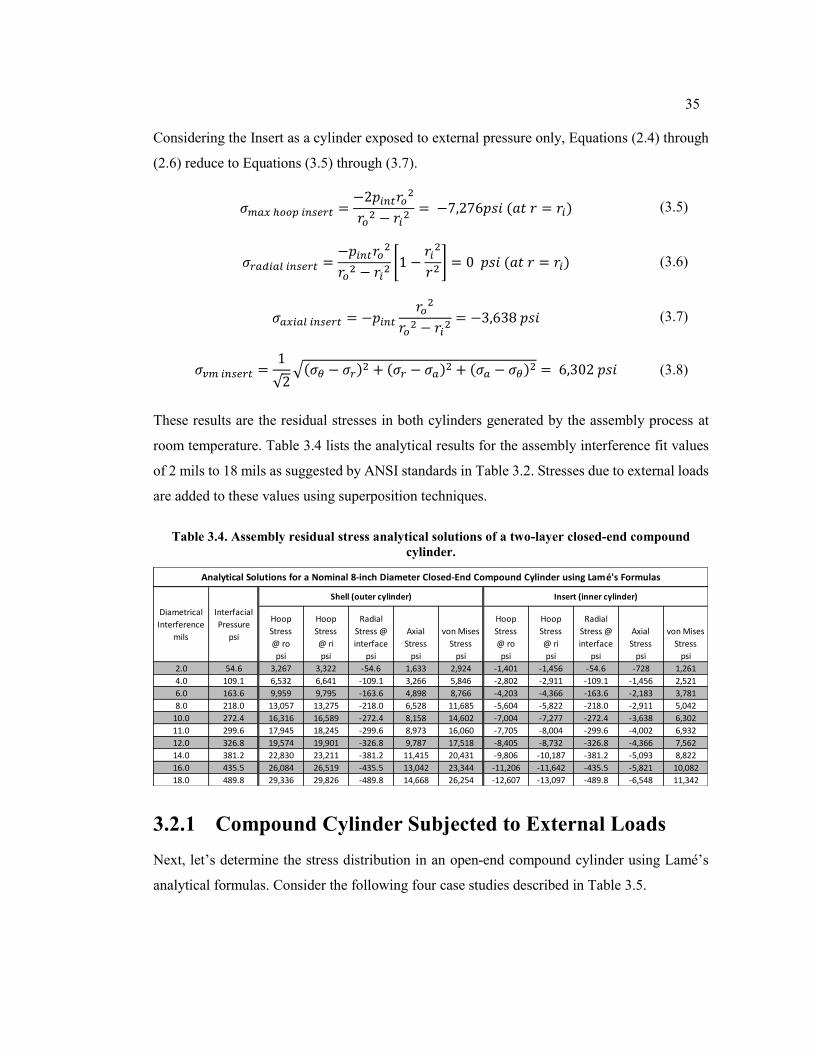
35

Considering the Insert as a cylinder exposed to external pressure only, Equations (2.4) through

(2.6) reduce to Equations (3.5) through (3.7).

𝜎𝑚𝑎𝑥 ℎ𝑜𝑜𝑝 𝑖𝑛𝑠𝑒𝑟𝑡 =−2𝑝𝑖𝑛𝑡𝑟𝑜

2


2= −7,276𝑝𝑠𝑖 (𝑎𝑡 𝑟 = 𝑟𝑖) (3.5)

𝜎𝑟𝑎𝑑𝑖𝑎𝑙 𝑖𝑛𝑠𝑒𝑟𝑡 =−𝑝𝑖𝑛𝑡𝑟𝑜

2


2[1 −

𝑟𝑖2

𝑟2] = 0 𝑝𝑠𝑖 (𝑎𝑡 𝑟 = 𝑟𝑖) (3.6)

𝜎𝑎𝑥𝑖𝑎𝑙 𝑖𝑛𝑠𝑒𝑟𝑡 = −𝑝𝑖𝑛𝑡𝑟𝑜2


2= −3,638 𝑝𝑠𝑖 (3.7)

𝜎𝑣𝑚 𝑖𝑛𝑠𝑒𝑟𝑡 =1

√2√(𝜎𝜃 − 𝜎𝑟)

2 + (𝜎𝑟 − 𝜎𝑎)2 + (𝜎𝑎 − 𝜎𝜃)

2 = 6,302 𝑝𝑠𝑖 (3.8)

These results are the residual stresses in both cylinders generated by the assembly process at

room temperature. Table 3.4 lists the analytical results for the assembly interference fit values

of 2 mils to 18 mils as suggested by ANSI standards in Table 3.2. Stresses due to external loads

are added to these values using superposition techniques.

Table 3.4. Assembly residual stress analytical solutions of a two-layer closed-end compound

cylinder.

3.2.1 Compound Cylinder Subjected to External Loads

Next, let’s determine the stress distribution in an open-end compound cylinder using Lamé’s

analytical formulas. Consider the following four case studies described in Table 3.5.

Hoop

Stress

@ ro

psi

Hoop

Stress

@ ri

psi

Radial

Stress @

interface

psi

Axial

Stress

psi

von Mises

Stress

psi

Hoop

Stress

@ ro

psi

Hoop

Stress

@ ri

psi

Radial

Stress @

interface

psi

Axial

Stress

psi

von Mises

Stress

psi

2.0 54.6 3,267 3,322 -54.6 1,633 2,924 -1,401 -1,456 -54.6 -728 1,261

4.0 109.1 6,532 6,641 -109.1 3,266 5,846 -2,802 -2,911 -109.1 -1,456 2,521

6.0 163.6 9,959 9,795 -163.6 4,898 8,766 -4,203 -4,366 -163.6 -2,183 3,781

8.0 218.0 13,057 13,275 -218.0 6,528 11,685 -5,604 -5,822 -218.0 -2,911 5,042

10.0 272.4 16,316 16,589 -272.4 8,158 14,602 -7,004 -7,277 -272.4 -3,638 6,302

11.0 299.6 17,945 18,245 -299.6 8,973 16,060 -7,705 -8,004 -299.6 -4,002 6,932

12.0 326.8 19,574 19,901 -326.8 9,787 17,518 -8,405 -8,732 -326.8 -4,366 7,562

14.0 381.2 22,830 23,211 -381.2 11,415 20,431 -9,806 -10,187 -381.2 -5,093 8,822

16.0 435.5 26,084 26,519 -435.5 13,042 23,344 -11,206 -11,642 -435.5 -5,821 10,082

18.0 489.8 29,336 29,826 -489.8 14,668 26,254 -12,607 -13,097 -489.8 -6,548 11,342

Shell (outer cylinder) Insert (inner cylinder)

Interfacial

Pressure

psi

Analytical Solutions for a Nominal 8-inch Diameter Closed-End Compound Cylinder using Lamé's Formulas

Diametrical

Interference

mils

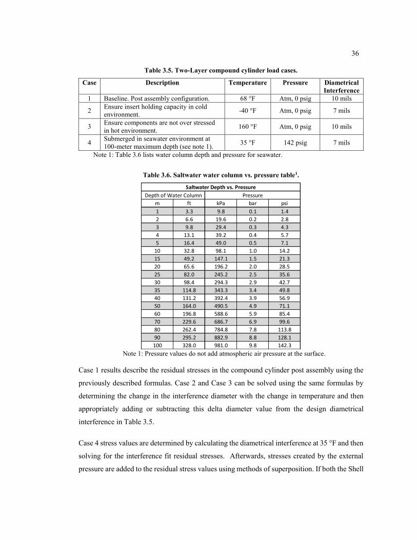
36

Table 3.5. Two-Layer compound cylinder load cases.

Case Description Temperature Pressure Diametrical

Interference

1 Baseline. Post assembly configuration. 68 °F Atm, 0 psig 10 mils

2 Ensure insert holding capacity in cold

environment. -40 °F Atm, 0 psig 7 mils

3 Ensure components are not over stressed

in hot environment. 160 °F Atm, 0 psig 10 mils

4 Submerged in seawater environment at

100-meter maximum depth (see note 1). 35 °F 142 psig 7 mils

Note 1: Table 3.6 lists water column depth and pressure for seawater.

Table 3.6. Saltwater water column vs. pressure table1.

Note 1: Pressure values do not add atmospheric air pressure at the surface.

Case 1 results describe the residual stresses in the compound cylinder post assembly using the

previously described formulas. Case 2 and Case 3 can be solved using the same formulas by

determining the change in the interference diameter with the change in temperature and then

appropriately adding or subtracting this delta diameter value from the design diametrical

interference in Table 3.5.

Case 4 stress values are determined by calculating the diametrical interference at 35 °F and then

solving for the interference fit residual stresses. Afterwards, stresses created by the external

pressure are added to the residual stress values using methods of superposition. If both the Shell

m ft kPa bar psi

1 3.3 9.8 0.1 1.4

2 6.6 19.6 0.2 2.8

3 9.8 29.4 0.3 4.3

4 13.1 39.2 0.4 5.7

5 16.4 49.0 0.5 7.1

10 32.8 98.1 1.0 14.2

15 49.2 147.1 1.5 21.3

20 65.6 196.2 2.0 28.5

25 82.0 245.2 2.5 35.6

30 98.4 294.3 2.9 42.7

35 114.8 343.3 3.4 49.8

40 131.2 392.4 3.9 56.9

50 164.0 490.5 4.9 71.1

60 196.8 588.6 5.9 85.4

70 229.6 686.7 6.9 99.6

80 262.4 784.8 7.8 113.8

90 295.2 882.9 8.8 128.1

100 328.0 981.0 9.8 142.3

Depth of Water Column Pressure

Saltwater Depth vs. Pressure

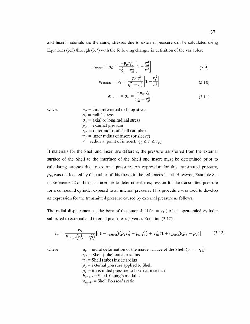
37

and Insert materials are the same, stresses due to external pressure can be calculated using

Equations (3.5) through (3.7) with the following changes in definition of the variables:

𝜎ℎ𝑜𝑜𝑝 = 𝜎𝜃 =−𝑝𝑜𝑟𝑡𝑜

2

𝑟𝑡𝑜2 − 𝑟𝑠𝑖

2 [1 +𝑟𝑠𝑖2

𝑟2] (3.9)

𝜎𝑟𝑎𝑑𝑖𝑎𝑙 = 𝜎𝑟 =−𝑝𝑜𝑟𝑡𝑜

2


2 [1 −𝑟𝑠𝑖2

𝑟2] (3.10)

𝜎𝑎𝑥𝑖𝑎𝑙 = 𝜎𝑎 =−𝑝𝑜𝑟𝑡𝑜

2


2 (3.11)

where 𝜎𝜃 = circumferential or hoop stress

𝜎𝑟 = radial stress

𝜎𝑎 = axial or longitudinal stress


𝑟𝑡𝑜 = outer radius of shell (or tube)

𝑟𝑠𝑖 = inner radius of insert (or sleeve)

𝑟 = radius at point of interest, 𝑟𝑠𝑖 ≤ 𝑟 ≤ 𝑟𝑡𝑜

If materials for the Shell and Insert are different, the pressure transferred from the external

surface of the Shell to the interface of the Shell and Insert must be determined prior to

calculating stresses due to external pressure. An expression for this transmitted pressure,

𝑝𝑇 , was not located by the author of this thesis in the references listed. However, Example 8.4

in Reference 22 outlines a procedure to determine the expression for the transmitted pressure

for a compound cylinder exposed to an internal pressure. This procedure was used to develop

an expression for the transmitted pressure caused by external pressure as follows.

The radial displacement at the bore of the outer shell (𝑟 = 𝑟𝑡𝑖) of an open-ended cylinder

subjected to external and internal pressure is given as Equation (3.12):

𝑢𝑟 =𝑟𝑡𝑖

𝐸𝑠ℎ𝑒𝑙𝑙(𝑟𝑡𝑜2 − 𝑟𝑡𝑖

2)[(1 − 𝜈𝑠ℎ𝑒𝑙𝑙)(𝑝𝑇𝑟𝑡𝑖

2 − 𝑝𝑜𝑟𝑡𝑜2 ) + 𝑟𝑡𝑜

2 (1 + 𝜈𝑠ℎ𝑒𝑙𝑙)(𝑝𝑇 − 𝑝𝑜)] (3.12)

where 𝑢𝑟 = radial deformation of the inside surface of the Shell ( 𝑟 = 𝑟𝑡𝑖) 𝑟𝑡𝑜 = Shell (tube) outside radius

𝑟𝑡𝑖 = Shell (tube) inside radius

𝑝𝑜 = external pressure applied to Shell

𝑝𝑇 = transmitted pressure to Insert at interface

𝐸𝑠ℎ𝑒𝑙𝑙 = Shell Young’s modulus

𝜈𝑠ℎ𝑒𝑙𝑙 = Shell Poisson’s ratio

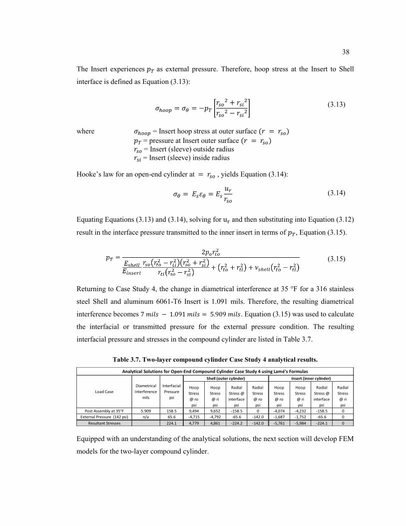
38

The Insert experiences 𝑝𝑇 as external pressure. Therefore, hoop stress at the Insert to Shell

interface is defined as Equation (3.13):

𝜎ℎ𝑜𝑜𝑝 = 𝜎𝜃 = −𝑝𝑇 [𝑟𝑠𝑜

2 + 𝑟𝑠𝑖2

𝑟𝑠𝑜2 − 𝑟𝑠𝑖

2]

(3.13)

where 𝜎ℎ𝑜𝑜𝑝 = Insert hoop stress at outer surface (𝑟 = 𝑟𝑠𝑜)

𝑝𝑇 = pressure at Insert outer surface (𝑟 = 𝑟𝑠𝑜) 𝑟𝑠𝑜 = Insert (sleeve) outside radius

𝑟𝑠𝑖 = Insert (sleeve) inside radius

Hooke’s law for an open-end cylinder at = 𝑟𝑠𝑜 , yields Equation (3.14):

𝜎𝜃 = 𝐸𝑠휀𝜃 = 𝐸𝑠𝑢𝑟𝑟𝑠𝑜

(3.14)

Equating Equations (3.13) and (3.14), solving for ur and then substituting into Equation (3.12)

result in the interface pressure transmitted to the inner insert in terms of 𝑝𝑇, Equation (3.15).

(3.15)

Returning to Case Study 4, the change in diametrical interference at 35 °F for a 316 stainless

steel Shell and aluminum 6061-T6 Insert is 1.091 mils. Therefore, the resulting diametrical

interference becomes 7 𝑚𝑖𝑙𝑠 − 1.091 𝑚𝑖𝑙𝑠 = 5.909 𝑚𝑖𝑙𝑠. Equation (3.15) was used to calculate

the interfacial or transmitted pressure for the external pressure condition. The resulting

interfacial pressure and stresses in the compound cylinder are listed in Table 3.7.

Table 3.7. Two-layer compound cylinder Case Study 4 analytical results.

Equipped with an understanding of the analytical solutions, the next section will develop FEM

models for the two-layer compound cylinder.

Hoop

Stress

@ ro

psi

Hoop

Stress

@ ri

psi

Radial

Stress @

interface

psi

Radial

Stress

@ ro

psi

Hoop

Stress

@ ro

psi

Hoop

Stress

@ ri

psi

Radial

Stress @

interface

psi

Radial

Stress

@ ri

psi

Post Assembly at 35°F 5.909 158.5 9,494 9,652 -158.5 0 -4,074 -4,232 -158.5 0

External Pressure (142 psi) n/a 65.6 -4,715 -4,792 -65.6 -142.0 -1,687 -1,752 -65.6 0

Resultant Stresses 224.1 4,779 4,861 -224.2 -142.0 -5,761 -5,984 -224.1 0

Analytical Solutions for Open-End Compound Cylinder Case Study 4 using Lamé's Formulas

Load Case

Diametrical

Interference

mils

Interfacial

Pressure

psi

Shell (outer cylinder) Insert (inner cylinder)

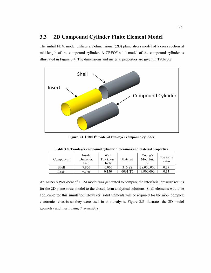
39

3.3 2D Compound Cylinder Finite Element Model

The initial FEM model utilizes a 2-dimensional (2D) plane stress model of a cross section at

mid-length of the compound cylinder. A CREO® solid model of the compound cylinder is

illustrated in Figure 3.4. The dimensions and material properties are given in Table 3.8.

Figure 3.4. CREO® model of two-layer compound cylinder.

Table 3.8. Two-layer compound cylinder dimensions and material properties.

Component

Inside

Diameter,

Inch

Wall

Thickness,

Inch

Material

Young’s

Modulus,

psi

Poisson’s

Ratio

Shell 7.850 0.065 316 SS 28,000,000 0.27

Insert varies 0.150 6061-T6 9,900,000 0.33

An ANSYS Workbench® FEM model was generated to compare the interfacial pressure results

for the 2D plane stress model to the closed-form analytical solutions. Shell elements would be

applicable for this simulation. However, solid elements will be required for the more complex

electronics chassis so they were used in this analysis. Figure 3.5 illustrates the 2D model

geometry and mesh using ¼ symmetry.

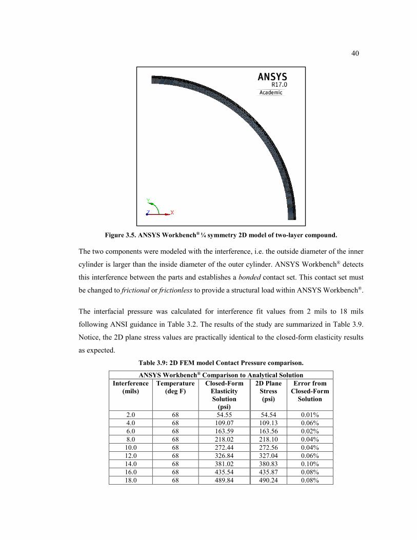
40

Figure 3.5. ANSYS Workbench® ¼ symmetry 2D model of two-layer compound.

The two components were modeled with the interference, i.e. the outside diameter of the inner

cylinder is larger than the inside diameter of the outer cylinder. ANSYS Workbench® detects

this interference between the parts and establishes a bonded contact set. This contact set must

be changed to frictional or frictionless to provide a structural load within ANSYS Workbench®.

The interfacial pressure was calculated for interference fit values from 2 mils to 18 mils

following ANSI guidance in Table 3.2. The results of the study are summarized in Table 3.9.

Notice, the 2D plane stress values are practically identical to the closed-form elasticity results

as expected.

Table 3.9: 2D FEM model Contact Pressure comparison.

ANSYS Workbench® Comparison to Analytical Solution

Interference

(mils)

Temperature

(deg F)

Closed-Form

Elasticity

Solution

(psi)

2D Plane

Stress

(psi)

Error from

Closed-Form

Solution

2.0 68 54.55 54.54 0.01%

4.0 68 109.07 109.13 0.06%

6.0 68 163.59 163.56 0.02%

8.0 68 218.02 218.10 0.04%

10.0 68 272.44 272.56 0.04%

12.0 68 326.84 327.04 0.06%

14.0 68 381.02 380.83 0.10%

16.0 68 435.54 435.87 0.08%

18.0 68 489.84 490.24 0.08%

41

Comparison of the 2D FEM model stress distribution to the analytical results for interference

fits of 2 mils, 10 mils and 18 mils are listed in Table 3.10. Observe that there is only a slight

difference in the results as expected since the contact pressure results are also nearly identical.

Table 3.10: Assembly residual stress results of a 2D FEM Plane Stress Model Comparison to the

Analytical Solutions.

The above values are the results of assembling the two-layer compound cylinder. No external

loads have been applied.

3.3.1 2D Compound Cylinder Subjected to External Loads

Next, consider the effects of external loads on the 2D plane stress model of the two-layer multi-

material compound cylinder assembly using shrink-fit guidance listed in Table 3.11 and the load

cases listed in Table 3.12.

Hoop

Stress

@ ro

psi

Hoop

Stress

@ ri

psi

Radial

Stress @

interface

psi

von Mises

Stress

psi

Hoop

Stress

@ ro

psi

Hoop

Stress

@ ri

psi

Radial

Stress @

interface

psi

von Mises

Stress

psi

2.0 54.6 3,267 3,322 -54.6 3,349 -1,401 -1,456 -54.6 1,456

10.0 272.4 16,316 16,589 -272.4 16,723 -7,004 -7,277 -272.4 7,275

18.0 489.8 29,336 29,826 -489.8 30,074 -12,607 -13,097 -489.8 13,097

Hoop

Stress

@ ro

psi

Hoop

Stress

@ ri

psi

Radial

Stress @

interface

psi

von Mises

Stress

psi

Hoop

Stress

@ ro

psi

Hoop

Stress

@ ri

psi

Radial

Stress @

interface

psi

von Mises

Stress

psi

2.0 54.6 3,268 3,322 -54.5 3,309 -1,401 -1,455 -54.6 1,414

10.0 272.5 16,332 16,605 -272.5 16,536 -6,997 -7,269 -272.5 7,060

18.0 490.2 29,399 29,889 -490.1 29,766 -12,586 -13,076 -489.9 12,702

Hoop

Stress

@ ro

psi

Hoop

Stress

@ ri

psi

Radial

Stress @

interface

psi

von Mises

Stress

psi

Hoop

Stress

@ ro

psi

Hoop

Stress

@ ri

psi

Radial

Stress @

interface

psi

von Mises

Stress

psi

2.0 0.00% 0.02% 0.02% 0.01% 1.21% 0.03% 0.03% 0.03% 2.91%

10.0 0.02% 0.10% 0.10% 0.02% 1.12% 0.11% 0.11% 0.02% 2.96%

18.0 0.08% 0.22% 0.21% 0.06% 1.02% 0.16% 0.16% 0.02% 3.02%

Analytical Solutions for a Nominal 8-inch Diameter Compound Cylinder using Lamé's Formulas

Diametrical

Interference

mils

Interfacial

Pressure

psi

Shell Insert

Diametrical

Interference

mils

Interfacial

Pressure

psi

Shell Insert

2D FEM Plane Stress Model Solution

Diametrical

Interference

mils

Interfacial

Pressure

psi

Shell Insert

% Error

42

Table 3.11. Comparison of ANSI Shrink Fit results for nominal 8-inch compound cylinder.

Table 3.12. Two-Layer compound cylinder load cases.


Interference




3 Ensure components not over stressed in

hot environment. 160 °F Atm, 0 psig 10 mils

4 Submerged in seawater environment at

100-meter maximum depth (see note 1). 35 °F 142 psig 7 mils

A Class FN 1 fit will produce only a “more or less permanent assembly.” The Insert must remain

permanent so a Class FN 2 fit is chosen as the minimum shrink fit for Case 2. Figure 3.2

illustrates that a change in temperature from 68 °F to -40 °F creates a 3.5 mils reduction in

interference diameter. Adding 3.5 mils to the Class FN 2 values equates to a minimum

diametrical interference fit range of 6.7 to 9.7 mils. Rounding up, the interference fit range for

the nominal 8-inch diameter assembly case study is chosen to be 7 mils to 10 mils.

To select the Shell material and nominal wall thickness, we need evaluate the failure mode for

the submerged Case 4. The buckling pressure and yielding pressure of a multi-material

compound cylinder is not easily calculated. A worst-case approximation can be obtained by

considering only the Shell as a standalone monobloc cylinder. Figure 3.6 through Figure 3.8

compare the minimum wall thickness of three commonly used pressure vessel materials: 316

stainless steel, grade 2 titanium and alloy 6061-T6 aluminum monobloc cylinders based on the

failure modes described by Equations (2.11), (2.13) and (2.18). In all materials, the predicted

failure mode at 142 psi is buckling, not yielding, in accordance with Equation (2.13).

Class FN 1 Class FN 2 Class FN 3 Class FN 4 Class FN 5

Diametrical Interference min. 2.3 3.2 5.2 8.2 13.2

mils max. 4.3 6.2 8.2 11.2 17.8

Interfacial Pressure min. 61.7 85.9 139.5 139.5 353.8

psi max. 115.4 166.3 219.9 300.3 476.7

Axial Holding Force min. 10,961 15,249 24,774 24,770 62,815

lbf max. 20,487 29,532 39,050 53,313 84,651

Holding Torque min. 43,022 59,853 97,236 97,222 246,547

lbf-inch max. 80,412 115,914 153,270 209,254 332,256

Note: 1 mil = 1/1000 inch

ANSI Standard Force and Shrink Fits ANSI B4.1-1969 (R1987)

Nominal 8-inch diameter by 24-inch long Compound Cylinder

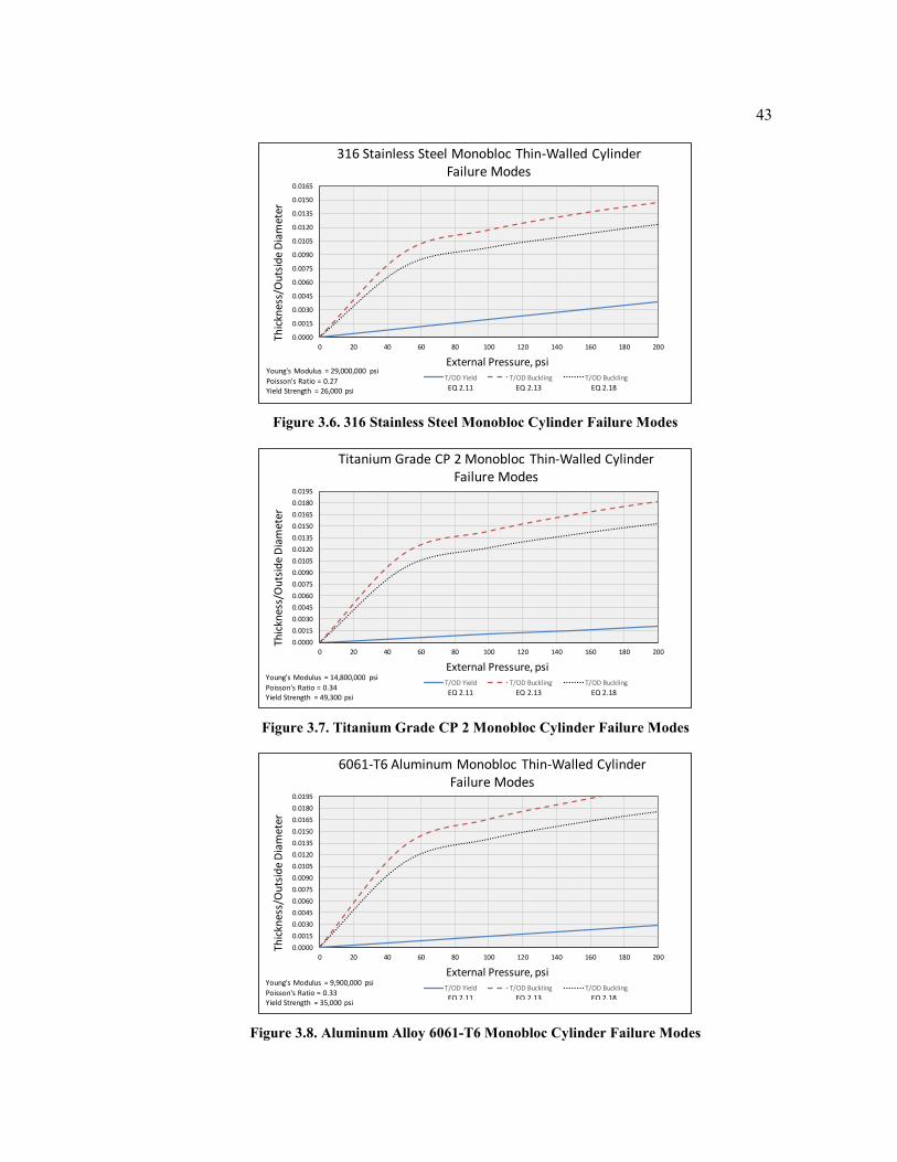
43

Figure 3.6. 316 Stainless Steel Monobloc Cylinder Failure Modes

Figure 3.7. Titanium Grade CP 2 Monobloc Cylinder Failure Modes

Figure 3.8. Aluminum Alloy 6061-T6 Monobloc Cylinder Failure Modes

0.0000

0.0015

0.0030

0.0045

0.0060

0.0075

0.0090

0.0105

0.0120

0.0135

0.0150

0.0165

0 20 40 60 80 100 120 140 160 180 200

Thic

knes

s/O

uts

ide

Dia

met

er


316 Stainless Steel Monobloc Thin-Walled Cylinder Failure Modes

T/OD Yield T/OD Buckling T/OD Buckling

EQ 2.11 EQ 2.13 EQ 2.18



0.0000

0.0015

0.0030

0.0045

0.0060

0.0075

0.0090

0.0105

0.0120

0.0135

0.0150

0.0165

0.0180

0.0195

0 20 40 60 80 100 120 140 160 180 200

Thic

knes

s/O

uts

ide

Dia

met

er


Titanium Grade CP 2 Monobloc Thin-Walled Cylinder Failure Modes


EQ 2.11 EQ 2.13 EQ 2.18



0.0000

0.0015

0.0030

0.0045

0.0060

0.0075

0.0090

0.0105

0.0120

0.0135

0.0150

0.0165

0.0180

0.0195

0 20 40 60 80 100 120 140 160 180 200

Thic

knes

s/O

uts

ide

Dia

met

er


6061-T6 Aluminum Monobloc Thin-Walled Cylinder Failure Modes


EQ 2.11 EQ 2.13 EQ 2.18



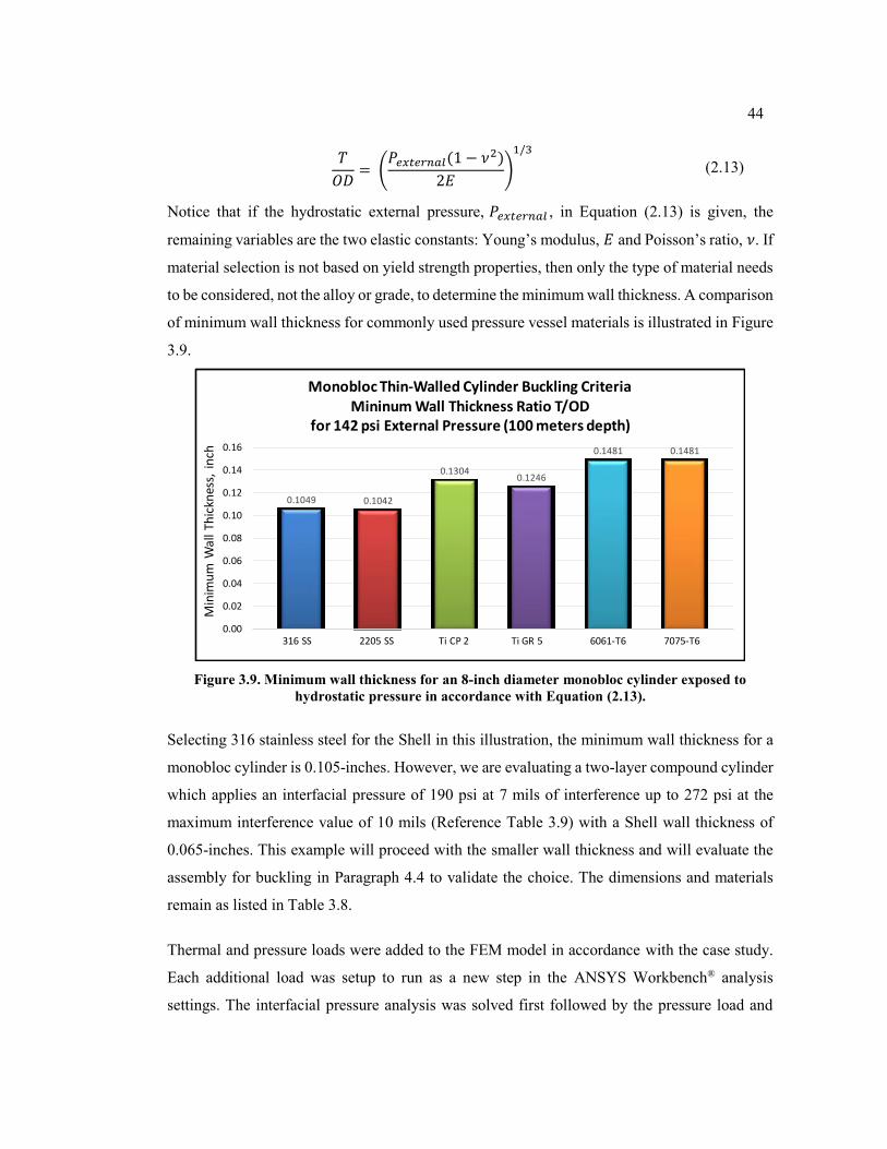
44

𝑇

𝑂𝐷= (

𝑃𝑒𝑥𝑡𝑒𝑟𝑛𝑎𝑙(1 − 𝜈2)

2𝐸)

1/3

(2.13)

Notice that if the hydrostatic external pressure, 𝑃𝑒𝑥𝑡𝑒𝑟𝑛𝑎𝑙 , in Equation (2.13) is given, the

remaining variables are the two elastic constants: Young’s modulus, 𝐸 and Poisson’s ratio, 𝜈. If

material selection is not based on yield strength properties, then only the type of material needs

to be considered, not the alloy or grade, to determine the minimum wall thickness. A comparison

of minimum wall thickness for commonly used pressure vessel materials is illustrated in Figure

3.9.

Figure 3.9. Minimum wall thickness for an 8-inch diameter monobloc cylinder exposed to

hydrostatic pressure in accordance with Equation (2.13).

Selecting 316 stainless steel for the Shell in this illustration, the minimum wall thickness for a

monobloc cylinder is 0.105-inches. However, we are evaluating a two-layer compound cylinder

which applies an interfacial pressure of 190 psi at 7 mils of interference up to 272 psi at the

maximum interference value of 10 mils (Reference Table 3.9) with a Shell wall thickness of

0.065-inches. This example will proceed with the smaller wall thickness and will evaluate the

assembly for buckling in Paragraph 4.4 to validate the choice. The dimensions and materials

remain as listed in Table 3.8.

Thermal and pressure loads were added to the FEM model in accordance with the case study.

Each additional load was setup to run as a new step in the ANSYS Workbench® analysis

settings. The interfacial pressure analysis was solved first followed by the pressure load and

0.1049 0.1042

0.13040.1246

0.1481 0.1481

0.00

0.02

0.04

0.06

0.08

0.10

0.12

0.14

0.16

Min

imu

m W

all

Thic

knes

s, i

nch

Monobloc Thin-Walled Cylinder Buckling Criteria Mininum Wall Thickness Ratio T/OD

for 142 psi External Pressure (100 meters depth)

316 SS 2205 SS Ti CP 2 Ti GR 5 6061-T6 7075-T6

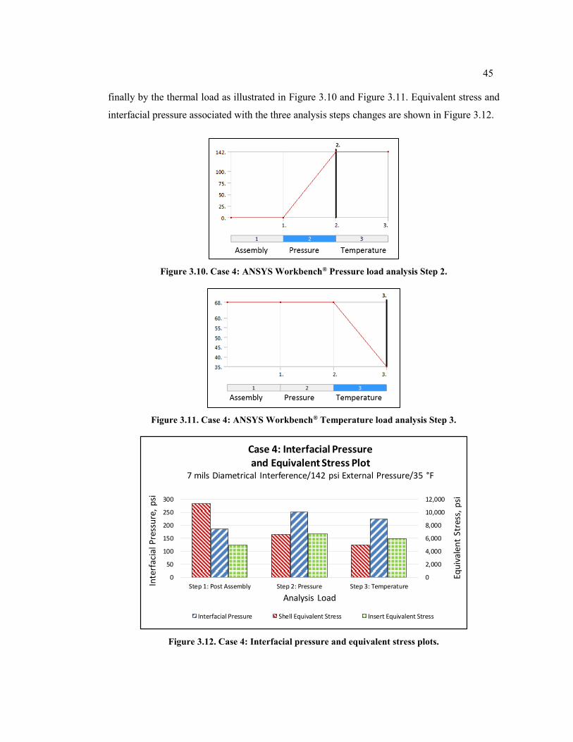
45

finally by the thermal load as illustrated in Figure 3.10 and Figure 3.11. Equivalent stress and

interfacial pressure associated with the three analysis steps changes are shown in Figure 3.12.

Figure 3.10. Case 4: ANSYS Workbench® Pressure load analysis Step 2.

Figure 3.11. Case 4: ANSYS Workbench® Temperature load analysis Step 3.

Figure 3.12. Case 4: Interfacial pressure and equivalent stress plots.

0

2,000

4,000

6,000

8,000

10,000

12,000

0

50

100

150

200

250

300

Step 1: Post Assembly Step 2: Pressure Step 3: Temperature

Equ

ival

ent

Stre

ss,

psi

Inte

rfac

ial P

ress

ure

, p

si

Analysis Load

Case 4: Interfacial Pressure and Equivalent Stress Plot

7 mils Diametrical Interference/142 psi External Pressure/35 °F

Interfacial Pressure Shell Equivalent Stress Insert Equivalent Stress

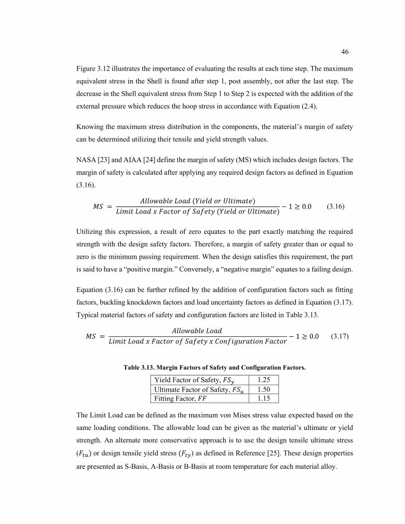
46

Figure 3.12 illustrates the importance of evaluating the results at each time step. The maximum

equivalent stress in the Shell is found after step 1, post assembly, not after the last step. The

decrease in the Shell equivalent stress from Step 1 to Step 2 is expected with the addition of the

external pressure which reduces the hoop stress in accordance with Equation (2.4).

Knowing the maximum stress distribution in the components, the material’s margin of safety

can be determined utilizing their tensile and yield strength values.

NASA [23] and AIAA [24] define the margin of safety (MS) which includes design factors. The

margin of safety is calculated after applying any required design factors as defined in Equation

(3.16).

𝑀𝑆 = 𝐴𝑙𝑙𝑜𝑤𝑎𝑏𝑙𝑒 𝐿𝑜𝑎𝑑 (𝑌𝑖𝑒𝑙𝑑 𝑜𝑟 𝑈𝑙𝑡𝑖𝑚𝑎𝑡𝑒)

𝐿𝑖𝑚𝑖𝑡 𝐿𝑜𝑎𝑑 𝑥 𝐹𝑎𝑐𝑡𝑜𝑟 𝑜𝑓 𝑆𝑎𝑓𝑒𝑡𝑦 (𝑌𝑖𝑒𝑙𝑑 𝑜𝑟 𝑈𝑙𝑡𝑖𝑚𝑎𝑡𝑒)− 1 ≥ 0.0 (3.16)

Utilizing this expression, a result of zero equates to the part exactly matching the required

strength with the design safety factors. Therefore, a margin of safety greater than or equal to

zero is the minimum passing requirement. When the design satisfies this requirement, the part

is said to have a “positive margin.” Conversely, a “negative margin” equates to a failing design.

Equation (3.16) can be further refined by the addition of configuration factors such as fitting

factors, buckling knockdown factors and load uncertainty factors as defined in Equation (3.17).

Typical material factors of safety and configuration factors are listed in Table 3.13.

𝑀𝑆 = 𝐴𝑙𝑙𝑜𝑤𝑎𝑏𝑙𝑒 𝐿𝑜𝑎𝑑

𝐿𝑖𝑚𝑖𝑡 𝐿𝑜𝑎𝑑 𝑥 𝐹𝑎𝑐𝑡𝑜𝑟 𝑜𝑓 𝑆𝑎𝑓𝑒𝑡𝑦 𝑥 𝐶𝑜𝑛𝑓𝑖𝑔𝑢𝑟𝑎𝑡𝑖𝑜𝑛 𝐹𝑎𝑐𝑡𝑜𝑟− 1 ≥ 0.0 (3.17)

Table 3.13. Margin Factors of Safety and Configuration Factors.

Yield Factor of Safety, 𝐹𝑆𝑦 1.25

Ultimate Factor of Safety, 𝐹𝑆𝑢 1.50

Fitting Factor, 𝐹𝐹 1.15

The Limit Load can be defined as the maximum von Mises stress value expected based on the

same loading conditions. The allowable load can be given as the material’s ultimate or yield

strength. An alternate more conservative approach is to use the design tensile ultimate stress

(𝐹𝑡𝑢) or design tensile yield stress (𝐹𝑡𝑦) as defined in Reference [25]. These design properties

are presented as S-Basis, A-Basis or B-Basis at room temperature for each material alloy.

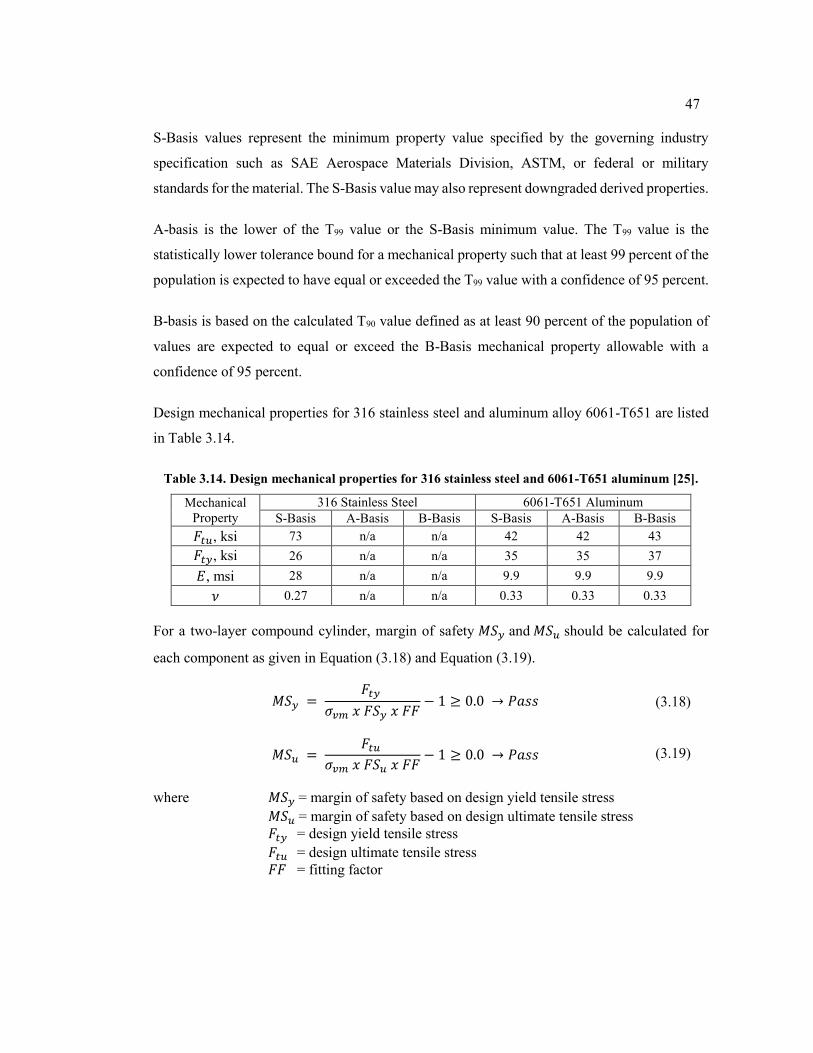
47

S-Basis values represent the minimum property value specified by the governing industry

specification such as SAE Aerospace Materials Division, ASTM, or federal or military

standards for the material. The S-Basis value may also represent downgraded derived properties.

A-basis is the lower of the T99 value or the S-Basis minimum value. The T99 value is the

statistically lower tolerance bound for a mechanical property such that at least 99 percent of the

population is expected to have equal or exceeded the T99 value with a confidence of 95 percent.

B-basis is based on the calculated T90 value defined as at least 90 percent of the population of

values are expected to equal or exceed the B-Basis mechanical property allowable with a

confidence of 95 percent.

Design mechanical properties for 316 stainless steel and aluminum alloy 6061-T651 are listed

in Table 3.14.

Table 3.14. Design mechanical properties for 316 stainless steel and 6061-T651 aluminum [25].

Mechanical

Property

316 Stainless Steel 6061-T651 Aluminum

S-Basis A-Basis B-Basis S-Basis A-Basis B-Basis

𝐹𝑡𝑢, ksi 73 n/a n/a 42 42 43

𝐹𝑡𝑦, ksi 26 n/a n/a 35 35 37

𝐸, msi 28 n/a n/a 9.9 9.9 9.9

𝜈 0.27 n/a n/a 0.33 0.33 0.33

For a two-layer compound cylinder, margin of safety 𝑀𝑆𝑦 and 𝑀𝑆𝑢 should be calculated for

each component as given in Equation (3.18) and Equation (3.19).

𝑀𝑆𝑦 = 𝐹𝑡𝑦

𝜎𝑣𝑚 𝑥 𝐹𝑆𝑦 𝑥 𝐹𝐹− 1 ≥ 0.0 → 𝑃𝑎𝑠𝑠 (3.18)

𝑀𝑆𝑢 = 𝐹𝑡𝑢

𝜎𝑣𝑚 𝑥 𝐹𝑆𝑢 𝑥 𝐹𝐹− 1 ≥ 0.0 → 𝑃𝑎𝑠𝑠 (3.19)

where 𝑀𝑆𝑦 = margin of safety based on design yield tensile stress

𝑀𝑆𝑢 = margin of safety based on design ultimate tensile stress

𝐹𝑡𝑦 = design yield tensile stress

𝐹𝑡𝑢 = design ultimate tensile stress

𝐹𝐹 = fitting factor

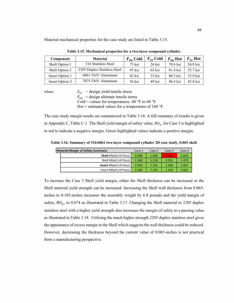
48

Material mechanical properties for the case study are listed in Table 3.15.

Table 3.15. Mechanical properties for a two-layer compound cylinder.

Component Material 𝑭𝒕𝒖 Cold 𝑭𝒕𝒚 Cold 𝑭𝒕𝒖 Hot 𝑭𝒕𝒚 Hot

Shell Option 1 316 Stainless Steel 73 ksi 26 ksi 70.6 ksi 24.8 ksi

Shell Option 2 2205 Duplex Stainless Steel 95 ksi 65 ksi 81.4 ksi 55.7 ksi

Insert Option 1 6061-T651 Aluminum 42 ksi 35 ksi 40.3 ksi 33.9 ksi


where 𝐹𝑡𝑦 = design yield tensile stress


Cold = values for temperatures -40 °F to 68 °F.

Hot = estimated values for a temperature of 160 °F.

The case study margin results are summarized in Table 3.16. A full summary of results is given

in Appendix C, Table C-1. The Shell yield margin of safety value, 𝑀𝑆𝑦 , for Case 3 is highlighted

in red to indicate a negative margin. Green highlighted values indicate a positive margin.

Table 3.16. Summary of 316/6061 two-layer compound cylinder 2D case study, 0.065 shell.

To increase the Case 3 Shell yield margin, either the Shell thickness can be increased or the

Shell material yield strength can be increased. Increasing the Shell wall thickness from 0.065-

inches to 0.105-inches increases the assembly weight by 6.8 pounds and the yield margin of

safety, 𝑀𝑆𝑦, to 0.074 as illustrated in Table 3.17. Changing the Shell material to 2205 duplex

stainless steel with a higher yield strength also increases the margin of safety to a passing value

as illustrated in Table 3.18. Utilizing the much higher strength 2205 duplex stainless steel gives

the appearance of excess margin in the Shell which suggests the wall thickness could be reduced.

However, decreasing the thickness beyond the current value of 0.065-inches is not practical

from a manufacturing perspective.

Case Description: Case 1 Case 2 Case 3 Case 4

Interference: Max Min Max Min

Temperature: Room Cold Hot Cold

Pressure: None None None High

Geometry: Case 1 Case 2 Case 3 Case 4

Shell Material:

Shell ID (in): 7.850 7.850 7.850 7.850

Shell Wall Thickness (in): 0.065 0.065 0.065 0.065

Insert Material:

Insert OD (in): 7.860 7.857 7.860 7.857

Insert Wall Thickness (in) 0.150 0.150 0.150 0.150

Interference-Fit Diametric Interference (mil): 10.0 7.0 10.0 7.0

Length of Shell (in): 24.0 24.0 24.0 24.0

Length of Insert (in): 24.0 24.0 24.0 24.0

Thermal Case: Case 1 Case 2 Case 3 Case 4

T (F): 68.0 -40.0 160.0 35.0

T (C): 20.0 -40.0 71.1 1.7

Pressure Case: Case 1 Case 2 Case 3 Case 4

Pressure (psig): 0.0 0.0 0.0 142.0

Results: Case 1 Case 2 Case 3 Case 4

Max. Contact Pressure (psi): 268.6 111.2 345.3 224.8

Average Contact Pressure (psi): 268.2 110.8 344.9 224.4

Max. Shell Hoop Stress (psi): 16,344.0 6,749.8 21,019.0 4,874.9

Max. Shell Radial Stress (psi): -268.6 -111.2 -345.6 -224.8

Max. Shell von Mises Stress (psi): 16,480.0 6,805.9 21,194.0 4,990.8

Max. Insert Hoop Stress (psi): -7,154.9 -2,958.2 -9,193.2 -5,987.1

Max. Insert Radial Stress (psi): -268.4 -111.1 -344.9 -224.7

Max. Insert von Mises Stress (psi): 7,154.9 2,958.1 9,193.2 5,987.1

Material Margin of Safety Summary: Case 1 Case 2 Case 3 Case 4

Shell MSyld (>0 Pass): 0.098 1.658 -0.187 2.624

Shell MSult (>0 Pass): 1.568 5.218 0.931 7.479

Insert MSyld (>0 Pass): 2.403 7.231 1.569 3.067

Insert MSult (>0 Pass): 2.403 7.231 1.543 3.067

Radial Deformation (2x Max/Min for Diametric): Case 1 Case 2 Case 3 Case 4

Shell X-Deformation (mil): 2.3 -3.0 6.1 -0.6

Shell Y-Deformation (mil): 2.3 -3.0 6.1 -0.6

Out of Round Dimension (mil): 0.0 0.0 0.0 0.0

Slippage Summary: Case 1 Case 2 Case 3 Case 4

Axial Holding Force (lbf): 47,628 19,677 61,238 39,850

Holding Torque (in-lb): 186,939 77,232 240,359 156,413

316 Stainless Steel

Aluminum Alloy 6061-T651

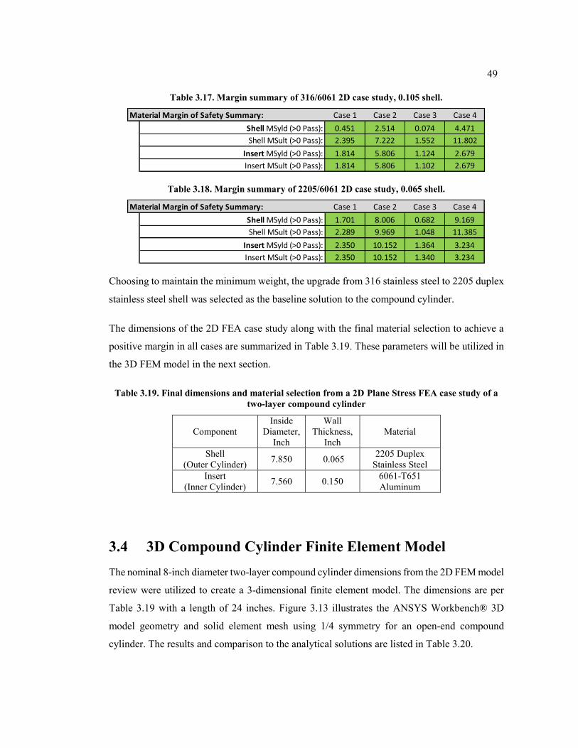
49

Table 3.17. Margin summary of 316/6061 2D case study, 0.105 shell.

Table 3.18. Margin summary of 2205/6061 2D case study, 0.065 shell.

Choosing to maintain the minimum weight, the upgrade from 316 stainless steel to 2205 duplex

stainless steel shell was selected as the baseline solution to the compound cylinder.

The dimensions of the 2D FEA case study along with the final material selection to achieve a

positive margin in all cases are summarized in Table 3.19. These parameters will be utilized in

the 3D FEM model in the next section.

Table 3.19. Final dimensions and material selection from a 2D Plane Stress FEA case study of a

two-layer compound cylinder

Component

Inside

Diameter,

Inch

Wall

Thickness,

Inch

Material

Shell

(Outer Cylinder) 7.850 0.065

2205 Duplex

Stainless Steel

Insert

(Inner Cylinder) 7.560 0.150

6061-T651

Aluminum

3.4 3D Compound Cylinder Finite Element Model

The nominal 8-inch diameter two-layer compound cylinder dimensions from the 2D FEM model

review were utilized to create a 3-dimensional finite element model. The dimensions are per

Table 3.19 with a length of 24 inches. Figure 3.13 illustrates the ANSYS Workbench® 3D

model geometry and solid element mesh using 1/4 symmetry for an open-end compound

cylinder. The results and comparison to the analytical solutions are listed in Table 3.20.


Shell MSyld (>0 Pass): 0.451 2.514 0.074 4.471

Shell MSult (>0 Pass): 2.395 7.222 1.552 11.802




Shell MSyld (>0 Pass): 1.701 8.006 0.682 9.169

Shell MSult (>0 Pass): 2.289 9.969 1.048 11.385



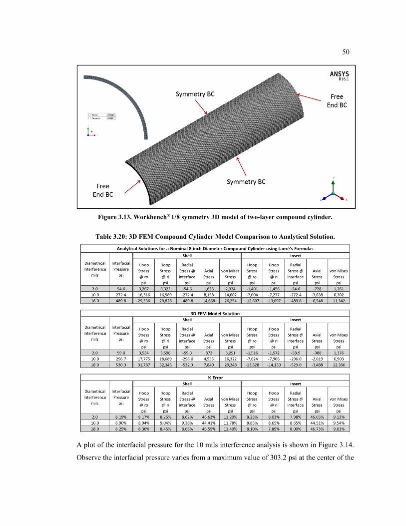
50

Figure 3.13. Workbench® 1/8 symmetry 3D model of two-layer compound cylinder.

Table 3.20: 3D FEM Compound Cylinder Model Comparison to Analytical Solution.

A plot of the interfacial pressure for the 10 mils interference analysis is shown in Figure 3.14.

Observe the interfacial pressure varies from a maximum value of 303.2 psi at the center of the

Hoop

Stress

@ ro

psi

Hoop

Stress

@ ri

psi

Radial

Stress @

interface

psi

Axial

Stress

psi

von Mises

Stress

psi

Hoop

Stress

@ ro

psi

Hoop

Stress

@ ri

psi

Radial

Stress @

interface

psi

Axial

Stress

psi

von Mises

Stress

psi

2.0 54.6 3,267 3,322 -54.6 1,633 2,924 -1,401 -1,456 -54.6 -728 1,261

10.0 272.4 16,316 16,589 -272.4 8,158 14,602 -7,004 -7,277 -272.4 -3,638 6,302

18.0 489.8 29,336 29,826 -489.8 14,668 26,254 -12,607 -13,097 -489.8 -6,548 11,342

Hoop

Stress

@ ro

psi

Hoop

Stress

@ ri

psi

Radial

Stress @

interface

psi

Axial

Stress

psi

von Mises

Stress

psi

Hoop

Stress

@ ro

psi

Hoop

Stress

@ ri

psi

Radial

Stress @

interface

psi

Axial

Stress

psi

von Mises

Stress

psi

2.0 59.0 3,534 3,596 -59.3 872 3,251 -1,516 -1,572 -58.9 -388 1,376

10.0 296.7 17,775 18,089 -298.0 4,535 16,322 -7,624 -7,906 -296.0 -2,019 6,903

18.0 530.3 31,787 32,345 -532.3 7,840 29,248 -13,628 -14,130 -529.0 -3,488 12,366

Hoop

Stress

@ ro

psi

Hoop

Stress

@ ri

psi

Radial

Stress @

interface

psi

Axial

Stress

psi

von Mises

Stress

psi

Hoop

Stress

@ ro

psi

Hoop

Stress

@ ri

psi

Radial

Stress @

interface

psi

Axial

Stress

psi

von Mises

Stress

psi

2.0 8.19% 8.17% 8.26% 8.62% 46.62% 11.20% 8.23% 8.03% 7.98% 46.65% 9.13%

10.0 8.90% 8.94% 9.04% 9.38% 44.41% 11.78% 8.85% 8.65% 8.65% 44.51% 9.54%

18.0 8.25% 8.36% 8.45% 8.68% 46.55% 11.40% 8.10% 7.89% 8.00% 46.73% 9.03%

Shell Insert

Interfacial

Pressure

psi

Interfacial

Pressure

psi

Analytical Solutions for a Nominal 8-inch Diameter Compound Cylinder using Lamé's Formulas

3D FEM Model SolutionShell Insert

% ErrorShell Insert

Diametrical

Interference

mils

Interfacial

Pressure

psi

Diametrical

Interference

mils

Diametrical

Interference

mils

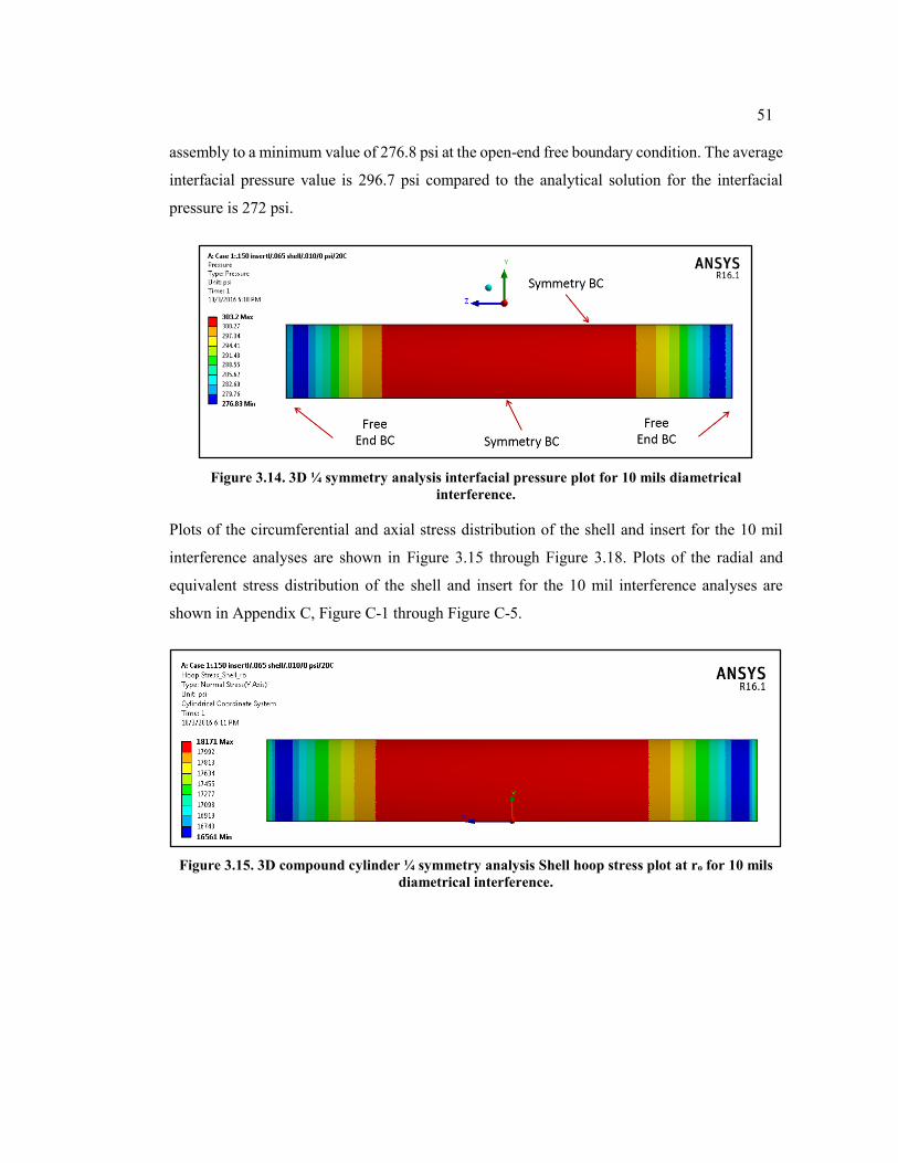
51

assembly to a minimum value of 276.8 psi at the open-end free boundary condition. The average

interfacial pressure value is 296.7 psi compared to the analytical solution for the interfacial

pressure is 272 psi.

Figure 3.14. 3D ¼ symmetry analysis interfacial pressure plot for 10 mils diametrical

interference.

Plots of the circumferential and axial stress distribution of the shell and insert for the 10 mil

interference analyses are shown in Figure 3.15 through Figure 3.18. Plots of the radial and

equivalent stress distribution of the shell and insert for the 10 mil interference analyses are

shown in Appendix C, Figure C-1 through Figure C-5.

Figure 3.15. 3D compound cylinder ¼ symmetry analysis Shell hoop stress plot at ro for 10 mils

diametrical interference.

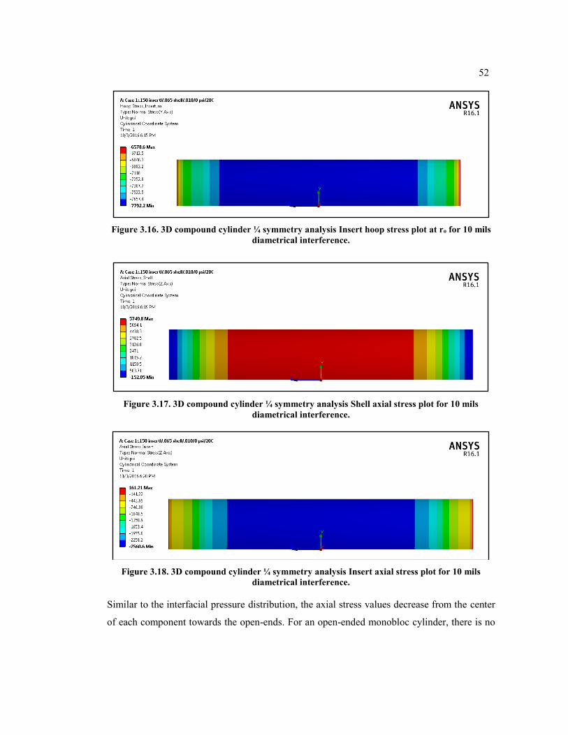
52

Figure 3.16. 3D compound cylinder ¼ symmetry analysis Insert hoop stress plot at ro for 10 mils


Figure 3.17. 3D compound cylinder ¼ symmetry analysis Shell axial stress plot for 10 mils


Figure 3.18. 3D compound cylinder ¼ symmetry analysis Insert axial stress plot for 10 mils


Similar to the interfacial pressure distribution, the axial stress values decrease from the center

of each component towards the open-ends. For an open-ended monobloc cylinder, there is no

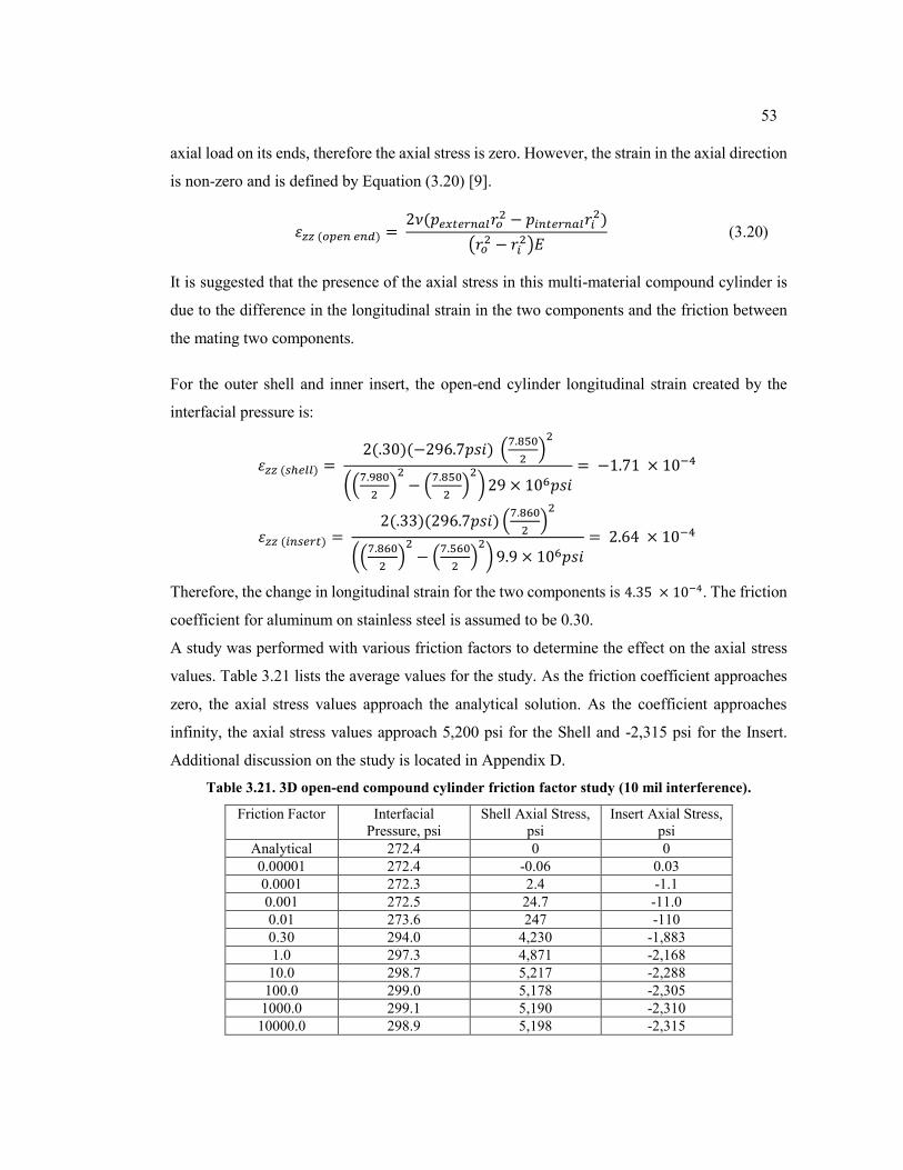
53

axial load on its ends, therefore the axial stress is zero. However, the strain in the axial direction

is non-zero and is defined by Equation (3.20) [9].

휀𝑧𝑧 (𝑜𝑝𝑒𝑛 𝑒𝑛𝑑) = 2𝜈(𝑝𝑒𝑥𝑡𝑒𝑟𝑛𝑎𝑙𝑟𝑜

2 − 𝑝𝑖𝑛𝑡𝑒𝑟𝑛𝑎𝑙𝑟𝑖2)

(𝑟𝑜2 − 𝑟𝑖

2)𝐸 (3.20)

It is suggested that the presence of the axial stress in this multi-material compound cylinder is

due to the difference in the longitudinal strain in the two components and the friction between

the mating two components.

For the outer shell and inner insert, the open-end cylinder longitudinal strain created by the

interfacial pressure is:

휀𝑧𝑧 (𝑠ℎ𝑒𝑙𝑙) = 2(.30)(−296.7𝑝𝑠𝑖) (

7.850

2)2

((7.980

2)2− (

7.850

2)2)29 × 106𝑝𝑠𝑖

= −1.71 × 10−4

휀𝑧𝑧 (𝑖𝑛𝑠𝑒𝑟𝑡) = 2(.33)(296.7𝑝𝑠𝑖) (

7.860

2)2

((7.860

2)2− (

7.560

2)2) 9.9 × 106𝑝𝑠𝑖

= 2.64 × 10−4

Therefore, the change in longitudinal strain for the two components is 4.35 × 10−4. The friction

coefficient for aluminum on stainless steel is assumed to be 0.30.

A study was performed with various friction factors to determine the effect on the axial stress

values. Table 3.21 lists the average values for the study. As the friction coefficient approaches

zero, the axial stress values approach the analytical solution. As the coefficient approaches

infinity, the axial stress values approach 5,200 psi for the Shell and -2,315 psi for the Insert.

Additional discussion on the study is located in Appendix D.

Table 3.21. 3D open-end compound cylinder friction factor study (10 mil interference).

Friction Factor Interfacial

Pressure, psi

Shell Axial Stress,

psi

Insert Axial Stress,

psi

Analytical 272.4 0 0

0.00001 272.4 -0.06 0.03

0.0001 272.3 2.4 -1.1

0.001 272.5 24.7 -11.0

0.01 273.6 247 -110

0.30 294.0 4,230 -1,883

1.0 297.3 4,871 -2,168

10.0 298.7 5,217 -2,288

100.0 299.0 5,178 -2,305

1000.0 299.1 5,190 -2,310

10000.0 298.9 5,198 -2,315

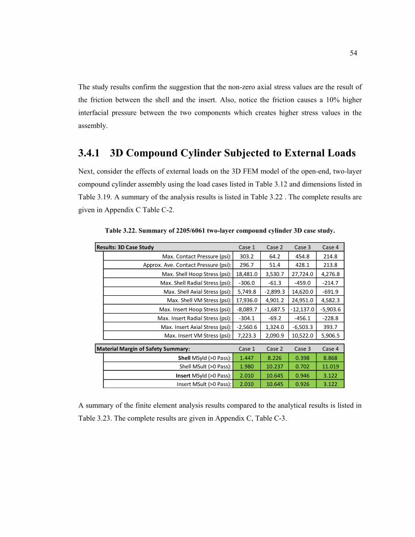
54

The study results confirm the suggestion that the non-zero axial stress values are the result of

the friction between the shell and the insert. Also, notice the friction causes a 10% higher

interfacial pressure between the two components which creates higher stress values in the

assembly.

3.4.1 3D Compound Cylinder Subjected to External Loads

Next, consider the effects of external loads on the 3D FEM model of the open-end, two-layer

compound cylinder assembly using the load cases listed in Table 3.12 and dimensions listed in

Table 3.19. A summary of the analysis results is listed in Table 3.22 . The complete results are

given in Appendix C Table C-2.

Table 3.22. Summary of 2205/6061 two-layer compound cylinder 3D case study.

A summary of the finite element analysis results compared to the analytical results is listed in

Table 3.23. The complete results are given in Appendix C, Table C-3.

Results: 3D Case Study Case 1 Case 2 Case 3 Case 4


Approx. Ave. Contact Pressure (psi): 296.7 51.4 428.1 213.8



Max. Shell Axial Stress (psi): 5,749.8 -2,899.3 14,620.0 -691.9

Max. Shell VM Stress (psi): 17,936.0 4,901.2 24,951.0 4,582.3



Max. Insert Axial Stress (psi): -2,560.6 1,324.0 -6,503.3 393.7

Max. Insert VM Stress (psi): 7,223.3 2,090.9 10,522.0 5,906.5


Shell MSyld (>0 Pass): 1.447 8.226 0.398 8.868

Shell MSult (>0 Pass): 1.980 10.237 0.702 11.019



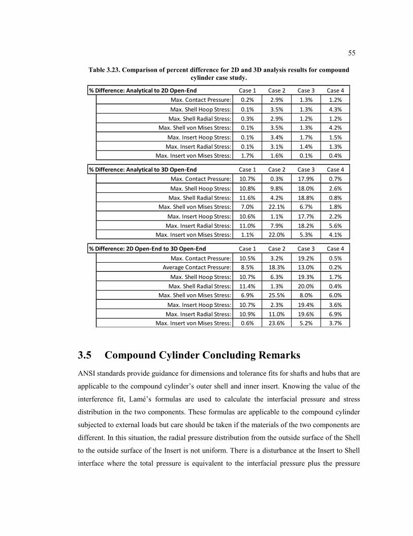
55

Table 3.23. Comparison of percent difference for 2D and 3D analysis results for compound

cylinder case study.

3.5 Compound Cylinder Concluding Remarks

ANSI standards provide guidance for dimensions and tolerance fits for shafts and hubs that are

applicable to the compound cylinder’s outer shell and inner insert. Knowing the value of the

interference fit, Lamé’s formulas are used to calculate the interfacial pressure and stress

distribution in the two components. These formulas are applicable to the compound cylinder

subjected to external loads but care should be taken if the materials of the two components are

different. In this situation, the radial pressure distribution from the outside surface of the Shell

to the outside surface of the Insert is not uniform. There is a disturbance at the Insert to Shell

interface where the total pressure is equivalent to the interfacial pressure plus the pressure

% Difference: Analytical to 2D Open-End Case 1 Case 2 Case 3 Case 4

Max. Contact Pressure: 0.2% 2.9% 1.3% 1.2%

Max. Shell Hoop Stress: 0.1% 3.5% 1.3% 4.3%

Max. Shell Radial Stress: 0.3% 2.9% 1.2% 1.2%

Max. Shell von Mises Stress: 0.1% 3.5% 1.3% 4.2%

Max. Insert Hoop Stress: 0.1% 3.4% 1.7% 1.5%

Max. Insert Radial Stress: 0.1% 3.1% 1.4% 1.3%

Max. Insert von Mises Stress: 1.7% 1.6% 0.1% 0.4%

% Difference: Analytical to 3D Open-End Case 1 Case 2 Case 3 Case 4








% Difference: 2D Open-End to 3D Open-End Case 1 Case 2 Case 3 Case 4


Average Contact Pressure: 8.5% 18.3% 13.0% 0.2%







56

transmitted from the outer surface of the Shell to the inner Surface of the Shell as described in

Equation (3.16).

As expected, the analytical solution and the 2D FEM model solution are nearly identical for the

study cases without external loads. Both contact pressure and stress values are up to 4% higher

for the external load cases. Similarly, the 3D FEM model solutions contact pressure and stress

values are up to 24% higher than the analytical solutions. A summary of the finite element

analysis results compared to the analytical results is listed in Table 3.23. The complete results

are given in Appendix C, Table C-3.

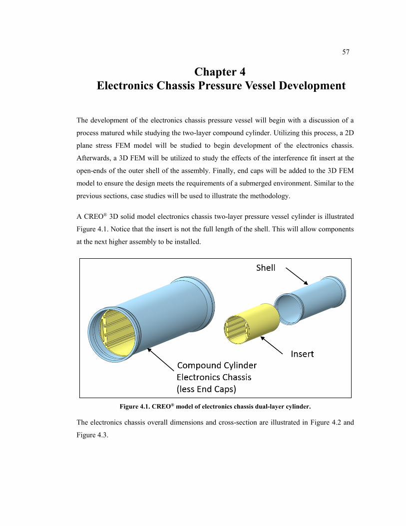
57

Chapter 4

Electronics Chassis Pressure Vessel Development

The development of the electronics chassis pressure vessel will begin with a discussion of a

process matured while studying the two-layer compound cylinder. Utilizing this process, a 2D

plane stress FEM model will be studied to begin development of the electronics chassis.

Afterwards, a 3D FEM will be utilized to study the effects of the interference fit insert at the

open-ends of the outer shell of the assembly. Finally, end caps will be added to the 3D FEM

model to ensure the design meets the requirements of a submerged environment. Similar to the

previous sections, case studies will be used to illustrate the methodology.

A CREO® 3D solid model electronics chassis two-layer pressure vessel cylinder is illustrated

Figure 4.1. Notice that the insert is not the full length of the shell. This will allow components

at the next higher assembly to be installed.

Figure 4.1. CREO® model of electronics chassis dual-layer cylinder.

The electronics chassis overall dimensions and cross-section are illustrated in Figure 4.2 and

Figure 4.3.

58

Figure 4.2. Overall dimensions of the electronics chassis pressure vessel cylinder.

Figure 4.3. Mid-length cross-section of the electronics chassis pressure vessel cylinder.

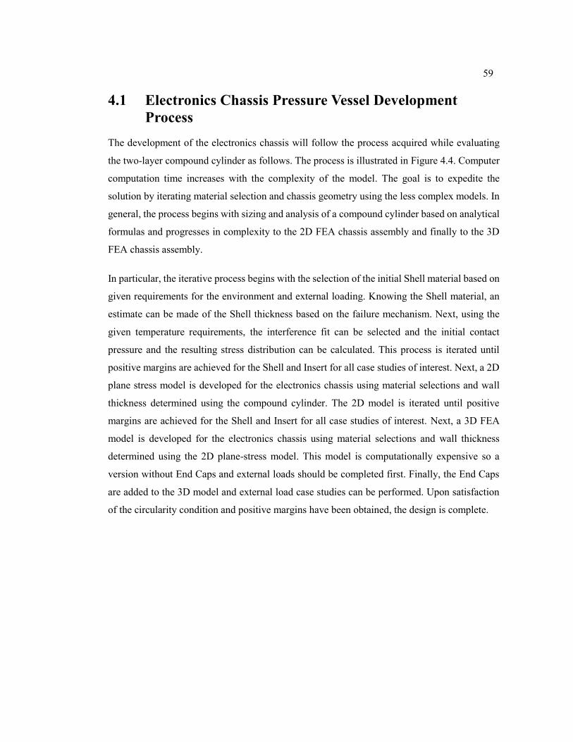
59

4.1 Electronics Chassis Pressure Vessel Development

Process

The development of the electronics chassis will follow the process acquired while evaluating

the two-layer compound cylinder as follows. The process is illustrated in Figure 4.4. Computer

computation time increases with the complexity of the model. The goal is to expedite the

solution by iterating material selection and chassis geometry using the less complex models. In

general, the process begins with sizing and analysis of a compound cylinder based on analytical

formulas and progresses in complexity to the 2D FEA chassis assembly and finally to the 3D

FEA chassis assembly.

In particular, the iterative process begins with the selection of the initial Shell material based on

given requirements for the environment and external loading. Knowing the Shell material, an

estimate can be made of the Shell thickness based on the failure mechanism. Next, using the

given temperature requirements, the interference fit can be selected and the initial contact

pressure and the resulting stress distribution can be calculated. This process is iterated until

positive margins are achieved for the Shell and Insert for all case studies of interest. Next, a 2D

plane stress model is developed for the electronics chassis using material selections and wall

thickness determined using the compound cylinder. The 2D model is iterated until positive

margins are achieved for the Shell and Insert for all case studies of interest. Next, a 3D FEA

model is developed for the electronics chassis using material selections and wall thickness

determined using the 2D plane-stress model. This model is computationally expensive so a

version without End Caps and external loads should be completed first. Finally, the End Caps

are added to the 3D model and external load case studies can be performed. Upon satisfaction

of the circularity condition and positive margins have been obtained, the design is complete.

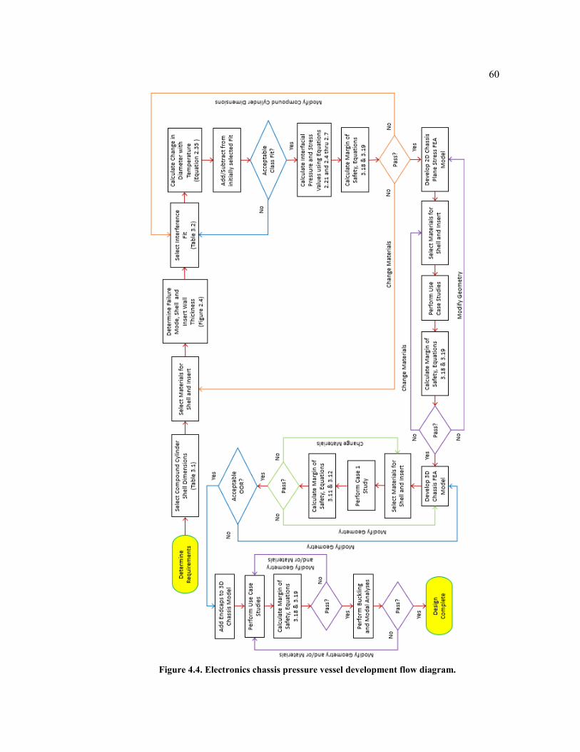
60

Figure 4.4. Electronics chassis pressure vessel development flow diagram.

61

4.2 2D Electronics Chassis Finite Element Model

Similar to the compound cylinders, the effects of assembly and the external environment on the

two-layer electronics chassis 2D plane stress model will be studied using the load cases listed

in Table 4.1. Nominal dimensions and material properties are listed in Table 4.2 and Table 4.3.

Table 4.1. Two-Layer electronics chassis pressure vessel load cases.


Interference




3 Ensure not over stressed in hot

environment. 160 °F Atm, 0 psig 10 mils

4 Submerged in seawater environment

at 100-meter maximum depth. 35 °F 142 psig 7 mils

Table 4.2. Two-layer electronics chassis pressure vessel dimensions and materials.

Component

Inside

Diameter,

Inch

Wall

Thickness,

Inch

Material

Shell 7.850 0.065 2205 Duplex Stainless Steel

Insert varies 0.150 6061-T651 Aluminum

Table 4.3. Mechanical properties for two-layer electronics chassis pressure vessel.

Material

Young’s

Modulus,

psi

Poisson’s

Ratio 𝐹𝑡𝑢

Cold

𝐹𝑡𝑦

Cold

𝐹𝑡𝑢 Hot

𝐹𝑡𝑦

Hot

2205 Duplex

Stainless Steel 29,000,000 0.30 95 ksi 65 ksi 81.4 ksi 55.7 ksi

6061-T651

Aluminum 9,900,000 0.33 42 ksi 35 ksi 40.3 ksi 33.9 ksi





Figure 4.5 illustrates the ¼ symmetry ANSYS Workbench® 2D model geometry and mesh.

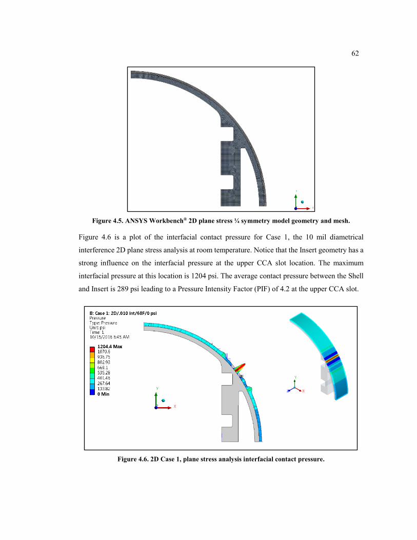
62

Figure 4.5. ANSYS Workbench® 2D plane stress ¼ symmetry model geometry and mesh.

Figure 4.6 is a plot of the interfacial contact pressure for Case 1, the 10 mil diametrical

interference 2D plane stress analysis at room temperature. Notice that the Insert geometry has a

strong influence on the interfacial pressure at the upper CCA slot location. The maximum

interfacial pressure at this location is 1204 psi. The average contact pressure between the Shell

and Insert is 289 psi leading to a Pressure Intensity Factor (PIF) of 4.2 at the upper CCA slot.

Figure 4.6. 2D Case 1, plane stress analysis interfacial contact pressure.

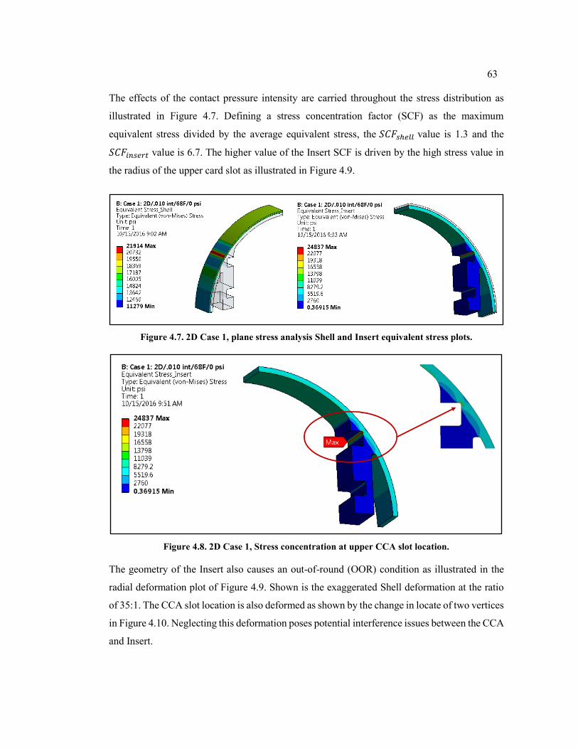
63

The effects of the contact pressure intensity are carried throughout the stress distribution as

illustrated in Figure 4.7. Defining a stress concentration factor (SCF) as the maximum

equivalent stress divided by the average equivalent stress, the 𝑆𝐶𝐹𝑠ℎ𝑒𝑙𝑙 value is 1.3 and the

𝑆𝐶𝐹𝑖𝑛𝑠𝑒𝑟𝑡 value is 6.7. The higher value of the Insert SCF is driven by the high stress value in

the radius of the upper card slot as illustrated in Figure 4.9.

Figure 4.7. 2D Case 1, plane stress analysis Shell and Insert equivalent stress plots.

Figure 4.8. 2D Case 1, Stress concentration at upper CCA slot location.

The geometry of the Insert also causes an out-of-round (OOR) condition as illustrated in the

radial deformation plot of Figure 4.9. Shown is the exaggerated Shell deformation at the ratio

of 35:1. The CCA slot location is also deformed as shown by the change in locate of two vertices

in Figure 4.10. Neglecting this deformation poses potential interference issues between the CCA

and Insert.

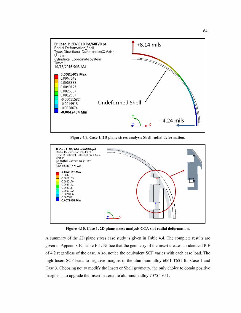
64

Figure 4.9. Case 1, 2D plane stress analysis Shell radial deformation.

Figure 4.10. Case 1, 2D plane stress analysis CCA slot radial deformation.

A summary of the 2D plane stress case study is given in Table 4.4. The complete results are

given in Appendix E, Table E-1. Notice that the geometry of the insert creates an identical PIF

of 4.2 regardless of the case. Also, notice the equivalent SCF varies with each case load. The

high Insert SCF leads to negative margins in the aluminum alloy 6061-T651 for Case 1 and

Case 3. Choosing not to modify the Insert or Shell geometry, the only choice to obtain positive

margins is to upgrade the Insert material to aluminum alloy 7075-T651.

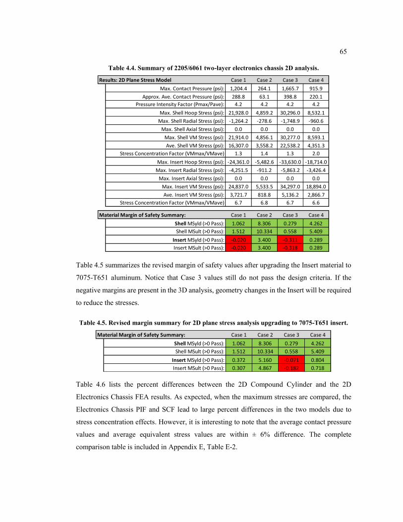
65

Table 4.4. Summary of 2205/6061 two-layer electronics chassis 2D analysis.

Table 4.5 summarizes the revised margin of safety values after upgrading the Insert material to

7075-T651 aluminum. Notice that Case 3 values still do not pass the design criteria. If the

negative margins are present in the 3D analysis, geometry changes in the Insert will be required

to reduce the stresses.

Table 4.5. Revised margin summary for 2D plane stress analysis upgrading to 7075-T651 insert.

Table 4.6 lists the percent differences between the 2D Compound Cylinder and the 2D

Electronics Chassis FEA results. As expected, when the maximum stresses are compared, the

Electronics Chassis PIF and SCF lead to large percent differences in the two models due to

stress concentration effects. However, it is interesting to note that the average contact pressure

values and average equivalent stress values are within ± 6% difference. The complete

comparison table is included in Appendix E, Table E-2.

Results: 2D Plane Stress Model Case 1 Case 2 Case 3 Case 4

Max. Contact Pressure (psi): 1,204.4 264.1 1,665.7 915.9


Pressure Intensity Factor (Pmax/Pave): 4.2 4.2 4.2 4.2


Max. Shell Radial Stress (psi): -1,264.2 -278.6 -1,748.9 -960.6

Max. Shell Axial Stress (psi): 0.0 0.0 0.0 0.0


Ave. Shell VM Stress (psi): 16,307.0 3,558.2 22,538.2 4,351.3

Stress Concentration Factor (VMmax/VMave) 1.3 1.4 1.3 2.0


Max. Insert Radial Stress (psi): -4,251.5 -911.2 -5,863.2 -3,426.4

Max. Insert Axial Stress (psi): 0.0 0.0 0.0 0.0


Ave. Insert VM Stress (psi): 3,721.7 818.8 5,136.2 2,866.7



Shell MSyld (>0 Pass): 1.062 8.306 0.279 4.262

Shell MSult (>0 Pass): 1.512 10.334 0.558 5.409

Insert MSyld (>0 Pass): -0.020 3.400 -0.311 0.289

Insert MSult (>0 Pass): -0.020 3.400 -0.318 0.289


Shell X-Deformation (mil): -4.2 -4.3 -3.2 -5.6

Shell Y-Deformation (mil): 8.1 -1.7 13.9 4.3

Out of Round Dimension (mil): -24.8 -5.3 -34.2 -19.8


Shell MSyld (>0 Pass): 1.062 8.306 0.279 4.262

Shell MSult (>0 Pass): 1.512 10.334 0.558 5.409

Insert MSyld (>0 Pass): 0.372 5.160 -0.071 0.804

Insert MSult (>0 Pass): 0.307 4.867 -0.182 0.718

66

Table 4.6. Percent difference 2D Compound Cylinder to the 2D Electronics Chassis.

4.3 3D Electronics Chassis Finite Element Model

This section progresses with the development of the compound cylinder electronics chassis with

the addition of the end caps to close the open-ended Shell. End Caps will be added to the case

studies per Table 4.7. There are many types of end caps including spherical head, dished head

and flat head. Examples of dished head and flat head end caps are illustrated in Figure 4.11 and

Figure 4.12.

Table 4.7. Two-Layer electronics chassis pressure vessel load cases for 3D FEA.

Case Description End

Cap

Temperature Pressure Diametrical

Interference

1 Baseline. Post assembly

configuration. No 68 °F Atm, 0 psig 10 mils

2 Ensure insert holding capacity

in cold environment. Yes -40 °F Atm, 0 psig 7 mils


environment. Yes 160 °F Atm, 0 psig 10 mils

4

Submerged in seawater

environment at 100-meter

maximum depth.

Yes 35 °F 142 psig 7 mils

Case 1 Case 2 Case 3 Case 4






Ave. Shell von Mises Stress: 2.6% 6.4% 2.2% 0.8%




Ave. Insert von Mises Stress: 64.5% 67.3% 64.2% 66.0%

% Difference: 2D Compound Cylinder to

2D Electronics Chassis

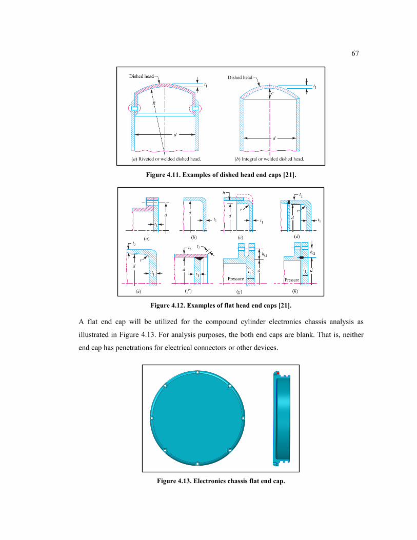
67

Figure 4.11. Examples of dished head end caps [21].

Figure 4.12. Examples of flat head end caps [21].

A flat end cap will be utilized for the compound cylinder electronics chassis analysis as

illustrated in Figure 4.13. For analysis purposes, the both end caps are blank. That is, neither

end cap has penetrations for electrical connectors or other devices.

Figure 4.13. Electronics chassis flat end cap.

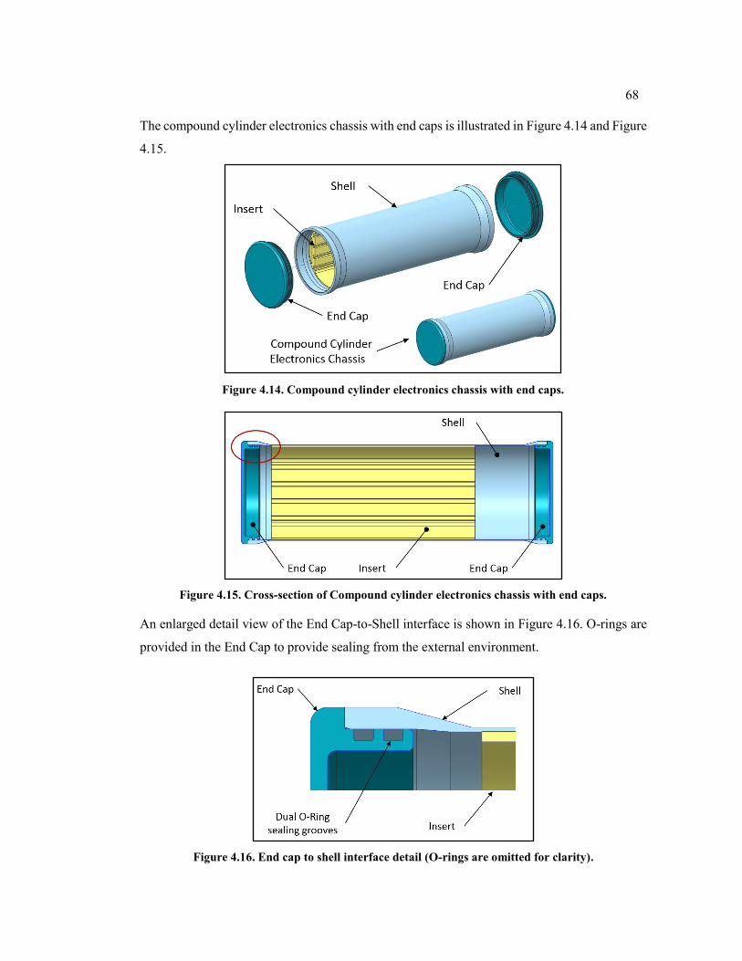
68

The compound cylinder electronics chassis with end caps is illustrated in Figure 4.14 and Figure

4.15.

Figure 4.14. Compound cylinder electronics chassis with end caps.

Figure 4.15. Cross-section of Compound cylinder electronics chassis with end caps.

An enlarged detail view of the End Cap-to-Shell interface is shown in Figure 4.16. O-rings are

provided in the End Cap to provide sealing from the external environment.

Figure 4.16. End cap to shell interface detail (O-rings are omitted for clarity).

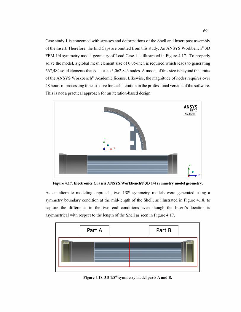
69

Case study 1 is concerned with stresses and deformations of the Shell and Insert post assembly

of the Insert. Therefore, the End Caps are omitted from this study. An ANSYS Workbench® 3D

FEM 1/4 symmetry model geometry of Load Case 1 is illustrated in Figure 4.17. To properly

solve the model, a global mesh element size of 0.05-inch is required which leads to generating

667,484 solid elements that equates to 3,062,843 nodes. A model of this size is beyond the limits

of the ANSYS Workbench® Academic license. Likewise, the magnitude of nodes requires over

48 hours of processing time to solve for each iteration in the professional version of the software.

This is not a practical approach for an iteration-based design.

Figure 4.17. Electronics Chassis ANSYS Workbench® 3D 1/4 symmetry model geometry.

As an alternate modeling approach, two 1/8th symmetry models were generated using a

symmetry boundary condition at the mid-length of the Shell, as illustrated in Figure 4.18, to

capture the difference in the two end conditions even though the Insert’s location is

asymmetrical with respect to the length of the Shell as seen in Figure 4.17.

Figure 4.18. 3D 1/8th symmetry model parts A and B.

70

Each half-length model (Part A and Part B) was sliced into three segments to study the stress

distribution at locations away from the disturbances of the end boundary conditions and at the

locations of the maximum stress values. Contacts between the slices are treated as bonded.

Contacts between the Shell and Insert are treated as frictional with a friction coefficient of 0.30.

The geometry of the two halves is illustrated in Figure 4.19 and Figure 4.20.

Figure 4.19. Case 1, Electronics Chassis 3D 1/8th symmetry model geometry Part A.

Figure 4.20. Case 1, Electronics Chassis 3D 1/8th symmetry model geometry Part B.

4.3.1 Stress Distribution Away from Boundary Conditions

The resulting Case 1 interfacial pressure plots for Parts A and B Segment 2 are illustrated in

Figure 4.21. The Shell, Part A and Part B, equivalent stress plots are shown in Figure 4.22.

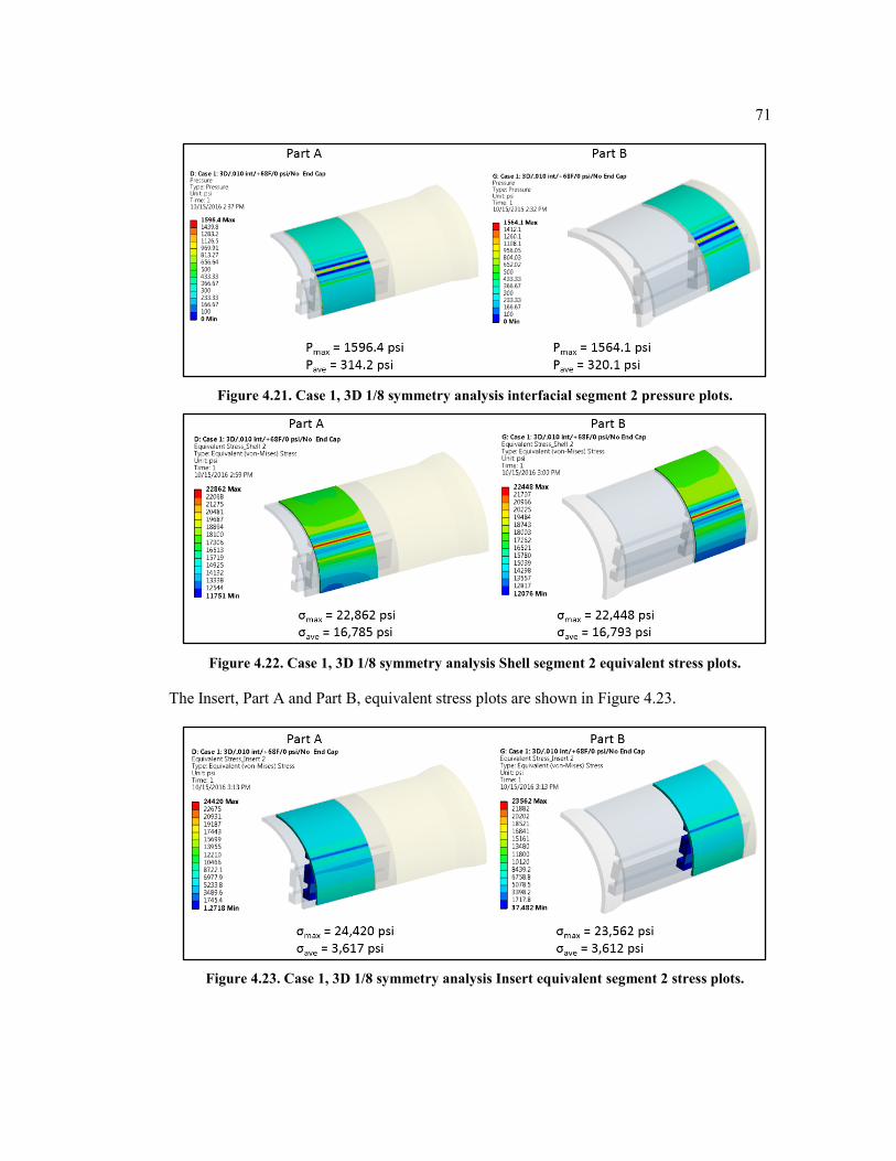
71

Figure 4.21. Case 1, 3D 1/8 symmetry analysis interfacial segment 2 pressure plots.

Figure 4.22. Case 1, 3D 1/8 symmetry analysis Shell segment 2 equivalent stress plots.

The Insert, Part A and Part B, equivalent stress plots are shown in Figure 4.23.

Figure 4.23. Case 1, 3D 1/8 symmetry analysis Insert equivalent segment 2 stress plots.

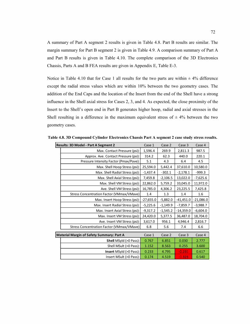
72

A summary of Part A segment 2 results is given in Table 4.8. Part B results are similar. The

margin summary for Part B segment 2 is given in Table 4.9. A comparison summary of Part A

and Part B results is given in Table 4.10. The complete comparison of the 3D Electronics

Chassis, Parts A and B FEA results are given in Appendix E, Table E-3.

Notice in Table 4.10 that for Case 1 all results for the two parts are within ± 4% difference

except the radial stress values which are within 10% between the two geometry cases. The

addition of the End Caps and the location of the Insert from the end of the Shell have a strong

influence in the Shell axial stress for Cases 2, 3, and 4. As expected, the close proximity of the

Insert to the Shell’s open end in Part B generates higher hoop, radial and axial stresses in the

Shell resulting in a difference in the maximum equivalent stress of ± 4% between the two

geometry cases.

Table 4.8. 3D Compound Cylinder Electronics Chassis Part A segment 2 case study stress results.

Results: 3D Model - Part A Segment 2 Case 1 Case 2 Case 3 Case 4






Max. Shell Axial Stress (psi): 7,459.8 -2,106.5 13,022.0 -7,625.6





Max. Insert Radial Stress (psi): -5,225.6 -1,149.9 -7,859.7 -3,988.7

Max. Insert Axial Stress (psi): -9,317.2 -1,545.2 -14,359.0 -6,604.0




Material Margin of Safety Summary: Part A Case 1 Case 2 Case 3 Case 4

Shell MSyld (>0 Pass): 0.767 6.851 0.030 2.777

Shell MSult (>0 Pass): 1.152 8.563 0.255 3.600



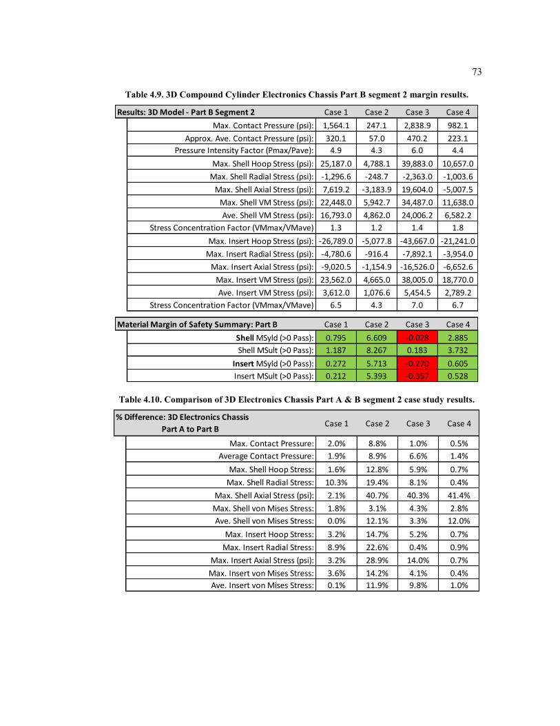
73

Table 4.9. 3D Compound Cylinder Electronics Chassis Part B segment 2 margin results.

Table 4.10. Comparison of 3D Electronics Chassis Part A & B segment 2 case study results.

Results: 3D Model - Part B Segment 2 Case 1 Case 2 Case 3 Case 4





Max. Shell Radial Stress (psi): -1,296.6 -248.7 -2,363.0 -1,003.6









Ave. Insert VM Stress (psi): 3,612.0 1,076.6 5,454.5 2,789.2


Material Margin of Safety Summary: Part B Case 1 Case 2 Case 3 Case 4

Shell MSyld (>0 Pass): 0.795 6.609 -0.028 2.885

Shell MSult (>0 Pass): 1.187 8.267 0.183 3.732








Max. Shell Axial Stress (psi): 2.1% 40.7% 40.3% 41.4%





Max. Insert Axial Stress (psi): 3.2% 28.9% 14.0% 0.7%



% Difference: 3D Electronics Chassis

Part A to Part B

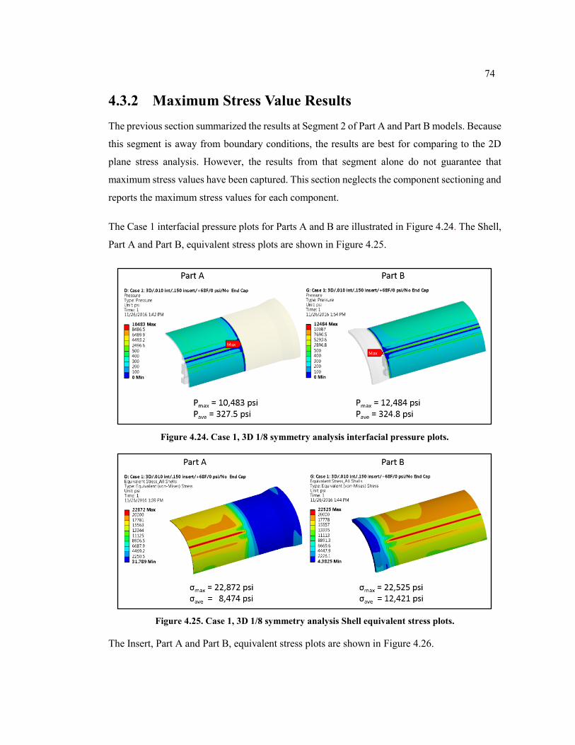
74

4.3.2 Maximum Stress Value Results

The previous section summarized the results at Segment 2 of Part A and Part B models. Because

this segment is away from boundary conditions, the results are best for comparing to the 2D

plane stress analysis. However, the results from that segment alone do not guarantee that

maximum stress values have been captured. This section neglects the component sectioning and

reports the maximum stress values for each component.

The Case 1 interfacial pressure plots for Parts A and B are illustrated in Figure 4.24. The Shell,

Part A and Part B, equivalent stress plots are shown in Figure 4.25.

Figure 4.24. Case 1, 3D 1/8 symmetry analysis interfacial pressure plots.

Figure 4.25. Case 1, 3D 1/8 symmetry analysis Shell equivalent stress plots.

The Insert, Part A and Part B, equivalent stress plots are shown in Figure 4.26.

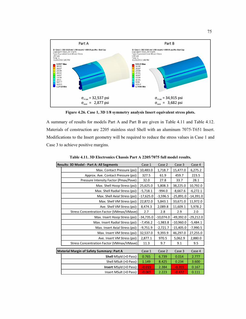
75

Figure 4.26. Case 1, 3D 1/8 symmetry analysis Insert equivalent stress plots.

A summary of results for models Part A and Part B are given in Table 4.11 and Table 4.12.

Materials of construction are 2205 stainless steel Shell with an aluminum 7075-T651 Insert.

Modifications to the Insert geometry will be required to reduce the stress values in Case 1 and

Case 3 to achieve positive margins.

Table 4.11. 3D Electronics Chassis Part A 2205/7075 full model results.

Results: 3D Model - Part A: All Segments Case 1 Case 2 Case 3 Case 4

Max. Contact Pressure (psi): 10,483.0 1,718.7 15,477.0 6,275.2





Max. Shell Axial Stress (psi): -17,625.0 -3,596.5 -25,891.0 -14,391.0










Material Margin of Safety Summary: Part A Case 1 Case 2 Case 3 Case 4

Shell MSyld (>0 Pass): 0.765 6.739 0.014 2.777

Shell MSult (>0 Pass): 1.149 8.425 0.234 3.600



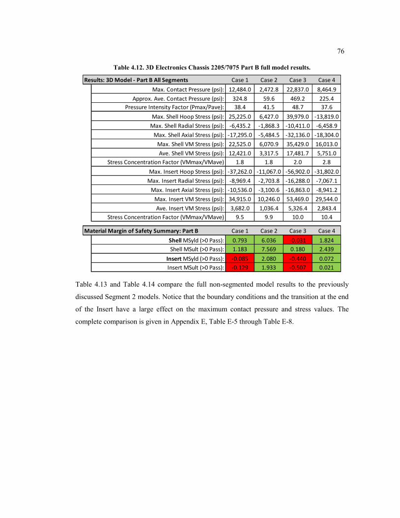
76

Table 4.12. 3D Electronics Chassis 2205/7075 Part B full model results.

Table 4.13 and Table 4.14 compare the full non-segmented model results to the previously

discussed Segment 2 models. Notice that the boundary conditions and the transition at the end

of the Insert have a large effect on the maximum contact pressure and stress values. The

complete comparison is given in Appendix E, Table E-5 through Table E-8.

Results: 3D Model - Part B All Segments Case 1 Case 2 Case 3 Case 4




Max. Shell Hoop Stress (psi): 25,225.0 6,427.0 39,979.0 -13,819.0

Max. Shell Radial Stress (psi): -6,435.2 -1,868.3 -10,411.0 -6,458.9











Material Margin of Safety Summary: Part B Case 1 Case 2 Case 3 Case 4

Shell MSyld (>0 Pass): 0.793 6.036 -0.031 1.824

Shell MSult (>0 Pass): 1.183 7.569 0.180 2.439



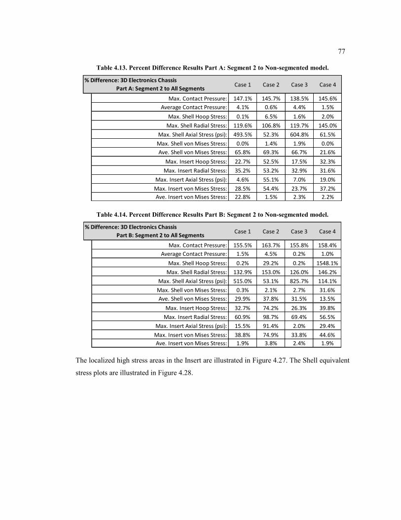
77

Table 4.13. Percent Difference Results Part A: Segment 2 to Non-segmented model.

Table 4.14. Percent Difference Results Part B: Segment 2 to Non-segmented model.

The localized high stress areas in the Insert are illustrated in Figure 4.27. The Shell equivalent

stress plots are illustrated in Figure 4.28.















Part A: Segment 2 to All Segments















Part B: Segment 2 to All Segments

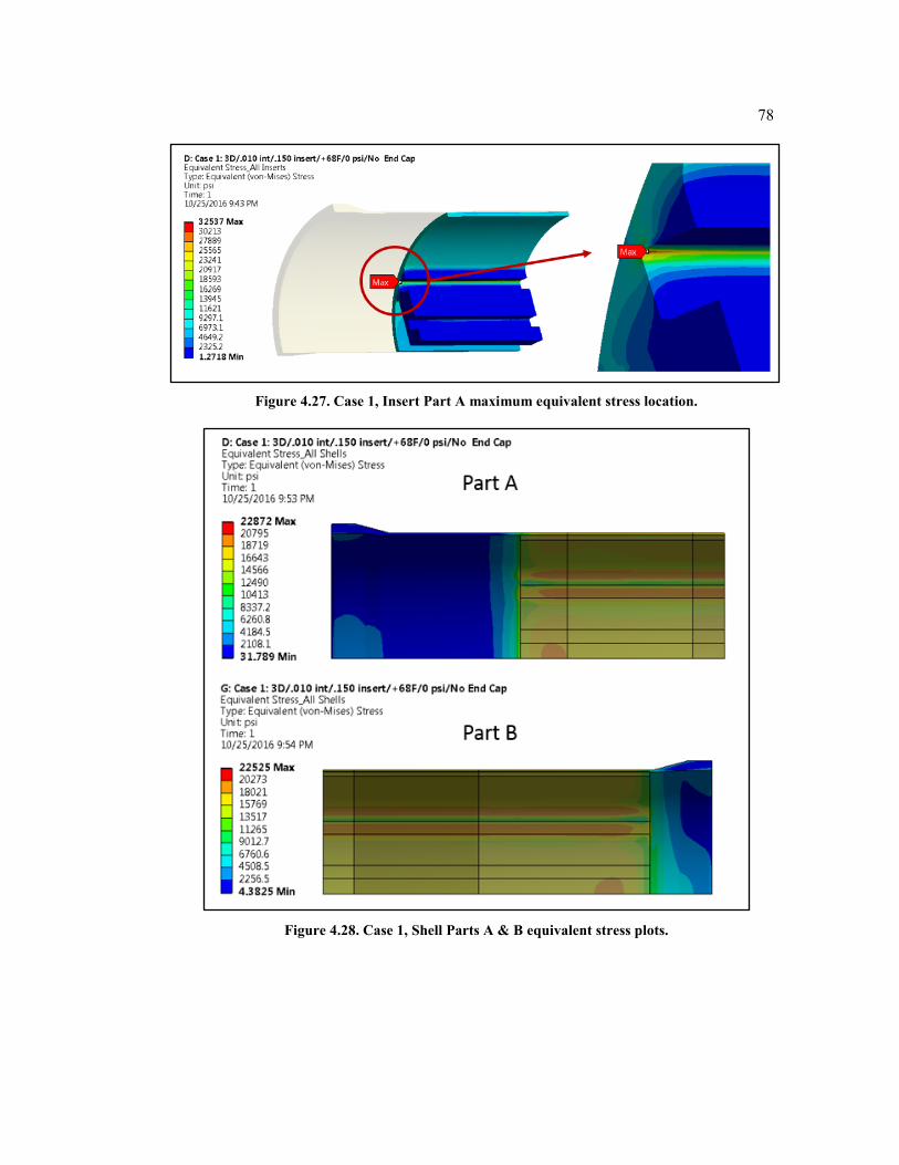
78

Figure 4.27. Case 1, Insert Part A maximum equivalent stress location.

Figure 4.28. Case 1, Shell Parts A & B equivalent stress plots.

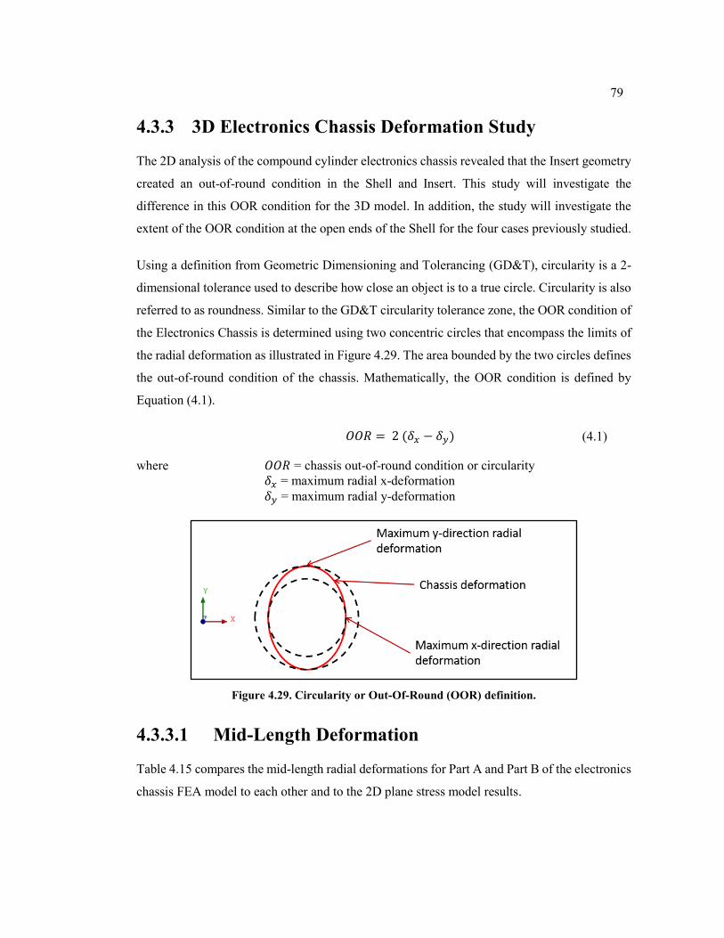
79

4.3.3 3D Electronics Chassis Deformation Study

The 2D analysis of the compound cylinder electronics chassis revealed that the Insert geometry

created an out-of-round condition in the Shell and Insert. This study will investigate the

difference in this OOR condition for the 3D model. In addition, the study will investigate the

extent of the OOR condition at the open ends of the Shell for the four cases previously studied.

Using a definition from Geometric Dimensioning and Tolerancing (GD&T), circularity is a 2-

dimensional tolerance used to describe how close an object is to a true circle. Circularity is also

referred to as roundness. Similar to the GD&T circularity tolerance zone, the OOR condition of

the Electronics Chassis is determined using two concentric circles that encompass the limits of

the radial deformation as illustrated in Figure 4.29. The area bounded by the two circles defines

the out-of-round condition of the chassis. Mathematically, the OOR condition is defined by

Equation (4.1).

𝑂𝑂𝑅 = 2 (𝛿𝑥 − 𝛿𝑦) (4.1)

where 𝑂𝑂𝑅 = chassis out-of-round condition or circularity

𝛿𝑥 = maximum radial x-deformation

𝛿𝑦 = maximum radial y-deformation

Figure 4.29. Circularity or Out-Of-Round (OOR) definition.

4.3.3.1 Mid-Length Deformation

Table 4.15 compares the mid-length radial deformations for Part A and Part B of the electronics

chassis FEA model to each other and to the 2D plane stress model results.

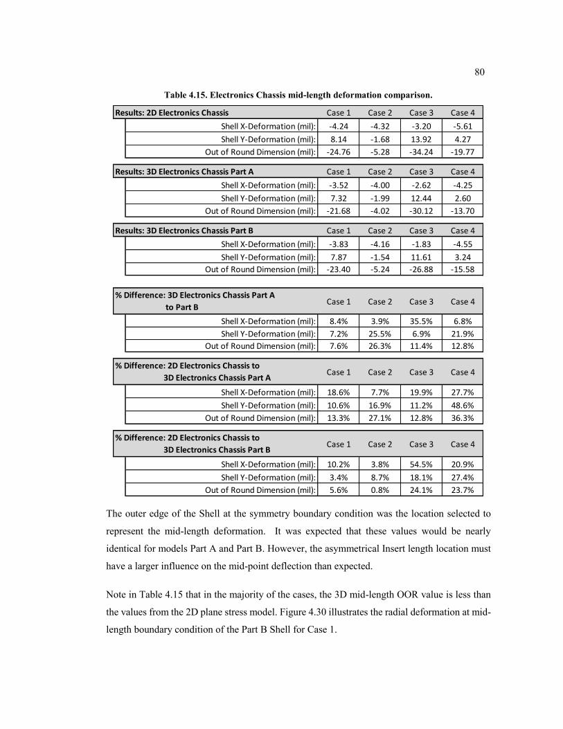
80

Table 4.15. Electronics Chassis mid-length deformation comparison.

The outer edge of the Shell at the symmetry boundary condition was the location selected to

represent the mid-length deformation. It was expected that these values would be nearly

identical for models Part A and Part B. However, the asymmetrical Insert length location must

have a larger influence on the mid-point deflection than expected.

Note in Table 4.15 that in the majority of the cases, the 3D mid-length OOR value is less than

the values from the 2D plane stress model. Figure 4.30 illustrates the radial deformation at mid-

length boundary condition of the Part B Shell for Case 1.

Results: 2D Electronics Chassis Case 1 Case 2 Case 3 Case 4




Results: 3D Electronics Chassis Part A Case 1 Case 2 Case 3 Case 4




Results: 3D Electronics Chassis Part B Case 1 Case 2 Case 3 Case 4





Shell X-Deformation (mil): 8.4% 3.9% 35.5% 6.8%

Shell Y-Deformation (mil): 7.2% 25.5% 6.9% 21.9%

Out of Round Dimension (mil): 7.6% 26.3% 11.4% 12.8%









% Difference: 2D Electronics Chassis to

3D Electronics Chassis Part A

% Difference: 2D Electronics Chassis to

3D Electronics Chassis Part B

% Difference: 3D Electronics Chassis Part A

to Part B

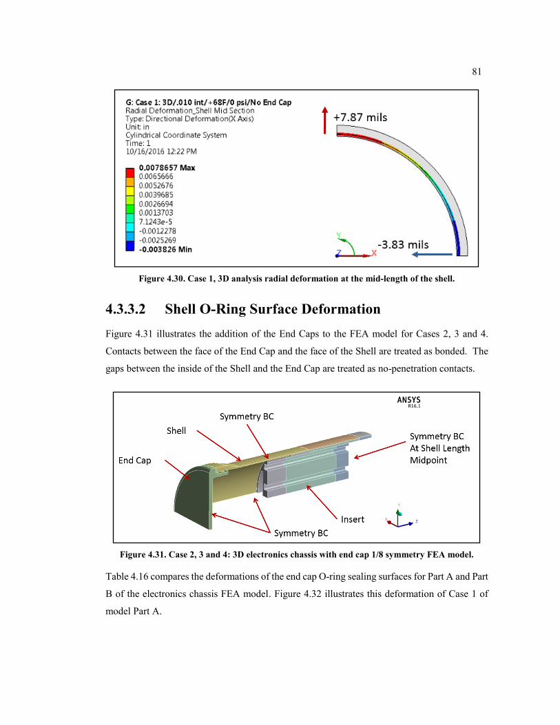
81

Figure 4.30. Case 1, 3D analysis radial deformation at the mid-length of the shell.

4.3.3.2 Shell O-Ring Surface Deformation

Figure 4.31 illustrates the addition of the End Caps to the FEA model for Cases 2, 3 and 4.

Contacts between the face of the End Cap and the face of the Shell are treated as bonded. The

gaps between the inside of the Shell and the End Cap are treated as no-penetration contacts.

Figure 4.31. Case 2, 3 and 4: 3D electronics chassis with end cap 1/8 symmetry FEA model.

Table 4.16 compares the deformations of the end cap O-ring sealing surfaces for Part A and Part

B of the electronics chassis FEA model. Figure 4.32 illustrates this deformation of Case 1 of

model Part A.

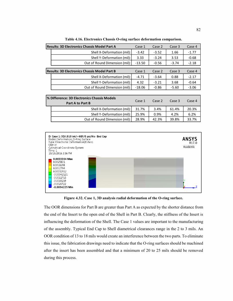
82

Table 4.16. Electronics Chassis O-ring surface deformation comparison.

Figure 4.32. Case 1, 3D analysis radial deformation of the O-ring surface.

The OOR dimensions for Part B are greater than Part A as expected by the shorter distance from

the end of the Insert to the open end of the Shell in Part B. Clearly, the stiffness of the Insert is

influencing the deformation of the Shell. The Case 1 values are important to the manufacturing

of the assembly. Typical End Cap to Shell diametrical clearances range in the 2 to 3 mils. An

OOR condition of 13 to 18 mils would create an interference between the two parts. To eliminate

this issue, the fabrication drawings need to indicate that the O-ring surfaces should be machined

after the insert has been assembled and that a minimum of 20 to 25 mils should be removed

during this process.

Results: 3D Electronics Chassis Model Part A Case 1 Case 2 Case 3 Case 4

Shell X-Deformation (mil): -3.42 -3.52 1.66 -1.77



Results: 3D Electronics Chassis Model Part B Case 1 Case 2 Case 3 Case 4








% Difference: 3D Electronics Chassis Models

Part A to Part B

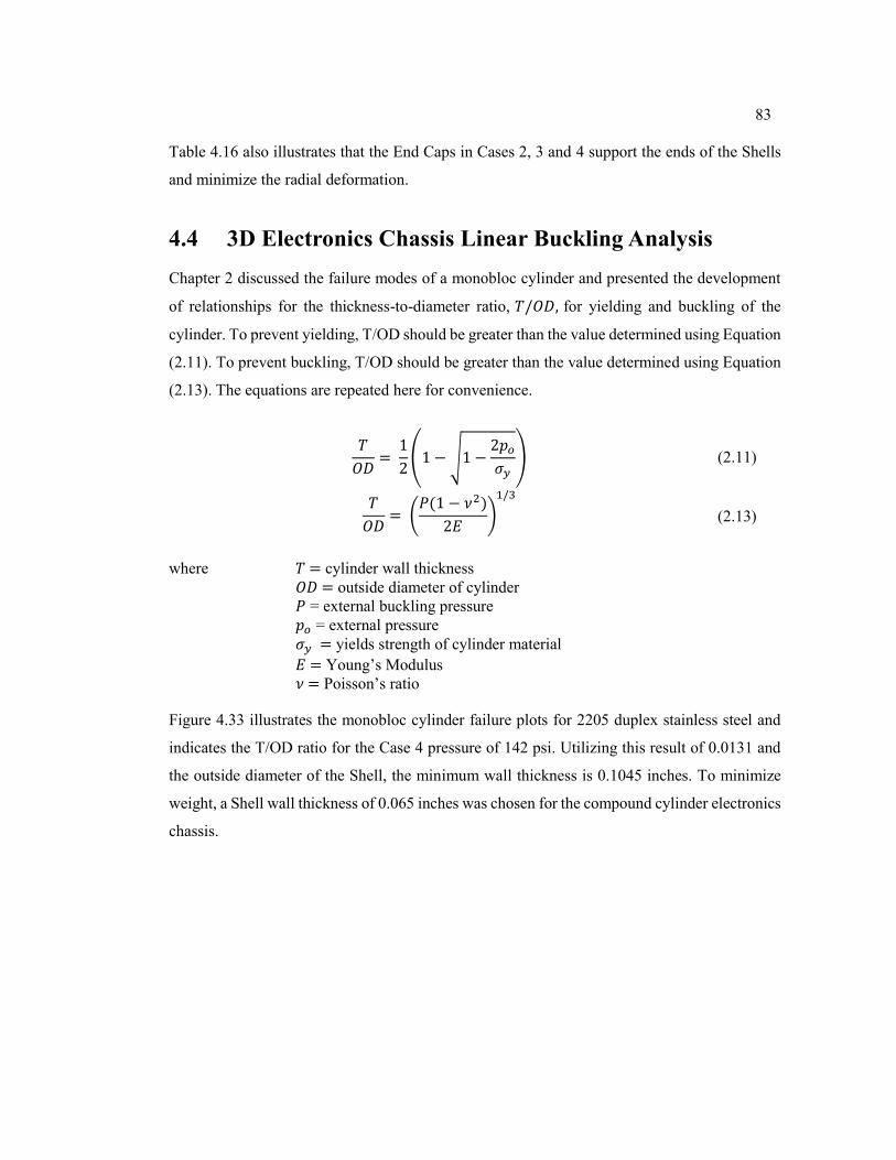
83

Table 4.16 also illustrates that the End Caps in Cases 2, 3 and 4 support the ends of the Shells

and minimize the radial deformation.

4.4 3D Electronics Chassis Linear Buckling Analysis

Chapter 2 discussed the failure modes of a monobloc cylinder and presented the development

of relationships for the thickness-to-diameter ratio, 𝑇/𝑂𝐷, for yielding and buckling of the

cylinder. To prevent yielding, T/OD should be greater than the value determined using Equation

(2.11). To prevent buckling, T/OD should be greater than the value determined using Equation

(2.13). The equations are repeated here for convenience.

𝑇

𝑂𝐷= 1

2(1 − √1 −

2𝑝𝑜𝜎𝑦) (2.11)

𝑇

𝑂𝐷= (

𝑃(1 − 𝜈2)

2𝐸)

1/3

(2.13)

where 𝑇 = cylinder wall thickness


𝑃 = external buckling pressure


𝜎𝑦 = yields strength of cylinder material

𝐸 = Young’s Modulus


Figure 4.33 illustrates the monobloc cylinder failure plots for 2205 duplex stainless steel and

indicates the T/OD ratio for the Case 4 pressure of 142 psi. Utilizing this result of 0.0131 and

the outside diameter of the Shell, the minimum wall thickness is 0.1045 inches. To minimize

weight, a Shell wall thickness of 0.065 inches was chosen for the compound cylinder electronics

chassis.

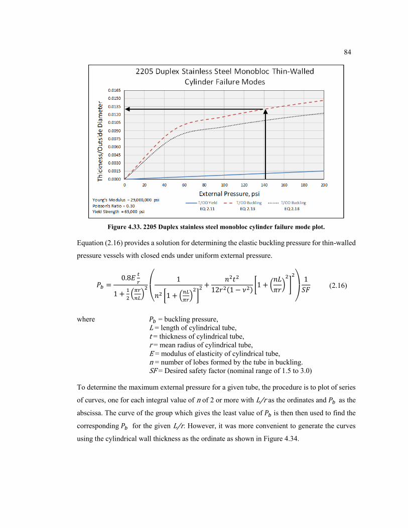
84

Figure 4.33. 2205 Duplex stainless steel monobloc cylinder failure mode plot.

Equation (2.16) provides a solution for determining the elastic buckling pressure for thin-walled

pressure vessels with closed ends under uniform external pressure.

𝑃𝑏 =0.8𝐸

𝑡

𝑟

1 +1

2(𝜋𝑟

𝑛𝐿)2

(

1

𝑛2 [1 + (𝑛𝐿

𝜋𝑟)2]2 +

𝑛2𝑡2

12𝑟2(1 − 𝜈2)[1 + (

𝑛𝐿

𝜋𝑟)2

]

2

)

1

𝑆𝐹 (2.16)

where 𝑃𝑏 = buckling pressure,

L = length of cylindrical tube,

t = thickness of cylindrical tube,

r = mean radius of cylindrical tube,

E = modulus of elasticity of cylindrical tube,

n = number of lobes formed by the tube in buckling.

SF = Desired safety factor (nominal range of 1.5 to 3.0)

To determine the maximum external pressure for a given tube, the procedure is to plot of series

of curves, one for each integral value of n of 2 or more with L/r as the ordinates and 𝑃𝑏 as the

abscissa. The curve of the group which gives the least value of 𝑃𝑏 is then then used to find the

corresponding 𝑃𝑏 for the given L/r. However, it was more convenient to generate the curves

using the cylindrical wall thickness as the ordinate as shown in Figure 4.34.

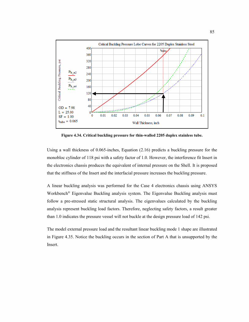
85

Figure 4.34. Critical buckling pressure for thin-walled 2205 duplex stainless tube.

Using a wall thickness of 0.065-inches, Equation (2.16) predicts a buckling pressure for the

monobloc cylinder of 118 psi with a safety factor of 1.0. However, the interference fit Insert in

the electronics chassis produces the equivalent of internal pressure on the Shell. It is proposed

that the stiffness of the Insert and the interfacial pressure increases the buckling pressure.

A linear buckling analysis was performed for the Case 4 electronics chassis using ANSYS

Workbench® Eigenvalue Buckling analysis system. The Eigenvalue Buckling analysis must

follow a pre-stressed static structural analysis. The eigenvalues calculated by the buckling

analysis represent buckling load factors. Therefore, neglecting safety factors, a result greater

than 1.0 indicates the pressure vessel will not buckle at the design pressure load of 142 psi.

The model external pressure load and the resultant linear buckling mode 1 shape are illustrated

in Figure 4.35. Notice the buckling occurs in the section of Part A that is unsupported by the

Insert.

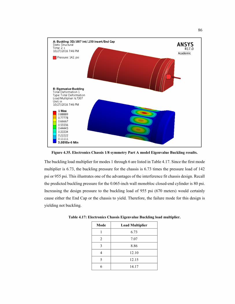
86

Figure 4.35. Electronics Chassis 1/8 symmetry Part A model Eigenvalue Buckling results.

The buckling load multiplier for modes 1 through 6 are listed in Table 4.17. Since the first mode

multiplier is 6.73, the buckling pressure for the chassis is 6.73 times the pressure load of 142

psi or 955 psi. This illustrates one of the advantages of the interference fit chassis design. Recall

the predicted buckling pressure for the 0.065-inch wall monobloc closed-end cylinder is 80 psi.

Increasing the design pressure to the buckling load of 955 psi (670 meters) would certainly

cause either the End Cap or the chassis to yield. Therefore, the failure mode for this design is

yielding not buckling.

Table 4.17: Electronics Chassis Eigenvalue Buckling load multiplier.

Mode Load Multiplier

1 6.73

2 7.07

3 8.86

4 12.10

5 12.15

6 14.17

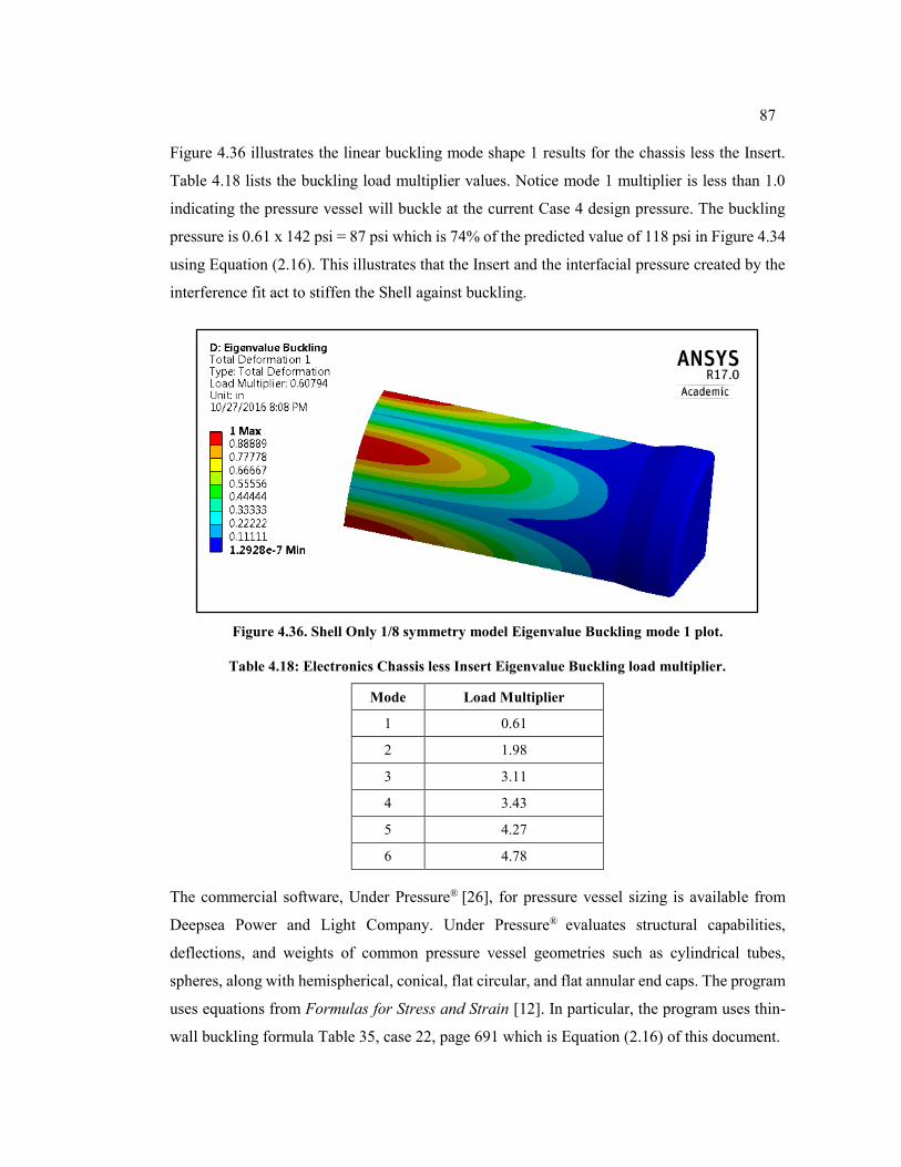
87

Figure 4.36 illustrates the linear buckling mode shape 1 results for the chassis less the Insert.

Table 4.18 lists the buckling load multiplier values. Notice mode 1 multiplier is less than 1.0

indicating the pressure vessel will buckle at the current Case 4 design pressure. The buckling

pressure is 0.61 x 142 psi = 87 psi which is 74% of the predicted value of 118 psi in Figure 4.34

using Equation (2.16). This illustrates that the Insert and the interfacial pressure created by the

interference fit act to stiffen the Shell against buckling.

Figure 4.36. Shell Only 1/8 symmetry model Eigenvalue Buckling mode 1 plot.

Table 4.18: Electronics Chassis less Insert Eigenvalue Buckling load multiplier.

Mode Load Multiplier

1 0.61

2 1.98

3 3.11

4 3.43

5 4.27

6 4.78

The commercial software, Under Pressure® [26], for pressure vessel sizing is available from

Deepsea Power and Light Company. Under Pressure® evaluates structural capabilities,

deflections, and weights of common pressure vessel geometries such as cylindrical tubes,

spheres, along with hemispherical, conical, flat circular, and flat annular end caps. The program

uses equations from Formulas for Stress and Strain [12]. In particular, the program uses thin-

wall buckling formula Table 35, case 22, page 691 which is Equation (2.16) of this document.

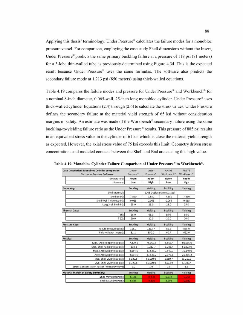
88

Applying this thesis’ terminology, Under Pressure® calculates the failure modes for a monobloc

pressure vessel. For comparison, employing the case study Shell dimensions without the Insert,

Under Pressure® predicts the same primary buckling failure at a pressure of 118 psi (81 meters)

for a 3-lobe thin-walled tube as previously determined using Figure 4.34. This is the expected

result because Under Pressure® uses the same formulas. The software also predicts the

secondary failure mode at 1,213 psi (850 meters) using thick-walled equations.

Table 4.19 compares the failure modes and pressure for Under Pressure® and Workbench® for

a nominal 8-inch diameter, 0.065-wall, 25-inch long monobloc cylinder. Under Pressure® uses

thick-walled cylinder Equations (2.4) through (2.6) to calculate the stress values. Under Pressure

defines the secondary failure at the material yield strength of 65 ksi without consideration

margins of safety. An estimate was made of the Workbench® secondary failure using the same

buckling-to-yielding failure ratio as the Under Pressure® results. This pressure of 885 psi results

in an equivalent stress value in the cylinder of 61 ksi which is close the material yield strength

as expected. However, the axial stress value of 75 ksi exceeds this limit. Geometry driven stress

concentrations and modeled contacts between the Shell and End are causing this high value.

Table 4.19. Monobloc Cylinder Failure Comparison of Under Pressure® to Workbench®.

Under

Pressure®

Under

Pressure®

ANSYS

Workbench®

ANSYS

Workbench®

Temperature: Room Room Room Room

Pressure: Low High Low High

Geometry: Buckling Yielding Buckling Yielding

Shell Material:

Shell ID (in): 7.850 7.850 7.850 7.850



Thermal Case: Buckling Yielding Buckling Yielding

T (F): 68.0 68.0 68.0 68.0

T (C): 20.0 20.0 20.0 20.0

Pressure Case: Buckling Yielding Buckling Yielding

Failure Pressure (psig): 118.1 1212.7 86.3 885.0

Failure Depth (meter): 81.1 850.0 60.7 622.0

Results: Buckling Yielding Buckling Yielding

Max. Shell Hoop Stress (psi): -7,309.1 -75,052.5 -5,863.4 -60,665.0

Max. Shell Radial Stress (psi): -118.1 -1,212.7 -3,286.4 -51,023.0


Ave Shell Axial Stress (psi): -3,654.5 -37,526.2 -2,076.6 -21,355.2




Material Margin of Safety Summary: Buckling Yielding Buckling Yielding

Shell MSyld (>0 Pass): 5.186 -0.398 6.712 -0.261

Shell MSult (>0 Pass): 6.535 -0.266 8.393 -0.100

Case Description: Monobloc Cylinder comparison

To Under Pressure Software

2205 Duplex Stainless Steel

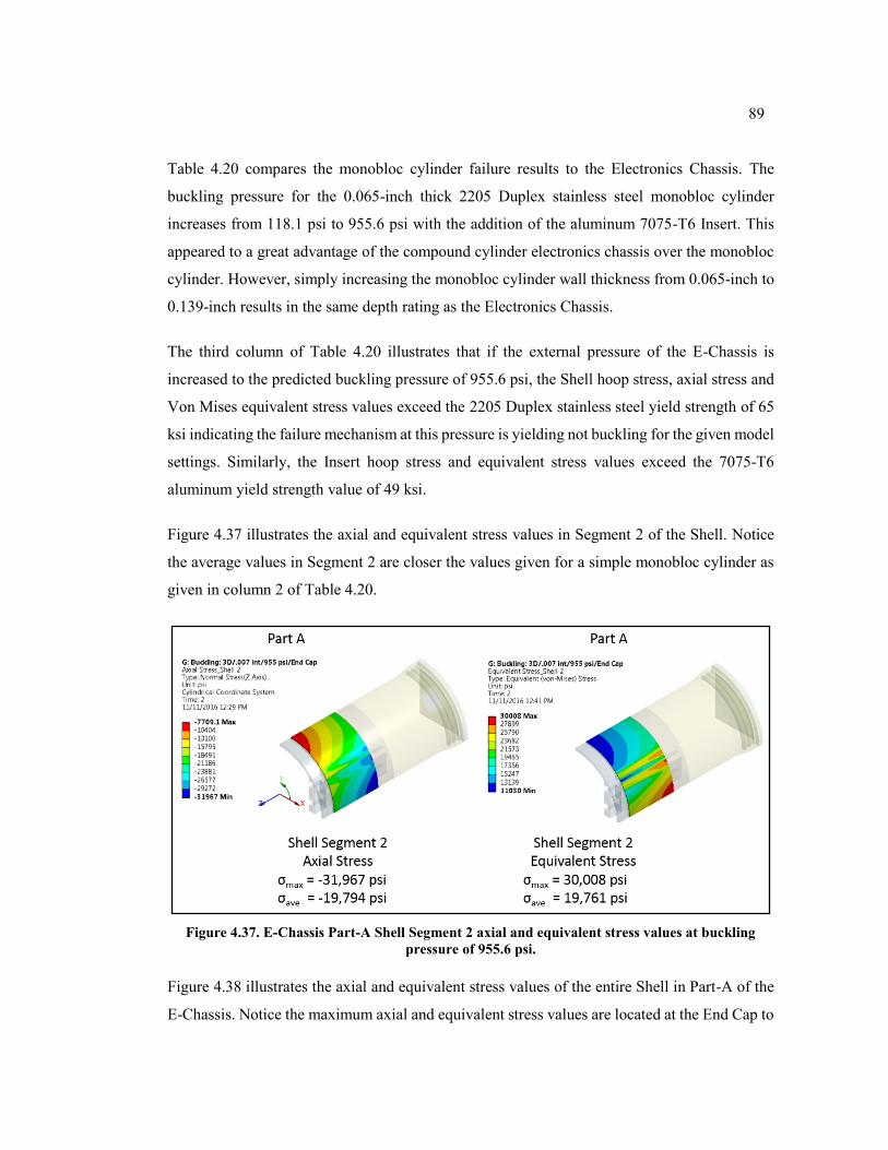
89

Table 4.20 compares the monobloc cylinder failure results to the Electronics Chassis. The

buckling pressure for the 0.065-inch thick 2205 Duplex stainless steel monobloc cylinder

increases from 118.1 psi to 955.6 psi with the addition of the aluminum 7075-T6 Insert. This

appeared to a great advantage of the compound cylinder electronics chassis over the monobloc

cylinder. However, simply increasing the monobloc cylinder wall thickness from 0.065-inch to

0.139-inch results in the same depth rating as the Electronics Chassis.

The third column of Table 4.20 illustrates that if the external pressure of the E-Chassis is

increased to the predicted buckling pressure of 955.6 psi, the Shell hoop stress, axial stress and

Von Mises equivalent stress values exceed the 2205 Duplex stainless steel yield strength of 65

ksi indicating the failure mechanism at this pressure is yielding not buckling for the given model

settings. Similarly, the Insert hoop stress and equivalent stress values exceed the 7075-T6

aluminum yield strength value of 49 ksi.

Figure 4.37 illustrates the axial and equivalent stress values in Segment 2 of the Shell. Notice

the average values in Segment 2 are closer the values given for a simple monobloc cylinder as

given in column 2 of Table 4.20.

Figure 4.37. E-Chassis Part-A Shell Segment 2 axial and equivalent stress values at buckling

pressure of 955.6 psi.

Figure 4.38 illustrates the axial and equivalent stress values of the entire Shell in Part-A of the

E-Chassis. Notice the maximum axial and equivalent stress values are located at the End Cap to

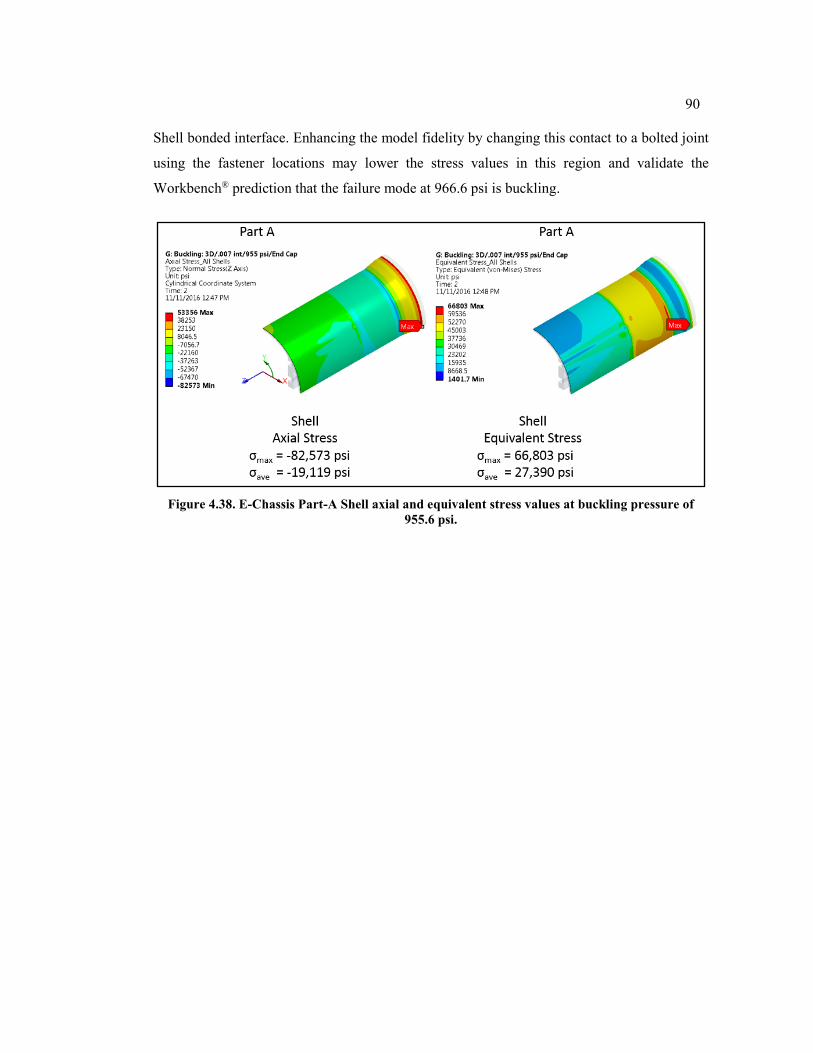
90

Shell bonded interface. Enhancing the model fidelity by changing this contact to a bolted joint

using the fastener locations may lower the stress values in this region and validate the

Workbench® prediction that the failure mode at 966.6 psi is buckling.

Figure 4.38. E-Chassis Part-A Shell axial and equivalent stress values at buckling pressure of

955.6 psi.

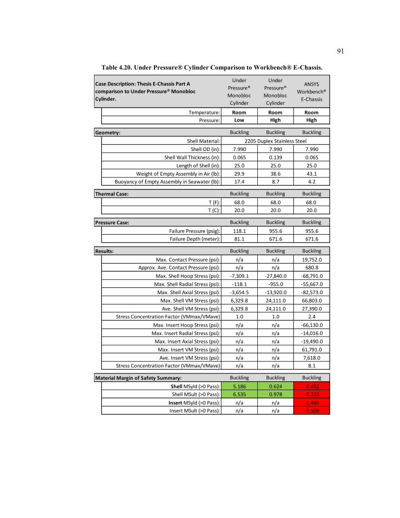
91

Table 4.20. Under Pressure® Cylinder Comparison to Workbench® E-Chassis.

Under

Pressure®

Monobloc

Cylinder

Under

Pressure®

Monobloc

Cylinder

ANSYS

Workbench®

E-Chassis

Temperature: Room Room Room

Pressure: Low High High

Geometry: Buckling Buckling Buckling

Shell Material:

Shell OD (in): 7.990 7.990 7.990

Shell Wall Thickness (in): 0.065 0.139 0.065

Length of Shell (in): 25.0 25.0 25.0

Weight of Empty Assembly in Air (lb): 29.9 38.6 43.1

Buoyancy of Empty Assembly in Seawater (lb): 17.4 8.7 4.2

Thermal Case: Buckling Buckling Buckling

T (F): 68.0 68.0 68.0

T (C): 20.0 20.0 20.0

Pressure Case: Buckling Buckling Buckling

Failure Pressure (psig): 118.1 955.6 955.6

Failure Depth (meter): 81.1 671.6 671.6

Results: Buckling Buckling Buckling

Max. Contact Pressure (psi): n/a n/a 19,752.0

Approx. Ave. Contact Pressure (psi): n/a n/a 680.8

Max. Shell Hoop Stress (psi): -7,309.1 -27,840.0 -68,791.0

Max. Shell Radial Stress (psi): -118.1 -955.0 -55,667.0

Max. Shell Axial Stress (psi): -3,654.5 -13,920.0 -82,573.0

Max. Shell VM Stress (psi): 6,329.8 24,111.0 66,803.0

Ave. Shell VM Stress (psi): 6,329.8 24,111.0 27,390.0

Stress Concentration Factor (VMmax/VMave) 1.0 1.0 2.4

Max. Insert Hoop Stress (psi): n/a n/a -66,130.0

Max. Insert Radial Stress (psi): n/a n/a -14,016.0

Max. Insert Axial Stress (psi): n/a n/a -19,490.0

Max. Insert VM Stress (psi): n/a n/a 61,791.0

Ave. Insert VM Stress (psi): n/a n/a 7,618.0

Stress Concentration Factor (VMmax/VMave) n/a n/a 8.1

Material Margin of Safety Summary: Buckling Buckling Buckling

Shell MSyld (>0 Pass): 5.186 0.624 -0.452

Shell MSult (>0 Pass): 6.535 0.978 -0.333

Insert MSyld (>0 Pass): n/a n/a -0.485

Insert MSult (>0 Pass): n/a n/a -0.509


Case Description: Thesis E-Chassis Part A

comparison to Under Pressure® Monobloc

Cylinder.

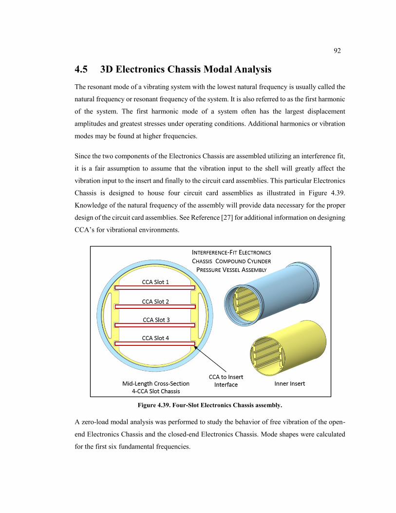
92

4.5 3D Electronics Chassis Modal Analysis

The resonant mode of a vibrating system with the lowest natural frequency is usually called the

natural frequency or resonant frequency of the system. It is also referred to as the first harmonic

of the system. The first harmonic mode of a system often has the largest displacement

amplitudes and greatest stresses under operating conditions. Additional harmonics or vibration

modes may be found at higher frequencies.

Since the two components of the Electronics Chassis are assembled utilizing an interference fit,

it is a fair assumption to assume that the vibration input to the shell will greatly affect the

vibration input to the insert and finally to the circuit card assemblies. This particular Electronics

Chassis is designed to house four circuit card assemblies as illustrated in Figure 4.39.

Knowledge of the natural frequency of the assembly will provide data necessary for the proper

design of the circuit card assemblies. See Reference [27] for additional information on designing

CCA’s for vibrational environments.

Figure 4.39. Four-Slot Electronics Chassis assembly.

A zero-load modal analysis was performed to study the behavior of free vibration of the open-

end Electronics Chassis and the closed-end Electronics Chassis. Mode shapes were calculated

for the first six fundamental frequencies.

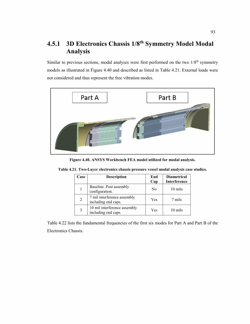
93

4.5.1 3D Electronics Chassis 1/8th Symmetry Model Modal

Analysis

Similar to previous sections, modal analyses were first performed on the two 1/8th symmetry

models as illustrated in Figure 4.40 and described as listed in Table 4.21. External loads were

not considered and thus represent the free vibration modes.

Figure 4.40. ANSYS Workbench FEA model utilized for modal analysis.

Table 4.21. Two-Layer electronics chassis pressure vessel modal analysis case studies.


Cap

Diametrical

Interference


configuration. No 10 mils

2 7 mil interference assembly

including end caps. Yes 7 mils

3 10 mil interference assembly

including end caps. Yes 10 mils

Table 4.22 lists the fundamental frequencies of the first six modes for Part A and Part B of the

Electronics Chassis.

94

Table 4.22. First six fundamental frequencies of E-Chassis Parts A and B using 1/8th symmetry

models.

As listed in Table 4.22, the resonant frequencies vary from models Part A and Part B. Notice

that Part B has the higher values indicating this is the stiffer section as expected by the shorter

Shell unsupported length. It is interesting to note that the change in the interference fit from 7

mils to 10 mils for Cases 2 and 3 has no effect on the resonant frequencies.

4.5.2 3D Electronics Chassis Full Model Modal Analysis

The 1/8th symmetry solutions are a relatively fast analysis to perform but given the symmetry

boundary conditions and the asymmetry in Parts A and B may lead to incorrect values. Although

computationally costly, the analysis was repeated with the full electronics chassis model less

the End Caps to ensure the correct fundamental frequencies are captured for the assembly.

Table 4.23 lists the fundamental frequencies of the first fourteen modes for Case 1 Electronics

Chassis as illustrated in Figure 4.41.

Geometry: Case 1 Case 2 Case 3

Shell Material:

Shell ID (in): 7.850 7.850 7.850

Shell Wall Thickness (in): 0.065 0.065 0.065

Insert Material:

Insert OD (in): 7.860 7.857 7.860

Insert Wall Thickness (in) 0.150 0.150 0.150

Interference-Fit Diametric Interference (mil): 10.0 7.0 10.0

Length of Shell (in): 24.0 24.0 24.0

Length of Insert (in): 24.0 24.0 24.0

Results: 3D Electronics Chassis Part A Case 1 Case 2 Case 3

Mode 1: 497 642 644

Mode 2: 838 1,482 1,482

Mode 3: 1,805 2,163 2,163

Mode 4: 2,384 2,285 2,286

Mode 5: 2,538 2,438 2,438

Mode 6: 2,627 2,611 2,612

Results: 3D Electronics Chassis Part B Case 1 Case 2 Case 3

Mode 1: 567 660 661

Mode 2: 907 1,520 1,520

Mode 3: 2,317 1,872 1,872

Mode 4: 2,613 2,603 2,604

Mode 5: 2,727 2,899 2,900

Mode 6: 3,128 3,059 3,059

Case 1 Case 2 Case 3

Mode 1: 13.2% 2.8% 2.6%

Mode 2: 7.9% 2.5% 2.5%

Mode 3: 24.8% 14.4% 14.4%

Mode 4: 9.2% 13.0% 13.0%

Mode 5: 7.2% 17.3% 17.3%

Mode 6: 17.4% 15.8% 15.8%




Part A to Part B Modal Analysis

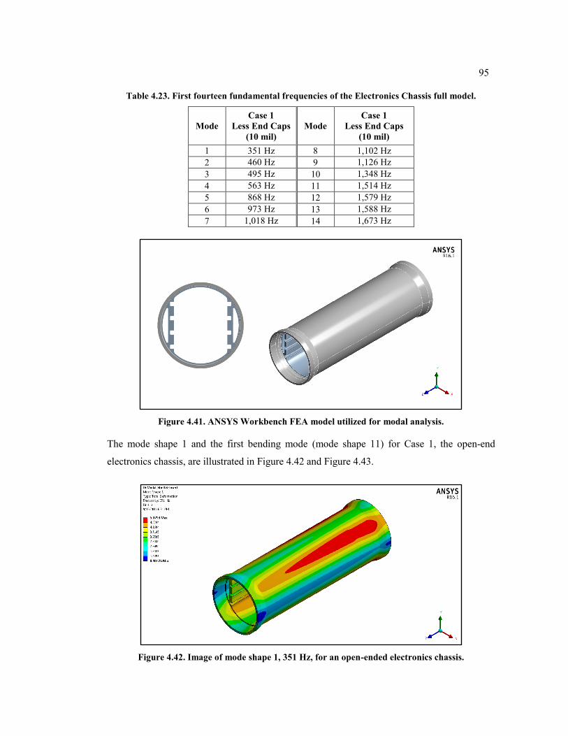
95

Table 4.23. First fourteen fundamental frequencies of the Electronics Chassis full model.

Mode

Case 1

Less End Caps

(10 mil)

Mode

Case 1

Less End Caps

(10 mil)

1 351 Hz 8 1,102 Hz

2 460 Hz 9 1,126 Hz

3 495 Hz 10 1,348 Hz

4 563 Hz 11 1,514 Hz

5 868 Hz 12 1,579 Hz

6 973 Hz 13 1,588 Hz

7 1,018 Hz 14 1,673 Hz

Figure 4.41. ANSYS Workbench FEA model utilized for modal analysis.

The mode shape 1 and the first bending mode (mode shape 11) for Case 1, the open-end

electronics chassis, are illustrated in Figure 4.42 and Figure 4.43.

Figure 4.42. Image of mode shape 1, 351 Hz, for an open-ended electronics chassis.

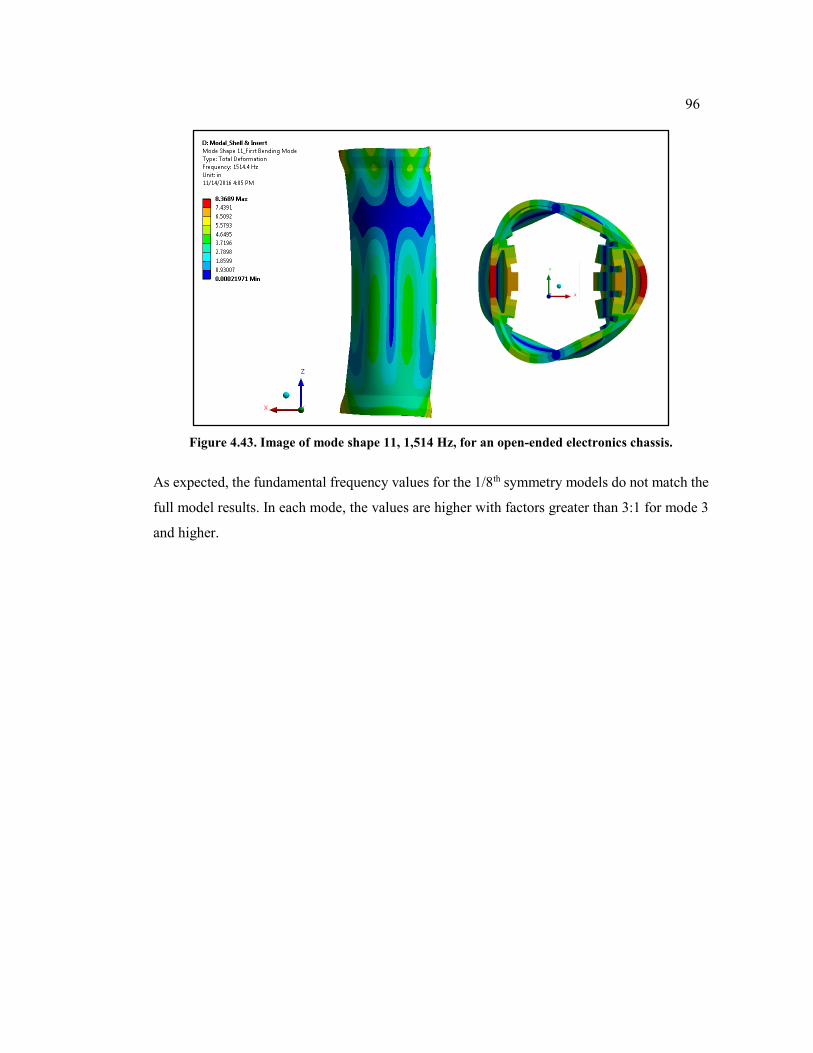
96

Figure 4.43. Image of mode shape 11, 1,514 Hz, for an open-ended electronics chassis.

As expected, the fundamental frequency values for the 1/8th symmetry models do not match the

full model results. In each mode, the values are higher with factors greater than 3:1 for mode 3

and higher.

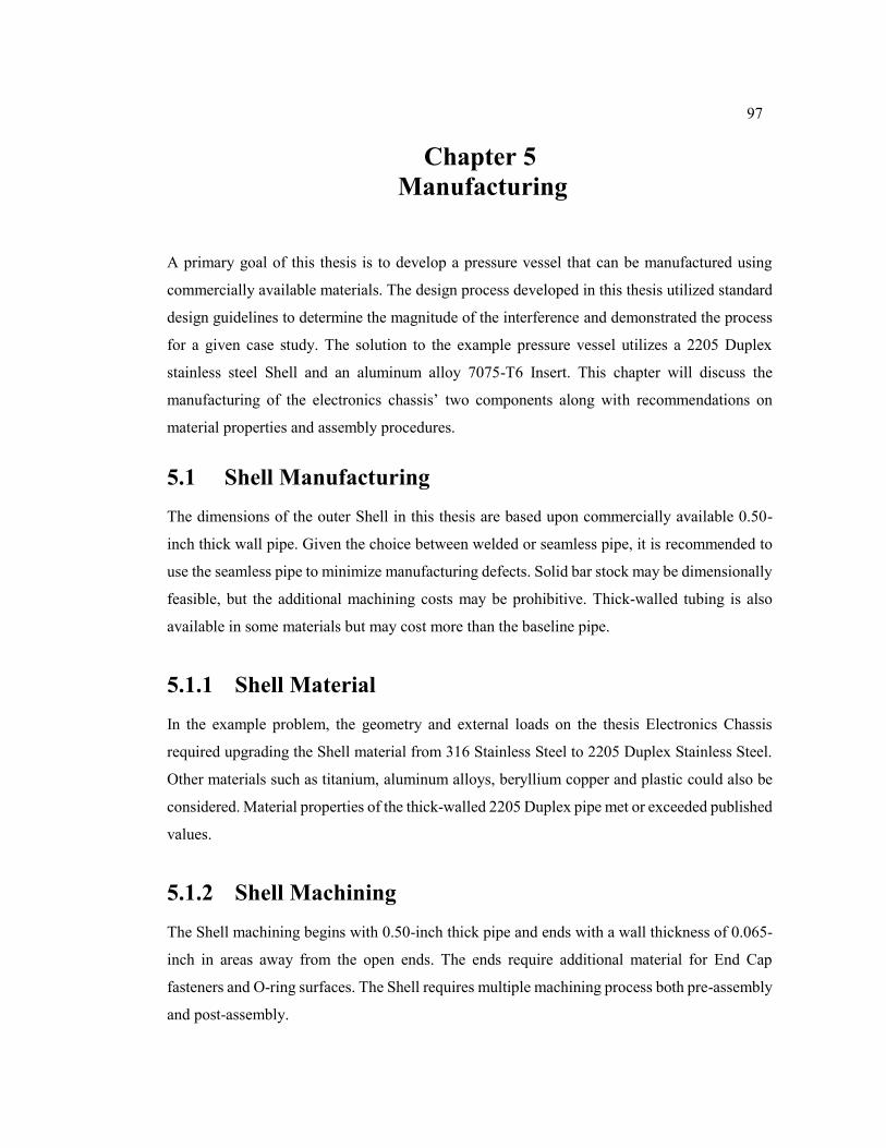
97

Chapter 5

Manufacturing

A primary goal of this thesis is to develop a pressure vessel that can be manufactured using

commercially available materials. The design process developed in this thesis utilized standard

design guidelines to determine the magnitude of the interference and demonstrated the process

for a given case study. The solution to the example pressure vessel utilizes a 2205 Duplex

stainless steel Shell and an aluminum alloy 7075-T6 Insert. This chapter will discuss the

manufacturing of the electronics chassis’ two components along with recommendations on

material properties and assembly procedures.

5.1 Shell Manufacturing

The dimensions of the outer Shell in this thesis are based upon commercially available 0.50-

inch thick wall pipe. Given the choice between welded or seamless pipe, it is recommended to

use the seamless pipe to minimize manufacturing defects. Solid bar stock may be dimensionally

feasible, but the additional machining costs may be prohibitive. Thick-walled tubing is also

available in some materials but may cost more than the baseline pipe.

5.1.1 Shell Material

In the example problem, the geometry and external loads on the thesis Electronics Chassis

required upgrading the Shell material from 316 Stainless Steel to 2205 Duplex Stainless Steel.

Other materials such as titanium, aluminum alloys, beryllium copper and plastic could also be

considered. Material properties of the thick-walled 2205 Duplex pipe met or exceeded published

values.

5.1.2 Shell Machining

The Shell machining begins with 0.50-inch thick pipe and ends with a wall thickness of 0.065-

inch in areas away from the open ends. The ends require additional material for End Cap

fasteners and O-ring surfaces. The Shell requires multiple machining process both pre-assembly

and post-assembly.

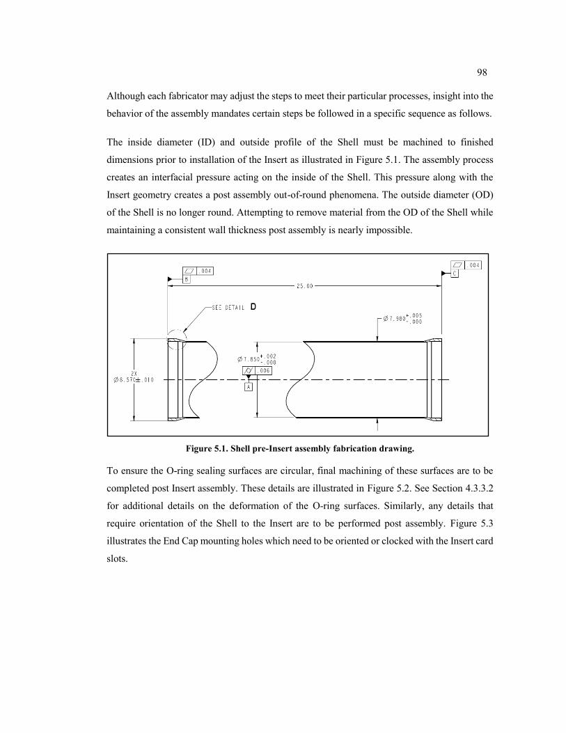
98

Although each fabricator may adjust the steps to meet their particular processes, insight into the

behavior of the assembly mandates certain steps be followed in a specific sequence as follows.

The inside diameter (ID) and outside profile of the Shell must be machined to finished

dimensions prior to installation of the Insert as illustrated in Figure 5.1. The assembly process

creates an interfacial pressure acting on the inside of the Shell. This pressure along with the

Insert geometry creates a post assembly out-of-round phenomena. The outside diameter (OD)

of the Shell is no longer round. Attempting to remove material from the OD of the Shell while

maintaining a consistent wall thickness post assembly is nearly impossible.

Figure 5.1. Shell pre-Insert assembly fabrication drawing.

To ensure the O-ring sealing surfaces are circular, final machining of these surfaces are to be

completed post Insert assembly. These details are illustrated in Figure 5.2. See Section 4.3.3.2

for additional details on the deformation of the O-ring surfaces. Similarly, any details that

require orientation of the Shell to the Insert are to be performed post assembly. Figure 5.3

illustrates the End Cap mounting holes which need to be oriented or clocked with the Insert card

slots.

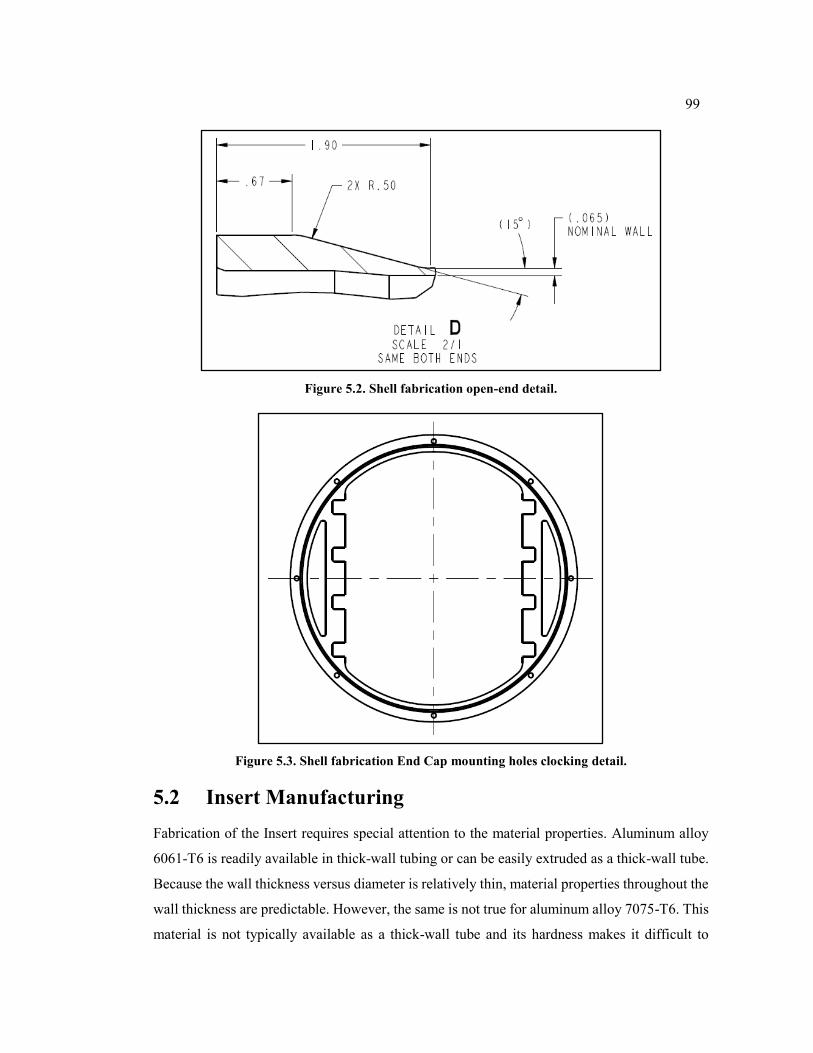
99

Figure 5.2. Shell fabrication open-end detail.

Figure 5.3. Shell fabrication End Cap mounting holes clocking detail.

5.2 Insert Manufacturing

Fabrication of the Insert requires special attention to the material properties. Aluminum alloy

6061-T6 is readily available in thick-wall tubing or can be easily extruded as a thick-wall tube.

Because the wall thickness versus diameter is relatively thin, material properties throughout the

wall thickness are predictable. However, the same is not true for aluminum alloy 7075-T6. This

material is not typically available as a thick-wall tube and its hardness makes it difficult to

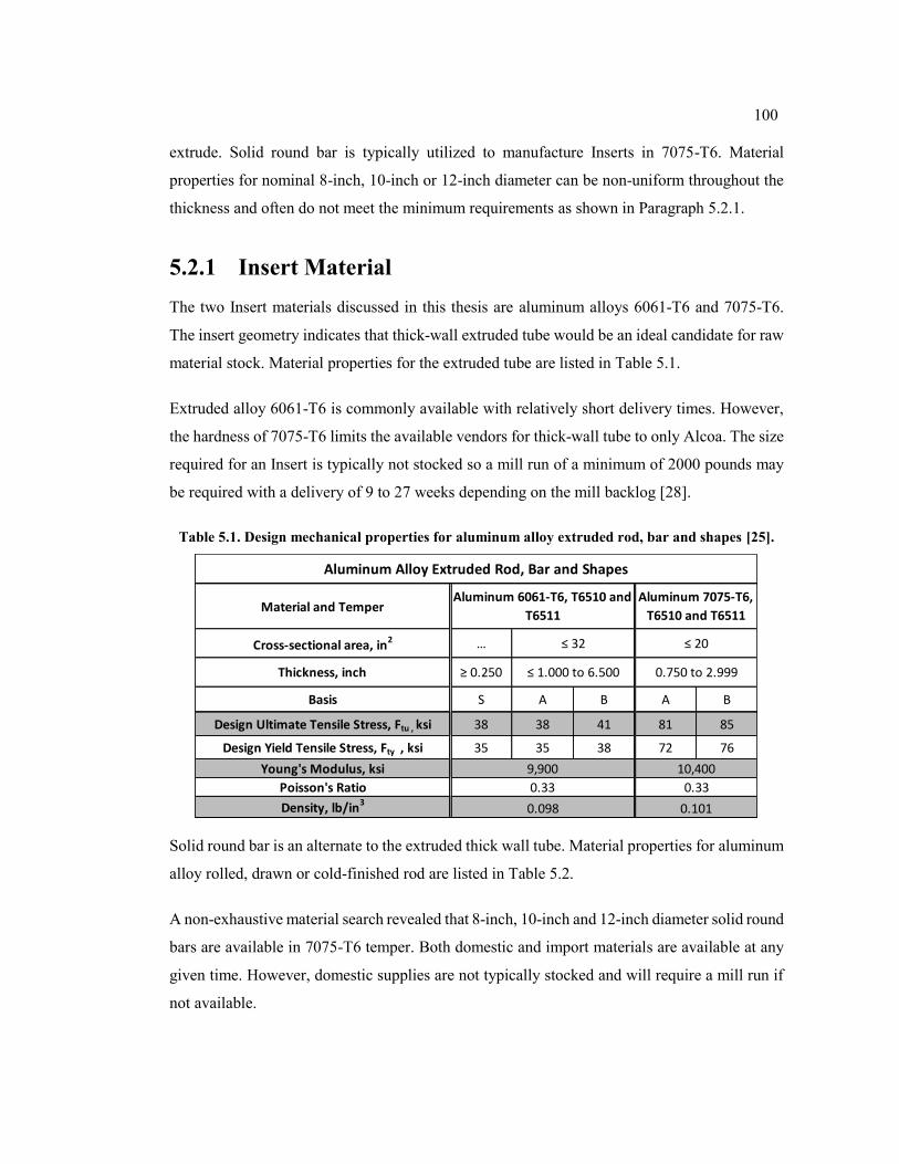
100

extrude. Solid round bar is typically utilized to manufacture Inserts in 7075-T6. Material

properties for nominal 8-inch, 10-inch or 12-inch diameter can be non-uniform throughout the

thickness and often do not meet the minimum requirements as shown in Paragraph 5.2.1.

5.2.1 Insert Material

The two Insert materials discussed in this thesis are aluminum alloys 6061-T6 and 7075-T6.

The insert geometry indicates that thick-wall extruded tube would be an ideal candidate for raw

material stock. Material properties for the extruded tube are listed in Table 5.1.

Extruded alloy 6061-T6 is commonly available with relatively short delivery times. However,

the hardness of 7075-T6 limits the available vendors for thick-wall tube to only Alcoa. The size

required for an Insert is typically not stocked so a mill run of a minimum of 2000 pounds may

be required with a delivery of 9 to 27 weeks depending on the mill backlog [28].

Table 5.1. Design mechanical properties for aluminum alloy extruded rod, bar and shapes [25].

Solid round bar is an alternate to the extruded thick wall tube. Material properties for aluminum

alloy rolled, drawn or cold-finished rod are listed in Table 5.2.

A non-exhaustive material search revealed that 8-inch, 10-inch and 12-inch diameter solid round

bars are available in 7075-T6 temper. Both domestic and import materials are available at any

given time. However, domestic supplies are not typically stocked and will require a mill run if

not available.

Material and Temper

Cross-sectional area, in2 …

Thickness, inch ≥ 0.250

Basis S A B A B

Design Ultimate Tensile Stress, Ftu , ksi 38 38 41 81 85

Design Yield Tensile Stress, Fty , ksi 35 35 38 72 76

Young's Modulus, ksi

Poisson's Ratio

Density, lb/in3

9,900 10,400

0.33 0.33

0.098 0.101

Aluminum Alloy Extruded Rod, Bar and Shapes

Aluminum 6061-T6, T6510 and

T6511

Aluminum 7075-T6,

T6510 and T6511

≤ 32 ≤ 20

≤ 1.000 to 6.500 0.750 to 2.999

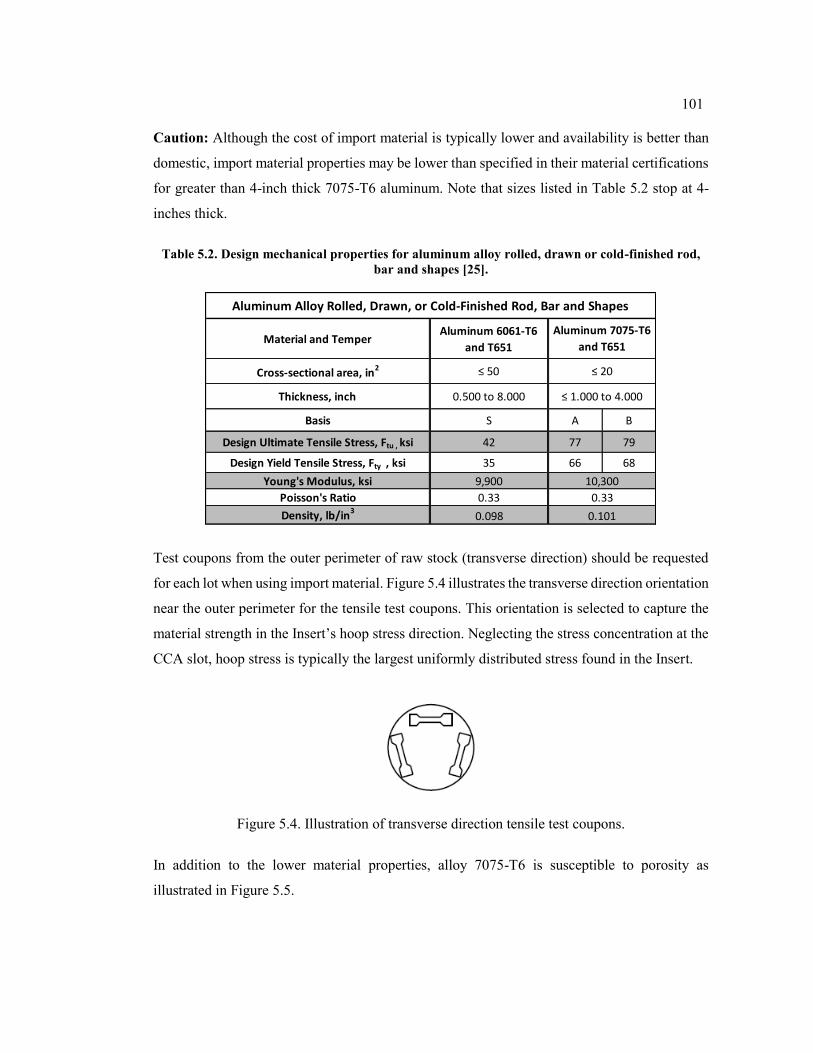
101

Caution: Although the cost of import material is typically lower and availability is better than

domestic, import material properties may be lower than specified in their material certifications

for greater than 4-inch thick 7075-T6 aluminum. Note that sizes listed in Table 5.2 stop at 4-

inches thick.

Table 5.2. Design mechanical properties for aluminum alloy rolled, drawn or cold-finished rod,

bar and shapes [25].

Test coupons from the outer perimeter of raw stock (transverse direction) should be requested

for each lot when using import material. Figure 5.4 illustrates the transverse direction orientation

near the outer perimeter for the tensile test coupons. This orientation is selected to capture the

material strength in the Insert’s hoop stress direction. Neglecting the stress concentration at the

CCA slot, hoop stress is typically the largest uniformly distributed stress found in the Insert.

Figure 5.4. Illustration of transverse direction tensile test coupons.

In addition to the lower material properties, alloy 7075-T6 is susceptible to porosity as

illustrated in Figure 5.5.

Material and TemperAluminum 6061-T6

and T651

Cross-sectional area, in2 ≤ 50

Thickness, inch 0.500 to 8.000

Basis S A B

Design Ultimate Tensile Stress, Ftu , ksi 42 77 79

Design Yield Tensile Stress, Fty , ksi 35 66 68

Young's Modulus, ksi 9,900

Poisson's Ratio 0.33

Density, lb/in3

0.098

10,300

0.33

0.101

Aluminum Alloy Rolled, Drawn, or Cold-Finished Rod, Bar and Shapes

Aluminum 7075-T6

and T651

≤ 20

≤ 1.000 to 4.000

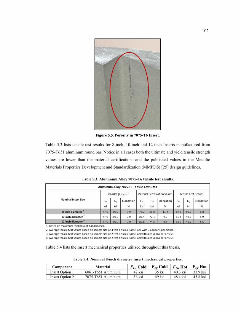
102

Figure 5.5. Porosity in 7075-T6 Insert.

Table 5.3 lists tensile test results for 8-inch, 10-inch and 12-inch Inserts manufactured from

7075-T651 aluminum round bar. Notice in all cases both the ultimate and yield tensile strength

values are lower than the material certifications and the published values in the Metallic

Materials Properties Development and Standardization (MMPDS) [25] design guidelines.

Table 5.3. Aluminum Alloy 7075-T6 tensile test results.

Table 5.4 lists the Insert mechanical properties utilized throughout this thesis.

Table 5.4. Nominal 8-inch diameter Insert mechanical properties.

Component Material 𝑭𝒕𝒖 Cold 𝑭𝒕𝒚 Cold 𝑭𝒕𝒖 Hot 𝑭𝒕𝒚 Hot



Ftu Fty Elongation Ftu Fty Elongation Ftu Fty Elongation

ksi ksi % ksi ksi % ksi ksi %

8-inch diameter 2 77.0 66.0 7.0 75.2 59.8 11.4 64.6 50.0 6.8

10-inch diameter 3 77.0 66.0 7.0 83.4 72.1 9.0 61.3 49.9 5.9

12-inch diameter 4 77.0 66.0 7.0 82.6 74.5 9.5 63.9 46.7 8.5

1. Based on maximum thickness of 4.000 inches.

2. Average tensile test values based on sample size of 4 test articles (same lot) with 3 coupons per article.



MMPDS (A-basis)1 Tensile Test Results

Nominal Insert Size

Material Certification Values

Aluminum Alloy 7075-T6 Tensile Test Data

103





5.2.2 Insert Machining

The Insert of study is 17-inches long. The geometry of the Insert is illustrated in Figure 5.6. The

accuracy required for the card slot locations require the part be manufactured using precision

Wire Electric Discharge Machining (EDM) process. Wire EDM is a method utilized to cut

conductive materials with a thin wire electrode that follows a programmed path. The hardness

of the work piece material has no detrimental effect on the cutting speed. Wire EDM can be

accurate to ± 0.0001 inches. The wire EDM process does not generate burrs. However, the

process can generate sharp edges so care should be taken to add small fillets (radii) where

necessary to eliminate the sharp edges.

Although many machine shops have wire EDM capabilities, the length of the Insert requires a

deep reach wire EDM. This requirement reduces the number of available wire EDM facilities.

To manufacture the Insert, the outside diameter of the thick-walled tube or solid round bar, is

machined down from the raw stock diameter to a dimension larger than is required for the

interference fit. The inner profile is then cut to shape using the wire EDM process. The Insert

final OD is machined to final dimensions after the wire EDM operation. If a chemical

conversion process is required, it is to be performed after final machining of the Insert and prior

the Insert being installed in the Shell. Dimensional inspection of the Insert is also to be

performed prior to assembly. Recall, the post assembly out-of-round phenomena changes the

dimensions of the insert which make it nearly impossible to inspect to pre-assembly dimensions.

104

Figure 5.6. Case 1 and Case 3 Insert cross-section pre-assembly dimensions (10 mil interference).

5.3 Chassis Assembly

In general, the Shell and Insert are to be assembled by creating a temperature difference between

the two components. It is permissible to heat the Shell and cool the Insert and then “drop” the

insert into the shell and allow the temperatures of the parts to return to room temperature.

In some applications, only cooling of the insert is adequate to assemble the two parts. Care

should be taken to not affect the temper of the materials during this process. If the Shell is

fabricated using 2205 Duplex stainless steel, the maximum recommended temperature is 450°F.

If the Insert is fabricated from aluminum alloy 7075-T6, the lowest minimum temperature is -

320°F which is the nominal temperature of liquid nitrogen. To determine if both processes are

105

required, the dimensions and OOR condition of the Insert can be modeled at this cold

temperature. If adequate clearance exists between the worst case OOR dimensions and the room

temperature Shell, heating of the Shell step can be ignored.

Figure 5.7 illustrates the radial deformation of the Insert at -320°F. Notice that the overall shape

of the outside diameter remains round. That is, no circularity deformation is present. The radial

deformation is approximately 20 mils radial which will provide adequate assembly clearance

without heating the Shell.

Figure 5.7. Insert radial deformation at temperature of -320°F.

However, if heating of the Shell is desired for additional clearance, the increase in the radius is

11 mils minimum as illustrated in Figure 5.8 and Figure 5.9.

Once assembled, the maximum temperature of the assembly is to be 350°F to prevent affecting

the temper of the aluminum Insert. To minimize post assembly thermal stresses, it is

recommended to heat the assembly to 220°F and hold for 60 minutes. Afterwards, the assembly

is to be slow cooled to room temperature in still air.

106

Figure 5.8. Shell radial deformation at temperature of +450°F.

Figure 5.9. Shell radial deformation at temperature of +450°F.

As discussed in Paragraph 5.1.2, final machining of the Shell to Insert clocking features are to

be performed post assembly. Final machining of the O-ring surfaces also need to be performed

post assembly as illustrated in Figure 5.10 and Figure 5.11.

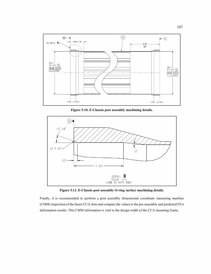
107

Figure 5.10. E-Chassis post assembly machining details.

Figure 5.11. E-Chassis post assembly O-ring surface machining details.

Finally, it is recommended to perform a post assembly dimensional coordinate measuring machine

(CMM) inspection of the Insert CCA slots and compare the values to the pre-assembly and predicted FEA

deformation results. This CMM information is vital to the design width of the CCA mounting frame.

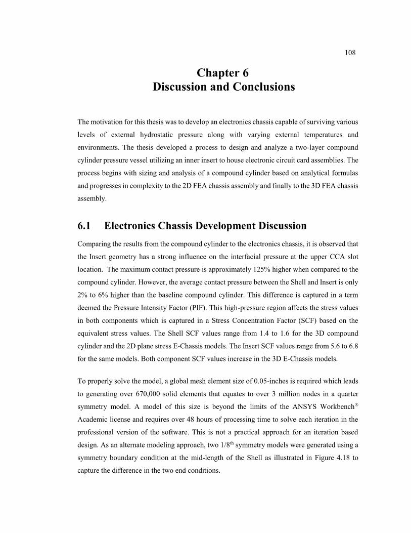
108

Chapter 6

Discussion and Conclusions

The motivation for this thesis was to develop an electronics chassis capable of surviving various

levels of external hydrostatic pressure along with varying external temperatures and

environments. The thesis developed a process to design and analyze a two-layer compound

cylinder pressure vessel utilizing an inner insert to house electronic circuit card assemblies. The

process begins with sizing and analysis of a compound cylinder based on analytical formulas

and progresses in complexity to the 2D FEA chassis assembly and finally to the 3D FEA chassis

assembly.

6.1 Electronics Chassis Development Discussion

Comparing the results from the compound cylinder to the electronics chassis, it is observed that

the Insert geometry has a strong influence on the interfacial pressure at the upper CCA slot

location. The maximum contact pressure is approximately 125% higher when compared to the

compound cylinder. However, the average contact pressure between the Shell and Insert is only

2% to 6% higher than the baseline compound cylinder. This difference is captured in a term

deemed the Pressure Intensity Factor (PIF). This high-pressure region affects the stress values

in both components which is captured in a Stress Concentration Factor (SCF) based on the

equivalent stress values. The Shell SCF values range from 1.4 to 1.6 for the 3D compound

cylinder and the 2D plane stress E-Chassis models. The Insert SCF values range from 5.6 to 6.8

for the same models. Both component SCF values increase in the 3D E-Chassis models.

To properly solve the model, a global mesh element size of 0.05-inches is required which leads

to generating over 670,000 solid elements that equates to over 3 million nodes in a quarter

symmetry model. A model of this size is beyond the limits of the ANSYS Workbench®

Academic license and requires over 48 hours of processing time to solve each iteration in the

professional version of the software. This is not a practical approach for an iteration based

design. As an alternate modeling approach, two 1/8th symmetry models were generated using a

symmetry boundary condition at the mid-length of the Shell as illustrated in Figure 4.18 to

capture the difference in the two end conditions.

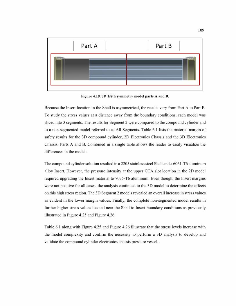
109

Figure 4.18. 3D 1/8th symmetry model parts A and B.

Because the Insert location in the Shell is asymmetrical, the results vary from Part A to Part B.

To study the stress values at a distance away from the boundary conditions, each model was

sliced into 3 segments. The results for Segment 2 were compared to the compound cylinder and

to a non-segmented model referred to as All Segments. Table 6.1 lists the material margin of

safety results for the 3D compound cylinder, 2D Electronics Chassis and the 3D Electronics

Chassis, Parts A and B. Combined in a single table allows the reader to easily visualize the

differences in the models.

The compound cylinder solution resulted in a 2205 stainless steel Shell and a 6061-T6 aluminum

alloy Insert. However, the pressure intensity at the upper CCA slot location in the 2D model

required upgrading the Insert material to 7075-T6 aluminum. Even though, the Insert margins

were not positive for all cases, the analysis continued to the 3D model to determine the effects

on this high stress region. The 3D Segment 2 models revealed an overall increase in stress values

as evident in the lower margin values. Finally, the complete non-segmented model results in

further higher stress values located near the Shell to Insert boundary conditions as previously

illustrated in Figure 4.25 and Figure 4.26.

Table 6.1 along with Figure 4.25 and Figure 4.26 illustrate that the stress levels increase with

the model complexity and confirm the necessity to perform a 3D analysis to develop and

validate the compound cylinder electronics chassis pressure vessel.

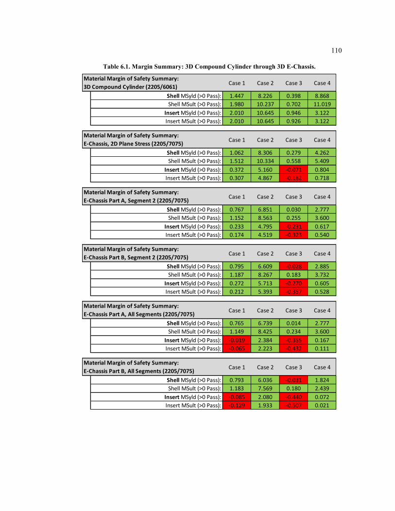
110

Table 6.1. Margin Summary: 3D Compound Cylinder through 3D E-Chassis.


Shell MSyld (>0 Pass): 1.447 8.226 0.398 8.868

Shell MSult (>0 Pass): 1.980 10.237 0.702 11.019




Shell MSyld (>0 Pass): 1.062 8.306 0.279 4.262

Shell MSult (>0 Pass): 1.512 10.334 0.558 5.409




Shell MSyld (>0 Pass): 0.767 6.851 0.030 2.777

Shell MSult (>0 Pass): 1.152 8.563 0.255 3.600




Shell MSyld (>0 Pass): 0.795 6.609 -0.028 2.885

Shell MSult (>0 Pass): 1.187 8.267 0.183 3.732




Shell MSyld (>0 Pass): 0.765 6.739 0.014 2.777

Shell MSult (>0 Pass): 1.149 8.425 0.234 3.600




Shell MSyld (>0 Pass): 0.793 6.036 -0.031 1.824

Shell MSult (>0 Pass): 1.183 7.569 0.180 2.439



Material Margin of Safety Summary:

E-Chassis, 2D Plane Stress (2205/7075)


E-Chassis Part A, Segment 2 (2205/7075)


E-Chassis Part B, Segment 2 (2205/7075)


E-Chassis Part A, All Segments (2205/7075)


E-Chassis Part B, All Segments (2205/7075)


3D Compound Cylinder (2205/6061)

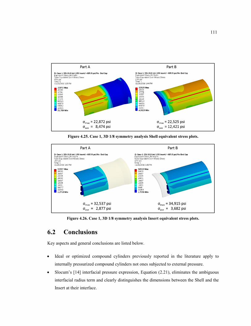
111

Figure 4.25. Case 1, 3D 1/8 symmetry analysis Shell equivalent stress plots.

Figure 4.26. Case 1, 3D 1/8 symmetry analysis Insert equivalent stress plots.

6.2 Conclusions

Key aspects and general conclusions are listed below.

Ideal or optimized compound cylinders previously reported in the literature apply to

internally pressurized compound cylinders not ones subjected to external pressure.

Slocum’s [14] interfacial pressure expression, Equation (2.21), eliminates the ambiguous

interfacial radius term and clearly distinguishes the dimensions between the Shell and the

Insert at their interface.

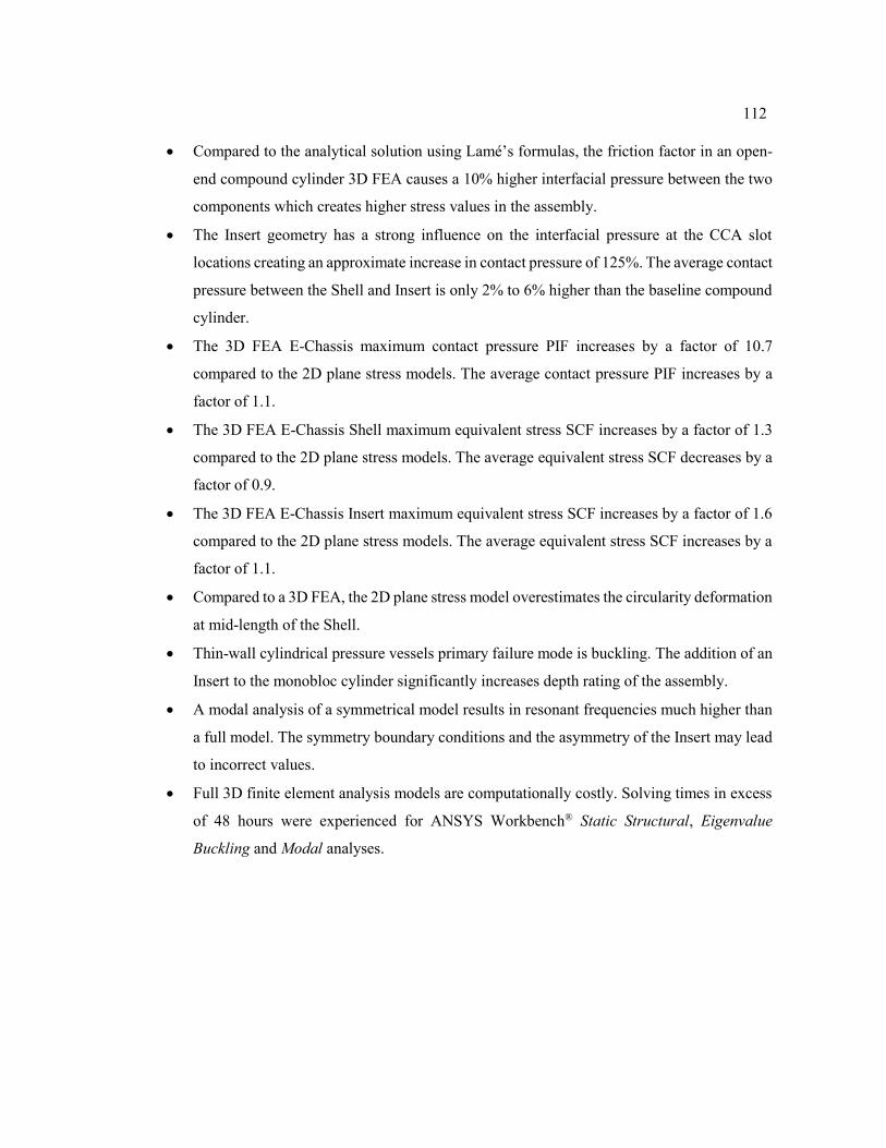
112

Compared to the analytical solution using Lamé’s formulas, the friction factor in an open-

end compound cylinder 3D FEA causes a 10% higher interfacial pressure between the two

components which creates higher stress values in the assembly.

The Insert geometry has a strong influence on the interfacial pressure at the CCA slot

locations creating an approximate increase in contact pressure of 125%. The average contact

pressure between the Shell and Insert is only 2% to 6% higher than the baseline compound

cylinder.

The 3D FEA E-Chassis maximum contact pressure PIF increases by a factor of 10.7

compared to the 2D plane stress models. The average contact pressure PIF increases by a

factor of 1.1.

The 3D FEA E-Chassis Shell maximum equivalent stress SCF increases by a factor of 1.3

compared to the 2D plane stress models. The average equivalent stress SCF decreases by a

factor of 0.9.

The 3D FEA E-Chassis Insert maximum equivalent stress SCF increases by a factor of 1.6

compared to the 2D plane stress models. The average equivalent stress SCF increases by a

factor of 1.1.

Compared to a 3D FEA, the 2D plane stress model overestimates the circularity deformation

at mid-length of the Shell.

Thin-wall cylindrical pressure vessels primary failure mode is buckling. The addition of an

Insert to the monobloc cylinder significantly increases depth rating of the assembly.

A modal analysis of a symmetrical model results in resonant frequencies much higher than

a full model. The symmetry boundary conditions and the asymmetry of the Insert may lead

to incorrect values.

Full 3D finite element analysis models are computationally costly. Solving times in excess

of 48 hours were experienced for ANSYS Workbench® Static Structural, Eigenvalue

Buckling and Modal analyses.

113

6.3 Recommendations

The thesis concentrated on the structural aspects of the design but a major advantage of the

interference fit design is an improved thermal path from the Insert’s card slots to the Shell’s

outer surface. Creating a thermal model to study the heat transfer through the chassis and

determine the thermal capacity in various thermal conductivity environments is of vital interest

in the full development of the electronics chassis.

A second item of interest is the holding capacity of the insert versus the surface finish. Slocum

[14] stated that the holding power of an interference fit depends on the coefficient of friction

and the amount by which the surface roughness of the two parts dig into each other forming a

mechanical bond. In general, the finer the surface finish, the more the joint appears to be solid.

Slocum suggests that clean, high surface finish parts actually cold weld together after they are

press fit. If this phenomenon can be validated, perhaps lower interference fit values can be

utilized which will lower stress values and make fabrication and assembly of the two

components more efficient. Boutoutaou et al. [18] presented a methodology for a computer-

aided design of shrink fits that considers the roughness and form defects of the manufacturing

process. Only the bore defects in the outer disk were considered. Generalizing the approach for

defects in both parts with the is necessary to complete the study.

A third item of interest is the buckling capacity of the assembly. Eigenvalue buckling generally

yields non-conservative results. Both this thesis and commercially available pressure vessel

software utilize a linear buckling analysis because the results are computationally relatively

inexpensive and the buckling mode shapes can be used for comparison to the more realistic

nonlinear buckling analysis.

A fourth area of interest is the validation of material properties in thick alloyed aluminum plate

and shapes. The occurrence appears to be more relevant when imported materials are used.

However, this has not been fully vetted. The majority of alloy 7075-T6 is currently

manufactured overseas in Alcoa plants.

Finally, this thesis demonstrated the development of the compound cylinder electronics chassis

pressure vessel using a nominal 8-inch outside diameter Shell. As the diameter of the compound

cylinder is increased, the magnitude of the interfacial pressure decreases for a given interference

114

value. This suggests that a larger interference fit value will be required for a 10-inch and 12-

inch assembly to obtain the same holding capacity as an 8-inch assembly. Both 10-inch and 12-

inch chassis have been design and fabricated based on results of a 2D plane stress analysis. It

will be of interest to evaluate the results of a 3D FEM analysis.

115

References

[1] Prevco Subsea Housings, [Products], https://prevco.com/products, [cited 10 April

2016].

[2] Bitller, J. P., Pascal, F., Hang-Hu, M., Pelet, A. (To Alcatel CIT), “Electronic Circuit

Housing,” U. S. Patent 4,858,068, August 15, 1989.

[3] Hutchinson, R. D., Schiffbauer, R., Smith, K. (To the Special Product Company),

“Concentrical Slot Telecommunications Equipment,” U. S. Patent 6,404,637 B2, June

11, 2002.

[4] Ferris, C., Petersen, C. D. (To Fogg and Associates, LLC), “Heat Dissipation for

Electronic Enclosures,” U. S. Patent Application Publication US 2005/0068743 A1,

March 31, 2005.

[5] Davey, P. J. (To Vetco Gray Controls Limited), “Subsea Electronic Modules,” U. S.

Patent 8,373,418 B2, February 12, 2013.

[6] Davis, J. R. (To Vetco Gray Controls Limited), “Subsea Electronic Modules,” U. S.

Patent 8,493,741 B2, July 23, 2013.

[7] Shigley, J. E. and Mischke, C. R., “Press and Shrink Fits,” Mechanical Engineering

Design, 8th ed., McGraw-Hill, New York, 2006, pp. 107-112.

[8] Sadd, M. H., Elasticity. Theory, Applications, and Numerics, 2e, Academic Press, 2009,

pp. 172-173.

[9] Boresi, A. P. and Schmidt, R. J., Advanced Mechanics of Materials, 6th ed., John Wiley

& Sons, 2003, pp. 389-397.

[10] Sharp, A. G., “Design Curves for Oceanographic Pressure-Resistant Housings,”

Technical Memorandum 3-81, Woods Hole Oceanographic Institution, Office of Naval

Research Contract No. N00014-73-C-0097, 1981, pp. 1 – 8.

[11] Cortesi, R., “Crush Depth of Simple Cylinders and Endcaps,” Massachusetts Institute of

Technology Mechanical Engineering, Cambridge, Massachusetts, June 2002,

[http://rogercortesi.com/portf/pressvesfailure/presvesfail.html. Accessed 7/13/16.]

[12] Young, W. C., “Table 32 Formula’s for thick-walled vessels under internal and

external loading, Case 1c,” Roark’s Formulas for Stress and Strain, 6th ed., McGraw-

Hill, New York, pp. 638.

[13] PTC Mathcad version 15.0.

[14] Slocum, A. H., ”Interference Fit Joints,” Precision Machine Design, 1st ed., Prentice-

Hall, 1992, pp. 384-393.

[15] Davidson, T. E., and Kendall, D. P., “The Design of Pressure Vessels for Very High

Pressure Operation,” Technical Report WVT-6917, Benet R&E Laboratories,

Watervliet Arsenal, U.S. Army Weapons Command, May 1969, pp. 4-16.

[16] Majumder, T., “Optimum Design of Compound Cylindrical Pressure Vessel by Finite

Element Analysis,” MS Thesis, Jadavpur University, Kolkata, India, 2014.

https://prevco.com/products

116

[17] Doležel, I., Kotlan, V., Ulrych, B., “Design of joint between disk and shaft based on

induction shrink fit,” Journal of Computational and Applied Mathematics, Elsevier,

Vol. 270, 2014, pp. 52-62.

[18] Boutoutaou, H. and Fontaine, J. F., “Methodology for a Computer-Aided Design of

Shrink Fits that Considers the Roughness and Form Defects of the Manufacturing

Process,” Journal of Mechanical Science and Technology, Vol. 29, No. 5, 2015, pp.

2097-2103.

[19] “Standard Specifications for General Requirements for Alloy and Stainless Steel Pipe,”

ASTM A999/A 999M, Sections 10, 11 and 12, ASTM International, West

Conshohocken, PA, 2004.

[20] Oberg, E., Jones, F. D., Horton, H. L. and Ryffel, H. H., “Allowances and Tolerances,”

Machinery’s Handbook, 26th ed., Industrial Press, New York, 2000, pp. 621-641.

[21] Khurmi, R. S. and Gupta, J. K., A Textbook of Machine Design, 14th ed., Eurasia

Publishing House Ltd., New Delhi, 2015, pp. 241-246.

[22] Ugural, A. C. and Fenster, S. K., Advanced Mechanics of Materials and Applied

Elasticity, 6th ed., Prentice Hall, 2012, pp. 408-419.

[23] Roe Jr., R. R., “Structural Design and Test Factors for Spaceflight Hardware,” NASA-

STD-5001B, April 2016.

[24] “Space Systems - Structures, Structural Components, and Structural Assemblies,”

AIAA S-110, 2005.

[25] Rice, R. C., Jackson, J. L., Bakuckas, J., and Thompson, S., “Metallic Materials

Properties Development and Standardization (MMPDS),” DOT/FAA/AR-MMMPDS-

01, January 2003.

[26] Deepsea Power & Light, “Under Pressure Version 4.0 User Manual,”

[http://www.deepsea.com/knowledgebase/design-tools/under-pressure-design-

software/. Accessed 10/28/16.]

[27] Steinberg, D. S., Vibration Analysis for Electronics Equipment, 3rd ed., John Wiley &

Sons, New York, 2000.

[28] Personal communication with Alcoa Forgings and Extrusions division, Lafayette,

Indiana Plant, 5/13/2013 and 3/15/2016.

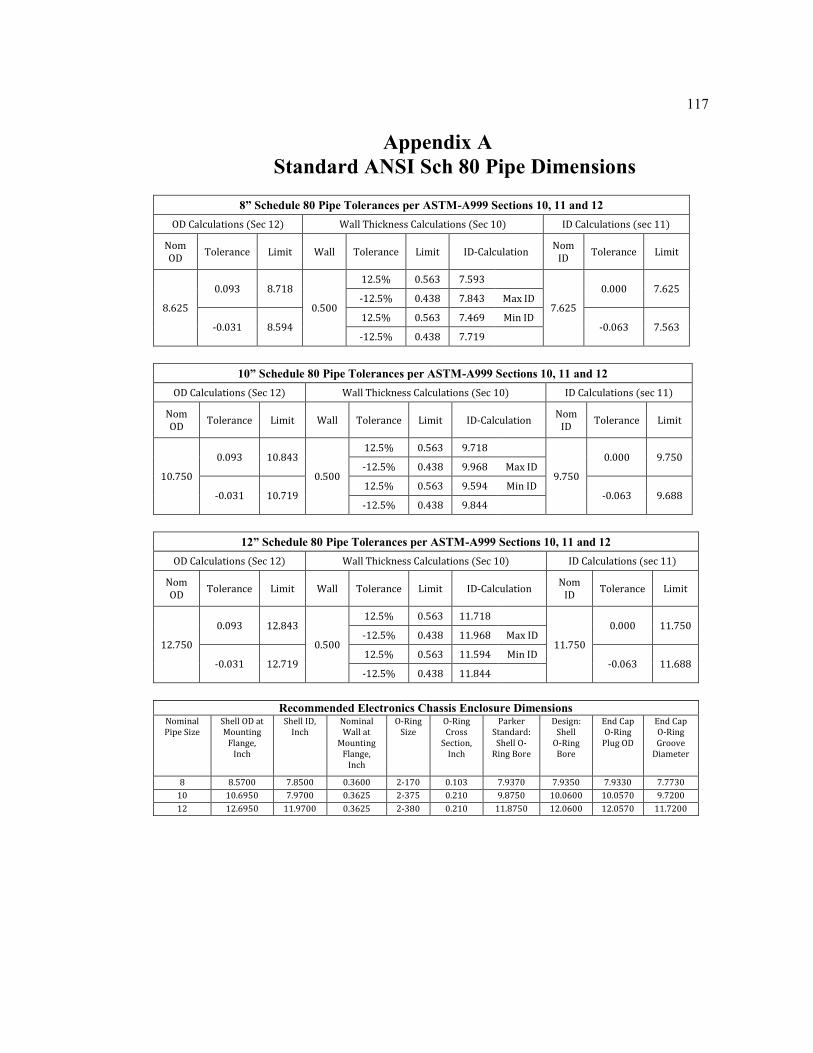
117

Appendix A

Standard ANSI Sch 80 Pipe Dimensions



Nom OD


ID Tolerance Limit

8.625

0.093 8.718

0.500

12.5% 0.563 7.593

7.625

0.000 7.625 -12.5% 0.438 7.843 Max ID

-0.031 8.594 12.5% 0.563 7.469 Min ID

-0.063 7.563 -12.5% 0.438 7.719



Nom OD


ID Tolerance Limit

10.750

0.093 10.843

0.500

12.5% 0.563 9.718

9.750

0.000 9.750 -12.5% 0.438 9.968 Max ID

-0.031 10.719 12.5% 0.563 9.594 Min ID

-0.063 9.688 -12.5% 0.438 9.844



Nom OD


ID Tolerance Limit

12.750

0.093 12.843

0.500

12.5% 0.563 11.718

11.750

0.000 11.750 -12.5% 0.438 11.968 Max ID

-0.031 12.719 12.5% 0.563 11.594 Min ID

-0.063 11.688 -12.5% 0.438 11.844

Recommended Electronics Chassis Enclosure Dimensions

Nominal Pipe Size

Shell OD at Mounting

Flange, Inch

Shell ID, Inch

Nominal Wall at

Mounting Flange,

Inch

O-Ring Size

O-Ring Cross

Section, Inch

Parker Standard: Shell O-

Ring Bore

Design: Shell

O-Ring Bore

End Cap O-Ring

Plug OD

End Cap O-Ring Groove

Diameter

8 8.5700 7.8500 0.3600 2-170 0.103 7.9370 7.9350 7.9330 7.7730

10 10.6950 7.9700 0.3625 2-375 0.210 9.8750 10.0600 10.0570 9.7200

12 12.6950 11.9700 0.3625 2-380 0.210 11.8750 12.0600 12.0570 11.7200

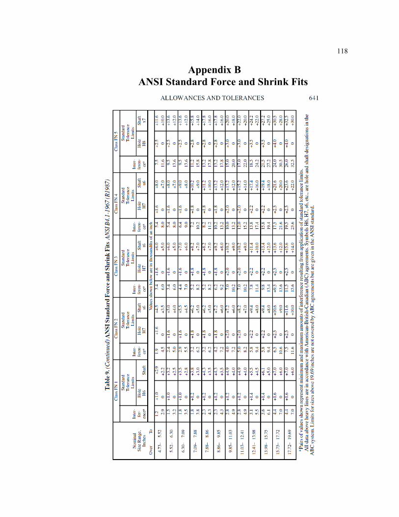
118

Appendix B

ANSI Standard Force and Shrink Fits

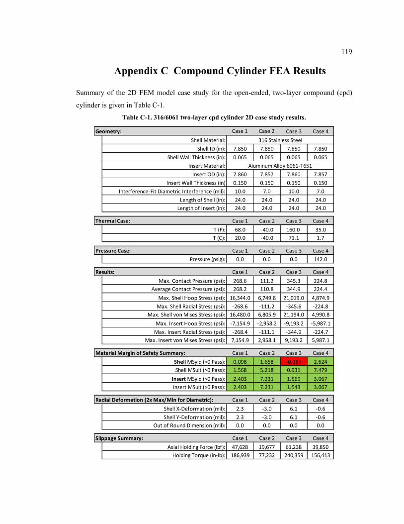
119

Appendix C Compound Cylinder FEA Results

Summary of the 2D FEM model case study for the open-ended, two-layer compound (cpd)

cylinder is given in Table C-1.

Table C-1. 316/6061 two-layer cpd cylinder 2D case study results.






Shell Material:

Shell ID (in): 7.850 7.850 7.850 7.850


Insert Material:

Insert OD (in): 7.860 7.857 7.860 7.857






T (F): 68.0 -40.0 160.0 35.0

T (C): 20.0 -40.0 71.1 1.7


Pressure (psig): 0.0 0.0 0.0 142.0











Shell MSyld (>0 Pass): 0.098 1.658 -0.187 2.624

Shell MSult (>0 Pass): 1.568 5.218 0.931 7.479










316 Stainless Steel


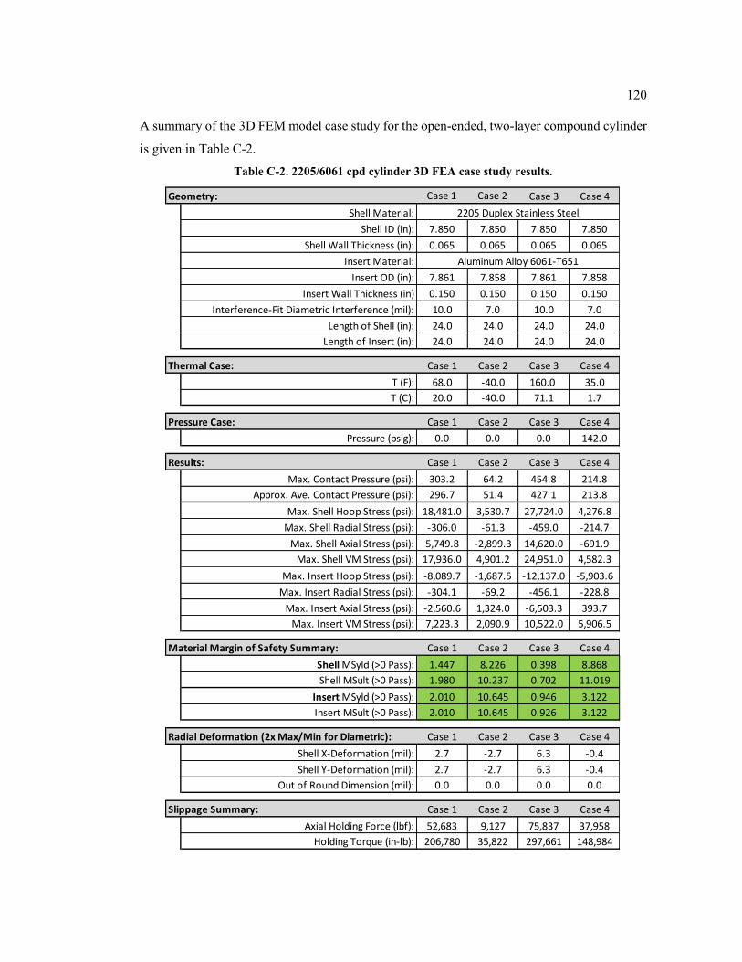
120

A summary of the 3D FEM model case study for the open-ended, two-layer compound cylinder

is given in Table C-2.

Table C-2. 2205/6061 cpd cylinder 3D FEA case study results.

Case Description: 3D Open-End Compound Cyl. Case 1 Case 2 Case 3 Case 4





Shell Material:

Shell ID (in): 7.850 7.850 7.850 7.850


Insert Material:

Insert OD (in): 7.861 7.858 7.861 7.858






T (F): 68.0 -40.0 160.0 35.0

T (C): 20.0 -40.0 71.1 1.7


Pressure (psig): 0.0 0.0 0.0 142.0













Shell MSyld (>0 Pass): 1.447 8.226 0.398 8.868

Shell MSult (>0 Pass): 1.980 10.237 0.702 11.019












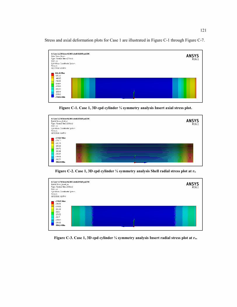
121

Stress and axial deformation plots for Case 1 are illustrated in Figure C-1 through Figure C-7.

Figure C-1. Case 1, 3D cpd cylinder ¼ symmetry analysis Insert axial stress plot.

Figure C-2. Case 1, 3D cpd cylinder ¼ symmetry analysis Shell radial stress plot at ri.

Figure C-3. Case 1, 3D cpd cylinder ¼ symmetry analysis Insert radial stress plot at ro.

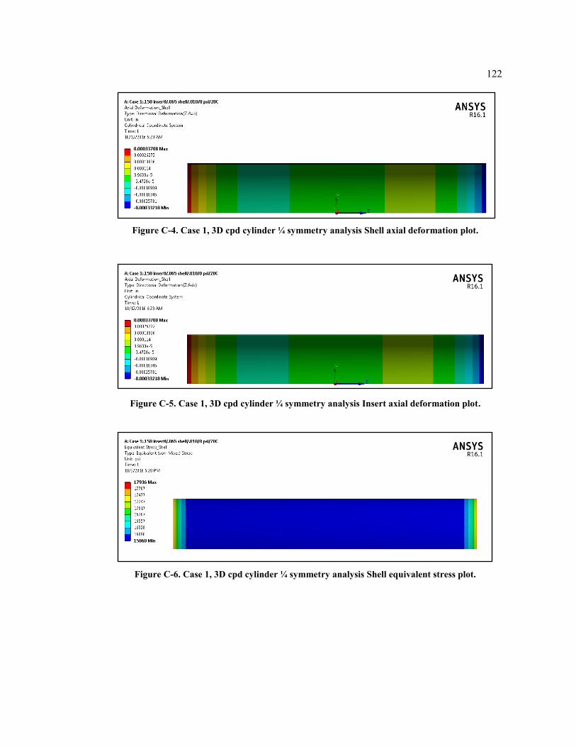
122

Figure C-4. Case 1, 3D cpd cylinder ¼ symmetry analysis Shell axial deformation plot.

Figure C-5. Case 1, 3D cpd cylinder ¼ symmetry analysis Insert axial deformation plot.

Figure C-6. Case 1, 3D cpd cylinder ¼ symmetry analysis Shell equivalent stress plot.

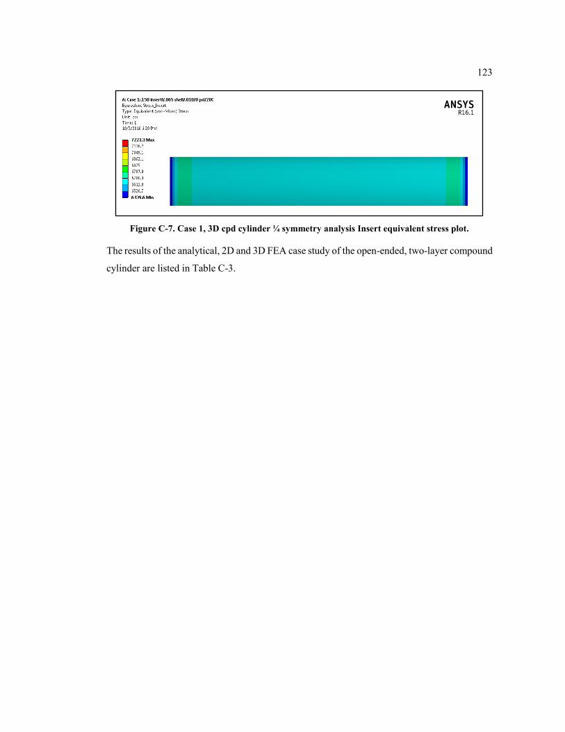
123

Figure C-7. Case 1, 3D cpd cylinder ¼ symmetry analysis Insert equivalent stress plot.

The results of the analytical, 2D and 3D FEA case study of the open-ended, two-layer compound

cylinder are listed in Table C-3.

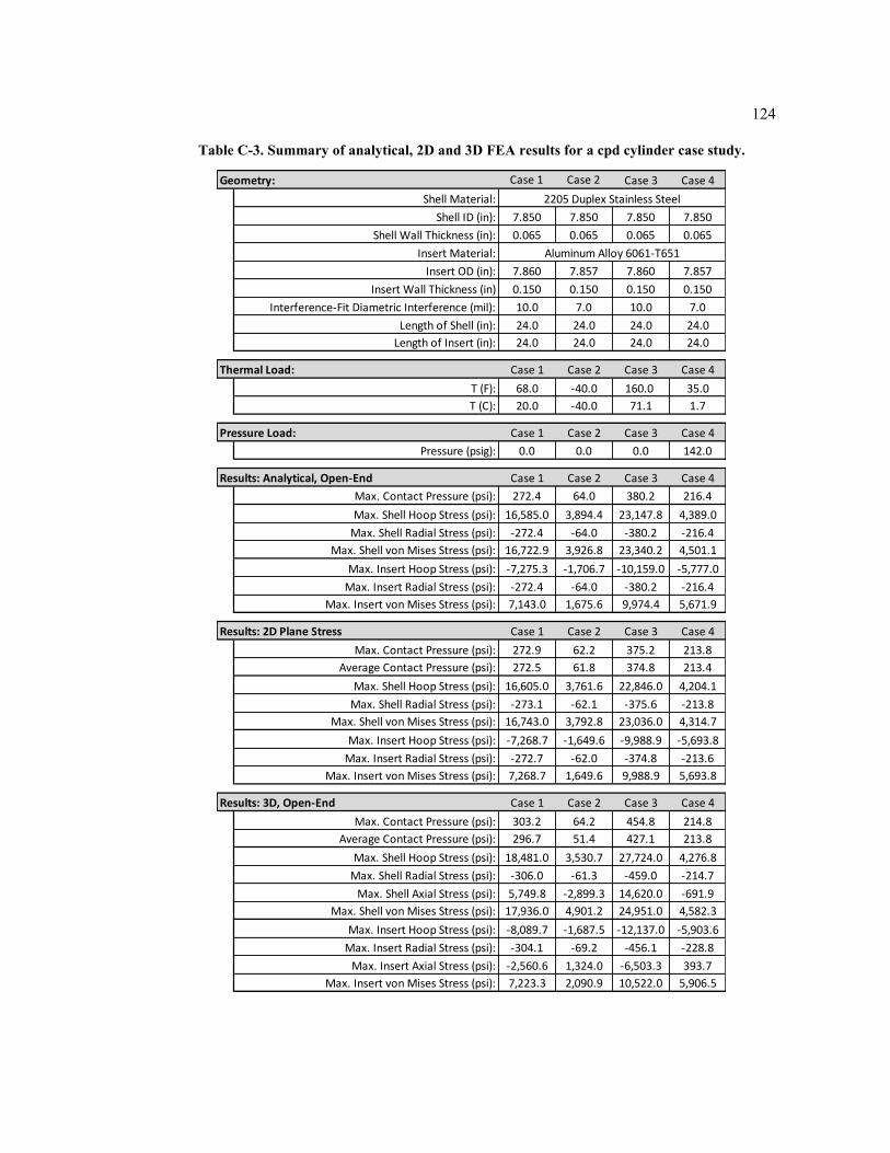
124

Table C-3. Summary of analytical, 2D and 3D FEA results for a cpd cylinder case study.




External Pressure: None None None High


Shell Material:

Shell ID (in): 7.850 7.850 7.850 7.850


Insert Material:

Insert OD (in): 7.860 7.857 7.860 7.857





Thermal Load: Case 1 Case 2 Case 3 Case 4

T (F): 68.0 -40.0 160.0 35.0

T (C): 20.0 -40.0 71.1 1.7

Pressure Load: Case 1 Case 2 Case 3 Case 4

Pressure (psig): 0.0 0.0 0.0 142.0

Results: Analytical, Open-End Case 1 Case 2 Case 3 Case 4








Results: 2D Plane Stress Case 1 Case 2 Case 3 Case 4









Results: 3D, Open-End Case 1 Case 2 Case 3 Case 4













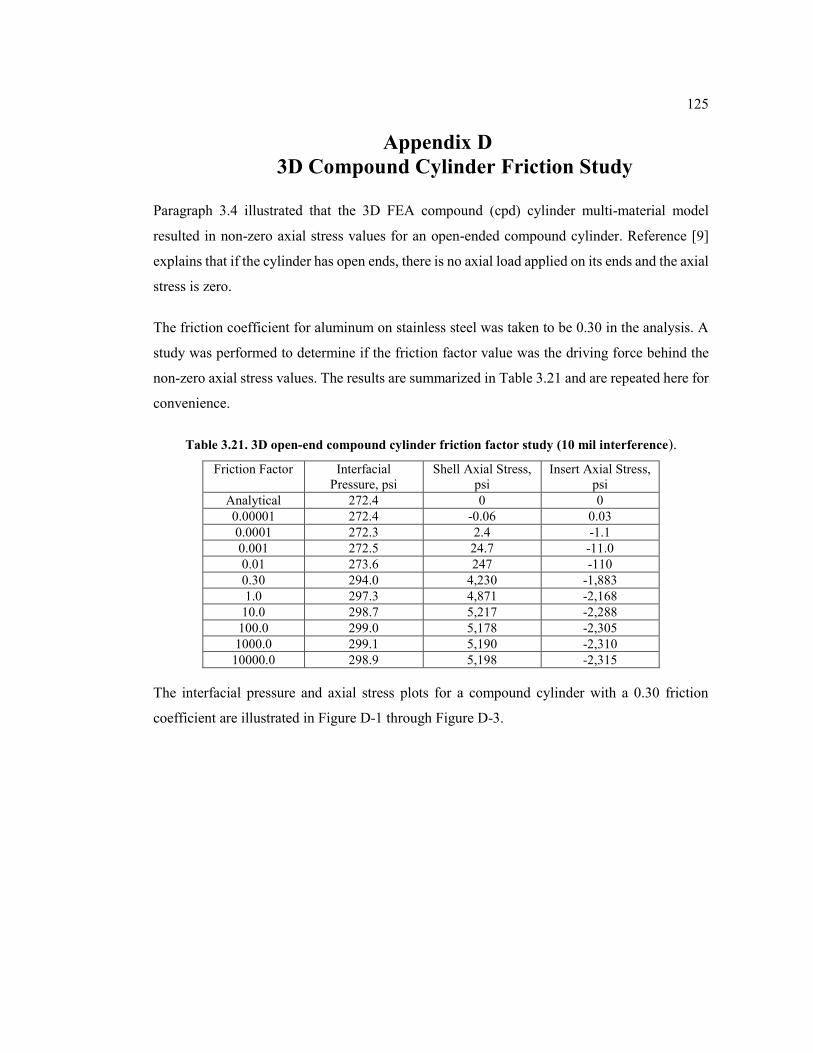
125

Appendix D

3D Compound Cylinder Friction Study

Paragraph 3.4 illustrated that the 3D FEA compound (cpd) cylinder multi-material model

resulted in non-zero axial stress values for an open-ended compound cylinder. Reference [9]

explains that if the cylinder has open ends, there is no axial load applied on its ends and the axial

stress is zero.

The friction coefficient for aluminum on stainless steel was taken to be 0.30 in the analysis. A

study was performed to determine if the friction factor value was the driving force behind the

non-zero axial stress values. The results are summarized in Table 3.21 and are repeated here for

convenience.

Table 3.21. 3D open-end compound cylinder friction factor study (10 mil interference).

Friction Factor Interfacial

Pressure, psi

Shell Axial Stress,

psi

Insert Axial Stress,

psi

Analytical 272.4 0 0

0.00001 272.4 -0.06 0.03

0.0001 272.3 2.4 -1.1

0.001 272.5 24.7 -11.0

0.01 273.6 247 -110

0.30 294.0 4,230 -1,883

1.0 297.3 4,871 -2,168

10.0 298.7 5,217 -2,288

100.0 299.0 5,178 -2,305

1000.0 299.1 5,190 -2,310

10000.0 298.9 5,198 -2,315

The interfacial pressure and axial stress plots for a compound cylinder with a 0.30 friction

coefficient are illustrated in Figure D-1 through Figure D-3.

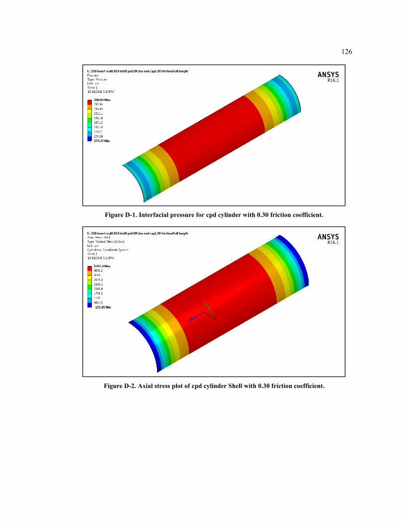
126

Figure D-1. Interfacial pressure for cpd cylinder with 0.30 friction coefficient.

Figure D-2. Axial stress plot of cpd cylinder Shell with 0.30 friction coefficient.

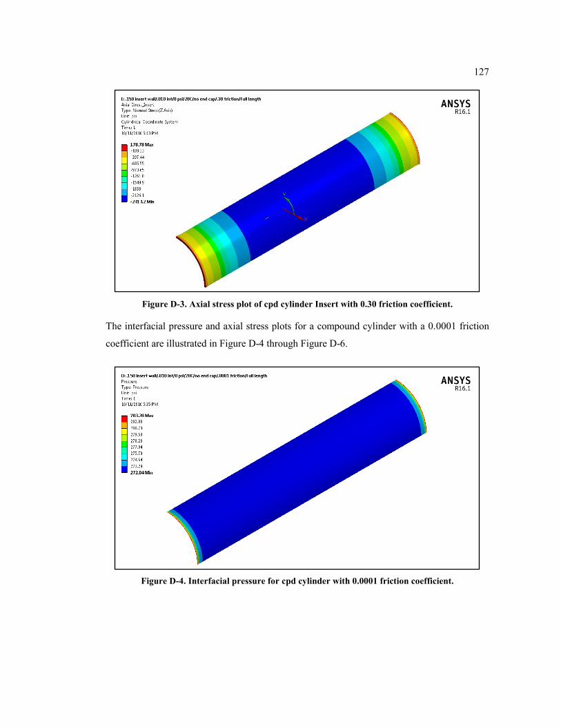
127

Figure D-3. Axial stress plot of cpd cylinder Insert with 0.30 friction coefficient.

The interfacial pressure and axial stress plots for a compound cylinder with a 0.0001 friction

coefficient are illustrated in Figure D-4 through Figure D-6.

Figure D-4. Interfacial pressure for cpd cylinder with 0.0001 friction coefficient.

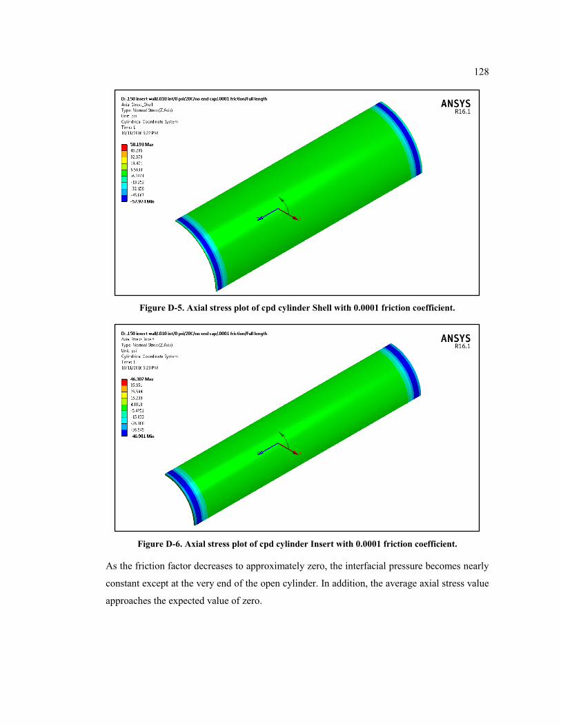
128

Figure D-5. Axial stress plot of cpd cylinder Shell with 0.0001 friction coefficient.

Figure D-6. Axial stress plot of cpd cylinder Insert with 0.0001 friction coefficient.

As the friction factor decreases to approximately zero, the interfacial pressure becomes nearly

constant except at the very end of the open cylinder. In addition, the average axial stress value

approaches the expected value of zero.

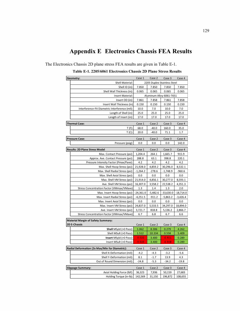
129

Appendix E Electronics Chassis FEA Results

The Electronics Chassis 2D plane stress FEA results are given in Table E-1.

Table E-1. 2205/6061 Electronics Chassis 2D Plane Stress Results


Shell Material:

Shell ID (in): 7.850 7.850 7.850 7.850


Insert Material:

Insert OD (in): 7.861 7.858 7.861 7.858






T (F): 68.0 -40.0 160.0 35.0

T (C): 20.0 -40.0 71.1 1.7


Pressure (psig): 0.0 0.0 0.0 142.0

Results: 2D Plane Stress Model Case 1 Case 2 Case 3 Case 4






Max. Shell Axial Stress (psi): 0.0 0.0 0.0 0.0






Max. Insert Axial Stress (psi): 0.0 0.0 0.0 0.0





Shell MSyld (>0 Pass): 1.062 8.306 0.279 4.262

Shell MSult (>0 Pass): 1.512 10.334 0.558 5.409













2D E-Chassis

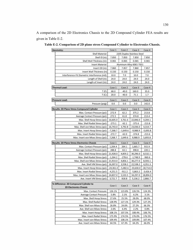
130

A comparison of the 2D Electronics Chassis to the 2D Compound Cylinder FEA results are

given in Table E-2.

Table E-2. Comparison of 2D plane stress Compound Cylinder to Electronics Chassis.


Shell Material:

Shell ID (in): 7.850 7.850 7.850 7.850


Insert Material:

Insert OD (in): 7.860 7.857 7.860 7.857






T (F): 68.0 -40.0 160.0 35.0

T (C): 20.0 -40.0 71.1 1.7


Pressure (psig): 0.0 0.0 0.0 142.0

Results: 2D Plane Stress Compound Cylinder Case 1 Case 2 Case 3 Case 4









Results: 2D Plane Stress Electronics Chassis Case 1 Case 2 Case 3 Case 4
























% Difference: 2D Compound Cylinder to

2D Electronics Chassis

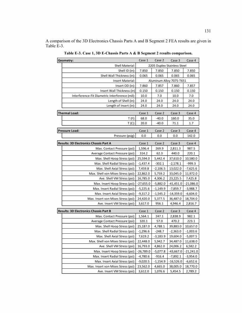
131

A comparison of the 3D Electronics Chassis Parts A and B Segment 2 FEA results are given in

Table E-3.

Table E-3. Case 1, 3D E-Chassis Parts A & B Segment 2 results comparison.


Shell Material:

Shell ID (in): 7.850 7.850 7.850 7.850


Insert Material:

Insert OD (in): 7.860 7.857 7.860 7.857






T (F): 68.0 -40.0 160.0 35.0

T (C): 20.0 -40.0 71.1 1.7


Pressure (psig): 0.0 0.0 0.0 142.0





























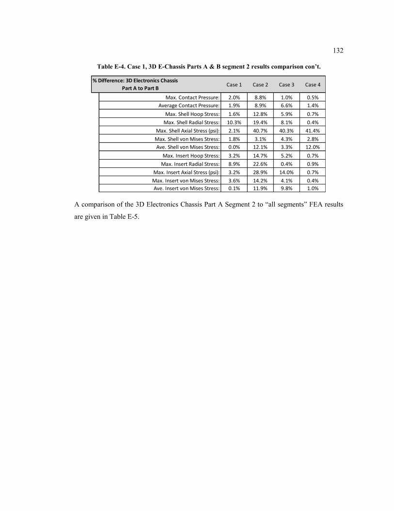
132

Table E-4. Case 1, 3D E-Chassis Parts A & B segment 2 results comparison con’t.

A comparison of the 3D Electronics Chassis Part A Segment 2 to “all segments” FEA results

are given in Table E-5.


Shell Material:

Shell ID (in): 7.850 7.850 7.850 7.850


Insert Material:

Insert OD (in): 7.860 7.857 7.860 7.857






T (F): 68.0 -40.0 160.0 35.0

T (C): 20.0 -40.0 71.1 1.7


Pressure (psig): 0.0 0.0 0.0 142.0











































Part A to Part B

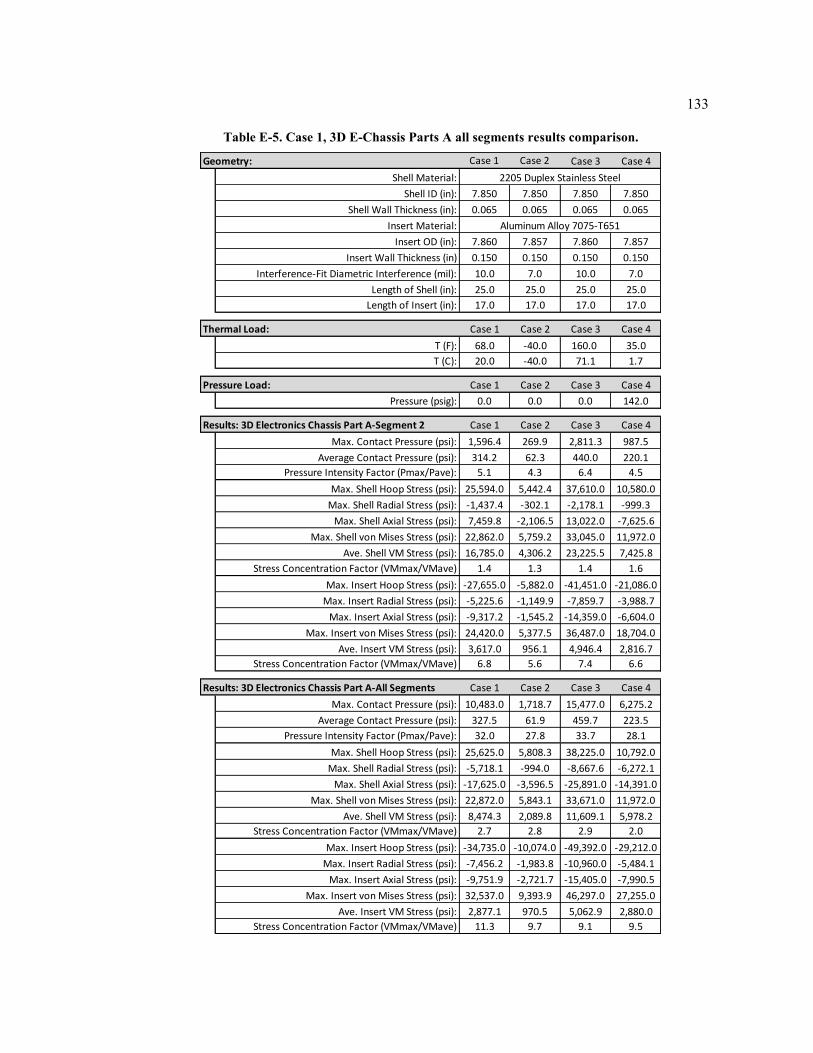
133

Table E-5. Case 1, 3D E-Chassis Parts A all segments results comparison.


Shell Material:

Shell ID (in): 7.850 7.850 7.850 7.850


Insert Material:

Insert OD (in): 7.860 7.857 7.860 7.857






T (F): 68.0 -40.0 160.0 35.0

T (C): 20.0 -40.0 71.1 1.7


Pressure (psig): 0.0 0.0 0.0 142.0

Results: 3D Electronics Chassis Part A-Segment 2 Case 1 Case 2 Case 3 Case 4
















Results: 3D Electronics Chassis Part A-All Segments Case 1 Case 2 Case 3 Case 4


















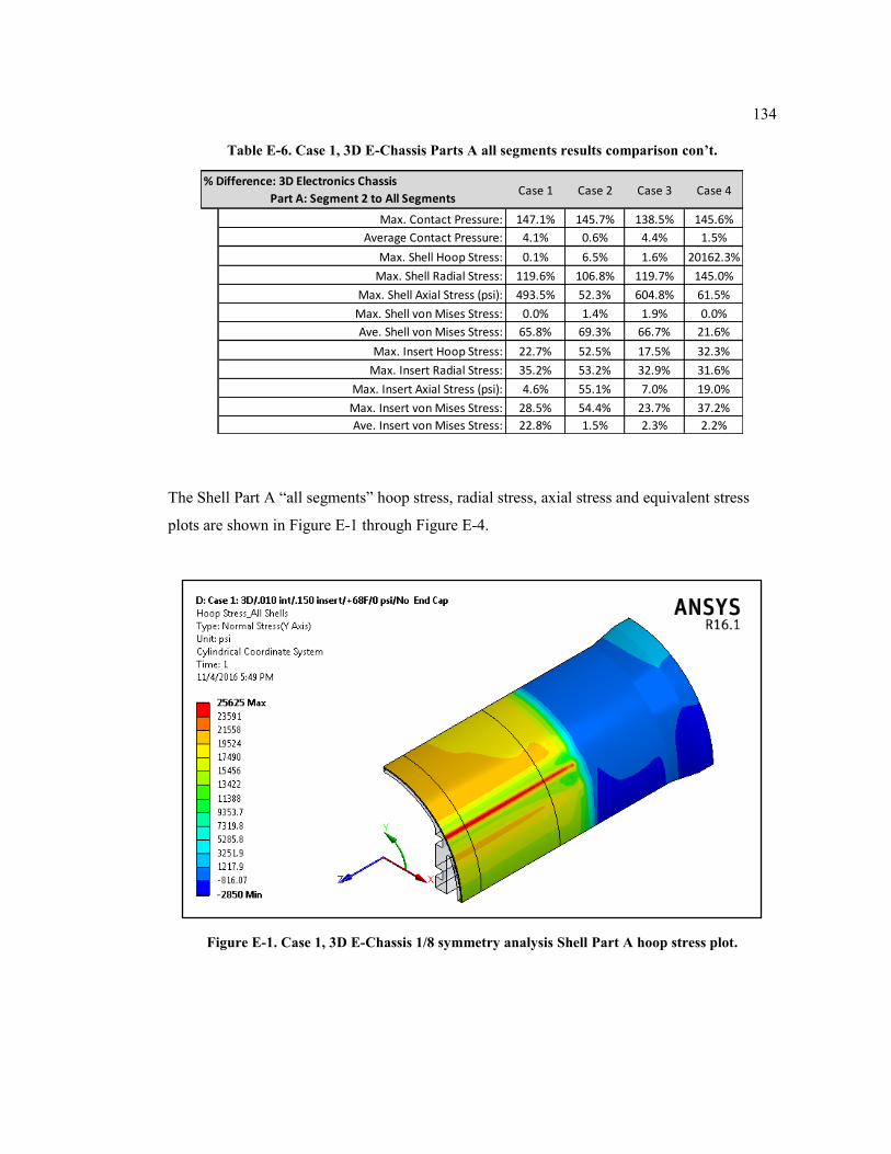
134

Table E-6. Case 1, 3D E-Chassis Parts A all segments results comparison con’t.

The Shell Part A “all segments” hoop stress, radial stress, axial stress and equivalent stress

plots are shown in Figure E-1 through Figure E-4.

Figure E-1. Case 1, 3D E-Chassis 1/8 symmetry analysis Shell Part A hoop stress plot.


Shell Material:

Shell ID (in): 7.850 7.850 7.850 7.850


Insert Material:

Insert OD (in): 7.860 7.857 7.860 7.857






T (F): 68.0 -40.0 160.0 35.0

T (C): 20.0 -40.0 71.1 1.7


Pressure (psig): 0.0 0.0 0.0 142.0

Results: 3D Electronics Chassis Part A-Segment 2 Case 1 Case 2 Case 3 Case 4
















Results: 3D Electronics Chassis Part A-All Segments Case 1 Case 2 Case 3 Case 4
































Part A: Segment 2 to All Segments

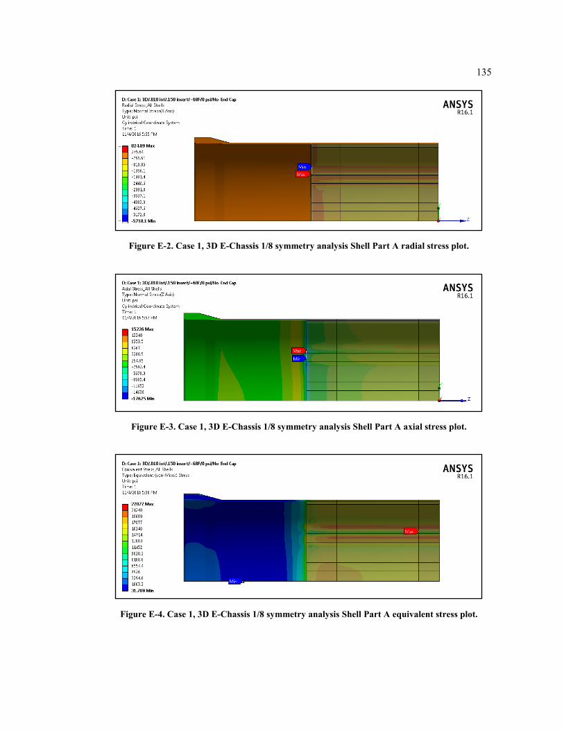
135

Figure E-2. Case 1, 3D E-Chassis 1/8 symmetry analysis Shell Part A radial stress plot.

Figure E-3. Case 1, 3D E-Chassis 1/8 symmetry analysis Shell Part A axial stress plot.

Figure E-4. Case 1, 3D E-Chassis 1/8 symmetry analysis Shell Part A equivalent stress plot.

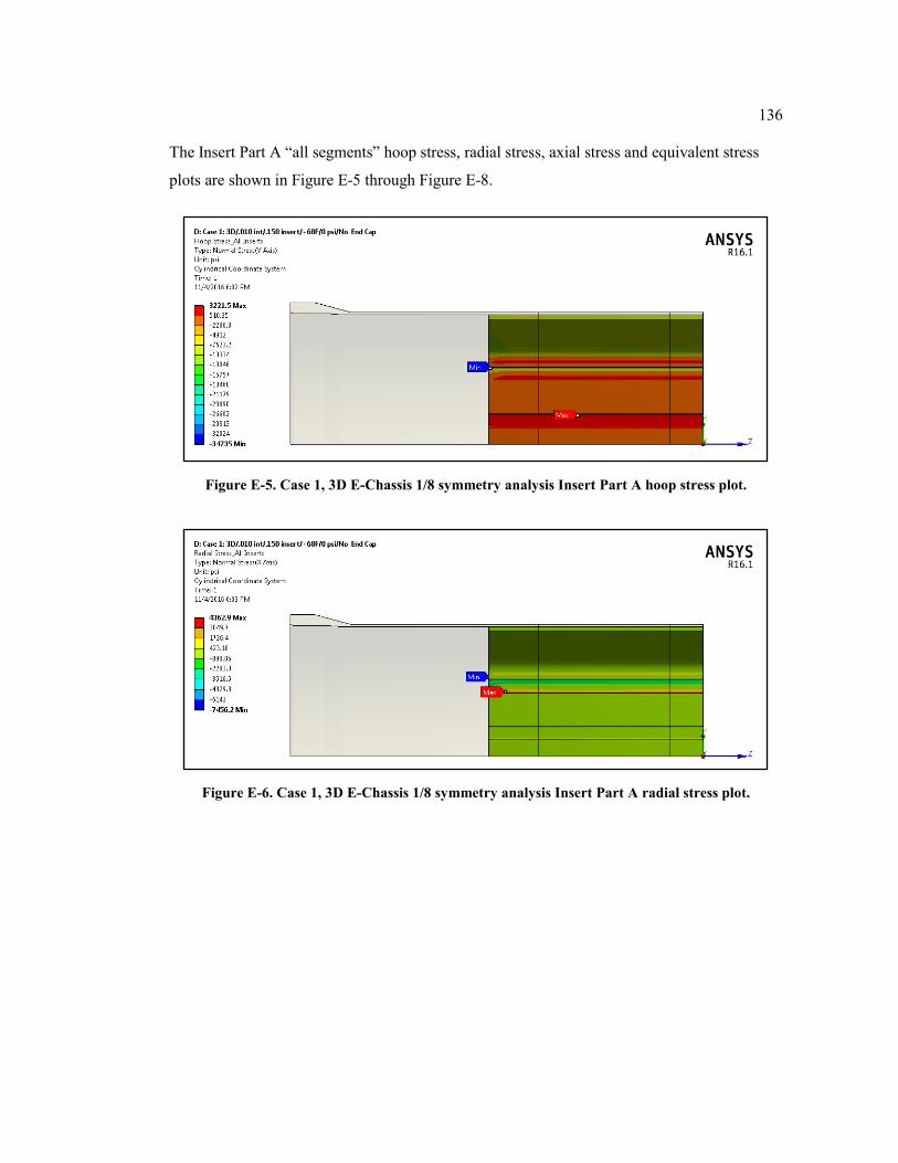
136

The Insert Part A “all segments” hoop stress, radial stress, axial stress and equivalent stress


Figure E-5. Case 1, 3D E-Chassis 1/8 symmetry analysis Insert Part A hoop stress plot.

Figure E-6. Case 1, 3D E-Chassis 1/8 symmetry analysis Insert Part A radial stress plot.

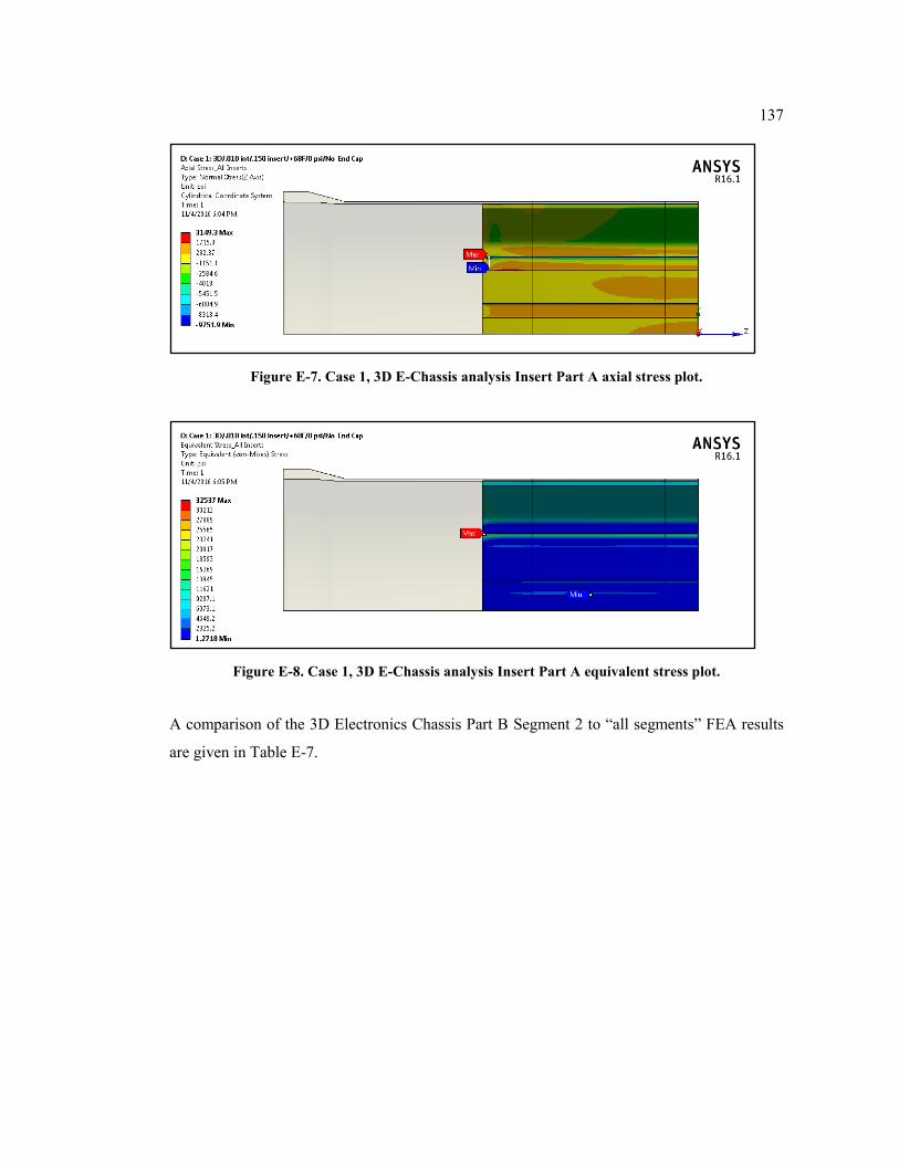
137

Figure E-7. Case 1, 3D E-Chassis analysis Insert Part A axial stress plot.

Figure E-8. Case 1, 3D E-Chassis analysis Insert Part A equivalent stress plot.

A comparison of the 3D Electronics Chassis Part B Segment 2 to “all segments” FEA results

are given in Table E-7.

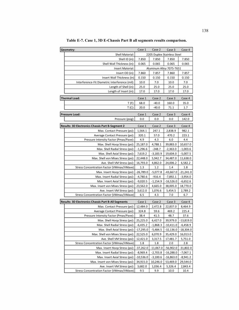
138

Table E-7. Case 1, 3D E-Chassis Part B all segments results comparison.


Shell Material:

Shell ID (in): 7.850 7.850 7.850 7.850


Insert Material:

Insert OD (in): 7.860 7.857 7.860 7.857






T (F): 68.0 -40.0 160.0 35.0

T (C): 20.0 -40.0 71.1 1.7


Pressure (psig): 0.0 0.0 0.0 142.0

Results: 3D Electronics Chassis Part B-Segment 2 Case 1 Case 2 Case 3 Case 4
















Results: 3D Electronics Chassis Part B-All Segments Case 1 Case 2 Case 3 Case 4


















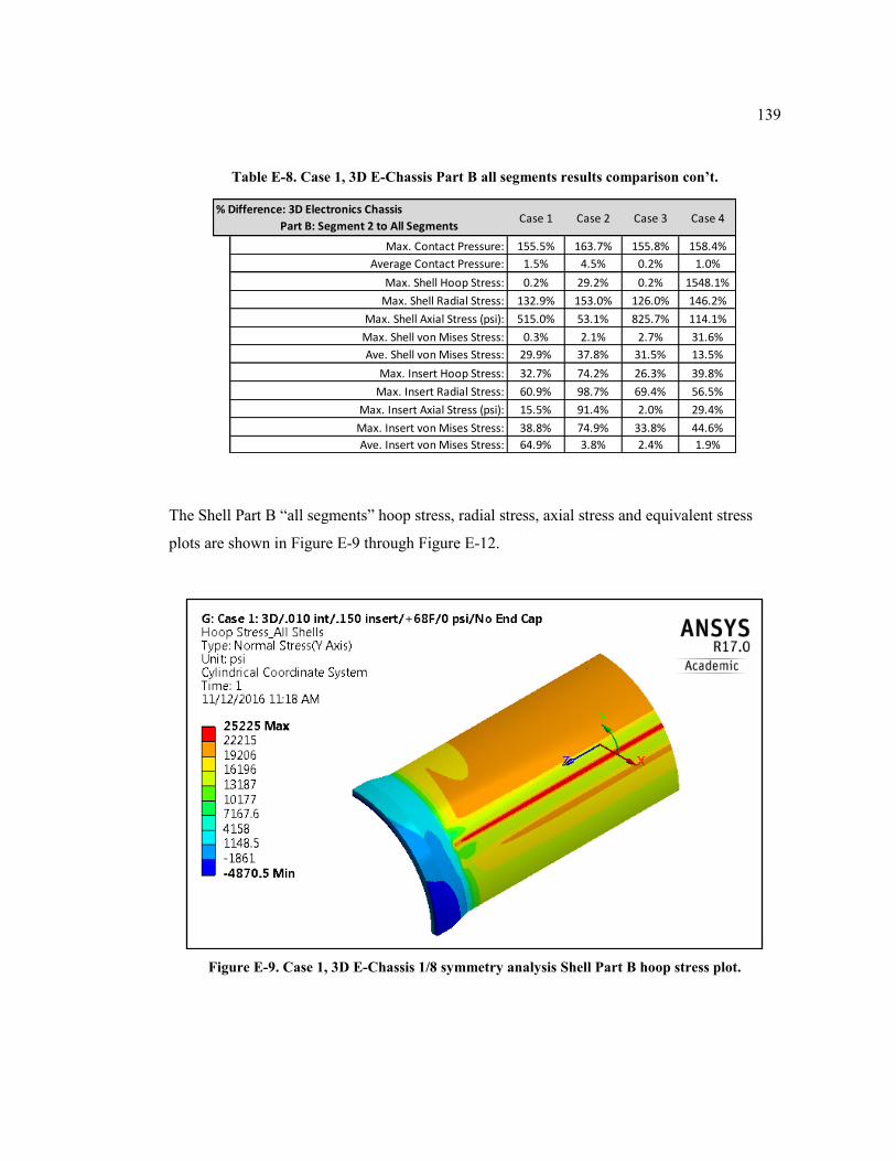
139

Table E-8. Case 1, 3D E-Chassis Part B all segments results comparison con’t.

The Shell Part B “all segments” hoop stress, radial stress, axial stress and equivalent stress


Figure E-9. Case 1, 3D E-Chassis 1/8 symmetry analysis Shell Part B hoop stress plot.


Shell Material:

Shell ID (in): 7.850 7.850 7.850 7.850


Insert Material:

Insert OD (in): 7.860 7.857 7.860 7.857






T (F): 68.0 -40.0 160.0 35.0

T (C): 20.0 -40.0 71.1 1.7


Pressure (psig): 0.0 0.0 0.0 142.0

Results: 3D Electronics Chassis Part B-Segment 2 Case 1 Case 2 Case 3 Case 4
















Results: 3D Electronics Chassis Part B-All Segments Case 1 Case 2 Case 3 Case 4
































Part B: Segment 2 to All Segments

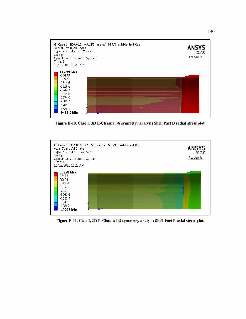
140

Figure E-10. Case 1, 3D E-Chassis 1/8 symmetry analysis Shell Part B radial stress plot.

Figure E-11. Case 1, 3D E-Chassis 1/8 symmetry analysis Shell Part B axial stress plot.

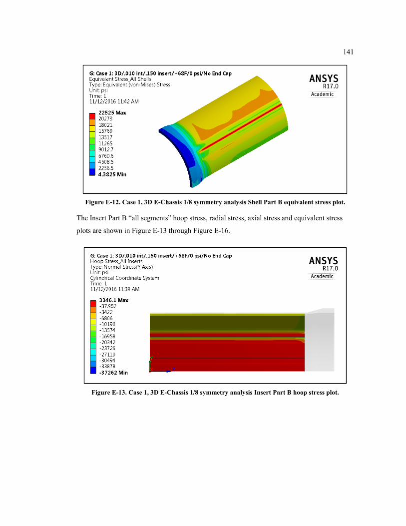
141

Figure E-12. Case 1, 3D E-Chassis 1/8 symmetry analysis Shell Part B equivalent stress plot.

The Insert Part B “all segments” hoop stress, radial stress, axial stress and equivalent stress


Figure E-13. Case 1, 3D E-Chassis 1/8 symmetry analysis Insert Part B hoop stress plot.

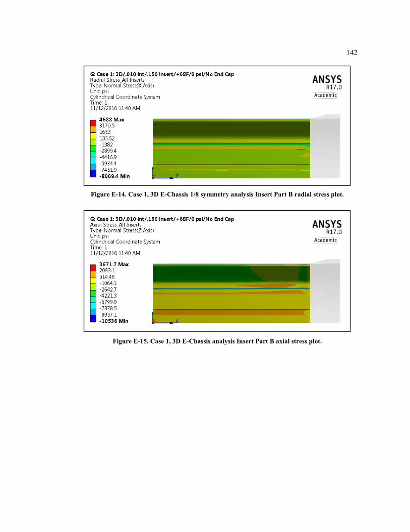
142

Figure E-14. Case 1, 3D E-Chassis 1/8 symmetry analysis Insert Part B radial stress plot.

Figure E-15. Case 1, 3D E-Chassis analysis Insert Part B axial stress plot.

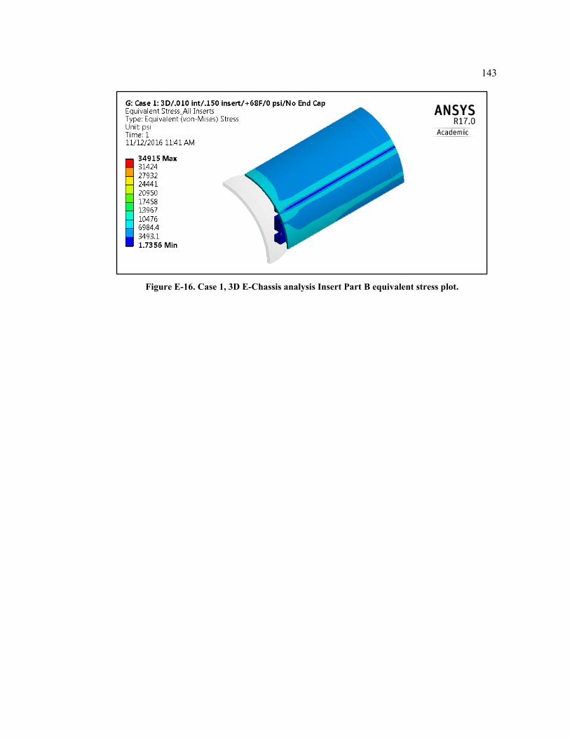
143

Figure E-16. Case 1, 3D E-Chassis analysis Insert Part B equivalent stress plot.

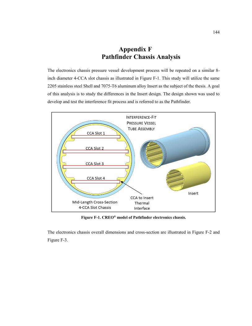
144

Appendix F

Pathfinder Chassis Analysis

The electronics chassis pressure vessel development process will be repeated on a similar 8-

inch diameter 4-CCA slot chassis as illustrated in Figure F-1. This study will utilize the same

2205 stainless steel Shell and 7075-T6 aluminum alloy Insert as the subject of the thesis. A goal

of this analysis is to study the differences in the Insert design. The design shown was used to

develop and test the interference fit process and is referred to as the Pathfinder.

Figure F-1. CREO® model of Pathfinder electronics chassis.

The electronics chassis overall dimensions and cross-section are illustrated in Figure F-2 and

Figure F-3.

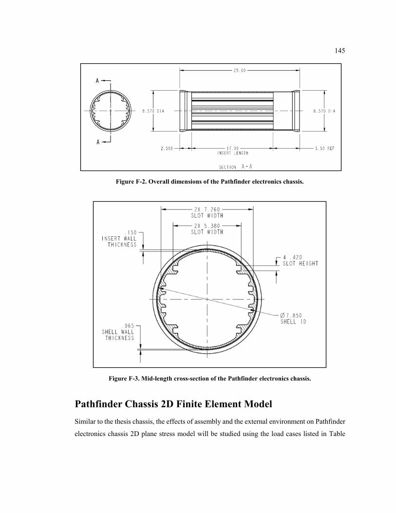
145

Figure F-2. Overall dimensions of the Pathfinder electronics chassis.

Figure F-3. Mid-length cross-section of the Pathfinder electronics chassis.

Pathfinder Chassis 2D Finite Element Model

Similar to the thesis chassis, the effects of assembly and the external environment on Pathfinder

electronics chassis 2D plane stress model will be studied using the load cases listed in Table

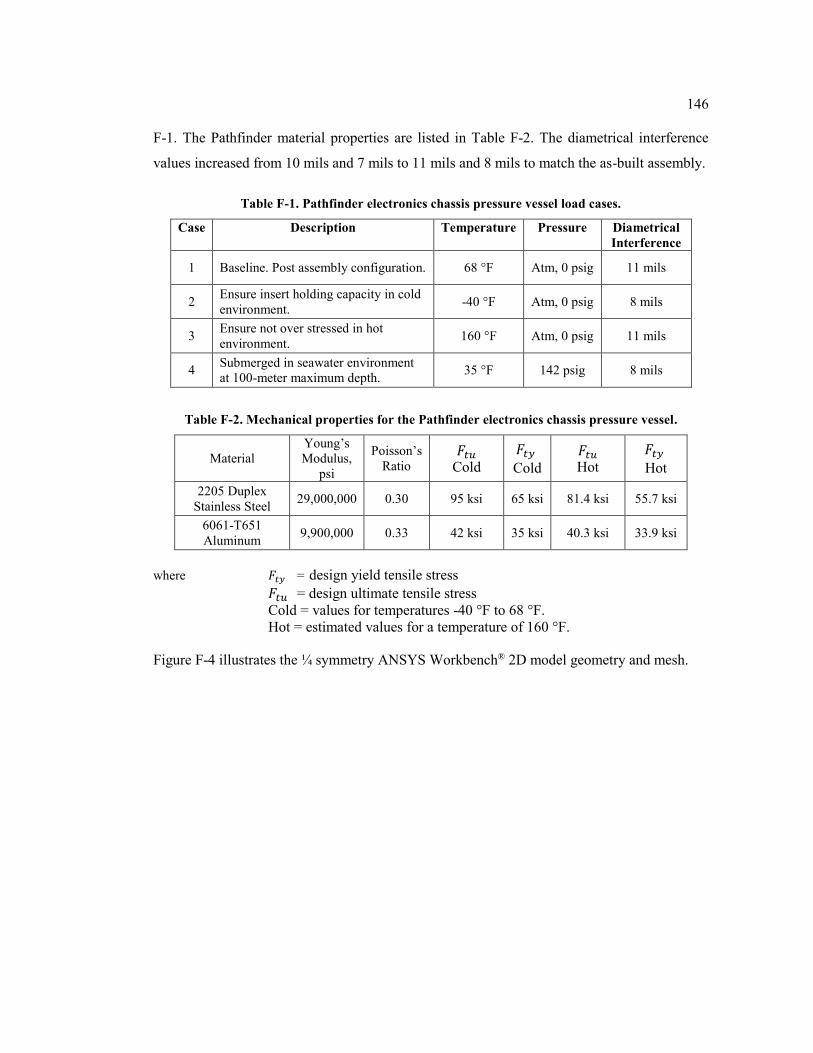
146

F-1. The Pathfinder material properties are listed in Table F-2. The diametrical interference

values increased from 10 mils and 7 mils to 11 mils and 8 mils to match the as-built assembly.

Table F-1. Pathfinder electronics chassis pressure vessel load cases.


Interference





environment. 160 °F Atm, 0 psig 11 mils

4 Submerged in seawater environment

at 100-meter maximum depth. 35 °F 142 psig 8 mils

Table F-2. Mechanical properties for the Pathfinder electronics chassis pressure vessel.

Material

Young’s

Modulus,

psi

Poisson’s

Ratio 𝐹𝑡𝑢

Cold

𝐹𝑡𝑦

Cold

𝐹𝑡𝑢 Hot

𝐹𝑡𝑦

Hot

2205 Duplex

Stainless Steel 29,000,000 0.30 95 ksi 65 ksi 81.4 ksi 55.7 ksi

6061-T651

Aluminum 9,900,000 0.33 42 ksi 35 ksi 40.3 ksi 33.9 ksi





Figure F-4 illustrates the ¼ symmetry ANSYS Workbench® 2D model geometry and mesh.

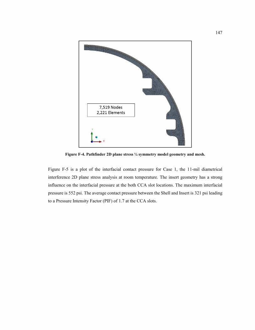
147

Figure F-4. Pathfinder 2D plane stress ¼ symmetry model geometry and mesh.

Figure F-5 is a plot of the interfacial contact pressure for Case 1, the 11-mil diametrical

interference 2D plane stress analysis at room temperature. The insert geometry has a strong

influence on the interfacial pressure at the both CCA slot locations. The maximum interfacial

pressure is 552 psi. The average contact pressure between the Shell and Insert is 321 psi leading

to a Pressure Intensity Factor (PIF) of 1.7 at the CCA slots.

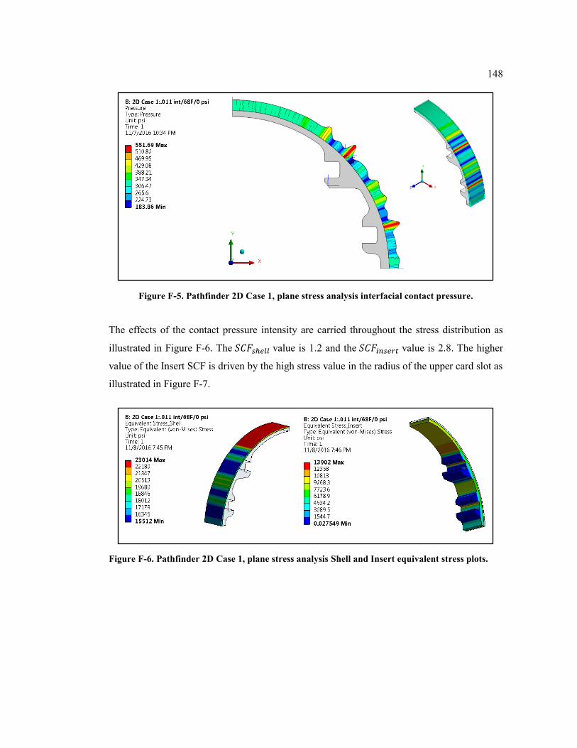
148

Figure F-5. Pathfinder 2D Case 1, plane stress analysis interfacial contact pressure.

The effects of the contact pressure intensity are carried throughout the stress distribution as

illustrated in Figure F-6. The 𝑆𝐶𝐹𝑠ℎ𝑒𝑙𝑙 value is 1.2 and the 𝑆𝐶𝐹𝑖𝑛𝑠𝑒𝑟𝑡 value is 2.8. The higher

value of the Insert SCF is driven by the high stress value in the radius of the upper card slot as

illustrated in Figure F-7.

Figure F-6. Pathfinder 2D Case 1, plane stress analysis Shell and Insert equivalent stress plots.

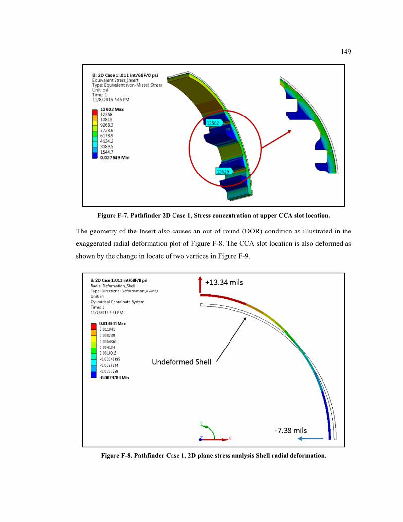
149

Figure F-7. Pathfinder 2D Case 1, Stress concentration at upper CCA slot location.

The geometry of the Insert also causes an out-of-round (OOR) condition as illustrated in the

exaggerated radial deformation plot of Figure F-8. The CCA slot location is also deformed as

shown by the change in locate of two vertices in Figure F-9.

Figure F-8. Pathfinder Case 1, 2D plane stress analysis Shell radial deformation.

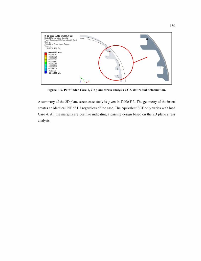
150

Figure F-9. Pathfinder Case 1, 2D plane stress analysis CCA slot radial deformation.

A summary of the 2D plane stress case study is given in Table F-3. The geometry of the insert

creates an identical PIF of 1.7 regardless of the case. The equivalent SCF only varies with load

Case 4. All the margins are positive indicating a passing design based on the 2D plane stress

analysis.

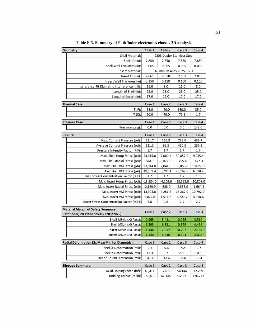
151

Table F-3. Summary of Pathfinder electronics chassis 2D analysis.


Shell Material:

Shell ID (in): 7.850 7.850 7.850 7.850


Insert Material:

Insert OD (in): 7.861 7.858 7.861 7.858






T (F): 68.0 -40.0 160.0 35.0

T (C): 20.0 -40.0 71.1 1.7


Pressure (psig): 0.0 0.0 0.0 142.0




Pressure Intensity Factor (PIF): 1.7 1.7 1.7 1.7





Shell Stress Concentration Factor (SCF): 1.2 1.2 1.2 1.5





Insert Stress Concentration Factor (SCF): 2.8 2.8 2.7 2.7


Shell MSyld (>0 Pass): 0.965 5.421 0.256 3.510

Shell MSult (>0 Pass): 1.393 6.821 0.529 4.492





Shell Y-Deformation (mil): 13.3 0.7 20.6 10.0








Pathfinder, 2D Plane Stress (2205/7075)

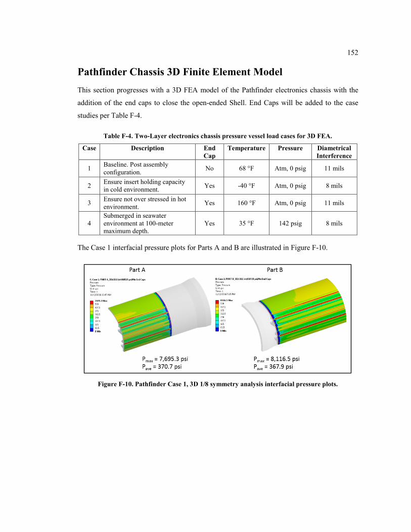
152

Pathfinder Chassis 3D Finite Element Model

This section progresses with a 3D FEA model of the Pathfinder electronics chassis with the

addition of the end caps to close the open-ended Shell. End Caps will be added to the case

studies per Table F-4.

Table F-4. Two-Layer electronics chassis pressure vessel load cases for 3D FEA.


Cap

Temperature Pressure Diametrical

Interference


configuration. No 68 °F Atm, 0 psig 11 mils

2 Ensure insert holding capacity

in cold environment. Yes -40 °F Atm, 0 psig 8 mils


environment. Yes 160 °F Atm, 0 psig 11 mils

4

Submerged in seawater

environment at 100-meter

maximum depth.

Yes 35 °F 142 psig 8 mils

The Case 1 interfacial pressure plots for Parts A and B are illustrated in Figure F-10.

Figure F-10. Pathfinder Case 1, 3D 1/8 symmetry analysis interfacial pressure plots.

153

The Shell, Part A and Part B, equivalent stress plots are shown in Figure F-11.

Figure F-11. Pathfinder Case 1, 3D 1/8 symmetry analysis Shell equivalent stress plots.

The Insert, Part A and Part B, equivalent stress plots are shown in Figure F-12.

Figure F-12. Case 1, 3D 1/8 symmetry analysis Insert equivalent stress plots.

A summary of results for Pathfinder models Parts A and B are given in Table F-5 and Table

F-6.

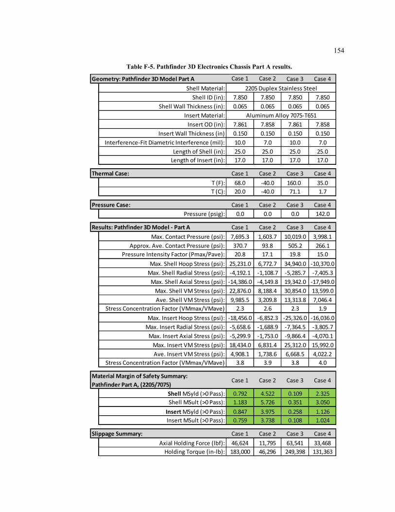
154

Table F-5. Pathfinder 3D Electronics Chassis Part A results.

Geometry: Pathfinder 3D Model Part A Case 1 Case 2 Case 3 Case 4

Shell Material:

Shell ID (in): 7.850 7.850 7.850 7.850


Insert Material:

Insert OD (in): 7.861 7.858 7.861 7.858






T (F): 68.0 -40.0 160.0 35.0

T (C): 20.0 -40.0 71.1 1.7


Pressure (psig): 0.0 0.0 0.0 142.0

Results: Pathfinder 3D Model - Part A Case 1 Case 2 Case 3 Case 4






Max. Shell Axial Stress (psi): -14,386.0 -4,149.8 19,342.0 -17,949.0











Shell MSyld (>0 Pass): 0.792 4.522 0.109 2.325

Shell MSult (>0 Pass): 1.183 5.726 0.351 3.050









Pathfinder Part A, (2205/7075)

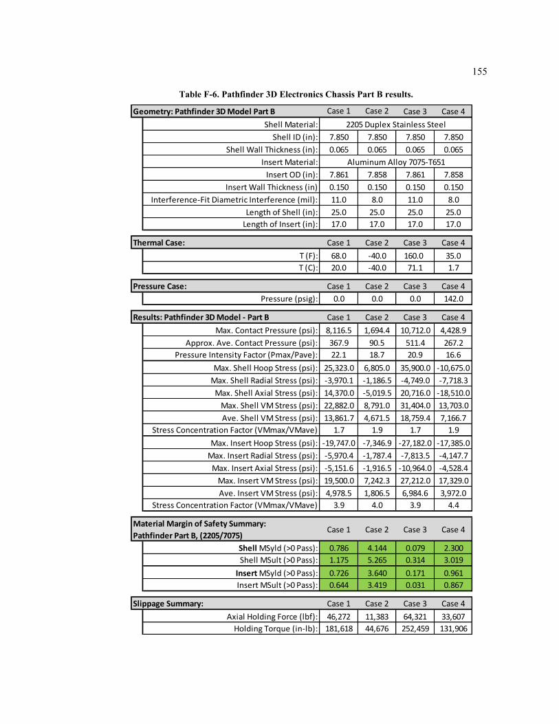
155

Table F-6. Pathfinder 3D Electronics Chassis Part B results.

Geometry: Pathfinder 3D Model Part B Case 1 Case 2 Case 3 Case 4

Shell Material:

Shell ID (in): 7.850 7.850 7.850 7.850


Insert Material:

Insert OD (in): 7.861 7.858 7.861 7.858






T (F): 68.0 -40.0 160.0 35.0

T (C): 20.0 -40.0 71.1 1.7


Pressure (psig): 0.0 0.0 0.0 142.0

Results: Pathfinder 3D Model - Part B Case 1 Case 2 Case 3 Case 4

















Shell MSyld (>0 Pass): 0.786 4.144 0.079 2.300

Shell MSult (>0 Pass): 1.175 5.265 0.314 3.019









Pathfinder Part B, (2205/7075)

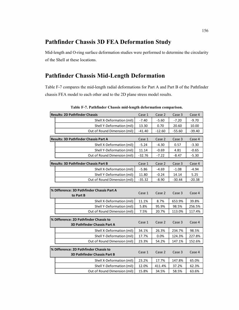
156

Pathfinder Chassis 3D FEA Deformation Study

Mid-length and O-ring surface deformation studies were performed to determine the circularity

of the Shell at these locations.

Pathfinder Chassis Mid-Length Deformation

Table F-7 compares the mid-length radial deformations for Part A and Part B of the Pathfinder

chassis FEA model to each other and to the 2D plane stress model results.

Table F-7. Pathfinder Chassis mid-length deformation comparison.

Results: 2D Pathfinder Chassis Case 1 Case 2 Case 3 Case 4


Shell Y-Deformation (mil): 13.30 0.70 20.60 10.00


Results: 3D Pathfinder Chassis Part A Case 1 Case 2 Case 3 Case 4




Results: 3D Pathfinder Chassis Part B Case 1 Case 2 Case 3 Case 4
















% Difference: 2D Pathfinder Chassis to

3D Pathfinder Chassis Part B

% Difference: 3D Pathfinder Chassis Part A

to Part B

% Difference: 2D Pathfinder Chassis to

3D Pathfinder Chassis Part A

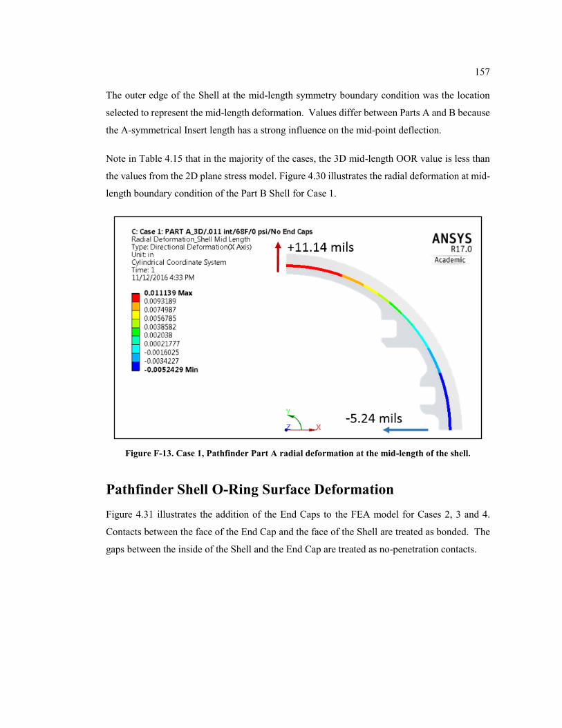
157

The outer edge of the Shell at the mid-length symmetry boundary condition was the location

selected to represent the mid-length deformation. Values differ between Parts A and B because

the A-symmetrical Insert length has a strong influence on the mid-point deflection.

Note in Table 4.15 that in the majority of the cases, the 3D mid-length OOR value is less than

the values from the 2D plane stress model. Figure 4.30 illustrates the radial deformation at mid-

length boundary condition of the Part B Shell for Case 1.

Figure F-13. Case 1, Pathfinder Part A radial deformation at the mid-length of the shell.

Pathfinder Shell O-Ring Surface Deformation

Figure 4.31 illustrates the addition of the End Caps to the FEA model for Cases 2, 3 and 4.

Contacts between the face of the End Cap and the face of the Shell are treated as bonded. The

gaps between the inside of the Shell and the End Cap are treated as no-penetration contacts.

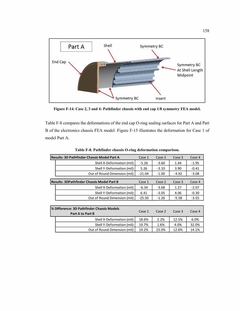
158

Figure F-14. Case 2, 3 and 4: Pathfinder chassis with end cap 1/8 symmetry FEA model.

Table F-8 compares the deformations of the end cap O-ring sealing surfaces for Part A and Part

B of the electronics chassis FEA model. Figure F-15 illustrates the deformation for Case 1 of

model Part A.

Table F-8. Pathfinder chassis O-ring deformation comparison.

Results: 3D Pathfinder Chassis Model Part A Case 1 Case 2 Case 3 Case 4




Results: 3DPathfinder Chassis Model Part B Case 1 Case 2 Case 3 Case 4








% Difference: 3D Pathfinder Chassis Models

Part A to Part B

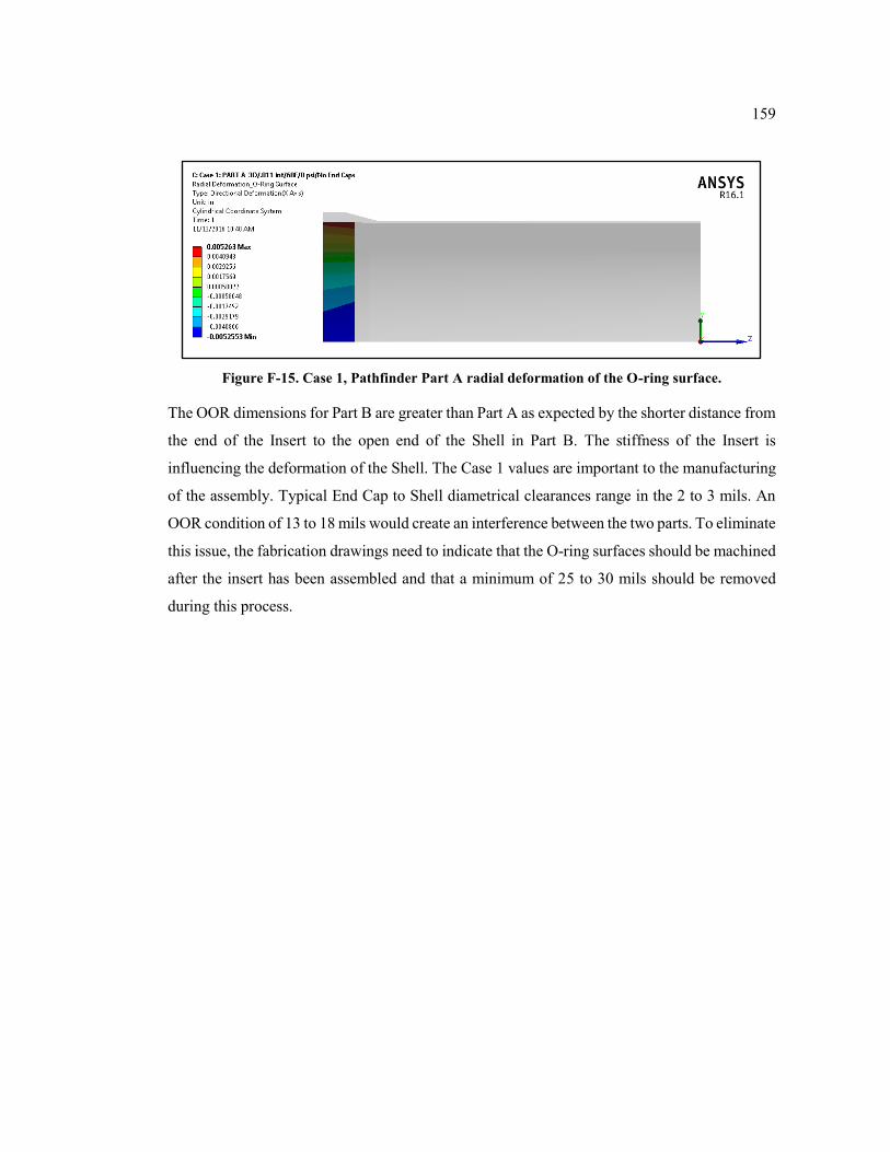
159

Figure F-15. Case 1, Pathfinder Part A radial deformation of the O-ring surface.

The OOR dimensions for Part B are greater than Part A as expected by the shorter distance from

the end of the Insert to the open end of the Shell in Part B. The stiffness of the Insert is

influencing the deformation of the Shell. The Case 1 values are important to the manufacturing

of the assembly. Typical End Cap to Shell diametrical clearances range in the 2 to 3 mils. An

OOR condition of 13 to 18 mils would create an interference between the two parts. To eliminate

this issue, the fabrication drawings need to indicate that the O-ring surfaces should be machined

after the insert has been assembled and that a minimum of 25 to 30 mils should be removed

during this process.

astudy to develop an electronics chassis compound cylinder

Documents