arX

iv:h

ep-p

h/06

0619

9 v1

19

Jun

200

6A Theory of Cosmic Rays

Arnon DarDepartment of Physics and Space Research Institute,

Technion, Haifa 32000, Israel

A. De RujulaTheory Unit, CERN, 1211 Geneva 23, Switzerland; Physics Department, Boston University, USA

(Dated: June 20, 2006)

We present a theory of non-solar cosmic rays (CRs) based on a single type of CR source at allenergies. The total luminosity of the Galaxy, the broken power-law spectra with their observedslopes, the position of the ‘knee(s)’ and ‘ankle’, and the CR composition and its variation withenergy are all predicted in terms of very simple and completely ‘standard’ physics. The sourceof CRs is extremely ‘economical’: it has only one parameter to be fitted to the ensemble of allof the mentioned data. All other inputs are ‘priors’, that is, theoretical or observational items ofinformation independent of the properties of the source of CRs, and chosen to lie in their pre-established ranges. The theory is part of a ‘unified view of high-energy astrophysics’ —based on the‘Cannonball’ model of the relativistic ejecta of accreting black holes and neutron stars. If correct,this model is only lacking a satisfactory theoretical understanding of the ‘cannon’ that emits thecannonballs in catastrophic processes of accretion.

PACS numbers: 98.70.Sa Cosmic rays: sources, origin, acceleration, interactions;97.60.Bw Supernovae; 98.70.Rz Gamma-ray bursts

I. INTRODUCTION AND OUTLOOK

The field of cosmic-ray (CR) physics was born as alucky failure. The 1912 attempt by Victor Hess to mea-sure the decrease of the Earth’s radioactivity in an as-cending balloon gave an opposite result: there was anextra-terrestrial source of what are now known to behigh-energy nuclei and electrons. Some 94 years later,the origin of non-solar CRs is still a subject of intense re-search and little consensus [1]. We shall refer throughoutto non-solar cosmic rays simply as CRs.

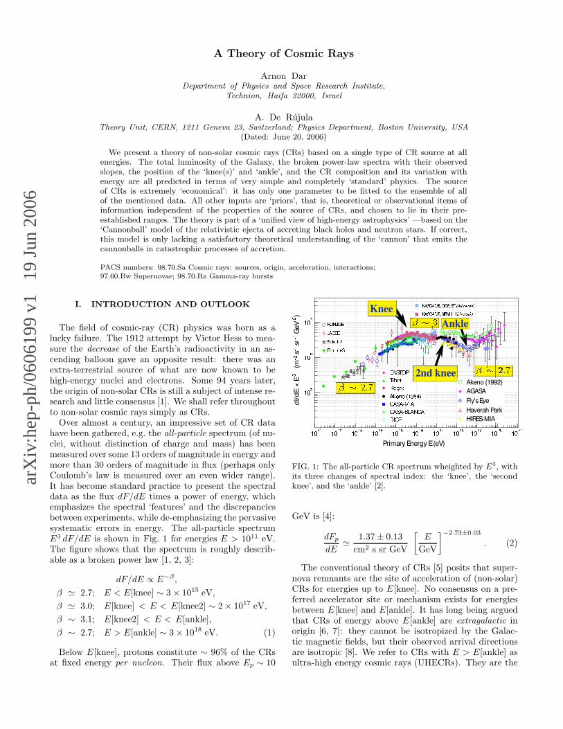
Over almost a century, an impressive set of CR datahave been gathered, e.g. the all-particle spectrum (of nu-clei, without distinction of charge and mass) has beenmeasured over some 13 orders of magnitude in energy andmore than 30 orders of magnitude in flux (perhaps onlyCoulomb’s law is measured over an even wider range).It has become standard practice to present the spectraldata as the flux dF/dE times a power of energy, whichemphasizes the spectral ‘features’ and the discrepanciesbetween experiments, while de-emphasizing the pervasivesystematic errors in energy. The all-particle spectrumE3 dF/dE is shown in Fig. 1 for energies E > 1011 eV.The figure shows that the spectrum is roughly describ-able as a broken power law [1, 2, 3]:

dF/dE ∝ E−β ,

β ≃ 2.7; E < E[knee] ∼ 3 × 1015 eV,

β ≃ 3.0; E[knee] < E < E[knee2] ∼ 2 × 1017 eV,

β ∼ 3.1; E[knee2] < E < E[ankle],

β ∼ 2.7; E > E[ankle] ∼ 3 × 1018 eV. (1)

Below E[knee], protons constitute ∼ 96% of the CRsat fixed energy per nucleon. Their flux above Ep ∼ 10

FIG. 1: The all-particle CR spectrum wheighted by E3, withits three changes of spectral index: the ‘knee’, the ‘secondknee’, and the ‘ankle’ [2].

GeV is [4]:

dFp

dE≃ 1.37 ± 0.13

cm2 s sr GeV

[

E

GeV

]−2.73±0.03

. (2)

The conventional theory of CRs [5] posits that super-nova remnants are the site of acceleration of (non-solar)CRs for energies up to E[knee]. No consensus on a pre-ferred accelerator site or mechanism exists for energiesbetween E[knee] and E[ankle]. It has long being arguedthat CRs of energy above E[ankle] are extragalactic inorigin [6, 7]: they cannot be isotropized by the Galac-tic magnetic fields, but their observed arrival directionsare isotropic [8]. We refer to CRs with E > E[ankle] asultra-high energy cosmic rays (UHECRs). They are the

2

TABLE I: Frequently used abbreviations

Afterglow(s) AG(s)Cosmic Background Radiation CBR[Non-solar] Cosmic Ray(s) CR(s)Cosmic-Ray Electron(s) CRE(s)Gamma Background Radiation GBR[Long-duration] Gamma-Ray Burst(s) GRB(s)Inter-Galactic Medium IGMInter-Stellar Medium ISMInverse Compton Scattering ICSGreisen, Zatsepin & Kuzmin GZKLorentz Factor(s) LF(s)Magnetic Field(s) MF(s)Superbubble(s) SB(s)Supernova(e) SN(e)Supernova Remnant(s) SNR(s)Ultra-High Energy Cosmic Ray(s) UHECR(s)

subject of great interest, considerable controversy andimaginative model-building; see, for instance, the reviewby J. Cronin in [1]. In this paper we use many abbrevi-ations. They are listed in Table I.

Radio, X-ray and γ-ray observations of supernova rem-nants (SNRs) provide clear evidence that electrons areaccelerated to high energies in these sites. So far, theyhave not provided unambiguous evidence that SNRs ac-celerate CR nuclei and are their main source in any en-ergy range [9]. Moreover, SNRs cannot accelerate CRs toenergies as large as E[knee] [10], though this point is stilldebated. A direct proof —such as a localized source—of an extragalactic origin of the UHECRs is also lacking[1, 8].

There is mounting observational evidence that, in ad-dition to the ejection of a non-relativistic spherical shell,the explosion of a core-collapse supernova (SN) resultsin the emission of highly relativistic bipolar jets of plas-moids of ordinary matter, Cannonballs. Evidence for theejection of such jets in SN explosions is not limited toGRBs but comes also from optical observations of SN1987A [11], from X-ray [12] and infrared [13] observa-tions of Cassiopeia A and, perhaps, from the morphologyof radio SNRs [14]. These jets may be the main source ofCR nuclei at all energies [15, 16, 17]. They also explainlong-duration GRBs [18], as advocated in the CB model[19, 20].

In this paper we elaborate on a previous theory of CRs[15], which is very different from the conventionally ac-cepted theories [1]. For much of the required input, weexploit the subsequently acquired information providedby the CB-model analysis of long-duration γ-ray bursts(GRBs). The jets of CBs responsible for GRBs are anal-ogous to the jets of CBs emitted by quasars and micro-quasars. The former jets, we shall argue, are also respon-sible for the generation of CRs.

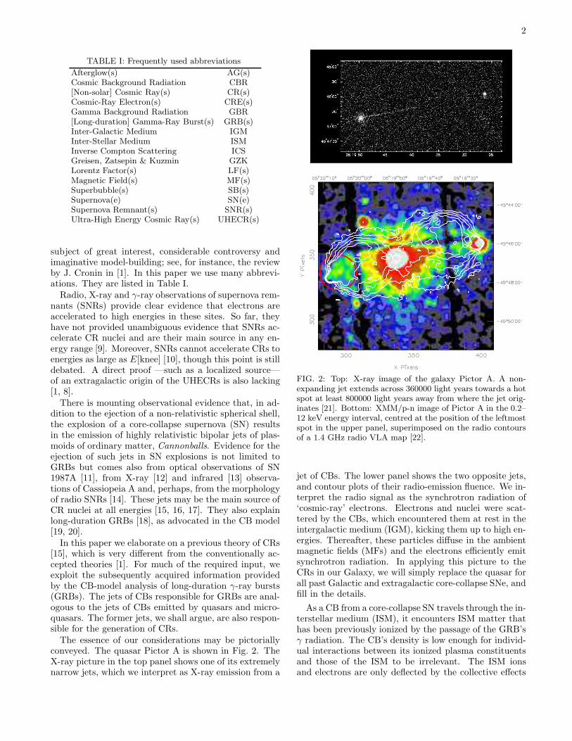
The essence of our considerations may be pictoriallyconveyed. The quasar Pictor A is shown in Fig. 2. TheX-ray picture in the top panel shows one of its extremelynarrow jets, which we interpret as X-ray emission from a

FIG. 2: Top: X-ray image of the galaxy Pictor A. A non-expanding jet extends across 360000 light years towards a hotspot at least 800000 light years away from where the jet orig-inates [21]. Bottom: XMM/p-n image of Pictor A in the 0.2–12 keV energy interval, centred at the position of the leftmostspot in the upper panel, superimposed on the radio contoursof a 1.4 GHz radio VLA map [22].

jet of CBs. The lower panel shows the two opposite jets,and contour plots of their radio-emission fluence. We in-terpret the radio signal as the synchrotron radiation of‘cosmic-ray’ electrons. Electrons and nuclei were scat-tered by the CBs, which encountered them at rest in theintergalactic medium (IGM), kicking them up to high en-ergies. Thereafter, these particles diffuse in the ambientmagnetic fields (MFs) and the electrons efficiently emitsynchrotron radiation. In applying this picture to theCRs in our Galaxy, we will simply replace the quasar forall past Galactic and extragalactic core-collapse SNe, andfill in the details.

As a CB from a core-collapse SN travels through the in-terstellar medium (ISM), it encounters ISM matter thathas been previously ionized by the passage of the GRB’sγ radiation. The CB’s density is low enough for individ-ual interactions between its ionized plasma constituentsand those of the ISM to be irrelevant. The ISM ionsand electrons are only deflected by the collective effects

3

of the CB’s inner MFs, generated by the very same ionsand electrons. We shall see in detail that this makes a CBact as a formidably efficient relativistic magnetic-racketaccelerator, which loses essentially all of its energy to therecoiling particles: the newly born CRs. We argue thatthis very simple concept explains all observed propertiesof non-solar CRs at all observed energies.

Cosmic-ray sources other than high-energy jets —suchas the traditional expanding SN envelopes, novae, stellarflares, stellar winds and non-relativistic jets— may berelevant at low energies. Galactic high-energy CRs arealso emitted by ordinary pulsars, by soft γ-ray repeaters,by microquasars, and probably in the final merger of neu-tron stars and black holes in binary systems. The totalCR luminosity of these objects is smaller than the ob-served one by more than two orders of magnitude. Sim-ilar considerations lead us to neglect the extragalacticcontribution generated by relativistic jets from massiveblack holes in active galactic nuclei, perhaps the mostluminous potentially competitive sources. These topicsare discussed in Appendix E.

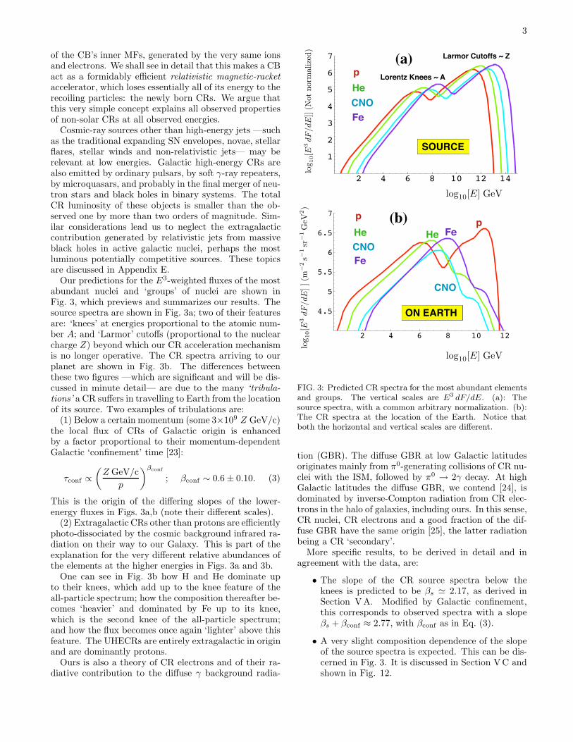
Our predictions for the E3-weighted fluxes of the mostabundant nuclei and ‘groups’ of nuclei are shown inFig. 3, which previews and summarizes our results. Thesource spectra are shown in Fig. 3a; two of their featuresare: ‘knees’ at energies proportional to the atomic num-ber A; and ‘Larmor’ cutoffs (proportional to the nuclearcharge Z) beyond which our CR acceleration mechanismis no longer operative. The CR spectra arriving to ourplanet are shown in Fig. 3b. The differences betweenthese two figures —which are significant and will be dis-cussed in minute detail— are due to the many ‘tribula-tions’ a CR suffers in travelling to Earth from the locationof its source. Two examples of tribulations are:

(1) Below a certain momentum (some 3×109 Z GeV/c)the local flux of CRs of Galactic origin is enhancedby a factor proportional to their momentum-dependentGalactic ‘confinement’ time [23]:

τconf ∝(

Z GeV/c

p

)βconf

; βconf ∼ 0.6 ± 0.10. (3)

This is the origin of the differing slopes of the lower-energy fluxes in Figs. 3a,b (note their different scales).

(2) Extragalactic CRs other than protons are efficientlyphoto-dissociated by the cosmic background infrared ra-diation on their way to our Galaxy. This is part of theexplanation for the very different relative abundances ofthe elements at the higher energies in Figs. 3a and 3b.

One can see in Fig. 3b how H and He dominate upto their knees, which add up to the knee feature of theall-particle spectrum; how the composition thereafter be-comes ‘heavier’ and dominated by Fe up to its knee,which is the second knee of the all-particle spectrum;and how the flux becomes once again ‘lighter’ above thisfeature. The UHECRs are entirely extragalactic in originand are dominantly protons.

Ours is also a theory of CR electrons and of their ra-diative contribution to the diffuse γ background radia-

2 4 6 8 10 12

4.5

5

5.5

6

6.5

7

2 4 6 8 10 12 14

1

2

3

4

5

6

7

SOURCE

ON EARTH

p

He

CNO

Fe

p

He

CNO

Fe

log10[E

3dF

/dE

]](m

−2s−

1sr

−1G

eV2)

log10

[E] GeV

log10[E

3dF

/dE

]](N

ot

norm

alize

d)

log10

[E] GeV

pFeHe

CNO

Larmor Cutoffs ~ Z

Lorentz Knees ~ A

(a)

(b)

FIG. 3: Predicted CR spectra for the most abundant elementsand groups. The vertical scales are E3 dF/dE. (a): Thesource spectra, with a common arbitrary normalization. (b):The CR spectra at the location of the Earth. Notice thatboth the horizontal and vertical scales are different.

tion (GBR). The diffuse GBR at low Galactic latitudesoriginates mainly from π0-generating collisions of CR nu-clei with the ISM, followed by π0 → 2γ decay. At highGalactic latitudes the diffuse GBR, we contend [24], isdominated by inverse-Compton radiation from CR elec-trons in the halo of galaxies, including ours. In this sense,CR nuclei, CR electrons and a good fraction of the dif-fuse GBR have the same origin [25], the latter radiationbeing a CR ‘secondary’.

More specific results, to be derived in detail and inagreement with the data, are:

• The slope of the CR source spectra below theknees is predicted to be βs ≃ 2.17, as derived inSection VA. Modified by Galactic confinement,this corresponds to observed spectra with a slopeβs + βconf ≈ 2.77, with βconf as in Eq. (3).

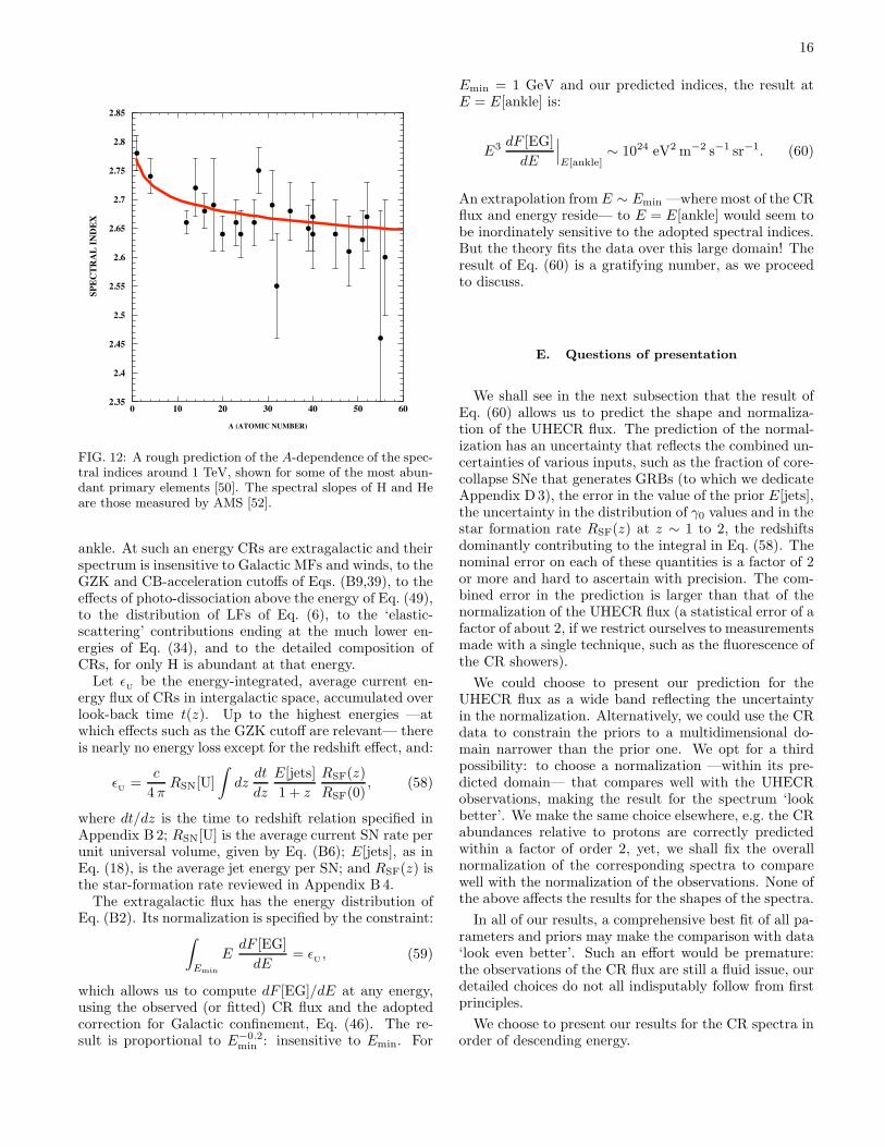
• A very slight composition dependence of the slopeof the source spectra is expected. This can be dis-cerned in Fig. 3. It is discussed in Section VC andshown in Fig. 12.

4

• The CR spectra at the lowest energies are affectedby solar effects. The predictions agree with thedata at minimum solar activity; see Section V J andFig. 16.

• The spectra of the individual CR nuclei are pre-dicted to have ‘knees’, scaling as the atomic weight,at energies around E[knee] ∼ 3× 1015 A eV; seeEq. (34) and Figs. 3, 10. The observed and pre-dicted spectra for the individual elements H, Heand Fe, at energies up to their knees, are shown inFig. 15.

• The CR spectrum is predicted to change ratherabruptly in slope, dominant composition (Fe to H)and dominant origin (Galactic to extragalactic) atthe ‘ankle’ energy, E[ankle] ∼ 3× 1018 eV, see Sec-tion VG.

• Our CR acceleration mechanism has a cutoff atthe energies of Eq. (39), proportional to atomiccharge and roughly coincident with the conven-tional Greisen–Zatsepi–Kuzmin (GZK) cutoff [26].These cutoffs do not seem to be present in theAGASA data [27], but are compatible with theHIRES [8] and Fly’s Eyes data, which agree wellwith our theory: see Fig. 13.

• The predicted normalization of the UHECR flux isapproximate but ‘absolute’, i.e. parameter-free; seeSection VF.

• The prediction for the all-particle spectrum is com-pared with the data in Fig. 14.

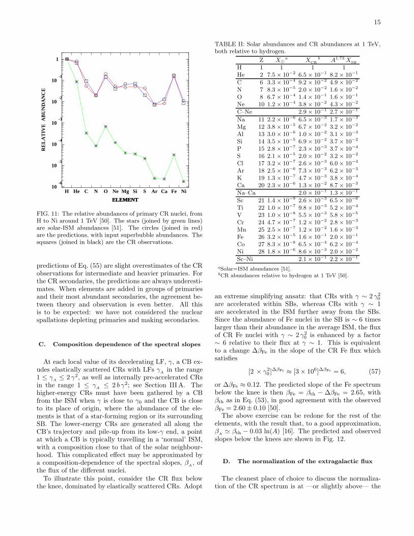
• Detailed predictions for the ‘primary’ CR abun-dances relative to hydrogen are discussed in Sec-tion VB. They are compared with data at 1 TeVin Table II and illustrated in Fig. 11.

• Data on two rough indicators of the evolution ofCR composition with energy, 〈lnA〉 and the depthof shower maximum Xmax, are compared with pre-dictions in Figs. 17 and 18.

• The confinement volume and the confinement timeof CRs in the Galaxy can be estimated theoreti-cally. They agree with the estimates extracted fromobservations, as discussed in Section VL.

• Below their respective knees, the source spectra ofCR nuclei and electrons are predicted to have thesame slope: βs = 13/6. For relatively high-energyelectrons, radiation cooling steepens the slope toβe = βs +1 ∼ 3.17. The observed slope is ≃ 3.2, asshown in Fig. 21. The normalization of the electronspectrum, we cannot predict.

• The slope of the diffuse GBR is predicted to be(βe + 1)/2 ≃ 2.08. The observation is ≃ 2.1, asshown in Fig. 22.

Admittedly, the ‘predictions’ we have referred to inthe above items are ‘postdictions’ of existing data. Yet,the theory on which they are based is very ‘predictive’:only one parameter specific to the CR source will be fit-ted to the hadronic CR data. Otherwise, only priors(items of information independent of the CR source) havebeen used as inputs, and kept at their ‘central’ values, orwithin their error brackets [28].

A posteriori the distinction between post- and pre-dictions, or parameters and priors, is somewhat artificial.But there are other assets of the CR theory presentedhere: it works simply and very well, and it is basedon a single source of CR acceleration at all energies.Moreover, the underlying theory —originally inspired byan analogy with the relativistic ejecta of quasars andmicroquasars— is part of a unified model of high-energyastrophysical phenomena [17], which also offers simpleand successful explanations of the origin and propertiesof ‘long-duration’ GRBs and X-ray flashes and their re-spective afterglows (AGs) [20, 29, 30, 31], the natal kicksof neutron stars [15], the MFs and radio emission fromwithin and near galaxy clusters [32], and the X-ray emis-sion from galactic clusters allegedly harbouring ‘coolingflows’ [33].

The many titles and subtitles in this paper shouldsuffice to convey its organization. We discuss in de-tail or summarize in Appendices some of the relevantbackground information: how a CB expands, photo-dissociation, the least debatable ‘priors’ common to alltheories of CRs, jets in astrophysics, the CB model, theevidence for the ejection of relativistic jets in SN ex-plosions, the supernova–GRB association and the powersupply by CR accelerators other than the one we propose.

Our main point is our proposed mechanism of CR ac-celeration. A reader primarily interested in it may chooseto read first Section III A on ‘Collisionless magnetic rack-ets’. A reader primarily intrigued by the results maychoose to start with Chapter V.

II. CB PRIORS

The ‘cannon’ of the CB model is analogous to the onesresponsible for the ejecta of quasars and microquasars.As an ordinary core-collapse SN implodes into a blackhole or neutron star and sheds an exploding shell, anaccretion disk or torus is hypothesized to be producedaround the newly born compact object, either by stellarmaterial originally close to the surface of the implodingcore and left behind by the explosion-generating outgoingshock, or by more distant stellar matter falling back afterits passage [19, 20, 34]. A CB is emitted, as observed inmicroquasars [35, 36], when part of the accretion diskfalls abruptly onto the compact object [19, 20].

In the case of a core-collapse SN, the accretion torus isnot fed by a companion, it has a finite mass and can feeda limited number of accretion episodes. Each episodecorresponds to the bipolar emission of a CB pair. A CB

5

FIG. 4: An ‘artist’s view” (not to scale) of the CB modelof long-duration GRBs [20]. A core-collapse SN results in acompact object and a fast-rotating torus of non-ejected fallen-back material. Matter (not shown) abruptly accreting into thecentral object produces a narrowly collimated beam of CBs,of which only some of the ‘northern” ones are depicted. Asthese CBs move through the ‘ambient light” surrounding thestar, they Compton up-scatter its photons to GRB energies.

generates a forward cone of high-energy photons as itsconstituent electrons Compton-up-scatter ambient light.If the jet is directed close to the line of sight of an ob-server, each of its CBs generates a pulse in a GRB signal;a bit more off axis, an X-ray flash (XRF) is observed. TheCBs, like the matter that feeds them from the accretingtorus, are made of ordinary-matter plasma. The typicalinitial Lorentz factor (LF) of a CB, γ0, and its typicalinitial baryon number, N

B, are [20]:

γ0 ≡ E/(M0 c2) ∼ O(103), (4)

NB

∼ 1050. (5)

The value of M0 ∼ NB

mp c2 roughly corresponds to halfof the mass of Mercury, a very small number in com-parison with the mass of the parent exploding star. Anartist’s view of the CB model is given in Fig. 4.

The CB model of GRBs and their AGs is briefly dis-cussed in Appendix D. Some of the distributions andaverage values of the input priors required in our theoryof CRs are specific to this model. They are summarizedin this section, along with the other ingredients of theCB model relevant to CR production.

A. The distribution of initial Lorentz factors

Let γ0 denote the value of the LF of a CB as it is origi-nally emitted by a SN and produces a GRB’s γ-ray pulseby inverse Compton scattering (ICS), before it is sloweddown by the ISM while generating the GRB’s afterglowby synchrotron radiation. An average value γ0 ∼ 103

was first estimated using the rough hypothesis that anasymmetry between the momenta of the diametricallyopposed jets was responsible for the ‘natal kick’ velocityof neutron stars, the remnants of the core-collapse SNexplosions of relatively light progenitors [15]. This value

2.4 2.6 2.8 3 3.2 3.40

0.2

0.4

0.6

0.8

1

γLog[ ]0

FIG. 5: Distribution of log10(γ0) values for GRBs of knownredshift [20]. The continuous curve is a log-normal fit.

of γ0 was confirmed by a first study of GRBs [19] withinthe CB model. It is also compatible with the roughly 1to 1 SN–GRB association discussed in Appendix D3.

A subsequent analysis of GRB afterglows (AGs) at in-frared and optical [29] as well as radio [30] frequenciesconfirmed γ0 ∼ 103 as the average initial LF. The distri-bution of γ0 values obtained from these analyses for theensemble of GRBs of known redshift is shown in Fig. 5,constructed with the results of Ref. [30]. The figure refersto data obtained with the selection criteria for the detec-tion of GRBs, which discriminates in favour of large LFs,and is the result of fits to AGs which —with the excep-tion of some GRBs clearly dominated by two CBs— aremade with the simplification of substituting an ensembleof CBs for a single ‘average’ one. This tends to make theextracted γ0 distribution narrower than the ‘real’ one,and its real average somewhat uncertain.

The properties of CRs depend on the ‘real’ γ0 distri-bution, which we parametrize as:

D(γ0, γ0) ∝ exp

[

−(

log γ0 − log γ0

log w

)2]

. (6)

The distribution of Fig. 5 has γ0 = 1070 and ω = 0.8.It results in a good description of CR data, but, notsurprisingly, a somewhat broader distribution gives aneven better description, as discussed in Section V I. Thepredictions are insensitive to the assumed form of thelower-energy tail of D(γ0, γ0).

6

B. The deceleration of CBs in the ISM

While a CB exits from its parent SN and emits a GRBpulse, it is assumed [19] to be expanding, in its rest sys-tem, at a speed comparable to that of sound in a relativis-tic plasma (vs = c/

√3). In their voyage, CBs continu-

ously intercept the electrons and nuclei of the ISM, previ-ously ionized by the GRB’s γ-rays. In seconds of (highlyDoppler-foreshortened) GRB observer’s time, such an ex-panding CB becomes ‘collisionless’, that is, its radius be-comes smaller than a typical interaction length betweena constituent of the CB and an ISM particle. But a CBstill interacts with the charged ISM particles it encoun-ters, for, as we discuss in detail in subsection II E, itcontains a strong magnetic field.

Consider a CB of initial mass M0 and initial LF γ0.As it travels in the ISM its LF diminishes all the way tounity. We assume that the ISM particles entering a CB’smagnetic mesh are trapped in it and slowly re-exit bydiffusion. To a fair approximation, a CB simply accumu-lates the ISM particles that it intercepts. In this case,energy–momentum conservation implies that the CB’smass increases as:

MCB ≈ M0γ0

β γ,[

β ≡√

γ2 − 1/γ]

, (7)

and, for an approximately hydrogenic ISM of local den-sity dnin, the LF decreases as:

d γ

β3 γ3≈ − mp

M0 γ0dnin(γ). (8)

To compute the spectrum of the CRs produced by aCB in its voyage through the ISM, we shall have to per-form a dnin integral over its trajectory, as the CB de-celerates from γ = γ0 to γ = 1. Given Eq. (8), this istantamount to integrating the CR spectra at local valuesof γ with a weight factor dnin ∝ dγ/(γ3 β3). Notice thatthe CB’s deceleration law of Eq. (8) depends explicitlyon the number of ISM particles it intercepts, but not onany CB properties other than M0 and γ0.

C. The expansion of a CB

We approximate a CB, in its rest system, by a sphereof radius R(γ). The value of R(γ0) is immaterial, for itbecomes rapidly negligible as the CB initially expands ata speed ∼ c/

√3. The ISM particles that are intercepted

—isotropized in the CB’s inner magnetic mesh, and re-emitted— exert an inwards force on it that counteractsits expansion. This expansion, in the ‘fast elastic’ case ofinstantaneous re-emission, was studied in [29, 30]. Thecase of ‘diffusive’ re-emission results in a slightly betterdescription of more recent data [37]. We discuss it indetail in Appendix A and we adopt it here.

The behaviour of R(γ) is shown in Fig. 6. It has threedistinct phases. The initial rapidly expanding quasi-inertial phase plays a crucial role in the description of

0 200 400 600 800 10001

100

10000

1. ! 106 R / R0

γ0 / γ

Diffusion

DDD 2002

FIG. 6: Expansion of a CB as its LF γ diminishes along itstrajectory from an initial γ0 = 103. The dotted line is for thecase of fast elastic CB interactions with the ISM, discussed in[29, 30]. The continuous line is for the case discussed here, inwhich the ISM gathered by the CB slowly oozes out of it bydiffusion. These are two limiting cases.

GRB pulse shapes and is supported by the CB-model’scorrect prediction of all their other properties [20]. Theproperties of the intermediate coasting phase are sup-ported by the CB-model’s successful description of GRBAGs; see, e.g. [29, 30, 37]. The final blow-up phase maydescribe the observed lobes of quasars and microquasars,such as the one at the right of Pictor A in Fig. 2.

A CB converts the ISM into CRs at a rate proportionalto R2

CB. The initially fast-expanding phase in R

CB(γ) has

negligible effects. The subsequent behaviour of RCB

(γ),in the diffusive case and for typical (or average) CB pa-rameters, is well described by:

RCB

(γ) ≈ R0

(

γ0

β γ

)2/3

,

R0 ∼ 1014 cm. (9)

This behaviour gives the best description of GRB after-glows, as discussed in [37] and Appendix A.

D. The trajectories of CBs

How far does a CB travel before the collisions with theISM stop it? The answer crucially depends on the distri-bution of ISM densities that the CB encounters, and therelativistic approximation (β ≈ 1) suffices to give it withthe required precision. In the ‘slow’ approximation —inwhich the rate at which the ISM particles enter the CBis faster than the rate at which they exit it by diffusion—every ISM proton intercepted by a CB increases its massby γ mp. The mass increase per travel length dx is:

dMCB

= π R2CB

γ mp np dx. (10)

7

The relation between dMCB

and dγ is, according toEq. (7), γ dM

CB= M0 γ0 dγ/γ0, and R

CBis given in

Eq. (9). Gathering this information and integrating theresult in dx and dγ we obtain:

x = xstop

(

1

γ2/3− 1

γ2/30

)

,

xstop ≡ 3 NB

2π R20 γ

1/30

np = (18 kpc) ×

[

NB

1050

] [

1014 cm

R0

]2 [10−2 cm−3

np

] [

103

γ0

]13

, (11)

where np, an adequately averaged ISM density along agiven CB’s trajectory, is perhaps the most uncertain ofthe case-by-case varying inputs in xstop.

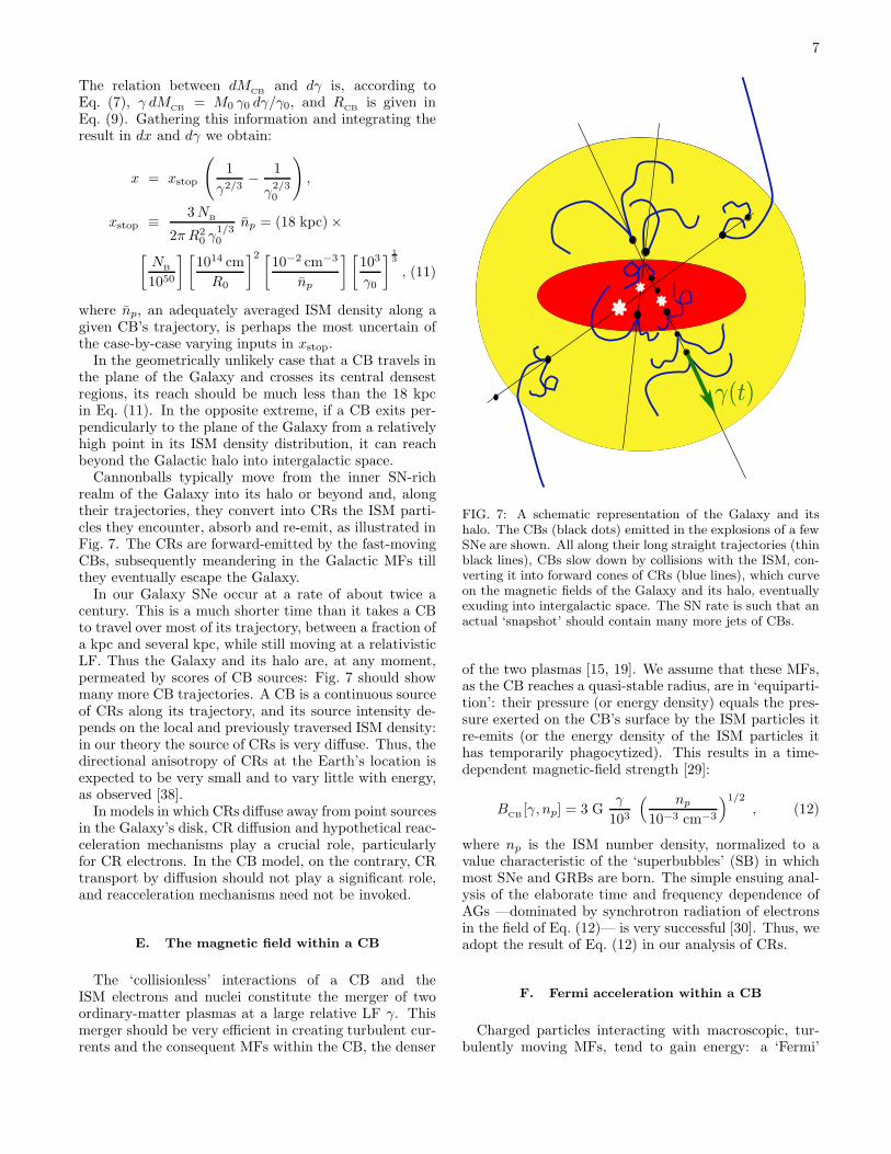
In the geometrically unlikely case that a CB travels inthe plane of the Galaxy and crosses its central densestregions, its reach should be much less than the 18 kpcin Eq. (11). In the opposite extreme, if a CB exits per-pendicularly to the plane of the Galaxy from a relativelyhigh point in its ISM density distribution, it can reachbeyond the Galactic halo into intergalactic space.

Cannonballs typically move from the inner SN-richrealm of the Galaxy into its halo or beyond and, alongtheir trajectories, they convert into CRs the ISM parti-cles they encounter, absorb and re-emit, as illustrated inFig. 7. The CRs are forward-emitted by the fast-movingCBs, subsequently meandering in the Galactic MFs tillthey eventually escape the Galaxy.

In our Galaxy SNe occur at a rate of about twice acentury. This is a much shorter time than it takes a CBto travel over most of its trajectory, between a fraction ofa kpc and several kpc, while still moving at a relativisticLF. Thus the Galaxy and its halo are, at any moment,permeated by scores of CB sources: Fig. 7 should showmany more CB trajectories. A CB is a continuous sourceof CRs along its trajectory, and its source intensity de-pends on the local and previously traversed ISM density:in our theory the source of CRs is very diffuse. Thus, thedirectional anisotropy of CRs at the Earth’s location isexpected to be very small and to vary little with energy,as observed [38].

In models in which CRs diffuse away from point sourcesin the Galaxy’s disk, CR diffusion and hypothetical reac-celeration mechanisms play a crucial role, particularlyfor CR electrons. In the CB model, on the contrary, CRtransport by diffusion should not play a significant role,and reacceleration mechanisms need not be invoked.

E. The magnetic field within a CB

The ‘collisionless’ interactions of a CB and theISM electrons and nuclei constitute the merger of twoordinary-matter plasmas at a large relative LF γ. Thismerger should be very efficient in creating turbulent cur-rents and the consequent MFs within the CB, the denser

γ(t)

FIG. 7: A schematic representation of the Galaxy and itshalo. The CBs (black dots) emitted in the explosions of a fewSNe are shown. All along their long straight trajectories (thinblack lines), CBs slow down by collisions with the ISM, con-verting it into forward cones of CRs (blue lines), which curveon the magnetic fields of the Galaxy and its halo, eventuallyexuding into intergalactic space. The SN rate is such that anactual ‘snapshot’ should contain many more jets of CBs.

of the two plasmas [15, 19]. We assume that these MFs,as the CB reaches a quasi-stable radius, are in ‘equiparti-tion’: their pressure (or energy density) equals the pres-sure exerted on the CB’s surface by the ISM particles itre-emits (or the energy density of the ISM particles ithas temporarily phagocytized). This results in a time-dependent magnetic-field strength [29]:

BCB

[γ, np] = 3 Gγ

103

( np

10−3 cm−3

)1/2

, (12)

where np is the ISM number density, normalized to avalue characteristic of the ‘superbubbles’ (SB) in whichmost SNe and GRBs are born. The simple ensuing anal-ysis of the elaborate time and frequency dependence ofAGs —dominated by synchrotron radiation of electronsin the field of Eq. (12)— is very successful [30]. Thus, weadopt the result of Eq. (12) in our analysis of CRs.

F. Fermi acceleration within a CB

Charged particles interacting with macroscopic, tur-bulently moving MFs, tend to gain energy: a ‘Fermi’

8

FIG. 8: Results of a simulation of the merger of two plasmasat a relative LF γ = 3. The left panel shows the longitudinalelectron current density through a cut transverse to the di-rection of motion of the incoming plasma, with a small insetshowing the ion current in the same plane. The right panelshows the ion current deeper into the target plasma, with thesmall inset now showing the electron current instead. Thearrows represent the transverse magnetic field [39].

acceleration process. This acceleration is very efficientfor a relativistic ‘injection’, the case relevant to a CB,which is subject, in its rest system, to a flow of ISMelectrons and nuclei arriving with a large common LF. A‘first-principle’ numerical analysis [39] of the merging oftwo plasmas at a moderately high γ —based on followingeach particle’s individual trajectory as governed by theLorentz force and Maxwell’s equations— demonstratesthe generation of such chaotic MFs, and the accelerationof particles to a spectrum with a power-law tail:

dNac

dE∼ E−βac Θ(E − γ M c2), βac ≈ 2.2. (13)

The Heaviside Θ function is an approximate characteri-zation of the fact that it is much more likely for the lightparticles to gain than to lose energy in their elastic col-lisions with the heavy ‘particles’ (the CB’s turbulentlymoving collective plasma and MF domains). The numer-ical analysis [39] shows that this acceleration occurs ina total absence of shocks, very much unlike what is gen-erally assumed for CRs accelerated in shocks producedby expanding SN shells [5]. In Fig. 8 we reproduce aplot of [39] showing the ion and electron currents at twodepths into the denser of the merging plasmas.

In our analysis of the radio, infrared, optical, UVand X-ray AGs of GRBs, we assumed that a fractionof the ISM electrons entering a CB was accelerated as inEq. (13), the majority remaining unaccelerated at theirincoming LF. In the case of electrons, both populations‘cool’ by synchrotron radiation in the CB’s MFs. Theensuing synchrotron radiation —the afterglow— has acomplex frequency and time dependence, which is in ex-cellent agreement with observations and confirms thatEqs. (12) (13) are adequate; see e.g. [29, 30, 37].

We assume that CR nuclei entering a CB from theISM are also accelerated as in Eq. (13). This acceleration

cannot extend to arbitrarily high energies; there must bea Larmor cutoff, for a CB has a finite radius and MF. ACB cannot significantly bend or accelerate a particle ofenergy larger than:

E[Larmor] ≃ 9 × 1016 Z eVB

CB[γ0, np]

3 G

RCB

1014 cm, (14)

with RCB

as in Eq. (9) and BCB

as in Eq. (12). Thiscorresponds to a maximum LF in the CB’s rest system:

γmax(γ) = b γ1/3 (15)

b ≃ 105 γ2/30 (Z/A). (16)

The distribution of the LFs, γA, of the Fermi-acceleratednuclei that entered a CB with a Lorentz factor γ, is:

dN

dγA

∝ γ−βac

AΘ(γ

A− γ)Θ[γmax(γ) − γ

A], (17)

where the second Θ function is a rough characterizationof the Larmor cutoff. But for the small dependence ofthe coefficient b on the nuclear identity (the factor Z/A),the spectrum of Eq. (17) is universal.

G. The energy of the jets of CBs

The baryon number NB

of a CB —or, equivalently, itsmass M ≃ N

Bmp— can be roughly estimated from the

fluence of the AG of GRBs [29, 30] and better constrainedfrom the ‘spherical-equivalent’ total energy and numberof the γ-rays in a single GRB pulse [20]. The averageresult is N

B∼ 1050, cited in Eq. (5).

The observed average number [40] of significant pulsesin a GRB’s γ-ray light curve is ∼ 6. The total energy ofthe two jets of CBs in a GRB event is therefore:

E[jets] ≃ 12 γ0 NB

mp c2 ≃ 2×1051 erg. (18)

Practically all of this energy will, in our model, be trans-ferred to CRs.

H. The CR luminosity of the Galaxy

In a steady state, if the low-energy rays dominatingthe CR luminosity are chiefly Galactic in origin, theiraccelerators must compensate for the escape of CRs fromthe Galaxy. The Milky Way’s luminosity in CRs musttherefore satisfy:

LCR ≃ Lp =4π

c

∫

VCR

dV

∫

dE

τconfE

dFp

dE, (19)

with dFp/dE as in Eq. (2), τconf as in Eq. (3), and VCR

the volume to which low-energy CRs are confined. Thecoefficient 1/τconf , for Z = 1, converts the observed pro-ton spectrum into the corresponding source spectrum.

9

The conventional result of detailed models of CR pro-duction and diffusion [41] is:

LCR ∼ 2 × 1041 erg s−1 . (20)

Let RSN be the SN rate in our Galaxy, discussed inAppendix B3, and given by Eq. (B4). The estimate ofLCR in the CB model is simply:

LCR[MW]≈RSN[MW] E[jets]≈1.3 × 1042 erg s−1, (21)

with E[jets] as in Eq. (18). This estimate is uncertainby a factor of at least 2, for two reasons. First, SNeare observed to produce roughly spherical non-relativisticejecta, whose kinetic energy is comparable to E[jets].The luminosity is dominated by low-energy CRs, whichmay also be produced —with debatable efficiency— bythese ejecta, as in the generally accepted models. Thismay increase the result of Eq. (21) by a factor ≤2. Sec-ond, we contend [32] that the MFs observed in the MilkyWay and in galaxy clusters are generated by CRs, andare in energy equipartition with them, as observed in theGalaxy [42], for which

ρE[CR] =

4 π

c

∫

dF

dEE dE ≈ 0.5 eV cm−3, (22)

and

B2/(8 π) ≈ ρE[CR], for B ∼ 5 µG. (23)

The transfer to MFs of ∼ 50% of the original CR energymay decrease the result of Eq. (21) by a factor ∼2 [43].

III. A THEORY OF THE CR SOURCE

A. Collisionless magnetic rackets

The essence of our theory of CRs is kinematical andtrivial. A very massive object (a CB) travelling with aLorentz factor γ and colliding with a light object (anISM particle) can boost the light object (now a CR) toextremely high energy.

By definition, in an elastic interaction of a CB at restwith ISM electrons or ions of LF γ, the light recoilingparticles retain their incoming energy. Viewed in thesystem in which the ISM is at rest, the light recoilingparticles (of mass m) have an energy spectrum extending,for large γ, up to E ≃ 2 γ2 m c2. A moving CB is aLorentz-boost accelerator of gorgeous efficiency: the ISMparticles it scatters reach up to γ

CR≃ 2 γ2, with 〈γ

CR〉 ∼

γ2 for any non-singular scattering-angle distribution inthe CB’s rest system. In a single scattering with a CB ofγ ∼ 103, and with 100% efficiency, the energy of an ISMparticle increases a million-fold from its value at rest.The ‘accelerator’ is also good at focusing: it produces aforward-collimated beam of CRs, the initial divergence ofwhose angular distribution is characterized by an angleθ ∼ 1/γ.

A particle with a LF γ entering a CB at rest can beaccelerated by elastic interactions with the CB’s turbu-lently moving plasma. Viewed in the rest system of thebulk of the CB the interaction is ‘inelastic’: the light par-ticle gained energy. Its LF can reach γmax ∼ 107 γ; seeEqs. (15,16). Boosted by the CB’s motion the spectrumof the scattered particles extends to γ

CR∼ 2× 107 γ2, in

the UHECR domain, for γ ∼ γ0 ∼ 103. This powerfulFermi–Lorentz accelerator completes our theory of CRs.

We have tacitly assumed in the previous paragraphthat interactions are instantaneous: a CB has the sameLF when a given ISM particle enters and leaves it; the CBhas not decelerated in the meantime via collisions withmany other ISM nuclei. Borrowing from the language ofparticles more elementary than CBs, we called the inter-actions inelastic or elastic. In what follows we retractthe cited assumption, but we keep the italicized nomen-clature to refer to our results for particles that have —orhave not— been Fermi-accelerated within a CB.

B. Exiting a CB by diffusion

Let γin be the LF of a given ISM proton that entereda CB. Its momentum stays fixed as it is tossed aroundby the CB’s inner chaotic magnetic field, or is increasedby the acceleration mechanism we have discussed. Forthe ISM nuclei, as opposed to electrons, radiative andcollisional losses are negligible. We assume that thesetrapped particles ooze out of the CB by diffusion, muchas CRs do in the Galaxy. The characteristic diffusiontime when the LF [radius] of the CB has reached a valueγ [R

CB(γ)] is:

τ =R2

CB

D, (24)

with D = D(γin, γ) a diffusion coefficient. The rate atwhich the diffusing particles are exuded by the CB isr = βin/τ .

In the CB model, the MF of the Galaxy [32] and thatwithin a CB are both made by the same turbulence, in-duced by the injection of relativistic particles (the ISMin the case of a CB, CRs in the case of the Galaxy).Consequently, we expect D to have the same energy de-

pendence as observed for CRs: D ∝ pβconf

in , with the sameβconf as in Eq. (3). In the case of a CB, the diffusion oc-curs in a MF with an energy density assumed to be inapproximate equipartition with the kinetic energy den-sity of the particles entering the CB at a given momentB ∝ γ − 1, and D should reflect the B-, A- and Z-dependence of the corresponding Larmor radius, that is:

D ∝(

E

B

)βconf

∝[

Aγin

Z (γ − 1)

]βconf

. (25)

The diffusion, out of a CB, of the fraction of ISM nu-clei that are accelerated within it, will be treated in anentirely analogous fashion.

10

C. ‘Elastic’ scattering

We have assumed that, to a good approximation, aCB ingurgitates most of the ISM nuclei that it interceptsin its voyage, and that, within a CB, a fraction of thesenuclei keeps the energy at which they entered it. In thisapproximation, and at the moment when the CB’s LFhas descended from γ0 to γ, the distribution of LFs, γco,of the collected nuclei is:

dNco

dγco=

∫ γ0

γ

dnin

dγinδ(γco − γin)

∝ 1

β3co γ3

co

Θ(γ ≤ γco ≤ γ0), (26)

where we have used Eq. (8) and an unconventional buttransparent notation for the Heaviside step function Θ.

The collected particles exit the CB in its rest systemat a rate βin/τ , so that the doubly differential (γ, γco)oozing out rate is:

dNout

dγ dγco=

dNco

dγco

dtCB

dγ

βco

τ, (27)

where

− dtCB

dγ∝ 1

β4 γ4 R2CB

, (28)

obtained by inserting

dnin(γ) ≈ −π R2CB

c np β γ dtCB

(29)

into Eq. (8).To obtain the distribution of LFs γ

CRof the CRs in

the ISM rest system, we must perform the correspond-ing boost over an assumed isotropic distribution of exitdirections in the CB’s rest system:

dNout

dγCR

dγ dγco=

∫

d cos θ

2

dNout

dγ dγcoδ[γ

CR− γ γco (1 + β βco cos θ)]. (30)

The condition | cos θ| ≤ 1 introduces two constraintswhich, solved for γco, read:

γco ≤ T (γ, γCR

) ≡ γ γCR

(1 + β βCR

),

γco ≥ B(γ, γCR

) ≡ γ γCR

(1 − β βCR

). (31)

To compute the CR flux dF/dγCR

, we must integrateover γ and γco. Collecting all the results of this sectionand using Eqs. (9), (24) and (25), we obtain:

dFelast

dγCR

∝ nAβ

CR

(

A

Z

)βconf∫ γ0

1

dγ

(β γ)7/3

G[γ, γCR

]

(γ − 1)βconf,

G[γ, γCR

] ≡∫ min(γ0,T)

max(γ,B)

βco dγco

(βco γco)4−βconf, (32)

where we have introduced the factor nA

= n(A, Z) of pro-portionality to the number-density of intercepted ISMnuclear species, thereby specifying the full A- and Z-dependence of the result. Except for the overall factor(A/Z)βconf , Eq. (32) is very insensitive to βconf (over mostof their extension, the integrals are powers and the pow-ers of γβconf and γ−βconf

co simply cancel). It is also, downto γ ∼ 2, well approximated by its very simple, relativis-tic and analytical version:

dFelast

dγCR

∝ nA

(

A

Z

)βconf∫ γ0

1

dγ

γ7/3G[γ, γ

CR] ,

G[γ, γCR

] ≡∫ min[γ0,2 γ γ

CR]

max[γ,γCR

/(2 γ)]

dγco

γ4co

, (33)

from which we have eliminated the weak dependenceof the integrand on βconf . Notice that the functiondFelast/dγ

CRdepends only on the priors n

A, βconf , and

γ0, but not on any parameter specific to the mechanismof CR acceleration.

The flux of Eq. (33) has an abrupt upper limit at γCR

≃2 γ2

0 . The initial LFs of CBs peak at γ0 ∼ 103 and have adistribution extending up to γ0 ∼ 1.5× 103, as in Fig. 5.Thus, the spectrum of a nucleus elastically scattered byCBs should end at a knee energy [15]:

Eknee(A) ∼ (2 to 4) × 1015 A eV. (34)

In our comparisons of theory and data, the distributionin Eq. (33) is convoluted with distributions of γ0 valuesdescribed by Eq. (6).

D. ‘Inelastic’ scattering

A fraction of the ISM nuclei impinging on a CB isFermi-accelerated within it. We assume this process tobe fast on the scale of a CB’s slow-down time. At a fixedLF of the CB, the spectral shape of the accelerated nuclei,in the CB’s rest system, is that of Eq. (17), independentof the particle’s species and proportional to the numberdensity of intercepted ISM particles n

A. We assume that

a fixed, A-independent fraction of nA

is thus accelerated,so that —in the CB’s rest system— their instantaneousdistribution of LFs, γ

ac, is of the form:

dN inst

dγ dγac

∝ nA

γ4−βac

1

γβacac

Θ(γac− γ)Θ(b γ1/3 − γ

ac), (35)

where, for the typical reference parameters of Eq. (16),b ∼ 107. In analogy with the ‘elastic’ case, we assumethat these particles keep the energy to which they werefastly accelerated within the CB. At the moment whenthe CB’s LF, γ

CB, has descended from γ0 to γ, the dis-

tribution of LFs, γac, of the accumulated and acceleratedparticles is:

dNac

dγac

∝∫ γ0

γ

dγCB

dN inst

dγCB

dγac

∝ 1

γβacac

F,

11

F ≡ − 1

γ3−βacCB

∣

∣

∣

U

DΘ(U − D),

U ≡ min[γ0, γac],

D ≡ max[γ, (γac

/b)3]. (36)

The accelerated particles exit the CB by diffusion, asin Eq. (27), and are Lorentz-boosted by the CB’s motion,as in Eq. (30). The accelerated contribution to the CRspectrum is important only for energies above the knees,and the relativistic (β ∼ 1) approximation is good, ex-cept in some of the integration limits, wherein factorssuch as 1− β do appear. The final result for this ‘Fermi-accelerated’ or ‘inelastic’ contribution to the flux is:

dFinel

dγCR

∝ nA

(

A

Z

)βconf∫ γ0

1

dγ

γβconf+7/3

∫ S

C

F dγac

γβac+1−βconfac

,

(37)where F is defined in Eq. (36) and

C ≡ min[b γ1/30 , T (γ, γ

CR)]

S ≡ max[γ, B(γ, γCR

)], (38)

with T and B as in Eq. (31). Once again, except for theoverall factor (A/Z)βconf , Eq. (37) is very insensitive toβconf . As for the elastic case, the function dFinel/dγ

CR

depends only on the priors nA, βconf , βac and γ0, but

not on any parameter not previously constrained. Inour comparisons of theory and data, the distribution inEq. (37) will be convoluted with distributions of γ0 valuesdescribed by Eq. (6).

The flux of Eqs. (37), (38) cuts off at a maximumenergy: nuclei exiting a CB after having been acceler-ated within it have energies extending up to Eend =2 γ0 E[Larmor], with E[Larmor] as in Eq. (14), that is:

Eend(Z) ∼ (2 to 6) × 1020 Z eV. (39)

These ‘end-points” scale as Z, unlike the knees, whichscale like A. The predictions in Eq. (39) will not be easyto test, for three reasons: the end-point energies are inthe same ball-park as the GZK cutoff; for A > 1 theultra-high energy flux is strongly suppressed by photo-dissociation; and the extraction of relative CR abun-dances at very high energies is a very difficult task.

E. The complete spectrum

The complete source spectrum of each CR nucleus isthe sum of an elastic and an inelastic contribution. Thissum and its addends are illustrated, for protons, in Fig. 9.The figure shows an elastic flux larger than the inelasticone by a factor f ≃ 10 at the nominal position of theproton’s knee. This ratio f is the only required input forwhich we have no ‘prior’ information. It is the only pa-rameter we need to choose in an unpredetermined range.We assume f to be the same for all nuclei, in accordancewith the purely ‘kinematical’ character of the accelera-tion by ‘magnetic racket’ CBs.

2 4 6 8 10 12

-4

-3

-2

-1

f

NpInelastic

Total

Elastic

Proton flux

Log[E dF/dE]

2

Log[E(GeV)]

FIG. 9: Elastic and inelastic contributions to the protonsource spectrum. The vertical scale is E2 dF/dE.

The other parameter in Fig. 9, Np, is the normaliza-tion of the proton inelastic flux at the nominal position ofthe proton’s knee. Albeit within large error bars, Np willbe determined from the predicted luminosity of Eq. (21),in the way discussed in Sections VD, VG. The abun-dances of the other elements relative to protons —or,equivalently, the normalization of their fluxes— are pre-dicted, as discussed in Section VB. Thus, the ensembleof source fluxes in Fig. 3a has been constructed with justone source parameter: f .

Notice in Fig. 9 the different shapes of the elastic andinelastic contributions, implying that the fraction of ac-celerated nuclei is small, as in the results of the numericalanalysis of the relativistic merging of plasmas [39].

Many salient features of the source fluxes of CRs —thepronounced knees in the individual-element spectra, thedifferential changes of slope, and a maximum energy forproton acceleration— survive unscathed the many tribu-lations transmogrifying the source spectra into the ob-served ones. To discuss the comparison of predictionsand data we must first summarize these tribulations.

IV. TRIBULATIONS OF A COSMIC RAY

On its way from its source to the Earth’s upper at-mosphere, a CR is influenced by the ambient magneticfields, radiation and matter, which it encounters. Extra-galactic CRs are also affected by cosmological redshift(z) and the dependence of their source strength on thestar-formation rate as a function of ‘look-back time’. Inthis section we list the tribulations of CRs —which arediscussed in detail in several Appendices— and we sum-marize the choices we make for the priors that are notvery well understood either observationally or theoreti-cally. Three types of interactions constitute a CR tribu-lation:

12

• Interactions with magnetic fields that permeategalaxies and clusters and, presumably, the IGM.

The fluxes of CRs of Galactic origin are, below theirfree-escape energy, enhanced by a factor propor-tional to their confinement time. At higher energiesthey escape the Galaxy practically unhindered.

Extragalactic CRs entering the Galaxy must over-come the effect of its exuding magnetic wind.

• Interactions with radiation, significant for CRs ofextragalactic origin. The best studied one is π pho-toproduction by nuclei on the cosmic microwavebackground radiation, the GZK effect [26].

Pair (e+e−) production is akin to the GZK effect.

The photo-dissociation of extragalactic CR nuclei,mainly on the cosmic infrared background radia-tion, is also extremely relevant.

• Interactions with the ISM are fairly well understoodfor relatively low-energy CRs of Galactic origin.Their spallation gives rise to ‘secondary’ stable andunstable isotopes in the CR flux.

Of the above items, three need be discussed here:

A. Magnetic confinement and escape; the ankles

The Galaxy’s MF, whose typical value is of O(5)µG,as in Eq. (23), varies on scales ranging up to a ‘coherencelength’ of O(1) kpc. The MF in the Galaxy’s halo is notwell charted; its typical value is similar. The Larmorradius of a CR of charge e Z and momentum p(E) is:

RL ≈ 0.65 kpc5 µG

B

p(E)

Eankle(Z)(40)

Eankle(Z) ≡ Z × (3 × 1018 eV). (41)

A CR of energy E ≥ Eankle cannot be significantly bentin the Galaxy. For Z = 1, Eq. (41) coincides with the‘ankle’ in the CR flux, see Eqs. (1).

At E ∼ Eankle(Z), Galactic CR nuclei undergo a ran-dom walk process of moderate deflections on the Galac-tic MF domains. Their cumulative deflection angle hasa Gaussian distribution, analogous to the one describingthe multiple deflection of high-energy muons in matter[44]. The escapees are the CRs deflected by less than anangle of order one radian. We need a rough descriptionof the corresponding confinement and escape probabilies,which we characterize by:

Pconf = 1 − Pesc = exp

[

−(

E

Eankle(Z)

)2]

. (42)

The Galactic CR flux is modulated by the momentumdependence of the CR confinement time, τconf , in the diskand halo of the galaxy, affecting the different species in

the same way, at fixed p/Z. Confinement effects are notwell understood [23, 45], but observations of astrophysi-cal and solar plasmas indicate that [23]:

τconf ∼ K

(

Z GeV/c

p

)βconf

, (43)

K ∼ 2 × 107 y, (44)

βconf ∼ 0.6 ± 0.1. (45)

Measurements of the relative abundances of secondaryCR isotopes [23] agree with the functional form ofEq. (43). The observed ratios of unstable CR isotopes[46] result in K as in Eq. (44), but the method is wellknown to be biased towards low-K values [42]. Our the-ory predicts a somewhat larger value of K, as discussedin Sections VL, VII.

The spectrum of observable CRs of Galactic origin,dFGal/dE, is their source spectrum, dFs/dE, modifiedby confinement [47] so that dF ∝Pconf τconf dFs, or:

dFGal

dE= C(E, Z)

dFs

dE,

C(E, Z) ≡ Pconf

[

Eankle(Z)

p(E)

]βconf

, (46)

with EL and Pconf as in Eqs. (41), (42). Note thatC(E, Z) does not depend on the magnitude of the factorK in Eq. (44).

B. CR penetration into the Galaxy

In a steady-state situation, the CR flux escaping agalaxy has the energy dependence of the source flux, notthe confinement-modified flux. In our CR theory, the ex-tragalactic flux arriving to our Galaxy is simply the CRflux exiting other galaxies, modified by the tribulationsof an intergalactic journey. How do these extragalacticCRs penetrate our Galaxy?

The penetration of Galactic CRs into the solar systemis hindered by the ‘wind’ of solar CRs and MFs. Anal-ogously, we proceed to argue, the penetration of extra-galactic CRs into the Galaxy is hindered by the ‘wind’of Galactic CRs and MFs. The Galaxy certainly exudesa wind of CRs: in a steady state the outgoing Galacticflux is that of the sum of Galactic sources. The ques-tion is whether the Galaxy also has an accompanyingMF ‘wind’.

The Galactic CR- and MF-energy densities are knownto be approximately coincident, a strong hint of an inti-mate relationship. In the CB model CRs are the dom-inant source of MFs in galaxies, clusters and the IGM(this is a tenable statement for two reasons: CR sourcesare kiloparsecs-long CB trajectories, as opposed to SNshells in star-formation regions, and the Galactic CR lu-minosity is almost one order of magnitude bigger than inthe conventional view). For all these systems, the sim-ple hypothesis of rough energy–density equipartition be-

13

tween CRs and MFs results in correct predictions for theintensity of the latter [32].

If the interaction between CRs and the ambientmedium results in turbulent currents whose MFs end upstoring some 50% of the energy density, we expect a largefraction of the momentum of CRs to be transferred to theMFs. This would imply the existence of a hefty GalacticMF wind. The expanding shells of SNe —and the su-perbubbles that ensembles of SNe generate— should alsocarry in their motion a Galactic MF wind.

Knowing little about the magnetic wind of the Galaxy,we cannot ascertain the probability Ppen(E, Z) that anextragalactic CR penetrates it. The flux of such CRs atthe Sun’s location is renormalized by a factor C′(E, Z) ∝Ppen τconf , the extragalactic source analogue to C(E, Z)in Eq. (46). In the absence of a wind the Galaxy wouldact as a diffusive magnetic ‘trap’ and, for a steady-stateexternal flux, Ppen = 1. At energies above the ankle, Ppen

and C′ must be close to unity. At smaller energies Ppen

must decrease in a manner reminiscent of the quenchingof low-energy CRs by the Sun’s wind.

We have faced our ignorance on C′ by trying very manydifferent ansatzes. The features of the source spectrum(slopes, knees, ankle) are very ‘robust’ and survive un-scathed the choice of a reasonable C′. This is true evenfor the extreme ‘no-wind’ possibility: Ppen = 1 at allenergies. However, the overall description of the data ismuch more satisfactory if Ppen < 1 below the ankle or, atleast, below the knees. To illustrate this, we shall reportresults for two very different cases:

(a) C′(E, Z) = 1 (47)

(b) C′(E, Z) =

[

Eankle(Z)

p(E)

]−βconf

for E < Eankle(Z)

= 1 for E > Eankle(Z). (48)

Case (a) corresponds to a Galactic wind that quenchesthe entrance of extragalactic CRs by as much as theGalactic confinement enhances their flux, once they arein. Case (b), with βconf as in Eq. (45), corresponds to awind that is ‘twice as repellent’ as in case (a).

C. Photo-dissociation

At energies higher than a few 108 GeV, CR nuclei ofextragalactic origin interact with the cosmic backgroundradiation (CBR) and are photo-dissociated: one or a fewnucleons per collision are stripped off. The importantCBR wavelength domain extends from the ultraviolet tothe far infrared, corresponding to centre-of-mass energiesat which the giant dipole resonance lies. Computing theeffects of photo-dissociation for a given CR source spec-trum and composition, given present and past radiationdensities, and given cross sections and lifetimes for par-ent and daughter nuclei, would be straightforward butextremely lengthy. For our current purposes it suffices to

estimate the effect, which we do in Appendix B 8, sum-marized below.

Independent of atomic number, the approximate en-ergy at which the mean photo-dissociation time of a nu-cleus travelling in the current CBR coincides with theage of the Universe is:

EPhD ≃ 7 × 1017 eV, (49)

The photo-dissociation effect on the extragalactic CRflux of (arrival) energy E and (departure) atomic weightA is well approximated by an attenuation factor:

APhD(E, A) ≈ 1√

1 + [3.15 E/(n(A)EPhD)]2, (50)

where n(A) is an estimate of the average number of suc-cessive photo-dissociations required to reduce to A/2 thelargest fragment of an original nucleus A.

D. The processed fluxes

The Galactic and extragalactic fluxes at the Earth’s lo-cation are affected by the tribulations we just discussed.To illustrate this point we have split the proton andFe fluxes of Fig. 3b into their Galactic and extragalac-tic contributions, and we report the result in Fig. 10.The cutoffs in the Galactic fluxes are due to CR escape,parametrized as in Eq. (46). The extragalactic fluxes aresuppressed below the ankle by the Galactic penetrabil-ity effect of Eq. (47) or (48) and redshifted as discussedin Appendix B 2. The high-energy flux of extragalac-tic Fe is attenuated by photo-dissociation, parametrizedby Eq. (50). The ultra-high energy proton flux is al-most exclusively extragalactic in origin. Its shape at thehighest energies is governed by the acceleration end-pointof Eq. (39), the GZK cutoff of Eq. (B9) and the pair-production suppression of Eq. (B11).

V. DETAILED CB-MODEL RESULTS

A. The index below the knee

The elastic contribution to the CR flux dominates be-low the knee, as can be seen in Fig. 9. For a large rangeof energies (∼ ten to a million times Amp c2), this sourceflux is very well approximated by a power law:

dFelast

dγCR

∝ γ−βs

CR. (51)

The value of βs can be trivially extracted from Eq. (33).It is:

βs =13

6≈ 2.17. (52)

14

4 6 8 10 12

4.5

5

5.5

6

6.5

7

7.5Proton

FluxKnee

Ankle

Galactic

Escape

Cutoff

Total

Extra-

Galactic

Log[E/GeV]Log[E dI/dEGeV /(m s sr)]

32

2

GZK/Larmor Cutoffs

Galactic

Escape

Cutoff

Total

Extra-

Galactic

Log[E/GeV]Log[E dI/dEGeV /(m s sr)]

32

2

4 6 8 10 12

4

4.5

5

5.5

6

6.5

Fe Flux

FIG. 10: Features of the CR spectra for protons and Fe.

The observed spectrum should be steeper, in accordancewith the Galactic confinement effect of Eq. (3). The pre-dicted index is:

βth = βs + βconf ≈ 2.77 ± 0.10, (53)

in agreement with the observed value, 2.73 ± 0.03 forprotons, reported in Eq. (2); or ∼2.7 for the all-particleflux, as in Eq. (1). Above the knee and over the range,illustrated in Fig. 9, in which the inelastic contributiondFinel/dγ

CRis well described by a power law, γ−β′

sCR

, itsslope is steeper than that in Eq. (51): β′

s ≈ βs + 0.3.

The prediction of the spectral index is gratifying: sim-ple, analytical, and almost exclusively based on trivialkinematics. It is, moreover, very insensitive to many as-sumptions, e.g. any non-singular non-isotropic angulardistribution of particles elastically scattered by the CBin its rest system gives the same result for βs as theisotropic distribution we used here.

B. Relative abundances

It is customary to present results on the compositionof CRs at a fixed energy per nucleus E

A= 1 TeV, as

opposed to a fixed LF. This chosen energy is relativistic(E

A≃ p

A), it is below the corresponding knees for all

A, and it is in the domain wherein the source fluxes aredominantly elastic and are very well approximated by thepower-law in Eq. (51), with the index βs of Eq. (52). Upto a common species-independent factor, then:

dFsource

dγCR

∝ nA

(

A

Z

)βconf

γ−βs

CR, (54)

where we have taken into account the species depen-dence of the source flux, as in Eq. (33). Change variables(E

A∝Aγ) in Eq. (54) and modify the result by the mul-

tiplicative confinement factor, (Z/E)βconf , of Eq. (43) toobtain the prediction for the observed fluxes:

dFobs

dEA

∝ nA

Aβth−1 E−βth

A, βth − 1 ∼ 1.77, (55)

with nA

an average ISM nuclear abundance and βth fromEq. (53). At fixed energy the predictions for the CRabundances X

CRrelative to protons are:

XCR

(A) ≈ Xamb(A) A1.77,

Xamb(A) ≡ nA/np, (56)

where Xamb are the ambient ‘target’ abundances relativeto hydrogen.

Cannonballs produce CRs while travelling in the large‘metallicity’ environments of a SN-rich domain and theenclosing superbubble (SB). Let X

SBbe the abundances

in these domains, relative to H. Only late in their voyagedo CBs reach regions wherein the relative abundances ofthe ISM are solar-like, Xamb ≃X⊙. For He the observa-tions yield X

SB≃ X⊙. For the intermediate elements

ranging from C to Ne, XSB

≃ 2 X⊙ [48]. The abun-dances of heavier metals in SBs are poorly known. Theyshould be close to those of old SNRs, also not well mea-sured. One exception is SNR W49B, recently observedwith XMM-newton [49]. The best-fitted spectral param-eters have resulted in X

SNR/X⊙ values, 3.3 ± 0.2 for Si,

3.7 +0.1/−0.2 for S, 4.2 +0.3/−0.4 for Ar, 6.4 ± 0.5 forCa, 6 +0.1/−0.2 for Fe and 10 +4/−1 for Ni. We usethese values in the predictions of Eq. (55), reported inFig. 11 and Table II, even though the mean abundancesin SBs may differ from those measured in a given SNR.

The results of Fig. 11 are for the most abundant, dom-inantly primary CRs. We have suppressed the error barsof the input X

SBvalues: even the size of the errors is de-

batable. Yet, the results are satisfactory. In spite of itssimplicity, Eq. (55) snugly reproduces the large enhance-ments in the heavy CR abundances relative to hydrogen,with respect to solar or SB abundances.

In Table II we report in detail the abundances of theprimary and secondary (mainly odd-Z) elements. The

15

ELEMENTELEMENTELEMENT

RE

LA

TIV

E A

BU

ND

AN

CE

10-6

10-5

10-4

10-3

10-2

10-1

1

H He C N O Ne Mg Si S Ar Ca Fe Ni

FIG. 11: The relative abundances of primary CR nuclei, fromH to Ni around 1 TeV [50]. The stars (joined by green lines)are solar-ISM abundances [51]. The circles (joined in red)are the predictions, with input superbubble abundances. Thesquares (joined in black) are the CR observations.

predictions of Eq. (55) are slight overestimates of the CRobservations for intermediate and heavier primaries. Forthe CR secondaries, the predictions are always underesti-mates. When elements are added in groups of primariesand their most abundant secondaries, the agreement be-tween theory and observation is even better. All thisis to be expected: we have not considered the nuclearspallations depleting primaries and making secondaries.

C. Composition dependence of the spectral slopes

At each local value of its decelerating LF, γ, a CB ex-udes elastically scattered CRs with LFs γ

Ain the range

1 ≤ γA≤ 2 γ2, as well as internally pre-accelerated CRs

in the range 1 ≤ γA

≤ 2 b γ2; see Section III A. Thehigher-energy CRs must have been gathered by a CBfrom the ISM when γ is close to γ0 and the CB is closeto its place of origin, where the abundance of the ele-ments is that of a star-forming region or its surroundingSB. The lower-energy CRs are generated all along theCB’s trajectory and pile-up from its low-γ end, a pointat which a CB is typically travelling in a ‘normal’ ISM,with a composition close to that of the solar neighbour-hood. This complicated effect may be approximated bya composition-dependence of the spectral slopes, β

A, of

the flux of the different nuclei.To illustrate this point, consider the CR flux below

the knee, dominated by elastically scattered CRs. Adopt

TABLE II: Solar abundances and CR abundances at 1 TeV,both relative to hydrogen.

Z X⊙a X

CR

b A1.73 XSB

H 1 1 1 1He 2 7.5 × 10−2 6.5 × 10−1 8.2 × 10−1

C 6 3.3 × 10−4 9.2 × 10−2 4.9 × 10−2

N 7 8.3 × 10−5 2.0 × 10−2 1.6 × 10−2

O 8 6.7 × 10−4 1.4 × 10−1 1.6 × 10−1

Ne 10 1.2 × 10−4 3.8 × 10−2 4.3 × 10−2

C–Ne 2.9 × 10−1 2.7 × 10−1

Na 11 2.2 × 10−6 6.5 × 10−3 1.7 × 10−3

Mg 12 3.8 × 10−5 6.7 × 10−2 3.2 × 10−2

Al 13 3.0 × 10−6 1.0 × 10−2 3.1 × 10−3

Si 14 3.5 × 10−5 6.9 × 10−2 3.7 × 10−2

P 15 2.8 × 10−7 2.3 × 10−3 3.7 × 10−4

S 16 2.1 × 10−5 2.0 × 10−2 3.2 × 10−2

Cl 17 3.2 × 10−7 2.6 × 10−3 6.0 × 10−4

Ar 18 2.5 × 10−6 7.3 × 10−3 6.2 × 10−3

K 19 1.3 × 10−7 4.7 × 10−3 3.8 × 10−4

Ca 20 2.3 × 10−6 1.3 × 10−2 8.7 × 10−3

Na–Ca 2.0 × 10−1 1.3 × 10−1

Sc 21 1.4 × 10−9 2.6 × 10−3 6.5 × 10−6

Ti 22 1.0 × 10−7 9.8 × 10−3 5.2 × 10−4

V 23 1.0 × 10−8 5.5 × 10−3 5.8 × 10−5

Cr 24 4.7 × 10−7 1.2 × 10−2 2.8 × 10−3

Mn 25 2.5 × 10−7 1.2 × 10−2 1.6 × 10−3

Fe 26 3.2 × 10−5 1.6 × 10−1 2.0 × 10−1

Co 27 8.3 × 10−8 6.5 × 10−4 6.2 × 10−4

Ni 28 1.8 × 10−6 8.6 × 10−3 2.0 × 10−2

Sc–Ni 2.1 × 10−1 2.2 × 10−1

aSolar=ISM abundances [51].bCR abundances relative to hydrogen at 1 TeV [50].

an extreme simplifying ansatz: that CRs with γ ∼ 2 γ20

are accelerated within SBs, whereas CRs with γ ∼ 1are accelerated in the ISM further away from the SBs.Since the abundance of Fe nuclei in the SB is ∼ 6 timeslarger than their abundance in the average ISM, the fluxof CR Fe nuclei with γ ∼ 2 γ2

0 is enhanced by a factor∼ 6 relative to their flux at γ ∼ 1. This is equivalentto a change ∆βFe in the slope of the CR Fe flux whichsatisfies

[2 × γ20 ]∆βFe ≈ [3 × 106]∆βFe = 6, (57)

or ∆βFe ≈ 0.12. The predicted slope of the Fe spectrumbelow the knee is then βFe = βth − ∆βFe = 2.65, withβth as in Eq. (53), in good agreement with the observedβFe = 2.60 ± 0.10 [50].

The above exercise can be redone for the rest of theelements, with the result that, to a good approximation,β

A≃ βth − 0.03 ln(A) [16]. The predicted and observed

slopes below the knees are shown in Fig. 12.

D. The normalization of the extragalactic flux

The cleanest place of choice to discuss the normaliza-tion of the CR spectrum is at —or slightly above— the

16

A (ATOMIC NUMBER)

SPECTRAL INDEX

2.35

2.4

2.45

2.5

2.55

2.6

2.65

2.7

2.75

2.8

2.85

0 10 20 30 40 50 60

FIG. 12: A rough prediction of the A-dependence of the spec-tral indices around 1 TeV, shown for some of the most abun-dant primary elements [50]. The spectral slopes of H and Heare those measured by AMS [52].

ankle. At such an energy CRs are extragalactic and theirspectrum is insensitive to Galactic MFs and winds, to theGZK and CB-acceleration cutoffs of Eqs. (B9,39), to theeffects of photo-dissociation above the energy of Eq. (49),to the distribution of LFs of Eq. (6), to the ‘elastic-scattering’ contributions ending at the much lower en-ergies of Eq. (34), and to the detailed composition ofCRs, for only H is abundant at that energy.

Let ǫU

be the energy-integrated, average current en-ergy flux of CRs in intergalactic space, accumulated overlook-back time t(z). Up to the highest energies —atwhich effects such as the GZK cutoff are relevant— thereis nearly no energy loss except for the redshift effect, and:

ǫU

=c

4 πRSN[U]

∫

dzdt

dz

E[jets]

1 + z

RSF(z)

RSF(0), (58)

where dt/dz is the time to redshift relation specified inAppendix B 2; RSN[U] is the average current SN rate perunit universal volume, given by Eq. (B6); E[jets], as inEq. (18), is the average jet energy per SN; and RSF(z) isthe star-formation rate reviewed in Appendix B 4.

The extragalactic flux has the energy distribution ofEq. (B2). Its normalization is specified by the constraint:

∫

Emin

EdF [EG]

dE= ǫ

U, (59)

which allows us to compute dF [EG]/dE at any energy,using the observed (or fitted) CR flux and the adoptedcorrection for Galactic confinement, Eq. (46). The re-sult is proportional to E−0.2

min : insensitive to Emin. For

Emin = 1 GeV and our predicted indices, the result atE = E[ankle] is:

E3 dF [EG]

dE

∣

∣

∣

E[ankle]∼ 1024 eV2 m−2 s−1 sr−1. (60)

An extrapolation from E ∼ Emin —where most of the CRflux and energy reside— to E = E[ankle] would seem tobe inordinately sensitive to the adopted spectral indices.But the theory fits the data over this large domain! Theresult of Eq. (60) is a gratifying number, as we proceedto discuss.

E. Questions of presentation

We shall see in the next subsection that the result ofEq. (60) allows us to predict the shape and normaliza-tion of the UHECR flux. The prediction of the normal-ization has an uncertainty that reflects the combined un-certainties of various inputs, such as the fraction of core-collapse SNe that generates GRBs (to which we dedicateAppendix D3), the error in the value of the prior E[jets],the uncertainty in the distribution of γ0 values and in thestar formation rate RSF(z) at z ∼ 1 to 2, the redshiftsdominantly contributing to the integral in Eq. (58). Thenominal error on each of these quantities is a factor of 2or more and hard to ascertain with precision. The com-bined error in the prediction is larger than that of thenormalization of the UHECR flux (a statistical error of afactor of about 2, if we restrict ourselves to measurementsmade with a single technique, such as the fluorescence ofthe CR showers).

We could choose to present our prediction for theUHECR flux as a wide band reflecting the uncertaintyin the normalization. Alternatively, we could use the CRdata to constrain the priors to a multidimensional do-main narrower than the prior one. We opt for a thirdpossibility: to choose a normalization —within its pre-dicted domain— that compares well with the UHECRobservations, making the result for the spectrum ‘lookbetter’. We make the same choice elsewhere, e.g. the CRabundances relative to protons are correctly predictedwithin a factor of order 2, yet, we shall fix the overallnormalization of the corresponding spectra to comparewell with the normalization of the observations. None ofthe above affects the results for the shapes of the spectra.

In all of our results, a comprehensive best fit of all pa-rameters and priors may make the comparison with data‘look even better’. Such an effort would be premature:the observations of the CR flux are still a fluid issue, ourdetailed choices do not all indisputably follow from firstprinciples.

We choose to present our results for the CR spectra inorder of descending energy.

17

log10 E(eV)

Flux * E3 (1024 eV2 m-2 s-1 sr-1)

HiRes-2

HiRes-1

Flys Eye stereo

0.3

0.4

0.5

0.6

0.7

0.8

0.91

2

3

4

5

6

7

17 17.5 18 18.5 19 19.5 20 20.5

FIG. 13: Predicted and observed [3] UHECR spectrum. Thevertical scale is E3 dF/dE. The normalization and shape ofthe spectrum above the ankle do not involve any fit param-eters, only choices of priors within their predetermined do-mains.

F. The UHECR spectrum

Our prediction for the UHECR all-particle spectrumis shown in Fig. 13. At E = E[ankle] the extragalacticcontribution of Eq. (60) is about 1/2 of the observationsreported in the figure. Its normalization, at this energyor above it, is approximate but ‘absolute’, in the sensediscussed in the previous subsection. The shape of theflux above the ankle is entirely predicted; it is the shapeof the redshifted flux of Eq. (B2).

The two curves of Fig. 13 correspond to the two choicesof penetrability of extragalactic CRs to the Galaxy: theblue curve rising higher uses Eq. (48) with βconf = 0.55,the red curve uses Eq. (48) with βconf = 0.5. The curveshave slightly different central values and widths of the γ0

distributions of Eq. (6), both within the correspondingprior domains: γ0 = 1200 (1300), w = 0.4 (0.5) for theblue (red) lines. In the two curves in Fig. 13 the shapeof the high-energy end-point and the height of the humpreflect not only the GZK cutoff of Eq. (B9), but also theacceleration-cutoff energy for protons, which has beenproperly smeared with the corresponding γ0 distribution.

G. The ankle region and the flux normalization

Above the ankle, the CR flux is dominated by pro-tons of extragalactic origin belonging to the high-energy‘inelastic’ part of their source spectrum. The overall nor-malization of this spectrum is the quantity Np illustratedin Fig. 9, whose approximate predicted value is impliedby Eq. (60). The refinement of this prediction to agreewith the data shown in Fig. 13 narrows down the valueof Np to better than a factor of 2.

To fit the flux of protons below the proton knee, wewill have to fix our only free parameter: the elastic-to-inelastic ratio f of Fig. 9. In our theory, f is species-independent and the relative CR abundances are pre-dicted. Hence, once Np and f are fixed, the spectrum ofCRs of all nuclear species is fixed. In particular, the Feflux is predicted. The knee of the Fe flux dominates theall-particle spectrum just below the ankle. At the an-kle, its contribution to the total flux of Fig. 13 is about50%. So, the ankle is indeed the energy above which theextragalactic flux takes over [6].

The ankle may be defined as the energy at which CRprotons are no longer expected to be confined to theGalaxy, as in Eqs. (40),(41). The ankle happens to occurat this energy, but it is not the end-point of a dominantlyGalactic proton flux. It is, however, the starting point ofa dominantly extragalactic proton flux. This is not theonly ‘ankle coincidence’. The shape of the CR flux, at theankle and just above it, is partly due to the effect of e+e−

production on the extragalactic proton flux, illustrated inFig. 25. The energy at which this attenuating effect ismaximal coincides with Eankle(Z = 1), but has nothingto do with CR confinement in the Galaxy. In galaxiesunlike ours these coincidences need not take place. Thisprediction may be particularly difficult to test.

H. The all-particle spectrum

Our results for the all-particle spectrum are shown inFig. 14. The normalization of this plot is fixed by theparameter f (fit to proton data at the knee), the combi-nation of priors Np (adjusted within its pre-establisheddomain) and the predicted relative abundances of the CRelements. The shape of the theoretical curves is therebyfixed. Naturally, their tilt and the sharpness of the ankleare sensitive to the chosen value of βconf , which appearsin the exponential of an energy dependence that extendsover many decades. The colour-coded lines correspondto the same choices as in Section VF and Fig. 13.

I. The knee region

There are recent data from the KASKADE collabora-tion attempting to disentangle the spectra of individualelements or groups in the knee region. The data are pre-liminary in that their dependence on the Monte Carlo

18

Primary Energy E (eV)

1011

1012

1013

1014

1015

1016

1017

1018

1019

1020

1021

2 G

eV

)

-1 s

r-1

s-2

(m

3 E×

dI/

dE

105

106

107

EASTOP

Tibet

Hegra

Akeno (1984)

CASA-MIA

CASA-BLANCA

DICE

KASCADE, QGSJET (this work)

KASCADE, SIBYLL (this work)

RUNJOB

JACEE

Sokol-2

Proton-3

Akeno (1992)

AGASA

Fly's Eye

Haverah Park

HIRES-MIA

FIG. 14: Fitted and observed all-particle CR spectrum. Thevertical scale is E3 dF/dE. Some of the UHECR data in thisfigure disagree with the ones in Fig. 13. The color-coded linescorrespond to the same choices as in Section VF and Fig. 13.

programs used to simulate hadronic showers is still un-satisfactorily large. Our predictions for the spectra of H,He and Fe are shown in Fig. 15. The red and blue linescorrespond to the same choices as in Section VF andFig. 13. The green line in the proton entry has w = 0.8for the width of the γ0 distribution, as in Fig. 5, the redand green lines correspond to distributions about 2σ and3σ wider and, within the large systematic uncertaintiesof the data, seem to be ‘better’.

At the highest energies, the blue line in the H figurecurves up, as the corresponding inelastic contribution be-gins to dominate. Since the elastic and accelerated distri-butions are additive, the theory predicts not only a knee—at the point where the elastic contribution is rapidlycut off— but rather a ‘kneecap’, ending at the point atwhich the inelastic contribution takes over. This is moreclearly visible in Fig. 9.

J. The low-energy spectra

The lower the energy, the easier the sieving of CRsinto individual elements and their isotopes. In Fig. 16 weshow the weighted spectra E2.5

k dF/dEk of protons andα particles, as functions of Ek, the kinetic energy pernucleon. The figure shows data taken at various timesin the 11-year solar cycle. The most intense fluxes corre-spond to data taken close to a solar-minimum time. Thetheoretical curves do not include an attempt to model theeffects of the solar wind. They should agree best with thesolar-minimum data, as they do, particularly for protons.

The theoretical spectra, dominated by the elastic con-tribution to the CR spectrum, are given by Eq. (33).The data in Fig. 16 are well below the elastic cutoff atγ

CR≃ 2 γ2

0 , meaning that the result is independent of thechosen γ0 distribution. Thus, the shape of the theoreti-

FIG. 15: Measurements of individual-element CR spectra inthe ‘knee’ region [53]. The vertical scales are E2.5 dF/dE.Top: protons; Middle: α particles; Bottom: iron nuclei. Thecolour-coded lines correspond to the same choices as in Sec-tion V F and Fig. 13. The green line in the proton entry hasw = 0.8 for the width of the γ0 distribution, as in Fig. 5.The compilation of data was kindly provided to us by K.H.Kampert.

cal source spectra is, in this energy domain, parameter-free. At the lowest energies shown in Fig. 16, the dif-ferences between the exact result of Eq. (32) and itsnon-relativistic approximation of Eq. (33) are at the 20%level. At these energies CRs are confined for very longtimes and their interactions with the ISM —which wehave not corrected for— result in similar corrections.Uncertainties of the same order are also introduced byour neglect of solar-neighbourhood effects. The resultsof Fig. 16 may look better than they should.

The result in Fig. 16 is sensitive to the chosen value ofthe confinement exponent βconf of Eq. (3), which governsthe overall ‘tilt’ of the curves. In this figure we have cho-sen βconf = 0.6, reflecting a general tendency of the datato be better described by slightly higher values of βconf

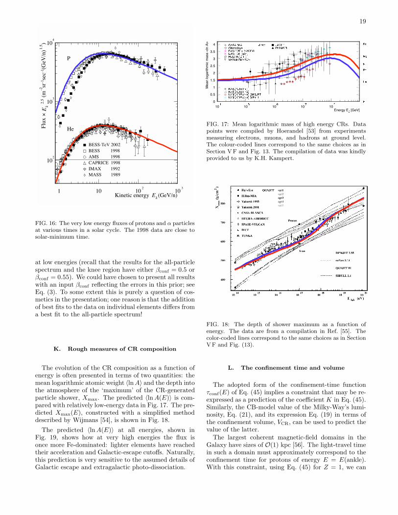
19

Kinetic energy (GeV/n)1 10 10

2

103

)1.5

(GeV/n)

-1sec

-1sr

-2 (m

2.5

×Flux

102

103

104

kE

kE

P

He

BESS-TeV 2002

BESS 1998

AMS 1998

CAPRICE 1998

IMAX 1992

MASS 1989

FIG. 16: The very low energy fluxes of protons and α particlesat various times in a solar cycle. The 1998 data are close tosolar-minimum time.

at low energies (recall that the results for the all-particlespectrum and the knee region have either βconf = 0.5 orβconf = 0.55). We could have chosen to present all resultswith an input βconf reflecting the errors in this prior; seeEq. (3). To some extent this is purely a question of cos-metics in the presentation; one reason is that the additionof best fits to the data on individual elements differs froma best fit to the all-particle spectrum!

K. Rough measures of CR composition

The evolution of the CR composition as a function ofenergy is often presented in terms of two quantities: themean logarithmic atomic weight 〈lnA〉 and the depth intothe atmosphere of the ‘maximum’ of the CR-generatedparticle shower, Xmax. The predicted 〈lnA(E)〉 is com-pared with relatively low-energy data in Fig. 17. The pre-dicted Xmax(E), constructed with a simplified methoddescribed by Wijmans [54], is shown in Fig. 18.

The predicted 〈lnA(E)〉 at all energies, shown inFig. 19, shows how at very high energies the flux isonce more Fe-dominated: lighter elements have reachedtheir acceleration and Galactic-escape cutoffs. Naturally,this prediction is very sensitive to the assumed details ofGalactic escape and extragalactic photo-dissociation.

FIG. 17: Mean logarithmic mass of high energy CRs. Datapoints were compiled by Hoerandel [53] from experimentsmeasuring electrons, muons, and hadrons at ground level.The colour-coded lines correspond to the same choices as inSection VF and Fig. 13. The compilation of data was kindlyprovided to us by K.H. Kampert.

FIG. 18: The depth of shower maximum as a function ofenergy. The data are from a compilation in Ref. [55]. Thecolor-coded lines correspond to the same choices as in SectionVF and Fig. (13).

L. The confinement time and volume

The adopted form of the confinement-time functionτconf(E) of Eq. (45) implies a constraint that may be re-expressed as a prediction of the coefficient K in Eq. (45).Similarly, the CB-model value of the Milky-Way’s lumi-nosity, Eq. (21), and its expression Eq. (19) in terms ofthe confinement volume, VCR, can be used to predict thevalue of the latter.

The largest coherent magnetic-field domains in theGalaxy have sizes of O(1) kpc [56]. The light-travel timein such a domain must approximately correspond to theconfinement time for protons of energy E = E(ankle).With this constraint, using Eq. (45) for Z = 1, we can

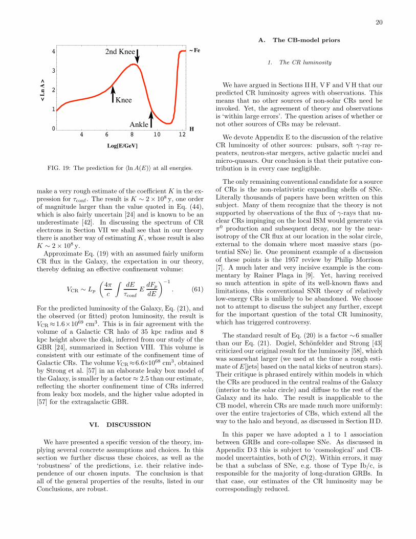
20

Log[E/GeV]

< Ln A >

H

~ Fe

4 6 8 10 120

1

2

3

4

Knee

2nd Knee

Ankle

FIG. 19: The prediction for 〈ln A(E)〉 at all energies.

make a very rough estimate of the coefficient K in the ex-pression for τconf . The result is K ∼ 2× 108 y, one orderof magnitude larger than the value quoted in Eq. (44),which is also fairly uncertain [24] and is known to be anunderestimate [42]. In discussing the spectrum of CRelectrons in Section VII we shall see that in our theorythere is another way of estimating K, whose result is alsoK ∼ 2 × 108 y.

Approximate Eq. (19) with an assumed fairly uniformCR flux in the Galaxy, the expectation in our theory,thereby defining an effective confinement volume:

VCR ∼ Lp

(

4π

c

∫

dE

τconfE

dFp

dE

)−1

. (61)

For the predicted luminosity of the Galaxy, Eq. (21), andthe observed (or fitted) proton luminosity, the result isVCR ≈1.6×1069 cm3. This is in fair agreement with thevolume of a Galactic CR halo of 35 kpc radius and 8kpc height above the disk, inferred from our study of theGBR [24], summarized in Section VIII. This volume isconsistent with our estimate of the confinement time ofGalactic CRs. The volume VCR≈6.6×1068 cm3, obtainedby Strong et al. [57] in an elaborate leaky box model ofthe Galaxy, is smaller by a factor ≈ 2.5 than our estimate,reflecting the shorter confinement time of CRs inferredfrom leaky box models, and the higher value adopted in[57] for the extragalactic GBR.

VI. DISCUSSION

We have presented a specific version of the theory, im-plying several concrete assumptions and choices. In thissection we further discuss these choices, as well as the‘robustness’ of the predictions, i.e. their relative inde-pendence of our chosen inputs. The conclusion is thatall of the general properties of the results, listed in ourConclusions, are robust.

A. The CB-model priors

1. The CR luminosity

We have argued in Sections II H, VF and VH that ourpredicted CR luminosity agrees with observations. Thismeans that no other sources of non-solar CRs need beinvoked. Yet, the agreement of theory and observationsis ‘within large errors’. The question arises of whether ornot other sources of CRs may be relevant.

We devote Appendix E to the discussion of the relativeCR luminosity of other sources: pulsars, soft γ-ray re-peaters, neutron-star mergers, active galactic nuclei andmicro-quasars. Our conclusion is that their putative con-tribution is in every case negligible.

The only remaining conventional candidate for a sourceof CRs is the non-relativistic expanding shells of SNe.Literally thousands of papers have been written on thissubject. Many of them recognize that the theory is notsupported by observations of the flux of γ-rays that nu-clear CRs impinging on the local ISM would generate viaπ0 production and subsequent decay, nor by the near-isotropy of the CR flux at our location in the solar circle,external to the domain where most massive stars (po-tential SNe) lie. One prominent example of a discussionof these points is the 1957 review by Philip Morrison[7]. A much later and very incisive example is the com-mentary by Rainer Plaga in [9]. Yet, having receivedso much attention in spite of its well-known flaws andlimitations, this conventional SNR theory of relativelylow-energy CRs is unlikely to be abandoned. We choosenot to attempt to discuss the subject any further, exceptfor the important question of the total CR luminosity,which has triggered controversy.

The standard result of Eq. (20) is a factor ∼6 smallerthan our Eq. (21). Dogiel, Schonfelder and Strong [43]criticized our original result for the luminosity [58], whichwas somewhat larger (we used at the time a rough esti-mate of E[jets] based on the natal kicks of neutron stars).Their critique is phrased entirely within models in whichthe CRs are produced in the central realms of the Galaxy(interior to the solar circle) and diffuse to the rest of theGalaxy and its halo. The result is inapplicable to theCB model, wherein CRs are made much more uniformly:over the entire trajectories of CBs, which extend all theway to the halo and beyond, as discussed in Section II D.

In this paper we have adopted a 1 to 1 associationbetween GRBs and core-collapse SNe. As discussed inAppendix D3 this is subject to ‘cosmological’ and CB-model uncertainties, both of O(2). Within errors, it maybe that a subclass of SNe, e.g. those of Type Ib/c, isresponsible for the majority of long-duration GRBs. Inthat case, our estimates of the CR luminosity may becorrespondingly reduced.

21

2. The deceleration of a CB and the index below the knee

In deriving Eqs. (7,8) we have worked in the approxi-mation wherein the diffusive rate of escape of ISM par-ticles from a CB is slower than their incoming rate. Tostudy a large range of possibilities, consider the oppositeextreme, in which the escape is instantaneous at all valuesof the CB’s LF γ. Let a be the ratio between the averageenergy of a nucleus exiting a CB in its rest system and theenergy at which the nucleus entered, so that 〈γout〉 ≡ a γ.For elastic scattering, a = 1; for nuclei phagocytized bythe CB, a = 0; and for those Fermi-accelerated withinthe CB, a > 1. Let a be the mean value in the averageover these processes. Energy–momentum conservationimplies a CB’s deceleration law:

dγ

βk γk≃ −mp

M0γa−10 dnp , k ≡ 3 − a , (62)

and a CB’s inertial mass evolving as:

M = M0

(

β γ

γ0

)2−k

. (63)

For a > 0, Eqs. (62,63), imply a slightly different de-celeration law than Eqs. (7,8), and a smaller βs thanthat of Eq. (52). A related uncertainty is the one intro-duced by the adopted form of RCB(γ), which affects βs

via Eqs. (24), (28). We argue in detail in Appendix Athat this is the right choice, and is supported by GRBX-ray AG data, but our theoretical arguments are ad-mittedly over-simplifications of the extremely complexproblem of the CB–ISM collisional process. Yet anothersource of uncertainty in the prediction of βth relates tothe fact that cosmic MFs are in rough energy equipar-tition with CRs, both in the Galaxy and in larger sys-tems [32]. The transfer of as much as 50% of their initialenergy from CRs to the MFs they generate may affectthe slope of the CR spectrum, if the transfer efficiencyis not energy-independent. In spite of all these caveats,since the errors in the uncertainty βconf of Eq. (3) arelarge, the prediction for the observed βth of Eq. (53) isstill acceptable.

The prediction of the spectral slope of Eq. (52) is in-sensitive to all other details of its derivation. An exam-ple: we have assumed the re-emission of ISM particlesin the CB’s rest system to be isotropic. We may haveassumed the distribution to be that of scattering by ahard ball (modelling a CB’s highly magnetized surface),by a monopole (modelling an electrically charged CB)or a dipole (modelling a CB’s longest-range MF compo-nent). These distributions do not affect βs, though theygive slightly different shapes to the elastic flux close tothe knee.

3. Location of the CR sources

We have adopted here a version of our theory whereinthe rate at which CRs exit a CB is much slower than that

at which they enter it, as in our recent study of X-rayAGs [37]. In previous analyses of GRB AGs [29, 30], aswell as in our first results on CRs [17], we studied the‘fast’ opposite limit: the ISM particles intercepted by aCB are instantaneously scattered. The results in the twolimits, for AGs and CRs, are very similar: we have noconvincing way to opt for one or the other limit.

Let ~r be the vector position of a point in the Galaxyrelative to its centre. Let n(~r) be the ISM density. Tosketch a point, consider the rough approximation whereinSNe occur only close to the Galactic centre. In the ‘fast’limit, the CR source is distributed in proportion to n(~r)times the density of CB trajectories, that is n(~r)/r2. Inthe extreme ‘slow’ limit [15] the sources of CRs are lo-cated at the points where CBs end their voyage; a pre-diction of their distribution would require a very detailedmodelling of the distribution n(~r) in the entire Galaxy.

There is yet another source of uncertainty in the pre-cise distribution of the CR sources. The narrow con-ical beams of CRs produced by the decelerating CBsmay propagate collectively, sweeping up the MF in frontof them until the energy density in the beam becomessmaller than that of the field. Thereafter the CRs wouldbegin to diffuse in the ambient MF as individual particles.Such a mechanism may effectively remove the source fur-ther away from the SNe firing the CBs, and contributeto the explanation of the high isotropy of Galactic CRsat all energies.

4. Fermi acceleration within a CB

We have been very specific in choosing the Fermi-accelerated spectrum of Eq. (17). Its abrupt thresh-old Θ(γA − γ) may be substituted by a much smootherfunction describing how unlikely it may be to ‘Fermi-decelerate’ a fraction of the particles tossed aroundby moving MFs. Once processed through the CB-deceleration integrals in Eq. (37), no significant changesoccur in the predicted CR flux, except that the ‘littleknee’ shown in Fig. 9 at E ∼ 108 GeV becomes less pro-nounced (depending on the specific choices of this andother priors, one may obtain smoother spectra, such asthose in Fig. 3, or move the little knee to an energy atwhich it looks like a ‘rotula’ before the steepening atthe knee). The results are even more insensitive to theabrupt Larmor cutoff Θ(γmax−γA) of the assumed inputspectrum. The prediction of the UHECR flux would onlybe affected if the radius of a CB, or the MF within it,were smaller than the ones of Eqs. (9), or (12), by morethan one order of magnitude.

In the calculations we have presented, we used βac =2.2, as in Eq. (13). This affects the slope of the accel-erated flux via Eq. (37). We have also worked out theresults for βac = 2.2±0.2. For the upper value, they ‘lookeven better’ than the results we have presented. For thelower value they are similar, for slightly different chosenvalues of the confinement exponent βconf and the width

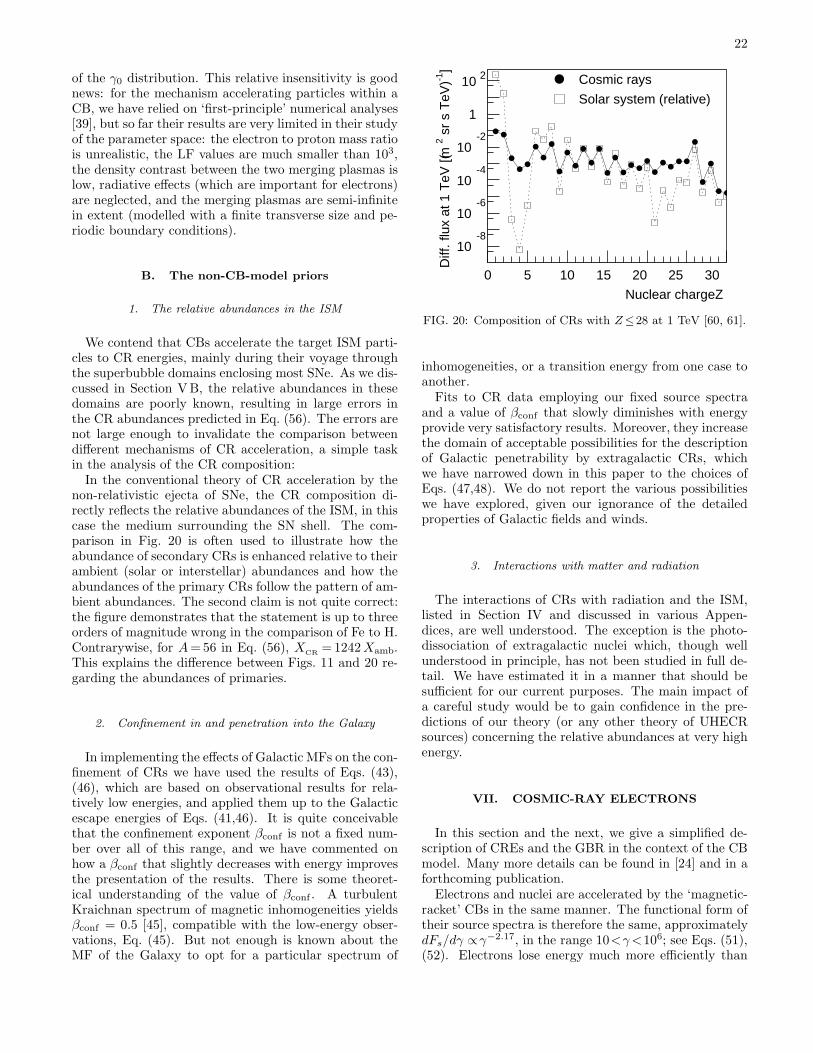
22

of the γ0 distribution. This relative insensitivity is goodnews: for the mechanism accelerating particles within aCB, we have relied on ‘first-principle’ numerical analyses[39], but so far their results are very limited in their studyof the parameter space: the electron to proton mass ratiois unrealistic, the LF values are much smaller than 103,the density contrast between the two merging plasmas islow, radiative effects (which are important for electrons)are neglected, and the merging plasmas are semi-infinitein extent (modelled with a finite transverse size and pe-riodic boundary conditions).

B. The non-CB-model priors

1. The relative abundances in the ISM

We contend that CBs accelerate the target ISM parti-cles to CR energies, mainly during their voyage throughthe superbubble domains enclosing most SNe. As we dis-cussed in Section VB, the relative abundances in thesedomains are poorly known, resulting in large errors inthe CR abundances predicted in Eq. (56). The errors arenot large enough to invalidate the comparison betweendifferent mechanisms of CR acceleration, a simple taskin the analysis of the CR composition:

In the conventional theory of CR acceleration by thenon-relativistic ejecta of SNe, the CR composition di-rectly reflects the relative abundances of the ISM, in thiscase the medium surrounding the SN shell. The com-parison in Fig. 20 is often used to illustrate how theabundance of secondary CRs is enhanced relative to theirambient (solar or interstellar) abundances and how theabundances of the primary CRs follow the pattern of am-bient abundances. The second claim is not quite correct:the figure demonstrates that the statement is up to threeorders of magnitude wrong in the comparison of Fe to H.Contrarywise, for A = 56 in Eq. (56), X

CR= 1242 Xamb.

This explains the difference between Figs. 11 and 20 re-garding the abundances of primaries.

2. Confinement in and penetration into the Galaxy

In implementing the effects of Galactic MFs on the con-finement of CRs we have used the results of Eqs. (43),(46), which are based on observational results for rela-tively low energies, and applied them up to the Galacticescape energies of Eqs. (41,46). It is quite conceivablethat the confinement exponent βconf is not a fixed num-ber over all of this range, and we have commented onhow a βconf that slightly decreases with energy improvesthe presentation of the results. There is some theoret-ical understanding of the value of βconf . A turbulentKraichnan spectrum of magnetic inhomogeneities yieldsβconf = 0.5 [45], compatible with the low-energy obser-vations, Eq. (45). But not enough is known about theMF of the Galaxy to opt for a particular spectrum of

10 -8

10 -6

10 -4

10 -2

1

10 2

0 5 10 15 20 25 30

Nuclear charge Z

Diff

. flu

x at

1 T

eV [(

m 2 s

r s

TeV

) -1 ]

Cosmic rays

Solar system (relative)

FIG. 20: Composition of CRs with Z≤28 at 1 TeV [60, 61].

inhomogeneities, or a transition energy from one case toanother.

Fits to CR data employing our fixed source spectraand a value of βconf that slowly diminishes with energyprovide very satisfactory results. Moreover, they increasethe domain of acceptable possibilities for the descriptionof Galactic penetrability by extragalactic CRs, whichwe have narrowed down in this paper to the choices ofEqs. (47,48). We do not report the various possibilitieswe have explored, given our ignorance of the detailedproperties of Galactic fields and winds.

3. Interactions with matter and radiation

The interactions of CRs with radiation and the ISM,listed in Section IV and discussed in various Appen-dices, are well understood. The exception is the photo-dissociation of extragalactic nuclei which, though wellunderstood in principle, has not been studied in full de-tail. We have estimated it in a manner that should besufficient for our current purposes. The main impact ofa careful study would be to gain confidence in the pre-dictions of our theory (or any other theory of UHECRsources) concerning the relative abundances at very highenergy.

VII. COSMIC-RAY ELECTRONS

In this section and the next, we give a simplified de-scription of CREs and the GBR in the context of the CBmodel. Many more details can be found in [24] and in aforthcoming publication.

Electrons and nuclei are accelerated by the ‘magnetic-racket’ CBs in the same manner. The functional form oftheir source spectra is therefore the same, approximatelydFs/dγ ∝γ−2.17, in the range 10<γ <106; see Eqs. (51),(52). Electrons lose energy much more efficiently than

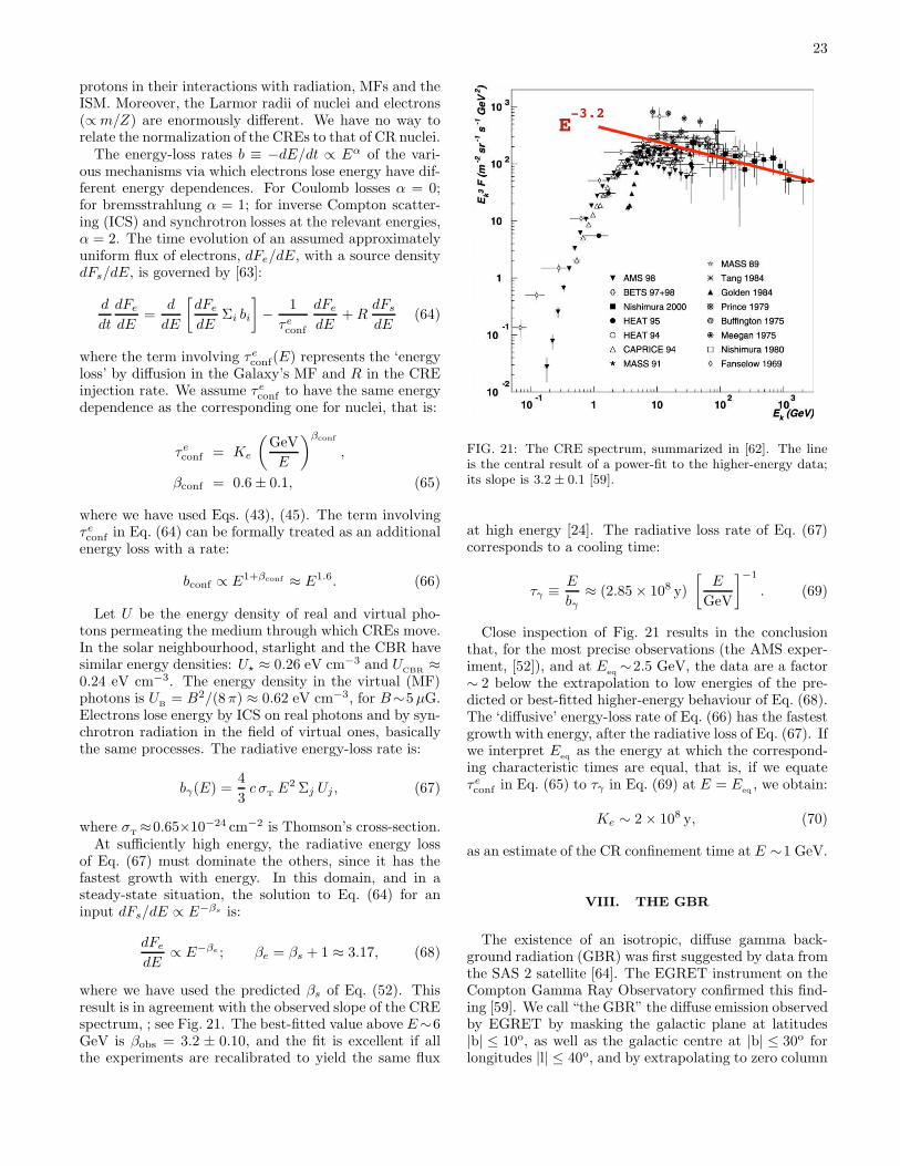
23

protons in their interactions with radiation, MFs and theISM. Moreover, the Larmor radii of nuclei and electrons(∝ m/Z) are enormously different. We have no way torelate the normalization of the CREs to that of CR nuclei.

The energy-loss rates b ≡ −dE/dt ∝ Eα of the vari-ous mechanisms via which electrons lose energy have dif-ferent energy dependences. For Coulomb losses α = 0;for bremsstrahlung α = 1; for inverse Compton scatter-ing (ICS) and synchrotron losses at the relevant energies,α = 2. The time evolution of an assumed approximatelyuniform flux of electrons, dFe/dE, with a source densitydFs/dE, is governed by [63]:

d

dt

dFe

dE=

d

dE

[

dFe

dEΣi bi

]

− 1

τeconf

dFe

dE+ R

dFs

dE(64)

where the term involving τeconf(E) represents the ‘energy

loss’ by diffusion in the Galaxy’s MF and R in the CREinjection rate. We assume τe

conf to have the same energydependence as the corresponding one for nuclei, that is:

τeconf = Ke

(

GeV

E

)βconf

,

βconf = 0.6 ± 0.1, (65)

where we have used Eqs. (43), (45). The term involvingτeconf in Eq. (64) can be formally treated as an additional

energy loss with a rate:

bconf ∝ E1+βconf ≈ E1.6. (66)

Let U be the energy density of real and virtual pho-tons permeating the medium through which CREs move.In the solar neighbourhood, starlight and the CBR havesimilar energy densities: U⋆ ≈ 0.26 eV cm−3 and U

CBR≈

0.24 eV cm−3. The energy density in the virtual (MF)photons is U

B= B2/(8 π) ≈ 0.62 eV cm−3, for B∼5 µG.

Electrons lose energy by ICS on real photons and by syn-chrotron radiation in the field of virtual ones, basicallythe same processes. The radiative energy-loss rate is:

bγ(E) =4

3c σ

TE2 Σj Uj , (67)

where σT≈0.65×10−24 cm−2 is Thomson’s cross-section.

At sufficiently high energy, the radiative energy lossof Eq. (67) must dominate the others, since it has thefastest growth with energy. In this domain, and in asteady-state situation, the solution to Eq. (64) for aninput dFs/dE ∝ E−βs is:

dFe

dE∝ E−βe ; βe = βs + 1 ≈ 3.17, (68)

where we have used the predicted βs of Eq. (52). Thisresult is in agreement with the observed slope of the CREspectrum, ; see Fig. 21. The best-fitted value above E∼6GeV is βobs = 3.2 ± 0.10, and the fit is excellent if allthe experiments are recalibrated to yield the same flux

E-3.2

FIG. 21: The CRE spectrum, summarized in [62]. The lineis the central result of a power-fit to the higher-energy data;its slope is 3.2 ± 0.1 [59].

at high energy [24]. The radiative loss rate of Eq. (67)corresponds to a cooling time:

τγ ≡ E

bγ≈ (2.85 × 108 y)

[

E

GeV

]−1

. (69)

Close inspection of Fig. 21 results in the conclusionthat, for the most precise observations (the AMS exper-iment, [52]), and at E

eq∼2.5 GeV, the data are a factor

∼ 2 below the extrapolation to low energies of the pre-dicted or best-fitted higher-energy behaviour of Eq. (68).The ‘diffusive’ energy-loss rate of Eq. (66) has the fastestgrowth with energy, after the radiative loss of Eq. (67). Ifwe interpret E

eqas the energy at which the correspond-

ing characteristic times are equal, that is, if we equateτeconf in Eq. (65) to τγ in Eq. (69) at E = E

eq, we obtain:

Ke ∼ 2 × 108 y, (70)

as an estimate of the CR confinement time at E ∼1 GeV.

VIII. THE GBR

The existence of an isotropic, diffuse gamma back-ground radiation (GBR) was first suggested by data fromthe SAS 2 satellite [64]. The EGRET instrument on theCompton Gamma Ray Observatory confirmed this find-ing [59]. We call “the GBR” the diffuse emission observedby EGRET by masking the galactic plane at latitudes|b| ≤ 10o, as well as the galactic centre at |b| ≤ 30o forlongitudes |l| ≤ 40o, and by extrapolating to zero column

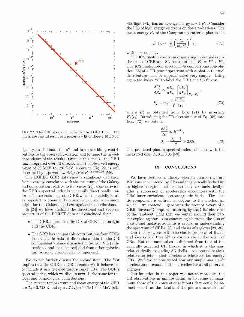
24

Energy (MeV)

Photons/(cm2 s sr MeV)

10-13

10-12

10-11

10-10

10-9

10-8

10-7

10-6

10-5

102

103

104

105

E-2.1

FIG. 22: The GBR spectrum, measured by EGRET [59]. Theline is the central result of a power-law fit of slope 2.10±0.03.

density, to eliminate the π0 and bremsstrahlung contri-butions to the observed radiation and to tame the model-dependence of the results. Outside this ‘mask’, the GBRflux integrated over all directions in the observed energyrange of 30 MeV to 120 GeV, shown in Fig. 22, is welldescribed by a power law dFγ/dE∝E−2.10±0.03 [59].

The EGRET GBR data show a significant deviationfrom isotropy, correlated with the structure of the Galaxyand our position relative to its centre [25]. Contrariwise,the GBR’s spectral index is uncannily directionally uni-form. These facts suggest a GBR which is partially local,as opposed to dominantly cosmological, and a commonorigin for the Galactic and extragalactic contributions.

In [24] we have analized the directional and spectralproperties of the EGRET data and concluded that:

• The GBR is produced by ICS of CREs on starlightand the CBR.

• The GBR has comparable contributions from CREsin a Galactic halo of dimensions akin to the CRconfinement volume discussed in Section VL (a di-rectional and local source) and from other galaxies(an isotropic cosmological component).

We do not further discuss the second item. The firstimplies that the GBR is a CR ‘secondary’: it behoves usto include it in a detailed discussion of CRs. The GBR’sspectral index, which we discuss next, is the same for thelocal and cosmological contributions.

The current temperature and mean energy of the CBRare T0 =2.728 K and ǫ0≈2.7 kT0≈6.36×10−10 MeV [65].

Starlight (SL) has an average energy ǫ⋆∼1 eV. Considerthe ICS of high energy electrons on these radiations. Themean energy Eγ of the Compton upscattered photons is:

Eγ(ǫi) ≈4

3

(

Ee

me c2

)2

ǫi , (71)

with ǫi = ǫ0 or ǫ⋆.The ICS photon spectrum originating in our galaxy is

the sum of CBR and SL contributions: Fγ = F 0γ + F ⋆

γ .The ICS final-photon spectrum –a cumbersome convolu-tion [66] of a CR power spectrum with a photon thermaldistribution– can be approximated very simply. Usingagain the index “i” to label the CBR and SL fluxes:

dF iγ

dEγ∝ dEi

e

dEγ

[

dFe

dEe

]

Ee=Eie

,

Eie ≡ mec

2

√

3 Eγ

4 ǫi, (72)

where Eie is obtained from Eqs. (71) by inverting

Eγ(ǫi). Introducing the CR-electron flux of Eq. (68) intoEqs. (72), we obtain:

dF iγ

dE∝ E−βγ ,

βγ =βe − 1

2≃ 2.08. (73)

The predicted photon spectral index coincides with themeasured one, 2.10 ± 0.03 [59].

IX. CONCLUSIONS

We have sketched a theory wherein cosmic rays areISM ions encountered by CBs and magnetically kicked upto higher energies —either elastically, or ‘inelastically’:after a succession of accelerating encounters with theCBs’ inner turbulent electromagnetic fields. The elas-tic component is entirely analogous to the mechanismwhich —we contend— generates the prompt γ-rays of aGRB: ‘inverse’ Compton scattering by the CBs’ electronsof the ‘ambient’ light they encounter around their par-ent exploding star. Also concerning electrons, the sum ofelastic and inelastic addends is crucial in understandingthe spectrum of GRBs [20] and theirs afterglows [29, 30].

Our theory agrees with the classic proposal of Baadeand Zwicky [67] that SN explosions are at the origin ofCRs. But our mechanism is different from that of thegenerally accepted CR theory, in which it is the non-relativistically-expanding SN shells —as opposed to theirrelativistic jets— that accelerate relatively low-energyCRs. We have demonstrated how our simple and singleaccelerators —cannonballs— are effective at all observedenergies.

Our intention in this paper was not to reproduce theCR observations in minute detail, or to refine at maxi-mum those of the conventional inputs that could be re-fined —such as the details of the photo-dissociation of

25

UHECRs. Thus, we have chosen to minimize the num-ber of fit parameters to a grand total of one. The rest ofthe required input has been gathered from informationindependent of the theory of the source of CRs, or fixedfrom the simplest choices we could make at each point.

Most of our results are ‘robust’ in that —within verylarge brackets— they do not depend on the specificchoices of parameters and priors:

• An all-particle power-law spectrum with four suc-cessive features: two steepenings at the knee andthe second knee, a softening at the ankle, and anend-point at the GZK and proton-acceleration cut-offs, which are roughly coincident.

• An UHECR flux above the ankle, which is pre-dicted —to within a factor of a few— and otherwiseparameter-free.

• A composition dependence at 1 TeV with the ob-served trend, so different from that of the ISM forthe relative abundances of H and He versus thoseof the heavier elements.

• A very low-energy flux whose spectral shape is in-dependent of any CB-model ‘prior’ parameters.

• Individual-element knees that scale like A and oc-cur at the predicted energies.

• A non-trivial shape of the individual knees: anabrupt decrease in flux, followed by a spectrumsteeper than that below the knee.

• An ankle with the observed shape. The domi-nantly Galactic-Fe flux below it and the dominantlyextragalactic-proton flux above it are comparablein magnitude at the estimated escape energy ofGalactic protons.

• A composition dependence that is almost energy-independent below the knee, becomes ‘heavier’from the knee to the second knee, ‘lighter’ againabove it, and finally heavier at yet-unmeasuredultra-high energies.

• An ‘extended’ distribution of CR sources along CBtrajectories emerging from the central realms of theGalaxy, where most SN explosions take place, im-plying a CR flux at the Earth’s position with amuch smaller and less energy-dependent anisotropythan that of conventional SNR models of CRs.

• Predictions for the values of a consistently relatedset of observables: the CR luminosity, confinementtime and volume of the Galaxy, the spectral indicesof CR electrons and of the diffuse GBR.

Our results describe the observed properties of hadronicnon-solar CRs very well from the lowest energies to∼ 1010 GeV. Above that energy and up to the highestobserved energies, ∼ 1011 GeV, our theory opts for the

data gathered with fluorescence detectors. Overall, theenergy range for which the theory is successful covers tendecades and the flux extends over three times as many.

The CR theory we have discussed is currently incom-plete in various respects. The confinement of CRs, ei-ther in the Galaxy or in the CBs themselves, is not wellunderstood, but our assumptions on the subject —thesimplest— appear to work very well. There is insuffi-cient information on the Galactic CR wind to model itseffects with confidence; we have had to experiment withvarious possibilities. We have argued that CR diffusionneed not be explicitly considered, but we have not provedthat to be the case, by considering it in detail. Moreover,our theory is based on a two-stage acceleration: that ofCRs by CBs and that of CBs by exploding SNe. For thelatter, we have relied on observations, rather than on adeeper understanding.

In spite of the above limitations, our claims are sup-ported by the simplicity of the theory, its extreme econ-omy of free parameters, and by the good quality of itsdescription of the fairly elaborate ensemble of CR data.The theory is an item in a more general understanding ofhigh-energy astrophysical phenomena, including GRBs,XRFs, cooling flows and large-scale magnetic fields.

We contend that we have identified the accelerationmechanism promoting the constituents of the interstellarmedium of our Galaxy and others to become the bulk ofthe cosmic rays of all energies, and the ‘magnetic-racket’accelerators themselves: the cannon balls emitted byordinary core-collapse supernovae.

Aknowledgements We are indebted to GiuseppeCocconi, Andy Cohen, Shlomo Dado, Friedrich Dydak,Shelly Glashow, Karl-Heinz Kampert, Etienne Parizotand Rainer Plaga for discussions, and to the last of themfor his comments on the manuscript. This research wassupported in part by the Helen Asher Space ResearchFund at the Technion Institute. AD thanks the THdivision at CERN for its hospitality. ADR thanks theTechnion Institute at Haifa for the same reason.

APPENDIX A: MORE ON THE EXPANSION OFA CB

Observed at X-ray wavelengths, the CBs emitted invarious astronomical systems appear —within the lim-its of observational resolution— not to expand sideways.The example of Pictor A is shown in Fig. 2. Part of thiseffect may be a trivial relativistic mirage. Consider anobject expanding in its rest system at a fraction βT ofthe speed of light and travelling with a large LF γ(t). Adistant observer seeing the object move across the skywould see it trace a trajectory with an opening angleβT /γ, as measured from the trajectories origin: a verythin ‘trumpet’ if γ(t) is originally large and diminisheswith time.

We have first studied the expansion of CBs in [29].

26

We assumed the CBs emitted by SNe to expand initiallyat a speed comparable to that of sound in a relativisticplasma: βT ∼ O(1/

√3). We also assumed a large frac-

tion of the intercepted ISM particles to be elastically andrapidly scattered, isotropically in the CB’s rest system.The rate per unit surface of the momentum carried bythe exuding particles corresponds to a surface pressurePout. In the approximation of a hydrogenic ISM and aNewtonian force law (to be justified a posteriori), theCB’s radius as a function of CB’s time t satisfies:

3

4

MCB

4π R2CB

d2RCB

dt2≈ −Pout (A1)

Pout ≈1

4mpγ

2 np c2, (A2)

where the factor 3/4 is for an assumed homogeneous ex-pansion. For an assumed constant ISM density np alongthe CB’s trajectory, the resulting R

CBincreases very fast

(in minutes of GRB observer’s time, for typical param-eters) to a coasting value R

CB(t) ∝ [γ0/γ(t)]2/3 [29], as

illustrated in the (blue) dashed line of Fig. 6.Here we also explore a different extreme, that the ISM

particles are phagocytized by the CB and exit it by dif-fusion in its entangled magnetic field, rather than beingimmediately and elastically scattered (the fraction thatis accelerated within the CB before they are re-emittedis small, as in [29] and in our current discussion of CRs).We shall see anon that the functional form of R

CB(γ) is

that of the (red) continuous line of Fig. 6.The characteristic diffusion time when the LF [radius]

of the CB has reached a value γ [RCB

(γ)] is given byEq. (24) with D = D(γin, γ) the diffusion coefficient ofEq. (25). The rate at which the diffusing particles areexuded by the CB is r = βin/τ .

The rate of momentum loss per unit surface on a CBis proportional to the average momentum ∼ mp c 〈γin〉 ofthe particles exiting at time, LF and radius t, γ(t) andR

CB(γ), to wit:

Pout =mp c

4π R2CB

∫ γ0

γ

βin γin1

τdnin(γin)

∝ M0 γ0

4π R4CB

γ

(

A

Z

)βconf

F (γ),

F (γ) =1

(γ − 1)βconf

∫ γ0

γ

dγin

(βin γin)2−βconf, (A3)

where we have used dnin as in Eq. (8). Insert this resultinto Eq. (A1), with MCB as in Eq. (7), to obtain:

− R2CB

RCB

∝ γ F (γ). (A4)

This equation, along with Eq. (28), can be solved withvarious initial conditions at t = 0: R

CB(0) ≃ 0, βT ∼

O(1/√

3), βconf ∼ 0.5, γ0 ∼ 103. The results are veryinsensitive to reasonable variations of these input values.An example with the specified initial values is given inFig. 6 as the (red) continuous line. The coasting value

of RCB

(γ) is sensitive to the proportionality factors inEqs. (7), (24), (25), but its γ-dependence is not. It isonly this last dependence that plays a role in our studyof CRs.

As shown in Fig. 6, the two solutions to Eqs. (A1) and(28), (A4) have very similar shapes. Neither shape is tobe taken too ‘seriously’, for the assumptions made in de-riving them are oversimplifications of a very complicatedproblem. Moreover, the solutions we have presented arefor a constant ISM density np, an approximation thatwe know to be incorrect, given in particular the observed‘bumps’ in AG light curves [20, 37].

In our study of GRB AGs we have analysed severalγ-dependences of R

CB(γ), including a constant radius. It

is only the relatively late AG that is sensitive to RCB

(γ).For optical AGs, on which the data were abundant for al-most a decade, it was very difficult to decide on the ‘best’R

CB(γ), since the late AGs have contributions from the

GRB-associated SN and the host galaxy, and the correc-tions for absorption are not negligible. None of this isthe case for the recent X-ray AG data of SWIFT. There,the ‘best’ dependence [37] is that of [29, 30], given byEq. (9). Given its success in describing GRB data withinthe same CB model, and for the sake of consistency, theabove R

CBdependence is the one we adopt here, even

though a best fit to CR data would result in a slightlysmaller power in Eq. (9). During the fast-rising part ofR

CB(γ) in Fig. 6, Eq. (9) is very incorrect. But the frac-

tional CR production is small during this phase in whichthe surface of the CB is also relatively small; we shalluse Eq. (9) at all values of γ. This makes the results ofSections III C and III D simple and analytical.

A question arises in the ‘diffusive’ case we have dis-cussed, which did not in the ‘fast elastic scattering’ caseof Eqs. (A1) and ref. [29]: if the intercepted ISM particlesspend time diffusing within a CB, why do they not exerta pressure similar in magnitude and opposite in sign tothat of Eq. (A2)? Moreover, we contend that the CB’smagnetic field is in rough energy–density equipartitionwith the ISM particles it engulfs. Also, why does thepressure of this field not contribute? The short answeris that the CB may be ‘self-confining’, that is, closer ina sense to a liquid or a solid than to a perfect gas orplasma. The longer answer is the following: a gas ofmagnetic dipoles, if polarized in a single direction, has a‘positive’ contribution to its pressure from the repulsionbetween the dipoles. For the unpolarized case this effectvanishes on the average (it may even correspond to anattraction: a collection of magnets allowed to coalesceat random would form a bound state). A CB’s MF ischaotic in its structure and in the orientation of its co-herent ‘cells’, i.e. ‘unpolarized’, and pressureless... or evenself-confining. There are low-energy CRs confined to theMF lines of the Earth, spiralling North to a higher-fieldposition where they back up South, to reverse the processperiodically. These confined particles do not contribute apressure on a hypothetical surface enclosing their boundtrajectories. Once again, the high-energy constituents of

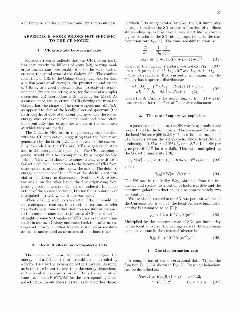
27

a CB may be similarly confined and, thus, ‘pressureless’.

APPENDIX B: MORE PRIORS NOT SPECIFICTO THE CB MODEL

1. CR cross-talk between galaxies

Meteorite records indicate that the CR flux on Earthhas been steady for billions of years [42], barring mod-erate fluctuations presumably due to the solar systemcrossing the spiral arms of the Galaxy [68]. The confine-ment time of CRs to the Galaxy being much shorter thana billion years at all energies, the production and escapeof CRs is, to a good approximation, a steady-state phe-nomenon (we are neglecting here, for the sake of a simplerdiscussion, CR interactions with anything but MFs). Asa consequence, the spectrum of CRs flowing out from theGalaxy has the shape of the source spectrum, dFs/dE,as opposed to that of the locally observed spectrum (thepath lengths of CRs of different energy differ, the lower-energy ones cross our local neighbourhood more often,but eventually they escape the Galaxy at the same rateat which they are made).

The Galactic MFs are in rough energy equipartitionwith the CR population, suggesting that the former aregenerated by the latter [42]. This ansatz can be success-fully extended to the CRs and MFs in galaxy clustersand in the intergalactic space [32]. The CRs escaping agalaxy would thus be accompanied by a magnetic-field‘wind’. This wind should, to some extent, constitute aGalactic ‘shield’: it counteracts the income of CRs fromother galaxies, at energies below the ankle. The detailedenergy–dependence of the effect of the shield is not cru-cial in our theory, as discussed in Section IVD. Abovethe ankle, on the other hand, the flux originating fromother galaxies enters our Galaxy unhindered. Its shapeis that of the source spectrum, but for the tribulations ofintergalactic travel, which we discuss next.

When dealing with extragalactic CRs, it would bemore adequate, contrary to established custom, to referto a ‘look-back’ time rather than to a redshift or distanceto the source —since the trajectories of CRs need not bestraight— some ‘extragalactic’ CRs may even have origi-nated in our own Galaxy and come back to it after an ex-tragalactic foray. In what follows, distances or redshiftsare to be understood as measures of look-back time.

2. Redshift effects on extragalactic CRs

The momentum —or, for relativistic energies, theenergy— of a CR emitted at a redshift z is degraded bya factor 1+ z by the expansion of the Universe. Assume,as is the case in our theory, that the energy dependenceof the local source spectrum of CRs is the same at alltimes, and let dF [EG]/dE be the corresponding inter-galactic flux. In our theory, as well as in any other theory

in which CRs are generated by SNe, the CR luminosityis proportional to the SN rate as a function of z. Sincestars ending up as SNe have a very short life by cosmo-logical standards, the SN rate is proportional to the starformation rate RSF(z). The time–redshift relation is:

dt

dz=

1

H0

1

g(z),

g(z) ≡ (1 + z)√

ΩΛ + ΩM (1 + z)3 , (B1)

where, in the current ‘standard’ cosmology, H0 = 100 hkm s−1 Mpc−1, h∼0.65, ΩΛ∼0.7 and ΩM ≃ 1 − ΩΛ.

The extragalactic flux currently impinging on theGalaxy has a spectral distribution:

dF [EG]

dE∝∫ ∞

0

dFs

dE

∣

∣

∣

Ez

RSF(z)

RSF(0)

(1 + z) dz

g(z), (B2)

where the dFs/dE is the source flux at Ez = (1 + z)E,‘uncorrected’ for the effect of Galactic confinement.

3. The rate of supernova explosions

In galaxies such as ours, the SN rate is approximatelyproportional to the luminosity. The measured SN rate inthe local Universe [69] is 2.8 y−1, in a ‘fiducial sample’ of342 galaxies within the Virgo circle, whose total B-bandluminosity is 1.35 h−2 × 1012 LB

⊙, or ∼ 8.7× 10−3 SN per

year per 1010 LB⊙ for h = 0.65. This ratio multiplied by

the Galactic luminosity [70],

L⋆[MW] = 2.3 × 1010 L⊙ = 8.85 × 1043 erg s−1, (B3)

yields:

RSN[MW]≈1/50 y−1. (B4)

The SN rate in the Milky Way, obtained from the fre-quency and spatial distribution of historical SNe and themeasured galactic extinction, is also approximately twoper century [69].

We are also interested in the SN rate per unit volume inthe Universe. For h = 0.65, the local-Universe luminositydensity is estimated to be [71]:

ρL ∼ 1.2 × 108 L⊙ Mpc−3. (B5)

Multiplied by the measured rate of SNe per luminosityin the local Universe, the average rate of SN explosionsper unit volume in the current Universe is:

RSN[U] ≈ 10−4 Mpc−3 y−1. (B6)

4. The star-formation rate

A compilation of the observational data [72] on thefunction RSF(z) is shown in Fig. 23. Its rough behaviourcan be described as:

RSF(z) ≃ RSF(0) (1 + z)4 z ≤ 1.2;

≃ RSF(1.2) 1.4 < z ≤ 5. (B7)

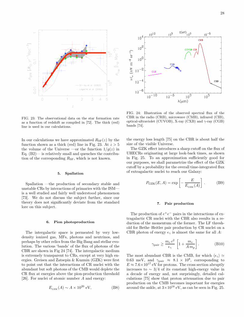
28

FIG. 23: The observational data on the star formation rateas a function of redshift as compiled in [72]. The thick (red)line is used in our calculations.

In our calculations we have approximated RSF(z) by thefunction shown as a thick (red) line in Fig. 23. At z > 5the volume of the Universe —or the function 1/g(z) inEq. (B2)— is relatively small and quenches the contribu-tion of the corresponding RSF, which is not known.

5. Spallation

Spallation —the production of secondary stable andunstable CRs by interactions of primaries with the ISM—is a well studied and fairly well understood phenomenon[73]. We do not discuss the subject further, since ourtheory does not significantly deviate from the standardlore on this subject.

6. Pion photoproduction

The intergalactic space is permeated by very low-density ionized gas, MFs, photons and neutrinos, andperhaps by other relics from the Big Bang and stellar evo-lution. The various ‘bands’ of the flux of photons of theCBR are shown in Fig 24 [74]. The intergalactic mediumis extremely transparent to CRs, except at very high en-ergies. Greisen and Zatsepin & Kuzmin (GZK) were firstto point out that the interactions of CR nuclei with theabundant but soft photons of the CMB would deplete theCR flux at energies above the pion-production threshold[26]. For nuclei of atomic number A and energy:

EGZK

(A) ∼ A × 1020 eV, (B8)

FIG. 24: Illustration of the observed spectral flux of theCBR in the radio (CRB), microwave (CMB), infrared (CIB),optical-ultraviolet (CUVOB), X-ray (CXB) and γ-ray (CGB)bands [74].

the energy loss length [75] on the CBR is about half thesize of the visible Universe.

The GZK effect introduces a sharp cutoff on the flux ofUHECRs originating at large look-back times, as shownin Fig. 25. To an approximation sufficiently good forour purposes, we shall parametrize the effect of the GZKcutoff by a probability for the overall time-integrated fluxof extragalactic nuclei to reach our Galaxy:

PGZK(E, A) = exp

[

− E

EGZK

(A)

]

. (B9)

7. Pair production

The production of e+e− pairs in the interactions of ex-tragalactic CR nuclei with the CBR also results in a re-duction of the momentum of the former. The LF thresh-old for Bethe–Heitler pair production by CR nuclei on aCBR photon of energy ǫγ is almost the same for all A:

γpair ≥me c2

ǫγ

[

1 +me

Amp

]

. (B10)

The most abundant CBR is the CMB, for which 〈ǫγ〉 ≃0.63 meV, and γpair ≈ 8.1 × 108, corresponding toE ≈ 7.6×1017 eV for protons. The cross section abruptlyincreases to ∼ 3/4 of its constant high-energy value ina decade of energy and, not surprisingly, detailed cal-culations [75] show that proton attenuation due to pairproduction on the CMB becomes important for energiesaround the ankle, at 3×1018 eV, as can be seen in Fig. 25.

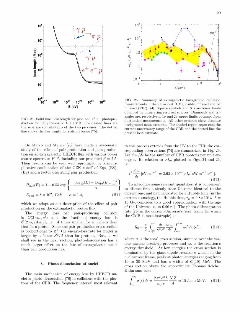
29

1017

1018

1019

1020

1021

1022

E !eV"

100

101

102

103

104

105

losslength!Mpc"

γ p→

→

γ p

π p

e+

e−

p

FIG. 25: Solid line: loss length for pion and e+ e− photopro-duction for CR protons on the CMB. The dashed lines arethe separate contributions of the two processes. The dottedline shows the loss length for redshift losses [75].

De Marco and Stanev [75] have made a systematicstudy of the effect of pair production and pion produc-tion on an extragalactic UHECR flux with various powersource spectra ∝ E−β , including our predicted β ≃ 2.5.Their results can be very well reproduced by a multi-plicative combination of the GZK cutoff of Eqs. (B8),(B9) and a factor describing pair production:

Ppair(E) = 1 − 0.55 exp

− [log10(E) − log10(Epair)]2

α

Epair = 8 × 109, GeV α = 1.4, (B11)

which we adopt as our description of the effect of pairproduction on the extragalactic proton flux.

The energy loss per pair-producing collisionis O(2 γme c2) and the fractional energy loss isO(2 me/Amp), i.e. A times smaller for a nucleus thanthat for a proton. Since the pair-production cross sectionis proportional to Z2, the energy-loss rate for nuclei islarger by a factor Z2/A than for protons. But, as weshall see in the next section, photo-dissociation has amuch larger effect on the fate of extragalactic nucleithan pair production has.

8. Photo-dissociation of nuclei

The main mechanism of energy loss by UHECR nu-clei is photo-dissociation [76] in collisions with the pho-tons of the CBR. The frequency interval most relevant

FIG. 26: Summary of extragalactic background radiationmeasurements in the ultraviolet (UV), visible, infrared and farinfrared (FIR) [74]. Square symbols and X’s are lower limitsobtained by integrating resolved sources. Diamonds and tri-angles are, respectively, 1σ and 2σ upper limits obtained fromfluctuation measurements. All other symbols show absolutebackground measurements. The shaded region represents thecurrent uncertainty range of the CBR and the dotted line thepresent best estimate.

to this process extends from the UV to the FIR; the cor-responding observations [74] are summarized in Fig. 26.Let dnγ/dǫ be the number of CBR photons per unit en-ergy ǫ. Its relation to ν Iν , plotted in Figs. 24 and 26,is:

ǫ2dnγ

dǫ[eV cm−3] = 2.62 × 10−4 ν Iν [nW m−2 sr−1].

(B12)To introduce some relevant quantities, it is convenient

to discuss first a steady-state Universe identical to thecurrent one, and having existed for a Hubble time (in thecurrent cosmology, the Hubble time, τ

H= 9.8×109 h−1 =

15 Gy, coincides to a good approximation with the ageof the Universe: t

U≈ 0.96 τ

H). The photo-disintegration

rate [76] in the current-Universe’s ‘rest’ frame (in whichthe CMB is most isotropic) is:

R0 =c

2

∫ ∞

ǫth2γ

dǫ

γ2 ǫ2dnγ

dǫ

∫ 2γǫ

ǫth

dǫ′ ǫ′σ(ǫ′), (B13)

where σ is the total cross section, summed over the var-ious nuclear break-up processes and ǫth is the reaction’senergy threshold. At low energies the cross section isdominated by the giant dipole resonance which, in thenuclear rest frame, peaks at photon energies ranging from10 to 30 MeV and has a width of O(10) MeV. Thecross section obeys the approximate Thomas–Reiche–Kuhn sum rule:∫ ∞

ǫth

σ(ǫ) dǫ =2 π2 e2

~

mp c

N Z

A≈ 15 Amb MeV, (B14)

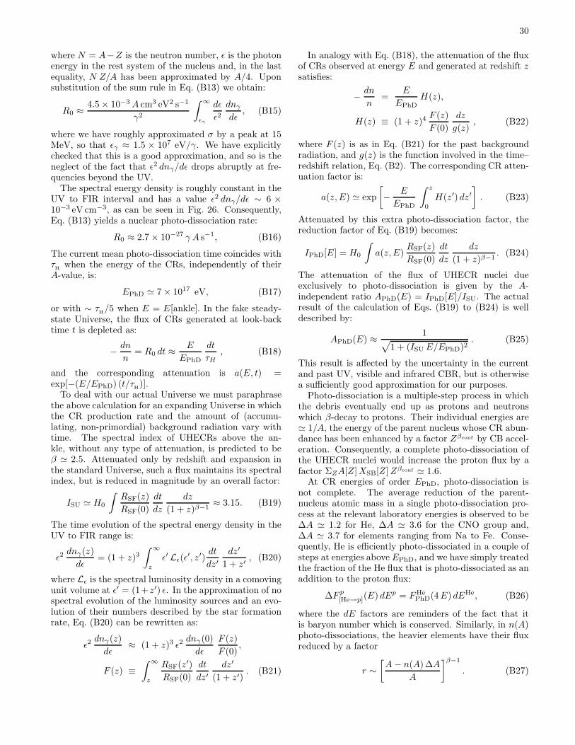
30

where N = A−Z is the neutron number, ǫ is the photonenergy in the rest system of the nucleus and, in the lastequality, N Z/A has been approximated by A/4. Uponsubstitution of the sum rule in Eq. (B13) we obtain:

R0 ≈ 4.5 × 10−3 A cm3 eV2 s−1

γ2

∫ ∞

ǫγ

dǫ

ǫ2dnγ

dǫ, (B15)

where we have roughly approximated σ by a peak at 15MeV, so that ǫγ ≈ 1.5 × 107 eV/γ. We have explicitlychecked that this is a good approximation, and so is theneglect of the fact that ǫ2 dnγ/dǫ drops abruptly at fre-quencies beyond the UV.

The spectral energy density is roughly constant in theUV to FIR interval and has a value ǫ2 dnγ/dǫ ∼ 6 ×10−3 eV cm−3, as can be seen in Fig. 26. Consequently,Eq. (B13) yields a nuclear photo-dissociation rate:

R0 ≈ 2.7 × 10−27 γ A s−1, (B16)

The current mean photo-dissociation time coincides withτH

when the energy of the CRs, independently of theirA-value, is:

EPhD ≃ 7 × 1017 eV, (B17)

or with ∼ τH/5 when E = E[ankle]. In the fake steady-

state Universe, the flux of CRs generated at look-backtime t is depleted as:

− dn

n= R0 dt ≈ E

EPhD

dt

τH, (B18)

and the corresponding attenuation is a(E, t) =exp[−(E/EPhD) (t/τ

H)].

To deal with our actual Universe we must paraphrasethe above calculation for an expanding Universe in whichthe CR production rate and the amount of (accumu-lating, non-primordial) background radiation vary withtime. The spectral index of UHECRs above the an-kle, without any type of attenuation, is predicted to beβ ≃ 2.5. Attenuated only by redshift and expansion inthe standard Universe, such a flux maintains its spectralindex, but is reduced in magnitude by an overall factor:

ISU ≃ H0

∫

RSF(z)

RSF(0)

dt

dz

dz

(1 + z)β−1≈ 3.15. (B19)

The time evolution of the spectral energy density in theUV to FIR range is:

ǫ2dnγ(z)

dǫ= (1 + z)3

∫ ∞

z

ǫ′ Lǫ(ǫ′, z′)

dt

dz′dz′

1 + z′, (B20)

where Lǫ is the spectral luminosity density in a comovingunit volume at ǫ′ = (1+z′) ǫ. In the approximation of nospectral evolution of the luminosity sources and an evo-lution of their numbers described by the star formationrate, Eq. (B20) can be rewritten as:

ǫ2dnγ(z)

dǫ≈ (1 + z)3 ǫ2

dnγ(0)

dǫ

F (z)

F (0),

F (z) ≡∫ ∞

z

RSF(z′)

RSF(0)

dt

dz′dz′

(1 + z′). (B21)

In analogy with Eq. (B18), the attenuation of the fluxof CRs observed at energy E and generated at redshift zsatisfies:

− dn

n=

E

EPhDH(z),

H(z) ≡ (1 + z)4F (z)

F (0)

dz

g(z), (B22)

where F (z) is as in Eq. (B21) for the past backgroundradiation, and g(z) is the function involved in the time–redshift relation, Eq. (B2). The corresponding CR atten-uation factor is:

a(z, E) ≃ exp

[

− E

EPhD

∫ z

0

H(z′) dz′]

. (B23)

Attenuated by this extra photo-dissociation factor, thereduction factor of Eq. (B19) becomes:

IPhD[E] = H0

∫

a(z, E)RSF(z)

RSF(0)

dt

dz

dz

(1 + z)β−1. (B24)

The attenuation of the flux of UHECR nuclei dueexclusively to photo-dissociation is given by the A-independent ratio APhD(E) = IPhD[E]/ISU. The actualresult of the calculation of Eqs. (B19) to (B24) is welldescribed by:

APhD(E) ≈ 1√

1 + (ISU E/EPhD)2. (B25)

This result is affected by the uncertainty in the currentand past UV, visible and infrared CBR, but is otherwisea sufficiently good approximation for our purposes.

Photo-dissociation is a multiple-step process in whichthe debris eventually end up as protons and neutronswhich β-decay to protons. Their individual energies are≃ 1/A, the energy of the parent nucleus whose CR abun-dance has been enhanced by a factor Zβconf by CB accel-eration. Consequently, a complete photo-dissociation ofthe UHECR nuclei would increase the proton flux by afactor ΣZA[Z] XSB[Z] Zβconf ≃ 1.6.

At CR energies of order EPhD, photo-dissociation isnot complete. The average reduction of the parent-nucleus atomic mass in a single photo-dissociation pro-cess at the relevant laboratory energies is observed to be∆A ≃ 1.2 for He, ∆A ≃ 3.6 for the CNO group and,∆A ≃ 3.7 for elements ranging from Na to Fe. Conse-quently, He is efficiently photo-dissociated in a couple ofsteps at energies above EPhD, and we have simply treatedthe fraction of the He flux that is photo-dissociated as anaddition to the proton flux:

∆F p[He→p](E) dEp = FHe

PhD(4 E) dEHe, (B26)

where the dE factors are reminders of the fact that itis baryon number which is conserved. Similarly, in n(A)photo-dissociations, the heavier elements have their fluxreduced by a factor

r ∼[

A − n(A)∆A

A

]β−1

. (B27)

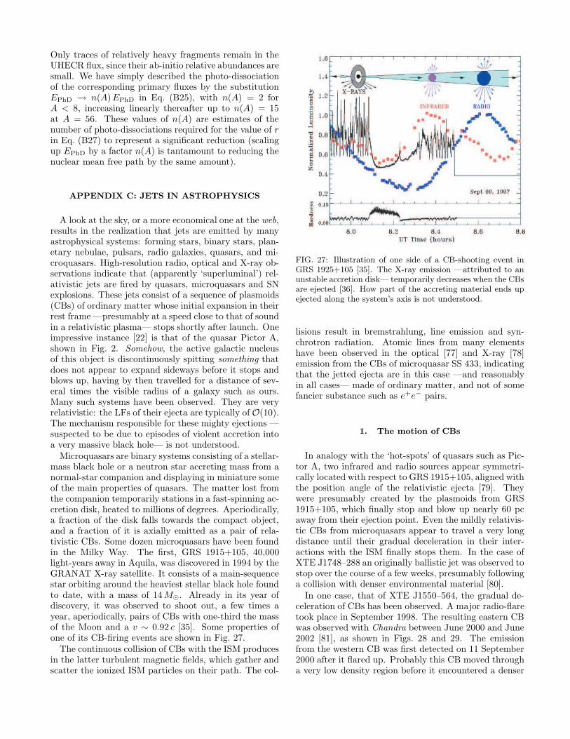
31

Only traces of relatively heavy fragments remain in theUHECR flux, since their ab-initio relative abundances aresmall. We have simply described the photo-dissociationof the corresponding primary fluxes by the substitutionEPhD → n(A)EPhD in Eq. (B25), with n(A) = 2 forA < 8, increasing linearly thereafter up to n(A) = 15at A = 56. These values of n(A) are estimates of thenumber of photo-dissociations required for the value of rin Eq. (B27) to represent a significant reduction (scalingup EPhD by a factor n(A) is tantamount to reducing thenuclear mean free path by the same amount).

APPENDIX C: JETS IN ASTROPHYSICS

A look at the sky, or a more economical one at the web,results in the realization that jets are emitted by manyastrophysical systems: forming stars, binary stars, plan-etary nebulae, pulsars, radio galaxies, quasars, and mi-croquasars. High-resolution radio, optical and X-ray ob-servations indicate that (apparently ‘superluminal’) rel-ativistic jets are fired by quasars, microquasars and SNexplosions. These jets consist of a sequence of plasmoids(CBs) of ordinary matter whose initial expansion in theirrest frame —presumably at a speed close to that of soundin a relativistic plasma— stops shortly after launch. Oneimpressive instance [22] is that of the quasar Pictor A,shown in Fig. 2. Somehow, the active galactic nucleusof this object is discontinuously spitting something thatdoes not appear to expand sideways before it stops andblows up, having by then travelled for a distance of sev-eral times the visible radius of a galaxy such as ours.Many such systems have been observed. They are veryrelativistic: the LFs of their ejecta are typically of O(10).The mechanism responsible for these mighty ejections —suspected to be due to episodes of violent accretion intoa very massive black hole— is not understood.

Microquasars are binary systems consisting of a stellar-mass black hole or a neutron star accreting mass from anormal-star companion and displaying in miniature someof the main properties of quasars. The matter lost fromthe companion temporarily stations in a fast-spinning ac-cretion disk, heated to millions of degrees. Aperiodically,a fraction of the disk falls towards the compact object,and a fraction of it is axially emitted as a pair of rela-tivistic CBs. Some dozen microquasars have been foundin the Milky Way. The first, GRS 1915+105, 40,000light-years away in Aquila, was discovered in 1994 by theGRANAT X-ray satellite. It consists of a main-sequencestar orbiting around the heaviest stellar black hole foundto date, with a mass of 14 M⊙. Already in its year ofdiscovery, it was observed to shoot out, a few times ayear, aperiodically, pairs of CBs with one-third the massof the Moon and a v ∼ 0.92 c [35]. Some properties ofone of its CB-firing events are shown in Fig. 27.

The continuous collision of CBs with the ISM producesin the latter turbulent magnetic fields, which gather andscatter the ionized ISM particles on their path. The col-

FIG. 27: Illustration of one side of a CB-shooting event inGRS 1925+105 [35]. The X-ray emission —attributed to anunstable accretion disk— temporarily decreases when the CBsare ejected [36]. How part of the accreting material ends upejected along the system’s axis is not understood.

lisions result in bremstrahlung, line emission and syn-chrotron radiation. Atomic lines from many elementshave been observed in the optical [77] and X-ray [78]emission from the CBs of microquasar SS 433, indicatingthat the jetted ejecta are in this case —and reasonablyin all cases— made of ordinary matter, and not of somefancier substance such as e+e− pairs.

1. The motion of CBs

In analogy with the ‘hot-spots’ of quasars such as Pic-tor A, two infrared and radio sources appear symmetri-cally located with respect to GRS 1915+105, aligned withthe position angle of the relativistic ejecta [79]. Theywere presumably created by the plasmoids from GRS1915+105, which finally stop and blow up nearly 60 pcaway from their ejection point. Even the mildly relativis-tic CBs from microquasars appear to travel a very longdistance until their gradual deceleration in their inter-actions with the ISM finally stops them. In the case ofXTE J1748–288 an originally ballistic jet was observed tostop over the course of a few weeks, presumably followinga collision with denser environmental material [80].

In one case, that of XTE J1550–564, the gradual de-celeration of CBs has been observed. A major radio-flaretook place in September 1998. The resulting eastern CBwas observed with Chandra between June 2000 and June2002 [81], as shown in Figs. 28 and 29. The emissionfrom the western CB was first detected on 11 September2000 after it flared up. Probably this CB moved througha very low density region before it encountered a denser

32

NE

2 arcsec

2000 June 9

Eastern X-Ray Jet XTE J1550-564 Western X-Ray Jet

NE

2 arcsec

2002 June 19

Eastern X-Ray Jet XTE J1550-564 Western X-Ray Jet

NE

2 arcsec

2002 March 11

Eastern X-Ray Jet XTE J1550-564 Western X-Ray Jet

NE

2 arcsec

2000 September 11

Eastern X-Ray Jet XTE J1550-564 Western X-Ray Jet

NE

2 arcsec

2000 August 21

Eastern X-Ray Jet XTE J1550-564 Western X-Ray Jet

FIG. 28: Five Chandra 0.3–8 keV images showing the mi-croquasar XTE J1550–564 and the evolution of the easternand western X-ray emitting CBs between June 2000 and June2002. The observations are ordered chronologically from topto bottom, and each image is labelled with the observationdate. The dashed lines mark the positions of XTE J1550-564and the eastern X-ray jet on 11 September 2000 [81].

region and flared up.

2. CBs or conical jets?

The conical or trumpet-like radio and optical imagesof some astrophysical jets are often interpreted as beingproduced by conical ejecta. Conical-like images are oftenproduced by precession of the ejection axis around therotation axis, as in the case of SS433 [82].

0 500 1000 1500 2000Time after X-ray flare (days)

0

5

10

15

20

25

30

35

An

gu

lar

sep

erat

ion

(ar

csec

)

FIG. 29: The decelerating motion of the CBs of the µ-quasarXTE J1550–564 [81].

The conical flows that are produced along the motionof the decelerating CBs can also generate conical-lookingtrails. Radiation and charged particles (swept in ion-ized ISM particles), which are emitted isotropically inthe CBs’ rest frame, are beamed forward by its motion.

Let primed quantities denote their values in the CB’srest frame and unprimed quantities their correspondingvalues in the SN frame. The angle θ′ —relative to theCBs’ direction of motion— of the particles emitted inthe CBs’ rest frame, and the corresponding angle θ inthe SN’s rest frame, are related through:

cos θ′ =cos θ − β

1 − β cos θ. (C1)

Applied to an isotropic distribution of emitted particlesin the CBs’ rest frame, Eq. (C1) results in a distributionin the SN’s frame:

dn

dΩ=

dn

dΩ′

dcosθ′

dcosθ≈ n

4 πδ2 ≈ n

4 π

[

2γ

1 + γ2 θ2

]2

, (C2)

where the Doppler factor δ of the CB’s radiation, asviewed from an angle θ, was approximated by:

δ =1

γ (1 − β cos θ)≈ 2γ

1 + γ2 θ2, (C3)

which is well satisfied for CBs with γ2 ≫ 1 , and θ2 ≪1. The ISM particles, which are isotropized elasticallywithin the moving CB, are emitted with energy 〈ǫ〉 =γ δ m c2. Hence, the energy outflow from a CB is:

dE

dΩ=

n m c2 γ δ3

4 π≈ n γ m c2

4 π

[

2 γ

1 + γ2 θ2

]3

. (C4)

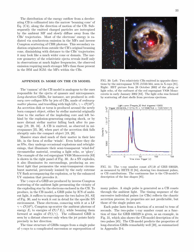
33

The distribution of the energy outflow from a deceler-ating CB is collimated into the narrow ‘beaming cone’ ofEq. (C4), along the direction of motion of the CB. Sub-sequently the emitted charged particles are isotropizedby the ambient MF and slowly diffuse away from theCBs’ trajectories. Most of the electrons’ energy is ra-diated via synchrotron emission in the MFs and inverseCompton scattering of CBR photons. This secondary ra-diation originates from outside the CB’s original beamingcone, diminishing with distance to the CBs’ trajectories:it may look like a much wider cone or domain. The nar-row geometry of the relativistic ejecta reveals itself onlyin observations at much higher frequencies, the observedemission requiring much stronger MFs than those presentin the ISM and IGM: the MFs within the CBs.

APPENDIX D: MORE ON THE CB MODEL

The ‘cannon’ of the CB model is analogous to the onesresponsible for the ejecta of quasars and microquasars.Long-duration GRBs, for instance, are produced in ordi-nary core-collapse SNe by jets of CBs, made of ordinary-matter plasma, and travelling with high LFs, γ ∼ O(103).An accretion disk or torus is produced around the newlyborn compact object, either by stellar material originallyclose to the surface of the imploding core and left be-hind by the explosion-generating outgoing shock, or bymore distant stellar matter falling back after its pas-sage [19, 20, 34]. A CB is emitted, as observed in mi-croquasars [35, 36], when part of the accretion disk fallsabruptly onto the compact object [19, 20].

Massive stars shed much of their matter in their latelife, in the form of stellar ‘winds’. Even before they dieas SNe, they undergo occasional explosions and rebright-enings, that illuminate their semi-transparent ‘wind-fed’circumstellar material, creating a light echo, or ‘glory’.The example of the red supergiant V838 Monocerotis [83]is shown in the right panel of Fig. 30. As a SN explodes,it also illuminates its surroundings, producing an am-bient light that permeates the semi-transparent circum-burst material, previously ionized by the early extremeUV flash accompanying the explosion, or by the enhancedUV emission that precedes it.

The γ-rays of a GRB are produced by inverse Comptonscattering of the ambient light permeating the vicinity ofthe exploding star by the electrons enclosed in the CB. Toproduce, in the CB model, a GRB pulse by ICS of ambi-ent light, it suffices to superimpose the two halves [81, 83]of Fig. 30, and to work it out in detail for the specific SNenvironment. These electrons, comoving with it at a LFγ ∼ O(103), Compton up-scatter the ambient photons ofenergy Ei to energies of O(γ2 Ei), while beaming themforward at angles of O(1/γ). The collimated GRB isseen by a distant observer only when the jet points fairlyprecisely in her direction.

The time structure of GRBs ranges from a single pulseof γ-rays to a complicated succession or superposition of

E

N

FIG. 30: Left: Two relativistic CBs emitted in opposite direc-tions by the microquasar XTE J1550-564, seen in X-rays [81].Right: HST picture from 28 October 2002 of the glory, orlight echo, of the outburst of the red supergiant V838 Mono-cerotis in early January 2002 [83]. The light echo was formedby scattering off dust shells from previous ejections.

FIG. 31: The γ-ray number count dN/dt of GRB 030329,as measured by HETE II [84], showing two dominant pulses,or CB contributions. The continuous line is the CB-model’sdescription of the line shapes [85].

many pulses. A single pulse is generated as a CB coaststhrough the ambient light. The timing sequence of thesuccessive individual pulses (or CBs) reflects the chaoticaccretion process; its properties are not predictable, butthose of the single pulses are.

Each pulse lasts from a fraction of a second to tens ofseconds. The two-pulse γ-ray number count as a func-tion of time for GRB 030329 is given, as an example, inFig. 31, which also shows the CB-model description of itstwo pulses [85]. The CB-model predicts the properties oflong-duration GRBs remarkably well [20], as summarizedin Appendix D4.

34

FIG. 32: The two CBs emitted by SN1987A in opposite axialdirections [11]. The northern and southern bright spots arecompatible with being jets of CBs emitted at the time of theSN explosion and travelling at a velocity equal, within errors,to that of light. One of the apparent velocities is superluminal.The corresponding GRBs were not pointing in our direction,which may have been a blessing.

Long-duration GRBs have ‘afterglows’ (AGs), longterm emissions that are often observable at frequenciesranging from radio to X-rays, for months after their γ-rays are seen. The rapid expansion of the CBs stopsshortly after ejection by their interaction with the ISM[29]. During a CB’s rapid expansion and cooling phase,its AG is usually dominated by thermal bremstrahlungand line-cooling. Later, the emission is dominated bysynchrotron radiation from swept in ISM electrons, whichspiral in the CBs’ enclosed MF. This picture yields an ex-cellent description of the entire AG phase and allows usto infer the parameters of CBs [29, 30], as discussed inAppendix D 5. These parameters and their distributions,employed as ‘priors’, can be used to predict the proper-ties of the prompt γ-ray phase of GRBs [20], much as weuse them here to predict the properties of CRs.

1. Do supernovae emit cannonballs?

Up to quite recently, there was only one case in whichthe data were good enough to tell: SN1987A, the core-collapse SN in the LMC, whose neutrino emission wasdetected. Speckle interferometry measurements made 30and 38 days after the explosion [11] did show two rel-ativistic CBs, emitted in opposite directions, as shownin Fig. 32. The apparent motion of the approaching CBis ‘superluminal’: it appears to have moved faster thanlight and further than the receding CB in the same time,even if their real speeds are comparable.

Another resolved image of what appears like relativis-tic CBs emitted in a SN explosion was obtained recentlywith the Spitzer Space Telescope [13]. Two FIR images ofCassiopeia A, the youngest observed SNR in our Galaxy(about 325 years old) show discrete compact structuresat a distance of more than 20 arcmin from the SNR, mov-ing in opposite directions at roughly the speed of light.The trail of the CBs inside and outside the SNR is stillvisible in an X-ray image of Cassiopeia A obtained by

Chandra [12].Cosmic GRBs are usually too far away to provide re-

solved (radio) images of CBs or their trails, except for rel-atively nearby GRBs such as GRB980425, at z = 0.0085[86] and GRB030329, at z = 0.16 [87]. In the case ofGRB980425, the possibility was overlooked. The situa-tion concerning GRB 030329 is debated. The supernovaexplosion SN2003dh that produced GRB 030329 was firstdetected spectroscopically on day 10 after the GRB [88],as predicted by the CB model [85]. The properties of itscomplex AG are also understood [89]. However, while weclaim that the two CBs of this two-pulse GRB have beenseen, in high-resolution radio observations, moving apartat an apparently superluminal velocity, at the predictedangular separation [90], as shown in Fig. 33, the authorsof the corresponding radio observations claim that theirobserved superluminal velocity does not agree with thatpredicted [91].

2. Are GRBs made by SNe?

For long-duration GRBs, the answer is affirmative [20,29, 92]. The first evidence for a GRB–SN associationcame from the discovery of SN1998bw [86], at redshiftz = 0.0085, within the directional error cone [93] towardsGRB 980425. The time of the SN explosion was within− 2 to + 0.7 days of the GRB [94]. The observationsdid not fit at all into the framework of the ‘standard’fireball model. This GRB’s fluence was ‘normal”, but thetotal ‘equivalent isotropic’ γ-ray energy was ∼105 timessmaller than that of ‘classical’ GRBs, with z = O(1),transported to z=0.0085.

In the CB model the GRB emission is very narrowlyforward-peaked, with a characteristic opening angle ∼1/γ∼ 1 mrad along the opposite jets of CBs. GRBs aredetectable if the observer is within an angle θ∼1/γ rela-tive to the emission axis. GRB 980425 was seen unusuallyfar off-axis, its close location resulting in a ‘normal” flu-ence. Its associated SN was seen unusually close to itsaxis of rotational symmetry. Both the GRB and the SNwere otherwise ‘normal” [20, 29, 30].

The optical luminosity of a 1998bw-like SN peaks at∼ 15 (1 + z) days. The SN light competes at that timeand frequency with the AG of its GRB, and it is notalways easily detectable. In the CB model, it makes senseto test whether long-duration GRBs are associated witha ‘standard torch” SN, akin to SN1998bw, ‘transported”to their respective redshifts. The test works optimally:for all cases in which such a SN could be seen, it was seen(with varying degrees of significance) and for all cases inwhich the SN could not be seen, it was not seen [29]. Thenumber of cases is now over 30; the redshift establishingin practice the transition to SN undetectability is z∼1.1.

Naturally, truly ‘standard torches” do not exist, butSN1998bw made such a good job of it that it was possibleto predict [85, 95] the SN contribution to the AG in all re-cent cases of early detection of the AGs of nearby GRBs

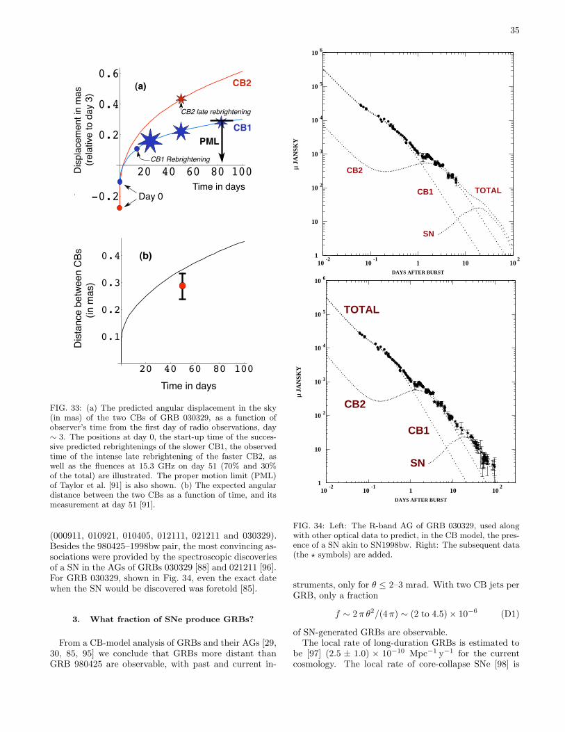
35

PML

CB2

CB1

20 40 60 80 100

-0.2

0.2

0.4

0.6

Time in daysDay 0

Displacement in mas

(relative to day 3)

CB1 Rebrightening

(a)

CB2 late rebrightening

20 40 60 80 100

0.1

0.2

0.3

0.4

Time in days

Distance between CBs

(in mas)

(b)

FIG. 33: (a) The predicted angular displacement in the sky(in mas) of the two CBs of GRB 030329, as a function ofobserver’s time from the first day of radio observations, day∼ 3. The positions at day 0, the start-up time of the succes-sive predicted rebrightenings of the slower CB1, the observedtime of the intense late rebrightening of the faster CB2, aswell as the fluences at 15.3 GHz on day 51 (70% and 30%of the total) are illustrated. The proper motion limit (PML)of Taylor et al. [91] is also shown. (b) The expected angulardistance between the two CBs as a function of time, and itsmeasurement at day 51 [91].

(000911, 010921, 010405, 012111, 021211 and 030329).Besides the 980425–1998bw pair, the most convincing as-sociations were provided by the spectroscopic discoveriesof a SN in the AGs of GRBs 030329 [88] and 021211 [96].For GRB 030329, shown in Fig. 34, even the exact datewhen the SN would be discovered was foretold [85].

3. What fraction of SNe produce GRBs?

From a CB-model analysis of GRBs and their AGs [29,30, 85, 95] we conclude that GRBs more distant thanGRB 980425 are observable, with past and current in-

DAYS AFTER BURST

µ JA

NSK

Y

1

10

10 2

10 3

10 4

10 5

10 6

10-2

10-1

1 10 102

TOTAL

SN

CB2

CB1

DAYS AFTER BURST

µ JA

NSK

Y

1

10

10 2

10 3

10 4

10 5

10 6

10-2

10-1

1 10 102

CB2

CB1

SN

TOTAL

FIG. 34: Left: The R-band AG of GRB 030329, used alongwith other optical data to predict, in the CB model, the pres-ence of a SN akin to SN1998bw. Right: The subsequent data(the ⋆ symbols) are added.

struments, only for θ ≤ 2–3 mrad. With two CB jets perGRB, only a fraction

f ∼ 2 π θ2/(4 π) ∼ (2 to 4.5) × 10−6 (D1)

of SN-generated GRBs are observable.The local rate of long-duration GRBs is estimated to

be [97] (2.5 ± 1.0) × 10−10 Mpc−1 y−1 for the currentcosmology. The local rate of core-collapse SNe [98] is

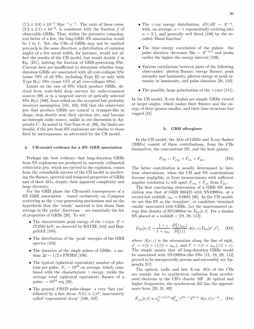
36

(7.5 ± 3.8) × 10−5 Mpc−1 y−1. The ratio of these rates,(3.3 ± 2.1) × 10−6, is consistent with the fraction f ofobservable GRBs. Thus, within the pervasive cosmolog-ical factor of a few, the long-GRB–SN association wouldbe 1 to 1. Yet, the CBs of GRBs may not be emittedprecisely in the same direction; a distribution of emissionangles of a few mrad width, for instance, would not af-fect the results of the CB model, but would double f inEq. (D1), halving the fraction of GRB-generating SNe.Current data are insufficient to determine whether long-duration GRBs are associated with all core-collapse SNe(some 70% of all SNe, including Type II) or only withType Ib/c SNe (some 15% of all core-collapse SNe).

Limits on the rate of SNe which produce GRBs, de-rived from wide-field deep surveys for radio-transientsources [99] or in a targeted survey of optically selectedSNe Ib/c [100], have relied on the accepted but probablyincorrect assumption [101, 102, 103] that the relativisticjets that produce GRBs are conical or trumpet-like inshape, stop shortly near their ejection site, and becomean isotropic radio source, unlike in our discussion in Ap-pendix C. As noted by Gal-Yam et al. [99], the limits areinvalid, if the jets from SN explosions are similar to thosefired by microquasars, as advocated by the CB model.

4. CB-model evidence for a SN–GRB association

Perhaps the best evidence that long-duration GRBsfrom SN explosions are produced by narrowly collimatedrelativistic jets, which are ejected in the explosion, comesfrom the remarkable success of the CB model in predict-ing the fluence, spectral and temporal properties of GRBsand of their AGs, despite their apparent complexity andlarge diversity.

For the GRB phase the CB-model consequences of aSN–GRB association —based exclusively on Comptonscattering as the γ-ray-generating mechanism and on thehypothesis that the ‘windy’ material is less dense thanaverage in the ‘polar’ directions— are essentially the listof properties of GRBs [20]. To wit:

• The characteristic peak energy of the γ-rays: E =O(250) keV, as observed by BATSE [104] and Bep-poSAX [105].

• The distribution of the ‘peak’ energies of the GRBspectra [104].

• The duration of the single pulses of GRBs: a me-dian ∆t ∼ 1/2 s FWHM [106].

• The typical (spherical equivalent) number of pho-tons per pulse, Nγ ∼ 1059 on average, which, com-bined with the characteristic γ energy, yields theaverage total (spherical equivalent) fluence of apulse: ∼ 1053 erg [20].

• The general FRED pulse-shape: a very ‘fast rise’followed by a fast decay N(t) ∝ 1/t2, inaccuratelycalled ‘exponential decay’ [106, 107].

• The γ-ray energy distribution, dN/dE ∼ E−α,with, on average, α ∼ 1 exponentially evolving intoα ∼ 2.1, and generally well fitted [108] by the so-called ‘Band function”.

• The time–energy correlation of the pulses: thepulse duration decreases like ∼ E−0.4 and peaksearlier the higher the energy interval [109].

• Various correlations between pairs of the followingobservables: photon fluence, energy fluence, peakintensity and luminosity, photon energy at peak in-tensity or luminosity, and pulse duration [20, 110].

• The possibly large polarization of the γ-rays [111].

In the CB model, X-ray flashes are simply GRBs viewedat larger angles, which makes their fluence and the en-ergy of their quanta smaller, and their time structure lessrugged [31].

5. GRB afterglows

In the CB model, the AGs of GRBs and X-ray flashes(XRFs) consist of three contributions, from the CBsthemselves, the concomitant SN, and the host galaxy:

FAG = FCBs

+ FSN

+ FHG

. (D2)

The latter contribution is usually determined by late-time observations, when the CB and SN contributionsbecome negligible, or from measurements with sufficientangular resolution to tell apart F

CBs+ F

SNfrom F

HG.

The first convincing observation of a GRB–SN asso-ciation was that of GRB 980425 with SN1998bw, at arecord-low redshift zbw = 0.0085 [86]. In the CB model,we use this SN as the ‘template’, or candidate ‘standardcandle’ associated with GRBs. Let the unattenuated en-ergy flux density of SN1998bw be Fbw[ν, t]. For a similarSN placed at a redshift z [19, 29, 112]:

FSN[ν, t] =1 + z

1 + zbw

D2L(zbw)

D2L(z)

A(ν, z)Fbw[ν′, t′] , (D3)

where A(ν, z) is the attenuation along the line of sight,ν′ = ν (1 + z)/(1 + zbw), and t′ = t (1 + zbw)/(1 + z).The simple ansatz that all long-duration GRBs wouldbe associated with SN1998bw-like SNe [15, 19, 29, 112]proved to be unexpectedly precise and successful; see Ap-pendix D2.

The optical, radio and late X-ray AGs of the CBsare mainly due to synchrotron radiation from acceler-ated electrons in the CB’s chaotic MF. At optical andhigher frequencies, the synchrotron AG has the approxi-mate form [29, 31, 89]:

FCB

[ν, t] ∝ n(1+α)/2p R2

CBγ3α−1 δ3+α A(ν, t) ν−α , (D4)

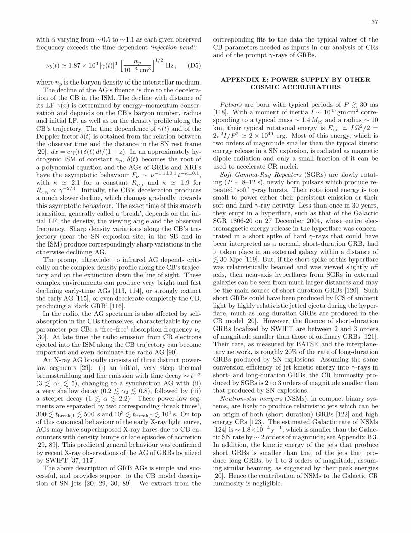
37

with α varying from ∼0.5 to ∼1.1 as each given observedfrequency exceeds the time-dependent ‘injection bend’:

νb(t) ≃ 1.87 × 103 [γ(t)]3[ np

10−3 cm3

]1/2

Hz , (D5)

where np is the baryon density of the interstellar medium.The decline of the AG’s fluence is due to the decelera-

tion of the CB in the ISM. The decline with distance ofits LF γ(x) is determined by energy–momentum conser-vation and depends on the CB’s baryon number, radiusand initial LF, as well as on the density profile along theCB’s trajectory. The time dependence of γ(t) and of theDoppler factor δ(t) is obtained from the relation betweenthe observer time and the distance in the SN rest frame[20], dx = c γ(t) δ(t) dt/(1 + z). In an approximately hy-drogenic ISM of constant np, δ(t) becomes the root ofa polynomial equation and the AGs of GRBs and XRFshave the asymptotic behaviour Fν ∼ ν−1.1±0.1 t−κ±0.1,with κ ≃ 2.1 for a constant R

CBand κ ≃ 1.9 for

RCB

∝ γ−2/3. Initially, the CB’s deceleration producesa much slower decline, which changes gradually towardsthis asymptotic behaviour. The exact time of this smoothtransition, generally called a ‘break’, depends on the ini-tial LF, the density, the viewing angle and the observedfrequency. Sharp density variations along the CB’s tra-jectory (near the SN explosion site, in the SB and inthe ISM) produce correspondingly sharp variations in theotherwise declining AG.

The prompt ultraviolet to infrared AG depends criti-cally on the complex density profile along the CB’s trajec-tory and on the extinction down the line of sight. Thesecomplex environments can produce very bright and fastdeclining early-time AGs [113, 114], or strongly extinctthe early AG [115], or even decelerate completely the CB,producing a ‘dark GRB’ [116].

In the radio, the AG spectrum is also affected by self-absorption in the CBs themselves, characterizable by oneparameter per CB: a ‘free–free’ absorption frequency νa

[30]. At late time the radio emission from CR electronsejected into the ISM along the CB trajectory can becomeimportant and even dominate the radio AG [90].

An X-ray AG broadly consists of three distinct power-law segments [29]: (i) an initial, very steep thermalbremsstrahlung and line emission with time decay ∼ t−α

(3 . α1 . 5), changing to a synchrotron AG with (ii)a very shallow decay (0.2 . α2 . 0.8), followed by (iii)a steeper decay (1 . α . 2.2). These power-law seg-ments are separated by two corresponding ‘break times’,300 . tbreak,1 . 500 s and 103 . tbreak,2 . 104 s. On topof this canonical behaviour of the early X-ray light curve,AGs may have superimposed X-ray flares due to CB en-counters with density bumps or late episodes of accretion[29, 89]. This predicted general behaviour was confirmedby recent X-ray observations of the AG of GRBs localizedby SWIFT [37, 117].

The above description of GRB AGs is simple and suc-cessful, and provides support to the CB model descrip-tion of SN jets [20, 29, 30, 89]. We extract from the

corresponding fits to the data the typical values of theCB parameters needed as inputs in our analysis of CRsand of the prompt γ-rays of GRBs.

APPENDIX E: POWER SUPPLY BY OTHERCOSMIC ACCELERATORS

Pulsars are born with typical periods of P & 30 ms[118]. With a moment of inertia I ∼ 1045 gmcm2 corre-sponding to a typical mass ∼ 1.4 M⊙ and a radius ∼ 10km, their typical rotational energy is Erot ≃ I Ω2/2 =2π2I/P 2 ≃ 2 × 1049 erg. Most of this energy, which istwo orders of magnitude smaller than the typical kineticenergy release in a SN explosion, is radiated as magneticdipole radiation and only a small fraction of it can beused to accelerate CR nuclei.

Soft Gamma-Ray Repeaters (SGRs) are slowly rotat-ing (P ∼ 8–12 s), newly born pulsars which produce re-peated ‘soft’ γ-ray bursts. Their rotational energy is toosmall to power either their persistent emission or theirsoft and hard γ-ray activity. Less than once in 30 years,they erupt in a hyperflare, such as that of the GalacticSGR 1806-20 on 27 December 2004, whose entire elec-tromagnetic energy release in the hyperflare was concen-trated in a short spike of hard γ-rays that could havebeen interpreted as a normal, short-duration GRB, hadit taken place in an external galaxy within a distance of. 30 Mpc [119]. But, if the short spike of this hyperflarewas relativistically beamed and was viewed slightly offaxis, then near-axis hyperflares from SGRs in externalgalaxies can be seen from much larger distances and maybe the main source of short-duration GRBs [120]. Suchshort GRBs could have been produced by ICS of ambientlight by highly relativistic jetted ejecta during the hyper-flare, much as long-duration GRBs are produced in theCB model [20]. However, the fluence of short-durationGRBs localized by SWIFT are between 2 and 3 ordersof magnitude smaller than those of ordinary GRBs [121].Their rate, as measured by BATSE and the interplane-tary network, is roughly 20% of the rate of long-durationGRBs produced by SN explosions. Assuming the sameconversion efficiency of jet kinetic energy into γ-rays inshort- and long-duration GRBs, the CR luminosity pro-duced by SGRs is 2 to 3 orders of magnitude smaller thanthat produced by SN explosions.

Neutron-star mergers (NSMs), in compact binary sys-tems, are likely to produce relativistic jets which can bean origin of both (short-duration) GRBs [122] and highenergy CRs [123]. The estimated Galactic rate of NSMs[124] is ∼ 1.8×10−4 y−1, which is smaller than the Galac-tic SN rate by ∼ 2 orders of magnitude; see Appendix B 3.In addition, the kinetic energy of the jets that produceshort GRBs is smaller than that of the jets that pro-duce long GRBs, by 1 to 3 orders of magnitude, assum-ing similar beaming, as suggested by their peak energies[20]. Hence the contribution of NSMs to the Galactic CRluminosity is negligible.

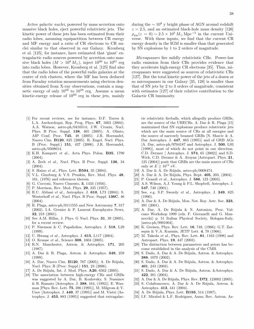
38

Active galactic nuclei, powered by mass accretion ontomassive black holes, eject powerful relativistic jets. Thekinetic power of these jets has been estimated from theirradio lobes, assuming equipartition between CR energyand MF energy and a ratio of CR electrons to CR nu-clei similar to that observed in our Galaxy. Kronberget al. [125], for instance, have estimated that ‘giant’ ex-tragalactic radio sources powered by accretion onto mas-sive black holes (M > 108 M⊙), inject 1060 to 1061 erginto radio lobes. However, Kronberg et al. [125] find alsothat the radio lobes of the powerful radio galaxies at thecentre of rich clusters, where the MF has been deducedfrom Faraday rotation measurements using electron den-sities obtained from X-ray observations, contain a mag-netic energy of only 1058 to 1059 erg. Assume a meankinetic-energy release of 1060 erg in these jets, mainly

during the ∼ 108 y bright phase of AGN around redshiftz = 2.5, and an estimated black-hole mass density [126]ρ

BH(z = 0) ∼ 2.5 × 105 M⊙ Mpc−3 in the current Uni-

verse. With these inputs, we find that the current CRenergy density in the IGM is smaller than that generatedby SN explosions by 1 to 2 orders of magnitude.

Microquasars fire mildly relativistic CBs. Power-lawradio emission from their CBs provides evidence thatthey accelerate high-energy CR electrons [35]. Thus, mi-croquasars were suggested as sources of relativistic CRs[127]. But the total kinetic power of the jets of a dozen orso microquasars in our Galaxy [35, 128] is smaller thanthat of SN jets by 2 to 3 orders of magnitude, consistentwith estimates [127] of their relative contribution to theGalactic CR luminosity.

[1] For recent reviews, see for instance, D.F. Torres &L.A. Anchordoqui, Rep. Prog. Phys. 67, 1663 (2004);A.A. Watson, astro-ph/0410514; J.W. Cronin, Nucl.Phys. B Proc. Suppl. 138, 465 (2005); A. Olinto,AIP Conf. Proc. 745, 48 (2005); J.R. Hoerandel,Nuovo Cim. B120, 825 (2005). R. Engel, Nucl. Phys.B (Proc. Suppl.) 151, 437 (2006). J.R. Hoerandel,astro-ph/0508014.

[2] K.H. Kampert et al., Acta Phys. Polon. B35, 1799(2004).

[3] A. Zech et al., Nucl. Phys. B Proc. Suppl. 136, 34(2004).

[4] S. Haino et al., Phys. Lett. B594, 35 (2004).[5] V.L. Ginzburg & V.S. Ptuskin, Rev. Mod. Phys. 48,

161, (1976) and references therein.[6] G. Cocconi, Nuovo Cimento, 3, 1433 (1956).[7] P. Morrison, Rev. Mod. Phys. 29, 235 (1957).[8] R.U. Abbasi et al., Astrophys. J. 610, L73 (2004); S.

Westerhoff et al., Nucl. Phys. B Proc. Suppl. 136C, 46(2004).

[9] R. Plaga, astro-ph/0111555 and New Astronomy 7, 317(2002). I.A. Grenier & P. Laurent Europhysics News,32, 218 (2001).

[10] See A.M. Hillas, J. Phys. G Nucl. Phys. 31, 39 (2005),for a recent review.

[11] P. Nisenson & C. Papaliolios, Astrophys. J. 518, L29(1999).

[12] U. Hwang et al., Astrophys. J. 615, L117 (2004).[13] O. Krause et al., Science 308, 1604 (2005).[14] R.N. Manchester, Astron. & Astrophys. 171, 205

(1987).[15] A. Dar & R. Plaga, Astron. & Astrophys. 349, 259

(1999).[16] A. Dar, Nuovo Cim. B120, 767 (2005); A. De Rujula,

Nucl. Phys. B (Proc. Suppl.) 151, 23 (2006).[17] A. De Rujula, Int. J. Mod. Phys. A20, 6562 (2005).[18] The association between high-energy CRs and GRBs

was suggested by A. Dar, B. Kozlovsky, S. Nussinov& R. Ramaty [Astrophys. J. 388, 164, (1992)]. E. Wax-man [Phys. Rev. Lett. 75, 386 (1995)], M. Milgrom & V.Usov [Astrophys. J. 449, 37 (1995)] and M. Vietri [As-trophys. J. 453, 883 (1995)] suggested that extragalac-

tic relativistic fireballs, which allegedly produce GRBs,are the source of the UHECRs. A. Dar & R. Plaga [15]maintained that SN explosions produce relativistic jetswhich are the main source of CRs at all energies andthe source of narrowly beamed GRBs [N. Shaviv & A.Dar Astrophys. J. 447, 863 (1995)] and of GRB AGs[A. Dar, astro-ph/9704187 and Astrophys. J. 500, L93(1998)], most of which do not point in our direction.C.D. Dermer [ Astrophys. J. 574, 65 (2002)] and S.D.Wick, C.D. Dermer & A. Atoyan [Astropart. Phys. 21,125 (2004)] posit that GRBs are the main source of CRsonly at E ≥ 1014 eV.

[19] A. Dar & A. De Rujula, astro-ph/0008474.[20] A. Dar & A. De Rujula, Phys. Rept. 405, 203, (2004).[21] P. Grandi et al., Astrophys. J. 586, 123 (2003).[22] A.S. Wilson, A.J. Young & P.L. Shopbell, Astrophys. J.

547, 740 (2001).[23] See, e.g. S.P. Swordy et al., Astrophys. J. 349, 625

(1990).[24] A. Dar & A. De Rujula, Mon. Not. Roy. Astr. Soc. 323,

391 (2001).[25] A. Dar, A. De Rujula & N. Antoniou, Proc. Vul-

cano Workshop 1999 (eds. F. Giovanelli and G. Man-nocchi) p. 51 Italian Physical Society, Bologna-Italy,[astro-ph/9901004].

[26] K. Greisen, Phys. Rev. Lett. 16, 748, (1966); G.T. Zat-sepin & V.A. Kuzmin, JETP Lett. 4, 78 (1966).

[27] M. Takeda et al., Phys. Rev. Lett. 81, 1163 (1998) andAstropart. Phys. 19, 447 (2003).

[28] The distinction between parameters and priors has be-come established in the analysis of the CMB.

[29] S. Dado, A. Dar & A. De Rujula, Astron. & Astrophys.388, 1079 (2002).

[30] S. Dado, A. Dar & A. De Rujula, Astron. & Astrophys.401, 243 (2003).

[31] S. Dado, A. Dar & A. De Rujula, Astron. &Astrophys.422, 381 (2004).

[32] A. Dar & A. De Rujula, Phys. Rev. D72, 123002 (2005).[33] S. Colafrancesco, A. Dar & A. De Rujula, Astron. &

Astrophys. 413, 441 (2004).[34] A. De Rujula, Phys. Lett. B193, 514 (1987).[35] I.F. Mirabel & L.F. Rodriguez, Annu. Rev. Astron. As-

39

trophys. 37, 409 (1999).[36] V. Dhawan, I. F. Mirabel & L.F. Rodriguez, Astrophys.

J. 543, 373 (2000).[37] S. Dado, A. Dar & A. De Rujula, Astrophys. J. (in

press) [astro-ph/0512196].[38] There is no confirmed deviation from isotropy above the

ankle, e.g. [8], or above the knee, e.g. T. Antoni et al.

[Astrophys. J. 604, 687 (2004)] and any anisotropies atlower energies are very small. See e.g. A.G.K.Smith &R.W. Clay [Aust. J. Phys. 50, 827 (1997)] and R.W.Clay, M.A. McDonough & A.G.K. Smith [Publ. Astron.Soc. Aust. 15, 208 (1998)].

[39] J.K. Frederiksen et al., Astrophys. J. 608, L13 (2004).[40] F. Quilligan et al., Astron. & Astrophys. 385, 377

(2002).[41] A.W. Strong & A.V. Moskalenko, Proc. 27th Int.

Cosmic-Ray Conf. (Hamburg) p. 1964 (2001); A. W.Strong, I. V. Moskalenko, & O. Reimer, Astrophys. J.613, 962 (2004).

[42] M.S. Longair, High Energy Astrophysics (CambridgeUniversity Press, 1992), and references therein.

[43] V.A. Dogiel, V. Schonfelder & A.W. Strong, Astrophys.J. 572, L157 (2002).

[44] D.E. Groom et al., Review of Particle Physics, Eur.Phys. J. C15, 1-878 (2000), p. 166.

[45] A turbulent Kolmogoroff spectrum of magnetic inhomo-geneities yields βconf = 0.33 while a Kraichnan spectrumyields βconf = 0.5; see V.S. Ptuskin et al. [Adv. Sp. Res.35, 162 (2005)] and references therein.

[46] J.J. Connell, Astrophys. J. 501, 59 (1998); J.J. Connell,Sp. Sci. Rev. 99, 41 (2001).

[47] W.I. Axford, Proc. Int. Cosmic Ray Conf. (Paris), 12,155 (1981).

[48] J.C. Higdon & R.E. Lingenfelter, Astrophys. J. 628, 738(2005) and references therein.

[49] M. Miceli et al., astro-ph/0602518.[50] B. Wiebel-Sooth, P. Bierman & H. Meyer, Astron. &

Astrophys. 330, 37 (1998).[51] N. Grevesse & A.J. Sauval, 1998, Sp. Sci. Rev. 85, 161

(1998); N. Grevesse & A.J. Sauval, Adv. Sp. Res. 30, 3,(2002).

[52] M. Aguilar et al., Phys. Rep. 366, 331 (2002).[53] J.R. Hoerandel, Proc.“Workshop on Physics of the End

of the Galactic Cosmic Ray Spectrum”, Aspen, USA,2005 [astro-ph/0508014].

[54] R. Wijmans, Astropart. Phys. 19, 379 (2003).[55] M. Zha, J. Knapp & S. Ostapchenko, Proc. 28th Int.

Cos. Ray Conf. (Tsukuba), ICRC 2, 515 (2003).[56] R. Beck, Space Science Reviews, 99, 243 (2001).[57] A. W. Strong, I. V. Moskalenko & O. Reimer, Astro-

phys. J. 613, 962 (2004).[58] A. Dar & A. De Rujula, Astrophys. J. 547, L33 (2001).[59] P. Sreekumar et al., Astrophys. J. 494, 523 (1998), and

references therein.[60] B. Wiebel-Soth et al., Astron. & Astrophys. 330, 389

(1998).[61] J.R. Hoerandel, Astropart. Phys. 19, 193 (2003).[62] M. Sapinski et al., Proc. 29th International Cosmic Ray

Conference, Pune, India, 101106 (2005).[63] V.L. Ginzburg & S.I. Syrovatskii, Origin of cosmic rays

The Macmillan Pub. Co. New York 1964.[64] D.J. Thompson & C.E. Fichtel, Astron. & Astrophys.

109, 352 (1982).[65] J.C. Mather et al., Astrophys. J. 432, L15, (1993). D.J.

Fixsen et al., Astrophys. J. 473, 576 (1996).[66] J.E. Felten & P. Morrison, Astrophys. J. 146, 686

(1996).[67] W. Baade, & F. Zwicky, Proc. Nat. Acad. Sci. USA,

20/5, 259 (1934).[68] See, e.g., N.J. Shaviv, New Astron. 8, 39 (2002) and

Phys. Rev. Lett. 89, 051102 (2002).[69] S. van den Bergh & G. A. Tammann, Annu. Rev. As-

tron. Astrophys. 29, 363 (1991).[70] C.J. Pritchet & S. van den Bergh, Astron. J. 118, 883

(1999).[71] R.S. Ellis, Annu. Rev. Astron. Astrophys. 35, 389

(1997).[72] P.G. Perez-Gonzalez et al., Astrophys. J. 630 82 (2005).

D. Schiminovich et al., Astrophys. J. 619, L47 (2005)and references therein.

[73] R. Silberberg & C.H. Tsao, Phys. Rep. 191, 351 (1990).[74] M.G. Hauser & E. Dwek, Annu. Rev. Astron. Astro-

phys. 39, 249 (2001) and references therein.[75] V.S. Berezinsky, A.Z. Gazizov & S.I. Grigorieva, Phys.

Lett. B612, 147 (2005); D. De Marco & T. Stanev,Phys. Rev. D72, 081301 (2005) E. Khan et al. As-tropart. Phys. 23, 191 (2005) and references therein.

[76] W. Tkaczyk, J. Wdowczyk & A.W. Wolfendale, J. Phys.A. 8 1518 (1975); J.L. Puget, F.W. Stecker & J.H.Bredekamp, Astrophys. J. 205, 638 (205); S. Karakula& W. Tkaczyk, Astropart. Phys. 1, 229 (1993); F.W.Stecker & M.H. Salomon, Astrophys. J. 512, 521 (1999);L.N. Epele & E. Roulet, JHEP 9810, 9 (1998); J. Can-dia, L.N. Epele & E. Roulet, Astropart. Phys. 17, 23(2002); E. Khan et al., Astropar. Phys. 23, 191 (2005).

[77] S.S. Eikenberry et al., Astrophys. J. 561, 1027 (2001);D.R. Gies et al., Astrophys. J. 566, 1069 (2001).

[78] M.G. Watson et al., Mon. Not. Roy. Astron. Soc. 222,261 (1986); T. Kotani et al., Publ. Astron. Soc. Jap.48, 619 (1996); H.L. Marshall, C.R. Canizares & N.S.Schulz, Astrophys. J. 564, 941 (2002); S. Migliari, R.Fender & M. Mendez, Science 297, 1673 (2002); M.Namiki et al., Publ. Astron. Soc. Jap. 55, 1 (2003).

[79] L.F. Rodriguez & I.F Mirabel, New Astron. Rev. 42,649 (1998).

[80] T. Kotani et al., Astrophys. J. 543, L133 (2000).[81] S. Corbel et al., New Astron. Rev. 47, 477 (2003).[82] B. Margon, Annu. Rev. Astron. Astrophys. 22, 507

(1984).[83] H.E. Bond et al., Nature 422, 425 (2003).[84] R. Vanderspek et al., 2003, http://space.mit.edu/

HETE/Bursts/GRB030329.[85] S. Dado, A. Dar & A. De Rujula, Astrophys. J. 594,

L89 (2003).[86] T. J. Galama et al., Nature 395, 670 (1998).[87] J. Greiner et al., GCN Circ. 2020 (2003).[88] K.Z. Stanek et al., Astrophys. J. 591, L17 (2003); J.

Hjorth et al., Nature 423, 847 (2003).[89] S. Dado, A. Dar & A. De Rujula, astro-ph/0402374.[90] S. Dado, A. Dar & A. De Rujula, astro-ph/0406325.[91] G.B. Taylor et al., Astrophys. J. 622, 986 (2005).[92] A. Dar, astro-ph/0405386.[93] P. Soffitta et al., IAU Circ. 6884 (1998).[94] K. Iwamoto et al., Nature 395, 672 (1998).[95] S. Dado, A. Dar & A. De Rujula, Astrophys. J. 572,

L143 (2002); S. Dado, A. Dar & A. De Rujula, Astron.& Astrophys. 393, L25 (2002); S. Dado, A. Dar & A.De Rujula, Astrophys. J. 593, 961 (2003).

40

[96] M. Della Valle et al., Astron. & Astrophys. 406, L33(2003).

[97] M. Schmidt, Astrophys. J. 559, L79 (2001).[98] E. Capellaro, in Supernovae and GRBs, ed. K. W.

Weiler (Springer, Berlin, 2003), p. 37.[99] A. Levinson et al., Astrophys. J. 576, 923 (2002); A.

Gal-Yam et al., Astrophys. J. 639, 331 (2006). The com-ment in [103] also applies here and to [100].

[100] A.M. Soderberg, D.A. Frail & M.H. Wieringa, Astro-phys. J. 607, L1 (2004).

[101] J. E. Rhoads, Astrophys. J. 525, 737 (1999).[102] R. Sari, T. Piran & J.P. Halpern, Astrophys. J. 519,

L17 (1999).[103] For a small opening angle, θj ≪ 1, a conical GRB lights

up a fraction fb ≃ θ2j /16 of the full celestial sphere, or a

fraction fb ≃ θ2j /4, if θj is defined to be half the open-

ing angle of the cone. The relation fb ≃ θ2j /2 has been

widely used by D.A. Frail et al. [Astrophys. J. 562, L55(2001)] and by many other authors in their estimates ofthe true γ-ray energy of GRBs from the ‘Frail relation’,Eγ = fb Eiso, where Eiso is the equivalent isotropic en-ergy of the GRB deduced from its redshift and its mea-sured fluence. The fraction of the full celestial spherelighted up by two opposite conical GRBs, each of half

opening angle θj ≪ 1, is fb ≃ θ2j /2 and it should be used

for estimating Eiso under the fireball-model assumptionthat two identical conical GRBs are emitted simultane-ously in opposite directions.

[104] R.D. Preece et al., Astrophys. J. Suppl. 126, 19 (2000).[105] L. Amati et al., Astron. & Astrophys. 390, 81 (2002).[106] S. McBreen et al., AIP Conf. Proc. 662, 280 (2003).[107] R.J. Nemiroff et al., Astrophys. J. 414, 36 (1993); R.J.

Nemiroff, AIP Conf. Proc. 307, 7300 (1994); B. Link &R.I. Epstein, Astrophys. J. 466, 764 (1996).

[108] D. Band et al., Astrophys. J. 413, 281 (1993).[109] E.E. Fenimore et al., Astrophys. J. 448, L101 (1995);

J.P. Norris et al., Astrophys. J. 459, 393 (1996); B. Wu& E.E. Fenimore, Astrophys. J. 535, L29 (2000); E.Ramirez-Ruiz & E.E. Fenimore, Astrophys. J. 539, 12(2000).

[110] S. Dado & A. Dar, Astrophys. J. 627, L109 (2005).[111] W. Coburn & S.E. Boggs, Nature 423, 415 (2003); D.

R. Willis et al., Astron. & Astrophys. 439, 245 (2005).[112] A. Dar, Astron. & Astrophys. Suppl. 138, 505 (1999).[113] C. Akerlof et al., Nature 398, 400 (1999).[114] S. Dado, A. Dar & A. De Rujula, Astrophys. J. 585,

L15 (2003).[115] E. S. Rykoff et al., Astrophys. J. 601, 1013 (2004) and

631, L121 (2005).[116] D. Malesani et al., Nuovo Cim. 28C, 515 (2005).[117] G. Chincarini et al., astro-ph/0506453. J.A. Nousek et

al., Astrophys. J. 642, 389 (2006).[118] D.R. Lorimer, astro-ph/0301327.[119] S. Dado, A. Dar & A. De Rujula, GCN Circ. 2942

(2004); K. Hurley et al., Nature 434, 1098 (2005).[120] S. Dado, A. Dar & A. De Rujula, in preparation.[121] E. Berger et al., Nature 438, 988 (2005).[122] J. Goodman, A. Dar & S. Nussinov, Astrophys. J. 314,

L7 (1987).[123] A. Dar, A. Laor & N.J. Shaviv, Phys. Rev. Lett. 80,

5813 (1998).[124] V. Kalogera et al., Astrophys. J. 601, L179 (2004); E.S.

Phinney, Astrophys. J. 380, L17 (1991).[125] P.P. Kronberg et al., Astrophys. J. 604, 77 (2004).[126] Q. Yu and S. Tremaine, Mon. Not. Roy. Ast. Soc. 335,

965 (2002).[127] S. Heinz & R. Sunyaev, Astron. & Astrophys. 390, 751

(2002).[128] P. Kaaret et al., Nucl. Phys. B (Proc. Suppl.) 132, 354

(2004).