arxiv:hep-ph/0405244v2 8 jun 2004
TRANSCRIPT
arX
iv:h
ep-p
h/04
0524
4v2
8 J
un 2
004
hep-ph/0405244
MADPH–04–1376
UPR–1043T
UCD–2004–20
The Higgs Sector in a U(1)′ Extension of the MSSM
Tao Han1,4, Paul Langacker2, Bob McElrath3
1Department of Physics, University of Wisconsin, Madison, WI 53706
2Department of Physics and Astronomy, University of Pennsylvania, Philadelphia, PA 19104
3Department of Physics, University of California, Davis, CA 95616
4Institute of Theoretical Physics, Academia Sinica, Beijing 100080, China
Abstract
We consider the Higgs sector in an extension of the MSSM with extra SM singlets, involving
an extra U(1)′ gauge symmetry, in which the domain-wall problem is avoided and the effective
µ parameter is decoupled from the new gauge boson Z ′ mass. The model involves a rich Higgs
structure very different from that of the MSSM. In particular, there are large mixings between
Higgs doublets and the SM singlets, significantly affecting the Higgs spectrum, production
cross sections, decay modes, existing exclusion limits, and allowed parameter range. Scalars
considerably lighter than the LEP2 bound (114 GeV) are allowed, and the range tan β ∼ 1
is both allowed and theoretically favored. Phenomenologically, we concentrate our study on
the lighter (least model-dependent, yet characteristic) Higgs particles with significant SU(2)-
doublet components to their wave functions, for the case of no explicit CP violation in the
Higgs sector. We consider their spectra, including the dominant radiative corrections to their
masses from the top/stop loop. We computed their production cross sections and reexamine
the existing exclusion limits at LEP2. We outline the searching strategy for some representative
scenarios at a future linear collider. We emphasize that gaugino, Higgsino, and singlino decay
modes are indicative of extended models and have been given little attention. We present a
comprehensive list of model scenarios in the Appendices.
1
I. INTRODUCTION
Supersymmetry (SUSY) is probably the leading candidate for physics beyond the Standard
Model (SM). By adding partners of opposite statistics to the SM particles, it is able to cancel the
quadratically divergent contribution to the Higgs mass. The leading phenomenological model
for SUSY is the Minimal Supersymmetric Standard Model (MSSM), which incorporates two
Higgs doublets rather than one as in the Standard Model. Two are required to give masses to
both up-type and down-type fermions, and to prevent anomalies coming from triangle diagrams
involving the Higgs superpartner, the Higgsino.
The MSSM suffers from the “µ problem” [1]. The superpotential for the MSSM contains the
supersymmetric mass term µH2H1. The minimization condition for the MSSM scalar potential
relates µ to MZ and soft SUSY breaking parameters. One expects all these quantities to be
the same order of magnitude to avoid the need for miraculous cancellations. However, µ is an
input-scale parameter and therefore should have mass O(MP l) or O(MGUT ). This has led to a
widespread belief that the MSSM must be extended at high energies to include a mechanism
which relates µ to the SUSY breaking mechanism.
One possibility is the next-to-minimal Supersymmetric Standard Model (NMSSM) [2], which
has been studied extensively [2, 3]. The NMSSM solves the µ problem by relating µ to the
vacuum expectation value of a Standard Model singlet. The model contains a single extra
gauge singlet superfield, S, and a superpotential of the form:
WNMSSM =1
6kS3 +
1
2µSS
2 + hSH2H1 +WMSSM , (1)
where WMSSM is the superpotential of the MSSM without an elementary µ term 1. If the
scalar component of S has a vacuum expectation value, an effective µ term h〈S〉 is induced.
However, to have the appropriate hierarchy of mass scales, the term µS should be disallowed.
Otherwise, it should also naturally have a mass near MP l, which would make it unnatural for S
to obtain a weak-scale vacuum expectation value. Similar statements apply to the addition of
a term linear in S to WNMSSM . These can be removed by invoking a Z3 discrete symmetry in
the superpotential. However this would lead to domain walls in the early universe, a situation
which is strongly disfavored cosmologically [5]. Attempts to remedy this either reintroduce
some form of the µ problem or lead to other difficulties [6].
In string motivated models, bare mass terms in the superpotential are generically of order
the string scale Mstring. This means that any field impacting low energy physics must not
1 Some treatments include an elementary µ term in addition to the effective one in order to avoid the cosmo-
logical domain wall problem, but this reintroduces the µ problem [4].
2

have a mass term like µ or µS. Additionally, in many constructions (e.g., heterotic and inter-
secting brane) superpotential terms are typically off-diagonal in the fields, which disallows the
NMSSM kS3 term. Thus, we are led to consider larger models that may be derived from string
constructions.
All of these difficulties can be solved in extended models involving an additional (non-
anomalous) U(1)′ gauge symmetry, which is very well-motivated as an extension to the MSSM.
U(1) gauge groups arise naturally out of many Grand Unified Theories (GUT’s) and string
constructions [7], as do the SM singlets needed to break the U(1)′. Experimental limits on the
Z ′ mass and mixings are model-dependent, but typically one requires [8, 9] MZ′ > 500 − 800
GeV and a Z − Z ′ mixing smaller than a few ×10−3.
U(1)′ models are similar to the NMSSM in that they involve a SM singlet field S which
yields an effective µ parameter h〈S〉, where the superpotential includes the term hSH2H1,
solving the µ problem [10, 11]. S will in general be charged under the U(1)′ gauge symmetry,
so that its expectation value also gives mass to the new Z ′ gauge boson. The extended gauge
symmetry forbids an elementary µ term as well as terms like Sn in the superpotential (the
role of the S3 term in generating quartic terms in the potential is played by D-terms and
possibly off-diagonal superpotential terms involving additional SM singlets). Such models do
not need to invoke discrete symmetries (the Z3 of the NMSSM is embedded in the U(1)′) so
there are no domain wall problems. Such constructions may also solve other problems, such as
naturally forbidding R-parity violating terms which could lead to rapid proton decay [12]. Other
implications include the presence of exotic chiral supermultiplets [12]; non-standard sparticle
spectra [13]; possible flavor changing neutral current effects [14], with implications for rare B
decays [15]; new sources of CP violation [16]; new dark matter candidates [17]; and enhanced
possibilities for electroweak baryogenesis [18].
As mentioned, string constructions frequently lead to the prediction of one or more additional
U(1)′ symmetries at low energies and to the existence of exotic chiral supermultiplets, including
SM singlets which can break the extra symmetries. However, no fully realistic model has
emerged. We therefore take the bottom-up approach and add the minimal supersymmetric
matter content necessary to solve the µ problem without introducing extra undesirable global
or discrete symmetries.
In this paper we explore the extended Higgs sector in a particular U(1)′ model involving
several SM singlet fields [19]. This has the advantage of decoupling the effective µ parameter
from the Z ′ mass, and leads naturally to a sufficiently heavy Z ′. It will be seen that the Higgs
physics is very rich and quite different from that of the MSSM. We expect that the generic
features will be representative of a wider class of constructions, and that they can be tested
by the next generation of high energy experiments and thus provide further guidance toward
3

constructing the correct SUSY theory. In the event that the data from the LHC deviates
significantly from MSSM expectations, it will be especially important to consider non-minimal
models. It is useful in planning for future experimental analysis programs to have a variety of
well-motivated alternatives in mind.
In Section II we describe the model. We first outline the general structure of the model in
Sec. IIA, and discuss the electroweak symmetry breaking and the radiative corrections to the
light Higgs mass in Sec. II B. We then explore the phenomenological constraints on the model
parameters in Sec. III. In particular, we find that the MSSM upper bound on the light Higgs
mass and the lower bound (direct search from LEP2) can both be relaxed. In order to carry out
further quantitative studies, we perform a comprehensive examination of the mass spectrum for
the Higgs bosons in Sec. IV. We classify the Higgs bosons according to their similarity to the
MSSM spectrum and experimental signatures. The decay modes of the Higgs bosons and their
production cross sections at e+e− colliders are studied in Sec. V, including phenomenological
implications and search strategies. We summarize our results in Sec. VI.
II. THE MODEL
A. General structure
The model we consider, first introduced in [19], has the superpotential:
W = hSH2H1 + λS1S2S3 +WMSSM (2)
S, S1, S2, and S3 are standard model singlets, but are charged under an extra U(1)′ gauge
symmetry. The off-diagonal nature of the second term is inspired by string constructions, and
the model is such that the potential has an F and D-flat direction in the limit λ → 0, allowing
a large (TeV scale ) Z ′ mass for small λ. The use of an S field different from the Si in the first
term allows a decoupling of MZ′ from the effective µ. W leads to the F -term scalar potential:
VF = h2 (|H2|2|H1|2 + |S|2|H2|2 + |S|2|H1|2)+ λ2 (|S1|2|S2|2 + |S2|2|S3|2 + |S3|2|S1|2) (3)
The D-term potential is:
VD =G2
8
(
|H2|2 − |H1|2)2
+1
2g2Z′
(
QS|S|2 +QH1|H1|2 +QH2
|H2|2 +3∑
i=1
QSi|Si|2
)2
, (4)
where G2 = g21 + g22 = g22/ cos2 θW . g1, g2, and gZ′ are the coupling constants for U(1), SU(2)
and U(1)′, respectively, and θW is the weak angle. Qφ is the U(1)′ charge of the field φ. We
will take gZ′ ∼√
5/3g1 (motivated by gauge unification) for definiteness.
4
We do not specify a SUSY breaking mechanism but rather parameterize the breaking with
the soft terms
Vsoft = m2H1|H1|2 +m2
H2|H2|2 +m2
S|S|2 +3∑
i=1
m2Si|Si|2
− (AhhSH1H2 + AλλS1S2S3 +H.C.)
+ (m2SS1
SS1 +m2SS2
SS2 +H.C.) (5)
The last two terms are necessary to break two unwanted global U(1) symmetries, and require
QS1= QS2
= −QS . The potential V = VF + VD + Vsoft was studied in [19], where it was
shown that for appropriate parameter ranges it is free of unwanted runaway directions and has
an appropriate minimum. We denote the vacuum expectation values of Hi, S, and Si by vi, vs,
and vsi, respectively, i.e., without a factor of 1/√2. Without loss of generality we can choose
Ahh > 0, Aλλ > 0 and m2SSi
< 0 in which case the minimum occurs for the expectation values
all real and positive.
So far we have only specified the Higgs sector, which is the focus of this study. Fermions
must also be charged under the U(1)′ symmetry in order for the fermion superpotential Yukawa
terms Wfermion = uyuQH2 − dydQH1 − eyeLH1 to be gauge invariant. The U(1)′ charges for
fermions do not contribute significantly to Higgs production or decay, if sfermions and the Z ′
superpartner are heavy. We therefore ignore them this study.
Anomaly cancellation in U(1)′ models generally requires the introduction of additional chiral
supermultiplets with exotic SM quantum numbers [11, 12, 18, 20]. These can be consistent
with gauge unification, but do introduce additional model-dependence. The exotics can be
given masses by the same scalars that give rise to the heavy Z ′ mass. The exotic sector is not
the focus of this study. We therefore consider the scenario in which the Z ′ and other matter
necessary to cancel anomalies is too heavy to significantly affect the production and decays of
the lighter Higgs particles.
B. Higgs sector and electroweak symmetry breaking
The Higgs sector for this model contains 6 CP-even scalars and 4 physical CP-odd scalars,
which we label H1...H6 and A1...A4, respectively, in order of increasing mass.
We compute the six CP-even scalar masses including the dominant 1-loop contribution
coming from the top/stop loop. Using the effective potential approach [21], one writes down
the radiatively corrected effective potential including leading order (0) and 1-loop corrections (1)
Veff = V (0) + V (1) + ... (6)
5
and then requires that the effective potential be minimized to obtain the vacuum expectation
values for the fields. In practice we find it simpler to eliminate the soft (mass)2 parameters
using the minimization conditions rather than solve for vacuum expectation values.
The full scalar potential is then
Veff = VD + VF + Vsoft +3
16π2
m4t
v4(v22 + v21)
2
(
ℜH2√2v2
+ 1
)4
3
2− ln
m2t
m2t
(
ℜH2√2v2
+ 1
)2
(7)
At one loop only the H2 gauge eigenstate gets a correction. At two loops both H1 and H2 get
corrections from the top and stop. We have written v, v1 and v2 in such a way so that v1 and
v2 can be considered rescaled quantities, while v,mt, and mt (which only occur in ratios) are
fixed at their physical values (as given in Table I). To avoid computational round-off error we
treat Veff as a dimensionless quantity with all values O(1), and rescale dimensionful quantities
by v/√
(v22 + v21) after a viable minimum is found.
In the ℜ(H2, H1, S, S1, S2, S3) gauge basis, the resulting mass matrix can be parameterized
as M2tree + δM2, where
δM2 =
(
δm2H2
05×1
01×5
05×5
)
, δm2H2
=3
4π2
m4t
v22ln
m2t
m2t
(8)
in the no-stop mixing limit mt1 = mt2 [21]. Since in this model tan β ≃ 1 generically, the
contribution from the bottom loop is negligible so we do not include it. We also neglect
renormalization scale-dependence and assume the renormalization scale Q2 = m2t. The singlets
cannot couple directly to the top at tree level, so the large top loop does not contribute to
the masses of any of the new singlets except by mixing. The correction δm2H2
has the value
(90GeV)2 for the MSSM with mt = 1TeV in the large tanβ limit. In the MSSM this is then
split among the h and H mass eigenstates. All other quantities are evaluated at tree level,
using tree level relations.
We find viable electroweak symmetry breaking minima by scanning over the vacuum expec-
tation values of the six CP-even scalar fields. We require that the CP-even mass matrix be
positive definite numerically, which guarantees a local minima, while simultaneously eliminating
the soft mass squared for each field. The soft masses reported in the appendices are evaluated
including the above 1-loop correction. The CP-odd mass matrix is guaranteed to be positive
semi-definite at tree level (and thus, all VEV’s are real) by appropriate redefinitions of the fields
and choices of parameters as described in Sec. IIIA. The expressions for the first-derivative
conditions to eliminate the soft masses are given in [19]. The procedure outlined guarantees a
local minimum for each parameter point, but does not guarantee a global minimum.
The parameters m2SS1
and m2SS2
must be chosen to avoid directions in the potential that are
unbounded from below. We require
m2S +m2
Si+ 2m2
SSi> 0, (9)
6

to avoid unbounded directions with vs = vsi and the other VEV’s vanishing.
We scan over vacuum expectation values such that the three singlets S1, S2, and S3 typically
have larger VEV’s than the other three fields. We allow points in our Monte Carlo scan that
fluctuate from all VEV’s equal up to 〈S〉 approximately 1 TeV and 〈Si〉 approximately 10 TeV,
as we specify in Table I. This generically results in a spectrum with 1-5 relatively light CP-even
states, often with one of them lighter than the LEP2 mass bound, but having a relatively small
overlap with the MSSM H2 and H1. It is necessary that at least one of the singlets have an
O(TeV) vacuum expectation value, so that the mass of the Z ′ gauge boson is sufficently heavy
that it evades current experimental bounds, and any extra matter needed to cancel anomalies
is heavy enough to not significantly affect light Higgs production or decay.
A bound exists on the mass of the lightest Higgs particle in any perturbatively valid super-
symmetric theory [22, 23]. The limit on the lightest MSSM-like CP-even Higgs mass in this
model is:
M2h ≤ h2v2 + (M2
Z − h2v2) cos2 2β + 2g2Z′v2(QH2cos2 β + sin2 βQH1
)2
+3
4
m4t
π2v2ln
mt1mt2
m2t
. (10)
This is obtained by taking the limit as the equivalent of the B-term in the MSSM goes to
infinity, B = Ahhvs → ∞, in the 2 × 2 submatrix containing H2 and H1. In the MSSM this
is equivalent to taking MA → ∞, the decoupling limit. This expression is the same as in the
NMSSM, except for the gZ′ (D-term) contribution. Perturbativity to a GUT or Planck scale
places an upper limit O(0.8) on h [19], which is less stringent than the corresponding limit in
the NMSSM [24] due to the U(1)′ contributions to its renormalization group equations. Larger
values would be allowed if another scale entered before the Planck scale. We will allow h as
large as 1 in the interest of exploring the low energy effective potential. The second term of
Eq. (10) vanishes for tanβ = 1. Since tan β ≃ 1 generically in these models, the lightest Higgs
mass is determined mostly by the new F and D-term contributions proportional to h2 and g2Z′.
In this model, as with any model with many Higgs particles, a situation can arise in which
the MSSM-like couplings are shared among many states, allowing unusually heavy states or
unusually light states that evade current experimental bounds.
The four CP-odd masses can in principle be found algebraically but the results are compli-
cated and not very illuminating. Perhaps the most striking feature of the mass spectrum is
that the A1 is allowed to be very light, a feature shared with the NMSSM [2]. This is caused
by a combination of small m2SS1
or m2SS2
and a small value of vs compared to the vsi. In the
limit that vsi (i = 1 or 2) is the largest scale in the problem, the lightest A mass is
m2A1
= −m2SSi
vsvsiv2si + v2s3
+O(
1
v4si
)
. (11)
7

In the limit that s3 is large we obtain
m2A1
= −4m2SSi
vsvsiv2s + v2s1 + v2s2
+O(
1
vs3
)
. (12)
In our scans, −m2SSi
is approximately in the range (0 − 1000 GeV)2. An example where this
occurs is presented in Appendix (A-1). However, this requires a hierarchy between the off-
diagonal soft masses mSSiand the other soft masses mS and mSi
. This might be difficult to
achieve depending on the SUSY breaking mechanism. A similar analysis holds for H1, but
an algebraic expression cannot be derived since the eigenvalues of a 6 × 6 matrix cannot be
expressed algebraically. Examples of spectra with a light H1 are given in Appendices (A-2,A-3).
To make comparisons to the MSSM, we define the “MSSM fraction” ξMSSM. For a given
Higgs state Hi (Ai) in the mass basis,
ξiMSSM =2∑
j=1
(Rji)2, (13)
where R is the matrix that rotates the interaction fields to the mass basis, and the index j runs
over MSSM states. In the case of the CP-even Higgs this corresponds to adding in quadrature
the eigenvector components of a state in the H2 and H1 directions. When a state is MSSM-like,
ξMSSM = 1 and it has no mixing with singlet Higgs bosons. If the two lightest CP-even states
and the lightest CP-odd state all have ξMSSM ≃ 1, the theory is MSSM-like and the extra
scalars are decoupled. An example of such a spectrum is presented in Appendix (A-4). There
is always a massless CP-odd scalar with ξMSSM ≃ 1, and another with ξMSSM ≃ 0. These are
the Goldstone bosons corresponding to the Z and Z ′ gauge bosons, respectively.
A similar quantity is defined for the neutralinos by summing in quadrature over the eigenvec-
tor components corresponding to B, Z, H2 and H1. The “Singlino fraction” ξs and “Zino-prime
fraction” ξZ′ are defined in an analogous manner.
III. PHENOMENOLOGICAL CONSTRAINTS
Due to the introduction of the Higgs singlets, there are several more parameters than in the
MSSM Higgs sector. We follow the global symmetry breaking structure of Model I of Ref. [19].
Existing experimental measurements already constrain any new model. In our parameter space
scans, we apply the constraints in the following subsections.
A. Parameter Space
We list the model parameters in Table I. Besides the SM gauge couplings, gZ′ is chosen
as√
5/3g1 that unifies with g2 and g3 in simple GUT models. However, we do not require
8

g1 = 0.36 g2 = 0.65 gZ′ =√
5/3g1
mt = 174.3GeV v = 174GeV mt1= mt2
= 1TeV
QH2= 1/4 QH1
= 1/4 QS = −1/2
QS1= 1/2 QS2
= 1/2 QS3= −1
h = −1 ... 1 λ = −0.2 ... 0.2
Ah = 0.0 ... 50 Aλ =0.0 ... 50
|m2SS1
| = 0 ... 100 |m2SS2
| =0 ... 100 mS1S2= 0
M2 = −10 ... 10 M1 = −5 ... 5 M ′1 = −20 ... 20
v1,2 = 1 ... e vs = 1 ... e2 vs1,2,3 = 1 ... e4
TABLE I: Input values and the ranges for model parameters.
unification of the gaugino masses. We have fixed the U(1)′ charges for definiteness. The
parameters Ah, Aλ, mSS1, and mS1S2
, and M2 are of course dimensionful, as are the expectation
values vi, vs, and vsi. For our computation we choose arbitrary units to start, and use the
analytical minimization conditions for the VEV’s as given in Ref. [19], eliminating the soft
mass square parameters. We check that the VEV’s obtained from scanning are a minimum
by explicitly verifying that the matrix of second derivatives is positive definite. After finding
a viable minimum, we rescale all dimensionful parameters by v/√
v22 + v21, where v is fixed at
174 GeV, which shifts the Higgs vacuum expectation value to its measured value. The other
dimensionful parameters mt, v, mSUSY , mt1 and mt2 enter the Higgs potential at one loop as
given by Eq. (7). However, they enter in ratios so that the units cancel out. tan β = v2/v1 is
therefore an output.
In the MSSM the sign of µ is a free parameter. In this model µ = hvs, and vs is taken to
be positive at the minimum, meaning that the sign of µ is really the sign of h. We can absorb
any overall phase of Ahh by a redefinition of the fields, in exactly the same way a phase of B
can be absorbed in the MSSM, and B = Ahh taken to be positive. Any phase appearing in
the soft-masses −m2SS1
and −m2SS2
can be absorbed by a field redefinition on S1 or S2, so that
m2SSi
are negative. λAλ can be taken to be positive by redefining S3. This uses up our freedom
to redefine our fields, leaving a true phase in h and λ that cannot be rotated away. With
these field redefinitions Ahh, Aλλ, −m2SS1
, and −m2SS2
are all positive 2, and all of the VEV’s
will be real and positive at the minimum. There is not enough freedom left to rotate away a
phase appearing in a possible additional term m2S1S2
S†1S2. We have thus taken this parameter
to be zero. A phase in this parameter would provide for CP violation in the Higgs sector, and
therefore lead to mixing between scalars and pseudoscalars. Although such a term is useful for
electroweak baryogenesis [18], it is beyond the scope of the present investigation.
2 These two parameters are chosen negative to conform to the convention of Ref. [19].
9

With these conventions the gaugino masses can be either positive or negative. The scalar
potential and therefore vacuum expectation values are insensitive to the signs of h and λ at tree
level, since it always appears as Ahh and Aλλ whose phases can be rotated away, or |h|2 and
|λ|2. Only the charginos and neutralinos are sensitive to the signs of h and λ. The neutralino
and chargino mass matrices are given in Ref. [19]. We allow both positive and negative values
for h, λ, and the gaugino masses.
B. Z ′ Mass and Z − Z ′ Mixing
Limits on the Z ′ mass and Z − Z ′ mixing angle are model-dependent. However, for typical
models the Z pole data indicate that the Z − Z ′ mixing must be less than a few ×10−3 [8],
while direct searches at the Tevatron limit the mass of the Z ′ to be greater than ∼ 500 − 800
GeV [9]. Therefore, we require of the Z − Z ′ mixing angle:
αZ−Z′ =1
2arctan
(
2M2ZZ′
M2Z′ −M2
Z
)
<∼ 5× 10⁻³ (14)
where M2ZZ′ is the off-diagonal entry in the mass-squared matrix, and M2
Z , M2Z′ are the diagonal
entries. We require for the mass:
MZ′ ≥ 500GeV. (15)
The Z ′ would be produced at tree level at the Tevatron, since if we require that fermions
receive mass through the usual Higgs mechanism, they must be charged under U(1)′ to keep
the superpotential Yukawa terms gauge invariant. We do not calculate the Z ′ production cross
section to avoid the necessity of having to specify the fermion U(1)′ charges. This model does
not particularly care how heavy the Z ′ is. Since there are four singlets contributing to its mass,
it is not difficult to give some of them large vacuum expectation values, resulting in a heavy
Z ′. This occurs naturally for small λ.
A lighter Z ′ near the experimental limit is also not a problem. The singlets must have
smaller vacuum expectation values, and therefore smaller masses, but since they do not couple
directly to the Standard Model except by mixing with the MSSM Higgs bosons, they can be
light. The typical scale for exotics introduced to cancel anomalies is near the Z ′ mass.
The mixing constraint in (14) is most easily satisfied forMZ′ in the TeV range. Smaller values
of MZ′ , such as we allow, generally require a suppressed value for M2ZZ′ = gZ′
√g2 + g′2(QH2
v22−QH1
v21). Since tanβ is typically close to unity, this is achieved for the choice QH2= QH1
, which
we have assumed3.
3 Small mixing was achieved in [19] with QH26= QH1
because of rather large Z ′ masses.
10
C. Chargino and Neutralino Mass Bounds
The chargino in this model is essentially identical to the MSSM chargino. There are no
new tree-level modifications to the chargino couplings or mass. As reported by the LEP2
experiments, we require that the chargino mass be
Mχ± ≥ 103GeV. (16)
We place no constraints on the neutralino. Current constraints are very model-dependent.
Even with the MSSM it has been demonstrated that the LSP can be as light as 6GeV [25].
With the additional assumption that the LSP is mostly singlet, it can be lighter still (including
massless [26]). Such light singlinos may provide a very interesting candidate for the dark matter
component of the universe [27].
D. LEP2 Bounds on the Higgs Masses
The pair creation of the charged Higgs boson H+H− in e+e− collisions provides a model-
independent channel for the Higgs search. The non-observation of this signal at LEP2 requires
MH± ≥ 71.5GeV. (17)
Limits were placed on cross sections for e+e− → Zh and e+e− → Ah, AH at LEP2 up
to energies of 209 GeV. We impose on our model that it not violate these bounds by directly
computing these cross sections. For a theory with two Higgs doublets plus any number of
singlets, the cross section for a Higgs boson radiation off a Z is simply related to the SM cross
section by
σ(e+e− → ZH i) = (Ri1H sin β − Ri2
H cos β)2σSM(e+e− → Zh), (18)
where RH is the matrix that diagonalizes the CP-even Higgs mass matrix. Similarly, the cross
section for Higgs pair production via Z exchange is obtained by scaling the MSSM result
σ(e+e− → H iAj) = (Ri1HR
j1A −Ri2
HRj2A )2
λ(MAj ,MHi)3/2
(12M2Z/s+ λ(MZ ,Mh))λ(MZ ,Mh)1/2
σSM(e+e− → hZ)
(19)
where RA is the matrix that diagonalizes the CP-odd Higgs mass matrix. λ(m1, m2) = (1 −(m1 +m2)
2/s)(1 − (m1 −m2)2/s). The explicit indices 1 and 2 correspond to the H1 and H2
columns, respectively. The cross section can be written in this simple form because the ZhA
vertex comes entirely from the covariant derivatives of H2 and H1.
We impose that these two cross sections be less than the LEP2 limits for all mass eigenstates
with each production channel separately4. For the ZH case we use the LEP2 limit Mh ≥
4 In some cases the bounds would be strengthened if one summed over the production channels.
11

0 10 20 30 40 50 60 70 80 90 100 110 120M
H
0
50
100
150
200
250
300
350
400σ(
e+e- -
> Z
H)
(fb)
H1
H2
Standard ModelMSSM NLO (tanβ=5)MSSM NLO (tanβ=10)MSSM NLO (tanβ=20)
LEP2 (209 GeV) Higgsstrahlung Cross Section
0 25 50 75 100 125 150M
A (GeV)
1e-06
0.001
1
1000
σ(e+
e- ->
H A
) (f
b)
H1 A
1
H1 A
2
H2 A
1
MSSM NLO (tanβ=5)
LEP2 H A Cross Section
FIG. 1: Cross sections at LEP2 (a) for ZHi production and (b) for AiHj production versus the
relevant Higgs boson mass. In (a), the solid curve is the SM production, and the dashed, dotted and
dash-dotted are for the MSSM with tan β = 5, 10, 20, respectively. In (b), the curves is with tan β = 5.
114.1GeV, which leads to a cross section of 184 fb as an upper bound at√s = 209GeV. We
then require that the cross section in this model be less than that value. Since the cross section
increases as the Higgs mass is decreased, this gives a conservative estimate of when a model is
inconsistent with the LEP2 bound and is thus ruled out in terms of the Higgs mass and other
coupling parameters. For HA channels, using the LEP2 MSSM mass limits Mh ≤ 91.0GeV
and MA ≤ 91.9GeV, we compute the hA cross section to be 48.3 fb at√s = 209GeV. This
is the value one obtains omitting factors of cos/sin α and β. It is exactly correct when either
sin(β − α) = 1 or cos(β − α) = 1 for one of the CP-even Higgs states.
We also require that the light Higgs bosons do not increase the Z width beyond experimen-
tally measured bounds. The decays Z → Hie+e− and Z → HiAj are each required to have a
partial width less than 2.3 MeV.
We have not attempted to include acceptance effects, such as may be associated with the
nonstandard decay modes for the H i and Aj. These effects would tend to weaken the con-
straints.
We show the production cross sections at LEP2 versus the relevant Higgs boson mass pa-
rameter in Fig. 1 for (a) the ZHi channels and (b) AiHj channels. Each symbol point indicates
a solution satisfying all the constraints listed in this section. For comparison, the SM produc-
tion rate is plotted by the solid curve in (a), and the dashed, dotted, and dash-dotted, are for
the MSSM with tan β = 5, 10, 20, respectively. In (b), the curve is with tan β = 5. MSSM
curves are at NLO using the software HPROD [28]. It is interesting that there are solutions
that have a CP-even Higgs as light as MH1≈ 8 GeV, and a CP-odd state MA1
≈ 6 GeV, that
satisfy the LEP2 bounds. After removing the solutions incompatible with the ZH bound from
12
0 100 200 300 400 500M
A(GeV)
0
100
200
300
400
500M
H(G
eV)
ξMSSM
> 0
ξMSSM
> 0.001
ξMSSM
> 0.01
ξMSSM
> 0.1
ξMSSM
> 0.9
MH
vs. MA
by MSSM fraction
0 500 1000 1500 2000M
A(GeV)
0
500
1000
1500
2000
MH
+(G
eV)
AMSSM
A1
A2
A3
A4
Charged Higgs Mass vs. A Masses
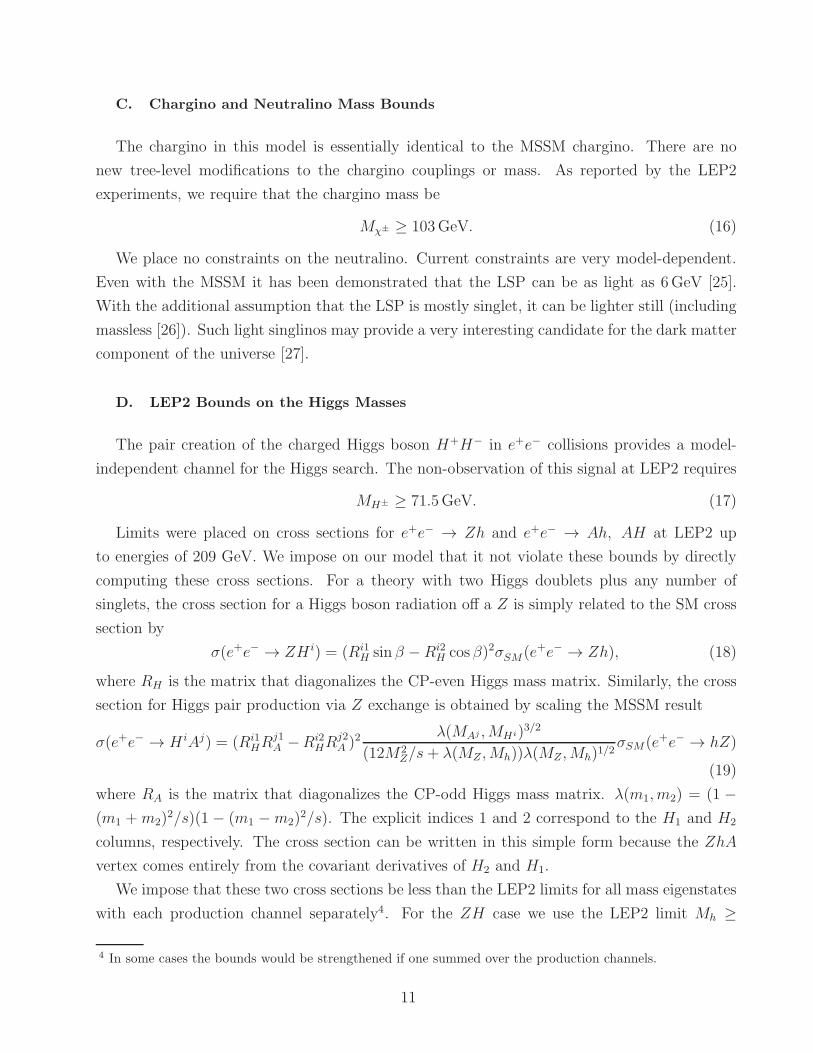
FIG. 2: (a) MH −MA mass plane, labeled according to MSSM fraction ξMSSM. For each point both
Hi and Ai satisfy the condition ξMSSM > 0, 0.001, 0.01, 0.1, or 0.9. All pairs (MHi,MAj
) are plotted.
(b) MH+ − MA mass plane with the MSSM AMSSM mass MMSSMA = 2Ahhvs/ sin 2β included for
comparison.
LEP2, there are essentially no solutions that lead to sizable cross sections in the AH channel,
as seen in Fig. 1(b). The size of these masses reflects only the range of parameters we chose for
scanning. As long as the light states are mostly singlet in composition, they can be arbitrarily
light. As shown in Eq. (11) and Eq. (12), the A1 can be tuned to be very light.
IV. MASS SPECTRUM AND COUPLINGS FOR HIGGS BOSONS
We first point out the relaxed upper bound on the mass of the lightest CP-even Higgs boson.
As given in Eq. (10), the lightest CP-even Higgs boson mass at tree level would vanish in the
limit h → 0, gZ′ → 0 and tanβ → 1. Using the parameters discussed in IIIA, the upper limit
on the lightest Higgs boson mass at tree level as given by the first two terms in Eq. (10) is
142GeV. Including the effects of Higgs mixing and the one-loop top correction, we find masses
up to ∼ 168GeV. The mass could be made even larger if we allowed h > 1, although the
perturbativity requirement up to the GUT scale at 1-loop level would imply that h ≤ 0.8. We
know that new heavy exotic matter must enter this model to cancel anomalies, so it is not
necessarily justified to require h to be perturbative to the Planck scale by calculating its 1-loop
running using only low energy fields.
The masses of the various Higgs particles are a function of the mixing parameters, and most
of the simple MSSM relations among masses are broken. It is quite common to have a light
singlet with sizable MSSM fraction that can still evade the LEP2 bounds. Typical allowed light
CP-even and odd masses are shown in Fig. 2(a) for various ranges of MSSM fractions. We see
13
10 100 1000 10000M
H(GeV)
0
0.2
0.4
0.6
0.8
1M
SSM
Fra
ctio
nξ M
SSM
H1
H2
H3
H4
H5
H6
CP-Even MSSM fractions
1 10 100 1000 10000M
A(GeV)
0
0.2
0.4
0.6
0.8
1
MSS
M F
ract
ion
ξ MSS
M
A1
A2
A3
A4
CP-Odd MSSM fractions
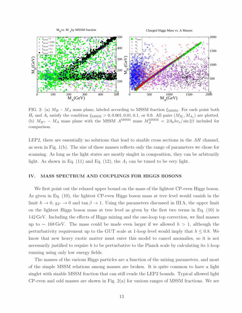
FIG. 3: The MSSM fraction (a) for the CP-even and (b) for the CP-odd states.
that it is possible to have light MSSM Higgs bosons below about 100 GeV without conflicting
the LEP2 searches. This is because of the reduced couplings to the Z when the MSSM fraction
becomes small. One can clearly make out the usual MSSM structure when ξMSSM is large, with
the diagonal band for ξMSSM > 0.9 being MMSSMH ≃ MMSSM
A , and the horizontal band being the
saturation of MMSSMh at its upper bound in the decoupling limit. As ξMSSM decreases, we can
see points in the lower left that are able to evade the LEP2 bounds on Mh,H and MA.
The mass range for the charged Higgs boson is demonstrated in Fig. 2(b). There is still a
linear relationship between the charged Higgs mass and the MSSM A mass since the singlets do
not affect the H+ mass. However, after mixing there is not necessarily a state with that mass,
or the identity of the state is obscured. Most of the parameter space has a single state that
can be identified as MSSM-like, with ξMSSM ∼ 1; in such circumstances there is also generally
an H very close in mass to both the A and H+. This is demonstrated in Appendix (A-3) with
MA3= 774, MH+ = 792, and MH4
= 780 GeV. However, the difference between MH+ and the
MAican be 50 GeV or more due to mixing, especially when the MSSM-like state is not clearly
identifiable. Such an example is presented in Appendix (A-5).
The MSSM fractions are shown versus the masses of Hi and Ai in Fig. 3. It becomes more
transparent that lighter Higgs bosons can be consistent with the LEP bound as long as the
MSSM fraction is less than about 0.2. Another way to illustrate this is via the ZZH coupling
relative to its SM value, as shown in Fig. 4. We see that the LEP2 bound for MH > 114 GeV
is restored only for those Hi states in which the couplings to Z become substantial. This figure
is remarkably similar to Fig. 3 because the ZZH coupling is√ξMSSM cos(α− β)λZZH,SM where
α is the angle that diagonalizes the CP-even mass matrix in the MSSM.
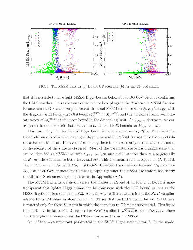
One of the most important parameters in the SUSY Higgs sector is tan β. In the model
14

100 1000M
H(GeV)
0
0.2
0.4
0.6
0.8
1Z
ZH
/ZZ
HSM
H1
H2
H3
ZZH Coupling relative to Standard Model
1000 10000M
H(GeV)
1e-06
1e-05
0.0001
0.001
0.01
0.1
ZZ
H/Z
ZH
SM
H4
H5
H6
ZZH Coupling relative to Standard Model
FIG. 4: ZZH coupling of the CP-even Higgs, relative to the Standard Model ZZH coupling.
under consideration, tanβ ≈ 1 is favored (because Ah must be large enough to ensure SU(2)
breaking). We show the value of tan β versus the allowed ranges of masses of Hi and Ai in
Fig. 5. Though the model naturally favors tan β ≈ 1, there are solutions deviating from this
relation. The actual range reflects our parameter scanning methodology shown in Table I,
which results in 1/e < tanβ < e.
V. HIGGS BOSON DECAY AND PRODUCTION IN e+e− COLLISIONS
Due to the rather distinctive features of the Higgs sector different from the SM and MSSM,
it is important to study how the lightest Higgs bosons decay in order to explore their possible
observation at future collider experiments. The lightest Higgs bosons can decay to quite non-
standard channels, leading to distinctive, yet sometimes difficult experimental signatures. For
the Higgs boson production and signal observation, we concentrate on an e+e− linear collider.
It is known that a linear collider can provide a clean experimental environment to sensitively
search for and accurately study new physics signatures. If the Higgs bosons are discovered at
the LHC, a linear collider would be needed to disentangle the complicated signals in this class
of models. If, on the other hand, a Higgs boson is not observed at the LHC due to the decay
modes difficult to observe at the hadron collider environment, a linear collider will serve as a
discovery machine.
A. Lightest CP-Even State H1
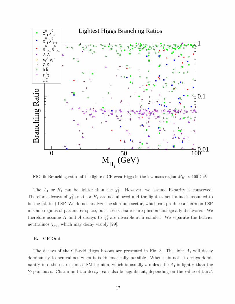
The main decay modes and corresponding branching fractions for the lightest CP-even Higgs
H1 are presented in Fig. 6. For lightest Higgs masses below approximately 100 GeV, the LEP2
15
0 100 200 300 400 500 600 700 800 900 1000M
H(GeV)
0.75
1
1.5
2.5
0.5
1
2
tan
β
H1
H2
H3
H4
MH
vs. tan β
0 100 200 300 400 500 600 700 800 900 1000M
A (GeV)
0.5
0.75
1
1.5
2
2.5
0.5
1
2
tan
β
A1
A2
A3
A4
MA
vs. tan β
FIG. 5: Range of tan β versus (a) the CP-even, and (b) CP-odd masses.
constraint is very tight, and the lightest Higgs must be mostly singlet. Thus, the decay modes
to A1A1 and χ01χ
01 are dominant when they are kinematically allowed, due to the presence of
the extra U(1)′ gauge coupling and trilinear superpotential terms proportional to h and λ.
When those modes are not kinematically accessible, the decays are very similar to the MSSM
modulo an eigenvector factor that is essentially how much of H2 and H1 are in the lightest
state. Therefore bb, cc and τ+τ− decays dominate, with cc and τ+τ− approximately an order of
magnitude smaller than bb, due to the difference in their Yukawa couplings. Examples of this
kind can be seen in Appendices (A-3, A-5). Since tan β ≈ 1, the cc mode can be competitive
with both τ+τ− and bb since their masses are similar. In the MSSM the cc mode is suppressed
because tanβ is expected to be larger.
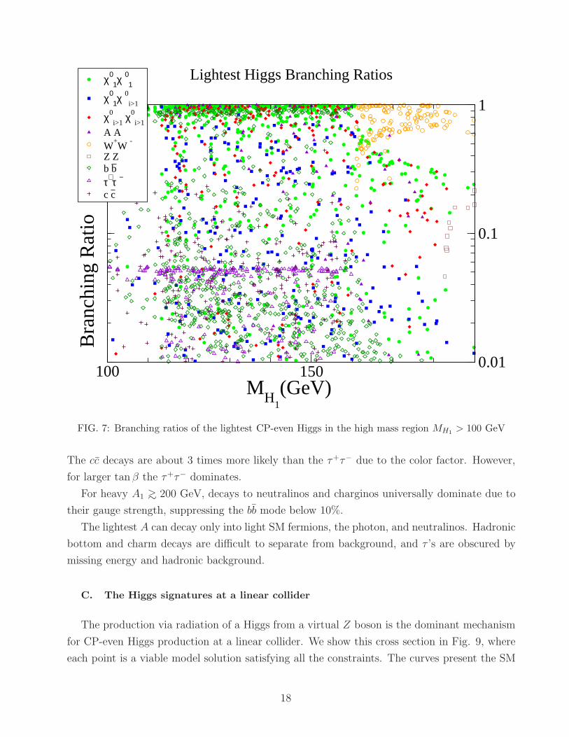
When the lightest Higgs is heavier than the LEP2 bound, it does not need to be mostly
singlet, and there can be a continuum of branching ratios to A1A1, χ01χ
01 or SM particles,
depending on how much singlet is in the lightest state. This is indeed seen in Fig. 7 for a
heavier H1 where the modes H1 → W+W−, ZZ become substantial.
A striking feature of this graph is that the usual “discovery” modes for MH1< 140, H1 →
bb, τ+τ− are often strongly suppressed by decays to A1 and χ01. Only H1 → W+W−, ZZ
decays are able to compete with the new A1 and χ01 decays, which are all of gauge strength. A
striking example of this is Appendix (A-6) and (A-7). One can see that the traditional shape
of the W+W− and ZZ threshold is obscured by the presence of χ01 and A decays, depending
on what is kinematically accessible. For a H1 heavy enough for these decay modes to be open,
however, the coupling h is typically greater than 0.8, large enough that it will become non-
perturbative before the Planck scale unless new thresholds enter at a lower scale to modify its
running. Such examples can be seen in Appendices (A-2, A-7, A-8).
16
0 50 100M
H1 (GeV)
0.01
0.1
1B
ranc
hing
Rat
ioχ0
1 χ01
χ01 χ
0
i>1
χ0
i>1χ0
i>1
A AW
+ W
-
Z Zb bτ+ τ−
c c
Lightest Higgs Branching Ratios
FIG. 6: Branching ratios of the lightest CP-even Higgs in the low mass region MH1< 100 GeV
The A1 or H1 can be lighter than the χ01. However, we assume R-parity is conserved.
Therefore, decays of χ01 to A1 or H1 are not allowed and the lightest neutralino is assumed to
be the (stable) LSP. We do not analyze the sfermion sector, which can produce a sfermion LSP
in some regions of parameter space, but these scenarios are phenomenologically disfavored. We
therefore assume H and A decays to χ01 are invisible at a collider. We separate the heavier
neutralinos χ0i>1 which may decay visibly [29].
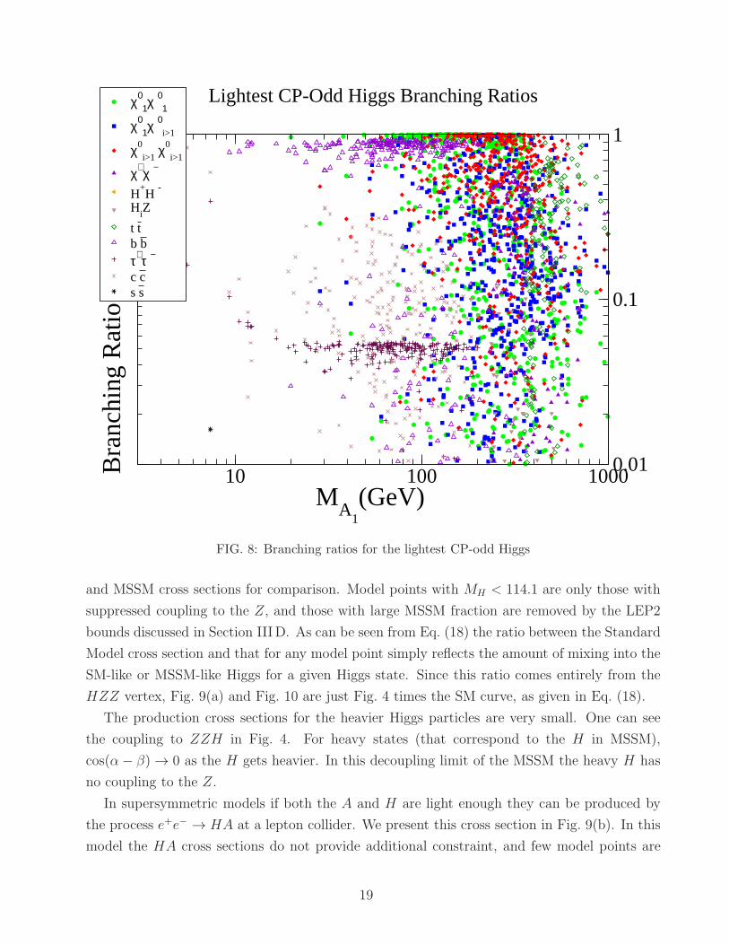
B. CP-Odd
The decays of the CP-odd Higgs bosons are presented in Fig. 8. The light A1 will decay
dominantly to neutralinos when it is kinematically possible. When it is not, it decays domi-
nantly into the nearest mass SM fermion, which is usually b unless the A1 is lighter than the
bb pair mass. Charm and tau decays can also be significant, depending on the value of tanβ.
17
100 150M
H1(GeV)
0.01
0.1
1B
ranc
hing
Rat
ioχ0
1χ01
χ01χ
0
i>1
χ0
i>1χ0
i>1
A AW
+W
-
Z Zb bτ+τ −
c c
Lightest Higgs Branching Ratios
FIG. 7: Branching ratios of the lightest CP-even Higgs in the high mass region MH1> 100 GeV
The cc decays are about 3 times more likely than the τ+τ− due to the color factor. However,
for larger tan β the τ+τ− dominates.
For heavy A1 >∼ 200 GeV, decays to neutralinos and charginos universally dominate due to
their gauge strength, suppressing the bb mode below 10%.
The lightest A can decay only into light SM fermions, the photon, and neutralinos. Hadronic
bottom and charm decays are difficult to separate from background, and τ ’s are obscured by
missing energy and hadronic background.
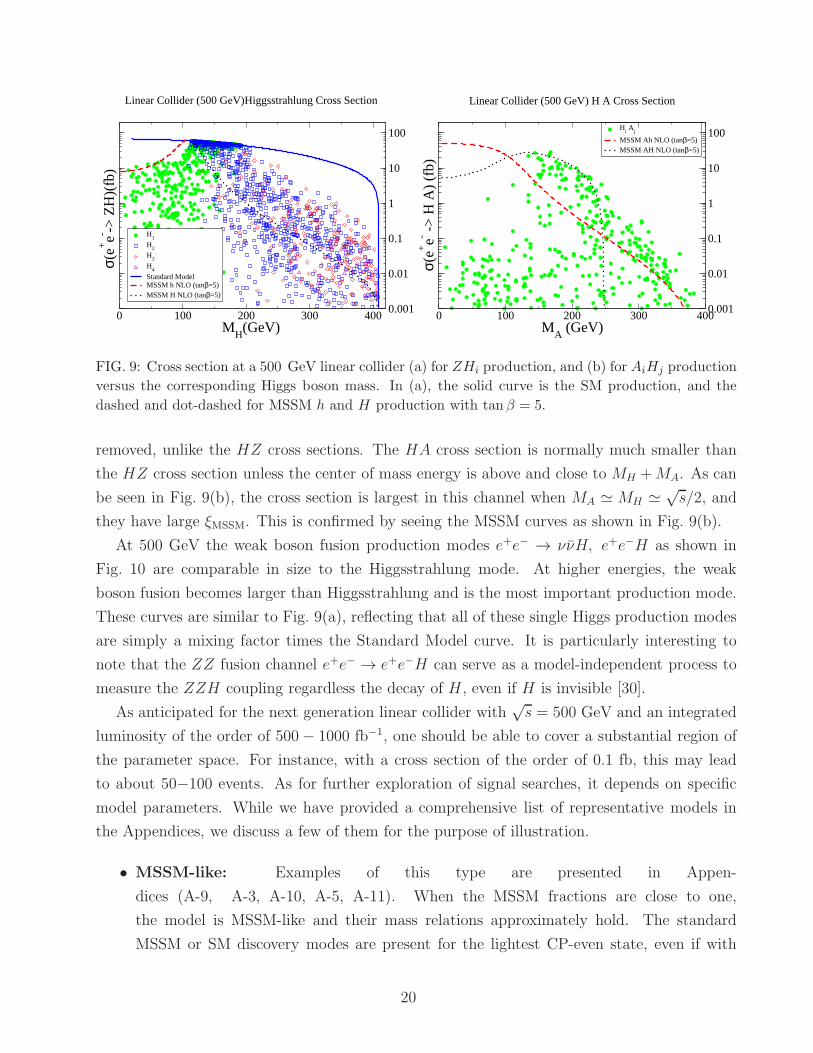
C. The Higgs signatures at a linear collider
The production via radiation of a Higgs from a virtual Z boson is the dominant mechanism
for CP-even Higgs production at a linear collider. We show this cross section in Fig. 9, where
each point is a viable model solution satisfying all the constraints. The curves present the SM
18
10 100 1000M
A1(GeV)
0.01
0.1
1B
ranc
hing
Rat
ioχ0
1χ01
χ01χ
0i>1
χ0
i>1χ0
i>1
χ+χ −
H+H
-
HiZ
t tb bτ+τ −
c cs s
Lightest CP-Odd Higgs Branching Ratios
FIG. 8: Branching ratios for the lightest CP-odd Higgs
and MSSM cross sections for comparison. Model points with MH < 114.1 are only those with
suppressed coupling to the Z, and those with large MSSM fraction are removed by the LEP2
bounds discussed in Section IIID. As can be seen from Eq. (18) the ratio between the Standard
Model cross section and that for any model point simply reflects the amount of mixing into the
SM-like or MSSM-like Higgs for a given Higgs state. Since this ratio comes entirely from the
HZZ vertex, Fig. 9(a) and Fig. 10 are just Fig. 4 times the SM curve, as given in Eq. (18).
The production cross sections for the heavier Higgs particles are very small. One can see
the coupling to ZZH in Fig. 4. For heavy states (that correspond to the H in MSSM),
cos(α− β) → 0 as the H gets heavier. In this decoupling limit of the MSSM the heavy H has
no coupling to the Z.
In supersymmetric models if both the A and H are light enough they can be produced by
the process e+e− → HA at a lepton collider. We present this cross section in Fig. 9(b). In this
model the HA cross sections do not provide additional constraint, and few model points are
19
0 100 200 300 400M
H(GeV)
0.001
0.01
0.1
1
10
100
σ(e+
e- -> Z
H)(
fb)
H1
H2
H3
H4
Standard ModelMSSM h NLO (tanβ=5)MSSM H NLO (tanβ=5)
Linear Collider (500 GeV)Higgsstrahlung Cross Section
0 100 200 300 400M
A (GeV)
0.001
0.01
0.1
1
10
100
σ(e+
e- ->
H A
) (f
b)
Hi A
j
MSSM Ah NLO (tanβ=5)MSSM AH NLO (tanβ=5)
Linear Collider (500 GeV) H A Cross Section
FIG. 9: Cross section at a 500 GeV linear collider (a) for ZHi production, and (b) for AiHj production
versus the corresponding Higgs boson mass. In (a), the solid curve is the SM production, and the
dashed and dot-dashed for MSSM h and H production with tan β = 5.
removed, unlike the HZ cross sections. The HA cross section is normally much smaller than
the HZ cross section unless the center of mass energy is above and close to MH +MA. As can
be seen in Fig. 9(b), the cross section is largest in this channel when MA ≃ MH ≃ √s/2, and
they have large ξMSSM. This is confirmed by seeing the MSSM curves as shown in Fig. 9(b).
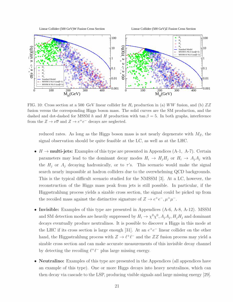
At 500 GeV the weak boson fusion production modes e+e− → ννH, e+e−H as shown in
Fig. 10 are comparable in size to the Higgsstrahlung mode. At higher energies, the weak
boson fusion becomes larger than Higgsstrahlung and is the most important production mode.
These curves are similar to Fig. 9(a), reflecting that all of these single Higgs production modes
are simply a mixing factor times the Standard Model curve. It is particularly interesting to
note that the ZZ fusion channel e+e− → e+e−H can serve as a model-independent process to
measure the ZZH coupling regardless the decay of H , even if H is invisible [30].
As anticipated for the next generation linear collider with√s = 500 GeV and an integrated
luminosity of the order of 500− 1000 fb−1, one should be able to cover a substantial region of
the parameter space. For instance, with a cross section of the order of 0.1 fb, this may lead
to about 50−100 events. As for further exploration of signal searches, it depends on specific
model parameters. While we have provided a comprehensive list of representative models in
the Appendices, we discuss a few of them for the purpose of illustration.
• MSSM-like: Examples of this type are presented in Appen-
dices (A-9, A-3, A-10, A-5, A-11). When the MSSM fractions are close to one,
the model is MSSM-like and their mass relations approximately hold. The standard
MSSM or SM discovery modes are present for the lightest CP-even state, even if with
20
0 100 200 300 400M
H(GeV)
0.001
0.01
0.1
1
10
100
σ(e+
e- ->ν
νH)(
fb)
H1
H2
H3
H4
Standard ModelMSSM h NLO (tanβ=5)MSSM H NLO (tanβ=5)
Linear Collider (500 GeV)W Fusion Cross Section
0 100 200 300 400M
H(GeV)
0.001
0.01
0.1
1
10
100
σ(e+
e- -> e
+e
- H)(
fb)
H1
H2
H3
H4
Standard ModelMSSM h NLO (tanβ=5)MSSM H NLO (tanβ=5)
Linear Collider (500 GeV)Z Fusion Cross Section
FIG. 10: Cross section at a 500 GeV linear collider for Hi production in (a) WW fusion, and (b) ZZ
fusion versus the corresponding Higgs boson mass. The solid curves are the SM production, and the
dashed and dot-dashed for MSSM h and H production with tan β = 5. In both graphs, interference
from the Z → νν and Z → e+e− decays are neglected.
reduced rates. As long as the Higgs boson mass is not nearly degenerate with MZ , the
signal observation should be quite feasible at the LC, as well as at the LHC.
• H → multi-jets: Examples of this type are presented in Appendices (A-1, A-7). Certain
parameters may lead to the dominant decay modes Hi → HjHj or Hi → AjAj with
the Hj or Aj decaying hadronically, or to τ ’s. This scenario would make the signal
search nearly impossible at hadron colliders due to the overwhelming QCD backgrounds.
This is the typical difficult scenario studied for the NMSSM [3]. At a LC, however, the
reconstruction of the Higgs mass peak from jets is still possible. In particular, if the
Higgsstrahlung process yields a sizable cross section, the signal could be picked up from
the recoiled mass against the distinctive signature of Z → e+e−, µ+µ−.
• Invisible: Examples of this type are presented in Appendices (A-6, A-8, A-12). MSSM
and SM detection modes are heavily suppressed by Hi → χ0χ0, AjAj , HjHj and dominant
decays eventually produce neutralinos. It is possible to discover a Higgs in this mode at
the LHC if its cross section is large enough [31]. At an e+e− linear collider on the other
hand, the Higgsstrahlung process with Z → ℓ+ℓ− and the ZZ fusion process may yield a
sizable cross section and can make accurate measurements of this invisible decay channel
by detecting the recoiling ℓ+ℓ− plus large missing energy.
• Neutralino: Examples of this type are presented in the Appendices (all appendices have
an example of this type). One or more Higgs decays into heavy neutralinos, which can
then decay via cascade to the LSP, producing visible signals and large missing energy [29].
21

If the lightest neutralino is mostly singlino or Z ′-ino, the usual MSSM limits on neutralino
mass do not apply, and couplings between it and Higgs bosons can be large. This mode is
extremely important, and dominates the Higgs decays due to the presence of Higgs-singlet
interaction h, singlet-singlet interactions λ and the Z ′ coupling. This mode has received
some attention in the literature [32] but clearly warrants more due to its dominance in
parameter space.
It is clear that the model studied in this paper presents very rich physics in the Higgs sector.
An e+e− linear collider will be ideally suited for the detailed exploration of the non-standard
Higgs physics. Analyses for the LHC should also be performed, particularly for the non-MSSM
modes [3].
VI. SUMMARY AND CONCLUSIONS
We have considered the Higgs sector in an extension of the MSSM with extra SM singlets.
By exploiting an extra U(1)′ gauge symmetry, the domain-wall problem is avoided. An effective
µ parameter can be generated by a singlet VEV, which can be decoupled from the new gauge
boson Z ′ mass.
The model involves a rich Higgs structure very different from that of the MSSM. In particular,
there are large mixings between Higgs doublets and SM singlets. The lightest CP even Higgs
boson can have a mass up to about 170 GeV. Higgs bosons considerably lighter than the LEP2
bound are allowed. The parameter tanβ ∼ 1 is both allowed and theoretically favored.
We parameterize the Higgs coupling strengths relative to the MSSM, called the MSSM
fraction ξMSSM. We find that besides the typical SM-like and MSSM-like Higgs bosons, there
are model points leading to very different signatures from those. One of the features for the
Higgs boson decay is to have possibly a large invisible decay mode to LSP. We present a
comprehensive list of model scenarios in the Appendices.
Concentrating on a future e+e− linear collider with√s = 500 GeV, we found that in a large
parameter region the Higgs bosons are accessible through the production channels e+e− →ZHi, HiAj as well as WW and ZZ fusion. We outlined the searching strategy for some
representative scenarios at a future linear collider.
We find that this model has a large parameter space where the Higgs bosons decay hadron-
ically or invisibly. As these modes are very difficult at the LHC, effort should be invested in
ways to discover or exclude such modes at the LHC. If discovery is not possible, a linear collider
will absolutely be required.
We emphasize the importance of neutralino decays, which dominate the parameter space
due to Higgs self-interactions and the U(1)′ gauge coupling. These decays are generically
22
present and dominant in extended models [32], and thus should be paid more attention by
phenomenologists and experimentalists.
Acknowledgments
We thank V. Barger, J. Erler, J. Gunion, T. Li, and J. Wells, for useful discussions. This
work was supported in part by DOE grants DE–FG02–95ER–40896, DE–FG03–91ER–40674
and DOE–EY–76–02–3071; also in part by the Wisconsin Alumni Research Foundation, the
National Natural Science Foundation of China, the Davis Institute for High Energy Physics,
and the U.C. Davis Dean’s office.
23

A-1. LIGHTEST A1
tan β = 0.522 MZ′ = 2415 GeV MH+ = 826 GeV αZZ′ =-2.7·10−4
MH 118 654 843 1731 2330 7839
ξMSSM 1 1.2·10−3 1 3.3·10−3 2.4·10−4 0
σ(HiZ) 58
σ(Hiνν) 87
σ(Hie+e−) 8.3
MA 6 821 1741 7839 0 0
ξMSSM 3.2·10−4 0.99 5.9·10−3 0 1 5.4·10−4
σ(H1A) 4.8·10−6
Mχ0 42 165 213 284 470 774 778 1834 3222
ξMSSM 0.24 0.95 0.81 1 1 0 2.1·10−5 9.7·10−5 4.5·10−5
ξs 0.76 0.047 0.19 1.1·10−3 9.2·10−5 0.99 0.99 0.65 0.37
ξZ′ 0 0 0 0 0 5.3·10−3 0.012 0.35 0.63
Mχ+ 173 470
Cross sections quoted are in fb for a linear e+e− collider at center-of-mass energy 500 GeV.
v2 = 80GeV v1 = 154GeV vs = 272GeV
vs1 = 117GeV vs2 = 3504GeV vs3 = 3256GeV
m2Hu
= (849GeV)2 m2Hd
= (595GeV)2 m2S = (1585GeV)2
m2S1
= (7817GeV)2 m2S2
= (496GeV)2 m2S3
= −(1115GeV)2
h = 0.608 Ah = 1704GeV µ = hvs = 166GeV
λ = 0.173 Aλ = 3622GeV
M1 = −267GeV M ′1 = 1385GeV M2 = 459GeV
m2SS1
= −(48GeV)2 m2SS2
= −(479GeV)2
Branching Ratios for dominant decay modes (greater than 1% excluding model-dependent
squark, slepton, Z ′ and exotic decays; χ0i>1 are summed):
H1 A1A1 81% χ01χ
01 18% bb 1%
H2 χ+1 χ
−1 25% χ0
1χ0i>1 17% W+W− 14% χ0
i>1χ0i>1 14% tt 13% H1H1 11%
H3 tt 77% χ0i>1χ
0i>1 8% χ0
1χ0i>1 8% χ0
1χ01 3% χ+
1 χ−2 2% H1H1 1%
H4 A1A2 27% χ+1 χ
−1 23% χ0
i>1χ0i>1 18% H1H3 7% χ0
1χ0i>1 6% W+W− 4%
H5 W+W− 24% H1H1 24% ZZ 12% H2H2 9% χ0i>1χ
0i>1 7% χ+
1 χ−1 6%
H6 χ0i>1χ
0i>1 95% H2H5 3% H2H2 1%
A1 cc 83% τ+τ− 16% ss 1%
A2 tt 79% χ0i>1χ
0i>1 9% χ0
1χ01 6% χ0
1, χ0i>1 5% χ+
1 χ−1 1%
A3 H2Z 97% χ+1 χ
−1 1% χ0
i>1χ0i>1 1%
A4 H2Z 64% H5Z 31% χ0i>1χ
0i>1 3% A1H2 1%
24
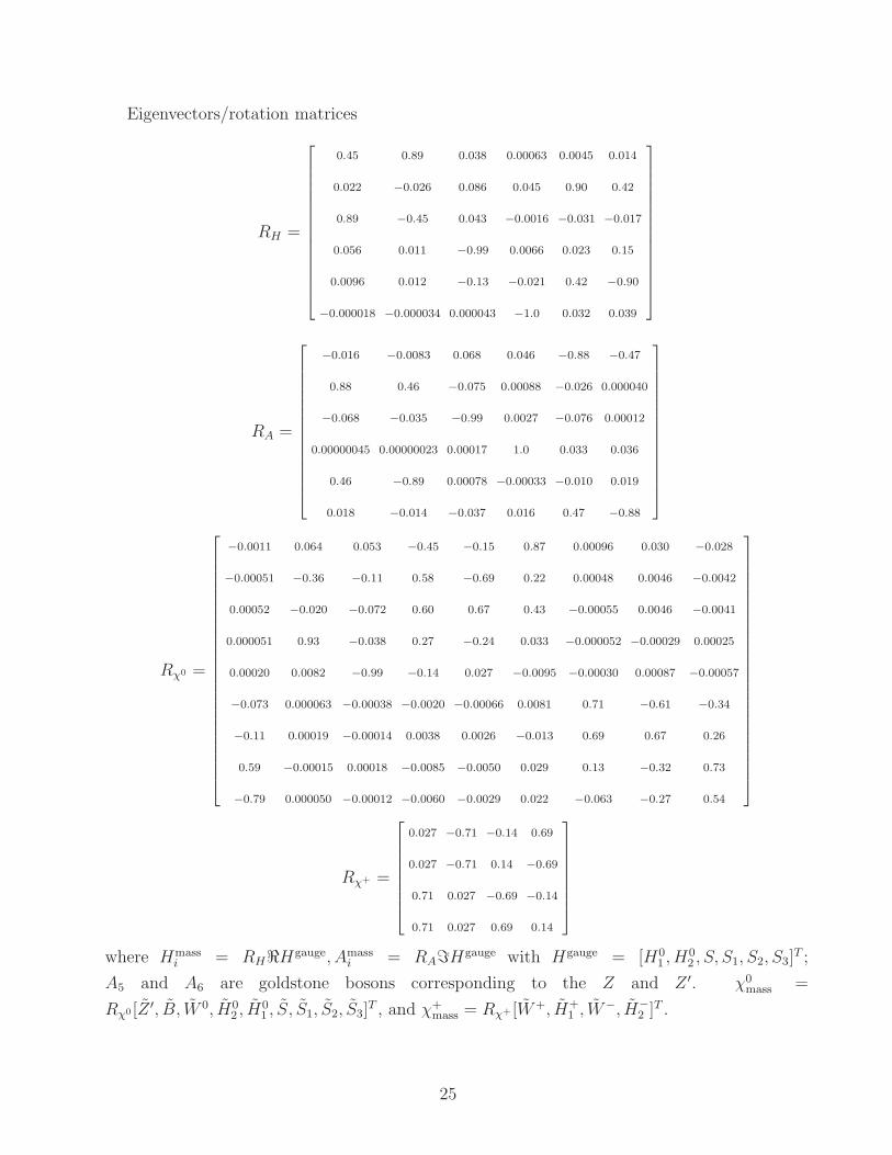
Eigenvectors/rotation matrices
RH =
0.45 0.89 0.038 0.00063 0.0045 0.014
0.022 −0.026 0.086 0.045 0.90 0.42
0.89 −0.45 0.043 −0.0016 −0.031 −0.017
0.056 0.011 −0.99 0.0066 0.023 0.15
0.0096 0.012 −0.13 −0.021 0.42 −0.90
−0.000018 −0.000034 0.000043 −1.0 0.032 0.039
RA =
−0.016 −0.0083 0.068 0.046 −0.88 −0.47
0.88 0.46 −0.075 0.00088 −0.026 0.000040
−0.068 −0.035 −0.99 0.0027 −0.076 0.00012
0.00000045 0.00000023 0.00017 1.0 0.033 0.036
0.46 −0.89 0.00078 −0.00033 −0.010 0.019
0.018 −0.014 −0.037 0.016 0.47 −0.88
Rχ0 =
−0.0011 0.064 0.053 −0.45 −0.15 0.87 0.00096 0.030 −0.028
−0.00051 −0.36 −0.11 0.58 −0.69 0.22 0.00048 0.0046 −0.0042
0.00052 −0.020 −0.072 0.60 0.67 0.43 −0.00055 0.0046 −0.0041
0.000051 0.93 −0.038 0.27 −0.24 0.033 −0.000052 −0.00029 0.00025
0.00020 0.0082 −0.99 −0.14 0.027 −0.0095 −0.00030 0.00087 −0.00057
−0.073 0.000063 −0.00038 −0.0020 −0.00066 0.0081 0.71 −0.61 −0.34
−0.11 0.00019 −0.00014 0.0038 0.0026 −0.013 0.69 0.67 0.26
0.59 −0.00015 0.00018 −0.0085 −0.0050 0.029 0.13 −0.32 0.73
−0.79 0.000050 −0.00012 −0.0060 −0.0029 0.022 −0.063 −0.27 0.54
Rχ+ =
0.027 −0.71 −0.14 0.69
0.027 −0.71 0.14 −0.69
0.71 0.027 −0.69 −0.14
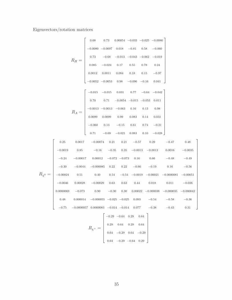
0.71 0.027 0.69 0.14
where Hmassi = RHℜHgauge, Amass
i = RAℑHgauge with Hgauge = [H01 , H
02 , S, S1, S2, S3]
T ;
A5 and A6 are goldstone bosons corresponding to the Z and Z ′. χ0mass =
Rχ0 [Z ′, B, W 0, H02 , H
01 , S, S1, S2, S3]
T , and χ+mass = Rχ+ [W+, H+
1 , W−, H−
2 ]T .
25

A-2. LIGHTEST H1
tan β = 0.614 MZ′ = 626 GeV MH+ = 444 GeV αZZ′ =-3.3·10−3
MH 8 127 471 627 1071 1762
ξMSSM 0.013 0.99 1 1.4·10−3 4.5·10−5 3.6·10−4
σ(HiZ) 0.86 55
σ(Hiνν) 2.5 78 3.5·10−5
σ(Hie+e−) 0.23 7.5 3.2·10−6
MA 172 446 1067 1757 0 0
ξMSSM 2.0·10−4 1 1.4·10−4 6.2·10−4 1 1.7·10−3
σ(H1A) 1.1·10−7 6.8·10−6
σ(H2A) 2.3·10−5
Mχ0 44 47 58 62 120 170 286 556 1357
ξMSSM 0.98 0.3 2.3·10−4 4.4·10−4 0.94 0.77 3.2·10−3 1 3.1·10−4
ξs 0.015 0.7 1 1 0.059 0.23 0.82 0 0.18
ξZ′ 0 1.2·10−4 3.4·10−4 5.3·10−5 4.7·10−5 0 0.18 0 0.82
Mχ+ 103 556
Cross sections quoted are in fb for a linear e+e− collider at center-of-mass energy 500 GeV.
v2 = 91GeV v1 = 148GeV vs = 212GeV
vs1 = 1726GeV vs2 = 120GeV vs3 = 397GeV
m2Hu
= (194GeV)2 m2Hd
= −(184GeV)2 m2S = (1770GeV)2
m2S1
= −(310GeV)2 m2S2
= (1001GeV)2 m2S3
= (580GeV)2
h = −0.552 Ah = 764GeV µ = hvs = −117GeV
λ = 0.035 Aλ = 3234GeV
M1 = −31GeV M ′1 = −1067GeV M2 = 542GeV
m2SS1
= −(587GeV)2 m2SS2
= −(536GeV)2
Branching Ratios for dominant decay modes (greater than 1% excluding model-dependent
squark, slepton, Z ′ and exotic decays; χ0i>1 are summed):
H1 τ+τ− 59% cc 38% ss 2%
H2 χ0i>1χ
0i>1 60% χ0
1χ0i>1 17% χ0
1χ01 13% H1H1 6% bb 4%
H3 tt 66% χ0i>1χ
0i>1 20% χ0
1χ0i>1 8% H2H2 4% W+W− 1% ZZ 1%
H4 A1A1 41% H1H1 35% χ0i>1χ
0i>1 12% H2H2 3% W+W− 3% χ+
1 χ−1 2%
H5 χ0i>1χ
0i>1 59% χ+
1 χ−1 13% H1H1 8% A1A1 4% A2A2 4% H1H4 3%
H6 χ0i>1χ
0i>1 41% χ+
1 χ−1 38% A2A2 5% H3H3 4% χ0
1χ0i>1 3% H2H3 2%
A1 χ0i>1χ
0i>1 98% χ0
1χ01 2% χ0
1, χ0i>1 1%
A2 tt 62% χ0i>1χ
0i>1 26% χ0
1, χ0i>1 7% χ+
1 χ−1 2% H2Z 1% χ0
1χ01 1%
A3 H2Z 100%
A4 χ0i>1χ
0i>1 44% χ+
1 χ−1 41% H2Z 4% A1H1 3% χ0
1, χ0i>1 3% H5Z 2%
26

Eigenvectors/rotation matrices
RH =
0.062 0.094 0.072 0.46 0.18 0.86
0.46 0.88 0.0025 −0.082 −0.017 −0.083
−0.88 0.47 −0.015 −0.010 −0.00038 0.020
−0.0028 0.037 0.13 0.87 −0.052 −0.47
−0.0067 −0.0011 0.14 −0.060 0.97 −0.18
−0.018 −0.0070 0.98 −0.14 −0.15 0.023
RA =
0.012 0.0074 −0.033 0.42 −0.16 0.89
0.85 0.52 −0.021 −0.045 0.0074 0.0058
−0.0099 −0.0061 −0.15 −0.0052 0.97 0.17
0.021 0.013 0.98 0.11 0.15 0.010
0.52 −0.85 −0.00057 0.0047 0.00032 −0.0021
0.032 0.026 −0.11 0.90 0.063 −0.41
Rχ0 =
0.0012 0.95 −0.039 0.21 −0.20 −0.12 −0.019 0.0091 −0.0033
0.011 0.18 0.051 −0.48 −0.18 0.82 0.14 0.021 −0.022
−0.019 0.012 −0.00096 0.0093 0.0016 −0.012 0.30 −0.71 0.63
−0.0073 0.0064 0.0023 −0.019 −0.0052 0.030 −0.27 −0.70 −0.66
0.0069 −0.25 −0.17 0.58 −0.72 0.24 0.031 −0.0013 −0.014
0.0029 −0.057 0.020 −0.60 −0.63 −0.48 −0.0095 −0.0017 0.0052
−0.42 0.0017 0.0039 −0.039 −0.040 0.12 −0.82 −0.021 0.36
−0.0019 0.013 −0.98 −0.14 0.11 −0.0023 −0.0019 −0.000088 0.00085
−0.91 0.00028 −0.00036 0.015 0.0085 −0.045 0.38 0.030 −0.18
Rχ+ =
−0.10 0.70 −0.14 0.69
0.10 −0.70 −0.14 0.69
0.70 0.10 0.69 0.14
0.70 0.10 −0.69 −0.14
27

A-3. TYPICAL LIGHT H1 → SM DOMINANT
tan β = 2.64 MZ′ = 828 GeV MH+ = 792 GeV αZZ′ =3.1·10−3
MH 46 119 332 780 828 1558
ξMSSM 3.5·10−3 0.99 1.9·10−5 0.92 0.064 0.019
σ(HiZ) 0.23 57 0.00018
σ(Hiνν) 0.54 85 5.9·10−5
σ(Hie+e−) 0.051 8.2 5.7·10−6
MA 59 337 774 1558 0 0
ξMSSM 0 0 0.97 0.026 0.99 5.7·10−3
σ(H1A) 2.4·10−9 1.6·10−10
σ(H2A) 6.1·10−8 1.7·10−9
σ(H3A) 3.8·10−10
Mχ0 42 72 79 104 180 216 290 627 1102
ξMSSM 0.8 4.2·10−3 8.9·10−5 0.72 0.8 0.68 0.99 9.6·10−4 3.7·10−4
ξs 0.2 0.99 1 0.28 0.2 0.32 0.01 0.64 0.36
ξZ′ 1.1·10−5 1.8·10−3 1.3·10−3 0 1.5·10−5 0 0 0.36 0.64
Mχ+ 124 289Cross sections quoted are in fb for a linear e+e− collider at center-of-mass energy 500 GeV.
v2 = 163GeV v1 = 62GeV vs = 128GeV
vs1 = 2434GeV vs2 = 679GeV vs3 = 96GeV
m2Hu
= −(338GeV)2 m2Hd
= (602GeV)2 m2S = (1640GeV)2
m2S1
= −(577GeV)2 m2S2
= −(583GeV)2 m2S3
= (884GeV)2
h = −0.920 Ah = 1818GeV µ = hvs = −118GeV
λ = 0.035 Aλ = 184GeV
M1 = −88GeV M ′1 = 482GeV M2 = 268GeV
m2SS1
= −(336GeV)2 m2SS2
= −(136GeV)2
Branching Ratios for dominant decay modes (greater than 1% excluding model-dependent
squark, slepton, Z ′ and exotic decays; χ0i>1 are summed):
H1 bb 64% cc 32% τ+τ− 4%
H2 bb 41% H1H1 27% cc 23% χ01χ
01 5% τ+τ− 2% A1A1 1%
H3 χ0i>1χ
0i>1 72% H1H1 21% A1A1 4% H2H2 1% χ0
1χ0i>1 1% W+W− 1%
H4 χ0i>1χ
0i>1 41% tt 21% χ0
1χ0i>1 16% χ0
1χ01 11% χ+
1 χ−1 8% H2H2 1%
H5 H3H3 33% A1A1 16% H1H1 14% χ0i>1χ
0i>1 13% tt 8% χ0
1χ0i>1 4%
H6 A2A3 25% χ+1 χ
−1 18% χ0
i>1χ0i>1 14% H2H4 11% χ0
1χ0i>1 10% A3Z 7%
A1 bb 93% τ+τ− 5% cc 1%
A2 χ0i>1χ
0i>1 97% A1H1 2% χ0
1, χ0i>1 1%
A3 χ0i>1χ
0i>1 35% χ0
1, χ0i>1 24% tt 19% χ+
1 χ−1 9% χ+
1 χ−2 8% χ0
1χ01 5%
A4 H3Z 93% χ+1 χ
−1 2% χ0
i>1χ0i>1 2% H4Z 1% A2H5 1% χ0
1, χ0i>1 1%
28
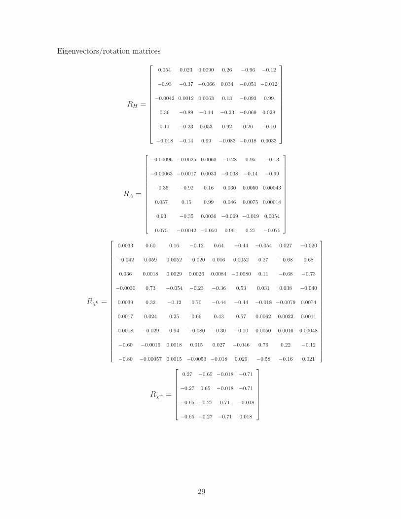
Eigenvectors/rotation matrices
RH =
0.054 0.023 0.0090 0.26 −0.96 −0.12
−0.93 −0.37 −0.066 0.034 −0.051 −0.012
−0.0042 0.0012 0.0063 0.13 −0.093 0.99
0.36 −0.89 −0.14 −0.23 −0.069 0.028
0.11 −0.23 0.053 0.92 0.26 −0.10
−0.018 −0.14 0.99 −0.083 −0.018 0.0033
RA =
−0.00096 −0.0025 0.0060 −0.28 0.95 −0.13
−0.00063 −0.0017 0.0033 −0.038 −0.14 −0.99
−0.35 −0.92 0.16 0.030 0.0050 0.00043
0.057 0.15 0.99 0.046 0.0075 0.00014
0.93 −0.35 0.0036 −0.069 −0.019 0.0054
0.075 −0.0042 −0.050 0.96 0.27 −0.075
Rχ0 =
0.0033 0.60 0.16 −0.12 0.64 −0.44 −0.054 0.027 −0.020
−0.042 0.059 0.0052 −0.020 0.016 0.0052 0.27 −0.68 0.68
0.036 0.0018 0.0029 0.0026 0.0084 −0.0080 0.11 −0.68 −0.73
−0.0030 0.73 −0.054 −0.23 −0.36 0.53 0.031 0.038 −0.040
0.0039 0.32 −0.12 0.70 −0.44 −0.44 −0.018 −0.0079 0.0074
0.0017 0.024 0.25 0.66 0.43 0.57 0.0062 0.0022 0.0011
0.0018 −0.029 0.94 −0.080 −0.30 −0.10 0.0050 0.0016 0.00048
−0.60 −0.0016 0.0018 0.015 0.027 −0.046 0.76 0.22 −0.12
−0.80 −0.00057 0.0015 −0.0053 −0.018 0.029 −0.58 −0.16 0.021
Rχ+ =
0.27 −0.65 −0.018 −0.71
−0.27 0.65 −0.018 −0.71
−0.65 −0.27 0.71 −0.018
−0.65 −0.27 −0.71 0.018
29
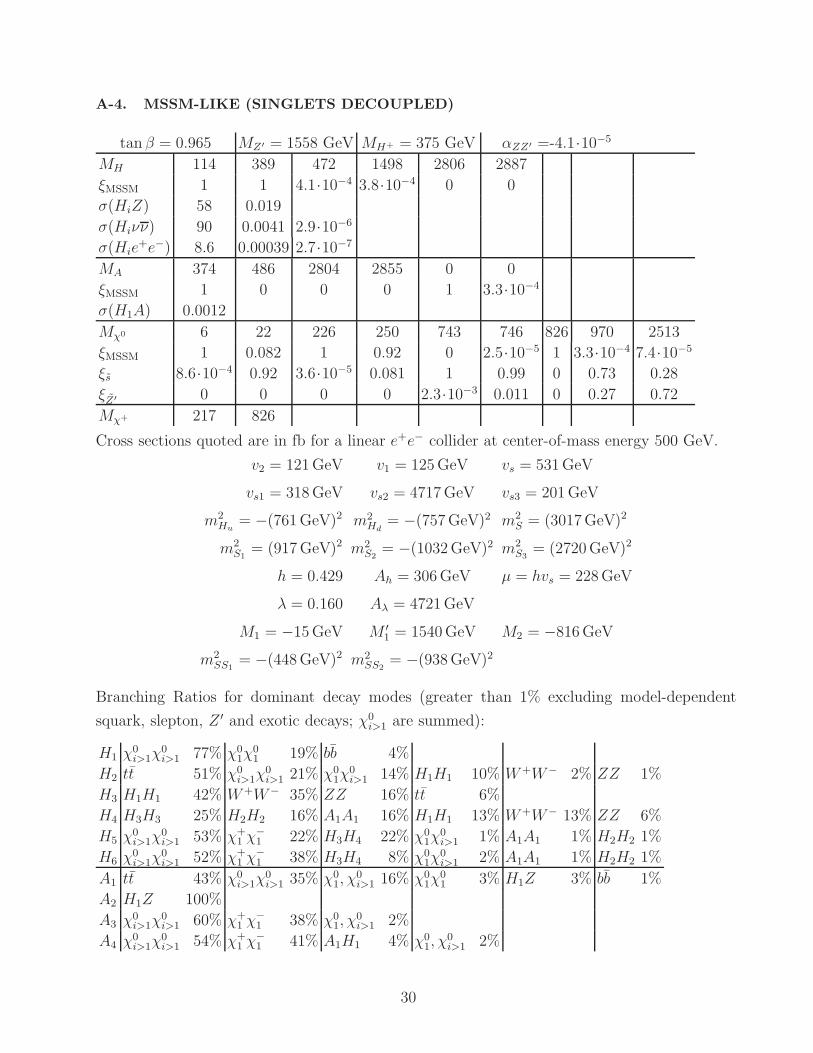
A-4. MSSM-LIKE (SINGLETS DECOUPLED)
tan β = 0.965 MZ′ = 1558 GeV MH+ = 375 GeV αZZ′ =-4.1·10−5
MH 114 389 472 1498 2806 2887
ξMSSM 1 1 4.1·10−4 3.8·10−4 0 0
σ(HiZ) 58 0.019
σ(Hiνν) 90 0.0041 2.9·10−6
σ(Hie+e−) 8.6 0.00039 2.7·10−7
MA 374 486 2804 2855 0 0
ξMSSM 1 0 0 0 1 3.3·10−4
σ(H1A) 0.0012
Mχ0 6 22 226 250 743 746 826 970 2513
ξMSSM 1 0.082 1 0.92 0 2.5·10−5 1 3.3·10−4 7.4·10−5
ξs 8.6·10−4 0.92 3.6·10−5 0.081 1 0.99 0 0.73 0.28
ξZ′ 0 0 0 0 2.3·10−3 0.011 0 0.27 0.72
Mχ+ 217 826
Cross sections quoted are in fb for a linear e+e− collider at center-of-mass energy 500 GeV.
v2 = 121GeV v1 = 125GeV vs = 531GeV
vs1 = 318GeV vs2 = 4717GeV vs3 = 201GeV
m2Hu
= −(761GeV)2 m2Hd
= −(757GeV)2 m2S = (3017GeV)2
m2S1
= (917GeV)2 m2S2
= −(1032GeV)2 m2S3
= (2720GeV)2
h = 0.429 Ah = 306GeV µ = hvs = 228GeV
λ = 0.160 Aλ = 4721GeV
M1 = −15GeV M ′1 = 1540GeV M2 = −816GeV
m2SS1
= −(448GeV)2 m2SS2
= −(938GeV)2
Branching Ratios for dominant decay modes (greater than 1% excluding model-dependent
squark, slepton, Z ′ and exotic decays; χ0i>1 are summed):
H1 χ0i>1χ
0i>1 77% χ0
1χ01 19% bb 4%
H2 tt 51% χ0i>1χ
0i>1 21% χ0
1χ0i>1 14% H1H1 10% W+W− 2% ZZ 1%
H3 H1H1 42% W+W− 35% ZZ 16% tt 6%
H4 H3H3 25% H2H2 16% A1A1 16% H1H1 13% W+W− 13% ZZ 6%
H5 χ0i>1χ
0i>1 53% χ+
1 χ−1 22% H3H4 22% χ0
1χ0i>1 1% A1A1 1% H2H2 1%
H6 χ0i>1χ
0i>1 52% χ+
1 χ−1 38% H3H4 8% χ0
1χ0i>1 2% A1A1 1% H2H2 1%
A1 tt 43% χ0i>1χ
0i>1 35% χ0
1, χ0i>1 16% χ0
1χ01 3% H1Z 3% bb 1%
A2 H1Z 100%
A3 χ0i>1χ
0i>1 60% χ+
1 χ−1 38% χ0
1, χ0i>1 2%
A4 χ0i>1χ
0i>1 54% χ+
1 χ−1 41% A1H1 4% χ0
1, χ0i>1 2%
30
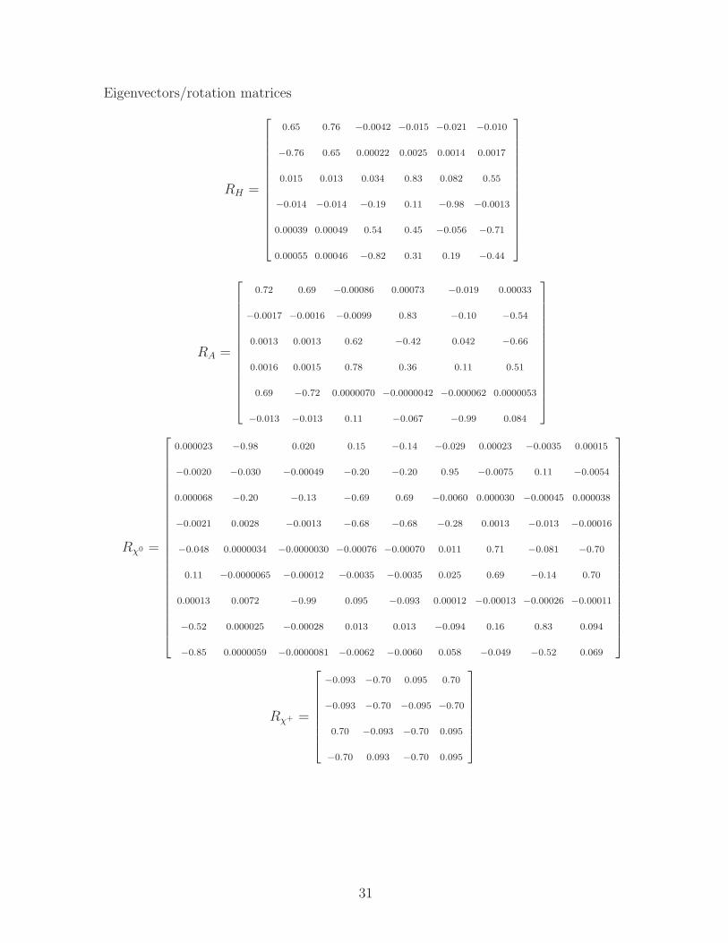
Eigenvectors/rotation matrices
RH =
0.65 0.76 −0.0042 −0.015 −0.021 −0.010
−0.76 0.65 0.00022 0.0025 0.0014 0.0017
0.015 0.013 0.034 0.83 0.082 0.55
−0.014 −0.014 −0.19 0.11 −0.98 −0.0013
0.00039 0.00049 0.54 0.45 −0.056 −0.71
0.00055 0.00046 −0.82 0.31 0.19 −0.44
RA =
0.72 0.69 −0.00086 0.00073 −0.019 0.00033
−0.0017 −0.0016 −0.0099 0.83 −0.10 −0.54
0.0013 0.0013 0.62 −0.42 0.042 −0.66
0.0016 0.0015 0.78 0.36 0.11 0.51
0.69 −0.72 0.0000070 −0.0000042 −0.000062 0.0000053
−0.013 −0.013 0.11 −0.067 −0.99 0.084
Rχ0 =
0.000023 −0.98 0.020 0.15 −0.14 −0.029 0.00023 −0.0035 0.00015
−0.0020 −0.030 −0.00049 −0.20 −0.20 0.95 −0.0075 0.11 −0.0054
0.000068 −0.20 −0.13 −0.69 0.69 −0.0060 0.000030 −0.00045 0.000038
−0.0021 0.0028 −0.0013 −0.68 −0.68 −0.28 0.0013 −0.013 −0.00016
−0.048 0.0000034 −0.0000030 −0.00076 −0.00070 0.011 0.71 −0.081 −0.70
0.11 −0.0000065 −0.00012 −0.0035 −0.0035 0.025 0.69 −0.14 0.70
0.00013 0.0072 −0.99 0.095 −0.093 0.00012 −0.00013 −0.00026 −0.00011
−0.52 0.000025 −0.00028 0.013 0.013 −0.094 0.16 0.83 0.094
−0.85 0.0000059 −0.0000081 −0.0062 −0.0060 0.058 −0.049 −0.52 0.069
Rχ+ =
−0.093 −0.70 0.095 0.70
−0.093 −0.70 −0.095 −0.70
0.70 −0.093 −0.70 0.095
−0.70 0.093 −0.70 0.095
31

A-5. LARGE MIXING AMONG CP-ODD HIGGSES
tanβ = 1.05 MZ′ = 996 GeV MH+ = 368 GeV αZZ′ =1.3·10−4
MH 62 161 381 472 998 1510
ξMSSM 0.12 0.87 1 1.8·10−3 8.9·10−4 0
σ(HiZ) 8 44 0.025
σ(Hiνν) 17 49 0.0056 8.8·10−6
σ(Hie+e−) 1.6 4.8 0.00054 8.2·10−7
MA 262 332 445 1510 0 0
ξMSSM 0.18 0.34 0.48 2.3·10−5 2.8·10−3 1
σ(H1A) 0.0026 0.002
σ(H2A) 0.0039 0.00017
Mχ0 67 162 164 187 237 250 309 568 1746
ξMSSM 0.22 0 3.8·10−5 1 0.78 1 1 1.0·10−3 1.6·10−4
ξs 0.78 1 1 3.6·10−4 0.22 3.6·10−4 4.2·10−5 0.75 0.25
ξZ′ 4.0·10−5 3.2·10−5 2.7·10−4 0 0 0 0 0.25 0.75
Mχ+ 183 308
Cross sections quoted are in fb for a linear e+e− collider at center-of-mass energy 500 GeV.
v2 = 126GeV v1 = 120GeV vs = 233GeV
vs1 = 260GeV vs2 = 87GeV vs3 = 1516GeV
m2Hu
= (379GeV)2 m2Hd
= (400GeV)2 m2S = −(207GeV)2
m2S1
= (610GeV)2 m2S2
= (1535GeV)2 m2S3
= −(695GeV)2
h = −0.727 Ah = 426GeV µ = hvs = −170GeV
λ = 0.106 Aλ = 2202GeV
M1 = 246GeV M ′1 = 1176GeV M2 = 294GeV
m2SS1
= −(202GeV)2 m2SS2
= −(635GeV)2
Branching Ratios for dominant decay modes (greater than 1% excluding model-dependent
squark, slepton, Z ′ and exotic decays; χ0i>1 are summed):
H1 bb 88% cc 6% τ+τ− 5%
H2 H1H1 49% χ01χ
01 29% W+W− 21% bb 1%
H3 χ01χ
0i>1 49% tt 34% H2H2 7% A1Z 5% W+W− 2% H1H2 1%
H4 χ+1 χ
−1 38% χ0
1χ0i>1 20% χ0
i>1χ0i>1 17% H2H2 7% H1H1 6% χ0
1χ01 5%
H5 H1H4 33% A1A2 17% H2H2 9% W+W− 7% χ0i>1χ
0i>1 6% A2A3 6%
H6 χ0i>1χ
0i>1 53% χ+
1 χ−1 19% H1H5 14% χ0
1χ0i>1 4% H2H5 2% H3H3 2%
A1 χ01χ
01 99%
A2 χ01χ
01 86% χ0
1, χ0i>1 8% A1H1 5% H1Z 1% H2Z 1%
A3 H2Z 41% H1Z 32% tt 11% χ0i>1χ
0i>1 7% χ+
1 χ−1 6% χ0
1χ01 3%
A4 χ0i>1χ
0i>1 22% A2H4 20% A2H3 17% χ+
1 χ−1 12% A2H2 9% H3Z 5%
32
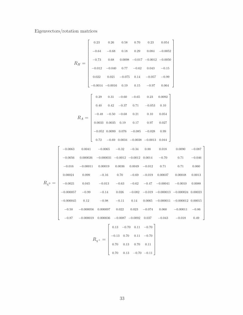
Eigenvectors/rotation matrices
RH =
0.23 0.26 0.58 0.70 0.23 0.054
−0.64 −0.68 0.18 0.29 0.084 −0.0052
−0.73 0.68 0.0098 −0.017 −0.0012 −0.0050
−0.012 −0.040 0.77 −0.62 0.043 −0.15
0.022 0.021 −0.075 0.14 −0.057 −0.99
−0.0014 −0.0016 0.19 0.15 −0.97 0.064
RA =
0.29 0.31 −0.60 −0.65 0.23 0.0092
0.40 0.42 −0.37 0.71 −0.053 0.10
−0.48 −0.50 −0.68 0.21 0.10 0.054
0.0033 0.0035 0.19 0.17 0.97 0.027
−0.052 0.0099 0.076 −0.085 −0.028 0.99
0.72 −0.69 0.0034 −0.0038 −0.0013 0.044
Rχ0 =
−0.0063 0.0041 −0.0065 −0.32 −0.34 0.88 0.018 0.0090 −0.087
−0.0056 0.000026 −0.000031 −0.0012 −0.0012 0.0014 −0.70 0.71 −0.046
−0.016 −0.00011 0.00019 0.0036 0.0049 −0.012 0.71 0.71 0.060
0.00024 0.099 −0.16 0.70 −0.69 −0.019 0.00037 0.00048 0.0013
−0.0021 0.045 −0.013 −0.63 −0.62 −0.47 −0.00041 −0.0010 0.0088
−0.000057 −0.99 −0.14 0.026 −0.082 −0.019 −0.000013 −0.000024 0.00023
−0.000045 0.12 −0.98 −0.11 0.14 0.0065 −0.000011 −0.000012 0.00015
−0.50 −0.000056 0.000097 0.022 0.023 −0.074 0.060 −0.00011 −0.86
−0.87 −0.000019 0.000036 −0.0087 −0.0092 0.037 −0.043 −0.018 0.49
Rχ+ =
0.13 −0.70 0.11 −0.70
−0.13 0.70 0.11 −0.70
0.70 0.13 0.70 0.11
0.70 0.13 −0.70 −0.11
33
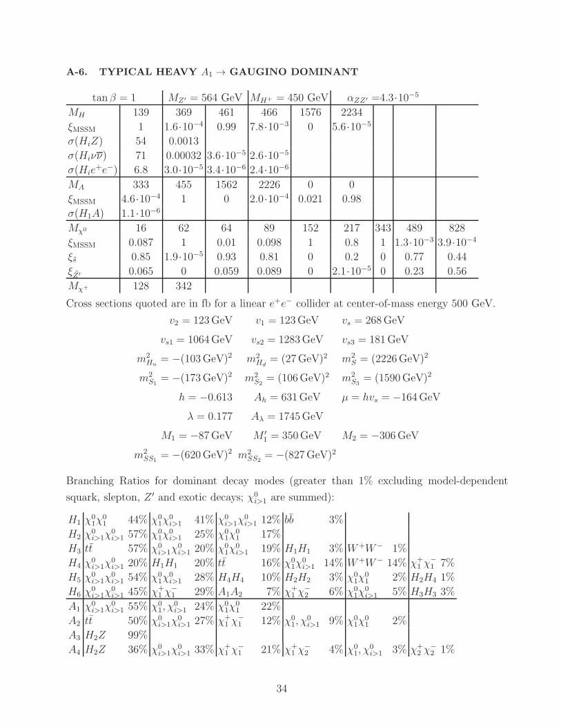
A-6. TYPICAL HEAVY A1 → GAUGINO DOMINANT
tanβ = 1 MZ′ = 564 GeV MH+ = 450 GeV αZZ′ =4.3·10−5
MH 139 369 461 466 1576 2234
ξMSSM 1 1.6·10−4 0.99 7.8·10−3 0 5.6·10−5
σ(HiZ) 54 0.0013
σ(Hiνν) 71 0.00032 3.6·10−5 2.6·10−5
σ(Hie+e−) 6.8 3.0·10−5 3.4·10−6 2.4·10−6
MA 333 455 1562 2226 0 0
ξMSSM 4.6·10−4 1 0 2.0·10−4 0.021 0.98
σ(H1A) 1.1·10−6
Mχ0 16 62 64 89 152 217 343 489 828
ξMSSM 0.087 1 0.01 0.098 1 0.8 1 1.3·10−3 3.9·10−4
ξs 0.85 1.9·10−5 0.93 0.81 0 0.2 0 0.77 0.44
ξZ′ 0.065 0 0.059 0.089 0 2.1·10−5 0 0.23 0.56
Mχ+ 128 342
Cross sections quoted are in fb for a linear e+e− collider at center-of-mass energy 500 GeV.
v2 = 123GeV v1 = 123GeV vs = 268GeV
vs1 = 1064GeV vs2 = 1283GeV vs3 = 181GeV
m2Hu
= −(103GeV)2 m2Hd
= (27GeV)2 m2S = (2226GeV)2
m2S1
= −(173GeV)2 m2S2
= (106GeV)2 m2S3
= (1590GeV)2
h = −0.613 Ah = 631GeV µ = hvs = −164GeV
λ = 0.177 Aλ = 1745GeV
M1 = −87GeV M ′1 = 350GeV M2 = −306GeV
m2SS1
= −(620GeV)2 m2SS2
= −(827GeV)2
Branching Ratios for dominant decay modes (greater than 1% excluding model-dependent
squark, slepton, Z ′ and exotic decays; χ0i>1 are summed):
H1 χ01χ
01 44% χ0
1χ0i>1 41% χ0
i>1χ0i>1 12% bb 3%
H2 χ0i>1χ
0i>1 57% χ0
1χ0i>1 25% χ0
1χ01 17%
H3 tt 57% χ0i>1χ
0i>1 20% χ0
1χ0i>1 19% H1H1 3% W+W− 1%
H4 χ0i>1χ
0i>1 20% H1H1 20% tt 16% χ0
1χ0i>1 14% W+W− 14% χ+
1 χ−1 7%
H5 χ0i>1χ
0i>1 54% χ0
1χ0i>1 28% H4H4 10% H2H2 3% χ0
1χ01 2% H2H4 1%
H6 χ0i>1χ
0i>1 45% χ+
1 χ−1 29% A1A2 7% χ+
1 χ−2 6% χ0
1χ0i>1 5% H3H3 3%
A1 χ0i>1χ
0i>1 55% χ0
1, χ0i>1 24% χ0
1χ01 22%
A2 tt 50% χ0i>1χ
0i>1 27% χ+
1 χ−1 12% χ0
1, χ0i>1 9% χ0
1χ01 2%
A3 H2Z 99%
A4 H2Z 36% χ0i>1χ
0i>1 33% χ+
1 χ−1 21% χ+
1 χ−2 4% χ0
1, χ0i>1 3% χ+
2 χ−2 1%
34
Eigenvectors/rotation matrices
RH =
0.68 0.73 0.00054 −0.033 −0.025 −0.0086
−0.0080 −0.0097 0.018 −0.81 0.58 −0.060
0.73 −0.68 −0.013 −0.043 −0.062 −0.019
0.085 −0.024 0.17 0.55 0.78 0.24
0.0012 0.0011 0.084 0.18 0.15 −0.97
−0.0052 −0.0053 0.98 −0.096 −0.16 0.041
RA =
−0.015 −0.015 0.031 0.77 −0.64 −0.042
0.70 0.71 −0.0054 −0.015 −0.053 0.011
−0.0013 −0.0013 −0.063 0.16 0.13 0.98
0.0099 0.0099 0.99 0.083 0.14 0.031
−0.060 0.13 −0.15 0.61 0.74 −0.21
0.71 −0.69 −0.021 0.083 0.10 −0.028
Rχ0 =
0.25 0.0017 −0.00074 0.21 0.21 −0.57 0.29 −0.47 0.48
−0.0019 0.85 −0.16 −0.35 0.35 −0.0013 −0.0013 0.0016 −0.0035
−0.24 −0.00017 0.00012 −0.072 −0.073 0.16 0.66 −0.48 −0.49
−0.30 −0.0044 −0.000085 0.22 0.22 −0.66 −0.19 0.16 −0.56
−0.00024 0.51 0.40 0.54 −0.54 −0.0019 −0.00021 −0.0000081 −0.00051
−0.0046 0.00028 −0.00029 0.63 0.63 0.44 0.018 0.011 −0.026
0.0000069 −0.073 0.90 −0.30 0.30 0.00022 −0.000038 −0.000035 −0.000042
0.48 0.000014 −0.000055 −0.025 −0.025 0.093 −0.54 −0.58 −0.36
−0.75 −0.0000057 0.0000083 −0.014 −0.014 0.077 −0.38 −0.43 0.31
Rχ+ =
−0.29 −0.64 0.29 0.64
0.29 0.64 0.29 0.64
0.64 −0.29 0.64 −0.29
0.64 −0.29 −0.64 0.29
35
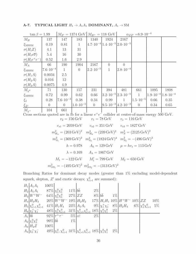
A-7. TYPICAL LIGHT H1 → A1A1 DOMINANT, A1 → SM
tanβ = 1.99 MZ′ = 1374 GeV MH+ = 118 GeV αZZ′ =8.9·10−4
MH 137 147 183 1340 1924 2167
ξMSSM 0.19 0.81 1 4.7·10−4 1.4·10−5 2.0·10−5
σ(HiZ) 4.1 13 31
σ(Hiνν) 5.4 16 30
σ(Hie+e−) 0.52 1.6 2.9
MA 66 190 1904 2167 0 0
ξMSSM 7.6·10−4 1 0 2.2·10−5 1 2.8·10−4
σ(H1A) 0.0034 2.5
σ(H2A) 0.016 12
σ(H3A) 0.0075 4.9
Mχ0 71 130 157 231 394 481 661 1095 1808
ξMSSM 0.72 0.99 0.62 0.66 3.2·10−5 2.3·10−5 1 1.9·10−4 1.8·10−4
ξs 0.28 7.6·10−3 0.38 0.34 0.99 1 1.5·10−5 0.66 0.35
ξZ′ 0 0 1.0·10−5 0 9.5·10−3 4.2·10−3 0 0.34 0.65
Mχ+ 104 661Cross sections quoted are in fb for a linear e+e− collider at center-of-mass energy 500 GeV.
v2 = 156GeV v1 = 78GeV vs = 116GeV
vs1 = 2059GeV vs2 = 351GeV vs3 = 1827GeV
m2Hu
= (203GeV)2 m2Hd
= (239GeV)2 m2S = (2125GeV)2
m2S1
= (369GeV)2 m2S2
= (1824GeV)2 m2S3
= −(496GeV)2
h = 0.978 Ah = 129GeV µ = hvs = 113GeV
λ = 0.169 Aλ = 1867GeV
M1 = −122GeV M ′1 = 799GeV M2 = 650GeV
m2SS1
= −(495GeV)2 m2SS2
= −(313GeV)2
Branching Ratios for dominant decay modes (greater than 1% excluding model-dependent
squark, slepton, Z ′ and exotic decays; χ0i>1 are summed):
H1 A1A1 100%
H2 A1A1 87% χ01χ
01 11% bb 2%
H3 W+W− 64% χ01χ
01 27% ZZ 8% bb 1%
H4 H3H3 20% W+W− 19% H2H2 17% H1H1 10% H+W− 10% ZZ 10%
H5 χ0i>1χ
0i>1 41% H1H4 23% A1A1 9% χ+
1 χ−1 8% H2H4 6% χ0
1χ0i>1 5%
H6 χ+1 χ
−1 48% χ0
1χ0i>1 31% χ0
i>1χ0i>1 18% χ0
1χ01 2%
A1 bb 92% τ+τ− 5% cc 2%
A2 χ01χ
01 99% bb 1%
A3 H2Z 100%
A4 χ+1 χ
−1 49% χ0
1, χ0i>1 31% χ0
i>1χ0i>1 18% χ0
1χ01 2%
36

Eigenvectors/rotation matrices
RH =
0.40 −0.18 −0.046 −0.76 −0.20 −0.44
0.78 −0.45 0.017 0.36 0.097 0.22
−0.48 −0.87 0.00072 −0.023 −0.0098 −0.034
0.019 0.0094 0.055 0.53 −0.22 −0.82
0.0035 0.0014 0.092 −0.079 0.95 −0.30
0.0044 −0.00088 0.99 −0.064 −0.086 0.049
RA =
0.012 0.025 −0.040 0.86 −0.23 0.46
0.45 0.89 −0.0031 −0.032 0.0052 0.0017
0.00035 0.00069 0.13 −0.16 −0.96 −0.18
0.0021 0.0042 0.99 0.068 0.12 0.018
0.89 −0.45 −0.000033 0.00059 0.00010 −0.0010
0.0063 0.015 −0.027 0.49 0.083 −0.87
Rχ0 =
0.0028 −0.18 −0.11 0.16 −0.81 0.52 0.021 0.0022 −0.019
0.00022 −0.98 0.019 −0.14 0.13 −0.087 −0.0031 0.00033 0.0025
−0.0032 −0.084 −0.087 0.75 −0.22 −0.62 −0.014 −0.0028 0.013
0.00012 0.072 −0.016 −0.63 −0.52 −0.58 −0.00074 0.00021 0.00048
−0.097 −0.00065 0.00031 0.0017 0.0054 −0.0076 0.68 −0.70 0.22
0.064 0.00014 0.00089 0.0030 0.0036 −0.0066 0.59 0.69 0.41
0.00067 −0.0079 0.99 0.075 −0.12 −0.0035 0.00032 −0.00049 −0.0014
−0.58 −0.00041 0.00041 0.0055 0.013 −0.018 0.34 0.19 −0.71
−0.80 −0.00017 0.00052 −0.0064 −0.012 0.018 −0.28 0.0014 0.52
Rχ+ =
0.12 −0.70 −0.074 0.70
−0.12 0.70 −0.074 0.70
0.70 0.12 −0.70 −0.074
0.70 0.12 0.70 0.074
37

A-8. TYPICAL LIGHT A1 → INVISIBLE DOMINANT
tanβ = 1.08 MZ′ = 2831 GeV MH+ = 622 GeV αZZ′ =2.7·10−5
MH 116 564 629 2739 3077 8917
ξMSSM 1 1.9·10−4 1 4.3·10−5 1.3·10−4 0
σ(HiZ) 58
σ(Hiνν) 88
σ(Hie+e−) 8.5
MA 78 621 3045 8916 0 0
ξMSSM 3.0·10−4 1 1.5·10−4 0 1 1.0·10−4
σ(H1A) 5.0·10−6
Mχ0 36 159 176 191 335 666 696 2236 3630
ξMSSM 0.17 1 0.83 1 1 0 0 5.2·10−5 4.1·10−5
ξs 0.83 4.1·10−4 0.17 9.0·10−4 0 1 1 0.63 0.38
ξZ′ 0 0 0 0 0 4.9·10−3 3.0·10−3 0.37 0.62
Mχ+ 154 335
Cross sections quoted are in fb for a linear e+e− collider at center-of-mass energy 500 GeV.
v2 = 128GeV v1 = 118GeV vs = 308GeV
vs1 = 118GeV vs2 = 4171GeV vs3 = 3800GeV
m2Hu
= (673GeV)2 m2Hd
= (702GeV)2 m2S = (2934GeV)2
m2S1
= (8914GeV)2 m2S2
= (699GeV)2 m2S3
= −(1201GeV)2
h = 0.456 Ah = 1371GeV µ = hvs = 140GeV
λ = 0.128 Aλ = 4510GeV
M1 = 185GeV M ′1 = −1425GeV M2 = 321GeV
m2SS1
= −(770GeV)2 m2SS2
= −(814GeV)2
Branching Ratios for dominant decay modes (greater than 1% excluding model-dependent
squark, slepton, Z ′ and exotic decays; χ0i>1 are summed):
H1 χ01χ
01 97% bb 3%
H2 H1H1 26% W+W− 21% χ+1 χ
−1 15% χ0
i>1χ0i>1 12% ZZ 10% tt 8%
H3 tt 70% χ01χ
0i>1 14% χ0
i>1χ0i>1 10% χ+
1 χ−2 4% H1H1 1%
H4 A1A2 40% H3H3 19% χ+1 χ
−1 13% χ0
i>1χ0i>1 13% H1H1 4% W+W− 4%
H5 χ+1 χ
−1 37% χ0
i>1χ0i>1 33% χ0
1χ0i>1 7% A1A2 7% H1H1 4% W+W− 4%
H6 χ0i>1χ
0i>1 96% H2H4 2% H2H2 1%
A1 χ01χ
01 99% bb 1%
A2 tt 73% χ0i>1χ
0i>1 12% χ0
1, χ0i>1 7% χ0
1χ01 5% χ+
1 χ−1 2%
A3 H2Z 100%
A4 χ0i>1χ
0i>1 67% H5Z 27% A1H2 4% A2H5 1%
38
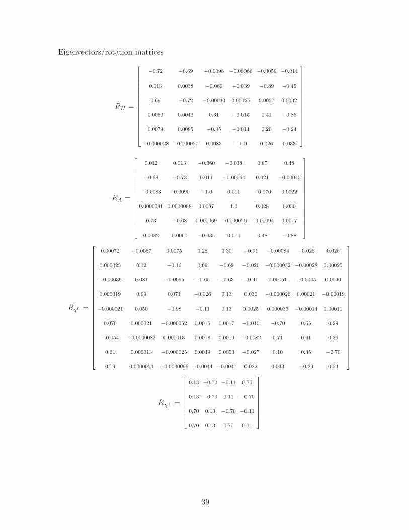
Eigenvectors/rotation matrices
RH =
−0.72 −0.69 −0.0098 −0.00066 −0.0059 −0.014
0.013 0.0038 −0.069 −0.039 −0.89 −0.45
0.69 −0.72 −0.00030 0.00025 0.0057 0.0032
0.0050 0.0042 0.31 −0.015 0.41 −0.86
0.0079 0.0085 −0.95 −0.011 0.20 −0.24
−0.000028 −0.000027 0.0083 −1.0 0.026 0.033
RA =
0.012 0.013 −0.060 −0.038 0.87 0.48
−0.68 −0.73 0.011 −0.00064 0.021 −0.00045
−0.0083 −0.0090 −1.0 0.011 −0.070 0.0022
0.0000081 0.0000088 0.0087 1.0 0.028 0.030
0.73 −0.68 0.000069 −0.000026 −0.00094 0.0017
0.0082 0.0060 −0.035 0.014 0.48 −0.88
Rχ0 =
0.00072 −0.0067 0.0075 0.28 0.30 −0.91 −0.00084 −0.028 0.026
0.000025 0.12 −0.16 0.69 −0.69 −0.020 −0.000032 −0.00028 0.00025
−0.00036 0.081 −0.0095 −0.65 −0.63 −0.41 0.00051 −0.0045 0.0040
0.000019 0.99 0.071 −0.026 0.13 0.030 −0.000026 0.00021 −0.00019
−0.000021 0.050 −0.98 −0.11 0.13 0.0025 0.000036 −0.00014 0.00011
0.070 0.000021 −0.000052 0.0015 0.0017 −0.010 −0.70 0.65 0.29
−0.054 −0.0000082 0.000013 0.0018 0.0019 −0.0082 0.71 0.61 0.36
0.61 0.000013 −0.000025 0.0049 0.0053 −0.027 0.10 0.35 −0.70
0.79 0.0000054 −0.0000096 −0.0044 −0.0047 0.022 0.033 −0.29 0.54
Rχ+ =
0.13 −0.70 −0.11 0.70
0.13 −0.70 0.11 −0.70
0.70 0.13 −0.70 −0.11
0.70 0.13 0.70 0.11
39

A-9. TYPICAL HEAVY H1 → W+W− DOMINANT
tan β = 0.909 MZ′ = 1200 GeV MH+ = 326 GeV αZZ′ =-1.8·10−4
MH 178 346 367 1051 1224 3379
ξMSSM 1 1 1.2·10−3 1.3·10−4 4.1·10−4 1.4·10−5
σ(HiZ) 47 0.18 0.0025
σ(Hiνν) 47 0.051 0.00061
σ(Hie+e−) 4.5 0.0049 5.9·10−5
MA 351 367 1082 3378 0 0
ξMSSM 0.91 0.091 0 4.9·10−5 1 5.7·10−4
Mχ0 97 111 203 209 232 339 546 847 1711
ξMSSM 0.81 0.5 3.1·10−5 4.7·10−5 0.68 1 1 2.7·10−4 2.1·10−4
ξs 0.19 0.5 1 1 0.32 0 0 0.67 0.33
ξZ′ 0 1.2·10−5 1.5·10−3 5.6·10−4 0 0 0 0.33 0.67
Mχ+ 109 546
Cross sections quoted are in fb for a linear e+e− collider at center-of-mass energy 500 GeV.
v2 = 117GeV v1 = 129GeV vs = 137GeV
vs1 = 3643GeV vs2 = 436GeV vs3 = 114GeV
m2Hu
= −(574GeV)2 m2Hd
= −(573GeV)2 m2S = (3473GeV)2
m2S1
= −(837GeV)2 m2S2
= −(720GeV)2 m2S3
= (1572GeV)2
h = 0.907 Ah = 502GeV µ = hvs = 124GeV
λ = 0.058 Aλ = 1343GeV
M1 = 332GeV M ′1 = 871GeV M2 = 531GeV
m2SS1
= −(601GeV)2 m2SS2
= −(729GeV)2
Branching Ratios for dominant decay modes (greater than 1% excluding model-dependent
squark, slepton, Z ′ and exotic decays; χ0i>1 are summed):
H1 W+W− 99% bb 1%
H2 χ01χ
01 38% χ0
1χ0i>1 30% χ0
i>1χ0i>1 24% W+W− 5% ZZ 2%
H3 χ01χ
0i>1 30% χ+
1 χ−1 27% W+W− 15% H1H1 11% χ0
i>1χ0i>1 8% ZZ 7%
H4 H3H3 24% H1H1 16% W+W− 14% H2H2 13% χ0i>1χ
0i>1 12% A1A1 11%
H5 H3H3 21% H2H2 16% A1A1 14% H1H1 13% χ0i>1χ
0i>1 13% W+W− 12%
H6 χ+1 χ
−1 45% χ0
i>1χ0i>1 22% χ0
1χ0i>1 22% χ0
1χ01 8% H2H2 1% A1A1 1%
A1 χ01, χ
0i>1 63% χ0
i>1χ0i>1 28% χ+
1 χ−1 5% H1Z 2% tt 1% χ0
1χ01 1%
A2 H1Z 94% χ01, χ
0i>1 2% χ0
i>1χ0i>1 2% χ+
1 χ−1 1% tt 1%
A3 H1Z 53% χ0i>1χ
0i>1 39% H2Z 4% A1H1 2% χ+
1 χ−1 1%
A4 χ+1 χ
−1 46% χ0
i>1χ0i>1 23% χ0
1, χ0i>1 22% χ0
1χ01 8% H5Z 1%
40
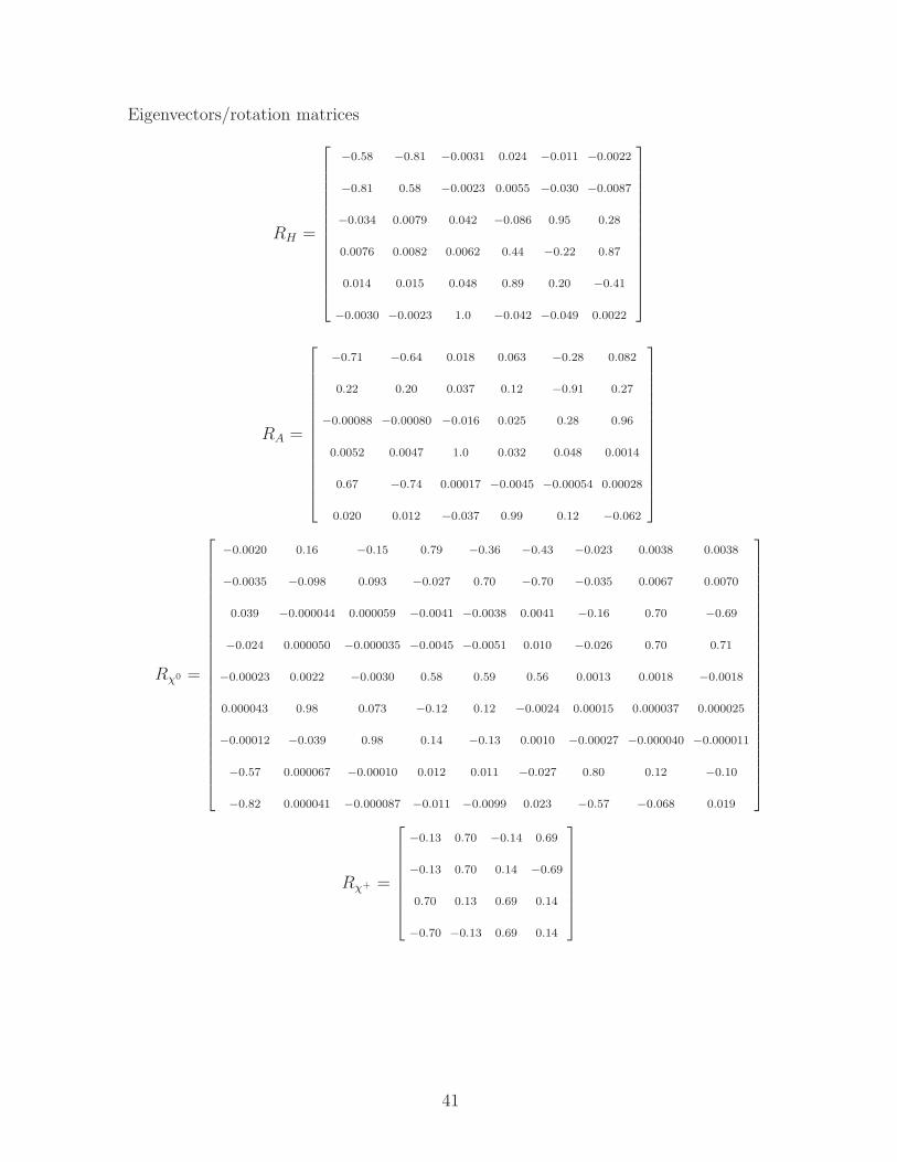
Eigenvectors/rotation matrices
RH =
−0.58 −0.81 −0.0031 0.024 −0.011 −0.0022
−0.81 0.58 −0.0023 0.0055 −0.030 −0.0087
−0.034 0.0079 0.042 −0.086 0.95 0.28
0.0076 0.0082 0.0062 0.44 −0.22 0.87
0.014 0.015 0.048 0.89 0.20 −0.41
−0.0030 −0.0023 1.0 −0.042 −0.049 0.0022
RA =
−0.71 −0.64 0.018 0.063 −0.28 0.082
0.22 0.20 0.037 0.12 −0.91 0.27
−0.00088 −0.00080 −0.016 0.025 0.28 0.96
0.0052 0.0047 1.0 0.032 0.048 0.0014
0.67 −0.74 0.00017 −0.0045 −0.00054 0.00028
0.020 0.012 −0.037 0.99 0.12 −0.062
Rχ0 =
−0.0020 0.16 −0.15 0.79 −0.36 −0.43 −0.023 0.0038 0.0038
−0.0035 −0.098 0.093 −0.027 0.70 −0.70 −0.035 0.0067 0.0070
0.039 −0.000044 0.000059 −0.0041 −0.0038 0.0041 −0.16 0.70 −0.69
−0.024 0.000050 −0.000035 −0.0045 −0.0051 0.010 −0.026 0.70 0.71
−0.00023 0.0022 −0.0030 0.58 0.59 0.56 0.0013 0.0018 −0.0018
0.000043 0.98 0.073 −0.12 0.12 −0.0024 0.00015 0.000037 0.000025
−0.00012 −0.039 0.98 0.14 −0.13 0.0010 −0.00027 −0.000040 −0.000011
−0.57 0.000067 −0.00010 0.012 0.011 −0.027 0.80 0.12 −0.10
−0.82 0.000041 −0.000087 −0.011 −0.0099 0.023 −0.57 −0.068 0.019
Rχ+ =
−0.13 0.70 −0.14 0.69
−0.13 0.70 0.14 −0.69
0.70 0.13 0.69 0.14
−0.70 −0.13 0.69 0.14
41

A-10. LIGHT CHARGED HIGGS
tan β = 1.38 MZ′ = 595 GeV MH+ = 76 GeV αZZ′ =2.5·10−3
MH 118 168 199 550 1767 1932
ξMSSM 1 0.42 0.58 3.6·10−3 0 1.6·10−5
σ(HiZ) 0.017 21 25
σ(Hiνν) 0.025 22 22
σ(Hie+e−) 0.0024 2.1 2.1
MA 117 168 1760 1930 0 0
ξMSSM 0 1 0 3.3·10−5 1 2.1·10−3
σ(H1A) 8.2·10−5 28
σ(H2A) 3.0·10−8 0.0099
σ(H3A) 9.6·10−10 0.00029
Mχ0 54 118 150 156 182 230 552 600 676
ξMSSM 0.97 0.49 0.18 0.71 9.5·10−5 0.65 1.6·10−3 1 9.0·10−4
ξs 0.031 0.51 0.8 0.29 0.98 0.35 0.6 7.4·10−5 0.44
ξZ′ 0 1.3·10−3 0.019 2.8·10−3 0.017 0 0.4 6.6·10−5 0.56
Mχ+ 115 600Cross sections quoted are in fb for a linear e+e− collider at center-of-mass energy 500 GeV.
v2 = 141GeV v1 = 102GeV vs = 109GeV
vs1 = 538GeV vs2 = 1714GeV vs3 = 141GeV
m2Hu
= −(325GeV)2 m2Hd
= −(309GeV)2 m2S = (1963GeV)2
m2S1
= (57GeV)2 m2S2
= −(375GeV)2 m2S3
= (1783GeV)2
h = −0.976 Ah = 126GeV µ = hvs = −107GeV
λ = 0.114 Aλ = 3860GeV
M1 = −90GeV M ′1 = 157GeV M2 = 591GeV
m2SS1
= −(266GeV)2 m2SS2
= −(462GeV)2
Branching Ratios for dominant decay modes (greater than 1% excluding model-dependent
squark, slepton, Z ′ and exotic decays; χ0i>1 are summed):
H1 χ01χ
01 56% bb 39% τ+τ− 2% cc 2%
H2 W+W− 77% H+W− 11% H+H− 6% χ01χ
01 6% bb 1%
H3 W+W− 56% H+W− 20% ZZ 20% χ01χ
01 2% H+H− 2% χ0
1χ0i>1 1%
H4 H2H3 18% H1H1 17% W+W− 15% χ0i>1χ
0i>1 11% H+W− 9% ZZ 7%
H5 χ0i>1χ
0i>1 79% H2H4 10% H3H4 8% χ+
1 χ−1 1% H2H2 1%
H6 χ+1 χ
−1 47% χ0
i>1χ0i>1 36% χ0
1χ0i>1 13% χ0
1χ01 3% H1H1 1%
A1 χ01χ
01 91% bb 8%
A2 H+W− 60% H+H− 24% χ01χ
01 11% bb 4%
A3 χ0i>1χ
0i>1 97% A2H3 1% χ+
1 χ−1 1% A1H2 1%
A4 χ+1 χ
−1 46% χ0
i>1χ0i>1 35% χ0
1, χ0i>1 13% χ0
1χ01 3% A2H4 1% χ+
1 χ−2 1%
42
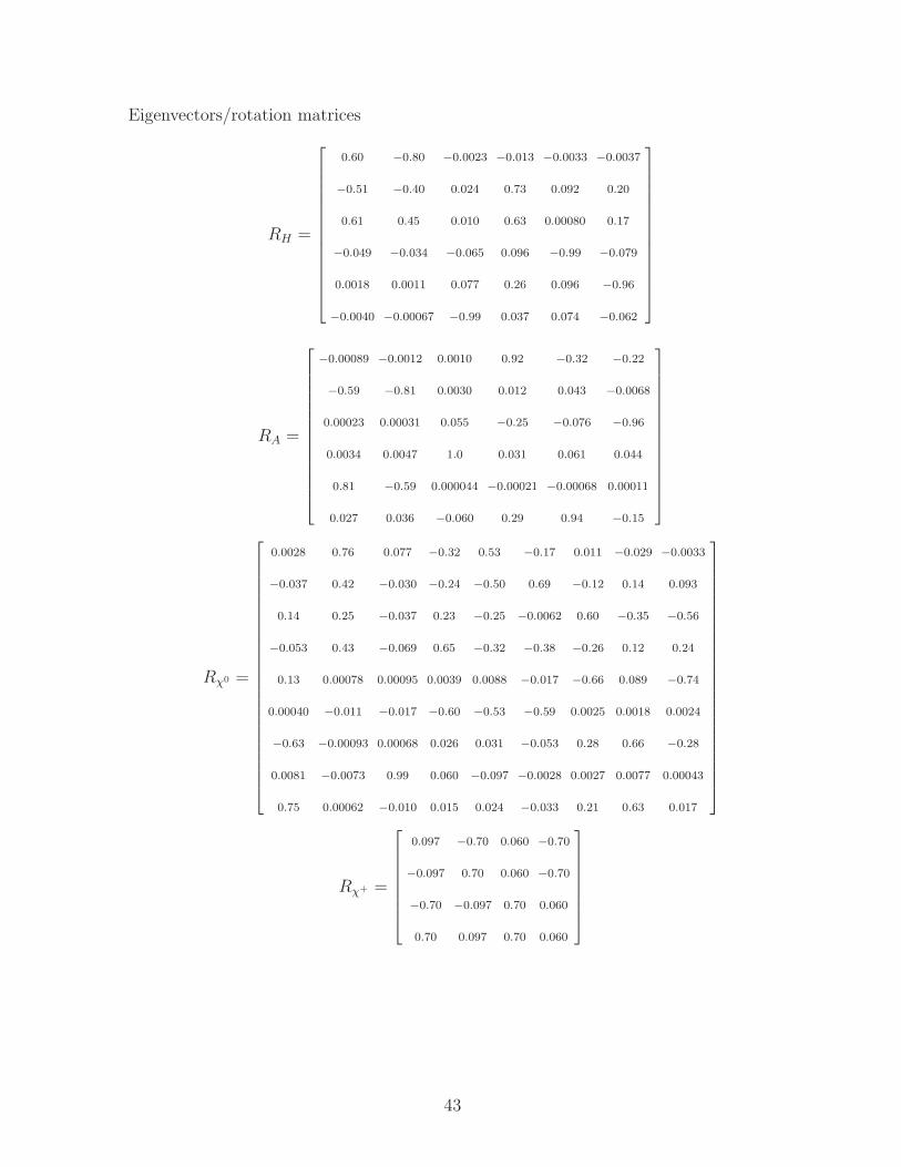
Eigenvectors/rotation matrices
RH =
0.60 −0.80 −0.0023 −0.013 −0.0033 −0.0037
−0.51 −0.40 0.024 0.73 0.092 0.20
0.61 0.45 0.010 0.63 0.00080 0.17
−0.049 −0.034 −0.065 0.096 −0.99 −0.079
0.0018 0.0011 0.077 0.26 0.096 −0.96
−0.0040 −0.00067 −0.99 0.037 0.074 −0.062
RA =
−0.00089 −0.0012 0.0010 0.92 −0.32 −0.22
−0.59 −0.81 0.0030 0.012 0.043 −0.0068
0.00023 0.00031 0.055 −0.25 −0.076 −0.96
0.0034 0.0047 1.0 0.031 0.061 0.044
0.81 −0.59 0.000044 −0.00021 −0.00068 0.00011
0.027 0.036 −0.060 0.29 0.94 −0.15
Rχ0 =
0.0028 0.76 0.077 −0.32 0.53 −0.17 0.011 −0.029 −0.0033
−0.037 0.42 −0.030 −0.24 −0.50 0.69 −0.12 0.14 0.093
0.14 0.25 −0.037 0.23 −0.25 −0.0062 0.60 −0.35 −0.56
−0.053 0.43 −0.069 0.65 −0.32 −0.38 −0.26 0.12 0.24
0.13 0.00078 0.00095 0.0039 0.0088 −0.017 −0.66 0.089 −0.74
0.00040 −0.011 −0.017 −0.60 −0.53 −0.59 0.0025 0.0018 0.0024
−0.63 −0.00093 0.00068 0.026 0.031 −0.053 0.28 0.66 −0.28
0.0081 −0.0073 0.99 0.060 −0.097 −0.0028 0.0027 0.0077 0.00043
0.75 0.00062 −0.010 0.015 0.024 −0.033 0.21 0.63 0.017
Rχ+ =
0.097 −0.70 0.060 −0.70
−0.097 0.70 0.060 −0.70
−0.70 −0.097 0.70 0.060
0.70 0.097 0.70 0.060
43
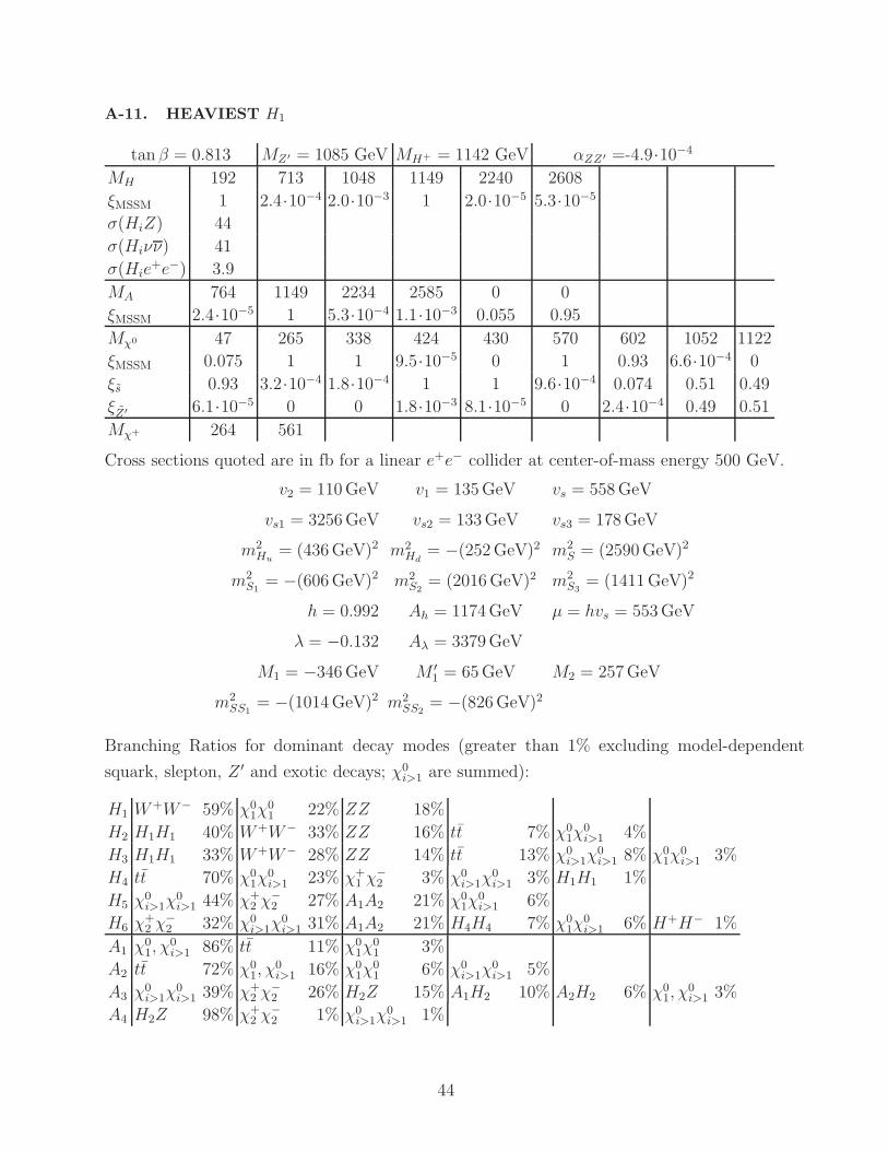
A-11. HEAVIEST H1
tan β = 0.813 MZ′ = 1085 GeV MH+ = 1142 GeV αZZ′ =-4.9·10−4
MH 192 713 1048 1149 2240 2608
ξMSSM 1 2.4·10−4 2.0·10−3 1 2.0·10−5 5.3·10−5
σ(HiZ) 44
σ(Hiνν) 41
σ(Hie+e−) 3.9
MA 764 1149 2234 2585 0 0
ξMSSM 2.4·10−5 1 5.3·10−4 1.1·10−3 0.055 0.95
Mχ0 47 265 338 424 430 570 602 1052 1122
ξMSSM 0.075 1 1 9.5·10−5 0 1 0.93 6.6·10−4 0
ξs 0.93 3.2·10−4 1.8·10−4 1 1 9.6·10−4 0.074 0.51 0.49
ξZ′ 6.1·10−5 0 0 1.8·10−3 8.1·10−5 0 2.4·10−4 0.49 0.51
Mχ+ 264 561
Cross sections quoted are in fb for a linear e+e− collider at center-of-mass energy 500 GeV.
v2 = 110GeV v1 = 135GeV vs = 558GeV
vs1 = 3256GeV vs2 = 133GeV vs3 = 178GeV
m2Hu
= (436GeV)2 m2Hd
= −(252GeV)2 m2S = (2590GeV)2
m2S1
= −(606GeV)2 m2S2
= (2016GeV)2 m2S3
= (1411GeV)2
h = 0.992 Ah = 1174GeV µ = hvs = 553GeV
λ = −0.132 Aλ = 3379GeV
M1 = −346GeV M ′1 = 65GeV M2 = 257GeV
m2SS1
= −(1014GeV)2 m2SS2
= −(826GeV)2
Branching Ratios for dominant decay modes (greater than 1% excluding model-dependent
squark, slepton, Z ′ and exotic decays; χ0i>1 are summed):
H1 W+W− 59% χ01χ
01 22% ZZ 18%
H2 H1H1 40% W+W− 33% ZZ 16% tt 7% χ01χ
0i>1 4%
H3 H1H1 33% W+W− 28% ZZ 14% tt 13% χ0i>1χ
0i>1 8% χ0
1χ0i>1 3%
H4 tt 70% χ01χ
0i>1 23% χ+
1 χ−2 3% χ0
i>1χ0i>1 3% H1H1 1%
H5 χ0i>1χ
0i>1 44% χ+
2 χ−2 27% A1A2 21% χ0
1χ0i>1 6%
H6 χ+2 χ
−2 32% χ0
i>1χ0i>1 31% A1A2 21% H4H4 7% χ0
1χ0i>1 6% H+H− 1%
A1 χ01, χ
0i>1 86% tt 11% χ0
1χ01 3%
A2 tt 72% χ01, χ
0i>1 16% χ0
1χ01 6% χ0
i>1χ0i>1 5%
A3 χ0i>1χ
0i>1 39% χ+
2 χ−2 26% H2Z 15% A1H2 10% A2H2 6% χ0
1, χ0i>1 3%
A4 H2Z 98% χ+2 χ
−2 1% χ0
i>1χ0i>1 1%
44
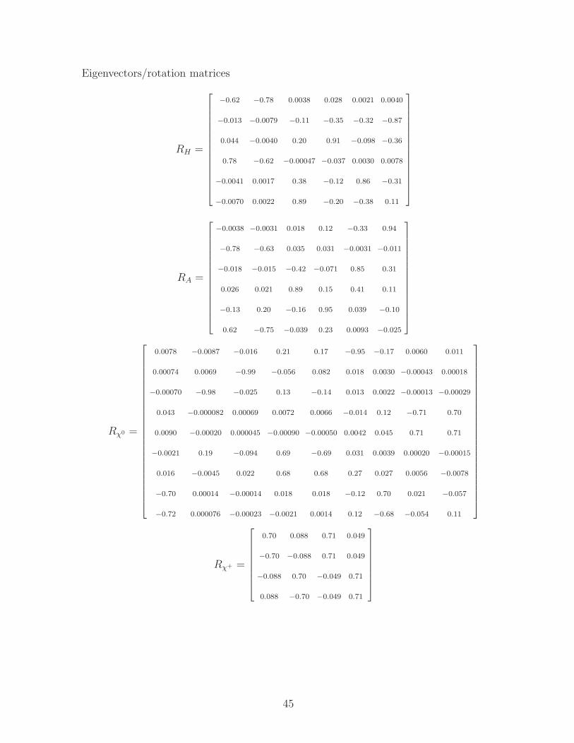
Eigenvectors/rotation matrices
RH =
−0.62 −0.78 0.0038 0.028 0.0021 0.0040
−0.013 −0.0079 −0.11 −0.35 −0.32 −0.87
0.044 −0.0040 0.20 0.91 −0.098 −0.36
0.78 −0.62 −0.00047 −0.037 0.0030 0.0078
−0.0041 0.0017 0.38 −0.12 0.86 −0.31
−0.0070 0.0022 0.89 −0.20 −0.38 0.11
RA =
−0.0038 −0.0031 0.018 0.12 −0.33 0.94
−0.78 −0.63 0.035 0.031 −0.0031 −0.011
−0.018 −0.015 −0.42 −0.071 0.85 0.31
0.026 0.021 0.89 0.15 0.41 0.11
−0.13 0.20 −0.16 0.95 0.039 −0.10
0.62 −0.75 −0.039 0.23 0.0093 −0.025
Rχ0 =
0.0078 −0.0087 −0.016 0.21 0.17 −0.95 −0.17 0.0060 0.011
0.00074 0.0069 −0.99 −0.056 0.082 0.018 0.0030 −0.00043 0.00018
−0.00070 −0.98 −0.025 0.13 −0.14 0.013 0.0022 −0.00013 −0.00029
0.043 −0.000082 0.00069 0.0072 0.0066 −0.014 0.12 −0.71 0.70
0.0090 −0.00020 0.000045 −0.00090 −0.00050 0.0042 0.045 0.71 0.71
−0.0021 0.19 −0.094 0.69 −0.69 0.031 0.0039 0.00020 −0.00015
0.016 −0.0045 0.022 0.68 0.68 0.27 0.027 0.0056 −0.0078
−0.70 0.00014 −0.00014 0.018 0.018 −0.12 0.70 0.021 −0.057
−0.72 0.000076 −0.00023 −0.0021 0.0014 0.12 −0.68 −0.054 0.11
Rχ+ =
0.70 0.088 0.71 0.049
−0.70 −0.088 0.71 0.049
−0.088 0.70 −0.049 0.71
0.088 −0.70 −0.049 0.71
45

A-12. HEAVIEST A1
tanβ = 0.71 MZ′ = 1263 GeV MH+ = 1275 GeV αZZ′ =-5.8·10−4
MH 130 973 1209 1283 2003 2369
ξMSSM 1 5.2·10−4 0.012 0.99 2.3·10−3 1.0·10−4
σ(HiZ) 56
σ(Hiνν) 77
σ(Hie+e−) 7.4
MA 998 1269 1966 2364 0 0
ξMSSM 8.8·10−4 0.99 0.011 2.6·10−4 8.7·10−3 0.99
Mχ0 33 198 198 398 412 507 509 809 1973
ξMSSM 0.08 1 1 1 0.92 0 0 6.2·10−4 9.0·10−5
ξs 0.92 1.7·10−3 1.0·10−3 2.4·10−3 0.076 1 1 0.71 0.29
ξZ′ 1.5·10−5 0 0 0 2.4·10−5 3.3·10−4 3.1·10−4 0.29 0.71
Mχ+ 197 389
Cross sections quoted are in fb for a linear e+e− collider at center-of-mass energy 500 GeV.
v2 = 101GeV v1 = 142GeV vs = 544GeV
vs1 = 102GeV vs2 = 3826GeV vs3 = 93GeV
m2Hu
= (734GeV)2 m2Hd
= (133GeV)2 m2S = (2149GeV)2
m2S1
= (1836GeV)2 m2S2
= −(829GeV)2 m2S3
= (1833GeV)2
h = −0.693 Ah = 2048GeV µ = hvs = −377GeV
λ = 0.133 Aλ = 3752GeV
M1 = −208GeV M ′1 = 1164GeV M2 = 187GeV
m2SS1
= −(707GeV)2 m2SS2
= −(729GeV)2
Branching Ratios for dominant decay modes (greater than 1% excluding model-dependent
squark, slepton, Z ′ and exotic decays; χ0i>1 are summed):
H1 χ01χ
01 97% bb 3%
H2 W+W− 22% H1H1 21% χ+2 χ
−2 17% χ0
i>1χ0i>1 17% ZZ 11% χ0
1χ0i>1 10%
H3 tt 35% χ0i>1χ
0i>1 28% χ+
2 χ−2 21% χ0
1χ0i>1 12% χ+
1 χ−2 4%
H4 tt 71% χ01χ
0i>1 14% χ0
i>1χ0i>1 9% χ+
1 χ−2 6%
H5 χ+2 χ
−2 33% χ0
i>1χ0i>1 32% W+W− 9% H1H1 9% χ0
1χ0i>1 6% ZZ 5%
H6 χ0i>1χ
0i>1 50% χ+
2 χ−2 20% A1A2 9% W+W− 4% H1H1 4% χ0
1χ0i>1 4%
A1 χ+2 χ
−2 33% tt 25% χ0
i>1χ0i>1 25% χ0
1, χ0i>1 15% χ0
1χ01 2%
A2 tt 73% χ01, χ
0i>1 12% χ0
i>1χ0i>1 10% χ0
1χ01 3% χ+
2 χ−2 1% χ+
1 χ−1 1%
A3 χ0i>1χ
0i>1 33% χ+
2 χ−2 31% H2Z 28% A2H2 4% χ0
1, χ0i>1 3% tt 2%
A4 H2Z 99% H3Z 1%
46
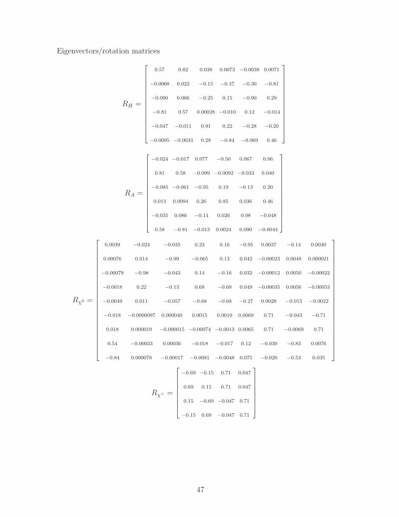
Eigenvectors/rotation matrices
RH =
0.57 0.82 0.038 0.0073 −0.0038 0.0071
−0.0068 0.022 −0.15 −0.47 −0.30 −0.81
−0.090 0.066 −0.25 0.15 −0.90 0.29
−0.81 0.57 0.00028 −0.010 0.12 −0.014
−0.047 −0.011 0.91 0.22 −0.28 −0.20
−0.0095 −0.0033 0.28 −0.84 −0.069 0.46
RA =
−0.024 −0.017 0.077 −0.50 0.067 0.86
0.81 0.58 −0.099 −0.0092 −0.033 0.040
−0.085 −0.061 −0.95 0.19 −0.13 0.20
0.013 0.0094 0.26 0.85 0.036 0.46
−0.035 0.086 −0.14 0.026 0.98 −0.048
0.58 −0.81 −0.013 0.0024 0.090 −0.0044
Rχ0 =
0.0039 −0.024 −0.035 0.23 0.16 −0.95 0.0037 −0.14 0.0040
0.00076 0.014 −0.99 −0.065 0.13 0.042 −0.00023 0.0048 0.000021
−0.00079 −0.98 −0.043 0.14 −0.16 0.032 −0.00012 0.0050 −0.00022
−0.0018 0.22 −0.13 0.68 −0.68 0.049 −0.00035 0.0056 −0.00053
−0.0049 0.011 −0.057 −0.68 −0.68 −0.27 0.0028 −0.015 −0.0022
−0.018 −0.0000097 0.000040 0.0015 0.0019 0.0069 0.71 −0.043 −0.71
0.018 0.000019 −0.000015 −0.00074 −0.0013 0.0065 0.71 −0.0069 0.71
0.54 −0.00033 0.00036 −0.018 −0.017 0.12 −0.030 −0.83 0.0076
−0.84 0.000078 −0.00017 −0.0081 −0.0048 0.075 −0.020 −0.53 0.035
Rχ+ =
−0.69 −0.15 0.71 0.047
0.69 0.15 0.71 0.047
0.15 −0.69 −0.047 0.71
−0.15 0.69 −0.047 0.71
47
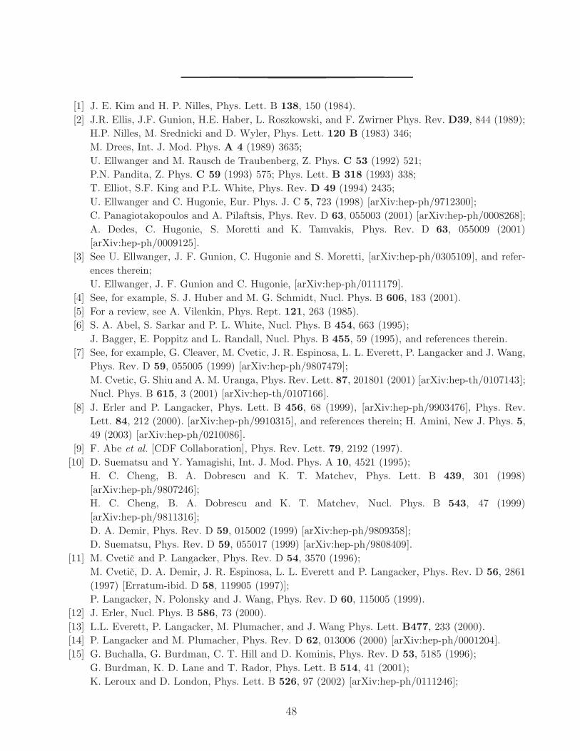
[1] J. E. Kim and H. P. Nilles, Phys. Lett. B 138, 150 (1984).
[2] J.R. Ellis, J.F. Gunion, H.E. Haber, L. Roszkowski, and F. Zwirner Phys. Rev. D39, 844 (1989);
H.P. Nilles, M. Srednicki and D. Wyler, Phys. Lett. 120 B (1983) 346;
M. Drees, Int. J. Mod. Phys. A 4 (1989) 3635;
U. Ellwanger and M. Rausch de Traubenberg, Z. Phys. C 53 (1992) 521;
P.N. Pandita, Z. Phys. C 59 (1993) 575; Phys. Lett. B 318 (1993) 338;
T. Elliot, S.F. King and P.L. White, Phys. Rev. D 49 (1994) 2435;
U. Ellwanger and C. Hugonie, Eur. Phys. J. C 5, 723 (1998) [arXiv:hep-ph/9712300];
C. Panagiotakopoulos and A. Pilaftsis, Phys. Rev. D 63, 055003 (2001) [arXiv:hep-ph/0008268];
A. Dedes, C. Hugonie, S. Moretti and K. Tamvakis, Phys. Rev. D 63, 055009 (2001)
[arXiv:hep-ph/0009125].
[3] See U. Ellwanger, J. F. Gunion, C. Hugonie and S. Moretti, [arXiv:hep-ph/0305109], and refer-
ences therein;
U. Ellwanger, J. F. Gunion and C. Hugonie, [arXiv:hep-ph/0111179].
[4] See, for example, S. J. Huber and M. G. Schmidt, Nucl. Phys. B 606, 183 (2001).
[5] For a review, see A. Vilenkin, Phys. Rept. 121, 263 (1985).
[6] S. A. Abel, S. Sarkar and P. L. White, Nucl. Phys. B 454, 663 (1995);
J. Bagger, E. Poppitz and L. Randall, Nucl. Phys. B 455, 59 (1995), and references therein.
[7] See, for example, G. Cleaver, M. Cvetic, J. R. Espinosa, L. L. Everett, P. Langacker and J. Wang,
Phys. Rev. D 59, 055005 (1999) [arXiv:hep-ph/9807479];
M. Cvetic, G. Shiu and A. M. Uranga, Phys. Rev. Lett. 87, 201801 (2001) [arXiv:hep-th/0107143];
Nucl. Phys. B 615, 3 (2001) [arXiv:hep-th/0107166].
[8] J. Erler and P. Langacker, Phys. Lett. B 456, 68 (1999), [arXiv:hep-ph/9903476], Phys. Rev.
Lett. 84, 212 (2000). [arXiv:hep-ph/9910315], and references therein; H. Amini, New J. Phys. 5,
49 (2003) [arXiv:hep-ph/0210086].
[9] F. Abe et al. [CDF Collaboration], Phys. Rev. Lett. 79, 2192 (1997).
[10] D. Suematsu and Y. Yamagishi, Int. J. Mod. Phys. A 10, 4521 (1995);
H. C. Cheng, B. A. Dobrescu and K. T. Matchev, Phys. Lett. B 439, 301 (1998)
[arXiv:hep-ph/9807246];
H. C. Cheng, B. A. Dobrescu and K. T. Matchev, Nucl. Phys. B 543, 47 (1999)
[arXiv:hep-ph/9811316];
D. A. Demir, Phys. Rev. D 59, 015002 (1999) [arXiv:hep-ph/9809358];
D. Suematsu, Phys. Rev. D 59, 055017 (1999) [arXiv:hep-ph/9808409].
[11] M. Cvetic and P. Langacker, Phys. Rev. D 54, 3570 (1996);
M. Cvetic, D. A. Demir, J. R. Espinosa, L. L. Everett and P. Langacker, Phys. Rev. D 56, 2861
(1997) [Erratum-ibid. D 58, 119905 (1997)];
P. Langacker, N. Polonsky and J. Wang, Phys. Rev. D 60, 115005 (1999).
[12] J. Erler, Nucl. Phys. B 586, 73 (2000).
[13] L.L. Everett, P. Langacker, M. Plumacher, and J. Wang Phys. Lett. B477, 233 (2000).
[14] P. Langacker and M. Plumacher, Phys. Rev. D 62, 013006 (2000) [arXiv:hep-ph/0001204].
[15] G. Buchalla, G. Burdman, C. T. Hill and D. Kominis, Phys. Rev. D 53, 5185 (1996);
G. Burdman, K. D. Lane and T. Rador, Phys. Lett. B 514, 41 (2001);
K. Leroux and D. London, Phys. Lett. B 526, 97 (2002) [arXiv:hep-ph/0111246];
48
V. Barger, C. W. Chiang, P. Langacker and H. S. Lee, Phys. Lett. B 580, 186 (2004)
[arXiv:hep-ph/0310073];
A. Martin and K. Lane, [arXiv:hep-ph/0404107];
X. G. He and G. Valencia, arXiv:hep-ph/0404229;
V. Barger, C. W. Chiang, J. Jiang and P. Langacker, [arXiv:hep-ph/0405108].
[16] D. A. Demir and L. L. Everett, Phys. Rev. D 69, 015008 (2004) [arXiv:hep-ph/0306240].
[17] B. de Carlos and J. R. Espinosa, Phys. Lett. B 407, 12 (1997) [arXiv:hep-ph/9705315].
[18] J. Kang, P. Langacker, T. J. Li, and T. Liu; [arXiv:hep-ph/0402086].
[19] J. Erler, P. Langacker and T. J. Li, Phys. Rev. D 66, 015002 (2002) [arXiv:hep-ph/0205001].
[20] P. Langacker and J. Wang, Phys. Rev. D 58, 115010 (1998) [arXiv:hep-ph/9804428].
[21] J. R. Espinosa and R. J. Zhang, JHEP 0003, 026 (2000) [arXiv:hep-ph/9912236];
R. J. Zhang, [arXiv:hep-ph/0003248];
Y. Okada, M. Yamaguchi and T. Yanagida, Prog. Theor. Phys. 85, 1 (1991);
J. R. Ellis, G. Ridolfi and F. Zwirner, Phys. Lett. B 257, 83 (1991);
H. E. Haber and R. Hempfling, Phys. Rev. Lett. 66, 1815 (1991).
[22] G. L. Kane, C. F. Kolda and J. D. Wells, Phys. Rev. Lett. 70, 2686 (1993) [arXiv:hep-ph/9210242].
[23] J. R. Espinosa and M. Quiros, Phys. Rev. Lett. 81, 516 (1998) [arXiv:hep-ph/9804235];
[arXiv:hep-ph/9809269].
[24] U. Ellwanger and M. Lindner, Phys. Lett. B 301, 365 (1993);
U. Ellwanger and C. Hugonie, [arXiv:hep-ph/0006222];
Eur. Phys. J. C 25, 297 (2002) [arXiv:hep-ph/9909260].
[25] D. Hooper and T. Plehn, Phys. Lett. B 562, 18 (2003) [arXiv:hep-ph/0212226];
A. Bottino, F. Donato, N. Fornengo and S. Scopel, Phys. Rev. D 68, 043506 (2003)
[arXiv:hep-ph/0304080].
[26] I. Gogoladze, J. Lykken, C. Macesanu and S. Nandi, Phys. Rev. D 68, 073004 (2003)
[arXiv:hep-ph/0211391].
[27] B. de Carlos and J. R. Espinosa, Phys. Lett. B 407, 12 (1997) [arXiv:hep-ph/9705315];
D. Hooper, B. McElrath, L. Wang, in preparation.
[28] A. Djouadi, Note GDR-S-012.
[29] S. Ambrosanio and B. Mele, Phys. Rev. D 53, 2541 (1996) [arXiv:hep-ph/9508237];
D. Suematsu, Phys. Rev. D 57, 1738 (1998) [arXiv:hep-ph/9708413].
[30] J. F. Gunion, T. Han and R. Sobey, Phys. Lett. B 429, 79 (1998) [arXiv:hep-ph/9801317].
[31] D. Cavalli et al., [arXiv:hep-ph/0203056], p.43.
[32] F. Franke and S. Hesselbach, Phys. Lett. B 526, 370 (2002) [arXiv:hep-ph/0111285];
U. Ellwanger and C. Hugonie, Eur. Phys. J. C 13, 681 (2000) [arXiv:hep-ph/9812427];
U. Ellwanger and C. Hugonie, Eur. Phys. J. C 5, 723 (1998) [arXiv:hep-ph/9712300];
S. Y. Choi, J. Kalinowski, G. Moortgat-Pick and P. M. Zerwas, Eur. Phys. J. C 22, 563 (2001)
[Addendum-ibid. C 23, 769 (2002)] [arXiv:hep-ph/0108117];
F. Franke and H. Fraas, Z. Phys. C 72, 309 (1996) [arXiv:hep-ph/9511275];
S. Hesselbach, F. Franke and H. Fraas, Phys. Lett. B 492, 140 (2000) [arXiv:hep-ph/0007310];
D. Suematsu, Phys. Rev. D 57, 1738 (1998) [arXiv:hep-ph/9708413].
49