arX

iv:h

ep-t

h/98

0905

6v1

8 S

ep 1

998

§§§§§§§§§§§§§§§§§§§§§§§§§§§§§§§§§§§§§§§§§§§§§§§§§§§§§§§§§§§§§§§§§§§§§§§§§§§§§§§§§§§§§§§§§§§§§§§§§§§§§§§§§§§§§§§§§§§§§§§§§§§§§§§§

§§§§§§§§§§§§§§§§§§§§§§§§§§§§§§§§§§§§§§§§§§§§§§§§§§§§§§§§§§§§§§§§§§§§§§§§§§§§§§§§§§§§§§§§§§§§§§§§§§§§§§§§§§§§§§§§§§§§§§§§§§§§§§§§

University of Maryland Elementary Particle Physics University of Maryland Elementary Particle Physics University of Maryland Elementary Particle Physics

University of Maryland Elementary Particle Physics University of Maryland Elementary Particle Physics University of Maryland Elementary Particle Physics

✝✆

✞ ☎

September 1998 UMDEPP 98-06

ECTOPLASM HAS NO TOPOLOGY1

S. James Gates, Jr.2

Department of Physics

University of Maryland at College Park

College Park, MD 20742-4111, USA

ABSTRACT

In a new approach to the theory of integration over Wess-Zumino su-

permanifolds, we suggest that a fundamental principle is their consistency

with an “Ethereal Conjecture” that asserts the topology of the superman-

ifold must be generated essentially from its bosonic submanifold. This

naturally leads to a theory of “ectoplasmic” integration based on super

p-forms. One consequence of this approach is that the derivation of “den-

sity projection operators” becomes trivial in a number of supergravity

theories.

1Research supported by NSF grant # PHY-98-02551 and by NATO Grant CRG-93-07892gates@bouchet.physics.umd.edu

I. Introduction

In some of the literature on supermanifolds, the bosonic sub-manifold of the su-

perspace is referred to as the “body” of the superspace. Similarly, the remainder of

the superspace has been called its “soul3.” This set of conventions permits us the

frivolity of referring to the “spiritual” part of superspace as its “ectoplasm.” Inte-

gration theory over bosonic manifolds has been defined in a number of ways, i.e.

Riemann-Steljes, Lebesque, etc. However, for a long time there was an open question

regarding the issue of a general theory of integration over local supersymmetry man-

ifolds [1], also called Wess-Zumino superspaces. One approach requires the existence

of a local supersymmetry measure over which the integration of all the superspace

coordinates can be performed. In principle, for a superspace with NB (sometimes

denoted by the symbol D in the following) bosonic and NF (sometimes denoted by

the symbol N in the following) fermionic coordinates, such measures are provided by∫dNB+NF z [sdet(EA

M)]−1. In practice knowing this does not simply lead to an explicit

expression in terms of the component fields of the supergravity multiplet and other

supermultiplets to which it may couple. For this purpose, it is most convenient to

define an operator known as the “local density projector.” The local density projec-

tor is the crucial ingredient in conveniently obtaining component results directly from

superspace without need for explicit θ-expansions. Alternately, the use of the local

density projector is equivalent to local “ectoplasmic” integration (i.e. integration over

all θ’s in a Wess-Zumino superspace).

Until quite recently, the construction of such projectors had been done on a case-

by-case basis. Only recently [2] has a complete theory that extends the definition of

rigid Berezinian-type Grassmannian integration to the construction of density pro-

jectors in the local case of superspace manifolds been initiated along the two distinct

lines; (a.) super-differential forms [3] and (b.) normal coordinate expansion [4]. In

the latter work it was shown that a normal coordinate expansion technique is well able

to compute density projectors in complete generality. The former approach, however,

seems to be related to the deeper issue of topology of supersymmetry manifolds.

An outstanding question in supergravity theory (as formulated in its natural set-

ting of curved Wess-Zumino superspace) may be cast in the form, “What is the fun-

damental reason why superspace supergravity theories must be formulated in terms

of constraints on torsion and curvature supertensors?” A closely related question

is,“How should these constraints be chosen for an arbitrary supergravity theory?”4

3We take our “otherworldly” sounding title in deference to this set of conventions.4We can expand these questions, of course, to cover all supersymmetric gauge theories.

2

These types of questions have plagued the superspace formulation of supergravity

theory for about two decades with no satisfactory answers to date. In one of our

earliest works [5], we began to grope toward answers that led to the realization of

the importance of representation-preserving constraints, conventional constraints, and

conformal scale-breaking constraints [6] in classifying the types of constraints imposed

in supergravity theory. A definite role for the superconformal group was noted and

it was found that different versions of off-shell 4D, N = 1 supergravity correspond

to different choices of how superconformal symmetry is broken to become Poincare

supersymmetry.

This scheme represented progress but did not provide a completely satisfactory

rationale for why the constraints exists. Nor does it lend great insight into how to

choose complete sets of constraints. Another serious deficit of this approach is that it

explains the supergravity constraints in terms of the local extension of certain matter

field representations from the case of global supersymmetry to local supersymmetry.

Such an approach necessarily requires the existence of matter supermultiplets. For

many cases of interest, such matter multiplets do not exist. The need for a deeper

understanding is clearly indicated. We now believe this issue is closely related to the

first class of questions that we raised in the three paragraphs above.

One other question concerning the nature of local supersymmetry is the possible

topological super-extensions of arbitrary manifolds [7]. Stated most simply, “Is it

possible to have superspaces where the topological properties of the superspace are

substantially different from the bosonic sub-manifold it contains?” In all known

examples in supergravity theories the answer to this question is no.

This suggests a very interesting approach to solving the puzzles described above.

It, perhaps, is reasonable to assert that a hitherto unrecognized guiding principle

may be at work here. As a working assumption we will assert that this is the case by

proposing what we will refer to in the following discussion as the “Ethereal Conjecture

of Local Extended Manifolds” Our colloquial statement of this conjecture is,

The topology of an “extended” manifold must essentially arise from

its bosonic sub-manifold.

Since it is known that superspace does not possess a de Rahm cohomology, it may

well be that the Ethereal Conjecture is precisely what is needed to fill this gap. In

the following, we will show evidence for the conjecture.

The organization of this paper is as follows. In section two, we introduce our ap-

proach to the formulation of topological invariants in superspace. The discussion be-

gins by introducing the “Ectoplasmic Integration Theorem” for general curved Wess-

3

Zumino superspaces. This is shown to be consistent with the usual “components-

by-projection” technique for evaluating rigid superfield actions. The generalization

of this technique to curved superspace is found to lead to an expansion as first en-

visioned by Zumino. For the first time to our knowledge, a definition of a general

superspace topological index is proposed and related to the Ectoplasmic Integration

Theorem.

In sections three through five, since at present it is not possible to construct a

proof5, we have gathered together a survey of theories in 2D, 3D and 4D superspaces

which all demonstrate the previously unrecognized realization of the Ethereal Con-

jecture as a universal feature.

In section six, we discuss the case of the 2D, (4,4) theory. Since we have yet

to establish a complete understanding of this new approach, we use this particular

example as an illustration of some difficulties that remain. As we shall show, compli-

cations do arise here. We believe that these problems are generic when NF > NB (as

is the case with most of the interesting theories).

In section seven, we slightly change our perspective. In the previous sections, our

attention was directed toward the problem of defining a general theory of integration

on local supersymmetry manifolds. In the seventh section, the focus is mainly directed

to the question of how the Ethereal Conjecture may be la forza del primo behind

why constraints must be imposed on all supersymmetric theories. In the example

discussed, we shall see that the constraints may be interpreted as the topological

obstructions to the realization of the Ethereal Conjecture.

In section eight we give our prospectives on applying these ideas to find new

techniques with which to attack long unsolved problems of finding off-shell constraints

for 10D supersymmetrical field theories.

II. The Ectoplasmic Integration Theorem and Topological Invariants

The theory of integrating fermionic numbers received its beginning with the

work of Berezin [8], who defined properties of quantities such as∫dNB+NF z over

“flat supermanifolds.” This was extended to the case of “curved supermanifolds”

when Arnowitt, Nath and Zumino (ANZ) [9] showed how to formally (and explicitly)

define the super-determinant. This permits one to write∫dNB+NF z [sdet(EA

M)]−1 as

5A proof of the Ethereal Conjecture within the context of supersymmetrical theories would first

require that the off-shell constraints of all supersymmetric theories be known!

4

a formal way to integrate over curved supermanifolds6. As we pointed out above, this

expression is of limited practical value. For practical (i.e. component) calculations it

is required to have an equation of the form7,∫dNB+NF z E−1L =

∫dNBz e−1 [ DNFL| ] ,

→ DNF ≡ e∫dNF z E−1 ,

(1)

for an arbitrary superfunction L. Here EAM denotes the inverse supervielbein for the

entire superspace and eam denotes the inverse vielbein on the body of the superspace.

(Also we have used the notations [sdet(EAM)]−1 ≡ E−1 and [det(ea

m)]−1 ≡ e−1.) The

symbols∫dNB+NF z and

∫dNBz denote integrations over the full superspace and the

body of the superspace, respectively. In the equation above, DNF denotes a particular

NF -order differential operator constructed from the supergravity covariant derivative

∇α. Furthermore, DNFL | corresponds to the action of first applying the operator

DNF to L and afterward in that result setting all the fermionic coordinates to zero.

The range of integration on the right hand side of the equation above is evaluated on

a sub-space of the range of integration on the left hand side. The a priori derivation

of DNF has until recently been an unsolved problem that will be our main concern in

the following. We call the quantity e−1[DNFL| ] the “local density projector” acting

on L.

Let us point out that it is not our goal to derive equation (1). This is the starting

point of the works in [2, 4]. There it is shown that a normal coordinate expansion can

be applied to the left hand side of (1) and used to rigorously derive the Ectoplasmic

Integration Theorem or E. I. T. Instead we wish to take the right hand side of the

equation as a starting point and attempt to formulate a logically consistent formalism

that can be used to derive the operatorDNF from some principle and with no reference

to the superdeterminant. As we will see in the following there is no need to introduce

the notion of a superdeterminant. Our operatorial oriented approach is an entirely

different way to view this problem and based upon the fact that super forms have a

well defined meaning. We have previously given a short introduction to this alternate

approach [3].

The operator DNF must be the local extension of a well known result from rigid

6See also DeWitt [10] who discussed related issues. Unfortunately, his discussion of integration

over curved manifolds is restricted to Riemannian supermanifolds which are not relevant to

supergravity theories.7We call this the “Ectoplasmic Integration Theorem.” It vaguely resembles the Stoke’s Theorem

of multi-variable calculus and allows us to completely perform the integrations over the “soul”

or ectoplasm of the superspace.

5

supersymmetry. Within rigid supersymmetry theories, it is permissible to write as

an extension of Berezin’s original definition8

∫dNB+NF z L ≡

∫dNBz

[(D · · · D)NFL|

], (2)

where D is a symbolic representation of all of the spinorial derivatives of the super-

space with NF Grassmann coordinates. For 4D, N = 1 superspace as an example,

we write, ∫d4x d2θ d2θ L ≡ 1

2

{ ∫d4x [D2D2 L | ] + h. c.

}. (3)

In the local case, there must exist the extension

∫dNB+NF z E−1 L =

∫dNBz e−1

[ NF∑

i=0

c(NF−i) (∇ · · · ∇)NF−i L|]

≡∫dNBz e−1

[DNFL |

],

(4)

where∇ represents the supergravity spinorial derivatives that describe the correspond-

ing curved Wess-Zumino superspace. The coefficients c(NF−i) in this expansion are

not constants. In general they depend on the supergravity component fields (both

physical and auxiliary). The challenged raised by Zumino [1] (which has now been

definitively answered [2, 4]) was to find a method by which these coefficients might

be calculated from some principle. This problem had remained unsolved (and usually

unrecognized) in most of the years since it was first noted.

For a long time it has been known that the leading coefficient, c(NF ), can be

set equal to a constant. In the rigid limit, where all supergravity component fields

vanish, this permits the result of (4) to agree with (2). Similarly, it is known that the

remaining coefficients represent an expansion involving the gravitino and other fields

of the supergravity multiplet. For example, in many (but not all) theories we find

c(NF−1) ∝ iψaβ(γa)β

α . (5)

It is also clear that the volume of the full superspace is given by∫dNB+NF z E−1 =

∫dNBz e−1 c(0) , (6)

so that the volume vanishes whenever c(0) = 0.

Since to our knowledge, the whole topic of topology of supermanifolds is not well

developed mathematically, we will proceed as cautiously as possible recognizing that

there may not be rigorous mathematical definitions for all of the steps we define

8This differs from Berezin’s original definition only by total derivative terms.

6

operationally and heuristically. Let us set up the general situation. We use L(I) to

represent some superspace topological invariant (i.e. we have in mind some index

associated with a field theory). If it is a topological invariant then we demand that

by definition the following condition be satisfied.

∫dNBz e−1[ DNFL(I) | ] =

∫dNBz e−1

[ea

m∂m( J(I)a + J(E)

a )]

,

=∫dNBz

[∂m( J(I)

m + J(E)m )

]. (7)

for some quantities J(I)m ≡ J(I)

aeam and J(E)

m ≡ J(E)aea

m. As can been clearly

seen, these are integrals of total divergences and hence their values can only depend

on the values of fields at the boundary of the integration. The first integral on the

right hand side is, in fact, the corresponding topological invariant on the body of

the superspace. The integrand of the second must correspond to an exact globally

well defined quantity. Roughly speaking the above equations suggest that in all local

supersymmetry theories the following equation is true

H(sMNB+NF) ≈ H(MNB

) , (8)

where H(sMNB+NF) denotes any homotopy group (or element thereof) of the su-

permanifold with NB bosonic coordinates and NF fermionic coordinates. A similar

interpretation of the symbol H(MNB) is to be understood for the purely bosonic

sub-manifold of dimension NB.

Another question that arises is, “Which topological invariants are to be used in

calculating the local density projector?” Our answer to this is that all topological

invariants which can be constructed in the class of field theories over a given manifold

should satisfy this condition if that manifold is regarded as the body of a superman-

ifold. This statement implies that any topological invariant that can be written is a

candidate to use for the derivation of the local density projector. Furthermore, given

that the local density projector has been calculated using one topological invariant,

our previous statement implies that the same answer will be obtained from the use

of any other topological invariant that exists over the body of the superspace.

With the idea that topology lies at the heart of the problem of finding the c(NF−i)

coefficients, a role for super p-forms can be discerned. The 4D, N = 1 superspace

formulation of irreducible super p-forms [11] can, in principle, be extended to all

values9 of D and N . In a superspace of NB bosonic coordinates, a special role is

9Discussions of this nature can be seen in some of the recent works on D-p-branes and type IIB

supergravity [12].

7

accorded to super NB-forms. A topological index ∆ results from an integral of a

closed but not exact NB-form.

For any closed super NB-form, by a choice of Wess-Zumino gauge10 it follows that

in the presence of supergravity, the component of the super NB-form that possesses

only bosonic indices satisfies11,(Fa1···aNB

|)

=[fa1···aNB

+ λ(NB ,1)ψ[a1|α1

(Fα1|a2···aNB

]|)

+ λ(NB ,2)ψ[a1|α1ψ|a2|

α2

(Fα1α2|a3···aNB

]|)· · ·

+ λ(NB ,NB)[ψa1α1ψa2

α2 · · ·ψaNB

αNB ](Fα1α2···αNB

|) ]

,

(9)

where λ(NB ,i) are some normalization constants that are easy to calculate and ψaα

denotes the gravitino. The explicit value of these constants depend on NB and NF .

In fact, a normal coordinate expansion should offer the simplest way to derive this

equation.

Above fa1···aNBis a non-supersymmetric bosonic NB-form component field. If

fa1···aNBis closed (which implies that FA1···ANB

is super closed), it follows that a

topological index (∆) is defined through the equation,

∆ ≡ (NB!)−1

∫dNBz e−1 ǫ

a1···aNB fa1···aNB. (10)

Now using (9) we see that ∆ = ∆ where

∆ ≡∫dNBz e−1 ǫ

a1···aNB

[(NB!)

−1(Fa1···aNB

|)− λ(NB ,1)ψa1

α1

(Fα1a2···aNB

|)

− λ(NB ,2)ψa1α1ψa2

α2

(Fα1α2a3···aNB

|)· · ·

− λ(NB ,NB)(NB!)−1[ψa1

α1 · · ·ψaNB

αNB ](Fα1α2···αNB

|) ]

(11)

is used as a definition. One might not expect the equation ∆ = ∆ (which may be

regarded as an expansion in terms of the gravitino) to contain any information. It

seems to be a simple tautology. However, in the presence of constraints (required to

define irreducible p-forms) and via the solution to the Bianchi identities on FA1···ANB,

this equation can in many cases be used to derive the operator DNF . What emerges

from this approach is that the gravitino expansion in (11) often directly produces the

10 We first derived this result for the case of the 2-form within 4D, N = 4 supergravity theory

[13].

That derivation can easily be extended to all values p, NB and NF .11We emphasize that this equation is valid independent of the constraints to which FA

1···A

NB

is

subject.

8

coefficients c(NF−i) of the local density projector. Let us further note that we may

write

dNBz e−1 ǫa1 ··· aNB = dzm1 ∧ · · · ∧ dz

mNB em1

a1 · · · emNB

aNB ≡ dωa1 ···aNB . (12)

In the paragraph above, we mentioned that in order to be irreducible, the super

p-form FA1···ANBmust be subject to a set of constraints. It is our belief that even in

those cases where the equation (11) does not lead to a complete determination of the

density projector12, it is still of importance because it seems to completely determine

the gravitino field dependence of the density projector. We conjecture13 that it is

always the case that

DNF = ǫa1···aNB

[(NB!)

−1Da1···aNB− λ(NB ,1)ψa1

α1Dα1a2···aNB

− λ(NB ,2)ψa1α1ψa2

α2Dα1α2a3···aNB· · ·

− λ(NB ,NB)(NB!)−1[ψa1

α1 · · ·ψaNB

αNB ]Dα1α2···αNB

],

(13)

where the operators Da1···aNB,..., Dα1···αNB

are independent of the gravitino field and

spacetime derivatives. Dimensional analysis implies that Da1···aNBmust be of order

NF in ∇α, Dα1a2···aNBmust be of order NF − 1 in ∇α, and so forth until one gets to

Dα1α2···αNBwhich must be of order NF −NB in ∇α. The coefficients of the operators

Da1···aNB,..., Dα1···αNB

can only depend on the superspace torsions and their spinorial

derivatives. A notable implication of (13) is that the gravitino has a maximum power

to which it is raised in the density projector, i.e. NB in the final term above. This

property is not at all obvious from the ANZ local measure.

We note that any closed super NB-form can be used to play the role of FA1···ANB.

Thus, even in a theory with no matter superfields, topological indices may be con-

structed directly from the supergravity multiplet. In this way, we may say that the

topology of the bosonic sub-manifold determines the local theory of superspace inte-

gration.

Let us discuss a bit about some additional notation. The index ∆ is defined for

fa1···aNB, the leading term in (9). Since this quantity is closed, it is possible to add an

exact NB-form to it without changing the fact that fa1···aNBis closed. In many classes

of interest, this form can be thus separated where the exact form is constructed from

12We define such density projectors as stage-II density projectors. An example of such a system

will be discussed in a later section.13With the application of the normal coordinate expansion technique [2, 4], it should be possible

to investigate this.

9

fermionic fields or other “matter” fields. This is responsible for the structure of (7).

We may thus introduce another non-supersymmetric index (denoted by ∆) by taking

the limit of fa1···aNBwhere all matter fields are set to zero.

Our considerations also suggest some further interesting observations. For ex-

ample, we can consider a closed super p-form (with p < NB in a superspace of NB

bosonic and NF fermionic coordinates), for which it follows there exists f (p)a1···ap

such

thatf (p)a1···ap

≡[ (

Fa1···ap|)− λ(p,1)ψ[ a1|

α1

(Fα1| a2···ap ]|

)

− λ(p,2)ψ[ a1|α1ψ|a2|

α2

(Fα1α2| a3···ap ]|

)· · ·

− λ(p,p) [ψa1α1 · · ·ψap

αp ](Fα1α2···αp

|) ]

.

(14)

If there are defects or surfaces of interest characterized by differentials dωa1···ap, these

may be coupled to a super p-form FA1···Apby use of (14) and

S(ω) ≡ (p!)−1∫

dωa1···ap f (p)a1···ap

. (15)

Since defects or surfaces are used to define S(ω), this may (partially) break supersym-

metry. This observation may be of use in discussing the coupling to branes. Equations

(14,15) constitute the definition of a theory of integration for super p-forms.

The crucial features of the arguments in this section are the existence of the

formulae (9) and (14). In turn the most critical features of these formulae are the

coefficients λ(NB ,ℓ), and λ(p,ℓ) where ℓ is a dummy index that ranges appropriately for

each of these. It turns out that their determination follows by a simple observation

[2]. We may return to (12) and consider its existence in a purely bosonic space where

we can use it to show

dωa1 ··· aNB fa1 ···aNB

= dzm1 ∧ · · · ∧ dzmNB em1

a1 · · · emNB

aNB fa1 ···aNB

= dzm1 ∧ · · · ∧ dzmNB fm1 ···mNB

.(16)

In a purely bosonic spacetime we also have

fm1 ···mNB= em1

a1 · · · emNB

aNB fa1 ···aNB. (17)

In a superspace, however, this equation must be generalized to

fm1 ···mNB= (−1)

[NB

2 ]EmNB

ANB · · · Em1

A1 FA1 ···ANB, (18)

where [NB

2 ] denotes the greatest integer in NB

2 and

EmA ≡ (−ψm

α(x), ema(x) ) . (19)

10

When these components for the supervielbein are substituted into (18) and it is ex-

panded over the super indices A1, . . . , ANB, the required coefficients (λ(NB ,ℓ)) appear.

This same argument applies to the other set of coefficients in (14)14. The remarkable

feature of the argument in this paragraph is that the supervielbein that appears in

(19) is a superfield whereas the fields that appear on the right hand side are sim-

ple component fields. Although seemingly contradictory, this identification is correct

within the context it is used.

III. 2D Local Ectoplasmic Integration

We begin with the simplest possible 2D superspace supergravity theory that ex-

ists (i.e., (1,0) supergravity). The superspace description of this theory has been

known for some time [15]. Its superspace supergravity covariant derivative (∇A ≡

(∇+,∇ ,∇ ) satisfies

[∇+,∇+} = i2∇ , [∇+,∇ } = 0 , ∇+Σ+ = 1

2R , (20)

[∇+,∇ } = −i2Σ+M , [∇ ,∇ } = −( Σ+∇+ +RM) . (21)

The quantities Σ+ and R are superfield field strengths and M denotes the generator

of SO(1,1), the 2D Lorentz group. On defining Σ+ | as the limit of Σ+(zM) as ζ+ → 0

and similarly for R|, we find

Σ+ | = − ψ ,+ = −[ e ψ + − e ψ + − c , ψ + − c , ψ + ] , (22)

r , (ω) = − [ e ω − e ω − c , ω − c , ω ] , (23)

∇+Σ+ | = − 1

2 [ r , (ω) + i2ψ +ψ ,+ ] , (24)

∇ ≡ e + ω M , ∇ ≡ e + ω M , ω = c , , (25)

ω = c , + i2ψ +ψ + , ea ≡ eam∂m , [ea, eb] = ca,b

cec . (26)

The Lorentz generator M above is defined to act according to the rules; [M, ψ+] =12ψ+, [M, ψ−] = −1

2ψ−, [M, e ] = e and [M, e ] = −e .

From equation (22), we see that ψ ,+ = −Σ+ and upon substituting into (24) we

obtain

− 12 r , = (∇+ − iψ + )Σ+ | ≡

[D+Σ

+ |]

. (27)

14At least one prior effort [14] has appeared, in which some discussion of superspace integration

and super p-forms was given.

11

Further multiplying this equation by e−1 and integrating over the 2-manifold we find

∆ = − 12

∫d2σ e−1 r , =

∫d2σ e−1

[D+Σ

+ |]≡ ∆ . (28)

According to the Ectoplasmic Integration Theorem

∫d2σ dζ− E−1Σ+ ≡

∫d2σ e−1

[D+Σ

+ |]

, (29)

and Σ+ may be replaced by any general (1,0) superfield Lagrangian L−. Notice that

(28) realizes the Ethereal Conjecture precisely in the form of (1) and (7), since the the

spin-connection (defined in (25) and (26)) contains a contribution from the gravitino

bilinear. As shown previously [15] the density projector in (27) leads to all of the

(1,0) superspace results appropriate for describing the heterotic string. The index ∆

can be related to ∆ (the index of the non-supersymmetric theory) by the following

arguments.

In the non-supersymmetric theory, the curvature tensor is defined as in (23).

However, the connection in the non-supersymmetric theory does not contain the

fermionic terms in ω as given in (26). This means that the curvature tensor in

the non-supersymmetric theory (denoted by rB, ) is related to r , via

r , = rB, + i2[∇ (e)(ψ +ψ + )

], (30)

so that integrating both sides of this equation yields

∆ = ∆ − i

∫d2σ

{∂m[ e

m(ψ +ψ + ) ]}

. (31)

In equation (30) ∇ (e) refers to the 2D gravitational covariant derivative constructed

solely from the zweibein fields. Equations (30,31) provide a concrete example of

our general discussion surrounding equation (7). In all examples known to us, a

topological index calculated from superfields possesses the structure of (7). So even

when adding surface terms to supersymmetrical theories, such terms must have more

than purely bosonic parts if they are to be consistent with a superfield formulation.

This feature has often been ignored in the literature in various discussions at the

component level of anomalies, boundary terms, duality transformations, etc.

Along the same lines, one can look at 2D, N = 1 supergravity. The solution to

the Bianchi identities are given as,

[ ∇α , ∇β } = i2(γa)αβ∇a + 2(γ3)αβRM , (32)

[ ∇α , ∇b } = i[ 12R(γb)α

β∇β + (γ3γb)αβ(∇βR)M ] , (33)

12

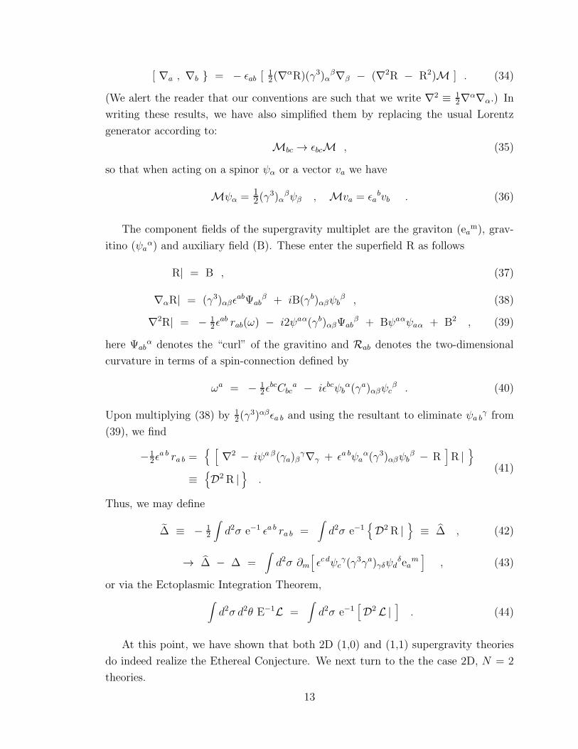
[ ∇a , ∇b } = − ǫab [12(∇

αR)(γ3)αβ∇β − (∇2R − R2)M ] . (34)

(We alert the reader that our conventions are such that we write ∇2 ≡ 12∇

α∇α.) In

writing these results, we have also simplified them by replacing the usual Lorentz

generator according to:

Mbc → ǫbcM , (35)

so that when acting on a spinor ψα or a vector va we have

Mψα = 12(γ

3)αβψβ , Mva = ǫa

bvb . (36)

The component fields of the supergravity multiplet are the graviton (eam), grav-

itino (ψaα) and auxiliary field (B). These enter the superfield R as follows

R| = B , (37)

∇αR| = (γ3)αβǫabΨab

β + iB(γb)αβψbβ , (38)

∇2R| = − 12ǫ

ab rab(ω) − i2ψaα(γb)αβΨabβ + Bψaαψaα + B2 , (39)

here Ψabα denotes the “curl” of the gravitino and Rab denotes the two-dimensional

curvature in terms of a spin-connection defined by

ωa = − 12ǫ

bcCbca − iǫbcψb

α(γa)αβψcβ . (40)

Upon multiplying (38) by 12(γ

3)αβǫa b and using the resultant to eliminate ψa bγ from

(39), we find

−12ǫ

a b ra b ={ [

∇2 − iψa β(γa)βγ∇γ + ǫa bψa

α(γ3)αβψbβ − R

]R |

}

≡{D2R |

}.

(41)

Thus, we may define

∆ ≡ − 12

∫d2σ e−1 ǫa b ra b =

∫d2σ e−1

{D2R |

}≡ ∆ , (42)

→ ∆ − ∆ =∫d2σ ∂m

[ǫc dψc

γ(γ3γa)γδψdδea

m]

, (43)

or via the Ectoplasmic Integration Theorem,∫d2σ d2θ E−1L =

∫d2σ e−1

[D2L |

]. (44)

At this point, we have shown that both 2D (1,0) and (1,1) supergravity theories

do indeed realize the Ethereal Conjecture. We next turn to the the case 2D, N = 2

theories.

13

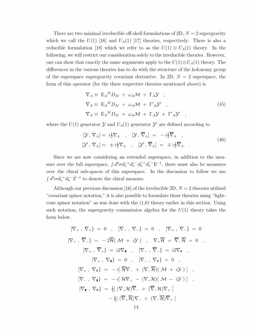
There are two minimal irreducible off-shell formulations of 2D, N = 2 supergravity

which we call the U(1) [16] and UA(1) [17] theories, respectively. There is also a

reducible formulation [18] which we refer to as the U(1) ⊗ UA(1) theory. In the

following, we will restrict our consideration solely to the irreducible theories. However,

one can show that exactly the same arguments apply to the U(1)⊗UA(1) theory. The

differences in the various theories has to do with the structure of the holonomy group

of the superspace supergravity covariant derivative. In 2D, N = 2 superspace, the

form of this operator (for the three respective theories mentioned above) is

∇A ≡ EAMDM + ωAM + ΓAY ,

∇A ≡ EAMDM + ωAM + Γ′

AY′ ,

∇A ≡ EAMDM + ωAM + ΓAY + Γ′

AY′ ,

(45)

where the U(1) generator Y and UA(1) generator Y′ are defined according to

[Y , ∇±] = i12∇± , [Y , ∇±] = − i12∇± ,

[Y ′ , ∇±] = ± i12∇± , [Y ′ , ∇±] = ∓ i12∇± .(46)

Since we are now considering an extended superspace, in addition to the mea-

sure over the full superspace,∫d2σdζ+dζ−dζ+dζ−E−1, there must also be measures

over the chiral sub-spaces of this superspace. In the discussion to follow we use∫d2σdζ+dζ−E−1 to denote the chiral measure.

Although our previous discussion [16] of the irreducible 2D,N = 2 theories utilized

“covariant spinor notation,” it is also possible to formulate these theories using “light-

cone spinor notation” as was done with the (1,0) theory earlier in this section. Using

such notation, the supergravity commutator algebra for the U(1) theory takes the

form below.

[∇+ , ∇+} = 0 , [∇− , ∇−} = 0 , [∇+ , ∇−} = 0

[∇+ , ∇−} = − 2H( M + iY ) , ∇+H = ∇−H = 0 ,

[∇+ , ∇+} = i2∇ , [∇− , ∇−} = i2∇ ,

[∇+ , ∇ } = 0 , [∇− , ∇ } = 0 ,

[∇+ , ∇ } = − i[ H∇− + (∇−H)( M + iY ) ] ,

[∇− , ∇ } = − i[ H∇+ − (∇+H)( M − iY ) ] ,

[∇ , ∇ } = 12 [ (∇+H)∇− + (∇−H)∇+ ]

− 12 [ (∇+H)∇− + (∇−H)∇+ ]

14

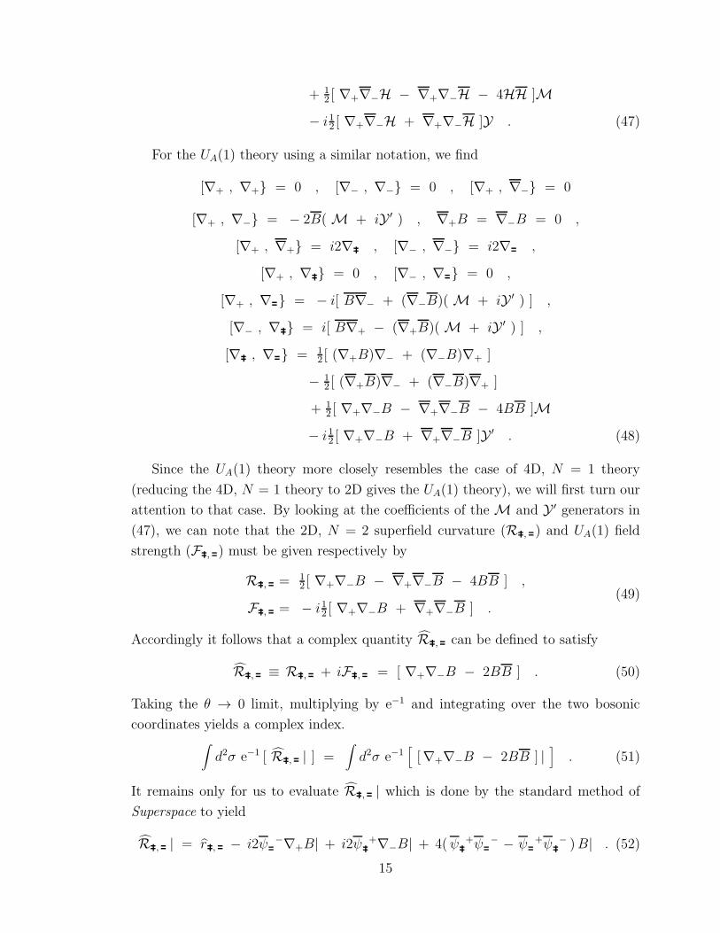
+ 12 [ ∇+∇−H − ∇+∇−H − 4HH ]M

− i12 [ ∇+∇−H + ∇+∇−H ]Y . (47)

For the UA(1) theory using a similar notation, we find

[∇+ , ∇+} = 0 , [∇− , ∇−} = 0 , [∇+ , ∇−} = 0

[∇+ , ∇−} = − 2B( M + iY ′ ) , ∇+B = ∇−B = 0 ,

[∇+ , ∇+} = i2∇ , [∇− , ∇−} = i2∇ ,

[∇+ , ∇ } = 0 , [∇− , ∇ } = 0 ,

[∇+ , ∇ } = − i[ B∇− + (∇−B)( M + iY ′ ) ] ,

[∇− , ∇ } = i[ B∇+ − (∇+B)( M + iY ′ ) ] ,

[∇ , ∇ } = 12 [ (∇+B)∇− + (∇−B)∇+ ]

− 12 [ (∇+B)∇− + (∇−B)∇+ ]

+ 12 [ ∇+∇−B − ∇+∇−B − 4BB ]M

− i12 [ ∇+∇−B + ∇+∇−B ]Y ′ . (48)

Since the UA(1) theory more closely resembles the case of 4D, N = 1 theory

(reducing the 4D, N = 1 theory to 2D gives the UA(1) theory), we will first turn our

attention to that case. By looking at the coefficients of the M and Y ′ generators in

(47), we can note that the 2D, N = 2 superfield curvature (R , ) and UA(1) field

strength (F , ) must be given respectively by

R , = 12 [ ∇+∇−B − ∇+∇−B − 4BB ] ,

F , = − i12 [ ∇+∇−B + ∇+∇−B ] .(49)

Accordingly it follows that a complex quantity R , can be defined to satisfy

R , ≡ R , + iF , = [ ∇+∇−B − 2BB ] . (50)

Taking the θ → 0 limit, multiplying by e−1 and integrating over the two bosonic

coordinates yields a complex index.∫d2σ e−1 [ R , | ] =

∫d2σ e−1

[[∇+∇−B − 2BB ] |

]. (51)

It remains only for us to evaluate R , | which is done by the standard method of

Superspace to yield

R , | = r , − i2ψ −∇+B| + i2ψ +∇−B| + 4(ψ +ψ − − ψ +ψ − )B| . (52)

15

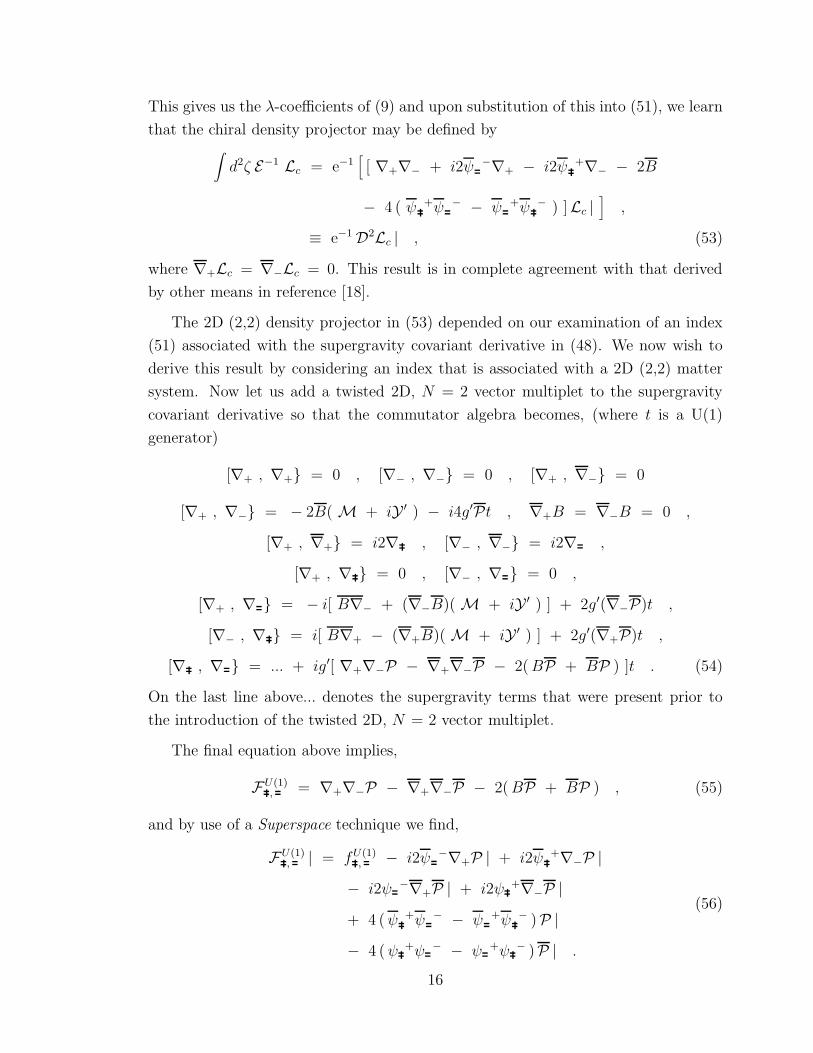
This gives us the λ-coefficients of (9) and upon substitution of this into (51), we learn

that the chiral density projector may be defined by∫d2ζ E−1 Lc = e−1

[[ ∇+∇− + i2ψ −∇+ − i2ψ +∇− − 2B

− 4 ( ψ +ψ − − ψ +ψ − ) ]Lc |]

,

≡ e−1 D2Lc | , (53)

where ∇+Lc = ∇−Lc = 0. This result is in complete agreement with that derived

by other means in reference [18].

The 2D (2,2) density projector in (53) depended on our examination of an index

(51) associated with the supergravity covariant derivative in (48). We now wish to

derive this result by considering an index that is associated with a 2D (2,2) matter

system. Now let us add a twisted 2D, N = 2 vector multiplet to the supergravity

covariant derivative so that the commutator algebra becomes, (where t is a U(1)

generator)

[∇+ , ∇+} = 0 , [∇− , ∇−} = 0 , [∇+ , ∇−} = 0

[∇+ , ∇−} = − 2B( M + iY ′ ) − i4g′Pt , ∇+B = ∇−B = 0 ,

[∇+ , ∇+} = i2∇ , [∇− , ∇−} = i2∇ ,

[∇+ , ∇ } = 0 , [∇− , ∇ } = 0 ,

[∇+ , ∇ } = − i[ B∇− + (∇−B)( M + iY ′ ) ] + 2g′(∇−P)t ,

[∇− , ∇ } = i[ B∇+ − (∇+B)( M + iY ′ ) ] + 2g′(∇+P)t ,

[∇ , ∇ } = ... + ig′[ ∇+∇−P − ∇+∇−P − 2(BP + BP ) ]t . (54)

On the last line above... denotes the supergravity terms that were present prior to

the introduction of the twisted 2D, N = 2 vector multiplet.

The final equation above implies,

FU(1), = ∇+∇−P − ∇+∇−P − 2(BP + BP ) , (55)

and by use of a Superspace technique we find,

FU(1), | = fU(1)

, − i2ψ −∇+P | + i2ψ +∇−P |

− i2ψ −∇+P | + i2ψ +∇−P |

+ 4 (ψ +ψ − − ψ +ψ − )P |

− 4 (ψ +ψ − − ψ +ψ − )P | .

(56)

16

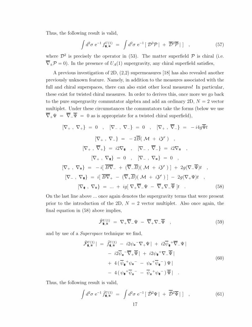
Thus, the following result is valid,∫d2σ e−1 fU(1)

, =∫d2σ e−1 [ D2P | + D2P | ] , (57)

where D2 is precisely the operator in (53). The matter superfield P is chiral (i.e.

∇±P = 0). In the presence of UA(1) supergravity, any chiral superfield satisfies,

A previous investigation of 2D, (2,2) supermeasures [18] has also revealed another

previously unknown feature. Namely, in addition to the measures associated with the

full and chiral superspaces, there can also exist other local measures! In particular,

these exist for twisted chiral measures. In order to derives this, once more we go back

to the pure supergravity commutator algebra and add an ordinary 2D, N = 2 vector

multiplet. Under these circumstances the commutators take the forms (below we use

∇+Ψ = ∇−Ψ = 0 as is appropriate for a twisted chiral superfield),

[∇+ , ∇+} = 0 , [∇− , ∇−} = 0 , [∇+ , ∇−} = − i4gΨt

[∇+ , ∇−} = − 2B( M + iY ′ ) ,

[∇+ , ∇+} = i2∇ , [∇− , ∇−} = i2∇ ,

[∇+ , ∇ } = 0 , [∇− , ∇ } = 0 ,

[∇+ , ∇ } = − i[ B∇− + (∇−B)( M + iY ′ ) ] + 2g(∇−Ψ)t ,

[∇− , ∇ } = i[ B∇+ − (∇+B)( M + iY ′ ) ] − 2g(∇+Ψ)t ,

[∇ , ∇ } = ... + ig[ ∇+∇−Ψ − ∇+∇−Ψ ]t . (58)

On the last line above ... once again denotes the supergravity terms that were present

prior to the introduction of the 2D, N = 2 vector multiplet. Also once again, the

final equation in (58) above implies,

FU(1), = ∇+∇−Ψ − ∇+∇−Ψ , (59)

and by use of a Superspace technique we find,

FU(1), | = fU(1)

, − i2ψ −∇+Ψ | + i2ψ +∇−Ψ |

− i2ψ −∇+Ψ | + i2ψ +∇−Ψ |

+ 4 (ψ +ψ − − ψ +ψ − ) Ψ |

− 4 (ψ +ψ − − ψ +ψ − ) Ψ | .

(60)

Thus, the following result is valid,∫d2σ e−1 fU(1)

, =∫d2σ e−1 [ D2Ψ | + D2Ψ | ] , (61)

17

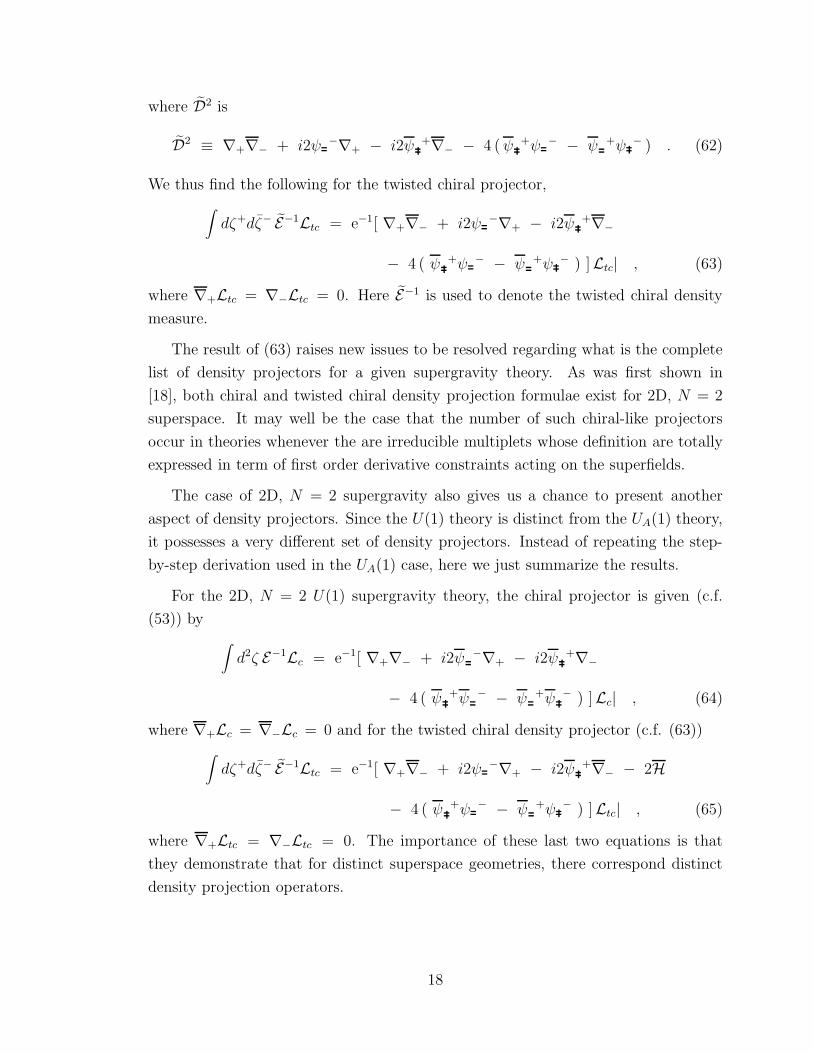
where D2 is

D2 ≡ ∇+∇− + i2ψ −∇+ − i2ψ +∇− − 4 (ψ +ψ − − ψ +ψ − ) . (62)

We thus find the following for the twisted chiral projector,

∫dζ+dζ− E−1Ltc = e−1[ ∇+∇− + i2ψ −∇+ − i2ψ +∇−

− 4 ( ψ +ψ − − ψ +ψ − ) ]Ltc| , (63)

where ∇+Ltc = ∇−Ltc = 0. Here E−1 is used to denote the twisted chiral density

measure.

The result of (63) raises new issues to be resolved regarding what is the complete

list of density projectors for a given supergravity theory. As was first shown in

[18], both chiral and twisted chiral density projection formulae exist for 2D, N = 2

superspace. It may well be the case that the number of such chiral-like projectors

occur in theories whenever the are irreducible multiplets whose definition are totally

expressed in term of first order derivative constraints acting on the superfields.

The case of 2D, N = 2 supergravity also gives us a chance to present another

aspect of density projectors. Since the U(1) theory is distinct from the UA(1) theory,

it possesses a very different set of density projectors. Instead of repeating the step-

by-step derivation used in the UA(1) case, here we just summarize the results.

For the 2D, N = 2 U(1) supergravity theory, the chiral projector is given (c.f.

(53)) by

∫d2ζ E−1Lc = e−1[ ∇+∇− + i2ψ −∇+ − i2ψ +∇−

− 4 ( ψ +ψ − − ψ +ψ − ) ]Lc| , (64)

where ∇+Lc = ∇−Lc = 0 and for the twisted chiral density projector (c.f. (63))

∫dζ+dζ− E−1Ltc = e−1[ ∇+∇− + i2ψ −∇+ − i2ψ +∇− − 2H

− 4 ( ψ +ψ − − ψ +ψ − ) ]Ltc| , (65)

where ∇+Ltc = ∇−Ltc = 0. The importance of these last two equations is that

they demonstrate that for distinct superspace geometries, there correspond distinct

density projection operators.

18

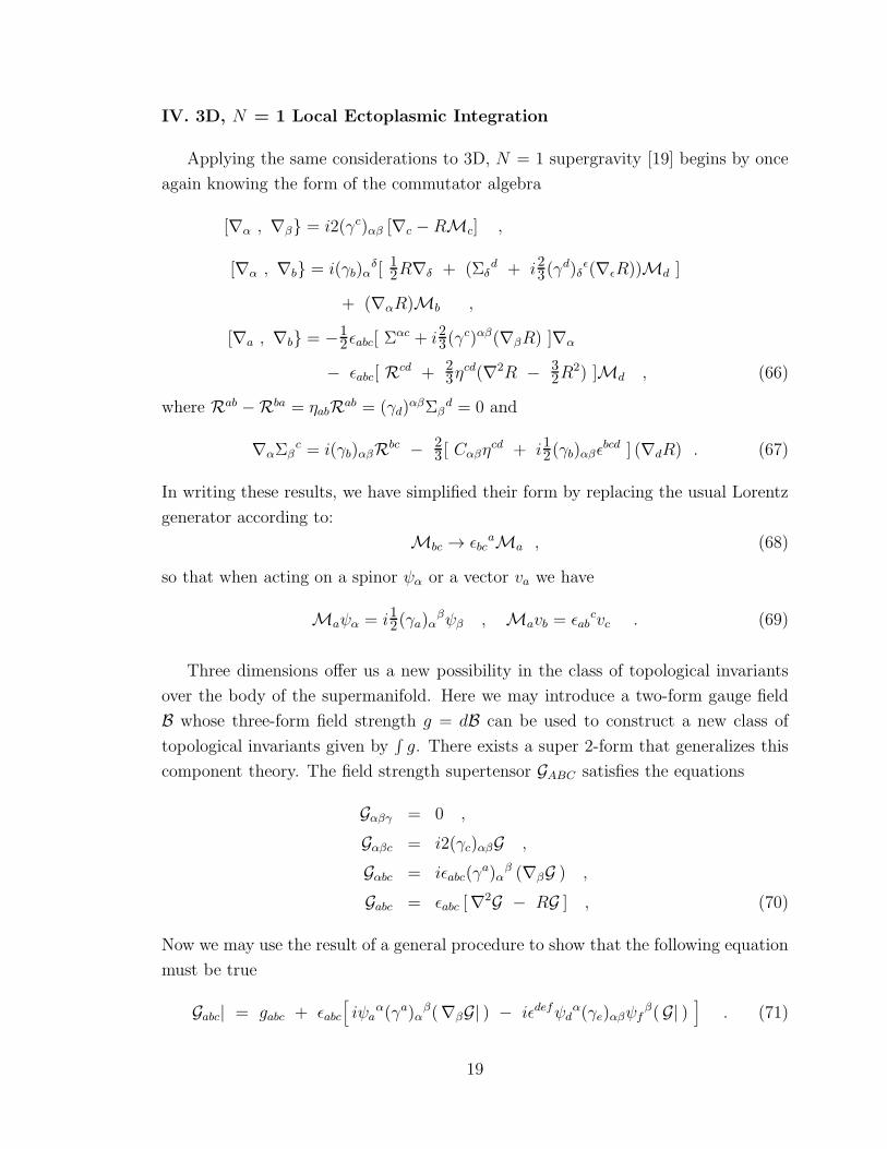
IV. 3D, N = 1 Local Ectoplasmic Integration

Applying the same considerations to 3D, N = 1 supergravity [19] begins by once

again knowing the form of the commutator algebra

[∇α , ∇β} = i2(γc)αβ [∇c − RMc] ,

[∇α , ∇b} = i(γb)αδ[ 1

2R∇δ + (Σδd + i

23(γ

d)δǫ(∇ǫR))Md ]

+ (∇αR)Mb ,

[∇a , ∇b} = −12ǫabc[ Σ

αc + i23(γ

c)αβ(∇βR) ]∇α

− ǫabc[ Rcd + 2

3ηcd(∇2R − 3

2R2) ]Md , (66)

where Rab −Rba = ηabRab = (γd)

αβΣβd = 0 and

∇αΣβc = i(γb)αβR

bc − 23 [ Cαβη

cd + i12(γb)αβǫ

bcd ] (∇dR) . (67)

In writing these results, we have simplified their form by replacing the usual Lorentz

generator according to:

Mbc → ǫbcaMa , (68)

so that when acting on a spinor ψα or a vector va we have

Maψα = i12(γa)α

βψβ , Mavb = ǫabcvc . (69)

Three dimensions offer us a new possibility in the class of topological invariants

over the body of the supermanifold. Here we may introduce a two-form gauge field

B whose three-form field strength g = dB can be used to construct a new class of

topological invariants given by∫g. There exists a super 2-form that generalizes this

component theory. The field strength supertensor GABC satisfies the equations

Gαβγ = 0 ,

Gαβc = i2(γc)αβG ,

Gαbc = iǫabc(γa)α

β (∇βG ) ,

Gabc = ǫabc [∇2G − RG ] , (70)

Now we may use the result of a general procedure to show that the following equation

must be true

Gabc| = gabc + ǫabc[iψa

α(γa)αβ(∇βG| ) − iǫdefψd

α(γe)αβψfβ(G| )

]. (71)

19

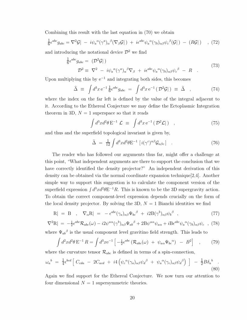
Combining this result with the last equation in (70) we obtain

16ǫ

abcgabc = ∇2G| − iψaα(γa)α

β(∇βG| ) + iǫabcψaα(γb)αβψc

β(G| ) − (RG| ) , (72)

and introducing the notational device D2 we find

16ǫ

abcgabc = (D2G| )

D2 ≡ ∇2 − iψaα(γa)α

β∇β + iǫabcψaα(γb)αβψc

β − R .(73)

Upon multiplying this by e−1 and integrating both sides, this becomes

∆ ≡∫d3x e−1 1

6ǫabcgabc =

∫d3x e−1 (D2G| ) ≡ ∆ , (74)

where the index on the far left is defined by the value of the integral adjacent to

it. According to the Ethereal Conjecture we may define the Ectoplasmic Integration

theorem in 3D, N = 1 superspace so that it reads∫d3xd2θE−1 L ≡

∫d3x e−1 (D2L| ) , (75)

and thus and the superfield topological invariant is given by,

∆ = 112

∫d3xd2θE−1 [ i(γc)αβGαβc ] . (76)

The reader who has followed our arguments thus far, might offer a challenge at

this point, “What independent arguments are there to support the conclusion that we

have correctly identified the density projector?” An independent derivation of this

density can be obtained via the normal coordinate expansion technique[2,4]. Another

simple way to support this suggestion is to calculate the component version of the

superfield expression∫d3xd2θE−1R. This is known to be the 3D supergravity action.

To obtain the correct component-level expression depends crucially on the form of

the local density projector. By solving the 3D, N = 1 Bianchi identities we find

R| = B , ∇αR| = − ǫabc(γa)αβΨbcβ + i2B(γb)αβψb

β , (77)

∇2R| = −12ǫ

abcRabc(ω)− i2ψaα(γb)αβΨabβ + 2Bψaαψaα + iBǫabcψa

α(γb)αβψc , (78)

where Ψabβ is the usual component level gravitino field strength. This leads to

∫d2xd2θE−1R =

∫d3xe−1

[−1

2ǫabc (Rabc(ω) + ψaαΨbc

α) − B2]

, (79)

where the curvature tensor Rabc is defined in terms of a spin-connection,

ωab = 1

4ǫbcd

[Ccda − 2Cacd + i4

(ψc

α(γa)αβψdβ + ψa

α(γc)αβψdβ) ]

− 12Bδa

b .

(80)

Again we find support for the Ethereal Conjecture. We now turn our attention to

four dimensional N = 1 supersymmetric theories.

20

V. 4D, N = 1 Local Ectoplasmic Integration

Minimal 4D, N = 1 supergravity is described by three fields strength tensors

denoted by Wαβγ , Gαα, and R. The form of the theory is completely described by

[∇α , ∇β} = − 2RMαβ ,

[∇α , ∇β} = i∇αβ ,

[∇α , ∇b} = − iCαβ [ R∇β − Gγβ ∇γ ] − i(∇βR )Mαβ

+ iCαβ [ W βγδMδ

γ − (∇γGδβ)Mγδ ] ,

[∇a , ∇b} = { [ CαβWαβγ + Cαβ(∇αG

γβ ) − Cαβ(∇αR ) δβ

γ ]∇γ

+ iCαβGγβ∇γα − [Cαβ(∇α∇

δGγβ )

− Cαβ(∇αWβγδ + (∇

2R + RR )Cγβδα

δ) ]Mδγ }

+ h. c. (81)

We now apply our method by introducing a 3-form gauge field matter multiplet

as first appeared very long ago [11]. In the context of 4D, N = 1 superspace, such a

supermultiplet is described by a super 4-form field strength FABC D that is known to

satisfy the constraints,

Fαβ γ D = Fα.β γ D = Fα

.β c d = 0 , Fαβ c d = Cγ

.δ.Cα(γCδ)βF . (82)

After the imposition of the constraints and solving the Bianchi identities on

FABC D in the presence of the old minimal supergravity derivative commutator alge-

bra we find,

Fα b c d = − ǫa b c d∇α.F , Fα

.b c d = ǫa b c d∇

αF , ∇α. F = 0 ,

Fa b c d = iǫa b c d

{[ (∇2 + 3R )F ] − [ (∇

2+ 3R )F ]

},

(83)

ǫa b c d ≡ i 12 [ CαβCγδCα

.(γ.Cδ.)β. − Cα

.β.Cγ.δ.Cα(γCδ)β ] . (84)

The θ → 0 limit of all types of component level supercovariantized gauge field

strengths is defined in an unambiguous manner as was discussed in Superspace. We

21

need only slightly generalize the formulae given there to find (c.f. (9))(Fa b c d |

)= fa b c d + [ 1

3!ψ[a|α(Fα |b c d] | ) + 1

4ψ[a|αψ|b|

β(Fαβ |c d] | ) + h. c. ]

+ 12ψ[a|

αψ|b|β(Fα β |c d] | ) − [ 1

3!ψ[a|αψ|b|

βψ|c|γ(Fαβ γ |d] | ) + h. c. ]

− 12 [ψ[a|

αψ|b|βψ|c|

γ(Fαβ γ |d] | ) + h. c. ]

− [ψaαψb

βψcγψd

δ(Fαβ γ δ | ) + h. c. ]

− [ 13!ψ[a|

αψ|b|βψ|c|

γψ|d|δ(Fαβ γ δ | ) + h. c. ]

− 14ψ[a|

αψ|b|βψ|c|

γψ|d|δ(Fαβ γ δ | ) .

(85)

Due to the constraints (83) on the 4-form supermultiplet, we can re-write this as

fa b c d =(Fa b c d |

)− [ 1

3!ψ[a|α(Fα |b c d] | ) +

14ψ[a|

αψ|b|β(Fαβ |c d] | ) + h. c. ] . (86)

Integrating both sides of this equation leads to,

∆ =∫d4x e−1ǫa b c d

[14!

(Fa b c d |

)− [ 1

3!ψaα(Fα b c d | )

+ 14ψa

αψbβ(Fαβ c d | ) + h. c. ]

].

(87)

where ∆ denotes the supersymmetric version of the index described by (11). Next

we use the solution to the Bianchi identities for Fa b c d and Fα b c d (from (83)), which

upon substitution into (87) yields,

∆ =∫d4x e−1

[− i (D2F |) + h. c.

], (88)

where the operator D2 is defined by

D2 ≡ ∇2 + iψaα∇α + 3R + 1

2Cαβψa

(α ψbβ) . (89)

Now we see that a superdifferential operator appears acting on the superfield F .

This superdifferential operator is, in fact, the chiral density projector for old minimal

supergravity. We continue by noting that the chiral density projector∫d2θ E−1 may

be defined by the equation∫d4x d2θ E−1Lc ≡

∫d4x e−1 (D2Lc | ) , (90)

for any chiral superfield, Lc. Finally since any chiral superfield Lc in the presence of

old minimal supergravity satisfies Lc = (∇2 + R)L, where L is a general superfield,

we also have∫d4x d2θ d2θ E−1L ≡ 1

2

[ ∫d4x d2θ E−1 ( (∇2 + R)L ) + h. c.

]

= 12

∫d4x e−1

[[ (D2 (∇2 + R)L| ) + h. c. ]

].

(91)

22

On setting L = 1, we derive the action for old minimal supergravity. The fourth

order differential operator D4 = 12D

2 (∇2 +R) + h.c. can be expanded in the form

∫d4x d2θ d2θ E−1L =

∫d4x e−1

{ [c(2,2)αβαβ∇α∇β∇α∇β + c(1,2)ααβ∇α∇α∇β

+ c(2,0)αβ∇α∇β + c(0,2) αβ∇α∇β

+ c(1,0)α∇α + c(0,0)]L| + h. c.

},

(92)

where the coefficients are given by

c(2,2)αβαβ = 14C

αβC αβ , c(1,2)ααβ = − i12ψ

αγγC

αβ ,

c(2,0)αβ = − 12C

αβR , c(0,2) αβ = − 12C

αβ( 3R + 12C

αβψαγ(γ ψβδ

δ) ) ,

c(1,0)α = [ (∇αR ) + iψaαR ] ,

c(0,0) = [ (∇2R ) + iψaα(∇αR ) + 3|R|2 + 1

2Cαβψa

(α ψbβ)R ] .

(93)

This form of the density projector shows that we have achieved our goal of calculating,

from an a priori principle, the form of the coefficients described abstractly in equation

(4). We also see that the respective volumes of 4D, N = 1 chiral and full superspaces

for old minimal supergravity are∫d4x d2θ E−1 =

∫d4x e−1 [ − Cαβ c

(0,2) αβ ] ,

∫d4x d2θ d2θ E−1 =

∫d4x e−1 [ c(0,0) + c(0,0) ] .

(94)

The nonminimal 4D, N = 1 supergravity formulation is the oldest “off-shell” form

of the theory known, having first been introduced by Breitenlohner [20] in a not quite

irreducible form. Nonminimal 4D, N = 1 supergravity is described by three fields

strength tensors just as in the minimal case. Here these are denoted by Wαβγ , Gαα,

and Tα. The derivation of the local density projector in the theory is much more

complicated than in the case of the minimal case. So much so that to our knowledge,

the explicit density projector for the nonminimal theory has never been presented

in the literature previously. Using the “Ethereal Conjecture”, this calculation is

rendered very simple. We will next present its explicit derivation.

Our derivation begins by giving an explicit form of the nonminimal 4D, N = 1

23

supergravity commutators. These may be written as

[∇α , ∇β} = 12T(α∇β) − 2RMαβ ,

[∇α , ∇β.} = i∇αβ

. ,

[∇α , ∇b} = 12 Tβ∇αβ

. + i [ Cαβ Gγβ. + 1

2(∇β.Tα )δβ

γ ]∇γ

− i [ Cαβ (∇γGδβ

.)Mγδ + (∇β

.R )Mαβ ]

+ i Cαβ [ W β.γ. δ.Mδ. γ.+ 1

6 ( (∇γ + 1

2Tγ )∇γ T γ

. ) Mβ. γ.] .

(95)

The final commutator [∇a , ∇b} can be explicitly found from the equation

[∇a , ∇b} = − i [∇β. , [∇a , ∇β} } − i [∇β , [∇a , ∇β

.} } . (96)

In the equations above we have also made a choice of the superconformal symmetry

parameter n = 1 [21], so that we have

R = − 14∇

αTα . (97)

Other consequences of the constraints (96) are that

∇α[ R − 14 T

α.T α. ] = 0 , ∇δ

. (∇2 + 34T

γ.∇γ. − R + 1

4Tγ.T γ. ) = 0 . (98)

Now we once again simply use the constraints of the 4-form and solve its Bianchi

identities in the presence of the non-minimal supergravity commutator algebra to

find,

Fα b c d = − ǫa b c d [ (∇α.− T

α.)F ] , (∇

α.− T

α.)F = 0 ,

Fα.b c d = ǫa b c d [ (∇α − T α)F ] ,

Fa b c d = iǫa b c d

{12 [∇

ǫ (∇ǫ + Tǫ )F ] − 12 [∇

ǫ.(∇ǫ

. + T ǫ. )F ]

}.

(99)

So that the quantity ∆ here takes the form,

∆ =∫d4x e−1

[− i (D2F |) + h. c.

](100)

where now the operator D2 is defined by

D2 ≡ ∇2 + [ iψaα − 1

2Tα ]∇α + [ 2R − iψa

αTα + 12C

αβψa(α ψb

β) ] . (101)

(This projector provides an explicit example of the comment that was made above

equation (5) since c(NF−1) is not strictly proportional to the gravitino. This behavior

generically occurs in the presence of spinorial auxiliary fields.)

24

If we replace F by a chiral Lagrangian Lc in (100) above, we seem to have reached

our goal of finding a chiral-type density projector for the nonminimal theory

∫d4x d2θ E−1 Lc =

∫d4x e−1 (D2Lc |) , (∇α

. − T α.) Lc = 0 . (102)

However, the discerning reader will note a slight remaining problem. Namely the

modified definition of chirality satisfied by Lc is not the usual one. One way to

remedy this is to note that there exists a superfield Tα satisfying ∇αTβ +∇βTα = 0.

The solution of this implies that there exist another superfield T such that Tα = ∇αT .

It therefore follows that

(∇α. − T α

.)Lc = 0 & Lc ≡ eT Lc → ∇α. Lc = 0 . (103)

In order to use the superfield T to obtain a component level expression, we need to

observe T | = 0 in a suitable Wess-Zumino gauge. Assembling all of these pieces we

find for the nonminimal supergravity theory,∫d4x d2θ d2θ E−1L ≡ 1

2

[ ∫d4x d2θ E−1 ( (∇2 + 3

4Tγ.∇γ. − R + 1

4Tγ.T γ. )L )

+ h. c.]

= 12

∫d4x e−1

[[ (D2 eT (∇2 + 3

4Tγ.∇γ. − R + 1

4Tγ.T γ. )L ) | ]

+ h. c.]

.

(104)

In this equation, the quantity E−1 is the usual density for ordinary chiral superfields.

In fact it is defined by

∫d4x d2θ d2θE−1 [R − 1

4 TαTα ]

−1 ≡∫d4x d2θ E−1 . (105)

The appearance of T still makes for an ungainly way to proceed. So we may insert a

factor of 1 = exp[−T ]exp[T ] in front of L and “push” the factor of exp[−T ] through

the chiral projection operator until it annihilates the pre-factor of exp[T ]. Now we

can redefine L to absorb the other exponential. The net effect of these operations is

to “change” the chiral projection operator according to

(∇2+ 3

4Tγ.∇γ. − R + 1

4Tγ.T γ. ) → ∇2 − 1

4Tβ.∇β. + R = 1

2∇β.[ ∇β

. − 12T β

. ] , (106)

and the final form of the density projector for the nonminimal supergravity theory

described by (103) can be cast into the form,

∫d4x d2θ d2θ E−1 L = 1

4

{ ∫d4x e−1 [D2∇β

.[ ∇β

. − 12T β

. ]L ]∣∣∣ + h. c.

}. (107)

25

We believe that it is appropriate to note that equation (107) immediately above marks

the first time, to our knowledge, that a density projection operator for nonminimal

supergravity has appeared in the physics literature.

Some time ago we proposed [22] that the 4D, N = 1 limit of heterotic string theory

was most likely to be an unusual formulation of 4D, N = 1 supergravity combined

with a 4D, N = 1 super gauge 2-form multiplet. We presently call this the 4D, N = 1

“βFFC supergeometry”15. The form of the commutator algebra for this formulation

is

[∇α,∇β} = 0 ,

[∇α,∇α} = i∇a + HβαMαβ − HαβMα

β + HaY ,

[∇α,∇b} = i(∇βHγβ) [ Mαγ + δα

γ Y ]

+ i[ Cαβ W βγδ − 1

3δβδ( 2∇αHβγ + ∇βHαγ ) ]Mδ

γ ,

[∇a,∇b} = { 12Cαβ[ iH

γ(α∇γβ) − (∇γ∇(αHγ β))Y ]

+ [ Cαβ( Wαβγ − 1

6(∇γH(αγ)δβ)

γ ) − 12Cαβ(∇(αH

γβ)) ]∇γ

− Cαβ [ Wαβγδ + i14Cγ(α|(∇|β)ǫHδǫ) + 1

12Cγ(αCβ)δ(∇ǫ∇ǫHǫǫ) ]M

γδ

+ 12Cαβ[ ∇γ∇(αHδβ) ]M

γδ + h.c. } .

(108)

The self-consistency of the Bianchi identities of the commutator algebra above requires

that the following differential equation must also be satisfied.

∇aHa = 0 , ∇βWαβγ = 0 , ∇β∇βHa = 0 ,

∇αWαβγ = − 16∇(β∇

γHγ)γ − 12∇

γ∇(βHγ)γ . (109)

Finally, since the theory contains a gauge 2-form, there occurs a super 3-form field

strength whose various components are given by

Hαβγ = Hαβγ = Hαβγ = Hαβc = Hαβc − i12CαγCβγ = 0 ,

Hαbc = 0 , Habc = i14 [ CβγCα(βHαγ) − CβγCα(βHγ)α ] . (110)

Repeating the step of solving the Bianchi identity in the presence of the constraints

leads to

Fα b c d = − ǫa b c d∇α.F , Fα

.b c d = ǫa b c d∇

αF , ∇α. F = 0 ,

Fa b c d = iǫa b c d [∇2F − ∇2F ] .

(111)

15 The name “βFFC” (≡ beta-function favored constraints) was suggested by H.Nishino.

26

These are substituted into (87) and as previously, we see that a superdifferential

operator appears acting on the superfield F . This time the superdifferential operator

is the chiral density projector for βFFC supergravity. We continue by noting that the

chiral density projector∫d2θ E−1 may be defined by the equation

∫d4xd2θ E−1Lc ≡

∫d4x e−1 (D2Lc | ) ,

D2 ≡ ∇2 + iψaα∇α + 1

2Cαβψa

(α ψbβ) .

(112)

for any chiral superfield, Lc. Finally since any chiral superfield Lc in the presence of

βFFC supergravity satisfies Lc = ∇2L, where L is a general superfield, we also have

∫d4xd2θd2θ E−1L ≡ 1

2

[ ∫d4xd2θ E−1 (∇2L ) + h. c.

]. (113)

On setting L = 1, we derive

VβFFC =∫d4x d2θ d2θ E−1 = 0 , (114)

since any purely derivative operator acting on a constant vanishes, i.e. the volume

of the full βFFC superspace vanishes. Interestingly enough, however, the volume of

the 4D, N = 1 βFFC chiral superspace is non-vanishing. If we introduce a complex

parameter µc we find

V cβFFC =

∫d4xd2θ E−1 µc =

∫d4x e−1[D2

β(µc | ) ]

= 12µc

∫d4x e−1 [ψα(α|

αψ α|β)

β ] .

(115)

This last expression (taken together with its conjugate) is recognizable as a mass

term for the gravitino. Thus we find the very elegant result that the mass of the

gravitino in 4D, N = 1 βFFC supergravity is proportional to the volume of chiral

superspace. Since we have proposed that βFFC supergeometry is the limit of the

supergravity theory associated with heterotic and superstring theory, the results in

(114) and (115) must have interesting “string” implications.

We simply close this section by noting that we have presented a number of results

that have not appeared previously to our knowledge. These were given in (107),

(114) and (115). With this we end our discussion of examples of how to derive

density projectors. The methods that we have described in the last two sections may

be extended to a number of other supergravity theories with no impediments.

27

VI. Stage-II Density Projection Operators

In the previous sections, we have presented evidence from a wide number of ex-

amples which show that density projection operators can often be derived by looking

at topological indices. One feature of all of the examples is that the construction of

the density projection operators were obtained by essentially algebraic means. We

shall call these Stage-I density projection operators. There are cases, however, where

this is not the case and the derivation of density projection operators seem to require

solving for some “prepotential16.” The density projection operators of this type will

be called Stage-II density projection operators. Derivations for Stage-II projectors

are more complicated than for Stage-I projectors. As an illustration of such a theory,

we shall describe the treatment of the local 2D, N = 4 theory.

A minimal off-shell 2D, N = 4 supergravity theory [22] consists of the component

fields (eam, ψa

αi, Aaij , B, G, H). These are the components of that remain after

imposing the following constraints on the 2D,N = 4 superspace supergravity covariant

derivative, (with φαβ ≡ −i[CαβG+ i(γ3)αβH ])

[∇αi,∇βj} = 2B[CαβC ijM − (γ3)αβY ij] ,

[∇αi, ∇βj} = 2[ iδi

j(γc)αβ∇c + δijφα

γ(γ3)γβM − iφαβY ij ] ,

[∇αi,∇b} = i12φα

γ(γb)γβ∇βi + i1

2(γ3γb)α

βBC ij∇βj

− i(γ3γb)αβΣβiM + i(γb)αβΣ

βjY i

j ,

[∇a,∇b} = −12ǫab[(γ

3)αβΣαi∇βi + (γ3)α

βΣαi∇β

i + RM + iF ijYj

i] .

(116)

The consistency of the Bianchi identities constructed from the commutator algebra

above required the conditions,

∇αiB = 0 , ∇αiB = −2C ij(γ

3)αβΣβj ,

∇αiG = Σαi , ∇αiH = i(γ3)αβΣβi, ,

∇αiΣβj = iC ij(γ3γa)α

β∇aB ,

∇αiΣβj = 1

2δα

βδij[R − 2G2 − 2H2 − 2BB] + i(γ3)α

βF ij

+ i12δi

j(γa)αβ(∇aG)−

12δi

j(γ3γa)αβ(∇aH) .

(117)

16By prepotential, we mean in the original sense for which the word was coined [23], not in the

more recent usage as widely appears in N = 2 SUSY YM theory.

28

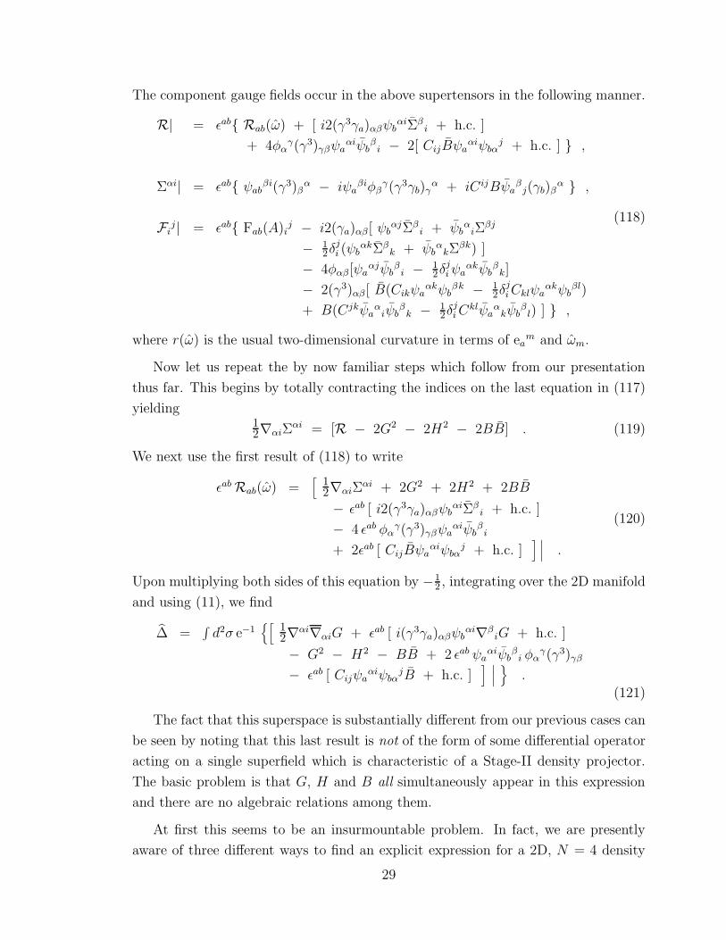
The component gauge fields occur in the above supertensors in the following manner.

R| = ǫab{ Rab(ω) + [ i2(γ3γa)αβψbαiΣβ

i + h.c. ]

+ 4φαγ(γ3)γβψa

αiψbβi − 2[ CijBψa

αiψbαj + h.c. ] } ,

Σαi| = ǫab{ ψabβi(γ3)β

α − iψaβiφβ

γ(γ3γb)γα + iC ijBψa

βj(γb)β

α } ,

Fij | = ǫab{ Fab(A)i

j − i2(γa)αβ[ ψbαjΣβ

i + ψbαiΣ

βj

− 12δ

ji (ψb

αkΣβk + ψb

αkΣ

βk) ]

− 4φαβ[ψaαjψb

βi − 1

2δjiψa

αkψbβk]

− 2(γ3)αβ[ B(Cikψaαkψb

βk − 12δ

jiCklψa

αkψbβl)

+ B(Cjkψaαiψb

βk − 1

2δjiC

klψaαkψb

βl) ] } ,

(118)

where r(ω) is the usual two-dimensional curvature in terms of eam and ωm.

Now let us repeat the by now familiar steps which follow from our presentation

thus far. This begins by totally contracting the indices on the last equation in (117)

yielding12∇αiΣ

αi = [R − 2G2 − 2H2 − 2BB] . (119)

We next use the first result of (118) to write

ǫab Rab(ω) =[12∇αiΣ

αi + 2G2 + 2H2 + 2BB

− ǫab [ i2(γ3γa)αβψbαiΣβ

i + h.c. ]

− 4 ǫab φαγ(γ3)γβψa

αiψbβi

+ 2ǫab [ CijBψaαiψbα

j + h.c. ]] ∣∣∣ .

(120)

Upon multiplying both sides of this equation by −12 , integrating over the 2D manifold

and using (11), we find

∆ =∫d2σ e−1

{[12∇

αi∇αiG + ǫab [ i(γ3γa)αβψbαi∇β

iG + h.c. ]

− G2 − H2 − BB + 2 ǫab ψaαiψb

βi φα

γ(γ3)γβ

− ǫab [ Cijψaαiψbα

jB + h.c. ]] ∣∣∣

}.

(121)

The fact that this superspace is substantially different from our previous cases can

be seen by noting that this last result is not of the form of some differential operator

acting on a single superfield which is characteristic of a Stage-II density projector.

The basic problem is that G, H and B all simultaneously appear in this expression

and there are no algebraic relations among them.

At first this seems to be an insurmountable problem. In fact, we are presently

aware of three different ways to find an explicit expression for a 2D, N = 4 density

29

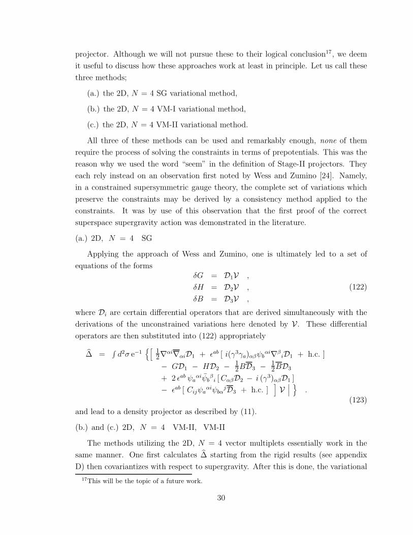
projector. Although we will not pursue these to their logical conclusion17, we deem

it useful to discuss how these approaches work at least in principle. Let us call these

three methods;

(a.) the 2D, N = 4 SG variational method,

(b.) the 2D, N = 4 VM-I variational method,

(c.) the 2D, N = 4 VM-II variational method.

All three of these methods can be used and remarkably enough, none of them

require the process of solving the constraints in terms of prepotentials. This was the

reason why we used the word “seem” in the definition of Stage-II projectors. They

each rely instead on an observation first noted by Wess and Zumino [24]. Namely,

in a constrained supersymmetric gauge theory, the complete set of variations which

preserve the constraints may be derived by a consistency method applied to the

constraints. It was by use of this observation that the first proof of the correct

superspace supergravity action was demonstrated in the literature.

(a.) 2D, N = 4 SG

Applying the approach of Wess and Zumino, one is ultimately led to a set of

equations of the formsδG = D1V ,

δH = D2V ,

δB = D3V ,

(122)

where Di are certain differential operators that are derived simultaneously with the

derivations of the unconstrained variations here denoted by V. These differential

operators are then substituted into (122) appropriately

∆ =∫d2σ e−1

{[12∇

αi∇αiD1 + ǫab [ i(γ3γa)αβψbαi∇β

iD1 + h.c. ]

− GD1 − HD2 − 12BD3 − 1

2BD3

+ 2 ǫab ψaαiψb

βi [CαβD2 − i (γ3)αβD1 ]

− ǫab [ Cijψaαiψbα

jD3 + h.c. ]]V

∣∣∣}

.

(123)

and lead to a density projector as described by (11).

(b.) and (c.) 2D, N = 4 VM-II, VM-II

The methods utilizing the 2D, N = 4 vector multiplets essentially work in the

same manner. One first calculates ∆ starting from the rigid results (see appendix

D) then covariantizes with respect to supergravity. After this is done, the variational

17This will be the topic of a future work.

30

approach of Wess and Zumino is applied only to the portions of the commutator

algebra describing the matter multiplets. In these cases, this leads ultimately to a set

of equations analogous to (122) which are then substituted in the expressions for the

respective ∆’s to yield an explicit expression for the projector.

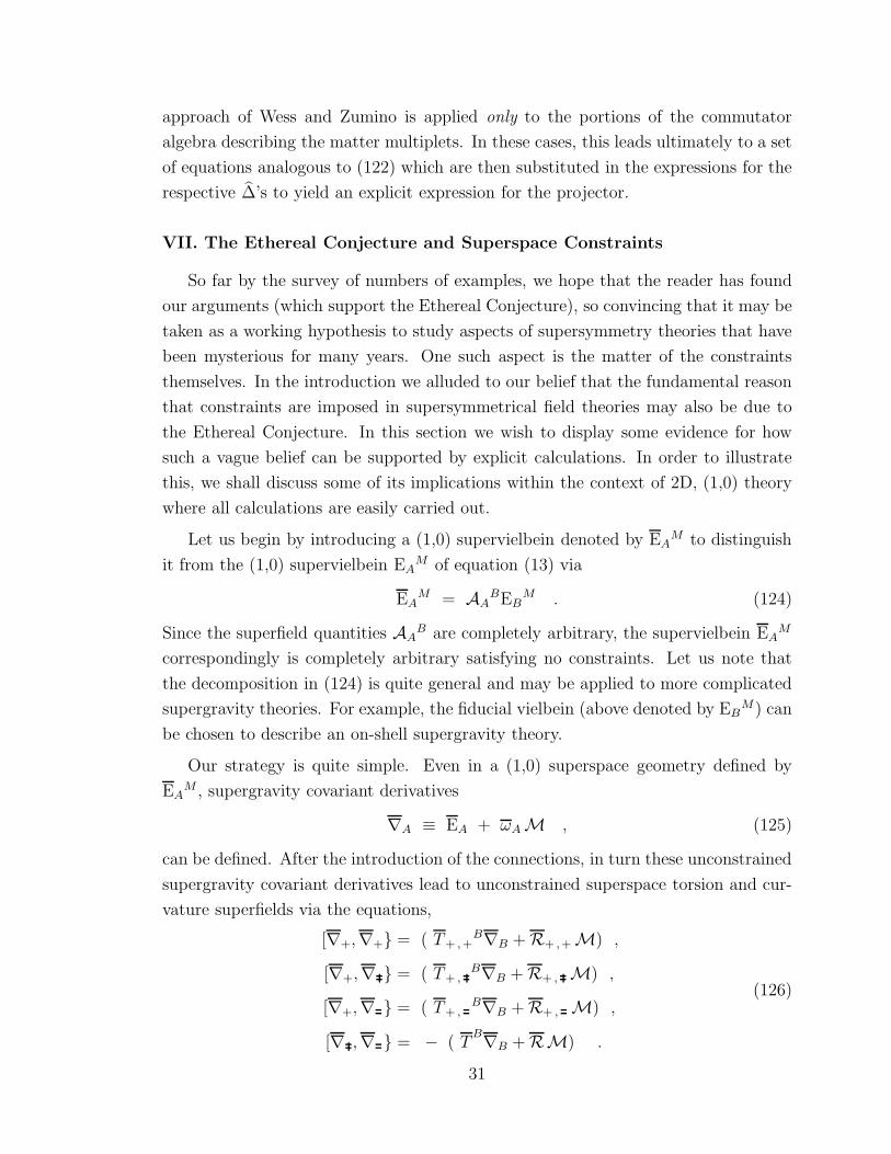
VII. The Ethereal Conjecture and Superspace Constraints

So far by the survey of numbers of examples, we hope that the reader has found

our arguments (which support the Ethereal Conjecture), so convincing that it may be

taken as a working hypothesis to study aspects of supersymmetry theories that have

been mysterious for many years. One such aspect is the matter of the constraints

themselves. In the introduction we alluded to our belief that the fundamental reason

that constraints are imposed in supersymmetrical field theories may also be due to

the Ethereal Conjecture. In this section we wish to display some evidence for how

such a vague belief can be supported by explicit calculations. In order to illustrate

this, we shall discuss some of its implications within the context of 2D, (1,0) theory

where all calculations are easily carried out.

Let us begin by introducing a (1,0) supervielbein denoted by EAM to distinguish

it from the (1,0) supervielbein EAM of equation (13) via

EAM = AA

BEBM . (124)

Since the superfield quantities AAB are completely arbitrary, the supervielbein EA

M

correspondingly is completely arbitrary satisfying no constraints. Let us note that

the decomposition in (124) is quite general and may be applied to more complicated

supergravity theories. For example, the fiducial vielbein (above denoted by EBM) can

be chosen to describe an on-shell supergravity theory.

Our strategy is quite simple. Even in a (1,0) superspace geometry defined by

EAM , supergravity covariant derivatives

∇A ≡ EA + ωA M , (125)

can be defined. After the introduction of the connections, in turn these unconstrained

supergravity covariant derivatives lead to unconstrained superspace torsion and cur-

vature superfields via the equations,

[∇+,∇+} = ( T+ ,+B∇B +R+ ,+ M) ,

[∇+,∇ } = ( T+ ,B∇B +R+ , M) ,

[∇+,∇ } = ( T+ ,B∇B +R+ , M) ,

[∇ ,∇ } = − ( TB∇B +RM) .

(126)

31

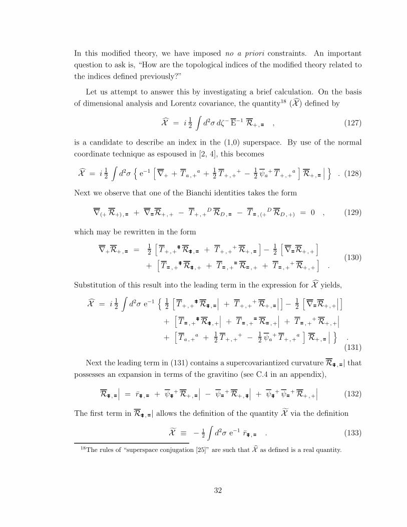
In this modified theory, we have imposed no a priori constraints. An important

question to ask is, “How are the topological indices of the modified theory related to

the indices defined previously?”

Let us attempt to answer this by investigating a brief calculation. On the basis

of dimensional analysis and Lorentz covariance, the quantity18 (X ) defined by

X = i12

∫d2σ dζ−E−1 R+ , , (127)

is a candidate to describe an index in the (1,0) superspace. By use of the normal

coordinate technique as espoused in [2, 4], this becomes

X = i12

∫d2σ

{e−1

[∇+ + T a ,+

a + 12 T+ ,+

+ − 12 ψa

+ T+ ,+a]R+ ,

∣∣∣}

. (128)

Next we observe that one of the Bianchi identities takes the form

∇(+ R+) , + ∇ R+ ,+ − T+ ,+D RD , − T , (+

D RD ,+) = 0 , (129)

which may be rewritten in the form

∇+R+ , = 12

[T+ ,+ R , + T+ ,+

+ R+ ,

]− 1

2

[∇ R+ ,+

]

+[T ,+ R ,+ + T ,+ R ,+ + T ,+

+ R+ ,+

].

(130)

Substitution of this result into the leading term in the expression for X yields,

X = i12

∫d2σ e−1

{12

[T+ ,+ R ,

∣∣∣ + T+ ,++ R+ ,

∣∣∣]− 1

2

[∇ R+ ,+

∣∣∣]

+[T ,+ R ,+

∣∣∣ + T ,+ R ,+

∣∣∣ + T ,++R+ ,+

∣∣∣

+[T a ,+

a + 12 T+ ,+

+ − 12 ψa

+ T+ ,+a]R+ ,

∣∣∣}

.

(131)

Next the leading term in (131) contains a supercovariantized curvature R , | that

possesses an expansion in terms of the gravitino (see C.4 in an appendix),

R ,

∣∣∣ = r , + ψ +R+ ,

∣∣∣ − ψ +R+ ,

∣∣∣ + ψ + ψ + R+ ,+

∣∣∣ (132)

The first term in R , | allows the definition of the quantity X via the definition

X ≡ − 12

∫d2σ e−1 r , . (133)

18The rules of “superspace conjugation [25]” are such that X as defined is a real quantity.

32

Using these facts, we finally arrive at the equation X − X = OT where

OT = i12

∫d2σ e−1

{12 ( T+ ,+ − i2 )R , +

[T+ ,+

+ − T+ ,

− 12 ψ

+ T+ ,+ − 12 ψ

+ ( T+ ,+ − i2 )]R+ ,

− 12∇ R+ ,+ +

[T ,+

+ + i ψ + ψ +]R+ ,+

−[T ,+ + i ψ +

]R+ ,

} ∣∣∣ .

(134)

It can be seen that when the usual (1,0) superspace constraints are imposed,

T+ ,+ = i2 , T+ ,++ = T+ , = T+ ,+ = R+ ,+ = R+ , = 0 (135)

all of the terms of OT , which we regard as the obstruction to the topological triviality

of the ectoplasm (or “ectoplasmic obstruction”), vanish up to total derivatives. In our

formulation of the Ethereal Conjecture, OT must be trivial in order for the conjecture

to be valid. So this equation shows that within the context of (1,0) supergravity, the

E.C. is not satisfied without the imposition of the supergravity constraints. This

strongly suggests that the reasons for the constraints in all supergravity theories have

their origins in topology! However, additional study of this matter is needed in order

to construct a rigorous proof of this more generally. The Ethereal Conjecture is, we

believe, equivalent to the triviality of OT .

The method of carrying out the calculation of OT above can be graphically illus-

trated. If we imagine that superspace is a sphere, the quantityX corresponds to an

ANZ based calculation of an index throughout the bulk of superspace (i.e. the interior

of the sphere). Since purely bosonic p-forms have their support only on the bound-

ary of the sphere, the quantity X corresponds to the index calculated on the purely

bosonic sub-manifold of superspace (i.e. the surface of the sphere). The quantity OT

measures the difference of these two definitions.

VIII. Future Prospectives

We have seen that there is evidence from a number of supergravity theories

that topology is at the heart of the process of defining the integration of Grassmann

variables over local supersymmetry manifolds. If our conjecture is taken as a working

assumption, future efforts may have a basis for adding to a new level of understanding

of off-shell field representations of supersymmetric theories. In particular, we must

begin to understand how to extend the argument of the last section to the cases of

more interesting supergravity theories.

33

Since perhaps the most important theories which would prove of the widest interest

are 10D theories, it is appropriate to review exactly what topological invariants might

be available to test the Ethereal Conjecture. For the case of the coupled 10D, N = 1

supergravity-Yang-Mills system, the topological invariants may be denoted by

∆p q r(SG + YM) =∫Tr

[F r ∧ Rp ∧ Hq ∧ (dΦ)10−2(p+r)−3q

]. (136)

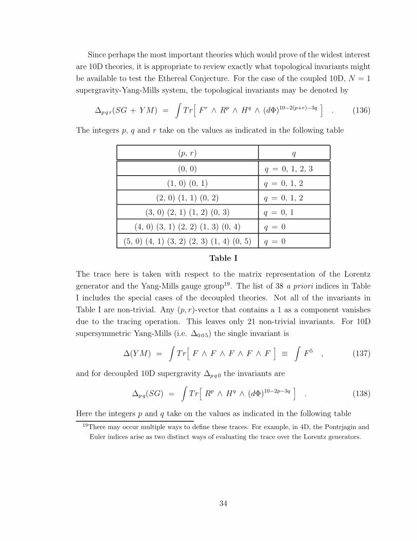
The integers p, q and r take on the values as indicated in the following table

(p, r) q

(0, 0) q = 0, 1, 2, 3

(1, 0) (0, 1) q = 0, 1, 2

(2, 0) (1, 1) (0, 2) q = 0, 1, 2

(3, 0) (2, 1) (1, 2) (0, 3) q = 0, 1

(4, 0) (3, 1) (2, 2) (1, 3) (0, 4) q = 0

(5, 0) (4, 1) (3, 2) (2, 3) (1, 4) (0, 5) q = 0

Table I

The trace here is taken with respect to the matrix representation of the Lorentz

generator and the Yang-Mills gauge group19. The list of 38 a priori indices in Table

I includes the special cases of the decoupled theories. Not all of the invariants in

Table I are non-trivial. Any (p, r)-vector that contains a 1 as a component vanishes

due to the tracing operation. This leaves only 21 non-trivial invariants. For 10D

supersymmetric Yang-Mills (i.e. ∆0 0 5) the single invariant is

∆(YM) =∫Tr

[F ∧ F ∧ F ∧ F ∧ F

]≡

∫F 5 , (137)

and for decoupled 10D supergravity ∆p q 0 the invariants are

∆p q(SG) =∫Tr

[Rp ∧ Hq ∧ (dΦ)10−2p−3q

]. (138)

Here the integers p and q take on the values as indicated in the following table

19There may occur multiple ways to define these traces. For example, in 4D, the Pontrjagin and

Euler indices arise as two distinct ways of evaluating the trace over the Lorentz generators.

34

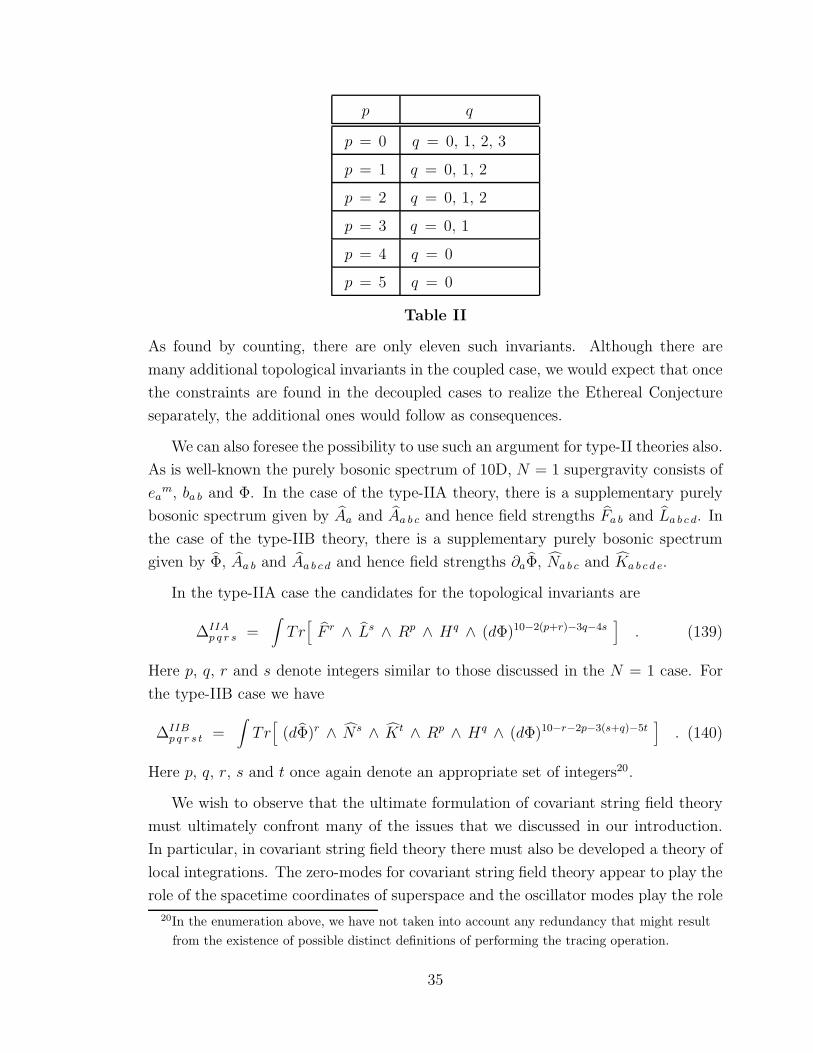
p q

p = 0 q = 0, 1, 2, 3

p = 1 q = 0, 1, 2

p = 2 q = 0, 1, 2

p = 3 q = 0, 1

p = 4 q = 0

p = 5 q = 0

Table II

As found by counting, there are only eleven such invariants. Although there are

many additional topological invariants in the coupled case, we would expect that once

the constraints are found in the decoupled cases to realize the Ethereal Conjecture

separately, the additional ones would follow as consequences.

We can also foresee the possibility to use such an argument for type-II theories also.

As is well-known the purely bosonic spectrum of 10D, N = 1 supergravity consists of

eam, ba b and Φ. In the case of the type-IIA theory, there is a supplementary purely

bosonic spectrum given by Aa and Aa b c and hence field strengths Fa b and La b c d. In

the case of the type-IIB theory, there is a supplementary purely bosonic spectrum

given by Φ, Aa b and Aa b c d and hence field strengths ∂aΦ, Na b c and Ka b c d e.

In the type-IIA case the candidates for the topological invariants are

∆IIAp q r s =

∫Tr

[F r ∧ Ls ∧ Rp ∧ Hq ∧ (dΦ)10−2(p+r)−3q−4s

]. (139)

Here p, q, r and s denote integers similar to those discussed in the N = 1 case. For

the type-IIB case we have

∆IIBp q r s t =

∫Tr

[(dΦ)r ∧ N s ∧ Kt ∧ Rp ∧ Hq ∧ (dΦ)10−r−2p−3(s+q)−5t

]. (140)

Here p, q, r, s and t once again denote an appropriate set of integers20.

We wish to observe that the ultimate formulation of covariant string field theory

must ultimately confront many of the issues that we discussed in our introduction.

In particular, in covariant string field theory there must also be developed a theory of

local integrations. The zero-modes for covariant string field theory appear to play the

role of the spacetime coordinates of superspace and the oscillator modes play the role

20In the enumeration above, we have not taken into account any redundancy that might result

from the existence of possible distinct definitions of performing the tracing operation.

35

of the Grassmann coordinates. We believe that it will be the case that the concept

of stringy p-forms should play an important role.

The super forms in (18) obviously belong to the general class of super forms given

by

fµ1 ···µpm1 ···mq= (−1)

[NB

2 ]Eµq

Cq · · · Eµ1

C1 Emp

Ap · · · Em1

A1 FA1 ···ApC1 ···Cq. (141)

It is our contention that the Ethereal Conjecture likely is equivalent to the following

statement

The topology of super manifolds with NF and NB fermionic and bosonic

coordinates, respectively, arises solely from its purely bosonic p-forms.

The mixed and purely fermionic super p-forms although topologically insignificant,

are useful for other aspects. For example, the case of p = 1, q = 0 and p = 0, q = 1

has been used previously [11, 26] to define supersymmetric gauge phase factors.

Finally, the coefficients given in (9) are such that ∆ defined by (11) corresponds

to the integration of the super NB-form fm1...mNBover a hypersurface in superspace.

The hypersurface corresponds to the bosonic spacetime manifold. From this vantage

point, it should be clear that the theory of ectoplasmic integration that we have de-

scribed is based on the use of superdifferential forms and follows the path that is

standard for ordinary bosonic differential forms. This observation dramatically em-

phasizes that the definition of ectoplasmic integration defined in the present work is

logically independent of ANZ local superspace integration theory [9]. Dramatically,

our new approach to local superspace integration is totally independent of the superde-

terminant. More remarkably however, the local ectoplasmic integration operator DNF

derived on the basis of super p-forms (11-13) agrees exactly with the local ANZ inte-

gration operator21 DNF derived on the basis of a normal coordinate expansion of the

superdeterminant (1). Whether this statement is necessarily true for all supergravity

theories is an interesting question to pursue.

“I have no special talents. I am only passionately curious.” – Einstein

Acknowledgment

The author wishes to acknowledge the hospitality of the Mathematical Sciences

21Whimsically, we might call this the ANZIO-i.e. the ANZ integration operator.

36

Research Institute where this work was initiated and which inspired him to re-consider

the problem of a local superspace integration theory and the possible role of topology.

He has also benefitted greatly from numerous critical comments and inputs from

M. T. Grisaru, W. Siegel and especially M. E. Knutt-Wehlau for her assistance in

section seven.

37

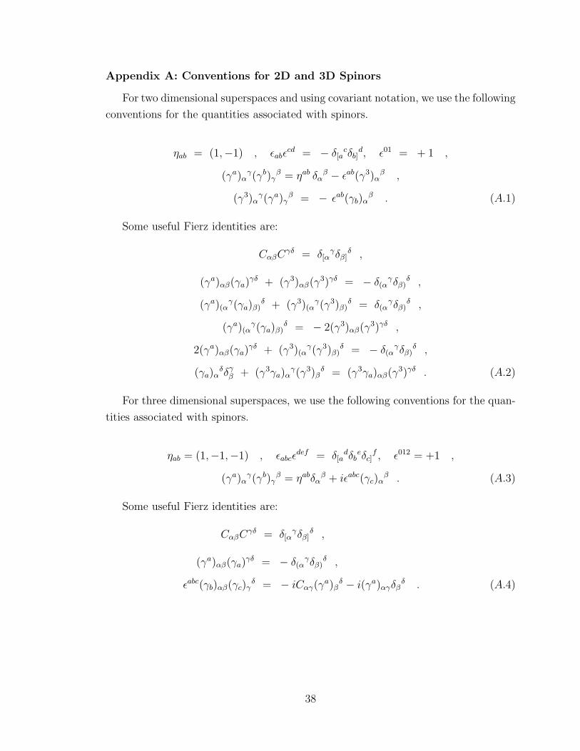
Appendix A: Conventions for 2D and 3D Spinors

For two dimensional superspaces and using covariant notation, we use the following

conventions for the quantities associated with spinors.

ηab = (1,−1) , ǫabǫcd = − δ[a

cδb]d, ǫ01 = + 1 ,

(γa)αγ(γb)γ

β = ηab δαβ − ǫab(γ3)α

β ,

(γ3)αγ(γa)γ

β = − ǫab(γb)αβ . (A.1)

Some useful Fierz identities are:

CαβCγδ = δ[α

γδβ]δ ,

(γa)αβ(γa)γδ + (γ3)αβ(γ

3)γδ = − δ(αγδβ)

δ ,

(γa)(αγ(γa)β)

δ + (γ3)(αγ(γ3)β)

δ = δ(αγδβ)

δ ,

(γa)(αγ(γa)β)

δ = − 2(γ3)αβ(γ3)γδ ,

2(γa)αβ(γa)γδ + (γ3)(α

γ(γ3)β)δ = − δ(α

γδβ)δ ,

(γa)αδδ

γβ + (γ3γa)α

γ(γ3)βδ = (γ3γa)αβ(γ

3)γδ . (A.2)

For three dimensional superspaces, we use the following conventions for the quan-

tities associated with spinors.

ηab = (1,−1,−1) , ǫabcǫdef = δ[a

dδbeδc]

f , ǫ012 = +1 ,

(γa)αγ(γb)γ

β = ηabδαβ + iǫabc(γc)α

β . (A.3)

Some useful Fierz identities are:

CαβCγδ = δ[α

γδβ]δ ,

(γa)αβ(γa)γδ = − δ(α

γδβ)δ ,

ǫabc(γb)αβ(γc)γδ = − iCαγ(γ

a)βδ − i(γa)αγδβ

δ . (A.4)

38

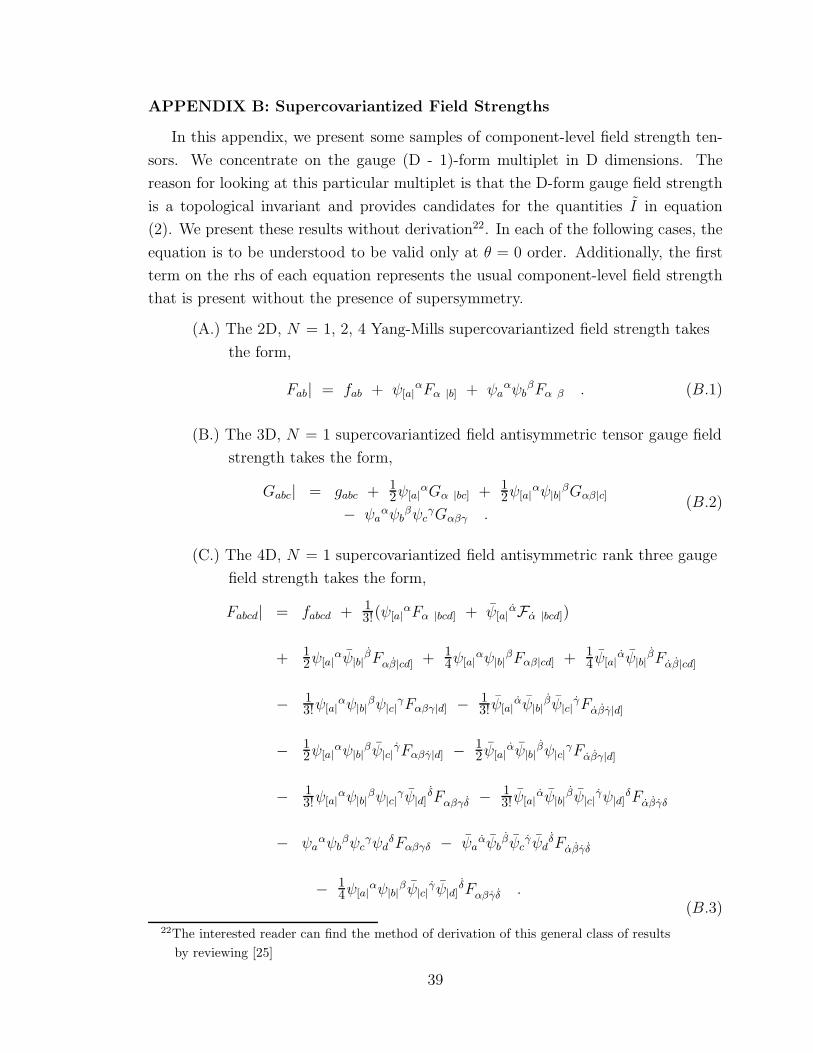
APPENDIX B: Supercovariantized Field Strengths

In this appendix, we present some samples of component-level field strength ten-

sors. We concentrate on the gauge (D - 1)-form multiplet in D dimensions. The

reason for looking at this particular multiplet is that the D-form gauge field strength

is a topological invariant and provides candidates for the quantities I in equation

(2). We present these results without derivation22. In each of the following cases, the

equation is to be understood to be valid only at θ = 0 order. Additionally, the first

term on the rhs of each equation represents the usual component-level field strength

that is present without the presence of supersymmetry.

(A.) The 2D, N = 1, 2, 4 Yang-Mills supercovariantized field strength takes

the form,

Fab| = fab + ψ[a|αFα |b] + ψa

αψbβFα β . (B.1)

(B.) The 3D, N = 1 supercovariantized field antisymmetric tensor gauge field

strength takes the form,

Gabc| = gabc + 12ψ[a|

αGα |bc] + 12ψ[a|

αψ|b|βGαβ|c]

− ψaαψb

βψcγGαβγ .

(B.2)

(C.) The 4D, N = 1 supercovariantized field antisymmetric rank three gauge

field strength takes the form,

Fabcd| = fabcd + 13!(ψ[a|

αFα |bcd] + ψ[a|αFα |bcd])

+ 12ψ[a|

αψ|b|βFαβ|cd] + 1

4ψ[a|αψ|b|

βFαβ|cd] + 14ψ[a|

αψ|b|βFαβ|cd]

− 13!ψ[a|

αψ|b|βψ|c|

γFαβγ|d] − 13!ψ[a|

αψ|b|βψ|c|

γFαβγ|d]

− 12ψ[a|

αψ|b|βψ|c|

γFαβγ|d] − 12ψ[a|

αψ|b|βψ|c|

γFαβγ|d]

− 13!ψ[a|

αψ|b|βψ|c|

γψ|d]δFαβγδ − 1

3!ψ[a|αψ|b|

βψ|c|γψ|d]

δFαβγδ

− ψaαψb

βψcγψd

δFαβγδ − ψaαψb

βψcγψd

δFαβγδ

− 14ψ[a|

αψ|b|βψ|c|

γψ|d]δFαβγδ .

(B.3)

22The interested reader can find the method of derivation of this general class of results

by reviewing [25]

39

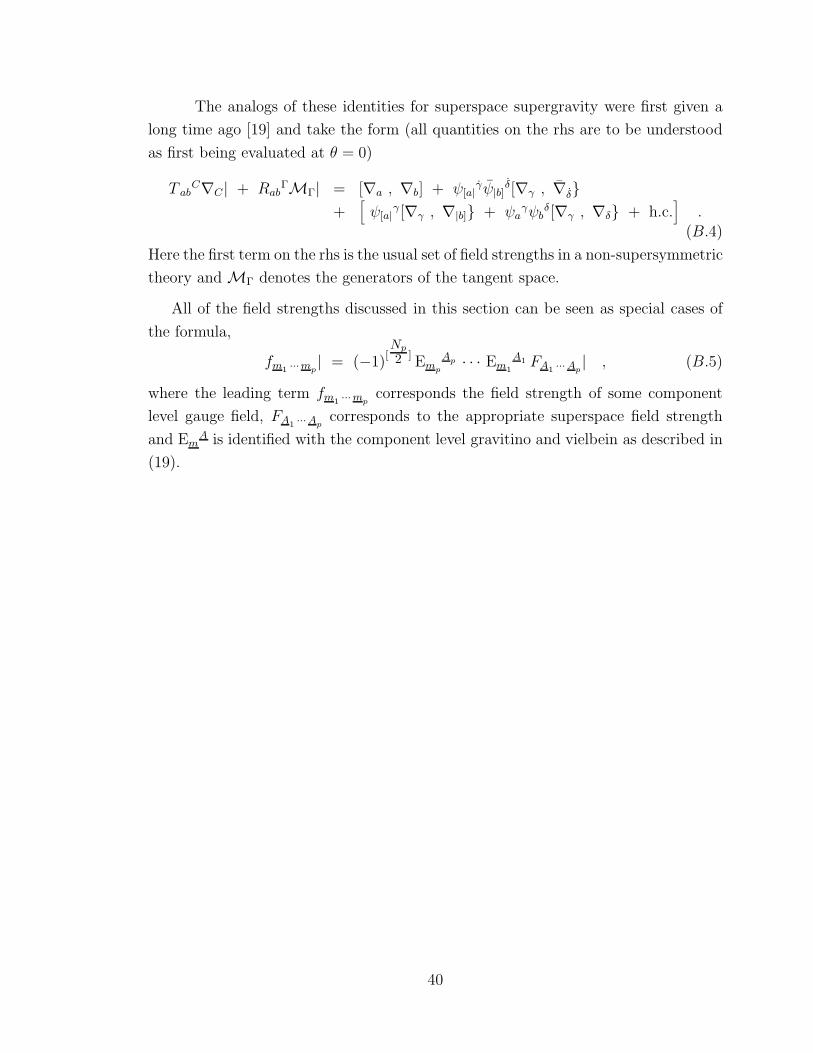
The analogs of these identities for superspace supergravity were first given a

long time ago [19] and take the form (all quantities on the rhs are to be understood

as first being evaluated at θ = 0)

T abC∇C | + Rab

ΓMΓ| = [∇a , ∇b] + ψ[a|γψ|b]

δ[∇γ , ∇δ}

+[ψ[a|

γ[∇γ , ∇|b]} + ψaγψb

δ[∇γ , ∇δ} + h.c.]

.

(B.4)

Here the first term on the rhs is the usual set of field strengths in a non-supersymmetric

theory and MΓ denotes the generators of the tangent space.

All of the field strengths discussed in this section can be seen as special cases of

the formula,

fm1 ···mp| = (−1)

[Np

2 ]Emp

Ap · · · Em1

A1 FA1 ···Ap| , (B.5)

where the leading term fm1 ···mpcorresponds the field strength of some component

level gauge field, FA1 ···Apcorresponds to the appropriate superspace field strength

and EmA is identified with the component level gravitino and vielbein as described in

(19).

40

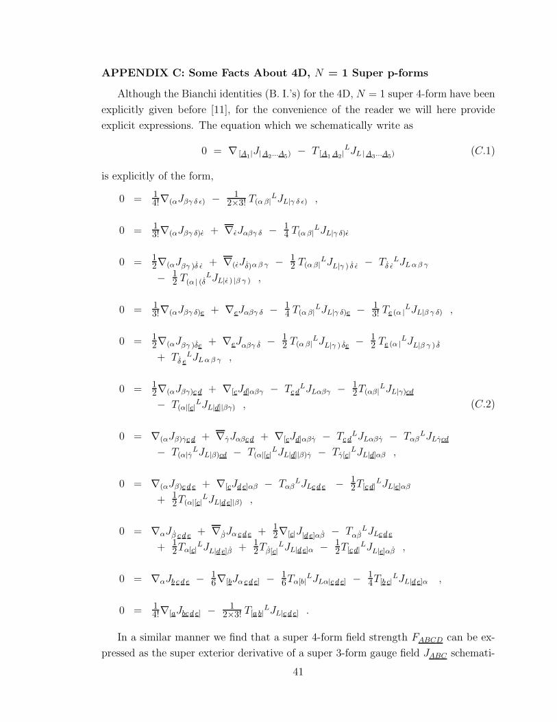
APPENDIX C: Some Facts About 4D, N = 1 Super p-forms

Although the Bianchi identities (B. I.’s) for the 4D, N = 1 super 4-form have been

explicitly given before [11], for the convenience of the reader we will here provide

explicit expressions. The equation which we schematically write as

0 = ∇ [A1|J|A2...A5)

− T [A1 A2|LJL |A3...A5)

(C.1)

is explicitly of the form,

0 = 14!∇(αJβγ δ ǫ) − 1

2×3! T(αβ|LJL|γ δ ǫ) ,

0 = 13!∇(αJβγ δ)ǫ + ∇ǫJαβγ δ − 1

4 T(αβ|LJL|γ δ)ǫ

0 = 12∇(αJβγ )δ ǫ + ∇(ǫJδ)αβ γ − 1

2 T(αβ|LJL|γ ) δ ǫ − Tδ ǫ

LJLαβ γ

− 12 T(α | (δ

LJL|ǫ ) |β γ ) ,

0 = 13!∇(αJβγ δ)e + ∇eJαβγ δ − 1

4 T(αβ|LJL|γ δ)e − 1

3! Te (α |LJL|β γ δ) ,

0 = 12∇(αJβγ )δe + ∇eJαβγ δ − 1

2 T(αβ|LJL|γ ) δe − 1

2 Te (α |LJL|β γ ) δ

+ Tδ eLJLαβ γ ,

0 = 12∇(αJβγ)c d + ∇[cJd]αβγ − Tc d

LJLαβγ − 12T(αβ|

LJL|γ)cd

− T(α|[c|LJL|d]|βγ) ,

0 = ∇(αJβ)γc d + ∇γJαβc d + ∇[cJd]αβγ − Tc dLJLαβγ − Tαβ

LJLγcd

− T(α|γLJL|β)cd − T(α|[c|

LJL|d]|β)γ − Tγ[c|LJL|d]αβ ,

0 = ∇(αJβ)c d e + ∇[cJd e]αβ − TαβLJLc d e − 1

2T[c d|LJL|e]αβ

+ 12T(α|[c|

LJL|d e]|β) ,

0 = ∇αJβ c d e + ∇βJα c d e + 12∇[c|J|d e]αβ − Tαβ

LJLc d e

+ 12Tα[c|

LJL|d e]β + 12Tβ[c|

LJL|d e]α − 12T[c d|

LJL|e]αβ ,

0 = ∇αJb c d e − 16∇[bJα c d e] − 1

6Tα[b|LJLα|c d e] − 1

4T[b c|LJL|d e]α ,

0 = 14!∇[aJbc d e] − 1

2×3! T[a b|LJL|c d e] .

(C.2)

In a similar manner we find that a super 4-form field strength FABCD can be ex-

pressed as the super exterior derivative of a super 3-form gauge field JABC schemati-

41

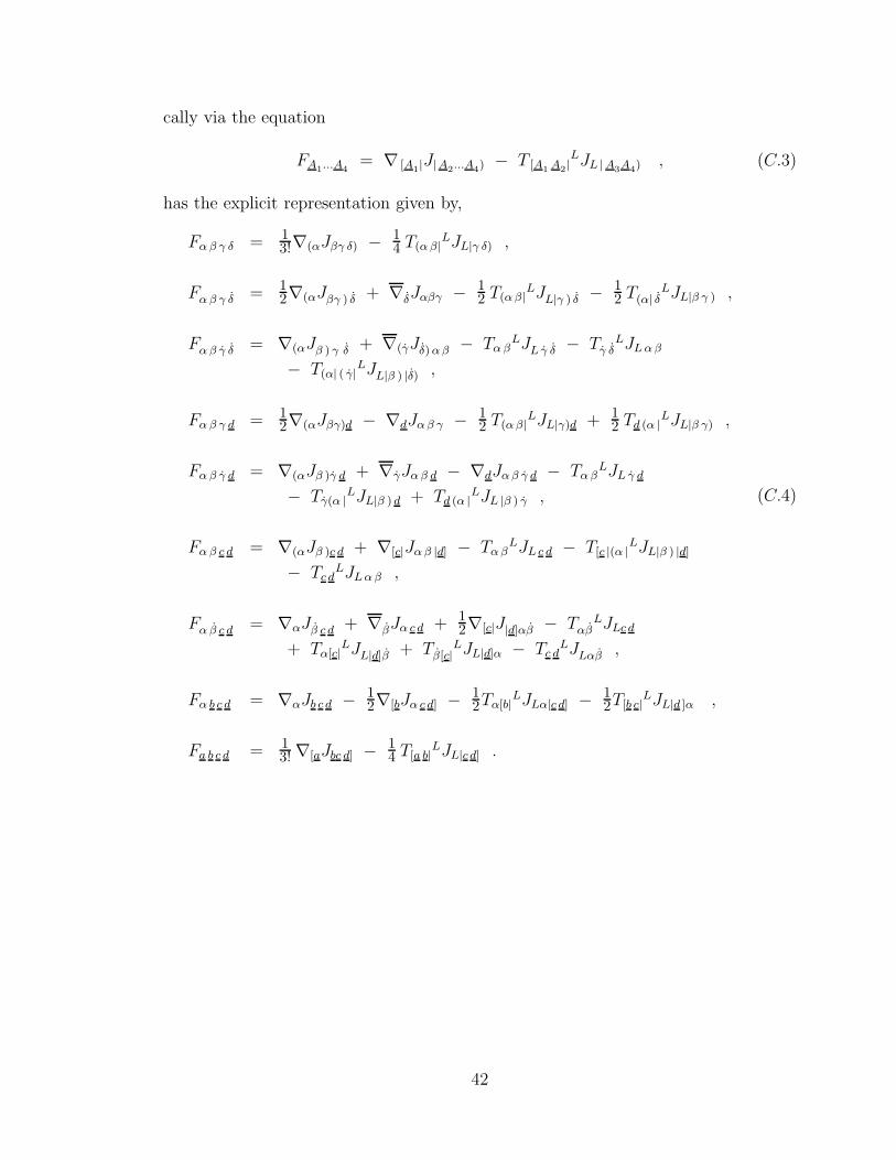
cally via the equation

FA1...A4= ∇ [A1|

J|A2...A4)− T [A1 A2|

LJL |A3A4), (C.3)

has the explicit representation given by,

Fαβ γ δ = 13!∇(αJβγ δ) − 1

4 T(αβ|LJL|γ δ) ,

Fαβ γ δ = 12∇(αJβγ ) δ + ∇δJαβγ − 1

2 T(αβ|LJL|γ ) δ − 1

2 T(α| δLJL|β γ ) ,

Fαβ γ δ = ∇(αJβ ) γ δ + ∇(γJδ)αβ − TαβLJL γ δ − Tγ δ

LJLαβ

− T(α| ( γ|LJL|β ) |δ) ,

Fαβ γ d = 12∇(αJβγ)d − ∇dJαβ γ − 1

2 T(αβ|LJL|γ)d + 1

2 Td (α |LJL|β γ) ,

Fαβ γ d = ∇(αJβ )γ d + ∇γJαβ d − ∇dJαβ γ d − TαβLJL γ d

− Tγ(α |LJL|β ) d + Td (α |

LJL |β ) γ ,

Fαβ c d = ∇(αJβ )c d + ∇[c|Jαβ |d] − TαβLJLc d − T[c |(α |

LJL|β ) |d]

− Tc dLJLαβ ,

Fα β c d = ∇αJβ c d + ∇βJα c d + 12∇[c|J|d]αβ − Tαβ

LJLc d

+ Tα[c|LJL|d]β + Tβ[c|

LJL|d]α − Tc dLJLαβ ,

Fα b c d = ∇αJb c d − 12∇[bJα c d] − 1

2Tα[b|LJLα|c d] − 1

2T[b c|LJL|d ]α ,

Fa b c d = 13! ∇[aJbc d] − 1

4 T[a b|LJL|c d] .

(C.4)

42

References

[1] To our knowledge B.Zumino first raised such questions in the early eighties.

[2] S.J.Gates, Jr., M.T. Grisaru, M.E. Knutt-Wehlau and W. Siegel, Phys. Lett.

421B (1998) 203.

[3] S.J.Gates, Jr., “Ectoplasm Has No Topology: The Prelude,” Univ. of MD

preprint UMDEPP 98-13, (Sept., 1997) hep-th/9709104, to appear in the pro-

ceedings of the International Seminar on “Supersymmetries and Quantum Sym-

metries,” Dubna, Russia, July 22, 1997.

[4] M.T. Grisaru, M.E. Knutt-Wehlau and W. Siegel, Nucl. Phys. 523B (1998) 663.

[5] S.J.Gates, Jr., in Supergravity, eds. van Nieuwenhuizen and Freedman, North-

Holland, Amsterdam, (1979) 215.

[6] S.J.Gates, Jr., Nucl. Phys. B162 (1980) 79; S.J.Gates, Jr. and W. Siegel, Nucl.

Phys. B163 (1980) 519; S.J.Gates, Jr., K.S.Stelle and P.C.West, Nucl. Phys.

B169 (1980) 347.

[7] A.Rogers, J. Math. Phys. 21 (1980) 1352.

[8] F.A.Berezin, The Method of Second Quantization, Academic Press, New York,

(1966).

[9] R.Arnowitt, B.Zumino and P.Nath, Phys. Lett. 56B (1975) 81.

[10] B. DeWitt, Supermanifolds, Cambridge University Press, London, (1984).

[11] S.J.Gates, Jr., Nucl. Phys. B184 (1981) 381.

[12] M.Cederwall, A.von Gussich, B.E.W.Nilsson, P.Sundell, and A.Westerberg,

Nucl. Phys. B490 (1997) 163; ibid. 179.

[13] S.J.Gates, Jr., Nucl. Phys. B213 (1983) 409.

[14] B. Zupnik, Theor. Math. Phys. 89, Vol. 2 (1991) 1191; idem. Phys. Lett. 254B

(1991) 127.

[15] R. Brooks, F. Muhammad and S.J.Gates, Jr., Nucl. Phys. B268 (1986) 599.

[16] S.J.Gates, Jr., L.Lu, R.N.Oerter, Phys. Lett. 218B (1989) 33; S.J.Gates, Jr.,

Y.Hassoun and P.van Nieuwenhuizen, Nucl. Phys. B317 (1989) 302.

43

[17] S.J.Gates, Jr., M.T.Grisaru, M.Rocek, and W.Siegel, Superspace, Ben-

jamin/Cummings Publishing Co., Inc. (Reading, MA), 1983, p. 469; P. Howe

and G. Papadopoulos, Class. & Quant. Grav. 4 (1987) 11.

[18] M.T. Grisaru, M. E. Wehlau, Int. J. Mod.Phys. A10 (1995) 753; idem. Nucl.

Phys. B453 (1995) 489; ibid. B457 (1995) 219.

[19] S. J. Gates, Jr. and M. Brown, Annals of Physics, 2, Vol. 122, (1979) 443.

[20] P.Breitenlohner, Phys. Lett. 67B (1977) 49, idem. Nucl. Phys. B124 (1977) 500.

[21] W.Siegel and S.J.Gates, Jr., Nucl. Phys. B147 (1979) 77.

[22] S.J.Gates, Jr., P.Majumdar, R.N. Oerter and A. van de Ven, Phys. Lett. 214B

(1988) 26; J.de Boer and K.Skenderis, Nucl. Phys. B481 (1996) 129.

[23] S.J.Gates, Jr. and and W.Siegel, Nucl. Phys. B164 (1980) 484.

[24] J.Wess and B.Zumino, Phys. Lett. 74B (1978) 415.

[25] S.J.Gates, Jr., M.T.Grisaru, M.Rocek, and W.Siegel, Superspace, Benjamin-

Cummings Publishing Company (1983), Reading, MA.

[26] S.J.Gates, Jr., Phys. Rev. D16 (1977) 1727; S.J.Gates, Jr., M.T.Grisaru,

M.Rocek, and W.Siegel, Superspace, Benjamin/Cummings Publishing Co., Inc.

(Reading, MA), 1983, p. 177.

44