Queensland University of Technology

School of Engineering Systems

INCORPORATING INTERDPENDENCE IN RISK

LIKELIHOOD ANALYSIS TO ENHANCE

DIAGNOSTICS IN CONDITION MONITORING Volume 1 of 2

Leonard Wiliem

Bachelor of Engineering (Mechanical), Sarjana Teknik

Principal Supervisor:

Prof. Prasad K.D.V. Yarlagadda

Associate Supervisors:

Prof. Doug Hargreaves Dr. Fred Stapelberg

Submitted to

Queensland University of Technology for the degree of

DOCTOR OF PHILOSOPHY

2008

i

ABSTRACT

This research is aimed at addressing problems in the field of asset management relating to

risk analysis and decision making based on data from a Supervisory Control and Data

Acquisition (SCADA) system. It is apparent that determining risk likelihood in risk

analysis is difficult, especially when historical information is unreliable. This relates to a

problem in SCADA data analysis because of nested data. A further problem is in

providing beneficial information from a SCADA system to a managerial level

information system (e.g. Enterprise Resource Planning/ERP). A Hierarchical Model is

developed to address the problems. The model is composed of three different Analyses:

Hierarchical Analysis, Failure Mode and Effect Analysis, and Interdependence Analysis.

The significant contributions from the model include: (a) a new risk analysis model,

namely an Interdependence Risk Analysis Model which does not rely on the existence of

historical information because it utilises Interdependence Relationships to determine the

risk likelihood, (b) improvement of the SCADA data analysis problem by addressing the

nested data problem through the Hierarchical Analysis, and (c) presentation of a

framework to provide beneficial information from SCADA systems to ERP systems. The

case study of a Water Treatment Plant is utilised for model validation.

Keywords:

Hierarchical Analysis, Failure Mode and Effect Analysis, Risk Analysis, SCADA, ERP,

Interdependence Analysis

ii

ACKNOWLEDGEMENTS

I would like to express my deep and sincere gratitude to my principal supervisor Professor Prasad Yarlagadda for his pertinent guidance, support and encouragement during my candidature at Queensland University of Technology. Professor Doug Hargreaves as my associate supervisor also deserves my sincere thanks for his constant and unquestionable commitment to this research. I am deeply grateful to my external supervisor Dr. Fred Stapelberg for his detailed and constructive comments, and his important support throughout this work.

I would like to say thanks to Dr. Zhou for his help at the very beginning of this research.

I wish to express my warm and sincere thanks to Dr. Ron King, and Dr. Prasad Gudimetla for their valuable advice that helped in developing this thesis.

My personal thanks to Mr. Peter Nelson for his help during the drafting phase of my thesis.

I owe my loving thanks to my wife Monica. She has lost a lot due to my research. Without her encouragement and understanding it would have been impossible for me to finish this work. My special gratitude is due to my brother, Arnold Wiliem, for his support during my experiment. I would also want to thank my parents for their loving support

My sincere appreciation to all of my fellow students and colleagues for their company and interesting discussions over the past four years.

I would like to convey my thanks to SunWater for all their support in providing information that I needed.

The financial support of the Queensland University of Technology and Cooperative Research Centre for Integrated Engineering Asset Management is gratefully acknowledged

Brisbane, Australia, May 2008

Leonard Wiliem

iii

The work contained in this thesis has not been previously submitted to meet the

requirements for an award at this or any other higher education institution. To the best of

my knowledge and belief, the thesis contains no material previously published or written

by another person except where due reference is made.

Leonard Wiliem

iv

List of Publications Accepted

1. L.WILIEM, D.HARGREAVES, YARLAGADDA, P. K. D. V. &

STAPELBERG, R. F., “Development of Real-Time Data Filtering for SCADA

System”, Journal of Achievement in Materials and Manufacturing Engineering,

21(2007), 89-92.

2. L.WILIEM, YARLAGADDA, P. K. D. V., D.HARGRAVES, MA, L. &

STAPELBERG, R. F., “A Real-Time Lossless Compressing Algorithm for Real-

Time Condition Monitoring System”, Proceeding of COMADEM – 2006. Lulea

University of Technology, Sweden, 113-118.

3. L.WILIEM, YARLAGADDA, P. K. D. V. & ZHOU, S., “A Real-Time Lossless

Compressing Algorithm for Real-Time Condition Monitoring System”,

Proceeding of COMADEM – 2006. Lulea University of Technology, Sweden,

119-129.

List of Publications Submitted and Under Review

1. L.WILIEM, YARLAGADDA, P. K. D. V. & STAPELBERG, R. F.,

D.HARGREAVES, “Identification of Critical Criteria of On-Line Data

Acquisition System”, 9th Global Congress on Manufacturing and Management

[abstract accepted].

List of Publications in preparation

1. L.WILIEM, YARLAGADDA, P. K. D. V. & STAPELBERG, R. F.,

D.HARGREAVES, “Hierarchical Model: Interdependence Risk Analysis”..

2. L.WILIEM, YARLAGADDA, P. K. D. V. & STAPELBERG, R. F.,

D.HARGREAVES, “Hierarchical Model: Utilising Hierarchical and

Interdependence Analyses to Analyse SCADA Data”.

v

Volume 1 of 2 Table of Contents ABSTRACT......................................................................................................................... i ACKNOWLEDGEMENTS................................................................................................ ii List of Publications Accepted ............................................................................................ iv List of Publications Submitted and Under Review............................................................ iv List of Publications in preparation..................................................................................... iv Volume 1 of 2 Table of Contents........................................................................................ v List of Figures .................................................................................................................... ix List of Tables .................................................................................................................... xii CHAPTER 1 INTRODUCTION ...................................................................................... 13

1.1. Background Information........................................................................................ 13 1.2. Research Problems................................................................................................. 14 1.3. Research Hypotheses ............................................................................................. 16 1.4. Research Aim and Objectives................................................................................ 17 1.5. Overview of Research Methodology ..................................................................... 18 1.6. Research Contributions.......................................................................................... 19 1.7. Thesis Organisation ............................................................................................... 19

CHAPTER 2 LITERATURE REVIEW........................................................................... 21

2.1. Introduction............................................................................................................ 21 2.2. On-Line Data Connectivity: Problem Identification.............................................. 22

2.2.1. Maintenance Philosophies ............................................................................... 22 2.2.2. Condition Based Maintenance and Condition Monitoring ............................ 23 2.2.3. Supervisory Control and Data Acquisition (SCADA)..................................... 25 2.2.4. Problems in SCADA Data Analysis ................................................................. 28 2.2.5. Discussion........................................................................................................ 41

2.3. On-line Data Connectivity: Solution Formulation................................................. 43 2.3.1. Proposed Model Criteria Formulation............................................................. 44 2.3.2. Further Literature Study ................................................................................. 46 2.3.3. Formulation of the Final Proposed Model: Hierarchical Model ..................... 61 2.3.4. Discussion........................................................................................................ 64

2.4. Risk Analysis: Problems Identification ................................................................. 67 2.4.1. Background ...................................................................................................... 67 2.4.2. Problems.......................................................................................................... 69 2.4.3. Discussion........................................................................................................ 75

2.5. Risk Analysis: A Different Perspective ................................................................. 75 2.5.1. Interdependence Risk Analysis ....................................................................... 75 2.5.2. Discussion........................................................................................................ 78

2.6. Formulation of Research Hypotheses, Aim, and Objectives ................................. 78 2.7. Summary................................................................................................................ 82

vi

CHAPTER 3 RESEARCH METHODOLOGY ............................................................... 83 3.1. Introduction............................................................................................................ 83 3.2. Experimentation: Real-Time Water Quality Condition Monitoring System......... 83

3.2.1. Introduction ..................................................................................................... 83 3.2.2. System Architecture ........................................................................................ 84 3.2.3. On-line Data Acquisition Prototype Development ......................................... 85 3.2.4. Identification of Critical Criteria of On-line Data Acquisition Systems ........ 91 3.2.5. Discussion........................................................................................................ 91

3.3. Experimentation: SCADA Test Rig....................................................................... 92 3.3.1. Introduction ..................................................................................................... 92 3.3.2. Data Source ...................................................................................................... 94 3.3.3. Data Transfer Process ...................................................................................... 94 3.3.4. Data Processing and Display ........................................................................... 94 3.3.5. Data Storage..................................................................................................... 95 3.3.6. Discussion ........................................................................................................ 95

3.4. Theory Development: Algorithm Formulation (Data Compression Algorithm)... 96 3.4.1. Introduction ..................................................................................................... 96 3.4.2. Experiment Overview ..................................................................................... 97 3.4.3. Data Base Analysis ........................................................................................... 99 3.4.4. Real-Time Compression Algorithm .............................................................. 101 3.4.5. Results ........................................................................................................... 103 3.4.6. Discussion...................................................................................................... 104

3.5. Theory Development: Algorithm Formulation (Data Filtering Algorithm) ........ 105 3.5.1. Introduction ................................................................................................... 105 3.5.2. Algorithm Development ................................................................................ 106 3.5.3. Experiment Overview.................................................................................... 108 3.5.4. Results ........................................................................................................... 110 3.5.5. Discussion...................................................................................................... 112

3.6. Theory Development: Hierarchical Model (Brief Introduction) ......................... 113 3.7. Theory Development: Hierarchical Model (Hierarchical Analysis).................... 113

3.7.1. Introduction ................................................................................................... 113 3.7.2. System Breakdown Structure (SBS).............................................................. 114 3.7.3. Discussion ...................................................................................................... 116

3.8. Theory Development: Hierarchical Model (Failure Mode and Effect Analysis) 116 3.8.1. Introduction ................................................................................................... 116 3.8.2. Explanation of FMEA.................................................................................... 116 3.8.3. Discussion ...................................................................................................... 118

3.9. Theory Development: Interdependence Analysis................................................ 119 3.9.1. Introduction ................................................................................................... 119 3.9.2. Functional and Causal Relationship Diagram (FCRD) ................................ 120 3.9.3. Interdependence Risk Analysis (IRA)........................................................... 126 3.9.4. Discussion...................................................................................................... 131

3.10. Implementation: Data Bridge............................................................................. 132 3.10.1. Introduction.................................................................................................. 132 3.10.2. Implementation step .................................................................................... 132

vii

3.10.3. Discussion .................................................................................................... 135 3.11 Summary............................................................................................................. 135 3.12. Verification: Case Study.................................................................................... 140

3.12.1. Brief Introduction of Chapters 4, 5, and 6 .................................................... 140 3.12.2. Water Utility Industry Case Study ............................................................. 141 3.12.3. Analysis and Criteria of Data Filtering ........................................................ 142

CHAPTER 4 CASE STUDY: MODEL DEVELOPMENT.......................................... 146

4.1. Introduction.......................................................................................................... 146 4.2. Data Bridge Development: Hierarchical Analysis............................................... 146

4.2.1. Introduction................................................................................................... 146 4.2.2. System Breakdown Structure ....................................................................... 147 4.2.3. Discussion...................................................................................................... 156

4.3. Data Bridge Development: Failure Mode and Effect analysis (FMEA).............. 157 4.3.1. Introduction ................................................................................................... 157 4.3.2. Development Process of Water Treatment Plant FMEA .............................. 157 4.3.3. Discussion...................................................................................................... 160

4.4. Data Bridge Development: Interdependence Analysis ........................................ 161 4.4.1. Introduction................................................................................................... 161 4.4.2. FCRD Stage 1................................................................................................. 161 4.4.3. FCRD Stage 2 ................................................................................................ 168 4.4.4. Discussion ..................................................................................................... 186

4.5. Data Bridge Development: Filtering Algorithm.................................................. 187 4.5.1. Introduction ................................................................................................... 187 4.5.2. Development of the Filtering Algorithm ....................................................... 187 4.5.3. Discussion...................................................................................................... 190

4.6. Data Bridge Development: Knowledge Base ...................................................... 191 4.6.1. Introduction................................................................................................... 191 4.6.2. Data Base ....................................................................................................... 191 4.6.3. Inference Engine ............................................................................................ 195 4.6.4. Discussion ..................................................................................................... 196

4.7. Risk Ranking Development by Utilising Interdependence Risk Analysis .......... 196 4.7.1. Introduction ................................................................................................... 196 4.7.2. Risk Ranking Development........................................................................... 197 4.7.3. Discussion...................................................................................................... 207

4.8. Summary.............................................................................................................. 208 CHAPTER 5 CASE STUDY: MODEL DATA ANALYSIS ....................................... 213

5.1. Introduction.......................................................................................................... 213 5.2. Quantitative Data Analysis .................................................................................. 213

5.2.1. Introduction ................................................................................................... 213 5.2.2. Data Cleansing............................................................................................... 214 5.2.3. Discussion and Conclusion for Data Cleansing ............................................ 215 5.2.4. Statistical Analysis: Descriptive Statistics.................................................... 216 5.2.5. Discussion and Conclusion for Descriptive Statistics .................................. 223

viii

5.2.6. Statistical Analysis: Correlation Analysis ..................................................... 227 5.2.7. Discussion and Conclusion for Correlation Analysis .................................... 230

5.3. Qualitative Data Analysis .................................................................................... 230 5.3.1. Introduction ................................................................................................... 230 5.3.2. Qualitative Data Analysis: Trouble Shooting ................................................ 231 5.3.3. Discussion and Conclusion............................................................................ 232

5.4. Summary.............................................................................................................. 232 CHAPTER 6 CASE STUDY: MODEL DATA VALIDATION .................................. 235

6.1. Introduction.......................................................................................................... 235 6.2. Validation A (Validation of SCADA Model Data) ............................................. 237

6.2.1. Introduction ................................................................................................... 237 6.2.2. Validation of SCADA data analysis in a “real time” time frame .................... 240 6.2.3. Validation of the Nested Data Issue .............................................................. 246 6.2.4. Conclusions ................................................................................................... 253

6.3. Validation B (Validation of Interdependence Model Data)................................. 255 6.3.1. Introduction ................................................................................................... 255 6.3.2. Validation of the Interdependence Risk Analysis ......................................... 256 6.3.3. Conclusions ................................................................................................... 266

6.4. Validation C (Validation of Data Connectivity).................................................. 267 6.4.1. Introduction................................................................................................... 267 6.4.2. Performing Validation C ............................................................................... 267 6.4.3. Conclusions ................................................................................................... 270

6.5. Summary.............................................................................................................. 271 CHAPTER 7 SUMMARY AND CONCLUSIONS...................................................... 277

7.1. Introduction.......................................................................................................... 277 7.2. Summary.............................................................................................................. 277 7.3. Conclusions.......................................................................................................... 284 7.4. Contributions........................................................................................................ 287 7.5. Future Work ......................................................................................................... 291

References....................................................................................................................... 293

ix

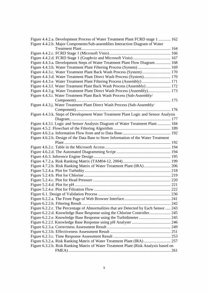
List of Figures

Figure 2.2.1. Diagram of Maintenance Philosophies (Stoneham, 1998) .......................... 22 Figure 2.2.3.a. Structure of SCADA systems (Laboratories, 2004) ................................. 26 Figure 2.2.3.b. Networking system (Qiu et al., 2002) ...................................................... 27 Figure 2.2.4.a. Fuzzy Logic Systems (Mendel, 1995) ...................................................... 31 Figure 2.2.4.b. ERP Structure (Musaji, 2002) .................................................................. 36 Figure 2.2.4.c. Plant Asset Management System Framework (Bever, 2000. op cit; Stapelberg, 2006) ...................................................................................... 37 Figure 2.3.1. Preliminary Model to Address Research Problems..................................... 45 Figure 2.3.2.a. Process Flow Diagram of Coal Fired Power Station (Stapelberg, 1993) . 51 Figure 2.3.2.b. Process Flow Block Diagram of Haul Truck Power Train System (Stapelberg, 1993)..................................................................................... 52 Figure 2.3.2.c. Example of System Description (Stapelberg, 1993)................................. 54 Figure 2.3.3. Hierarchical Model ...................................................................................... 62 Figure 2.4.2. Risk Analysis Step (TAM04-12, 2004)....................................................... 69 Figure 2.5.1. Hierarchical Model with Addition of Interdependence Risk Analysis ....... 77 Figure 3.2.2. Layered Structure Diagram of Remote Water Quality Monitoring System 85 Figure 3.2.3.a. LabVIEW Based Web Technologies for Communication over The Internet ...................................................................................................... 86 Figure 3.2.3.b. The Framework Diagram of Local Measurement Station........................ 87 Figure 3.2.3.c. Real-time Water Quality Condition Displayed on Local Measurement Station Terminal........................................................................................ 88 Figure 3.2.3.d. An Interface of Central Control Station Terminal.................................... 89 Figure 3.2.3.e. Water Quality Condition Displayed on the Remote Browse Station ....... 90 Figure 3.2.3.f. History Data of Water Quality Condition on the Local Measurement Station ....................................................................................................... 90 Figure 3.3.1. Critical Criteria of On-line Data Acquisition System ................................. 93 Figure 3.4.2. Experiment Scheme..................................................................................... 98 Figure 3.4.4.a. Algorithm Design ................................................................................... 102 Figure 3.4.4.b. Real-time Compression Algorithm......................................................... 102 Figure 3.4.5. Experiment Result ..................................................................................... 103 Figure 3.5.2.a. Steps of The Filtering Algorithm............................................................ 106 Figure 3.5.2.b. Flowchart of Checking of Data Changing.............................................. 107 Figure 3.5.3.a. Stage of the Experiment.......................................................................... 109 Figure 3.5.3.b. Detail of The Data Filtering Process Simulation.................................... 109 Figure 3.5.4.a. Record of Ten Last Data from Each Parameter before Data Change..... 110 Figure 3.5.4.b. Record of Code, Index, Date and Time of when Data Change Occur ... 111 Figure 3.5.4.c. Data Change Count from Different Parameters...................................... 111 Figure 3.7.2. System Breakdown Structure Procedure ................................................... 115 Figure 3.10.2.a. Process in Data Bridge.......................................................................... 133 Figure 3.10.2.b. Flowchart of Information Processing in Data Bridge .......................... 134 Figure 4.2.1. Process Development of Water Treatment Plant SBS .............................. 147 Figure 4.2.2. Process Block Diagram of Moogerah Township Water Treatment Plant . 149 Figure 4.3.1. Development Process of Water Treatment Plant FMEA .......................... 157

x

Figure 4.4.2.a. Development Process of Water Treatment Plant FCRD stage 1 ............ 162 Figure 4.4.2.b. Major Components/Sub-assemblies Interaction Diagram of Water Treatment Plant....................................................................................... 164 Figure 4.4.2.c. FCRD Stage 1 (Microsoft Visio)............................................................ 166 Figure 4.4.2.d. FCRD Stage 1 (Graphviz and Microsoft Visio)..................................... 167 Figure 4.4.3.a. Development Steps of Water Treatment Plant Flow Diagram ............... 168 Figure 4.4.3.b. Water Treatment Plant Filtering Process (System) ................................ 169 Figure 4.4.3.c. Water Treatment Plant Back Wash Process (System)............................ 170 Figure 4.4.3.d. Water Treatment Plant Direct Wash Process (System).......................... 170 Figure 4.4.3.e. Water Treatment Plant Filtering Process (Assembly) ............................ 171 Figure 4.4.3.f. Water Treatment Plant Back Wash Process (Assembly) ........................ 172 Figure 4.4.3.g. Water Treatment Plant Direct Wash Process (Assembly)...................... 173 Figure 4.4.3.i. Water Treatment Plant Back Wash Process (Sub-Assembly/ Component)............................................................................................. 175 Figure 4.4.3.j. Water Treatment Plant Direct Wash Process (Sub-Assembly/ Component)............................................................................................. 176 Figure 4.4.3.k. Steps of Development Water Treatment Plant Logic and Sensor Analysis Diagram................................................................................................... 177 Figure 4.4.3.l. Logic and Sensor Analysis Diagram of Water Treatment Plant ............. 184 Figure 4.5.2. Flowchart of the Filtering Algorithm ........................................................ 189 Figure 4.6.2.a. Information Flow from and to Data Base............................................... 192 Figure 4.6.2.b. Design of the Data Base to Store Information of the Water Treatment Plant ........................................................................................................ 192 Figure 4.6.2.c. Table in the Microsoft Access ................................................................ 194 Figure 4.6.2.d. The Automated Diagramming Script ..................................................... 194 Figure 4.6.3. Inference Engine Design ........................................................................... 195 Figure 4.7.2.a. Risk Ranking Matrix (TAM04-12, 2004)............................................... 199 Figure 4.7.2.b. Risk Ranking Matrix of Water Treatment Plant (IRA) .......................... 206 Figure 5.2.4.a. Plot for Turbidity .................................................................................... 218 Figure 5.2.4.b. Plot for Chlorine..................................................................................... 219 Figure 5.2.4.c. Plot for Head Pressure ............................................................................ 220 Figure 5.2.4.d. Plot for pH .............................................................................................. 221 Figure 5.2.4.e. Plot for Filtration Flow ........................................................................... 222 Figure 6.1. Design of Validation Process ....................................................................... 236 Figure 6.2.2.a. The Front Page of Web Browser Interface ............................................. 241 Figure 6.2.2.b. Filtering Result ....................................................................................... 242 Figure 6.2.2.c. The Percentage of Abnormalities that are Detected by Each Sensor ..... 243 Figure 6.2.2.d. Knowledge Base Response using the Chlorine Controller..................... 245 Figure 6.2.2.e. Knowledge Base Response using the Turbidimeter ............................... 245 Figure 6.2.2.f. Knowledge Base Response using pH Analyser ...................................... 246 Figure 6.2.3.a. Correctness Assessment Result .............................................................. 249 Figure 6.2.3.b. Effectiveness Assessment Result ........................................................... 251 Figure 6.2.3.c. Time Response Assessment Result ........................................................ 253 Figure 6.3.2.a. Risk Ranking Matrix of Water Treatment Plant (IRA) .......................... 257 Figure 6.3.2.b. Risk Ranking Matrix of Water Treatment Plant (Risk Analysis based on FMEA) .................................................................................................... 261

xi

Figure 6.3.2.c. Risk Ranking Based on Risk Factor Comparison................................... 262 Figure 6.3.2.d. Risk Ranking based on Risk Ranking matrix Comparison .................... 263 Figure 6.3.2.e. Prioritisation Based on the Risk Factor (TAM04-12, 2004) .................. 264

xii

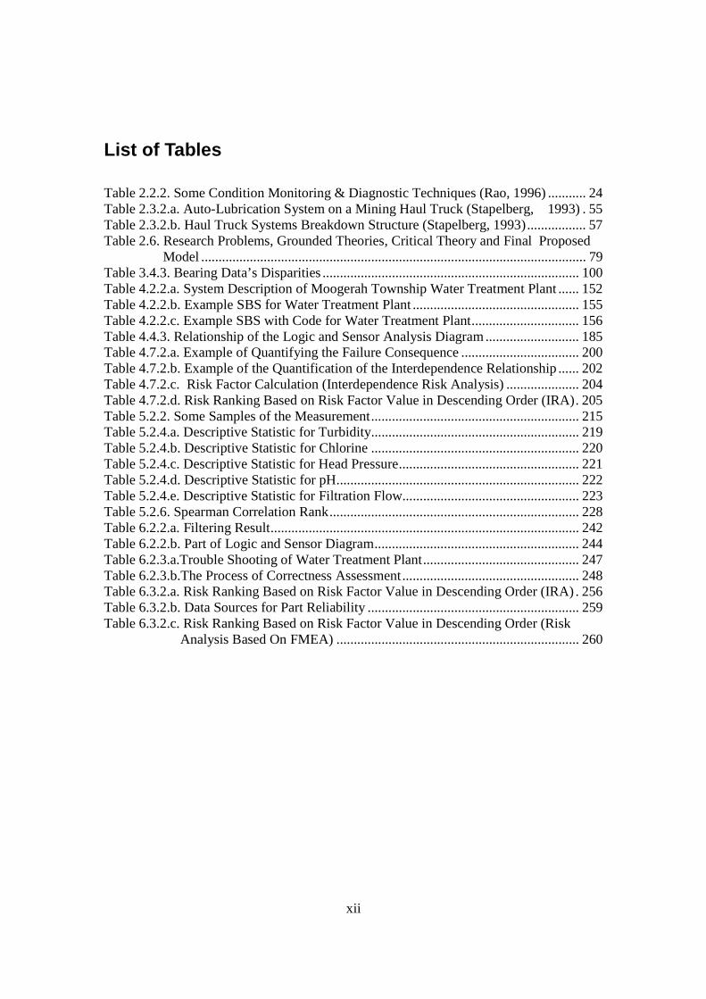
List of Tables Table 2.2.2. Some Condition Monitoring & Diagnostic Techniques (Rao, 1996) ........... 24 Table 2.3.2.a. Auto-Lubrication System on a Mining Haul Truck (Stapelberg, 1993) . 55 Table 2.3.2.b. Haul Truck Systems Breakdown Structure (Stapelberg, 1993)................. 57 Table 2.6. Research Problems, Grounded Theories, Critical Theory and Final Proposed Model ............................................................................................................... 79 Table 3.4.3. Bearing Data’s Disparities .......................................................................... 100 Table 4.2.2.a. System Description of Moogerah Township Water Treatment Plant ...... 152 Table 4.2.2.b. Example SBS for Water Treatment Plant ................................................ 155 Table 4.2.2.c. Example SBS with Code for Water Treatment Plant............................... 156 Table 4.4.3. Relationship of the Logic and Sensor Analysis Diagram........................... 185 Table 4.7.2.a. Example of Quantifying the Failure Consequence .................................. 200 Table 4.7.2.b. Example of the Quantification of the Interdependence Relationship ...... 202 Table 4.7.2.c. Risk Factor Calculation (Interdependence Risk Analysis) ..................... 204 Table 4.7.2.d. Risk Ranking Based on Risk Factor Value in Descending Order (IRA). 205 Table 5.2.2. Some Samples of the Measurement............................................................ 215 Table 5.2.4.a. Descriptive Statistic for Turbidity............................................................ 219 Table 5.2.4.b. Descriptive Statistic for Chlorine ............................................................ 220 Table 5.2.4.c. Descriptive Statistic for Head Pressure.................................................... 221 Table 5.2.4.d. Descriptive Statistic for pH...................................................................... 222 Table 5.2.4.e. Descriptive Statistic for Filtration Flow................................................... 223 Table 5.2.6. Spearman Correlation Rank........................................................................ 228 Table 6.2.2.a. Filtering Result......................................................................................... 242 Table 6.2.2.b. Part of Logic and Sensor Diagram........................................................... 244 Table 6.2.3.a.Trouble Shooting of Water Treatment Plant............................................. 247 Table 6.2.3.b.The Process of Correctness Assessment................................................... 248 Table 6.3.2.a. Risk Ranking Based on Risk Factor Value in Descending Order (IRA) . 256 Table 6.3.2.b. Data Sources for Part Reliability ............................................................. 259 Table 6.3.2.c. Risk Ranking Based on Risk Factor Value in Descending Order (Risk Analysis Based On FMEA) ...................................................................... 260

13

CHAPTER 1

INTRODUCTION

1.1. Background Information

The motivation behind the research reported in this thesis is to develop a model to

enhance diagnostics in condition monitoring by incorporating the interdependence

analysis in risk likelihood analysis. Currently, asset risk is measured in terms of a

combination of consequences of an event and their likelihood. According to the literature,

the consequence of risk can be determined by assessing the severity of the impact, and

the likelihood of risk is determined by how frequently the risks occur. However, it is

quite difficult to determine Risk Likelihood, because it is traditionally based on historical

information/experience base. Sometimes, this kind of information is not available or, if

available, it is incomplete or incomprehensible.

Till now, The most common implementation of condition monitoring is the Supervisory

Control and Data Acquisition (SCADA) system. One of the crucial aspects in the

SCADA system is data analysis, as decision is made mainly on its outcomes. A review of

the literature indicates data, which is collected by a SCADA system, is influenced by

other factors (such as: environment condition, human error, etc.) and cannot be assumed

independent. This data is called nested data. However, if nested data is assumed to be

independent and linear, the result of analysis will be incorrect. Until now, not many

researchers in the SCADA area have been concerned with nested data.

14

A further problem is incorporating the monitoring results from the SCADA system in an

Enterprise Resource Planning (ERP) system. SAP as one of the most successful

Enterprise Resource Planning (ERP) systems in the world, has already embedded

Manufacturing Execution System (MES) in their SAP-R/3 package. Although MES is

able to integrate ERP and SCADA systems, the focus has only been on the Supervisory

Control part of SCADA systems. A method is needed to integrate ERP and SCADA

systems in terms of nested data acquisition and to incorporate the analysis results into an

ERP system.

1.2. Research Problems

In the Literature Study in Chapter 2, three main problems are identified:

• SCADA data analysis

One of the crucial problems in the SCADA system is data. Until now, not many

researchers in the SCADA area have been concerned with nested data problems.

Nested data is data which is influenced by other factors and cannot be assumed to

be independent (Kreft et al., 2000). Several main methods have been proposed to

address the SCADA data analysis problem, such as: Artificial Neural Networks

(Kolla and Varatharasa, 2000, Weerasinghe et al., 1998), Fuzzy Logic (Liu and

Schulz, 2002, Venkatesh and Ranjan, 2003), Expert Systems (Kontopoulos et al.,

1997b), Knowledge Base Systems (de Silva and Wickramarachchi, 1998a, de

Silva and Wickramarachchi, 1998b, Teo, 1995, Vale et al., 1998, Comas et al.,

2003), and Data Mining (Wachla and Moczulski, 2007). After reviewing them, it

has been found that few of these are practically effective in addressing the

problem. Several additional problems have also been identified based on the

review of the proposed methods:

1. The need for historical data at the first step of the method development

(historical data is not always available).

15

2. The need for adaptation capability to the new information on SCADA data

analysis models to cope with the dynamics of the system.

Note: The dynamic in this case means the system is transient. Thus, the change in

one variable will influence the other variables.

• Connectivity of SCADA systems and ERP systems

Based on the Literature Review, the need for integrating both SCADA and ERP

systems is apparent. Gupta (1998) claimed that information from different

systems can be integrated by utilising a Data Bridge. Therefore, some available

Data Bridges to connect SCADA systems and ERP systems are reviewed. From

the review, it is concluded that in general, the concepts of a Data Bridge are still

far from ideal, because most only integrate the data base or even copy the data

directly from SCADA systems data base to the ERP systems data base. Bridging

these two systems only by copying or integrating their data bases will not solve

the problem, because data from the SCADA systems is still raw. In addition, there

has to be several steps to extract appropriate information, such as: Integrated

Condition Monitoring, Asset Health and Prognosis, and Asset Risk Analysis. This

can also be seen from Bever’s Plant Asset Management System (PAM)

Framework (Bever, 2000 op cit Stapelberg, 2006). Thus, a new concept of Data

Bridge is needed to integrate the ERP and SCADA systems in terms of the Data

Acquisition and to incorporate the analysis results into the ERP system.

• Determining Risk Likelihood

Risk Analysis is initiated by identifying the risks, and assessing risk by

determining or estimating both the risk likelihood and consequences. The last step

is determining the significance of the risk in the form of Risk Ranking (TAM04-

12, 2004). The most critical step is determining or estimating the risk likelihood

and risk consequences. It is concluded from the Literature Review that most of the

Risk Analysis methods encounter a significant difficulty in determining Risk

Likelihood. This will lead to difficulty in conducting a conclusive Risk Analysis.

16

1.3. Research Hypotheses

Related to the research problems identified above, several hypotheses can be proposed

(refer to Section 2.6.):

a. The problem in SCADA data analysis, such as nested data, can be addressed

by analysing design information of monitored and monitoring systems

through the Hierarchical Model.

This hypothesis is developed based on the research problem of difficulty in

SCADA data analysis because of nested data. According to the literature review,

data from SCADA is difficult to analyse. The explanation behind this difficulty is

that data from SCADA systems is nested data: data that is influenced by other

factors. The Hierarchical Model is proposed to solve this problem.

b. Interdependence Risk Analysis method can address current Risk Analysis

methods problem, i.e. the need of sophisticated historical information as an

input for Risk Likelihood.

As highlighted in the literature review, the critical problem in current Risk

Analysis is determining the Risk Likelihood. Determining Risk Likelihood is

difficult because of the need for historical information; in most cases, this

information is not available, or if available, is incomplete. Therefore, a new

concept of Risk Analysis by utilising an interdependence relationship is proposed

in this research to address the problem, and is referred to as Interdependence Risk

Analysis.

c. The Data Bridge developed from the Hierarchical Model will address the

connectivity problem between SCADA systems and ERP systems, whereby

significant information can be drawn out from SCADA’s “raw data” and

transferred into ERP.

According to information from the literature review, the need for integrating both

SCADA and ERP systems is apparent. Furthermore, the literature review finds

that several companies offer solutions for integrating SCADA systems and ERP

systems by utilising the Data Bridge concept. However the concept is still far

from ideal, because most of them only directly integrate both systems’ data base.

17

The Hierarchical Model proposed in this model is able to develop a specific data

bridge to facilitate the connectivity between SCADA and ERP systems.

These hypotheses will be tested in this research in accordance with the aim and objectives

stated below.

1.4. Research Aim and Objectives

A research aim is formulated as a guide to test the research hypotheses stated before. The

aim of this research is:

To develop a new model in order to improve the analyses and diagnostics in

condition monitoring by using Interdependence in Risk Likelihood analysis, and test

this model through the Water Treatment Plant Case Study.

This will be investigated through the development of a Hierarchical Model. However,

there are several objectives that must be achieved to test the set hypotheses. These are

(refer to Section 2.6.):

a. Development of a prototype SCADA system in LabVIEW to identify critical

criteria of on-line data acquisition.

b. Development of a data filtering algorithm using the algorithmic approach of data

compression to remove redundant data.

c. Development of a Hierarchical Model

d. Validating the Hierarchical Model through the Water Treatment Plant Case Study

18

1.5. Overview of Research Methodology

The methodology used in this research is briefly summarised in this subsection; the detail

is explained in Chapters 2 and 3. Methodology in this research is a combination of

qualitative and quantitative research:

1. Establishment of grounded theory from the literature review (qualitative

approach)

According to Haig (1995), grounded theory is typically presented as an approach

to doing qualitative research, in that its procedures are neither statistical, nor

quantitative in some other way. Certain grounded theory is then established in this

research from the literature review as a base for critical theory development.

2. Experimental modelling method (quantitative approach)

The prototype of a Real-Time On-Line Water Condition Monitoring Model is

developed in this research to identify critical criteria of on-line data acquisition

systems. These criteria are then utilised to standardise a SCADA test rig to

validate the research findings.

3. Algorithm modelling method (quantitative approach)

The algorithm that is formulated in this research is a Data Compression

Algorithm, which is further developed into Data Filtering Algorithm. This

algorithm is used as one module in the Data Bridge Model; that is, Filtering

Module, to filter out inessential data.

4. Hierarchical Modelling method (qualitative and quantitative approach)

In Hierarchical Modelling, several analyses, such as Hierarchical Analysis,

Failure Mode and Effect Analysis, Failure Mode Effect and Criticality Analysis,

and Interdependence Analysis are developed and modelled. This is the target

approach to answering the research problems, because information from this

model will be used to develop the Data Bridge and Risk Analysis in the

implementation of the Data Bridge. The model validation is intended to prove that

the identified problems can be addressed.

19

1.6. Research Contributions

Interdependence Analysis, together with Hierarchical Analysis, and Failure Mode and

Effect Analysis are brought together to address the research problems, resulting in the

following research contributions (more explanation is in Chapter 7):

1. Interdependence Analysis offers a novel method to predict and analyse risk where

historical data is insufficient or unreliable.

2. The Hierarchical Model is a novel approach to SCADA data analysis.

3. This research presents a framework to transfer information from SCADA systems

to ERP systems.

Besides these main research contributions, there are several secondary research

contributions, such as:

1. A better understanding of problems in SCADA data analysis, such as nested data

2. A better understanding of connecting SCADA systems and ERP systems

3. A better understanding of on-line condition monitoring systems by identifying

Critical Criteria of On-line Data Acquisition Systems

4. Development of Real-Time SCADA Data Compression Algorithm

5. A better understanding of SCADA data

6. Development of Real-Time SCADA Data Filtering Algorithm

7. A better understanding of Risk Ranking calculation

1.7. Thesis Organisation The chapters of this thesis are arranged as follows: Chapter 2 provides a review of literature to identify grounded theory and for the

development of critical theory as a consequence of limitations of the grounded theory.

This chapter is divided into two main sections: On-line Data Connectivity and Risk

Analysis.

20

Chapter 3 details the proposed model for the experimental method: Real-Time Water

Quality Condition Monitoring System and SCADA test rig. It then describes Theory

Development: Algorithm Formulation and the Hierarchical Model. Finally the Data

Bridge is described in the implementation phase. A brief introduction about the

background information of the case study is presented.

Chapter 4 focuses on the implementation of a Hierarchical Model to develop the Data

Bridge and Risk Ranking. The Data Bridge is developed by processing information from

the case study through the Hierarchical Model. The result from this process is utilised in

the validation step. A Risk Factor and Risk Ranking Matrix are utilised to develop the

Risk Ranking. Interdependence Risk Analysis is employed to develop Risk Ranking.

Chapter 5 provides real-time SCADA data analysis. Some statistical analyses are used to

describe the characteristics and relationships within the data. Based on analysis, the

consistency of the data can be clarified, since inconsistent data tends to produce a poor

result in the validation step. Results from the statistical analysis will be utilised in the

validation step.

Chapter 6 is a validation of the research findings. There are two aspects in this validation:

the first is to prove that Interdependence Risk Analysis can predict Risk, and the second

is to prove that the proposed Hierarchical Model can address the SCADA Data Analysis

Problem. These aspects are also expected to address the connectivity problem between

SCADA and ERP systems. In this validation, justification of the hypotheses will be

sought.

Chapter 7 draws conclusions by analysing the proposed method in addressing the

research problems. The chapter also provides a summary of the whole thesis, detail about

the research contributions, and some recommendations for further research in the area.

21

CHAPTER 2

LITERATURE REVIEW

2.1. Introduction The purpose of this literature review is to identify grounded theory. This will be followed

by the development of critical theory as a consequence of the limitations of the grounded

theory. The definition of grounded theory is taken from the “Basics of Qualitative

Research Techniques and Procedures of Developing Grounded Theory” by Strauss et al.

(1998):

“Grounded theory is derived from data systematically gathered and analysed

through the research process.”

Grounded Theory in this literature review is identified from various relevant sources by

utilising a comparative method of qualitative analysis that was proposed by Glaser

(1994). The four stages of the constant comparative method are:

1. Comparing incidents applicable to each category

2. Integrating categories and their properties

3. Delimiting the theory

4. Writing the theory

Critical theory is social theory which critiques and changes society as a whole (Calhoun,

1995). In this research, the definition of critical theory has been adapted as: the theory

that is developed to address the limitations of a critiqued theory, i.e. the grounded theory.

The Literature Review is divided into two main topics: On-line Data Connectivity and

Risk Analysis. A review of each topic will begin with identifying possible problems in

22

resolving the objectives of this research, and related gaps in the literature, followed by

solution formulation.

2.2. On-Line Data Connectivity: Problem Identification This chapter initially identifies problems in on-line data connectivity, and reviews

proposed methods to address these problems in order to identify any possible limitations

of each method and any further gaps in the literature.

2.2.1. Maintenance Philosophies

According to Stoneham (1998), maintenance philosophy is divided into two main groups:

planned maintenance and unplanned maintenance. In unplanned maintenance, there is

only corrective maintenance (including emergency), whereas planned maintenance is

divided into routine maintenance and preventive maintenance (including deferred).

Preventive maintenance is further divided into scheduled maintenance (scheduled

shutdowns) and condition based maintenance.

1Figure 2.2.1. Diagram of Maintenance Philosophies (Stoneham, 1998)

23

The focus of this research is on condition based maintenance; therefore, only this type of

maintenance philosophy will be considered.

2.2.2. Condition Based Maintenance and Condition Monitoring

“Condition based maintenance relies on the detection and monitoring of selected

equipment parameters, the interpretation of readings, the reporting of deterioration and

the vital warnings of impending failure” (Stoneham, 1998). Based on this definition,

condition monitoring is the most important part of condition based maintenance.

“Condition monitoring is a unit that continuously checks itself and needs no maintenance

intervention or downtime until work is required” (Borris, 2006). This is to say that

condition monitoring makes use of a unit that continuously checks the monitored object,

and will raise any abnormality alarm if abnormality is detected in the monitored object.

This process has improved significantly with the introduction of better electronics and

microcomputers where data can be continuously recorded and made available for

retrospective analysis (Borris, 2006, Itschner et al., 1998, Laugier et al., 1996, Zhou et al.,

2002).

Currently, there are many different types of condition monitoring and diagnostic methods

developed and employed world-wide. However, because each of them utilises a specific

method, they can only detect specific failure. Some of the available condition monitoring

and diagnostic techniques are specified in Table 2.2.2.

24

1Table 2.2.2. Some Condition Monitoring & Diagnostic Techniques (Rao, 1996)

Based on how the data is transferred, condition monitoring can be categorised into two

groups: off-line condition monitoring systems and on-line condition monitoring systems

(Wilson, 2002). For data collection, off-line condition monitoring systems employ a

portable hand-held collector. The data is collected by an individual visiting the

measurement point at a certain time (once per-week, once per-month, etc.). Then, at the

location of the central computer, the data is transferred from the portable hand-held

collector into the main computer for further analyses. By contrast, on-line condition

monitoring systems exploit the cost effective transfer of data through networking, such as

25

a Local Area Network (LAN) (Wilson, 2002), and Internet (Ozaki, 2002). Thus, on-line

condition monitoring systems can have high sampling frequencies (down to

milliseconds). The utilization for each type of condition monitoring system depends on

the situation. An off-line condition monitoring system is lower in capital but does not

have a high data sampling rate. Conversely, an on-line condition monitoring system is

higher in capital but has a high rate of data sampling. Furthermore, this research focuses

on on-line more than off-line condition monitoring systems; therefore, only on-line

condition monitoring systems are considered, unless stated otherwise.

2.2.3. Supervisory Control and Data Acquisition (SCADA)

Due to the higher capital cost, an on-line condition monitoring system is only employed

to monitor critical components (Orpin and Farnham, 1998). Currently, in order to more

efficiently monitor and control the state of remote equipment, the on-line condition

monitoring system is combined with supervisory control, and known as a Supervisory

Control and Data Acquisition (SCADA) System (Preu et al., 2003). The definition of

SCADA can be given as (Online, 2005):

An industrial measurement and control system consisting of a central host or master

(usually called a master station, master terminal unit or MTU); one or more field data

gathering and control units or remotes (usually called remote stations, remote terminal

units, or RTUs); and a collection of standard and/or custom software used to monitor

and control remotely located field data elements. Contemporary SCADA Systems exhibit

predominantly open-loop control characteristics and utilize predominantly long distance

communications, although some elements of closed-loop control and/or short distance

communications may also be present.

26

From the above definition, it can be considered that SCADA consists of:

1. Central or Master Terminal Unit (MTU)

2. One or more field (remote) data gathering and control units (RTU)

3. Communication between MTU and RTU

4. Distance between MTU and RTU

5. A collection of standard and/or custom software used to monitor and control

remotely located field data elements.

SCADA systems were already being implemented in the 1960s as the need arose to more

efficiently monitor and control the state of remote equipment (Laboratories, 2004). The

use of SCADA systems rapidly spread to various industries, such as the metal smelting

industry (Kontopoulos et al., 1997a), the manufacturing industry (Young et al., 2001), the

pharmaceutical industry (Preu[beta] et al., 2003), the power utility industry (Stojkovic,

2004), and the water utility industry (Preu[beta] et al., 2003) which is the main concern of

this research. Traditionally, the structure of a SCADA system can be presented as

(Laboratories, 2004):

2Figure 2.2.3.a. Structure of SCADA systems (Laboratories, 2004)

The figure above shows that a traditional SCADA system consists of several Real Time

Units (RTU), several Sub Master Stations and one Master Station. Data is taken from the

RTU then transmitted to sub master stations where it is pre-processed. Finally, the result

of the pre-processed data is then transmitted to a master station where further data

27

analyses are conducted. Results from the data analysis in the master station, including the

original data, are stored in a data base. In this traditional configuration, each of the

SCADA components is interconnected in the internal networking (such as intranet). With

new advances in computer technology, especially Internet technology, the SCADA

components are no longer interconnected only in the internal networking, but also to

external networks. Some SCADA systems are networked by combining internal

networking with the Internet (Dreyer et al., 2003). It is therefore possible to allow for a

wide distribution of each of the components of the SCADA systems. Furthermore,

current Internet technology enables data analysis results, including the raw data, to be

published widely (Qiu and Gooi, 2000, Medida et al., 1998). According to Qiu et al.

(2002), a typical structure of a SCADA system employing Internet technology in

networking can be illustrated as shown in Figure 2.2.3.b :

3Figure 2.2.3.b. Networking system (Qiu et al., 2002) Wireless technology, a more advanced and flexible networking technology, was

introduced by Molina et al. (2003).

However, since SCADA is a real-time system, the system’s data base will rapidly

accumulate a large amount of data if some or other data elimination or handling

protocol is not adopted (Stoneham, 1998). Matus-Castillejos and Jentzsch (2005)

28

concluded that a data base of a real-time system must be stringently managed.

Problems associated with SCADA systems will be explained in the next section.

2.2.4. Problems in SCADA Data Analysis

As indicated previously, one of the crucial aspects in the SCADA system is data analysis.

However, analysing data which is collected by a SCADA system is uneasy since it is

influenced by other factors (such as: environmental factor, human error, etc.). For

example, if SCADA identifies an abnormality (that is, out of threshold data) in data, this

abnormality can be caused either by the change to the installation environment or by

deterioration of the machine’s condition (Stoneham, 1998). Data that is influenced by

other factors and cannot be assumed independent is called nested data (Kreft et al.,

2000). In addition, Guo (2005) concludes that if nested data is assumed independent and

linear, the result of the analysis will be incorrect. Up until now, there have not been many

researchers in the SCADA area concerned with the problem of nested data, whereas in

other areas such as the social sciences, researchers have identified the problem and

proposed a hierarchical method as the solution (Ciarleglio and Makuch, 2007). It is

concluded that Hierarchical Method, which is explained by Ciarleglio (2007), is

adoptable because it is able to address the Nested Data issue (more detail in Section

2.3.2.) However, it is important to review other existing approaches to solving data

analysis problems in the SCADA system before formulating a final method and

approach.

In order to identify the existing methods which would address any data analysis issues in

SCADA systems, a review of journal papers relating to SCADA identified proposed

methods such as: Artificial Neural Network (Kolla and Varatharasa, 2000; Weerasinghe

et al., 1998), Fuzzy Logic (Liu and Schulz, 2002; Venkatesh and Ranjan, 2003), Expert

System (Kontopoulos et al., 1997b), Knowledge Base System (de Silva and

Wickramarachchi, 1998a; de Silva and Wickramarachchi, 1998b; Teo, 1995; Vale et al.,

1998; Comas et al., 2003), a combination of Artificial Neural Network with Fuzzy Logic

29

(Palluat et al., 2006; Horng, 2002), a combination of Artificial Neural Network with

Expert System (Zhang et al., 1998), a combination of Fuzzy Logic with Expert System

(Shen and Hsu, 1999), and Data Mining (Wachla and Moczulski, 2007).

It is clear that - besides the main methods of Artificial Neural Network, Fuzzy Logic,

Data Mining, Knowledge Base, and Expert System - the others comprise only

combinations of these main methods and are designed to address specific problems in

SCADA data analysis by combining the advantages of each method. However, even

though they are combined, they are still separated in the actual process. Thus, the

combination cannot be assumed as a new method. It was concluded that this review focus

only on the main methods in order to identify their advantages and limitations. These

methods include the following:

Artificial Neural Network (ANN)

“Neural networks are composed of basic units somewhat analogous to neurons” (Abdi,

1994). In other words, ANN is an information processing paradigm which is inspired and

motivated by the way the human brain works. In the SCADA area, ANN is used to

analyse data in order to identify the cause of any abnormalities (Weerasinghe et al.,

1998). Before using ANN, there are three steps which should be followed (Jain et al.,

1996):

• Step 1: Choose the structure/topology of Neural Network

• Step 2: Choose the training algorithm

• Step 3: Train the Neural Network by utilising the sample set

There are some advantages which can be gained from using ANN in SCADA data

analysis (Weerasinghe et al., 1998):

• Learning ability; thus, a prior understanding of the process is not necessary.

• Ability to handle incomplete and uncertain data.

• Ability to handle complex and non-linear processes, and robust to noisy data.

30

However, ANN has one crucial weakness: the requirement of appropriate training data to

develop a proper ANN (Kolla and Varatharasa, 2000). Although this weakness may not

be a significant problem in other areas, in SCADA systems the training data (which is

historical data/information) is not always available, or if available, may be incomplete

(Zhang et al., 1998). If incorrect/improper training data is supplied, the trained neural

networks will not be able to produce a good decision (widely known as “garbage in,

garbage out”).

Furthermore, the ANN approach is data oriented. This means that the only required

information to construct the neural network is data from SCADA Systems, and

there is no analysis of the system. Therefore, this approach cannot address the

nested data issue.

Fuzzy Logic

In the area of logic, there is a Dual Logic theory (Mendel, 1995) where a logical

algorithm only recognizes two values: 0 and 1. However, in reality, it is very difficult to

describe our daily life with values of only 0 and 1. There are always conditions in

between. For example, between tall and short, there is medium. In this case, fuzzy logic

tries to accommodate this condition and it is proven that fuzzy logic is able to answer the

limitation of that dual logic theory (Venkatesh and Ranjan, 2003).

“…, a FLS [Fuzzy Logic System] is a nonlinear mapping of an input data (feature)

vector into a scalar output (the vector output case decomposes into a collection of

independent multi-input/single-output systems)” (Mendel, 1995).

31

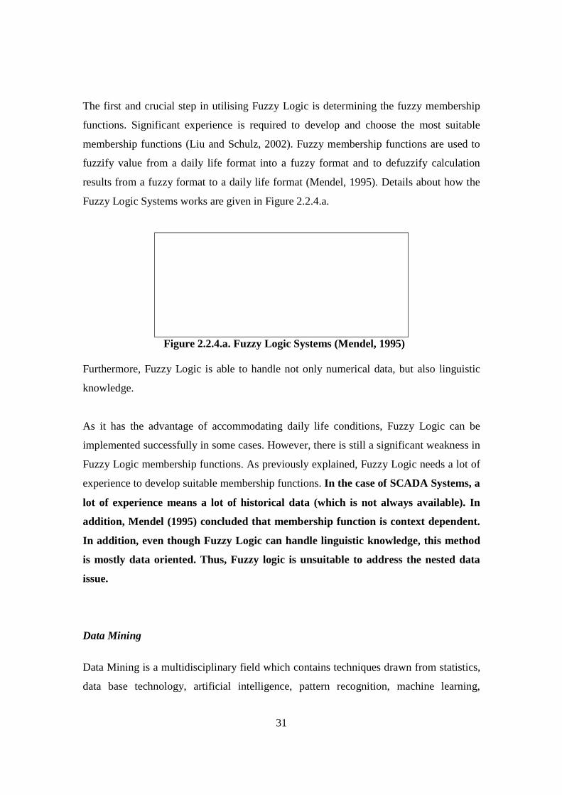
The first and crucial step in utilising Fuzzy Logic is determining the fuzzy membership

functions. Significant experience is required to develop and choose the most suitable

membership functions (Liu and Schulz, 2002). Fuzzy membership functions are used to

fuzzify value from a daily life format into a fuzzy format and to defuzzify calculation

results from a fuzzy format to a daily life format (Mendel, 1995). Details about how the

Fuzzy Logic Systems works are given in Figure 2.2.4.a.

4Figure 2.2.4.a. Fuzzy Logic Systems (Mendel, 1995)

Furthermore, Fuzzy Logic is able to handle not only numerical data, but also linguistic

knowledge.

As it has the advantage of accommodating daily life conditions, Fuzzy Logic can be

implemented successfully in some cases. However, there is still a significant weakness in

Fuzzy Logic membership functions. As previously explained, Fuzzy Logic needs a lot of

experience to develop suitable membership functions. In the case of SCADA Systems, a

lot of experience means a lot of historical data (which is not always available). In

addition, Mendel (1995) concluded that membership function is context dependent.

In addition, even though Fuzzy Logic can handle linguistic knowledge, this method

is mostly data oriented. Thus, Fuzzy logic is unsuitable to address the nested data

issue.

Data Mining

Data Mining is a multidisciplinary field which contains techniques drawn from statistics,

data base technology, artificial intelligence, pattern recognition, machine learning,

32

information theory, control theory, information retrieval, high-speed computing, and data

visualisation. The aim of Data Mining is to extract implicit, previously unknown, and

potentially useful (or actionable) patterns and models from data (Zurada and Kantardzic,

2005). Data mining was established when the size and number of existing data bases had

grown significantly and exceeded human analysis capabilities (Wachla and Moczulski,

2007, Cercone, http://www4.comp.polyu.edu.hk). Cercone suggest that data mining will

be more efficient if the data has already been warehoused. Until now, data mining has

been applied in various fields, such as in the prediction of water demand (An et al.,

1996), the diagnosis of boiler faults (Yang and Liu, 2004), the diagnosis of power cable

faults (Gulski et al., 2003), modelling water supply (Babovic et al., 2002), and modelling

operational information in a power plant (Ordieres Mere et al., 1997).

According to the literature, a combination of data warehousing and data mining

appears to be the best method to address the data analysis problem of SCADA

systems. However, this method needs a lot of historical data as initial input and this

is not always available. In addition, the method tends to neglect the validity of the

data. This is the most critical factor because the data is assumed to be valid and

reflects the real condition of the monitored system.

In reality, data from SCADA systems is nested data which means it is influenced by

many factors (Guo, 2005). If it is assumed that the data is not nested data, the

analysis may be incorrect or incomplete, and any decisions based on this analysis

may be incorrect as well.

Knowledge Base System and Expert System

Although some of the literature defines the Knowledge Base System and the Expert

System as being different, their basic method is in fact the same. The only difference is in

the type of collected knowledge. Lucas and Gaag (1991) conclude that the Expert System

is a Knowledge Base System which is developed by utilising experience and knowledge

33

from experts. It means that the Expert System is part of a Knowledge Base System. The

review is therefore focused on the Knowledge Base System.

“Knowledge Base Systems (KBS) are computational tools that enable the integration of

numerical data and heuristic knowledge and mimic the human decision making processes

to solve complex problems” (Comas et al., 2003). In other words, the Knowledge Base

System contains a collection of different types of knowledge and information (one being

human expertise or experience) which is then utilised to support the decision making

process to solve problems. According to Comas, two steps are required to develop the

Knowledge Base System: Knowledge Acquisition and Knowledge Representation

(Comas et al., 2003).

Knowledge Acquisition is the step that searches and compiles information contained in

diverse sources of knowledge, and identifies the reasoning mechanisms followed by

experts to detect and solve the problem (Comas et al., 2003). This is the most difficult

and crucial step, because the success of a Knowledge Base System depends on the quality

of the collected knowledge which can only be collected by a suitable process.

Moreover, based on this statement, it can be identified that the development of a good

Knowledge Base System should be based on a combination of reasoning mechanisms and

expert justification, not on expert justification alone.

Knowledge Representation is the next step after all the symptoms, facts, relationships and

methods used by experts in their reasoning strategy have been identified. In this step, all

of the knowledge is organized and documented (Comas et al., 2003).

After the two steps have been completed, an inference engine is developed to extract and

draw conclusions from the knowledge base (Zhang et al., 1998).

The advantages of utilising a Knowledge Base System in supporting decision making are

that compared to experts, it is able to handle a large volume of problems and make

34

decisions without any stress (human decisions are sometimes influenced by the condition

of stress) (Vale et al., 1998); and in cases where the expert is not available, a Knowledge

Base System can support an inexperienced operator/person to make decisions.

Although it seems that the Knowledge Base System is a novel method to solve SCADA

data analysis, its ability to solve the real problem depends on the development step

(Knowledge Acquisition). For example the development step determines the ability of a

Knowledge Base System (KBS) to address the issue of nested data. If the development

step is data oriented (only based on historical data), then KBS will not be able to address

the nested data issue. However, if the development step applies further consideration into

the system, then it has a potency to address the nested data issue.

Another issue that has to be considered is knowledge base management, because the

knowledge is always dynamic. Knowledge base management is needed to delete existing

knowledge, adjust existing knowledge and add new knowledge (Zhang et al., 1998).

From this review, it can be justified that the Knowledge Base System is a suitable

approach to address SCADA data analysis. The only crucial issue that must be

addressed is at the development step (knowledge acquisition).

Review of the existing proposed methods to address SCADA data analysis reveals that

the advantages and disadvantages of each of those methods can be identified. This will

then be used to formulate the method that is proposed by this research (refer to Section

2.3.3.).

Connectivity with ERP

Before exploring the proposed method formulation, there is another issue in SCADA

systems that must be reviewed. This concerns the integrations of the SCADA systems

with ERP systems.

35

Enterprise business process systems, such as ERP (Enterprise Resource Planning),

represent a significant business investment. ERP systems help to assure competitiveness,

responsiveness to customer needs, productivity, and flexibility in doing business in a

global economy (Sumner, 2005). In recent years, ERP systems have progressively

become the preferred reference solution for the information systems of companies

throughout the world, whatever their activity (Dillard and Yuthas, 2006). The main

reason for this success is the capacity of enterprise business process systems to address

information from all departments and functions across an organisation in a single unified

computer system (Grabot and Botta-Genoulaz, 2005). In fact, similar systems have been

implemented by companies in different countries such as China (Yusuf et al., n.d.) and

Denmark (Rikhardsson and Kraemmergaard, n.d.). ERP systems were used mainly for

manufacturing, but recently, service organizations have invested considerable amounts of

resources in the implementation of ERP systems (Botta-Genoulaz and Millet, 2006).

According to Musaji (2002), the structure of ERP system is as depicted in Figure 2.2.4.b.:

36

5Figure 2.2.4.b. ERP Structure (Musaji, 2002)

The base of the pyramid is the physical security of the hardware; that is, the machine, the

data base, and the off-line storage media (such as tape or cartridges). The second layer

deals with the operating system. The third layer focuses on the security software.

Typically, an ERP system uses or is integrated with a Relational Data Base System. A

Relational Data Base is a collection of data items organised as a set of formally described

tables from which data can be accessed or reassembled in many different ways without

having to recognize the data base tables. A relational data base consists of a set of tables

containing data in predefined categories. Each table, sometimes called a relation, contains

one or more data categories in columns. Each row contains a unique instance of data for

the categories defined by the columns. For example, a typical business order entry data

base would include a table that describes a customer by using columns for name, address,

phone number and so on. Another table would describe an order with columns for

product, customer, data, sales price, and so on. From the data base, an overview that fits

the user’s needs could be obtained. For example, a branch office manager might require

an overview or report of all customers that had bought products after a certain date. From

37

the same tables, financial service managers in the same company could obtain a report on

accounts that needed to be paid.

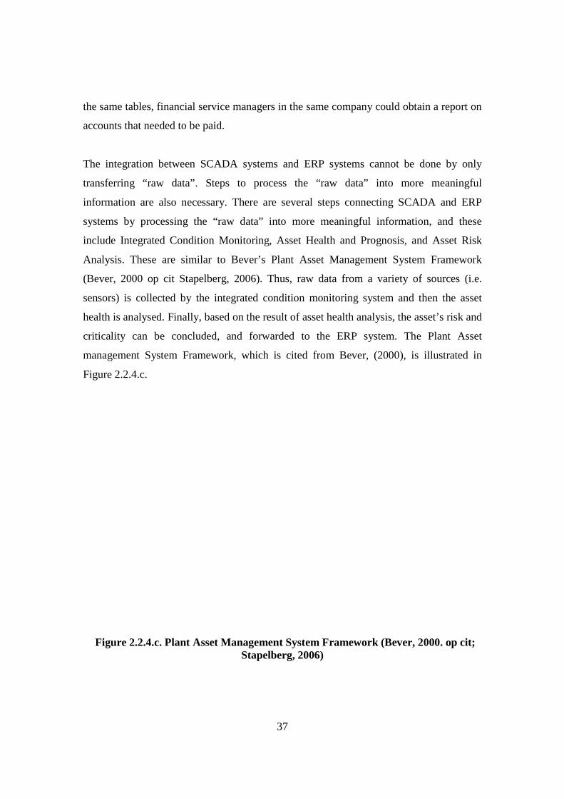
The integration between SCADA systems and ERP systems cannot be done by only

transferring “raw data”. Steps to process the “raw data” into more meaningful

information are also necessary. There are several steps connecting SCADA and ERP

systems by processing the “raw data” into more meaningful information, and these

include Integrated Condition Monitoring, Asset Health and Prognosis, and Asset Risk

Analysis. These are similar to Bever’s Plant Asset Management System Framework

(Bever, 2000 op cit Stapelberg, 2006). Thus, raw data from a variety of sources (i.e.

sensors) is collected by the integrated condition monitoring system and then the asset

health is analysed. Finally, based on the result of asset health analysis, the asset’s risk and

criticality can be concluded, and forwarded to the ERP system. The Plant Asset

management System Framework, which is cited from Bever, (2000), is illustrated in

Figure 2.2.4.c.

6Figure 2.2.4.c. Plant Asset Management System Framework (Bever, 2000. op cit;

Stapelberg, 2006)

38

A review of several academic papers has been done to elicit the integration of SCADA

systems and ERP systems. “Although Enterprise Resource Planning (ERP) packages

strive to integrate all the major processes of a firm, customers typically discover that

some essential functionality is lacking” (LISA, J. E., 2000). This statement declares that

ERP is fundamentally designed to integrate all the major processes of a company.

However, the ERP users have experienced some difficulties, because in reality, not all

processes in the company can be integrated. Therefore, further research and development

is needed to overcome this failing. On the other hand, researchers in the SCADA area

have tried to make it more available to other systems by developing standard protocol

(Hong and Jianhua, 2006).

In conclusion, there is a definite need for integrating both SCADA and ERP systems as

indicated by academics and industry. Furthermore, SAP as one of the most successful

ERP software companies in the world, has already embedded Manufacturing Execution

System (MES) in the SAP-R/3 packages (Schumann, 1997). MES is able to integrate

production information such as SCADA systems and business information, which can

help the manager to make decisions (Hwang, 2006).

Although MES is able to integrate ERP and SCADA systems, the focus is only on

the Supervisory Control part of SCADA systems. However, the aspect of SCADA

that has to be explored and developed further is Data Acquisition. This research

focuses on the integration of both systems through further exploration of the development

of the data acquisition part of SCADA.

Data Bridge

The next step in the literature review is to identify methods that have been proposed to

integrate SCADA systems and ERP systems by further development and exploration of

SCADA’s data acquisition.

39

Gupta (1998) claimed that information from different systems can be integrated by

utilising a Data Bridge. Moreover, a properly designed Data Bridge can help information

process transfer within the integrated systems (Momoh et al., 1991). According to Gupta,

a proper Data Bridge should have three main components (Gupta, 1998):

• Wrappers

To obtain access from the data sources

• Extractors

To process data into useful information

• Mappers

To perform conversions

Therefore, a good Data Bridge must have the ability to access data from various data

sources and process the data into useful information, in addition to converting the

information into a suitable format for the destination system. In conclusion, the Data

Bridge concept has the potential to be utilised in the connection of SCADA and ERP

systems.

The literature review further investigates any proposed Data Bridge which would link

these systems. Unfortunately, it proved difficult to find suitable references in academic

papers, resulting in the review being featured in proprietary websites on the internet

extended into available commercial products.

In some of these websites, several companies were found to offer direct integration

between the SCADA systems and the ERP systems by interfacing the data base. Below is

a list of several websites that explain the concept or the product:

1. http://www.esri.com/library/reprints/pdfs/enercur-geonis.pdf

The data bridge in this website focuses on direct integration of a SCADA data

base to a GIS data base which has been integrated to the ERP system.

2. http://www.documentcorp.com/au/Contents/News/newsarticle.asp?id=archive/06

0523

40

The data bridge in this website focuses on the direct integration of SCADA

documents to ERP documents.

3. http://www.kalkitech.com/sds.htm

The data bridge in this website focuses on direct integration of a SCADA data

base into an ERP data base.

4. http://www.junotsystems.com/Products/opc.asp

The data bridge in this website also focuses on the direct integration of a SCADA

data base into an ERP data base.

5. http://www.english.icg.pl/sap/index.php/lg/en/page/co_robimy/sub/ikomponenty/s

ub1/icada

The data bridge in this website filters the information from a SCADA system to

an ERP system, so that only the production data is forwarded.

6. http://www.citect.com/index.php?option=com_content&task=view&id=3&Itemid

=5

The method in this product is the closest to the data bridge method in this research

as there is data filtering and interpreting instead of direct integration of the

SCADA data base into ERP data base.

It can generally be concluded from the information in these websites that, the

concepts of Data Bridge are still far from ideal. For example, some concepts only

integrate the data base or simply copy the data directly from the SCADA system

data base to the ERP system data base. However, bridging these two systems by

copying or integrating their data bases alone will not solve the problem because data

from the SCADA systems is still raw. In addition, there must be several steps to extract

the appropriate data for conversion to useful information.

In conclusion, although the proposed Data Bridge concept from Gupta (1998) is ideal, the

actual implementation of the Data Bridge to link SCADA and ERP systems is still far

from realising the ideal concept. Thus, this research will adopt Gupta’s Data Bridge

concept which is blended with the steps to extract appropriate information.

41

2.2.5. Discussion

This discussion highlights the problems and gaps identified in the on-line data

connectivity topic which require further research and development. Two of the main

problems in the on-line data connectivity topic are identified as: SCADA data analysis,

and the Connectivity of SCADA systems and ERP systems.

SCADA Data Analysis

As SCADA is a real-time system, the system’s data base will rapidly accumulate a large

amount of data if some or other data elimination or handling protocol is not adopted

(Stoneham, 1998). Matus-Castillejos and Jentzsch (2005) conclude that a data base of a

real-time system must be stringently managed. Therefore, it can be concluded that one of

the crucial problems in the SCADA system is data. However, data which is collected by

the SCADA system is influenced by other factors. For example: if SCADA identifies an

abnormality in the data, this abnormality can either be caused by change in the

installation environment or by deterioration of the machine’s condition (Stoneham,

1998). Data that is influenced by other factors and cannot be assumed as independent is

called nested data (Kreft et al., 2000). In addition, Guo (2005) concludes that if nested

data is assumed independent and linear, the results of the analysis will be incorrect. Until

now however, there have been few researchers in the SCADA area concerned with nested

data problems.

The literature review reveals several methods proposed to address the problem of

SCADA data analysis. These can be identified as: Artificial Neural Networks, Fuzzy

Logic, Data Mining, and Knowledge Base Systems and Expert Systems. Limitations/gaps

in each of the proposed methods are as follows:

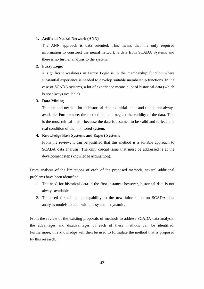
42

1. Artificial Neural Network (ANN)

The ANN approach is data oriented. This means that the only required

information to construct the neural network is data from SCADA Systems and

there is no further analysis to the system.

2. Fuzzy Logic

A significant weakness in Fuzzy Logic is in the membership function where

substantial experience is needed to develop suitable membership functions. In the

case of SCADA systems, a lot of experience means a lot of historical data (which

is not always available).

3. Data Mining

This method needs a lot of historical data as initial input and this is not always

available. Furthermore, the method tends to neglect the validity of the data. This

is the most critical factor because the data is assumed to be valid and reflects the

real condition of the monitored system.

4. Knowledge Base Systems and Expert Systems

From the review, it can be justified that this method is a suitable approach to

SCADA data analysis. The only crucial issue that must be addressed is at the

development step (knowledge acquisition).

From analysis of the limitations of each of the proposed methods, several additional

problems have been identified:

1. The need for historical data in the first instance; however, historical data is not

always available.

2. The need for adaptation capability to the new information on SCADA data

analysis models to cope with the system’s dynamic.

From the review of the existing proposals of methods to address SCADA data analysis,

the advantages and disadvantages of each of these methods can be identified.

Furthermore, this knowledge will then be used to formulate the method that is proposed

by this research.

43

Connectivity of SCADA Systems and ERP Systems

Based on the review, the need for integrating both SCADA and ERP systems is apparent.

SAP has embedded the Manufacturing Execution System (MES) in the SAP-R/3

package. Although MES is able to integrate ERP and SCADA systems, the focus is only

on the Supervisory Control part of SCADA systems.

The literature review identified methods proposed to integrate SCADA and ERP systems

in terms of SCADA’s data acquisition. It was observed that the Data Bridge concept has

great potential to be utilised in the connection of SCADA and ERP systems. It was found

that several companies offer direct integration between the SCADA and ERP systems by

interfacing the data base. However, the limitations of these concepts are still far from an

ideal concept of Data Bridge.

In conclusion, a new concept of Data Bridge is needed to integrate ERP and SCADA

systems in terms of the Data Acquisition and to incorporate the analysis results into the

ERP system. This Data Bridge concept will incorporate the three steps to extract

appropriate information.

2.3. On-line Data Connectivity: Solution Formulation

Based on the identified problems and gaps in on-line data connectivity a model is

formulated to address any possible solution. Section 2.3. provides information about the

proposed model. Initially, the required criteria which the proposed model needs to fulfill

is considered, The focus then turns to on further literature review to identify some

grounded theory which will be adopted in developing critical theory. This approach then

progress to the final model proposed; that is, the Hierarchical Model.

44

2.3.1. Proposed Model Criteria Formulation

The first step in formulating a solution is composing suitable criteria for the model/theory

based on the literature review findings.

There are two main problems that are identified based on the literature review:

• Nested data problem (SCADA data analysis)

• Connectivity of SCADA systems and ERP systems problem (Integration)

In terms of SCADA data analysis, several additional problems were identified:

• The need for historical data at the first step of development (historical data is not

always available).

• The need for adaptation capability of the SCADA data analysis model because the

system is dynamic.

Several of the methods and concepts proposed can be adopted because they can be

justified as suitable to address the problems that have been identified. They are:

• The Knowledge Base Method

This method can be adopted because it is able to integrate numerical data and

heuristic knowledge, and mimic human decision making processes to solve

complex problems. However, more consideration must be given to the

development step; that is, the Knowledge Acquisition, because this step

determines the quality of the knowledge base.

• Data Bridge Concept

According to the literature review, the Data Bridge concept proposed by Gupta

(1998) is justified as an appropriate approach to integrate/connect SCADA

systems with ERP systems, especially in terms of integrating the part of SCADA

systems concerned with data analysis into the ERP systems. However, more work

is required to incorporate the concept of systems integration.

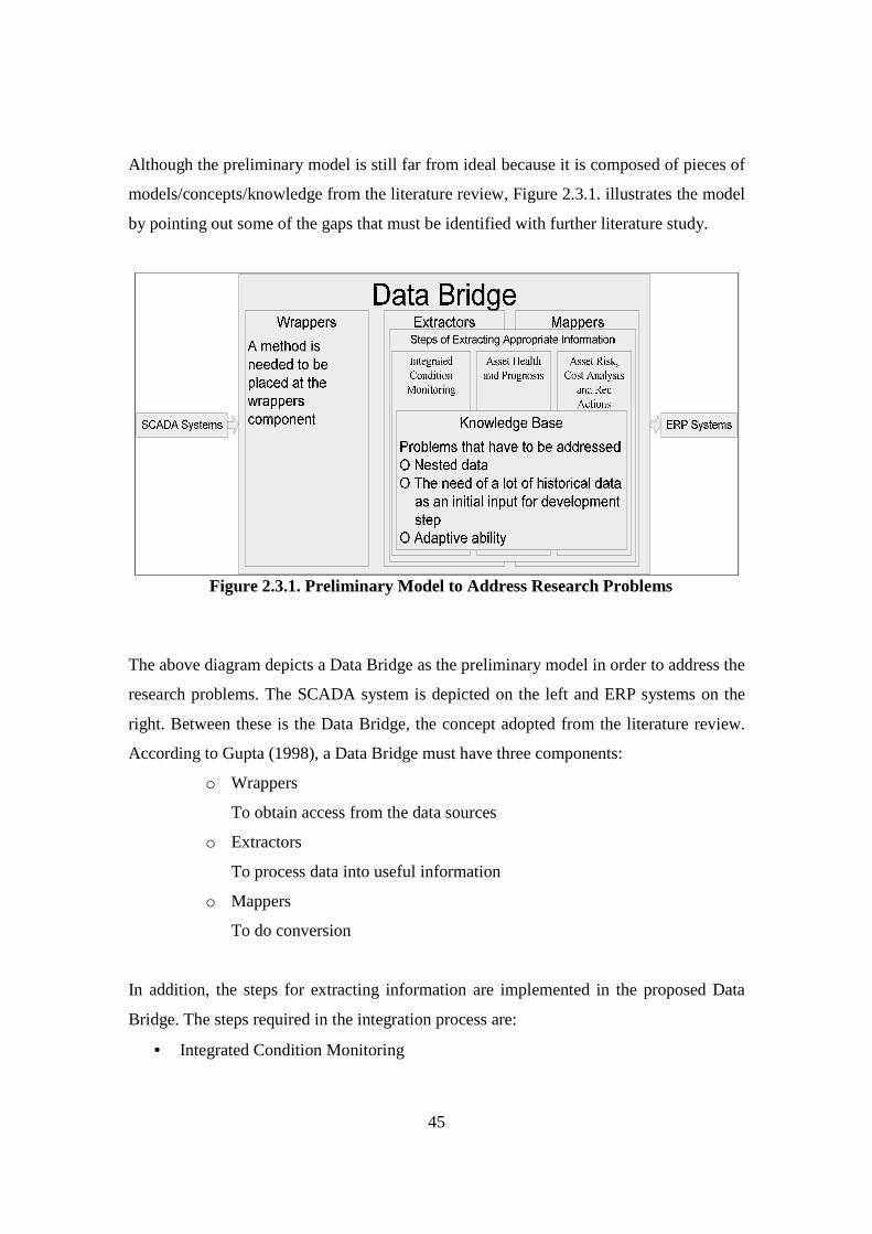
45

Although the preliminary model is still far from ideal because it is composed of pieces of

models/concepts/knowledge from the literature review, Figure 2.3.1. illustrates the model

by pointing out some of the gaps that must be identified with further literature study.

7Figure 2.3.1. Preliminary Model to Address Research Problems

The above diagram depicts a Data Bridge as the preliminary model in order to address the

research problems. The SCADA system is depicted on the left and ERP systems on the

right. Between these is the Data Bridge, the concept adopted from the literature review.

According to Gupta (1998), a Data Bridge must have three components:

o Wrappers

To obtain access from the data sources

o Extractors

To process data into useful information

o Mappers

To do conversion

In addition, the steps for extracting information are implemented in the proposed Data

Bridge. The steps required in the integration process are:

• Integrated Condition Monitoring

46

• Asset Health and Prognosis

• Asset Risk Analysis

The three steps for extracting appropriate information in the concept of system

integration are implemented on the Extractors and Mappers of Data Bridge. The process

of analysis is conducted in the Extractors and then the processed information is passed on

by the Mappers. A method must also be developed or adopted to be placed as a Wrappers

component.

Moreover, the Knowledge Base method is adopted to facilitate analyses at the steps for

extracting appropriate information. However, further development and research is

necessary in order to address the problems concerning:

• Nested data

• The need for a significant amount of historical data as initial input for the

development step

• Adaptive ability

Finally, the criteria for the proposed model can be formulated as being:

• Able to be developed by utilising original design information as an initial input

• Able to analyse SCADA data in a “real time” time frame

• Able to solve Nested Data issues

• Able to pass the results to the ERP System

2.3.2. Further Literature Study

After the criteria for the proposed method have been set, the next step formulates the

proposed model by filling in the gaps in the preliminary model. The review covers three

topics: the Hierarchical Approach, Root Cause Analysis, and the Interdependence and

Diagramming Method.

47

Hierarchical Approach

The explanation in Section 2.2.4. identified data from the SCADA system as Nested

Data. In addition, it mentions that the Hierarchical Method is able to address the Nested

Data issue. Further review of the Hierarchical Method is as follows:

According to Ciarleglio and Markuch (2007), the Hierarchical Method is a useful

technique to address Nested Data, since in fact, it contains a multi-level structure.

Therefore, Nested Data can be identified as a Hierarchical Data set. “A hierarchical data

set contains measurements on at least two different levels of a hierarchy” such as

measurement of patients and hospitals where the lower level (patients) is nested with the

higher level (hospitals) (Kreft et al., 2000). Thus, the lower level data which is nested at

the particular higher level data, is influenced by and influences other lower level data

which is nested at the same higher level data (Ciarleglio and Makuch, 2007). In SCADA

for example, the data which comes from the motor bearing temperature sensor, is

influenced by other impacting factors that exist in the motor assembly.

In addition, it is concluded that SCADA data analysis results will be more accurate if the

hierarchical method is implemented during the analysis process. The next step is to

formulate a suitable format for implementing the hierarchical method into SCADA data

analysis.

Root Cause Analysis

“The central aim of root cause analysis is to find points in a system where improvements

are feasible that will reduce the likelihood of another similar accident/negative event in

the future”(Rzepnicki and Johnson, 2005).

According to Wilson et al. (1993), Root Cause Analysis refers to the process of

identifying the most basic reason for an undesirable condition or problem which if

48

eliminated or corrected, would have prevented it from existing or occurring. Based on

these definitions, it can be concluded that Root Cause Analysis is a method of identifying

the source of something occurring that is not expected and eliminating it either at that

particular time or in the future. One of the advantages of Root Cause Analysis is the

systematic examination of multiple systems and causes which may contribute to an

adverse event (Wilson et al., 1993).

There are several analysis methods in Root Cause Analysis (Wilson et al., 1993):

• Change Analysis:

Change Analysis is an analysis method which identifies the root cause of any

unwanted event or problem, based on the “Change” element which can be

detected from symptoms. In addition, the “Change” element is a force that can

make a difference (positive or negative) in the way a system, process or person

functions.

• Event and Causal Factors Analysis:

“For every accident, incident or problem, there was a previous or missed event or

an underlying condition (conditions that caused it to happen).” In conclusion, this

method provides a detailed analysis of the event sequence and its associated

causes or conditions.

• Tree Diagrams:

A Tree Diagram utilises a graph as a tool for visualising a number of potential

contributory factors to an event. This method is extremely useful in helping

visualisation and analysis of more complex systems or problem situations.

Failure Mode and Effect Analysis (FMEA) is proposed as one of the better analysis

methods for Root Cause Analysis (Latino and Latino, 1999). FMEA is actually a well

known method in industry for assessing all of the events and their individual impact on

performance. FMEA was developed for the aerospace industry and the first formal

FMEAs were conducted in the mid 1960s (McDermott et al., 1996).

In FMEA, the failure is assessed based on several criteria such as (McDermott et al.,

1996; Latino and Latino, 1999):

49

• Failure Cause

• Failure Mode

• Failure Effect

• Failure Consequence

Failure Consequence, as one of the outcomes from FMEA, will be utilised to determine

risk in the Criticality Analysis of the FMECA (Failure Mode Effect and Criticality

Analysis). Based on the preliminary model, some of the final and most valuable

information that will be passed to the ERP system is “Risk”. Thus, it is suitable to adopt

FMEA to form the proposed model of this research.

In addition, it can be identified that the Hierarchical concept can be implemented through

the FMEA, and this is also mentioned by Latino and Latino (1999):

“So the first thing we might do is take that aircraft and break it down into smaller

subsystems.”

The above quote clearly states that the FMEA process is initiated by breaking down the

source of information hierarchically (Aircraft), in order to enable a more accurate

information extraction process. Furthermore, Stapelberg (1993) also proposes a FMEA in

his Reliability Availability and Maintainability book which begins with a System

Breakdown Structure (SBS) to breakdown the system hierarchically. “A System

Breakdown Structure is a systematic hierarchical representation of the equipment, broken

down into its logical Areas, Units, Systems, Assemblies and Component levels”

(Stapelberg, 1993).

There are three steps in developing SBS (Stapelberg, 1993):

• Process Analysis

In this step, the existing processes in the system are analysed and then depicted in

a Process Block Diagram. The purpose of this step is to determine the nature of

50

the process flow and understand it clearly in order to logically determine different

hierarchical levels in the system.

Prior to further explanation on the development of the Process Block Diagram, it

is important to define several terms, which will be used throughout this section

(Stapelberg, 1993):

o Interface Components

These are components on systems’ boundaries which need to be clearly

specified as they experience functional failures frequently.

o Block Diagramming

This is an important and useful technique which can be used during

functional systems’ analysis to depict a variety of relationships, including

input and output relationships, process flow, and the functions to be

performed at each stage of the systems’ hierarchy.

o Process Flow Block Diagrams

Process Flow Diagrams depict the process flow and can be used to show

the conversion of inputs into outputs which subsequently form inputs into

the next system.

The reason for drawing a detailed diagram is to determine and clearly understand

the nature of the process flow, in order to determine logically different

hierarchical levels in the asset. In most companies, the Process Flow Diagrams are

available and they are the source of information which investigates the material

flow and state changes in the process.

The investigation is carried out by a detailed analysis of inputs and outputs from

different parts of the systems. The systems’ boundaries and interface components

can therefore be identified.

Examples of Process Flow Block Diagrams are given in Figure 2.3.2.a. and Figure

2.3.2.b. (courtesy of ICS Industrial Consulting Services Pty Ltd) (Stapelberg,

51

1993). The first example is a Process Flow Block Diagram illustrating the basic

process in a coal fired power station and can be regarded as a “high level” process

flow block diagram. The other is the power train system of a haul truck and is

taken down to the assembly level. Even though no physical medium flows

through the process, the state changes in transmitting the rotational drive provide

a clear indication of the boundaries between the various assemblies.

8Figure 2.3.2.a. Process Flow Diagram of Coal Fired Power Station (Stapelberg,

1993)

52

9Figure 2.3.2.b. Process Flow Block Diagram of Haul Truck Power Train System

(Stapelberg, 1993)

• System Description

A system can be defined as follows (Stapelberg, 1993):

“A system is a collection of subsystems, assemblies and components for which the

availability can be optimised”.

From a reliability viewpoint, a system can be defined as (Stapelberg, 1993):

“... a collection of subsystems and assemblies for which the value of system

reliability can be determined, and is dependent on the interaction of the

reliabilities and physical configuration of its constituent assemblies”.

Based on these definitions, it can be concluded that a system consists of a

collection of sub-systems, assemblies and components which work in synergy to

process an input into an output.

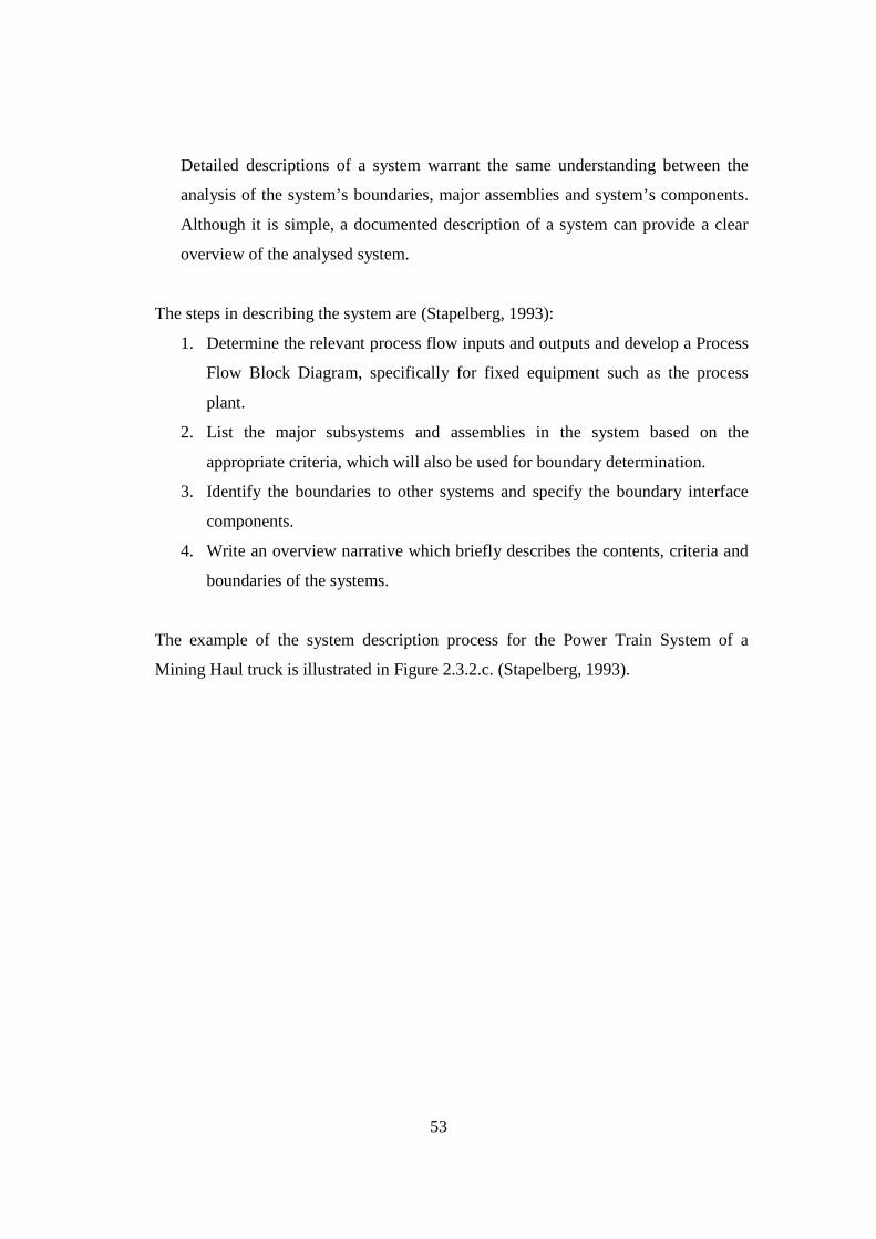
53

Detailed descriptions of a system warrant the same understanding between the

analysis of the system’s boundaries, major assemblies and system’s components.

Although it is simple, a documented description of a system can provide a clear

overview of the analysed system.

The steps in describing the system are (Stapelberg, 1993):

1. Determine the relevant process flow inputs and outputs and develop a Process

Flow Block Diagram, specifically for fixed equipment such as the process

plant.

2. List the major subsystems and assemblies in the system based on the

appropriate criteria, which will also be used for boundary determination.

3. Identify the boundaries to other systems and specify the boundary interface

components.

4. Write an overview narrative which briefly describes the contents, criteria and

boundaries of the systems.

The example of the system description process for the Power Train System of a

Mining Haul truck is illustrated in Figure 2.3.2.c. (Stapelberg, 1993).

54

10Figure 2.3.2.c. Example of System Description (Stapelberg, 1993)

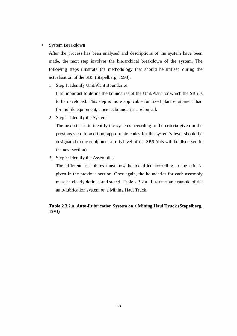
55

• System Breakdown

After the process has been analysed and descriptions of the system have been

made, the next step involves the hierarchical breakdown of the system. The

following steps illustrate the methodology that should be utilised during the

actualisation of the SBS (Stapelberg, 1993):

1. Step 1: Identify Unit/Plant Boundaries

It is important to define the boundaries of the Unit/Plant for which the SBS is

to be developed. This step is more applicable for fixed plant equipment than

for mobile equipment, since its boundaries are logical.

2. Step 2: Identify the Systems

The next step is to identify the systems according to the criteria given in the

previous step. In addition, appropriate codes for the system’s level should be

designated to the equipment at this level of the SBS (this will be discussed in

the next section).

3. Step 3: Identify the Assemblies

The different assemblies must now be identified according to the criteria

given in the previous section. Once again, the boundaries for each assembly

must be clearly defined and stated. Table 2.3.2.a. illustrates an example of the

auto-lubrication system on a Mining Haul Truck.

2 Table 2.3.2.a. Auto-Lubrication System on a Mining Haul Truck (Stapelberg, 1993)

56

4. Step 4: Identify the Sub-Assemblies/Components

Once the systems and assemblies have been identified, the next step involves

identifying each assembly’s components according to the criteria given in the

following definition (Stapelberg, 1993):

“A component is a collection of parts which constitute a functional unit for

which the physical condition can be measured and reliability and

maintainability data can be collected.”

Additionally, a “part” can be defined as (Stapelberg, 1993):

“A single element of a component which contributes towards the component’s

function.”

5. Step 5: Depict the Relationship of SBS Levels

Once the 4 previous steps have been completed, the system hierarchy is now

properly identified. Therefore, the relationship of the SBS level can be

depicted. The typical SBS listing or “spreadsheet” depicts the relationship of

each component to an assembly and to a system. It also shows the codes at all

levels. The following is an example of the Haul Truck Systems Breakdown

Structure.

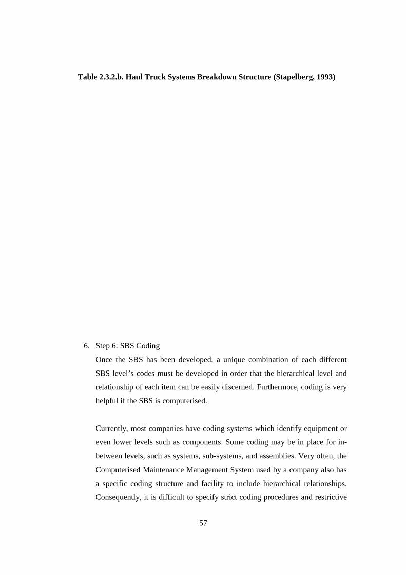
57

3Table 2.3.2.b. Haul Truck Systems Breakdown Structure (Stapelberg, 1993)

6. Step 6: SBS Coding

Once the SBS has been developed, a unique combination of each different

SBS level’s codes must be developed in order that the hierarchical level and

relationship of each item can be easily discerned. Furthermore, coding is very

helpful if the SBS is computerised.

Currently, most companies have coding systems which identify equipment or

even lower levels such as components. Some coding may be in place for in-

between levels, such as systems, sub-systems, and assemblies. Very often, the

Computerised Maintenance Management System used by a company also has

a specific coding structure and facility to include hierarchical relationships.

Consequently, it is difficult to specify strict coding procedures and restrictive

58

codes. It would be rather more appropriate to identify some basic guidelines

which should be considered when conducting the SBS coding, such as the

following (Stapelberg, 1993):

1. The code has to be structured in such a way that each of the items on any

specific level of the SBS has a unique code and these codes are logically

structured.

2. If any code systems exist, then any additional code development for SBS

should utilise the same logic as the existing code structures.

3. Any limitations imposed on the coding structure by the computer system

in use also need to be considered with regard to size and hierarchical

relationships.

Many plants utilise alpha-numeric codes that follow a logical structure, in

which an item is described according to a hierarchy - from Unit down to

System, Subsystem, Assembly and Component - in a sequence of codes from

left to right.

The following is an example of an SBS code from a Haul Truck:

010715 Haul truck water pump

where “01” is the Engine System

“07” is the Cooling Subsystem

and “15” is the component number in the assembly; that is the water pump

The SBS is justified as a suitable method to be adopted in this research.

The focus of this literature study now moves to a justification of the other analysis

methods of Root Cause Analysis.

59

Change Analysis can be deemed suitable to be adopted and placed at the Wrapper

component, since any change in system conditions can be an indicator of the occurrence

of abnormality. In addition, “change” can be implemented on the Compression Algorithm

to reduce storage space (Chan et al., 1993). Thus, the implementation of Change Analysis

will be conducted on the Filtering Algorithm and Compression Algorithm.

Wilson et al. (1993) indicate that Event and Causal Analysis and Tree Diagrams are

different. However, a review of both methods reveals that they are interconnected. While

Event and Causal Factors Analysis is the step for analysing the accident, incident or

problem by interrelating them with the cause, Tree Diagrams depict the analysis results in

diagram format. In conclusion, adopting both methods is suitable for the proposed model.

Interdependence and Diagramming Method

In this section, the literature study focuses on the Interdependence and Diagramming

method. In the Random House Unabridged Dictionary, “interdependence” means being

mutually dependent or depending on each other. According to WordNet 3.0 by

Princenton University, “interdependence” means a reciprocal relation between

interdependent entities (objects or individuals or groups).

Interdependence is a relationship between entities which are dependent upon each other.

Interdependence is a result of integration of several factors that work together to produce

a result (Cho, 1995); for example, interdependence between groups within a country,

between nations or between groups of nations (Beddis, 1989). Furthermore,

interdependence in economics leads to conflict (Campbell, 1997).

In terms of Condition Monitoring, a system is either the monitored system or monitoring

system, or is an integration of several components to produce results. Therefore,

interdependence between each component exists. In other words, they influence each

other. Hence, the Interdependence concept can be adopted to support the Effect and

60

Cause Analysis method where the effect and cause of an event can be identified through

the interdependence between components in the system.

As mentioned previously, this interdependence is identified as a source of

conflict/problem. Furthermore, Drew et al. (2002) conclude that interdependence is

measurable. This leads to the idea of quantifying risk based on interdependence (refer to

Section 2.5.1.).

“A picture is worth a thousand words” means that complex stories can be told with just a

single image, or an image may be more influential than a story (Rogers, 1986). Thus,

analysis results that are presented in graphical diagrams can be understood more easily

(Stiern, 1999). In addition, as one of the analysis methods of Root Cause Analysis, Tree

Diagrams utilise the power of a diagram to visualize and analyse more complex systems

or problem situations (Wilson et al., 1993). Hence, a suitable diagramming method is

adopted in the proposed model as a tool to present the analysis results for further

investigation. The adopted diagramming method must also facilitate the development

process of the Knowledge Base.

There are many diagramming tools that can be adopted for the proposed model, such as:

Flowchart, Data Flow Diagrams, Use Case Diagrams, Entity-Relationship Diagrams, and

State Transition Diagrams (Nitakorn, (http: //www.umsl.edu)). In addition, the most

important criterion of the adopted diagramming tool is the ability to present the

interdependent relationship between each component in the system. Based on

comparisons by Nitakorn, the Entity Relationship Diagram is the only diagramming tool

that focuses on presenting data relationships. Furthermore, the first intention of the Entity

Relationship Diagram concept is to facilitate data base concept development. Thus, this

diagramming concept is justified as being capable of facilitating the development process

of the Knowledge Base.

61

In conclusion, adopting the concept of the Entity Relationship Diagram is more than

suitable for the proposed model. Furthermore, as only the concept of an Entity

Relationship Diagram (ERD) is adopted, further development of a suitable diagramming

tool for the proposed model is required.

2.3.3. Formulation of the Final Proposed Model: Hierarchical Model

The Preliminary Model proposed to address the research problem can now be evolved to

the Final Model by adding the methods and concepts which were identified in the study

of additional literature, and deemed suitable for the model. Figure 2.3.3. illustrates the

Hierarchical Model as the Final Model.

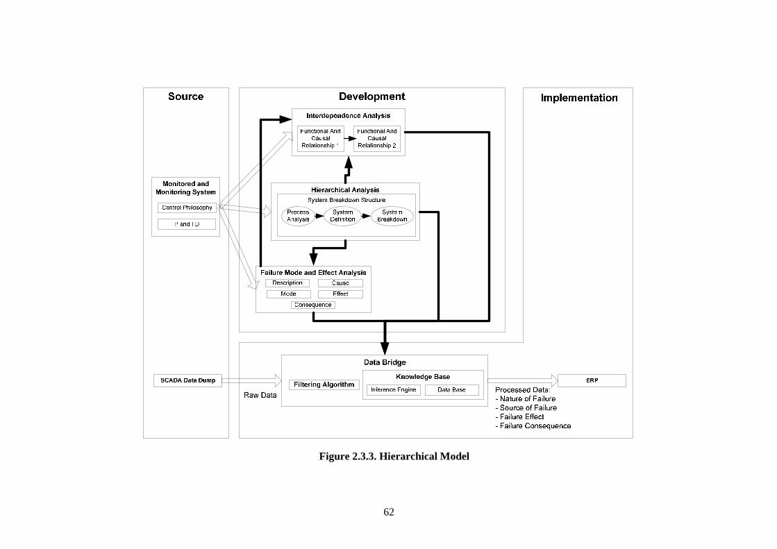
62

11Figure 2.3.3. Hierarchical Model

63

In the Hierarchical Model, information from sources, namely Control Philosophy and

P&ID (Process and Instrumentation Diagram), is analysed through the Hierarchical

Analysis. A System Breakdown Structure (SBS) is developed in the Hierarchical

Analysis through Process Analysis, System Definition and System Breakdown. Results

from the Hierarchical Analysis and any further information are then included in the

Failure Mode and Effect Analysis (FMEA).

In FMEA, failure at the system’s component level is investigated based on Failure Cause,

Failure Mode, Failure Effect and Failure Consequence. Following the FMEA, results

from the FMEA and Hierarchical Analysis, including additional information, are

transferred to the Interdependence Analysis step.

There are two stages of analysis in the Interdependence Analysis: FCRD (Functional and

Causal Relationship Diagram) Stage 1 and FCRD Stage 2. FCRD Stage 1 analyses the

Dynamic Relationship at the system’s component level which is then depicted in a

diagramming format for easier analysis. At a later stage, risk and criticality can be

calculated based on component interdependencies. FCRD stage 2 transforms information

into a more manageable format for input into the Data Base. In addition, all information

from the Hierarchical Analysis, Failure Mode and Effect Analysis and Interdependence

Analysis is then inputted to the Data Base. An Inference Engine is then developed to

query information from the Data Base. Furthermore, the Data Base and Inference Engine

are then paired and called a Knowledge Base. In order to extract significant information

from the Raw Data, a Filtering algorithm is then developed based on the information

about the limit of normal and abnormal data from the Control Philosophy while

conducting the Hierarchical Analysis, Failure Mode and Effect Analysis, and

Interdependence Analysis.

64

It is important that in the implementation step, the Filtering Algorithm is placed before

the Knowledge Base in the Data Bridge. The algorithm extracts essential information

from the SCADA Raw Data. The Knowledge Base then processes this essential

information into more meaningful information, such as: Nature of Failure, Source of

Failure, Failure Effect and Failure Consequence. Finally, this meaningful information is

passed to the ERP system.

2.3.4. Discussion This section highlights some of the essential findings on the process of a solution

formulation from the literature review. Solution formulation is conducted in three steps:

Proposed Model Criteria Formulation, Further Literature Study and Final Proposed

Model Formulation (Hierarchical Model).

In the Proposed Model Criteria Formulation step, some criteria are set as a guide to

design and develop the model. The development of these criteria is based on the

identified problems and gaps. The criteria of the proposed model can be formulated as

being:

• Able to be developed by utilising original design information as an initial input

• Able to analyse SCADA data in a “real time” time frame

• Able to solve the Nested Data issue

• Able to pass the results to the ERP System

The next step after the Proposed Model Criteria has been formulated involves further

literature study. The review covers three topics: the Hierarchical Approach, Root Cause

Analysis and Interdependence and Diagramming Method.

According to the literature study on the issue of addressing Nested Data, the Hierarchical

Method is identified as the most popular and effective method. In addition, the

Hierarchical Method has been proven to address this issue in varied fields, with the

exception of SCADA data analysis.

65

The literature study then focuses on Root Cause Analysis, a classic method to identify the

root cause of any unwanted event or problem. Furthermore, the literature study reveals

several analysis methods in Root Cause Analysis. The literature study then focuses on

identifying which methods can be suitably adopted for the model.

As mentioned, Change Analysis is judged suitable to be adopted in the proposed model;

therefore a Compression and Filtering Algorithm have been developed based on the

concept (refer to Section 3.4. and Section 3.5.).

Event and Causal Factors Analysis, and Tree Diagrams are concluded as being suitable

for the proposed model. Furthermore, a method called Functional and Causal

Relationship Diagram (FCRD) has been developed based on the Event and Causal

Factors Analysis, Tree Diagrams, Interdependence Concept and Entity Relationship

Diagram.

As the name suggests, FCRD is a method to investigate and analyse the functional and

causal relationship between each component where the results are depicted in a diagram.

There are two stages of FCRD. Stage 1 investigates the dynamic interdependent

relationship between each component in the system which is depicted in the diagramming

format. This stage inspires the development of new risk calculation based on the

components interdependence. In the second stage, the information from stage 1 is

transformed into a more comprehensive and manageable format so that it can be input

into the Knowledge Base. Further detail on FCRD is in Section 3.9.

66

Below are the justifications for FMEA’s adoptability:

• FMEA is initiated by hierarchically breaking down the source of information to

enable a more accurate information extraction process. Thus, it is justified as a

suitable method to implement the hierarchical method.

• One of the analysis results from FMEA is risk analysis which is then extended to

criticality analysis in the Failure Mode Effect and Criticality Analysis. Therefore,

it is justified as being able to fulfil the steps of extracting appropriate information

because the final and valuable information that will be passed to the ERP system

is “Risk”.

Stapelberg (1993) proposes a FMEA, which is initiated by the System Breakdown

Structure (SBS) to break down the system hierarchically. Therefore, the SBS is justifiably

suitable to be adopted in this research.

The step involving further literature study revealed that Grounded Theory can be

identified, the following ways:

• Hierarchical method is identified as the most popular and effective method to

address a nested data problem.

• There are several analysis methods within Root Cause Analysis, a classic method

to identify the root cause of any unwanted event or problem, such as: Change

Analysis, Event and Causal Factors Analysis, and Tree Diagrams. These Analysis

methods are adopted as Grounded Theory.

• The concept of an Entity Relationship Diagram as one of the Diagramming tools

is adopted as Grounded Theory to present the analysis results.

• Interdependence concept is adopted to support the Effect and Cause Analysis

method.

• Failure Mode and Effect Analysis and System Breakdown Structure proposed by

Stapelberg (1993).

67

In the Final Proposed Model Formulation a Critical Theory named as Interdependence

Analysis is developed based on the Grounded Theory: Event and Causal Factors

Analysis, Tree Diagrams, Interdependence Concept and the Entity Relationship Diagram.

Interdependence Analysis, together with Failure Mode and Effect Analysis and

Hierarchical Analysis, as Grounded Theory are then combined to form the proposed

Hierarchical Model to address the identified research problems. Also, System Breakdown

Structure (SBS) is adopted as the implementation of the Hierarchical Analysis and a

Real-Time Filtering algorithm, based on the Change Analysis.

2.4. Risk Analysis: Problems Identification Section 2.4. involves a critical review of the problems encountered by current Risk

Analysis Methods. This review begins by providing a brief background about Risk.

2.4.1. Background “Risks arise because of limited knowledge, experience or information and uncertainty

about the future...” (TAM04-12, 2004)

From the statement above, risk is related to a lack of knowledge and information which

leads to uncertainty. Risk management tries to identify and analyse uncertainty, so that,

strategies can be developed to deal with it. After applying risk management, the term of

risk and uncertainty can be distinguished as follows:

“When making decisions under condition of risk, the probability of the risk event being

examined is usually known. When making the decisions under conditions of uncertainty,

the probability is usually unknown” (Stapelberg, 2006).

68

According to AS/NZS 4360/2004, risk is measured in terms of a combination of

consequences of an event and their likelihood (4360:2004, 2004).

Risk management is a process to assist planners and managers to systematically identify

risks. Thus, more reliable planning, and greater certainty about financial and management

outcomes can be achieved (TAM04-12, 2004). Risk analysis is part of risk management.

Frame (2003) reveals that risk management prepares an organisation to reduce the

number of surprises encountered in its work effort and to handle undesirable events when

they arise. Therefore, risk management is not “a magic” that is able to eliminate any

undesirable event.

Frame (2003) proposes a Risk Management Framework, which is adapted from the Guide

to Project Management Body of Knowledge (Project Management Institute., 2000).

There are 5 steps in the Framework:

1. Step 1: Plan for Risk

Prepare to manage risk consciously. Effective risk management does not occur by

accident. It is the result of careful forethought and planning.

2. Step 2: Identify Risk

Routinely scan the organisation’s internal and external environment to surface

risk events that might affect its operations and well-being. Through this process, a

good sense is obtained of undesirable events that might be encountered in projects

and operations.

3. Step 3: Examine Risk Impacts/Risk Analysis (both qualitative and quantitative)

After identifying possible risk events that might be encountered, systematically

determine the consequences associated with their occurrences, and think through

hard to measure consequences by means of a qualitative analysis. Measurable

consequences are modelled with quantitative analysis.

4. Step 4: Develop Risk-Handling Strategies

Knowing what risk events might be encountered (Step 2) and the consequences

associated with them (Step 3), strategies can now be developed to deal with them.

69

5. Step 5: Monitor and Control Risks

As organisational operations and projects are underway, the organisation’s risk

space needs to be monitored to see if undesirable events have arisen that need to

be handled. If the monitoring effort identifies problems in the process, then steps

should be taken to control them.

Out of these five steps, this research focuses more on Step 3; that is, “Examine the Risk

Impact”. The process of examining the risk impact is called Risk Analysis (Project

Management Institute, 2000).

2.4.2. Problems

This section explains the identification of problems in risk analysis. These problems will

be addressed by designing and developing a novel approach to Risk Analysis.

12Figure 2.4.2. Risk Analysis Step (TAM04-12, 2004)

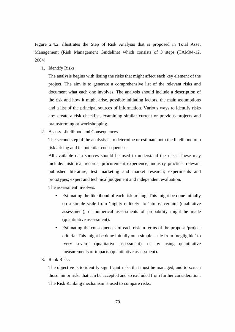
70

Figure 2.4.2. illustrates the Step of Risk Analysis that is proposed in Total Asset

Management (Risk Management Guideline) which consists of 3 steps (TAM04-12,

2004):

1. Identify Risks

The analysis begins with listing the risks that might affect each key element of the

project. The aim is to generate a comprehensive list of the relevant risks and

document what each one involves. The analysis should include a description of

the risk and how it might arise, possible initiating factors, the main assumptions

and a list of the principal sources of information. Various ways to identify risks

are: create a risk checklist, examining similar current or previous projects and

brainstorming or workshopping.

2. Assess Likelihood and Consequences

The second step of the analysis is to determine or estimate both the likelihood of a

risk arising and its potential consequences.

All available data sources should be used to understand the risks. These may

include: historical records; procurement experience; industry practice; relevant

published literature; test marketing and market research; experiments and

prototypes; expert and technical judgement and independent evaluation.

The assessment involves:

• Estimating the likelihood of each risk arising. This might be done initially

on a simple scale from ‘highly unlikely’ to ‘almost certain’ (qualitative

assessment), or numerical assessments of probability might be made

(quantitative assessment).

• Estimating the consequences of each risk in terms of the proposal/project

criteria. This might be done initially on a simple scale from ‘negligible’ to

‘very severe’ (qualitative assessment), or by using quantitative

measurements of impacts (quantitative assessment).

3. Rank Risks

The objective is to identify significant risks that must be managed, and to screen

those minor risks that can be accepted and so excluded from further consideration.

The Risk Ranking mechanism is used to compare risks.

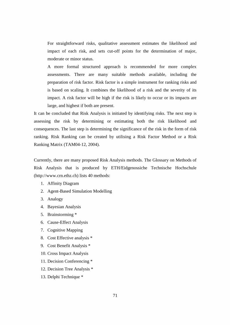
71

For straightforward risks, qualitative assessment estimates the likelihood and

impact of each risk, and sets cut-off points for the determination of major,

moderate or minor status.

A more formal structured approach is recommended for more complex

assessments. There are many suitable methods available, including the

preparation of risk factor. Risk factor is a simple instrument for ranking risks and

is based on scaling. It combines the likelihood of a risk and the severity of its

impact. A risk factor will be high if the risk is likely to occur or its impacts are

large, and highest if both are present.

It can be concluded that Risk Analysis is initiated by identifying risks. The next step is

assessing the risk by determining or estimating both the risk likelihood and

consequences. The last step is determining the significance of the risk in the form of risk

ranking. Risk Ranking can be created by utilising a Risk Factor Method or a Risk

Ranking Matrix (TAM04-12, 2004).

Currently, there are many proposed Risk Analysis methods. The Glossary on Methods of

Risk Analysis that is produced by ETH/Eidgenossiche Technische Hochschule

(http://www.crn.ethz.ch) lists 40 methods:

1. Affinity Diagram

2. Agent-Based Simulation Modelling

3. Analogy

4. Bayesian Analysis

5. Brainstorming *

6. Cause-Effect Analysis

7. Cognitive Mapping

8. Cost Effective analysis *

9. Cost Benefit Analysis *

10. Cross Impact Analysis

11. Decision Conferencing *

12. Decision Tree Analysis *

13. Delphi Technique *

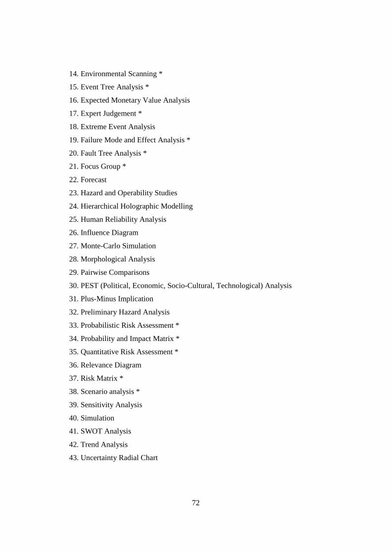
72

14. Environmental Scanning *

15. Event Tree Analysis *

16. Expected Monetary Value Analysis

17. Expert Judgement *

18. Extreme Event Analysis

19. Failure Mode and Effect Analysis *

20. Fault Tree Analysis *

21. Focus Group *

22. Forecast

23. Hazard and Operability Studies

24. Hierarchical Holographic Modelling

25. Human Reliability Analysis

26. Influence Diagram

27. Monte-Carlo Simulation

28. Morphological Analysis

29. Pairwise Comparisons

30. PEST (Political, Economic, Socio-Cultural, Technological) Analysis

31. Plus-Minus Implication

32. Preliminary Hazard Analysis

33. Probabilistic Risk Assessment *

34. Probability and Impact Matrix *

35. Quantitative Risk Assessment *

36. Relevance Diagram

37. Risk Matrix *

38. Scenario analysis *

39. Sensitivity Analysis

40. Simulation

41. SWOT Analysis

42. Trend Analysis

43. Uncertainty Radial Chart

73

Out of these Risk Analysis methods, Stapelberg (2006) concluded that the 17 methods

indicated by asterisks are the most commonly used methods.

Frame (2003) reveals that the usefulness of Risk Analysis is limited by the quality and

quantity of information available. In addition, lack of information will restrict the amount

of effective Risk Analysis that can be carried out (Stapelberg, 2006). Furthermore, the

need of Risk Analysis is often greatest in situations where information is lacking (Frame,

2003).

Two crucial components have to be determined before risk can be calculated: Likelihood

and Consequence of Risk. The Consequence of Risk can be determined by assessing the

severity of the impact. Although there are several methods to determine the risk

consequences, such as expert judgement, the easiest and most common method is by

quantifying the cost that has to be paid if the risk occurs (Stapelberg, 1993). The

Likelihood of Risk is determined from how frequently the risks occur.

However, it is quite difficult to determine Risk Likelihood, because it needs a

sophisticated historical information/experience. Sometimes, this kind of information is

not available or, if available, it is incomplete. There are several sources of Risk

Likelihood (TAM04-12, 2004):

1. Historical records

2. Procurement experience

3. Industry practice

4. Relevant published literature

5. Test marketing and market research

6. Experiment and prototype

7. Expert and technical judgement

8. Independent evaluation

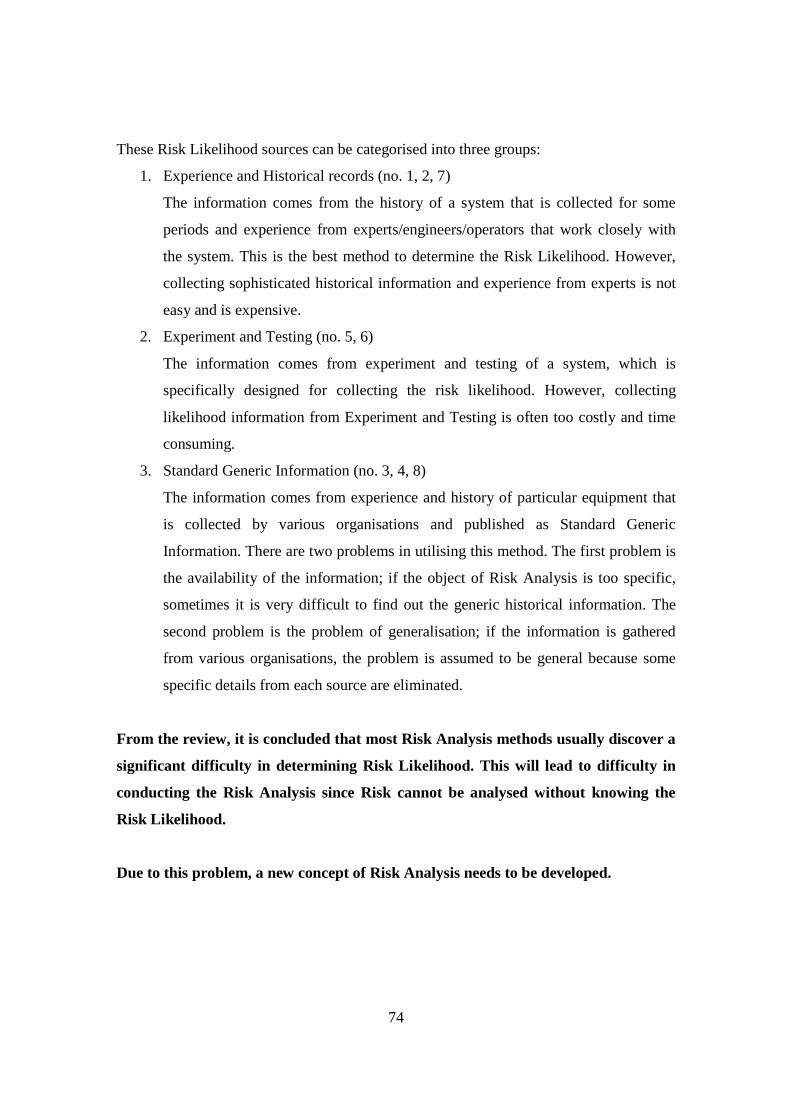
74

These Risk Likelihood sources can be categorised into three groups:

1. Experience and Historical records (no. 1, 2, 7)

The information comes from the history of a system that is collected for some

periods and experience from experts/engineers/operators that work closely with

the system. This is the best method to determine the Risk Likelihood. However,

collecting sophisticated historical information and experience from experts is not

easy and is expensive.

2. Experiment and Testing (no. 5, 6)

The information comes from experiment and testing of a system, which is

specifically designed for collecting the risk likelihood. However, collecting

likelihood information from Experiment and Testing is often too costly and time

consuming.

3. Standard Generic Information (no. 3, 4, 8)

The information comes from experience and history of particular equipment that

is collected by various organisations and published as Standard Generic

Information. There are two problems in utilising this method. The first problem is

the availability of the information; if the object of Risk Analysis is too specific,

sometimes it is very difficult to find out the generic historical information. The

second problem is the problem of generalisation; if the information is gathered

from various organisations, the problem is assumed to be general because some

specific details from each source are eliminated.

From the review, it is concluded that most Risk Analysis methods usually discover a

significant difficulty in determining Risk Likelihood. This will lead to difficulty in

conducting the Risk Analysis since Risk cannot be analysed without knowing the

Risk Likelihood.

Due to this problem, a new concept of Risk Analysis needs to be developed.

75

2.4.3. Discussion The literature review highlights the critical problem in current Risk Analysis methods:

determining Risk Likelihood. Determining Risk Likelihood is difficult because of the

need for historical information. In most cases, this information is not available, or if it is

available, it is incomplete. Therefore, a new concept of Risk Analysis is needed to

address this problem.

2.5. Risk Analysis: A Different Perspective

This section explains the design and development method of a new concept of Risk

Analysis to address the identified problems.

2.5.1. Interdependence Risk Analysis

There are several criteria for the new concept:

1. It does not depend on the availability of Risk Likelihood.

2. It is able to include the individual analysis of each risk analysis object into the

calculation, thus, unique conditions of each object can be obtained.

76

In order to combine the research into one theme, the new concept of Risk Analysis is

linked to the Hierarchical Model (refer to Section 2.3.3.). In addition, the stepping stones

to this concept are:

• In economics, interdependence leads to conflict. (Campbell, 1997)

If interdependence leads to conflict, it also leads to failure. Thus, there is always a

risk in interdependent conditions.

• Interdependence is measurable (Drew et al., 2002)

Based on analysis from the previous point, there is always a risk in interdependent

conditions. Therefore, Risk Analysis can begin by measuring the risk in

interdependence.

In the Hierarchical Model that is proposed by this research, there is an Interdependence

Analysis. The tool of Interdependence Analysis in the Hierarchical Model is a Functional

and Causal Relationship Diagram (FCRD). There are two stages in FCRD. Risk Analysis

based on Interdependence Analysis is established in the first stage of FCRD.

Figure 2.5.1. illustrates the Hierarchical Model with the addition of Interdependence Risk

Analysis. Results from Interdependence Risk Analysis then become the initial input for

the Failure Mode Effect and Criticality Analysis (FMECA).

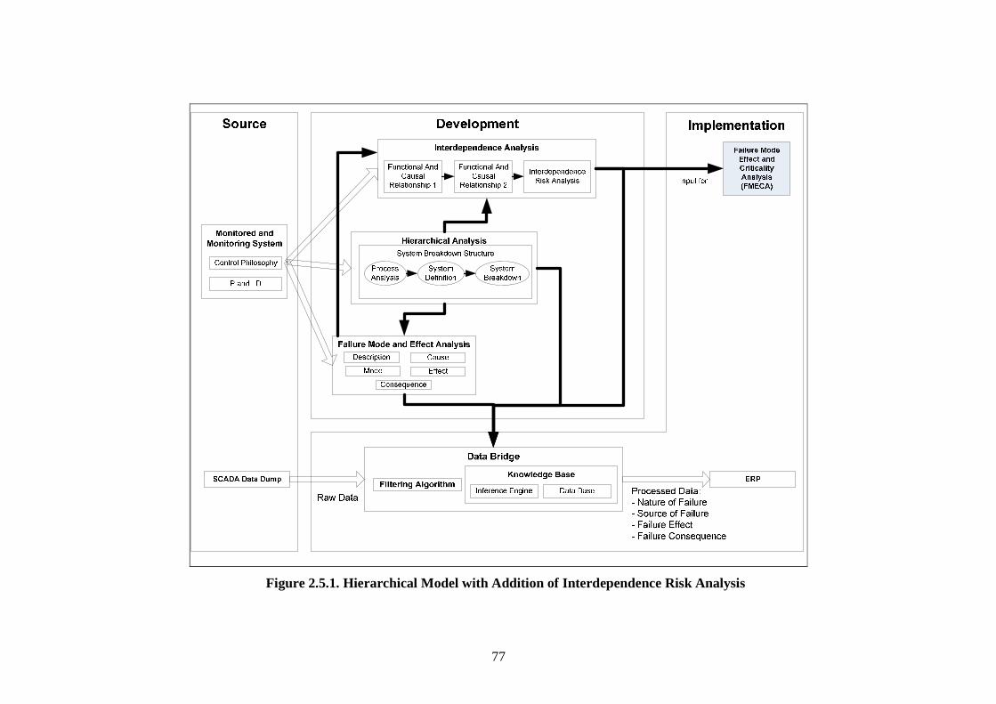
77

13Figure 2.5.1. Hierarchical Model with Addition of Interdependence Risk Analysis

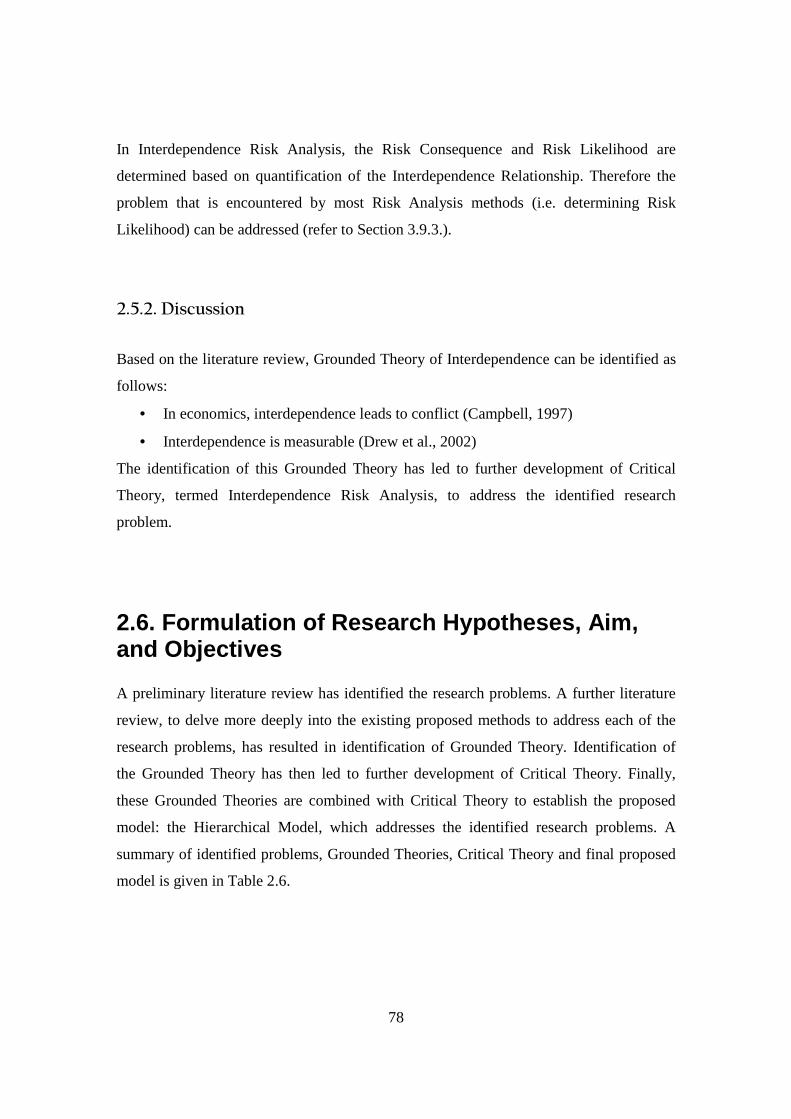
78

In Interdependence Risk Analysis, the Risk Consequence and Risk Likelihood are

determined based on quantification of the Interdependence Relationship. Therefore the

problem that is encountered by most Risk Analysis methods (i.e. determining Risk

Likelihood) can be addressed (refer to Section 3.9.3.).

2.5.2. Discussion

Based on the literature review, Grounded Theory of Interdependence can be identified as

follows:

• In economics, interdependence leads to conflict (Campbell, 1997)

• Interdependence is measurable (Drew et al., 2002)

The identification of this Grounded Theory has led to further development of Critical

Theory, termed Interdependence Risk Analysis, to address the identified research

problem.

2.6. Formulation of Research Hypotheses, Aim, and Objectives A preliminary literature review has identified the research problems. A further literature

review, to delve more deeply into the existing proposed methods to address each of the

research problems, has resulted in identification of Grounded Theory. Identification of

the Grounded Theory has then led to further development of Critical Theory. Finally,

these Grounded Theories are combined with Critical Theory to establish the proposed

model: the Hierarchical Model, which addresses the identified research problems. A

summary of identified problems, Grounded Theories, Critical Theory and final proposed

model is given in Table 2.6.

79

4Table 2.6. Research Problems, Grounded Theories, Critical Theory and Final Proposed Model

Based on information from the literature review, several hypotheses are proposed:

a. Problems in SCADA data analysis, such as nested data, can be addressed by

analysing design information of monitored and monitoring systems through

the Hierarchical Model.

This hypothesis is developed based on research problem number 1 (refer to

Table 2.6.a.). According to the literature review, the identified data from SCADA

is difficult to analyse. The explanation behind this difficulty is that data from

SCADA systems is nested data, data that is influenced by other factors. The

Hierarchical Model is proposed to solve this problem. Validation is needed to

prove this hypothesis.

b. The Interdependence Risk Analysis method can address current Risk

Analysis method problems, i.e. the need for sophisticated historical

information as an input for Risk Likelihood.

As highlighted in the literature review, a critical problem in current Risk Analysis

methods is determining the Risk Likelihood (refer to Table 2.6.a.). Determining

Risk Likelihood is difficult because of the need for historical information. In most

cases, this information is not available, or if it is available, it is incomplete.

Therefore, to address the problem a new concept of Risk Analysis -

(Interdependence Risk Analysis) - utilising interdependence relationship is

proposed in this research. The validation of this hypothesis is given in Section 6.3.

80

c. The data bridge developed from the Hierarchical Model will address the

connectivity problem between SCADA systems and ERP systems, whereby

significant information can be drawn out from SCADA’s “raw data” and

transferred into ERP.

According to information from the literature review, the need for integrating both

SCADA and ERP systems is apparent. Furthermore, the literature review found

that several companies offer solutions integrating SCADA systems and ERP

systems by utilising the Data Bridge concept. However the concept of Data

Bridge is still far from ideal because most of them directly integrate both of these

systems’ data bases. The Hierarchical Model proposed in this thesis is able to

develop a specific data bridge to facilitate the connectivity between SCADA and

ERP systems. In the validation step (refer to Section 6.4.), this hypothesis is

tested.

A research aim is formulated as a guide to test the research hypotheses stated above. It

contains a summary of the research problems and proposed methods to address them. The

research aim of this thesis is:

To develop a new model in order to improve the analyses and predictions in

condition monitoring by using Interdependence in Risk Likelihood analysis, and test

this model through the Water Treatment Plant Case Study.

Several objectives must be achieved to test the set hypotheses. These objectives are:

a. Development of a prototype SCADA system in LabVIEW to identify critical

criteria of on-line data acquisition.

This objective is aimed at investigating the construct of SCADA systems in order

to determine its on-line data acquisition characteristics and behaviours. To further

achieve this objective, a typical SCADA system is developed and simulated, and a

prototype is modelled in Lab VIEW.

81

b. Development of a data filtering algorithm using the algorithmic approach of

data compression to remove redundant data.

A data filtering algorithm is needed to transfer only relevant information. A data

compression algorithmic approach, in which the underlying philosophy is to

remove redundant data, will be used to develop the filtering algorithm. A data

compression algorithm which is specifically targeted for real-time data, has been

developed and successfully shown that redundant data can be reduced. This data

compression algorithm is further modified and refined into a data filtering

algorithm. Investigation into actual SCADA data must be conducted before the

data filtering algorithm is applied. By achieving this objective, a data filtering

algorithm, which is able to filter data redundancy from SCADA data, can be

utilised in the validation of the hierarchical interface.

c. Development of a Hierarchical Model

The hierarchical Model is composed of three different analyses: Hierarchical

Analysis, Failure Mode and Effect Analysis, and Interdependence Analysis.

Hierarchical Analysis, and Failure Mode and Effect Analysis are Grounded

Theories. Grounded Theory is identified from analysis of various relevant sources

by utilising a constant comparative method of qualitative analysis.

Interdependence Analysis is a Critical Theory which is developed in this research

by utilising an interdependence relationship to model the system related criteria.

Critical Theory is developed to address the limitations of a critiqued theory; that

is, the Grounded Theory.

d. Validating the Hierarchical Model through the water treatment plant case

study

The validity of the Hierarchical Model is tested by applying it to the Water

Treatment Plant Case Study.

82

2.7. Summary

This chapter has provided a review of the literature relevant to on-line data connectivity

and risk analysis topics. Problems and gaps on those topics are identified as follows:

• SCADA data analysis

• Connectivity of SCADA systems and ERP systems

• Determining Risk Likelihood

Also, several Grounded Theories are identified, such as:

1. Concept of Entity Relationship Diagram

2. Interdependence Concept

3. Failure Mode and Effect Analysis (Stapelberg, 1993)

4. System Breakdown Structure (Stapelberg, 1993)

5. In economics, Interdependence leads to Conflict (Campbell, 1997)

6. Interdependence is measurable (Drew et al., 2002)

This research then continues to the formulation of the Critical Theory based on the

identified research problems and Grounded Theories. The Critical Theory in this research

is Interdependence Analysis which is developed by utilising an interdependence

relationship to model the system related criteria. A new concept of risk analysis, namely

Interdependence Risk Analysis, is formulated based on the Interdependence Analysis.

The final proposed model is then explained. The final proposed model in this research is

the Hierarchical Model which is comprised of three different analyses: Hierarchical

Analysis, Failure Mode and Effect Analysis and Interdependence Analysis.

83

CHAPTER 3

RESEARCH METHODOLOGY

3.1. Introduction The essence of Chapter 3 is the detailed explanation of the final proposed model which

has been introduced in Chapter 2. The chapter begins by describing the experimental

method - Real-Time Water Quality Condition Monitoring System and SCADA test rig -

and then continues to the Development Theory - Algorithm Formulation and Hierarchical

Model. Finally, the Data Bridge as the implementation phase is described.

3.2. Experimentation: Real-Time Water Quality Condition Monitoring System

3.2.1. Introduction

This model is developed to achieve the first objective of this research and as a support to

the proposed model. This model is developed to mimic the data acquisition part of a real

SCADA system. It is then tested by monitoring water quality. The test resulted in the

identification of critical criteria of on-line data acquisition. These criteria are utilised to

design the SCADA test rig for testing the research findings. The study was initialised by

designing a real-time water quality monitoring system architecture, followed by

prototype development and testing of an on-line data acquisition system.

84

3.2.2. System Architecture The system structure consists of three stations, namely local measurement, central

control, and a remote browse station (illustrated in Figure 3.2.2.). Located close to the

measurement point, the local station measures water quality, displays a real-time data

chart, performs basic data analysis, transmits data to the central station, and receives

response commands from the central control station.

All data from different local measurement stations is centralized in the central control

station for further data analysis. The central control station displays the real-time water

quality condition from different monitoring stations, stores the data history, sends

commands and messages to the local measurement stations, and generates periodic

reports of water quality. The main program in the central control station is used to

analyse the collected data (advanced analyses), show diagrams of the measured

parameters, and communicate with the measurement stations and remote browse stations.

The remote browse station is a general computer used to log onto the web site of the

water quality monitoring system to browse the information and retrieve data related to

water quality.

The whole system is built over the Internet and is based on a client-server mechanism.

The HTTP server of the central control station services the remote browse stations. It

connects and interacts with a data base through CGI (Common Gateway Interface) and/or

ADO (ActiveX Data Objects) plus ODBC (Open Data Base Connectivity). The remote

browser searches through retrieved data from the central control station or local

measurement stations through an ActiveX control enabled Web browser, Java Applet, or

HTML pages.

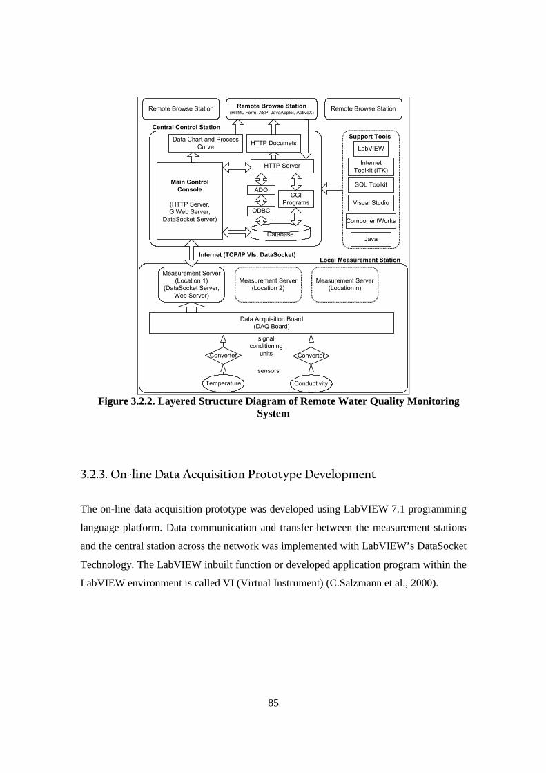
85

sensors

Data Acquisition Board

(DAQ Board)

Measurement Server

(Location 1)

(DataSocket Server,

Web Server)

Measurement Server

(Location 2)

Measurement Server

(Location n)

Main Control

Console

(HTTP Server,

G Web Server,

DataSocket Server)

HTTP Server

CGI

Programs

ADO

Database

Local Measurement Station

HTTP DocumetsData Chart and Process

Curve LabVIEW

Visual Studio

Java

Support Tools

Central Control Station

Remote Browse Station Remote Browse Station(HTML Form, ASP, JavaApplet, ActiveX)

Remote Browse Station

Internet (TCP/IP VIs. DataSocket)

Internet

Toolkit (ITK)

SQL Toolkit

ODBC

ComponentWorks

Conductivity

Converter

Temperature

Converter

signal

conditioning

units

14Figure 3.2.2. Layered Structure Diagram of Remote Water Quality Monitoring

System

3.2.3. On-line Data Acquisition Prototype Development

The on-line data acquisition prototype was developed using LabVIEW 7.1 programming

language platform. Data communication and transfer between the measurement stations

and the central station across the network was implemented with LabVIEW’s DataSocket

Technology. The LabVIEW inbuilt function or developed application program within the

LabVIEW environment is called VI (Virtual Instrument) (C.Salzmann et al., 2000).

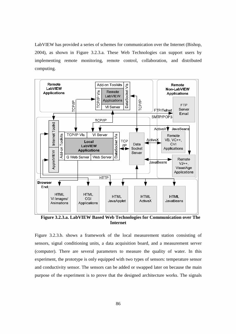
86

LabVIEW has provided a series of schemes for communication over the Internet (Bishop,

2004), as shown in Figure 3.2.3.a. These Web Technologies can support users by

implementing remote monitoring, remote control, collaboration, and distributed

computing.

15Figure 3.2.3.a. LabVIEW Based Web Technologies for Communication over The

Internet

Figure 3.2.3.b. shows a framework of the local measurement station consisting of

sensors, signal conditioning units, a data acquisition board, and a measurement server

(computer). There are several parameters to measure the quality of water. In this

experiment, the prototype is only equipped with two types of sensors: temperature sensor

and conductivity sensor. The sensors can be added or swapped later on because the main

purpose of the experiment is to prove that the designed architecture works. The signals

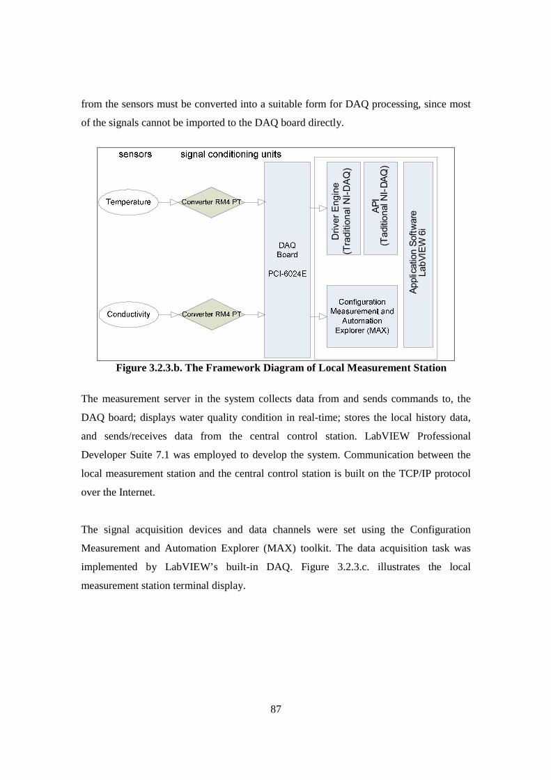
87

from the sensors must be converted into a suitable form for DAQ processing, since most

of the signals cannot be imported to the DAQ board directly.

Driver Engine

(Traditional NI-DAQ)

API

(TaditionalNI-DAQ)

ApplicationSoftware

LabVIEW6i

16Figure 3.2.3.b. The Framework Diagram of Local Measurement Station

The measurement server in the system collects data from and sends commands to, the

DAQ board; displays water quality condition in real-time; stores the local history data,

and sends/receives data from the central control station. LabVIEW Professional

Developer Suite 7.1 was employed to develop the system. Communication between the

local measurement station and the central control station is built on the TCP/IP protocol

over the Internet.

The signal acquisition devices and data channels were set using the Configuration

Measurement and Automation Explorer (MAX) toolkit. The data acquisition task was

implemented by LabVIEW’s built-in DAQ. Figure 3.2.3.c. illustrates the local

measurement station terminal display.

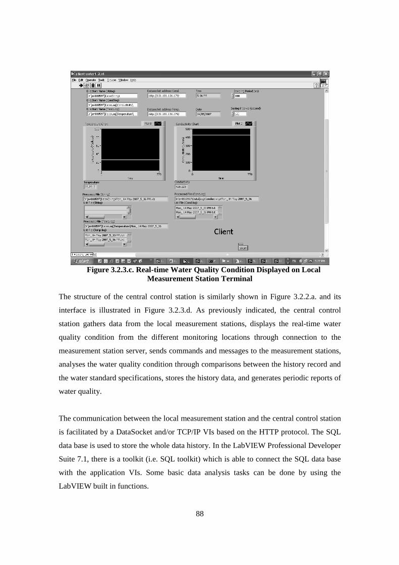
88

17Figure 3.2.3.c. Real-time Water Quality Condition Displayed on Local

Measurement Station Terminal

The structure of the central control station is similarly shown in Figure 3.2.2.a. and its

interface is illustrated in Figure 3.2.3.d. As previously indicated, the central control

station gathers data from the local measurement stations, displays the real-time water

quality condition from the different monitoring locations through connection to the

measurement station server, sends commands and messages to the measurement stations,

analyses the water quality condition through comparisons between the history record and

the water standard specifications, stores the history data, and generates periodic reports of

water quality.

The communication between the local measurement station and the central control station

is facilitated by a DataSocket and/or TCP/IP VIs based on the HTTP protocol. The SQL

data base is used to store the whole data history. In the LabVIEW Professional Developer

Suite 7.1, there is a toolkit (i.e. SQL toolkit) which is able to connect the SQL data base

with the application VIs. Some basic data analysis tasks can be done by using the

LabVIEW built in functions.

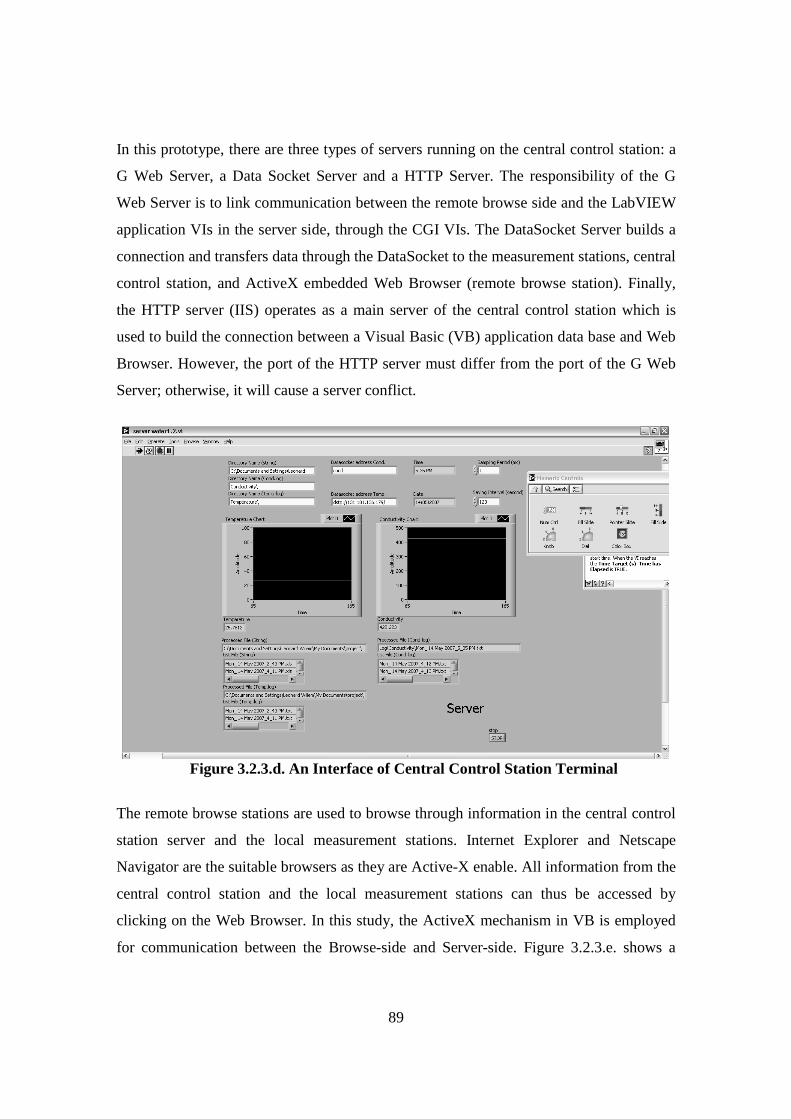
89

In this prototype, there are three types of servers running on the central control station: a

G Web Server, a Data Socket Server and a HTTP Server. The responsibility of the G

Web Server is to link communication between the remote browse side and the LabVIEW

application VIs in the server side, through the CGI VIs. The DataSocket Server builds a

connection and transfers data through the DataSocket to the measurement stations, central

control station, and ActiveX embedded Web Browser (remote browse station). Finally,

the HTTP server (IIS) operates as a main server of the central control station which is

used to build the connection between a Visual Basic (VB) application data base and Web

Browser. However, the port of the HTTP server must differ from the port of the G Web

Server; otherwise, it will cause a server conflict.

18Figure 3.2.3.d. An Interface of Central Control Station Terminal

The remote browse stations are used to browse through information in the central control

station server and the local measurement stations. Internet Explorer and Netscape

Navigator are the suitable browsers as they are Active-X enable. All information from the

central control station and the local measurement stations can thus be accessed by

clicking on the Web Browser. In this study, the ActiveX mechanism in VB is employed

for communication between the Browse-side and Server-side. Figure 3.2.3.e. shows a

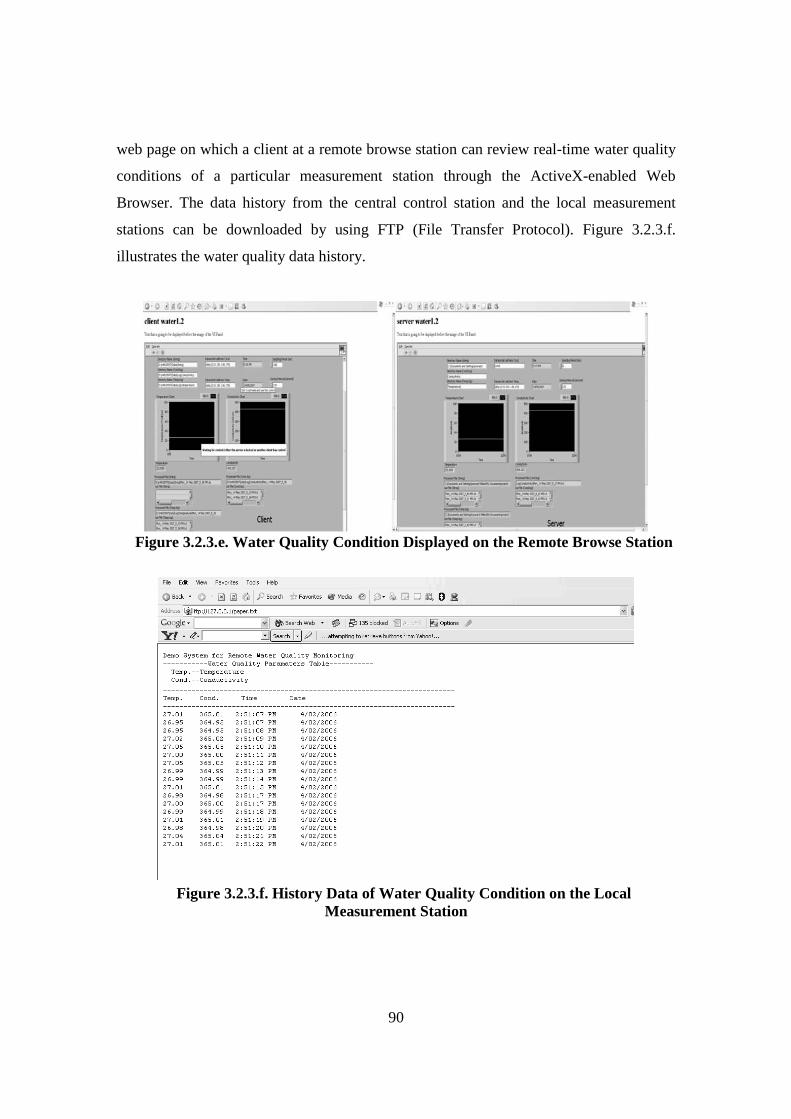
90

web page on which a client at a remote browse station can review real-time water quality

conditions of a particular measurement station through the ActiveX-enabled Web

Browser. The data history from the central control station and the local measurement

stations can be downloaded by using FTP (File Transfer Protocol). Figure 3.2.3.f.

illustrates the water quality data history.

19Figure 3.2.3.e. Water Quality Condition Displayed on the Remote Browse Station

20Figure 3.2.3.f. History Data of Water Quality Condition on the Local

Measurement Station

91

3.2.4. Identification of Critical Criteria of On-line Data Acquisition Systems Brindley et al. (1998) concludes that the identification of Critical Criteria of a system

provides deeper understanding about the system. Shahriari et al. (2006) revealed that

Critical Criteria can only be identified by conducting close investigation of the system.

The investigation of the On-line Data Acquisition System has been carried out in the

development of the Prototype of Real-time Water Quality Condition Monitoring System.

Therefore, it leads to a more comprehensive and deeper understanding of the On-line

Data Acquisition System.

The goal is to develop a test rig to be used to validate some of the research findings.

Initially, the Critical Criteria of On-line Data Acquisition Systems have to be identified.

These criteria can be used as a guide to develop a standard SCADA test rig and provide

increased confidence in the result generated during such testing (Bolton and Linden,

2003).

The Critical Criteria of the On-line Data Acquisition System are determined based on the

development and testing process of the Real-Time Water Quality Condition Monitoring

System model. The Criteria are:

• Data source

• Data transfer process

• Data processing and display

• Data storage

3.2.5. Discussion Real-Time Water Quality Condition Monitoring Model has been successfully developed

and simulated. It is developed based on Web technology (DataSocket, ActiveX) and

software (LabVIEW, and VB). The structure of the model consists of three components:

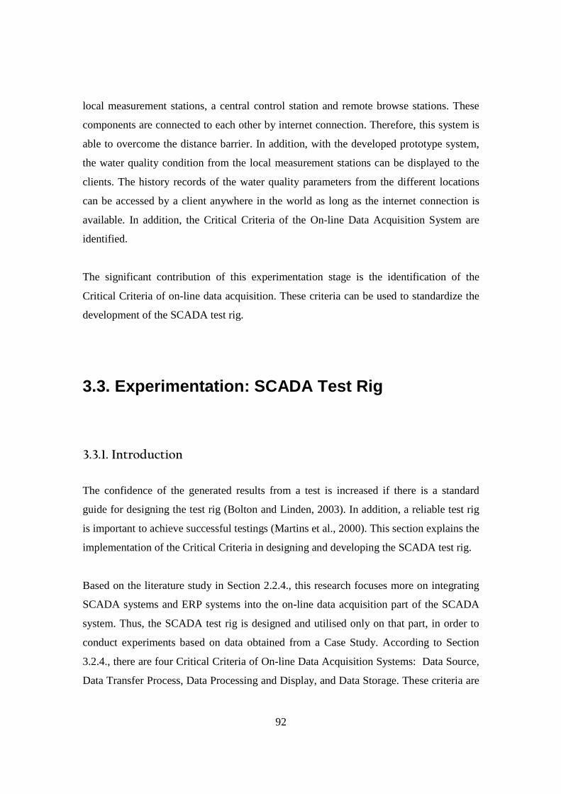
92

local measurement stations, a central control station and remote browse stations. These

components are connected to each other by internet connection. Therefore, this system is

able to overcome the distance barrier. In addition, with the developed prototype system,

the water quality condition from the local measurement stations can be displayed to the

clients. The history records of the water quality parameters from the different locations

can be accessed by a client anywhere in the world as long as the internet connection is

available. In addition, the Critical Criteria of the On-line Data Acquisition System are

identified.

The significant contribution of this experimentation stage is the identification of the

Critical Criteria of on-line data acquisition. These criteria can be used to standardize the

development of the SCADA test rig.

3.3. Experimentation: SCADA Test Rig

3.3.1. Introduction

The confidence of the generated results from a test is increased if there is a standard

guide for designing the test rig (Bolton and Linden, 2003). In addition, a reliable test rig

is important to achieve successful testings (Martins et al., 2000). This section explains the

implementation of the Critical Criteria in designing and developing the SCADA test rig.

Based on the literature study in Section 2.2.4., this research focuses more on integrating

SCADA systems and ERP systems into the on-line data acquisition part of the SCADA

system. Thus, the SCADA test rig is designed and utilised only on that part, in order to

conduct experiments based on data obtained from a Case Study. According to Section

3.2.4., there are four Critical Criteria of On-line Data Acquisition Systems: Data Source,

Data Transfer Process, Data Processing and Display, and Data Storage. These criteria are

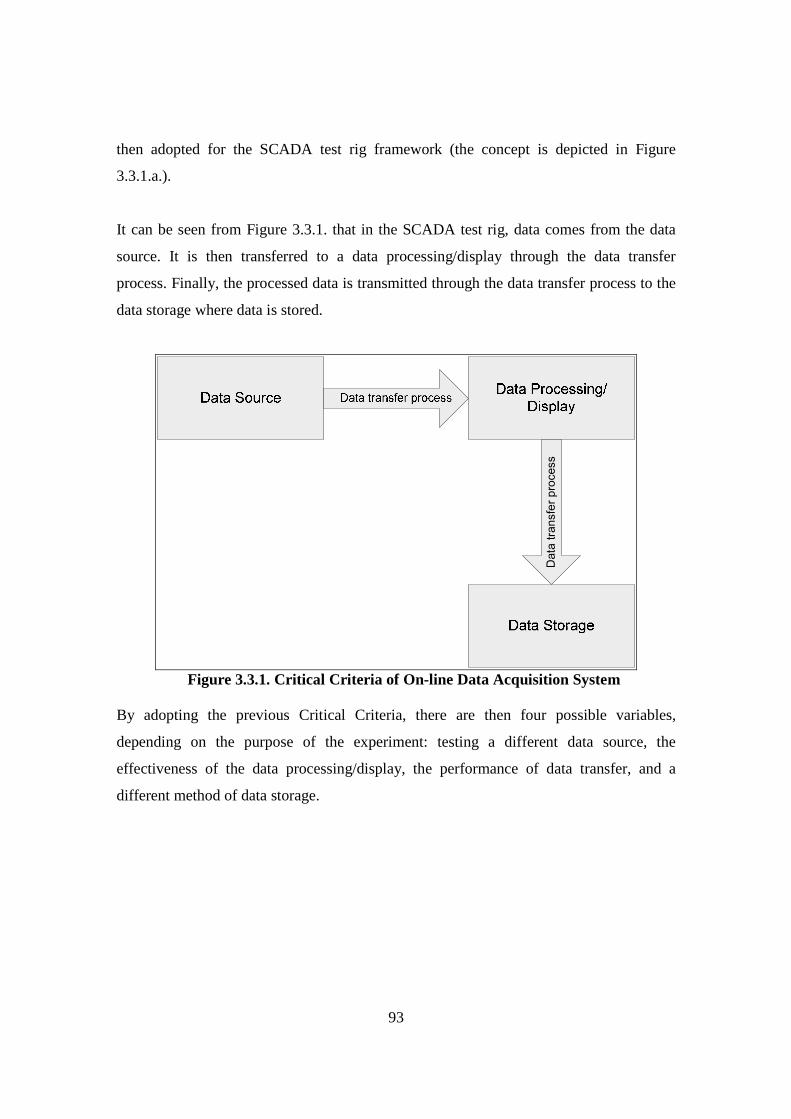
93

then adopted for the SCADA test rig framework (the concept is depicted in Figure

3.3.1.a.).

It can be seen from Figure 3.3.1. that in the SCADA test rig, data comes from the data

source. It is then transferred to a data processing/display through the data transfer

process. Finally, the processed data is transmitted through the data transfer process to the

data storage where data is stored.

Data transfer process

21Figure 3.3.1. Critical Criteria of On-line Data Acquisition System

By adopting the previous Critical Criteria, there are then four possible variables,

depending on the purpose of the experiment: testing a different data source, the

effectiveness of the data processing/display, the performance of data transfer, and a

different method of data storage.

94

3.3.2. Data Source In the On-line data acquisition system, the process is initiated from the location where

data is produced (i.e. data source). Therefore, the presence of the data source is the most

critical criterion of the on-line data acquisition system, since the basic function of the

system is to acquire data from a data source to be processed and stored. In a real system,

data may come from sensors and alarm/event signals. On the other hand, for laboratory

purposes, the data source can be a data base from a real system.

3.3.3. Data Transfer Process Data transfer is one of the main functions of the On-line Data Acquisition System. The

basic philosophy of this system is to obtain data from a data source, transfer it to the

location where it is processed, and then transfer the result to data storage (data base). In

real on-line data acquisition systems, the data transfer process is performed by utilising

various kinds of available technology which can be grouped into two types: wired [for

example: RS 232 (Zhou and Yarlagadda, n.d.), Fieldbus network (El-Shtewi et al., 2001),

and wireless for example: Bluetooth technology (Lahdelma and Pyssysalo, 2001 ; Halme

et al., 2003), and Radio Frequency (Yun et al., 2004)]. However, because the SCADA

test is developed and run at a single PC, the data transfer process is performed inside the

PC itself (i.e. transferring one file from one folder, processing it, and then storing it into

another folder).

3.3.4. Data Processing and Display Data processing depends on the purpose of the SCADA test rig. For example: in Section

3.4, the SCADA test rig is developed and used to test the compression and filtering

algorithm; therefore, the data processing is designed specifically for compressing and

filtering data.

95

Data display is designed based on the requirement of the SCADA test rig; some tests

require a graph to represent data fluctuation, but other tests only require display of the

count of data that has been processed.

3.3.5. Data Storage Data storage is the final process in the on-line data acquisition system. After data is

gathered from a data source and processed, it is then stored. The types of data storage

vary from a simple file to a complex and sophisticated data base. Data storage in the

SCADA test rig is a process of writing the processed data into a text file or Comma

Separate Value (CSV) file.

3.3.6. Discussion The framework for designing the SCADA test rig adopts the identified Critical Criteria of

On-line Data Acquisition System (refer to Section 3.2.4.). This framework will be used to

develop various SCADA test rigs with different purposes to validate the research

findings. There are four possible variables, depending on the purpose of the experiment:

testing different data sources, the effectiveness of the data processing/display, the

performance of data transfer, and different methods of data storage.

96

3.4. Theory Development: Algorithm Formulation (Data Compression Algorithm)

3.4.1. Introduction The purpose of this stage of the research is to determine a means for compressing data

that is produced from a SCADA system. The approach is to study the characteristics of

the data from the SCADA system in detail. It was found that much data from a SCADA

system is redundant in terms of relevance. Several experiments are conducted to observe

the feasibility of reducing this redundancy, and to determine an effective means to reduce

data size.

In this case, data storage becomes a serious problem with on-line data acquisition systems

since masses of data are collected and dumped into storage every day (Matus-Castillejos

and Jentzsch, 2005). Furthermore, if the storage is not managed properly, it soon

becomes overwhelmed by redundant data (Lee, 2002). For example, a single day

measurement of 1 sample every 10 seconds, where the size of each sample is 8 bytes,

requires 69.120 kilobytes storage. Ten channels of such data demand about 7 Mbytes of

disk space. Hence, redundant data filtering through compression techniques is important.

In addition, if a large amount of data needs to be transferred to a remote station, the use

of data compression greatly reduces the transfer time needed. Benedetti et al. (1988)

propose a method of compression by using the least significant word algorithm; however,

it is not easy to implement this method.

97

3.4.2. Experiment Overview

The experiment is conducted in two stages. The first stage is a data base analysis,

followed by Real-time Data Compression Algorithm modelling. The second stage of the

experiment is testing of the algorithm; the experiment is conducted by using a SCADA

test rig. After that, the result from the test is analysed and discussed.

The first stage of the experiment is initialised by reading and manipulating data from a

water utility company’s data base, since the data is still raw and unreadable. After some

manipulation processes to make the data readable, statistical analysis can be conducted

by using Microsoft Excel©. Based on the analysis, the pattern of the data can be

identified. This data pattern can then be used to model the Real-time Data Compression

Algorithm.

In the second stage of the experiment, the algorithm is tested through the SCADA test rig

in which the compression algorithm has been added. Details of the first and second stage

of the experiment are presented in Figure 3.4.2.

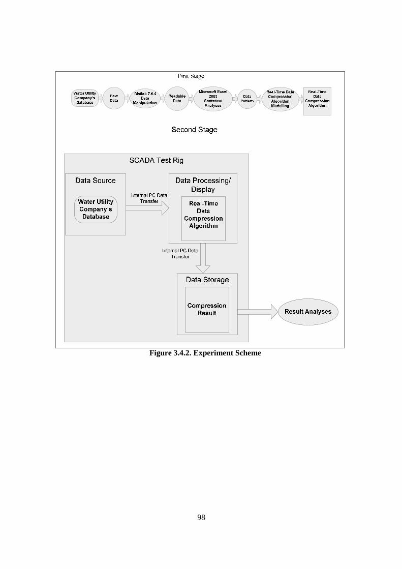
98

22Figure 3.4.2. Experiment Scheme

99

3.4.3. Data Base Analysis

Initially, data was stored and encrypted in the SCADA (Supervisory Control and Data

Acquisition) archive file formats. The data can be converted to a TXT format by using

data reader software supplied by the SCADA provider. It can be manipulated by

subtracting previous data from current data to calculate a disparities pattern. The

manipulation algorithm is:

Y(n) = d(n) – d(n-1) Equation 1.

Where:

Y = data disparities

n = sampling number

d = data absolute value

Matlab 7.0.4 is employed to manipulate the data. The data which is used in this

experiment is from a motor at the pump station. Originally, there were ten different

parameters. However, only two parameters are used to generate the algorithm;

specifically temperature data from two different motor bearings. The results of the

manipulation are in Table 3.4.3.

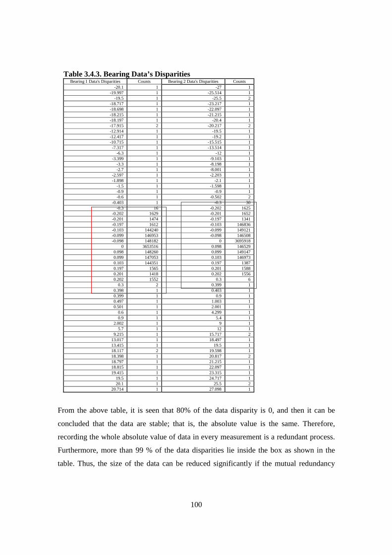
100

5Table 3.4.3. Bearing Data’s Disparities Bearing 1 Data's Disparities Counts Bearing 2 Data's Disparities Counts

-20.1 1 -27 1 -19.997 1 -25.514 1

-19.5 1 -25.5 2 -18.717 1 -23.217 1 -18.698 1 -22.097 1 -18.215 1 -21.215 1 -18.197 1 -20.4 1 -17.915 2 -20.217 2 -12.914 1 -19.5 1 -12.417 1 -19.2 1 -10.715 1 -15.515 1 -7.317 1 -13.514 1

-6.3 1 -12 1 -3.399 1 -9.103 1

-3.3 1 -8.198 1 -2.7 1 -8.001 1

-2.597 1 -2.203 1 -1.898 1 -2.1 1

-1.5 1 -1.598 1 -0.9 1 -0.9 1 -0.6 1 -0.502 2

-0.403 1 -0.3 30 -0.3 16 -0.202 1625

-0.202 1629 -0.201 1652 -0.201 1474 -0.197 1341 -0.197 1612 -0.103 146836 -0.103 144240 -0.099 149121 -0.099 146953 -0.098 146508 -0.098 148182 0 3695918

0 3653516 0.098 146529 0.098 148260 0.099 149147 0.099 147053 0.103 146973 0.103 144351 0.197 1387 0.197 1565 0.201 1588 0.201 1418 0.202 1556 0.202 1552 0.3 6

0.3 2 0.399 1 0.398 1 0.403 1 0.399 1 0.9 1 0.497 1 1.003 1 0.501 1 2.001 1

0.6 1 4.299 1 0.9 1 5.4 1

2.002 1 9 1 5.7 1 12 1

9.215 1 15.717 2 13.017 1 18.497 1 13.415 1 19.5 1 18.117 2 19.598 1 18.398 1 20.817 2 18.797 1 21.215 1 18.815 1 22.097 1 19.415 1 23.315 1

19.5 1 24.717 1 20.1 1 25.5 2

20.714 1 27.098 1

From the above table, it is seen that 80% of the data disparity is 0, and then it can be

concluded that the data are stable; that is, the absolute value is the same. Therefore,

recording the whole absolute value of data in every measurement is a redundant process.

Furthermore, more than 99 % of the data disparities lie inside the box as shown in the

table. Thus, the size of the data can be reduced significantly if the mutual redundancy

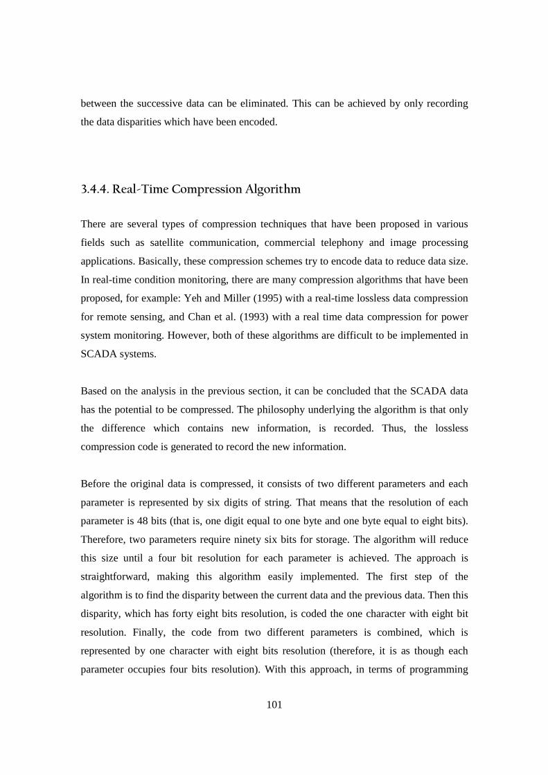
101

between the successive data can be eliminated. This can be achieved by only recording

the data disparities which have been encoded.

3.4.4. Real-Time Compression Algorithm

There are several types of compression techniques that have been proposed in various

fields such as satellite communication, commercial telephony and image processing

applications. Basically, these compression schemes try to encode data to reduce data size.

In real-time condition monitoring, there are many compression algorithms that have been

proposed, for example: Yeh and Miller (1995) with a real-time lossless data compression

for remote sensing, and Chan et al. (1993) with a real time data compression for power

system monitoring. However, both of these algorithms are difficult to be implemented in

SCADA systems.

Based on the analysis in the previous section, it can be concluded that the SCADA data

has the potential to be compressed. The philosophy underlying the algorithm is that only

the difference which contains new information, is recorded. Thus, the lossless

compression code is generated to record the new information.

Before the original data is compressed, it consists of two different parameters and each

parameter is represented by six digits of string. That means that the resolution of each

parameter is 48 bits (that is, one digit equal to one byte and one byte equal to eight bits).

Therefore, two parameters require ninety six bits for storage. The algorithm will reduce

this size until a four bit resolution for each parameter is achieved. The approach is

straightforward, making this algorithm easily implemented. The first step of the

algorithm is to find the disparity between the current data and the previous data. Then this

disparity, which has forty eight bits resolution, is coded the one character with eight bit

resolution. Finally, the code from two different parameters is combined, which is

represented by one character with eight bits resolution (therefore, it is as though each

parameter occupies four bits resolution). With this approach, in terms of programming

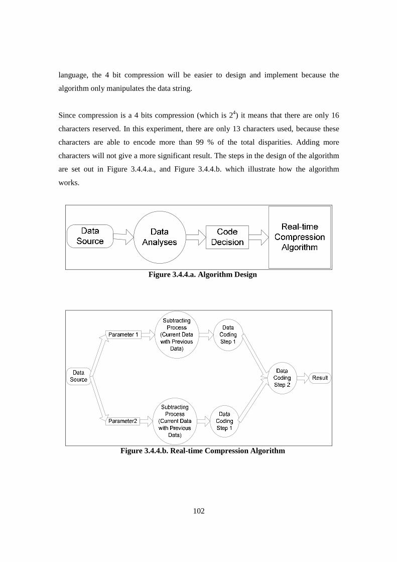
102

language, the 4 bit compression will be easier to design and implement because the

algorithm only manipulates the data string.

Since compression is a 4 bits compression (which is 24) it means that there are only 16

characters reserved. In this experiment, there are only 13 characters used, because these

characters are able to encode more than 99 % of the total disparities. Adding more

characters will not give a more significant result. The steps in the design of the algorithm

are set out in Figure 3.4.4.a., and Figure 3.4.4.b. which illustrate how the algorithm

works.

23Figure 3.4.4.a. Algorithm Design

24Figure 3.4.4.b. Real-time Compression Algorithm

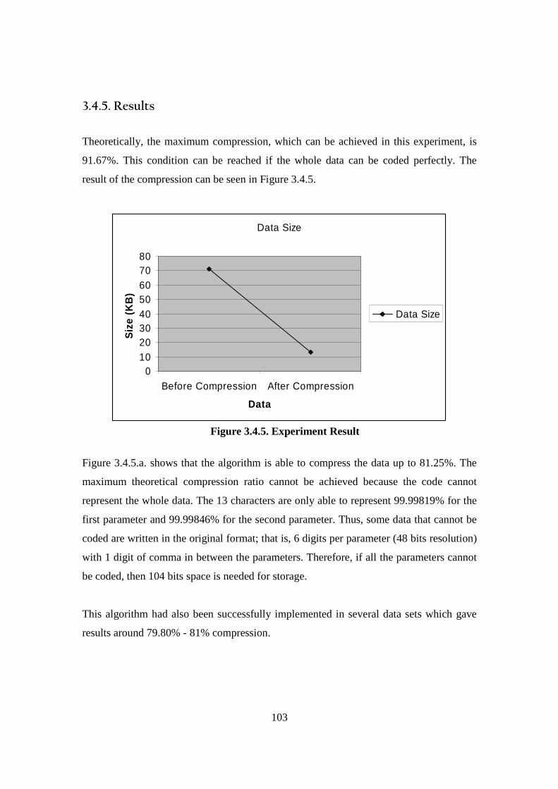
103

3.4.5. Results

Theoretically, the maximum compression, which can be achieved in this experiment, is

91.67%. This condition can be reached if the whole data can be coded perfectly. The

result of the compression can be seen in Figure 3.4.5.

Data Size

01020304050607080

Before Compression After Compression

Data

Siz

e (K

B)

Data Size

25Figure 3.4.5. Experiment Result

Figure 3.4.5.a. shows that the algorithm is able to compress the data up to 81.25%. The

maximum theoretical compression ratio cannot be achieved because the code cannot

represent the whole data. The 13 characters are only able to represent 99.99819% for the

first parameter and 99.99846% for the second parameter. Thus, some data that cannot be

coded are written in the original format; that is, 6 digits per parameter (48 bits resolution)

with 1 digit of comma in between the parameters. Therefore, if all the parameters cannot

be coded, then 104 bits space is needed for storage.

This algorithm had also been successfully implemented in several data sets which gave

results around 79.80% - 81% compression.

104

In conclusion, this algorithm is able to reduce the size of data significantly and the

compression process is done in a real-time timeframe. The more data disparities that can

be represented by the reserve characters, the greater compression ratio can be achieved.

Data that cannot be represented by the characters will be stored in the original format;

thus the size of these data will be 6.5 times larger in maximum than the perfectly

compressed data. Theoretically, the maximum compression ratio that can be achieved by

this algorithm is 91.57%.

Aside from the data set in the experiment, this algorithm had been successfully

implemented with other data sets and the results are between 79.80% - 81% compression.

Therefore, this algorithm is very suitable for real-time condition monitoring system,

especially SCADA systems.

3.4.6. Discussion

The Data Compression Algorithm has been successfully developed and tested. This

algorithm is a generic algorithm, since it can be applied to data from any SCADA

System. The Data Compression Algorithm development framework is initiated by

reading and manipulating data, so that data are in a readable format. After that, a simple

statistical analysis can be conducted. The pattern of data can be identified based on the

statistical analysis, and this pattern is used to generate the real-time data compression

algorithm.

The next step is simulation, testing and validation. The SCADA test rig is utilised to

perform the experiment. Prior to conducting the experiment, consideration of the Critical

Criteria of the On-line Data Acquisition System must be carried out. In this case, the data

source is the water utility industry data base; the data transfer is an internal PC data

transfer; the data processing/display is the compression algorithm with a data counter

display; and the data storage is a TXT file of compressed data. According to the

experiment result, the algorithm had successfully reduced up to 81 % of SCADA data.

105

Theoretically, this algorithm is able to reduce data up to 91.57%. However, because some

data cannot be compressed properly, this maximum theoretical compression rate cannot

be achieved. The significant benefit of this algorithm is that the compression works in a

real-time timeframe.

Another significant contribution from this study is the identification of the nature of

SCADA data, where 80 % of data is static (i.e. the sensor shows the same value). This

finding is then used as a basic consideration in developing a data filtering algorithm.

3.5. Theory Development: Algorithm Formulation (Data Filtering Algorithm)

3.5.1. Introduction

It has been noted in many research papers that a SCADA system is able to increase the

efficiency of the monitoring itself (Hongseng et al., 2000). However, SCADA systems

create a huge amount of data; this is difficult to analyse (Taylor, 2001; Matus-Castillejos

and Jentzsch, 2005). In addition, according to the data compression algorithm study, 80%

or SCADA data is stable where the sensor gives the same value. Generally, the state of

the monitored object does not change (i.e. normal condition) when the results of

monitoring gives the same value (Bansal et al., 2004). Therefore, there has to be a

mechanism to filter SCADA data in order to detect abnormal conditions by capturing the

occurrence of data change.

This study proposes a novel real-time data filtering for SCADA system where a suitable

algorithm to filter data from SCADA system is developed. The philosophy that is applied

in this algorithm is to capture the occurrence of data change in SCADA data, which is

followed by storing several data before this data change occurs. As a result, SCADA data

analysis will become easier, because only essential information remains.

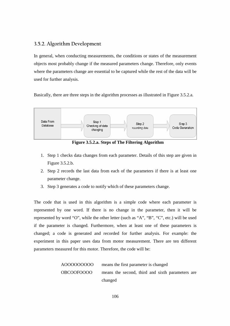
106

3.5.2. Algorithm Development In general, when conducting measurements, the conditions or states of the measurement

objects most probably change if the measured parameters change. Therefore, only events

where the parameters change are essential to be captured while the rest of the data will be

used for further analysis.

Basically, there are three steps in the algorithm processes as illustrated in Figure 3.5.2.a.

26Figure 3.5.2.a. Steps of The Filtering Algorithm

1. Step 1 checks data changes from each parameter. Details of this step are given in

Figure 3.5.2.b.

2. Step 2 records the last data from each of the parameters if there is at least one

parameter change.

3. Step 3 generates a code to notify which of these parameters change.

The code that is used in this algorithm is a simple code where each parameter is

represented by one word. If there is no change in the parameter, then it will be

represented by word “O”, while the other letter (such as “A”, “B”, “C”, etc.) will be used

if the parameter is changed. Furthermore, when at least one of these parameters is

changed; a code is generated and recorded for further analysis. For example: the

experiment in this paper uses data from motor measurement. There are ten different

parameters measured for this motor. Therefore, the code will be:

AOOOOOOOOO means the first parameter is changed

OBCOOFOOOO means the second, third and sixth parameters are

changed

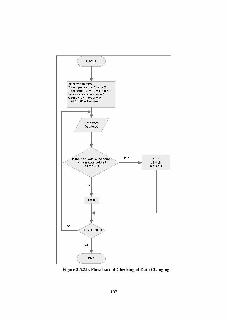
107

27Figure 3.5.2.b. Flowchart of Checking of Data Changing

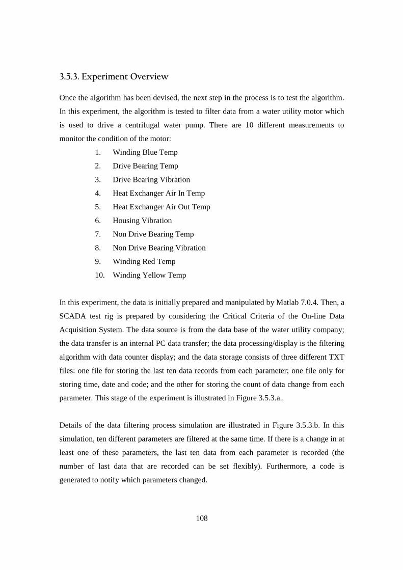
108

3.5.3. Experiment Overview Once the algorithm has been devised, the next step in the process is to test the algorithm.

In this experiment, the algorithm is tested to filter data from a water utility motor which

is used to drive a centrifugal water pump. There are 10 different measurements to

monitor the condition of the motor:

1. Winding Blue Temp

2. Drive Bearing Temp

3. Drive Bearing Vibration

4. Heat Exchanger Air In Temp

5. Heat Exchanger Air Out Temp

6. Housing Vibration

7. Non Drive Bearing Temp

8. Non Drive Bearing Vibration

9. Winding Red Temp

10. Winding Yellow Temp

In this experiment, the data is initially prepared and manipulated by Matlab 7.0.4. Then, a

SCADA test rig is prepared by considering the Critical Criteria of the On-line Data

Acquisition System. The data source is from the data base of the water utility company;

the data transfer is an internal PC data transfer; the data processing/display is the filtering

algorithm with data counter display; and the data storage consists of three different TXT

files: one file for storing the last ten data records from each parameter; one file only for

storing time, date and code; and the other for storing the count of data change from each

parameter. This stage of the experiment is illustrated in Figure 3.5.3.a..

Details of the data filtering process simulation are illustrated in Figure 3.5.3.b. In this

simulation, ten different parameters are filtered at the same time. If there is a change in at

least one of these parameters, the last ten data from each parameter is recorded (the

number of last data that are recorded can be set flexibly). Furthermore, a code is

generated to notify which parameters changed.

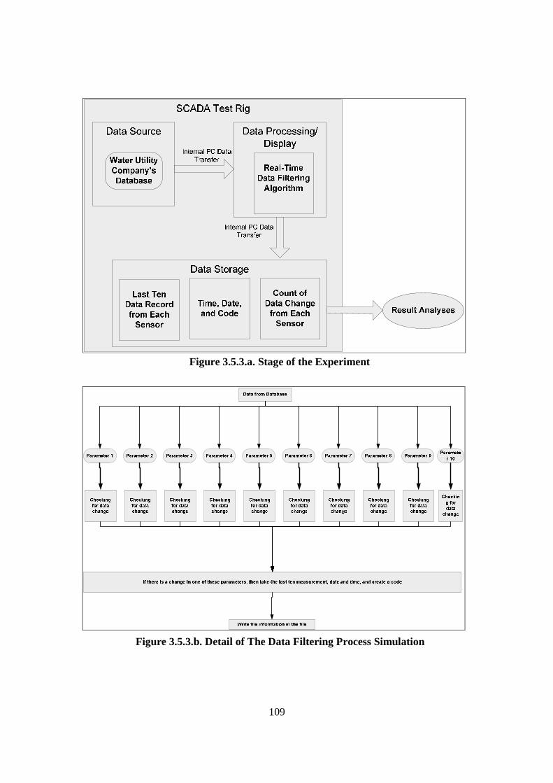
109

28Figure 3.5.3.a. Stage of the Experiment

29Figure 3.5.3.b. Detail of The Data Filtering Process Simulation

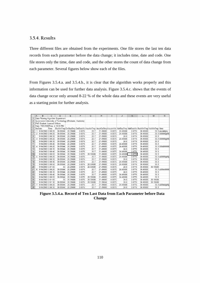
110

3.5.4. Results Three different files are obtained from the experiments. One file stores the last ten data

records from each parameter before the data change; it includes time, date and code. One

file stores only the time, date and code, and the other stores the count of data change from

each parameter. Several figures below show each of the files.

From Figures 3.5.4.a. and 3.5.4.b., it is clear that the algorithm works properly and this

information can be used for further data analysis. Figure 3.5.4.c. shows that the events of

data change occur only around 8-22 % of the whole data and these events are very useful

as a starting point for further analysis.

30Figure 3.5.4.a. Record of Ten Last Data from Each Parameter before Data Change

111

31Figure 3.5.4.b. Record of Code, Index, Date and Time of when Data Change Occur

Data Change Count From Different Parameter on Motor 0

0

200000

400000

600000

800000

1000000

1200000

BluWinT

mp

DrvBea

Tmp

DrvBea

Vib

HexAIn

Tmp

HexAOuT

mp

Housin

Vib

NdrBeaT

mp

NdrBea

Vib

RedW

inTm

p

YelWinT

mp

Name of Parameter

Nu

mb

er

Data Change Count

32Figure 3.5.4.c. Data Change Count from Different Parameters

112

In conclusion, the proposed algorithm is able to notify when the event of data change

occurs and is able to capture essential information by recording a number of last data bits

before this event occurs. By utilizing this algorithm, data analysis will become easier,

since the information has been filtered; only the essential information as a starting point

of analysis remains. Therefore, this algorithm is suitable to be applied in SCADA

systems.

3.5.5. Discussion A Data Filtering Algorithm has been successfully developed and tested. This study is

motivated by the finding from the data compression algorithm study where 80% of

SCADA data is stable; that is, the sensor shows the same value. The purpose of this

algorithm is to filter data from SCADA Systems to capture significant data. Further

analysis is performed by using this significant data as a starting point. The Data Filtering

Algorithm checks any data change. The reason is that when conducting measurements, if

the measured parameters change, the conditions or states of the measured objects will

most probably change. Therefore, only events whose parameters change, are essential to

be captured. In the implementation of the Hierarchical Model (Data Bridge), the filtering

algorithm is utilised to filter only significant data from the SCADA data dump. It is

developed based on the information from Control Philosophy.

This algorithm is tested through the SCADA test rig and data from the water utility

company is used as a data source in the final stage. Results from the experiment show

that the significant data from the SCADA Systems is only around 8% - 20% of the whole

data. In addition, this algorithm works in a real-time timeframe.

The significant contribution of this study is the fact that SCADA data analysis is more

effective and efficient if the raw data is filtered to capture significant data. In this study, it

is assumed that data becomes significant when the value changes. The reason behind this

113

assumption is a lack of information on the rate of data change. However, despite this

assumption, the experiment results are astonishing, where only about 20% of data

changed. This 20% represents significant data. In fact, this algorithm will be better if the

limit of normal and abnormal data is known. Therefore, only data which are out of

threshold are captured. In the implementation stage (Data Bridge), the information on the

limit of normal and abnormal data can be obtained from a Control Philosophy while

conducting Hierarchical Analysis, Failure Mode and Effect Analysis, and

Interdependence Analysis. Furthermore, this data filtering algorithm is one of the data

bridge components for filtering and capturing abnormal data.

3.6. Theory Development: Hierarchical Model (Brief Introduction)

The Hierarchical Model consists of three analyses: Hierarchical Analysis, Failure Mode

and Effect Analysis, and Interdependence Analysis. These three analyses have to be done

in sequence, where results from the previous analysis will be used in the next analysis.

Details about these three analyses are given in Section 3.7., 3.8., and 3.9.

3.7. Theory Development: Hierarchical Model (Hierarchical Analysis)

3.7.1. Introduction

The first analysis in the Hierarchical Model is Hierarchical Analysis. The purpose of this

analysis is to break the system hierarchically down. The System Breakdown that is

proposed by Stapelberg in his book RAM Machine Analysis (Stapelberg, 1993) is

114

adopted as a tool in this analysis. Originally, the SBS is proposed to analyse assets

without the presence of the SCADA System. In this research, the SBS is used to analyse

assets, together with the SCADA System which monitors the assets.

3.7.2. System Breakdown Structure (SBS)

The purpose of the SBS is to describe the whole system in a hierarchical manner by

applying a system breakdown. It is then easier to conduct a Root Cause Analysis if fault

occurs. The benefits that are obtained from a correctly structured SBS of the critical

equipment include the following (Stapelberg, 1993):

1. It enables the collection, grouping and selection of failure history of an individual

component, assembly or system.

2. It allows for similar grouping of maintenance costs at component, assembly or

subsystem levels.

3. It enables the effects of component failures to be related back to their specific

assemblies and systems.

4. It allows for the determination of availability and reliability up to assembly and

system levels.

In general, the SBS breaks down the assets into Plant, Area, Unit, System, Sub-

System/Assembly, and Sub-assembly/Component (Figure 3.7.2.) (Stapelberg, 1993):

115

33Figure 3.7.2. System Breakdown Structure Procedure

• System

A System is a collection of subsystems and assemblies for which the value of

availability can be determined and optimised.

• Sub-System/Assembly

A Sub-System/Assembly is a collection of components for which the operational

condition can be monitored.

• Sub-Assembly/Component

Sub-Assembly/Component is a collection of parts which constitute a functional

unit for which the physical condition can be measured and reliability and

maintainability data can be collected.

In order to develop the SBS of the assets, including the monitoring systems, there are

three steps that have to be undertaken (refer to Section 2.3.2.):

1. Process Analysis

2. System Description

3. System Breakdown.

116

3.7.3. Discussion

A System Breakdown Structure (Stapelberg, 1993) is adopted in the Hierarchical

Analysis. The purpose of the Hierarchical Analysis is to describe the whole system in a

hierarchical manner whereby it is easier to conduct Root Cause Analysis if a fault occurs.

There are three steps in performing a Hierarchical Analysis: Process Analysis, System

Description, and System Breakdown.

3.8. Theory Development: Hierarchical Model (Failure Mode and Effect Analysis)

3.8.1. Introduction

Failure Mode and Effect Analysis (FMEA) techniques have existed for over 30 years

(McDermott et al., 1996). According to McDermott et al. (1996), FMEA is a systematic

method of identifying and preventing product and process problems before they occur.

3.8.2. Explanation of FMEA

Stapelberg (1993) suggests that FMEA is carried out at the Components or Sub-

Assemblies level of the equipment SBS, as preventive maintenance can only be

effectively performed at this level. Based on the proposed Hierarchical Model (refer to

Section 2.3.3.), there are five aspects in FMEA that have to be conducted (Stapelberg,

1993): Failure Definition, Failure Cause, Failure Mode, Failure Effect and Failure

Consequence. However, each Component/sub-assembly function has to be clarified prior

to assessing these five aspects. In order to standardize functional explanation, the

function is determined based on:

• What this item does

• From where

• Through what

117

• To where

Information sources to answer the above questions are the Process and Instrumentation

Diagram (P&ID) and the Control Philosophy. Answers from each are combined to

compose a sentence, which explains the function of the component or sub-assembly.

The definition of function is “The work that an item is designed to perform” (Stapelberg,

1993). Therefore, a failure of the item’s function means a failure of the work that the item

is designed to perform; that is, a Functional Failure. In other words, the functional failure

can be defined as “the inability of an item to carry out the work that it has been designed

to perform within specified limits of performance”. In fact, functional failure can result in

a complete loss of function (Total Loss of Function) or a partial loss of the item’s

function (Partial Loss of Function). Explaining the function of each SBS item at the

component or subassembly level will help in determining failure.

For Failure Description, the nature of the failure is described clearly. For example: Seals

are leaking (Water Pump Failure), many particles build up in the multi-media filter

(Media Filtration Vessel), etc.

Failure Mode can be defined as: “the method or manner of failure”. Since failure mode is

the manner or method by which the failure occurs, the obvious question to ask in

determining failure mode is: “How (or in which manner) can the loss of the function

occur?” For the failure mode, there are two degrees of severity: Total Loss of Function

(TLF), which can be defined as “the item cannot carry out any of the work that it was

designed to perform”, and Partial Loss of Function (PLF), which can be defined as “the

item is unable to function within specified limits of performance”.

Failure Consequence is the severity of the effect that the failure of the components/sub-

assemblies under analysis has on the system. Determining failure consequences is,

therefore, a very important portion of the FMEA development process. In essence, the

consequence of failure can be determined by asking the question: “What happens to the

118

system as a whole when the component under consideration fails in a specific mode or

manner?”

The definition of cause is “that which produces an effect”. Therefore, failure causes can

be defined as “failures which produce an effect”. In fact, there are many potential failure

causes, such as contamination, electrolytic changes, fatigue, film deposition, friction,

mechanical stresses, wear and many more potential failure causes.

According to Moubray (1997), there are several sources of information about component

failure:

1. The manufacturer or vendor of component

2. Generic list of failure modes

3. Other users of the same component

4. Technical history records

5. The people who operate and maintain the equipment

The decision of utilising one or a combination of them mostly depends on their

availability.

3.8.3. Discussion

FMEA is a systematic method of identifying and preventing product and process

problems before they occur. Therefore, information about the root of any emerged

abnormalities in the asset can be revealed by applying this process to each

component/sub-assembly. There are five aspects that have to be undertaken to develop

FMEA of an asset: Failure Definition, Failure Cause, Failure Mode, Failure Effect and

Failure Consequence. From these five aspects, it is clear that the most important

knowledge that will be obtained by applying FMEA is the information about possible

failure of each component/sub-assembly. However, each Component/sub-assembly

function has to be clarified prior to assessing these five aspects.

119

3.9. Theory Development: Interdependence Analysis

3.9.1. Introduction

Based on the literature, interdependence is a result of integration of several factors that

work together to produce a result (Cho, 1995). In addition, when a system works and is

monitored with a condition monitoring system with the purpose to produce results,

interdependence exists. Also, according to Campbell (1997), Interdependence leads to

conflict. Hence, conducting an analysis of the interdependence relationship within the

system is a good approach in determining any problem that exists or will exist (risk

estimating). In terms of presenting the analysis results, Stiern (1999) reveals that analysis

results that are presented in the graphical diagrams are easier to understand. Furthermore,

based on Nitakorn’s (http://www.umsl.edu) comparison of different diagramming tools,

the Entity Relationship Diagram (ERD) concept is justified as a suitable diagramming

concept.

Interdependence Analysis in this research is facilitated through a Functional and Causal

Relationship Diagram (FCRD). Besides facilitating the Interdependence Analysis, FCRD

also adopts the ERD concept to present the analysis results. Based on its name, the

Functional and Causal Relationship Diagram utilises a diagramming method to explain

the functional and causal relationship between the Components/Sub-Assembly in the

assets.

Based on the Hierarchical Model (refer to Section 2.3.3.), Interdependence Analysis can

only be carried out after the Hierarchical Analysis and FMEA have been done, since their

results are part of an Interdependency Analysis input. In addition, the Interdependence

Analysis is applied at the components/sub-assemblies level.

120

As mentioned in Section 2.3.3., there are two stages of analysis in the Interdependence

Analysis. FCRD Stage 1 analyses the Dynamic Relationship at the system’s component

level which is then depicted in a diagrammatic format for easier analysis. Risk and

criticality can be calculated based on the interdependence of components. FCRD Stage 2

transforms information into a more manageable format to be input into the Data Base.

Detail on FCRD and Interdependence Risk Analysis is given in the next section.

3.9.2. Functional and Causal Relationship Diagram (FCRD)

The benefits from a correctly structured FCRD are:

• Information is easier to be understood by presenting it in diagram format.

• It assists in failure tracing based on abnormality which is captured by sensors and

alarms.

• It assists the Interdependence Risk Analysis

FCRD Stage 1 The results of FCRD Stage 1 (that is, the identified interdependence relationships) will be

used as inputs for FCRD Stage 2 and Interdependence Risk Analysis. In FCRD Stage 1,

the interdependence relationships at the components/sub-assemblies level are identified

by assessing the functional and causal relationships between them.

Based on the direction of influence, the identified interdependence relationships can be

grouped into three types:

1. One way relationship

In a one way relationship, one component/sub assembly is more influenced by the

other. Furthermore, to provide more understanding and an easier way in entering

information into the table, this relationship is categorised into two types:

121

a. 1st to 2nd

The second component/sub assembly is influenced more by the first

component/sub assembly.

b. 2nd to 1st

The first component/sub assembly is influenced more by the second

component/sub assembly.

2. Two ways relationship

In two ways relationship, both components/sub assemblies influence each other.

3. Don’t care relationship

In this relationship, both components/sub assemblies are closely or physically

connected; however, if one of them fails, then there is no significant effect/impact

on the other.

The FCRD development process is divided into four steps:

1. Step 1: Major Components/Sub-Assemblies Analysis

In Step 1, major Components/Sub-Assemblies are identified. Major

Components/Sub-Assemblies are vital items in the whole process, where a failure

of one of them may cause stoppage of the whole process. This threat can be

prevented by identifying major Components/Sub-Assemblies. Furthermore,

because the Components/Sub-Assemblies are vital, the relationship between them

is a two ways relationship.

2. Step 2: Major Components/Sub-Assemblies Interaction Diagram Development

The purpose of a Major Components/Sub-Assemblies Interaction Diagram is to

provide a clear understanding of the Major Components/Sub-Assemblies and their

interaction. The Diagram is developed by utilising information from the previous

step.

3. Step 3: Components/Sub-Assemblies Relationship Analysis

In this step, the relationships between each of the Components/Sub-Assemblies of

the whole system are analysed and identified. In order to make the process easier,

the analysis begins from the Major Components/Sub-Assemblies Interaction

122

Diagram which depicts the Major Components/Sub-Assemblies and their

relationships. The relationships between each are then justified.

4. Step 4: Generate the FCRD

The next step is generating the FCRD by utilising information from previous

steps. The use of drawing/diagramming software, such as Microsoft Visio©,

Graphviz© and Inkscape© will help the process of generating FCRD, because

FCRD would become a complex diagram.

FCRD Stage 2

FCRD Stage 1 results in the identification of dynamic interdependence relationships

between components/sub-assemblies. These results are depicted in a single diagram

format and utilised as an input for FCRD Stage 2. FCRD Stage 2 transforms information

into a more comprehensive and manageable format so that it can be entered into a Data

Base. An Inference Engine is developed to query information from the Data Base. Pairing

Data Base with Inference Engine is known as a Knowledge Base.

Based on the analysis, the nature of the relationships in FCRD Stage 1 can be categorised

into two different types:

• Direct Relationship (Physical Relationship)

Direct relationship is a relationship between components/sub-assemblies that are

physically related. It can be identified easily from the Process and Instrumentation

Diagram (P&ID). Based on process sequence, this relationship type can be

grouped into two different diagrams:

o Process sequence-related relationship

The components/sub-assemblies are also related in process sequence.

o Non-process sequence-related relationship

Although the components/sub-assemblies are physically related, they are

not related in process sequence.

123

• Indirect Relationship

Indirect relationship is a relationship where the components/sub-assemblies are

related indirectly. Two types of indirect relationships are:

o Logic Control relationship

In logic control relationship, the components/sub-assemblies are indirectly

related based on the logic control of the system. It can be identified easily

from the control philosophy.

o Sensing mechanism relationship

In the sensing mechanism relationship, the components/sub-assemblies are

indirectly related based on the connection between the functions of

components/sub-assemblies and the sensing mechanism of sensors. It can

be identified easily by analysing and comparing the components/sub-

assemblies functions to the sensing mechanism of the sensors.

In order to refine the results from FCRD Stage 1 into a more comprehensive and

manageable format, these two different types are depicted in two different diagrams:

• Flow Diagram

Flow Diagram depicts the process as a sequence-related relationship. Actually, this

diagram has been established in one of the SBS development steps (that is, process

analysis) and is called a process block diagram. However, this diagram only depicts

the system process flow at the system and assembly hierarchical level. Therefore, the

flow diagram can be developed by lowering the hierarchical level from system and

assembly to the components or sub-assemblies. In addition, instead of presenting all

processes together in one diagram, it is better to separate them into individual flow

diagrams. The purpose of a flow diagram is to describe the process flows in

components/sub-assemblies hierarchical level. It enables easier and more accurate

failure tracing.

• Logic and Sensor Analysis Diagram:

This diagram depicts a system indirect relationship (logic control and sensing

mechanism relationship). The logic and sensor analysis diagram depicts relationship

124

information between sensor/alarm and components/sub-assemblies. This is because

the process in SCADA Systems can only be monitored through sensors and events.

Some elements in this diagram are:

o Sensor

Sensor is used to sense and monitor the system process

o Component/Sub-Assembly

In the System Breakdown Structure, a system is hierarchically structured into

System, Sub-System, Assembly, Sub-Assembly and Component. Component/sub-

assembly is the lowest level of the process.

o Event

Event can be defined as:

� Symptom that can be detected by a sensor, for example:

� The pattern of the occurrence of sensor value that exceeds a certain

threshold

� Alarm signal from SCADA

Event has to be defined clearly to enable the filtering algorithm to detect it.

o Flow Diagram

Flow Diagram is a diagram that shows the process flow of the system

o External Entity

It is an element of the diagram that cannot be categorized as a component, sensor,

event or flow diagram.

o Relationship

It is an element that connects one element to another element in the diagram.

The following is a comprehensive framework for defining relationships between

event/sensor and other elements:

1. All components and sub-assemblies which do not have any component are

investigated and classified as either component elements or sensor elements.

2. Identify the correlation between the sensor and component based on their

functional explanation. For example; the function of a water flow meter is to

measure the flow of water in the process, and the function of pump is to pump

125

water to the whole system. It can be concluded that there is a correlation between

them.

3. The relationship can also be identified by utilising a control philosophy.

Candidates of relationship can be identified from such control philosophy. Further

analysis has to be carried out to determine whether the relationship can contribute

to the failure analysis. There are three different relationships between the

component and sensor in a control philosophy:

a. The sensor senses a condition of one particular component and the

outcome is used to control the stage of another component; for example,

whether the component should be turned off or on. However, this

condition is influenced by the second component, instead of the first

component; for example, if a Pressure Indicator Transmitter senses the

water level in a filtered water tank, then the water pump is started. In this

condition, the Pressure Indicator Transmitter cannot sense any failure at

the pump; it is only used to sense the water level in the filtered water tank.

b. The sensor senses a condition and then the outcome is used to control the

stage of a component. This condition is influenced by the component; for

example, The pH analyser senses the pH level of water and if the pH level

exceeds a certain level, then the dosing pump is turned off to restore the

pH Level.

c. The sensor senses a condition that is caused by a component, but the result

is not used to control the operating stage of that component; for example,

The Water Flow Meter senses the flow of water in the process; the water

flow is caused by the pumping effect that is performed by the Pump.

Among those relationship types, only the second (b) and third (c) type can be

determined as a relationship that can contribute to failure analysis.

4. Determining the relationship of an event with other elements, except the sensor.

For example: the event of pump failure can be correlated easily to the pump, the

event of mixer failure is also can be correlated easily to the mixer, etc.

5. External entity can be determined based on external factors that influence the

process, for example: In a water treatment plant, raw water quality is classified as

126

an external entity, because it is not one of the components in the system and

cannot be controlled.

6. The logic and sensor analysis diagram is linked to the flow diagram to provide

more comprehensive information for examining the root cause of any system

abnormalities.

3.9.3. Interdependence Risk Analysis (IRA)

Interdependence Risk Analysis (IRA) is inspired by the following statements:

“Interdependence is a result of integration of several factors that work together to

produce a result.”(Cho, 1995)

“In economic, interdependence leads to conflict.” (Campbell, 1997)

“Interdependence is measurable.” (Drew et al., 2002)

Based on the above statements, it can be concluded that:

• As long as elements work together to produce a result, there is a interdependent

relation between them. In other words, there is no work without interdependence

relationship.

• Interdependence relationship is identified as a source of

conflicts/problems/failures in all work to produce a result.

• Although the interdependence relationship is justified qualitatively, it is

measurable. In other words, interdependence relationship can be quantified.

• Therefore, the potential of conflicts/problems/failures can be measured.

Measurement of the potential/possibility of conflicts/problems/failures is a basic

theory of Risk Analysis (Stapelberg, 2006).

127

Apart from the above statements about interdependence, IRA is also inspired by the

success of FCRD development.

Results from IRA are utilised as input for Failure Mode Effect and Criticality Analysis

(FMECA). FMECA is a further analysis based on the components’ criticality which has

been determined by IRA to establish further maintenance requirements (Stapelberg,

1993).

Theory

Besides the results from FCRD Stage 1, results from the Hierarchical Analysis and

FMEA, including the system’s original design information, are utilised as information

sources for IRA.

As mentioned in Section 2.4.2., the conventional approach for estimating probabilities of

failure and the likelihood of the occurrence of the consequences as a result of failure, to

determine risk, is inadequate. The conventional approach is based on the relationship:

Risk = Consequence x Likelihood Equation. 2

The estimated probabilities of consequence can range descriptively from extreme, very

high, high, to insignificant. The estimated probabilities of likelihood can range from

highly likely to unlikely. Each descriptive probability is designated a quantitative value

ranging from 0 to 1.

In a systems hierarchy context, where multiple systems are integrated, often in a complex

structure, factors, such as system-component and component-system causal relationship;

system failure mode severity and component failure mode effect; system likelihood of

failure; criticality of systems level; criticality at component level; as well as the impact of

failure in complex integrated systems structures, need to be taken into consideration.

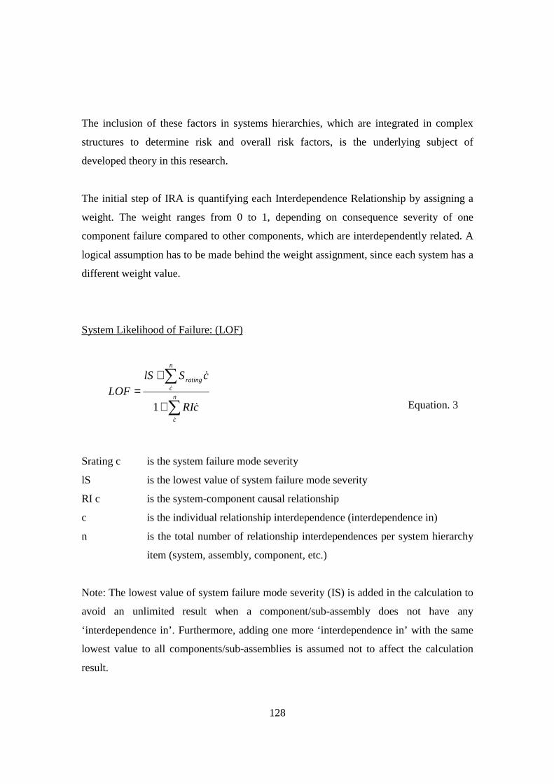
128

The inclusion of these factors in systems hierarchies, which are integrated in complex

structures to determine risk and overall risk factors, is the underlying subject of

developed theory in this research.

The initial step of IRA is quantifying each Interdependence Relationship by assigning a

weight. The weight ranges from 0 to 1, depending on consequence severity of one

component failure compared to other components, which are interdependently related. A

logical assumption has to be made behind the weight assignment, since each system has a

different weight value.

System Likelihood of Failure: (LOF)

Equation. 3

Srating c is the system failure mode severity

lS is the lowest value of system failure mode severity

RI c is the system-component causal relationship

c is the individual relationship interdependence (interdependence in)

n is the total number of relationship interdependences per system hierarchy

item (system, assembly, component, etc.)

Note: The lowest value of system failure mode severity (IS) is added in the calculation to

avoid an unlimited result when a component/sub-assembly does not have any

‘interdependence in’. Furthermore, adding one more ‘interdependence in’ with the same

lowest value to all components/sub-assemblies is assumed not to affect the calculation

result.

∑

∑

+

+=

n

c

n

crating

cRI

cSlSLOF

&

&

&

&

1

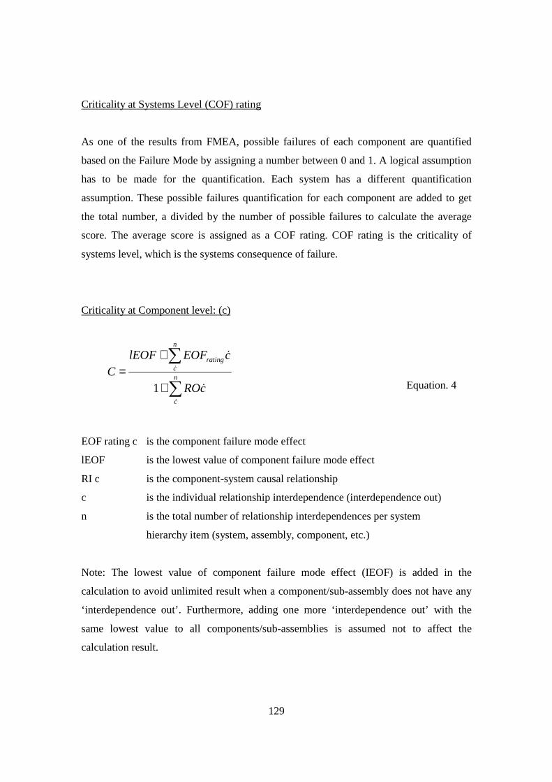
129

Criticality at Systems Level (COF) rating

As one of the results from FMEA, possible failures of each component are quantified

based on the Failure Mode by assigning a number between 0 and 1. A logical assumption

has to be made for the quantification. Each system has a different quantification

assumption. These possible failures quantification for each component are added to get

the total number, a divided by the number of possible failures to calculate the average

score. The average score is assigned as a COF rating. COF rating is the criticality of

systems level, which is the systems consequence of failure.

Criticality at Component level: (c)

Equation. 4

EOF rating c is the component failure mode effect

lEOF is the lowest value of component failure mode effect

RI c is the component-system causal relationship

c is the individual relationship interdependence (interdependence out)

n is the total number of relationship interdependences per system

hierarchy item (system, assembly, component, etc.)

Note: The lowest value of component failure mode effect (IEOF) is added in the

calculation to avoid unlimited result when a component/sub-assembly does not have any

‘interdependence out’. Furthermore, adding one more ‘interdependence out’ with the

same lowest value to all components/sub-assemblies is assumed not to affect the

calculation result.

∑

∑

+

+=

n

c

n

crating

cRO

cEOFlEOFC

&

&

&

&

1

130

Impact of Failure in Complex Integrated Systems (I)

Equation. 5

The impact is a measure of the criticality at systems level (COFrating) together with the

criticality at component level (C). Thus, it is a measure of the systems consequence of

failure with consideration of the effect of failure at component level, and the component-

system causal relationship interdependence.

Risk of Systems Integration in a Complex Structure: (R)

ratingCOFLOFR ×= Equation. 6

Risk, due to complex systems integration, is a measure of the system likelihood of failure

(LOF) together with the criticality at systems level, or systems consequence of failure

(COFrating)

Risk Factor of Systems Hierarchies that are Integrated in a Complex Structure

Equation. 7

The risk factor is a measure of the criticality at system level (COFrating) together with the

criticality at the component level (C) i.e. the overall impact of failure in complex

integrated systems, and the system likelihood of failure (LOF). The risk factor takes into

consideration the severity and effect of failure at the systems and component level,

together with the systems causal relationship interdependences, as well as the systems

hierarchies and integration in complex structures.

CCOFI rating ×=

)()( ILOFILOFRF ×−+=

131

3.9.4. Discussion

Interdependence Analysis is carried out by identifying the interdependence relationship

between components/sub-assemblies. Conducting an interdependence relationship

analysis within the system is a good approach to determine any problem that exists or

will exist (risk estimating). Interdependence Analysis in this research is facilitated

through the Functional and Causal Relationship Diagram (FCRD). There are two stages

of analysis in the Interdependence Analysis. FCRD Stage 1 analyses the Dynamic

Relationship on the system’s component level which is then depicted in diagram format

for easier analysis. Risk and criticality can be calculated based on components

interdependences. FCRD stage 2 transforms information into a more manageable format

to be input into the Data Base and Knowledge Base.

Besides FCRD, IRA is a part of Interdependence Analysis. IRA uses information from

Hierarchical Analysis, Failure Mode and Effect Analysis, and FCRD Stage 1 as input.

IRA is motivated by the idea that interdependence exists in all work; interdependence

leads to conflict; and interdependence is measurable. In the classic Risk Analysis method,

asset risk is measured in terms of a combination of consequence of an event and their

likelihood. IRA still follows this classic approach. however, IRA offers a different

method to determine the Risk Consequence and Risk Likelihood. In the conventional

Risk Analysis, the consequence of risk can be determined by assessing severity of the

impact, and the likelihood of risk is determined from how frequently the risks occur. In

IRA, the Risk Consequence and Risk Likelihood are determined based on quantification

of the Interdependence Relationship. This method of determining Risk Consequence and

Risk Likelihood makes IRA remarkable and able to overcome the problem that is

encountered by most Risk Analysis methods (i.e. determining Risk Likelihood).

132

3.10. Implementation: Data Bridge

3.10.1. Introduction

According to the Literature Review (Section 2.2.4.), the Data Bridge concept is adopted

as an implementation step to bridge the SCADA System and ERP system. In addition, the

Data Bridge is composed of two parts: Filtering Algorithm and Knowledge Base.

3.10.2. Implementation step

In the implementation step, the Filtering Algorithm utilises information from the

Hierarchical Analysis, FMEA and Interdependence Analysis as input.

The Knowledge Base consists of two parts:

• Data Base

Data Base is the location where all information from the Hierarchical Analysis,

FMEA and Interdependence Analysis is stored.

• Inference Engine

The purpose of the Inference Engine is to query information from the Data Base if

any abnormality is detected and filtered by the Filtering Algorithm.

As depicted in Figure 3.10.2.a., the process in the Data Bridge can be described as:

• Receiving data from the SCADA System

• Modifying the data set through the Data filtering Algorithm

• Comparative Evaluation against Knowledge Base

• Making assessment from comparison

• Converting data to information and transferring to the ERP System

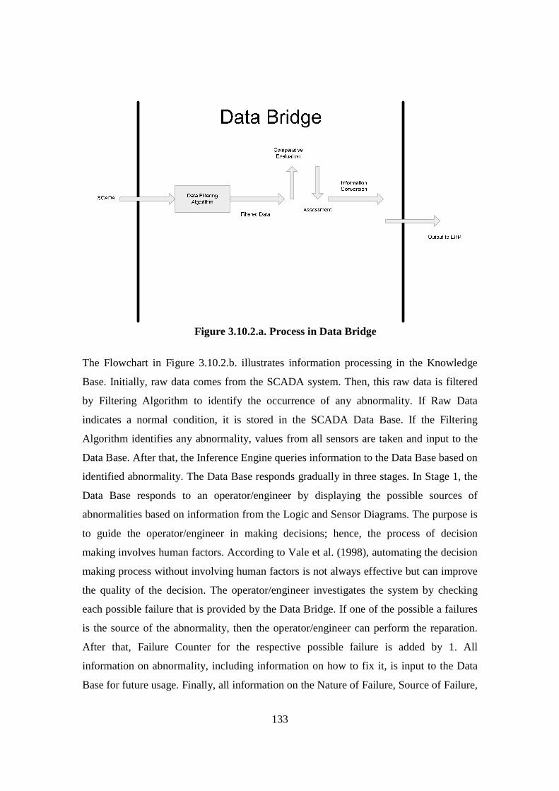
133

34Figure 3.10.2.a. Process in Data Bridge

The Flowchart in Figure 3.10.2.b. illustrates information processing in the Knowledge

Base. Initially, raw data comes from the SCADA system. Then, this raw data is filtered

by Filtering Algorithm to identify the occurrence of any abnormality. If Raw Data

indicates a normal condition, it is stored in the SCADA Data Base. If the Filtering

Algorithm identifies any abnormality, values from all sensors are taken and input to the

Data Base. After that, the Inference Engine queries information to the Data Base based on

identified abnormality. The Data Base responds gradually in three stages. In Stage 1, the

Data Base responds to an operator/engineer by displaying the possible sources of

abnormalities based on information from the Logic and Sensor Diagrams. The purpose is

to guide the operator/engineer in making decisions; hence, the process of decision

making involves human factors. According to Vale et al. (1998), automating the decision

making process without involving human factors is not always effective but can improve

the quality of the decision. The operator/engineer investigates the system by checking

each possible failure that is provided by the Data Bridge. If one of the possible a failures

is the source of the abnormality, then the operator/engineer can perform the reparation.

After that, Failure Counter for the respective possible failure is added by 1. All

information on abnormality, including information on how to fix it, is input to the Data

Base for future usage. Finally, all information on the Nature of Failure, Source of Failure,

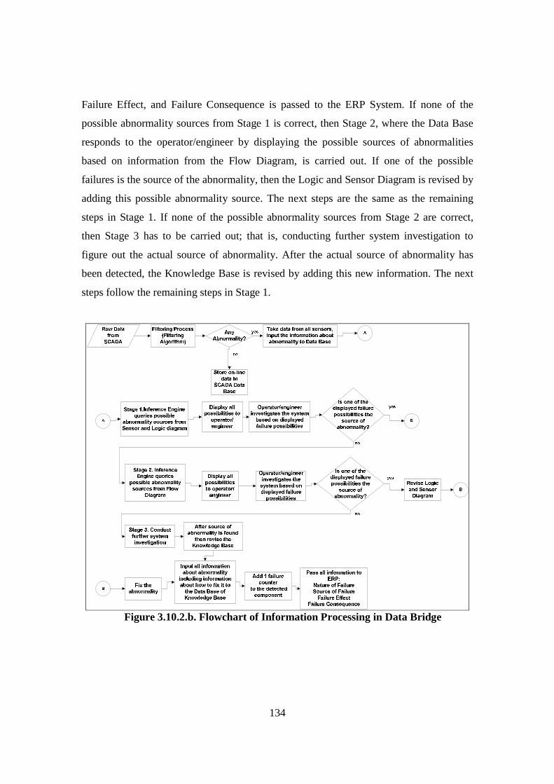
134

Failure Effect, and Failure Consequence is passed to the ERP System. If none of the

possible abnormality sources from Stage 1 is correct, then Stage 2, where the Data Base

responds to the operator/engineer by displaying the possible sources of abnormalities

based on information from the Flow Diagram, is carried out. If one of the possible

failures is the source of the abnormality, then the Logic and Sensor Diagram is revised by

adding this possible abnormality source. The next steps are the same as the remaining

steps in Stage 1. If none of the possible abnormality sources from Stage 2 are correct,

then Stage 3 has to be carried out; that is, conducting further system investigation to

figure out the actual source of abnormality. After the actual source of abnormality has

been detected, the Knowledge Base is revised by adding this new information. The next

steps follow the remaining steps in Stage 1.

35Figure 3.10.2.b. Flowchart of Information Processing in Data Bridge

135

3.10.3. Discussion

A Data Bridge is one of the elements in the implementation of the Hierarchical Model,

besides Risk Analysis. The Data Bridge consists of two parts: the Filtering Algorithm and

Knowledge Base. Filtering Algorithm has been described. The Knowledge Base consists

of a Data Base and Inference Engine. All of the Data Bridge components are developed

based on information from Hierarchical Analysis, FMEA and Interdependence Analysis.

The purpose of the Data Bridge is to process and transform “raw data” from SCADA

Systems into more meaningful information, and then transfer this information to the ERP.

According to design of information in the Data Bridge, the Data Base is designed to

respond gradually in three stages. The purpose of designing three stages of response is to

guide the operator/engineer in making decision in order to improve the quality of the

decision. Furthermore, this design of information in the Data Bridge also facilitates

Continuous Risk Analysis and the learning ability of the Knowledge Base. Continuous

Risk Analysis implies that the risk of each component/sub-assembly is analysed

continuously as the system is working. Learning ability of the Knowledge Base is the

ability to adapt easily to new information.

3.11 Summary Chapter 3 elucidates the final proposed model, the Hierarchical Model. It begins by

describing the experimental method: Real-Time Water Quality Condition Monitoring

System and SCADA test rig; and then continues by describing the Development Theory:

Algorithm Formulation and Hierarchical Model. Finally, the Data Bridge as

implementation phase is described.

The Real-Time Water Quality Condition Monitoring System is developed to achieve the

first objective of this research, and as an experimentation basis for the proposed model.

At first, this model is developed to mimic the data acquisition part of the real SCADA

system. Then, it is tested by monitoring water quality. The test resulted in identification

136

of critical criteria of on-line data acquisition. These criteria can be utilised to design the

SCADA test rig for testing the research findings. The study was initialised by designing

real-time water quality monitoring system architecture, followed by prototype

development and testing of an On-line Data Acquisition System. The system is developed

based on Web technology (DataSocket, ActiveX) and software (LabVIEW, and VB). The

structure of the model consists of three components: local measurement stations, a central

control station and remote browse stations. These components are connected to each

other by internet connection. Therefore, the system is able to overcome the distance

barrier. In addition, with the developed prototype system, the water quality condition

from the local measurement stations can be displayed to clients. The history records of

water quality parameters from the different locations can be accessed by the client

anywhere in the world as long as the internet connection is available. In addition, the

Critical Criteria of On-line Data Acquisition System have been identified. The significant

contribution to this thesis is the identification of the Critical Criteria. These criteria can

be used to standardize the development of the SCADA test rig.

The SCADA test rig is designed and utilised to conduct experiments based on data and

information from a Case Study. There are four Critical Criteria of On-line Data

Acquisition Systems: Data Source, Data Transfer Process, Data Processing and Display,

and Data Storage. These criteria are then adopted as a basis for of the SCADA test rig

framework. This framework is used to develop various SCADA tests with different

purposes to validate the research findings. By adopting the Critical Criteria, it means that

there are four variables that can be varied, depending on the purpose of the experiment:

testing different data sources, the effectiveness the data processing/display, the

performance of data transfer, or different methods of data storage.

It was found that much data from a SCADA System is redundant in terms of relevance.

Therefore, a compression algorithm for a SCADA System is developed. A Data

Compression Algorithm development framework is initiated by reading and manipulating

data, so that data are in a readable format. After that, simple statistical analysis can be

conducted. The pattern of data can be identified based on the statistical analysis, and this

137

pattern is used to generate the real-time data compression algorithm. According to

experiment results, the algorithm had successfully reduced up to 81 % of SCADA

Systems data. Theoretically, this algorithm is able to reduce data up to 91.57%. However,

because some data cannot be compressed properly, this maximum theoretical

compression rate cannot be achieved. In addition, the benefit of this algorithm is that the

compression works in a real-time timeframe. This algorithm is a generic algorithm, since

it can be applied to data from any SCADA System. Another significant contribution from

this study is the identification of the nature of SCADA data. It is identified that the nature

of SCADA data is stable, where 80 % of data is static (that is the sensor shows the same

value). This finding is then used as a basic consideration in developing a Data Filtering

Algorithm.

A novel real-time data filtering algorithm for a SCADA System is proposed in this study

where a suitable algorithm to filter data from the SCADA System is developed.

Philosophy that is applied in this algorithm is only to capture the occurrence of data

change in SCADA data. This is followed by storing several data before this data change

occurs. As a result, SCADA data analysis will become easier, because only essential

information remains. This algorithm is tested through the SCADA test rig and data from

a water utility company is used as data source in the final stage. Results from experiments

show that the significant data from the SCADA System is only around 8% - 20% of the

whole data. In addition, this algorithm works in a real-time timeframe. In the

implementation step (Data Bridge), the information on the limit of normal and abnormal

data can be obtained from a Control Philosophy while conducting Hierarchical Analysis,

Failure Mode and Effect Analysis, and Interdependence Analysis. Furthermore, this data

filtering algorithm is one of the data bridge components for filtering and capturing

abnormal data.

The Hierarchical Model consists of three analyses: Hierarchical Analysis, Failure Mode

and Effect Analysis, and Interdependence Analysis. These analyses have to be conducted

in series.

138

A System Breakdown Structure (Stapelberg, 1993) is adopted in the Hierarchical

Analysis. The purpose of the Hierarchical Analysis is to describe the whole system in

hierarchical manner by applying a system breakdown. Therefore, it is easier to conduct

Root Cause Analysis if any fault occurs. There are three steps in performing a

Hierarchical Analysis: Process Analysis, System Description, and System Breakdown.

The Failure Mode and Effect Analysis is carried out after the system has been structured

properly. The purpose of this analysis is to systematically identify and prevent product

and process problems before they occur. There are five aspects in FMEA that have to be

undertaken (Stapelberg, 1993): Failure Definition, Failure Cause, Failure Mode, Failure

Effect, and Failure Consequence. However, each component/sub-assembly function has

to be clarified prior to assessing the five aspects.

Interdependence Analysis is carried out by identifying an interdependence relationship

between components/sub-assemblies. Conducting interdependence relationship analysis

within the system is a good approach to figure out any problem that exists or will exist

(risk estimating). Interdependence Analysis in this research is facilitated through

Functional and Causal Relationship Diagram (FCRD). There are two stages of analysis in

the Interdependence Analysis. FCRD Stage 1 analyses the Dynamic Relationship at the

system’s component level and is then depicted in diagram format for easier analysis. Risk

and criticality can be calculated based on components interdependences. FCRD Stage 2

transforms information into a more manageable format to be input into the Data Base.

Besides FCRD, IRA is a part of Interdependence Analysis. IRA uses information from

Hierarchical Analysis, Failure Mode and Effect Analysis and FCRD Stage 1 as the input.

IRA is motivated by the idea that interdependence exists in all work; interdependence

leads to conflict; and interdependence is measurable. In the classic Risk Analysis method,

asset risk is measured in terms of a combination of consequence of an event and their

likelihood. IRA still follows this classic approach; however, IRA offers a different

method to determine the Risk Consequence and Risk Likelihood. In conventional Risk

Analysis, the consequence of risk can be determined by assessing severity of the impact,

139

and the likelihood of risk is determined from how frequently the risks occur. In IRA, the

Risk Consequence and Risk Likelihood are determined based on the quantification of the

Interdependence Relationship. This method of determining Risk Consequence and Risk

Likelihood makes IRA remarkable and able to overcome the problem that is encountered

by most Risk Analysis methods (that is, determining Risk Likelihood).

From the three analyses in the Hierarchical Model, information on the monitored and

monitoring systems is collected. This information is input to the Data Bridge at the

implementation step. The Data Bridge is used to process the raw SCADA data by

filtering any abnormality and provide information on possible abnormality sources. The

Data Bridge is one of the implementation stages of the Hierarchical Model, besides Risk

Analysis. The Data Bridge consists of two parts: Filtering Algorithm and Knowledge

Base. Knowledge Base consists of a Data Base and Inference Engine. All the Data Bridge

components are developed based on information from the Hierarchical Analysis, FMEA

and Interdependence Analysis. The purpose of the Data Bridge is to process and

transform “raw data” from the SCADA system into more meaningful information, and

then transfer this information to the ERP. According to design of information in the Data

Bridge, a Data Base is designed to respond gradually in three stages. The purpose of

designing three stages of response is to guide an operator/engineer in making a decision

in order to improve the quality of the decision. Furthermore, this design of information in

the Data Bridge also facilitates Continuous Risk Analysis, and learning ability of the

Knowledge Base. Continuous Risk Analysis implies that the risk of each component/sub-

assembly is analysed continuously as the system is working. Learning ability of the

Knowledge Base is the ability to adapt easily to new information.

140

3.12. Verification: Case Study

3.12.1. Brief Introduction of Chapters 4, 5, and 6 The validation in this research is conducted by implementing the Hierarchical Model

through the Water Treatment Plant Case Study. Chapter 4, Chapter 5 and Chapter 6

provide a comprehensive explanation about the process of implementing the Hierarchical

Model to the Case Study. The process is initiated from the development of Data Bridge,

Risk Ranking and Risk Ranking Matrix (Chapter 4), continued with Real-Time SCADA

Data Analysis (Chapter 5), and ended with Model Validation (Chapter 6).

Chapter 4 focuses on the implementation of Hierarchical Model to develop Data Bridge

and Risk Ranking. Data Bridge is developed by processing information from the case

study through the Hierarchical Model. Data Bridge is, as a result of this process, utilised

in the validation step. In this research, Risk Factor and Risk Ranking Matrix are utilised

to develop the Risk Ranking Matrix. Interdependence Risk Analysis is employed to

develop Risk Ranking through these two approaches.

Chapter 5 provides real-time SCADA data analysis. Some statistical analyses are used to

describe the characteristics and relationship within the data. Based on the analysis, the

consistency of the data can be clarified, since inconsistent data tends to produce an

unsatisfactory result in the Validation step. Results from the statistical analysis will be

utilised in the validation step.

The focus in Chapter 6 is validation of the research findings. There are two aspects in this

research validation: the first is to prove that Interdependence Risk Analysis can predict

Risk, and the second is to prove that the proposed Hierarchical Model can address the

SCADA Data Analysis Problem. These aspects are also expected to address the

connectivity problem between SCADA and ERP systems. Therefore, by the end of

Chapter 6, the validity of the hypotheses will be revealed.

141

In this Brief Introduction, a brief explanation of the case study together with analysis and

criteria of data filtering is provided. The explanation in the data justification involves

defining the required data for the Validation step. This clarifies the accessible data from

the case study. Some assumptions are made because access from companies is very

limited due to their internal confidentiality policy.

3.12.2. Water Utility Industry Case Study

The case study is a water treatment plant in the Moogerah Township. This water

treatment plant is operated and monitored by a SCADA System. According to the Control

Philosophy, the water treatment plant is designed to supply 100m3/day of safe drinking

water and complies with the requirements of the Australian Drinking Water Guidelines

(2004). The system works as follows:

• At first, water is pumped from a raw water tank by feed pumps through the pre-filter,

and delivered to the filtration system. A level switch is located in the raw water tank

to protect the feed pumps from running without water.

• Then, alum solution (coagulant) is injected to the raw water to create aggregates for

efficient filtration through the media filter. The solution is injected by dosing pump 1.

The added chemical is mixed in static mixer hydrocylone type.

• Following the hydrocylone, water enters multi-media vertical pressure filter for

turbidity removal. The filtrate flows to the activated carbon filter.

• The granular activated carbon filter is to remove colour, the residues of the algal

toxins, chlorine, dissolved organic matters, traces of certain heavy metals and fine

particles. The activated carbon improves the taste and odour of the treated water.

• The filter is particularly suitable for backwash (a process involving reversal of the

water flow and causing a turbulent expansion of the media like a fluidized bed, which

flushes out the entrapped debris effectively). Non-chlorinated filtered water is

collected in the backwash water storage tank. The backwash of each filter (multi

142

media and granular activated carbon) is performed by backwash pumps using water

from the backwash water storage tank. After the backwash cycle, a fast rinse in the

downward flow direction is done for a few minutes (direct wash) to ensure complete

washing of the filter. The direct wash is performed by the feed pump, using raw water

from the raw water tank. After the washing cycle is completed, the filter resumes its

normal filtering modes as clean as a new filter.

• The sodium hypochlorite solution is used as a disinfecting agent. The solution is

dosed by the dosing pump. Sodium hypochlorite dosing pump 2 is being controlled

by the flow meter with electrical output and residual chlorine transmitter, located in

the system outlet. Soda ash/acid solution is transferred to the line by dosing pump 3.

The pH is corrected to the required value and controlled according to the pH analyser.

The treated water is collected in the treated water storage tank.

3.12.3. Analysis and Criteria of Data Filtering

The Hierarchical Model in this research (refer to Section 2.3.3.) is designed based on

several criteria:

• Ability to be developed by utilising original design information as an initial input

• Ability to analyse SCADA data in a “real time” time frame

• Ability to solve Nested Data issue

• Ability to pass the results to ERP System

The Validation step (explained in Chapter 6) is to test the effectiveness of the method in

satisfying each criterion.

In addition, the case study from the water utility industry is utilised to validate this

research. The case study is a water treatment plant which is designed to supply

100m3/day of safe drinking water. The system is monitored by a SCADA System with

twelve on-line sensors. Information from the water treatment plant is supplied from

several documents, such as: P&ID (Process and Instrumentation Diagram), Control

143

Philosophy, and SCADA Data Dump. Furthermore, data from the documents can be

classified as qualitative data and quantitative data. Qualitative data is information that is

difficult to measure, count, or express in numerical terms (U.S.EPA, 2007); whereas

quantitative data is information that can be expressed in numerical terms, counted, or

compared on a scale (U.S.EPA, 2007). On top of that, each data type will be analysed

differently (refer to Section 5.2.1.).

The following analysis specifies the required data for testing each criterion:

• Ability to be developed by utilising original design information as an initial input

In order to satisfy this criterion, the method must be able to be developed based

only on P&ID and Control Philosophy as the initial inputs. Therefore, the required

data to validate the method against this criterion are P&ID and Control

Philosophy.

• Ability to analyse SCADA data in a “real time” time frame

To test whether the method can satisfy this criterion, a process that mimics the

real SCADA process must be designed and developed. The process itself can be

created in a SCADA test rig (refer to Section 3.3). However, input data is needed.

Therefore, SCADA Data Dump is required as an input for the process.

• Ability to solve Nested Data Issue

This means that the method must be able to produce information on the possible

source of failure, based on the nature of the failure. Therefore, failure history is

required to validate the method.

• Ability to pass the results to ERP System

This criterion can only be satisfied after all previous criteria have been satisfied,

and where the processed information is ready to be passed to the ERP System.

Therefore, all the above data are needed.

144

However, not all required information can be gathered from the case study. In addition,

based on the required data analysis, four documents are needed in the validation process:

• P&ID

• Control Philosophy

• SCADA Data Dump

• Failure history

Only the first three documents are available from the company. Therefore, further

analysis on the available documents must be conducted to work out the replacement of

the failure history. The analysis reveals that Trouble Shooting in the Control Philosophy

can be used as the replacement for the failure history. Trouble shooting is a systematic

approach to locate the cause of a fault, based on a system’s abnormality information

(Jeng and Liang, 1998). It consists of a list of potential failures based on the designer or

maker experience. It is concluded that the output from the proposed method can be

compared with the output from the trouble shooting, based on the same system’s

abnormality information.

The following is a comparison between failure history and trouble shooting utilisation in

the validation step:

• Failure history

SCADA Data Dump is data which is taken from the SCADA data base. The data

base records SCADA measurement results. In most cases, system abnormality can

be noticed from this measurement results before the failure occurs. Therefore, if

the failure history is directly related to the SCADA Data Dump, the validation

step of SCADA data analysis in a “real time” time frame can be linked to the

validation step of solving Nested Data issues, by performing the following steps:

o SCADA data dump is streamed into the Data Bridge. If at least one of the

sensors indicates an abnormal value, the value is captured by the Filtering

Algorithm (this is the validation step of SCADA data analysis in a “real time”

time frame).

145

o After that, a query is done to the knowledge base to reveal any components

relating to the sensors.

o Finally, the information on the related components (that is, the probable

source of abnormality) is matched against the failure history to discover the

effectiveness of the method (this is the validation step of the Nested Data

issue).

• Trouble shooting

If the trouble shooting is used, the validation step of SCADA data analysis in a

“real time” time frame can not be linked to the validation step of solving Nested

Data issues. The reason is that there is no link between trouble shooting and

SCADA Data Dump. Below are the steps, which should be followed:

o Validation step of SCADA data analysis in a “real time” time frame

SCADA data dump is streamed into the Data Bridge. If at least one of the

sensors shows abnormality value, the value is captured by the Filtering

Algorithm. Then, a query is done to the knowledge base to reveal any

components relating to the sensors.

o Validation step of the Nested Data issue

Trouble shooting contains information on the nature of the failure (such as the

status of the value from the sensor) and description of why the sensor value is

out of the threshold. The nature of the failure information is used to set up the

value of the SCADA test rig. Then, the test is performed. The Data Filtering

Algorithm in Data Bridge can capture the failure, since one or more status of

the value from the sensors is out of threshold. After that, a query is done to the

knowledge base to reveal any components relating to the sensors. Finally, the

information on the related components (that is, probable source of

abnormality) is matched against the listed cause of failure in the trouble

shooting to discover the effectiveness of the method.

It can be seen that both failure history and trouble shooting can be used to validate the

ability of the method in addressing the two criteria. Hence, it is justified that trouble

shooting is suitable to replace the failure history.

146

CHAPTER 4

CASE STUDY: MODEL

DEVELOPMENT

4.1. Introduction Chapter 4 outlines the development of Data Bridge, and Risk Ranking. The process is

initiated by analysing the source of information (P&ID, and Control Philosophy) through

the analyses in the Hierarchical Model (Hierarchical Analysis, Failure Mode and Effect

Analysis and Interdependence Analysis). On the one hand, the processed information is

then utilised to develop the Filtering Algorithm and Knowledge Base which are the

components of Data Bridge. On the other hand, in the Interdependence Analysis, the

processed information is passed through the Interdependence Risk Analysis to determine

Risk Consequence and Risk Likelihood as an input to develop the Risk Ranking.

4.2. Data Bridge Development: Hierarchical Analysis

4.2.1. Introduction

The purpose of the Hierarchical Analysis is to break down information hierarchically, in

order to enable a more accurate information extraction process. As mentioned in Chapter

2 this System Breakdown Structure (SBS) is adopted to implement the Hierarchical

Model. There are three steps to develop the SBS as seen in Figure 4.2.1.

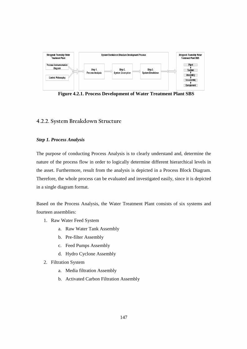
147

36Figure 4.2.1. Process Development of Water Treatment Plant SBS

4.2.2. System Breakdown Structure

Step 1. Process Analysis

The purpose of conducting Process Analysis is to clearly understand and, determine the

nature of the process flow in order to logically determine different hierarchical levels in

the asset. Furthermore, result from the analysis is depicted in a Process Block Diagram.

Therefore, the whole process can be evaluated and investigated easily, since it is depicted

in a single diagram format.

Based on the Process Analysis, the Water Treatment Plant consists of six systems and

fourteen assemblies:

1. Raw Water Feed System

a. Raw Water Tank Assembly

b. Pre-filter Assembly

c. Feed Pumps Assembly

d. Hydro Cyclone Assembly

2. Filtration System

a. Media filtration Assembly

b. Activated Carbon Filtration Assembly

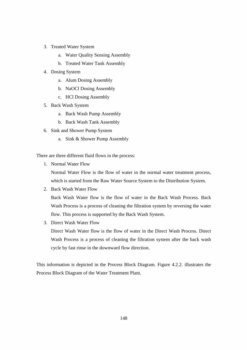
148

3. Treated Water System

a. Water Quality Sensing Assembly

b. Treated Water Tank Assembly

4. Dosing System

a. Alum Dosing Assembly

b. NaOCl Dosing Assembly

c. HCl Dosing Assembly

5. Back Wash System

a. Back Wash Pump Assembly

b. Back Wash Tank Assembly

6. Sink and Shower Pump System

a. Sink & Shower Pump Assembly

There are three different fluid flows in the process:

1. Normal Water Flow

Normal Water Flow is the flow of water in the normal water treatment process,

which is started from the Raw Water Source System to the Distribution System.

2. Back Wash Water Flow

Back Wash Water flow is the flow of water in the Back Wash Process. Back

Wash Process is a process of cleaning the filtration system by reversing the water

flow. This process is supported by the Back Wash System.

3. Direct Wash Water Flow

Direct Wash Water flow is the flow of water in the Direct Wash Process. Direct

Wash Process is a process of cleaning the filtration system after the back wash

cycle by fast rinse in the downward flow direction.

This information is depicted in the Process Block Diagram. Figure 4.2.2. illustrates the

Process Block Diagram of the Water Treatment Plant.

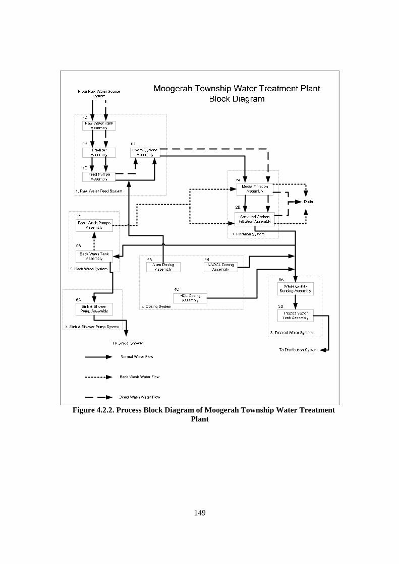
149

37Figure 4.2.2. Process Block Diagram of Moogerah Township Water Treatment Plant

150

Step 2. System Description

In this step, the Water Treatment Plant is described in terms of:

• Description details

There are six description criteria that can be selected to create a detailed

description: Primary Function, Material Flow, Process Flow, Mechanical Action,

State Change and Inputs and Outputs.

In the Water Treatment Plant Case Study, the Primary Function is chosen as the

selected description criteria, since it is clearly stated in the Control Philosophy of

this plant. The description detail of the system primary function is:

The primary function of Water Treatment Plant is to supply 100 m3/day of safe

drinking water and complies with the requirement of the Australia Drinking

Water Guidelines – 2004 (published by the National Health and Medical

Research Council).

• Major subsystems and assemblies

It is clearly depicted in the Process Flow Diagram of the Water Treatment Plant

that the plant consists of six systems: Water Feed System, Filtration System,

Treated Water System, Dosing System, Back Wash system, and Sink and Shower

System.

• Boundaries to other systems and boundary interface components

The system boundaries and interface components are also depicted in the Process

Flow Diagram. System boundaries and interface components for the Water

Treatment Plant are:

i. Raw Water Tank interfaces to the Raw Water Source System

ii. Sink and Shower Pump System interfaces to the Sink and Shower

System

iii. Media Filtration System and Activated Carbon Filtration System

interfaces to the drain at the Back Wash Water Flow

iv. Treated Water System interfaces to the Distribution System

151

• A brief description about contents, criteria and boundaries of the systems

The Water Treatment Plant treats water from Raw Water Source. Therefore, the

water is safe to be drunk before it is passed to the Distribution System. Raw Water

is then transferred to the Water Feed System. In this System, water is stored in

Raw Water Tank. After that, raw water is pumped from Raw Water Tank by Feed

Pumps System through the Pre-filter System, and delivered to the filtration

system.

The above information is written down in a standardised format, as illustrated in Table

4.2.2.a.

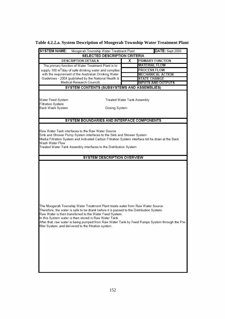
152

6Table 4.2.2.a. System Description of Moogerah Township Water Treatment Plant

153

Step 3. System Breakdown The next step is breaking down the system hierarchically. As mentioned in Section 2.3.2.,

there are six steps in the methodology to actualise the SBS:

• Step 1: Identify Unit/Plant Boundaries

The unit/plant boundaries in the Water Treatment Plant have been identified and

documented in Step 2 of SBS Development (that is, System Description):

o Raw Water Tank interface to the Raw Water Source System

o Sink and Shower Pump System interfaces to the Sink and Shower System

o Media Filtration System and Activated Carbon Filtration System interfaces to

the drain at the Back Wash Water Flow

o Treated Water System interfaces to the Distribution System

• Step 2: Identify the Systems

The Systems in the Water Treatment Plant have been identified and documented in

Step 1 of SBS Development (that is, Process Analysis):

o Water Feed System

o Filtration System

o Treated Water System

o Dosing System

o Back Wash System

o Sink and Shower Pump System

• Step 3: Identify the Assemblies

The assemblies in the Water Treatment Plant have been identified and documented in

Step 1 of SBS Development (that is, Process Analysis):

o Raw Water Tank Assembly (Raw Water Feed System)

o Pre-filter Assembly (Raw Water Feed System)

o Feed Pumps Assembly (Raw Water Feed System)

o Hydro Cyclone Assembly (Raw Water Feed System)

o Media Filtration Assembly (Filtration System)

o Activated Carbon Filtration Assembly (Filtration System)

o Water Quality Sensing Assembly (Treated Water System

o Treated Water Tank Assembly (Treated Water System)

154

o Aluminium Dosing Assembly (Dosing System)

o NaOCl Dosing Assembly (Dosing System)

o HCl Dosing Assembly (Dosing System)

o Back Wash Pumps Assembly (Back Wash System)

o Back Wash Tank Assembly (Back Wash System)

o Sink & Shower Pump Assembly (Sink & Shower Pump System)

• Step 4: Identify the Components

This is the last step of element identification in the SBS where the identified element

is at the lowest level of the SBS. The lowest level element in the SBS is the

Component. However, some elements’ level in the Water Treatment Plant is in

between the Assembly and Component; therefore, they are categorised as Sub-

Assembly. In addition, some components in Water Treatment Plant’s SBS belong to

the sub-assembly, and some others belong directly to the assembly. Further detail on

the complete System Breakdown Structure of Water Treatment Plant is in Step 5 of

Actualise the SBS.

• Step 5: Depict the Relationship of SBS level

In this step, the relationship of SBS level is depicted in a table. The example

relationship of SBS level of Water Treatment Plant is illustrated in Table 4.2.2.b. (the

complete SBS level of the Water Treatment Plant is in Appendix D)

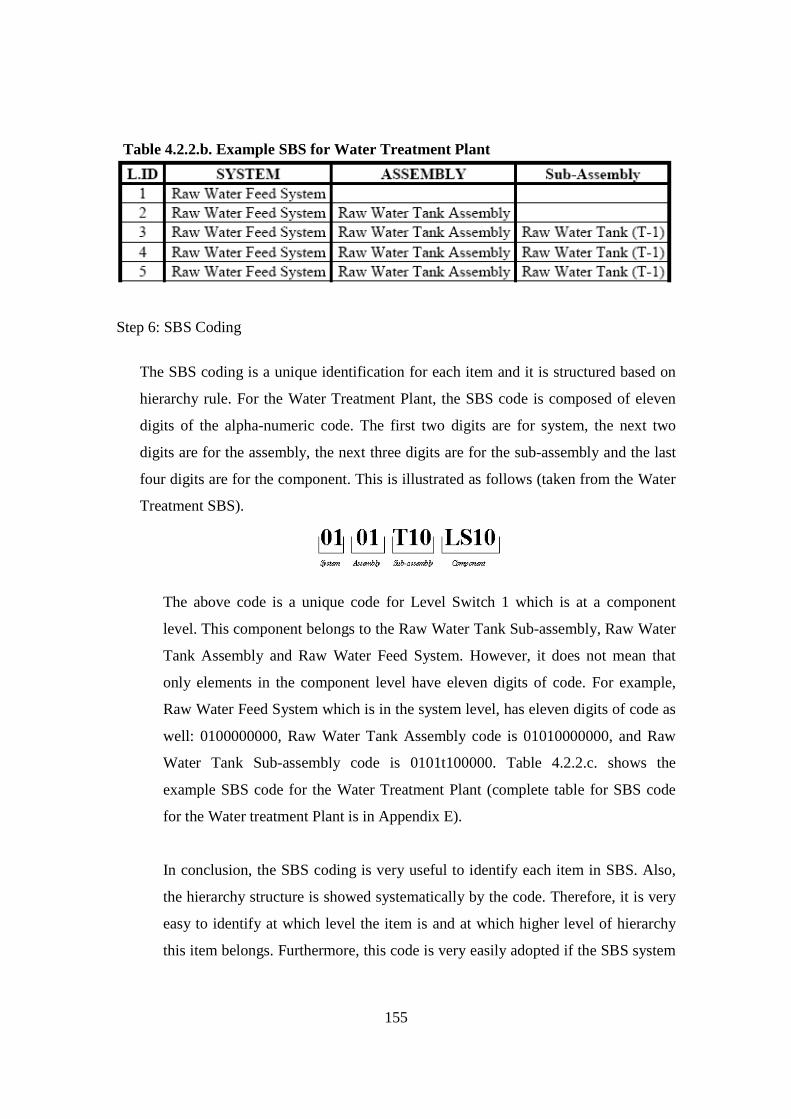
155

7Table 4.2.2.b. Example SBS for Water Treatment Plant

Step 6: SBS Coding

The SBS coding is a unique identification for each item and it is structured based on

hierarchy rule. For the Water Treatment Plant, the SBS code is composed of eleven

digits of the alpha-numeric code. The first two digits are for system, the next two

digits are for the assembly, the next three digits are for the sub-assembly and the last

four digits are for the component. This is illustrated as follows (taken from the Water

Treatment SBS).

The above code is a unique code for Level Switch 1 which is at a component

level. This component belongs to the Raw Water Tank Sub-assembly, Raw Water

Tank Assembly and Raw Water Feed System. However, it does not mean that

only elements in the component level have eleven digits of code. For example,

Raw Water Feed System which is in the system level, has eleven digits of code as

well: 0100000000, Raw Water Tank Assembly code is 01010000000, and Raw

Water Tank Sub-assembly code is 0101t100000. Table 4.2.2.c. shows the

example SBS code for the Water Treatment Plant (complete table for SBS code

for the Water treatment Plant is in Appendix E).

In conclusion, the SBS coding is very useful to identify each item in SBS. Also,

the hierarchy structure is showed systematically by the code. Therefore, it is very

easy to identify at which level the item is and at which higher level of hierarchy

this item belongs. Furthermore, this code is very easily adopted if the SBS system

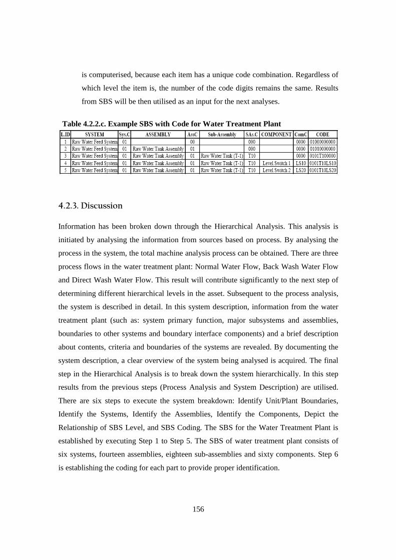
156

is computerised, because each item has a unique code combination. Regardless of

which level the item is, the number of the code digits remains the same. Results

from SBS will be then utilised as an input for the next analyses.

8Table 4.2.2.c. Example SBS with Code for Water Treatment Plant

4.2.3. Discussion Information has been broken down through the Hierarchical Analysis. This analysis is

initiated by analysing the information from sources based on process. By analysing the

process in the system, the total machine analysis process can be obtained. There are three

process flows in the water treatment plant: Normal Water Flow, Back Wash Water Flow

and Direct Wash Water Flow. This result will contribute significantly to the next step of

determining different hierarchical levels in the asset. Subsequent to the process analysis,

the system is described in detail. In this system description, information from the water

treatment plant (such as: system primary function, major subsystems and assemblies,

boundaries to other systems and boundary interface components) and a brief description

about contents, criteria and boundaries of the systems are revealed. By documenting the

system description, a clear overview of the system being analysed is acquired. The final

step in the Hierarchical Analysis is to break down the system hierarchically. In this step

results from the previous steps (Process Analysis and System Description) are utilised.

There are six steps to execute the system breakdown: Identify Unit/Plant Boundaries,

Identify the Systems, Identify the Assemblies, Identify the Components, Depict the

Relationship of SBS Level, and SBS Coding. The SBS for the Water Treatment Plant is

established by executing Step 1 to Step 5. The SBS of water treatment plant consists of

six systems, fourteen assemblies, eighteen sub-assemblies and sixty components. Step 6

is establishing the coding for each part to provide proper identification.

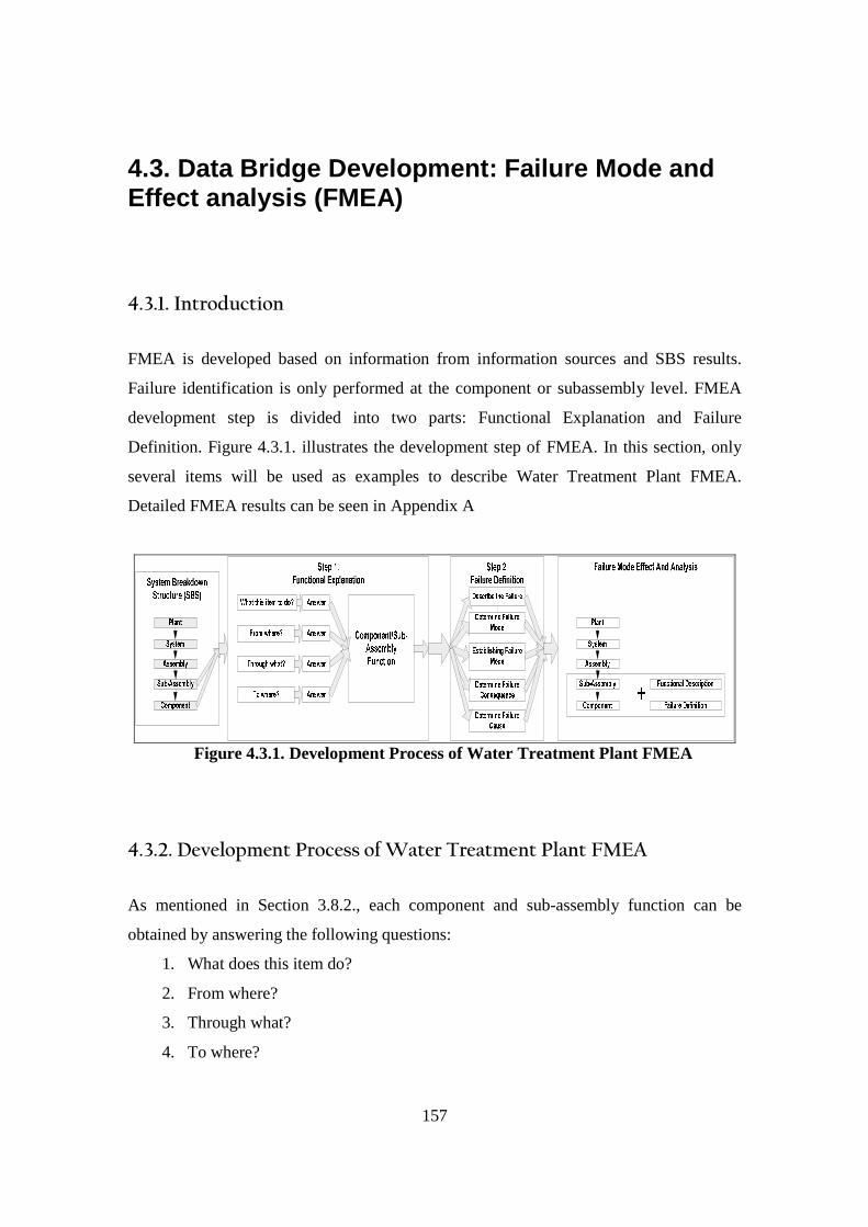
157

4.3. Data Bridge Development: Failure Mode and Effect analysis (FMEA)

4.3.1. Introduction

FMEA is developed based on information from information sources and SBS results.

Failure identification is only performed at the component or subassembly level. FMEA

development step is divided into two parts: Functional Explanation and Failure

Definition. Figure 4.3.1. illustrates the development step of FMEA. In this section, only

several items will be used as examples to describe Water Treatment Plant FMEA.

Detailed FMEA results can be seen in Appendix A

38Figure 4.3.1. Development Process of Water Treatment Plant FMEA

4.3.2. Development Process of Water Treatment Plant FMEA

As mentioned in Section 3.8.2., each component and sub-assembly function can be

obtained by answering the following questions:

1. What does this item do?

2. From where?

3. Through what?

4. To where?

158

The function of an item is a combination of answers from the above questions.

The following is an example of functional explanation from the Raw Water Tank, which

is at sub-assembly hierarchy level:

1. What does this item do?

To store raw water temporary.

2. From where?

Raw Water Tank Inlet

3. Through what?

Raw Water Tank

4. To where?

Raw Water Tank Outlet

Then, the function of Raw Water Tank is:

To store raw water temporarily; from the raw water tank inlet, to raw water tank outlet,

through the raw water tank.

Another example is from the Pre-filter. This item is at component hierarchy level:

1. What does this item do?

To perform the pre-filtration process

2. From where?

Pre-filter Inlet

3. Through what?

Internal Filter

4. To where?

Pre-filter Outlet

Then, the function of Pre-filter is:

To perform the pre-filtration process; from pre-filter inlet, to pre-filter outlet, through the

internal filter.

159

The next step is defining possible failures from each component and sub-assembly.

Section 3.8.2. reveals five possible information sources for defining possible failures.

Due to time and information source constraints, only information from other users of the

same component is utilised. The “RAM Expert Systems Gas Drying and Drying Acid

Cooling Section F.M.E.C.A. and Maintenance Task Specifications” report, developed by

ICS Pty. Ltd., is referenced as an information source (ICSPty.Ltd., 1996). It is assumed

that the same type of components/sub-assemblies in the case study and report have

similar failure possibilities.

The following are two examples of failure definition, and to make a clear picture, the two

examples that are used in the first step, are used again here:

Raw Water Tank

There are two possible causes of failure for the Raw Water Tank:

• Internal corrosion

The description of this failure is: Fails to contain water (leakage)

The mode of this failure is Partial Loss of Function (PLF), since the effect of this

failure is: if leakage is significant, then the Pump cannot perform its function. The

most fatal effect is System Shutdown. The consequence of this failure is quality

disturbance.

• Internal blockage due to debris

The description of this failure is: failure to receive and deliver water

The mode of this failure is Total Loss of Function (TLF), since the effect of this

failure is Blockages, preventing the water to be delivered or received, resulting in

pump failure. The consequence of this failure is production disturbance.

Pre-filter

There are four possible causes of failure for the Pre-filter:

• The filter element is bypassed due to a perforated element

The description of this failure is: Delivery of unfiltered water

The mode of this failure is Total Loss of Function (TLF), since the effect of this

failure can result in other filter failure, alarm and system shutdown. The

consequence of this failure is production disturbance.

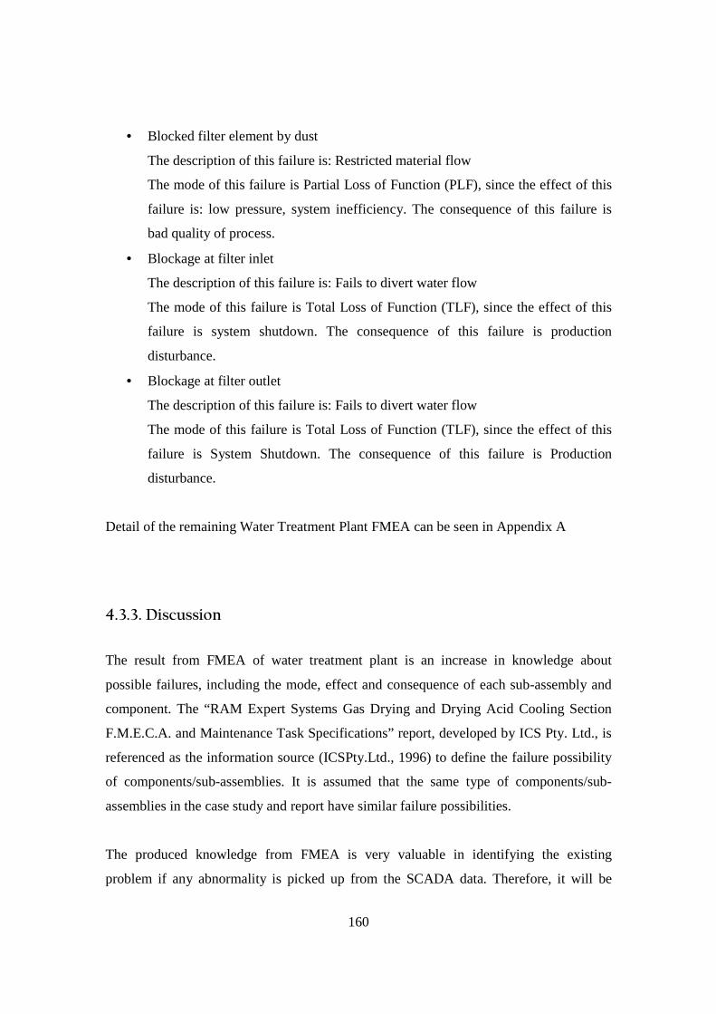
160

• Blocked filter element by dust

The description of this failure is: Restricted material flow

The mode of this failure is Partial Loss of Function (PLF), since the effect of this

failure is: low pressure, system inefficiency. The consequence of this failure is

bad quality of process.

• Blockage at filter inlet

The description of this failure is: Fails to divert water flow

The mode of this failure is Total Loss of Function (TLF), since the effect of this

failure is system shutdown. The consequence of this failure is production

disturbance.

• Blockage at filter outlet

The description of this failure is: Fails to divert water flow

The mode of this failure is Total Loss of Function (TLF), since the effect of this

failure is System Shutdown. The consequence of this failure is Production

disturbance.

Detail of the remaining Water Treatment Plant FMEA can be seen in Appendix A

4.3.3. Discussion

The result from FMEA of water treatment plant is an increase in knowledge about

possible failures, including the mode, effect and consequence of each sub-assembly and

component. The “RAM Expert Systems Gas Drying and Drying Acid Cooling Section

F.M.E.C.A. and Maintenance Task Specifications” report, developed by ICS Pty. Ltd., is

referenced as the information source (ICSPty.Ltd., 1996) to define the failure possibility

of components/sub-assemblies. It is assumed that the same type of components/sub-

assemblies in the case study and report have similar failure possibilities.

The produced knowledge from FMEA is very valuable in identifying the existing

problem if any abnormality is picked up from the SCADA data. Therefore, it will be

161

inputted to the Knowledge Base. Also, this result will be utilised in the Interdependence

Analysis.

4.4. Data Bridge Development: Interdependence Analysis

4.4.1. Introduction The purpose of implementing the Interdependence Analysis to the case study is to

identify any interdependent relationship in the system. The result from this analysis can

be used to assist in failure tracing based on the abnormality, which is captured by sensors

and alarms. The implementation of the Interdependence Analysis for the case study is

facilitated through the Functional and Causal Relationship Diagram (FCRD).

Furthermore, FCRD is able to present the result of analysis in an easy to understand

format - a diagram.

Two stages of FCRD of the case study will be developed. FCRD Stage 1 is to analyse the

Dynamic Relationship on the system’s component level. FCRD Stage 2 is to transform

information into a more comprehensive and manageable format to be inputted into the

Data Base. Besides assisting the development of the Data Bridge, the result from FCRD

will also be utilised to assist the risk calculation on the Interdependence Risk Analysis.

4.4.2. FCRD Stage 1 The information source for this implementation process is P&ID, Control Philosophy of

Water Treatment Plant, results from Hierarchical Analysis and FMEA. The information

from these documents is investigated prior to performing FCRD Stage 1 for the Water

Treatment Plant. The next step is executing the four steps of generating the FCRD Stage

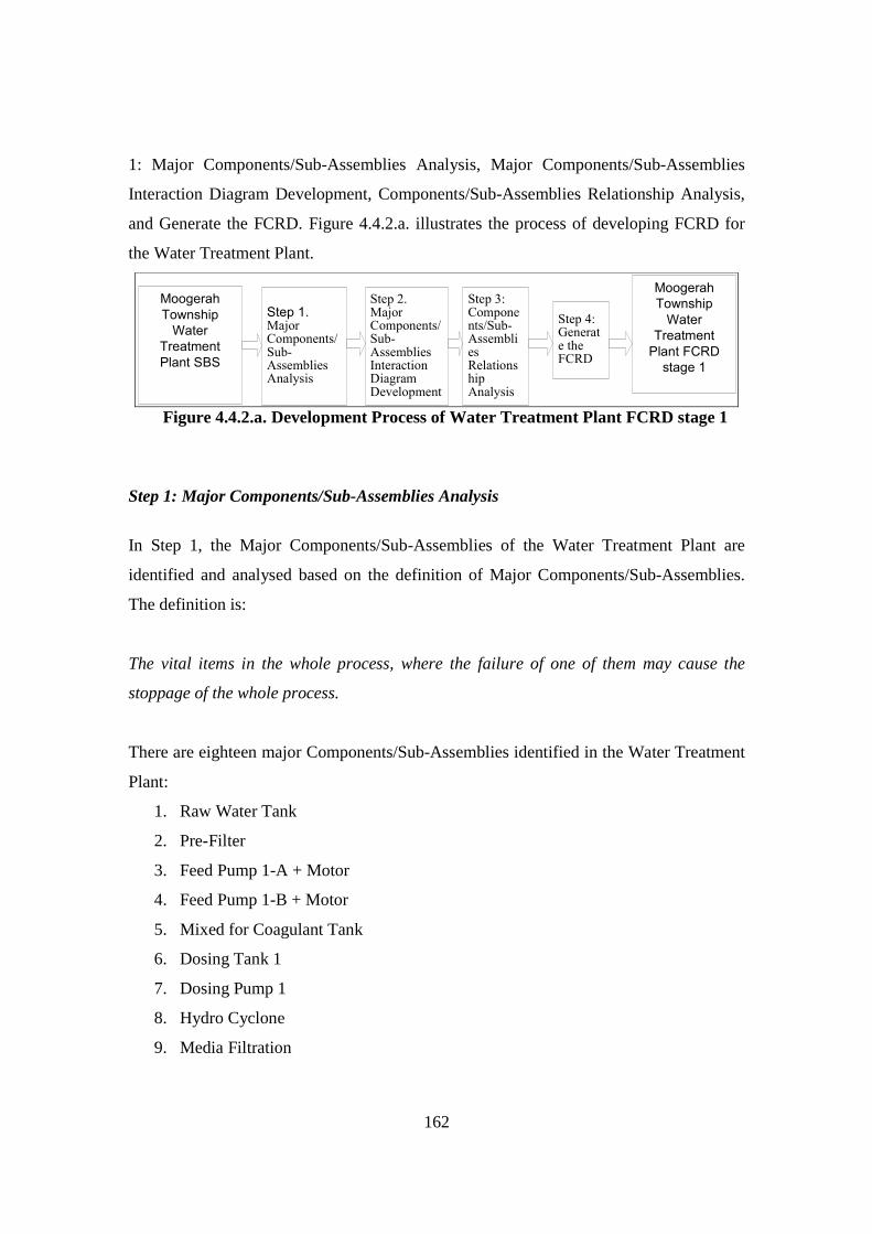
162

1: Major Components/Sub-Assemblies Analysis, Major Components/Sub-Assemblies

Interaction Diagram Development, Components/Sub-Assemblies Relationship Analysis,

and Generate the FCRD. Figure 4.4.2.a. illustrates the process of developing FCRD for

the Water Treatment Plant.

Moogerah

Township

Water

Treatment

Plant SBS

Step 1. Major Components/Sub-Assemblies Analysis

Step 2. Major Components/Sub-Assemblies Interaction Diagram Development

Step 3: Components/Sub-Assemblies Relationship Analysis

Moogerah

Township

Water

Treatment

Plant FCRD

stage 1

Step 4: Generate the FCRD

39Figure 4.4.2.a. Development Process of Water Treatment Plant FCRD stage 1

Step 1: Major Components/Sub-Assemblies Analysis

In Step 1, the Major Components/Sub-Assemblies of the Water Treatment Plant are

identified and analysed based on the definition of Major Components/Sub-Assemblies.

The definition is:

The vital items in the whole process, where the failure of one of them may cause the

stoppage of the whole process.

There are eighteen major Components/Sub-Assemblies identified in the Water Treatment

Plant:

1. Raw Water Tank

2. Pre-Filter

3. Feed Pump 1-A + Motor

4. Feed Pump 1-B + Motor

5. Mixed for Coagulant Tank

6. Dosing Tank 1

7. Dosing Pump 1

8. Hydro Cyclone

9. Media Filtration

163

10. Activated Carbon Filtration

11. Dosing Tank 2

12. Dosing Tank 3

13. Dosing Pump 2

14. Dosing Pump 3

15. Treated Water Tank

16. Back Wash Tank

17. Back Wash Pump 2-A + Motor

18. Back Wash Pump 2-B + Motor

Step 2: Major Components/Sub-assemblies Interaction Diagram Development

The next step is conducting analysis to identify interaction between each of major

components/sub-assemblies. The identification is based on fluid flows in the process. As

mentioned in Section 4.2.2., there are three different flows in the process:

1. Normal Water Flow

In Normal Water Flow, water flows from Raw Water Tank through the Pre Filter.

Then, it flows to either Feed Pump 1-A + Motor or Feed Pump 1-B + Motor. The

water flows to Hydro Cyclone, the Media Filtration and Activated Carbon Filter.

It is then ended in the Treated Water Tank.

2. Back Wash Water Flow

Back Wash Water Flow is initiated from Back Wash Water Tank through either

Back Wash Pump 2-A + Motor or Back Wash Pump 2-B + Motor. Then, the

water flows to both the Media Filtration and Activated Carbon Filtration. The

Flow is ended in the Drain.

4. Direct Wash Water Flow

Direct Wash Water Flow is the water flow in Direct Wash Process. Direct Wash

Process is a process of cleaning the filtration system after the back wash cycle by

fast rinse in the downward flow direction.

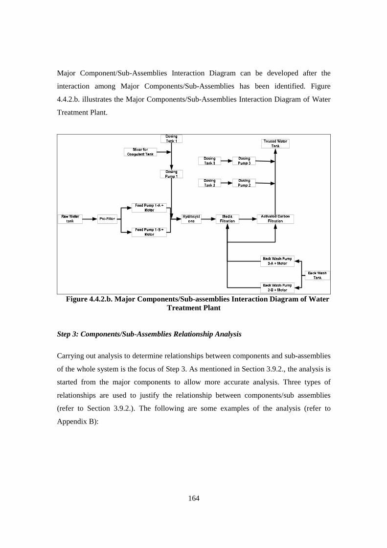
164

Major Component/Sub-Assemblies Interaction Diagram can be developed after the

interaction among Major Components/Sub-Assemblies has been identified. Figure

4.4.2.b. illustrates the Major Components/Sub-Assemblies Interaction Diagram of Water

Treatment Plant.

40Figure 4.4.2.b. Major Components/Sub-assemblies Interaction Diagram of Water Treatment Plant

Step 3: Components/Sub-Assemblies Relationship Analysis

Carrying out analysis to determine relationships between components and sub-assemblies

of the whole system is the focus of Step 3. As mentioned in Section 3.9.2., the analysis is

started from the major components to allow more accurate analysis. Three types of

relationships are used to justify the relationship between components/sub assemblies

(refer to Section 3.9.2.). The following are some examples of the analysis (refer to

Appendix B):

165

1. Raw Water Tank is related to:

• Level Switch 1 1 way relationship 1st to 2nd

• Level Switch 2 1 way relationship 1st to 2nd

• Raw Water Resource 2 ways relationship n.a.

• Pre-filter 2 ways relationship n.a.

• Hand Valve 5 1 way relationship 2nd to 1st

2. Pre-filter is related to:

• Hand Valve 5 1 way relationship 2nd to 1st

• Hand Valve 6 1 way relationship 2nd to 1st

• Raw Water Tank 2 ways relationship n.a.

• Feed Pump 1-A + Motor 2 ways relationship n.a.

• Feed Pump 1-B + Motor 2 ways relationship n.a.

Step 4: Generate the FCRD

In this step, all information from the previous steps is presented in a diagram (that is,

Functional and Causal Relationship Diagram). At this moment, there are several

diagramming softwares available in the market for helping in developing the diagram,

such as: Microsoft Visio, Graphviz, Inkscape, etc. In this research, Microsoft Visio is

utilised to draw the diagram manually. However, in some cases, the diagram could be

complicated and manual diagramming is too difficult. Therefore, an automatic

diagramming algorithm is developed. Graphviz is utilised in the automatic diagramming

algorithm to facilitate the process (refer to Section 4.6.2.)

Figure 4.4.2.c. and Figure 4.4.2.d. depict the FCRD Stage 1 (Figure 4.4.2.c. is drawn

manually by utilising Microsoft Visio and Figure 4.4.2.d. is drawn automatically by

utilising Graphviz and displayed by Microsoft Visio).

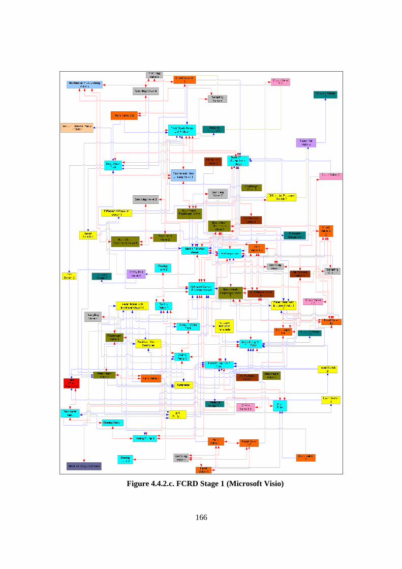
166

41Figure 4.4.2.c. FCRD Stage 1 (Microsoft Visio)

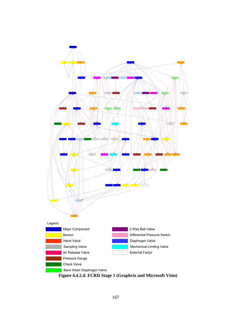
167

R aw Wat e r Tank

Le v e l Swi t c h 1 Le v e l Swi t c h 2 H and V al v e 5

Pr e - Fi l t e rR aw Wat e r R e s o ur c e

Fe e d Pump 1-A + Mo t o r

Fe e d Pump 1-B + Mo t o r

H an d V al v e 6

Sa mpl i ng V al v e 9

H and V al v e 1 -1

H and V al v e 1- 2Tur b i d i me t e r

Pr e s s ur e G aug e 1- 1

Che c k V al v e 1 - 1 Hy dr o c yc l o ne

D o s i n g Pump 1

pH A nal ys e r

Wat e r Me t e r wi t h El e c t r i c a l Out pu t 2

Pr e s s ur e In d i c a t o r Tr ans mi t t e r

Pr e s s u r e G a ug e 1- 2

Che c k V al v e 1- 2

A i r R e l e a s e V al v e 1

H a nd V a l v e 2- 1

H a nd V a l v e 2- 2

Sampl i ng V a l v e 1D i aphr ag m V al v e 6

Wa t e r M e t e r wi t h El e c t r i c a l Out put 1

R e s i dua l Chl o r i n e Co nt r o l l e r

D i aphr a gm V a l v e 9

H and V al v e 7

Me d i a Fi l t r a t i o n V e s s e l

B ac k Was h D i aphr agm V al v e 1

D i aphr a gm V a l v e 2 B ac k Was h D i ap hr agm V al v e 33 Way B al l V al v e 1

D i f f e r e nt i a l Pr e s s ur e Swi t c h 1

D i aph r agm V al v e 4 A i r R e l e a s e V al v e 3 A c t i va t e d Ca r bo n Fi l t r a t i o n V e s s e l

B ac k Was h Pump 2- A + M o t o r

B ac k Was h PU mp 2- B + M o t o r

Me c hani c a l Fl o w Li mi t i ng V al v e 1

Sampl i ng V al v e 2

A i r R e l e a s e V A l ve 2

Sa mpl i ng V al v e 3

B ac k Was h D i ap hr agm V al v e 5

B ac k Was h D i aphr a gm V a l v e 7

A i r R e l e a s e V al v e 5

Samp l i ng V al v e 7

H a nd V a l v e 4- 1 H and V al v e 4 -2

Pr e s s ur e G aug e 2

Sampl i ng V a l v e 5

M e c han i c a l Fl ow Li mi t i ng V al v e 2

Samp l i ng V al v e 6

A i r R e l e a s e V al v e 43 Wa y B al l V al v e 2

D i f f e r e nt i a l Pr e s s ur e Swi t c h 2

Sampl i ng V a l v e 4

D i aphr a gm V a l v e 8

D o s i ng Pump 2

D o s i n g Pump 3

Tr e a t e d Wat e r Tank

Pr e s s ur e G aug e 3

D o s i ng Ta nk 1

M i x e r f o r Co ag ul an t Tank

D o s i ng Tank 2

D o s i ng Tank 3

H a nd V a l v e 3-1

Pr e s s u r e G a ug e 4 -1

Che c k V al v e 2-1 B a c k Wa s h Tan k

Le ve l Swi t c h 4

H a nd V a l v e 3 -2

Sampl i ng V al v e 8

Pr e s s ur e G au g e 4 - 2

Che c k V al v e 2- 2

Le ve l Swi t c h 3 Si nk and Powe r Pump + Mo t o r

Legend

Major Component

Sensor

Hand Valve

Sampling Valve

Air Release Valve

Pressure Gauge

Check Valve

Back Wash Diaphragm Valve

3 Way Ball Valve

Differential Pressure Switch

Diaphragm Valve

Mechanical Limiting Valve

External Factor

42Figure 4.4.2.d. FCRD Stage 1 (Graphviz and Microsoft Visio)

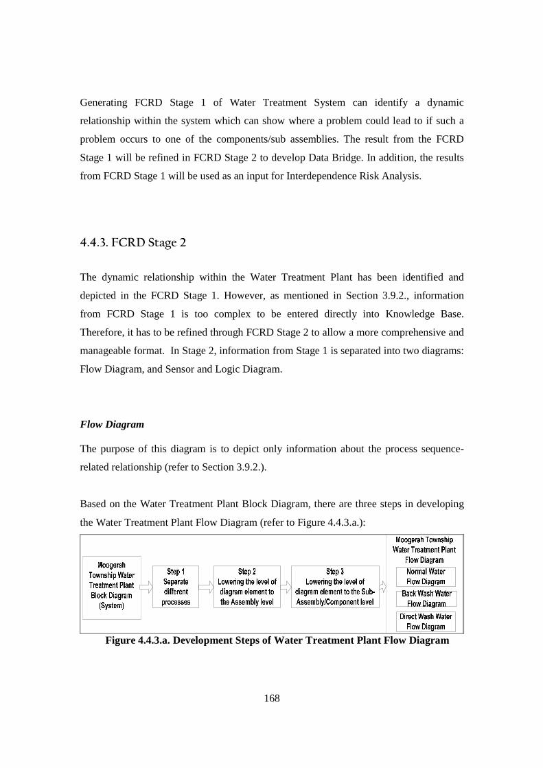
168

Generating FCRD Stage 1 of Water Treatment System can identify a dynamic

relationship within the system which can show where a problem could lead to if such a

problem occurs to one of the components/sub assemblies. The result from the FCRD

Stage 1 will be refined in FCRD Stage 2 to develop Data Bridge. In addition, the results

from FCRD Stage 1 will be used as an input for Interdependence Risk Analysis.

4.4.3. FCRD Stage 2

The dynamic relationship within the Water Treatment Plant has been identified and

depicted in the FCRD Stage 1. However, as mentioned in Section 3.9.2., information

from FCRD Stage 1 is too complex to be entered directly into Knowledge Base.

Therefore, it has to be refined through FCRD Stage 2 to allow a more comprehensive and

manageable format. In Stage 2, information from Stage 1 is separated into two diagrams:

Flow Diagram, and Sensor and Logic Diagram.

Flow Diagram The purpose of this diagram is to depict only information about the process sequence-

related relationship (refer to Section 3.9.2.).

Based on the Water Treatment Plant Block Diagram, there are three steps in developing

the Water Treatment Plant Flow Diagram (refer to Figure 4.4.3.a.):

43Figure 4.4.3.a. Development Steps of Water Treatment Plant Flow Diagram

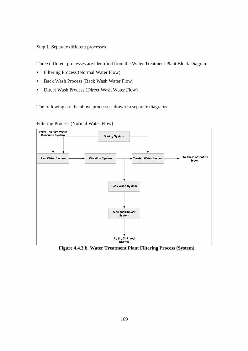
169

Step 1. Separate different processes

Three different processes are identified from the Water Treatment Plant Block Diagram:

• Filtering Process (Normal Water Flow)

• Back Wash Process (Back Wash Water Flow)

• Direct Wash Process (Direct Wash Water Flow)

The following are the above processes, drawn in separate diagrams:

Filtering Process (Normal Water Flow)

44Figure 4.4.3.b. Water Treatment Plant Filtering Process (System)

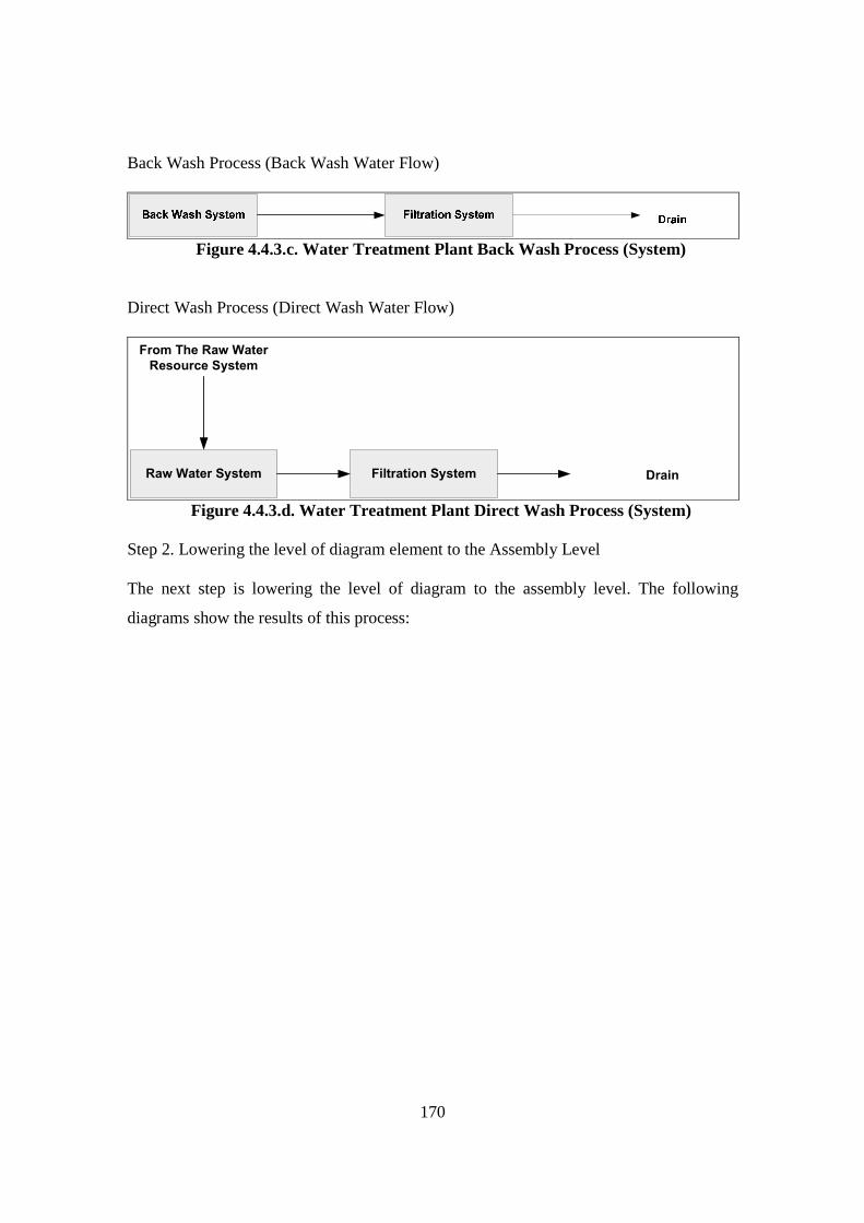
170

Back Wash Process (Back Wash Water Flow)

45Figure 4.4.3.c. Water Treatment Plant Back Wash Process (System) Direct Wash Process (Direct Wash Water Flow)

Raw Water System

From The Raw Water

Resource System

Filtration System Drain

46Figure 4.4.3.d. Water Treatment Plant Direct Wash Process (System) Step 2. Lowering the level of diagram element to the Assembly Level The next step is lowering the level of diagram to the assembly level. The following

diagrams show the results of this process:

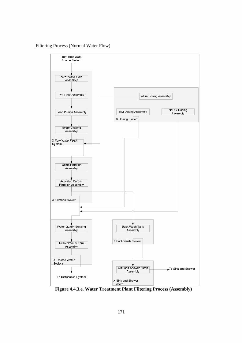
171

Filtering Process (Normal Water Flow)

47Figure 4.4.3.e. Water Treatment Plant Filtering Process (Assembly)

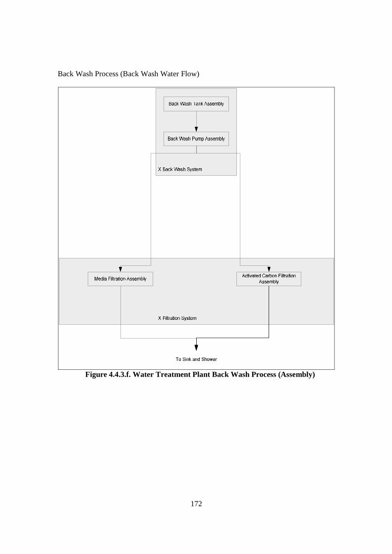
172

Back Wash Process (Back Wash Water Flow)

48Figure 4.4.3.f. Water Treatment Plant Back Wash Process (Assembly)

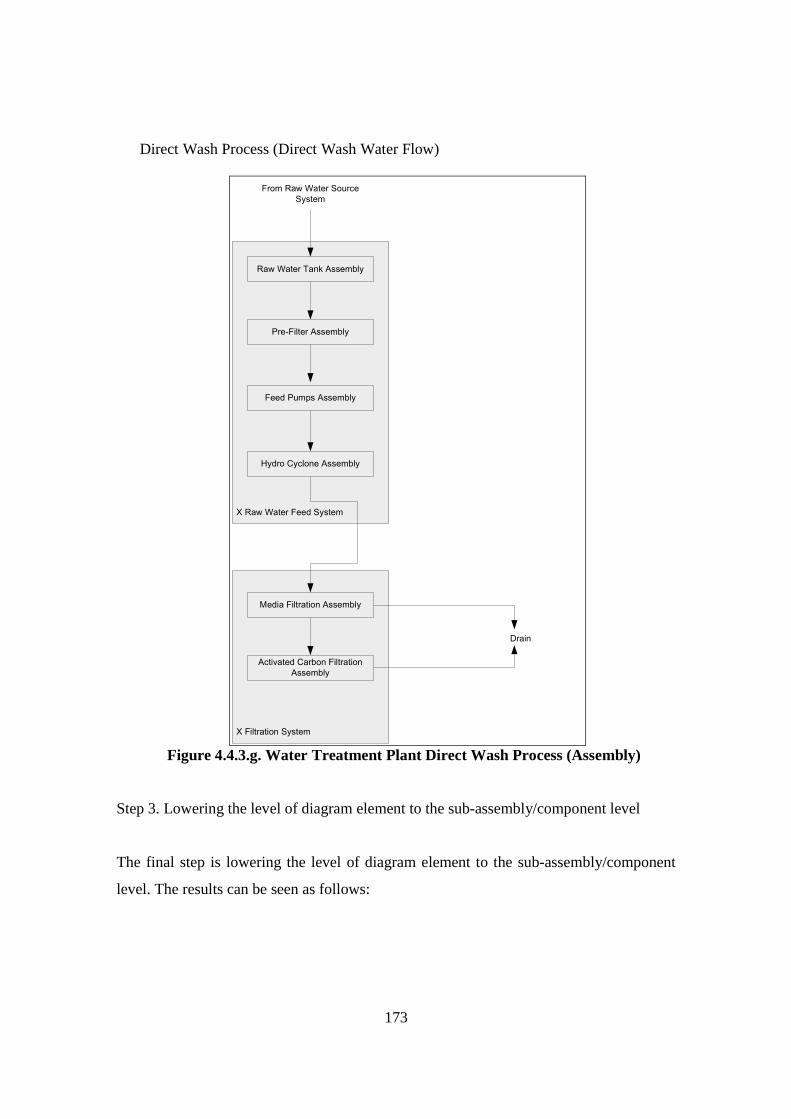
173

Direct Wash Process (Direct Wash Water Flow)

Raw Water Tank Assembly

From Raw Water Source

System

Pre-Filter Assembly

Feed Pumps Assembly

Hydro Cyclone Assembly

X Raw Water Feed System

Media Filtration Assembly

Activated Carbon Filtration

Assembly

X Filtration System

Drain

49Figure 4.4.3.g. Water Treatment Plant Direct Wash Process (Assembly)

Step 3. Lowering the level of diagram element to the sub-assembly/component level

The final step is lowering the level of diagram element to the sub-assembly/component

level. The results can be seen as follows:

174

Filtering Process (Normal Water Flow)

50Figure 4.4.3.h. Water Treatment Plant Filtering Process (Sub-

Assembly/Component)

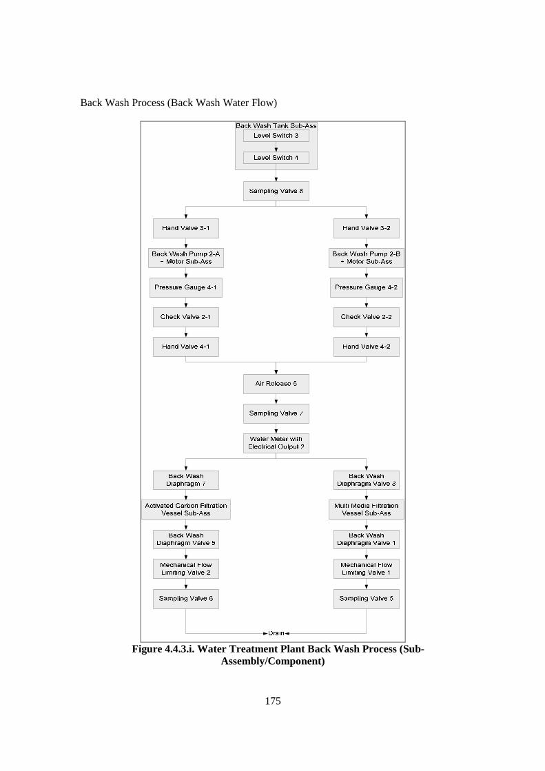
175

Back Wash Process (Back Wash Water Flow)

51Figure 4.4.3.i. Water Treatment Plant Back Wash Process (Sub-

Assembly/Component)

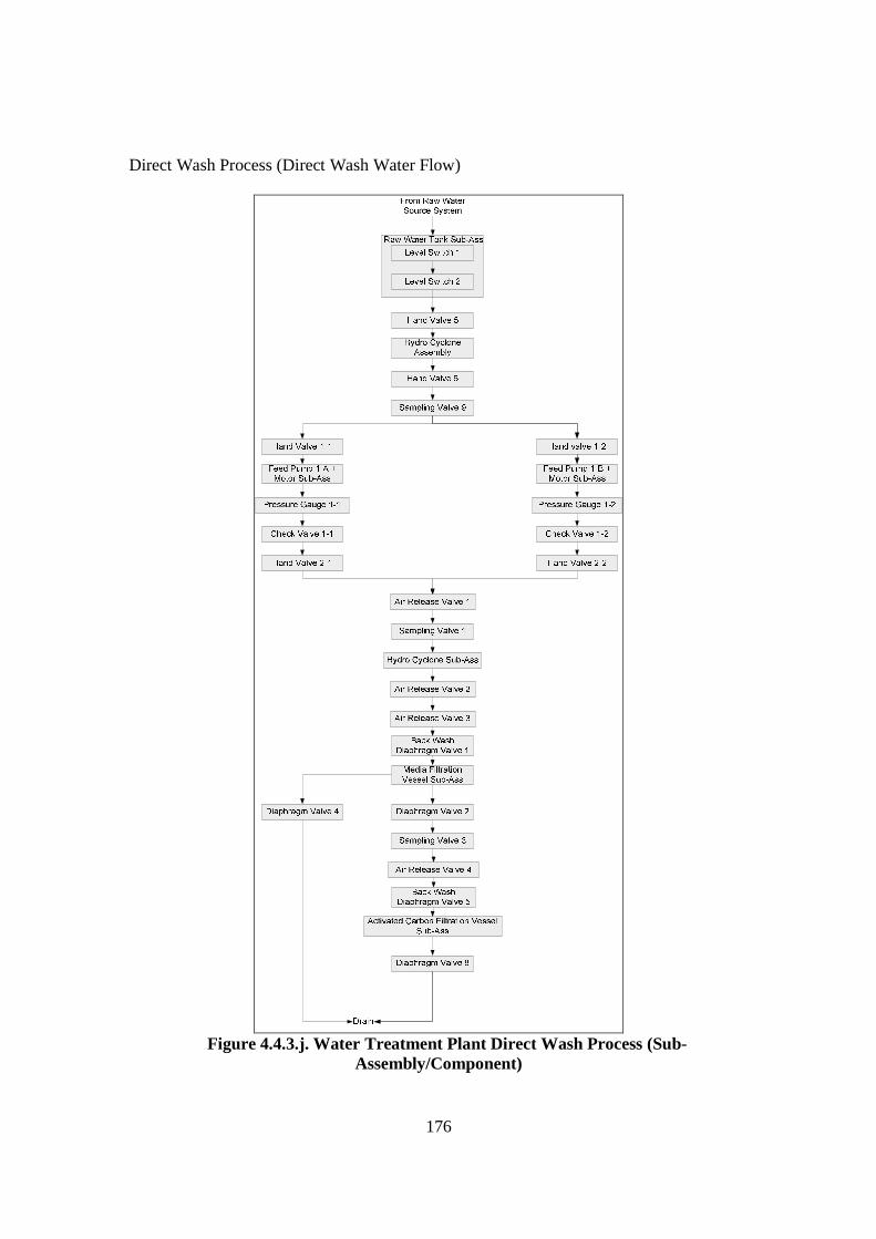
176

Direct Wash Process (Direct Wash Water Flow)

52Figure 4.4.3.j. Water Treatment Plant Direct Wash Process (Sub-

Assembly/Component)

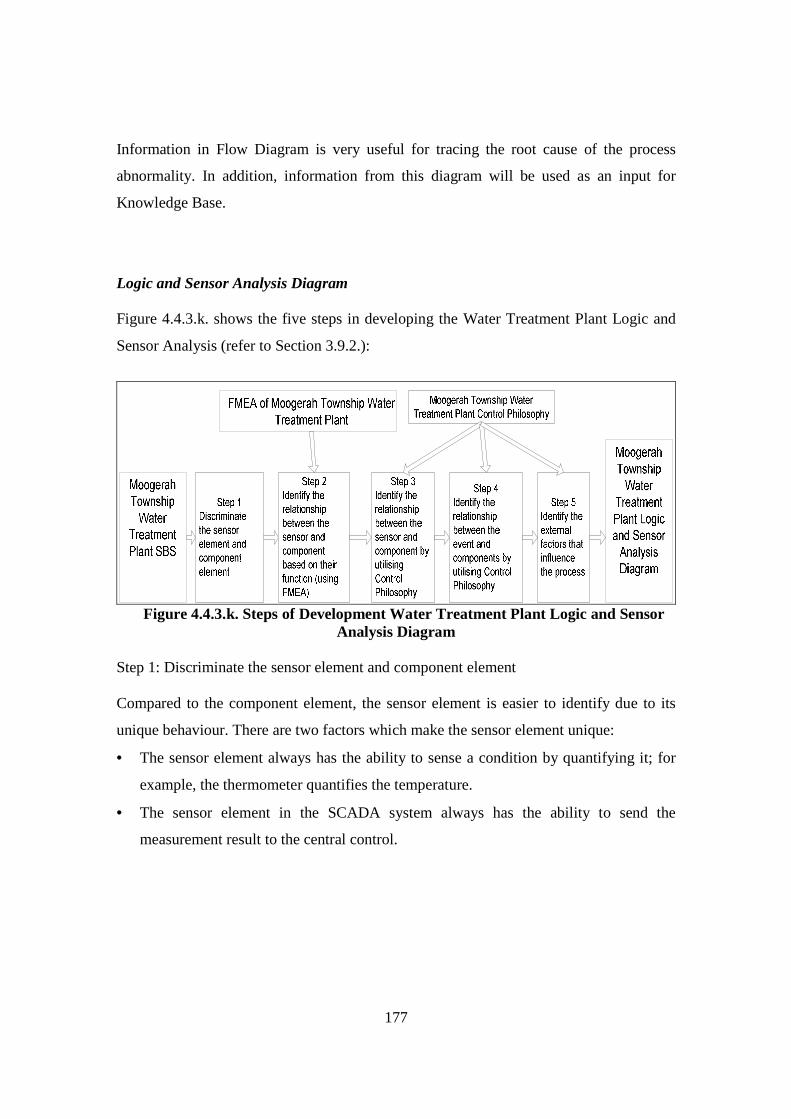
177

Information in Flow Diagram is very useful for tracing the root cause of the process

abnormality. In addition, information from this diagram will be used as an input for

Knowledge Base.

Logic and Sensor Analysis Diagram Figure 4.4.3.k. shows the five steps in developing the Water Treatment Plant Logic and

Sensor Analysis (refer to Section 3.9.2.):

53Figure 4.4.3.k. Steps of Development Water Treatment Plant Logic and Sensor Analysis Diagram

Step 1: Discriminate the sensor element and component element Compared to the component element, the sensor element is easier to identify due to its

unique behaviour. There are two factors which make the sensor element unique:

• The sensor element always has the ability to sense a condition by quantifying it; for

example, the thermometer quantifies the temperature.

• The sensor element in the SCADA system always has the ability to send the

measurement result to the central control.

178

From 80 sub-assemblies/components, there are twelve sensor elements:

• Level Switch 1

• Level Switch 2

• Pressure Indicator Transmitter

• Water Meter with Electrical Output 1

• Residual Chlorine Controller

• pH Analyser

• Turbidimeter

• Water Meter with Electrical Output 2

• Level Switch 3

• Level Switch 4

The rest are component elements.

Step 2: Identify the relationship between the sensor and component based on their

function (using FMEA)

In this step, FMEA is used to identify the relationship between the sensor and component

based on their function. For example:

• Level Switch 1

Function:

To monitor the high level of water in the raw water tank and to send a notification of

the high water level. From the floater, to the central control, through the electrical

mechanisms.

It can be concluded that the Level Switch is related to the Raw Water Tank.

• Differential Pressure 2

Function:

To measure the pressure difference between the inlet and outlet of the activated

carbon filtration vessel. From the differential pressure switch 2 inlet, to the central

control, through the pressure sensor.

179

It can be concluded that Differential Pressure 2 is related to the Activated Carbon

Filtration.

This step identifies relationships, such as:

• Level Switch 1 � Raw Water Tank

• Level Switch 2 � Raw Water Tank

• Turbidimeter � Activated Carbon Filter

• Turbidimeter � Multi Media filter

• Turbidimeter � Hydro Cyclone

• Turbidimeter � Pre-Filter

• Level Switch 3 � Back Wash Tank

• Level Switch 4 � Back Wash Tank

• Differential Pressure Switch 1 � Multi Media Filter

• Differential Pressure Switch 2 � Activated Carbon Filter

Step 3: Identify the relationship between the sensor and component by utilising Control Philosophy The next step is utilising Control Philosophy to identify more relationships between the

sensor and component.

This step identifies relationships, such as:

• Chlorine Controller � Dosing Tank 2

• Chlorine Controller � Dosing Pump 2

• pH Analyser � Dosing Tank 3

• pH Analyser � Dosing Pump 3

• Differential Pressure Switch 1 � Multi Media filter

• Differential Pressure 2 � Activated Carbon Filter

This step strengthens some relationships, which have been identified in Step 2.

180

Step 4: Identify the relationship between the event and component by utilising Control Philosophy Step 4 identifies relationship between event and component based on Control Philosophy.

According to Control Philosophy, there are five different system alarms:

• Feed Pump 1-A Failure Alarm

• Feed Pump 1-B Failure Alarm

• Back Wash Pump 2-A Failure Alarm

• Back Wash Pump 2-B Failure Alarm

• Alum Mixer Failure Alarm

Control philosophy also mentions a symptom to justify whether Multi Media Filter and

Activated Carbon Filter are in a deteriorating condition and require further maintenance.

This is based on the behaviour of Differential Pressure Switch value. If Differential

Pressure Switch 1 shows value of 0.5 bars or more, a back wash process will be triggered.

If this event occurs at least three times within one hour, it means that further maintenance

must be applied to the Multi Media Filter. Similarly, if the Differential Pressure Switch 2

shows value of 0.5 bars or more, the back wash process will also be triggered; and if this

event occurs at least three times within one hour, it means that further maintenance

attention must be applied to the Activated Carbon Filter.

These symptoms can be justified as events:

• Multi Media back Wash Cycle Counter Event

• Activated Carbon Filter Back Wash Cycle Counter Event

This step identifies relationships, such as:

• Feed Pump 1-A Failure Event � Feed Pump 1-A

• Feed Pump 1-B Failure Event � Feed Pump 1-B

• Back Wash Pump 2-A Failure Event � Back Wash Pump 2-A

• Back Wash Pump 2-B Failure Even � Back Wash Pump 2-B

• Alum Mixer Failure Event � Alum Mixer

• Multi Media Filter Back Wash Cycle Counter Event � Multi Media Filter

• Activated Carbon Filter Back Wash Cycle Counter Event � Activated Carbon Filter

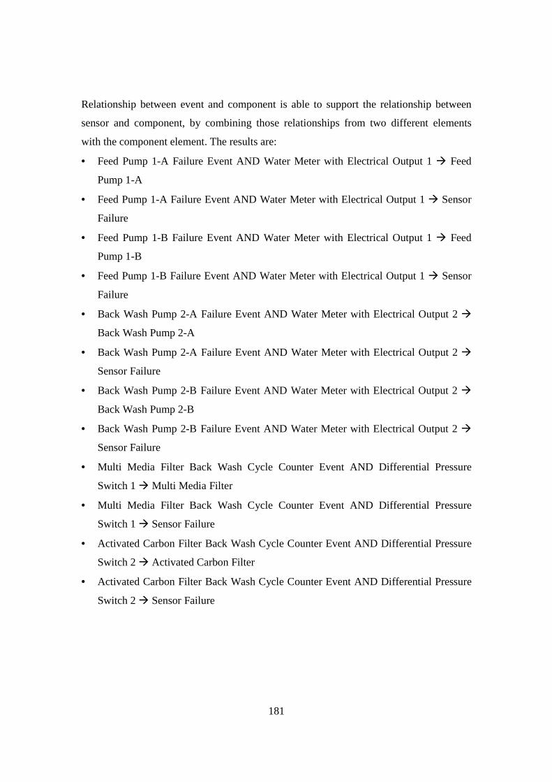
181

Relationship between event and component is able to support the relationship between

sensor and component, by combining those relationships from two different elements

with the component element. The results are:

• Feed Pump 1-A Failure Event AND Water Meter with Electrical Output 1 � Feed

Pump 1-A

• Feed Pump 1-A Failure Event AND Water Meter with Electrical Output 1 � Sensor

Failure

• Feed Pump 1-B Failure Event AND Water Meter with Electrical Output 1 � Feed

Pump 1-B

• Feed Pump 1-B Failure Event AND Water Meter with Electrical Output 1 � Sensor

Failure

• Back Wash Pump 2-A Failure Event AND Water Meter with Electrical Output 2 �

Back Wash Pump 2-A

• Back Wash Pump 2-A Failure Event AND Water Meter with Electrical Output 2 �

Sensor Failure

• Back Wash Pump 2-B Failure Event AND Water Meter with Electrical Output 2 �

Back Wash Pump 2-B

• Back Wash Pump 2-B Failure Event AND Water Meter with Electrical Output 2 �

Sensor Failure

• Multi Media Filter Back Wash Cycle Counter Event AND Differential Pressure

Switch 1 � Multi Media Filter

• Multi Media Filter Back Wash Cycle Counter Event AND Differential Pressure

Switch 1 � Sensor Failure

• Activated Carbon Filter Back Wash Cycle Counter Event AND Differential Pressure

Switch 2 � Activated Carbon Filter

• Activated Carbon Filter Back Wash Cycle Counter Event AND Differential Pressure

Switch 2 � Sensor Failure

182

The Alum Mixer Failure Event cannot be combined with the sensor because there is no

relationship between the Alum Mixer and sensor. Utilising AND operator to combine the

relationship between the event/sensor and component means that if both elements (event

and sensor) are triggered at a same time, it is suspected that the cause of abnormality is

the related component. This also allows for shorter and more accurate Root Cause

Analysis.

Step 5: Identify the external factors that influence the process

This step identifies any external factors that can influence the process. The source of

identification process is Control Philosophy.

According to Control Philosophy, one of the important factors that can influence the final

result for the treatment process is the quality of raw water. In addition, the quality of raw

water is related to sensors that measure the quality of treated water; that is, Turbidimeter,

pH Analyser, and Chlorine Controller. Therefore, the relationships are:

• Turbidimeter � Raw Water Quality

• pH Analyser � Raw Water Quality

• Chlorine Controller � Raw Water Quality

On the other hand, there is one external entity that always occurs when utilising sensors:

sensor failure. Therefore, the relationships will be:

• Level Switch 1 � Sensor Failure

• Level Switch 2 � Sensor Failure

• Pressure Indicator Transmitter � Sensor Failure

• Water Meter with Electrical Output 1 � Sensor Failure

• Residual Chlorine Controller � Sensor Failure

• pH Analyser � Sensor Failure

• Turbidimeter � Sensor Failure

• Water Meter with Electrical Output 2 � Sensor Failure

• Level Switch 3 � Sensor Failure

• Level Switch 4 � Sensor Failure

183

The last step is relating each sensor and event to the process flow diagram to provide

further guidance on tracing the abnormality. The purpose of this relationship is to provide

further guidance, when none of the components that are related to sensor/event are the

cause of the abnormality.

If none of the related components is the cause of the abnormality, then information from

the process flow diagram will guide in checking each component that is involved in the

process. This process is valuable, because as soon as the component which causes the

abnormality can be identified, the new relationship with the respective sensor/event is

included in the Logic and Sensor Analysis Diagram.

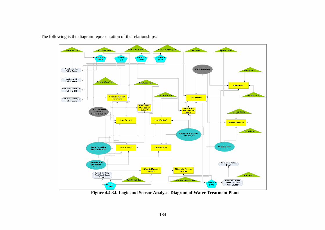
184

The following is the diagram representation of the relationships:

54Figure 4.4.3.l. Logic and Sensor Analysis Diagram of Water Treatment Plant

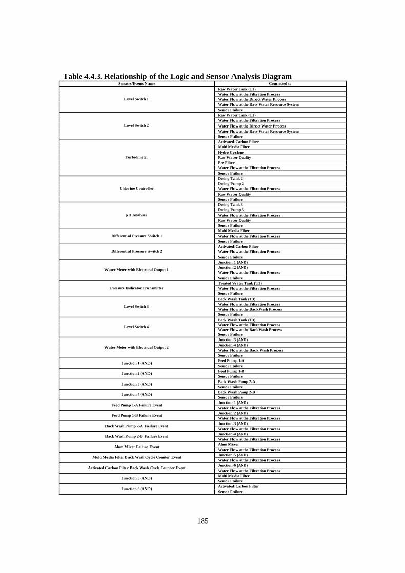
185

9Table 4.4.3. Relationship of the Logic and Sensor Analysis Diagram Sensors/Events Name Connected to

Raw Water Tank (T1) Water Flow at the Filtration Process Water Flow at the Direct Water Process Water Flow at the Raw Water Resource System

Level Switch 1

Sensor Failure Raw Water Tank (T1) Water Flow at the Filtration Process Water Flow at the Direct Water Process Water Flow at the Raw Water Resource System

Level Switch 2

Sensor Failure Activated Carbon Filter Multi Media Filter Hydro Cyclone Raw Water Quality Pre-Filter Water Flow at the Filtration Process

Turbidimeter

Sensor Failure Dosing Tank 2 Dosing Pump 2 Water Flow at the Filtration Process Raw Water Quality

Chlorine Controller

Sensor Failure Dosing Tank 3 Dosing Pump 3 Water Flow at the Filtration Process Raw Water Quality

pH Analyser

Sensor Failure Multi Media Filter Water Flow at the Filtration Process Differential Pressure Switch 1 Sensor Failure Activated Carbon Filter Water Flow at the Filtration Process Differential Pressure Switch 2 Sensor Failure Junction 1 (AND) Junction 2 (AND) Water Flow at the Filtration Process

Water Meter with Electrical Output 1

Sensor Failure Treated Water Tank (T2) Water Flow at the Filtration Process Pressure Indicator Transmitter Sensor Failure Back Wash Tank (T3) Water Flow at the Filtration Process Water Flow at the BackWash Process

Level Switch 3

Sensor Failure Back Wash Tank (T3) Water Flow at the Filtration Process Water Flow at the BackWash Process

Level Switch 4

Sensor Failure Junction 3 (AND) Junction 4 (AND) Water Flow at the Back Wash Process

Water Meter with Electrical Output 2

Sensor Failure Feed Pump 1-A Junction 1 (AND) Sensor Failure Feed Pump 1-B Junction 2 (AND) Sensor Failure Back Wash Pump 2-A Junction 3 (AND) Sensor Failure Back Wash Pump 2-B Junction 4 (AND) Sensor Failure Junction 1 (AND) Feed Pump 1-A Failure Event Water Flow at the Filtration Process Junction 2 (AND) Feed Pump 1-B Failure Event Water Flow at the Filtration Process Junction 3 (AND) Back Wash Pump 2-A Failure Event Water Flow at the Filtration Process Junction 4 (AND) Back Wash Pump 2-B Failure Event Water Flow at the Filtration Process Alum Mixer Alum Mixer Failure Event Water Flow at the Filtration Process Junction 5 (AND) Multi Media Filter Back Wash Cycle Counter Event Water Flow at the Filtration Process Junction 6 (AND) Activated Carbon Filter Back Wash Cycle Counter Event Water Flow at the Filtration Process Multi Media Filter Junction 5 (AND) Sensor Failure Activated Carbon Filter Junction 6 (AND) Sensor Failure

186

4.4.4. Discussion Through the Interdependence Analysis, results from the previous two analyses together

with information from the information source are further processed.

In the FCRD Stage 1, the major component can be identified. Major components are the

vital items in the whole process, where the failure of one of them may cause the stoppage

of the whole process. This result is very important in developing the Interdependence

Risk Analysis. Also, the results from FCRD Stage 1 reveal the dynamic relationship

within the water treatment system. This information is presented in a diagram; thus, it is

clearer and easier to be understood. The combination of Graphviz and Microsoft Visio

can assist in developing the automatic diagramming algorithm. This algorithm is able to

draw the diagram automatically by only inputting the information. Therefore, a complex

diagram can be drawn easily. Further information about the automatic diagramming

algorithm is found in Section. 4.7.

In FCRD Stage 2, the information from the water treatment plant is processed into a more

manageable format to be inputted to the Knowledge Base (refer to Section 4.6.2.). FCRD

Stage 2 is facilitated by developing two diagrams: The Flow Diagram, and Sensor and

Logic Diagram. The Flow Diagram depicts only information about the process sequence-

related relationship. According to the result of Hierarchical Analysis, there are three

different process flows in the water treatment plant. This information is utilised as a

stepping stone to develop the Flow Diagram. This diagram provides more comprehensive

information to trace any interruption in the process flow. Sensor and Logic Diagram

depicts system indirect relationship (logic control and sensing mechanism relationship).

Information about the cause of any detected abnormality by sensor/alarm is more

apparent by developing this diagram, because this diagram depicts relationship

information between sensor/alarm and components/sub-assemblies.

187

4.5. Data Bridge Development: Filtering Algorithm

4.5.1. Introduction The filtering algorithm filters only significant data from the SCADA data dump. The

filtering algorithm is developed based on the information from the Control Philosophy

and P&ID of a Water Treatment Plant Case Study.

4.5.2. Development of the Filtering Algorithm The Water Treatment Plant is monitored by twelve different sensors. However, based on

the SCADA Data Dump document, only seven sensors are recorded regularly.

Furthermore, from the seven recorded parameters, based on Control Philosophy, only five

are crucial in the water treatment process:

• Turbidity � comes from Turbidimeter sensor

• pH � comes from pH Controller sensor

• Chlorine � comes from Residual Chlorine Controller sensor

• Water Flow � comes from Flow Meter with Electrical Output 1 sensor

• Head Pressure � comes from Differential Pressure 1 sensor

The other two parameters only provide information on the water level in the tank.

Therefore, the filtering algorithm is only developed for those five sensors:

a. Turbidimeter

Turbidimeter is a sensor to measure the level of treated water turbidity. According to

the Control Philosophy, the maximum value to raise the high turbidity alarm (which

indicates the system works properly) is 1 TU (Turbidity Unit). Therefore, the

comparison factor for turbidimeter is 1 TU, where data is taken when the turbidimeter

value is equal or greater than 1 TU.

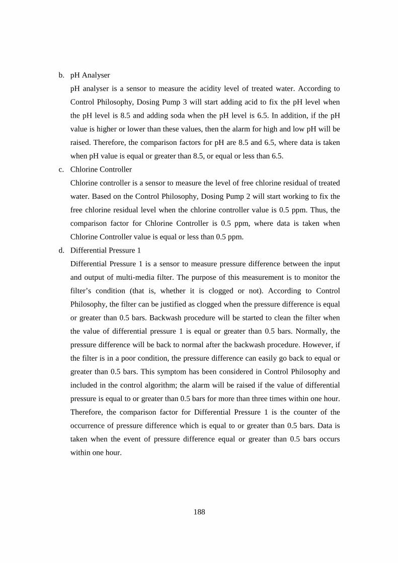
188

b. pH Analyser

pH analyser is a sensor to measure the acidity level of treated water. According to

Control Philosophy, Dosing Pump 3 will start adding acid to fix the pH level when

the pH level is 8.5 and adding soda when the pH level is 6.5. In addition, if the pH

value is higher or lower than these values, then the alarm for high and low pH will be

raised. Therefore, the comparison factors for pH are 8.5 and 6.5, where data is taken

when pH value is equal or greater than 8.5, or equal or less than 6.5.

c. Chlorine Controller

Chlorine controller is a sensor to measure the level of free chlorine residual of treated

water. Based on the Control Philosophy, Dosing Pump 2 will start working to fix the

free chlorine residual level when the chlorine controller value is 0.5 ppm. Thus, the

comparison factor for Chlorine Controller is 0.5 ppm, where data is taken when

Chlorine Controller value is equal or less than 0.5 ppm.

d. Differential Pressure 1

Differential Pressure 1 is a sensor to measure pressure difference between the input

and output of multi-media filter. The purpose of this measurement is to monitor the

filter’s condition (that is, whether it is clogged or not). According to Control

Philosophy, the filter can be justified as clogged when the pressure difference is equal

or greater than 0.5 bars. Backwash procedure will be started to clean the filter when

the value of differential pressure 1 is equal or greater than 0.5 bars. Normally, the

pressure difference will be back to normal after the backwash procedure. However, if

the filter is in a poor condition, the pressure difference can easily go back to equal or

greater than 0.5 bars. This symptom has been considered in Control Philosophy and

included in the control algorithm; the alarm will be raised if the value of differential

pressure is equal to or greater than 0.5 bars for more than three times within one hour.

Therefore, the comparison factor for Differential Pressure 1 is the counter of the

occurrence of pressure difference which is equal to or greater than 0.5 bars. Data is

taken when the event of pressure difference equal or greater than 0.5 bars occurs

within one hour.

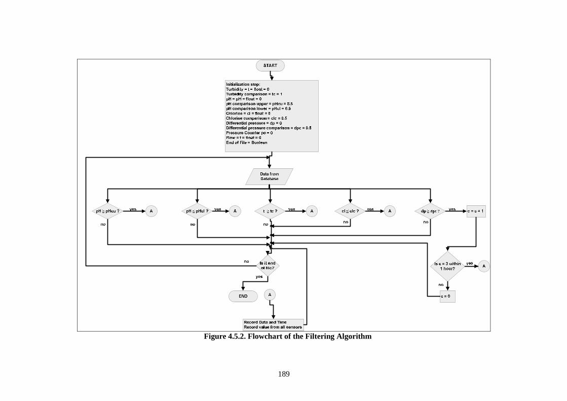
189

55Figure 4.5.2. Flowchart of the Filtering Algorithm

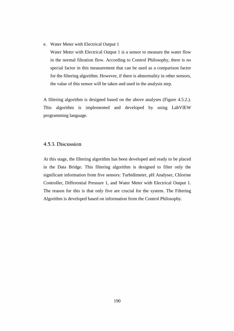
190

e. Water Meter with Electrical Output 1

Water Meter with Electrical Output 1 is a sensor to measure the water flow

in the normal filtration flow. According to Control Philosophy, there is no

special factor in this measurement that can be used as a comparison factor

for the filtering algorithm. However, if there is abnormality in other sensors,

the value of this sensor will be taken and used in the analysis step.

A filtering algorithm is designed based on the above analyses (Figure 4.5.2.).

This algorithm is implemented and developed by using LabVIEW

programming language.

4.5.3. Discussion

At this stage, the filtering algorithm has been developed and ready to be placed

in the Data Bridge. This filtering algorithm is designed to filter only the

significant information from five sensors: Turbidimeter, pH Analyser, Chlorine

Controller, Differential Pressure 1, and Water Meter with Electrical Output 1.

The reason for this is that only five are crucial for the system. The Filtering

Algorithm is developed based on information from the Control Philosophy.

191

4.6. Data Bridge Development: Knowledge Base

4.6.1. Introduction A data base can only be justified as a knowledge base if there is a rule to extract

the information (Google, 2007), namely Inference Engine. Therefore, the

Knowledge Base is formed by the synergy of The Data Base and Inference

Engine.

In this research, the Knowledge Base is adopted because of its ability to store

and retrieve information. All information from the three analyses in

Hierarchical Model is inputted to a data base. An inference engine is then

developed to retrieve the stored information from the data base. The following

explanation concerns the design of the data base and inference engine.

4.6.2. Data Base

The data base is developed in Microsoft Access and deployed in website using

MySQL. Microsoft Access is used because it is user friendly. The data base is

deployed in the website to increase accessibility, so that information can be

inputted and accessed from anywhere.

Apart from supplying information based on a query from the inference engine,

the information in the Data Base is utilised by automated diagramming script to

generate a diagram (FCRD, Flow Diagram, and Logic and Sensor Diagram).

The following diagram illustrates the information flow from and to the data

base:

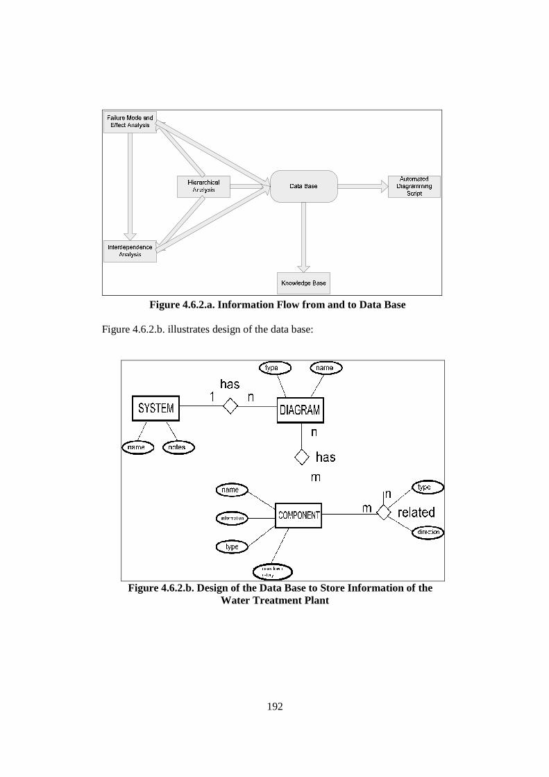
192

56Figure 4.6.2.a. Information Flow from and to Data Base

Figure 4.6.2.b. illustrates design of the data base:

57Figure 4.6.2.b. Design of the Data Base to Store Information of the

Water Treatment Plant

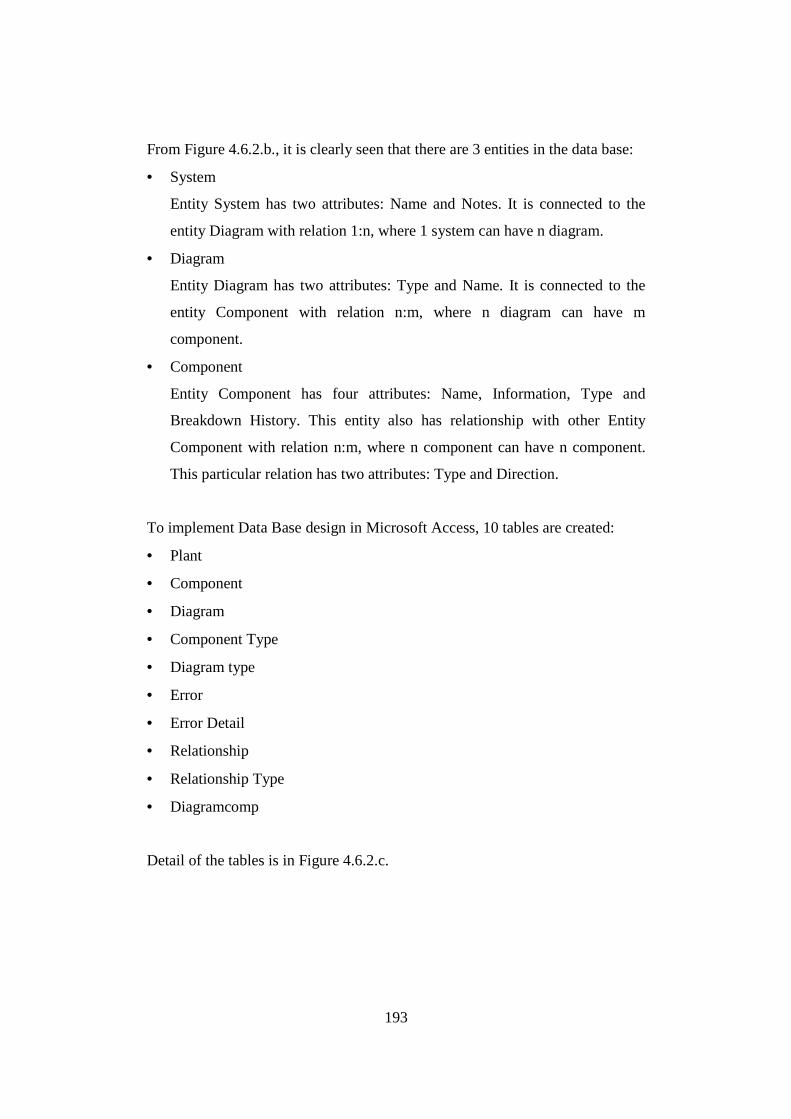
193

From Figure 4.6.2.b., it is clearly seen that there are 3 entities in the data base:

• System

Entity System has two attributes: Name and Notes. It is connected to the

entity Diagram with relation 1:n, where 1 system can have n diagram.

• Diagram

Entity Diagram has two attributes: Type and Name. It is connected to the

entity Component with relation n:m, where n diagram can have m

component.

• Component

Entity Component has four attributes: Name, Information, Type and

Breakdown History. This entity also has relationship with other Entity

Component with relation n:m, where n component can have n component.

This particular relation has two attributes: Type and Direction.

To implement Data Base design in Microsoft Access, 10 tables are created:

• Plant

• Component

• Diagram

• Component Type

• Diagram type

• Error

• Error Detail

• Relationship

• Relationship Type

• Diagramcomp

Detail of the tables is in Figure 4.6.2.c.

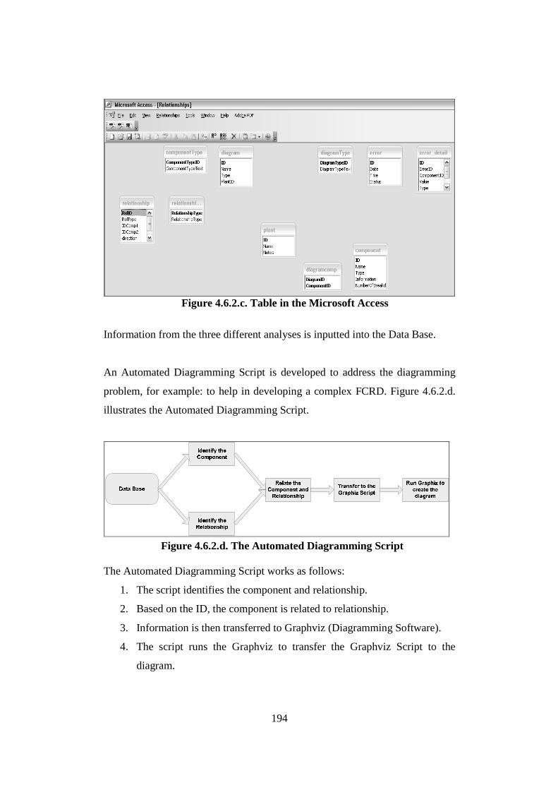
194

58Figure 4.6.2.c. Table in the Microsoft Access

Information from the three different analyses is inputted into the Data Base.

An Automated Diagramming Script is developed to address the diagramming

problem, for example: to help in developing a complex FCRD. Figure 4.6.2.d.

illustrates the Automated Diagramming Script.

59Figure 4.6.2.d. The Automated Diagramming Script

The Automated Diagramming Script works as follows:

1. The script identifies the component and relationship.

2. Based on the ID, the component is related to relationship.

3. Information is then transferred to Graphviz (Diagramming Software).

4. The script runs the Graphviz to transfer the Graphviz Script to the

diagram.

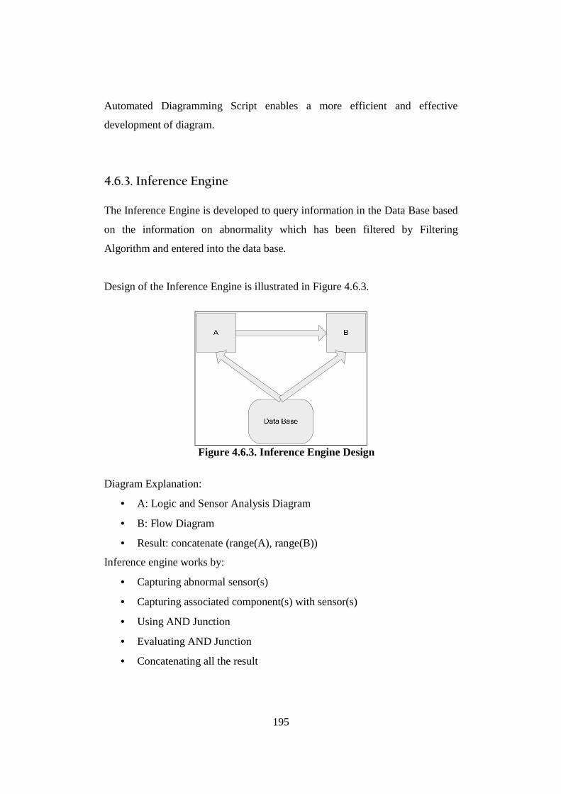
195

Automated Diagramming Script enables a more efficient and effective

development of diagram.

4.6.3. Inference Engine The Inference Engine is developed to query information in the Data Base based

on the information on abnormality which has been filtered by Filtering

Algorithm and entered into the data base.

Design of the Inference Engine is illustrated in Figure 4.6.3.

60Figure 4.6.3. Inference Engine Design

Diagram Explanation:

• A: Logic and Sensor Analysis Diagram

• B: Flow Diagram

• Result: concatenate (range(A), range(B))

Inference engine works by:

• Capturing abnormal sensor(s)

• Capturing associated component(s) with sensor(s)

• Using AND Junction

• Evaluating AND Junction

• Concatenating all the result

196

4.6.4. Discussion After the Filtering Algorithm has been developed (refer to section. 4.5.), The

Knowledge Base is the final component that has to be developed. The

Knowledge Base consists of the Data Base and Inference Engine. In this

research, the Data Base is developed in Microsoft Access and deployed in

website using MySQL. All information from the Hierarchical Model is inputted

to this Data Base. As well as supplying information based on a query from the

inference engine, the information in the Data Base is utilised by an automated

diagramming script to generate a diagram (FCRD, Flow Diagram, and Logic

and Sensor Diagram). The Automated Diagramming Script is developed to

enable a more efficient and effective complex diagram development.

An Inference Engine is developed to query information in the Data Base based

on the information on abnormality which has been filtered by the Filtering

Algorithm and entered into the data base.

At this point, the Knowledge Base is ready to be tested to validate the research

finding. Detail about Data Bridge validation is in the Section 6.2..

4.7. Risk Ranking Development by Utilising Interdependence Risk Analysis

4.7.1. Introduction

Interdependence Risk Analysis (IRA) is proposed in this research to address the

problem in the current Risk Analysis method (i.e. lack of information to define

Risk Likelihood), by utilising interdependence relationship.

197

The explanation in Section 4.7 involves the implementation of Interdependence

Risk Analysis to develop Risk Ranking of components/sub-assemblies of water

treatment plant. According to Total Asset Management (Risk Management

Guideline) (TAM04-12, 2004) there are two approaches that are commonly

used in industry to develop Risk Ranking: Risk Factor and Risk Ranking

Matrix. However, Risk Consequence and Risk Likelihood of each

component/sub-assembly have to be determined before these two approaches

can be carried on to develop the Risk Ranking. IRA will be used to determine

the Risk Consequence and Risk Likelihood of each component/sub-assembly.

These are then used to develop the Risk Rankings based on Risk Factor and

Risk Ranking Matrix. This process will reveal the potency of IRA to address

problems in the current Risk Analysis method (that is, lack of information to

define Risk Likelihood). In the validation step, the Risk Ranking based on

information from Interdependence Risk Analysis, will be compared with Risk

Ranking based on information from Risk Analysis based on Failure Mode and

Effect Analysis method, which has been acknowledged in industry. This

comparison will verify the validity of the IRA method. Detail about the

comparison is in Section 6.3..

4.7.2. Risk Ranking Development

The development of the Risk Ranking follows the Step of Risk Analysis that is

proposed in Total Asset Management (Risk Management Guideline) (TAM04-

12, 2004):

1. Identify Risks

In this step, each component/sub-assembly is identified as source of

risk.

2. Assess Likelihood and Consequences

In this step, each Risk Analysis approach has to assess each

component/sub-assembly’s likelihood and consequences.

198

3. Risk Ranks

The Likelihood and Consequences of each component/sub-assembly are

utilised to produce Risk Ranking. There are two proposed approaches to

produce Risk Ranking: Risk Factor and Risk Ranking Matrix.

Risk Factor

Formula for calculating Risk Factor is (TAM04-12, 2004):

RF = (L + I) – (L x I) Equation. 8

RF = risk factor;

L = measured risk likelihood, on a scale 0 to 1

= average of likelihood factors

I = measured impact (consequence), on a scale 0 to 1

= average of impact (consequence) factors

Risk Ranking Matrix

Risk Ranking Matrix is proposed in (TAM04-12, 2004) to provide a graphic

presentation of risk classes and assist in reporting. Figure 4.7.2.a. Illustrates the

Risk Ranking Matrix

199

61Figure 4.7.2.a. Risk Ranking Matrix (TAM04-12, 2004)

From Figure 4.7.2.a., it can be seen that each component/sub-assembly is

placed in the matrix based on two axes: impact axis and likelihood axis. The

matrix area is divided into four regions by placing a line in mid value of each

axis. The four regions are:

1. Minor Risks can be accepted or ignored.

2. Moderate Risks are either likely to occur or have large impacts.

Management measures should be specified for all moderate risks.

3. Major Risks are those risks with both a high likelihood of creating and a

large impact; these risks will require close management attention, and

the preparation of a formal risk action schedule.

FCRD Stage 1 of the Water Treatment Plant Case Study has been established

(refer to Section 4.4.2.) and will be used as an information source.

There are seven steps that have to be followed in applying IRA to the Water

Treatment Plant Case Study:

1. Step 1: Define the Criticality at Systems Level based on impact from

FMEA (COF rating)

200

In this step, the consequence of possible components/sub-assemblies

failures in FMEA is quantified by assigning weight value ranging from 0 to

1. To determine the logical weight, a logical assumption has to be made

based on the information from Control Philosophy and P&ID:

“Production means that the failure of a component will result in total system

failure, causing systems or equipment downtime and will end up with lost

of production plus maintenance cost. Quality means that the component

functional failures cause a degradation of the primary system function,

resulting in a maintenance cost (e.g.: failure of a water tank due to corrosion

will degrade the lifetime of filter).”

From the above assumption, the assigned weight is:

Production : 0.9

Quality : 0.09

All component/sub-assembly’s possible failures are then quantified by

utilising the above assigned weight. Table 4.7.2.a. is an example of the

process of Quantifying the Failure Consequence. Detail is in Appendix A

10Table 4.7.2.a. Example of Quantifying the Failure Consequence

201

As seen in the Table 4.7.2.a. above, the total of the whole assigned weight

for each possible failure in one component/sub-assembly is called

Consequence Score. This Consequence Score will be divided by the number

of possible failures to obtain Impact.

2. Step 2: Quantify the Interdependence Relationship

In FCRD, there are three types of relationships: 1 way, 2 ways and don’t

care. The relationships that are used in IRA are 1 way and 2 ways.

However, if the relationship is observed from a components/sub-assemblies

point of view, there are 2 types of relationships:

1. Interdependence Relationship In

a. Component is influenced by any incident of other component

that is connected.

b. Justified as Risk In or likelihood of component failure

2. Interdependence Relationship Out

a. Component influences other component that is connected

b. Justified as Risk Out or Consequence to the System

In this step, the quantification is applied to those two types of

Interdependence Relationships.

Based on the Interdependence Level (i.e. severity level of consequence

to other component if there is trouble in a component which is

interdependently related), Interdependence Relationship is categorised

into 3 levels:

• High (weighted 0.9)

Incident in one component will give a significant consequence to the

other.

• Medium (weighted 0.09)

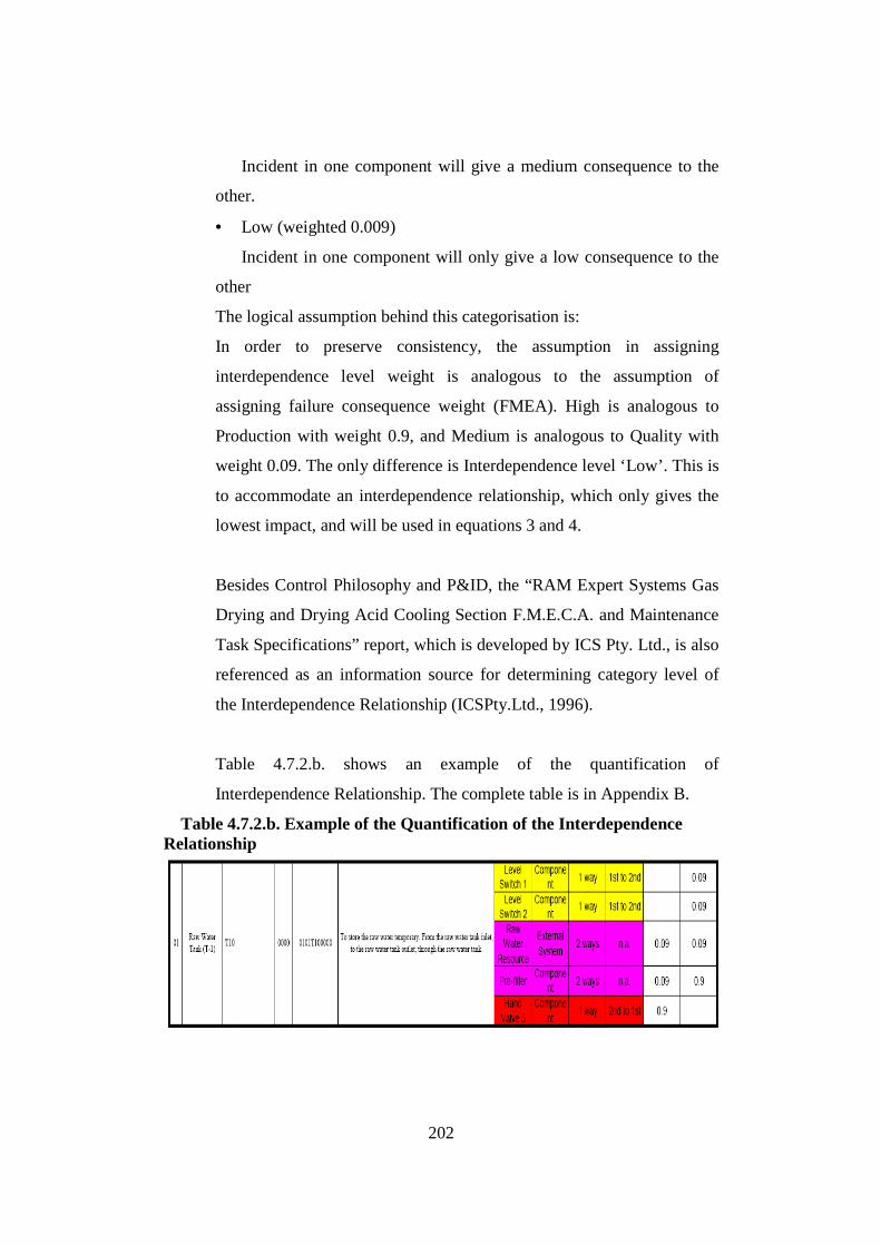
202

Incident in one component will give a medium consequence to the

other.

• Low (weighted 0.009)

Incident in one component will only give a low consequence to the

other

The logical assumption behind this categorisation is:

In order to preserve consistency, the assumption in assigning

interdependence level weight is analogous to the assumption of

assigning failure consequence weight (FMEA). High is analogous to

Production with weight 0.9, and Medium is analogous to Quality with

weight 0.09. The only difference is Interdependence level ‘Low’. This is

to accommodate an interdependence relationship, which only gives the

lowest impact, and will be used in equations 3 and 4.

Besides Control Philosophy and P&ID, the “RAM Expert Systems Gas

Drying and Drying Acid Cooling Section F.M.E.C.A. and Maintenance

Task Specifications” report, which is developed by ICS Pty. Ltd., is also

referenced as an information source for determining category level of

the Interdependence Relationship (ICSPty.Ltd., 1996).

Table 4.7.2.b. shows an example of the quantification of

Interdependence Relationship. The complete table is in Appendix B.

11Table 4.7.2.b. Example of the Quantification of the Interdependence Relationship

203

3. Step 3: Calculate the Likelihood of Failure (LOF) based on

Interdependency In

The Likelihood of Failure (LOF) formula (refer to Section 3.9.3.) is applied

in this step.

4. Step 4: Calculate the Criticality at the Component Level (C) based on

Interdependency Out

The Criticality at the Component Level (C) formula (refer to Section 3.9.3.)

is applied in this step.

5. Step 5: Calculate Impact

The Impact formula (refer to Section 3.9.3.) is applied in this step.

6. Step 6: Generate the Risk Ranking based on the Risk Factor

The Risk Factor formula (refer to Section 3.9.3.) is applied in this step.

The Risk Factor calculation is in Table 4.7.2.c.

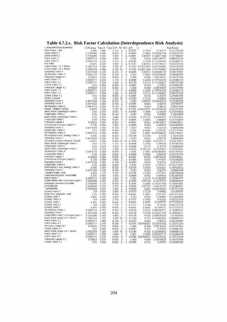
204

12Table 4.7.2.c. Risk Factor Calculation (Interdependence Risk Analysis)

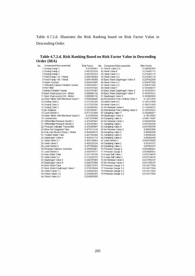
205

Table 4.7.2.d. Illustrates the Risk Ranking based on Risk Factor Value in

Descending Order.

13Table 4.7.2.d. Risk Ranking Based on Risk Factor Value in Descending Order (IRA)

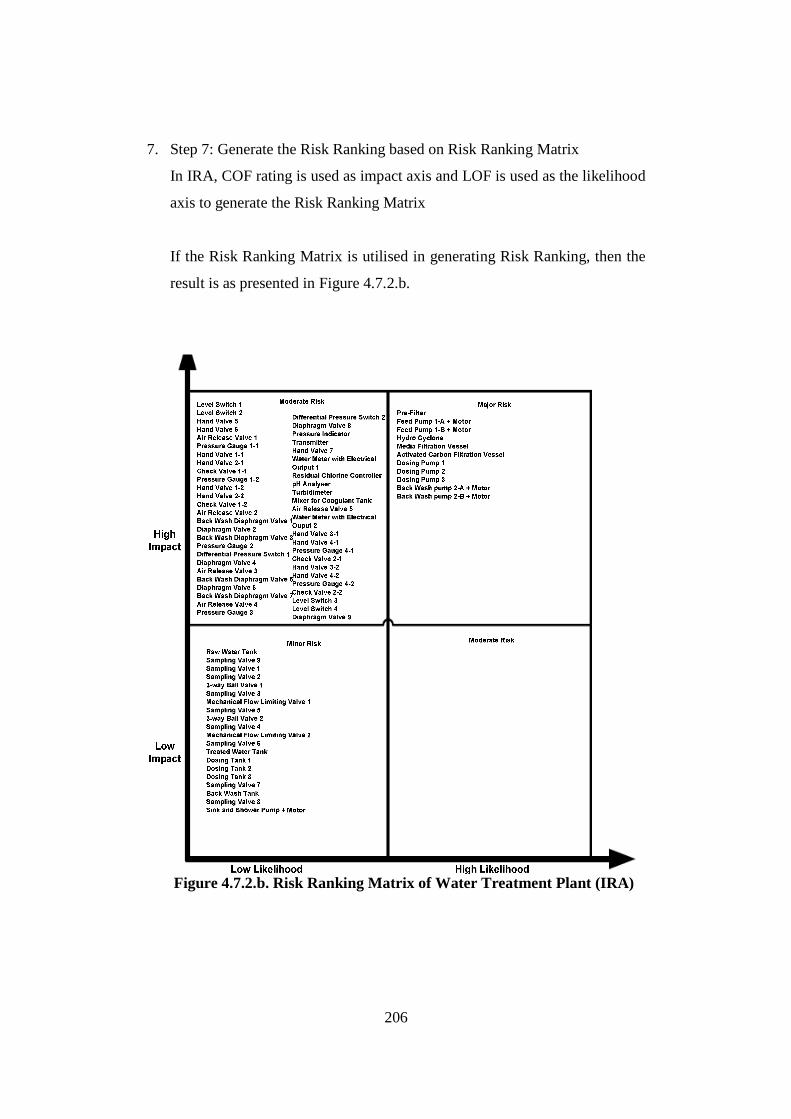
206

7. Step 7: Generate the Risk Ranking based on Risk Ranking Matrix

In IRA, COF rating is used as impact axis and LOF is used as the likelihood

axis to generate the Risk Ranking Matrix

If the Risk Ranking Matrix is utilised in generating Risk Ranking, then the

result is as presented in Figure 4.7.2.b.

62Figure 4.7.2.b. Risk Ranking Matrix of Water Treatment Plant (IRA)

207

From Figure 4.7.2.b., it can be seen that:

1. There are 20 components/sub-assemblies in Minor Risk region (Low

Impact and Low Likelihood)

2. There are 48 components/sub-assemblies in Moderate Risk region (High

Impact and Low Likelihood)

3. There are 0 components/sub-assemblies in Moderate Risk region (Low

Impact and High Likelihood)

4. There are 11 components/sub-assemblies in Major Risk region (High

Impact and High Likelihood)

4.7.3. Discussion IRA method has been used to determine the Risk Consequence and Risk

Likelihood of each component/sub-assembly from the water treatment plant.

The information about Risk Consequence and Risk Likelihood is then

employed as input to the Risk Ranking Development. Two common approaches

to develop Risk Ranking (that is, Risk Factor and Risk Ranking Matrix) are

used. This process has demonstrated the potency of the IRA to address the

problem in the current Risk Analysis method (that is, lack of information to

define Risk Likelihood), because IRA utilised the Interdependence Relationship

to define the Risk Likelihood instead of historical information. However, this

result needs to be validated through the comparison process with the Risk

Ranking of the water treatment plant that is produced by another acknowledged

Risk Analysis method. Risk Analysis based on Failure Mode and Effect

Analysis (FMEA) is chosen to develop the Risk Ranking of the water treatment

plant as the comparator. This method is chosen because:

1. the required information is available

FMEA as the most important information source for this method is

available.

2. it has been acknowledged in industry

208

The RAM Machine Analysis book by Fred Stapelberg from ICS Pty Ltd

(Stapelberg, 1993) suggests this method to perform Risk Analysis.

4.8. Summary

Chapter 4 describes the implementation of Hierarchical Model in developing

Data Bridge and Risk Ranking. Data Bridge development implicitly consists of

two large parts. One part is about implementation of the three analyses in

Hierarchical Model: Hierarchical Analysis, Failure Mode and Effect Analysis,

and Interdependence Analysis. Another part is about the development of Data

Bridge components: Filtering Algorithm, and Knowledge Base.

The purpose of the Hierarchical Analysis is to break down information

hierarchically in order to enable a more accurate information extraction process.

There are three steps in Hierarchical Analysis: Process Analysis, System

Description and System Breakdown. According to Process Analysis, there are

three process flows in the water treatment plant: Normal Water Flow, Back

Wash Water Flow and Direct Wash Water Flow. In the system description,

information from the water treatment plant - such as system primary function,

major subsystems and assemblies, boundaries to other systems and boundary

interface components, and brief description of contents, criteria and boundaries

of the systems - are revealed. By documenting the system description, a clear

overview of the system being analysed is acquired. System Breakdown utilises

results from the previous steps. There are six steps to execute the system

breakdown: Identify Unit/Plant Boundaries; Identify the Systems; Identify the

Assemblies; Identify the Components; Depict the Relationship of SBS Level;

and develop SBS Coding. The SBS for the Water Treatment Plant is established

by executing Step 1 to Step 5. The SBS of water treatment plant consists of 6

systems, 14 assemblies, 18 sub-assemblies and 60 components. Step 6

establishes coding for each part to provide proper identification.

209

FMEA is developed based on information from information sources and SBS

results. Failure identification is only performed at the component or

subassembly level. FMEA development step is divided into two parts,

Functional Explanation and Failure Definition. Result from the FMEA of the

water treatment plant is knowledge of possible failures, including mode, effect

and consequence of each sub-assembly and component. The produced

knowledge from FMEA is very valuable in identifying existing problems if any

abnormality arises from the SCADA data. Therefore, it will be inputted to the

Knowledge Base. Also, this result will be utilised in the Interdependence

Analysis.

Interdependence Analysis is implemented in the case study in order to identify

any interdependence relationship in the system. The result from this analysis

can be used to assist in failure tracing based on the abnormality which is

captured by sensors and alarms. The implementation of the Interdependence

Analysis for the case study is facilitated through Functional and Causal

Relationship Diagram (FCRD). Furthermore, FCRD is able to present the result

of analysis in an easy to understand format - a diagram. Two stages of FCRD of

the case study are developed.

FCRD Stage 1 is to analyse the Dynamic Relationship on the system’s

component level. From the FCRD stage 1 of water treatment plant, major

components can be identified. Major components are the vital items in the

whole process, where the failure of one of them may cause the stoppage of the

whole process. This result is very important in developing the Interdependence

Risk Analysis. Also, the results from FCRD Stage 1 reveal the dynamic

relationship within the water treatment system. This information is presented in

a diagram; thus, it is clearer and easier to understand. The combination of

Graphviz and Microsoft Visio can assist in developing the automatic

diagramming algorithm. This algorithm is able to draw the diagram

210

automatically by only inputting the information. Therefore, a complex diagram

can be drawn easily.

FCRD stage 2 is to transform information into more comprehensive and

manageable format to be inputted into the Data Base. According to the FCRD

stage 2 of water treatment plant, the information from the water treatment plant

is processed into a more manageable format to be inputted to the Knowledge

Base. FCRD Stage 2 is facilitated by developing two diagrams Flow Diagram,

and Sensor and Logic Diagram. Flow Diagram depicts only information on

process sequence-related relationship. According to the result of the

Hierarchical Analysis, there are three different process flows in the water

treatment plant. This information is utilised as a stepping stone to develop the

Flow Diagram. This diagram provides more comprehensive information to

trace any interruption in the process flow. Sensor and Logic Diagram depicts

system indirect relationship (logic control and sensing mechanism relationship).

Information about the cause of any detected abnormality by sensor/alarm is

more apparent by developing this diagram, as it depicts relationship information

between sensor/alarm and components/sub-assemblies. Besides assisting the

development of the Data Bridge, the result from FCRD will also be utilised to

assist the risk calculation on the Interdependence Risk Analysis.

The Filtering algorithm filters only significant data from SCADA data dump.

The filtering algorithm is developed based on the information from Control

Philosophy and P&ID of a Water Treatment Plant Case Study. The filtering

algorithm for the case study is designed to filter only the significant information

from five sensors: Turbidimeter, pH Analyser, Chlorine Controller, Differential

Pressure 1, and Water Meter with Electrical Output 1. The reason the filtering

algorithm is only designed for five sensors is because only five are crucial for

the system.

211

Knowledge Base is adopted in this research because of its ability to store and

retrieve information. All information from the three analyses in the Hierarchical

Model is inputted to a data base. In this research, Data Base is developed in

Microsoft Access and deployed in website using MySQL. All information from

Hierarchical Model is inputted to this Data Base. Besides supplying information

based on a query from the inference engine, the information in Data Base is

utilised by automated diagramming script to generate a diagram (FCRD, Flow

Diagram and Logic and Sensor Diagram). The Automated Diagramming Script

is developed to enable a more efficient and effective complex diagram

development. An Inference Engine is then developed to query information in

the Data Base based on the information on abnormality which has been filtered

by Filtering Algorithm and entered into the data base.

Interdependence Risk Analysis (IRA) is proposed in this research to address the

problem in the current Risk Analysis method (that is, lack of information to

define Risk Likelihood), by utilising interdependence relationship. IRA method

has been used to determine the Risk Consequence and Risk Likelihood of each

component/sub-assembly from the water treatment plant. The information about

Risk Consequence and Risk Likelihood are then employed as inputs to the Risk

Ranking Development. Two common approaches to develop Risk Ranking (i.e.

Risk Factor and Risk Ranking Matrix) are used. This process has demonstrated

the potency of the IRA to address problems in current Risk Analysis methods

(that is, lack of information to define Risk Likelihood), because IRA utilised

Interdependence Relationship to define the Risk Likelihood instead of historical

information. However, this result needs to be validated through the comparison

process with the Risk Ranking of water treatment plant that is produced by

another acknowledged Risk Analysis method. Risk Analysis based on Failure

Mode and Effect Analysis (FMEA) is chosen to develop the Risk Ranking of

the water treatment plant as the comparator. This method is chosen because:

1. the required information is available

212

FMEA as the most important information source for this method is

available.

2. it has been acknowledged in industry

The RAM Machine Analysis book by Fred Stapelberg from ICS Pty Ltd

(Stapelberg, 1993) suggests this as an appropriate method to perform Risk

Analysis.

213

CHAPTER 5

CASE STUDY: MODEL DATA

ANALYSIS

5.1. Introduction

The case study of water treatment plant contains two different data types:

qualitative data and quantitative data. Qualitative data comes from P&ID,

Control Philosophy and Trouble Shooting, while quantitative data comes from

SCADA Data Dump. In addition, because the data comes in two different types,

the analysis must be separated. Quantitative data can be analysed

mathematically and statistically (refer to Section 5.2.), while qualitative data

cannot be analysed either by using a mathematical operation nor statistical

method (refer to Section 5.3.).

5.2. Quantitative Data Analysis

5.2.1. Introduction There are two important components of quantitative data analysis: data

cleansing and statistical analysis. According to Wikipedia (2006), data

cleansing is detecting and correcting (or removing) corrupt, inaccurate or

redundant records from a record set. Applying data cleansing to the SCADA

data dump before utilising them in the validation, is essential to avoid

214

inaccurate validation results which lead to incorrect analysis. Statistical analysis

is applied to the SCADA data dump to reveal further information that can be

useful in the validation process. Statistical methods that will be applied are

Descriptive Statistic and Correlation Analysis.

5.2.2. Data Cleansing

The SCADA data dump from the case study contains the sensor values which

are recorded every one hour for 22 days (521 points of measurement). The first

step in data cleansing is to identify any measurement points that have the

potential to cause inaccurate validation results. After further analysis of the 521

points of measurements, 240 points of measurement have the potential to cause

inaccurate validation results. It is because the value of the flow sensor is 0 (that

is, no flow) when the 240 points of measurement were taken. If those 240

points of measurement are still used in the validation step, the result tends to be

inaccurate, since those measurement points contain biased information. The

reason is that the values of the three other sensors (pH, Chlorine, and Turbidity)

fluctuate when the system is not working (detail in Table 5.2.2.). This means

that the fluctuating sensors’ value is not caused by the components in the

system. Thus, these measurement points are excluded in the validation step to

avoid any inaccurate validation results.

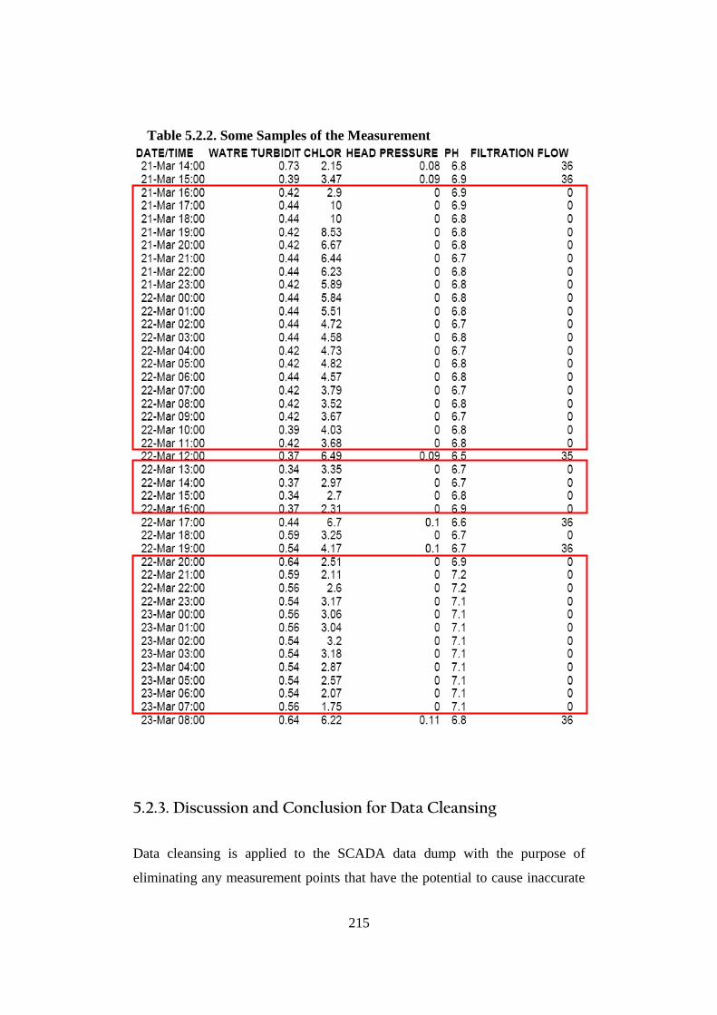
215

14Table 5.2.2. Some Samples of the Measurement

5.2.3. Discussion and Conclusion for Data Cleansing

Data cleansing is applied to the SCADA data dump with the purpose of

eliminating any measurement points that have the potential to cause inaccurate

216

validation results. After the whole data is analysed, it is identified that 240

points of measurement have the potential to give inaccurate validation results

because they contain biased information. Thus these measurement points are

excluded in the validation step.

5.2.4. Statistical Analysis: Descriptive Statistics

Statistical Analysis of the SCADA data dump is performed to reveal further

information that can be useful in the validation step. At first, the Descriptive

Statistics method is employed to gain further information from the SCADA

data dump. The result from the Descriptive Statistics (that is, the determination

of whether the data distribution of each sensor is normal distribution or not)

will determine the method that will be employed in the Correlation Analysis.

In the Descriptive Statistic, initially the data from each sensor is plotted on the

histogram to provide preliminary information about the data distribution. Then,

several parameters are assessed such as:

• Mean

• Median

• Mode

• Variance

• Standard Deviation

• Maximum

• Minimum

• Range

• Interquartile Range

• Skewness and

• Kurtosis

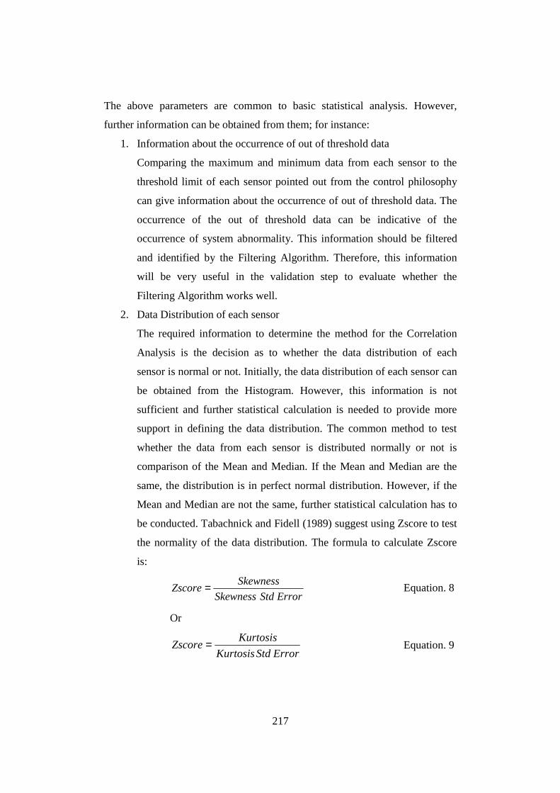
217

The above parameters are common to basic statistical analysis. However,

further information can be obtained from them; for instance:

1. Information about the occurrence of out of threshold data

Comparing the maximum and minimum data from each sensor to the

threshold limit of each sensor pointed out from the control philosophy

can give information about the occurrence of out of threshold data. The

occurrence of the out of threshold data can be indicative of the

occurrence of system abnormality. This information should be filtered

and identified by the Filtering Algorithm. Therefore, this information

will be very useful in the validation step to evaluate whether the

Filtering Algorithm works well.

2. Data Distribution of each sensor

The required information to determine the method for the Correlation

Analysis is the decision as to whether the data distribution of each

sensor is normal or not. Initially, the data distribution of each sensor can

be obtained from the Histogram. However, this information is not

sufficient and further statistical calculation is needed to provide more

support in defining the data distribution. The common method to test

whether the data from each sensor is distributed normally or not is

comparison of the Mean and Median. If the Mean and Median are the

same, the distribution is in perfect normal distribution. However, if the

Mean and Median are not the same, further statistical calculation has to

be conducted. Tabachnick and Fidell (1989) suggest using Zscore to test

the normality of the data distribution. The formula to calculate Zscore

is:

ErrorStdSkewness

SkewnessZscore= Equation. 8

Or

ErrorStdKurtosis

KurtosisZscore= Equation. 9

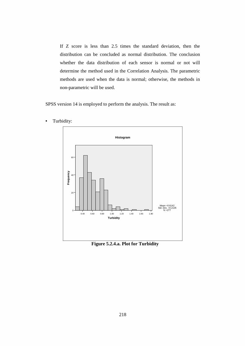
218

If Z score is less than 2.5 times the standard deviation, then the

distribution can be concluded as normal distribution. The conclusion

whether the data distribution of each sensor is normal or not will

determine the method used in the Correlation Analysis. The parametric

methods are used when the data is normal; otherwise, the methods in

non-parametric will be used.

SPSS version 14 is employed to perform the analysis. The result as:

• Turbidity:

1.801.601.401.201.000.800.600.40

Turbidity

60

40

20

0

Fre

qu

ency

Mean =0.6142;Std. Dev. =0.2135;

N =277

Histogram

63Figure 5.2.4.a. Plot for Turbidity

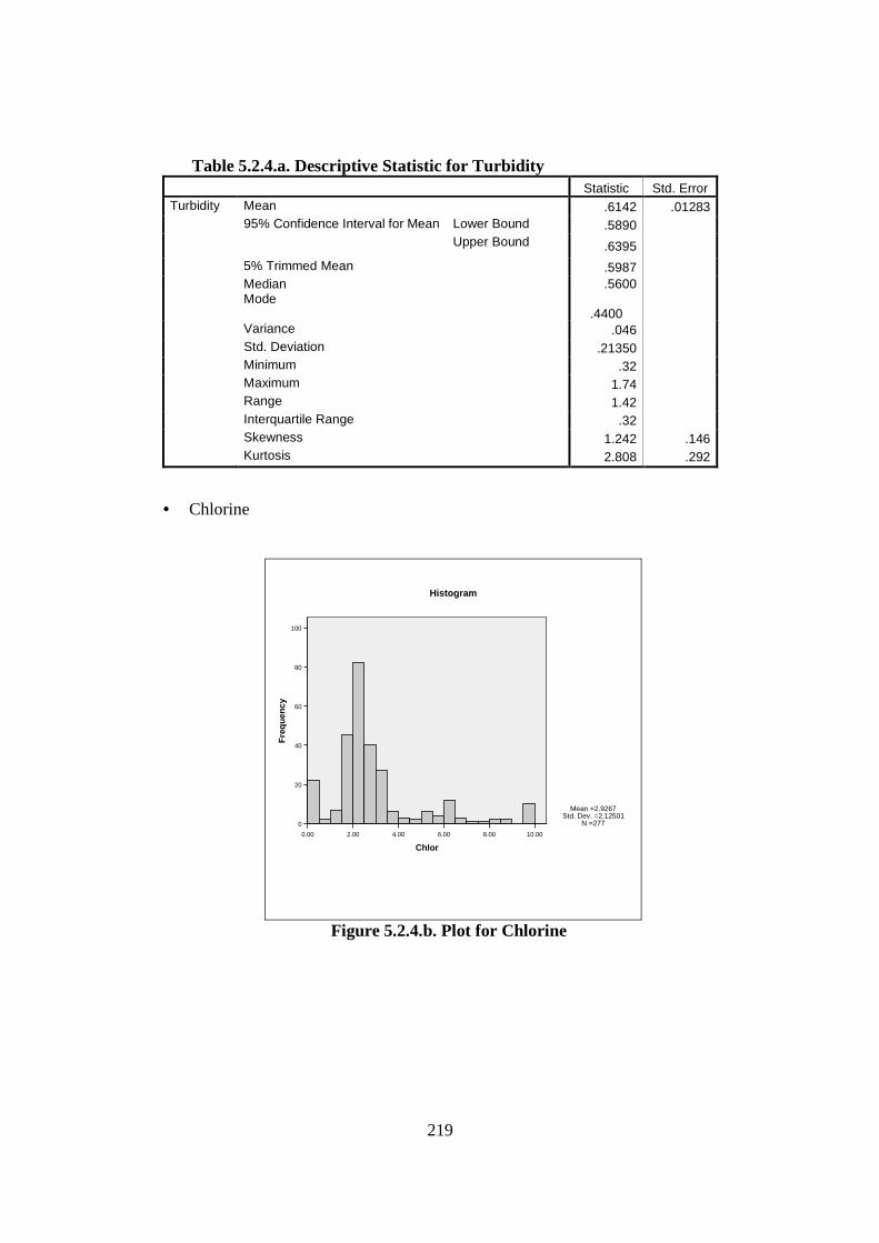
219

15Table 5.2.4.a. Descriptive Statistic for Turbidity Statistic Std. Error Turbidity Mean .6142 .01283 95% Confidence Interval for Mean Lower Bound .5890 Upper Bound .6395

5% Trimmed Mean .5987 Median

Mode .5600

.4400

Variance .046 Std. Deviation .21350 Minimum .32 Maximum 1.74 Range 1.42 Interquartile Range .32 Skewness 1.242 .146 Kurtosis 2.808 .292

• Chlorine

10.008.006.004.002.000.00

Chlor

100

80

60

40

20

0

Fre

qu

ency

Mean =2.9267;Std. Dev. =2.12501;

N =277

Histogram

64Figure 5.2.4.b. Plot for Chlorine

220

16Table 5.2.4.b. Descriptive Statistic for Chlorine Statistic Std. Error Chlor Mean 2.9267 .12768 95% Confidence

Interval for Mean Lower Bound 2.6754

Upper Bound 3.1781

5% Trimmed Mean 2.7197 Median

Mode 2.3000

.00

Variance 4.516 Std. Deviation 2.12501 Minimum .00 Maximum 10.00 Range 10.00 Interquartile Range 1.21 Skewness 1.713 .146 Kurtosis 3.148 .292

• Head Pressure

0.400.200.00

HPressure

100

80

60

40

20

0

Fre

qu

ency

Mean =0.1031;Std. Dev. =0.05195;

N =277

Histogram

65Figure 5.2.4.c. Plot for Head Pressure

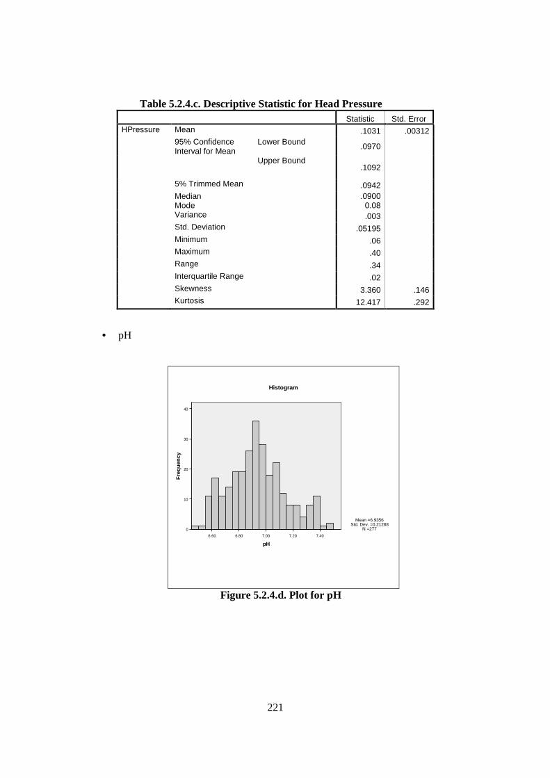
221

17Table 5.2.4.c. Descriptive Statistic for Head Pressure Statistic Std. Error HPressure Mean .1031 .00312 95% Confidence

Interval for Mean Lower Bound .0970

Upper Bound .1092

5% Trimmed Mean .0942 Median

Mode .0900

0.08

Variance .003 Std. Deviation .05195 Minimum .06 Maximum .40 Range .34 Interquartile Range .02 Skewness 3.360 .146 Kurtosis 12.417 .292

• pH

7.407.207.006.806.60

pH

40

30

20

10

0

Fre

qu

ency

Mean =6.9356;Std. Dev. =0.21288;

N =277

Histogram

66Figure 5.2.4.d. Plot for pH

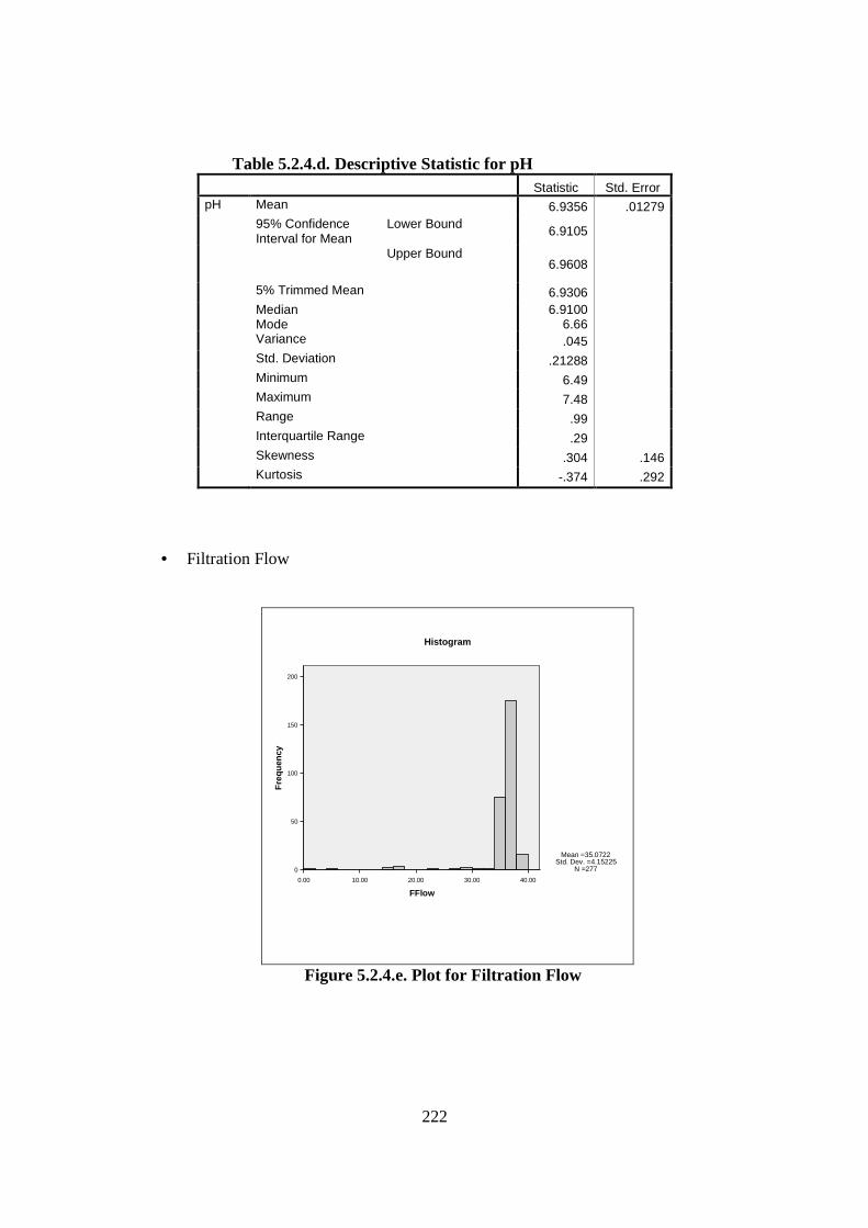
222

18Table 5.2.4.d. Descriptive Statistic for pH Statistic Std. Error pH Mean 6.9356 .01279 95% Confidence

Interval for Mean Lower Bound 6.9105

Upper Bound 6.9608

5% Trimmed Mean 6.9306 Median

Mode 6.9100

6.66

Variance .045 Std. Deviation .21288 Minimum 6.49 Maximum 7.48 Range .99 Interquartile Range .29 Skewness .304 .146 Kurtosis -.374 .292

• Filtration Flow

40.0030.0020.0010.000.00

FFlow

200

150

100

50

0

Fre

qu

ency

Mean =35.0722;Std. Dev. =4.15225;

N =277

Histogram

67Figure 5.2.4.e. Plot for Filtration Flow

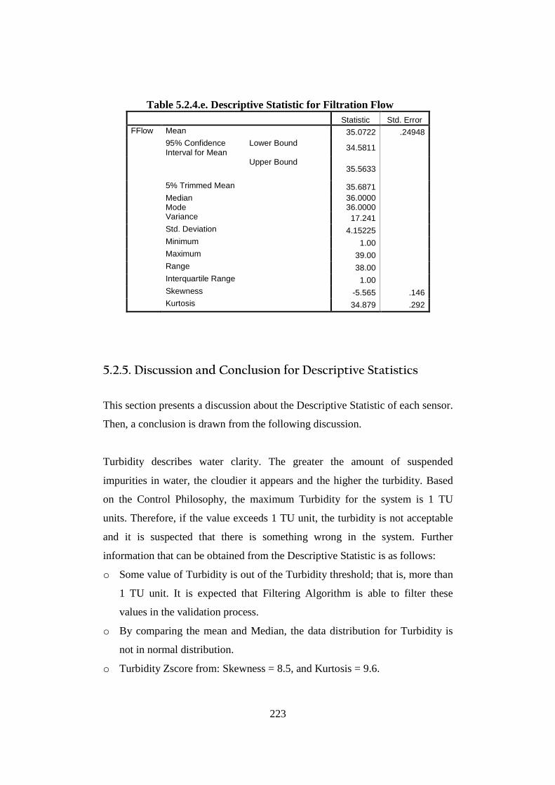
223

19Table 5.2.4.e. Descriptive Statistic for Filtration Flow Statistic Std. Error FFlow Mean 35.0722 .24948 95% Confidence

Interval for Mean Lower Bound 34.5811

Upper Bound 35.5633

5% Trimmed Mean 35.6871 Median

Mode 36.0000 36.0000

Variance 17.241 Std. Deviation 4.15225 Minimum 1.00 Maximum 39.00 Range 38.00 Interquartile Range 1.00 Skewness -5.565 .146 Kurtosis 34.879 .292

5.2.5. Discussion and Conclusion for Descriptive Statistics

This section presents a discussion about the Descriptive Statistic of each sensor.

Then, a conclusion is drawn from the following discussion.

Turbidity describes water clarity. The greater the amount of suspended

impurities in water, the cloudier it appears and the higher the turbidity. Based

on the Control Philosophy, the maximum Turbidity for the system is 1 TU

units. Therefore, if the value exceeds 1 TU unit, the turbidity is not acceptable

and it is suspected that there is something wrong in the system. Further

information that can be obtained from the Descriptive Statistic is as follows:

o Some value of Turbidity is out of the Turbidity threshold; that is, more than

1 TU unit. It is expected that Filtering Algorithm is able to filter these

values in the validation process.

o By comparing the mean and Median, the data distribution for Turbidity is

not in normal distribution.

o Turbidity Zscore from: Skewness = 8.5, and Kurtosis = 9.6.

224

2.5 x Standard Deviation = 0.53375.

Therefore, the Zscore is much larger than 2.5 times standard deviation. The

result from this test supports the conclusion that the data distribution for

Turbidity is not a normal distribution.

In the water treatment process, the sodium hypochlorite solution is used as a

disinfecting agent. However, the minimum level of free chlorine residual has to

be maintained in order to achieve good potable water. According to the control

philosophy, the minimum level of the free chlorine residual is 0.4 mg/L. If the

value is below this level, the system probably does not work properly. Further

information that can be obtained from the Descriptive Statistic is:

o Some value of Chlorine is out of the Chlorine threshold; that is, less than

0.4 mg/L. It is expected that the Filtering Algorithm is able to filter these

values in the validation process.

o By comparing the Mean and Median, the data distribution for Chlorine is

not a normal distribution.

o Chlorine Zscore from: Skewness = 11.73, and Kurtosis = 10.78.

2.5 x Standard Deviation = 5.312525.

Therefore, the Zscore is much larger than 2.5 times standard deviation.

Results from this test give more support to the conclusion that the data

distribution for Chlorine is not in normal distribution.

The Head Pressure value is taken from the differential pressure transmitter,

which is located at the multi media filter. The value of head pressure represents

the condition of the filter – whether in a good or clogged condition. The higher

the pressure, the more it is clogged. Therefore, the head pressure is important to

be monitored. From the Control Philosophy, the maximum value of the head

pressure is 0.5 bar. If the value of the head pressure is more than 0.5 bar, then

the backwash process is operated. However, if the value is still more than 0.5

bar, then there could be abnormality in the system. Further information that can

be obtained from the Descriptive Statistic is:

225

o No value of Head Pressure is above the Head Pressure threshold. The

Filtering Algorithm is not expected to filter any value out of this sensor in

the validation process.

o By comparing the mean and Median, the data distribution for Head Pressure

is not normal distribution.

o Head Pressure Zscore from: Skewness = 23.02, and Kurtosis = 42.52.

2.5 x Standard Deviation = 0.129875.

Therefore, the Zscore is much larger than 2.5 times standard deviation. The

result from this test gives more support for the conclusion that the data

distribution for Head Pressure is not in normal distribution.

The pH measurement is used to determine the relative acidic or basic level of

water by measuring the concentration of hydrogen ions. The pH scale ranges

from 0 to 14; pH 7 means neutral, below 7 is more acidic and above 7 is more

basic. pH is one of the crucial parameter for potable water; therefore, it is very

important to monitor the pH level. Based on the Control Philosophy, the pH

must be maintained between 6.5 and 8.5. If pH is outside that range, the

mechanism to revise the pH level is triggered to take the pH level back in the

range. Therefore, if the value from the pH sensor is out of the range, it means

that there is something wrong with the mechanism to revise the pH level.

Further information that can be obtained from the Descriptive Statistic as:

o Some value of pH is out of the pH threshold. It is expected that the Filtering

Algorithm is able to filter these values in the validation process.

o By comparing the Mean and Median, the data distribution for pH is not

normal distribution.

o pH Zscore from: Skewness = 2.56, and Kurtosis = 1.04.

2.5 x Standard Deviation = 0.5322.

Therefore, the Zscore is much larger than 2.5 times standard deviation. The

result from this test gives more support to the conclusion that the data

distribution for pH is not in normal distribution.

226

Filtration Flow is measured by water flow meter 1. From this measurement, the

state of the system is known (whether the process is running or not). As

mentioned before, the data which will be used for the validation step is only

when the system is working. Therefore, there is no 0 value of the filtration flow.

Further information that can be obtained from the Descriptive Statistic is:

o No value of Filtration Flow is out of the Filtration Flow threshold. The

Filtering Algorithm is not expected to filter any value out of this sensor in

the validation process.

o By comparing the mean and median, the data distribution for Filtration

Flow is not in normal distribution.

o Head Pressure Zscore from: Skewness = 23.84, and Kurtosis = 1.88.

2.5 x Standard Deviation = 1.038.

Therefore, the Zscore is much larger than 2.5 times standard deviation. The

result from this test gives more support to the conclusion that the data

distribution for Filtration Flow is not in normal distribution.

Hence, the conclusions from the Descriptive Statistic are:

• Some values from three sensors - Turbidity, Chlorine, and pH - are out of

the threshold. Therefore, Filtering Algorithm is expected to filter and pick

these values in the validation process.

• No value from two sensors: Head Pressure and Filtration Flow is out of the

threshold. Therefore, Filtering Algorithm is not expected to filter any value

out of this sensor in the validation process.

• None of the data distribution from these sensors is in normal distribution.

Thus, only non-parametric methods can be employed in the Correlation

Analysis.

227

5.2.6. Statistical Analysis: Correlation Analysis

A correlation is a single number that describes the degree of relationship

between two variables (Trochim, 2006). The most famous method for testing

the strength of linear association between measured variables is the Pearson

Correlation method. However, the Pearson Correlation method can only be

applied to normal distributed data. According to the Descriptive Statistical

analysis, none of the parameters is distributed normally. Therefore, the Pearson

Correlation method cannot be utilised for the data.

If the parameter is not distributed normally, then the most suitable correlation

method is Non-Parametric (Tabachnick and Fidell, 1989). The derivation of the

Pearson Correlation method for the non-parametric statistical analysis domain

is the Spearman Correlation Method. Therefore, the Spearman Correlation

Method is used to test the correlation between each parameter.

The main purpose of this analysis is to verify that data from Turbidity, Chlorine

and pH sensors are related to each other. These parameters are used to justify

the quality of water. Typically, Turbidity can influence the value of pH and

Chlorine (Health, 2008); and changes in Chlorine can influence the value of pH

(IOTEG, 2008). Therefore, there has to be a correlation between the

measurements from these sensors to verify that they are logically acceptable.

However, besides these three sensors, Correlation Analysis is also conducted

for the other two sensors (Head Pressure and Filtration Flow) to discover any

relationship between them.

SPSS 14 is employed to perform the statistical process. Following is the result

from this process:

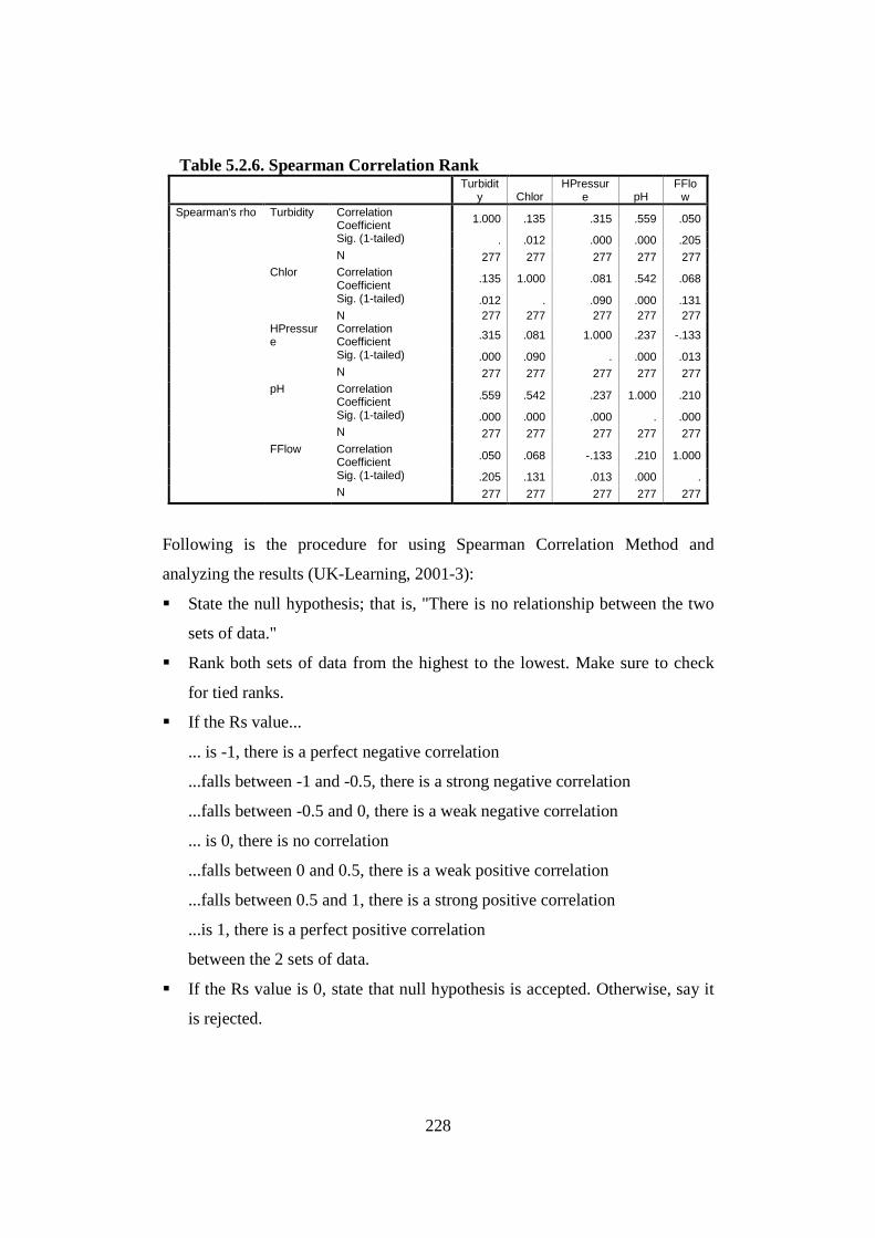
228

20Table 5.2.6. Spearman Correlation Rank

Turbidit

y Chlor HPressur

e pH FFlo

w Spearman's rho Turbidity Correlation

Coefficient 1.000 .135 .315 .559 .050

Sig. (1-tailed) . .012 .000 .000 .205 N 277 277 277 277 277 Chlor Correlation

Coefficient .135 1.000 .081 .542 .068

Sig. (1-tailed) .012 . .090 .000 .131 N 277 277 277 277 277 HPressur

e Correlation Coefficient .315 .081 1.000 .237 -.133

Sig. (1-tailed) .000 .090 . .000 .013 N 277 277 277 277 277 pH Correlation

Coefficient .559 .542 .237 1.000 .210

Sig. (1-tailed) .000 .000 .000 . .000 N 277 277 277 277 277 FFlow Correlation

Coefficient .050 .068 -.133 .210 1.000

Sig. (1-tailed) .205 .131 .013 .000 . N 277 277 277 277 277

Following is the procedure for using Spearman Correlation Method and

analyzing the results (UK-Learning, 2001-3):

� State the null hypothesis; that is, "There is no relationship between the two

sets of data."

� Rank both sets of data from the highest to the lowest. Make sure to check

for tied ranks.

� If the Rs value...

... is -1, there is a perfect negative correlation

...falls between -1 and -0.5, there is a strong negative correlation

...falls between -0.5 and 0, there is a weak negative correlation

... is 0, there is no correlation

...falls between 0 and 0.5, there is a weak positive correlation

...falls between 0.5 and 1, there is a strong positive correlation

...is 1, there is a perfect positive correlation

between the 2 sets of data.

� If the Rs value is 0, state that null hypothesis is accepted. Otherwise, say it

is rejected.

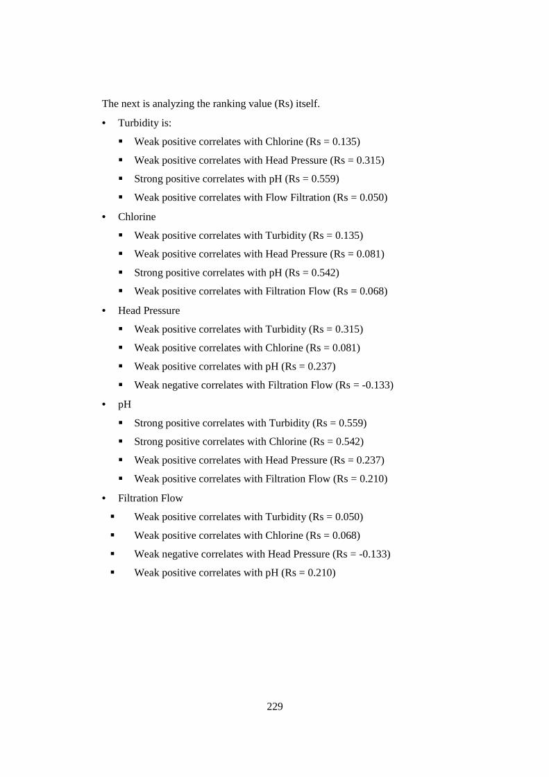
229

The next is analyzing the ranking value (Rs) itself.

• Turbidity is:

� Weak positive correlates with Chlorine (Rs = 0.135)

� Weak positive correlates with Head Pressure (Rs = 0.315)

� Strong positive correlates with pH (Rs = 0.559)

� Weak positive correlates with Flow Filtration (Rs = 0.050)

• Chlorine

� Weak positive correlates with Turbidity (Rs = 0.135)

� Weak positive correlates with Head Pressure (Rs = 0.081)

� Strong positive correlates with pH (Rs = 0.542)

� Weak positive correlates with Filtration Flow (Rs = 0.068)

• Head Pressure

� Weak positive correlates with Turbidity (Rs = 0.315)

� Weak positive correlates with Chlorine (Rs = 0.081)

� Weak positive correlates with pH (Rs = 0.237)

� Weak negative correlates with Filtration Flow (Rs = -0.133)

• pH

� Strong positive correlates with Turbidity (Rs = 0.559)

� Strong positive correlates with Chlorine (Rs = 0.542)

� Weak positive correlates with Head Pressure (Rs = 0.237)

� Weak positive correlates with Filtration Flow (Rs = 0.210)

• Filtration Flow

� Weak positive correlates with Turbidity (Rs = 0.050)

� Weak positive correlates with Chlorine (Rs = 0.068)

� Weak negative correlates with Head Pressure (Rs = -0.133)

� Weak positive correlates with pH (Rs = 0.210)

230

5.2.7. Discussion and Conclusion for Correlation Analysis

Results from the Correlation Analysis show that data from Chlorine, Turbidity

and pH have a strong positive correlation with each other. Thus, this result

verifies that data from these sensors are logically acceptable because they

follow the common facts. Data from the other two sensors (Head Pressure and

Filtering Flow) only have a weak correlation with the others.

5.3. Qualitative Data Analysis

5.3.1. Introduction

Qualitative data cannot be analysed with quantitative data analysis (neither

mathematically nor statistically). Jorgensen (1989) concluded that qualitative

data analysis is about sorting and shifting the data to search for types, classes,

sequences, processes, patterns or wholes.

The purpose of this analysis is to discover any important information from the

qualitative data. This information will be then utilised to support the validation

process.

From the case study, there are three documents that contain qualitative data:

P&ID, Control Philosophy, and Trouble Shooting. P&ID and Control

Philosophy are analysed based on the developed model (Hierarchical Model).

Therefore, no analysis is applied to those documents in this Chapter; only

trouble shooting is analysed.

231

5.3.2. Qualitative Data Analysis: Trouble Shooting

Trouble shooting is a systematic approach to locate the cause of a fault, based

on a system’s abnormality information (Jeng and Liang, 1998). It consists of a

list of potential failure based on the designer or maker experience. The Trouble

Shooting of a water treatment plant is in table format with three columns. The

first column is the explanation of the abnormality, the second column is the

possible causes of the abnormality and the third column is the solutions to the

abnormality. This Trouble Shooting will be used as the comparator in the

validation step where output from the proposed method will be compared with

the output from the trouble shooting, based on the same system’s abnormality

information.

There are 10 abnormal cases listed in the trouble shooting. Those abnormal

cases are sorted by classifying the information source of the abnormality; that

is, whether the information source is from sensors or not. The reason behind

this is that SCADA can only detect abnormality/failure based on the sensors’

measurement. Therefore, abnormalities/failures, which cannot be identified by

sensors, are irrelevant for the validation step. Based on the sorting, only four

abnormal cases are relevant for the validation step:

• Back-flush is repetitive

• Filtered water quality is bad according to Turbidimeter

• Residual chlorine low alarm is on

• pH high or low alarm is on.

Hence, in the validation process, information from these four abnormal cases

will be utilised as an input to the proposed method (Data Bridge). Then, the

output from the Data Bridge will be compared with the solution from the

Trouble Shooting (information in Column 3).

232

5.3.3. Discussion and Conclusion

Qualitative Analysis has been performed to analyse qualitative data with the

purpose to discover any further important information to be used in the

validation process. There are several documents from the case study that

contain qualitative data: P&ID, Control Philosophy and Trouble Shooting.

P&ID and Control Philosophy are analysed based on the developed method

(Hierarchical Model). Thus, only Trouble Shooting is analysed qualitatively.

The Trouble Shooting of the case study encloses ten abnormal cases. Each

abnormal case has the explanation of the abnormality, possible causes of the

abnormality and solutions to the abnormality. The Qualitative Analysis is

initiated by sorting out the abnormality based on the source of information.

Only abnormalities which can be identified by the sensor are applicable in the

validation process. The reason behind this is that SCADA can only detect

abnormality/failure based on the sensors measurement. There are four abnormal

cases that can be identified by sensor: Back-flush is repetitive, Filtered water

quality is bad according to Turbidimeter, Residual Chlorine low alarm is on,

and pH high or low alarm is on. Therefore, these four abnormal cases will be

employed as comparators in validation process.

5.4. Summary Chapter 5 elucidates the Data Analysis of the case study of water treatment

plant. The case study of water treatment plant contains two different data types:

qualitative data and quantitative data. Qualitative data comes from P&ID,

Control Philosophy and Trouble Shooting, while quantitative data comes from

SCADA Data Dump. In addition, because the data comes in two different types,

the analysis must be separated. Quantitative data can be analysed

mathematically and statistically, while qualitative data cannot be analysed

either by using mathematical operation or statistical method.

233

Quantitative Data Analysis is initiated with Data Cleansing. It is applied to the

SCADA data dump before utilising them in the validation system with the

purpose to identify and correct corrupt, inaccurate or redundant data. Therefore,

inaccurate validation results which lead to incorrect analysis can be avoided.

After the whole data is analysed, it is identified that 240 points of measurement

have the potential to cause inaccurate validation results because they contain

biased information. Thus, these measurement points are excluded in the

validation step.

The next step in Quantitative Data Analysis is to conduct a Statistical Analysis

of the SCADA data dump with the purpose to reveal further information that

can be useful in the validation process. The statistical methods that will be

applied are Descriptive Statistic and Correlation Analysis.

Further information that can be explored as a result of Descriptive Statistic is:

• Some values from three sensors - Turbidity, Chlorine, and pH - are out of

the threshold. Therefore, Filtering Algorithm is expected to filter and pick

these values in validation process.

• No value from two sensors - Head Pressure and Filtration Flow - is out of

the threshold. Therefore, Filtering Algorithm is not expected to filter any

value out of this sensor in validation process.

• None of the data distribution from these sensors is normal distribution.

Thus, only non-parametric methods can be employed in the Correlation

Analysis.

The Statistical Method that is used in the Correlation Analysis is the Spearman

Correlation Method, because none of the parameters’ distribution is normal

according to the Descriptive Statistic result. Mainly, the purpose of this analysis

is to verify that data from Turbidity, Chlorine and pH sensors are related to

each other, because they are typically related according to the literature.

Therefore, there has to be a correlation between the measurements from these

sensors to verify that they are logically acceptable. However, besides these

234

three sensors, Correlation Analysis is also conducted on the other two sensors

(Head Pressure and Filtration Flow) to discover any relationship between them.

Results from the Correlation Analysis show that data from Chlorine, Turbidity

and pH have strong positive correlation with each other. Thus, this result

verifies that data from these sensors are logically acceptable because they

follow the common facts. Data from the other two sensors (Head Pressure and

Filtering Flow) only have weak correlation with the others.

Qualitative Data Analysis is conducted to analyse the Qualitative Data with the

purpose to discover any important information from the qualitative data. This

information will be then utilised to support the validation process. From the

case study, there are three documents that contain qualitative data: P&ID,

Control Philosophy, and Trouble Shooting. P&ID and Control Philosophy are

analysed based on the developed model (Hierarchical Model). Therefore,

Qualitative Data Analysis is only applied to the Trouble Shooting document.

The Trouble Shooting of the case study encloses ten abnormal cases. Each

abnormal case has the explanation of the abnormality, possible causes of the

abnormality and solutions to the abnormality. The Qualitative Analysis is

initiated by sorting out the abnormality based on the source of information.

Only abnormalities which can be identified by sensor are applicable in the

validation process. The reason behind this is that only SCADA can detect

abnormality/failure based on the sensors measurement. There are 4 abnormal

cases that can be identified by sensor: Back-flush is repetitive, Filtered water

quality is bad according to Turbidimeter, Residual Chlorine low alarm is on,

and pH high or low alarm is on. Therefore, these four abnormal cases will be

employed as comparators in the validation process.

235

CHAPTER 6

CASE STUDY: MODEL DATA

VALIDATION

6.1. Introduction In the previous Chapter 4 and Chapter 5, all information from the water

treatment plant was compiled and prepared for validation. In this chapter, all

information is utilised to validate the proposed model by testing the proposed

hypotheses. There are 3 hypotheses proposed in this research:

1. Problems in SCADA data analysis, such as nested data, can be addressed by

analysing design information of monitored and monitoring systems through

the Hierarchical Model.

2. The Interdependence Risk Analysis method can address current Risk

Analysis method problems; that is, the need for sophisticated historical

information as an input for Risk Likelihood.

3. The data bridge developed from the Hierarchical Model will address the

connectivity problem between SCADA systems and ERP systems, whereby

significant information can be drawn out from SCADA’s “raw data” and

transferred into ERP.

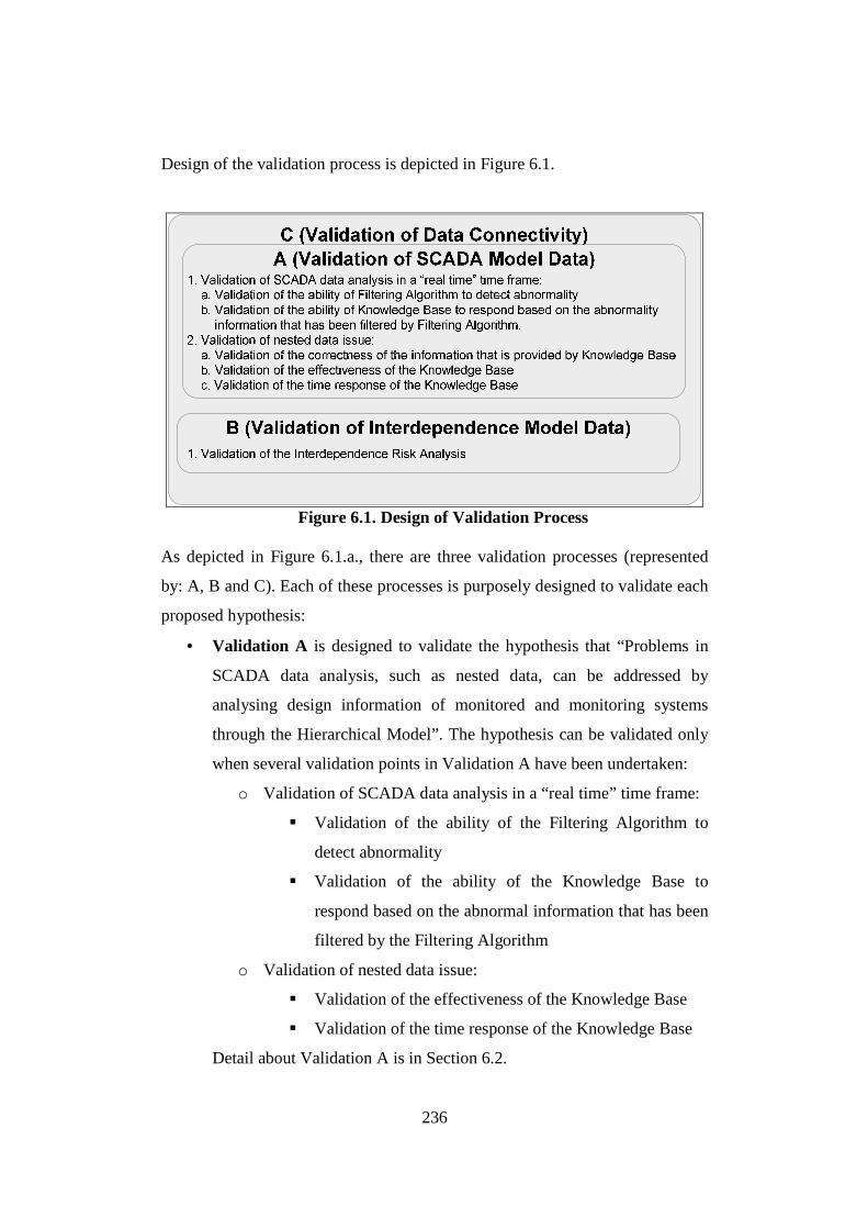
236

Design of the validation process is depicted in Figure 6.1.

68Figure 6.1. Design of Validation Process

As depicted in Figure 6.1.a., there are three validation processes (represented

by: A, B and C). Each of these processes is purposely designed to validate each

proposed hypothesis:

• Validation A is designed to validate the hypothesis that “Problems in

SCADA data analysis, such as nested data, can be addressed by

analysing design information of monitored and monitoring systems

through the Hierarchical Model”. The hypothesis can be validated only

when several validation points in Validation A have been undertaken:

o Validation of SCADA data analysis in a “real time” time frame:

� Validation of the ability of the Filtering Algorithm to

detect abnormality

� Validation of the ability of the Knowledge Base to

respond based on the abnormal information that has been

filtered by the Filtering Algorithm

o Validation of nested data issue:

� Validation of the effectiveness of the Knowledge Base

� Validation of the time response of the Knowledge Base

Detail about Validation A is in Section 6.2.

237

• Validation B is designed to validate the hypothesis: “The

Interdependence Risk Analysis method can address current Risk

Analysis method problems; that is, the need for sophisticated historical

information as an input for Risk Likelihood”. This hypothesis can be

validated only when the “Validation of the Interdependence Risk

Analysis” has been done. Detail about Validation B is in Section 6.3.

• Validation C is designed to validate the hypothesis: “The data bridge

developed from the Hierarchical Model will address the connectivity

problem between SCADA systems and ERP systems, whereby

significant information can be drawn out from SCADA’s “raw data”

and transferred into ERP”. The validation of this hypothesis depends on

the success of the other two validations (A and B), where the success of

those two validations will automatically ensure the Validation C

process. Detail about Validation C is in Section 6.4.

6.2. Validation A (Validation of SCADA Model Data)

6.2.1. Introduction

Validation of the hypothesis that “Problems in SCADA data analysis, such as

nested data, can be addressed by analysing design information of monitored and

monitoring systems through the Hierarchical Model” is carried out in

Validation A. There are two points that need to be validated:

• Validation of SCADA data analysis in a “real time” time frame

At this point, Data Bridge as the end result from the Hierarchical Model

is validated whether it can work as it is designed or not. The validation

is carried out by feeding the SCADA Data Dump into the Data Bridge.

Then, it will analyse the data, find any abnormality and provide

238

information about the possible abnormality sources. The results will be

compared with information from Statistical Analysis, and the Sensor

and Logic Diagram. There are two parts in this validation:

o Validation of the ability of the Filtering Algorithm to detect

abnormality

In this part, the validation is focused on the Filtering

Algorithm’s ability to detect any abnormality based on data from

sensors. Results from Statistical Analysis (identified data that is

out of threshold) are used as a comparison.

o Validation of the ability of the Knowledge Base to respond

based on the abnormal information that has been filtered by

filtering algorithm.

This part is the continuation of the previous part where the

Filtering Algorithm is tested in terms of its ability to detect any

abnormality based on SCADA data. By design, the Knowledge

Base will respond if any abnormality is filtered out by the

Filtering Algorithm, by providing information about possible

sources of that abnormality. Information from the Sensor and

Logic Diagram will be used as a comparison to verify whether or

not the Knowledge Base works as it is designed.

• Validation of the nested data issue

The purpose of this validation is to prove that the proposed Hierarchical

Model is able to solve the nested data issue. The validation is carried out

by comparing information, which is provided by Data Bridge, to the

Trouble Shooting from the system designer. In the previous point, the

source of abnormalities is not known. The only known information is

SCADA Data Dump. SCADA Data Dump is then fed into the Filtering

Algorithm to find any abnormalities, and then transmits this information

to the Knowledge Base. The Knowledge Base responds by providing

information on the possible causes of the system abnormality. However,

at this point, the abnormal condition is known and gathered from

239

Trouble Shooting. The data from sensors is situated as if the abnormal

condition was present. After that, this data is fed into the Knowledge

Base. The Knowledge Base will respond by providing information on

the possible sources of abnormality. The result is then validated by

comparing the response from the Knowledge Base to the known

abnormality. There are three validation parts to measure the success of

the proposed Hierarchical Model in addressing the nested data issue:

o Validation of correctness of the information that is provided by

the Knowledge Base

In this part, validation is used to measure the ability of the

Knowledge Base to provide the correct information on the

possible abnormality sources based on the situated abnormal

condition. Trouble Shooting is used as the comparison in this

validation.

o Validation of the effectiveness of the Knowledge Base

The focus of this validation is beyond the correctness of the

response from the Knowledge Base; it is about effectiveness.

Sometimes, the correct answer is not always effective when the

Knowledge Base can provide a response which ranges from 1 to

the maximum possible number of abnormality sources. If the

Knowledge Base provides the maximum number of possible

abnormality sources, it could mean that the Knowledge Base

tells the operator to check the whole components/sub-assemblies

in the system. Providing this type of information cannot be

judged to be incorrect; in fact, the greater the number of possible

abnormality sources, the higher the chance of correctness.

However, the greater the number of possible information

sources, the more time is spent checking each possibility. The

ideal condition of each abnormality inspection will result in only

one correct solution.

o Validation of the time response of the Knowledge Base

240

This validation phase tries to measure the time required by the

Knowledge Base to provide a response based on abnormal

information.

6.2.2. Validation of SCADA data analysis in a “real time” time frame In this validation, SCADA Data Dump is streamed into Data Bridge. If at least

one of the sensors shows an abnormality value, the value is captured by the

Filtering Algorithm. Then, a query is applied to the Knowledge Base to reveal

any components relating to the sensors.

The SCADA test rig is designed to perform the validation; the focus of this

SCADA test rig is on Data Processing/Display. Detail is as follows:

Data Source

• Data Source is SCADA Data Dump from the Water Treatment Plant

Data Processing/Display

There are several modules in Data Processing:

• The Filtering Algorithm that is developed in LabVIEW

• The Data Base in Microsoft Access that is deployed in a website using

MySQL

• The Inference Engine that is developed in NET (C#)

The data display in this test rig is interfaced by a Web Browser. Figure 6.2.2.a.

illustrates the front page of the Web Browser interface:

241

69Figure 6.2.2.a. The Front Page of Web Browser Interface

Data Transfer

• Data Transfer is a combination of internal PC data transfer and Internet.

Data Storage

• No data is stored in this test rig.

Validation of the ability of the Filtering Algorithm to detect abnormality

Firstly, the SCADA Data Dump was fed into the Filtering Algorithm (the

complete SCADA Data Dump is in Appendix C) to be filtered. The Filtering

Algorithm filtered 34 abnormal conditions from the SCADA Data Dump. Some

of the filtering results can be seen in Figure 6.2.2.b., and detail is in Table

6.2.2.a.

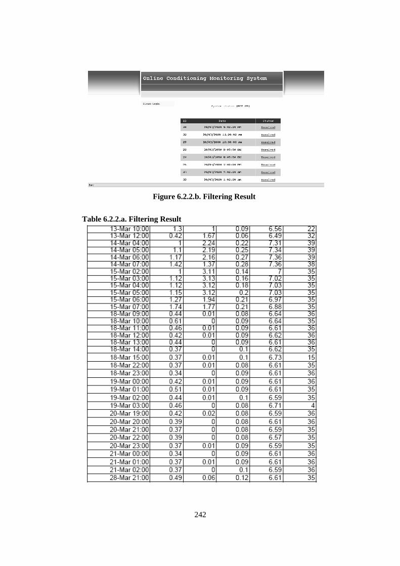
242

70Figure 6.2.2.b. Filtering Result

21Table 6.2.2.a. Filtering Result

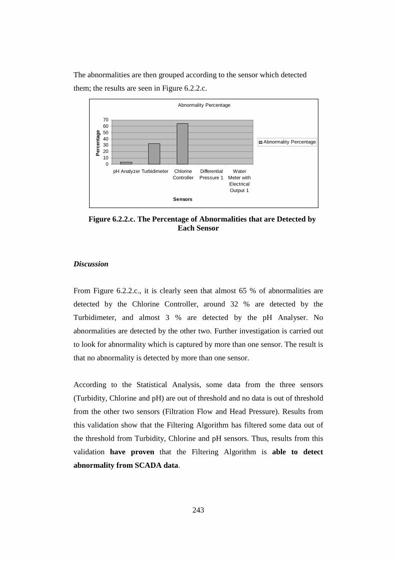
243

The abnormalities are then grouped according to the sensor which detected

them; the results are seen in Figure 6.2.2.c.

Abnormality Percentage

010203040506070

pH Analyzer Turbidimeter ChlorineController

DifferentialPressure 1

WaterMeter withElectricalOutput 1

Sensors

Per

cen

tag

e

Abnormality Percentage

71Figure 6.2.2.c. The Percentage of Abnormalities that are Detected by Each Sensor

Discussion

From Figure 6.2.2.c., it is clearly seen that almost 65 % of abnormalities are

detected by the Chlorine Controller, around 32 % are detected by the

Turbidimeter, and almost 3 % are detected by the pH Analyser. No

abnormalities are detected by the other two. Further investigation is carried out

to look for abnormality which is captured by more than one sensor. The result is

that no abnormality is detected by more than one sensor.

According to the Statistical Analysis, some data from the three sensors

(Turbidity, Chlorine and pH) are out of threshold and no data is out of threshold

from the other two sensors (Filtration Flow and Head Pressure). Results from

this validation show that the Filtering Algorithm has filtered some data out of

the threshold from Turbidity, Chlorine and pH sensors. Thus, results from this

validation have proven that the Filtering Algorithm is able to detect

abnormality from SCADA data.

244

Validation of the ability of the Knowledge Base to respond based on the

abnormality information that has been filtered by a filtering algorithm

The next step is validating the response from the Knowledge Base by

comparing the response to part of the Logic and Sensor Diagram (Table

6.2.2.b.).

22Table 6.2.2.b. Part of Logic and Sensor Diagram Activated Carbon Filter Multi Media Filter Hydro Cyclone Raw Water Quality Pre-Filter Water Flow at the Filtration Process

Turbidimeter

Sensor Failure Dosing Tank 2 Dosing Pump 2 Water Flow at the Filtration Process Raw Water Quality

Chlorine Controller

Sensor Failure Dosing Tank 3 Dosing Pump 3 Water Flow at the Filtration Process Raw Water Quality

pH Analyser

Sensor Failure

The following figures show different responses from the Knowledge Base for

abnormality that is captured by three different sensors:

245

72Figure 6.2.2.d. Knowledge Base Response using the Chlorine Controller

73Figure 6.2.2.e. Knowledge Base Response using the Turbidimeter

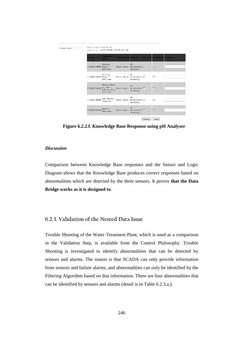
246

74Figure 6.2.2.f. Knowledge Base Response using pH Analyser

Discussion

Comparison between Knowledge Base responses and the Sensor and Logic

Diagram shows that the Knowledge Base produces correct responses based on

abnormalities which are detected by the three sensors. It proves that the Data

Bridge works as it is designed to.

6.2.3. Validation of the Nested Data Issue

Trouble Shooting of the Water Treatment Plant, which is used as a comparison

in the Validation Step, is available from the Control Philosophy. Trouble

Shooting is investigated to identify abnormalities that can be detected by

sensors and alarms. The reason is that SCADA can only provide information

from sensors and failure alarms, and abnormalities can only be identified by the

Filtering Algorithm based on that information. There are four abnormalities that

can be identified by sensors and alarms (detail is in Table 6.2.3.a.).

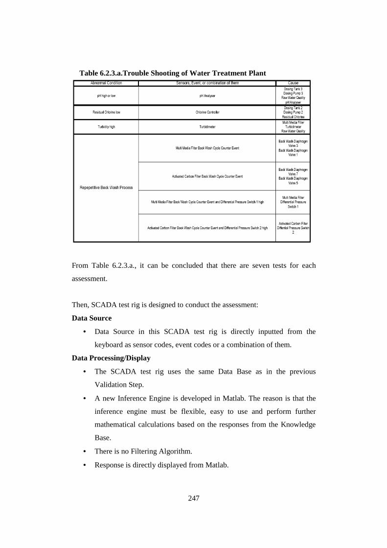
247

23Table 6.2.3.a.Trouble Shooting of Water Treatment Plant

From Table 6.2.3.a., it can be concluded that there are seven tests for each

assessment.

Then, SCADA test rig is designed to conduct the assessment:

Data Source

• Data Source in this SCADA test rig is directly inputted from the

keyboard as sensor codes, event codes or a combination of them.

Data Processing/Display

• The SCADA test rig uses the same Data Base as in the previous

Validation Step.

• A new Inference Engine is developed in Matlab. The reason is that the

inference engine must be flexible, easy to use and perform further

mathematical calculations based on the responses from the Knowledge

Base.

• There is no Filtering Algorithm.

• Response is directly displayed from Matlab.

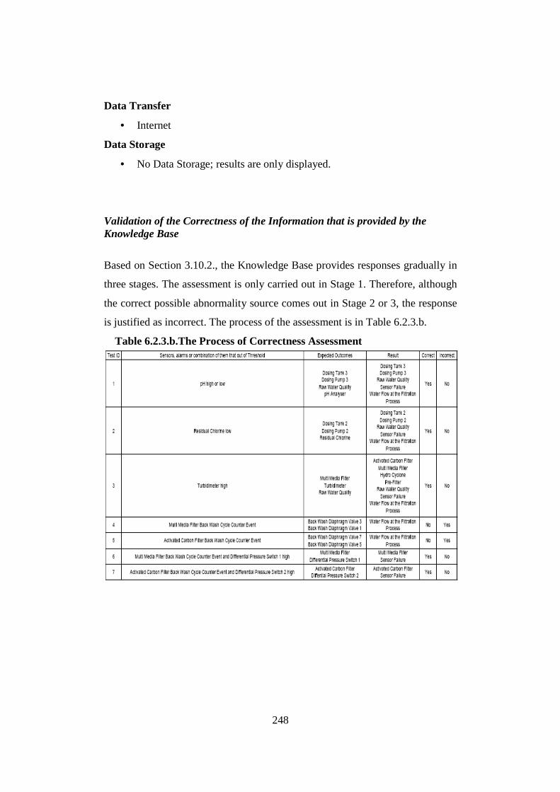
248

Data Transfer

• Internet

Data Storage

• No Data Storage; results are only displayed.

Validation of the Correctness of the Information that is provided by the Knowledge Base

Based on Section 3.10.2., the Knowledge Base provides responses gradually in

three stages. The assessment is only carried out in Stage 1. Therefore, although

the correct possible abnormality source comes out in Stage 2 or 3, the response

is justified as incorrect. The process of the assessment is in Table 6.2.3.b.

24Table 6.2.3.b.The Process of Correctness Assessment

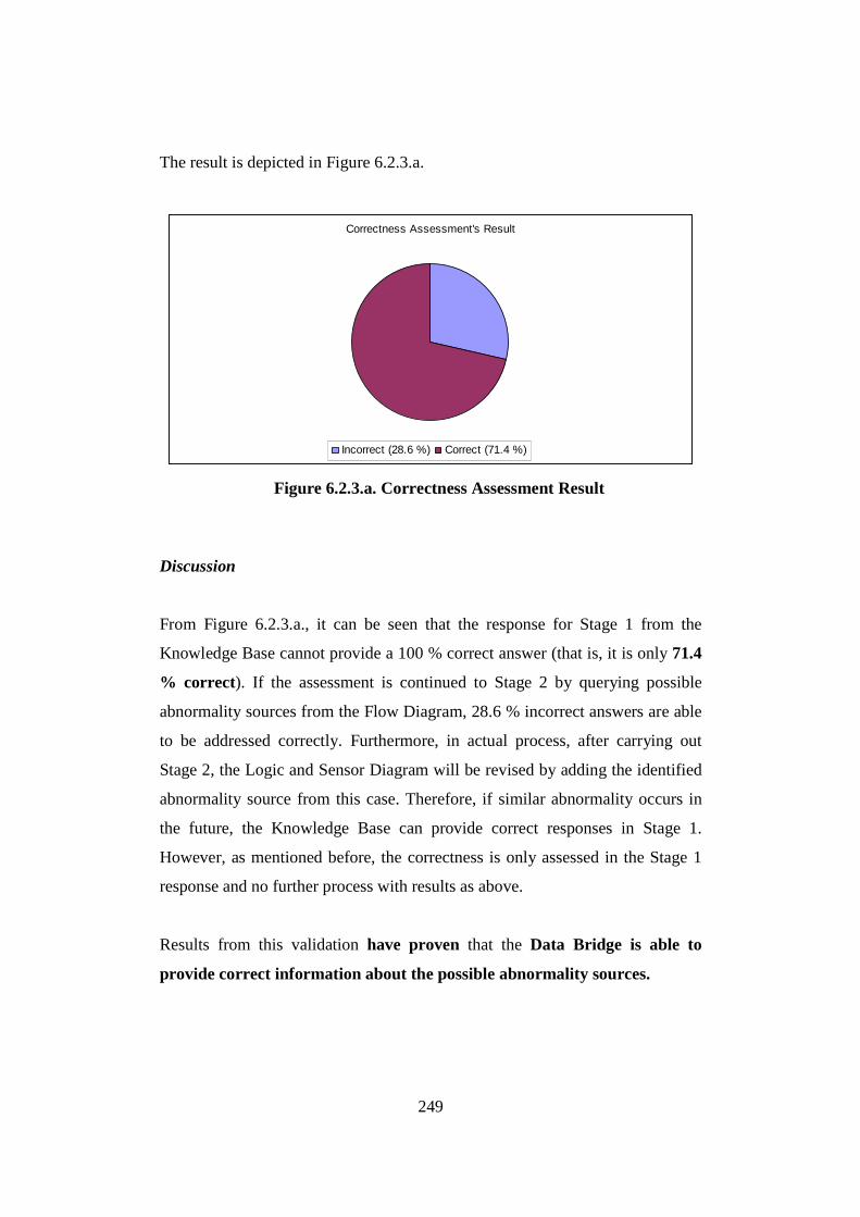
249

The result is depicted in Figure 6.2.3.a.

Correctness Assessment's Result

Incorrect (28.6 %) Correct (71.4 %)

75Figure 6.2.3.a. Correctness Assessment Result

Discussion

From Figure 6.2.3.a., it can be seen that the response for Stage 1 from the

Knowledge Base cannot provide a 100 % correct answer (that is, it is only 71.4

% correct). If the assessment is continued to Stage 2 by querying possible

abnormality sources from the Flow Diagram, 28.6 % incorrect answers are able

to be addressed correctly. Furthermore, in actual process, after carrying out

Stage 2, the Logic and Sensor Diagram will be revised by adding the identified

abnormality source from this case. Therefore, if similar abnormality occurs in

the future, the Knowledge Base can provide correct responses in Stage 1.

However, as mentioned before, the correctness is only assessed in the Stage 1

response and no further process with results as above.

Results from this validation have proven that the Data Bridge is able to

provide correct information about the possible abnormality sources.

250

Validation of the Effectiveness of the Knowledge Base

The effectiveness of the Knowledge Base is assessed by utilising the same input

as in the Correctness Assessment. The criterion of this assessment is based on

the number of possible abnormality sources that are provided in the Knowledge

Bases response. The greater the number of possible abnormality sources, the

longer the time required by the operator/engineer to investigate them. Hence,

the more time used, the lower the effectiveness of the Knowledge Base

response. The ideal Knowledge Base response based on abnormal information

only provides the correct abnormality sources.

The formula for calculating the effectiveness of the Knowledge Base is:

100⊗=Outcomes

tcomesExpectedOuessEffectiven Equation 10

However, there is one condition that has to be satisfied before the effectiveness

can be calculated:

• All Expected Outcomes must have been covered in the Outcomes. If

Stage 1 cannot cover all the Expected Outcomes, then continue with

Stage 2, and if Stage 2 cannot cover them, then continue with Stage 3.

After conducting seven tests, the expected outcomes and outcomes are as

follows:

1. Test ID 1:

Expected Outcomes = 4

Outcomes = 5

2. Test ID 2

Expected Outcomes = 4

Outcomes = 5

3. Test ID 3

Expected Outcomes = 4

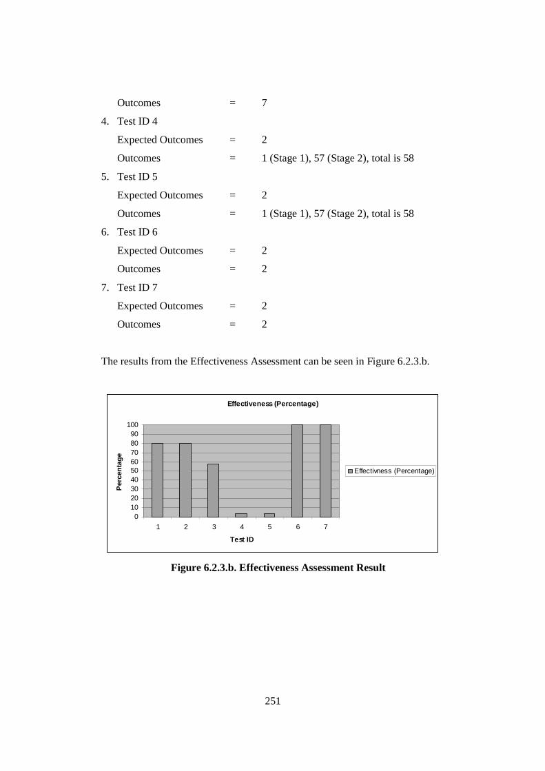
251

Outcomes = 7

4. Test ID 4

Expected Outcomes = 2

Outcomes = 1 (Stage 1), 57 (Stage 2), total is 58

5. Test ID 5

Expected Outcomes = 2

Outcomes = 1 (Stage 1), 57 (Stage 2), total is 58

6. Test ID 6

Expected Outcomes = 2

Outcomes = 2

7. Test ID 7

Expected Outcomes = 2

Outcomes = 2

The results from the Effectiveness Assessment can be seen in Figure 6.2.3.b.

Effectiveness (Percentage)

0102030405060708090

100

1 2 3 4 5 6 7

Test ID

Per

cen

tag

e

Effectivness (Percentage)

76Figure 6.2.3.b. Effectiveness Assessment Result

252

Discussion

From Figure 6.2.3.b., it can be seen that Tests 4 and 5 are the least effective.

This is because abnormalities in both of them cannot be addressed in the

Knowledge Base response in Stage 1. Therefore, by progressing the Knowledge

Base response to the next stage, the effectiveness of the response will be

reduced, because the number of possible abnormality sources increases. In fact,

the whole system has to be investigated in Stage 3; this means that the

effectiveness of Stage 3 is close to 0 due to a great number of possible

abnormality sources that have to be investigated. All tests in which the

abnormalities can be addressed in the Knowledge Base’s response Stage 1

have a higher level of effectiveness. Test 6 and Test 7 can reach the highest

effectiveness. This is because, compared to other tests, which can be addressed

in Stage 1, information sources in both Tests 6 and 7 are a combination of event

and sensor by utilising AND junction. This combination results in more specific

information and therefore increases the effectiveness of the Knowledge Base

Response.

Results from this validation show that the designed three stage response

framework from the Data Bridge provides comprehensive steps to identify

the actual source of abnormality. Also, this framework presents the

learning ability of the Knowledge Base. Thus, it can adapt easily to new

information.

Validation of the Time Response of the Knowledge Base

This assessment measures the time response of the Knowledge Base by utilising

a script which is developed in Matlab. The response that is measured is only

response Stage 1. The purpose of this assessment is to grasp a sense of

knowledge base response time. In this assessment, the Data Base is deployed in

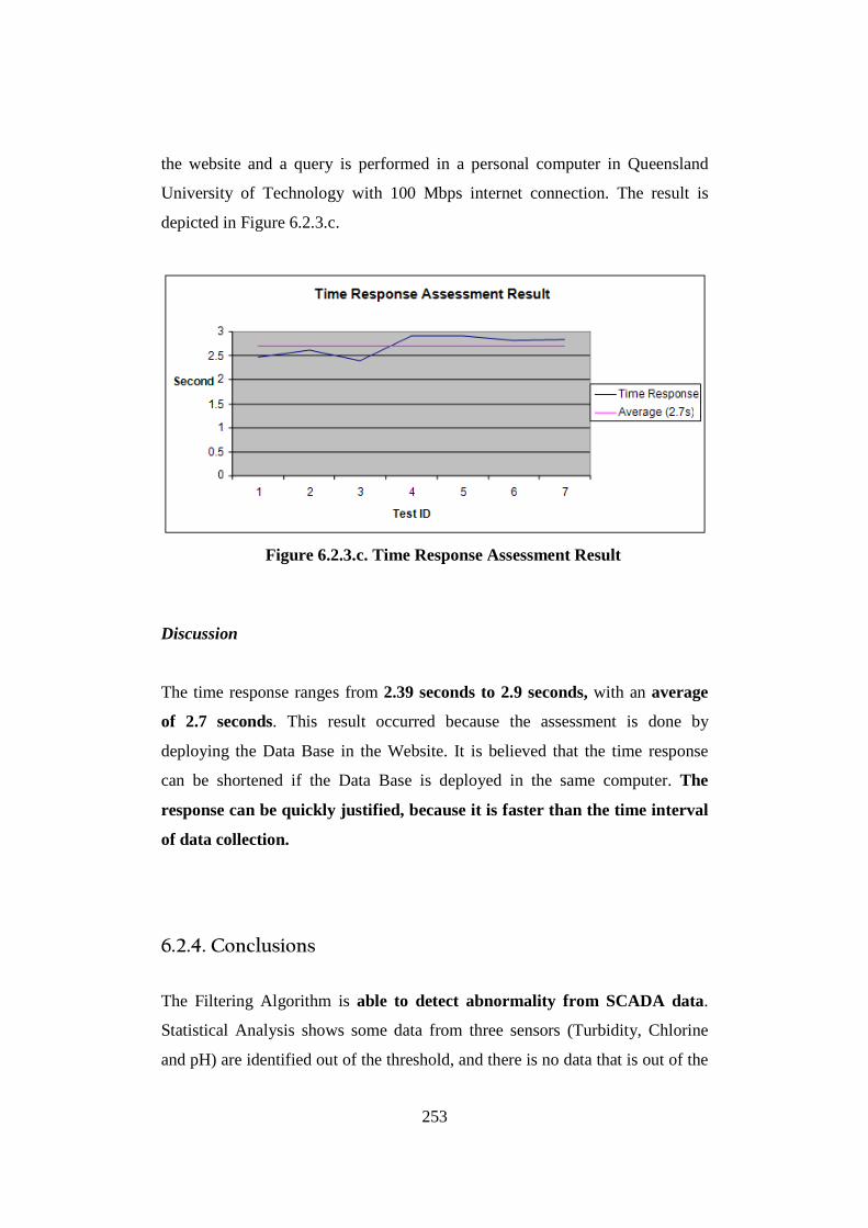
253

the website and a query is performed in a personal computer in Queensland

University of Technology with 100 Mbps internet connection. The result is

depicted in Figure 6.2.3.c.

77Figure 6.2.3.c. Time Response Assessment Result

Discussion

The time response ranges from 2.39 seconds to 2.9 seconds, with an average

of 2.7 seconds. This result occurred because the assessment is done by

deploying the Data Base in the Website. It is believed that the time response

can be shortened if the Data Base is deployed in the same computer. The

response can be quickly justified, because it is faster than the time interval

of data collection.

6.2.4. Conclusions

The Filtering Algorithm is able to detect abnormality from SCADA data.

Statistical Analysis shows some data from three sensors (Turbidity, Chlorine

and pH) are identified out of the threshold, and there is no data that is out of the

254

threshold from the other two sensors (Filtration Flow and Head Pressure).

Results from this validation show that the Filtering Algorithm has filtered some

data out of the threshold from Turbidity, Chlorine and pH sensors.

The Data Bridge works properly as it is designed, because comparison

between the Knowledge Base responses and the Sensor and Logic Diagram

shows that the Knowledge Base produces correct responses based on

abnormalities which are detected by the three sensors.

The Data Bridge is able to provide correct information about the possible

abnormality sources. Response from Stage 1 of the Knowledge Base cannot

provide a 100 % correct answer (that is, only 71.4 % correct). However, if the

assessment is continued to Stage 2, by querying possible abnormality sources

from the Flow Diagram, 28.6 % incorrect answers are able to be addressed

correctly. Furthermore, in actual process, after carrying out Stage 2, the Logic

and Sensor Diagram will be revised by adding the identified abnormality source

from this case. Therefore, if similar abnormality occurs in the future, the

Knowledge Base can provide correct responses in Stage 1.

The designed three stage response framework from the Data Bridge

provides comprehensive steps to identify the actual source of abnormality.

Also, this framework presents the learning ability of the Knowledge Base.

Thus, it can adapt easily to new information.

The time response is justified as fast enough (ranges from 2.39 to 2.9 seconds

with the average 2.7 seconds), because it is faster than the time interval of

data collection (every hour).

Finally, the vital conclusion that can be drawn from Validation A is that the

hypothesis that “Problems in SCADA data analysis, such as nested data, can be

255

addressed by analysing design information of monitored and monitoring

systems through the Hierarchical Model” has been proved.

6.3. Validation B (Validation of Interdependence Model Data)

6.3.1. Introduction

In Validation B, the hypothesis that “The Interdependence Risk Analysis

method can address current Risk Analysis method problems, i.e. the need for

sophisticated historical information as an input for Risk Likelihood” is

validated. There is one point that needs to be validated:

• Validation of the Interdependence Risk Analysis

In this validation, the claim that Interdependence Risk Analysis can

address the need for sophisticated historical information is determined.

In the validation, IRA and Risk Analysis based on FMEA are separately

utilised to determine the Risk Consequence and the Risk Likelihood of

each component/sub-assembly from the water treatment plant. The

information about Risk Consequence and Risk Likelihood are then

employed as inputs to the Risk Ranking Development. Two common

approaches to developing the Risk Ranking (that is, the Risk Factor and

Risk Ranking Matrix) are used. Finally, Risk Rankings that are

produced based on IRA are compared to Risk Rankings that are

produced based on Risk Analysis based on FMEA. Section 4.7. has

explained the success of the Interdependence Risk Analysis to produce

the Risk Ranking based on the Risk Factor and Risk Ranking based on

the Risk Ranking Matrix of the water treatment plant. The produced

Risk Rankings are shown again in Section 6.3.2. to assist in the reading

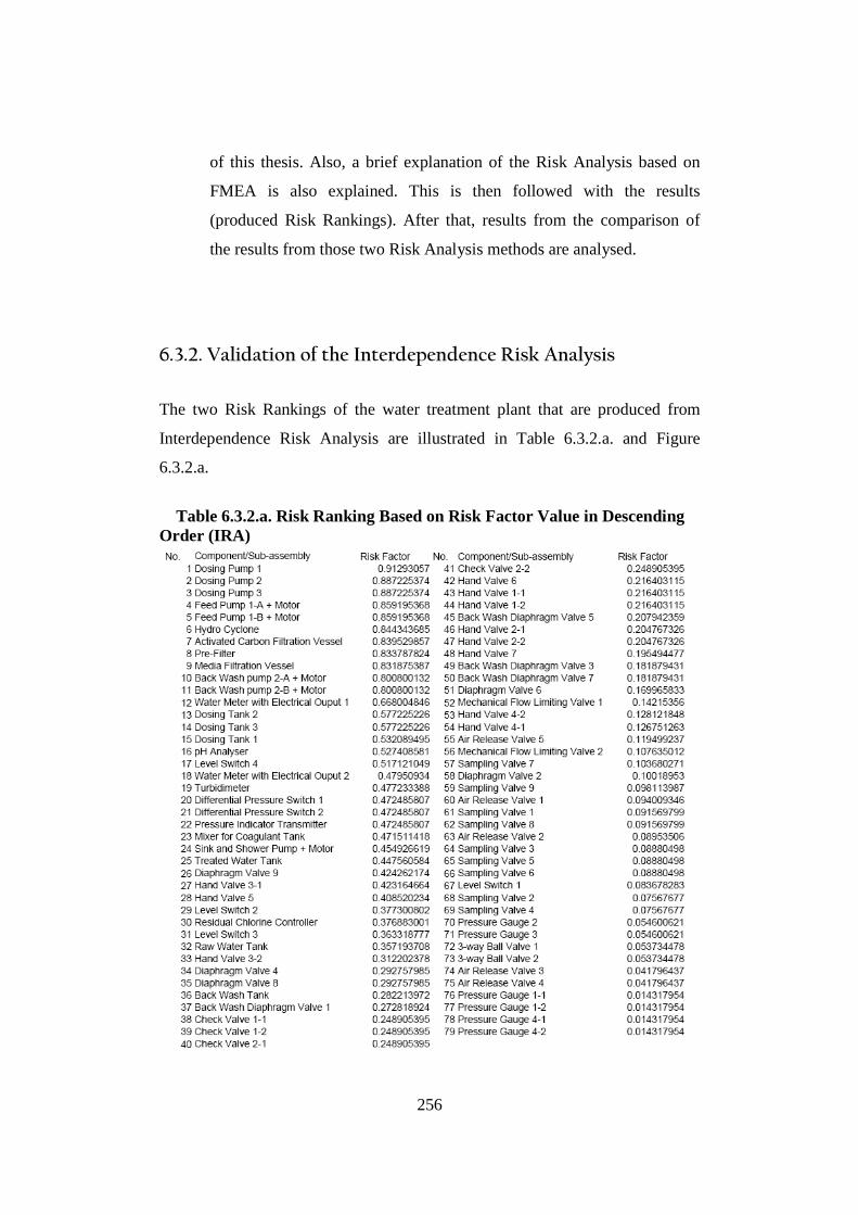
256

of this thesis. Also, a brief explanation of the Risk Analysis based on

FMEA is also explained. This is then followed with the results

(produced Risk Rankings). After that, results from the comparison of

the results from those two Risk Analysis methods are analysed.

6.3.2. Validation of the Interdependence Risk Analysis

The two Risk Rankings of the water treatment plant that are produced from

Interdependence Risk Analysis are illustrated in Table 6.3.2.a. and Figure

6.3.2.a.

25Table 6.3.2.a. Risk Ranking Based on Risk Factor Value in Descending Order (IRA)

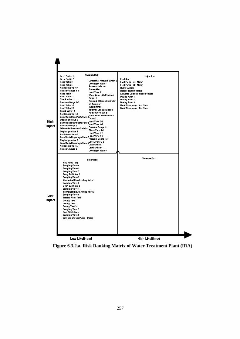
257

78Figure 6.3.2.a. Risk Ranking Matrix of Water Treatment Plant (IRA)

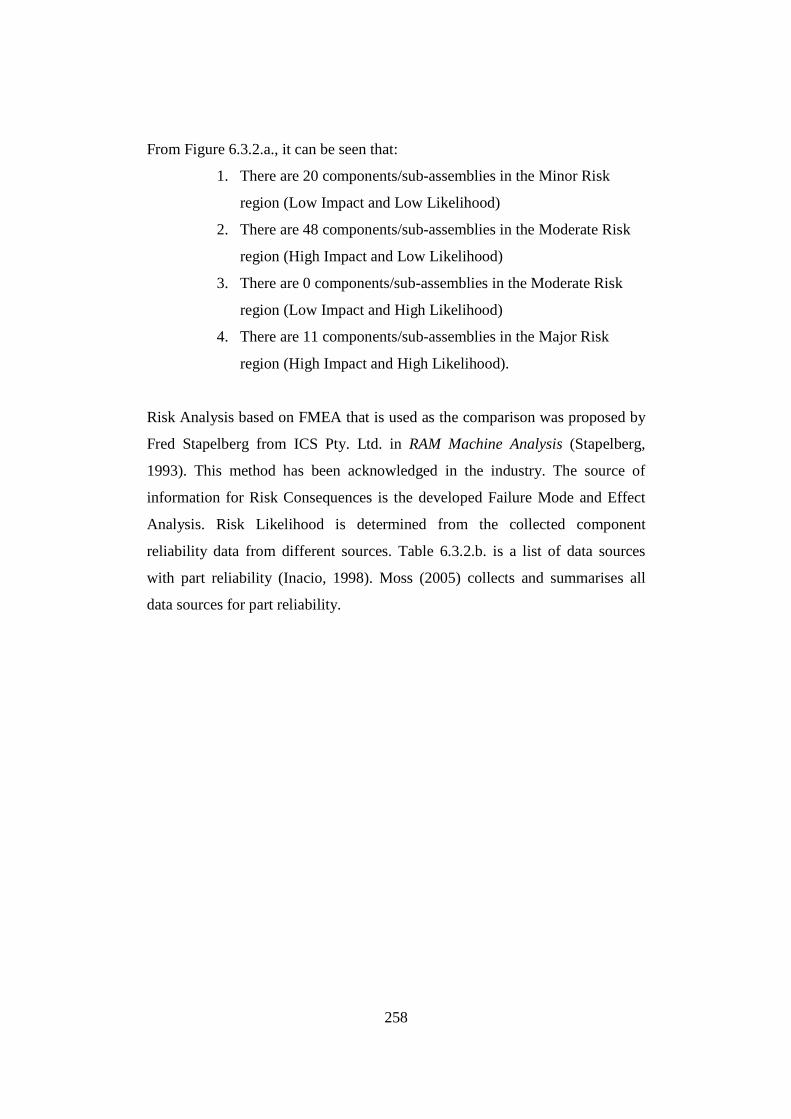
258

From Figure 6.3.2.a., it can be seen that:

1. There are 20 components/sub-assemblies in the Minor Risk

region (Low Impact and Low Likelihood)

2. There are 48 components/sub-assemblies in the Moderate Risk

region (High Impact and Low Likelihood)

3. There are 0 components/sub-assemblies in the Moderate Risk

region (Low Impact and High Likelihood)

4. There are 11 components/sub-assemblies in the Major Risk

region (High Impact and High Likelihood).

Risk Analysis based on FMEA that is used as the comparison was proposed by

Fred Stapelberg from ICS Pty. Ltd. in RAM Machine Analysis (Stapelberg,

1993). This method has been acknowledged in the industry. The source of

information for Risk Consequences is the developed Failure Mode and Effect

Analysis. Risk Likelihood is determined from the collected component

reliability data from different sources. Table 6.3.2.b. is a list of data sources

with part reliability (Inacio, 1998). Moss (2005) collects and summarises all

data sources for part reliability.

259

26Table 6.3.2.b. Data Sources for Part Reliability

The two Risk Rankings of the water treatment plant that are produced from

Risk Analysis based on FMEA are illustrated in Table 6.3.2.c. and Figure

6.3.2.b.

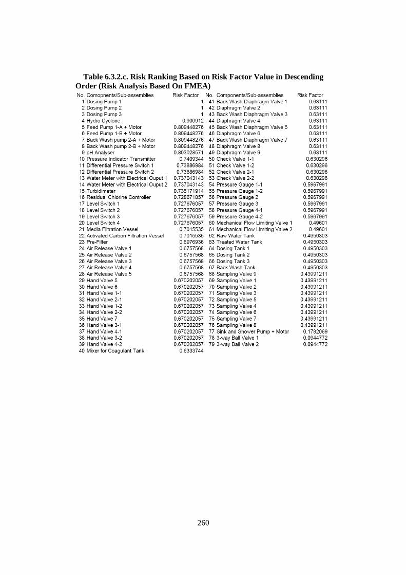
260

27Table 6.3.2.c. Risk Ranking Based on Risk Factor Value in Descending Order (Risk Analysis Based On FMEA)

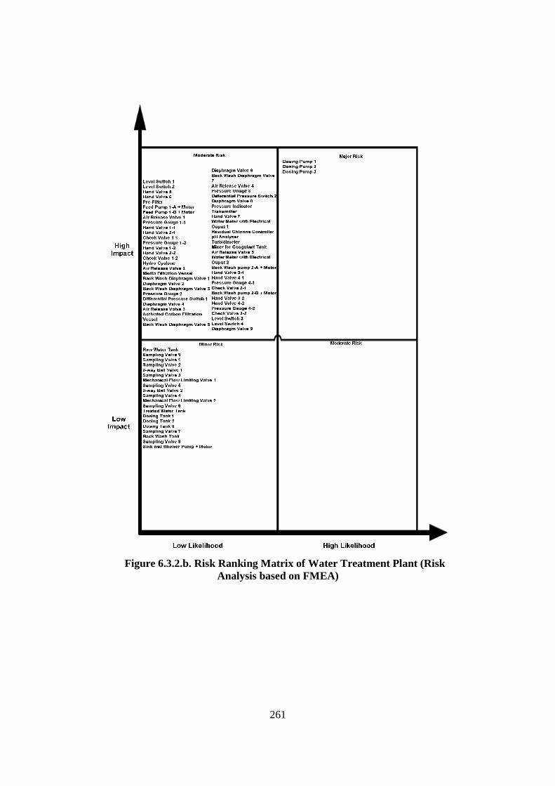
261

79Figure 6.3.2.b. Risk Ranking Matrix of Water Treatment Plant (Risk Analysis based on FMEA)

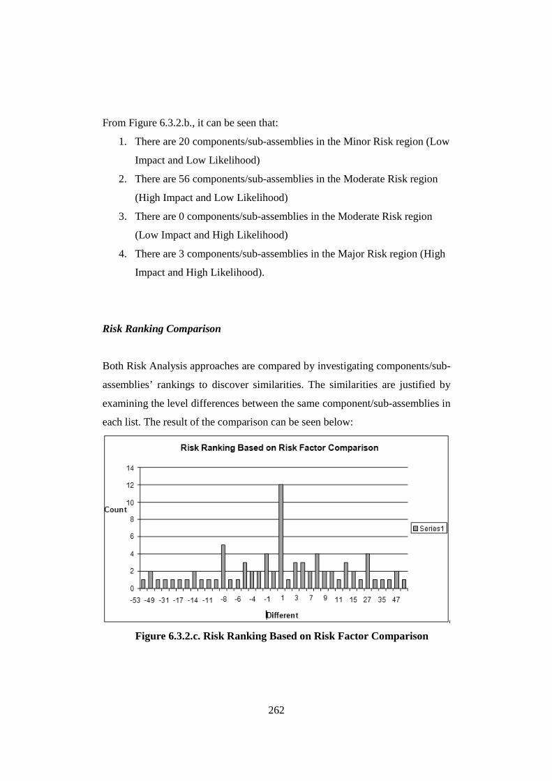
262

From Figure 6.3.2.b., it can be seen that:

1. There are 20 components/sub-assemblies in the Minor Risk region (Low

Impact and Low Likelihood)

2. There are 56 components/sub-assemblies in the Moderate Risk region

(High Impact and Low Likelihood)

3. There are 0 components/sub-assemblies in the Moderate Risk region

(Low Impact and High Likelihood)

4. There are 3 components/sub-assemblies in the Major Risk region (High

Impact and High Likelihood).

Risk Ranking Comparison

Both Risk Analysis approaches are compared by investigating components/sub-

assemblies’ rankings to discover similarities. The similarities are justified by

examining the level differences between the same component/sub-assemblies in

each list. The result of the comparison can be seen below:

80Figure 6.3.2.c. Risk Ranking Based on Risk Factor Comparison

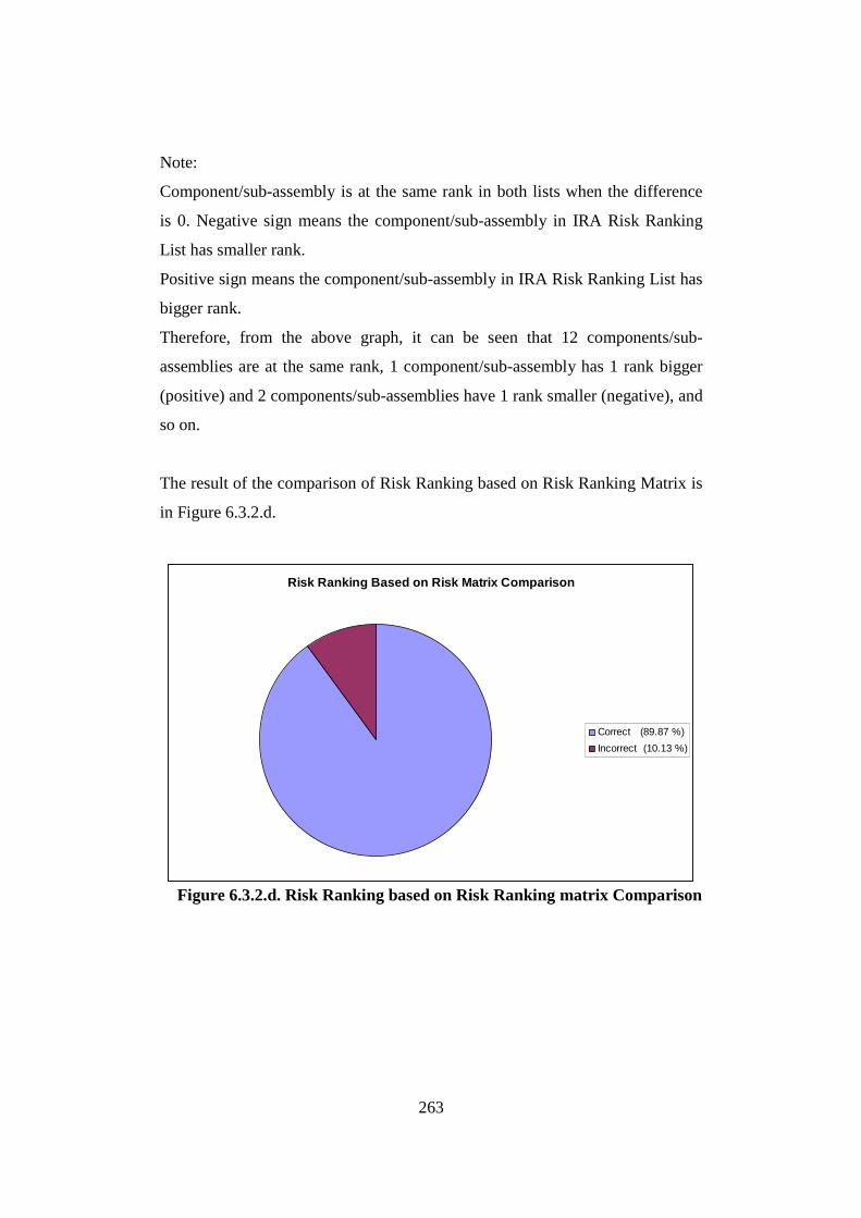
263

Note:

Component/sub-assembly is at the same rank in both lists when the difference

is 0. Negative sign means the component/sub-assembly in IRA Risk Ranking

List has smaller rank.

Positive sign means the component/sub-assembly in IRA Risk Ranking List has

bigger rank.

Therefore, from the above graph, it can be seen that 12 components/sub-

assemblies are at the same rank, 1 component/sub-assembly has 1 rank bigger

(positive) and 2 components/sub-assemblies have 1 rank smaller (negative), and

so on.

The result of the comparison of Risk Ranking based on Risk Ranking Matrix is

in Figure 6.3.2.d.

Risk Ranking Based on Risk Matrix Comparison

Correct (89.87 %)

Incorrect (10.13 %)

81Figure 6.3.2.d. Risk Ranking based on Risk Ranking matrix Comparison

264

Discussion

In proportion, the Risk Ranking based on Risk Factor Comparison can be

presented as (neglecting the sign):

• Exactly the same 15.19 %

• Misses 5 positions or less 39.24 %

• Misses 10 positions or less 63.29 %

• Misses 15 positions or less 77.22 %

• Misses 20 positions or less 83.54 %

The reason for using the above format is that Risk Ranking is used to enable

Risk Management Priorities. Risk Management Priorities is carried out by

dividing the components/sub-assemblies into several regions based on the Risk

Factor. Different priorities are applied to different regions. An example of this

prioritisation is in Figure 6.3.2.e.:

82Figure 6.3.2.e. Prioritisation Based on the Risk Factor (TAM04-12, 2004)

265

The decision on regions depends on the management; for example: a region can

be determined based on the Risk Factor ranging from 0.7-0.9, 0.5-0.69, and so

on. The number of components/sub-assemblies within the region varies; it

could be 5, 10 or even more than 20 components/sub-assemblies. Therefore, in

terms of the comparison, 20 levels of difference in rank may not be a problem

as long as the region consists of more than 20 components/sub-assemblies,

because the priority and treatment will still be the same. On the contrary, 1 or 2

level differences could make a big difference if one of the components/sub-

assemblies is located in a different region.

According to the Risk Ranking based on Risk Ranking Matrix Comparison,

89.87 % of components/sub-assemblies is in the same region. Hence, those

Risk Rankings based on the Risk Ranking Matrix are very close.

In the Risk Ranking based on Risk Factor, each component has its own Risk

Factor which determines the component ranking. The analyst can then group

the components based on the Risk Factor number to the number of groups in

order to apply different treatments. The number of groups in this case is up to

the analyst (could be 2, 3, 4, etc.). In risk ranking based on the Risk Ranking

Matrix, each component is placed in the matrix based on two axes: impact axis

and likelihood axis. The matrix is divided into four regions by placing a line in

the mid value of each axis. Therefore, all components are only grouped into 4

groups. It can be concluded that the Risk Factor approach provides more detail

information and flexibility than the Risk Ranking Matrix approach, where in

the Risk Factor the differentiation between components is clear and the analyst

can determine the number of groups according to the need. However, the

implementation of the Risk Ranking Matrix approach is simpler and easier than

the Risk Factor approach, as the calculation in the Risk Ranking Matrix

approach is much simpler and the determination of groups is straight forward. It

is up to the analyst to determine which approach is suitable out of these two

approaches.

266

6.3.3. Conclusions

In conclusion, results from both approaches are similar. In terms of Risk

Ranking based on Risk Factor; 15 percent of components/sub-assemblies are

exactly at the same rank, almost 40 percent of components/sub-assemblies

display only 5 levels of difference, more than 60 percent of

components/sub-assemblies have 10 levels of difference, almost 78 percent

components/sub-assemblies are 15 levels different and 83 percents are 20

levels different. Less than 17 percent of components/sub-assemblies differ

significantly. This significant difference is caused by a difference in starting

points of the two approaches; Risk Analysis based on FMEA utilises the

consequence of failure mode and generic part reliability data. On the other

hand, although IRA still utilises FMEA, this is built up from the

Interdependence Relationship between each component/sub-assembly.

Furthermore, results from the comparison of Risk Ranking based on Risk

Ranking Matrixes, which are produced by two approaches, strengthen the

conclusion, because almost 90% of components/sub-assemblies in both

matrixes are in the same region. With this outcome, IRA has made a

significant contribution in the Risk Analysis domain, because proper

historical data, which is difficult to obtain, is not necessary in IRA, but is

required in most Risk Analysis methods.

Finally, the vital conclusion that can be drawn from Validation B is that the

hypothesis that “The Interdependence Risk Analysis method can address

current Risk Analysis method problems, i.e. the need for sophisticated historical

information as an input for Risk Likelihood” has been proved.

267

6.4. Validation C (Validation of Data Connectivity)

6.4.1. Introduction

The purpose of Validation C is to validate the hypothesis: “The data bridge

developed from the Hierarchical Model will address the connectivity problem

between SCADA systems and ERP systems, whereby significant information

can be drawn out from SCADA’s ‘raw data’ and transferred into ERP”. As

mentioned before, this validation depends on the success of the other two

validations (A and B) where the success of those two validations will

automatically complete this Validation C process. Based on the explanations in

Section 6.2. and Section 6.3., Validations A and B have been done successfully.

Thus, Validation C must have been validated, and Section 6.4. needs to explain

what has been validated.

6.4.2. Performing Validation C

The point that needs to be validated in the hypothesis that “The Data Bridge

developed from the Hierarchical Model will address the connectivity problem

between the SCADA systems and ERP systems, whereby significant

information can be drawn out from SCADA’s ‘raw data’ and transferred into

ERP” is whether the Data Bridge is able to address the connectivity problem

between the SCADA systems and ERP systems by pulling significant

information from SCADA’s “raw data” and transferring that information to

ERP.

268

According to the Literature Review, the connectivity between the SCADA

systems and ERP systems cannot be done only by transferring “raw data”; there

have to be some steps taken to process the “raw data” into more meaningful

information. There are several steps connecting SCADA and ERP systems by

processing the “raw data” into more meaningful information, such as:

Integrated Condition Monitoring, Asset Health and Prognosis, and Asset Risk

Analysis. These are similar to Bever’s Plant Asset Management System

Framework (Bever, 2000, op. cit. Stapelberg, 2006) Thus, the raw data from

various sources (that is, sensors) is collected by an integrated condition

monitoring system, then the asset health is analysed. Finally, the asset’s risk

and criticality can be concluded based on the result of the asset health analysis,

and then it is forwarded to the ERP system.

Validation as to whether the developed Data Bridge is able to address the

connectivity between the SCADA and ERP systems is carried on by analysing

whether the Data Bridge is able to fulfil the three identified steps to connect

SCADA and ERP. Further explanation of the justification that Data Bridge has

fulfilled the three identified steps is in the discussion section, and the discussion

will focus on the statement: “The success of Validation A and Validation B will

automatically completee the Validation C process”.

Discussion

Firstly, the analysis is about whether the Data Bridge has fulfilled the Integrated

Condition Monitoring step. By design, the Data Bridge is used to process

data/information from a SCADA that monitors an asset. The SCADA system is

designed to integrate information from data that is taken from various sensors

in order to justify the condition of assets. Therefore, it can be concluded that the

Data Bridge has fulfilled the Integrated Condition Monitoring Step.

269

Analysis to justify whether the Data Bridge has fulfilled the Asset Health and

Prognosis Step is then continued. Based on Validation A, Data Bridge is proven

able to address the data analysis problem in the SCADA system that is caused

by the nested data problem, where it is able to process SCADA “raw data” into

more meaningful information about the asset condition. Hence, the Data Bridge

has fulfilled the Asset Health and Prognosis Step.

The third aspect that has to be fulfilled by the Data Bridge is the Asset Risk

Analysis Step. The Data Bridge is developed from the Hierarchical Model, the

proposed model in this research. Risk Analysis in the Hierarchical Model is

carried out in two ways: at the beginning and continuously as the system is

working. Risk Analysis at the beginning is performed the first time the

Hierarchical Model is applied to analyse the monitored and monitoring systems.

Usually there is not much information - especially historical information - at

this time. Therefore, this risk analysis is performed by Interdependence Risk

Analysis (part of the Hierarchical Model) that utilises interdependent

relationships between components. Analysing Risk at the beginning is very

crucial to obtain information about risk to each component in the system,

because it can be utilised to determine further maintenance priority. Continuous

Risk Analysis is conducted as the system is working. It is facilitated through the

design of information process in the Data Bridge (refer to Section 3.10.2),

where information about abnormality frequency is taken and used as Risk

Likelihood. This Risk Likelihood will be developed as the system is working.

Risk Likelihood together with the Risk Consequence that has been determined

based on Failure Mode and Effect Analysis are then utilised to conduct Risk

Analysis. Ultimately, it can be concluded that the Data Bridge has fulfilled the

Asset Risk Analysis Step.

270

6.4.3. Conclusions

In conclusion, the Data Bridge has fulfilled the three identified steps to connect

SCADA and ERP systems. More specifically:

• The Integrated Condition Monitoring Step is justified because the

Data Bridge is designed to process data/information from SCADA. The

SCADA System is designed to integrate information from data that is

taken from various sensors in order to justify the condition of monitored

assets.

• The Asset Health and Prognosis Step is justified because the Data

Bridge is able to monitor the asset condition based on SCADA data. In

Validation A, it is proven that the Data Bridge is able to address one of

the data analysis problems in the SCADA System; that is, nested data.

• The Asset Risk Analysis Step is justified because the Hierarchical

Model (from which the Data Bridge is developed) conducts Risk

Analysis in two ways: at the beginning, and continuously as the system

is working. Risk Analysis at the beginning is conducted by the

Interdependence Risk Analysis to obtain information about risk of each

component in the system. Continuous Risk Analysis is facilitated in the

Hierarchical Model through the design of information process in the

Data Bridge.

The final conclusion from this validation after considering these results is that

the hypothesis that “The Data Bridge developed from the Hierarchical Model

will address the connectivity problem between SCADA systems and ERP

systems, whereby significant information can be drawn out from SCADA’s

‘raw data’ and transferred into ERP” has been proved.

271

6.5. Summary Chapter 6 reveals one of the most crucial elements of information about this

research: Model Validation. The Case Study is chosen to validate the proposed

model. Three validations are designed (Validation A, Validation B and

Validation C) to validate the three proposed hypotheses in this research:

1. Problems in SCADA data analysis, such as nested data, can be addressed by

analysing design information of monitored and monitoring systems through

the Hierarchical Model. This hypothesis is validated in Validation A.

2. The Interdependence Risk Analysis method can address a current Risk

Analysis method problem: the need for sophisticated historical information

as an input for Risk Likelihood. This hypothesis is validated in Validation

B.

3. The Data Bridge developed from the Hierarchical Model will address the

connectivity problem between SCADA systems and ERP systems, whereby

significant information can be drawn out from SCADA’s “raw data” and

transferred into ERP. This hypothesis is validated in Validation C.

In Validation A there are two points of validation, as explained below:

• Validation of SCADA data analysis in a “real-time” time frame

This validation is to determine whether the Data Bridge as the end result

from the Hierarchical Model can work as it is designed. There are two parts

to this validation:

o Validation of the ability of the Filtering Algorithm to detect abnormality

In this part, the validation is focused on the Filtering Algorithm’s ability

to detect any abnormality based on data from sensors. Results from

Statistical Analysis (identified data that is out of threshold) are used as a

comparison. The conclusion from this validation is that:

The Filtering Algorithm is able to detect abnormality from

SCADA data. Statistical Analysis shows some data from three

272

sensors (Turbidity, Chlorine and pH) are out of threshold, and no

data that is out of threshold from the other two sensors

(Filtration Flow and Head Pressure). Results from this validation

show the Filtering Algorithm has filtered some data that is out of

threshold from Turbidity, Chlorine and pH sensors.

o Validation of the ability of the Knowledge Base to respond based on the

abnormality information that has been filtered by the Filtering

Algorithm

Validation in this part is to find out whether the Knowledge Base works

as it is designed to in terms of responding to the filtered abnormality

information from the Filtering Algorithm. Information from the Sensor

and Logic Diagram will be used as a comparison. The Conclusion from

this part is as follows:

The Data Bridge works properly as it is designed, because

comparison between the Knowledge Base responses and the

Sensor and Logic Diagram shows that the Knowledge Base

produces correct responses based on abnormalities which are

detected by the three sensors.

• Validation of nested data issue

The purpose of this validation is to prove that the proposed Hierarchical

Model is able to solve the nested data issue. The validation is carried out by

comparing information which is provided by Data Bridge, to the Trouble

Shooting from the system designer. In the previous point, the source of

abnormalities is not known. The only known information is the SCADA

Data Dump. However, in this point, the abnormal condition is known and

gathered from Trouble Shooting. There are three validation parts to measure

the success of the proposed Hierarchical Model in addressing nested data

issue:

o Validation of the correctness of the information that is provided by

Knowledge Base

273

In this part, the validation is to measure the ability of the Knowledge

Base to provide the correct information on the possible abnormality

sources based on the situated abnormal condition. Trouble Shooting is

used as the comparison in this validation. The conclusion is that:

The Data Bridge is able to provide correct information about

the possible abnormality sources. Response to Stage 1 from

the Knowledge Base cannot provide 100 % correct answers (that

is, only 71.4 % correct). However, if the assessment is

continued to Stage 2 by querying possible abnormality sources

from the Flow Diagram, 28.6 % incorrect answers are able to be

addressed correctly. Furthermore, in the actual process, after

carrying out Stage 2, the Logic and Sensor Diagram will be

revised by adding the identified abnormality source from this

case. Therefore, if similar abnormality occurs in the future, the

Knowledge Base can provide correct responses in Stage 1.

o Validation of the Effectiveness of the Knowledge Base

The focus of this validation part is beyond the correctness of the

response from the Knowledge Base; it is about effectiveness.

Sometimes, the correct answer is not always effective. Knowledge Base

can provide responses, which ranges from 1 to maximum possible

number of abnormality source. The conclusion from this validation is

that:

The designed three stage response framework from the Data

Bridge provides a comprehensive step to identifying the

actual source of abnormality. Also, this framework presents

the learning ability for the Knowledge Base. Thus, it can

adapt easily to new information.

o Validation of the time response to the Knowledge Base

This validation part tries to measure the time required by the Knowledge

Base to provide a response based on abnormality information. The

conclusion is that:

274

The time response is justified fast enough (it ranges from 2.39

to 2.9 seconds with the average 2.7 seconds), because it is faster

than the time interval of data collection (every hour).

The final and vital conclusion that can be drawn from Validation A is that the

hypothesis that “Problems in SCADA data analysis, such as nested data, can be

addressed by analysing design information of monitored and monitoring

systems through the Hierarchical Model” has been proved.

Validation B consists of one point that needs to be validated:

• Validation of the Interdependence Risk Analysis

In this validation, the claim that Interdependence Risk Analysis can address

the need of sophisticated historical information is validated. This validation

is carried out by comparing the developed Risk Ranking Based on Risk

Factor and Risk Ranking based on Risk Ranking Matrix that are produced

by utilising Interdependence Risk Analysis with Risk Ranking based on

Risk Factor, and Risk Ranking based on Risk Ranking Matrix that are

produced by utilising Risk Analysis based on Failure Mode and Effect

Analysis (FMEA). The conclusion from this validation is that:

Results from both Risk Analysis approaches are justified similar. In

terms of Risk Ranking based on Risk Factor, 15 percent of

components/sub-assemblies are exactly at the same rank, almost 40

percent are only 5 levels different, more than 60 percents

components/sub-assemblies are 10 levels different, almost 78

percents components/sub-assemblies are 15 levels different and 83

percents are 20 levels different. Only when the measure is less than

17 percent does the components/sub-assemblies differ significantly.

This significant difference is caused by a difference in starting

points of the two approaches; Risk Analysis based on FMEA utilises

the consequence of failure mode and generic part reliability data. On the

other hand, although IRA still utilises FMEA, it is built up from

Interdependence Relationship between each component/sub-assembly.

275

Furthermore, results from the comparison of Risk Ranking based on

Risk Ranking Matrixes which are produced by the two approaches,

strengthen the conclusion, because almost 90 percent of

components/sub-assemblies in both matrixes are in the same region.

With this outcome, IRA has made a significant contribution in the

Risk Analysis domain, because proper historical data which is

difficult to obtain, is not necessary in IRA, but is required in most

Risk Analysis methods.

The final conclusion from Validation B is that the hypothesis that “The

Interdependence Risk Analysis method can address the current Risk Analysis

method problem - the need for sophisticated historical information as an input

for Risk Likelihood” has been proved.

The point that needs to be validated in Validation C is whether the Data Bridge

is able to address the connectivity problem between SCADA systems and ERP

systems by pulling significant information from SCADA’s “raw data” and

transferring that information to ERP. Validation C is correlated closely with the

other two validations (A and B), where the success of the other two validations

will automatically complete the Validation C process. According to the

Literature Review, the connectivity between SCADA systems and ERP systems

cannot be done only by transferring “raw data”; there have to be some steps to

process the “raw data” into more meaningful information. There are several

steps connecting SCADA and ERP systems by processing the “raw data” into

more meaningful information, such as: Integrated Condition Monitoring, Asset

Health and Prognosis, and Asset Risk Analysis, which are similar to Bever’s

Plant Asset Management System Framework (Bever, 2000, op. cit. Stapelberg,

2006). Validation of the developed Data Bridge’s ability to address the

connectivity between SCADA and ERP systems is carried out by analysing

whether the Data Bridge is able to fulfil the three identified steps to connect

SCADA and ERP.

276

In conclusion, the Data Bridge has fulfilled the three identified steps to

connect SCADA and ERP systems, as explained below:

o The Integrated Condition Monitoring step is justified

because the Data Bridge is designed to process data/information

from SCADA. The SCADA System is designed to integrate

information from data that is taken from various sensors in order

to justify the condition of monitored assets.

o The Asset Health and Prognosis step is justified because the

Data Bridge is able to monitor the asset condition based on

SCADA data. In Validation A, it is proven that the Data Bridge

is able to address one of the data analysis problems in the

SCADA System; that is, nested data.

o The Asset Risk Analysis step is justified because the

Hierarchical Model (from which the Data Bridge is developed)

conducts Risk Analysis in two ways: at the beginning, and

continuously as the system is working. Risk Analysis at the

beginning is conducted by the Interdependence Risk Analysis to

obtain information about risk to each component in the system.

Continuous Risk Analysis is facilitated in the Hierarchical

Model through the design of information process in the Data

Bridge.

Therefore, the hypothesis that “The data bridge developed from the

Hierarchical Model will address the connectivity problem between SCADA

systems and ERP systems, whereby significant information can be drawn out

from SCADA’s ‘raw data’ and transferred into ERP” has been proved.

277

CHAPTER 7

SUMMARY AND CONCLUSIONS

7.1. Introduction

Chapter 7 contains a summary of the research work, including the research

problems, hypotheses and methods, and research validation through case study

and outcomes analysis. Specific conclusions and contributions of the work are

given, and topics for further research are proposed.

7.2. Summary This research project is in the field of asset management relating to asset risk

analysis and decision making based on data from an on-line condition

monitoring system. The literature review has identified gaps in the following

areas:

1. SCADA data analysis

2. Connectivity of SCADA systems and ERP systems

3. Determining Risk Likelihood

Several Grounded Theories have also been identified (that is, theory that is

identified from analysis of various relevant sources by utilising constant

comparative methods of qualitative analysis). These theories relate specifically

to:

1. the Concept of Entity Relationship Diagram

2. the Interdependence Concept

3. Failure Mode and Effect Analysis (Stapelberg, 1996)

4. System Breakdown Structure (Stapelberg, 1996)

278

5. the concept that, in Economics, Interdependence leads to Conflict

(Campbell, 1997)

6. the fact that Interdependence is measurable (Drew et al., 2002)

Critical Theory is then formulated based on the identified research problems

and Grounded Theories. Critical Theory is the theory that is developed to

address the limitation of the critiqued theory; that is, the Grounded Theory. The

Critical Theory in this research is Interdependence Analysis which is developed

by utilising interdependence relationships to model system related criteria. A

new concept of risk analysis, namely Interdependence Risk Analysis, is

formulated based on Interdependence Analysis. The final proposed model in

this research is a Hierarchical Model which is comprised of three different

analyses: Hierarchical Analysis, Failure Mode and Effect Analysis, and

Interdependence Analysis. Based on the identified problems, Grounded Theory

and Critical Theory, three hypotheses are proposed to be tested:

1. Problems in SCADA data analysis, such as nested data, can be

addressed by analysing design information of monitored and monitoring

systems through the Hierarchical Model.

2. The Interdependence Risk Analysis method can address current Risk

Analysis method problems; that is, the need for sophisticated historical

information as an input for Risk Likelihood.

3. The Data Bridge developed from the Hierarchical Model will address

the connectivity problem between SCADA systems and ERP systems,

whereby significant information can be drawn out from SCADA’s “raw

data” and transferred into ERP.

Besides the Hierarchical Model, several research methodologies have been

developed:

1. Experimentation: Real-Time Water Quality Condition Monitoring

System

279

This model is developed to mimic the data acquisition part of the real

SCADA System. It is then tested by monitoring water quality. The test

resulted in identification of critical criteria of an On-line Data

Acquisition System: data source, data transfer process, data processing

and display, and data storage. These criteria can be utilised to design a

SCADA test rig for testing the research findings.

2. Experimentation: SCADA test rig

The SCADA test rig is developed based on the identified critical criteria

of the On-line Data Acquisition System. This SCADA test rig will be

utilised to conduct experiments based on data and information from the

Case Study.

3. Development Theory: Algorithm Formulation (Data Compression

Algorithm and Data Filtering Algorithm)

There are two algorithms formulated in this research. First is the Data

Compression Algorithm. The Data Compression Algorithm is

developed to reduce data size from the SCADA System, because it is

found that much data from a SCADA System is redundant in terms of

relevance. According to the experimental results, the algorithm

successfully reduced up to 81 % of the SCADA System data. This study

identified that the nature of SCADA data is stable, where 80 % of the

data is static (i.e. the sensor shows the same value). The development

Data Filtering Algorithm is motivated by the finding from the

development Data Compression Algorithm, where 80 % of SCADA

data is stable. Therefore there needs to be a mechanism to filter SCADA

data in order to detect any abnormal condition by capturing the

occurrence of data change. In the implementation step, the Filtering

Algorithm will be implemented in the Data Bridge.

The Water Treatment Plant Case Study is chosen to validate the findings of this

research. The validation is conducted by implementing three analyses of the

Hierarchical Model in the Case Study. Information for the Case Study is

280

assembled from three different sources: the Control Philosophy, SCADA Data

Dump, and Process and Instrumentation Diagram (P&ID). First, information

from the Control Philosophy and P&ID is analysed through Hierarchical

Analysis to break the information down hierarchically, in order to enable a

more accurate information extraction process. Then the FMEA is applied to

produce knowledge about failure modes and effects from each component in

the system. This knowledge is very valuable in identifying an existing problem

if any abnormality is picked up from SCADA data. Finally, an Interdependence

Analysis is implemented in the Case Study in order to identify any

interdependence relationships in the system. The results from this analysis can

be used to assist in failure tracing based on any abnormality, which is captured

by sensors and alarms. Results from the Hierarchical Model are then utilised to

develop:

1. Data Bridge

There are two components in the Data Bridge: a Filtering Algorithm and

Knowledge Base. Both are developed with the results from the

Hierarchical Model.

2. Risk Ranking

Risk Ranking for the Water Treatment Plant Case Study is developed by

using results from the Interdependence Risk Analysis (IRA). Two

common approaches in developing Risk Ranking are utilised: Risk

Factor and the Risk Ranking Matrix.

Information from the SCADA Data Dump and Trouble Shooting from the

Control Philosophy, which has not been analysed by the Hierarchical Model, is

analysed through quantitative and qualitative analyses:

1. Quantitative Analysis

This analysis is applied to data that can be analysed mathematically and

statistically. The quantitative data from the Case Study is a SCADA

Data Dump. Quantitative Data Analysis is initiated with Data Cleansing,

the purpose of which is to identify and correct any corrupt, inaccurate or

281

redundant data. Therefore, inaccurate validation results which lead to

incorrect analysis can be avoided. Several data are identified in terms of

their potential to cause inaccurate validation results because they

contain biased information; thus, these data are excluded in the

validation step. The next step in Quantitative Data Analysis is to

conduct Statistical Analysis to the SCADA Data Dump with the purpose

of revealing further information that can be useful in the validation

process. Descriptive Statistic and Correlation Analysis are utilised in the

Statistical Analysis. The Descriptive Statistics revealed that some values

from three sensors (Turbidity, Chlorine and pH) are out of the threshold;

thus, it is expected that the Filtering Algorithm would filter these values

in the validation process. No values from the two sensors (Head

Pressure and Filtration Flow) are out of the threshold; thus, the filtering

algorithm is not expected to filter any value out of this sensor in the

validation process. None of the data from these sensors have a normal

distribution; thus, only non-parametric methods can be used in the

Correlation Analysis. The Spearman Correlation Method is employed in

the Correlation Analysis. Results from Correlation Analysis verify that

data from the sensors are logically acceptable because they follow

common facts.

2. Qualitative Analysis

Qualitative Data Analysis is conducted to analyse qualitative data that

cannot be analysed using mathematical operation. Trouble Shooting is

analysed with Qualitative Data Analysis. From the Qualitative Data

Analysis, four abnormal cases have been identified which can be

employed as comparisons in the validation process.

After all information from the Water Treatment Case Study has been analysed,

the next step is to conduct the validation. The purpose of the justification

process is to validate the three proposed hypotheses in this research. Three

282

different validation approaches are designed and conducted to test the proposed

hypotheses:

1. Validation A

Validation A is designed to validate the hypothesis: “Problems in

SCADA data analysis, such as nested data, can be addressed by

analysing design information of monitored and monitoring systems

through the Hierarchical Model”. There are two aspects to this

validation:

• Validation of SCADA data analysis in a “real time” time frame

This validation is to determine whether the Data Bridge (the end

result of the Hierarchical Model) can work as it is designed to.

There are two parts to this validation:

i. Validation of the ability of the Filtering Algorithm to detect

abnormality.

The result of this validation proved that the Filtering

Algorithm is able to detect abnormality from SCADA data.

ii. Validation of the Knowledge Base to respond according to the

abnormality information that has been filtered by the Filtering

Algorithm

The result of this validation proved that the Data Bridge works

properly as it is designed.

• Validation of the nested data issue

The purpose of this validation is to prove that the proposed

Hierarchical Model is able to solve the nested data issue. There

are three validation parts to measure the success of the proposed

Hierarchical Model in addressing the nested data issue:

i. Validation of the correctness of the information that is

provided by the Knowledge Base

Result: The Data Bridge is able to provide correct information

about the possible abnormality sources.

ii. Validation of the effectiveness of the Knowledge Base

283

Result: The designed three stage response framework of the

Data Bridge provides a comprehensive step to identifying the

actual source of abnormality. Also, this framework presents

the learning ability of the Knowledge Base; thus, it can adapt

easily to new information.

iii. Validation of the time response to the Knowledge Base

Result: The time response is justified as being fast enough

(ranging from 2.39 to 2.9 seconds), because it is faster than the

time interval of data collection.

2. Validation B

In Validation B, the hypothesis that “The Interdependence Risk

Analysis method can address the current Risk Analysis problem - the

need for sophisticated historical information as an input for Risk

Likelihood” needs to be validated. There is one point that is validated:

• Validation of the Interdependence Risk Analysis.

This validation determines whether Interdependence Risk

Analysis can address the need for sophisticated historical

information. The validation is carried out by comparing: (a) the

developed Risk Ranking based on a Risk Factor, and (b) Risk

Rankings based on a Risk Ranking Matrix, that are produced by

utilising Interdependence Risk Analysis, with (c) Risk Ranking

based on Failure Mode and Effect Analysis (FMEA).

Result: Outcomes from the Risk Analysis approaches are almost

similar. Thus, IRA can address problems in current risk analysis;

that is, the need for sophisticated historical information.

3. Validation C

The hypothesis that “The data bridge developed from the Hierarchical

Model will address the connectivity problem between SCADA systems

and ERP systems, whereby significant information can be drawn out

from SCADA’s ‘raw data’ and transferred into ERP”, is validated

whether the Data Bridge is able to address the connectivity problem

284

between SCADA systems and ERP systems by extracting significant

information from SCADA’s “raw data” and transferring that

information to ERP. According to the Literature Review, the

connectivity between SCADA systems and ERP systems cannot be done

only by transferring “raw data”, as there have to be some steps to

process the “raw data” into more meaningful information. There are

several steps connecting SCADA and ERP systems by processing “raw

data” into more meaningful information such as: Integrated Condition

Monitoring, Asset Health and Prognosis, and Asset Risk Analysis,

which are similar to Bever’s Plant Asset Management System

Framework (Bever, 2000, op. cit. Stapelberg, 2006). Validation is

carried out by analysing whether the Data Bridge is able to fulfil the

three identified steps to connect SCADA and ERP.

Result: The Data Bridge has fulfilled the three identified steps to

connect SCADA and ERP systems.

The validation of the Hierarchical Model through the Water Treatment Plant

Case Study demonstrates that the Hierarchical Model is able to:

1. Determine Risk Likelihood through the Interdependence Risk Analysis.

2. Solve the nested data problem in SCADA data analysis by breaking

down the information through the Hierarchical Analysis.

3. Present the framework to transfer information from SCADA systems to

ERP systems.

7.3. Conclusions Overall, the aim of the research has been met since each objective has been

fulfilled, i.e.:

a. Development of a prototype SCADA system in LabVIEW to identify

critical criteria of on-line data acquisition.

285

In order to fulfil this objective, the Real-Time Water Quality Condition

Monitoring System is developed, which is resulting in the identification

of the Critical Criteria of On-line Data Acquisition Systems (refer to

Sub-Chapter 3.2.). The Critical Criteria is then utilised as a guide to

develop the SCADA Test Rig (refer to Sub-Chapter 3.3.).

b. Development of a data filtering algorithm using the algorithmic

approach of data compression to remove redundant data.

A Data Filtering Algorithm has been developed in this research with the

purpose only to filter the essential information (refer to Sub-Chapter

3.5.). This algorithm has been tested through the SCADA test rig and

data from the water utility company.

c. Development of a Hierarchical Model

The Hierarchical Model is developed as the Final Model to solve the

identified research problems. It is formulated after considering the

advantages and disadvantages of other available concepts. (refer to

Chapter 2)

d. Validating the Hierarchical Model through the Water Treatment Plant

Case Study

In the final step, the Hierarchical Model is validated through the Water

Treatment Case Study. (refer to Chapter 6)

Based on the validation process (detail is in Chapter 6), it can be concluded that

the hypotheses at the beginning of this research have been validated:

1. The hypothesis that the problem in SCADA data analysis, such as nested

data, can be addressed by analysing design information of monitored and

monitoring system through the Hierarchical Model has been proved

because:

• The Filtering Algorithm is able to detect abnormality from SCADA

data.

• The Data Bridge works properly as it is designed to.

286

• The Data Bridge is able to provide correct information about possible

abnormality sources.

• The designed three stage response framework from the Data Bridge

provides comprehensive steps to identifying the actual source of

abnormality. Also, this framework presents the learning ability for the

Knowledge Base. Thus, it can adapt easily to new information.

• The time response is justified as fast enough.

2. The Interdependence Risk Analysis (IRA) method can address the current

Risk Analysis methods problem; that is, the need for sophisticated historical

information as an input for Risk Likelihood has been proved:

• IRA has made a significant contribution in the Risk Analysis domain,

because proper historical data which is difficult to obtain, is not

necessary in IRA, but is required in most Risk Analysis methods.

3. The Data Bridge developed from the Hierarchical Model will address the

connectivity problem between SCADA systems and ERP systems, whereby

significant information can be drawn out from SCADA’s “raw data” and

transferred into ERP This has been proven because:

• The Data Bridge has fulfilled the three identified steps to connect

SCADA and ERP systems.

As indicated above, the Hierarchical Model has been validated through the

Water Treatment Plant Case Study, and the results from the validation

demonstrate that the Hierarchical Model is able to:

� Present a remarkable approach to utilising Interdependence Analysis to

determine Risk Likelihood, which is then employed in Risk Analysis.

� Address the Nested Data problem in SCADA analysis by systematically

breaking down the information from the monitored and monitoring system

through the Hierarchical Analysis, to enable a more accurate information

extraction process.

� Provide a framework to transfer information from SCADA systems to ERP

systems.

287

This validation is justified as adequate. However, as this model has the

potential for commercial utility, it should be refined through further testing of

various case studies. Thus, its robustness, scalability and effectiveness can be

verified. In addition, the Interdependence Risk Analysis has potential to be used

in other areas where risk analysis is needed (especially when the historical

information as an input for Risk Likelihood is unreliable or unavailable), such

as: insurance, investment, banking, project management, etc. In this case, IRA

would be able to assist the process of risk analysis. Also, the Hierarchical

Model has potential to be utilised in SCADA systems that are implemented in

different types of assets, such as: power plant, train system control, pumping

station, dam, manufacturing plant, etc. Hierarchical Model would be utilised to

enhance the data analysis and information bridging from SCADA to the

management system, such as ERP.

7.4. Contributions The specific main contributions of the research can be summarised as:

1. Interdependence Analysis offers a novel method to predict and analyse

risk where historical data is insufficient or unreliable.

The most critical step in Risk Analysis is determining or estimating the

risk likelihood and risk consequences. It is concluded from the

Literature Review that most Risk Analysis methods encounter a

significant difficulty in determining Risk Likelihood. This will lead to

difficulty in conducting a conclusive Risk Analysis. Therefore, this

research proposes Interdependence Risk Analysis (as part of the

Hierarchical Model) to address this problem. Interdependence Risk

Analysis uses quantification of Interdependence Relationships to

analyse risk. In Validation B, IRA is used to analyse risk of each

component of a Water Treatment Plant Case Study. Another Risk

Analysis method that has been acknowledged is based on Failure Mode

288

and Effect Analysis (FMEA). This is also used to analyse the risk of

each component from the Water Treatment Plant Case Study. Results

from these two risk analysis methods are compared in Validation B. The

comparison shows that outcomes from these two methods are very

close. Thus, utilising the Interdependence Relationship approach to

analyse risk is as good as utilising the Historical Information approach;

however, obtaining Interdependence Relationship information is often

much easier than obtaining Historical Information. As mentioned in the

Literature Review, good Historical Information sometimes is not

available or, if available, it is incomplete. With this outcome, IRA can

make a significant contribution in the Risk Analysis domain, because

proper historical data, which is difficult to obtain, is not necessary in

IRA, but is required in most Risk Analysis methods.

2. The Hierarchical Model is a novel approach to SCADA data analysis

Most researchers in the SCADA area face a SCADA data analysis

problem. There are many methods proposed to address this problem, but

only a few of these are practically effective. This research has attempted

to identify the root of the problem in the SCADA data analysis: nested

data. Until now, there are not many researchers in the SCADA area who

are concerned with nested data problems. Nested data is data which is

influenced by other factors and cannot be assumed independent (Kreft et

al., 2000). The Hierarchical Model is proposed in this research to

address this problem. Through Validation A, it is proven that the

Hierarchical Model can address this nested data problem. The

Hierarchical Model thus contributes to SCADA data analysis.

3. This research presents a framework to transfer information from

SCADA systems to ERP systems.

Based on the Literature Review, the need for integrating both SCADA

and ERP systems is apparent. The Literature Review has also indicated

that the Data Bridge is proposed to address this problem. There are

some available commercial Data Bridge products in the market which

289

offer the solution of integrating SCADA and ERP systems. However,

from the review, it is concluded that in general, the concepts of Data

Bridge are still far from ideal, because most concepts only integrate the

data base, or copy the data directly from a SCADA System Data Base to

an ERP System Data Base. Bridging these two systems only by copying

or integrating their data bases will not solve the problem, because data

from the SCADA System is still raw. In addition, there have to be

several steps to extract appropriate information, such as: Integrated

Condition Monitoring, Asset Health and Prognosis, and Asset Risk

Analysis. This research proposes a new concept of Data Bridge, which

is developed based on information from the Hierarchical Model.

Analysis in Validation C has proven that the Data Bridge that is

proposed in this research can process “raw data” from a SCADA

System then transform in into more meaningful information. The

concept of a Data Bridge from this research presents a framework to

transfer information from SCADA systems to ERP systems.

Besides these main research contributions, there are several secondary research

contributions, such as:

1. A better understanding of problems in SCADA data analysis, such as

nested data.

As mentioned, every researcher in SCADA is faced with the SCADA

data analysis problem. However, not many of them are aware that the

root of this problem is because data from the SCADA system is nested

data. This finding contributes to the SCADA data analysis area and can

be used to improve the analysis.

2. A better understanding of the need for connecting SCADA systems and

ERP systems

The Literature Review from this research provides comprehensive

information about the need for connecting SCADA systems and ERP

systems. The information ranges from the reason why it is needed, to

290

the limitation of other proposed methods to address this problem. This

contribution is valuable to improve the current method in connecting

SCADA systems and ERP systems.

3. A better understanding of on-line condition monitoring systems by

identifying Critical Criteria of On-line Data Acquisition Systems

Critical Criteria of On-line Data Acquisition Systems are identified

based on analysis of the results from the Water Quality Condition

Monitoring System. These criteria are used in this research to

standardise the development of a SCADA test rig. This finding

contributes to on-line data acquisition, where the criteria can be used to

develop a test rig for different purposes.

4. A better understanding of SCADA data

It is identified that the nature of SCADA data is stable, where 80% of

the data is static (that is. the sensor shows the same value). This finding

leads to the development of a Real-Time SCADA Data Compression

Algorithm and Real-Time Data Filtering Algorithm. The outcome

contributes to a better understanding of SCADA.

5. Development of a Real-Time SCADA Data Compression Algorithm

The identification of SCADA data as being stable generates an idea to

compress the data. Some literature shows that the size of data from

SCADA becomes a crucial issue, especially when data is transferred or

stored. Therefore, a data compression algorithm that suits a SCADA

System is needed. This research proposes a Real-Time SCADA Data

Compression Algorithm which is able to accommodate the most

important SCADA System behaviours; that is, running in a real-time

time frame, and all information is important. This algorithm is a

valuable contribution to the SCADA field, and it is ready to be

implemented in any kind of SCADA System.

6. Development of a Real-Time SCADA Data Filtering Algorithm

The development of this algorithm is motivated by the finding of the

stable nature of SCADA data. Generally, the state of a monitored object

291

does not change (that is, normal condition) when the results of

monitoring gives the same value (Bansal et al., 2004). Therefore, there

has to be a mechanism to filter SCADA data in order to detect any

abnormal condition by capturing the occurrence of data change. By

utilizing this algorithm, data analysis will become easier, since the

information has been filtered; only the essential information as a

starting point of analysis remains. This algorithm also makes a valuable

contribution to SCADA, and it is ready to be implemented in any kind

of SCADA System.

7. A better understanding of Risk Ranking calculation

Validation B is about validating a new concept of analysing risk; that

is, Interdependence Risk Analysis. The validation is carried out by

implementing IRA and another risk analysis method (Risk Analysis

based on FMEA) to produce the Risk Ranking of each component from

a Water Treatment Plant Case Study. There are two approaches to

produce Risk Ranking: Risk Factor and Risk Ranking Matrix. From

this process, it can be concluded that the Risk Factor approach provides

more detailed information and flexibility than the Risk Ranking Matrix

approach, where in Risk Factor the differentiation between components

is clear and the analyst can determine a number of groups according to

the need. However, the implementation of a Risk Ranking Matrix

approach is simpler and easier than the Risk Factor approach because,

in the former, the calculation is much simpler and the determination of

groups is straight forward. This contribution gives more information in

utilising these two Risk Ranking calculation approaches

7.5. Future Work

Though the proposed model is successful in addressing the identified research

problems, further work is suggested as follows:

292

• Interdependence Risk Analysis can solve the problem of determining risk

likelihood, and thus lead to significant research contributions. Delving more

into Interdependence Risk Analysis by applying it into various areas that

need Risk Analysis (especially when the historical information as an input

for Risk Likelihood is unreliable or unavailable), such as: insurance, project

management, etc., would contribute strongly to the available research and

knowledge.

• The proposed Hierarchical Model is able to address the nested data problem

in the SCADA data analysis domain. More information would be acquired,

in regards to the robustness of this model, by implementing this model to

analyse data from SCADA systems that are applied in various industries,

such as: power plant, manufacturing plant, etc.

• The Knowledge Base in this research is equipped only with a very simple

Inference Engine. Improving the Knowledge Base by adding a more

advanced Inference Engine (that is, “Smart” Inference Engine), would

narrow down the possible abnormality sources, and would result in more

accurate and effective analysis results.

• In IRA, there are two processes of quantification: Quantification of Failure

Mode and Quantification of Interdependence Relationship. In this research,

the quantification only utilises a simple scaling system proposed by

Stapelberg (1993). The quantification process would be more accurate if it

utilised a comprehensive quantification scheme/model.

• This research has successfully developed a framework to process SCADA

“raw data” into more meaningful information. This information is ready to

be transferred to the ERP system. The next step is to implement the

framework into the real situation, where the processed information is

transferred to an on-line ERP system. More insight would be acquired

through this process.

293

References 4360:2004, A. N. (2004) Risk Management. Australia/New Zealand Standard. ABDI, H. (1994) A Neural Network Primer. Journal of Biological Systems, 2, 247-283. AN, A., SHAN, N., CHAN, C., CERCONE, N. & ZIARKO, W. (1996) Discovering Rules from Data for Water Demand Prediction. Engineering Applications of Artificial Intelligence, 9, 645-654. BABOVIC, V., DRECOURT, J.-P., KEIJZER, M. & FRISS HANSEN, P. (2002) A data mining approach to modelling of water supply assets. Urban Water, 4, 401-414. BANSAL, D., EVANS, D. J. & JONES, B. (2004) A Real-Time Predictive Maintenance System for Machine Systems. International Journal of Machine Tools and Manufacture, 44, 759-766. BEDDIS, R. A. (1989) The Third World : development and interdependence, Oxford, Oxford University Press. BENEDETTI, M., MORGENSTERN, V. M. & CARRICA, D. O. (1988) Improved data-acquisition system for microprocessor-based applications using a least significant word algorithm. Instrumentation and Measurement, IEEE Transactions on, 37, 464-466. BISHOP, R. H. (2004) Learning with LabVIEW 7 express, Upper Saddle River, NJ, Pearson Prentice Hall. BOLTON, J. R. & LINDEN, K. G. (2003) Standardization of methods for fluence (UV Dose) determination in bench-scale UV experiments. Journal of Environmental Engineering, 129, 209-215. BORRIS, S. (2006) Total productive maintenance, New York, McGraw-Hill. BOTTA-GENOULAZ, V. & MILLET, P.-A. (2006) An investigation into the use of ERP systems in the service sector. International Journal of Production Economics Control and Management of Productive Systems, 99, 202-221. BRINDLEY, J., GRIFFITHS, J. F., ZHANG, J., HAFIZ, N. A. & MCINTOSCH, A. C. (1998) Critical criteria for ignition of combustible fluids in insulation materials. AIChE Journal, 44, 1027-1037.

294

C.SALZMANN, D.GILLET & P.HUGUENIN (2000) Introduction to real-time control using LabVIEW with an application to distance learning. Int.J.Eng.Educ, 16, 255-272. CALHOUN, C. J. (1995) Critical social theory : culture, history, and the challenge of difference, Cambridge, Mass Oxford, UK, Blackwell. CAMPBELL, D. C. (1997) Regionalization and labour market interdependence in East and Southeast Asia, New York, St. Martin's Press. CERCONE, N. (n.d.) What data mining is and (probably) isn't: a tutorial. [Online]. Available: http://www4.comp.polyu.edu.hk/~cswshop/doc/Cercone,Nick/020208/papers/pdf/whatDataMiningIs.pdf. CHAN, W. L., SO, A. T. P. & LI, K. C. (1993) Real time data compression for power system monitoring using programmable gate array. TENCON '93. Proceedings. Computer, Communication, Control and Power Engineering.1993 IEEE Region 10 Conference on. CHO, G. (1995) Trade, aid, and global interdependence, London New York, Routledge. CIARLEGLIO, M. M. & MAKUCH, R. W. (2007) Hierarchical linear modeling: An overview. Child Abuse & Neglect, 31, 91-98. COMAS, J., RODRIGUEZ-RODA, I., SANCHEZ-MARRE, M., CORTES, U., FREIXO, A., ARRAEZ, J. & POCH, M. (2003) A knowledge-based approach to the deflocculation problem: integrating on-line, off-line, and heuristic information. Water Research, 37, 2377-2387. DE SILVA, C. W. & WICKRAMARACHCHI, N. (1998a) Knowledge-based supervisory control system of a fish processing workcell; Part I: system development. Engineering Applications of Artificial Intelligence, 11, 97-118. DE SILVA, C. W. & WICKRAMARACHCHI, N. (1998b) Knowledge-based supervisory control system of a fish processing workcell; Part II: implementation and evaluation. Engineering Applications of Artificial Intelligence, 11, 119-134. DILLARD, J. F. & YUTHAS, K. (2006) Enterprise resource planning systems and communicative action. Critical Perspectives on Accounting European Critical Accounting Symposium: Leicester Special Issue, 17, 202-223.

295

DREW, M. E., CHONG, L. & QUEENSLAND UNIVERSITY OF TECHNOLOGY. SCHOOL OF ECONOMICS AND FINANCE. (2002) Stock market interdependence : evidence from Australia, Brisbane, Qld., Queensland University of Technology School of Economics and Finance. DREYER, T., LEAL, D. & SCHRODER, A. (2003) SCADA On Web - Web Based Supervisory Control and Data Acquisition. Lecture Notes in Computer Science, 788-801. E., J. & LISA (2000) Enhancing functionality in an enterprise software package. Information & Management, 37, 111-122. EL-SHTEWI, H., PIETRUSZKIEWICZ, R., F.GU & A.BALL (2001) The Use of The Fieldbus Network for Maintenance Data Communication. Condition Monitoring and Diagnostic Engineering Management, 367-373. ETH (n.d.) Glosary on Methods of Risk Analysis. IN CSS (Ed.), [Online]. Available: http://www.crn.ethz.ch/_docs_public/GlossaryOnMethodsOfRiskAnalysis.pdf. FRAME, J. D. (2003) Managing risk in organizations : a guide for managers, San Francisco, Jossey-Bass. GLASER, B. G. (1994) More grounded theory methodology : a reader, Mill Valley, CA, Sociology Press. GOOGLE (2007) Define: Knowledge Base. [Online]. Available: http://www.google.com.au/search?hl=en&q=define%3A+Knowledge+base&btnG=Google+Search&meta=. GRABOT, B. & BOTTA-GENOULAZ, V. (2005) Special issue on Enterprise Resource Planning (ERP) systems. Computers in Industry Current trends in ERP implementations and utilisation, 56, 507-509. GULSKI, E., QUAK, B., WESTER, F. J., DE VRIES, F. & MAYORAL, M. B. (2003) Application of datamining techniques for power cable diagnosis. Properties and Applications of Dielectric Materials, 2003. Proceedings of the 7th International Conference on. GUO, S. (2005) Analyzing grouped data with hierarchical linear modeling. Children and Youth Services Review, 27, 637-652. GUPTA, A. (1998) Junglee: integrating data of all shapes and sizes. Data Engineering, 1998. Proceedings., 14th International Conference on. HAIG, B. D. (1995) Grounded Theory as Scientific Method. [Online]. Available: http://www.ed.uiuc.edu/EPS/PES-yearbook/95_docs/haig.html.

296

HALME, J., VIDQVIST, V. & HELLE, A. (2003) Wireless Communication Methods in Condition Monitoring. Condition Monitoring and Diagnostic Engineering Management, 185-197. HEALTH, C. (2008) Relationship Between Turbidity and Other Water Quality Parameters. [Online]: http://www.hc-sc.gc.ca/ewh-semt/pubs/water-eau/turbidity/chap_5_e.html. HONG, X. & JIANHUA, W. (2006) Using standard components in automation industry: A study on OPC Specification. Computer Standards & Interfaces, 28, 386-395. HONGSENG, L., TIELIN, S., SHUZI, Y., ZHIJIAN, L., YUNFENG, T. & WENWU, C. (2000) Internet-Based Remote Diagnosis: Concept, System Architecture and Prototype. IN IEEE (Ed.) Intelligent Control and Automated. HORNG, J.-H. (2002) SCADA system of DC motor with implementation of fuzzy logic controller on neural network. Advances in Engineering Software, 33, 361-364. HWANG, Y.-D. (2006) The practices of integrating manufacturing execution systems and Six Sigma methodology. The International Journal of Advanced Manufacturing Technology, 31, 145-154. ICSPTY.LTD. (1996) RAM Expert Systems Gas Drying and Drying Acid Cooling Section. F.M.E.C.A. and Maintenance Task Specifications. Brisbane, Authorized by Rudolph Frederick Stapelberg as a Director of ICS. INACIO, C. (1998) Mechanical Reliability. Dependable Embedded System. Carnegie Mellon University [Online]. Available: http://www.ece.cmu.edu/~koopman/des_s99/mechanical/. IOTEG, A. (2008) Iodine vs Chlorine. [Online]: http://www.ioteq.com/technology_ivc.cfm. ITSCHNER, R., POMMERELL, C. & RUTISHAUER, M. (1998) GLASS: Remote monitoring of embedded systems in power engineering. IEEE Internet Computing, 2, 46-48. JAIN, A. K., JIANCHANG, M. & MOHIUDDIN, K. M. (1996) Artificial neural networks: a tutorial. Computer, 29, 31-44. JENG, W. H. & LIANG, G. R. (1998) Reliable automated manufacturing system design based on SMT framework. Computers in Industry, 35, 121-147. JORGENSEN, D. L. (1989) Participant Observation: A Methodology for Human Studies, Newbury Park, Sage Publications.

297

KOLLA, S. & VARATHARASA, L. (2000) Identifying three-phase induction motor faults using artificial neural networks. ISA Transactions, 39, 433-439. KONTOPOULOS, A., KRALLIS, K., KOUKOURAKIS, E., DENAXAS, N., KOSTIS, N., BROUSSAUD, A. & GUYOT, O. (1997a) A hybrid, knowledge-based system as a process control 'tool' for improved energy efficiency in alumina calcining furnaces. Applied Thermal Engineering, 17, 935-945. KONTOPOULOS, A., KRALLIS, K., KOUKOURAKIS, E., DENAXAS, N., KOSTIS, N., BROUSSAUD, A. & GUYOT, O. (1997b) A hybrid, knowledge-based system as a process control `tool' for improved energy efficiency in alumina calcining furnaces. Applied Thermal Engineering, 17, 935-945. KREFT, I. G. G., HOWARD, E. A. T. & STEVEN, D. B. (2000) Using Random Coefficient Linear Models for the Analysis of Hierarchically Nested Data. Handbook of Applied Multivariate Statistics and Mathematical Modeling. San Diego, Academic Press. LABORATORIES, S. N. (2004) History of SCADA. [Online]. Available: http://www.sandia.gov/scada/history.htm. LAHDELMA, S., PROF, & PYSSYSALO, T., PROF, (2001) Intelligent Signal Analysis and Wireless Signal Transfer for Purposes of Condition Monitoring. Condition Monitoring and Diagnostic Engineering Management, 119-126. LATINO, R. J. & LATINO, K. C. (1999) Root cause analysis : improving performance for bottom line results, Boca Raton, CRC Press. LAUGIER, A., ALLAHWERDI, N., BAUDIN, J., GAFFNEY, P., GRIMSON, W., GROTH, T. & SCHILDERS, L. (1996) Remote instrument telemaintenance. Computer Methods and Programs in Biomedicine, 50, 187-194. LEE, J. (2002) Active archiving minimizes data growth. IN ONLINE, C. S. N. W. (Ed.) [Online]. Available: http://www.snwonline.com/tech_edge/active_archiving_09-23-02.asp?article_id=161. LISA, J. E. (2000) Enhancing functionality in an enterprise software package. Information & Management, 37, 111-122.

298

LIU, Y. & SCHULZ, N. N. (2002) Integrated fuzzy filter for distribution outage information. Electric Power Systems Research, 63, 177-184. LUCAS, P. & GAAG, L. V. D. (1991) Principles of Expert Systems, Addison-Wesley MARTINS, A. S., SILVA, M. A. D. M., MATSUBARA, B. B., ARAGON, F. & PADOVANI, C. R. (2000) Standardization of an Experimental Model of Parabiotic Isolated Heart in Rabbits. Acta Cir Bras 9Serial Online), 15, Available from: URL: http://www.scielo.br/acb. MATUS-CASTILLEJOS, A. & JENTZSCH, R. (2005) A time series data management framework. Information Technology: Coding and Computing, 2005. ITCC 2005. International Conference on. MCDERMOTT, R. E., MIKULAK, R. J. & BEAUREGARD, M. R. (1996) The Basics of FMEA, Portland, OR, Productivity Inc. MEDIDA, S., N, S. & PRASAD, K. V. (1998) SCADA-EMS on the Internet. IN IEEE (Ed.) Proceedings of the International Conference on Energy Management and Power Delivery. India, EMPD. MENDEL, J. M. (1995) Fuzzy Logic Systems for Engineeing: A Tutorial. IEEE. MOLINA, F. J., BARBANCHO, J. & LUQUE, J. (2003) Automated Meter Reading and SCADA Application for Wireless Sensor Network. Lecture Notes in Computer Science, 223-234. MOMOH, I. A., CHUKU, A. U. & AUSTIN, R. (1991) Bridging the gap for future educators and researchers in electric energy systems. Power Systems, IEEE Transactions on, 6, 1254-1258. MOSS, T. R. (2005) The reliability data handbook, London, Professional Engineering. MOUBRAY, J. (1997) Reliability-centered maintenance, New York, Industrial Press. MUSAJI, Y. F. (2002) Integrated auditing of ERP systems, New York, John Wiley & Sons. Inc. NITAKORN, T. ((n.d.)) Comparison of Diagramming Tools. [Online]. Available: http://www.umsl.edu/~sauterv/analysis/f06Papers/Nitakorn/. ONLINE, S. (2005) Spread Spectrum Online Glossary. [Online]. Available: http://www.sss-mag.com/glossary/page4.html.

299

ORDIERES MERE, J., ORTEGA, F., BELLO, A., MENENDEZ, C. & VALLINA, V. (1997) Operational information system in a power plant. Systems, Man, and Cybernetics, 1997. 'Computational Cybernetics and Simulation'., 1997 IEEE International Conference on. ORPIN, P. & FARNHAM, R. (1998) Integration of a low cost condition monitoring system for auxiliary plant with standard SCADA systems. Power Station Maintenance - Profitability Through Reliability, 1998. First IEE/IMechE International Conference on (Conf. Publ. No. 452). OZAKI, N. (2002) Visually enhanced CCTV digital surveillance utilizing Intranet and Internet. ISA Transactions, 41, 303-315. PALLUAT, N., RACOCEANU, D. & ZERHOUNI, N. (2006) A neuro-fuzzy monitoring system: Application to flexible production systems. Computers in Industry, 57, 528-538. PREU, K., LE LANN, M. V., CABASSUD, M. & ANNE-ARCHARD, G. (2003) Implementation procedure of an advanced supervisory and control strategy in the pharmaceutical industry. Control Engineering Practice, 11, 1449-1458. PROJECT MANAGEMENT INSTITUTE. (2000) A guide to the project management body of knowledge (PMBOK guide), Newtown Square, Penn., USA, Project Management Institute. QIU, B. & GOOI, H. B. (2000) Web-Baed SCADA Display Systems (WSDS) for Access via Internet. IEE Transaction on Power Systems, 15, 681-686. QIU, B., GOOI, H. B., LIU, Y. & CHAN, E. K. (2002) Internet-Based SCADA Display System. IN IEEE (Ed.) Computer Applications in Power. RAO, B. K. N. (1996) Handbook of condition monitoring, Oxford, UK, Elsevier Advanced Technology. RIKHARDSSON, P. & KRAEMMERGAARD, P. (n.d.) Identifying the impacts of enterprise system implementation and use: Examples from Denmark. International Journal of Accounting Information Systems, In Press, Corrected Proof. ROGERS, J. (1986) Dictionary of cliches : the meanings and origins of 2000 over-used and under-appreciated expressions, North Ryde, N.S.W., Angus & Robertson. RZEPNICKI, T. L. & JOHNSON, P. R. (2005) Examining decision errors in child protection: A new application of root cause analysis. Children and Youth Services Review, 27, 393-407.

300

SCHUMANN, A. (1997) SAP-R/3 in process industries: expectations, experiences and outlooks. ISA Transactions, 36, 161-166. SHEN, L.-C. & HSU, P.-L. (1999) An intelligent supervisory system for ion implantation in IC fabrication processes. Control Engineering Practice, 7, 241-247. STAPELBERG, D. R. F. (2006) Risk Based Decision Making (RDBM) in Integrated Asset Management From Development of Asset Management Frameworks to Development of Asset Risk Management Plans, Brisbane, Cooperative Research Centre for Integrated Engineering Asset Management (CIEAM), ISBN 0-980312-0-2, Brisbane, Queensland, Australia STAPELBERG, R. F. (1993) RAM Machine Analysis, ICS. Industrial Consulting Services white paper, Miami, Queensland, Australia STIERN, K. (1999) Comparison of Diagramming Methods. [Online]. Available: http://www.umsl.edu/~sauterv/analysis/dfd/DiagrammingMethods.html. STOJKOVIC, B. (2004) An original approach for load-frequency control-the winning solution in the Second UCTE Synchronous Zone. Electric Power Systems Research, 69, 59-68. STONEHAM, D. (1998) The maintenance management and technology handbook, Oxford England New York, NY, USA, Elsevier. STRAUSS, A. L. & CORBIN, J. M. (1998) Basics of qualitative research : techniques and procedures for developing grounded theory, Thousand Oaks, Sage. SUMNER, M. (2005) Enterprise resource planning, Upper Saddle River, N,J., Prentice Hall. TABACHNICK, B. G. & FIDELL, L. S. (1989) Using multivariate statistics, New York, HarperCollins. TAM04-12 (2004) Risk Management Guideline. NSW Treasury Office of Financial Management,Executive Office, Level 27 Governor Macquarie Tower 1 Ferrer Place Sydney NSW 2000. TAYLOR, A. G. (2001) Database development for dummies, Foster City, CA, IDG Books Worldwide.

301

TEO, C. Y. (1995) Machine learning and knowledge building for fault diagnosis in distribution network. International Journal of Electrical Power & Energy Systems, 17, 119-122. TROCHIM, W. M. K. (2006) Correlation. [Online]. Available: http://www.socialresearchmethods.net/kb/statcorr.php. U.S.EPA (2007) Glossary. [Online]. http://www.epa.gov/evaluate/glossary/q-esd.htm. UK-LEARNING (2001-3) Spearman's Rank Correlation. [Online]. Available: http://www.revision-notes.co.uk/revision/181.html. VALE, Z. A., FERNANDES, M. F., ROSADO, C., MARQUES, A., RAMOS, C. & FARIA, L. (1998) Better KBS for real-time applications in power system control centers: the experience of SPARSE project. Computers in Industry, 37, 97-111. VENKATESH, B. & RANJAN, R. (2003) Optimal radial distribution system reconfiguration using fuzzy adaptation of evolutionary programming. International Journal of Electrical Power & Energy Systems, 25, 775-780. WACHLA, D. & MOCZULSKI, W. A. (2007) Identification of dynamic diagnostic models with the use of methodology of knowledge discovery in databases. Engineering Applications of Artificial Intelligence, 20, 699-707. WEERASINGHE, M., GOMM, J. B. & WILLIAMS, D. (1998) Neural networks for fault diagnosis of a nuclear fuel processing plant at different operating points. Control Engineering Practice, 6, 281-289. WIKIPEDIA (2006) Data Cleansing. [Online]. Available: http://en.wikipedia.org/wiki/Data_cleansing. WILSON, A. (2002) Asset maintenance management : a guide to developing strategy & improving performance, New York, Industrial Press. WILSON, P. F., DELL, L. D. & ANDERSON, G. F. (1993) Root cause analysis : a tool for total quality management, Milwaukee, Wis, ASQC Quality Press. YANG, P. & LIU, S. S. (2004) Fault diagnosis for boilers in thermal power plant by data mining. Control, Automation, Robotics and Vision Conference, 2004. ICARCV 2004 8th. YEH, P.-S. & MILLER, W. H. (1995) A real time lossless data compression technology for remote-sensing and other applications. Circuits and Systems, 1995. ISCAS '95., 1995 IEEE International Symposium on.

302

YOUNG, K. W., PIGGIN, R. & RACHITRANGSAN, P. (2001) An Object-Oriented Approach to an Agile Manufacturing Control System Design. The International Journal of Advanced Manufacturing Technology, 17, 840-859. YUN, K.-S., GIL, J., KIM, J., KIM, H.-J., KIM, K., PARK, D., KIM, M. S., SHIN, H., LEE, K., KWAK, J. & YOON, E. (2004) A miniaturized low-power wireless remote environmental monitoring system based on electrochemical analysis. Sensors and Actuators B: Chemical, 102, 27-34. YUSUF, Y., GUNASEKARAN, A. & WU, C. (n.d.) Implementation of enterprise resource planning in China. Technovation, In Press, Corrected Proof. ZHANG, J., YANG, Q., ZHANG, S. & HOWELL, J. (1998) An integrated neural-network and expert-system approach to the supervision of reactor operating states in polyethylene terephthalate production. Control Engineering Practice, 6, 581-591. ZHOU, F. B., DUTA, M. D., HENRY, M. P., BAKER, S. & BURTON, C. (2002) Remote condition monitoring for railway point machine. Railroad Conference, 2002 ASME/IEEE Joint. ZHOU, S. & YARLAGADDA, P. K. D. V. (n.d.) A Scheme for Internet-Based Distributed Remote Condition Monitoring. Queensland, QUT. ZURADA, J. & KANTARDZIC, M. (2005) Next generation of data mining applications, Hoboken, N.J. Great Britain, Wiley-Interscience.