application of the apos-ace theory to improve students
TRANSCRIPT
EURASIA Journal of Mathematics, Science and Technology Education, 2018, 14(7), 2947-2967 ISSN:1305-8223 (online) 1305-8215 (print) OPEN ACCESS Research Paper https://doi.org/10.29333/ejmste/91451
© 2018 by the authors; licensee Modestum Ltd., UK. This article is an open access article distributed under the terms and conditions of the Creative Commons Attribution License (http://creativecommons.org/licenses/by/4.0/).
[email protected] [email protected] (*Correspondence) [email protected]
Application of the APOS-ACE Theory to improve Students’ Graphical Understanding of Derivative Vahid Borji 1, Hassan Alamolhodaei 1*, Farzad Radmehr 1
1 Department of Applied Mathematics, Faculty of Mathematical Sciences, Ferdowsi University of Mashhad, IRAN
Received 7 January 2018 ▪ Revised 26 March 2018 ▪ Accepted 12 April 2018
ABSTRACT APOS-ACE (Action, Process, Object, and Schema-Activities, Classroom discussion, and Exercises) is applied in this article to explore the teaching and learning of derivative by giving emphasis on its graphical understanding. For this purpose, a Genetic Decomposition is developed based on the outcomes of previous studies and on our personal teaching experiences. An ACE cycle is designed with the help of the Maple software and implemented on a group of freshmen Iranian students (experimental group). The outcomes of this implementation are evaluated by comparing the performance of the experimental group to the performance of another equivalent student group (control group), to which the same subject was taught in the traditional, lecture-based way. Our findings demonstrated students’ who were in the experimental group shown a better understanding of the derivate compared to the control group. Therefore, such ACE cycle with Maple could be used more frequently for teaching calculus, especially derivative.
Keywords: teaching and learning, derivative, graphs of functions, tangent at a point of a graph, APOS theory, genetic decomposition, ACE cycle, Maple software
INTRODUCTION Differential Calculus has become nowadays the core of the upper secondary school mathematics (Zandieh, 2000). At university level, it constitutes the basis for the study and better understanding of many mathematical topics, as well as of a variety of other scientific disciplines, including Physics, Economics, Engineering, etc. (Stewart, 2010).
There is a difference between the description of a concept, which specifies some properties of that concept and the formal concept definition (Giraldo, Carvalho, & Tall, 2003). In particular, Giraldo et al. (2003) noted that a commonly used description of the derivative at a point a of the domain of a function (if it exists) is that it gives the slope of the tangent line to the function’s graph at the point (𝑎𝑎, 𝑓𝑓(𝑎𝑎)). We recall that another common description of the derivative is that it expresses the rate of change of the function with respect to x, while its physical meaning is connected to the speed and to the acceleration at a moment of time of a moving object under the action of a force. On the contrary, the formal definition of the derivative of 𝑓𝑓(𝑥𝑥) at 𝑥𝑥 = 𝑎𝑎 is given by 𝑓𝑓′(𝑎𝑎) = lim
𝑥𝑥→𝑎𝑎𝑓𝑓(𝑥𝑥)−𝑓𝑓(𝑎𝑎)
𝑥𝑥−𝑎𝑎.
Previous studies reported although students’ procedural knowledge about differentiation is usually adequate, most of them have little intuitive or conceptual knowledge of the derivative (Asiala, Cottrill, Dubinsky, & Schwingendorf, 1997; Clark et al., 1997; Dominguez, Barniol, & Zavala, 2017; Ferrini-Mundy & Graham, 1994; Orton, 1983; Tall, 1993; Thompson 1994; Uygur & Özdaş, 2005). It seems that several students perform poorly because they are unable to adequately handle information given in symbolic form which represents abstract entities, for example functions, or/and they lack adequate schema or frameworks, which helps to organize and link different objects (Maharaj, 2005). The implications of such findings are a variety of representations should be used, and that students should be encouraged to engage with a flexibility of mathematical conceptions of the derivative (Andresen, 2007; Maharaj, 2010, 2013). Hähkiöniemi (2004), as well as Roorda, Vos, and Goedhart (2009) noted that growth in understanding depends on a variety of connections, both between and within representations, and also between a physical application and mathematical representations.

Borji et al. / APOS-ACE for Graphical Understanding of Derivative
2948
Many calculus students are proficient in differentiating a function and finding its critical values (Baker, Cooley & Trigueros, 2000; Cooley, Trigueros & Baker, 2007). However, can students conceptualize these actions and work with them if they are not presented in equation form? Ferrini-Mundy and Graham (1994) described students’ difficulties in trying to sketch the derivative of a given function presented only graphically. They found that many of them tried first to find an algebraic representation, in fact students desired to find an equation for a function given only graphically before attempting to sketch the graph of the derivative. Asiala et al. (1997), in their report on students’ graphical understanding of the derivative, stated that the majority of students in their study displayed a reasonable understanding of the relationship between the slope of the tangent and the derivative. Zandieh (2000) observed that students prefer the graphical representation in tasks and explanations about derivatives. This was supported by Tall (2010) who made a strong argument for direct links between visualization and symbolization when teaching the derivative.
The APOS-ACE (Action, Process, Object, and Schema-Activities, Classroom discussion, and Exercises) instructional treatment of mathematics, developed during the 1990’s in the USA by Ed Dubinsky and his collaborators (e.g., Asiala et al., 1996; Dubinsky & McDonald, 2001) has been applied by earlier papers for teaching and learning the irrational numbers (Voskoglou, 2012) and the polar coordinates in the plane (Borji & Voskoglou, 2016, 2017). Therefore, we refer to the above papers for the central ideas of the APOS theory, while for more details we suggest Arnon et al. (2014).
The majority of the APOS studies focused on constructing a Genetic Decomposition (GD) and analyzing students’ thinking based on the GD. A few studies have focused on using the APOS theory and ACE teaching cycle in conjunction (e.g., Arnon et al., 2014). This paper reports on the application of APOS-ACE theory to the teaching of the derivative in a first year undergraduate course. The main contribution of this study is that attention is drawn to the use of MAPLE based on APOS-ACE framework to support the visual representation of derivative in the genetic decomposition and teaching cycle.
THEORETICAL FRAMEWORK In this section the theoretical frameworks of the study (i.e., APOS-ACE) are described to frame the study.
APOS Theory The APOS theory states that the teaching and learning of mathematics should be based on helping students to
use the mental structures that they already have and to develop new, more powerful structures, for handling more and more advanced mathematics (Arnon et al., 2014). These structures include Actions, Processes, Objects and Schemas, the acronym APOS being formed by the initial letters of the above four words. A mathematical concept is first formed as an action, which is, an externally directed transformation of a previously conceived object (or objects). Action is an external conception in the sense that each step of the transformation needs to be performed explicitly and instructed by external guidance; additionally, each step operates the next, that is, the steps of the action cannot be imagined and none can be skipped (Arnon et al., 2014, p. 19).
As the individual repeats and reflects on this action it may be interiorized to a mental process. A process performs the same operation as the action, but wholly in the mind of the individual enabling him/her to imagine performing the corresponding operation without having to execute each step explicitly. If one becomes aware of a mental process as a totality and can construct transformations acting on this totality, then he/she has encapsulated the process into a cognitive object. A mathematical topic often involves many actions, processes and objects that need to be organized into a coherent framework that enables the individual to decide which mental constructions to use in dealing with a mathematical situation. Such a framework is called a schema. In concluding, the APOS theory considers actions, processes, objects and schemas as an individual’s successive mental constructions in learning a mathematical topic and interiorization, encapsulation as the only mental mechanisms needed to build those mental constructions (Arnon et al., 2014).
Contribution of this paper to the literature
• Use of MAPLE based on APOS-ACE framework to support the visual representation of derivative in the genetic decomposition and teaching cycle.
• The ACE cycle designed was implemented on an experimental group of freshmen students. The performance of the experimental group was compared to that of an equivalent group of students of the same university attending the same Calculus course.
• The outcomes shown a clearly better mean performance and a much better quality performance of the experimental group and this indicate a strong evidence about the success of our APOS-ACE instruction of derivative.
EURASIA J Math Sci and Tech Ed
2949
For example, if one can think of a function only through an explicit expression connecting the two variables involved, then he/she is having an action understanding of functions. On the contrary, a process understanding of a function enables the individual to think about it in terms of inputs, possibly unspecified, and transformations of those inputs to produce outputs. Further, an object understanding allows one to form sets of functions, to define operations on such sets, to equip them with a topology, etc. Finally, it is the schema structure that helps to see a function in a given mathematical or real world situation. The coherence of a Schema depends on one’s ability to ascertain whether the schema can be used in solving a particular mathematics problem (Arnon et al., 2014).
In the following, we report some of the studies that used APOS theory in particular for derivative. In Badillo’s research (2003), the APOS theory is used for constructing a GD for derivative. This GD then used to explore teachers’ understanding of derivative. The most relevant contribution was a new proposal of GD for the concept of derivative, elaborated from the proposal of Asiala et al. (1997). This GD incorporated, on the one hand, the need to integrate the meanings associated with objects derived at a point (𝑓𝑓′(𝑎𝑎)) and the derivative function (𝑓𝑓′(𝑥𝑥)) in different contexts (speed, slope of a line and rate of variation), and on the other hand, the semiotic complexity associated with the relations between 𝑓𝑓′(𝑎𝑎) and 𝑓𝑓′(𝑥𝑥). The results show that teachers’ understanding of these two macro objects, 𝑓𝑓′(𝑎𝑎) and 𝑓𝑓′(𝑥𝑥), may be related to the structure of the graphical and algebraic schemas of the same, and to the associated semiotic conflicts (Badillo, Azcárate, & Font, 2011).
In Gavilan (2005), Gavilan, Garcia, and Llinares (2007a, 2007b), and Garcia, Gavilan, and Llinares (2012) the teaching of derivative is described from the point of view of the constructivism (Beth & Piaget, 1974). For this purpose, they propose an investigation based on the study of two cases of teachers of high school. The most relevant contribution of this study to the APOS theory and teacher education is that they introduced and validated empirically the notion of modeling a mechanism of construction of key knowledge in the analysis of teachers’ practices and beliefs.
ACE Cycle Dubinsky and Leron (1994) highlighted that, for each mental construction that comes out from a Genetic
Decomposition (GD), one can find a computer task such that, if a student engages in this task, it is fairly likely to build the corresponding mental construction. This was a starting point to a pedagogical approach connected to the APOS theory and named as the ACE teaching circle (Arnon et al., 2014). The ACE is a repeated circle of three components: Activities on the computer, Classroom discussion, and Exercises done outside the class (Arnon et al., 2014).
In relation to Activities, the first step of the cycle, students work cooperatively in groups on tasks designed to help them to make the mental constructions suggested by the genetic decomposition. The focus of these tasks is to promote reflective abstraction rather than to obtain correct answers. This is often achieved by having students write short computer programs using a mathematical programming language (Weller, Arnon, & Dubinsky, 2009, 2011).
The Classroom Discussion, the second part of the cycle, involves small group and instructor-led class discussion, as students work on paper and pencil tasks that build on the lab activities completed in the Activities phase and calculations assigned by the instructor. The class discussions and in-class work give students an opportunity to reflect on their work, particularly the activities done in the lab. As the instructor guides the discussion, he or she may provide definitions, offer explanations, and/or present an overview to tie together what the students have been thinking about and working on (Weller et al., 2009, 2011).
Homework exercises, the third part of the cycle, consist of fairly standard problems designed to reinforce the computer activities and the classroom discussion. The exercises help to support continued development of the mental constructions suggested by the genetic decomposition (Dubinsky, Weller, & Arnon, 2013). They also help students to apply what they have learned and to consider related mathematical ideas (Dubinsky et al., 2013). The relationship between ACE cycle and Genetic Decomposition are illustrated in Figure 1.

Borji et al. / APOS-ACE for Graphical Understanding of Derivative
2950
METHODOLOGY In Arnon et al. (2014), APOS Theory is referred as a paradigm, since:
“(1) it differs from most mathematics education research in its theoretical approach, methodology, and types of results offered; (2) it contains theoretical, methodological, and pedagogical components that are closely linked together; (3) it continues to attract researchers who find it useful to answer questions related to the learning of numerous mathematical concepts, and (4) it continues to supply open-ended questions to be resolved by the research community (p. 93).”
The studies that adopt APOS as a framework used all or some of the elements of this paradigm. What we are describing as our methodology framework can be considered as a research study in which the APOS paradigm is used in mathematics education research. The methodology organized as follows: First we make a GD (the APOS theoretical analysis) for teaching and learning the derivative concept by giving emphasis to its graphical representation. Second, the corresponding ACE cycle is designed and applied on an experimental group of university students from Iran. Third, we designed a written test comprised of 4 questions to compare the performance of the experimental group with the performance of another equivalent student group (control group). The test was designed by consulting relevant resources in mathematics education, in particular the teaching and learning of derivative (e.g., Asiala et al., 1997; Cooley et al., 2007; Dominguez et al., 2017).
Participants Two groups of university students in electrical engineering major participated in this study. At the beginning
of the semester, students were divided homogeneously in two groups based on their high school math grade. In addition, to check the homogeneity of the groups, a pre-test was performed at the beginning of the semester, the results of which confirmed that both groups are homogeneous and equivalent. The pre-test questions were about the derivative (Appendix 1) and designed based on the high school mathematics curriculum (Research and Educational Planning Organization, 2013).
The teaching time dedicated to the concept of the derivative was equal for both groups. The only difference was the experimental group spent half of this time in the computer laboratory concentrating on writing computer programs with Maple and the rest of it in the classroom for the other teaching activities. On the contrary, the lectures to the control group were delivered on board with chalk. Power Point was also used for presenting images of functions when necessary. The same textbook (Stewart, 2010) was given to both groups. The experimental group includes 26 and the control group includes 24 students. All of them participated voluntarily in the study.
In both experimental and control groups, the teaching of the derivative focused on the graphical understanding. In the control group, all relations between a function and its derivative were explained by the lecturer on the blackboard or using PowerPoint. In detail, the lecturer used PowerPoint to describe the relationship among the graph of a function, tangent line, and the graph of the derivative function. For instance, finding the equation of the tangent line at a given point of a function presented with an algebraic form. The lecturer also showed graphically on the blackboard the followings objectives:
• The relationship between the limit of the slope of secant lines (lim𝑥𝑥→𝑎𝑎
𝑓𝑓(𝑥𝑥)−𝑓𝑓(𝑎𝑎)𝑥𝑥−𝑎𝑎
) and the slope of the tangent line at the point (𝑎𝑎, 𝑓𝑓(𝑎𝑎)).
• The relation between the derivative at a point of a graph and the value of the tangent line at that point. • The process of sketching a graph of the derivative function of the graph of the original function.
Figure 1. The ACE Cycle and its relationship to the genetic decomposition
EURASIA J Math Sci and Tech Ed
2951
As such, the teaching process in the control group was lecture based and students only wrote notes from on the blackboard.
Genetic Decomposition The implementation of the APOS theory as a framework for teaching and learning mathematics involves a
theoretical analysis of the concepts under study, called a Genetic Decomposition (GD) (Asiala et al., 1996). The following GD was designed for teaching and learning the concept of the derivative based on the previous studies (Asiala et al., 1997; Font, Trigueros, Badillo, & Rubio, 2016) and our personal teaching insights giving emphasis to its graphical understanding:
I) Definition of the derivative of a function at x using the tangent of its graph. 1. Connecting two points 𝐴𝐴�𝑎𝑎, 𝑓𝑓(𝑎𝑎)� and 𝐵𝐵 (𝑏𝑏, 𝑓𝑓(𝑏𝑏)) on a given curve 𝑦𝑦 = 𝑓𝑓(𝑥𝑥) to construct its corresponding
chord and actions needed to calculate the slope 𝑚𝑚 = 𝑓𝑓(𝑏𝑏)−𝑓𝑓(𝑎𝑎)𝑏𝑏−𝑎𝑎
of this chord.
2. Interiorization of the above actions to the process of calculating the slope of a secant line at a point a as the other point b approaches it.
3. Encapsulation of the above process in two objects, the tangent line at a point (𝑎𝑎, 𝑓𝑓(𝑎𝑎)) of the graph of 𝑓𝑓(𝑥𝑥) and the slope of the tangent, i.e. the derivative 𝑓𝑓′(𝑎𝑎) = lim
𝑥𝑥→𝑎𝑎𝑓𝑓(𝑥𝑥)−𝑓𝑓(𝑎𝑎)
𝑥𝑥−𝑎𝑎 of the function 𝑓𝑓(𝑥𝑥) at 𝑥𝑥 = 𝑎𝑎.
II) Sketching the graph of 𝑓𝑓′(𝑥𝑥). 4. Actions to calculate the derivative at a point 𝑥𝑥 = 𝑎𝑎 of the domain of 𝑓𝑓(𝑥𝑥) and to plot the point (𝑎𝑎, 𝑓𝑓′(𝑎𝑎))
beside the graph of the function 𝑓𝑓(𝑥𝑥). 5. Interiorization of the actions described in step 4 to the process of calculating the derivative 𝑓𝑓′(𝑥𝑥) at any
point 𝑥𝑥 of the domain of 𝑓𝑓(𝑥𝑥) and of plotting the point (𝑥𝑥, 𝑓𝑓′(𝑥𝑥)) in the same coordinate system with the graph of 𝑓𝑓(𝑥𝑥).
6. Encapsulation of the above process to the object of sketching the graph of 𝑓𝑓′(𝑥𝑥) when the graph of 𝑓𝑓(𝑥𝑥) is given.
III) Organization in a coherent schema 7. When the above actions, processes and objects are organized in a coherent schema, then students become
able to deal with any problems and applications concerning the graphical representation of the derivative.
Design and Implementation of the ACE Cycle Based on the GD presented in Section 3.2 an ACE cycle for the derivative was designed. The Maple software
was used in the design of the ACE. The ACE cycle was implemented on the experimental group. Before the ACE cycle, all students of experimental group attended a Maple-lab class for six hours (1.5 hours per week, for four weeks), where they had learned commands in Maple such as “plot”, “pointplot”, “evalf”, “simplify”, “seq”, “subs”, “limit”, etc.. The ACE cycle is described in the following:
Activities on the computer The Activities phase involves completion of cooperative series of tasks informed by the genetic decomposition.
It is based on the fact that activities involving use of a mathematical programming language might be effective in helping students in learning a mathematical concept using the mental constructions called for by a genetic decomposition for the concept. Three computer activities were designed using the Maple software corresponding to three iterations of the ACE cycle. The first activity focused on a limit process, where the point 𝐵𝐵(𝑏𝑏, 𝑓𝑓(𝑏𝑏)) moving on the graph of f(x) approaching the fixed point (𝑎𝑎, 𝑓𝑓(𝑎𝑎)) , which means that the corresponding secant line approaches the tangent line of the graph at the point 𝐴𝐴. In the second activity, students wrote a procedure in Maple designing the graph of 𝑓𝑓(𝑥𝑥) and its tangent line at 𝑥𝑥 = 𝑎𝑎, computing the slope of the tangent and plotting the point (𝑎𝑎, 𝑓𝑓′(𝑎𝑎)) in the same coordinate system. The third activity expanded the second one to a procedure that plots any points of the form (𝑥𝑥, 𝑓𝑓′(𝑥𝑥)) when the graph of 𝑓𝑓(𝑥𝑥) is given and designs the graph of the function 𝑓𝑓′(𝑥𝑥) in the same coordinate system.
These activities took place in a computer laboratory. The students of the experimental group were divided to smaller groups of three or four students working together. The instructor helped them when they faced problems in writing their codes, or when their codes had errors. After writing a procedure for each task, students used it for several functions and points to understand the aim of the task. The details of these three activities are described in the following:
First activity: (Related to the steps 1 – 4 of the GD)
Borji et al. / APOS-ACE for Graphical Understanding of Derivative
2952
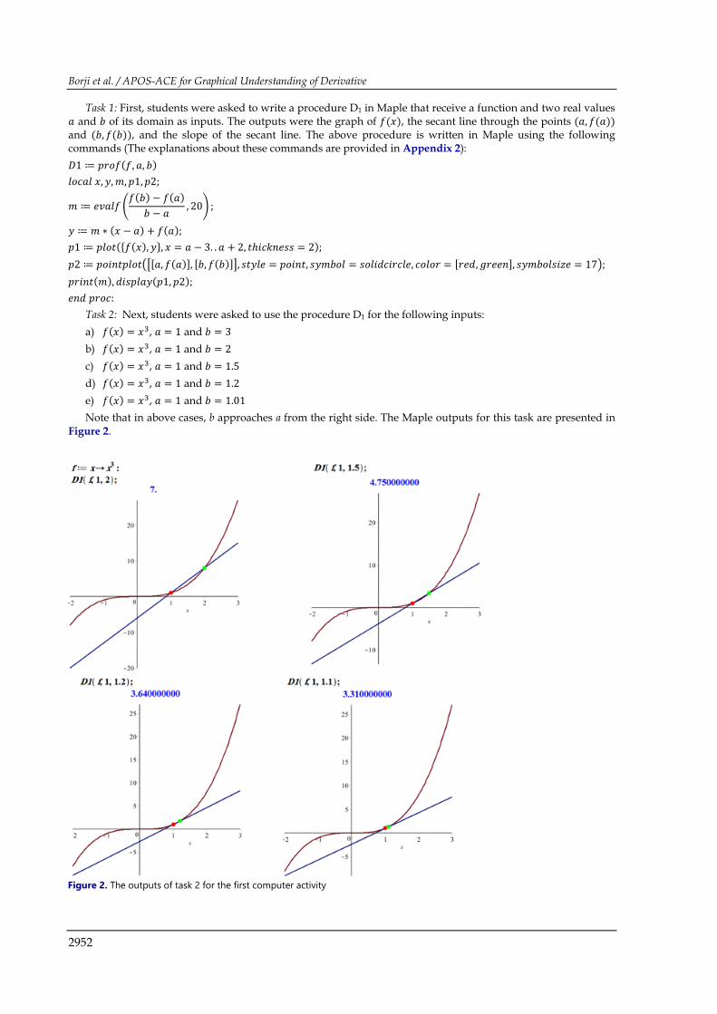
Task 1: First, students were asked to write a procedure D1 in Maple that receive a function and two real values 𝑎𝑎 and 𝑏𝑏 of its domain as inputs. The outputs were the graph of 𝑓𝑓(𝑥𝑥), the secant line through the points (𝑎𝑎, 𝑓𝑓(𝑎𝑎)) and (𝑏𝑏, 𝑓𝑓(𝑏𝑏)), and the slope of the secant line. The above procedure is written in Maple using the following commands (The explanations about these commands are provided in Appendix 2): 𝐷𝐷1 ≔ 𝑝𝑝𝑝𝑝𝑝𝑝𝑓𝑓(𝑓𝑓, 𝑎𝑎, 𝑏𝑏) 𝑙𝑙𝑝𝑝𝑙𝑙𝑎𝑎𝑙𝑙 𝑥𝑥,𝑦𝑦,𝑚𝑚, 𝑝𝑝1,𝑝𝑝2;
𝑚𝑚 ≔ 𝑒𝑒𝑒𝑒𝑎𝑎𝑙𝑙𝑓𝑓 �𝑓𝑓(𝑏𝑏) − 𝑓𝑓(𝑎𝑎)
𝑏𝑏 − 𝑎𝑎 , 20� ;
𝑦𝑦 ≔ 𝑚𝑚 ∗ (𝑥𝑥 − 𝑎𝑎) + 𝑓𝑓(𝑎𝑎); 𝑝𝑝1 ≔ 𝑝𝑝𝑙𝑙𝑝𝑝𝑝𝑝({𝑓𝑓(𝑥𝑥),𝑦𝑦}, 𝑥𝑥 = 𝑎𝑎 − 3. . 𝑎𝑎 + 2, 𝑝𝑝ℎ𝑖𝑖𝑙𝑙𝑖𝑖𝑖𝑖𝑒𝑒𝑖𝑖𝑖𝑖 = 2); 𝑝𝑝2 ≔ 𝑝𝑝𝑝𝑝𝑖𝑖𝑖𝑖𝑝𝑝𝑝𝑝𝑙𝑙𝑝𝑝𝑝𝑝��[𝑎𝑎, 𝑓𝑓(𝑎𝑎)], [𝑏𝑏, 𝑓𝑓(𝑏𝑏)]�, 𝑖𝑖𝑝𝑝𝑦𝑦𝑙𝑙𝑒𝑒 = 𝑝𝑝𝑝𝑝𝑖𝑖𝑖𝑖𝑝𝑝, 𝑖𝑖𝑦𝑦𝑚𝑚𝑏𝑏𝑝𝑝𝑙𝑙 = 𝑖𝑖𝑝𝑝𝑙𝑙𝑖𝑖𝑠𝑠𝑙𝑙𝑖𝑖𝑝𝑝𝑙𝑙𝑙𝑙𝑒𝑒, 𝑙𝑙𝑝𝑝𝑙𝑙𝑝𝑝𝑝𝑝 = [𝑝𝑝𝑒𝑒𝑠𝑠,𝑔𝑔𝑝𝑝𝑒𝑒𝑒𝑒𝑖𝑖], 𝑖𝑖𝑦𝑦𝑚𝑚𝑏𝑏𝑝𝑝𝑙𝑙𝑖𝑖𝑖𝑖𝑠𝑠𝑒𝑒 = 17�; 𝑝𝑝𝑝𝑝𝑖𝑖𝑖𝑖𝑝𝑝(𝑚𝑚),𝑠𝑠𝑖𝑖𝑖𝑖𝑝𝑝𝑙𝑙𝑎𝑎𝑦𝑦(𝑝𝑝1, 𝑝𝑝2); 𝑒𝑒𝑖𝑖𝑠𝑠 𝑝𝑝𝑝𝑝𝑝𝑝𝑙𝑙:
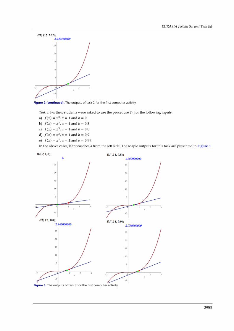
Task 2: Next, students were asked to use the procedure D1 for the following inputs: a) 𝑓𝑓(𝑥𝑥) = 𝑥𝑥3, 𝑎𝑎 = 1 and 𝑏𝑏 = 3 b) 𝑓𝑓(𝑥𝑥) = 𝑥𝑥3, 𝑎𝑎 = 1 and 𝑏𝑏 = 2 c) 𝑓𝑓(𝑥𝑥) = 𝑥𝑥3, 𝑎𝑎 = 1 and 𝑏𝑏 = 1.5 d) 𝑓𝑓(𝑥𝑥) = 𝑥𝑥3, 𝑎𝑎 = 1 and 𝑏𝑏 = 1.2 e) 𝑓𝑓(𝑥𝑥) = 𝑥𝑥3, 𝑎𝑎 = 1 and 𝑏𝑏 = 1.01 Note that in above cases, b approaches a from the right side. The Maple outputs for this task are presented in
Figure 2.
Figure 2. The outputs of task 2 for the first computer activity
EURASIA J Math Sci and Tech Ed
2953
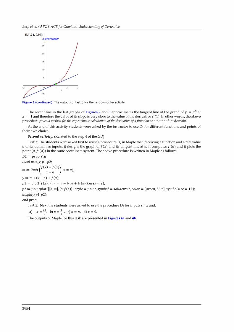
Task 3: Further, students were asked to use the procedure D1 for the following inputs: a) 𝑓𝑓(𝑥𝑥) = 𝑥𝑥3, 𝑎𝑎 = 1 and 𝑏𝑏 = 0 b) 𝑓𝑓(𝑥𝑥) = 𝑥𝑥3, 𝑎𝑎 = 1 and 𝑏𝑏 = 0.5 c) 𝑓𝑓(𝑥𝑥) = 𝑥𝑥3, 𝑎𝑎 = 1 and 𝑏𝑏 = 0.8 d) 𝑓𝑓(𝑥𝑥) = 𝑥𝑥3, 𝑎𝑎 = 1 and 𝑏𝑏 = 0.9 e) 𝑓𝑓(𝑥𝑥) = 𝑥𝑥3, 𝑎𝑎 = 1 and 𝑏𝑏 = 0.99 In the above cases, b approaches a from the left side. The Maple outputs for this task are presented in Figure 3.
Figure 2 (continued). The outputs of task 2 for the first computer activity
Figure 3. The outputs of task 3 for the first computer activity
Borji et al. / APOS-ACE for Graphical Understanding of Derivative
2954
The secant line in the last graphs of Figures 2 and 3 approximates the tangent line of the graph of 𝑦𝑦 = 𝑥𝑥3 at 𝑥𝑥 = 1 and therefore the value of its slope is very close to the value of the derivative 𝑓𝑓′(1). In other words, the above procedure gives a method for the approximate calculation of the derivative of a function at a point of its domain.
At the end of this activity students were asked by the instructor to use D1 for different functions and points of their own choice.
Second activity: (Related to the step 4 of the GD) Task 1: The students were asked first to write a procedure D2 in Maple that, receiving a function and a real value
𝑎𝑎 of its domain as inputs, it designs the graph of 𝑓𝑓(𝑥𝑥) and its tangent line at 𝑎𝑎, it computes 𝑓𝑓′(𝑎𝑎) and it plots the point (𝑎𝑎, 𝑓𝑓′(𝑎𝑎)) in the same coordinate system. The above procedure is written in Maple as follows: 𝐷𝐷2 ≔ 𝑝𝑝𝑝𝑝𝑝𝑝𝑙𝑙(𝑓𝑓, 𝑎𝑎) 𝑙𝑙𝑝𝑝𝑙𝑙𝑎𝑎𝑙𝑙 𝑚𝑚, 𝑥𝑥,𝑦𝑦, 𝑝𝑝1,𝑝𝑝2;
𝑚𝑚 ≔ 𝑙𝑙𝑖𝑖𝑚𝑚𝑖𝑖𝑝𝑝 �𝑓𝑓(𝑥𝑥) − 𝑓𝑓(𝑎𝑎)
𝑥𝑥 − 𝑎𝑎� , 𝑥𝑥 = 𝑎𝑎);
𝑦𝑦 ≔ 𝑚𝑚 ∗ (𝑥𝑥 − 𝑎𝑎) + 𝑓𝑓(𝑎𝑎); 𝑝𝑝1 ≔ 𝑝𝑝𝑙𝑙𝑝𝑝𝑝𝑝({𝑓𝑓(𝑥𝑥),𝑦𝑦}, 𝑥𝑥 = 𝑎𝑎 − 4. . 𝑎𝑎 + 4, 𝑝𝑝ℎ𝑖𝑖𝑙𝑙𝑖𝑖𝑖𝑖𝑒𝑒𝑖𝑖𝑖𝑖 = 2); 𝑝𝑝2 ≔ 𝑝𝑝𝑝𝑝𝑖𝑖𝑖𝑖𝑝𝑝𝑝𝑝𝑙𝑙𝑝𝑝𝑝𝑝��[𝑎𝑎,𝑚𝑚], [𝑎𝑎,𝑓𝑓(𝑎𝑎)]�, 𝑖𝑖𝑝𝑝𝑦𝑦𝑙𝑙𝑒𝑒 = 𝑝𝑝𝑝𝑝𝑖𝑖𝑖𝑖𝑝𝑝, 𝑖𝑖𝑦𝑦𝑚𝑚𝑏𝑏𝑝𝑝𝑙𝑙 = 𝑖𝑖𝑝𝑝𝑙𝑙𝑖𝑖𝑠𝑠𝑙𝑙𝑖𝑖𝑝𝑝𝑙𝑙𝑙𝑙𝑒𝑒, 𝑙𝑙𝑝𝑝𝑙𝑙𝑝𝑝𝑝𝑝 = [𝑔𝑔𝑝𝑝𝑒𝑒𝑒𝑒𝑖𝑖,𝑏𝑏𝑙𝑙𝑏𝑏𝑒𝑒], 𝑖𝑖𝑦𝑦𝑚𝑚𝑏𝑏𝑝𝑝𝑙𝑙𝑖𝑖𝑖𝑖𝑠𝑠𝑒𝑒 = 17�; 𝑠𝑠𝑖𝑖𝑖𝑖𝑝𝑝𝑙𝑙𝑎𝑎𝑦𝑦(𝑝𝑝1, 𝑝𝑝2); 𝑒𝑒𝑖𝑖𝑠𝑠 𝑝𝑝𝑝𝑝𝑝𝑝𝑙𝑙:
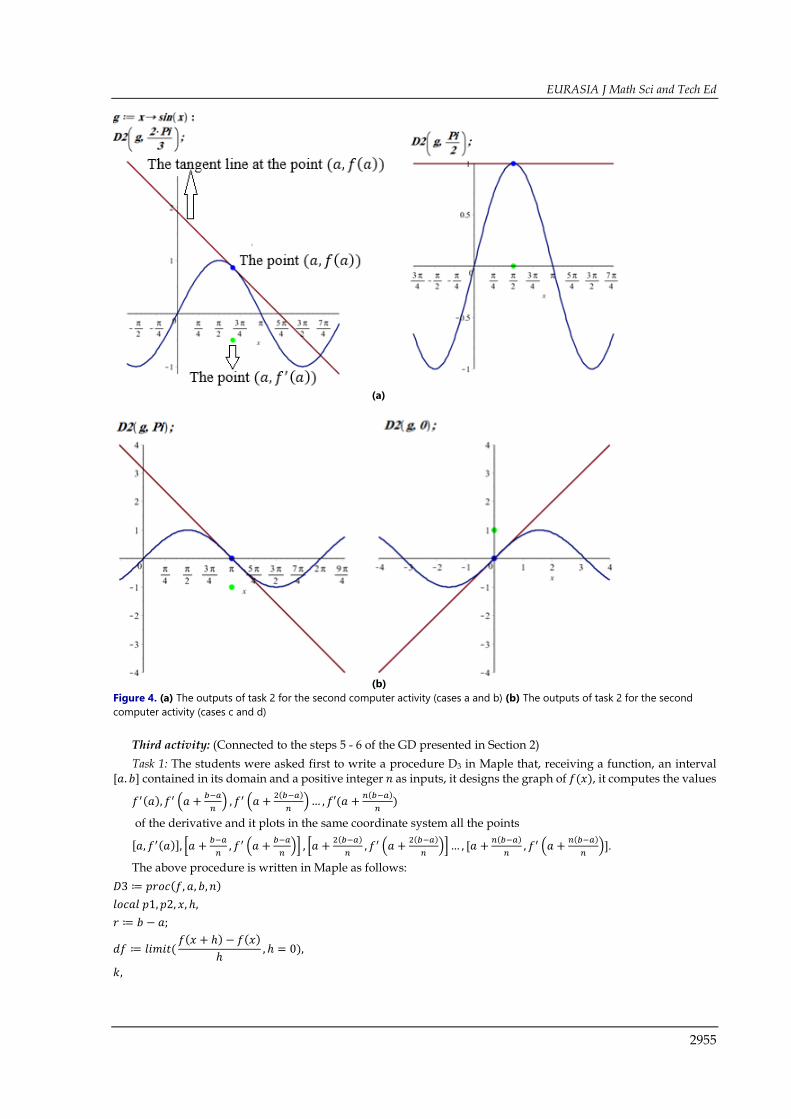
Task 2: Next the students were asked to use the procedure D2 for inputs sin x and:
a) 𝑥𝑥 = 2𝜋𝜋3
, b) 𝑥𝑥 = 𝜋𝜋2 , c) 𝑥𝑥 = 𝜋𝜋, d) 𝑥𝑥 = 0.
The outputs of Maple for this task are presented in Figures 4a and 4b.
Figure 3 (continued). The outputs of task 3 for the first computer activity
EURASIA J Math Sci and Tech Ed
2955
Third activity: (Connected to the steps 5 - 6 of the GD presented in Section 2) Task 1: The students were asked first to write a procedure D3 in Maple that, receiving a function, an interval
[𝑎𝑎. 𝑏𝑏] contained in its domain and a positive integer 𝑖𝑖 as inputs, it designs the graph of 𝑓𝑓(𝑥𝑥), it computes the values
𝑓𝑓′(𝑎𝑎),𝑓𝑓′ �𝑎𝑎 + 𝑏𝑏−𝑎𝑎𝑛𝑛� ,𝑓𝑓′ �𝑎𝑎 + 2(𝑏𝑏−𝑎𝑎)
𝑛𝑛�… , 𝑓𝑓′(𝑎𝑎 + 𝑛𝑛(𝑏𝑏−𝑎𝑎)
𝑛𝑛)
of the derivative and it plots in the same coordinate system all the points
[𝑎𝑎, 𝑓𝑓′(𝑎𝑎)], �𝑎𝑎 + 𝑏𝑏−𝑎𝑎𝑛𝑛
, 𝑓𝑓′ �𝑎𝑎 + 𝑏𝑏−𝑎𝑎𝑛𝑛�� , �𝑎𝑎 + 2(𝑏𝑏−𝑎𝑎)
𝑛𝑛,𝑓𝑓′ �𝑎𝑎 + 2(𝑏𝑏−𝑎𝑎)
𝑛𝑛��… , [𝑎𝑎 + 𝑛𝑛(𝑏𝑏−𝑎𝑎)
𝑛𝑛, 𝑓𝑓′ �𝑎𝑎 + 𝑛𝑛(𝑏𝑏−𝑎𝑎)
𝑛𝑛�].
The above procedure is written in Maple as follows: 𝐷𝐷3 ≔ 𝑝𝑝𝑝𝑝𝑝𝑝𝑙𝑙(𝑓𝑓, 𝑎𝑎, 𝑏𝑏,𝑖𝑖) 𝑙𝑙𝑝𝑝𝑙𝑙𝑎𝑎𝑙𝑙 𝑝𝑝1,𝑝𝑝2,𝑥𝑥, ℎ, 𝑝𝑝 ≔ 𝑏𝑏 − 𝑎𝑎;
𝑠𝑠𝑓𝑓 ≔ 𝑙𝑙𝑖𝑖𝑚𝑚𝑖𝑖𝑝𝑝(𝑓𝑓(𝑥𝑥 + ℎ) − 𝑓𝑓(𝑥𝑥)
ℎ, ℎ = 0),
𝑖𝑖,
(a)
(b) Figure 4. (a) The outputs of task 2 for the second computer activity (cases a and b) (b) The outputs of task 2 for the second computer activity (cases c and d)

Borji et al. / APOS-ACE for Graphical Understanding of Derivative
2956
𝑥𝑥𝑖𝑖 ≔ �𝑖𝑖𝑒𝑒𝑠𝑠 �𝑎𝑎 + 𝑖𝑖 ∗𝑝𝑝𝑖𝑖 , 𝑖𝑖 = 0. .𝑖𝑖�� ;
𝑝𝑝1 ≔ 𝑝𝑝𝑙𝑙𝑝𝑝𝑝𝑝(𝑓𝑓(𝑥𝑥), 𝑥𝑥 = 𝑎𝑎. . 𝑏𝑏, 𝑝𝑝ℎ𝑖𝑖𝑙𝑙𝑖𝑖𝑖𝑖𝑒𝑒𝑖𝑖𝑖𝑖 = 4); 𝑝𝑝2 ≔ 𝑝𝑝𝑝𝑝𝑖𝑖𝑖𝑖𝑝𝑝𝑝𝑝𝑙𝑙𝑝𝑝𝑝𝑝([𝑖𝑖𝑒𝑒𝑠𝑠([𝑖𝑖, 𝑖𝑖𝑏𝑏𝑏𝑏𝑖𝑖(𝑥𝑥 = 𝑖𝑖,𝑠𝑠𝑓𝑓)], 𝑖𝑖 = 𝑥𝑥𝑖𝑖)], 𝑖𝑖𝑝𝑝𝑦𝑦𝑙𝑙𝑒𝑒 = 𝑝𝑝𝑝𝑝𝑖𝑖𝑖𝑖𝑝𝑝, 𝑖𝑖𝑦𝑦𝑚𝑚𝑏𝑏𝑝𝑝𝑙𝑙𝑒𝑒 = 𝑖𝑖𝑝𝑝𝑙𝑙𝑖𝑖𝑠𝑠𝑙𝑙𝑖𝑖𝑝𝑝𝑙𝑙𝑙𝑙𝑒𝑒, 𝑙𝑙𝑝𝑝𝑙𝑙𝑝𝑝𝑝𝑝
= 𝑔𝑔𝑝𝑝𝑒𝑒𝑒𝑒𝑖𝑖, 𝑖𝑖𝑦𝑦𝑚𝑚𝑏𝑏𝑝𝑝𝑙𝑙𝑖𝑖𝑖𝑖𝑠𝑠𝑒𝑒 = 15); 𝐷𝐷𝑖𝑖𝑖𝑖𝑝𝑝𝑙𝑙𝑎𝑎𝑦𝑦(𝑝𝑝1,𝑝𝑝2); 𝑒𝑒𝑖𝑖𝑠𝑠 𝑝𝑝𝑝𝑝𝑝𝑝𝑙𝑙:
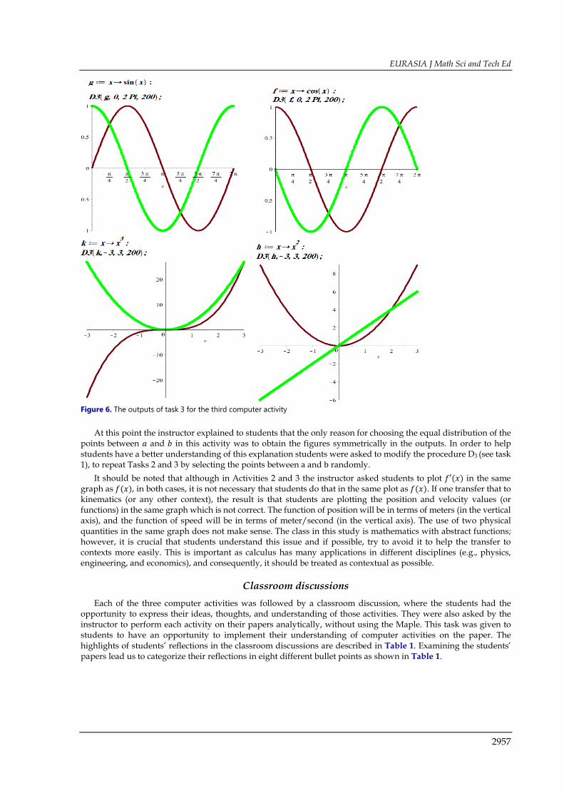
Task 2: Next the students were asked to use the procedure D3 for: a) The function 𝑖𝑖𝑖𝑖𝑖𝑖 𝑥𝑥 on the interval [0, 2𝜋𝜋], with 𝑖𝑖 = 20 b) The function cos𝑥𝑥 on the interval [0, 2𝜋𝜋], with 𝑖𝑖 = 20 c) The function 𝑥𝑥3 on the interval [−3, 3], with 𝑖𝑖 = 20 d) The function 𝑥𝑥2 on the interval [−3, 3], with 𝑖𝑖 = 15 The outputs of Maple for this task are presented in Figure 5. Task 3: Further, the students were asked to use the procedure D3 for: e) The function 𝑖𝑖𝑖𝑖𝑖𝑖 𝑥𝑥 on the interval [0, 2𝜋𝜋], with 𝑖𝑖 = 200 f) The function cos𝑥𝑥 on the interval [0, 2𝜋𝜋], with 𝑖𝑖 = 200 g) The function 𝑥𝑥3 on the interval [−3, 3], with 𝑖𝑖 = 200 h) The function 𝑥𝑥2 on the interval [−3, 3], with 𝑖𝑖 = 150 The outputs of Maple for this task are presented in Figure 6.
Figure 5. The outputs of task 2 for the third computer activity
EURASIA J Math Sci and Tech Ed
2957
At this point the instructor explained to students that the only reason for choosing the equal distribution of the points between 𝑎𝑎 and 𝑏𝑏 in this activity was to obtain the figures symmetrically in the outputs. In order to help students have a better understanding of this explanation students were asked to modify the procedure D3 (see task 1), to repeat Tasks 2 and 3 by selecting the points between a and b randomly.
It should be noted that although in Activities 2 and 3 the instructor asked students to plot 𝑓𝑓′(𝑥𝑥) in the same graph as 𝑓𝑓(𝑥𝑥), in both cases, it is not necessary that students do that in the same plot as 𝑓𝑓(𝑥𝑥). If one transfer that to kinematics (or any other context), the result is that students are plotting the position and velocity values (or functions) in the same graph which is not correct. The function of position will be in terms of meters (in the vertical axis), and the function of speed will be in terms of meter/second (in the vertical axis). The use of two physical quantities in the same graph does not make sense. The class in this study is mathematics with abstract functions; however, it is crucial that students understand this issue and if possible, try to avoid it to help the transfer to contexts more easily. This is important as calculus has many applications in different disciplines (e.g., physics, engineering, and economics), and consequently, it should be treated as contextual as possible.
Classroom discussions Each of the three computer activities was followed by a classroom discussion, where the students had the
opportunity to express their ideas, thoughts, and understanding of those activities. They were also asked by the instructor to perform each activity on their papers analytically, without using the Maple. This task was given to students to have an opportunity to implement their understanding of computer activities on the paper. The highlights of students’ reflections in the classroom discussions are described in Table 1. Examining the students’ papers lead us to categorize their reflections in eight different bullet points as shown in Table 1.
Figure 6. The outputs of task 3 for the third computer activity

Borji et al. / APOS-ACE for Graphical Understanding of Derivative
2958
The findings reported in Table 1 shows that a significant number of students (80.76%) understood the relation between the tangent line and the limit of the difference quotient, and they also understood that the value of the slope of the tangent line at a point of the graph of 𝑓𝑓(𝑥𝑥) is equal to the value of the derivative at that point. In addition, they understood how they can sketch the graph of 𝑓𝑓′ when given the graph of 𝑓𝑓. Furthermore, five students expressed interesting remarks: “if the graph of a function is increasing / decreasing in an interval, then the graph of 𝑓𝑓′(𝑥𝑥) is above / below of the x - axis in that interval. If the concavity of the function is upward / downward in an interval, then the graph of 𝑓𝑓′(𝑥𝑥) is increasing / decreasing in that interval”. This shows that the computer activities could help students to improve their understanding of derivative and students could find valuable relationships between the graph of a function and the graph of its derivative.
Exercises The Exercises phase of the ACE Cycle reinforces the Activity and Classroom Discussion phases. In particular,
students continued to build and expand their derivative graphical schema by working on tangent lines and the limit of difference quotients, slopes of tangent lines and derivative at different points, sketching the graph of a derivative function, when the graph of a function is given. The exercises were designed and given to students as homework and comprised different mathematics situations. Some of the exercises are described in the following.
Exercise 1 (Related to the first computer activity): Using the graph of the function 𝑓𝑓(𝑥𝑥) (Figure 7) and the table of its values given below, approximate the value of the derivative 𝑓𝑓′(𝑥𝑥) at 𝑥𝑥 = 0.04.
Table 1. Students’ reflections in the Classroom discussion Activity Subject Students’ reflections N
1
Tangent line and the limit of the difference quotient.
• The tangent line at a point 𝑎𝑎 on the graph of a function is the limit position of the sequence of secant lines through two points 𝑥𝑥 and 𝑎𝑎, when the point 𝑥𝑥 approaches the point 𝑎𝑎. The limit value of the slopes of these secant lines is equal to the value of the slope of the tangent line at 𝑎𝑎, which is therefore calculated by computing the lim𝑥𝑥→𝑎𝑎
𝑓𝑓(𝑥𝑥)−𝑓𝑓(𝑎𝑎)𝑥𝑥−𝑎𝑎
.
21 (80.76%)
2 & 3
The slope of the tangent line and the derivative at a point. Sketching the graph of the derivative function, when the graph of the function is given.
• The value of the slope of the tangent line at a point of the graph of 𝑓𝑓(𝑥𝑥) is equal to the value of the derivative at that point. 21 (80.76%)
• Since the slope of the tangent line at each point of the graph of 𝑓𝑓(𝑥𝑥) is uniquely determined, the derivative of a function is also a function 18 (69.23%)
• One can compute the value of the derivative of a function at a point of its domain from its graph by calculating the slope of the tangent line at that point. Further, computing the derivative of 𝑓𝑓′(𝑥𝑥) at an adequate number of suitably chosen points 𝑥𝑥, he/she can sketch the graph of 𝑓𝑓′(𝑥𝑥) by plotting the points (𝑥𝑥, 𝑓𝑓′(𝑥𝑥)) on the same Cartesian coordinate system.
15 (57.69%)
• Before performing these activities, if the graph of 𝑓𝑓(𝑥𝑥) was given and we wanted to sketch the graph of 𝑓𝑓′(𝑥𝑥), we tried first to find the analytic expression of the function 𝑓𝑓(𝑥𝑥) via its graph, then we computed the analytic expression of 𝑓𝑓′(𝑥𝑥) and finally we used this expression for sketching the graph of 𝑓𝑓′(𝑥𝑥).
10 (38.46%)
• If the graph of a function 𝑓𝑓(𝑥𝑥) is increasing / decreasing in an interval, then the graph of 𝑓𝑓′(𝑥𝑥) is above / below of the x - axis in that interval. Also, if the concavity of the function 𝑓𝑓(𝑥𝑥) is upward / downward in an interval, then the graph of 𝑓𝑓′(𝑥𝑥) is increasing / decreasing in that interval.
• The first part of the above remark corresponds to the well-known result that the function 𝑓𝑓(𝑥𝑥) is strictly increasing / decreasing in an interval, if, and only if, 𝑓𝑓′(𝑥𝑥) >0 (< 0) in that interval. Hence, 𝑓𝑓′(𝑥𝑥) is strictly increasing / decreasing in an interval, if, and only if, 𝑓𝑓′′(𝑥𝑥) > 0 (< 0) in that interval. Therefore, the second part of the above remark corresponds to the well-known result that, the concavity of the function 𝑓𝑓(𝑥𝑥) is upward / downward in an interval, if, and only if 𝑓𝑓′′(𝑥𝑥) > 0 (< 0).
5 (19.23%)
5 (19.23%)
Figure 7. The data of Exercise 1

EURASIA J Math Sci and Tech Ed
2959
Exercise 2 (Related to the second computer activity): Suppose that the line 𝑳𝑳 is the tangent to the graph of the function 𝑓𝑓(𝑥𝑥) at the point (4,4) presented in the Figure 8. Calculate the value of 𝑓𝑓′(4).
Exercise 3 (Related to the third computer activity): The graphs of two functions are given in Figure 9. Use them to sketch the graph of their derivatives.
Students reinforced the knowledge they obtained in the computer activities and in the classroom discussions by using it in solving the exercises. In other words, it was expected that through the classroom discussions and doing homework exercises the majority of students organized the concept of derivative and in particular its graphical understanding in their proper mental schemas.
Written Test Asiala et al. (1996) proposed a specific framework for the APOS theory based research consist of the following
three components: 1) Development of the corresponding GD (Theoretical analysis), 2) Design and implementation of the proper ACE cycle (instruction), and 3) Collection and analysis of the data obtained by the implementation of the ACE cycle (Figure 10). The data analysis could lead to modifications of the initial GD for the mathematical topic under study.
In the previous two sections we have already completed the first two components for the case of the derivative. In this section, we cover the third component. For this, the performance of the experimental group is compared to the performance of the control group.
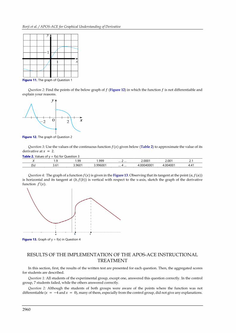
The written test included the following four questions that are designed by the authors of this article. Question 1: Use the given graph of 𝑓𝑓 (Figure 11) to estimate the value of 𝑓𝑓′(2).
Figure 8. The graph of Exercise 2
Figure 10. Research cycle (Asiala et al. 1996)
Figure 9. The graphs of Exercise 3
Borji et al. / APOS-ACE for Graphical Understanding of Derivative
2960
Question 2: Find the points of the below graph of 𝑓𝑓 (Figure 12) in which the function 𝑓𝑓 is not differentiable and explain your reasons.
Question 3: Use the values of the continuous function 𝑓𝑓(𝑥𝑥) given below (Table 2) to approximate the value of its derivative at 𝑥𝑥 = 2.
Question 4: The graph of a function 𝑓𝑓(𝑥𝑥) is given in the Figure 13. Observing that its tangent at the point (𝑎𝑎,𝑓𝑓(𝑎𝑎)) is horizontal and its tangent at (𝑏𝑏, 𝑓𝑓(𝑏𝑏)) is vertical with respect to the x-axis, sketch the graph of the derivative function 𝑓𝑓′(𝑥𝑥).
RESULTS OF THE IMPLEMENTATION OF THE APOS-ACE INSTRUCTIONAL TREATMENT
In this section, first, the results of the written test are presented for each question. Then, the aggregated scores for students are described.
Question 1: All students of the experimental group, except one, answered this question correctly. In the control group, 7 students failed, while the others answered correctly.
Question 2: Although the students of both groups were aware of the points where the function was not differentiable (𝑥𝑥 = −4 and 𝑥𝑥 = 0), many of them, especially from the control group, did not give any explanations.
Figure 11. The graph of Question 1
Figure 12. The graph of Question 2
Table 2. Values of y = f(x) for Question 3 X 1.9 1.99 1.999 … 2 … 2.0001 2.001 2.1
f(x) 3.61 3.9601 3.996001 … 4 … 4.00040001 4.004001 4.41
Figure 13. Graph of y = f(x) in Question 4
EURASIA J Math Sci and Tech Ed
2961
6 students from experimental and 15 students from control groups could not bring a correct reason for their answers.
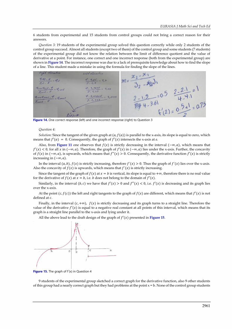
Question 3: 19 students of the experimental group solved this question correctly while only 2 students of the control group succeed. Almost all students (except two of them) of the control group and some students (7 students) of the experimental group did not know the relation between the limit of difference quotient and the value of derivative at a point. For instance, one correct and one incorrect response (both from the experimental group) are shown in Figure 14. The incorrect response was due to a lack of prerequisite knowledge about how to find the slope of a line. This student made a mistake in using the formula for finding the slope of the lines.
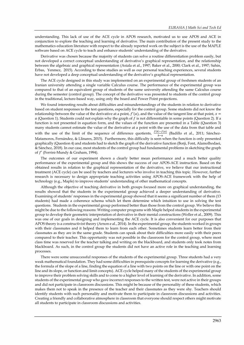
Question 4: Solution: Since the tangent of the given graph at (𝑎𝑎, 𝑓𝑓(𝑎𝑎)) is parallel to the x-axis, its slope is equal to zero, which
means that 𝑓𝑓′(𝛼𝛼) = 0. Consequently, the graph of 𝑓𝑓′(𝑥𝑥) intersects the x-axis at a. Also, from Figure 11 one observes that 𝑓𝑓(𝑥𝑥) is strictly decreasing in the interval (−∞, 𝑎𝑎), which means that
𝑓𝑓′(𝑥𝑥) < 0, for all 𝑥𝑥 in (−∞, 𝑎𝑎). Therefore, the graph of 𝑓𝑓′(𝑥𝑥) in (−∞, 𝑎𝑎) lies under the x-axis. Further, the concavity of 𝑓𝑓(𝑥𝑥) in (−∞,𝑎𝑎), is upwards, which means that 𝑓𝑓′′(𝑥𝑥) > 0. Consequently, the derivative function 𝑓𝑓′(𝑥𝑥) is strictly increasing in (−∞, 𝑎𝑎).
In the interval (𝑎𝑎, 𝑏𝑏), 𝑓𝑓(𝑥𝑥) is strictly increasing, therefore 𝑓𝑓΄(𝑥𝑥) > 0. Thus the graph of 𝑓𝑓΄(𝑥𝑥) lies over the x-axis. Also the concavity of 𝑓𝑓(𝑥𝑥) is upwards, which means that 𝑓𝑓΄(𝑥𝑥) is strictly increasing.
Since the tangent of the graph of 𝑓𝑓(𝑥𝑥) at 𝑥𝑥 = 𝑏𝑏 is vertical, its slope is equal to +∞, therefore there is no real value for the derivative of 𝑓𝑓(𝑥𝑥) at 𝑥𝑥 = 𝑏𝑏, i.e. 𝑏𝑏 does not belong to the domain of 𝑓𝑓′(𝑥𝑥).
Similarly, in the interval (𝑏𝑏, 𝑙𝑙) we have that 𝑓𝑓′(𝑥𝑥) > 0 and 𝑓𝑓′′(𝑥𝑥) < 0, i.e. 𝑓𝑓′(𝑥𝑥) is decreasing and its graph lies over the x-axis.
At the point (𝑙𝑙, 𝑓𝑓(𝑙𝑙)) the left and right tangents to the graph of 𝑓𝑓(𝑥𝑥) are different, which means that 𝑓𝑓′(𝑥𝑥) is not defined at 𝑙𝑙.
Finally, in the interval (𝑙𝑙, +∞), 𝑓𝑓(𝑥𝑥) is strictly decreasing and its graph turns to a straight line. Therefore the value of the derivative 𝑓𝑓′(𝑥𝑥) is equal to a negative real constant at all points of this interval, which means that its graph is a straight line parallel to the x-axis and lying under it.
All the above lead to the draft design of the graph of 𝑓𝑓′(𝑥𝑥) presented in Figure 15.
9 students of the experimental group sketched a correct graph for the derivative function, also 9 other students of this group had a nearly correct graph but they had problems at the point x = b. None of the control group students
Figure 14. One correct response (left) and one incorrect response (right) to Question 3
Figure 15. The graph of f΄(x) in Question 4

Borji et al. / APOS-ACE for Graphical Understanding of Derivative
2962
correctly answered this question. In Figure 16 some of students’ responses to Question 4 are shown. The first row is from students of the experimental, while the second row is from students of the control group.
Students’ answers were marked in a score range from 0 to 10 based on a scoring system (Table 3) and the scores of the two groups are presented in Table 4.
The mean score for the control group was 5.33 and the mean score for the experimental group was 7.26. Therefore, the experimental group demonstrated a clearly better mean performance compared to the control group. Considering the results of each question and the scores from both groups shows that the quality performance of the experimental group was much better than that of the control group. It should be said here, in regards to calculating and using scores of the students in both experimental and control groups, we do not want to link them to the students’ mental constructions. We only used this data to explore the effects of our ACE teaching cycle by comparing the scores of the experimental and control groups.
DISCUSSION AND CONCLUSION APOS theory has been used in several studies on calculus concepts (Badillo et al., 2011; Baker et al., 2000; Borji
& Voskoglou, 2016), however, ACE has been less widely used. The majority of previous APOS research, focused on exploring students’ understanding of a concept rather than how the teaching can impact on students’
Figure 16. Student responses for Question 2
Table 3. Scoring system Question Total Score Score system Question 1 1 If student estimate 𝑓𝑓′(2) correctly (score 1).
Question 2 2 • Function at 𝑥𝑥 = −4 is not differentiable (score 0.5) and its reason (score 0.5). • Function at 𝑥𝑥 = 0 is not differentiable (score 0.5) and its reason (score 0.5).
Question 3 3 • Computing left derivative at 𝑥𝑥 = 2, 𝑓𝑓−′(2), (score 1). • Computing right derivative at 𝑥𝑥 = 2, 𝑓𝑓+′(2), (score 1). • Computing derivative at 𝑥𝑥 = 2, 𝑓𝑓′(2), (score 1).
Question 4 4
• Sketching 𝑓𝑓′(𝑥𝑥) on (−∞,𝑎𝑎] correctly (score 1). • Sketching 𝑓𝑓′(𝑥𝑥) on [𝑎𝑎, 𝑏𝑏] correctly (score 1). • Sketching 𝑓𝑓′(𝑥𝑥) on [b, 𝑙𝑙] correctly (score 1). • Sketching 𝑓𝑓′(𝑥𝑥) on [𝑙𝑙, +∞] correctly (score 1).
Table 4. Scores of the control and the experimental group Scores 10 9 8 7 6 5 4 3 2
Frequency for the control group 0 1 4 3 4 4 3 3 2 Frequency for the experimental group 4 5 4 5 3 2 1 1 1
EURASIA J Math Sci and Tech Ed
2963
understanding. This lack of use of the ACE cycle in APOS research, motivated us to use APOS and ACE in conjunction to explore the teaching and learning of derivative. The main contribution of the present study to the mathematics education literature with respect to the already reported work on the subject is the use of the MAPLE software based on ACE cycle to teach and enhance students’ understanding of the derivative.
Derivative was chosen because the majority of students can solve a routine differentiation problem easily, but not developed a correct conceptual understanding of derivative’s graphical representation, and the relationship between the algebraic and graphical representation (Asiala et al., 1997; Baker et al., 2000; Clark et al., 1997; Sahin, Erbas, Yenmez, 2015). According to these studies as well as our personal teaching experiences, several students have not developed a deep conceptual understanding of the derivative’s graphical representation.
The ACE cycle designed in this study was implemented on an experimental group of freshmen students of an Iranian university attending a single variable Calculus course. The performance of the experimental group was compared to that of an equivalent group of students of the same university attending the same Calculus course during the semester (control group). The concept of the derivative was presented to students of the control group in the traditional, lecture-based way, using only the board and Power Point projections.
We found interesting results about difficulties and misunderstandings of the students in relation to derivative based on student responses to the test questions, especially for the control group. Some students did not know the relationship between the value of the derivative at a point, 𝑓𝑓′(𝑎𝑎), and the value of the tangent line at that point, 𝑥𝑥 =𝑎𝑎 (Question 1). Students could not explain why the graph of 𝑓𝑓 is not differentiable in some points (Question 2). If a function is not presented in equation form, and the values of the function are presented in a Table (Question 3) many students cannot estimate the value of the derivative at a point with the use of the data from that table and with the use of the limit of the sequence of difference quotients, 𝑓𝑓(𝑏𝑏)−𝑓𝑓(𝑎𝑎)
𝑏𝑏−𝑎𝑎 (Badillo et al., 2011; Sánchez-
Matamoros, Fernández, & Llinares, 2015). Furthermore, this difficulty is seen when the function is only presented graphically (Question 4) and students had to sketch the graph of the derivative function (Borji, Font, Alamolhodaei, & Sánchez, 2018). In our case, most students of the control group had fundamental problems in sketching the graph of 𝑓𝑓′ (Ferrini-Mundy & Graham, 1994).
The outcomes of our experiment shown a clearly better mean performance and a much better quality performance of the experimental group and this shows the success of our APOS-ACE instruction. Based on the obtained results in relation to the graphical representation of the derivative, we believe that our instructional treatment (ACE cycle) can be used by teachers and lecturers who involve in teaching this topic. However, further research is necessary to design appropriate teaching activities using APOS-ACE framework with the help of technology (e.g., Maple) to improve students’ understanding of other mathematical concepts.
Although the objective of teaching derivative in both groups focused more on graphical understanding, the results showed that the students in the experimental group achieved a deeper understanding of derivative. Examining of students’ responses in the experimental group showed that it seems a significant number of them (13 students) had made a coherence schema which let them determine which intuition to use in solving the test questions. Students in the experimental group performed better than those from the control group. We believe this might be due to the following reasons: Writing computer programs with Maple helped students in the experimental group to develop their geometric interpretation of derivative in their mental constructions (Weller et al., 2009). This was one of our goals in designing and implementing the ACE cycle. It is also convenient for our purposes that APOS theory is a constructivist theory (Arnon e al., 2014). In the experimental group, the students worked in groups with their classmates and it helped them to learn from each other. Sometimes students learn better from their classmates as they are in the same grade. Students can speak about their difficulties more easily with their peers compared to their teacher. This opportunity was not possible in the classroom for the control group, where most class time was reserved for the teacher talking and writing on the blackboard, and students only took notes from blackboard. As such, in the control group the students did not have an active role in the teaching and learning processes.
There were some unsuccessful responses of the students of the experimental group. Three students had a very weak mathematical foundation. They had some difficulties in prerequisite concepts for learning the derivative (e.g., the formula of the slope of a line, finding the equation of a line with two points on the line or with one point on the line and its slope, or function and limit concepts). ACE cycle helped many of the students of the experimental group to improve their problem solving skills and to come to a higher level of learning of the derivative. In addition, some students of the experimental group who gave incorrect responses to the written test, were not active in their groups and did not participate in classroom discussions. This might be because of the personality of these students, which makes them not to speak in the presence of the teacher and their classmates as they were shy. Teachers should identify students with such personality and motivate them to participate in classroom discussions and activities. Creating a friendly and collaborative atmosphere in classroom that everyone should respect others might motivate all students to participate in classroom discussions and activities.
Borji et al. / APOS-ACE for Graphical Understanding of Derivative
2964
Teachers and lecturers have a very important role in teaching mathematics. They should be aware of the importance of using technology (activities with computers) in the teaching and learning (Blyth & Labovic, 2009; Samkova, 2012). In addition, they should be familiar with mathematical software programs and technologies (e.g., Maple) in order to be able to design teaching activities that improve students’ understanding, and also encourage students to use technologies to enhance their learning. There are several studies that show that the use of technology improves students’ understanding of mathematical concepts (Abu-Naja, 2008; Chamble, Slough, & Wunsch, 2008; Lyublinskaya & Zhou, 2008; Merriweather & Tharp, 1999; Ng, Tan, & Ng, 2009; Özmantar, Akkoç, Bingölbali, Demir, & Ergene, 2010). In addition, the National Council of Teachers of Mathematics (NCTM, 1989) also recommended teachers to use technology to design new teaching activities (e.g., design graphical representations with the use of mathematical software).
Furthermore, teachers and lecturers should be aware of the diversity of representations, especially graphical representation, of the mathematical concepts (Pino-Fan, Font, Gordillo, Larios, & Breda, 2017). The use of different representations (graphical, algebraic, symbolic and etc) in teaching and learning Calculus concepts and transition between these representations will help students to acquire a deeper understanding of the concepts (Breda, Pino-Fan, & Font, 2017; Mallet, 2007; NCTM, 1989; Park, 2015; Tall, 1996; Tiwari, 2007). By understanding the role of representations in teaching mathematics, teachers and lecturers would have an opportunity to design an ACE cycle that improve students’ mathematical understanding.
ACKNOWLEDGEMENT The authors would like to acknowledge the constructive feedback of Professor Vicenç Font (University of
Barcelona) on this article.
REFERENCES Abu-Naja, M. (2008). The influence of graphic calculators on secondary school pupils’ ways of thinking about the
topic “positivity and negativity of functions”. International Journal for Technology in Mathematics Education, 15(3), 103-117.
Andresen, M. (2007), Introduction of a new construct: The conceptual tool “Flexibility”, The Montana Mathematics Enthusiast, 4(2), 230-250.
Arnon, I., Cottrill, J. Dubinsky, E., Oktac, A., Roa, S., Trigueros, M., & Weller, K. (2014), APOS Theory: A Framework for Research and Curriculum Development in Mathematics Education, Springer, NY, Heidelberg, Dondrecht, London. https://doi.org/10.1007/978-1-4614-7966-6
Asiala, M., Brown, A., DeVries, D. J., Dubinsky, E., Mathews, D., & Thomas, K. (1996), A framework for research and development in undergraduate mathematics education. Research in Collegiate Mathematics Education, 6(2), 1-32. https://doi.org/10.1090/cbmath/006/01
Asiala, M., Cottrill, J., Dubinsky, E., & Schwingendorf, K. E. (1997). The development of students’ graphical understanding of the derivative. Journal of Mathematical Behavior, 16(4), 399-431. https://doi.org/10.1016/S0732-3123(97)90015-8
Badillo, E. (2003). La Derivada como objeto matemático y como objeto de enseñanza y aprendizaje en profesores de matemática de Colombia (Doctoral Thesis). University Autonoma of Barcelona, Espain.
Badillo, E., Azcárate, C., & Font, V. (2011). Análisis de los niveles de comprensión de los objetos f’(a) y f’(x) de profesores de matemáticas. Enseñanza de las Ciencias, 29(2), 191-206. https://doi.org/10.5565/rev/ec/v29n2.546
Baker, B., Cooley, L., & Trigueros, M. (2000). A Calculus Graphing Schema, Journal for Research in Mathematics Education, 31(5), 557-576. https://doi.org/10.2307/749887
Beth, E. W., & Piaget, J. (1974). Mathematical epistemology and psychology (W. Mays, Trans.). Dordrecht, the Netherlands: D. Reidel. https://doi.org/10.1007/978-94-017-2193-6
Blyth, B., & Labovic, A. (2009). Using Maple to implement eLearning integrated with computer aided assessment. International Journal of Mathematical Education in Science and Technology, 40(7), 975-988. https://doi.org/10.1080/00207390903226856
Borji, V., Font, V., Alamolhodaei, H., & Sánchez, A. (2018). Application of the Complementarities of Two Theories, APOS and OSA, for the Analysis of the University Students’ Understanding on the Graph of the Function and its Derivative. EURASIA Journal of Mathematics, Science and Technology Education, 14(6), 2301-2315. https://doi.org/10.29333/ejmste/89514
EURASIA J Math Sci and Tech Ed
2965
Borji, V., & Voskoglou, M. Gr. (2016). Applying the APOS Theory to Study the Student Understanding of the Polar Coordinates, American Journal of Educational Research, 4(16), 1149-1156.
Borji, V., & Voskoglou, M.Gr. (2017), Designing an ACE Approach for Teaching the Polar Coordinates, American Journal of Educational Research, 5(3), 303-309.
Breda, A., Pino-Fan, L., & Font, V. (2017). Meta didactic-mathematical knowledge of teachers: criteria for the reflection and assessment on teaching practice. EURASIA Journal of Mathematics, Science & Technology Education, 13(6), 1893-1918. https://doi.org/10.12973/eurasia.2017.01207a
Chamblee, G. E., Slough, S. W., & Wunsch, G. (2008). Measuring high school mathematics teachers’ concerns about graphing calculators and change: A yearlong study. Journal of Computers in Mathematics and Science Teaching, 27(2), 183–194.
Clark J. M., Cordero, F., Cottrill, J., Czarnocha, B., DeVries, D. J., St. John, D., Tolias T., & Vidakovic, D. (1997). Constructing a schema: The case of the chain rule. Journal of Mathematical Behavior, 16(4), 345-364. https://doi.org/10.1016/S0732-3123(97)90012-2
Cooley, L., Trigueros, M., & Baker, B. (2007). Schema Thematization: A Framework and an Example. Journal for Research in Mathematics Education, 38(4), 370-392. https://doi.org/10.2307/30034879
Dominguez, A., Barniol, P., & Zavala, G. (2017). Test of Understanding Graphs in Calculus: Test of Students’ Interpretation of Calculus Graphs. EURASIA Journal of Mathematics, Science and Technology Education. 13(10), 6507-6531. https://doi.org/10.12973/ejmste/78085
Dubinsky, E., & Leron, U. (1994). Learning abstract algebra with ISETL. New York: Springer. https://doi.org/10.1007/978-1-4612-2602-4
Dubinsky, E., & McDonald, M. A. (2001). APOS: A constructivist theory of learning in undergraduate mathematics education research, in D Holton (Ed.), The teaching and learning of mathematics at university level: An ICMI study. Kluwer, Dordrecht.
Dubinsky, E., Weller, K., & Arnon, I. (2013). Pre-service teachers’ understanding of the relation between a fraction or integer and its decimal expansion: The Case of 0.999...and 1.Canadian Journal of Science, Mathematics, and Technology Education, 13(3), 5-28. https://doi.org/10.1080/14926150902817381
Ferrini-Mundy, J., & Graham, K. (1994). Research in calculus learning: Understanding limits, derivatives, and integrals, in E. Dubinsky & J. Kaput (Eds.), Research issues in undergraduate mathematics learning (pp. 19-26), Mathematical Association of America.
Font, V., Trigueros, M., Badillo, E., & Rubio, N. (2016). Mathematical objects through the lens of two different theoretical perspectives: APOS and OSA. Educational Studies in Mathematics, 91(1), 107–122. https://doi.org/10.1007/s10649-015-9639-6
García, M., Gavilán, J. M., & Llinares, S. (2012). Perspectiva de la práctica del profesor de matemáticas de secundaria sobre la enseñanza de la derivada. Relaciones entre la práctica y la perspectiva del profesor. Enseñanza de las Ciencias, 30(3), 219-235.
Gavilán, J. M. (2005). El papel del profesor en la enseñanza de la derivada. Análisis desde una perspectiva cognitiva (Doctoral Thesis). Departamento de Didáctica de las Matemáticas. Universidad de Sevilla, España.
Gavilán, J. M., García, M., & Llinares, S. (2007a). Una perspectiva para el análisis de la práctica del profesor de matemáticas. Implicaciones metodológicas. Enseñanza de las Ciencias, 25(2), 157-170.
Gavilán, J. M., García, M., & Llinares, S. (2007b). La modelación de la descomposición genética de una noción matemática. Explicando la práctica del profesor desde el punto de vista del aprendizaje de los estudiantes. Educación Matemática, 19(2), 5-39.
Giraldo, V., Carvalho, L. M., & Tall, D. (2003). Descriptions and Definitions in the Teaching of Elementary Calculus. Proceedings of the 27th Conference of the International Group for the Psychology of Mathematics Education, 2, 445-452.
Hähkiöniemi, M. (2004). Perceptual and symbolic representations as a starting point of the acquisition of the derivative. Proceedings of the 28th Conference of the International Group for the Psychology of Mathematics Education, 3, 73-80.
Lyublinskaya, I., & Zhou, G. (2008). Integrating graphing calculators and Probe ware into science methods courses: Impacts on pre-service elementary teachers’ confidence and perspectives on technology for learning and teaching. Journal of Computers in Mathematics and Science Teaching, 27(2), 163–182.
Maharaj, A. (2005). Investigating the Senior Certificate Mathematics examination in South Africa: Implications for teaching (Doctoral Thesis), Pretoria, University of South Africa.
Borji et al. / APOS-ACE for Graphical Understanding of Derivative
2966
Maharaj, A. (2010). An APOS Analysis of Students’ Understanding of the Concept of a Limit of a Function. Pythagoras, 71(6), 41-52. https://doi.org/10.4102/pythagoras.v0i71.6
Maharaj, A. (2013). An APOS Analysis of natural science students’ understanding of the derivatives, South African Journal of Education, 33(1), 1-19. https://doi.org/10.15700/saje.v33n1a458
Mallet, D. (2007). Multiple representations for Systems of Linear Equations via the Computer Algebra system Maple. International Electronic Journal of Mathematics Education, 2(1), 16-31.
Merriweather, M., & Tharp, M. L. (1999). The effects of instruction with graphing calculators on how general mathematics students naturalistically solve algebraic problems. Journal of Computers in Mathematics and Science Teaching, 18(1), 7–22.
National Council of Teachers and Mathematics. (1989). Curriculum and Evaluation Standards for School Mathematics. National Council of Teachers and Mathematics, Reston, VA.
Ng, W. L., Tan, W. C., & Ng, M. L. (2009). Teaching and learning calculus with the TI-Nspire: A design experiment. In T. Alwis, M. Majewski, & W.C. Yang (eds.), Proceedings of Asian Technology Conference in Mathematics (pp. 345–356). Beijing, China: Beijing Normal University.
Orton, A. (1983). Students’ Understanding of Differentiation, Educational Studies in Mathematics, 14(3), 235-250. https://doi.org/10.1007/BF00410540
Özmantar, M. F., Akkoç, H., Bingölbali, E., Demir, S., & Ergene, B. (2010). Pre-Service Mathematics Teachers’ Use of Multiple Representations in Technology-Rich Environments. EURASIA Journal of Mathematics, Science and Technology Education, 6(1), 19-36. https://doi.org/10.12973/ejmste/75224
Park, J. (2015). Is the derivative a function? If so, how do we teach it? Educational Studies in Mathematics, 89(2), 233–250. https://doi.org/10.1007/s10649-015-9601-7
Pino-Fan, L., Font, V., Gordillo, W., Larios, V. & Breda, A. (2017). Analysis of the Meanings of the Antiderivative Used by Students of the First Engineering Courses. International Journal of Science and Mathematics Education, 1-23. https://doi.org/10.1007/s10763-017-9826-2
Research and Educational Planning Organization. (2013). Secretariat of designing and producing the mathematics curriculum of Islamic Republic of Iran [In Persian].
Roorda, G., Vos, P. & Goedhart, M. (2009). Derivatives and applications; development of one student’s understanding. Proceedings of CERME 6. Retrieved from www.inrp.fr/editions/cerme6
Sahin, Z., Erbas, A. K., & Yenmez, A. A. (2015). Relational Understanding of the Derivative Concept through Mathematical Modeling: A Case Study. EURASIA Journal of Mathematics, Science & Technology Education, 11(1), 177-188. https://doi.org/10.12973/eurasia.2015.1149a
Samkova, L. (2012). Calculus of one and more variables with Maple. International Journal of Mathematical Education in Science and Technology, 43(2), 230-244. https://doi.org/10.1080/0020739X.2011.582248
Sánchez-Matamoros, G., Fernández, C., & Llinares, S. (2015). Developing pre-service teachers’ noticing of students’ understanding of the derivative concept. International Journal of Science and Mathematics Education. 13(6), 1305–1329. https://doi.org/10.1007/s10763-014-9544-y
Stewart, J. (2010). Calculus (7th Ed.). Brooks/Cole Cengage Learning, Mason. Tall, D. (1993). Students’ Difficulties in Calculus, Plenary Address, Proceedings of ICME-7, 13–28, Québec, Canada. Tall, D. (1996). Functions and calculus, in International Handbook of Mathematics Education, A. J. Bishop, K.
Clement, J. Kilpatrick, and C. Laborde (Eds.), Dordrecht, The Netherlands: Kluwer Academic. https://doi.org/10.1007/978-94-009-1465-0_10
Tall, D. (2010). A sensible approach to the calculus (Plenary talk), National and International Meeting on the Teaching of Calculus, Puebla, Mexico. Retrieved from http://homepages.warwick.ac.uk/staff/David.Tall/downloads.html
Thompson, P. W. (1994). Images of rate and operational understanding of the fundamental theorem of calculus. Educational Studies in Mathematics, 26(2), 229-274. https://doi.org/10.1007/BF01273664
Tiwari, T. K. (2007). Computers graphics as an instructional aid in an introductory differential Calculus course. International Electronic Journal of Mathematics Education, 2(1), 32-48.
Uygur, T., & Özdaş, A. (2005). Misconceptions and difficulties with the chain rule, The Mathematics Education into the 21st century Project. Malaysia: University of Technology. Retrieved from http://math.unipa.it/~grim/21 _project/21_malasya_Uygur209-213_05.pdf
Voskoglou, M. Gr. (2013). An application of the APOS/ACE approach in teaching the irrational numbers, Journal of Mathematical Sciences and Mathematics Education, 8(1), 30-47.

EURASIA J Math Sci and Tech Ed
2967
Weller, K., Arnon, I., & Dubinsky, E. (2009). Pre-service teachers’ understanding of the relation between a fraction or integer and its decimal expansion. Canadian Journal of Science, Mathematics, and Technology Education, 9(1), 5-28. https://doi.org/10.1080/14926150902817381
Weller, K., Arnon, I., & Dubinsky, E. (2011). Pre-service teachers’ understanding of the relation between a fraction or integer and its decimal expansion: Strength and stability of belief. Canadian Journal of Science, Mathematics, and Technology Education, 11(2), 129–159. https://doi.org/10.1080/14926156.2011.570612
Zandieh M. (2000). A theoretical framework for analyzing students understanding of the concept of derivative. In E. Dubinsky, A. H. Schoenfeld & J. Kaput, Research in Collegiate Mathematics Education (Vol IV, pp.103–127). Providence, RI: American Mathematical Society.
APPENDIX 1
Pre-test questions used to check the homogeneity of the groups 1. If 𝑓𝑓(𝑥𝑥) = √𝑥𝑥, find the derivative of 𝑓𝑓 with respect to 𝑥𝑥. 2. Find an equation of the tangent line to the curve at the given point.
𝑦𝑦 = 4𝑥𝑥 − 3𝑥𝑥2, (2,−4) 3. If 𝑓𝑓(𝑥𝑥) = 2𝑥𝑥2 − 𝑥𝑥3, find 𝑓𝑓′′′(𝑥𝑥). The mean values of the pre-test scores were 5 for the control and 4.54 for the experimental group. Also the
approximate GPA values were 0.87 for the control and 0.61 for the experimental group respectively.
APPENDIX 2
Explanations about the use of the Maple software in the classroom activities The explanations are only provided for D1 in the first activity as the explanations for D2 and D3 are similar. 𝐷𝐷1 ≔ 𝑝𝑝𝑝𝑝𝑝𝑝𝑓𝑓(𝑓𝑓, 𝑎𝑎,𝑏𝑏) //The name of program is D1 and it receives 𝑓𝑓, 𝑎𝑎 and 𝑏𝑏 as input data// 𝑙𝑙𝑝𝑝𝑙𝑙𝑎𝑎𝑙𝑙 𝑥𝑥,𝑦𝑦,𝑚𝑚, 𝑝𝑝1,𝑝𝑝2; //This line defines variables 𝑥𝑥,𝑦𝑦,𝑚𝑚, 𝑝𝑝1 and 𝑝𝑝2 as local variables//
𝑚𝑚 ≔ 𝑒𝑒𝑒𝑒𝑎𝑎𝑙𝑙𝑓𝑓 �𝑓𝑓(𝑏𝑏)−𝑓𝑓(𝑎𝑎)𝑏𝑏−𝑎𝑎
, 20� ; //This line evaluates the difference quotient 𝑓𝑓(𝑏𝑏)−𝑓𝑓(𝑎𝑎)𝑏𝑏−𝑎𝑎
to 20 decimal places and assigns it to 𝑚𝑚//
𝑦𝑦 ≔ 𝑚𝑚 ∗ (𝑥𝑥 − 𝑎𝑎) + 𝑓𝑓(𝑎𝑎); //This line assigns the expression 𝑚𝑚 ∗ (𝑥𝑥 − 𝑎𝑎) + 𝑓𝑓(𝑎𝑎) to 𝑦𝑦// 𝑝𝑝1 ≔ 𝑝𝑝𝑙𝑙𝑝𝑝𝑝𝑝({𝑓𝑓(𝑥𝑥),𝑦𝑦},𝑥𝑥 = 𝑎𝑎 − 3. . 𝑎𝑎 + 2, 𝑝𝑝ℎ𝑖𝑖𝑙𝑙𝑖𝑖𝑖𝑖𝑒𝑒𝑖𝑖𝑖𝑖 = 2); //This line plots graphs 𝑓𝑓(𝑥𝑥) and 𝑦𝑦 on interval [𝑎𝑎 − 3, 𝑎𝑎 +
3] with thickness 2// 𝑝𝑝2 ≔ 𝑝𝑝𝑝𝑝𝑖𝑖𝑖𝑖𝑝𝑝𝑝𝑝𝑙𝑙𝑝𝑝𝑝𝑝��[𝑎𝑎, 𝑓𝑓(𝑎𝑎)], [𝑏𝑏, 𝑓𝑓(𝑏𝑏)]�, 𝑖𝑖𝑝𝑝𝑦𝑦𝑙𝑙𝑒𝑒 = 𝑝𝑝𝑝𝑝𝑖𝑖𝑖𝑖𝑝𝑝, 𝑖𝑖𝑦𝑦𝑚𝑚𝑏𝑏𝑝𝑝𝑙𝑙 = 𝑖𝑖𝑝𝑝𝑙𝑙𝑖𝑖𝑠𝑠𝑙𝑙𝑖𝑖𝑝𝑝𝑙𝑙𝑙𝑙𝑒𝑒, 𝑙𝑙𝑝𝑝𝑙𝑙𝑝𝑝𝑝𝑝 = [𝑝𝑝𝑒𝑒𝑠𝑠,𝑔𝑔𝑝𝑝𝑒𝑒𝑒𝑒𝑖𝑖], 𝑖𝑖𝑦𝑦𝑚𝑚𝑏𝑏𝑝𝑝𝑙𝑙𝑖𝑖𝑖𝑖𝑠𝑠𝑒𝑒 =
17�; //This line plots the points [𝑎𝑎, 𝑓𝑓(𝑎𝑎)] and [𝑏𝑏, 𝑓𝑓(𝑏𝑏)] accompanied by options such as style, color and size// 𝑝𝑝𝑝𝑝𝑖𝑖𝑖𝑖𝑝𝑝(𝑚𝑚),𝑠𝑠𝑖𝑖𝑖𝑖𝑝𝑝𝑙𝑙𝑎𝑎𝑦𝑦(𝑝𝑝1,𝑝𝑝2); //This line shows the value of 𝑚𝑚, the graphs and the points in 𝑝𝑝1 and 𝑝𝑝2 at output// 𝑒𝑒𝑖𝑖𝑠𝑠 𝑝𝑝𝑝𝑝𝑝𝑝𝑙𝑙: //End of procedure//
http://www.ejmste.com