Application of

a Multimodal Polarimetric Imager to Study the Polarimetric Response of

Scattering Media and Microstructures

Thèse de doctorat de l'Université Paris-Saclay préparée à l’Ecole polytechnique

École doctorale n°573 : interfaces : approches

interdisciplinaires, fondements, applications et innovation (Interfaces)

Spécialité de doctorat: Physique

Thèse présentée et soutenue à Palaiseau, le 10 déc. 2018, par

Thomas Sang Hyuk Yoo Composition du Jury : Morten KILDEMO Prof., Norwegian University of Science and Technology (Norway) Rapporteur Kurt HINGERL Prof., ZONA, Johannes Kepler Universität Linz (Austria) Président/Rapporteur Oriol ARTEAGA Dr., Univ. de Barcelona (Spain) Examinateur Matthieu BOFFETY Dr., Institut d'Optique Graduate School (France) Examinateur Razvigor OSSIKOVSKI Prof., LPICM, Ecole Polytechnique (France) Directeur Enrique GARCIA-CAUREL Dr., LPICM, Ecole Polytechnique (France) Co-Directeur Bruno GALLAS Dr., INSP, Sorbonne Université (France) Invité Iryna GOZHYK Dr., Saint-Gobain Recherche (France) Invité Matthieu LANCRY Dr., ICMMO, Université Paris Sud (France) Invité Bertrand POUMELLEC Dr., ICMMO, Université Paris Sud (France) Invité Ingve SIMONSEN Prof., Norwegian University of Science and Technology (Norway) Invité

NN

T :

20

18S

AC

LX1

06

Doctoral thesis in Physics

Application of a Multimodal Polarimetric Imager to Study

the Polarimetric Response of Scattering Media and Microstructures

Thomas Sang Hyuk YOO

the 30th of September 2018, in front of the following juries:

Prof. Morten Kildemo Norwegian University of Science and Technology (Norway) Reviewer Prof. Kurt Hingerl Johannes Kepler Universität Linz (Austria) Reviewer Dr. Oriol Arteaga Univ. de Barcelona (Spain) Examiner Dr. Matthieu Boffety Institut d'Optique Graduate School (France) Examiner Prof. Razvigor Ossikovski Ecole Polytechnique (France) Supervisor Dr. Enrique Garcia-Caurel Ecole Polytechnique (France) Co-supervisor

To my love who kept me from falling, to my family who offered me a drink of water, to my friends and colleagues who ran with me not to lose my pace, to my directors, Enric and Razvigor, who guided me to the right direction, and to the late Antonello De Martino who brought me to this 3 year-journey.

It was a great marathon.

Contents ACKNOWLEDGEMENTS ........................................................................................................................ 1

RESUME ............................................................................................................................................... 2

ABSTRACT ............................................................................................................................................ 3

CHAPTER 1. INTRODUCTION ................................................................................................................ 4

1.1. SCATTERING OF LIGHT ........................................................................................................................... 5 1.2. ANALYSIS OF SCATTERED LIGHT .............................................................................................................. 11 1.3. POLARIMETRIC INSTRUMENTATION ........................................................................................................ 15 1.4. MOTIVATION AND GOAL OF THESIS ........................................................................................................ 16 1.5. OVERVIEW OF THESIS .......................................................................................................................... 16

CHAPTER 2. FUNDAMENTALS OF POLARIZATION OF LIGHT ............................................................... 19

2.1. MUELLER FORMALISM ......................................................................................................................... 20 2.2. BASIC POLARIMETRIC PROPERTIES .......................................................................................................... 21 2.3. EXTRACTION OF POLARIMETRIC PROPERTIES ............................................................................................. 29 2.4. CONCLUSION ..................................................................................................................................... 33

CHAPTER 3. INSTRUMENTATION........................................................................................................ 34

3.1. ORIGINAL PROTOTYPES ........................................................................................................................ 35 3.2. MULTIMODAL IMAGING POLARIMETRIC MICROSCOPE ................................................................................ 36 3.3. GENERAL CALIBRATION METHOD ........................................................................................................... 46 3.4. VERIFICATION OF SYSTEM ..................................................................................................................... 48 3.5. CONCLUSION ..................................................................................................................................... 53

CHAPTER 4. POLARIMETRIC IMAGING IN OBLIQUE INCIDENCE AND GEOMETRIC PHASES ................. 54

4.1. SCATTERING CONFIGURATION IN OBLIQUE INCIDENCE ................................................................................ 55 4.2. VECTORIAL RAY TRACING AND POLARIZATION TRANSFORMATION BY HIGH NA LENSES ...................................... 58 4.3. VECTORIAL POLARIMETRY APPLIED TO LINEAR RADIATING DIPOLE ................................................................. 61 4.4. VECTORIAL POLARIMETRY APPLIED TO SPHERICAL PARTICLES ........................................................................ 71 4.5. VECTORIAL POLARIMETRY APPLIED TO CHARACTERIZE SPHERICAL AND SPHEROIDAL PARTICLES ............................ 82 4.6. CONCLUSION ..................................................................................................................................... 97

CHAPTER 5. IMAGING OF COMPLEX MEDIA AND BIOMEDICAL TISSUES ............................................ 98

5.1. INTRODUCTION .................................................................................................................................. 99 5.2. ANISOTROPIC TURBID MEDIA: SCOTCH TAPE ANALYSIS................................................................................ 99 5.3. EX-VIVO ANALYSIS ............................................................................................................................ 107 5.4. CONCLUSION ................................................................................................................................... 120

CHAPTER 6. OTHER APPLICATIONS .................................................................................................. 121

6.1. OPTICAL PROPERTIES OF NANO-PATTERNED SAMPLES .............................................................................. 122 6.2. OPTICAL PROPERTIES OF SAMPLES MODIFIED BY FEMTOSECOND LASER DIRECT WRITING .................................. 127 6.3. OPTICAL PROPERTIES OF CYLINDRICAL MICROPARTICLES ............................................................................ 133

CHAPTER 7. GENERAL CONCLUSIONS AND PERSPECTIVES ............................................................... 142

LIST OF PUBLICATIONS ..................................................................................................................... 146

REFERENCES ..................................................................................................................................... 149

1

Acknowledgements

First of all, I am grateful to my thesis supervisors, Prof. Razvigor Ossikovski and Dr. Enric Garcia-Caurel. Without their everlasting encouragement and the scientific discussions, I could never have finished this study. With a perpetual care from Dr. Enric Garcia-Caurel and also from Mrs. Han Yang, I could settle down well at the scientific area in France. Enric has guided me to be a humane researcher from the beginning of my scientific life in France. I also would like to be thankful to Prof. Pere Roca i Cabarrocas as he helped me to solve all the problems in the laboratory. I would like to express my gratitude to the members of our laboratory, also to the members of AOP group. Tatiana always gave me fruitful discussions as a group leader with her student Hee Ryung, as my close neighborhood. Angelo gave me motivations for the biomedical tissues as a biomedical team leader. Antonino always encouraged me as a close advisor. Aleix gave me adorable working atmosphere to refresh. Jérémy gave me a lecture when I needed a complementary theoretical explanation. Jean and Stan gave me a consultation even after their departure from the laboratory. Junha made me also as an afterwork beer-mate with Hyeonseok. Anna gave me important words as a senior researcher and also as an advisor. Tanguy assisted me when I prepared the next step after my thesis and it worked well. Jacqueline gave me a hand when I needed to know how to analyze the surface of my samples using AFM and SEM and it was helpful. Shubham became a scientific friend who helped me to study the theoretical background on scattering by particles. Martin helped me by giving me sharp reviews on my subject. Lukas offered me supplementary ideas and data to prepare my thesis. Pavel cared me as a kind helper with Tatiana. Chloé made our laboratory better place by organizing main laboratory events. Chiara and Alba spared no pains for me from the beginning of my thesis until now. They kindly help me whenever I need their hands. Furthermore, I would like to appreciate for all your support and guidance, Camille Gennet and Petite, Bernard, Boris, Dmitri, Denis, Erik, François Silva, Gael, Gookbin, Holger, Jean-Charles, Jean-Eric, Jean-Luc Maurice and Moncel, Letian, Mariam, Minjin, Mutaz, Patxi, Qiqiao, Xinyang, Yvan. Especially, thanks to the great aids from Laurence, Fabienne, Gabriela, Cyril, Jérôme, Jungkang, Eric neuf, and Frédéric, I could make progress of my thesis without any administrative and technical issue. Moreover, I could enjoy working thanks to my officemates, Dr. Slikboer Elmar let me know the best moment to drink a beer, Arvid was always there to help me even during his busy schedule as a president of SCOP, and Mengzhu offered an awesome dinner. Bandar spares no pains whenever I needed his hands. I would like to appreciate Lipsa as a previous president of SCOP. I could participate in the chapter’s activities thanks to our chapter members, especially Guillaume, Wiebke, Mengkoing, Marco, and Joséphine. I could learn many transferable skills from those events. In addition, Seonyong and Virginie always ready to lend a helping hand to me, so thank you again.

I would like to thank our collaborators, Andrea as a close buddy, Prof. Fernando Moreno, Dr. Jose M. Saiz from Universidad de Cantabria. I could understand FDTD method and the optical response from spheroidal particles. Dr. Oriol Arteaga from Universitat de Barcelona offered me theoretical background for the geometric phase. Colette and Dr. Iryna Gozhyk from Saint-Gobain Research, and Prof. Ingve Simonsen from Norwegian University of Science and Technology helped me to analyze the optical response from the micro-pillars. Tsanislava as a pally-wally friend and Prof. Ekaterina Borisova from Bulgarian Academy of Science, and Mr. Florian Kai GroeberBecker and Dr. Sofia Dembski from Fraunhofer Institute offered me nice samples, so I could learn the meaningful response from the different types of bio-tissues. Dr. Bruno Gallas from INSP at Sorbonne Université helped me with an interesting meta-materials with circular dichroism. The discussions with Jing and Dr. Lancry Matthieu from ICMMO at Université Paris-Sud were fruitful since FLDW brings a possibility to use our system for polarimetric scattering effects.

I am extremely grateful to my family, my fiancée. Donghee, her family, and my dear Pyeoli. They have helped me to focus on my research and their kind words cheer me up always. I would like to cherish the memory of the late Professor Antonello De Martino who introduced me a Mueller Polarimetry for the first time. I would like to extend my sincere gratitude and appreciation to his favor.

This work is supported by a public grant overseen by the French National research Agency (ANR) as part of the « Investissement d’Avenir » program, through the "IDI 2015" project funded by the IDEX Paris-Saclay, ANR-11-IDEX0003-02.

2

Résumé

Les travaux réalisés au cours cette thèse ont eu comme objectif l’étude de l’interaction de la lumière polarisée avec des milieux et des particules diffusants. Ces travaux s’inscrivent dans un contexte collaboratif fort entre le LPICM et différents laboratoires privés et publics. Des aspects très variées ont été traités en profondeur dont le développement instrumental, la simulation numérique avancée et la création de protocoles de mesure pour l’interprétation de donnés à caractère complexe.

La partie instrumentale de la thèse a été consacrée au développement d’un instrument novateur, adapté à la prise d’images polarimétriques à différents échelles (du millimètre au micron) pouvant être rapidement reconfigurable pour offrir différents modes d’imagerie du même échantillon. Les deux aspects principaux qui caractérisent l’instrument sont i) la possibilité d’obtenir des images polarimétriques réelles de l’échantillon et des images de la distribution angulaire de lumière diffusé par une zone sur l’échantillon dont sa taille et position peuvent être sélectionnée par l’utilisateur à volonté, ii) le contrôle total de l’état de polarisation, de la taille et de la divergence des faisceaux utilisés pour l’éclairage de l’échantillon et pour la réalisation des images de celui-ci. Ces deux aspects ne se trouvent réunis sur aucun autre appareil commercial ou expérimental actuel.

Le premier objet d’étude en utilisant le polarimètre imageur multimodal a été l’étude de l’effet de l’épaisseur d’un milieu diffusant sur sa réponse optique. En imagerie médicale il existe un large consensus sur les avantages de l’utilisation de différentes propriétés polarimétriques pour améliorer l’efficacité de techniques optiques de dépistage de différentes maladies. En dépit de ces avantages, l’interprétation des observables polarimétriques en termes de propriétés physiologiques des tissus se trouve souvent obscurcie par l’influence de l’épaisseur, souvent inconnue, de l’échantillon étudié. L’objectif des travaux a été donc, de mieux comprendre la dépendance des propriétés polarimétriques de différents matériaux diffusants avec l’épaisseur de ceux-ci. En conclusion, il a été possible de montrer que, de manière assez universelle, les propriétés polarimétriques des milieux diffusants varient proportionnellement au chemin optique que la lumière a parcouru à l’intérieur du milieu, tandis que le dégrée de polarisation dépend quadratiquement de ce chemin. Cette découverte a pu être ensuite utilisée pour élaborer une méthode d’analyse de données qui permet de s’affranchir de l’effet des variations d’épaisseur des tissus, rendant ainsi les mesures très robustes et liées uniquement aux propriétés intrinsèques des échantillons étudiés.

Un deuxième objet d’étude a été la réponse polarimétrique de particules de taille micrométrique. La sélection des particules étudiées par analogie à la taille des cellules qui forment les tissus biologiques et qui sont responsables de la dispersion de la lumière. Grâce à des mesures polarimétriques, il a été découvert que lorsque les microparticules sont éclairées avec une incidence oblique par rapport à l’axe optique du microscope, celles-ci semblent se comporter comme si elles étaient optiquement actives. D’ailleurs, il a été trouvé que la valeur de cette activité optique apparente dépend de la forme des particules étudiées. L’explication de ce phénomène est basée sur l’apparition d’une phase topologique dans le faisceau de lumière à cause d’un non-parallélisme du référentiel principal de l'échantillon et du référentiel utilisé par l'instrument pour mesurer la polarisation. Cette phase topologique dépend du parcours de la lumière diffusée à l’intérieur du microscope. L’observation inédite de cette phase topologique a été possible grâce au fait que l’imageur polarimétrique multimodale permet un éclairage des échantillons à l’incidence oblique. Cette découverte peut améliorer significativement l’efficacité de méthodes optiques pour la détermination de la forme de micro-objets.

Dans le cadre de diverses collaborations avec différentes équipes, il a été possible de réaliser des études sur les réponses optiques des métamatériaux, des verres irradiés par des impulsions laser femtosecondes, et des cylindres sur un substrat de verre. Un résumé des résultats les plus significatifs, publiés dans des revues à comité de lecture, est également présenté dans la dernière partie du manuscrit.

3

Abstract

The work carried out during this thesis was aimed to study the interaction of polarized light from the scattering media and particles. This work is part of a strong collaborative context between the LPICM and various private and public laboratories. A wide variety of aspects have been treated deeply, including instrumental development, advanced numerical simulation and the creation of measurement protocols for the interpretation of complex data.

The instrumental part of the thesis was devoted to the development of an innovative instrument, suitable for taking polarimetric images at different scales (from millimeters to microns) that can be quickly reconfigured to offer different imaging modes of the same sample. The two main aspects that characterize the instrument are i) the possibility of obtaining real polarimetric images of the sample and the angular distribution of light scattered by an illuminated zone whose size and position can be controlled, ii) the total control of the polarization state, size and divergence of the beams. These two aspects are not united on any other commercial or experimental apparatus today.

The first object of the study using the multimodal imaging polarimeter was to study the effect of the thickness from a scattering medium on its optical response. In medical imaging, there is a broad consensus on the benefits of using different polarimetric properties to improve the effectiveness of optical screening techniques for different diseases. Despite these advantages, the interpretation of the polarimetric responses in terms of the physiological properties of tissues has been obscured by the influence of the unknown thickness of the sample. The objective of the work was, therefore, to better understand the dependence of the polarimetric properties of different scattering materials with the known thickness. In conclusion, it is possible to show that the polarimetric properties of the scattering media vary proportionally with the optical path that the light has traveled inside the medium, whereas the degree of polarization depends quadratically on the optical path. This discovery could be used to develop a method of data analysis that overcomes the effect of thickness variations, thus making the measurements very robust and related only to the intrinsic properties of the samples studied.

The second object of study was to study the polarimetric responses from particles of micrometric size. The selection of the particles studied by analogy to the size of the cells that form the biological tissues, and which are responsible for the dispersion of light. By means of the polarimetric measurements, it has been discovered that when the microparticles are illuminated with an oblique incidence with respect to the optical axis of the microscope, they appear to behave as if they were optically active. Moreover, it has been found that the value of this apparent optical activity depends on the shape of the particles. The explanation of this phenomenon is based on the appearance of a topological phase of the beam due to a non-parallelism of the main reference frame of the sample and the reference frame used by the instrument to measure polarization. This topological phase depends on the path of the light scattered inside the microscope. The unprecedented observation of this topological phase has been done by the fact that the multimodal polarimetric imager allows illumination of the samples at the oblique incidence. This discovery can significantly improve the efficiency of optical methods for determining the shape of micro-objects.

In the framework of various collaborations which were created during the thesis with different research teams, it was possible to carry out studies on the optical responses from metamaterials, glasses irradiated with femtosecond laser pulses, and cylinders on a glass substrate. A summary of the most significant result, published in peer-reviewed journals, is also presented in the last part of the manuscript.

4

Chapter 1. Introduction

Contents

1.1. Scattering of light .................................................................................................. 5

1.1.1. Examples of scattering media ............................................................................ 6

1.1.2. Scattering regimes .............................................................................................. 7

1.1.3. Mie scattering ...................................................................................................... 8

1.2. Analysis of scattered light ..................................................................................... 11

1.2.1. Goniometric scatterometer ................................................................................. 11

1.2.2. Integrating sphere .............................................................................................. 11

1.2.3. Conoscopic scatterometer ................................................................................... 12

1.2.4. Multimodal imaging polarimeter ....................................................................... 13

1.3. Polarimetric instrumentation ................................................................................ 15

1.3.1. Applications of polarimetry ................................................................................ 16

1.4. Motivation and goal of thesis ................................................................................ 16

1.5. Overview of thesis ................................................................................................. 16

Why should we study light scattering? Because light scattering is everywhere in our life. A bluish or reddish sky, white clouds, and fogs, etc. Besides these common examples, light scattering is also shown in many technical applications and they have polarimetric properties. So, studying their polarimetric properties as well as light scattering brings us another idea to characterize the studied applications. Since different types of conventional scatterometers have been used to study light scattering but they have not considered the polarimetric properties.

A polarimeter is an instrument used to measure the polarimetric properties of light after its interaction with a studied sample. Polarimetric instrumentation has seen an important development over the past decades accompanied by the rapid improvement of the technical performances of the optical and electronic devices uses to build them, and the progress in the capacity of computers used to control the polarimeters and to treat the polarimetric data. Thanks to that it has been possible to move from punctual measurements at a given configuration to spectral or even imaging polarimetric measurements at multiple wavelengths or multiple measurement configurations such as the angle of incidence or the orientation of the light respect to a given reference frame. The advent of complete polarimeters, capable of measuring the full proprieties of a partially polarized beam, has been based in the rapid development of ellipsometry, which can be considered as a particular case of polarimetry because it can be used to measure fully polarized light only. The development of ellipsometry has been driven by industrial applications such as the optical characterization of thin films used in the semiconductor industry followed by other ones such as pharmaceutical, biomedical, astrophysical, and food industries, etc.1–3

5

Nowadays polarimetry is widely formulated on the basis of an algebraic formalism, known as Mueller-Stokes formalism, introduced in 1943, by Hans Mueller, which is a complete way to represent the polarimetric properties of light.4 Therefore, Muller polarimetry is a measurement technique used to get the Mueller matrix of sample based on its polarimetric response.5 Because of its generality, Mueller formalism can be applied to multiple types of samples and physical situations. An important domain that can be explored using complete polarimetry, is the scattering of light by different types of material. When scattering takes place, an initial beam of light, which eventually had a well-defined polarization and propagation direction, will give rise to a distribution of scattered beams, each one, by a well-defined intensity, polarization and propagation direction. The distribution of the intensity, the polarization and the direction of light, is a characteristic of each type of sample and therefore, when properly measured, it can be used to study the properties of the latter. Based on this assessment, the measurement of scattered light with sensitive instruments, each one to extent to the polarization properties of light, has been developed since long time. One of the purposes of this Ph.D. was to develop and to present a particular type of polarimeter, capable of measuring the full polarimetric properties of light, and well suited to measure the distribution of polarization and intensity of a scattered light in a given range of directions. As it will be discussed in detail in a forthcoming section, the most remarkable characteristic of the instrument developed in this Ph.D. is the absence of moving parts, and the fact that the distribution of properties of scattered light is measured in a single shot using an imaging approach. This will be clarified and discussed further in the present manuscript and we refer to this instrument as a multimodal imaging Mueller polarimeter integrated with a microscope.

In this chapter, light scattering is introduced with the representative scattering regime, which is called Mie scattering, in micrometric dimensional structures. We introduce several technical applications which show light scattering. At the following section, we show the conventional way to study light scattering.

1.1. Scattering of light

Light can be directed in many directions when it is scattered. This scattering depends on the wavelength of light, and dimensions of scattering media. Scattering takes place because the light encounters media with different refractive indexes. Let’s think in a different way. The light scattering can be explained by the combination of an excitation and a reradiation. When the incident light meets an object (or an obstacle) such as a single electron, an atom or molecule, a solid or liquid particle, electric charges oscillate by the electric field of the incident light. Those excited electric charges radiate electromagnetic energy in all direction which is called “secondary radiation”; that is called light scattering. If the excited charges transform into other forms of energy like thermal energy, we can call this phenomenon as an absorption. That is, the light scattering can simultaneously accompany the absorption.

If we assume in the case of a simple reflection and refraction occurred by a glass matter, those reflected and reflected light from and through the matter is a result of the scattering. Material media are the result of the aggregation of many molecules. An incident light or field around a single molecule inside the matter induces the oscillation of dipole moment and it gives secondary dipole radiation. This secondary dipole radiation creates an excitation to other neighboring molecules, which looks like a collective oscillation. For the refracted light, according to the Ewald-Oseen extinction theorem6, the incident electromagnetic waves are fully extinguished inside of the media giving rise to the refracted wave with the propagation velocity 𝑐/𝑛, where c is the velocity of the light in vacuum and n is the refractive index. Since the refractive index depends on the number of molecules per unit volume and the polarizability of a single molecule, the refractive index is an exhibition of the scattering by the

6

molecules in concerned matters.7 For the reflected light, the waves result from the secondary dipole radiation on the surface of illuminated matters.

We have discussed a microscopic description of light scattering. In a real life or practical measurement situations, we assume that the material media are homogeneous when the average number of their molecules in a given volume comparable to the wavelength of light is constant. However, when there is a local fluctuation in the density of molecules it induces a local variation of the associated refractive index of light, which indeed is at the origin of scattering when a light beam encounters it. For instance, a sugar solution in liquid such as water, juice or blood, can produce light scattering because of eventual local fluctuations of sugar concentrations, which can be characterized when measured with the adequate instrument.

On the other hand, there is another type of scattering occurred by particles. When the incident light illuminates a single particle in a homogeneous medium whose molecular heterogeneity is small compared with the wavelength of the light, the dipole moment is induced on the molecules inside of the medium. The dipole moment generates the secondary radiation in all directions with the same frequency of oscillation as the incident light. Since the scattering by the dipole is coherent, the phase relation of each individual scattered ray can be different depending on the scattering angle when the particle is large compared with the wavelength. However, when the particle is small compared with the wavelength, the scattered rays in all directions (angles) are in phase. In this case angular dependence of intensity and polarization of light is almost constant. In contrast, when the size of particles increases, light radiated from different points of the particle have different phases, then interference phenomena can appear. Interference gives rise to complex angular distributions of light intensity and polarization which are characteristic of the wavelength of light, the size of the particle, and the refractive index of the media and the surrounding media. Scattering by particles smaller than the wavelength of light is known as Rayleigh scattering while scattering created by particles with a size comparable or bigger than the wavelength of light is known as Mie scattering. Since the typical size-range of particles considered in this Ph.D. is about some tens of microns, Mie scattering will be the dominant phenomenon and therefore a forthcoming section will be devoted to give an overview of its mathematical description.

In the case of collective particles, the total scattered field is the superposition of the fields scattered from the individual particles under the condition of incoherent scattering; i.e. randomly distributed particles, except in the forward scattering which is coherent scattering. In this case, total irradiance from the collective particles is the sum of the irradiances from the individual particle. This is not valid when the multiple scattering is dominant between the particles; i.e. clouds.

Since the two different types of scattering; scattering by fluctuations and scattering by particles, are expressed differently in a physical expression, we need to clarify the exact phenomenon of scattering that we are covering in this thesis. For example, the scattering by fluctuations involves thermodynamic arguments whereas the scattering by particles does not. Here we mainly focus on the scattering by particles. In practice, it is quite common to find examples which show light scattering, and since the way the light is scattered depends on the material properties, it is important to develop a compact and sensitive instrument to characterize the way light is scattered.

1.1.1. Examples of scattering media

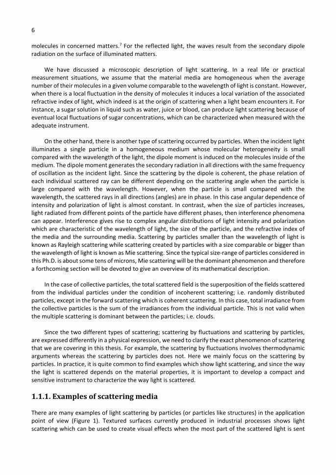
There are many examples of light scattering by particles (or particles like structures) in the application point of view (Figure 1). Textured surfaces currently produced in industrial processes shows light scattering which can be used to create visual effects when the most part of the scattered light is sent

7

out to the sample, or in other cases it can be used for different purposed when the light is directed into the sample. An interesting application of scattered light engineering (or management) is the association of rough surfaces on top of solar cells. The idea is to use the scattering properties of the surfaces to direct a maximum of light inside of the solar cell to optimize the chances of absorption and thus the conversion of luminous energy to electric energy by the photovoltaic effect.8 In another typical application, the wettability of a surface of glass can be enhanced by adding a structured roughness. The latter can be used to turn a standard glass surface into a superhydrophobic surface.9 A third example corresponds to the optical texturing of surfaces using a femtosecond laser direct writing method, which show scattering because they create nano-fingerprint structures.10–14 A final example that we would like to mention is the light scattering occurring in natural surfaces as a cuticle structures of the scarab beetle15, wings of a Morpho butterflies16, or human tissues17.

Figure 1. Different types of scattering media from the application point of view; surface texturing on photovoltaics, superhydrophobic micro-structured surfaces, optical manufacturing using the femtosecond laser, and biomedical imaging with human tissues, to the natural photonic structures; the scarab beetle and wings of a Morpho butterflies.

1.1.2. Scattering Regimes

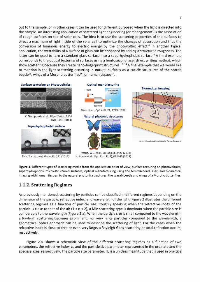
As previously mentioned, scattering by particles can be classified in different regimes depending on the dimension of the particle, refractive index, and wavelength of the light. Figure 2 illustrates the different scattering regimes as a function of particle size. Roughly speaking when the refractive index of the particle is close to that of the air (1 < n < 2), a Mie scattering type is dominant when the particle size is comparable to the wavelength (Figure 2.a). When the particle size is small compared to the wavelength, a Rayleigh scattering becomes prominent. For very large particles compared to the wavelength, a geometrical optics approach can be used to describe the scattering of light. For the cases when the refractive index is close to zero or even very large, a Rayleigh-Gans scattering or total reflection occurs, respectively.

Figure 2.a. shows a schematic view of the different scattering regimes as a function of two parameters, the refractive index, n, and the particle size parameter represented in the ordinate and the abscissa axes, respectively. The particle size parameter, X, is a unitless magnitude that is used in practice

8

to characterize the radius, a, and refractive index, n, of the particle with respect to the wavelength of light, 𝜆. The size parameter is defined as:

𝑋 =2π𝑎𝑛

𝜆 (Eq. 1)

Figure 2.b. shows another possible classification of the different scattering regimes as a function of the particle size and the wavelength of light. In particular it is shown that depending of the size parameter, i.e. the refractive index and the wavelength, a particle with a given size can scatter light in different regimes. The second interesting aspect that can be shown with the aid of Figure 2.b, is that the type of particles considered in this Ph.D., characterized by a few microns in size, refractive indexes ranging between 1.3 and 2, and, proved with visible light (450 nm to 650 nm) show an optical response determined by the Mie scattering regime.

Figure 2. (a) Schematic representation of the different types of scattering regimes organized according the refractive index (ordinate axis) and particle size (abscissa axis) to the wavelength of light b) An alternative schematic representation of the different scattering regimes, now organized according the particle radius (ordinate axis) and the wavelength of light (abscissa axis). Dotted lines, which correspond, each one, to specific size parameters X, noted in the figure, are used to roughly indicate the frontiers between the different scattering regimes. Credit: W. Brune (after Grant Petty).

1.1.3. Mie scattering

The Mie scattering was firstly introduced by Gustav Mie in 190818 after the publishing of Rayleigh’s research19. The Mie scattering handles particle-light interaction by a homogeneous sphere as well as infinite cylinders, or other geometries. It proposes the solution of Maxwell’s equations which illustrates the scattering of an electromagnetic wave traversing particles whose size is comparable to the wavelength of the light. The solution of Mie scattering which represents the intensity of scattered light results in the infinite series of terms whereas the Rayleigh approximation gives a simple mathematical expression.

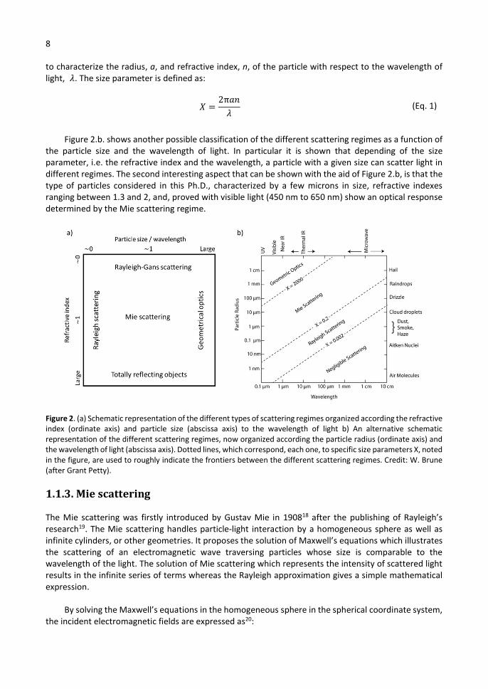
By solving the Maxwell’s equations in the homogeneous sphere in the spherical coordinate system, the incident electromagnetic fields are expressed as20:

9

𝐻 = −𝑖𝑘

𝜔𝜇𝐴 , �⃗� , + 𝐵 , 𝑀 , (Eq. 2)

�⃗� =𝑘

𝜔 𝜖 𝜇𝐴 , 𝑀 , + 𝐵 , �⃗� , (Eq. 3)

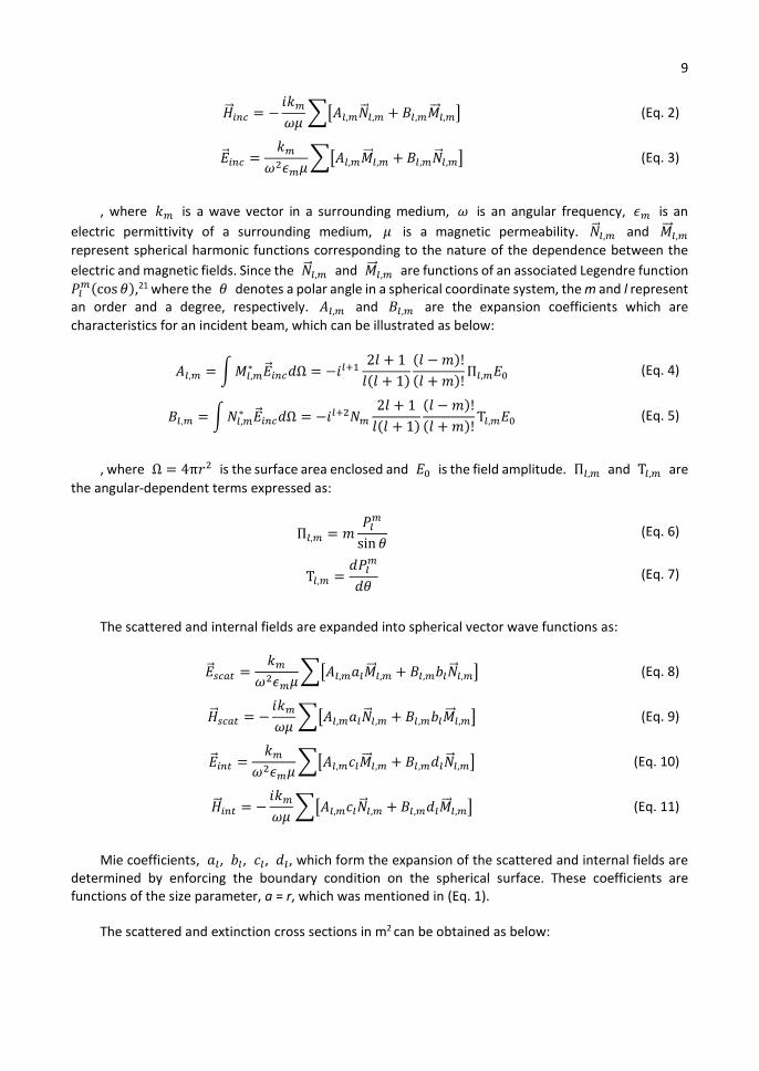
, where 𝑘 is a wave vector in a surrounding medium, 𝜔 is an angular frequency, 𝜖 is an electric permittivity of a surrounding medium, 𝜇 is a magnetic permeability. �⃗� , and 𝑀 , represent spherical harmonic functions corresponding to the nature of the dependence between the electric and magnetic fields. Since the �⃗� , and 𝑀 , are functions of an associated Legendre function 𝑃 (cos 𝜃),21 where the 𝜃 denotes a polar angle in a spherical coordinate system, the m and l represent an order and a degree, respectively. 𝐴 , and 𝐵 , are the expansion coefficients which are characteristics for an incident beam, which can be illustrated as below:

𝐴 , = 𝑀 ,∗ �⃗� 𝑑Ω = −𝑖

2𝑙 + 1

𝑙(𝑙 + 1)

(𝑙 − 𝑚)!

(𝑙 + 𝑚)!Π , 𝐸 (Eq. 4)

𝐵 , = 𝑁 ,∗ �⃗� 𝑑Ω = −𝑖 𝑁

2𝑙 + 1

𝑙(𝑙 + 1)

(𝑙 − 𝑚)!

(𝑙 + 𝑚)!T , 𝐸 (Eq. 5)

, where Ω = 4π𝑟 is the surface area enclosed and 𝐸 is the field amplitude. Π , and T , are the angular-dependent terms expressed as:

Π , = 𝑚𝑃

sin 𝜃 (Eq. 6)

T , =𝑑𝑃

𝑑𝜃 (Eq. 7)

The scattered and internal fields are expanded into spherical vector wave functions as:

�⃗� =𝑘

𝜔 𝜖 𝜇𝐴 , 𝑎 𝑀 , + 𝐵 , 𝑏 �⃗� , (Eq. 8)

𝐻 = −𝑖𝑘

𝜔𝜇𝐴 , 𝑎 �⃗� , + 𝐵 , 𝑏 𝑀 , (Eq. 9)

�⃗� =𝑘

𝜔 𝜖 𝜇𝐴 , 𝑐 𝑀 , + 𝐵 , 𝑑 �⃗� , (Eq. 10)

𝐻 = −𝑖𝑘

𝜔𝜇𝐴 , 𝑐 �⃗� , + 𝐵 , 𝑑 𝑀 , (Eq. 11)

Mie coefficients, 𝑎 , 𝑏 , 𝑐 , 𝑑 , which form the expansion of the scattered and internal fields are determined by enforcing the boundary condition on the spherical surface. These coefficients are functions of the size parameter, a = r, which was mentioned in (Eq. 1).

The scattered and extinction cross sections in m2 can be obtained as below:

10

𝐶 =𝑊

𝐼 (Eq. 12)

𝐶 =𝑊

𝐼 (Eq. 13)

, where 𝐼 is an intensity of the incident light on the surface of the particle. 𝑊 and 𝑊 are the scattered and extinction energies given by:

𝑊 =1

2Re (𝐸 × 𝐻∗ )𝑟 sin 𝜃 𝑑𝜃𝑑𝜙

=1

2Re 𝐸 , × 𝐻 ,

∗ − 𝐸 , × 𝐻 ,∗ 𝑟 sin 𝜃 𝑑𝜃𝑑𝜙

(Eq. 14)

𝑊 =1

2Re (𝐸 × 𝐻∗ )𝑟 sin 𝜃 𝑑𝜃𝑑𝜙

=1

2Re 𝐸 , × 𝐻 ,

∗ − 𝐸 , × 𝐻 ,∗ − 𝐸 , × 𝐻 ,

∗

+ 𝐸 , × 𝐻 ,∗ 𝑟 sin 𝜃 𝑑𝜃𝑑𝜙

(Eq. 15)

, where 𝜙 and r are the azimuth and the radius in the spherical coordinate system.

By applying (Eq. 14) and (Eq. 15) into the (Eq. 12) and (Eq. 13), we can derive the final scattered and extinction cross sections as:

𝐶 =2𝜋

𝑘(2𝑙 + 1)(𝑎 𝐻 , + 𝑏 𝐹 , ) (Eq. 16)

𝐶 =2𝜋

𝑘Re (2𝑙 + 1)(𝑎 𝐻 , + 𝑏 𝐹 , ) (Eq. 17)

, where 𝐻 , and 𝐹 , are the angular functions expressed as:

𝐻 , =2

𝑙(𝑙 + 1)

(𝑙 − 𝑚)!

(𝑙 + 𝑚)!T , (Eq. 18)

𝐹 , =2

𝑙(𝑙 + 1)

(𝑙 − 𝑚)!

(𝑙 + 𝑚)!Π , (Eq. 19)

We conclude that the intensity of the scattered or extinctic light depends on the polar angle, 𝜃, and the size of the particle, a = r, in the homogenous spherical particle. The scattering in this range of particle sizes differs from Rayleigh scattering in several respects: it is roughly independent of wavelength and it is larger in the forward direction than in the reverse direction. The greater the particle size, the more of the light is scattered in the forward direction whereas the Rayleigh scattering shows the same

11

portion of back- and forward-scatterings. This size dependent characteristic of Mie scattering makes it a particularly useful formalism when using scattered light to measure a particle size. The most work of this thesis has been done in the visible wavelength region with the micrometric sized samples, the Mie scattering is a major phenomenon.

1.2. Analysis of scattered light

The standard characterization of scattering media is currently done by measuring the angular distribution of the intensity of light scattered by the probed media. The instruments used to carry out such type of measurements, called scatterometers, show different types of configurations: integrating sphere, goniometric or conoscopic scatterometers. In this section, we introduce each conventional method and we compare them to the original instrument developed in the framework of this thesis, a multimodal imaging polarimeter which is coupled to microscope and which can work as a scatterometer.

1.2.1. Goniometric scatterometer

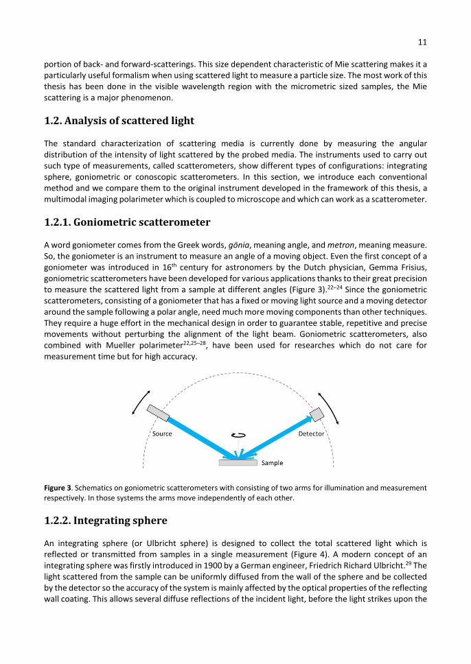
A word goniometer comes from the Greek words, gōnia, meaning angle, and metron, meaning measure. So, the goniometer is an instrument to measure an angle of a moving object. Even the first concept of a goniometer was introduced in 16th century for astronomers by the Dutch physician, Gemma Frisius, goniometric scatterometers have been developed for various applications thanks to their great precision to measure the scattered light from a sample at different angles (Figure 3).22–24 Since the goniometric scatterometers, consisting of a goniometer that has a fixed or moving light source and a moving detector around the sample following a polar angle, need much more moving components than other techniques. They require a huge effort in the mechanical design in order to guarantee stable, repetitive and precise movements without perturbing the alignment of the light beam. Goniometric scatterometers, also combined with Mueller polarimeter22,25–28, have been used for researches which do not care for measurement time but for high accuracy.

Figure 3. Schematics on goniometric scatterometers with consisting of two arms for illumination and measurement respectively. In those systems the arms move independently of each other.

1.2.2. Integrating sphere

An integrating sphere (or Ulbricht sphere) is designed to collect the total scattered light which is reflected or transmitted from samples in a single measurement (Figure 4). A modern concept of an integrating sphere was firstly introduced in 1900 by a German engineer, Friedrich Richard Ulbricht.29 The light scattered from the sample can be uniformly diffused from the wall of the sphere and be collected by the detector so the accuracy of the system is mainly affected by the optical properties of the reflecting wall coating. This allows several diffuse reflections of the incident light, before the light strikes upon the

12

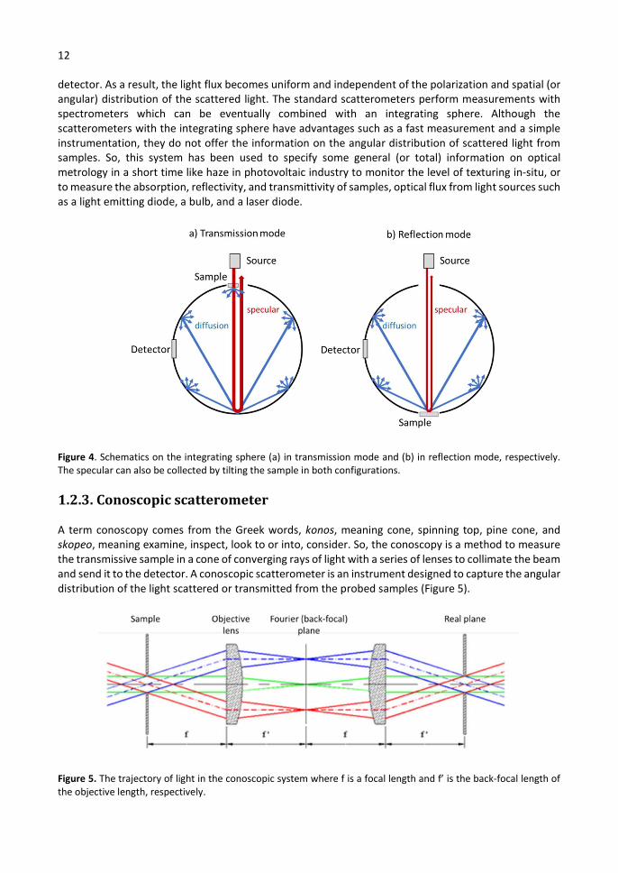
detector. As a result, the light flux becomes uniform and independent of the polarization and spatial (or angular) distribution of the scattered light. The standard scatterometers perform measurements with spectrometers which can be eventually combined with an integrating sphere. Although the scatterometers with the integrating sphere have advantages such as a fast measurement and a simple instrumentation, they do not offer the information on the angular distribution of scattered light from samples. So, this system has been used to specify some general (or total) information on optical metrology in a short time like haze in photovoltaic industry to monitor the level of texturing in-situ, or to measure the absorption, reflectivity, and transmittivity of samples, optical flux from light sources such as a light emitting diode, a bulb, and a laser diode.

Figure 4. Schematics on the integrating sphere (a) in transmission mode and (b) in reflection mode, respectively. The specular can also be collected by tilting the sample in both configurations.

1.2.3. Conoscopic scatterometer

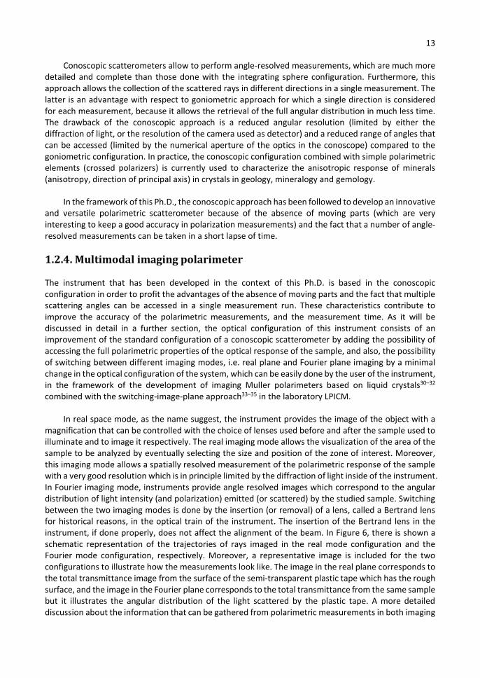
A term conoscopy comes from the Greek words, konos, meaning cone, spinning top, pine cone, and skopeo, meaning examine, inspect, look to or into, consider. So, the conoscopy is a method to measure the transmissive sample in a cone of converging rays of light with a series of lenses to collimate the beam and send it to the detector. A conoscopic scatterometer is an instrument designed to capture the angular distribution of the light scattered or transmitted from the probed samples (Figure 5).

Figure 5. The trajectory of light in the conoscopic system where f is a focal length and f’ is the back-focal length of the objective length, respectively.

13

Conoscopic scatterometers allow to perform angle-resolved measurements, which are much more detailed and complete than those done with the integrating sphere configuration. Furthermore, this approach allows the collection of the scattered rays in different directions in a single measurement. The latter is an advantage with respect to goniometric approach for which a single direction is considered for each measurement, because it allows the retrieval of the full angular distribution in much less time. The drawback of the conoscopic approach is a reduced angular resolution (limited by either the diffraction of light, or the resolution of the camera used as detector) and a reduced range of angles that can be accessed (limited by the numerical aperture of the optics in the conoscope) compared to the goniometric configuration. In practice, the conoscopic configuration combined with simple polarimetric elements (crossed polarizers) is currently used to characterize the anisotropic response of minerals (anisotropy, direction of principal axis) in crystals in geology, mineralogy and gemology.

In the framework of this Ph.D., the conoscopic approach has been followed to develop an innovative and versatile polarimetric scatterometer because of the absence of moving parts (which are very interesting to keep a good accuracy in polarization measurements) and the fact that a number of angle-resolved measurements can be taken in a short lapse of time.

1.2.4. Multimodal imaging polarimeter

The instrument that has been developed in the context of this Ph.D. is based in the conoscopic configuration in order to profit the advantages of the absence of moving parts and the fact that multiple scattering angles can be accessed in a single measurement run. These characteristics contribute to improve the accuracy of the polarimetric measurements, and the measurement time. As it will be discussed in detail in a further section, the optical configuration of this instrument consists of an improvement of the standard configuration of a conoscopic scatterometer by adding the possibility of accessing the full polarimetric properties of the optical response of the sample, and also, the possibility of switching between different imaging modes, i.e. real plane and Fourier plane imaging by a minimal change in the optical configuration of the system, which can be easily done by the user of the instrument, in the framework of the development of imaging Muller polarimeters based on liquid crystals30–32 combined with the switching-image-plane approach33–35 in the laboratory LPICM.

In real space mode, as the name suggest, the instrument provides the image of the object with a magnification that can be controlled with the choice of lenses used before and after the sample used to illuminate and to image it respectively. The real imaging mode allows the visualization of the area of the sample to be analyzed by eventually selecting the size and position of the zone of interest. Moreover, this imaging mode allows a spatially resolved measurement of the polarimetric response of the sample with a very good resolution which is in principle limited by the diffraction of light inside of the instrument. In Fourier imaging mode, instruments provide angle resolved images which correspond to the angular distribution of light intensity (and polarization) emitted (or scattered) by the studied sample. Switching between the two imaging modes is done by the insertion (or removal) of a lens, called a Bertrand lens for historical reasons, in the optical train of the instrument. The insertion of the Bertrand lens in the instrument, if done properly, does not affect the alignment of the beam. In Figure 6, there is shown a schematic representation of the trajectories of rays imaged in the real mode configuration and the Fourier mode configuration, respectively. Moreover, a representative image is included for the two configurations to illustrate how the measurements look like. The image in the real plane corresponds to the total transmittance image from the surface of the semi-transparent plastic tape which has the rough surface, and the image in the Fourier plane corresponds to the total transmittance from the same sample but it illustrates the angular distribution of the light scattered by the plastic tape. A more detailed discussion about the information that can be gathered from polarimetric measurements in both imaging

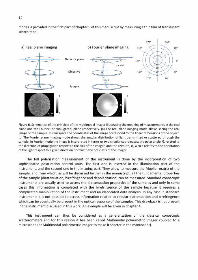
14

modes is provided in the first part of chapter 5 of this manuscript by measuring a thin film of translucent scotch tape.

Figure 6. Schematics of the principle of the multimodal imager illustrating the meaning of measurements in the real plane and the Fourier (or conjugated) plane respectively. (a) The real plane imaging mode allows seeing the real image of the sample. In real space the coordinates of the image correspond to the linear dimensions of the object. (b) The Fourier plane imaging mode shows the angular distribution of light transmitted or scattered through the sample. In Fourier mode the image is interpreted in terms or two circular coordinates: the polar angle, θ, related to the direction of propagation respect to the axis of the imager, and the azimuth, ϕ, which relates to the orientation of the light respect to a given direction normal to the optic axis of the imager.

The full polarization measurement of the instrument is done by the incorporation of two sophisticated polarization control units. The first one is inserted in the illumination part of the instrument, and the second one in the imaging part. They allow to measure the Mueller matrix of the sample, and from which, as will be discussed further in the manuscript, all the fundamental properties of the sample (diattenuation, birefringence and depolarization) can be measured. Standard conoscopic instruments are usually used to access the diattenuation properties of the samples and only in some cases this information is completed with the birefringence of the sample because it requires a complicated manipulation of the instrument and an elaborated data analysis. In any case in standard instruments it is not possible to access information related to circular diattenuation and birefringence which can be eventually be present in the optical response of the samples. This drawback is not present in the instrument discussed in this work. An example will be given in chapter 4.

This instrument can thus be considered as a generalization of the classical conoscopic scatterometers and for this reason it has been called Multimodal polarimetric imager coupled to a microscope (or Multimodal polarimetric imager to make it shorter in the manuscript).

15

1.3. Polarimetric instrumentation

Different types of polarimeter have been developed and they can be categorized depending on their applications and measurement techniques.36,37 The most basic concept of polarimeter is a Stokes polarimeter. Generally speaking, Stokes polarimeters consist of single optical arm which is equipped with a polarization state analyzer (PSA) and a detector to measure the Stokes vector components (I, Q, U, and V). In the most general configuration, the PSA is made of succession of retarders, used to get access to the different types of retardation (linear and circular) as well as their orientation, followed by a linear and polarizer, used to determine the diattenuation properties of the beam as well as its orientation. Since the Stokes polarimeters do not have an illumination arm to control the incident polarization states, they are applicable in the areas such as astronomy, remote sensing, or characterization of light sources.38–40 The first type of polarimeters are usually referred as Stokesmeters.

In the second type of polarimeter, the polarization of both, the illumination and the analysis part can be controlled. In general, the second type of polarimeters are made of two arms and the sample to be studied is placed between them. Each one of the arms is equipped with optical elements to control the polarization of the light. In the first arm polarization states are generated, and in the second arm polarization states are analyzed. In normal operation, the sample is sequentially illuminated with a set of well-defined polarization states. Then, each one of these states, after being modified by the sample, is analyzed by the optical elements in the second arm. As a result, a collection of measurements is retrieved which allows to characterize the optical response of the sample. In general, the set of measurements are presented (or arranged) to form a matrix. Depending on the physical properties of the sample, and the instrumentation used to build the polarimeter, the formalism used to write the matrices will be different.

If the interaction with the sample modifies the polarization state of the incoming light but preserves the polarization purity (or polarization degree) then by convention there is tendency to refer to the instrument used to do the measurements as an ellipsometer, and the technique, whose goal is to characterize the optical properties of the sample is called ellipsometry. Thanks to their fast, accurate, and precise properties, the spectroscopic ellipsometers have achieved great success in semiconductor industries or other in-situ real-time characterization in the process of a glass fabrication. However, they remain as an incomplete characterization technique since the Jones vectors are defined only for fully polarized states, so they cannot use conveniently to explore situations in which the interaction of the light beam with the sample and the instrument itself modifies to a given point its degree of polarization.

A Mueller polarimeter, in contrast to an ellipsometer, is an instrument which is able to measure light which is partially polarized. Since a Mueller polarimeter can be also used as an ellipsometer to measure fully polarized light, a Mueller polarimeter can be understood as the most general and complete form of an ellipsometer. When working with partially polarized light, it is common to use a mathematical formalism representing polarization as a four-dimensional vector, the Stokes vector, and consequently the optical properties of the sample in the form of a 4 by 4 matrix, called the Mueller matrix.

Regarding Mueller polarimeters, they can be sub-divided into two great categories: spectroscopic polarimeters or imaging polarimeters. The spectroscopic polarimeters give a multi-wavelength approach on the sample. The polarimetric imagers measure the spatial information of the sample. The spatial information can be a real surface of the sample when the system measures the real plane of the imaging lens. Another capability of the polarimetric imager is that it measures a spatial distribution of the scattered, transmitted, or reflected light when it focuses on Fourier plane of the imaging lens. As we

16

discussed in the previous section, the measurement in Fourier plane corresponds to the angle resolved measurement or the conoscopic measurement.

1.3.1. Applications of polarimetry

In the past decades, there have been plenty of applications and researches using the polarimeter. Astronomy is one of the applications.41 The light from the Sun through a telescope is polarized and is related with the magnetic fields in the Sun following a Zeeman effect.40 The structure of the magnetic field between stars has been acquired by measuring the polarization properties of the starlight42,43 , which can be useful to study a distance to external galaxies44 and planetary atmosphere45.

The great success of ellipsometry in the multidisciplinary areas is a matter of course.46 The Mueller polarimeter has been applied in optical metrology, materials science, atmospheric remote sensing, and target detection.47–49 In biomedical imaging, the polarimeter has been considered as a useful technique to characterize biological tissues since the biological tissue itself has a nature that it shows polarimetric properties such as birefringence, diattenuation, and depolarization because of its specific structure.50,51 Moreover, it can be extended to the applications for the freshness and quality control in food industries.

1.4. Motivation and goal of thesis

Why should we need to know the polarimetric properties of scattered light? Because the scattered light intensity is a function of polarization. It is well-known that sunglasses decrease the glare of reflected light because the reflected glare light has a much dominant horizontal polarization component than the vertical polarization component. So, the sunglasses which have vertically oriented polarizers block the horizontal component of reflected light. We can also find that the brightness is different when we see the blue sky by rotating the sunglasses between 0° and 90° since the light comes from the blue sky undergoes scattering so that it has more vertical polarization component.

As it was already discussed in section 1.1, all the activities of transmitted or reflected light are the results from the scattering phenomena; light-matter interactions. Those two simple examples with sunglasses in our real-life show that the scattered light has a polarization property. When we analyze a desired sample which shows scattering, this polarization property can depend on the form of the sample, material indices, and the properties of incident light; an initial polarization, a wavelength, an amplitude (or number of rays), and an angle of incidence (AoI). Moreover, the polarization property accompanies a depolarization property depending on the measurement condition and this depolarization property will be illustrated in the following chapter. So, if the conditions of incident light are well controllable, the analysis of polarization and depolarization properties of scattered light can be useful to characterize the sample properties.

The goal of this thesis is i) to design and describe an innovative multimodal Mueller polarimetric imager, ii) to introduce possible applications discovering an optical response with applicable parameters, iii) to explain the optical response from the studied sample with a proper theory and modelling.

1.5. Overview of thesis

In the present chapter, the light-matter interaction was illustrated as a scattering phenomenon. Some examples of scattering media with different scattering regimes were introduced depending on the material indices, the wavelength of light, and the dimension of the particles. Some scatterometry and polarimetric techniques are presented followed by the multimodal imaging approach.

17

In chapter 2, fundamentals of polarization properties are introduced based on Jones and Mueller calculus. A Mueller matrix and its decomposition are focused in the following sections.

In chapter 3, the technical characteristics and optical configuration of the Multimodal imaging polarimeter developed in the framework of this Ph.D. and installed in the laboratory LPICM are described and discussed. A detailed description of the multimodal imaging Mueller polarimetric microscope is shown with the design principle of the polarization state generator (PSG) and analyzer (PSA). The multimodal imaging configuration is presented based on ray tracing modelling. The description of the operation mode is completed with a description of the method to calibrate the polarimetric and radiometric response of the system. Finally, a set of representative results used to illustrate the verification of technical capabilities of the polarimetric imager are shown in the end of this chapter.

Chapter 4 is devoted to discussing the polarimetric properties of small particles observed at normal incidence (the standard configuration), or at oblique incidence. Different cases are discussed in depth including the ideal case of a linear dipole, a spherical particle of different sizes and spheroidal particles of different shapes. The modeling of polarimetric data makes use of a combination of the vectorial polarimetric approach with either exact methods such as the Mie theory for spherical particles, or approximated numerical methods for spheroidal particles. One interesting and unattended effect seen in the polarimetric data simulated or measured at oblique incidence is the development of an intense apparent circular birefringence which depends on the shape of the particles and the illumination conditions. The apparent circular birefringence is interpreted as a topological phase arising from the fact that the illumination and the observation frames are not collinear. The chapter ends with a comparison of experimental and simulated data of different types of particles and the demonstration that the topologic phase can be used to characterize the shape of the measured particles.

In chapter 5, polarimetric responses on complex media are studied, which introduce birefringence and depolarization at the same time. In the first part, the method uses to analyze how polarization and depolarization properties depend on the size of the optical path that the light has travelled inside of the scattering medium. In particular it is shown that the polarization properties depend linearly on the thickness of the scattering medium and the depolarization (the loss of polarization) depends quadratically on this same thickness. The validity of this approach is illustrated with the use of simple samples used as a reference. The curious dependence of both, polarization and depolarization properties with the optical path length inside of the sample is used to study the thickness dependence of samples consisting on histological cuts of biological tissues. In particular a practical method is discussed that can be used to get rid of the effect of thickness fluctuations in histological cuts prepared in a biology laboratory, which can induce ambiguities in the interpretation of polarimetric data by a human operator.

In chapter 6, we briefly review the main results obtained in the framework of various collaborative works developed during the Ph.D. with different research groups interested in the possibility of using the multimodal imaging polarimeter to characterize the optical response of different types of samples. The examples discussed include: i) nano-patterned samples to measure a pseudo-chirality caused by the plasmonic effect, ii) samples modified by a femtosecond laser direct writing (FLDW), and iii) cylindrical microparticles for a hydrophobic surface to analyze their structures. The interest that the multimodal microscope has created in persons appertaining at different communities is a proof of the added value of the use of fully polarimetric capabilities combined with a multimodal imager. They are included here to illustrate a part of the work done in the context of the Ph.D. and because the part of this work has been published in different articles and shown in international conferences.

18

In the last chapter, all the work done in the framework of the Ph.D. are summarized and concluded with some perspectives to guide future works in the field of polarimetric scatterometry and polarimetric microscopy.

19

Chapter 2. Fundamentals of polarization of light

Contents

2.1. Mueller formalism ................................................................................................. 20

2.1.1. Stokes vector and the Poincaré sphere .............................................................. 20

2.1.2. Mueller matrix .................................................................................................... 21

2.2. Basic polarimetric properties ................................................................................ 21

2.2.1. Dichroism and diattenuation ............................................................................. 22

2.2.2. Retardation and birefringence ........................................................................... 23

2.2.3. Depolarization ..................................................................................................... 26

2.2.4. Polarizance .......................................................................................................... 28

2.3. Extraction of polarimetric properties .................................................................... 29

2.3.1. Productive decomposition ................................................................................... 29

2.3.2. Sum decomposition ............................................................................................. 30

2.3.3. Logarithmic decomposition ................................................................................ 31

2.4. Conclusion ............................................................................................................. 33

Before discussing the optical design, characteristics and applications of the multimodal polarimeter, it is necessary to introduce fundamentals of polarization of light. In this chapter, the concept of polarization of light together with the basic polarimetric properties; dichroism, birefringence, and depolarization are introduced. We also discuss the Stokes formalism and the Mueller calculus formalism, which is a complete mathematical approach to describe the polarimetric light-matter interaction. We illustrate how the basic polarimetric properties are extracted through a post treatment method called decomposition based on linear algebra properties of Mueller matrices. We introduce different types of the decomposition methods depending on the sample structure, yielding a different mathematical description. A special emphasis is put to describe the logarithmic (also called by some authors differential) decomposition, since this latter will be extensively used to treat the simulated and experimental data discussed in the forthcoming chapters of the manuscript.

20

2.1. Mueller formalism

The state of light of a fully polarized beam can be described using the Jones formalism which was discovered by R. C. Jones in 1941. Jones approach is simplest way to treat polarized light and uses a complex bidimensional vector to describe a given state of polarization, and the corresponding 2 by 2 complex Jones matrix the transformation action of a sample or an optical element on the polarization state of an illuminating beam. Although the Jones calculus is an intuitive method to treat the polarization, it can be only applied when the light is the totally polarized light.

Mueller calculus, which was completed in 1943 by Hans Mueller is a generalization of the Jones formalisms and can be used to represent any state of polarization including partially polarized light and the unpolarized light. The Mueller calculus is general and can always be applied but is mandatory when partially polarized light is to be treated.

2.1.1. Stokes vector and the Poincaré sphere

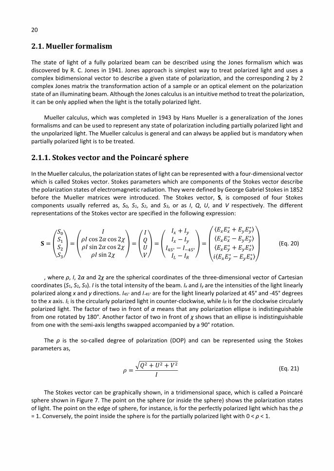
In the Mueller calculus, the polarization states of light can be represented with a four-dimensional vector which is called Stokes vector. Stokes parameters which are components of the Stokes vector describe the polarization states of electromagnetic radiation. They were defined by George Gabriel Stokes in 1852 before the Mueller matrices were introduced. The Stokes vector, S, is composed of four Stokes components usually referred as, S0, S1, S2, and S3, or as I, Q, U, and V respectively. The different representations of the Stokes vector are specified in the following expression:

𝐒 =

𝑆𝑆𝑆𝑆

=

𝐼𝜌𝐼 cos 2𝛼 cos 2𝜒𝜌𝐼 sin 2𝛼 cos 2𝜒

𝜌𝐼 sin 2𝜒

=

𝐼𝑄𝑈𝑉

=

𝐼 + 𝐼

𝐼 − 𝐼

𝐼 ° − 𝐼 °

𝐼 − 𝐼

=

⎝

⎜⎛

⟨𝐸 𝐸∗ + 𝐸 𝐸∗⟩

⟨𝐸 𝐸∗ − 𝐸 𝐸∗⟩

⟨𝐸 𝐸∗ + 𝐸 𝐸∗⟩

𝑖⟨𝐸 𝐸∗ − 𝐸 𝐸∗⟩⎠

⎟⎞

(Eq. 20)

, where ρ, I, 2α and 2χ are the spherical coordinates of the three-dimensional vector of Cartesian coordinates (S1, S2, S3). I is the total intensity of the beam. Ix and Iy are the intensities of the light linearly polarized along x and y directions. I45° and I-45° are for the light linearly polarized at 45° and -45° degrees to the x axis. IL is the circularly polarized light in counter-clockwise, while IR is for the clockwise circularly polarized light. The factor of two in front of α means that any polarization ellipse is indistinguishable from one rotated by 180°. Another factor of two in front of χ shows that an ellipse is indistinguishable from one with the semi-axis lengths swapped accompanied by a 90° rotation.

The ρ is the so-called degree of polarization (DOP) and can be represented using the Stokes parameters as,

𝜌 =𝑄 + 𝑈 + 𝑉

𝐼 (Eq. 21)

The Stokes vector can be graphically shown, in a tridimensional space, which is called a Poincaré sphere shown in Figure 7. The point on the sphere (or inside the sphere) shows the polarization states of light. The point on the edge of sphere, for instance, is for the perfectly polarized light which has the ρ = 1. Conversely, the point inside the sphere is for the partially polarized light with 0 < ρ < 1.

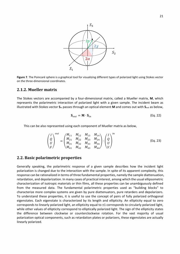
21

Figure 7. The Poincaré sphere is a graphical tool for visualizing different types of polarized light using Stokes vector on the three-dimensional coordinates.

2.1.2. Mueller matrix

The Stokes vectors are accompanied by a four-dimensional matrix, called a Mueller matrix, M, which represents the polarimetric interaction of polarized light with a given sample. The incident beam as illustrated with Stokes vector Sin passes through an optical element M and comes out with Sout as below,

𝐒 = 𝐌 ∙ 𝐒 (Eq. 22)

This can be also represented using each component of Mueller matrix as below,

𝐼𝑄𝑈𝑉

=

𝑀 𝑀 𝑀 𝑀𝑀 𝑀 𝑀 𝑀𝑀 𝑀 𝑀 𝑀𝑀 𝑀 𝑀 𝑀

∙

𝐼𝑄𝑈𝑉

(Eq. 23)

2.2. Basic polarimetric properties

Generally speaking, the polarimetric response of a given sample describes how the incident light polarization is changed due to the interaction with the sample. In spite of its apparent complexity, this response can be rationalized in terms of three fundamental properties, namely the sample diattenuation, retardation, and depolarization. In many cases of practical interest, among which the usual ellipsometric characterization of isotropic materials or thin films, all these properties can be unambiguously defined from the measured data. The fundamental polarimetric properties used as “building blocks” to characterize more complex systems are given by pure diattenuators, pure retarders and depolarizers. To understand these properties, it is useful to use the concept of pairs of fully polarized orthogonal eigenstates. Each eigenstate is characterized by its length and ellipticity. An ellipticity equal to zero corresponds to linearly polarized light, an ellipticity equal to ±1 corresponds to circularly polarized light, while other values of ellipticity correspond to elliptically polarized light. The sign of the ellipticity states the difference between clockwise or counterclockwise rotation. For the vast majority of usual polarization optical components, such as retardation plates or polarizers, these eigenstates are actually linearly polarized.

22

2.2.1. Dichroism and diattenuation

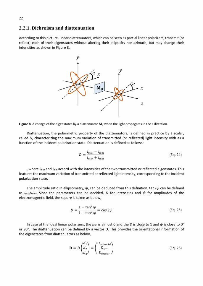
According to this picture, linear diattenuators, which can be seen as partial linear polarizers, transmit (or reflect) each of their eigenstates without altering their ellipticity nor azimuth, but may change their intensities as shown in Figure 8.

Figure 8. A change of the eigenstates by a diattenuator MD when the light propagates in the z direction.

Diattenuation, the polarimetric property of the diattenuators, is defined in practice by a scalar, called D, characterizing the maximum variation of transmitted (or reflected) light intensity with as a function of the incident polarization state. Diattenuation is defined as follows:

𝐷 =𝐼max − 𝐼min

𝐼max + 𝐼min

(Eq. 24)

, where Imax and Imin accord with the intensities of the two transmitted or reflected eigenstates. This features the maximum variation of transmitted or reflected light intensity, corresponding to the incident polarization state.

The amplitude ratio in ellipsometry, ψ, can be deduced from this definition. tan2ψ can be defined as Imax/Imin. Since the parameters can be decided, D for intensities and ψ for amplitudes of the electromagnetic field, the square is taken as below,

𝐷 =1 − tan 𝜓

1 + tan 𝜓= cos 2𝜓 (Eq. 25)

In case of the ideal linear polarizers, the Imin is almost 0 and the D is close to 1 and ψ is close to 0° or 90°. The diattenuation can be defined by a vector D. This provides the orientational information of the eigenstates from diattenuators as below,

𝐃 = 𝐷

𝑑𝑑𝑑

=

𝐷horizontal𝐷 °

𝐷circular

(Eq. 26)

23

, where 𝑑 + 𝑑 + 𝑑 = 1 and the polarization eigenstates of the Stokes vectors are given by,

𝐒max = (1, 𝑑 , 𝑑 , 𝑑 ), 𝐒min = (1, −𝑑 , −𝑑 , −𝑑 ) (Eq. 27)

The components of the vector D describe the horizontal, the 45°, and the circular diattenuation, respectively. In the Mueller matrix, the D of any sample can be represented as a simple function of the first row of Mueller matrix as below,

𝐃 =1

𝑀

𝑀𝑀𝑀

(Eq. 28)

The Mueller matrix of an ideal diattenuator MD can be defined with the scalar diattenuation D and the diattenuation vector D as below,

𝐌 = 𝜏1 𝐃𝐃 𝐦

, and 𝐦 = 1 − 𝐷 𝐈 + (1 − 1 − 𝐷 )𝐃𝐃 (Eq. 29)

, where the first-row element and the first-column element are illustrated by the D. The md is a three-dimensional symmetric sub-matrix which is composed of the 3 × 3 identity matrix I3, the D, and the D. The τ shows the entire transmittance or reflectivity of the sample when the incident light is perfectly depolarized.

2.2.2. Retardation and birefringence

Linear retarders also called waveplates pass their eigenstates conserving their ellipticity, ε, and azimuth, α. and the intensities but modifying only their phases as shown in Figure 9.

Figure 9. A change of the eigenstates by a retarder MR when the light propagates in the z direction.

When light travels from one medium to another, the speed and wavelength change since the electric field of the light interacts with the electrons in the medium. The refractive index can also be stated in terms of wavelength. The refractive index shows different values depending on the type of material by the natural frequency. Even though the speed changes and wavelength changes, the frequency of the light will be constant. In Figure 10.a., the black circles represent the motion of electrons

24

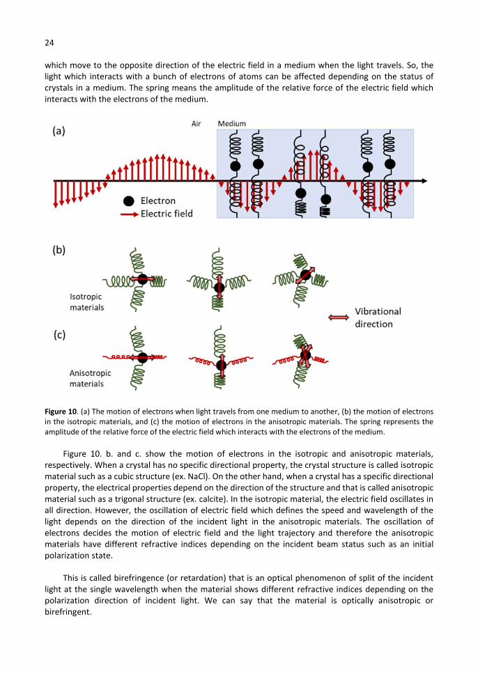
which move to the opposite direction of the electric field in a medium when the light travels. So, the light which interacts with a bunch of electrons of atoms can be affected depending on the status of crystals in a medium. The spring means the amplitude of the relative force of the electric field which interacts with the electrons of the medium.

Figure 10. (a) The motion of electrons when light travels from one medium to another, (b) the motion of electrons in the isotropic materials, and (c) the motion of electrons in the anisotropic materials. The spring represents the amplitude of the relative force of the electric field which interacts with the electrons of the medium.

Figure 10. b. and c. show the motion of electrons in the isotropic and anisotropic materials, respectively. When a crystal has no specific directional property, the crystal structure is called isotropic material such as a cubic structure (ex. NaCl). On the other hand, when a crystal has a specific directional property, the electrical properties depend on the direction of the structure and that is called anisotropic material such as a trigonal structure (ex. calcite). In the isotropic material, the electric field oscillates in all direction. However, the oscillation of electric field which defines the speed and wavelength of the light depends on the direction of the incident light in the anisotropic materials. The oscillation of electrons decides the motion of electric field and the light trajectory and therefore the anisotropic materials have different refractive indices depending on the incident beam status such as an initial polarization state.

This is called birefringence (or retardation) that is an optical phenomenon of split of the incident light at the single wavelength when the material shows different refractive indices depending on the polarization direction of incident light. We can say that the material is optically anisotropic or birefringent.

25

This birefringence can be expressed mathematically,

Δ𝑛 = 𝑛 − 𝑛 (Eq. 30)

, where no is the refractive index for an ordinary ray whose oscillation direction of the electric field (or a polarization direction) is perpendicular to the optical axis, ne is the refractive index for an extraordinary ray parallel to the optical axis. The ordinary axis is called slow axis through which the light propagates slower than in other axes. And the extraordinary axis is called the fast axis through which the light propagates faster than in other axes. The material which having a negative Δ𝑛 shows negative birefringence and the material having a positive Δ𝑛 shows a positive birefringence.

Then the retardance, the difference in phase shift between two different polarization states, δ, is given by,

𝛿 =2πΔ𝑛𝑑

𝜆 (Eq. 31)

, where d presents the optical path length.

In case of a half-waveplate, the orientation of the fast axis is what determines the orientation of the linearly polarized light emitting from the retarder. As a result, if a half-waveplate is rotated at 45° with respect to the linear polarized light incoming the waveplate, the transmitted light from the waveplate will be rotated at 90° with respect to the polarization direction of the incident light.

As the diattenuation was defined in the previous section, the time delay between two eigenstates after they propagate through an ideal waveplate can be described by the scalar retardance, R, using a vector representation, R as below,

𝐑 = 𝑅

𝑟𝑟𝑟

=

𝑅horizontal𝑅 °

𝑅circular

(Eq. 32)

, where 𝑟 + 𝑟 + 𝑟 = 1. The components of R show the horizontal, the 45°, and the circular retardance, respectively.

The Stokes vectors of the fast and the slow eigenstates Sf and Ss are respectively defined by,

𝐒 = (1, 𝑟 , 𝑟 , 𝑟 ), 𝐒 = (1, −𝑟 , −𝑟 , −𝑟 ) (Eq. 33)

An ideal retarder is illustrated geometrically as the rotation in the space of Stokes vectors. The Mueller matrix of an ideal retarder MR can be expressed as,

𝐌 =1 𝟎𝟎 𝐦

, and (𝐦 ) = 𝛿 cos 𝑅 + 𝑟 𝑟 (1 − cos 𝑅) 𝜀 𝑟 sin 𝑅 (Eq. 34)

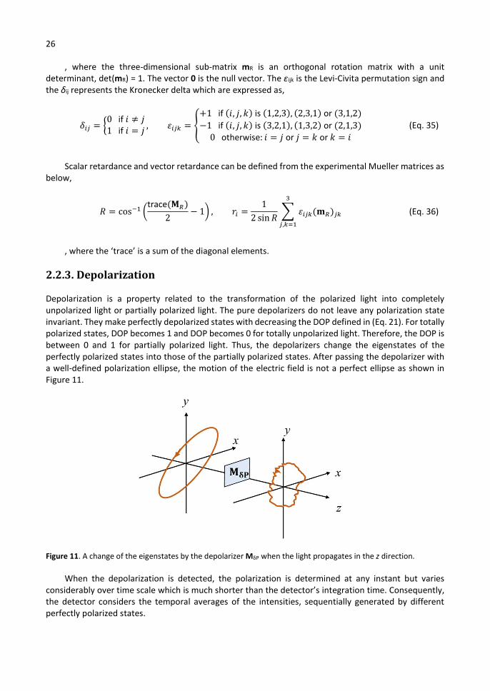
26

, where the three-dimensional sub-matrix mR is an orthogonal rotation matrix with a unit determinant, det(mR) = 1. The vector 0 is the null vector. The εijk is the Levi-Civita permutation sign and the δij represents the Kronecker delta which are expressed as,

𝛿 =0 if 𝑖 ≠ 𝑗1 if 𝑖 = 𝑗

, 𝜀 =

+1 if (𝑖, 𝑗, 𝑘) is (1,2,3), (2,3,1) or (3,1,2)

−1 if (𝑖, 𝑗, 𝑘) is (3,2,1), (1,3,2) or (2,1,3)

0 otherwise: 𝑖 = 𝑗 or 𝑗 = 𝑘 or 𝑘 = 𝑖

(Eq. 35)

Scalar retardance and vector retardance can be defined from the experimental Mueller matrices as below,

𝑅 = costrace(𝐌 )

2− 1 , 𝑟 =

1

2 sin 𝑅𝜀 (𝐦 )

,

(Eq. 36)

, where the ‘trace’ is a sum of the diagonal elements.

2.2.3. Depolarization

Depolarization is a property related to the transformation of the polarized light into completely unpolarized light or partially polarized light. The pure depolarizers do not leave any polarization state invariant. They make perfectly depolarized states with decreasing the DOP defined in (Eq. 21). For totally polarized states, DOP becomes 1 and DOP becomes 0 for totally unpolarized light. Therefore, the DOP is between 0 and 1 for partially polarized light. Thus, the depolarizers change the eigenstates of the perfectly polarized states into those of the partially polarized states. After passing the depolarizer with a well-defined polarization ellipse, the motion of the electric field is not a perfect ellipse as shown in Figure 11.

Figure 11. A change of the eigenstates by the depolarizer MδP when the light propagates in the z direction.

When the depolarization is detected, the polarization is determined at any instant but varies considerably over time scale which is much shorter than the detector’s integration time. Consequently, the detector considers the temporal averages of the intensities, sequentially generated by different perfectly polarized states.

27

A multiple scattering makes depolarization of the incident polarized light, the depolarization depends on the way of illuminating the sample and the way of detecting the emerging light. The perfectly depolarized light needs that the detected signal is the sum of intensities because of various polarized contributions with different polarization states. As a result, this summation would be done temporally, spatially or spectrally. That is, the depolarization depends not only on the sample, but also on the characteristics of the illumination source and the detector.

The Mueller matrix of an ideal depolarizer MδP can be defined as below,

𝐌 =1 𝟎𝟎 𝐦

(Eq. 37)

, where the mδ is a 3 × 3 symmetric matrix and it would be simplified to a diagonal form in a suitable orthonormal basis defined by three eigenvectors vi. Consequently, in a basis represented by the four Stokes vectors as (Eq. 38), the Mueller matrix MδP becomes diagonal as expressed below,

𝐒 = (1,0,0,0), 𝑎𝑛𝑑 𝐒 = (1, 𝐯 ), (1 ≤ 𝑖 ≤ 3) (Eq. 38)

𝐌 =

1 0 0 00 𝑎 0 00 0 𝑏 00 0 0 𝑐

(Eq. 39)

, where the eigenvalues of mδ (a, b, and c) are real numbers from -1 to 1. As we discussed the DOP, the MδP shows that the DOP decreases by a factor equal to the corresponding eigenvalue a, b or c, while the perfectly depolarized state remains unchanged. Namely, a general depolarizer has only one eigenpolarization, concerning the perfectly depolarized state.

Since mδ is symmetry, the Mueller matrices of the ideal depolarizers MδP explicitly depend on six parameters. Due to this dependence on six parameters, depolarizers are more mathematically complex than retarders or diattenuators, which involve only three parameters each. However, the symmetry properties of the sample can considerably reduce the number of independent parameters. When we observe in forward or backward scattering geometries, a suspension of spherical (or statistically isotropic) scatterers acts as an ideal depolarizer with different depolarization powers for linearly and circularly polarized incident states. Furthermore, for the specific case of a suspension of spheres, the depolarization power for linear states is independent of the orientation of the polarization of incident light. These properties can be mathematically represented as,

𝑎 = 𝑏 ≠ 𝑐, and 𝐯 = (cos 𝛼 , sin 𝛼 , 0), 𝐯 = (−sin 𝛼 , cos 𝛼 , 0), 𝐯 = (0,0,1) (Eq. 40)

, where α can be chosen arbitrarily.

It is convenient for practical reasons to define a single numerical function defining the entire depolarization power of a depolarizer to characterize the depolarizing properties of general Mueller matrices mathematically. The depolarizing power varies from 0 to 1. If the value is 0, it means that the matrix is non-depolarizing. If the value is 1, it means the matrix behaves as a total depolarizer. The first example of such function is the quadratic depolarization index, Pq, for the general Mueller matrix and the pure depolarizers expressed as below,

28

𝑃 =∑ 𝑀 − 𝑀

3𝑀=

trace(𝐌 𝐌) − 𝑀

3𝑀 (Eq. 41)

A physically reasonable Mueller matrix is non-depolarizing, if any perfectly polarized input Stokes vector is converted into a perfectly polarized output Stokes vector without decreasing the DOP. Conversely, the DOP of output Stokes vector is smaller than that of input Stokes vector for depolarizing Mueller matrices. For any resulting Mueller matrix, the decrease of the DOP depends on the input state. For example, a given sample can be more depolarizing for input circular states than for input linear ones, or vice versa. It is unfeasible to specifically represent the depolarization power of a generic Mueller matrix M. The depolarization index, Pq, to illustrate the depolarization power of a sample represented by the M has a range between 0 (for a total depolarizer) and 1 (for non-depolarizing matrices).

Another way to define this depolarization power has been studied specifically for depolarizers by Lu and Chipman as the expression below,

Δ = 1 −1

3(|𝑎| + |𝑏| + |𝑐|), 0 ≤ ∆≤ 1 (Eq. 42)

, where Δ is the average of the principal depolarization factors and indicates the averaged depolarization capability of the depolarizer. Thus, it can be also called the depolarization power.52 There have been many possible propositions on the definition of this depolarization53,54 and another way to define the depolarization using the logarithmic decomposition will be introduced in the following section.

2.2.4. Polarizance

Polarizance is an ability to transform the unpolarized light into the polarized light. In other words, the polarizance increases the DOP of an incident unpolarized or partially polarized light. When the incident unpolarized light travels through the sample, the out Stokes vector is expressed as below,

𝐒out = 𝐌

1000

=

𝑀𝑀𝑀𝑀

(Eq. 43)

The scalar polarizance, P, can be described with the DOP of the output Stokes vector as below,

𝑃 =𝑀 + 𝑀 + 𝑀

𝑀 (Eq. 44)

Then the polarizance vector, P, can be expressed as below,

𝐏 =1

𝑀

𝑀𝑀𝑀

(Eq. 45)

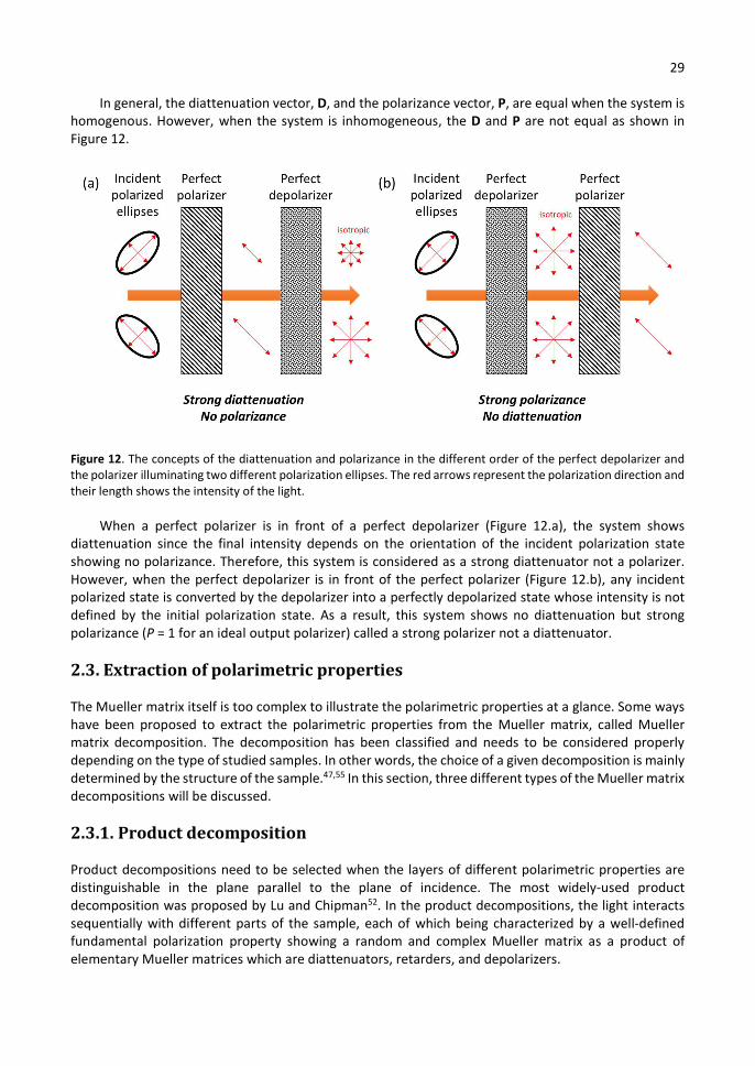
29

In general, the diattenuation vector, D, and the polarizance vector, P, are equal when the system is homogenous. However, when the system is inhomogeneous, the D and P are not equal as shown in Figure 12.

Figure 12. The concepts of the diattenuation and polarizance in the different order of the perfect depolarizer and the polarizer illuminating two different polarization ellipses. The red arrows represent the polarization direction and their length shows the intensity of the light.

When a perfect polarizer is in front of a perfect depolarizer (Figure 12.a), the system shows diattenuation since the final intensity depends on the orientation of the incident polarization state showing no polarizance. Therefore, this system is considered as a strong diattenuator not a polarizer. However, when the perfect depolarizer is in front of the perfect polarizer (Figure 12.b), any incident polarized state is converted by the depolarizer into a perfectly depolarized state whose intensity is not defined by the initial polarization state. As a result, this system shows no diattenuation but strong polarizance (P = 1 for an ideal output polarizer) called a strong polarizer not a diattenuator.

2.3. Extraction of polarimetric properties

The Mueller matrix itself is too complex to illustrate the polarimetric properties at a glance. Some ways have been proposed to extract the polarimetric properties from the Mueller matrix, called Mueller matrix decomposition. The decomposition has been classified and needs to be considered properly depending on the type of studied samples. In other words, the choice of a given decomposition is mainly determined by the structure of the sample.47,55 In this section, three different types of the Mueller matrix decompositions will be discussed.

2.3.1. Product decomposition

Product decompositions need to be selected when the layers of different polarimetric properties are distinguishable in the plane parallel to the plane of incidence. The most widely-used product decomposition was proposed by Lu and Chipman52. In the product decompositions, the light interacts sequentially with different parts of the sample, each of which being characterized by a well-defined fundamental polarization property showing a random and complex Mueller matrix as a product of elementary Mueller matrices which are diattenuators, retarders, and depolarizers.

30

There are three kinds of Mueller matrices comprising a diattenuator, a retarder, and a depolarizer. The one way of ordering them is represented as below,

𝐌 = 𝐌 𝐌 𝐌 (Eq. 46)

, where MδP is a Mueller matrix for a depolarizer, the MR is a Mueller matrix for a retarder, and the MD is a Mueller matrix for a diattenuator.

When the diattenuator and the retarder are in the ideal forms, then the depolarizer cannot be an ideal form since the Mueller matrix, M, should not show the polarizance as shown in Figure 12.a. Consequently, the depolarizer has the non-zero polarizance and its Mueller matrix is illustrated as below,

𝐌 =1 𝟎𝐏 𝐦

(Eq. 47)

Following these assumptions, the procedure would be numerically stable, and it would always provide physically possible elementary matrices MδP, MR and MD. If the order of the elementary components is changed, a simple calculation illustrates that the above results are simply generalized to the other two cases,

𝐌′ = 𝐌 𝐌 𝐌 or 𝐌′′ = 𝐌 𝐌 𝐌 (Eq. 48)

Strictly speaking, the matrices of depolarizers conserve the form in the (Eq. 47) and the M' and M'' matrices are derived from those provided by the standard decomposition of the (Eq. 46) by the unitary transformations. This simple generalization, however, is no longer valid when the depolarizer is located before the diattenuator as shown in Figure 12.b. J. Morio and F. Goudail introduced a reverse decomposition for these three cases with the same definition of the depolarizer.56 However, this procedure could show unstable or unphysical results when there is strong depolarization. This issue has been solved by R. Ossikovski et al. assuming that the depolarizer is before the diattenuator.57 The standard reverse product decomposition is shown as below,

𝐌 = 𝐌 𝐌 𝐌 , where 𝐌 =1 𝐃′𝟎 𝐦

(Eq. 49)

2.3.2. Sum decomposition

Sum decompositions or parallel decompositions should be considered when the beam comprises different polarimetric properties that is, the discrete polarimetric properties are in the plane vertical to the plane of incidence. The sum decompositions; a Cloude decomposition58 and a Le Roy-Brehonnet decomposition59, utilize the depolarizing Mueller matrix, M, as an incoherent addition of non-depolarizing matrices, Mk, as shown in the equation below and Figure 13.

𝐌 = 𝜆 𝐌 + 𝜆 𝐌 + 𝜆 𝐌 + 𝜆 𝐌 , 𝑤ℎ𝑒𝑟𝑒 𝜆 > 0 (Eq. 50)

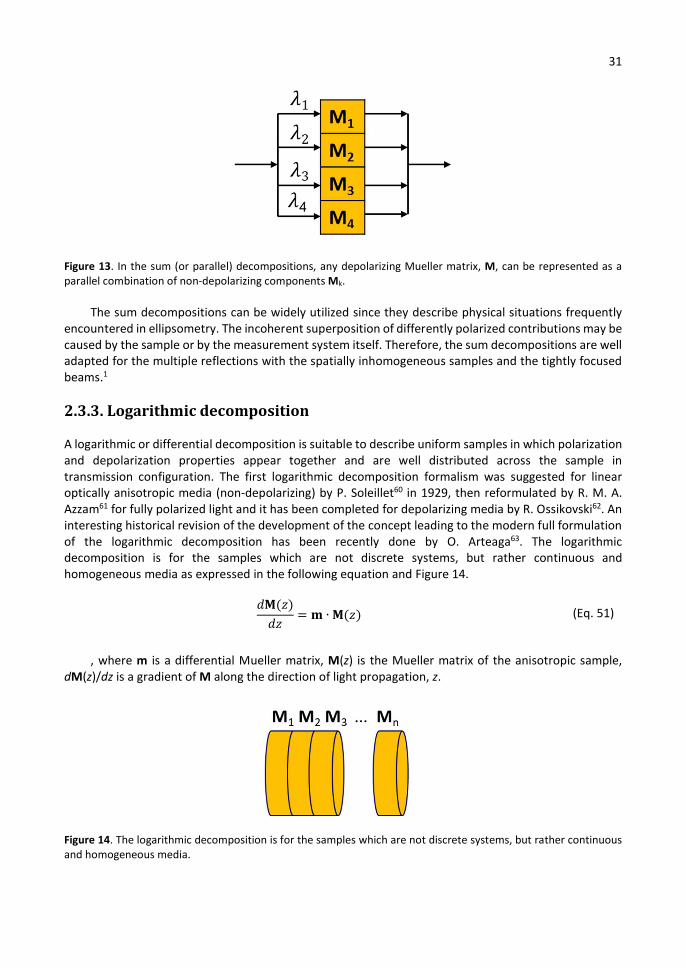
31

Figure 13. In the sum (or parallel) decompositions, any depolarizing Mueller matrix, M, can be represented as a parallel combination of non-depolarizing components Mk.

The sum decompositions can be widely utilized since they describe physical situations frequently encountered in ellipsometry. The incoherent superposition of differently polarized contributions may be caused by the sample or by the measurement system itself. Therefore, the sum decompositions are well adapted for the multiple reflections with the spatially inhomogeneous samples and the tightly focused beams.1

2.3.3. Logarithmic decomposition

A logarithmic or differential decomposition is suitable to describe uniform samples in which polarization and depolarization properties appear together and are well distributed across the sample in transmission configuration. The first logarithmic decomposition formalism was suggested for linear optically anisotropic media (non-depolarizing) by P. Soleillet60 in 1929, then reformulated by R. M. A. Azzam61 for fully polarized light and it has been completed for depolarizing media by R. Ossikovski62. An interesting historical revision of the development of the concept leading to the modern full formulation of the logarithmic decomposition has been recently done by O. Arteaga63. The logarithmic decomposition is for the samples which are not discrete systems, but rather continuous and homogeneous media as expressed in the following equation and Figure 14.

𝑑𝐌(𝑧)

𝑑𝑧= 𝐦 ∙ 𝐌(𝑧) (Eq. 51)

, where m is a differential Mueller matrix, M(z) is the Mueller matrix of the anisotropic sample, dM(z)/dz is a gradient of M along the direction of light propagation, z.

Figure 14. The logarithmic decomposition is for the samples which are not discrete systems, but rather continuous and homogeneous media.

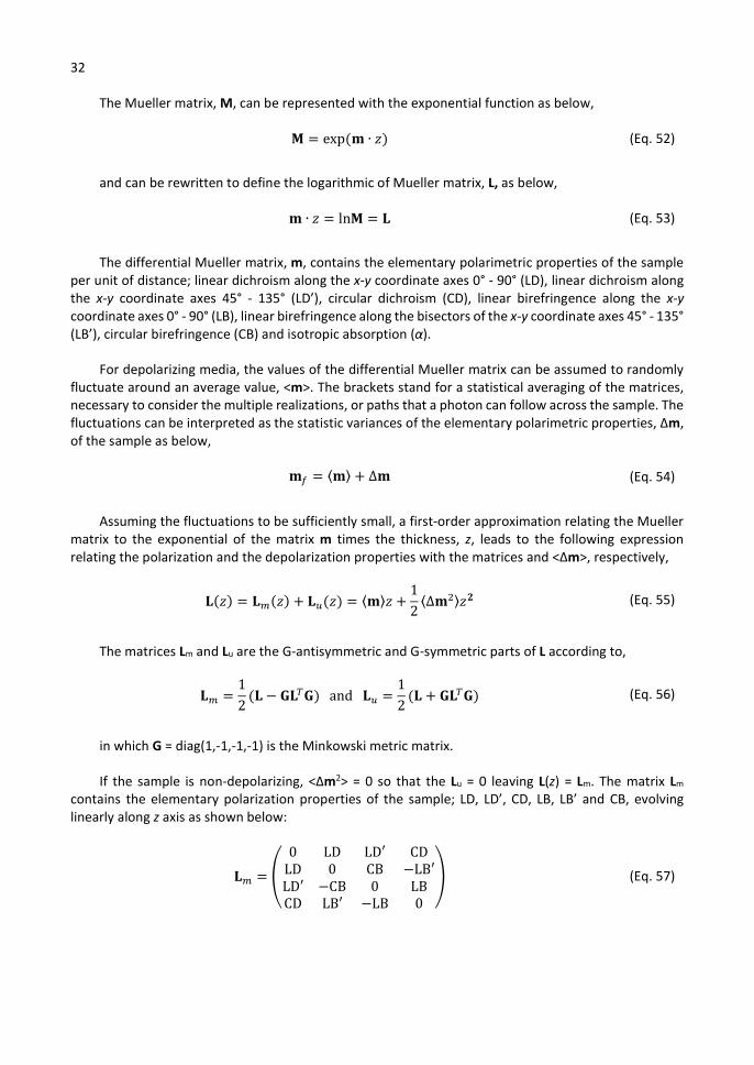
32

The Mueller matrix, M, can be represented with the exponential function as below,

𝐌 = exp(𝐦 ∙ 𝑧) (Eq. 52)

and can be rewritten to define the logarithmic of Mueller matrix, L, as below,

𝐦 ∙ 𝑧 = ln𝐌 = 𝐋 (Eq. 53)

The differential Mueller matrix, m, contains the elementary polarimetric properties of the sample per unit of distance; linear dichroism along the x-y coordinate axes 0° - 90° (LD), linear dichroism along the x-y coordinate axes 45° - 135° (LD’), circular dichroism (CD), linear birefringence along the x-y coordinate axes 0° - 90° (LB), linear birefringence along the bisectors of the x-y coordinate axes 45° - 135° (LB’), circular birefringence (CB) and isotropic absorption (α).

For depolarizing media, the values of the differential Mueller matrix can be assumed to randomly fluctuate around an average value, <m>. The brackets stand for a statistical averaging of the matrices, necessary to consider the multiple realizations, or paths that a photon can follow across the sample. The fluctuations can be interpreted as the statistic variances of the elementary polarimetric properties, Δm, of the sample as below,

𝐦 = ⟨𝐦⟩ + ∆𝐦 (Eq. 54)

Assuming the fluctuations to be sufficiently small, a first-order approximation relating the Mueller matrix to the exponential of the matrix m times the thickness, z, leads to the following expression relating the polarization and the depolarization properties with the matrices and <Δm>, respectively,

𝐋(𝑧) = 𝐋 (𝑧) + 𝐋 (𝑧) = ⟨𝐦⟩𝑧 +1

2⟨∆𝐦 ⟩𝑧𝟐 (Eq. 55)

The matrices Lm and Lu are the G-antisymmetric and G-symmetric parts of L according to,

𝐋 =1

2(𝐋 − 𝐆𝐋 𝐆) and 𝐋 =

1

2(𝐋 + 𝐆𝐋 𝐆) (Eq. 56)

in which G = diag(1,-1,-1,-1) is the Minkowski metric matrix.

If the sample is non-depolarizing, <Δm2> = 0 so that the Lu = 0 leaving L(z) = Lm. The matrix Lm contains the elementary polarization properties of the sample; LD, LD’, CD, LB, LB’ and CB, evolving linearly along z axis as shown below:

𝐋 =

0 LD LD′ CDLD 0 CB −LB′LD′ −CB 0 LBCD LB′ −LB 0

(Eq. 57)

33

However, if the sample is depolarizing, <Δm2> ≠ 0 and the diagonal elements of Lu show the depolarization coefficients, diag(Lu) = (0, α1, α2, α3), which depend quadratically on the propagation distance along z.

2.4. Conclusion

In this chapter, we introduced the fundamentals of polarization of light with a linear algebra called Mueller calculus. The three main polarimetric properties are introduced; the dichroism (or diattenuation), the birefringence (or retardation) and the depolarization. For the depolarizing power which shows the capability to decrease the DOP, there have been many studies to define it. We mainly focused on the parameters from the logarithmic decomposition such as the polarization properties (LD, LD’, CD, LB, LB’ and CB) and the depolarization coefficients that were discussed in the previous section, since the configuration of the polarimeter in this thesis is in transmission and the studied samples are transparent without discrete layers which show separated polarimetric responses. As a perspective, different type of decomposition method can be applied depending on different type of sample structures to compare errors.

34

Chapter 3. Instrumentation

Contents

3.1. Original prototypes ................................................................................................ 35

3.1.1. Mueller microscope in reflection mode .............................................................. 35

3.1.2. Mueller macroscope in transmission mode ....................................................... 36

3.2. Multimodal imaging polarimetric microscope ....................................................... 36

3.2.1. System design ...................................................................................................... 37

3.2.2. Design of PSG and PSA ...................................................................................... 38

3.2.2.1. Condition number ......................................................................................... 40

3.2.3. Multimodal imaging ............................................................................................ 42

3.2.3.1. Fourier (back-focal) plane imaging mode .................................................... 43

3.2.3.2. Real plane imaging mode ............................................................................. 45

3.3. General calibration method ................................................................................... 46

3.3.1. Eigenvalue calibration method (ECM) .............................................................. 46

3.3.2. Radiometric calibration ...................................................................................... 48

3.4. Verification of system ............................................................................................ 48

3.4.1. Spatial homogeneity analysis............................................................................. 49

3.4.2. Repeatability analysis ........................................................................................ 52

3.5. Conclusion ............................................................................................................. 53

The present chapter is devoted to discussing instrumental aspects of polarimeters, and in particular the multimodal imaging polarimeter developed in the framework of this thesis. Firstly, the original prototypes of imaging polarimeters developed in the laboratory LPICM previously to the one discussed here are shortly introduced. The imaging system that I have contributed to develop, called Multimodal imaging Mueller polarimetric microscope, is illustrated in a transmission mode. We show the design principle of the optical elements and methods of the system; the polarization state generator and analyzer (PSG and PSA), the multimodal imaging approach, and the calibration methods called an eigenvalue calibration method (ECM) and a radiometric calibration are also discussed. The spatial homogeneity and the repeatability analyses are done from the acquired images from the system to verify the stability of the system.

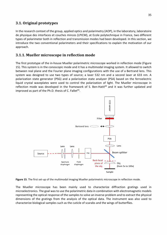
35

3.1. Original prototypes

In the research context of the group, applied optics and polarimetry (AOP), in the laboratory, laboratoire de physique des interfaces et couches minces (LPICM), at Ecole polytechnique in France, two different types of polarimeter both in reflection and transmission modes had been developed. In this section, we introduce the two conventional polarimeters and their specifications to explain the motivation of our approach.

3.1.1. Mueller microscope in reflection mode

The first prototype of the in-house Mueller polarimetric microscope worked in reflection mode (Figure 15). This system is in the conoscopic mode and it has a multimodal imaging system. It allowed to switch between real plane and the Fourier plane imaging configurations with the use of a Bertrand lens. This system was designed to use two types of source; a laser 532 nm and a second laser at 633 nm. A polarization state generator (PSG) and a polarization state analyzer (PSA) based on the ferroelectric liquid crystal waveplates were used to control the polarization of light. The Mueller microscope in reflection mode was developed in the framework of S. Ben-Hatit64 and it was further updated and improved as part of the Ph.D. thesis of C. Fallet65.

Figure 15. The first set-up of the multimodal imaging Mueller polarimetric microscope in reflection mode.

The Mueller microscope has been mainly used to characterize diffraction gratings used in microelectronics. The goal was to use the polarimetric data in combination with electromagnetic models representing the optical response of the samples to solve an inverse problem and to extract the physical dimensions of the gratings from the analysis of the optical data. The instrument was also used to characterize biological samples such as the cuticle of scarabs and the wings of butterflies.

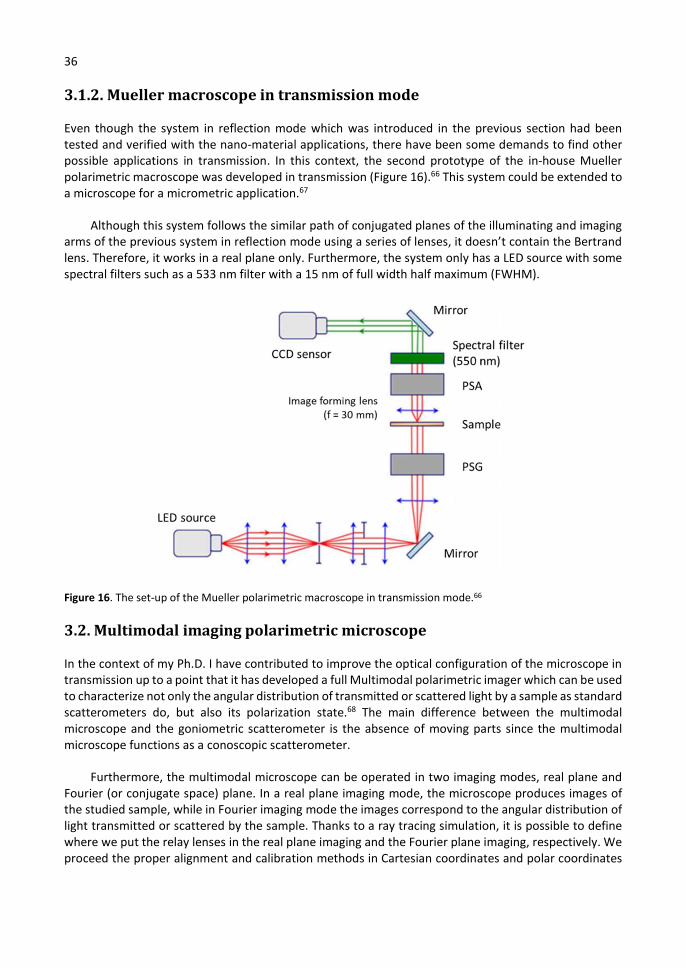
36

3.1.2. Mueller macroscope in transmission mode

Even though the system in reflection mode which was introduced in the previous section had been tested and verified with the nano-material applications, there have been some demands to find other possible applications in transmission. In this context, the second prototype of the in-house Mueller polarimetric macroscope was developed in transmission (Figure 16).66 This system could be extended to a microscope for a micrometric application.67

Although this system follows the similar path of conjugated planes of the illuminating and imaging arms of the previous system in reflection mode using a series of lenses, it doesn’t contain the Bertrand lens. Therefore, it works in a real plane only. Furthermore, the system only has a LED source with some spectral filters such as a 533 nm filter with a 15 nm of full width half maximum (FWHM).

Figure 16. The set-up of the Mueller polarimetric macroscope in transmission mode.66

3.2. Multimodal imaging polarimetric microscope

In the context of my Ph.D. I have contributed to improve the optical configuration of the microscope in transmission up to a point that it has developed a full Multimodal polarimetric imager which can be used to characterize not only the angular distribution of transmitted or scattered light by a sample as standard scatterometers do, but also its polarization state.68 The main difference between the multimodal microscope and the goniometric scatterometer is the absence of moving parts since the multimodal microscope functions as a conoscopic scatterometer.

Furthermore, the multimodal microscope can be operated in two imaging modes, real plane and Fourier (or conjugate space) plane. In a real plane imaging mode, the microscope produces images of the studied sample, while in Fourier imaging mode the images correspond to the angular distribution of light transmitted or scattered by the sample. Thanks to a ray tracing simulation, it is possible to define where we put the relay lenses in the real plane imaging and the Fourier plane imaging, respectively. We proceed the proper alignment and calibration methods in Cartesian coordinates and polar coordinates

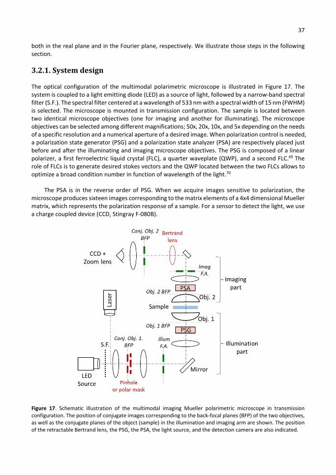
37

both in the real plane and in the Fourier plane, respectively. We illustrate those steps in the following section.

3.2.1. System design

The optical configuration of the multimodal polarimetric microscope is illustrated in Figure 17. The system is coupled to a light emitting diode (LED) as a source of light, followed by a narrow-band spectral filter (S.F.). The spectral filter centered at a wavelength of 533 nm with a spectral width of 15 nm (FWHM) is selected. The microscope is mounted in transmission configuration. The sample is located between two identical microscope objectives (one for imaging and another for illuminating). The microscope objectives can be selected among different magnifications; 50x, 20x, 10x, and 5x depending on the needs of a specific resolution and a numerical aperture of a desired image. When polarization control is needed, a polarization state generator (PSG) and a polarization state analyzer (PSA) are respectively placed just before and after the illuminating and imaging microscope objectives. The PSG is composed of a linear polarizer, a first ferroelectric liquid crystal (FLC), a quarter waveplate (QWP), and a second FLC.69 The role of FLCs is to generate desired stokes vectors and the QWP located between the two FLCs allows to optimize a broad condition number in function of wavelength of the light.70

The PSA is in the reverse order of PSG. When we acquire images sensitive to polarization, the microscope produces sixteen images corresponding to the matrix elements of a 4x4 dimensional Mueller matrix, which represents the polarization response of a sample. For a sensor to detect the light, we use a charge coupled device (CCD, Stingray F-080B).

Figure 17. Schematic illustration of the multimodal imaging Mueller polarimetric microscope in transmission configuration. The position of conjugate images corresponding to the back-focal planes (BFP) of the two objectives, as well as the conjugate planes of the object (sample) in the illumination and imaging arm are shown. The position of the retractable Bertrand lens, the PSG, the PSA, the light source, and the detection camera are also indicated.

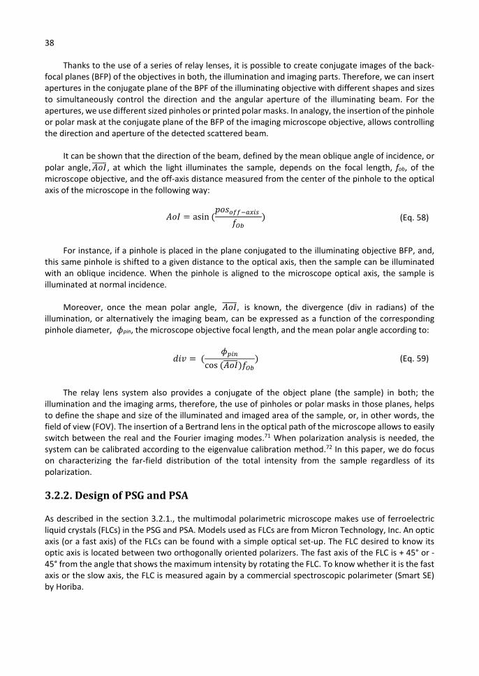
38

Thanks to the use of a series of relay lenses, it is possible to create conjugate images of the back-focal planes (BFP) of the objectives in both, the illumination and imaging parts. Therefore, we can insert apertures in the conjugate plane of the BPF of the illuminating objective with different shapes and sizes to simultaneously control the direction and the angular aperture of the illuminating beam. For the apertures, we use different sized pinholes or printed polar masks. In analogy, the insertion of the pinhole or polar mask at the conjugate plane of the BFP of the imaging microscope objective, allows controlling the direction and aperture of the detected scattered beam.

It can be shown that the direction of the beam, defined by the mean oblique angle of incidence, or polar angle, 𝐴𝑜𝐼 , at which the light illuminates the sample, depends on the focal length, fob, of the microscope objective, and the off-axis distance measured from the center of the pinhole to the optical axis of the microscope in the following way:

𝐴𝑜𝐼 = asin (𝑝𝑜𝑠

𝑓) (Eq. 58)

For instance, if a pinhole is placed in the plane conjugated to the illuminating objective BFP, and, this same pinhole is shifted to a given distance to the optical axis, then the sample can be illuminated with an oblique incidence. When the pinhole is aligned to the microscope optical axis, the sample is illuminated at normal incidence.

Moreover, once the mean polar angle, 𝐴𝑜𝐼, is known, the divergence (div in radians) of the illumination, or alternatively the imaging beam, can be expressed as a function of the corresponding pinhole diameter, 𝜙pin, the microscope objective focal length, and the mean polar angle according to:

𝑑𝑖𝑣 = (𝜙

cos (𝐴𝑜𝐼)𝑓) (Eq. 59)

The relay lens system also provides a conjugate of the object plane (the sample) in both; the illumination and the imaging arms, therefore, the use of pinholes or polar masks in those planes, helps to define the shape and size of the illuminated and imaged area of the sample, or, in other words, the field of view (FOV). The insertion of a Bertrand lens in the optical path of the microscope allows to easily switch between the real and the Fourier imaging modes.71 When polarization analysis is needed, the system can be calibrated according to the eigenvalue calibration method.72 In this paper, we do focus on characterizing the far-field distribution of the total intensity from the sample regardless of its polarization.

3.2.2. Design of PSG and PSA

As described in the section 3.2.1., the multimodal polarimetric microscope makes use of ferroelectric liquid crystals (FLCs) in the PSG and PSA. Models used as FLCs are from Micron Technology, Inc. An optic axis (or a fast axis) of the FLCs can be found with a simple optical set-up. The FLC desired to know its optic axis is located between two orthogonally oriented polarizers. The fast axis of the FLC is + 45° or - 45° from the angle that shows the maximum intensity by rotating the FLC. To know whether it is the fast axis or the slow axis, the FLC is measured again by a commercial spectroscopic polarimeter (Smart SE) by Horiba.

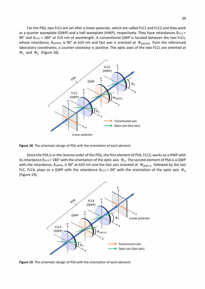
39

For the PSG, two FLCs are set after a linear polarizer, which are called FLC1 and FLC2 and they work as a quarter waveplate (QWP) and a half waveplate (HWP), respectively. They have retardances δFLC1 = 90° and δFLC2 = 180° at 510 nm of wavelength. A conventional QWP is located between the two FLCs, whose retardance, δQWPW, is 90° at 633 nm and fast axis is oriented at Φ from the referenced laboratory coordinates; a counter-clockwise is positive. The optic axes of the two FLCs are oriented at Φ and Φ (Figure 18).

Figure 18. The schematic design of PSG with the orientation of each element.

Since the PSA is in the reverse order of the PSG, the first element of PSA, FLC3, works as a HWP with its retardance δFLC3 = 180° with the orientation of the optic axis Φ . The second element of PSA is a QWP with the retardance, δQWPA, is 90° at 633 nm and the fast axis oriented at Φ followed by the last FLC, FLC4, plays as a QWP with the retardance δFLC4 = 90° with the orientation of the optic axis Φ (Figure 19).

Figure 19. The schematic design of PSA with the orientation of each element.

40

The angles of optic axes in PSA oriented from the referenced laboratory coordinates satisfy the relations below since the PSA is a mirror shape of the PSG,

Φ = 180° − Φ , Φ = 180° − Φ , Φ = 180° − Φ (Eq. 60)

In the ideal case, the optic axis of the FLCs rotates 45° between in the negative biased state and in the positive biased state. However, the optic axis of the FLC products that we used represent slightly different rotation angle of the optic axis; for the PSG, 46° of rotation between -3V and +3V in the QWP and 43° of rotation between -5V and +5V for in the HWP, for the PSA, 45° of rotation between -3V and +3V in the QWP and 41° of rotation between -5V and +5V for in the HWP (Figure 20).

To get the Mueller matrix of the measured sample, the 16 different polarization states are necessary by changing the state of PSG and PSA. As shown in Figure 20, the 16 intensities are measured by sequencing the four FLCs.

Figure 20. The chronogram of the signal control of liquid crystals with the definition of the 16 elements of intensity to build a Mueller matrix.

3.2.2.1. Condition number

The condition number in Linear algebra has been studied to increase the precision and accuracy of the measured data. In the Mueller matrix polarimetric imager, optimizing the condition numbers of the matrices of PSG and PSA, W and A respectively, is important since they are directly related to the signal to noise ratio on the image.72,73

Let’s say we have a system of linear equation,

41

𝐀𝐗 = 𝐁 (Eq. 61)

, where the A is a certain matrix and the 𝐗 and the 𝐁 are the vectors. The solution of 𝐗 can be determined by the inversion of the A. The condition number can be roughly thought as the rate at which the solution of an equation will change with respect to the change in initial members. So, the large value of the condition number may cause a large error on the 𝐗 even a small change in 𝐁. On the other hand, the small condition number cause small errors on 𝐗 which is not bigger that the errors on 𝐁. If we represent this error of 𝐁 as δ𝐁, the relative error of 𝐗, 𝛿𝐗 / 𝐗 , can be illustrated as below,

𝛿𝐗

𝐗≤ ‖𝐀 𝟏‖‖𝐀‖

δ�⃗�

𝐁 (Eq. 62)

, where the symbol, ‖ ‖, represents the vector or matrix norm. The condition number of the matrix A is defined as below,

𝜅(𝐀) = ‖𝐀 ‖‖𝐀‖ =𝜎

𝜎 (Eq. 63)

, where the 𝜎 and 𝜎 are the maximum and minimum values of the matrix A different from zero.74 In the Mueller polarimeter, we need to vectorize the equation below to get the condition number,

𝐌 = 𝐀 𝐈𝐖 (Eq. 64)

, where the M is the Mueller matrix of the sample, the I is the intensity matrix, A and W are the matrices of the PSA and the PSG, respectively. After the vectorization of the (Eq. 64), the following equation in produced,

𝐌 = ((𝐖 ) ⨂𝐀 )𝐈 (Eq. 65)

, where the symbol ⨂ represents the Kronecker. The (Eq. 65) can be rewritten like below,

𝐌 = ((𝐖 ) ⨂𝐀 )𝐈 = ((𝐖 )⨂𝐀) 𝐈 = 𝐐 𝐈 (Eq. 66)

, where the (𝐖 )⨂𝐀 is equal to Q. So, the (Eq. 73) can be illustrated using the elements, Q, M, and I.

𝛿𝐌

𝐌≤ 𝜅(𝐐)

δ𝐈

𝐈 (Eq. 67)

, where the 𝜅(𝐐) = ‖𝐐 ‖‖𝐐‖ is the condition number of matrix Q. So, if we want to minimize the error of the Mueller matrix, M, we need to minimize the condition number of Q. The condition number of the inverse of a matrix is equal to the condition number of the matrix. The condition number of a product is the product of the condition number. So, we can get the equation below,

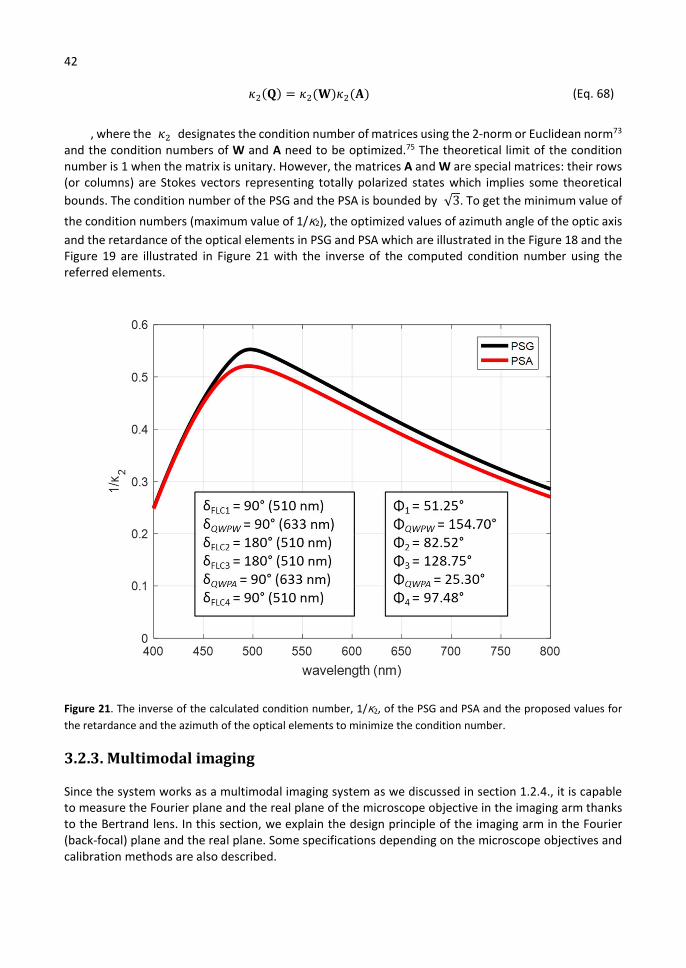
42

𝜅 (𝐐) = 𝜅 (𝐖)𝜅 (𝐀) (Eq. 68)

, where the 𝜅 designates the condition number of matrices using the 2-norm or Euclidean norm73 and the condition numbers of W and A need to be optimized.75 The theoretical limit of the condition number is 1 when the matrix is unitary. However, the matrices A and W are special matrices: their rows (or columns) are Stokes vectors representing totally polarized states which implies some theoretical bounds. The condition number of the PSG and the PSA is bounded by √3. To get the minimum value of

the condition numbers (maximum value of 1/κ2), the optimized values of azimuth angle of the optic axis and the retardance of the optical elements in PSG and PSA which are illustrated in the Figure 18 and the Figure 19 are illustrated in Figure 21 with the inverse of the computed condition number using the referred elements.

Figure 21. The inverse of the calculated condition number, 1/κ2, of the PSG and PSA and the proposed values for the retardance and the azimuth of the optical elements to minimize the condition number.

3.2.3. Multimodal imaging

Since the system works as a multimodal imaging system as we discussed in section 1.2.4., it is capable to measure the Fourier plane and the real plane of the microscope objective in the imaging arm thanks to the Bertrand lens. In this section, we explain the design principle of the imaging arm in the Fourier (back-focal) plane and the real plane. Some specifications depending on the microscope objectives and calibration methods are also described.

43

3.2.3.1. Fourier (back-focal) plane imaging mode

Thanks to a 2D ray tracing simulation software based on geometrical optics (ray optics), OptGeo, we can build the imaging arm based on a sophisticated design using the Bertrand lens71; defining where to locate the PSA, lenses, and the CCD sensor (Figure 22). To avoid focusing on the dust particles or even the shape of LC states on the PSA, the PSA (or a mirror) should be in the area where the rays are not converging both in the Fourier plane and the real plane configurations. The CCD should be at the point where the concerned rays are converged. In the Fourier plane imaging mode, the red rays refer to an aperture in Fourier plane (FoV). So, to capture all the incident rays, neither to lose the incident rays, the red rays should be filled with the size of CCD sensor as much as possible.

Figure 22. The blue rays which introduce the Fourier plane imaging start to diverge from the Fourier plane of the microscope objective and converge to the several planes (conjugated) and to the CCD sensor; Fourier plane imaging mode. When we change the Bertrand lens to the lens which has 80 mm focal length, then the red rays will be converged to the CCD sensor; real plane imaging mode.

An angular coordinate system in Fourier plane is defined depending on the numerical aperture of an imaging microscope objective. The polar angle of the coordinate system is calibrated using a simple diffraction grating equation (Eq. 73) by measuring a well-known diffraction grating (Figure 23),

𝑑 sin 𝜃 = 𝑚𝜆 (Eq. 69)

, where the dg is the period between each grid, 𝜃 is the diffracted angle of m-th order of transmitted light, m is the number of the order, and the λ is the wavelength of the incident light. This equation can be rewritten as below to know the 𝜃 ,

𝜃 = sin𝑚𝜆

𝑑 (Eq. 70)

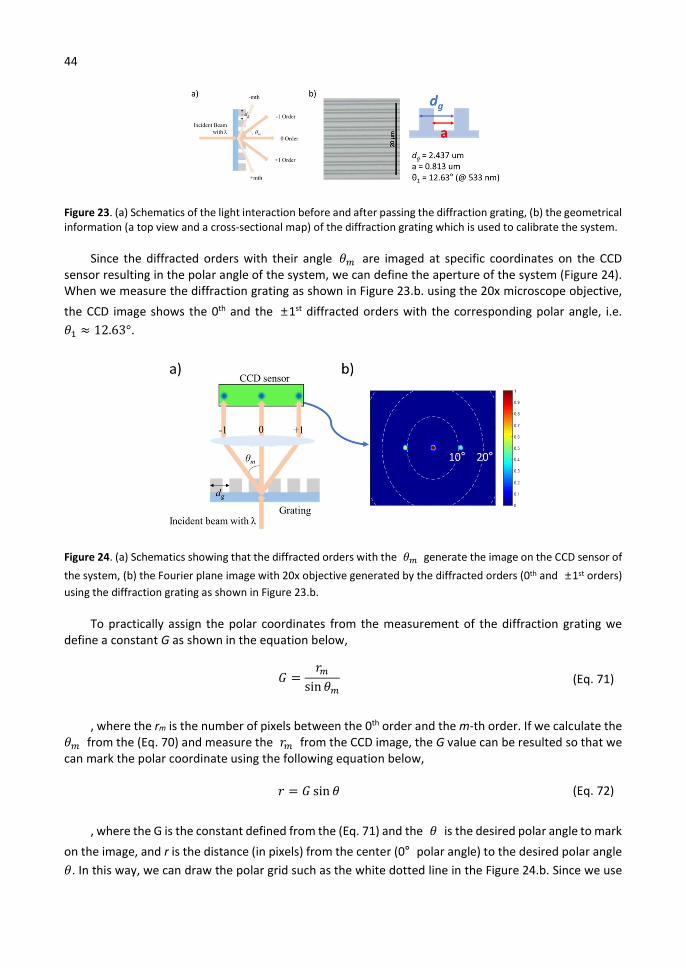
44

Figure 23. (a) Schematics of the light interaction before and after passing the diffraction grating, (b) the geometrical information (a top view and a cross-sectional map) of the diffraction grating which is used to calibrate the system.

Since the diffracted orders with their angle 𝜃 are imaged at specific coordinates on the CCD sensor resulting in the polar angle of the system, we can define the aperture of the system (Figure 24). When we measure the diffraction grating as shown in Figure 23.b. using the 20x microscope objective,

the CCD image shows the 0th and the ±1st diffracted orders with the corresponding polar angle, i.e. 𝜃 ≈ 12.63°.

Figure 24. (a) Schematics showing that the diffracted orders with the 𝜃 generate the image on the CCD sensor of

the system, (b) the Fourier plane image with 20x objective generated by the diffracted orders (0th and ±1st orders) using the diffraction grating as shown in Figure 23.b.

To practically assign the polar coordinates from the measurement of the diffraction grating we define a constant G as shown in the equation below,

𝐺 =𝑟

sin 𝜃 (Eq. 71)

, where the rm is the number of pixels between the 0th order and the m-th order. If we calculate the 𝜃 from the (Eq. 70) and measure the 𝑟 from the CCD image, the G value can be resulted so that we can mark the polar coordinate using the following equation below,

𝑟 = 𝐺 sin 𝜃 (Eq. 72)

, where the G is the constant defined from the (Eq. 71) and the 𝜃 is the desired polar angle to mark

on the image, and r is the distance (in pixels) from the center (0° polar angle) to the desired polar angle 𝜃. In this way, we can draw the polar grid such as the white dotted line in the Figure 24.b. Since we use

45

different type of the microscope objectives depending on the different magnification factors, the specifications of microscope in the Fourier plane are represented in the following table.

Table 1. Specifications of microscope in the Fourier plane depending on the magnification factor of microscope objectives.

Magnification factor

Numerical aperture

Theoretical aperture in polar angle (°)

Actual aperture in polar angle (°)

20 x 0.45 27.1 ~ 24 50 x 0.85 58.5 ~ 45

3.2.3.2. Real plane imaging mode

Since the Bertrand lens is switched to the lens with f = 80 mm in the real plane imaging mode, all the rays from the same point at the sample plane should be reached to the same point on the CCD sensor regardless of the angle of the outgoing beams (Figure 25). The specifications of the microscope in the real plane imaging mode are illustrated in the Table 2 with the different type of the objectives.

Figure 25. The red rays which introduce the real plane imaging start to diverge from a single point of the sample plane and converge to the several planes (conjugated) and to the CCD sensor; real plane imaging mode. When we change the Bertrand lens to the lens which has 40 mm focal length, then the blue rays will be converged to the CCD sensor; Fourier plane imaging mode.

Table 2. Specifications of microscope in the real plane depending on the magnification factor of microscope objectives.

Magnification factor FoV (µm) Pixel size (µm) 20x ~ 600 ~ 1 50x ~ 300 ~ 0.5

46

3.3. General calibration method

In this section, we introduce two general calibration methods; the eigenvalue calibration method (ECM) and the radiometric calibration. The ECM is considered to eliminate the effect of the optical elements of the system to extract only the Mueller matrix of the sample.

3.3.1. Eigenvalue calibration method (ECM)

A modulation matrix, W, is a sequence of the four stokes vectors from PSG. An analysis matrix, A, is a transpose of W.

𝐖 = 𝑆 𝑆 𝑆 𝑆 , 𝐀 = 𝐖𝐭 (Eq. 73)

The matrix A can be easily calculated once W is determined. So, the first step of the ECM is to measure the air which gives a unitary matrix B0.

𝐁𝟎 = 𝐀 𝐈 𝐖 (Eq. 74)

, where 𝐈 is an identity matrix. The analysis matrix, A, can be illustrated as below:

𝐀 = 𝐁𝟎 𝐖 𝟏 (Eq. 75)

𝐁𝒊 = 𝐀 𝐌𝒊𝐖 (i = 1, …, n) (Eq. 76)

, where Bi are the measured intensity matrices for known calibrating samples, n is the number of calibrating samples (n = 3). The Mueller matrices of the calibrating samples are illustrated in the equation below:

𝐌𝒊(𝜏 , Ψ , 𝛿 , Φ ) = 𝜏 𝐑(Φ )

1 − cos 2Ψ 0 0− cos 2Ψ 1 0 0

0 0 sin 2Ψ cos 𝛿 sin 2Ψ sin 𝛿0 0 − sin 2Ψ sin 𝛿 sin 2Ψ cos 𝛿

𝐑(−Φ ) (Eq. 77)

, where 𝜏 is a transmission coefficient of the sample for the totally depolarized light, Ψ is a linear dichroic angle of the sample, 𝛿 is a retardance of the sample, and Φ is a rotation angle of the optic axis of the sample. We can define the eigenvalues of the Mueller matrix of each sample which doesn’t depend on the rotation angle Φ as below:

𝜆 = 2𝜏 cos Ψ , 𝜆 = 2𝜏 sin Ψ , 𝜆 = 𝜏 sin 2Ψ 𝑒 , 𝜆 = 𝜏 sin 2Ψ 𝑒 (Eq. 78)

𝜆 𝜆

𝜆 𝜆= 1 (Eq. 79)

We define 𝐂𝒊 from the (Eq. 75) and (Eq. 76).

𝐂𝒊 = 𝐁𝟎𝟏 𝐁𝒊 = 𝐖 𝟏 𝐌𝒊 𝐖 (Eq. 80)

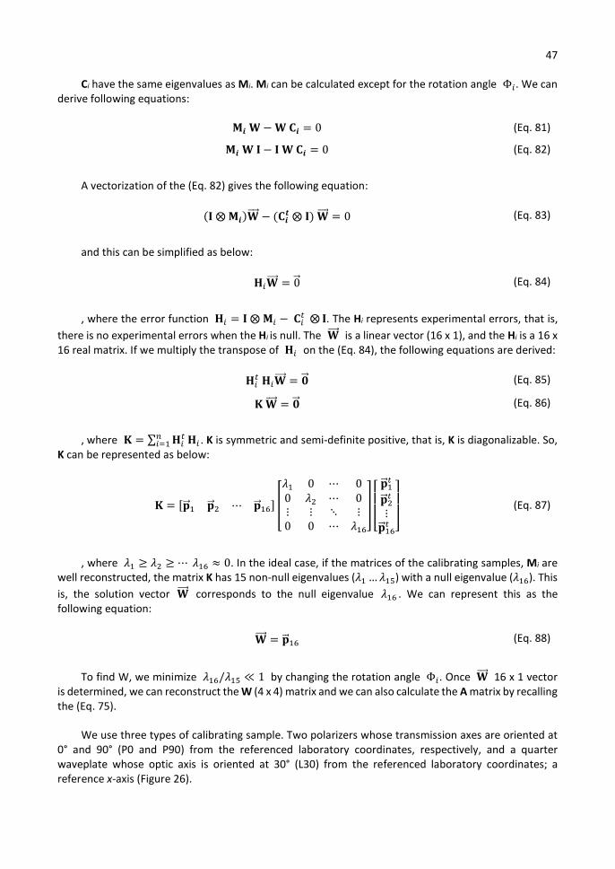
47

Ci have the same eigenvalues as Mi. Mi can be calculated except for the rotation angle Φ . We can derive following equations:

𝐌𝒊 𝐖 − 𝐖 𝐂𝒊 = 0 (Eq. 81)

𝐌𝒊 𝐖 𝐈 − 𝐈 𝐖 𝐂𝒊 = 0 (Eq. 82)

A vectorization of the (Eq. 82) gives the following equation:

(𝐈 ⨂ 𝐌𝒊)𝐖 − (𝐂𝒊𝒕 ⨂ 𝐈) 𝐖 = 0 (Eq. 83)

and this can be simplified as below:

𝐇 𝐖 = 0⃗ (Eq. 84)

, where the error function 𝐇 = 𝐈 ⨂ 𝐌 − 𝐂 ⨂ 𝐈. The Hi represents experimental errors, that is, there is no experimental errors when the Hi is null. The 𝐖 is a linear vector (16 x 1), and the Hi is a 16 x 16 real matrix. If we multiply the transpose of 𝐇 on the (Eq. 84), the following equations are derived:

𝐇 𝐇 𝐖 = �⃗� (Eq. 85)

𝐊 𝐖 = �⃗� (Eq. 86)

, where 𝐊 = ∑ 𝐇 𝐇 . K is symmetric and semi-definite positive, that is, K is diagonalizable. So, K can be represented as below:

𝐊 = [�⃗� �⃗� ⋯ �⃗� ]

𝜆 0 ⋯ 00 𝜆 ⋯ 0⋮ ⋮ ⋱ ⋮0 0 ⋯ 𝜆 ⎣

⎢⎢⎡

�⃗�

�⃗�⋮

�⃗� ⎦⎥⎥⎤ (Eq. 87)

, where 𝜆 ≥ 𝜆 ≥ ⋯ 𝜆 ≈ 0. In the ideal case, if the matrices of the calibrating samples, Mi are well reconstructed, the matrix K has 15 non-null eigenvalues (𝜆 … 𝜆 ) with a null eigenvalue (𝜆 ). This is, the solution vector 𝐖 corresponds to the null eigenvalue 𝜆 . We can represent this as the following equation:

𝐖 = �⃗� (Eq. 88)

To find W, we minimize 𝜆 /𝜆 ≪ 1 by changing the rotation angle Φ . Once 𝐖 16 x 1 vector is determined, we can reconstruct the W (4 x 4) matrix and we can also calculate the A matrix by recalling the (Eq. 75).

We use three types of calibrating sample. Two polarizers whose transmission axes are oriented at 0° and 90° (P0 and P90) from the referenced laboratory coordinates, respectively, and a quarter waveplate whose optic axis is oriented at 30° (L30) from the referenced laboratory coordinates; a reference x-axis (Figure 26).

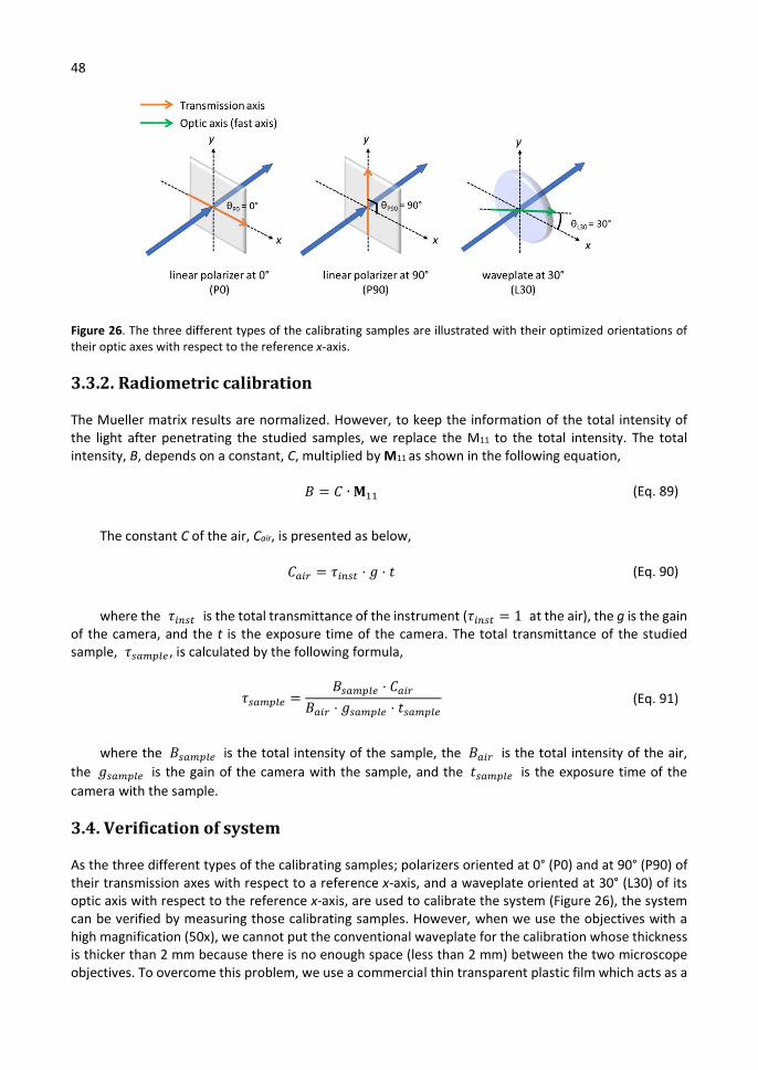
48

Figure 26. The three different types of the calibrating samples are illustrated with their optimized orientations of their optic axes with respect to the reference x-axis.

3.3.2. Radiometric calibration

The Mueller matrix results are normalized. However, to keep the information of the total intensity of the light after penetrating the studied samples, we replace the M11 to the total intensity. The total intensity, B, depends on a constant, C, multiplied by M11 as shown in the following equation,

𝐵 = 𝐶 ∙ 𝐌 (Eq. 89)

The constant C of the air, Cair, is presented as below,

𝐶 = 𝜏 ⋅ 𝑔 ⋅ 𝑡 (Eq. 90)

where the 𝜏 is the total transmittance of the instrument (𝜏 = 1 at the air), the g is the gain of the camera, and the t is the exposure time of the camera. The total transmittance of the studied sample, 𝜏 , is calculated by the following formula,

𝜏 =𝐵 ⋅ 𝐶

𝐵 ⋅ 𝑔 ⋅ 𝑡 (Eq. 91)

where the 𝐵 is the total intensity of the sample, the 𝐵 is the total intensity of the air, the 𝑔 is the gain of the camera with the sample, and the 𝑡 is the exposure time of the camera with the sample.

3.4. Verification of system

As the three different types of the calibrating samples; polarizers oriented at 0° (P0) and at 90° (P90) of their transmission axes with respect to a reference x-axis, and a waveplate oriented at 30° (L30) of its optic axis with respect to the reference x-axis, are used to calibrate the system (Figure 26), the system can be verified by measuring those calibrating samples. However, when we use the objectives with a high magnification (50x), we cannot put the conventional waveplate for the calibration whose thickness is thicker than 2 mm because there is no enough space (less than 2 mm) between the two microscope objectives. To overcome this problem, we use a commercial thin transparent plastic film which acts as a

49

waveplate with the properties which are measured by a commercial spectroscopic Mueller polarimetry and an imaging polarimetric microscope. The results are represented in Figure 27.

Since the polarimetric imager uses the spectral filter with the wavelength of 533 nm using LED source, the retardance of the thin transparent plastic film as a waveplate at the same wavelength @ 533 nm shows 0.9 rad (51.6°) measured by a commercial Mueller polarimetry and 0.99 rad (56.7°) measured by the polarimetric imager from the value in the center (~0° in polar angle) in Fourier image, showing 9.9 % error. This error can be occurred because of the tilted angle of incidence (in polar angle) at each instrument. The quality of the calibration can be bad using 50x objective because the retardance of the plastic film at the edge of the image (maximum polar angle in Fourier plane) is close to null value.

Figure 27. The measured retardance in radians of the thin transparaent plastic film in different views. (a) the retardance in the spectroscopic view measured by a commercial Mueller polarimetry, (b) the image of the retardance in the Fourier plane at 533 nm of the wavelength measured by the multimodal polarimetric imager with the 50x objective, (c) the cross-sectional plot of figure b (black dashed line).

The other results of the measurement on the calibrating samples are shown in the following sections with different function of variables such as a spatial homogeneity and a measurement time to verify the stability of the system. The parameters are the condition number of PSG and PSA, 1

𝜅 (W), 1𝜅 (A), the transmittance of the polarizers, τP0, τP90, the azimuth of the transmission axis of

the P0 and P90, θP0, θP90, the retardance of the waveplate, ΔL30, and the azimuth of the optic axis of L30, θL30.

3.4.1. Spatial homogeneity analysis

Since the instrument is working in imaging mode, it is important to analyze the spatial homogeneity of each image. This analysis has been done with the spectral filter with the wavelength of 533 nm using a LED source and the image plane is the real plane using the 20x microscope objective. The measurement results from the calibrating samples are shown in the following figures.

As the first calibrating sample, a polarizer oriented at 0° of the azimuth of its transmission axis, P0, is analyzed in the Figure 28. The Figure 28.a shows the total transmittance of the sample based on the (Eq. 91). The thin film polarizer is manufactured from Thorlabs (model: LPVISE2X2) and it shows 38 % of the average unpolarized nominal transmittance over the specified wavelength range (400 - 700 nm). Since the transmittance of P0, τP0, shows 41.44 % of with the 0.2 % of the standard deviation, it shows the error less than 10 %. The Figure 28.b shows 0.02° of the azimuth of the transmission axis with 0.24° of standard deviation, which is well matched with the 0° of reference value.

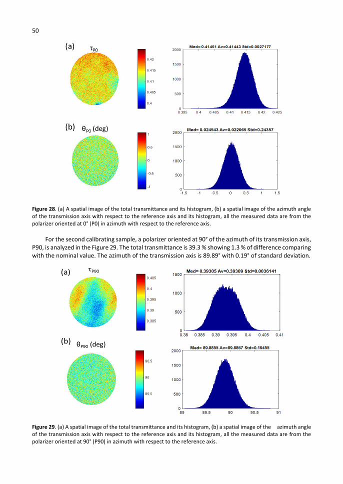
50

Figure 28. (a) A spatial image of the total transmittance and its histogram, (b) a spatial image of the azimuth angle of the transmission axis with respect to the reference axis and its histogram, all the measured data are from the polarizer oriented at 0° (P0) in azimuth with respect to the reference axis.

For the second calibrating sample, a polarizer oriented at 90° of the azimuth of its transmission axis, P90, is analyzed in the Figure 29. The total transmittance is 39.3 % showing 1.3 % of difference comparing with the nominal value. The azimuth of the transmission axis is 89.89° with 0.19° of standard deviation.

Figure 29. (a) A spatial image of the total transmittance and its histogram, (b) a spatial image of the azimuth angle of the transmission axis with respect to the reference axis and its histogram, all the measured data are from the polarizer oriented at 90° (P90) in azimuth with respect to the reference axis.

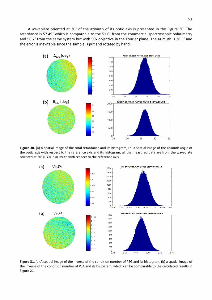
51

A waveplate oriented at 30° of the azimuth of its optic axis is presented in the Figure 30. The retardance is 57.49° which is comparable to the 51.6° from the commercial spectroscopic polarimetry and 56.7° from the same system but with 50x objective in the Fourier plane. The azimuth is 28.5° and the error is inevitable since the sample is put and rotated by hand.

Figure 30. (a) A spatial image of the total retardance and its histogram, (b) a spatial image of the azimuth angle of the optic axis with respect to the reference axis and its histogram, all the measured data are from the waveplate oriented at 30° (L30) in azimuth with respect to the reference axis.

Figure 31. (a) A spatial image of the inverse of the condition number of PSG and its histogram, (b) a spatial image of the inverse of the condition number of PSA and its histogram, which can be comparable to the calculated results in Figure 21.

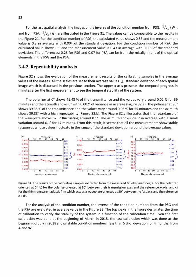
52

For the last spatial analysis, the images of the inverse of the condition number from PSG, 1𝜅 (W),

and from PSA, 1𝜅 (A), are illustrated in the Figure 31. The values can be comparable to the results in

the Figure 21. For the condition number of PSG, the calculated value shows 0.53 and the measurement value is 0.3 in average with 0.004 of the standard deviation. For the condition number of PSA, the calculated value shows 0.5 and the measurement value is 0.43 in average with 0.005 of the standard deviation. The differences; 0.23 for PSG and 0.07 for PSA can be from the misalignment of the optical elements in the PSG and the PSA.

3.4.2. Repeatability analysis

Figure 32 shows the evaluation of the measurement results of the calibrating samples in the average values of the images. All the scales are set to their average values ± standard deviation of each spatial image which is discussed in the previous section. The upper x-axis presents the temporal progress in minutes after the first measurement to see the temporal stability of the system.

The polarizer at 0° shows 41.43 % of the transmittance and the values vary around 0.02 % for 59 minutes and the azimuth shows 0° with 0.002° of variance in average (Figure 32.a). The polarizer at 90° shows 39.35 % of the transmittance and the values vary around 0.05 % for 55 minutes and the azimuth shows 89.88° with a high repeatability (Figure 32.b). The Figure 32.c illustrates that the retardance of the waveplate shows 57.6° fluctuating around 0.1°. The azimuth shows 28.5° in average with a small variation around 0.1° for 47 minutes. From this result, it seems that all the measurements show stable responses whose values fluctuate in the range of the standard deviation around the average values.

Figure 32. The results of the calibrating samples extracted from the measured Mueller matrices; a) for the polarizer oriented at 0°, b) for the polarize oriented at 90° between their transmission axes and the reference x-axis, and c) for the thin transparent plastic film which acts as a waveplate oriented at 30° between the fast axis and the reference x-axis.

For the analysis of the condition number, the inverse of the condition numbers from the PSG and the PSA are evaluated in average value in the Figure 33. The top x-axis in the figure designates the time of calibration to verify the stability of the system in a function of the calibration time. Even the first calibration was done at the beginning of March in 2018, the last calibration which was done at the beginning of July in 2018 shows stable condition numbers (less than 5 % of deviation for 4 months) from A and W.

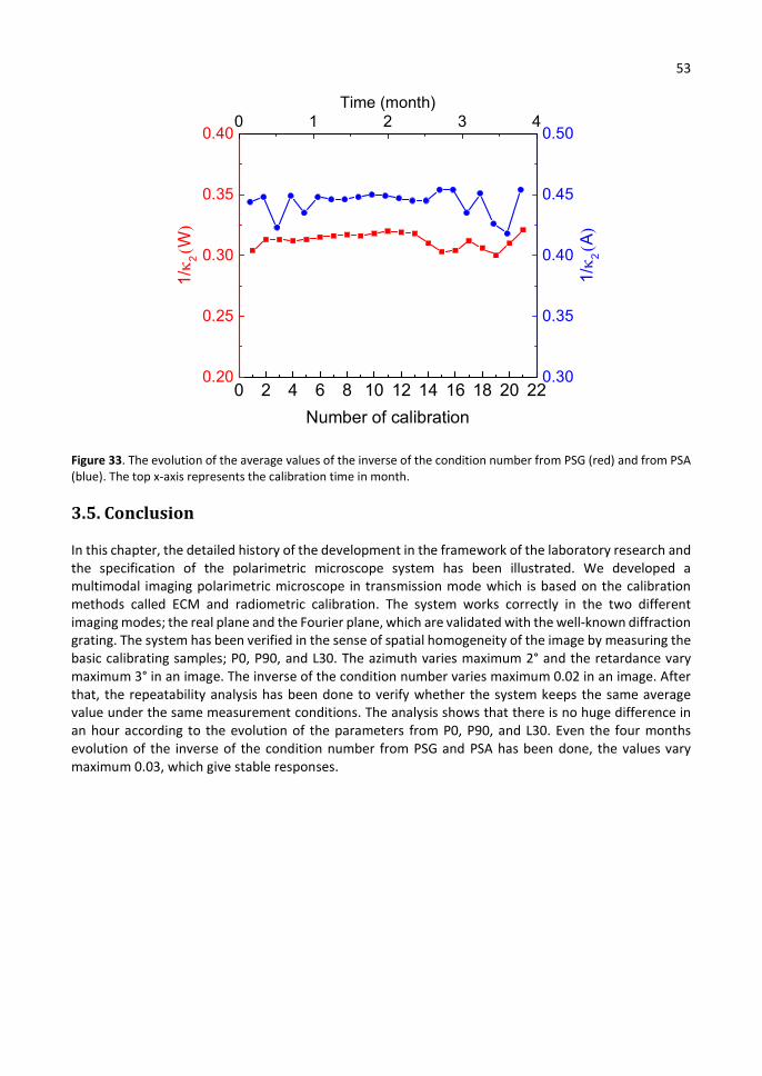
53

Figure 33. The evolution of the average values of the inverse of the condition number from PSG (red) and from PSA (blue). The top x-axis represents the calibration time in month.

3.5. Conclusion

In this chapter, the detailed history of the development in the framework of the laboratory research and the specification of the polarimetric microscope system has been illustrated. We developed a multimodal imaging polarimetric microscope in transmission mode which is based on the calibration methods called ECM and radiometric calibration. The system works correctly in the two different imaging modes; the real plane and the Fourier plane, which are validated with the well-known diffraction grating. The system has been verified in the sense of spatial homogeneity of the image by measuring the basic calibrating samples; P0, P90, and L30. The azimuth varies maximum 2° and the retardance vary maximum 3° in an image. The inverse of the condition number varies maximum 0.02 in an image. After that, the repeatability analysis has been done to verify whether the system keeps the same average value under the same measurement conditions. The analysis shows that there is no huge difference in an hour according to the evolution of the parameters from P0, P90, and L30. Even the four months evolution of the inverse of the condition number from PSG and PSA has been done, the values vary maximum 0.03, which give stable responses.

Number of calibration

0 2 4 6 8 10 12 14 16 18 20 220.20

0.25

0.30

0.35

0.40

1/

2(W

)

0.30

0.35

0.40

0.45

0.50

1/ 2

(A)

0 1 2 3 4Time (month)

54

Chapter 4. Polarimetric imaging in oblique incidence and geometric phases

Contents

4.1. Scattering configuration in oblique incidence ....................................................... 55

4.1.1. Standard description of radiation beam by single object ................................. 55

4.1.2. Scattering measurement with multimodal polarimetric imager ..................... 56

4.2. Vectorial ray tracing and polarization transformation by high NA lenses ........... 58

4.3. Vectorial polarimetry applied to linear radiating dipole ....................................... 61

4.4. Vectorial polarimetry applied to spherical particles ............................................. 71

4.4.1. Polarimetric response of a small sphere ............................................................ 75

4.4.2. Polarimetric response of a big sphere ................................................................ 77

4.5. Vectorial polarimetry applied to characterize spherical and spheroidal particles 82

4.5.1. Finite-difference time-domain (FDTD) method ................................................ 82

4.5.2. Sample preparation ............................................................................................ 92

4.5.3. Measurement and modelling .............................................................................. 93

4.6. Conclusion ............................................................................................................. 97

In this chapter, we introduce the polarimetric imaging in a normal incidence and an oblique incidence, yielding an apparent optical response which can be related to geometric phases. We describe a reference frame to explain the scattering configuration. An explanation of standard scattering experiment is illustrated, which is implemented in the multimodal polarimetric imager configured to make images in the Fourier (reciprocal space) mode. After that, a detailed description the above-mentioned intuitive ideas will be given such as mathematical formalisms to explain the transformation of a radiation beam when it is focused and then reimaged by a pair of high numerical aperture objectives based on a vectorial ray tracing. Thanks to the vectorial description, the effect of the interaction of the focused beam is discussed with a single dipole. Moreover, it has been shown that the logarithmic decomposition can be very useful to disentangle the polarimetric properties and, therefore, it is systematically used in combination with the respective Mueller matrix to interpret the results. We applied this approach to the Mueller matrix measurement of spherical and spheroidal particles and compared the Mueller matrices from the combined Finite-difference time-domain (FDTD) method approach, which is validated by benchmarking other commercial ellipsometry software.

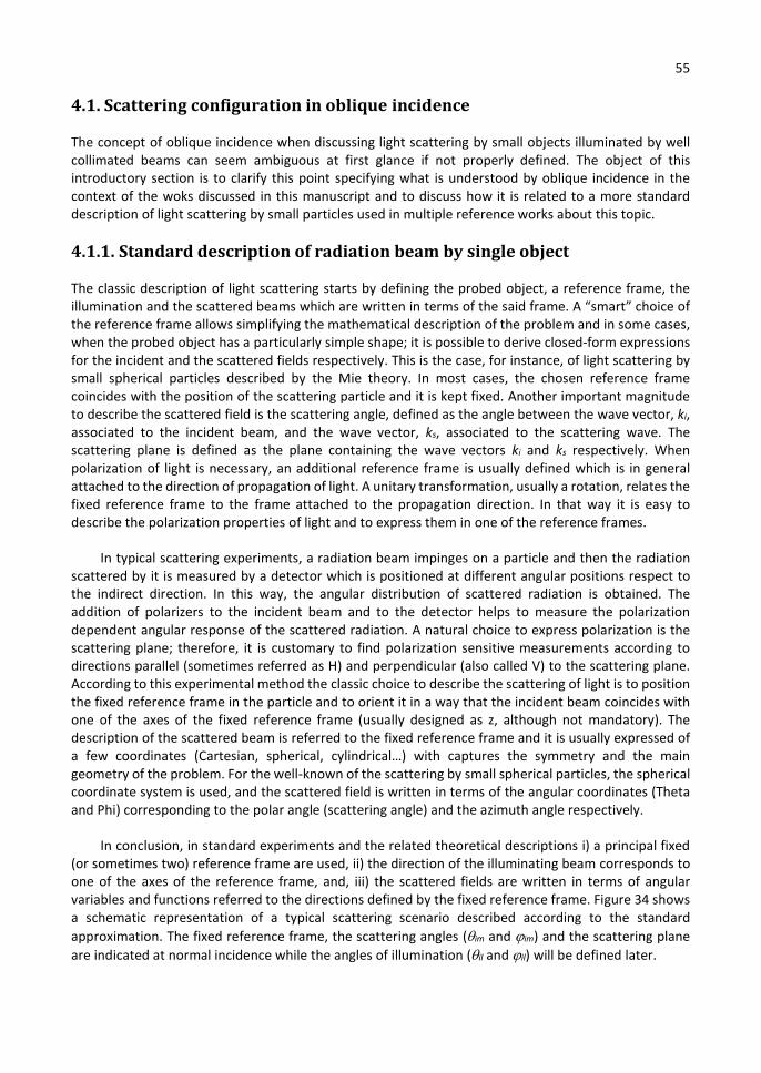
55

4.1. Scattering configuration in oblique incidence

The concept of oblique incidence when discussing light scattering by small objects illuminated by well collimated beams can seem ambiguous at first glance if not properly defined. The object of this introductory section is to clarify this point specifying what is understood by oblique incidence in the context of the woks discussed in this manuscript and to discuss how it is related to a more standard description of light scattering by small particles used in multiple reference works about this topic.

4.1.1. Standard description of radiation beam by single object

The classic description of light scattering starts by defining the probed object, a reference frame, the illumination and the scattered beams which are written in terms of the said frame. A “smart” choice of the reference frame allows simplifying the mathematical description of the problem and in some cases, when the probed object has a particularly simple shape; it is possible to derive closed-form expressions for the incident and the scattered fields respectively. This is the case, for instance, of light scattering by small spherical particles described by the Mie theory. In most cases, the chosen reference frame coincides with the position of the scattering particle and it is kept fixed. Another important magnitude to describe the scattered field is the scattering angle, defined as the angle between the wave vector, ki, associated to the incident beam, and the wave vector, ks, associated to the scattering wave. The scattering plane is defined as the plane containing the wave vectors ki and ks respectively. When polarization of light is necessary, an additional reference frame is usually defined which is in general attached to the direction of propagation of light. A unitary transformation, usually a rotation, relates the fixed reference frame to the frame attached to the propagation direction. In that way it is easy to describe the polarization properties of light and to express them in one of the reference frames.

In typical scattering experiments, a radiation beam impinges on a particle and then the radiation scattered by it is measured by a detector which is positioned at different angular positions respect to the indirect direction. In this way, the angular distribution of scattered radiation is obtained. The addition of polarizers to the incident beam and to the detector helps to measure the polarization dependent angular response of the scattered radiation. A natural choice to express polarization is the scattering plane; therefore, it is customary to find polarization sensitive measurements according to directions parallel (sometimes referred as H) and perpendicular (also called V) to the scattering plane. According to this experimental method the classic choice to describe the scattering of light is to position the fixed reference frame in the particle and to orient it in a way that the incident beam coincides with one of the axes of the fixed reference frame (usually designed as z, although not mandatory). The description of the scattered beam is referred to the fixed reference frame and it is usually expressed of a few coordinates (Cartesian, spherical, cylindrical…) with captures the symmetry and the main geometry of the problem. For the well-known of the scattering by small spherical particles, the spherical coordinate system is used, and the scattered field is written in terms of the angular coordinates (Theta and Phi) corresponding to the polar angle (scattering angle) and the azimuth angle respectively.

In conclusion, in standard experiments and the related theoretical descriptions i) a principal fixed (or sometimes two) reference frame are used, ii) the direction of the illuminating beam corresponds to one of the axes of the reference frame, and, iii) the scattered fields are written in terms of angular variables and functions referred to the directions defined by the fixed reference frame. Figure 34 shows a schematic representation of a typical scattering scenario described according to the standard approximation. The fixed reference frame, the scattering angles (im and im) and the scattering plane are indicated at normal incidence while the angles of illumination (il and il) will be defined later.

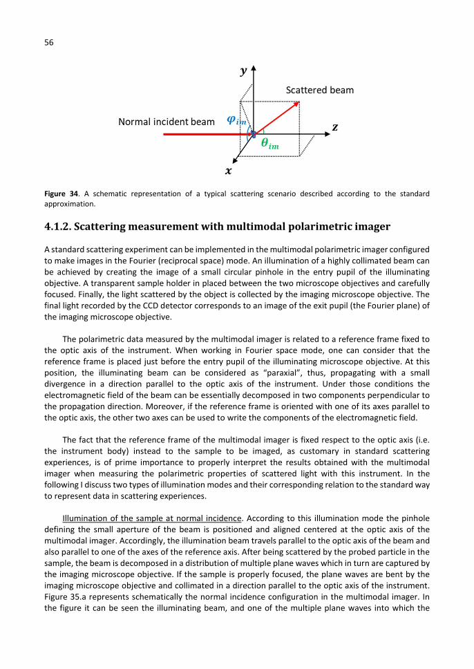
56

Figure 34. A schematic representation of a typical scattering scenario described according to the standard approximation.

4.1.2. Scattering measurement with multimodal polarimetric imager

A standard scattering experiment can be implemented in the multimodal polarimetric imager configured to make images in the Fourier (reciprocal space) mode. An illumination of a highly collimated beam can be achieved by creating the image of a small circular pinhole in the entry pupil of the illuminating objective. A transparent sample holder in placed between the two microscope objectives and carefully focused. Finally, the light scattered by the object is collected by the imaging microscope objective. The final light recorded by the CCD detector corresponds to an image of the exit pupil (the Fourier plane) of the imaging microscope objective.

The polarimetric data measured by the multimodal imager is related to a reference frame fixed to the optic axis of the instrument. When working in Fourier space mode, one can consider that the reference frame is placed just before the entry pupil of the illuminating microscope objective. At this position, the illuminating beam can be considered as “paraxial”, thus, propagating with a small divergence in a direction parallel to the optic axis of the instrument. Under those conditions the electromagnetic field of the beam can be essentially decomposed in two components perpendicular to the propagation direction. Moreover, if the reference frame is oriented with one of its axes parallel to the optic axis, the other two axes can be used to write the components of the electromagnetic field.

The fact that the reference frame of the multimodal imager is fixed respect to the optic axis (i.e. the instrument body) instead to the sample to be imaged, as customary in standard scattering experiences, is of prime importance to properly interpret the results obtained with the multimodal imager when measuring the polarimetric properties of scattered light with this instrument. In the following I discuss two types of illumination modes and their corresponding relation to the standard way to represent data in scattering experiences.

Illumination of the sample at normal incidence. According to this illumination mode the pinhole defining the small aperture of the beam is positioned and aligned centered at the optic axis of the multimodal imager. Accordingly, the illumination beam travels parallel to the optic axis of the beam and also parallel to one of the axes of the reference axis. After being scattered by the probed particle in the sample, the beam is decomposed in a distribution of multiple plane waves which in turn are captured by the imaging microscope objective. If the sample is properly focused, the plane waves are bent by the imaging microscope objective and collimated in a direction parallel to the optic axis of the instrument. Figure 35.a represents schematically the normal incidence configuration in the multimodal imager. In the figure it can be seen the illuminating beam, and one of the multiple plane waves into which the

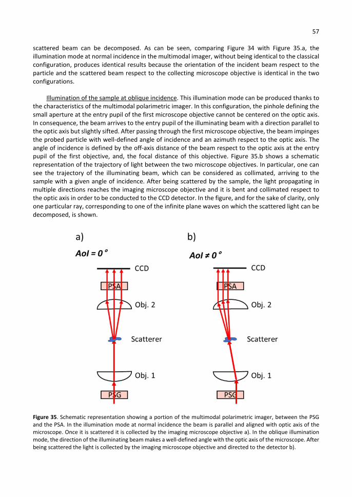
57

scattered beam can be decomposed. As can be seen, comparing Figure 34 with Figure 35.a, the illumination mode at normal incidence in the multimodal imager, without being identical to the classical configuration, produces identical results because the orientation of the incident beam respect to the particle and the scattered beam respect to the collecting microscope objective is identical in the two configurations.

Illumination of the sample at oblique incidence. This illumination mode can be produced thanks to the characteristics of the multimodal polarimetric imager. In this configuration, the pinhole defining the small aperture at the entry pupil of the first microscope objective cannot be centered on the optic axis. In consequence, the beam arrives to the entry pupil of the illuminating beam with a direction parallel to the optic axis but slightly sifted. After passing through the first microscope objective, the beam impinges the probed particle with well-defined angle of incidence and an azimuth respect to the optic axis. The angle of incidence is defined by the off-axis distance of the beam respect to the optic axis at the entry pupil of the first objective, and, the focal distance of this objective. Figure 35.b shows a schematic representation of the trajectory of light between the two microscope objectives. In particular, one can see the trajectory of the illuminating beam, which can be considered as collimated, arriving to the sample with a given angle of incidence. After being scattered by the sample, the light propagating in multiple directions reaches the imaging microscope objective and it is bent and collimated respect to the optic axis in order to be conducted to the CCD detector. In the figure, and for the sake of clarity, only one particular ray, corresponding to one of the infinite plane waves on which the scattered light can be decomposed, is shown.

Figure 35. Schematic representation showing a portion of the multimodal polarimetric imager, between the PSG and the PSA. In the illumination mode at normal incidence the beam is parallel and aligned with optic axis of the microscope. Once it is scattered it is collected by the imaging microscope objective a). In the oblique illumination mode, the direction of the illuminating beam makes a well-defined angle with the optic axis of the microscope. After being scattered the light is collected by the imaging microscope objective and directed to the detector b).

58

When comparing Figure 34 (or Figure 35.a) with Figure 35.b, it is clear that the two optical setups cannot produce analog results. The comparison between the two setups suggests the following intuitive ideas concerning the differences between the two setups. First of all, when one considers non-polarized intensity it is easy to realize that the radiation pattern produced by the scattering object in the experience shown in Figure 35.b is rotated respect to that of Figure 34 (or Figure 35.b). In addition, and as consequence of the limited numerical aperture of the imaging microscope objective, the distribution of scattering angles that can be captured in the configuration represented in Figure 35.a is different than that of Figure 35.b. When considering polarized light, additional differences between the two configurations will arise. Since the reference frame is the same for the two configurations, the fact that the radiation pattern of scattered light has been turned, will produce an apparent rotation of the polarization of some components of the scattered beam when measured with one configuration respect to the other. This latter difference between illuminations at normal and at oblique incidence can explain the observation of an apparent optical activity in measurements done at oblique incidence respect to that done at normal incidence. At this point it is worth to note here that the origin of the differences between the two configurations is purely topological (or geometrical) and it is due to a rotation of the physical scenario respect to the observer. Consequently, the apparent optical activity will be connected to a topological phase in circularly polarized light (or a rotation of linearly polarized light). The value of the topological phase will be connected to the particular path that each component of the beam has followed in the space from the point of emission by the particle, to the point of collection by the imaging microscope objective.

In the forthcoming sections of this chapter, a detailed description the above-mentioned intuitive ideas will be given. In particular, it will be discussed how to model and represent the Mueller matrix of a sample when measured in normal illumination configuration and in oblique incidence configuration respectively.

4.2. Vectorial ray tracing and polarization transformation by high NA lenses

In this section, the formalism is described to explain the transformation of a radiation beam when it is focused and then reimaged by a pair of high numerical aperture objectives. In the following, it will be assumed that the two high numerical systems are aplanatic and identical, that the system is perfectly aligned and focused. Accordingly, it is assumed that when an ideal well-collimated beam with homogeneous polarization and intensity is incident on the entry pupil (or back focal plane 1) of the first objective, it is focused up to the diffraction limit, to a point placed at a focal distance, f, from this objective. The sample to be studied must be eventually positioned at this focal point. Moreover, the light focused at the focal point is collected by a second-high numerical aperture microscope. The second-high numerical aperture objective, being placed at a distance, f, from the focal point, produces a well-collimated beam at the exit pupil (or back focal plane 2, BFP2). This ideal physical situation is depicted in Figure 36 where the high numerical aperture objectives are schematically represented together with the respective back-focal planes and also the position of the focal point. The optic axis is represented by a line and a Cartesian reference frame with coordinates x, y and z is placed at the focal point of the first objective. Moreover, two angular coordinates and are also represented. Those coordinates are the spherical coordinates associated to the Cartesian frame and are useful to represent the distribution of plane waves on which either the focused beam or the imaged beam, can be decomposed in order to provide a convenient mathematical analysis of the polarization transformation. The coordinate represents the polar angle and it is associated to the angle of incidence before the sample or the scattering angle after the sample. The angle is related to the azimuthal angle measured from the x axis. The range of the angle goes from 0 rad (normal incidence) to a maximum value, asin(NA), given by the numerical aperture (NA) of the microscope. The range of goes from 0 to 2.

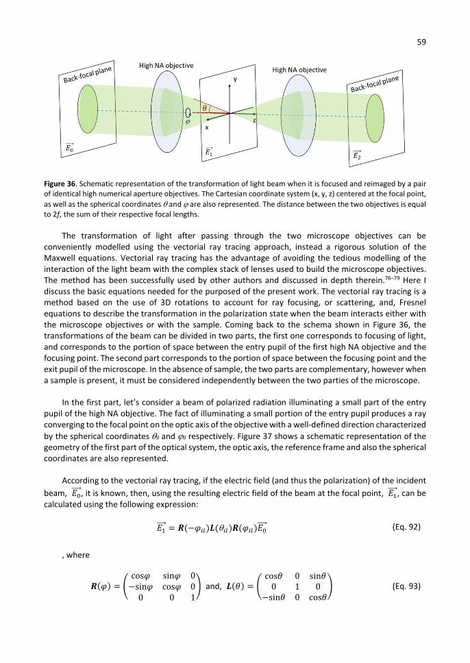
59

Figure 36. Schematic representation of the transformation of light beam when it is focused and reimaged by a pair of identical high numerical aperture objectives. The Cartesian coordinate system (x, y, z) centered at the focal point, as well as the spherical coordinates and are also represented. The distance between the two objectives is equal to 2f, the sum of their respective focal lengths.

The transformation of light after passing through the two microscope objectives can be conveniently modelled using the vectorial ray tracing approach, instead a rigorous solution of the Maxwell equations. Vectorial ray tracing has the advantage of avoiding the tedious modelling of the interaction of the light beam with the complex stack of lenses used to build the microscope objectives. The method has been successfully used by other authors and discussed in depth therein.76–79 Here I discuss the basic equations needed for the purposed of the present work. The vectorial ray tracing is a method based on the use of 3D rotations to account for ray focusing, or scattering, and, Fresnel equations to describe the transformation in the polarization state when the beam interacts either with the microscope objectives or with the sample. Coming back to the schema shown in Figure 36, the transformations of the beam can be divided in two parts, the first one corresponds to focusing of light, and corresponds to the portion of space between the entry pupil of the first high NA objective and the focusing point. The second part corresponds to the portion of space between the focusing point and the exit pupil of the microscope. In the absence of sample, the two parts are complementary, however when a sample is present, it must be considered independently between the two parties of the microscope.

In the first part, let’s consider a beam of polarized radiation illuminating a small part of the entry pupil of the high NA objective. The fact of illuminating a small portion of the entry pupil produces a ray converging to the focal point on the optic axis of the objective with a well-defined direction characterized by the spherical coordinates il and il respectively. Figure 37 shows a schematic representation of the geometry of the first part of the optical system, the optic axis, the reference frame and also the spherical coordinates are also represented.

According to the vectorial ray tracing, if the electric field (and thus the polarization) of the incident beam, 𝐸⃗, it is known, then, using the resulting electric field of the beam at the focal point, 𝐸⃗, can be calculated using the following expression:

𝐸⃗ = 𝑹(−𝜑 )𝑳( )𝑹(𝜑 )𝐸⃗ (Eq. 92)

, where

𝑹(𝜑) =cos𝜑 sin𝜑 0

−sin𝜑 cos𝜑 00 0 1

and, 𝑳(𝜃) =cos𝜃 0 sin𝜃

0 1 0−sin𝜃 0 cos𝜃

(Eq. 93)

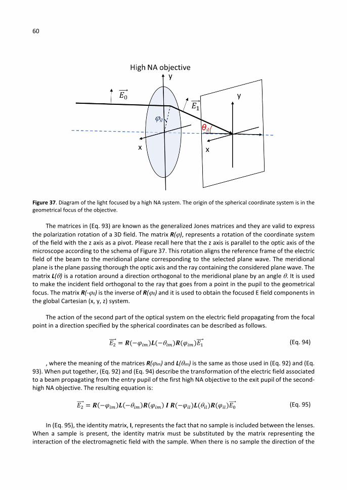
60

Figure 37. Diagram of the light focused by a high NA system. The origin of the spherical coordinate system is in the geometrical focus of the objective.

The matrices in (Eq. 93) are known as the generalized Jones matrices and they are valid to express the polarization rotation of a 3D field. The matrix R(), represents a rotation of the coordinate system of the field with the z axis as a pivot. Please recall here that the z axis is parallel to the optic axis of the microscope according to the schema of Figure 37. This rotation aligns the reference frame of the electric field of the beam to the meridional plane corresponding to the selected plane wave. The meridional plane is the plane passing thorough the optic axis and the ray containing the considered plane wave. The matrix L() is a rotation around a direction orthogonal to the meridional plane by an angle . It is used to make the incident field orthogonal to the ray that goes from a point in the pupil to the geometrical focus. The matrix R(-il) is the inverse of R(il) and it is used to obtain the focused E field components in the global Cartesian (x, y, z) system.

The action of the second part of the optical system on the electric field propagating from the focal point in a direction specified by the spherical coordinates can be described as follows.

𝐸⃗ = 𝑹(−𝜑 )𝑳(− )𝑹(𝜑 )𝐸⃗ (Eq. 94)

, where the meaning of the matrices R(im) and L(im) is the same as those used in (Eq. 92) and (Eq. 93). When put together, (Eq. 92) and (Eq. 94) describe the transformation of the electric field associated to a beam propagating from the entry pupil of the first high NA objective to the exit pupil of the second-high NA objective. The resulting equation is:

𝐸⃗ = 𝑹(−𝜑 )𝑳(− )𝑹(𝜑 ) 𝑰 𝑹(−𝜑 )𝑳( )𝑹(𝜑 )𝐸⃗ (Eq. 95)

In (Eq. 95), the identity matrix, I, represents the fact that no sample is included between the lenses. When a sample is present, the identity matrix must be substituted by the matrix representing the interaction of the electromagnetic field with the sample. When there is no sample the direction of the

61

incident beam is not modified, thus the value of the spherical components in the illumination space and the imaging space are related as follows: 𝜑 = 𝜋 − 𝜑 and = . In this conditions, (Eq. 95) says that if diffraction effects due to for instance, the finite size of the aperture of the pupils of the objectives, or, the fact some high spatial frequencies are not transmitted by the limited aperture of the objectives, then the resulting field, 𝐸⃗, must be identical to the incident field, 𝐸⃗, thus polarization is not modified.

In the present section the general frame of the vectorial polarization ray tracing has been reviewed. In the following section this framework will be used to discuss the interaction of the focused beam with a very simple and ideal sample, a single dipole.

4.3. Vectorial polarimetry applied to linear radiating dipole

In this section, the effect of the interaction of the focused beam is discussed with a single dipole. Despite of the fact that single dipole represents a situation which is to some extent quite ideal, it has a relatively simple mathematical representation therefore can be used as an illustration of the effect of the normal incidence illumination, as well as oblique incidence illumination in the angular distribution of the polarization of the scattered beam. Moreover, since the single dipole approximation also represents reasonably well the scattering of light by very small real particles compared to the wavelength of light, it can be used as a benchmark to test the accuracy of more complex models.

The scattered field 𝐸⃗ in the far-field region of a single dipole characterized by a dipole moment, 𝑝, which is proportional to the incident field 𝐸⃗ s given by the following expression80:

𝐸⃗( , , ) = −

1

4𝜋𝜖

𝑘 𝑒

𝑟𝑟 × (𝑟 × 𝑝) (Eq. 96)

This expression says that the field radiated by the dipole is a spherical wave, whose absolute phase is proportional to the product of the wave vector, k, and the distance, r, between the point at which the field is observed and the position of the dipole. The amplitude of the field is inversely proportional to the distance from the dipole, and the polarization is a complex vectorial function of the space coordinates (x, y, z) at which the field is observed and the orientation of the dipole moment. Assuming that the dipole moment is proportional to the incident field, and that the position vector, 𝑟, can be written as a function of the spherical coordinates, 𝑟( , , ) = (sin 𝜃 cos 𝜑, sin 𝜃 sin 𝜑, cos 𝜃) , then (Eq. 96) can be rewritten in the following form:

𝐸⃗( , , ) =

−𝑘 𝑒

4𝜋𝜖 𝑟

⎝

⎛

1 − sin 𝜃 ∙ cos 𝜑 −12 sin 𝜃 ∙ cos 2𝜑 −1

2 sin2𝜃 ∙ cos 𝜑

−12 sin 𝜃 ∙ cos 2𝜑 1 − sin 𝜃 ∙ sin 𝜑 −1

2 sin2𝜃 ∙ sin 𝜑

−12 sin2𝜃 ∙ cos 𝜑 −1

2 sin2𝜃 ∙ sin 𝜑 1 − cos 𝜃 ⎠

⎞ 𝐸⃗( , , ) = 𝑱𝒅𝒊𝒑 ∙ 𝐸⃗

( , , ) (Eq. 97)

The subscript (x, y, z) is to recall that the components of the corresponding vector are written in the (x, y, z) reference frame attached to the optic axis of the microscope. In the following, the global phase in (Eq. 97) will be dropped since it does not affect the final result when formulated in the Stokes-Mueller formalism. Moreover, since the particle is considered to be smaller than the focal distance, f, at which the field is collected by the imaging high NA lens, and that we assume that the particle is always observed in focus, the dependence of the field amplitude with, r can be considered as a constant and it will also be omitted.

62

The interest of (Eq. 97) is that it represents the action of a dipole on an incident field in a matrix form, which can be understood, as the extended Jones matrix of the dipole. The extended Jones matrix is derived for treating the transmission of off-axis light81–83 and this matrix can be used in (Eq. 95) to simulate the optical response of a single dipole when illuminated by a beam focused by a high NA objective. Accordingly, (Eq. 95) can be modified as follows:

𝐸⃗ = 𝑹(−𝜑 )𝑳(− )𝑹(𝜑 ) 𝑱𝒅𝒊𝒑 𝑹(−𝜑 )𝑳( )𝑹(𝜑 )𝐸⃗ (Eq. 98)

, where the identity matrix, I, has been substituted by the extended Jones matrix of the dipole Jdip. In (Eq. 98), a distinction is done between the direction of the illumination beam and the propagation direction of scattered wave.

The extended Jones matrix of the entire system i.e. the illumination high NA objective, the dipole and the imaging high NA objective can be easily obtained by evaluating the components of the scattered field when the dipole is sequentially illuminated by a beam with orthogonal polarizations to each other respectively. The use of (Eq. 98) is particularly useful because it connects the components of the field in the paraxial region, just before and just after the two high NA objectives. In those conditions, the longitudinal component of the electric field (along the propagation direction, z) vanishes, and therefore the only non-null components of the scattered electric filed correspond to the transversal ones, which can be used to build a standard 2 x 2 Jones matrix. Once the Jones matrix is known, it can be converted to a Mueller matrix using the following transformation:

𝑴 = 𝑨(𝑱 ⊗ 𝑱∗)𝑨 , where 𝑨 =

1 01 0

0 10 −1

0 10 𝑖

1 0−𝑖 0

(Eq. 99)

, where the matrices M and J correspond to the Mueller and the Jones matrix respectively, the symbol ⊗ is for the Kronecker product and the superscript * means conjugate transpose.

The choice of the two orthogonal polarizations to be transformed by the dipole as well as the reference basis on which they are expressed depends on the problem. In the case of the system considered a natural and easy choice is the Cartesian (x, y, z) frame and the two orthogonal polarizations directed along the x and the y directions respectively. The combination of (Eq. 98) and (Eq. 99) allows calculating the Mueller matrix of the scattered light of the dipole, for an illumination direction specified by the spherical coordinates il and il, and a scattering direction specified by the coordinates im and im respectively. In the following the Mueller matrix of the single dipole is discussed in the cases of interest: illumination in normal incidence and illumination in oblique incidence.

Case of normal incidence

All the Muller matrix images in this chapter are described in the polar coordinates (, ) in the back-focal (Fourier) plane which are comparable to far-field distribution. The polar angle, , corresponds to the distance from the center of the circle and the azimuth, , corresponds to the anticlockwise rotation angle as previously shown in the Fourier plane coordinates in Figure 6.b. At normal incidence, both, il and il are equal to 0°. If the Mueller matrix of the scattered light in the forward direction is of interest, then the variables im and im that can be used are bounded respectively to 0 ≤ im ≤ 90° and 0 ≤ im ≤ 360°. Figure 38 shows the result of the evaluation of the Mueller matrix of the dipole in forward direction.

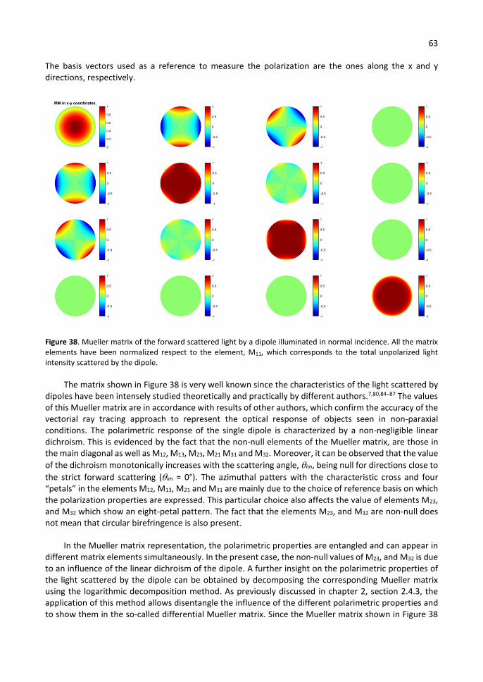
63

The basis vectors used as a reference to measure the polarization are the ones along the x and y directions, respectively.

Figure 38. Mueller matrix of the forward scattered light by a dipole illuminated in normal incidence. All the matrix elements have been normalized respect to the element, M11, which corresponds to the total unpolarized light intensity scattered by the dipole.

The matrix shown in Figure 38 is very well known since the characteristics of the light scattered by dipoles have been intensely studied theoretically and practically by different authors.7,80,84–87 The values of this Mueller matrix are in accordance with results of other authors, which confirm the accuracy of the vectorial ray tracing approach to represent the optical response of objects seen in non-paraxial conditions. The polarimetric response of the single dipole is characterized by a non-negligible linear dichroism. This is evidenced by the fact that the non-null elements of the Mueller matrix, are those in the main diagonal as well as M12, M13, M23, M21 M31 and M32. Moreover, it can be observed that the value of the dichroism monotonically increases with the scattering angle, im, being null for directions close to the strict forward scattering (im = 0°). The azimuthal patters with the characteristic cross and four “petals” in the elements M12, M13, M21 and M31 are mainly due to the choice of reference basis on which the polarization properties are expressed. This particular choice also affects the value of elements M23, and M32 which show an eight-petal pattern. The fact that the elements M23, and M32 are non-null does not mean that circular birefringence is also present.

In the Mueller matrix representation, the polarimetric properties are entangled and can appear in different matrix elements simultaneously. In the present case, the non-null values of M23, and M32 is due to an influence of the linear dichroism of the dipole. A further insight on the polarimetric properties of the light scattered by the dipole can be obtained by decomposing the corresponding Mueller matrix using the logarithmic decomposition method. As previously discussed in chapter 2, section 2.4.3, the application of this method allows disentangle the influence of the different polarimetric properties and to show them in the so-called differential Mueller matrix. Since the Mueller matrix shown in Figure 38

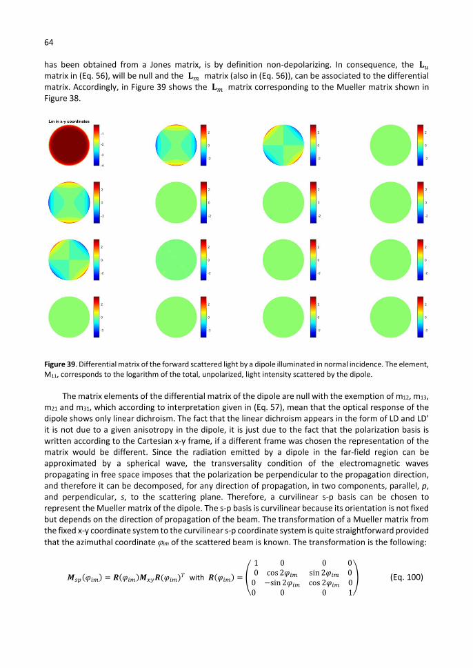
64

has been obtained from a Jones matrix, is by definition non-depolarizing. In consequence, the 𝐋 matrix in (Eq. 56), will be null and the 𝐋 matrix (also in (Eq. 56)), can be associated to the differential matrix. Accordingly, in Figure 39 shows the 𝐋 matrix corresponding to the Mueller matrix shown in Figure 38.

Figure 39. Differential matrix of the forward scattered light by a dipole illuminated in normal incidence. The element, M11, corresponds to the logarithm of the total, unpolarized, light intensity scattered by the dipole.

The matrix elements of the differential matrix of the dipole are null with the exemption of m12, m13, m21 and m31, which according to interpretation given in (Eq. 57), mean that the optical response of the dipole shows only linear dichroism. The fact that the linear dichroism appears in the form of LD and LD’ it is not due to a given anisotropy in the dipole, it is just due to the fact that the polarization basis is written according to the Cartesian x-y frame, if a different frame was chosen the representation of the matrix would be different. Since the radiation emitted by a dipole in the far-field region can be approximated by a spherical wave, the transversality condition of the electromagnetic waves propagating in free space imposes that the polarization be perpendicular to the propagation direction, and therefore it can be decomposed, for any direction of propagation, in two components, parallel, p, and perpendicular, s, to the scattering plane. Therefore, a curvilinear s-p basis can be chosen to represent the Mueller matrix of the dipole. The s-p basis is curvilinear because its orientation is not fixed but depends on the direction of propagation of the beam. The transformation of a Mueller matrix from the fixed x-y coordinate system to the curvilinear s-p coordinate system is quite straightforward provided that the azimuthal coordinate im of the scattered beam is known. The transformation is the following:

𝑴 (𝜑 ) = 𝑹(𝜑 )𝑴 𝑹(𝜑 ) with 𝑹(𝜑 ) =

1 00 cos 2𝜑

0 0sin 2𝜑 0

0 −sin 2𝜑0 0

cos 2𝜑 00 1

(Eq. 100)

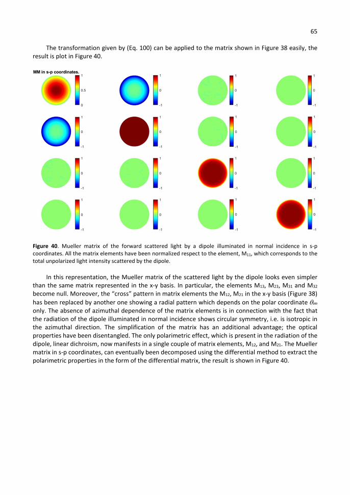
65

The transformation given by (Eq. 100) can be applied to the matrix shown in Figure 38 easily, the result is plot in Figure 40.

Figure 40. Mueller matrix of the forward scattered light by a dipole illuminated in normal incidence in s-p coordinates. All the matrix elements have been normalized respect to the element, M11, which corresponds to the total unpolarized light intensity scattered by the dipole.

In this representation, the Mueller matrix of the scattered light by the dipole looks even simpler than the same matrix represented in the x-y basis. In particular, the elements M13, M23, M31 and M32 become null. Moreover, the “cross” pattern in matrix elements the M12, M21 in the x-y basis (Figure 38) has been replaced by another one showing a radial pattern which depends on the polar coordinate im only. The absence of azimuthal dependence of the matrix elements is in connection with the fact that the radiation of the dipole illuminated in normal incidence shows circular symmetry, i.e. is isotropic in the azimuthal direction. The simplification of the matrix has an additional advantage; the optical properties have been disentangled. The only polarimetric effect, which is present in the radiation of the dipole, linear dichroism, now manifests in a single couple of matrix elements, M12, and M21. The Mueller matrix in s-p coordinates, can eventually been decomposed using the differential method to extract the polarimetric properties in the form of the differential matrix, the result is shown in Figure 40.

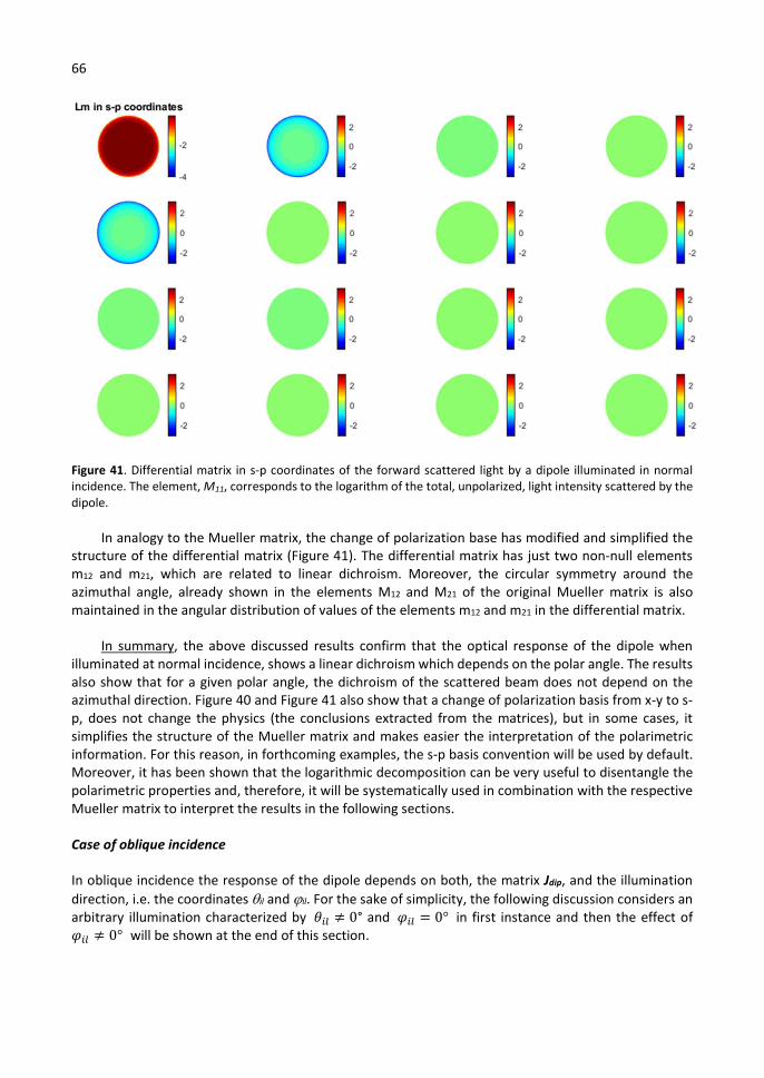
66

Figure 41. Differential matrix in s-p coordinates of the forward scattered light by a dipole illuminated in normal incidence. The element, M11, corresponds to the logarithm of the total, unpolarized, light intensity scattered by the dipole.

In analogy to the Mueller matrix, the change of polarization base has modified and simplified the structure of the differential matrix (Figure 41). The differential matrix has just two non-null elements m12 and m21, which are related to linear dichroism. Moreover, the circular symmetry around the azimuthal angle, already shown in the elements M12 and M21 of the original Mueller matrix is also maintained in the angular distribution of values of the elements m12 and m21 in the differential matrix.

In summary, the above discussed results confirm that the optical response of the dipole when illuminated at normal incidence, shows a linear dichroism which depends on the polar angle. The results also show that for a given polar angle, the dichroism of the scattered beam does not depend on the azimuthal direction. Figure 40 and Figure 41 also show that a change of polarization basis from x-y to s-p, does not change the physics (the conclusions extracted from the matrices), but in some cases, it simplifies the structure of the Mueller matrix and makes easier the interpretation of the polarimetric information. For this reason, in forthcoming examples, the s-p basis convention will be used by default. Moreover, it has been shown that the logarithmic decomposition can be very useful to disentangle the polarimetric properties and, therefore, it will be systematically used in combination with the respective Mueller matrix to interpret the results in the following sections.

Case of oblique incidence

In oblique incidence the response of the dipole depends on both, the matrix Jdip, and the illumination direction, i.e. the coordinates il and il. For the sake of simplicity, the following discussion considers an arbitrary illumination characterized by 𝜃 ≠ 0° and 𝜑 = 0° in first instance and then the effect of 𝜑 ≠ 0° will be shown at the end of this section.

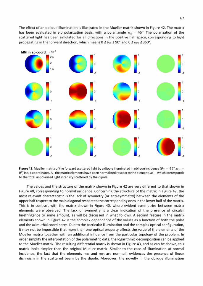
67

The effect of an oblique illumination is illustrated in the Mueller matrix shown in Figure 42. The matrix has been evaluated in s-p polarization basis, with a polar angle 𝜃 = 45° The polarization of the scattered light has been simulated for all directions in the positive half space, corresponding to light propagating in the forward direction, which means 0 ≤ im ≤ 90° and 0 ≤ im ≤ 360°.

Figure 42. Mueller matrix of the forward scattered light by a dipole illuminated in oblique incidence (𝜃 = 45°, 𝜑 =0°) in s-p coordinates. All the matrix elements have been normalized respect to the element, M11, which corresponds to the total unpolarized light intensity scattered by the dipole.

The values and the structure of the matrix shown in Figure 42 are very different to that shown in Figure 40, corresponding to normal incidence. Concerning the structure of the matrix in Figure 42, the most relevant characteristic is the lack of symmetry (or anti-symmetry) between the elements of the upper half respect to the main diagonal respect to the corresponding ones in the lower half of the matrix. This is in contrast with the matrix shown in Figure 40, where evident symmetries between matrix elements were observed. The lack of symmetry is a clear indication of the presence of circular birefringence to some amount, as will be discussed in what follows. A second feature in the matrix elements shown in Figure 42 is the complex dependence of the values as a function of both the polar and the azimuthal coordinates. Due to the particular illumination and the complex optical configuration, it may not be impossible that more than one optical property affects the value of the elements of the Mueller matrix together with an additional influence from the particular topology of the problem. In order simplify the interpretation of the polarimetric data; the logarithmic decomposition can be applied to the Mueller matrix. The resulting differential matrix is shown in Figure 43, and as can be shown, this matrix looks simpler than the original Mueller matrix. Similar to the case of illumination at normal incidence, the fact that the elements m12 and m13 are non-null, evidences the presence of linear dichroism in the scattered beam by the dipole. Moreover, the novelty in the oblique illumination

68

configuration case, is the non-null values of elements m23 and m32, which indicate the presence of a (quite strong indeed) circular birefringence. Since the linear dipole considered here has no optical activity, the circular birefringence can be attributed, not to the intrinsic properties of the dipole, but to the particular geometry (or topology) of the illumination and observation geometry as will be discussed in the following, therefore, in this text the term apparent circular birefringence is preferred to the term circular birefringence. Therefore, in view of the differential matrix, the optical response of the dipole in oblique incidence is characterized by both, linear dichroism and apparent circular birefringence.

Figure 43. Differential matrix in s-p coordinates of the forward scattered light by a dipole illuminated in oblique incidence (𝜃 = 45°, 𝜑 = 0°). The element, M11, corresponds to the logarithm of the total, unpolarized, light intensity scattered by the dipole.

Concerning the linear dichroism, and despite of having represented in s-p polarization basis, it may seem, that the angular distribution of dichroism is quite complex, compared to the simple circular symmetry when measurements were done in normal incidence. The apparent complexity is just a geometric effect due to the fact that the direction of the illumination beam and the axis of the microscope are not collinear. A powerful and easy way to remove the effect of the geometry in the linear dichroism is to consider the absolute value of the total dichroism, TotalLD, calculated as follows:

𝑇𝑜𝑡𝑎𝑙𝐿𝐷 = 𝐿𝐷 + 𝐿𝐷′ (Eq. 101)

Since the absolute value of the linear dichroism is a polarimetric invariant, then it must be independent of the basis and the reference frame chosen to observe the polarization. Total linear

69

dichroism represented in Figure 44 together with the corresponding values of LD and LD’, shown in Figure 43.

Figure 44. Linear dichroism components (LD and LD’) together to the corresponding Total LD for a dipole illuminated at oblique incidence with: 𝜃 = 45° and 𝜑 = 0°.

Figure 45. Linear dichroism components (LD and LD’) together to the corresponding Total LD for a dipole illuminated at oblique incidence with: 𝜃 = 22.5° and 𝜑 = 0°.

Figure 46. Linear dichroism components (LD and LD’) together to the corresponding Total LD for three different cases a dipole illuminated at normal incidence with: 𝜃 = 0° and 𝜑 = 0°.

The pattern of the TotalLD is considerably simplified, and now it resembles to the pattern of LD shown for illumination at normal incidence. In order to illustrate the interpretation of the angular dependence of the TotalLD at oblique incidence, the data shown in Figure 44 should be compared to that shown in Figure 45 and Figure 46. In the latter figures the values of LD, LD’, TotalLD and the log of M11 is shown for oblique illumination at lower polar angle (22.5°) and normal incidence respectively. It is curious to see that when observed from top to bottom the patterns in LD’, TotalLD and log(M11) seem to “rotate” to the left. This effect can be easily understood as an effect of the illumination angle of incidence and can be explained considering the illumination and the scattering processes as seen from the point of view of the dipole and the microscope respectively. This situation is schematically depicted in Figure 47.

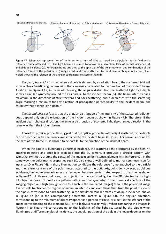
70

Figure 47. Schematic representation of the intensity pattern of light scattered by a dipole in the far-field and a reference frame attached to it. The light beam is assumed to follow the z1 direction. Case of normal incidence (a), and oblique incidence (b). Reference frame attached to the optic axis of the polarimeter (c) and combination of the reference frame of the polarimeter (orange - red) and frame attached to the dipole in oblique incidence (blue - violet) showing the relation of the angular coordinates related to them d).

The first physical fact is that when a dipole is shinned by a radiation beam, the scattered light will show a characteristic angular emission that can easily be related to the direction of the incident beam. As shown in Figure 47.a, in terms of intensity, the angular distribution the scattered light by a dipole shows a circular symmetry around the axis parallel to the incident beam (z1). The beam intensity has a maximum in the directions of strict forward and back scattering, and it decreases with the scattering angle reaching a minimum for any direction of propagation perpendicular to the incident beam, one could say that it looks like a peanut.

The second physical fact is that the angular distribution of the intensity of the scattered radiation does depend only on the orientation of the incident beam as shown in Figure 47.b. Therefore, if the incident beam changes direction, the angular distribution of scattered light also changes direction in the same way than the incident beam.

Those two physical properties suggest that the optical properties of the light scattered by the dipole can be described with a reference axis attached to the incident beam (x1, y1, z1). For convenience one of the axes of this frame, z1, is chosen to be parallel to the direction of the incident beam.

When the dipole is illuminated at normal incidence, the scattered light is captured by the high-NA imaging objective and once it is projected into the 2D camera, it produces a circular pattern with azimuthal symmetry around the center of the image (see for instance, element M11, in Figure 40). In the same way, the polarimetric properties such LD, also show a well-defined azimuthal symmetry (see for instance LD in Figure 46). In those illumination conditions the reference frame attached to the particle and the reference frame of the polarimeter, attached to the optic axis, coincide. However, at oblique incidence, the two reference frames are decoupled because one is rotated respect to the other as shown in Figure 47.d. In those conditions, the projection of the scattered light on the 2D detector by the high-NA objective does not produce a pattern with azimuthal symmetry. If the numerical aperture of the imaging objective is high enough (close to 1 such in the simulated images) then in the projected image it is possible to observe the regions of minimum intensity and even those that, from the point of view of the dipole, correspond to back-scattering. In the simulated Mueller matrix at oblique incidence, shown in Figure 42 (or in the corresponding differential matrix in Figure 43), the angular directions corresponding to the minimum of intensity appear as a portion of circle (or a belt) in the left part of the image corresponding to the element M11 (or to log(M11) respectively). When comparing the images in Figure 44 to Figure 46 corresponding to the log(M11), of the light scattered by the dipole when illuminated at different angles of incidence, the angular position of the belt in the image depends on the

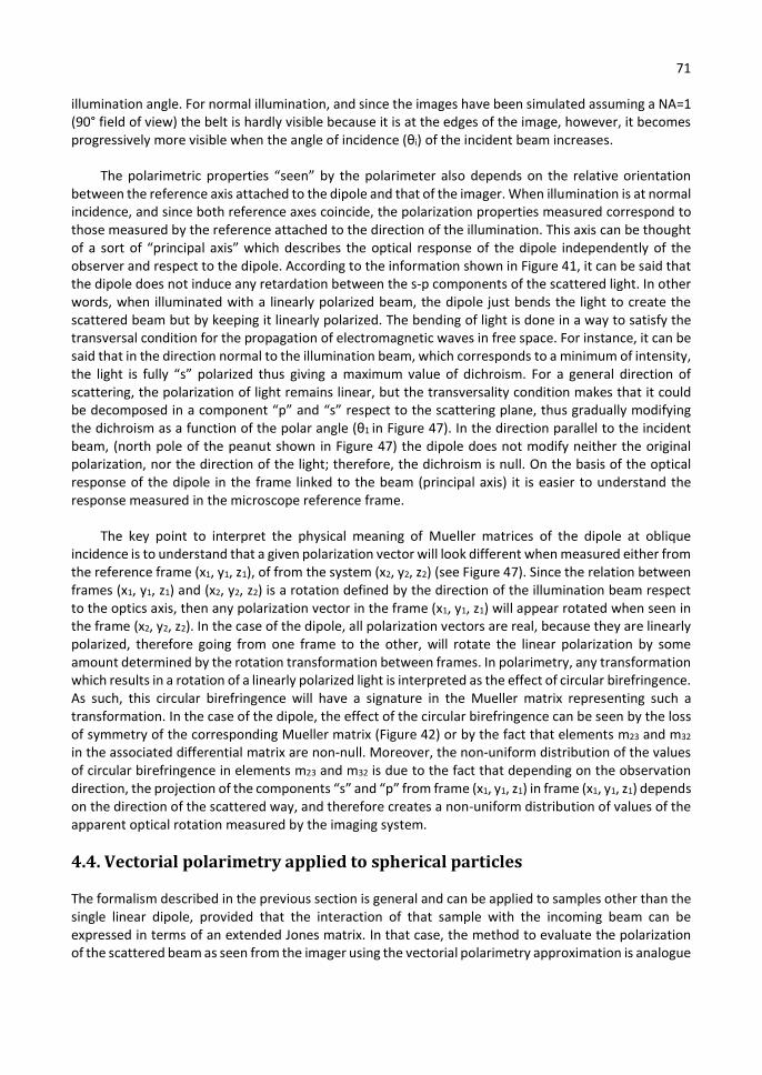
71

illumination angle. For normal illumination, and since the images have been simulated assuming a NA=1 (90° field of view) the belt is hardly visible because it is at the edges of the image, however, it becomes progressively more visible when the angle of incidence (θi) of the incident beam increases.

The polarimetric properties “seen” by the polarimeter also depends on the relative orientation between the reference axis attached to the dipole and that of the imager. When illumination is at normal incidence, and since both reference axes coincide, the polarization properties measured correspond to those measured by the reference attached to the direction of the illumination. This axis can be thought of a sort of “principal axis” which describes the optical response of the dipole independently of the observer and respect to the dipole. According to the information shown in Figure 41, it can be said that the dipole does not induce any retardation between the s-p components of the scattered light. In other words, when illuminated with a linearly polarized beam, the dipole just bends the light to create the scattered beam but by keeping it linearly polarized. The bending of light is done in a way to satisfy the transversal condition for the propagation of electromagnetic waves in free space. For instance, it can be said that in the direction normal to the illumination beam, which corresponds to a minimum of intensity, the light is fully “s” polarized thus giving a maximum value of dichroism. For a general direction of scattering, the polarization of light remains linear, but the transversality condition makes that it could be decomposed in a component “p” and “s” respect to the scattering plane, thus gradually modifying the dichroism as a function of the polar angle (θ1 in Figure 47). In the direction parallel to the incident beam, (north pole of the peanut shown in Figure 47) the dipole does not modify neither the original polarization, nor the direction of the light; therefore, the dichroism is null. On the basis of the optical response of the dipole in the frame linked to the beam (principal axis) it is easier to understand the response measured in the microscope reference frame.

The key point to interpret the physical meaning of Mueller matrices of the dipole at oblique incidence is to understand that a given polarization vector will look different when measured either from the reference frame (x1, y1, z1), of from the system (x2, y2, z2) (see Figure 47). Since the relation between frames (x1, y1, z1) and (x2, y2, z2) is a rotation defined by the direction of the illumination beam respect to the optics axis, then any polarization vector in the frame (x1, y1, z1) will appear rotated when seen in the frame (x2, y2, z2). In the case of the dipole, all polarization vectors are real, because they are linearly polarized, therefore going from one frame to the other, will rotate the linear polarization by some amount determined by the rotation transformation between frames. In polarimetry, any transformation which results in a rotation of a linearly polarized light is interpreted as the effect of circular birefringence. As such, this circular birefringence will have a signature in the Mueller matrix representing such a transformation. In the case of the dipole, the effect of the circular birefringence can be seen by the loss of symmetry of the corresponding Mueller matrix (Figure 42) or by the fact that elements m23 and m32 in the associated differential matrix are non-null. Moreover, the non-uniform distribution of the values of circular birefringence in elements m23 and m32 is due to the fact that depending on the observation direction, the projection of the components “s” and “p” from frame (x1, y1, z1) in frame (x1, y1, z1) depends on the direction of the scattered way, and therefore creates a non-uniform distribution of values of the apparent optical rotation measured by the imaging system.

4.4. Vectorial polarimetry applied to spherical particles

The formalism described in the previous section is general and can be applied to samples other than the single linear dipole, provided that the interaction of that sample with the incoming beam can be expressed in terms of an extended Jones matrix. In that case, the method to evaluate the polarization of the scattered beam as seen from the imager using the vectorial polarimetry approximation is analogue

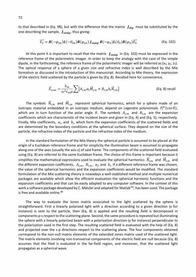
72

to that described in (Eq. 98), but with the difference that the matrix 𝑱𝒅𝒊𝒑 must be substituted by the one describing the sample, 𝑱𝒔𝒂𝒎𝒑, thus giving:

𝐸⃗ = 𝑹(−𝜑 )𝑳(− )𝑹(𝜑 ) 𝑱𝒔𝒂𝒎𝒑 𝑹(−𝜑 )𝑳( )𝑹(𝜑 )𝐸⃗ (Eq. 102)

At this point it is important to recall that the matrix 𝑱𝒔𝒂𝒎𝒑 in (Eq. 102) must be expressed in the reference frame of the polarimetric imager. In order to keep the analogy with the case of the simple dipole, in the forthcoming, the reference frame of the polarimetric imager will be referred as (x2, y2, z2). The optical response of a sphere of a given size and refractive index is well described by the Mie formalism as discussed in the introduction of this manuscript. According to Mie theory, the expression of the electric field scattered by the particle is given by (Eq. 8). Recalled here for convenience,

�⃗� =𝑘

𝜔 𝜖 𝜇𝐴 , 𝑎 𝑀 , + 𝐵 , 𝑏 �⃗� , (Eq. 8) recall

The symbols �⃗� , and 𝑀 , represent spherical harmonics, which for a sphere made of an isotropic material embedded in an isotropic medium, depend on Legendre polynomials 𝑃 (cos 𝜃), which are in turn function of the polar angle 𝜃 . The symbols 𝐴 , and 𝐵 , are the expansion coefficients which are characteristic of the incident beam and given in (Eq. 4) and (Eq. 5), respectively. Finally, Mie coefficients, 𝑎 , and 𝑏 , which form the expansion coefficients of the scattered fields and are determined by the boundary conditions at the spherical surface. They depend on the size of the particle, the refractive index of the particle and the refractive index of the medium.

In the standard formulation of the Mie theory the spherical particle is assumed to be placed at the origin of a Euclidean reference frame and for simplicity the illumination beam is assumed to propagate along one of the axes (usually the axis z) of said frame. The components of the scattered field evaluated using (Eq. 8) are referred to the same Euclidean frame. The choice of this frame is important because it simplifies the mathematical expressions used to evaluate the spherical harmonics �⃗� , and 𝑀 , and the different expansion coefficients, 𝐴 , , 𝐵 , , 𝑎 , and 𝑏 . If a different reference frame was chosen, the value of the spherical harmonics and the expansion coefficients would be modified. The standard formulation of the Mie scattering theory is nowadays a well-stablished method and multiple numerical packages are available which allow the efficient evaluation the spherical harmonic functions and the expansion coefficients and that can be easily adapted to any computer software. In the context of this work a software package developed by C. Mätzler and adapted for MatlabTM, has been used. The package is free and available online.88

The way to evaluate the Jones matrix associated to the light scattered by the sphere is straightforward. First a linearly polarized light with a direction according to a given direction (x for instance) is sent to the particle, then (Eq. 8) is applied and the resulting field is decomposed in components p-s respect to the scattering plane. Second, the same procedure is repeated but illuminating the sphere with a linearly polarized beam with a polarization direction (y for instance) perpendicular to the polarization used in the first step. The resulting scattered field is evaluated with the help of (Eq. 8) and projected over the s-p directions respect to the scattering plane. The four components obtained correspond to the non-null matrix elements of the extended Jones matrix used of the scattered light. The matrix elements involving non-transversal components of the electric field are null because (Eq. 8) assumes that the filed is evaluated in the far-field region, and moreover, that the scattered light propagates as a spherical wave.

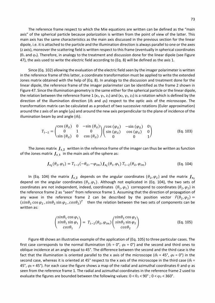
73

The reference frame respect to which the Mie equations are written can be defined as the “main axis” of the spherical particle because polarization is written from the point of view of the latter. This main axis has the same characteristics as the main axis discussed in the previous section for the linear dipole, i.e. it is attached to the particle and the illumination direction is always parallel to one or the axes (z axis), moreover the scattering field is written respect to this frame (eventually in spherical coordinates (s and s). Therefore, in analogy to the treatment and discussion done for the linear dipole (see Figure 47), the axis used to write the electric field according to (Eq. 8) will be defined as the axis 1.

Since (Eq. 102) allowing the evaluation of the electric field seen by the imager polarimeter is written in the reference frame of this latter, a coordinate transformation must be applied to write the extended Jones matrix obtained with the help of (Eq. 8). In analogy to the discussion and treatment done for the linear dipole, the reference frame of the imager polarimeter can be identified as the frame 2 shown in Figure 47. Since the illumination geometry is the same either for the spherical particle or the linear dipole, the relation between the reference frame 1 (x1, y1, z1) and (x2, y2, z2) is a rotation which is defined by the direction of the illumination direction (il and il) respect to the optic axis of the microscope. The transformation matrix can be calculated as a product of two successive rotations (Euler approximation) around the z axis of an angle (il) and around the new axis perpendicular to the plane of incidence of the illumination beam by and angle (il).

𝑇 =cos (𝜃 ) 0 −sin (𝜃 )

0 1 0sin (𝜃 ) 0 cos (𝜃 )

cos (𝜑 ) −sin (𝜑 ) 0

sin (𝜑 ) cos (𝜑 ) 00 0 1

(Eq. 103)

The Jones matrix 𝑱𝒔_𝟐 written in the reference frame of the imager can thus be written as function of the Jones matrix 𝑱𝒔_𝟏 in the main axis of the sphere as:

𝑱𝒔𝟐(𝜃 , 𝜑 ) = 𝑇 (−𝜃 , −𝜑 ) 𝑱𝒔𝟏

(𝜃 , 𝜑 ) 𝑇 (𝜃 , 𝜑 ) (Eq. 104)

In (Eq. 104) the matrix 𝑱𝒔_𝟐 depends on the angular coordinates (𝜃 , 𝜑 ) and the matrix 𝑱𝒔𝟏

depend on the angular coordinates (𝜃 , 𝜑 ) . Although not explicated in (Eq. 104), the two sets of coordinates are not independent, indeed, coordinates (𝜃 , 𝜑 ) correspond to coordinates (𝜃 , 𝜑 ) in the reference frame 2 as “seen” from reference frame 1. Assuming that the direction of propagation of any wave in the reference frame 2 can be described by the position vector 𝑟(𝜃 , 𝜑 ) =(𝑠𝑖𝑛𝜃 cos 𝜑 , 𝑠𝑖𝑛𝜃 sin 𝜑 , 𝑐𝑜𝑠𝜃 ) then the relation between the two sets of components can be written as:

𝑠𝑖𝑛𝜃 cos 𝜑𝑠𝑖𝑛𝜃 sin 𝜑

𝑐𝑜𝑠𝜃= 𝑇 (𝜃 , 𝜑 )

𝑠𝑖𝑛𝜃 cos 𝜑𝑠𝑖𝑛𝜃 sin 𝜑

𝑐𝑜𝑠𝜃 (Eq. 105)

Figure 48 shows an illustrative example of the application of (Eq. 105) to three particular cases. The first case corresponds to the normal illumination (il = 0°, il = 0°) and the second and third ones to oblique incidence at an angle equal to 45°. The difference between the second and the third case is the fact that the illumination is oriented parallel to the x axis of the microscope (il = 45°, il = 0°) in the second case, whereas it is oriented at 45° respect to the x axis of the microscope in the third case (il = 45°, il = 45°). For each case the figure shows a map of the radial and azimuthal coordinates and as seen from the reference frame 1. The radial and azimuthal coordinates in the reference frame 2 used to evaluate the figures are bounded between the following values: 0 < 2 < 90° ; 0 < 2 < 360°.

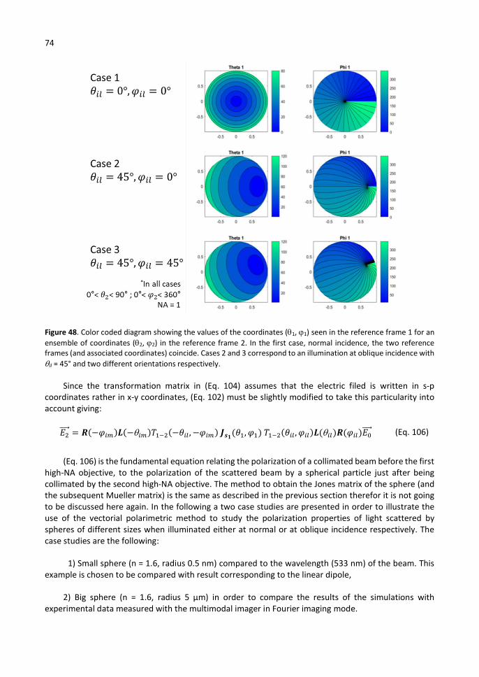
74

Figure 48. Color coded diagram showing the values of the coordinates (1, 1) seen in the reference frame 1 for an ensemble of coordinates (2, 2) in the reference frame 2. In the first case, normal incidence, the two reference frames (and associated coordinates) coincide. Cases 2 and 3 correspond to an illumination at oblique incidence with il = 45° and two different orientations respectively.

Since the transformation matrix in (Eq. 104) assumes that the electric filed is written in s-p coordinates rather in x-y coordinates, (Eq. 102) must be slightly modified to take this particularity into account giving:

𝐸⃗ = 𝑹(−𝜑 )𝑳(− )𝑇 (−𝜃 , −𝜑 ) 𝑱𝒔𝟏(𝜃 , 𝜑 ) 𝑇 (𝜃 , 𝜑 )𝑳( )𝑹(𝜑 )𝐸⃗ (Eq. 106)

(Eq. 106) is the fundamental equation relating the polarization of a collimated beam before the first high-NA objective, to the polarization of the scattered beam by a spherical particle just after being collimated by the second high-NA objective. The method to obtain the Jones matrix of the sphere (and the subsequent Mueller matrix) is the same as described in the previous section therefor it is not going to be discussed here again. In the following a two case studies are presented in order to illustrate the use of the vectorial polarimetric method to study the polarization properties of light scattered by spheres of different sizes when illuminated either at normal or at oblique incidence respectively. The case studies are the following:

1) Small sphere (n = 1.6, radius 0.5 nm) compared to the wavelength (533 nm) of the beam. This example is chosen to be compared with result corresponding to the linear dipole,

2) Big sphere (n = 1.6, radius 5 µm) in order to compare the results of the simulations with experimental data measured with the multimodal imager in Fourier imaging mode.

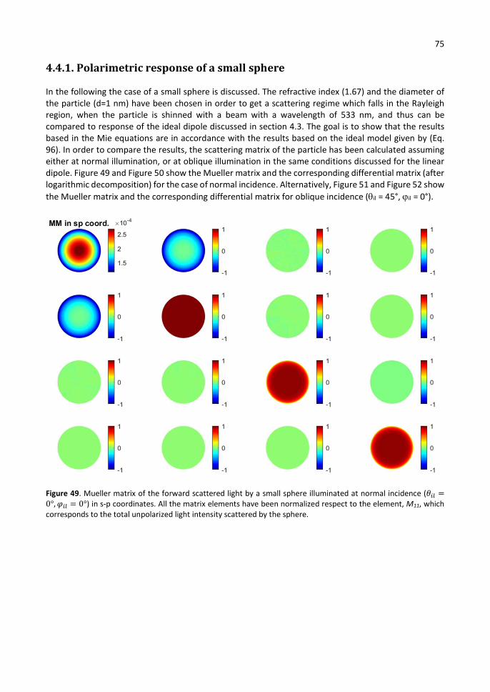
75

4.4.1. Polarimetric response of a small sphere

In the following the case of a small sphere is discussed. The refractive index (1.67) and the diameter of the particle (d=1 nm) have been chosen in order to get a scattering regime which falls in the Rayleigh region, when the particle is shinned with a beam with a wavelength of 533 nm, and thus can be compared to response of the ideal dipole discussed in section 4.3. The goal is to show that the results based in the Mie equations are in accordance with the results based on the ideal model given by (Eq. 96). In order to compare the results, the scattering matrix of the particle has been calculated assuming either at normal illumination, or at oblique illumination in the same conditions discussed for the linear dipole. Figure 49 and Figure 50 show the Mueller matrix and the corresponding differential matrix (after logarithmic decomposition) for the case of normal incidence. Alternatively, Figure 51 and Figure 52 show the Mueller matrix and the corresponding differential matrix for oblique incidence (il = 45°, il = 0°).

Figure 49. Mueller matrix of the forward scattered light by a small sphere illuminated at normal incidence (𝜃 =0°, 𝜑 = 0°) in s-p coordinates. All the matrix elements have been normalized respect to the element, M11, which corresponds to the total unpolarized light intensity scattered by the sphere.

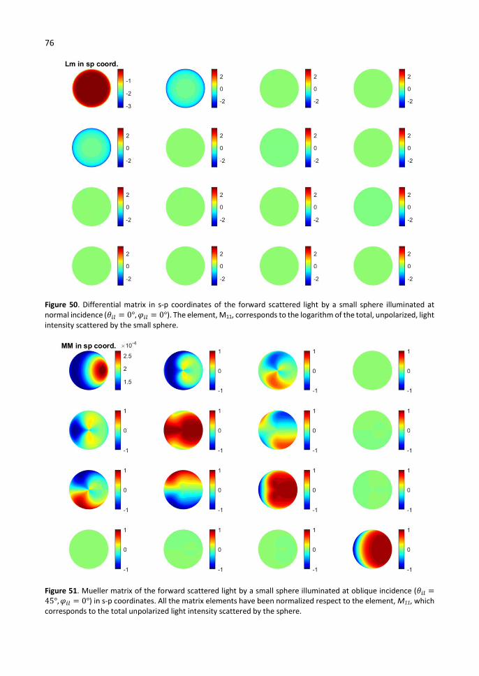
76

Figure 50. Differential matrix in s-p coordinates of the forward scattered light by a small sphere illuminated at normal incidence (𝜃 = 0°, 𝜑 = 0°). The element, M11, corresponds to the logarithm of the total, unpolarized, light intensity scattered by the small sphere.

Figure 51. Mueller matrix of the forward scattered light by a small sphere illuminated at oblique incidence (𝜃 =45°, 𝜑 = 0°) in s-p coordinates. All the matrix elements have been normalized respect to the element, M11, which corresponds to the total unpolarized light intensity scattered by the sphere.

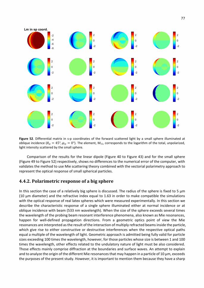
77

Figure 52. Differential matrix in s-p coordinates of the forward scattered light by a small sphere illuminated at oblique incidence (𝜃 = 45°, 𝜑 = 0°). The element, M11, corresponds to the logarithm of the total, unpolarized, light intensity scattered by the small sphere.

Comparison of the results for the linear dipole (Figure 40 to Figure 43) and for the small sphere (Figure 49 to Figure 52) respectively, shows no differences to the numerical error of the computer, with validates the method to use Mie scattering theory combined with the vectorial polarimetry approach to represent the optical response of small spherical particles.

4.4.2. Polarimetric response of a big sphere

In this section the case of a relatively big sphere is discussed. The radius of the sphere is fixed to 5 µm (10 µm diameter) and the refractive index equal to 1.63 in order to make compatible the simulations with the optical response of real latex spheres which were measured experimentally. In this section we describe the characteristic response of a single sphere illuminated either at normal incidence or at oblique incidence with beam (533 nm wavelength). When the size of the sphere exceeds several times the wavelength of the probing beam resonant interference phenomena, also known as Mie resonances, happen for well-defined propagation directions. From a geometric optics point of view the Mie resonances are interpreted as the result of the interaction of multiply refracted beams inside the particle, which give rise to either constructive or destructive interferences when the respective optical paths equal a multiple of the wavelength of light. Geometric approach is admitted being fully valid for particle sizes exceeding 100 times the wavelength, however, for those particles whose size is between 1 and 100 times the wavelength, other effects related to the undulatory nature of light must be also considered. Those effects mainly comprise diffraction at the boundaries and surface waves. An attempt to explain and to analyze the origin of the different Mie resonances that may happen in a particle of 10 µm, exceeds the purposes of the present study. However, it is important to mention them because they have a sharp

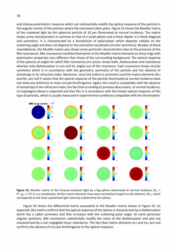
78

and intense polarimetric response which can substantially modify the optical response of the particle in the angular vicinity of the position where the resonance takes place. Figure 53 shows the Mueller matrix of the scattered light by the spherical particle of 10 µm illuminated at normal incidence. The matrix shows some characteristics in common to that of a small sphere and a linear dipole: It is block diagonal and symmetric. It is characterized by a distribution of polarization which depends radially on the scattering angle and does not depend on the azimuthal coordinate (circular symmetry). Besides of those resemblances, the Mueller matrix also shows some particular characteristics due to the presence of the Mie resonances. Mie resonances manifest themselves in the Mueller matrix elements as sharp rings with polarization properties very different than those of the surrounding background. The optical response of the spheres at angles for which Mie resonances are active, shows both, diattenuation and retardance whereas only diattenuation is non-null for angles out of the resonance. Each resonance shows circular symmetry which is in accordance with the geometric symmetry of the particle and the absence of anisotropy in its refractive index. Moreover, since the matrix is symmetric and the matrix elements M23 and M32 are null it seems that the optical response of the particle illuminated at normal incidence does not show any (intrinsic) or main circular birefringence. Again, this result is compatible with the absence of anisotropy in the refractive index, the fact that according to previous discussions, at normal incidence, no topological phase is expected and also this is in accordance with the known optical response of this type of particles, which is usually measured in experimental conditions compatible with this illumination.

Figure 53. Mueller matrix of the forward scattered light by a big sphere illuminated at normal incidence (𝜃 =0°, 𝜑 = 0°) in s-p coordinates. All the matrix elements have been normalized respect to the element, M11, which corresponds to the total unpolarized light intensity scattered by the sphere.

Figure 54 shows the differential matrix associated to the Mueller matrix shown in Figure 53. As expected, this matrix confirms that the optical response of the sphere is characterized by a diattenuation which has a radial symmetry and that increases with the scattering polar angle. At some particular angular positions, Mie resonances substantially modify the value of the diattenuation and also are characterized by a non-negligible linear retardance. The fact that matrix elements m23 and m32 are null confirms the absence of circular birefringence in the optical response.

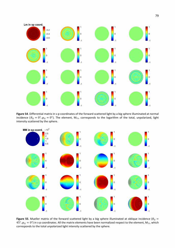
79

Figure 54. Differential matrix in s-p coordinates of the forward scattered light by a big sphere illuminated at normal incidence (𝜃 = 0°, 𝜑 = 0°). The element, M11, corresponds to the logarithm of the total, unpolarized, light intensity scattered by the sphere.

Figure 55. Mueller matrix of the forward scattered light by a big sphere illuminated at oblique incidence (𝜃 =45°, 𝜑 = 0°) in s-p coordinates. All the matrix elements have been normalized respect to the element, M11, which corresponds to the total unpolarized light intensity scattered by the sphere.

80

When the sphere is illuminated at oblique incidence (45°), the optical response is considerably modified, because of the change of reference frames, as it happened with the small sphere and the dipole. The resulting Mueller matrix is shown in Figure 55.

As in previous cases, the presence of an apparent circular birefringence manifests its effects by the lack of symmetry between the matrix elements of the Mueller matrix and also by the fact that the elements M23 and M32 are non-null. The presence of Mie resonances in the optical response of the sphere is also clearly visible by sharp features which are no more azimuthally symmetric in the reference system of the polarimeter. Interestingly, the presence of Mie resonances does not only induce linear birefringence, but also slightly modifies the angular distribution of the values of circular birefringence.

Figure 56 shows the differential matrix associated to the Mueller matrix shown in Figure 55. As expected, this matrix confirms that the optical response of the sphere is characterized by a diattenuation which has a radial symmetry and that increases with the scattering polar angle. The fact that matrix elements m23 and m32 are non-null confirms the presence of circular birefringence in the optical response which is symmetric.

Figure 56. Differential matrix in s-p coordinates of the forward scattered light by a big sphere illuminated at oblique incidence (𝜃 = 45°, 𝜑 = 0°). The element, M11, corresponds to the logarithm of the total, unpolarized, light intensity scattered by the sphere.

The rich structure of the polarization response of the sphere is even better seen when the matrix elements of the differential matrix are combined to evaluate the TotalLD and the total linear birefringence as 𝑇𝑜𝑡𝑎𝑙𝐿𝐵 = √𝐿𝐵 + 𝐿𝐵′ . The interest of these two observables is that they are invariant under rotations, which means that they are not affected by the coordinate transformation used

81

to go from the coordinate axis of the particle and that of the polarimeter. The resulting values are shown in Figure 57.

Figure 57. Rotation invariant observables related to the polarimetric properties of the big sphere illuminated at oblique incidence.

The presence of Mie resonances is clearly seen by circular rings. They are not centered in the image because they have been projected from the coordinate frame of the particle to the coordinate frame of the polarimeter. Keeping this on mind it can be easily seen that the coordinate transformation preserves the physics of the scattering, i. e. the resonances as well as the overall optical response keep a circular symmetry respect of the axis of the illumination beam. When all the artifacts due to the coordinate transformation are considered, or even removed, the physics that can be explored from images taken with an illumination at normal incidence and with an illumination at oblique incidence are quite similar. The advantages of the images in oblique incidence are that the tilt of the illumination gives access to a range of angular coordinates that cannot be explored in normal incidence. Moreover, the fact of measuring the apparent circular birefringence can in some cases enhance information aspects related to the optical response of the sample that would be difficult to measure otherwise.

The interest of measuring the circular birefringence is further discussed and illustrated in the following sections. The goal is to show the sensitivity of the angular distribution of the apparent optical activity to the shape of particles.

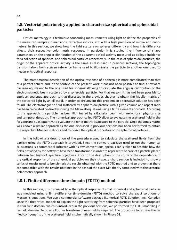
82

4.5. Vectorial polarimetry applied to characterize spherical and spheroidal particles

Optical metrology is a technique concerning measurements using light to define the properties of the measured samples; dimensions, refractive indices, etc. with a high precision of micro- and nano-meters. In this section, we show how the light scatters on spheres differently and how this difference affects their respective polarimetric response. In particular it is studied the influence of shape parameters on the angular distribution of the apparent optical activity measured at oblique incidence for a collection of spherical and spheroidal particles respectively. In the case of spheroidal particles, the origin of the apparent optical activity is the same as discussed in previous sections, the topological transformation from a given reference frame used to illuminate the particle to another one used to measure its optical response.

The mathematical description of the optical response of a spheroid is more complicated than that of a perfect sphere and in the context of the present work it has not been possible to find a software package equivalent to the one used for spheres allowing to calculate the angular distribution of the electromagnetic beam scattered by a spheroidal particle. For that reason, it has not been possible to apply an analogue approach to that discussed in the previous chapter to obtain the Mueller matrix of the scattered light by an ellipsoid. In order to circumvent this problem an alternative solution has been found. The electromagnetic field scattered by a spheroidal particle with a given volume and aspect ratio has been calculated by directly solving the Maxwell equations using a finite element approach. According to this approach, the particle has been illuminated by a Gaussian beam with well-chosen physical size and temporal duration. The numerical approach called FDTD allow to evaluate the scattered field in the far zone and subsequently, to evaluate the Jones matrix associated to the particle. Once the Jones matrix was known a similar approach as the one discussed in previous sections has been performed to obtain the respective Mueller matrices and to derive the optical properties of the spheroidal particles.

In the following a description of the procedure used to calculate the scattered fields from the particle using the FDTD approach is provided. Since the software package used to run the numerical calculations is a commercial software with its own conventions, special care is taken to describe how the fields provided by the software have been transformed in order to represent the case of a particle placed between two high-NA aperture objectives. Prior to the description of the study of the dependence of the optical response of the spheroidal particles on their shape, a short section is included to show a series of results used to benchmark the results obtained with the FDTD method and to prove that there are compatible with the results obtained in the basis of the exact Mie theory combined with the vectorial polarimetry approach.

4.5.1. Finite-difference time-domain (FDTD) method

In this section, it is discussed how the optical response of small spherical and spheroidal particles was modeled using a finite-difference time-domain (FDTD) method to solve the exact solutions of Maxwell’s equations. We use a commercial software package (Lumerical FDTD Solution, Inc., Canada). Since the theoretical models to explain the light scattering from spherical particles have been proposed in a far-field domain, which is introduced in the previous sections, we performed the FDTD modelling in far-field domain. To do so a Fourier transform of near-field is required. The procedure to retrieve the far filed components of the scattered field is schematically shown in Figure 58.

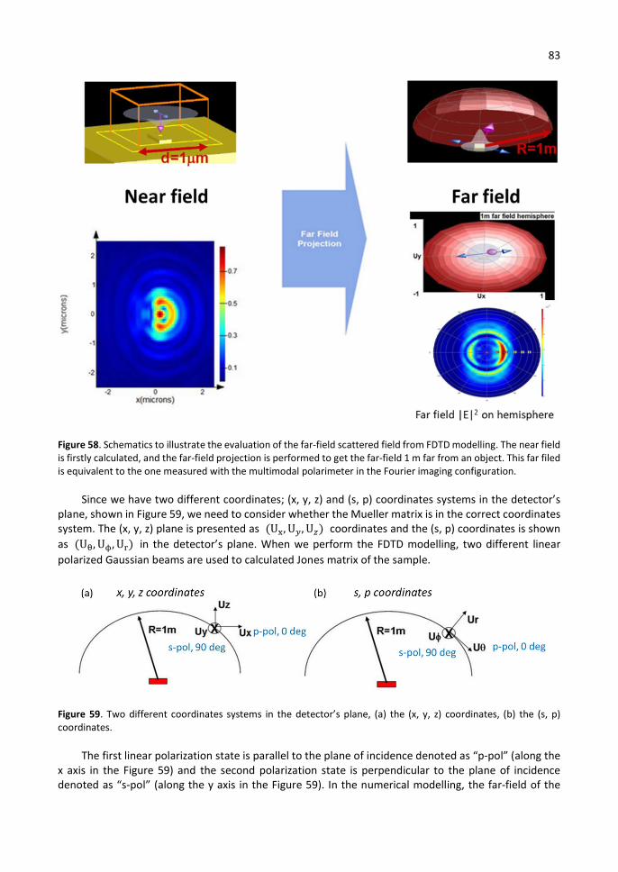
83

Figure 58. Schematics to illustrate the evaluation of the far-field scattered field from FDTD modelling. The near field is firstly calculated, and the far-field projection is performed to get the far-field 1 m far from an object. This far filed is equivalent to the one measured with the multimodal polarimeter in the Fourier imaging configuration.

Since we have two different coordinates; (x, y, z) and (s, p) coordinates systems in the detector’s plane, shown in Figure 59, we need to consider whether the Mueller matrix is in the correct coordinates system. The (x, y, z) plane is presented as (U , U , U ) coordinates and the (s, p) coordinates is shown as (U , U , U ) in the detector’s plane. When we perform the FDTD modelling, two different linear polarized Gaussian beams are used to calculated Jones matrix of the sample.

Figure 59. Two different coordinates systems in the detector’s plane, (a) the (x, y, z) coordinates, (b) the (s, p) coordinates.

The first linear polarization state is parallel to the plane of incidence denoted as “p-pol” (along the x axis in the Figure 59) and the second polarization state is perpendicular to the plane of incidence denoted as “s-pol” (along the y axis in the Figure 59). In the numerical modelling, the far-field of the

84

specific direction of the electric field can be extracted. For example, when the p-polarization beam is launched, the far-field of �⃗� , , 𝐸 , , �⃗� , can be extracted and also for the s-polarization beam; yielding �⃗� , , 𝐸 , , 𝐸 , . In this way, the Jones matrix in the (x, y, z) coordinates is intuitionally obtained as below equation,

𝐉𝒙𝒚𝒛 =𝐽 𝐽𝐽 𝐽

=�⃗� , �⃗� ,

�⃗� , �⃗� ,

(Eq. 107)

However, in reality the commercial ellipsometry measurement is performed in the (s, p) coordinates system, considering the z axis component to the U . The electric fields in the (x, y, z) coordinates can be transformed to the electric fields in the (s, p) coordinates through the simple rotation matrix. The description is illustrated in Figure 60.

Figure 60. Description of the coordinate transformation from (x, y, z) to (s, p), (a) rotation along the polar angle, 𝜃, (b) rotation along the azimuth, .

𝐸 and 𝐸 corresponds to the same direction along U and U , respectively. Figure 60.a shows the rotation along the polar angle, 𝜃, which can be derived in the following equation,

𝐸

𝐸𝐸

=𝑐𝑜𝑠𝜃 0 −𝑠𝑖𝑛𝜃

0 1 0𝑠𝑖𝑛𝜃 0 𝑐𝑜𝑠𝜃

𝐸𝐸

𝐸=

𝐸 𝑐𝑜𝑠𝜃 − 𝐸 𝑠𝑖𝑛𝜃𝐸

𝐸 𝑠𝑖𝑛𝜃 + 𝐸 𝑐𝑜𝑠𝜃 (Eq. 108)

Figure 60.b shows the rotation along the azimuth, , which can be derived in the following equation,

𝐸

𝐸𝐸

=𝑐𝑜𝑠𝜑 −𝑠𝑖𝑛𝜑 0𝑠𝑖𝑛𝜑 𝑐𝑜𝑠𝜑 0

0 0 1

𝐸 𝑐𝑜𝑠𝜃 − 𝐸 𝑠𝑖𝑛𝜃𝐸

𝐸 𝑠𝑖𝑛𝜃 + 𝐸 𝑐𝑜𝑠𝜃=

𝐸 𝑐𝑜𝑠𝜃𝑐𝑜𝑠𝜑 − 𝐸 𝑠𝑖𝑛𝜑 − 𝐸 𝑠𝑖𝑛𝜃𝑐𝑜𝑠𝜑

𝐸 𝑐𝑜𝑠𝜃𝑠𝑖𝑛𝜑 + 𝐸 𝑐𝑜𝑠𝜑 − 𝐸 𝑠𝑖𝑛𝜃𝑠𝑖𝑛𝜑

𝐸 𝑠𝑖𝑛𝜃 + 𝐸 𝑐𝑜𝑠𝜃

(Eq. 109)

Finally, the corrected Jones matrix is derived in the (s, p) coordinates as below,

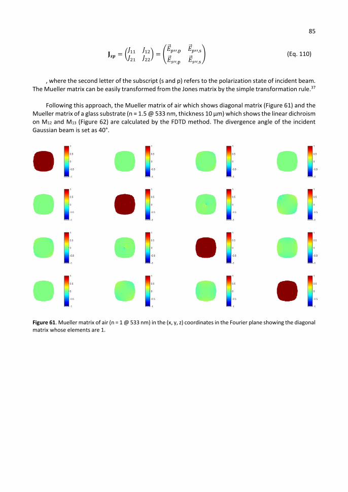
85

𝐉𝒔𝒑 =𝐽 𝐽𝐽 𝐽

=�⃗� , �⃗� ,

�⃗� , �⃗� ,

(Eq. 110)

, where the second letter of the subscript (s and p) refers to the polarization state of incident beam. The Mueller matrix can be easily transformed from the Jones matrix by the simple transformation rule.37

Following this approach, the Mueller matrix of air which shows diagonal matrix (Figure 61) and the Mueller matrix of a glass substrate (n = 1.5 @ 533 nm, thickness 10 µm) which shows the linear dichroism on M12 and M13 (Figure 62) are calculated by the FDTD method. The divergence angle of the incident Gaussian beam is set as 40°.

Figure 61. Mueller matrix of air (n = 1 @ 533 nm) in the (x, y, z) coordinates in the Fourier plane showing the diagonal matrix whose elements are 1.

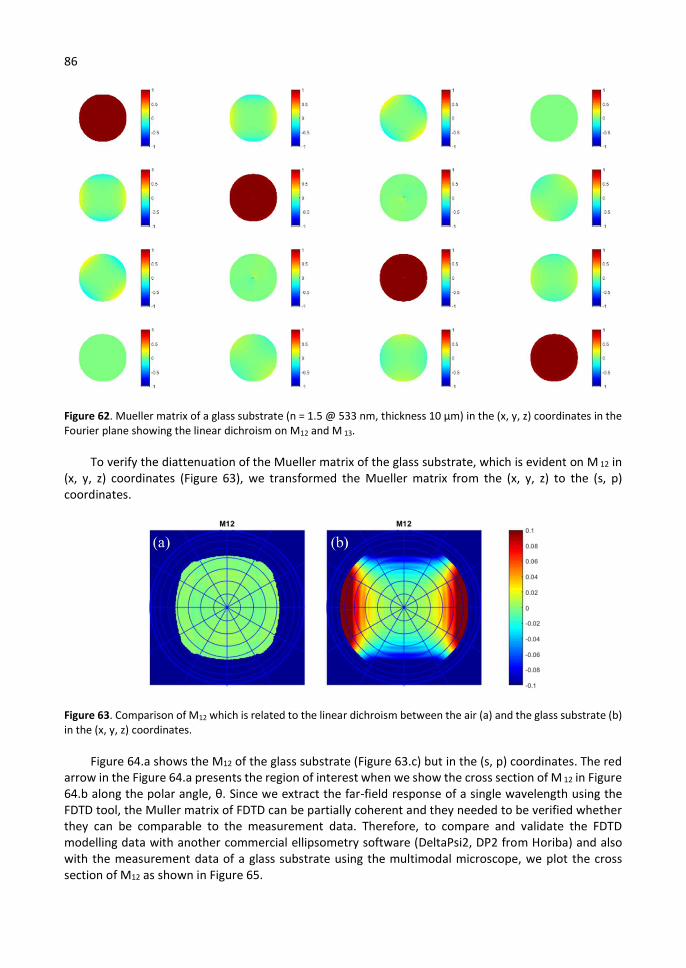
86

Figure 62. Mueller matrix of a glass substrate (n = 1.5 @ 533 nm, thickness 10 µm) in the (x, y, z) coordinates in the Fourier plane showing the linear dichroism on M12 and M 13.

To verify the diattenuation of the Mueller matrix of the glass substrate, which is evident on M 12 in (x, y, z) coordinates (Figure 63), we transformed the Mueller matrix from the (x, y, z) to the (s, p) coordinates.

Figure 63. Comparison of M12 which is related to the linear dichroism between the air (a) and the glass substrate (b) in the (x, y, z) coordinates.

Figure 64.a shows the M12 of the glass substrate (Figure 63.c) but in the (s, p) coordinates. The red arrow in the Figure 64.a presents the region of interest when we show the cross section of M 12 in Figure 64.b along the polar angle, θ. Since we extract the far-field response of a single wavelength using the FDTD tool, the Muller matrix of FDTD can be partially coherent and they needed to be verified whether they can be comparable to the measurement data. Therefore, to compare and validate the FDTD modelling data with another commercial ellipsometry software (DeltaPsi2, DP2 from Horiba) and also with the measurement data of a glass substrate using the multimodal microscope, we plot the cross section of M12 as shown in Figure 65.

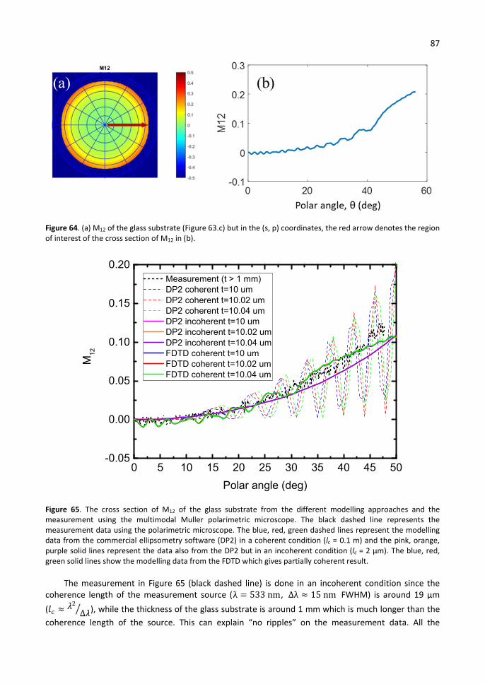
87

Figure 64. (a) M12 of the glass substrate (Figure 63.c) but in the (s, p) coordinates, the red arrow denotes the region of interest of the cross section of M12 in (b).

Figure 65. The cross section of M12 of the glass substrate from the different modelling approaches and the measurement using the multimodal Muller polarimetric microscope. The black dashed line represents the measurement data using the polarimetric microscope. The blue, red, green dashed lines represent the modelling data from the commercial ellipsometry software (DP2) in a coherent condition (lc = 0.1 m) and the pink, orange, purple solid lines represent the data also from the DP2 but in an incoherent condition (lc = 2 µm). The blue, red, green solid lines show the modelling data from the FDTD which gives partially coherent result.

The measurement in Figure 65 (black dashed line) is done in an incoherent condition since the coherence length of the measurement source (λ = 533 nm, Δλ ≈ 15 nm FWHM) is around 19 μm

(𝑙 ≈ 𝜆Δ𝜆), while the thickness of the glass substrate is around 1 mm which is much longer than the

coherence length of the source. This can explain “no ripples” on the measurement data. All the

0 5 10 15 20 25 30 35 40 45 50-0.05

0.00

0.05

0.10

0.15

0.20 Measurement (t > 1 mm) DP2 coherent t=10 um DP2 coherent t=10.02 um DP2 coherent t=10.04 um DP2 incoherent t=10 um DP2 incoherent t=10.02 um DP2 incoherent t=10.04 um FDTD coherent t=10 um FDTD coherent t=10.02 um FDTD coherent t=10.04 um

Polar angle (deg)

M12

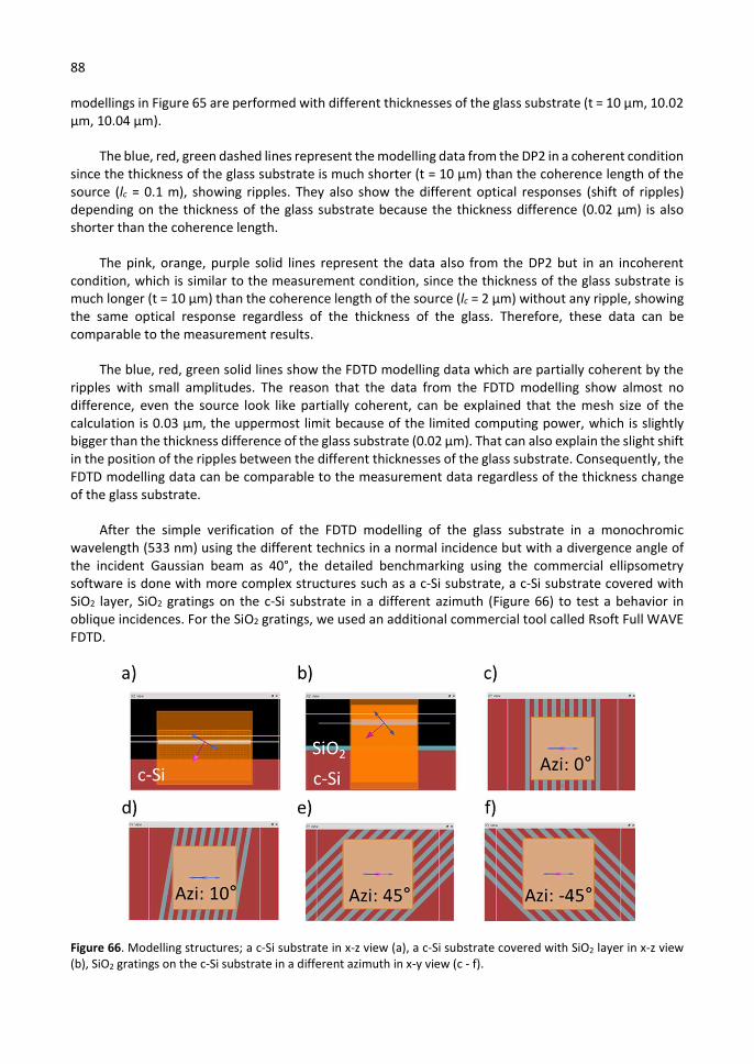
88

modellings in Figure 65 are performed with different thicknesses of the glass substrate (t = 10 µm, 10.02 µm, 10.04 µm).

The blue, red, green dashed lines represent the modelling data from the DP2 in a coherent condition since the thickness of the glass substrate is much shorter (t = 10 µm) than the coherence length of the source (lc = 0.1 m), showing ripples. They also show the different optical responses (shift of ripples) depending on the thickness of the glass substrate because the thickness difference (0.02 µm) is also shorter than the coherence length.

The pink, orange, purple solid lines represent the data also from the DP2 but in an incoherent condition, which is similar to the measurement condition, since the thickness of the glass substrate is much longer (t = 10 µm) than the coherence length of the source (lc = 2 µm) without any ripple, showing the same optical response regardless of the thickness of the glass. Therefore, these data can be comparable to the measurement results.

The blue, red, green solid lines show the FDTD modelling data which are partially coherent by the ripples with small amplitudes. The reason that the data from the FDTD modelling show almost no difference, even the source look like partially coherent, can be explained that the mesh size of the calculation is 0.03 µm, the uppermost limit because of the limited computing power, which is slightly bigger than the thickness difference of the glass substrate (0.02 µm). That can also explain the slight shift in the position of the ripples between the different thicknesses of the glass substrate. Consequently, the FDTD modelling data can be comparable to the measurement data regardless of the thickness change of the glass substrate.

After the simple verification of the FDTD modelling of the glass substrate in a monochromic wavelength (533 nm) using the different technics in a normal incidence but with a divergence angle of the incident Gaussian beam as 40°, the detailed benchmarking using the commercial ellipsometry software is done with more complex structures such as a c-Si substrate, a c-Si substrate covered with SiO2 layer, SiO2 gratings on the c-Si substrate in a different azimuth (Figure 66) to test a behavior in oblique incidences. For the SiO2 gratings, we used an additional commercial tool called Rsoft Full WAVE FDTD.

Figure 66. Modelling structures; a c-Si substrate in x-z view (a), a c-Si substrate covered with SiO2 layer in x-z view (b), SiO2 gratings on the c-Si substrate in a different azimuth in x-y view (c - f).

89

Since we want to validate the behavior in multi-oblique incidences, the divergence angle of incident beam is limited as 4° which is the same condition as the measurement system and we perform the modelling in multiple angle of incidences (AoI) from 0° to 50° with a step of 10° as shown in Figure 67.

Figure 67. Total intensity, M11, of the Mueller matrix in the Fourier plane in the (s, p) coordinates of air calculated from FDTD method in a different angle of incidence (AoI).

Figure 68 to Figure 73 show the full Mueller matrix results from the different modelling approaches which correspond to the structures presented in the Figure 66.

Figure 68. Full Mueller matrix of a c-Si substrate in the function of angle of incidence from the FDTD method and the commercial ellipsometry software called delta-phi 2 (DP2).

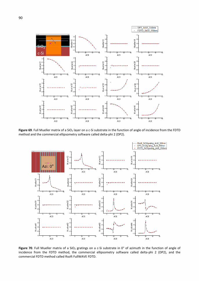
90

Figure 69. Full Mueller matrix of a SiO2 layer on a c-Si substrate in the function of angle of incidence from the FDTD method and the commercial ellipsometry software called delta-phi 2 (DP2).

Figure 70. Full Mueller matrix of a SiO2 gratings on a c-Si substrate in 0° of azimuth in the function of angle of incidence from the FDTD method, the commercial ellipsometry software called delta-phi 2 (DP2), and the commercial FDTD method called Rsoft FullWAVE FDTD.

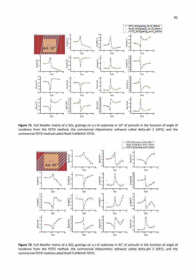
91

Figure 71. Full Mueller matrix of a SiO2 gratings on a c-Si substrate in 10° of azimuth in the function of angle of incidence from the FDTD method, the commercial ellipsometry software called delta-phi 2 (DP2), and the commercial FDTD method called Rsoft FullWAVE FDTD.

Figure 72. Full Mueller matrix of a SiO2 gratings on a c-Si substrate in 45° of azimuth in the function of angle of incidence from the FDTD method, the commercial ellipsometry software called delta-phi 2 (DP2), and the commercial FDTD method called Rsoft FullWAVE FDTD.

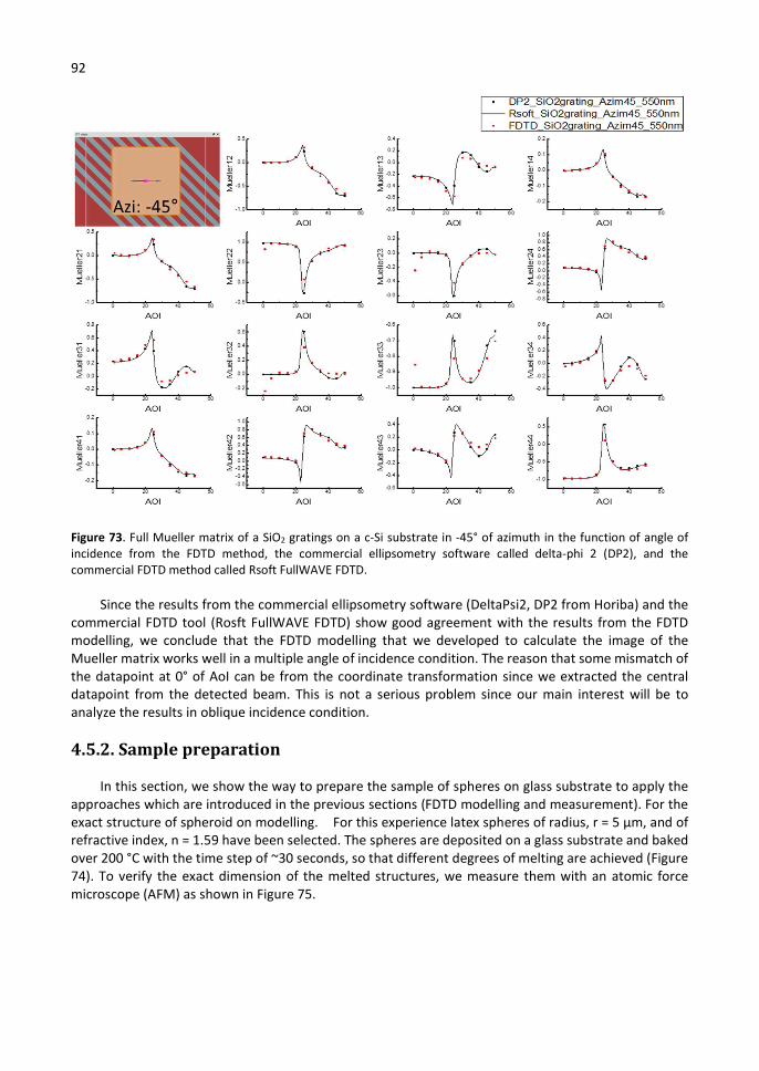
92

Figure 73. Full Mueller matrix of a SiO2 gratings on a c-Si substrate in -45° of azimuth in the function of angle of incidence from the FDTD method, the commercial ellipsometry software called delta-phi 2 (DP2), and the commercial FDTD method called Rsoft FullWAVE FDTD.

Since the results from the commercial ellipsometry software (DeltaPsi2, DP2 from Horiba) and the commercial FDTD tool (Rosft FullWAVE FDTD) show good agreement with the results from the FDTD modelling, we conclude that the FDTD modelling that we developed to calculate the image of the Mueller matrix works well in a multiple angle of incidence condition. The reason that some mismatch of the datapoint at 0° of AoI can be from the coordinate transformation since we extracted the central datapoint from the detected beam. This is not a serious problem since our main interest will be to analyze the results in oblique incidence condition.

4.5.2. Sample preparation

In this section, we show the way to prepare the sample of spheres on glass substrate to apply the approaches which are introduced in the previous sections (FDTD modelling and measurement). For the exact structure of spheroid on modelling. For this experience latex spheres of radius, r = 5 µm, and of refractive index, n = 1.59 have been selected. The spheres are deposited on a glass substrate and baked over 200 °C with the time step of ~30 seconds, so that different degrees of melting are achieved (Figure 74). To verify the exact dimension of the melted structures, we measure them with an atomic force microscope (AFM) as shown in Figure 75.

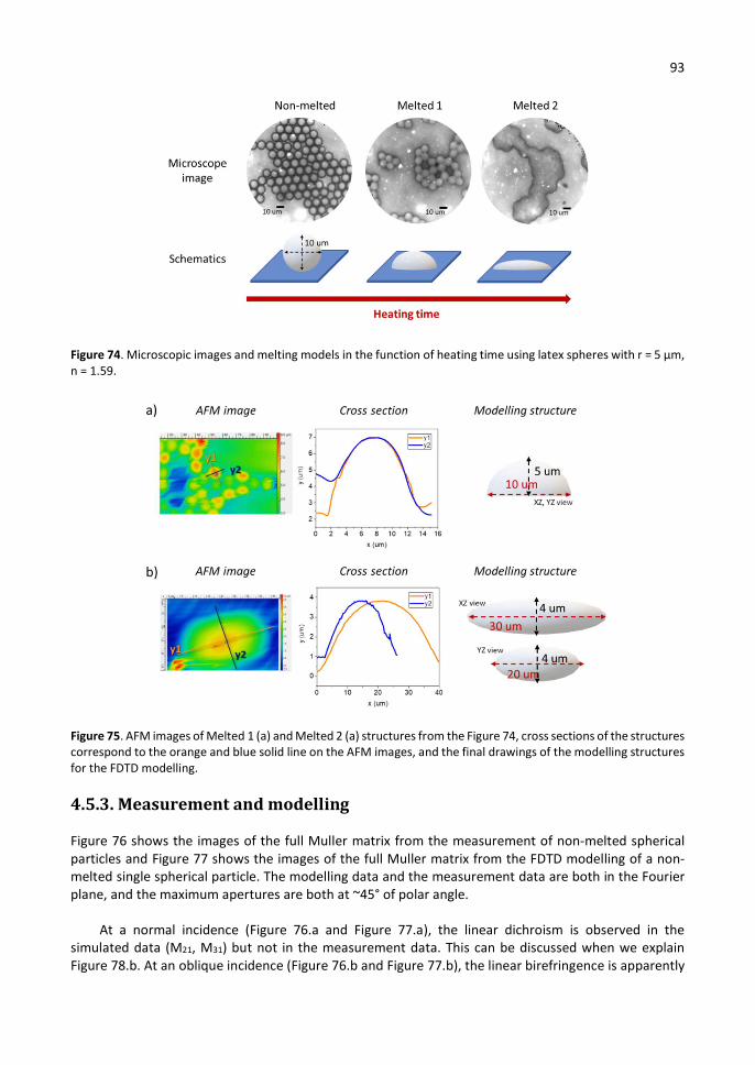
93

Figure 74. Microscopic images and melting models in the function of heating time using latex spheres with r = 5 µm, n = 1.59.

Figure 75. AFM images of Melted 1 (a) and Melted 2 (a) structures from the Figure 74, cross sections of the structures correspond to the orange and blue solid line on the AFM images, and the final drawings of the modelling structures for the FDTD modelling.

4.5.3. Measurement and modelling

Figure 76 shows the images of the full Muller matrix from the measurement of non-melted spherical particles and Figure 77 shows the images of the full Muller matrix from the FDTD modelling of a non-melted single spherical particle. The modelling data and the measurement data are both in the Fourier plane, and the maximum apertures are both at ~45° of polar angle.

At a normal incidence (Figure 76.a and Figure 77.a), the linear dichroism is observed in the simulated data (M21, M31) but not in the measurement data. This can be discussed when we explain Figure 78.b. At an oblique incidence (Figure 76.b and Figure 77.b), the linear birefringence is apparently

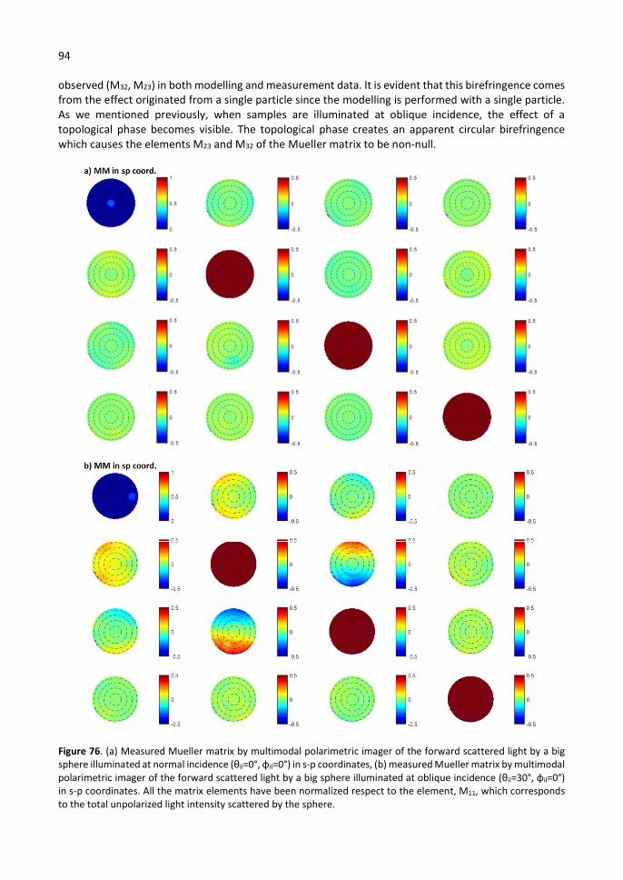
94

observed (M32, M23) in both modelling and measurement data. It is evident that this birefringence comes from the effect originated from a single particle since the modelling is performed with a single particle. As we mentioned previously, when samples are illuminated at oblique incidence, the effect of a topological phase becomes visible. The topological phase creates an apparent circular birefringence which causes the elements M23 and M32 of the Mueller matrix to be non-null.

Figure 76. (a) Measured Mueller matrix by multimodal polarimetric imager of the forward scattered light by a big sphere illuminated at normal incidence (θil=0°, φil=0°) in s-p coordinates, (b) measured Mueller matrix by multimodal polarimetric imager of the forward scattered light by a big sphere illuminated at oblique incidence (θil=30°, φil=0°) in s-p coordinates. All the matrix elements have been normalized respect to the element, M11, which corresponds to the total unpolarized light intensity scattered by the sphere.

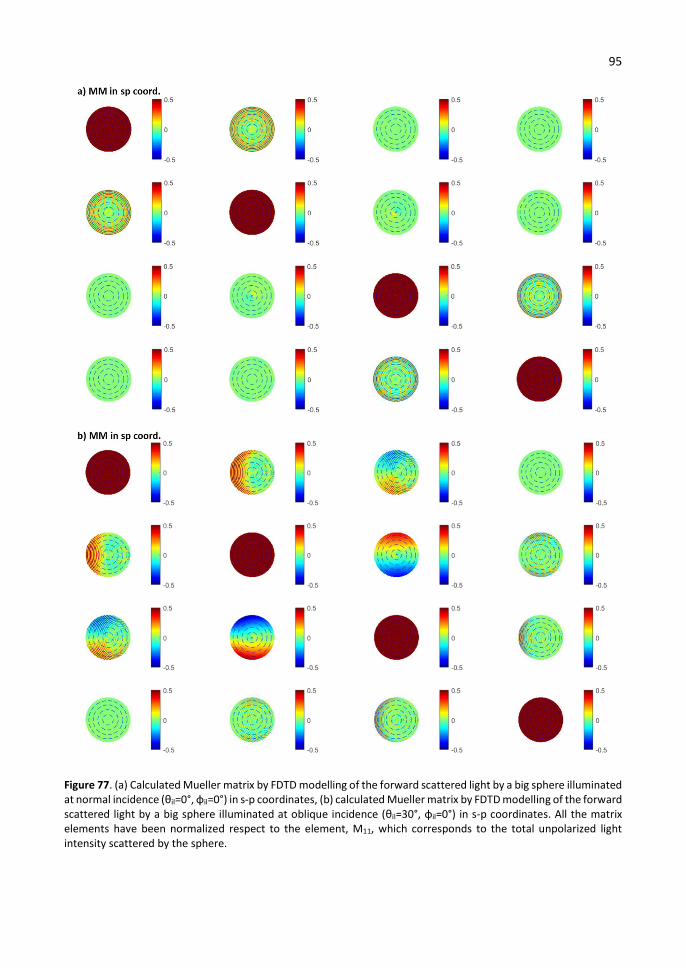
95

Figure 77. (a) Calculated Mueller matrix by FDTD modelling of the forward scattered light by a big sphere illuminated at normal incidence (θil=0°, φil=0°) in s-p coordinates, (b) calculated Mueller matrix by FDTD modelling of the forward scattered light by a big sphere illuminated at oblique incidence (θil=30°, φil=0°) in s-p coordinates. All the matrix elements have been normalized respect to the element, M11, which corresponds to the total unpolarized light intensity scattered by the sphere.

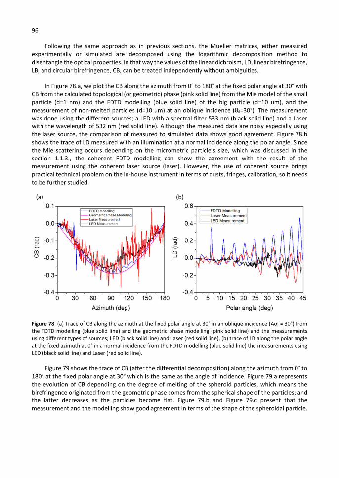
96

Following the same approach as in previous sections, the Mueller matrices, either measured experimentally or simulated are decomposed using the logarithmic decomposition method to disentangle the optical properties. In that way the values of the linear dichroism, LD, linear birefringence, LB, and circular birefringence, CB, can be treated independently without ambiguities.

In Figure 78.a, we plot the CB along the azimuth from 0° to 180° at the fixed polar angle at 30° with CB from the calculated topological (or geometric) phase (pink solid line) from the Mie model of the small particle (d=1 nm) and the FDTD modelling (blue solid line) of the big particle (d=10 um), and the measurement of non-melted particles (d=10 um) at an oblique incidence (θil=30°). The measurement was done using the different sources; a LED with a spectral filter 533 nm (black solid line) and a Laser with the wavelength of 532 nm (red solid line). Although the measured data are noisy especially using the laser source, the comparison of measured to simulated data shows good agreement. Figure 78.b shows the trace of LD measured with an illumination at a normal incidence along the polar angle. Since the Mie scattering occurs depending on the micrometric particle’s size, which was discussed in the section 1.1.3., the coherent FDTD modelling can show the agreement with the result of the measurement using the coherent laser source (laser). However, the use of coherent source brings practical technical problem on the in-house instrument in terms of dusts, fringes, calibration, so it needs to be further studied.

Figure 78. (a) Trace of CB along the azimuth at the fixed polar angle at 30° in an oblique incidence (AoI = 30°) from the FDTD modelling (blue solid line) and the geometric phase modelling (pink solid line) and the measurements using different types of sources; LED (black solid line) and Laser (red solid line), (b) trace of LD along the polar angle at the fixed azimuth at 0° in a normal incidence from the FDTD modelling (blue solid line) the measurements using LED (black solid line) and Laser (red solid line).

Figure 79 shows the trace of CB (after the differential decomposition) along the azimuth from 0° to 180° at the fixed polar angle at 30° which is the same as the angle of incidence. Figure 79.a represents the evolution of CB depending on the degree of melting of the spheroid particles, which means the birefringence originated from the geometric phase comes from the spherical shape of the particles; and the latter decreases as the particles become flat. Figure 79.b and Figure 79.c present that the measurement and the modelling show good agreement in terms of the shape of the spheroidal particle.

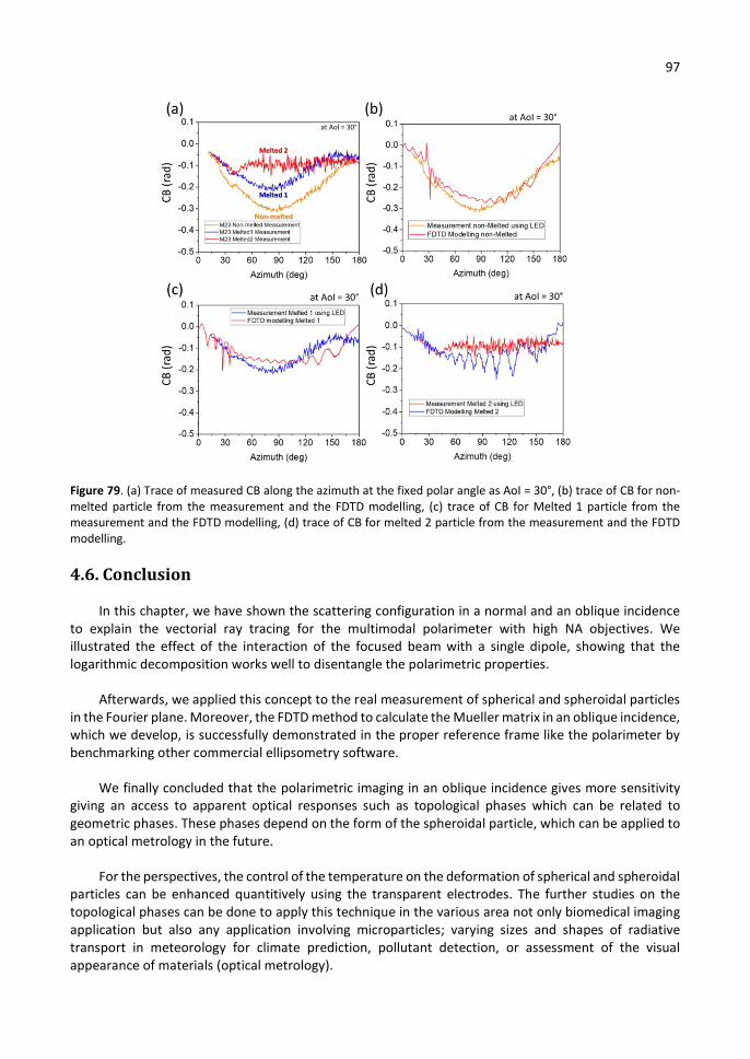
97

Figure 79. (a) Trace of measured CB along the azimuth at the fixed polar angle as AoI = 30°, (b) trace of CB for non-melted particle from the measurement and the FDTD modelling, (c) trace of CB for Melted 1 particle from the measurement and the FDTD modelling, (d) trace of CB for melted 2 particle from the measurement and the FDTD modelling.

4.6. Conclusion

In this chapter, we have shown the scattering configuration in a normal and an oblique incidence to explain the vectorial ray tracing for the multimodal polarimeter with high NA objectives. We illustrated the effect of the interaction of the focused beam with a single dipole, showing that the logarithmic decomposition works well to disentangle the polarimetric properties.

Afterwards, we applied this concept to the real measurement of spherical and spheroidal particles in the Fourier plane. Moreover, the FDTD method to calculate the Mueller matrix in an oblique incidence, which we develop, is successfully demonstrated in the proper reference frame like the polarimeter by benchmarking other commercial ellipsometry software.

We finally concluded that the polarimetric imaging in an oblique incidence gives more sensitivity giving an access to apparent optical responses such as topological phases which can be related to geometric phases. These phases depend on the form of the spheroidal particle, which can be applied to an optical metrology in the future.

For the perspectives, the control of the temperature on the deformation of spherical and spheroidal particles can be enhanced quantitively using the transparent electrodes. The further studies on the topological phases can be done to apply this technique in the various area not only biomedical imaging application but also any application involving microparticles; varying sizes and shapes of radiative transport in meteorology for climate prediction, pollutant detection, or assessment of the visual appearance of materials (optical metrology).

98

Chapter 5. Imaging of complex media and biomedical tissues

Contents

5.1. Introduction ........................................................................................................... 99

5.2. Anisotropic turbid media: Scotch tape analysis .................................................... 99

5.2.1. Sample description .............................................................................................. 100

5.2.2. Results ................................................................................................................. 101

5.3. Ex-vivo analysis ..................................................................................................... 107

5.3.1. Human basal tissues ........................................................................................... 107

5.3.1.1. Sample description and results .................................................................... 107

5.3.2. Artificial tissues .................................................................................................. 114

5.3.2.1. Sample description and results .................................................................... 114

5.4. Conclusion ............................................................................................................. 120

This chapter shows the application of the multimodal Muller polarimetric microscope for an imaging of complex media such as biomedical tissues since the biomedical tissues show the scattering with the polarimetric properties such as depolarization and birefringence. Firstly, the system is tested in transmission mode with anisotropic turbid media; semi-transparent rough stretched plastic sheets called Scotch® magicTM tape, applying the differential decomposition of the measured Mueller matrices. The validation of the system that the polarimetric data extracted from the measured Mueller matrix of the plastic tape with the different configurations is published in a peer-reviewed journal68. Following the same approach with the plastic tape with differential decomposition, we perform an ex-vivo analyses of the different types of biomedical tissues such as human basal tissues and artificial tissues thanks to the international collaborations to verify whether the biomedical tissues follow the mathematical model of the differential decomposition. We also proposed practical way to enhance the contrast of the polarimetric images by eliminating the effect of the inhomogeneous thickness, which can be simply applied. These analyses can pave the way, giving the possibility to use the Mueller matrix polarimeter to offer polarimetric indicators to distinguish abnormal pathological changes of the biomedical tissues.

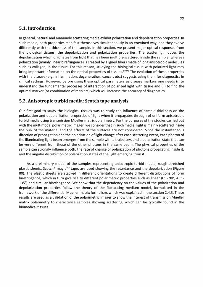
99

5.1. Introduction

In general, natural and manmade scattering media exhibit polarization and depolarization properties. In such media, both properties manifest themselves simultaneously in an entwined way, and they evolve differently with the thickness of the sample. In this section, we present major optical responses from the biological tissues; the depolarization and polarization properties. The scattering induces the depolarization which originates from light that has been multiply-scattered inside the sample, whereas polarization (mainly linear birefringence) is created by aligned fibers made of long anisotropic molecules such as collagen, in the tissue. For this reason, studying the biological tissue with polarized light may bring important information on the optical properties of tissues.89,90 The evolution of these properties with the disease (e.g., inflammation, degeneration, cancer, etc.) suggests using them for diagnostics in clinical settings. However, before using these optical parameters as disease markers one needs (i) to understand the fundamental processes of interaction of polarized light with tissue and (ii) to find the optimal marker (or combination of markers) which will increase the accuracy of diagnostics.

5.2. Anisotropic turbid media: Scotch tape analysis

Our first goal to study the biological tissues was to study the influence of sample thickness on the polarization and depolarization properties of light when it propagates through of uniform anisotropic turbid media using transmission Mueller matrix polarimetry. For the purposes of the studies carried out with the multimodal polarimetric imager, we consider that in such media, light is mainly scattered inside the bulk of the material and the effects of the surfaces are not considered. Since the instantaneous direction of propagation and the polarization of light change after each scattering event, each photon of the illuminating light beam emerges from the sample with a trajectory, and a polarization state that can be very different from those of the other photons in the same beam. The physical properties of the sample can strongly influence both, the rate of change of polarization of photons propagating inside it, and the angular distribution of polarization states of the light emerging from it.

As a preliminary model of the samples representing anisotropic turbid media, rough stretched plastic sheets, Scotch® magicTM tape, are used showing the retardance and the depolarization (Figure 80). The plastic sheets are stacked in different orientations to create different distributions of form birefringence, which in turn give rise to different polarimetric properties such as linear (0° - 90°, 45° - 135°) and circular birefringence. We show that the dependency on the values of the polarization and depolarization properties follow the theory of the fluctuating medium model, formulated in the framework of the differential Mueller matrix formalism, which was explained in the section 2.4.3. These results are used as a validation of the polarimetric imager to show the interest of transmission Mueller matrix polarimetry to characterize samples showing scattering, which can be typically found in the biomedical tissues.

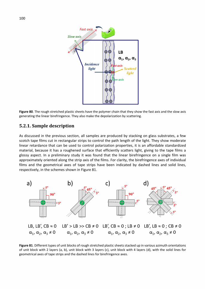
100

Figure 80. The rough stretched plastic sheets have the polymer chain that they show the fast axis and the slow axis generating the linear birefringence. They also make the depolarization by scattering.

5.2.1. Sample description

As discussed in the previous section, all samples are produced by stacking on glass substrates, a few scotch tape films cut in rectangular strips to control the path length of the light. They show moderate linear retardance that can be used to control polarization properties, it is an affordable standardized material, because it has a roughened surface that efficiently scatters light, giving to the tape films a glossy aspect. In a preliminary study it was found that the linear birefringence on a single film was approximately oriented along the strip axis of the films. For clarity, the birefringence axes of individual films and the geometrical axes of tape strips have been indicated by dashed lines and solid lines, respectively, in the schemes shown in Figure 81.

Figure 81. Different types of unit blocks of rough stretched plastic sheets stacked up in various azimuth orientations of unit block with 2 layers (a, b), unit block with 3 layers (c), unit block with 4 layers (d), with the solid lines for geometrical axes of tape strips and the dashed lines for birefringence axes.

101

A single film behaves as a depolarizing linear waveplate, and therefore it shows LB when observed individually. By stacking the films according to different directions, it is possible to artificially create a sort of “form birefringence” which results in non-null LB, LB’ and CB. Since our goal was to study a maximum number of polarization properties (not only LB) to validate theoretical predictions, we fabricated four types of samples arranging the tape films according to different patterns as shown in Figure 81. Sample 1, (Figure 81.a) was made by stacking the films in successive “unit blocks”. Each block consisted of two crossed films. Sample 1 is expected to show depolarization and no net retardance because the retardation produced by the first film in each unit block, is compensated by the retardation created by the second film in the same unit block. The second type of unit block used in sample 2, (Figure 81.b), was made of 2 layers with their axes oriented at an angle of 45° to each other. This type of block is expected to create LB, LB’, CB properties, and depolarization. The first film in each block contributes to LB, the second one to LB’ and the fact that each block has a chiral structure, lack of simultaneous vertical and horizontal symmetry planes, contribute to the generation of CB. The third type of unit block, sample 3, shown in Figure 81.c, consisted of 3 layers. Two of them, the first and the third ones, were vertically oriented, whereas the second layer was horizontally oriented. Sample 3 is expected to show a net LB, because the retardation produced by the first and the third layers of each block can only be partially compensated by the second film of the block. The last type of unit block, shown in Figure 81.d, consists of 4 layers piled-up according to a helical pattern. Each layer in the block is oriented at an angle of 45° respect to the layers on top and beneath of it. Since the linear retardation of the first layer in each block is compensated by that of the third one, and the retardation of the second layer in the same block is compensated by the fourth one, sample 4 is expected to show depolarization and CB, because each block has a chiral structure. The “rightness” or the “leftness” of the spiral structure determines the sign of the CB.

5.2.2. Results

The four samples were measured in both, the real and Fourier planes. The measurement process started with the bare glass substrate, then for each sample, one “unit block” was stacked and the sample measured again, in the real and Fourier planes respectively. Once the sample was measured, another “unit block” was added and the measuring process was successively repeated. An increase of the number of “unit blocks” was accompanied by an increase of light scattered by the sample, resulting in a decrease in the signal detected by the camera in both measuring configurations, real and Fourier plane imaging. Therefore, the number of “unit blocks” was increased until the signal level measured by the CCD, was high enough to produce polarimetric data with accuracy better than 1 %. Each experimental Mueller matrix in either, the real or Fourier plane and the corresponding differential matrices Lm and Lu, were extracted.

According to an optical configuration of the microscope, images in the real plane allow the study of the spatial distribution of the sample properties with a lateral resolution below 1 µm. On the other hand, images in the Fourier plane allow studying the angular distribution of polarized light with a polar and azimuthal resolution better than 0.1°. However, since in this study we are interested in exploring the dependence of the global properties of the sample instead of either, spatial-resolved or angular-resolved ones, we average the information on all pixels of a given polarimetric image to obtain a single, global, Mueller matrix. In a polarimetric image, each pixel is associated to an individual Mueller matrix. Since the camera used had 800 * 600 pixels, a polarimetric image contains 240,000 pixelated Mueller matrices! When it comes to average multiple Mueller matrices it is important to consider the specific “weight” of each one to make that the averaged matrix be physical, and to retain the main properties of the sample. The relative weight of each Mueller matrix is given by the value of the corresponding matrix element M11, which is related to the total intensity of light impinging on each pixel of the detector. The intensity

102

distribution of images recorded in the real plane is very different than that of images measured in the Fourier plane. For illustration purposes, Figure 82 shows the Mueller matrix element M11 obtained from images of the same sample taken in both, the real and Fourier planes.

Figure 82. Images of the Mueller matrix coefficient M11 (a, c), and degree of polarization (b, d). Images a), and b) are taken in the real plane and images c) and d) in the Fourier plane. All images are taken from the sample 2 (Figure 81.b) with 3-unit blocks.

In the real plane, the intensity shows a rather uniform distribution with random fluctuations around a given mean value. In the Fourier plane, light intensity shows a non-uniform distribution. At low polar angles, the intensity is very high, whereas at higher polar angles, it decreases considerably. Figure 82 also shows the degree of polarization associated with the two M11 elements shown in the same figure.

The degree of polarization is defined here as the norm of the depolarization factors, ,

deduced from the logarithmic decomposition. In both cases, the real and Fourier planes, the degree of polarization is correlated to the values of the matrix element M11. According to the characteristics of the sample, it is plausible that pixels showing high values of the element M11 are illuminated with mostly non-scattered light, while pixels showing low values of the element M11 values are illuminated with scattered light. Accordingly, pixels illuminated with direct light show a polarization degree higher than pixels shined with scattered light. For instance, in Figure 82.c, non-scattered light falls in the center of

the Fourier plane (polar angle around 8°) and the scattered rays which exhibit depolarization are in the corner of the Fourier plane. Figure 82.d shows the depolarization corresponding to Figure 82.c. In the zone of the image corresponding to non-scattered rays, the depolarization coefficients are close to zero, that is, the light is fully polarized. The rays which undergo multiple scattering shows higher depolarization coefficients than those of specular region.

Averaging the information contained in all pixels of a polarimetric image into a single matrix can be compared with what would happen if the CCD camera in the above described instrument was substituted by a punctual detector. In that case, all rays captured by the optical system coming from different parts of the sample with possibly different polarization states, would converge into a single detector and their respective contributions would sum incoherently to create a partial polarized beam. The sum of light rays would be weighted in the real system by their respective intensity in the same way as the Mueller matrices of each one of the pixels were averaged in our experiment to study the global properties of the sample. Averaging the information of all the pixels implies a loss of information related

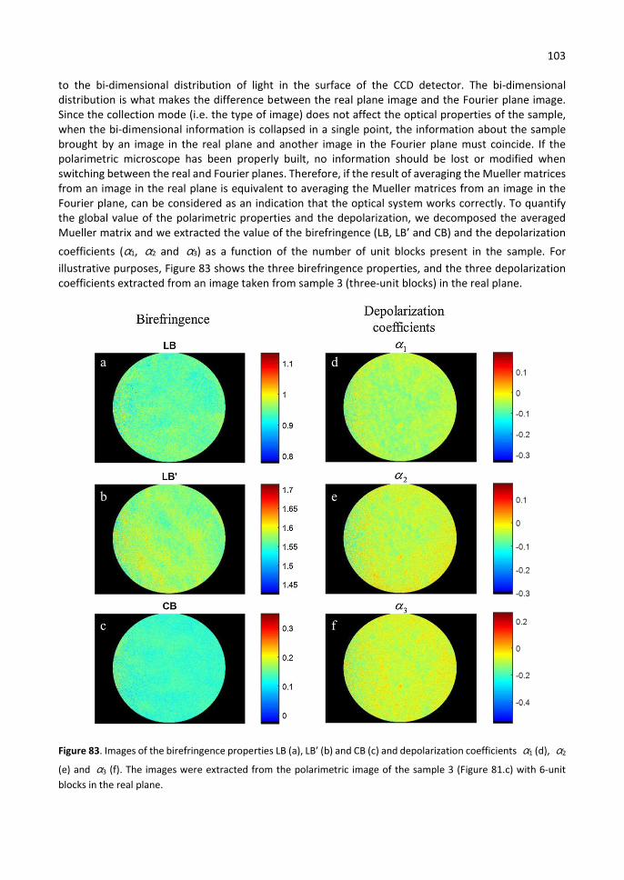
103

to the bi-dimensional distribution of light in the surface of the CCD detector. The bi-dimensional distribution is what makes the difference between the real plane image and the Fourier plane image. Since the collection mode (i.e. the type of image) does not affect the optical properties of the sample, when the bi-dimensional information is collapsed in a single point, the information about the sample brought by an image in the real plane and another image in the Fourier plane must coincide. If the polarimetric microscope has been properly built, no information should be lost or modified when switching between the real and Fourier planes. Therefore, if the result of averaging the Mueller matrices from an image in the real plane is equivalent to averaging the Mueller matrices from an image in the Fourier plane, can be considered as an indication that the optical system works correctly. To quantify the global value of the polarimetric properties and the depolarization, we decomposed the averaged Mueller matrix and we extracted the value of the birefringence (LB, LB’ and CB) and the depolarization

coefficients (α1, α2 and α3) as a function of the number of unit blocks present in the sample. For illustrative purposes, Figure 83 shows the three birefringence properties, and the three depolarization coefficients extracted from an image taken from sample 3 (three-unit blocks) in the real plane.

Figure 83. Images of the birefringence properties LB (a), LB’ (b) and CB (c) and depolarization coefficients α1 (d), α2

(e) and α3 (f). The images were extracted from the polarimetric image of the sample 3 (Figure 81.c) with 6-unit blocks in the real plane.

104

Figure 84 shows the three birefringence properties, and the three depolarization coefficients extracted from an image taken from sample 3 (three-unit blocks) in the Fourier plane. Despite of the fact that the polarimetric information is displayed differently, depending on the optical plane imaged, the averaged images show equivalent information as will be discussed in what follows.

Figure 84. Images of the birefringence properties LB (a), LB’ (b) and CB (c) and depolarization coefficients α1 (d), α2

(e) and α3 (f). The images were extracted from the polarimetric image of the sample 3 (Figure 81.c) with 6-unit blocks in the Fourier plane.

The results for sample 1 are shown in Figure 85.a and e. As expected, no global retardation is observed, neither in the real nor the Fourier plane because of compensation of vertical and horizontal orientations, and only depolarization is apparent. A parabolic fitting of the depolarization coefficients as a function of unit blocks shows a quadratic dependence, in perfect agreement with the theoretical predictions. The error bars correspond to the standard deviation of the spatial distribution. No significant differences were found between the results obtained from measurements in the real and Fourier planes, as expected.

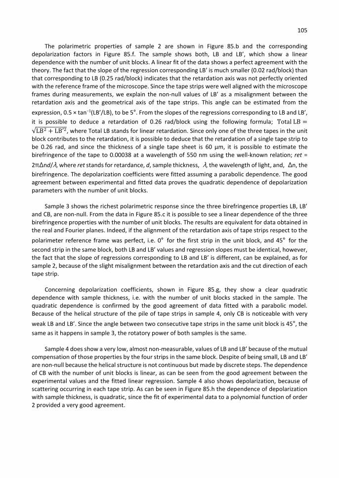
105

The polarimetric properties of sample 2 are shown in Figure 85.b and the corresponding depolarization factors in Figure 85.f. The sample shows both, LB and LB’, which show a linear dependence with the number of unit blocks. A linear fit of the data shows a perfect agreement with the theory. The fact that the slope of the regression corresponding LB’ is much smaller (0.02 rad/block) than that corresponding to LB (0.25 rad/block) indicates that the retardation axis was not perfectly oriented with the reference frame of the microscope. Since the tape strips were well aligned with the microscope frames during measurements, we explain the non-null values of LB’ as a misalignment between the retardation axis and the geometrical axis of the tape strips. This angle can be estimated from the

expression, 0.5 × tan−1(LB’/LB), to be 5°. From the slopes of the regressions corresponding to LB and LB’, it is possible to deduce a retardation of 0.26 rad/block using the following formula; Total LB =

√LB + LB′ , where Total LB stands for linear retardation. Since only one of the three tapes in the unit block contributes to the retardation, it is possible to deduce that the retardation of a single tape strip to be 0.26 rad, and since the thickness of a single tape sheet is 60 µm, it is possible to estimate the birefringence of the tape to 0.00038 at a wavelength of 550 nm using the well-known relation; ret =

2πΔnd/λ, where ret stands for retardance, d, sample thickness, λ, the wavelength of light, and, Δn, the birefringence. The depolarization coefficients were fitted assuming a parabolic dependence. The good agreement between experimental and fitted data proves the quadratic dependence of depolarization parameters with the number of unit blocks.

Sample 3 shows the richest polarimetric response since the three birefringence properties LB, LB’ and CB, are non-null. From the data in Figure 85.c it is possible to see a linear dependence of the three birefringence properties with the number of unit blocks. The results are equivalent for data obtained in the real and Fourier planes. Indeed, if the alignment of the retardation axis of tape strips respect to the

polarimeter reference frame was perfect, i.e. 0° for the first strip in the unit block, and 45° for the second strip in the same block, both LB and LB’ values and regression slopes must be identical, however, the fact that the slope of regressions corresponding to LB and LB’ is different, can be explained, as for sample 2, because of the slight misalignment between the retardation axis and the cut direction of each tape strip.

Concerning depolarization coefficients, shown in Figure 85.g, they show a clear quadratic dependence with sample thickness, i.e. with the number of unit blocks stacked in the sample. The quadratic dependence is confirmed by the good agreement of data fitted with a parabolic model. Because of the helical structure of the pile of tape strips in sample 4, only CB is noticeable with very

weak LB and LB’. Since the angle between two consecutive tape strips in the same unit block is 45°, the same as it happens in sample 3, the rotatory power of both samples is the same.

Sample 4 does show a very low, almost non-measurable, values of LB and LB’ because of the mutual compensation of those properties by the four strips in the same block. Despite of being small, LB and LB’ are non-null because the helical structure is not continuous but made by discrete steps. The dependence of CB with the number of unit blocks is linear, as can be seen from the good agreement between the experimental values and the fitted linear regression. Sample 4 also shows depolarization, because of scattering occurring in each tape strip. As can be seen in Figure 85.h the dependence of depolarization with sample thickness, is quadratic, since the fit of experimental data to a polynomial function of order 2 provided a very good agreement.

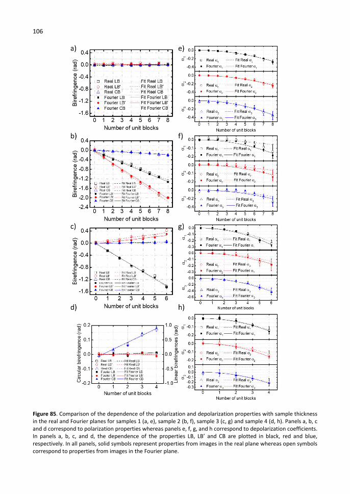
106

Figure 85. Comparison of the dependence of the polarization and depolarization properties with sample thickness in the real and Fourier planes for samples 1 (a, e), sample 2 (b, f), sample 3 (c, g) and sample 4 (d, h). Panels a, b, c and d correspond to polarization properties whereas panels e, f, g, and h correspond to depolarization coefficients. In panels a, b, c, and d, the dependence of the properties LB, LB’ and CB are plotted in black, red and blue, respectively. In all panels, solid symbols represent properties from images in the real plane whereas open symbols correspond to properties from images in the Fourier plane.

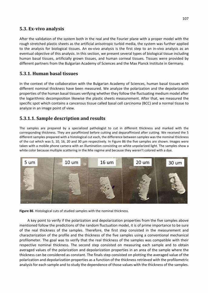
107

5.3. Ex-vivo analysis

After the validation of the system both in the real and the Fourier plane with a proper model with the rough stretched plastic sheets as the artificial anisotropic turbid media, the system was further applied to the analysis for biological tissues. An ex-vivo analysis is the first step to an in-vivo analysis as an eventual objective of this analysis. In this section, we present several types of biological tissue including human basal tissues, artificially grown tissues, and human corneal tissues. Tissues were provided by different partners from the Bulgarian Academy of Sciences and the Max Planck Institute in Germany.

5.3.1. Human basal tissues

In the context of the collaboration with the Bulgarian Academy of Sciences, human basal tissues with different nominal thickness have been measured. We analyze the polarization and the depolarization properties of the human basal tissues verifying whether they follow the fluctuating medium model after the logarithmic decomposition likewise the plastic sheets measurement. After that, we measured the specific spot which contains a cancerous tissue called basal cell carcinoma (BCC) and a normal tissue to analyze in an image point of view.

5.3.1.1. Sample description and results

The samples are prepared by a specialized pathologist to cut in different thickness and marked with the corresponding thickness. They are paraffinized before cutting and deparaffinized after cutting. We received the 5 different samples prepared with a histological cut each, the difference between samples was the nominal thickness of the cut which was 5, 10, 16, 20 and 30 µm respectively. In Figure 86 the five samples are shown. Images were taken with a mobile phone camera with an illumination consisting on white unpolarized light. The samples show a white color because multiple scattering in the Mie regime and because they weren’t colored with a dye.

Figure 86. Histological cuts of studied samples with the nominal thickness.

A key point to verify if the polarization and depolarization properties from the five samples above mentioned follow the predictions of the random fluctuation model, it is of prime importance to be sure of the real thickness of the samples. Therefore, the first step consisted in the measurement and characterization of the profile and the thickness of the five samples using a conventional mechanical profilometer. The goal was to verify that the real thickness of the samples was compatible with their respective nominal thickness. The second step consisted on measuring each sample and to obtain averaged values of the polarization and depolarization properties in an area of the sample where the thickness can be considered as constant. The finals step consisted on plotting the averaged value of the polarization and depolarization properties as a function of the thickness retrieved with the profilometric analysis for each sample and to study the dependence of those values with the thickness of the samples.

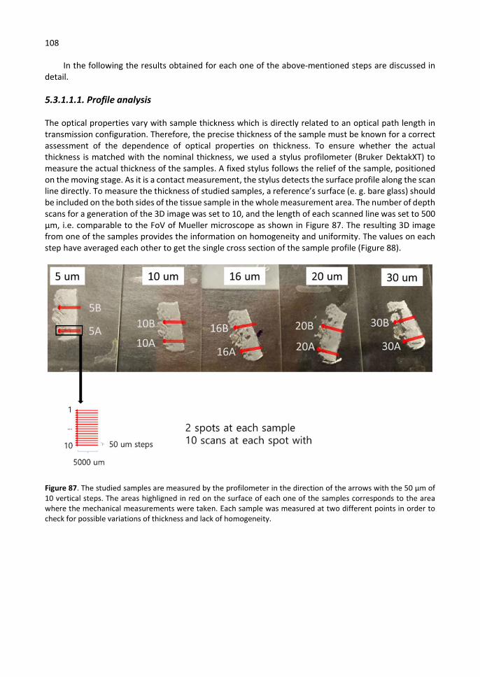
108

In the following the results obtained for each one of the above-mentioned steps are discussed in detail.

5.3.1.1.1. Profile analysis

The optical properties vary with sample thickness which is directly related to an optical path length in transmission configuration. Therefore, the precise thickness of the sample must be known for a correct assessment of the dependence of optical properties on thickness. To ensure whether the actual thickness is matched with the nominal thickness, we used a stylus profilometer (Bruker DektakXT) to measure the actual thickness of the samples. A fixed stylus follows the relief of the sample, positioned on the moving stage. As it is a contact measurement, the stylus detects the surface profile along the scan line directly. To measure the thickness of studied samples, a reference’s surface (e. g. bare glass) should be included on the both sides of the tissue sample in the whole measurement area. The number of depth scans for a generation of the 3D image was set to 10, and the length of each scanned line was set to 500 μm, i.e. comparable to the FoV of Mueller microscope as shown in Figure 87. The resulting 3D image from one of the samples provides the information on homogeneity and uniformity. The values on each step have averaged each other to get the single cross section of the sample profile (Figure 88).

Figure 87. The studied samples are measured by the profilometer in the direction of the arrows with the 50 µm of 10 vertical steps. The areas highligned in red on the surface of each one of the samples corresponds to the area where the mechanical measurements were taken. Each sample was measured at two different points in order to check for possible variations of thickness and lack of homogeneity.

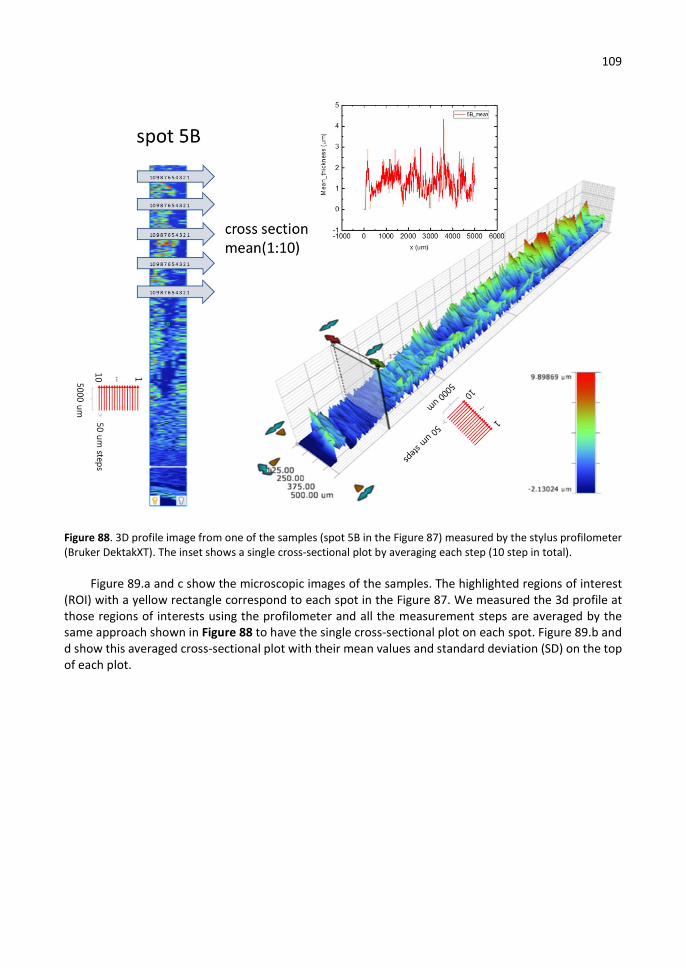
109

Figure 88. 3D profile image from one of the samples (spot 5B in the Figure 87) measured by the stylus profilometer (Bruker DektakXT). The inset shows a single cross-sectional plot by averaging each step (10 step in total).

Figure 89.a and c show the microscopic images of the samples. The highlighted regions of interest (ROI) with a yellow rectangle correspond to each spot in the Figure 87. We measured the 3d profile at those regions of interests using the profilometer and all the measurement steps are averaged by the same approach shown in Figure 88 to have the single cross-sectional plot on each spot. Figure 89.b and d show this averaged cross-sectional plot with their mean values and standard deviation (SD) on the top of each plot.

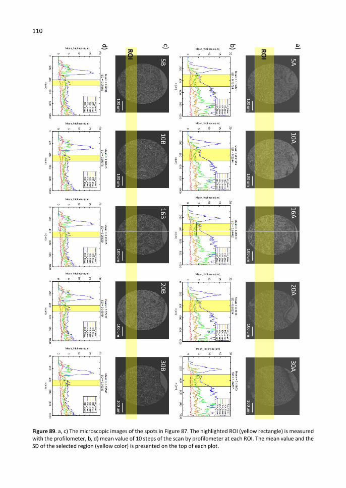
110

Figure 89. a, c) The microscopic images of the spots in Figure 87. The highlighted ROI (yellow rectangle) is measured with the profilometer, b, d) mean value of 10 steps of the scan by profilometer at each ROI. The mean value and the SD of the selected region (yellow color) is presented on the top of each plot.

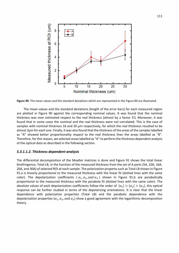
111

Figure 90. The mean values and the standard deviations which are represented in the Figure 89 are illustrated.

The mean values and the standard deviations (length of the error bars) for each measured region are plotted in Figure 90 against the corresponding nominal values. It was found that the nominal thickness was over estimated respect to the real thickness (almost by a factor 5!). Moreover, it was found that in some cases the nominal and the real thickness were not correlated. This is the case of samples with nominal thickness 16 and 20 µm respectively, for which the real thickness resulted to be almost 3µm for each one. Finally, it was also found that the thickness of the areas of the samples labelled as “A” showed better proportionality respect to the real thickness than the areas labelled as ”B”. Therefore, for this reason, we selected areas labelled as “A” to perform the thickness dependent analysis of the optical data as described in the following section.

5.3.1.1.2. Thickness dependent analysis

The differential decomposition of the Mueller matrices is done and Figure 91 shows the total linear birefringence, Total LB, in the function of the measured thickness from the set of A parts (5A, 10A, 16A, 20A, and 30A) of selected ROI at each sample. The polarization property such as Total LB shown in Figure 91.a is linearly proportional to the measured thickness with the linear fit (dotted lines with the same color). The depolarization coefficients ( 𝛼 , 𝛼 , and 𝛼 ) shown in Figure 91.b are parabolically proportional to the measured thickness with the parabola fit (dotted lines with the same color). The absolute values of each depolarization coefficients follow the order of |𝛼 | > |𝛼 | > |𝛼 |, this optical response can be further studied in terms of the depolarizing orientations. It is clear that the linear dependence with polarization properties (Total LB) and the parabolic dependence with the depolarization properties (𝛼 , 𝛼 , and 𝛼 ) show a good agreement with the logarithmic decomposition theory.

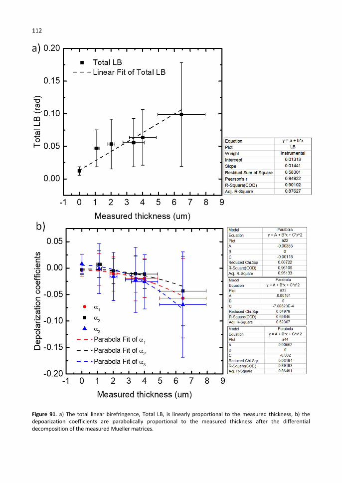
112

Figure 91. a) The total linear birefringence, Total LB, is linearly proportional to the measured thickness, b) the depoarization coefficients are parabolically proportional to the measured thickness after the differential decomposition of the measured Mueller matrices.

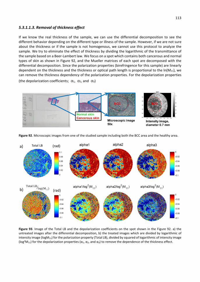
113

5.3.1.1.3. Removal of thickness effect

If we know the real thickness of the sample, we can use the differential decomposition to see the different behavior depending on the different type or illness of the sample. However, if we are not sure about the thickness or if the sample is not homogenous, we cannot use this protocol to analyze the sample. We try to eliminate the effect of thickness by dividing the logarithmic of the transmittance of the sample based on a Beer-Lambert law. We focus on a spot which contains both cancerous and normal types of skin as shown in Figure 92, and the Mueller matrices of each spot are decomposed with the differential decomposition. Since the polarization properties (birefringence for this sample) are linearly dependent on the thickness and the thickness or optical path length is proportional to the ln(M11), we can remove the thickness dependency of the polarization properties. For the depolarization properties

(the depolarization coefficients; α1, α2, and α3)

Figure 92. Microscopic images from one of the studied sample including both the BCC area and the healthy area.

Figure 93. Image of the Total LB and the depolarization coefficients on the spot shown in the Figure 92. a) the untreated images after the differential decomposition, b) the treated images which are divided by logarithmic of intensity image (logM11) for the polarization property (Total LB), divided by squared of logarithmic of intensity image (log2M11) for the depolarization properties (α1, α2, and α3) to remove the dependence of the thickness effect.

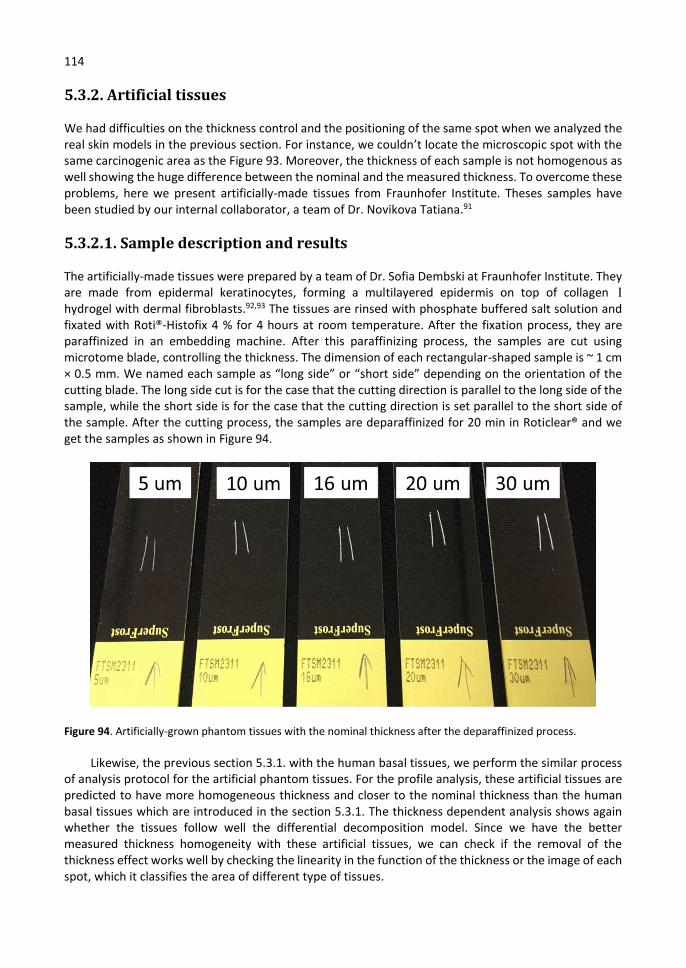
114

5.3.2. Artificial tissues

We had difficulties on the thickness control and the positioning of the same spot when we analyzed the real skin models in the previous section. For instance, we couldn’t locate the microscopic spot with the same carcinogenic area as the Figure 93. Moreover, the thickness of each sample is not homogenous as well showing the huge difference between the nominal and the measured thickness. To overcome these problems, here we present artificially-made tissues from Fraunhofer Institute. Theses samples have been studied by our internal collaborator, a team of Dr. Novikova Tatiana.91

5.3.2.1. Sample description and results

The artificially-made tissues were prepared by a team of Dr. Sofia Dembski at Fraunhofer Institute. They are made from epidermal keratinocytes, forming a multilayered epidermis on top of collagen I hydrogel with dermal fibroblasts.92,93 The tissues are rinsed with phosphate buffered salt solution and fixated with Roti®-Histofix 4 % for 4 hours at room temperature. After the fixation process, they are paraffinized in an embedding machine. After this paraffinizing process, the samples are cut using microtome blade, controlling the thickness. The dimension of each rectangular-shaped sample is ~ 1 cm × 0.5 mm. We named each sample as “long side” or “short side” depending on the orientation of the cutting blade. The long side cut is for the case that the cutting direction is parallel to the long side of the sample, while the short side is for the case that the cutting direction is set parallel to the short side of the sample. After the cutting process, the samples are deparaffinized for 20 min in Roticlear® and we get the samples as shown in Figure 94.

Figure 94. Artificially-grown phantom tissues with the nominal thickness after the deparaffinized process.

Likewise, the previous section 5.3.1. with the human basal tissues, we perform the similar process of analysis protocol for the artificial phantom tissues. For the profile analysis, these artificial tissues are predicted to have more homogeneous thickness and closer to the nominal thickness than the human basal tissues which are introduced in the section 5.3.1. The thickness dependent analysis shows again whether the tissues follow well the differential decomposition model. Since we have the better measured thickness homogeneity with these artificial tissues, we can check if the removal of the thickness effect works well by checking the linearity in the function of the thickness or the image of each spot, which it classifies the area of different type of tissues.

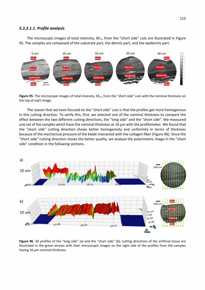
115

5.3.2.1.1. Profile analysis

The microscopic images of total intensity, M11, from the “short side” cuts are illustrated in Figure 95. The samples are composed of the substrate part, the dermis part, and the epidermis part.

Figure 95. The microscopic images of total intensity, M11, from the “short side” cuts with the nominal thickness on the top of each image.

The reason that we have focused on the “short side” cuts is that the profiles get more homogenous in this cutting direction. To verify this, first, we selected one of the nominal thickness to compare the effect between the two different cutting directions, the “long side” and the “short side”. We measured one set of the samples which have the nominal thickness as 16 µm with the profilometer. We found that the “short side” cutting direction shows better homogeneity and uniformity in terms of thickness because of the mechanical pressure of the blade interacted with the collagen fiber (Figure 96). Since the “short side” cutting direction shows the better quality, we analyze the polarimetric image in the “short side” condition in the following sections.

Figure 96. 3D profiles of the “long side” (a) and the “short side” (b), cutting directions of the artificial tissue are illustrated in the green arrows with their microscopic images on the right side of the profiles from the samples having 16 µm nominal thickness.

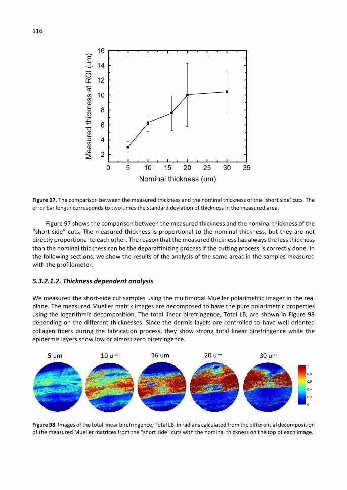
116

Figure 97. The comparison between the measured thickness and the nominal thickness of the “short side’ cuts. The error bar length corresponds to two times the standard deviation of thickness in the measured area.

Figure 97 shows the comparison between the measured thickness and the nominal thickness of the “short side” cuts. The measured thickness is proportional to the nominal thickness, but they are not directly proportional to each other. The reason that the measured thickness has always the less thickness than the nominal thickness can be the deparaffinizing process if the cutting process is correctly done. In the following sections, we show the results of the analysis of the same areas in the samples measured with the profilometer.

5.3.2.1.2. Thickness dependent analysis

We measured the short-side cut samples using the multimodal Mueller polarimetric imager in the real plane. The measured Mueller matrix images are decomposed to have the pure polarimetric properties using the logarithmic decomposition. The total linear birefringence, Total LB, are shown in Figure 98 depending on the different thicknesses. Since the dermis layers are controlled to have well oriented collagen fibers during the fabrication process, they show strong total linear birefringence while the epidermis layers show low or almost zero birefringence.

Figure 98. Images of the total linear birefringence, Total LB, in radians calculated from the differential decomposition of the measured Mueller matrices from the “short side” cuts with the nominal thickness on the top of each image.

0 5 10 15 20 25 30 35

2

4

6

8

10

12

14

16

Me

asu

red

thic

knes

s a

t R

OI

(um

)

Nominal thickness (um)

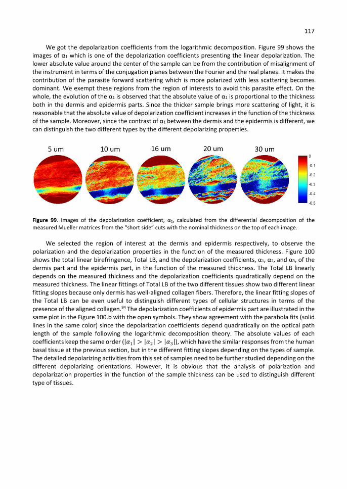
117

We got the depolarization coefficients from the logarithmic decomposition. Figure 99 shows the images of α1 which is one of the depolarization coefficients presenting the linear depolarization. The lower absolute value around the center of the sample can be from the contribution of misalignment of the instrument in terms of the conjugation planes between the Fourier and the real planes. It makes the contribution of the parasite forward scattering which is more polarized with less scattering becomes dominant. We exempt these regions from the region of interests to avoid this parasite effect. On the whole, the evolution of the α1 is observed that the absolute value of α1 is proportional to the thickness both in the dermis and epidermis parts. Since the thicker sample brings more scattering of light, it is reasonable that the absolute value of depolarization coefficient increases in the function of the thickness of the sample. Moreover, since the contrast of α1 between the dermis and the epidermis is different, we can distinguish the two different types by the different depolarizing properties.

Figure 99. Images of the depolarization coefficient, α1, calculated from the differential decomposition of the measured Mueller matrices from the “short side” cuts with the nominal thickness on the top of each image.

We selected the region of interest at the dermis and epidermis respectively, to observe the polarization and the depolarization properties in the function of the measured thickness. Figure 100 shows the total linear birefringence, Total LB, and the depolarization coefficients, α1, α2, and α3, of the dermis part and the epidermis part, in the function of the measured thickness. The Total LB linearly depends on the measured thickness and the depolarization coefficients quadratically depend on the measured thickness. The linear fittings of Total LB of the two different tissues show two different linear fitting slopes because only dermis has well-aligned collagen fibers. Therefore, the linear fitting slopes of the Total LB can be even useful to distinguish different types of cellular structures in terms of the presence of the aligned collagen.94 The depolarization coefficients of epidermis part are illustrated in the same plot in the Figure 100.b with the open symbols. They show agreement with the parabola fits (solid lines in the same color) since the depolarization coefficients depend quadratically on the optical path length of the sample following the logarithmic decomposition theory. The absolute values of each coefficients keep the same order (|𝛼 | > |𝛼 | > |𝛼 |), which have the similar responses from the human basal tissue at the previous section, but in the different fitting slopes depending on the types of sample. The detailed depolarizing activities from this set of samples need to be further studied depending on the different depolarizing orientations. However, it is obvious that the analysis of polarization and depolarization properties in the function of the sample thickness can be used to distinguish different type of tissues.

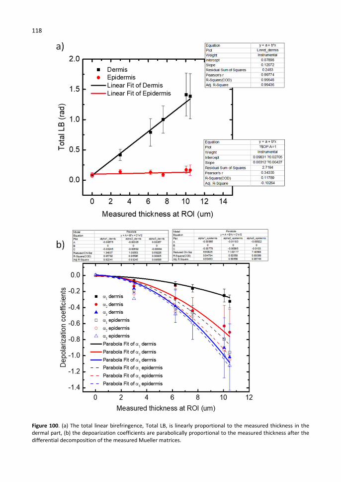
118

Figure 100. (a) The total linear birefringence, Total LB, is linearly proportional to the measured thickness in the dermal part, (b) the depoarization coefficients are parabolically proportional to the measured thickness after the differential decomposition of the measured Mueller matrices.

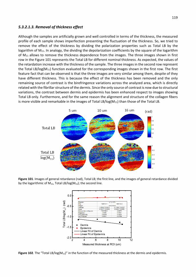
119

5.3.2.1.3. Removal of thickness effect

Although the samples are artificially grown and well controlled in terms of the thickness, the measured profile of each sample shows imperfection presenting the fluctuation of the thickness. So, we tried to remove the effect of the thickness by dividing the polarization properties such as Total LB by the logarithm of M11. In analogy, the dividing the depolarization coefficients by the square of the logarithm of M11 allows to remove the thickness dependence from the images. The three images shown in first row in the Figure 101 represents the Total LB for different nominal thickness. As expected, the values of the retardation increase with the thickness of the sample. The three images in the second row represent the Total LB/log(M11) function evaluated for the corresponding images shown in the first row. The first feature fact that can be observed is that the three images are very similar among them, despite of they have different thickness. This is because the effect of the thickness has been removed and the only remaining source of contrast is the birefringence variations across the analyzed area, which is directly related with the fibrillar structure of the dermis. Since the only source of contrast is now due to structural variations, the contrast between dermis and epidermis has been enhanced respect to images showing Total LB only. Furthermore, and for the same reason the alignment and structure of the collagen fibers is more visible and remarkable in the images of Total LB/log(M11) than those of the Total LB.

Figure 101. Images of general retardance (rad), Total LB; the first line, and the images of general retardance divided by the logarithmic of M11, Total LB/log(M11); the second line.

Figure 102. The “Total LB/log(M11)” in the function of the measured thickness at the dermis and epidermis.

120

When we plot the mean values of Total LB/log(M11) at each type of tissue in the function of the measured thickness as shown in Figure 102, we can verify that the dependency of the birefringence property on the thickness as shown in Figure 100.a. is removed.

5.4. Conclusion

We validated the use of the multimodal polarimetric microscope in both, the real and Fourier modes, by to characterize the optical properties of scattering media by measuring simple samples such as Scotch® which can be considered as reference samples because of his homogeneity and standard optical properties were used to experimentally verify the theoretical predictions given by the random fluctuating model. According to it the polarization properties of the sample depend linearly on the optical path length travelled by the light inside of a scattering medium, whereas the depolarization properties vary quadratically. After performing a series of measurements with different sets of samples it was possible to verify that the dependence of both, polarization and depolarization properties with the sample thickness, were in perfect accordance with the predictions of the theoretical model.

The experimental studies of two different types of histological tissue cuts; both the human basal tissue cuts and the artificial tissue cuts, with the polarimetric Mueller microscope have confirmed the validity of the phenomenological model of the randomly fluctuating media for the description of the dependence of both polarization and depolarization properties with tissue thickness. Accordingly, it was possible to experimentally show that whenever the studied tissue had a homogeneous thickness, the retardance of tissue depended linearly on the thickness while the depolarization properties showed a parabolic dependence with it. Moreover, it was show that the coefficients describing either the straight lines or the parabolas related to the dependence of the polarization or depolarization properties respectively, varied from a type of type to another. Therefore, it was shown that these coefficients could be used as a tool to discriminate among different types of tissues.

An important issue, overlooked by many researchers working in the field of polarized light histology, appears to be the control and characterization of real thickness of studied tissue cuts. The pathological changes of tissues (cancer, fibrosis, inflammation, etc.) will affect measured polarization and depolarization properties of a sample. However, changing the optical path length will also affect these properties. Thus, for reliable diagnostics of tissue with polarized light, the impact of the varying optical path length on polarization and depolarization optical markers of the specific disease must be considered. In this context, we proposed the method to remove the effect of the thickness in such inhomogeneous samples by dividing the polarimetric properties by the total intensity, M11, to suggest a different analytical point of view. Following this method, we could enhance the contrast of the image to distinguish better the type of the tissue and the composition, i.e. orientation of the collagen fibers, than the untreated birefringence image.

121

Chapter 6. Other applications

Contents

6.1. Optical properties of nano-patterned samples ...................................................... 122

6.1.1. Introduction to pseudochiral metasurfaces ....................................................... 122

6.1.2. Sample preparation ............................................................................................ 123

6.1.3. Mueller imaging measurement results with modelling ................................... 124

6.1.4. Conclusion .......................................................................................................... 126

6.2. Optical properties of samples modified by femtosecond laser direct writing ........ 127

6.2.1. Introduction to femtosecond laser direct writing (FLDW) ............................... 127

6.2.2. Sample preparation ............................................................................................ 128

6.2.3. Spectroscopic Mueller ellipsometry measurement with modelling ................. 128

6.2.4. Conclusion ........................................................................................................... 132

6.3. Optical properties of cylindrical microparticles .................................................... 133

6.3.1. Introduction to cylindrical microparticles ......................................................... 133

6.3.2. Sample preparation ............................................................................................ 134

6.3.3. Optical response based on haze and gloss ......................................................... 135

6.3.4. Optical response based on BTDF and non-polarimetric microscope ............... 136

6.3.5. Conclusion ........................................................................................................... 141

In the framework of various collaborations which were created during the thesis with different research teams, it was possible to carry out studies on the optical response of a variety of samples including meta-materials, glasses irradiated with femtosecond laser pulses, or micro-patterned surfaces. A summary of the most significant results of these studies illustrating three possible applications using the polarimetric microscope is presented in this chapter, which corresponds to the last part of the manuscript; i) nano-patterned samples to measure a pseudo-chirality caused by the plasmonic effect, ii) samples modified by a femtosecond laser direct writing (FLDW), and iii) cylindrical microparticles for a hydrophobic surface to analyze their structures. Most of the cited works have been published in peer-reviewed journals or international conferences, and as such they are can be found in the forthcoming chapter summarizing the list of publications.

122

6.1. Optical properties of nano-patterned samples

Thanks to the localized surface plasmon resonance, metallic nano-scatterers can interact with the incident light. In the area of anticounterfeiting applications, there have been many studies to generate covert images using this effect using the grating effect, called Plasmonic colors, with dielectric or metallic sub-wavelength structures.95–99 Since the plasmonic effect is very limited in terms of spectral range, however, it is important to study the way to give additional degrees of freedom. Furthermore, a very important point is to produce effects that are specific to one structure and that would not be reproduced by low-cost process such as inkjet printing.

We collaborated with Institut des NanoSciences de Paris (INSP) at Sorbonne Université to study a palette of luminance which is suggested for anticounterfeiting applications. This U-shaped palette is observable only in circular dichroism by engineering the shapes and positions of the resonators. In the following sections, the basic theory of CD induced by pseudo chiral nano-antennas is explained followed by the observation of the variations of the image of the Mueller matrix with different angle of incidence.

6.1.1. Introduction to pseudochiral metasurfaces

Pseudochiral resonators are nonchiral resonators exhibit an optical activity which originates from a magneto-electric coupling between the electric and magnetic components of some resonances in well-defined spectral ranges.100–103 A characteristic unique to pseudochiral resonators is that the sign of the optical activity depends on the direction of propagation of the incoming light. Among the different types of resonators that exhibit this property, U-shaped resonators are the most commonly used since they feature strong magnetoelectric coupling and are easy to fabricate (Figure 103).102–105

Figure 103. (a) Sketch of the dipole moments excited in an isolated U-shaped resonator associated with the current distribution at resonance, (b) influence of an array of U-shaped resonators on the reflected polarization.

The subject of the collaboration was how plasmon resonances with magnetoelectric coupling can be used to encode images in circular polarization with contrast reversal depending on the direction of observation. The results of the study were illustrated by the realization of practical demonstrator in which a series of U-shaped resonators were realized in a way that they created a grey level image of Mona Lisa by Leonardo Da Vinci when observed at oblique incidence. The goal was to demonstrate that the grey level of the Mona Lisa were visible only when circular polarization was considered and invisible otherwise. Moreover, it was important to show that the grey scale could be inverted by modifying the direction of observation.

123

6.1.2. Sample preparation

The plasmonic resonators were fabricated with electron beam lithography followed by a conventional lift-off method. A 130 nm thick layer of poly methyl methacrylate (PMMA) was spin-coated on a clean glass substrate (BK7), and a thin layer of aluminum was thermally evaporated on the PMMA to avoid any charging effect during the exposure with electrons. After exposure and before the development of the resist, this conductive layer was removed in a KOH bath. After development, a 4 nm chromium layer was evaporated to ensure the adhesion of the 40 nm gold layer on the glass substrate. The resist was then lifted-off with acetone, and the substrate subsequently rinsed in ethanol to reveal the U-shaped scatterers. Such resonators exhibit a resonance with magneto-electric coupling near 770 nm excited by the component of the electric field of light parallel to the y-axis. To investigate the dependence of the scattered intensity in circular polarization as a function of the resonator’s density, a palette of pixels was prepared where pixels consisted of a 3 × 3 matrix of resonators with a total footprint of 1.4 × 1.4 μm2 per pixel. The number of U-shaped resonators in each pixel varied between 1 and 9 (Figure 104.a). When only U-shaped resonators are used, the transmittance of the surface scales inversely with the number of resonators. To keep the transmittance constant across all pixel configurations, the missing resonators were replaced by circular resonators in each pixel, and all the surfaces in between the palette were also filled with circular resonators. In this way an encoded pattern observed with unpolarized light will be invisible, whereas it will be clearly visible when seen between crossed polarizers at oblique incidence.

Figure 104.b shows that the absorbance was approximately constant across all configurations and that the U-shaped resonators could not be distinguished from the circular ones with a diffraction-limited resolution. In contrast, Figure 104.c presents a microscopy image of the palette of Figure 104.b taken between crossed linear polarizers at an oblique incidence. It can be seen that light was transmitted in these conditions in the area containing the U-shaped resonators, with a luminance scaling approximately with the number of U-shaped resonators in each pixel. The topmost row of the palette in Figure 104.c contains arrays of pixels containing 3 × 3 resonators, among which are three U-shaped resonators but with different positions in each pixel.

Figure 104. (a) SEM image of a pixel with three U-shaped resonators and six disks placed on a square lattice with a constant of 400 nm, (b) optical microscopy image in transmission at normal incidence (×50) using unpolarized white light of the palette made of U-shaped resonators and disks. The area containing pixels with three U-shaped resonators has been highlighted with dotted lines for illustration purposes. (c) the same palette as in (b) but observed between crossed polarizers at oblique incidence. The orientations of the linear polarizer (P) and linear analyzer (A) are indicated in the figure. The number of U-shaped resonators per pixels is indicated for each array (labeled 1 to 9). On the top row, four different configurations of U-shaped resonators are displayed (labeled 3a to 3d).

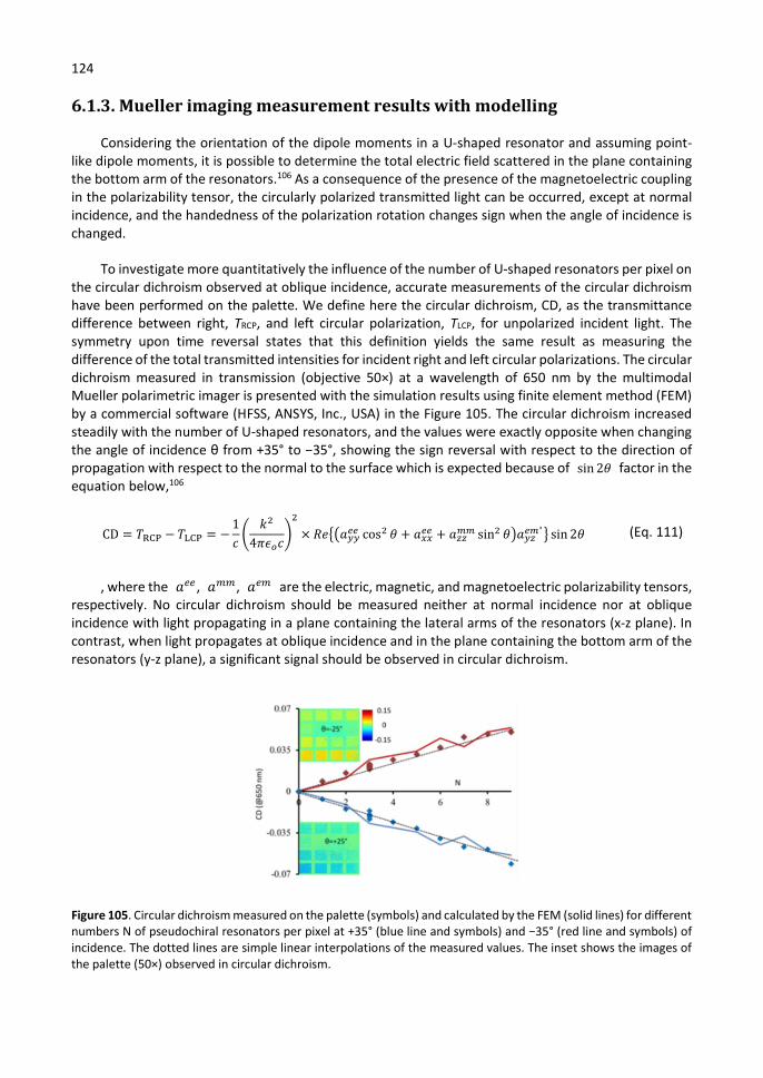
124

6.1.3. Mueller imaging measurement results with modelling

Considering the orientation of the dipole moments in a U-shaped resonator and assuming point-like dipole moments, it is possible to determine the total electric field scattered in the plane containing the bottom arm of the resonators.106 As a consequence of the presence of the magnetoelectric coupling in the polarizability tensor, the circularly polarized transmitted light can be occurred, except at normal incidence, and the handedness of the polarization rotation changes sign when the angle of incidence is changed.

To investigate more quantitatively the influence of the number of U-shaped resonators per pixel on the circular dichroism observed at oblique incidence, accurate measurements of the circular dichroism have been performed on the palette. We define here the circular dichroism, CD, as the transmittance difference between right, TRCP, and left circular polarization, TLCP, for unpolarized incident light. The symmetry upon time reversal states that this definition yields the same result as measuring the difference of the total transmitted intensities for incident right and left circular polarizations. The circular dichroism measured in transmission (objective 50×) at a wavelength of 650 nm by the multimodal Mueller polarimetric imager is presented with the simulation results using finite element method (FEM) by a commercial software (HFSS, ANSYS, Inc., USA) in the Figure 105. The circular dichroism increased steadily with the number of U-shaped resonators, and the values were exactly opposite when changing the angle of incidence θ from +35° to −35°, showing the sign reversal with respect to the direction of propagation with respect to the normal to the surface which is expected because of sin 2𝜃 factor in the equation below,106

CD = 𝑇 − 𝑇 = −1

𝑐

𝑘

4𝜋𝜖 𝑐× 𝑅𝑒 𝑎 cos 𝜃 + 𝑎 + 𝑎 sin 𝜃 𝑎

∗sin 2𝜃 (Eq. 111)

, where the 𝑎 , 𝑎 , 𝑎 are the electric, magnetic, and magnetoelectric polarizability tensors, respectively. No circular dichroism should be measured neither at normal incidence nor at oblique incidence with light propagating in a plane containing the lateral arms of the resonators (x-z plane). In contrast, when light propagates at oblique incidence and in the plane containing the bottom arm of the resonators (y-z plane), a significant signal should be observed in circular dichroism.

Figure 105. Circular dichroism measured on the palette (symbols) and calculated by the FEM (solid lines) for different numbers N of pseudochiral resonators per pixel at +35° (blue line and symbols) and −35° (red line and symbols) of incidence. The dotted lines are simple linear interpolations of the measured values. The inset shows the images of the palette (50×) observed in circular dichroism.

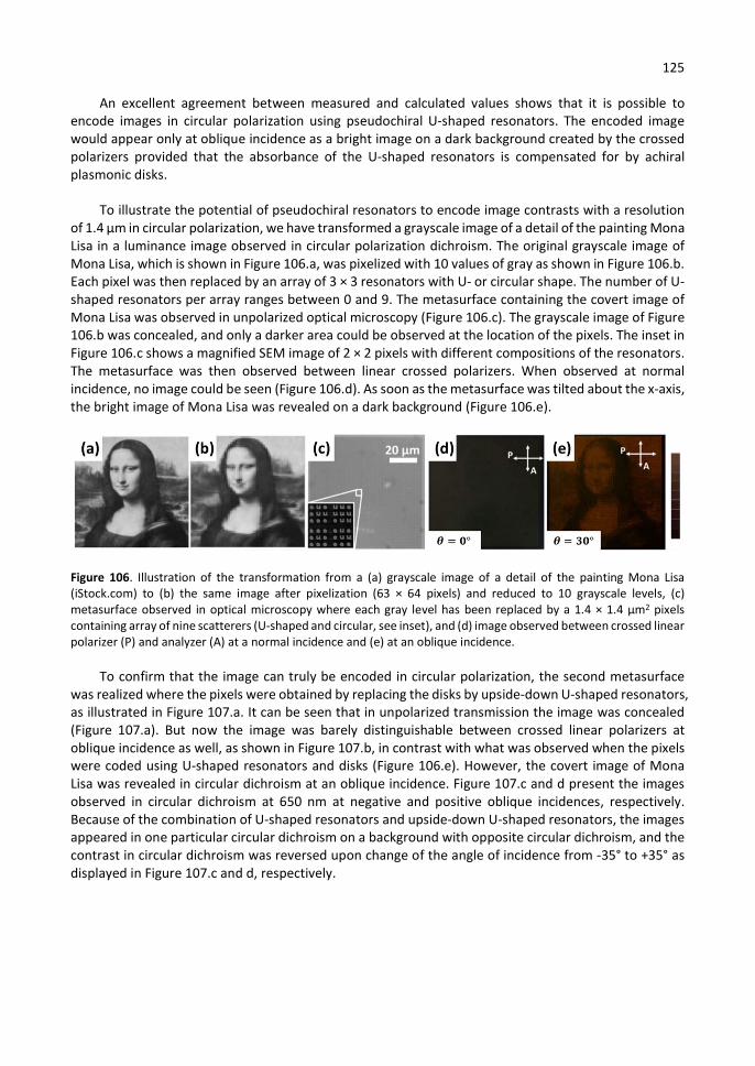
125

An excellent agreement between measured and calculated values shows that it is possible to encode images in circular polarization using pseudochiral U-shaped resonators. The encoded image would appear only at oblique incidence as a bright image on a dark background created by the crossed polarizers provided that the absorbance of the U-shaped resonators is compensated for by achiral plasmonic disks.

To illustrate the potential of pseudochiral resonators to encode image contrasts with a resolution of 1.4 μm in circular polarization, we have transformed a grayscale image of a detail of the painting Mona Lisa in a luminance image observed in circular polarization dichroism. The original grayscale image of Mona Lisa, which is shown in Figure 106.a, was pixelized with 10 values of gray as shown in Figure 106.b. Each pixel was then replaced by an array of 3 × 3 resonators with U- or circular shape. The number of U-shaped resonators per array ranges between 0 and 9. The metasurface containing the covert image of Mona Lisa was observed in unpolarized optical microscopy (Figure 106.c). The grayscale image of Figure 106.b was concealed, and only a darker area could be observed at the location of the pixels. The inset in Figure 106.c shows a magnified SEM image of 2 × 2 pixels with different compositions of the resonators. The metasurface was then observed between linear crossed polarizers. When observed at normal incidence, no image could be seen (Figure 106.d). As soon as the metasurface was tilted about the x-axis, the bright image of Mona Lisa was revealed on a dark background (Figure 106.e).

Figure 106. Illustration of the transformation from a (a) grayscale image of a detail of the painting Mona Lisa (iStock.com) to (b) the same image after pixelization (63 × 64 pixels) and reduced to 10 grayscale levels, (c) metasurface observed in optical microscopy where each gray level has been replaced by a 1.4 × 1.4 μm2 pixels containing array of nine scatterers (U-shaped and circular, see inset), and (d) image observed between crossed linear polarizer (P) and analyzer (A) at a normal incidence and (e) at an oblique incidence.

To confirm that the image can truly be encoded in circular polarization, the second metasurface was realized where the pixels were obtained by replacing the disks by upside-down U-shaped resonators, as illustrated in Figure 107.a. It can be seen that in unpolarized transmission the image was concealed (Figure 107.a). But now the image was barely distinguishable between crossed linear polarizers at oblique incidence as well, as shown in Figure 107.b, in contrast with what was observed when the pixels were coded using U-shaped resonators and disks (Figure 106.e). However, the covert image of Mona Lisa was revealed in circular dichroism at an oblique incidence. Figure 107.c and d present the images observed in circular dichroism at 650 nm at negative and positive oblique incidences, respectively. Because of the combination of U-shaped resonators and upside-down U-shaped resonators, the images appeared in one particular circular dichroism on a background with opposite circular dichroism, and the contrast in circular dichroism was reversed upon change of the angle of incidence from -35° to +35° as displayed in Figure 107.c and d, respectively.

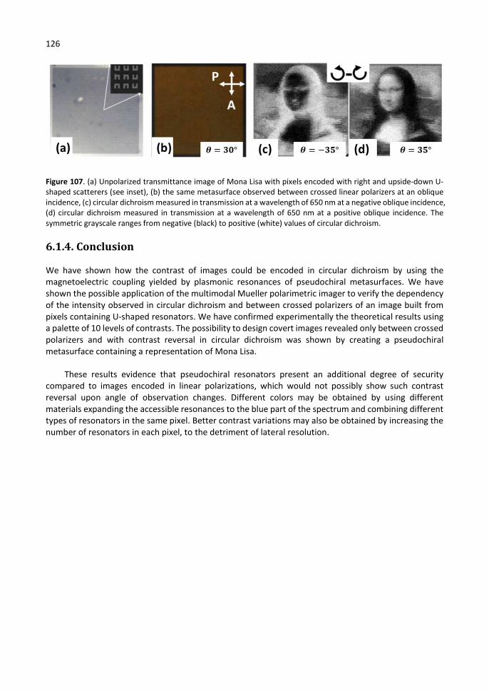
126

Figure 107. (a) Unpolarized transmittance image of Mona Lisa with pixels encoded with right and upside-down U-shaped scatterers (see inset), (b) the same metasurface observed between crossed linear polarizers at an oblique incidence, (c) circular dichroism measured in transmission at a wavelength of 650 nm at a negative oblique incidence, (d) circular dichroism measured in transmission at a wavelength of 650 nm at a positive oblique incidence. The symmetric grayscale ranges from negative (black) to positive (white) values of circular dichroism.

6.1.4. Conclusion

We have shown how the contrast of images could be encoded in circular dichroism by using the magnetoelectric coupling yielded by plasmonic resonances of pseudochiral metasurfaces. We have shown the possible application of the multimodal Mueller polarimetric imager to verify the dependency of the intensity observed in circular dichroism and between crossed polarizers of an image built from pixels containing U-shaped resonators. We have confirmed experimentally the theoretical results using a palette of 10 levels of contrasts. The possibility to design covert images revealed only between crossed polarizers and with contrast reversal in circular dichroism was shown by creating a pseudochiral metasurface containing a representation of Mona Lisa.

These results evidence that pseudochiral resonators present an additional degree of security compared to images encoded in linear polarizations, which would not possibly show such contrast reversal upon angle of observation changes. Different colors may be obtained by using different materials expanding the accessible resonances to the blue part of the spectrum and combining different types of resonators in the same pixel. Better contrast variations may also be obtained by increasing the number of resonators in each pixel, to the detriment of lateral resolution.

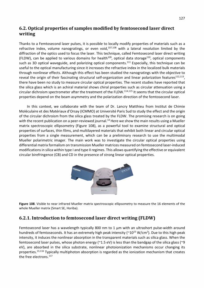
127

6.2. Optical properties of samples modified by femtosecond laser direct writing

Thanks to a Femtosecond laser pulses, it is possible to locally modify properties of materials such as a refractive index, volume nanogratings, or even void,107,108 with a lateral resolution limited by the diffraction of the optics used to focus the laser. This technique, called Femtosecond laser direct writing (FLDW), can be applied to various domains for health109, optical data storage110, optical components such as 3D optical waveguide, and polarizing optical components.111 Especially, this technique can be useful to the optical manufacturing since it increases the refractive index in the localized bulk materials through nonlinear effects. Although this effect has been studied the nanogratings with the objective to reveal the origin of their fascinating structural self-organization and linear polarization features112,113, there have been no study to measure circular optical properties. The recent studies have reported that the silica glass which is an achiral material shows chiral properties such as circular attenuation using a circular dichroism spectrometer after the treatment of the FLDW.114,115 It seems that the circular optical properties depend on the beam asymmetry and the polarization direction of the femtosecond laser.

In this context, we collaborate with the team of Dr. Lancry Matthieu from Institut de Chimie Moléculaire et des Matériaux d’Orsay (ICMMO) at Université Paris Sud to study the effect and the origin of the circular dichroism from the silica glass treated by the FLDW. The promising research is on going with the recent publication on a peer-reviewed journal.14 Here we show the main results using a Mueller matrix spectroscopic ellipsometry (Figure 108), as a powerful tool to examine structural and optical properties of surfaces, thin films, and multilayered materials that exhibit both linear and circular optical properties from a single measurement, which can be a preliminary research to use the multimodal Mueller polarimetric imager. The main work was to investigate the circular optical properties using differential matrix formalism on transmission Mueller matrices measured on femtosecond laser-induced modifications in silica within type I and type II regimes. This allows quantifying the effective or equivalent circular birefringence (CB) and CD in the presence of strong linear optical properties.

Figure 108. Visible to near infrared Mueller matrix spectroscopic ellipsometry to measure the 16 elements of the whole Mueller matrix (Smart SE, Horiba).

6.2.1. Introduction to femtosecond laser direct writing (FLDW)

Femtosecond laser has a wavelength typically 800 nm to 1 µm with an ultrashort pulse-width around hundreds of femtoseconds. It has an extremely high peak intensity (~1015 W/cm2). Due to this high peak intensity, it induces the nonlinear absorption in the transparent materials such as silica glass. When the femtosecond laser pulses, whose photon energy (~1.5 eV) is less than the bandgap of the silica glass (~9 eV), are absorbed in the silica substrate, nonlinear photoionization mechanisms occur changing its properties.13,116 Typically multiphoton absorption is regarded as the ionization mechanism that creates the free electrons.117

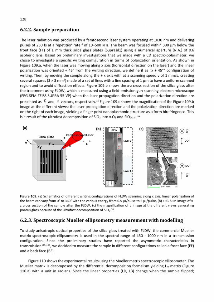
128

6.2.2. Sample preparation

The laser radiation was produced by a femtosecond laser system operating at 1030 nm and delivering pulses of 250 fs at a repetition rate f of 10–500 kHz. The beam was focused within 300 μm below the front face (FF) of 1 mm thick silica glass plates (Suprasil1) using a numerical aperture (N.A.) of 0.6 aspheric lens. Based on preliminary investigations that we made with a CD spectro-polarimeter, we chose to investigate a specific writing configuration in terms of polarization orientation. As shown in Figure 109.a, when the laser was moving along x axis (horizontal direction on the laser) and the linear polarization was oriented + 45° from the writing direction, we define it as “x + 45°” configuration of writing. Then, by moving the sample along the + x axis with at a scanning speed v of 1 mm/s, creating several squares (3 × 3 mm2) made of a set of lines with a line spacing of 1 μm to have a uniform scanned region and to avoid diffraction effects. Figure 109.b shows the x-z cross section of the silica glass after the treatment using FLDW, which is measured using a field-emission gun scanning electron microscope (FEG-SEM ZEISS SUPRA 55 VP) when the laser propagation direction and the polarization direction are presented as �⃗� and 𝑒 vectors, respectively.10 Figure 109.c shows the magnification of the Figure 109.b image at the different views; the laser propagation direction and the polarization direction are marked on the right of each image, yielding a finger print nanoplasmonic structure as a form birefringence. This is a result of the ultrafast decomposition of SiO2 into x.O2 and SiO2(1-x).10

Figure 109. (a) Schematics of different writing configurations of FLDW scanning along x axis, linear polarization of the beam can vary from 0° to 360° with the various energy from 0.5 µJ/pulse to 6 µJ/pulse, (b) FEG-SEM image of x-z cross section of the sample after the FLDW, (c) the magnification of b image at the different views generating porous glass because of the ultrafast decomposition of SiO2.10

6.2.3. Spectroscopic Mueller ellipsometry measurement with modelling

To study anisotropic optical properties of the silica glass treated with FLDW, the commercial Mueller matrix spectroscopic ellipsometry is used in the spectral range of 450 - 1000 nm in a transmission configuration. Since the preliminary studies have reported the asymmetric characteristics in transmission115,118, we decided to measure the sample in different configurations called a front face (FF) and a back face (BF).

Figure 110 shows the experimental results using the Mueller matrix spectroscopic ellipsometer. The Mueller matrix is decomposed by the differential decomposition formalism yielding Lm matrix (Figure 110.a) with a unit in radians. Since the linear properties (LD, LB) change when the sample flipped;

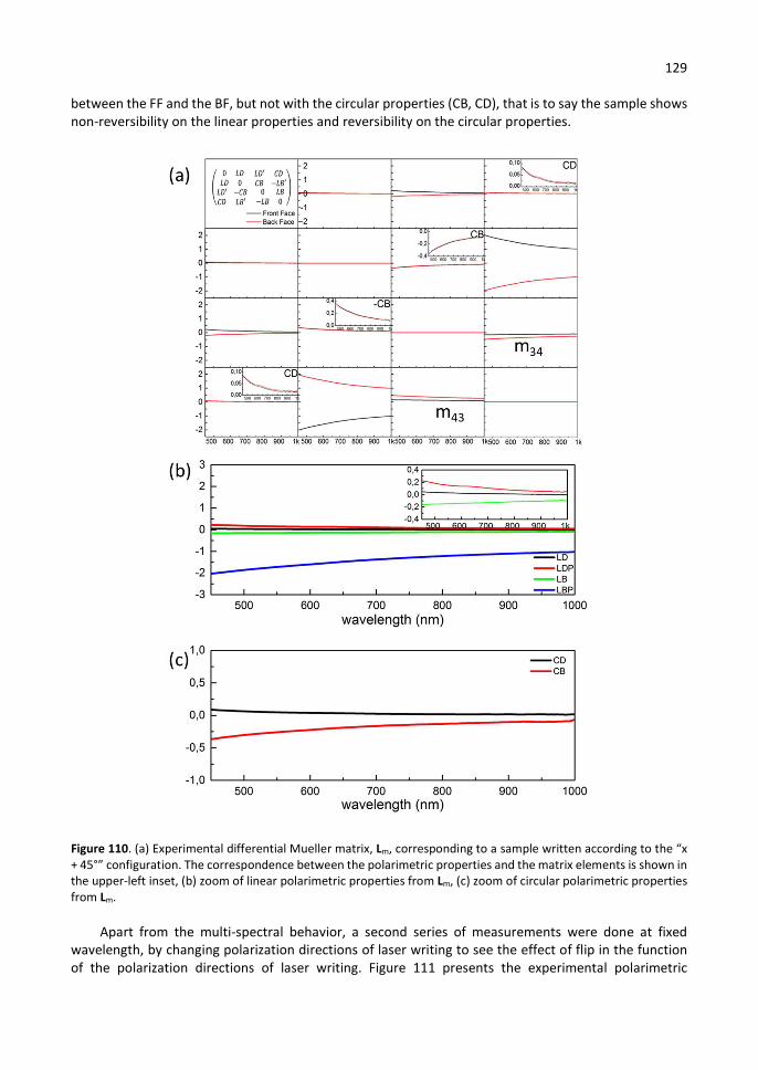
129

between the FF and the BF, but not with the circular properties (CB, CD), that is to say the sample shows non-reversibility on the linear properties and reversibility on the circular properties.

Figure 110. (a) Experimental differential Mueller matrix, Lm, corresponding to a sample written according to the “x + 45°” configuration. The correspondence between the polarimetric properties and the matrix elements is shown in the upper-left inset, (b) zoom of linear polarimetric properties from Lm, (c) zoom of circular polarimetric properties from Lm.

Apart from the multi-spectral behavior, a second series of measurements were done at fixed wavelength, by changing polarization directions of laser writing to see the effect of flip in the function of the polarization directions of laser writing. Figure 111 presents the experimental polarimetric

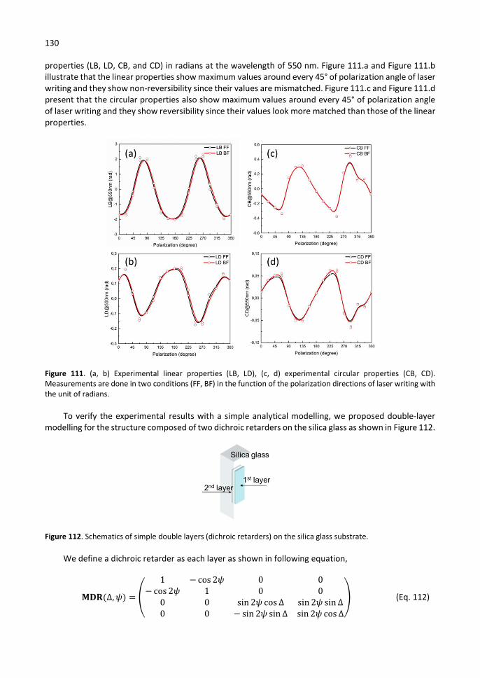
130

properties (LB, LD, CB, and CD) in radians at the wavelength of 550 nm. Figure 111.a and Figure 111.b illustrate that the linear properties show maximum values around every 45° of polarization angle of laser writing and they show non-reversibility since their values are mismatched. Figure 111.c and Figure 111.d present that the circular properties also show maximum values around every 45° of polarization angle of laser writing and they show reversibility since their values look more matched than those of the linear properties.

Figure 111. (a, b) Experimental linear properties (LB, LD), (c, d) experimental circular properties (CB, CD). Measurements are done in two conditions (FF, BF) in the function of the polarization directions of laser writing with the unit of radians.

To verify the experimental results with a simple analytical modelling, we proposed double-layer modelling for the structure composed of two dichroic retarders on the silica glass as shown in Figure 112.

Figure 112. Schematics of simple double layers (dichroic retarders) on the silica glass substrate.

We define a dichroic retarder as each layer as shown in following equation,

𝐌𝐃𝐑(Δ, 𝜓) =

1 − cos 2𝜓 0 0− cos 2𝜓 1 0 0

0 0 sin 2𝜓 cos Δ sin 2𝜓 sin Δ0 0 − sin 2𝜓 sin Δ sin 2𝜓 cos Δ

(Eq. 112)

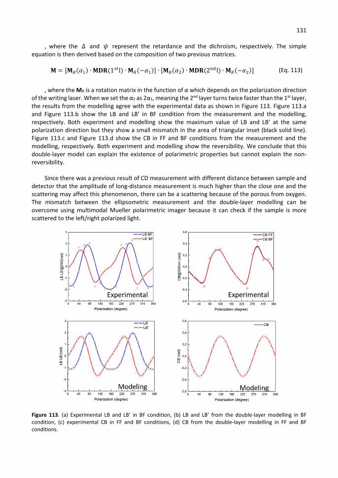
131

, where the ∆ and 𝜓 represent the retardance and the dichroism, respectively. The simple equation is then derived based on the composition of two previous matrices.

𝐌 = [𝐌 (𝛼 ) ∙ 𝐌𝐃𝐑(1 l) ∙ 𝐌 (−𝛼 )] ∙ [𝐌 (𝛼 ) ∙ 𝐌𝐃𝐑(2 l) ∙ 𝐌 (−𝛼 )] (Eq. 113)

, where the MR is a rotation matrix in the function of α which depends on the polarization direction of the writing laser. When we set the α2 as 2α1, meaning the 2nd layer turns twice faster than the 1st layer, the results from the modelling agree with the experimental data as shown in Figure 113. Figure 113.a and Figure 113.b show the LB and LB’ in BF condition from the measurement and the modelling, respectively. Both experiment and modelling show the maximum value of LB and LB’ at the same polarization direction but they show a small mismatch in the area of triangular inset (black solid line). Figure 113.c and Figure 113.d show the CB in FF and BF conditions from the measurement and the modelling, respectively. Both experiment and modelling show the reversibility. We conclude that this double-layer model can explain the existence of polarimetric properties but cannot explain the non-reversibility.

Since there was a previous result of CD measurement with different distance between sample and detector that the amplitude of long-distance measurement is much higher than the close one and the scattering may affect this phenomenon, there can be a scattering because of the porous from oxygen. The mismatch between the ellipsometric measurement and the double-layer modelling can be overcome using multimodal Mueller polarimetric imager because it can check if the sample is more scattered to the left/right polarized light.

Figure 113. (a) Experimental LB and LB’ in BF condition, (b) LB and LB’ from the double-layer modelling in BF condition, (c) experimental CB in FF and BF conditions, (d) CB from the double-layer modelling in FF and BF conditions.

132

6.2.4. Conclusion

We've seen experimentally non-reversibility on the linear properties (LD, LB) and reversibility on the circular properties (CD, CB). The double layer modelling to explain the existence of the circular and linear polarimetric properties of silica glass treated by the FLDW process works well explaining the existence of polarimetric properties.

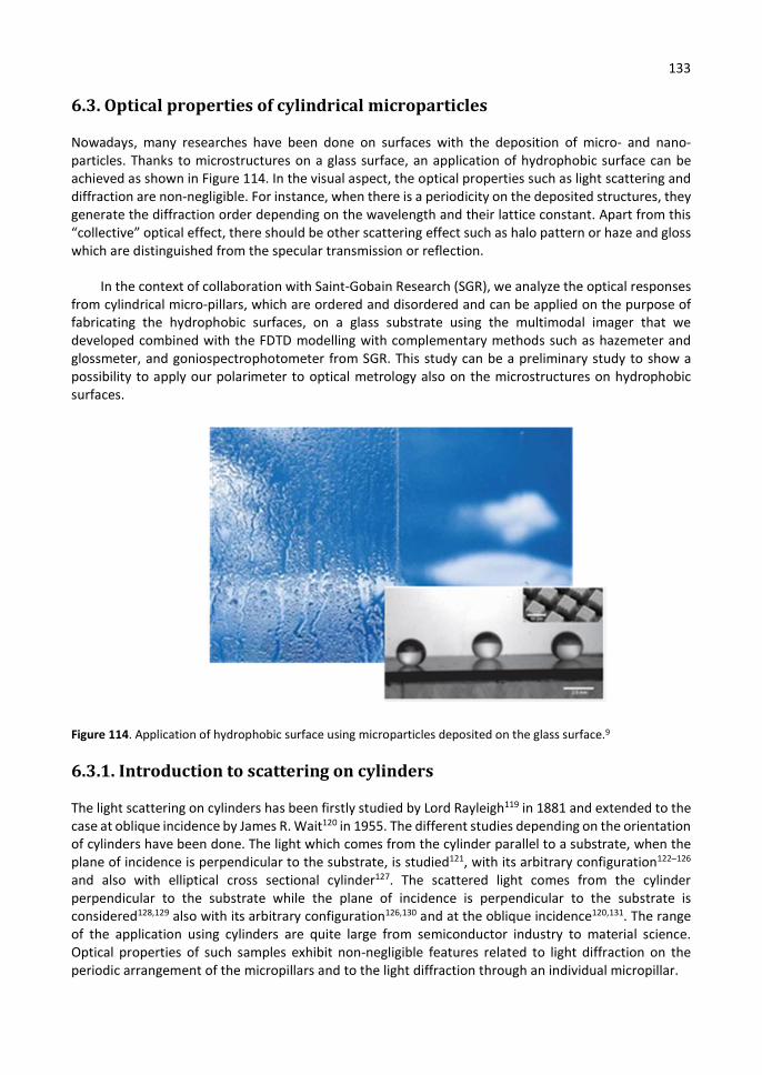
133

6.3. Optical properties of cylindrical microparticles

Nowadays, many researches have been done on surfaces with the deposition of micro- and nano-particles. Thanks to microstructures on a glass surface, an application of hydrophobic surface can be achieved as shown in Figure 114. In the visual aspect, the optical properties such as light scattering and diffraction are non-negligible. For instance, when there is a periodicity on the deposited structures, they generate the diffraction order depending on the wavelength and their lattice constant. Apart from this “collective” optical effect, there should be other scattering effect such as halo pattern or haze and gloss which are distinguished from the specular transmission or reflection.

In the context of collaboration with Saint-Gobain Research (SGR), we analyze the optical responses from cylindrical micro-pillars, which are ordered and disordered and can be applied on the purpose of fabricating the hydrophobic surfaces, on a glass substrate using the multimodal imager that we developed combined with the FDTD modelling with complementary methods such as hazemeter and glossmeter, and goniospectrophotometer from SGR. This study can be a preliminary study to show a possibility to apply our polarimeter to optical metrology also on the microstructures on hydrophobic surfaces.

Figure 114. Application of hydrophobic surface using microparticles deposited on the glass surface.9

6.3.1. Introduction to scattering on cylinders

The light scattering on cylinders has been firstly studied by Lord Rayleigh119 in 1881 and extended to the case at oblique incidence by James R. Wait120 in 1955. The different studies depending on the orientation of cylinders have been done. The light which comes from the cylinder parallel to a substrate, when the plane of incidence is perpendicular to the substrate, is studied121, with its arbitrary configuration122–126 and also with elliptical cross sectional cylinder127. The scattered light comes from the cylinder perpendicular to the substrate while the plane of incidence is perpendicular to the substrate is considered128,129 also with its arbitrary configuration126,130 and at the oblique incidence120,131. The range of the application using cylinders are quite large from semiconductor industry to material science. Optical properties of such samples exhibit non-negligible features related to light diffraction on the periodic arrangement of the micropillars and to the light diffraction through an individual micropillar.

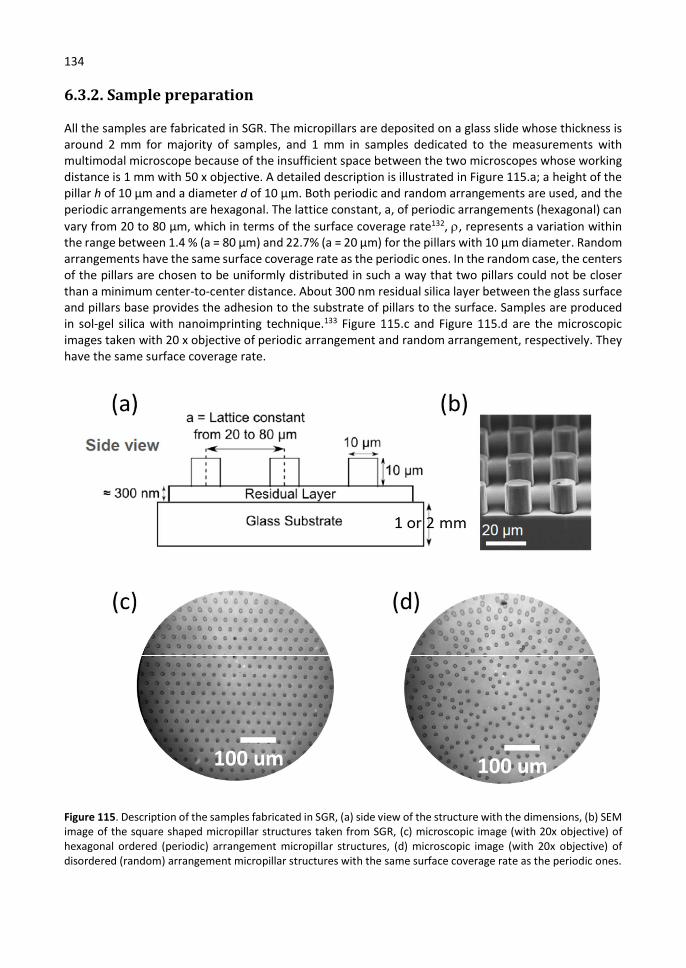
134

6.3.2. Sample preparation

All the samples are fabricated in SGR. The micropillars are deposited on a glass slide whose thickness is around 2 mm for majority of samples, and 1 mm in samples dedicated to the measurements with multimodal microscope because of the insufficient space between the two microscopes whose working distance is 1 mm with 50 x objective. A detailed description is illustrated in Figure 115.a; a height of the pillar h of 10 µm and a diameter d of 10 µm. Both periodic and random arrangements are used, and the periodic arrangements are hexagonal. The lattice constant, a, of periodic arrangements (hexagonal) can vary from 20 to 80 µm, which in terms of the surface coverage rate132, , represents a variation within the range between 1.4 % (a = 80 µm) and 22.7% (a = 20 µm) for the pillars with 10 µm diameter. Random arrangements have the same surface coverage rate as the periodic ones. In the random case, the centers of the pillars are chosen to be uniformly distributed in such a way that two pillars could not be closer than a minimum center-to-center distance. About 300 nm residual silica layer between the glass surface and pillars base provides the adhesion to the substrate of pillars to the surface. Samples are produced in sol-gel silica with nanoimprinting technique.133 Figure 115.c and Figure 115.d are the microscopic images taken with 20 x objective of periodic arrangement and random arrangement, respectively. They have the same surface coverage rate.

Figure 115. Description of the samples fabricated in SGR, (a) side view of the structure with the dimensions, (b) SEM image of the square shaped micropillar structures taken from SGR, (c) microscopic image (with 20x objective) of hexagonal ordered (periodic) arrangement micropillar structures, (d) microscopic image (with 20x objective) of disordered (random) arrangement micropillar structures with the same surface coverage rate as the periodic ones.

135

6.3.3. Optical response based on haze and gloss

In this section, we introduce the conventional measurements of the samples on a haze and a gloss which have been done in the framework of research in SGR. The haze is defined as percentage of transmitted light, passing through a specimen, which deviates from the incident light more than 0.044 rad (2.5°) by forward scattering. 134 The gloss describes specular component of reflected or transmitted light, while haze describes the integrated scattering either from the surface (haze in reflection) or through the sample (haze in transmission). The gloss can be measured at three different incidences: 20°, 60° and 80°.135 For historical reasons, the haze measurement is generally performed in transmission at normal incidence, while the gloss is measured in reflection at various angles of incidence. A model of the hazemeter is “BYK Gardner Haze-gard plus” in transmission and a model of the glossmeter is “Enrichsen-Pico Glossemaster Model 500” in reflection.

Figure 116 shows the results of haze and gloss measurements as a function of lattice constant and pillar coverage ratio, showing the difference between haze and gloss from the periodic hexagonal arrangement sample (Figure 116.a). The gloss is measured at an oblique incidence of 20°. Figure 116.b shows the different on haze between ordered and disordered arrangement samples. According to these results, the haze increases while the gloss decreases as a function of the pillar coverage ratio and this behavior indicates the increase in the amount of light transmitted out of the specular direction. It can be assumed that the specular component progressively decreases while the diffuse component increases regardless of the arrangement of the pillars. This observation is consistent with the decreasing level of measured gloss level. However, these standard approaches using the glossmeter and the hazemeter have a difficulty to observe angle-resolved optical response.132 Since the angle-resolved optical responses are the non-negligible parameter in terms of an aesthetic issue on glass products, the angle-resolved measurements using an imaging system in the Fourier plane are necessary to complete this analysis

Figure 116. (a) Experimental haze and gloss levels of micropillars. Gloss measured at 20° of angle of incidence and haze measured at normal incidence on periodic hexagonal arrangements of micropillars, (b) comparison of experimental haze between the periodic hexagonal and random arrangements of micropillars.

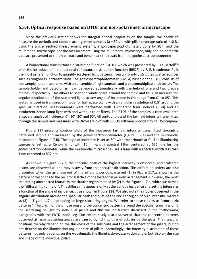
136

6.3.4. Optical response based on BTDF and non-polarimetric microscope

Since the previous section shows the integral optical properties on the sample, we decide to measure the periodic and random arrangement samples (a = 30 μm with pillar coverage ratio of ~10 %) using the angle-resolved measurement systems, a goniospectrophotometer; done by SGR, and the multimodal microscope. For the measurement using the multimodal microscope, only non-polarimetric data are presented to simply validate and benchmark the result from the goniospectrophotometer.

A bidirectional transmittance distribution function (BTDF), which was presented by F. O. Bartell136 after the introduce of a bidirectional reflectance distribution function (BRDF) by F. E. Nicodemus137, is the most general function to quantify scattered light patterns from uniformly distributed scatter sources such as roughness in transmission. The goniospectrophotometer (OMS4) based on the BTDF consists of the sample holder, two arms with an ensemble of light sources, and a photomultiplicator detector. The sample holder and detector arm can be moved automatically with the help of one and two precise motors, respectively. This allows to scan the whole space around the sample and thus, to measure the angular distribution of the scattered light, at any angle of incidence in the range from 0° to 85°. This system is used in transmission mode for half space scans with an angular resolution of 0.5° around the specular direction. Measurements were performed with 3 coherent laser sources (RGB) and an incoherent Xenon lamp light with and without color filters. The BTDF of the samples is then evaluated at several angles of incidence: 0°, 10°, 30° and 60°. All contour plots of the far-field intensity transmitted through the sample and measured with OMS4 are plot with SPEOS software provided by OPTIS company.

Figure 117 presents contour plots of the measured far-field intensity transmitted through a patterned sample and measured by the goniospectrophotometer (Figure 117.a) and the multimodal microscope (Figure 117.b). The angle of incidence is set as 30° with the azimuth at 0°. The illuminating sources is set as a Xenon lamp with 10 nm-width spectral filter centered at 535 nm for the goniospectrophotometer, while the multimodal microscope uses a laser with a spectral width less than 1 nm centered at 532 nm.

As shown in Figure 117.a, the specular peak of the highest intensity is observed, and scattered beams are observed as one moves away from the specular direction. The diffraction orders are also presented when the arrangement of the pillars is periodic, marked (1) in Figure 117.a, showing the pattern corresponds to the reciprocal lattice of the hexagonal periodic arrangement. However, the most interesting unexpected feature is the circular region marked by (2) in the Figure 117.a, which we named the “diffuse ring (or halo)”. This diffuse ring appears only at the oblique incidence and getting intense as a function of the angle of incidence, i, as shown in Figure 118. We also note the ripples observed in the angular distribution around the specular peak and outside the circular region of high intensity, marked as (3) in Figure 117.a, spreading to large scattering angles. We refer to these ripples as “concentric patterns”. The origin of the diffuse ring and the concentric patterns around the specular transmission is the scattering of light by individual pillars and this will be further discussed in the forthcoming paragraphs with the FDTD modelling. Our recent study also discovered that the concentric patterns observed at large scattering angles are caused by light guiding effects inside the glass. Their angular positions thereby depend on the thickness of the substrate and the arrangement of the pillars, but do not depend on the illumination angle or size of pillars. Accordingly, the intensity distribution of those patterns not only depends on the wavelength, the illumination/observation angle, but also on the size and shape of the individual pillars.

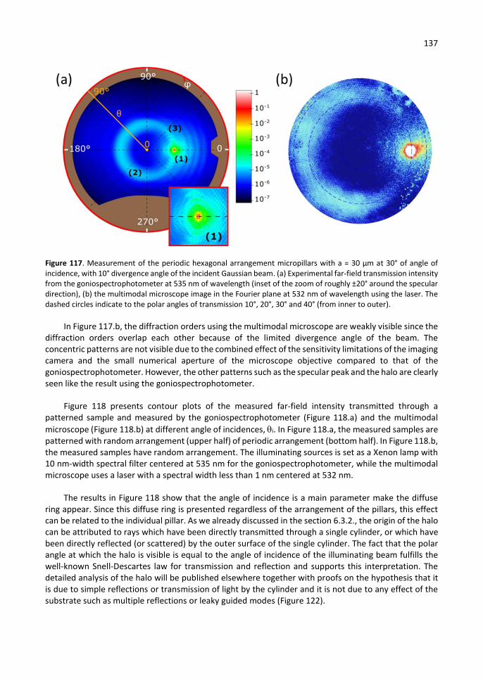
137

Figure 117. Measurement of the periodic hexagonal arrangement micropillars with a = 30 µm at 30° of angle of incidence, with 10° divergence angle of the incident Gaussian beam. (a) Experimental far-field transmission intensity from the goniospectrophotometer at 535 nm of wavelength (inset of the zoom of roughly ±20° around the specular direction), (b) the multimodal microscope image in the Fourier plane at 532 nm of wavelength using the laser. The dashed circles indicate to the polar angles of transmission 10°, 20°, 30° and 40° (from inner to outer).

In Figure 117.b, the diffraction orders using the multimodal microscope are weakly visible since the diffraction orders overlap each other because of the limited divergence angle of the beam. The concentric patterns are not visible due to the combined effect of the sensitivity limitations of the imaging camera and the small numerical aperture of the microscope objective compared to that of the goniospectrophotometer. However, the other patterns such as the specular peak and the halo are clearly seen like the result using the goniospectrophotometer.

Figure 118 presents contour plots of the measured far-field intensity transmitted through a patterned sample and measured by the goniospectrophotometer (Figure 118.a) and the multimodal microscope (Figure 118.b) at different angle of incidences, i. In Figure 118.a, the measured samples are patterned with random arrangement (upper half) of periodic arrangement (bottom half). In Figure 118.b, the measured samples have random arrangement. The illuminating sources is set as a Xenon lamp with 10 nm-width spectral filter centered at 535 nm for the goniospectrophotometer, while the multimodal microscope uses a laser with a spectral width less than 1 nm centered at 532 nm.

The results in Figure 118 show that the angle of incidence is a main parameter make the diffuse ring appear. Since this diffuse ring is presented regardless of the arrangement of the pillars, this effect can be related to the individual pillar. As we already discussed in the section 6.3.2., the origin of the halo can be attributed to rays which have been directly transmitted through a single cylinder, or which have been directly reflected (or scattered) by the outer surface of the single cylinder. The fact that the polar angle at which the halo is visible is equal to the angle of incidence of the illuminating beam fulfills the well-known Snell-Descartes law for transmission and reflection and supports this interpretation. The detailed analysis of the halo will be published elsewhere together with proofs on the hypothesis that it is due to simple reflections or transmission of light by the cylinder and it is not due to any effect of the substrate such as multiple reflections or leaky guided modes (Figure 122).

138

Figure 118. (a) BTDF measurement of the sample with periodic hexagonal (bottom half) pattern of micro-pillars of the lattice constant 30 µm and the equivalent random (upper half) pattern. θi of 10°, 30° and 60°, measured with filtered Xenon lamp (535 nm). The insets show zoom of roughly ±20° around the specular direction. (b) Measured in Fourier imaging mode, far-field distribution of the normalized total intensity, transmitted through glass patterned with random arrangement of micropillars with surface coverage ratio of 10%. Illumining beam was set at three different angles of incidence 0°, 10°, 20° and 30°. The angular aperture of the illumination beam was set to 10° in all the three cases. All measurements were done at 532 nm.

139

After the analysis with the measurement data, the FDTD modelling is done with a single pillar to focus on the optical response from the individual pillar. Figure 119 shows the normalized far-field intensity transmitted through a single cylinder at an oblique incidence, θi = 30° (a) and θi = 60° (b), calculated using the FDTD method with the wavelength of 532 nm. There are no diffraction orders since the modelling is done with a single pillar but the other patterns such as specular peak, diffuse ring, and concentric patters are clearly visible.

Figure 119. Modelling of normalized far-field intensity transmitted through a single cylinder at an oblique incidence, θi = 30° (a) and θi = 60° (b) using the FDTD method.

In Figure 120, we model by changing the diameter (d = 10 µm, 5 µm) of a single pillar to verify how the concentric patterns change as a function of the diameter of an individual pillar. Figure 120.a and Figure 120.b show the normalized far-field intensity transmitted through a single cylinder at an oblique incidence, θi = 30°, varying the diameter of single pillar, d = 10 µm, d = 5 µm, respectively. If we compare the values in the region of interest as a function of the plane of incidence marked as orange solid square, it is obvious that the frequency of the concentric patterns varies with the diameter of individual pillar (Figure 120.c). According to this, like the diffuse ring, the origin of the concentric patterns can also be understood in the framework of either the extended Mie theory for non-spherical particles131, or the Debye series approach138.

Figure 120. Modelling of normalized far-field intensity transmitted through a single cylinder at an oblique incidence, θi = 30°, varying the diameter of single pillar, d = 10 µm (a), d = 5 µm (b), and the cross-sectional plot (c) along the plane of incidence at 0° of azimuth in the region of interest (orange solid square) using the FDTD method.

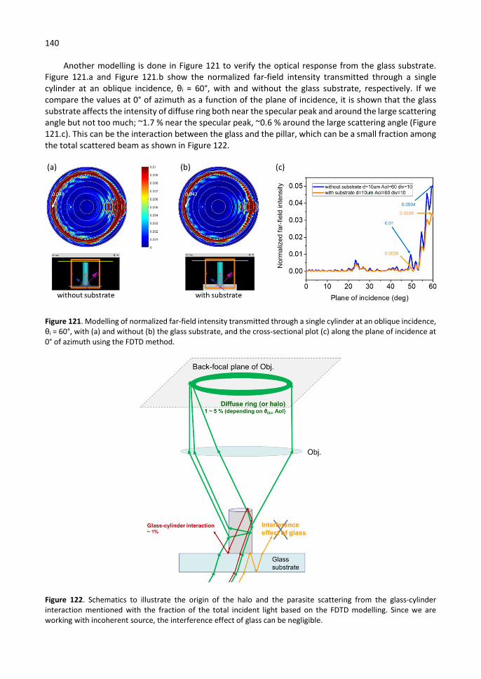
140

Another modelling is done in Figure 121 to verify the optical response from the glass substrate. Figure 121.a and Figure 121.b show the normalized far-field intensity transmitted through a single cylinder at an oblique incidence, θi = 60°, with and without the glass substrate, respectively. If we compare the values at 0° of azimuth as a function of the plane of incidence, it is shown that the glass substrate affects the intensity of diffuse ring both near the specular peak and around the large scattering angle but not too much; ~1.7 % near the specular peak, ~0.6 % around the large scattering angle (Figure 121.c). This can be the interaction between the glass and the pillar, which can be a small fraction among the total scattered beam as shown in Figure 122.

Figure 121. Modelling of normalized far-field intensity transmitted through a single cylinder at an oblique incidence, θi = 60°, with (a) and without (b) the glass substrate, and the cross-sectional plot (c) along the plane of incidence at 0° of azimuth using the FDTD method.

Figure 122. Schematics to illustrate the origin of the halo and the parasite scattering from the glass-cylinder interaction mentioned with the fraction of the total incident light based on the FDTD modelling. Since we are working with incoherent source, the interference effect of glass can be negligible.

141

6.3.5. Conclusion

In this section, the angular-resolved optical response of glass substrates uniformly covered cylindrical micropillars. Although in practice, these microstructures are interesting for they wettability properties, when integrated in building elements such windows, they optical response may have a visual effect that may impact the esthetic properties of the final product and therefore it is necessary to understand and to control them. The general protocol to characterize the optical response of glossy (or scattering) surfaces is done with integral measurements, however, it was found that due to the complex optical response of the micropillars the integral measurements do not provide enough information reason why angular-resolved measurements were used.

Thanks to the use of two complementary angle resolved instruments; the goniospectrophotometer from SGR and the multimodal polarimetric microscope, it was possible to identify three different optical features: diffraction orders when the micropillars are deposited in ordered patters, a diffuse ring, and interference patterns.

We concluded that the halo and the concentric patterns around the specular transmission come from the light scattered by every individual pillar. The intensity distribution of those patterns not only depends on the wavelength, the illumination or observation angle, but also on the size and shape of the individual pillars. The effect of glass substrate was also studied. It was concluded that it has a minor effect on the intensity distribution of the interference patters near the specular peak and around the large scattering angles. This is due to the fact that the substrate has a low refractive index and also this index is well-matched with that of the micropillars.

It has been shown that the multimodal polarimetric microscope combined with the FDTD numerical modelling can provide equivalent information than the BTDF measurements with the goniospectrophotometer, which is a well stablished technique in optical metrology. Therefore, these results show that the multimodal polarimetric microscope can be considered as a valid approach for in-situ or ex-situ characterization of patterned samples with microstructures showing a complex optical response.

142

Chapter 7. General conclusions and perspectives

The main objective of this thesis was to study the interaction of polarized light from the scattering media and particles. A variety of aspects have been treated, including the basic theory on Muller polarimetry, the instrumental development, the advanced numerical simulation, and the creation of measurement protocols for the interpretation of complex data. In the first part of the present manuscript prior to the presentation of the different aspects treated during the Ph.D., a general overview is provided on basic concepts of polarimetric instrumentation, mathematical formalisms, the three main polarimetric properties which were extensively used in the Ph.D. together with the concept of logarithmic (or differential) decomposition used to disentangle polarimetric information from Mueller matrices.

The first part of the Ph.D. was devoted to the development of an innovative instrument, called Multimodal Muller Polarimetric Imager, which is suitable for taking polarimetric images at different scales (from millimeters to microns) and which can be quickly reconfigured to offer different imaging modes. The multimodal imaging allows obtaining polarimetric images in either real or Fourier planes, which is equivalent to get information about the spatial resolved, or the angular-resolved polarimetric response of the sample. The system also allows a precise control of the size of the sample that it is illuminated, and the aperture of the beam used either to illuminate or to analyze the sample by the use of pinholes in the conjugated planes of i) the object and ii) the Fourier planes of the two microscope objectives. The system has been characterized to determine its repeatability, precision and accuracy.

An important effort has been put to study the polarimetric response of particles of micrometric size. The selection of the particles studied was done in analogy to the size of the cells in biological tissues, and which are responsible for the dispersion of light. This choice is motivated by the fact that we believe that the multimodal polarimetric microscope can be successfully applied in the area of biomedical optics to study and characterize the optical properties of thin histological cuts which are frequently used by pathologists and medical doctors to study or to diagnose pathologies. To do so the polarimetric properties of light scattered by the microparticles was analyzed when they were illuminated at either normal incidence or at oblique incidence respect to the axis of the microscope. The illumination at normal incidence showed consistent results with previous studies, which were used to validate the operation mode of the multimodal microscope and the data analysis protocol. The illumination at oblique incidence was a novelty since none other study in the literature has been performed in such conditions. This was possible thanks to the unique characteristics of the multimodal polarimeter, which allows a precise control of the direction and aperture used to illuminate the sample. The results of the measurements at oblique incidence show a surprisingly strong apparent optical activity in the optical response of the microparticles. Interestingly it was found that the apparent optical activity was sensitive to the illumination direction but also to the shape of the proved particles. A very precise and meticulous modelling of the transformations of light polarization due to the sample and the focusing and imaging by high aperture objectives was needed to conclude that the origin of the apparent circular birefringence was due to topological phase due to the fact that the main axis of the particle and the polarimeter are not parallel for illumination at oblique incidence. In order to prove the topological origin of the apparent circular birefringence as well as its sensitivity to the shape of the proved particles the following case studies were extensively analyzed: the single linear dipole, the spherical particle and the spheroidal particles. The linear dipole and the spherical particles were treated with an exact formalism, whereas the spheroids were modelled using a numerical solution of Maxwell equations. In all cases the results consistent results were obtained, and the model predictions were confirmed by experimental results.

143

The further studies on the topological phases can be done to apply this technique in different areas, not only biomedical imaging, but also any application involving the use of microparticles such as meteorology for climate prediction, pollutant detection, or assessment of the visual appearance of materials.

A second topic related to the use the multimodal polarimetric imager to study the dependence of the polarization and depolarization properties of a scattering media with their thickness, was also extensively explored. The motivation of the work is that the polarization response of complex media such histological cuts of biologic tissues is not only affected by the intrinsic properties of the proved media but also other parameters such as their thickness. In practice unexpected, unknown or uncontrolled thickness variations (less than 1 µm) in preparation of histological cuts can cause great uncertainty when it comes to interpret polarimetric data measured from them. Thanks to the approach followed in this work it has been possible to devise a method to eliminate the effect of the sample thickness from the polarimetric response of the sample. The method is based on the validity of the randomly fluctuating medium model. According to the latter, the polarimetric properties are proportional to the thickness of the sample whereas the depolarization is proportional to the square of this latter one. The model was first validated with reference samples and then applied to real tissues. In all cases the results predicted by the model were in accordance with the experimental observations. Those results allowed to develop a method which allowed to efficiently remove the effect of the thickness from the polarization properties of the sample. This discovery could be used to develop a method of data analysis that overcomes the effect of thickness variations, thus making the measurements very robust and related only to the intrinsic properties of the samples studied.

For other possible applications of our multimodal imager, we carried out the study on the optical responses from the pseudo-chiral metasurfaces as an application of anticounterfeiting. We have shown how the contrast of images could be encoded in circular dichroism by using the magnetoelectric coupling yielded by plasmonic resonances of pseudochiral metasurfaces. We have shown the possible application of the multimodal Mueller polarimetric imager to verify the dependency of the intensity observed in circular dichroism and between crossed polarizers of an image built from pixels containing U-shaped resonators. We have confirmed experimentally the theoretical results using a palette of 10 levels of contrasts. The possibility to design covert images revealed only between crossed polarizers and with contrast reversal in circular dichroism was shown by creating a pseudochiral metasurface containing a representation of Mona Lisa. These results evidence that pseudochiral resonators present an additional degree of security compared to images encoded in linear polarizations, which would not possibly show such contrast reversal upon angle of observation changes. Different colors may be obtained by using different materials expanding the accessible resonances to the blue part of the spectrum and combining different types of resonators in the same pixel. Better contrast variations may also be obtained by increasing the number of resonators in each pixel, to the detriment of lateral resolution.

In addition to the main topic of the Ph.D., the development of the multimodal polarimetric imager attracted the attention of a number of researchers, and as a result, a number of new collaborations were created. The results of the work done in the framework of three of these collaborations have been summarized in the last chapter of the manuscript. The three collaborations were selected because of the extent of the work done, and also for the relevance of the explored topics to illustrate the multiple applications of multimodal polarimetric imager.

In the first case it has been shown how contrasts of images could be encoded in circular dichroism by using the magneto-electric coupling yielded by plasmonic resonances of pseudo-chiral metasurfaces. The modeling the optical response of pseudo-chiral plasmonic resonators it was possible to derive the

144

equations yielding the dependency of the intensity observed in circular dichroism and between crossed polarizers of an image built from pixels containing U-shaped resonators. The theoretical predictions were proved experimentally with the design of a palette of resonators showing 10 levels of contrasts. The possibility to design covert images revealed only between crossed polarizers and with contrast reversal in circular dichroism, was shown by creating a pseudo-chiral metasurface containing a representation of Mona Lisa and fully characterized with the multimodal imager.

In the second case, the object of study focused on the characterization of the optical properties of glasses which had been irradiated with femtosecond laser pulses. The effect of the femtosecond laser pulses was to locally modify the structure of the glasses, which induced form of birefringence which could be measured with a spectroscopic polarimeter. It was found that some of the samples studied showed an unexpected non-reversible optical response which could be explained with the use of a double layer model describing a non-uniform distribution of birefringence in the direction of propagation of the femtosecond laser pulse. The non-uniform birefringence induced a strong circular retardance, which was responsible of the observed non-reversibility. The significant linear and circular properties induced by the irradiation of laser pulses on glasses open the possibility to use them to design innovative optical elements to control the transmission and polarization properties in a non-conventional way.

Finally, in the third case, the multimodal imaging polarimeter was used to study the optical properties of glass substrates with surfaces patterned by an ensemble of micropillars. The multimodal imaging polarimeter was used to complete with angularly resolved measurements the information retrieved with standard techniques based in the evaluation of gloss and haze which are integrated observables. As a result, it was possible to identify three different optical effects induced by the presence of the micropillars on the surface of the samples. The results obtained with the multimodal imaging polarimeter were in accordance those obtained with a goniospectrophotometer, which is considered a standard instrument to perform angular-resolved measurements. The latter result demonstrated the validity of the multimodal imaging polarimeter to be used for in-situ and ex-situ characterization of patterned surfaces showing complex optical responses.

I have shown many possible applications of the Muller polarimetric microscope developed in the framework of this Ph.D. The successful application of the Mueller polarimetric imager to a variety of studies is very encouraging and suggests plenty of research topics that hopeful will be developed in the near future. Among them it is possible to cite for example:

i) the application of different Mueller matrix decompositions on different samples to further improve our understanding of how different scattering process contribute to explain the polarization and depolarization properties of light,

ii) the detailed explanation on the topological phases with well-defined or controlled spheroidal curvatures to improve the precision and accuracy with which the polarimetric measurements can be used to characterize the shape of micrometric objects,

iii) to develop new observables and image process methods to improve the analysis efficiency of polarimetric images of thin sections of histological tissues which can be used to develop either basic science in biology or to the diagnosis of pathologies by medical doctors,

145

iv) to further study the origin of reversibility and non-reversibility on the polarimetric properties on FLDW application,

v) the development of robust and easy to use FDTD based scripts and software applications to model the optical response of complex samples in terms of Mueller matrices

In any case at the end of this Ph.D., I’m sure that the fact that the multimodal Muller polarimetric microscope is a promising tool for many uncovered applications in science and technology is beyond question.

146

List of publications

Peer-reviewed journals

[1] Jing Tian, Rubing Li, Sang Hyuk Yoo, Bertrand Poumellec, Enric Garcia-Caurel, Razvigor Ossikovski, Michel Stchakovsky, Céline Eypert, John Canning and Matthieu Lancry, “Spectral dependence of femtosecond laser induced circular optical properties in silica,” OSA Continuum 2, 1233-1241 (2019).

[2] Colette Turbil, Thomas Sang Hyuk Yoo, Ingve Simonsen, Jeremie Teisseire, Iryna Gozhyk, Enric Garcia-Caurel, “Experimental studies of the transmission of light through low-coverage regular or random arrays of silica micropillars supported by a glass substrate,” Appl. Opt. 58, 9267-9278 (2019).

[3] Hee Ryung Lee, Pengcheng Li, Thomas Sang Hyuk Yoo, Christian Lotz, Florian Kai Groeber-Becker, Sofia Dembski, Enric Garcia-Caurel, Razvigor Ossikovski, Hui Ma, Tatiana Novikova, "Digital histology with Mueller microscopy: how to mitigate an impact of tissue cut thickness fluctuations," J. Biomed. Opt. 24(7) 076004 (2019).

[4] Thomas Sang Hyuk Yoo, Johann Berthelot, Géraldine Guida, Dominique Demaille, Enric Garcia-Caurel, Nicolas Bonod, and Bruno Gallas, “Circularly Polarized Images with Contrast Reversal Using Pseudochiral Metasurfaces,” ACS Photonics, 5 (10), pp. 4068-4073 (2018).

[5] Razvigor Ossikovski, Oriol Arteaga, Sang Hyuk Yoo, Enric Garcia-Caurel, and Kurt Hingerl, “Experimental evidence for partial spatial coherence in imaging Mueller polarimetry,” Optics Letters, Vol. 42, Issue 22, pp. 4740-4743 (2017).

[6] J. Tian, M. Lancry, S. H. Yoo, E. Garcia-Caurel, R. Ossikovski, and B. Poumellec, “Study of femtosecond laser-induced circular optical properties in silica by Mueller matrix spectropolarimetry,” Optics Letters, Vol. 42, Issue 20, pp. 4103-4106 (2017).

[7] Sang Hyuk Yoo, Razvigor Ossikovski and Enric Garcia-Caurel, “Experimental study of thickness dependence of polarization and depolarization properties of anisotropic turbid media using Mueller matrix polarimetry and differential decomposition,” Applied Surface Science 421PB, pp. 870-877 (2017).

Conference proceedings

[1] Thomas Sang Hyuk Yoo, Andrea Fernández, Fernando Moreno, Jose Maria Saiz, Razvigor Ossikovski, Enric Garcia-Caurel, “Multimodal imaging Mueller polarimetric microscope to study polarimetric properties of spheroidal microparticles,” Proc. SPIE 10678, Optical Micro- and Nanometrology VII, 106780J (24 May 2018).

Oral presentations [1] “Mueller matrix imaging polarimetric scatterometry to study polarimetric properties of diffraction

gratings,” SPIE Photonics Europe 2018, Strasbourg, France, 22-26 April (2018).

[2] “Transmission Mueller Polarimetry and Differential Decomposition: Thickness Dependence of the Depolarization and Polarization Properties of Isotropic and Anisotropic Turbid Media,” 1st International Conference on Optics, Photonic and Materials (NICE OPTICS), Nice, France, 26-28 October (2016).

147

Poster presentations

[1] “Effect of Geometric Phases in the Polarimetric Response of Small Particles Illuminated at Oblique Incidence,” 2nd International Workshop on Biophotonics and Optical Angular Momentum (BIOAM-2018), Palaiseau, France, 25-26 October (2018).

[2] “Multimodal imaging Mueller polarimetric microscope on geometrical analysis of spheroidal microparticles,” OSA Frontiers in Optics 2018 (FiO), Washington, USA, 16-20 September (2018).

[3] “Variation of polarimetric properties of isotropic and anisotropic scattering samples with thickness within the framework of differential Mueller matrix formalism,” 1st European Workshop on Biophotonics and Optical Angular Momentum (BIOAM), Palaiseau, France, 14-15 November (2016).

[4] “Experimental Study of Thickness Dependence of the Polarization and Depolarization Properties of Anisotropic Turbid Media using Mueller matrix Polarimetry and Differential Decomposition,” 7th International Conference on Spectroscopic Ellipsometry (ICSE-7), Berlin, Germany, June 06-10 (2016).

Other contributions

[1] Sergey SAVENKOV, Thomas Sang Hyuk YOO, Enric GARCIA-CAUREL, Yevgen OBEREMOK, Ivan KOLOMIETS, Tatiana NOVIKOVA, Razvigor OSSIKOVSKI, and Alexander KLIMOV, “Polarization Memory in Inhomogeneous Elliptical Birefringent Medium,” 2nd International Workshop on Biophotonics and Optical Angular Momentum (BIOAM-2018), Palaiseau, France, 25-26 October (2018).

[2] Heeryung LEE, Thomas Sang Hyuk Yoo, Pengcheng Li, Christian Lotz, Florian Kai Groeber-Becker, Sofia Dembski, Enric Garcia-Caurel, Razvigor Ossikovski, and Tatiana Novikova, “Digital Histology with Mueller Polarimetry,” 2nd International Workshop on Biophotonics and Optical Angular Momentum (BIOAM-2018), Palaiseau, France, 25-26 October (2018).

[3] A. Fernández, Thomas Sang Hyuk Yoo, J.L. Fernández-Luna, F. Moreno, Enric Garcia-Caurel, J.M. Saiz, “Modelling the Adhesion of a Spherical Particle to a Substrate with Geometric Optics and Polarimetry,” 2nd International Workshop on Biophotonics and Optical Angular Momentum (BIOAM-2018), Palaiseau, France, 25-26 October (2018).

[4] A. Fernández, Thomas Sang Hyuk Yoo, J.L. Fernández-Luna, F. Moreno, Enric Garcia-Caurel, J.M. Saiz, “Modelling the Adherence of a Cell to a Flat Substrate through Polarimetric Methods Based on Mueller Matrix Formalism,” Progress in Electromagnetics Research Symposium (PIERS 2018), Toyama, Japan, 1-4 August (2018).

[5] J. Tian, M. Lancry, S. H. Yoo, E. Garcia-Caurel, R. Ossikovski, and B. Poumellec, “Evidence by Mueller spectropolarimetry of optical rotation imprinted by femtosecond laser in silica,” OSA Advanced Photonics Congress 2018, Zürich, Switzerland, 2-5 July (2018).

[6] Hee Ryung Lee, Thomas Sang Hyuk Yoo, Pengcheng Li, Enric Garcia-Caurel, Razvigor Ossikovski, Christian Lotz, Florian Kai Groeber-Becker, Sofia Dembski, Tatiana Novikova, “Mueller microscopy of anisotropic scattering media: theory and experiments,” SPIE Photonics Europe 2018, Strasbourg, France, 22-26 April (2018).

[7] Tsanislava I. Genova-Hristova, Thomas Sang Hyuk Yoo, Hee Ryung Lee, Ekaterina G. Borisova, Enric Garcia-Caurel, Razvigor Ossikovski, Tatiana Novikova, Oxana Semyachkina-Glushkovskaya, Daniil Bratashov, Dmitry Gorin, Ivan Terziev, “Feasibility study of polarization imaging and confocal

148

fluorescence microscopy for histology analysis of soft tissue neoplasia,” SPIE Photonics Europe 2018, Strasbourg, France, 22-26 April (2018).

[8] Thomas Sang Hyuk Yoo, Tsanislava Genova-Hristova, Hee Ryung Lee, Ekaterina Borisova, Ivan Terziev, Enric Garcia-Caurel, Razvigor Ossikovski, Tatiana Novikova, “Polarized light histology of tissue and differential Mueller matrix formalism,” SPIE Photonics West 2018, San Francisco, California, United States, 27 January-1 February (2018).

[9] Jing Tian, Sang Hyuk Yoo, Enric Garcia-Caurel, Razvigor Ossikovski, Bertrand Poumellec, Matthieu Lancry, “Study of femtosecond laser induced circular optical properties in silica by Mueller matrix spectro-polarimetry,” SPIE Photonics West 2018, San Francisco, California, United States, 27 January-1 February (2018).

[10] Thomas Sang Hyuk Yoo, Tsanislava Genova, Hee Ryung Lee, Ekaterina Borisova, Ivan Terziev, Enric Garcia-Caurel, Razvigor Ossikovski, Tatiana Novikova, “Polarization image contrast between tumor and healthy tissues - ex vivo investigations,” 21st International School for Junior Scientists and Students on Optics, Laser Physics & Biophotonics (SFM’17), Saratov, Russia, 25-29 September (2017).

[11] H. R. Lee, S. H. Yoo, T. Genova-Hristova, E. Garcia-Caurel, E. Borisova, R. Ossikovski, T. Novikova, “Biomedical applications of Mueller polarimetry,” 4th International Conference on Optical Angular Momentum (ICOAM 17), Anacapri, Italy, 18-22 September (2017).

[12] Sergey Savenkov, Sanghyuk Yoo, Enric Garcia-Caurel, Yevgen Oberemok, Ivan Kolomiets, Tatiana Novikova, Razvigor Ossikovski, and Alexander Klimov, “Linear polarization memory of inhomogeneous birefringent medium in visible wavelength range,” 16th Electromagnetic and Light Scattering Conference ELS-XVI, Maryland/College Park, MD, United States, 19-25 March (2017).

[13] Elmar Slikboer, Sang Hyuk Yoo, Olivier Guaitella, Ana Sobota, and Enric Garcia-Caurel, “Characterization of Bismuth Silicon Oxide Crystals Using Imaging Mueller Ellipsometry,” 7th International Conference on Spectroscopic Ellipsometry (ICSE-7), Berlin, Germany, 06-10 June (2016).

149

References

[1] Garcia-Caurel, E., Ossikovski, R., Foldyna, M., Drévillon, B. and Martino, A. De., [Ellipsometry at the Nanoscale], Springer Berlin Heidelberg, Berlin, Heidelberg (2013).

[2] Azzam, R. M. A., “The intertwined history of polarimetry and ellipsometry,” Thin Solid Films 519(9), 2584–2588 (2011).

[3] Costa, E., Soffitta, P., Bellazzini, R., Brez, A., Lumb, N. and Spandre, G., “An efficient photoelectric X-ray polarimeter for the study of black holes and neutron stars,” Nature 411(6838), 662–665 (2001).

[4] Jarrendahl, K. and Kahr, B., “Hans Mueller (1900-1965),” J.A. Woollam Co., Inc.(12), 8–9 (2011).

[5] Azzam, R. M. a., “Stokes-vector and Mueller-matrix polarimetry [ Invited ],” J. Opt. Soc. Am. A 33(7), 1396–1408 (2016).

[6] Born, M. and Wolf, E., [Principles of Optics, 4th ed.], Pergamon Press, Oxford (1970).

[7] Bohren, C. F. and Huffman, D. R., [Absorption and Scattering of Light by Small Particles], Wiley-VCH Verlag GmbH, Weinheim, Germany (1998).

[8] Trompoukis, C., Abdo, I., Cariou, R., Cosme, I., Chen, W., Deparis, O., Dmitriev, A., Drouard, E., Foldyna, M., Caurel, E. G.-, Gordon, I., Heidari, B., Herman, A., Lalouat, L., Lee, K.-D., Liu, J., Lodewijks, K., Mandorlo, F., Massiot, I., et al., “Photonic nanostructures for advanced light trapping in thin crystalline silicon solar cells,” Phys. status solidi 212(1), 140–155 (2015).

[9] Tian, Y. and Jiang, L., “Wetting: Intrinsically robust hydrophobicity,” Nat. Mater. 12(4), 291–292 (2013).

[10] Lancry, M., Poumellec, B., Canning, J., Cook, K., Poulin, J. C. and Brisset, F., “Ultrafast nanoporous silica formation driven by femtosecond laser irradiation,” Laser Photonics Rev. 7(6), 953–962 (2013).

[11] Richter, S., Plech, A., Steinert, M., Heinrich, M., Döring, S., Zimmermann, F., Peschel, U., Kley, E. B., Tünnermann, A. and Nolte, S., “On the fundamental structure of femtosecond laser-induced nanogratings,” Laser Photonics Rev. 6(6), 787–792 (2012).

[12] Ghabbach, A., Zerrad, M., Soriano, G., Liukaityte, S. and Amra, C., “Depolarization and enpolarization DOP histograms measured for surface and bulk speckle patterns,” Opt. Express 22(18), 21427–21440 (2014).

[13] Davis, K. M., Miura, K., Sugimoto, N. and Hirao, K., “Writing waveguides in glass with a femtosecond laser,” Opt. Lett. 21(21), 1729 (1996).

[14] Tian, J., Lancry, M., Yoo, S. H., Garcia-Caurel, E., Ossikovski, R. and Poumellec, B., “Study of femtosecond laser-induced circular optical properties in silica by Mueller matrix spectropolarimetry,” Opt. Lett. 42(20), 4103 (2017).

[15] Arwin, H., Berlind, T., Johs, B. and Järrendahl, K., “Cuticle structure of the scarab beetle Cetonia aurata analyzed by regression analysis of Mueller-matrix ellipsometric data,” Opt. Express 21(19), 22645 (2013).

[16] Wang, W., Zhang, W., Gu, J., Liu, Q., Deng, T., Zhang, D. and Lin, H.-Q., “Design of a structure with low incident and viewing angle dependence inspired by Morpho butterflies.,” Sci. Rep. 3, 3427 (2013).

150

[17] Keereweer, S., Van Driel, P. B. A. A., Snoeks, T. J. A., Kerrebijn, J. D. F., De Jong, R. J. B., Vahrmeijer, A. L., Sterenborg, H. J. C. M. and Löwik, C. W. G. M., “Optical image-guided cancer surgery: Challenges and limitations,” Clin. Cancer Res. 19(14), 3745–3754 (2013).

[18] Mie, G., “Beitrage zur Optik truber Medien, speziell kolloidaler Metallosungen,” Ann. Phys. 25(3), 377–445 (1908).

[19] John Strutt., “On the light from the sky, its polarization and colour,” Philos. Mag. Ser. 4, 107–120, 274–279 (1871).

[20] Bohren, C. F., “Scattering by Particles,” [Handbook of Optics], M. Bass, Ed., McGraw Hill (1995).

[21] Gonzaga-Galeana, J. A. and Zurita-Sánchez, J. R., “Alternative angular spectrum derivation of beam-shape coefficients of generalized Lorenz–Mie theory: scattering of light coming from two pinholes,” J. Electromagn. Waves Appl. 32(9), 1106–1125 (2018).

[22] Germer, T. A. and Asmail, C. C., “Goniometric optical scatter instrument for out-of-plane ellipsometry measurements,” Rev. Sci. Instrum. 70(9), 3688–3695 (1999).

[23] Henn, M.-A., Gross, H., Scholze, F., Elster, C. and Bär, M., “A maximum likelihood approach to the inverse problem of scatterometry,” Opt. Express 20(12), 1068–1076 (2012).

[24] Wurm, M., Pilarski, F. and Bodermann, B., “A new flexible scatterometer for critical dimension metrology,” Rev. Sci. Instrum. 81(2) (2010).

[25] Stabo-Eeg, F., Kildemo, M., Nerbo, I. S. and Lindgren, M., “Well-conditioned multiple laser Mueller matrix ellipsometer,” Opt. Eng. 47(7), 073604 (2008).

[26] Compain, E. and Drevillon, B., “Complete high-frequency measurement of Mueller matrices based on a new coupled-phase modulator,” Rev. Sci. Instrum. 68(7), 2671–2680 (1997).

[27] Germer, T. A., “Polarized light scattering by microroughness and small defects in dielectric layers,” J. Opt. Soc. Am. A. Opt. Image Sci. Vis. 18(6), 1279–1288 (2001).

[28] Germer, T. A., Sharma, K. A., Brown, T. G. and Oliver, J. B., “Polarized optical scattering by inhomogeneities and surface roughness in an anisotropic thin film,” J. Opt. Soc. Am. A 34(11), 1974 (2017).

[29] ULBRICHT, R., “Die Bestimmung der mittleren räumlichen Lichtintensität durch nur eine Messung,” Elektrotech Z 21, 595–597 (1900).

[30] Laude-Boulesteix, B., De Martino, A., Le Naour, G., Genestie, C., Schwartz, L., Garcia-Caurel, E. and Drevillon, B., “Mueller polarimetric microscopy,” 13 July 2004, 112.

[31] Laude-Boulesteix, B., De Martino, A., Drévillon, B. and Schwartz, L., “Mueller polarimetric imaging system with liquid crystals,” Appl. Opt. 43(14), 2824 (2004).

[32] De Martino, A., Kim, Y.-K., Garcia-Caurel, E., Laude, B. and Drévillon, B., “Optimized Mueller polarimeter with liquid crystals,” Opt. Lett. 28(8), 616 (2003).

[33] De Martino, A., Ben Hatit, S. and Foldyna, M., “Mueller polarimetry in the back focal plane,” 16 March 2007, 65180X.

[34] Ibrahim, B. H., Hatit, S. Ben and Martino, A. De., “Angle resolved Mueller polarimetry with a high numerical aperture and characterization of transparent biaxial samples,” 5025–5034 (2009).

151

[35] Ben Hatit, S., Foldyna, M., De Martino, A. and Drévillon, B., “Angle-resolved Mueller polarimeter using a microscope objective,” Phys. status solidi 205(4), 743–747 (2008).

[36] Chipman, R. A., [“Polarimetry” in Handbook of Optics, 2nd ed.], McGraw Hill, New York (1995).

[37] Goldstein, D. H., [Polarized Light, Second], Mercel Dekker, New York (2010).

[38] Kemp, J. C., Henson, G. D., Steiner, C. T. and Powell, E. R., “The optical polarization of the Sun measured at a sensitivity of parts in ten million,” Nature 326(6110), 270–273 (1987).

[39] Povel, H. P., Keller, C. U. and Yadigaroglu, I. a., “Two-dimensional polarimeter with a charge-coupled-device image sensor and a piezoelastic modulator.,” Appl. Opt. 33(19), 4254–4260 (1994).

[40] Stenflo, J., “Stokes polarimetry of the Zeeman and Hanle effects,” Issi Sr-009, 15 (2010).

[41] Uribe-Patarroyo, N., Alvarez-Herrero, A., Heredero, R. L., del Toro Iniesta, J. C., López Jiménez, A. C., Domingo, V., Gasent, J. L., Jochum, L., Martínez Pillet, V. and The IMaX Team., “IMaX: a polarimeter based on Liquid Crystal Variable Retarders for an aerospace mission,” Phys. status solidi 5(5), 1041–1045 (2008).

[42] Greaves, J. S., Holland, W. S., Jenness, T. and Hawarden, T. G., “Magnetic field surrounding the starburst nucleus of the galaxy M82 from polarized dust emission,” Nature 404(6779), 732–733 (2000).

[43] Tinbergen, J., “Interstellar polarization in the immediate solar neighbourhood,” Astron. Astrophys. 105, 53–64 (1982).

[44] Sparks, W. B., “A direct way to measure the distances of galaxies,” Astrophys. J. 433, 19 (1994).

[45] Berdyugina, S. V., Berdyugin, A. V., Fluri, D. M. and Piirola, V., “First Detection of Polarized Scattered Light from an Exoplanetary Atmosphere,” Astrophys. J. 673(1), L83–L86 (2008).

[46] Losurdo, M., Bergmair, M., Bruno, G., Cattelan, D., Cobet, C., De Martino, A., Fleischer, K., Dohcevic-Mitrovic, Z., Esser, N., Galliet, M., Gajic, R., Hemzal, D., Hingerl, K., Humlicek, J., Ossikovski, R., Popovic, Z. V. and Saxl, O., “Spectroscopic ellipsometry and polarimetry for materials and systems analysis at the nanometer scale: State-of-the-art, potential, and perspectives,” J. Nanoparticle Res. 11(7), 1521–1554 (2009).

[47] Perez, J. and Ossikovski, R., [Polarized Light and the Mueller Matrix Approach], CRC Press (2016).

[48] Savenkov, S. N., “Mueller Matrix Polarimetry in Material Science, Biomedical and Environmental Applications,” [Handbook of Coherent-Domain Optical Methods], 946–970 (2013).

[49] Snik, F., Craven-Jones, J., Escuti, M., Fineschi, S., Harrington, D., De Martino, A., Mawet, D., Riedi, J. and Tyo, J. S., “An overview of polarimetric sensing techniques and technology with applications to different research fields,” Proc. SPIE(May 2014), D. B. Chenault and D. H. Goldstein, Eds., 90990B (2014).

[50] Pierangelo, A., Manhas, S., Benali, A., Fallet, C., Totobenazara, J.-L., Antonelli, M.-R., Novikova, T., Gayet, B., De Martino, A., Validire, P., Martino, A. De and Validire, P., “Multispectral Mueller polarimetric imaging detecting residual cancer and cancer regression after neoadjuvant treatment for colorectal carcinomas,” J. Biomed. Opt. 18(4), 046014 (2013).

152

[51] V.V. Tuchin, L.V. Wang, D. A. Z., [Optical Polarizationin Biomedical Applications], Springer Berlin Heidelberg (2006).

[52] Lu, S. and Chipman, R. A., “Interpretation of Mueller matrices based on polar decomposition,” J. Opt. Soc. Am. A 13(5), 1106–1113 (1996).

[53] Espinosa-Luna, R., Atondo-Rubio, G., Bernabeu, E. and Hinojosa-Ruíz, S., “Dealing depolarization of light in Mueller matrices with scalar metrics,” Optik (Stuttg). 121(12), 1058–1068 (2010).

[54] Ossikovski, R., “Alternative depolarization criteria for Mueller matrices,” J. Opt. Soc. Am. A 27(4), 808 (2010).

[55] Ossikovski, R., “Differential and product Mueller matrix decompositions: a formal comparison,” Opt. Lett. 37(2), 220 (2012).

[56] Morio, J. and Goudail, F., “Influence of the order of diattenuator, retarder, and polarizer in polar decomposition of Mueller matrices,” Opt. Lett. 29(19), 2234 (2004).

[57] Ossikovski, R., De Martino, A. and Guyot, S., “Forward and reverse product decompositions of depolarizing Mueller matrices.,” Opt. Lett. 32(6), 689–691 (2007).

[58] S. R. Cloude., “Group theory and polarisation algebra,” Optik (Stuttg). 75, 26–36 (1986).

[59] Le Roy-Brehonnet, F. and Le Jeune, B., “Utilization of Mueller matrix formalism to obtain optical targets depolarization and polarization properties,” Prog. Quantum Electron. 21(2), 109–151 (1997).

[60] Soleillet, P., “Sur les paramètres caractérisant la polarisation partielle de la lumière dans les phénomènes de fluorescence,” Ann. Phys. (Paris). 10(12), 23–97 (1929).

[61] Azzam, R. M. a., “Propagation of partially polarized light through anisotropic media with or without depolarization: A differential 4 × 4 matrix calculus,” J. Opt. Soc. Am. 68(12), 1756 (1978).

[62] Ossikovski, R., “Differential matrix formalism for depolarizing anisotropic media.,” Opt. Lett. 36(12), 2330–2332 (2011).

[63] Arteaga, O., “Historical revision of the differential Stokes–Mueller formalism: discussion,” J. Opt. Soc. Am. A 34(3), 410 (2017).

[64] Ben Hatit, S., “Polarimétrie de Mueller résolue en angle” (2009).

[65] Fallet, C., “Angle resolved Mueller polarimetry, applications to periodic structures” (2011).

[66] Agarwal, N., Yoon, J., Garcia-Caurel, E., Novikova, T., Vanel, J.-C., Pierangelo, A., Bykov, A., Popov, A., Meglinski, I. and Ossikovski, R., “Spatial evolution of depolarization in homogeneous turbid media within the differential Mueller matrix formalism,” Opt. Lett. 40(23), 5634–5637 (2015).

[67] Kim, K., Ibrahim, B. H., Johnson, E. V, Martino, A. De and Cabarrocas, P. R. i., “Real-time transmission Mueller polarimetry on hydrogenated polymorphous silicon under current injection,” J. Phys. D. Appl. Phys. 46(4), 045304 (2013).

[68] Yoo, S. H., Ossikovski, R. and Garcia-Caurel, E., “Experimental study of thickness dependence of polarization and depolarization properties of anisotropic turbid media using Mueller matrix polarimetry and differential decomposition,” Appl. Surf. Sci. 421, 870–877 (2017).

153

[69] Garcia-Caurel, E., De Martino, A. and Drévillon, B., “Spectroscopic Mueller polarimeter based on liquid crystal devices,” Thin Solid Films 455–456, 120–123 (2004).

[70] V., J., “Conception d’un dispositif de caracterisation polarimetrique de Mueller a travers une fibre optique endoscopique, destine a l’imagerie biomedicale avancee” (2015).

[71] Jonathan A. Kurvits, Mingming Jiang, and R. Z., “Comparative analysis of imaging configurations and objectives for Fourier microscopy,” J. Opt. Soc. Am. A 32(11), 2082–2092 (2015).

[72] Compain, E., Poirier, S. and Drevillon, B., “General and self-consistent method for the calibration of polarization modulators, polarimeters, and mueller-matrix ellipsometers.,” Appl. Opt. 38(16), 3490–3502 (1999).

[73] Tyo, J. S., “Signal-To-Noise Ratio and Minimization of Systematic Error,” Appl. Opt. 41(4), 619–630 (2002).

[74] Forsythe, G. E., Malcolm, M. A. and Moler, C. B., [Computer Methods for Mathematical Computations, 1st ed.], Prentice Hall, New Jersey (1977).

[75] Twietmeyer, K. and Chipman, R., “Condition Number as a Metric for the Effectiveness of Polarimetric Algorithms,” Opt. Eng. 25(16), 2493–2493 (2005).

[76] Rodríguez-Herrera, O. G., Lara, D., Bliokh, K. Y., Ostrovskaya, E. A. and Dainty, C., “Optical Nanoprobing via Spin-Orbit Interaction of Light,” Phys. Rev. Lett. 104(25), 253601 (2010).

[77] Torok, P., Higdon, P. D. and Wilsö, T., “On the general properties of polarised light conventional and confocal microscopes,” Opt. Commun. 148(March), 300–315 (1998).

[78] Rodríguez-Herrera, O. G., Lara, D. and Dainty, C., “Far-field polarization-based sensitivity to sub-resolution displacements of a sub-resolution scatterer in tightly focused fields,” Opt. Express 18(6), 5609 (2010).

[79] Macias-Romero, C., Foreman, M. R., Munro, P. R. T. and Török, P., “Confocal polarization imaging in high-numerical-aperture space,” Opt. Lett. 39(8), 2322 (2014).

[80] J. D. Jackson., [Classical Electrodynamics, 3rd Ed.], John Wiley and Sons, New York (1998).

[81] Gu, C. and Yeh, P., “Extended Jones matrix method II,” J. Opt. Soc. Am. A 10(5), 966 (1993).

[82] Yeh, P., “Extended Jones matrix method,” J. Opt. Soc. Am. 72(4), 507 (1982).

[83] LIEN, A., “A detailed derivation of extended Jones matrix representation for twisted nematic liquid crystal displays,” Liq. Cryst. 22(2), 171–175 (1997).

[84] Kokhanenko, G. P., “Mueller matrix form for the case of molecular light scattering by atmospheric gases,” Atmos. Ocean. Opt. 26(3), 190–193 (2013).

[85] Herrera, O. G. R., “Farfeld method for the characterisation of three-dimensional fields: vectorial polarimetry” (2009).

[86] Arteaga, O., Nichols, S. and Kahr, B., “Mueller matrices in fluorescence scattering,” Opt. Lett. 37(14), 2835 (2012).

[87] Perrin, F., “Polarization of Light Scattered by Isotropic Opalescent Media,” J. Chem. Phys. 10(7), 415–427 (1942).

[88] C. Mätzler., “Matlab functions for Mie Scattering and Absorption (Version 2),” <https://omlc.org/software/mie/maetzlermie/Maetzler2002.pdf>.

154

[89] Sun, M., He, H., Zeng, N., Du, E., Guo, Y., Liu, S., Wu, J., He, Y. and Ma, H., “Characterizing the microstructures of biological tissues using Mueller matrix and transformed polarization parameters,” Biomed. Opt. Express 5(12), 4223 (2014).

[90] Ghosh, N., Wood, M. F. G., Li, S., Weisel, R. D., Wilson, B. C., Li, R.-K. and Vitkin, I. A., “Mueller matrix decomposition for polarized light assessment of biological tissues,” J. Biophotonics 2(3), 145–156 (2009).

[91] Lee, H. R., Yoo, T. S. H., Li, P., Lotz, C., Groeber-Becker, F. K., Dembski, S., Garcia-Caurel, E., Ossikovski, R. and Novikova, T., “Mueller microscopy of anisotropic scattering media: theory and experiments,” Proc. SPIE 10677, Unconv. Opt. Imaging, 1067718 (2018).

[92] Reuter, C., Walles, H. and Groeber, F., “Preparation of a Three-Dimensional Full Thickness Skin Equivalent,” [3D Cell Culture: Methods and Protocols], Z. Koledova, Ed., Springer New York, New York, NY, 191–198 (2017).

[93] Rossi, A., Appelt-Menzel, A., Kurdyn, S., Walles, H. and Groeber, F., “Generation of a Three-dimensional Full Thickness Skin Equivalent and Automated Wounding,” J. Vis. Exp.(96), 1–7 (2015).

[94] Ackerman, A. B., Böer, A., Bennin, B. and Gottlieb, G. J., [Histologic Diagnosis of Inflammatory Skin Diseases] (1978).

[95] Proust, J., Bedu, F., Gallas, B., Ozerov, I. and Bonod, N., “All-Dielectric Colored Metasurfaces with Silicon Mie Resonators,” ACS Nano 10(8), 7761–7767 (2016).

[96] Kumar, K., Duan, H., Hegde, R. S., Koh, S. C. W., Wei, J. N. and Yang, J. K. W., “Printing colour at the optical diffraction limit,” Nat. Nanotechnol. 7(9), 557–561 (2012).

[97] Flauraud, V., Reyes, M., Paniagua-Domínguez, R., Kuznetsov, A. I. and Brugger, J., “Silicon Nanostructures for Bright Field Full Color Prints,” ACS Photonics 4(8), 1913–1919 (2017).

[98] Tan, S. J., Zhang, L., Zhu, D., Goh, X. M., Qiu, C-W., Yang, J. K. W., “Wide-range Plasmonic Palette for Photorealistic Color Printing with Aluminum Nanostructures,” Nano Lett. (2014).

[99] Sun, S., Zhou, Z., Zhang, C., Gao, Y., Duan, Z., Xiao, S. and Song, Q., “All-Dielectric Full-Color Printing with TiO 2 Metasurfaces,” ACS Nano 11(5), 4445–4452 (2017).

[100] Alizadeh, M. H. and Reinhard, B. M., “Plasmonically enhanced chiral optical fields and forces in achiral split ring resonators,” ACS Photonics 2(3), 361–368 (2015).

[101] Proust, J., Bonod, N., Grand, J. and Gallas, B., “Optical Monitoring of the Magnetoelectric Coupling in Individual Plasmonic Scatterers,” ACS Photonics 3(9), 1581–1588 (2016).

[102] Sersic, I., Tuambilangana, C., Kampfrath, T. and Koenderink, A. F., “Magnetoelectric point scattering theory for metamaterial scatterers,” Phys. Rev. B - Condens. Matter Mater. Phys. 83(24), 1–12 (2011).

[103] Arango, F. B., Coenen, T. and Koenderink, A. F., “Underpinning Hybridization Intuition for Complex Nanoantennas by Magnetoelectric Quadrupolar Polarizability Retrieval,” ACS Photonics 1(5), 444–453 (2014).

[104] Sersic, I., Frimmer, M., Verhagen, E. and Koenderink, A. F., “Electric and Magnetic Dipole Coupling in Near-Infrared Split-Ring Metamaterial Arrays,” Phys. Rev. Lett. 103(21), 1–4 (2009).

[105] Guth, N., Gallas, B., Rivory, J., Grand, J., Ourir, A., Guida, G., Abdeddaim, R., Jouvaud, C. and De Rosny, J., “Optical properties of metamaterials: Influence of electric multipoles,

155

magnetoelectric coupling, and spatial dispersion,” Phys. Rev. B - Condens. Matter Mater. Phys. 85(11), 1–8 (2012).

[106] Yoo, T. S. H., Berthelot, J., Guida, G., Demaille, D., Garcia-Caurel, E., Bonod, N. and Gallas, B., “Circularly Polarized Images with Contrast Reversal Using Pseudochiral Metasurfaces,” ACS Photonics 5(10), 4068–4073 (2018).

[107] Gattass, R. R. and Mazur, E., “Femtosecond laser micromachining in transparent materials,” Nat. Photonics 2(4), 219–225 (2008).

[108] Canning, J., Lancry, M., Cook, K., Weickman, A., Brisset, F. and Poumellec, B., “Anatomy of a femtosecond laser processed silica waveguide [Invited],” Opt. Mater. Express 1(5), 998 (2011).

[109] Shen, N., Datta, D., Schaffer, C. B., LeDuc, P., Ingber, D. E. and Mazur, E., “Ablation of cytoskeletal filaments and mitochondria in live cells using a femtosecond laser nanoscissor,” Mech. Chem. Biosyst. 2(1), 17–25 (2005).

[110] Zhang, J., Gecevičius, M., Beresna, M. and Kazansky, P. G., “Seemingly unlimited lifetime data storage in nanostructured glass,” Phys. Rev. Lett. 112(3), 1–5 (2014).

[111] Osellame, R., Cerullo, G. and Ramponi, R., [Femtosecond Laser Micromachining], Springer Berlin Heidelberg, Berlin, Heidelberg (2012).

[112] Shimotsuma, Y., Kazansky, P. G., Qiu, J. and Hirao, K., “Self-organized nanogratings in glass irradiated by ultrashort light pulses,” Phys. Rev. Lett. 91(24), 1–4 (2003).

[113] Mafi, A., “Transverse Anderson localization of light: a tutorial review,” 293–339 (2015).

[114] Poumellec, B., Lancry, M., Desmarchelier, R., Hervé, E. and Bourguignon, B., “Parity violation in chiral structure creation under femtosecond laser irradiation in silica glass?,” Light Sci. Appl. 5(11), e16178–e16178 (2016).

[115] Desmarchelier, R., Lancry, M., Tian, J. and Poumellec, B., “Chiroptical properties photo-induced by femtosecond laser irradiation in silica glass,” Appl. Phys. Lett. 110(2) (2017).

[116] Royon, A., Petit, Y., Papon, G., Richardson, M. and Canioni, L., “Femtosecond laser induced photochemistry in materials tailored with photosensitive agents [Invited],” Opt. Mater. Express 1(5), 866 (2011).

[117] Karamatskou, A., “Nonlinear effects in photoionization over a broad photon-energy range within the TDCIS scheme,” J. Phys. B At. Mol. Opt. Phys. 50(1) (2017).

[118] Taylor, R. S., Simova, E. and Hnatovsky, C., “Creation of chiral structures inside fused silica glass,” Opt. Lett. 33(12), 1312 (2008).

[119] Rayleigh, Lord., “On the electromagnetic theory of light,” Philos. Mag. Ser. 5 12(73), 81–101 (1881).

[120] James R. Wait., “Scattering of a plane wave from a circular dielectric cylinder at oblique incidence,” Can. J. Phys. 33(5), 189–195 (1955).

[121] Taubenblatt, M. A., “Light scattering from cylinderical structures on surfaces,” Opt. Express 15(5), 255–257 (1989).

[122] Twersky, V., “Multiple Scattering of Radiation by an Arbitrary Configuration of Parallel Cylinders,” J. Acoust. Soc. Am. 24(1), 42–46 (1952).

156

[123] Osallaei, H. O. M., “Robust technique for computation of scattering and absorption of light by array of nanowires on layered substrate,” 2448–2461 (2015).

[124] Frezza, F., Pajewski, L., Ponti, C. and Schettini, G., “Scattering by dielectric circular cylinders in a dielectric slab,” J. Opt. Soc. Am. A Opt. Image Sci. Vis. 27(4) (2010).

[125] Borghi, R., Santarsiero, M., Frezza, F. and Schettini, G., “Plane-wave scattering by a dielectric circular cylinder parallel to a general reflecting flat surface,” J. Opt. Soc. Am. A 14(7), 1500 (1997).

[126] Richmond, J., “Scattering by a dielectric cylinder of arbitrary cross section shape,” IEEE Trans. Antennas Propag. 13(3), 334–341 (1965).

[127] Adler, C. L., Lock, J. A. and Stone, B. R., “Rainbow scattering by a cylinder with a nearly elliptical cross section.,” Appl. Opt. 37(9), 1540–1550 (1998).

[128] Ruppin, R., “Electromagnetic scattering from finite dielectric cylinders,” J. Phys. D. Appl. Phys. 23(7), 757–763 (1990).

[129] Lock, J. A. and Adler, C. L., “Debye-series analysis of the first-order rainbow produced in scattering of a diagonally incident plane wave by a circular cylinder,” J. Opt. Soc. Am. A 14(6), 1316–1328 (1997).

[130] Cohen, L. D., Haracz, R. D., Cohen, A. and Acquista, C., “Scattering of light from arbitrarily oriented finite cylinders,” Appl. Opt. 22(5), 742 (1983).

[131] Cohen, A. and Acquista, C., “Light scattering by tilted cylinders : properties of partial wave coefficients,” J. Opt. Soc. Am. 72(5), 531–534 (1982).

[132] Turbil, C., Gozhyk, I., Teisseire, J., Simonsen, I., Ged, I. and Obein, G., “Predicting Changes in Visual Appearance of Periodic Surface From Brdf Measurements,” 4th CIE Expert Symp. Colour Vis. Appear., pp.103-110, Prague, Czech Republic (2016).

[133] Dubov, A. L., Perez-Toralla, K., Letailleur, A., Barthel, E. and Teisseire, J., “Superhydrophobic silica surfaces: Fabrication and stability,” J. Micromechanics Microengineering 23(12) (2013).

[134] Simonsen, I., Larsen, Å., Andreassen, E., Ommundsen, E. and Nord-Varhaug, K., “Haze of surface random systems: An approximate analytic approach,” Phys. Rev. A - At. Mol. Opt. Phys. 79(6), 1–16 (2009).

[135] Simonsen, I., Larsen, A. G., Andreassen, E., Ommundsen, E. and Nord-Varhaug, K., “Estimation of gloss from rough surface parameters,” Phys. Status Solidi Basic Res. 242(15), 2995–3000 (2005).

[136] Bartell, F. O., Dereniak, E. L. and Wolfe, W. L., “The Theory And Measurement Of Bidirectional Reflectance Distribution Function (Brdf) And Bidirectional Transmittance Distribution Function (BTDF),” SPIE Radiat. Scatt. Opt. Syst. 0257, 154–160 (1980).

[137] Nicodemus, F. E., “Directional Reflectance and Emissivity of an Opaque Surface,” Appl. Opt. 4(7), 767 (1965).

[138] Xu, F., Lock, J. a and Tropea, C., “Debye series for light scattering by a spheroid,” J. Opt. Soc. Am. A. Opt. Image Sci. Vis. 27(4), 671–686 (2010).

Université Paris-Saclay Espace Technologique / Immeuble Discovery Route de l’Orme aux Merisiers RD 128 / 91190 Saint-Aubin, France

Titre : Application d'un imageur polarimétrique multimodal pour l'étude de la réponse optique de milieux et de microstructures diffusantes

Mots clés : Polarimétrie, Matrice de Mueller, Milieux diffusantes, Modélisation numérique, Imageur multimodal, Métrologie optique

Résumé : L’objet de cette thèse est l’étude de l’interaction de la lumière polarisée avec des milieux diffusants. Compte tenu de l’ampleur de ce domaine, seulement quelques cas ayant un fort intérêt fondamental ou applicatif ont été étudiés. Pour ce faire, un imageur polarimétrique multimodale unique et novateur a été développé dans le cadre de la thèse. Cet instrument a été appliqué à l’étude de l’effet de l’épaisseur des milieux diffusants sur leur réponse optique polarimétrique. Ainsi, il a été possible de développer une méthode d’analyse qui permet de s’affranchir de l’effet des variations d’épaisseur des milieux, rendant ainsi les mesures très robustes et liées uniquement aux propriétés intrinsèques des échantillons étudiés.

Concernant la réponse optique d’un objet unique, il a été montré pour la première fois que lorsque des microparticules sont éclairées en incidence oblique, une phase topologique apparait, créant ainsi une activité optique apparente. La phase topologique dépend de la forme des microparticules et peut être utilisée pour améliorer l’efficacité des méthodes optiques de métrologie. Dans le cadre de diverses collaborations avec différentes équipes, il a été possible de réaliser des études sur les réponses optiques des métamatériaux, des verres irradiés par des impulsions laser femtosecondes, et des cylindres sur un substrat de verre. Un résumé des résultats les plus significatifs est également présenté.

Title : Application of a Multimodal Polarimetric Imager to Study the Optical Response of Scattering Media and Microstructures

Keywords : Polarimetry, Mueller matrix, Scattering media, Numerical modelling, Multimodal imaging, Optical metrology

Abstract : The purpose of this thesis is to study the interaction of polarized light from scattering media or particles. Given the scale of this area, only a few cases with a strong fundamental or applicative interest have been studied. To do this, a unique and innovative multimodal polarimetric imager was developed. This instrument has been applied to study the effect of the thickness of scattering media on their polarimetric optical response. Thus, it became possible to develop an analysis method that makes it possible to overcome the effect of variations in thickness of the media, making the measurements very robust and related only to the intrinsic properties of the samples.

Concerning the optical response from a single object, it has been shown for the first time that when microparticles are illuminated at an oblique incidence, a topological phase appears, creating an apparent optical activity. The topological phase depends on the shape of the microparticles and can be used to improve the efficiency of optical metrology methods. In the framework of various collaborations which were created during the thesis with different research teams, it was possible to carry out studies on the optical responses from metamaterials, glasses irradiated with femtosecond laser pulses, and cylinders on a glass substrate. A summary of the most significant results is presented.