hydrometeor classification from polarimetric radar measurements: a clustering approach

Atmos. Meas. Tech., 8, 149–170, 2015

www.atmos-meas-tech.net/8/149/2015/

doi:10.5194/amt-8-149-2015

© Author(s) 2015. CC Attribution 3.0 License.

Hydrometeor classification from polarimetric radar measurements:

a clustering approach

J. Grazioli1, D. Tuia2, and A. Berne1

1Environmental Remote Sensing Laboratory (LTE), École Polytechnique Fédérale de Lausanne (EPFL),

Lausanne, Switzerland2Laboratory of Geographic Information Systems (LASIG), École Polytechnique Fédérale de Lausanne (EPFL),

Lausanne, Switzerland

Correspondence to: A. Berne ([email protected])

Received: 24 July 2014 – Published in Atmos. Meas. Tech. Discuss.: 19 August 2014

Revised: 12 November 2014 – Accepted: 30 November 2014 – Published: 9 January 2015

Abstract. A data-driven approach to the classification of hy-

drometeors from measurements collected with polarimetric

weather radars is proposed. In a first step, the optimal num-

ber of hydrometeor classes (nopt) that can be reliably identi-

fied from a large set of polarimetric data is determined. This

is done by means of an unsupervised clustering technique

guided by criteria related both to data similarity and to spatial

smoothness of the classified images. In a second step, the nopt

clusters are assigned to the appropriate hydrometeor class by

means of human interpretation and comparisons with the out-

put of other classification techniques. The main innovation in

the proposed method is the unsupervised part: the hydrome-

teor classes are not defined a priori, but they are learned from

data. The approach is applied to data collected by an X-band

polarimetric weather radar during two field campaigns (from

which about 50 precipitation events are used in the present

study).

Seven hydrometeor classes (nopt=7) have been found in the

data set, and they have been identified as light rain (LR),

rain (RN), heavy rain (HR), melting snow (MS), ice crys-

tals/small aggregates (CR), aggregates (AG), and rimed-ice

particles (RI).

1 Introduction

Hydrometeor classification (HC) from weather radar data

refers to a family of techniques and algorithms that retrieve

qualitative information about precipitation: the dominant hy-

drometeor type within a given sampling volume, where the

term “dominant” is used to underline that the actual hydrom-

eteor content is usually a mixture. These methods use as in-

put a set of quantitative measurements provided by the radar

itself and some additional information from external sources,

such as vertical profiles of temperature or estimates of the

0 ◦C isotherm height.

The classification is conducted on the spatial scale of the

radar resolution volume (radar range gate), and its inputs are

usually a set of polarimetric variables, such as the radar re-

flectivity factor at horizontal polarization ZH, differential re-

flectivity ZDR, the copolar correlation coefficient ρhv, and

the specific differential phaseKdp1 (definitions in Bringi and

Chandrasekar, 2001; Berne and Krajewski, 2013).

The most recent HC techniques require polarimetric ca-

pabilities. This allows a single instrument, the radar, to ac-

quire multiple simultaneous measurements that are sensitive

to distinct characteristics of precipitation. This facilitates the

understanding of many microphysical processes (e.g. Seliga

and Bringi, 1976; Jameson, 1983; Vivekanandan et al., 1994;

Ryzhkov et al., 2005; Bechini et al., 2013; Schneebeli et al.,

2013).

Different HC algorithms are used at different frequencies,

as in Straka et al. (2000); Liu and Chandrasekar (2000) for

S-band, Marzano et al. (2007); Dolan et al. (2013) for C-

band, and Dolan and Rutledge (2009); Snyder et al. (2010);

Marzano et al. (2010) for X-band. This is necessary because

the scattering properties of hydrometeors vary with respect

1In the present paper we denote the variables expressed in deci-

bels (ZH and ZDR) with capital subscripts and other variables with

lower-case subscripts (ρhv, Kdp).

Published by Copernicus Publications on behalf of the European Geosciences Union.

150 J. Grazioli et al.: Hydrometeor classification from polarimetric radar measurements

to the incident wavelength. Recently, after many years of im-

provements, HC has become a common product, provided

operationally by national meteorological services (e.g. Gour-

ley et al., 2007; Al-Sakka et al., 2013; Chandrasekar et al.,

2013).

Most HC methods are based on similar principles: they

start by selecting the number and type of hydrometeor classes

undergoing classification. Then, through scattering simula-

tions, the theoretical radar observations associated with these

hydrometeor classes are reconstructed. Finally, actual obser-

vations are associated (labelled) with the appropriate class

according to their degree of similarity with the sets of simula-

tions available. This last step is often conducted by means of

a fuzzy-logic input–output association (e.g. Dolan and Rut-

ledge, 2009) or by means of Bayesian (Marzano et al., 2010)

or neural network (Liu and Chandrasekar, 2000) techniques.

In some cases these relations rely entirely on the simula-

tion framework available (e.g. Dolan and Rutledge, 2009). In

other cases, they are instead adapted and modified in order

to adequately reproduce actual observations (e.g. Marzano

et al., 2007) or according to empirical constraints (e.g. Al-

Sakka et al., 2013).

The typical HC techniques mentioned above have become

a state-of-the-art approach, stable and robust enough to be

implemented operationally. However, it is important to un-

derline that these approaches have some limitations since

they rely on strong assumptions. First, the choice of the hy-

drometeor classes, meaning their content and their number, is

mostly subjective. Secondly, the scattering simulations (e.g.

Mishchenko et al., 1996), which are usually very accurate

for rainfall, are uncertain for ice-phase hydrometeors because

of the complex geometries, dielectric properties, and largely

unknown size distributions of ice particles (Tyynela et al.,

2011). Finally, it is not easy to take into account the accuracy

of actual radar measurements when comparing simulations

and observations. In the present paper we propose a differ-

ent approach to HC, in which the classifier is built on actual

measured radar data and is not constrained by the output of

numerical simulations.

A clustering technique, i.e. a technique that is used to

find patterns (groups) in data sets in an unsupervised way

(see Jain et al., 1999; Xu and Wunsch, 2005; Von Luxburg,

2007, for a complete overview), is applied to a database

of precipitation measurements collected by an X-band dual-

polarization Doppler radar. An optimal partition of these data

into nopt groups is found as a trade-off between data similar-

ity (of polarimetric observations within each group) and spa-

tial smoothness of the partition. The content of these groups

is then interpreted a posteriori, and a hydrometeor class is

assigned to each of them.

The paper is structured as follows. Section 2 provides

some background on clustering algorithms, and Sect. 3

presents the polarimetric data employed in the study. Sec-

tion 4 describes the unsupervised part of the classification

method, and Sect. 5 is devoted to the identification of the

optimal number of clusters in the data set. Section 6 deals

with the labelling of the nopt clusters identified, and Sect. 7

presents the summary, discussion, and conclusions.

2 Background on clustering techniques

The proposed approach to HC is data-driven. The first two

necessary steps are therefore to identify groups (clusters) in

the available data set and then to select the optimal number of

these groups. In this section we provide some background on

the clustering methods that will be employed in the following

sections.

2.1 Hierarchical data clustering

We define all techniques that aim at organizing a given set

of objects (observations) in a certain number of groups (clus-

ters) as unsupervised data clustering techniques. The shape

(or functional form) of these groups, as well as their number,

is unknown a priori (Jain et al., 2000).

We consider here a particular type of clustering tech-

nique: agglomerative hierarchical clustering (Ward, 1963,

AHC hereafter). AHC is a stepwise approach that is used to

group a set of ND objects into nc clusters (nc ≤ND) in such

a way that objects belonging to the same cluster are more

similar to each other than to those belonging to others. The

technique is called agglomerative because at a step i

nic =ND − i. (1)

This means that, at the initial step (i = 0), individual ob-

jects populate the clusters, while at each step two objects (the

most similar) are merged, thus reducing the total number of

clusters by one. The method is nested, in the sense that, once

two samples are grouped in the same cluster, they remain

clustered in all the following levels of the hierarchy.

In order to define which objects are the most similar,

two criteria need to be defined (Xu and Wunsch, 2005):

(i) a metric, i.e. a measure of distance between objects, and

(ii) a merging rule. At each step i the pair of objects that are

situated at the closest distance (according to a certain merg-

ing rule) are merged together.

2.2 Distance metric

Let x and y be two objects, or vectors, defined in a d-

dimensional space. They therefore have d components:

x = {x[1], . . .x[d]}

y = {y[1], . . .y[d]}.

A list of common distance metrics used to measure the

distance D(x,y) between x and y is provided in Table 1.

Each of these metrics is designed to capture a particular type

Atmos. Meas. Tech., 8, 149–170, 2015 www.atmos-meas-tech.net/8/149/2015/

J. Grazioli et al.: Hydrometeor classification from polarimetric radar measurements 151

Table 1. Example of commonly used distance metrics D(x,y).

The notation ||x||p refers to the p-norm of x: ||x||p =(d∑i=1

|x[i]|p

)1/p

.

D(x,y) Expression Definitions

Minkowksi ||x− y||p p: free parameter

CosinexTy

||x||2 ||y||2T: transpose

Correlative

√1−r(x,y)

2r: Pearson correlation coefficient

of similarity between pairs of objects. For instance, the Eu-

clidean distance2 is defined in a d-dimensional space as

D(x,y)=

√√√√ d∑i=1

|x[i] − y[i]|2, (2)

and it is a good metric to evaluate the similarity between x

and y when all the d components have the same order of

magnitude. Conversely, the “correlative distance” (see Ta-

ble 1) is less affected by unbalanced components but might

be ill-defined when d is small.

2.3 Merging rule

The second concept to be introduced is the merging rule.

A merging rule defines the criteria that an object x, or a clus-

ter of objects CI (a group of objects x ∈ CI ), has to satisfy in

order to be merged with another cluster CJ . In other words, it

generalizes the concept of distance between single objects of

Table 1 to distances between two clusters, or between a clus-

ter and a single object. Even though many merging rules ex-

ist, in this paper we present the weighted pairwise average

(WPA) and weighted centroid (WC) rules (Jain and Dubes,

1988):

– WPA defines the distance between CI and CJ as the av-

erage distance between couples of objects belonging to

the two clusters, weighted by the number of objects in

each subcluster. In this case the definition of distance

between clusters, employed as merging rule, is recur-

sive. As an example, given CI = CK ∪CL

D(CI ,CJ )=D(CK∪L,CJ )

=nKD(CK ,CJ )+ nLD(CL,CJ )

nK + nL, (3)

where nK and nL are the number of objects contained

in the clusters CK and CL, respectively.

– WC defines the distance between clusters as the dis-

tance between the (weighted) centroids of each cluster.

2A particular case of “Minkowski distance”, when p = 2, ac-

cording to the notation of Table 1.

Table 2. Main characteristic of the X-band dual-polarization radar

MXPol. Additional information on the instrument can be found in

Scipion et al. (2013).

Parameter Value

Radar Type Pulsed

Frequency 9.41 [GHz]

Polarization H-V orthogonal

Transmission/reception Simultaneous

3 dB beamwidth 1.45 [◦]

Max. range 30–35 [km]

Range resolution 75 [m]

The centroid is the centre of mass of a cluster CI . It is

computed as the average position of all the subclusters

CK ⊂ CI , weighted by the number of objects in each

CK . Thus,

D(CI ,CJ )=D(xCI ,xCJ ), (4)

where xCI is the weighted centroid of cluster CI , de-

fined as

xCI =

∑CK⊂CI

nK∑x∈CK

x

nI. (5)

All hierarchical cluster methods start with N objects dis-

tributed into N clusters, and they end with N objects in

one single cluster. The key point of any clustering method

is therefore the selection of the optimal intermediate parti-

tion, named nopt, between the starting and the ending point.

A universally applicable criterion to guide this choice does

not exist. This selection is usually performed by taking into

account the compactness of the clusters, their relative sepa-

rability (Halkidi et al., 2002), and the available prior knowl-

edge about the data undergoing clustering (Wilks, 2011).

3 Data and processing

The present section provides a description of the data em-

ployed in the following analysis, and some details about data

processing.

3.1 Data source

The polarimetric radar data considered here were collected

with an X-band dual-polarization Doppler weather radar

(MXPol), whose characteristics are summarized in Table 2.

In the present work we employ radar data collected dur-

ing two field deployments. The first one took place in Davos

(CH), in the Swiss Alps, from September 2009 to July 2011.

The radar was deployed at 2133 m a.s.l. on a ski slope domi-

nating the valley of Davos, as shown in Fig. 1a. The altitude

of the deployment site made it possible, during cold seasons,

www.atmos-meas-tech.net/8/149/2015/ Atmos. Meas. Tech., 8, 149–170, 2015


Figure 1. Maps of the two field deployments of MXPol considered in this study. (a) Deployment in Davos (CH); (b) deployment in Ardèche

(FR) . The yellow lines indicates the extent of the PPI sector scans, while the white lines indicates the directions of the RHI scans. Red circles

are used to mark the locations of instruments directly employed in the study (MXPol and a 2DVD two-dimensional video disdrometer), while

blue squares are used for laser disdrometers (Parsivel) employed only to parametrize the attenuation correction of ZH and ZDR. The source

of the aerial view of (a) is http://www.geo.admin.ch, and that of (b) is http://www.geoportail.gouv.fr/.

to collect many observations of ice-phase precipitation when

the radar itself was located above the melting layer and there-

fore did not suffer from liquid-water signal attenuation. Such

radar observations represent the main peculiarity of this field

campaign (e.g. Schneebeli et al., 2013; Scipion et al., 2013).

However, during warm seasons, the melting layer was often

higher than the radar site and relevant observations of liquid

phase precipitation, both in stratiform and convective cases,

were collected as well. The climate of the Davos region is

characterized by approximately 130 days of precipitation per

year and total yearly accumulations of about 1100 mm. The

most intense snowfall events in winter are associated with

north-westerly fluxes (Mott et al., 2014). The scanning se-

quence of the radar, repeated approximately every 5 min, in-

cluded plan position indicator (PPI) sector scans over the val-

ley of Davos (at elevation angles of 0, 2, 5, 9, 14, 18, 20, and

27◦), a range height indicator (RHI), and a vertically pointing

PPI used for the zeroing of ZDR.

The second field deployment, shown in Fig 1b, took place

in the Ardèche region (FR) from September to Novem-

ber 2012, at an altitude of 605 m a.s.l.. This deployment was

part of the HYdrological cycle in the Mediterranean EX-

periment (HyMeX) experiment (www.hymex.org; Ducrocq

et al., 2014; Bousquet et al., 2014). Stratiform and convec-

tive Mediterranean precipitation events were sampled during

this campaign, with the radar always located below the melt-

ing layer. Convective precipitation included vigorous thun-

derstorms with intense electric activity. In Ardèche, precipi-

tation (in the fall season) is mainly associated with eastward-

moving troughs from the Atlantic region that are at first

slowed by the anticyclonic system over Russia and interact

with the complex topography of the coastal region in the

south of France (Miniscloux et al., 2001; Boudevillain et al.,

2011). The scanning sequence of the radar included, in this

case, wider (200◦ in azimuth) sector scans at elevation angles

of 3.5, 4, 6, 9, and 10◦. Additionally, two or three RHIs to-

wards different directions and a vertically pointing PPI were

collected during each cycle of 5 min.

3.2 Two-dimensional video disdrometer data

The novel hydrometeor classification method proposed in

this work is entirely based on radar data. However, in the

following sections we will use, for validation purposes, data

collected by a two-dimensional video disdrometer (2DVD;

see Kruger and Krajewski, 2002). One 2DVD (second-

generation, “low”-profile version) was deployed during the

Davos field campaign at an altitude of 2543 m and at a


http://www.geo.admin.ch

http://www.geoportail.gouv.fr/

www.hymex.org


horizontal distance of 5.2 km from MXPol, as shown in

Fig. 1a. The 2DVD is a disdrometer that measures sur-

face precipitation with a sampling area of about 125 cm2.

It provides the fall velocity as well as a couple of orthogo-

nal two-dimensional views of any object crossing the sam-

pling area, and its measurements have been recently used to

perform ground-based hydrometeor classification (Grazioli

et al., 2014).

3.3 Polarimetric data

The polarimetric variables calculated from the measurements

of MXPol and employed in the following analysis are ZH

[dBZ], ZDR [dB], Kdp [◦ km−1], and ρhv [–].

ZH and ZDR are corrected for attenuation (in rain only)

using the relations linking Kdp, ZH, specific horizontal at-

tenuation αH [dB km−1], and differential attenuation αDR

[dBkm−1] according to the method of Testud et al. (2000).

The power laws between these variables are parametrized

using disdrometer measurements for the data collected in

France (locations shown in Fig. 1b) and using simulated real-

istic drop size distribution fields (Schleiss et al., 2012) for the

data collected in Switzerland. The set of observations corre-

sponding to events during which the radar was located above

the melting layer were not corrected for attenuation, assum-

ing the attenuation in dry snow to be negligible (Matrosov,

1992).

Kdp is estimated from the total differential phase shift 9dp

[◦] using a method based on Kalman filtering (Schneebeli

et al., 2014). The algorithm is designed to ensure the inde-

pendence betweenKdp estimates and other polarimetric vari-

ables and to capture the fine-scale variations of Kdp. All the

polarimetric variables are censored with a mask of signal-to-

noise ratio SNR> 8 dB, and all the radar range gates poten-

tially contaminated by ground clutter are censored as well,

by means of a threshold of 0.7 on ρhv.

4 Clustering of polarimetric radar data

Hierarchical clustering is applied to radar observations (ob-

jects) x, defined in the multidimensional space of the polari-

metric variables. Here we present in detail our clustering ap-

proach, and we apply it to the database of Sect. 3.

4.1 Data preparation

The data object x is a five-dimensional vector defined for

each valid radar resolution volume. The components of x are

x = {ZH,ZDR,Kdp,ρhv,1z}. (6)

The last component (x[5] =1z) is not a polarimetric vari-

able, and it is defined as

1zi = zi − z0◦ , (7)

where zi [m] is the altitude above sea level of the ith res-

olution volume and z0◦ is the estimated altitude of the 0 ◦C

isotherm, taken as a reference. A positive1z refers to a mea-

surement collected at temperature ranges where ice-phase

hydrometeors are expected, while a negative one refers to

a measurement likely taken in liquid-phase precipitation.

This variable is used as prior information for the clustering

algorithm in order to take into account the approximate en-

vironmental conditions associated with each measurement.

The altitude of the 0◦C isotherm z0◦ is approximated by

means of the linear interpolation of ground-based tempera-

ture measurements collected at a distance ≤ 40 km from the

radar location and by assuming a constant lapse rate with al-

titude. It could also be estimated directly from other sources,

such as soundings, numerical models, or radar data directly,

when a melting layer is sampled.

The vector x is not yet suitable to undergo cluster analysis.

Two issues need to be tackled.

1. The skewed distribution of Kdp values. At X-band, Kdp

ranges approximately from −1 to 15◦ km−1 (e.g. Otto

and Russchenberg, 2011; Schneebeli and Berne, 2012),

but its probability distribution, calculated over a large

set of observations, is positively skewed, with typical

modal values below 0.5◦ km−1. This issue is tackled by

log-transforming Kdp values. Before log-transforming

we add 1◦ km−1 to Kdp in order to consider Kdp values

in the range [−1,15] 3.

2. Due to the differences in their units, the different radar

variable fields contained in x have a typical range of

values that differs by several orders of magnitude. For

instance,ZH can vary over tens of decibels relative to Z.,

while ZDR and Kdp are smaller by one order of magni-

tude and ρhv even by two orders of magnitude. This is-

sue is tackled by means of data standardization (stretch-

ing). Even though a classical approach would be to use

a z-score transformation, based on mean and standard

deviation of a sample of data (e.g. Wilks, 2011), we

selected a method based on minimum and maximum

boundaries that allows us to preselect physically rele-

vant bounds. The components x[i]∗ of the standardized

data are obtained as

x[i]∗ =x[i] − xmin[i]

xmax[i] − xmin[i]i ∈ {1,2,3,4}, (8)

where xmin[i] (xmax[i]) is the minimum (maximum)

bound allowed for each polarimetric variable. The

boundaries employed in the present study are −10 to

60 dBZ for ZH, −1.5 to 5 dB for ZDR, −3 to 3 for

the logarithmically transformed Kdp, and 0.7 to 1 for

ρhv (1z is considered in the next paragraph). Variations

of the order of ±20 % around the proposed boundaries

3Kdp <−1◦ km−1 occurs in less than 0.01 % of the cases in our

database.



have a negligible impact on the results presented in the

following sections, and the most sensitive boundaries

are associated with ZH .

1z is stretched within a smaller range of variation in the

following way:

x[5]∗ =

0 if 1z ≤−400m;

κ if 1z > 400m;

f (1z)× κ if − 400m<1z ≤ 400m

(9)

0< κ ≤ 1.

κ is a scaling factor and f (1z) denotes any monotoni-

cally increasing functional form that gives continuity to

Eq. (9). Gaussian, sigmoid, and logistic functions have

been tested and appeared to be equally adequate. The

threshold of ±400 m is the (rounded) standard devia-

tion of z0◦ estimates. The reason for a different stan-

dardization of 1z is to reduce the weight of this non-

polarimetric input in the clustering process: this param-

eter is intended only to flag positive and negative tem-

peratures in a quasi-binary way and not to substitute

the information provided by the polarimetric variables

(therefore, κ is kept strictly ≤ 1). κ factors ranging be-

tween 0.3 and 0.9 lead to similar outputs, and an inter-

mediate value of 0.5 was used.

With the standardization detailed in Eqs. (8) and (9), the

radar observations collected at each radar range gate are

summarized by the observation vector x∗, whose entries

are now expressed with a similar order of magnitude.

4.2 Subset undergoing clustering analysis

Agglomerative clustering algorithms are generally computa-

tionally expensive, because the distances between all sam-

ples (and then groups) to be clustered are computed at each

step of the hierarchical aggregation chain. Therefore, we

opted to define the clusters using a subset of the data and then

assign the whole data set to these clusters using a nearest-

cluster rule (e.g. Volpi et al., 2012).

About 50 precipitation events belonging to the data set of

Sect. 3 were manually selected. These events cover the range

of precipitation types observed by MXPol during the field

campaigns of Davos (CH) and Ardèche (FR), and they are

assumed to be a representative sample of midlatitude tem-

perate precipitation.

A subset of data is taken randomly from these 50 precip-

itation events from PPI scans conducted at elevation angles

between 3.5◦ and 10◦ (free of ground clutter contamination).

This amount, consisting of 20 000 observations x∗ (defined

in Eqs. 6, 8, and 9), is used as input to the subsequent cluster

analysis. Different seeds of the initial random selection led to

the same results, suggesting that the random sampling does

not affect the outcome of the clustering technique presented

in the next section.

Figure 2. Flow chart of the clustering algorithm presented in

Sect. 4.

4.3 Clustering algorithm: data similarity and spatial

smoothness

An AHC is applied to the polarimetric data set of x∗ objects

in order to obtain an optimal partition of the data into a set of

clusters.

This technique is a trade-off between purely data-driven

clustering, as it was described in Sect. 2 (that only looks for

similarity in the five-dimensional feature space of x∗), and

spatial smoothness of the partition in the physical space. In

other words, hydrometeor classes should contain both objects

that are similar to each other (data-wise) and that also exhibit

spatial consistency, since we assume spatial smoothness of

the geographic distribution of precipitation types. Here, and

in the following, we will refer to a Euclidean distance met-

ric and WPA merging rule. Of the other possible combina-

tions of the distance metrics and merging rules presented in

Sect. 2, similar results were obtained with the correlative dis-

tance and WC rule. The method developed in the present pa-

per is sketched in the flow chart of Fig. 2. Panel (a) of the

figure is explained step by step in the following sections.

4.3.1 Step1: Fig. 2a1

Initially the 20 000 selected objects populate nc = 20 000

clusters. A first hierarchical aggregation is conducted on the

data, until reaching a number of 1 000 clusters in the data



set4. This step aims at merging the most similar objects be-

fore proceeding with more computationally expensive calcu-

lations.

4.3.2 Step2: Fig. 2a2

Given the remaining nc = 1000 clusters, referred to as CL(L= 1, . . .nc), we proceed to the classification of the entire

PPI images from which the original 20 000 objects were ex-

tracted. Let x∗p 6∈ CL (L= 1, . . .nc) be an object taken from

one of the PPI images and not belonging to any cluster CL.

This object is now classified into one of the nc clusters avail-

able, specifically the one related to the minimal distance to

the object (according to the given merging rule). We proceed

until all the objects of the PPI images are classified into one

of the nc clusters available.

At this point we evaluate the spatial smoothness of the par-

tition into nc clusters. Each object x∗p has been assigned to

a cluster CM (1<M ≤ nc). We start by defining a spatial

smoothness index (SSI) associated with x∗p. This index eval-

uates the spatial consistency of the classification of an object

with respect to the classification of its neighbouring objects:

SSI(x∗p,CM)=1

nNN

nNN∑i(p)=1

δi(p), (10)

where

δi(p) =

{0 if x∗i(p) 6∈ CM

1 if x∗i(p) ∈ CM ,

where nNN (number of nearest neighbours) is the number

of nearest objects considered in the construction of SSI and

x∗i(p) indicates the ith nearest object of x∗p. In the present

work nNN = 4, and very similar results are obtained for

nNN = 2,4,8. The identification of the nearest neighbours

is performed in polar coordinates, and the distance between

objects is the distance between their respective radar reso-

lution volumes. SSI ranges between 0 and 1. If all the nNN

objects belong to the cluster CM , then SSI is equal to 1. SSI

indices are calculated for each x∗p, and they are summarized

in a nc× nc matrix M, hereafter called spatial smoothness

matrix. The elements MI,J of M are defined as

MI,J =

NI∑p=1

SSI(x∗p,CJ ), (11)

where NI is the total number of objects x∗p satisfying the

condition x∗p ∈ CI . The matrix M is conceptually similar to

a confusion matrix, commonly used to evaluate the goodness

of categorical classifications (e.g. Wilks, 2011). Diagonal en-

tries MI,I quantify the spatial smoothness of the cluster CI ,

4By doing this we assume that the optimal partitions of the data

set are found when nc ≤ 1000.

while the off-diagonal termsMI,J (I 6= J ) quantify the prob-

ability of objects belonging to a cluster CI to be surrounded

by objects of the cluster CJ .

Analogously to a confusion matrix, the information con-

tained in M can be further summarized by means of quality

indices. As an example, Cohen’s kappa can be used to evalu-

ate the global spatial smoothness of a partition of the data set

into nc clusters. Cohen’s kappa is defined as

kappa=SSO− Sest

1− Sest

, (12)

where

SSO=

nc∑I=1

MI,I

N(13)

and

Sest =

nc∑I=1

[(nc∑J=1

MJ,I

)(nc∑J=1

MI,J

)]N2

. (14)

N is the total sum (over rows and columns) of all the ele-

ments of M. Kappa ranges from −1 to 1 and increases as

the level of spatial smoothness increases. Furthermore, it is

a robust estimator in the case of unbalanced clusters. In fact,

it takes into account the globally observed spatial smooth-

ness (SSO) as well as the contribution occurring by chance,

namely Sest. Kappa evaluates the global spatial smoothness

of a partition, but the smoothness of each cluster CM can be

evaluated individually. For this purpose we define the spatial

smoothness per cluster (SSM ) index:

SSM =MM,M

nc∑I=1

MM,I

. (15)

4.3.3 Step 3: Fig. 2a3

At this stage, the set of observations is divided into nc clus-

ters, and the spatial smoothness of this partition has been

evaluated. A classical hierarchical approach would now pro-

ceed by merging the two most similar clusters data-wise, re-

ducing the total number of clusters to nc−1 at each iteration.

In our case, we make additional use of the information pro-

vided by Eq. (15). Let the cluster CW with the lowest spatial

smoothness score be defined as

CW s.t. SSW =minL=1,...,nc{SSL} . (16)

The cluster CW is forced to disappear, and it is merged

with the most similar (data-wise) one according to the link-

age method and the distance metric selected.

In this way, at each step of the AHC, spatial smoothness

is used to identify the cluster that exhibits the highest spatial



discontinuity (lowest spatial smoothness), while data similar-

ity is used to merge it with one of the other nc− 1 available

clusters. The reader should be aware that different constraints

on spatial smoothness could be implemented at this stage,

and the constraint used in this work is a specific example.

The aggregative algorithm detailed in steps 1–3 recursively

repeats step 2 and step 3 until nc = 2.

5 Selection of the optimal cluster partition

An important step of hierarchical clustering is the selection

of the optimal partition (nopt) of the data set. In the present

section we introduce some indices that evaluate the quality of

data partitions and that are used to guide the final selection

of nopt.

5.1 Cluster quality metrics

The spatial quality of each partition of the data set is quanti-

fied by means of two indices:

1. Kappa (Foody, 2004), defined in Eq. (12); Kappa quan-

tifies the global degree of spatial smoothness of a given

partition.

2. The accuracy spread index (AS), derived from Eq. (15)

as follows:

AS=maxL∈{1,...nc}{SSL}−minL∈{1,...nc}

{SSL} . (17)

This index evaluates the inhomogeneity of the spatial

characteristics of a partition into nc clusters. The lower

it is, the more homogeneously the nc clusters perform in

terms of spatial smoothness. Lower values are therefore

associated with better partitions.

Other indices can be employed to evaluate each partition

from the point of view of data similarity only. Most of these

indices evaluate the scattering inside each cluster with re-

spect to the distance between clusters, and they assign rel-

atively better scores to partitions with compact and well-

separated clusters. In the present work we employ one index

of this kind: the SD index (e.g. Halkidi et al., 2002). SD takes

into account the average scattering of the clusters (Scat) and

the total separation between clusters (Dist). For a partition of

the data set into nc clusters, Scat is defined as

Scat(nc)=1

nc

nc∑L=1

||σ (CL)||2

||σData||2, (18)

where the vector σ (CL) is the total variance of theLth cluster

CL, the vector σData is the total variance of the data set, and

the ||•||2 operator is the 2-norm, defined in Table 1. Note that,

in a d-dimensional space, these quantities are vectors and not

scalar. The separation between clusters (Dist) is defined as

Dist(nc)=Dmin

Dmax

nc∑L=1

(nc∑

M=1 6=L

||xCM − xCL ||2

)−1

, (19)

Figure 3. Evolution of kappa, accuracy spread (AS) index, and SD

index as a function of the number of clusters in the data set. The SD

index is stretched between 0 and 1 for illustration purposes. The yel-

low vertical line at nc = 7 shows the selected final number of clus-

ters, corresponding to a minimum AS and SD. Each curve shows

the mean behaviour over 100 runs of the clustering algorithm.

where xCM and xCL are the centres of mass of the Mth and

Lth clusters, respectively (see Eq. 5).Dmin (Dmax) is the min-

imum (maximum) distance between all the couples of mass

centres. Finally, the SD index is defined as

SD(nc)= aScat(nc)+Dist(nc), (20)

where a is a normalization factor, equal to Dist(nmax), that

forces Scat and Dist to be of the same order of magnitude. SD

takes lower values for compact (low Scat) and well-separated

(low Dist) partitions; therefore, the optimal number of clus-

ters nopt in a database should exhibit a minimum SD.

5.2 Selection of nopt: Fig. 2b

Figure 3 illustrates the behaviour of the quality indices de-

fined in Sect. 5.1 as a function of the number of clusters in

the data set for the interval 1≤ nc ≤ 30. The curves shown

in the figure are obtained as an average of 100 runs of the

clustering algorithm.

An optimal solution is selected here when nc = nopt = 7

clusters. In fact, we can observe that nc = 7 corresponds to

a local minimum for both the SD index and the AS index.

When nc = 7 the spatial behaviour of the seven clusters is

the most homogeneous (low AS) and the trade-off between

compactness and separability of the clusters is optimal (low-

est SD).



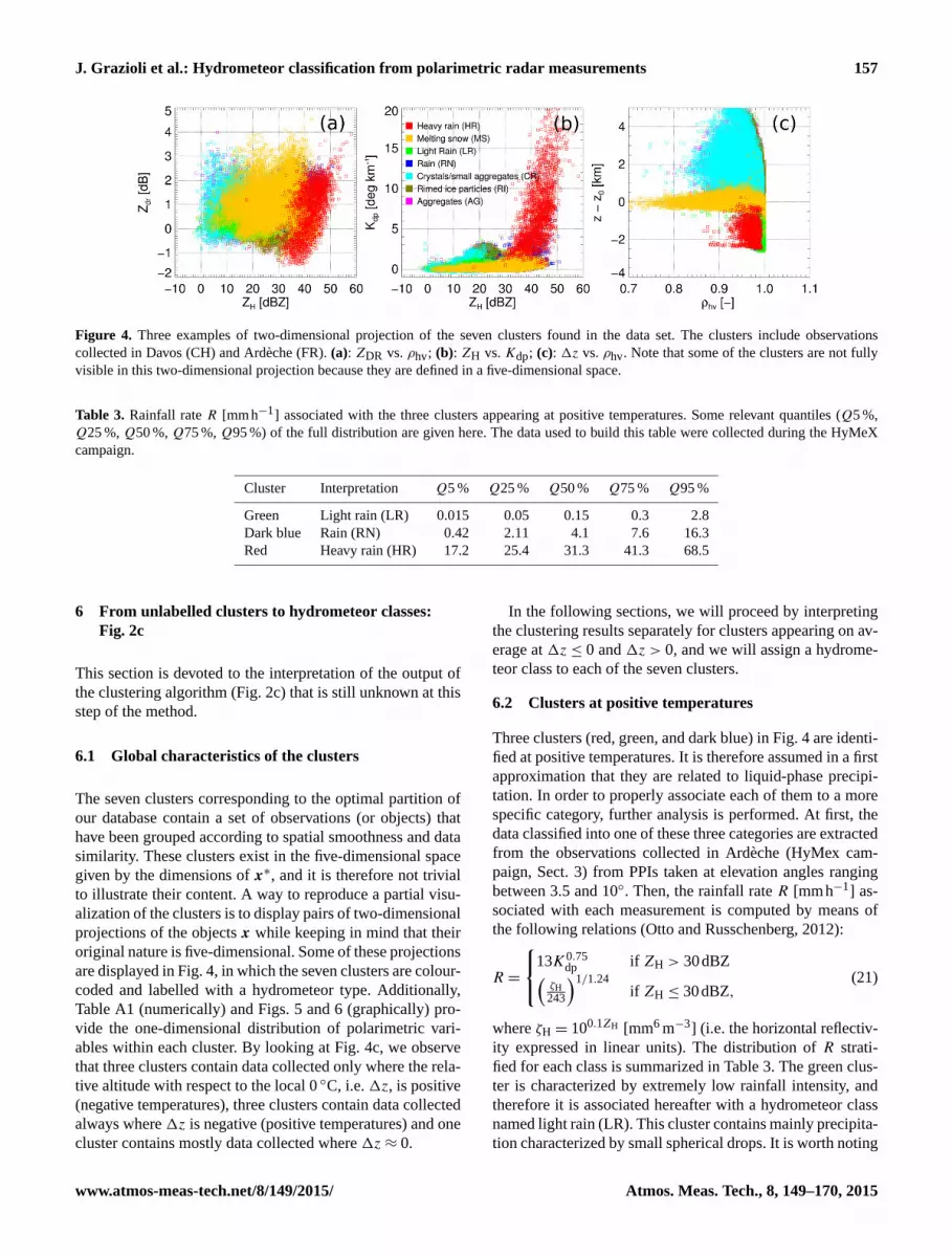
Figure 4. Three examples of two-dimensional projection of the seven clusters found in the data set. The clusters include observations

collected in Davos (CH) and Ardèche (FR). (a): ZDR vs. ρhv; (b): ZH vs. Kdp; (c): 1z vs. ρhv. Note that some of the clusters are not fully

visible in this two-dimensional projection because they are defined in a five-dimensional space.

Table 3. Rainfall rate R [mmh−1] associated with the three clusters appearing at positive temperatures. Some relevant quantiles (Q5 %,

Q25 %, Q50 %, Q75 %, Q95 %) of the full distribution are given here. The data used to build this table were collected during the HyMeX

campaign.

Cluster Interpretation Q5 % Q25 % Q50 % Q75 % Q95 %

Green Light rain (LR) 0.015 0.05 0.15 0.3 2.8

Dark blue Rain (RN) 0.42 2.11 4.1 7.6 16.3

Red Heavy rain (HR) 17.2 25.4 31.3 41.3 68.5

6 From unlabelled clusters to hydrometeor classes:

Fig. 2c

This section is devoted to the interpretation of the output of

the clustering algorithm (Fig. 2c) that is still unknown at this

step of the method.

6.1 Global characteristics of the clusters

The seven clusters corresponding to the optimal partition of

our database contain a set of observations (or objects) that

have been grouped according to spatial smoothness and data

similarity. These clusters exist in the five-dimensional space

given by the dimensions of x∗, and it is therefore not trivial

to illustrate their content. A way to reproduce a partial visu-

alization of the clusters is to display pairs of two-dimensional

projections of the objects x while keeping in mind that their

original nature is five-dimensional. Some of these projections

are displayed in Fig. 4, in which the seven clusters are colour-

coded and labelled with a hydrometeor type. Additionally,

Table A1 (numerically) and Figs. 5 and 6 (graphically) pro-

vide the one-dimensional distribution of polarimetric vari-

ables within each cluster. By looking at Fig. 4c, we observe

that three clusters contain data collected only where the rela-

tive altitude with respect to the local 0 ◦C, i.e. 1z, is positive

(negative temperatures), three clusters contain data collected

always where1z is negative (positive temperatures) and one

cluster contains mostly data collected where 1z≈ 0.

In the following sections, we will proceed by interpreting

the clustering results separately for clusters appearing on av-

erage at 1z ≤ 0 and 1z > 0, and we will assign a hydrome-

teor class to each of the seven clusters.

6.2 Clusters at positive temperatures

Three clusters (red, green, and dark blue) in Fig. 4 are identi-

fied at positive temperatures. It is therefore assumed in a first

approximation that they are related to liquid-phase precipi-

tation. In order to properly associate each of them to a more

specific category, further analysis is performed. At first, the

data classified into one of these three categories are extracted

from the observations collected in Ardèche (HyMex cam-

paign, Sect. 3) from PPIs taken at elevation angles ranging

between 3.5 and 10◦. Then, the rainfall rate R [mmh−1] as-

sociated with each measurement is computed by means of

the following relations (Otto and Russchenberg, 2012):

R =

13K0.75dp if ZH > 30dBZ(

ζH

243

)1/1.24

if ZH ≤ 30dBZ,(21)

where ζH = 100.1ZH [mm6 m−3] (i.e. the horizontal reflectiv-

ity expressed in linear units). The distribution of R strati-

fied for each class is summarized in Table 3. The green clus-

ter is characterized by extremely low rainfall intensity, and

therefore it is associated hereafter with a hydrometeor class

named light rain (LR). This cluster contains mainly precipita-

tion characterized by small spherical drops. It is worth noting



Table 4. Confusion matrix comparing the classification of liquid

phase hydrometeor classes (1z < 0) obtained with the clustering

method described in the paper and the output of the fuzzy-logic

method DR2009, described in Appendix B. The classes of the novel

method are light rain (LR), rain (RN), and heavy rain (HR). The el-

ements Mi,j of the matrix contain the percentage of liquid phase

observations classified in the ith class of the first method and si-

multaneously in the j th class of the second method. The data are

obtained from 100 runs of the clustering algorithm.

Novel method

DR

20

09 LR RN HR

Drizzle 59 % 1 % 0 %

Rain 7 % 29 % 6 %

(Fig. 5b and c) that LR contains ZDR values lower than 1 dB,

with a mode around 0.25 dB, and Kdp values always close to

0 ◦ km−1. LR therefore contains drizzle and the lightest rain-

fall intensities. The dark blue cluster is characterized by low

to intermediate rainfall intensity, and therefore it is associ-

ated with a category named rain (RN). Finally, the red cluster

contains by far the highest rainfall intensities, and it is here-

after called heavy rain (HR). We also hypothesize that, when

hail occurs, it is classified as HR. We base this assumption on

the fact that HR includes observations with a low-correlation

coefficient ρhv (Fig. 5d) as well as near-zero or negative ZDR

(Fig. 5b). These signatures have been documented in cases

where hail was measured by polarimetric weather radars (Al-

Sakka et al., 2013).

As an additional test, the classification output of our

method is compared with a fuzzy-logic classification scheme

based on the parametrization of Dolan and Rutledge (2009),

hereafter DR2009 (see Appendix B for the details). DR2009

does not provide three “liquid-phase” hydrometeor classes

but only rain and drizzle. The contingency table of Table 4

shows that the HR class of our method is entirely classified

as rain by DR2009. The RN class is mainly classified as rain,

and LR is almost entirely associated with drizzle. We con-

clude that results from the proposed method agree well with

DR2009 for liquid phase hydrometeor classes.

Figure 7 illustrates a case where LR, RN, and HR are clas-

sified on the same PPI radar image. This case was collected

on 24 September 2012 during the HyMeX campaign, when

a high-intensity convective line was approaching the radar lo-

cation from the west side of the domain (more details about

the storm in Bousquet et al., 2014). This resulted in a layer

of high values of ZH, ZDR, and Kdp. The transition from LR

to HR within few kilometres appears qualitatively to be a

satisfactory illustration of the incoming front. Figure 7 also

shows a map of classification accuracy. This parameter is de-

fined for each observation (valid range gate) as the difference

between the distance of the observation with respect to the

two closest clusters, and it is normalized by the smaller dis-

tance. The classification accuracy is therefore lower in the ar-

eas of transition between different hydrometeor types, where

the polarimetric signatures change as the dominant hydrom-

eteor type changes.

6.3 Cluster around 0 ◦C

The yellow cluster of Figs. 4 and 5 appears on average around

the 0 ◦C isotherm, and it is interpreted as melting snow (MS).

Figure 8 shows an example of classification output, where

a melting layer is clearly visible in the polarimetric observa-

tions. The MS category can be seen to delimit the transition

between ice-phase and liquid-phase hydrometeors. The sig-

natures of this transition can also be seen in ZH, ZDR, and

ρhv. Kdp does not exhibit any obvious signature in the re-

gions classified as MS (in agreement with observations doc-

umented by Thompson et al., 2014).

6.4 Clusters at negative temperatures

The clusters identified at negative temperatures (dark green,

pink, and cyan clusters in Fig. 4) should be attributed to

ice-phase hydrometeors. To classify these clusters, we pro-

ceed as follows: first we examine the behaviour of the polari-

metric variables within these three clusters, then we com-

pare the classification with the output of DR2009. Subse-

quently we compare the classification with qualitative (hy-

drometeor classification) and quantitative (snowfall inten-

sity) observations provided by a two-dimensional video dis-

drometer (2DVD) and with the output of a numerical weather

prediction model (Consortium for Small-scale Modeling

(COSMO)).

6.4.1 Polarimetric signatures

Figure 6 presents the distribution of the polarimetric vari-

ables ZH, ZDR, Kdp, and ρhv, as well as the relative altitude

1z for the three “ice-phase” clusters.

By looking at panel (a), we can observe a clear ZH signa-

ture. ZH is the lowest in the cyan cluster (mode ≈ 12 dBZ),

it is slightly higher in the pink cluster (mode ≈ 15 dBZ), and

it is the highest in the dark-green cluster (mode> 20 dBZ).

Higher ZH indicates higher hydrometeor concentration, size,

and/or ice density.

ZDR, shown in panel (b), exhibits a different pattern. The

cyan cluster and the pink cluster show some variability in

ZDR. ZDR ranges from −0.3 to 2.5 dB (mode 0.8 dB) in the

cyan cluster and from −0.3 to 1.6 dB (mode 0.5 dB) in the

pink cluster. We interpret this behaviour as the signature of

particle shape and orientation variability in the cyan and pink

clusters, with the pink cluster containing on average hydrom-

eteors that are more geometrically isotropic. The dark-green

cluster behaves differently: ZDR has a clear mode around

0.3 dB, the distribution of ZDR values is narrow (ranging be-

tween −0.6 and 1 dB), and it includes many negative values,

i.e. prolate particles.



Figure 5. Distribution within the four clusters found at positive temperatures (1z ≤ 0) of (a) ZH [dBZ], (b) ZDR [dB], (c) Kdp [◦ km−1],

(d) ρhv [–], and (e) 1z [km]. The curves are obtained considering the content of 100 runs of the clustering algorithm.

ρhv has a clear signature for the cyan cluster only, charac-

terized by low values that often depart from 1. We interpret

this behaviour as an additional effect of the variability of par-

ticle shapes within the radar resolution volume.

Kdp, shown in panel (c), is lower than 1◦ km−1 for the pink

cluster and the cyan cluster. The dark-green cluster exhibits

instead relatively large values of 2.5◦ km−1. Kdp depends on

size, concentration, shape, and density of the particles in the

radar resolution volume and therefore the dark green clus-

ter contains, on average, more oblate hydrometeors and/or

oblate hydrometeors of a larger size and density.

Finally, by looking at panel (e), we observe that the dark-

green cluster is found over a broad range of altitudes (tem-

peratures) and that the cyan cluster generally appears at lower

temperatures than the other two.

From this analysis, we observed that the three clusters

exhibit distinct polarimetric signatures, which led us to hy-

pothesize the following associations. The cyan cluster corre-

sponds to individual crystals and small aggregates (denoted

CR): it appears in the coldest areas of precipitation, it shows

significant variability of shapes, and low-intensityZH returns

due to the low concentration and small size of the hydromete-

ors. The pink cluster corresponds to aggregates (AG). Aggre-

gates generate larger ZH returns due to their larger sizes, and

they tumble as they fall, thus lowering ZDR. The dark green

cluster corresponds to heavily rimed-ice particles (RI). The

larger density of rimed particles lead to significant ZH signa-

tures, and the dielectric properties of dense ice (very differ-

ent with respect to dry crystals and aggregates; Vivekanan-

dan et al., 1994) lead to a response also in Kdp. ZDR is

low because riming tends to smooth particle shapes, and it

shows negative values when conically shaped rimed parti-

cles are formed (Evaristo et al., 2013). These hypotheses are

discussed in the next sections.



Figure 6. Distribution within the three clusters found at negative temperatures (1z > 0) of (a) ZH [dBZ], (b) ZDR [dB], (c) Kdp [◦ km−1],

(d) ρhv [–], and (e) 1z [km]. The curves are obtained considering the content of 100 runs of the clustering algorithm.

Table 5. As in Table 4 but comparing the classification of ice phase

hydrometeor classes (1z > 0). The classes of the novel method are

crystal (CR), aggregates (AG), and rimed-ice particles (RI). The el-

ements Mi,j of the matrix contain the percentage of ice phase ob-

servations classified in the ith class of the first method and simulta-

neously in the j th class of the second method. The data are obtained

from 100 runs of the clustering algorithm.

Novel method

DR

20

09

CR AG RI

Crystals 6 % 2 % 0 %

Aggregates 17 % 24 % 6 %

High-dens. graupel 5 % 7 % 5 %

Low-dens. graupel 0 % 1 % 15 %

Vertical Ice 6 % 5 % 1 %

6.4.2 Comparison with DR2009

In Sect. 6.2 we compared the liquid-phase clusters of our

method with the output of DR2009. We now perform a sim-

ilar evaluation, focussing on the ice-phase clusters. As a re-

minder, our method provides three ice-phase classes: crys-

tal and small aggregates (CR), aggregates (AG), and rimed-

ice particles (RI). DR2009 instead provides five ice-phase

classes: crystals (CR), aggregates (AG), high-density graupel

(HDG), low-density graupel (LDG), and vertically aligned

ice (VI, which denotes oblate ice crystals aligned vertically

because of an electric field). The contingency table between

these categories is shown in Table 5. We observe that the

methods are in overall good agreement. The CR class is as-

sociated mostly with the DR2009 classes of aggregates, crys-

tals, and vertical ice. AG is associated with aggregates, and

RI is associated with the two graupel categories of DR2009.

The only notable discrepancy between the methods happens

for the high-density graupel category of DR2009: this class

is evenly distributed among CR, AG, and RI, indicating that

there is not a clear match for this hydrometeor type.

6.4.3 Comparison with 2DVD classification output

An additional comparison is conducted with the output of an

HC scheme developed for two-dimensional video disdrom-

eters. This method, hereafter called HC2DVD is described



Figure 7. Hydrometeor classification and polarimetric observation from a PPI sector scan collected on the 24 September during HyMeX

Special Observation Period (SOP) 2012 at 02:12 UTC with an elevation angle of 3.5◦. The different panels show the following variables:

hydrometeor classification with the clustering approach, classification accuracy, ZH [dBZ], ZDR [dB], Kdp [◦ km−1], and ρhv [–]. The

spatial coordinates x and y originate at the radar location.

in detail in Grazioli et al. (2014). HC2DVD takes as in-

put a set of two-dimensional particles images, collected by

a 2DVD, and it provides as output an estimate of the dom-

inant hydrometeor type within time intervals of 60 s. The

method does not classify individual particles but populations

of hydrometeors. HC2DVD discriminates between eight hy-

drometeor classes: small particle-like (SP), dendrite-like (D),

column-like (C), graupel-like (G), rimed-particle-like (RIM),

aggregate-like (AG), melting-snow-like (MS), and rain (R)5.

The “-like” is added to underline that this algorithm assigns

5We use here the abbreviations of Grazioli et al. (2014).

a dominant type of hydrometeor to each time step, but there

is usually a mixture of different hydrometeors captured by

the 2DVD so they do not necessarily exhibit a single pristine

shape.

Here we compare HC2DVD with the output of the cluster-

ing algorithm for snowfall events collected during the cam-

paign of Davos 2009–2011 (Sect. 3). The PPI of the lowest

elevation not contaminated by clutter was taken at 9◦ eleva-

tion with a repetition interval of 5 min. This PPI is used for a

comparison with HC2DVD.

Before discussing the comparison, it must be kept in mind

that (i) the closest radar resolution volume centre was about



Figure 8. Hydrometeor classification and polarimetric observation from an RHI collected on 29 September during HyMeX SOP 2012

at 14:29 UTC. The different panels show the following variables: hydrometeor classification with the clustering approach, classification

accuracy, ZH [dBZ], ZDR [dB], Kdp [◦ km−1], and ρhv [–]. The altitude of the radar is 605 m.

Table 6. Confusion matrix comparing the classification of ice

phase hydrometeor classes during the measurement campaign of

Davos as estimated from the clustering method and from the 2DVD

(HC2DVD; Grazioli et al. (2014)), taken as ground reference. The

comparison is conducted on three hydrometeor classes: crystal

(CR), aggregates (AG), and rimed-ice particles (RI). In this case,

the matrix is 3×3, with similar classes in rows and columns, and it

can be used to evaluate quantitatively the agreement among meth-

ods. The overall accuracy of the comparison is 49 %, and Cohen’s

kappa is 0.23.

Novel method

HC

2D

VD CR AG RI

HC2DVD-CR 27.9 % 13.9 % 0.5 %

HC2DVD-AG 4.5 % 18.2 % 1.0 %

HC2DVD-RI 15.7 % 16.5 % 1.8 %

400 m above the 2DVD and crystal habits can change over

this altitude range, and (ii) the sampling times and volumes of

the two instruments are different, even though the sampling

times overlap.

The comparison is conducted on a subset of about 30 man-

ually selected snowfall events. We excluded any precipita-

tion event with a visible melting layer or positive temper-

atures at the radar location as well as any event character-

ized by evident spatial and temporal variabilities on the small

scale. Radar resolution volumes within 150 m in horizon-

tal distance from the 2DVD location are compared with the

HC2DVD output. A buffer of +2 min is applied in order to

match multiple 2DVD observations with a single radar scan.

In order to simplify the comparison, we aggregate some

of the categories from HC2DVD as follows. We merge to-

gether small particles (SP), dendrites (D), and columns (C)

into a single class called “crystals” (HC2DVD-CR). We keep

aggregates (AG) in a single class, and we name it HC2DVD-

AG. Finally, we merge graupel (G) and rimed particles (RIM)

into a “rimed-ice” class (HC2DVD-RI).

Table 6 presents the confusion matrix of the comparison

between the novel clustering algorithm and HC2DVD. The

agreement between CR and HC2DVD-CR is very good, as

is the agreement between AG and HC2DVD-AG. Rimed-

ice particles, in contrast, exhibit a good accuracy of detec-

tion (when they are detected, their presence is confirmed



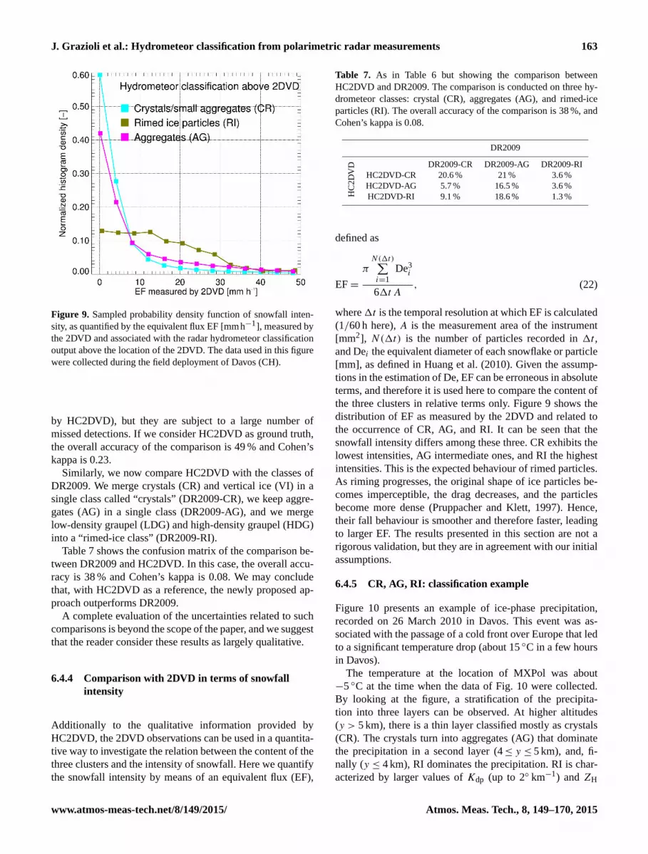
Figure 9. Sampled probability density function of snowfall inten-

sity, as quantified by the equivalent flux EF [mmh−1], measured by

the 2DVD and associated with the radar hydrometeor classification

output above the location of the 2DVD. The data used in this figure

were collected during the field deployment of Davos (CH).

by HC2DVD), but they are subject to a large number of

missed detections. If we consider HC2DVD as ground truth,

the overall accuracy of the comparison is 49 % and Cohen’s

kappa is 0.23.

Similarly, we now compare HC2DVD with the classes of

DR2009. We merge crystals (CR) and vertical ice (VI) in a

single class called “crystals” (DR2009-CR), we keep aggre-

gates (AG) in a single class (DR2009-AG), and we merge

low-density graupel (LDG) and high-density graupel (HDG)

into a “rimed-ice class” (DR2009-RI).

Table 7 shows the confusion matrix of the comparison be-

tween DR2009 and HC2DVD. In this case, the overall accu-

racy is 38 % and Cohen’s kappa is 0.08. We may conclude

that, with HC2DVD as a reference, the newly proposed ap-

proach outperforms DR2009.

A complete evaluation of the uncertainties related to such

comparisons is beyond the scope of the paper, and we suggest

that the reader consider these results as largely qualitative.

6.4.4 Comparison with 2DVD in terms of snowfall

intensity

Additionally to the qualitative information provided by

HC2DVD, the 2DVD observations can be used in a quantita-

tive way to investigate the relation between the content of the

three clusters and the intensity of snowfall. Here we quantify

the snowfall intensity by means of an equivalent flux (EF),

Table 7. As in Table 6 but showing the comparison between

HC2DVD and DR2009. The comparison is conducted on three hy-

drometeor classes: crystal (CR), aggregates (AG), and rimed-ice

particles (RI). The overall accuracy of the comparison is 38 %, and

Cohen’s kappa is 0.08.

DR2009

HC

2D

VD DR2009-CR DR2009-AG DR2009-RI

HC2DVD-CR 20.6 % 21 % 3.6 %

HC2DVD-AG 5.7 % 16.5 % 3.6 %

HC2DVD-RI 9.1 % 18.6 % 1.3 %

defined as

EF=

πN(1t)∑i=1

De3i

61t A, (22)

where1t is the temporal resolution at which EF is calculated

(1/60 h here), A is the measurement area of the instrument

[mm2], N(1t) is the number of particles recorded in 1t ,

and Dei the equivalent diameter of each snowflake or particle

[mm], as defined in Huang et al. (2010). Given the assump-

tions in the estimation of De, EF can be erroneous in absolute

terms, and therefore it is used here to compare the content of

the three clusters in relative terms only. Figure 9 shows the

distribution of EF as measured by the 2DVD and related to

the occurrence of CR, AG, and RI. It can be seen that the

snowfall intensity differs among these three. CR exhibits the

lowest intensities, AG intermediate ones, and RI the highest

intensities. This is the expected behaviour of rimed particles.

As riming progresses, the original shape of ice particles be-

comes imperceptible, the drag decreases, and the particles

become more dense (Pruppacher and Klett, 1997). Hence,

their fall behaviour is smoother and therefore faster, leading

to larger EF. The results presented in this section are not a

rigorous validation, but they are in agreement with our initial

assumptions.

6.4.5 CR, AG, RI: classification example

Figure 10 presents an example of ice-phase precipitation,

recorded on 26 March 2010 in Davos. This event was as-

sociated with the passage of a cold front over Europe that led

to a significant temperature drop (about 15 ◦C in a few hours

in Davos).

The temperature at the location of MXPol was about

−5 ◦C at the time when the data of Fig. 10 were collected.

By looking at the figure, a stratification of the precipita-

tion into three layers can be observed. At higher altitudes

(y > 5 km), there is a thin layer classified mostly as crystals

(CR). The crystals turn into aggregates (AG) that dominate

the precipitation in a second layer (4≤ y ≤ 5 km), and, fi-

nally (y ≤ 4 km), RI dominates the precipitation. RI is char-

acterized by larger values of Kdp (up to 2◦ km−1) and ZH



Figure 10. As in Fig. 8 but for the snowfall event of the 26 March 2010, at 15:31 UTC in Davos (CH). The altitude of the radar is 2133 m.

(up to 28 dBZ). CR is instead characterized by low values

of ZH and ρhv (as low as 0.9) and very low values of Kdp,

between −0.1 and 0.1 ◦ km−1. In this example, AG exhibits

polarimetric signatures that are somewhat intermediate be-

tween CR and RI.

For illustrative purpose, the situation corresponding to

Fig. 10 was simulated using the numerical weather model

COSMO (see http://www.cosmo-model.org), operationally

used by MeteoSwiss. The model was run at 2 km resolu-

tion with forcing from MeteoSwiss reanalysis. As shown in

Fig. 11, COSMO predicts the presence of supercooled liquid

water (QC) at altitudes between 2.5 and 3 km. Additionally,

at altitudes between 2 and 6 km, we observe large quantities

of graupel (QG) mixed with snow (QS). Both the presence of

supercooled liquid water in the clouds and the explicit pres-

ence of graupel are in agreement with the layer of rimed par-

ticles RI identified in Fig. 10.

7 Summary and conclusions

A novel approach to hydrometeor classification from a po-

larimetric weather radar was presented in this paper. The

method was applied to polarimetric data collected by an X-

band radar in the Swiss Alps and in the French Prealps. The

novel approach was not based on numerical-scattering simu-

lations. The number of hydrometeor classes was not defined

a priori, but it was learned from the data, and the content of

each hydrometeor class was manually interpreted.

A subset of 20 000 polarimetric observations was ran-

domly extracted from the available data set. A hierarchical

clustering algorithm with spatial constraints was applied to

the subset in order to merge observations according to both

the similarity of polarimetric data and the spatial smoothness

of each partition. This means that we made the assumption

of smooth spatial transitions between hydrometeor types.

Following this strategy, an optimal number of seven clus-

ters was found. Three clusters were found at positive tem-

peratures, and they were interpreted as light rain (LR), rain

(RN), and heavy rain (HR). One cluster appeared systemat-


http://www.cosmo-model.org


Figure 11. Mixing ratios of hydrometeor contents obtained with the COSMO2 numerical weather model along the RHI transect of MXPol

(same as Fig. 10) at 15:15 UTC on the 26 March 2010 in Davos (CH). Mixing ratios are given for cloud ice (QI), snow (QS), cloud water

(QC), and graupel (QG).

ically around 0 ◦C, and it was associated with melting snow

(MS). Finally, three clusters were found at negative tempera-

tures and their polarimetric signatures were interpreted as be-

ing of crystals/small aggregates (CR), aggregates (AG), and

rimed-ice particles (RI). The content of the clusters agrees

well with the outcome of a fuzzy-logic algorithm, denoted

as DR2009 (Dolan and Rutledge, 2009). Additionally, the

novel approach obtained scores better than DR2009 when

compared to a ground-based (video-disdrometer-based) hy-

drometeor classification scheme, hence suggesting that the

new method was better tailored to the observations of the X-

band radar employed in this study.

The proposed approach is the first attempt, using unsuper-

vised classification, to move the starting point of a classifica-

tion algorithm away from scattering simulations conducted

over an arbitrarily defined number of hydrometeor classes to

the identification of relevant clusters in the data themselves.

The initial identification of the clusters is computationally

expensive, but this operation is performed only once and the

classification of newly collected radar images can be con-

ducted in real time.

Some of the advantages of this approach are that it is

immune to possible radar miscalibration and that the data-

driven approach ensures that the identified clusters take into

account the accuracy of the instrument. Finally, the method is

adaptable to other radar systems and can be tuned to include

other constraints regarding the spatial smoothness of the par-

tition or temporal consistency. The main limitations of the

method are related to the manual interpretation of the con-

tent of the clusters. This may not be trivial, especially in the

absence of surface precipitation type reports for comparison.

Additionally, the method is as representative as the available

database is, and the clusters identified are a priori valid only

for the instrument employed to collect the data. We neverthe-

less expect the number and type of clusters to be very similar

for other X-band dual-polarization radars of similar sensitiv-

ity.

It is interesting to note that the method exploits a simple

hypothesis about the spatial smoothness of the hydrometeor

types and that this rule is applied only in the initial steps

(when the nopt clusters are identified). Future work will be

devoted to also extending the constraints involving spatial

smoothness to newly classified images or to including physi-

cally justified contiguity rules for specific hydrometeor types.

In addition, this clustering approach (or some steps of the ap-

proach) could be employed as a support to fuzzy-logic-based

classification methods to improve or adapt the membership

functions according to the clustering outputs in specific data

sets.



Appendix A: Polarimetric characteristics of the seven

clusters

Table A1 provides the relevant statistics of each of the seven

clusters identified in this work from a database of X-band

radar data.

Table A1. Statistics describing the content of the seven clusters identified in Sects. 5 and 6. For each polarimetric variable and for each

cluster, we provide the mean value, standard deviation σ , and a set of quantiles (Q1 %, Q5 %, 10 %, Q25 %, Q50 %, Q75 %, Q90 %,

Q95 %, Q99 %).

Var. Class Colour Mean σ Q1 % Q5 % Q10 % Q25 % Q50 % Q75 % Q90 % Q95 % Q99 %

ZH Melting snow (MS) 30.2 6.2 14.1 18.8 21.5 26.6 30.9 34.5 37.6 39.5 42.3

ZDR Melting snow (MS) 1.4 0.74 −0.2 0.2 0.4 0.8 1.3 1.7 2.3 2.6 3.2

Kdp Melting snow (MS) 0.3 0.29 −0.2 −0.1 0.0 0.2 0.3 0.5 0.7 0.9 1.2

ρhv Melting snow (MS) 0.92 0.041 0.78 0.83 0.86 0.9 0.93 0.95 0.96 0.97 0.97

ZH Heavy rain (HR) 42.3 4.2 32.7 35.3 36.8 39.3 42.4 45.3 47.4 50.6 53.1

ZDR Heavy rain (HR) 0.9 0.97 −1.2 −0.8 −0.6 0.2 1.1 1.6 2.0 2.4 2.9

Kdp Heavy rain (HR) 6.1 3.87 0.91 2.2 2.5 3.3 5.3 8.2 11.8 14.2 18.5

ρhv Heavy rain (HR) 0.97 0.015 0.92 0.94 0.95 0.96 0.97 0.98 0.99 0.99 0.99

ZH Light rain (LR) 20.1 4.5 9.2 12.8 14.8 18 21 24 26.4 27.8 30.4

ZDR Light rain (LR) 0.4 0.3 −0.2 −0.1 −0.1 0.1 0.2 0.4 0.6 0.8 1.1

Kdp Light rain (LR) 0.05 0.18 −0.2 −0.1 0 0 0 0.1 0.2 0.4 0.8

ρhv Light rain (LR) 0.99 0.009 0.97 0.98 0.99 0.99 0.99 1 1 1 1

ZH Rain (RN) 32.2 3.9 24.1 26.3 27.4 29.4 32.1 34.9 37.1 38.5 41.8

ZDR Rain (RN) 1.2 0.44 0.3 0.5 0.6 0.8 1.1 1.4 1.8 1.9 2.3

Kdp Rain (RN) 0.3 0.42 −0.1 −0.05 0 0.1 0.2 0.4 0.8 1.3 2.1

ρhv Rain (RN) 0.99 0.007 0.97 0.98 0.98 0.99 0.99 0.99 1 1 1

ZH Crystals/small aggregates (CR) 11.2 4.1 −1.1 2.2 6.2 9.5 12.2 14.9 17 18 20.3

ZDR Crystals/small aggregates (CR) 0.8 0.57 −0.3 0 0.1 0.4 0.8 1.2 1.7 2.1 2.5

Kdp Crystals/small aggregates (CR) 0.25 0.42 −0.2 −0.15 −0.1 0 0.2 0.4 0.8 1.3 1.9

ρhv Crystals/small aggregates (CR) 0.93 0.03 0.85 0.88 0.89 0.92 0.94 0.95 0.96 0.97 0.97

ZH Rimed-ice particles (RI) 24 4.4 16.5 18.2 19.6 21.2 23.3 25.9 29.6 33.2 38.2

ZDR Rimed-ice particles (RI) 0.24 0.35 −0.6 −0.3 −0.2 0 0.3 0.5 0.7 0.8 1

Kdp Rimed-ice particles (RI) 0.7 0.64 −0.1 0 0.1 0.2 0.5 1 1.6 2 2.6

ρhv Rimed-ice particles (RI) 0.99 0.01 0.95 0.97 0.97 0.98 0.99 0.99 0.99 0.99 0.99

ZH Aggregates (AG) 16.5 7.7 10.9 12 14 16.5 19 21 22.1 24

ZDR Aggregates (AG) 0.6 0.45 −0.3 −0.1 0 0.2 0.5 0.8 1.2 1.4 1.6

Kdp Aggregates (AG) 0.25 0.4 −0.2 −0.1 0 0.1 0.2 0.4 0.8 1.2 1.9

ρhv Aggregates (AG) 0.98 0.009 0.96 0.96 0.97 0.97 0.98 0.99 0.99 0.99 0.99



Appendix B: DR2009 algorithm

The algorithm denoted as DR2009 in this paper is based on

the work of Dolan and Rutledge (2009), with some adapta-

tions that we will highlight as they appear in this section. In

this Appendix, we provide the exact parametrization of the

membership functions for the fuzzy-logic scheme, as well

as the weights assigned to each polarimetric variable. The

input variables of the algorithm are ZH [dBZ], ZDR [dB],

Kdp [◦ km−1], ρhv [–], and 1z [m], and their weights in the

fuzzy-logic scheme are 0.25, 0.25, 0.25, 0.08, and 0.17, re-

spectively. 1z is the relative altitude with respect to the 0◦C

isotherm, as defined in Sec 4.1, and this input is not used in

Dolan and Rutledge (2009).

The hydrometeor classes available are aggregates (AG),

crystals (CR), drizzle (DZ), high-density graupel (HDG),

low-density graupel (LDG), rain (R), vertical ice (VI), and

wet snow (WS; not present in Dolan and Rutledge, 2009).

The membership function employed for all the polarimetric

inputs is a membership beta function β, while for1z a trape-

zoidal one is used. β is defined as

β =1

1+(x−ma

)2b , (B1)

where x is the considered polarimetric variable,m is the mid-

point, a is the width, and b the slope. Table B1 summarizes

the values of the parameters for each polarimetric variable

and each hydrometeor class.

The trapezoidal membership function T employed for 1z

instead takes the form of

T =

0 if x < l1;x−l1l2−l1

if l1 < x ≤ l2;

1 if l2 < x ≤ r1;r2−xr2−r1

if r1 < x ≤ r2;

0 if x > r2,

(B2)

where l1, l2, r1, and r2 define the four vertices of the trape-

zoid. The values for these parameters are reported in Ta-

ble B2.

Table B1. Parameters of the membership beta functions β employed

in the DR2009 algorithm: midpoint m, width a, and slope b for the

available hydrometeor classes.

Variable Class a m b

ZH Aggregates (AG) 17.0 16.0 3.0

ZDR Aggregates (AG) 0.7 0.7 3.0

Kdp Aggregates (AG) 0.2 0.2 2.0

ρhv Aggregates (AG) 0.011 0.989 1.0

ZH Crystals (CR) 22.0 −3.0 3.0

ZDR Crystals (CR) 2.6 3.2 3.0

Kdp Crystals (CR) 0.15 0.15 2.0

ρhv Crystals (CR) 0.015 0.985 1.0

ZH Drizzle (DZ) 29.0 2.0 3.0

ZDR Drizzle (DZ) 0.5 0.5 3.0

Kdp Drizzle (DZ) 0.18 0.18 2.0

ρhv Drizzle (DZ) 0.007 0.992 1.0

ZH High-density graupel (HDG) 11.0 43.0 3.0

ZDR High-density graupel (HDG) 2.5 1.2 3.0

Kdp High-density graupel (HDG) 5.1 2.5 2.0

ρhv High-density graupel (HDG) 0.018 0.983 1.0

ZH Low-density graupel (LDG) 10.0 34.0 3.0

ZDR Low-density graupel (LDG) 1.0 0.3 3.0

Kdp Low-density graupel (LDG) 2.1 0.7 2.0

ρhv Low-density graupel (LDG) 0.007 0.993 1.0

ZH Rain (R) 17.0 42.0 3.0

ZDR Rain (R) 2.8 2.7 3.0

Kdp Rain (R) 12.9 12.6 2.0

ρhv Rain (R) 0.01 0.99 1.0

ZH Vertical ice (VI) 28.5 3.5 3.0

ZDR Vertical ice (VI) 1.3 −0.8 3.0

Kdp Vertical ice (VI) 0.08 −0.1 2.0

ρhv Vertical ice (VI) 0.035 0.965 1.0

ZH Wet snow (WS) 20.0 30.0 3.0

ZDR Wet snow (WS) 1.4 2.2 3.0

Kdp Wet snow (WS) 1.0 1.0 2.0

ρhv Wet snow (WS) 0.135 0.835 1.0



Table B2. Parameters of the trapezoidal membership function T applied to the relative altitude with respect to the 0 ◦C isotherm (1z [m]).

l1, l2, l3, and l4 are the four vertices of the trapezoid T .

Variable Class l1 l2 r1 r2

1z Aggregates (AG) 0 500 20 000 25 000

1z Crystals (CR) 0 500 20 000 25 000

1z Drizzle (DZ) −25 000 −20 000 −100 0

1z High-density graupel (HDG) −600 100 20 000 25 000

1z Low-density graupel (LDG) −600 100 20 000 25 000

1z Rain (R) −25 000 −20 000 −100 0

1z Vertical ice (VI) −50 0 20 000 25 000

1z Wet snow (WS) −1000 −700 700 1000



Acknowledgements. This work is a contribution to the HyMeX

programme. The authors acknowledge Météo-France for supplying

temperature data and the HyMeX database teams (ESPRI/IPSL and

SEDOO/Observatoire Midi-Pyrénées) for their help in accessing

the data. The contribution of the second author was supported by

the Swiss National Science Foundation under grant 136827. The

authors are thankful to Daniel Wolfensberger (EPFL-LTE) for the

COSMO2 simulations of Sect. 6.4.5 and to all the members of

EPFL-LTE who were involved during the field campaigns. The

authors thank the two anonymous reviewers and Earle Williams

of the Massachusetts Institute of Technology (MIT) for the many

constructive comments and suggestions.

Edited by: S. J. Munchak

References

Al-Sakka, H., Boumahmoud, A.-A., Fradon, B., Frasier, S. J., and

Tabary, P.: A new fuzzy logic hydrometeor classification scheme

applied to the French X-, C-, and S-band polarimetric radars, J.

Appl. Meteor. Clim., 52, 2328–2344, doi:10.1175/JAMC-D-12-

0236.1, 2013.

Bechini, R., Baldini, L., and Chandrasekar, V.: Polarimetric Radar

Observations in the Ice Region of Precipitating Clouds at C-

Band and X-Band Radar Frequencies, J. Appl. Meteor. Clim.,

52, 1147–1169, doi:10.1175/JAMC-D-12-055.1, 2013.

Berne, A. and Krajewski, W. F.: Radar for hydrology: Unfulfilled

promise or unrecognized potential?, Adv. Water Resour., 51,

357–366, doi:10.1016/j.advwatres.2012.05.005, 2013.

Boudevillain, B., Delrieu, G., Galabertier, B., Bonnifait, L.,

Bouilloud, L., Kirstetter, P.-E., and Mosini, M.-L.: The

Cévennes-Vivarais Mediterranean Hydrometeorological

Observatory database, Water Resour. Res., 47, W07701,

doi:10.1029/2010WR010353, 2011.

Bousquet, O., Berne, A., Delanoë, J., Dufournet, Y., Gourley, J. J.,

Van-Baelen, J., Augros, C., Besson, L., Boudevillain, B., Cau-

mont, O., Defer, E., Grazioli, J., Jorgensen, D. J., Kirstetter, P.-

E., Ribaud, J.-F., Beck, J., Delrieu, G., Ducrocq, V., Scipion, D.,

Schwarzenboeck, A., and Zwiebel, J.: Multiple-frequency radar

observations collected in southern france during the field phase

of the hydrometeorological cycle in the mediterranean experi-

ment (HyMeX), Bull. Amer. Meteor. Soc., doi:10.1175/BAMS-

D-13-00076.1, online first, 2014.

Bringi, V. N. and Chandrasekar, V.: Polarimetric doppler weather

radar, Cambridge University Press, 2001.

Chandrasekar, V., Keranen, R., Lim, S., and Moisseev, D.: Re-

cent advances in classification of observations from dual

polarization weather radars, Atmos. Res., 119, 97–111,

doi:10.1016/j.atmosres.2011.08.014, 2013.

Dolan, B. and Rutledge, S. A.: A theory-based hydrom-

eteor identification algorithm for X-band polarimet-

ric radars, J. Atmos. Oceanic Technol., 26, 2071–2088,

doi:10.1175/2009JTECHA1208.1, 2009.

Dolan, B., Rutledge, S. A., Lim, S., Chandrasekar, V., and Thu-

rai, M.: A robust C-band hydrometeor identification algorithm

and application to a long-term polarimetric radar dataset, J. Appl.

Meteor. Clim., 52, 2162–2186, doi:10.1175/JAMC-D-12-0275.1,

2013.

Ducrocq, V., Braud, I., Davolio, S., Ferretti, R., Flamant, C., Jansa,

A., Kalthoff, N., Richard, E., Taupier-Letage, I., Ayral, P., Be-

lamari, S., Berne, A., Borga, M., Boudevillain, B., Bock, O.,

Boichard, J., Bouin, M., Bousquet, O., Bouvier, C., Chiggiato,

J., Cimini, D., Corsmeier, U., Coppola, L., Cocquerez, P., Defer,

E., Delanoe, J., Di Girolamo, P., Doerenbecher, A., Drobinski,

P., Dufournet, Y., Fourrie, N., Gourley, J. J., Labatut, L., Lam-

bert, D., Le Coz, J., Marzano, F. S., Molinie, G., Montani, A.,

Nord, G., Nuret, M., Ramage, K., Rison, W., Roussot, O., Said,

F., Schwarzenboeck, A., Testor, P., Van Baelen, J., Vincendon,

B., Aran, M., and Tamayo, J.: HYMEX-SOPI The Field Cam-

paign Dedicated to Heavy Precipitation and Flash Flooding in

the Northwestern Mediterranean, Bull. Amer. Meteor. Soc., 95,

1083, doi:10.1175/BAMS-D-12-00244.1, 2014.

Evaristo, R., Bals-Elsholz, T., Williams, E., Fenn, A. J., Donovan,

M., and Smalley, D.: Relationship of graupel shape to differential

reflectivity: theory and observations, in: 29th Conference on En-

vironmental Information Processing Technologies, Austin, USA,

2013.

Foody, G. M.: Thematic Map Comparison: Evaluating the Statisti-

cal Significance of Differences in Classification Accuracy, Pho-

togramm. Eng. Rem. S., 50, 627–633, 2004.

Gourley, J. J., Tabary, P., and Parent-du Chatelet, J.: A fuzzy logic

algorithm for the separation of precipitating from nonprecipi-

tating echoes using polarimetric radar observations, J. Atmos.

Oceanic Technol., 24, 1439–1451, doi:10.1175/JTECH2035.1,

2007.

Grazioli, J., Tuia, D., Monhart, S., Schneebeli, M., Raupach, T.,

and Berne, A.: Hydrometeor classification from two-dimensional

video disdrometer data, Atmos. Meas. Tech., 7, 2869–2882,

doi:10.5194/amt-7-2869-2014, 2014.

Halkidi, M., Batistakis, Y., and Vazirgiannis, M.: Clustering validity

checking methods: Part II, SIGMOD Rec., 31, 19–27, 2002.

Huang, G., Bringi, V. N., Cifelli, R., Hudak, D., and Petersen, W. A.:

A methodology to derive radar reflectivity liquid equivalent snow

rate relations using C-band radar and a 2D video disdrometer, J.

Atmos. Oceanic Technol., 27, 637–651, 2010.

Jain, A. K. and Dubes, R. C.: Algorithms for Clustering Data,

Prentice-Hall, Inc., Upper Saddle River, NJ, USA, 1988.

Jain, A. K., Murty, M. N., and Flynn, P. J.: Data clustering: a review,

ACM Computing Survey, 31, 264–323, 1999.

Jain, A. K., Duin, R. P. W., and Mao, J. C.: Statistical pattern recog-

nition: A review, IEEE Trans. Pattern Analysis Machine Intell.,

22, 4–37, doi:10.1109/34.824819, 2000.

Jameson, A. R.: Microphysical interpretation of multi-parameter

radar measurements in rain: Part II: estimation of raindrop dis-

tribution parameters by combined dual-wavelength and polariza-

tion measurements, J. Atmos. Sci., 40, 1803–1813, 1983.

Kruger, A. and Krajewski, W. F.: Two-dimensional video disdrom-

eter: a description, J. Atmos. Oceanic Technol., 19, 602–617,

2002.

Liu, H. P. and Chandrasekar, V.: Classification of hydromete-

ors based on polarimetric radar measurements: Development of

fuzzy logic and neuro-fuzzy systems, and in situ verification, J.

Atmos. Oceanic Technol., 17, 140–164, 2000.

Marzano, F., Scaranari, D., and Vulpiani, G.: Supervised fuzzy-

logic classification of hydrometeors using C-band weather

radars, IEEE T. Geosci. Remote Sens., 45, 3784–3799,

doi:10.1109/TGRS.2007.903399, 2007.


http://dx.doi.org/10.1175/JAMC-D-12-0236.1



http://dx.doi.org/10.1016/j.advwatres.2012.05.005

http://dx.doi.org/10.1029/2010WR010353

http://dx.doi.org/10.1175/BAMS-D-13-00076.1


http://dx.doi.org/10.1016/j.atmosres.2011.08.014

http://dx.doi.org/10.1175/2009JTECHA1208.1



http://dx.doi.org/10.1175/JTECH2035.1

http://dx.doi.org/10.5194/amt-7-2869-2014

http://dx.doi.org/10.1109/34.824819

http://dx.doi.org/10.1109/TGRS.2007.903399


Marzano, F. S., Botta, G., and Montopoli, M.: Iterative Bayesian re-

trieval of hydrometeor content from X-band polarimetric weather

radar, IEEE T. Geosci. Remote Sens., 48, 3059–3074, 2010.

Matrosov, S. Y.: Radar reflectivity in snowfall, IEEE T. Geosci. Re-

mote Sens., 30, 454–461, 1992.

Miniscloux, F., Creutin, J.-D., and Anquetin, S.: Geostatistical anal-

ysis of orographic rain bands, J. Appl. Meteor., 40, 1835–1854,

doi:10.1175/1520-0450(2001)040<1835:GAOOR>2.0.CO;2,

2001.

Mishchenko, M. I., Travis, L. D., and Mackowski, D. W.: T-matrix

computations of light scattering by nonspherical particles: A re-

view, J. Quant. Spectrosc. Radiat. Transfer, 55, 535–575, 1996.

Mott, R., Scipion, D., Schneebeli, M., Dawes, N., Berne, A., and

Lehning, M.: Orographic effects on snow deposition patterns in

mountainous terrain, J Geophys. Res. Atmos., 119, 1419–1439,

doi:10.1002/2013JD019880, 2014.

Otto, T. and Russchenberg, H. W. J.: Estimation of specific differ-

ential phase and differential backscatter phase from polarimetric

weather radar measurements of rain, IEEE Geosci. Remote Sens.

Lett., 8, 988–992, doi:10.1109/LGRS.2011.2145354, 2011.

Otto, T. and Russchenberg, H. W. J.: Rainfall rate retrieval with

IDRA, the polarimetric X-band radar at Cabauw, Netherlands, in:

Proc. ERAD 2012 – The seventh European conference on radar

in meteorology and hydrology, Toulouse, FR, 2012.

Pruppacher, H. R. and Klett, R. L.: Microphysics of clouds and pre-

cipitation, no. 18 in Atmospheric and Oceanographic Sciences

Library, Kluwer Academic Press, 2nd Edn., 1997.

Ryzhkov, A. V., Schuur, T. J., Burgess, D. W., Heinselman, P. L.,

Giangrande, S. E., and Zrnic, D. S.: The joint polarization

experiment, polarimetric rainfall measurements and hydrom-

eteor classification, Bull. Amer. Meteor. Soc., 86, 809–824,

doi:10.1175/BAMS-86-6-809, 2005.

Schleiss, M., Jaffrain, J., and Berne, A.: Stochastic simulation of

intermittent DSD fields in time, J. Hydrometeor., 13, 621–637,

doi:10.1175/JHM-D-11-018.1, 2012.

Schneebeli, M. and Berne, A.: An extended Kalman filter frame-

work for polarimetric X-band weather radar data processing, J.

Atmos. Oceanic Technol., 29, 711–730, doi:10.1175/JTECH-D-

10-05053.1, 2012.

Schneebeli, M., Dawes, N., Lehning, M., and Berne, A.: High-

resolution vertical profiles of polarimetric X-band weather radar

observables during snowfall in the Swiss Alps, J. Appl. Meteor.

Clim., 52, 378–394, doi:10.1175/JAMC-D-12-015.1, 2013.

Schneebeli, M., Grazioli, J., and Berne, A.: Improved Estimation

of the Specific Differential Phase Shift Using a Compilation of

Kalman Filter Ensembles, IEEE T. Geosci. Remote Sens., 52,

5137–5149, doi:10.1109/TGRS.2013.2287017, 2014.

Scipion, D., Mott, R., Lehning, M., Schneebeli, M., and Berne,

A.: Seasonal small-scale spatial variability in alpine snowfall

and snow accumulation, Water Resour. Res., 49, 1446–1457,

doi:10.1002/wrcr.20135, 2013.

Seliga, T. A. and Bringi, V. N.: Potential use of differential reflectiv-

ity measurements at orthogonal polarizations for measuring pre-

cipitation, J. Appl. Meteor., 15, 69–76, 1976.

Snyder, J. C., Bluestein, H. B., Zhang, G., and Frasier, S. J.:

Attenuation correction and hydrometeor classification of high-

resolution, X-band, dual-polarized mobile measurements in se-

vere convective storms, J. Atmos. Oceanic Technol., 27, 1979–

2001, doi:10.1175/2010JTECHA1356.1, 2010.

Straka, J. M., Zrnic, D. S., and Ryzhkov, A. V.: Bulk hydrometeor

classification and quantification using polarimetric radar data:

synthesis of relations, J. Appl. Meteor., 39, 1341–1372, 2000.

Testud, J., Le Bouar, E., Obligis, E., and Ali-Mehenni, M.: The rain

profiling algorithm applied to polarimetric weather radar, J. At-

mos. Oceanic Technol., 17, 332–356, 2000.

Thompson, E. J., Rutledge, S. A., Dolan, B., Chandrasekar, V.,

and Cheong, B. L.: A Dual-Polarization Radar Hydrometeor

Classification Algorithm for Winter Precipitation, J. Atmos.

Oceanic Technol., 31, 1457–1481, doi:10.1175/JTECH-D-13-

00119.1, 2014.

Tyynela, J., Leinonen, J., Moisseev, D., and Nousiainen, T.: Radar

backscattering from snowflakes: comparison of fractal, aggre-

gate, and soft spheroid models, J. Atmos. Oceanic Technol., 28,

1365–1372, doi:10.1175/JTECH-D-11-00004.1, 2011.

Vivekanandan, J., Bringi, V. N., Hagen, M., and Meischner, P.: Po-

larimetric radar studies of atmospheric ice particles, IEEE T.

Geosci. Remote Sens., 32, 1–10, 1994.

Volpi, M., Tuia, D., and Kanevski, M.: Memory-Based Cluster

Sampling for Remote Sensing Image Classification, IEEE Trans.

Geosci. Remote Sens., 50, 3096–3106, 2012.

Von Luxburg, U.: A tutorial on spectral clustering, Statistics and

Computing, 17, 395–416, 2007.

Ward, J.: Hierarchical grouping to optimize an objective function,

J. Am. Stat. Assoc., 58, 236–244, 1963.

Wilks, D. S. (Ed.): Statistical Methods in the Atmospheric Sciences,

vol. 100 of International Geophysics, Academic Press, 2011.

Xu, R. and Wunsch, D.: Survey of clustering algorithms, IEEE

T. Neural Netw., 16, 645–678, doi:10.1109/TNN.2005.845141,

2005.


http://dx.doi.org/10.1175/1520-0450(2001)040<1835:GAOOR>2.0.CO;2

http://dx.doi.org/10.1002/2013JD019880

http://dx.doi.org/10.1109/LGRS.2011.2145354

http://dx.doi.org/10.1175/BAMS-86-6-809

http://dx.doi.org/10.1175/JHM-D-11-018.1

http://dx.doi.org/10.1175/JTECH-D-10-05053.1



http://dx.doi.org/10.1109/TGRS.2013.2287017

http://dx.doi.org/10.1002/wrcr.20135

http://dx.doi.org/10.1175/2010JTECHA1356.1




http://dx.doi.org/10.1109/TNN.2005.845141

hydrometeor classification from polarimetric radar measurements: a clustering approach

Documents