a quality control concept for radar reflectivity, polarimetric parameters, and doppler velocity

A Quality Control Concept for Radar Reflectivity, Polarimetric Parameters, andDoppler Velocity

KATJA FRIEDRICH* AND MARTIN HAGEN

Institut für Physik der Atmosphäre, Deutsches Zentrum für Luft -und Raumfahrt, Oberpfaffenhofen, Wessling, Germany

THOMAS EINFALT

einfalt&hydrotec GbR, Lübeck, Germany

(Manuscript received 17 February 2005, in final form 1 January 2006)

ABSTRACT

Over the last few years the use of weather radar data has become a fundamental part of variousapplications like rain-rate estimation, nowcasting of severe weather events, and assimilation into numericalweather prediction models. The increasing demand for radar data necessitates an automated, flexible, andmodular quality control. In this paper a quality control procedure is developed for radar reflectivity factors,polarimetric parameters, and Doppler velocity. It consists of several modules that can be extended, modi-fied, and omitted depending on the user requirement, weather situation, and radar characteristics. Dataquality is quantified on a pixel-by-pixel basis and encoded into a quality-index field that can be easilyinterpreted by a nontrained end user or an automated scheme that generates radar products. The quality-index algorithms detect and quantify the influence of beam broadening, the height of the first radar echo,ground clutter contamination, return from non-weather-related objects, and attenuation of electromagneticenergy by hydrometeors on the quality of the radar measurement. The quality-index field is transferredtogether with the radar data to the end user who chooses the amount of data and the level of quality usedfor further processing. The calculation of quality-index fields is based on data measured by the polarimetricC-band Doppler radar (POLDIRAD) located in the Alpine foreland in southern Germany.

1. Introduction

Quality characterization of observational data is oneof the most important steps before applying processingalgorithms. At the same time, as data quantity andnumber of various types of applications increase, thedemand for automated and flexible quality character-ization and correction rises. Since the number of opera-tional weather radar systems has increased over thelast few years, radar-based precipitation forecast andsevere weather warning systems have become a funda-mental part in everyday life, for instance, the IntegratedTerminal Weather System (ITWS; Evans and Ducot1994), the Generating Advanced Nowcasts for Devel-

opment in Operational Landbased Flood Forecast(GANDOLF; Pierce et al. 2000), or Convection in Ra-dar (CONRAD; Lang 2001). Ongoing research focusesintensively on the use of radar data for assimilation innumerical weather prediction and hydrological modelsto improve quantitative precipitation forecasts. As partof this goal, the European cooperation in the field ofscientific and technical research (COST) Action 717investigated how to make the best use of radar infor-mation (Rossa et al. 2005). This paper presents thework of one part of this COST Action 717 dealing withthe quantification of radar data errors. It is based on asurvey on user and application requirements conductedby several European weather services.

Weather radars sample reflectivity factor (hereinaf-ter referred to as reflectivity), in some cases Dopplervelocity and polarimetric parameters, over a wide hori-zontal range (�250 km) with a spatial resolution ofseveral hundred meters and a temporal resolutionwithin minutes. Radar data are often biased by variousfactors. Echo returns from non-weather-related objects,

* Current affiliation: MeteoSwiss, Locarno, Switzerland.

Corresponding author address: Katja Friedrich, MeteoSwiss,Via ai Monti 146, CH-6605 Locarno Monti, Switzerland.E-mail: [email protected]

VOLUME 23 J O U R N A L O F A T M O S P H E R I C A N D O C E A N I C T E C H N O L O G Y JULY 2006

© 2006 American Meteorological Society 865

JTECH1920

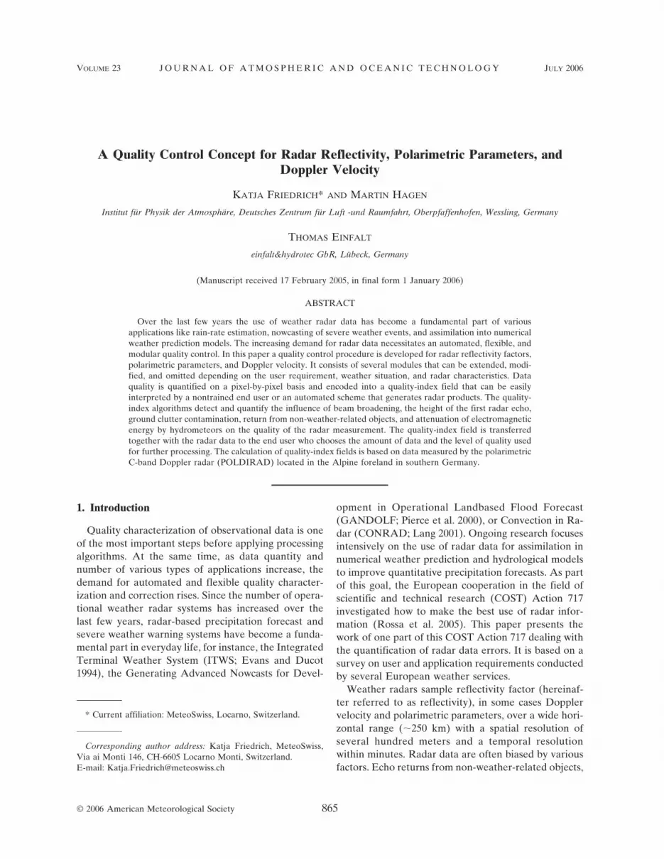
for example, ground and sea clutter, birds, and attenu-ation of the transmitted electromagnetic wave by hy-drometeors, are the main factors contributing to uncer-tainties in the measurement. Figure 1 shows a reflectiv-ity field during the passage of a squall line measured bythe polarimetric diversity C-band Doppler radar(POLDIRAD). The radar is operated by the DeutscheZentrum für Luft- und Raumfahrt at Oberpfaffen-hofen, which is located 30 km southwest of Munich inGermany. The reflectivity data are contaminated byground clutter from the Alps south of the radar andattenuation by hydrometeors behind the squall linewest of the radar. Those biases affect the data and yieldto mismatches in determining radar products like rain-rate estimation. A variety of error sources and theirimpact on radar measurements have been studied in-tensively and are summarized, for instance, in Battan(1973), Zawadzki (1984), Hannesen (2001), Alberoni etal. (2002), and Meischner (2003), among other studies.

Over the years algorithms have been developed toeither detect or correct contaminations. Grecu andKrajewski (2000) and Krajewski and Vignal (2001) forinstance developed a methodology for detectinganomalous propagation echoes using neural networks.Data quality of the Next-Generation Weather Radar(NEXRAD) has been constantly optimized using re-

flectivity and Doppler velocity in a fuzzy logic–basedanomalous propagation clutter mitigation schemes(Kessinger et al. 2003). Steiner and Smith (2002) usedthe three-dimensional reflectivity structures to detectautomatically sea clutter and anomalous propagationeither separated from or embedded within precipitationechoes. Sempere-Torres et al. (2003) developed an al-gorithm to detect signal instabilities of radar measure-ments by analyzing temporal variations of mountainreturns. A correction for precipitation attenuationbased on the minimization of a cost function is sug-gested by Berenguer et al. (2002). Attenuation correc-tion using dual-polarization radar measurements hasbeen discussed by Aydin et al. (1989), Bringi et al.(1990), and Gorgucci et al. (1996). This listing presentsonly a short extraction of the large number of differentradar correction and error detecting algorithms. Pro-cessing and scanning techniques have also been im-proved to overcome certain shortages like Dopplerspectrum aliasing, ground clutter contamination, andsecond-trip echo return. Unal and Moisseev (2004) in-troduced a simple processing technique for the Doppleranalysis combining simultaneous measures required forpolarimetry analysis and maximum unambiguousDoppler velocity. Many operational Doppler weatherradars operate with a dual-pulse-repetition frequency(dual-PRF) technique in order to extend the unambigu-ous Doppler velocity interval (Dazhang et al. 1982;Holleman and Beekhuis 2003). Alternatively, a stag-gered-pulse-repetition frequency allows the increase ofthe maximum unambiguous velocity while maintainingan adequate unambiguous range (Zrnic and Mahapatra1985). Phase coding techniques have been employed inorder to isolate radar echoes returning from a transmit-ted pulse at times subsequent to when previous pulseshave been transmitted (Sachidananda 1997).

For broader usage in terms of different applications,increasing numbers of measured quantities, and an in-creasing number of radar systems, most of the afore-mentioned correction algorithms and processing tech-niques are lacking in a few key respects. First, they onlyfocused on specific kinds of contamination for specificapplications, which complicates the combination of sev-eral algorithms. Most algorithms focus on data correc-tion rather than quality characterization. Also, no in-formation about the corrections applied and the qualityof the data is provided to the end user or for productgeneration. Finally, data correction is not standardizedat present, and therefore, these procedures may pro-duce different results, even when applying the samebasic method.

To properly address these issues, a consistent qualitycontrol concept needs to be developed. This is accom-

FIG. 1. Reflectivity factor field (Ze) displayed as PPI at 0.7°-elevation angle. Measurements were achieved by POLDIRAD(located in the center) at 1953 UTC on 21 Jul 1992. Grayscale forreflectivity is shown at top. Radar measurements are contami-nated by ground clutter from the Alps, which are located south ofPOLDIRAD. Data are also contaminated by attenuation of elec-tromagnetic energy caused by hydrometeors that occur west ofthe squall line located about 40 km west of POLDIRAD.

866 J O U R N A L O F A T M O S P H E R I C A N D O C E A N I C T E C H N O L O G Y VOLUME 23

plished in this paper by characterizing the quality ofradar reflectivity, polarimetric parameters, and Dopp-ler velocity to be used for any application. This conceptis unique for the following reasons.

• A consistent strategy is applied on a pixel-by-pixelbasis to all three quantities.

• This is the first quality control concept for polarimet-ric parameters.

• The concept focuses primarily on the quality charac-terization without applying data modification.

• End users have access to values quantifying theamount of contamination. Therewith, they will beable to choose the amount of data and the level ofdata quality required for their specific application.

Section 2 describes the concept for the quality controlscheme. The determination of quality-index fields is theonly part of this concept that is discussed in detail inthis paper. The quality characterization for reflectivityis described in section 3, the quality characterization forpolarimetric parameters is described in section 4, andthe quality of the Doppler velocity is quantified in sec-tion 5. Finally, conclusions are presented in section 6.

2. Concept for the quality control scheme

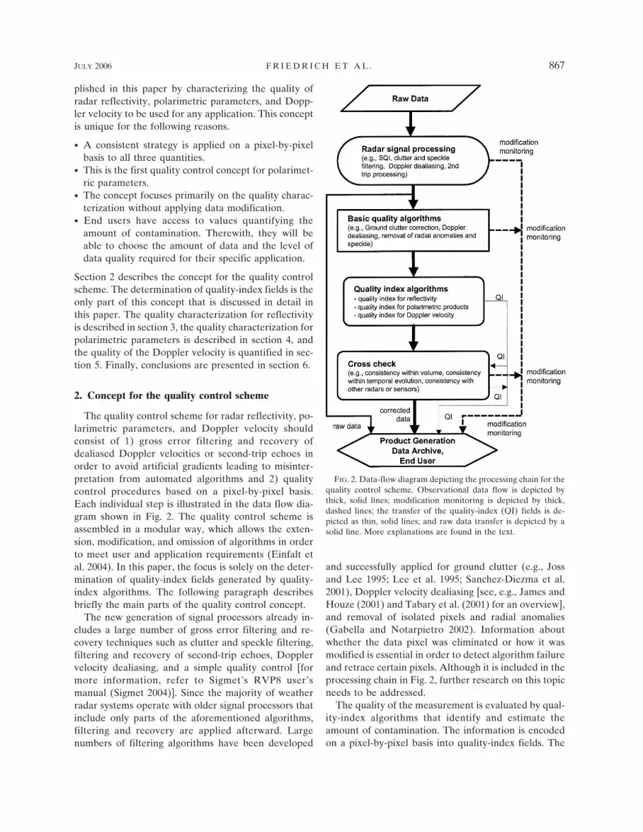
The quality control scheme for radar reflectivity, po-larimetric parameters, and Doppler velocity shouldconsist of 1) gross error filtering and recovery ofdealiased Doppler velocities or second-trip echoes inorder to avoid artificial gradients leading to misinter-pretation from automated algorithms and 2) qualitycontrol procedures based on a pixel-by-pixel basis.Each individual step is illustrated in the data flow dia-gram shown in Fig. 2. The quality control scheme isassembled in a modular way, which allows the exten-sion, modification, and omission of algorithms in orderto meet user and application requirements (Einfalt etal. 2004). In this paper, the focus is solely on the deter-mination of quality-index fields generated by quality-index algorithms. The following paragraph describesbriefly the main parts of the quality control concept.

The new generation of signal processors already in-cludes a large number of gross error filtering and re-covery techniques such as clutter and speckle filtering,filtering and recovery of second-trip echoes, Dopplervelocity dealiasing, and a simple quality control [formore information, refer to Sigmet’s RVP8 user’smanual (Sigmet 2004)]. Since the majority of weatherradar systems operate with older signal processors thatinclude only parts of the aforementioned algorithms,filtering and recovery are applied afterward. Largenumbers of filtering algorithms have been developed

and successfully applied for ground clutter (e.g., Jossand Lee 1995; Lee et al. 1995; Sanchez-Diezma et al.2001), Doppler velocity dealiasing [see, e.g., James andHouze (2001) and Tabary et al. (2001) for an overview],and removal of isolated pixels and radial anomalies(Gabella and Notarpietro 2002). Information aboutwhether the data pixel was eliminated or how it wasmodified is essential in order to detect algorithm failureand retrace certain pixels. Although it is included in theprocessing chain in Fig. 2, further research on this topicneeds to be addressed.

The quality of the measurement is evaluated by qual-ity-index algorithms that identify and estimate theamount of contamination. The information is encodedon a pixel-by-pixel basis into quality-index fields. The

FIG. 2. Data-flow diagram depicting the processing chain for thequality control scheme. Observational data flow is depicted bythick, solid lines; modification monitoring is depicted by thick,dashed lines; the transfer of the quality-index (QI) fields is de-picted as thin, solid lines; and raw data transfer is depicted by asolid line. More explanations are found in the text.

JULY 2006 F R I E D R I C H E T A L . 867

quality-index schemes for reflectivity, polarimetric pa-rameters, and Doppler velocity are discussed in moredetail in the following sections.

The second part in the quality control includes thefinal check for spatial and temporal consistency (de-noted as “cross-check” in Fig. 2). Multiple sensor infor-mation, for example, from independent radars, are usedto cross-check the radar measurements. An example ofa cross-check procedure is given by Friedrich andHagen (2004) using multiple-Doppler information todetect irregularities in the Doppler velocity measure-ment. Additional data sources can also include satellitedata, surface synoptic stations, radiosoundings, or nu-merical model output. After the data passed the qualitycontrol scheme, radar products can be generated. Miss-ing single rays or small wholes in the radar pictures canbe filled applying simple interpolation algorithms (Golzet al. 2004). Data can be smoothed, filtered, or extrap-olated. The end user has access to the quality-controlled observational data or the generated prod-ucts, the respective averaged quality-index field, andpossibly the modification monitoring field.

3. Quality-index scheme for reflectivity

a. Methodology

Over the years four main factors have been identifiedthat contribute to uncertainties in radar reflectivitymeasurements:

1) beam broadening and height of the first radar echo(denoted as Frange),

2) partial or complete beam shielding due to groundclutter (denoted as Fshield),

3) attenuation of electromagnetic energy by hydro-meteors (denoted as Fatt),

4) inhomogeneous vertical profile of reflectivity (de-noted as Fvpr).

While factors 1 and 2 can be considered persistent, thatis, constant for a given radar installation and indepen-dent of the weather situation, the type of error denotedas 3 and 4 is an intermittent bias and needs to be cal-culated separately for each radar volume. The averagedquality-index field for reflectivity, FZe

, is computed as

FZe� �0 for Fatt � 0 or Fshield � 0

1�CZe�WrangeFrange � WshieldFshield � WattFatt � WvprFvpr� else,

�1�

where

CZe� Wrange � Wshield � Watt � Wvpr,

with Wrange, Wshield, Watt, and Wvpr being the respectiveweights. Weighting factors are set according to theweather situation, the location of the radar, and the

application. Table 1 gives an overview of weighting fac-tor ranges that will be discussed in more detail in thefollowing sections.

Each quality-index field and the average index fieldrange between zero and one. When data are contami-nated by ground clutter, indicated as Fshield � 0, orstrongly attenuated by hydrometeors, indicated as

TABLE 1. Weighting factor combinations for nowcasting, assimilation, and rain-rate estimation to be applied for differentweather situations such as stratiform precipitation, convective precipitation, and a combination of both (denoted as hybrid) forPOLDIRAD.

Wrange Wshield Watt Wvpr Wbea Wrain Wcon Wsq Wnp

NowcastingStratiform 1 0.5–1 0.4–0.6 0 0.5 0 0 1 1Convective 1 0.5–1 1 0 0.5 0 0 1 0.6–0.8Hybrid 1 0.5–1 1 0 0.5 0 0 1 0.8AssimilationStratiform 1 0.8–1 0.4–0.6 0.8 0.5 0 0 1 1Convective 1 0.8–1 1 0.8 0.5 0 0 1 0.6–0.8Hybrid 1 0.8–1 1 0.8 0.5 0 0 1 0.8Rain-rate estimationStratiform 1 1 0.4–0.6 1 1 1 0.5 1 1Convective 1 1 1 1 0.5 1 1 1 0.6–0.8Hybrid 1 1 1 1 0.5 1 1 1 0.8


Fatt � 0, these pixels will not be used for further dataprocessing, and FZe

is set to zero. The interpolationfrom the respective parameter field to the quality-indexfield is schematically illustrated in Fig. 3. The determi-nation of FZe

is exemplified using reflectivity measure-ment achieved by POLDIRAD on 21 July 1992 (Fig. 1).The quality-index field is based on radar reflectivitysince this is the quantity mostly provided by radar sys-tems. However, this quality-index scheme can be ap-plied in the same way to reflectivity products that arebased on radar power measurements such as precipita-tion estimation.

b. Utilizing beam broadening and height of the firstradar echo

For measurements taken at far distance, the radarbeam expands in horizontal and vertical directions.

Consequently, the probability rises that the radar beamis inhomogeneously filled by meteorological targets.Brightband correction becomes difficult when the radarbeam extent is larger than the brightband thickness.Additionally, the height of the radar beam increaseswith range. This can lead to overshooting precipitationand errors when extrapolating data to the ground. Ef-fects due to anomalous propagation of the radar beamintensify with increasing range from the radar yieldingto a wrong spatial positioning of the precipitation areasand to ground clutter contamination. Table 2 lists sev-eral factors contributing to uncertainties and theirtrends with increasing range and beam elevation. Onecan assume that the accuracy of the reflectivitymeasurements decreases linearly with increasing dis-tance from the radar (Fig. 3a). Therefore, Frange is de-termined as

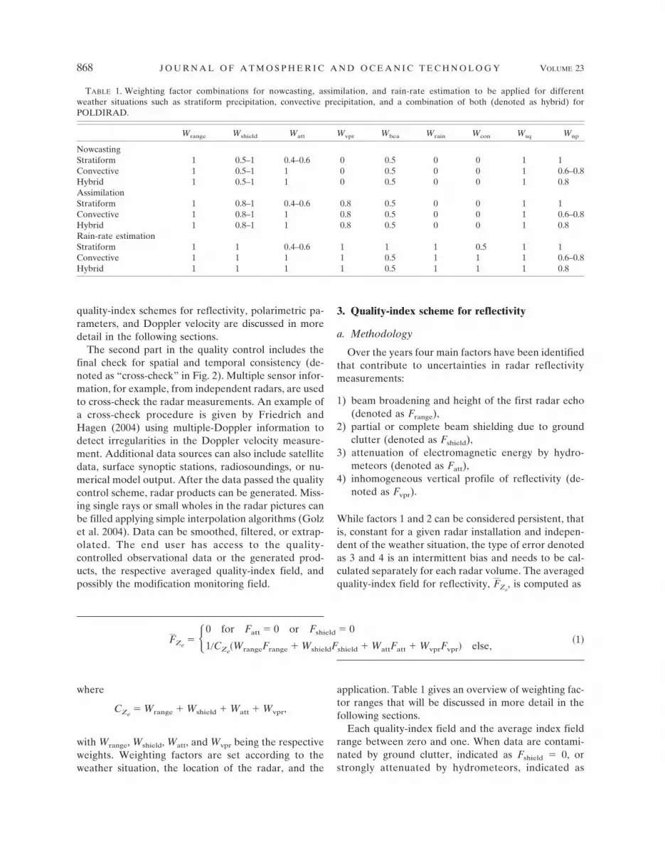
FIG. 3. Computation of the quality-index field (a) Frange based on the influence of range resolution, (b) Fshield

based on the amount of beam shielding due to ground clutter, (c) Fatt based on the amount of pathlengthattenuation, and (d) Fvpr based on the variability of the vertical reflectivity profile. (a) Maximum and minimumsample range are denoted as rmin, rmax. (b) The 3-dB beamwidth is margined by ��3dB and ��3dB. The elevationangle of the mainlobe axis is denoted as �0. (c) The thresholds for maximum and minimum attenuation are Kmax

and Kmin, respectively. (d) The thickness of the melting layer is defined as freezing level plus 200 m, hFL�200, andfreezing level minus 500 m is denoted as hFL�500.

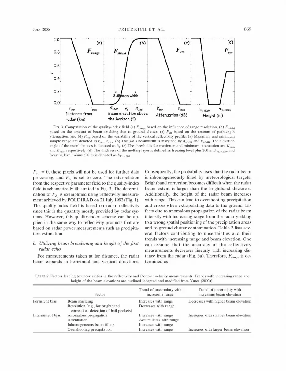
TABLE 2. Factors leading to uncertainties in the reflectivity and Doppler velocity measurements. Trends with increasing range andheight of the beam elevations are outlined [adapted and modified from Yuter (2003)].

FactorTrend of uncertainty with

increasing rangeTrend of uncertainty withincreasing beam elevation

Persistent bias Beam shielding Increases with range Decreases with higher beam elevationResolution (e.g., for brightband

correction, detection of hail pockets)Decreases with range

Intermittent bias Anomalous propagation Increases with range Increases with smaller beam elevationAttenuation Accumulates with rangeInhomogeneous beam filling Increases with rangeOvershooting precipitation Increases with range Increases with larger beam elevation


Frange � �0 for r � rmax

1 for r � rmin

rmax � r

rmax � rmin

for rmin � r � rmax ,

�2�

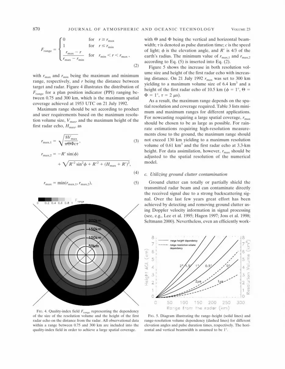
with rmax and rmin being the maximum and minimumrange, respectively, and r being the distance betweentarget and radar. Figure 4 illustrates the distribution ofFrange for a plan position indicator (PPI) ranging be-tween 0.75 and 300 km, which is the maximum spatialcoverage achieved at 1953 UTC on 21 July 1992.

Maximum range should be set according to productand user requirements based on the maximum resolu-tion volume size, Vmax, and the maximum height of thefirst radar echo, Hmax, as

rmax,1 �� 8Vmax

��c�, �3�

rmax,2 � �R sin��

� �R2 sin2 � R2 � �Hmax � R�2,

�4�

rmax � min�rmax,1, rmax,2�, �5�

with and being the vertical and horizontal beam-width; � is denoted as pulse duration time; c is the speedof light; � is the elevation angle, and R is 4/3 of theearth’s radius. The minimum value of rmax,1 and rmax,2

according to Eq. (5) is inserted into Eq. (2).Figure 5 shows the increase in both resolution vol-

ume size and height of the first radar echo with increas-ing distance. On 21 July 1992 rmax was set to 300 kmyielding to a maximum volume size of 6.4 km3 and aheight of the first radar echo of 10.5 km (� � 1°, � � 1°, � � 2 �s).

As a result, the maximum range depends on the spa-tial resolution and coverage required. Table 3 lists mini-mum and maximum ranges for different applications.For nowcasting requiring a large spatial coverage, rmax

should be chosen to be as large as possible. For rain-rate estimations requiring high-resolution measure-ments close to the ground, the maximum range shouldnot exceed 130 km yielding to a maximum resolutionvolume of 0.61 km3 and the first radar echo at 3.3-kmheight. For data assimilation, however, rmax should beadjusted to the spatial resolution of the numericalmodel.

c. Utilizing ground clutter contamination

Ground clutter can totally or partially shield thetransmitted radar beam and can contaminate directlythe received signal due to a strong backscattering sig-nal. Over the last few years great effort has beenachieved by detecting and removing ground clutter us-ing Doppler velocity information in signal processing(see, e.g., Lee et al. 1995; Hagen 1997; Joss et al. 1998;Seltmann 2000). Nevertheless, even an efficiently work-

FIG. 4. Quality-index field Frange representing the dependencyof the size of the resolution volume and the height of the firstradar echo on the distance from the radar. All observational datawithin a range between 0.75 and 300 km are included into thequality-index field in order to achieve a large spatial coverage.

FIG. 5. Diagram illustrating the range–height (solid lines) andrange-resolution volume dependency (dashed lines) for differentelevation angles and pulse duration times, respectively. The hori-zontal and vertical beamwidth is assumed to be 1°.


ing Doppler velocity filter can incorrectly remove pre-cipitation information especially for slowly moving orstationary precipitation and does not consider beam-shielding effects.

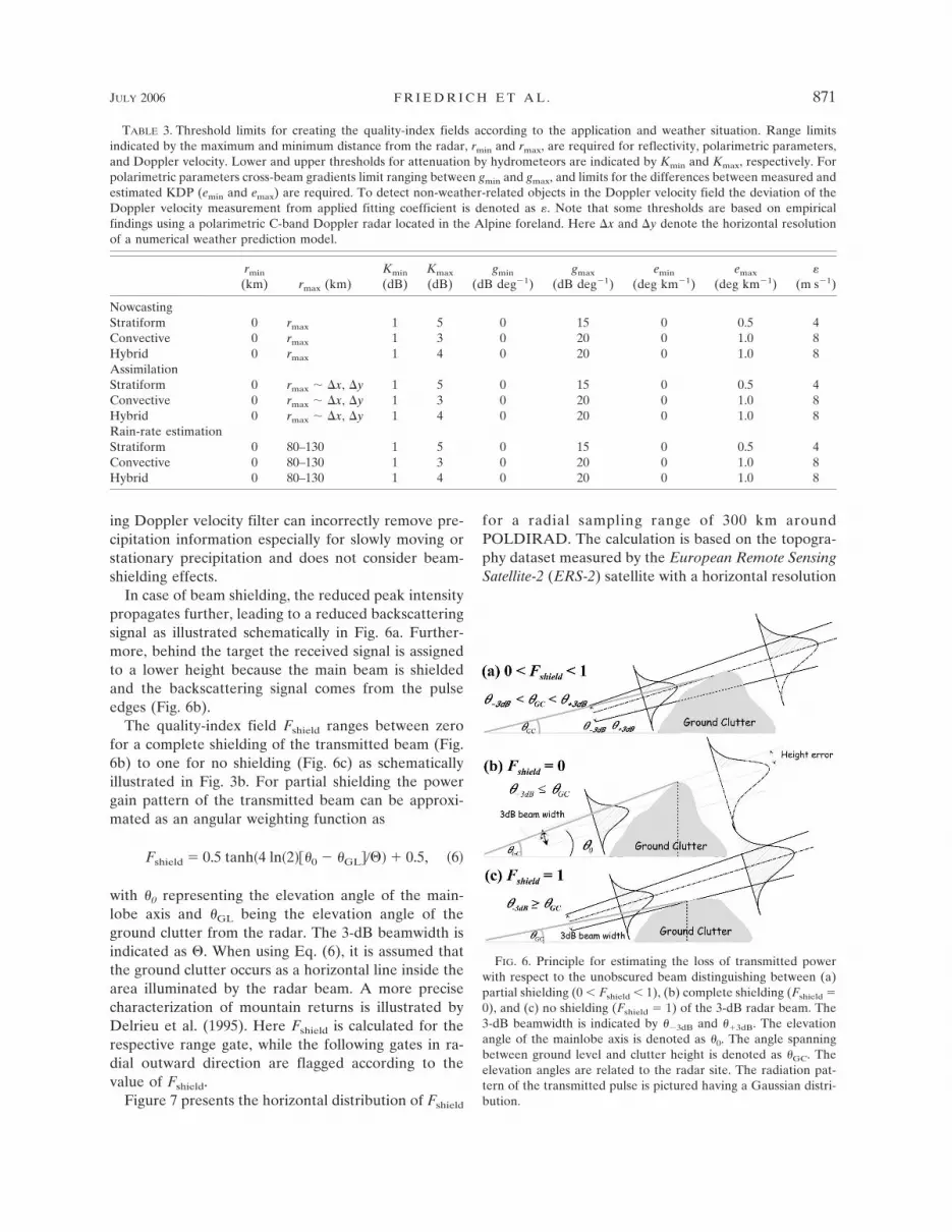
In case of beam shielding, the reduced peak intensitypropagates further, leading to a reduced backscatteringsignal as illustrated schematically in Fig. 6a. Further-more, behind the target the received signal is assignedto a lower height because the main beam is shieldedand the backscattering signal comes from the pulseedges (Fig. 6b).

The quality-index field Fshield ranges between zerofor a complete shielding of the transmitted beam (Fig.6b) to one for no shielding (Fig. 6c) as schematicallyillustrated in Fig. 3b. For partial shielding the powergain pattern of the transmitted beam can be approxi-mated as an angular weighting function as

Fshield � 0.5 tanh�4 ln�2��0 � �GL�� 0.5, �6�

with �0 representing the elevation angle of the main-lobe axis and �GL being the elevation angle of theground clutter from the radar. The 3-dB beamwidth isindicated as . When using Eq. (6), it is assumed thatthe ground clutter occurs as a horizontal line inside thearea illuminated by the radar beam. A more precisecharacterization of mountain returns is illustrated byDelrieu et al. (1995). Here Fshield is calculated for therespective range gate, while the following gates in ra-dial outward direction are flagged according to thevalue of Fshield.

Figure 7 presents the horizontal distribution of Fshield

for a radial sampling range of 300 km aroundPOLDIRAD. The calculation is based on the topogra-phy dataset measured by the European Remote SensingSatellite-2 (ERS-2) satellite with a horizontal resolution

TABLE 3. Threshold limits for creating the quality-index fields according to the application and weather situation. Range limitsindicated by the maximum and minimum distance from the radar, rmin and rmax, are required for reflectivity, polarimetric parameters,and Doppler velocity. Lower and upper thresholds for attenuation by hydrometeors are indicated by Kmin and Kmax, respectively. Forpolarimetric parameters cross-beam gradients limit ranging between gmin and gmax, and limits for the differences between measured andestimated KDP (emin and emax) are required. To detect non-weather-related objects in the Doppler velocity field the deviation of theDoppler velocity measurement from applied fitting coefficient is denoted as �. Note that some thresholds are based on empiricalfindings using a polarimetric C-band Doppler radar located in the Alpine foreland. Here �x and �y denote the horizontal resolutionof a numerical weather prediction model.

rmin

(km) rmax (km)Kmin

(dB)Kmax

(dB)gmin

(dB deg�1)gmax

(dB deg�1)emin

(deg km�1)emax

(deg km�1)�

(m s�1)

NowcastingStratiform 0 rmax 1 5 0 15 0 0.5 4Convective 0 rmax 1 3 0 20 0 1.0 8Hybrid 0 rmax 1 4 0 20 0 1.0 8AssimilationStratiform 0 rmax � �x, �y 1 5 0 15 0 0.5 4Convective 0 rmax � �x, �y 1 3 0 20 0 1.0 8Hybrid 0 rmax � �x, �y 1 4 0 20 0 1.0 8Rain-rate estimationStratiform 0 80–130 1 5 0 15 0 0.5 4Convective 0 80–130 1 3 0 20 0 1.0 8Hybrid 0 80–130 1 4 0 20 0 1.0 8

FIG. 6. Principle for estimating the loss of transmitted powerwith respect to the unobscured beam distinguishing between (a)partial shielding (0 � Fshield � 1), (b) complete shielding (Fshield �0), and (c) no shielding (Fshield � 1) of the 3-dB radar beam. The3-dB beamwidth is indicated by ��3dB and ��3dB. The elevationangle of the mainlobe axis is denoted as �0. The angle spanningbetween ground level and clutter height is denoted as �GC. Theelevation angles are related to the radar site. The radiation pat-tern of the transmitted pulse is pictured having a Gaussian distri-bution.


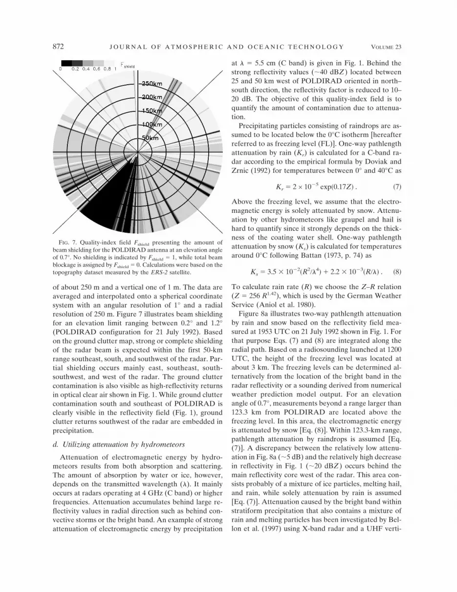
of about 250 m and a vertical one of 1 m. The data areaveraged and interpolated onto a spherical coordinatesystem with an angular resolution of 1° and a radialresolution of 250 m. Figure 7 illustrates beam shieldingfor an elevation limit ranging between 0.2° and 1.2°(POLDIRAD configuration for 21 July 1992). Basedon the ground clutter map, strong or complete shieldingof the radar beam is expected within the first 50-kmrange southeast, south, and southwest of the radar. Par-tial shielding occurs mainly east, southeast, south-southwest, and west of the radar. The ground cluttercontamination is also visible as high-reflectivity returnsin optical clear air shown in Fig. 1. While ground cluttercontamination south and southeast of POLDIRAD isclearly visible in the reflectivity field (Fig. 1), groundclutter returns southwest of the radar are embedded inprecipitation.

d. Utilizing attenuation by hydrometeors

Attenuation of electromagnetic energy by hydro-meteors results from both absorption and scattering.The amount of absorption by water or ice, however,depends on the transmitted wavelength (�). It mainlyoccurs at radars operating at 4 GHz (C band) or higherfrequencies. Attenuation accumulates behind large re-flectivity values in radial direction such as behind con-vective storms or the bright band. An example of strongattenuation of electromagnetic energy by precipitation

at � � 5.5 cm (C band) is given in Fig. 1. Behind thestrong reflectivity values (�40 dBZ) located between25 and 50 km west of POLDIRAD oriented in north–south direction, the reflectivity factor is reduced to 10–20 dB. The objective of this quality-index field is toquantify the amount of contamination due to attenua-tion.

Precipitating particles consisting of raindrops are as-sumed to be located below the 0°C isotherm [hereafterreferred to as freezing level (FL)]. One-way pathlengthattenuation by rain (Kr) is calculated for a C-band ra-dar according to the empirical formula by Doviak andZrnic (1992) for temperatures between 0° and 40°C as

Kr � 2 × 10�5 exp�0.17Z� . �7�

Above the freezing level, we assume that the electro-magnetic energy is solely attenuated by snow. Attenu-ation by other hydrometeors like graupel and hail ishard to quantify since it strongly depends on the thick-ness of the coating water shell. One-way pathlengthattenuation by snow (Ks) is calculated for temperaturesaround 0°C following Battan (1973, p. 74) as

Ks � 3.5 � 10�2�R2��4� � 2.2 � 10�3�R�� . �8�

To calculate rain rate (R) we choose the Z–R relation(Z � 256 R1.42), which is used by the German WeatherService (Aniol et al. 1980).

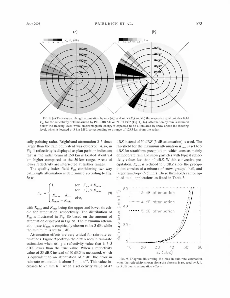
Figure 8a illustrates two-way pathlength attenuationby rain and snow based on the reflectivity field mea-sured at 1953 UTC on 21 July 1992 shown in Fig. 1. Forthat purpose Eqs. (7) and (8) are integrated along theradial path. Based on a radiosounding launched at 1200UTC, the height of the freezing level was located atabout 3 km. The freezing levels can be determined al-ternatively from the location of the bright band in theradar reflectivity or a sounding derived from numericalweather prediction model output. For an elevationangle of 0.7°, measurements beyond a range larger than123.3 km from POLDIRAD are located above thefreezing level. In this area, the electromagnetic energyis attenuated by snow [Eq. (8)]. Within 123.3-km range,pathlength attenuation by raindrops is assumed [Eq.(7)]. A discrepancy between the relatively low attenu-ation in Fig. 8a (�5 dB) and the relatively high decreasein reflectivity in Fig. 1 (�20 dBZ) occurs behind themain reflectivity core west of the radar. This area con-sists probably of a mixture of ice particles, melting hail,and rain, while solely attenuation by rain is assumed[Eq. (7)]. Attenuation caused by the bright band withinstratiform precipitation that also contains a mixture ofrain and melting particles has been investigated by Bel-lon et al. (1997) using X-band radar and a UHF verti-

FIG. 7. Quality-index field Fshield presenting the amount ofbeam shielding for the POLDIRAD antenna at an elevation angleof 0.7°. No shielding is indicated by Fshield � 1, while total beamblockage is assigned by Fshield � 0. Calculations were based on thetopography dataset measured by the ERS-2 satellite.


cally pointing radar. Brightband attenuation 3–5 timeslarger than the rain equivalent was observed. Also, inFig. 1 reflectivity is displayed as plan position indicator;that is, the radar beam at 150 km is located about 2.4km higher compared to the 50-km range. Areas oflower reflectivity are intersected at farther ranges.

The quality-index field Fatt considering two-waypathlength attenuation is determined according to Fig.3c as

Fatt � �1 for Kr,s � Kmin

0 for Kr,s Kmax

Kmax � Kr,s

Kmax � Kmin

else,�9�

with Kmax and Kmin being the upper and lower thresh-old for attenuation, respectively. The distribution ofFatt is illustrated in Fig. 8b based on the amount ofattenuation displayed in Fig. 8a. The maximum attenu-ation rate Kmax is empirically chosen to be 3 dB, whilethe minimum is set to 1 dB.

Attenuation effects are very critical for rain-rate es-timations. Figure 9 portrays the differences in rain-rateestimation when using a reflectivity value that is 3–5dBZ lower than the true value. When a reflectivityvalue of 35 dBZ instead of 40 dBZ is measured, whichis equivalent to an attenuation of 5 dB, the error inrain-rate estimation is about 7 mm h�1. This value in-creases to 25 mm h�1 when a reflectivity value of 47

dBZ instead of 50 dBZ (3-dB attenuation) is used. Thethreshold for the maximum attenuation Kmax is set to 5dBZ for stratiform precipitation, which consists mainlyof moderate rain and snow particles with typical reflec-tivity values less than 40 dBZ. Within convective pre-cipitation, Kmax is reduced to 3 dBZ since the precipi-tation consists of a mixture of snow, graupel, hail, andlarger raindrops (�5 mm). These thresholds can be ap-plied to all applications as listed in Table 3.

FIG. 8. (a) Two-way pathlength attenuation by rain (Kr) and snow (Ks) and (b) the respective quality-index fieldFatt for the reflectivity field measured by POLDIRAD on 21 Jul 1992 (Fig. 1). (a) Attenuation by rain is assumedbelow the freezing level, while electromagnetic energy is expected to be attenuated by snow above the freezinglevel, which is located at 3 km MSL corresponding to a range of 123.3 km from the radar.

FIG. 9. Diagram illustrating the bias in rain-rate estimationwhen the reflectivity shown along the abscissa is reduced by 3, 4,or 5 dB due to attenuation effects.


e. Utilizing vertical reflectivity profile

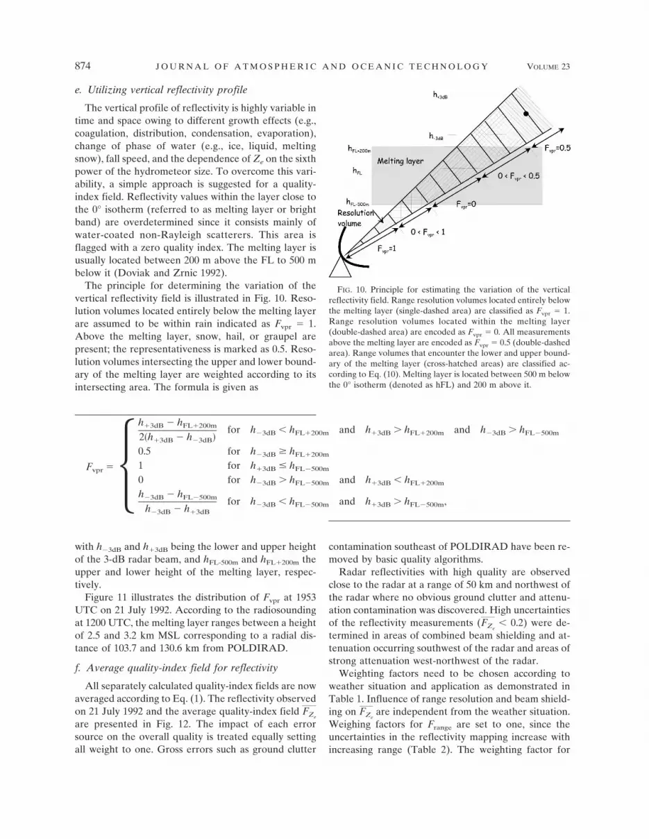
The vertical profile of reflectivity is highly variable intime and space owing to different growth effects (e.g.,coagulation, distribution, condensation, evaporation),change of phase of water (e.g., ice, liquid, meltingsnow), fall speed, and the dependence of Ze on the sixthpower of the hydrometeor size. To overcome this vari-ability, a simple approach is suggested for a quality-index field. Reflectivity values within the layer close tothe 0° isotherm (referred to as melting layer or brightband) are overdetermined since it consists mainly ofwater-coated non-Rayleigh scatterers. This area isflagged with a zero quality index. The melting layer isusually located between 200 m above the FL to 500 mbelow it (Doviak and Zrnic 1992).

The principle for determining the variation of thevertical reflectivity field is illustrated in Fig. 10. Reso-lution volumes located entirely below the melting layerare assumed to be within rain indicated as Fvpr � 1.Above the melting layer, snow, hail, or graupel arepresent; the representativeness is marked as 0.5. Reso-lution volumes intersecting the upper and lower bound-ary of the melting layer are weighted according to itsintersecting area. The formula is given as

Fvpr ��h�3dB � hFL�200m

2�h�3dB � h�3dB�for h�3dB � hFL�200m and h�3dB hFL�200m and h�3dB hFL�500m

0.5 for h�3dB � hFL�200m

1 for h�3dB � hFL�500m

0 for h�3dB hFL�500m and h�3dB � hFL�200m

h�3dB � hFL�500m

h�3dB � h�3dB

for h�3dB � hFL�500m and h�3dB hFL�500m,

with h�3dB and h�3dB being the lower and upper heightof the 3-dB radar beam, and hFL-500m and hFL�200m theupper and lower height of the melting layer, respec-tively.

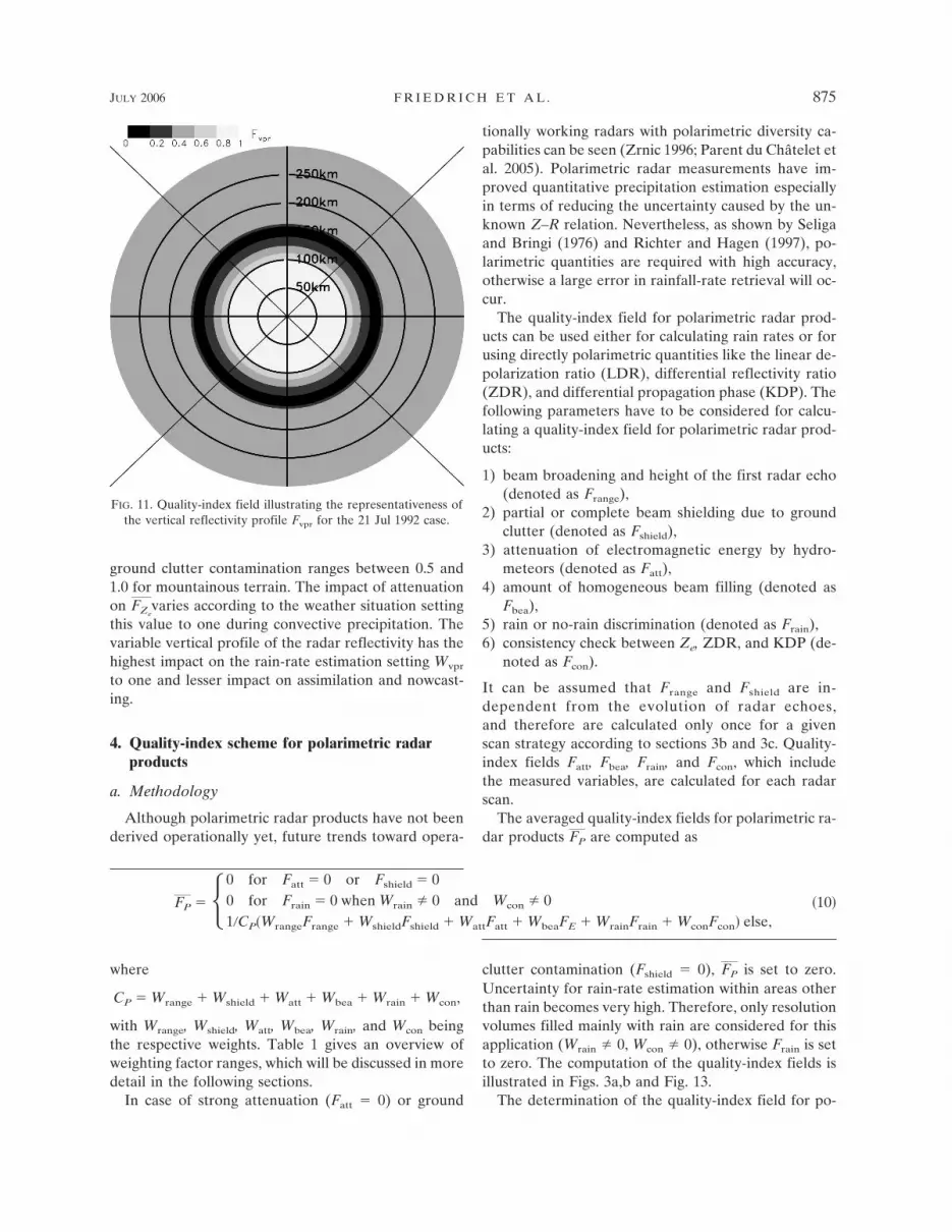
Figure 11 illustrates the distribution of Fvpr at 1953UTC on 21 July 1992. According to the radiosoundingat 1200 UTC, the melting layer ranges between a heightof 2.5 and 3.2 km MSL corresponding to a radial dis-tance of 103.7 and 130.6 km from POLDIRAD.

f. Average quality-index field for reflectivity

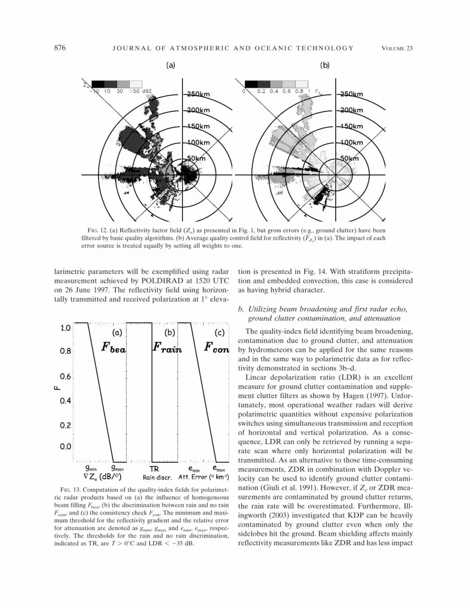
All separately calculated quality-index fields are nowaveraged according to Eq. (1). The reflectivity observedon 21 July 1992 and the average quality-index field FZe

are presented in Fig. 12. The impact of each errorsource on the overall quality is treated equally settingall weight to one. Gross errors such as ground clutter

contamination southeast of POLDIRAD have been re-moved by basic quality algorithms.

Radar reflectivities with high quality are observedclose to the radar at a range of 50 km and northwest ofthe radar where no obvious ground clutter and attenu-ation contamination was discovered. High uncertaintiesof the reflectivity measurements (FZe

� 0.2) were de-termined in areas of combined beam shielding and at-tenuation occurring southwest of the radar and areas ofstrong attenuation west-northwest of the radar.

Weighting factors need to be chosen according toweather situation and application as demonstrated inTable 1. Influence of range resolution and beam shield-ing on FZe

are independent from the weather situation.Weighing factors for Frange are set to one, since theuncertainties in the reflectivity mapping increase withincreasing range (Table 2). The weighting factor for

FIG. 10. Principle for estimating the variation of the verticalreflectivity field. Range resolution volumes located entirely belowthe melting layer (single-dashed area) are classified as Fvpr � 1.Range resolution volumes located within the melting layer(double-dashed area) are encoded as Fvpr � 0. All measurementsabove the melting layer are encoded as Fvpr � 0.5 (double-dashedarea). Range volumes that encounter the lower and upper bound-ary of the melting layer (cross-hatched areas) are classified ac-cording to Eq. (10). Melting layer is located between 500 m belowthe 0° isotherm (denoted as hFL) and 200 m above it.


ground clutter contamination ranges between 0.5 and1.0 for mountainous terrain. The impact of attenuationon FZe

varies according to the weather situation settingthis value to one during convective precipitation. Thevariable vertical profile of the radar reflectivity has thehighest impact on the rain-rate estimation setting Wvpr

to one and lesser impact on assimilation and nowcast-ing.

4. Quality-index scheme for polarimetric radarproducts

a. Methodology

Although polarimetric radar products have not beenderived operationally yet, future trends toward opera-

tionally working radars with polarimetric diversity ca-pabilities can be seen (Zrnic 1996; Parent du Châtelet etal. 2005). Polarimetric radar measurements have im-proved quantitative precipitation estimation especiallyin terms of reducing the uncertainty caused by the un-known Z–R relation. Nevertheless, as shown by Seligaand Bringi (1976) and Richter and Hagen (1997), po-larimetric quantities are required with high accuracy,otherwise a large error in rainfall-rate retrieval will oc-cur.

The quality-index field for polarimetric radar prod-ucts can be used either for calculating rain rates or forusing directly polarimetric quantities like the linear de-polarization ratio (LDR), differential reflectivity ratio(ZDR), and differential propagation phase (KDP). Thefollowing parameters have to be considered for calcu-lating a quality-index field for polarimetric radar prod-ucts:

1) beam broadening and height of the first radar echo(denoted as Frange),

2) partial or complete beam shielding due to groundclutter (denoted as Fshield),

3) attenuation of electromagnetic energy by hydro-meteors (denoted as Fatt),

4) amount of homogeneous beam filling (denoted asFbea),

5) rain or no-rain discrimination (denoted as Frain),6) consistency check between Ze, ZDR, and KDP (de-

noted as Fcon).

It can be assumed that Frange and Fshield are in-dependent from the evolution of radar echoes,and therefore are calculated only once for a givenscan strategy according to sections 3b and 3c. Quality-index fields Fatt, Fbea, Frain, and Fcon, which includethe measured variables, are calculated for each radarscan.

The averaged quality-index fields for polarimetric ra-dar products FP are computed as

FP � �0 for Fatt � 0 or Fshield � 00 for Frain � 0 when Wrain � 0 and Wcon � 01�CP�WrangeFrange � WshieldFshield � WattFatt � WbeaFE � WrainFrain � WconFcon� else,

�10�

where

CP � Wrange � Wshield � Watt � Wbea � Wrain � Wcon,

with Wrange, Wshield, Watt, Wbea, Wrain, and Wcon beingthe respective weights. Table 1 gives an overview ofweighting factor ranges, which will be discussed in moredetail in the following sections.

In case of strong attenuation (Fatt � 0) or ground

clutter contamination (Fshield � 0), FP is set to zero.Uncertainty for rain-rate estimation within areas otherthan rain becomes very high. Therefore, only resolutionvolumes filled mainly with rain are considered for thisapplication (Wrain � 0, Wcon � 0), otherwise Frain is setto zero. The computation of the quality-index fields isillustrated in Figs. 3a,b and Fig. 13.

The determination of the quality-index field for po-

FIG. 11. Quality-index field illustrating the representativeness ofthe vertical reflectivity profile Fvpr for the 21 Jul 1992 case.


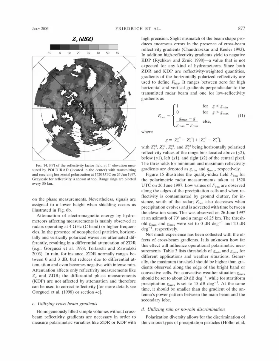
larimetric parameters will be exemplified using radarmeasurement achieved by POLDIRAD at 1520 UTCon 26 June 1997. The reflectivity field using horizon-tally transmitted and received polarization at 1° eleva-

tion is presented in Fig. 14. With stratiform precipita-tion and embedded convection, this case is consideredas having hybrid character.

b. Utilizing beam broadening and first radar echo,ground clutter contamination, and attenuation

The quality-index field identifying beam broadening,contamination due to ground clutter, and attenuationby hydrometeors can be applied for the same reasonsand in the same way to polarimetric data as for reflec-tivity demonstrated in sections 3b–d.

Linear depolarization ratio (LDR) is an excellentmeasure for ground clutter contamination and supple-ment clutter filters as shown by Hagen (1997). Unfor-tunately, most operational weather radars will derivepolarimetric quantities without expensive polarizationswitches using simultaneous transmission and receptionof horizontal and vertical polarization. As a conse-quence, LDR can only be retrieved by running a sepa-rate scan where only horizontal polarization will betransmitted. As an alternative to those time-consumingmeasurements, ZDR in combination with Doppler ve-locity can be used to identify ground clutter contami-nation (Giuli et al. 1991). However, if Ze or ZDR mea-surements are contaminated by ground clutter returns,the rain rate will be overestimated. Furthermore, Ill-ingworth (2003) investigated that KDP can be heavilycontaminated by ground clutter even when only thesidelobes hit the ground. Beam shielding affects mainlyreflectivity measurements like ZDR and has less impact

FIG. 13. Computation of the quality-index fields for polarimet-ric radar products based on (a) the influence of homogeneousbeam filling Fbea, (b) the discrimination between rain and no rainFrain, and (c) the consistency check Fcon. The minimum and maxi-mum threshold for the reflectivity gradient and the relative errorfor attenuation are denoted as gmin, gmax and emin, emax, respec-tively. The thresholds for the rain and no rain discrimination,indicated as TR, are T � 0°C and LDR � �35 dB.

FIG. 12. (a) Reflectivity factor field (Ze) as presented in Fig. 1, but gross errors (e.g., ground clutter) have beenfiltered by basic quality algorithms. (b) Average quality control field for reflectivity (FZe

) in (a). The impact of eacherror source is treated equally by setting all weights to one.


on the phase measurements. Nevertheless, signals areassigned to a lower height when shielding occurs asillustrated in Fig. 6b.

Attenuation of electromagnetic energy by hydro-meteors affecting measurements is mainly observed atradars operating at 4 GHz (C band) or higher frequen-cies. In the presence of nonspherical particles, horizon-tally and vertically polarized waves are attenuated dif-ferently, resulting in a differential attenuation of ZDR(e.g., Gorgucci et al. 1998; Torlaschi and Zawadzki2003). In rain, for instance, ZDR normally ranges be-tween 0 and 3 dB, but reduces due to differential at-tenuation and even becomes negative with intense rain.Attenuation affects only reflectivity measurements likeZe and ZDR; the differential phase measurements(KDP) are not affected by attenuation and thereforecan be used to correct reflectivity [for more details seeGorgucci et al. (1998) or section 4e].

c. Utilizing cross-beam gradients

Homogeneously filled sample volumes without cross-beam reflectivity gradients are necessary in order tomeasure polarimetric variables like ZDR or KDP with

high precision. Slight mismatch of the beam shape pro-duces enormous errors in the presence of cross-beamreflectivity gradients (Chandrasekar and Keeler 1993).In addition high-reflectivity gradients yield to negativeKDP (Ryzhkov and Zrnic 1998)—a value that is notexpected for any kind of hydrometeors. Since bothZDR and KDP are reflectivity-weighted quantities,gradients of the horizontally polarized reflectivity areused to define Fbea. It ranges between zero for highhorizontal and vertical gradients perpendicular to thetransmitted radar beam and one for low-reflectivitygradients as

Fbea � �1 for g � gmin

0 for g gmax

gmax � g

gmax � gmin

else,�11�

where

g � |Zey2 � Ze

y1| � |Zex1 � Ze

x2|,

with Zy2e , Zy1

e , Zx1e , and Zx2

e being horizontally polarizedreflectivity values of the range bins located above (y2),below (y1), left (x1), and right (x2) of the central pixel.The thresholds for minimum and maximum reflectivitygradients are denoted as gmin and gmax, respectively.

Figure 15 illustrates the quality-index field Fbea forthe polarimetric radar measurements taken at 1520UTC on 26 June 1997. Low values of Fbea are observedalong the edges of the precipitation cells and when re-flectivity is contaminated by ground clutter, for in-stance, south of the radar; Fbea also decreases whenprecipitation evolves and is advected with time betweenthe elevation scans. This was observed on 26 June 1997at an azimuth of 70° and a range of 25 km. The thresh-old gmin and gmax were set to 0 dB deg�1 and 20 dBdeg�1, respectively.

Not much experience has been collected with the ef-fects of cross-beam gradients. It is unknown how farthis effect will influence operational polarimetric mea-surements. Table 3 lists thresholds of gmin and gmax fordifferent applications and weather situations. Gener-ally, the maximum threshold should be higher than gra-dients observed along the edge of the bright band orconvective cells. For convective weather situation gmax

should be set to about 20 dB deg�1, while for stratiformprecipitation gmax is set to 15 dB deg�1. At the sametime, it should be smaller than the gradient of the an-tenna’s power pattern between the main beam and thesecondary lobe.

d. Utilizing rain or no-rain discrimination

Polarization diversity allows for the discrimination ofthe various types of precipitation particles (Höller et al.

FIG. 14. PPI of the reflectivity factor field at 1° elevation mea-sured by POLDIRAD (located in the center) with transmittingand receiving horizontal polarization at 1520 UTC on 26 Jun 1997.Grayscale for reflectivity is shown at top. Range rings are plottedevery 50 km.


1994; Vivekanandan et al. 1999). A quality-index fieldFrain is introduced in order to estimate polarimetricrainfall rate solely within regions dominated by rain-drops.

Based on the classification introduced by Höller et al.(1994), the presence of rain (Frain � 1) can be assumedwhen both the air temperature is above 0°C and LDRis below �35 dB, or when LDR ranges between �35and �25 dB and ZDR is above 1 dB. Measurementsindicating hydrometeors other than rain are denoted asFrain � 0 as schematically indicated in Fig. 13b; Frain canbe defined in a similar way using other classificationschemes like the fuzzy logic scheme introduced byVivekanandan et al. (1999).

Figure 16 shows the quality-index field Frain for themeasurements obtained at 1520 UTC on 26 June 1997.Based on the radiosounding launched at 1200 UTC atMunich-Oberschleissheim located about 27 km north-east of the radar, the 0° isotherm was located at about1.8 km above the radar. As a result, hydrometeors ob-served beyond the 80-km range are considered to in-clude an ice phase. Ground clutter close to the radarand south of the radar are identified correctly as no rainby the algorithm. The areas with Frain � 0 to the westand east of the radar were identified as melting graupel

or snow by the classification scheme (Höller et al.1994).

e. Consistency check using Ze, ZDR, and KDP

The consistency check between Ze, ZDR, and KDPwas originally proposed by Goddard et al. (1994) and ina different description by Scarchilli et al. (1996) in orderto check the performance of radar systems within rain.Here Ze and ZDR are used to first derive the raindropsize distribution and then estimate KDP from the rain-drop size distribution. The latter is denoted as K̂DP. IfK̂DP and the measured KDP agree, the data are con-sistent.

An alternative approach was proposed by Gorgucciet al. (1998). They used Ze and ZDR in order to derivethe attenuation in rain (denoted as �H). On the otherhand, KDP can also be used to estimate the attenuationin rain (referred to as �*H). If �H and �*H agree, themeasurements of Ze, ZDR, and KDP are consideredto be consistent. Differences between K̂DP � KDPand �H � �*H result from calibration errors or wrongassumptions concerning scattering properties andsize distribution of raindrops (Gorgucci et al. 1998).The consistency check, however, will fail for hydrom-

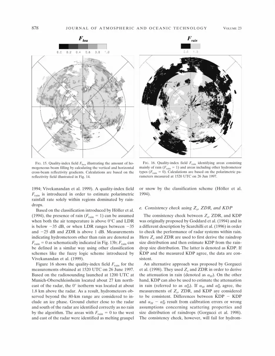
FIG. 15. Quality-index field Fbea illustrating the amount of ho-mogeneous beam filling by calculating the vertical and horizontalcross-beam reflectivity gradients. Calculations are based on thereflectivity field illustrated in Fig. 14.

FIG. 16. Quality-index field Frain identifying areas consistingmainly of rain (Frain � 1) and areas including other hydrometeortypes (Frain � 0). Calculations are based on the polarimetric pa-rameters measured at 1520 UTC on 26 Jun 1997.


eteor types other than rain since up to now it is onlydefined for rain. It also will fail for strong attenuationthat is not considered by the procedure proposed byGorgucci et al. (1998).

The quality-index field Fcon can be computed as

Fcon � �1 for e � emin

0 for e emax

emax � e

emax � emin

else,

e � |K̂DP � KDP|, �12�

where emin and emax are the thresholds for minimumand maximum KDP difference. The interpolation be-tween Fcon and e is schematically indicated in Fig. 13c.

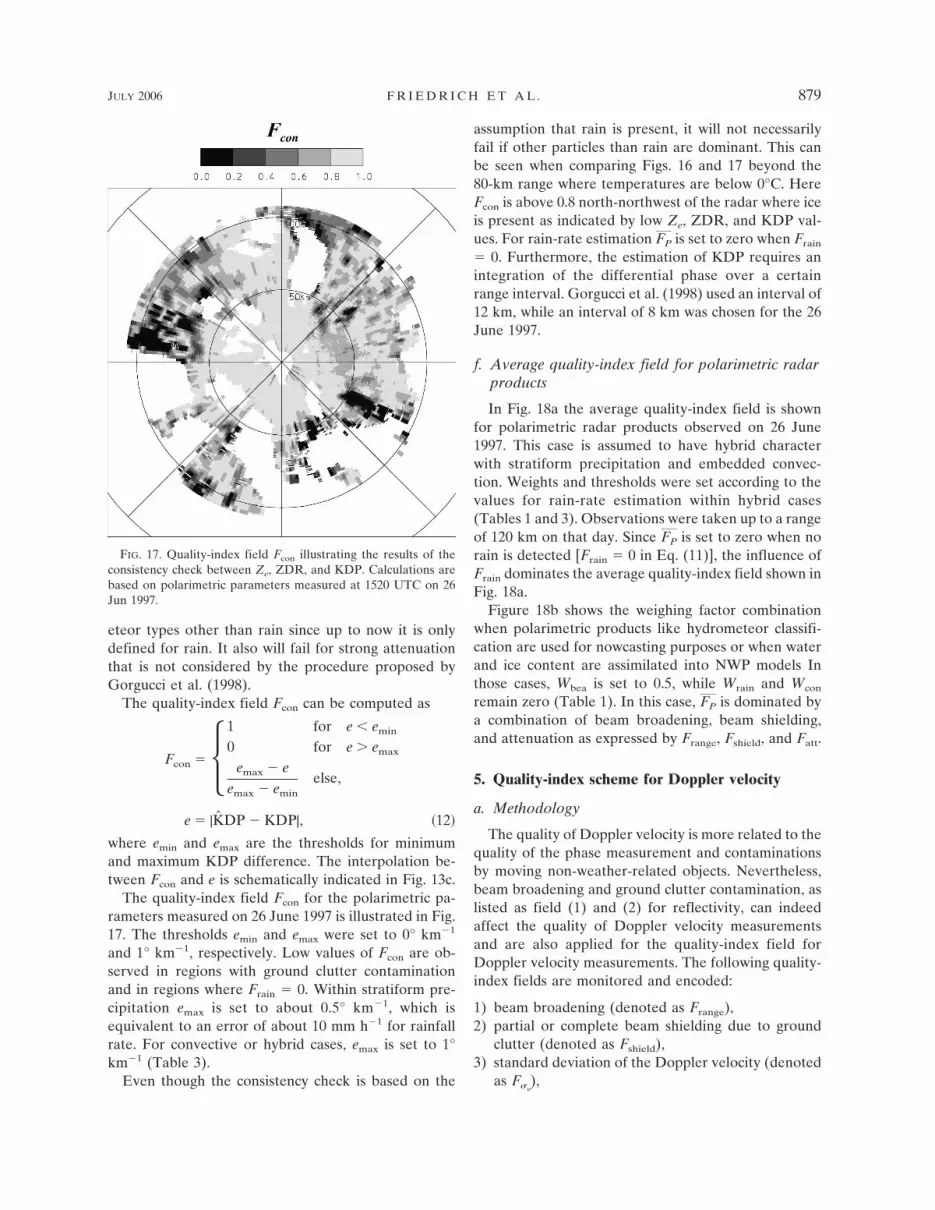
The quality-index field Fcon for the polarimetric pa-rameters measured on 26 June 1997 is illustrated in Fig.17. The thresholds emin and emax were set to 0° km�1

and 1° km�1, respectively. Low values of Fcon are ob-served in regions with ground clutter contaminationand in regions where Frain � 0. Within stratiform pre-cipitation emax is set to about 0.5° km�1, which isequivalent to an error of about 10 mm h�1 for rainfallrate. For convective or hybrid cases, emax is set to 1°km�1 (Table 3).

Even though the consistency check is based on the

assumption that rain is present, it will not necessarilyfail if other particles than rain are dominant. This canbe seen when comparing Figs. 16 and 17 beyond the80-km range where temperatures are below 0°C. HereFcon is above 0.8 north-northwest of the radar where iceis present as indicated by low Ze, ZDR, and KDP val-ues. For rain-rate estimation FP is set to zero when Frain

� 0. Furthermore, the estimation of KDP requires anintegration of the differential phase over a certainrange interval. Gorgucci et al. (1998) used an interval of12 km, while an interval of 8 km was chosen for the 26June 1997.

f. Average quality-index field for polarimetric radarproducts

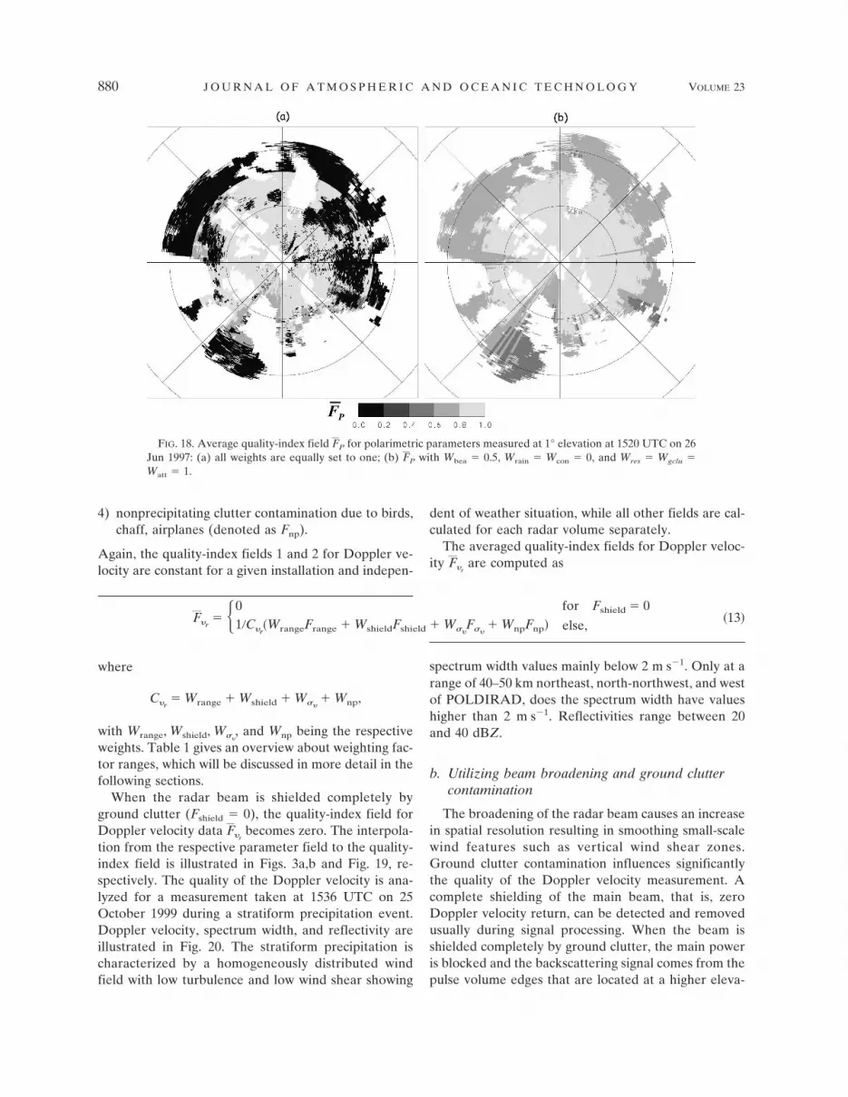
In Fig. 18a the average quality-index field is shownfor polarimetric radar products observed on 26 June1997. This case is assumed to have hybrid characterwith stratiform precipitation and embedded convec-tion. Weights and thresholds were set according to thevalues for rain-rate estimation within hybrid cases(Tables 1 and 3). Observations were taken up to a rangeof 120 km on that day. Since FP is set to zero when norain is detected [Frain � 0 in Eq. (11)], the influence ofFrain dominates the average quality-index field shown inFig. 18a.

Figure 18b shows the weighing factor combinationwhen polarimetric products like hydrometeor classifi-cation are used for nowcasting purposes or when waterand ice content are assimilated into NWP models Inthose cases, Wbea is set to 0.5, while Wrain and Wcon

remain zero (Table 1). In this case, FP is dominated bya combination of beam broadening, beam shielding,and attenuation as expressed by Frange, Fshield, and Fatt.

5. Quality-index scheme for Doppler velocity

a. Methodology

The quality of Doppler velocity is more related to thequality of the phase measurement and contaminationsby moving non-weather-related objects. Nevertheless,beam broadening and ground clutter contamination, aslisted as field (1) and (2) for reflectivity, can indeedaffect the quality of Doppler velocity measurementsand are also applied for the quality-index field forDoppler velocity measurements. The following quality-index fields are monitored and encoded:

1) beam broadening (denoted as Frange),2) partial or complete beam shielding due to ground

clutter (denoted as Fshield),3) standard deviation of the Doppler velocity (denoted

as F��),

FIG. 17. Quality-index field Fcon illustrating the results of theconsistency check between Ze, ZDR, and KDP. Calculations arebased on polarimetric parameters measured at 1520 UTC on 26Jun 1997.


4) nonprecipitating clutter contamination due to birds,chaff, airplanes (denoted as Fnp).

Again, the quality-index fields 1 and 2 for Doppler ve-locity are constant for a given installation and indepen-

dent of weather situation, while all other fields are cal-culated for each radar volume separately.

The averaged quality-index fields for Doppler veloc-ity F�r

are computed as

F�r� �0 for Fshield � 0

1�C�r�WrangeFrange � WshieldFshield � W��

F�� WnpFnp� else, �13�

where

C�r� Wrange � Wshield � W��

� Wnp,

with Wrange, Wshield, W��, and Wnp being the respective

weights. Table 1 gives an overview about weighting fac-tor ranges, which will be discussed in more detail in thefollowing sections.

When the radar beam is shielded completely byground clutter (Fshield � 0), the quality-index field forDoppler velocity data F�r

becomes zero. The interpola-tion from the respective parameter field to the quality-index field is illustrated in Figs. 3a,b and Fig. 19, re-spectively. The quality of the Doppler velocity is ana-lyzed for a measurement taken at 1536 UTC on 25October 1999 during a stratiform precipitation event.Doppler velocity, spectrum width, and reflectivity areillustrated in Fig. 20. The stratiform precipitation ischaracterized by a homogeneously distributed windfield with low turbulence and low wind shear showing

spectrum width values mainly below 2 m s�1. Only at arange of 40–50 km northeast, north-northwest, and westof POLDIRAD, does the spectrum width have valueshigher than 2 m s�1. Reflectivities range between 20and 40 dBZ.

b. Utilizing beam broadening and ground cluttercontamination

The broadening of the radar beam causes an increasein spatial resolution resulting in smoothing small-scalewind features such as vertical wind shear zones.Ground clutter contamination influences significantlythe quality of the Doppler velocity measurement. Acomplete shielding of the main beam, that is, zeroDoppler velocity return, can be detected and removedusually during signal processing. When the beam isshielded completely by ground clutter, the main poweris blocked and the backscattering signal comes from thepulse volume edges that are located at a higher eleva-

FIG. 18. Average quality-index field FP for polarimetric parameters measured at 1° elevation at 1520 UTC on 26Jun 1997: (a) all weights are equally set to one; (b) FP with Wbea � 0.5, Wrain � Wcon � 0, and Wres � Wgclu �Watt � 1.


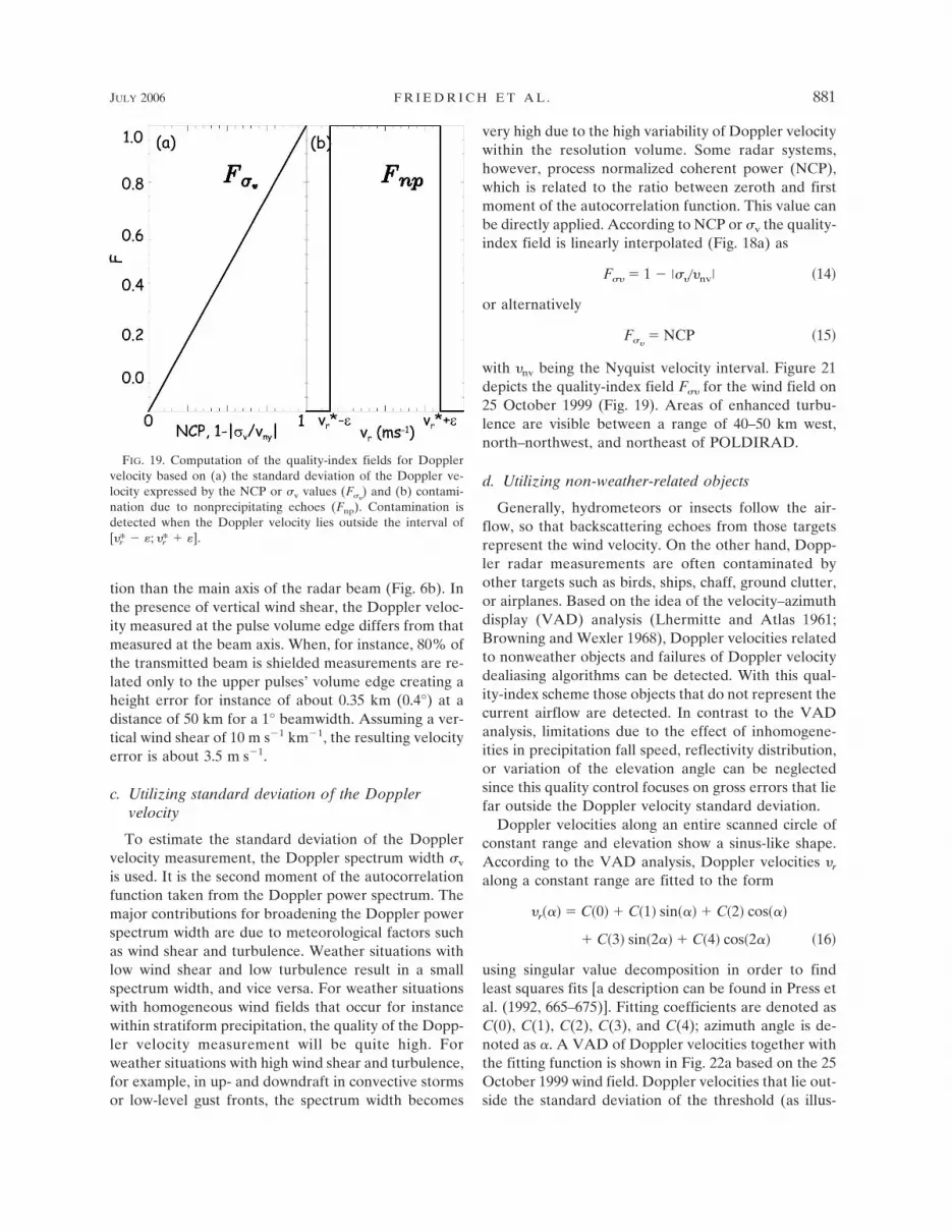
tion than the main axis of the radar beam (Fig. 6b). Inthe presence of vertical wind shear, the Doppler veloc-ity measured at the pulse volume edge differs from thatmeasured at the beam axis. When, for instance, 80% ofthe transmitted beam is shielded measurements are re-lated only to the upper pulses’ volume edge creating aheight error for instance of about 0.35 km (0.4°) at adistance of 50 km for a 1° beamwidth. Assuming a ver-tical wind shear of 10 m s�1 km�1, the resulting velocityerror is about 3.5 m s�1.

c. Utilizing standard deviation of the Dopplervelocity

To estimate the standard deviation of the Dopplervelocity measurement, the Doppler spectrum width �v

is used. It is the second moment of the autocorrelationfunction taken from the Doppler power spectrum. Themajor contributions for broadening the Doppler powerspectrum width are due to meteorological factors suchas wind shear and turbulence. Weather situations withlow wind shear and low turbulence result in a smallspectrum width, and vice versa. For weather situationswith homogeneous wind fields that occur for instancewithin stratiform precipitation, the quality of the Dopp-ler velocity measurement will be quite high. Forweather situations with high wind shear and turbulence,for example, in up- and downdraft in convective stormsor low-level gust fronts, the spectrum width becomes

very high due to the high variability of Doppler velocitywithin the resolution volume. Some radar systems,however, process normalized coherent power (NCP),which is related to the ratio between zeroth and firstmoment of the autocorrelation function. This value canbe directly applied. According to NCP or �v the quality-index field is linearly interpolated (Fig. 18a) as

F�� 1 � ��nv� �14�

or alternatively

F�� NCP �15�

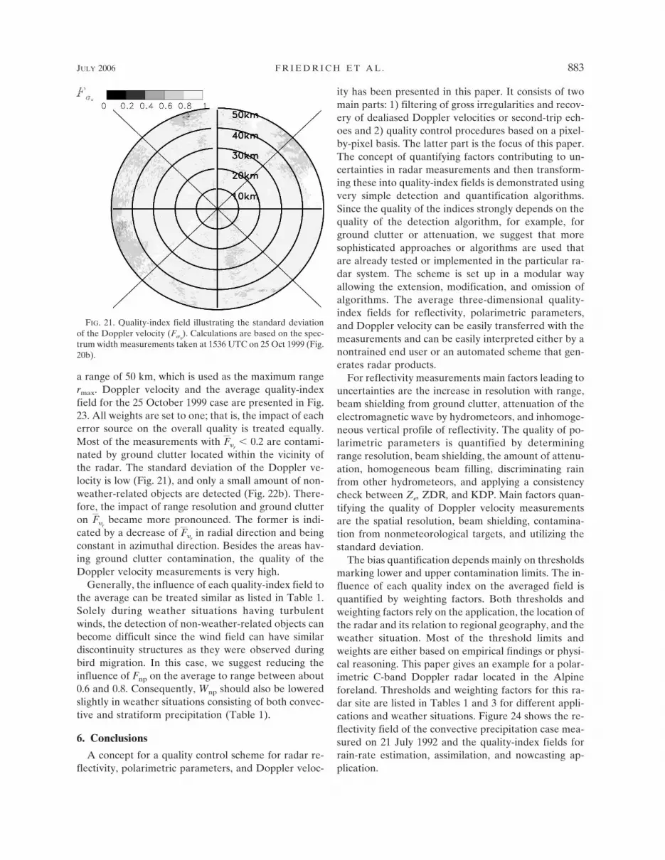
with �nv being the Nyquist velocity interval. Figure 21depicts the quality-index field F�� for the wind field on25 October 1999 (Fig. 19). Areas of enhanced turbu-lence are visible between a range of 40–50 km west,north–northwest, and northeast of POLDIRAD.

d. Utilizing non-weather-related objects

Generally, hydrometeors or insects follow the air-flow, so that backscattering echoes from those targetsrepresent the wind velocity. On the other hand, Dopp-ler radar measurements are often contaminated byother targets such as birds, ships, chaff, ground clutter,or airplanes. Based on the idea of the velocity–azimuthdisplay (VAD) analysis (Lhermitte and Atlas 1961;Browning and Wexler 1968), Doppler velocities relatedto nonweather objects and failures of Doppler velocitydealiasing algorithms can be detected. With this qual-ity-index scheme those objects that do not represent thecurrent airflow are detected. In contrast to the VADanalysis, limitations due to the effect of inhomogene-ities in precipitation fall speed, reflectivity distribution,or variation of the elevation angle can be neglectedsince this quality control focuses on gross errors that liefar outside the Doppler velocity standard deviation.

Doppler velocities along an entire scanned circle ofconstant range and elevation show a sinus-like shape.According to the VAD analysis, Doppler velocities �r

along a constant range are fitted to the form

�r�� C�0� � C�1� sin�� C�2� cos��

� C�3� sin�2�� C�4� cos�2�� 16�

using singular value decomposition in order to findleast squares fits [a description can be found in Press etal. (1992, 665–675)]. Fitting coefficients are denoted asC(0), C(1), C(2), C(3), and C(4); azimuth angle is de-noted as �. A VAD of Doppler velocities together withthe fitting function is shown in Fig. 22a based on the 25October 1999 wind field. Doppler velocities that lie out-side the standard deviation of the threshold (as illus-

FIG. 19. Computation of the quality-index fields for Dopplervelocity based on (a) the standard deviation of the Doppler ve-locity expressed by the NCP or �v values (F��

) and (b) contami-nation due to nonprecipitating echoes (Fnp). Contamination isdetected when the Doppler velocity lies outside the interval of[�*r � �; �*r � �].


trated in Fig. 22a as thick, solid lines) are flagged as Fnp

� 0. Therefore, the quality-index field is determined as

Fnp � �1 for �*r �� vr�� *r ��

0 else,

�17�

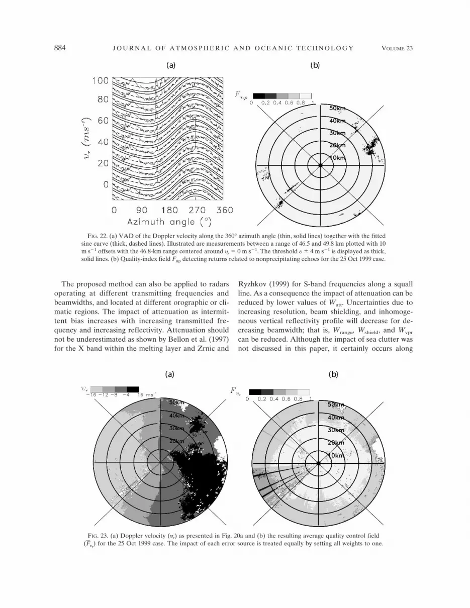
while � is set to 4 m s�1. The fitting function based onthe calculated fitting coefficients (illustrated in Fig. 22aas thick, dashed lines) is denoted as �*r (�). An illustra-tion of Fnp is given in Fig. 22b for Doppler velocitiesmeasured on 25 October 1999 (Fig. 20a). For wind

fields within stratiform precipitation the threshold is setto one-fourth of the Nyquist velocity interval. For moreturbulent wind fields, for example, during convectiveweather, the threshold is increased to one-half of theNyquist velocity for all applications.

e. Average quality-index field for Doppler velocity

To determine the quality of Doppler velocity mea-surements, the four separately calculated quality-indexfields are weighted and averaged according to Eq. (13).Both Frange and Fshield are calculated according to Eqs.(2) and (6). On that day, data were only available up to

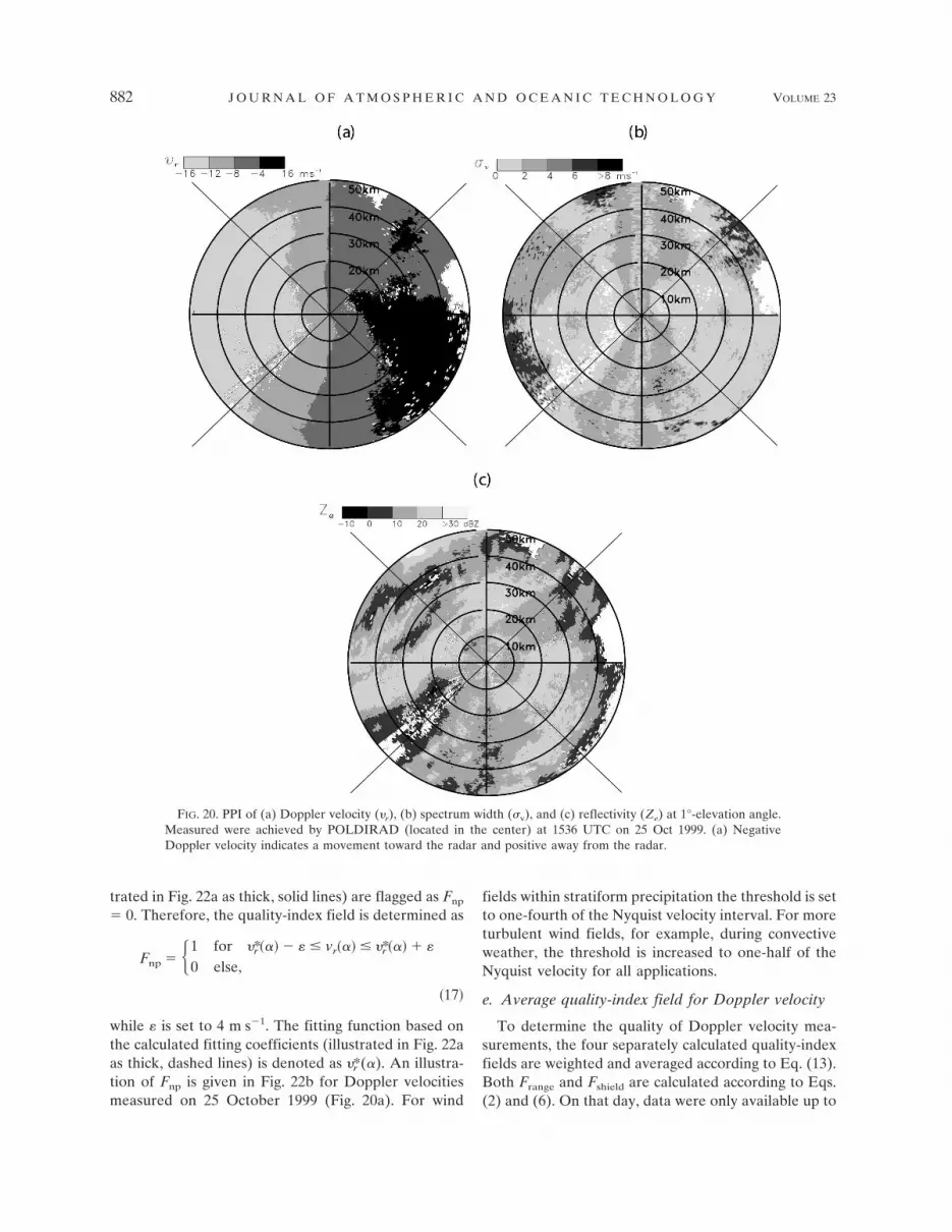
FIG. 20. PPI of (a) Doppler velocity (�r), (b) spectrum width (�v), and (c) reflectivity (Ze) at 1°-elevation angle.Measured were achieved by POLDIRAD (located in the center) at 1536 UTC on 25 Oct 1999. (a) NegativeDoppler velocity indicates a movement toward the radar and positive away from the radar.


a range of 50 km, which is used as the maximum rangermax. Doppler velocity and the average quality-indexfield for the 25 October 1999 case are presented in Fig.23. All weights are set to one; that is, the impact of eacherror source on the overall quality is treated equally.Most of the measurements with F�r

� 0.2 are contami-nated by ground clutter located within the vicinity ofthe radar. The standard deviation of the Doppler ve-locity is low (Fig. 21), and only a small amount of non-weather-related objects are detected (Fig. 22b). There-fore, the impact of range resolution and ground clutteron F�r

became more pronounced. The former is indi-cated by a decrease of F�r

in radial direction and beingconstant in azimuthal direction. Besides the areas hav-ing ground clutter contamination, the quality of theDoppler velocity measurements is very high.

Generally, the influence of each quality-index field tothe average can be treated similar as listed in Table 1.Solely during weather situations having turbulentwinds, the detection of non-weather-related objects canbecome difficult since the wind field can have similardiscontinuity structures as they were observed duringbird migration. In this case, we suggest reducing theinfluence of Fnp on the average to range between about0.6 and 0.8. Consequently, Wnp should also be loweredslightly in weather situations consisting of both convec-tive and stratiform precipitation (Table 1).

6. Conclusions

A concept for a quality control scheme for radar re-flectivity, polarimetric parameters, and Doppler veloc-

ity has been presented in this paper. It consists of twomain parts: 1) filtering of gross irregularities and recov-ery of dealiased Doppler velocities or second-trip ech-oes and 2) quality control procedures based on a pixel-by-pixel basis. The latter part is the focus of this paper.The concept of quantifying factors contributing to un-certainties in radar measurements and then transform-ing these into quality-index fields is demonstrated usingvery simple detection and quantification algorithms.Since the quality of the indices strongly depends on thequality of the detection algorithm, for example, forground clutter or attenuation, we suggest that moresophisticated approaches or algorithms are used thatare already tested or implemented in the particular ra-dar system. The scheme is set up in a modular wayallowing the extension, modification, and omission ofalgorithms. The average three-dimensional quality-index fields for reflectivity, polarimetric parameters,and Doppler velocity can be easily transferred with themeasurements and can be easily interpreted either by anontrained end user or an automated scheme that gen-erates radar products.

For reflectivity measurements main factors leading touncertainties are the increase in resolution with range,beam shielding from ground clutter, attenuation of theelectromagnetic wave by hydrometeors, and inhomoge-neous vertical profile of reflectivity. The quality of po-larimetric parameters is quantified by determiningrange resolution, beam shielding, the amount of attenu-ation, homogeneous beam filling, discriminating rainfrom other hydrometeors, and applying a consistencycheck between Ze, ZDR, and KDP. Main factors quan-tifying the quality of Doppler velocity measurementsare the spatial resolution, beam shielding, contamina-tion from nonmeteorological targets, and utilizing thestandard deviation.

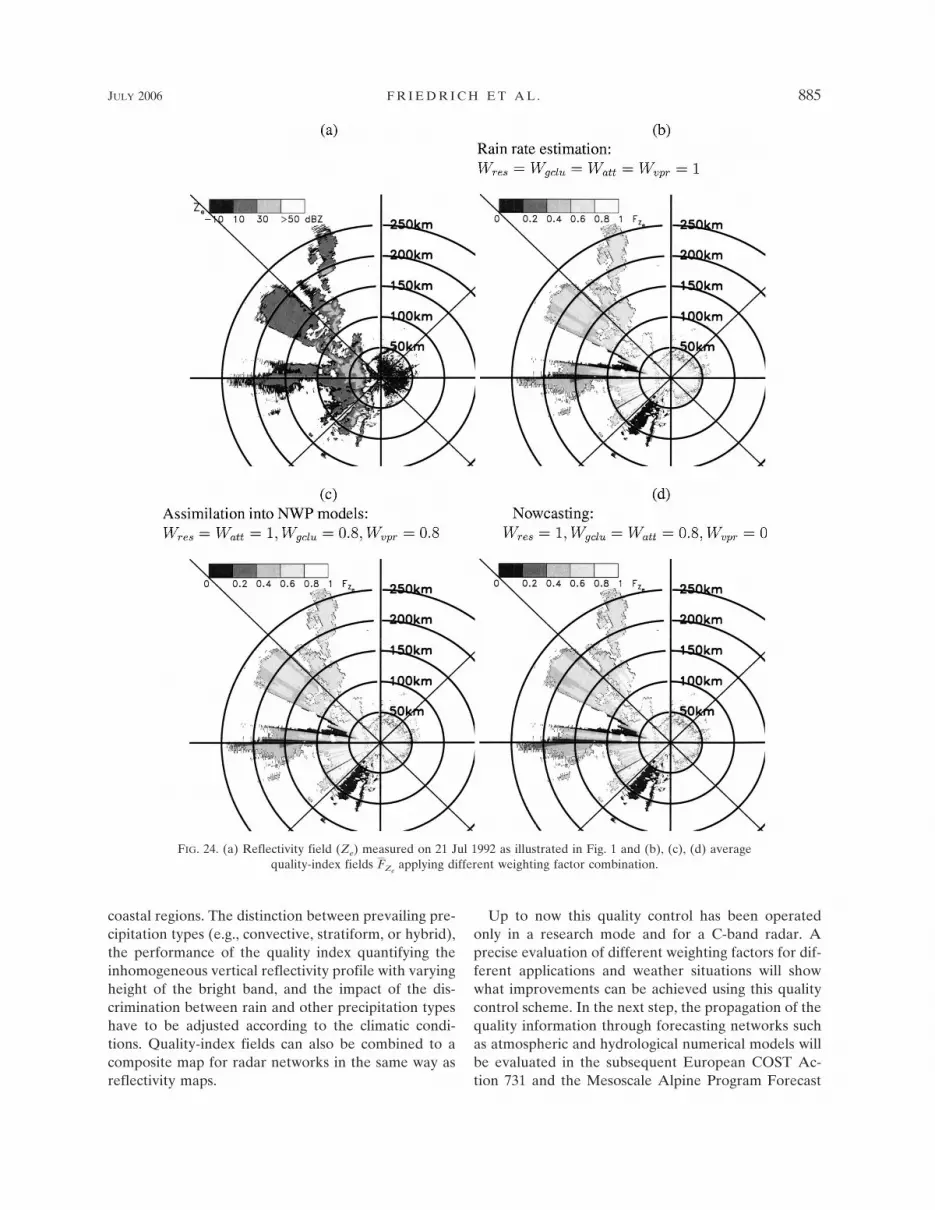
The bias quantification depends mainly on thresholdsmarking lower and upper contamination limits. The in-fluence of each quality index on the averaged field isquantified by weighting factors. Both thresholds andweighting factors rely on the application, the location ofthe radar and its relation to regional geography, and theweather situation. Most of the threshold limits andweights are either based on empirical findings or physi-cal reasoning. This paper gives an example for a polar-imetric C-band Doppler radar located in the Alpineforeland. Thresholds and weighting factors for this ra-dar site are listed in Tables 1 and 3 for different appli-cations and weather situations. Figure 24 shows the re-flectivity field of the convective precipitation case mea-sured on 21 July 1992 and the quality-index fields forrain-rate estimation, assimilation, and nowcasting ap-plication.

FIG. 21. Quality-index field illustrating the standard deviationof the Doppler velocity (F��

). Calculations are based on the spec-trum width measurements taken at 1536 UTC on 25 Oct 1999 (Fig.20b).


The proposed method can also be applied to radarsoperating at different transmitting frequencies andbeamwidths, and located at different orographic or cli-matic regions. The impact of attenuation as intermit-tent bias increases with increasing transmitted fre-quency and increasing reflectivity. Attenuation shouldnot be underestimated as shown by Bellon et al. (1997)for the X band within the melting layer and Zrnic and

Ryzhkov (1999) for S-band frequencies along a squallline. As a consequence the impact of attenuation can bereduced by lower values of Watt. Uncertainties due toincreasing resolution, beam shielding, and inhomoge-neous vertical reflectivity profile will decrease for de-creasing beamwidth; that is, Wrange, Wshield, and Wvpr

can be reduced. Although the impact of sea clutter wasnot discussed in this paper, it certainly occurs along

FIG. 23. (a) Doppler velocity (�r) as presented in Fig. 20a and (b) the resulting average quality control field(F�r

) for the 25 Oct 1999 case. The impact of each error source is treated equally by setting all weights to one.

FIG. 22. (a) VAD of the Doppler velocity along the 360° azimuth angle (thin, solid lines) together with the fittedsine curve (thick, dashed lines). Illustrated are measurements between a range of 46.5 and 49.8 km plotted with 10m s�1 offsets with the 46.8-km range centered around �r � 0 m s�1. The threshold � � 4 m s�1 is displayed as thick,solid lines. (b) Quality-index field Fnp detecting returns related to nonprecipitating echoes for the 25 Oct 1999 case.


coastal regions. The distinction between prevailing pre-cipitation types (e.g., convective, stratiform, or hybrid),the performance of the quality index quantifying theinhomogeneous vertical reflectivity profile with varyingheight of the bright band, and the impact of the dis-crimination between rain and other precipitation typeshave to be adjusted according to the climatic condi-tions. Quality-index fields can also be combined to acomposite map for radar networks in the same way asreflectivity maps.

Up to now this quality control has been operatedonly in a research mode and for a C-band radar. Aprecise evaluation of different weighting factors for dif-ferent applications and weather situations will showwhat improvements can be achieved using this qualitycontrol scheme. In the next step, the propagation of thequality information through forecasting networks suchas atmospheric and hydrological numerical models willbe evaluated in the subsequent European COST Ac-tion 731 and the Mesoscale Alpine Program Forecast

FIG. 24. (a) Reflectivity field (Ze) measured on 21 Jul 1992 as illustrated in Fig. 1 and (b), (c), (d) averagequality-index fields FZe

applying different weighting factor combination.


Demonstration Project (MAP D-PHASE) under theaegis of the World Meteorological Organization(WMO) World Weather Research Program (WWRP).

Acknowledgments. First we thank all the members ofthe COST 717 Working Group 3, especially DanielMichaelson, Iwan Holleman, and Andrea Rossa. With-out the encouraging discussions about error sources,user requirements, and realistic realization within anoperational requirement, we would not be able to as-semble this quality control concept. We extend specialthanks to the three anonymous reviewers for providingcomments and suggestions that enhanced the quality ofthe paper.

REFERENCES

Alberoni, P. P., and Coauthors, 2002: Quality and assimilation ofradar data for NWP—A review. COST 717 Working Doc.EUR 20600, 38 pp. [Available online at http://www.smhi.se/cost717/.]

Aniol, R., J. Riedl, and M. Dieringer, 1980: Ueber kleinraeumigeund zeitliche Variationen der Niederschlagsintensitaet. Me-teor. Rdsch., 33, 50–56.

Aydin, K., Y. Zhao, and T. A. Seliga, 1989: Rain-induced attenu-ation effects on C-band dual-polarization meteorological ra-dars. IEEE Trans. Geosci. Remote Sens., 27, 57–66.

Battan, L. J., 1973: Radar Observation of the Atmosphere. TheUniversity of Chicago Press, 324 pp.

Bellon, A., I. Zawadzki, and F. Fabry, 1997: Measurements ofmelting layer attenuation at X-band frequencies. Radio Sci.,32, 943–955.

Berenguer, M., G. W. Lee, D. Sempere-Torres, and I. Zawadzki,2002: A variational method for attenuation correction of ra-dar signal. Preprints, European Conf. on Radar Meteorology,Delft, Netherlands, European Meteorological Society andCopernicus Gesellschaft mbH, 11–16.

Bringi, V. N., V. Chandrasekar, N. Balakrishnan, and D. S. Zrnic,1990: An examination of propagation effects in rainfall onradar measurements at microwave frequencies. J. Atmos.Oceanic Technol., 7, 829–840.

Browning, K. A., and R. Wexler, 1968: The determination of ki-nematic properties of a wind field using Doppler radar. J.Appl. Meteor., 7, 105–113.

Chandrasekar, V., and R. J. Keeler, 1993: Antenna pattern analy-sis and measurements for multiparameter radars. J. Atmos.Oceanic Technol., 10, 674–683.

Dazhang, T., S. G. Geotis, R. E. Passarelli Jr., A. L. Hansen, andC. L. Frush, 1982: Evaluation of an alternating-PRF methodfor extending the range of unambiguous Doppler velocity.Preprints, 22nd Int. Conf. on Radar Meteorology, Zurich,Switzerland, Amer. Meteor. Soc., 523–527.

Delrieu, G., J. Creutin, and H. Andrieu, 1995: Simulation of radarmountain returns using a digitized terrain model. J. Atmos.Oceanic Technol., 12, 1038–1049.

Doviak, J. R., and D. S. Zrnic, 1992: Doppler Radar and WeatherObservations. 2d ed. Academic Press, 562 pp.

Einfalt, T., K. Arnbjerg-Nielsen, C. Golz, N. E. Jensen, M. Quirm-bach, G. Vaes, and B. Vieux, 2004: Towards a roadmap for

use of radar rainfall data use in urban drainage. J. Hydrol.,299, 186–202.

Evans, J. E., and E. R. Ducot, 1994: The Integrated TerminalWeather System (ITWS). Lincoln Lab. J., 7, 449–474. [Avail-able online at http://www.ll.mit.edu/AviationWeather/evansitws.pdf.]

Friedrich, K., and M. Hagen, 2004: Wind synthesis and qualitycontrol of multiple-Doppler-derived horizontal wind fields. J.Appl. Meteor., 43, 38–57.

Gabella, M., and R. Notarpietro, 2002: Ground clutter character-ization and elimination in mountainous terrain. Preprints,Second European Conf. on Radar Meteorology, Delft, Neth-erlands, European Meteorological Society and CopernicusGesellschaft mbH, 305–311.

Giuli, D., M. Gherardelli, A. Freni, T. Seliga, and K. Aydin, 1991:Rainfall and clutter discrimination by means of dual-linearpolarization radar measurements. J. Atmos. Oceanic Tech-nol., 8, 777–789.

Goddard, J. W. F., J. Eastment, and J. Tan, 1994: Self consistentmeasurements of differential phase and differential reflectiv-ity in rain. Preprints, IGARSS 1994, Pasadena, CA, IEEE,369–371.

Golz, C., T. Einfalt, and M. Jessen, 2004: Radar data quality con-trol procedures. Preprints, Third European Conf. on RadarMeteorology, Visby, Sweden, 435–437.

Gorgucci, E., G. Scarchilli, and V. Chandrasekar, 1996: Errorstructure of radar rainfall measurement at C-band frequen-cies with dual polarization algorithm for attenuation correc-tion. J. Geophys. Res., 101, 26 461–26 471.

——, ——, ——, P. Meischner, and M. Hagen, 1998: Intercom-parison of techniques to correct for attenuation of C-bandweather radar signals. J. Appl. Meteor., 37, 845–853.

Grecu, M., and W. F. Krajewski, 2000: An efficient methodologyfor detection of anomalous propagation echoes in radar re-flectivity data using neutral networks. J. Atmos. OceanicTechnol., 17, 121–129.

Hagen, M., 1997: Identification of ground clutter by polarimetricradar. Preprints, 28th Int. Conf. on Radar Meteorology, Aus-tin, TX, Amer. Meteor. Soc., 67–68.

Hannesen, R., 2001: Quantitative precipitation estimation fromradar data—A review of current methodologies. Deliverable4.1 for the research project MUSIC supported by the Euro-pean Commission, 31 pp. [Available online at http://www.geomin.unibo.it/orgv/hydro/music/reports/D4.1 QPE-revi.pdf.]

Holleman, I., and H. Beekhuis, 2003: Analysis and correction ofdual PRF velocity data. J. Atmos. Oceanic Technol., 20, 443–453.

Höller, H., V. N. Bringi, J. Hubbert, M. Hagen, and P. F.Meischner, 1994: Life cycle and precipitation formation in ahybrid-type hailstorm revealed by polarimetric and Dopplerradar measurements. J. Atmos. Sci., 51, 2500–2522.

Illingworth, A. J., 2003: Improved precipitation rates and dataquality by using polarimetric measurements. Weather Radar:Principles and Advanced Applications, P. Meischner, Ed.,Springer-Verlag, 130–166.

James, C. N., and R. A. Houze, 2001: A real-time four-dimensional Doppler dealiasing scheme. J. Atmos. OceanicTechnol., 18, 1674–1683.

Joss, J., and R. Lee, 1995: The application of radar-gauge com-parisons to operational precipitation profile corrections. J.Appl. Meteor., 34, 2612–2630.

——, and Coauthors, 1998: Final report NFP31: Operational use


of radar for precipitation measurements in Switzerland. Tech.Rep., vdf Hochschulverlag AG an der ETH Zuerich, 108 pp.

Kessinger, C., S. Ellis, J. van Andel, J. Hubbert, and R. J. Keeler,2003: NEXRAD data quality optimization. Tech. Rep., Re-search Application Program/Atmospheric Technology Divi-sion, National Center of Atmospheric Research, 70 pp.[Available online at http://www.atd.ucar.edu/rsf/NEXRAD/index.htm.]

Krajewski, W. F., and B. Vignal, 2001: Evaluation of anomalouspropagation echo detection in WSR-88D data: A largesample case study. J. Atmos. Oceanic Technol., 18, 807–814.

Lang, P., 2001: Cell tracking and warning indicators derived fromoperational radar products. Preprints, 30th Int. Conf. on Ra-dar Meteorology, Munich, Germany, Amer. Meteor. Soc.,245–247.

Lee, R., G. D. Bruna, and J. Joss, 1995: Intensity of ground clutterand of echoes of anomalous propagation and its elimination.Preprints, 27th Conf. on Radar Meteorology, Vail, CO, Amer.Meteor. Soc., 651–652.

Lhermitte, R. M., and D. Atlas, 1961: Precipitation motion bypulse Doppler. Preprints, Ninth Weather Radar Conf., Bos-ton, MA, Amer. Meteor. Soc., 498–503.

Meischner, P., Ed., 2003: Weather Radar: Principles and AdvancedApplications. Springer-Verlag, 300 pp.

Parent du Châtelet, J., P. Tabary, and M. Guimera, 2005: ThePanthere Project and the evolution of the French operationalradar network and products: Rain-estimation, Dopplerwinds, and dual-polarisation. Preprints, 32d Conf. on RadarMeteorology, Albuquerque, NM, Amer. Meteor. Soc., CD-ROM, 14R.6.

Pierce, C. E., P. J. Hardaker, C. G. Collier, and C. M. Haggett,2000: Gandolf: A system for generating automated nowcastsof convective precipitation. Meteor. Appl., 7, 341–360.

Press, W. H., S. A. Teukolsky, W. T. Vetterling, and B. P. Flan-nery, 1992: Numerical Recipes in Fortran 77. 2d ed. Cam-bridge University Press, 933 pp.

Richter, C., and M. Hagen, 1997: Dropsize distributions of rain-drops by polarisation radar and simultaneous measurementswith disdrometer, windprofiler and pms-probes. Quart. J.Roy. Meteor. Soc., 123, 2277–2296.

Rossa, A., M. Bruen, D. Fruehwald, B. MacPherson, I. Holle-mann, D. Michaelson, and S. Michaelides, 2005: Use of radarobservations in hydrological and NWP models. COST 717Working Doc., 292 pp. [Available online at http://www.smhi.se/cost717/.]

Ryzhkov, A., and D. Zrnic, 1998: Beamwidth effects on the dif-ferential phase measurements of rain. J. Atmos. OceanicTechnol., 15, 624–634.

Sachidananda, M., 1997: Signal design and processing techniquesfor WSR-88D ambiguity resolution. Part 1. Tech. Rep.NOAA/NSSL, 100 pp.

Sanchez-Diezma, R., D. Sempere-Torres, G. Delrieu, and I.Zawadzki, 2001: An improved methodology for ground clut-

ter substitution based on a pre-classification of precipitationtypes. Preprints, 30th Int. Conf. on Radar Meteorology, Mu-nich, Germany, Amer. Meteor. Soc., 271–273.

Scarchilli, G., E. Gorgucci, V. Chandrasekar, and A. Dobaie,1996: Self-consistency of poarization diversity measurementof rainfall. IEEE Trans. Geosci. Remote Sens., 34, 22–26.

Seliga, T. A., and V. N. Bringi, 1976: Potential use of radar dif-ferential reflectivity measurements at orthogonal polariza-tion for measuring precipitation. J. Appl. Meteor., 15, 69–76.

Seltmann, E. E. J., 2000: Clutter versus radar winds. Phys. Chem.Earth, B25, 1173–1178.

Sempere-Torres, D., R. Sanchez-Diezma, M. Berenguer, R. Pas-cual, and I. Zawadzki, 2003: Improving radar rainfall mea-surement stability using mountain returns in real time. Pre-prints, 31st Int. Conf. on Radar Meteorology, Seattle, WA,Amer. Meteor. Soc., CD-ROM, 4B.4.

Sigmet, 2004: RVP8—Digital IF receiver/Doppler signal proces-sor: User’s manual. Sigmet, 409 pp. [Available online athttp://www.sigmet.com.]

Steiner, M., and J. A. Smith, 2002: Use of three-dimensional re-flectivity structure of automated detection and removal ofnonprecipitating echoes in radar data. J. Atmos. OceanicTechnol., 19, 673–686.

Tabary, P., G. Scialom, and U. Germann, 2001: Real-time re-trieval of the wind from aliased velocities measured by Dopp-ler radars. J. Atmos. Oceanic Technol., 18, 875–882.

Torlaschi, E., and I. Zawadzki, 2003: The effect of mean anddifferential attenuation on the precision and accuracy of theestimates of reflectivity and differential reflectivity. J. Atmos.Oceanic Technol., 20, 362–371.

Unal, C. M. H., and D. N. Moisseev, 2004: Combined Doppler andpolarimetric radar measurements: Correction for spectrumaliasing and nonsimultaneous polarimetric measurements. J.Atmos. Oceanic Technol., 21, 443–456.

Vivekanandan, J., D. S. Zrnic, S. M. Ellis, R. Oye, A. V. Ryzhkov,and J. Straka, 1999: Cloud microphysics retrieval using S-band dual-polarization radar measurements. Bull. Amer. Me-teor. Soc., 80, 381–388.

Yuter, S. E., 2003: Precipitation radar. Encyclopedia of Atmo-spheric Sciences, J. R. Holton, J. Pyle, and J. Curry, Eds.,1833–1851.

Zawadzki, I., 1984: Factors affecting the precision of radar mea-surement of rain. Preprints, 22nd Conf. on Radar Meteorol-ogy, Zurich, Switzerland, Amer. Meteor. Soc., 251–256.

Zrnic, D. S., 1996: Weather radar polarimetry—Trends towardoperational applications. Bull. Amer. Meteor. Soc., 77, 1529–1534.

——, and P. Mahapatra, 1985: Two methods of ambiguity resolu-tion in pulse Doppler weather radars. IEEE Trans. Aerosp.Elec. Syst., 4, 470–483.

——, and A. V. Ryzhkov, 1999: Polarimetry for weather surveil-lance radars. Bull. Amer. Meteor. Soc., 80, 389–406.


a quality control concept for radar reflectivity, polarimetric parameters, and doppler velocity

Documents