analyzing graph transformation systems through constraint
TRANSCRIPT
Under consideration for publication in Theory and Practice of Logic Programming 1
Analyzing Graph Transformation Systemsthrough Constraint Handling Rules
FRANK RAISER
THOM FRUHWIRTH
Faculty of Engineering and Computer Sciences, Ulm University, Germany(e-mail: {Frank.Raiser|Thom.Fruehwirth}@uni-ulm.de)
submitted 25 September 2009; revised 18 April 2010; accepted 2 June 2010
Abstract
Graph transformation systems (GTS) and constraint handling rules (CHR) are non-deterministic rule-based state transition systems. CHR is well-known for its powerful con-fluence and program equivalence analyses, for which we provide the basis in this work toapply them to GTS. We give a sound and complete embedding of GTS in CHR, investigateconfluence of an embedded GTS, and provide a program equivalence analysis for GTS viathe embedding. The results confirm the suitability of CHR-based program analyses forother formalisms embedded in CHR.
KEYWORDS: Graph Transformation Systems, Constraint Handling Rules, Program Anal-ysis
1 Introduction
Graph transformation systems (GTS) are used to describe complex structures and
systems in a concise, readable, and easily understandable way. They have ap-
plications ranging from implementations of programming languages over model
transformations to graph-based models of computation (Blostein et al. 1995; Ehrig
et al. 2006). Graph transformation systems see widespread use in many applications
(Ehrig et al. 2006), and hence performing program analysis on them is becoming
more important.
Constraint handling rules (CHR) (Fruhwirth 2009) on the other side allows
for rapid prototyping of constraint-based algorithms. Besides constraint reasoning,
CHR has been used for such diverse applications as type system design for Haskell
(Sulzmann et al. 2006), time tabling (Abdennadher and Marte 2000), computa-
tional linguistics (Dahl and Maharshak 2009), chip card verification (Pretschner
et al. 2004), computational biology (Bavarian and Dahl 2006), and decision sup-
port for cancer diagnosis (Barranco-Mendoza 2005). Essentially, CHR performs
guarded multiset rewriting, extended by a complete and decidable constraint the-
ory. A specific strength of CHR is the wide array of available program analyses.
Other formalisms have been embedded in CHR in order to compare and mutually
arX
iv:1
006.
1497
v2 [
cs.L
O]
15
Jun
2010
2 Frank Raiser, Thom Fruhwirth
σr1
v~ uuuuuuuuu
uuuuuuuuur2
(IIIIIIIII
IIIIIIIII
σ1
∗
�'HHHHHHHH
HHHHHHHH σ2
∗
w� vvvvvvvv
vvvvvvvv
σ′1 ' σ′2
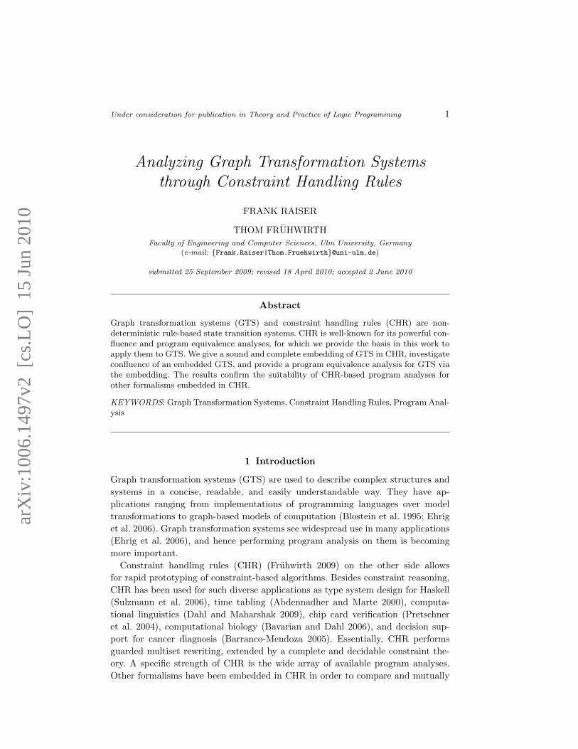
Fig. 1. Confluence Property for rules r1 and r2
σP1
v~ uuuuuuuuu
uuuuuuuuuP2
(IIIIIIIII
IIIIIIIII
σ1
P∗1
�'HHHHHHHH
HHHHHHHH σ2
P∗2
w� vvvvvvvv
vvvvvvvv
σ′1 ' σ′2
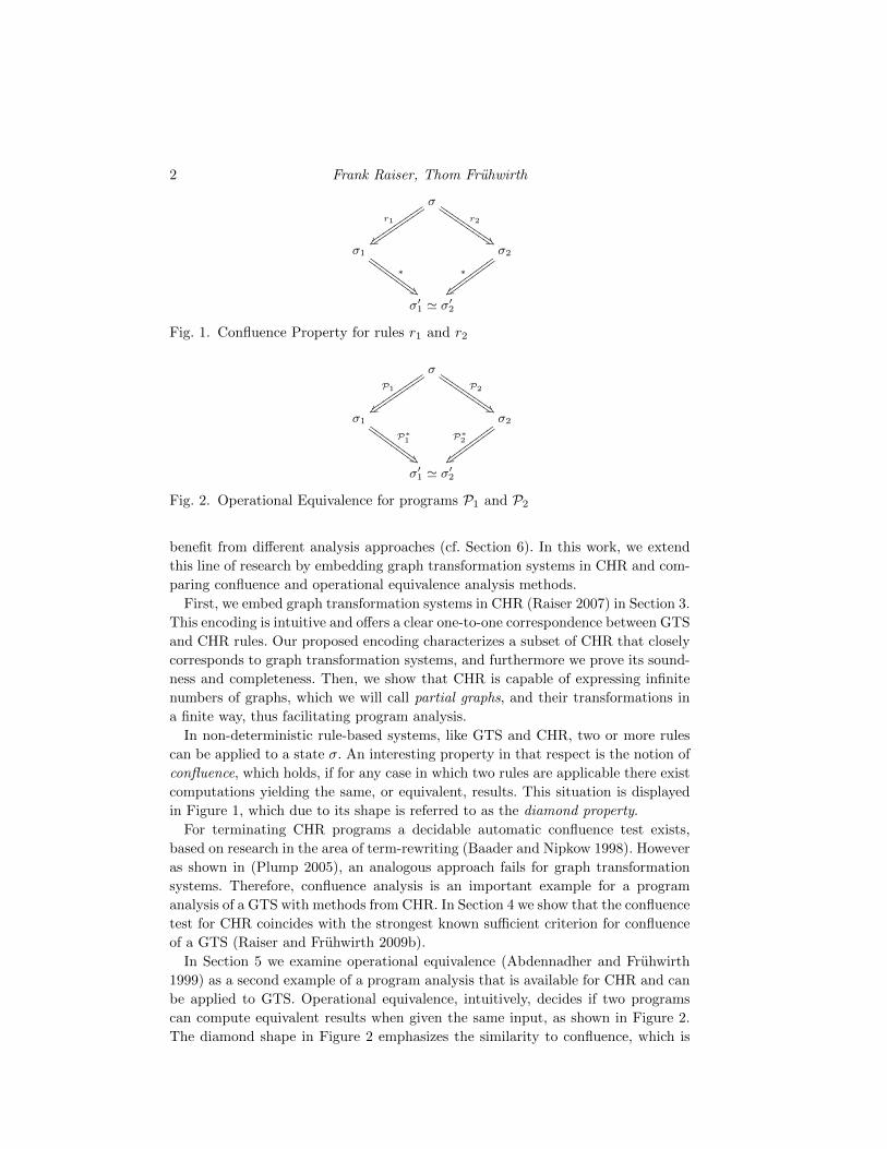
Fig. 2. Operational Equivalence for programs P1 and P2
benefit from different analysis approaches (cf. Section 6). In this work, we extend
this line of research by embedding graph transformation systems in CHR and com-
paring confluence and operational equivalence analysis methods.
First, we embed graph transformation systems in CHR (Raiser 2007) in Section 3.
This encoding is intuitive and offers a clear one-to-one correspondence between GTS
and CHR rules. Our proposed encoding characterizes a subset of CHR that closely
corresponds to graph transformation systems, and furthermore we prove its sound-
ness and completeness. Then, we show that CHR is capable of expressing infinite
numbers of graphs, which we will call partial graphs, and their transformations in
a finite way, thus facilitating program analysis.
In non-deterministic rule-based systems, like GTS and CHR, two or more rules
can be applied to a state σ. An interesting property in that respect is the notion of
confluence, which holds, if for any case in which two rules are applicable there exist
computations yielding the same, or equivalent, results. This situation is displayed
in Figure 1, which due to its shape is referred to as the diamond property.
For terminating CHR programs a decidable automatic confluence test exists,
based on research in the area of term-rewriting (Baader and Nipkow 1998). However
as shown in (Plump 2005), an analogous approach fails for graph transformation
systems. Therefore, confluence analysis is an important example for a program
analysis of a GTS with methods from CHR. In Section 4 we show that the confluence
test for CHR coincides with the strongest known sufficient criterion for confluence
of a GTS (Raiser and Fruhwirth 2009b).
In Section 5 we examine operational equivalence (Abdennadher and Fruhwirth
1999) as a second example of a program analysis that is available for CHR and can
be applied to GTS. Operational equivalence, intuitively, decides if two programs
can compute equivalent results when given the same input, as shown in Figure 2.
The diamond shape in Figure 2 emphasizes the similarity to confluence, which is
Analyzing GTS through CHR 3
also found in the respective program analysis methods. We introduce operational
equivalence in the GTS context in analogy to CHR (Raiser and Fruhwirth 2009a).
Then, we prove that deciding operational equivalence of a CHR program, derived
from a GTS, is a sufficient criterion for operational equivalence of the corresponding
GTS.
An interesting application of this result is the possibility to detect and remove re-
dundant rules using the test for operational equivalence. Redundant rules of graph
transformation systems have been formally defined in (Kreowski and Valiente 2000),
however to the best of our knowledge, this is the first available algorithm for de-
tecting them in a GTS.
This work presents a unified treatment and considerable extension of previously
published works (Raiser 2007; Raiser et al. 2009; Raiser 2009; Raiser and Fruhwirth
2009a; Raiser and Fruhwirth 2009b). In (Raiser et al. 2009) a formal treatment of
CHR state equivalence is provided and, derived from that, a simplified formulation
of the operational semantics of CHR. This novel formulation allows us to unify
our previous works while simplifying presentation and formal proofs significantly.
Furthermore, the state equivalence definition from (Raiser et al. 2009) is the basis
for new insights on CHR states that encode graphs.
2 Preliminaries
In this section we introduce the required formalisms for graph transformation sys-
tems in Section 2.1 and constraint handling rules in Section 2.2.
2.1 Graph Transformation System
The following definitions for graphs and graph transformation systems (GTS) have
been adapted from (Ehrig et al. 2006).
Definition 2.1 (graph)
A graph G = (V,E, src, tgt) consists of a finite set V of nodes, a finite set E of
edges and two functions src, tgt : E → V specifying source and target of an edge,
respectively. A type graph TG is a graph with unique labels for all nodes and edges.
For simplicity, we avoid an additional label function in favor of identifying variable
names with labels. For multiple graphs we refer to the node set V of a graph G as VGand analogously for edge sets and the src, tgt functions. We further define the degree
of a node as deg : V → N, v 7→ #{e ∈ E | src(e) = v}+ #{e ∈ E | tgt(e) = v}. As
there may be multiple graphs containing the same node, we use degG(v) to specify
the degree of a node v with respect to the graph G. When the context graph is
clear the subscript is omitted.
In this work, we consider typed graphs, i.e. graphs in which nodes and edges are
assigned types from a type graph.
Definition 2.2 (graph morphism,typed graph)
4 Frank Raiser, Thom Fruhwirth
type graph
use
typed graph
type morphism
Process Resource
Fig. 3. Example of a type graph and typed graph
Given graphs G1, G2 with Gi = (Vi, Ei, srci, tgti) for i = 1, 2 a graph morphism
f : G1 → G2, f = (fV , fE) consists of two functions fV : V1 → V2 and fE :
E1 → E2 that preserve the source target functions, i.e. fV ◦ src1 = src2 ◦fE and
fV ◦ tgt1 = tgt2 ◦fE .
A graph morphism f is injective (or surjective) if both functions fV , fE are
injective (or surjective, respectively); f is called isomorphic if it is bijective. f is
called an inclusion if fV (V1) ⊆ V1 and fE(E1) ⊆ E1. When the context is clear, we
simply refer to graph morphisms as morphisms.
A typed graph G is a tuple (V,E, src, tgt, type, TG) where (V,E, src, tgt) is a
graph, TG a type graph, and type a graph morphism with type = (typeV , typeE)
and typeV : V → TGV , typeE : E → TGE .
For a typed graph G = (V,E, src, tgt, type, TG) we define a subgraph H as a
typed graph (V ′, E′, src′, tgt′, type′, TG) such that V ′ ⊆ V ∧E′ ⊆ E∧ src′ = src |E′∧ tgt′ = tgt |E′ ∧ type′V = typeV |V ′ ∧ type′E = typeE |E′ with ∀e ∈ E′. src′(e) ∈V ′ ∧ tgt′(e) ∈ V ′.
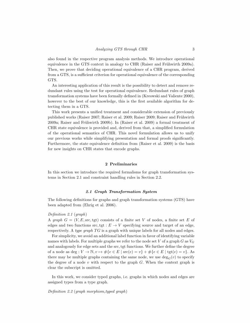
Example 2.1
Figure 3 shows an example for a type graph and a corresponding typed graph.
The type graph at the top defines two types of nodes: processes and resources.
Furthermore, it defines use edges going from processes to resources. The typed
graph is one possible instance of a graph modeling processes and resources being
used by those processes. The type graph morphism is represented by the dotted
lines, showing how the nodes are typed as processes or resources, respectively.
Definition 2.3 (GTS, rule)
A Graph Transformation System (GTS) is a tuple consisting of a type graph and
a set of graph production rules. A graph production rule – simply called rule if the
context is clear – is a tuple p = (Ll← K
r→ R) of graphs L,K, and R with inclusion
morphisms l : K → L and r : K → R.

Analyzing GTS through CHR 5
L
m
��(1)
Kloo
k
��
r //
(2)
R
n
��G D
foo g // H
Fig. 4. Double-pushout approach
We distinguish two kinds of typed graphs: rule graphs and host graphs. Rule
graphs are the graphs L,K,R of a graph production rule p and host graphs are
graphs to which the graph production rules are applied. This work is based on the
double-pushout approach (DPO) as defined in (Ehrig et al. 2006). Most notably,
we require a match morphism m : L → G to apply a rule p to a typed host
graph G. The transformation yielding the typed graph H is written as Gp,m=⇒ H.
H is given mathematically by constructing D as shown in Figure 4, such that (1)
and (2) are pushouts in the category of typed graphs. Intuitively, the graph L
is matched to a subgraph of G and its occurrence in G is then replaced by the
graph R. The intermediate graph K is the context graph, which contains the nodes
and edges in both L and R, i.e. all nodes and edges matched to K remain during
the transformation.
A graph production rule p can only be applied to a host graph G if the following
gluing condition is satisfied. In fact, (Ehrig et al. 2006) shows, that D and the
pushout (1) exist if and only if this gluing condition is satisfied. It is based on the
following three sets (Ehrig et al. 2006):
• gluing points: GP = l(K)
• identification points: IP = {v ∈ VL | ∃w ∈ VL, w 6= v : m(v) = m(w)} ∪ {e ∈EL | ∃f ∈ EL, e 6= f : m(e) = m(f)}
• dangling points: DP = {v ∈ VL | ∃e ∈ EG \ m(EL) : srcG(e) = m(v) ∨tgtG(e) = m(v)}
Definition 2.4 (gluing condition)
The gluing condition is defined as IP ∪DP ⊆ GP .
If the gluing condition is satisfied for a rule p = (Ll← K
r→ R) the application of
the rule consists of transforming G into H by performing the construction described
above. An implementation-oriented interpretation of a rule application is that all
nodes and edges in m(L \ l(K)) are removed from G to create D = (G \m(L)) ∪m(l(K)) and then all nodes and edges in n(R \ r(K)) are added to create H =
D ∪ n(R \ r(K)).
Example 2.2
Figure 5 shows two graph production rules in a shorthand notation that defines
the morphisms l and r implicitly by the labels of the nodes which are mapped onto
each other. The resulting graph transformation system is implicitly defined over the
simple type graph consisting only of a single node with a loop, depicted in Figure 6.
The two rules constitute a graph transformation system for detecting cyclic lists.
The basic idea of the unlink rule is to remove intermediate nodes of the list, while
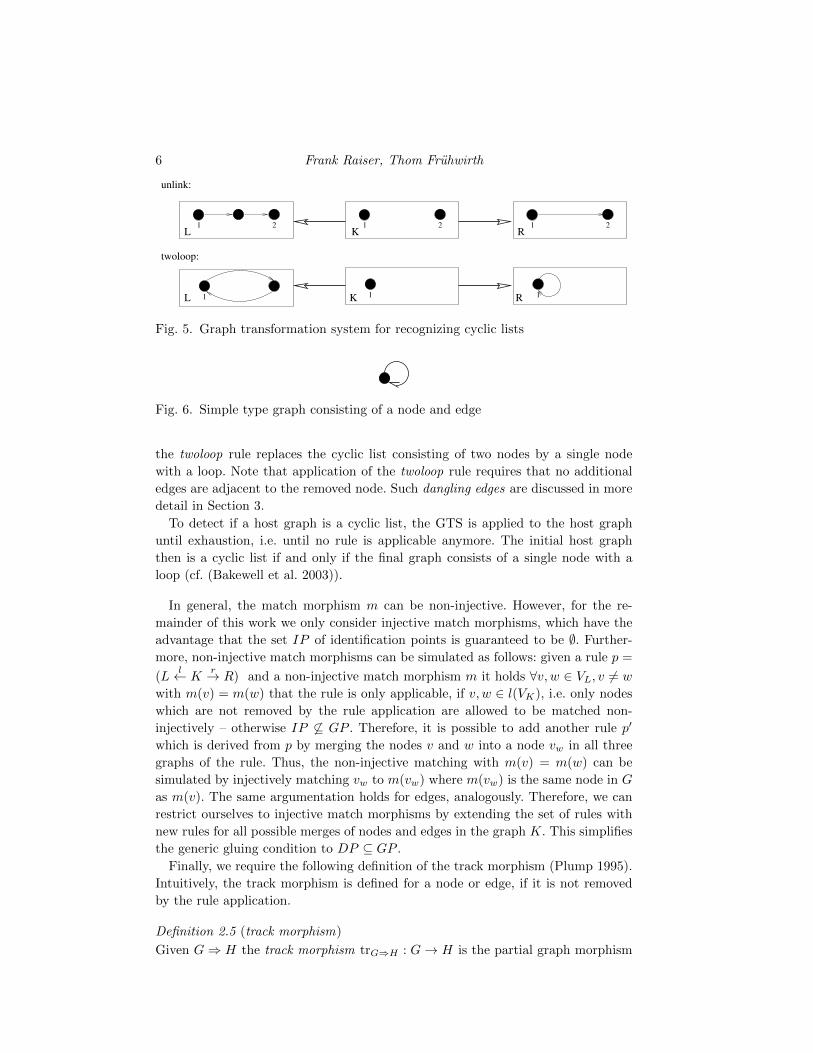
6 Frank Raiser, Thom Fruhwirth
L1 2
unlink:
twoloop:
K RL
RK1 2 1 2
1 11
Fig. 5. Graph transformation system for recognizing cyclic lists
Fig. 6. Simple type graph consisting of a node and edge
the twoloop rule replaces the cyclic list consisting of two nodes by a single node
with a loop. Note that application of the twoloop rule requires that no additional
edges are adjacent to the removed node. Such dangling edges are discussed in more
detail in Section 3.
To detect if a host graph is a cyclic list, the GTS is applied to the host graph
until exhaustion, i.e. until no rule is applicable anymore. The initial host graph
then is a cyclic list if and only if the final graph consists of a single node with a
loop (cf. (Bakewell et al. 2003)).
In general, the match morphism m can be non-injective. However, for the re-
mainder of this work we only consider injective match morphisms, which have the
advantage that the set IP of identification points is guaranteed to be ∅. Further-
more, non-injective match morphisms can be simulated as follows: given a rule p =
(Ll← K
r→ R) and a non-injective match morphism m it holds ∀v, w ∈ VL, v 6= w
with m(v) = m(w) that the rule is only applicable, if v, w ∈ l(VK), i.e. only nodes
which are not removed by the rule application are allowed to be matched non-
injectively – otherwise IP 6⊆ GP . Therefore, it is possible to add another rule p′
which is derived from p by merging the nodes v and w into a node vw in all three
graphs of the rule. Thus, the non-injective matching with m(v) = m(w) can be
simulated by injectively matching vw to m(vw) where m(vw) is the same node in G
as m(v). The same argumentation holds for edges, analogously. Therefore, we can
restrict ourselves to injective match morphisms by extending the set of rules with
new rules for all possible merges of nodes and edges in the graph K. This simplifies
the generic gluing condition to DP ⊆ GP .
Finally, we require the following definition of the track morphism (Plump 1995).
Intuitively, the track morphism is defined for a node or edge, if it is not removed
by the rule application.
Definition 2.5 (track morphism)
Given G⇒ H the track morphism trG⇒H : G→ H is the partial graph morphism
Analyzing GTS through CHR 7
defined by
trG⇒H(x) =
{g(f−1(x)) if x ∈ f(D),
undefined otherwise.
Here f : D → G and g : D → H are the morphisms in the lower row of the
pushout (1) in Figure 4 and f−1 : f(D)→ D maps each item f(x) to x.
The track morphism of a derivation ∆ : G0 ⇒∗ Gn is defined by tr∆ = idG0
if n = 0 and tr∆ = trG1⇒∗Gn◦ trG0⇒G1
otherwise, where idG0is the identity
morphism on G0.
2.2 Constraint Handling Rules
This section presents the syntax and operational semantics of Constraint Handling
Rules (CHR) (Sneyers et al. 2009; Fruhwirth 2009). Constraints are first-order
predicates which we separate into built-in constraints and user-defined constraints.
Built-in constraints are provided by the constraint solver while user-defined con-
straints are defined by a CHR program. The notation c/n, where c is called the
constraint symbol and n the arity, is used for both types of constraints.
Its semantics is based on an underlying complete constraint theory CT on built-in
constraints for which satisfiability and entailment are decidable. In general, CHR
allows arbitrary constraint theories for CT , requiring only that it contains at least
Clark’s equality theory for syntactic equality. In addition to that, in this work we
also require CT to cover the elementary arithmetic operations + and −. Further-
more, > denotes the built-in which is always true and ⊥ denotes false, respectively.
The survey (Sneyers et al. 2009) provides an overview over the different techniques
used in CHR implementations and the book (Fruhwirth 2009) details the different
available operational semantics for CHR. In this work we abstract from specific
implementations and rely on the operational semantics given in (Raiser et al. 2009),
which corresponds to the very abstract operational semantics in (Fruhwirth 2009).
CHR is a state transition system over the set of states given in the following
definition.
Definition 2.6 (CHR states)
A (CHR) state is a tuple
〈G,B,V〉.G is a multiset of user-defined constraints called the goal (or (user-defined) con-
straint store), B is a conjunction of built-in constraints called the built-in (con-
straint) store, and V is the set of global variables.
In this work σ, τ, . . . denote CHR states and Σ denotes the set of all CHR states.
The following definition introduces the different types of variables we distinguish
for a given CHR state.
Definition 2.7 (Variable Types)
For the variables occurring in a state σ = 〈G,B,V〉 we distinguish three different
types:
8 Frank Raiser, Thom Fruhwirth
1. a variable v ∈ V is called a global variable
2. a variable v 6∈ V is called a local variable
3. a variable v 6∈ (V ∪ vars(G)) is called a strictly local variable
The following equivalence relation ≡ between CHR states (Raiser et al. 2009) is
an important tool that facilitates a succinct definition of the operational semantics
of CHR and simplifies proofs.
Definition 2.8 (State Equivalence)
Equivalence between CHR states is the smallest equivalence relation ≡ over CHR
states that satisfies the following conditions:
1. (Substitution)
〈G, x .= t ∧ B,V〉 ≡ 〈G [x/t] , x
.= t ∧ B,V〉
2. (Transformation of the Constraint Store) If CT |= ∃s.B ↔ ∃s′.B′ where s, s′
are the strictly local variables of B,B′, respectively, then:
〈G,B,V〉 ≡ 〈G,B′,V〉
3. (Omission of Non-Occurring Global Variables) If X is a variable that does
not occur in G or B then:
〈G,B, {X} ∪ V〉 ≡ 〈G,B,V〉
4. (Equivalence of Failed States)
〈G,⊥,V〉 ≡ 〈G′,⊥,V〉
The following lemma presents basic properties of this equivalence relation:
Lemma 1 (Properties of State Equivalence (Raiser et al. 2009))
The equivalence relation over CHR states, given in Definition 2.8, has the following
properties:
1. (Renaming of Local Variables) Let x, y be variables such that x, y 6∈ V and y
does not occur in G or B:
〈G,B,V〉 ≡ 〈G [x/y] ,B [x/y] ,V〉
2. (Partial Substitution) Let G [x o t] be a multiset where some occurrences of x
are substituted with t:
〈G, x .= t ∧ B,V〉 ≡ 〈G [x o t] , x .
= t ∧ B,V〉
3. (Logical Equivalence) If
〈G,B,V〉 ≡ 〈G′,B′,V′〉
then CT |= ∃y.G ∧ B ↔ ∃y′.G′ ∧ B′, where y, y′ are the local variables of
〈G,B,V〉, 〈G′,B′,V′〉, respectively.
Decidability of state equivalence is a result of the following theorem from (Raiser
et al. 2009):
Analyzing GTS through CHR 9
Theorem 2 (Criterion for ≡ (Raiser et al. 2009))
Let σ = 〈G,B,V〉, σ′ = 〈G′,B′,V〉 be CHR states with local variables y, y′ that
have been renamed apart.
σ ≡ σ′ iff CT |= ∀(B→ ∃y′.((G = G′) ∧ B′)) ∧ ∀(B′ → ∃y.((G = G′) ∧ B))
As CHR is a rule-based programming language we now introduce the different
types of possible CHR rules.
Definition 2.9 (CHR Rules, CHR Program)
For multisets H1, H2, Bc of user-defined constraints with H1, H2 6= ∅ and conjunc-
tions G,Bb of built-in constraints a CHR simpagation rule is of the form
H1\H2 ⇔ G | Bc, Bb.
For the case H1 = ∅ we call the rule a simplification rule and denote it as
H2 ⇔ G | Bc, Bb
and for the case H2 = ∅ we call the rule a propagation rule and denote it as
H1 ⇒ G | Bc, Bb.
If G = > it can be omitted together with the ′ |′.A CHR program is a set of CHR rules.
Next, we define the operational semantics of CHR by introducing its transition
relation � based on the formulation given in (Raiser et al. 2009), which relies
on equivalence classes of CHR states. In the remainder of this work we take the
liberty of notationally identifying a CHR state σ with its equivalence class [σ].
Furthermore, we simplify multiset expressions like {a} ] {b} to a ] b or a, b.
Definition 2.10 (Operational Semantics)
For a CHR program P we define the state transition system (Σ/≡,�) as follows.
The application of a rule r ∈ P assumes a copy of it that contains only fresh
variables.
r @ H1\H2 ⇔ G | Bc, Bb
[〈H1 ]H2 ]G, G ∧ B,V〉]� [〈H1 ]Bc ]G, G ∧Bb ∧ B,V〉]
Simplification rules are only syntactically different, but operate as described by
Definition 2.10 with H1 = ∅, respectively. Note that propagation rules lead to trivial
non-termination in this formulation, however that is no problem here, because the
work at hand requires no propagation rules.
A rule r ∈ P is applicable to a state σ if and only if there exists a state τ such
that σ� τ . We say that a state σ is final if and only if there exists no state τ with
σ� τ . As usual, �∗ denotes the reflexive-transitive closure of �. When we want
to emphasize that a transition uses a specific rule r we denote this by �r. When
discussing multiple programs, �P denotes a transition using a rule of program P.
10 Frank Raiser, Thom Fruhwirth
Example 2.3 (Example Computation)
In this comprehensive example, we present a complete computation in CHR. Read-
ers already familiar with CHR may want to skip this.
The following rule (Fruhwirth 2009) is a program for computing the minimum of
a multiset of numbers:
min(N)\min(M)⇔ N ≤M | >
Intuitively, two min constraints are matched and the one with the larger number
is removed. We will now walk through the detailed computation of running the
following input σ on the above program, in order to determine the minimum of the
numbers 1, 3, and 4:
σ = 〈min(1) ]min(3) ]min(X), X = 4, {X}〉
First, we take a fresh copy of the rule as demanded by Definition 2.10:
min(N1)\min(M1)⇔ N1 ≤M1 | >
Next, we apply Definition 2.8 in order to show that σ is contained in the equiv-
alence class required for applying this rule (we use V = {X} here):
σCT≡ 〈min(1) ]min(3) ]min(X), N1 ≤M1 ∧X = 4 ∧N1 = 1 ∧M1 = 3,V〉
Subst≡ 〈min(N1) ]min(M1) ]min(X), N1 ≤M1 ∧X = 4 ∧N1 = 1 ∧M1 = 3,V〉= 〈min(N1) ]min(M1) ]G, N1 ≤M1 ∧ B,V〉
Hence, all conditions for Definition 2.10 are satisfied, so we can apply the rule to
the equivalence class of σ, getting σ� τ , or more precisely, [σ]� [τ ]:
σ� 〈min(N1) ]G, N1 ≤M1 ∧ > ∧ B,V〉= 〈min(N1) ]min(X), N1 ≤M1 ∧ > ∧X = 4 ∧N1 = 1 ∧M1 = 3,V〉
Subst≡ 〈min(1) ]min(X), N1 ≤M1 ∧ > ∧X = 4 ∧N1 = 1 ∧M1 = 3,V〉CT≡ 〈min(1) ]min(X), X = 4,V〉 = τ
Next, we repeat this procedure for another application of the above rule, based
on the following fresh copy:
min(N2)\min(M2)⇔ N2 ≤M2 | >
This results in the expected answer, that 1 is the minimum of the numbers 1, 3,
and 4:
τCT≡ 〈min(1) ]min(X), N2 ≤M2 ∧N2 = 1 ∧M2 = X ∧X = 4,V〉
Subst≡ 〈min(N2) ]min(M2), N2 ≤M2 ∧N2 = 1 ∧M2 = X ∧X = 4,V〉� 〈min(N2), N2 ≤M2 ∧ > ∧N2 = 1 ∧M2 = X ∧X = 4,V〉
Subst≡ 〈min(1), N2 ≤M2 ∧ > ∧N2 = 1 ∧M2 = X ∧X = 4,V〉CT≡ 〈min(1), X = 4,V〉
We can also witness the difference between global and local variables in this
computation. While the variable X is no longer used in a CHR constraint in the

Analyzing GTS through CHR 11
final state, we still have to keep track of the information X = 4, because it is a
global variable. The auxiliary variables N1,M1, . . . instead, are local when used in a
CHR constraint and strictly local, when only occurring in the built-in store. In the
latter case we may replace the built-in store by a logically equivalent representation
that removes the strictly local variables.
3 Embedding GTS in CHR
In this section we encode rules of a graph transformation system as CHR rules and
discuss how host graphs are encoded in CHR to work with these rules. Section 3.1
defines the necessary encoding and presents an example computation in CHR. We
then analyze formal properties of graph transformation systems embedded in CHR
in Section 3.2. Finally, Section 3.3 discusses the suitability of this encoding for
program analysis and variations of the encoding.
In this work, we assume that the CHR programs resulting from encoding a GTS
are executed only with encodings of graphs. Naturally, we may provide the CHR
programs with completely different inputs or inconsistently encoded graphs. It is
clear, that we cannot expect any meaningful results from such computations, hence,
for the remainder of this work we restrict all observations to programs and states
that correspond to GTS and graphs. We formalize this restriction in Section 3.2 by
means of an invariant. Therefore, on one hand any state that violates the invariant
will not be considered as input, and on the other hand any graph can be encoded
into a state that satisfies the invariant. We show in Section 3.2.2 that execution of
the encoded GTS in CHR for invariant-satisying states always leads to results that
also satisfy the invariant. In other words, when providing a graph as input to the
CHR program, the result will also be a graph, as is to be expected.
3.1 CHR Encoding of a GTS
First, we determine the necessary constraint symbols for encoding rule and host
graphs. At this point we require the GTS to be typed, so this can be directly
inferred from the corresponding type graph as explained in Definition 3.1. Note
that this is not a restriction though, as every untyped graph can be typed over the
type graph consisting of a single node with a loop (cf. Figure 6).
Definition 3.1 (type graph encoding)
For a type graph TG we define the set C of required constraint symbols to encode
graphs typed over TG as the minimal set satisfying:
• If v ∈ VTG then v/2 ∈ C.• If e ∈ ETG then e/3 ∈ C.
We assume that all constraints introduced by Definition 3.1 have unique names.
Furthermore, for graphs to be encoded with these constraints, we associate elements
of the set V of nodes with integer numbers or letters that can be used as arguments.

12 Frank Raiser, Thom Fruhwirth
Fig. 7. Cyclic graph consisting of two nodes
Definition 3.2 (typed graph encoding)
We define the following helpful mappings for an infinite set of variables VARS:
• typeG(x) denotes the corresponding constraint symbol for encoding a node
or edge of the given type.
• var : G → VARS, x 7→ Xx such that Xx is a unique variable associated to x,
i.e. var is injective for X being the set of all graph nodes and edges.
• dvar : G → VARS, x 7→ Xx such that Xx is a unique variable associated to
x, i.e. dvar is injective for X being the set of all graph nodes and edges and
different from var.
Using these mappings we define the following encoding of graphs:
chrG(E, x) =
typeG(x)(var(x),degG(x)) if x ∈ VG ∧ E = ground
typeG(x)(var(x),dvar(x)) if x ∈ VG ∧ E = keep
typeG(x)(var(x), var(src(x)), var(tgt(x))) if x ∈ EG
We use the notations chr(ground, G) = {chrG(ground, x) | x ∈ G} as well as
chr(keep, G) = {chrG(keep, x) | x ∈ G}. Furthermore, we omit the index G if the
context is clear. We call dvar(v) the degree variable for a node v.
A host graph G is encoded in CHR as 〈chr(ground, G),>,V〉, where V can be
chosen freely.
Example 3.1 (cont)
For our example of the GTS for recognizing cyclic lists we assume the type graph
in Figure 6. Based on this type graph we need the constraints node /2 and edge /3.
The host graph G given in Figure 7 that contains a cyclic list consisting of exactly
two nodes is encoded in chr(ground, G) as:
node(N1, 2),node(N2, 2), edge(E1, N1, N2), edge(E2, N2, N1)
The same graph G encoded in chr(keep, G) has the following form:
node(N1, D1),node(N2, D2), edge(E1, N1, N2), edge(E2, N2, N1)
We can now encode a complete graph production rule based on these definitions:
Definition 3.3 (GTS rule in CHR)
For a graph production rule p = (Ll← K
r→ R) from a GTS we define %(p) =
(p @ CL ⇔ CuR, CbR) with
• CL = {chrL(keep, x) | x ∈ K} ] {chrL(ground, x) | x ∈ L \K}• CuR = {chrR(ground, x) | x ∈ R \K} ] {chrR(keep, e) | e ∈ EK}]{chrR(keep, v′) | v ∈ VK}
Analyzing GTS through CHR 13
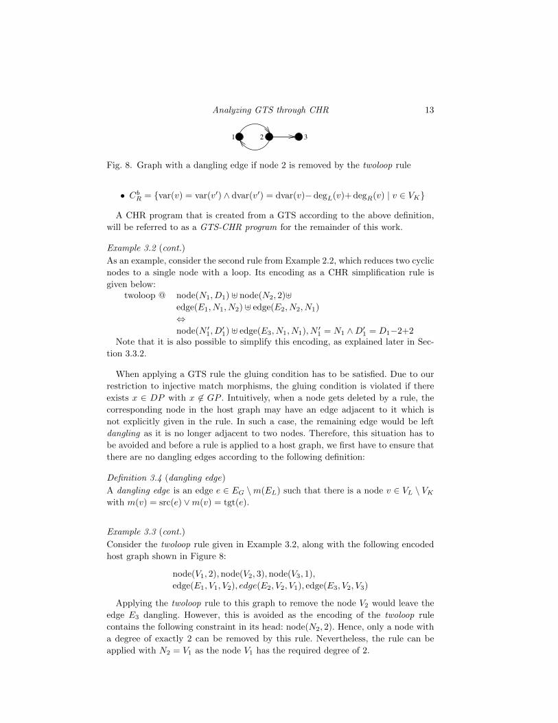
21 3
Fig. 8. Graph with a dangling edge if node 2 is removed by the twoloop rule
• CbR = {var(v) = var(v′) ∧ dvar(v′) = dvar(v)−degL(v)+ degR(v) | v ∈ VK}
A CHR program that is created from a GTS according to the above definition,
will be referred to as a GTS-CHR program for the remainder of this work.
Example 3.2 (cont.)
As an example, consider the second rule from Example 2.2, which reduces two cyclic
nodes to a single node with a loop. Its encoding as a CHR simplification rule is
given below:twoloop @ node(N1, D1) ] node(N2, 2)]
edge(E1, N1, N2) ] edge(E2, N2, N1)
⇔node(N ′1, D
′1) ] edge(E3, N1, N1), N ′1 = N1 ∧D′1 = D1−2+2
Note that it is also possible to simplify this encoding, as explained later in Sec-
tion 3.3.2.
When applying a GTS rule the gluing condition has to be satisfied. Due to our
restriction to injective match morphisms, the gluing condition is violated if there
exists x ∈ DP with x 6∈ GP . Intuitively, when a node gets deleted by a rule, the
corresponding node in the host graph may have an edge adjacent to it which is
not explicitly given in the rule. In such a case, the remaining edge would be left
dangling as it is no longer adjacent to two nodes. Therefore, this situation has to
be avoided and before a rule is applied to a host graph, we first have to ensure that
there are no dangling edges according to the following definition:
Definition 3.4 (dangling edge)
A dangling edge is an edge e ∈ EG \m(EL) such that there is a node v ∈ VL \ VKwith m(v) = src(e) ∨m(v) = tgt(e).
Example 3.3 (cont.)
Consider the twoloop rule given in Example 3.2, along with the following encoded
host graph shown in Figure 8:
node(V1, 2),node(V2, 3),node(V3, 1),
edge(E1, V1, V2), edge(E2, V2, V1), edge(E3, V2, V3)
Applying the twoloop rule to this graph to remove the node V2 would leave the
edge E3 dangling. However, this is avoided as the encoding of the twoloop rule
contains the following constraint in its head: node(N2, 2). Hence, only a node with
a degree of exactly 2 can be removed by this rule. Nevertheless, the rule can be
applied with N2 = V1 as the node V1 has the required degree of 2.
14 Frank Raiser, Thom Fruhwirth
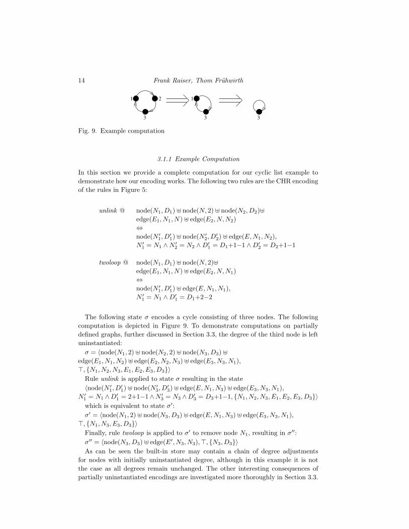
3
1 2
3
1
3
Fig. 9. Example computation
3.1.1 Example Computation
In this section we provide a complete computation for our cyclic list example to
demonstrate how our encoding works. The following two rules are the CHR encoding
of the rules in Figure 5:
unlink @ node(N1, D1) ] node(N, 2) ] node(N2, D2)]edge(E1, N1, N) ] edge(E2, N,N2)
⇔node(N ′1, D
′1) ] node(N ′2, D
′2) ] edge(E,N1, N2),
N ′1 = N1 ∧N ′2 = N2 ∧D′1 = D1+1−1 ∧D′2 = D2+1−1
twoloop @ node(N1, D1) ] node(N, 2)]edge(E1, N1, N) ] edge(E2, N,N1)
⇔node(N ′1, D
′1) ] edge(E,N1, N1),
N ′1 = N1 ∧D′1 = D1+2−2
The following state σ encodes a cycle consisting of three nodes. The following
computation is depicted in Figure 9. To demonstrate computations on partially
defined graphs, further discussed in Section 3.3, the degree of the third node is left
uninstantiated:
σ = 〈node(N1, 2) ] node(N2, 2) ] node(N3, D3) ]edge(E1, N1, N2) ] edge(E2, N2, N3) ] edge(E3, N3, N1),
>, {N1, N2, N3, E1, E2, E3, D3}〉Rule unlink is applied to state σ resulting in the state
〈node(N ′1, D′1) ] node(N ′3, D
′3) ] edge(E,N1, N3) ] edge(E3, N3, N1),
N ′1 = N1 ∧D′1 = 2+1−1∧N ′3 = N3 ∧D′3 = D3+1−1, {N1, N2, N3, E1, E2, E3, D3}〉which is equivalent to state σ′:
σ′ = 〈node(N1, 2) ] node(N3, D3) ] edge(E,N1, N3) ] edge(E3, N3, N1),
>, {N1, N3, E3, D3}〉Finally, rule twoloop is applied to σ′ to remove node N1, resulting in σ′′:
σ′′ = 〈node(N3, D3) ] edge(E′, N3, N3),>, {N3, D3}〉As can be seen the built-in store may contain a chain of degree adjustments
for nodes with initially uninstantiated degree, although in this example it is not
the case as all degrees remain unchanged. The other interesting consequences of
partially uninstantiated encodings are investigated more thoroughly in Section 3.3.
Analyzing GTS through CHR 15
3.2 Formal Properties
This section examines formal properties of the encoding given in Section 3.1. First,
Section 3.2.1 analyzes the special CHR states found when working with a GTS-
CHR program. Then we prove soundness and completeness of the encoding in Sec-
tion 3.2.2.
Our encoding is based on the assumption that the resulting CHR programs are
executed only for initial states that correspond to graphs. We are not interested in
executions for arbitrary CHR states.
3.2.1 States Encoding Graphs
In this section we compare the different equivalence notions, i.e. graph isomorphism
and CHR state equivalence, and present a formal characterization of a CHR state σ
that is the encoding of a graph G.
In order to determine if a CHR state encodes a graph, we define a predicate that
holds if and only if this is the case. It is intuitively clear, that starting with the
encoding of a graph and transforming it via a graph transformation rule yields the
encoding of a graph again. Formally, this is an invariant according to the following
definition. The first appearance of invariants in CHR research is found in (Lam and
Sulzmann 2006) in the context of agent programming.
Definition 3.5 (Invariant)An invariant I is a predicate such that for all σ0 and σ1, we have that if σ0 � σ1
(or σ0 ≡ σ1) and I(σ0) then I(σ1).
The definition below introduces our desired property for CHR states. Note that
it is referred to as an invariant here, although we do not require it to be an invariant
throughout this section. In Section 3.2.2, more precisely Corollary 6, we will show
that it is indeed a proper invariant.
Definition 3.6 (Graph Invariant)Let σ = 〈G,Bc ∧ Ba,V〉 be a state where Bc are constraints of the form X = c for
constants c and Ba are constraints of the form X = Y+c1−c2 for constants c1, c2.
The graph invariant G holds for state σ if and only if there exists a graph G and
a conjunction B of equality constraints of the form X = c for a variable X and
constant c, such that
〈G,Bc ∧ Ba ∧B, ∅〉 ≡ 〈chr(ground, G),>, ∅〉
For a state σ for which G(σ) holds with a graph G we say σ is a G-state based on G.
Example 3.4Consider again the final state σ′′ from the example computation in Section 3.1.1:
σ′′ = 〈node(N3, D3) ] edge(E′, N3, N3),>, {N3, D3}〉
By using the equality constraint B = (D3 = 2) the resulting state for Defini-
tion 3.6 is equivalent to:
〈node(N3, 2) ] edge(E′, N3, N3),>, ∅〉
16 Frank Raiser, Thom Fruhwirth
Let G be the graph consisting of a node v with a loop, then chr(ground, G) =
node(Nv, 2) ] edge(E,Nv, Nv). Therefore, the invariant G is satisfied for the above
state σ′′ as the corresponding states are equivalent by renaming of local variables.
This example further shows why the variable set V is disregarded for the two
states. The variable given by var for a node of the graph has to coincide with the
corresponding global variable for both states to be equivalent. Hence, for the above
graph with node v, knowledge of the state σ′′ would be necessary to determine
that var(v) = N3. Omitting global variables from both states, however, allows us
to freely map v to any variable through var(v).
Example 3.5
For the state σ = 〈chr(keep, G),>,V〉 there clearly exists such a graph G, for which
B simply assigns the corresponding degree variables. States may also be in-between
chr(ground, G) and chr(keep, G) in the sense that only some of the degree variables
are instantiated, resulting in a state σ′ = 〈chr(keep, G),Bc,V〉 with Bc being the
corresponding equality constraints. By instantiating the remaining degrees it is clear
that G(σ′) holds.
Note that arithmetic built-in constraints, introduced by bodies of rules in order
to adjust a node’s degree, are covered by the above graph invariant definition: The
introduction of the corresponding degree equality constraint leads to a collapse of
the chain of arithmetic constraints. Hence, the concept of a G-state based on G
also applies to intermediate computation states, which gives rise to the following
lemma.
Lemma 3 (Graph States)
Let G(σ) hold for a state σ, then there exists a graph G such that
σ ≡ 〈chr(keep, G),Bc ∧ Ba,V〉
• Bc is a conjunction of dvar(v) = degG(v) constraints
• Ba is a conjunction of dvar(v′) = dvar(v)+c1−c2 constraints
Proof
Let σ = 〈G,Bc ∧ Ba,V〉, then by Def. 3.6 we have that 〈G,Bc ∧ Ba ∧ B, ∅〉 ≡〈chr(ground, G),>, ∅〉 for a graph G and X = k constraints B.
W.l.o.g. all identifier variables occurring in chr(ground, G) (and therefore in
chr(keep, G)) also occur in G as identifier variables. Due to the state equivalence
the difference between G and chr(keep, G) can then only consist in G specifying
some node degrees by constants (for degree variables we can again assume that they
are the same as in chr(keep, G)).
Let Θ be a conjunction of equality constraints of the form X = c for each degree
specified explicitly in G, using fresh variables forX. Interpreting Θ as a substitution,
replacing X with c for each of the equivalences, we have that
σ ≡ 〈chr(keep, G)Θ,Bc ∧ Ba,V〉.
Analyzing GTS through CHR 17
As all variables occurring in Θ are local, we get by Def. 2.8:
σCT≡ 〈chr(keep, G)Θ,Bc ∧ Ba ∧Θ,V〉
Subst≡ 〈chr(keep, G),Bc ∧ Ba ∧Θ,V〉= 〈chr(keep, G),B′c ∧ Ba,V〉
The reverse direction of Lemma 3 does not hold in general: The state σ = 〈∅, D =
0 ∧X = 1 ∧D = X+2−0, ∅〉 satisfies the conditions for an empty graph G, but of
course G(σ) does not hold, as 〈∅,⊥, ∅〉 6≡ 〈∅,>, ∅〉.The following lemma presents an interesting fact of the correspondence between
state equivalence and graph isomorphism: equivalent CHR states encoding two
graphs imply that these graphs are isomorphic.
Lemma 4 (Equivalent G-states imply Graph Isomorphism)
Given a state σ1 = 〈chr(keep, G1),B1,V〉, a G-state based on G1, and a state
σ2 = 〈chr(keep, G2),B2,V〉, a G-state based on G2, then
σ1 ≡ σ2 ⇒ G1 ' G2
Proof
First, we note that B1,B2 consist only of degree equalities or adjustments. There-
fore, we consider the following states instead, which are already sufficient to imply
the isomorphism:
〈chr(keep, G1),>,V〉 ≡ 〈chr(keep, G2),>,V〉
W.l.o.g. let the local variables occurring in the two states be disjoint (it is clear that
otherwise we can consider equivalent states that only differ by renaming of local
variables and that these states all provide corresponding graph isomorphisms).
Let y1 and y2 be the set of local variables of the two states. We can then apply
the criterion from Thm. 2 to get
CT |= ∃y1.chr(keep, G1) = chr(keep, G2).
As there are only variable terms contained in this equivalence we have the following
conclusion, where c(t) is any constraint with argument terms, i.e. variables, t.
∃f : y1 → y2 with c(t) ∈ chr(keep, G1)→ c(f(t)) ∈ chr(keep, G2)
We know that f is surjective (as the variables are disjoint and the above equality
demands that at least one variable from y1 is mapped to each variable in y2). A
consequence of this is that |y1| ≥ |y2|.Analogously, we get from CT |= ∃y2.chr(keep, G1) = chr(keep, G2) that |y2| ≥
|y1|, and hence, |y1| = |y2|. From this follows that f is also injective, and therefore,
bijective.
Next we realize, that by the above equality, f has to map local variables corre-
sponding to node identifiers to local variables that also correspond to node identi-
fiers. Let yn1 ⊂ y1, yn2 ⊂ y2 be the local variables used for node identifiers, then
18 Frank Raiser, Thom Fruhwirth
f ′ : yn1 → yn2, y 7→ f(y) is a well-defined and bijective function. We use this to
define the actual graph isomorphism function g : VG1→ VG2
:
g(v) =
{v if var(v) ∈ Vv′ if var(v) ∈ yn1 and f ′(var(v)) = var(v′)
g is well-defined: for every node there is a corresponding node identifier variable
and it has to be either global or local. If it is local, then f ′ has to map it to another
local variable, as otherwise the ≡ relation cannot hold. Furthermore, g is bijective
as well, because it is defined bijectively via f ′ on local variables and the identity
function on global variables.
Finally, g is a graph isomorphism: By the above equality we have corresponding
pairs of edge constraints. For every edge adjacent to a node given by a global
variable, the corresponding edge has to be adjacent to the same node with the same
global variable in order to satisfy ≡. If the edge is adjacent to a node identified by
a local variable, then this variable is bijectively mapped to another local variable
and the above equality ensures that the corresponding edge is adjacent to the same
node as well.
The reverse direction of Lemma 4 cannot hold in general: The encoding of the
graphs G1 and G2 are independent from determining the set V of global variables.
Even a graph consisting of a single node only can be encoded in two ways, such
that the states are not equivalent:
〈node(N, 0),>, ∅〉 6≡ 〈node(N, 0),>, {N}〉
As indicated in Section 3.1.1, states may contain node encodings with a variable
degree. As these states are fundamental for program analysis the following definition
characterizes the set of these nodes.
Definition 3.7 (Strong Nodes)
For a CHR state σ ≡ 〈chr(keep, G),B,V〉 which is a G-state based on G we define
the set of strong nodes as:
S(σ) = {v ∈ VG | dvar(v) = degG(v) 6∈ B}
The effect of strong nodes on computations and their use in program analysis is
discussed in detail in Section 3.3.
3.2.2 Soundness and Completeness
In this section, we prove soundness and completeness of our embedding. That Gis an invariant for a GTS-CHR program and that termination of a GTS and its
GTS-CHR program coincide, are then derived as consequences of the main theorem
below.
Theorem 5 (Soundness and Completeness)
Let σ ≡ 〈chr(keep, G),B,V〉 be a CHR state with G(σ) holding with graph G. Then
Gr,m=⇒ H with {v ∈ VG | trG⇒H(v) defined} ⊇ S(σ)

Analyzing GTS through CHR 19
if and only if
σ�r τ ≡ 〈chr(keep, H),B′,V〉 and G(τ) holds with graph H.
Proof
In order to shorten this proof we use k(G) and g(G) to denote chr(keep, G) and
chr(ground, G), respectively.
“=⇒”:
Let Gr,m=⇒ H and let r : L← K → R.
Let G := k(G) = k(G \m(L)) ] k(m(EL)) ] k(m(VK)) ] k(m(VL \ VK)) ⇒ σ ≡〈G,B,V〉.
Let %(r) = (r @ CL ⇔ CbR, CuR) with CL = k(K) ] g(L \K).
For v ∈ VL we have typeG(v)(var(v), ) ∈ CL and
typeG(v)(var(m(v)),dvar(m(v))) ∈ k(m(VK)), as the types match due to m being
a graph morphism.
As we have a fresh rule using node v that does not occur elsewhere we can say
that σCT≡ 〈G, var(m(v)) = var(v) ∧ B,V〉, and hence
σSubst≡ 〈G[var(m(v))/ var(v)], var(m(v)) = var(v) ∧ B,V〉 (1)
Consider v ∈ VL \VK , then typeG(v)(var(v),degL(v)) ∈ CL. Assume that m(v) ∈S(σ), then trG⇒H(m(v)) is defined, which is a contradiction to v ∈ VL \VK . There-
fore, m(v) 6∈ S(σ) and hence dvar(m(v)) = degG(m(v)) ∈ B. As Gr,m=⇒ H satisfies
the gluing condition, we know that degL(v) = degG(m(v)). Therefore, we have that
σSubst≡ 〈G[var(m(v))/ var(v)][dvar(m(v))/degG(m(v))],
var(m(v)) = var(v) ∧ B,V〉
From (1) for nodes v ∈ VK and the above for nodes v ∈ VL \ VK follows for a
conjunction of equality constraints E that
σ ≡ 〈k(G \m(L)) ] k(m(EL)) ] k(VK) ] g(VL \ VK),B ∧ E,V〉 = 〈G′,B ∧ E,V〉
Let e ∈ EL, than typeG(e)(var(e), var(src(e)), var(tgt(e))) ∈ CL and after the
previous substitutions have been made for node identifier variables, and as k(e) =
g(e), we get typeG(m(e))(var(m(e)), var(src(e)), var(tgt(e))) ∈ σ . We then have
σ ≡ 〈G′[var(m(e))/ var(e)], var(m(e)) = var(e) ∧ B ∧ E,V〉 (2)
By applying this substitution for all edges e ∈ EL and extending E with the
required equalities to E′ we get:
σ ≡ 〈k(G \m(L)) ] k(EK) ] g(EL \ EK) ] k(VK) ] g(VL \ VK),B ∧ E′,V〉
Hence, σ ≡ 〈k(G \m(L)) ] CL,B ∧ E′,V〉 such that we apply the rule %(r) to σ:
σ�r τ ≡ 〈k(G \m(L)) ] CuR,B ∧ E′ ∧ CbR,V〉≡ 〈k(G \m(L)) ] g(R \K) ] k(EK) ] k(V ′K),B ∧ E′ ∧ CbR,V〉
As CbR contains var(v′) = var(v)∀v ∈ VK let C ′R be CbR without these constraints,
20 Frank Raiser, Thom Fruhwirth
then
τSubst≡ 〈k(G \m(L)) ] g(R \K) ] k(EK) ] k(VK),B ∧ E′ ∧ CbR,V〉CT≡ 〈k(G \m(L)) ] g(R \K) ] k(EK) ] k(VK),B ∧ E′ ∧ C ′R,V〉
Let G := k(G\m(L))]k(K), then τCT≡ 〈G]g(R\K),B∧E′∧C ′R∧DR,V〉 with
∀v ∈ VR \ VK .dvar(v) = degR(v) ∈ DR. Furthermore, consider Θ a substitution
corresponding to the reverse reading of E′ which undoes the ideas of (1) and (2)
for all affected nodes and edges. We then get
τSubst≡ 〈G ] k(R \K), DR ∧ C ′R ∧ B ∧ E′,V〉Subst≡ 〈k(G \m(L \K)) ] (k(R \K)Θ), DR ∧ C ′R ∧ B ∧ E′,V〉CT≡ 〈k(G \m(L \K)) ] (k(R \K)Θ), DR ∧ C ′RΘ ∧ B,V〉≡ 〈k(H),B′,V〉
We get the graph H as its DPO construction corresponds to the removal of
m(L \ K) and addition of R \ K. Θ is needed to attach the new nodes of R \ Kto nodes from VK and C ′R contains degree adjustments for those nodes that are
correct by construction. Hence, it also holds that G(τ) is satisfied with graph H.
“⇐=”:
Let σ �r τ with τ ≡ 〈k(H),B′,V〉 and G(τ) holds with graph H. Let %(r) =
(r @ CL ⇔ CbR, CuR with CL = k(K) ] g(L \K). From Def. 2.10 follows that
σ ≡ 〈k(K) ] g(L \K) ] k(G \ L),B1,V〉 (3)
Using Lemma 3 and with E being a conjunction of var(m(x)) = var(x) constraints
for x ∈ L we get:
σ ≡ 〈k(G),Bc ∧ Ba,V〉≡ 〈k(K) ] k(L \K) ] k(G \m(L)),Bc ∧ Ba ∧ E,V〉(3)≡ 〈k(K) ] g(L \K) ] k(G \m(L)),Bc ∧ Ba ∧ E′,V〉
where E′ is the extension of E with dvar(m(v)) = degG(v) constraints for v ∈VL \ VK and B1 = Bc ∧ Ba ∧ E′.m : L→ G is well-defined and injective by the multiset semantics of CHR and it
remains to be shown, that m is a graph morphism. Therefore, let e ∈ EL, then
typeL(e)(var(e), var(src(e)), var(tgt(e))) ∈ CL and typeL(src(e))(var(src(e)), ) ]typeL(tgt(e))(var(tgt(e)), ) ∈ CL. Hence, var(m(e)) = var(e), var(m(src(e))) =
var(src(e)) and var(m(tgt(e))) = var(tgt(e)) are all in B1. Therefore, m(src(e)) =
src(m(e)) ∧m(tgt(e)) = tgt(m(e)).
The gluing condition is satisfied, as ∀v ∈ VL \ VK the matched degree ensures
that there are no dangling edges, hence, r is GTS-applicable to G. Similarly to the
other proof direction, we show that the DPO construction of H coincides with the
construction of τ by CHR rule application:
Analyzing GTS through CHR 21
σ�r τ ≡ 〈k(K) ] g(R \K) ] k(G \m(L)),Bc ∧ Ba ∧ E′ ∧ CbR,V〉CT≡ 〈k(K) ] g(R \K) ] k(G \m(L)),Bc ∧ Ba ∧ E ∧ CbR,V〉
Subst≡ 〈k(m(K)) ] g(R \K) ] k(G \m(L)),Bc ∧ Ba ∧ E ∧ CbR,V〉= 〈g(R \K) ] k(G \m(L \K)),Bc ∧ Ba ∧ E ∧ CbR,V〉≡ 〈g(R \K)Θ ] k(G \m(L \K)),Bc ∧ Ba ∧ CbR,V〉≡ 〈k(H),B′,V〉
where Θ is the reverse substitution for E similar to the other proof direction. The
final equivalence comes from extracting the degrees of constraints in g(R \K) into
equality constraints contained in B′. As can be seen here, the application of the
rule results in a state encoding the graph H, such that G(τ) holds.
Finally, for the set S(σ) we know that the nodes cannot be removed by rule r:
For a node v ∈ VL \ VK we have typeL(v)(var(v),degL(v)) ∈ CL, but this cannot
be matched with σ, as by Def. 3.7 the corresponding degree is unavailable. Hence,
none of the nodes from S(σ) are removed by the rule application Gr,m=⇒ H, i.e.
trG⇒H(v) is defined for all v ∈ S(σ).
As can be seen in the proof of Theorem 5, a GTS-CHR rule application on a
G-state based on G always results in a state encoding a corresponding graph H,
which gives us the following corollary.
Corollary 6 (G Invariant)
For a GTS-CHR program G is an invariant.
A closer look at the conditions required in Theorem 5 reveals that for a state σ
with S(σ) = ∅, i.e. for an encoding of a graph with all degrees explicitly given, we
have unrestricted soundness and completeness.
Corollary 7 (Unrestricted Soundness and Completeness)
Let σ ≡ 〈chr(ground, G),>,V〉 be a CHR state with G(σ) holding with graph G.
Then
Gr,m=⇒ H
if and only if
σ�r τ ≡ 〈chr(ground, H),>,V〉 and G(τ) holds with graph H
Proof
This follows from Theorem 5 and the following insight: as all degrees of G are
specified explicitly and all nodes added by the rule are also given explicit degrees,
all degrees in H are given explicitly as well, which allows us to use chr(ground, H)
here.
Finally, the soundness and completeness result induces a termination correspon-
dence between a GTS and its GTS-CHR program. Again, we restrict our observation
to graph-encoding states.
22 Frank Raiser, Thom Fruhwirth
Corollary 8 (Termination Correspondence)A GTS is terminating if and only if its corresponding GTS-CHR program is G-
terminating, i.e. terminating for all G-states.
ProofIf a GTS contains a non-terminating derivation, we have the corresponding compu-
tation in its GTS-CHR program by Corollary 7. Similarly, if the GTS-CHR program
has a non-terminating computation, there exists a corresponding non-terminating
GTS derivation according to Theorem 5.
3.3 Discussion
In this section we discuss our previously presented encoding. First, Section 3.3.1
investigates that a GTS-CHR program works with partially defined graphs and
explains the suitability of these graphs for program analysis. Then we present ways
to simplify the encoding of GTS-CHR rules in Section 3.3.2.
3.3.1 Partially Defined Graphs
In the example computation given in Section 3.1.1 the input contains a node with a
variable degree: node(N3, D3). Nevertheless, computations on this input are possible
and the example resulted in the final state:
〈node(N3, D3) ] edge(E′, N3, N3),>, {N3, D3}〉
In general, a variable node degree will cause a chain of degree adjustment con-
straints to be created, i.e. constraints of the form X = Y+c1−c2. These stem from
the node being involved in a rule application that affects its degree.
It is important to realize that we can only match such a node in rules that do not
remove it. A rule that removes a node contains the explicit degree for that node in
the head, which cannot be matched through a variable degree. As a consequence,
specifying variable degrees in the input ensures that the corresponding nodes will
not be removed by the computation. This also becomes clear from the investigation
of strong nodes in the previous section.
While this is an interesting feature in its own right, it provides the basis for many
forms of program analysis. The aim of program analysis is to make statements on
an infinite number of graphs, while only having to investigate a small selection of
graphs. Graph encodings with variable degrees can here be thought of as partially
defined graphs, i.e. there may be any number of further edges being connected to
a node with a variable degree.
Note that partially defined graphs only exist within the CHR context. In a GTS
the degree of a node is implicitly given by the adjacent edges. As a consequence,
leaving a node’s degree undefined in the CHR encoding ensures, that this node will
not be removed during computation. In the GTS context we have no such option
available for host graphs.
By the above argument, the state
〈node(N,D),>, {N,D}〉
Analyzing GTS through CHR 23
therefore not only represents the graph consisting of a single node and no edges.
Instead, it represents the set of all graphs with at least one node. Similarly, the
above final state from Section 3.1.1 stands for the set of graphs that contain at
least one node with a loop.
Every computation performed on an input with variable degrees actually repre-
sents computations for an infinite set of graphs. This is a fundamental feature for
the usage of our encoding in program analysis and will be exploited in Sections 4
and 5.
3.3.2 Different Encoding Possibilities
The encoding proposed in this work can be varied in several different ways. We
chose the encoding in Definition 3.2 and Definition 3.3 for this work, because it is a
verbose encoding, hence, directly presenting all its components and simplifying the
proofs. In practice however, a less verbose encoding resulting in shorter rules can be
used instead. In this section we present different possible simplifications achieving
this.
The different simplifications are illustrated by applying them to the twoloop rule
which is of the following form when encoded as specified in Definition 3.3:
twoloop @ node(N1, D1) ] node(N2, 2)]edge(E1, N1, N2) ] edge(E2, N2, N1)
⇔node(N ′1, D
′1) ] edge(E3, N1, N1), N ′1 = N1 ∧D′1 = D1−2+2
There are two ways to specify the degree of nodes in L \K. The one chosen in
Definition 3.3 explicitly specifies the respective degree in the head. Another way
is to keep the degree as a variable D in the head and add the built-in constraint
D = k to the guard of the rule. However, most current CHR compilers detect these
equalities and automatically transform between them to the representation most
suitable for an optimization. Therefore, in this work we directly specify the degree
in the head to avoid guards altogether.
Variable Elimination As Definition 3.3 encodes a node v ∈ VK using a new node
identifier v′ with var(v) = var(v′) and var(v′) is not used elsewhere, this substitution
can be included directly into the rule encoding:
twoloop @ node(N1, D1) ] node(N2, 2)]edge(E1, N1, N2) ] edge(E2, N2, N1)
⇔node(N1, D
′1) ] edge(E3, N1, N1), D′1 = D1−2+2
Note that we perform variable elimination on node identifiers by default in the re-
mainder of this work. However, as we need to take degree adjustments into account,
the formulation of Definition 3.3 is simplified by the variable duplication.
24 Frank Raiser, Thom Fruhwirth
Arithmetic Simplification The degree adjustments in Definition 3.3 explicitly con-
tain the information on how many edges the rule deletes and creates. For the ad-
justment itself, however, it is sufficient to simply adjust the degree by the actual
change in the number of edges. Additionally, if the change is 0, like in the twoloop
rule, the extra local variable used for the degree can be substituted, resulting in:
twoloop @ node(N1, D1) ] node(N2, 2)]edge(E1, N1, N2) ] edge(E2, N2, N1)
⇔node(N1, D1) ] edge(E3, N1, N1)
Elimination of Edge Identifiers The edge identifier variables are used throughout
this work, because they simplify dealing with the multiset semantics of CHR with
respect to the edge constraint representing exactly one edge of a graph. In a CHR
implementation, however, every constraint is implemented as a unique object –
sometimes even annotated with an identifier number – which makes the explicit
edge identifiers redundant. Using this idea the twoloop rule can be further simplified
to:
twoloop @ node(N1, D1) ] node(N2, 2)]edge(N1, N2) ] edge(N2, N1)
⇔node(N1, D1) ] edge(N1, N1)
Note that the same argumentation cannot be applied to node identifiers, as those
are required for specifying the source and target of edge constraints.
Simpagation Rules Some nodes and edges of the left-hand rule graph L of a GTS
rule can occur only to specify a certain graph context and are unaffected by the
rule application. For nodes this can also happen if the modification to adjacent
edges results in no change to the degree, as in the twoloop rule. In those cases, the
node or edge is encoded in exactly the same way in the head and body of the rule.
Therefore, during the rule application the corresponding constraint is removed and
introduced again. Using a simpagation rule allows us to move such a constraint
into the part of the head which is not removed during the rule application. This
reduces the textual size of the rule as well as its execution time, because it avoids
the generation of a new constraint during the rule application.
After applying all the previous simplifications to the twoloop rule and transform-
ing it into a simpagation rule we get the following simplified rule:
twoloop @ node(N1, D1)\node(N2, 2) ] edge(N1, N2) ] edge(N2, N1)
⇔edge(N1, N1)
One might be tempted to always create simpagation rules in Definition 3.3, based
on the idea that the context graph K already identifies non-removed nodes. How-
ever, the above creation of simpagation rules with node constraints among the kept
Analyzing GTS through CHR 25
constraints, is only possible if the respective node’s degree remains unchanged by
the rule application.
Readers more familiar with CHR may also wonder if propagation rules could be
used as well. It is technically possible to define a GTS rule that does not remove any
elements, but only adds new nodes and edges. However, a thusly created GTS would
suffer from a problem that in CHR literatue is referred to as trivial non-termination
(see e.g., (Fruhwirth 2009)), i.e. such a rule could be applied infinitely often. For this
reason, most CHR implementations restrict propagation rule applications, hence,
our encoding using simplification or simpagation rules remains more faithful to the
semantics of graph transformations.
4 Analyzing Confluence
The confluence property is relevant to both, graph transformation systems and
Constraint Handling Rules. It guarantees that any terminating computation made
for an initial state results in the same final state no matter in which order applicable
rules are applied.
In Section 4.1 we formally introduce confluence, both for GTS and CHR. Further-
more, we give the definitions for critical pairs in both systems, which are derived
directly from the rules. Investigation of critical pairs for determining confluence of
a terminating rewrite system goes back to research about term rewriting systems
(Huet 1980), and both, GTS and CHR, have adapted the corresponding criteria.
Next, Section 4.2 examines the relation between critical pairs of a GTS and its
corresponding GTS-CHR program. We then introduce the concept of observable
confluence (Duck et al. 2007). It is a technical means to restrict our observations to
CHR states that correspond to graphs. This in turn results in a closer correspon-
dence between GTS and CHR for later results.
For terminating GTS, confluence analysis proved to be undecidable: (Plump
2005) showed that the critical pair analysis gives only a sufficient criterion for
confluence. We show that the decidable observable confluence test of a GTS-CHR
program coincides with this criterion.
The discrepance in decidability of the two systems’ confluence properties is dis-
cussed in Section 4.3 for exemplary critical pair analyses.
4.1 Preliminaries
This subsection introduces the necessary definitions for GTS and CHR confluence
before comparing the two notions. Unless noted otherwise, the involved graph trans-
formation systems and GTS-CHR programs are assumed to be terminating.
Definition 4.1 (GTS Confluence)A GTS is called confluent if, for all typed graph transformations G
∗=⇒ H1 and
G∗
=⇒ H2, there is a typed graph X together with typed graph transformations
H1∗
=⇒ X and H2∗
=⇒ X. Local confluence means that this property holds for all
pairs of direct typed graph transformations G ⇒ H1 and G ⇒ H2 (Ehrig et al.
2006).

26 Frank Raiser, Thom Fruhwirth
Newman’s general result for rewriting systems (Newman 1942) implies that it is
sufficient to consider local confluence for terminating graph transformation systems.
To verify local confluence, we particularly need to study critical pairs and their
joinability, according to the following definition based on (Ehrig et al. 2006; Plump
2005).
Definition 4.2 (Joinability of Critical GTS Pair)
Let r1 = (L1l← K1
r→ R1), r2 = (L2l← K2
r→ R2) be two GTS rules. A pair
P1r1,m1⇐= G
r2,m2=⇒ P2 of direct typed graph transformations is called a critical GTS
pair if it is parallel dependent, and minimal in the sense that the pair (m1,m2) of
matches m1 : L1 → G and m2 : L2 → G is jointly surjective.
A pair P1r1,m1⇐= G
r2,m2=⇒ P2 of direct typed graph transformations is called parallel
independent if m1(L1)∩m2(L2) ⊆ m1(K1)∩m2(K2), otherwise it is called parallel
dependent.
A critical GTS pair P1r1,m1⇐= G
r2,m2=⇒ P2 is called joinable if there exist typed
graphs X1, X2 together with typed graph transformations P1∗
=⇒ X1 ' X2∗⇐= P2.
It is strongly joinable if there is an isomorphism f : X1 → X2 such that for each
node v, for which trG⇒P1(v) and trG⇒P2
(v) are defined, the following holds:
1. trG⇒P1⇒X1(v) and trG⇒P2⇒X2
(v) are defined and
2. fV (trG⇒P1⇒X1(v)) = trG⇒P2⇒X2
(v)
A similar notion of confluence has been developed for CHR. The following defi-
nition is an adaptation of (Fruhwirth 2009) to the operational semantics on equiv-
alence classes.
Definition 4.3 (CHR Confluence)
A CHR program is called confluent if for all states σ, σ1, and σ2: If σ1∗� σ�∗ σ2,
then σ1 and σ2 are joinable. Two states σ1 and σ2 are called joinable if there exists
a state τ such that σ1 �∗ τ ∗� σ2.
Analogous to a GTS, the confluence property for terminating CHR programs is
determined by local confluence which can be checked through critical pairs. The
following definition is adapted to the situation in this work, i.e. it only considers
simplification rules and no guards.
Definition 4.4 (Joinability of Critical CHR Pair)
Let ri, i = 1, 2 be two (not necessarily different) simplification rules of the following
kind with variables that have been renamed apart:
Hi ]Ai ⇔ Bui , Bbi
Then an overlap σCP of r1 and r2 is σCP = 〈H1]A1]H2, A1 = A2,V〉, provided
A1 and A2 are non-empty multisets, V = vars(H1]A1]H2]A2) and CT |= ∃(A1 =
A2).
Let σ1 = 〈Bu1 ]H2, Bb1 ∧ (A1 = A2),V〉 and σ2 = 〈Bu2 ]H1, B
b2 ∧ (A1 = A2),V〉.
Then the tuple CP = (σ1, σ2) is a critical CHR pair of r1 and r2. A critical CHR
pair (σ1, σ2) is joinable if σ1 and σ2 are joinable.

Analyzing GTS through CHR 27
4.2 Analyzing Confluence via Critical Pairs
After defining the different notions of confluence we now further investigate the
difference between critical GTS pairs and critical CHR pairs for GTS-CHR pro-
grams. The following lemma shows that there exists a corresponding overlap for
each critical GTS pair. Therefore, by examining the overlaps and using the previ-
ous soundness result we can transfer joinability results to the critical GTS pair.
Lemma 9 (Overlap for Critical GTS Pair)
If P1r1,m1⇐= G
r2,m2=⇒ P2 is a critical GTS pair, then there exists an overlap σCP
of %(r1) = (r1 @ CL1 ⇔ CuR1, CbR1) and %(r2) = (r2 @ CL2 ⇔ CuR2, C
bR2) which
is a G-state based on G and a critical CHR pair (σ1, σ2) such that σ1 is a G-
state based on P1 and σ2 is a G-state based on P2.
Proof
Let the two GTS rules be Li ← Ki → Ri for i = 1, 2 and let M = m1(L1)∩m2(L2).
We then define the following sets of constraints from which we construct the overlap:
H1 = {chrL1(keep, x) | x ∈ L1 ∧m1(x) 6∈M}
H2 = {chrL2(keep, x) | x ∈ L2 ∧m2(x) 6∈M}A1 = {chrL1
(keep, x) | x ∈ L1 ∧m1(x) ∈M}A2 = {chrL2(keep, x) | x ∈ L2 ∧m2(x) ∈M}C1 = {dvar(v) = degL1
(v) | v ∈ VL1\ VK1
}C2 = {dvar(v) = degL2
(v) | v ∈ VL2 \ VK2}
Let V = vars(H1 ] H2 ] A1 ] A2) and let σ = 〈H1, C1,V〉, then σ ≡ σ′ =
〈{chrL1(keep, x) | x ∈ K1∧m1(x) 6∈M}]{chrL1(ground, x) | x ∈ L1\K1∧m1(x) 6∈M},>,V〉 =: 〈H ′2,>,V〉 by applying C1 as a substitution to H1, and then removing
C1 as all dvar(v) variables for v ∈ VL1 \ VK1 are then strictly local.
Similarly, 〈A1, C1,V〉 ≡ 〈{chr(keep, x) | x ∈ K1∧m1(x) ∈M}]{chr(ground, x) |x ∈ L1 \K1 ∧m1(x) ∈ M,>,V〉 =: 〈A′1,>,V〉, and analogously, we define H ′2 and
A′2.
By Def. 3.3 we have that H ′1]A′1 = CL1 and H ′2]A′2 = CL2. As M 6= ∅ it follows
that A′1 and A′2 are non-empty. To investigate if CT |= ∃(A′1 = A′2) we take a closer
look at the equality constraints imposed by A′1 = A′2:
{var(v1) = var(v2) | v1 ∈ VL1 ∧ v2 ∈ VL2 ,m1(v1) = m2(v2)}∧ {dvar(v1) = dvar(v2) | v1 ∈ VK1
∧ v2 ∈ VK2∧m1(v1) = m2(v2)}
∧ {dvar(v1) = degL2(v2) | v1 ∈ VK1
∧ v2 ∈ VL2\ VK2
∧m1(v1) = m2(v2)}∧ {dvar(v2) = degL1
(v1) | v1 ∈ VL1\ VK1
∧ v2 ∈ VK2∧m1(v1) = m2(v2)}
∧ {var(e1) = var(e2) | e1 ∈ EK1∧ e2 ∈ EK2
∧m1(e1) = m2(e2)}∧ {degL1
(v1) = degL2(v2) | v1 ∈ VL1 \ VK1 ∧ v2 ∈ VL1 \ VK2∧
m1(v1) = m2(v2)}
Except for the last row, the above equality constraints can easily be satisfied
under existential quantification. Hence, the only remaining problematic case is when
two node constraints with constant degrees are overlapped. However, the degree of
m1(v1) = m2(v2) equals the degree of v1 and the degree of v2 due to the gluing
28 Frank Raiser, Thom Fruhwirth
L K R1 1 1
Fig. 10. Graph production rule for removing a loop
condition being satisfied, such that this case can only occur with equal constant
degrees.
Hence, σCP = 〈H ′1]A′1]H ′2, A′1 = A′2,V〉 is an overlap of %(r1) and %(r2) with the
critical CHR pair (〈CuR1]H ′2, A′1 = A′2∧CbR1,V〉, 〈CR2]H ′1, A′1 = A′2∧CbR2,V〉.
If we try to directly transfer the confluence property of a GTS to the correspond-
ing GTS-CHR program, we cannot succeed however, as in general there are too
many critical CHR pairs that could cause the GTS-CHR program to become non-
confluent. The following example provides a rule which only has one critical GTS
pair, but for which the corresponding CHR rule has three critical CHR pairs.
Example 4.1
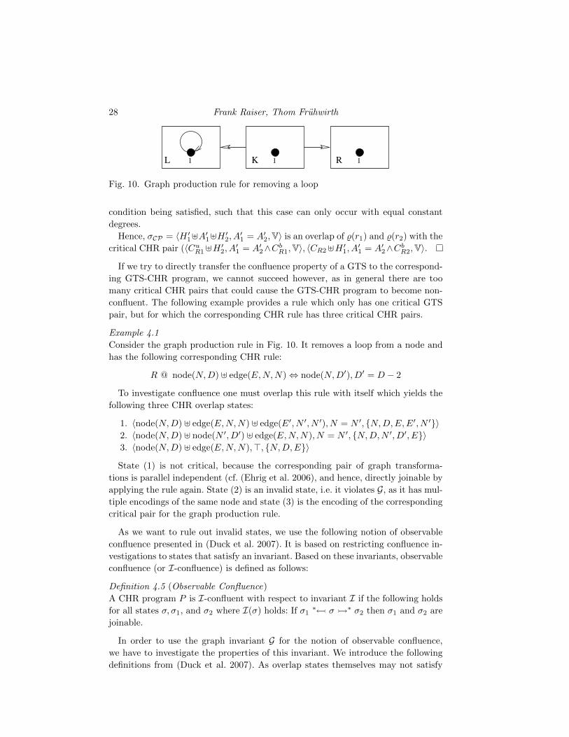
Consider the graph production rule in Fig. 10. It removes a loop from a node and
has the following corresponding CHR rule:
R @ node(N,D) ] edge(E,N,N)⇔ node(N,D′), D′ = D − 2
To investigate confluence one must overlap this rule with itself which yields the
following three CHR overlap states:
1. 〈node(N,D) ] edge(E,N,N) ] edge(E′, N ′, N ′), N = N ′, {N,D,E,E′, N ′}〉2. 〈node(N,D) ] node(N ′, D′) ] edge(E,N,N), N = N ′, {N,D,N ′, D′, E}〉3. 〈node(N,D) ] edge(E,N,N),>, {N,D,E}〉
State (1) is not critical, because the corresponding pair of graph transforma-
tions is parallel independent (cf. (Ehrig et al. 2006), and hence, directly joinable by
applying the rule again. State (2) is an invalid state, i.e. it violates G, as it has mul-
tiple encodings of the same node and state (3) is the encoding of the corresponding
critical pair for the graph production rule.
As we want to rule out invalid states, we use the following notion of observable
confluence presented in (Duck et al. 2007). It is based on restricting confluence in-
vestigations to states that satisfy an invariant. Based on these invariants, observable
confluence (or I-confluence) is defined as follows:
Definition 4.5 (Observable Confluence)
A CHR program P is I-confluent with respect to invariant I if the following holds
for all states σ, σ1, and σ2 where I(σ) holds: If σ1∗� σ�∗ σ2 then σ1 and σ2 are
joinable.
In order to use the graph invariant G for the notion of observable confluence,
we have to investigate the properties of this invariant. We introduce the following
definitions from (Duck et al. 2007). As overlap states themselves may not satisfy
Analyzing GTS through CHR 29
the invariant we have to examine all possible extensions that satisfy it. Note that
in (Duck et al. 2007) CHR states are defined as 5-tuples consisting of a goal, user
store, built-in store, token store, and the set of global variables. As such a verbose
definition is not necessary for the remainder of this work, we use the more concise
state definition from Section 2.2 and have adjusted the work from (Duck et al. 2007)
accordingly.
Definition 4.6 (Extension, Valid Extension)
A state σ = 〈G,B,V〉 can be extended by another state σe = 〈Ge,Be,Ve〉 as follows.
σ C σe = 〈G ]Ge,B ∧ Be,Ve〉
We say that σe is an extension of σ. A valid extension σe of a state σ is an extension
such that
v ∈ vars(G,B) ∧ v 6∈ V⇒ v 6∈ vars(Ge,Be,Ve).
When applied to confluence checking with critical pairs there are generally in-
finitely many possible extensions of a critical pair. To get a decidable criterion, the
following relation on extensions 1 allows us to consider only minimal elements.
Definition 4.7 (Relation on Extensions)
Let σ = 〈G,B,V〉 be a state, and let σe1 = 〈Ge1,Be1,Ve1〉 and σe2 = 〈Ge2,Be2,Ve2〉be valid extensions of σ. Then we define σe1 �σ σe2 to hold if
1. there exists a valid extension σe3 of (σCσe1) such that (σCσe1)Cσe3 ≡ σCσe22. V− Ve1 ⊆ V− Ve2 holds.
Note that for any extension σe = 〈Ge,Be,Ve〉 of a state σ = 〈G,B,V〉 there
exists a valid extension σ∅ = 〈∅,>,V〉 with σ∅ �σ σe, simply because the second
condition in Definition 4.7 is trivially satisfied and σe3 = 〈Ge,Be,Ve〉 satisfies the
first condition.
In the following we want to discuss overlap states that do not satisfy an invari-
ant I. Therefore, we are interested in extensions of those states, such that the
result satisfies the invariant I. The following definition introduces the set of all
those extensions and their minimal elements with respect to the previously defined
relation.
Definition 4.8
Let Σe(σ) be the set of all valid extensions of a state σ, and let ΣIe (σ) = {σe |σe ∈ Σe(σ)∧I(σCσe)} be the set of all valid extensions satisfying the invariant I.
Finally, let MIe (σ) be the ≺σ-minimal elements of ΣIe (σ).
As shown in (Duck et al. 2007) the analysis of critical pairs can be extended
to this context. Instead of requiring joinability of a critical pair – which might
not satisfy the invariant G – we require joinability for all possible extensions of
a critical pair that satisfy G. We make use of the relation on extensions here,
1 Originally, in (Duck et al. 2007) this relation is defined as a partial order, despite being neithertransitive nor anti-symmetric. However, it is sufficient for this work to consider it as a reflexivebinary relation.
30 Frank Raiser, Thom Fruhwirth
such that we only have to investigate minimal extensions. Note that we implicitly
consider minimal elements modulo built-in equivalence, e.g., the built-in storeD = 1
subsumes equivalent stores, like D = D′ + 1 ∧D′ = 0.
Definition 4.9
A program P is minimal extension joinable if for all critical pairs CP = (σ1, σ2)
with overlap σCP , and for all σe ∈ MIe (σCP), we have that (σ1 C σe, σ2 C σe) is
joinable.
It has been shown in (Duck et al. 2007) that joinability of critical pairs, stemming
from overlaps with minimal extensions, is a necessary and sufficient criterion for
I-local-confluence if the relation on extensions is well-founded.
Lemma 10 (Deciding I-Local-Confluence)
Given that ≺σCP is well-founded for all overlaps σCP , then: P is I-local-confluent
if and only if P is minimal extension joinable.
Although, in our programs built-in constraints + and − occur, we can consider
≺σCP well-founded for the following reason: On state components other than the
built-in store the ≺σCP -relation corresponds to the well-founded subset ordering
with the minimal element ∅ (cf. (Duck et al. 2007)). For the built-ins, we can con-
sider + and − as successor/predecessor terms (as they are only used with constants
in rules), and hence, we get well-foundedness via proposition 1 of (Duck et al. 2007).
We further note, that for any extension σe and state σCP holds that σ∅ ≺σCPσe. The following discussion shows that either MGe (σCP) = {σ∅} or ΣGe (σCP) =
MGe (σCP) = ∅. Whether the minimal element σ∅ exists depends solely on G(σCP)
holding as the following lemma shows.
Lemma 11 (No Minimal Elements)
If G(σCP) is violated for an overlap σCP then no extension σe exists such that
G(σCP C σe) is satisfied, i.e. ΣGe (σCP) =MGe (σCP) = ∅.
Proof
We proof this by a structural analysis of the overlap which gives the different
possibilities for G(σCP) to be violated. W.l.o.g. the overlap stems from the two
rules %(r1) = (r1 @ CL1⇔ CuR1
, CbR1) and %(r2) = (r2 @ CL2
⇔ CuR2, CbR2
) with
the corresponding rule graphs L1, L2,K1,K2, R1, and R2.
First consider the case of nodes v1 and v2 being overlapped:
Let typeL1(v1)(var(v1), D1) ∈ CL1 and typeL2
(v2)(var(v2), D2) ∈ CL2 be over-
lapped with typeL1(v1) = typeL2
(v2). The equality constraint var(v1) = var(v2) ∈σCP resembles the merging of the two graph nodes v1 and v2. However, for the
degree equalities different possibilities exist:
• D1 and D2 are constants: Then D1 = D2 = degL1(v1) = degL2
(v2) = k,
as the overlap is impossible otherwise. Then σCP contains only one con-
straint typeL1(v1)(var(v1),degL1
(v1)). As in L1 and L2 the nodes each have
k adjacent edges, all constraints corresponding to adjacent edges in both rule
graphs have to be contained in the overlap as well. If at least one such con-
straint is not part of the overlap then σCP contains more than k constraints
Analyzing GTS through CHR 31
corresponding to edges adjacent to v1 = v2. As the degree for the node is a
constant it cannot be changed by any extension and the additional edge con-
straints cannot be removed either. Therefore in such a case, no extension σecan correct the degree inconsistency and G(σCP C σe) cannot hold.
• D1 and D2 are variable: In this case the overlap is possible without any
problems. Depending on the number of overlapped adjacent edge constraints
the degree variables can always be instantiated with the correct degree, thus
satisfying the invariant G.
• w.l.o.g. D1 = k and D2 is a variable: this means D2 = k ∈ σCP , therefore,
all edge constraints of CL2of edges adjacent to v2 have to be overlapped
with edge constraints of CL1 corresponding to edges adjacent to v1. If there is
such an edge constraint from CL2which is not contained in the overlap, then
σCP contains more than k edge constraints corresponding to edges adjacent
to v1. Again the degree of v1 is specified as the constant k in σCP , and thus,
an extension cannot correct this degree inconsistency. If however, all these
edge constraints are contained in the overlap, G is satisfied again, as there are
exactly k such edge constraints coming from CL1.
Finally, consider an edge being overlapped:
Let typeL1(var(e1), var(src(e1)), var(tgt(e1))) ∈ CL1
and
typeL2(var(e2), var(src(e2)), var(tgt(e2))) ∈ CL2 , then
var(e1) = var(e2) ∧ var(src(e1)) = var(src(e2)) ∧ var(tgt(e1)) = var(tgt(e2)) ∈σCP . By Def. 3.3 we have constraints typeL1
(src(e1))(var(src(e1)), ) ∈ CL1 and
typeL2(src(e2))(var(src(e2)), ) ∈ CL2
. If these two constraints are not part of the
overlap, the corresponding equality constraint var(src(e1)) = var(src(e2)) ∈ σCPresults in a single graph node being represented by two constraints. This is a vio-
lation of G, as chr(ground, G) contains exactly one constraint for each node. This
violation cannot be fixed by an extension, as the conflicting additional node con-
straint cannot be removed. Analogously, the two node constraints corresponding to
tgt(e1) and tgt(e2) have to be contained in the overlap.
Therefore, an overlap σCP which violates the invariant G has to violate it due to
one of the above reasons for which it cannot be extended by an extension σe such
that G(σCP C σe) is satisfied.
Combining these two results yields the criterion in Corollary 12 for deciding G-
local-confluence. Note that this decision criterion is essentially the same criterion
as used for traditional local confluence, except that the invariant G restricts the set
of investigated overlaps.
Corollary 12 (Deciding G-Local-Confluence)
P is G-local-confluent if and only if for all critical pairs CP = (σ1, σ2) with over-
lap σCP , for which G(σCP) holds, CP is joinable.
Proof
This follows from the combination of Lemma 10, Lemma 11 and the insight that
σ∅ is the unique minimal extension in the case of G(σCP) holding.
Next we transfer the joinability of critical CHR pairs to strong joinability in GTS:
32 Frank Raiser, Thom Fruhwirth
Lemma 13 (G-Confluence Implies Strong Joinability)
If a terminating GTS-CHR program is G-confluent, then all critical GTS pairs are
strongly joinable.
Proof
Let P1r1,m1⇐= G
r2,m2=⇒ P2 be a critical GTS pair. Let ri = (Li ← Ki → Ri) and
%(ri) = (ri @ CLi⇔ CuRi
, CbRi) for i = 1, 2.
By Lemma 9 there exists an overlap σCP which is a G-state based on G. As the
critical pair (σ1, σ2) created by the overlap σCP is joinable we have the computations
σCP � σ1 �∗ τ1 and σCP � σ2 �∗ τ2 with τ1 ≡ τ2. From Thm. 5 we know that
there exist corresponding GTS transformations Gr1,m1=⇒ P1 =⇒∗ X1 ' X2
∗⇐=
P2r2,m2⇐= G. The isomorphism between X1 and X2 follows from Lemma 4. Hence,
the critical GTS pair is joinable.
To see that it is strongly joinable consider the set S(σCP). Every node v for which
trG⇒P1(v) and trG⇒P2(v) are defined is a node which is not deleted by either r1
or r2. As m1 and m2 are jointly surjective w.l.o.g. there exists a node v′ ∈ VL1of
rule r1 with m(v′) = v. As the node is not removed we know v′ ∈ VK1, and therefore,
typeK1(v′)(var(v′),dvar(v′)) ∈ CL1
. Either the node is not part of the overlap in
σCP , or if it is overlapped with a node v′′ ∈ VL2such that m(v′) = m(v′′), then we
also know that v′′ ∈ VK2 due to the defined track morphism. Therefore, we always
have the node constraint typeK1(v′)(var(v),dvar(v)) ∈ σCP and v ∈ S(σCP). As
this node cannot be removed during the transformation, a variant of this constraint
with adjusted degree is also present in τ1 and τ2. These two variant constraints are
uniquely determined, as var(v) ∈ V by Def. 4.4, and hence, they both have to use
var(v) for the node identifier variable. This means we still have to show for such a
node v that the two conditions from Def. 4.2 are satisfied:
1. trG⇒P1⇒X1(v) and trG⇒P2⇒X2(v) are defined:
By Thm. 5 we know that the GTS transformations are strong w.r.t. S(σCP).
As v ∈ S(σCP) this implies v ∈ m(K) ∨ v 6∈ m(L) for each of the applied
rules, i.e. the node remains during the transformation and hence the track
morphisms are defined as in Def. 2.5.
2. fV (trG⇒P1⇒X1(v)) = trG⇒P2⇒X2
(v):
As the isomorphism f is derived from τ1 ≡ τ2 and var(v) ∈ V this isomorphism
correctly relates the original node v with its occurrences in τ1, resp. X1, and
τ2, resp. X2.
The reverse direction holds as well, as the following lemma shows.
Lemma 14 (Strong Joinability Implies G-Confluence)
If all critical GTS pairs of a terminating GTS are strongly joinable, then the cor-
responding GTS-CHR program is G-confluent.
Proof
Consider an overlap σCP for the critical CHR pair (σ1, σ2). W.l.o.g. G(σCP) holds
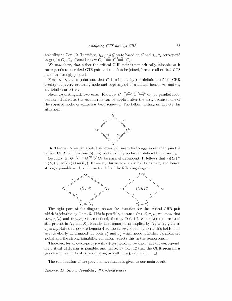
Analyzing GTS through CHR 33
according to Cor. 12. Therefore, σCP is a G-state based on G and σ1, σ2 correspond
to graphs G1, G2. Consider now G1r1,m1⇐= G
r2,m2=⇒ G2.
We now show, that either the critical CHR pair is non-critically joinable, or it
corresponds to a critical GTS pair and can thus be joined, because all critical GTS
pairs are strongly joinable.
First, we want to point out that G is minimal by the definition of the CHR
overlap, i.e. every occurring node and edge is part of a match, hence, m1 and m2
are jointly surjective.
Next, we distinguish two cases: First, let G1r1,m1⇐= G
r2,m2=⇒ G2 be parallel inde-
pendent. Therefore, the second rule can be applied after the first, because none of
the required nodes or edges has been removed. The following diagram depicts this
situation:
Gr1
z� }}}}
}}}
}}}}
}}}
r2
�$AA
AAAA
A
AAAA
AAA
G1
r2
�$AA
AAAA
A
AAAA
AAA
G2
r1
z� }}}}
}}}
}}}}
}}}
XBy Theorem 5 we can apply the corresponding rules to σCP in order to join the
critical CHR pair, because S(σCP) contains only nodes not deleted by r1 and r2.
Secondly, let G1r1,m1⇐= G
r2,m2=⇒ G2 be parallel dependent. It follows that m(L1) ∩
m(L2) 6⊆ m(K1) ∩ m(K2). However, this is now a critical GTS pair, and hence,
strongly joinable as depicted on the left of the following diagram:
Gr1
v~ uuuuu
uuuuu
uuuuuu
uuuu
r2
(IIIIII
IIII
IIIIII
IIII σCP
r1
{{wwwwwwwwwr2
##GGGG
GGGG
GG
G1
∗
�'HHHHHHHHH
HHHHHHHHH (GTS) G2
∗
w� vvvvvvvvv
vvvvvvvvvσ1
∗
##FFFF
FFFF
F (CHR) σ2
∗
{{xxxx
xxxx
x
X1 ' X2 σ′1 ≡ σ′2The right part of the diagram shows the situation for the critical CHR pair
which is joinable by Thm. 5. This is possible, because ∀v ∈ S(σCP) we know that
trG⇒G1(v) and trG⇒G2
(v) are defined, thus by Def. 4.2, v is never removed and
still present in X1 and X2. Finally, the isomorphism implied by X1 ' X2 gives us
σ′1 ≡ σ′2. Note that despite Lemma 4 not being reversible in general this holds here,
as it is clearly determined for both σ′1 and σ′2 which node identifier variables are
global and the strong joinability condition reflects this in the isomorphism.
Therefore, for all overlaps σCP with G(σCP) holding we know that the correspond-
ing critical CHR pair is joinable, and hence, by Cor. 12 that the CHR program is
G-local-confluent. As it is terminating as well, it is G-confluent.
The combination of the previous two lemmata gives us our main result:
Theorem 15 (Strong Joinability iff G-Confluence)
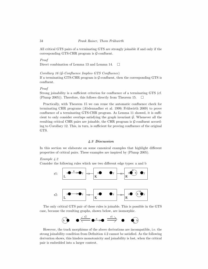
34 Frank Raiser, Thom Fruhwirth
All critical GTS pairs of a terminating GTS are strongly joinable if and only if the
corresponding GTS-CHR program is G-confluent.
Proof
Direct combination of Lemma 13 and Lemma 14.
Corollary 16 (G-Confluence Implies GTS Confluence)
If a terminating GTS-CHR program is G-confluent, then the corresponding GTS is
confluent.
Proof
Strong joinability is a sufficient criterion for confluence of a terminating GTS (cf.
(Plump 2005)). Therefore, this follows directly from Theorem 15.
Practically, with Theorem 15 we can reuse the automatic confluence check for
terminating CHR programs (Abdennadher et al. 1999; Fruhwirth 2009) to prove
confluence of a terminating GTS-CHR program. As Lemma 11 showed, it is suffi-
cient to only consider overlaps satisfying the graph invariant G. Whenever all the
resulting critical CHR pairs are joinable, the CHR program is G-confluent accord-
ing to Corollary 12. This, in turn, is sufficient for proving confluence of the original
GTS.
4.3 Discussion
In this section we elaborate on some canonical examples that highlight different
properties of critical pairs. These examples are inspired by (Plump 2005).
Example 4.2
Consider the following rules which use two different edge types: a and b
yx
yx
K
yx
K
yx
R
yx b
Lr1:
r2:L
a
R
yx b
The only critical GTS pair of these rules is joinable. This is possible in the GTS
case, because the resulting graphs, shown below, are isomorphic.
ar1r2
b‘b
However, the track morphisms of the above derivations are incompatible, i.e. the
strong joinability condition from Definition 4.2 cannot be satisfied. As the following
derivation shows, this hinders monotonicity and joinability is lost, when the critical
pair is embedded into a larger context.
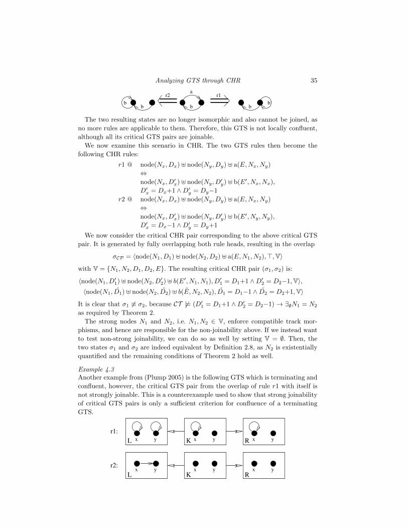
Analyzing GTS through CHR 35
bb b
r1r2
b‘b
a
The two resulting states are no longer isomorphic and also cannot be joined, as
no more rules are applicable to them. Therefore, this GTS is not locally confluent,
although all its critical GTS pairs are joinable.
We now examine this scenario in CHR. The two GTS rules then become the
following CHR rules:
r1 @ node(Nx, Dx) ] node(Ny, Dy) ] a(E,Nx, Ny)
⇔node(Nx, D
′x) ] node(Ny, D
′y) ] b(E′, Nx, Nx),
D′x = Dx+1 ∧D′y = Dy−1
r2 @ node(Nx, Dx) ] node(Ny, Dy) ] a(E,Nx, Ny)
⇔node(Nx, D
′x) ] node(Ny, D
′y) ] b(E′, Ny, Ny),
D′x = Dx−1 ∧D′y = Dy+1
We now consider the critical CHR pair corresponding to the above critical GTS
pair. It is generated by fully overlapping both rule heads, resulting in the overlap
σCP = 〈node(N1, D1) ] node(N2, D2) ] a(E,N1, N2),>,V〉
with V = {N1, N2, D1, D2, E}. The resulting critical CHR pair (σ1, σ2) is:
〈node(N1, D′1) ] node(N2, D
′2) ] b(E′, N1, N1), D′1 = D1+1 ∧D′2 = D2−1,V〉,
〈node(N1, D1) ] node(N2, D2) ] b(E,N2, N2), D1 = D1−1 ∧ D2 = D2+1,V〉
It is clear that σ1 6≡ σ2, because CT 6|= (D′1 = D1+1 ∧D′2 = D2−1)→ ∃∅N1 = N2
as required by Theorem 2.
The strong nodes N1 and N2, i.e. N1, N2 ∈ V, enforce compatible track mor-
phisms, and hence are responsible for the non-joinability above. If we instead want
to test non-strong joinability, we can do so as well by setting V = ∅. Then, the
two states σ1 and σ2 are indeed equivalent by Definition 2.8, as N2 is existentially
quantified and the remaining conditions of Theorem 2 hold as well.
Example 4.3Another example from (Plump 2005) is the following GTS which is terminating and
confluent, however, the critical GTS pair from the overlap of rule r1 with itself is
not strongly joinable. This is a counterexample used to show that strong joinability
of critical GTS pairs is only a sufficient criterion for confluence of a terminating
GTS.
yx KL
r1:
L K R
r2:
yx R yx
x y x yx y
36 Frank Raiser, Thom Fruhwirth
The GTS works as follows: If there is at least one loop in the graph, then all
but a last loop are removed by the first rule. Additionally, all non-loop edges are
removed by the second rule. Therefore, the remaining final graph contains zero or
one loops and no other edges, and hence the GTS is terminating and confluent due
to graph isomorphism. The first rule is encoded in CHR as follows:
r1 @ node(Nx, Dx) ] node(Ny, Dy)]a(Ex, Nx, Nx) ] a(Ey, Ny, Ny)
⇔node(Nx, Dx) ] node(Ny, D
′y) ] a(Ex, Nx, Nx),
D′y = Dy − 2
Completely overlapping the rule with itself yields the overlap
σCP = 〈node(N1, D1) ] node(N2, D2) ] a(E1, N1, N1) ] a(E2, N2, N2),>,V〉
with V = {N1, N2, D1, D2, E1, E2} resulting in the critical CHR pair (σ1, σ2) with:
σ1 = 〈node(N1, D1) ] node(N2, D′2) ] a(E1, N1, N1), D′2 = D2 − 2,V〉
σ2 = 〈node(N1, D′1) ] node(N2, D2) ] a(E2, N2, N2), D′1 = D1 − 2,V〉
Analogously to the previous example, the two states are not equivalent and can-
not be joined, therefore the corresponding critical GTS pair is not strongly joinable.
Again, setting V = ∅ results in both states becoming equivalent. As before, this re-
flects that for the critical GTS pairs the two corresponding graphs are isomorphic.
5 Analyzing Operational Equivalence
Constraint Handling Rules is well-known for its decidable, sufficient, and necessary
criterion for operational equivalence of terminating and confluent programs (Ab-
dennadher and Fruhwirth 1999; Fruhwirth 2009). After presenting this result in
Section 5.1, we introduce the concept of operational equivalence for graph trans-
formation systems in Section 5.2. Then we investigate operational equivalence of
GTS-CHR programs and show that it is sufficient for operational equivalence of the
original GTS. We further demonstrate its application to detect redundant rules of
a GTS.
The contents of this section are a revised and extended version of (Raiser and
Fruhwirth 2009a).
5.1 Operational Equivalence in CHR
Operational equivalence, intuitively, means that two programs should be able to
compute equivalent outputs given the same input. Applied to a single state, this
behavior is called P1,P2-joinability:
Definition 5.1 (P1,P2-joinability)
Let P1,P2 be CHR programs. A state σ is P1,P2-joinable, if and only if there are
computations σ �∗P1σ1 and σ �∗P2
σ2 with σ1 ≡ σ2 where all σi are final states
with respect to Pi.
Analyzing GTS through CHR 37
If P1,P2-joinability is given for all states the programs are considered opera-
tionally equivalent:
Definition 5.2 (Operational Equivalence)
Let P1,P2 be CHR programs.
P1,P2 are operationally equivalent if and only if all states σ are P1,P2-joinable.
As mentioned before, operational equivalence is decidable for terminating and
confluent CHR programs. Similarly to confluence, the decision algorithm investi-
gates critical states created from rule heads.
Definition 5.3 (Critical States)
Let P1,P2 be CHR programs. The set of critical states of P1 and P2 is defined as
{〈H,>, vars(H)〉 | (H ⇔ Bc, Bb) ∈ P1 ∪ P2}.
Note that we had to consider observable confluence for CHR, because overlap
states constructed for critical pair analysis may not always encode a graph. The
critical states used for operational equivalence here, however, stem directly from
a complete head of a rule, which in turn was derived from a GTS rule graph.
Therefore, all critical states of GTS-CHR programs are valid encodings of graphs.
The following theorem, adapted from (Abdennadher and Fruhwirth 1999), is
based on the idea to determine P1,P2-joinability of these critical states. The mono-
tonicity property of CHR ensures, that if all critical states are P1,P2-joinable, then
all states are. Additionally demanding termination and confluence of the programs,
allows us to decide P1,P2-joinability simply by executing a critical state in each of
the programs and then comparing the resulting final states.
Theorem 17 (Operational Equivalence via Critical States)
Let P1,P2 be terminating and confluent CHR programs. P1,P2 are operationally
equivalent if and only if for all critical states σ of P1 and P2 it holds that σ is
P1,P2-joinable.
Proof
Given in (Abdennadher and Fruhwirth 1999).
Note that in contrast to confluence, Theorem 17 will always consider states sat-
isfying the G-invariant, when applied to a GTS-CHR program. This follows from
the fact, that each critical state is the head of a rule, and in turn, corresponds to a
rule graph from the GTS by construction.
5.2 Analyzing Operational Equivalence in GTS
In this section we introduce the notion of operational equivalence for GTS. Based on
the previous embedding of GTS in CHR, we use the existing decision algorithm from
CHR as a sufficient criterion for operational equivalence of two graph transformation
systems.
First, we define the property of S1,S2-joinability for two graph transformation
systems S1,S2, analogously to P1,P2-joinability.
38 Frank Raiser, Thom Fruhwirth
Definition 5.4 (S1,S2-joinability)
Let S1,S2 be two graph transformation systems. A typed graph G is S1,S2-joinable
if and only if there are derivations G ⇒∗S1 G1 and G ⇒∗S2 G2 with G1 ' G2 being
final with respect to S1 and S2.
Here ' denotes traditional graph isomorphism and a graph G is considered final
with respect to S iff there is no transition G⇒S H for any graph H.
Building on S1,S2-joinability, we now define operational equivalence for graph
transformation systems with the same intuitive understanding: two operationally
equivalent GTS should be able to produce the same result graphs up to isomorphism
given an input graph:
Definition 5.5 (GTS Operational Equivalence)
Let S1 = (P1, TG) and S2 = (P2, TG) be two graph transformation systems.
S1,S2 are operationally equivalent if and only if for all graphs G typed over TG
it holds that G is S1,S2-joinable.
Similar to operational equivalence in CHR, where it is futile to directly compare
programs that use different constraints, Definition 5.5 requires S1 and S2 to be
based on the same type graph TG. With the previous results from (Raiser and
Fruhwirth 2009b) we can directly use CHR’s operational equivalence as a sufficient
criterion for deciding operational equivalence of two GTS:
Theorem 18 (GTS-CHR Operational Equivalence)
Let S1,S2 be graph transformation systems and P1,P2 their corresponding GTS-
CHR programs. S1,S2 are operationally equivalent if P1,P2 are operationally equiv-
alent.
Proof
Let G be a graph typed over TG. Then the state σ = 〈chr(ground, G),>, ∅〉 is
P1,P2-joinable by Def. 5.1. Therefore, there exist the final states σ1 ≡ σ2 with
σ�∗P1σ1 and σ�∗P2
σ2.
By Thm. 5 we know that there exist corresponding derivations G ⇒∗S1 G1 and
G⇒∗S2 G2 such that σ1 is a G-state based on G1 and σ2 is a G-state based on G2.
The graphs G1 and G2 are final states w.r.t. S1 and S2, and finally, the isomor-
phism between G1 and G2 is implied by σ1 ≡ σ2 according to Lemma 4. Therefore,
G is S1,S2-joinable.
An interesting application of the above theorem is the removal of redundant rules.
Originally proposed in (Abdennadher and Fruhwirth 2003), decidable operational
equivalence of CHR programs implies a straight-forward redundant rule removal
algorithm: Remove a single rule from the program, then compare the operational
equivalence of the program thus created and the original program. If the two pro-
grams are operationally equivalent the selected rule is shown to be redundant and
can be removed.
Clearly, program equivalence in general is undecidable, and hence, we cannot
expect such an algorithm to correctly identify all redundant rules. Nevertheless, the
algorithm was applied in CHR research to great success on automatically generated
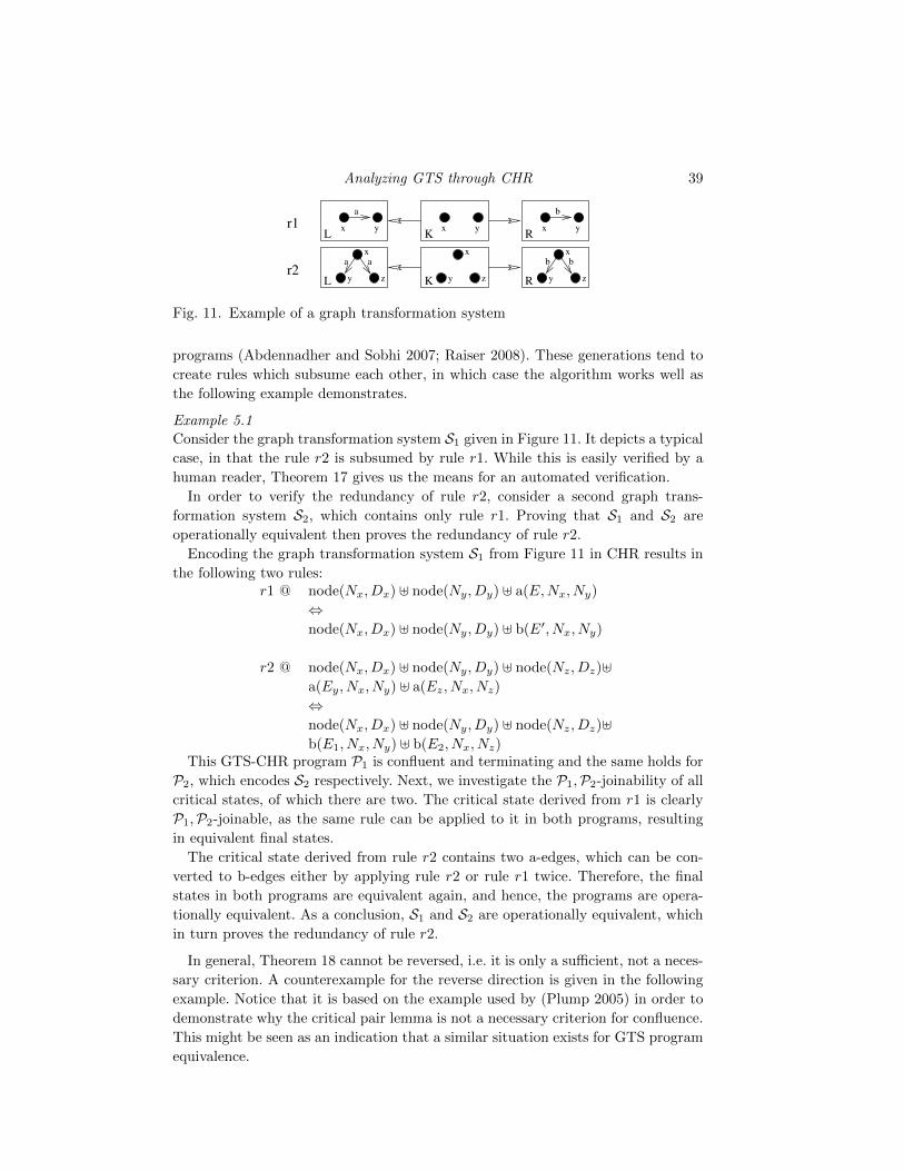
Analyzing GTS through CHR 39
x y x y
x
y z
x
y z
a
L K R
b
x y
a
L K R
x
y z
b ba
r1
r2
Fig. 11. Example of a graph transformation system
programs (Abdennadher and Sobhi 2007; Raiser 2008). These generations tend to
create rules which subsume each other, in which case the algorithm works well as
the following example demonstrates.
Example 5.1
Consider the graph transformation system S1 given in Figure 11. It depicts a typical
case, in that the rule r2 is subsumed by rule r1. While this is easily verified by a
human reader, Theorem 17 gives us the means for an automated verification.
In order to verify the redundancy of rule r2, consider a second graph trans-
formation system S2, which contains only rule r1. Proving that S1 and S2 are
operationally equivalent then proves the redundancy of rule r2.
Encoding the graph transformation system S1 from Figure 11 in CHR results in
the following two rules:r1 @ node(Nx, Dx) ] node(Ny, Dy) ] a(E,Nx, Ny)
⇔node(Nx, Dx) ] node(Ny, Dy) ] b(E′, Nx, Ny)
r2 @ node(Nx, Dx) ] node(Ny, Dy) ] node(Nz, Dz)]a(Ey, Nx, Ny) ] a(Ez, Nx, Nz)
⇔node(Nx, Dx) ] node(Ny, Dy) ] node(Nz, Dz)]b(E1, Nx, Ny) ] b(E2, Nx, Nz)
This GTS-CHR program P1 is confluent and terminating and the same holds for
P2, which encodes S2 respectively. Next, we investigate the P1,P2-joinability of all
critical states, of which there are two. The critical state derived from r1 is clearly
P1,P2-joinable, as the same rule can be applied to it in both programs, resulting
in equivalent final states.
The critical state derived from rule r2 contains two a-edges, which can be con-
verted to b-edges either by applying rule r2 or rule r1 twice. Therefore, the final
states in both programs are equivalent again, and hence, the programs are opera-
tionally equivalent. As a conclusion, S1 and S2 are operationally equivalent, which
in turn proves the redundancy of rule r2.
In general, Theorem 18 cannot be reversed, i.e. it is only a sufficient, not a neces-
sary criterion. A counterexample for the reverse direction is given in the following
example. Notice that it is based on the example used by (Plump 2005) in order to
demonstrate why the critical pair lemma is not a necessary criterion for confluence.
This might be seen as an indication that a similar situation exists for GTS program
equivalence.
40 Frank Raiser, Thom Fruhwirth
Example 5.2
Consider two GTS with the first being the one from Example 4.3 and the second
GTS is identical to the first except for rule r1, in which the loop for node x is
removed instead. It is clear, that both programs are terminating, confluent, and
operationally equivalent. The following two rules are from the corresponding GTS-
CHR programs P1 and P2:r1 @ node(Nx, Dx) ] node(Ny, Dy)]
a(Ex, Nx, Nx) ] a(Ey, Ny, Ny)
⇔node(Nx, Dx) ] node(Ny, D
′y) ] a(Ex, Nx, Nx),
D′y = Dy−2
r1′ @ node(Nx, Dx) ] node(Ny, Dy)]a(Ex, Nx, Nx) ] a(Ey, Ny, Ny)
⇔node(Nx, D
′x) ] node(Ny, Dy) ] a(Ey, Ny, Ny),
D′x = Dx−2We can now investigate the following critical state σ according to Theorem 18,
where V = {Nx, Ny, Dx, Dy, Ex, Ey}:
σ = 〈node(Nx, Dx) ] node(Ny, Dy) ] a(Ex, Nx, Nx) ] a(Ey, Ny, Ny),>,V〉
The critical state σ is not P1,P2-joinable, as there is only one rule applicable in
each program and the resulting states are not equivalent:σ�r1
P1〈node(Nx, Dx) ] node(Ny, D
′y) ] a(Ex, Nx, Nx), D′y = Dy−2,V〉 = τ1
6≡σ�r1′
P2〈node(Nx, D
′x) ] node(Ny, Dy) ] a(Ey, Ny, Ny), D′x = Dx−2,V〉 = τ2
6 Related and Future Work
The relation of CHR to other formalisms has been thoroughly investigated in the
literature. This includes comparison to logical formalisms (e.g., linear logic (Betz
and Fruhwirth 2005)), term rewriting ((Duck et al. 2006)), Join-Calculus ((Lam
and Sulzmann 2008)), and Petri nets (Betz 2007). More detailled surveys of these
relations can be found in (Sneyers et al. 2009) and (Fruhwirth 2009).
The relation of graph transformation systems to CHR differs from these other
formalisms, because firstly, it is a graph-based formalism, and secondly, there are
significant differences in program analysis results. Most importantly, confluence of
terminating GTS is undecidable (Plump 2005) whereas confluence of terminating
CHR programs is decidable (Abdennadher et al. 1999). Furthermore, no opera-
tional equivalence analysis exists for GTS, as opposed to the situation in CHR
(Abdennadher and Fruhwirth 1999).
The operational equivalence test presented in Section 5 yields a method for re-
moval of redundant rules, which is remarkable for another reason: In (Kreowski and
Valiente 2000) the notions of redundancy and subsumptions have been introduced
for GTS, however, the authors only gave the definitions and a sufficient condition
Analyzing GTS through CHR 41
for redundancy, but no verification procedure. While the notion of redundancy in
that paper is slightly different from the one found in (Abdennadher and Fruhwirth
2003), the adaptation of the algorithm to GTS-CHR programs is to the best of our
knowledge the only available verification procedure for redundant GTS rules.
Note, that operational equivalence, as defined here, is only one possible notion of
equivalence between programs. It was used in this work as an example of CHR pro-
gram analyses applied to embedded graph transformation systems. Another, more
popular, notion of equivalence of GTS is bisimilarity, introduced in the GTS context
in (Ehrig and Konig 2004). It has been successfully applied to determine behavioral
equivalence of graph transformation systems in (Rangel et al. 2008). While bisimi-
larity originated from process calculi and is focused on the transitions made during
computations of a result, operational equivalence on the other hand, only compares
the final computational results, independently of how they are reached.
The encoding of GTS in CHR, as presented in Section 3, is based on the double-
pushout approach for graph transformation systems. A related graph rewriting
mechanism, the single-pushout approach, was introduced in (Lowe 1993). Instead
of demanding two pushouts, as in Figure 4, rewriting is defined there over a cate-
gory of partial graph morphisms, hence only a single pushout construction is used.
Intuitively, this results in a different behavior with respect to dangling edges: While
the double-pushout approach prohibits a rule application in case a dangling edge
would remain, the single-pushout approach removes all dangling edges instead. In
(Lowe and Muller 1993) the authors investigate confluence for single-pushout graph
rewriting. In particular, the critical pair analysis is shown to be only a sufficient
criterion as well, not a necessary one.
In this work, we based our encoding on the DPO approach as the non-applicability
of rules due to the dangling edge condition corresponds nicely to non-applicability
of corresponding CHR rules. In order to support the approach from (Lowe 1993),
remaining dangling edges would need to be removed by an additional rule, hence,
we would lose the one-on-one correspondence of GTS and CHR rules.
Our encoding further serves as the foundation of the extensible platform for the
analysis of graph transformation systems using constraint handling rules presented
in the diploma thesis (Wasserthal 2009). This platform is based on JCHR (Van
Weert 2008), a Java-based implementation of CHR and the work presented in Sec-
tion 3. The developed tool presents a graphical view of a GTS which is synchronized
with the corresponding GTS-CHR program at all times. Furthermore, it provides
an interface for program analysis plug-ins, which can work directly on the GTS or
on the GTS-CHR program.
As this work demonstrated, our embedding leads to cross-fertilizations of CHR
and GTS research. Future work should therefore concentrate on further comparing
the different approaches to program analysis. In particular, CHR provides several
approaches to termination analysis (Fruhwirth 2000; Voets et al. 2008; Pilozzi and
De Schreye 2008) that GTS research may profit from.
Research on GTS contains several extensions for the typed graphs and rules con-
sidered in this work. One such extension adds attributes (Ehrig et al. 2006) to
graphs, which can then be modified by rules. We assume that built-in constraints
42 Frank Raiser, Thom Fruhwirth
available in CHR could closely correspond to attributes. Another important exten-
sion, is the addition of negative application conditions (Ehrig et al. 2006), i.e. ap-
plying a rule requires the absence of certain graph structures. This is more difficult
to achieve in CHR, as it traditionally has no support for negation as absence. How-
ever, there exist proposed extensions of CHR with negation as absence (Van Weert
et al. 2006) and aggregates (Van Weert et al. 2008), which could help in extending
our encoding to allow application conditions.
Our work on operational equivalence for graph transformation systems yielded a
first useable criterion. However, there is lot of remaining work in this field. From
a decidability point of view, operational equivalence is in a similar situation as
confluence: (Plump 2005) showed that confluence is undecidable even for terminat-
ing GTS and we expect a similar result for operational equivalence. Therefore, our
criterion might only be applicable to a small subset of all GTS.
Similarly, in CHR research, the operational equivalence result assumes that both
programs use the same constraint symbols in the same manner. While this restric-
tion yields a decidable criterion, it also means that it seldomly applies to real-world
programs. Traditionally, one may be able to manually show operational equivalence
for two concrete programs by taking into account known restrictions on data struc-
tures or inputs and ignoring irrelevant states. The same situation was present for
confluence (e.g., (Fruhwirth 2005)) until observable confluence (Duck et al. 2007)
succeeded in providing an extended approach.
We plan to develop such an invariant-based approach for operational equivalence
in CHR as well, which extends Theorem 17. Combined with a better criterion
for operational equivalence in GTS, including the track morphism similarly to the
critical pair approach, this might reveal a closer correspondence between operational
equivalence in both systems.
7 Conclusion
We have shown that constraint handling rules (CHR) provides an elegant way
for embedding graph transformation systems (GTS). The resulting rules are con-
cise and directly related to the corresponding graph production rules. We proved
soundness and completeness of this embedding and verified formal properties of
CHR states that encode graphs. Furthermore, we considered partial graphs and
showed that the CHR embedding naturally supports these, hence facilitating pro-
gram analysis.
Next, we analyzed confluence and showed that observable confluence of a GTS-
CHR program is a sufficient criterion for confluence of the analyzed GTS. Further-
more, we transferred the notion of operational equivalence from CHR to GTS and
discussed the CHR-based decision algorithm for redundant rule removal.
References
Abdennadher, S. and Fruhwirth, T. 1999. Operational equivalence of CHR programsand constraints. In Principles and Practice of Constraint Programming, CP 1999, J. Jaf-far, Ed. Lecture Notes in Computer Science, vol. 1713. Springer-Verlag, 43–57.
Analyzing GTS through CHR 43
Abdennadher, S. and Fruhwirth, T. 2003. Integration and optimization of rule-basedconstraint solvers. In Logic Based Program Synthesis and Transformation, 13th In-ternational Symposium LOPSTR 2003, Uppsala, Sweden, August 25-27, 2003, RevisedSelected Papers, M. Bruynooghe, Ed. Lecture Notes in Computer Science, vol. 3018.Springer-Verlag, 198–213.
Abdennadher, S., Fruhwirth, T., and Meuss, H. 1999. Confluence and semantics ofconstraint simplification rules. Constraints 4, 2, 133–165.
Abdennadher, S. and Marte, M. 2000. University course timetabling using Con-straint Handling Rules. In Special Issue on Constraint Handling Rules, C. Holzbaurand T. Fruhwirth, Eds. Journal of Applied Artificial Intelligence, vol. 14(4). Taylor &Francis, 311–325.
Abdennadher, S. and Sobhi, I. 2007. Generation of rule-based constraint solvers: Com-bined approach. In Logic-Based Program Synthesis and Transformation, 17th Inter-national Symposium, LOPSTR 2007, Kongens Lyngby, Denmark, August 23-24, 2007,Revised Selected Papers, A. King, Ed. Lecture Notes in Computer Science, vol. 4915.Springer-Verlag, 106–120.
Baader, F. and Nipkow, T. 1998. Term rewriting and all that. Cambridge UniversityPress, New York, NY, USA.
Bakewell, A., Plump, D., and Runciman, C. 2003. Specifying pointer structures bygraph reduction. In Applications of Graph Transformations with Industrial Relevance,Second International Workshop, AGTIVE 2003, Revised Selected and Invited Papers,J. L. Pfaltz, M. Nagl, and B. Bohlen, Eds. Lecture Notes in Computer Science, vol.3062. Springer-Verlag, Charlottesville, VA, USA, 30–44.
Barranco-Mendoza, A. 2005. Stochastic and heuristic modelling for analysis of thegrowth of pre-invasive lesions and for a multidisciplinary approach to early cancer di-agnosis. Ph.D. thesis, Simon Fraser University, Burnaby, Canada.
Bavarian, M. and Dahl, V. 2006. Constraint based methods for biological sequenceanalysis. J. Universal Computer Science 12, 11, 1500–1520.
Betz, H. 2007. Relating coloured Petri nets to Constraint Handling Rules. In CHR ’07(Porto, Portugal), K. Djelloul, G. J. Duck, and M. Sulzmann, Eds. 33–47.
Betz, H. and Fruhwirth, T. 2005. A Linear-Logic Semantics for Constraint HandlingRules. In Principles and Practice of Constraint Programming, 11th International Con-ference, CP 2005, P. van Beek, Ed. Lecture Notes in Computer Science, vol. 3709.Springer-Verlag, Sitges, Spain, 137–151.
Blostein, D., Fahmy, H., and Grbavec, A. 1995. Practical use of graph rewriting.In 5th Workshop on Graph Grammars and Their Application To Computer Science.Lecture Notes in Computer Science, vol. 1073. Springer-Verlag, 38–55.
Dahl, V. and Maharshak, E. 2009. DNA replication as a model for computational lin-guistics. In IWINAC ’09: Proc. Third Intl. Work-Conf. on the Interplay Between Nat-ural and Artificial Computation. Lecture Notes in Computer Science. Springer-Verlag,346–355.
Duck, G. J., Stuckey, P. J., and Brand, S. 2006. ACD term rewriting. In ICLP ’06(Seattle, Washington), S. Etalle and M. Truszczynski, Eds. Lecture Notes in ComputerScience, vol. 4079. Springer-Verlag, 117–131.
Duck, G. J., Stuckey, P. J., and Sulzmann, M. 2007. Observable confluence forconstraint handling rules. In Logic Programming, 23rd International Conference, ICLP2007, V. Dahl and I. Niemela, Eds. Lecture Notes in Computer Science, vol. 4670.Springer-Verlag, Porto, Portugal, 224–239.
Ehrig, H., Ehrig, K., Prange, U., and Taentzer, G. 2006. Fundamentals of AlgebraicGraph Transformation. Springer-Verlag.
44 Frank Raiser, Thom Fruhwirth
Ehrig, H. and Konig, B. 2004. Deriving bisimulation congruences in the DPO approachto graph rewriting. In Foundations of Software Science and Computation Structures,7th International Conference, FOSSACS 2004, I. Walukiewicz, Ed. Lecture Notes inComputer Science, vol. 2987. Springer-Verlag, Barcelona, Spain, 151–166.
Fruhwirth, T. 2000. Proving termination of constraint solver programs. In SelectedPapers from the Joint ERCIM/Compulog Net Workshop on New Trends in Constraints.Lecture Notes in Computer Science, vol. 1865. Springer-Verlag, 298–317.
Fruhwirth, T. 2005. Parallelizing union-find in constraint handling rules using confluenceanalysis. In Principles and Practice of Constraint Programming, 11th InternationalConference, CP 2005. Sitges, Spain.
Fruhwirth, T. 2009. Constraint Handling Rules. Cambridge University Press.
Huet, G. 1980. Confluent reductions: Abstract properties and applications to term rewrit-ing systems: Abstract properties and applications to term rewriting systems. Journalof the ACM 27, 4, 797–821.
Kreowski, H.-J. and Valiente, G. 2000. Redundancy and subsumption in high-levelreplacement systems. In TAGT’98: Selected papers from the 6th International Workshopon Theory and Application of Graph Transformations. Springer-Verlag, 215–227.
Lam, E. S. and Sulzmann, M. 2006. Towards Agent Programming in CHR. In CHR’06: Proc. 3rd Workshop on Constraint Handling Rules. 17–31.
Lam, E. S. and Sulzmann, M. 2008. Finally, a comparison between Constraint HandlingRules and join-calculus. In CHR ’08 (Hagenberg, Austria), T. Schrijvers, F. Raiser, andT. Fruhwirth, Eds. RISC Report Series 08-10, University of Linz, Austria, 51–66.
Lowe, M. 1993. Algebraic approach to single-pushout graph transformation. TheoreticalComputer Science 109, 1&2, 181–224.
Lowe, M. and Muller, J. 1993. Algebraische Graphersetzung: mathematische Model-lierung und Konfluenz. Tech. Rep. 93-37, Technische Universitat Berlin.
Newman, M. 1942. On theories with a combinatorial definition of equivalence. Annals ofMathematics 43, 2, 223–242.
Pilozzi, P. and De Schreye, D. 2008. Termination analysis of CHR revisited. In ICLP’08, M. Garcıa de la Banda and E. Pontelli, Eds. Lecture Notes in Computer Science,vol. 5366. Springer-Verlag, 501–515.
Plump, D. 1995. On Termination of Graph Rewriting. In Graph-Theoretic Concepts inComputer Science, 21st International Workshop, WG ’95, Proceedings, M. Nagl, Ed.Lecture Notes in Computer Science, vol. 1017. Aachen, Germany, 88–100.
Plump, D. 2005. Confluence of graph transformation revisited. In Processes, Terms andCycles, A. Middeldorp, V. van Oostrom, F. van Raamsdonk, and R. C. de Vrijer, Eds.Lecture Notes in Computer Science, vol. 3838. Springer-Verlag, 280–308.
Pretschner, A., Slotosch, O., Aiglstorfer, E., and Kriebel, S. 2004. Model-basedtesting for real. J. Software Tools for Technology Transfer (STTT) 5, 2–3, 140–157.
Raiser, F. 2007. Graph Transformation Systems in CHR. In Logic Programming, 23rdInternational Conference, ICLP 2007, V. Dahl and I. Niemela, Eds. Lecture Notes inComputer Science, vol. 4670. Springer-Verlag, Porto, Portugal, 240–254.
Raiser, F. 2008. Semi-automatic generation of CHR solvers for global constraints. InPrinciples and Practice of Constraint Programming, 14th International Conference, CP2008, P. J. Stuckey, Ed. Lecture Notes in Computer Science, vol. 5202. Springer-Verlag,Sydney, Australia, 588–592.
Raiser, F. 2009. Research summary: Analysing graph transformation systems usingextended methods from constraint handling rules. In 25th International Conferenceon Logic Programming, ICLP, P. M. Hill and D. S. Warren, Eds. Lecture Notes inComputer Science, vol. 5649. Springer-Verlag, Pasadena, CA, USA, 540–541.
Analyzing GTS through CHR 45
Raiser, F., Betz, H., and Fruhwirth, T. 2009. Equivalence of CHR states revisited.In 6th International Workshop on Constraint Handling Rules (CHR), F. Raiser andJ. Sneyers, Eds. 34–48.
Raiser, F. and Fruhwirth, T. 2009a. Operational equivalence of graph transformationsystems. In 6th International Workshop on Constraint Handling Rules (CHR), F. Raiserand J. Sneyers, Eds. 49–62.
Raiser, F. and Fruhwirth, T. 2009b. Strong joinability analysis for graph transforma-tion systems in CHR. Electronic Notes in Theoretical Computer Science – Proceedingsof the Fifth International Workshop on Computing with Terms and Graphs (TERM-GRAPH 2009) 253, 4, 91–111.
Rangel, G., Lambers, L., Konig, B., Ehrig, H., and Baldan, P. 2008. Behaviorpreservation in model refactoring using DPO transformations with borrowed contexts.In Proc. of ICGT ’08 (International Conference on Graph Transformation). LectureNotes in Computer Science, vol. 5214. Springer-Verlag, 242–256.
Sneyers, J., Van Weert, P., Schrijvers, T., and De Koninck, L. 2009. As timegoes by: Constraint Handling Rules – A survey of CHR research between 1998 and2007. Theory and Practice of Logic Programming . accepted.
Sulzmann, M., Schrijvers, T., and Stuckey, P. J. 2006. Principal type inferencefor GHC-style multi-parameter type classes. In APLAS ’06: Proc. 4th Asian Symp. onProgramming Languages and Systems (Sydney, Australia), N. Kobayashi, Ed. LectureNotes in Computer Science, vol. 4279. Springer-Verlag, 26–43.
Van Weert, P. 2008. JCHR. http://www.cs.kuleuven.be/~petervw/JCHR.
Van Weert, P., Sneyers, J., and Demoen, B. 2008. Aggregates for CHR throughprogram transformation. In LOPSTR ’07, Revised Selected Papers (Kongens Lyngby,Denmark), A. King, Ed. Lecture Notes in Computer Science, vol. 4915. 59–73.
Van Weert, P., Sneyers, J., Schrijvers, T., and Demoen, B. 2006. Extending CHRwith negation as absence. In CHR ’06 (Venice, Italy), T. Schrijvers and T. Fruhwirth,Eds. K.U.Leuven, Department of Computer Science, Technical report CW 452, 125–140.
Voets, D., Pilozzi, P., and De Schreye, D. 2008. A new approach to terminationanalysis of CHR. Tech. Rep. CW 506, K.U.Leuven, Department of Computer Science,Leuven, Belgium. Jan.
Wasserthal, M. 2009. Diploma thesis, Ulm University. An Extensible Platform for theAnalysis of Graph Transformation Systems using Constraint Handling Rules.