analytical modelling of the filament winding process - core
TRANSCRIPT
Hugo Faria
Analytical and Numerical Modelling of
the Filament Winding Process
PhD Thesis
© Universidade do Porto 2013

PhD Thesis
Hugo Faria
Analytical and Numerical Modelling of
the Filament Winding Process
Supervisor: Professor António Torres Marques
Co-Supervisor: Prof. Francisco M. Andrade Pires
April 2013
This thesis is submitted in partial fulfilment of the requirements for the
degree of Doctor of Philosophy in Mechanical Engineering
© Universidade do Porto 2013

i
Abstract
The filament winding process, used for the manufacture of a wide variety of
composite parts and components, is being increasingly applied in structurally
demanding applications. In such cases, the ability to accurately control the
manufacturing parameters and their specific influence on the final quality of the
laminates becomes increasingly more relevant as well.
In this research program, the filament winding process was studied and modelled
in detail. The several physical phenomena interacting at the layer/laminate level were
analytically described independently and a meso-scale overall decoupled original model
was proposed. Namely, the consolidation pressure, the resin flow, the resin mixing
between adjacent layers, the resin cure kinetics and rheology, the fibre bed compaction
and the varying layers’ stiffness were attained. The stress-strain constitutive relations
were modelled taking into account the influence of the thermal, chemical and
mechanical effects of all the interacting phenomena. Also, process-intrinsic specific
features like fibre misalignment, through-the-thickness gradients and incremental
discrete lay-up were included in the analyses. A modular approach, based on
sub-models each referring to a relevant group of physical phenomena acting at the
layer-laminate level, was designed. This option allowed settling a model applicable to a
broader range of real configurations and applications of the filament winding
manufacturing process as is required by the industry. The methodology used is suitable
both for thermosetting and thermoplastic resin systems, as well as for any geometry or
lay-up. In addition, the decoupled structure foresees easier improvements in the future
due to the independent analyses of each relevant phenomenon.
In order to evaluate the multi-physical descriptions and interactions, a numerical
code was devised and implemented that simulated prescribed winding conditions. This
code followed the same modular structure and dedicated sub-routines were written for
each sub-model. A FORTRAN® user-routine was associated an ABAQUS® explicit
formulation in which the former contained the constitutive model of the consolidating
material. An input library was written to include different matrix material possibilities,
thus accounting for both previously established and original kinetic and rheological
models. Alternative formulations for the stress-strain constitutive relations were also
coded in view of further testing those. A fully functional numerical program was, thus,
established.
Finally, a comprehensive experimental program was conducted to measure and
evaluate all the process variables under certain processing conditions. This program
aimed at reliably validating the process model, thus adding relevance and utility to the
study. Several experimental procedures and techniques were used and new
sub-techniques were developed to retrieve the necessary data. Namely, innovative
differential scanning calorimetry and rheology tests under manufacturer’s recommended
cure cycles, complementary thermography analysis, monitored filament winding setup
or even resin colourizing techniques to measure in-situ flow. Partial and full validations
of the process model were, thus, progressively achieved.
The validated process model is described, step by step, throughout the thesis,
together with the analytical, numerical and experimental procedures conducted to
accomplish it. Desirably, the reader is given a deep but logical gradual insight to the
modelling strategy and results.
ii
Resumo
O processo de enrolamento filamentar, utilizado no fabrico de vários
componentes compósitos, está a ser cada vez mais empregue em aplicações
estruturalmente exigentes. Nestes casos, a capacidade de controlar com precisão os
parâmetros de produção e a sua influência na qualidade final dos laminados torna-se
mais relevante também.
Neste estudo, o processo de enrolamento filamentar, foi estudado e modelado em
detalhe. Os diversos fenómenos físicos que interagem ao nível da camada/laminado
foram descritos analiticamente de forma independente e um novo modelo mesoscópico
desacoplado do processo global foi proposto. Designadamente, a pressão de
consolidação, o escoamento da resina, a mistura de resina entre camadas adjacentes, a
cinética e reologia de cura da resina, a compactação da malha de fibras e a rigidez
variável das camadas foram atentados. As relações constitutivas tensão-deformação
foram modeladas tendo em conta a influência dos efeitos térmicos, químicos e
mecânicos de todos os fenómenos com interação. Além disso, características intrínsecas
ao próprio processo, tais como desalinhamento das fibras, gradientes ao longo da
espessura e laminação incremental discreta das camadas foram incluídas nas análises.
Uma abordagem modular, baseada em sub-modelos, cada um referente a um grupo
relevante de fenómenos físicos, foi desenhada. Esta opção permitiu alargar a gama de
configurações e aplicações modeláveis pela ferramenta desenvolvida, como é exigido
pela indústria. A metodologia utilizada é adequada para resinas termoendurecíveis e
termoplásticos, bem como para qualquer geometria ou sequência de laminação. Além
disso, a estrutura desacoplada prevê maior facilidade em futuros desenvolvimentos e
melhorias devido às análises independentes de cada um fenómeno relevante.
A fim de avaliar as descrições e interações multi-físicas, um código numérico foi
implementado para simular certas condições prescritas. Este código seguiu a mesma
estrutura modular com sub-rotinas dedicadas a cada sub-modelo. Uma rotina em
FORTRAN® contendo o modelo constitutivo do material em consolidação foi
associada a uma formulação explícita do software ABAQUS®. Uma biblioteca de
entrada foi escrita para incluir diferentes possibilidades matrizes, com modelos cinéticos
e reológicos previamente estabelecidos e modelos originais. Formulações constitutivas
tensão-deformação alternativas foram codificadas com vista ao seu teste e comparação.
Um programa numérico totalmente funcional foi, assim, estabelecido.
Finalmente, um amplo programa experimental foi realizado para medir todas as
variáveis do processo sob determinadas condições de fabrico. Este programa visou
validar o modelo de processo, conferindo-lhe relevância e utilidade. Vários
procedimentos experimentais foram usados e novas sub-técnicas foram desenvolvidas
para obter os dados necessários. Entre eles a calorimetria diferencial e reometria usadas
em ciclos de cura recomendados pelo fabricante, análise de termografia complementar,
desenvolvimento de vários elementos de monitorização do processo de enrolamento
filamentar ou mesmo a técnica de coloração local de resina medir o seu fluxo in-situ.
Validações parciais e totais do modelo foram, assim, progressivamente alcançadas.
O modelo de processo validado é descrito, passo a passo, ao longo da tese,
juntamente com os procedimentos analíticos, numéricos e experimentais realizados para
o atingir. Desejavelmente, ao leitor é dada uma visão gradualmente profunda, mas
lógica, para a estratégia de modelação e os resultados.
iii
Acknowledgements
This thesis is the visible expression of a deep, long and mostly lonely journey in
which several personal frontiers have been approached, eventually touched, surely
enriching myself as a person and, hopefully, as an engineer and researcher. Along this
path, the support given by Rosinda, substantiated in true care and understanding was
invaluable. To her, I am truly grateful.
The work itself, benefited, in several points, of the collaboration and/or assistance
of colleagues and organizations, whom I would like to acknowledge:
• INEGI administration board, for allowing my partial dedication to this programme and
also for the highly valuable conditions provided in laboratorial means and facilities;
• Agnieszka Żmijewska Rocha, David Miranda and Henrique Neves, for their valuable
contributions in the early identification of relevant phenomena, in the development of
the numerical code and in its early debugging, respectively;
• Vanessa Silva Gomes, for the valuable contribution in the analysis and review of
available stress-strain and micro-mechanical models;
• Gilmar Pereira, for the support in early experimental trials for resin flow analyses;
• Prof. Luisa Madureira, for the intensive help with the analytical solving and
manipulation of complex mathematical descriptions, within the stress-strain averaging
analyses;
• Dr. Alex Skordos, for the breakthrough help with the early kinetics modelling phase;
• Dr. Celeste Pereira, for the assistance in the DSC tests program.
The collaboration or help of the following people and organizations was also
gratefully appreciated:
João Rodrigues (INEGI); Loic Hilliou (DEP UMinho); Armanda Teixeira (INEGI); Dr.
David Ayre (Cranfield University); Prof. Andrew Long (University of Nottingham).
To my supervisors, I would also like to thank the continuous availability to follow
the incidences of the work and advise me. Whenever asked or needed, their support was
effective and, therefore, I am grateful. It has been a pleasure and an advantage to work
with both.

iv
List of Symbols
a characteristic amplitude of the sinusoidal pattern of the fibres // constant (viscosity/curing sub-model)
iA constants (crystallization/curing sub-model)
rrA area of resin mixing (transverse to flow) around the point of interest
degree of cure of resin
0 initial degree of cure
gel // lim degree of cure at which gelation occurs (gel point)
b tow bandwidth (multiple rovings, complete bundle) // constant (viscosity/curing sub-model)
B constant (curing sub-model)
cij thermal expansion coefficient in the ijth direction in cured state
ucij thermal expansion coefficient in the ijth direction in uncured (initial) state
c crystallinity // constant (curing sub-model)
C specific heat of composite
fC specific heat of fibres
rC specific heat of resin
ijC components of the on-axis (1,2,3) stiffness matrix
ijC components of the off-axis (1,2,3) stiffness matrix
ijC~
components of the off-axis (1,2,3) stiffness matrix
rc relative crystallinity
d constant (curing sub-model)
iE // iU activation energies for curing/crystallization/viscosity sub-models
fE Young’s modulus of fibres
mE YOUNG’s modulus of resin (Matrix)
m
cE Young’s modulus of resin (matrix) in cured state
m
ucE Young’s modulus of resin (matrix) in uncured state
iiE Young’s moduli in the iith principal material axis
fbE1 Young’s modulus of the fibre bed in direction 1
fb
bE Young’s modulus of the fibre bed in direction b (bulk)
ij components of the on-axis ( 3,2,1 ) strains // components of the off-axis ( z , , r ) strains
fibre misalignment angle
windingF winding force
winding angle
ijG shear moduli
cijG shear modulus of the resin in cured state
ucijG shear modulus of the resin in uncured state
tH total heat of crystallization/curing
uH ultimate heat of crystallization of polymer
cij chemical change coefficient in the ijth direction in cured state

v
ucij chemical change coefficient in the ijth direction in cured state
k thermal conductivity of the composite
fk thermal conductivity of fibres
mk thermal conductivity of resin (matrix)
m
ck thermal conductivity of resin (matrix) in cured state
m
uck thermal conductivity of resin (matrix) in uncured state
'k modified Kozeny constant
ik constants (curing sub-model)
L characteristic length of the sinusoidal pattern of the fibres
aL buckling ratio (waviness ratio)
resin (matrix) viscosity
ch resin (matrix) chemical viscosity
gel viscosity at gel point
constant (viscosity sub-model)
n order of curing reaction (curing sub-model)
ij Poisson’s ratio in ijth direction
cij Poisson’s ratio in ijth direction in cured state
ucij Poisson’s ratio in ijth direction in uncured state
fp pressure hold by the fibres
rp pressure hold by the resin (matrix)
windingp winding pressure (radial)
dr
dP radial pressure gradient
Q rate at which heat is generated by the curing or crystallizing resin (matrix)
R universal gas constant
fr radius of the fibres (filaments)
fsr radial position of the fibre sheet (layer)
mandrelr radius of the mandrel
c density of composite
f density of fibres
m density of resin (matrix)
m
c density of matrix in cured state
m
uc density of matrix in uncured state
S apparent permeability of the fibre sheet
ij stress in the in ijth direction
lt layer thickness
lt0 initial layer thickness of the (outer) layers
T temperature
0T initial temperature
r
ru resin (matrix) radial velocity

vi
0V initial fibre volume fraction
fV fibre volume fraction
mV resin (matrix) volume fraction
j
rV volume of resin from the jth ply into the “current” layer
aV maximum achievable fibre volume fraction
aV ' modified maximum achievable fibre volume fraction
U constant independent of temperature (viscosity sub-model)
m
j relative concentration of different constituents in the mth layer
vii
Table of Contents
Abstract .............................................................................................................................. i
Resumo ..............................................................................................................................ii
Acknowledgements ......................................................................................................... iii
List of Symbols ................................................................................................................ iv
CHAPTER 1 INTRODUCTION ...................................................................................... 1
1.1. Motivations and Objectives ....................................................................................... 2
1.2. Thesis Organization................................................................................................... 5
CHAPTER 2 LITERATURE REVIEW ........................................................................... 7
2.1. Scope of the Review .................................................................................................. 8
2.2. Process Modelling in Composites Manufacturing .................................................. 10
2.2.1. Process Parameters ............................................................................................ 10 2.2.2. Compaction of the Fibres .................................................................................. 13 2.2.3. Resin Flow......................................................................................................... 18
2.2.4. Resin Kinetics ................................................................................................... 25 2.2.5. Stress-Strain ...................................................................................................... 34
2.2.5.1. Stress-Strain Constitutive Relations ........................................................... 36 2.2.5.2. Thermal and Chemical Induced Stresses and Strains ................................ 41
2.2.6. Global Process Models ...................................................................................... 44
2.2.6.1. Sequential Compaction Model ................................................................... 44
2.2.6.2. Squeezed Sponge Model ............................................................................. 47 2.2.6.3. Other Modelling Approaches ..................................................................... 48
2.3. Experimental Procedures and Measuring Techniques ............................................ 51
2.3.1. Compaction of the Fibres .................................................................................. 51
2.3.2. Resin Flow......................................................................................................... 53 2.3.3. Resin Kinetics ................................................................................................... 57 2.3.4. Stress-Strain ...................................................................................................... 59
2.4. Critical Remarks ...................................................................................................... 65
CHAPTER 3 PROCESS MODEL .................................................................................. 67
3.1. Modelling Strategy .................................................................................................. 68
3.2. Mechanical Analysis ............................................................................................... 71
3.2.1. Consolidation Pressure Sub-Model ................................................................... 71 3.2.1.1. Analytical Description................................................................................ 71 3.2.1.2. Boundary Conditions ................................................................................. 77
3.2.2. Stress-Strain Sub-Model ................................................................................... 79 3.2.2.1. Theoretical Background ............................................................................. 79
viii
3.2.2.2. Analytical Description................................................................................ 85
3.2.2.3. Boundary Conditions ................................................................................. 90
3.3. Flow/Compaction Analysis ..................................................................................... 91
3.3.1. Resin Flow Sub-Model...................................................................................... 91
3.3.1.1. Analytical Description................................................................................ 91 3.3.1.2. Boundary Conditions ................................................................................. 92
3.3.2. Resin Mixing Sub-Model .................................................................................. 92 3.3.2.1. Analytical Description................................................................................ 92 3.3.2.2. Boundary Conditions ................................................................................. 93
3.3.3. Fibre Bed Compaction Sub-Model ................................................................... 93 3.3.3.1. Background ................................................................................................ 93 3.3.3.2. Analytical Description................................................................................ 95 3.3.3.2. Boundary Conditions ................................................................................. 96
3.4. Thermo-Chemical Analysis .................................................................................... 97
3.4.1. Heat Transfer Sub-Model .................................................................................. 97 3.4.1.1. Analytical Description................................................................................ 97
3.4.1.2. Boundary Conditions ................................................................................. 98 3.4.2. Resin Cure/Crystallization Sub-Model ............................................................. 98 3.4.3. Resin Viscosity Sub-Model ............................................................................... 98
3.5. Main Assumptions and Limitations ..................................................................... 100
CHAPTER 4 EXPERIMENTAL PROCEDURES ....................................................... 101
4.1. Validation Methodology ....................................................................................... 102
4.2. Experimental Assessment to Model Input Data .................................................... 106
4.2.1. Resins Cure Kinetics ....................................................................................... 106 4.2.1.1. Experimental Procedure .......................................................................... 106
4.2.1.2. Characterization/Modelling of Two Epoxy Systems ................................ 108
4.2.2. Resins Rheological Behaviour ........................................................................ 135 4.2.2.1. Experimental Procedures ......................................................................... 136
4.2.2.2. Characterization/Modelling of Two Epoxy Systems ................................ 139 4.2.3. Resins Mixing Behaviour ................................................................................ 163
4.2.3.1. Experimental Procedures ......................................................................... 163
4.2.3.2. Experimental Results ................................................................................ 164 4.2.4. Process Related Input Variables ...................................................................... 174 4.2.5. Material Related Input Variables .................................................................... 177 4.2.6. Unmeasured Input Variables ........................................................................... 179
4.3. Experimental Validation of Model Output............................................................ 180
4.3.1. Wet Filament Winding Monitoring Setup ....................................................... 180 4.3.2. Radial Pressure ................................................................................................ 185 4.3.3. Resin Flow....................................................................................................... 187 4.3.4. Compaction of the Laminate ........................................................................... 191
4.3.5. Relative Phases Content .................................................................................. 194 4.3.6. Resin Mixing ................................................................................................... 196 4.3.7. Fibre Waviness ................................................................................................ 197
4.4. Remarks ................................................................................................................. 199
ix
CHAPTER 5 NUMERICAL IMPLEMENTATION AND VALIDATION................. 201
5.1. Objectives and Methods ........................................................................................ 202
5.2. Discretization of the Analytical Descriptions ....................................................... 204
5.2.1. Resin Flow Sub-Model.................................................................................... 204
5.2.2. Fibre Bed Compaction Sub-Model ................................................................. 204 5.2.3. Heat Transfer Sub-Model ................................................................................ 205 5.2.4. Resin Cure/Crystallization Sub-Model ........................................................... 205
5.3. Numerical Code..................................................................................................... 206
5.4. Sensitivity and Compatibility Tests ...................................................................... 207
5.4.1. Early Code Debugging .................................................................................... 207 5.4.2. Qualitative Behaviour Evaluations.................................................................. 209
5.5 Validation of the Process Model ........................................................................... 212
5.5.1. Comparison of Experimental and Numerical Results ..................................... 212 5.5.2. Advantages/Disadvantages of the Adopted Methodology .............................. 221 5.5.3. Assumptions and Limitations .......................................................................... 222
5.5.4. Process Model Validity ................................................................................... 222
CHAPTER 6 CONCLUSIONS ..................................................................................... 225
6.1. Objectives vs Results ............................................................................................. 226
6.2. With Respect to the State of the Art ...................................................................... 232
6.3. Future Work .......................................................................................................... 234
Bibliography .................................................................................................................. 235


CHAPTER 1
INTRODUCTION

CHAPTER 1
2
INTRODUCTION
3
1.1. Motivations and Objectives
The filament winding (FW) process, used for the manufacture of a wide variety of
composite parts and components, has proved to be technically effective and cost
competitive through the last few decades. For specific emergent and high demanding
applications, it turns to be the most appropriate manufacturing process. Axis-symmetric
composite parts like sewage or supply piping systems, high pressure vessels, water
storage tanks, aircraft fuselage sections, transmission shafts, fishing rods, golf club
shafts but also non axis-symmetric ones like wind turbine blades, buses chassis are
among these identified applications.
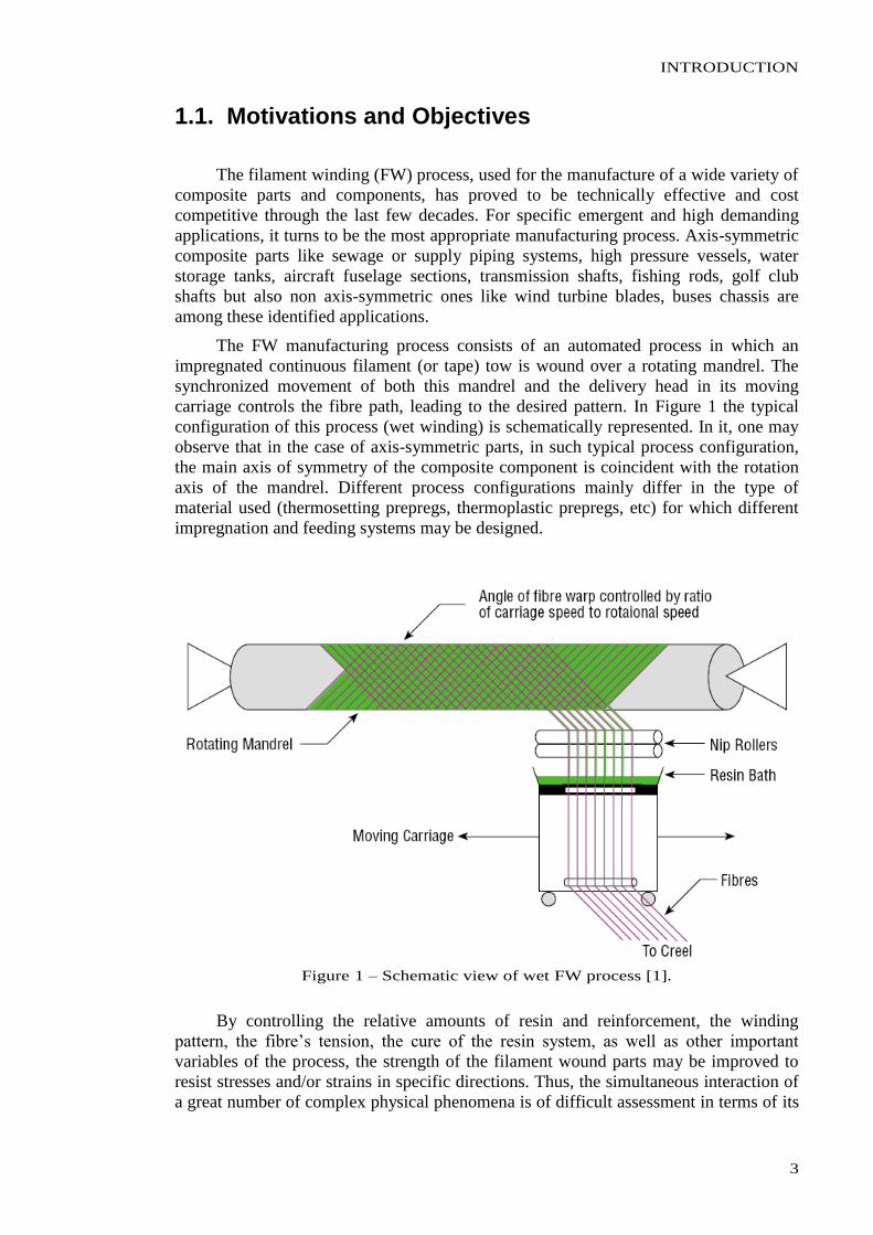
The FW manufacturing process consists of an automated process in which an
impregnated continuous filament (or tape) tow is wound over a rotating mandrel. The
synchronized movement of both this mandrel and the delivery head in its moving
carriage controls the fibre path, leading to the desired pattern. In Figure 1 the typical
configuration of this process (wet winding) is schematically represented. In it, one may
observe that in the case of axis-symmetric parts, in such typical process configuration,
the main axis of symmetry of the composite component is coincident with the rotation
axis of the mandrel. Different process configurations mainly differ in the type of
material used (thermosetting prepregs, thermoplastic prepregs, etc) for which different
impregnation and feeding systems may be designed.
Figure 1 – Schematic view of wet FW process [1].
By controlling the relative amounts of resin and reinforcement, the winding
pattern, the fibre’s tension, the cure of the resin system, as well as other important
variables of the process, the strength of the filament wound parts may be improved to
resist stresses and/or strains in specific directions. Thus, the simultaneous interaction of
a great number of complex physical phenomena is of difficult assessment in terms of its
CHAPTER 1
4
modelling and precise measurement. However, with the increasing demands on safety
and reliability issues, in short- as well as in long-term applications, it is of absolute need
to achieve better knowledge and more accurate models of the physical phenomena
acting in the FW process. Only realistic models, capable of relating the input with the
output relevant parameters of this multi-physical process will allow a reliable design
and control of the FW manufacturing process for each application. A better
understanding of the coupled behaviour of those phenomena and of their influence on
the final quality of the manufactured parts will, ultimately, allow to optimize them and
achieve weight and costs savings in the final products. Questions on the level of
reproducibility, predictability and dimensional tolerances may also be further addressed.
This study aimed at developing and validating a multi-physical process model for
the FW manufacturing technique. A modular approach, based on sub-models each
referring to a relevant group of physical phenomena acting at the layer-laminate level,
was designed. This option allowed to settle a model applicable to a broader range of real
configurations and applications of the FW manufacturing process as it is now required
by the industry.
INTRODUCTION
5
1.2. Thesis Organization
This thesis is divided into six chapters, each addressing a relevant stage within the
development and analysis of the present process model. Each chapter is built
independently both thematically and in the logical arguments construction. However,
the six chapters report the natural sequence of the whole study, from the problem
identification, to the proposition of a solution and its validation.
After this introductory chapter (chapter 1) a comprehensive literature review is set
in chapter 2. In this review, the available knowledge on processes and/or sub-processes
that correlate with the FW process are identified. Several works published by different
authors in the past are critically analysed and the background for this study is therefore
enriched. In chapter 3 the FW process model is established. The several physical
phenomena acting within the laminate being manufactured are analytically modelled.
Each decoupled group of phenomena is described in a dedicated sub-model. The overall
architecture of the multi-physical process model is also presented. The experimental
tests conducted to assess and measure the evolution of the several physical parameters
during the FW process are fully addressed in chapter 4. This chapter holds the detailed
description of the experimental procedures and respective results, covering the main
process input and output variables. Critical analysis of these results is produced in view
of comparing with the numerical ones. Chapter 5 covers the numerical implementation
of the process model. Several sub-routines, each relating to a sub-model, are coded into
numerical algorithms. These are assembled through a main routine that guarantees the
proper flow of variables information and interaction between the several sub-routines
accordingly with the model architecture defined. At the end of this chapter, critical
comparisons between numerical and experimental results are presented and the
validation of the process model is, thus, discussed. In chapter 6, the conclusions are
drawn for the entire study. The degree of accomplishment of the objectives and thus the
usefulness and validity of the present work are discussed. Future improvements and
developments to be further addressed are identified as well.


CHAPTER 2
LITERATURE REVIEW

CHAPTER 2
8
LITERATURE REVIEW
9
2.1. Scope of the Review
In this chapter the state of the art referred to the FW process modelling and
characterization is addressed through a comprehensive literature review of relevant
technical and scientific papers and thesis published in the last four decades. Previous
works covering all the relevant fields related to the modelling of this process were
studied. Very few researchers focused strictly in the FW process. On the other hand,
however, a considerable number of studies led on other processes and/or the detailed
characterization of several of the physical and chemical phenomena acting within
consolidating composite laminates have been published.
The review is divided in the main sub-themes that correspond to the different
physical phenomena governing the consolidation and behaviour of composite laminates.
Namely, identification of the FW process parameters, fibre’s compaction, resin flow,
resin kinetics, stress-strain and global process models are critically identified and
described in separated sections. Despite the coupled nature of some mechanisms in the
consolidation of composite laminates, independent sections deal with each group of
phenomena identified in order to allow a deep understanding of them. Since different
authors referred to similar phenomena with different nomenclature or even
mathematical symbols, effort is made in homogenizing the relevant information and
presenting it in the symbology and nomenclature adopted in the present work. For
clarity, the matrix is frequently named resin, independently of thermosetting and/or
thermoplastic being considered throughout this chapter. Experimental techniques for the
measurement of parameters and/or model validation which are thought relevant for the
present study were also reviewed from the literature.
Since the scope of the present thesis is to model a multi-physical process that
involves a broad range of correlated research fields, contributions from a wide range of
sources are studied. Therefore, although the following literature review may appear
reasonably extensive, it strictly covers the relevant knowledge that supports the strategy
for the development and establishment of the present FW process model. Further
detailed analysis is addressed in chapter 3, when setting the assumptions and
formulations of each sub-model.
CHAPTER 2
10
2.2. Process Modelling in Composites Manufacturing
In this section, the literature addressing the theoretical modelling of each
phenomenon governing the behaviour of composite laminates under consolidation is
critically reviewed. An overview of the main studies published in the last four decades
is drawn. As far as possible, the review is divided in the relevant sub-themes as
mentioned above. The sub-themes were chosen upon identification of the process
parameters and/or variables which govern it.
2.2.1. Process Parameters
In the FW manufacturing process there are several physical parameters whose
different combinations allow a wide range of mechanical and geometrical results. These
parameters may be divided into two categories: the user-controllable process parameters
and the other process parameters inherent to the physics of the process. By user it is
meant the designer and/or operator of the manufacturing process. In a process model
development, the final objective is to get the user-controllable process parameters to be
the input variables and the inherent variables (which are not directly controllable
throughout the process) to be the output ones. Only with sound and correct physical
descriptions of each phenomenon one may get a profitable tool for design and process
optimization purposes.
The main user-controllable process parameters are:
the choice of the material system (the reinforcing fibres and the matrix);
the geometry of the mandrel;
the initial fibre’s tension;
the cross-section of the fibre’s bundle (incl. bandwidth and/or thickness);
the path of the fibres onto the mandrel;
the winding angle;
the initial fibre’s degree of impregnation;
the processing temperature;
the winding speed;
the lay-up sequence; and
the curing time after winding.
The main process inherent parameters or phenomena are typically variable during
the process, may vary with time and space, and are:
the fibre’s motion;
the matrix flow through the fibre’s bed;
the matrix degree of conversion (cure/crystallization);
the matrix viscosity;
the stresses and strains in the fibres;
the temperature;
the fibre’s, resin and void’s volume fraction; and
the fibre characteristic waviness.
A few more parameters could be pointed out, such as the permeability of the fibre
bed to the resin and air, or the layer’s interaction by way of the compaction pressure and
LITERATURE REVIEW
11
resin mixing. However, these may be identified as sub-parameters that influence the
main ones previously identified. Moreover, these sub-parameters need to be specifically
analysed in each case as they are highly dependent on the material system used together
with other main configuration options for the FW process.
Lee and Springer [2] summarized the critical issues to consider when selecting the
proper combination of the input variables. Thus, for most of the applications, the values
of the controllable process variables must be selected such that:
the temperature inside the material is below the maximum allowable value
at any time during processing;
the material is cured completely and uniformly;
at the end of the cure the fibre distribution is uniform and has the desired
value;
the fibre tension is positive, but doesn’t exceed prescribed limits at any
time during processing;
the cured composite has the lowest possible residual stresses;
the cured composite’s total residual strains are within the prescribed limits;
the cured composite has the lowest possible void content;
the processing is executed in the shortest possible time.
It becomes clear that, either for process model validation or manufacturing
purposes, considerable set of measuring devices is needed in order to guarantee that the
user-controllable process variables really are within the admissible ranges and
combinations that lead the outputs to the desired optimum values.
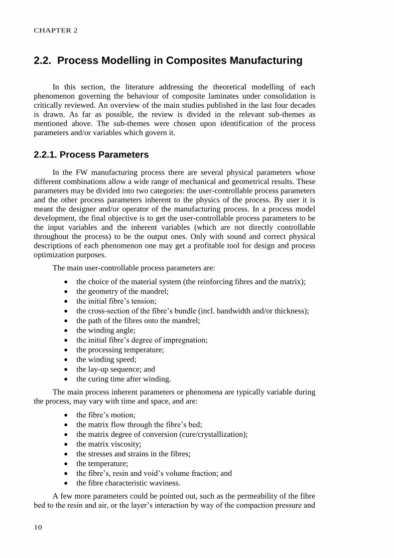
Relatively to the winding patterns, there are mainly three types of winding:
circumferential (hoop), polar (longitudinal) and helical winding (Figure 2). The helical
winding, if neglecting shear strength between surfaces (friction factor virtually null),
implies the deposition of the fibres along a geodesic isotensional trajectory. In such
condition, Clairaut’s theorem [3] may be expressed as follows:
ntconstar sin , (2.1)
where r is the radial coordinate of the fibre bundle and is the winding angle. The
geodesic trajectories defined as in the equation (2.1) typically don’t correspond to the
principal stress directions of the composite part when º90º0 . Further attention is
given to this problem in section 2.2.5. In polar winding, on the other hand, one may
experience considerable difference (from 12% up to 40% of the maximum value) on the
fibre’s tension in the edges (callouts or domes) or in the mid-section (cylindrical) of the
composite part [4]. In this case the isotensoidal assumption is not valid anymore.
Analytical and numerical solutions for the kinematics of FW have extensively
been investigated during the last decades. Koussios et al. [5,6] recently proposed
consensual and updated kinematical models for ellipsoidal and cylindrical wound parts.
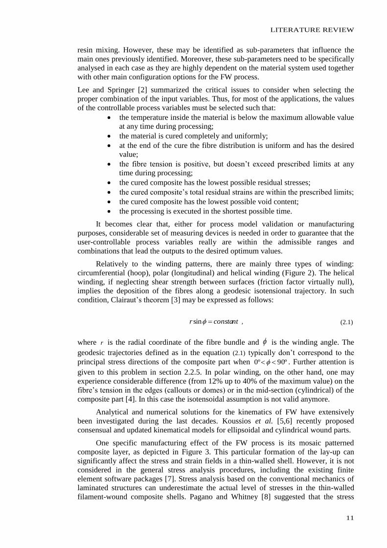
One specific manufacturing effect of the FW process is its mosaic patterned
composite layer, as depicted in Figure 3. This particular formation of the lay-up can
significantly affect the stress and strain fields in a thin-walled shell. However, it is not
considered in the general stress analysis procedures, including the existing finite
element software packages [7]. Stress analysis based on the conventional mechanics of
laminated structures can underestimate the actual level of stresses in the thin-walled
filament-wound composite shells. Pagano and Whitney [8] suggested that the stress
CHAPTER 2
12
field within a highly anisotropic cylinder, even under simple loading conditions, is far
from uniform.
Figure 2 – Schematic representation of circumferential (hoop) winding (top left),
polar (longitudinal) winding (top right) and helical winding (bottom) [9].
Each filament-wound layer is typically composed by two plies with and
fibre’s orientation angles, respectively. As these plies are interlaced throughout the part
being wound they are actually identified as a single layer. Morozov [7] studied this
characteristic of the FW process and showed how this structural feature affected the
strength of the composite parts. He modelled the composite material in a mosaic way
where each alternating triangle was defined as either [ ] or [ ].
Figure 3 - Angle-ply layer of a filament wound shell [7].
Different configurations of the manufacturing process, whether it is used a
thermosetting or a thermoplastic matrix system, will greatly influence the degree of
homogeneity of the impregnation as well as the processing temperature. Furthermore,
the interaction between layers (adhesion and exchange of mass and heat) and the
LITERATURE REVIEW
13
consolidation of the laminate is strongly dependent of the matrix properties. In the next
sections, whenever the choice of the matrix type is critical, it is discussed in detail.
2.2.2. Compaction of the Fibres
The winding tension applied to the fibres during the FW process has an indirect
influence on the fibre volume fraction and void content. Higher tension causes higher
pressure build-up and as a consequence higher amounts of resin and voids are squeezed
through or outwards the laminate. The fibre volume fraction increases and the fibre bed
becomes stiffer. However, when the fibres’ content is too high there might be lack of
matrix to keep fibres together and part performance may decrease significantly.
Several authors studied the pressure build-up phenomenon in self-acting foil
bearings in the past century [10-13]. These systems present some similarities with the
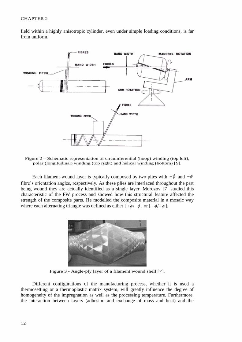
FW process and are, thus, worth observing. Blok and Rossum [10] have shown that a
flexible impermeable tape in contact with a rotating cylinder and lubricating oil would
cause the oil pressure to increase between the tape and the cylinder in a wedge-shaped
entrance region (Figure 4). Following the wedge-shaped entrance region, the oil was
observed to form a constant thickness film gap between tape and cylinder. For a wide
range of test conditions, the outward oil pressure, p , in this constant thickness region
was observed to be equal to the inward compressive stress, , given by:
rb
F , (2.2)
where F is the inlet tape force, b is the tape bandwidth and r is the pin radius.
Figure 4 – Schematic cross-sectional of a tape being pulled over a cylindrical pin.
The pressure build-up in the wedge entrance is also shown [14].
Similar relations between the constant thickness and processing parameters such
as tape tension, width, oil viscosity, relative tape/cylinder speed and cylinder radius
were presented by all those researchers. They developed the “lubrication number”
concept. It is clear from the preceding analysis that fibre tension plays an important role
in pressure build-up in such a fibres/mandrel interaction.
Bates et al. [14,15] studied the pressure build-up during melt impregnation of
glass-fibre roving. They set the melt pressure at the roving/pin interface to be given by:
CHAPTER 2
14
rb
Ffp , (2.3)
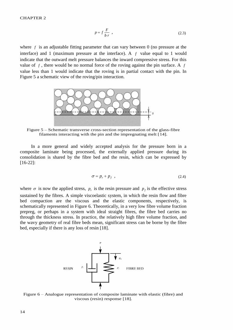
where f is an adjustable fitting parameter that can vary between 0 (no pressure at the
interface) and 1 (maximum pressure at the interface). A f value equal to 1 would
indicate that the outward melt pressure balances the inward compressive stress. For this
value of f , there would be no normal force of the roving against the pin surface. A f
value less than 1 would indicate that the roving is in partial contact with the pin. In
Figure 5 a schematic view of the roving/pin interaction.
Figure 5 – Schematic transverse cross-section representation of the glass-fibre
filaments interacting with the pin and the impregnating melt [14].
In a more general and widely accepted analysis for the pressure born in a
composite laminate being processed, the externally applied pressure during its
consolidation is shared by the fibre bed and the resin, which can be expressed by
[16-22]:
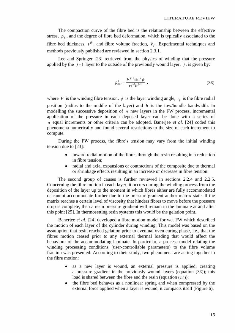
fr pp , (2.4)
where is now the applied stress, rp is the resin pressure and fp is the effective stress
sustained by the fibres. A simple viscoelastic system, in which the resin flow and fibre
bed compaction are the viscous and the elastic components, respectively, is
schematically represented in Figure 6. Theoretically, in a very low fibre volume fraction
prepreg, or perhaps in a system with ideal straight fibres, the fibre bed carries no
through the thickness stress. In practice, the relatively high fibre volume fraction, and
the wavy geometry of real fibre beds mean, significant stress can be borne by the fibre
bed, especially if there is any loss of resin [18].
Figure 6 – Analogue representation of composite laminate with elastic (fibre) and
viscous (resin) response [18].
LITERATURE REVIEW
15
The compaction curve of the fibre bed is the relationship between the effective
stress, fp , and the degree of fibre bed deformation, which is typically associated to the
fibre bed thickness, fbt , and fibre volume fraction, fV . Experimental techniques and
methods previously published are reviewed in section 2.3.1.
Lee and Springer [23] retrieved from the physics of winding that the pressure
applied by the 1j layer to the outside of the previously wound layer, j , is given by:
11
21 sin
jj
f
jj
outbr
Fp
, (2.5)
where F is the winding fibre tension, is the layer winding angle, fr is the fibre radial
position (radius to the middle of the layer) and b is the tow/bundle bandwidth. In
modelling the successive deposition of n new layers in the FW process, incremental
application of the pressure in each deposed layer can be done with a series of
n equal increments or other criteria can be adopted. Banerjee et al. [24] coded this
phenomena numerically and found several restrictions to the size of each increment to
compute.
During the FW process, the fibre’s tension may vary from the initial winding
tension due to [23]:
inward radial motion of the fibres through the resin resulting in a reduction
in fibre tension;
radial and axial expansions or contractions of the composite due to thermal
or shrinkage effects resulting in an increase or decrease in fibre tension.
The second group of causes is further reviewed in sections 2.2.4 and 2.2.5.
Concerning the fibre motion in each layer, it occurs during the winding process from the
deposition of the layer up to the moment in which fibres either are fully accommodated
or cannot accommodate further due to the pressure gradient and/or matrix state. If the
matrix reaches a certain level of viscosity that hinders fibres to move before the pressure
drop is complete, then a resin pressure gradient will remain in the laminate at and after
this point [25]. In thermosetting resin systems this would be the gelation point.
Banerjee et al. [24] developed a fibre motion model for wet FW which described
the motion of each layer of the cylinder during winding. This model was based on the
assumption that resin reached gelation prior to eventual oven curing phase, i.e., that the
fibres motion ceased prior to any external thermal loading that would affect the
behaviour of the accommodating laminate. In particular, a process model relating the
winding processing conditions (user-controllable parameters) to the fibre volume
fraction was presented. According to their study, two phenomena are acting together in
the fibre motion:
as a new layer is wound, an external pressure is applied, creating
a pressure gradient in the previously wound layers (equation (2.5)); this
load is shared between the fibre and the resin (equation (2.4));
the fibre bed behaves as a nonlinear spring and when compressed by the
external force applied when a layer is wound, it compacts itself (Figure 6).
CHAPTER 2
16
A specific case of sponge squeeze model, previously developed by Gutowski et
al. [26] (and reviewed in section 2.2.6), was considered in their study:
as the resin cured, fibre motion ceased in a particular layer;
resin in adjacent layers had different viscosities;
a modified stiffness formulation was adopted.
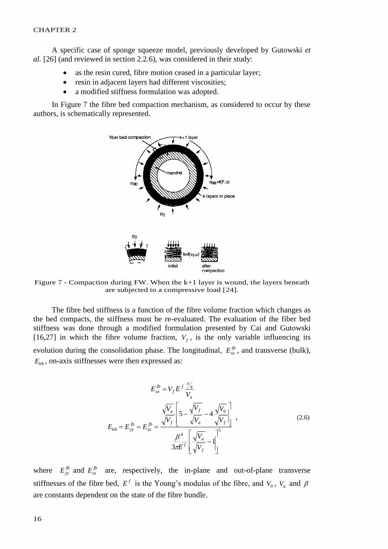
In Figure 7 the fibre bed compaction mechanism, as considered to occur by these
authors, is schematically represented.
Figure 7 - Compaction during FW. When the k+1 layer is wound, the layers beneath
are subjected to a compressive load [24].
The fibre bed stiffness is a function of the fibre volume fraction which changes as
the bed compacts, the stiffness must be re-evaluated. The evaluation of the fiber bed
stiffness was done through a modified formulation presented by Cai and Gutowski
[16,27] in which the fibre volume fraction, fV , is the only variable influencing its
evolution during the consolidation phase. The longitudinal, fbxxE , and transverse (bulk),
bbE , on-axis stiffnesses were then expressed as:
54
0
4
13
45
f
a
f
fa
f
f
a
fbzz
fbyybb
a
ff
fbxx
V
V
E
V
V
V
V
V
V
EEE
VEVE
, (2.6)
where fbyyE and fb
zzE are, respectively, the in-plane and out-of-plane transverse
stiffnesses of the fibre bed, fE is the Young’s modulus of the fibre, and 0V , aV and
are constants dependent on the state of the fibre bundle.
LITERATURE REVIEW
17
Once the layer displacements ju are determined for the mth load increment, the
radial positions of the layers in place klj .. are updated as follows:
mjmj
i
mji
mjmjo
mjo
urr
urr
)1(1
)(1
, (2.7)
where jor and j
ir are the outer and inner radii of the jth layer, respectively.
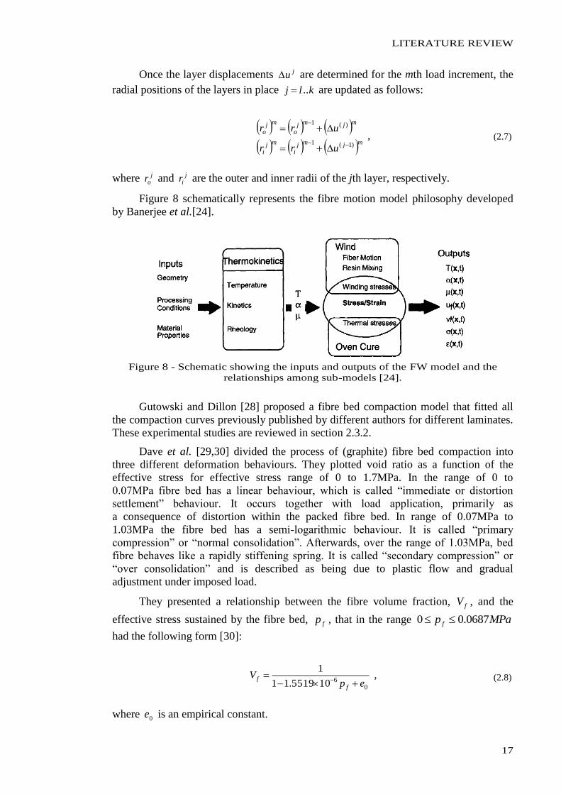
Figure 8 schematically represents the fibre motion model philosophy developed
by Banerjee et al.[24].
Figure 8 - Schematic showing the inputs and outputs of the FW model and the
relationships among sub-models [24].
Gutowski and Dillon [28] proposed a fibre bed compaction model that fitted all
the compaction curves previously published by different authors for different laminates.
These experimental studies are reviewed in section 2.3.2.
Dave et al. [29,30] divided the process of (graphite) fibre bed compaction into
three different deformation behaviours. They plotted void ratio as a function of the
effective stress for effective stress range of 0 to 1.7MPa. In the range of 0 to
0.07MPa fibre bed has a linear behaviour, which is called “immediate or distortion
settlement” behaviour. It occurs together with load application, primarily as
a consequence of distortion within the packed fibre bed. In range of 0.07MPa to
1.03MPa the fibre bed has a semi-logarithmic behaviour. It is called “primary
compression” or “normal consolidation”. Afterwards, over the range of 1.03MPa, bed
fibre behaves like a rapidly stiffening spring. It is called “secondary compression” or
“over consolidation” and is described as being due to plastic flow and gradual
adjustment under imposed load.
They presented a relationship between the fibre volume fraction, fV , and the
effective stress sustained by the fibre bed, fp , that in the range MPap f 0687.00
had the following form [30]:
06105519.11
1
epV
f
f
, (2.8)
where 0e is an empirical constant.
CHAPTER 2
18
Following Cai and Gutowski’s work [16,26,27,31], Agah-Tehrani and Teng [32]
proposed a continuum consolidation model for macroscopic analysis of fibre motion
during FW of thermosetting cylinders of arbitrary thickness. Their model was limited to
winding at a constant (hoop) winding angle throughout the process and constant
viscosity resins. The model indicated one zone in which consolidation has ceased and
one other in which fibre bundles were continuing to compact due to the applied tension.
Hojjati and Hoa [33] and Shin and Hahn [20] also followed and applied Gutowski’s
continuum equation governing the through-the-thickness compaction behaviour
(one-dimensional, r ) of consolidating laminates as follows:
22
2
r
pS
W
V
t
p rfr
, (2.9)
where rp is the resin pressure, W and S are the tangent compliance and the
permeability of the fibre bed, respectively, is the resin viscosity. The tangent
compliance described a change in the fibre volume fraction resulting from a change in
the effective compressive fibre stress.
Gutowski et al. [34] derived several alternative expressions relating fibre effective
stress, fp , to the fibre volume fraction, fV , based upon the assumption that the fibre
network stiffness was governed by the bending beam behaviour of the fibre between
multiple contact points. The most widely used by several authors is the following
formulation:
4
0
4
1
13
f
a
f
f
V
V
V
V
Ep
, (2.10)
where 0V is a certain “minimum” fibre volume fraction bellow which the fibres carry no
load, aV is the maximum available fibre volume fraction at which resin flow stops, is
the typical waviness ratio (span length/span height) of the fibres and E is the flexural
modulus of the fibres.
The lamina stress-strain behaviour has been found to greatly influence the
compaction behaviour of the laminate during its consolidation. Laminae with hardening
stress-strain behaviour, which is characteristic of real composite layered laminates, have
the fastest compaction times [35]. Although this output comes from studies conducted
in autoclave/vacuum degassing processes, attention must be given to it. Specific
stress-strain constitutive relations are discussed in section 2.2.5.
2.2.3. Resin Flow
Resin flow is the other mechanism (adding to those described in the previous
section) that greatly influences the fibre motion and positioning within the layers during
FW process. Although in the FW process modelling the resin (matrix) flow and/or cure
phenomenological sub-models cannot be separated from the fibre motion sub-models,
LITERATURE REVIEW
19
here we try to summarize them in a decoupled manner. This option is supported by the
fact that the resin flow is itself a physical process that can be independently described
analytically.
The fluid flow through porous media has been extensively studied in the past.
Numerous studies have been published concerning the modelling and characterization
of such phenomenon. Among those, soils consolidation, filters behaviour and
impregnation of fibrous beds were the most studied. From them, relevant knowledge
was gathered to the “recent” composites manufacturing processes.
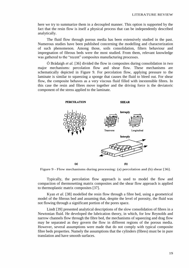
Ó Brádaigh et al. [36] divided the flow in composites during consolidation in two
major mechanisms: percolation flow and shear flow. These mechanisms are
schematically depicted in Figure 9. For percolation flow, applying pressure to the
laminate is similar to squeezing a sponge that causes the fluid to bleed out. For shear
flow, the composite behaves as a very viscous fluid filled with inextensible fibres. In
this case the resin and fibres move together and the driving force is the deviatoric
component of the stress applied to the laminate.
Figure 9 - Flow mechanisms during processing: (a) percolation and (b) shear [36].
Typically, the percolation flow approach is used to model the flow and
compaction of thermosetting matrix composites and the shear flow approach is applied
to thermoplastic matrix composites [37].
Kyan et al. [38] modelled the resin flow through a fibre bed, using a geometrical
model of the fibrous bed and assuming that, despite the level of porosity, the fluid was
not flowing through a significant portion of the pores space.
Lindt [39] presented analytical descriptions of the slow consolidation of fibres in a
Newtonian fluid. He developed the lubrication theory, in which, for low Reynolds and
narrow channels flow through the fibre bed, the mechanisms of squeezing and drag flow
may be separated as they govern the flow in different regions of the porous media.
However, several assumptions were made that do not comply with typical composite
fibre beds properties. Namely the assumptions that the cylinders (fibres) must be in pure
translation and have smooth surfaces.
CHAPTER 2
20
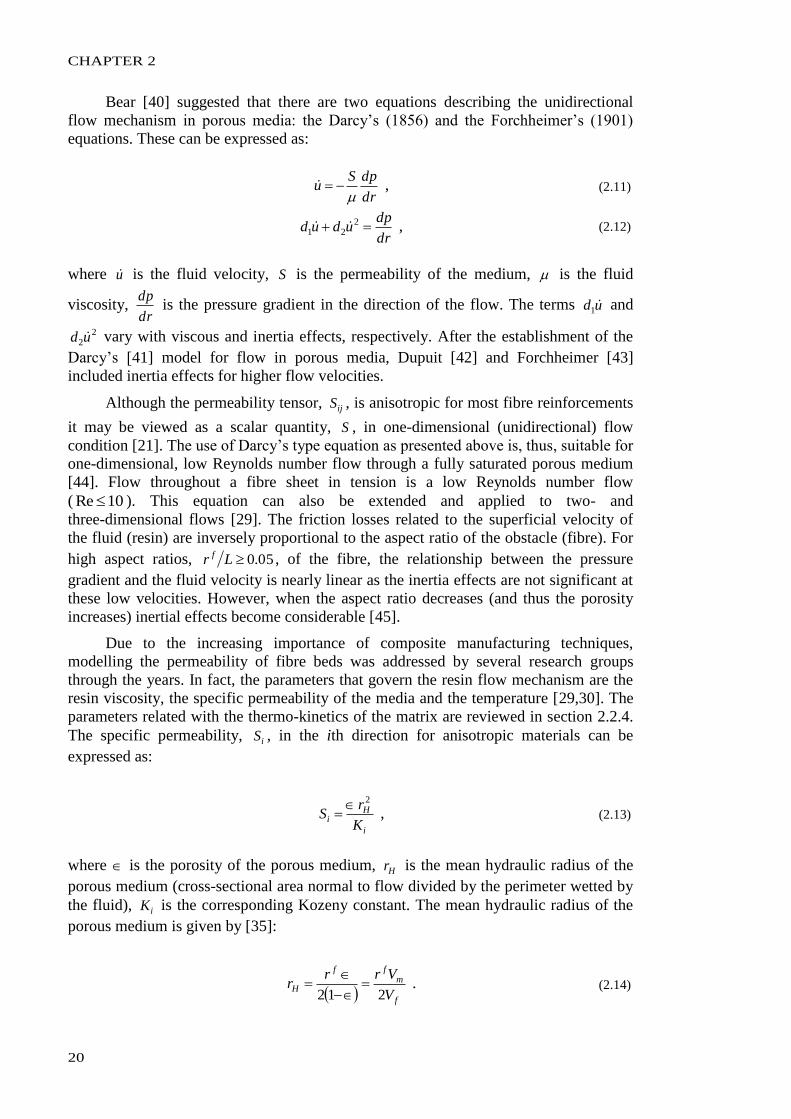
Bear [40] suggested that there are two equations describing the unidirectional
flow mechanism in porous media: the Darcy’s (1856) and the Forchheimer’s (1901)
equations. These can be expressed as:
dr
dpSu
, (2.11)
dr
dpudud 2
21 , (2.12)
where u is the fluid velocity, S is the permeability of the medium, is the fluid
viscosity, dr
dp is the pressure gradient in the direction of the flow. The terms ud
1 and
22ud vary with viscous and inertia effects, respectively. After the establishment of the
Darcy’s [41] model for flow in porous media, Dupuit [42] and Forchheimer [43]
included inertia effects for higher flow velocities.
Although the permeability tensor, ijS , is anisotropic for most fibre reinforcements
it may be viewed as a scalar quantity, S , in one-dimensional (unidirectional) flow
condition [21]. The use of Darcy’s type equation as presented above is, thus, suitable for
one-dimensional, low Reynolds number flow through a fully saturated porous medium
[44]. Flow throughout a fibre sheet in tension is a low Reynolds number flow
( 10Re ). This equation can also be extended and applied to two- and
three-dimensional flows [29]. The friction losses related to the superficial velocity of
the fluid (resin) are inversely proportional to the aspect ratio of the obstacle (fibre). For
high aspect ratios, 05.0Lr f , of the fibre, the relationship between the pressure
gradient and the fluid velocity is nearly linear as the inertia effects are not significant at
these low velocities. However, when the aspect ratio decreases (and thus the porosity
increases) inertial effects become considerable [45].
Due to the increasing importance of composite manufacturing techniques,
modelling the permeability of fibre beds was addressed by several research groups
through the years. In fact, the parameters that govern the resin flow mechanism are the
resin viscosity, the specific permeability of the media and the temperature [29,30]. The
parameters related with the thermo-kinetics of the matrix are reviewed in section 2.2.4.
The specific permeability, iS , in the ith direction for anisotropic materials can be
expressed as:
i
Hi
K
rS
2 , (2.13)
where is the porosity of the porous medium, Hr is the mean hydraulic radius of the
porous medium (cross-sectional area normal to flow divided by the perimeter wetted by
the fluid), iK is the corresponding Kozeny constant. The mean hydraulic radius of the
porous medium is given by [35]:
f
mff
HV
Vrrr
212
. (2.14)
LITERATURE REVIEW
21
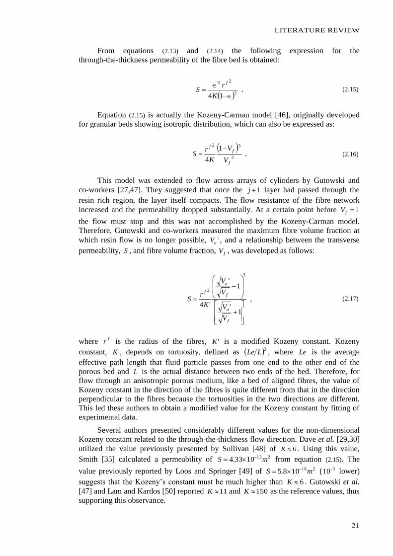
From equations (2.13) and (2.14) the following expression for the
through-the-thickness permeability of the fibre bed is obtained:
2
23
14
K
rS
f
. (2.15)
Equation (2.15) is actually the Kozeny-Carman model [46], originally developed
for granular beds showing isotropic distribution, which can also be expressed as:
2
321
4f
ff
V
V
K
rS
. (2.16)
This model was extended to flow across arrays of cylinders by Gutowski and
co-workers [27,47]. They suggested that once the 1j layer had passed through the
resin rich region, the layer itself compacts. The flow resistance of the fibre network
increased and the permeability dropped substantially. At a certain point before 1fV
the flow must stop and this was not accomplished by the Kozeny-Carman model.
Therefore, Gutowski and co-workers measured the maximum fibre volume fraction at
which resin flow is no longer possible, 'aV , and a relationship between the transverse
permeability, S , and fibre volume fraction, fV , was developed as follows:
1'
1'
'4
3
2
f
a
f
a
f
V
V
V
V
K
rS , (2.17)
where fr is the radius of the fibres, 'K is a modified Kozeny constant. Kozeny
constant, K , depends on tortuosity, defined as 2LLe , where Le is the average
effective path length that fluid particle passes from one end to the other end of the
porous bed and L is the actual distance between two ends of the bed. Therefore, for
flow through an anisotropic porous medium, like a bed of aligned fibres, the value of
Kozeny constant in the direction of the fibres is quite different from that in the direction
perpendicular to the fibres because the tortuosities in the two directions are different.
This led these authors to obtain a modified value for the Kozeny constant by fitting of
experimental data.
Several authors presented considerably different values for the non-dimensional
Kozeny constant related to the through-the-thickness flow direction. Dave et al. [29,30]
utilized the value previously presented by Sullivan [48] of 6K . Using this value,
Smith [35] calculated a permeability of 2131033.4 mS from equation (2.15). The
value previously reported by Loos and Springer [49] of 216108.5 mS ( 310 lower)
suggests that the Kozeny’s constant must be much higher than 6K . Gutowski et al.
[47] and Lam and Kardos [50] reported 11K and 150K as the reference values, thus
supporting this observance.
CHAPTER 2
22
Springer [51] studied the relationship between the applied pressure and the resin
flow during the cure of fibre-reinforced composites, where the layers were found to
consolidate in a wavelike manner. Loos and Springer [49] developed resin flow and
void models of the curing process. The resin velocity was related to the pressure
gradient, fibre permeability and resin viscosity through the Darcy’s type equation for
flow in porous media (equation (2.11)).
For aligned cylinders, analytical models based on drag, or on the lubrication
approach, were developed for Newtonian and generalized fluids by several authors
[52-58]. Some of these are available for low porosity, others for high porosity values.
Happel and Brenner [54] developed analytical solutions of the Navier-Stokes
equation for flows parallel and normal to an array of cylinders of a given diameter.
Sahraoui and Kaviany [57] used a finite-difference numerical method to solve the same
equation for a two-dimensional (simultaneous) flow through an array of cylinders. They
presented a relation between the permeability of the porous media, S , and its porosity,
, as follows:
8.04.0
140606.0
4
1.5
2
fr
S , (2.18)
where fr is the radius of the fibres.
Sangani and Acrivos [55] established the following relationship between the
transverse permeability, S , of circular tows arranged in hexagonal arrays and the fibre
volume fraction, fV :
25
321
227
12
f
ff
V
Vr
S . (2.19)
These models have shown a rather good agreement with experiments [59,60].
The correct modelling of the tow cross-section is also of great importance because
of its influence on the resin flow and, consequently, in the fibre’s compaction behaviour
and interaction between layers. Sherrer [61] compared both the rectangular fibre model
of Cutler (1961) and the hexagonally arranged Hashin’s fibre model (1964) with
experimental data obtained in his compression, torsion and tension tests conducted on
cylindrical wound specimens. Both Cutler’s and Hashin’s models presented relevant
limitations due to their restrictive assumptions and results were not satisfactory.
Looking to the topology of the fibre tows when being wound, it is commonly
accepted that they present an elliptical cross-section shape. In conventional FW
configurations, the fibre bundle incorporates several fibre tows each including several
hundreds or thousands of individual filaments. The higher the winding force is, the
cross-sectional shape of each tow becomes more flattened, thus approximating the
bundle cross-section to a homogenous random distribution of individual cylindrical
filaments. However, in the conventional range of winding forces, the tow elliptical
cross-section and individuality may govern the permeability characteristic of the fibre
bed. Some studies intended to approach these topologies. Epstein and Masliyah [62]
LITERATURE REVIEW
23
numerically solved the problem of normal flow through elliptical fibres by extending
both the Happel and Brenner [54] free surface and the Kuwabara [52] zero vorticity cell
models. They showed that fibres with an aspect ratio of 5:1 have a permeability that is
75% lower than obtained for circular fibres when the major axis is perpendicular to the
flow as is the case in transverse permeability measurements (and of FW). The volume
fractions studied were above 10%, since for lower volume fractions the cross-section
exerted a minor effect.
Later, the increasing importance of liquid moulding techniques using fabrics led
to the development of further models, which took into account not only the ellipticity of
the fibre tows, but also their intrinsic permeability. Phelan and Wise [63] proposed a
semi-analytical model based on lubrication approximation, and validated it with
computational fluid dynamics, and a few experimental observations. Ranganathan et al.
[64] extended this model and proposed for a solid ellipse an empirical relationship of
the form:
B
f
f
V
VA
ba
S
1
max
, (2.20)
where a and b are the axes of the ellipse, maxfV the maximum packing fraction for a
given packing geometry and A and B depend on the axes ratio. For example,
32max fV for a proportionally hexagonal packing. For the flow perpendicular to
the large axis of the elliptical fibres, and a shape factor greater than 5, they proposed the
following relationship:
62.2
max
2167.0
f
f
V
V
b
S . (2.21)
They extended this approach to porous tows, pointing out the use of a ‘‘nominal
volume fraction’’, inalnomfV , which refers to the volume occupied by the ellipses, and is
related to the actual volume fraction, actualfV , by:
towf
inalnomf
actualf VVV , (0.22)
where towfV is the volume fraction of fibres within a single tow. They showed that the
intrinsic porosity of the elliptical tows does not exert much of an influence, until the
ratio of the tow permeability over the overall permeability is greater than 0.001. This
was later confirmed using boundary element methods (BEM) and computational fluid
dynamics (CFD) calculations [65,66]. Extension of these models to the flow of
non-Newtonian fluids was also presented [67].
In the FW process the phenomenon of resin flow is strongly related with tension
applied to the fibre bundle during the winding that creates compaction gradient pressure
in previously wound layers. This causes resin to squeeze and flow through the porous
fibre bed [24]. As the fibre bed below compacts, the fibre volume fraction increases and
CHAPTER 2
24
uncured excess resin from previously wound layers bleeds through the surface. When
pressure inside laminate becomes equal to the pressure on its boundaries, there is no
more resin flow, no further compaction of the bed, and the specific permeability in any
particular direction is constant throughout the bed.
As Cai et al. [16] identified fibre bed compaction as being a dominant process in
wet FW, they also defined the time required for the resin to flow through a certain
ply/layer, ft . It was defined as:
2
20* 4
fs
f
rA
hKtt
, (2.23)
where *t is a dimensionless time at which the fluid pressure drops substantially, fr is
the radius of the fibres, K is the Kozeny constant, is the fluid viscosity, 0h is the
layer thickness and sA is a fibre bed spring constant. For processing conditions in which
the flow time, ft , is less than the winding time, wt , for a layer, the fluid (matrix) would
have ample time to flow through the compacting fibre bed.
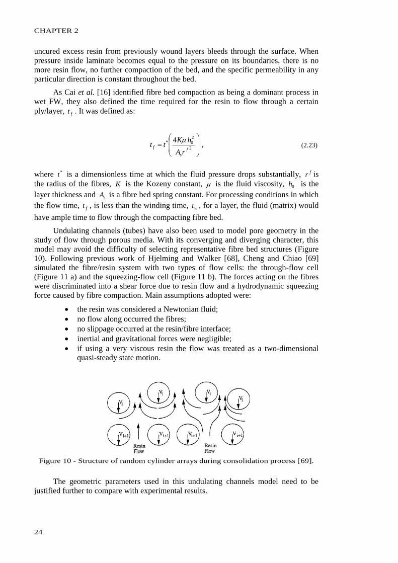
Undulating channels (tubes) have also been used to model pore geometry in the
study of flow through porous media. With its converging and diverging character, this
model may avoid the difficulty of selecting representative fibre bed structures (Figure
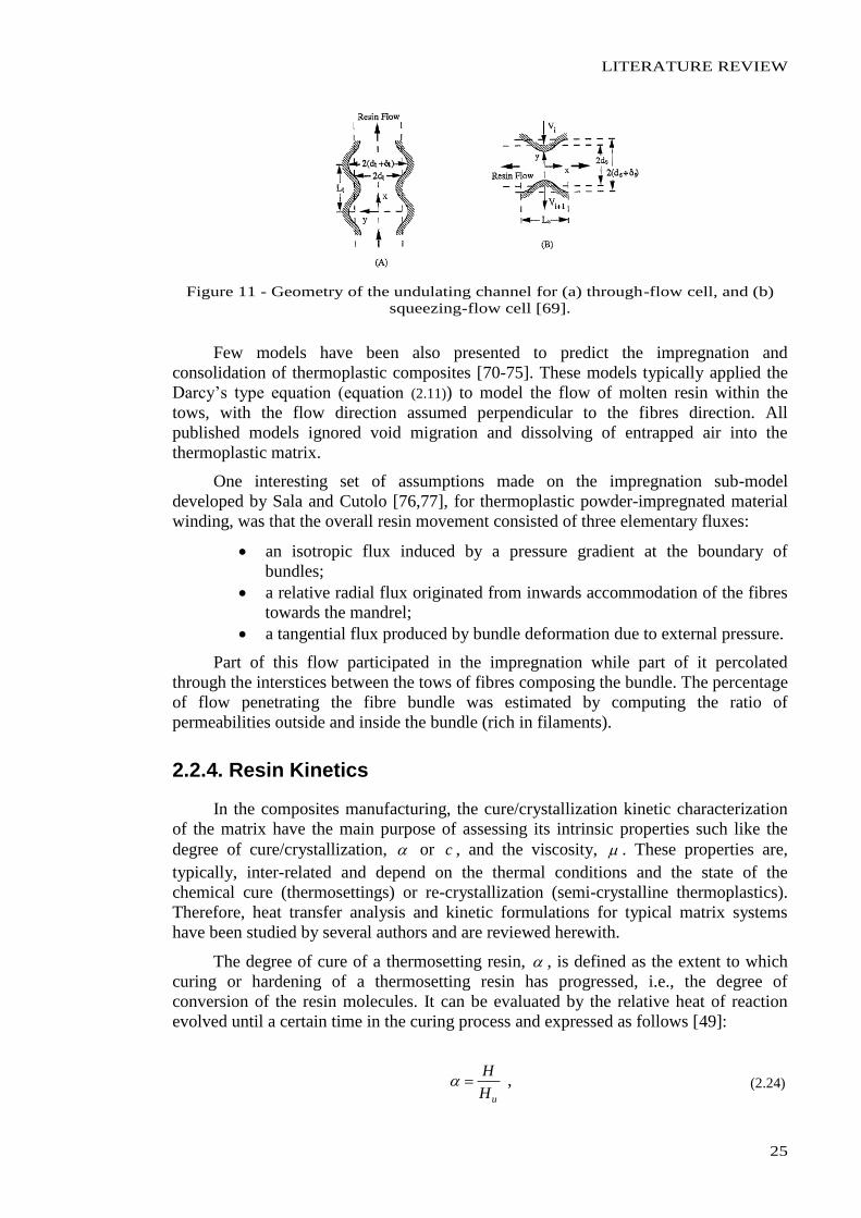
10). Following previous work of Hjelming and Walker [68], Cheng and Chiao [69]
simulated the fibre/resin system with two types of flow cells: the through-flow cell
(Figure 11 a) and the squeezing-flow cell (Figure 11 b). The forces acting on the fibres
were discriminated into a shear force due to resin flow and a hydrodynamic squeezing
force caused by fibre compaction. Main assumptions adopted were:
the resin was considered a Newtonian fluid;
no flow along occurred the fibres;
no slippage occurred at the resin/fibre interface;
inertial and gravitational forces were negligible;
if using a very viscous resin the flow was treated as a two-dimensional
quasi-steady state motion.
Figure 10 - Structure of random cylinder arrays during consolidation process [69].
The geometric parameters used in this undulating channels model need to be
justified further to compare with experimental results.
LITERATURE REVIEW
25
Figure 11 - Geometry of the undulating channel for (a) through-flow cell, and (b)
squeezing-flow cell [69].
Few models have been also presented to predict the impregnation and
consolidation of thermoplastic composites [70-75]. These models typically applied the
Darcy’s type equation (equation (2.11)) to model the flow of molten resin within the
tows, with the flow direction assumed perpendicular to the fibres direction. All
published models ignored void migration and dissolving of entrapped air into the
thermoplastic matrix.
One interesting set of assumptions made on the impregnation sub-model
developed by Sala and Cutolo [76,77], for thermoplastic powder-impregnated material
winding, was that the overall resin movement consisted of three elementary fluxes:
an isotropic flux induced by a pressure gradient at the boundary of
bundles;
a relative radial flux originated from inwards accommodation of the fibres
towards the mandrel;
a tangential flux produced by bundle deformation due to external pressure.
Part of this flow participated in the impregnation while part of it percolated
through the interstices between the tows of fibres composing the bundle. The percentage
of flow penetrating the fibre bundle was estimated by computing the ratio of
permeabilities outside and inside the bundle (rich in filaments).
2.2.4. Resin Kinetics
In the composites manufacturing, the cure/crystallization kinetic characterization
of the matrix have the main purpose of assessing its intrinsic properties such like the
degree of cure/crystallization, or c , and the viscosity, . These properties are,
typically, inter-related and depend on the thermal conditions and the state of the
chemical cure (thermosettings) or re-crystallization (semi-crystalline thermoplastics).
Therefore, heat transfer analysis and kinetic formulations for typical matrix systems
have been studied by several authors and are reviewed herewith.
The degree of cure of a thermosetting resin, , is defined as the extent to which
curing or hardening of a thermosetting resin has progressed, i.e., the degree of
conversion of the resin molecules. It can be evaluated by the relative heat of reaction
evolved until a certain time in the curing process and expressed as follows [49]:
uH
H , (2.24)
CHAPTER 2
26
where H is the heat evolved from time 0t to time t , uH is the total (ultimate) heat
of reaction of the resin. Alternatively, it may be expressed as [78]:
u
r
H
H1 , (2.25)
where rH is the residual and/or remaining heat of reaction.
In order to model the cure (in the case of thermosetting systems) or crystallization
(in the case of semi-crystalline thermoplastic systems) of composite laminates, the
energy conservation principle must be considered. Following previous works presented
by Springer and co-workers [49,2,79], Zhao et al. [80] modelled the
through-the-thickness heat transfer in cylindrical wound composites by neglecting
convection heat and thus applying the one-dimensional heat conduction equation in the
form:
Qr
Tk
rrt
TC r
1 , (2.26)
where t
T
and
r
T
are the thermal gradients in time and space, respectively, r is the
radial coordinate, is the density of the composite, C is the specific heat of the
composite, rk is the thermal conductivity of the composite in the radial direction and Q
is the heat generation rate.
For thermosetting resins, the heat generation term was typically described as a
function of the rate of cure, dt
d, accordingly to the following relation [34]:
umm H
dt
dVQ
, (2.27)
where m and mV are the density and volume fraction of the matrix, respectively, uH ,
is the total heat of reaction. Alternatively, this term has also been described as [81]:
um H
dt
dQ
, (2.28)
where is the porosity of the fibre bed. From equations (2.27) and (2.28) it is clear that
the porosity of the fibre bed is intimately related with the matrix volume fraction within
the laminate.
Shin and Hahn [20] simulated the heat transfer and compaction along a
bleeder-composite laminate assembly processed in autoclave. They used the cure
kinetics model of Lee et al. [82] for the Hercules®
3501-6 epoxy resin. Their results
showed that using variable resin properties instead of constant ones, better predictions
of through-the-thickness temperature distribution were achieved. Namely, the resin
LITERATURE REVIEW
27
density, m , specific heat, mC , and thermal conductivity, mk , during its curing process
were calculated through the following equations [83]:
45.0272.1
45.0232.109.0
m , (2.29)
141.010975.5468.0184.4 4 TCm , (2.30)
41.0035.085.304184.0 Tk m , (2.31)
where T is the temperature and is the degree of cure.
For thermoplastic resins, Lee and Springer [84] utilized the same heat conduction
equation and associated Q to the rate at which heat was released or absorbed by the
composite during heating and cooling, thus expressing the heat generation term as:
umm H
dt
dcVQ
, (2.32)
where dtdc is the rate of change of crystallinity, conceptually identical to the curing
rate in thermosetting resins.
Several semi-empirical analytical models were established and presented for the
isothermal curing process of epoxy resin systems in the last decades. Most of the
models were devised from curve-fitting of experimental differential scanning
calorimetry (DSC) tests.
Early studies conducted by Horie et al. [85] suggested an autocatalytic
four-parameter model describing rate of cure for an isothermal curing reaction without
consideration of diffusion control as follows:
nmkkdt
d)1)(( 21
, (2.33)
where dt
d is the curing rate, 1k and 2k are the rate constants, m and n are the orders
of cure reaction. m and n are related, respectively, to the initiation and propagation of
the cure reaction [86]. Later, Chern and Poehlein [87] modified this autocatalytic
four-parameter model in order to account for the effect of the diffusion, by including a
diffusion factor as follows:
nm
cCkk
edt
d)1)((
1
121
, (2.34)
where C and c are temperature-dependent empirical constants. These constants were
experimentally determined for different temperatures through nonlinear least squares
curve fitting of the )(t curve. The denominator of the expression takes into account the
slowing down of the reaction at high degrees of cure due to the onset of diffusion
CHAPTER 2
28
control at a temperature-dependent critical degree of cure, c . Cole et al. [88] proposed
a similar modelling approach to account for the shift from kinetics to diffusion control
in the curing process, developing the following relation:
nm
cCK
edt
d)1(
1
1
, (2.35)
RT
E
AeK
. (2.36)
During the curing process of thermosetting resins, the glass transition temperature, gT ,
of the system gradually increases. When the isothermal cure reaction reaches a certain
stage, the gT of the system changes from below the cure reaction to equal or above the
cure temperature, and vitrification (glassy state) occurs. At this stage, the mobility of
the system decreases dramatically. Therefore, the rate of the curing reaction undergoes a
significant decrease and falls below the kinetic rate as the curing reaction becomes
diffusion controlled [89]. Accordingly, the degree of curing increases very little in the
glassy state.
Sourour and Kamal [90] presented a mechanistic model for the early stages of
cure of an epoxy-diamine resin system. However, it was clearly not valid for the later
stages of cure. Lee et al. [82] studied the epoxy resin Hercules® 3501-6 and, based on
that model, proposed a piece-wise relationship between the rate of cure, dt
d, and the
degree of cure, , as follows:
3.0)1(
3.0))(1)((
3
21
Kdt
d
BKKdt
d
, (2.37)
3,2,1
ieAK RT
E
ii
i
, (2.38)
where iA are the pre-exponential constants, iE is the activation energy, B is a
constant, R is the universal gas constant and T is the absolute temperature.
Ng et al. [91] tested two resin systems, 8552 and 977-3 HM® epoxies, and found
the following equation describing the kinetic behaviour of both:
432
23
1 KKKKdt
d , (2.39)
4,3,2,1
ieAK RT
E
ii
i
. (2.40)
Banerjee et al. [24] and Zhao et al. [80] used an isothermal analytical model of
HBRF 55-A epoxy resin, firstly developed by Pearce and Mijovic [92], in order to
model the process of FW. The equation was as follows:
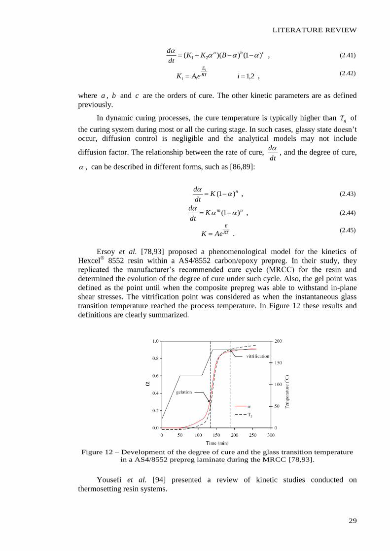
LITERATURE REVIEW
29
cba BKKdt
d)1())(( 21
, (2.41)
2,1 ieAK RT
E
ii
i
, (2.42)
where a , b and c are the orders of cure. The other kinetic parameters are as defined
previously.
In dynamic curing processes, the cure temperature is typically higher than gT of
the curing system during most or all the curing stage. In such cases, glassy state doesn’t
occur, diffusion control is negligible and the analytical models may not include
diffusion factor. The relationship between the rate of cure, dt
d, and the degree of cure,
, can be described in different forms, such as [86,89]:
nKdt
d)1(
, (2.43)
nmKdt
d)1(
, (2.44)
RT
E
AeK . (2.45)
Ersoy et al. [78,93] proposed a phenomenological model for the kinetics of
Hexcel® 8552 resin within a AS4/8552 carbon/epoxy prepreg. In their study, they
replicated the manufacturer’s recommended cure cycle (MRCC) for the resin and
determined the evolution of the degree of cure under such cycle. Also, the gel point was
defined as the point until when the composite prepreg was able to withstand in-plane
shear stresses. The vitrification point was considered as when the instantaneous glass
transition temperature reached the process temperature. In Figure 12 these results and
definitions are clearly summarized.
Figure 12 – Development of the degree of cure and the glass transition temperature
in a AS4/8552 prepreg laminate during the MRCC [78,93].
Yousefi et al. [94] presented a review of kinetic studies conducted on
thermosetting resin systems.
CHAPTER 2
30
Within the composites research field, the cure kinetics of thermosetting resins has
been far more studied than the crystallization process of thermoplastic resins. Few
studies and models were, however, established for the thermoplastic-based composites.
Mantell and Springer [95] presented a general model for manufacturing processes
of thermoplastic composites. They used a crystallinity function proposed by Maffezzoli
et al. [96] for the modelling of APC-2/AS4 resin during the heating stage, expressed as:
dt
dXc
dt
dc f
in , (2.46)
nf
fXK
dt
dX 1 , (2.47)
in
inf
c
ccX
, (2.48)
RT
Ea
eAK 0 , (2.49)
where dt
dc is the rate of change of crystallinity, inc and c are the crystallinity at initial
and “current” stages, respectively, 0A is a pre-exponential constant, aE is the activation
energy, R is the universal gas constant and T is the absolute temperature. To describe
the evolution of the crystallinity of APC-2/AS4 resin during the cooling stage they
applied two models, one developed by Lee and Springer [84] which was formulated as:
dt
dc
H
H
dt
dc r
u
t , (2.50)
21 ln Adt
dTA
H
H
u
t
, (2.51)
1
1
nrr
dt
dT
dT
d
cdt
dc
, (2.52)
43 ATAe
, (2.53)
and the other developed by Seferis and Velisaris [97,98] with the following relations:
2211 VCVC FWFWdt
dc
dt
dc , (2.54)
121 WW ,
(2.55)
2,1exp1
)1(
0
6,51
1
232
idttnTeCF in
ii
tTTT
C
TT
C
iVCii
imi
i
g
i
, (2.56)
LITERATURE REVIEW
31
where rc is the relative crystallinity, c is the equilibrium volume fraction crystallinity,
iA , iC , in and it are constants, tH is the heat evolved until “current” time t , uH is the
theoretical ultimate heat of crystallinity. The quantities T and gT are the absolute and
the glass-transition temperatures, respectively, dt
dT is the cooling rate.
The rigorous way to include crystallization in a heat transfer model would be to
solve simultaneously a kinetic equation for crystallization (similarly to equations
(2.50)-(2.53)) and the energy equation for temperature (equation (2.26)). Hwang and
Tucker III [99], however, modelled the crystallization during cooling of carbon/PEEK
laminates through a simpler method by replacing the actual specific heat, mC , of the
matrix with an effective value, effC , given by:
tT
tcHCC u
meff
, (2.57)
If the crystallization rate, dt
dc, was known exactly, this method would be exact.
Since the crystallization rate for each material point in the composite laminate is hardly
assessed, this method was only approximate.
Within the scope of composites process modelling, the main purpose of the
studies on the kinetics and rheology of the matrix systems is to assess their viscosities,
since this is a governing parameter for the flow and the mechanical properties of the
laminate during its consolidation. Resin (matrix) viscosity, , has been described as a
function of temperature and degree of curing/crystallization by several authors
[24,80,82,84,91,95,100-102]. In thermoplastic resin systems, as the temperature
increases, the viscosity decreases. Although different behaviours are observed in
different types of thermoplastic, this qualitative relationship is always applicable. On
the other hand, in thermosetting resin systems, the viscosity shows an additional
dependency on the extension of the curing reaction, which makes their viscosity models
more complex and sensitive.
An analytical model for the viscosity of Hercules® 3501-6 was developed by Lee
et al. [82] and expressed as:
K
RT
U
e
, (2.58)
where is a constant, U is the activation energy, K is a constant independent of
temperature, T , and R is the universal gas constant. At degrees of cure higher than 0.5
( 5.0 ), equation (2.58) wasn’t applicable due to gelation of the resin.
The applicability of the analytical model for 8552 and 977-3 HM® resins
presented by Ng et al. [91] was also limited to the middle stage of the curing reaction. It
took the following form:
2
21 KK
RT
U
e
. (2.59)
CHAPTER 2
32
In order to model the viscosity of thermosetting resins in the FW process Zhao et
al. [80] used an equation developed by Macosko [100] for resins typically used in
another manufacturing process. They utilized, thus, the following expression:
)(
ba
gel
gelRT
U
e
, (2.60)
where the constants , U , a and b were obtained by curve fitting to the experimental
resin viscosity data, gel is the degree of cure at which gelation point occurs. In this
model the resin viscosity at the beginning of gelation is captured by the )(
ba
gel
gel
term. The effect of temperature is dual in this model: an increase of the
temperature lowers the viscosity of the resin but simultaneously promotes the cure
reaction and therefore increases the viscosity.
Although Banerjee et al. [24] also used HBRF-55A resin in their studies, the
analytical model utilized for the viscosity was different than the one used by Zhao et al.
[80]. In fact they found the previous model of Lee et al. [82] to reasonably fit this
specific resin system, with the following expression:
gel
KRT
U
e
, (2.61)
where gel is the degree of cure at which resin gels.
Most of the isothermal models presented above are not able to reasonably predict
rheological behaviour during initial reaction and heating stages nor after resin gelation.
The classical concept of thermoplastic polymer crystallization involves two
independent phenomena: nucleation and growth of the crystalline forms. The
crystallization kinetics has been defined by several methods and models, depending on
the regime (isothermal or non-isothermal), [103,104] but the most frequently used
expression is the Avrami equation, that can be expressed as [105]:
ntTk
f eX 1 , (2.62)
where Tk is a rate constant and n is the Avrami exponent. In highly filled systems (as
is the case of fibre reinforced thermoplastic polymers) the original three-dimensional
geometry of the polymer spherulites can be changed to two- or one-dimensional entities
and a lower growth order leads to lower value for the exponent n . These effects
influence the validity of the simple form of the Avrami equation.
The spherulite growth rate and the nucleous density data obtained by light
microscopy were used to model the rheological results of thermoplastics at a given
temperature. Under the assumption that the density remained constant during
crystallization of filled thermoplastic composites, van Ruth et al. [101] utilized the
Krieger-Dougherty model to determine the viscosity of the laminate (matrix filled with
short fibres/inclusions). This model was expressed as:
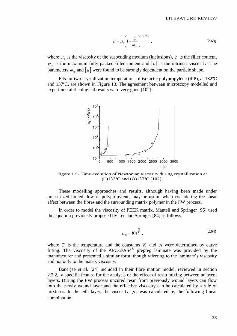
LITERATURE REVIEW
33
m
m
s
1 , (2.63)
where s is the viscosity of the suspending medium (inclusions), is the filler content,
m is the maximum fully packed filler content and is the intrinsic viscosity. The
parameters m and were found to be strongly dependent on the particle shape.
Fits for two crystallization temperatures of isotactic polypropylene (iPP), at 132ºC
and 137ºC, are shown in Figure 13. The agreement between microscopy modelled and
experimental rheological results were very good [102].
Figure 13 - Time evolution of Newtonian viscosity during crystallization at
()132ºC and (Ο)137ºC [102].
These modelling approaches and results, although having been made under
pressurized forced flow of polypropylene, may be useful when considering the shear
effect between the fibres and the surrounding matrix polymer in the FW process.
In order to model the viscosity of PEEK matrix, Mantell and Springer [95] used
the equation previously proposed by Lee and Springer [84] as follows:
T
A
m eK , (2.64)
where T is the temperature and the constants K and A were determined by curve
fitting. The viscosity of the APC-2/AS4®
prepreg laminate was provided by the
manufacturer and presented a similar form, though referring to the laminate’s viscosity
and not only to the matrix viscosity.
Banerjee et al. [24] included in their fibre motion model, reviewed in section
2.2.2, a specific feature for the analysis of the effect of resin mixing between adjacent
layers. During the FW process uncured resin from previously wound layers can flow
into the newly wound layer and the effective viscosity can be calculated by a rule of
mixtures. In the mth layer, the viscosity, , was calculated by the following linear
combination:
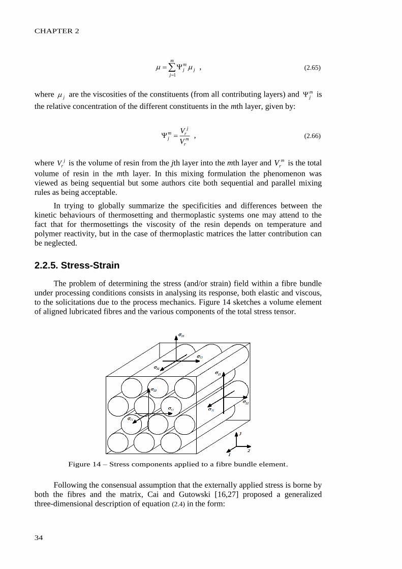
CHAPTER 2
34
m
jj
mj
1
, (2.65)
where j are the viscosities of the constituents (from all contributing layers) and mj is
the relative concentration of the different constituents in the mth layer, given by:
mr
jrm
jV
V , (2.66)
where jrV is the volume of resin from the jth layer into the mth layer and m
rV is the total
volume of resin in the mth layer. In this mixing formulation the phenomenon was
viewed as being sequential but some authors cite both sequential and parallel mixing
rules as being acceptable.
In trying to globally summarize the specificities and differences between the
kinetic behaviours of thermosetting and thermoplastic systems one may attend to the
fact that for thermosettings the viscosity of the resin depends on temperature and
polymer reactivity, but in the case of thermoplastic matrices the latter contribution can
be neglected.
2.2.5. Stress-Strain
The problem of determining the stress (and/or strain) field within a fibre bundle
under processing conditions consists in analysing its response, both elastic and viscous,
to the solicitations due to the process mechanics. Figure 14 sketches a volume element
of aligned lubricated fibres and the various components of the total stress tensor.
Figure 14 – Stress components applied to a fibre bundle element.
Following the consensual assumption that the externally applied stress is borne by
both the fibres and the matrix, Cai and Gutowski [16,27] proposed a generalized
three-dimensional description of equation (2.4) in the form:
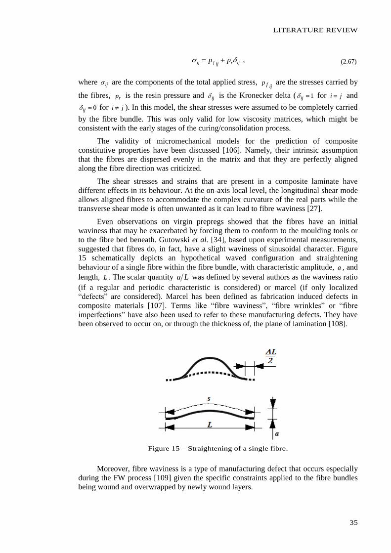
LITERATURE REVIEW
35
ijrijfij pp , (2.67)
where ij are the components of the total applied stress, ijfp are the stresses carried by
the fibres, rp is the resin pressure and ij is the Kronecker delta ( 1ij for ji and
0ij for ji ). In this model, the shear stresses were assumed to be completely carried
by the fibre bundle. This was only valid for low viscosity matrices, which might be
consistent with the early stages of the curing/consolidation process.
The validity of micromechanical models for the prediction of composite
constitutive properties have been discussed [106]. Namely, their intrinsic assumption
that the fibres are dispersed evenly in the matrix and that they are perfectly aligned
along the fibre direction was criticized.
The shear stresses and strains that are present in a composite laminate have
different effects in its behaviour. At the on-axis local level, the longitudinal shear mode
allows aligned fibres to accommodate the complex curvature of the real parts while the
transverse shear mode is often unwanted as it can lead to fibre waviness [27].
Even observations on virgin prepregs showed that the fibres have an initial
waviness that may be exacerbated by forcing them to conform to the moulding tools or
to the fibre bed beneath. Gutowski et al. [34], based upon experimental measurements,
suggested that fibres do, in fact, have a slight waviness of sinusoidal character. Figure
15 schematically depicts an hypothetical waved configuration and straightening
behaviour of a single fibre within the fibre bundle, with characteristic amplitude, a , and
length, L . The scalar quantity La was defined by several authors as the waviness ratio
(if a regular and periodic characteristic is considered) or marcel (if only localized
“defects” are considered). Marcel has been defined as fabrication induced defects in
composite materials [107]. Terms like “fibre waviness”, “fibre wrinkles” or “fibre
imperfections” have also been used to refer to these manufacturing defects. They have
been observed to occur on, or through the thickness of, the plane of lamination [108].
Figure 15 – Straightening of a single fibre.
Moreover, fibre waviness is a type of manufacturing defect that occurs especially
during the FW process [109] given the specific constraints applied to the fibre bundles
being wound and overwrapped by newly wound layers.
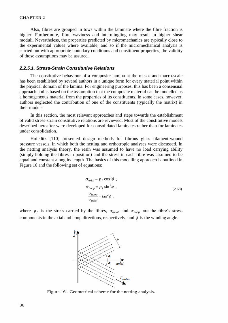
CHAPTER 2
36
Also, fibres are grouped in tows within the laminate where the fibre fraction is
higher. Furthermore, fibre waviness and intermingling may result in higher shear
moduli. Nevertheless, the properties predicted by micromechanics are typically close to
the experimental values where available, and so if the micromechanical analysis is
carried out with appropriate boundary conditions and constituent properties, the validity
of those assumptions may be assured.
2.2.5.1. Stress-Strain Constitutive Relations
The constitutive behaviour of a composite lamina at the meso- and macro-scale
has been established by several authors in a unique form for every material point within
the physical domain of the lamina. For engineering purposes, this has been a consensual
approach and is based on the assumption that the composite material can be modelled as
a homogeneous material from the properties of its constituents. In some cases, however,
authors neglected the contribution of one of the constituents (typically the matrix) in
their models.
In this section, the most relevant approaches and steps towards the establishment
of valid stress-strain constitutive relations are reviewed. Most of the constitutive models
described hereafter were developed for consolidated laminates rather than for laminates
under consolidation.
Hofeditz [110] presented design methods for fibrous glass filament-wound
pressure vessels, in which both the netting and orthotropic analyses were discussed. In
the netting analysis theory, the resin was assumed to have no load carrying ability
(simply holding the fibres in position) and the stress in each fibre was assumed to be
equal and constant along its length. The basics of this modelling approach is outlined in
Figure 16 and the following set of equations:
2cosfaxial p ,
2sinfhoop p ,
2tanaxial
hoop ,
(2.68)
where fp is the stress carried by the fibres, axial and hoop are the fibre’s stress
components in the axial and hoop directions, respectively, and is the winding angle.
Figure 16 - Geometrical scheme for the netting analysis.
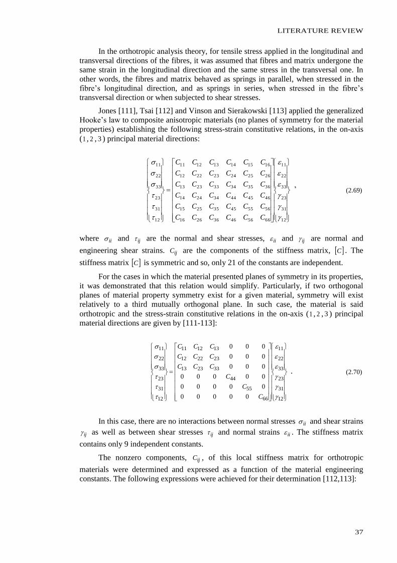
LITERATURE REVIEW
37
In the orthotropic analysis theory, for tensile stress applied in the longitudinal and
transversal directions of the fibres, it was assumed that fibres and matrix undergone the
same strain in the longitudinal direction and the same stress in the transversal one. In
other words, the fibres and matrix behaved as springs in parallel, when stressed in the
fibre’s longitudinal direction, and as springs in series, when stressed in the fibre’s
transversal direction or when subjected to shear stresses.
Jones [111], Tsai [112] and Vinson and Sierakowski [113] applied the generalized
Hooke’s law to composite anisotropic materials (no planes of symmetry for the material
properties) establishing the following stress-strain constitutive relations, in the on-axis
(1 , 2 , 3 ) principal material directions:
12
31
23
33
22
11
665646362616
565545352515
464544342414
363534332313
262524232212
161514131211
12
31
23
33
22
11
CCCCCC
CCCCCC
CCCCCC
CCCCCC
CCCCCC
CCCCCC
’ (2.69)
where ii and ij are the normal and shear stresses, ii and ij are normal and
engineering shear strains. ijC are the components of the stiffness matrix, C . The
stiffness matrix C is symmetric and so, only 21 of the constants are independent.
For the cases in which the material presented planes of symmetry in its properties,
it was demonstrated that this relation would simplify. Particularly, if two orthogonal
planes of material property symmetry exist for a given material, symmetry will exist
relatively to a third mutually orthogonal plane. In such case, the material is said
orthotropic and the stress-strain constitutive relations in the on-axis (1 , 2 , 3 ) principal
material directions are given by [111-113]:
12
31
23
33
22
11
66
55
44
332313
232212
131211
12
31
23
33
22
11
00000
00000
00000
000
000
000
C
C
C
CCC
CCC
CCC
. (2.70)
In this case, there are no interactions between normal stresses ii and shear strains
ij as well as between shear stresses ij and normal strains ii . The stiffness matrix
contains only 9 independent constants.
The nonzero components, ijC , of this local stiffness matrix for orthotropic
materials were determined and expressed as a function of the material engineering
constants. The following expressions were achieved for their determination [112,113]:
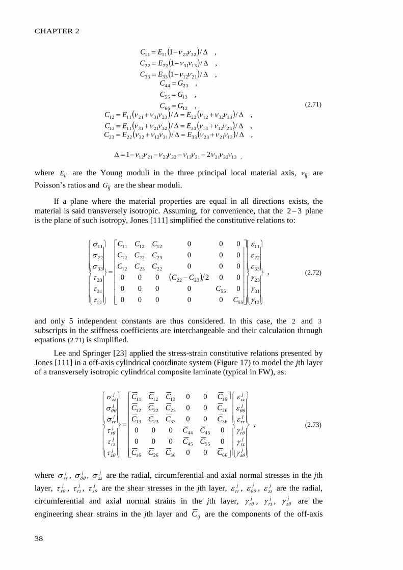
CHAPTER 2
38
,133221311332232112
132123333112322223
231213333221311113
133212222331211112
1266
1355
2344
21123333
13312222
32231111
21
,//
,//
,//
,
,
,
,/1
,/1
,/1
EEC
EEC
EEC
GC
GC
GC
EC
EC
EC
(2.71)
where iiE are the Young moduli in the three principal local material axis, ij are
Poisson’s ratios and ijG are the shear moduli.
If a plane where the material properties are equal in all directions exists, the
material is said transversely isotropic. Assuming, for convenience, that the 32 plane
is the plane of such isotropy, Jones [111] simplified the constitutive relations to:
12
31
23
33
22
11
55
55
2322
222312
232212
121211
12
31
23
33
22
11
00000
00000
002000
000
000
000
C
C
CC
CCC
CCC
CCC
, (2.72)
and only 5 independent constants are thus considered. In this case, the 2 and 3
subscripts in the stiffness coefficients are interchangeable and their calculation through
equations (2.71) is simplified.
Lee and Springer [23] applied the stress-strain constitutive relations presented by
Jones [111] in a off-axis cylindrical coordinate system (Figure 17) to model the jth layer
of a transversely isotropic cylindrical composite laminate (typical in FW), as:
jz
jrz
jr
jrr
j
jzz
jz
jrz
jr
jrr
j
jzz
CCCC
CC
CC
CCCC
CCCC
CCCC
66362616
5545
4544
36332313
26232212
16131211
00
0000
0000
00
00
00
, (2.73)
where j
rr , j
, j
zz are the radial, circumferential and axial normal stresses in the jth
layer, j
r , j
rz , j
z are the shear stresses in the jth layer, j
rr , j
, j
zz are the radial,
circumferential and axial normal strains in the jth layer, j
r , j
rz , j
z are the
engineering shear strains in the jth layer and ijC are the components of the off-axis
LITERATURE REVIEW
39
( z , , r ) stiffness matrix for the jth layer. ijC are calculated from ijC using the proper
(1 , 2 , 3 )-( z , , r ) transformation.
Assuming transverse isotropy in the 32 plane, Cai and Gutowski [27]
developed a local stress-strain constitutive relationship for a lubricated fibre bundle
where only two material directions are considered, the longitudinal (parallel to the
fibres) and the bulk (any direction in the 32 plane). Their empirical formulation was
developed under the main assumptions that
the aligned fibre bundles behaved as nonlinear elastic, porous networks
with no shear strength in the 32 plane,
the fibres had a slight waviness of sinusoidal character and made multiple
contacts between them,
the relevant quantities appearing in the 32 plane could be reduced to one
single transverse equivalent quantity Y (denoted by bY where the
subscript b referred to “bulk”),
the fibres were lubricated but in drained state,
and allowed to include directly the fibre volume fraction, fV , in the constitutive matrix.
It can be expressed as [27]:
,
45
13
54
141
1116
1
141
1
116
12
31
2
1
1112121
12114
1
0
5
4
4
00
0
3
2
2
3
0
3
2
2
3
00
0
2
1
bb
b
fa
f
f
a
f
a
f
fa
f
a
f
af
f
a
f
a
f
f
a
f
a
f
f
a
f
a
f
f
f
a
f
af
f
af
f
a
f
a
f
a
f
a
f
bb
b
V
V
V
V
V
V
V
V
aE
L
V
V
V
V
V
V
V
V
V
V
V
V
V
V
aE
L
V
V
V
V
V
V
V
V
V
V
aE
L
V
V
V
V
V
V
V
V
V
V
V
V
V
V
V
V
V
V
V
V
E
(2.74)
where b1 , b
b , b1 , b
b are the local (on-axis) strains and stresses in the 1 and b
directions, respectively. aV is the maximum available fibre volume fraction at which the
resin flow is not possible, 0V is the minimum volume fraction of fibres below which
fibres do not carry transverse load, aL is the ratio between the characteristic
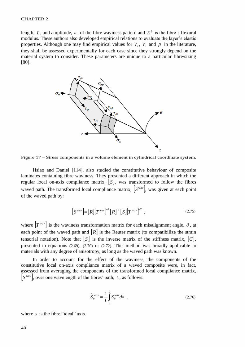
CHAPTER 2
40
length, L , and amplitude, a , of the fibre waviness pattern and fE is the fibre’s flexural
modulus. These authors also developed empirical relations to evaluate the layer’s elastic
properties. Although one may find empirical values for aV , 0V and in the literature,
they shall be assessed experimentally for each case since they strongly depend on the
material system to consider. These parameters are unique to a particular fibre/sizing
[80].
Figure 17 – Stress components in a volume element in cylindrical coordinate system.
Hsiao and Daniel [114], also studied the constitutive behaviour of composite
laminates containing fibre waviness. They presented a different approach in which the
regular local on-axis compliance matrix, S , was transformed to follow the fibres
waved path. The transformed local compliance matrix, wavS , was given at each point
of the waved path by:
Twavwavwav TSRTRS
11
, (2.75)
where wavT is the waviness transformation matrix for each misalignment angle, , at
each point of the waved path and R is the Reuter matrix (to compatibilize the strain
tensorial notation). Note that S is the inverse matrix of the stiffness matrix, C ,
presented in equations (2.69), (2.70) or (2.72). This method was broadly applicable to
materials with any degree of anisotropy, as long as the waved path was known.
In order to account for the effect of the waviness, the components of the
constitutive local on-axis compliance matrix of a waved composite were, in fact,
assessed from averaging the components of the transformed local compliance matrix,
wavS , over one wavelength of the fibres’ path, L , as follows:
L
wav
ij
wav
ij dxSL
S0
1~ , (2.76)
where x is the fibre “ideal” axis.
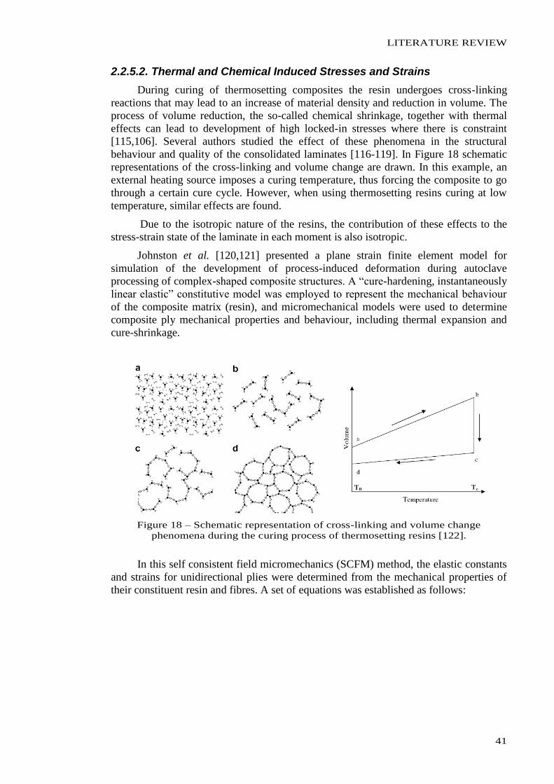
LITERATURE REVIEW
41
2.2.5.2. Thermal and Chemical Induced Stresses and Strains
During curing of thermosetting composites the resin undergoes cross-linking
reactions that may lead to an increase of material density and reduction in volume. The
process of volume reduction, the so-called chemical shrinkage, together with thermal
effects can lead to development of high locked-in stresses where there is constraint
[115,106]. Several authors studied the effect of these phenomena in the structural
behaviour and quality of the consolidated laminates [116-119]. In Figure 18 schematic
representations of the cross-linking and volume change are drawn. In this example, an
external heating source imposes a curing temperature, thus forcing the composite to go
through a certain cure cycle. However, when using thermosetting resins curing at low
temperature, similar effects are found.
Due to the isotropic nature of the resins, the contribution of these effects to the
stress-strain state of the laminate in each moment is also isotropic.
Johnston et al. [120,121] presented a plane strain finite element model for
simulation of the development of process-induced deformation during autoclave
processing of complex-shaped composite structures. A “cure-hardening, instantaneously
linear elastic” constitutive model was employed to represent the mechanical behaviour
of the composite matrix (resin), and micromechanical models were used to determine
composite ply mechanical properties and behaviour, including thermal expansion and
cure-shrinkage.
Figure 18 – Schematic representation of cross-linking and volume change
phenomena during the curing process of thermosetting resins [122].
In this self consistent field micromechanics (SCFM) method, the elastic constants
and strains for unidirectional plies were determined from the mechanical properties of
their constituent resin and fibres. A set of equations was established as follows:
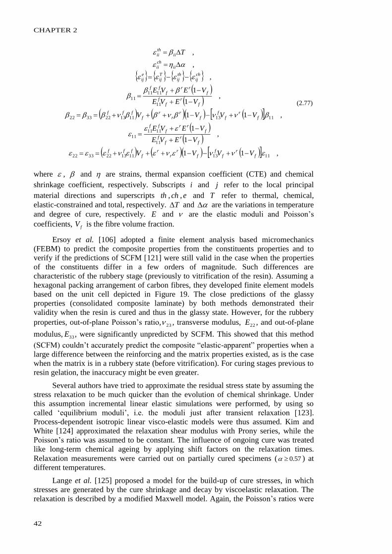
CHAPTER 2
42
,11
,1
1
,11
,1
1
,
,
,
11131113223322
11
1111
11
11131113223322
11
1111
11
fr
ff
fr
rr
ffff
fr
ff
frr
fff
fr
ff
fr
rr
ffff
fr
ff
frr
fff
chij
thij
Tij
eij
iichii
iithii
VVVV
VEVE
VEVE
VVVV
VEVE
VEVE
T
(2.77)
where , and are strains, thermal expansion coefficient (CTE) and chemical
shrinkage coefficient, respectively. Subscripts i and j refer to the local principal
material directions and superscripts th , ch , e and T refer to thermal, chemical,
elastic-constrained and total, respectively. T and are the variations in temperature
and degree of cure, respectively. E and are the elastic moduli and Poisson’s
coefficients, fV is the fibre volume fraction.
Ersoy et al. [106] adopted a finite element analysis based micromechanics
(FEBM) to predict the composite properties from the constituents properties and to
verify if the predictions of SCFM [121] were still valid in the case when the properties
of the constituents differ in a few orders of magnitude. Such differences are
characteristic of the rubbery stage (previously to vitrification of the resin). Assuming a
hexagonal packing arrangement of carbon fibres, they developed finite element models
based on the unit cell depicted in Figure 19. The close predictions of the glassy
properties (consolidated composite laminate) by both methods demonstrated their
validity when the resin is cured and thus in the glassy state. However, for the rubbery
properties, out-of-plane Poisson’s ratio, 23 , transverse modulus, 22E , and out-of-plane
modulus, 33E , were significantly unpredicted by SCFM. This showed that this method
(SCFM) couldn’t accurately predict the composite “elastic-apparent” properties when a
large difference between the reinforcing and the matrix properties existed, as is the case
when the matrix is in a rubbery state (before vitrification). For curing stages previous to
resin gelation, the inaccuracy might be even greater.
Several authors have tried to approximate the residual stress state by assuming the
stress relaxation to be much quicker than the evolution of chemical shrinkage. Under
this assumption incremental linear elastic simulations were performed, by using so
called ‘equilibrium moduli’, i.e. the moduli just after transient relaxation [123].
Process-dependent isotropic linear visco-elastic models were thus assumed. Kim and
White [124] approximated the relaxation shear modulus with Prony series, while the
Poisson’s ratio was assumed to be constant. The influence of ongoing cure was treated
like long-term chemical ageing by applying shift factors on the relaxation times.
Relaxation measurements were carried out on partially cured specimens ( 57.0 ) at
different temperatures.
Lange et al. [125] proposed a model for the build-up of cure stresses, in which
stresses are generated by the cure shrinkage and decay by viscoelastic relaxation. The
relaxation is described by a modified Maxwell model. Again, the Poisson’s ratios were
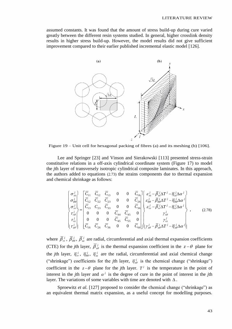
LITERATURE REVIEW
43
assumed constants. It was found that the amount of stress build-up during cure varied
greatly between the different resin systems studied. In general, higher crosslink density
results in higher stress build-up. However, the model results did not give sufficient
improvement compared to their earlier published incremental elastic model [126].
Figure 19 – Unit cell for hexagonal packing of fibres (a) and its meshing (b) [106].
Lee and Springer [23] and Vinson and Sierakowski [113] presented stress-strain
constitutive relations in a off-axis cylindrical coordinate system (Figure 17) to model
the jth layer of transversely isotropic cylindrical composite laminates. In this approach,
the authors added to equations (2.73) the strains components due to thermal expansion
and chemical shrinkage as follows:
jjz
jjz
jz
jrz
jr
jjrr
jjrr
jrr
jjjjj
jjzz
jjzz
jzz
jz
jrz
jr
jrr
j
jzz
T
T
T
T
CCCC
CC
CC
CCCC
CCCC
CCCC
66362616
5545
4544
36332313
26232212
16131211
00
0000
0000
00
00
00
, (2.78)
where j
rr , j
, j
zz are radial, circumferential and axial thermal expansion coefficients
(CTE) for the jth layer, j
z is the thermal expansion coefficient in the z plane for
the jth layer, jrr , j
, jzz are the radial, circumferential and axial chemical change
(“shrinkage”) coefficients for the jth layer, jz is the chemical change (“shrinkage”)
coefficient in the z plane for the jth layer. jT is the temperature in the point of
interest in the jth layer and j is the degree of cure in the point of interest in the jth
layer. The variations of some variables with time are denoted with .
Sproewitz et al. [127] proposed to consider the chemical change (“shrinkage”) as
an equivalent thermal matrix expansion, as a useful concept for modelling purposes.
CHAPTER 2
44
The equivalent CTE, eqCTE , was defined as the sum of thermal and chemical expansion
according to the following relation:
T
VCTEeq
3 , (2.79)
where is the thermal expansion coefficient, is the chemical change (“shrinkage”)
coefficient, V is the volumetric shrinkage and T is the temperature difference
between curing and room temperature. The volumetric isotropic nature of these
coefficients suggested that in equation jz
jzz
jjrr and j
zj
zzjj
rr .
2.2.6. Global Process Models
One- and two-dimensional resin flow/fibre compaction process models have been
developed in the last three decades. Most of the studies were not specifically dedicated
to the FW process. Nevertheless, their assumptions, modelling strategies and specific
features are of great interest in gathering the sense and knowledge to develop this
multi-physical process model, since many of the interacting phenomena are common to
several of these manufacturing processes. Three-dimensional approaches are much less
available in the literature, mainly due to the orthotropic and thin-walled characteristics
of most of the composite applications.
In the past, two well-established flow/compaction models were developed and
published. They were named the squeezed sponge (sometimes referred as the effective
stress model) and sequential compaction models, respectively. Although the sequential
and the squeezed sponge (effective stress) models based on different assumptions, they
predicted essentially the same results in the regime when the fibre bed carries no load
[37]. In the next sections, these two models are reviewed.
2.2.6.1. Sequential Compaction Model
Lee and Springer [23] presented a process model for FW of composite cylinders
with thermosetting resin systems. The model related the significant process variables,
such as
the winding speed,
the initial fibre tension (winding force),
the winding angle, and
the applied temperature,
to the thermal, chemical and mechanical behaviour of the composite cylinder and the
mandrel. Based on Loos and Springer previous work for flat laminates [49] and Calius
and Springer for thin cylinders [79], this study focused on relatively thick cylinders. A
user-friendly code (WINDTHICK®
) was written and used to calculate
the temperature in the cylinder and the mandrel,
the degree of cure and viscosity in the cylinder,
the viscosity through the cylinder,
the fibre tensions and positions,
the stresses and strains throughout the cylinder and in the mandrel, and
LITERATURE REVIEW
45
the void diameters in the cylinder.
The model was developed in five parts (sub-models):
the thermo-chemical sub-model
o outputs: temperature, degree of cure and viscosity,
the fibre motion sub-model
o outputs: radial fibre position,
the stress-strain sub-model
o outputs: stresses and strains in composite laminate,
the void growth sub-model
o outputs: size of a void at a given location as function of time,
the strength sub-model
o outputs: strength of the composite cylinder.
The thermo-chemical sub-model was based on the energy equation for the
two-dimensional heat flow, written in the form:
Qz
Tk
zr
Trk
rrt
TC zr
1 , (2.80)
where is the density, C is the specific heat of the composite or the mandrel, T is the
temperature, t is time, r and z are the radial and axial coordinates, rk and zk are the
thermal conductivities in the r and z directions and Q is the rate at which heat is
generated or absorbed by chemical reactions.
Since chemical reactions occurred only in the matrix, i.e., no heat generation or
absorption was attributed to the fibres nor to the mandrel, the last term of the energy
equation was re-written as:
m
mm QVQ , (2.81)
where m , mV and mQ are the density, volume fraction and heat generation rate of the
matrix, respectively.
Following previous works [49,82] the heating rate was assumed to be a function
of the degree of cure (or its rate), and the energy equation, for composites with
non-reacting fibres, became:
dt
dHV
z
Tk
zr
Trk
rrt
TC um
mzr
1 , (2.82)
where uH is the total heat of reaction and dt
d is the rate of degree of cure.
As discussed in section 2.2.4 several empirical expressions, relating dt
d to the
degree of cure, , and time, t , were established in the literature for several commercial
thermosetting resin systems [49,78,82,85-93,128-131]. Most of these studies also
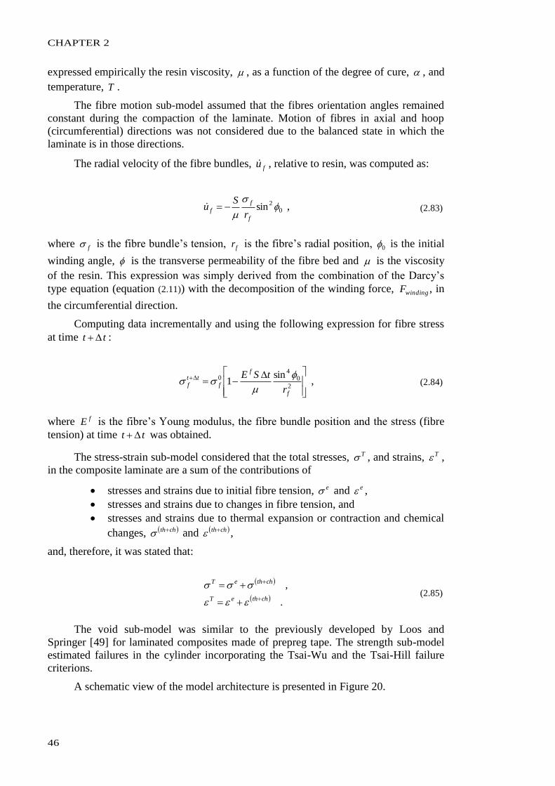
CHAPTER 2
46
expressed empirically the resin viscosity, , as a function of the degree of cure, , and
temperature, T .
The fibre motion sub-model assumed that the fibres orientation angles remained
constant during the compaction of the laminate. Motion of fibres in axial and hoop
(circumferential) directions was not considered due to the balanced state in which the
laminate is in those directions.
The radial velocity of the fibre bundles, fu , relative to resin, was computed as:
02sin
f
f
fr
Su , (2.83)
where f is the fibre bundle’s tension, fr is the fibre’s radial position, 0 is the initial
winding angle, is the transverse permeability of the fibre bed and is the viscosity
of the resin. This expression was simply derived from the combination of the Darcy’s
type equation (equation (2.11)) with the decomposition of the winding force, windingF , in
the circumferential direction.
Computing data incrementally and using the following expression for fibre stress
at time tt :
2
04
0 sin1
f
f
ftt
fr
tSE
, (2.84)
where fE is the fibre’s Young modulus, the fibre bundle position and the stress (fibre
tension) at time tt was obtained.
The stress-strain sub-model considered that the total stresses, T , and strains, T ,
in the composite laminate are a sum of the contributions of
stresses and strains due to initial fibre tension, e and e ,
stresses and strains due to changes in fibre tension, and
stresses and strains due to thermal expansion or contraction and chemical
changes, chth and chth ,
and, therefore, it was stated that:
.
,
chtheT
chtheT
(2.85)
The void sub-model was similar to the previously developed by Loos and
Springer [49] for laminated composites made of prepreg tape. The strength sub-model
estimated failures in the cylinder incorporating the Tsai-Wu and the Tsai-Hill failure
criterions.
A schematic view of the model architecture is presented in Figure 20.
LITERATURE REVIEW
47
Figure 20 - Outputs provided by the WINDTHICK
® code [2].
2.2.6.2. Squeezed Sponge Model
Based on experimental data on compaction of fibre beds, Gutowski et al. [26]
applied the effective stress (squeeze sponge) theory to the consolidation of composites
during cure. This theory formulation stated that at any point in the laminate the stress
was borne by both the fibres and the resin, accordingly with equation (2.4).
Given the continuity equation:
z
pk
zr
pk
rt
rz
rr
, (2.86)
where is the fibre bed porosity fV1 , rp is the resin pressure, is the resin
viscosity and rk and zk are the specific permeabilities of the fibre bed in the r and z
directions, respectively, Dave et al. [29,30] and Gutowski et al. [47] presented solutions
for their laminate consolidation models by solving it together with the stress equilibrium
equation (equation (2.4)). An important aspect of equation (2.86) was that it accounted for
resin mass loss due to resin flow out of the laminate. It also assumed that the fibre bed
was fully saturated, i.e., no voids were considered.
A key feature of Gutowski’s modelling approach for consolidation in FW of
cylinders, was that it included the elastic deformation of the fibre bundle. In [16] two
different cases (both typical in FW) were discussed. In one case, the resin flow time was
short compared to the winding time. Hence, the fibre distribution and other important
parameters were determined almost solely by the fibre deformation behaviour. In the
other case, the resin flow time was long compared to the winding time. Here, a
quasi-elastic analysis was used to determine the fibre distribution and stresses during
winding. These conditions were then used as inputs for the consolidation process model.
The winding and consolidation process was sought as a dynamic process involving fibre
bundle deformation and fluid mass flow. This process model predicted the time history
of process variables, such as fluid pressure, fibre distribution and structural dimensions.
CHAPTER 2
48
2.2.6.3. Other Modelling Approaches
Spencer [132] established an analytical model to predict the resin cure state,
layers’ locations and residual stress state in orthotropic filament-wound composite
cylinders. The study was focused in thermosetting resins based composites and
axis-symmetric cylinders. His model was mainly divided into four sub-models:
composite layer stiffness, resin flow, cure kinetics and heat transfer, each modelling the
corresponding group of physical phenomena. Three stages of fabrication were
considered and analysed separately: winding, curing and mandrel removal. Simplifying
assumptions were made as follows:
all the resin properties rather than elastic modulus and viscosity remained
constant during the curing process;
the resin and fibres’ properties were independent of the stress level;
as the plies were wound, the contribution of the resin to the stiffness and
pressure build-up were negligible;
the coefficients of thermal expansion (CTE) of the laminate were
considered linear and constants over the processing temperature range;
the shear stresses z in each ply ( ) were assumed to be equal and
opposite, producing negligible shear strain z ;
rzjiEE j
ji
i
ij,,,,
;
From the classical orthotropic stress-strain constitutive relationship as defined in
[23,113], considering the abovementioned assumptions, Spencer deduced the following
constitutive relationship for each layer expressed in cylindrical coordinates:
T
T
T
EEE
EEE
EEE
zz
rr
zz
rr
zzrrz
zzrr
zzrrr
zz
rr
1
1
1
, (2.87)
where ii and ii are the normal strains and stresses in the referred layer, iE are the
elastic modulus of the referred layer, ij are the Poisson’s ratios, ii are the linear CTE
and T is the temperature.
The changes in the fibre tension due to radial and axial displacements of the fibres
were defined as:
ffb
winding
fbz
fb
fbr
winding
EA
F
Z
u
r
u
F
cos2
, (2.88)
where windingF is the winding tension, fbru and fb
zu are the radial and axial displacements
of the fibre bundle, fbr is its radial position, Z is the length of the composite cylinder
being wound, fbA is the cross-sectional area of the fibre bundle, fE is the fibre elastic
LITERATURE REVIEW
49
modulus and is the winding angle. The calculation of the resin modulus, rE , in each
moment during cure was made by assuming its proportionality to the viscosity, , as:
rE , (2.89)
Using the easily known values for rE and in the fully cured state, and assuming that
at the initial state of cure both values are zero, the proportionality is easy applied. This
assumption was based on previous indicative results presented by Maximovich and
Galeos [133]. The resin flow, the resin kinetics and the heat transfer modelling
approaches were developed in a similar way of the ones discussed in previous sections
of this text.
Ikonomopoulos and Marchetti [134] coded a process model for the FW process,
based on the analytical descriptions of Lee and Springer [23]. The architecture of their
model accounted for six sub-models: (1) fibre motion, (2) heat transmission, (3)
chemical kinetic, (4) rheological, (5) winding stress-strain and (6) thermo-chemical
stress-strain. Olofsson [135,136] also presented a numerical code to predict the
temperature and stresses in filament-wound composite cylinders during the
manufacturing stage. Again, this work was based on previous models published by Lee
and Springer [23].
Hubert and Poursartip [37] provided a comprehensive review of flow and
compaction models for thermosetting matrix composites during curing. They divided
the review into the resin behaviour during cure, the fibre bed behaviour, and the flow-
compaction models.
Darcy’s type equation is the most used governing equation for analyze flow
through the laminate. However, Lindt [39] proposed a different approach to solve the
consolidation of composites using lubrication theory in his percolation flow model.
Lindt assumed the fibres to be straight parallel cylinders suspended in a viscous
incompressible fluid. From a force equilibrium involving drag and squeeze flow, the
motion of the fibre layers were calculated. This model predicts a symmetrical
consolidation from the laminate centre. Such behaviour has not been observed
experimentally.
Gutowski and co-workers [26,34] also described the compaction behaviour of
composite laminates (for autoclave processing) by applying the effective stress
formulation used in soil mechanics.
Loos and William [137] measured the resin flow from laminates with different ply
thicknesses, dimensions and ply-stacking sequences. They used the sequential model
and outputted that the ply-stacking sequence for flat laminates does not affect
significantly the total resin mass loss. Converting these results to wound laminates is
not straight forward.
Few models have been developed for FW process of thermoplastic-based
composites. Shih and Loos [138] and Toso et al. [139] studied the heat transfer of the
thermoplastic FW, considering a specific configuration of the process in which a gas
torch heats the fibres and resin immediately before the deposition onto the mandrel
surface. Song [140] modelled the heat transfer, the crystallization and the consolidation
of this process configuration using the finite element method (FEM). The theoretical
background supporting these models is the one previously discussed in section 2.2.4.
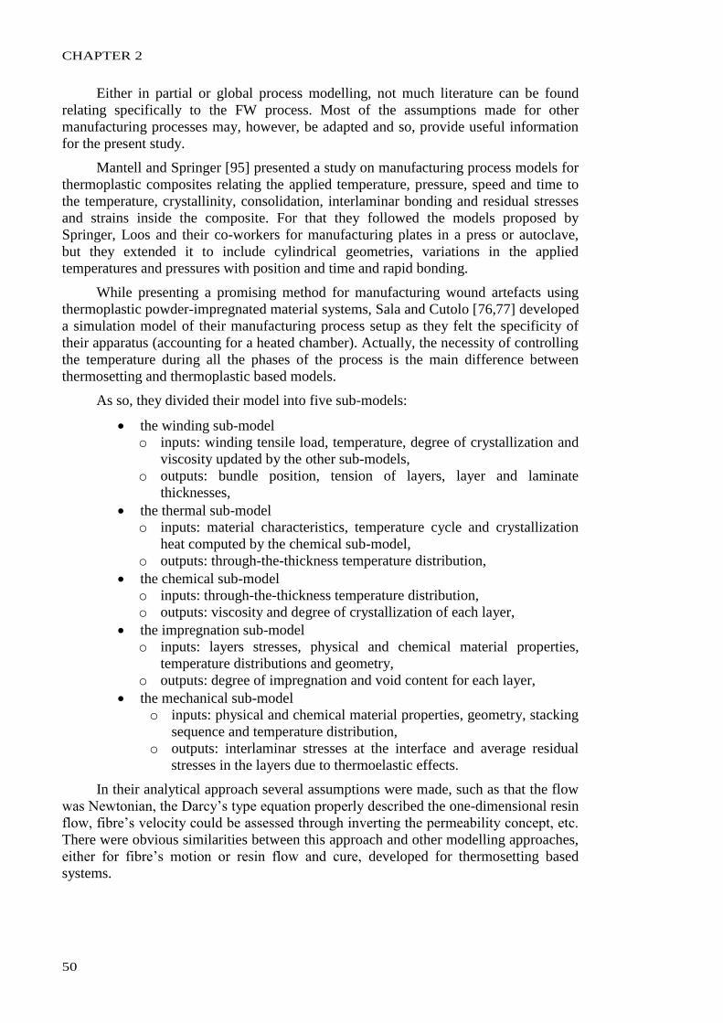
CHAPTER 2
50
Either in partial or global process modelling, not much literature can be found
relating specifically to the FW process. Most of the assumptions made for other
manufacturing processes may, however, be adapted and so, provide useful information
for the present study.
Mantell and Springer [95] presented a study on manufacturing process models for
thermoplastic composites relating the applied temperature, pressure, speed and time to
the temperature, crystallinity, consolidation, interlaminar bonding and residual stresses
and strains inside the composite. For that they followed the models proposed by
Springer, Loos and their co-workers for manufacturing plates in a press or autoclave,
but they extended it to include cylindrical geometries, variations in the applied
temperatures and pressures with position and time and rapid bonding.
While presenting a promising method for manufacturing wound artefacts using
thermoplastic powder-impregnated material systems, Sala and Cutolo [76,77] developed
a simulation model of their manufacturing process setup as they felt the specificity of
their apparatus (accounting for a heated chamber). Actually, the necessity of controlling
the temperature during all the phases of the process is the main difference between
thermosetting and thermoplastic based models.
As so, they divided their model into five sub-models:
the winding sub-model
o inputs: winding tensile load, temperature, degree of crystallization and
viscosity updated by the other sub-models,
o outputs: bundle position, tension of layers, layer and laminate
thicknesses,
the thermal sub-model
o inputs: material characteristics, temperature cycle and crystallization
heat computed by the chemical sub-model,
o outputs: through-the-thickness temperature distribution,
the chemical sub-model
o inputs: through-the-thickness temperature distribution,
o outputs: viscosity and degree of crystallization of each layer,
the impregnation sub-model
o inputs: layers stresses, physical and chemical material properties,
temperature distributions and geometry,
o outputs: degree of impregnation and void content for each layer,
the mechanical sub-model
o inputs: physical and chemical material properties, geometry, stacking
sequence and temperature distribution,
o outputs: interlaminar stresses at the interface and average residual
stresses in the layers due to thermoelastic effects.
In their analytical approach several assumptions were made, such as that the flow
was Newtonian, the Darcy’s type equation properly described the one-dimensional resin
flow, fibre’s velocity could be assessed through inverting the permeability concept, etc.
There were obvious similarities between this approach and other modelling approaches,
either for fibre’s motion or resin flow and cure, developed for thermosetting based
systems.
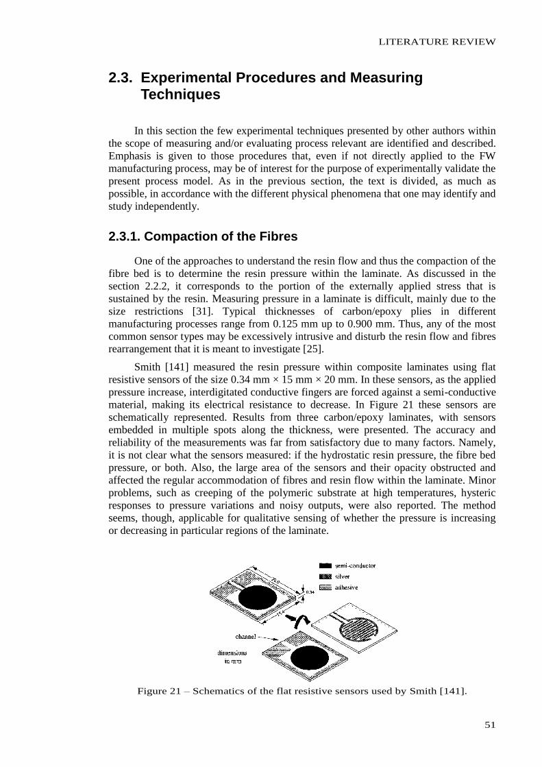
LITERATURE REVIEW
51
2.3. Experimental Procedures and Measuring Techniques
In this section the few experimental techniques presented by other authors within
the scope of measuring and/or evaluating process relevant are identified and described.
Emphasis is given to those procedures that, even if not directly applied to the FW
manufacturing process, may be of interest for the purpose of experimentally validate the
present process model. As in the previous section, the text is divided, as much as
possible, in accordance with the different physical phenomena that one may identify and
study independently.
2.3.1. Compaction of the Fibres
One of the approaches to understand the resin flow and thus the compaction of the
fibre bed is to determine the resin pressure within the laminate. As discussed in the
section 2.2.2, it corresponds to the portion of the externally applied stress that is
sustained by the resin. Measuring pressure in a laminate is difficult, mainly due to the
size restrictions [31]. Typical thicknesses of carbon/epoxy plies in different
manufacturing processes range from 0.125 mm up to 0.900 mm. Thus, any of the most
common sensor types may be excessively intrusive and disturb the resin flow and fibres
rearrangement that it is meant to investigate [25].
Smith [141] measured the resin pressure within composite laminates using flat
resistive sensors of the size 0.34 mm × 15 mm × 20 mm. In these sensors, as the applied
pressure increase, interdigitated conductive fingers are forced against a semi-conductive
material, making its electrical resistance to decrease. In Figure 21 these sensors are
schematically represented. Results from three carbon/epoxy laminates, with sensors
embedded in multiple spots along the thickness, were presented. The accuracy and
reliability of the measurements was far from satisfactory due to many factors. Namely,
it is not clear what the sensors measured: if the hydrostatic resin pressure, the fibre bed
pressure, or both. Also, the large area of the sensors and their opacity obstructed and
affected the regular accommodation of fibres and resin flow within the laminate. Minor
problems, such as creeping of the polymeric substrate at high temperatures, hysteric
responses to pressure variations and noisy outputs, were also reported. The method
seems, though, applicable for qualitative sensing of whether the pressure is increasing
or decreasing in particular regions of the laminate.
Figure 21 – Schematics of the flat resistive sensors used by Smith [141].
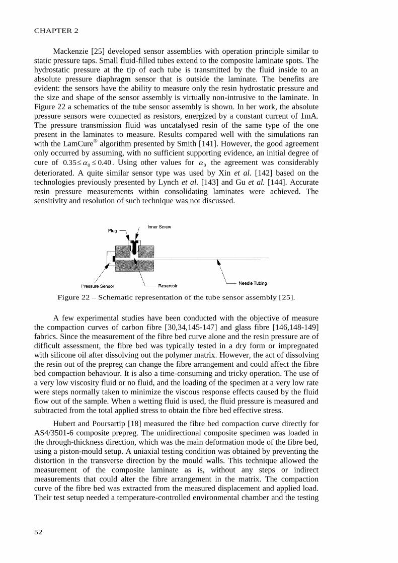
CHAPTER 2
52
Mackenzie [25] developed sensor assemblies with operation principle similar to
static pressure taps. Small fluid-filled tubes extend to the composite laminate spots. The
hydrostatic pressure at the tip of each tube is transmitted by the fluid inside to an
absolute pressure diaphragm sensor that is outside the laminate. The benefits are
evident: the sensors have the ability to measure only the resin hydrostatic pressure and
the size and shape of the sensor assembly is virtually non-intrusive to the laminate. In
Figure 22 a schematics of the tube sensor assembly is shown. In her work, the absolute
pressure sensors were connected as resistors, energized by a constant current of 1mA.
The pressure transmission fluid was uncatalysed resin of the same type of the one
present in the laminates to measure. Results compared well with the simulations ran
with the LamCure® algorithm presented by Smith [141]. However, the good agreement
only occurred by assuming, with no sufficient supporting evidence, an initial degree of
cure of 40.035.0 0 . Using other values for 0 the agreement was considerably
deteriorated. A quite similar sensor type was used by Xin et al. [142] based on the
technologies previously presented by Lynch et al. [143] and Gu et al. [144]. Accurate
resin pressure measurements within consolidating laminates were achieved. The
sensitivity and resolution of such technique was not discussed.
Figure 22 – Schematic representation of the tube sensor assembly [25].
A few experimental studies have been conducted with the objective of measure
the compaction curves of carbon fibre [30,34,145-147] and glass fibre [146,148-149]
fabrics. Since the measurement of the fibre bed curve alone and the resin pressure are of
difficult assessment, the fibre bed was typically tested in a dry form or impregnated
with silicone oil after dissolving out the polymer matrix. However, the act of dissolving
the resin out of the prepreg can change the fibre arrangement and could affect the fibre
bed compaction behaviour. It is also a time-consuming and tricky operation. The use of
a very low viscosity fluid or no fluid, and the loading of the specimen at a very low rate
were steps normally taken to minimize the viscous response effects caused by the fluid
flow out of the sample. When a wetting fluid is used, the fluid pressure is measured and
subtracted from the total applied stress to obtain the fibre bed effective stress.
Hubert and Poursartip [18] measured the fibre bed compaction curve directly for
AS4/3501-6 composite prepreg. The unidirectional composite specimen was loaded in
the through-thickness direction, which was the main deformation mode of the fibre bed,
using a piston-mould setup. A uniaxial testing condition was obtained by preventing the
distortion in the transverse direction by the mould walls. This technique allowed the
measurement of the composite laminate as is, without any steps or indirect
measurements that could alter the fibre arrangement in the matrix. The compaction
curve of the fibre bed was extracted from the measured displacement and applied load.
Their test setup needed a temperature-controlled environmental chamber and the testing
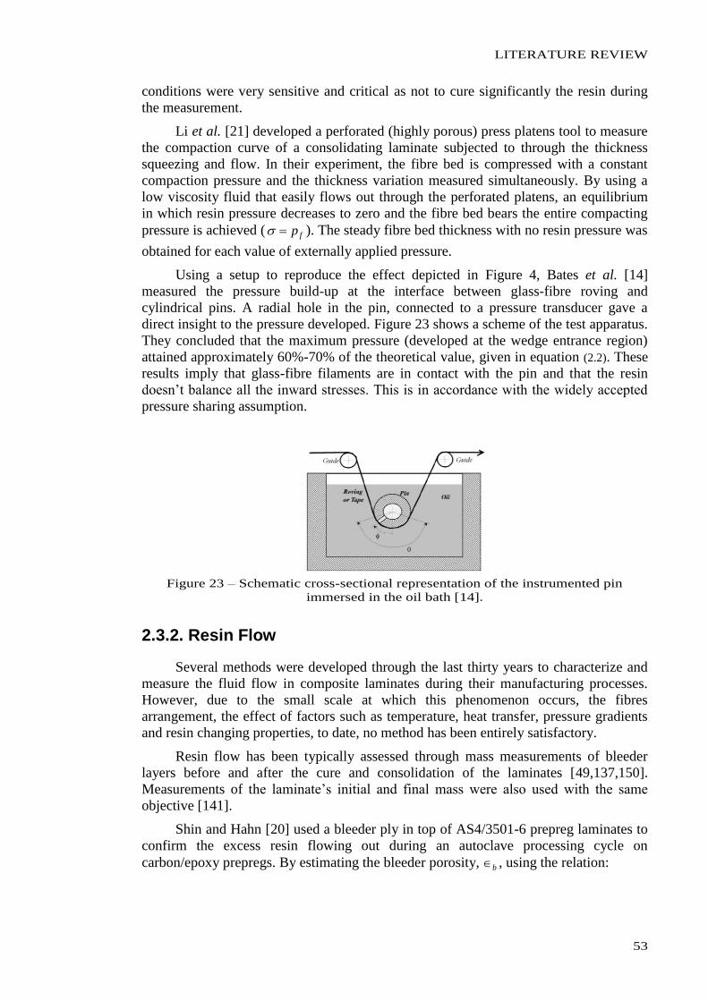
LITERATURE REVIEW
53
conditions were very sensitive and critical as not to cure significantly the resin during
the measurement.
Li et al. [21] developed a perforated (highly porous) press platens tool to measure
the compaction curve of a consolidating laminate subjected to through the thickness
squeezing and flow. In their experiment, the fibre bed is compressed with a constant
compaction pressure and the thickness variation measured simultaneously. By using a
low viscosity fluid that easily flows out through the perforated platens, an equilibrium
in which resin pressure decreases to zero and the fibre bed bears the entire compacting
pressure is achieved ( fp ). The steady fibre bed thickness with no resin pressure was
obtained for each value of externally applied pressure.
Using a setup to reproduce the effect depicted in Figure 4, Bates et al. [14]
measured the pressure build-up at the interface between glass-fibre roving and
cylindrical pins. A radial hole in the pin, connected to a pressure transducer gave a
direct insight to the pressure developed. Figure 23 shows a scheme of the test apparatus.
They concluded that the maximum pressure (developed at the wedge entrance region)
attained approximately 60%-70% of the theoretical value, given in equation (2.2). These
results imply that glass-fibre filaments are in contact with the pin and that the resin
doesn’t balance all the inward stresses. This is in accordance with the widely accepted
pressure sharing assumption.
Figure 23 – Schematic cross-sectional representation of the instrumented pin
immersed in the oil bath [14].
2.3.2. Resin Flow
Several methods were developed through the last thirty years to characterize and
measure the fluid flow in composite laminates during their manufacturing processes.
However, due to the small scale at which this phenomenon occurs, the fibres
arrangement, the effect of factors such as temperature, heat transfer, pressure gradients
and resin changing properties, to date, no method has been entirely satisfactory.
Resin flow has been typically assessed through mass measurements of bleeder
layers before and after the cure and consolidation of the laminates [49,137,150].
Measurements of the laminate’s initial and final mass were also used with the same
objective [141].
Shin and Hahn [20] used a bleeder ply in top of AS4/3501-6 prepreg laminates to
confirm the excess resin flowing out during an autoclave processing cycle on
carbon/epoxy prepregs. By estimating the bleeder porosity, b , using the relation:
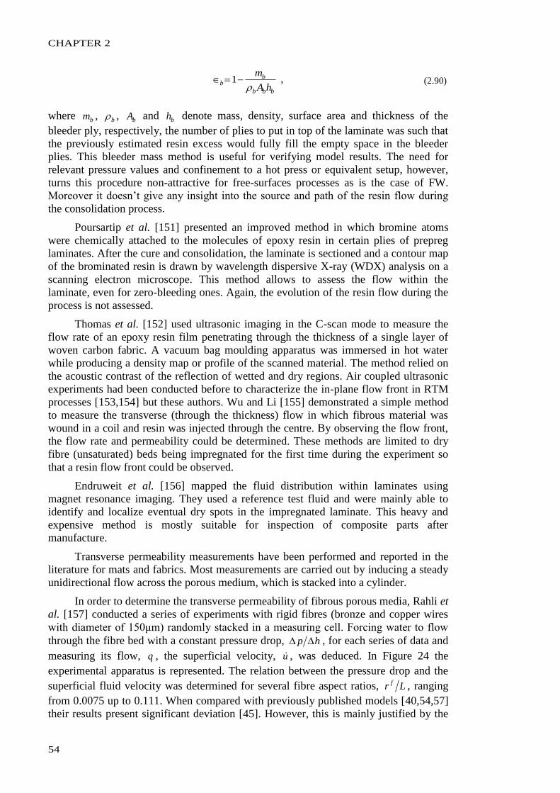
CHAPTER 2
54
bbb
bb
hA
m
1 , (2.90)
where bm , b , bA and bh denote mass, density, surface area and thickness of the
bleeder ply, respectively, the number of plies to put in top of the laminate was such that
the previously estimated resin excess would fully fill the empty space in the bleeder
plies. This bleeder mass method is useful for verifying model results. The need for
relevant pressure values and confinement to a hot press or equivalent setup, however,
turns this procedure non-attractive for free-surfaces processes as is the case of FW.
Moreover it doesn’t give any insight into the source and path of the resin flow during
the consolidation process.
Poursartip et al. [151] presented an improved method in which bromine atoms
were chemically attached to the molecules of epoxy resin in certain plies of prepreg
laminates. After the cure and consolidation, the laminate is sectioned and a contour map
of the brominated resin is drawn by wavelength dispersive X-ray (WDX) analysis on a
scanning electron microscope. This method allows to assess the flow within the
laminate, even for zero-bleeding ones. Again, the evolution of the resin flow during the
process is not assessed.
Thomas et al. [152] used ultrasonic imaging in the C-scan mode to measure the
flow rate of an epoxy resin film penetrating through the thickness of a single layer of
woven carbon fabric. A vacuum bag moulding apparatus was immersed in hot water
while producing a density map or profile of the scanned material. The method relied on
the acoustic contrast of the reflection of wetted and dry regions. Air coupled ultrasonic
experiments had been conducted before to characterize the in-plane flow front in RTM
processes [153,154] but these authors. Wu and Li [155] demonstrated a simple method
to measure the transverse (through the thickness) flow in which fibrous material was
wound in a coil and resin was injected through the centre. By observing the flow front,
the flow rate and permeability could be determined. These methods are limited to dry
fibre (unsaturated) beds being impregnated for the first time during the experiment so
that a resin flow front could be observed.
Endruweit et al. [156] mapped the fluid distribution within laminates using
magnet resonance imaging. They used a reference test fluid and were mainly able to
identify and localize eventual dry spots in the impregnated laminate. This heavy and
expensive method is mostly suitable for inspection of composite parts after
manufacture.
Transverse permeability measurements have been performed and reported in the
literature for mats and fabrics. Most measurements are carried out by inducing a steady
unidirectional flow across the porous medium, which is stacked into a cylinder.
In order to determine the transverse permeability of fibrous porous media, Rahli et
al. [157] conducted a series of experiments with rigid fibres (bronze and copper wires
with diameter of 150μm) randomly stacked in a measuring cell. Forcing water to flow
through the fibre bed with a constant pressure drop, hp , for each series of data and
measuring its flow, q , the superficial velocity, u , was deduced. In Figure 24 the
experimental apparatus is represented. The relation between the pressure drop and the
superficial fluid velocity was determined for several fibre aspect ratios, Lr f , ranging
from 0.0075 up to 0.111. When compared with previously published models [40,54,57]
their results present significant deviation [45]. However, this is mainly justified by the
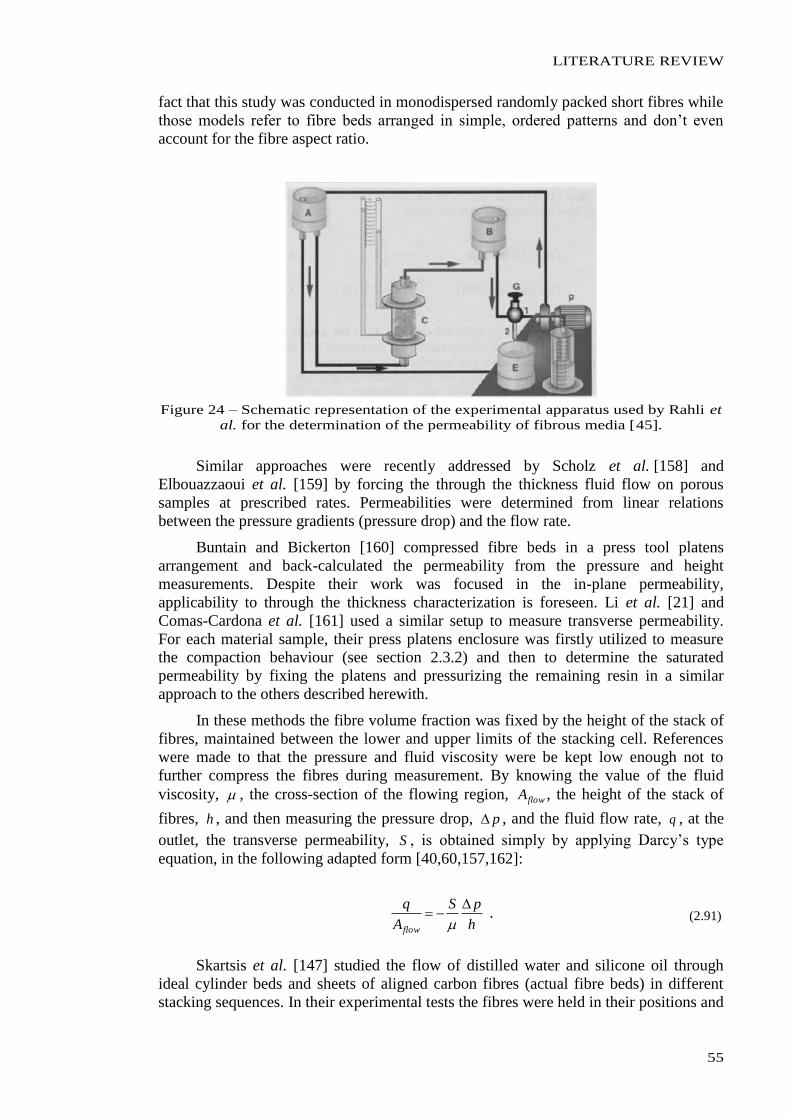
LITERATURE REVIEW
55
fact that this study was conducted in monodispersed randomly packed short fibres while
those models refer to fibre beds arranged in simple, ordered patterns and don’t even
account for the fibre aspect ratio.
Figure 24 – Schematic representation of the experimental apparatus used by Rahli et
al. for the determination of the permeability of fibrous media [45].
Similar approaches were recently addressed by Scholz et al. [158] and
Elbouazzaoui et al. [159] by forcing the through the thickness fluid flow on porous
samples at prescribed rates. Permeabilities were determined from linear relations
between the pressure gradients (pressure drop) and the flow rate.
Buntain and Bickerton [160] compressed fibre beds in a press tool platens
arrangement and back-calculated the permeability from the pressure and height
measurements. Despite their work was focused in the in-plane permeability,
applicability to through the thickness characterization is foreseen. Li et al. [21] and
Comas-Cardona et al. [161] used a similar setup to measure transverse permeability.
For each material sample, their press platens enclosure was firstly utilized to measure
the compaction behaviour (see section 2.3.2) and then to determine the saturated
permeability by fixing the platens and pressurizing the remaining resin in a similar
approach to the others described herewith.
In these methods the fibre volume fraction was fixed by the height of the stack of
fibres, maintained between the lower and upper limits of the stacking cell. References
were made to that the pressure and fluid viscosity were be kept low enough not to
further compress the fibres during measurement. By knowing the value of the fluid
viscosity, , the cross-section of the flowing region, flowA , the height of the stack of
fibres, h , and then measuring the pressure drop, p , and the fluid flow rate, q , at the
outlet, the transverse permeability, S , is obtained simply by applying Darcy’s type
equation, in the following adapted form [40,60,157,162]:
h
pS
A
q
flow
. (2.91)
Skartsis et al. [147] studied the flow of distilled water and silicone oil through
ideal cylinder beds and sheets of aligned carbon fibres (actual fibre beds) in different
stacking sequences. In their experimental tests the fibres were held in their positions and
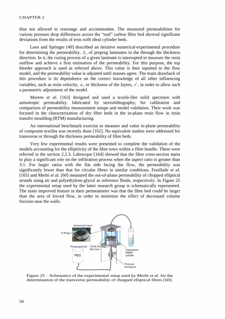
CHAPTER 2
56
thus not allowed to rearrange and accommodate. The measured permeabilities for
various pressure drop differences across the “real” carbon fibre bed showed significant
deviations from the results of tests with ideal cylinder beds.
Loos and Springer [49] described an iterative numerical-experimental procedure
for determining the permeability, S , of prepreg laminates in the through the thickness
direction. In it, the curing process of a given laminate is interrupted to measure the resin
outflow and achieve a first estimation of the permeability. For this purpose, the top
bleeder approach is used as referred above. This value is then inputted to the flow
model, and the permeability value is adjusted until masses agree. The main drawback of
this procedure is its dependence on the correct knowledge of all other influencing
variables, such as resin velocity, u , or thickness of the layers, lt , in order to allow such
a parametric adjustment of the model.
Morren et al. [163] designed and used a textile-like solid specimen with
anisotropic permeability, fabricated by stereolithography, for calibration and
comparison of permeability measurement setups and model validation. Their work was
focused in the characterization of dry fibre beds in the in-plane resin flow in resin
transfer moulding (RTM) manufacturing.
An international benchmark exercise to measure and value in-plane permeability
of composite textiles was recently done [162]. No equivalent studies were addressed for
transverse or through the thickness permeability of fibre beds.
Very few experimental results were presented to complete the validation of the
models accounting for the ellipiticity of the fibre tows within a fibre bundle. These were
referred in the section 2.2.3. Labrecque [164] showed that the fibre cross-section starts
to play a significant role on the infiltration process when the aspect ratio is greater than
3:1. For larger ratios with the flat side facing the flow, the permeability was
significantly lower than that for circular fibres in similar conditions. Feuillade et al.
[165] and Merhi et al. [60] measured the out-of-plane permeability of chopped elliptical
strands using air and polyethylene-glycol as reference fluids, respectively. In Figure 25
the experimental setup used by the latter research group is schematically represented.
The main improved feature in their permeameter was that the fibre bed could be larger
than the area of forced flow, in order to minimize the effect of decreased volume
fraction near the walls.
Figure 25 – Schematics of the experimental setup used by Merhi et al. for the
determination of the transverse permeability of chopped elliptical fibres [60].
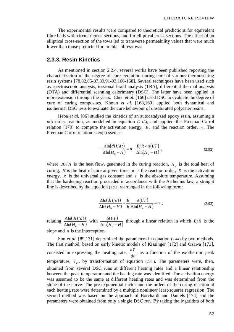
LITERATURE REVIEW
57
The experimental results were compared to theoretical predictions for equivalent
fibre beds with circular cross-sections, and for elliptical cross-sections. The effect of an
elliptical cross-section of the tows led to transverse permeability values that were much
lower than those predicted for circular fibres/tows.
2.3.3. Resin Kinetics
As mentioned in section 2.2.4, several works have been published reporting the
characterization of the degree of cure evolution during cure of various thermosetting
resin systems [78,82,85-87,89,91-93,166-168]. Several techniques have been used such
as spectroscopic analysis, torsional braid analysis (TBA), differential thermal analysis
(DTA) and differential scanning calorimetry (DSC). The latter have been applied in
more extension through the years. Chen et al. [166] used DSC to evaluate the degree of
cure of curing composites. Khoun et al. [168,169] applied both dynamical and
isothermal DSC tests to evaluate the cure behaviour of unsaturated polyester resins.
Heba et al. [86] studied the kinetics of an autocatalyzed epoxy resin, assuming a
nth order reaction, as modelled in equation (2.43), and applied the Freeman-Carrol
relation [170] to compute the activation energy, E , and the reaction order, n . The
Freeman Carrol relation is expressed as:
HH
TREn
HH
tddH
uu
ln
1
ln
ln , (2.92)
where tddH is the heat flow, generated in the curing reaction, uH is the total heat of
curing, H is the heat of cure at given time, n is the reaction order, E is the activation
energy, R is the universal gas constant and T is the absolute temperature. Assuming
that the hardening reaction proceeded in accordance with the Arrhenius law, a straight
line is described by the equation (2.92) rearranged in the following form:
nHH
T
R
E
HH
tddH
uu
ln
1
ln
ln , (2.93)
relating HH
tddH
u
ln
ln with
HH
T
u
ln
1 through a linear relation in which RE is the
slope and n is the interception.
Sun et al. [89,171] determined the parameters in equation (2.44) by two methods.
The first method, based on early kinetic models of Kissinger [172] and Ozawa [173],
consisted in expressing the heating rate, dt
dT, as a function of the exothermic peak
temperature, pT , by transformation of equation (2.44). The parameters were, then,
obtained from several DSC runs at different heating rates and a linear relationship
between the peak temperature and the heating rate was identified. The activation energy
was assumed to be the same at different heating rates and was determined from the
slope of the curve. The pre-exponential factor and the orders of the curing reaction at
each heating rate were determined by a multiple nonlinear least-squares regression. The
second method was based on the approach of Borchardt and Daniels [174] and the
parameters were obtained from only a single DSC run. By taking the logarithm of both
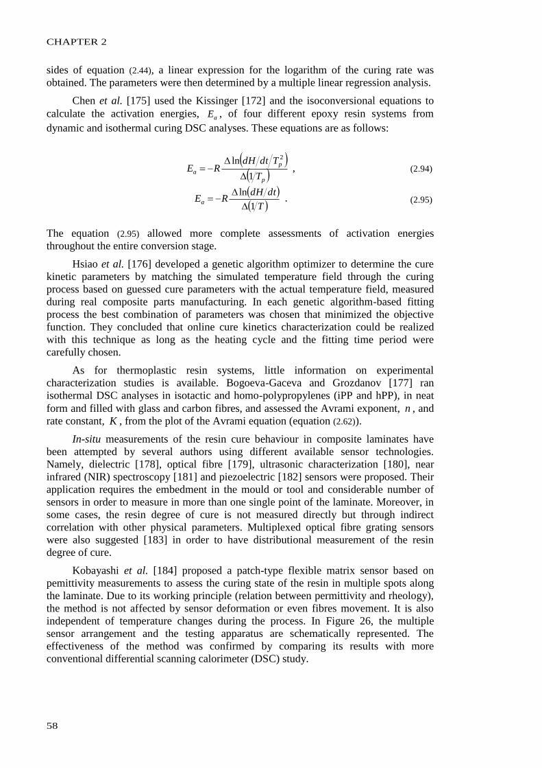
CHAPTER 2
58
sides of equation (2.44), a linear expression for the logarithm of the curing rate was
obtained. The parameters were then determined by a multiple linear regression analysis.
Chen et al. [175] used the Kissinger [172] and the isoconversional equations to
calculate the activation energies, aE , of four different epoxy resin systems from
dynamic and isothermal curing DSC analyses. These equations are as follows:
p
p
aT
TdtdHRE
1
ln 2
, (2.94)
T
dtdHREa
1
ln
. (2.95)
The equation (2.95) allowed more complete assessments of activation energies
throughout the entire conversion stage.
Hsiao et al. [176] developed a genetic algorithm optimizer to determine the cure
kinetic parameters by matching the simulated temperature field through the curing
process based on guessed cure parameters with the actual temperature field, measured
during real composite parts manufacturing. In each genetic algorithm-based fitting
process the best combination of parameters was chosen that minimized the objective
function. They concluded that online cure kinetics characterization could be realized
with this technique as long as the heating cycle and the fitting time period were
carefully chosen.
As for thermoplastic resin systems, little information on experimental
characterization studies is available. Bogoeva-Gaceva and Grozdanov [177] ran
isothermal DSC analyses in isotactic and homo-polypropylenes (iPP and hPP), in neat
form and filled with glass and carbon fibres, and assessed the Avrami exponent, n , and
rate constant, K , from the plot of the Avrami equation (equation (2.62)).
In-situ measurements of the resin cure behaviour in composite laminates have
been attempted by several authors using different available sensor technologies.
Namely, dielectric [178], optical fibre [179], ultrasonic characterization [180], near
infrared (NIR) spectroscopy [181] and piezoelectric [182] sensors were proposed. Their
application requires the embedment in the mould or tool and considerable number of
sensors in order to measure in more than one single point of the laminate. Moreover, in
some cases, the resin degree of cure is not measured directly but through indirect
correlation with other physical parameters. Multiplexed optical fibre grating sensors
were also suggested [183] in order to have distributional measurement of the resin
degree of cure.
Kobayashi et al. [184] proposed a patch-type flexible matrix sensor based on
pemittivity measurements to assess the curing state of the resin in multiple spots along
the laminate. Due to its working principle (relation between permittivity and rheology),
the method is not affected by sensor deformation or even fibres movement. It is also
independent of temperature changes during the process. In Figure 26, the multiple
sensor arrangement and the testing apparatus are schematically represented. The
effectiveness of the method was confirmed by comparing its results with more
conventional differential scanning calorimeter (DSC) study.
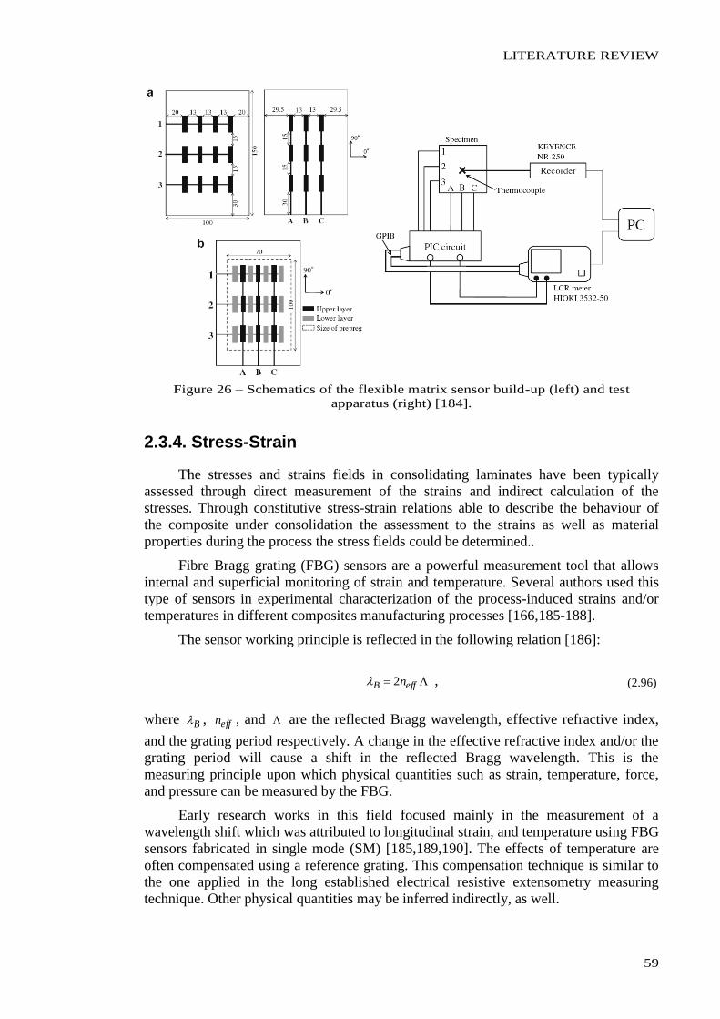
LITERATURE REVIEW
59
Figure 26 – Schematics of the flexible matrix sensor build-up (left) and test
apparatus (right) [184].
2.3.4. Stress-Strain
The stresses and strains fields in consolidating laminates have been typically
assessed through direct measurement of the strains and indirect calculation of the
stresses. Through constitutive stress-strain relations able to describe the behaviour of
the composite under consolidation the assessment to the strains as well as material
properties during the process the stress fields could be determined..
Fibre Bragg grating (FBG) sensors are a powerful measurement tool that allows
internal and superficial monitoring of strain and temperature. Several authors used this
type of sensors in experimental characterization of the process-induced strains and/or
temperatures in different composites manufacturing processes [166,185-188].
The sensor working principle is reflected in the following relation [186]:
effB n2 , (2.96)
where B , effn , and are the reflected Bragg wavelength, effective refractive index,
and the grating period respectively. A change in the effective refractive index and/or the
grating period will cause a shift in the reflected Bragg wavelength. This is the
measuring principle upon which physical quantities such as strain, temperature, force,
and pressure can be measured by the FBG.
Early research works in this field focused mainly in the measurement of a
wavelength shift which was attributed to longitudinal strain, and temperature using FBG
sensors fabricated in single mode (SM) [185,189,190]. The effects of temperature are
often compensated using a reference grating. This compensation technique is similar to
the one applied in the long established electrical resistive extensometry measuring
technique. Other physical quantities may be inferred indirectly, as well.
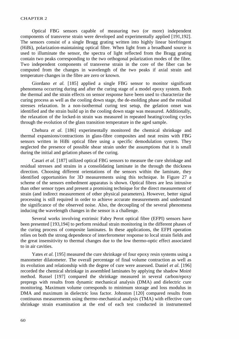
CHAPTER 2
60
Optical FBG sensors capable of measuring two (or more) independent
components of transverse strain were developed and experimentally applied [191,192].
The sensors consist of a single Bragg grating written into highly linear birefringent
(HiBi), polarization-maintaining optical fibre. When light from a broadband source is
used to illuminate the sensor, the spectra of light reflected from the Bragg grating
contain two peaks corresponding to the two orthogonal polarization modes of the fibre.
Two independent components of transverse strain in the core of the fiber can be
computed from the changes in wavelength of the two peaks if axial strain and
temperature changes in the fibre are zero or known.
Giordano et al. [185] applied a single FBG sensor to monitor significant
phenomena occurring during and after the curing stage of a model epoxy system. Both
the thermal and the strain effects on sensor response have been used to characterize the
curing process as well as the cooling down stage, the de-molding phase and the residual
stresses relaxation. In a non-isothermal curing test setup, the gelation onset was
identified and the strain build up in the cooling down stage was measured. Additionally,
the relaxation of the locked-in strain was measured in repeated heating/cooling cycles
through the evolution of the glass transition temperature in the aged sample.
Chehura et al. [186] experimentally monitored the chemical shrinkage and
thermal expansions/contractions in glass-fibre composites and neat resins with FBG
sensors written in HiBi optical fibre using a specific demodulation system. They
neglected the presence of possible shear strain under the assumptions that it is small
during the initial and gelation phases of the curing.
Casari et al. [187] utilized optical FBG sensors to measure the cure shrinkage and
residual stresses and strains in a consolidating laminate in the through the thickness
direction. Choosing different orientations of the sensors within the laminate, they
identified opportunities for 3D measurements using this technique. In Figure 27 a
scheme of the sensors embedment apparatus is shown. Optical fibres are less intrusive
than other sensor types and present a promising technique for the direct measurement of
strain (and indirect measurement of other physical parameters). However, better signal
processing is still required in order to achieve accurate measurements and understand
the significance of the observed noise. Also, the decoupling of the several phenomena
inducing the wavelength changes in the sensor is a challenge.
Several works involving extrinsic Fabry Perot optical fibre (EFPI) sensors have
been presented [193,194] to perform residual strain monitoring in the different phases of
the curing process of composite laminates. In these applications, the EFPI operation
relies on both the strong dependence of interferometer response to local strain fields and
the great insensitivity to thermal changes due to the low thermo-optic effect associated
to in air cavities.
Yates et al. [195] measured the cure shrinkage of four epoxy resin systems using a
manometer dilatometer. The overall percentage of final volume contraction as well as
its evolution and relationship with the degree of cure were assessed. Daniel et al. [196]
recorded the chemical shrinkage in assembled laminates by applying the shadow Moiré
method. Russel [197] compared the shrinkage measured in several carbon/epoxy
prepregs with results from dynamic mechanical analysis (DMA) and dielectric cure
monitoring. Maximum volume corresponds to minimum storage and loss modulus in
DMA and maximum in dielectric loss factor. Johnston [120] compared results from
continuous measurements using thermo-mechanical analysis (TMA) with effective cure
shrinkage strain examination at the end of each test conducted in instrumented
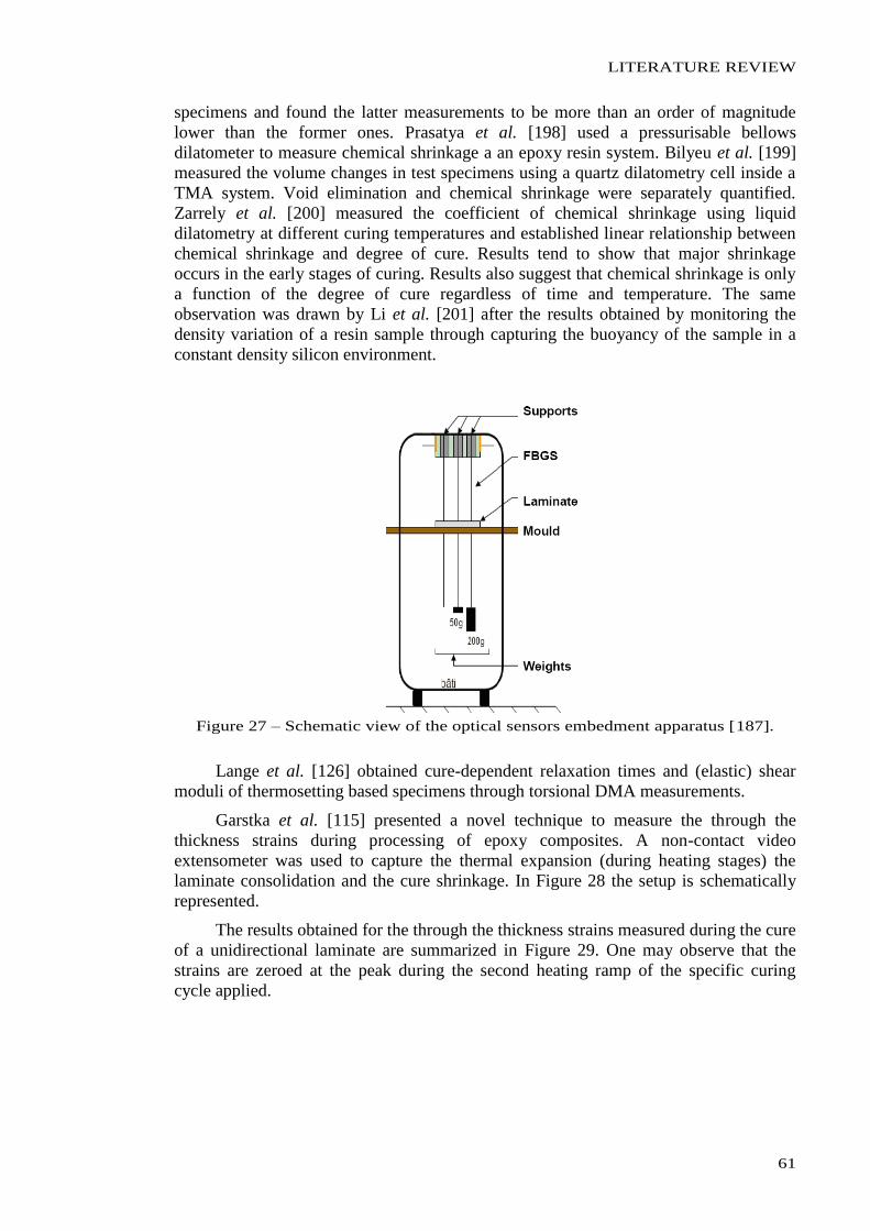
LITERATURE REVIEW
61
specimens and found the latter measurements to be more than an order of magnitude
lower than the former ones. Prasatya et al. [198] used a pressurisable bellows
dilatometer to measure chemical shrinkage a an epoxy resin system. Bilyeu et al. [199]
measured the volume changes in test specimens using a quartz dilatometry cell inside a
TMA system. Void elimination and chemical shrinkage were separately quantified.
Zarrely et al. [200] measured the coefficient of chemical shrinkage using liquid
dilatometry at different curing temperatures and established linear relationship between
chemical shrinkage and degree of cure. Results tend to show that major shrinkage
occurs in the early stages of curing. Results also suggest that chemical shrinkage is only
a function of the degree of cure regardless of time and temperature. The same
observation was drawn by Li et al. [201] after the results obtained by monitoring the
density variation of a resin sample through capturing the buoyancy of the sample in a
constant density silicon environment.
Figure 27 – Schematic view of the optical sensors embedment apparatus [187].
Lange et al. [126] obtained cure-dependent relaxation times and (elastic) shear
moduli of thermosetting based specimens through torsional DMA measurements.
Garstka et al. [115] presented a novel technique to measure the through the
thickness strains during processing of epoxy composites. A non-contact video
extensometer was used to capture the thermal expansion (during heating stages) the
laminate consolidation and the cure shrinkage. In Figure 28 the setup is schematically
represented.
The results obtained for the through the thickness strains measured during the cure
of a unidirectional laminate are summarized in Figure 29. One may observe that the
strains are zeroed at the peak during the second heating ramp of the specific curing
cycle applied.
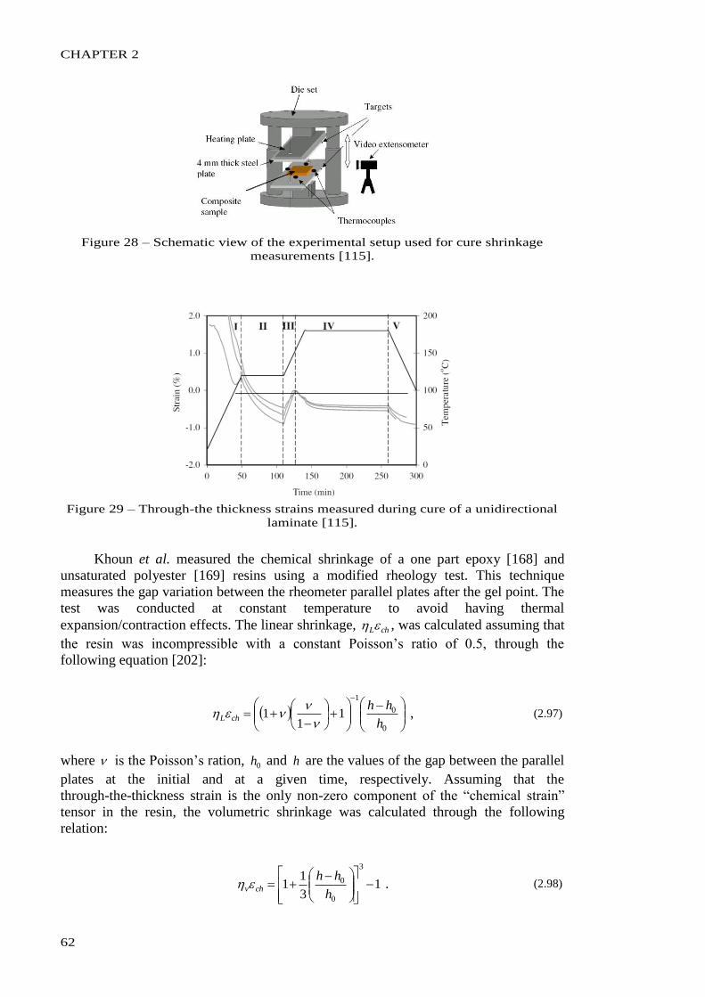
CHAPTER 2
62
Figure 28 – Schematic view of the experimental setup used for cure shrinkage
measurements [115].
Figure 29 – Through-the thickness strains measured during cure of a unidirectional
laminate [115].
Khoun et al. measured the chemical shrinkage of a one part epoxy [168] and
unsaturated polyester [169] resins using a modified rheology test. This technique
measures the gap variation between the rheometer parallel plates after the gel point. The
test was conducted at constant temperature to avoid having thermal
expansion/contraction effects. The linear shrinkage, chL , was calculated assuming that
the resin was incompressible with a constant Poisson’s ratio of 0.5, through the
following equation [202]:
0
0
1
11
1h
hhchL
, (2.97)
where is the Poisson’s ration, 0h and h are the values of the gap between the parallel
plates at the initial and at a given time, respectively. Assuming that the
through-the-thickness strain is the only non-zero component of the “chemical strain”
tensor in the resin, the volumetric shrinkage was calculated through the following
relation:
13
11
3
0
0
h
hhchv . (2.98)
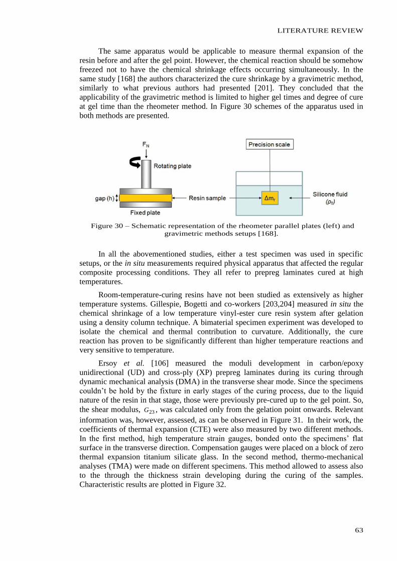
LITERATURE REVIEW
63
The same apparatus would be applicable to measure thermal expansion of the
resin before and after the gel point. However, the chemical reaction should be somehow
freezed not to have the chemical shrinkage effects occurring simultaneously. In the
same study [168] the authors characterized the cure shrinkage by a gravimetric method,
similarly to what previous authors had presented [201]. They concluded that the
applicability of the gravimetric method is limited to higher gel times and degree of cure
at gel time than the rheometer method. In Figure 30 schemes of the apparatus used in
both methods are presented.
Figure 30 – Schematic representation of the rheometer parallel plates (left) and
gravimetric methods setups [168].
In all the abovementioned studies, either a test specimen was used in specific
setups, or the in situ measurements required physical apparatus that affected the regular
composite processing conditions. They all refer to prepreg laminates cured at high
temperatures.
Room-temperature-curing resins have not been studied as extensively as higher
temperature systems. Gillespie, Bogetti and co-workers [203,204] measured in situ the
chemical shrinkage of a low temperature vinyl-ester cure resin system after gelation
using a density column technique. A bimaterial specimen experiment was developed to
isolate the chemical and thermal contribution to curvature. Additionally, the cure
reaction has proven to be significantly different than higher temperature reactions and
very sensitive to temperature.
Ersoy et al. [106] measured the moduli development in carbon/epoxy
unidirectional (UD) and cross-ply (XP) prepreg laminates during its curing through
dynamic mechanical analysis (DMA) in the transverse shear mode. Since the specimens
couldn’t be hold by the fixture in early stages of the curing process, due to the liquid
nature of the resin in that stage, those were previously pre-cured up to the gel point. So,
the shear modulus, 23G , was calculated only from the gelation point onwards. Relevant
information was, however, assessed, as can be observed in Figure 31. In their work, the
coefficients of thermal expansion (CTE) were also measured by two different methods.
In the first method, high temperature strain gauges, bonded onto the specimens’ flat
surface in the transverse direction. Compensation gauges were placed on a block of zero
thermal expansion titanium silicate glass. In the second method, thermo-mechanical
analyses (TMA) were made on different specimens. This method allowed to assess also
to the through the thickness strain developing during the curing of the samples.
Characteristic results are plotted in Figure 32.
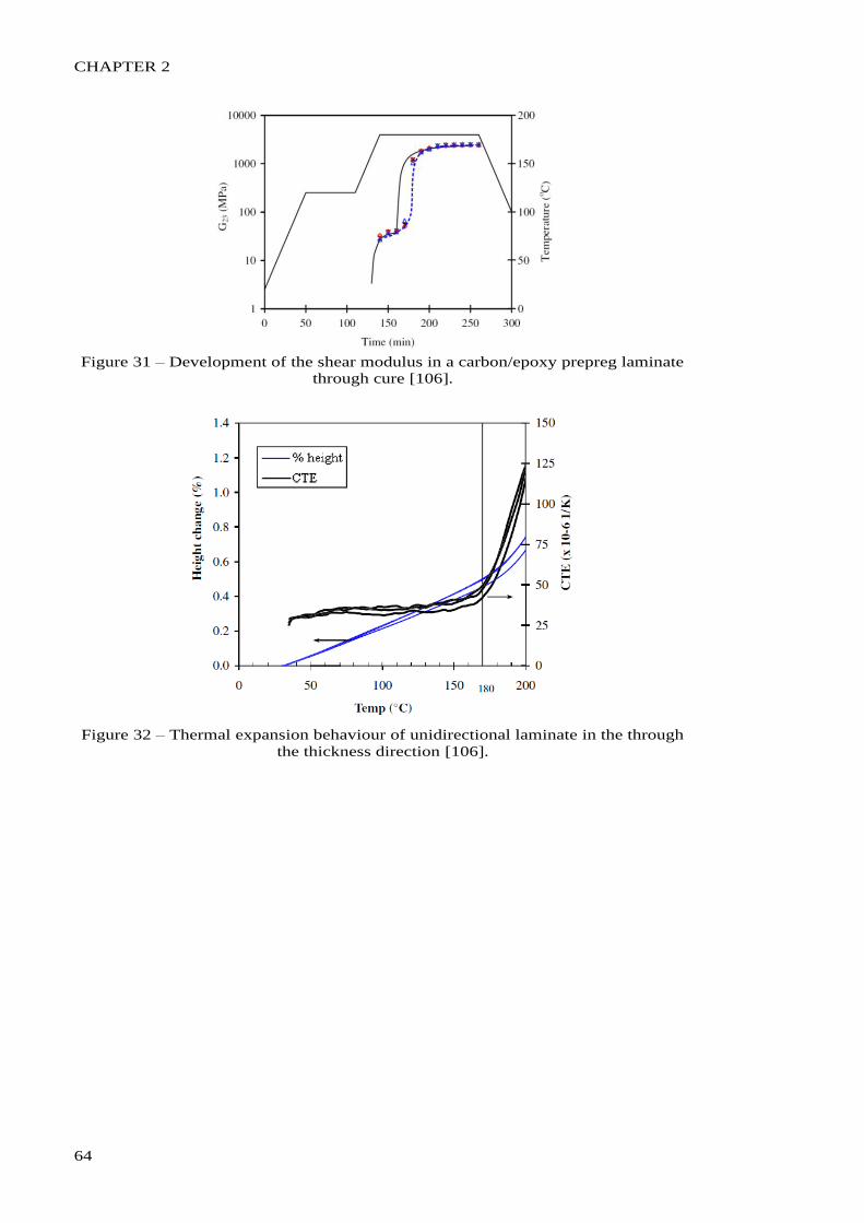
CHAPTER 2
64
Figure 31 – Development of the shear modulus in a carbon/epoxy prepreg laminate
through cure [106].
Figure 32 – Thermal expansion behaviour of unidirectional laminate in the through
the thickness direction [106].
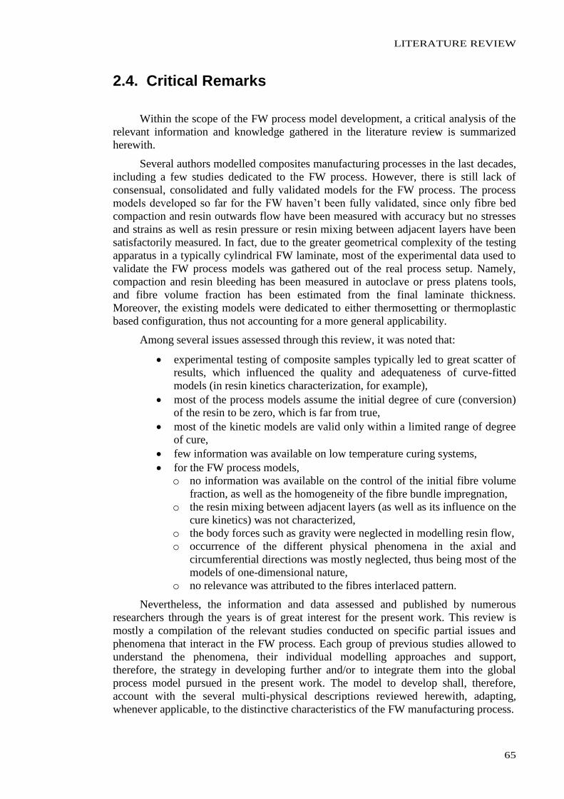
LITERATURE REVIEW
65
2.4. Critical Remarks
Within the scope of the FW process model development, a critical analysis of the
relevant information and knowledge gathered in the literature review is summarized
herewith.
Several authors modelled composites manufacturing processes in the last decades,
including a few studies dedicated to the FW process. However, there is still lack of
consensual, consolidated and fully validated models for the FW process. The process
models developed so far for the FW haven’t been fully validated, since only fibre bed
compaction and resin outwards flow have been measured with accuracy but no stresses
and strains as well as resin pressure or resin mixing between adjacent layers have been
satisfactorily measured. In fact, due to the greater geometrical complexity of the testing
apparatus in a typically cylindrical FW laminate, most of the experimental data used to
validate the FW process models was gathered out of the real process setup. Namely,
compaction and resin bleeding has been measured in autoclave or press platens tools,
and fibre volume fraction has been estimated from the final laminate thickness.
Moreover, the existing models were dedicated to either thermosetting or thermoplastic
based configuration, thus not accounting for a more general applicability.
Among several issues assessed through this review, it was noted that:
experimental testing of composite samples typically led to great scatter of
results, which influenced the quality and adequateness of curve-fitted
models (in resin kinetics characterization, for example),
most of the process models assume the initial degree of cure (conversion)
of the resin to be zero, which is far from true,
most of the kinetic models are valid only within a limited range of degree
of cure,
few information was available on low temperature curing systems,
for the FW process models,
o no information was available on the control of the initial fibre volume
fraction, as well as the homogeneity of the fibre bundle impregnation,
o the resin mixing between adjacent layers (as well as its influence on the
cure kinetics) was not characterized,
o the body forces such as gravity were neglected in modelling resin flow,
o occurrence of the different physical phenomena in the axial and
circumferential directions was mostly neglected, thus being most of the
models of one-dimensional nature,
o no relevance was attributed to the fibres interlaced pattern.
Nevertheless, the information and data assessed and published by numerous
researchers through the years is of great interest for the present work. This review is
mostly a compilation of the relevant studies conducted on specific partial issues and
phenomena that interact in the FW process. Each group of previous studies allowed to
understand the phenomena, their individual modelling approaches and support,
therefore, the strategy in developing further and/or to integrate them into the global
process model pursued in the present work. The model to develop shall, therefore,
account with the several multi-physical descriptions reviewed herewith, adapting,
whenever applicable, to the distinctive characteristics of the FW manufacturing process.


CHAPTER 3
PROCESS MODEL

CHAPTER 3
68
PROCESS MODEL
69
3.1. Modelling Strategy
In order to model the FW composites manufacturing process, analytical
descriptions of the different physical phenomena acting in this process were established
and are detailed herewith. The identification of the phenomena governing the
consolidation process at the layer/laminate level was achieved by combining the
knowledge gathered through a comprehensive literature review (chapter 2), the study of
the physics of the process and the practical experience on the process. Upon this, the
most relevant assumptions were drawn and a modelling strategy was devised.
The modelling strategy was settled upon the following principles and ideas:
the physics of the process was analysed and studied in three inter-related
groups of phenomena, namely:
o the “purely” mechanical phenomena, relating forces, pressures,
stresses, strains through elastic and/or elastic-apparent properties of the
materials and tools,
o the flow and compaction related phenomena, describing the
displacements and motions of the matrix and fibres,
o the thermo-chemical phenomena, defining the matrix rheological state,
the model accounted for both thermosetting and thermoplastic matrix
based composites,
each phenomenon (or group of phenomena) corresponding to an identified
sub-process was decoupled from the others as much as possible and
modelled separately in a dedicated sub-model,
for the numerical implementation of the model, each sub-process modelled
analytically corresponded to a sub-routine and a main routine guaranteed
the correct interaction and flow of variables between those,
the main input variables of the global model corresponded to the main
user-controllable process parameters,
the main output variables of the global model corresponded to the main
mechanical and geometrical properties of the produced laminates,
the global model was built in a modular configuration, grouping and
combining every sub-models for each process configuration accounted for.
The sub-division of the analysis in three groups of phenomena, allowed to
separate and focus the study of phenomena of different physical natures. The
interactions and properties that could be modelled by exact mechanical analytical
descriptions were grouped into the mechanical analysis. The other physical phenomena
that govern the matrix/fibres interactions and are described by empirical expressions
were grouped into the flow/compaction analysis. The thermal and chemical phenomena
governing the curing/crystallization and rheology of the matrix were grouped in the
thermo-chemical analysis. Although the analyses could be organized differently, this
sub-division is the one that better reveals the multi-physical nature of the FW process,
thus identifying the main fields of physics to be studied and modelled.
The option of accounting for both thermosetting and thermoplastic matrices, even
if slightly increasing the complexity and extent of the study and the model itself,
appeared to be of greater usefulness for the present industrial need. In the past, authors
treated thermosetting and thermoplastic based materials in different and separated
studies. Moreover, thermoplastic composite manufacturing process models have been
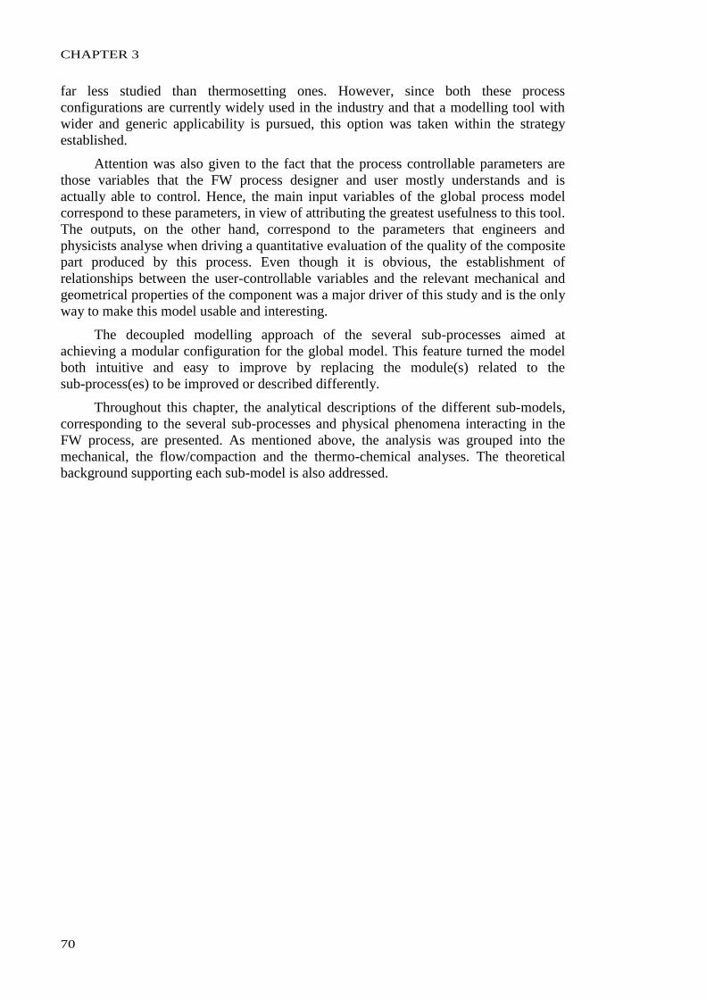
CHAPTER 3
70
far less studied than thermosetting ones. However, since both these process
configurations are currently widely used in the industry and that a modelling tool with
wider and generic applicability is pursued, this option was taken within the strategy
established.
Attention was also given to the fact that the process controllable parameters are
those variables that the FW process designer and user mostly understands and is
actually able to control. Hence, the main input variables of the global process model
correspond to these parameters, in view of attributing the greatest usefulness to this tool.
The outputs, on the other hand, correspond to the parameters that engineers and
physicists analyse when driving a quantitative evaluation of the quality of the composite
part produced by this process. Even though it is obvious, the establishment of
relationships between the user-controllable variables and the relevant mechanical and
geometrical properties of the component was a major driver of this study and is the only
way to make this model usable and interesting.
The decoupled modelling approach of the several sub-processes aimed at
achieving a modular configuration for the global model. This feature turned the model
both intuitive and easy to improve by replacing the module(s) related to the
sub-process(es) to be improved or described differently.
Throughout this chapter, the analytical descriptions of the different sub-models,
corresponding to the several sub-processes and physical phenomena interacting in the
FW process, are presented. As mentioned above, the analysis was grouped into the
mechanical, the flow/compaction and the thermo-chemical analyses. The theoretical
background supporting each sub-model is also addressed.
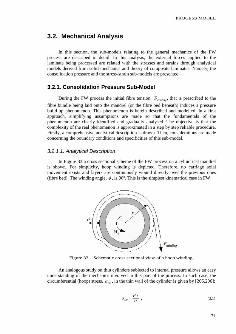
PROCESS MODEL
71
3.2. Mechanical Analysis
In this section, the sub-models relating to the general mechanics of the FW
process are described in detail. In this analysis, the external forces applied to the
laminate being processed are related with the stresses and strains through analytical
models derived from solid mechanics and theory of composite laminates. Namely, the
consolidation pressure and the stress-strain sub-models are presented.
3.2.1. Consolidation Pressure Sub-Model
During the FW process the initial fibre tension, windingF , that is prescribed to the
fibre bundle being laid onto the mandrel (or the fibre bed beneath) induces a pressure
build-up phenomenon. This phenomenon is herein described and modelled. In a first
approach, simplifying assumptions are made so that the fundamentals of the
phenomenon are clearly identified and gradually analysed. The objective is that the
complexity of the real phenomenon is approximated in a step by step reliable procedure.
Firstly, a comprehensive analytical description is drawn. Then, considerations are made
concerning the boundary conditions and specificities of this sub-model.
3.2.1.1. Analytical Description
In Figure 33 a cross sectional scheme of the FW process on a cylindrical mandrel
is shown. For simplicity, hoop winding is depicted. Therefore, no carriage axial
movement exists and layers are continuously wound directly over the previous ones
(fibre bed). The winding angle, , is 90º. This is the simplest kinematical case in FW.
Figure 33 – Schematic cross sectional view of a hoop winding.
An analogous study on thin cylinders subjected to internal pressure allows an easy
understanding of the mechanics involved in this part of the process. In such case, the
circumferential (hoop) stress, , in the thin wall of the cylinder is given by [205,206]:
wt
rP , (3.1)
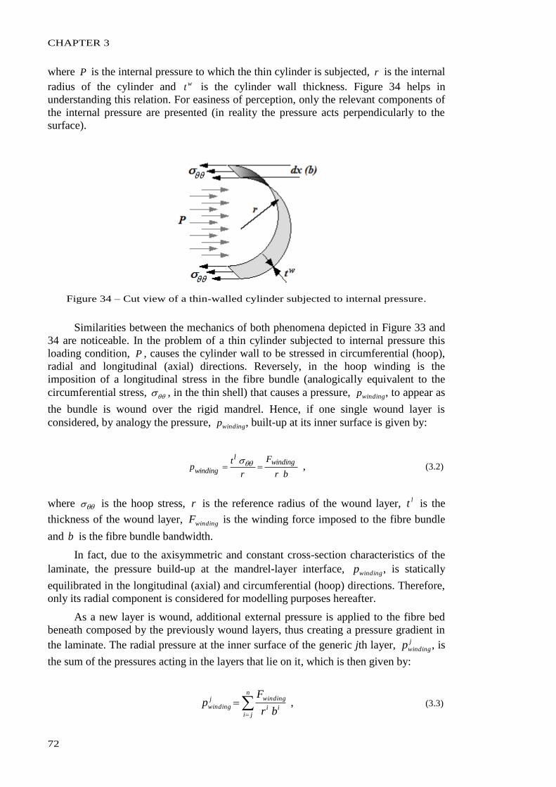
CHAPTER 3
72
where P is the internal pressure to which the thin cylinder is subjected, r is the internal
radius of the cylinder and wt is the cylinder wall thickness. Figure 34 helps in
understanding this relation. For easiness of perception, only the relevant components of
the internal pressure are presented (in reality the pressure acts perpendicularly to the
surface).
Figure 34 – Cut view of a thin-walled cylinder subjected to internal pressure.
Similarities between the mechanics of both phenomena depicted in Figure 33 and
34 are noticeable. In the problem of a thin cylinder subjected to internal pressure this
loading condition, P , causes the cylinder wall to be stressed in circumferential (hoop),
radial and longitudinal (axial) directions. Reversely, in the hoop winding is the
imposition of a longitudinal stress in the fibre bundle (analogically equivalent to the
circumferential stress, , in the thin shell) that causes a pressure, windingp , to appear as
the bundle is wound over the rigid mandrel. Hence, if one single wound layer is
considered, by analogy the pressure, windingp , built-up at its inner surface is given by:
br
F
r
tp
windingl
winding
, (3.2)
where is the hoop stress, r is the reference radius of the wound layer, lt is the
thickness of the wound layer, windingF is the winding force imposed to the fibre bundle
and b is the fibre bundle bandwidth.
In fact, due to the axisymmetric and constant cross-section characteristics of the
laminate, the pressure build-up at the mandrel-layer interface, windingp , is statically
equilibrated in the longitudinal (axial) and circumferential (hoop) directions. Therefore,
only its radial component is considered for modelling purposes hereafter.
As a new layer is wound, additional external pressure is applied to the fibre bed
beneath composed by the previously wound layers, thus creating a pressure gradient in
the laminate. The radial pressure at the inner surface of the generic jth layer, j
windingp , is
the sum of the pressures acting in the layers that lie on it, which is then given by:
n
jiii
windingj
windingbr
Fp , (3.3)
PROCESS MODEL
73
where n is the number of wound layers, ir is the reference radius of the ith layer
( nij ), ib is the fibre bundle bandwidth of the ith layer.
This simplified analytical model of the radial pressure generated in a hoop
winding is valid under several reasonable assumptions, such as:
the thickness, lt , of the layers is small when compared to the perimeter;
the deformability of each layer is negligible;
the longitudinal stress imposed to the fibre bundles being wound, , is
uniformly distributed between resin and fibres composing the bundles;
friction forces between composite layers and/or mandrel and composite
layer as well as interlaminar slippage are negligible;
thermo-chemical expansions and/or contractions of the laminate have
negligible contributions to the build-up of the consolidation pressure;
inertial and gravitational forces are negligible.
In a more accurate analysis, some of these assumptions might need to be
re-evaluated as they coarsely approach the reality.
In fact, when a new layer is wound, the external radial pressure that it builds over
the previously wound layers generates two main fibre motion mechanisms. One is the
uncured resin viscous flow through the porous fibre bed as it is squeezed. This flow
occurs in the radial, longitudinal and transversal directions of fibres, although in most of
the modelling approaches only the radial flow is considered, as discussed in chapter 2.
The other fibre motion mechanism is the fibre bed compaction itself, behaving as a
rapidly stiffening nonlinear spring, which is compressed by the external force applied
when a new layer is wound [26]. As the wound lay-up compacts, inner layers have a
higher fibre volume fraction and subsequently higher stiffness. These phenomena are
detailed and modelled in sections 3.3.1 and 3.3.3, respectively. They oppose, however,
the abovementioned assumption that each layer is not deformable.
In early stages of the winding and consolidation process, in which the resin
viscosity is low, the interlaminar slippage of adjacent layers may occur due to the
inward accommodation of the layers as the resin flows outwards. Low friction factors in
such a lubricated system contribute to this mechanism. Moreover, if higher winding
tension, windingF , is applied more likely it is to occur. This also questions the
abovementioned assumption that the interlaminar slippage is negligible. In later stages
of the process, thermo-chemical phenomena may induce expansion and/or contraction
of the laminate but the higher viscosity of the resin counter-balances these effects.
Equations (3.2) and (3.3) are, thus, reasonably valid for the initial stages of the
winding and consolidation process and are considered to properly describe the pressure
build-up by the action of the initial winding tension, windingF . However, the fibre bed,
composed by consolidating resin and fibres, will constantly try to get a new equilibrium
state. As said before, after a certain layer being wound, it tends to move inwards and so
the circumferential stress initially applied to the fibre bundle may be partially released.
The changes in the circumferential (hoop) stress, , due to the distributed radial
displacement of the layer may be evaluated through the following relation:
m
m
f
f VEVE , (3.4)
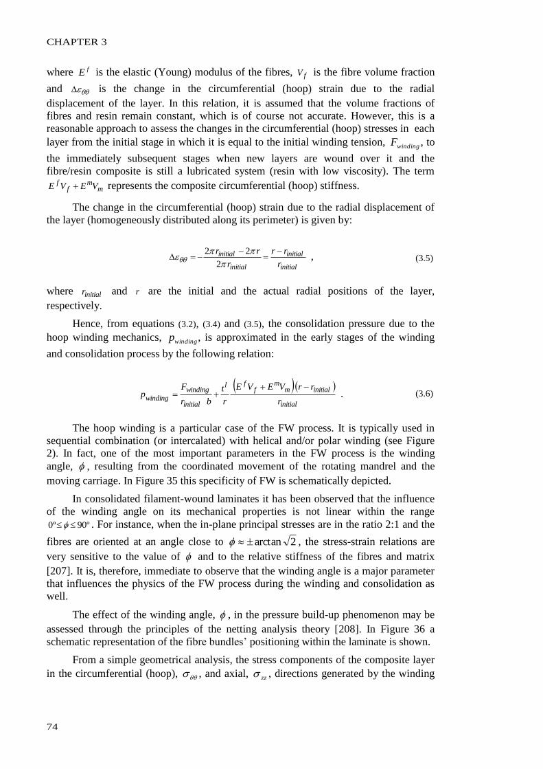
CHAPTER 3
74
where fE is the elastic (Young) modulus of the fibres, fV is the fibre volume fraction
and is the change in the circumferential (hoop) strain due to the radial
displacement of the layer. In this relation, it is assumed that the volume fractions of
fibres and resin remain constant, which is of course not accurate. However, this is a
reasonable approach to assess the changes in the circumferential (hoop) stresses in each
layer from the initial stage in which it is equal to the initial winding tension, windingF , to
the immediately subsequent stages when new layers are wound over it and the
fibre/resin composite is still a lubricated system (resin with low viscosity). The term
mm
ff VEVE represents the composite circumferential (hoop) stiffness.
The change in the circumferential (hoop) strain due to the radial displacement of
the layer (homogeneously distributed along its perimeter) is given by:
initial
initial
initial
initial
r
rr
r
rr
2
22 , (3.5)
where initialr and r are the initial and the actual radial positions of the layer,
respectively.
Hence, from equations (3.2), (3.4) and (3.5), the consolidation pressure due to the
hoop winding mechanics, windingp , is approximated in the early stages of the winding
and consolidation process by the following relation:
initial
initialmm
ffl
initial
winding
winding r
rrVEVE
r
t
br
Fp
. (3.6)
The hoop winding is a particular case of the FW process. It is typically used in
sequential combination (or intercalated) with helical and/or polar winding (see Figure
2). In fact, one of the most important parameters in the FW process is the winding
angle, , resulting from the coordinated movement of the rotating mandrel and the
moving carriage. In Figure 35 this specificity of FW is schematically depicted.
In consolidated filament-wound laminates it has been observed that the influence
of the winding angle on its mechanical properties is not linear within the range
º90º0 . For instance, when the in-plane principal stresses are in the ratio 2:1 and the
fibres are oriented at an angle close to 2arctan , the stress-strain relations are
very sensitive to the value of and to the relative stiffness of the fibres and matrix
[207]. It is, therefore, immediate to observe that the winding angle is a major parameter
that influences the physics of the FW process during the winding and consolidation as
well.
The effect of the winding angle, , in the pressure build-up phenomenon may be
assessed through the principles of the netting analysis theory [208]. In Figure 36 a
schematic representation of the fibre bundles’ positioning within the laminate is shown.
From a simple geometrical analysis, the stress components of the composite layer
in the circumferential (hoop), , and axial, zz , directions generated by the winding
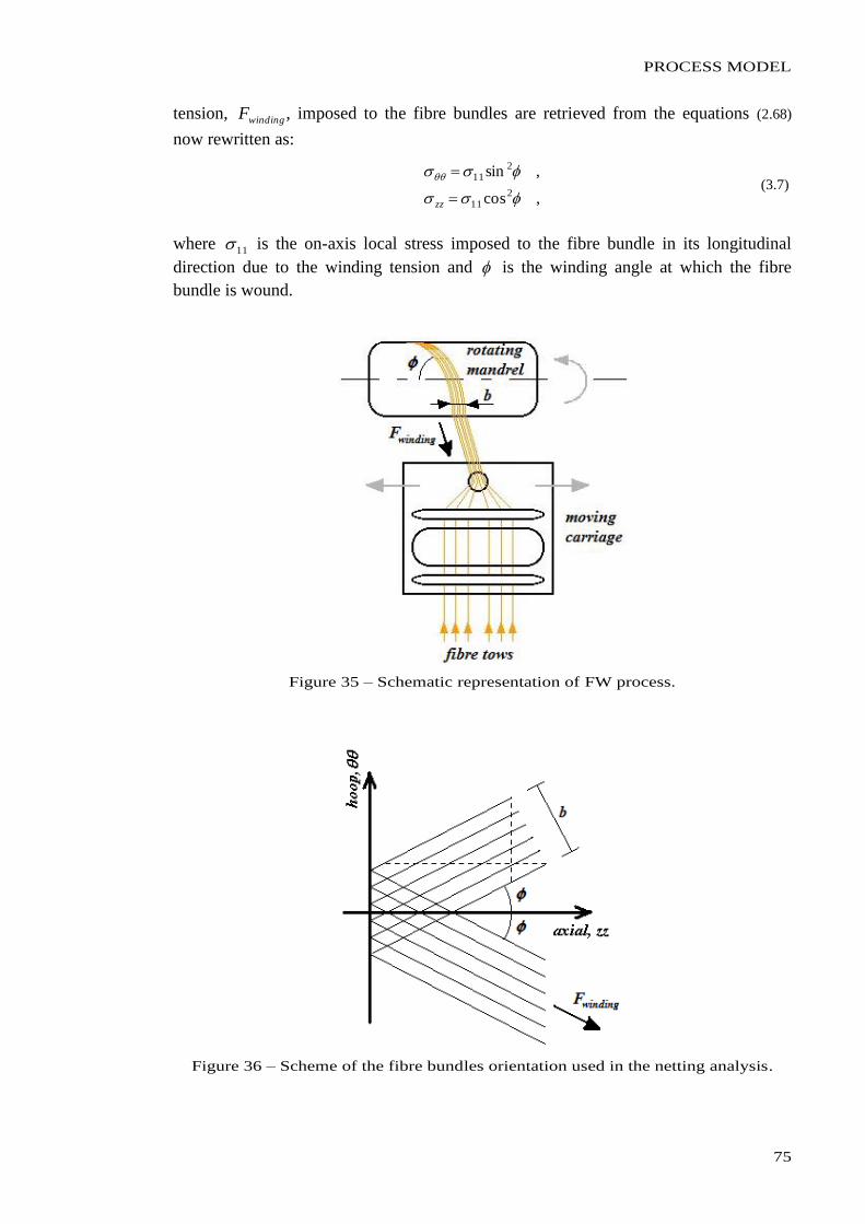
PROCESS MODEL
75
tension, windingF , imposed to the fibre bundles are retrieved from the equations (2.68)
now rewritten as:
,cos
,sin
211
211
zz
(3.7)
where 11 is the on-axis local stress imposed to the fibre bundle in its longitudinal
direction due to the winding tension and is the winding angle at which the fibre
bundle is wound.
Figure 35 – Schematic representation of FW process.
Figure 36 – Scheme of the fibre bundles orientation used in the netting analysis.
CHAPTER 3
76
While in the netting analysis the resin was assumed to have no load carrying ability,
here no such distinction is made since 11 is the local longitudinal stress of the fibre
bundle (including the resin). It is obvious that in early stages of the
curing/crystallization process both descriptions are reasonably equivalent. However, as
the process advances, the latter description (equation (3.7)) is more accurate and, thus,
has wider applicability for different process timings and conditions.
Taking the winding angle into consideration and, therefore, generalizing the
applicability of this sub-model, from equations (3.6) and (3.7), the consolidation pressure
due to the winding mechanics, windingp , is approximated in the early stages of the
winding and consolidation process by:
sin
sin
initial
initialm
m
f
fl
initial
winding
windingr
rrVEVE
r
t
br
Fp , (3.8)
where the circumferential (hoop) stiffness of the composite layer is approximated by the
term sinm
m
f
f VEVE . This formulation is based on the assumption that the
transverse stiffness of the fibre bundle is negligible in the early stages of the process
(while the lubricated bundle moves and accommodates).
Consequently, the consolidation pressure in the jth layer due to the winding
mechanics, j
windingp , including the effect of the winding angle, , and the inward
movement of the layer immediately after its winding is calculated as follows:
j
j
initial
j
initial
jj
m
jmj
f
f
j
ln
jiii
i
windingj
windingr
rrVEVE
r
t
br
Fp
sin
sin 2
, (3.9)
where the first term on the right hand side relates to the pressure imposed by newly
wound layers that lie on the jth layer and the second term relates to the specific radial
motion of the jth layer.
As discussed in section 2.2.2., the stress externally applied to the composite under
consolidation is shared by the fibres and the resin [16-22]. This was expressed in
equation (2.4). In equation (2.67) this principle was further generalized for a
three-dimensional description [16,27]. In accordance with both descriptions, the
consolidation pressure load due to the winding mechanics, windingp , is then distributed
as:
frwinding ppp , (3.10)
where rp is the resin pressure and fp is the effective stress sustained by the fibres.
The distribution of the pressure built-up during FW at each layer’s interface
between fibres and resin is governed by the relative content of each within the fibre
bundle (and, therefore, in the layer). The higher the fibres volume fraction, fV , is,
higher is their contribution to sustain the applied load and, thus, fp becomes higher.
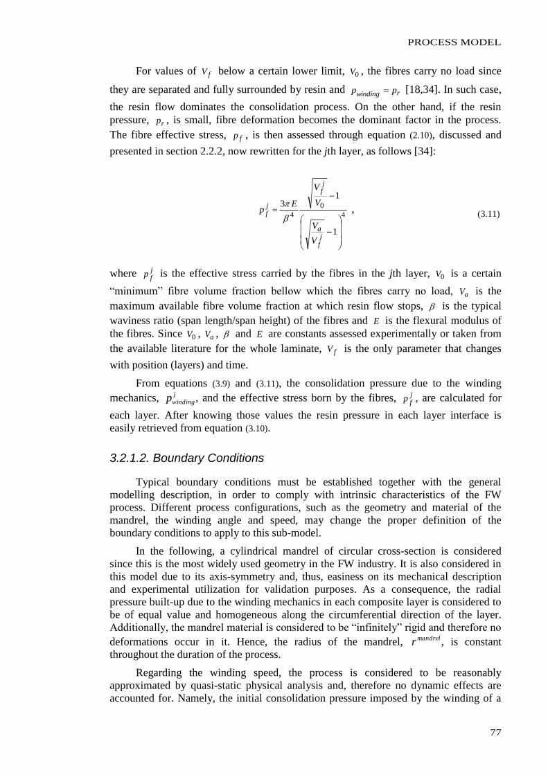
PROCESS MODEL
77
For values of fV below a certain lower limit, 0V , the fibres carry no load since
they are separated and fully surrounded by resin and rwinding pp [18,34]. In such case,
the resin flow dominates the consolidation process. On the other hand, if the resin
pressure, rp , is small, fibre deformation becomes the dominant factor in the process.
The fibre effective stress, fp , is then assessed through equation (2.10), discussed and
presented in section 2.2.2, now rewritten for the jth layer, as follows [34]:
4
0
4
1
13
jf
a
jf
jf
V
V
V
V
Ep
,
(3.11)
where jf
p is the effective stress carried by the fibres in the jth layer, 0V is a certain
“minimum” fibre volume fraction bellow which the fibres carry no load, aV is the
maximum available fibre volume fraction at which resin flow stops, is the typical
waviness ratio (span length/span height) of the fibres and E is the flexural modulus of
the fibres. Since 0V , aV , and E are constants assessed experimentally or taken from
the available literature for the whole laminate, fV is the only parameter that changes
with position (layers) and time.
From equations (3.9) and (3.11), the consolidation pressure due to the winding
mechanics, j
windingp , and the effective stress born by the fibres, jf
p , are calculated for
each layer. After knowing those values the resin pressure in each layer interface is
easily retrieved from equation (3.10).
3.2.1.2. Boundary Conditions
Typical boundary conditions must be established together with the general
modelling description, in order to comply with intrinsic characteristics of the FW
process. Different process configurations, such as the geometry and material of the
mandrel, the winding angle and speed, may change the proper definition of the
boundary conditions to apply to this sub-model.
In the following, a cylindrical mandrel of circular cross-section is considered
since this is the most widely used geometry in the FW industry. It is also considered in
this model due to its axis-symmetry and, thus, easiness on its mechanical description
and experimental utilization for validation purposes. As a consequence, the radial
pressure built-up due to the winding mechanics in each composite layer is considered to
be of equal value and homogeneous along the circumferential direction of the layer.
Additionally, the mandrel material is considered to be “infinitely” rigid and therefore no
deformations occur in it. Hence, the radius of the mandrel, mandrelr , is constant
throughout the duration of the process.
Regarding the winding speed, the process is considered to be reasonably
approximated by quasi-static physical analysis and, therefore no dynamic effects are
accounted for. Namely, the initial consolidation pressure imposed by the winding of a
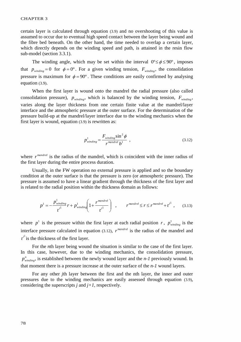
CHAPTER 3
78
certain layer is calculated through equation (3.9) and no overshooting of this value is
assumed to occur due to eventual high speed contact between the layer being wound and
the fibre bed beneath. On the other hand, the time needed to overlap a certain layer,
which directly depends on the winding speed and path, is attained in the resin flow
sub-model (section 3.3.1).
The winding angle, which may be set within the interval º90º0 , imposes
that 0windingp for º0 . For a given winding tension, windingF , the consolidation
pressure is maximum for º90 . These conditions are easily confirmed by analysing
equation (3.9).
When the first layer is wound onto the mandrel the radial pressure (also called
consolidation pressure), windingp , which is balanced by the winding tension, windingF ,
varies along the layer thickness from one certain finite value at the mandrel/layer
interface and the atmospheric pressure at the outer surface. For the determination of the
pressure build-up at the mandrel/layer interface due to the winding mechanics when the
first layer is wound, equation (3.9) is rewritten as:
1
2
1sin
br
Fp
andrelm
winding
winding
, (3.12)
where mandrelr is the radius of the mandrel, which is coincident with the inner radius of
the first layer during the entire process duration.
Usually, in the FW operation no external pressure is applied and so the boundary
condition at the outer surface is that the pressure is zero (or atmospheric pressure). The
pressure is assumed to have a linear gradient through the thickness of the first layer and
is related to the radial position within the thickness domain as follows:
1
1
1
1
1
1 ,1 landrelmandrelm
l
andrelm
windingl
windingtrrr
t
rpr
t
pp
, (3.13)
where 1p is the pressure within the first layer at each radial position r , 1
windingp is the
interface pressure calculated in equation (3.12), mandrelr is the radius of the mandrel and 1lt is the thickness of the first layer.
For the nth layer being wound the situation is similar to the case of the first layer.
In this case, however, due to the winding mechanics, the consolidation pressure, n
windingp , is established between the newly wound layer and the n-1 previously wound. In
that moment there is a pressure increase at the outer surface of the n-1 wound layers.
For any other jth layer between the first and the nth layer, the inner and outer
pressures due to the winding mechanics are easily assessed through equation (3.9),
considering the superscripts j and j+1, respectively.
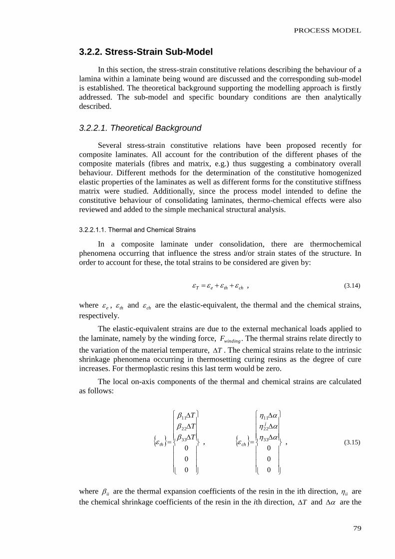
PROCESS MODEL
79
3.2.2. Stress-Strain Sub-Model
In this section, the stress-strain constitutive relations describing the behaviour of a
lamina within a laminate being wound are discussed and the corresponding sub-model
is established. The theoretical background supporting the modelling approach is firstly
addressed. The sub-model and specific boundary conditions are then analytically
described.
3.2.2.1. Theoretical Background
Several stress-strain constitutive relations have been proposed recently for
composite laminates. All account for the contribution of the different phases of the
composite materials (fibres and matrix, e.g.) thus suggesting a combinatory overall
behaviour. Different methods for the determination of the constitutive homogenized
elastic properties of the laminates as well as different forms for the constitutive stiffness
matrix were studied. Additionally, since the process model intended to define the
constitutive behaviour of consolidating laminates, thermo-chemical effects were also
reviewed and added to the simple mechanical structural analysis.
3.2.2.1.1. Thermal and Chemical Strains
In a composite laminate under consolidation, there are thermochemical
phenomena occurring that influence the stress and/or strain states of the structure. In
order to account for these, the total strains to be considered are given by:
chtheT , (3.14)
where e , th and ch are the elastic-equivalent, the thermal and the chemical strains,
respectively.
The elastic-equivalent strains are due to the external mechanical loads applied to
the laminate, namely by the winding force, windingF . The thermal strains relate directly to
the variation of the material temperature, T . The chemical strains relate to the intrinsic
shrinkage phenomena occurring in thermosetting curing resins as the degree of cure
increases. For thermoplastic resins this last term would be zero.
The local on-axis components of the thermal and chemical strains are calculated
as follows:
0
0
0
33
22
11
T
T
T
th
,
0
0
0
33
22
11
j
ch , (3.15)
where ii are the thermal expansion coefficients of the resin in the ith direction, ii are
the chemical shrinkage coefficients of the resin in the ith direction, T and are the
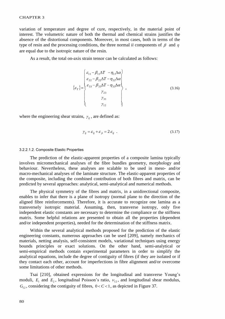
CHAPTER 3
80
variation of temperature and degree of cure, respectively, in the material point of
interest. The volumetric nature of both the thermal and chemical strains justifies the
absence of the distortional components. Moreover, in most cases, both in terms of the
type of resin and the processing conditions, the three normal ii components of and
are equal due to the isotropic nature of the resin.
As a result, the total on-axis strain tensor can be calculated as follows:
12
31
23
333333
222222
111111
T
T
T
T , (3.16)
where the engineering shear strains, ij , are defined as:
ijjiijij 2 . (3.17)
3.2.2.1.2. Composite Elastic Properties
The prediction of the elastic-apparent properties of a composite lamina typically
involves micromechanical analyses of the fibre bundles geometry, morphology and
behaviour. Nevertheless, these analyses are scalable to be used in meso- and/or
macro-mechanical analyses of the laminate structure. The elastic-apparent properties of
the composite, including the combined contribution of both fibres and matrix, can be
predicted by several approaches: analytical, semi-analytical and numerical methods.
The physical symmetry of the fibres and matrix, in a unidirectional composite,
enables to infer that there is a plane of isotropy (normal plane to the direction of the
aligned fibre reinforcements). Therefore, it is accurate to recognize one lamina as a
transversely isotropic material. Assuming, then, transverse isotropy, only five
independent elastic constants are necessary to determine the compliance or the stiffness
matrix. Some helpful relations are presented to obtain all the properties (dependent
and/or independent properties), needed for the determination of the stiffness matrix.
Within the several analytical methods proposed for the prediction of the elastic
engineering constants, numerous approaches can be used [209], namely mechanics of
materials, netting analysis, self-consistent models, variational techniques using energy
bounds principles or exact solutions. On the other hand, semi-analytical or
semi-empirical methods contain experimental parameters in order to simplify the
analytical equations, include the degree of contiguity of fibres (if they are isolated or if
they contact each other, account for imperfections in fibre alignment and/or overcome
some limitations of other methods.
Tsai [210], obtained expressions for the longitudinal and transverse Young’s
moduli, 1E and 2E , longitudinal Poisson’s ratio, 12 , and longitudinal shear modulus,
12G , considering the contiguity of fibres, 10 C , as depicted in Figure 37.
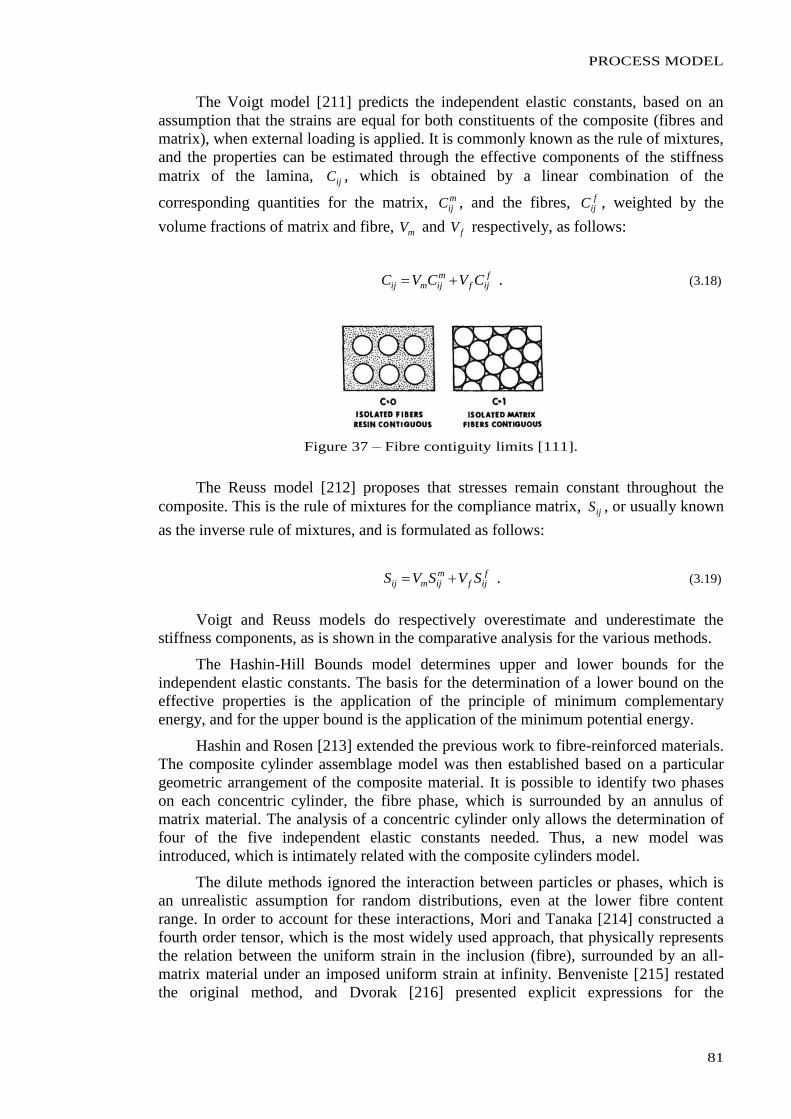
PROCESS MODEL
81
The Voigt model [211] predicts the independent elastic constants, based on an
assumption that the strains are equal for both constituents of the composite (fibres and
matrix), when external loading is applied. It is commonly known as the rule of mixtures,
and the properties can be estimated through the effective components of the stiffness
matrix of the lamina, ijC , which is obtained by a linear combination of the
corresponding quantities for the matrix, mijC , and the fibres, f
ijC , weighted by the
volume fractions of matrix and fibre, mV and fV respectively, as follows:
f
ijfmijmij CVCVC . (3.18)
Figure 37 – Fibre contiguity limits [111].
The Reuss model [212] proposes that stresses remain constant throughout the
composite. This is the rule of mixtures for the compliance matrix, ijS , or usually known
as the inverse rule of mixtures, and is formulated as follows:
f
ijfmijmij SVSVS . (3.19)
Voigt and Reuss models do respectively overestimate and underestimate the
stiffness components, as is shown in the comparative analysis for the various methods.
The Hashin-Hill Bounds model determines upper and lower bounds for the
independent elastic constants. The basis for the determination of a lower bound on the
effective properties is the application of the principle of minimum complementary
energy, and for the upper bound is the application of the minimum potential energy.
Hashin and Rosen [213] extended the previous work to fibre-reinforced materials.
The composite cylinder assemblage model was then established based on a particular
geometric arrangement of the composite material. It is possible to identify two phases
on each concentric cylinder, the fibre phase, which is surrounded by an annulus of
matrix material. The analysis of a concentric cylinder only allows the determination of
four of the five independent elastic constants needed. Thus, a new model was
introduced, which is intimately related with the composite cylinders model.
The dilute methods ignored the interaction between particles or phases, which is
an unrealistic assumption for random distributions, even at the lower fibre content
range. In order to account for these interactions, Mori and Tanaka [214] constructed a
fourth order tensor, which is the most widely used approach, that physically represents
the relation between the uniform strain in the inclusion (fibre), surrounded by an all-
matrix material under an imposed uniform strain at infinity. Benveniste [215] restated
the original method, and Dvorak [216] presented explicit expressions for the
CHAPTER 3
82
engineering constants of unidirectional composites, assumed as transversely isotropic
materials. The five constants are expressed as [217]:
*12
2*
2
2G
ppVpV
pppVppVp
mfmmf
mmfmmff
, (3.20)
1
*1
2*12
*2
*23
* 441
EEGmkVkV
kVkVmkkk
mfmmf
mmffmmf , (3.21)
*23
*
2
2G
mVmVmkmk
mVmVmkmkmmm
fmmfmmmm
mmffmmmmmf
, (3.22)
*12
** 2 kmkVmkV
mklVmklVl
mfmmmf
mfmmmmff
, (3.23)
*
2**1
2*12
**1
** 4k
lEkE
kk
lllVlVlnVnVn
mf
mfmmffmmff
. (3.24)
In a considerably different and unique approach, a direct relation between the
fibre bed stiffness, fbE , and the fibre volume fraction, fV , was used for stiffness
evaluation of the composite by Cai and Gutowski [27]. Assuming as well a transversely
isotropic behaviour, the fibre bed stiffnesses in the on-axis local 2-3 plane (Figure 14)
are considered to have the same value, fbbE , in which the subscript b refers to bulk. The
layer stiffnesses are then calculated by the following relations:
,
13
45
,
54
0
32
41
f
a
f
fa
f
f
a
fbfbfbb
a
ff
fb
V
V
E
V
V
V
V
V
V
EEE
VEVE
(3.25)
where fbiE are the fibre bed stiffness in the ith local direction, aV is the maximum
available volume fraction of fibres at which the resin flow stops [34], 0V is the
minimum volume fraction of fibres below which fibres do not carry transverse load,
aL is the ratio between the characteristic length, L , and amplitude, a , of the fibre
waviness pattern, fE is the fibre’s elastic modulus. As previously discussed in chapter
2, this approach was based on the beam theory, and was drawn to specifically attain the
waved misalignment of fibres, as an intrinsic characteristic of the FW process.
Therefore, this simpler set of equations is very attractive. Despite the fact that it is
possible to find in the literature empirical values for aV , 0V and , they shall be
assessed experimentally as they strongly depend on the material system and processing
conditions used.
PROCESS MODEL
83
3.2.2.1.3. Stress-Strain Constitutive Relations in Composite Lamina
The most commonly accepted constitutive relationships for composite laminates
are based on the generalized Hooke’s law and were already reviewed in chapter 2.
Namely, in equations (2.69), (2.70) and (2.72), the law applied to anisotropic, orthotropic
and transversely isotropic materials was respectively expressed. The main challenge is
then to select the most correct and adequate form, observing that during the FW
process, the compaction mechanisms act almost only in the radial direction. This aspect
promotes different stiffening behaviours between the local transverse (2-direction) and
radial (3-direction) directions. Such effect tends to attribute a local orthotropic nature,
rather than transversely isotropic, to the composite laminate being wound and
consolidated. Most previous authors studying the FW process, however, modelled the
laminate under assumptions of transverse isotropy.
Nonetheless, two other topics assume greater relevance for the FW process
modelling: the correct contemplation of the matrix contribution to the overall behaviour
through all the winding and curing/consolidation stages and the introduction of specific
features, such as intrinsic defects or variations in properties, which have particular
relevance in this process. The contribution of the viscous matrix to the composite
behaviour is normally accomplished through its elastic-apparent properties at each
moment. Its properties before complete cure/consolidation are almost not studied and no
reliable or accepted data exists in literature. Moreover, each matrix system has its own
characteristic evolution during curing/consolidation. Regarding the specific defects,
fibre waviness is highlighted as an intrinsic phenomenon in the FW process. As
mentioned above, some constitutive relations developed in the past accounted for this
effect. This will be further addressed herein.
The shear stresses and strains that are present in a composite laminate have
different effects in its behaviour. At the on-axis local level, the longitudinal shear mode
allows aligned fibres to accommodate the complex curvature of the real parts while the
transverse shear mode is often unwanted as it can lead to fibre waviness [27]. Terms
like “fibre wrinkles”, “fibre imperfections” or “marcel defects” have been used to refer
to this manufacturing defect. It has been observed to occur on, or through the thickness
of, the plane of lamination [108]. The fibre tows or bundles are not perfectly straight nor
perfectly aligned. It is, thus, practically unavoidable to have some waviness,
misalignment, entanglement or even breakage within a fibre bundle [16]. Moreover,
fibre waviness is a type of manufacturing defect that occurs especially during the FW
process [109] given the specific constraints applied to the fibre bundles being wound
and overwrapped by newly wound layers.
Since the exact waviness pattern and its degree of regularity is often of difficult
assessment, it is reasonable to assume some certain patterns with simple or convenient
analytical descriptive expressions. Sinusoidal waviness patterns were suggested as
reasonable approximations [27,109,218-220] where the characteristic amplitude, a , and
length, L , are the most relevant parameters.
Hsiao and Daniel [109], presented a different approach where the regular local
on-axis compliance matrix, regS , is transformed to follow the fibres’ path. The
transformed local compliance matrix, wavS , is, then, given at each point by:
Twavregwavwav TSRTRS
11
, (2.75)
CHAPTER 3
84
where wavT is the waviness transformation matrix for each at each point, R is the
Reuter matrix (to compatibilize the strain tensorial notation). Note that regS is the
inverse matrix of the stiffness matrix presented in equations (2.69), (2.70) and (2.72). The
waviness transformation matrix was given by:
cos0sin000
02sin2cos0sincos0sincos
sin0cos000
0sincos202cos02sin
000010
0sincos202sin02cos
wavT , (3.26)
where is the misalignment angle at each point of the assumed fibre waved path.
Then, the components of the constitutive local on-axis compliance matrix of a
waved composite were assessed from averaging the components of the transformed
local compliance matrix over one wavelength of the fibres’ path, as follows:
L
wavij
wavij dxS
LS
0
1 , (2.76)
where x is the fibre “ideal” axis and L is the wavelength of the sinusoidal pattern of the
fibres. In this way, the classical stress-strain constitutive relations used to describe
composite laminates’ behaviour were adapted to include the effect of fibre waviness.
The adequate transformations to the global coordinate system need to be properly
accounted as well, in order to match the stress, strain and stiffness properties with the
principal directions used for the other physical phenomena being modelled.
The off-axis quantities of a generic tensor, X , are then related to its on-axis
quantities, X , as follows [113]:
TTXTX
1 , (3.27)
where T is the transformation matrix. For the present case, the transformation matrix
from the on-axis (1,2,3) coordinate system to the off-axis ( z , , r ) cylindrical
coordinate system is given by [113]:
22
22
22
sincos000sincossincos
0cossin000
0sincos000
000100
sincos2000cossin
sincos2000sincos
T , (3.28)
where is the applicable winding angle.
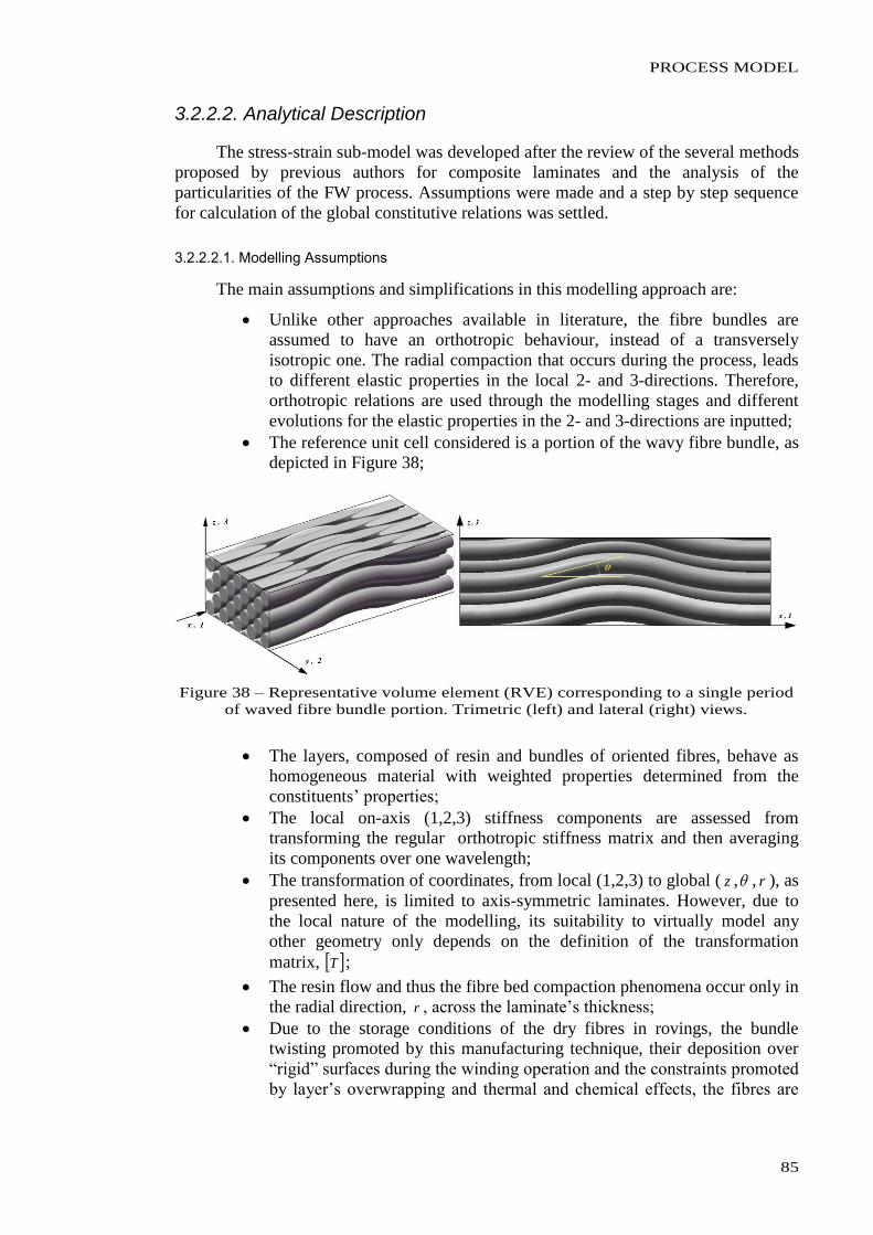
PROCESS MODEL
85
3.2.2.2. Analytical Description
The stress-strain sub-model was developed after the review of the several methods
proposed by previous authors for composite laminates and the analysis of the
particularities of the FW process. Assumptions were made and a step by step sequence
for calculation of the global constitutive relations was settled.
3.2.2.2.1. Modelling Assumptions
The main assumptions and simplifications in this modelling approach are:
Unlike other approaches available in literature, the fibre bundles are
assumed to have an orthotropic behaviour, instead of a transversely
isotropic one. The radial compaction that occurs during the process, leads
to different elastic properties in the local 2- and 3-directions. Therefore,
orthotropic relations are used through the modelling stages and different
evolutions for the elastic properties in the 2- and 3-directions are inputted;
The reference unit cell considered is a portion of the wavy fibre bundle, as
depicted in Figure 38;
Figure 38 – Representative volume element (RVE) corresponding to a single period
of waved fibre bundle portion. Trimetric (left) and lateral (right) views.
The layers, composed of resin and bundles of oriented fibres, behave as
homogeneous material with weighted properties determined from the
constituents’ properties;
The local on-axis (1,2,3) stiffness components are assessed from
transforming the regular orthotropic stiffness matrix and then averaging
its components over one wavelength;
The transformation of coordinates, from local (1,2,3) to global ( z , , r ), as
presented here, is limited to axis-symmetric laminates. However, due to
the local nature of the modelling, its suitability to virtually model any
other geometry only depends on the definition of the transformation
matrix, T ;
The resin flow and thus the fibre bed compaction phenomena occur only in
the radial direction, r , across the laminate’s thickness;
Due to the storage conditions of the dry fibres in rovings, the bundle
twisting promoted by this manufacturing technique, their deposition over
“rigid” surfaces during the winding operation and the constraints promoted
by layer’s overwrapping and thermal and chemical effects, the fibres are
CHAPTER 3
86
assumed to have a waviness pattern characterized by a function of the type
[27]:
L
xaz
2cos1
2 , (3.29)
where z is the transversal position measured perpendicularly to the “ideal”
axis, x , along the fibre, a and L are, respectively, the characteristic
amplitude and length of the sinusoidal pattern of the fibres. For
completeness, the fibre misalignment angle at each point is given by:
L
x
L
a
2sintan 1 ; (3.30)
Resin intrinsic properties that depend on the degree of cure, such as
thermal expansion coefficient, , chemical shrinkage coefficient, , and
thermal conductivity, k , are assumed to vary linearly between the known
initial and final values. Also the “elastic-apparent” constants of the resin,
like Young’s modulus, mE , shear modulus, ijG and Poisson’s ratios, ij ,
are assumed to vary in the same manner with the degree of cure, . The
following piecewise linear relations are considered to represent the
variation of such properties before and after the resin reach gelation, gel :
gelc
gelucc
YY
YYY
1 , (3.31)
where Y represents any of the above mentioned material properties, ucY
and cY its known values at the initial reference cure state and after cure
(consolidation), respectively. The quantity is the ratio defined as:
0
0
gel
. (3.32)
3.2.2.2.2. Composite elastic properties
The various methods available to determine the composite homogenized
properties were compared through evaluating their results for pre-selected cases. The
material properties used as constituents are indicated in Table 1. No difference was
observed for the longitudinal Young’s modulus calculation. In contrast, relevant
differences were observed in the other four elastic properties’ calculations, which are
depicted in Figure 39. The comparative predictions were realized for the range of fibre
volume fraction, fV , between 0.45 and 0.8.
From the results one may observe that the Reuss model typically underestimates
the elastic properties, except for the Poisson’s ratio. The Voigt model presents
consistent overestimations. The Mori-Tanaka method’s predictions consistently fitted
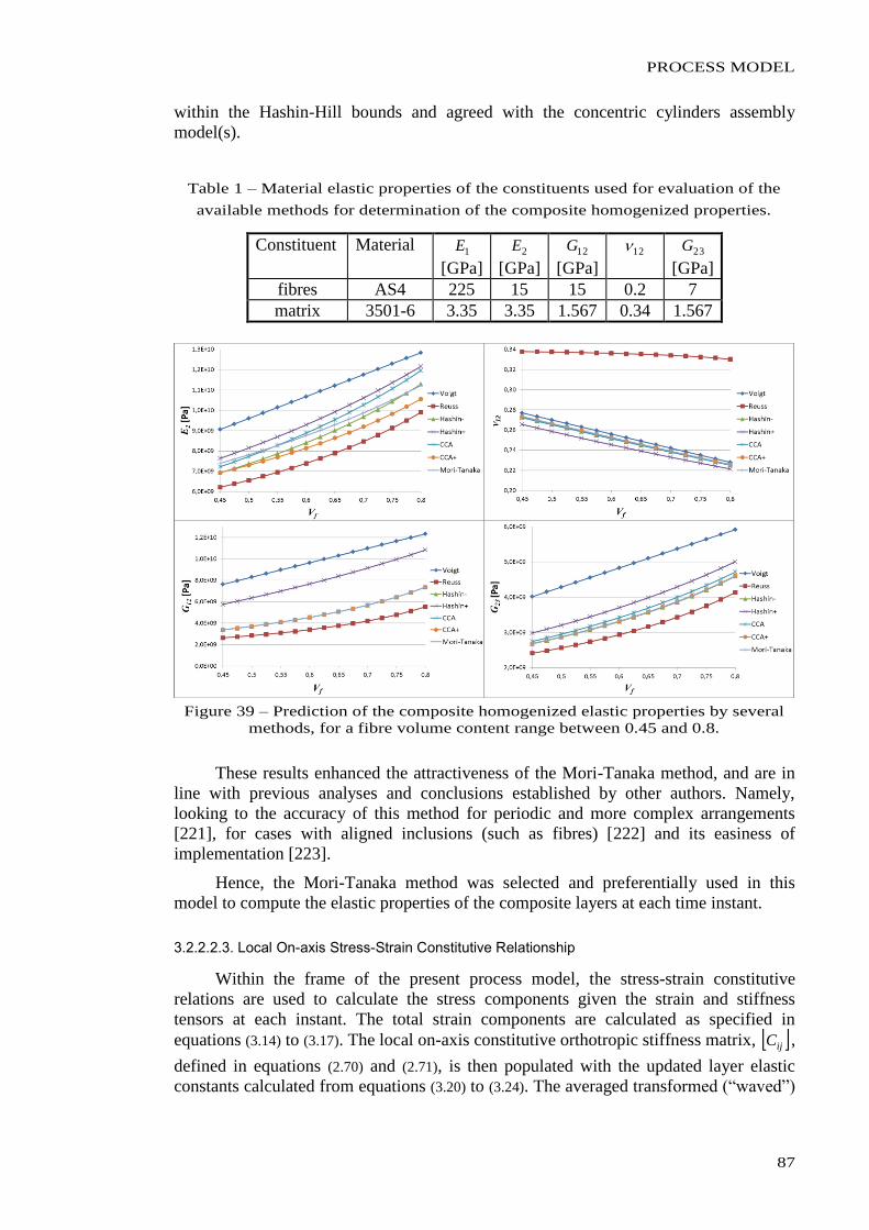
PROCESS MODEL
87
within the Hashin-Hill bounds and agreed with the concentric cylinders assembly
model(s).
Table 1 – Material elastic properties of the constituents used for evaluation of the
available methods for determination of the composite homogenized properties.
Constituent Material 1E
[GPa] 2E
[GPa] 12G
[GPa] 12 23G
[GPa]
fibres AS4 225 15 15 0.2 7
matrix 3501-6 3.35 3.35 1.567 0.34 1.567
Figure 39 – Prediction of the composite homogenized elastic properties by several
methods, for a fibre volume content range between 0.45 and 0.8.
These results enhanced the attractiveness of the Mori-Tanaka method, and are in
line with previous analyses and conclusions established by other authors. Namely,
looking to the accuracy of this method for periodic and more complex arrangements
[221], for cases with aligned inclusions (such as fibres) [222] and its easiness of
implementation [223].
Hence, the Mori-Tanaka method was selected and preferentially used in this
model to compute the elastic properties of the composite layers at each time instant.
3.2.2.2.3. Local On-axis Stress-Strain Constitutive Relationship
Within the frame of the present process model, the stress-strain constitutive
relations are used to calculate the stress components given the strain and stiffness
tensors at each instant. The total strain components are calculated as specified in
equations (3.14) to (3.17). The local on-axis constitutive orthotropic stiffness matrix, ijC ,
defined in equations (2.70) and (2.71), is then populated with the updated layer elastic
constants calculated from equations (3.20) to (3.24). The averaged transformed (“waved”)
CHAPTER 3
88
local stiffness matrix, wavijC , which accounts for the fibre waviness, is calculated as
follows:
L
wavij
wavwavij dxRTRCT
LC
0
111 , (3.33)
where wavT is the waviness transformation matrix for each at each point, presented
in equation (3.26), R is the Reuter matrix, x is the fibre “ideal” axis and L is the
wavelength of the sinusoidal pattern of fibres.
The constitutive relationship at the local on-axis coordinate system, keeping the
consideration of orthotropic material, is thus given by:
12
31
23
333333
222222
111111
12
31
23
33
22
11
T
T
T
C wavij , (3.34)
The 21 independent components of the un-averaged waviness transformed local
matrix, 11 RTRCTC wav
ijwavwav
ij , are expressed as:
225513
433
41111 42 nmCCnCmCC wav ,
223
21212 nCmCC wav ,
22553311
441313 4 nmCCCnmCC wav ,
nmnmCnmCCnmCCC wav 2255
33313
3131115 2 ,
2222 CC wav , 223
21223 mCnCC wav , nmCnmCC wav
231225 ,
225513
411
43333 42 nmCCnCmCC wav ,
nmnmCnmCCnmCCC wav 2255
31311
3331335 2 ,
266
24444 nCmCC wav , nmCnmCC wav
446646 ,
22255
2213331155 2 nmCnmCCCC wav ,
244
26666 nCmCC wav ,
05645363426241614 wavwavwavwavwavwavwavwav CCCCCCCC ,
(3.35)
where m and n are the director cosine and sine of the waviness transformation matrix,
respectively, and are assessed from the deformed shape of the chosen sinusoidal path,
presented in equation (3.29), written as:
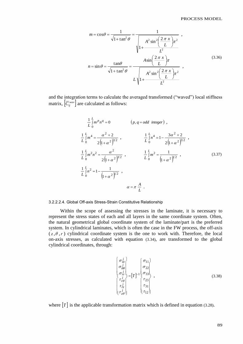
PROCESS MODEL
89
2
2222 2
sin
1
1
tan1
1cos
L
L
xA
m
,
2
2222 2
sin
1
2sin
tan1
tansin
L
L
xA
L
L
xA
n
,
(3.36)
and the integration terms to calculate the averaged transformed (“waved”) local stiffness
matrix, wavijC are calculated as follows:
L
qp ntegerioddqpnmL 0
,01
,
L
mL 0
232
24
12
21
,
L
nL 0
232
24
12
231
1
,
L
nmL 0
232
222
12
1
,
L
mL 0
212
2
1
11
,
2120
2
1
11
1
L
nL
,
L
A .
(3.37)
3.2.2.2.4. Global Off-axis Stress-Strain Constitutive Relationship
Within the scope of assessing the stresses in the laminate, it is necessary to
represent the stress states of each and all layers in the same coordinate system. Often,
the natural geometrical global coordinate system of the laminate/part is the preferred
system. In cylindrical laminates, which is often the case in the FW process, the off-axis
( z , , r ) cylindrical coordinate system is the one to work with. Therefore, the local
on-axis stresses, as calculated with equation (3.34), are transformed to the global
cylindrical coordinates, through:
12
31
23
33
22
11
1
T
jz
jrz
jr
jrr
j
jzz
, (3.38)
where T is the applicable transformation matrix which is defined in equation (3.28).
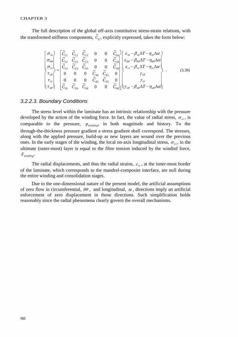
CHAPTER 3
90
The full description of the global off-axis constitutive stress-strain relations, with
the transformed stiffness components, ijC~
, explicitly expressed, takes the form below:
zzz
rz
r
rrrrrr
zzzzzz
z
rz
r
rr
zz
T
T
T
T
CCCC
CC
CC
CCCC
CCCC
CCCC
66362616
5545
4544
36332313
26232212
16131211
~00
~~~0
~~000
0~~
000
~00
~~~
~00
~~~
~00
~~~
. (3.39)
3.2.2.3. Boundary Conditions
The stress level within the laminate has an intrinsic relationship with the pressure
developed by the action of the winding force. In fact, the value of radial stress, rr , is
comparable to the pressure, windingp , in both magnitude and history. To the
through-the-thickness pressure gradient a stress gradient shall correspond. The stresses,
along with the applied pressure, build-up as new layers are wound over the previous
ones. In the early stages of the winding, the local on-axis longitudinal stress, 11 , in the
ultimate (outer-most) layer is equal to the fibre tension induced by the windinf force,
windingF .
The radial displacements, and thus the radial strains, rr , at the inner-most border
of the laminate, which corresponds to the mandrel-composite interface, are null during
the entire winding and consolidation stages.
Due to the one-dimensional nature of the present model, the artificial assumptions
of zero flow in circumferential, , and longitudinal, zz , directions imply an artificial
enforcement of zero displacement in those directions. Such simplification holds
reasonably since the radial phenomena clearly govern the overall mechanisms.
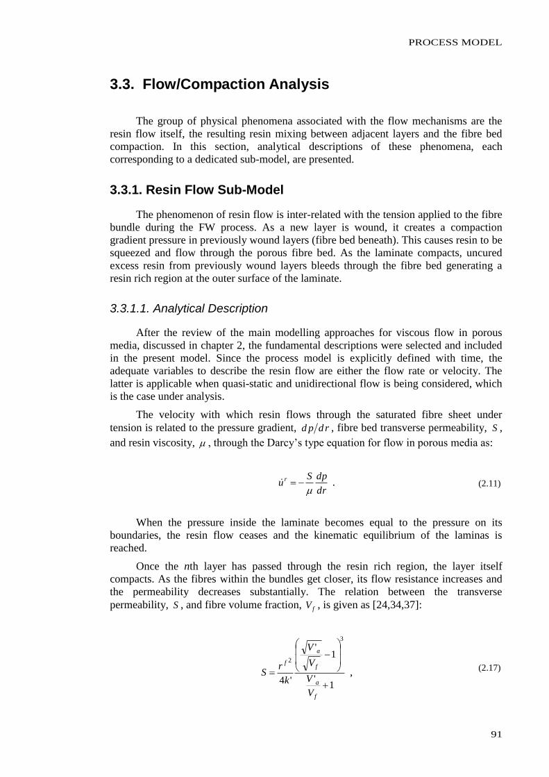
PROCESS MODEL
91
3.3. Flow/Compaction Analysis
The group of physical phenomena associated with the flow mechanisms are the
resin flow itself, the resulting resin mixing between adjacent layers and the fibre bed
compaction. In this section, analytical descriptions of these phenomena, each
corresponding to a dedicated sub-model, are presented.
3.3.1. Resin Flow Sub-Model
The phenomenon of resin flow is inter-related with the tension applied to the fibre
bundle during the FW process. As a new layer is wound, it creates a compaction
gradient pressure in previously wound layers (fibre bed beneath). This causes resin to be
squeezed and flow through the porous fibre bed. As the laminate compacts, uncured
excess resin from previously wound layers bleeds through the fibre bed generating a
resin rich region at the outer surface of the laminate.
3.3.1.1. Analytical Description
After the review of the main modelling approaches for viscous flow in porous
media, discussed in chapter 2, the fundamental descriptions were selected and included
in the present model. Since the process model is explicitly defined with time, the
adequate variables to describe the resin flow are either the flow rate or velocity. The
latter is applicable when quasi-static and unidirectional flow is being considered, which
is the case under analysis.
The velocity with which resin flows through the saturated fibre sheet under
tension is related to the pressure gradient, rdpd , fibre bed transverse permeability, S ,
and resin viscosity, , through the Darcy’s type equation for flow in porous media as:
dr
dpSu r
. (2.11)
When the pressure inside the laminate becomes equal to the pressure on its
boundaries, the resin flow ceases and the kinematic equilibrium of the laminas is
reached.
Once the nth layer has passed through the resin rich region, the layer itself
compacts. As the fibres within the bundles get closer, its flow resistance increases and
the permeability decreases substantially. The relation between the transverse
permeability, S , and fibre volume fraction, fV , is given as [24,34,37]:
1'
1'
'4
3
2
f
a
f
a
f
V
V
V
V
k
rS , (2.17)
CHAPTER 3
92
where fr is the fibre radius, 'k is a modified Kozeny constant ( 2.0'k for carbon fibre
beds [34]) and aV ' is the maximum available fibre volume fraction at which radial
flow stops ( 82.0'76.0 aV for carbon fibre beds [34]).
3.3.1.2. Boundary Conditions
Due to the geometrical arrangement of the composite laminate onto the cylindrical
mandrel, as well as the necessarily negative value of the radial pressure gradient, the
resin flow is known to occur only from inner to the outer regions (outward flow). At the
composite-mandrel interface no flow occurs. As mentioned previously, the flow ceases
when the pressure gradient becomes null. In practical terms, very high resin viscosity
and/or very low permeability promote the same effect of flow ceasing.
When the nth layer is wound, the thickness of the resin rich layer is assessed
through subtracting the nth layer inward displacement to the n-sum outer radial position.
This definition is slightly different from the one proposed by previous authors [24] and
comes from experimental evidence and the conservation of mass principle. Since no
relevant changes in density occur during the process, the principle of conservation of
mass reasonably holds the effective mass transfer events within the laminate’s
thickness.
The values of aV ' used to compute the permeability, depend on the type of fibre
packing arrangement considered at the micro-scale. These have relevant influence in the
calculation of this and sub-sequent parameters. Therefore, they are referred to and
assessed in chapter 4, in the experimental validation procedures.
3.3.2. Resin Mixing Sub-Model
In the FW process, resin from one layer can flow to an adjacent layer. Uncured
resin from previously wound layers can flow into the newly wound layer and the
effective properties of the layer’s matrix may change significantly. This phenomenon is
very intrinsic to wet FW and encloses very relevant influence to the cure/consolidation
of the composite laminate.
3.3.2.1. Analytical Description
When two portions of resin of the same type but with different
curing/consolidation histories mix, the joint behaviour of the blend follows a new
(unknown) path. This is valid for the mechanical and chemo-rheological properties. In
order to account for this effect in the process model, one or more physical parameters
representative of the changes in the behaviour should be modelled.
In the present model, the effective viscosity of the matrix is one of the most
relevant parameters, since it affects the flow ability, and therefore the consolidation, but
is directly related with the degree of cure/consolidation which is a fast evolving
property during the process. Thus, the viscosity was chosen as the reference property to
associate with the resin mixing.
The effective viscosity of a blend can be calculated by a rule of mixtures. In the
mth layer, the viscosity can be calculated by a linear combination as [24]:
PROCESS MODEL
93
m
jj
mj
1
, (3.40)
where j are the viscosities of the constituents (from all contributing layers), m
j is the
relative concentration of the different constituents in the mth layer, defined as:
mr
jrm
jV
V , (3.41)
where j
rV is the volume of resin from the jth ply into the mth layer and m
rV is the total
volume of resin in the mth layer. These volumes are readily calculated once the resin
velocity at the layer boundaries is known.
3.3.2.2. Boundary Conditions
The validity of the linear combination of the constituent’s viscosity, to evaluate
the joint viscosity was not questioned before. However, a specific study was carried out
and discussion on this aspect is addressed in chapter 4. The overall viscosity of the
blend (mixture of resins) evolves through two mechanisms: the update of the
constituents’ relative concentration in each layer (or material point) and the
self-evolution of each constituent’s viscosity due to thermo-chemical phenomena.
For long winding times, the viscosity of the resin in adjacent layers can be
significantly different. In the case of short winding times, that effect may be nearly
neglected. In any case, the history of the effective viscosity of the mixture differs from
its “ideal” history if no mixing occurs. The relevance of this phenomenon also varies
with the type of resin system: for thermoplastic resin systems, for example, the viscosity
of a previously wound layer is so high that mixture with new resin is unlikely to occur.
The interchangeable relation between the viscosity and the degree of cure/crystallization
of the resin, allows to infer its cure/consolidations state.
3.3.3. Fibre Bed Compaction Sub-Model
One of the immediate effects of the resin transfer between adjacent layers is the
correspondent motion of the fibre bed. This accommodation is further enforced by the
mechanical action of the incremental external pressure as the laminate is built.
Therefore, the radial positions of the layers evolve according with these actions. Their
thickness and available volume vary as a consequence, thus also the relative fibre/resin
contents. The description of these phenomena is carried out in this section.
3.3.3.1. Background
In typical FW, the radial position of the fibre bed (also called fibre sheet), may be
modified due to the following two reasons [23]:
Fibre tension in the curved fibre tows causes the fibres to move through
the resin while the resin viscosity is sufficient low. This is the reverse view
of the resin squeezed flow phenomenon. Once the viscosity becomes
CHAPTER 3
94
sufficiently high the fibres become “locked” into the resin and do not
move relatively to resin under the action of fibre tension;
Temperature variations of the mandrel/composite and chemically induced
changes (“shrinkage”) in the resin may cause expansions or contractions.
From integrating the stress-strain constitutive relations, equation (3.39), Lee and
Springer [23] modelled the radial displacement of the fibre bed due to an incremental
external pressure originated by the winding of new layers. For the generic jth layer,
within the fibre bed already in place while the new layer is wound, the radial
displacement, u , was expressed as
1,ln~2
~~
~2
~4
~2
~
1,~2
~
~~
~2
~4
~2
~
33
13121
2
2233
36261
111
2233
13121
2
2233
3626111
j
j
j
j
jjjj
j
j
j
j
jjjjj
rrC
CCdr
CC
CCcrbrau
rCC
CCdr
CC
CCcrbrau
j
, (3.42)
where ja1 , jb1 , jc1 and jd1 are constants evaluated from the known conditions at each
layer interface and at inner and outer surfaces of the composite “cylinder”, r is the
radial position, ijC~
are the components of the off-axis ( z , , r ) stiffness matrix and
j
j
C
C
33
22~
~
. (3.43)
For the determination of the constants, continuity of both displacements and radial
stresses at the layer’s interface was assumed. Similar analyses were made to derive the
displacements induced by thermal expansions or contractions and chemical changes
(“shrinkage”). These descriptions of the displacements are intrinsically related with the
stress and strain states in the laminate.
Cai and Gutowski [16] further modelled the effect of the displacement and
deformation of the fibre bed in the relative contents of fibres and matrix. Considering
fibre and resin continuity, unidirectional radial flow and taking the volume element
sketched in Figure 17 as reference, the mass conservation relationship for the deformed
volume element (with thickness of drr and radial displacement) was described
as:
01
q
trV
tf
, (3.44)
and the continuity condition for the fibre bundle as:
rrV
V
f
f
0 , (3.45)
PROCESS MODEL
95
where ur is the radial position of the volume element after displacement, fV is the
fibre volume fraction, 0fV is the fibre volume fraction at the reference state (when
0u ) and q is the flow rate per unit area in the radial direction. Combining equations
(3.44), (3.45) and (2.11), the consolidation equation in terms of the deformed variable, ,
was written as [16]:
011
rf
f
pS
t
V
V , (3.46)
where S is the apparent permeability of the medium, is the fluid viscosity and rp is
the resin pressure.
3.3.3.2. Analytical Description
The descriptions of the displacements and deformations of the fibre bed proposed
by the two groups of authors cited above are intrinsically coupled with the stress-strain
constitutive relations and the overall strain states, respectively. Herewith, for the
descriptions of the fibre compaction group of phenomena, simpler analyses were
realized, thus obtaining alternative relations which held realistic modelling approaches.
The main physical assumptions taken were the following ones:
The fibres angle remains constant during processing;
Motion of the fibre sheet in axial, zz , and hoop, , directions is not
considered once the components of fibre tension in these directions are
symmetrically balanced;
Any inertial effects are negligible;
The thickness of the fibre sheet is small when compared to the radial
positions (cylindrical shell analysis).
Under the assumptions described above, the force equilibrium for a given layer
may be expressed as [23]:
fsl rrd
pd
t
p
, (3.47)
where p is the radial pressure, lt is the layer thickness, is the hoop stress.
By combining equations (2.11), (3.7) and (3.47) the following expression is obtained
for the radial velocity of the fibre sheet:
211 sinfs
ffs
rr
Su , (3.48)
where S is the apparent permeability of the medium, is the fluid viscosity, f11 is the
fibre’s stress in the local on-axis longitudinal direction, fsr is the radial position of the
fibre sheet and is the winding angle.
CHAPTER 3
96
The instantaneous radial position of the fibre sheet, fsr , is given by:
fs
rfsfs urr 0 , (3.49)
where fsr0 is the radial position of the fibre sheet at a reference time (deposition time,
prior to the displacement) and fsru is the radial displacement of the fibre sheet relatively
to resin. The relative displacement fsru is determined by integrating equation (3.48).
The complementary contribution of the thermo-chemical strains to the motion or
displacement of the fibre sheet is evaluated by integrating the thermal and chemical
strain components, th and ch , in the radial direction, to calculate the thermal and
chemical displacements, thu and chu , respectively. Due to the volumetric nature of the
thermal and chemical strains, the corresponding radial displacements are:
Tu rrth 2
1 ,
rrchu2
1 ,
(3.50)
where rr and rr are the thermal expansion and chemical shrinkage coefficients and
T and are the variations of temperature and degree of cure, respectively. The
latter only applies for thermosetting resin systems. Equation (3.49) further completes as:
chthfs
rfsfs uuurr 0 . (3.51)
The variation of radial positions of the layers, may alter their thickness, lt , and
thus the relative contents of fibres, fV . Since only matrix flows in and/or out of each
layer (the fibres remain), the thickness variation is directly related with the relative
contents. Since only radial flow is considered and that the “circumferential length” of
each layer is assumed not to vary ( fsfsr ru ), the condition:
ntconstatV lf , (3.52)
holds for the entire consolidation process. The updated contents are then assessed.
3.3.3.2. Boundary Conditions
As in the case of the strains, the displacements at the mandrel-composite interface
are null. The mass conservation principle is transformed and used as volume
conservation principle throughout the process model. The variations of volume due to
thermal and/or chemical effects are ignored in the scope of this simplified principle.
Thus, the total thickness of the laminate remains constant after deposition of the
ultimate layer. Since no resin loss is admitted in the model, the outer layers will
incorporate all the excess of resin squeezed from inner layers. In practice, the so-called
resin rich region will be held by the outer layer(s).
PROCESS MODEL
97
3.4. Thermo-Chemical Analysis
The thermo-chemical group of physical phenomena includes the heat transfer, the
kinetics and the rheological behaviours of the matrix systems. The relationships
between the heat generation, temperature, cure or crystallinity and the viscosity of the
matrix are accounted in this group. In this section, analytical models of these
sub-processes taking place during resin cure or crystallization in FW are addressed.
These phenomena were extensively discussed in chapter 2 and were specifically
addressed through experimental procedures described in chapter 4 as well. Therefore,
herein, only the relevant equations chosen for the process model are presented.
3.4.1. Heat Transfer Sub-Model
The heat transfer within the laminate and between the laminate and the
neighbourhood may assume major relevance in certain process conditions. It allows for
the dissipation of the heat generated by chemical reactions, thus helping to maintain a
certain prescribed processing temperature that may be enforced from external sources.
Additionally, it may induce cure/crystallization accelerations or decelerations.
3.4.1.1. Analytical Description
The basis of this sub-model is the energy conservation equation extended with the
energy absorbed or released during cure of the thermoset resin or
crystallization/consolidation of the thermoplastic. In this model, only
through-the-thickness thermal gradients are considered. Neglecting energy transfer by
convection, the one-dimensional energy equation can be expressed as [80]:
Qr
Tk
rrt
TC r
1 , (2.26)
where t is time, r is the radial position, T is the temperature, is the density of the
composite, C is the specific heat of the composite, rk is the thermal conductivity in
radial direction and Q is the rate at which heat is generated by the curing or
crystallizing resin.
For thermosettings, the heat generation term is a function of the change in the
resin cure state, dtd , and takes the following form [27, 80]:
umm H
dt
dVQ
, (2.27)
where m and mV are the density and volume fraction of the matrix, respectively, uH ,
is the total heat of reaction (characteristic of each system).
For thermoplastics, Q is the rate at which heat is generated or absorbed by the
composite during heating and cooling and takes the following form [84]:
CHAPTER 3
98
umm H
dt
dcVQ
, (2.32)
where dtdTTcfdtdc ,,1 is the rate of change of crystallinity (or morphology for
amorphous thermoplastics), an empirically derived function of temperature and rate of
change of temperature.
3.4.1.2. Boundary Conditions
In the inner limits of the composite laminate, the mandrel exchanges heat with the
composite and the inner atmosphere. A simplification was introduced by neglecting this
phenomenon. The mandrel is assumed to be at room/processing temperature during the
winding and cure/consolidation phases.
The outer surface of the composite laminate is in direct contact with air at
room/processing temperature.
In thermosetting resins, the total heat of reaction, used in the determination of the
heat generation rate, is a characteristic property/value for each resin system. This is
further addressed in chapter 4, where the experimental values are listed.
3.4.2. Resin Cure/Crystallization Sub-Model
Accordingly with the literature review fully addressed in chapter 2, several
relationships between the degree of cure/crystallization and the temperature, like:
),( Tfdt
d
, (3.53)
),( Tcfdt
dc , (3.54)
were chosen and catalogued in the model library, thus accounting for several applicable
resin systems. The data for the thermosetting resins pre-selected for this library is
summarized in Table 2. Data for thermoplastic systems is less homogeneous (all
available equations have different parameters) and less consensual, as well. For this
reason these are not listed in the table.
For the specific resin systems used in the experimental validation, the governing
kinetic models were fully developed and are described in detail in chapter 4.
3.4.3. Resin Viscosity Sub-Model
The resin viscosity depends on the degree of cure, , and the temperature, T , in
the case of thermosetting systems, while for thermoplastics it is a single function of the
temperature, T . Similarly to the cure/crystallization sub-model, several relationships
between the degree of cure/crystallization and the temperature, of the types:
),( Tf , (3.55)
)(Tf , (3.56)
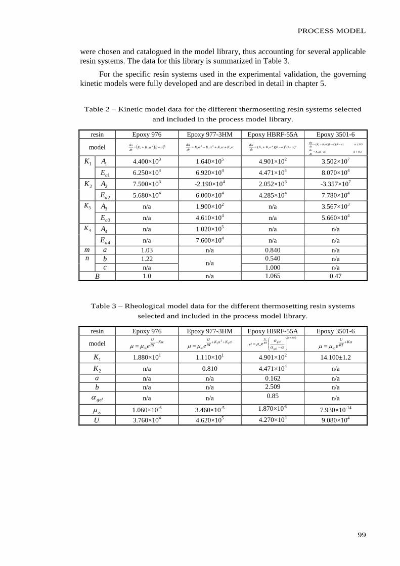
PROCESS MODEL
99
were chosen and catalogued in the model library, thus accounting for several applicable
resin systems. The data for this library is summarized in Table 3.
For the specific resin systems used in the experimental validation, the governing
kinetic models were fully developed and are described in detail in chapter 5.
Table 2 – Kinetic model data for the different thermosetting resin systems selected
and included in the process model library.
resin Epoxy 976 Epoxy 977-3HM Epoxy HBRF-55A Epoxy 3501-6
model ba BKKdt
d
21
43
2
2
3
1 KKKKdt
d
cba BKK
dt
d)1())(( 21
3.0)1(
3.0))(1)((
3
21
Kdt
d
BKKdt
d
1K
1A 4.400×10
3 1.640×10
5 4.901×10
2 3.502×10
7
1aE 6.250×10⁴ 6.920×10
4 4.471×10
4 8.070×10
4
2K
2A 7.500×10³ -2.190×10
4 2.052×10
3 -3.357×10
7
2aE 5.680×10⁴ 6.000×10
4 4.285×10
4 7.780×10
4
3K
3A n/a 1.900×10
2 n/a 3.567×10
3
3aE n/a 4.610×10⁴ n/a 5.660×10
4
4K
4A n/a 1.020×10
5 n/a n/a
4aE n/a 7.600×10⁴ n/a n/a
m a 1.03 n/a 0.840 n/a
n b 1.22 n/a
0.540 n/a
c n/a 1.000 n/a
B 1.0 n/a 1.065 0.47
Table 3 – Rheological model data for the different thermosetting resin systems
selected and included in the process model library.
resin Epoxy 976 Epoxy 977-3HM Epoxy HBRF-55A Epoxy 3501-6
model
K
RT
U
e
2
21 KK
RT
U
e
)(
ba
gel
gelRT
U
e
K
RT
U
e
1K 1.880×101 1.110×10
1 4.901×10
2 14.100±1.2
2K n/a 0.810 4.471×10⁴ n/a
a n/a n/a 0.162 n/a
b n/a n/a 2.509 n/a
gel n/a n/a 0.85 n/a
1.060×10⁻⁶
3.460×10⁻⁵
1.870×10⁻⁸
7.930×10⁻¹⁴
U 3.760×10⁴ 4.620×10
5 4.270×10
4 9.080×10
4
CHAPTER 3
100
3.5. Main Assumptions and Limitations
Several assumptions and limitations were introduced along with the description of
the sub-models. Nevertheless, some remarks have to be made on relevant aspects,
aiming and foreseeing the generalization of the FW process modelling. Herewith, the
most important aspects are highlighted.
Certain material properties varying during the process were assumed to change
linearly with the degree of cure. Some of them were also assumed to change linearly
across the layer’s thicknesses. It seemed reasonable, given the difficulty in accurately
assess those parameters.
No analysis was made to account for the eventual void inclusion and growth
during the process, since the FW characteristic of sequential lamination and relatively
low velocities make such phenomena nearly absent and therefore negligible even from
the theoretical point of view.
Concerning the applicability of the thermo-chemical data, efforts were made to
assess the kinetic and rheological behaviour under conditions that would approximate
the real ones occurring at the layer/laminate level. The information in the literature is
very limited on such conditions.
On the general applicability, this model is of local nature. Moreover, it has a
decoupled sub-modelling structure (modular architecture), thus making it virtually
applicable to any geometry and material system, provided that the adequate input data is
available. It accomplishes, in this way, the main objective of developing a basic
framework for further studies and developments, pursuing its usefulness to real
applications.
CHAPTER 4
EXPERIMENTAL PROCEDURES

CHAPTER 4
102
EXPERIMENTAL PROCEDURES
103
4.1. Validation Methodology
In the previous chapter, the relationships between the several physical variables
and parameters acting at the layer/laminate level during the FW process were identified.
A modular multi-physical process model was built in which the sub-models (each
modelling a specific group of phenomena) interact through the exchange and iterative
updating of the evolving variable/quantities. The accuracy (and validity) of this model
is, therefore, dependent upon
the values of the variables and/or properties used in it;
the correction of the physical descriptions of each phenomenon; and,
the assumptions made.
The variables and/or properties inputted to the model are divided in three groups:
the material thermal and mechanical properties, the input variables of the manufacturing
process and the input data that feed (independently) one or more sub-models. The first
group of properties is mainly provided by either the material manufacturer’s data sheets
or literature. The process related inputs are retrieved from process setup, experimental
measurements or previous knowledge. Among these are the fibre winding force,
windingF , winding angle, , tow bandwidth, b , mandrel radius, mandrelr , initial layer’s
thickness, lt0 , initial fibre volume fraction, 0V , and processing (room) temperature, prT .
The input data used in specific sub-models, such as resin cure (in the case of
thermosetting resins), resin viscosity or resin mixing, is assessed from both previously
established models and novel sub-models developed during the present work. These are
presented and discussed in the second section (section 4.2) of this chapter.
The correction of the physical descriptions of each phenomenon, i.e., the validity
of each of the sub-models established in the framework of the present multi-physical
process model, was discussed in the previous chapter, along with their own definitions
and theoretical support. Their experimental validation is, however, a very important part
of the model development, since it allows the evaluation of the overall applicability and
accuracy of the process model, through assessment to reliable “real” data and later
comparison with the numerical results simulating similar conditions. Moreover, the
difficulty in assessing and measure the relevant variables during the process (which
justifies the lack of comprehensive experimental validation of the main process models
developed in the last decades) determines the need to develop a few dedicated setups
and methods, which are quite unique and interesting per se. The measurement of the
relevant model outputs is presented and discussed in the third section (section 4.3) of
this chapter.
The main assumptions made in the model are related with the initial and boundary
conditions as well as with the evolution of properties of the matrix during the process.
The former were based on self-evident aspects of the process while the latter were
established to approximate matrix properties which are very difficult to assess. Namely,
values for matrix Young’s modulus, mE , shear modulus, mG , Poisson’s ratios, m ,
density, m , heat conductivity, mK , heat capacity, mC , thermal expansion coefficient, m , and shrinkage coefficient, m , are extremely difficult to assess in practical way
(unconsolidated matrix within the composite laminate) and are scarcely available in
literature. Thus, these were not specifically validated through external means rather than
just by the overall matching of the model results, addressed in chapter 5. Also, eventual
CHAPTER 4
104
formation of voids was not considered, since these were assumed negligible upon the
literature review made.
To accomplish the goal of verifying the validity of the process model, a
comprehensive experimental programme was followed. It included both the
development of new sub-models for the material systems used and measurement of the
change in the main process physical variables during the winding trials. Due to the
modular (decoupled) nature of the process model developed, the desirable independent
validation of each sub-model seemed applicable and was aimed from the beginning.
Such an independent validation would allow not only to test and evaluate each of the
relevant physical descriptions integrated in the model, but also to divide the
experimental programme into several dedicated tests thus attributing greater control and
accuracy to the validation procedure.
The methodology used for the experimental validation of the process model
consisted in generating sets of reliable data from the measurements done in several
winding trials. The value and variations of the main physical variables were assessed
using dedicated techniques and parametric configurations of the experiments.
Specifically, the main outputs of the model were measured and/or evaluated
through the following experiments:
an original experimental technique was developed to characterize the resin
flow within the laminate during the FW process;
the compaction of the laminate was measured through the comparison of
initial and final radial positions of the layers;
the variation of the relative phases content (fibre and matrix volume
fractions) was assessed both in global terms and through-the-thickness
final gradients;
the fibre waviness was characterized at initial and final stages of the
winding in order to support the assumptions made on typical fibres
misalignment pattern.
Regarding several other model parameters, which are mainly input values for relevant
sub-models, additional experiments were conducted. Based on existing techniques, the
following thermo-chemical phenomena were studied and modelled, considering the two
resin systems used in the winding trials:
novel kinetic models of the cure of two different thermosetting systems
were developed;
the rheology (evolution of viscosity during the cure process) was also
characterized and modelled for these resin systems;
the assumptions made in the resin mixing sub-model were evaluated
through an original rheological characterization of the two resin systems
under certain mixing conditions that reproduced the operating conditions
in wet FW.
As mentioned above, the input data relating to initial process conditions, were setup and
confirmed in the winding trials.
The experimental validation task conducted within the present study included
several dedicated techniques and methods, which are applicable and relevant to many
composite manufacturing processes, rather than just to FW. Therefore, the research
work and the knowledge gathered through the experimental programme had a greater

EXPERIMENTAL PROCEDURES
105
scope than the sole validation of the process model developed herewith. Moreover, a
few original methods and sub-models were developed thus enhancing the relevance and
value of this campaign.
In this chapter, the thermo-chemical, mechanical and manufacturing experimental
tests are presented. The procedures, results and their analysis are discussed in detail.
Throughout the following two sections, these are divided into the experimental
assessment to model input data and measurements of output data.
CHAPTER 4
106
4.2. Experimental Assessment to Model Input Data
In this section, the experimental procedures conducted to either generate reliable
input data for the thermo-chemical sub-models or measure main process input
parameters are described. Both the procedures and the results are presented.
4.2.1. Resins Cure Kinetics
The cure/consolidation behaviour of the matrix in composites is a major physical
phenomenon among those driving the morphological changes in a composite laminate
under processing conditions. Its characterization is, therefore, highly relevant for the
modelling of the manufacturing process.
In the FW process, the matrix systems used are grouped into thermosetting and
thermoplastic resins. When using thermosetting resins, both wet and prepreg dry
winding configurations could be setup, while in the case of thermoplastics only prepreg
winding may be practically implemented. Due to greater spread and applicability of
thermosettings in high-performance parts as well as the complexity of their
thermo-chemical behaviour, these were chosen for the experimental validation of the
current FW process model. Specifically, two epoxy resin systems used in wet FW were
selected and studied in detail and later added to the process model library. The two
systems were characterized and modelled through differential scanning calorimetry
(DSC) analysis. The kinetic parameters were determined and two original kinetic
models were established for these resin systems subjected to “real” processing
conditions. The aim was to assess the input data needed for the resin cure process
sub-model. Hereafter, the experimental procedure is described, together with its
validation and the kinetic models developed.
4.2.1.1. Experimental Procedure
The curing of thermosetting resins is almost invariably characterized by an
exothermic chemical reaction where low molecular weight monomers, in a mixture with
low weight hardeners and/or accelerators, change from a liquid state into a rubbery and
then solid glass states. Covalent crosslinks are formed during this curing process.
Although several reactions may take place (simultaneously or sequentially) the overall
transformation of reactants into products may be assessed through the global extent of
conversion. Since in thermosetting resins this process is accompanied by release of heat,
the extent of conversion may be evaluated as a fraction of the total heat released [224].
This quantity is the so-called degree of cure, , that was previously defined in equation
(2.24), recalled as:
uH
H , (2.24)
where H is the heat evolved from time 0t to time t and uH is the total (ultimate)
heat of reaction of the resin.
A few experimental techniques have been developed to characterize the behaviour
of material samples measurable through changes in temperature and/or other related
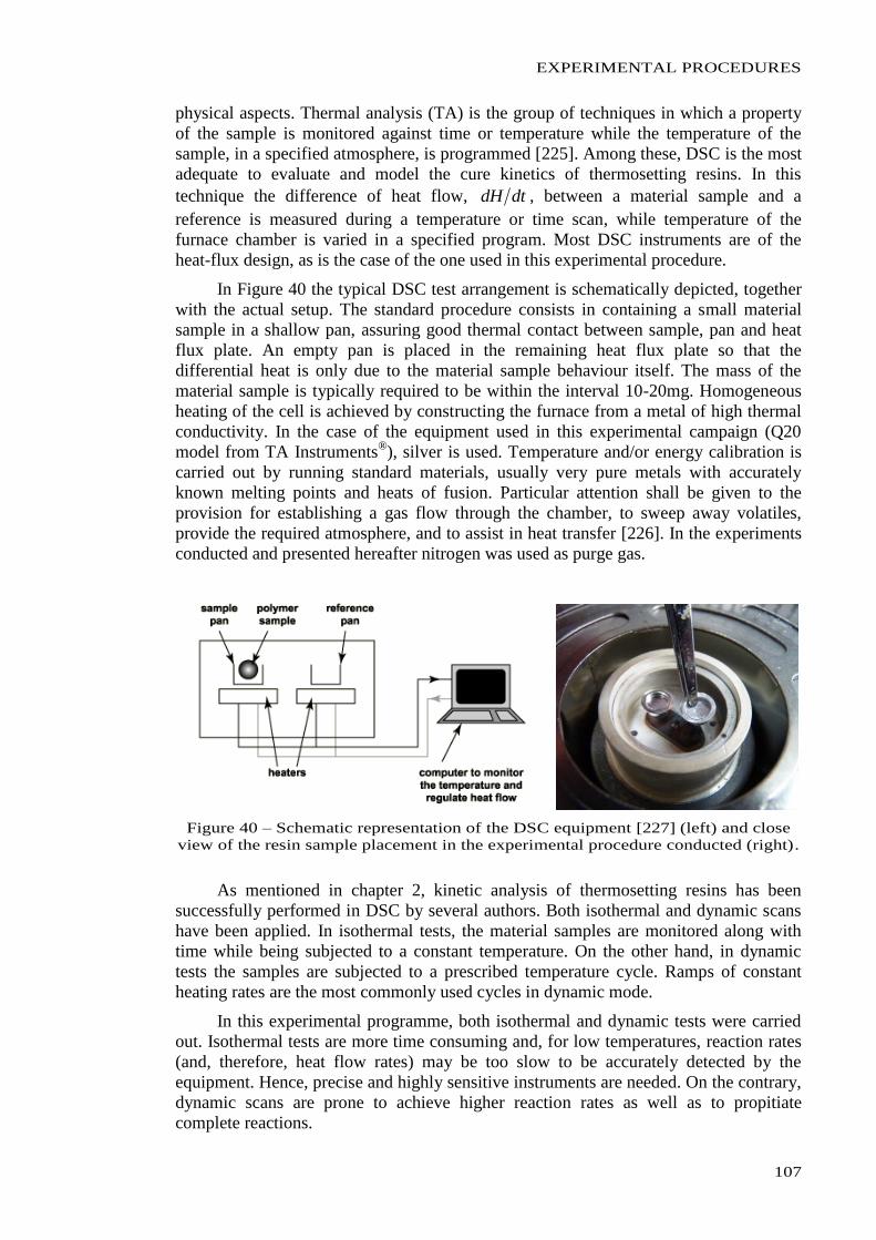
EXPERIMENTAL PROCEDURES
107
physical aspects. Thermal analysis (TA) is the group of techniques in which a property
of the sample is monitored against time or temperature while the temperature of the
sample, in a specified atmosphere, is programmed [225]. Among these, DSC is the most
adequate to evaluate and model the cure kinetics of thermosetting resins. In this
technique the difference of heat flow, dtdH , between a material sample and a
reference is measured during a temperature or time scan, while temperature of the
furnace chamber is varied in a specified program. Most DSC instruments are of the
heat-flux design, as is the case of the one used in this experimental procedure.
In Figure 40 the typical DSC test arrangement is schematically depicted, together
with the actual setup. The standard procedure consists in containing a small material
sample in a shallow pan, assuring good thermal contact between sample, pan and heat
flux plate. An empty pan is placed in the remaining heat flux plate so that the
differential heat is only due to the material sample behaviour itself. The mass of the
material sample is typically required to be within the interval 10-20mg. Homogeneous
heating of the cell is achieved by constructing the furnace from a metal of high thermal
conductivity. In the case of the equipment used in this experimental campaign (Q20
model from TA Instruments®), silver is used. Temperature and/or energy calibration is
carried out by running standard materials, usually very pure metals with accurately
known melting points and heats of fusion. Particular attention shall be given to the
provision for establishing a gas flow through the chamber, to sweep away volatiles,
provide the required atmosphere, and to assist in heat transfer [226]. In the experiments
conducted and presented hereafter nitrogen was used as purge gas.
Figure 40 – Schematic representation of the DSC equipment [227] (left) and close
view of the resin sample placement in the experimental procedure conducted (right).
As mentioned in chapter 2, kinetic analysis of thermosetting resins has been
successfully performed in DSC by several authors. Both isothermal and dynamic scans
have been applied. In isothermal tests, the material samples are monitored along with
time while being subjected to a constant temperature. On the other hand, in dynamic
tests the samples are subjected to a prescribed temperature cycle. Ramps of constant
heating rates are the most commonly used cycles in dynamic mode.
In this experimental programme, both isothermal and dynamic tests were carried
out. Isothermal tests are more time consuming and, for low temperatures, reaction rates
(and, therefore, heat flow rates) may be too slow to be accurately detected by the
equipment. Hence, precise and highly sensitive instruments are needed. On the contrary,
dynamic scans are prone to achieve higher reaction rates as well as to propitiate
complete reactions.
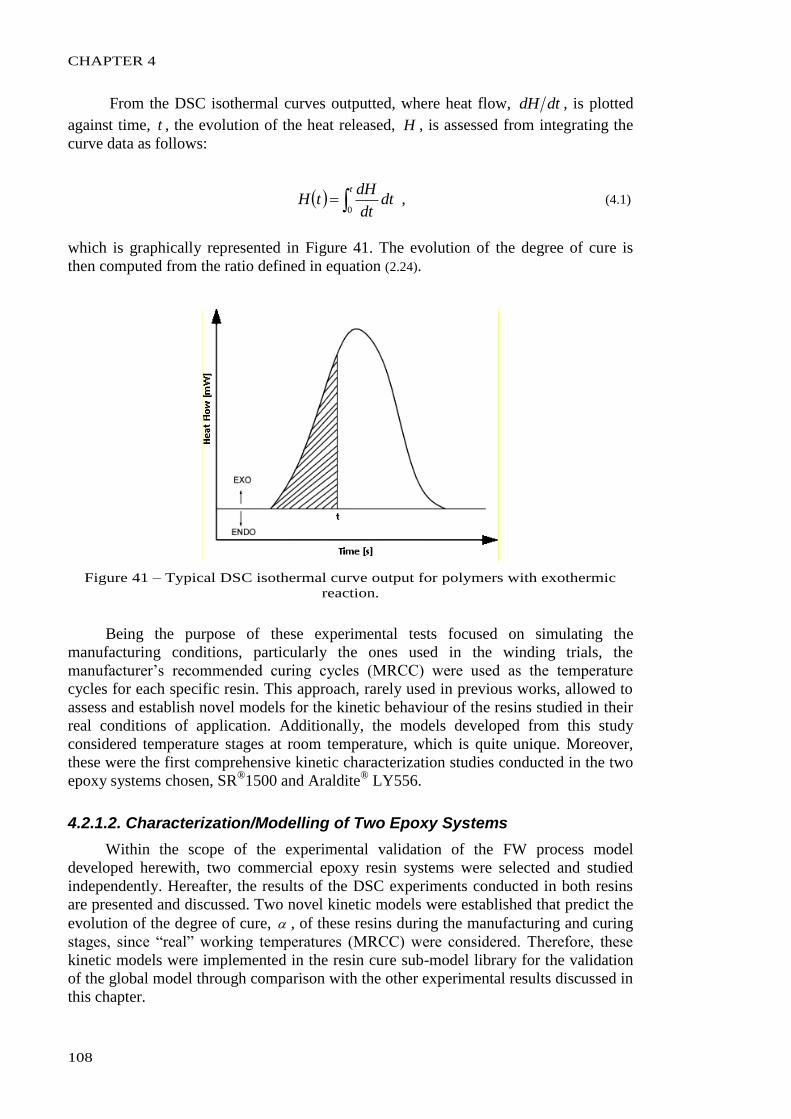
CHAPTER 4
108
From the DSC isothermal curves outputted, where heat flow, dtdH , is plotted
against time, t , the evolution of the heat released, H , is assessed from integrating the
curve data as follows:
t
dtdt
dHtH
0 , (4.1)
which is graphically represented in Figure 41. The evolution of the degree of cure is
then computed from the ratio defined in equation (2.24).
Figure 41 – Typical DSC isothermal curve output for polymers with exothermic
reaction.
Being the purpose of these experimental tests focused on simulating the
manufacturing conditions, particularly the ones used in the winding trials, the
manufacturer’s recommended curing cycles (MRCC) were used as the temperature
cycles for each specific resin. This approach, rarely used in previous works, allowed to
assess and establish novel models for the kinetic behaviour of the resins studied in their
real conditions of application. Additionally, the models developed from this study
considered temperature stages at room temperature, which is quite unique. Moreover,
these were the first comprehensive kinetic characterization studies conducted in the two
epoxy systems chosen, SR®1500 and Araldite
® LY556.
4.2.1.2. Characterization/Modelling of Two Epoxy Systems
Within the scope of the experimental validation of the FW process model
developed herewith, two commercial epoxy resin systems were selected and studied
independently. Hereafter, the results of the DSC experiments conducted in both resins
are presented and discussed. Two novel kinetic models were established that predict the
evolution of the degree of cure, , of these resins during the manufacturing and curing
stages, since “real” working temperatures (MRCC) were considered. Therefore, these
kinetic models were implemented in the resin cure sub-model library for the validation
of the global model through comparison with the other experimental results discussed in
this chapter.
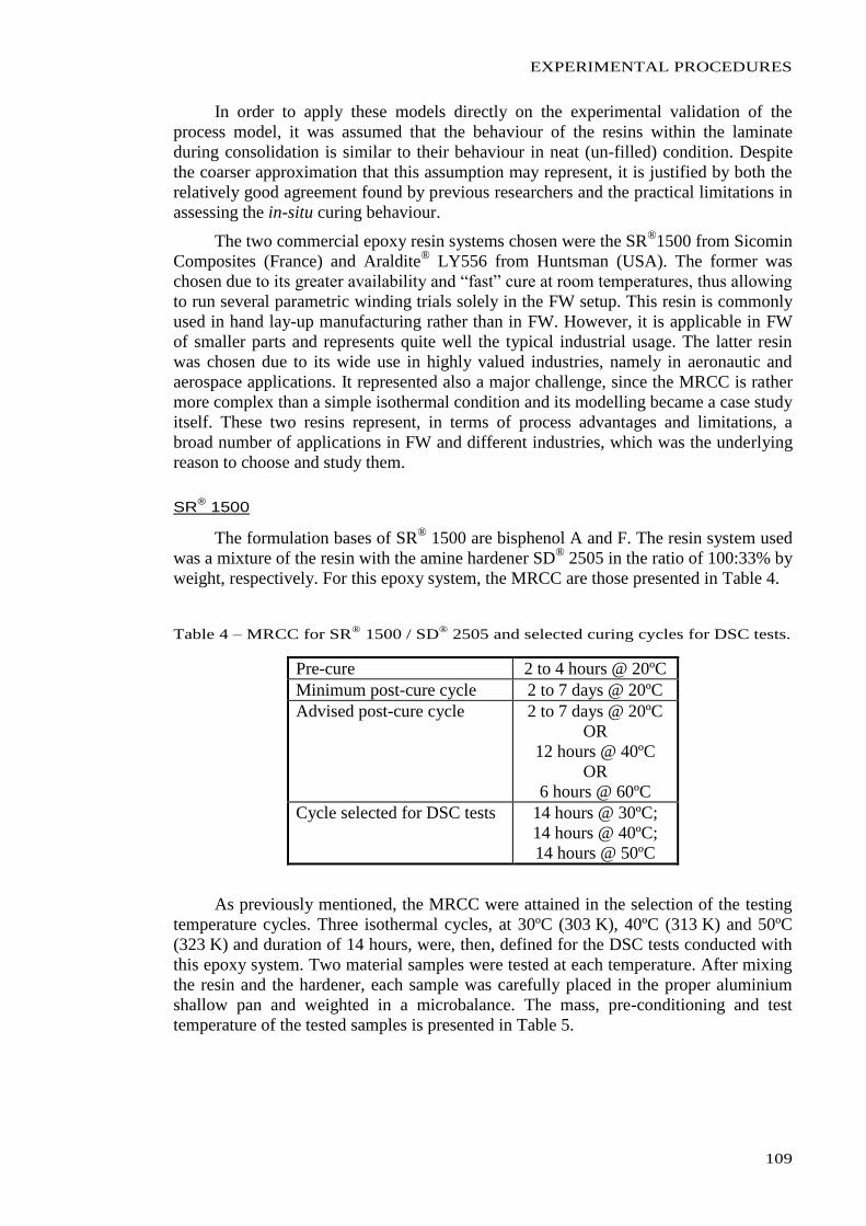
EXPERIMENTAL PROCEDURES
109
In order to apply these models directly on the experimental validation of the
process model, it was assumed that the behaviour of the resins within the laminate
during consolidation is similar to their behaviour in neat (un-filled) condition. Despite
the coarser approximation that this assumption may represent, it is justified by both the
relatively good agreement found by previous researchers and the practical limitations in
assessing the in-situ curing behaviour.
The two commercial epoxy resin systems chosen were the SR®1500 from Sicomin
Composites (France) and Araldite® LY556 from Huntsman (USA). The former was
chosen due to its greater availability and “fast” cure at room temperatures, thus allowing
to run several parametric winding trials solely in the FW setup. This resin is commonly
used in hand lay-up manufacturing rather than in FW. However, it is applicable in FW
of smaller parts and represents quite well the typical industrial usage. The latter resin
was chosen due to its wide use in highly valued industries, namely in aeronautic and
aerospace applications. It represented also a major challenge, since the MRCC is rather
more complex than a simple isothermal condition and its modelling became a case study
itself. These two resins represent, in terms of process advantages and limitations, a
broad number of applications in FW and different industries, which was the underlying
reason to choose and study them.
SR® 1500
The formulation bases of SR® 1500 are bisphenol A and F. The resin system used
was a mixture of the resin with the amine hardener SD®
2505 in the ratio of 100:33% by
weight, respectively. For this epoxy system, the MRCC are those presented in Table 4.
Table 4 – MRCC for SR® 1500 / SD
® 2505 and selected curing cycles for DSC tests.
Pre-cure 2 to 4 hours @ 20ºC
Minimum post-cure cycle 2 to 7 days @ 20ºC
Advised post-cure cycle 2 to 7 days @ 20ºC
OR
12 hours @ 40ºC
OR
6 hours @ 60ºC
Cycle selected for DSC tests 14 hours @ 30ºC;
14 hours @ 40ºC;
14 hours @ 50ºC
As previously mentioned, the MRCC were attained in the selection of the testing
temperature cycles. Three isothermal cycles, at 30ºC (303 K), 40ºC (313 K) and 50ºC
(323 K) and duration of 14 hours, were, then, defined for the DSC tests conducted with
this epoxy system. Two material samples were tested at each temperature. After mixing
the resin and the hardener, each sample was carefully placed in the proper aluminium
shallow pan and weighted in a microbalance. The mass, pre-conditioning and test
temperature of the tested samples is presented in Table 5.
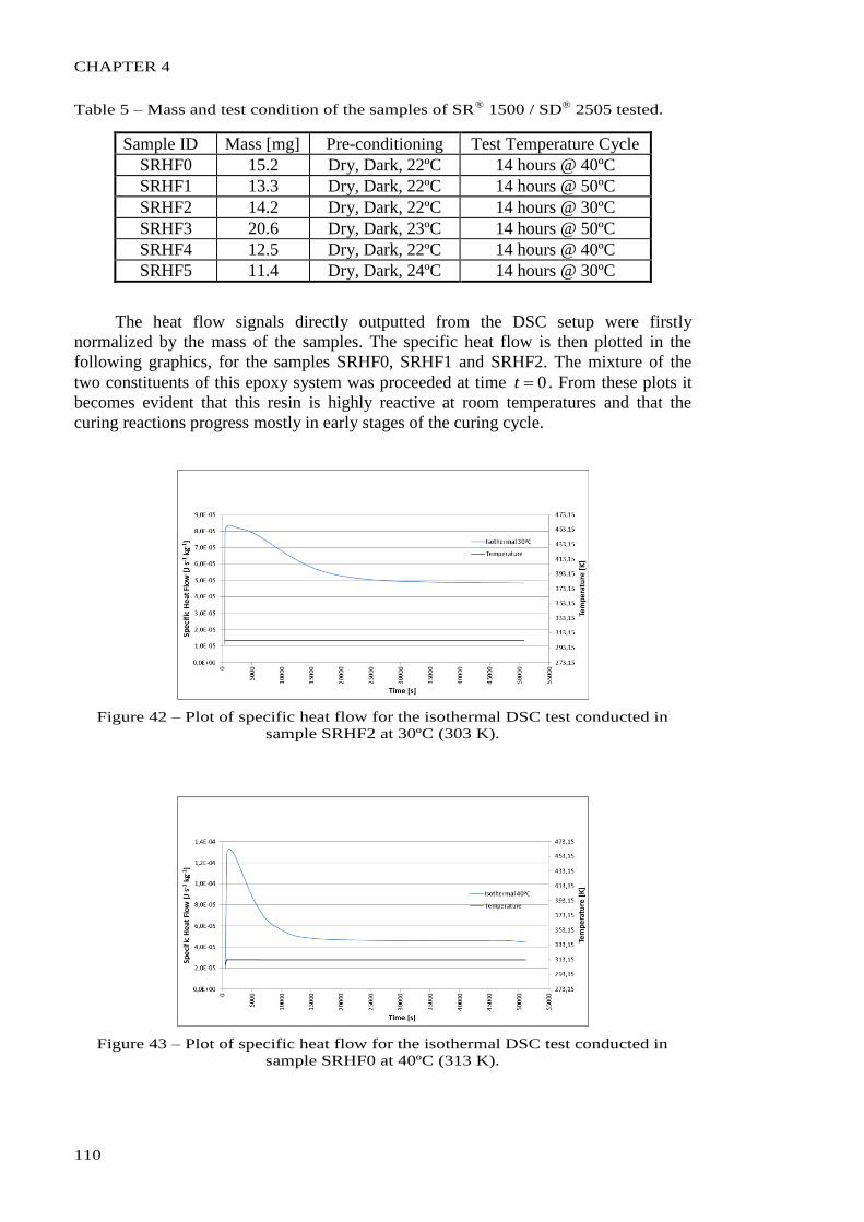
CHAPTER 4
110
Table 5 – Mass and test condition of the samples of SR® 1500 / SD
® 2505 tested.
Sample ID Mass [mg] Pre-conditioning Test Temperature Cycle
SRHF0 15.2 Dry, Dark, 22ºC 14 hours @ 40ºC
SRHF1 13.3 Dry, Dark, 22ºC 14 hours @ 50ºC
SRHF2 14.2 Dry, Dark, 22ºC 14 hours @ 30ºC
SRHF3 20.6 Dry, Dark, 23ºC 14 hours @ 50ºC
SRHF4 12.5 Dry, Dark, 22ºC 14 hours @ 40ºC
SRHF5 11.4 Dry, Dark, 24ºC 14 hours @ 30ºC
The heat flow signals directly outputted from the DSC setup were firstly
normalized by the mass of the samples. The specific heat flow is then plotted in the
following graphics, for the samples SRHF0, SRHF1 and SRHF2. The mixture of the
two constituents of this epoxy system was proceeded at time 0t . From these plots it
becomes evident that this resin is highly reactive at room temperatures and that the
curing reactions progress mostly in early stages of the curing cycle.
Figure 42 – Plot of specific heat flow for the isothermal DSC test conducted in
sample SRHF2 at 30ºC (303 K).
Figure 43 – Plot of specific heat flow for the isothermal DSC test conducted in
sample SRHF0 at 40ºC (313 K).
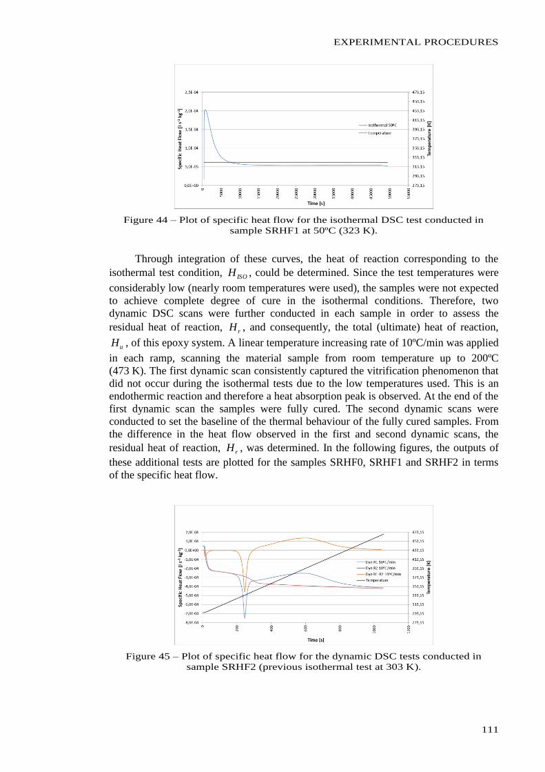
EXPERIMENTAL PROCEDURES
111
Figure 44 – Plot of specific heat flow for the isothermal DSC test conducted in
sample SRHF1 at 50ºC (323 K).
Through integration of these curves, the heat of reaction corresponding to the
isothermal test condition, ISOH , could be determined. Since the test temperatures were
considerably low (nearly room temperatures were used), the samples were not expected
to achieve complete degree of cure in the isothermal conditions. Therefore, two
dynamic DSC scans were further conducted in each sample in order to assess the
residual heat of reaction, rH , and consequently, the total (ultimate) heat of reaction,
uH , of this epoxy system. A linear temperature increasing rate of 10ºC/min was applied
in each ramp, scanning the material sample from room temperature up to 200ºC
(473 K). The first dynamic scan consistently captured the vitrification phenomenon that
did not occur during the isothermal tests due to the low temperatures used. This is an
endothermic reaction and therefore a heat absorption peak is observed. At the end of the
first dynamic scan the samples were fully cured. The second dynamic scans were
conducted to set the baseline of the thermal behaviour of the fully cured samples. From
the difference in the heat flow observed in the first and second dynamic scans, the
residual heat of reaction, rH , was determined. In the following figures, the outputs of
these additional tests are plotted for the samples SRHF0, SRHF1 and SRHF2 in terms
of the specific heat flow.
Figure 45 – Plot of specific heat flow for the dynamic DSC tests conducted in
sample SRHF2 (previous isothermal test at 303 K).
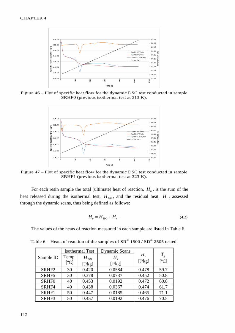
CHAPTER 4
112
Figure 46 – Plot of specific heat flow for the dynamic DSC test conducted in sample
SRHF0 (previous isothermal test at 313 K).
Figure 47 – Plot of specific heat flow for the dynamic DSC test conducted in sample
SRHF1 (previous isothermal test at 323 K).
For each resin sample the total (ultimate) heat of reaction, uH , is the sum of the
heat released during the isothermal test, ISOH , and the residual heat, rH , assessed
through the dynamic scans, thus being defined as follows:
rISOu HHH . (4.2)
The values of the heats of reaction measured in each sample are listed in Table 6.
Table 6 – Heats of reaction of the samples of SR® 1500 / SD
® 2505 tested.
Sample ID
Isothermal Test Dynamic Scans uH
[J/kg]
gT
[ºC] Temp.
[ºC] ISOH
[J/kg]
rH
[J/kg]
SRHF2 30 0.420 0.0584 0.478 59.7
SRHF5 30 0.378 0.0737 0.452 50.8
SRHF0 40 0.453 0.0192 0.472 60.8
SRHF4 40 0.438 0.0367 0.474 61.7
SRHF1 50 0.447 0.0185 0.465 71.1
SRHF3 50 0.457 0.0192 0.476 70.5
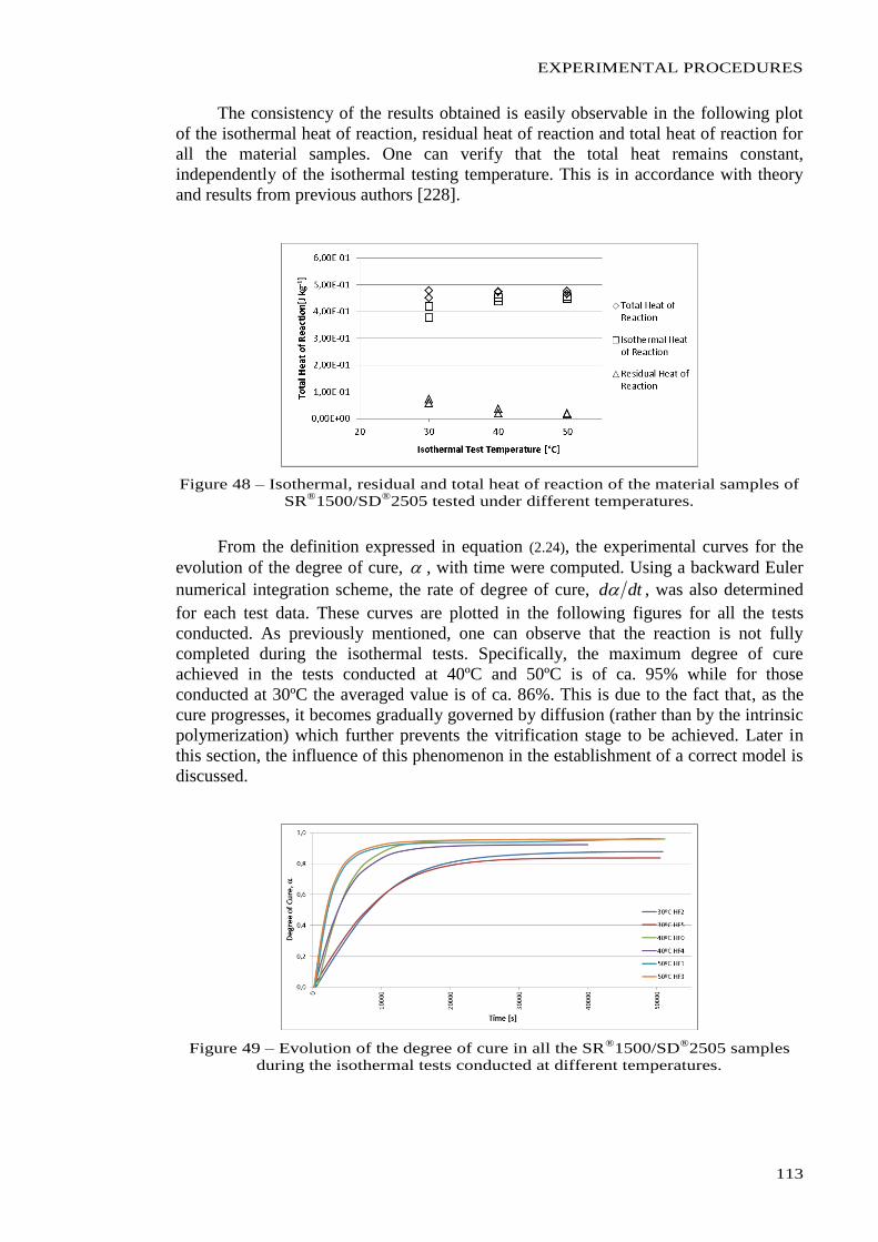
EXPERIMENTAL PROCEDURES
113
The consistency of the results obtained is easily observable in the following plot
of the isothermal heat of reaction, residual heat of reaction and total heat of reaction for
all the material samples. One can verify that the total heat remains constant,
independently of the isothermal testing temperature. This is in accordance with theory
and results from previous authors [228].
Figure 48 – Isothermal, residual and total heat of reaction of the material samples of
SR®
1500/SD®
2505 tested under different temperatures.
From the definition expressed in equation (2.24), the experimental curves for the
evolution of the degree of cure, , with time were computed. Using a backward Euler
numerical integration scheme, the rate of degree of cure, dtd , was also determined
for each test data. These curves are plotted in the following figures for all the tests
conducted. As previously mentioned, one can observe that the reaction is not fully
completed during the isothermal tests. Specifically, the maximum degree of cure
achieved in the tests conducted at 40ºC and 50ºC is of ca. 95% while for those
conducted at 30ºC the averaged value is of ca. 86%. This is due to the fact that, as the
cure progresses, it becomes gradually governed by diffusion (rather than by the intrinsic
polymerization) which further prevents the vitrification stage to be achieved. Later in
this section, the influence of this phenomenon in the establishment of a correct model is
discussed.
Figure 49 – Evolution of the degree of cure in all the SR®
1500/SD®
2505 samples
during the isothermal tests conducted at different temperatures.
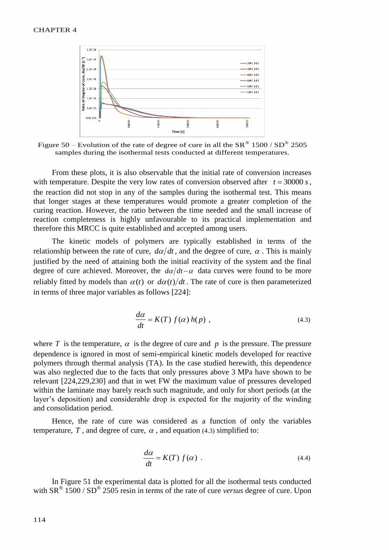
CHAPTER 4
114
Figure 50 – Evolution of the rate of degree of cure in all the SR® 1500 / SD
® 2505
samples during the isothermal tests conducted at different temperatures.
From these plots, it is also observable that the initial rate of conversion increases
with temperature. Despite the very low rates of conversion observed after st 30000 ,
the reaction did not stop in any of the samples during the isothermal test. This means
that longer stages at these temperatures would promote a greater completion of the
curing reaction. However, the ratio between the time needed and the small increase of
reaction completeness is highly unfavourable to its practical implementation and
therefore this MRCC is quite established and accepted among users.
The kinetic models of polymers are typically established in terms of the
relationship between the rate of cure, dtd , and the degree of cure, . This is mainly
justified by the need of attaining both the initial reactivity of the system and the final
degree of cure achieved. Moreover, the dtd data curves were found to be more
reliably fitted by models than )(t or dttd )( . The rate of cure is then parameterized
in terms of three major variables as follows [224]:
)()()( phfTKdt
d
, (4.3)
where T is the temperature, is the degree of cure and p is the pressure. The pressure
dependence is ignored in most of semi-empirical kinetic models developed for reactive
polymers through thermal analysis (TA). In the case studied herewith, this dependence
was also neglected due to the facts that only pressures above 3 MPa have shown to be
relevant [224,229,230] and that in wet FW the maximum value of pressures developed
within the laminate may barely reach such magnitude, and only for short periods (at the
layer’s deposition) and considerable drop is expected for the majority of the winding
and consolidation period.
Hence, the rate of cure was considered as a function of only the variables
temperature, T , and degree of cure, , and equation (4.3) simplified to:
)()(
fTKdt
d . (4.4)
In Figure 51 the experimental data is plotted for all the isothermal tests conducted
with SR® 1500 / SD
® 2505 resin in terms of the rate of cure versus degree of cure. Upon
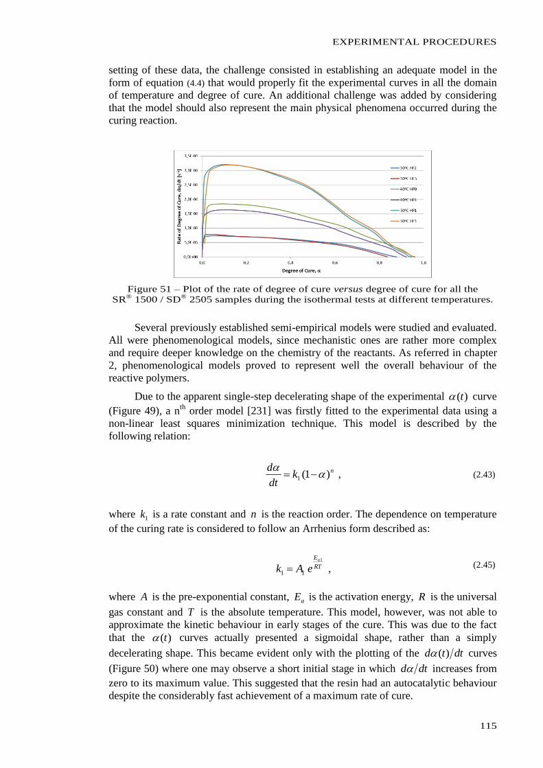
EXPERIMENTAL PROCEDURES
115
setting of these data, the challenge consisted in establishing an adequate model in the
form of equation (4.4) that would properly fit the experimental curves in all the domain
of temperature and degree of cure. An additional challenge was added by considering
that the model should also represent the main physical phenomena occurred during the
curing reaction.
Figure 51 – Plot of the rate of degree of cure versus degree of cure for all the
SR® 1500 / SD
® 2505 samples during the isothermal tests at different temperatures.
Several previously established semi-empirical models were studied and evaluated.
All were phenomenological models, since mechanistic ones are rather more complex
and require deeper knowledge on the chemistry of the reactants. As referred in chapter
2, phenomenological models proved to represent well the overall behaviour of the
reactive polymers.
Due to the apparent single-step decelerating shape of the experimental )(t curve
(Figure 49), a nth
order model [231] was firstly fitted to the experimental data using a
non-linear least squares minimization technique. This model is described by the
following relation:
nkdt
d)1(1
, (2.43)
where 1k is a rate constant and n is the reaction order. The dependence on temperature
of the curing rate is considered to follow an Arrhenius form described as:
RT
Ea
eAk1
11 , (2.45)
where A is the pre-exponential constant, aE is the activation energy, R is the universal
gas constant and T is the absolute temperature. This model, however, was not able to
approximate the kinetic behaviour in early stages of the cure. This was due to the fact
that the )(t curves actually presented a sigmoidal shape, rather than a simply
decelerating shape. This became evident only with the plotting of the dttd )( curves
(Figure 50) where one may observe a short initial stage in which dtd increases from
zero to its maximum value. This suggested that the resin had an autocatalytic behaviour
despite the considerably fast achievement of a maximum rate of cure.
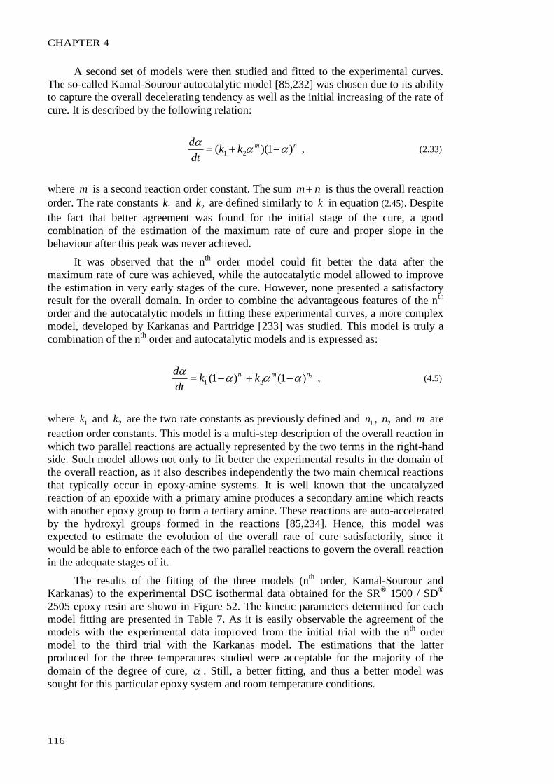
CHAPTER 4
116
A second set of models were then studied and fitted to the experimental curves.
The so-called Kamal-Sourour autocatalytic model [85,232] was chosen due to its ability
to capture the overall decelerating tendency as well as the initial increasing of the rate of
cure. It is described by the following relation:
nmkkdt
d)1)(( 21
, (2.33)
where m is a second reaction order constant. The sum nm is thus the overall reaction
order. The rate constants 1k and 2k are defined similarly to k in equation (2.45). Despite
the fact that better agreement was found for the initial stage of the cure, a good
combination of the estimation of the maximum rate of cure and proper slope in the
behaviour after this peak was never achieved.
It was observed that the nth
order model could fit better the data after the
maximum rate of cure was achieved, while the autocatalytic model allowed to improve
the estimation in very early stages of the cure. However, none presented a satisfactory
result for the overall domain. In order to combine the advantageous features of the nth
order and the autocatalytic models in fitting these experimental curves, a more complex
model, developed by Karkanas and Partridge [233] was studied. This model is truly a
combination of the nth
order and autocatalytic models and is expressed as:
21 )1()1( 21
nmnkk
dt
d
, (4.5)
where 1k and 2k are the two rate constants as previously defined and 1n , 2n and m are
reaction order constants. This model is a multi-step description of the overall reaction in
which two parallel reactions are actually represented by the two terms in the right-hand
side. Such model allows not only to fit better the experimental results in the domain of
the overall reaction, as it also describes independently the two main chemical reactions
that typically occur in epoxy-amine systems. It is well known that the uncatalyzed
reaction of an epoxide with a primary amine produces a secondary amine which reacts
with another epoxy group to form a tertiary amine. These reactions are auto-accelerated
by the hydroxyl groups formed in the reactions [85,234]. Hence, this model was
expected to estimate the evolution of the overall rate of cure satisfactorily, since it
would be able to enforce each of the two parallel reactions to govern the overall reaction
in the adequate stages of it.
The results of the fitting of the three models (nth
order, Kamal-Sourour and
Karkanas) to the experimental DSC isothermal data obtained for the SR® 1500 / SD
®
2505 epoxy resin are shown in Figure 52. The kinetic parameters determined for each
model fitting are presented in Table 7. As it is easily observable the agreement of the
models with the experimental data improved from the initial trial with the nth
order
model to the third trial with the Karkanas model. The estimations that the latter
produced for the three temperatures studied were acceptable for the majority of the
domain of the degree of cure, . Still, a better fitting, and thus a better model was
sought for this particular epoxy system and room temperature conditions.
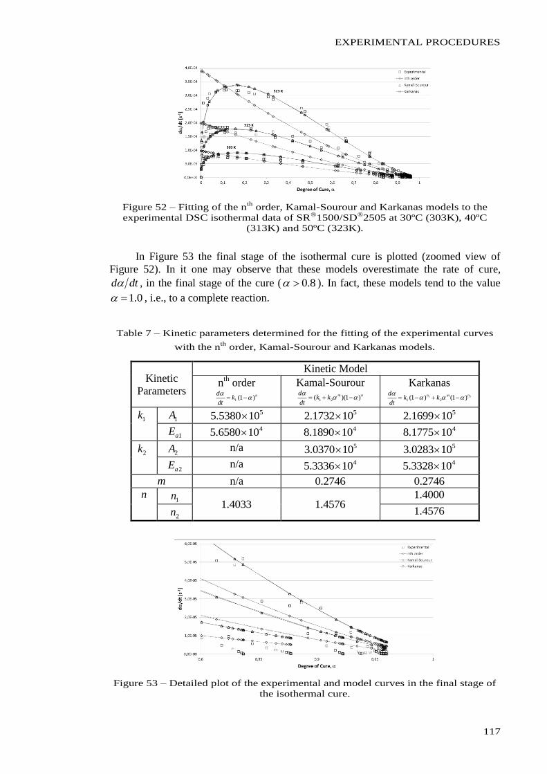
EXPERIMENTAL PROCEDURES
117
Figure 52 – Fitting of the nth
order, Kamal-Sourour and Karkanas models to the
experimental DSC isothermal data of SR®
1500/SD®
2505 at 30ºC (303K), 40ºC
(313K) and 50ºC (323K).
In Figure 53 the final stage of the isothermal cure is plotted (zoomed view of
Figure 52). In it one may observe that these models overestimate the rate of cure,
dtd , in the final stage of the cure ( 8.0 ). In fact, these models tend to the value
0.1 , i.e., to a complete reaction.
Table 7 – Kinetic parameters determined for the fitting of the experimental curves
with the nth
order, Kamal-Sourour and Karkanas models.
Kinetic
Parameters
Kinetic Model
nth
order nk
dt
d)1(1
Kamal-Sourour
nmkkdt
d)1)(( 21
Karkanas
21 )1()1( 21
nmnkk
dt
d
1k 1A 5105380.5 5101732.2 5101699.2
1aE 4106580.5 4101890.8 4101775.8
2k 2A n/a 5100370.3 5100283.3
2aE n/a 4103336.5 4103328.5
m n/a 2746.0 2746.0
n 1n
4033.1 4576.1 4000.1
2n 4576.1
Figure 53 – Detailed plot of the experimental and model curves in the final stage of
the isothermal cure.
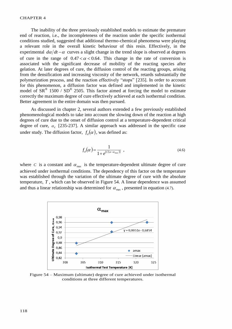
CHAPTER 4
118
The inability of the three previously established models to estimate the premature
end of reaction, i.e., the incompleteness of the reaction under the specific isothermal
conditions studied, suggested that additional thermo-chemical phenomena were playing
a relevant role in the overall kinetic behaviour of this resin. Effectively, in the
experimental dtd curves a slight change in the trend slope is observed at degrees
of cure in the range of 64.047.0 . This change in the rate of conversion is
associated with the significant decrease of mobility of the reacting species after
gelation. At later degrees of cure, the diffusion control of the reacting groups, arising
from the densification and increasing viscosity of the network, retards substantially the
polymerization process, and the reaction effectively “stops” [235]. In order to account
for this phenomenon, a diffusion factor was defined and implemented in the kinetic
model of SR®
1500 / SD® 2505. This factor aimed at forcing the model to estimate
correctly the maximum degree of cure effectively achieved at each isothermal condition.
Better agreement in the entire domain was then pursued.
As discussed in chapter 2, several authors extended a few previously established
phenomenological models to take into account the slowing down of the reaction at high
degrees of cure due to the onset of diffusion control at a temperature-dependent critical
degree of cure, c [235-237]. A similar approach was addressed in the specific case
under study. The diffusion factor, df , was defined as:
max1
1
Cde
f , (4.6)
where C is a constant and max is the temperature-dependent ultimate degree of cure
achieved under isothermal conditions. The dependency of this factor on the temperature
was established through the variation of the ultimate degree of cure with the absolute
temperature, T , which can be observed in Figure 54. A linear dependence was assumed
and thus a linear relationship was determined for max , presented in equation (4.7).
Figure 54 – Maximum (ultimate) degree of cure achieved under isothermal
conditions at three different temperatures.
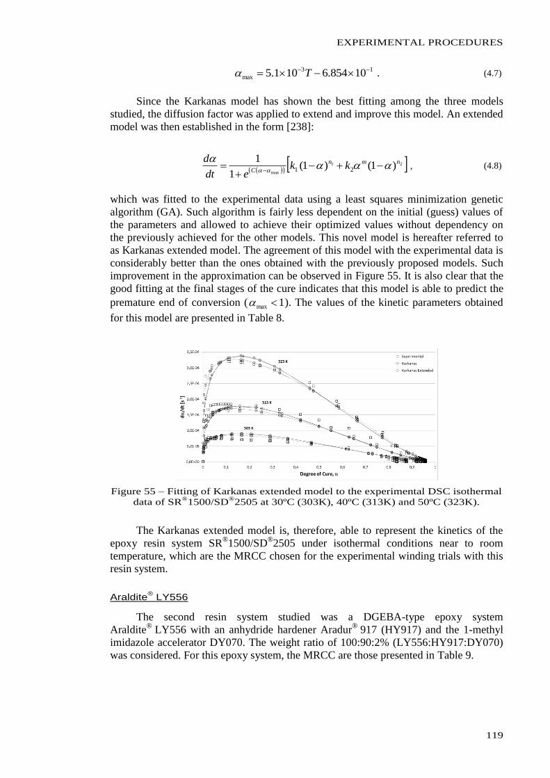
EXPERIMENTAL PROCEDURES
119
13
max 10854.6101.5 T . (4.7)
Since the Karkanas model has shown the best fitting among the three models
studied, the diffusion factor was applied to extend and improve this model. An extended
model was then established in the form [238]:
21
max)1()1(
1
121
nmn
Ckk
edt
d
, (4.8)
which was fitted to the experimental data using a least squares minimization genetic
algorithm (GA). Such algorithm is fairly less dependent on the initial (guess) values of
the parameters and allowed to achieve their optimized values without dependency on
the previously achieved for the other models. This novel model is hereafter referred to
as Karkanas extended model. The agreement of this model with the experimental data is
considerably better than the ones obtained with the previously proposed models. Such
improvement in the approximation can be observed in Figure 55. It is also clear that the
good fitting at the final stages of the cure indicates that this model is able to predict the
premature end of conversion ( 1max ). The values of the kinetic parameters obtained
for this model are presented in Table 8.
Figure 55 – Fitting of Karkanas extended model to the experimental DSC isothermal
data of SR®
1500/SD®
2505 at 30ºC (303K), 40ºC (313K) and 50ºC (323K).
The Karkanas extended model is, therefore, able to represent the kinetics of the
epoxy resin system SR®1500/SD
®2505 under isothermal conditions near to room
temperature, which are the MRCC chosen for the experimental winding trials with this
resin system.
Araldite® LY556
The second resin system studied was a DGEBA-type epoxy system
Araldite® LY556 with an anhydride hardener Aradur
® 917 (HY917) and the 1-methyl
imidazole accelerator DY070. The weight ratio of 100:90:2% (LY556:HY917:DY070)
was considered. For this epoxy system, the MRCC are those presented in Table 9.
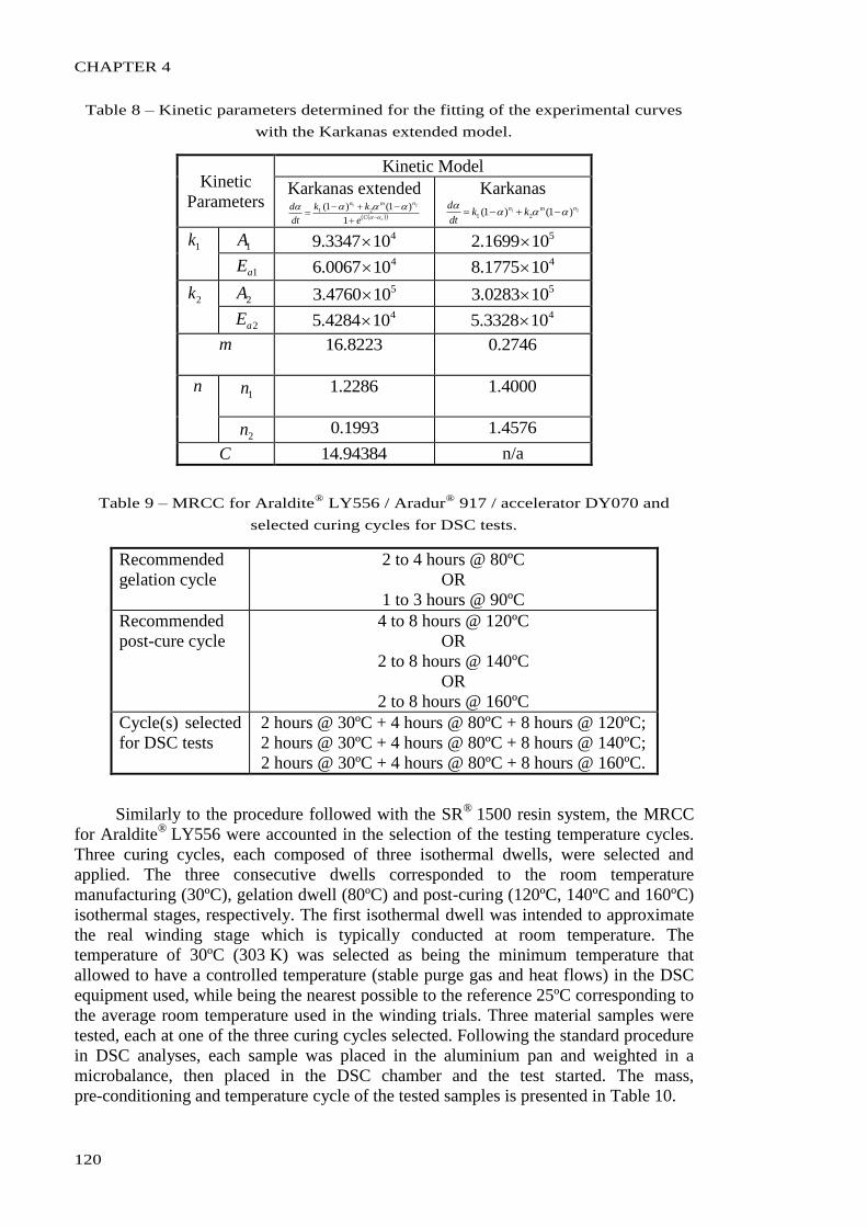
CHAPTER 4
120
Table 8 – Kinetic parameters determined for the fitting of the experimental curves
with the Karkanas extended model.
Kinetic
Parameters
Kinetic Model
Karkanas extended
cC
nmn
e
kk
dt
d
1
)1()1( 21
21
Karkanas 21 )1()1( 21
nmnkk
dt
d
1k 1A 4103347.9 5101699.2
1aE 4100067.6 4101775.8
2k 2A 5104760.3 5100283.3
2aE 4104284.5 4103328.5
m 8223.16
2746.0
n 1n 2286.1
4000.1
2n 1993.0 4576.1
C 94384.14 n/a
Table 9 – MRCC for Araldite® LY556 / Aradur
® 917 / accelerator DY070 and
selected curing cycles for DSC tests.
Recommended
gelation cycle
2 to 4 hours @ 80ºC
OR
1 to 3 hours @ 90ºC
Recommended
post-cure cycle
4 to 8 hours @ 120ºC
OR
2 to 8 hours @ 140ºC
OR
2 to 8 hours @ 160ºC
Cycle(s) selected
for DSC tests
2 hours @ 30ºC + 4 hours @ 80ºC + 8 hours @ 120ºC;
2 hours @ 30ºC + 4 hours @ 80ºC + 8 hours @ 140ºC;
2 hours @ 30ºC + 4 hours @ 80ºC + 8 hours @ 160ºC.
Similarly to the procedure followed with the SR® 1500 resin system, the MRCC
for Araldite® LY556 were accounted in the selection of the testing temperature cycles.
Three curing cycles, each composed of three isothermal dwells, were selected and
applied. The three consecutive dwells corresponded to the room temperature
manufacturing (30ºC), gelation dwell (80ºC) and post-curing (120ºC, 140ºC and 160ºC)
isothermal stages, respectively. The first isothermal dwell was intended to approximate
the real winding stage which is typically conducted at room temperature. The
temperature of 30ºC (303 K) was selected as being the minimum temperature that
allowed to have a controlled temperature (stable purge gas and heat flows) in the DSC
equipment used, while being the nearest possible to the reference 25ºC corresponding to
the average room temperature used in the winding trials. Three material samples were
tested, each at one of the three curing cycles selected. Following the standard procedure
in DSC analyses, each sample was placed in the aluminium pan and weighted in a
microbalance, then placed in the DSC chamber and the test started. The mass,
pre-conditioning and temperature cycle of the tested samples is presented in Table 10.
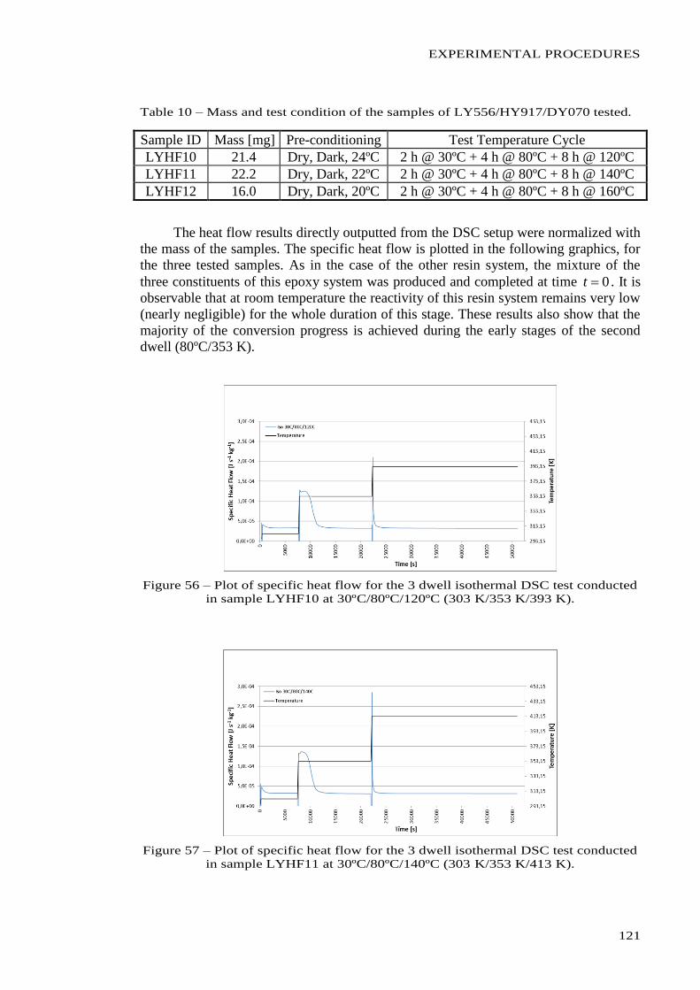
EXPERIMENTAL PROCEDURES
121
Table 10 – Mass and test condition of the samples of LY556/HY917/DY070 tested.
Sample ID Mass [mg] Pre-conditioning Test Temperature Cycle
LYHF10 21.4 Dry, Dark, 24ºC 2 h @ 30ºC + 4 h @ 80ºC + 8 h @ 120ºC
LYHF11 22.2 Dry, Dark, 22ºC 2 h @ 30ºC + 4 h @ 80ºC + 8 h @ 140ºC
LYHF12 16.0 Dry, Dark, 20ºC 2 h @ 30ºC + 4 h @ 80ºC + 8 h @ 160ºC
The heat flow results directly outputted from the DSC setup were normalized with
the mass of the samples. The specific heat flow is plotted in the following graphics, for
the three tested samples. As in the case of the other resin system, the mixture of the
three constituents of this epoxy system was produced and completed at time 0t . It is
observable that at room temperature the reactivity of this resin system remains very low
(nearly negligible) for the whole duration of this stage. These results also show that the
majority of the conversion progress is achieved during the early stages of the second
dwell (80ºC/353 K).
Figure 56 – Plot of specific heat flow for the 3 dwell isothermal DSC test conducted
in sample LYHF10 at 30ºC/80ºC/120ºC (303 K/353 K/393 K).
Figure 57 – Plot of specific heat flow for the 3 dwell isothermal DSC test conducted
in sample LYHF11 at 30ºC/80ºC/140ºC (303 K/353 K/413 K).
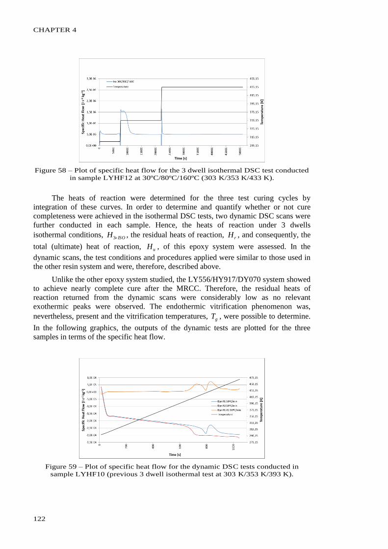
CHAPTER 4
122
Figure 58 – Plot of specific heat flow for the 3 dwell isothermal DSC test conducted
in sample LYHF12 at 30ºC/80ºC/160ºC (303 K/353 K/433 K).
The heats of reaction were determined for the three test curing cycles by
integration of these curves. In order to determine and quantify whether or not cure
completeness were achieved in the isothermal DSC tests, two dynamic DSC scans were
further conducted in each sample. Hence, the heats of reaction under 3 dwells
isothermal conditions, ISOH 3 , the residual heats of reaction, rH , and consequently, the
total (ultimate) heat of reaction, uH , of this epoxy system were assessed. In the
dynamic scans, the test conditions and procedures applied were similar to those used in
the other resin system and were, therefore, described above.
Unlike the other epoxy system studied, the LY556/HY917/DY070 system showed
to achieve nearly complete cure after the MRCC. Therefore, the residual heats of
reaction returned from the dynamic scans were considerably low as no relevant
exothermic peaks were observed. The endothermic vitrification phenomenon was,
nevertheless, present and the vitrification temperatures, gT , were possible to determine.
In the following graphics, the outputs of the dynamic tests are plotted for the three
samples in terms of the specific heat flow.
Figure 59 – Plot of specific heat flow for the dynamic DSC tests conducted in
sample LYHF10 (previous 3 dwell isothermal test at 303 K/353 K/393 K).
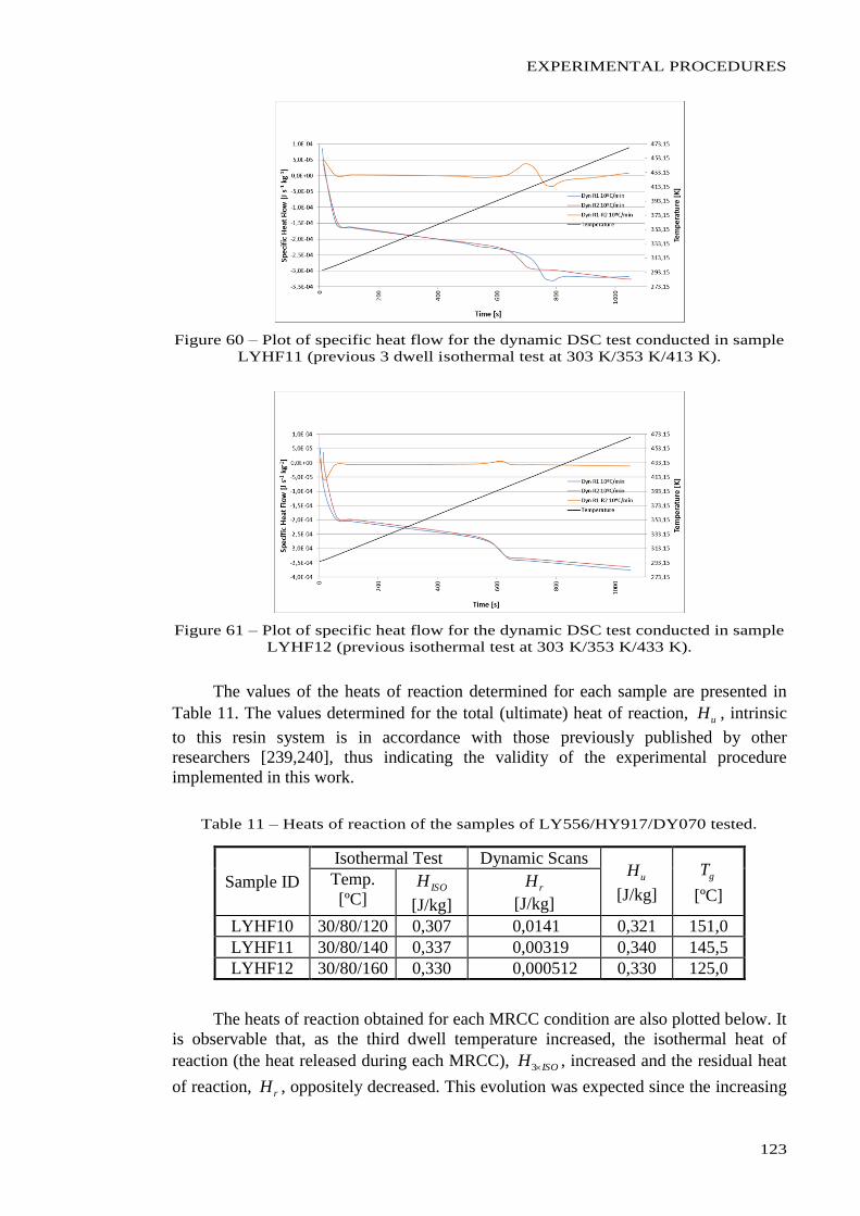
EXPERIMENTAL PROCEDURES
123
Figure 60 – Plot of specific heat flow for the dynamic DSC test conducted in sample
LYHF11 (previous 3 dwell isothermal test at 303 K/353 K/413 K).
Figure 61 – Plot of specific heat flow for the dynamic DSC test conducted in sample
LYHF12 (previous isothermal test at 303 K/353 K/433 K).
The values of the heats of reaction determined for each sample are presented in
Table 11. The values determined for the total (ultimate) heat of reaction, uH , intrinsic
to this resin system is in accordance with those previously published by other
researchers [239,240], thus indicating the validity of the experimental procedure
implemented in this work.
Table 11 – Heats of reaction of the samples of LY556/HY917/DY070 tested.
Sample ID
Isothermal Test Dynamic Scans uH
[J/kg]
gT
[ºC] Temp.
[ºC] ISOH
[J/kg]
rH
[J/kg]
LYHF10 30/80/120 0,307 0,0141 0,321 151,0
LYHF11 30/80/140 0,337 0,00319 0,340 145,5
LYHF12 30/80/160 0,330 0,000512 0,330 125,0
The heats of reaction obtained for each MRCC condition are also plotted below. It
is observable that, as the third dwell temperature increased, the isothermal heat of
reaction (the heat released during each MRCC), ISOH 3 , increased and the residual heat
of reaction, rH , oppositely decreased. This evolution was expected since the increasing
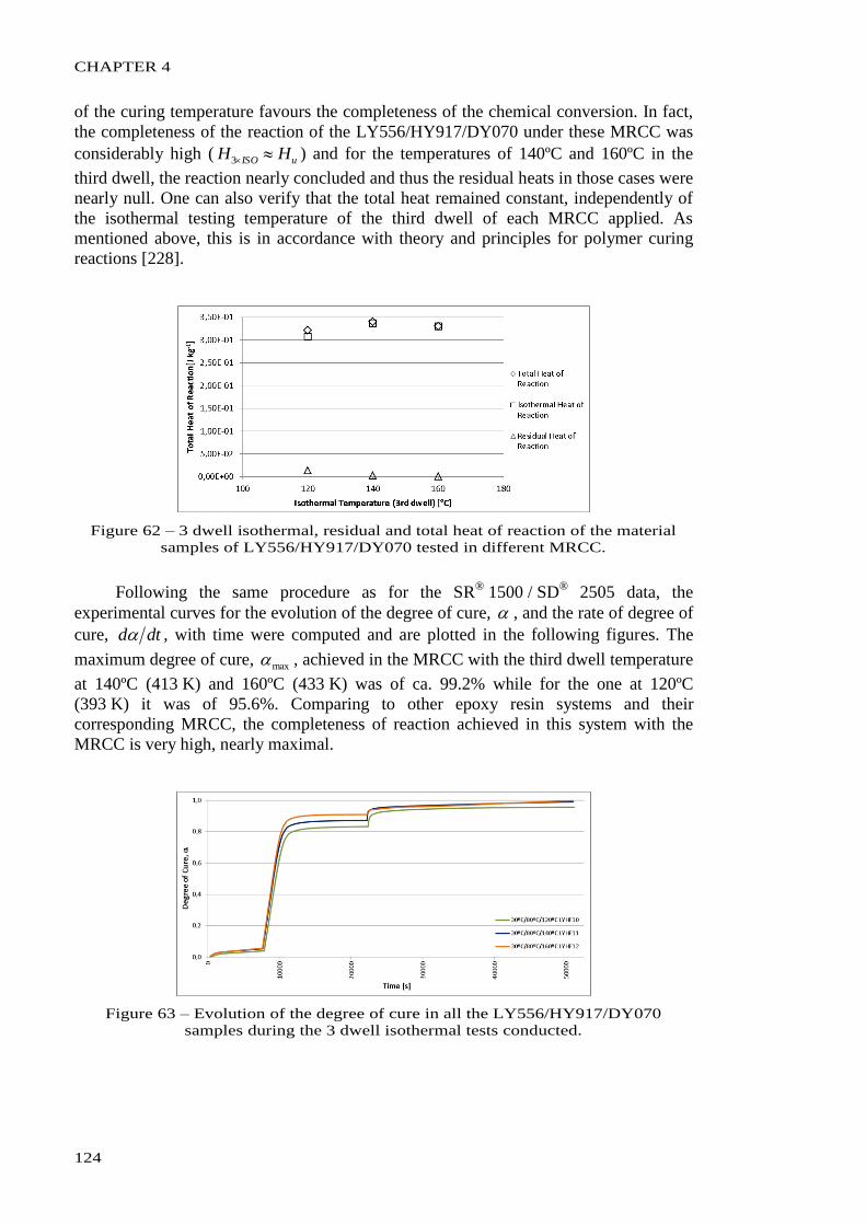
CHAPTER 4
124
of the curing temperature favours the completeness of the chemical conversion. In fact,
the completeness of the reaction of the LY556/HY917/DY070 under these MRCC was
considerably high ( uISO HH 3 ) and for the temperatures of 140ºC and 160ºC in the
third dwell, the reaction nearly concluded and thus the residual heats in those cases were
nearly null. One can also verify that the total heat remained constant, independently of
the isothermal testing temperature of the third dwell of each MRCC applied. As
mentioned above, this is in accordance with theory and principles for polymer curing
reactions [228].
Figure 62 – 3 dwell isothermal, residual and total heat of reaction of the material
samples of LY556/HY917/DY070 tested in different MRCC.
Following the same procedure as for the SR® 1500 / SD
® 2505 data, the
experimental curves for the evolution of the degree of cure, , and the rate of degree of
cure, dtd , with time were computed and are plotted in the following figures. The
maximum degree of cure, max , achieved in the MRCC with the third dwell temperature
at 140ºC (413 K) and 160ºC (433 K) was of ca. 99.2% while for the one at 120ºC
(393 K) it was of 95.6%. Comparing to other epoxy resin systems and their
corresponding MRCC, the completeness of reaction achieved in this system with the
MRCC is very high, nearly maximal.
Figure 63 – Evolution of the degree of cure in all the LY556/HY917/DY070
samples during the 3 dwell isothermal tests conducted.
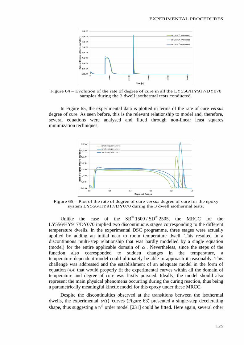
EXPERIMENTAL PROCEDURES
125
Figure 64 – Evolution of the rate of degree of cure in all the LY556/HY917/DY070
samples during the 3 dwell isothermal tests conducted.
In Figure 65, the experimental data is plotted in terms of the rate of cure versus
degree of cure. As seen before, this is the relevant relationship to model and, therefore,
several equations were analysed and fitted through non-linear least squares
minimization techniques.
Figure 65 – Plot of the rate of degree of cure versus degree of cure for the epoxy
system LY556/HY917/DY070 during the 3 dwell isothermal tests.
Unlike the case of the SR® 1500 / SD
® 2505, the MRCC for the
LY556/HY917/DY070 implied two discontinuous stages corresponding to the different
temperature dwells. In the experimental DSC programme, three stages were actually
applied by adding an initial near to room temperature dwell. This resulted in a
discontinuous multi-step relationship that was hardly modelled by a single equation
(model) for the entire applicable domain of . Nevertheless, since the steps of the
function also corresponded to sudden changes in the temperature, a
temperature-dependent model could ultimately be able to approach it reasonably. This
challenge was addressed and the establishment of an adequate model in the form of
equation (4.4) that would properly fit the experimental curves within all the domain of
temperature and degree of cure was firstly pursued. Ideally, the model should also
represent the main physical phenomena occurring during the curing reaction, thus being
a parametrically meaningful kinetic model for this epoxy under these MRCC.
Despite the discontinuities observed at the transitions between the isothermal
dwells, the experimental )(t curves (Figure 63) presented a single-step decelerating
shape, thus suggesting a nth
order model [231] could be fitted. Here again, several other
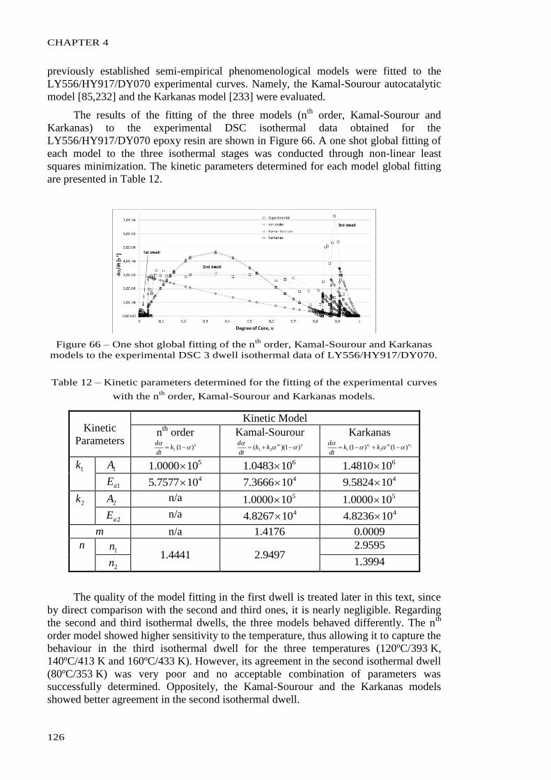
CHAPTER 4
126
previously established semi-empirical phenomenological models were fitted to the
LY556/HY917/DY070 experimental curves. Namely, the Kamal-Sourour autocatalytic
model [85,232] and the Karkanas model [233] were evaluated.
The results of the fitting of the three models (nth
order, Kamal-Sourour and
Karkanas) to the experimental DSC isothermal data obtained for the
LY556/HY917/DY070 epoxy resin are shown in Figure 66. A one shot global fitting of
each model to the three isothermal stages was conducted through non-linear least
squares minimization. The kinetic parameters determined for each model global fitting
are presented in Table 12.
Figure 66 – One shot global fitting of the nth
order, Kamal-Sourour and Karkanas
models to the experimental DSC 3 dwell isothermal data of LY556/HY917/DY070.
Table 12 – Kinetic parameters determined for the fitting of the experimental curves
with the nth
order, Kamal-Sourour and Karkanas models.
Kinetic
Parameters
Kinetic Model
nth
order nk
dt
d)1(1
Kamal-Sourour
nmkkdt
d)1)(( 21
Karkanas
21 )1()1( 21
nmnkk
dt
d
1k 1A 5100000.1 6100483.1 6104810.1
1aE 4107577.5 4103666.7 4105824.9
2k 2A n/a 5100000.1 5100000.1
2aE n/a 4108267.4 4108236.4
m n/a 4176.1 0009.0
n 1n
4441.1 9497.2 9595.2
2n 3994.1
The quality of the model fitting in the first dwell is treated later in this text, since
by direct comparison with the second and third ones, it is nearly negligible. Regarding
the second and third isothermal dwells, the three models behaved differently. The nth
order model showed higher sensitivity to the temperature, thus allowing it to capture the
behaviour in the third isothermal dwell for the three temperatures (120ºC/393 K,
140ºC/413 K and 160ºC/433 K). However, its agreement in the second isothermal dwell
(80ºC/353 K) was very poor and no acceptable combination of parameters was
successfully determined. Oppositely, the Kamal-Sourour and the Karkanas models
showed better agreement in the second isothermal dwell.
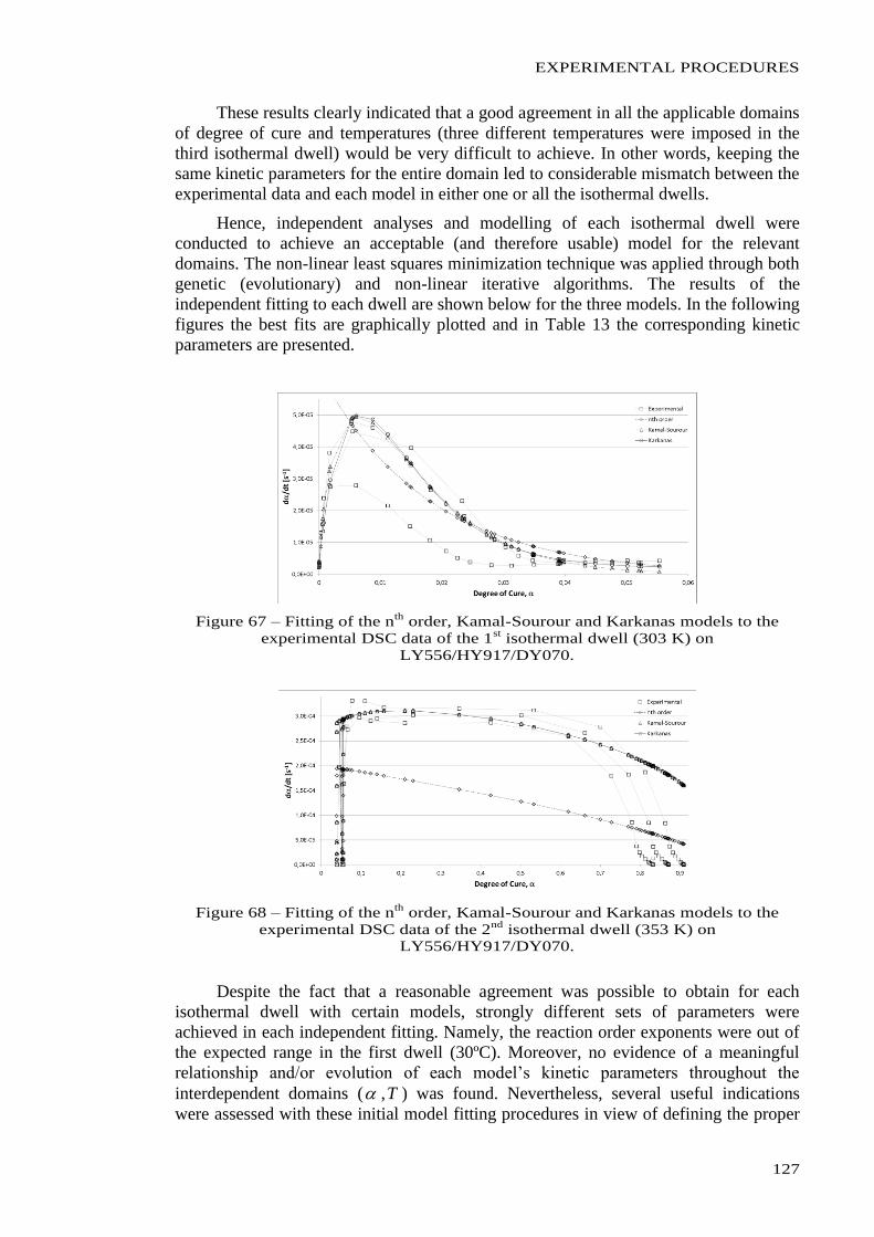
EXPERIMENTAL PROCEDURES
127
These results clearly indicated that a good agreement in all the applicable domains
of degree of cure and temperatures (three different temperatures were imposed in the
third isothermal dwell) would be very difficult to achieve. In other words, keeping the
same kinetic parameters for the entire domain led to considerable mismatch between the
experimental data and each model in either one or all the isothermal dwells.
Hence, independent analyses and modelling of each isothermal dwell were
conducted to achieve an acceptable (and therefore usable) model for the relevant
domains. The non-linear least squares minimization technique was applied through both
genetic (evolutionary) and non-linear iterative algorithms. The results of the
independent fitting to each dwell are shown below for the three models. In the following
figures the best fits are graphically plotted and in Table 13 the corresponding kinetic
parameters are presented.
Figure 67 – Fitting of the nth
order, Kamal-Sourour and Karkanas models to the
experimental DSC data of the 1st isothermal dwell (303 K) on
LY556/HY917/DY070.
Figure 68 – Fitting of the nth
order, Kamal-Sourour and Karkanas models to the
experimental DSC data of the 2nd
isothermal dwell (353 K) on
LY556/HY917/DY070.
Despite the fact that a reasonable agreement was possible to obtain for each
isothermal dwell with certain models, strongly different sets of parameters were
achieved in each independent fitting. Namely, the reaction order exponents were out of
the expected range in the first dwell (30ºC). Moreover, no evidence of a meaningful
relationship and/or evolution of each model’s kinetic parameters throughout the
interdependent domains ( ,T ) was found. Nevertheless, several useful indications
were assessed with these initial model fitting procedures in view of defining the proper
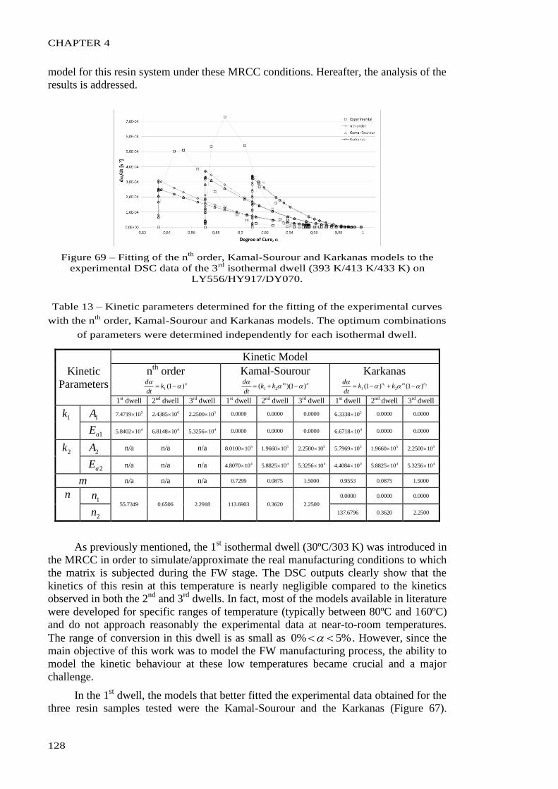
CHAPTER 4
128
model for this resin system under these MRCC conditions. Hereafter, the analysis of the
results is addressed.
Figure 69 – Fitting of the nth
order, Kamal-Sourour and Karkanas models to the
experimental DSC data of the 3rd
isothermal dwell (393 K/413 K/433 K) on
LY556/HY917/DY070.
Table 13 – Kinetic parameters determined for the fitting of the experimental curves
with the nth
order, Kamal-Sourour and Karkanas models. The optimum combinations
of parameters were determined independently for each isothermal dwell.
Kinetic
Parameters
Kinetic Model
nth
order nk
dt
d)1(1
Kamal-Sourour
nmkkdt
d)1)(( 21
Karkanas
21 )1()1( 21
nmnkk
dt
d
1st dwell 2nd dwell 3rd dwell 1st dwell 2nd dwell 3rd dwell 1st dwell 2nd dwell 3rd dwell
1k 1A 5104719.7 6104385.2 5102500.2 0000.0 0000.0 0000.0 5103338.6 0000.0 0000.0
1aE 4108402.5 4108148.6 4103256.5 0000.0 0000.0 0000.0 4106718.6 0000.0 0000.0
2k 2A n/a n/a n/a 5100100.8 5109660.1 5102500.2 5107969.5 5109660.1 5102500.2
2aE n/a n/a n/a 4108070.4 4108825.5 4103256.5 4104084.4 4108825.5 4103256.5
m n/a n/a n/a 7299.0 0875.0 5000.1 9553.0 0875.0 5000.1
n 1n
7349.55 6506.0 2918.2 6903.113 3620.0 2500.2 0000.0 0000.0 0000.0
2n 6796.137 3620.0 2500.2
As previously mentioned, the 1st isothermal dwell (30ºC/303 K) was introduced in
the MRCC in order to simulate/approximate the real manufacturing conditions to which
the matrix is subjected during the FW stage. The DSC outputs clearly show that the
kinetics of this resin at this temperature is nearly negligible compared to the kinetics
observed in both the 2nd
and 3rd
dwells. In fact, most of the models available in literature
were developed for specific ranges of temperature (typically between 80ºC and 160ºC)
and do not approach reasonably the experimental data at near-to-room temperatures.
The range of conversion in this dwell is as small as %5%0 . However, since the
main objective of this work was to model the FW manufacturing process, the ability to
model the kinetic behaviour at these low temperatures became crucial and a major
challenge.
In the 1st dwell, the models that better fitted the experimental data obtained for the
three resin samples tested were the Kamal-Sourour and the Karkanas (Figure 67).
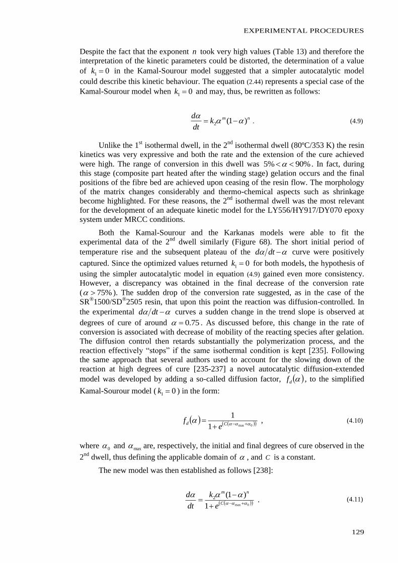
EXPERIMENTAL PROCEDURES
129
Despite the fact that the exponent n took very high values (Table 13) and therefore the
interpretation of the kinetic parameters could be distorted, the determination of a value
of 01 k in the Kamal-Sourour model suggested that a simpler autocatalytic model
could describe this kinetic behaviour. The equation (2.44) represents a special case of the
Kamal-Sourour model when 01 k and may, thus, be rewritten as follows:
nmkdt
d)1(2
. (4.9)
Unlike the 1st isothermal dwell, in the 2
nd isothermal dwell (80ºC/353 K) the resin
kinetics was very expressive and both the rate and the extension of the cure achieved
were high. The range of conversion in this dwell was %90%5 . In fact, during
this stage (composite part heated after the winding stage) gelation occurs and the final
positions of the fibre bed are achieved upon ceasing of the resin flow. The morphology
of the matrix changes considerably and thermo-chemical aspects such as shrinkage
become highlighted. For these reasons, the 2nd
isothermal dwell was the most relevant
for the development of an adequate kinetic model for the LY556/HY917/DY070 epoxy
system under MRCC conditions.
Both the Kamal-Sourour and the Karkanas models were able to fit the
experimental data of the 2nd
dwell similarly (Figure 68). The short initial period of
temperature rise and the subsequent plateau of the dtd curve were positively
captured. Since the optimized values returned 01 k for both models, the hypothesis of
using the simpler autocatalytic model in equation (4.9) gained even more consistency.
However, a discrepancy was obtained in the final decrease of the conversion rate
( %75 ). The sudden drop of the conversion rate suggested, as in the case of the
SR®1500/SD
®2505 resin, that upon this point the reaction was diffusion-controlled. In
the experimental dtd curves a sudden change in the trend slope is observed at
degrees of cure of around 75.0 . As discussed before, this change in the rate of
conversion is associated with decrease of mobility of the reacting species after gelation.
The diffusion control then retards substantially the polymerization process, and the
reaction effectively “stops” if the same isothermal condition is kept [235]. Following
the same approach that several authors used to account for the slowing down of the
reaction at high degrees of cure [235-237] a novel autocatalytic diffusion-extended
model was developed by adding a so-called diffusion factor, df , to the simplified
Kamal-Sourour model ( 01 k ) in the form:
0max1
1
Cde
f , (4.10)
where 0 and max are, respectively, the initial and final degrees of cure observed in the
2nd
dwell, thus defining the applicable domain of , and C is a constant.
The new model was then established as follows [238]:
0max1
)1(2
C
nm
e
k
dt
d . (4.11)
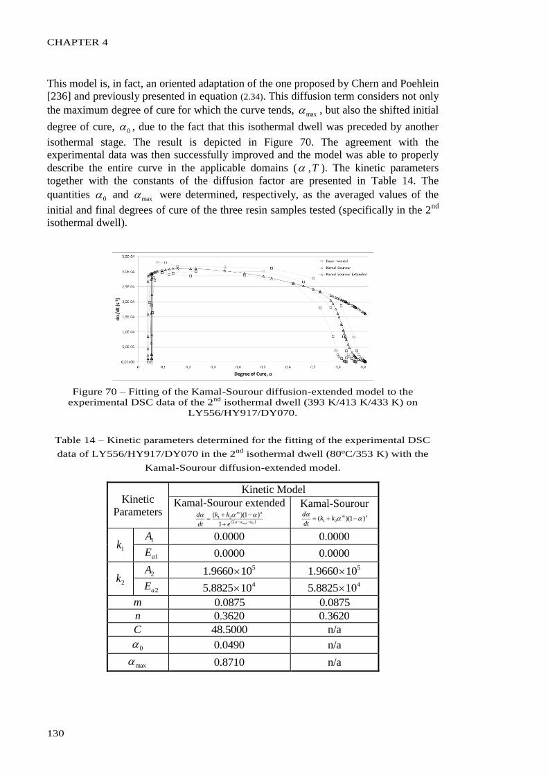
CHAPTER 4
130
This model is, in fact, an oriented adaptation of the one proposed by Chern and Poehlein
[236] and previously presented in equation (2.34). This diffusion term considers not only
the maximum degree of cure for which the curve tends, max , but also the shifted initial
degree of cure, 0 , due to the fact that this isothermal dwell was preceded by another
isothermal stage. The result is depicted in Figure 70. The agreement with the
experimental data was then successfully improved and the model was able to properly
describe the entire curve in the applicable domains ( ,T ). The kinetic parameters
together with the constants of the diffusion factor are presented in Table 14. The
quantities 0 and max were determined, respectively, as the averaged values of the
initial and final degrees of cure of the three resin samples tested (specifically in the 2nd
isothermal dwell).
Figure 70 – Fitting of the Kamal-Sourour diffusion-extended model to the
experimental DSC data of the 2nd
isothermal dwell (393 K/413 K/433 K) on
LY556/HY917/DY070.
Table 14 – Kinetic parameters determined for the fitting of the experimental DSC
data of LY556/HY917/DY070 in the 2nd
isothermal dwell (80ºC/353 K) with the
Kamal-Sourour diffusion-extended model.
Kinetic
Parameters
Kinetic Model
Kamal-Sourour extended
0max1
)1)(( 21
C
nm
e
kk
dt
d Kamal-Sourour
nmkkdt
d)1)(( 21
1k 1A 0000.0 0000.0
1aE 0000.0 0000.0
2k 2A 5109660.1 5109660.1
2aE 4108825.5 4108825.5
m 0875.0 0875.0
n 3620.0 3620.0
C 5000.48 n/a
0 0490.0 n/a
max 8710.0 n/a
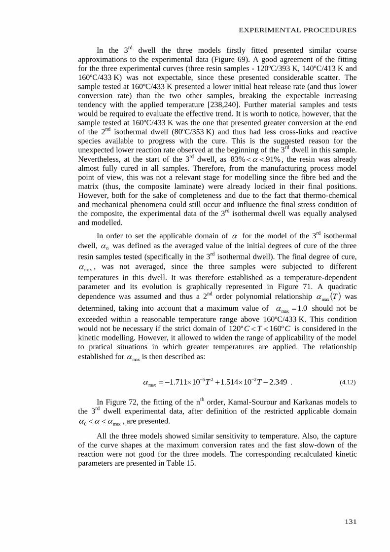
EXPERIMENTAL PROCEDURES
131
In the 3rd
dwell the three models firstly fitted presented similar coarse
approximations to the experimental data (Figure 69). A good agreement of the fitting
for the three experimental curves (three resin samples - 120ºC/393 K, 140ºC/413 K and
160ºC/433 K) was not expectable, since these presented considerable scatter. The
sample tested at 160ºC/433 K presented a lower initial heat release rate (and thus lower
conversion rate) than the two other samples, breaking the expectable increasing
tendency with the applied temperature [238,240]. Further material samples and tests
would be required to evaluate the effective trend. It is worth to notice, however, that the
sample tested at 160ºC/433 K was the one that presented greater conversion at the end
of the 2nd
isothermal dwell (80ºC/353 K) and thus had less cross-links and reactive
species available to progress with the cure. This is the suggested reason for the
unexpected lower reaction rate observed at the beginning of the 3rd
dwell in this sample.
Nevertheless, at the start of the 3rd
dwell, as %91%83 , the resin was already
almost fully cured in all samples. Therefore, from the manufacturing process model
point of view, this was not a relevant stage for modelling since the fibre bed and the
matrix (thus, the composite laminate) were already locked in their final positions.
However, both for the sake of completeness and due to the fact that thermo-chemical
and mechanical phenomena could still occur and influence the final stress condition of
the composite, the experimental data of the 3rd
isothermal dwell was equally analysed
and modelled.
In order to set the applicable domain of for the model of the 3rd
isothermal
dwell, 0 was defined as the averaged value of the initial degrees of cure of the three
resin samples tested (specifically in the 3rd
isothermal dwell). The final degree of cure,
max , was not averaged, since the three samples were subjected to different
temperatures in this dwell. It was therefore established as a temperature-dependent
parameter and its evolution is graphically represented in Figure 71. A quadratic
dependence was assumed and thus a 2nd
order polynomial relationship Tmax was
determined, taking into account that a maximum value of 0.1max should not be
exceeded within a reasonable temperature range above 160ºC/433 K. This condition
would not be necessary if the strict domain of CTC º160º120 is considered in the
kinetic modelling. However, it allowed to widen the range of applicability of the model
to pratical situations in which greater temperatures are applied. The relationship
established for max is then described as:
349.210514.110711.1 225
max TT . (4.12)
In Figure 72, the fitting of the nth
order, Kamal-Sourour and Karkanas models to
the 3rd
dwell experimental data, after definition of the restricted applicable domain
max0 , are presented.
All the three models showed similar sensitivity to temperature. Also, the capture
of the curve shapes at the maximum conversion rates and the fast slow-down of the
reaction were not good for the three models. The corresponding recalculated kinetic
parameters are presented in Table 15.
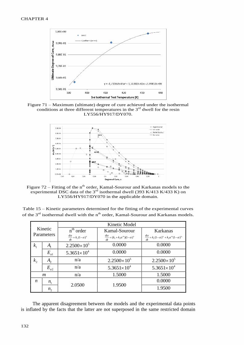
CHAPTER 4
132
Figure 71 – Maximum (ultimate) degree of cure achieved under the isothermal
conditions at three different temperatures in the 3rd
dwell for the resin
LY556/HY917/DY070.
Figure 72 – Fitting of the nth
order, Kamal-Sourour and Karkanas models to the
experimental DSC data of the 3rd
isothermal dwell (393 K/413 K/433 K) on
LY556/HY917/DY070 in the applicable domain.
Table 15 – Kinetic parameters determined for the fitting of the experimental curves
of the 3rd
isothermal dwell with the nth
order, Kamal-Sourour and Karkanas models.
Kinetic
Parameters
Kinetic Model
nth
order nk
dt
d)1(1
Kamal-Sourour
nmkkdt
d)1)(( 21
Karkanas
21 )1()1( 21
nmnkk
dt
d
1k 1A 5102500.2 0000.0 0000.0
1aE 4103651.5 0000.0 0000.0
2k 2A n/a 5102500.2 5102500.2
2aE n/a 4103651.5 4103651.5
m n/a 5000.1 5000.1
n 1n
0500.2 9500.1 0000.0
2n 9500.1
The apparent disagreement between the models and the experimental data points
is inflated by the facts that the latter are not superposed in the same restricted domain
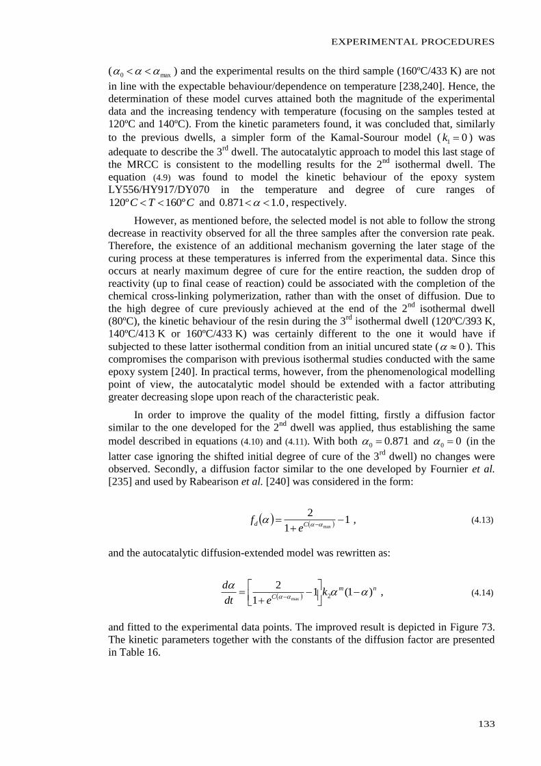
EXPERIMENTAL PROCEDURES
133
( max0 ) and the experimental results on the third sample (160ºC/433 K) are not
in line with the expectable behaviour/dependence on temperature [238,240]. Hence, the
determination of these model curves attained both the magnitude of the experimental
data and the increasing tendency with temperature (focusing on the samples tested at
120ºC and 140ºC). From the kinetic parameters found, it was concluded that, similarly
to the previous dwells, a simpler form of the Kamal-Sourour model ( 01 k ) was
adequate to describe the 3rd
dwell. The autocatalytic approach to model this last stage of
the MRCC is consistent to the modelling results for the 2nd
isothermal dwell. The
equation (4.9) was found to model the kinetic behaviour of the epoxy system
LY556/HY917/DY070 in the temperature and degree of cure ranges of
CTC º160º120 and 0.1871.0 , respectively.
However, as mentioned before, the selected model is not able to follow the strong
decrease in reactivity observed for all the three samples after the conversion rate peak.
Therefore, the existence of an additional mechanism governing the later stage of the
curing process at these temperatures is inferred from the experimental data. Since this
occurs at nearly maximum degree of cure for the entire reaction, the sudden drop of
reactivity (up to final cease of reaction) could be associated with the completion of the
chemical cross-linking polymerization, rather than with the onset of diffusion. Due to
the high degree of cure previously achieved at the end of the 2nd
isothermal dwell
(80ºC), the kinetic behaviour of the resin during the 3rd
isothermal dwell (120ºC/393 K,
140ºC/413 K or 160ºC/433 K) was certainly different to the one it would have if
subjected to these latter isothermal condition from an initial uncured state ( 0 ). This
compromises the comparison with previous isothermal studies conducted with the same
epoxy system [240]. In practical terms, however, from the phenomenological modelling
point of view, the autocatalytic model should be extended with a factor attributing
greater decreasing slope upon reach of the characteristic peak.
In order to improve the quality of the model fitting, firstly a diffusion factor
similar to the one developed for the 2nd
dwell was applied, thus establishing the same
model described in equations (4.10) and (4.11). With both 871.00 and 00 (in the
latter case ignoring the shifted initial degree of cure of the 3rd
dwell) no changes were
observed. Secondly, a diffusion factor similar to the one developed by Fournier et al.
[235] and used by Rabearison et al. [240] was considered in the form:
11
2max
Cd
ef , (4.13)
and the autocatalytic diffusion-extended model was rewritten as:
nm
Ck
edt
d)1(1
1
22
max
, (4.14)
and fitted to the experimental data points. The improved result is depicted in Figure 73.
The kinetic parameters together with the constants of the diffusion factor are presented
in Table 16.
CHAPTER 4
134
Figure 73 – Fitting of the nth
order, Kamal-Sourour and Karkanas models to the
experimental DSC data of the 3rd
isothermal dwell (393 K/413 K/433 K) on
LY556/HY917/DY070 in the applicable domain.
Table 16 – Kinetic parameters determined for the fitting of the experimental DSC
data of LY556/HY917/DY070 in the 3rd
isothermal dwell (393 K, 413 K and 433 K)
with the Kamal-Sourour diffusion-extended 2 model.
Kinetic
Parameters
Kinetic Model
Kamal-Sourour extended 2
nm
Ckk
edt
d)1)((1
1
221
max
Kamal-Sourour
nmkkdt
d)1)(( 21
1k 1A 0000.0 0000.0
1aE 0000.0 0000.0
2k 2A 5101562.3 5102500.2
2aE 4103651.5 4103651.5
m 5000.1 5000.1
n 9500.1 9500.1
C 20 n/a
max 349.210514.110711.1 225 TT n/a
Upon the analyses and development of the best phenomenological models for
each isothermal stage of the MRCC, the overall kinetic model for the entire MRCC was
obtained by assuming a piece-wise equation along the combined domains of and T .
This overall model is described by the following set of equations:
KKkedt
d
KTKe
k
dt
d
KTKkdt
d
nm
C
C
nm
nm
433373,1871.0,)1(11
2
353333,871.0049.0,1
)1(
308298,049.00,)1(
2
2
2
max
0max
, (4.15)
and graphically represented in Figure 74. It consisted, then, in a simplified
Kamal-Sourour autocatalytic model ( 01 k ) diffusion-extended for the 2nd
and 3rd
isothermal dwells. The kinetic parameters obtained for this model are in Table 17.
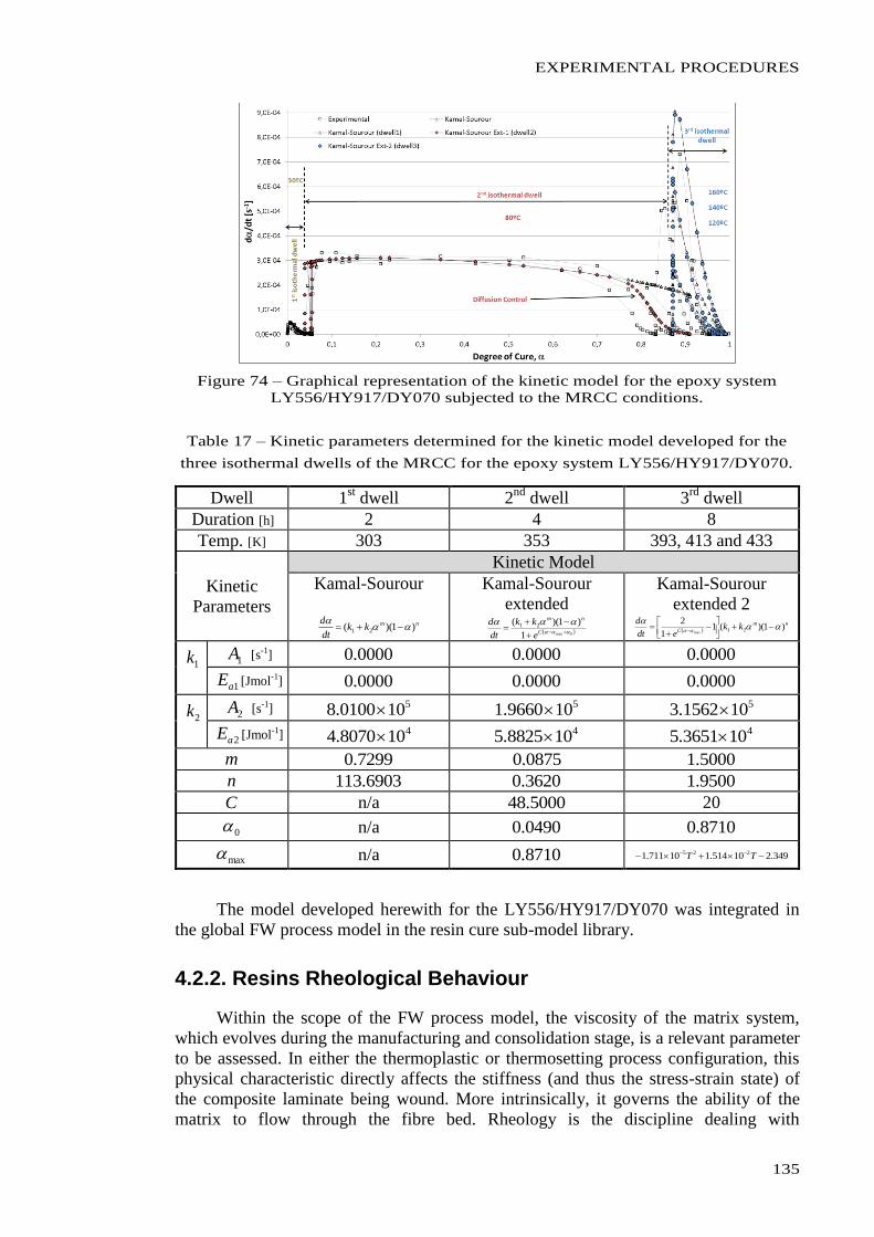
EXPERIMENTAL PROCEDURES
135
Figure 74 – Graphical representation of the kinetic model for the epoxy system
LY556/HY917/DY070 subjected to the MRCC conditions.
Table 17 – Kinetic parameters determined for the kinetic model developed for the
three isothermal dwells of the MRCC for the epoxy system LY556/HY917/DY070.
Dwell 1st dwell 2
nd dwell 3
rd dwell
Duration [h] 2 4 8
Temp. [K] 303 353 393, 413 and 433
Kinetic
Parameters
Kinetic Model
Kamal-Sourour
nmkk
dt
d)1)(( 21
Kamal-Sourour
extended
0max1
)1)(( 21
C
nm
e
kk
dt
d
Kamal-Sourour
extended 2
nm
Ckk
edt
d)1)((1
1
221
max
1k
1A [s-1] 0000.0 0000.0 0000.0
1aE [Jmol-1] 0000.0 0000.0 0000.0
2k
2A [s-1] 5100100.8 5109660.1 5101562.3
2aE [Jmol-1] 4108070.4 4108825.5 4103651.5
m 7299.0 0875.0 5000.1
n 6903.113 3620.0 9500.1
C n/a 5000.48 20
0 n/a 0490.0 8710.0
max n/a 8710.0 349.210514.110711.1 225 TT
The model developed herewith for the LY556/HY917/DY070 was integrated in
the global FW process model in the resin cure sub-model library.
4.2.2. Resins Rheological Behaviour
Within the scope of the FW process model, the viscosity of the matrix system,
which evolves during the manufacturing and consolidation stage, is a relevant parameter
to be assessed. In either the thermoplastic or thermosetting process configuration, this
physical characteristic directly affects the stiffness (and thus the stress-strain state) of
the composite laminate being wound. More intrinsically, it governs the ability of the
matrix to flow through the fibre bed. Rheology is the discipline dealing with
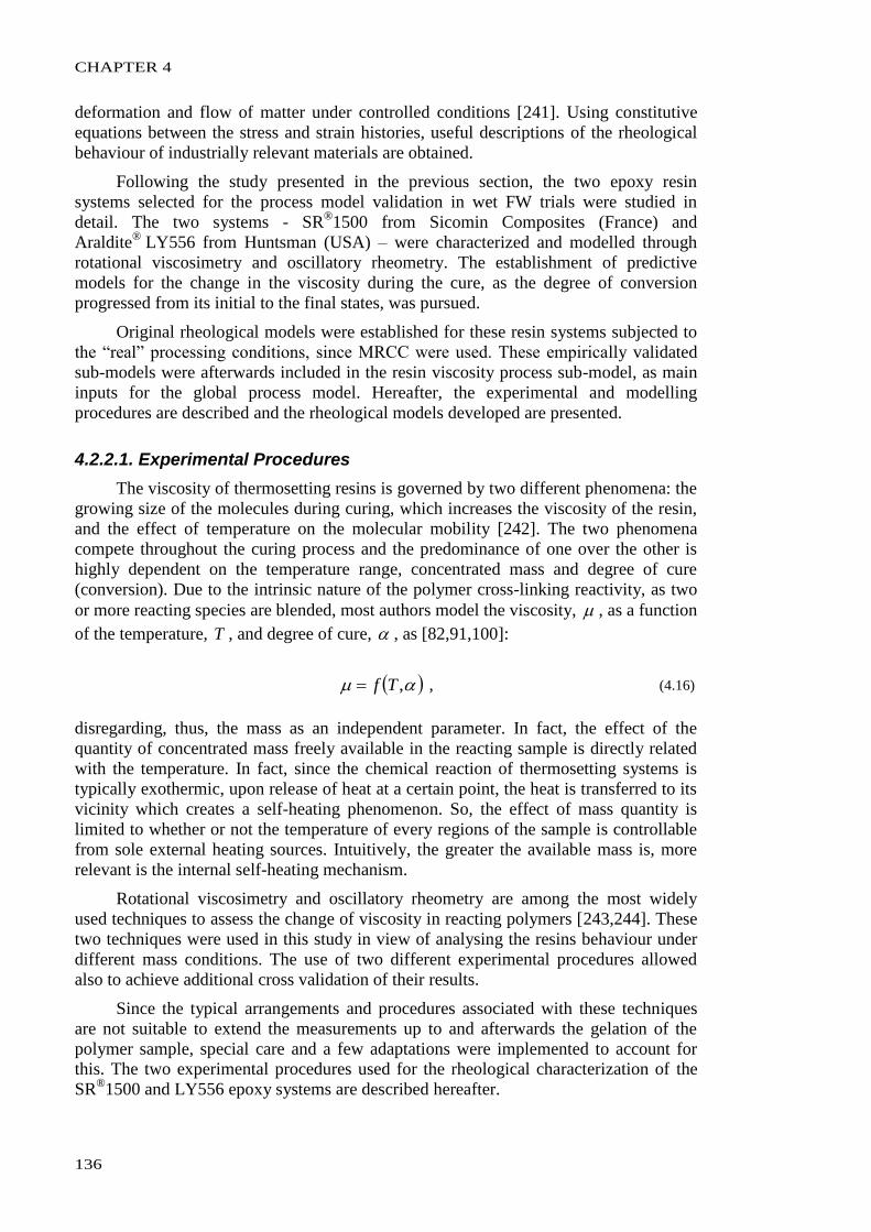
CHAPTER 4
136
deformation and flow of matter under controlled conditions [241]. Using constitutive
equations between the stress and strain histories, useful descriptions of the rheological
behaviour of industrially relevant materials are obtained.
Following the study presented in the previous section, the two epoxy resin
systems selected for the process model validation in wet FW trials were studied in
detail. The two systems - SR®1500 from Sicomin Composites (France) and
Araldite® LY556 from Huntsman (USA) – were characterized and modelled through
rotational viscosimetry and oscillatory rheometry. The establishment of predictive
models for the change in the viscosity during the cure, as the degree of conversion
progressed from its initial to the final states, was pursued.
Original rheological models were established for these resin systems subjected to
the “real” processing conditions, since MRCC were used. These empirically validated
sub-models were afterwards included in the resin viscosity process sub-model, as main
inputs for the global process model. Hereafter, the experimental and modelling
procedures are described and the rheological models developed are presented.
4.2.2.1. Experimental Procedures
The viscosity of thermosetting resins is governed by two different phenomena: the
growing size of the molecules during curing, which increases the viscosity of the resin,
and the effect of temperature on the molecular mobility [242]. The two phenomena
compete throughout the curing process and the predominance of one over the other is
highly dependent on the temperature range, concentrated mass and degree of cure
(conversion). Due to the intrinsic nature of the polymer cross-linking reactivity, as two
or more reacting species are blended, most authors model the viscosity, , as a function
of the temperature, T , and degree of cure, , as [82,91,100]:
,Tf , (4.16)
disregarding, thus, the mass as an independent parameter. In fact, the effect of the
quantity of concentrated mass freely available in the reacting sample is directly related
with the temperature. In fact, since the chemical reaction of thermosetting systems is
typically exothermic, upon release of heat at a certain point, the heat is transferred to its
vicinity which creates a self-heating phenomenon. So, the effect of mass quantity is
limited to whether or not the temperature of every regions of the sample is controllable
from sole external heating sources. Intuitively, the greater the available mass is, more
relevant is the internal self-heating mechanism.
Rotational viscosimetry and oscillatory rheometry are among the most widely
used techniques to assess the change of viscosity in reacting polymers [243,244]. These
two techniques were used in this study in view of analysing the resins behaviour under
different mass conditions. The use of two different experimental procedures allowed
also to achieve additional cross validation of their results.
Since the typical arrangements and procedures associated with these techniques
are not suitable to extend the measurements up to and afterwards the gelation of the
polymer sample, special care and a few adaptations were implemented to account for
this. The two experimental procedures used for the rheological characterization of the
SR®
1500 and LY556 epoxy systems are described hereafter.
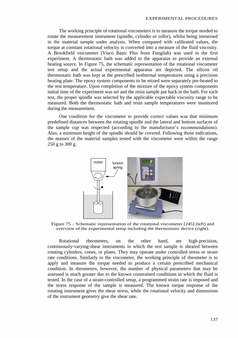
EXPERIMENTAL PROCEDURES
137
The working principle of rotational viscometers is to measure the torque needed to
rotate the measurement instrument (spindle, cylinder or roller), whilst being immersed
in the material sample under analysis. When compared with calibrated values, the
torque at constant rotational velocity is converted into a measure of the fluid viscosity.
A Brookfield viscometer (Visco Basic Plus from Fungilab) was used in the first
experiment. A thermostatic bath was added to the apparatus to provide an external
heating source. In Figure 75, the schematic representation of the rotational viscometer
test setup and the actual experimental apparatus are depicted. The silicon oil
thermostatic bath was kept at the prescribed isothermal temperatures using a precision
heating plate. The epoxy system components to be mixed were separately pre-heated to
the test temperature. Upon completion of the mixture of the epoxy system components
initial time of the experiment was set and the resin sample put back in the bath. For each
test, the proper spindle was selected by the applicable expectable viscosity range to be
measured. Both the thermostatic bath and resin sample temperatures were monitored
during the measurement.
One condition for the viscometer to provide correct values was that minimum
predefined distances between the rotating spindle and the lateral and bottom surfaces of
the sample cup was respected (according to the manufacturer’s recommendations).
Also, a minimum height of the spindle should be covered. Following those indications,
the masses of the material samples tested with the viscometer were within the range
250 g to 300 g.
Figure 75 – Schematic representation of the rotational viscometer [245] (left) and
overview of the experimental setup including the thermostatic device (right).
Rotational rheometers, on the other hand, are high-precision,
continuously-varying-shear instruments in which the test sample is sheared between
rotating cylinders, cones, or plates. They may operate under controlled stress or strain
rate conditions. Similarly to the viscometer, the working principle of rheometer is to
apply and measure the torque needed to produce a certain prescribed mechanical
condition. In rheometers, however, the number of physical parameters that may be
assessed is much greater due to the known constrained conditions in which the fluid is
tested. In the case of a strain-controlled setup, a programmed strain rate is imposed and
the stress response of the sample is measured. The known torque response of the
rotating instrument gives the shear stress, while the rotational velocity and dimensions
of the instrument geometry give the shear rate.
CHAPTER 4
138
The second group of rheological characterization tests was carried out using a
stress/strain control rheometer (Stresstech® from Reologica Instruments AB). In Figure
76 the schematic representation of the rotational viscometer test setup and the actual
experimental apparatus are depicted. The test equipment included an oven and a heated
bottom plate so that the isothermal temperatures were accurately imposed to the test
samples. Since the objective was to measure the evolution of the viscosity up to a high
degree of cure (past the gel point), disposable instruments were developed, adapted and
calibrated into the equipment. The plate-plate geometry with 40 mm in diameter was
selected due both to the easiness of manufacturing and the fact that a quasi-static shear
mode was foreseen. Thus, the inexistence of a constant through-the-thickness velocity
profile, as guaranteed by the cone-plate geometries, was negligible and reliable
measurements were possible to achieve with this simpler geometry. A small amplitude
oscillatory shear mode with strain control (2%) was programmed. Since the torque and
phase angle responses of viscoelastic materials are known to depend on the applied
oscillation frequency, multiple frequency experiments were conducted at 0.5 Hz, 1 Hz
and 5 Hz in each sample. The applicability of these frequencies was previously
determined through several frequency scans to dummy resin samples and corresponded
to the plateau of the corresponding viscosity-frequency curves.
Each test sample was prepared through mixing the components (without
pre-heating) and then placing it onto the bottom plate. As the top moving plate reached
the set gap of 1 mm, the sample was constrained in the narrow gap between the two
surfaces. The mass of sample required to properly fill the gap and barely oversize the
plates diameter was previously calculated and was around 2 g. The initial time was set
upon completion of the mixture.
Figure 76 – Schematic representation of the rotational rheometer (left) and overview
of the actual experimental setup (right).
In this experimental programme, the rheology of the two epoxy systems was
assessed by means of two different experimental techniques: rotational viscosimetry and
oscillatory rheometry. The information gathered in the two types of test was
considerably different both in terms of quality (the precision of the viscometer was
poor) and quantity. The rheometer apparatus allowed to retrieve the history of more
physical parameters, thus allowing a more complete analysis. Namely, the shear stress,
, the phase angle, , the storage (elastic) and the loss (viscous) moduli, 'G and ''G ,
were outputted from the rheometer integrated software. Nevertheless, the greater mass
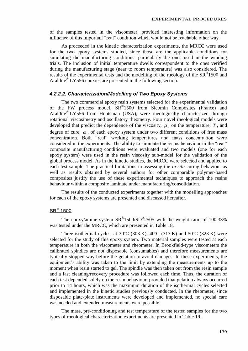
EXPERIMENTAL PROCEDURES
139
of the samples tested in the viscometer, provided interesting information on the
influence of this important “real” condition which would not be reachable other way.
As proceeded in the kinetic characterization experiments, the MRCC were used
for the two epoxy systems studied, since those are the applicable conditions for
simulating the manufacturing conditions, particularly the ones used in the winding
trials. The inclusion of initial temperature dwells correspondent to the ones verified
during the manufacturing stage (near to room temperature) was also considered. The
results of the experimental tests and the modelling of the rheology of the SR®1500 and
Araldite® LY556 epoxies are presented in the following section.
4.2.2.2. Characterization/Modelling of Two Epoxy Systems
The two commercial epoxy resin systems selected for the experimental validation
of the FW process model, SR®1500 from Sicomin Composites (France) and
Araldite® LY556 from Huntsman (USA), were rheologically characterized through
rotational viscosimetry and oscillatory rheometry. Four novel rheological models were
developed that predict the dependence of the viscosity, , on the temperature, T , and
degree of cure, , of each epoxy system under two different conditions of free mass
concentration. Both “real” working temperatures and mass concentration were
considered in the experiments. The ability to simulate the resins behaviour in the “real”
composite manufacturing conditions were evaluated and two models (one for each
epoxy system) were used in the resin viscosity sub-model for the validation of the
global process model. As in the kinetic studies, the MRCC were selected and applied to
each test sample. The practical limitations in assessing the in-situ curing behaviour as
well as results obtained by several authors for other comparable polymer-based
composites justify the use of these experimental techniques to approach the resins
behaviour within a composite laminate under manufacturing/consolidation.
The results of the conducted experiments together with the modelling approaches
for each of the epoxy systems are presented and discussed hereafter.
SR® 1500
The epoxy/amine system SR®1500/SD
®2505 with the weight ratio of 100:33%
was tested under the MRCC, which are presented in Table 18.
Three isothermal cycles, at 30ºC (303 K), 40ºC (313 K) and 50ºC (323 K) were
selected for the study of this epoxy system. Two material samples were tested at each
temperature in both the viscometer and rheometer. In Brookfield-type viscometers the
calibrated spindles are not disposable (consumables) and therefore measurements are
typically stopped way before the gelation to avoid damages. In these experiments, the
equipment’s ability was taken to the limit by extending the measurements up to the
moment when resin started to gel. The spindle was then taken out from the resin sample
and a fast cleaning/recovery procedure was followed each time. Thus, the duration of
each test depended solely on the resin behaviour, provided that gelation always occurred
prior to 14 hours, which was the maximum duration of the isothermal cycles selected
and implemented in the kinetic studies previously conducted. In the rheometer, since
disposable plate-plate instruments were developed and implemented, no special care
was needed and extended measurements were possible.
The mass, pre-conditioning and test temperature of the tested samples for the two
types of rheological characterization experiments are presented in Table 19.
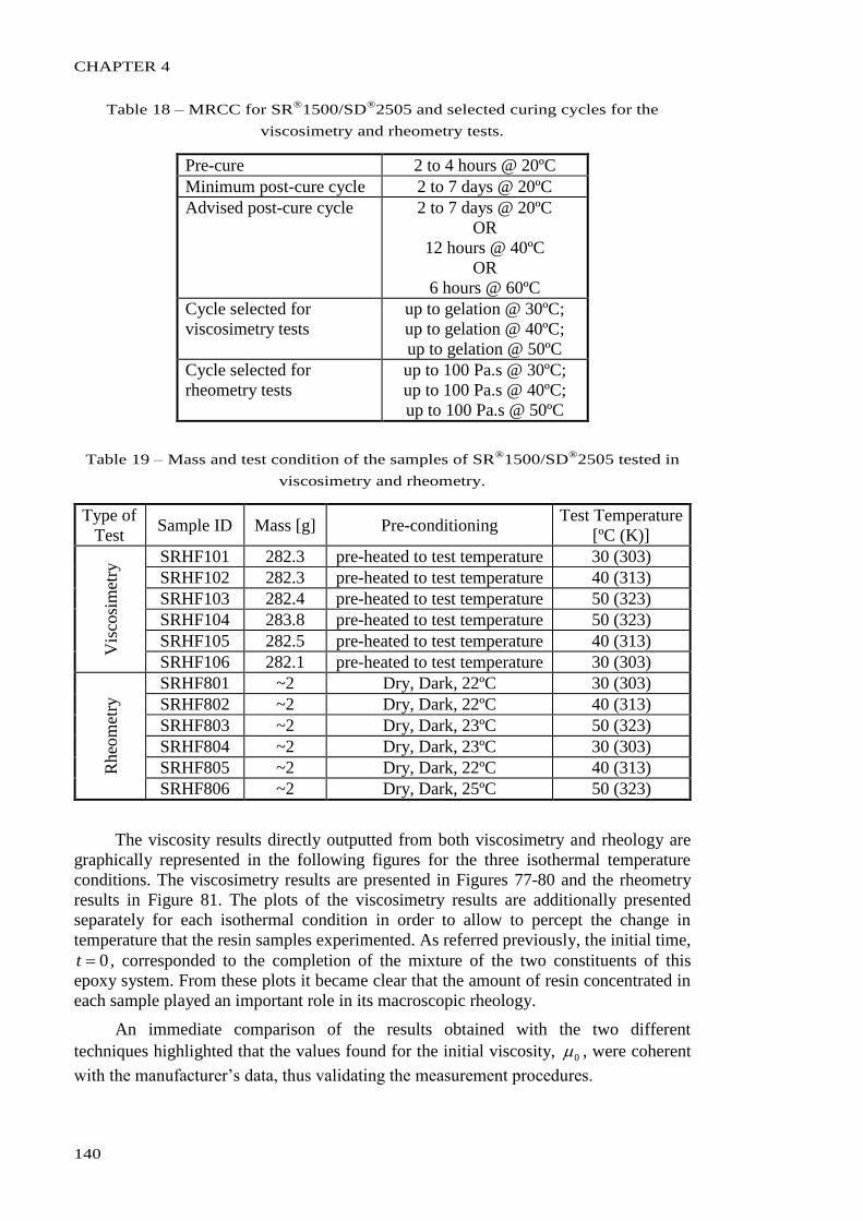
CHAPTER 4
140
Table 18 – MRCC for SR®
1500/SD®
2505 and selected curing cycles for the
viscosimetry and rheometry tests.
Pre-cure 2 to 4 hours @ 20ºC
Minimum post-cure cycle 2 to 7 days @ 20ºC
Advised post-cure cycle 2 to 7 days @ 20ºC
OR
12 hours @ 40ºC
OR
6 hours @ 60ºC
Cycle selected for
viscosimetry tests
up to gelation @ 30ºC;
up to gelation @ 40ºC;
up to gelation @ 50ºC
Cycle selected for
rheometry tests
up to 100 Pa.s @ 30ºC;
up to 100 Pa.s @ 40ºC;
up to 100 Pa.s @ 50ºC
Table 19 – Mass and test condition of the samples of SR®
1500/SD®
2505 tested in
viscosimetry and rheometry.
Type of
Test Sample ID Mass [g] Pre-conditioning
Test Temperature
[ºC (K)]
Vis
cosi
met
ry SRHF101 282.3 pre-heated to test temperature 30 (303)
SRHF102 282.3 pre-heated to test temperature 40 (313)
SRHF103 282.4 pre-heated to test temperature 50 (323)
SRHF104 283.8 pre-heated to test temperature 50 (323)
SRHF105 282.5 pre-heated to test temperature 40 (313)
SRHF106 282.1 pre-heated to test temperature 30 (303)
Rheo
met
ry
SRHF801 ~2 Dry, Dark, 22ºC 30 (303)
SRHF802 ~2 Dry, Dark, 22ºC 40 (313)
SRHF803 ~2 Dry, Dark, 23ºC 50 (323)
SRHF804 ~2 Dry, Dark, 23ºC 30 (303)
SRHF805 ~2 Dry, Dark, 22ºC 40 (313)
SRHF806 ~2 Dry, Dark, 25ºC 50 (323)
The viscosity results directly outputted from both viscosimetry and rheology are
graphically represented in the following figures for the three isothermal temperature
conditions. The viscosimetry results are presented in Figures 77-80 and the rheometry
results in Figure 81. The plots of the viscosimetry results are additionally presented
separately for each isothermal condition in order to allow to percept the change in
temperature that the resin samples experimented. As referred previously, the initial time,
0t , corresponded to the completion of the mixture of the two constituents of this
epoxy system. From these plots it became clear that the amount of resin concentrated in
each sample played an important role in its macroscopic rheology.
An immediate comparison of the results obtained with the two different
techniques highlighted that the values found for the initial viscosity, 0 , were coherent
with the manufacturer’s data, thus validating the measurement procedures.
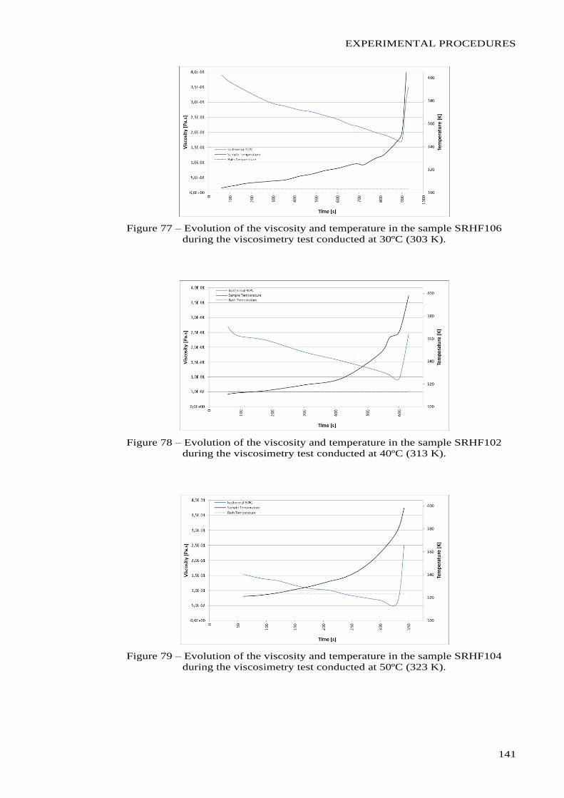
EXPERIMENTAL PROCEDURES
141
Figure 77 – Evolution of the viscosity and temperature in the sample SRHF106
during the viscosimetry test conducted at 30ºC (303 K).
Figure 78 – Evolution of the viscosity and temperature in the sample SRHF102
during the viscosimetry test conducted at 40ºC (313 K).
Figure 79 – Evolution of the viscosity and temperature in the sample SRHF104
during the viscosimetry test conducted at 50ºC (323 K).
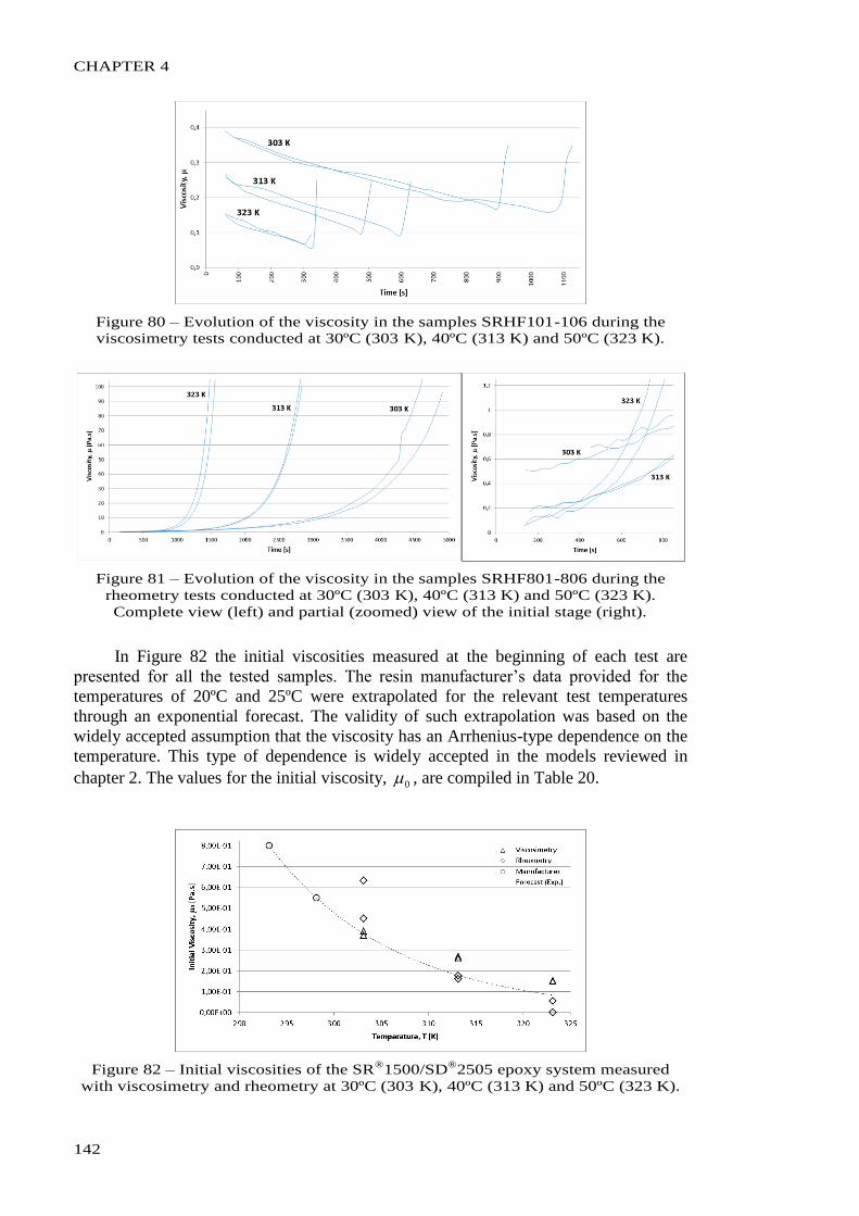
CHAPTER 4
142
Figure 80 – Evolution of the viscosity in the samples SRHF101-106 during the
viscosimetry tests conducted at 30ºC (303 K), 40ºC (313 K) and 50ºC (323 K).
Figure 81 – Evolution of the viscosity in the samples SRHF801-806 during the
rheometry tests conducted at 30ºC (303 K), 40ºC (313 K) and 50ºC (323 K).
Complete view (left) and partial (zoomed) view of the initial stage (right).
In Figure 82 the initial viscosities measured at the beginning of each test are
presented for all the tested samples. The resin manufacturer’s data provided for the
temperatures of 20ºC and 25ºC were extrapolated for the relevant test temperatures
through an exponential forecast. The validity of such extrapolation was based on the
widely accepted assumption that the viscosity has an Arrhenius-type dependence on the
temperature. This type of dependence is widely accepted in the models reviewed in
chapter 2. The values for the initial viscosity, 0 , are compiled in Table 20.
Figure 82 – Initial viscosities of the SR®
1500/SD®
2505 epoxy system measured
with viscosimetry and rheometry at 30ºC (303 K), 40ºC (313 K) and 50ºC (323 K).
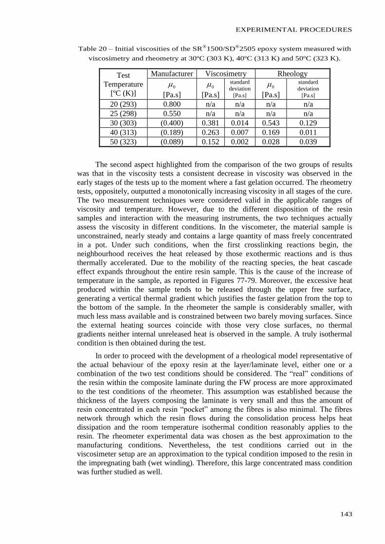
EXPERIMENTAL PROCEDURES
143
Table 20 – Initial viscosities of the SR®
1500/SD®
2505 epoxy system measured with
viscosimetry and rheometry at 30ºC (303 K), 40ºC (313 K) and 50ºC (323 K).
Test
Temperature
[ºC (K)]
Manufacturer Viscosimetry Rheology
0
[Pa.s]
0
[Pa.s]
standard
deviation
[Pa.s]
0
[Pa.s]
standard
deviation
[Pa.s]
20 (293) 0.800 n/a n/a n/a n/a
25 (298) 0.550 n/a n/a n/a n/a
30 (303) (0.400) 0.381 0.014 0.543 0.129
40 (313) (0.189) 0.263 0.007 0.169 0.011
50 (323) (0.089) 0.152 0.002 0.028 0.039
The second aspect highlighted from the comparison of the two groups of results
was that in the viscosity tests a consistent decrease in viscosity was observed in the
early stages of the tests up to the moment where a fast gelation occurred. The rheometry
tests, oppositely, outputted a monotonically increasing viscosity in all stages of the cure.
The two measurement techniques were considered valid in the applicable ranges of
viscosity and temperature. However, due to the different disposition of the resin
samples and interaction with the measuring instruments, the two techniques actually
assess the viscosity in different conditions. In the viscometer, the material sample is
unconstrained, nearly steady and contains a large quantity of mass freely concentrated
in a pot. Under such conditions, when the first crosslinking reactions begin, the
neighbourhood receives the heat released by those exothermic reactions and is thus
thermally accelerated. Due to the mobility of the reacting species, the heat cascade
effect expands throughout the entire resin sample. This is the cause of the increase of
temperature in the sample, as reported in Figures 77-79. Moreover, the excessive heat
produced within the sample tends to be released through the upper free surface,
generating a vertical thermal gradient which justifies the faster gelation from the top to
the bottom of the sample. In the rheometer the sample is considerably smaller, with
much less mass available and is constrained between two barely moving surfaces. Since
the external heating sources coincide with those very close surfaces, no thermal
gradients neither internal unreleased heat is observed in the sample. A truly isothermal
condition is then obtained during the test.
In order to proceed with the development of a rheological model representative of
the actual behaviour of the epoxy resin at the layer/laminate level, either one or a
combination of the two test conditions should be considered. The “real” conditions of
the resin within the composite laminate during the FW process are more approximated
to the test conditions of the rheometer. This assumption was established because the
thickness of the layers composing the laminate is very small and thus the amount of
resin concentrated in each resin “pocket” among the fibres is also minimal. The fibres
network through which the resin flows during the consolidation process helps heat
dissipation and the room temperature isothermal condition reasonably applies to the
resin. The rheometer experimental data was chosen as the best approximation to the
manufacturing conditions. Nevertheless, the test conditions carried out in the
viscosimeter setup are an approximation to the typical condition imposed to the resin in
the impregnating bath (wet winding). Therefore, this large concentrated mass condition
was further studied as well.
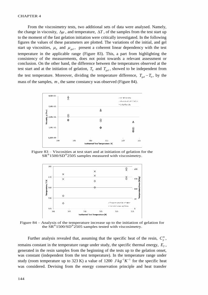
CHAPTER 4
144
From the viscosimetry tests, two additional sets of data were analysed. Namely,
the change in viscosity, , and temperature, T , of the samples from the test start up
to the moment of the fast gelation initiation were critically investigated. In the following
figures the values of these parameters are plotted. The variations of the initial, and gel
start up viscosities, 0 and gel , present a coherent linear dependency with the test
temperature in the applicable range (Figure 83). This, a part from highlighting the
consistency of the measurements, does not point towards a relevant assessment or
conclusion. On the other hand, the difference between the temperatures observed at the
test start and at the initiation of gelation, 0T and gelT , showed to be independent from
the test temperature. Moreover, dividing the temperature difference, 0TTgel , by the
mass of the samples, m , the same constancy was observed (Figure 84).
Figure 83 – Viscosities at test start and at initiation of gelation for the
SR®
1500/SD®
2505 samples measured with viscosimetry.
Figure 84 – Analysis of the temperature increase up to the initiation of gelation for
the SR®
1500/SD®
2505 samples tested with viscosimetry.
Further analysis revealed that, assuming that the specific heat of the resin, m
pC ,
remains constant in the temperature range under study, the specific thermal energy, TE ,
generated in the resin samples from the beginning of the tests up to the gelation onset,
was constant (independent from the test temperature). In the temperature range under
study (room temperature up to 323 K) a value of 111200 KkgJ for the specific heat
was considered. Devising from the energy conservation principle and heat transfer
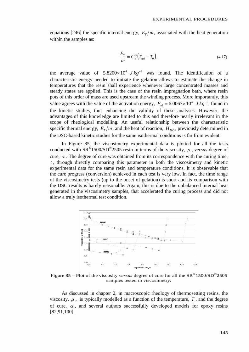
EXPERIMENTAL PROCEDURES
145
equations [246] the specific internal energy, mET , associated with the heat generation
within the samples as:
0TTC
m
Egel
m
pT , (4.17)
the average value of 14108200.5 kgJ was found. The identification of a
characteristic energy needed to initiate the gelation allows to estimate the change in
temperatures that the resin shall experience whenever large concentrated masses and
steady states are applied. This is the case of the resin impregnation bath, where resin
pots of this order of mass are used upstream the winding process. More importantly, this
value agrees with the value of the activation energy, 14
1 100067.6 kgJEa , found in
the kinetic studies, thus enhancing the validity of these analyses. However, the
advantages of this knowledge are limited to this and therefore nearly irrelevant in the
scope of rheological modelling. An useful relationship between the characteristic
specific thermal energy, mET , and the heat of reaction, ISOH , previously determined in
the DSC-based kinetic studies for the same isothermal conditions is far from evident.
In Figure 85, the viscosimetry experimental data is plotted for all the tests
conducted with SR®1500/SD
®2505 resin in terms of the viscosity, , versus degree of
cure, . The degree of cure was obtained from its correspondence with the curing time,
t , through directly comparing this parameter in both the viscosimetry and kinetic
experimental data for the same resin and temperature conditions. It is observable that
the cure progress (conversion) achieved in each test is very low. In fact, the time range
of the viscosimetry tests (up to the onset of gelation) is short and its comparison with
the DSC results is barely reasonable. Again, this is due to the unbalanced internal heat
generated in the viscosimetry samples, that accelerated the curing process and did not
allow a truly isothermal test condition.
Figure 85 – Plot of the viscosity versus degree of cure for all the SR®
1500/SD®
2505
samples tested in viscosimetry.
As discussed in chapter 2, in macroscopic rheology of thermosetting resins, the
viscosity, , is typically modelled as a function of the temperature, T , and the degree
of cure, , and several authors successfully developed models for epoxy resins
[82,91,100].
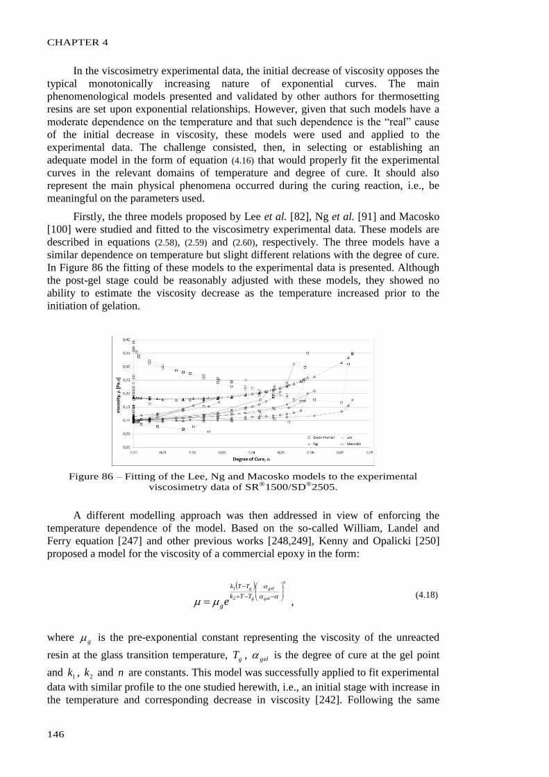
CHAPTER 4
146
In the viscosimetry experimental data, the initial decrease of viscosity opposes the
typical monotonically increasing nature of exponential curves. The main
phenomenological models presented and validated by other authors for thermosetting
resins are set upon exponential relationships. However, given that such models have a
moderate dependence on the temperature and that such dependence is the “real” cause
of the initial decrease in viscosity, these models were used and applied to the
experimental data. The challenge consisted, then, in selecting or establishing an
adequate model in the form of equation (4.16) that would properly fit the experimental
curves in the relevant domains of temperature and degree of cure. It should also
represent the main physical phenomena occurred during the curing reaction, i.e., be
meaningful on the parameters used.
Firstly, the three models proposed by Lee et al. [82], Ng et al. [91] and Macosko
[100] were studied and fitted to the viscosimetry experimental data. These models are
described in equations (2.58), (2.59) and (2.60), respectively. The three models have a
similar dependence on temperature but slight different relations with the degree of cure.
In Figure 86 the fitting of these models to the experimental data is presented. Although
the post-gel stage could be reasonably adjusted with these models, they showed no
ability to estimate the viscosity decrease as the temperature increased prior to the
initiation of gelation.
Figure 86 – Fitting of the Lee, Ng and Macosko models to the experimental
viscosimetry data of SR®
1500/SD®
2505.
A different modelling approach was then addressed in view of enforcing the
temperature dependence of the model. Based on the so-called William, Landel and
Ferry equation [247] and other previous works [248,249], Kenny and Opalicki [250]
proposed a model for the viscosity of a commercial epoxy in the form:
n
gel
gel
g
g
TTk
TTk
ge
2
1
, (4.18)
where g is the pre-exponential constant representing the viscosity of the unreacted
resin at the glass transition temperature, gT , gel is the degree of cure at the gel point
and 1k , 2k and n are constants. This model was successfully applied to fit experimental
data with similar profile to the one studied herewith, i.e., an initial stage with increase in
the temperature and corresponding decrease in viscosity [242]. Following the same
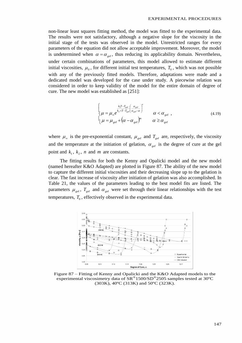
EXPERIMENTAL PROCEDURES
147
non-linear least squares fitting method, the model was fitted to the experimental data.
The results were not satisfactory, although a negative slope for the viscosity in the
initial stage of the tests was observed in the model. Unrestricted ranges for every
parameters of the equation did not allow acceptable improvement. Moreover, the model
is undetermined when gel , thus reducing its applicability domain. Nevertheless,
under certain combinations of parameters, this model allowed to estimate different
initial viscosities, 0 , for different initial test temperatures, 0T , which was not possible
with any of the previously fitted models. Therefore, adaptations were made and a
dedicated model was developed for the case under study. A piecewise relation was
considered in order to keep validity of the model for the entire domain of degree of
cure. The new model was established as [251]:
gel
m
gelgel
gel
TTk
TTkn
gel
gel
gel
gel
e
2
1
, (4.19)
where is the pre-exponential constant, gel and gelT are, respectively, the viscosity
and the temperature at the initiation of gelation, gel is the degree of cure at the gel
point and 1k , 2k , n and m are constants.
The fitting results for both the Kenny and Opalicki model and the new model
(named hereafter K&O Adapted) are plotted in Figure 87. The ability of the new model
to capture the different initial viscosities and their decreasing slope up to the gelation is
clear. The fast increase of viscosity after initiation of gelation was also accomplished. In
Table 21, the values of the parameters leading to the best model fits are listed. The
parameters gel , gelT and gel were set through their linear relationships with the test
temperatures, 0T , effectively observed in the experimental data.
Figure 87 – Fitting of Kenny and Opalicki and the K&O Adapted models to the
experimental viscosimetry data of SR®
1500/SD®
2505 samples tested at 30ºC
(303K), 40ºC (313K) and 50ºC (323K).
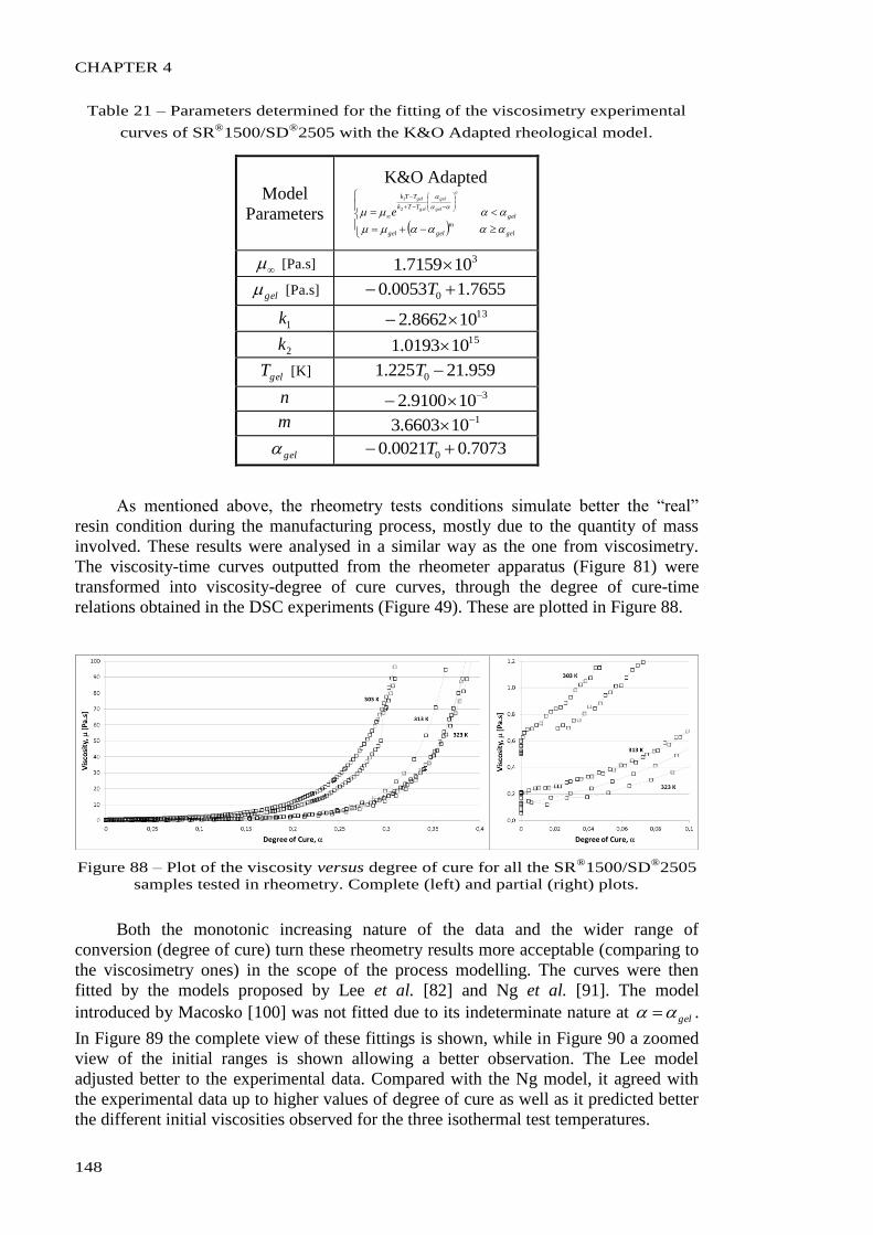
CHAPTER 4
148
Table 21 – Parameters determined for the fitting of the viscosimetry experimental
curves of SR®
1500/SD®
2505 with the K&O Adapted rheological model.
Model
Parameters
K&O Adapted
gel
m
gelgel
gel
TTk
TTkn
gel
gel
gel
gel
e
2
1
[Pa.s] 3107159.1
gel [Pa.s] 7655.10053.0 0 T
1k 13108662.2
2k 15100193.1
gelT [K] 959.21225.1 0 T
n 3109100.2
m 1106603.3
gel 7073.00021.0 0 T
As mentioned above, the rheometry tests conditions simulate better the “real”
resin condition during the manufacturing process, mostly due to the quantity of mass
involved. These results were analysed in a similar way as the one from viscosimetry.
The viscosity-time curves outputted from the rheometer apparatus (Figure 81) were
transformed into viscosity-degree of cure curves, through the degree of cure-time
relations obtained in the DSC experiments (Figure 49). These are plotted in Figure 88.
Figure 88 – Plot of the viscosity versus degree of cure for all the SR®
1500/SD®
2505
samples tested in rheometry. Complete (left) and partial (right) plots.
Both the monotonic increasing nature of the data and the wider range of
conversion (degree of cure) turn these rheometry results more acceptable (comparing to
the viscosimetry ones) in the scope of the process modelling. The curves were then
fitted by the models proposed by Lee et al. [82] and Ng et al. [91]. The model
introduced by Macosko [100] was not fitted due to its indeterminate nature at gel .
In Figure 89 the complete view of these fittings is shown, while in Figure 90 a zoomed
view of the initial ranges is shown allowing a better observation. The Lee model
adjusted better to the experimental data. Compared with the Ng model, it agreed with
the experimental data up to higher values of degree of cure as well as it predicted better
the different initial viscosities observed for the three isothermal test temperatures.
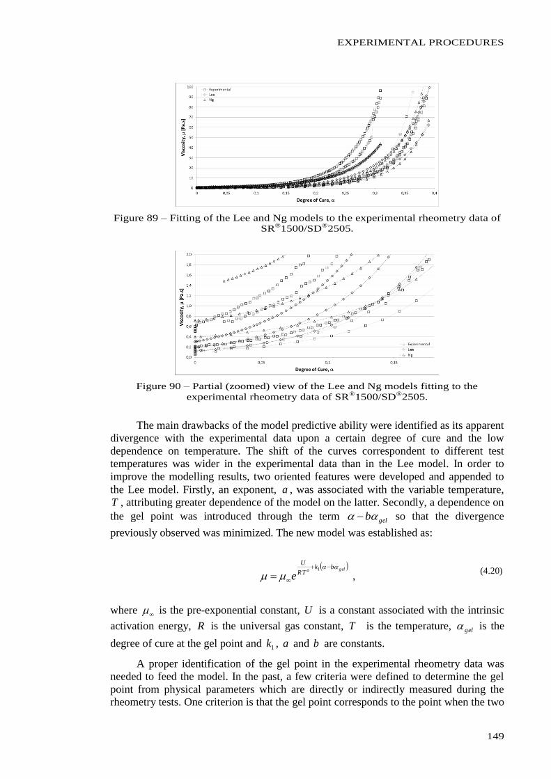
EXPERIMENTAL PROCEDURES
149
Figure 89 – Fitting of the Lee and Ng models to the experimental rheometry data of
SR®
1500/SD®
2505.
Figure 90 – Partial (zoomed) view of the Lee and Ng models fitting to the
experimental rheometry data of SR®
1500/SD®
2505.
The main drawbacks of the model predictive ability were identified as its apparent
divergence with the experimental data upon a certain degree of cure and the low
dependence on temperature. The shift of the curves correspondent to different test
temperatures was wider in the experimental data than in the Lee model. In order to
improve the modelling results, two oriented features were developed and appended to
the Lee model. Firstly, an exponent, a , was associated with the variable temperature,
T , attributing greater dependence of the model on the latter. Secondly, a dependence on
the gel point was introduced through the term gelb so that the divergence
previously observed was minimized. The new model was established as:
gelabk
TR
U
e
1
, (4.20)
where is the pre-exponential constant, U is a constant associated with the intrinsic
activation energy, R is the universal gas constant, T is the temperature, gel is the
degree of cure at the gel point and 1k , a and b are constants.
A proper identification of the gel point in the experimental rheometry data was
needed to feed the model. In the past, a few criteria were defined to determine the gel
point from physical parameters which are directly or indirectly measured during the
rheometry tests. One criterion is that the gel point corresponds to the point when the two
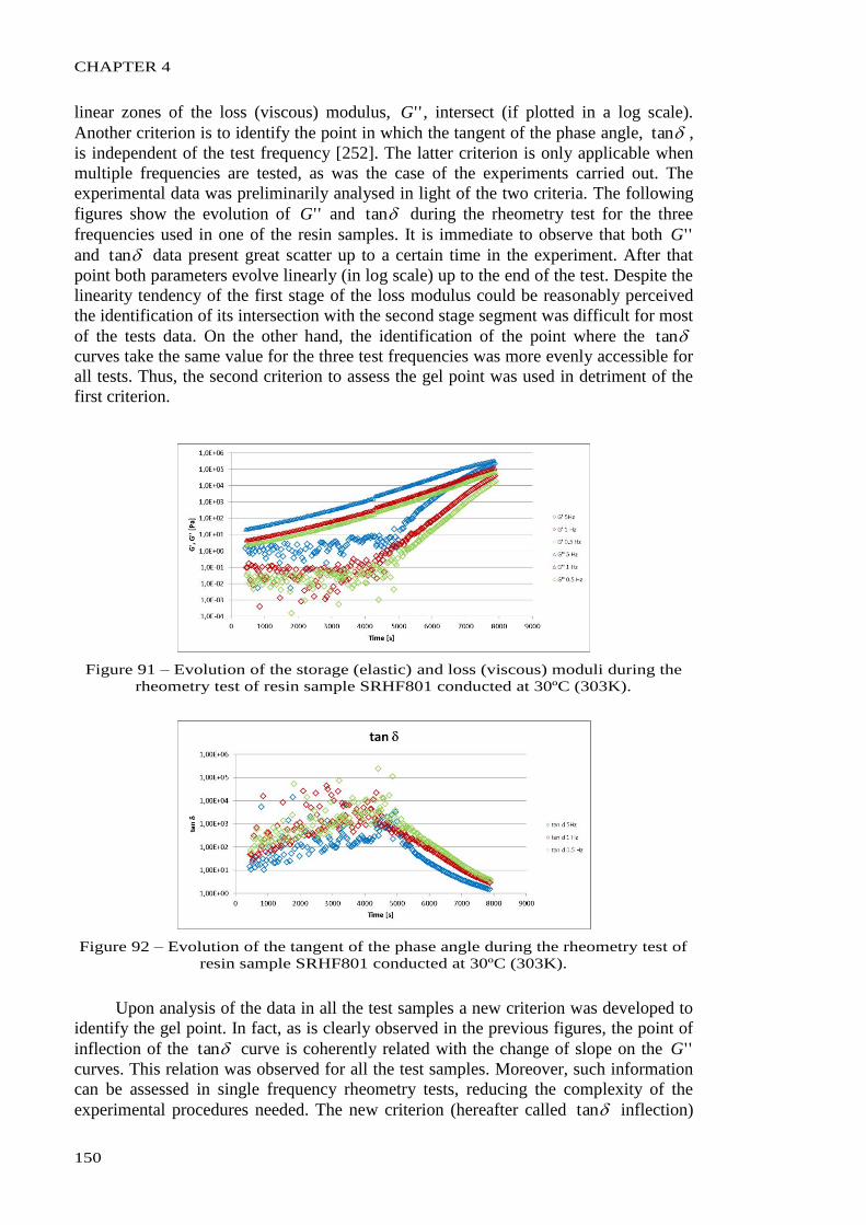
CHAPTER 4
150
linear zones of the loss (viscous) modulus, ''G , intersect (if plotted in a log scale).
Another criterion is to identify the point in which the tangent of the phase angle, tan ,
is independent of the test frequency [252]. The latter criterion is only applicable when
multiple frequencies are tested, as was the case of the experiments carried out. The
experimental data was preliminarily analysed in light of the two criteria. The following
figures show the evolution of ''G and tan during the rheometry test for the three
frequencies used in one of the resin samples. It is immediate to observe that both ''G
and tan data present great scatter up to a certain time in the experiment. After that
point both parameters evolve linearly (in log scale) up to the end of the test. Despite the
linearity tendency of the first stage of the loss modulus could be reasonably perceived
the identification of its intersection with the second stage segment was difficult for most
of the tests data. On the other hand, the identification of the point where the tan
curves take the same value for the three test frequencies was more evenly accessible for
all tests. Thus, the second criterion to assess the gel point was used in detriment of the
first criterion.
Figure 91 – Evolution of the storage (elastic) and loss (viscous) moduli during the
rheometry test of resin sample SRHF801 conducted at 30ºC (303K).
Figure 92 – Evolution of the tangent of the phase angle during the rheometry test of
resin sample SRHF801 conducted at 30ºC (303K).
Upon analysis of the data in all the test samples a new criterion was developed to
identify the gel point. In fact, as is clearly observed in the previous figures, the point of
inflection of the tan curve is coherently related with the change of slope on the ''G
curves. This relation was observed for all the test samples. Moreover, such information
can be assessed in single frequency rheometry tests, reducing the complexity of the
experimental procedures needed. The new criterion (hereafter called tan inflection)
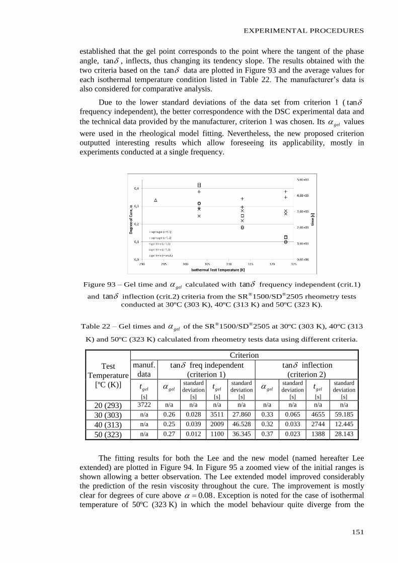
EXPERIMENTAL PROCEDURES
151
established that the gel point corresponds to the point where the tangent of the phase
angle, tan , inflects, thus changing its tendency slope. The results obtained with the
two criteria based on the tan data are plotted in Figure 93 and the average values for
each isothermal temperature condition listed in Table 22. The manufacturer’s data is
also considered for comparative analysis.
Due to the lower standard deviations of the data set from criterion 1 ( tan
frequency independent), the better correspondence with the DSC experimental data and
the technical data provided by the manufacturer, criterion 1 was chosen. Its gel values
were used in the rheological model fitting. Nevertheless, the new proposed criterion
outputted interesting results which allow foreseeing its applicability, mostly in
experiments conducted at a single frequency.
Figure 93 – Gel time and gel calculated with tan frequency independent (crit.1)
and tan inflection (crit.2) criteria from the SR®
1500/SD®
2505 rheometry tests
conducted at 30ºC (303 K), 40ºC (313 K) and 50ºC (323 K).
Table 22 – Gel times and gel of the SR®
1500/SD®
2505 at 30ºC (303 K), 40ºC (313
K) and 50ºC (323 K) calculated from rheometry tests data using different criteria.
Test
Temperature
[ºC (K)]
Criterion
manuf.
data tan freq independent
(criterion 1)
tan inflection
(criterion 2)
gelt
[s]
gel
standard
deviation
[s] gelt
[s]
standard
deviation
[s]
gel
standard
deviation
[s] gelt
[s]
standard
deviation
[s]
20 (293) 3722 n/a n/a n/a n/a n/a n/a n/a n/a
30 (303) n/a 0.26 0.028 3511 27.860 0.33 0.065 4655 59.185
40 (313) n/a 0.25 0.039 2009 46.528 0.32 0.033 2744 12.445
50 (323) n/a 0.27 0.012 1100 36.345 0.37 0.023 1388 28.143
The fitting results for both the Lee and the new model (named hereafter Lee
extended) are plotted in Figure 94. In Figure 95 a zoomed view of the initial ranges is
shown allowing a better observation. The Lee extended model improved considerably
the prediction of the resin viscosity throughout the cure. The improvement is mostly
clear for degrees of cure above 08.0 . Exception is noted for the case of isothermal
temperature of 50ºC (323 K) in which the model behaviour quite diverge from the
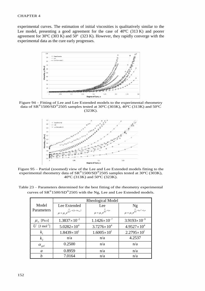
CHAPTER 4
152
experimental curves. The estimation of initial viscosities is qualitatively similar to the
Lee model, presenting a good agreement for the case of 40ºC (313 K) and poorer
agreement for 30ºC (303 K) and 50º (323 K). However, they rapidly converge with the
experimental data as the cure early progresses.
Figure 94 – Fitting of Lee and Lee Extended models to the experimental rheometry
data of SR®
1500/SD®
2505 samples tested at 30ºC (303K), 40ºC (313K) and 50ºC
(323K).
Figure 95 – Partial (zoomed) view of the Lee and Lee Extended models fitting to the
experimental rheometry data of SR®
1500/SD®
2505 samples tested at 30ºC (303K),
40ºC (313K) and 50ºC (323K).
Table 23 – Parameters determined for the best fitting of the rheometry experimental
curves of SR®
1500/SD®
2505 with the Ng, Lee and Lee Extended models.
Model
Parameters
Rheological Model
Lee Extended gela
bkTR
U
e
1
Lee
1k
TR
U
e
Ng
2
21 kk
TR
U
e
[Pa.s] 2103837.1 7101426.1 9109193.3
U [J mol-1
] 4100282.5 4107276.3 4109527.4
1k 1108439.1 1106005.1 1102795.2
2k n/a n/a 2537.4
gel 2500.0 n/a n/a
a 8959.0 n/a n/a
b 0164.7 n/a n/a
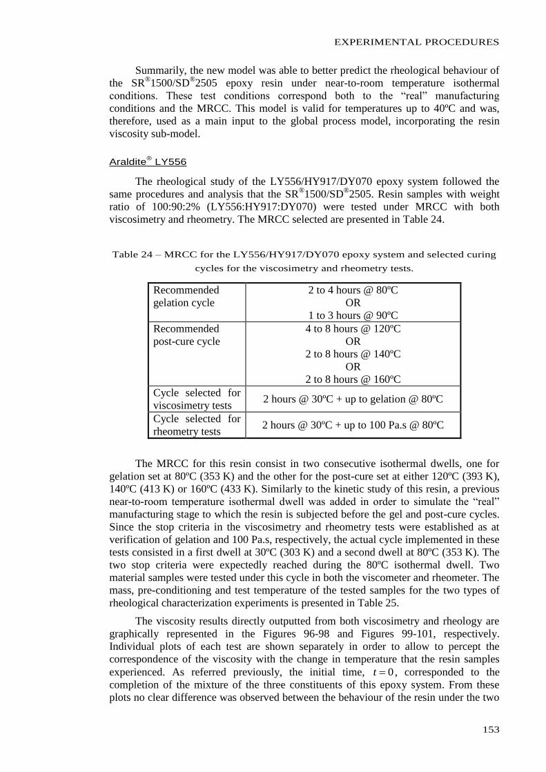
EXPERIMENTAL PROCEDURES
153
Summarily, the new model was able to better predict the rheological behaviour of
the SR®1500/SD
®2505 epoxy resin under near-to-room temperature isothermal
conditions. These test conditions correspond both to the “real” manufacturing
conditions and the MRCC. This model is valid for temperatures up to 40ºC and was,
therefore, used as a main input to the global process model, incorporating the resin
viscosity sub-model.
Araldite® LY556
The rheological study of the LY556/HY917/DY070 epoxy system followed the
same procedures and analysis that the SR®1500/SD
®2505. Resin samples with weight
ratio of 100:90:2% (LY556:HY917:DY070) were tested under MRCC with both
viscosimetry and rheometry. The MRCC selected are presented in Table 24.
Table 24 – MRCC for the LY556/HY917/DY070 epoxy system and selected curing
cycles for the viscosimetry and rheometry tests.
Recommended
gelation cycle
2 to 4 hours @ 80ºC
OR
1 to 3 hours @ 90ºC
Recommended
post-cure cycle
4 to 8 hours @ 120ºC
OR
2 to 8 hours @ 140ºC
OR
2 to 8 hours @ 160ºC
Cycle selected for
viscosimetry tests 2 hours @ 30ºC + up to gelation @ 80ºC
Cycle selected for
rheometry tests 2 hours @ 30ºC + up to 100 Pa.s @ 80ºC
The MRCC for this resin consist in two consecutive isothermal dwells, one for
gelation set at 80ºC (353 K) and the other for the post-cure set at either 120ºC (393 K),
140ºC (413 K) or 160ºC (433 K). Similarly to the kinetic study of this resin, a previous
near-to-room temperature isothermal dwell was added in order to simulate the “real”
manufacturing stage to which the resin is subjected before the gel and post-cure cycles.
Since the stop criteria in the viscosimetry and rheometry tests were established as at
verification of gelation and 100 Pa.s, respectively, the actual cycle implemented in these
tests consisted in a first dwell at 30ºC (303 K) and a second dwell at 80ºC (353 K). The
two stop criteria were expectedly reached during the 80ºC isothermal dwell. Two
material samples were tested under this cycle in both the viscometer and rheometer. The
mass, pre-conditioning and test temperature of the tested samples for the two types of
rheological characterization experiments is presented in Table 25.
The viscosity results directly outputted from both viscosimetry and rheology are
graphically represented in the Figures 96-98 and Figures 99-101, respectively.
Individual plots of each test are shown separately in order to allow to percept the
correspondence of the viscosity with the change in temperature that the resin samples
experienced. As referred previously, the initial time, 0t , corresponded to the
completion of the mixture of the three constituents of this epoxy system. From these
plots no clear difference was observed between the behaviour of the resin under the two
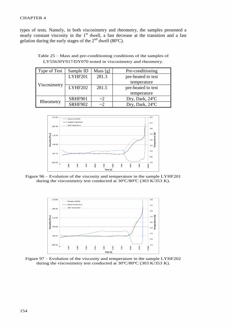
CHAPTER 4
154
types of tests. Namely, in both viscosimetry and rheometry, the samples presented a
nearly constant viscosity in the 1st dwell, a fast decrease at the transition and a fast
gelation during the early stages of the 2nd
dwell (80ºC).
Table 25 – Mass and pre-conditioning conditions of the samples of
LY556/HY917/DY070 tested in viscosimetry and rheometry.
Type of Test Sample ID Mass [g] Pre-conditioning
Viscosimetry
LYHF201 281.3 pre-heated to test
temperature
LYHF202 281.5 pre-heated to test
temperature
Rheometry SRHF901 ~2 Dry, Dark, 24ºC
SRHF902 ~2 Dry, Dark, 24ºC
Figure 96 – Evolution of the viscosity and temperature in the sample LYHF201
during the viscosimetry test conducted at 30ºC/80ºC (303 K/353 K).
Figure 97 – Evolution of the viscosity and temperature in the sample LYHF202
during the viscosimetry test conducted at 30ºC/80ºC (303 K/353 K).
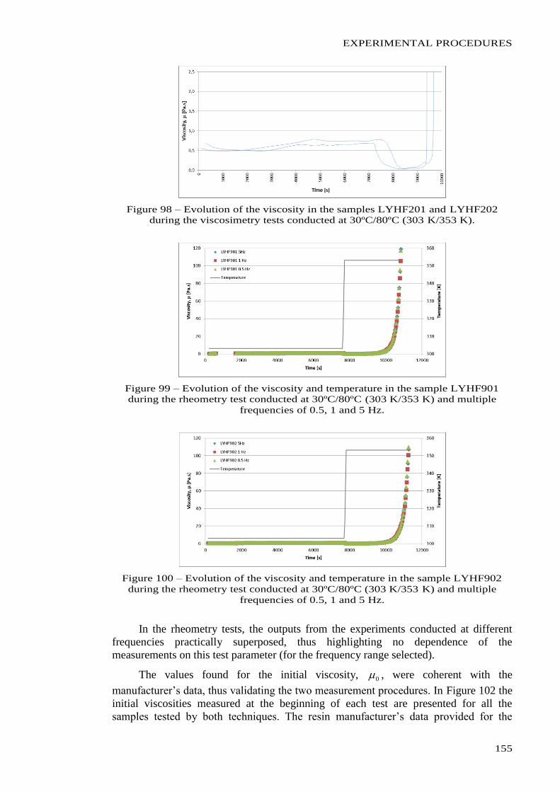
EXPERIMENTAL PROCEDURES
155
Figure 98 – Evolution of the viscosity in the samples LYHF201 and LYHF202
during the viscosimetry tests conducted at 30ºC/80ºC (303 K/353 K).
Figure 99 – Evolution of the viscosity and temperature in the sample LYHF901
during the rheometry test conducted at 30ºC/80ºC (303 K/353 K) and multiple
frequencies of 0.5, 1 and 5 Hz.
Figure 100 – Evolution of the viscosity and temperature in the sample LYHF902
during the rheometry test conducted at 30ºC/80ºC (303 K/353 K) and multiple
frequencies of 0.5, 1 and 5 Hz.
In the rheometry tests, the outputs from the experiments conducted at different
frequencies practically superposed, thus highlighting no dependence of the
measurements on this test parameter (for the frequency range selected).
The values found for the initial viscosity, 0 , were coherent with the
manufacturer’s data, thus validating the two measurement procedures. In Figure 102 the
initial viscosities measured at the beginning of each test are presented for all the
samples tested by both techniques. The resin manufacturer’s data provided for the
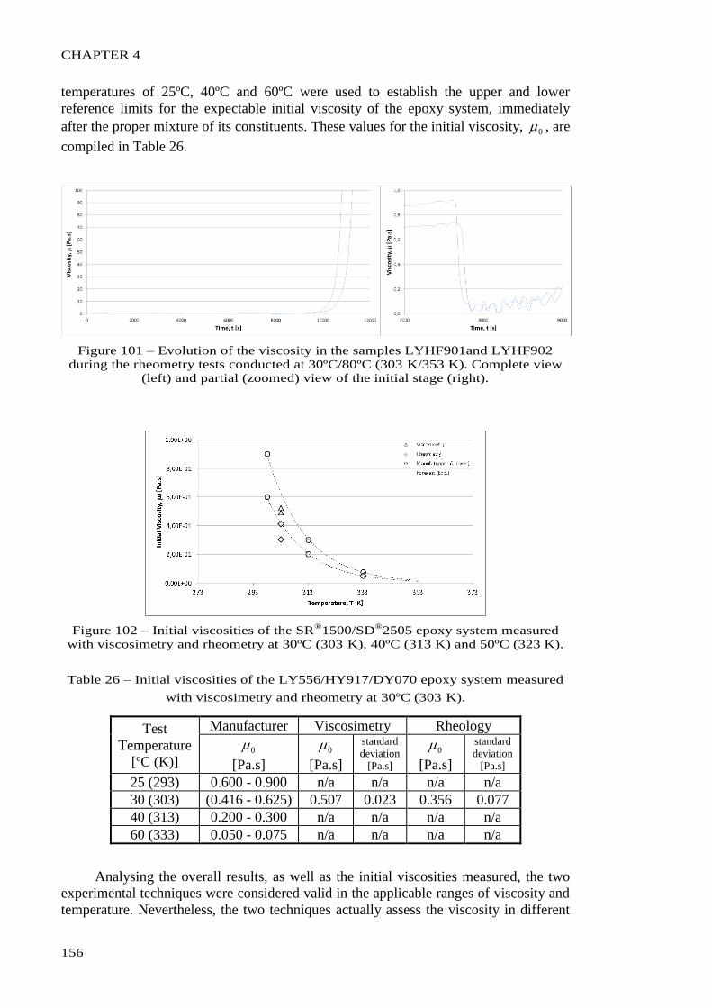
CHAPTER 4
156
temperatures of 25ºC, 40ºC and 60ºC were used to establish the upper and lower
reference limits for the expectable initial viscosity of the epoxy system, immediately
after the proper mixture of its constituents. These values for the initial viscosity, 0 , are
compiled in Table 26.
Figure 101 – Evolution of the viscosity in the samples LYHF901and LYHF902
during the rheometry tests conducted at 30ºC/80ºC (303 K/353 K). Complete view
(left) and partial (zoomed) view of the initial stage (right).
Figure 102 – Initial viscosities of the SR®
1500/SD®
2505 epoxy system measured
with viscosimetry and rheometry at 30ºC (303 K), 40ºC (313 K) and 50ºC (323 K).
Table 26 – Initial viscosities of the LY556/HY917/DY070 epoxy system measured
with viscosimetry and rheometry at 30ºC (303 K).
Test
Temperature
[ºC (K)]
Manufacturer Viscosimetry Rheology
0
[Pa.s]
0
[Pa.s]
standard
deviation
[Pa.s]
0
[Pa.s]
standard
deviation
[Pa.s]
25 (293) 0.600 - 0.900 n/a n/a n/a n/a
30 (303) (0.416 - 0.625) 0.507 0.023 0.356 0.077
40 (313) 0.200 - 0.300 n/a n/a n/a n/a
60 (333) 0.050 - 0.075 n/a n/a n/a n/a
Analysing the overall results, as well as the initial viscosities measured, the two
experimental techniques were considered valid in the applicable ranges of viscosity and
temperature. Nevertheless, the two techniques actually assess the viscosity in different
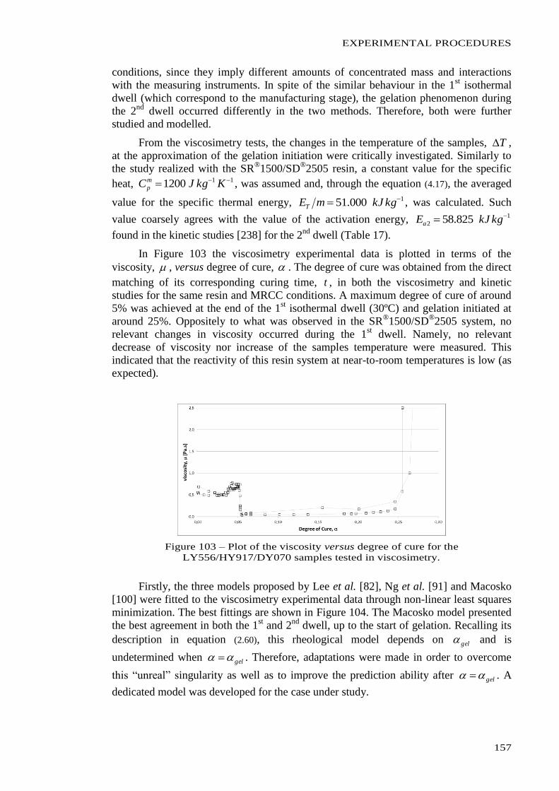
EXPERIMENTAL PROCEDURES
157
conditions, since they imply different amounts of concentrated mass and interactions
with the measuring instruments. In spite of the similar behaviour in the 1st isothermal
dwell (which correspond to the manufacturing stage), the gelation phenomenon during
the 2nd
dwell occurred differently in the two methods. Therefore, both were further
studied and modelled.
From the viscosimetry tests, the changes in the temperature of the samples, T ,
at the approximation of the gelation initiation were critically investigated. Similarly to
the study realized with the SR®1500/SD
®2505 resin, a constant value for the specific
heat, 111200 KkgJCm
p , was assumed and, through the equation (4.17), the averaged
value for the specific thermal energy, 1000.51 kgkJmET , was calculated. Such
value coarsely agrees with the value of the activation energy, 1
2 825.58 kgkJEa
found in the kinetic studies [238] for the 2nd
dwell (Table 17).
In Figure 103 the viscosimetry experimental data is plotted in terms of the
viscosity, , versus degree of cure, . The degree of cure was obtained from the direct
matching of its corresponding curing time, t , in both the viscosimetry and kinetic
studies for the same resin and MRCC conditions. A maximum degree of cure of around
5% was achieved at the end of the 1st isothermal dwell (30ºC) and gelation initiated at
around 25%. Oppositely to what was observed in the SR®1500/SD
®2505 system, no
relevant changes in viscosity occurred during the 1st dwell. Namely, no relevant
decrease of viscosity nor increase of the samples temperature were measured. This
indicated that the reactivity of this resin system at near-to-room temperatures is low (as
expected).
Figure 103 – Plot of the viscosity versus degree of cure for the
LY556/HY917/DY070 samples tested in viscosimetry.
Firstly, the three models proposed by Lee et al. [82], Ng et al. [91] and Macosko
[100] were fitted to the viscosimetry experimental data through non-linear least squares
minimization. The best fittings are shown in Figure 104. The Macosko model presented
the best agreement in both the 1st and 2
nd dwell, up to the start of gelation. Recalling its
description in equation (2.60), this rheological model depends on gel and is
undetermined when gel . Therefore, adaptations were made in order to overcome
this “unreal” singularity as well as to improve the prediction ability after gel . A
dedicated model was developed for the case under study.
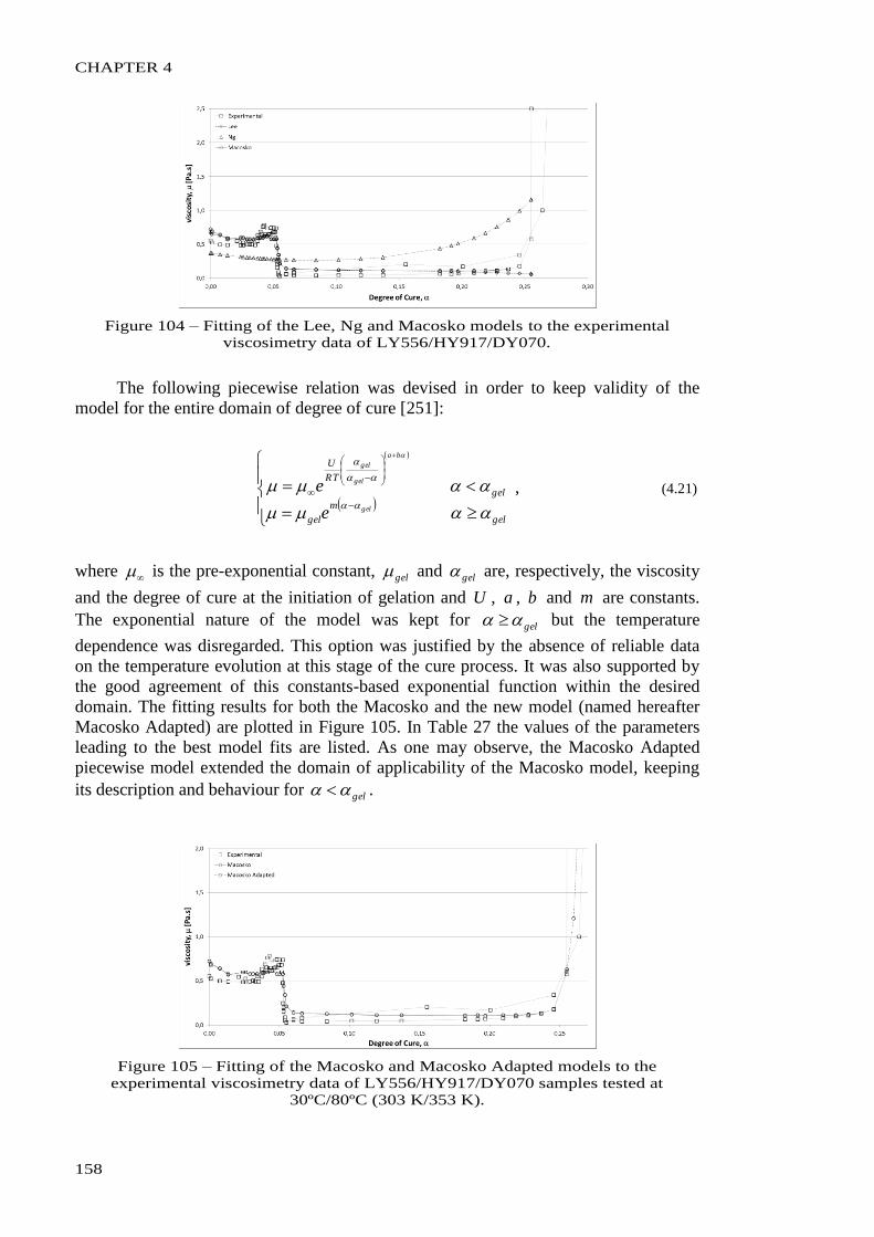
CHAPTER 4
158
Figure 104 – Fitting of the Lee, Ng and Macosko models to the experimental
viscosimetry data of LY556/HY917/DY070.
The following piecewise relation was devised in order to keep validity of the
model for the entire domain of degree of cure [251]:
gel
m
gel
gel
TR
U
gel
ba
gel
gel
e
e
, (4.21)
where is the pre-exponential constant, gel and gel are, respectively, the viscosity
and the degree of cure at the initiation of gelation and U , a , b and m are constants.
The exponential nature of the model was kept for gel but the temperature
dependence was disregarded. This option was justified by the absence of reliable data
on the temperature evolution at this stage of the cure process. It was also supported by
the good agreement of this constants-based exponential function within the desired
domain. The fitting results for both the Macosko and the new model (named hereafter
Macosko Adapted) are plotted in Figure 105. In Table 27 the values of the parameters
leading to the best model fits are listed. As one may observe, the Macosko Adapted
piecewise model extended the domain of applicability of the Macosko model, keeping
its description and behaviour for gel .
Figure 105 – Fitting of the Macosko and Macosko Adapted models to the
experimental viscosimetry data of LY556/HY917/DY070 samples tested at
30ºC/80ºC (303 K/353 K).
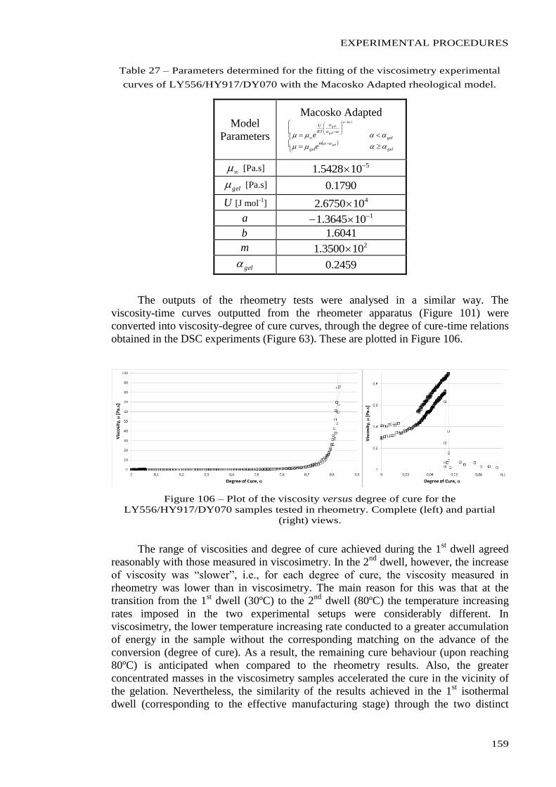
EXPERIMENTAL PROCEDURES
159
Table 27 – Parameters determined for the fitting of the viscosimetry experimental
curves of LY556/HY917/DY070 with the Macosko Adapted rheological model.
Model
Parameters
Macosko Adapted
gel
m
gel
gel
TR
U
gel
ba
gel
gel
e
e
[Pa.s] 5105428.1
gel [Pa.s] 1790.0
U [J mol-1
] 4106750.2
a 1103645.1
b 6041.1
m 2103500.1
gel 2459.0
The outputs of the rheometry tests were analysed in a similar way. The
viscosity-time curves outputted from the rheometer apparatus (Figure 101) were
converted into viscosity-degree of cure curves, through the degree of cure-time relations
obtained in the DSC experiments (Figure 63). These are plotted in Figure 106.
Figure 106 – Plot of the viscosity versus degree of cure for the
LY556/HY917/DY070 samples tested in rheometry. Complete (left) and partial
(right) views.
The range of viscosities and degree of cure achieved during the 1st dwell agreed
reasonably with those measured in viscosimetry. In the 2nd
dwell, however, the increase
of viscosity was “slower”, i.e., for each degree of cure, the viscosity measured in
rheometry was lower than in viscosimetry. The main reason for this was that at the
transition from the 1st dwell (30ºC) to the 2
nd dwell (80ºC) the temperature increasing
rates imposed in the two experimental setups were considerably different. In
viscosimetry, the lower temperature increasing rate conducted to a greater accumulation
of energy in the sample without the corresponding matching on the advance of the
conversion (degree of cure). As a result, the remaining cure behaviour (upon reaching
80ºC) is anticipated when compared to the rheometry results. Also, the greater
concentrated masses in the viscosimetry samples accelerated the cure in the vicinity of
the gelation. Nevertheless, the similarity of the results achieved in the 1st isothermal
dwell (corresponding to the effective manufacturing stage) through the two distinct
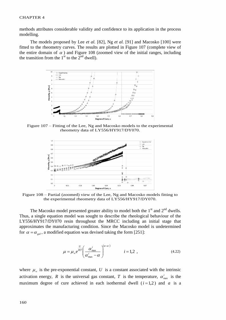
CHAPTER 4
160
methods attributes considerable validity and confidence to its application in the process
modelling.
The models proposed by Lee et al. [82], Ng et al. [91] and Macosko [100] were
fitted to the rheometry curves. The results are plotted in Figure 107 (complete view of
the entire domain of ) and Figure 108 (zoomed view of the initial ranges, including
the transition from the 1st to the 2
nd dwell).
Figure 107 – Fitting of the Lee, Ng and Macosko models to the experimental
rheometry data of LY556/HY917/DY070.
Figure 108 – Partial (zoomed) view of the Lee, Ng and Macosko models fitting to
the experimental rheometry data of LY556/HY917/DY070.
The Macosko model presented greater ability to model both the 1st and 2
nd dwells.
Thus, a single equation model was sought to describe the rheological behaviour of the
LY556/HY917/DY070 resin throughout the MRCC including an initial stage that
approximates the manufacturing condition. Since the Macosko model is undetermined
for gel , a modified equation was devised taking the form [251]:
2,1max
max
ie
a
i
iTR
U
, (4.22)
where is the pre-exponential constant, U is a constant associated with the intrinsic
activation energy, R is the universal gas constant, T is the temperature, i
max is the
maximum degree of cure achieved in each isothermal dwell ( 2,1i ) and a is a
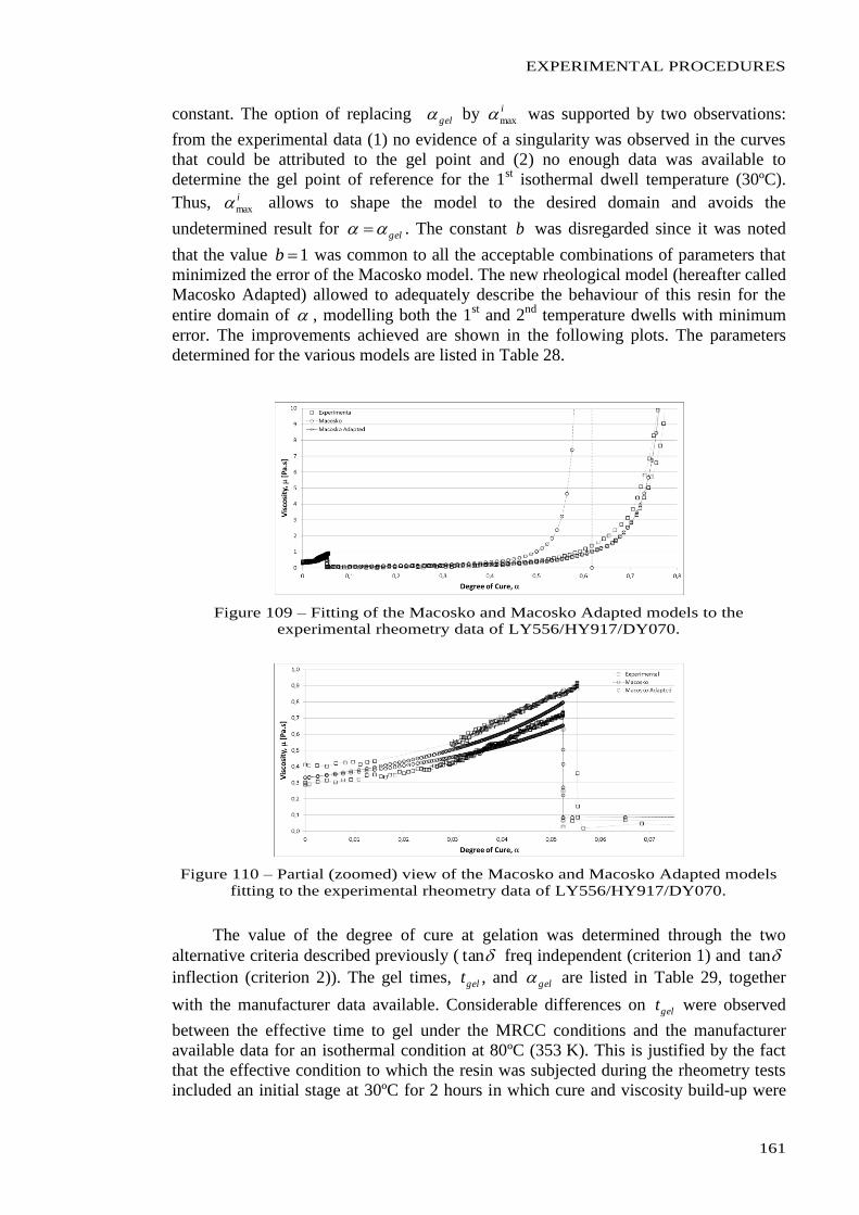
EXPERIMENTAL PROCEDURES
161
constant. The option of replacing gel by i
max was supported by two observations:
from the experimental data (1) no evidence of a singularity was observed in the curves
that could be attributed to the gel point and (2) no enough data was available to
determine the gel point of reference for the 1st isothermal dwell temperature (30ºC).
Thus, i
max allows to shape the model to the desired domain and avoids the
undetermined result for gel . The constant b was disregarded since it was noted
that the value 1b was common to all the acceptable combinations of parameters that
minimized the error of the Macosko model. The new rheological model (hereafter called
Macosko Adapted) allowed to adequately describe the behaviour of this resin for the
entire domain of , modelling both the 1st and 2
nd temperature dwells with minimum
error. The improvements achieved are shown in the following plots. The parameters
determined for the various models are listed in Table 28.
Figure 109 – Fitting of the Macosko and Macosko Adapted models to the
experimental rheometry data of LY556/HY917/DY070.
Figure 110 – Partial (zoomed) view of the Macosko and Macosko Adapted models
fitting to the experimental rheometry data of LY556/HY917/DY070.
The value of the degree of cure at gelation was determined through the two
alternative criteria described previously ( tan freq independent (criterion 1) and tan
inflection (criterion 2)). The gel times, gelt , and gel are listed in Table 29, together
with the manufacturer data available. Considerable differences on gelt were observed
between the effective time to gel under the MRCC conditions and the manufacturer
available data for an isothermal condition at 80ºC (353 K). This is justified by the fact
that the effective condition to which the resin was subjected during the rheometry tests
included an initial stage at 30ºC for 2 hours in which cure and viscosity build-up were
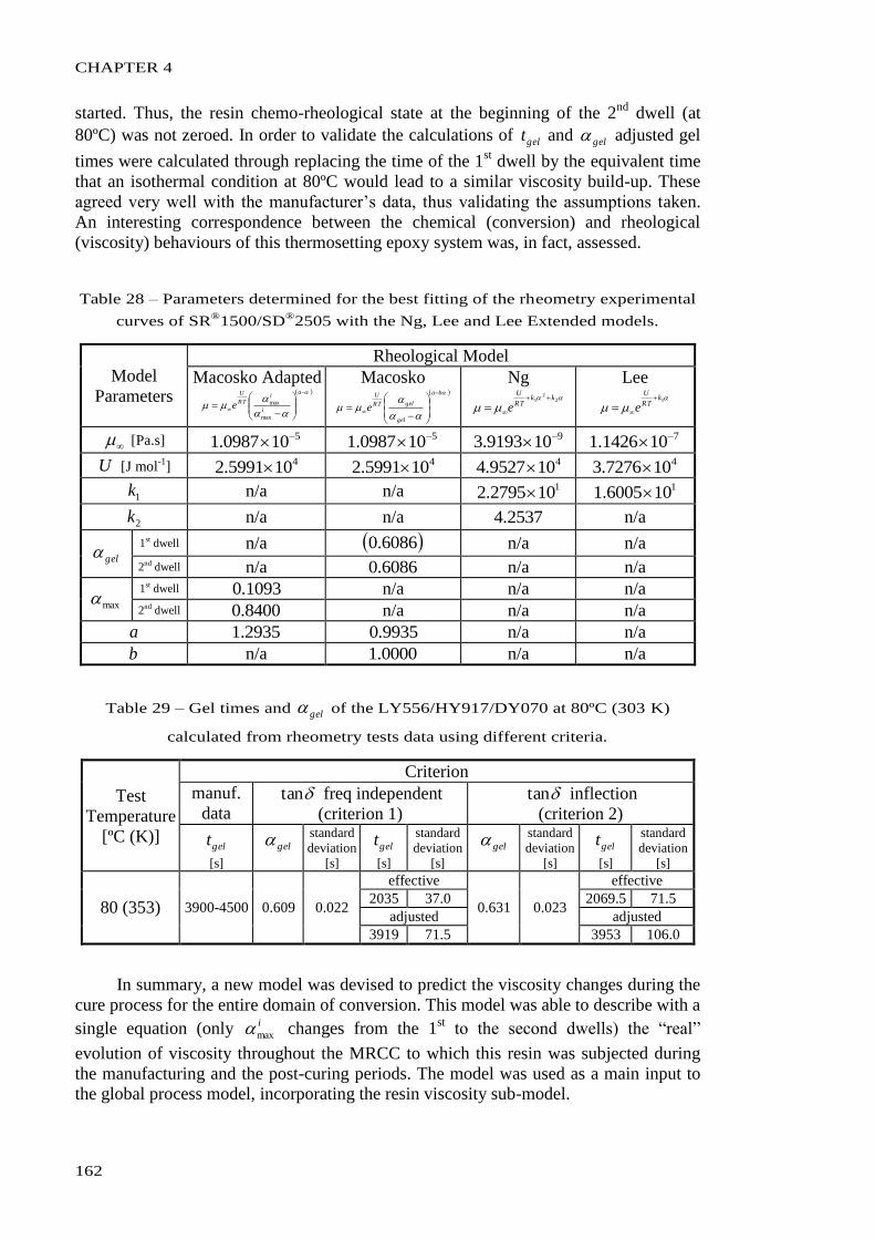
CHAPTER 4
162
started. Thus, the resin chemo-rheological state at the beginning of the 2nd
dwell (at
80ºC) was not zeroed. In order to validate the calculations of gelt and gel adjusted gel
times were calculated through replacing the time of the 1st dwell by the equivalent time
that an isothermal condition at 80ºC would lead to a similar viscosity build-up. These
agreed very well with the manufacturer’s data, thus validating the assumptions taken.
An interesting correspondence between the chemical (conversion) and rheological
(viscosity) behaviours of this thermosetting epoxy system was, in fact, assessed.
Table 28 – Parameters determined for the best fitting of the rheometry experimental
curves of SR®
1500/SD®
2505 with the Ng, Lee and Lee Extended models.
Model
Parameters
Rheological Model
Macosko Adapted
a
i
iTR
U
emax
max
Macosko
ba
gel
gelTR
U
e
Ng
2
21 kk
TR
U
e
Lee
1k
TR
U
e
[Pa.s] 5100987.1 5100987.1 9109193.3 7101426.1
U [J mol-1
] 4105991.2 4105991.2 4109527.4 4107276.3
1k n/a n/a 1102795.2 1106005.1
2k n/a n/a 2537.4 n/a
gel 1st dwell n/a 6086.0 n/a n/a
2nd dwell n/a 6086.0 n/a n/a
max 1st dwell 1093.0 n/a n/a n/a 2nd dwell 8400.0 n/a n/a n/a
a 2935.1 9935.0 n/a n/a
b n/a 0000.1 n/a n/a
Table 29 – Gel times and gel of the LY556/HY917/DY070 at 80ºC (303 K)
calculated from rheometry tests data using different criteria.
Test
Temperature
[ºC (K)]
Criterion
manuf.
data tan freq independent
(criterion 1)
tan inflection
(criterion 2)
gelt
[s]
gel
standard
deviation
[s] gelt
[s]
standard
deviation
[s]
gel
standard
deviation
[s] gelt
[s]
standard
deviation
[s]
80 (353) 3900-4500 0.609 0.022
effective
0.631 0.023
effective
2035 37.0 2069.5 71.5
adjusted adjusted
3919 71.5 3953 106.0
In summary, a new model was devised to predict the viscosity changes during the
cure process for the entire domain of conversion. This model was able to describe with a
single equation (only i
max changes from the 1st to the second dwells) the “real”
evolution of viscosity throughout the MRCC to which this resin was subjected during
the manufacturing and the post-curing periods. The model was used as a main input to
the global process model, incorporating the resin viscosity sub-model.
EXPERIMENTAL PROCEDURES
163
4.2.3. Resins Mixing Behaviour
In the previous sections, the kinetics and rheology of polymer matrices were
studied as partially intrinsic characteristics. Specifically, two thermosetting epoxy resins
were tested and modelled. The evolution of both the degree of cure, , and the
viscosity, , as the cure progresses govern the ability of the resin to flow through the
porous fibre bed and, thus, the consolidation of the composite laminate being
manufactured. The physical properties of the resin, such as the viscosity, are mostly
dependent on time, since the irreversible chemical reaction starts upon mixture of its
constituents. The studies conducted and discussed in the previous sections showed that
other conditions like the quantity of mass and the surrounding temperature also impact
significantly the kinetic and rheological behaviour. In the case of thermoplastics, the
increase of the viscosity (intrinsically reversible) is set by the retrieval of the external
heating source. In view of modelling the consolidation of composite laminates, the
degree of cure/crystallization and viscosity should be known for each point and each
moment. For the majority of the manufacturing processes, the assessment to the
intrinsic behaviour of the neat resin subjected to comparable temperature and mass
conditions is a very good approximation to its behaviour within the “real” laminate. In
FW, however, the laminate is built-up through discontinuous deposition of the
consecutive layers. As a new layer is wound it compresses the ones beneath and is
invaded by their resin. Therefore, resins with different curing histories are effectively
mixed in each layer. The effects of such mixture in the overall kinetics and rheology
were studied and are discussed hereafter.
The two epoxy resin systems selected for the process model validation in wet FW
trials were tested under different mixing conditions. In each test, two portions of the
same resin system, prepared in different times, were mixed and its joint behaviour was
analysed. The differences between the behaviour of this blend and the neat (unmixed)
resin were then critically assessed. The study was based on the variation of two
parameters: the time gap between the preparation of each portion of resin and the
mixing ratio of the two portions.
Both rotational viscosimetry and oscillatory rheometry were used to measure the
evolution of the viscosity of the two epoxy systems – SR®1500 from Sicomin
Composites (France) and Araldite® LY556 from Huntsman (USA) – under several
mixing conditions. The same MRCC previously applied in the kinetic and rheological
modelling studies [238,251] were imposed in order to maintain the focus in approaching
the “real” temperature conditions during manufacturing. The experimental procedures,
their results and the critical analysis are presented hereafter.
4.2.3.1. Experimental Procedures
Rotational viscosimetry and oscillatory rheometry have been widely used to
assess the change of viscosity in reacting polymers [243,244]. Herewith these
techniques were used to have an insight to the effect of mixing portions of resin with
different curing histories. As before, the use of two different experimental procedures
allowed also to achieve additional cross validation of the results outputted.
Since the typical arrangements and procedures associated with these techniques
are not suitable to extend the measurements up to and after the gelation of the polymer
sample, special care and a few adaptations were implemented to account for this. The
CHAPTER 4
164
two experimental procedures used for the rheological characterization of the SR®1500
and LY556 epoxy systems are described hereafter.
The same measuring instruments, adapted to allow extending the test up to and
after gelation, were used as for the rheological studies conducted with the neat resin
samples. A Brookfield viscometer (Visco Basic Plus from Fungilab) was used in the
first experiment. The setup is shown in Figure 75. In addition to the procedure
implemented previously, a second set of the same resin system was pre-heated to the
prescribed test temperature, then prepared (mixture of the constituents) with a time gap
to the first set and finally added to the running test sample. The time gap was defined as
the time interval occurred between preparation (mixing of constituents) of the first and
second portions. The rheometry tests were carried out using a stress/strain control
rheometer (Stresstech® from Reologica Instruments AB) with the setup shown in
Figure 76. The same apparatus was used as in the rheological tests on neat samples. The
relevant difference was that the blends of two portions of resin with different curing
histories were produced prior to the effective start. This meant that the rheometry tests
only registered the behaviour of the resin sample after the blend, thus not capturing the
change of behaviour at the time of the blend. This limitation was imposed by the
impracticability of changing the test sample (by adding and remixing fresh material)
in-situ. The need of calibrating the measurement instrument at the beginning of each test
was incompatible with the possibility of touching or repositioning it.
The results of the experimental tests on the SR®
1500 and Araldite® LY556
epoxies are presented and critically analysed below.
4.2.3.2. Experimental Results
The characterization of the rheological behaviour of the two commercial epoxies
selected under several prescribed mixing conditions was addressed through rotational
viscosimetry and oscillatory rheometry. A qualitative assessment to the influence of the
time gap in the curing history and the mass ratio of two blended portions of the same
type of resin was pursued. The objective was to validate (or improve) the assumption
introduced in the resin mixing sub-model translated in equation (3.40).
SR®1500
The epoxy/amine system SR®1500/SD
®2505 with the weight ratio of 100:33%
was rheologically characterized under the isothermal temperature of 30ºC (303 K),
mixture mass ratios of 1:1, 2:1 and 3:1 and cure time gaps of 5min, 8min and 11min.
These test conditions covered a considerable range of the comparable “real” conditions
that the resin could experience during the FW process. The near-to-room temperature
quite approached the “real” manufacturing temperature conditions. The selected mixing
ratios and time gaps covered an interesting range of possibilities within the overall short
working time window that this resin system allowed. The MRCC selected are indicated
in Table 30 and the mixing conditions listed in Table 31 for the tests carried out.
The direct results outputted from the viscosimetry tests are presented in Figures
111 and 112. A reference curve of the neat resin behaviour, taken from previous
measurements [251], is appended for comparison. In these plots the initial time, 0t ,
corresponded to the completion of the preparation (mixture of the two constituents,
SR®
1500 and SD®
2505) of the first portion of resin. The shift in the curves
corresponded to the moment when the second portion of resin was blended to the first.
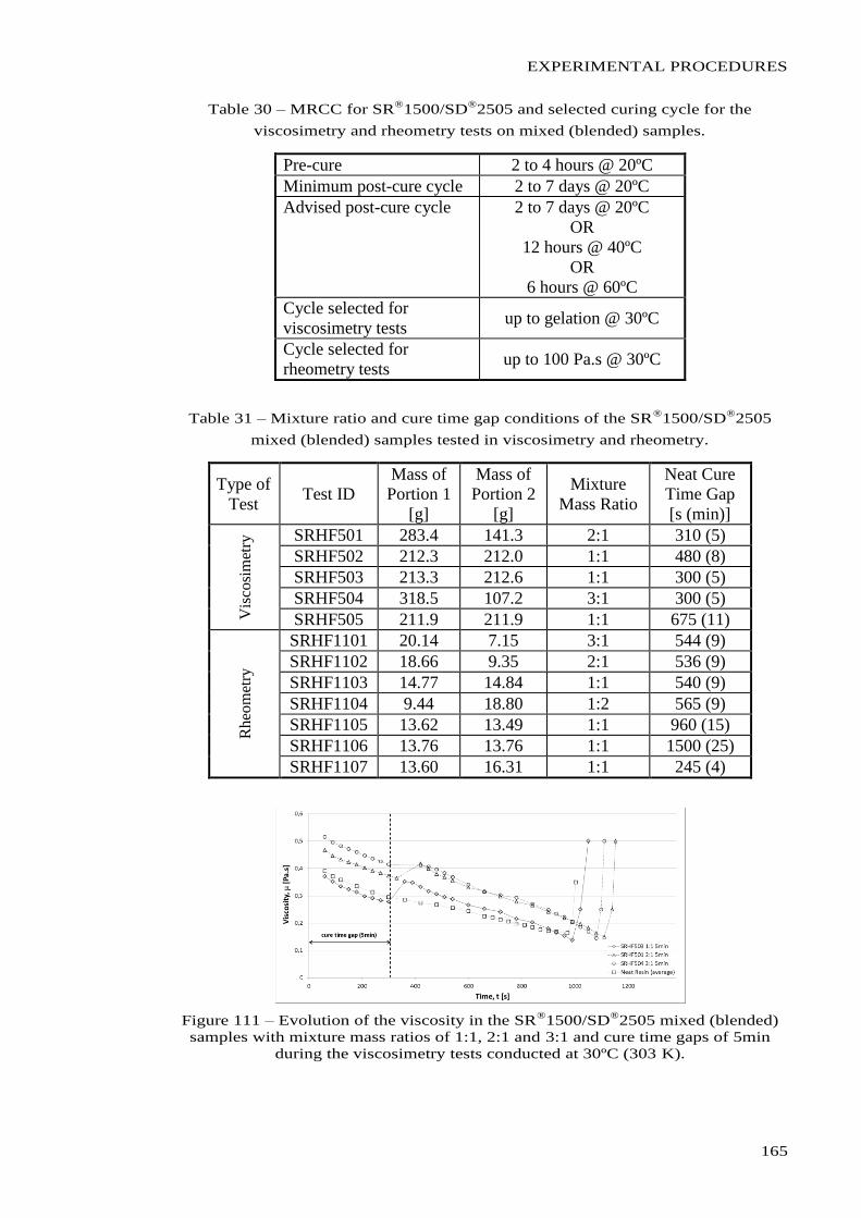
EXPERIMENTAL PROCEDURES
165
Table 30 – MRCC for SR®
1500/SD®
2505 and selected curing cycle for the
viscosimetry and rheometry tests on mixed (blended) samples.
Pre-cure 2 to 4 hours @ 20ºC
Minimum post-cure cycle 2 to 7 days @ 20ºC
Advised post-cure cycle 2 to 7 days @ 20ºC
OR
12 hours @ 40ºC
OR
6 hours @ 60ºC
Cycle selected for
viscosimetry tests up to gelation @ 30ºC
Cycle selected for
rheometry tests up to 100 Pa.s @ 30ºC
Table 31 – Mixture ratio and cure time gap conditions of the SR®
1500/SD®
2505
mixed (blended) samples tested in viscosimetry and rheometry.
Type of
Test Test ID
Mass of
Portion 1
[g]
Mass of
Portion 2
[g]
Mixture
Mass Ratio
Neat Cure
Time Gap
[s (min)]
Vis
cosi
met
ry SRHF501 283.4 141.3 2:1 310 (5)
SRHF502 212.3 212.0 1:1 480 (8)
SRHF503 213.3 212.6 1:1 300 (5)
SRHF504 318.5 107.2 3:1 300 (5)
SRHF505 211.9 211.9 1:1 675 (11)
Rheo
met
ry
SRHF1101 20.14 7.15 3:1 544 (9)
SRHF1102 18.66 9.35 2:1 536 (9)
SRHF1103 14.77 14.84 1:1 540 (9)
SRHF1104 9.44 18.80 1:2 565 (9)
SRHF1105 13.62 13.49 1:1 960 (15)
SRHF1106 13.76 13.76 1:1 1500 (25)
SRHF1107 13.60 16.31 1:1 245 (4)
Figure 111 – Evolution of the viscosity in the SR®
1500/SD®
2505 mixed (blended)
samples with mixture mass ratios of 1:1, 2:1 and 3:1 and cure time gaps of 5min
during the viscosimetry tests conducted at 30ºC (303 K).
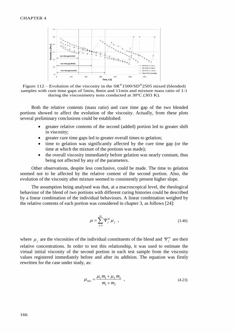
CHAPTER 4
166
Figure 112 – Evolution of the viscosity in the SR®
1500/SD®
2505 mixed (blended)
samples with cure time gaps of 5min, 8min and 11min and mixture mass ratio of 1:1
during the viscosimetry tests conducted at 30ºC (303 K).
Both the relative contents (mass ratio) and cure time gap of the two blended
portions showed to affect the evolution of the viscosity. Actually, from these plots
several preliminary conclusions could be established:
greater relative contents of the second (added) portion led to greater shift
in viscosity;
greater cure time gaps led to greater overall times to gelation;
time to gelation was significantly affected by the cure time gap (or the
time at which the mixture of the portions was made);
the overall viscosity immediately before gelation was nearly constant, thus
being not affected by any of the parameters.
Other observations, despite less conclusive, could be made. The time to gelation
seemed not to be affected by the relative content of the second portion. Also, the
evolution of the viscosity after mixture seemed to consistently present higher slope.
The assumption being analysed was that, at a macroscopical level, the rheological
behaviour of the blend of two portions with different curing histories could be described
by a linear combination of the individual behaviours. A linear combination weighed by
the relative contents of each portion was considered in chapter 3, as follows [24]:
m
j
j
m
j
1
, (3.40)
where j are the viscosities of the individual constituents of the blend and m
j are their
relative concentrations. In order to test this relationship, it was used to estimate the
virtual initial viscosity of the second portion in each test sample from the viscosity
values registered immediately before and after its addition. The equation was firstly
rewritten for the case under study, as:
21
2211
mm
mmmix
, (4.23)
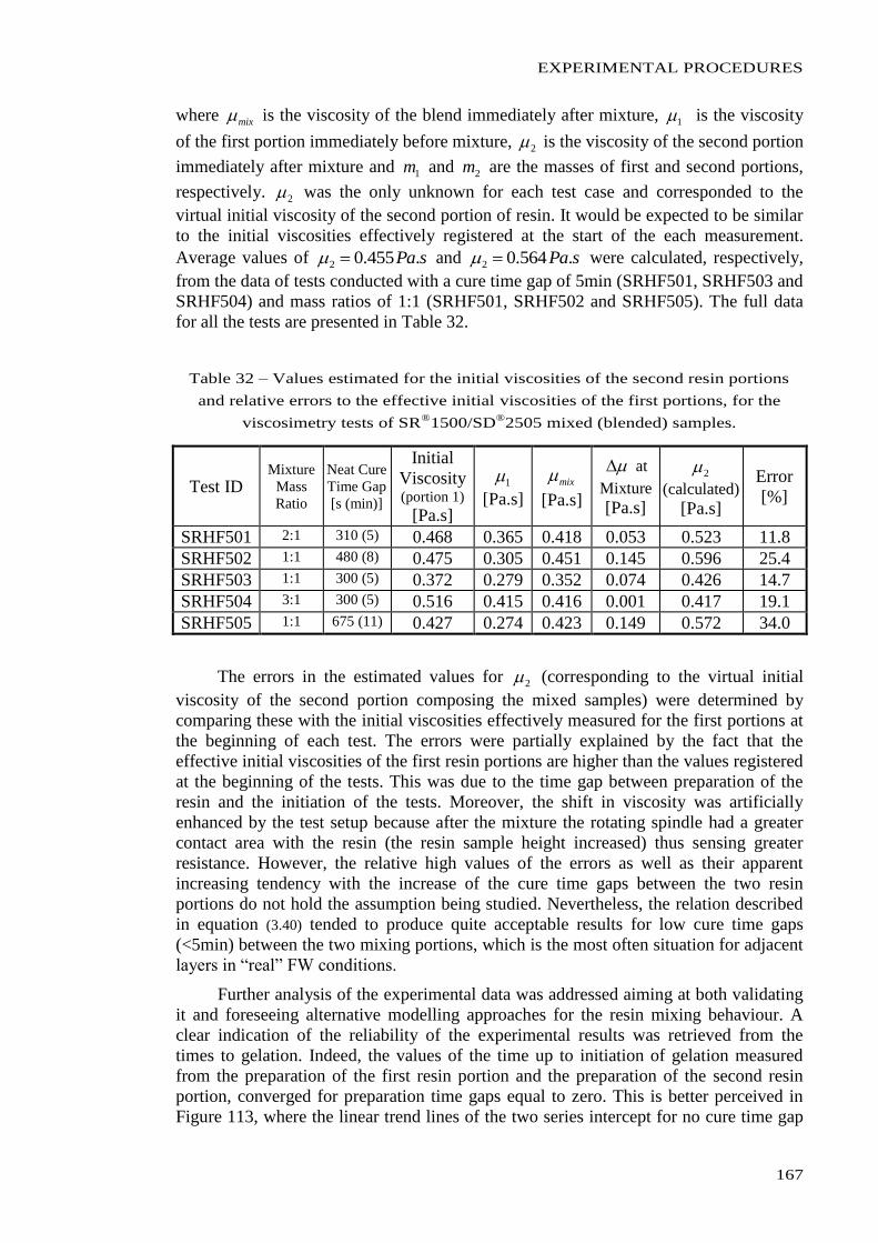
EXPERIMENTAL PROCEDURES
167
where mix is the viscosity of the blend immediately after mixture, 1 is the viscosity
of the first portion immediately before mixture, 2 is the viscosity of the second portion
immediately after mixture and 1m and 2m are the masses of first and second portions,
respectively. 2 was the only unknown for each test case and corresponded to the
virtual initial viscosity of the second portion of resin. It would be expected to be similar
to the initial viscosities effectively registered at the start of the each measurement.
Average values of sPa.455.02 and sPa.564.02 were calculated, respectively,
from the data of tests conducted with a cure time gap of 5min (SRHF501, SRHF503 and
SRHF504) and mass ratios of 1:1 (SRHF501, SRHF502 and SRHF505). The full data
for all the tests are presented in Table 32.
Table 32 – Values estimated for the initial viscosities of the second resin portions
and relative errors to the effective initial viscosities of the first portions, for the
viscosimetry tests of SR®
1500/SD®
2505 mixed (blended) samples.
Test ID Mixture
Mass
Ratio
Neat Cure
Time Gap
[s (min)]
Initial
Viscosity (portion 1)
[Pa.s]
1
[Pa.s] mix
[Pa.s]
at
Mixture [Pa.s]
2
(calculated) [Pa.s]
Error
[%]
SRHF501 2:1 310 (5) 0.468 0.365 0.418 0.053 0.523 11.8
SRHF502 1:1 480 (8) 0.475 0.305 0.451 0.145 0.596 25.4
SRHF503 1:1 300 (5) 0.372 0.279 0.352 0.074 0.426 14.7
SRHF504 3:1 300 (5) 0.516 0.415 0.416 0.001 0.417 19.1
SRHF505 1:1 675 (11) 0.427 0.274 0.423 0.149 0.572 34.0
The errors in the estimated values for 2 (corresponding to the virtual initial
viscosity of the second portion composing the mixed samples) were determined by
comparing these with the initial viscosities effectively measured for the first portions at
the beginning of each test. The errors were partially explained by the fact that the
effective initial viscosities of the first resin portions are higher than the values registered
at the beginning of the tests. This was due to the time gap between preparation of the
resin and the initiation of the tests. Moreover, the shift in viscosity was artificially
enhanced by the test setup because after the mixture the rotating spindle had a greater
contact area with the resin (the resin sample height increased) thus sensing greater
resistance. However, the relative high values of the errors as well as their apparent
increasing tendency with the increase of the cure time gaps between the two resin
portions do not hold the assumption being studied. Nevertheless, the relation described
in equation (3.40) tended to produce quite acceptable results for low cure time gaps
(<5min) between the two mixing portions, which is the most often situation for adjacent
layers in “real” FW conditions.
Further analysis of the experimental data was addressed aiming at both validating
it and foreseeing alternative modelling approaches for the resin mixing behaviour. A
clear indication of the reliability of the experimental results was retrieved from the
times to gelation. Indeed, the values of the time up to initiation of gelation measured
from the preparation of the first resin portion and the preparation of the second resin
portion, converged for preparation time gaps equal to zero. This is better perceived in
Figure 113, where the linear trend lines of the two series intercept for no cure time gap
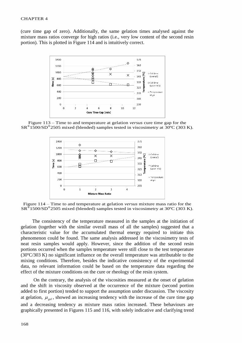
CHAPTER 4
168
(cure time gap of zero). Additionally, the same gelation times analysed against the
mixture mass ratios converge for high ratios (i.e., very low content of the second resin
portion). This is plotted in Figure 114 and is intuitively correct.
Figure 113 – Time to and temperature at gelation versus cure time gap for the
SR®
1500/SD®
2505 mixed (blended) samples tested in viscosimetry at 30ºC (303 K).
Figure 114 – Time to and temperature at gelation versus mixture mass ratio for the
SR®
1500/SD®
2505 mixed (blended) samples tested in viscosimetry at 30ºC (303 K).
The consistency of the temperature measured in the samples at the initiation of
gelation (together with the similar overall mass of all the samples) suggested that a
characteristic value for the accumulated thermal energy required to initiate this
phenomenon could be found. The same analysis addressed in the viscosimetry tests of
neat resin samples would apply. However, since the addition of the second resin
portions occurred when the samples temperature were still close to the test temperature
(30ºC/303 K) no significant influence on the overall temperature was attributable to the
mixing conditions. Therefore, besides the indicative consistency of the experimental
data, no relevant information could be based on the temperature data regarding the
effect of the mixture conditions on the cure or rheology of the resin system.
On the contrary, the analysis of the viscosities measured at the onset of gelation
and the shift in viscosity observed at the occurrence of the mixture (second portion
added to first portion) tended to support the assumption under discussion. The viscosity
at gelation, gel , showed an increasing tendency with the increase of the cure time gap
and a decreasing tendency as mixture mass ratios increased. These behaviours are
graphically presented in Figures 115 and 116, with solely indicative and clarifying trend
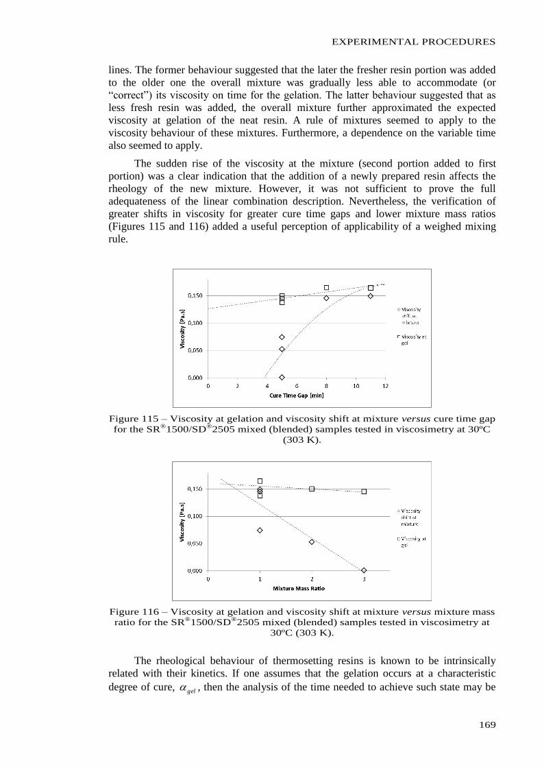
EXPERIMENTAL PROCEDURES
169
lines. The former behaviour suggested that the later the fresher resin portion was added
to the older one the overall mixture was gradually less able to accommodate (or
“correct”) its viscosity on time for the gelation. The latter behaviour suggested that as
less fresh resin was added, the overall mixture further approximated the expected
viscosity at gelation of the neat resin. A rule of mixtures seemed to apply to the
viscosity behaviour of these mixtures. Furthermore, a dependence on the variable time
also seemed to apply.
The sudden rise of the viscosity at the mixture (second portion added to first
portion) was a clear indication that the addition of a newly prepared resin affects the
rheology of the new mixture. However, it was not sufficient to prove the full
adequateness of the linear combination description. Nevertheless, the verification of
greater shifts in viscosity for greater cure time gaps and lower mixture mass ratios
(Figures 115 and 116) added a useful perception of applicability of a weighed mixing
rule.
Figure 115 – Viscosity at gelation and viscosity shift at mixture versus cure time gap
for the SR®
1500/SD®
2505 mixed (blended) samples tested in viscosimetry at 30ºC
(303 K).
Figure 116 – Viscosity at gelation and viscosity shift at mixture versus mixture mass
ratio for the SR®
1500/SD®
2505 mixed (blended) samples tested in viscosimetry at
30ºC (303 K).
The rheological behaviour of thermosetting resins is known to be intrinsically
related with their kinetics. If one assumes that the gelation occurs at a characteristic
degree of cure, gel , then the analysis of the time needed to achieve such state may be
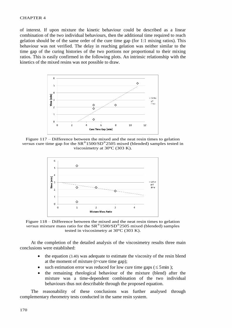
CHAPTER 4
170
of interest. If upon mixture the kinetic behaviour could be described as a linear
combination of the two individual behaviours, then the additional time required to reach
gelation should be of the same order of the cure time gap (for 1:1 mixing ratios). This
behaviour was not verified. The delay in reaching gelation was neither similar to the
time gap of the curing histories of the two portions nor proportional to their mixing
ratios. This is easily confirmed in the following plots. An intrinsic relationship with the
kinetics of the mixed resins was not possible to draw.
Figure 117 – Difference between the mixed and the neat resin times to gelation
versus cure time gap for the SR®
1500/SD®
2505 mixed (blended) samples tested in
viscosimetry at 30ºC (303 K).
Figure 118 – Difference between the mixed and the neat resin times to gelation
versus mixture mass ratio for the SR®
1500/SD®
2505 mixed (blended) samples
tested in viscosimetry at 30ºC (303 K).
At the completion of the detailed analysis of the viscosimetry results three main
conclusions were established:
the equation (3.40) was adequate to estimate the viscosity of the resin blend
at the moment of mixture (t=cure time gap);
such estimation error was reduced for low cure time gaps ( min5 );
the remaining rheological behaviour of the mixture (blend) after the
mixture was a time-dependent combination of the two individual
behaviours thus not describable through the proposed equation.
The reasonability of these conclusions was further analysed through
complementary rheometry tests conducted in the same resin system.
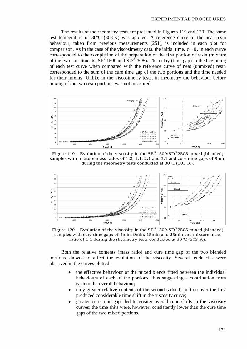
EXPERIMENTAL PROCEDURES
171
The results of the rheometry tests are presented in Figures 119 and 120. The same
test temperature of 30ºC (303 K) was applied. A reference curve of the neat resin
behaviour, taken from previous measurements [251], is included in each plot for
comparison. As in the case of the viscosimetry data, the initial time, 0t , in each curve
corresponded to the completion of the preparation of the first portion of resin (mixture
of the two constituents, SR®1500 and SD
®2505). The delay (time gap) in the beginning
of each test curve when compared with the reference curve of neat (unmixed) resin
corresponded to the sum of the cure time gap of the two portions and the time needed
for their mixing. Unlike in the viscosimetry tests, in rheometry the behaviour before
mixing of the two resin portions was not measured.
Figure 119 – Evolution of the viscosity in the SR®
1500/SD®
2505 mixed (blended)
samples with mixture mass ratios of 1:2, 1:1, 2:1 and 3:1 and cure time gaps of 9min
during the rheometry tests conducted at 30ºC (303 K).
Figure 120 – Evolution of the viscosity in the SR®
1500/SD®
2505 mixed (blended)
samples with cure time gaps of 4min, 9min, 15min and 25min and mixture mass
ratio of 1:1 during the rheometry tests conducted at 30ºC (303 K).
Both the relative contents (mass ratio) and cure time gap of the two blended
portions showed to affect the evolution of the viscosity. Several tendencies were
observed in the curves plotted:
the effective behaviour of the mixed blends fitted between the individual
behaviours of each of the portions, thus suggesting a contribution from
each to the overall behaviour;
only greater relative contents of the second (added) portion over the first
produced considerable time shift in the viscosity curve;
greater cure time gaps led to greater overall time shifts in the viscosity
curves; the time shits were, however, consistently lower than the cure time
gaps of the two mixed portions.
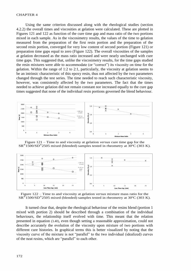
CHAPTER 4
172
Using the same criterion discussed along with the rheological studies (section
4.2.2) the overall times and viscosities at gelation were calculated. These are plotted in
Figures 121 and 122 as function of the cure time gap and mass ratio of the two portions
mixed in each sample. As in the viscosimetry results, the values of the time to gelation
measured from the preparation of the first resin portion and the preparation of the
second resin portion, converged for very low content of second portion (Figure 121) or
preparation time gaps equal to zero (Figure 122). The overall viscosities of the samples
at gelation decreased as the mass ratio increased and were nearly unchanged with cure
time gaps. This suggested that, unlike the viscosimetry results, for the time gaps studied
the resin mixtures were able to accommodate (or “correct”) its viscosity on time for the
gelation. Within the range of 1:2 to 2:1, particularly, the viscosity at gelation seems to
be an intrinsic characteristic of this epoxy resin, thus not affected by the two parameters
changed through the test series. The time needed to reach such characteristic viscosity,
however, was consistently affected by the two parameters. The fact that the times
needed to achieve gelation did not remain constant nor increased equally to the cure gap
times suggested that none of the individual resin portions governed the blend behaviour.
Figure 121 – Time to and viscosity at gelation versus cure time gap for the
SR®
1500/SD®
2505 mixed (blended) samples tested in rheometry at 30ºC (303 K).
Figure 122 – Time to and viscosity at gelation versus mixture mass ratio for the
SR®
1500/SD®
2505 mixed (blended) samples tested in rheometry at 30ºC (303 K).
It turned clear that, despite the rheological behaviour of the resins blend (portion 1
mixed with portion 2) should be described through a combination of the individual
behaviours, the relationship itself evolved with time. This meant that the relation
presented in equation (3.40), even though setting a reasonable approximation, could not
describe accurately the evolution of the viscosity upon mixture of two portions with
different cure histories. In graphical terms this is better visualized by noting that the
viscosity curve of the mixture is not “parallel” to the two individual (idealized) curves
of the neat resins, which are “parallel” to each other.
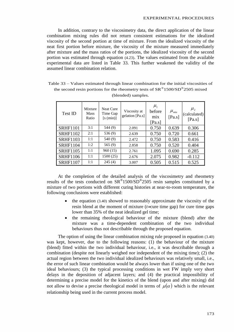
EXPERIMENTAL PROCEDURES
173
In addition, contrary to the viscosimetry data, the direct application of the linear
combination mixing rules did not return consistent estimations for the idealized
viscosity of the second portion at time of mixture. From the idealized viscosity of the
neat first portion before mixture, the viscosity of the mixture measured immediately
after mixture and the mass ratios of the portions, the idealized viscosity of the second
portion was estimated through equation (4.23). The values estimated from the available
experimental data are listed in Table 33. This further weakened the validity of the
assumed linear combination relation.
Table 33 – Values estimated through linear combination for the initial viscosities of
the second resin portions for the rheometry tests of SR®
1500/SD®
2505 mixed
(blended) samples.
Test ID Mixture
Mass
Ratio
Neat Cure
Time Gap
[s (min)]
Viscosity at
gelation [Pa.s]
1
before
mix
[Pa.s]
mix
[Pa.s]
2
(calculated) [Pa.s]
SRHF1101 3:1 544 (9) 2.091 0.750 0.639 0.306
SRHF1102 2:1 536 (9) 2.639 0.750 0.720 0.661
SRHF1103 1:1 540 (9) 2.472 0.750 0.583 0.416
SRHF1104 1:2 565 (9) 2.858 0.750 0.520 0.404
SRHF1105 1:1 960 (15) 2.761 1.095 0.690 0.285
SRHF1106 1:1 1500 (25) 2.676 2.075 0.982 -0.112
SRHF1107 1:1 245 (4) 3.007 0.505 0.515 0.525
At the completion of the detailed analysis of the viscosimetry and rheometry
results of the tests conducted on SR®1500/SD
®2505 resin samples constituted by a
mixture of two portions with different curing histories at near-to-room temperature, the
following conclusions were established:
the equation (3.40) showed to reasonably approximate the viscosity of the
resin blend at the moment of mixture (tcure time gap) for cure time gaps
lower than 35% of the neat idealized gel time;
the remaining rheological behaviour of the mixture (blend) after the
mixture was a time-dependent combination of the two individual
behaviours thus not describable through the proposed equation.
The option of using the linear combination mixing rule proposed in equation (3.40)
was kept, however, due to the following reasons: (1) the behaviour of the mixture
(blend) fitted within the two individual behaviour, i.e., it was describable through a
combination (despite not linearly weighed nor independent of the mixing time); (2) the
actual region between the two individual idealized behaviours was relatively small, i.e.,
the error of such linear combination would be always lower than if using one of the two
ideal behaviours; (3) the typical processing conditions in wet FW imply very short
delays in the deposition of adjacent layers; and (4) the practical impossibility of
determining a precise model for the kinetics of the blend (upon and after mixing) did
not allow to devise a precise rheological model in terms of which is the relevant
relationship being used in the current process model.
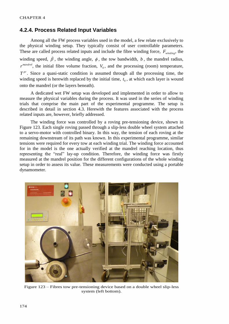
CHAPTER 4
174
4.2.4. Process Related Input Variables
Among all the FW process variables used in the model, a few relate exclusively to
the physical winding setup. They typically consist of user controllable parameters.
These are called process related inputs and include the fibre winding force, windingF , the
winding speed, , the winding angle, , the tow bandwidth, b , the mandrel radius, mandrelr , the initial fibre volume fraction, 0V , and the processing (room) temperature, prT . Since a quasi-static condition is assumed through all the processing time, the
winding speed is herewith replaced by the initial time, 0t , at which each layer is wound
onto the mandrel (or the layers beneath).
A dedicated wet FW setup was developed and implemented in order to allow to
measure the physical variables during the process. It was used in the series of winding
trials that comprise the main part of the experimental programme. The setup is
described in detail in section 4.3. Herewith the features associated with the process
related inputs are, however, briefly addressed.
The winding force was controlled by a roving pre-tensioning device, shown in
Figure 123. Each single roving passed through a slip-less double wheel system attached
to a servo-motor with controlled binary. In this way, the tension of each roving at the
remaining downstream of its path was known. In this experimental programme, similar
tensions were required for every tow at each winding trial. The winding force accounted
for in the model is the one actually verified at the mandrel reaching location, thus
representing the “real” lay-up condition. Therefore, the winding force was firstly
measured at the mandrel position for the different configurations of the whole winding
setup in order to assess its value. These measurements were conducted using a portable
dynamometer.
Figure 123 – Fibres tow pre-tensioning device based on a double wheel slip-less
system (left bottom).
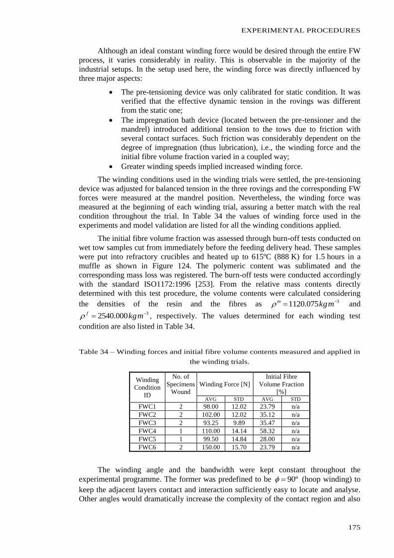
EXPERIMENTAL PROCEDURES
175
Although an ideal constant winding force would be desired through the entire FW
process, it varies considerably in reality. This is observable in the majority of the
industrial setups. In the setup used here, the winding force was directly influenced by
three major aspects:
The pre-tensioning device was only calibrated for static condition. It was
verified that the effective dynamic tension in the rovings was different
from the static one;
The impregnation bath device (located between the pre-tensioner and the
mandrel) introduced additional tension to the tows due to friction with
several contact surfaces. Such friction was considerably dependent on the
degree of impregnation (thus lubrication), i.e., the winding force and the
initial fibre volume fraction varied in a coupled way;
Greater winding speeds implied increased winding force.
The winding conditions used in the winding trials were settled, the pre-tensioning
device was adjusted for balanced tension in the three rovings and the corresponding FW
forces were measured at the mandrel position. Nevertheless, the winding force was
measured at the beginning of each winding trial, assuring a better match with the real
condition throughout the trial. In Table 34 the values of winding force used in the
experiments and model validation are listed for all the winding conditions applied.
The initial fibre volume fraction was assessed through burn-off tests conducted on
wet tow samples cut from immediately before the feeding delivery head. These samples
were put into refractory crucibles and heated up to 615ºC (888 K) for 1.5 hours in a
muffle as shown in Figure 124. The polymeric content was sublimated and the
corresponding mass loss was registered. The burn-off tests were conducted accordingly
with the standard ISO1172:1996 [253]. From the relative mass contents directly
determined with this test procedure, the volume contents were calculated considering
the densities of the resin and the fibres as 3075.1120 mkgm and 3000.2540 mkgf , respectively. The values determined for each winding test
condition are also listed in Table 34.
Table 34 – Winding forces and initial fibre volume contents measured and applied in
the winding trials.
Winding
Condition
ID
No. of
Specimens
Wound
Winding Force [N]
Initial Fibre
Volume Fraction
[%] AVG STD AVG STD
FWC1 2 98.00 12.02 23.79 n/a
FWC2 2 102.00 12.02 35.12 n/a
FWC3 2 93.25 9.89 35.47 n/a
FWC4 1 110.00 14.14 58.32 n/a
FWC5 1 99.50 14.84 28.00 n/a
FWC6 2 150.00 15.70 23.79 n/a
The winding angle and the bandwidth were kept constant throughout the
experimental programme. The former was predefined to be º90 (hoop winding) to
keep the adjacent layers contact and interaction sufficiently easy to locate and analyse.
Other angles would dramatically increase the complexity of the contact region and also
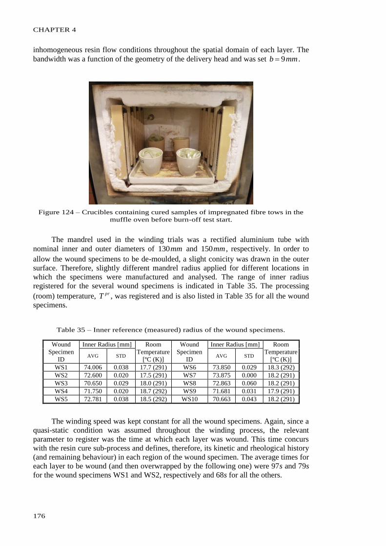
CHAPTER 4
176
inhomogeneous resin flow conditions throughout the spatial domain of each layer. The
bandwidth was a function of the geometry of the delivery head and was set mmb 9 .
Figure 124 – Crucibles containing cured samples of impregnated fibre tows in the
muffle oven before burn-off test start.
The mandrel used in the winding trials was a rectified aluminium tube with
nominal inner and outer diameters of mm130 and mm150 , respectively. In order to
allow the wound specimens to be de-moulded, a slight conicity was drawn in the outer
surface. Therefore, slightly different mandrel radius applied for different locations in
which the specimens were manufactured and analysed. The range of inner radius
registered for the several wound specimens is indicated in Table 35. The processing
(room) temperature, prT , was registered and is also listed in Table 35 for all the wound
specimens.
Table 35 – Inner reference (measured) radius of the wound specimens.
Wound
Specimen
ID
Inner Radius [mm] Room
Temperature
[ºC (K)]
Wound
Specimen
ID
Inner Radius [mm] Room
Temperature
[ºC (K)] AVG STD AVG STD
WS1 74.006 0.038 17.7 (291) WS6 73.850 0.029 18.3 (292)
WS2 72.600 0.020 17.5 (291) WS7 73.875 0.000 18.2 (291)
WS3 70.650 0.029 18.0 (291) WS8 72.863 0.060 18.2 (291)
WS4 71.750 0.020 18.7 (292) WS9 71.681 0.031 17.9 (291)
WS5 72.781 0.038 18.5 (292) WS10 70.663 0.043 18.2 (291)
The winding speed was kept constant for all the wound specimens. Again, since a
quasi-static condition was assumed throughout the winding process, the relevant
parameter to register was the time at which each layer was wound. This time concurs
with the resin cure sub-process and defines, therefore, its kinetic and rheological history
(and remaining behaviour) in each region of the wound specimen. The average times for
each layer to be wound (and then overwrapped by the following one) were 97s and 79s
for the wound specimens WS1 and WS2, respectively and 68s for all the others.
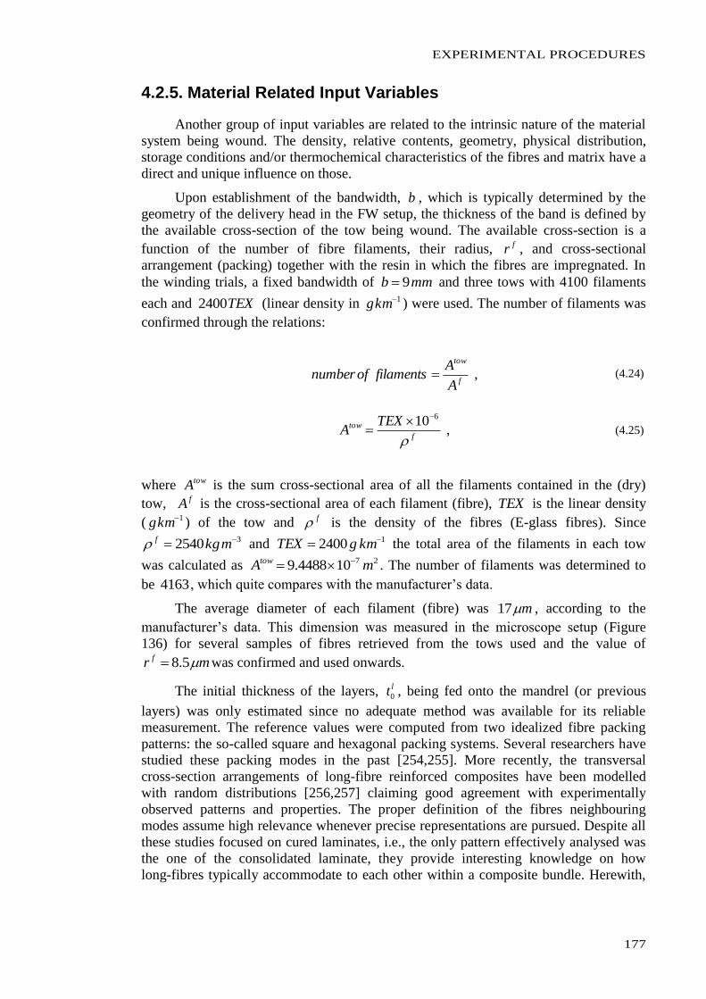
EXPERIMENTAL PROCEDURES
177
4.2.5. Material Related Input Variables
Another group of input variables are related to the intrinsic nature of the material
system being wound. The density, relative contents, geometry, physical distribution,
storage conditions and/or thermochemical characteristics of the fibres and matrix have a
direct and unique influence on those.
Upon establishment of the bandwidth, b , which is typically determined by the
geometry of the delivery head in the FW setup, the thickness of the band is defined by
the available cross-section of the tow being wound. The available cross-section is a
function of the number of fibre filaments, their radius, fr , and cross-sectional
arrangement (packing) together with the resin in which the fibres are impregnated. In
the winding trials, a fixed bandwidth of mmb 9 and three tows with 4100 filaments
each and TEX2400 (linear density in 1kmg ) were used. The number of filaments was
confirmed through the relations:
f
tow
A
Afilamentsofnumber , (4.24)
f
tow TEXA
610 , (4.25)
where towA is the sum cross-sectional area of all the filaments contained in the (dry)
tow, fA is the cross-sectional area of each filament (fibre), TEX is the linear density
( 1kmg ) of the tow and f is the density of the fibres (E-glass fibres). Since 32540 mkgf and 12400 kmgTEX the total area of the filaments in each tow
was calculated as 27104488.9 mAtow . The number of filaments was determined to
be 4163 , which quite compares with the manufacturer’s data.
The average diameter of each filament (fibre) was m17 , according to the
manufacturer’s data. This dimension was measured in the microscope setup (Figure
136) for several samples of fibres retrieved from the tows used and the value of
mr f 5.8 was confirmed and used onwards.
The initial thickness of the layers, lt0 , being fed onto the mandrel (or previous
layers) was only estimated since no adequate method was available for its reliable
measurement. The reference values were computed from two idealized fibre packing
patterns: the so-called square and hexagonal packing systems. Several researchers have
studied these packing modes in the past [254,255]. More recently, the transversal
cross-section arrangements of long-fibre reinforced composites have been modelled
with random distributions [256,257] claiming good agreement with experimentally
observed patterns and properties. The proper definition of the fibres neighbouring
modes assume high relevance whenever precise representations are pursued. Despite all
these studies focused on cured laminates, i.e., the only pattern effectively analysed was
the one of the consolidated laminate, they provide interesting knowledge on how
long-fibres typically accommodate to each other within a composite bundle. Herewith,
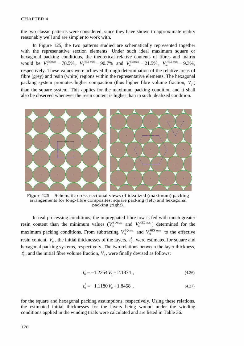
CHAPTER 4
178
the two classic patterns were considered, since they have shown to approximate reality
reasonably well and are simpler to work with.
In Figure 125, the two patterns studied are schematically represented together
with the representative section elements. Under such ideal maximum square or
hexagonal packing conditions, the theoretical relative contents of fibres and matrix
would be %5.78max SQ
fV , %7.90max HEX
fV and %5.21max SQ
mV , %3.9max HEX
mV ,
respectively. These values were achieved through determination of the relative areas of
fibre (grey) and resin (white) regions within the representative elements. The hexagonal
packing system promotes higher compaction (thus higher fibre volume fraction, fV )
than the square system. This applies for the maximum packing condition and it shall
also be observed whenever the resin content is higher than in such idealized condition.
Figure 125 – Schematic cross-sectional views of idealized (maximum) packing
arrangements for long-fibre composites: square packing (left) and hexagonal
packing (right).
In real processing conditions, the impregnated fibre tow is fed with much greater
resin content than the minimum values ( maxSQ
mV and maxHEX
mV ) determined for the
maximum packing conditions. From subtracting maxSQ
mV and maxHEX
mV to the effective
resin content, mV , the initial thicknesses of the layers, lt0 , were estimated for square and
hexagonal packing systems, respectively. The two relations between the layer thickness, lt0 , and the initial fibre volume fraction, 0V , were finally devised as follows:
1874.22254.1 00 Vt l , (4.26)
8458.11180.1 00 Vt l , (4.27)
for the square and hexagonal packing assumptions, respectively. Using these relations,
the estimated initial thicknesses for the layers being wound under the winding
conditions applied in the winding trials were calculated and are listed in Table 36.
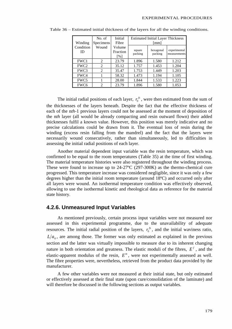
EXPERIMENTAL PROCEDURES
179
Table 36 – Estimated initial thickness of the layers for all the winding conditions.
Winding
Condition
ID
No. of
Specimens
Wound
Initial
Fibre
Volume
Fraction
[%]
Estimated Initial Layer Thickness
[mm]
square packing
hexagonal packing
experimental measurements
FWC1 2 23.79 1.896 1.580 1.212
FWC2 2 35.12 1.757 1.453 1.204
FWC3 2 35.47 1.753 1.449 1.203
FWC4 1 58.32 1.473 1.194 1.105
FWC5 1 28.00 1.844 1.533 1.223
FWC6 2 23.79 1.896 1.580 1.053
The initial radial positions of each layer, fsr0 , were then estimated from the sum of
the thicknesses of the layers beneath. Despite the fact that the effective thickness of
each of the nth-1 previous layers could not be assessed at the moment of deposition of
the nth layer (all would be already compacting and resin outward flown) their added
thicknesses fulfil a known value. However, this position was merely indicative and no
precise calculations could be drawn from it. The eventual loss of resin during the
winding (excess resin falling from the mandrel) and the fact that the layers were
necessarily wound consecutively, rather than simultaneously, led to difficulties in
assessing the initial radial positions of each layer.
Another material dependent input variable was the resin temperature, which was
confirmed to be equal to the room temperatures (Table 35) at the time of first winding.
The material temperature histories were also registered throughout the winding process.
These were found to increase up to 24-27ºC (297-300K) as the thermo-chemical cure
progressed. This temperature increase was considered negligible, since it was only a few
degrees higher than the initial room temperature (around 18ºC) and occurred only after
all layers were wound. An isothermal temperature condition was effectively observed,
allowing to use the isothermal kinetic and rheological data as reference for the material
state history.
4.2.6. Unmeasured Input Variables
As mentioned previously, certain process input variables were not measured nor
assessed in this experimental programme, due to the unavailability of adequate
resources. The initial radial position of the layers, fsr0 , and the initial waviness ratio,
0aL , are among those. The former was only estimated as explained in the previous
section and the latter was virtually impossible to measure due to its inherent changing
nature in both orientation and greatness. The elastic moduli of the fibres, fE , and the
elastic-apparent modulus of the resin, mE , were not experimentally assessed as well.
The fibre properties were, nevertheless, retrieved from the product data provided by the
manufacturer.
A few other variables were not measured at their initial state, but only estimated
or effectively assessed at their final state (upon cure/consolidation of the laminate) and
will therefore be discussed in the following sections as output variables.
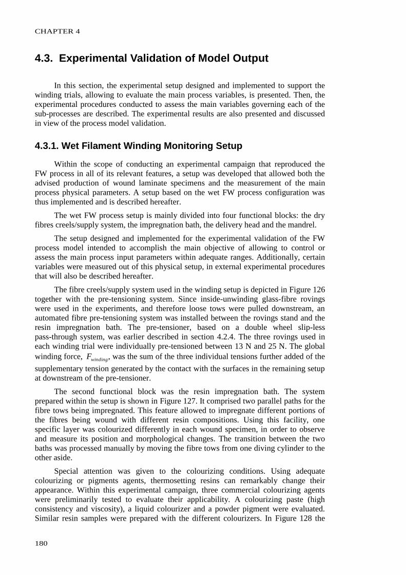
CHAPTER 4
180
4.3. Experimental Validation of Model Output
In this section, the experimental setup designed and implemented to support the
winding trials, allowing to evaluate the main process variables, is presented. Then, the
experimental procedures conducted to assess the main variables governing each of the
sub-processes are described. The experimental results are also presented and discussed
in view of the process model validation.
4.3.1. Wet Filament Winding Monitoring Setup
Within the scope of conducting an experimental campaign that reproduced the
FW process in all of its relevant features, a setup was developed that allowed both the
advised production of wound laminate specimens and the measurement of the main
process physical parameters. A setup based on the wet FW process configuration was
thus implemented and is described hereafter.
The wet FW process setup is mainly divided into four functional blocks: the dry
fibres creels/supply system, the impregnation bath, the delivery head and the mandrel.
The setup designed and implemented for the experimental validation of the FW
process model intended to accomplish the main objective of allowing to control or
assess the main process input parameters within adequate ranges. Additionally, certain
variables were measured out of this physical setup, in external experimental procedures
that will also be described hereafter.
The fibre creels/supply system used in the winding setup is depicted in Figure 126
together with the pre-tensioning system. Since inside-unwinding glass-fibre rovings
were used in the experiments, and therefore loose tows were pulled downstream, an
automated fibre pre-tensioning system was installed between the rovings stand and the
resin impregnation bath. The pre-tensioner, based on a double wheel slip-less
pass-through system, was earlier described in section 4.2.4. The three rovings used in
each winding trial were individually pre-tensioned between 13 N and 25 N. The global
winding force, windingF , was the sum of the three individual tensions further added of the
supplementary tension generated by the contact with the surfaces in the remaining setup
at downstream of the pre-tensioner.
The second functional block was the resin impregnation bath. The system
prepared within the setup is shown in Figure 127. It comprised two parallel paths for the
fibre tows being impregnated. This feature allowed to impregnate different portions of
the fibres being wound with different resin compositions. Using this facility, one
specific layer was colourized differently in each wound specimen, in order to observe
and measure its position and morphological changes. The transition between the two
baths was processed manually by moving the fibre tows from one diving cylinder to the
other aside.
Special attention was given to the colourizing conditions. Using adequate
colourizing or pigments agents, thermosetting resins can remarkably change their
appearance. Within this experimental campaign, three commercial colourizing agents
were preliminarily tested to evaluate their applicability. A colourizing paste (high
consistency and viscosity), a liquid colourizer and a powder pigment were evaluated.
Similar resin samples were prepared with the different colourizers. In Figure 128 the
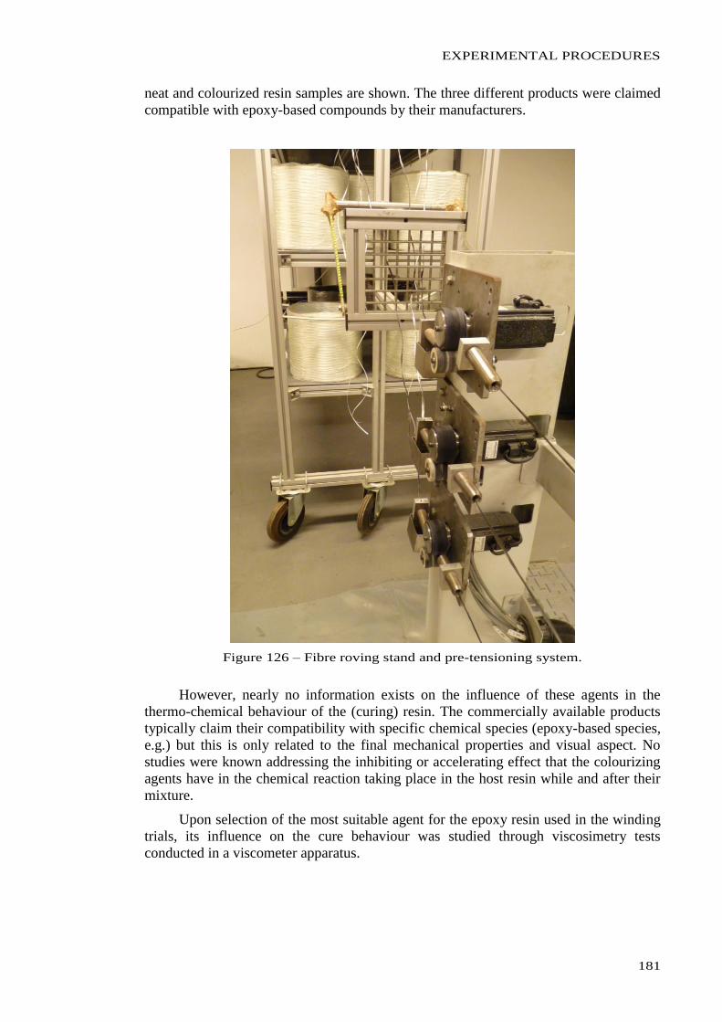
EXPERIMENTAL PROCEDURES
181
neat and colourized resin samples are shown. The three different products were claimed
compatible with epoxy-based compounds by their manufacturers.
Figure 126 – Fibre roving stand and pre-tensioning system.
However, nearly no information exists on the influence of these agents in the
thermo-chemical behaviour of the (curing) resin. The commercially available products
typically claim their compatibility with specific chemical species (epoxy-based species,
e.g.) but this is only related to the final mechanical properties and visual aspect. No
studies were known addressing the inhibiting or accelerating effect that the colourizing
agents have in the chemical reaction taking place in the host resin while and after their
mixture.
Upon selection of the most suitable agent for the epoxy resin used in the winding
trials, its influence on the cure behaviour was studied through viscosimetry tests
conducted in a viscometer apparatus.
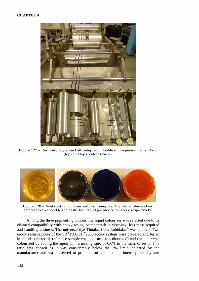
CHAPTER 4
182
Figure 127 – Resin impregnation bath setup with double impregnation paths. Front
(top) and top (bottom) views.
Figure 128 – Neat (left) and colourized resin samples. The black, blue and red
samples correspond to the paste, liquid and powder colourizers, respectively.
Among the three pigmenting options, the liquid colourizer was selected due to its
claimed compatibility with epoxy resins, better match in viscosity, less mass required
and handling easiness. The universal dye Tintalac from Robbialac® was applied. Two
epoxy resin samples of the SR®1500/SD
®2505 epoxy system were prepared and tested
in the viscometer. A reference sample was kept neat (uncolourized) and the other was
colourized by adding the agent with a mixing ratio of 0.6% to the mass of resin. This
ratio was chosen as it was considerably below the 3% limit indicated by the
manufacturer and was observed to promote sufficient colour intensity, opacity and
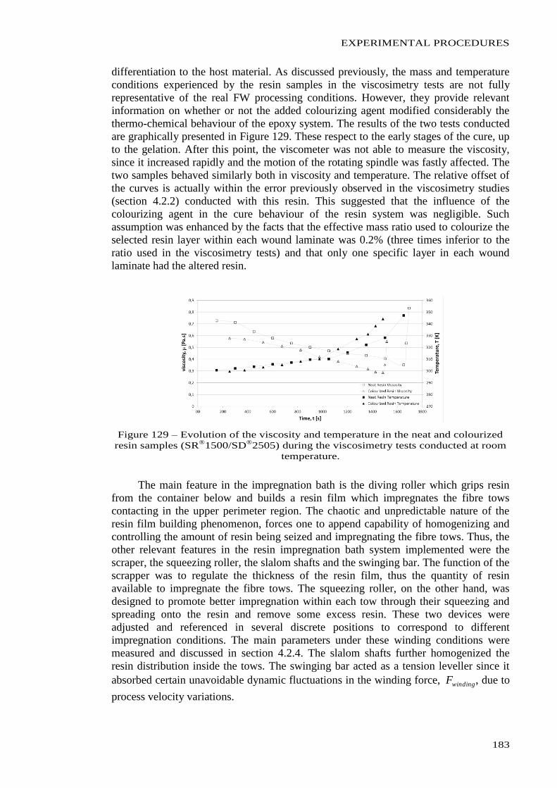
EXPERIMENTAL PROCEDURES
183
differentiation to the host material. As discussed previously, the mass and temperature
conditions experienced by the resin samples in the viscosimetry tests are not fully
representative of the real FW processing conditions. However, they provide relevant
information on whether or not the added colourizing agent modified considerably the
thermo-chemical behaviour of the epoxy system. The results of the two tests conducted
are graphically presented in Figure 129. These respect to the early stages of the cure, up
to the gelation. After this point, the viscometer was not able to measure the viscosity,
since it increased rapidly and the motion of the rotating spindle was fastly affected. The
two samples behaved similarly both in viscosity and temperature. The relative offset of
the curves is actually within the error previously observed in the viscosimetry studies
(section 4.2.2) conducted with this resin. This suggested that the influence of the
colourizing agent in the cure behaviour of the resin system was negligible. Such
assumption was enhanced by the facts that the effective mass ratio used to colourize the
selected resin layer within each wound laminate was 0.2% (three times inferior to the
ratio used in the viscosimetry tests) and that only one specific layer in each wound
laminate had the altered resin.
Figure 129 – Evolution of the viscosity and temperature in the neat and colourized
resin samples (SR®
1500/SD®
2505) during the viscosimetry tests conducted at room
temperature.
The main feature in the impregnation bath is the diving roller which grips resin
from the container below and builds a resin film which impregnates the fibre tows
contacting in the upper perimeter region. The chaotic and unpredictable nature of the
resin film building phenomenon, forces one to append capability of homogenizing and
controlling the amount of resin being seized and impregnating the fibre tows. Thus, the
other relevant features in the resin impregnation bath system implemented were the
scraper, the squeezing roller, the slalom shafts and the swinging bar. The function of the
scrapper was to regulate the thickness of the resin film, thus the quantity of resin
available to impregnate the fibre tows. The squeezing roller, on the other hand, was
designed to promote better impregnation within each tow through their squeezing and
spreading onto the resin and remove some excess resin. These two devices were
adjusted and referenced in several discrete positions to correspond to different
impregnation conditions. The main parameters under these winding conditions were
measured and discussed in section 4.2.4. The slalom shafts further homogenized the
resin distribution inside the tows. The swinging bar acted as a tension leveller since it
absorbed certain unavoidable dynamic fluctuations in the winding force, windingF , due to
process velocity variations.
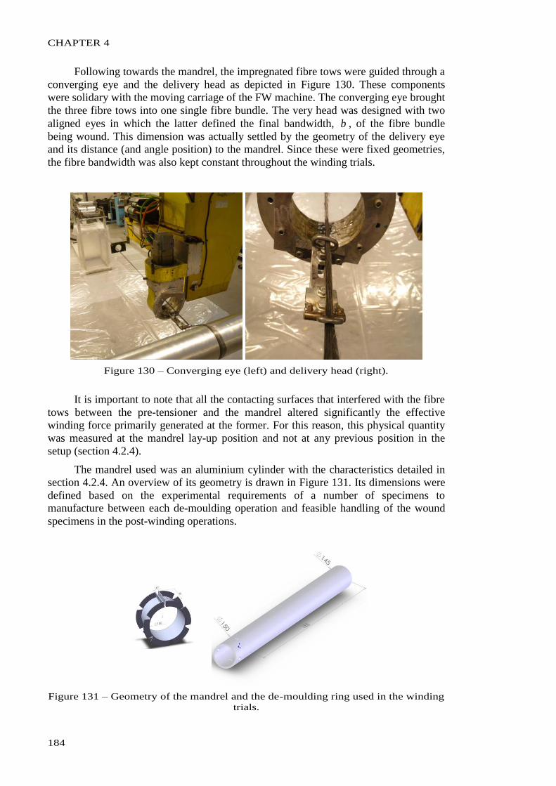
CHAPTER 4
184
Following towards the mandrel, the impregnated fibre tows were guided through a
converging eye and the delivery head as depicted in Figure 130. These components
were solidary with the moving carriage of the FW machine. The converging eye brought
the three fibre tows into one single fibre bundle. The very head was designed with two
aligned eyes in which the latter defined the final bandwidth, b , of the fibre bundle
being wound. This dimension was actually settled by the geometry of the delivery eye
and its distance (and angle position) to the mandrel. Since these were fixed geometries,
the fibre bandwidth was also kept constant throughout the winding trials.
Figure 130 – Converging eye (left) and delivery head (right).
It is important to note that all the contacting surfaces that interfered with the fibre
tows between the pre-tensioner and the mandrel altered significantly the effective
winding force primarily generated at the former. For this reason, this physical quantity
was measured at the mandrel lay-up position and not at any previous position in the
setup (section 4.2.4).
The mandrel used was an aluminium cylinder with the characteristics detailed in
section 4.2.4. An overview of its geometry is drawn in Figure 131. Its dimensions were
defined based on the experimental requirements of a number of specimens to
manufacture between each de-moulding operation and feasible handling of the wound
specimens in the post-winding operations.
Figure 131 – Geometry of the mandrel and the de-moulding ring used in the winding
trials.
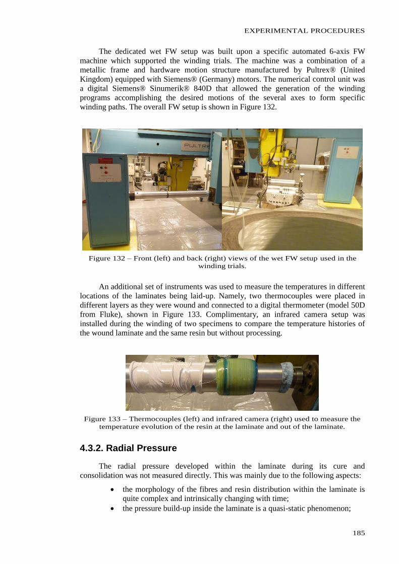
EXPERIMENTAL PROCEDURES
185
The dedicated wet FW setup was built upon a specific automated 6-axis FW
machine which supported the winding trials. The machine was a combination of a
metallic frame and hardware motion structure manufactured by Pultrex® (United
Kingdom) equipped with Siemens® (Germany) motors. The numerical control unit was
a digital Siemens® Sinumerik® 840D that allowed the generation of the winding
programs accomplishing the desired motions of the several axes to form specific
winding paths. The overall FW setup is shown in Figure 132.
Figure 132 – Front (left) and back (right) views of the wet FW setup used in the
winding trials.
An additional set of instruments was used to measure the temperatures in different
locations of the laminates being laid-up. Namely, two thermocouples were placed in
different layers as they were wound and connected to a digital thermometer (model 50D
from Fluke), shown in Figure 133. Complimentary, an infrared camera setup was
installed during the winding of two specimens to compare the temperature histories of
the wound laminate and the same resin but without processing.
Figure 133 – Thermocouples (left) and infrared camera (right) used to measure the
temperature evolution of the resin at the laminate and out of the laminate.
4.3.2. Radial Pressure
The radial pressure developed within the laminate during its cure and
consolidation was not measured directly. This was mainly due to the following aspects:
the morphology of the fibres and resin distribution within the laminate is
quite complex and intrinsically changing with time;
the pressure build-up inside the laminate is a quasi-static phenomenon;
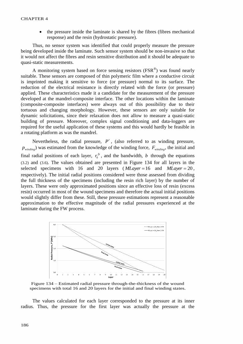
CHAPTER 4
186
the pressure inside the laminate is shared by the fibres (fibres mechanical
response) and the resin (hydrostatic pressure).
Thus, no sensor system was identified that could properly measure the pressure
being developed inside the laminate. Such sensor system should be non-invasive so that
it would not affect the fibres and resin sensitive distribution and it should be adequate to
quasi-static measurements.
A monitoring system based on force sensing resistors (FSR®) was found nearly
suitable. These sensors are composed of thin polymeric film where a conductive circuit
is imprinted making it sensitive to force (or pressure) normal to its surface. The
reduction of the electrical resistance is directly related with the force (or pressure)
applied. These characteristics made it a candidate for the measurement of the pressure
developed at the mandrel-composite interface. The other locations within the laminate
(composite-composite interfaces) were always out of this possibility due to their
tortuous and changing morphology. However, these sensors are only suitable for
dynamic solicitations, since their relaxation does not allow to measure a quasi-static
building of pressure. Moreover, complex signal conditioning and data-loggers are
required for the useful application of these systems and this would hardly be feasible in
a rotating platform as was the mandrel.
Nevertheless, the radial pressure, rP , (also referred to as winding pressure,
windingp ) was estimated from the knowledge of the winding force, windingF , the initial and
final radial positions of each layer, fsr0 , and the bandwidth, b through the equations
(3.2) and (3.6). The values obtained are presented in Figure 134 for all layers in the
selected specimens with 16 and 20 layers ( 16MLayer and 20MLayer ,
respectively). The initial radial positions considered were those assessed from dividing
the full thickness of the specimens (including the resin rich layer) by the number of
layers. These were only approximated positions since an effective loss of resin (excess
resin) occurred in most of the wound specimens and therefore the actual initial positions
would slightly differ from these. Still, these pressure estimations represent a reasonable
approximation to the effective magnitude of the radial pressures experienced at the
laminate during the FW process.
Figure 134 – Estimated radial pressure through-the-thickness of the wound
specimens with total 16 and 20 layers for the initial and final winding states.
The values calculated for each layer corresponded to the pressure at its inner
radius. Thus, the pressure for the first layer was actually the pressure at the
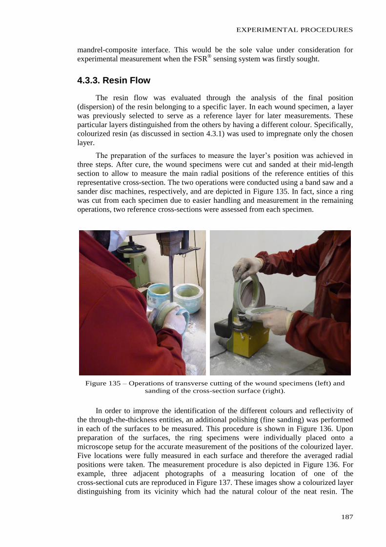
EXPERIMENTAL PROCEDURES
187
mandrel-composite interface. This would be the sole value under consideration for
experimental measurement when the FSR® sensing system was firstly sought.
4.3.3. Resin Flow
The resin flow was evaluated through the analysis of the final position
(dispersion) of the resin belonging to a specific layer. In each wound specimen, a layer
was previously selected to serve as a reference layer for later measurements. These
particular layers distinguished from the others by having a different colour. Specifically,
colourized resin (as discussed in section 4.3.1) was used to impregnate only the chosen
layer.
The preparation of the surfaces to measure the layer’s position was achieved in
three steps. After cure, the wound specimens were cut and sanded at their mid-length
section to allow to measure the main radial positions of the reference entities of this
representative cross-section. The two operations were conducted using a band saw and a
sander disc machines, respectively, and are depicted in Figure 135. In fact, since a ring
was cut from each specimen due to easier handling and measurement in the remaining
operations, two reference cross-sections were assessed from each specimen.
Figure 135 – Operations of transverse cutting of the wound specimens (left) and
sanding of the cross-section surface (right).
In order to improve the identification of the different colours and reflectivity of
the through-the-thickness entities, an additional polishing (fine sanding) was performed
in each of the surfaces to be measured. This procedure is shown in Figure 136. Upon
preparation of the surfaces, the ring specimens were individually placed onto a
microscope setup for the accurate measurement of the positions of the colourized layer.
Five locations were fully measured in each surface and therefore the averaged radial
positions were taken. The measurement procedure is also depicted in Figure 136. For
example, three adjacent photographs of a measuring location of one of the
cross-sectional cuts are reproduced in Figure 137. These images show a colourized layer
distinguishing from its vicinity which had the natural colour of the neat resin. The
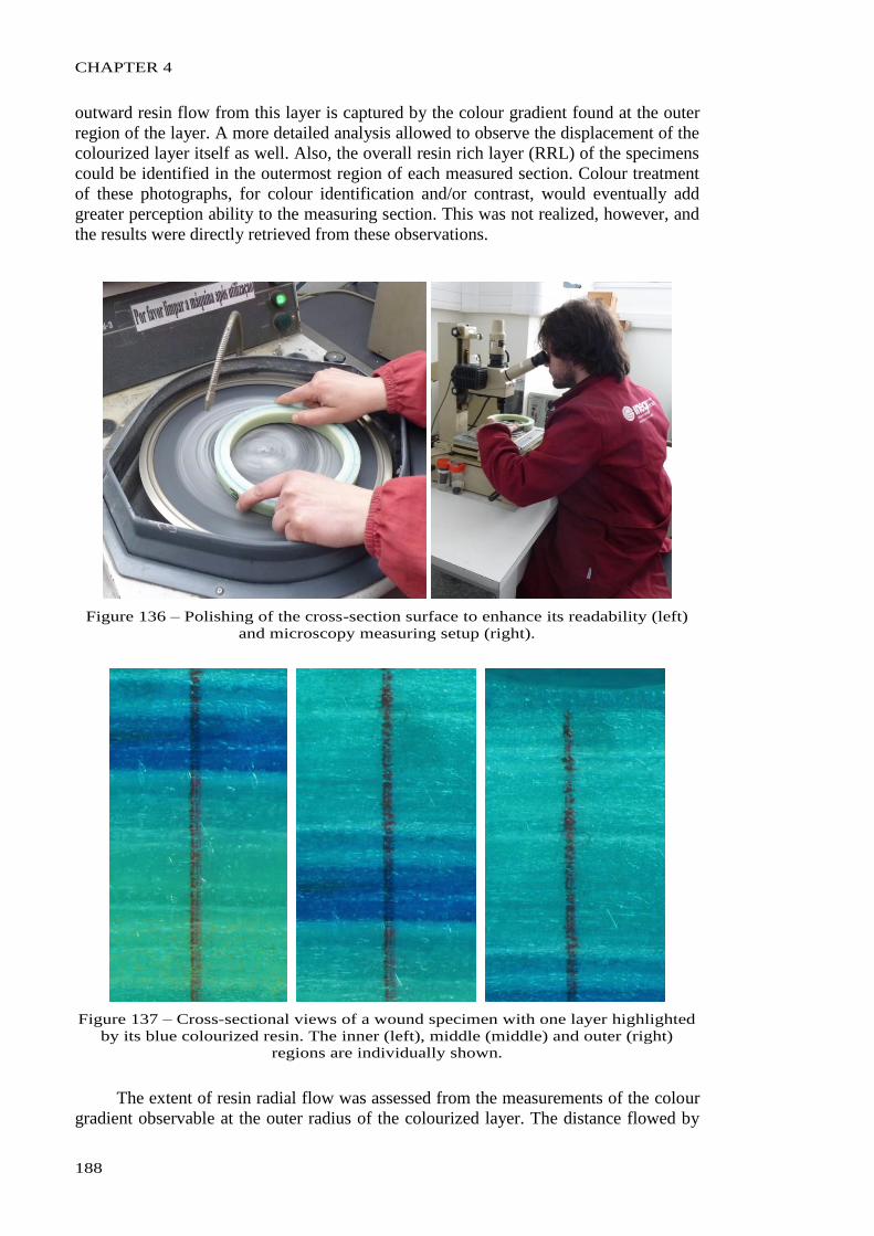
CHAPTER 4
188
outward resin flow from this layer is captured by the colour gradient found at the outer
region of the layer. A more detailed analysis allowed to observe the displacement of the
colourized layer itself as well. Also, the overall resin rich layer (RRL) of the specimens
could be identified in the outermost region of each measured section. Colour treatment
of these photographs, for colour identification and/or contrast, would eventually add
greater perception ability to the measuring section. This was not realized, however, and
the results were directly retrieved from these observations.
Figure 136 – Polishing of the cross-section surface to enhance its readability (left)
and microscopy measuring setup (right).
Figure 137 – Cross-sectional views of a wound specimen with one layer highlighted
by its blue colourized resin. The inner (left), middle (middle) and outer (right)
regions are individually shown.
The extent of resin radial flow was assessed from the measurements of the colour
gradient observable at the outer radius of the colourized layer. The distance flowed by
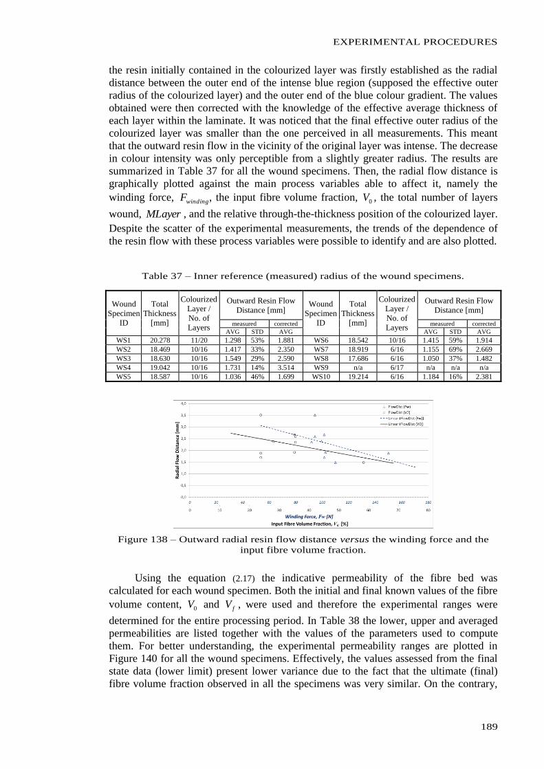
EXPERIMENTAL PROCEDURES
189
the resin initially contained in the colourized layer was firstly established as the radial
distance between the outer end of the intense blue region (supposed the effective outer
radius of the colourized layer) and the outer end of the blue colour gradient. The values
obtained were then corrected with the knowledge of the effective average thickness of
each layer within the laminate. It was noticed that the final effective outer radius of the
colourized layer was smaller than the one perceived in all measurements. This meant
that the outward resin flow in the vicinity of the original layer was intense. The decrease
in colour intensity was only perceptible from a slightly greater radius. The results are
summarized in Table 37 for all the wound specimens. Then, the radial flow distance is
graphically plotted against the main process variables able to affect it, namely the
winding force, windingF , the input fibre volume fraction, 0V , the total number of layers
wound, MLayer , and the relative through-the-thickness position of the colourized layer.
Despite the scatter of the experimental measurements, the trends of the dependence of
the resin flow with these process variables were possible to identify and are also plotted.
Table 37 – Inner reference (measured) radius of the wound specimens.
Wound
Specimen
ID
Total
Thickness
[mm]
Colourized
Layer /
No. of
Layers
Outward Resin Flow
Distance [mm] Wound
Specimen
ID
Total
Thickness
[mm]
Colourized
Layer /
No. of
Layers
Outward Resin Flow
Distance [mm]
measured corrected measured corrected
AVG STD AVG AVG STD AVG
WS1 20.278 11/20 1.298 53% 1.881 WS6 18.542 10/16 1.415 59% 1.914
WS2 18.469 10/16 1.417 33% 2.350 WS7 18.919 6/16 1.155 69% 2.669
WS3 18.630 10/16 1.549 29% 2.590 WS8 17.686 6/16 1.050 37% 1.482
WS4 19.042 10/16 1.731 14% 3.514 WS9 n/a 6/17 n/a n/a n/a
WS5 18.587 10/16 1.036 46% 1.699 WS10 19.214 6/16 1.184 16% 2.381
Figure 138 – Outward radial resin flow distance versus the winding force and the
input fibre volume fraction.
Using the equation (2.17) the indicative permeability of the fibre bed was
calculated for each wound specimen. Both the initial and final known values of the fibre
volume content, 0V and fV , were used and therefore the experimental ranges were
determined for the entire processing period. In Table 38 the lower, upper and averaged
permeabilities are listed together with the values of the parameters used to compute
them. For better understanding, the experimental permeability ranges are plotted in
Figure 140 for all the wound specimens. Effectively, the values assessed from the final
state data (lower limit) present lower variance due to the fact that the ultimate (final)
fibre volume fraction observed in all the specimens was very similar. On the contrary,
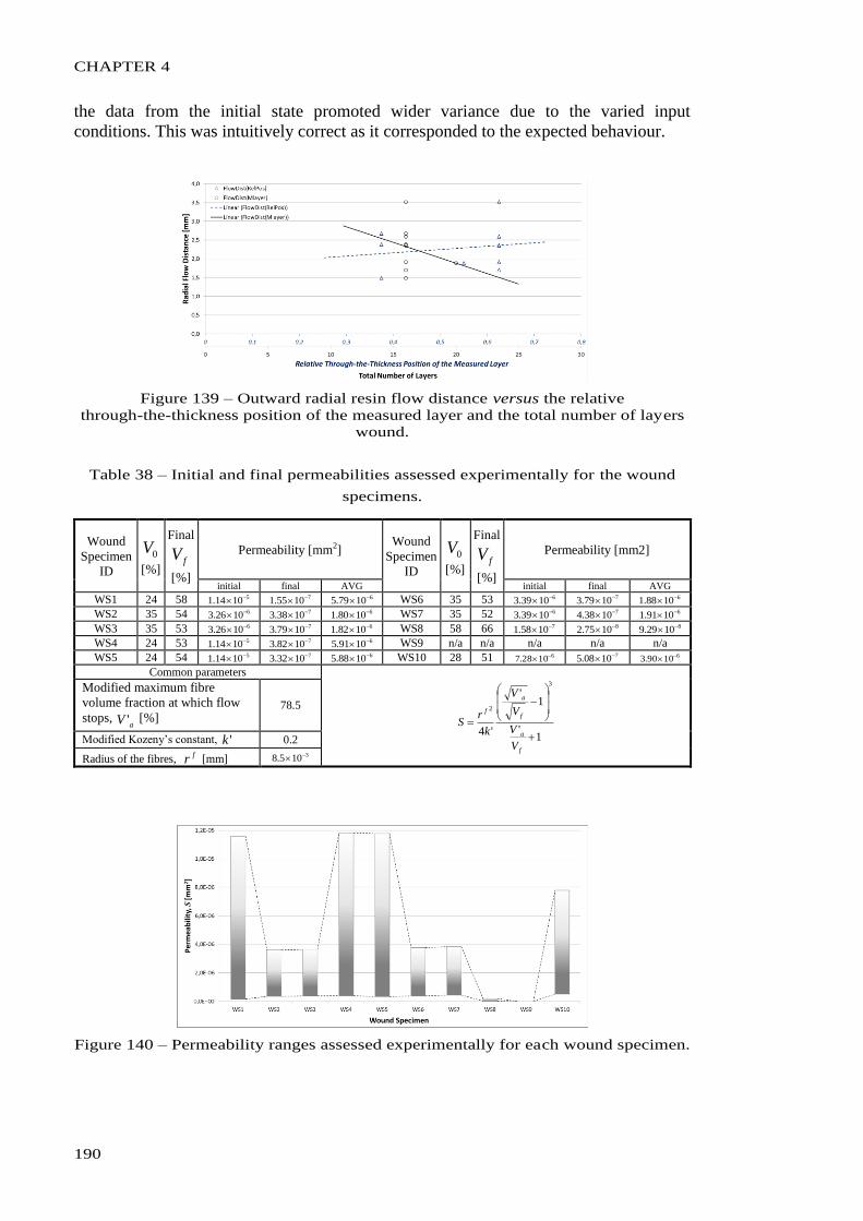
CHAPTER 4
190
the data from the initial state promoted wider variance due to the varied input
conditions. This was intuitively correct as it corresponded to the expected behaviour.
Figure 139 – Outward radial resin flow distance versus the relative
through-the-thickness position of the measured layer and the total number of layers
wound.
Table 38 – Initial and final permeabilities assessed experimentally for the wound
specimens.
Wound
Specimen
ID
0V
[%]
Final
fV
[%]
Permeability [mm2] Wound
Specimen
ID
0V
[%]
Final
fV
[%]
Permeability [mm2]
initial final AVG initial final AVG
WS1 24 58 51014.1 71055.1 61079.5 WS6 35 53 61039.3 71079.3 61088.1
WS2 35 54 61026.3 71038.3 61080.1 WS7 35 52 61039.3 71038.4 61091.1
WS3 35 53 61026.3 71079.3 61082.1 WS8 58 66 71058.1 81075.2 81029.9
WS4 24 53 51014.1 71082.3 61091.5 WS9 n/a n/a n/a n/a n/a
WS5 24 54 51014.1 71032.3 61088.5 WS10 28 51 61028.7 71008.5 61090.3
Common parameters
1'
1'
'4
3
2
f
a
f
a
f
V
V
V
V
k
rS
Modified maximum fibre
volume fraction at which flow
stops, aV ' [%]
78.5
Modified Kozeny’s constant, 'k 0.2
Radius of the fibres, fr [mm]
3105.8
Figure 140 – Permeability ranges assessed experimentally for each wound specimen.
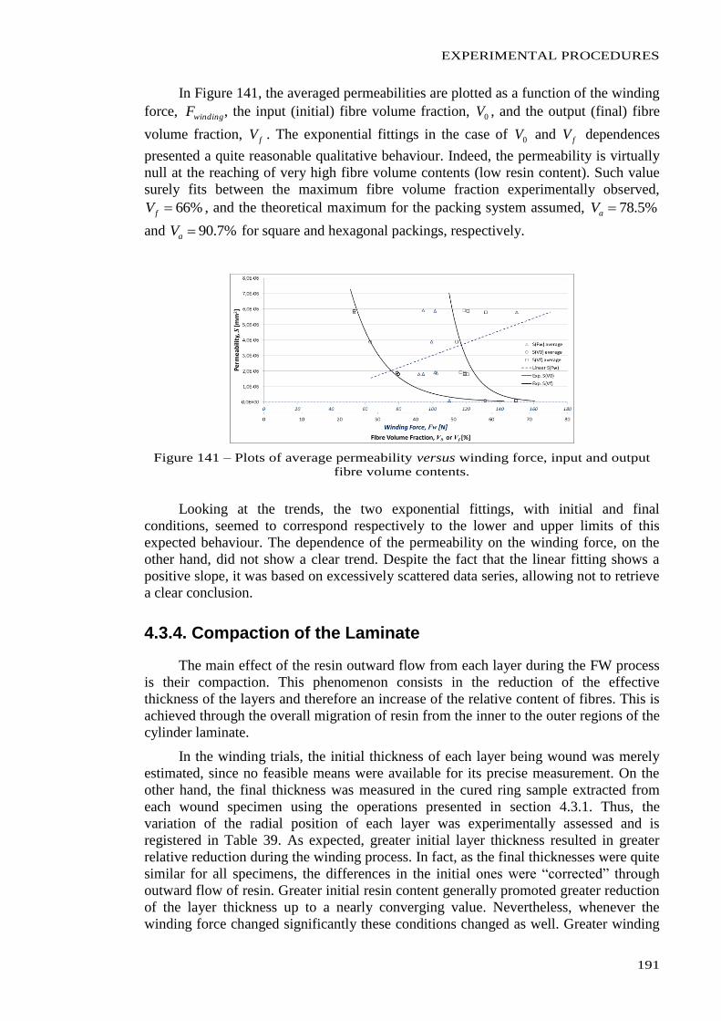
EXPERIMENTAL PROCEDURES
191
In Figure 141, the averaged permeabilities are plotted as a function of the winding
force, windingF , the input (initial) fibre volume fraction, 0V , and the output (final) fibre
volume fraction, fV . The exponential fittings in the case of 0V and fV dependences
presented a quite reasonable qualitative behaviour. Indeed, the permeability is virtually
null at the reaching of very high fibre volume contents (low resin content). Such value
surely fits between the maximum fibre volume fraction experimentally observed,
%66fV , and the theoretical maximum for the packing system assumed, %5.78aV
and %7.90aV for square and hexagonal packings, respectively.
Figure 141 – Plots of average permeability versus winding force, input and output
fibre volume contents.
Looking at the trends, the two exponential fittings, with initial and final
conditions, seemed to correspond respectively to the lower and upper limits of this
expected behaviour. The dependence of the permeability on the winding force, on the
other hand, did not show a clear trend. Despite the fact that the linear fitting shows a
positive slope, it was based on excessively scattered data series, allowing not to retrieve
a clear conclusion.
4.3.4. Compaction of the Laminate
The main effect of the resin outward flow from each layer during the FW process
is their compaction. This phenomenon consists in the reduction of the effective
thickness of the layers and therefore an increase of the relative content of fibres. This is
achieved through the overall migration of resin from the inner to the outer regions of the
cylinder laminate.
In the winding trials, the initial thickness of each layer being wound was merely
estimated, since no feasible means were available for its precise measurement. On the
other hand, the final thickness was measured in the cured ring sample extracted from
each wound specimen using the operations presented in section 4.3.1. Thus, the
variation of the radial position of each layer was experimentally assessed and is
registered in Table 39. As expected, greater initial layer thickness resulted in greater
relative reduction during the winding process. In fact, as the final thicknesses were quite
similar for all specimens, the differences in the initial ones were “corrected” through
outward flow of resin. Greater initial resin content generally promoted greater reduction
of the layer thickness up to a nearly converging value. Nevertheless, whenever the
winding force changed significantly these conditions changed as well. Greater winding
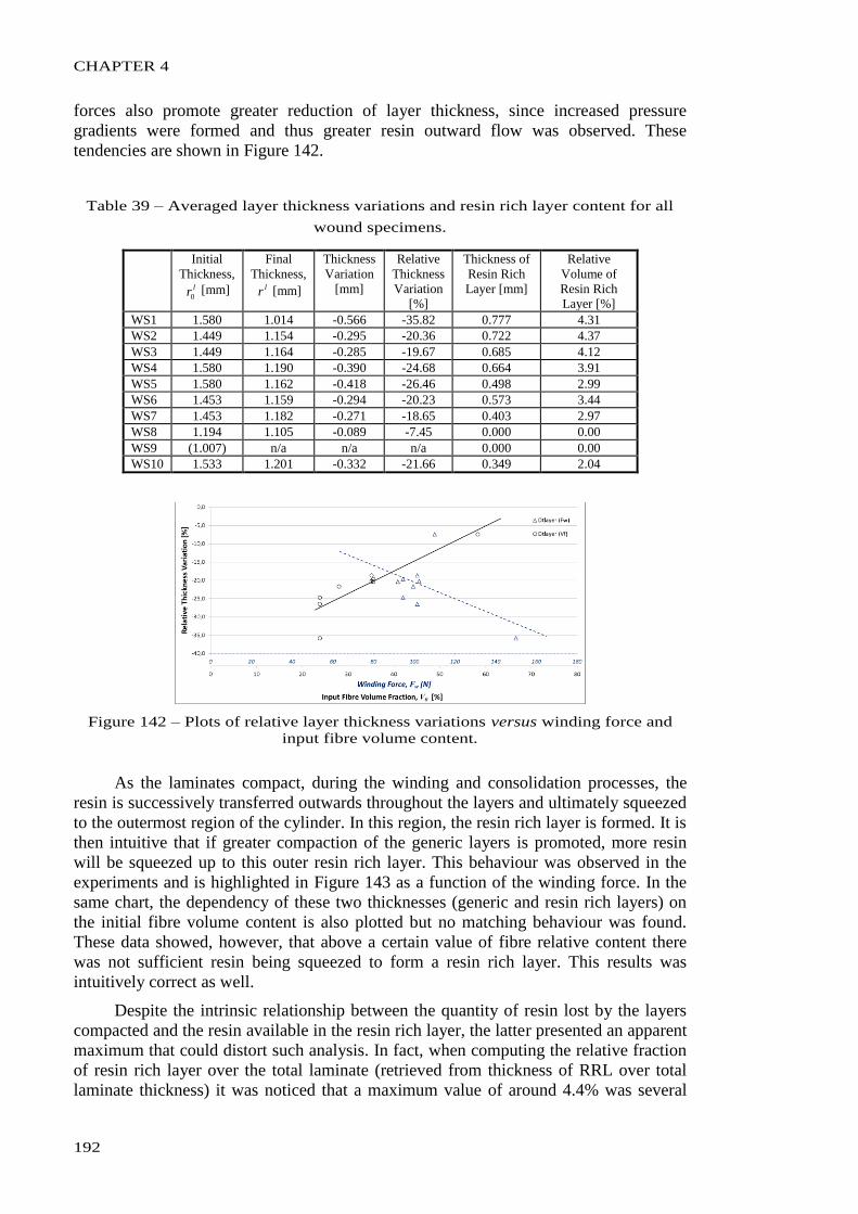
CHAPTER 4
192
forces also promote greater reduction of layer thickness, since increased pressure
gradients were formed and thus greater resin outward flow was observed. These
tendencies are shown in Figure 142.
Table 39 – Averaged layer thickness variations and resin rich layer content for all
wound specimens.
Initial
Thickness, lr0 [mm]
Final
Thickness, lr [mm]
Thickness
Variation
[mm]
Relative
Thickness
Variation
[%]
Thickness of
Resin Rich
Layer [mm]
Relative
Volume of
Resin Rich
Layer [%]
WS1 1.580 1.014 -0.566 -35.82 0.777 4.31
WS2 1.449 1.154 -0.295 -20.36 0.722 4.37
WS3 1.449 1.164 -0.285 -19.67 0.685 4.12
WS4 1.580 1.190 -0.390 -24.68 0.664 3.91
WS5 1.580 1.162 -0.418 -26.46 0.498 2.99
WS6 1.453 1.159 -0.294 -20.23 0.573 3.44
WS7 1.453 1.182 -0.271 -18.65 0.403 2.97
WS8 1.194 1.105 -0.089 -7.45 0.000 0.00
WS9 (1.007) n/a n/a n/a 0.000 0.00
WS10 1.533 1.201 -0.332 -21.66 0.349 2.04
Figure 142 – Plots of relative layer thickness variations versus winding force and
input fibre volume content.
As the laminates compact, during the winding and consolidation processes, the
resin is successively transferred outwards throughout the layers and ultimately squeezed
to the outermost region of the cylinder. In this region, the resin rich layer is formed. It is
then intuitive that if greater compaction of the generic layers is promoted, more resin
will be squeezed up to this outer resin rich layer. This behaviour was observed in the
experiments and is highlighted in Figure 143 as a function of the winding force. In the
same chart, the dependency of these two thicknesses (generic and resin rich layers) on
the initial fibre volume content is also plotted but no matching behaviour was found.
These data showed, however, that above a certain value of fibre relative content there
was not sufficient resin being squeezed to form a resin rich layer. This results was
intuitively correct as well.
Despite the intrinsic relationship between the quantity of resin lost by the layers
compacted and the resin available in the resin rich layer, the latter presented an apparent
maximum that could distort such analysis. In fact, when computing the relative fraction
of resin rich layer over the total laminate (retrieved from thickness of RRL over total
laminate thickness) it was noticed that a maximum value of around 4.4% was several
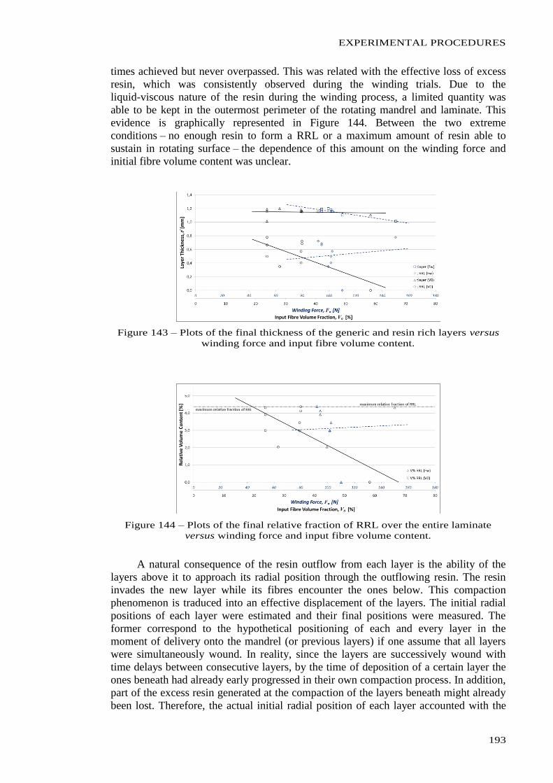
EXPERIMENTAL PROCEDURES
193
times achieved but never overpassed. This was related with the effective loss of excess
resin, which was consistently observed during the winding trials. Due to the
liquid-viscous nature of the resin during the winding process, a limited quantity was
able to be kept in the outermost perimeter of the rotating mandrel and laminate. This
evidence is graphically represented in Figure 144. Between the two extreme
conditions – no enough resin to form a RRL or a maximum amount of resin able to
sustain in rotating surface – the dependence of this amount on the winding force and
initial fibre volume content was unclear.
Figure 143 – Plots of the final thickness of the generic and resin rich layers versus
winding force and input fibre volume content.
Figure 144 – Plots of the final relative fraction of RRL over the entire laminate
versus winding force and input fibre volume content.
A natural consequence of the resin outflow from each layer is the ability of the
layers above it to approach its radial position through the outflowing resin. The resin
invades the new layer while its fibres encounter the ones below. This compaction
phenomenon is traduced into an effective displacement of the layers. The initial radial
positions of each layer were estimated and their final positions were measured. The
former correspond to the hypothetical positioning of each and every layer in the
moment of delivery onto the mandrel (or previous layers) if one assume that all layers
were simultaneously wound. In reality, since the layers are successively wound with
time delays between consecutive layers, by the time of deposition of a certain layer the
ones beneath had already early progressed in their own compaction process. In addition,
part of the excess resin generated at the compaction of the layers beneath might already
been lost. Therefore, the actual initial radial position of each layer accounted with the
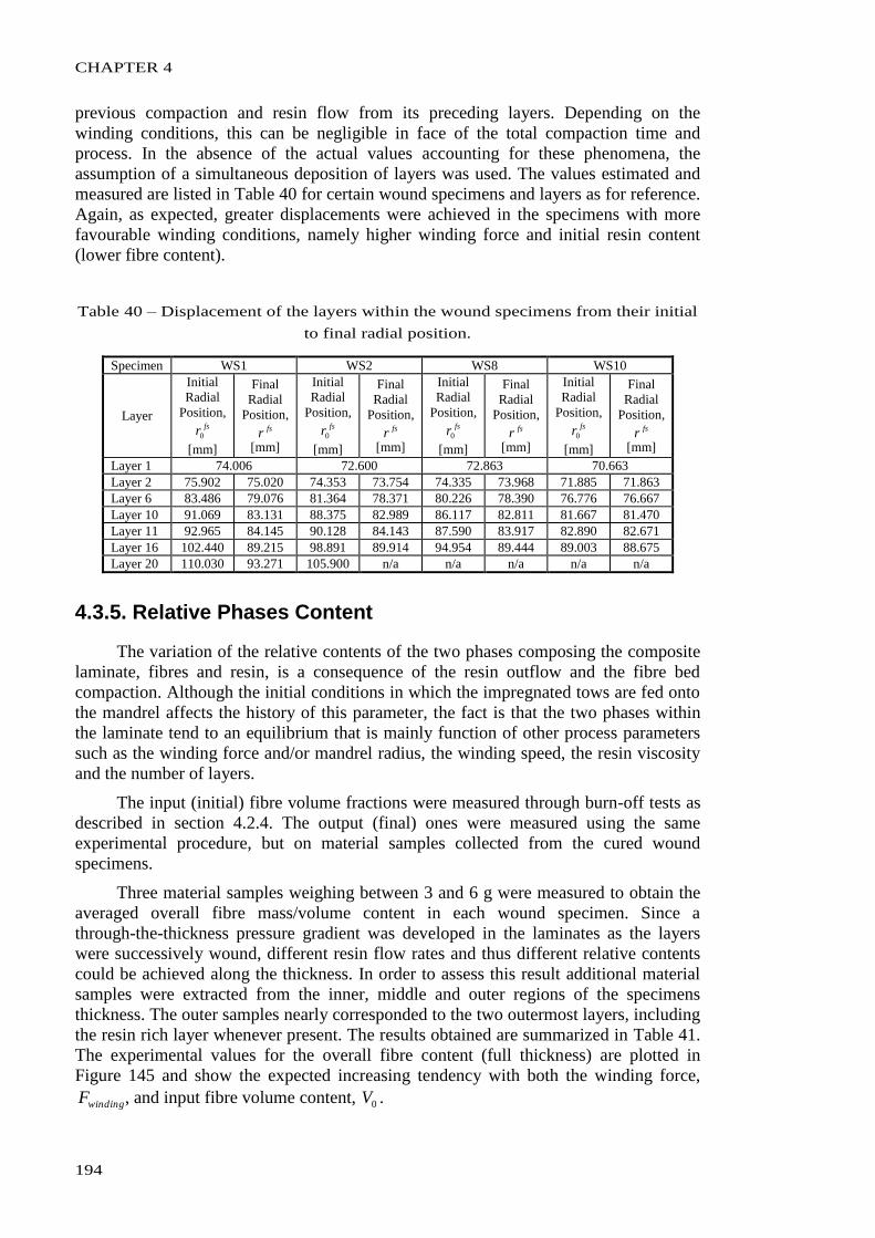
CHAPTER 4
194
previous compaction and resin flow from its preceding layers. Depending on the
winding conditions, this can be negligible in face of the total compaction time and
process. In the absence of the actual values accounting for these phenomena, the
assumption of a simultaneous deposition of layers was used. The values estimated and
measured are listed in Table 40 for certain wound specimens and layers as for reference.
Again, as expected, greater displacements were achieved in the specimens with more
favourable winding conditions, namely higher winding force and initial resin content
(lower fibre content).
Table 40 – Displacement of the layers within the wound specimens from their initial
to final radial position.
Specimen WS1 WS2 WS8 WS10
Layer
Initial
Radial
Position, fsr0
[mm]
Final
Radial
Position, fsr
[mm]
Initial
Radial
Position, fsr0
[mm]
Final
Radial
Position, fsr
[mm]
Initial
Radial
Position, fsr0
[mm]
Final
Radial
Position, fsr
[mm]
Initial
Radial
Position, fsr0
[mm]
Final
Radial
Position, fsr
[mm]
Layer 1 74.006 72.600 72.863 70.663
Layer 2 75.902 75.020 74.353 73.754 74.335 73.968 71.885 71.863
Layer 6 83.486 79.076 81.364 78.371 80.226 78.390 76.776 76.667
Layer 10 91.069 83.131 88.375 82.989 86.117 82.811 81.667 81.470
Layer 11 92.965 84.145 90.128 84.143 87.590 83.917 82.890 82.671
Layer 16 102.440 89.215 98.891 89.914 94.954 89.444 89.003 88.675
Layer 20 110.030 93.271 105.900 n/a n/a n/a n/a n/a
4.3.5. Relative Phases Content
The variation of the relative contents of the two phases composing the composite
laminate, fibres and resin, is a consequence of the resin outflow and the fibre bed
compaction. Although the initial conditions in which the impregnated tows are fed onto
the mandrel affects the history of this parameter, the fact is that the two phases within
the laminate tend to an equilibrium that is mainly function of other process parameters
such as the winding force and/or mandrel radius, the winding speed, the resin viscosity
and the number of layers.
The input (initial) fibre volume fractions were measured through burn-off tests as
described in section 4.2.4. The output (final) ones were measured using the same
experimental procedure, but on material samples collected from the cured wound
specimens.
Three material samples weighing between 3 and 6 g were measured to obtain the
averaged overall fibre mass/volume content in each wound specimen. Since a
through-the-thickness pressure gradient was developed in the laminates as the layers
were successively wound, different resin flow rates and thus different relative contents
could be achieved along the thickness. In order to assess this result additional material
samples were extracted from the inner, middle and outer regions of the specimens
thickness. The outer samples nearly corresponded to the two outermost layers, including
the resin rich layer whenever present. The results obtained are summarized in Table 41.
The experimental values for the overall fibre content (full thickness) are plotted in
Figure 145 and show the expected increasing tendency with both the winding force,
windingF , and input fibre volume content, 0V .
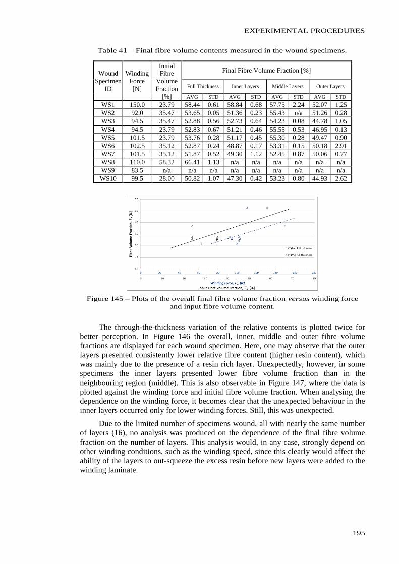
EXPERIMENTAL PROCEDURES
195
Table 41 – Final fibre volume contents measured in the wound specimens.
Wound
Specimen
ID
Winding
Force
[N]
Initial
Fibre
Volume
Fraction
[%]
Final Fibre Volume Fraction [%]
Full Thickness Inner Layers Middle Layers Outer Layers
AVG STD AVG STD AVG STD AVG STD
WS1 150.0 23.79 58.44 0.61 58.84 0.68 57.75 2.24 52.07 1.25
WS2 92.0 35.47 53.65 0.05 51.36 0.23 55.43 n/a 51.26 0.28
WS3 94.5 35.47 52.88 0.56 52.73 0.64 54.23 0.08 44.78 1.05
WS4 94.5 23.79 52.83 0.67 51.21 0.46 55.55 0.53 46.95 0.13
WS5 101.5 23.79 53.76 0.28 51.17 0.45 55.30 0.28 49.47 0.90
WS6 102.5 35.12 52.87 0.24 48.87 0.17 53.31 0.15 50.18 2.91
WS7 101.5 35.12 51.87 0.52 49.30 1.12 52.45 0.87 50.06 0.77
WS8 110.0 58.32 66.41 1.13 n/a n/a n/a n/a n/a n/a
WS9 83.5 n/a n/a n/a n/a n/a n/a n/a n/a n/a
WS10 99.5 28.00 50.82 1.07 47.30 0.42 53.23 0.80 44.93 2.62
Figure 145 – Plots of the overall final fibre volume fraction versus winding force
and input fibre volume content.
The through-the-thickness variation of the relative contents is plotted twice for
better perception. In Figure 146 the overall, inner, middle and outer fibre volume
fractions are displayed for each wound specimen. Here, one may observe that the outer
layers presented consistently lower relative fibre content (higher resin content), which
was mainly due to the presence of a resin rich layer. Unexpectedly, however, in some
specimens the inner layers presented lower fibre volume fraction than in the
neighbouring region (middle). This is also observable in Figure 147, where the data is
plotted against the winding force and initial fibre volume fraction. When analysing the
dependence on the winding force, it becomes clear that the unexpected behaviour in the
inner layers occurred only for lower winding forces. Still, this was unexpected.
Due to the limited number of specimens wound, all with nearly the same number
of layers (16), no analysis was produced on the dependence of the final fibre volume
fraction on the number of layers. This analysis would, in any case, strongly depend on
other winding conditions, such as the winding speed, since this clearly would affect the
ability of the layers to out-squeeze the excess resin before new layers were added to the
winding laminate.
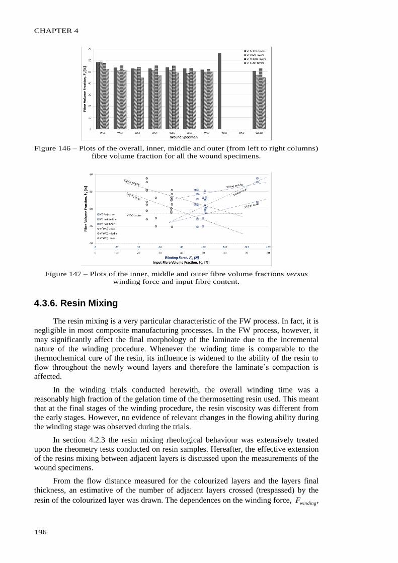
CHAPTER 4
196
Figure 146 – Plots of the overall, inner, middle and outer (from left to right columns)
fibre volume fraction for all the wound specimens.
Figure 147 – Plots of the inner, middle and outer fibre volume fractions versus
winding force and input fibre content.
4.3.6. Resin Mixing
The resin mixing is a very particular characteristic of the FW process. In fact, it is
negligible in most composite manufacturing processes. In the FW process, however, it
may significantly affect the final morphology of the laminate due to the incremental
nature of the winding procedure. Whenever the winding time is comparable to the
thermochemical cure of the resin, its influence is widened to the ability of the resin to
flow throughout the newly wound layers and therefore the laminate’s compaction is
affected.
In the winding trials conducted herewith, the overall winding time was a
reasonably high fraction of the gelation time of the thermosetting resin used. This meant
that at the final stages of the winding procedure, the resin viscosity was different from
the early stages. However, no evidence of relevant changes in the flowing ability during
the winding stage was observed during the trials.
In section 4.2.3 the resin mixing rheological behaviour was extensively treated
upon the rheometry tests conducted on resin samples. Hereafter, the effective extension
of the resins mixing between adjacent layers is discussed upon the measurements of the
wound specimens.
From the flow distance measured for the colourized layers and the layers final
thickness, an estimative of the number of adjacent layers crossed (trespassed) by the
resin of the colourized layer was drawn. The dependences on the winding force, windingF ,
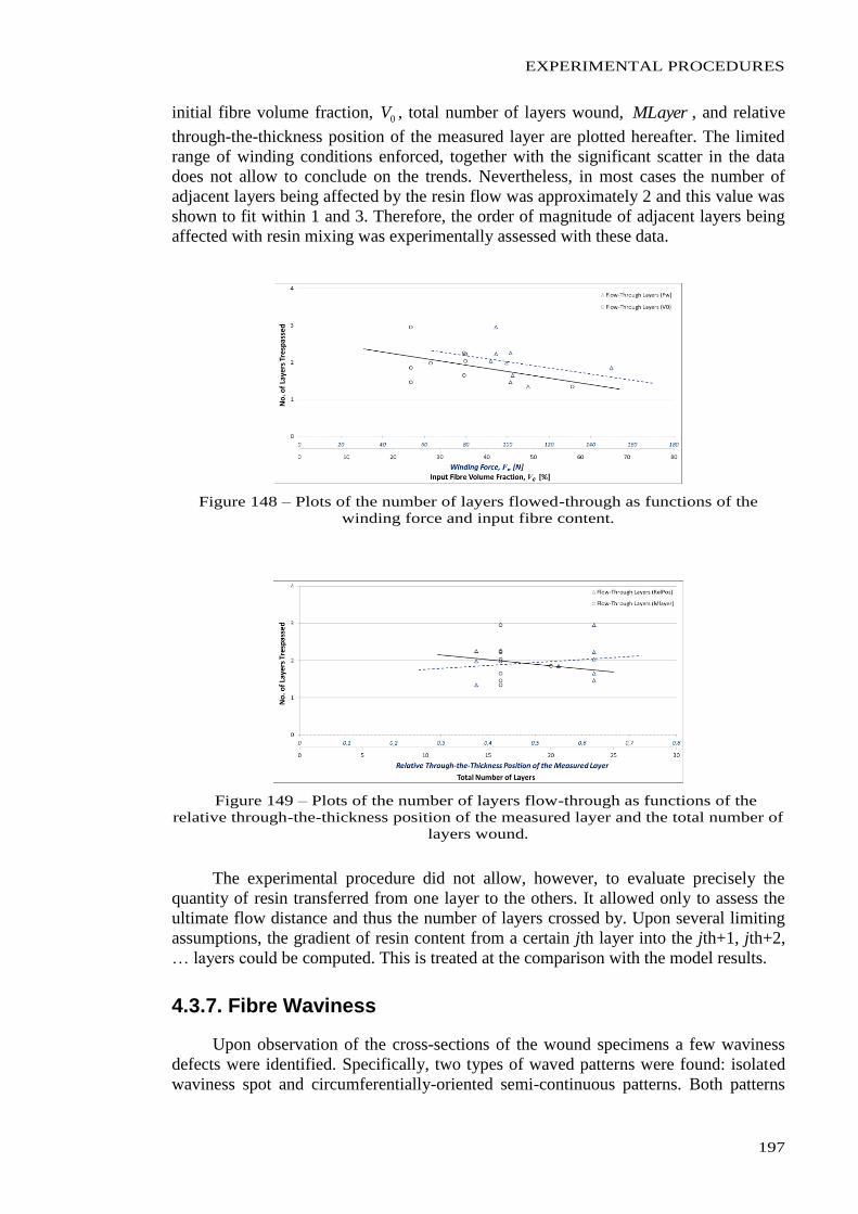
EXPERIMENTAL PROCEDURES
197
initial fibre volume fraction, 0V , total number of layers wound, MLayer , and relative
through-the-thickness position of the measured layer are plotted hereafter. The limited
range of winding conditions enforced, together with the significant scatter in the data
does not allow to conclude on the trends. Nevertheless, in most cases the number of
adjacent layers being affected by the resin flow was approximately 2 and this value was
shown to fit within 1 and 3. Therefore, the order of magnitude of adjacent layers being
affected with resin mixing was experimentally assessed with these data.
Figure 148 – Plots of the number of layers flowed-through as functions of the
winding force and input fibre content.
Figure 149 – Plots of the number of layers flow-through as functions of the
relative through-the-thickness position of the measured layer and the total number of
layers wound.
The experimental procedure did not allow, however, to evaluate precisely the
quantity of resin transferred from one layer to the others. It allowed only to assess the
ultimate flow distance and thus the number of layers crossed by. Upon several limiting
assumptions, the gradient of resin content from a certain jth layer into the jth+1, jth+2,
… layers could be computed. This is treated at the comparison with the model results.
4.3.7. Fibre Waviness
Upon observation of the cross-sections of the wound specimens a few waviness
defects were identified. Specifically, two types of waved patterns were found: isolated
waviness spot and circumferentially-oriented semi-continuous patterns. Both patterns
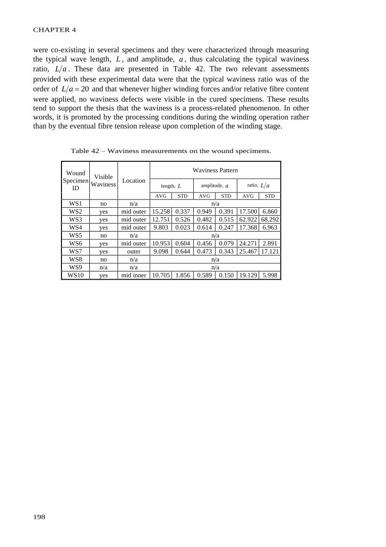
CHAPTER 4
198
were co-existing in several specimens and they were characterized through measuring
the typical wave length, L , and amplitude, a , thus calculating the typical waviness
ratio, aL . These data are presented in Table 42. The two relevant assessments
provided with these experimental data were that the typical waviness ratio was of the
order of 20aL and that whenever higher winding forces and/or relative fibre content
were applied, no waviness defects were visible in the cured specimens. These results
tend to support the thesis that the waviness is a process-related phenomenon. In other
words, it is promoted by the processing conditions during the winding operation rather
than by the eventual fibre tension release upon completion of the winding stage.
Table 42 – Waviness measurements on the wound specimens.
Wound
Specimen
ID
Visible
Waviness Location
Waviness Pattern
length, L amplitude, a ratio, aL
AVG STD AVG STD AVG STD
WS1 no n/a n/a
WS2 yes mid outer 15.258 0.337 0.949 0.391 17.500 6.860
WS3 yes mid outer 12.751 0.526 0.482 0.515 62.922 68.292
WS4 yes mid outer 9.803 0.023 0.614 0.247 17.368 6.963
WS5 no n/a n/a
WS6 yes mid outer 10.953 0.604 0.456 0.079 24.271 2.891
WS7 yes outer 9.098 0.644 0.473 0.343 25.467 17.121
WS8 no n/a n/a
WS9 n/a n/a n/a
WS10 yes mid inner 10.705 1.856 0.589 0.150 19.129 5.998

EXPERIMENTAL PROCEDURES
199
4.4. Remarks
The experimental results achieved gathered extensive and reliable sets of data.
These results globally show the ability to measure most of the main process parameters
and variables. Such level of integration of procedures, covering a wide range of physical
phenomena, from chemo-rheological to mechanical interactions, was not made aware of
by prior authors or publications. Therefore, it substantiates, itself, increments to the
actual state of the art regarding FW and even correlated manufacturing processes.
However, these results per se, do not validate the process model under analysis.
With this aim, a numerical code was devised and several simulations were run, in an
attempt to reproduce pre-selected experimental conditions. This is fully addressed in
next chapter.


CHAPTER 5
NUMERICAL IMPLEMENTATION AND
VALIDATION

CHAPTER 5
202
NUMERICAL IMPLEMENTATION AND VALIDATION
203
5.1. Objectives and Methods
Due to the multi-physical nature of the FW process model developed in this work,
it accounts for various inter-dependent analytical descriptions of physical phenomena.
The inter-dependence arises from the effective coupling of the different sub-processes
modelled by the referred descriptions. Despite the analytical modelling methodology
applied was based on the modular and decoupled study and description of every
particular phenomenon, their real behaviour is obviously coupled by sharing common
variables. Therefore, a numerical code incorporating discretized formulations of the
several phenomena was devised to allow simulating the global process with incremental
evolutions of the variables through their flow and exchange between related
sub-models.
The discretization of the differential equations was mostly achieved by backwards
or forwards finite-difference schemes, accordingly with the domain and the available
data for each specific case. Both spatial and temporal discretizations were operated.
The numerical code built upon these discrete formulations of each physical
phenomenon was structured with as many sub-routines as the sub-models earlier
presented in chapter 3. A root main routine was responsible for the variables flow
between the called sub-routines, as well as for the necessary external updates and formal
actions from the programming view point.
In the following sections the discretization of the main analytical equations and
the overall numerical model scheme are described. Also, sensitivity and compatibility
tests conducted to analyse the modelling abilities of the written code are presented.
Finally, full winding conditions were simulated and the results for the main process
variables were compared with the experimental ones. This last analysis intended to
evaluate the overall validity of the FW process model developed.
CHAPTER 5
204
5.2. Discretization of the Analytical Descriptions
Herewith, the discretizations in the time and/or spatial variables of the analytical
formulations developed are presented. For the analytical equations not explicitly
depending on time and/or spatial variables, as well as those of non-differential form, no
specific discretization procedure was implemented. Only the analytical descriptions
requiring translation to algebraic formulation are treated hereafter. In each sub-process,
highlight is given to the fundamental equations.
5.2.1. Resin Flow Sub-Model
The resin flow modelling was set upon the Darcy’s type equation, and is
substantiated in equation (2.11). It was discretized and numerically implemented in the
form:
r
pS
t
u
, (5.1)
where u is the radial distance flown by the resin during the time increment t , p is
the pressure spatial gradient in the radial position interval r and S and are the
permeability of the fibre bed and the resin viscosity, respectively. For the jth layer, the
incremental discrete formulation to calculate the updated position in instant tt is:
trr
ppSuu
jt
jt
jt
jt
j
jj
tj
tt
1
1
, (5.2)
where the subscripts and superscripts refer to time and layer, respectively.
5.2.2. Fibre Bed Compaction Sub-Model
The main equation settling the compaction of the fibre sheet is equation (3.9)
which was discretized for the jth layer, similarly to the above equation, into:
tr
Suu j
jfs
jf
j
jj
tj
tt
211 sin , (5.3)
where f11 is the fibre’s stress in the local on-axis longitudinal direction, fsr is the radial
position of the fibre sheet and is the winding angle. As in the previous equation, the
subscripts and superscripts refer to time and layer, respectively.
NUMERICAL IMPLEMENTATION AND VALIDATION
205
5.2.3. Heat Transfer Sub-Model
The one-dimensional heat transfer, defined in equation (2.26) was used to calculate
the temperature, T , in the following algebraic form:
tQ
rr
TTT
r
k
CTT m
jj
jjj
j
j
rjt
jtt
21
11 21 , (5.4)
where r is the radial position, and m are is the densities of the composite and
resin, respectively, C is the specific heat of the composite, rk is the thermal
conductivity in radial direction and Q is the rate at which heat is generated by the
curing or crystallizing resin. A central finite-difference scheme was used to discretize
the 2nd
order spatial derivative of the temperature.
The term Qm was defined in equations (2.27) and (2.32) which contain
time-differential 1st order derivatives. These are, however, specifically treated in the
following section.
5.2.4. Resin Cure/Crystallization Sub-Model
The kinetic behaviour of the resins was modelled through analytical descriptions
of the types indicated in equations (3.53) and (3.54). The derivatives of the degree of cure,
dtd , or crystallization, dtcd , are explicit functions of the degree of cure, , or
degree of crystallization, c , respectively, and temperature, T . For the discretization and
calculation of the updated or c the following formulations were set:
tTf ttttt ),( , (5.5)
tTcfcc ttttt ),( , (5.6)
and applied for the dedicated models included in the library for each specific resin
system.

CHAPTER 5
206
5.3. Numerical Code
A numerical code was written to implement the FW process model into a finite
element platform. A VUMAT® user routine coded in FORTRAN® was devised and
applied to an ABAQUS® explicit code. The main root routine was co-structured into
several child sub-routines, each corresponding to a sub-model of the overall process
model developed. A global simplified scheme of the model structure is depicted in
Figure 150. In it, the interactions between the different sub-models are expressed
through the flow of the main process variables. The flow and/or update of the fibre
volume fraction, fV , the radial positions, fsr , the temperature, T , the resin velocity, ru ,
the degree of cure or crystallization, or c , the “chemical” and effective viscosities,
ch and , the stresses, , strains, , and stiffness components, C , are specifically
drawn.
Figure 150 – Overall main scheme of the FW process model.
NUMERICAL IMPLEMENTATION AND VALIDATION
207
5.4. Sensitivity and Compatibility Tests
After setting the numerical code, it was tested under specific inputs in order to
evaluate its sensitivity to pre-determined conditions and qualitative behaviour. In this
section, the first difficulties found at the early debugging tests as well as later
evaluations related with specific flow restrictions are presented.
5.4.1. Early Code Debugging
The first series of numerical tests had the sole objective of early detecting
significant errors in the code and/or programming in order to debug it. Two major
unexpected errors were initially impeding the useful application of the model, and
therefore, are briefly discussed hereafter.
Several unexpected errors occurred in the first testing stages. Namely,
hardware-software incompatibilities (previously unknown) such as the limitation of the
finite elements commercial software used to 32-bit platforms when running explicit
analysis. Several 32-bit platforms were purposely kept during the period of intensive
usage of the first version of the code, in order to guarantee the compatibility with the
required versions of the software. Such drawback is not a problem anymore, since
newer versions of the software released in past two years overcame this limitation.
Other difficulty arose with the existence of very large and very small numbers in the
code. Numerical instabilities were observed and non-systematic errors inhibited the
correct running of the program. This problem was solved by using “double precision”
form which duplicates the bytes available for each variable value allocation.
Complementarily, scaled dummy variables were set to avoid the worst case
combinations. This problem is reported because the multi-physical nature of the process
model favours such numerical instabilities. In fact, by including variables and quantities
of very different nature in the same algorithm, the possibilities of promoting algebraic
operations which encounter both very high and very small numbers increase
substantially. Several other minor errors were successively detected and solved, but
with no relevant relationship with the nature or technical features of the process model.
The two major unexpected errors abovementioned are, however, presented
hereafter, since they represent relevant difficulties associated with the type of model and
numerical program selected.
The first series of tests with the devised code, were carried out with a single finite
element (2D quadrilateral, CPE4 from the ABAQUS® library) subjected to the four
load cases depicted in Figure 151. The aim was to excite different stress and strain
states and evaluate the outputs under such conditions. The first results achieved showed
unexpected and perturbed behaviours. Due to the explicit dependence on time, the
numerical program was devised and used in time-explicit mode. This meant that
eventual dynamic effects should have been attained. The material mechanical properties
defined within the process model, were based on the elastic-apparent properties, i.e., no
viscous or damping properties were considered. The instantaneous application of the
load, generated waved sinusoidal responses. Since no damping properties were known
for the composite material system that could be applied without undesired effects on the
other properties, the problem was solved through applying a smoothing function to the
load. This function, of sigmoidal type, affected the initial stages of the load application,
allowing to achieve the prescribed level of load only after a certain number of time
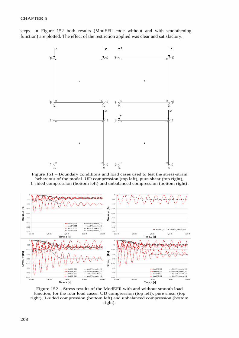
CHAPTER 5
208
steps. In Figure 152 both results (ModEFil code without and with smoothening
function) are plotted. The effect of the restriction applied was clear and satisfactory.
Figure 151 – Boundary conditions and load cases used to test the stress-strain
behaviour of the model. UD compression (top left), pure shear (top right),
1-sided compression (bottom left) and unbalanced compression (bottom right).
Figure 152 – Stress results of the ModEFil with and without smooth load
function, for the four load cases: UD compression (top left), pure shear (top
right), 1-sided compression (bottom left) and unbalanced compression (bottom
right).
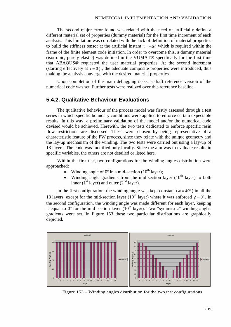
NUMERICAL IMPLEMENTATION AND VALIDATION
209
The second major error found was related with the need of artificially define a
different material set of properties (dummy material) for the first time increment of each
analysis. This limitation was correlated with the lack of definition of material properties
to build the stiffness tensor at the artificial instant tt which is required within the
frame of the finite element code initiation. In order to overcome this, a dummy material
(isotropic, purely elastic) was defined in the VUMAT® specifically for the first time
that ABAQUS® requested the user material properties. At the second increment
(starting effectively at 0t ) , the adequate composite properties were introduced, thus
making the analysis converge with the desired material properties.
Upon completion of the main debugging tasks, a draft reference version of the
numerical code was set. Further tests were realized over this reference baseline.
5.4.2. Qualitative Behaviour Evaluations
The qualitative behaviour of the process model was firstly assessed through a test
series in which specific boundary conditions were applied to enforce certain expectable
results. In this way, a preliminary validation of the model and/or the numerical code
devised would be achieved. Herewith, the two tests dedicated to enforce specific resin
flow restrictions are discussed. These were chosen by being representative of a
characteristic feature of the FW process, since they relate with the unique geometry and
the lay-up mechanism of the winding. The two tests were carried out using a lay-up of
18 layers. The code was modified only locally. Since the aim was to evaluate results in
specific variables, the others are not detailed or listed here.
Within the first test, two configurations for the winding angles distribution were
approached:
Winding angle of 0º in a mid-section (10th
layer);
Winding angle gradients from the mid-section layer (10th
layer) to both
inner (1st layer) and outer (2
nd layer).
In the first configuration, the winding angle was kept constant ( º40 ) in all the
18 layers, except for the mid-section layer (10th
layer) where it was enforced º0 . In
the second configuration, the winding angle was made different for each layer, keeping
it equal to 0º for the mid-section layer (10th
layer). Two “symmetric” winding angles
gradients were set. In Figure 153 these two particular distributions are graphically
depicted.
WINANG
0
10
20
30
40
1 2 3 4 5 6 7 8 9 10 11 12 13 14 15 16 17 18
Ilayer
Win
din
g A
ng
le [
º]
WINANG
WINANG
0
10
20
30
40
50
60
70
80
90
1 2 3 4 5 6 7 8 9 10 11 12 13 14 15 16 17 18
Ilayer
Win
din
g A
ng
le [
º]
WINANG
Figure 153 – Winding angles distribution for the two test configurations.
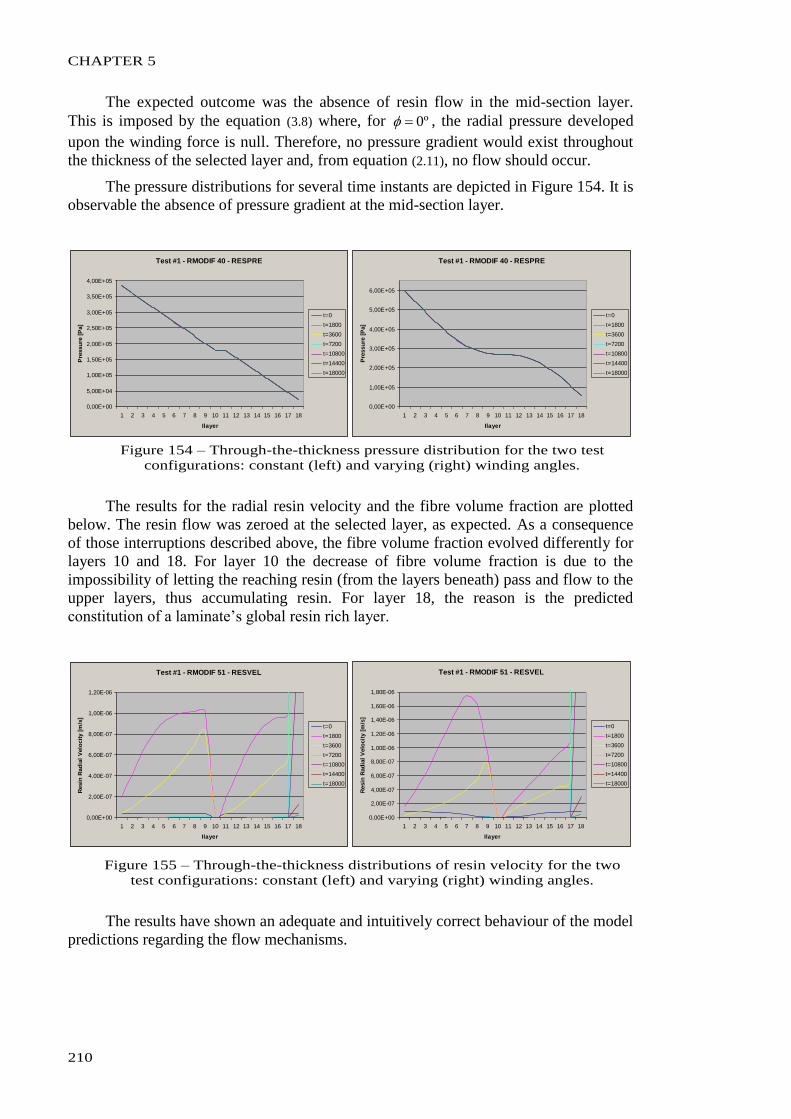
CHAPTER 5
210
The expected outcome was the absence of resin flow in the mid-section layer.
This is imposed by the equation (3.8) where, for º0 , the radial pressure developed
upon the winding force is null. Therefore, no pressure gradient would exist throughout
the thickness of the selected layer and, from equation (2.11), no flow should occur.
The pressure distributions for several time instants are depicted in Figure 154. It is
observable the absence of pressure gradient at the mid-section layer.
Test #1 - RMODIF 40 - RESPRE
0,00E+00
5,00E+04
1,00E+05
1,50E+05
2,00E+05
2,50E+05
3,00E+05
3,50E+05
4,00E+05
1 2 3 4 5 6 7 8 9 10 11 12 13 14 15 16 17 18
Ilayer
Pre
ssu
re [
Pa]
t=0
t=1800
t=3600
t=7200
t=10800
t=14400
t=18000
Test #1 - RMODIF 40 - RESPRE
0,00E+00
1,00E+05
2,00E+05
3,00E+05
4,00E+05
5,00E+05
6,00E+05
1 2 3 4 5 6 7 8 9 10 11 12 13 14 15 16 17 18
Ilayer
Pre
ssu
re [
Pa]
t=0
t=1800
t=3600
t=7200
t=10800
t=14400
t=18000
Figure 154 – Through-the-thickness pressure distribution for the two test
configurations: constant (left) and varying (right) winding angles.
The results for the radial resin velocity and the fibre volume fraction are plotted
below. The resin flow was zeroed at the selected layer, as expected. As a consequence
of those interruptions described above, the fibre volume fraction evolved differently for
layers 10 and 18. For layer 10 the decrease of fibre volume fraction is due to the
impossibility of letting the reaching resin (from the layers beneath) pass and flow to the
upper layers, thus accumulating resin. For layer 18, the reason is the predicted
constitution of a laminate’s global resin rich layer.
Test #1 - RMODIF 51 - RESVEL
0,00E+00
2,00E-07
4,00E-07
6,00E-07
8,00E-07
1,00E-06
1,20E-06
1 2 3 4 5 6 7 8 9 10 11 12 13 14 15 16 17 18
Ilayer
Resin
Rad
ial
Velo
cit
y [
m/s
]
t=0
t=1800
t=3600
t=7200
t=10800
t=14400
t=18000
Test #1 - RMODIF 51 - RESVEL
0,00E+00
2,00E-07
4,00E-07
6,00E-07
8,00E-07
1,00E-06
1,20E-06
1,40E-06
1,60E-06
1,80E-06
1 2 3 4 5 6 7 8 9 10 11 12 13 14 15 16 17 18
Ilayer
Resin
Rad
ial
Velo
cit
y [
m/s
]
t=0
t=1800
t=3600
t=7200
t=10800
t=14400
t=18000
Figure 155 – Through-the-thickness distributions of resin velocity for the two
test configurations: constant (left) and varying (right) winding angles.
The results have shown an adequate and intuitively correct behaviour of the model
predictions regarding the flow mechanisms.
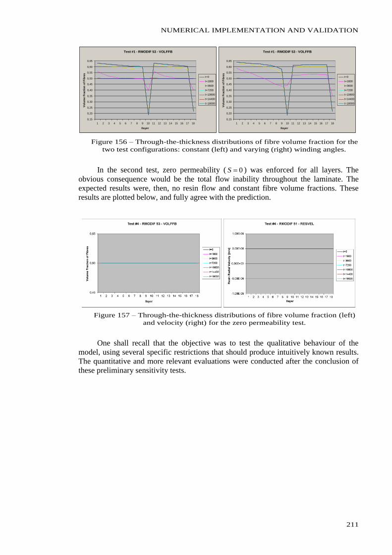
NUMERICAL IMPLEMENTATION AND VALIDATION
211
Test #1 - RMODIF 53 - VOLFFB
0,15
0,20
0,25
0,30
0,35
0,40
0,45
0,50
0,55
0,60
0,65
1 2 3 4 5 6 7 8 9 10 11 12 13 14 15 16 17 18
Ilayer
Vo
lum
e F
racti
on
of
Fib
res
t=0
t=1800
t=3600
t=7200
t=10800
t=14400
t=18000
Test #1 - RMODIF 53 - VOLFFB
0,15
0,20
0,25
0,30
0,35
0,40
0,45
0,50
0,55
0,60
0,65
1 2 3 4 5 6 7 8 9 10 11 12 13 14 15 16 17 18
Ilayer
Vo
lum
e F
racti
on
of
Fib
res
t=0
t=1800
t=3600
t=7200
t=10800
t=14400
t=18000
Figure 156 – Through-the-thickness distributions of fibre volume fraction for the
two test configurations: constant (left) and varying (right) winding angles.
In the second test, zero permeability ( 0S ) was enforced for all layers. The
obvious consequence would be the total flow inability throughout the laminate. The
expected results were, then, no resin flow and constant fibre volume fractions. These
results are plotted below, and fully agree with the prediction.
Figure 157 – Through-the-thickness distributions of fibre volume fraction (left)
and velocity (right) for the zero permeability test.
One shall recall that the objective was to test the qualitative behaviour of the
model, using several specific restrictions that should produce intuitively known results.
The quantitative and more relevant evaluations were conducted after the conclusion of
these preliminary sensitivity tests.
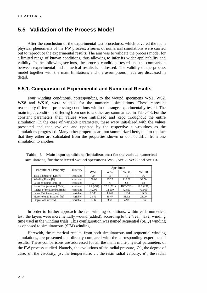
CHAPTER 5
212
5.5 Validation of the Process Model
After the conclusion of the experimental test procedures, which covered the main
physical phenomena of the FW process, a series of numerical simulations were carried
out to reproduce the experimental results. The aim was to validate the process model for
a limited range of known conditions, thus allowing to infer its wider applicability and
validity. In the following sections, the process conditions tested and the comparison
between experimental and numerical results is addressed. The validity of the process
model together with the main limitations and the assumptions made are discussed in
detail.
5.5.1. Comparison of Experimental and Numerical Results
Four winding conditions, corresponding to the wound specimens WS1, WS2,
WS8 and WS10, were selected for the numerical simulations. These represent
reasonably different processing conditions within the range experimentally tested. The
main input conditions differing from one to another are summarized in Table 43. For the
constant parameters their values were initialized and kept throughout the entire
simulation. In the case of variable parameters, these were initialized with the values
presented and then evolved and updated by the respective sub-routines as the
simulations progressed. Many other properties are not summarized here, due to the fact
that they either are calculated from the properties shown or do not differ from one
simulation to another.
Table 43 – Main input conditions (initializations) for the various numerical
simulations, for the selected wound specimens WS1, WS2, WS8 and WS10.
Parameter / Property History Specimen
WS1 WS2 WS8 WS10 Total Number of Layers constant 20 16 16 16
Winding Force [N] constant 150.00 93.25 110.00 99.50
Layer Winding Time [s] constant 97 79 68 68
Room Temperature [ºC (K)] constant 17.7 (291) 17.5 (291) 18.2 (291) 18.2 (291)
Radius of the Mandrel [mm] constant 74.006 72.600 72.863 70.663
Layer Thickness [mm] variable 1.580 1.449 1.194 1.533
Fibre Volume Fraction [%] variable 23.79 35.47 58.32 28.00
Degree of Cure [%] variable 3.86 3.58 4.93 3.56
In order to further approach the real winding conditions, within each numerical
test, the layers were incrementally wound (added), according to the “real” layer winding
time used in the winding trials. This configuration was named sequential (SEQ) winding
as opposed to simultaneous (SIM) winding.
Herewith, the numerical results, from both simultaneous and sequential winding
simulations, are presented and directly compared with the corresponding experimental
results. These comparisons are addressed for all the main multi-physical parameters of
the FW process studied. Namely, the evolutions of the radial pressure, rP , the degree of
cure, , the viscosity, , the temperature, T , the resin radial velocity, ru , the radial
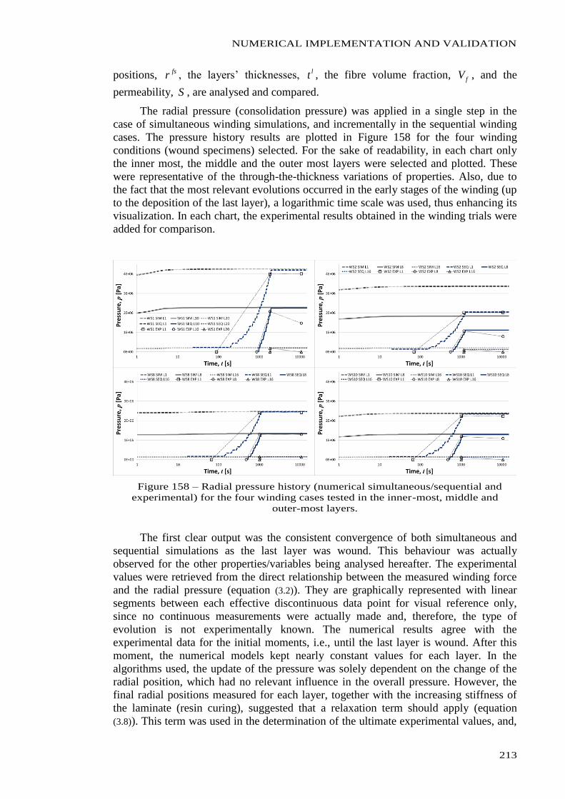
NUMERICAL IMPLEMENTATION AND VALIDATION
213
positions, fsr , the layers’ thicknesses, lt , the fibre volume fraction, fV , and the
permeability, S , are analysed and compared.
The radial pressure (consolidation pressure) was applied in a single step in the
case of simultaneous winding simulations, and incrementally in the sequential winding
cases. The pressure history results are plotted in Figure 158 for the four winding
conditions (wound specimens) selected. For the sake of readability, in each chart only
the inner most, the middle and the outer most layers were selected and plotted. These
were representative of the through-the-thickness variations of properties. Also, due to
the fact that the most relevant evolutions occurred in the early stages of the winding (up
to the deposition of the last layer), a logarithmic time scale was used, thus enhancing its
visualization. In each chart, the experimental results obtained in the winding trials were
added for comparison.
Figure 158 – Radial pressure history (numerical simultaneous/sequential and
experimental) for the four winding cases tested in the inner-most, middle and
outer-most layers.
The first clear output was the consistent convergence of both simultaneous and
sequential simulations as the last layer was wound. This behaviour was actually
observed for the other properties/variables being analysed hereafter. The experimental
values were retrieved from the direct relationship between the measured winding force
and the radial pressure (equation (3.2)). They are graphically represented with linear
segments between each effective discontinuous data point for visual reference only,
since no continuous measurements were actually made and, therefore, the type of
evolution is not experimentally known. The numerical results agree with the
experimental data for the initial moments, i.e., until the last layer is wound. After this
moment, the numerical models kept nearly constant values for each layer. In the
algorithms used, the update of the pressure was solely dependent on the change of the
radial position, which had no relevant influence in the overall pressure. However, the
final radial positions measured for each layer, together with the increasing stiffness of
the laminate (resin curing), suggested that a relaxation term should apply (equation
(3.8)). This term was used in the determination of the ultimate experimental values, and,
CHAPTER 5
214
as one can see, they diverge after the initial agreement. Exception was noted for the
WS8 case, since in this case no inward movement of layers was observed, and therefore,
no relaxation occurred as well. In this latter condition, the numerical models fully agree
with experimental data for the entire time range (even after all layers’ deposition).
The degree of cure, , had a particular condition to be accounted in its
initialization. In fact, the initial extent of cure, i.e., the cure state at the first
deposition/winding time, varied from layer to layer since all were wound/deposited at
different times. The different values for every layer were found through linearly
interpolating the estimated )(t curve at room temperature, for the corresponding
winding times (multiples of the unitary layer winding time). The linear relations
achieved for the determinations of each layer’s initial degree of cure, ilayer
0 , were
written as:
bilayerailayer 0 , (5.7)
where ilayer is the layer being attributed an initial value and a and b are constants.
These constants are listed in Table 44 for the four selected simulation cases.
Table 44 – Values for the constants a and b in the linear relation determining the
initial degree of cure for each layer within the laminate being wound and simulated.
Wound
Specimen
constant
a b WS1 0.00289 0.03568
WS2 0.00235 0.03342
WS8 0.00202 0.04729
WS10 0.00202 0.03354
The evolutions of the degree of cure in the four winding cases are plotted in
Figure 159. The numerical simultaneous and sequential windings are directly compared
with the experimentally estimated )(t curve at room temperature. This estimation was
achieved by exponentially extrapolating to the applicable room temperature the
experimental curves obtained for six samples tested in DSC at three higher temperatures
(303K, 313K and 323K).
From the plots one can observe that the different layers tend to a common final
degree of cure and that the simultaneous winding simulations lasted longer, as expected,
to converge with the experimental curves. In fact, in the simultaneous winding
simulations, the initial degree of cure of all layers except the first one (inner-most) were
“artificially” set at 0t instead at the moment of each one’s winding. In all the cases,
an initial overestimation and final underestimation of the expected degree of cure by the
numerical models were found. Nevertheless, since the experimental data was estimated
by a different method than the kinetic model equation developed for this resin and
implemented in the numerical code, and also that the effective temperatures experienced
during the winding and curing stages were non-isothermal, the numerical and
experimental results can only be qualitatively compared. Such qualitative comparison
shows reasonable agreement for the relevant time domain. The differences observed
from intermediate degree of cure onwards are justified later in the discussion of similar
behaviours for other variables.
NUMERICAL IMPLEMENTATION AND VALIDATION
215
Figure 159 – Evolutions of the degree of cure (numerical simultaneous/sequential
and experimental) for the four winding cases tested in inner-most, middle and
outer-most layers.
Similarly to the degree of cure, also the initial viscosities of the several layers at
their deposition/winding time are expectedly different, since ),( Tf . However,
these were not initialized in the same way of , because the model calculates
viscosities in a sub-sequent sub-routine. The specificity of the viscosity sub-model is
that it accounts for the possibility of mixture of resins from adjacent layers. This is a
major aspect of the FW process governed by the outward resin flow as discussed in
previous chapters. Therefore, two resin histories were written and analysed: the
so-called “chemical” viscosity, ch , which corresponds to the plain evolution of the
viscosity without external mixing effects, and the effective viscosity, , resulting from
eventual mixings. The “chemical” viscosities are plotted in Figure 160 where they are
also compared with the experimental curves obtained with neat (unmixed) resin at the
nearest possible temperature (303K). In Figure 161 the effective viscosities are plotted.
Since the range of viscosities experienced by the resin is very wide, and that, again, the
main mixing events occurred in early stages of the process, log-log scales are used for
better visualization.
Despite differences were observed between “chemical” and effective viscosity
numerical data, these were minimal. This was mainly due to the fact that the viscosities
of the adjacent layers exchanging resin, through its flow, were very similar. In other
words, the resins being mixed were very similar (similar degrees of cure and viscosities)
and no relevant mixing effects were visible in these four cases selected. Longer winding
times would need to be implemented to allow observing stronger mixing effects.
Under these conditions, the main physical factor influencing the evolution of
viscosity, a part from time, was the temperature. This is the reason why the “chemical”
viscosities of the layers being wound later were also affected at the early stages of their
winding. Heat transfer with the layers beneath promoted sudden increase of temperature
and consequent variations of viscosity at and immediately after the deposition of each
layer. This was particularly observable in the WS1 case at the outer-most layer.
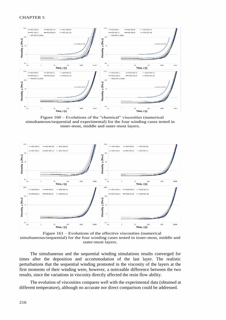
CHAPTER 5
216
Figure 160 – Evolutions of the “chemical” viscosities (numerical
simultaneous/sequential and experimental) for the four winding cases tested in
inner-most, middle and outer-most layers.
Figure 161 – Evolutions of the effective viscosities (numerical
simultaneous/sequential) for the four winding cases tested in inner-most, middle and
outer-most layers.
The simultaneous and the sequential winding simulations results converged for
times after the deposition and accommodation of the last layer. The realistic
perturbations that the sequential winding promoted in the viscosity of the layers at the
first moments of their winding were, however, a noticeable difference between the two
results, since the variations in viscosity directly affected the resin flow ability.
The evolution of viscosities compares well with the experimental data (obtained at
different temperature), although no accurate nor direct comparison could be addressed.
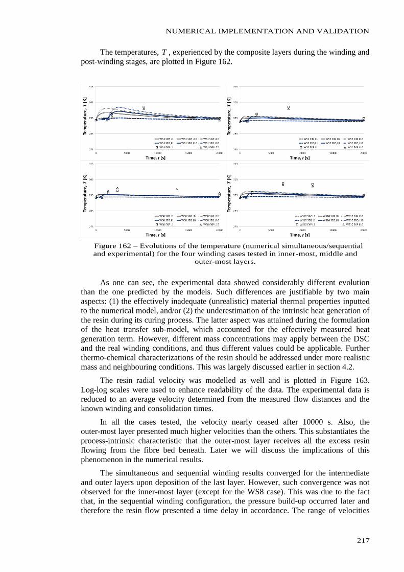
NUMERICAL IMPLEMENTATION AND VALIDATION
217
The temperatures, T , experienced by the composite layers during the winding and
post-winding stages, are plotted in Figure 162.
Figure 162 – Evolutions of the temperature (numerical simultaneous/sequential
and experimental) for the four winding cases tested in inner-most, middle and
outer-most layers.
As one can see, the experimental data showed considerably different evolution
than the one predicted by the models. Such differences are justifiable by two main
aspects: (1) the effectively inadequate (unrealistic) material thermal properties inputted
to the numerical model, and/or (2) the underestimation of the intrinsic heat generation of
the resin during its curing process. The latter aspect was attained during the formulation
of the heat transfer sub-model, which accounted for the effectively measured heat
generation term. However, different mass concentrations may apply between the DSC
and the real winding conditions, and thus different values could be applicable. Further
thermo-chemical characterizations of the resin should be addressed under more realistic
mass and neighbouring conditions. This was largely discussed earlier in section 4.2.
The resin radial velocity was modelled as well and is plotted in Figure 163.
Log-log scales were used to enhance readability of the data. The experimental data is
reduced to an average velocity determined from the measured flow distances and the
known winding and consolidation times.
In all the cases tested, the velocity nearly ceased after 10000 s. Also, the
outer-most layer presented much higher velocities than the others. This substantiates the
process-intrinsic characteristic that the outer-most layer receives all the excess resin
flowing from the fibre bed beneath. Later we will discuss the implications of this
phenomenon in the numerical results.
The simultaneous and sequential winding results converged for the intermediate
and outer layers upon deposition of the last layer. However, such convergence was not
observed for the inner-most layer (except for the WS8 case). This was due to the fact
that, in the sequential winding configuration, the pressure build-up occurred later and
therefore the resin flow presented a time delay in accordance. The range of velocities
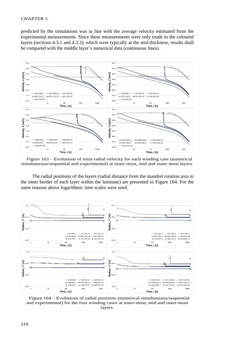
CHAPTER 5
218
predicted by the simulations was in line with the average velocity estimated from the
experimental measurements. Since these measurements were only made in the coloured
layers (sections 4.3.1 and 4.3.3), which were typically at the mid-thickness, results shall
be compared with the middle layer’s numerical data (continuous lines).
Figure 163 – Evolutions of resin radial velocity for each winding case (numerical
simultaneous/sequential and experimental) at inner-most, mid and outer-most layers.
The radial positions of the layers (radial distance from the mandrel rotation axis to
the inner border of each layer within the laminate) are presented in Figure 164. For the
same reasons above logarithmic time scales were used.
Figure 164 – Evolutions of radial positions (numerical simultaneous/sequential
and experimental) for the four winding cases at inner-most, mid and outer-most
layers.
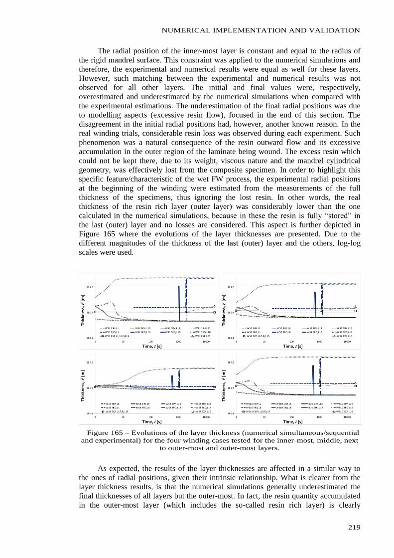
NUMERICAL IMPLEMENTATION AND VALIDATION
219
The radial position of the inner-most layer is constant and equal to the radius of
the rigid mandrel surface. This constraint was applied to the numerical simulations and
therefore, the experimental and numerical results were equal as well for these layers.
However, such matching between the experimental and numerical results was not
observed for all other layers. The initial and final values were, respectively,
overestimated and underestimated by the numerical simulations when compared with
the experimental estimations. The underestimation of the final radial positions was due
to modelling aspects (excessive resin flow), focused in the end of this section. The
disagreement in the initial radial positions had, however, another known reason. In the
real winding trials, considerable resin loss was observed during each experiment. Such
phenomenon was a natural consequence of the resin outward flow and its excessive
accumulation in the outer region of the laminate being wound. The excess resin which
could not be kept there, due to its weight, viscous nature and the mandrel cylindrical
geometry, was effectively lost from the composite specimen. In order to highlight this
specific feature/characteristic of the wet FW process, the experimental radial positions
at the beginning of the winding were estimated from the measurements of the full
thickness of the specimens, thus ignoring the lost resin. In other words, the real
thickness of the resin rich layer (outer layer) was considerably lower than the one
calculated in the numerical simulations, because in these the resin is fully “stored” in
the last (outer) layer and no losses are considered. This aspect is further depicted in
Figure 165 where the evolutions of the layer thicknesses are presented. Due to the
different magnitudes of the thickness of the last (outer) layer and the others, log-log
scales were used.
Figure 165 – Evolutions of the layer thickness (numerical simultaneous/sequential
and experimental) for the four winding cases tested for the inner-most, middle, next
to outer-most and outer-most layers.
As expected, the results of the layer thicknesses are affected in a similar way to
the ones of radial positions, given their intrinsic relationship. What is clearer from the
layer thickness results, is that the numerical simulations generally underestimated the
final thicknesses of all layers but the outer-most. In fact, the resin quantity accumulated
in the outer-most layer (which includes the so-called resin rich layer) is clearly
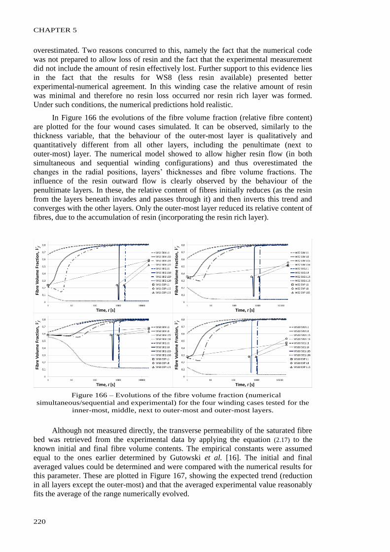
CHAPTER 5
220
overestimated. Two reasons concurred to this, namely the fact that the numerical code
was not prepared to allow loss of resin and the fact that the experimental measurement
did not include the amount of resin effectively lost. Further support to this evidence lies
in the fact that the results for WS8 (less resin available) presented better
experimental-numerical agreement. In this winding case the relative amount of resin
was minimal and therefore no resin loss occurred nor resin rich layer was formed.
Under such conditions, the numerical predictions hold realistic.
In Figure 166 the evolutions of the fibre volume fraction (relative fibre content)
are plotted for the four wound cases simulated. It can be observed, similarly to the
thickness variable, that the behaviour of the outer-most layer is qualitatively and
quantitatively different from all other layers, including the penultimate (next to
outer-most) layer. The numerical model showed to allow higher resin flow (in both
simultaneous and sequential winding configurations) and thus overestimated the
changes in the radial positions, layers’ thicknesses and fibre volume fractions. The
influence of the resin outward flow is clearly observed by the behaviour of the
penultimate layers. In these, the relative content of fibres initially reduces (as the resin
from the layers beneath invades and passes through it) and then inverts this trend and
converges with the other layers. Only the outer-most layer reduced its relative content of
fibres, due to the accumulation of resin (incorporating the resin rich layer).
Figure 166 – Evolutions of the fibre volume fraction (numerical
simultaneous/sequential and experimental) for the four winding cases tested for the
inner-most, middle, next to outer-most and outer-most layers.
Although not measured directly, the transverse permeability of the saturated fibre
bed was retrieved from the experimental data by applying the equation (2.17) to the
known initial and final fibre volume contents. The empirical constants were assumed
equal to the ones earlier determined by Gutowski et al. [16]. The initial and final
averaged values could be determined and were compared with the numerical results for
this parameter. These are plotted in Figure 167, showing the expected trend (reduction
in all layers except the outer-most) and that the averaged experimental value reasonably
fits the average of the range numerically evolved.
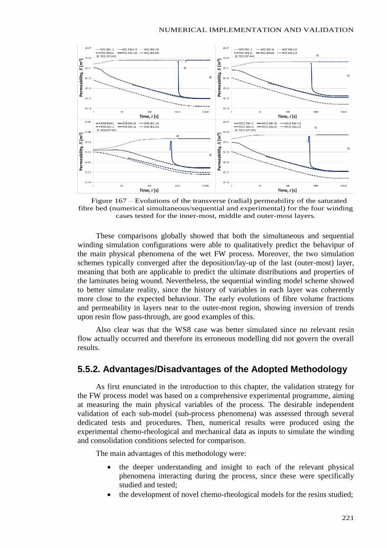
NUMERICAL IMPLEMENTATION AND VALIDATION
221
Figure 167 – Evolutions of the transverse (radial) permeability of the saturated
fibre bed (numerical simultaneous/sequential and experimental) for the four winding
cases tested for the inner-most, middle and outer-most layers.
These comparisons globally showed that both the simultaneous and sequential
winding simulation configurations were able to qualitatively predict the behavipur of
the main physical phenomena of the wet FW process. Moreover, the two simulation
schemes typically converged after the deposition/lay-up of the last (outer-most) layer,
meaning that both are applicable to predict the ultimate distributions and properties of
the laminates being wound. Nevertheless, the sequential winding model scheme showed
to better simulate reality, since the history of variables in each layer was coherently
more close to the expected behaviour. The early evolutions of fibre volume fractions
and permeability in layers near to the outer-most region, showing inversion of trends
upon resin flow pass-through, are good examples of this.
Also clear was that the WS8 case was better simulated since no relevant resin
flow actually occurred and therefore its erroneous modelling did not govern the overall
results.
5.5.2. Advantages/Disadvantages of the Adopted Methodology
As first enunciated in the introduction to this chapter, the validation strategy for
the FW process model was based on a comprehensive experimental programme, aiming
at measuring the main physical variables of the process. The desirable independent
validation of each sub-model (sub-process phenomena) was assessed through several
dedicated tests and procedures. Then, numerical results were produced using the
experimental chemo-rheological and mechanical data as inputs to simulate the winding
and consolidation conditions selected for comparison.
The main advantages of this methodology were:
the deeper understanding and insight to each of the relevant physical
phenomena interacting during the process, since these were specifically
studied and tested;
the development of novel chemo-rheological models for the resins studied;
CHAPTER 5
222
the understanding of main physical phenomena which are also present in
other composites manufacturing process;
the possibility of identifying the cause-effects relations between the
various parameters (process- and material-intrinsic) and their influence at a
greater detail level, due to the restricted ambit of each sub-model and
corresponding tests/measurements;
the comprehensive evaluation of the process modelling analytical
descriptions, by adding reliable experimental data for the analysis.
As for the disadvantages, the main were:
the pronounced variety of different physical phenomena being studied
independently, not allowing to deepen each one as desirable for greater
understanding and/or accuracy in the parametric analyses;
the absence of a dedicated strategy for the experimental validation of the
stress-strain relations, due to the inherent difficulty in assessing these
quantities during the process;
the difficulties in assessing the history of the main process variables, being
only discretely assessed at the initial and final conditions;
the need for estimation of some input quantities, such as the initial layer’s
thickness, due to the mentioned difficulty in assessing or measuring these
at the winding location, during the winding trials.
The approach drawn was, nevertheless, unique, comprehensive and proved to
allow achieving very useful and even innovative results, thus enhancing its validity.
5.5.3. Assumptions and Limitations
Two major weaknesses were highlighted throughout the comparison of the
numerical and experimental results: no stress-strain measurements were carried out that
could compare and/or validate the model predictions/assumptions and no pressure
release term was included in the numerical runs (despite analytically modelled in
chapter 3). The former limitation was due to the lack of experimental means to measure
stresses and/or strains accurately at local level during the process. These specific
measurements were not included in the experimental campaigns, since their complexity
justified a dedicated and deep specific study. The latter was specifically detected in
Figure 158, where the numerical results suggested a constant pressure level in every
layer after lay-up of the last one, which both experience and experimental evidence
opposed. The pressure release is effectively present in the FW process, since the inward
displacement of the layers (upon the resin outward flow) lead to a gradual decrease of
the circumferential tension promoted by the winding force. Nevertheless, this effect was
included in the process model (chapter 3) and was also treated in the chapter 4 along
with the experimental pressure estimations.
The main assumptions and limitations of the process model itself have been
focused in previous chapters.
5.5.4. Process Model Validity
The validity of the multi-physical model developed to represent the FW process
was assessed through comparison of experimental and numerical data for selected
NUMERICAL IMPLEMENTATION AND VALIDATION
223
winding conditions. This validity was analysed both in general and specific terms, i.e.,
both the global ability to model the overall evolutions of the main physical variables
and the particular results of each group of phenomena were observed.
As shown by the experimental-numerical comparisons, the evolutions of the main
process variables were qualitatively correct. In other words, the trends were logical and
correspondent with the observed reality. Furthermore, the predictions of the final states
of the main parameters reasonably agreed with the experimental data. The possibility of
replicating the real incremental nature of the lay-up mechanism further enhanced the
model ability and utility.
The two exceptions to the accurate predictions were the predictions of the
temperature and the resin flow history, which disagreed from the experimental
evidence. The former did not produce any relevant influence in the remaining results,
since the interval of temperatures experienced was nearly negligible in both numerical
and experimental tests. Nearly isothermal conditions could apply. The latter, however,
propagated severe influence on the other outputs, like radial positions, thicknesses, fibre
volume fractions and permeability of the layers. It is easy to observe that the
overestimation of the resin flow, in both magnitude and time duration, affected the
global results for all cases where this parameter governed the consolidation. This was
the case of WS1, WS2 and WS10 in which the high relative amount of resin available to
flow promoted such predominance. As referred previously, in WS8 the flow conditions
were minimal and thus the overall results returned correct and realistic. Based on the
Darcy’s type flow formulation, the analytical and numerical descriptions of the resin
flow, settled by equations (2.11) and (5.2), respectively, depended on the pressure
gradient, the resin viscosity and the permeability of the saturated media. Since the
pressure gradients and the resin viscosity were independently validated by the
experimental results, the factor influencing the flow behaviour seemed to be the
apparent permeability. This parameter is itself modelled as a function of the fibre
volume fraction and “external” empirical constants, by equation (2.17). Since the
evolution of the fibre volume fraction is directly dependent of the permeability and
consequent flow (the multi-physical phenomena are actually coupled), the reasonable
improvements to promote were on those empirical constants. These should be
determined by dedicated permeability tests, which are documented in literature and
were reviewed in chapter 2. Due to the limited time and resources, these tests were not
programmed and therefore, this improvement was not addressed. The alternative of
“adjust” the constants value until numerical and experimental results would match was
not addressed as well, due to the main universal principle that governed this study: all
the data used as inputs to the model were either collected experimentally within this
study or retrieved from consensual and consolidated studies from other authors. This
principle was justified by the objective of keeping high control of the sub-processes
modelling and model-reality close relations throughout the model development and
testing phases. The quality of the results achieved hold this principle successfully
accomplished.


CHAPTER 6
CONCLUSIONS

CHAPTER 6
226
CONCLUSIONS
227
6.1. Objectives vs Results
The work conducted and presented throughout this thesis was structured in view
of accomplishing the several objectives initially drawn. These were briefly identified in
chapter 1 and detailed in chapters 3 and 5, along with the analytical modelling and
validation discussions, respectively. The principal objective of developing and
validating a multi-physical process model for the FW manufacturing process was
further complemented with partial objectives during the realization of the work. These
aimed at addressing specific aspects of the manufacturing technique, thus increasing the
depth and utility of the study itself.
In brief, the main objectives established were the following:
Develop and validate a global FW process model;
Comprise both thermosetting and thermoplastic process configurations;
Model the effect of manufacturing features intrinsically related to FW:
o through-the-thickness gradients on pressure, flow and stiffness;
o misaligned pattern of the fibres at lay-up and compaction;
o incremental lay-up;
Develop experimental procedures for the measurement of main process
parameters and input/output variables;
Analyse and evaluate the model through parametric tests;
Foresee wider and useful applications of the process model to several
configurations of FW and/or to other FW-related techniques.
From chapters 2 to 5 the pursuing of these objectives was described in detail
through a comprehensive identification of the “problems”, proposition of both methods
and solutions, and their validation.
Despite several modifications were introduced in the course of the work, the main
scope and aims were kept and drove the decisions made. Such modifications mostly
referred to difficulties encountered to strictly fulfil the initial plan. Namely, the early
difficulties in establishing fully functional draft version of the numerical code, the lack
of validated data in literature to produce complete comparisons of the model, the need
of introducing and anticipating the chemo-rheological experimental program to develop
reliable input sub-models and the unmanageable logistics to set an experimental
program dedicated to the stresses and strains online measurements. Nevertheless, the
objectives listed above remained referential to evaluate the results achieved. Also, the
accuracy and applicability of the model can be discussed. This evaluation is addressed
next, point by point.
Development and Validation of Global FW Process Model
This main objective was early accomplished, since the analytical descriptive
sub-models dealing with the several physical phenomena identified as crucial within the
process, were developed in the first stage of the study. The validation, however, was
only concluded much later, with the comparisons of the experimental and numerical
results.
The validation was not fully accomplished as initially planned, due to the
remarkable difficulties in operating in-situ measurements of strains (and/or stresses)
CHAPTER 6
228
during the FW process. These were not included in the experimental program
becoming, in fact, the main weakness on the model validation produced. The
stress-strain sub-model was not directly validated through dedicated experiments, but
rather only through the overall analysis of the consistency of the results. This
sub-model, in particular, remains as a proposed approach. All the other relevant
sub-processes were validated through either dedicated experimental measurements and
tests or comparison with previously published models.
Nonetheless, the results achieved have shown the ability of the process model to
predict the behaviour of the main input/output variables and parameters, meaning that it
covered the essential physics of the manufacturing processes. This statement is
supported by the fact that no relevant parameter was identified during the “real”
winding trials that was not included in the model. Even the options of not including the
mandrel thermo-mechanical effects or the possibility of voids formation became
partially validated by the consistency of the results.
The results achieved, allow to conclude for the successful accomplishment of the
main objective initially drawn.
Inclusion of Both Thermosetting and Thermoplastic Process Configurations
This objective was established in order to enhance the utility of the present model.
It arose from several evidences: there is an increasing trend to use thermoplastic
matrices; there are almost no process models dealing with thermoplastics; many
industrial facilities are capable of using both thermosetting (wet or prepreg) and
thermoplastic (prepreg) FW process configurations.
In order to attain this key objective, the model was developed in a modular way.
The two advantages envisaged were the possibility of developing decoupled
sub-models, easy to study and improve independently, and the possibility of using the
same model for either thermosetting or thermoplastic resins, by simply adapting the
thermo-chemical sub-models (heat transfer, resin cure/crystallization and resin
viscosity). Through the correct definition of the input parameters, the model was able to
consider both process configurations. This objective was, thus, successfully achieved.
Model the Effect of FW Intrinsic Manufacturing Features
Among the composites manufacturing techniques, FW presents unique features
and specificities which required special attention. The three identified (listed above)
were the incremental nature of the winding lay-up, the gradients developed across the
laminate’s thickness and the twisted/waved pattern of the fibres roving fed onto the
laminate. These characteristic features were explicitly modelled.
The discrete and incremental building of the laminate (winding lay-up) was
attained in the numerical implementation of the process model, since the analytical
descriptions were kept generic. The results have shown the specific influence of this
phenomenon in several outputs.
The gradients across the laminate’s thickness formed naturally upon the correct
definitions of the correlated parameters and/or process variables. Namely, the pressure
gradients generated flow gradients. These produced, in the end, through-the-thickness
CONCLUSIONS
229
gradients of fibre relative contents, and, thus, stiffnesses. This is, in fact, one major
output of the current model.
The misaligned patterns of the fibres were modelled, through assuming sinusoidal
paths and including these in the determination of the stress-strain constitutive relations.
In fact, the constitutive stiffness matrix for each material point was calculated from
wave-transforming the local on-axis stiffness matrix components. These were then
averaged for one wavelength. In this way, the waved orientation of the fibres was
modelled and coherently affected the stress-strain states. The possibility of no-waviness
was considered as well, thus making the stress-strain descriptions universal. The
existence and measurement of the waved orientations of the fibre tows was validated
experimentally. Its particular parametric effect in the stress or strain states, as well as in
other eventual outputs, was not specifically validated, though.
Overall, the identified specificities of the FW process, distinguishing it from
other composites manufacturing techniques, were successfully addressed and included
in the analyses and results presented.
Experimental Procedures for the Assessment to Process Input/Output Variables
As extensively treated in chapter 5, a comprehensive experimental program was
designed and carried out for the validation of the several sub-models. This program
included several experimental procedures typically associated with different fields of
expertise. Namely, differential scanning calorimetry (DSC), typically used by
thermo-analysts, viscosimetry and rheology, used by polymer and/or product engineers,
burn-off calcination and morphological microscopy, typically used by materials
scientists, and infrared thermography, transversal to many engineering applications.
These procedures were used for the experimental evaluation of specific quantities. Since
they are quite established among the scientific community, they were firstly studied and
introduced by expert colleagues and then conducted following the existing
recommendations. Beyond the obvious enrichment of the overall validation results, the
use of such wide variety of procedures consisted itself in clear added value for the
practical knowledge put in service for the current model as well as for the expected
upcoming studies.
The main experimental technique used was, however, the FW. The conduction of
several winding trials, in which the main input/output variables were measured (either
in-situ or through one of the previously mentioned techniques), introduced a realistic
analysis in the whole process modelling approach. The prior expertise in this particular
process, allowed to further introduce reliable tools and sub-techniques to gather relevant
measurements. Namely, the ability to measure the winding tension in different points of
the setup, the development of a novel technique to measure the resin flow distance and
layer’s compaction, the online temperature measurement, the precise programming and
control of the lay-up sequence and the un-damaging de-moulding capability, were some
of the specific techniques developed and implemented throughout the trials. These
efforts also increased the available know-how.
In summary, both established and novel techniques and procedures were used in
the experimental program, aiming at enhancing the completeness of the model
validation. This objective was, then, successfully achieved as the results document.
CHAPTER 6
230
Model Evaluation Through Parametric Tests
Upon the establishment of a fully functional and process-representative numerical
code, the model was tested under several predetermined conditions. These conditions
typically consisted in artificially imposing a certain history for a selected variable, such
as winding angle, permeability, temperature, or winding force. From there, the specific
influence of that variable in the results was assessed. Qualitative evaluations were made
through comparing the evolutions of the relevant variables accordingly with prior
experience or evidence. These early tests are partially discussed in chapter 4. Later, at
the experimental program, the main process inputs, like winding force, number of layers
and initial fibre relative contents, were varied in ranges representing the typical
conditions used in real process applications. Therefore, the model validation included
parametric analyses as well. These are discussed in chapter 5. Despite deeper analyses
would be desired, the results achieved have shown trends and evolutions of the main
process outputs with the known variations of the main inputs, thus accomplishing the
main purpose of this objective.
Foresee Broader Applications for the Process Model
The wider and/or universal application of the current process model to other
manufacturing processes cannot be claimed entirely. As mentioned above, several
features relate exclusively to FW. However, several mechanisms governing physical
phenomena involved are common to other processes. These were, typically, initially
studied from literature related to those processes, as is clear in chapter 2. The range of
applications in which the model developed is of added value may be divided into two
main groups: the range of different applications within FW and the applicability to other
correlated processes.
Within FW, several process configurations may exist. The use of either
thermosetting or thermoplastic resins is one major differentiating aspect. The model
accounted for both possibilities, but only the wet thermosetting configurations was
effectively tested and validated. Increasing complexity, different geometries
(non-axissymmetric) could be explored. The model is of local nature, i.e., the variables
are defined at the material point. Therefore, the applicability of this model to any
laminate geometry is virtually unlimited, provided that the adequate transformations
from local to global definitions are implemented.
Strong limitation is seen in special cases. If, for example, a FW configuration is
considered that includes unfilled regions (promoted by bridging tows in concave
surfaces, e.g.), no clear applicability is obvious for all the sub-models. This and other
special (but also uncommon) situations, may introduce serious difficulties to the
application of the current process model.
Regarding other processes, immediate correlations exist with tow placement of
fibre placement techniques. The same fundamental physical phenomena are present and
interact in a similar way to the one observed in FW. Although specific features, such as
direct contacts promoting consolidation pressure, would need to be further studied and
implemented, the overall applicability of this model is clear. Many other processes
could benefit from this modelling strategy, and even the sub-models as they are defined.
However, processes like autoclave consolidation or resin transfer moulding, have ben
deeply studied by several groups of researchers and use typically only part of the
multi-physics modelled herewith. On the other hand, other processes, like pultrusion,
CONCLUSIONS
231
have been far less studied and would clearly accept many of the sub-modelling
approaches used in this model. Novel applications for improved versions of the process
model can be foreseen.
Concluding, the multi-physical model developed in this study has shown
consistent and coherent results when compared with reliable and dedicated experimental
data. The degree of validation for the winding conditions pre-selected is reasonably
high, thus suggesting a correct approach and methodology. The model was capable of
wisely relate the input with the output relevant parameters of this process, thus allowing
to foresee reliable design and controls of the FW manufacturing process for each
application. The modular structure and the comprehensive experimental validation
carried out further enhance the utility of the model developed. All the main objectives
were successfully accomplished and novel techniques and sub-models were established.
CHAPTER 6
232
6.2. With Respect to the State of the Art
After conclusion of this study, several contributions to the improvement of the
state of the art were settled and are identified henceforth. The global main contribution
substantiated with the multi-physical process model was always pursued and identified
from the early stages of this program. It is, naturally, the overall and more relevant
contribution to the state of the art. In addition, the knowledge gathered throughout the
developments will allow profitable and improved outcomes in the continuation of the
present work. However, several other contributions were made.
Within the scope of the analytical modelling, a novel definition of the radial
pressure release due to the inward motion of the fibre bed was developed and proposed.
This novel definition couples the winding force-pressure relation with the incremental
mechanical compressive state to which the layers are subjected during the referred
inward motion. The formulation, set in equation (3.8), is unique and novel, since no
previous author included such description in the several process models and sub-models
studied and analysed. This definition replaces complex descriptions proposed by
previous authors for the fibre motion [23,24], and showed to comply with reality.
Other innovative approach was set in the stress-strain sub-model, due to the
unique combination of the Mori-Tanaka [214] (and/or other methods for calculation of
the homogenized composite elastic-apparent properties) with the Hsiao & Daniel [114]
stress-strain constitutive relations including waviness. The novelty is the integrative
application of these methods to the FW process. Not only these two complementary
methods had not been combined before, as also none was previously applied to a
laminate’s consolidating state, but rather only to fully cured/consolidated parts. In fact,
the stress-strain sub-model contains another differentiating aspect regarding the
consideration of orthotropic laminate properties, instead of the commonly used
definition of transversely isotropic. Although not specifically compared or validated
experimentally, the definitions used are supported in the discussion set in chapter 3.
The inclusion of a sub-model dedicated to the resin mixing phenomenon is also an
improved approach. This had been previously addressed by Banerjee et al. [24], but
without critical analysis or experimental confirmation. In this work, the resins mixing
behaviour was studied in detail through rheological tests, and the linear combination
rule for the overall viscosity estimation was criticized. The validity of this study was
further substantiated by its publication [258] in a specialized journal. The tests
implemented allowed to confirm the incorrect results of such rule, although it was used
in absence of a better model for the mixture behaviour. Further studies, based on this
one, may now progress the knowledge from the critical analysis drawn.
The fibre bed compaction was modelled in a unique simplified way, when
compared to previous authors [23,24,34]. Namely, the continuity condition established
in equation (3.52) further simplified the analysis, with similar results. The coherent
definition of the inward movement of the fibres as symmetrical to the resin outward
flow, set in equation (3.48) also attributed uniqueness to the present modelling approach.
In the cure modelling, two novel kinetic models were proposed for the two resin
systems pre-selected. These are expressed in equations (4.8) and (4.15). These models
were achieved through oriented fitting of the experimental data, in accordance with the
best practices applied by several authors from both chemical and physical fields.
CONCLUSIONS
233
Meaningful models were developed with unique features, such as the consideration of
“real” manufacturing conditions and near-to-room temperatures. The interesting results
were published in a relevant journal in the field of polymers [238].
The viscosity modelling also included the full characterization and meaningful
modelling of two thermosetting resins. Dedicated viscosimetry and rheometry
procedures were implemented, with specific adaptions to extend the measurements up to
an after gelation, thus retrieving complete data. The four models developed, expressed
in equations (4.19) to (4.22), together with the unique features of the setups were
published as well [251].
Overall, the methods and results achieved, presented several relevant
contributions to the actual knowledge on composites multi-physical process modelling,
as well as for the research line being enforced on manufacturing processes. It is believed
that these contributions are valuable per se, but also of strategic importance to the
present and future activity of several research groups, naturally including the one in
which these thesis inserts in. None of these aspects were neglected during the realization
of the work.
CHAPTER 6
234
6.3. Future Work
The overall reliability and utility of the process model developed suggests that the
approach is globally kept and that further improvements may be implemented over it.
Hereafter, several improvements to be made are identified. These relate to either
corrections or enrichments of the model, thus approaching its accurate and real
applicability.
The first action to take will be the calibration of the current model to improve the
matching with experimental results. These “regulation” will focus on the
material-dependent constants which were assumed a certain value, without experimental
evidence. Parameters like thermal conductivity, chemical shrinkage, or constants like
the Kozeny’s or the maximum available fibre volume fraction at which resin flow stops,
affect considerably the final results. However, their values were used in accordance with
empirical proposition from previous authors and might not agree with required
conditions. This first series of improvements will allow to achieved nearly perfect
match on the main process physical variables and also to determine the coherent values
for those implicative empirical parameters.
Among the options and assumptions taken during the model development, the
negligibility of the mandrel thermo-mechanical interactions with the consolidating
laminate was not specifically proven. This interaction was previously considered by
other authors and might introduce relevant thermal and mechanical loadings when
higher temperatures are used. This improvement is considered of interest, although not
crucial.
More importance is given to the simplifying assumption that no void formations
existed. This phenomena actually exists (the assumption made was that it did not
produce relevant effects, as was consistently proven in the experimental tests for
thermosetting wet winding) and might assume relevant expressions when thermoplastics
are used. Other process conditions could favour such formation as well, such as higher
viscosities and winding tensions. This phenomenon is to be addressed in the future
through either validating its negligible effects or specifically modelling it.
During the experimental program, only thermosetting resins were tested and
sub-modelled. Therefore, the applicability of the process model to thermoplastic
configurations should be studied, in view of validating such extension.
Also, more complex laminate configurations and wider ranges of input conditions
shall be addressed. These include different angles, irregular thicknesses, longer winding
times, resins requiring elevated consolidation temperatures, etc. These studies will
potentially highlight difficulties which, at being solved, will widen the model robustness
and universality.
A specific improvement is thought for the accounting of the possibility of resin
loss at the resin rich layer. This was discussed earlier in chapter 5 and is not truly
relevant. However, a correct modelling of the resin “drop” conditions would allow to
understand its physics of interaction with itself and the moving laminate (mandrel
rotation).
Main activities like the adaptation of part or the entirety of this model to different
manufacturing processes is obviously envisaged in the continuation of the work.
Bibliography
[1] Composite Engineering Materials: Guide to Composites, GTC-1-1098, SP Systems,
Newport, 1999.
[2] S. Lee, G. S. Springer, Filament Winding Cylinders: III. Selection of the Process
Variables, Journal of Composite Materials, vol.24 (1990), pp.1344-1366.
[3] M. Clairaut, Theorie da la Figure de la Terre, Tirée des Principes de l’Hydrostatique,
Académie Royale des Sciences, London Royal Society Ed., 1743, Paris.
[4] J. A. O. Simões, O Enrolamento Filamentar, Department of Mechanical Engineering
and Industrial Management Engineering, Faculty of Engineering of University of Porto
[5] S. Koussios, O. K. Bergsma, A. Beukers, Filament Winding. Part 1: Determination of
the Wound Body Related Parameters, Composites Part A, vol.35 (2004), pp.181-195.
[6] S. Koussios, O. K. Bergsma, A. Beukers, Filament Winding. Part 2: Generic Kinematic
Model and Its Solutions, Composites Part A, vol.35 (2004), pp.187-212.
[7] E. V. Morozov, The Effect of Filament-Winding Mosaic Patterns on the Strength of
Thin-Walled Composite Shells, Composite Structures, vol.76 (2006), pp.123-129.
[8] N. J. Pagano, J. M. Whitney, Geometric Design of Composite Cylindrical
Characterization Specimens, Journal of Composite Materials, vol.4 (1970), pp.360-378.
[9] M. S. Babu, G. Srikanth, S. Biswas, Composite Fabrication by Filament Winding - An
Insight, TIFAC, India.
[10] H. Blok, J. J. van Rossum, The Foil Bearing – A New Departure in Hydrodynamic
Lubrication, Lubrication Engineering, vol.9 no.6 (1953), pp.316-320.
[11] A. Eshel, H. G. Elrod, The Theory of the Infinitely Wide, Perfectly Flexible, Self-Acting
Foil Bearing, ASME Journal of Basic Engineering, vol. 87 (1965), pp.831-836.
[12] J. T. S. Ma, An Investigation of Self-Acting Foil Bearings, ASME Journal of Basic
Engineering, vol. 87 (1965), pp.837-846.
[13] K. L. Knox, T. L. Sweeney, Fluid Effects Associated with Web Handling, Industrial &
Engineering Chemistry Process Design and Development, vol.10 no.2 (1971), pp.201-
206.
[14] P. J. Bates, J. Kendall, D. Taylor, M. Cunningham, Pressure Build-up During Melt
Impregnation, Composite Science and Technology, vol.62 (2002), pp.379-384.
[15] P. J. Bates, J. M. Charrier, Pulling Tension Monitoring During the Melt Impregnation of
Glass Roving, Journal of Polymer Composites, vol.21 (2000), pp.104-113.
[16] Z. Cai, T. Gutowski, S. Allen, Winding and Consolidation Analysis for Cylindrical
Composite Structures, Journal of Composite Materials, vol.26 (1992),
pp.1374-1399.
[17] W. B. Young, Compacting Pressure and Cure Cycle for Processing of Thick Composite
Laminates, Composite Science and Technology, vol.54 no.3 (1995), pp.299-306.
[18] Pascal Hubert; Anoush Poursartip, A Method for Direct Measurement of the Fibre Bed
Compaction Curve of Composite Prepregs, Composites: Part A, vol.32 (2001)
pp.179-187.
[19] V.A.F. Costa, A.C.M.Sousa, Modelling of Flow and Thermo-Kinetics During the Cure
of Thick Laminated Composites, International Journal of Thermal Sciences, vol.42
(2003), pp.15-22.
[20] Daniel D. Shin, H. Thomas Hahn, Compaction of Thick Composites: Simulation and
Experiment, Journal of Polymer Composites, vol.25 no.1 (2004), pp.49-59.
[21] Min Li, Yizhuo Gu, Zuoguang Zhang, Zhijie Sun, A simple Method for the
Measurement of Compaction and Corresponding Transverse Permeability of Composite
Prepregs, Journal of Polymer Composites, vol.28 no.1 (2007), pp.61-70.
[22] Pascal Hubert; Reza Vaziri, Anoush Poursartip, A Two-Dimensional Flow Model For
the Process Simulation of Complex Shape Composite, International Journal for
Numerical Methods in Engineering, vol.44 (2011), pp.1-26.
[23] S. Lee, G. S. Springer, Filament Winding Cylinders: I. Process Model, Journal of
Composite Materials, vol.24 (1990), pp.1270-1298.
[24] A. Banerjee, L. Sun, S. C. Mantell, D. Cohen, Model and Experimental Study of Fibre
Motion in Wet Filament Winding, Composites: Part A, vol.29 (1998), pp.251-263.
[25] Katherine A. Mackenzie, Measurement of Resin Pressure in Composite Laminates
During Cure, MSc Thesis, University of British Columbia, 1993.
[26] T. G. Gutowski, T. Morigaki, Z. Cai, The Consolidation of Laminate Composites,
Journal of Composite Materials, vol.21 (1987), pp.172-188.
[27] Z. Cai, T. Gutowski, The 3-D Deformation Behaviour of a Lubricated Fibre Bundle,
Journal of Composite Materials, vol.26 no.8 (1992), pp.1207-1237.
[28] T. G. Gutowski, G. Dillon, The Elastic Deformation of Lubricated Carbon Fiber
Bundles: Comparison of Theory and Experiments, Journal of Composite Materials,
vol.26 no.16 (1992), pp.2330-2347.
[29] R. Dave, J. L. Kardos, M. P. Duduković, A Model for Resin Flow During Composite
Processing: Part1 - General Mathematical Development, Journal of Polymer
Composites, vol.8 no.2 (1987), pp.29-38.
[30] R. Dave, J. L. Kardos, M. P. Duduković, A Model for Resin Flow During Composite
Processing: Part 2 – Numerical Analysis for Unidirectional Graphite/Epoxy Laminates,
Journal of Polymer Composites, vol.8 no.2 (1987), pp.123-132.
[31] Z.Cai, T.Gutowski, Fibre Distribution and Resin Flow in the Laminate Molding
Process, Proceedings of the 7th International Conference on Composite Materials
ICCM-7 (1991), Hawaii.
[32] A. Agah-Tehrani, H. Teng, Analysis of Fibre Motion During Wet Filament Winding of
Composite Cylinders with Arbitrary Thickness, International Journal of Solid Structures,
vol.29 (1992), pp.2649-2668.
[33] M. Hojjiati, S. V. Hoa, Curing Simulation of Thick Thermosetting Composites,
Composites Manufacturing, vol.5 no.3 (1994), pp.159-171.
[34] T. G. Gutowski, Z. Cai, S. Bauer, D. Boucher, J. Kingery, S. Wineman, Consolidation
Experiments for Laminate Composites, Journal of Composite Materials, vol.21 no.7
(1987), pp.650-669.
[35] Gregory David Smith, Modelling and Experimental Issues in the Processing of
Composite Laminates, MSc Thesis, University of British Columbia, 1992.
[36] C. M. Ó Brádaigh, G. B. McGuiness, R. B. Pipes, Numerical Analysis of Stresses and
Deformations in Composite Materials Sheet Forming: Central Indentation of a Circular
Sheet, Journal of Composites Manufacturing, vol.4 no.2 (1993), pp.67-83.
[37] P. Hubert, A. Pourtsartip, A Review of Flow and Compaction Modelling Relevant to
Thermoset Matrix Laminate Processing, Journal of Reinforced Plastics and Composites
17 4 (1998), pp. 286-318.
[38] C. P. Kyan, D. T. Wasan, R. C. Kintner, Flow of Single-Phase Fluids Through Fibrous
Beds, Industrial & Engineering Chemistry Fundamentals, vol.9 no.4 (1970),
pp.596-603.
[39] J. Thomas Lindt, Consolidation of Circular Cylinders in a Newtonian Fluid. I. Simple
Cubic Configuration, Journal of Rheology, vol.30 no.2 (1986), pp.251-269.
[40] J. Bear, Dynamics of Fluids in Porous Media, Dover Publications (1988), New York.
[41] Henry Darcy, Les Fointaines Publiques de la Ville de Dijon, Victor Dalmont Ed.
(1856), Paris.
[42] A. J. E. J. Dupuit, Etudes Théoriques et Pratiques sur le Mouvement des Eaux dans les
Canaux Découverts et à Travers les Terrains Perméables, Victor Dalmont Ed. (1863),
Paris.
[43] P. Forchheimer, Wassernewengung durch Boden, Zeitschrift des Vereines Deuts
Ingenieure, vol.45 (1901), pp.1736-1741,1781-1788.
[44] L. Skartsis, J. L. Kardos, B. Khomami, Resin Flow Through Fiber Beds During
Composite Manufacturing Processes. Part I: Review of Newtonian Flow Through Fiber
Beds, Journal of Polymer Engineering and Science, vol.32 no.4 (1992), pp.221-230.
[45] O. Rahli, L. Tadrist, M. Miscevic, Experimental Analysis of Fibrous Porous Media
Permeability, AIChE journal, vol.42 no.12 (1996), pp.3547-3549.
[46] J. Kozeny, Uber Kapillare Leitung das Wassers im Boden, Sitzungsberichte Wiener,
vol.136 no.2 (1927), pp.271-276.
[47] T. G. Gutowski, Z. Cai, S. Bauer, D. Boucher, Consolidation Experiments for Laminate
Composites, Journal of Composite Materials, vol.21 (1987), pp.650-669.
[48] R. R. Sullivan, K. L. Hertel, The Flow of Air Through Porous Media, Journal of
Applied Physics, vol.11 (1940), pp.761-765.
[49] Alfred C. Loos; George S. Springer, Curing of Epoxy Matrix Composites, Journal of
Composite Materials, vol.17 (1982), pp.135-168.
[50] R. C. Lam, J. L. Kardos, The Permeability of Aligned and Cross-Plied Fiber Beds
During Processing of Continuous Fiber Composites, Proceedings of the Third
Technical Conference of the American Society for Composites, Technomic Publishing
Co. Inc. (1986), pp.13-22.
[51] G. S. Springer, Resin Flow During the Cure of Fibre Reinforced Composites, Journal of
Composite Materials 17 (1982), pp.400-410.
[52] S. Kuwabara, The Forces Experienced by Randomly Distributed Parallel Circular
Cylinders or Spheres in a Viscous Flow at Low Reynolds Numbers, Journal of the
Physical Society of Japan, vol.14 (1959), pp.527-532.
[53] H. Hasimoto, On the Periodic Fundamental Solutions of the Stokes Equations and their
Application to Viscous Flow Past a Cubic Array of Spheres, Journal of Fluid
Mechanics, vol.5 (1959), pp.317-328.
[54] J. Happel, H. Brenner, Low Reynolds Number Hydrodynamics, Prentice-Hall
Englewood Cliffs Ed. (1962), New Jersey.
[55] A. Sangani, A. Acrivos, Slow Flow Past Periodic Arrays of Cylinders with Applications
to Heat Transfer, International Journal of Multiphase Flow, vol.8 (1982), pp.193-206.
[56] B. R. Gebart, Permeability of Unidirectional Reinforcements for RTM, Journal of
Composite Materials, vol.26 no.8 (1992), pp.1100-1133.
[57] M. Sahraoui, M. Kaviany, Slip and No-Slip Velocity Boundary Condition at Interface of
Porous, Plain Media, International Journal of Heat and Mass Transfer, vol.35 no.4
(1992), pp.927-943.
[58] M. Bruchke, S. Advani, Flow of Generalized Newtonian Fluids Across a Periodic Array
of Cylinders, Journal of Rheology, vol.37 no.3 (1993), pp.479-498.
[59] G. W. Jackson, D. James, The Permability of Fibrous Porous Media, Canadian Journal
of Chemical Engineering, vol.64 (1986), pp.364-374.
[60] D. Mehri, V. Michaud, L. Kämpfer, P. Vuilliomenet, J.-A. E. Manson, Transverse
Permeability of Chopped Fibre Bundle Beds, Composites: Part A, vol.38 (2007),
pp.739-746.
[61] R. E. Sherrer, Filament-Wound Cylinders with Axial-Symmetric Loads, Journal of
Composite Materials, vol.1 no.4 (1967), pp.344-355.
[62] N. Epstein, J. Masliyah, Creeping Flow Through Clusters of Spheroids and Elliptical
Cylinders, Journal of Chemical Engineering, vol.3 (1972), pp.169-175.
[63] F. R. Phelan, G. Wise, Analysis of Transverse Flow in Aligned Fibrous Porous Media,
Composites: Part A, vol.27 no.1 (1996), pp.25-34.
[64] S. Ranganathan, F. R. Phelan, S. G. Advani, A Generalized Model for the Transverse
Fluid Permeability in Unidirectional Fibrous Media, Journal of Polymer Composites,
vol.17 no.2 (1996), pp.222-230.
[65] T. D. Papathanasiou, E. M. Gravel, S. C. Barwick, E. D. Dendy, Non-Isotropic
Structured Fibrous Media: The Permeability of Arrays of Fibre Bundles of Elliptical
Cross-Section, Journal of Polymer Composites, vol.23 no.4 (2002), pp.520-529.
[66] B. Markicevic, T. D. Papathanasiou, An Explicit Physics-Based Model for the
Transverse Permeability of Multi-Material Dual Porosity Fibrous Media, Journal of
Transport in Porous Media, vol.53 no.3 (2003), pp.265-280.
[67] J. K. Woods, P. D. M. Spelt, P. D. Lee, T. Selerland, C. J. Lawrence, Creeping Flows of
Power-Law Fluids Through Periodic Arrays of Elliptical Cylinders, Journal of Non-
Newtonian Fluid Mechanics, vol.111 no.2-3 (2003), pp.211-228.
[68] L. N. Hjellming, J. S. Walker, Thermal Curing Cycles for Composite Cylinders with
Thick Walls and Thermoset Resins, Journal of Composite Materials, vol.23 (1989),
pp.1048-1064.
[69] H. Cheng, S. Chiao, Fibre Consolidation in The Filament Winding Process: Modelling
with Undulating Channels, Composite Science and Technology, vol.56 (1996),
pp.1161-1169.
[70] Avella, M., Martuscelli, E., Pascucci, B. and Raimo, M. (1992), Transcrystallinity
Phenomena in Fiber-Reinforced Polypropylene. II: Morphology, Thermal and
Mechanical Properties Relationships, Journal of Polymer Engineering & Science,
vol.32 (1992), pp.383-391.
[71] J. L. Thomason, A. A. Van Rooyen, Transcrystallized Interphase in Thermoplastic
Composites, Journal of Materials Science, vol.27 (1992), pp.889-896.
[72] D. Campbell, M. M. Qayyum, Melt Crystallization of Polypropylene: Effect of Contact
with Fiber Substrates, Journal of Polymer Science: Polymer Physics Edition, vol.18
(1980), pp.83-93.
[73] C. Wang, L. M. Hwang, Transcrystallization of PTFE Fiber/PP Composites (I)
Crystallization Kinetics and Morphology, Journal of Polymer Science Part B: Polymer
Physics, vol.34 (1996), pp.47-56.
[74] J. A. Martins, J. J. C. Cruz Pinto, Evaluation of the Instantaneous Nucleation Density in
the Isothermal Crystallization of Polymers, Polymer, vol.43 no.14, (2002),
pp.3999-4010.
[75] J. Varga, J. Karger-Kocsis, The Difference Between Transcrystallization and
Shear-Induced Cylindritic Crystallization in Fibre-Reinforced Polypropylene
Composites, Journal of Materials Science Letters, vol.13 (1994), pp.1069-1071.
[76] G. Sala, D. Cutolo, Heated Chamber Winding of Thermoplastic Powder-Impregnated
Composites: Part 1. Technology and Basic Thermo-chemical Aspects, Composites: Part
A, vol.27 (1996), pp. 387-392.
[77] G. Sala, D. Cutolo, Heated Chamber Winding of Thermoplastic Powder-Impregnated
Composites: Part 1. Influence of Degree of Impregnation on Mechanical Properties,
Composites: Part A, vol.27 (1996), pp.393-399.
[78] N Ersoy, K D Potter, M R Wisnom, M J Clegg, An Experimental Method to Study the
Frictional Processes During Composites Manufacturing, Composites: Part A, vol.36,
(2005), pp.1536-1544.
[79] E. P. Calius, G. S. Springer, A Model of Filament Wound Thin Cylinders, International
Journal of Solids and Structures, vol.26 (1990), pp.271-297.
[80] Liyang Zhao, Susan C.Mantell, David Cohen, Reed McPeak, Finite Element Modeling
of the Filament Winding Process, Composite Structures, vol.52 (2001), pp.499-510.
[81] Kuang-Ting Hsiao, Rex Little, Omar Restrepo, Bob Minaie, A Study of Direct Cure
Kinetics Characterization During Liquid Composite Molding, Composites: Part A,
vol.37 (2006), pp.925-933.
[82] W. I. Lee, A. C. Loos, G. S. Springer, Heat of Reaction, Degree of Cure, and Viscosity
of Hercules 3501-6 Resin, Journal of Composite Materials, vol.16 (1982), pp.510-520.
[83] J. Mijovic, H. T. Wang, Modeling of Processing of Composites Part II -Temperature
Distribution During Cure, SAMPE Journal , vol.24 (1988), pp.42-55.
[84] Woo Il Lee, George S. Springer, A Model of the Manufacturing Process of
Thermoplastic Matrix Composites, Journal of Composite Materials, vol.21 (1987),
pp.1017-1055.
[85] K. Horie, H. Hiura, M. Sawada, I. Mita, H. Kambe, Calorimetric Investigation of
Polymerization Reactions. III. Curing Reaction of Epoxides with Amines, Journal of
Polymer Science Part A-1: Polymer Chemistry, vol.8 (1970), pp.1357-1372.
[86] F. Heba, M. Mouzali, M. J. M. Abadie, Effect of the Crosslinking Degree on Curing
Kinetics of an Epoxy-Acid Copolymer System, Jounal of Applied Polymer Science,
vol.90 (2003), pp.2834-2839.
[87] C.-S. Chern, G. W. Poehlein, A Kinetic Model for Curing Reactions of Epoxides with
Amines, Polymer Engineering & Science, vol.27 (1987), pp.788-795.
[88] K. C. Cole, J. J. Hechler, D. Noel, A New Approach to Modeling the Cure Kinetics of
Epoxy/Amine Thermosetting Resins. 2. Application to a Typical System Based on bis[4-
(diglycidylamino)phenyl]methane and bis(4-aminophenyl) sulfone, Macromolecules,
vol.24 no.11 (1991), pp.3098-3110.
[89] L. Sun, I. I. Negulescu, S.-S. Pang, A. M. Sterling, Characterization of Epoxy Prepreg
Curing Process, Journal of Adhesion, vol.82 (2006), pp.161-179.
[90] S. Sourour, M.R. Kamal, Differential Scanning Calorimetry of Epoxy Cure: Isothermal
Cure Kinetics, Thermochemica Acta, vol.14 (1976), pp.41-59.
[91] S. J. Ng, R. Boswell, S. J. Claus, F. Arnold, A. Vizzini, Degree of Cure, Heat of
Reaction, and Viscosity of 8522 and 977-3 HM Epoxy Resin, Technical Report, Naval
Air Warfare Center Aircraft Division (2000), Maryland.
[92] E. M. Pearce, J. Mijovic, Final Report to NASA-Ames Research center on
Characterization-Curing-Property Studies of HBRF-55A Resin Formulations, Technical
Report, NASA-CR-175836 (1985), Moffett Field.
[93] N. Ersoy, K. Potter, M. R. Wisnom, M. J. Clegg, Development of Spring-in Angle
During Cure of a Thermosetting Composite, Composites: Part A, vol.36 (2005),
pp.1700-1706.
[94] A. Yousefi, P.G.Lafleur, Kinetic Studies of Thermoset Cure Reactions: A Review,
Polymer Composites, vol.18 no.2 (1997), pp.157-167.
[95] S. C. Mantell, G. S. Springer, Manufacturing Process Models for Thermoplastic
Composites, Journal of Composites Materials, vol.26 no.16 (1992), pp.2348-2377.
[96] A. M. Maffezzoli, J. M. Kenny, L. Nicolais, Welding of PEEK/Carbon Fiber Composite
Laminates, SAMPE Journal, vol.25 no.1 (1989), pp.35-39.
[97] J. C. Seferis, C. N. Velisaris, Modeling-Processing-Structure Relationships of
Polyetheretherketone (PEEK) Based Composites, Materials Sciences for the Future.
SAMPE (1986), pp.1236-1252.
[98] C. N. Velisaris, J. C. Seferis, Heat Transfer Effects on the Processing-Structure
Relationships of Polyetheretherketone (PEEK) Based Composites, Polymer Engineering
and Science, vol.28 (1988), pp.583-591.
[99] S. J. Hwang, C. L. Tucker III, Heat Transfer Analysis of Continuous
Fiber/Thermoplastic MatrixComposites During Manufacture, Journal of Thermoplastic
Composite Materials, vol.3 (1990), pp.41-51.
[100] C. W. Macosko, Rheology: Principles, Measurements and Applications, Wiley VCH
Ed., 1994.
[101] N. J. L. van Ruth, J. F. Vega, S. Rastogi, J. Martinez-Salazar, Viscoelastic Behaviour
During the Crystallisation of Isotactic Polypropylene, Journal of Materials Science,
vol.41 no.12 (2006), pp.3899-3905.
[102] G. V. Vinogradov, N. V. Prozorovskaya, Rheology of Polymers. Viscous Properties of
Polypropylene Melt, Rheologica Acta, vol.3 no.3 (1964), pp.156-163.
[103] B. Wunderlich, Macromolecular Physics, Academic press, New York, Vol.1-3, 1973.
[104] Y. Long, Z. H. Stachurski R. A. Shanks, A Practical Guide to Study Kinetics of Polymer
Crystallization, Progress in Polymer Science, vol.20 (1995), pp.651-701.
[105] G. Bogoeva-Gaceva, A. Grozdanov, Crystallization of Isotactic Polypropylene: The
Effect of Fiber Surface, Journal of the Serbian Chemical Society, vol.71 no.5 (2006),
pp.483-499.
[106] N. Ersoy, T. Garstka, K. D. Potter, M. R. Wisnom, D. Porter, M. J. Clegg, G. Stringer,
Development of the Properties of a Carbon Fibre Reinforced Thermosetting Composite
Through Cure, Composites: Part A, vol.41 (2010), pp.401-409.
[107] A. Caiazzo, M. Orlet, H. McShane, L. Strait, C. Rachau, The effects of Marcel Defects
on Composite Structural Properties, Composite Structures: Theory and Practice
ASTM-STP 1383, Ed. Peter Grant and Carl Q. Rousseau, 1999.
[108] H. G. Rai, E. V. Honein, M. I. Najjar, Mechanics of Laminated Composite Containing
Marcel Defects, Key Engineering Materials, vols.334-335 (2007), pp. 13-16.
[109] H. M. Hsiao, I. M. Daniel, Elastic Properties of Composites with Fiber Waviness,
Composites: Part A, vol.27, (1996), pp.931-941.
[110] J. T. Hofeditz, Structural Design Considerations for Fibrous Glass Pressure Vessels,
Modern Plastics, vol.41 (1964), pp.127-146.
[111] R. M. Jones, Mechanics of Composite Materials, McGraw-Hill Ed., Chapter 2, 1975.
[112] S. W. Tsai, Composites Design, 3rd edition, Think Composites, Chapter 2, Dayton, OH,
1987.
[113] J. R. Vinson, R. L. Sierakowski, Behavior of Structures Composed of Composite
Materials, 2nd edition, Kluwer Academics Publishers, 2002.
[114] H. M. Hsiao, I. M. Daniel, Elastic Properties of Composites with Fiber Waviness,
Composites: Part A, vol.27 (1996), pp.931-941.
[115] T. Garstka, N. Ersoy, K. D. Potter, M. R. Wisnom, In Situ Measurements of
Through-the-Thickness Strains During Processing of AS4-8552 Composite,
Composites: Part A, vol.38 (2007), pp.2517-2526.
[116] T. A. Bogetti, J. W. Gillepse Jr, Process Induced Stress and Deformation in
Thick-Section Thermoset Composite Laminates, Journal of Composite Materials, vol.26
no.5 (1992), pp.627-660.
[117] D. W. Radford, Cure Shrinkage Induced Warpage in Flat Uni-Axial Composites,
Journal of Composites Technological Resolutions, vol.15 no.4 (1993), pp.290-296.
[118] Y. K. Kim, S. R. White, Cure-Dependent Viscoelastic Residual Stress Analysis of
Filament-Wound Composite Cylinders, Mechanics of Composite Materials Structures,
vol.5 (1998), pp.327-354.
[119] L. G. Stringer, R. J. Hayman, M. J. Hinton, R. A. Badock, M. R. Wisnom, Curing
Stresses in Thick Polymer Composite Componets. Part II. Management of Residual
Stresses, Proceedings of the 12th International Conference on Composite Materials,
1999, Paris.
[120] Andrew A. Johnston, An Integrated Model of the Development of Process-Induced
Deformation in Autoclave Processing of Composite Structures, PhD Thesis, University
of British Columbia, 1997.
[121] A. Johnston, R. Vaziri, A. Poursartip, A Plane Strain Model for Process-Induced
Deformation of Laminated Composite Structures, Journal of Composite Materials,
vol.35 no.16 (2001), pp.1435-1469.
[122] R. B. Prime, Thermal Characterization of Polymer Materials, Academic Press: New
York (1982), pp.435-569.
[123] L. J. Ernst, C. van 't Hof, D. G. Yang, M. S. Kiasat, G. Q. Zhang, H. J. L. Bressers, J. F.
J. Caers, A. W. J. den Boer, J. Janssen, Determination of Visco-Elastic Properties
During the Curing Process of Underfill Materials, Proceedings of the Electronic
Components and Technology Conference, 2000.
[124] Y. K. Kim, S. R. White, Stress Relaxation Behavior of 3501-6 Epoxy Resin During
Cure, Polymer Engineering and Science, vol.46 no.23 (1996), pp.2852-2862.
[125] J. Lange, S. Toll, J. E. Manson, A. Hult, Residual Stress Build-up in Thermoset Films
Cured Below Their Ultimate Glass Transition Temperature, Polymer, vol.38 no.4
(1997), pp.809-815.
[126] J. Lange, S. Toll, J. E. Manson, A. Hult, Residual Stress Build-up in Thermoset Films
Cured Above Their Ultimate Glass Transition Temperature, Polymer, vol.36 no.16
(1995), pp.3135-3141.
[127] T. Sproewitz, T. Wille, M. Kleineberg, J. Tessmer, Spring-In – Simulation in Fiber-
Composite Manufacturing, Proceedings of the 13th European Conference on Composite
Materials, June 2nd – 5th, 2008, Stockholm.
[128] M. Li, C. L. Tucker, Optimal Curing for Thermoset Matrix Composites:
Thermochemical and Consolidation Consideration, Polymer Composites, vol.23 no.5
(2002), pp.739-757.
[129] S. T. Bhi, R. S. Hansen, B. Wilson, E. P. Calius, G. S. Springer, Degree of Cure and
Viscosity of Hercules HBRF-55 Resin, Proceedings of the 32nd International SAMPE
Symposium, pp.1114-1118.
[130] C. Dispenza, J. T. Carter, P. T. McGrail, G. Spadaro, Cure Behaviour of Epoxy Resin
Matrices for Carbon Fibre Composites, Polymer Composites, vol.48 (1999),
pp.1229-1236.
[131] M. J. Perry, L. J, Lee, Online Cure Monitoring of Epoxy / Graphite Composites Using a
Scaling Analysis and a Dual Heat Flux Sensors, Journal of Composite Materials, vol.26
no.2 (1992), pp.274-292.
[132] Brian E. Spencer, Prediction of Manufacturing Stresses in Thick-Walled Orthotropic
Cylinders, PhD Thesis, University of Nebraska, 1988.
[133] M. G. Maximovich, R. M. Galeos, Rheological Characterization of Advanced
Composite Prepreg Materials, Proceedings of the 28th National SAMPE Symposyum,
April 12th-14th, 1983, pp.569-580.
[134] G. Ikonomopoulos, M. Marchetti, Filament Winding Technology: A Numerical
Simulation and Experimental Validation of the Winding and Curing Phases, Science
and Engineering of Composite Materials, vol.7 no.3 (1998), pp.215-222.
[135] Kurt S. Olofsson, Temperature Predictions in Thick Composite Laminates at Low Cure
Temperatures, Applied Composite Materials , vol.4 (1997), pp.1-11.
[136] Kurt S. Olofsson, Stress Development in Wet Filament Wound Pipes, Journal of
Reinforced Plastics and Composites, vol.16 no.4 (1997), pp.372-390.
[137] A. C. Loos, W. T. Freeman Jr., Resin Flow During Autoclave Cure of Graphite-Epoxy
Composites, High Modulus Fiber Composites in Ground Transportation and High
Volume Applications, ASTM STP 873, D. W. Wilson Ed., Philadelphia, 1985,
pp.119-130.
[138] P. -J. Shih, A. C. Loos, Heat Transfer Analysis of the Thermoplastic Filament Winding
Process, Journal of Reinforced Plastics and Composites, vol.18 no.12 (1999),
pp.1103-1112.
[139] Y. M. P. Toso, P. Ermanni, D. Poulikakos, Thermal Phenomena in Fiber-Reinforced
Thermoplastic Tape Winding Process: Computational Simulations and Experimental
Validations, Journal of Composite Materials, vol.38 no.2 (2004), pp.107-135.
[140] Xiaolan Song, Modeling of Thermoplastic Composite Filament Winding, MSc Thesis,
Virginia Polytechnic Institute and State University, 2000.
[141] Gregory David Smith, Modelling and Experimental Issues in the Processing of
Composite Laminates, MSc Thesis, University of British Columbia, 1992.
[142] C. Xin, Y. Gu, M. Li, Y. Li, Z. Zhang, Online Monitoring and Analysis of Resin
Pressure Inside Composite Laminate During Zero-Bleeding Autoclave Process,
Polymer Composites, vol.32 no.2 (2011), pp.314-323.
[143] K. Lynch, P. Hubert, A. Poursartip, Use of a Simple, Inexpensive Pressure Sensor to
Measure Hydrostatic Resin Pressure during Process of Composite Laminates, Polymer
Composites, vol.20 no.4 (1999), pp.581-593.
[144] Y. Gu, Z. Zhang, M. Li, Resin Pressure Measuring System for Hot Pressing of
Composites, Acta Mater. Compos. Sin., vol.24 no.2 (2007), pp.23-27.
[145] R. C. Lam, J. L. Kardos, The Permeability and Compressibility of Aligned and
Cross-Plied Fiber Beds During Processing of Composites, ANTEC, vol.89 (1989),
pp.1408-1412.
[146] Y. R. Kim, S. P. McCarthy, J. P. Fanucci, Compressibility and Relaxation of Fiber
Reinforcements During Composite Processing, Polymer Composites, vol.12 no.1
(1991), pp.13-19.
[147] L. Skartsis, J. L. Kardos, Resin Flow Through Fiber Beds During Composite
Manufacturing Processes. Part II: Numerical and Experimental Studies of Newtonian
Flow Through Ideal and Actual Fiber Beds, Journal of Polymer Engineering and
Science, vol.32 no.4 (1992), pp.231-239.
[148] N. Pierce, J. Summerscales, The Compressibility of a Reinforcement Fabric, Journal of
Composites Manufacturing, vol.6 no.1 (995), pp.15-21.
[149] R. A. Saunders, C. Lekakou, M. G. Bader, Compression and Microstructure of Fibre
Plain Woven Cloths in the Processing of Polymer Composites, Composites: Part A,
vol.29 (1998), pp.443-454.
[150] J. T. Gotro, B. K. Appelt, T. L. Ellis, Characterization of Resin Flow in Composites,
Society of Plastic Engineers, Proceedings of the 44th Annual Technical Conference,
1986, pp.371-374.
[151] A. Poursartip, G. Riahi, L. Frederick, X. Lin, A Method to Determine Resin Flow
During Curing of Composite Laminates, Polymer Composites, vol.13 no.1 (1992),
pp.58-65.
[152] S. Thomas, C. Bongiovanni, S. R. Nutt, In Situ Estimation of Through-hickness Resin
Flow Using Ultrasound, Composites Science and Technology, vol.68 (2008),
pp.3093-3098.
[153] N. Pearce, F. Guild, J. Summerscales, A Study of the Convergent Flow Fronts on the
Properties of Fibre Reinforced Composites Produced by RTM, Composits: Part A,
vol.29 (1998), pp.141-152.
[154] T. Stöven, F. Weyrauch, P. Mitschang, M. Neitzel, Continuous Monitoring of
Three-Dimensional Resin Flow Through a Fiber Preform, Composites: Part A, vol.34
(2003), pp.475-480.
[155] X. Wu, J. Li, A New Method to Determine Fiber Transverse Permeability, Journal of
Composite Materials, vol.41 no.6 (2007), pp.747-756.
[156] A. Endruweit, P. Glover, K. Head, A. C. Long, Mapping of the Fluid Distribution in
Impregnated Reinforcement Textiles Using Magnetic Resonance Imaging: Methods and
Issues, Composites: Part A, vol.42 (2011), pp.265-273.
[157] O. Rahli, L. Tadrist, R. Santini, J. Pantaloni, Fluid Flow and Heat Transfer Analysis in
Fibrous Porous Media, Proceedings of the 3rd World Conference on Experimental Heat
Transfer, Fluid Mechanics and Thermodynamics, Vol. 2, Honolulu, 1993, p.1577.
[158] S. Scholz, J. W. Gillespie, D. Heider, Measurement of Transverse Permeability Using
Gaseous and Liquid Flow, Composites: Part A, vol.38 (2007), pp.2034-2040.
[159] O. Elbouazzaoui, S. Drapier, P. Henrat, An Experimental Assessment of the Saturated
Transverse Permeability of Non-crimped New Concept (nc2) Multiaxial Fabrics,
Journal of Composite Materials, vol.39 no.13 (2005), pp.1169-1193.
[160] M. J. Buntain, S. Bickerton, Compression Flow Permeability Measurement: A
Continuous Technique, Composites: Part A, vol.34 (2003), pp.445-457.
[161] S. Comas-Cardona, C. Binetruy, P. Krawczak, Unidirectional Compression of Fibre
Reinforcements. Part 2: A Continuous Permeability Tensor Measurement, Composites
Science and Technology, vol.67 no.3-4 (2007), pp.638-645.
[162] R. Arbter et al., Experimental determination of the permeability of textiles: A
benchmark exercise, Composites: Part A, vol.42 (2011), pp.1157-1168.
[163] G. Morren, M. Bottiglieri, S. Bossuyt, H. Sol, D. Lecompte, B. Verleye, S. V. Lomov, A
Reference Specimen for Permeability Measurements of Fibrous Reinforcements for
RTM, Composites: Part A, vol.40 (2009), pp.244-250.
[164] R. Labreque, The Effects of Fiber Cross-Sectional Shape on the Resistance to the Flow
of Fluids Through Fiber Mats, TAPPI, vol.51 (1968), pp.8-15.
[165] V. Feuillade, Etude de l’Influence da la Formulation de l’Ensimage des Fibres de Verre
sur la Qualité de Surface des Composites SMC de Type Classe A, PhD Thesis,
University of Montpelier II, 2003.
[166] J-. Y. Chen, S. V. Hoa, C.-K. Jen, H, Wang, Fibre-Optic and Ultrasonic Measurements
for In-Situ Cure Monitoring of Graphite/Epoxy Composites, Journal of Composite
Materials, vol.33 (1999), pp.1860-1881.
[167] A. Atarsia, R. Boukhili, Relationship Between Isothermal and Dynamic Cure of
Thermosets Via the Isoconversion Representation, Polymer Engineering and Science,
vol.40 No.3 (2000), pp.607-620.
[168] Loleï Khoun, Pascal Hubert, Cure Shrinkage Characterization of an Epoxy Resin
System by Two in Situ Measurement Methods, Polymer Composites, vol.31 no.9 (2010),
pp.1603-1610.
[169] Loleï Khoun, Geneviève Palardy, Pascal Hubert, Relation Between Volumetric Changes
of Unsaturated Polyester Resin and Surface Finish Quality of Fiberglass/Unsaturated
Polyester Composite Panels, Polymer Composites, vol.32 no.9 (2011), pp.1473-1480.
[170] E. S. Freeman, B. Carrol, The Application of Thermoanalytical Techniques to Reaction
Kinetics: The Thermogravimetric Evaluation of the Kinetics of the Decomposition of
Calcium Oxalate Monohydrate, Journal of Physical Chemistry, vol.62 no.4 (1958),
pp.394-397.
[171] L. Sun, S. Pang, A. M. Sterling, I. I. Negulescu, M. A. Stubblefield, Dynamic Modeling
of Curing Process of Epoxy Prepreg, Journal of Applied Polymer Science, vol.86
(2002), pp.1911-1923.
[172] H. E. Kissinger, Reaction Kinetics in Differential Thermal Analysis, Analytical
Chemistry, vol.29 no.11 (1957), pp.1702-1706.
[173] T. Ozawa, Kinetic analysis of Derivative Curves in Thermal Analysis, Journal of
Thermal Analysis and Calorimetry, vol.2 no.3 (1970), pp.301-324.
[174] H. J. Borchardt, F. Daniels, The Application of Differential Thermal Analysis to the
Study of Reaction Kinetics, Journal of the American Chemical Society, vol.79 no.1
(1957), pp.41-46.
[175] W. Chen, P. Li, Y. Yu, X. Yang, Curing Kinetics Study of an Epoxy Resin System for
T800 Carbon Fiber Filament Wound Composites by Dynamic and Isothermal DSC,
Journal of Applied Polymer Science, vol.107 (2008), pp.1493-1499.
[176] K.-T. Hsiao, R. Little, O. Restrepo, B. Minaie, A Study of Direct Cure Kinetics
Characterization During Liquid Composite Molding, Composites: Part A, vol.37
(2006), pp.925-933.
[177] Gordana Bogoeva-Gaceva, Anita Grozdanov, Crystallization of Isotactic
Polypropylene: The Effect of Fiber Surface, Journal of Serbian Chemical Society,
vol.71 (2006), pp.483-499.
[178] H. G. Kim, D. G. Lee, Dielectric Cure Monitoring for Glass/Polyester Prepreg
Composites, Composite Structures, vol.57 no.1-4 (2002), pp.91-99.
[179] D. L. Woerdeman, J. K. Spoerre, K. M. Flynn, R. S. Parnas, Cure Monitoring of the
Liquid Composite Molding Process Using Fiber Optic Sensors, Polymer Composites,
vol.18 no.1 (1997), pp.133-50.
[180] H. T. Hahn, Application of Ultrasonic Techniques to Cure Characterization of Epoxies,
Nondestructive Methods for Material Property Determination, C. O. Rudd and R. E.
Green Jr. Ed., Plenum Press, 1984, pp.315-326.
[181] B. Fanconi et al., Assessment of the State of the Art for Process Monitoring Sensors for
Polymer Composites, NISTIR 4514, 1991, pp.1-20.
[182] N. Oshima, K. Inoue, S. Motogi, T. Fukuda, Cure Monitoring of Composite Materials
by Using Impedance Changes of Piezoelectric Ceramics, Proceedings of the Dynamics
and Design Conference, 2002, pp.439-442.
[183] S. H. Eum, K. Kageyama, et al., Structural Health Monitoring Using Fiber Optic
Distributed Sensors for Vacuum-Assisted Resin Transfer Molding, Smart Materieals and
Structures, vol.16 no.6 (2007), pp.2627-35.
[184] S. Kobayashi, R. Matsuzaki, A. Todoroki, Multipoint Cure Monitoring of CFRP
Laminates Using a Flexible Matrix Sensor, Composites Science and Technology, vol.69
(2009), pp.378-384.
[185] M. Giordano, A. Laudati, J. Nasser, L. Nicolais, A. Cusano, A. Cutolo, Monitoring by a
Single Fiber Bragg Grating of the Process Induced Chemo-Physical Transformations of
a Model Thermoset, Sensors and Actuators, vol.A113 (2004), pp.166-173.
[186] E. Chehura, A. A. Skordos, C-. C. Ye, S. W. James, I. K. Partridge, R. P. Tatam, Strain
Development in Curing Epoxy Resin and Glass Fibre/Epoxy Composites Monitored by
Fibre Bragg Grating Sensors in Birefringent Optical Fibre, Smart Materials and
Structures, vol.14 (2005), pp.354-362.
[187] P. Casari, C. Lupi, P. –A. Morvan, D. Leduc, N. Daher, Sensing strain Gradients with
Embedded Bragg Gratings Across the Width of a Composite Laminate, Proceedings of
the CompTest2008 - 4th International Conference on Composites Testing and Model
Identification, 2008, Dayton, October 20th-22nd.
[188] L. Khoun, R. de Oliveira, V. Michaud, P. Hubert, Investigation of Process-Induced
Strains Development by fibre Bragg Grating Sensors in Resin Transfer Moulded
Composites, Composites: Part A, vol.42 no.3 (2011), pp.274-282.
[189] Y. J. Rao, Recent Progress in Applications of In-Fibre Bragg Grating Sensors, Optics
and Lasers in Engineering, vol.31 (1999), pp.297-324.
[190] S. W. James, M. L. Dockney, R. P. Tatam, Simultaneous Independent Temperature and
Strain Measurement Using In-Fibre Bragg Grating Sensors, Electronics Letters, vol.32
(1996), pp.1133-1134.
[191] C. M. Lawrence, D. V. Nelson, E. Udd, T. Bennett, A Fibre Optic Sensor for
Transverse Strain Measurement, Experimental Mechanics, vol.39 no.3 (1999),
pp.202-209.
[192] E. Udd, W. Schulz, J. Seim, E. Haugse, A. Trego, P. Johnson, T. Bennett, D. Nelson, A.
Makino, Multidimensional Strain Field Measurements Using Fibre Optic Grating
Sensors, Proceedings of SPIE 3986, 2000, pp.255-262.
[193] T. Liu, D. Brooks, G. Fernando, A Multimode Extrinsic Fabry Perot nterferometer
Strain Sensor, Smart Materials and Structures, vol.6 (1997), pp.464-469.
[194] A. Kalmakarov, S. Frotzgerald, O. Mac Donald, The Use of Fabry Perot Fiber Optic
Sensors to Monitor Residual Strains During Pultrusion of FRP Composites,
Composites: Part B, vol.30 (1999), pp.167-175.
[195] B. Yates, B. A. McCalla, L. N. Phillips, D. M. Kingston-Lee, K. F. Rogers, The
Thermal Expansion of Carbon Fibre-Reinforced Plastics, Journal of Materials Science,
vol.14 (1979), pp.1207-1217.
[196] I. M. Daniel, T.- M. Wang, D. Karalekas, J. T. Gotro, Determination of Chemical Cure
Shrinkage on Composite Laminates, Journal of Composite Technologic Resolutions,
vol.12 no.3 (1990), pp.172-176.
[197] J. D. Russell, Cure Shrinkage of Thermoset Composites, SAMPE Quarterly vol.24 no.2
(1993), pp.28-33.
[198] P. Prasatya, G. B. Mckenna, S. L. Simon, A Viscoelastic Model for Predicting Isotropic
Residual Stresses in Thermosetting Materials: Effect of Processing Parameters, Journal
of Composite Materials, vol.35 no.10 (2001), pp.826-848.
[199] B. Bilyeu, W. Brostow, K. P. Menard, Determination of Volume Changes During Cure
Via Void Elimination and Shrinkage of an Epoxy Prepreg Using a Quartz Dilatometry
Cell, Polimery, vol.46 no.11-12 (2001), pp.799-802 .
[200] M. Zarrelli, I. K. Partridge, A. D’Amore, Warpage Induced in Biomaterial Specimens:
Coefficient of Thermal Expansion, Chemical Shrinkage and Viscoelastic Modulus
Evolution During Cure, Composites: Part A, vol.37 no.4 (2006), pp.565-570.
[201] C. Li, K. Potter, M. R. Wisnom, G. Stringer, In-situ Measurement of Chemical
Shrinkage of MY750 Epoxy Resin by a Novel Gravimetric Method, Composites Science
and Technology, vol.64 (2004), pp.55-64.
[202] M. Haider, P. Hubert, L. Lessard, Cure Shrinkage Characterization and Modeling of a
Polyester Resin Containing Low Profile Additives, Composites: Part A, vol.38 no.3
(2007), pp.994-1009.
[203] M. A. Stone, B. K. Fink, T. A. Bogetti, J. W. Gillespie Jr, Thermo-Chemical Response
of Vinyl-Ester Resin, Polymer Engineering and Science, vol.40 no.12 (2000)
pp.2489-2497.
[204] F. Flores, J. W. Gillespie Jr, T. A. Bogetti, Experimental Investigation of the
Cure-Dependent Response of Vinyl Ester Resin, Polymer Engineering and Science,
vol.42 no.3 (2002), pp.582-590.
[205] A. Johnson, K. Sherwin, Foundations of Mechanical Engineering, Nelson Thornes Ltd,
2001, United Kingdom.
[206] eFunda, Inc., Thin-Walled Pressure Vessels (n.d.), eFunda.com, Retrieved October
26th, 2011 from http://www.efunda.com/formulae/solid_mechanics/mat_mechanics/
pressure_vessel.cfm
[207] J. T. Evans, A. G. Gibson, Composite angle ply laminates and netting analysis, Royal
Society of London Proceedings Series A, vol.458 (2002), pp.3079-3088.
[208] John T. Hofeditz, Structural Design Considerations for Fibrous Glass Pressure Vessels,
Proceedings of 18th Annual Conference of the Society of the Plastics Industry, Chicago,
1963.
[209] C. C. Chamis, G. P. Sendeckyj, Critique on Theories Predicting Thermoelastic
Properties of Fibrous Composites, Journal of Composite Materials, vol.2 (1968),
pp.332-358.
[210] Stephen W. Tsai, Structural Behaviour of Composite Materials, National Aeronautics
and Space Administration - CR-71, Washington, 1964.
[211] W. Voigt, Ueber die Beziehung Zwischen den Beiden Elasticitätsconstanten Isotroper
Körper, Annalen der Physik, vol.274 (1889), pp.573-587.
[212] A. Reuss, Berechnung der Fließgrenze von Mischkristallen auf Grund der
Plastizitätsbedingung für Einkristalle, ZAMM - Zeitschrift für Angewandte Mathematik
und Mechanik, vol.9 (1929), pp.49-58.
[213] Z. Hashin and B.W. Rosen, The Elastic Moduli of Fiber Reinforced Materials, Journal
of Applied Mechanics, vol.31 (1964), pp.223-232.
[214] T. Mori and K. Tanaka, Average Stress in Matrix and Average Elastic Energy of
Materials with Misfitting Inclusions, Acta Metallurgica, vol.21 (1973), pp.571-574.
[215] Y. Benveniste, A New Approach to the Application of Mori-Tanaka’s Theory in
Composite Materials, Mechanics of Materials, vol.6 (1987), pp.147-157.
[216] G. J. Dvorak, Plasticity theories for fibrous composite materials. Metal Matrix
Composites, Vol. 2: Mechanisms and Properties, R. K. Everett and R. J. Arsenault, eds,
Boston: Academic Press, 1990.
[217] Carl T. Herakovich, Mechanics of Fibrous Composites, John Wiley & Sons, 1998.
[218] Yu. M. Tarnopol’skii, G. G. Portnov, I. G. Zhigun, Effect of Fiber Curvature On the
Modulus of Elasticity for Unidirectional Glass-Reinforced Plastics in Tension, Polymer
Mechanics, vol.3 (1967), pp.161-166.
[219] T-W. Chou, K. Takahashi, Non-linear Elastic Behaviour of Flexible Fibre Composites,
Composites, vol.18 (1987), pp.25-34.
[220] C-M. Kuo, K. Takahashi, T-W. Chou, Effect of Fiber Waviness on the Nonlinear Elastic
Behavior of Flexible Composites, Journal of Composite Materials, vol.22 (1988),
pp.1004-1025.
[221] L. C. Brinson, W. S. Lin, Comparison of Micromechanics Methods for Effective
Properties of Multiphase Viscoelastic Composites, Composite Structures, vol.41 (1998),
pp.353-367.
[222] B. Gommers, I. Verpoest, P. Van Houtte, The Mori-Tanaka Method Applied to Textile
Composite Materials, Acta Metallurgica, vol.46 (1998), pp.2223-2235.
[223] A. J. Duncan, T. G. Mackay, A. Lakhtakia, On the Homogenization of Orthotropic
Elastic Composites by the Strong-Property-Fluctuation Theory, Journal of Applied
Mahematics, vol.74 (2009), pp.507-532.
[224] S. Vyazovkin, A. K. Burnham, J. M. Criado, L. A. Perez-Maqueda, C. Popescu, N.
Sbirrazzuoli, ICTAC Kinetics Committee Recommendations for Performing Kinetic
Computations on Thermal Data, Thermochimica Acta, vol.520 (2011), pp.1-19.
[225] For Better Thermal Analysis and Calorimetry, 3rd Edition, ICTAC Ed. (1991).
[226] TA Instruments – Thermal Analysis, T-2006A – DSC Products Brochure, retrieved May
07th, 2012, from http://www.tainstruments.co.jp/products/dsc/pdf/dsc_bro.pdf
[227] M. Tarr, Properties of Laminates, Advanced Microelectronics for Industrialists,
retrieved May 07th, 2012, from http://www.ami.ac.uk/courses/topics/0140_pl/
[228] A. Atarsia, R. Boukhili, Relationship Between Isothermal and Dynamic Cure of
Thermosets Via the Isoconversion Representation, Polymer Engineering and Science,
vol.40 (2000), pp.607-620.
[229] V. A. Beloshenko, M. K. Pacter, B. I. Beresnev, V. I. Zaika, T. P. Zaika, Structural and
Kinetic Aspects of Hydrostatic Pressure Effect on Polymer Network Formation, High
Pressure Research, vol.6 (1991), pp.203–212.
[230] J. A. Ramos, N. Pagani, C. C. Riccardi, J. Borrajo, S. N. Goyanes, I. Mondragon, Cure
Kinetics and Shrinkage Model for Epoxy-Amine Systems, Polymer Polymer, vol.46
(2005), pp.3323–3328.
[231] R. B. Prime, Differential Scanning Calorimetry of the Epoxy Cure Reaction, Polymer
Engineering & Science, vol.13 (1973), pp.365–371.
[232] M. R. Kamal, S. Sourour, Kinetics and Thermal Characterization of Thermoset Cure,
Polymer Engineering & Science, vol.13 (1973), pp.59–64.
[233] P. I. Karkanas, I. K. Partridge, D. Attwood, Modelling the Cure of a Commercial Epoxy
Resin for Applications in Resin Transfer Moulding, Polymer International, vol.41
(1996), pp.183–191.
[234] S. Sourour, M. R. Kamal, Differential Scanning Calorimetry of Epoxy Cure: Isothermal
Cure Kinetics, Thermochemica Acta, vol.14 (1976), pp.41-59.
[235] J. Fournier, G. Williams, C. Duch, G. A. Aldridge, Changes in Molecular Dynamics
during Bulk Polymerization of an Epoxide-Amine System As Studied by Dielectric
Relaxation Spectroscopy, Macromolecules, vol.29 (1996), pp.7097-7107.
[236] C.-S. Chern, G. W. Poehlein, A Kinetic Model for Curing Reactions of Epoxides with
Amines, Polymer Engineering & Science, vol.27 (1987), pp.788-795.
[237] K. C. Cole, J. J. Hechler, D. Noel, A New Approach to Modeling the Cure Kinetics of
Epoxy/Amine Thermosetting Resins. 2. Application to a Typical System Based on bis[4-
(diglycidylamino)phenyl]methane and bis(4-aminophenyl) sulfone, Macromolecules,
vol.24 no.11 (1991), pp.3098-3110.
[238] H. Faria, C. M. C. Pereira, F. M. A. Pires, A. T. Marques, Kinetic Models for the
SR1500 and LY556 Epoxies under Manufacturing Recommended Cure Cycles,
European Polymer Journal, (2013) submitted.
[239] G. Van Assche, A. Van Hemelrijck, H. Rahier, B. Van Mele, Modulated Differential
Scanning Calorimetry: Isothermal Cure and Vitrification of Thermosetting Systems,
Thermochimica Acta, vol.268 (1995), pp.121-142.
[240] N. Rabearison, Ch. Jochum, J. C. Grandidier, A Cure Kinetics, Diffusion Controlled and
Temperature Dependent, Identification of the Araldite LY556 Epoxy, Journals of
Materials Science, vol.46 (2011), pp.787-796.
[241] A. Somwangthanaroj, Rheology and Polymer Characterization, Chulalongkorn
University, September 20th, 2010, retrieved July 11th, 2012, from
http://pioneer.netserv.chula.ac.th/~sanongnl/course.html.
[242] A. Maffezzoli, A. Trivisano, M. Opalicki, J. Mijovic, J. M. Kenny, Correlation Between
Dielectric and Chemorheological Properies During Cure of Epoxy-based Composites,
Journal of Materials Science, vol.29 (1994), pp.800-808.
[243] J. Stabik, A. Dybowska, M. Szczepanik, Ł. Suchoń, Viscosity Measurements of Epoxy
Resin Filled with Ferrite Powders, Archives of Material Science and Engineering,
vol.38 (2009), pp.34-40.
[244] K. Hyun, M. Wilhelm, C. O. Klein, K. Soo Cho, J. G. Nam, K. H. Ahn, S. J. Lee, R. H.
Ewoldt, G. H. McKinley, A Review of Nonlinear Oscillatory Shear Tests: Analysis and
Application of Large Amplitude Oscillatory Shear (LAOS), Progress in Polymer
Science, vol.36 (2011), pp.1697-1753.
[245] V. A. Hackley, C. F. Ferraris, Guide to Rheological Nomenclature: Measurements in
Ceramics Particulate Systems - Special Publication 946, National Institute of Standards
and Technology, U.S. Department of Commerce, 2001.
[246] F. P. Incropera, D. P. DeWitt, T. L. Bergman, A. S. Lavine, Fundamentals of Heat and
Mass Transfer, 6th Edition, John Wiley & Sons, 2006, USA.
[247] M. L. Williams, R. F. Landel , J. D. Ferry, The Temperature Dependence of Relaxation
Mechanisms in Amorphous Polymers and Other Glass-forming Liquids, Journal of
American Chemical Society, vol.77 (1955), pp.3701-3707.
[248] N. F. Sheppard, S. D. Senturia, Dielectric Properties of Bisphenol-a Epoxy Resins,
Journal of Polymer Science. Part B: Polymer Physics, vol.27 (1989), pp.753-762.
[249] W. W. Bidstrup, S. D. Senturia, Monitoring the Cure of a Composite Matrix Resin with
Microdielectrometry, Polymer Engineering & Science, vol.29 (1989), pp.290-294.
[250] J. M. Kenny, M. Opalicki, Influence of the Chemorheology of Toughened Epoxy
Matrices on the Processing Behavior of High Performance Composites,
Makromolekulare Chemie. Macromolecular Symposia, vol.68 (1993), pp.41-56.
[251] H. Faria, F. M. A. Pires, A. T. Marques, Modelling the Rheology of SR1500 and LY556
Epoxies under Manufacturer's Recommended Cure Cycles After Viscosimetry and
Rheometry Characterization, Polymer Engineering & Science, in press.
[252] D. Harran, A. Laudouard, Caractérisation de la Gélification d'une Résine
Thermodurcissable par Méthode Rhéologique, Rheologica Acta, vol.24 (1985),
pp.596-602.
[253] ISO 1172:1996 – Textile-glass-reinforced plastics -- Prepregs, moulding compounds
and laminates -- Determination of the textile-glass and mineral-filler content --
Calcination methods, International Organization for Standardization, Geneva,
Switzerland.
[254] N. Pan, Theoretical Determination of the Optimal Fiber Volume Fraction and
Fiber-Matrix Property Compatibility of Short Fiber Composites, Polymer Composites,
vol.14 (1993), pp.85-93.
[255] S. Li, General Unit Cells for Micromechanical Analyses of Unidirectional Composites,
Composites: Part A, vol.32 (2000), pp.815-826.
[256] A. R. Melro, P. P. Camanho, S. T. Pinho, Generation of Random Distribution of Fibres
in Long-fibre Reinforced Composites, Composites Science and Technology, vol.68
(2008), pp.2092-2102.
[257] J. Zangenberg, J. B. Larsen, R. C. Østergaard, P. Brøndsted, Methodology for
Characterisation of Glass Fibre Composite Architecture, Plastics, Rubber and
Composites, vol.41 (2012), pp.187-193.

[258] H. Faria, F. M. A. Pires, A. T. Marques, Identification of the Combined Rheology of
Mixtures of Epoxy Resins With Different Initial Curing States, Applied Rheology,
vol.23 (2013), 42413.