dynamics of active filament systems
TRANSCRIPT
Dynamics ofActive Filament Systems
- The Role of FilamentPolymerization and Depolymerization -
Dissertation
zur Erlangung des akademischen GradesDoctor rerum naturalium (Dr. rer. nat.)
vorgelegtder Fakultat Mathematik und Naturwissenschaften
der Technischen Universitat Dresdenvon
Alexander Zumdieck
geboren am 31.10.1975 in Bielefeld
angefertigtan der Fakultat fur Mathematik und Naturwissenschaften
der Technischen Universitat Dresdenund am Max-Planck-Institut fur Physik komplexer Systeme
Dresden · 2005

Abstract
Active filament systems such as the cell cytoskeleton represent an intriguing class of novelmaterials that play an important role in nature. The cytoskeleton for example providesthe mechanical basis for many central processes in living cells, such as cell locomotionor cell division. It consists of protein filaments, molecular motors and a host of relatedproteins that can bind to and cross-link the filaments. The filaments themselves aresemiflexible polymers that are typically several micrometers long and made of severalhundreds to thousands of subunits. The filaments are structurally polar, i.e. they possessa directionality. This polarity causes the two distinct filament ends to exhibit differentproperties regarding polymerization and depolymerization and also defines the directionof movement of molecular motors. Filament polymerization as well as force generationand motion of molecular motors are active processes, that constantly use chemical energy.The cytoskeleton is thus an active gel, far from equilibrium.
We present theories of such active filament systems and apply them to geometriesreminiscent of structures in living cells such as stress fibers, contractile rings or mitoticspindles. Stress fibers are involved in cell locomotion and propel the cell forward,the mitotic spindle mechanically separates the duplicated sets of chromosomes priorto cell division and the contractile ring cleaves the cell during the final stages of celldivision. In our theory, we focus in particular on the role of filament polymerization anddepolymerization for the dynamics of these structures. Using a mean field descriptionof active filament systems that is based on the microscopic processes of filaments andmotors, we show how filament polymerization and depolymerization contribute to thetension in filament bundles and rings. We especially study filament treadmilling, anubiquitous process in cells, in which one filament end grows at the same rate as the otherone shrinks. A key result is that depolymerization of filaments in the presence of linkingproteins can induce bundle contraction even in the absence of molecular motors. Weextend this description and apply it to the mitotic spindle. Starting from force balanceconsiderations we discuss conditions for spindle formation and stability. We find thatmotor binding to filament ends is essential for spindle formation.
Furthermore we develop a generic continuum description that is based on symmetryconsiderations and independent of microscopic details. This theory allows us to presenta complementary view on filament bundles, as well as to investigate physical mechanismsbehind cell cortex dynamics and ring formation in the two dimensional geometry of acylinder surface. Finally we present a phenomenological description for the dynamics ofcontractile rings that is based on the balance of forces generated by active processes in thering with forces necessary to deform the cell. We find that filament turnover is essentialfor ring contraction with constant velocities such as observed in experiments with fissionyeast.
iii

iv
Zusammenfassung
Aktive Filament-Systeme, wie zum Beispiel das Zellskelett, sind Beispiele einer interessan-ten Klasse neuartiger Materialien, die eine wichtige Rolle in der belebten Natur spielen.Viele wichtige Prozesse in lebenden Zellen wie zum Beispiel die Zellbewegung oderZellteilung basieren auf dem Zellskelett. Das Zellskelett besteht aus Protein-Filamenten,molekularen Motoren und einer großen Zahl weiterer Proteine, die an die Filamentebinden und diese zu einem Netz verbinden konnen. Die Filamente selber sind semifexiblePolymere, typischerweise einige Mikrometer lang und bestehen aus einigen hundert bistausend Untereinheiten, typischerweise Mono- oder Dimeren. Die Filamente sind struk-turell polar, d.h. sie haben eine definierte Richtung, ahnlich einer Ratsche. Diese Polaritatbegrundet unterschiedliche Polymerisierungs- und Depolymerisierungs-Eigenschaften derbeiden Filamentenden und legt außerdem die Bewegungsrichtung molekularer Motorenfest. Die Polymerisation von Filamenten sowie Krafterzeugung und Bewegung moleku-larer Motoren sind aktive Prozesse, die kontinuierlich chemische Energie benotigen. DasZellskelett ist somit ein aktives Gel, das sich fern vom thermodynamischen Gleichgewichtbefindet.
In dieser Arbeit prasentieren wir Beschreibungen solcher aktiven Filament-Systeme undwenden sie auf Strukturen an, die eine ahnliche Geometrie wie zellulare Strukturen haben.Beispiele solcher zellularer Strukturen sind Spannungsfasern, kontraktile Ringe odermitotische Spindeln. Spannungsfasern sind fur die Zellbewegung essentiell; sie konnenkontrahieren und so die Zelle vorwarts bewegen. Die mitotische Spindel trennt Kopiender Erbsubstanz DNS vor der eigentlichen Zellteilung. Der kontraktile Ring schließlichtrennt die Zelle am Ende der Zellteilung. In unserer Theorie konzentrieren wir uns aufden Einfluß der Polymerisierung und Depolymerisierung von Filamenten auf die Dynamikdieser Strukturen. Wir zeigen, dass der kontinuierliche Umschlag (d.h. fortwahrendePolymerisierung und Depolymerisierung) von Filamenten unabdingbar ist fur die kontrak-tion eines Rings mit konstanter Geschwindigkeit, so wie in Experimenten mit Hefezellenbeobachtet. Mit Hilfe einer mikroskopisch motivierten Beschreibung zeigen wir, wie“filament treadmilling”, also Filament Polymerisierung an einem Ende mit der gleichenRate wie Depolymerisierung am anderen Ende, zur Spannung in Filament Bundeln undRingen beitragen kann. Ein zentrales Ergebnis ist, dass die Depolymerisierung vonFilamenten in Anwesenheit von filamentverbindenden Proteinen das Zusammenziehendieser Bundel sogar in Abwesenheit molekulare Motoren herbeifuhren kann.
Ferner entwickeln wir eine generische Kontinuumsbeschreibung aktiver Filament-Systeme, die ausschließlich auf Symmetrien der Systeme beruht und von mikroskopis-chen Details unabhangig ist. Diese Theorie erlaubt uns eine komplementare Sichtweiseauf solche aktiven Filament-Systeme. Sie stellt ein wichtiges Werkzeug dar, um diephysikalischen Mechanismen z.B. in Filamentbundeln aber auch bei der Bildung von Fil-amentringen im Zellkortex zu untersuchen. Schließlich entwickeln wir eine auf einemKraftegleichgewicht basierende Beschreibung fur bipolare Strukturen aktiver Filamenteund wenden diese auf die mitotische Spindel an. Wir diskutieren Bedingungen fur dieBildung und Stabilitat von Spindeln.
v
vi
Acknowledgment
I would like to thank Frank Julicher for accepting me into his group, his ongoing interestin my work and availability for many fruitful discussions. A constant fountain of ideas,you enhanced and sharpened my physical thinking in many ways.
This thesis in its present form would have never come into existence without thecontinuous and ongoing support of Karsten Kruse. Thank you.
Also I was fortunate to enjoy working with Marileen Dogterom and Bela Mulder whomI would like to thank for our fruitful collaboration and their hospitality at the AMOLFin Amsterdam. Marco Cosentino Lagomarsino and Catalin Tanase were fun to work anddiscuss with and are behind some of the most memorable moments of my thesis. Thankyou.
I thank Ewa Paluch for reading this manuscript and her support throughout my time inDresden. Her and Cecile Leduc I thank for sharing their manuscripts prior to publication.Furthermore, I would like to acknowledge the hospitality of Institute Curie and especiallythank Cecile Sykes, who hospitably shared her office with me several times.
Michael C. Cross taught me a novel style of doing physics. I very much enjoyed ourcollaboration and discussions.
Nadine Baldes is the invaluable soul of the group. Thank you for all support concerningeveryday survival, not only administratively.
Further I would like to thank Nils Becker, Tobias Bollenbach, Peter Borowski,Andreas Buchleitner, Ralf Everaers, Elisabeth Fischer, Stefan Gunther, Andrea Jimenez-Dalmaroni, Florian Mintert, Gernot Klein, Andreas Hilfinger, Giovanni Meacci, BjornNadrowski, Romain Nguyen Van Yen, Ingmar Riedel, Thomas Risler, Christian Simm,and Martin Zaptocky for the time we spent together.
Hubert Scherrer provided competent support in all questions regarding computers.This thesis would not have come into existence without you.
I would also like to thank Heidi Nather for providing me with even the most hiddenjournal articles. You always found a way to get them very rapidly.
Last but not least I would like to thank my parents and grandparents for all kinds ofsupport during my studies. Without you my studies and hence this thesis would not havebeen possible. Thank you.
I acknowledge support by the German National Merit Foundation (Studienstiftung desDeutschen Volkes) and financial support by the European Union, NATO and the Max-Planck-Society.
vii

viii
Contents
Acknowledgment vii
1 Introduction and Overview 11.1 Overview of this Manuscript . . . . . . . . . . . . . . . . . . . . . . . . . . . 2
2 The Cytoskeleton 52.1 Filaments and Molecular Motors . . . . . . . . . . . . . . . . . . . . . . . . 62.2 Actin and Actin Binding Proteins . . . . . . . . . . . . . . . . . . . . . . . . 7
2.2.1 G-actin and F-actin . . . . . . . . . . . . . . . . . . . . . . . . . . . 82.2.2 Actin Polymerization and Treadmilling . . . . . . . . . . . . . . . . 92.2.3 Actin Binding Proteins . . . . . . . . . . . . . . . . . . . . . . . . . 122.2.4 Myosin: The Actin Motor . . . . . . . . . . . . . . . . . . . . . . . . 142.2.5 Actin and Cell Locomotion . . . . . . . . . . . . . . . . . . . . . . . 18
2.3 Microtubules and Microtubule Associated Proteins . . . . . . . . . . . . . . 202.3.1 Microtubules and Dynamic Instability . . . . . . . . . . . . . . . . . 212.3.2 Microtubule Associated Proteins . . . . . . . . . . . . . . . . . . . . 222.3.3 Microtubule Motors: Kinesin and Dynein . . . . . . . . . . . . . . . 23
2.4 Dynamics of Individual Filaments . . . . . . . . . . . . . . . . . . . . . . . . 252.4.1 Nucleation, Polymerization and Treadmilling . . . . . . . . . . . . . 252.4.2 Force Generation by Polymerization and Depolymerization . . . . . 262.4.3 Force Generation by End-Tracking Proteins . . . . . . . . . . . . . . 28
2.5 Cytoskeletal Structures . . . . . . . . . . . . . . . . . . . . . . . . . . . . . 292.5.1 Mitotic and Meiotic Spindles . . . . . . . . . . . . . . . . . . . . . . 322.5.2 The Contractile Ring . . . . . . . . . . . . . . . . . . . . . . . . . . . 382.5.3 The Pre-Prophase-Band in Plant Cells . . . . . . . . . . . . . . . . . 432.5.4 Stress Fibers and Myofibrils . . . . . . . . . . . . . . . . . . . . . . . 46
3 Physics of Active Filament Systems 493.1 From Molecular Properties to Coarse Grained Descriptions . . . . . . . . . 49
3.1.1 Motors and Other Cross-Linkers . . . . . . . . . . . . . . . . . . . . 493.1.2 Dynamics of Filament Pairs with Cross-Linkers . . . . . . . . . . . . 523.1.3 Mean Field Description of Active Filament Systems . . . . . . . . . 56
3.2 Minimal Model of Active Filament Bundles . . . . . . . . . . . . . . . . . . 603.2.1 Bundles of Stabilized Filaments . . . . . . . . . . . . . . . . . . . . . 613.2.2 Treadmilling and Molecular Motors . . . . . . . . . . . . . . . . . . . 633.2.3 Passive End-Tracking Cross-Linkers . . . . . . . . . . . . . . . . . . 663.2.4 Polymerization of Entire Filaments . . . . . . . . . . . . . . . . . . . 703.2.5 Tension . . . . . . . . . . . . . . . . . . . . . . . . . . . . . . . . . . 72
3.3 Stochastic Simulation of Active Filament Bundles . . . . . . . . . . . . . . . 753.3.1 Stochastic Simulation . . . . . . . . . . . . . . . . . . . . . . . . . . 753.3.2 Stochastic Filament Dynamics in Bundle Geometry . . . . . . . . . 793.3.3 Currents in the Stochastic Simulations . . . . . . . . . . . . . . . . . 81
3.4 Stochastic Simulations and Mean Field Description . . . . . . . . . . . . . . 83
ix
x Contents
3.5 Discussion . . . . . . . . . . . . . . . . . . . . . . . . . . . . . . . . . . . . . 84
4 Stability of the Mitotic Spindle 874.1 Introduction . . . . . . . . . . . . . . . . . . . . . . . . . . . . . . . . . . . . 87
4.1.1 From Filament Bundles to the Mitotic Spindle . . . . . . . . . . . . 874.1.2 Computer Simulations of Interacting Asters . . . . . . . . . . . . . . 88
4.2 Mean Field Description of Mitotic Spindles . . . . . . . . . . . . . . . . . . 904.2.1 Spindle Geometry . . . . . . . . . . . . . . . . . . . . . . . . . . . . 904.2.2 Spindle Dynamics, Stability and Length . . . . . . . . . . . . . . . . 914.2.3 Force on Asters . . . . . . . . . . . . . . . . . . . . . . . . . . . . . . 924.2.4 Interaction between Filament Pairs . . . . . . . . . . . . . . . . . . . 924.2.5 Microtubule Length Distributions . . . . . . . . . . . . . . . . . . . . 95
4.3 Results . . . . . . . . . . . . . . . . . . . . . . . . . . . . . . . . . . . . . . . 994.3.1 Spindle Stability . . . . . . . . . . . . . . . . . . . . . . . . . . . . . 994.3.2 Spindle Length . . . . . . . . . . . . . . . . . . . . . . . . . . . . . . 1004.3.3 State Diagrams . . . . . . . . . . . . . . . . . . . . . . . . . . . . . . 1024.3.4 Comparison to Computer Simulations . . . . . . . . . . . . . . . . . 1044.3.5 Generality of Our Results . . . . . . . . . . . . . . . . . . . . . . . . 1054.3.6 Microtubule Dynamics, Chromosomes and Motor Transport . . . . . 106
4.4 Discussion . . . . . . . . . . . . . . . . . . . . . . . . . . . . . . . . . . . . . 107
5 Continuum Theory of the Cytoskeleton 1095.1 Phenomenological Description of Active Fluids . . . . . . . . . . . . . . . . 110
5.1.1 Dynamic Equations . . . . . . . . . . . . . . . . . . . . . . . . . . . 1105.1.2 Order Parameters . . . . . . . . . . . . . . . . . . . . . . . . . . . . 111
5.2 Active Filament Bundles . . . . . . . . . . . . . . . . . . . . . . . . . . . . . 1135.2.1 Fully Polar Fibers . . . . . . . . . . . . . . . . . . . . . . . . . . . . 1145.2.2 Non-Polar Fibers . . . . . . . . . . . . . . . . . . . . . . . . . . . . . 1175.2.3 Partial Polarization . . . . . . . . . . . . . . . . . . . . . . . . . . . 1175.2.4 Polymerization and Depolymerization of Filaments . . . . . . . . . . 1185.2.5 Filament Treadmilling . . . . . . . . . . . . . . . . . . . . . . . . . . 1205.2.6 Connection to the Minimal Model . . . . . . . . . . . . . . . . . . . 121
5.3 Active Fluid in Cortical Geometry . . . . . . . . . . . . . . . . . . . . . . . 1225.3.1 Continuum Description in 2D . . . . . . . . . . . . . . . . . . . . . . 1225.3.2 Rotationally Invariant Equations . . . . . . . . . . . . . . . . . . . . 1235.3.3 Stability and Phase Diagram . . . . . . . . . . . . . . . . . . . . . . 1255.3.4 Stationary and Oscillating Rings . . . . . . . . . . . . . . . . . . . . 133
5.4 Discussion . . . . . . . . . . . . . . . . . . . . . . . . . . . . . . . . . . . . . 134
6 Dynamics of the Contractile Ring 1376.1 Structure of the Contractile Ring . . . . . . . . . . . . . . . . . . . . . . . . 1376.2 Force Balance and Material Exchange During Ring Contraction . . . . . . . 1386.3 Ring Dynamics . . . . . . . . . . . . . . . . . . . . . . . . . . . . . . . . . . 139
6.3.1 Contraction of the Ring . . . . . . . . . . . . . . . . . . . . . . . . . 1406.3.2 Numerical Analysis of Ring Contraction . . . . . . . . . . . . . . . . 1426.3.3 Estimate of Parameter Values . . . . . . . . . . . . . . . . . . . . . . 1436.3.4 Parameter Dependence of Ring Dynamics . . . . . . . . . . . . . . . 144
6.4 Generality of the Description . . . . . . . . . . . . . . . . . . . . . . . . . . 1496.5 Stresses and Ring Contraction . . . . . . . . . . . . . . . . . . . . . . . . . . 151
6.5.1 Radial Stress and Normal Force . . . . . . . . . . . . . . . . . . . . . 151
Contents xi
6.5.2 Forces of Arbitrary Stress Tensor . . . . . . . . . . . . . . . . . . . . 1526.5.3 Generic Condition for Radial Contraction . . . . . . . . . . . . . . . 152
6.6 Discussion . . . . . . . . . . . . . . . . . . . . . . . . . . . . . . . . . . . . . 153
7 Summary and Perspectives 1557.1 Summary of the Results . . . . . . . . . . . . . . . . . . . . . . . . . . . . . 1557.2 Outlook and Perspectives . . . . . . . . . . . . . . . . . . . . . . . . . . . . 156
A Supplementary Analytic Calculations 159A.1 Minimal Model: Linear Stability Analysis . . . . . . . . . . . . . . . . . . . 159
A.1.1 Parameter Dependence of the Critical Alpha . . . . . . . . . . . . . 159A.1.2 Polymerization of Entire Filaments . . . . . . . . . . . . . . . . . . . 161
A.2 Minimal Model: Interaction Integrals . . . . . . . . . . . . . . . . . . . . . . 162A.3 Continuum Limit of the Minimal Model . . . . . . . . . . . . . . . . . . . . 162
B Numerical Methods 167B.1 Numerical Integration of the Mean Field Description . . . . . . . . . . . . . 167B.2 Numerical Integration of the Continuum Theory . . . . . . . . . . . . . . . 169
B.2.1 Description with Nematic Order . . . . . . . . . . . . . . . . . . . . 169B.2.2 Boundary Conditions . . . . . . . . . . . . . . . . . . . . . . . . . . 170
C Supplementary Calculations to the Spindle 173C.1 Forces between Asters . . . . . . . . . . . . . . . . . . . . . . . . . . . . . . 173
C.1.1 Motors Bound to the Bulk . . . . . . . . . . . . . . . . . . . . . . . . 173C.1.2 Motors at the ⊕-Ends . . . . . . . . . . . . . . . . . . . . . . . . . . 176C.1.3 Motors at the -Ends . . . . . . . . . . . . . . . . . . . . . . . . . . 178C.1.4 Example: Forces Between two Half Asters . . . . . . . . . . . . . . . 179C.1.5 Overview of Force Contributions from Ensembles of Motors . . . . . 182
C.2 Existence and Stability of Spindles . . . . . . . . . . . . . . . . . . . . . . . 184C.2.1 Half Asters . . . . . . . . . . . . . . . . . . . . . . . . . . . . . . . . 184C.2.2 Full Asters . . . . . . . . . . . . . . . . . . . . . . . . . . . . . . . . 187
C.3 Generality of Our Description . . . . . . . . . . . . . . . . . . . . . . . . . . 190C.3.1 Various distributions of -ends . . . . . . . . . . . . . . . . . . . . . 190C.3.2 Homogenous Half Asters . . . . . . . . . . . . . . . . . . . . . . . . . 191
C.4 Microtubule Distributions in 2D . . . . . . . . . . . . . . . . . . . . . . . . 193C.5 Additional Force Contributions of Motor Dimers . . . . . . . . . . . . . . . 195
C.5.1 Motors bound in the Bulk . . . . . . . . . . . . . . . . . . . . . . . . 195C.5.2 Forces due to Interactions between Bulk and ⊕-end . . . . . . . . . 196C.5.3 Forces due to Interactions between Bulk and -end . . . . . . . . . 198
D Stability of the Contractile Ring 201
Bibliography 203
xii Contents
1 Introduction and Overview
There is a biologist word for “stable”. It is “dead”.Jack Cohen
The concept of the cell as the smallest living unit was a major advance of ourunderstanding of living organisms. Scientists have always been interested in identifyingfundamental units of structure, such as the atom as the basic unit of matter. The cellis not only the basic structural unit of all living organisms, but also the basic func-tional unit of life. In this sense the cell truly qualifies as the atom of biology (Nurse, 2003).
Besides identifying and classifying objects, we also want to understand how they work,i.e. what they do, when and why. The range of actions biological cells can take isabsolutely amazing. Many cells are specialized to accomplish certain tasks, such as thetranslation of acoustic stimuli into nerve pulses by hair cells in the inner ear (Hudspeth,2005), the fast transmission of electrical signals by neurons in the brain (Hodgkin andHuxley, 1952) and central nervous system, or the rapid contraction of muscle cells (Hux-ley and Niedergerke, 1954). But despite such specializations, most cells are made ofcomparable constituents and share common features, such as the ability to control thedirected intracellular transport of cargo, or to duplicate and separate their DNA anddivide their cytoplasm. Hence there are processes in the cellular world, which may begoverned by general principles underlying the diversity. All of the common processesmentioned above are mediated by the cytoskeleton, an active material far from equilibriumthat consists mainly of protein filaments and molecular motors. Molecular motors areproteins that convert chemical energy into directed motion and mechanical force. Thecytoskeleton is furthermore responsible for active cell locomotion and also determines thecell shape. From the physical point of view the cytoskeleton is a paradigmatic exampleof a novel class of active materials, that require a wide range of techniques for their analysis.
Cytoskeletal protein filaments are typically several micrometers long. Their persistencelength is often of the same order, making them semiflexible polymers. They are polymer-ized from hundreds to thousands of polar subunits and are structurally polar themselves,i.e. they possess a directionality like e.g. a ratchet. These filaments interact withnumerous related proteins that bind and cross-link them or influence their polymerizationdynamics. The resulting physical gel can thus be effectively polar and exhibit complexdynamics. The polymerization of filaments as well as the action of molecular motorstakes place using chemical energy provided in the form of adenosine triphosphate (ATP)or guanine triphosphate (GTP). The energy is liberated when a an inorganic phosphategroup is cleaved of the molecule. Consecutively the energy is partially converted intomechanical work (Howard, 2001). The resulting aggregate is thus an active gel, thatprovides the mechanical basis for many fascinating cellular behaviors such as locomotionand division, that have captured the attention of biologists and physicist alike.
The action of molecular motors and their effect on the collective cytoskeletal dynamicshas been the topic of many physical investigations, see e.g. (Julicher and Prost, 1995;Nedelec et al., 1997; Kruse and Julicher, 2000, 2003; Liverpool and Marchetti, 2003;
1
2 CHAPTER 1. INTRODUCTION AND OVERVIEW
Kruse et al., 2004). Recent experiments have revealed that the polymerization and de-polymerization of filaments also generate forces at the sub-cellular level (Dogterom et al.,2005) and contribute to the observed cellular behavior. In this thesis we theoreticallyinvestigate the ubiquitous process of filament polymerization and depolymerization andfocus on its consequences for macroscopic intracellular dynamics.
An essential cellular structure is the contractile ring that cleaves the cell during thefinal stages of cell division. It consists of filaments of the cytoskeletal protein actin, thecorresponding myosin motors as well as many associated proteins. Together they form anequatorial band around the cell. After the DNA has been separated and distributed tothe two prospective daughter cells, the band condenses into a ring and starts to contract.This causes a radial movement of the cell membrane and finally cleavage of the cell.Recent experiments have shown that this cleavage is slower when actin polymerizationis inhibited (Pelham and Chang, 2002) and that under certain circumstances cells candivide even in the absence of myosin (Gerisch and Weber, 2000). How the contractile ringforms in the cell cortex, is another open question at the forefront of cell biology.
The contractile ring forms part of the group of filament bundles in the cell. Otherprominent members are stress fibers, that are involved in cell locomotion. Theoreticalinvestigations have shown that the action of motor dimers bound to filament pairs cangive rise to stress in such bundles and thereby lead to interesting dynamics ranging frombundle contraction to traveling density profiles (Kruse et al., 2001). Microscopically thedimers induce relative sliding of the filaments they are bound to. Besides motors, filamentpolymerization and depolymerization also contribute to bundle dynamics. Filamenttreadmilling, i.e. polymerization of one end and depolymerization of the other end at thesame rate is a ubiquitous process in the cytoskeleton. We show that the disassembly offilaments can also contribute to tension in bundles and rings. This effect is especiallyobvious when this depolymerization takes place in the presence of cross-linkers that areable to stay attached to filament ends.
Prior to cell cleavage by the contractile ring the duplicated DNA has to be distributedto the designated daughter cells. Mechanically this is accomplished by an apparatuscalled the mitotic spindle. The spindle is a bipolar arrangement of microtubules (anothertype of cytoskeletal filaments besides actin) around the condensed DNA in its middle.At the spindle poles there are microtubule organizing centers, the centrosomes. How thespindle forms, how its length is determined and what precisely triggers DNA separationare all open questions. Besides molecular motors and microtubules, many other regulatingproteins have been localized in the spindle. The microtubules are attached to thechromosomes at one end and to the centrosomes at the other while undergoing so calledpole-ward flux (Mitchison and Salmon, 2001), i.e. a constant treadmilling motion of themonomers in the microtubules towards the spindle poles. Filament polymerization anddepolymerization thus evidently plays an important role in this structure as well.
1.1 Overview of this Manuscript
In this thesis we consider two main issues that arise when investigating cytoskeletaldynamics. One is the role of polymerization and depolymerization in cytoskeletalsystems. These processes provide a way of generating dynamics in cytoskeletal systems,
1.1. OVERVIEW OF THIS MANUSCRIPT 3
as important as the action of molecular motors. But the effects of polymerization anddepolymerization on the dynamics of macroscopic cytoskeletal structures have been largelyneglected in theoretical descriptions of the dynamics of complex filament structures. Herewe investigate their role in the generation of stress and induction of dynamics in fil-ament rings and bundles by extending a microscopic theory with the appropriate processes.
The analysis of cytoskeletal systems despite the fact that not all proteins involvedor the details of their interactions are known is the second big topic we address. Tothis end we develop a generic continuum description of active cytoskeletal systemsthat allows us to unveil generic physical properties independent of microscopic de-tails. As the description is based on symmetries only, it is readily extended to higherdimensions, making it applicable to a wide variety of biologically more realistic geometries.
The organization of the thesis is as follows: in chapter 2 we introduce the cytoskeleton,its main constituents, substructures and functions. We also briefly discuss the dynamicsof polymerizing filaments as well as molecular motors. Our results are presented in thefollowing four chapters. In chapter 3 we present a description of filament bundles basedon microscopic processes such as filament treadmilling. Using this framework explicitlydiscuss the contribution of polymerization of filaments to the collective dynamics in thebundle. The following chapter 4 introduces a theory for the formation of the mitotic spindlebased on force balance considerations. In chapter 5 we then introduce the complementarygeneric continuum description, which we use to analyze filament bundles. Furthermore,we apply it to investigate physical mechanisms of ring formation in the cell cortex. Finally,we present our analysis of the contraction dynamics of the contractile ring in chapter 6 andhighlight the importance of filament turnover for the dynamics observed in experiments.The main part concludes with a summary and perspectives for future research in chapter 7.Supplementary calculations and methods are presented in the appendices.
4 CHAPTER 1. INTRODUCTION AND OVERVIEW
2 The Cytoskeleton
Cells are the smallest units of live. This concept was a major advance for our under-standing of living organisms. It allows us to ask more precise questions regarding howcells work, what they do, when and why. Many of these questions involve mechanicalaspects, such as e.g. the division of cells or cell locomotion. All cellular mechanic func-tions are based on the cytoskeleton. For a long time it was believed that the cytoskeletonwas exclusive to eucaryotic cells, i.e. cells that have a nucleus, such as animal or plantcells. Then it was discovered that bacteria also possess cytoskeletal proteins and form acytoskeleton (Lutkenhaus, 2003; Moller-Jensen and Lowe, 2005).
The cytoskeleton is a complex system of dynamic protein filaments, molecular motors,and other proteins. It provides the basis for many important cellular processes such ascell locomotion or morphogenesis, i.e. changes in cell shape. While cellular motilityis important for example for wound healing, fertilization of egg cells, development andplays a crucial role in cancer dissemination, cell division or cytokinesis is one of the mostprominent instances of a change in cell shape. Here one cell actively divides itself intotwo. The cytoskeleton also enables cells to regulate the organization of their internalcomponents. Many cellular organelles like e.g. the Golgi apparatus need to be rearrangede.g. when cells divide, react to changes in the external environment or simply grow. As allof these processes depend on the cytoskeleton, understanding of these key cellular processesinevitably requires a thorough understanding of the cytoskeleton.
Despite their apparently different strategies for life, animals and plants share the samecytoskeletal proteins. Although they do make different use of them – their strategies forcell division is vastly different for example. The cytoskeleton of bacteria on the other handinvolves different proteins, that however seem to be related to those found in animal andplant cells. Until now no molecular motors have been found in bacteria, which poses theinteresting question how their cytoskeleton achieves the necessary forces and movements.Polymerization and depolymerization as discussed in this thesis could give rise to theobserved dynamics. Moreover, while the biological details and functions of the cytoskeletonmay vary between different cells, the underlying physical principles are likely to be generic.
In this chapter we discuss the function of the cytoskeleton starting with a descriptionof its basic components: protein filaments and molecular motors in section 2.1. One ofthe most prominent cytoskeletal proteins actin and proteins related to it are discussedin section 2.2. Section 2.3 presents microtubules, the other class of cytoskeletal filamentsimportant for this thesis. The most important dynamical processes in the cytoskeleton aremovement of filaments induced by the action of molecular motors as well as filament poly-merization and depolymerization. We discuss the polymerization and depolymerizationdynamics of biopolymers and the forces generated in these processes in section 2.4. Sec-tion 2.5 concludes the chapter by presenting four cytoskeletal structures that are centralfor this thesis in greater detail: the contractile actin ring that cleaves the cell during celldivision, stress fibers which are important for cell motility, meiotic and mitotic spindlesthat separate chromosomes during mitosis, and the pre-prophase band, a microtubule ringaround plant cells that marks the division plane prior to cytokinesis but does not itselfcontract.
5
6 CHAPTER 2. THE CYTOSKELETON
2.1 Filaments and Molecular Motors
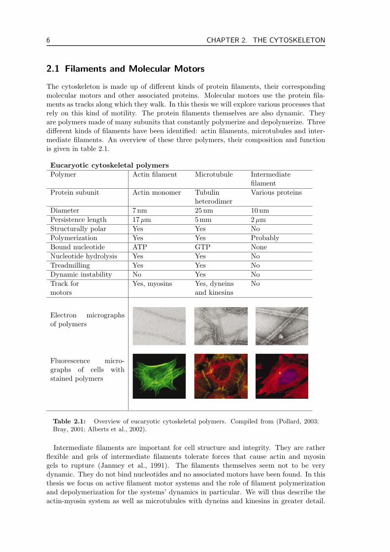
The cytoskeleton is made up of different kinds of protein filaments, their correspondingmolecular motors and other associated proteins. Molecular motors use the protein fila-ments as tracks along which they walk. In this thesis we will explore various processes thatrely on this kind of motility. The protein filaments themselves are also dynamic. Theyare polymers made of many subunits that constantly polymerize and depolymerize. Threedifferent kinds of filaments have been identified: actin filaments, microtubules and inter-mediate filaments. An overview of these three polymers, their composition and functionis given in table 2.1.
Eucaryotic cytoskeletal polymersPolymer Actin filament Microtubule Intermediate
filamentProtein subunit Actin monomer Tubulin Various proteins
heterodimerDiameter 7 nm 25 nm 10 nmPersistence length 17 µm 5 mm 2µmStructurally polar Yes Yes NoPolymerization Yes Yes ProbablyBound nucleotide ATP GTP NoneNucleotide hydrolysis Yes Yes NoTreadmilling Yes Yes NoDynamic instability No Yes NoTrack for Yes, myosins Yes, dyneins Nomotors and kinesins
Electron micrographsof polymers
Fluorescence micro-graphs of cells withstained polymers
Table 2.1: Overview of eucaryotic cytoskeletal polymers. Compiled from (Pollard, 2003;Bray, 2001; Alberts et al., 2002).
Intermediate filaments are important for cell structure and integrity. They are ratherflexible and gels of intermediate filaments tolerate forces that cause actin and myosingels to rupture (Janmey et al., 1991). The filaments themselves seem not to be verydynamic. They do not bind nucleotides and no associated motors have been found. In thisthesis we focus on active filament motor systems and the role of filament polymerizationand depolymerization for the systems’ dynamics in particular. We will thus describe theactin-myosin system as well as microtubules with dyneins and kinesins in greater detail.
2.2. ACTIN AND ACTIN BINDING PROTEINS 7
a b c d
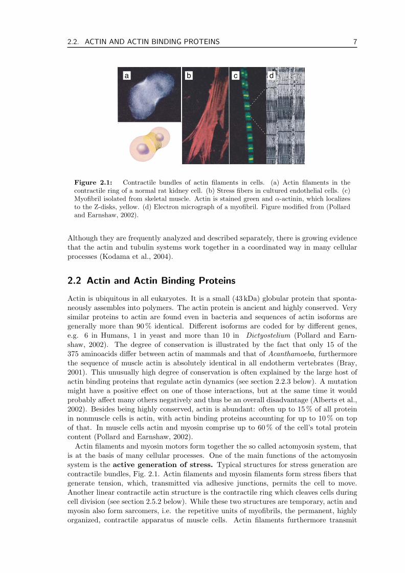
Figure 2.1: Contractile bundles of actin filaments in cells. (a) Actin filaments in thecontractile ring of a normal rat kidney cell. (b) Stress fibers in cultured endothelial cells. (c)Myofibril isolated from skeletal muscle. Actin is stained green and α-actinin, which localizesto the Z-disks, yellow. (d) Electron micrograph of a myofibril. Figure modified from (Pollardand Earnshaw, 2002).
Although they are frequently analyzed and described separately, there is growing evidencethat the actin and tubulin systems work together in a coordinated way in many cellularprocesses (Kodama et al., 2004).
2.2 Actin and Actin Binding Proteins
Actin is ubiquitous in all eukaryotes. It is a small (43 kDa) globular protein that sponta-neously assembles into polymers. The actin protein is ancient and highly conserved. Verysimilar proteins to actin are found even in bacteria and sequences of actin isoforms aregenerally more than 90% identical. Different isoforms are coded for by different genes,e.g. 6 in Humans, 1 in yeast and more than 10 in Dictyostelium (Pollard and Earn-shaw, 2002). The degree of conservation is illustrated by the fact that only 15 of the375 aminoacids differ between actin of mammals and that of Acanthamoeba, furthermorethe sequence of muscle actin is absolutely identical in all endotherm vertebrates (Bray,2001). This unusually high degree of conservation is often explained by the large host ofactin binding proteins that regulate actin dynamics (see section 2.2.3 below). A mutationmight have a positive effect on one of those interactions, but at the same time it wouldprobably affect many others negatively and thus be an overall disadvantage (Alberts et al.,2002). Besides being highly conserved, actin is abundant: often up to 15 % of all proteinin nonmuscle cells is actin, with actin binding proteins accounting for up to 10 % on topof that. In muscle cells actin and myosin comprise up to 60 % of the cell’s total proteincontent (Pollard and Earnshaw, 2002).
Actin filaments and myosin motors form together the so called actomyosin system, thatis at the basis of many cellular processes. One of the main functions of the actomyosinsystem is the active generation of stress. Typical structures for stress generation arecontractile bundles, Fig. 2.1. Actin filaments and myosin filaments form stress fibers thatgenerate tension, which, transmitted via adhesive junctions, permits the cell to move.Another linear contractile actin structure is the contractile ring which cleaves cells duringcell division (see section 2.5.2 below). While these two structures are temporary, actin andmyosin also form sarcomers, i.e. the repetitive units of myofibrils, the permanent, highlyorganized, contractile apparatus of muscle cells. Actin filaments furthermore transmit
8 CHAPTER 2. THE CYTOSKELETON
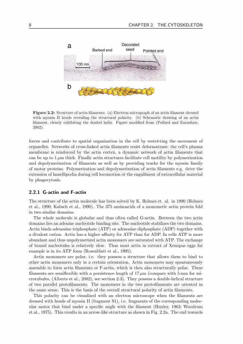
Figure 2.2: Structure of actin filaments. (a) Electron micrograph of an actin filament dressedwith myosin II heads revealing the structural polarity. (b) Schematic drawing of an actinfilament, clearly exhibiting the doubel helix. Figure modified from (Pollard and Earnshaw,2002).
forces and contribute to spatial organization in the cell by restricting the movement oforganelles. Networks of cross-linked actin filaments resist deformations: the cell’s plasmamembrane is reinforced by the actin cortex, a dynamic network of actin filaments thatcan be up to 1 µm thick. Finally actin structures facilitate cell motility by polymerizationand depolymerization of filaments as well as by providing tracks for the myosin familyof motor proteins. Polymerization and depolymerization of actin filaments e.g. drive theextension of lamellipodia during cell locomotion or the engulfment of extracellular materialby phagocytosis.
2.2.1 G-actin and F-actin
The structure of the actin molecule has been solved by K. Holmes et. al. in 1990 (Holmeset al., 1990; Kabsch et al., 1990). The 375 aminoacids of a monomeric actin protein foldin two similar domains.
The whole molecule is globular and thus often called G-actin. Between the two actindomains lies an adenine nucleotide binding site. The nucleotide stabilizes the two domains.Actin binds adenosine triphosphate (ATP) or adenosine diphosphate (ADP) together witha divalent cation. Actin has a higher affinity for ATP than for ADP. In cells ATP is moreabundant and thus unpolymerized actin monomers are saturated with ATP. The exchangeof bound nucleotides is relatively slow. Thus most actin in extract of Xenopus eggs forexample is in its ATP form (Rosenblatt et al., 1995).
Actin monomers are polar, i.e. they possess a structure that allows them to bind toother actin monomers only in a certain orientation. Actin monomers may spontaneouslyassemble to form actin filaments or F-actin, which is then also structurally polar. Thesefilaments are semiflexible with a persistence length of 17 µm (compare with 5mm for mi-crotubules, (Alberts et al., 2002), see section 2.3). They possess a double-helical structureof two parallel protofilaments. The monomers in the two protofilaments are oriented inthe same sense. This is the basis of the overall structural polarity of actin filaments.
This polarity can be visualized with an electron microscope when the filaments aredressed with heads of myosin II (fragment S1), i.e. fragments of the corresponding molec-ular motor that bind under a specific angle with the filament (Huxley, 1963; Woodrumet al., 1975). This results in an arrow-like structure as shown in Fig. 2.2a. The end towards

2.2. ACTIN AND ACTIN BINDING PROTEINS 9
a b
Figure 2.3: Schematic time course of actin polymerization in a test tube. (a) Polymer-ization is begun by raising the salt concentration in a solution of pure actin subunits. (b)Polymerization is begun in the same way, but with preformed fragments of actin filamentspresent to act as nuclei for filament growth. Modified from (Alberts et al., 2002).
which the arrows point is called the pointed end, the opposite end is the barbed end. Thisstructural polarity gives rise to the interesting polymerization dynamics of actin filamentsthat is essential for many cellular processes.
2.2.2 Actin Polymerization and Treadmilling
Actin filaments self-assemble from actin monomers via a series of bimolecular reac-tions (Pollard and Earnshaw, 2002). From in vitro experiments it seems that actinmonomers form first dimers and then trimers. These trimers consecutively serve as thenuclei for new actin filaments. The reactions necessary for filament polymerization aremore favorable than trimer formation, so that nucleation is the rate limiting step in poly-merizing new actin filaments. This shows up as a lag phase when filament polymerizationis induced, Fig. 2.3a. Cells use regulating proteins to overcome these limitations either bysevering existing filaments (e.g. via gelsolin) in order to provide several short filamentsas nuclei or by enhancing nucleation of filaments from monomeric actin (e.g. Formin,Arp2/3 complex). In in vitro experiments the lag phase is eliminated when small filamentfragments are added to the solution, Fig. 2.3b.
Once nucleated, a filament starts to grow by adding monomers at both ends. Thisprocess is reversible: filaments may shrink by loosing monomers from the ends as well.Filament growth is determined by the balance of polymerization and depolymerization atboth ends:
dnb
dt= kon,b c− koff,b (2.1)
dnp
dt= kon,p c− koff,p . (2.2)
where dnb/dt and dnp/dt denote the rates of monomer addition at the barbed end and atthe pointed end respectively. The on- and off- rates for monomers at both ends are givenby kon and koff and c is the concentration of monomeric actin in the surrounding solution.The polymerization rate is given by kon × c and depends on the monomer concentration.Note that we assume that the depolymerization rate koff is independent of the monomerconcentration.
10 CHAPTER 2. THE CYTOSKELETON
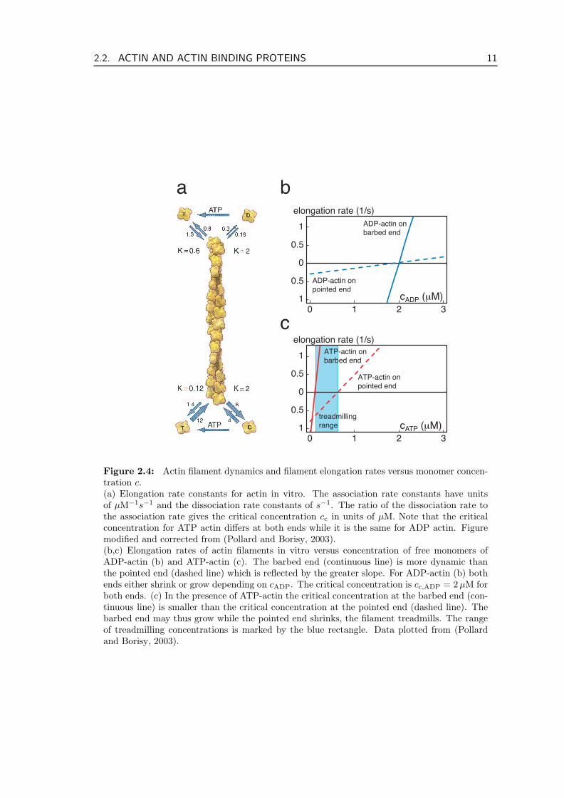
When a filament polymerizes, it diminishes the concentration of free monomers in thesolution until the critical concentration cc = koff/kon is reached. At the critical concentra-tion the growth and shrinkage of the filament exactly balance, the filament has reached astationary length. If one starts out with filaments and a monomer concentration c < cc
the filaments will depolymerize until c = cc.Due to the structural polarity of filaments, polymerization and depolymerization occur
with different rates at both ends (Pollard, 1986). While subunit dissociation is relativelyslow at both ends (between 1 and 10 subunits per second) filament growth is diffusionlimited at the barbed end and slower at the pointed end (Pollard and Borisy, 2003). Thebarbed end thus is more dynamic than the pointed end and grows more rapidly. That iswhy it is also called the plus end while the pointed end is called the minus end. Nonethelessin the absence of an external energy supply the equilibrium constant Keq = kon/koff = 1/cc
is the same for both ends, see Fig. 2.4.As already pointed out above, monomeric actin binds the nucleotide adenosine triphos-
phate (ATP) and possesses the capacity to hydrolyze it to adenosine diphosphate (ADP)and an inorganic phosphate Pi. This process frees about 20 kBT ' 20 × 4.1 pN nm permolecule and is irreversible (Carlier et al., 1988). Nucleotide hydrolysis is slow for indi-vidual monomers but accelerated in actin filaments with a half time of 2 s (Blanchoin andPollard, 2002). Phosphate dissociation is much slower with a half time of 350 s (Carlierand Pantaloni, 1986), so that ADP-Pi-actin is relatively long-lived in assembled actin fila-ments. Because monomeric actin in the cell is saturated with ATP, filaments will generallyincorporate ATP-actin. This results in a filament with a comparatively short actin-ATPcap and an actin-ADP tail in which phosphate is bound to some actin subunits but notto others. Due to the nucleotide hydrolysis it is energetically more favorable to dissociatean ADP-actin monomer than an ATP-actin monomer from the filament, cf. Fig 2.4a.
Filament Treadmilling
In the previous section we motivated, why the equilibrium constants at both ends are notequal in the presence of ATP. Typical values are c−c,ATP = 0.6 µM for the minus end ofa filament in solution with globular ATP-actin and c+
c,ATP = 0.12 µM for the plus endwith ATP-actin in vitro (Pollard, 1986; Pollard and Borisy, 2003), cf. Fig. 2.4a. So for aconcentration of ATP monomers c+
c,ATP < cATP < c−c,ATP, the filament will grow at the plusend while shrinking at the minus end. This is often called the treadmilling regime (bluerange in Fig. 2.4c). Under these conditions a monomer of ATP-actin is incorporated into afilament at the plus end, then its nucleotide is hydrolyzed. Some time later the inorganicphosphate is released, and finally the now ADP-actin monomer reaches the minus endand dissociates. While there is a whole range of concentrations for which the plus endgrows and the minus end shrinks, there is only one value for which these processes occur atprecisely the same rates. In this thesis we use the term treadmilling only for filaments thatpolymerize and depolymerize with equal rates at both ends. Taking the values reportedin (Pollard, 1986) for actin filaments in vitro, we find a critical treadmilling concentrationctm,ATP ' 0.14 µM where the polymerization rate for ATP-actin at the plus end exactlymatches the depolymerization rate for ADP-actin at the minus end, taking into accountthat in a cell monomeric actin is typically saturated with ATP, i.e. cADP ' 0. A filamentat this critical treadmilling concentration retains its length while continuously exchangingmonomers with the solution. The total turnover time for a 1µm long filament consistingof 370 monomers is about 20 min. This turnover time is greatly increased in lamellipodiaof motile cells or in the actin comets of bacterial pathogens where a 3 µm long filament
2.2. ACTIN AND ACTIN BINDING PROTEINS 11
2
2
0 1 2 3
0
1
1
0.5
0.5
treadmilling
range
elongation rate (1/s)
ATP-actin on
barbed end
ATP-actin on
pointed end
cATP (µM)
0 1 2 3
0
1
1
0.5
0.5
cADP (µM)
elongation rate (1/s)
ADP-actin on
barbed end
ADP-actin on
pointed end
a b
c
Figure 2.4: Actin filament dynamics and filament elongation rates versus monomer concen-tration c.(a) Elongation rate constants for actin in vitro. The association rate constants have unitsof µM−1s−1 and the dissociation rate constants of s−1. The ratio of the dissociation rate tothe association rate gives the critical concentration cc in units of µM. Note that the criticalconcentration for ATP actin differs at both ends while it is the same for ADP actin. Figuremodified and corrected from (Pollard and Borisy, 2003).(b,c) Elongation rates of actin filaments in vitro versus concentration of free monomers ofADP-actin (b) and ATP-actin (c). The barbed end (continuous line) is more dynamic thanthe pointed end (dashed line) which is reflected by the greater slope. For ADP-actin (b) bothends either shrink or grow depending on cADP. The critical concentration is cc,ADP = 2µM forboth ends. (c) In the presence of ATP-actin the critical concentration at the barbed end (con-tinuous line) is smaller than the critical concentration at the pointed end (dashed line). Thebarbed end may thus grow while the pointed end shrinks, the filament treadmills. The rangeof treadmilling concentrations is marked by the blue rectangle. Data plotted from (Pollardand Borisy, 2003).
12 CHAPTER 2. THE CYTOSKELETON
typically turns over in 1 min (Pantaloni et al., 2001). This increase is attributed to a hostof regulating factors, see section 2.2.3.
Filament treadmilling has been demonstrated to occur in the bulk cytoplasm of cellsbut it also occurs in the linear strucures of microvili, filopodia and stereocilia (Lin et al.,2005).
2.2.3 Actin Binding Proteins
The concentration of free actin monomers in cells was reported to be around 100 µM (Pol-lard et al., 2000; Plastino et al., 2004), i.e. two to three orders of magnitude larger than thecritical concentrations measured in vitro. Furthermore cell movement, which to a large ex-tend is driven by filament polymerization and depolymerization, can occur with velocitiesup to 10µm min−1 (Safer and Nachmias, 1994) and hence about two orders of magnitudefaster than filament treadmilling in vitro (Bray, 2001; Pollard and Borisy, 2003). Thepresence of regulatory proteins explains these differences.
Actin binds a substantial number of proteins collectively called actin binding proteins(ABPs). These proteins fall into more than 60 classes (Kreis and Vale, 1999) and recentlymore than 162 distinct and separate proteins were counted, without including their manysynonyms or isoforms (dos Remedios et al., 2003). These proteins influence actin dynamicsin various ways. They can:
1. bind to G-actin (e.g. profilin, thymosin-β 4, DNase) sometimes sequestering it andpreventing its polymerization
2. nucleate actin filaments (Arp2/3, formin)
3. depolymerize filaments (e.g. CapZ, ADF/cofilin)
4. cap the ends of F-actin, preventing the exchange of monomers (e.g. gelsolin, CapZ)
5. sever actin filaments by binding to their sides and cutting them (e.g. gelsolin)
6. cross-link filaments, thus forming gels and bundles (e.g. Arp2/3, α-actinin)
7. stabilize filaments by binding along their sides (e.g. tropomyosin)
8. actively walk along filaments using them as tracks (e.g. the myosin family of motorproteins, cf. section 2.2.4)
Here we briefly introduce some of the most common ABPs that are impor-tant for the main part of this thesis. These include the five proteins thatcan reconstitute bacterial motility in purified systems (i.e. ADF/cofilin (Bam-burg et al., 1999), capping protein (Cooper and Schafer, 2000), Arp2/3 com-plex (Pollard and Beltzner, 2002), an activator of Arp2/3 complex (Weaver et al.,2003), and profilin (Schluter et al., 1997)) as well as formin, which binds to fil-ament plus ends and α-actinin that cross-links filaments in bundles. Comprehen-sive lists and descriptions of actin binding proteins can be found in (Sheterlineet al., 1998; Kreis and Vale, 1999; dos Remedios and Thomas, 2001) and also onlineat http://www.bms.ed.ac.uk/research/others/smaciver/Encyclop/encycloABP.htm. Herewe stress the biochemical function of these components. Recent reviews highlight theirimplications e.g. for actin based motility in cells and bacterial pathogens (Plastino andSykes, 2005; Rafelski and Theriot, 2004; Gruenheid and Finlay, 2003; Pollard and Borisy,2003; Pantaloni et al., 2001).
2.2. ACTIN AND ACTIN BINDING PROTEINS 13
Arp2/3
G-actin
WASp-Scar
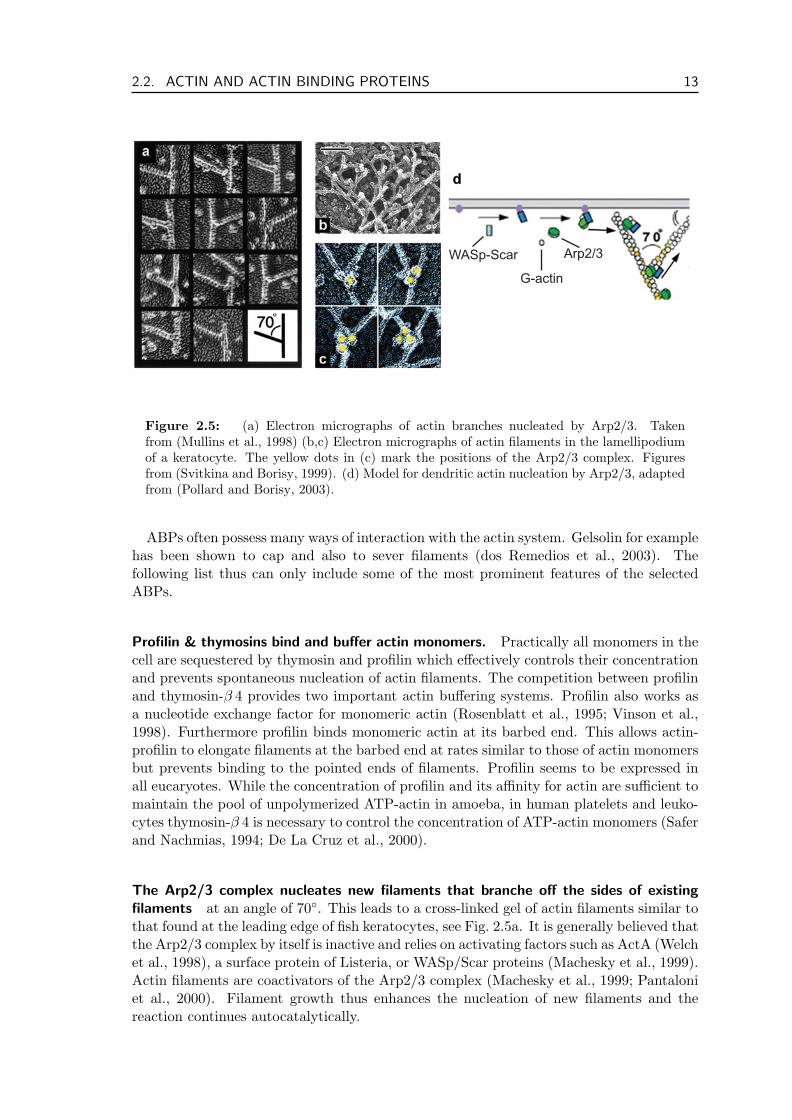
Figure 2.5: (a) Electron micrographs of actin branches nucleated by Arp2/3. Takenfrom (Mullins et al., 1998) (b,c) Electron micrographs of actin filaments in the lamellipodiumof a keratocyte. The yellow dots in (c) mark the positions of the Arp2/3 complex. Figuresfrom (Svitkina and Borisy, 1999). (d) Model for dendritic actin nucleation by Arp2/3, adaptedfrom (Pollard and Borisy, 2003).
ABPs often possess many ways of interaction with the actin system. Gelsolin for examplehas been shown to cap and also to sever filaments (dos Remedios et al., 2003). Thefollowing list thus can only include some of the most prominent features of the selectedABPs.
Profilin & thymosins bind and buffer actin monomers. Practically all monomers in thecell are sequestered by thymosin and profilin which effectively controls their concentrationand prevents spontaneous nucleation of actin filaments. The competition between profilinand thymosin-β 4 provides two important actin buffering systems. Profilin also works asa nucleotide exchange factor for monomeric actin (Rosenblatt et al., 1995; Vinson et al.,1998). Furthermore profilin binds monomeric actin at its barbed end. This allows actin-profilin to elongate filaments at the barbed end at rates similar to those of actin monomersbut prevents binding to the pointed ends of filaments. Profilin seems to be expressed inall eucaryotes. While the concentration of profilin and its affinity for actin are sufficient tomaintain the pool of unpolymerized ATP-actin in amoeba, in human platelets and leuko-cytes thymosin-β 4 is necessary to control the concentration of ATP-actin monomers (Saferand Nachmias, 1994; De La Cruz et al., 2000).
The Arp2/3 complex nucleates new filaments that branche off the sides of existingfilaments at an angle of 70. This leads to a cross-linked gel of actin filaments similar tothat found at the leading edge of fish keratocytes, see Fig. 2.5a. It is generally believed thatthe Arp2/3 complex by itself is inactive and relies on activating factors such as ActA (Welchet al., 1998), a surface protein of Listeria, or WASp/Scar proteins (Machesky et al., 1999).Actin filaments are coactivators of the Arp2/3 complex (Machesky et al., 1999; Pantaloniet al., 2000). Filament growth thus enhances the nucleation of new filaments and thereaction continues autocatalytically.
14 CHAPTER 2. THE CYTOSKELETON
WASp/Scar proteins are activators of the Arp2/3 complex. They are usually localizedat the leading edge of moving keratocytes or on the membrane of bacterial pathogens suchas Shigella (Gruenheid and Finlay, 2003).
Formin processively binds to filament barbed ends and promotes filament elongation(Kovar et al., 2003). Formins are nucleators of unbranched actin filaments and involvedin dynamic processes such as cell migration (Watanabe et al., 1997; Koka et al., 2003) orcell cleavage (Pelham and Chang, 2002; Wu et al., 2003). Formin can increase the rateconstant for profilin-actin association at the barbed end 15-fold (Romero et al., 2004) butdifferences between different members of the formin family appear to be important (Kovarand Pollard, 2004).
CapZ and Gelsolin are capping proteins that hinder monomer binding and unbindingat filament barbed ends. They limit the lengths of actin filaments and the numberof growing barbed ends in a gel. Short filaments are stiffer than long filaments, e.g.making the resulting gel more efficient in pushing the membrane in the lamellipodium.The concentration of CapZ in the cytoplasm is about 1 µM (Cooper and Schafer, 2000)and its rate constant for binding barbed ends accounts for a capping half time of about1 s (Schafer et al., 1996). Filaments that grow at velocities of 0.3 µm s−1 for about 1 sreach a length comparable to that of filaments found at the leading edge (Svitkina et al.,1997). Gelsolin is found mainly in higher eucaryotes (Sun et al., 1999).
ADF/cofilin promotes the disassembly of actin filaments by several mechanisms. Itsevers filaments (Maciver et al., 1991, 1998; Blanchoin and Pollard, 1999; Ichetovkin et al.,2000), promotes phosphate dissociation in filaments (Blanchoin and Pollard, 1999) andexhibits a higher affinity for ADP-actin monomers than for ADP-actin filaments. Fur-thermore it changes the twist of actin filaments (McGough et al., 1997), which can inducerupture and may debranche filaments (Pollard and Borisy, 2003). ADF/cofilin increasesthe off-rate at the pointed ends of filaments 30-fold (Ressad et al., 1998) without changingthe rates at barbed ends. As dissociation at the pointed ends of filaments is the ratelimiting step in filament treadmilling, ADF increases the treadmilling velocity. This effectis further increased in the presence of profilin. The rate of pointed end disassembly is thenincreased 125-fold by the combined action of ADF/cofilin and profilin (Didry et al., 1998).
α-actinin cross-links parallel actin filaments. Filament bundles linked by α-actinin arerather loosely packed, so that e.g. myosin-II can enter the bundle and contract it. α-actinin is a major component of the Z-disk in muscle cells (Bray, 2001). Fimbrin isanother bundling protein that however forms tightly packed filament bundles that are notcontractile (Alberts et al., 2002). Besides these proteins that link filaments parallel to eachother and thus promote the formation of bundles, other cross-linkers such as spectrin orfilamin or the Arp2/3 complex discussed above, link filaments at an angle and lead to theformation of gels. A review of actin cross-linkers is given in (Revenu et al., 2004).
2.2.4 Myosin: The Actin Motor
Besides the cross-linkers described above, myosin motors can also bind to and cross-linkfilaments. The cross-linkers are passive, i.e. they do themselves not consume energy.Motors on the other hand possess the ability to convert chemical energy, freed by thehydrolysis of ATP, into directed motion. From a physics point of view, molecular motors
2.2. ACTIN AND ACTIN BINDING PROTEINS 15
Figure 2.6: The Myosin Tree. From (Hodge and Cope, 2000).
can e.g. be understood as machines that rectify Brownian motion (Julicher et al., 1997;Duke, 2002a; Reimann, 2002). The dynamics of many motors acting collectively as isfrequently the case in the cytoskeleton displays a variety of surprising phenomena (Julicherand Prost, 1995, 1997; Duke, 1999; Badoual et al., 2002; Duke, 2002b).
Here we will concentrate on the effect of molecular motors on cytoskeletal dynamics. Theintrinsic activity of protein filaments (i.e. polymerization, depolymerization, treadmilling)as well as the action of molecular motors are crucial for many cellular processes. Both areactive, i.e. energy consuming, non-equilibrium processes. Gels of filaments, cross-linkers,regulating proteins and molecular motors are hence called active gels.
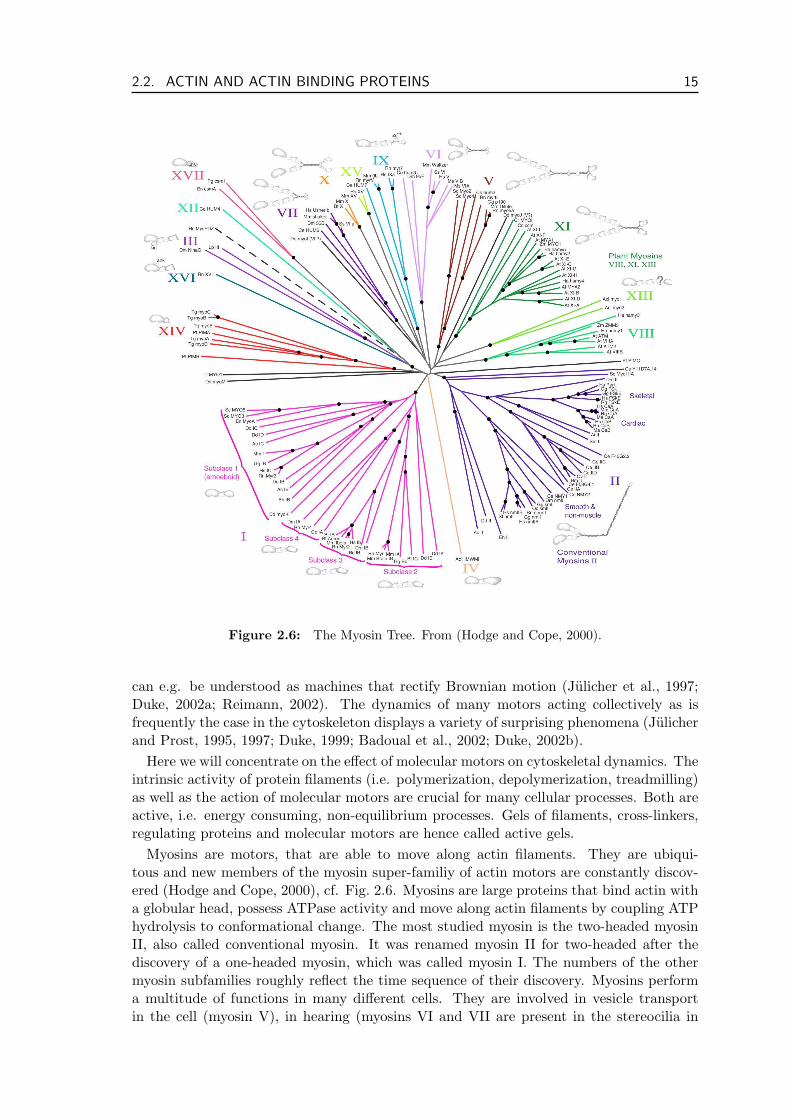
Myosins are motors, that are able to move along actin filaments. They are ubiqui-tous and new members of the myosin super-familiy of actin motors are constantly discov-ered (Hodge and Cope, 2000), cf. Fig. 2.6. Myosins are large proteins that bind actin witha globular head, possess ATPase activity and move along actin filaments by coupling ATPhydrolysis to conformational change. The most studied myosin is the two-headed myosinII, also called conventional myosin. It was renamed myosin II for two-headed after thediscovery of a one-headed myosin, which was called myosin I. The numbers of the othermyosin subfamilies roughly reflect the time sequence of their discovery. Myosins performa multitude of functions in many different cells. They are involved in vesicle transportin the cell (myosin V), in hearing (myosins VI and VII are present in the stereocilia in
16 CHAPTER 2. THE CYTOSKELETON
a b c
Chemotrypsin
treatment
LMM HMM
Papain
treatment
S1S2
tail neck head
essential light chain
regulatory light chain
100 nm
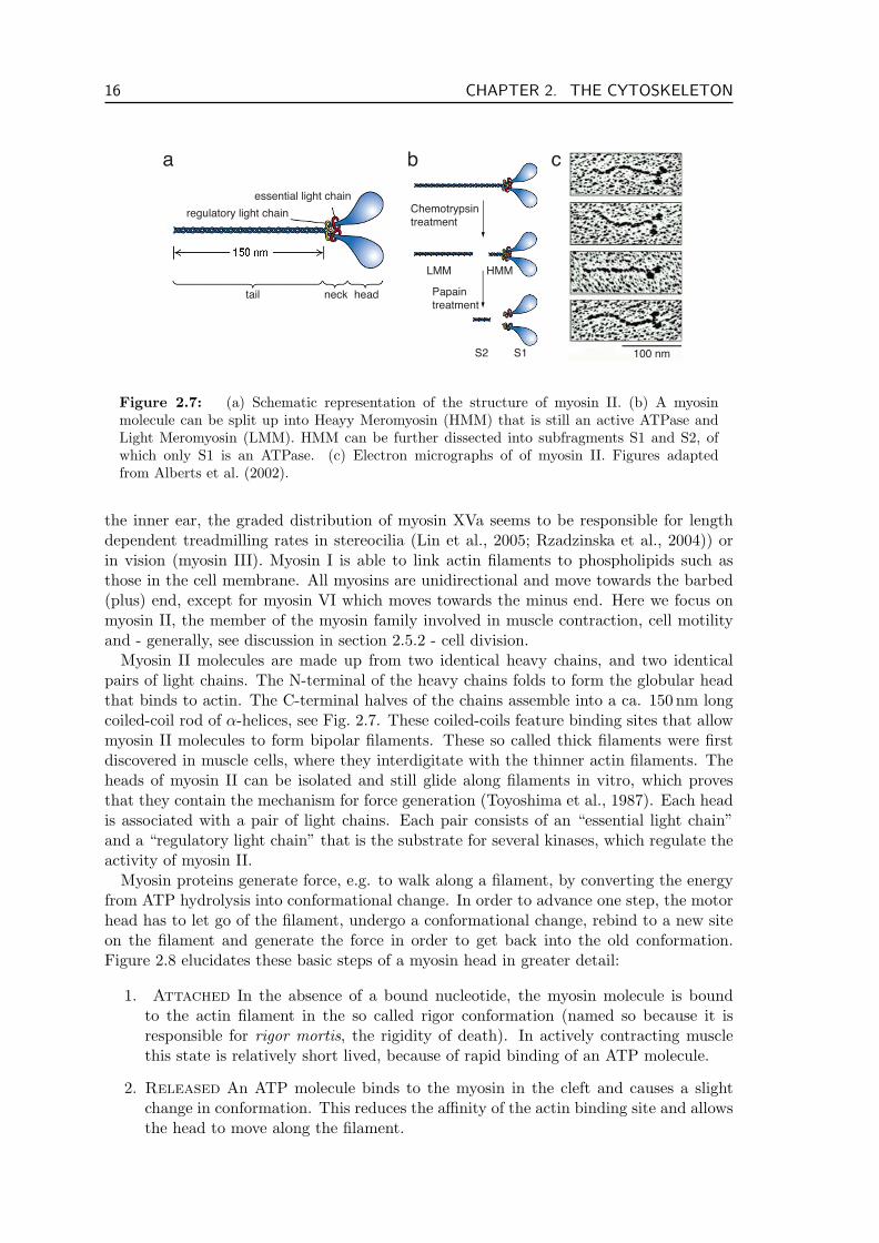
Figure 2.7: (a) Schematic representation of the structure of myosin II. (b) A myosinmolecule can be split up into Heayy Meromyosin (HMM) that is still an active ATPase andLight Meromyosin (LMM). HMM can be further dissected into subfragments S1 and S2, ofwhich only S1 is an ATPase. (c) Electron micrographs of of myosin II. Figures adaptedfrom Alberts et al. (2002).
the inner ear, the graded distribution of myosin XVa seems to be responsible for lengthdependent treadmilling rates in stereocilia (Lin et al., 2005; Rzadzinska et al., 2004)) orin vision (myosin III). Myosin I is able to link actin filaments to phospholipids such asthose in the cell membrane. All myosins are unidirectional and move towards the barbed(plus) end, except for myosin VI which moves towards the minus end. Here we focus onmyosin II, the member of the myosin family involved in muscle contraction, cell motilityand - generally, see discussion in section 2.5.2 - cell division.
Myosin II molecules are made up from two identical heavy chains, and two identicalpairs of light chains. The N-terminal of the heavy chains folds to form the globular headthat binds to actin. The C-terminal halves of the chains assemble into a ca. 150 nm longcoiled-coil rod of α-helices, see Fig. 2.7. These coiled-coils feature binding sites that allowmyosin II molecules to form bipolar filaments. These so called thick filaments were firstdiscovered in muscle cells, where they interdigitate with the thinner actin filaments. Theheads of myosin II can be isolated and still glide along filaments in vitro, which provesthat they contain the mechanism for force generation (Toyoshima et al., 1987). Each headis associated with a pair of light chains. Each pair consists of an “essential light chain”and a “regulatory light chain” that is the substrate for several kinases, which regulate theactivity of myosin II.
Myosin proteins generate force, e.g. to walk along a filament, by converting the energyfrom ATP hydrolysis into conformational change. In order to advance one step, the motorhead has to let go of the filament, undergo a conformational change, rebind to a new siteon the filament and generate the force in order to get back into the old conformation.Figure 2.8 elucidates these basic steps of a myosin head in greater detail:
1. Attached In the absence of a bound nucleotide, the myosin molecule is boundto the actin filament in the so called rigor conformation (named so because it isresponsible for rigor mortis, the rigidity of death). In actively contracting musclethis state is relatively short lived, because of rapid binding of an ATP molecule.
2. Released An ATP molecule binds to the myosin in the cleft and causes a slightchange in conformation. This reduces the affinity of the actin binding site and allowsthe head to move along the filament.
2.2. ACTIN AND ACTIN BINDING PROTEINS 17
1
5
4
3
2
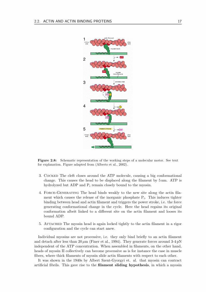
Figure 2.8: Schematic representation of the working steps of a molecular motor. See textfor explanation. Figure adapted from (Alberts et al., 2002).
3. Cocked The cleft closes around the ATP molecule, causing a big conformationalchange. This causes the head to be displaced along the filament by 5 nm. ATP ishydrolyzed but ADP and Pi remain closely bound to the myosin.
4. Force-Generating The head binds weakly to the new site along the actin fila-ment which causes the release of the inorganic phosphate Pi. This induces tighterbinding between head and actin filament and triggers the power stroke, i.e. the forcegenerating conformational change in the cycle. Here the head regains its originalconformation albeit linked to a different site on the actin filament and looses itsbound ADP.
5. Attached The myosin head is again locked tightly to the actin filament in a rigorconfiguration and the cycle can start anew.
Individual myosins are not processive, i.e. they only bind briefly to an actin filamentand detach after less than 20µm (Finer et al., 1994). They generate forces around 3-4 pNindependent of the ATP concentration. When assembled in filaments, on the other hand,heads of myosin II collectively can become processive as is for instance the case in musclefibers, where thick filaments of myosin slide actin filaments with respect to each other.
It was shown in the 1940s by Albert Szent-Gyorgyi et. al. that myosin can contractartificial fibrils. This gave rise to the filament sliding hypothesis, in which a myosin
18 CHAPTER 2. THE CYTOSKELETON
a cb
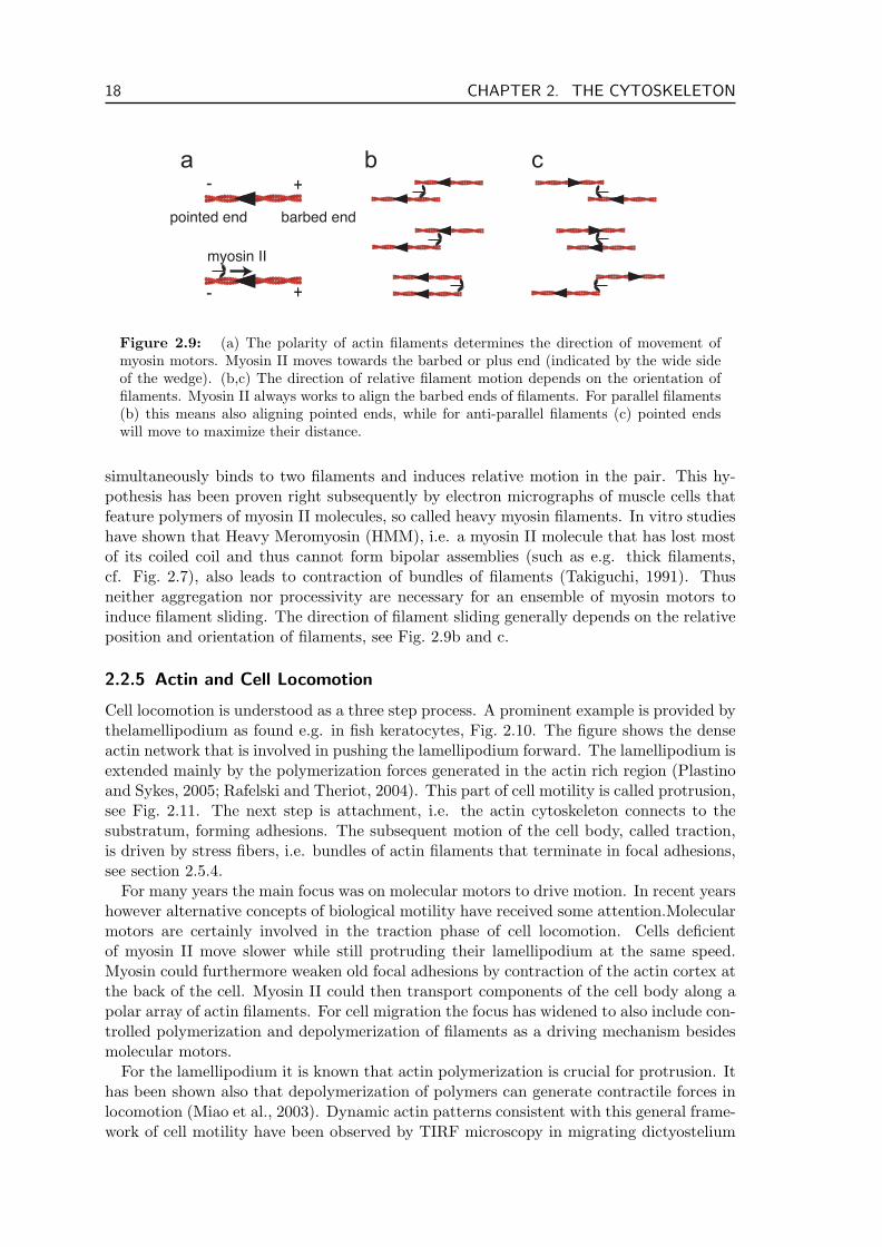
+-
barbed endpointed end
+-
myosin II
Figure 2.9: (a) The polarity of actin filaments determines the direction of movement ofmyosin motors. Myosin II moves towards the barbed or plus end (indicated by the wide sideof the wedge). (b,c) The direction of relative filament motion depends on the orientation offilaments. Myosin II always works to align the barbed ends of filaments. For parallel filaments(b) this means also aligning pointed ends, while for anti-parallel filaments (c) pointed endswill move to maximize their distance.
simultaneously binds to two filaments and induces relative motion in the pair. This hy-pothesis has been proven right subsequently by electron micrographs of muscle cells thatfeature polymers of myosin II molecules, so called heavy myosin filaments. In vitro studieshave shown that Heavy Meromyosin (HMM), i.e. a myosin II molecule that has lost mostof its coiled coil and thus cannot form bipolar assemblies (such as e.g. thick filaments,cf. Fig. 2.7), also leads to contraction of bundles of filaments (Takiguchi, 1991). Thusneither aggregation nor processivity are necessary for an ensemble of myosin motors toinduce filament sliding. The direction of filament sliding generally depends on the relativeposition and orientation of filaments, see Fig. 2.9b and c.
2.2.5 Actin and Cell Locomotion
Cell locomotion is understood as a three step process. A prominent example is provided bythelamellipodium as found e.g. in fish keratocytes, Fig. 2.10. The figure shows the denseactin network that is involved in pushing the lamellipodium forward. The lamellipodium isextended mainly by the polymerization forces generated in the actin rich region (Plastinoand Sykes, 2005; Rafelski and Theriot, 2004). This part of cell motility is called protrusion,see Fig. 2.11. The next step is attachment, i.e. the actin cytoskeleton connects to thesubstratum, forming adhesions. The subsequent motion of the cell body, called traction,is driven by stress fibers, i.e. bundles of actin filaments that terminate in focal adhesions,see section 2.5.4.
For many years the main focus was on molecular motors to drive motion. In recent yearshowever alternative concepts of biological motility have received some attention.Molecularmotors are certainly involved in the traction phase of cell locomotion. Cells deficientof myosin II move slower while still protruding their lamellipodium at the same speed.Myosin could furthermore weaken old focal adhesions by contraction of the actin cortex atthe back of the cell. Myosin II could then transport components of the cell body along apolar array of actin filaments. For cell migration the focus has widened to also include con-trolled polymerization and depolymerization of filaments as a driving mechanism besidesmolecular motors.
For the lamellipodium it is known that actin polymerization is crucial for protrusion. Ithas been shown also that depolymerization of polymers can generate contractile forces inlocomotion (Miao et al., 2003). Dynamic actin patterns consistent with this general frame-work of cell motility have been observed by TIRF microscopy in migrating dictyostelium
2.2. ACTIN AND ACTIN BINDING PROTEINS 19
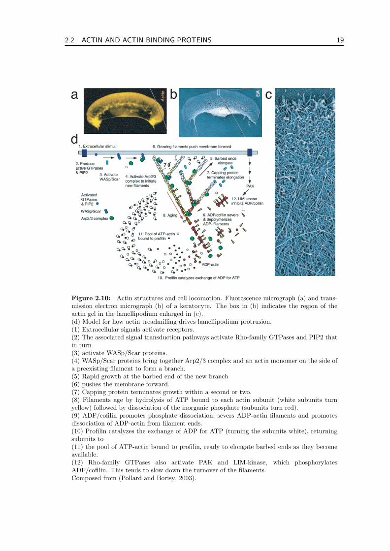
a cb
d
Figure 2.10: Actin structures and cell locomotion. Fluorescence micrograph (a) and trans-mission electron micrograph (b) of a keratocyte. The box in (b) indicates the region of theactin gel in the lamellipodium enlarged in (c).(d) Model for how actin treadmilling drives lamellipodium protrusion.(1) Extracellular signals activate receptors.(2) The associated signal transduction pathways activate Rho-family GTPases and PIP2 thatin turn(3) activate WASp/Scar proteins.(4) WASp/Scar proteins bring together Arp2/3 complex and an actin monomer on the side ofa preexisting filament to form a branch.(5) Rapid growth at the barbed end of the new branch(6) pushes the membrane forward.(7) Capping protein terminates growth within a second or two.(8) Filaments age by hydrolysis of ATP bound to each actin subunit (white subunits turnyellow) followed by dissociation of the inorganic phosphate (subunits turn red).(9) ADF/cofilin promotes phosphate dissociation, severs ADP-actin filaments and promotesdissociation of ADP-actin from filament ends.(10) Profilin catalyzes the exchange of ADP for ATP (turning the subunits white), returningsubunits to(11) the pool of ATP-actin bound to profilin, ready to elongate barbed ends as they becomeavailable.(12) Rho-family GTPases also activate PAK and LIM-kinase, which phosphorylatesADF/cofilin. This tends to slow down the turnover of the filaments.Composed from (Pollard and Borisy, 2003).
20 CHAPTER 2. THE CYTOSKELETON
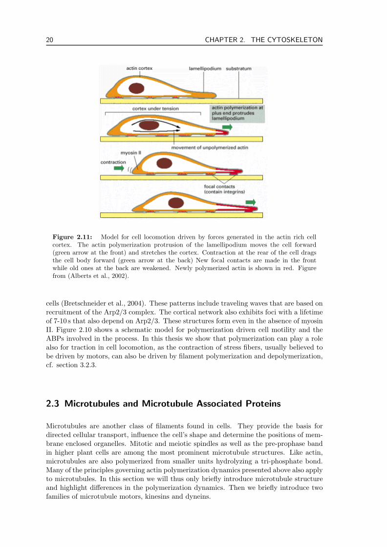
Figure 2.11: Model for cell locomotion driven by forces generated in the actin rich cellcortex. The actin polymerization protrusion of the lamellipodium moves the cell forward(green arrow at the front) and stretches the cortex. Contraction at the rear of the cell dragsthe cell body forward (green arrow at the back) New focal contacts are made in the frontwhile old ones at the back are weakened. Newly polymerized actin is shown in red. Figurefrom (Alberts et al., 2002).
cells (Bretschneider et al., 2004). These patterns include traveling waves that are based onrecruitment of the Arp2/3 complex. The cortical network also exhibits foci with a lifetimeof 7-10 s that also depend on Arp2/3. These structures form even in the absence of myosinII. Figure 2.10 shows a schematic model for polymerization driven cell motility and theABPs involved in the process. In this thesis we show that polymerization can play a rolealso for traction in cell locomotion, as the contraction of stress fibers, usually believed tobe driven by motors, can also be driven by filament polymerization and depolymerization,cf. section 3.2.3.
2.3 Microtubules and Microtubule Associated Proteins
Microtubules are another class of filaments found in cells. They provide the basis fordirected cellular transport, influence the cell’s shape and determine the positions of mem-brane enclosed organelles. Mitotic and meiotic spindles as well as the pre-prophase bandin higher plant cells are among the most prominent microtubule structures. Like actin,microtubules are also polymerized from smaller units hydrolyzing a tri-phosphate bond.Many of the principles governing actin polymerization dynamics presented above also applyto microtubules. In this section we will thus only briefly introduce microtubule structureand highlight differences in the polymerization dynamics. Then we briefly introduce twofamilies of microtubule motors, kinesins and dyneins.
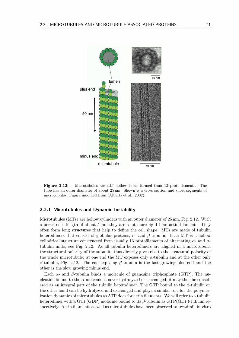
2.3. MICROTUBULES AND MICROTUBULE ASSOCIATED PROTEINS 21
lumen10 nm
50 nm
microtubule 50 nm
plus end
minus end
Figure 2.12: Microtubules are stiff hollow tubes formed from 13 protofilaments. Thetube has an outer diameter of about 25 nm. Shown is a cross section and short segments ofmicrotubules. Figure modified from (Alberts et al., 2002).
2.3.1 Microtubules and Dynamic Instability
Microtubules (MTs) are hollow cylinders with an outer diameter of 25 nm, Fig. 2.12. Witha persistence length of about 5mm they are a lot more rigid than actin filaments. Theyoften form long structures that help to define the cell shape. MTs are made of tubulinheterodimers that consist of globular proteins, α- and β-tubulin. Each MT is a hollowcylindrical structure constructed from usually 13 protofilaments of alternating α- and β-tubulin units, see Fig. 2.12. As all tubulin heterodimers are aligned in a microtubule,the structural polarity of the subunits thus directly gives rise to the structural polarity ofthe whole microtubule: at one end the MT exposes only α-tubulin and at the other onlyβ-tubulin, Fig. 2.12. The end exposing β-tubulin is the fast growing plus end and theother is the slow growing minus end.
Each α- and β-tubulin binds a molecule of guanosine triphosphate (GTP). The nu-cleotide bound to the α-molecule is never hydrolyzed or exchanged, it may thus be consid-ered as an integral part of the tubulin heterodimer. The GTP bound to the β-tubulin onthe other hand can be hydrolyzed and exchanged and plays a similar role for the polymer-ization dynamics of microtubules as ATP does for actin filaments. We will refer to a tubulinheterodimer with a GTP(GDP) molecule bound to its β-tubulin as GTP(GDP)-tubulin re-spectively. Actin filaments as well as microtubules have been observed to treadmill in vitro
22 CHAPTER 2. THE CYTOSKELETON
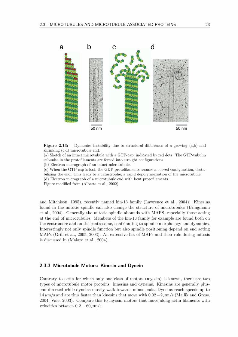
as well as in cells (Rodionov and Borisy, 1997a). It is believed that dynamic instabilityis the predominant behavior of microtubules in cells.
Dynamic instability refers to the sudden switching of a MT from steady growth to rapidshrinkage and then back to steady growth. The basis for this abrupt change is againnucleotide hydrolysis. If a microtubule is surrounded by a tubulin concentration betweenthe critical concentrations for the GDP- and the GTP-form of tubulin respectively (i.e.the concentration range where treadmilling is possible), any end exposing GDP-tubulinwill shrink while any end exposing GTP-tubulin will grow. If the rate of subunit additionis of the same magnitude as the rate of hydrolysis in the microtubule, growth may startout with GTP-tubulins, but eventually the hydrolysis can catch up with the addition ofGTP-units and thus the microtubule would expose GDP-tubulin at its end. But nowthe concentration of tubulin is below the critical concentration for GTP elongation andthe end will start to depolymerize. This rapid depolymerization takes place until themicrotubule is completely anihilated or regains its GTP-cap and starts to grow again.The rapid shrinking is called a catastrophe, while the change to growth is called a rescueevent.
Another reason for the rapid depolymerization of microtubules upon loss of their GTP-caps besides the kinetic arguments described above is the structural difference betweenGTP- and GDP-tubulin(Mahadevan and Mitchison, 2005) and their different bending flex-ibility (Wang and Nogales, 2005). GTP-tubulin forms straight protofilaments that makestrong and regular lateral contacts with other protofilaments. Hydrolysis of GTP to GDPinduces a little structural change in the heterodimers which leads to curved protofilaments.A GTP-cap on a fast growing microtubule constrains the curvature of the protofilamentsmade of GDP-tubulin. When it is lost, e.g. by hydrolysis, the curvature is not restrainedanymore and the protofilaments curve apart, see Fig. 2.13. The individual filaments thenpeel off rapidly.
2.3.2 Microtubule Associated Proteins
Like actin, microtubules interact with a large group of other proteins, collectively calledmicrotubule associated proteins (MAPs). Two important functions of MAPs are the sta-bilization or destabilization of microtubules, thus promoting or hindering MT depolymer-ization. Other MAPs mediate the interaction of MTs with other cellular components. Inneurons stabilized bundles of microtubules form the core of axons and dendrites. Thesebundles are held together by MAPs such as MAP2 or tau. Bundles packed by differentMAPs have different characteristics. MAP2 bundles for example feature bigger spacesbetween the microtubules while tau bundles are tightly packed. MAPs can also serve asnucleation cores in solutions of tubulin, as they bind tubulin dimers and thus stabilize theoligomers necessary to induce microtubule polymerization.
A very interesting class of MAPs is represented by XMAP215, a MAP found in thefrog Xenopus whose molecular weight is 215 kDa, hence the name. XMAP215 has closehomologs in many organisms that range from yeast to humans. XMAP215 binds to the sideof microtubules, but it also has the ability to stabilize free microtubule ends, preventingcatastrophes. This activity can be inhibited by phosphorylation of XMAP215. It hasbeen shown that this phosphorylation contributes to the ten-fold increase in MT dynamicinstability during mitosis (see also section 2.5.1). XMAP215 is one member of a largeclass of MT end binding or tracking proteins (Akhmanova and Hoogenraad, 2005). Othermembers of this class may processively depolymerize microtubules (Wordeman, 2005), suchas the Mitotic Centromere-Associated Kinesin/kinesin family 2 (MCAK/kif2) (Wordeman
2.3. MICROTUBULES AND MICROTUBULE ASSOCIATED PROTEINS 23
a b c d
50 nm 50 nm
Figure 2.13: Dynamics instability due to structural differences of a growing (a,b) andshrinking (c,d) microtubule end.(a) Sketch of an intact microtubule with a GTP-cap, indicated by red dots. The GTP-tubulinsubunits in the protofilaments are forced into straight configurations.(b) Electron micrograph of an intact microtubule.(c) When the GTP-cap is lost, the GDP-protofilaments assume a curved configuration, desta-bilizing the end. This leads to a catastrophe, a rapid depolymerization of the microtubule.(d) Electron micrograph of a microtubule end with bent protofilaments.Figure modified from (Alberts et al., 2002).
and Mitchison, 1995), recently named kin-13 family (Lawrence et al., 2004). Kinesinsfound in the mitotic spindle can also change the structure of microtubules (Bringmannet al., 2004). Generally the mitotic spindle abounds with MAPS, especially those actingat the end of microtubules. Members of the kin-13 family for example are found both onthe centromere and on the centrosome, contributing to spindle morphology and dynamics.Interestingly not only spindle function but also spindle positioning depend on end actingMAPs (Grill et al., 2005, 2003). An extensive list of MAPs and their role during mitosisis discussed in (Maiato et al., 2004).
2.3.3 Microtubule Motors: Kinesin and Dynein
Contrary to actin for which only one class of motors (myosin) is known, there are twotypes of microtubule motor proteins: kinesins and dyneins. Kinesins are generally plus-end directed while dyneins mostly walk towards minus ends. Dyneins reach speeds up to14 µm/s and are thus faster than kinesins that move with 0.02−2 µm/s (Mallik and Gross,2004; Vale, 2003). Compare this to myosin motors that move along actin filaments withvelocities between 0.2− 60 µm/s.
24 CHAPTER 2. THE CYTOSKELETON
Kinesin
Kinesins were first discovered in the squid giant axon where they walk away from the cellbody towards the plus end of the MTs, carrying membrane-enclosed organelles. Kinesinsalso play a role in mitosis, meiosis, transport of DNA and proteins, and MT polymerizationdynamics. In in vitro experiments kinesins have been shown to be strong enough to pullmembrane tubes from vesicles (Roux et al., 2002; Leduc et al., 2004; Leduc, 2005)
Kinesin is structurally similar to myosin II, as it also forms a dimer, having two globularmotor domains, possessing one heavy and two light chains each. These strucutral similar-ities hint to a common evolutionary origin (Alberts et al., 2002). Like myosin, kinesin isa member of a large protein superfamily - humans have 40 different kinesins for example.Most members of the at least 10 families of kinesin that make up the super family havetheir motor domain at the N-terminus of the heavy chain and walk towards the MT plusend. There is however at least one family that has the motor domain at the C-terminusand walks towards the minus end. Many kinesins are homo- or hetero-dimers; Kinesin-5(BimC) is a KRP family, whose members can associate and form bipolar motors. Theycan then slide two microtubules with respect to each others, similar to myosin II on actinfilaments. Most kinesins have binding sites for membrane-enclosed organelles or micro-tubules in their tails. Besides providing intracellular transport, kinesins have specific rolesin mitotic and meiotic spindle formation and dynamics. It has recently been shown thatfor example the mitotic kinesin Eg5, which is important for spindle integrity, can simulta-neously move along two microtubules and even stay attached to MT plus ends (Kapiteinet al., 2005).
Kinesins generally walk on one protofilament towards the MT plus end making 8 nmsteps. They hydrolyze one molecule of ATP per step and average about 125 steps beforeunbinding from the MT without any external force applied. The average velocity is on theorder of µm/s at 1 mM ATP (Howard et al., 1989; Block et al., 1990). The stall force atwhich the motor stops to advance is about 6 pN (Svoboda and Block, 1994) and dependson the ATP concentration (Block et al., 2003). Kinesin seems to walk in a bipedal manner,i.e. it walks like a person (Asbury, 2005).
Dynein
Dyneins are a family of minus end directed microtubule motors that are unrelated tothe kinesin superfamily. The dynein family has two branches: cytoplasmic and axonemaldyneins. Cytoplasmic dyneins are heavy chain homodimers (the heavy chain of dyneinscontains the motor domain) and are the more ancient form of dyneins. They are responsiblee.g. for vesicle transport in the cell. As microtubules tend to originate with their minusends close to the nucleus and their plus ends radiating outwards, dyneins will usuallytransport cargo towards the center of the cell. One particular example is the localizationof the Golgi apparatus close to the nucleus.
The other family are axonemal dyneins. They represent heavy chain heterodimers orheterodimers with two or three motor domains respectively. They are responsible andoptimized for the sliding motion of microtubules in beating cilia and flagella (Gibbons,1981; DiBella and King, 2001).
Dyneins are the largest known molecular motors and they are also among the fastest.Dynein structure and function are not as well understood as those of myosin and kinesin,e.g. as there is no crystal structure of dynein yet (Oiwa and Sakakibara, 2005). Dyneinshave been observed to take steps of 8 nm or 32 nm, depending on applied load and ATP
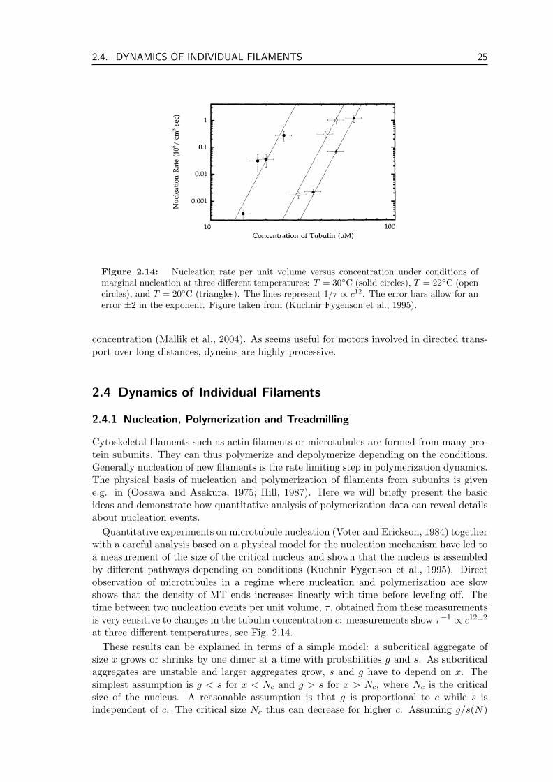
2.4. DYNAMICS OF INDIVIDUAL FILAMENTS 25
Figure 2.14: Nucleation rate per unit volume versus concentration under conditions ofmarginal nucleation at three different temperatures: T = 30C (solid circles), T = 22C (opencircles), and T = 20C (triangles). The lines represent 1/τ ∝ c12. The error bars allow for anerror ±2 in the exponent. Figure taken from (Kuchnir Fygenson et al., 1995).
concentration (Mallik et al., 2004). As seems useful for motors involved in directed trans-port over long distances, dyneins are highly processive.
2.4 Dynamics of Individual Filaments
2.4.1 Nucleation, Polymerization and Treadmilling
Cytoskeletal filaments such as actin filaments or microtubules are formed from many pro-tein subunits. They can thus polymerize and depolymerize depending on the conditions.Generally nucleation of new filaments is the rate limiting step in polymerization dynamics.The physical basis of nucleation and polymerization of filaments from subunits is givene.g. in (Oosawa and Asakura, 1975; Hill, 1987). Here we will briefly present the basicideas and demonstrate how quantitative analysis of polymerization data can reveal detailsabout nucleation events.
Quantitative experiments on microtubule nucleation (Voter and Erickson, 1984) togetherwith a careful analysis based on a physical model for the nucleation mechanism have led toa measurement of the size of the critical nucleus and shown that the nucleus is assembledby different pathways depending on conditions (Kuchnir Fygenson et al., 1995). Directobservation of microtubules in a regime where nucleation and polymerization are slowshows that the density of MT ends increases linearly with time before leveling off. Thetime between two nucleation events per unit volume, τ , obtained from these measurementsis very sensitive to changes in the tubulin concentration c: measurements show τ−1 ∝ c12±2
at three different temperatures, see Fig. 2.14.These results can be explained in terms of a simple model: a subcritical aggregate of
size x grows or shrinks by one dimer at a time with probabilities g and s. As subcriticalaggregates are unstable and larger aggregates grow, s and g have to depend on x. Thesimplest assumption is g < s for x < Nc and g > s for x > Nc, where Nc is the criticalsize of the nucleus. A reasonable assumption is that g is proportional to c while s isindependent of c. The critical size Nc thus can decrease for higher c. Assuming g/s(N)
26 CHAPTER 2. THE CYTOSKELETON
to be a step function and ignoring events involving more than one aggregate, a constantnucleation rate leads to a steady state of subcritical aggregates captured by
g n(N) = s n(N + 1) for N < Nc − 1 (2.3)
where n(N) is the number density of aggregates of size N . The nucleation rate in a VolumeV is then given by
1τ
= g n(1)(g
s
)Nc−2∝ cNc , (2.4)
where n(1) = c is the concentration of dimers. The exponent Nc = 12 ± 2 obtained frommeasurements thus implies a critical size of 12. The model only demands subsequentaggregation, not instantaneous condensation of 12 dimers.
In the other extreme regime of abundant nucleation microtubules are dense and cannotbe observed directly by light microscopy. It also turns out that the population of subcriticalaggregates is not steady state and that growth and shrinking depend on the size N . Amodified model to interpret the obtained measurements suggests that in he abundantregime nucleation takes place in three to four steps and the nucleus comprises 12 to 15dimers (Kuchnir Fygenson et al., 1995).
Once a filament is nucleated, new subunits can be added to its ends with rate kon andremoved with rate koff. The gain in length of a filament due to addition of a subunit isdenoted by a. It will be in general equal to or smaller than the length a of an individualsubunit. For simplicity we assume that a = a for the remainder of this thesis. Thevelocities of a polymerizing (plus) and a depolymerizing (minus) end of a filament aregiven by
v+ = a (k+on − k+
off) = a k+ (2.5)v− = a (k−on − k−off) = a k− . (2.6)
Here we have chosen to denote velocities towards the plus end with positive values. Ifkon > koff the respective filament end will grow. We define k± = k±on−k±off. If k+ 6= k− thelength will increase. Typically we have k+ > k− as the faster growing, more dynamic endis termed the plus end. If the concentration of subunits is constant, the filament growswith velocity
vg = v+ − v− = a(k+ − k−) . (2.7)
If the rates k+ and k− are of the same magnitude but have opposites signs, so that thevelocities of both ends obey
v = v+ = −v− , (2.8)
the filament does not change its length. If v > 0 the filament center of mass as well as bothends dislocate in space while the filament length remains constant. This type of filamentdynamics is called treadmilling, cf. section 2.2.2. The velocity v is called the treadmillingspeed.
2.4.2 Force Generation by Polymerization and Depolymerization
Forces in the cytoskeleton can be generated by molecular motors but also by the polymer-ization and depolymerization of protein filaments (Oosawa and Asakura, 1975; Hill, 1987).Due to their greater structural stability (e.g. greater persistence length) microtubulesseem to be better suited to transmit pulling as well as pushing forces than individualactin filaments. In this section we concentrate on microtubules. The general ideas be-hind the analysis do of course usually also apply to actin filaments. Examples of how the
2.4. DYNAMICS OF INDIVIDUAL FILAMENTS 27
polymerization forces are used to achieve important functions in cells have been reviewedrecently (Dogterom et al., 2005). In this section we will briefly review possible physicalmechanisms for this type of force generation.
Depending on the exact conditions MTs gain ∆G = 5 − 10 kBT per addition of aGTP-tubulin dimer. So in principle a microtubule that grows a = 8 nm by adding onetubulin dimer to each of the N = 13 protofilaments, could generate ∼ 50 pN force (F 'N∆G/a) (Inoue and Salmon, 1995; Desai and Mitchison, 1997). After hydrolysis of thetri-phosphate, the disassembly of GTP-tubulin from a microtubule also releases 5−10 kBTper dimer (Desai and Mitchison, 1997). Assembly and disassembly of microtubules arethus processes that release energy. This energy stems from the GTP-hydrolysis and canbe harnessed to do mechanical work. In addition to that, the GTP hydrolysis itself couldalso contribute to force generated by a microtubule. Forces due to polymerization anddepolymerization can be transmitted to other structures by proteins that track filamentends. The efficiency of these end-tracking proteins in transmitting forces might also dependon GTP-hydrolysis (Dickinson et al., 2004).
The polymerization forces of microtubules in vitro have been measured di-rectly (Dogterom and Yurke, 1997). The stall force for microtubule growth is at least5 pN, comparable to the stall force of molecular motors, e.g. 8 pN for kinesin (Verkhovskyet al., 1999). The force-velocity curves of polymerizing microtubules depend on the concen-tration of free tubulin (Janson and Dogterom, 2004a). Pushing on growing microtubulesin vitro increases the rate of catastrophes and slows growth (Janson et al., 2003).
These observations suggest a thermal or Brownian ratchet mechanism for MT forcegeneration by polymerization (Peskin et al., 1993). If a filament grows against an appliedforce (cf. Fig. 2.15a) thermal fluctuations of the target will occasionally allow the additionof new subunits to the filament. The filament will thus grow despite the applied force.Increasing the force decreases the amplitude of the fluctuations and consequently the rateof addition of new subunits (Mogilner and Oster, 1999). The stall force is the force atwhich the rates of subunit addition and removal are exactly equal and no net growthtakes place (van Doorn et al., 2000). An important extension of this model was theelastic Brownian ratchet (Mogilner and Oster, 1996), which also takes into account thefluctuations due to bending of the filament.
In terms of thermodynamics the observation that applied forces influence the polymer-ization dynamics can be understood as the presence of an external force Fext modifies theon- and off rates by a Boltzmann factor exp(Fexta1/kBT ) (Dogterom and Yurke, 1997;Kolomeisky and Fisher, 2001). Here Fexta1 is the most probable work needed to add asubunit against the force Fext and kBT is the thermal energy. The length a1 is a parameterwhich has to be determined experimentally. This give rise to a force dependent growthvelocity, i.e. Eq. (2.7) becomes
vg(Fext) = a
(kon exp
(qFexta1
kBT
)− koff exp
((1− q)
Fexta1
kBT
)). (2.9)
Here q is a parameter that characterizes the relative strength of influence of the externalforce on the on- and off-rate respectively. The stall force for which vg(Fs) = 0 is given by
Fs =kBT
a1ln
kon
koff(2.10)
and independent of q and a.These results have also been obtained by applying a generalized version of this Brownian
ratchet model to multi-filament microtubules (cf. Fig. 2.15b), which showed that the force
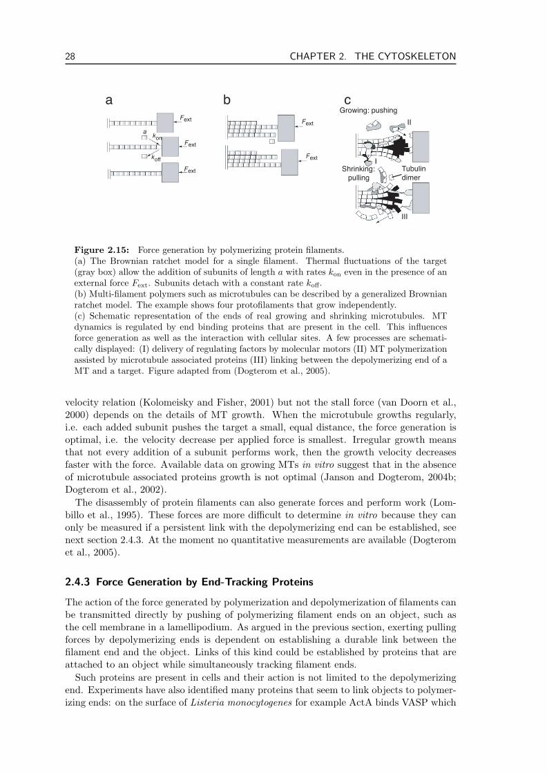
28 CHAPTER 2. THE CYTOSKELETON
a cb
akon
koff
Fext
Fext
Fext
Fext
Fext
Growing: pushing
Shrinking: pulling
Tubulin dimer
I
II
III
Figure 2.15: Force generation by polymerizing protein filaments.(a) The Brownian ratchet model for a single filament. Thermal fluctuations of the target(gray box) allow the addition of subunits of length a with rates kon even in the presence of anexternal force Fext. Subunits detach with a constant rate koff.(b) Multi-filament polymers such as microtubules can be described by a generalized Brownianratchet model. The example shows four protofilaments that grow independently.(c) Schematic representation of the ends of real growing and shrinking microtubules. MTdynamics is regulated by end binding proteins that are present in the cell. This influencesforce generation as well as the interaction with cellular sites. A few processes are schemati-cally displayed: (I) delivery of regulating factors by molecular motors (II) MT polymerizationassisted by microtubule associated proteins (III) linking between the depolymerizing end of aMT and a target. Figure adapted from (Dogterom et al., 2005).
velocity relation (Kolomeisky and Fisher, 2001) but not the stall force (van Doorn et al.,2000) depends on the details of MT growth. When the microtubule growths regularly,i.e. each added subunit pushes the target a small, equal distance, the force generation isoptimal, i.e. the velocity decrease per applied force is smallest. Irregular growth meansthat not every addition of a subunit performs work, then the growth velocity decreasesfaster with the force. Available data on growing MTs in vitro suggest that in the absenceof microtubule associated proteins growth is not optimal (Janson and Dogterom, 2004b;Dogterom et al., 2002).
The disassembly of protein filaments can also generate forces and perform work (Lom-billo et al., 1995). These forces are more difficult to determine in vitro because they canonly be measured if a persistent link with the depolymerizing end can be established, seenext section 2.4.3. At the moment no quantitative measurements are available (Dogteromet al., 2005).
2.4.3 Force Generation by End-Tracking Proteins
The action of the force generated by polymerization and depolymerization of filaments canbe transmitted directly by pushing of polymerizing filament ends on an object, such asthe cell membrane in a lamellipodium. As argued in the previous section, exerting pullingforces by depolymerizing ends is dependent on establishing a durable link between thefilament end and the object. Links of this kind could be established by proteins that areattached to an object while simultaneously tracking filament ends.
Such proteins are present in cells and their action is not limited to the depolymerizingend. Experiments have also identified many proteins that seem to link objects to polymer-izing ends: on the surface of Listeria monocytogenes for example ActA binds VASP which
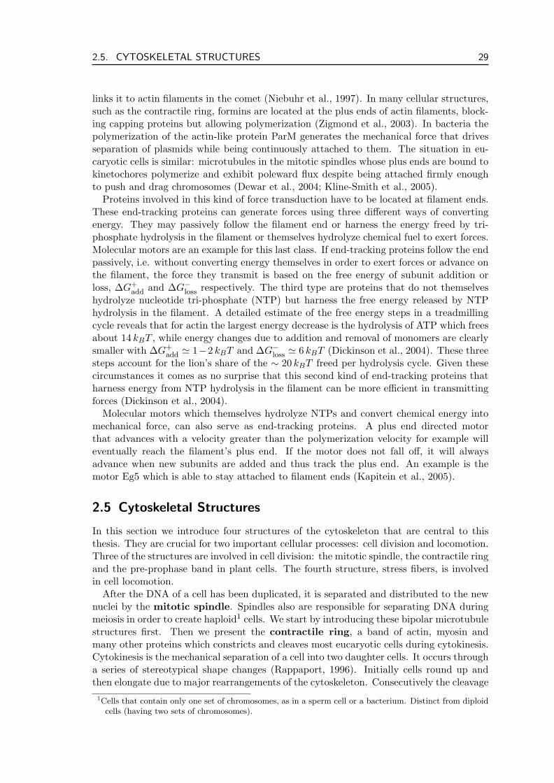
2.5. CYTOSKELETAL STRUCTURES 29
links it to actin filaments in the comet (Niebuhr et al., 1997). In many cellular structures,such as the contractile ring, formins are located at the plus ends of actin filaments, block-ing capping proteins but allowing polymerization (Zigmond et al., 2003). In bacteria thepolymerization of the actin-like protein ParM generates the mechanical force that drivesseparation of plasmids while being continuously attached to them. The situation in eu-caryotic cells is similar: microtubules in the mitotic spindles whose plus ends are bound tokinetochores polymerize and exhibit poleward flux despite being attached firmly enoughto push and drag chromosomes (Dewar et al., 2004; Kline-Smith et al., 2005).
Proteins involved in this kind of force transduction have to be located at filament ends.These end-tracking proteins can generate forces using three different ways of convertingenergy. They may passively follow the filament end or harness the energy freed by tri-phosphate hydrolysis in the filament or themselves hydrolyze chemical fuel to exert forces.Molecular motors are an example for this last class. If end-tracking proteins follow the endpassively, i.e. without converting energy themselves in order to exert forces or advance onthe filament, the force they transmit is based on the free energy of subunit addition orloss, ∆G+
add and ∆G−loss respectively. The third type are proteins that do not themselves
hydrolyze nucleotide tri-phosphate (NTP) but harness the free energy released by NTPhydrolysis in the filament. A detailed estimate of the free energy steps in a treadmillingcycle reveals that for actin the largest energy decrease is the hydrolysis of ATP which freesabout 14 kBT , while energy changes due to addition and removal of monomers are clearlysmaller with ∆G+
add ' 1−2 kBT and ∆G−loss ' 6 kBT (Dickinson et al., 2004). These three
steps account for the lion’s share of the ∼ 20 kBT freed per hydrolysis cycle. Given thesecircumstances it comes as no surprise that this second kind of end-tracking proteins thatharness energy from NTP hydrolysis in the filament can be more efficient in transmittingforces (Dickinson et al., 2004).
Molecular motors which themselves hydrolyze NTPs and convert chemical energy intomechanical force, can also serve as end-tracking proteins. A plus end directed motorthat advances with a velocity greater than the polymerization velocity for example willeventually reach the filament’s plus end. If the motor does not fall off, it will alwaysadvance when new subunits are added and thus track the plus end. An example is themotor Eg5 which is able to stay attached to filament ends (Kapitein et al., 2005).
2.5 Cytoskeletal Structures
In this section we introduce four structures of the cytoskeleton that are central to thisthesis. They are crucial for two important cellular processes: cell division and locomotion.Three of the structures are involved in cell division: the mitotic spindle, the contractile ringand the pre-prophase band in plant cells. The fourth structure, stress fibers, is involvedin cell locomotion.
After the DNA of a cell has been duplicated, it is separated and distributed to the newnuclei by the mitotic spindle. Spindles also are responsible for separating DNA duringmeiosis in order to create haploid1 cells. We start by introducing these bipolar microtubulestructures first. Then we present the contractile ring, a band of actin, myosin andmany other proteins which constricts and cleaves most eucaryotic cells during cytokinesis.Cytokinesis is the mechanical separation of a cell into two daughter cells. It occurs througha series of stereotypical shape changes (Rappaport, 1996). Initially cells round up andthen elongate due to major rearrangements of the cytoskeleton. Consecutively the cleavage
1Cells that contain only one set of chromosomes, as in a sperm cell or a bacterium. Distinct from diploidcells (having two sets of chromosomes).
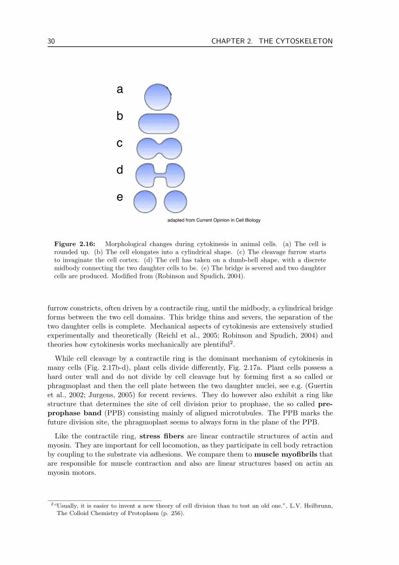
30 CHAPTER 2. THE CYTOSKELETON
a
adapted from Current Opinion in Cell Biology
e
d
c
b
Figure 2.16: Morphological changes during cytokinesis in animal cells. (a) The cell isrounded up. (b) The cell elongates into a cylindrical shape. (c) The cleavage furrow startsto invaginate the cell cortex. (d) The cell has taken on a dumb-bell shape, with a discretemidbody connecting the two daughter cells to be. (e) The bridge is severed and two daughtercells are produced. Modified from (Robinson and Spudich, 2004).
furrow constricts, often driven by a contractile ring, until the midbody, a cylindrical bridgeforms between the two cell domains. This bridge thins and severs, the separation of thetwo daughter cells is complete. Mechanical aspects of cytokinesis are extensively studiedexperimentally and theoretically (Reichl et al., 2005; Robinson and Spudich, 2004) andtheories how cytokinesis works mechanically are plentiful2.
While cell cleavage by a contractile ring is the dominant mechanism of cytokinesis inmany cells (Fig. 2.17b-d), plant cells divide differently, Fig. 2.17a. Plant cells possess ahard outer wall and do not divide by cell cleavage but by forming first a so called orphragmoplast and then the cell plate between the two daughter nuclei, see e.g. (Guertinet al., 2002; Jurgens, 2005) for recent reviews. They do however also exhibit a ring likestructure that determines the site of cell division prior to prophase, the so called pre-prophase band (PPB) consisting mainly of aligned microtubules. The PPB marks thefuture division site, the phragmoplast seems to always form in the plane of the PPB.
Like the contractile ring, stress fibers are linear contractile structures of actin andmyosin. They are important for cell locomotion, as they participate in cell body retractionby coupling to the substrate via adhesions. We compare them to muscle myofibrils thatare responsible for muscle contraction and also are linear structures based on actin anmyosin motors.
2“Usually, it is easier to invent a new theory of cell division than to test an old one.”, L.V. Heilbrunn,The Colloid Chemistry of Protoplasm (p. 256).
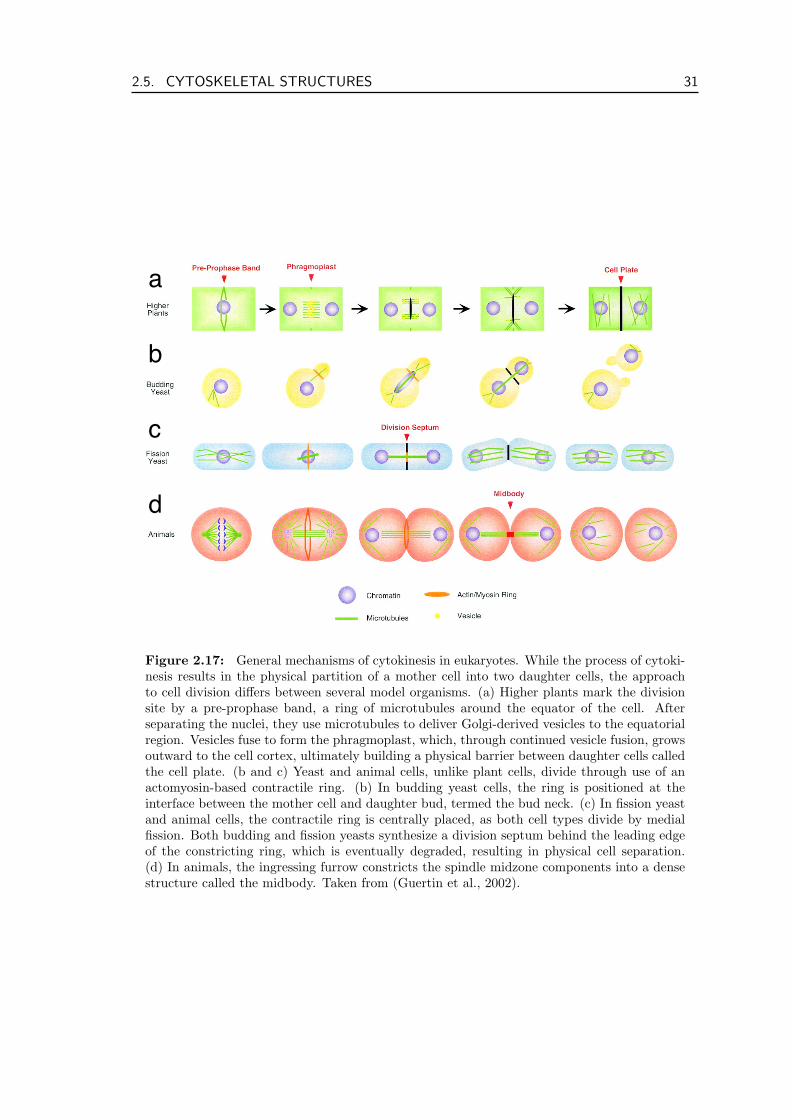
2.5. CYTOSKELETAL STRUCTURES 31
a
d
c
b
Figure 2.17: General mechanisms of cytokinesis in eukaryotes. While the process of cytoki-nesis results in the physical partition of a mother cell into two daughter cells, the approachto cell division differs between several model organisms. (a) Higher plants mark the divisionsite by a pre-prophase band, a ring of microtubules around the equator of the cell. Afterseparating the nuclei, they use microtubules to deliver Golgi-derived vesicles to the equatorialregion. Vesicles fuse to form the phragmoplast, which, through continued vesicle fusion, growsoutward to the cell cortex, ultimately building a physical barrier between daughter cells calledthe cell plate. (b and c) Yeast and animal cells, unlike plant cells, divide through use of anactomyosin-based contractile ring. (b) In budding yeast cells, the ring is positioned at theinterface between the mother cell and daughter bud, termed the bud neck. (c) In fission yeastand animal cells, the contractile ring is centrally placed, as both cell types divide by medialfission. Both budding and fission yeasts synthesize a division septum behind the leading edgeof the constricting ring, which is eventually degraded, resulting in physical cell separation.(d) In animals, the ingressing furrow constricts the spindle midzone components into a densestructure called the midbody. Taken from (Guertin et al., 2002).
32 CHAPTER 2. THE CYTOSKELETON
5µm
Figure 2.18: Mitotic spindle in a vertebrate cell during metaphase. Microtubules are labeledin green, kinetochores in red, and chromosomes in blue. Taken from (Desai, 2000).
2.5.1 Mitotic and Meiotic Spindles
Prior to cytokinesis, i.e. the division of the cytoplasm of the cell, each nascent daughtercell needs to be equipped with one of the two identical sets of chromosomes. The cell’sDNA thus has to be duplicated and then distributed to the two newly formed nuclei. In alleucaryotic cells this distribution is achieved by a bipolar spindle during mitosis. Spindlesare composed of microtubules and various other proteins such as molecular motors, kinasesthat interact with them and hundreds of other MAPs (Maiato et al., 2004). The typicalspindle is formed by two microtubule asters that become the spindle poles. These astersare linked to the chromosomes via kinetochores, Fig. 2.18. Microtubules of both astersalso reach out into the cytoplasm and can make contact with MTs from the other asteras well as the cell walls. Microtubules then shorten and spindle poles move away from thecenter thus separating the chromosomes. Spindles are also involved in meiosis, i.e. the celldivision in which haploid sperm cells and eggs are produced. In this case they are referredto as meiotic spindles.
The typical life cycle of a spindle is depicted in Fig. 2.19. Spindles generally start toform outside the nuclear membrane during prophase while the chromosomes condense.The centrosomes are duplicated and then separate. They start nucleating microtubules,forming the nascent poles of the future spindle. After nuclear envelope breakdown atprometaphase these microtubules can capture the condensed chromosomes. The chro-mosomes become aligned between the poles in the metaphase plate perpendicular to thespindle axis. During anaphase-A the chromosomes separate and move towards oppositespindle poles. Anaphase-B marks the further separation of the spindle poles from eachother. In mammalian cells, the spindle elongates up to 2-fold during anaphase. In someplant cells however, spindle length hardly changes at all while some protozoa representthe other extreme: here the chromosomes become separated 15 times their distance in themetaphase spindle (Bray, 2001).
Spindle Structure
The spindle microtubules (several thousands in mammalian cells) can be grouped into threeclasses depending on their properties: astral microtubules radiate from the spindle pole inall directions and are involved in force transmission between the pole and the cell mem-brane (Grill et al., 2003, 2001). These forces are responsible for spindle positioning andorientation (Grill and Hyman, 2005), spindle pole separation and spindle oscillations (Grill
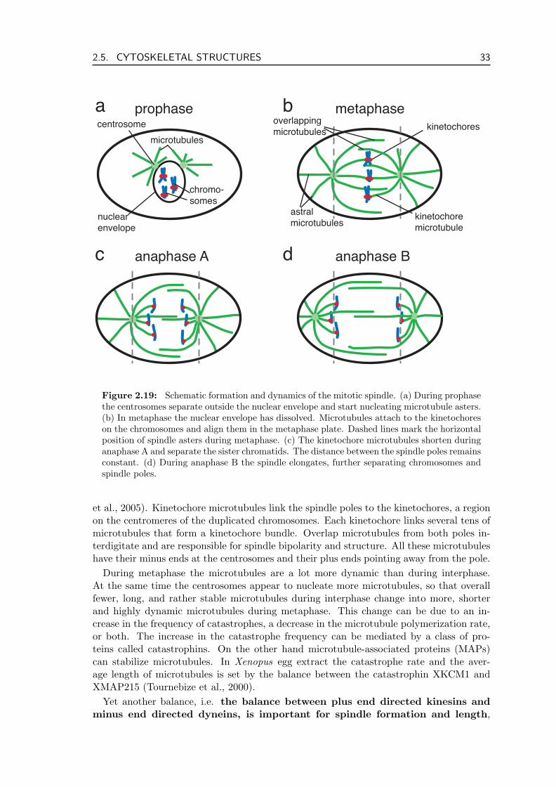
2.5. CYTOSKELETAL STRUCTURES 33
microtubulescentrosome
nuclearenvelope
chromo-somes
prophase metaphase
anaphase A anaphase B
astralmicrotubules
overlappingmicrotubules
kinetochore microtubule
kinetochores
a b
c d
Figure 2.19: Schematic formation and dynamics of the mitotic spindle. (a) During prophasethe centrosomes separate outside the nuclear envelope and start nucleating microtubule asters.(b) In metaphase the nuclear envelope has dissolved. Microtubules attach to the kinetochoreson the chromosomes and align them in the metaphase plate. Dashed lines mark the horizontalposition of spindle asters during metaphase. (c) The kinetochore microtubules shorten duringanaphase A and separate the sister chromatids. The distance between the spindle poles remainsconstant. (d) During anaphase B the spindle elongates, further separating chromosomes andspindle poles.
et al., 2005). Kinetochore microtubules link the spindle poles to the kinetochores, a regionon the centromeres of the duplicated chromosomes. Each kinetochore links several tens ofmicrotubules that form a kinetochore bundle. Overlap microtubules from both poles in-terdigitate and are responsible for spindle bipolarity and structure. All these microtubuleshave their minus ends at the centrosomes and their plus ends pointing away from the pole.
During metaphase the microtubules are a lot more dynamic than during interphase.At the same time the centrosomes appear to nucleate more microtubules, so that overallfewer, long, and rather stable microtubules during interphase change into more, shorterand highly dynamic microtubules during metaphase. This change can be due to an in-crease in the frequency of catastrophes, a decrease in the microtubule polymerization rate,or both. The increase in the catastrophe frequency can be mediated by a class of pro-teins called catastrophins. On the other hand microtubule-associated proteins (MAPs)can stabilize microtubules. In Xenopus egg extract the catastrophe rate and the aver-age length of microtubules is set by the balance between the catastrophin XKCM1 andXMAP215 (Tournebize et al., 2000).
Yet another balance, i.e. the balance between plus end directed kinesins andminus end directed dyneins, is important for spindle formation and length,
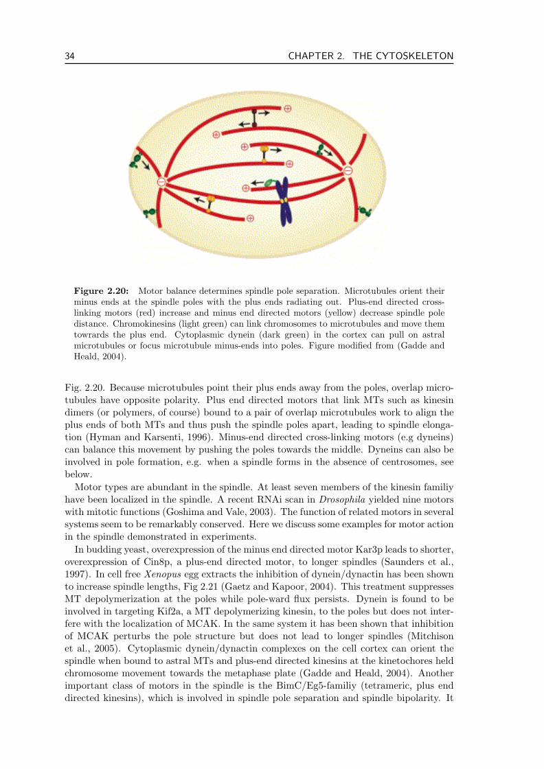
34 CHAPTER 2. THE CYTOSKELETON
Figure 2.20: Motor balance determines spindle pole separation. Microtubules orient theirminus ends at the spindle poles with the plus ends radiating out. Plus-end directed cross-linking motors (red) increase and minus end directed motors (yellow) decrease spindle poledistance. Chromokinesins (light green) can link chromosomes to microtubules and move themtowrards the plus end. Cytoplasmic dynein (dark green) in the cortex can pull on astralmicrotubules or focus microtubule minus-ends into poles. Figure modified from (Gadde andHeald, 2004).
Fig. 2.20. Because microtubules point their plus ends away from the poles, overlap micro-tubules have opposite polarity. Plus end directed motors that link MTs such as kinesindimers (or polymers, of course) bound to a pair of overlap microtubules work to align theplus ends of both MTs and thus push the spindle poles apart, leading to spindle elonga-tion (Hyman and Karsenti, 1996). Minus-end directed cross-linking motors (e.g dyneins)can balance this movement by pushing the poles towards the middle. Dyneins can also beinvolved in pole formation, e.g. when a spindle forms in the absence of centrosomes, seebelow.
Motor types are abundant in the spindle. At least seven members of the kinesin familiyhave been localized in the spindle. A recent RNAi scan in Drosophila yielded nine motorswith mitotic functions (Goshima and Vale, 2003). The function of related motors in severalsystems seem to be remarkably conserved. Here we discuss some examples for motor actionin the spindle demonstrated in experiments.
In budding yeast, overexpression of the minus end directed motor Kar3p leads to shorter,overexpression of Cin8p, a plus-end directed motor, to longer spindles (Saunders et al.,1997). In cell free Xenopus egg extracts the inhibition of dynein/dynactin has been shownto increase spindle lengths, Fig 2.21 (Gaetz and Kapoor, 2004). This treatment suppressesMT depolymerization at the poles while pole-ward flux persists. Dynein is found to beinvolved in targeting Kif2a, a MT depolymerizing kinesin, to the poles but does not inter-fere with the localization of MCAK. In the same system it has been shown that inhibitionof MCAK perturbs the pole structure but does not lead to longer spindles (Mitchisonet al., 2005). Cytoplasmic dynein/dynactin complexes on the cell cortex can orient thespindle when bound to astral MTs and plus-end directed kinesins at the kinetochores heldchromosome movement towards the metaphase plate (Gadde and Heald, 2004). Anotherimportant class of motors in the spindle is the BimC/Eg5-familiy (tetrameric, plus enddirected kinesins), which is involved in spindle pole separation and spindle bipolarity. It
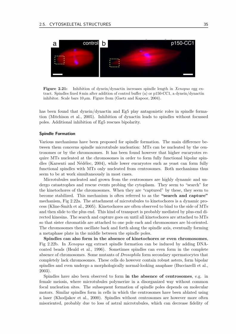
2.5. CYTOSKELETAL STRUCTURES 35
a b
Figure 2.21: Inhibition of dynein/dynactin increases spindle length in Xenopus egg ex-tract. Spindles fixed 8 min after addition of control buffer (a) or p150-CC1, a dynein/dynactininhibitor. Scale bars 10 µm. Figure from (Gaetz and Kapoor, 2004).
has been found that dynein/dynactin and Eg5 play antagonistic roles in spindle forma-tion (Mitchison et al., 2005). Inhibition of dynactin leads to spindles without focussedpoles. Additional inhibition of Eg5 rescues bipolarity.
Spindle Formation
Various mechanisms have been proposed for spindle formation. The main difference be-tween them concerns spindle microtubule nucleation: MTs can be nucleated by the cen-trosomes or by the chromosomes. It has been found however that higher eucaryotes re-quire MTs nucleated at the chromosomes in order to form fully functional bipolar spin-dles (Karsenti and Nedelec, 2004), while lower eucaryotes such as yeast can form fullyfunctional spindles with MTs only nucleated from centrosomes. Both mechanisms thusseem to be at work simultaneously in most cases.
Microtubules nucleated and grown from the centrosomes are highly dynamic and un-dergo catastrophes and rescue events probing the cytoplasm. They seem to “search” forthe kinetochores of the chromosomes. When they are “captured” by these, they seem tobecome stabilized. This mechanism is often referred to as the “search and capture”mechanism, Fig 2.22a. The attachment of microtubules to kinetochores is a dynamic pro-cess (Kline-Smith et al., 2005). Kinetochores are often observed to bind to the side of MTsand then slide to the plus end. This kind of transport is probably mediated by plus-end di-rected kinesins. The search and capture goes on until all kinetochores are attached to MTsso that sister chromatids are attached to one pole each and chromosomes are bi-oriented.The chromosomes then oscillate back and forth along the spindle axis, eventually forminga metaphase plate in the middle between the spindle poles.
Spindles can also form in the absence of kinetochores or even chromosomes,Fig 2.22b. In Xenopus egg extract spindle formation can be induced by adding DNA-coated beads (Heald et al., 1996). Sometimes spindles can even form in the completeabsence of chromosomes. Some mutants of Drosophila form secondary spermatocytes thatcompletely lack chromosomes. These cells do however contain robust asters, form bipolarspindles and even undergo a morphologically normal-looking anaphase (Bucciarelli et al.,2003).
Spindles have also been observed to form in the absence of centrosomes, e.g. infemale meiosis, where microtubules polymerize in a disorganized way without commonfocal nucleation sites. The subsequent formation of spindle poles depends on molecularmotors. Similar spindles form in cells in which the centrosomes have been ablated usinga laser (Khodjakov et al., 2000). Spindles without centrosomes are however more oftenmisoriented, probably due to loss of astral microtubules, which can decrease fidelity of
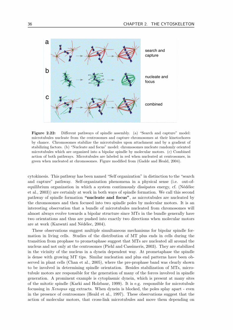
36 CHAPTER 2. THE CYTOSKELETON
a
b
c
search and capture
nucleate and focus
combined
Figure 2.22: Different pathways of spindle assembly. (a) “Search and capture” model:microtubules nucleate from the centrosomes and capture chromosomes at their kinetochoresby chance. Chromosomes stabilize the microtubules upon attachment and by a gradient ofstabilizing factors. (b) “Nucleate and focus” model: chromosomes nucleate randomly orientedmicrotubules which are organized into a bipolar spindle by molecular motors. (c) Combinedaction of both pathways. Microtubules are labeled in red when nucleated at centrosomes, ingreen when nucleated at chromosomes. Figure modified from (Gadde and Heald, 2004).
cytokinesis. This pathway has been named “Self organization” in distinction to the “searchand capture” pathway. Self-organization phenomena in a physical sense (i.e. out-of-equilibrium organization in which a system continuously dissipates energy, cf. (Nedelecet al., 2003)) are certainly at work in both ways of spindle formation. We call this secondpathway of spindle formation “nucleate and focus”, as microtubules are nucleated bythe chromosomes and then focused into two spindle poles by molecular motors. It is aninteresting observation that a bundle of microtubules nucleated from chromosomes willalmost always evolve towards a bipolar structure since MTs in the bundle generally havetwo orientations and thus are pushed into exactly two directions when molecular motorsare at work (Karsenti and Nedelec, 2004).
These observations suggest multiple simultaneous mechanisms for bipolar spindle for-mation in living cells. Studies of the distribution of MT plus ends in cells during thetransition from prophase to prometaphase suggest that MTs are nucleated all around thenucleus and not only at the centrosomes (Piehl and Cassimeris, 2003). They are stabilizedin the vicinity of the nucleus in a dynein dependent way. At prometaphase the spindleis dense with growing MT tips. Similar nucleation and plus end patterns have been ob-served in plant cells (Chan et al., 2005), where the pre-prophase band was clearly shownto be involved in determining spindle orientation. Besides stabilization of MTs, micro-tubule motors are responsible for the generation of many of the forces involved in spindlegeneration. A prominent example is cytoplasmic dynein, which is present at many sitesof the mitotic spindle (Karki and Holzbaur, 1999). It is e.g. responsible for microtubulefocussing in Xenopus egg extracts. When dynein is blocked, the poles splay apart - evenin the presence of centrosomes (Heald et al., 1997). These observations suggest that theaction of molecular motors, that cross-link microtubules and move them depending on
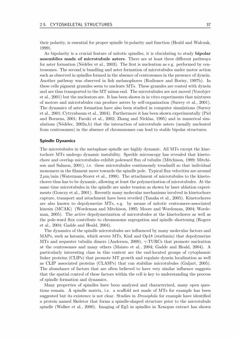
2.5. CYTOSKELETAL STRUCTURES 37
their polarity, is essential for proper spindle bi-polarity and function (Heald and Walczak,1999).
As bipolarity is a crucial feature of mitotic spindles, it is elucidating to study bipolarassemblies made of microtubule asters. There are at least three different pathwaysfor aster formation (Nedelec et al., 2003). The first is nucleation as e.g. performed by cen-trosomes. The second is bundling and aster formation of microtubules under motor actionsuch as observed in spindles formed in the absence of centrosomes in the presence of dynein.Another pathway was observed in fish melanophores (Rodionov and Borisy, 1997b). Inthese cells pigment granules seem to nucleate MTs. These granules are coated with dyneinand are thus transported to the MT minus end. The microtubules are not moved (Vorobjevet al., 2001) but the nucleators are. It has been shown in in vitro experiments that mixturesof motors and microtubules can produce asters by self-organization (Surrey et al., 2001).The dynamics of aster formation have also been studied in computer simulations (Surreyet al., 2001; Cytrynbaum et al., 2004). Furthermore it has been shown experimentally (Pieland Bornens, 2001; Faruki et al., 2002; Zhang and Nicklas, 1995) and in numerical sim-ulations (Nedelec, 2002a,b) that the interaction of microtubule asters (usually nucleatedfrom centrosomes) in the absence of chromosomes can lead to stable bipolar structures.
Spindle Dynamics
The microtubules in the metaphase spindle are highly dynamic. All MTs except the kine-tochore MTs undergo dynamic instability. Speckle microscopy has revealed that kineto-chore and overlap microtubules exhibit poleward flux of tubulin (Mitchison, 1989; Mitchi-son and Salmon, 2001), i.e. these microtubules continuously treadmill so that individualmonomers in the filament move towards the spindle pole. Typical flux velocities are around2 µm/min (Waterman-Storer et al., 1998). The attachment of microtubules to the kineto-chores thus has to be dynamic, allowing at least the polymerization of microtubules. At thesame time microtubules in the spindle are under tension as shown by laser ablation experi-ments (Gonczy et al., 2001). Recently many molecular mechanisms involved in kinetochorecapture, transport and attachment have been reveiled (Tanaka et al., 2005). Kinetochoresare also known to depolymerize MTs, e.g. by means of mitotic centromere-associatedkinesin (MCAK) (Wordeman and Mitchison, 1995; Moore and Wordeman, 2004; Worde-man, 2005). The active depolymerization of microtubules at the kinetochores as well asthe pole-ward flux contribute to chromosome segregation and spindle shortening (Rogerset al., 2004; Gadde and Heald, 2004).
The dynamics of the spindle microtubules are influenced by many molecular factors andMAPs, such as katanin, which severs MTs, KinI and Op18 (stathmin) that depolymerizeMTs and sequester tubulin dimers (Andersen, 2000), γ-TURCs that promote nucleationat the centrosomes and many others (Maiato et al., 2004; Gadde and Heald, 2004). Aparticularly interesting class in this context are the end-located groups of cytoplasmiclinker proteins (CLIPs) that promote MT growth and regulate dynein localization as wellas CLIP associated proteins (CLASPs) that can stabilize microtubules (Galjart, 2005).The abundance of factors that are often believed to have very similar influence suggeststhat the spatial control of these factors within the cell is key to understanding the processof spindle formation and dynamics.
Many properties of spindles have been analyzed and characterized, many open ques-tions remain. A spindle matrix, i.e. a scaffold not made of MTs for example has beensuggested but its existence is not clear. Studies in Drosophila for example have identifieda protein named Skeletor that forms a spindle-shaped structure prior to the microtubulespindle (Walker et al., 2000). Imaging of Eg5 in spindles in Xenopus extract has shown
38 CHAPTER 2. THE CYTOSKELETON
that Eg5 is stationary with respect to MTs that undergo pole-ward flux (Kapoor andMitchison, 2001). This hints towards the existence of a spindle matrix also in this system.
Furthermore an amusing parallel has been drawn between the dynamics of the mitoticspindle and a treadmilling actin gel in cell motility (Karsenti and Nedelec, 2004). Theactin comet polymerized by Listeria could be compared with microtubules nucleated fromchromosomes in a mitotic spindle. The chromatin thus corresponds to the bacterium. Likethe actin comet the microtubules treadmill away from the chromosomes as indicated bypole-ward flux. This can exert forces on the chromosomes either directly or by action ofplus end directed molecular motors such as kinesin. The most striking difference betweenthe two systems is their symmetry. While symmetry breaking and formation of a monopo-lar structure in actin gels is essential for motility, the spindle is only functional when itassumes a bipolar configuration.
2.5.2 The Contractile Ring
Once chromosome separation and distribution onto the two future daughter cells is com-pleted, most eucaryotic cells (the exception being higher plant cells as discussed in sec-tion 2.5.3 below) divide their cytoplasm by constriction of a contractile actomyosin bundle.This ring is often located at the cell’s equator. In many cases such as the fission yeastS. pombe (Pelham and Chang, 2002; Wu et al., 2003), Arbacia eggs (Schroeder, 1972),human HeLa cells (Schroeder, 1970; Maupin and Pollard, 1986) and many more, the bun-dle forms a contractile ring which encircles the cell, see Fig. 2.23. There is experimentalevidence that the location of the ring is dependent on microtubule structures (Pardo andNurse, 2003; Glotzer, 2004) that in turn depend on the actin ring (Murthy and Wadsworth,2005). In chapter 5 we show that self-organization phenomena can also be sufficient forring formation and positioning.
Electron microscopy suggested that contractile rings consist of many fila-ments (Schroeder, 1970). These filaments can be arranged in several distinct, closelypacked filament bundles, close to each other near the cell membrane (Maupin and Pollard,1986). The filaments were found to be actin (Schroeder, 1970, 1973) and myosin (Fujiwaraand Pollard, 1976; Otto and Schroeder, 1990). These findings provided further argumentsfor a muscle like, sliding filament contraction mechanism of the cleavage furrow. Thestructure of the cleavage furrow could support this theory (Sanger and Sanger, 1980), butuncontroversial evidence for structure and mechanism are still lacking (Schroeder, 1990).The orientation of actin filaments in the ring has been studied (Fishkind and Wang, 1993)during metaphase and anaphase. During metaphase the filaments have a slight orientationalong the spindle axis, while during anaphase the filaments in the furrow become orientedalong the equator. The degree of orientation seems to be largest in regions where the celladheres to a substrate or other cells.
Besides actin and myosin the ring contains many other proteins (Robinson and Spudich,2000; Feierbach and Chang, 2001). Prior to ring formation actin and a large number of as-sociated proteins are recruited to an equatorial domain of the cell cortex (Wu et al., 2003;Glotzer, 2005), seemingly in a precisely timed sequence. These proteins include myosinmotor proteins and tropomyosin that is highly concentrated in muscles and stabilizes F-actin. These proteins could play a role for the generation of contractile forces, bundlingproteins and cross-linkers such as alpha-actinin. Proteins can also be responsible for thelink between actin filaments in the ring and the cell’s plasma membrane (Satterwhite andPollard, 1992). Furthermore, several proteins are recruited that regulate the nucleation,polymerization and depolymerization of actin filaments (cf. section 2.2.3). These include
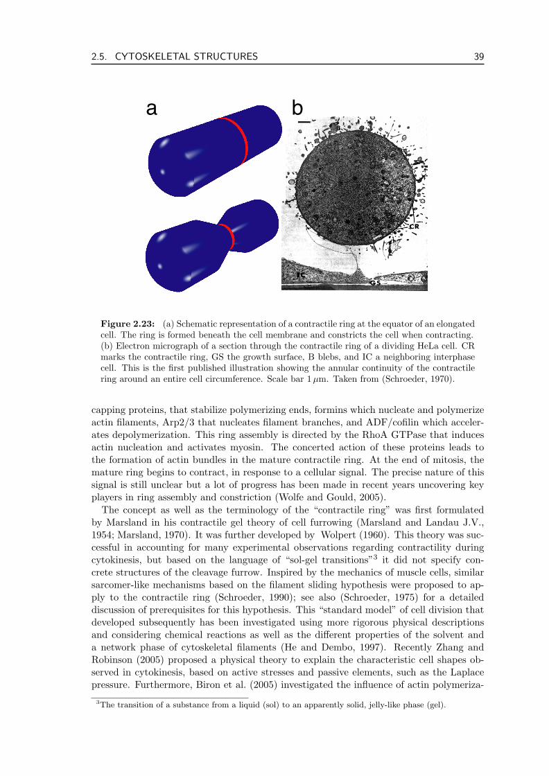
2.5. CYTOSKELETAL STRUCTURES 39
a b
Figure 2.23: (a) Schematic representation of a contractile ring at the equator of an elongatedcell. The ring is formed beneath the cell membrane and constricts the cell when contracting.(b) Electron micrograph of a section through the contractile ring of a dividing HeLa cell. CRmarks the contractile ring, GS the growth surface, B blebs, and IC a neighboring interphasecell. This is the first published illustration showing the annular continuity of the contractilering around an entire cell circumference. Scale bar 1 µm. Taken from (Schroeder, 1970).
capping proteins, that stabilize polymerizing ends, formins which nucleate and polymerizeactin filaments, Arp2/3 that nucleates filament branches, and ADF/cofilin which acceler-ates depolymerization. This ring assembly is directed by the RhoA GTPase that inducesactin nucleation and activates myosin. The concerted action of these proteins leads tothe formation of actin bundles in the mature contractile ring. At the end of mitosis, themature ring begins to contract, in response to a cellular signal. The precise nature of thissignal is still unclear but a lot of progress has been made in recent years uncovering keyplayers in ring assembly and constriction (Wolfe and Gould, 2005).
The concept as well as the terminology of the “contractile ring” was first formulatedby Marsland in his contractile gel theory of cell furrowing (Marsland and Landau J.V.,1954; Marsland, 1970). It was further developed by Wolpert (1960). This theory was suc-cessful in accounting for many experimental observations regarding contractility duringcytokinesis, but based on the language of “sol-gel transitions”3 it did not specify con-crete structures of the cleavage furrow. Inspired by the mechanics of muscle cells, similarsarcomer-like mechanisms based on the filament sliding hypothesis were proposed to ap-ply to the contractile ring (Schroeder, 1990); see also (Schroeder, 1975) for a detaileddiscussion of prerequisites for this hypothesis. This “standard model” of cell division thatdeveloped subsequently has been investigated using more rigorous physical descriptionsand considering chemical reactions as well as the different properties of the solvent anda network phase of cytoskeletal filaments (He and Dembo, 1997). Recently Zhang andRobinson (2005) proposed a physical theory to explain the characteristic cell shapes ob-served in cytokinesis, based on active stresses and passive elements, such as the Laplacepressure. Furthermore, Biron et al. (2005) investigated the influence of actin polymeriza-
3The transition of a substance from a liquid (sol) to an apparently solid, jelly-like phase (gel).
40 CHAPTER 2. THE CYTOSKELETON
tion and depolymerization for the dynamics. They suggest that the actin concentrationwithin the ring and thus the power the ring exerts both increase during contraction.
In this thesis we focus on the physical properties and mechanics of the contractile ring.We aim at analyzing key mechanisms involved in ring contraction. Although the contractilering occurs in cells that are very different in character such as protozoa, squid eggs or tissueculture cells, many ultrastructural features are very similar, even when the surroundingcircumstances vary (Schroeder, 1975). And although details of ring formation differ evenbetween budding yeast S. cerevisiae and fission yeast S. pombe, many aspects are similarall the way from yeast to animal cells (Balasubramanian et al., 2004). While the radiusvaries according to cell size, a “typical” contractile ring is a band about 5-10 µm wide(extreme cases beeing 20µm in large amphibean eggs and 3µm in tiny algal cells) and0.1-0.2 µm thick, see Fig. 2.24. It thus resembles a sheet (or a band) of microfilamentswrapped around the cell’s equator. The microfilaments are 5 nm thick, spaced ca 15 nmapart. In a cross section there are about 5000 of them (Schroeder, 1990). The thickness,width and microfilament spacing are constant during ring contraction (Schroeder, 1972).The ring has been measured to exert a force on the order of 10 nN (Schroeder, 1975;Rappaport, 1967; Burton and Taylor, 1997), but these measurements only provide anupper bound of the force generation and not necessarily the force employed during ringconstriction. The contraction velocity depends on the cell type: the ring constricts with avelocity ' 0.07 µm/min in fission yeast (Pelham and Chang, 2002) and ' 0.6 µm/min inSwiss 3T3 fibroblasts (DeBiasio et al., 1996).
How exactly the ring constricts is still a mystery (Alberts et al., 2002). It seems notto operate by a simple “purse-string” mechanism in which the actomyosin ring simplyconstricts by filament sliding due to myosin II motors such as in muscles. Electron micro-graphs of meridional cross-sections through the ring show that the area of the cross-sectionis conserved during ring constriction (Schroeder, 1972). As the density of material in thering does not change, this implicates that the ring looses material while constricting.The ring thus appears as a dynamic structure that is not only assembled prior to anddisassembled after use, but also constantly reorganized while cleaving the cell. It has beenshown that an actin gel solates or disassembles if a pressure is applied to it (Condeelis andTaylor, 1977). The tension generated by the ring itself could thus be a cause for partialring disassembly, similar to mechanisms proposed for the cell cortex (Paluch et al., 2005;Paluch, 2005).
In chapter 6 we study a mechanism for ring contraction that besides the action ofmolecular motors also can be driven by filament polymerization and depolymerization.The dynamics of the constituents of the ring, especially the turnover of actin, could thusbe directly contributing to ring contraction. Here we present some experimental resultsconcerning ring dynamics. The view of the contractile ring as a highly dynamic structurehas been strengthened by investigation of ring dynamics in fission yeast cells (Pelhamand Chang, 2002). The formation of the ring depends on actin asssembly either frompreexisting actin cables or de novo nucleation and polymerization. This polymerizationdepends on Arp2/3, formin, profilin or WASp, but not myosin II. It was shown that Arp3colocalizes with actin in an equatorial ring, Fig. 2.25. During the time course of ringcontraction (∼ 25 min for wild type S. pombe), many components of the ring (such asetropomyosin or a myosin light chain) are exchanged with a half time of usually less thanone minute. F-actin in particular is completely turned over about every minute. Similarrates have been measured in LLCPK1 epithelial cells (Murthy and Wadsworth, 2005). Innormal rat kidney cells the turnover time of actin in the equatorial region was doubled toabout 30 s after cells had been exposed to blebbistatin, a myosin II inhibitor (Guha et al.,
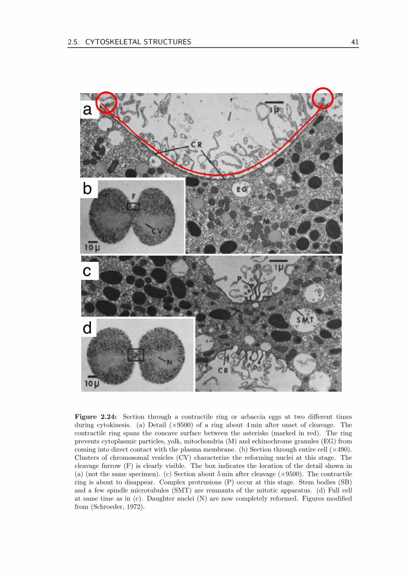
2.5. CYTOSKELETAL STRUCTURES 41
a
d
c
b
Figure 2.24: Section through a contractile ring or arbaccia eggs at two different timesduring cytokinesis. (a) Detail (×9500) of a ring about 4 min after onset of cleavage. Thecontractile ring spans the concave surface between the asterisks (marked in red). The ringprevents cytoplasmic particles, yolk, mitochondria (M) and echinochrome granules (EG) fromcoming into direct contact with the plasma membrane. (b) Section through entire cell (×490).Clusters of chromosomal vesicles (CV) characterize the reforming nuclei at this stage. Thecleavage furrow (F) is clearly visible. The box indicates the location of the detail shown in(a) (not the same specimen). (c) Section about 5 min after cleavage (×9500). The contractilering is about to disappear. Complex protrusions (P) occur at this stage. Stem bodies (SB)and a few spindle microtubules (SMT) are remnants of the mitotic apparatus. (d) Full cellat same time as in (c). Daughter nuclei (N) are now completely reformed. Figures modifiedfrom (Schroeder, 1972).
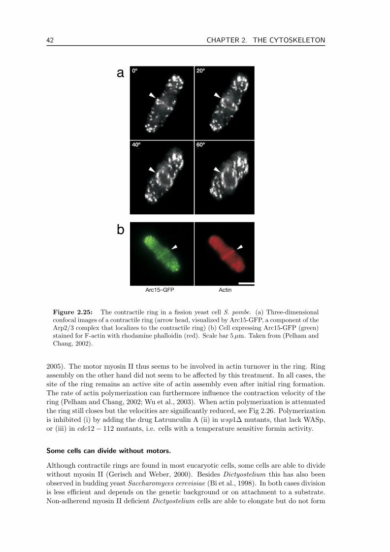
42 CHAPTER 2. THE CYTOSKELETON
a
b
Figure 2.25: The contractile ring in a fission yeast cell S. pombe. (a) Three-dimensionalconfocal images of a contractile ring (arrow head, visualized by Arc15-GFP, a component of theArp2/3 complex that localizes to the contractile ring) (b) Cell expressing Arc15-GFP (green)stained for F-actin with rhodamine phalloidin (red). Scale bar 5µm. Taken from (Pelham andChang, 2002).
2005). The motor myosin II thus seems to be involved in actin turnover in the ring. Ringassembly on the other hand did not seem to be affected by this treatment. In all cases, thesite of the ring remains an active site of actin assembly even after initial ring formation.The rate of actin polymerization can furthermore influence the contraction velocity of thering (Pelham and Chang, 2002; Wu et al., 2003). When actin polymerization is attenuatedthe ring still closes but the velocities are significantly reduced, see Fig 2.26. Polymerizationis inhibited (i) by adding the drug Latrunculin A (ii) in wsp1∆ mutants, that lack WASp,or (iii) in cdc12− 112 mutants, i.e. cells with a temperature sensitive formin activity.
Some cells can divide without motors.
Although contractile rings are found in most eucaryotic cells, some cells are able to dividewithout myosin II (Gerisch and Weber, 2000). Besides Dictyostelium this has also beenobserved in budding yeast Saccharomyces cerevisiae (Bi et al., 1998). In both cases divisionis less efficient and depends on the genetic background or on attachment to a substrate.Non-adherend myosin II deficient Dictyostelium cells are able to elongate but do not form
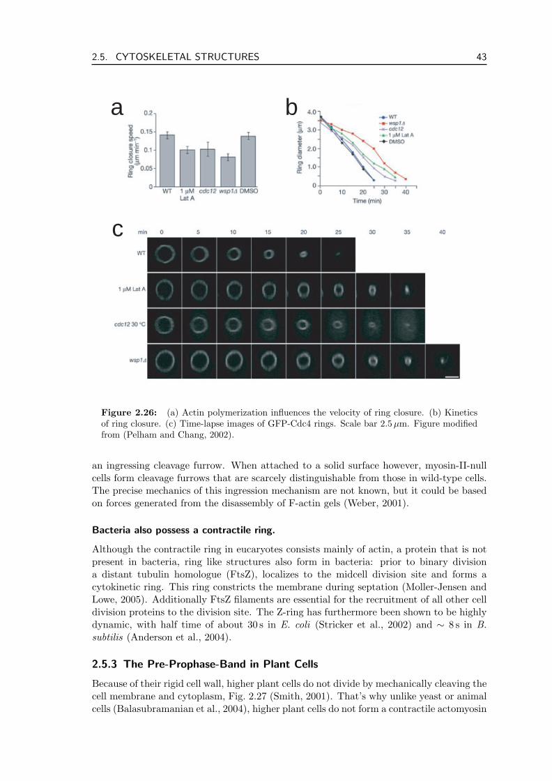
2.5. CYTOSKELETAL STRUCTURES 43
a
c
b
Figure 2.26: (a) Actin polymerization influences the velocity of ring closure. (b) Kineticsof ring closure. (c) Time-lapse images of GFP-Cdc4 rings. Scale bar 2.5µm. Figure modifiedfrom (Pelham and Chang, 2002).
an ingressing cleavage furrow. When attached to a solid surface however, myosin-II-nullcells form cleavage furrows that are scarcely distinguishable from those in wild-type cells.The precise mechanics of this ingression mechanism are not known, but it could be basedon forces generated from the disassembly of F-actin gels (Weber, 2001).
Bacteria also possess a contractile ring.
Although the contractile ring in eucaryotes consists mainly of actin, a protein that is notpresent in bacteria, ring like structures also form in bacteria: prior to binary divisiona distant tubulin homologue (FtsZ), localizes to the midcell division site and forms acytokinetic ring. This ring constricts the membrane during septation (Moller-Jensen andLowe, 2005). Additionally FtsZ filaments are essential for the recruitment of all other celldivision proteins to the division site. The Z-ring has furthermore been shown to be highlydynamic, with half time of about 30 s in E. coli (Stricker et al., 2002) and ∼ 8 s in B.subtilis (Anderson et al., 2004).
2.5.3 The Pre-Prophase-Band in Plant Cells
Because of their rigid cell wall, higher plant cells do not divide by mechanically cleaving thecell membrane and cytoplasm, Fig. 2.27 (Smith, 2001). That’s why unlike yeast or animalcells (Balasubramanian et al., 2004), higher plant cells do not form a contractile actomyosin
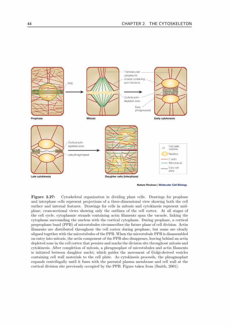
44 CHAPTER 2. THE CYTOSKELETON
Figure 2.27: Cytoskeletal organization in dividing plant cells. Drawings for prophaseand interphase cells represent projections of a three-dimensional view showing both the cellsurface and internal features. Drawings for cells in mitosis and cytokinesis represent mid-plane, cross-sectional views showing only the outlines of the cell cortex. At all stages ofthe cell cycle, cytoplasmic strands containing actin filaments span the vacuole, linking thecytoplasm surrounding the nucleus with the cortical cytoplasm. During prophase, a corticalpreprophase band (PPB) of microtubules circumscribes the future plane of cell division. Actinfilaments are distributed throughout the cell cortex during prophase, but some are clearlyaligned together with the microtubules of the PPB. When the microtubule PPB is disassembledon entry into mitosis, the actin component of the PPB also disappears, leaving behind an actindepleted zone in the cell cortex that persists and marks the division site throughout mitosis andcytokinesis. After completion of mitosis, a phragmoplast of microtubules and actin filamentsis initiated between daughter nuclei, which guides the movement of Golgi-derived vesiclescontaining cell wall materials to the cell plate. As cytokinesis proceeds, the phragmoplastexpands centrifugally until it fuses with the parental plasma membrane and cell wall at thecortical division site previously occupied by the PPB. Figure taken from (Smith, 2001).
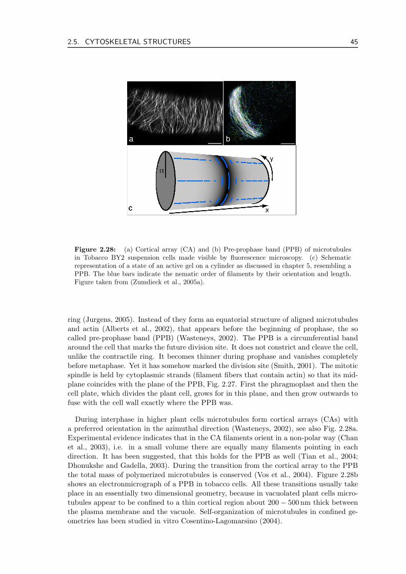
2.5. CYTOSKELETAL STRUCTURES 45
Figure 2.28: (a) Cortical array (CA) and (b) Pre-prophase band (PPB) of microtubulesin Tobacco BY2 suspension cells made visible by fluorescence microscopy. (c) Schematicrepresentation of a state of an active gel on a cylinder as discussed in chapter 5, resembling aPPB. The blue bars indicate the nematic order of filaments by their orientation and length.Figure taken from (Zumdieck et al., 2005a).
ring (Jurgens, 2005). Instead of they form an equatorial structure of aligned microtubulesand actin (Alberts et al., 2002), that appears before the beginning of prophase, the socalled pre-prophase band (PPB) (Wasteneys, 2002). The PPB is a circumferential bandaround the cell that marks the future division site. It does not constrict and cleave the cell,unlike the contractile ring. It becomes thinner during prophase and vanishes completelybefore metaphase. Yet it has somehow marked the division site (Smith, 2001). The mitoticspindle is held by cytoplasmic strands (filament fibers that contain actin) so that its mid-plane coincides with the plane of the PPB, Fig. 2.27. First the phragmoplast and then thecell plate, which divides the plant cell, grows for in this plane, and then grow outwards tofuse with the cell wall exactly where the PPB was.
During interphase in higher plant cells microtubules form cortical arrays (CAs) witha preferred orientation in the azimuthal direction (Wasteneys, 2002), see also Fig. 2.28a.Experimental evidence indicates that in the CA filaments orient in a non-polar way (Chanet al., 2003), i.e. in a small volume there are equally many filaments pointing in eachdirection. It has been suggested, that this holds for the PPB as well (Tian et al., 2004;Dhonukshe and Gadella, 2003). During the transition from the cortical array to the PPBthe total mass of polymerized microtubules is conserved (Vos et al., 2004). Figure 2.28bshows an electronmicrograph of a PPB in tobacco cells. All these transitions usually takeplace in an essentially two dimensional geometry, because in vacuolated plant cells micro-tubules appear to be confined to a thin cortical region about 200− 500 nm thick betweenthe plasma membrane and the vacuole. Self-organization of microtubules in confined ge-ometries has been studied in vitro Cosentino-Lagomarsino (2004).
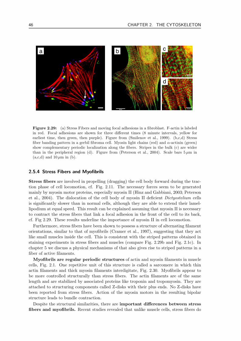
46 CHAPTER 2. THE CYTOSKELETON
a c
d
b
Figure 2.29: (a) Stress Fibers and moving focal adhesions in a fibroblast. F-actin is labeledin red. Focal adhesions are shown for three different times (8 minute intervals, yellow forearliest time, then green, then purple). Figure from (Smilenov et al., 1999). (b,c,d) Stressfiber banding pattern in a gerbil fibroma cell. Myosin light chains (red) and α-actinin (green)show complementary periodic localization along the fibers. Stripes in the bulk (c) are widerthan in the peripheral region (d). Figure from (Peterson et al., 2004). Scale bars 5µm in(a,c,d) and 10 µm in (b).
2.5.4 Stress Fibers and Myofibrils
Stress fibers are involved in propelling (dragging) the cell body forward during the trac-tion phase of cell locomotion, cf. Fig. 2.11. The necessary forces seem to be generatedmainly by myosin motor proteins, especially myosin II (Hinz and Gabbiani, 2003; Petersonet al., 2004). The dislocation of the cell body of myosin II deficient Dictyostelium cellsis significantly slower than in normal cells, although they are able to extend their lamel-lipodium at equal speed. This result can be explained assuming that myosin II is necessaryto contract the stress fibers that link a focal adhesion in the front of the cell to its back,cf. Fig 2.29. These results underline the importance of myosin II in cell locomotion.
Furthermore, stress fibers have been shown to possess a structure of alternating filamentorientations, similar to that of myofibrils (Cramer et al., 1997), suggesting that they actlike small muscles inside the cell. This is consistent with the striped patterns obtained instaining experiments in stress fibers and muscles (compare Fig. 2.29b and Fig. 2.1c). Inchapter 5 we discuss a physical mechanisms of that also gives rise to striped patterns in afiber of active filaments.
Myofibrils are regular periodic structures of actin and myosin filaments in musclecells, Fig. 2.1. One repetitive unit of this structure is called a sarcomere in which thinactin filaments and thick myosin filaments interdigitate, Fig. 2.30. Myofibrils appear tobe more controlled structurally than stress fibers. The actin filaments are of the samelength and are stabilized by associated proteins like troponin and tropomyosin. They areattached to structuring components called Z-disks with their plus ends. No Z-disks havebeen reported from stress fibers. Action of the myosin motors in the resulting bipolarstructure leads to bundle contraction.
Despite the structural similarities, there are important differences between stressfibers and myofibrils. Recent studies revealed that unlike muscle cells, stress fibers do
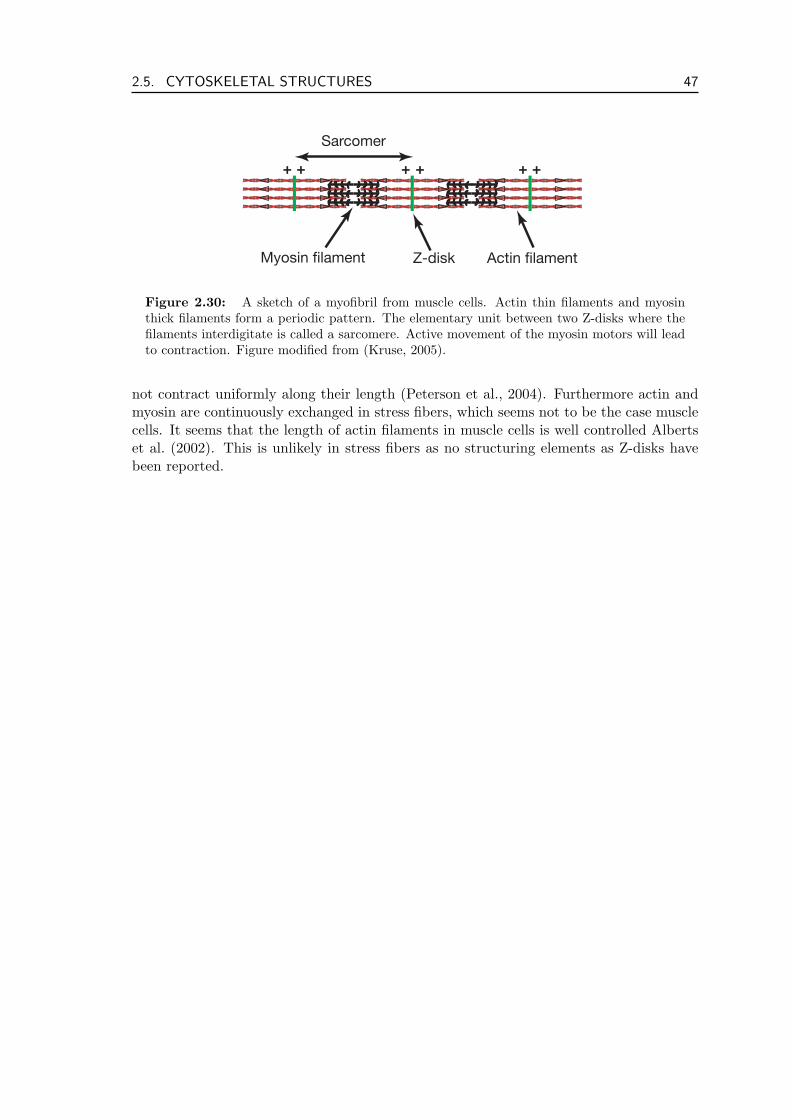
2.5. CYTOSKELETAL STRUCTURES 47
+ + + + + +
Actin filamentMyosin filament Z-disk
Sarcomer
Figure 2.30: A sketch of a myofibril from muscle cells. Actin thin filaments and myosinthick filaments form a periodic pattern. The elementary unit between two Z-disks where thefilaments interdigitate is called a sarcomere. Active movement of the myosin motors will leadto contraction. Figure modified from (Kruse, 2005).
not contract uniformly along their length (Peterson et al., 2004). Furthermore actin andmyosin are continuously exchanged in stress fibers, which seems not to be the case musclecells. It seems that the length of actin filaments in muscle cells is well controlled Albertset al. (2002). This is unlikely in stress fibers as no structuring elements as Z-disks havebeen reported.
48 CHAPTER 2. THE CYTOSKELETON
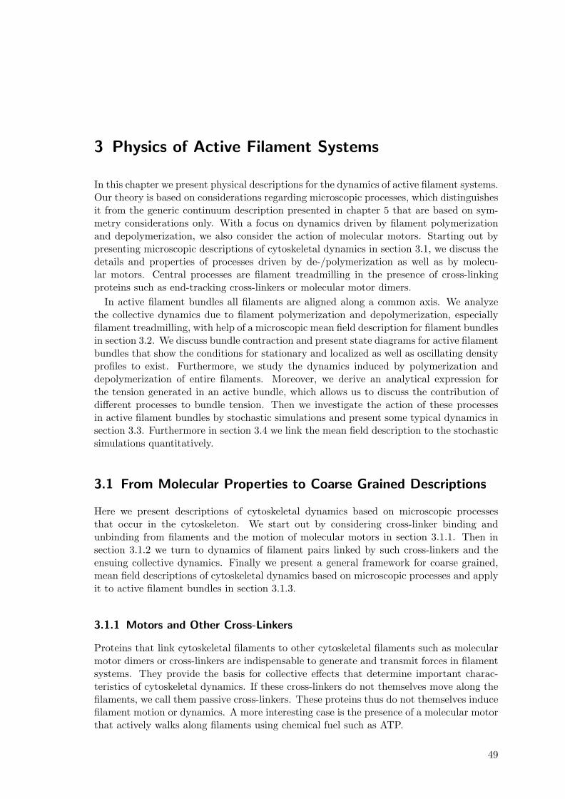
3 Physics of Active Filament Systems
In this chapter we present physical descriptions for the dynamics of active filament systems.Our theory is based on considerations regarding microscopic processes, which distinguishesit from the generic continuum description presented in chapter 5 that are based on sym-metry considerations only. With a focus on dynamics driven by filament polymerizationand depolymerization, we also consider the action of molecular motors. Starting out bypresenting microscopic descriptions of cytoskeletal dynamics in section 3.1, we discuss thedetails and properties of processes driven by de-/polymerization as well as by molecu-lar motors. Central processes are filament treadmilling in the presence of cross-linkingproteins such as end-tracking cross-linkers or molecular motor dimers.
In active filament bundles all filaments are aligned along a common axis. We analyzethe collective dynamics due to filament polymerization and depolymerization, especiallyfilament treadmilling, with help of a microscopic mean field description for filament bundlesin section 3.2. We discuss bundle contraction and present state diagrams for active filamentbundles that show the conditions for stationary and localized as well as oscillating densityprofiles to exist. Furthermore, we study the dynamics induced by polymerization anddepolymerization of entire filaments. Moreover, we derive an analytical expression forthe tension generated in an active bundle, which allows us to discuss the contribution ofdifferent processes to bundle tension. Then we investigate the action of these processesin active filament bundles by stochastic simulations and present some typical dynamics insection 3.3. Furthermore in section 3.4 we link the mean field description to the stochasticsimulations quantitatively.
3.1 From Molecular Properties to Coarse Grained Descriptions
Here we present descriptions of cytoskeletal dynamics based on microscopic processesthat occur in the cytoskeleton. We start out by considering cross-linker binding andunbinding from filaments and the motion of molecular motors in section 3.1.1. Then insection 3.1.2 we turn to dynamics of filament pairs linked by such cross-linkers and theensuing collective dynamics. Finally we present a general framework for coarse grained,mean field descriptions of cytoskeletal dynamics based on microscopic processes and applyit to active filament bundles in section 3.1.3.
3.1.1 Motors and Other Cross-Linkers
Proteins that link cytoskeletal filaments to other cytoskeletal filaments such as molecularmotor dimers or cross-linkers are indispensable to generate and transmit forces in filamentsystems. They provide the basis for collective effects that determine important charac-teristics of cytoskeletal dynamics. If these cross-linkers do not themselves move along thefilaments, we call them passive cross-linkers. These proteins thus do not themselves inducefilament motion or dynamics. A more interesting case is the presence of a molecular motorthat actively walks along filaments using chemical fuel such as ATP.
49
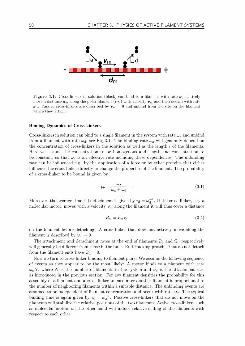
50 CHAPTER 3. PHYSICS OF ACTIVE FILAMENT SYSTEMS
dm
wa wdvm- +
Figure 3.1: Cross-linkers in solution (black) can bind to a filament with rate ωa, activelymove a distance dm along the polar filament (red) with velocity vm and then detach with rateωd. Passive cross-linkers are described by vm = 0 and unbind from the site on the filamentwhere they attach.
Binding Dynamics of Cross-Linkers
Cross-linkers in solution can bind to a single filament in the system with rate ωa and unbindfrom a filament with rate ωd, see Fig 3.1. The binding rate ωa will generally depend onthe concentration of cross-linkers in the solution as well as the length l of the filaments.Here we assume the concentration to be homogenous and length and concentration tobe constant, so that ωa is an effective rate including these dependences. The unbindingrate can be influenced e.g. by the application of a force or by other proteins that eitherinfluence the cross-linker directly or change the properties of the filament. The probabilityof a cross-linker to be bound is given by
pb =ωa
ωa + ωd. (3.1)
Moreover, the average time till detachment is given by τd = ω−1d . If the cross-linker, e.g. a
molecular motor, moves with a velocity vm along the filament it will thus cover a distance
dm = vmτd (3.2)
on the filament before detaching. A cross-linker that does not actively move along thefilament is described by vm = 0.
The attachment and detachment rates at the end of filaments Ωa and Ωd respectivelywill generally be different from those in the bulk. End-tracking proteins that do not detachfrom the filament ends have Ωd = 0.
Now we turn to cross-linker binding to filament pairs. We assume the following sequenceof events as they appear to be the most likely: A motor binds to a filament with rateωaN , where N is the number of filaments in the system and ωa is the attachment rateas introduced in the previous section. For low filament densities the probability for thisassembly of a filament and a cross-linker to encounter another filament is proportional tothe number of neighboring filaments within a suitable distance. The unbinding events areassumed to be independent of filament concentration and occur with rate ωd. The typicalbinding time is again given by τd = ω−1
d . Passive cross-linkers that do not move on thefilaments will stabilize the relative positions of the two filaments. Active cross-linkers suchas molecular motors on the other hand will induce relative sliding of the filaments withrespect to each other.
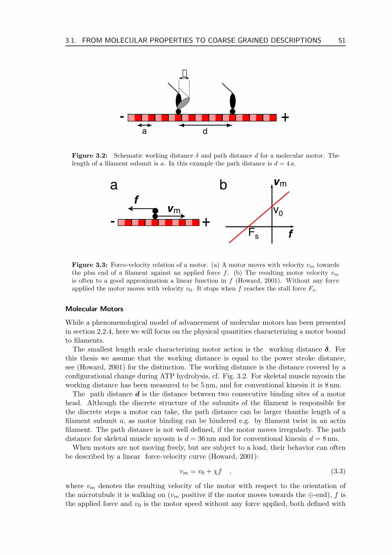
3.1. FROM MOLECULAR PROPERTIES TO COARSE GRAINED DESCRIPTIONS 51
- +da
d
Figure 3.2: Schematic working distance δ and path distance d for a molecular motor. Thelength of a filament subunit is a. In this example the path distance is d = 4 a.
vm- +
f
f
vma bv0
Fs
Figure 3.3: Force-velocity relation of a motor. (a) A motor moves with velocity vm towardsthe plus end of a filament against an applied force f . (b) The resulting motor velocity vm
is often to a good approximation a linear function in f (Howard, 2001). Without any forceappliied the motor moves with velocity v0. It stops when f reaches the stall force Fs.
Molecular Motors
While a phenomenological model of advancement of molecular motors has been presentedin section 2.2.4, here we will focus on the physical quantities characterizing a motor boundto filaments.
The smallest length scale characterizing motor action is the working distance δ. Forthis thesis we assume that the working distance is equal to the power stroke distance,see (Howard, 2001) for the distinction. The working distance is the distance covered by aconfigurational change during ATP hydrolysis, cf. Fig. 3.2. For skeletal muscle myosin theworking distance has been measured to be 5 nm, and for conventional kinesin it is 8 nm.
The path distance d is the distance between two consecutive binding sites of a motorhead. Although the discrete structure of the subunits of the filament is responsible forthe discrete steps a motor can take, the path distance can be larger thanthe length of afilament subunit a, as motor binding can be hindered e.g. by filament twist in an actinfilament. The path distance is not well defined, if the motor moves irregularly. The pathdistance for skeletal muscle myosin is d = 36nm and for conventional kinesin d = 8nm.
When motors are not moving freely, but are subject to a load, their behavior can oftenbe described by a linear force-velocity curve (Howard, 2001):
vm = v0 + χf , (3.3)
where vm denotes the resulting velocity of the motor with respect to the orientation ofthe microtubule it is walking on (vm positive if the motor moves towards the ⊕-end), f isthe applied force and v0 is the motor speed without any force applied, both defined with
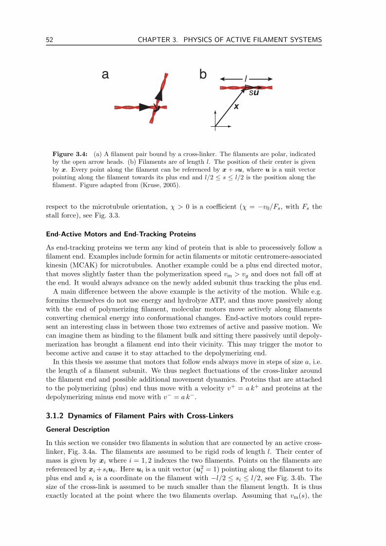
52 CHAPTER 3. PHYSICS OF ACTIVE FILAMENT SYSTEMS
x
su
a b l
Figure 3.4: (a) A filament pair bound by a cross-linker. The filaments are polar, indicatedby the open arrow heads. (b) Filaments are of length l. The position of their center is givenby x. Every point along the filament can be referenced by x + su, where u is a unit vectorpointing along the filament towards its plus end and l/2 ≤ s ≤ l/2 is the position along thefilament. Figure adapted from (Kruse, 2005).
respect to the microtubule orientation, χ > 0 is a coefficient (χ = −v0/Fs, with Fs thestall force), see Fig. 3.3.
End-Active Motors and End-Tracking Proteins
As end-tracking proteins we term any kind of protein that is able to processively follow afilament end. Examples include formin for actin filaments or mitotic centromere-associatedkinesin (MCAK) for microtubules. Another example could be a plus end directed motor,that moves slightly faster than the polymerization speed vm > vg and does not fall off atthe end. It would always advance on the newly added subunit thus tracking the plus end.
A main difference between the above example is the activity of the motion. While e.g.formins themselves do not use energy and hydrolyze ATP, and thus move passively alongwith the end of polymerizing filament, molecular motors move actively along filamentsconverting chemical energy into conformational changes. End-active motors could repre-sent an interesting class in between those two extremes of active and passive motion. Wecan imagine them as binding to the filament bulk and sitting there passively until depoly-merization has brought a filament end into their vicinity. This may trigger the motor tobecome active and cause it to stay attached to the depolymerizing end.
In this thesis we assume that motors that follow ends always move in steps of size a, i.e.the length of a filament subunit. We thus neglect fluctuations of the cross-linker aroundthe filament end and possible additional movement dynamics. Proteins that are attachedto the polymerizing (plus) end thus move with a velocity v+ = a k+ and proteins at thedepolymerizing minus end move with v− = a k−.
3.1.2 Dynamics of Filament Pairs with Cross-Linkers
General Description
In this section we consider two filaments in solution that are connected by an active cross-linker, Fig. 3.4a. The filaments are assumed to be rigid rods of length l. Their center ofmass is given by xi where i = 1, 2 indexes the two filaments. Points on the filaments arereferenced by xi +siui. Here ui is a unit vector (u2
i = 1) pointing along the filament to itsplus end and si is a coordinate on the filament with −l/2 ≤ si ≤ l/2, see Fig. 3.4b. Thesize of the cross-link is assumed to be much smaller than the filament length. It is thusexactly located at the point where the two filaments overlap. Assuming that vm(s), the
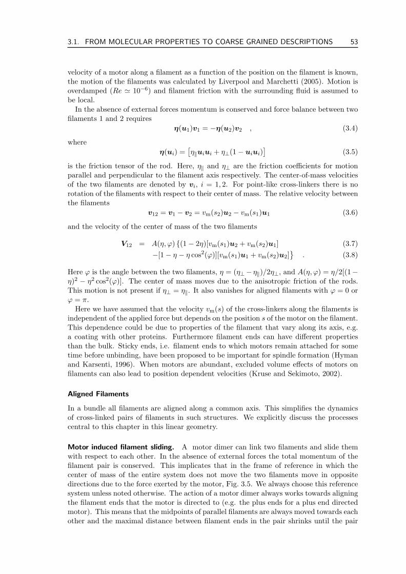
3.1. FROM MOLECULAR PROPERTIES TO COARSE GRAINED DESCRIPTIONS 53
velocity of a motor along a filament as a function of the position on the filament is known,the motion of the filaments was calculated by Liverpool and Marchetti (2005). Motion isoverdamped (Re ' 10−6) and filament friction with the surrounding fluid is assumed tobe local.
In the absence of external forces momentum is conserved and force balance between twofilaments 1 and 2 requires
η(u1)v1 = −η(u2)v2 , (3.4)
whereη(ui) =
[η‖uiui + η⊥(1− uiui)
](3.5)
is the friction tensor of the rod. Here, η‖ and η⊥ are the friction coefficients for motionparallel and perpendicular to the filament axis respectively. The center-of-mass velocitiesof the two filaments are denoted by vi, i = 1, 2. For point-like cross-linkers there is norotation of the filaments with respect to their center of mass. The relative velocity betweenthe filaments
v12 = v1 − v2 = vm(s2)u2 − vm(s1)u1 (3.6)
and the velocity of the center of mass of the two filaments
V12 = A(η, ϕ) (1− 2η)[vm(s1)u2 + vm(s2)u1] (3.7)−[1− η − η cos2(ϕ)][vm(s1)u1 + vm(s2)u2]
. (3.8)
Here ϕ is the angle between the two filaments, η = (η⊥− η‖)/2η⊥, and A(η, ϕ) = η/2[(1−η)2 − η2 cos2(ϕ)]. The center of mass moves due to the anisotropic friction of the rods.This motion is not present if η⊥ = η‖. It also vanishes for aligned filaments with ϕ = 0 orϕ = π.
Here we have assumed that the velocity vm(s) of the cross-linkers along the filaments isindependent of the applied force but depends on the position s of the motor on the filament.This dependence could be due to properties of the filament that vary along its axis, e.g.a coating with other proteins. Furthermore filament ends can have different propertiesthan the bulk. Sticky ends, i.e. filament ends to which motors remain attached for sometime before unbinding, have been proposed to be important for spindle formation (Hymanand Karsenti, 1996). When motors are abundant, excluded volume effects of motors onfilaments can also lead to position dependent velocities (Kruse and Sekimoto, 2002).
Aligned Filaments
In a bundle all filaments are aligned along a common axis. This simplifies the dynamicsof cross-linked pairs of filaments in such structures. We explicitly discuss the processescentral to this chapter in this linear geometry.
Motor induced filament sliding. A motor dimer can link two filaments and slide themwith respect to each other. In the absence of external forces the total momentum of thefilament pair is conserved. This implicates that in the frame of reference in which thecenter of mass of the entire system does not move the two filaments move in oppositedirections due to the force exerted by the motor, Fig. 3.5. We always choose this referencesystem unless noted otherwise. The action of a motor dimer always works towards aligningthe filament ends that the motor is directed to (e.g. the plus ends for a plus end directedmotor). This means that the midpoints of parallel filaments are always moved towards eachother and the maximal distance between filament ends in the pair shrinks until the pair
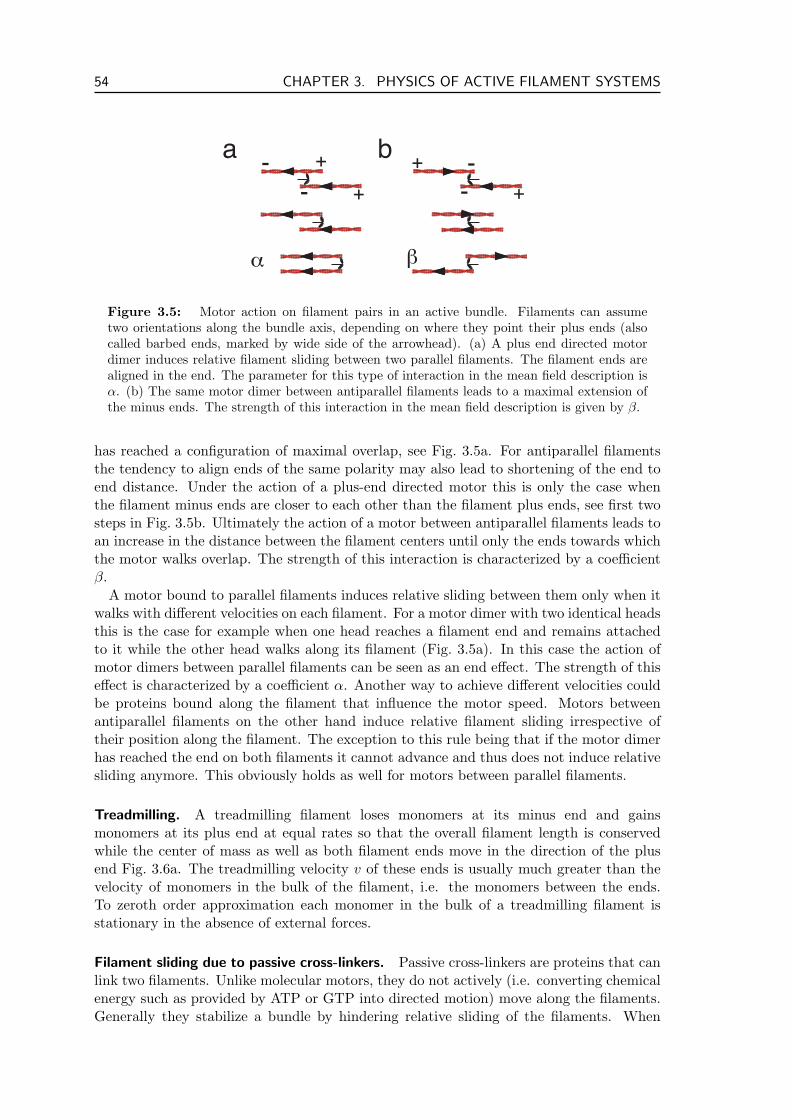
54 CHAPTER 3. PHYSICS OF ACTIVE FILAMENT SYSTEMS
β
b
α
a+-
+-
+ -
+-
Figure 3.5: Motor action on filament pairs in an active bundle. Filaments can assumetwo orientations along the bundle axis, depending on where they point their plus ends (alsocalled barbed ends, marked by wide side of the arrowhead). (a) A plus end directed motordimer induces relative filament sliding between two parallel filaments. The filament ends arealigned in the end. The parameter for this type of interaction in the mean field description isα. (b) The same motor dimer between antiparallel filaments leads to a maximal extension ofthe minus ends. The strength of this interaction in the mean field description is given by β.
has reached a configuration of maximal overlap, see Fig. 3.5a. For antiparallel filamentsthe tendency to align ends of the same polarity may also lead to shortening of the end toend distance. Under the action of a plus-end directed motor this is only the case whenthe filament minus ends are closer to each other than the filament plus ends, see first twosteps in Fig. 3.5b. Ultimately the action of a motor between antiparallel filaments leads toan increase in the distance between the filament centers until only the ends towards whichthe motor walks overlap. The strength of this interaction is characterized by a coefficientβ.
A motor bound to parallel filaments induces relative sliding between them only when itwalks with different velocities on each filament. For a motor dimer with two identical headsthis is the case for example when one head reaches a filament end and remains attachedto it while the other head walks along its filament (Fig. 3.5a). In this case the action ofmotor dimers between parallel filaments can be seen as an end effect. The strength of thiseffect is characterized by a coefficient α. Another way to achieve different velocities couldbe proteins bound along the filament that influence the motor speed. Motors betweenantiparallel filaments on the other hand induce relative filament sliding irrespective oftheir position along the filament. The exception to this rule being that if the motor dimerhas reached the end on both filaments it cannot advance and thus does not induce relativesliding anymore. This obviously holds as well for motors between parallel filaments.
Treadmilling. A treadmilling filament loses monomers at its minus end and gainsmonomers at its plus end at equal rates so that the overall filament length is conservedwhile the center of mass as well as both filament ends move in the direction of the plusend Fig. 3.6a. The treadmilling velocity v of these ends is usually much greater than thevelocity of monomers in the bulk of the filament, i.e. the monomers between the ends.To zeroth order approximation each monomer in the bulk of a treadmilling filament isstationary in the absence of external forces.
Filament sliding due to passive cross-linkers. Passive cross-linkers are proteins that canlink two filaments. Unlike molecular motors, they do not actively (i.e. converting chemicalenergy such as provided by ATP or GTP into directed motion) move along the filaments.Generally they stabilize a bundle by hindering relative sliding of the filaments. When
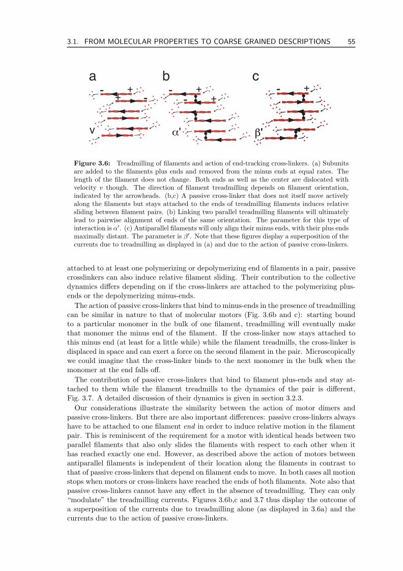
3.1. FROM MOLECULAR PROPERTIES TO COARSE GRAINED DESCRIPTIONS 55
v
a c
β'β'
+- +-
α'
b+-
+ - +-
Figure 3.6: Treadmilling of filaments and action of end-tracking cross-linkers. (a) Subunitsare added to the filaments plus ends and removed from the minus ends at equal rates. Thelength of the filament does not change. Both ends as well as the center are dislocated withvelocity v though. The direction of filament treadmilling depends on filament orientation,indicated by the arrowheads. (b,c) A passive cross-linker that does not itself move activelyalong the filaments but stays attached to the ends of treadmilling filaments induces relativesliding between filament pairs. (b) Linking two parallel treadmilling filaments will ultimatelylead to pairwise alignment of ends of the same orientation. The parameter for this type ofinteraction is α′. (c) Antiparallel filaments will only align their minus ends, with their plus endsmaximally distant. The parameter is β′. Note that these figures display a superposition of thecurrents due to treadmilling as displayed in (a) and due to the action of passive cross-linkers.
attached to at least one polymerizing or depolymerizing end of filaments in a pair, passivecrosslinkers can also induce relative filament sliding. Their contribution to the collectivedynamics differs depending on if the cross-linkers are attached to the polymerizing plus-ends or the depolymerizing minus-ends.
The action of passive cross-linkers that bind to minus-ends in the presence of treadmillingcan be similar in nature to that of molecular motors (Fig. 3.6b and c): starting boundto a particular monomer in the bulk of one filament, treadmilling will eventually makethat monomer the minus end of the filament. If the cross-linker now stays attached tothis minus end (at least for a little while) while the filament treadmills, the cross-linker isdisplaced in space and can exert a force on the second filament in the pair. Microscopicallywe could imagine that the cross-linker binds to the next monomer in the bulk when themonomer at the end falls off.
The contribution of passive cross-linkers that bind to filament plus-ends and stay at-tached to them while the filament treadmills to the dynamics of the pair is different,Fig. 3.7. A detailed discussion of their dynamics is given in section 3.2.3.
Our considerations illustrate the similarity between the action of motor dimers andpassive cross-linkers. But there are also important differences: passive cross-linkers alwayshave to be attached to one filament end in order to induce relative motion in the filamentpair. This is reminiscent of the requirement for a motor with identical heads between twoparallel filaments that also only slides the filaments with respect to each other when ithas reached exactly one end. However, as described above the action of motors betweenantiparallel filaments is independent of their location along the filaments in contrast tothat of passive cross-linkers that depend on filament ends to move. In both cases all motionstops when motors or cross-linkers have reached the ends of both filaments. Note also thatpassive cross-linkers cannot have any effect in the absence of treadmilling. They can only“modulate” the treadmilling currents. Figures 3.6b,c and 3.7 thus display the outcome ofa superposition of the currents due to treadmilling alone (as displayed in 3.6a) and thecurrents due to the action of passive cross-linkers.
56 CHAPTER 3. PHYSICS OF ACTIVE FILAMENT SYSTEMS
b
β''α''
a
+-+-
+-+-
+-+-
+ -
+-
+ -
+-
+ -
+-
Figure 3.7: Dynamics due to plus-end tracking cross-linkers in the presence of treadmilling.The cross-linkers possess a domain that allows them to processively follow the filaments plusend (blue ellipse) while another domain is linked to the bulk of the second filament (blackdot). The resulting dynamics is strikingly different from that found for minus-end trackingcross-linkers, cf. Fig. 3.6b and c. (a) Between parallel filaments the action of cross-linkersleads to a maximal separation of the filament centers. (b) Antiparallel filaments on the otherhand tend to get aligned under the action of these cross-linkers. The associated parametersare α′′ and β′′ respectively.
3.1.3 Mean Field Description of Active Filament Systems
An analytical description of systems of many individual filaments and cross-linkers is notto feasible because these are many body systems with complicated interactions. This sideof the challenge is more successfully tackled by computer simulations, cf. section 4.1.2.Mean field descriptions do provide a way to gain analytical insight into the exciting dy-namics of active filament systems despite this complexity (Nakazawa and Sekimoto, 1996;Sekimoto and Nakazawa, 2000; Kruse and Julicher, 2000; Liverpool and Marchetti, 2003).These descriptions are based on densities of filaments and cross-linkers, whose evolutionis described in equations that neglect higher order correlations. A general framework forthe derivation of such descriptions in one spatial dimension has been presented by Kruseand Julicher (2003). Here we report the generalization to arbitrary dimension as givenin (Kruse, 2005).
General Description
The description is centered around the interaction of filament pairs that move with re-spect to a non-moving background. As before filaments are described as thin, rigid rods.Filament bending and rotation around the longitudinal axis are ignored. The density offilaments that have their center at x and orientation u is given by Ψ(x,u). Motors areassumed to be small compared to filaments and are treated as point particles. The numberdensity of motors bound to filaments is denoted by m. The two densities evolve accordingto
∂tΨ−∇ ·[D‖uu+ D⊥(1− uu)
]· ∇Ψ−DrR · RΨ +∇ · Ja +R · Jr = S
(3.9)∂tm−Dm∆m +∇ · Jm = Sm ,
(3.10)
where R = u × ∂/∂u is the rotation operator. The filament currents Ja (translational)and Jr (rotational) as well as the motor current Jm are generated by the active interaction
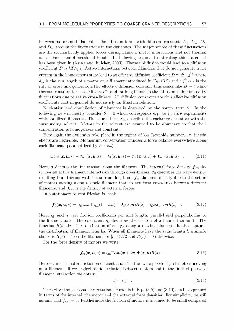
3.1. FROM MOLECULAR PROPERTIES TO COARSE GRAINED DESCRIPTIONS 57
between motors and filaments. The diffusion terms with diffusion constants D‖, D⊥, Dr,and Dm account for fluctuations in the dynamics. The major source of these fluctuationsare the stochastically applied forces during filament motor interactions and not thermalnoise. For a one dimensional bundle the following argument motivating this statementhas been given in (Kruse and Julicher, 2003): Thermal diffusion would lead to a diffusioncoefficient D ' kT/η‖l. Active interactions between filaments that do not generate a net
current in the homogenous state lead to an effective diffusion coefficient D ' d2mω
(2)a , where
dm is the run length of a motor on a filament introduced in Eq. (3.2) and ω(2)a ∼ l is the
rate of cross-link generation.The effective diffusion constant thus scales like D ∼ l whilethermal contributions scale like ∼ l−1 and for long filaments the diffusion is dominated byfluctuations due to active cross-linkers. All diffusion constants are thus effective diffusioncoefficients that in general do not satisfy an Einstein relation.
Nucleation and annihilation of filaments is described by the source term S. In thefollowing we will mostly consider S = 0 which corresponds e.g. to in vitro experimentswith stabilized filaments. The source term Sm describes the exchange of motors with thesurrounding solvent. Motors in the solvent are assumed to be abundant so that theirconcentration is homogenous and constant.
Here again the dynamics take place in the regime of low Reynolds number, i.e. inertiaeffects are negligible. Momentum conservation imposes a force balance everywhere alongeach filament (parametrized by x+ su):
u∂sσ(x,u, s)− fint(x,u, s) = ffl(x,u, s) + fm(x,u, s) + fext(x,u, s) . (3.11)
Here, σ denotes the line tension along the filament. The internal force density fint de-scribes all active filament interactions through cross-linkers, ffl describes the force densityresulting from friction with the surrounding fluid, fm the force density due to the actionof motors moving along a single filament that do not form cross-links between differentfilaments, and fext is the density of external forces.
In a stationary solvent friction is local:
ffl(x,u, s) =[η‖uu+ η⊥(1− uu)
]· Ja(x,u)R(s) + η0sJr × uR(s) . (3.12)
Here, η‖ and η⊥ are friction coefficients per unit length, parallel and perpendicular tothe filament axis. The coefficient η0 describes the friction of a filament subunit. Thefunction R(s) describes dissipation of energy along a moving filament. It also capturesthe distribution of filament lengths. When all filaments have the same length l, a simplechoice is R(x) = 1 on the filament for |x| ≤ l/2 and R(x) = 0 otherwise.
For the force density of motors we write
fm(x,u, s) = ηmΓum(x+ su)Ψ(x,u)R(s) . (3.13)
Here ηm is the motor friction coefficient and Γ is the average velocity of motors movingon a filament. If we neglect steric exclusion between motors and in the limit of pairwisefilament interaction we obtain
Γ = vm . (3.14)
The active translational and rotational currents in Eqs. (3.9) and (3.10) can be expressedin terms of the internal, the motor and the external force densities. For simplicity, we willassume that fext = 0. Furthermore the friction of motors is assumed to be small compared
58 CHAPTER 3. PHYSICS OF ACTIVE FILAMENT SYSTEMS
to the filament friction, i.e. the contribution of fm can be neglected. Integration ofEq. (3.11) with respect to s then yields
−∫
ds fint(x,u, s) =∫
ds ffl(x,u, s) (3.15)
= l[η‖uu+ η⊥(1− uu)
]· Ja(x,u) . (3.16)
Here we have used∫
ds R(s) = l and assumed R(s) = R(−s) so that
Ja(x,u) = −1l
[1η‖uu+
1η⊥
(1− uu)]·∫
ds fint(x,u, s) . (3.17)
Integrating Eq. (3.11) with∫
ds su× yields
Jr(x,u) = − 1η0χ2
∫ds su× fint(x,u, s) . (3.18)
Here we have introduced χ2 =∫
ds s2R(s) and used Jr(x,u) ⊥ u.The internal force density fint depends on the densities of filaments and cross-linkers.
We assume the cross-linkers to be point-like particles so that filaments can only be cross-linked when they cross. The internal force density acting at point s on a filament withorientation u and center at x is then given by
fint(x,u, s) =∫
dx′∫
du′∫
ds′Ψ(x,u)Ψ(x′,u′)Cx′,u′,s′x,u,s m(x+ su)F (x,u, s,x′,u′, s′) .
(3.19)Here Cx′,u′,s′
x,u,s = R(s)R(s′)δ(x+ su− x′ − s′u′) restricts the integration to filaments thatcross. The function F captures the average force between two filaments depending ontheir position and orientation. While the precise form of F is not determined, it has tofulfill some symmetry requirements. Due to translation invariance, F can only depend onthe relative positions of the filament centers
F (x,u, s,x′,u′, s′) ≡ F (x− x′,u, s,u′, s′) . (3.20)
Under rotation F has to transform like a vector (i.e. F is covariant)
F (Rx,Ru, s,Ru′, s′) = RF (x,u, s,u′, s′) , (3.21)
where R denotes the rotation operator.Newton’s law actio = reactio requires
F (x,u, s,u′, s′) = −F (−x,u′, s′,u, s) . (3.22)
And covariance under reflections imposes
F‖(x‖ + x⊥,u‖ + u⊥, s,u′‖ + u′⊥, s′) = F‖(x‖ − x⊥,u‖ − u⊥, s,u′‖ − u′⊥, s′)
(3.23)F⊥(x‖ + x⊥,u‖ + u⊥, s,u′‖ + u′⊥, s′) = −F⊥(x‖ − x⊥,u‖ − u⊥, s,u′‖ − u
′⊥, s′)
(3.24)
where the subscripts ‖ and ⊥ denote vector components along and perpendicular to thereflection axis, respectively. In the following section we will apply this description to afilament bundle.
3.1. FROM MOLECULAR PROPERTIES TO COARSE GRAINED DESCRIPTIONS 59
+ -c (x)-
l
+-c (x)+
x
a b
+
-
z
x
+-
F+-(x,z)=-F-+(-x,z-x)
Figure 3.8: (a) Filaments of length l in a bundle can be described by two filament densitiesc+ and c− depending on their orientation. (b) An active cross-link (i.e. a motor dimer) exertsa force on a filament pair with opposite orientations, see text for explanations. The motormoves towards the plus end on each filament.
Filament Bundles
Since linear cytoskeletal structures are important in live cells we will now derive a micro-scopic description of active filament bundles. In a bundle all filaments are aligned along acommon axis. This represents an effectively one dimensional geometry in which filamentscan only have one of two orientations, depending on where they point their plus end. Invitro experiments on such systems have shown that bundles of filaments with molecularmotors can contract and elongate and that filaments can be sorted due to their polar-ity and depending on their orientation (Takiguchi, 1991; Tanaka-Takiguchi et al., 2004).One dimensional structures in living cells include stress fibers, the contractile ring, andmyofibrils in muscle cells.
For the physical description of the bundle we choose the x-axis along the bundle axis. Allfilaments have the same length l. As only two orientations are possible, the filaments arecharacterized by two densities c+ and c−, for filaments that point their plus or minus endalong the positive x-axis respectively, see Fig 3.8a. The internal force densities acting onplus and minus filaments are composed of contributions from interactions between paralleland anti-parallel filaments:
f+int = f++
int + f+−int (3.25)
f−int = f−−int + f−+int (3.26)
Here f+−int denotes the forces on plus filaments due to the interaction with minus filaments.
The expression for the internal force (Eq. (3.19)) then becomes
f±∓int (x, s) =∫
dx′c±(x)c∓(x′)R(s)R(x + s− x′)m(x + s)F±∓(x′ − x, s) (3.27)
and corresponding expressions for f±±int . Here, F+−(ξ, ζ) is the average force on a plus-filament applied at a distance ζ from its center, exerted by minus-filaments located adistance ξ from the first, see Fig 3.8b. The symmetry relations (3.20)- (3.24) become inone dimension
F±±(ξ, ζ) = −F±±(−ξ, ζ − ξ) (3.28)F±∓(ξ, ζ) = −F∓±(−ξ, ζ − ξ) (3.29)F++(ξ, ζ) = −F−−(−ξ,−ζ) (3.30)F+−(ξ, ζ) = −F−+(−ξ,−ζ) . (3.31)
60 CHAPTER 3. PHYSICS OF ACTIVE FILAMENT SYSTEMS
Here we have analyzed the symmetry of such a bundle with pairwise filament interaction.It is independent of the precise nature of the forces acting on the filaments and the currentsthey induce. The following section provides a simple choice that obeys all relations derivedhere.
3.2 Minimal Model of Active Filament Bundles
A simple example for the dynamics of a bundle of polar filaments in the presence ofactive cross-linkers such as molecular motors is presented in (Kruse and Julicher, 2000).It represents a minimal model of active bundle contraction in the sense that it is basedon strongly simplifying assumptions and strives to bring out clearly the key mechanismsinvolved in stress generation in bundles. It is contained in the general framework presentedabove and corresponds to a set of filaments with length l for which R(x) = 1 for |x| < l/2and R(x) = 0 otherwise. Furthermore the forces are chosen as follows
F±±(ξ, ζ) ∼ sgn(ξ) (3.32)F±∓(ξ, ζ) ∼ ∓1 . (3.33)
Here sgn(ξ) = 1 for ξ > 0 and −1 otherwise, so that the symmetry requirements Eq. (3.28)-(3.31) are fulfilled. Motors are taken to be point-like cross-linkers that move with the samespeed everywhere on both filaments they link. The motor distribution is taken to alwaysbe homogenous and thus its dynamics can be neglected.
So far only interactions of pairs of stable, i.e. non-polymerizing filaments have beenstudied in this context. Here we present an extension of this framework to includepolymerizing and depolymerizing filaments. We especially focus on the dynamics causedby treadmilling in the presence of motor proteins and passive cross-linkers as outlined insection 3.1 but also consider the generation and destruction of entire filaments.
The description is formulated in terms of filament number densities c+ and c− for plusand minus filaments respectively that have their center at position x. The number offilaments in the interval [x, x+dx] is thus given by c(x)dx and N =
∫ L0 c(x)dx is the total
number of filaments in a system of length L. Filaments are of length l and polymerizefrom monomers that diffuse freely in the surrounding fluid. The monomer number densityis denoted by cm. These densities satisfy continuity equations of the form
∂tc+ = D∂2
xc+ − ∂xJ+ − k+d c+ + k+
p cm (3.34)
∂tc− = D∂2
xc− − ∂xJ− − k−d c− + k−p cm (3.35)
∂tcm = Dm∂2xcm + µk+
d c+ + k−d c− − µ(k+p + k−p )cm . (3.36)
Here, D is an effective diffusion coefficient as discussed in section 3.1.3, k±d and k±p denoterates of filament polymerization and depolymerization of plus and minus filaments respec-tively, µ is the number of monomers in a filament of length l, and Dm is the diffusioncoefficient of monomers in solution. Note that kd and kp describe the creation and annihi-lation of entire filaments. Interactions between filaments as well as filament treadmillinginduce active filament currents J± describing the rate at which filaments slide locally. Forpairwise interactions of filaments, these active currents depend quadratically on the localdensities c±(x). They are proportional to the interaction strengths α, β, α′, β′, α′′ and β′′
as well as to the treadmilling speed v, which correspond to the processes indicated inFigs. 3.5, 3.6 and 3.7.
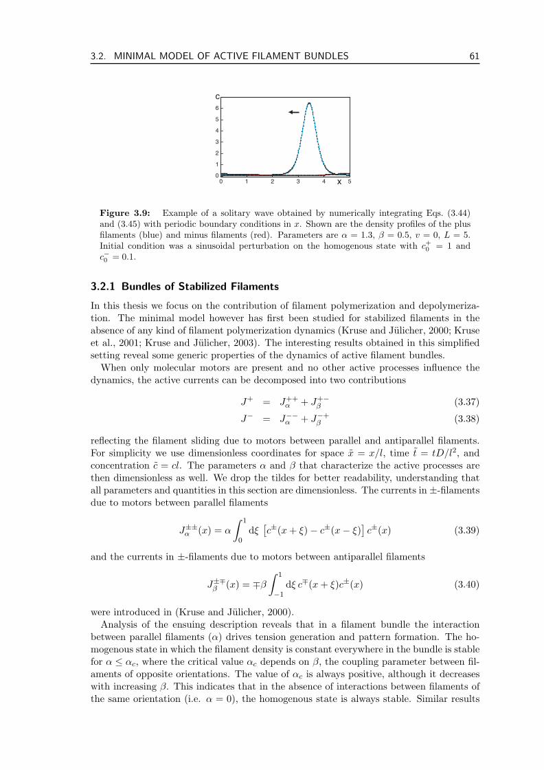
3.2. MINIMAL MODEL OF ACTIVE FILAMENT BUNDLES 61
0 1 2 3 4 5
0
1
2
3
4
5
6
c
x
Figure 3.9: Example of a solitary wave obtained by numerically integrating Eqs. (3.44)and (3.45) with periodic boundary conditions in x. Shown are the density profiles of the plusfilaments (blue) and minus filaments (red). Parameters are α = 1.3, β = 0.5, v = 0, L = 5.Initial condition was a sinusoidal perturbation on the homogenous state with c+
0 = 1 andc−0 = 0.1.
3.2.1 Bundles of Stabilized Filaments
In this thesis we focus on the contribution of filament polymerization and depolymeriza-tion. The minimal model however has first been studied for stabilized filaments in theabsence of any kind of filament polymerization dynamics (Kruse and Julicher, 2000; Kruseet al., 2001; Kruse and Julicher, 2003). The interesting results obtained in this simplifiedsetting reveal some generic properties of the dynamics of active filament bundles.
When only molecular motors are present and no other active processes influence thedynamics, the active currents can be decomposed into two contributions
J+ = J++α + J+−
β (3.37)
J− = J−−α + J−+β (3.38)
reflecting the filament sliding due to motors between parallel and antiparallel filaments.For simplicity we use dimensionless coordinates for space x = x/l, time t = tD/l2, andconcentration c = cl. The parameters α and β that characterize the active processes arethen dimensionless as well. We drop the tildes for better readability, understanding thatall parameters and quantities in this section are dimensionless. The currents in ±-filamentsdue to motors between parallel filaments
J±±α (x) = α
∫ 1
0dξ[c±(x + ξ)− c±(x− ξ)
]c±(x) (3.39)
and the currents in ±-filaments due to motors between antiparallel filaments
J±∓β (x) = ∓β
∫ 1
−1dξ c∓(x + ξ)c±(x) (3.40)
were introduced in (Kruse and Julicher, 2000).Analysis of the ensuing description reveals that in a filament bundle the interaction
between parallel filaments (α) drives tension generation and pattern formation. The ho-mogenous state in which the filament density is constant everywhere in the bundle is stablefor α ≤ αc, where the critical value αc depends on β, the coupling parameter between fil-aments of opposite orientations. The value of αc is always positive, although it decreaseswith increasing β. This indicates that in the absence of interactions between filaments ofthe same orientation (i.e. α = 0), the homogenous state is always stable. Similar results
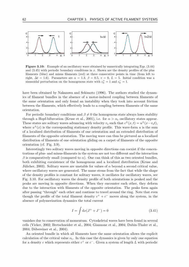
62 CHAPTER 3. PHYSICS OF ACTIVE FILAMENT SYSTEMS
0 1 2 3 4 50
2
4
6
c
x
t
0 1 2 3 4 50
2
4
6
c
x
t+∆t
0 1 2 3 4 50
2
4
6
c
x
t+2∆t
Figure 3.10: Example of an oscillatory wave obtained by numerically integrating Eqs. (3.44)and (3.45) with periodic boundary conditions in x. Shown are the density profiles of the plusfilaments (blue) and minus filaments (red) at three consecutive points in time (from left toright, ∆t = 1.6). Parameters are α = 1.3, β = 0.5, v = 0, L = 5. Initial condition was asinusoidal perturbation on the homogenous state with c+
0 = 1 and c−0 = 1.
have been obtained by Nakazawa and Sekimoto (1996). The authors studied the dynam-ics of filament bundles in the absence of a motor-induced coupling between filaments ofthe same orientation and only found an instability when they took into account frictionbetween the filaments, which effectively leads to a coupling between filaments of the sameorientation.
For periodic boundary conditions and β 6= 0 the homogenous state always loses stabilitythrough a Hopf-bifurcation (Kruse et al., 2001), i.e. for α > αc oscillatory states appear.These states are solitary waves advancing with velocity vs such that c±(x, t) = u±(x−vst),where u±(x) is the corresponding stationary density profile. This wave-form u is the sumof a localized distribution of filaments of one orientation and an extended distribution offilaments of the opposite orientation. The moving wave can thus be pictured as a localizeddistribution of filaments of one orientation gliding on a carpet of filaments of the oppositeorientation (cf. Fig. 3.9).
Interestingly two solitary waves moving in opposite directions can coexist if the concen-trations of plus- and minus-filaments in the system are not too different and the interactionβ is comparatively small (compared to α). One can think of this as two oriented bundles,both exhibiting coexistence of the homogenous and a localized distribution (Kruse andJulicher, 2003). Solitary waves are unstable for values of α beyond a second critical value,where oscillatory waves are generated. The name stems from the fact that while the shapeof the density profiles is constant for solitary waves, it oscillates for oscillatory waves, seeFig. 3.10. For oscillatory waves the density profile of both orientations is peaked and thepeaks are moving in opposite directions. When they encounter each other, they deformdue to the interaction with filaments of the opposite orientation. The peaks form againafter passing “through” each other and continue to travel around the ring. Note that eventhough the profile of the total filament density c+ + c− moves along the system, in theabsence of polymerization dynamics the total current
I =∫
dx(J+ + J−) = 0 (3.41)
vanishes due to conservation of momentum. Cytoskeletal waves have been found in severalcells (Vicker, 2002; Bretschneider et al., 2004; Giannone et al., 2004; Dubin-Thaler et al.,2004; Dobereiner et al., 2004).
An oriented bundle in which all filaments have the same orientation allows the explicitcalculation of the critical value αc. In this case the dynamics is given by only one equationfor a density c which represents either c+ or c−. Given a system of length L with periodic
3.2. MINIMAL MODEL OF ACTIVE FILAMENT BUNDLES 63
boundary conditions, linear stability analysis of the homogenous state c(x) = c0 revealsthe critical value αc explicitly:
αc =2π2
c0L2(1− cos(2π/L)). (3.42)
Its critical mode has wave number kc = 2π/L. The critical mode is thus determined bythe system size alone and not by features intrinsic to the dynamics. The critical value αc
decreases with increasing c0 and L. Beyond the instability, the homogenous state evolvesinto a stationary, localized, inhomogenous state. In this state the density distributionhas a clear peak, so that most of the filaments are centered around one point. Withincreasing values of α, this peak sharpens. For a range of parameter values αd ≤ α ≤ αc
an inhomogenous, stationary state coexists with the homogenous state.
3.2.2 Treadmilling and Molecular Motors
As filament polymerization is central to many cellular processes, we extend the minimalmodel to include such dynamics. We start out with filament treadmilling in the pres-ence of molecular motors but without passive end-tracking cross-linkers. We investigatethe influence of filament treadmilling alone, i.e. we do not consider polymerization anddepolymerization of entire filaments (kp = 0, kd = 0). Treadmilling induces only an orien-tation dependent drift in an individual filament. The dynamics become more interestingwhen interactions between filaments, e.g. via cross-linkers are taken into account.
Treadmilling gives rise to active currents of the form
J±v (x) = ±vc±(x) , (3.43)
which have to be added to the active currents J± as introduced in Eqs. (3.37)-(3.38).We note that these currents, like the currents due to interactions between antiparallelfilaments, Eq. (3.40), depend on the orientation of the filaments. The sign of the currentsis fixed by the fact that filaments grow at their plus end and shrink at their minus end.The dynamical equations are then explicitly (in dimensionless form):
∂tc+(x) = ∂2
xc+(x)− α∂x
∫ 1
0dξ[c+(x + ξ)− c+(x− ξ)
]c+(x) (3.44)
+β∂x
∫ 1
−1dξ c−(x + ξ)c+(x)− v∂xc+(x)
∂tc−(x) = ∂2
xc−(x)− α∂x
∫ 1
0dξ[c−(x + ξ)− c−(x− ξ)
]c−(x) (3.45)
−β∂x
∫ 1
−1dξ c+(x + ξ)c−(x) + v∂xc−(x)
In the following we will see, that although the treadmilling current introduced byEq. (3.43) seems just a minor change to the whole set of equations, it has a major im-pact on the system. In particular treadmilling (i) destabilizes the homogenous state, (ii)allows bundle contraction even in the absence of interactions between parallel filaments(i.e. αc < 0, where αc is the critical value below which the homogenous bundle is stable),(iii) can change the type of bifurcation by which the homogenous state loses stability andfinally (iv) increases the contractile tension in a bundle. We will now analyze the stabilityof the homogenous state on a filament bundle with length L > 1, which sheds light on howtreadmilling achieves the first three points on the list above. The fourth point is discussedin section 3.2.5.
64 CHAPTER 3. PHYSICS OF ACTIVE FILAMENT SYSTEMS
Linear Stability Analysis
The homogenous state c±(x) = c±0 (x) is a steady state of Eqs. (3.44) and (3.45). Here weanalyze its stability against small perturbations up to linear order and calculate the criticalvalue αc at which the homogenous state loses stability as a function of the treadmillingspeed v. In order to determine the development of a small perturbation δc±(x) aroundthe homogenous state, we expand the perturbation δc±(x) in Fourier modes
δc±(x) =∞∑
k=−∞c±k exp(ikx) , (3.46)
where c±k are coefficients of the Fourier sum. The details of this calculation are given inappendix A.2. The dynamic equations can be written in a compact way in dimensionlessquantities:
∂t
(c+k
c−k
)=(
Λ++ Λ+−
Λ−+ Λ−−
)(c+k
c−k
), (3.47)
where
Λ±± = −k2 − 2αc±0 (cos k − 1)± 2iβkc∓0 ∓ ivk (3.48)Λ±∓ = ±2iβc±0 sin k (3.49)
are the matrix elements.Note that if only filaments of one orientation are present stability is given by the real
part of the only eigenvalue Λ++ (w.o.l.g). In this case treadmilling does not influencethe stability of the homogenous state, because it only enters in the imaginary part of Λ±±
while the stability is determined by the real part. Thus we still find αc = k2/2c0(1−cos k),cf. (Kruse and Julicher, 2000). Here treadmilling just induces a drift with velocity v in thestationary state, be it homogenous or localized. This of course means that the stationary,localized filament distribution found in fully polar bundles ceases to exist, the peak moveswith the treadmilling velocity v.
When filaments of both orientations are present, the stability of the modes is determinedby the real part of the eigenvalues of the above matrix:
λ1,2 =Λ++ + Λ−−
2±√
(Λ++ + Λ−−)2
4+ Λ−+Λ+− (3.50)
We use these expressions to numerically determine the critical value αc(v), at which thehomogenous state is unstable. The results are displayed by the thick lines in Fig. 3.11.We find that treadmilling lowers αc, i.e. it destabilizes the homogenous state. In thepresence of treadmilling the homogenous state can become unstable even in the absenceof interactions between parallel filaments (α = 0). Interactions between antiparallel fila-ments (β 6= 0) are still necessary. If the densities of both filament orientations are equal,a new state emerges. For intermediate values of v the bifurcation becomes stationary(solid line in Fig. 3.11b). The resulting inhomogenous state is thus different from the sta-tionary or oscillatory waves observed without treadmilling. Note however, that unequalconcentrations of filaments of opposite orientations (c+
0 6= c−0 ) suppress the stationary bi-furcation. We will see below that polymerization and depolymerization of entire filamentsalso destroy this stationary bifurcation. This is consistent with the results from stochasticsimulations where no stationary states are observed in the presence of treadmilling. Thisstationary, localized state thus seems to be a particularity of the mean field description.The dependence of αc(v) on the other parameters is discussed explicitly in appendix A.1.
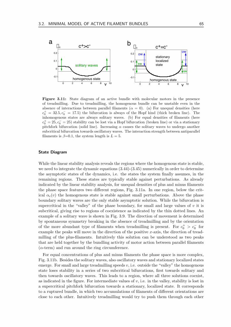
3.2. MINIMAL MODEL OF ACTIVE FILAMENT BUNDLES 65
a
0 2 4 6 8 10
0.1
0
-0.1
0.2
ac
vhomogenous state
solitary waves
c+>c- b
0 2 4 6 8 10
0.1
0
-0.1
0.2
ac
v
sw
sw
owow
stationarylocalizedstate
homogenous state
c+=c-
Figure 3.11: State diagram of an active bundle with molecular motors in the presenceof treadmilling. Due to treadmilling, the homogenous bundle can be unstable even in theabsence of interactions between parallel filaments (α = 0). (a) For unequal densities (herec+0 = 32.5, c−0 = 17.5) the bifurcation is always of the Hopf kind (thick broken line). The
inhomogenous states are always solitary waves. (b) For equal densities of filaments (herec+0 = 25, c−0 = 25) stability can be lost via a Hopf bifurcation (broken line) or via a stationary
pitchfork bifurcation (solid line). Increasing α causes the solitary waves to undergo anothersubcritical bifurcation towards oscillatory waves. The interaction strength between antiparallelfilaments is β=0.1, the system length is L = 5.
State Diagram
While the linear stability analysis reveals the regions where the homogenous state is stable,we need to integrate the dynamic equations (3.44)-(3.45) numerically in order to determinethe asymptotic states of the dynamics, i.e. the states the system finally assumes, in theremaining regions. These states are typically stable against perturbations. As alreadyindicated by the linear stability analysis, for unequal densities of plus and minus filamentsthe phase space features two different regions, Fig. 3.11a. In one region, below the crit-ical αc(v) the homogenous state is stable against small perturbations. Above the phaseboundary solitary waves are the only stable asymptotic solution. While the bifurcation issupercritical in the “valley” of the phase boundary, for small and large values of v it issubcritical, giving rise to regions of coexistence as indicated by the thin dotted lines. Anexample of a solitary wave is shown in Fig. 3.9. The direction of movement is determinedby spontaneous symmetry breaking in the absence of treadmilling and by the orientationof the more abundant type of filaments when treadmilling is present. For c+
0 > c−0 forexample the peaks will move in the direction of the positive x-axis, the direction of tread-milling of the plus-filaments. Intuitively this solution can be understood as two peaksthat are held together by the bundling activity of motor action between parallel filaments(α-term) and run around the ring circumference.
For equal concentrations of plus and minus filaments the phase space is more complex,Fig. 3.11b. Besides the solitary waves, also oscillatory waves and stationary localized statesemerge. For small and large treadmilling speeds v, i.e. outside the “valley” the homogenousstate loses stability in a series of two subcritical bifurcations, first towards solitary andthen towards oscillatory waves. This leads to a region, where all three solutions coexist,as indicated in the figure. For intermediate values of v, i.e. in the valley, stability is lost ina supercritical pitchfork bifurcation towards a stationary, localized state. It correspondsto a ruptured bundle, in which two accumulations of filaments of different orientations areclose to each other. Intuitively treadmilling would try to push them through each other
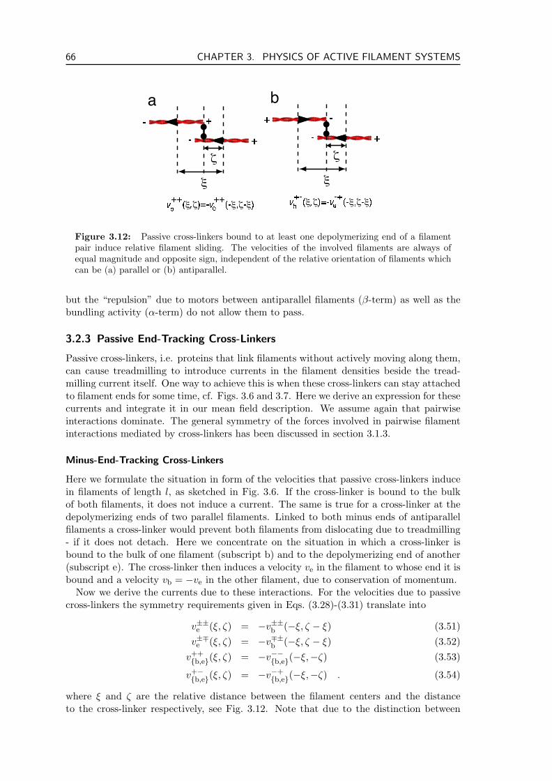
66 CHAPTER 3. PHYSICS OF ACTIVE FILAMENT SYSTEMS
Figure 3.12: Passive cross-linkers bound to at least one depolymerizing end of a filamentpair induce relative filament sliding. The velocities of the involved filaments are always ofequal magnitude and opposite sign, independent of the relative orientation of filaments whichcan be (a) parallel or (b) antiparallel.
but the “repulsion” due to motors between antiparallel filaments (β-term) as well as thebundling activity (α-term) do not allow them to pass.
3.2.3 Passive End-Tracking Cross-Linkers
Passive cross-linkers, i.e. proteins that link filaments without actively moving along them,can cause treadmilling to introduce currents in the filament densities beside the tread-milling current itself. One way to achieve this is when these cross-linkers can stay attachedto filament ends for some time, cf. Figs. 3.6 and 3.7. Here we derive an expression for thesecurrents and integrate it in our mean field description. We assume again that pairwiseinteractions dominate. The general symmetry of the forces involved in pairwise filamentinteractions mediated by cross-linkers has been discussed in section 3.1.3.
Minus-End-Tracking Cross-Linkers
Here we formulate the situation in form of the velocities that passive cross-linkers inducein filaments of length l, as sketched in Fig. 3.6. If the cross-linker is bound to the bulkof both filaments, it does not induce a current. The same is true for a cross-linker at thedepolymerizing ends of two parallel filaments. Linked to both minus ends of antiparallelfilaments a cross-linker would prevent both filaments from dislocating due to treadmilling- if it does not detach. Here we concentrate on the situation in which a cross-linker isbound to the bulk of one filament (subscript b) and to the depolymerizing end of another(subscript e). The cross-linker then induces a velocity ve in the filament to whose end it isbound and a velocity vb = −ve in the other filament, due to conservation of momentum.
Now we derive the currents due to these interactions. For the velocities due to passivecross-linkers the symmetry requirements given in Eqs. (3.28)-(3.31) translate into
v±±e (ξ, ζ) = −v±±b (−ξ, ζ − ξ) (3.51)v±∓e (ξ, ζ) = −v∓±b (−ξ, ζ − ξ) (3.52)
v++b,e(ξ, ζ) = −v−−b,e(−ξ,−ζ) (3.53)
v+−b,e(ξ, ζ) = −v−+
b,e(−ξ,−ζ) . (3.54)
where ξ and ζ are the relative distance between the filament centers and the distanceto the cross-linker respectively, see Fig. 3.12. Note that due to the distinction between
3.2. MINIMAL MODEL OF ACTIVE FILAMENT BUNDLES 67
end-bound cross-linkers and those that are bound to the bulk of filaments (subscriptse and b respectively) it is important if the symmetry requirement is due to momentumconservation or space inversion symmetry. Conservation of momentum always links abulk- to an end-bound cross-linker (Eqs. (3.51) and (3.52)). Space inversion on the otherhand changes the sign of all coordinates and orientations, but not the type of attachment(Eqs. (3.53) and (3.54)).
If we assume that the induced velocity is independent of the exact position in the bulkof one filament, ζ, we can furthermore deduce
v±∓e (ξ) = −v∓±b (−ξ) = v±∓b (ξ) . (3.55)
As for the minimal model outlined in section 3.2, a simple choice for the induced velocitiesis
v±±b,e (ξ) ∼ sgn(ξ) (3.56)
v±∓b,e (ξ) ∼ ∓1 (3.57)
A filament located at x will be subject to velocities induced by cross-linkers that bind toits bulk as well as cross-linkers that bind to its depolymerizing end. The resulting currentsfor parallel filaments in dimensionless quantities can then be written as
J++α′ =
∫ 0
−1d ξ c+(x)c+(x + ξ)v++
e (ξ) +∫ 1
0d ξ c+(x)c+(x + ξ)v++
b (ξ)
=∫ 1
0d ξ c+(x)v++
b (ξ)[c+(x + ξ)− c+(x− ξ)
]= α′c+(x)
∫ 1
0d ξ[c+(x + ξ)− c+(x− ξ)
](3.58)
J−−α′ =∫ 1
0d ξ c−(x)c−(x + ξ)v−−e (ξ) +
∫ 0
−1d ξ c−(x)c−(x + ξ)v−−b (ξ)
=∫ 1
0d ξ c−(x)v−−e (ξ)
[c−(x + ξ)− c−(x− ξ)
]= α′c−(x)
∫ 1
0d ξ [c−(x + ξ)− c−(x− ξ)] (3.59)
where we have used Eq. (3.56) and α′ is a dimensionless coupling coefficient.In conclusion, the action of passive, end-tracking cross-linkers in the presence of tread-
milling gives rise to a current exactly equal to the current induced by molecular motorsbetween two parallel filaments, Eq. (3.39). So treadmilling in combination with passivecross-linkers leads to an effective, (generally v-dependent) rescaling of the coupling coeffi-cient α.
The situation is different for antiparallel filaments. A passive cross-linker that is at-tached to the depolymerizing end of a plus-filament at position x may link to anotherfilament located between x − l and x (x and x + l for a linker attached to a minus fila-ment). If the linker is attached to the bulk of a plus filament at x then it only contributesto the current if it is linked to the end of a minus filament that is located between x− l and
68 CHAPTER 3. PHYSICS OF ACTIVE FILAMENT SYSTEMS
x (x and x + l respectively for a linker in the bulk of a minus filament). This asymmetryis reflected in the integrals of the ensuing currents:
J+−β′ (x) =
∫ 0
−1d ξ c+(x)c−(x + ξ)v+−
e (ξ) +∫ 0
−1d ξ c+(x)c−(x + ξ)v+−
b (ξ)
=∫ 1
0d ξ c+(x)c−(x− ξ)(v+−
e (−ξ) + v+−b (−ξ))
= −β′c+(x)∫ 1
0d ξ c−(x− ξ) (3.60)
J−+β′ (x) =
∫ 1
0d ξ c+(x)c−(x + ξ)v−+
e (ξ) +∫ 1
0d ξ c+(x)c−(x + ξ)v−+
b (ξ)
= c−(x)∫ 1
0d ξ c+(x + ξ)(v−+
e (ξ) + v−+b (ξ))
= +β′c−(x)∫ 1
0d ξ c+(x + ξ) (3.61)
Here we have used Eq. (3.55) and the simple choice presented in Eq. (3.57). The resultingcurrents are different from the current due to molecular motors because motors contributeto the current independent of whether they are attached to the ends or the bulk. Thisleads to a different range of integration from that used in Eq. (3.40) for filaments coupledby motors.
Adding these currents to the minimal model as given by Eqs. (3.44) and (3.45) givesrise to the following dynamic equations:
∂tc+(x) = ∂2
xc+(x)− v∂xc+(x)− (α + α′)∂xc+(x)∫ l
0dξ c+(x + ξ)− c+(x− ξ)
+β′∂x
∫ l
0dξ c+(x)c−(x− ξ) + β∂x
∫ l
−ldξ c+(x)c−(x + ξ) (3.62)
∂tc−(x) = ∂2
xc−(x) + v∂xc−(x)− (α + α′)∂xc−(x)∫ l
0dξ c−(x + ξ)− c−(x− ξ)
−β′∂x
∫ l
0dξ c−(x)c+(x + ξ)− β∂x
∫ l
−ldξ c−(x)c+(x + ξ) (3.63)
These equations reflect the fact that the currents due to the interaction between parallelfilaments are of equal functional form. In order to simplify the notation we introduce
α = α + α′ (3.64)
the combined coupling coefficient. This is mathematically sensible as both α and α′
capture currents of precisely the same form. Their assumed microscopic origin however isdifferent, so that we cannot identify one with the other. So would for instance the absenceof treadmilling require that α′ = 0 while it leaves α unchanged.
Now we investigate how the action of passive cross-linkers influences the dynamics ofactive filament bundles. We start out by presenting the results regarding the linear sta-bility of the homogenous state under these novel conditions and then briefly discuss theasymptotic dynamics in this setting.
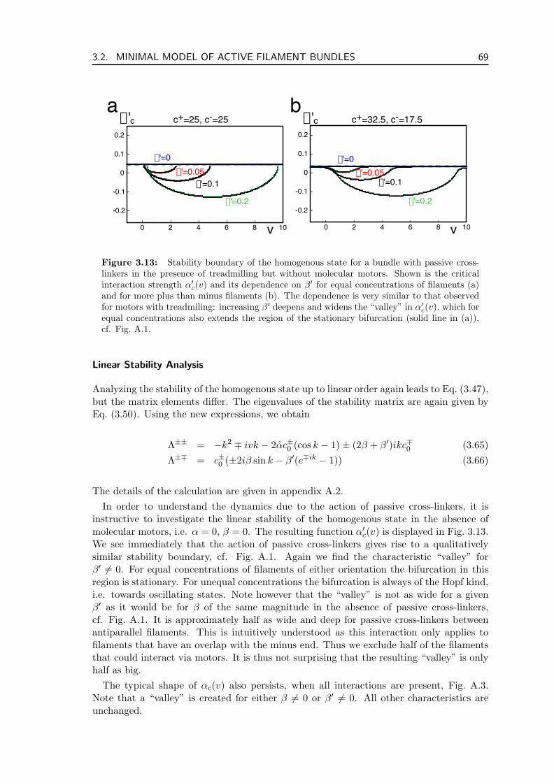
3.2. MINIMAL MODEL OF ACTIVE FILAMENT BUNDLES 69
0 2 4 6 8 10
0.1
0
-0.1
-0.2
0.2
v
a'c
b'=0
b'=0.2
b'=0.1b'=0.05
0 2 4 6 8 10
0.1
0
-0.1
-0.2
0.2
v
a'c
b'=0
b'=0.2
b'=0.1b'=0.05
a bc+=25, c-=25 c+=32.5, c-=17.5
Figure 3.13: Stability boundary of the homogenous state for a bundle with passive cross-linkers in the presence of treadmilling but without molecular motors. Shown is the criticalinteraction strength α′
c(v) and its dependence on β′ for equal concentrations of filaments (a)and for more plus than minus filaments (b). The dependence is very similar to that observedfor motors with treadmiling: increasing β′ deepens and widens the “valley” in α′
c(v), which forequal concentrations also extends the region of the stationary bifurcation (solid line in (a)),cf. Fig. A.1.
Linear Stability Analysis
Analyzing the stability of the homogenous state up to linear order again leads to Eq. (3.47),but the matrix elements differ. The eigenvalues of the stability matrix are again given byEq. (3.50). Using the new expressions, we obtain
Λ±± = −k2 ∓ ivk − 2αc±0 (cos k − 1)± (2β + β′)ikc∓0 (3.65)Λ±∓ = c±0 (±2iβ sin k − β′(e∓ik − 1)) (3.66)
The details of the calculation are given in appendix A.2.In order to understand the dynamics due to the action of passive cross-linkers, it is
instructive to investigate the linear stability of the homogenous state in the absence ofmolecular motors, i.e. α = 0, β = 0. The resulting function α′c(v) is displayed in Fig. 3.13.We see immediately that the action of passive cross-linkers gives rise to a qualitativelysimilar stability boundary, cf. Fig. A.1. Again we find the characteristic “valley” forβ′ 6= 0. For equal concentrations of filaments of either orientation the bifurcation in thisregion is stationary. For unequal concentrations the bifurcation is always of the Hopf kind,i.e. towards oscillating states. Note however that the “valley” is not as wide for a givenβ′ as it would be for β of the same magnitude in the absence of passive cross-linkers,cf. Fig. A.1. It is approximately half as wide and deep for passive cross-linkers betweenantiparallel filaments. This is intuitively understood as this interaction only applies tofilaments that have an overlap with the minus end. Thus we exclude half of the filamentsthat could interact via motors. It is thus not surprising that the resulting “valley” is onlyhalf as big.
The typical shape of αc(v) also persists, when all interactions are present, Fig. A.3.Note that a “valley” is created for either β 6= 0 or β′ 6= 0. All other characteristics areunchanged.
70 CHAPTER 3. PHYSICS OF ACTIVE FILAMENT SYSTEMS
State Diagram
The dynamics and state diagram of a bundle with all interactions is qualitatively verysimilar to the dynamics discussed in section 3.2.2. We again find solitary and oscillatorywaves and the overall topology of the state diagram is the same as displayed in Fig. 3.11.‘In particular stationary localized states are also only found for equal concentrations ofplus and minus filaments.
Plus-End-Tracking Cross-Linkers
Until now we have considered the action of cross-linkers that track the minus end of thefilaments involved. It is interesting to also consider cross-linkers, that continuously (pro-cessively) follow the polymerizing plus end of filament while being bound to another. Somecytoskeletal proteins are know to follow filament ends processively. These include forminsthat are located at the plus ends of actin filaments, or mitotic centromere-associated ki-nesin, which has been shown to track the ends of microtubules.
If e.g. formin, while being bound to a filament end links to a second filament, this linktogether with filament treadmilling will give rise to dynamics sketched in Fig. 3.7. Thisdynamics is remarkably different from that found for minus-end tracking cross-linkers(3.6b and c). These plus-end tracking cross-linkers tend to align ends of opposite polarity.Parallel filaments are thus driven towards a configuration where their centers are maximallyseparated, Fig. 3.7a. Antiparallel filaments on the other hand become aligned so that thefilament centers coincide. The associated parameters are α′′ and β′′ respectively.
These intuitive considerations can be formulated in the frame work of the mean fielddescription presented in this section. The corresponding current for parallel filaments is
J±±α′′ = −α′′c±(x)∫ 1
0d ξ[c±(x + ξ)− c±(x− ξ)
](3.67)
which is exactly the same expression as found for the other currents between parallelfilaments, except for the sign. This directly reflects the diametrical action of these plus-end tracking cross-linkers in the presence of filament treadmilling to the action of minus-end tracking cross-linkers considered so far. The current due to interactions betweenantiparallel filaments is given by
J±∓β′′ = ±β′′c±(x)∫ 1
0d ξc∓(x± ξ) (3.68)
which is different from the currents in Eqs. (3.60) and (3.61) by sign and range of integra-tion, reflecting the different polarity of the tracked end.
Having obtained these currents it is straightforward to turn the crank and analyzethe effects of these novel interactions on the bundle dynamics. We find that these termsstabilize the homogenous state and lower the tension. In fact, an explicit calculation showsthat the tension in a homogenous bundle with motors, cross-linkers that track both kindsof ends in the presence of treadmilling is lower than without them (see section 3.2.5).
3.2.4 Polymerization of Entire Filaments
Until now we have considered bundles of filaments in which the the number and orientationof filaments was conserved, as filaments could not entirely (de)polymerize or “flip” theirorientation. Now we turn to bundles in which filaments of length l can be generated(polymerized) and destroyed (depolymerized) from a pool of monomers according to the
3.2. MINIMAL MODEL OF ACTIVE FILAMENT BUNDLES 71
system described by Eqs. (3.34)-(3.36). For simplicity we assume equal polymerizationand depolymerization rates for plus and minus filaments, i.e. k±d = kd and k±p = kp. Wefirst discuss the dynamics of this polymerization and depolymerization from monomers inthe absence of treadmilling and molecular motors. Then we describe its influence on thedynamics of an active bundle in which all these effects are present.
Monomer Dynamics
We assume that only whole filaments of length l consisting of µ monomers are polymerizedor depolymerized and that the monomers diffuse freely if they are not incorporated in afilament. If filaments of both orientations are polymerized with equal probability, theensuing description for the dynamics of homogenous filament and monomer distributionsin the absence of treadmilling and molecular motors reads:
∂tc+ = kpcm − kdc
+ (3.69)∂tc
− = kpcm − kdc− (3.70)
∂tcm = −2kpµcm + kdµ(c+ + c−) (3.71)
Thus for any cm ∈ R+ the steady state is given by c±0 = cmkp/kd. Assume that the totalnumber of monomers M0 is conserved we write:
M0 = µc+ + µc− + cm
=(
2µkp
kd+ 1)
cm (3.72)
so that the concentrations of the steady state read
m0 =kd
2µkp + kdM0 and c+
0 = c−0 =kp
kdcm =
kp
2µkp + kdM0 (3.73)
We consider small small perturbations around this state c+ = c+0 + δc+, c− = c−0 +
δc−, cm = cm,0 + δcm. The perturbations evolve according to δc+
δc−
δcm
=
−kd 0 kp
0 −kd kp
µkd µkd −2µkp
δc+
δc−
δcm
(3.74)
The eigenvalues of this matrix are
λ0 = −kd (3.75)
λ1/2 =12
(−kd − 2µkp ±
√(kd − 2µkp)2 + 8µkpkd
)= 0 (3.76)
so that the steady state is always marginally stable.Note that the density of free monomers m is a free parameter in this model. For
given rates we can thus choose any concentrations c+0 = c−0 = cm,0 kp/kd as steady state.
Alternatively we can fix cm,0 by assuming conservation of the total monomer concentrationM0 as shown above. This makes M0 the free parameter. The steady state concentrationsof plus and minus filaments can be adjusted separately by choosing the (de)polymerizationrates accordingly.
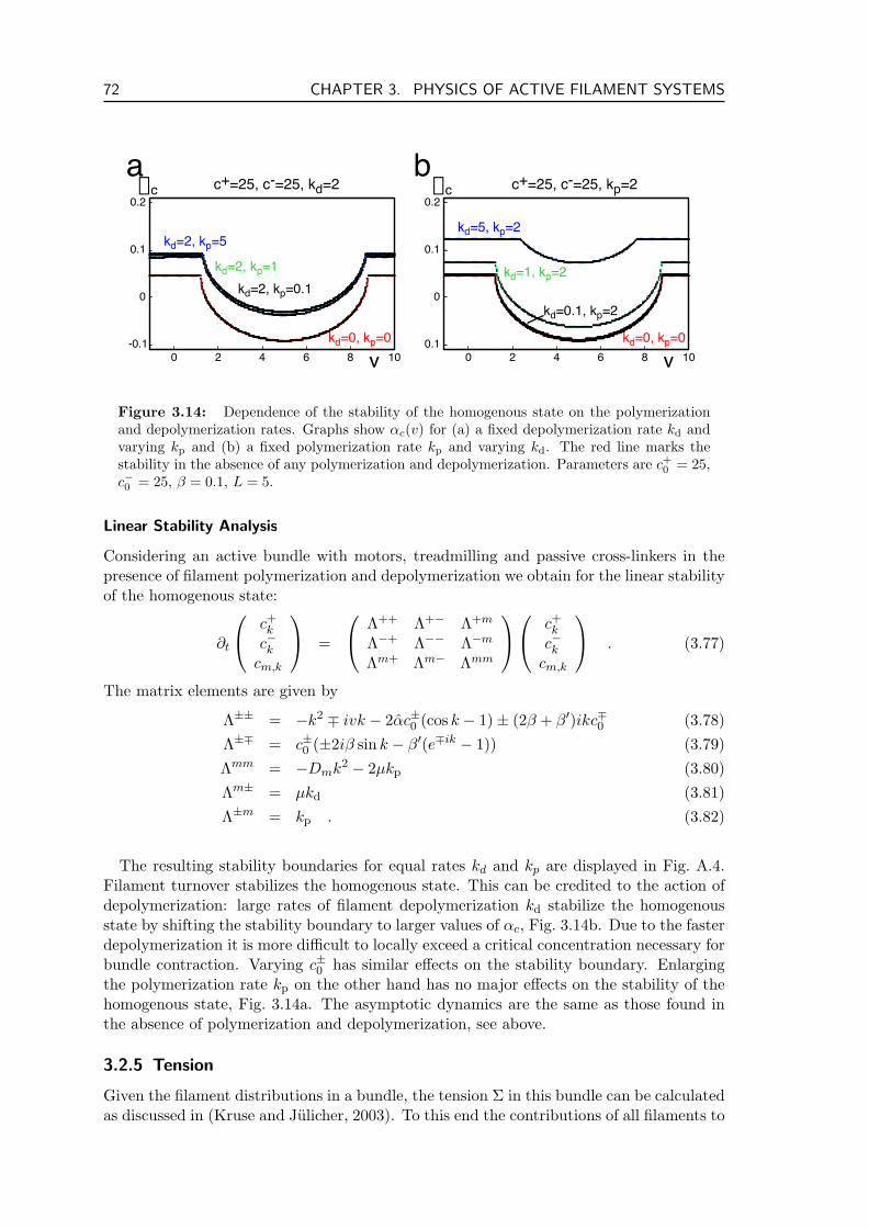
72 CHAPTER 3. PHYSICS OF ACTIVE FILAMENT SYSTEMS
a bc+=25, c-=25, kd=2
0 2 4 6 8 10
0.1
0
-0.1
0.2
kd=0, kp=0
v
ac
kd=2, kp=5
kd=2, kp=1kd=2, kp=0.1
0 2 4 6 8 10
0.1
0
0.1
0.2
kd=0, kp=0
v
ac
kd=5, kp=2
kd=1, kp=2
kd=0.1, kp=2
c+=25, c-=25, kp=2
Figure 3.14: Dependence of the stability of the homogenous state on the polymerizationand depolymerization rates. Graphs show αc(v) for (a) a fixed depolymerization rate kd andvarying kp and (b) a fixed polymerization rate kp and varying kd. The red line marks thestability in the absence of any polymerization and depolymerization. Parameters are c+
0 = 25,c−0 = 25, β = 0.1, L = 5.
Linear Stability Analysis
Considering an active bundle with motors, treadmilling and passive cross-linkers in thepresence of filament polymerization and depolymerization we obtain for the linear stabilityof the homogenous state:
∂t
c+k
c−kcm,k
=
Λ++ Λ+− Λ+m
Λ−+ Λ−− Λ−m
Λm+ Λm− Λmm
c+k
c−kcm,k
. (3.77)
The matrix elements are given by
Λ±± = −k2 ∓ ivk − 2αc±0 (cos k − 1)± (2β + β′)ikc∓0 (3.78)Λ±∓ = c±0 (±2iβ sin k − β′(e∓ik − 1)) (3.79)Λmm = −Dmk2 − 2µkp (3.80)Λm± = µkd (3.81)Λ±m = kp . (3.82)
The resulting stability boundaries for equal rates kd and kp are displayed in Fig. A.4.Filament turnover stabilizes the homogenous state. This can be credited to the action ofdepolymerization: large rates of filament depolymerization kd stabilize the homogenousstate by shifting the stability boundary to larger values of αc, Fig. 3.14b. Due to the fasterdepolymerization it is more difficult to locally exceed a critical concentration necessary forbundle contraction. Varying c±0 has similar effects on the stability boundary. Enlargingthe polymerization rate kp on the other hand has no major effects on the stability of thehomogenous state, Fig. 3.14a. The asymptotic dynamics are the same as those found inthe absence of polymerization and depolymerization, see above.
3.2.5 Tension
Given the filament distributions in a bundle, the tension Σ in this bundle can be calculatedas discussed in (Kruse and Julicher, 2003). To this end the contributions of all filaments to
3.2. MINIMAL MODEL OF ACTIVE FILAMENT BUNDLES 73
the tension at a point x are summed up (only filaments that overlap with x can contribute,of course):
Σ(x) =∫
dx′[σ+(x′, x) + σ−(x′, x)
]. (3.83)
Here σ±(x′, x) is the tension at x due to plus- and minus-filaments with centers at x′.Formally these tensions are obtained from the tension defined in Eq. (3.11) throughσ+(x′, x) = σ(x′, ex, s) with x = x′ + s and analogously for σ−.
In the absence of external forces and taking into account momentum conservation oneobtains
ddy
Σ(y) =∫
dx[f+fl + f−fl + f+
m + f−m]
, (3.84)
which permits the calculation of the tension when the filament currents are known. Thetotal tension in the bundle can be split in parts corresponding to the interaction of parallelfilaments Σ⇒ and antiparallel filaments Σ
Σ(y) = Σ⇒(y) + Σ(y) . (3.85)
From equation (3.84) it follows
Σ⇒(y) = −η
∫dx(J++(x) + J−−(x))Q(x− y) + Σ(0)
⇒ (3.86)
Σ(y) = −η
∫dx(J+−(x) + J−+(x))Q(x− y) + Σ(0)
, (3.87)
where (d/dx)Q(x) = R(x) with Q(0) = 0 and Σ(0)⇒ and Σ(0)
are constants of integration.To stress the point that tension is a local quantity, the authors introduce the functionP (x, ξ) = Q(x + ξ)−Q(x).
For the microscopic mean field description introduced in this chapter we set R(x) = 1for |x| < l/2 and R(x) = 0 otherwise. We can thus calculate the contributions from thecurrents due to molecular motors and treadmilling introduced in Eqs. (3.39)-(3.43) andthose due to the interaction via passive cross-linkers, Eqs. (3.58)-(3.61). We obtain asexpressions for tension due to the interaction of parallel filaments
Σ⇒(y) =12(α + α′)η
∫ l
−ldξ
∫dx c+(x)c+(x + ξ)sgn(ξ)P (x− y, ξ)
+12(α + α′)η
∫ l
−ldξ
∫dx c−(x)c−(x + ξ)sgn(ξ)P (x− y, ξ) (3.88)
and antiparallel filaments
Σ(y) =12η
[−β
∫ l
−ldξ
∫dx c+(x)c−(x + ξ)P (x− y, ξ)
+β
∫ l
−ldξ
∫dx c−(x)c+(x + ξ)P (x− y, ξ)
−β′∫ l
0dξ
∫dx c+(x)c−(x− ξ)P (x− y,−ξ)
+β′∫ l
0dξ
∫dx c−(x)c+(x + ξ)P (x− y, ξ)
], (3.89)
where we have dropped constant contributions arising from the boundaries. Note that forperiodic boundary conditions these boundary terms must vanish.
74 CHAPTER 3. PHYSICS OF ACTIVE FILAMENT SYSTEMS
The tension in a homogenous bundle c±(x) = c±0 is given by
Σ0 =12ηl3[(α + α′)(c+2
0 + c−20 ) + β′c+
0 c−0]
. (3.90)
A positive Σ corresponds to contractile tension in the bundle. Note that in a homogenousbundle only motors between parallel filaments (α) contribute to the tension, while passivecross-linkers contribute always (α′, β′). This is due to the symmetry of the integrals from−l to l in Eq. (3.89) for the homogenous state. The contributions of the first two termsthen exactly cancel. This is not the case for passive cross-linkers as this interaction isintrinsically asymmetric.
It is straightforward to extend the above calculation to include the action of passive, plus-end-tracking cross-linkers (Fig. 3.7). We find that these terms stabilize the homogenousstate and lower the tension. Our calculation shows that the tension in a homogenous bundlewith motors, cross-linkers that track both kinds of ends in the presence of treadmilling isexplicitly given by
Σ0 =12ηl3[(α + α′ − α′′)(c+2
0 + c−20 ) + (β′ − β′′)c+
0 c−0]
(3.91)
The action of plus-end tracking cross-linkers thus lowers the tension in homogenous bun-dles.
In muscle myofibrils the tension generation is due to motors linking antiparallel fila-ments only. This difference is due to the different symmetries of both structures. Inmyofibrils the filament position is very well defined and due to the attachment to the Z-disk filament centers never slide past each other. In filament bundles that lack this strictorganization, antiparallel filaments will be positioned randomly with respect to each otherand thus on average not contribute to the tension. In contractile rings or stress fibersno structuring elements such as Z-disks have been found. Furthermore the density seemsto be homogenous along the ring circumference. These observations shed light on motormediated interactions between parallel filaments for contractility.
Such a bundle may exert contractile forces. A ring can contract radially due to thetension generated along its circumference, see chapter 6. A bundle with two open ends,such as a stress fiber can pull on structures attached to its ends. Consider a homogenousbundle with c±(x) = c±0 inside a box 0 ≤ x ≤ L of size L and c±(x) = 0 elsewhere in theabsence of treadmilling. With boundary conditions that immobilize filaments within theintervals [0, l] and [L− l, L], this state is stable for α < αc on the interval [l, L− l].
The force balance equation (3.11) is only satisfied if a force density
fext(x) = ηl(l − x)[α(c+2
0 + c−20 )]
(3.92)
on x ∈ [0, l] is applied. Not immobilized filaments on [0, l] would flow according to
J±±(x) = αc±20 (l − x) (3.93)
J+−(x) = −βc+0 c−0 (l + x) (3.94)
J−+(x) = βc+0 c−0 (l + x) (3.95)
These fluxes are due to internal forces (cf. Eq. (3.16)). So the external force density, i.e.the strength with which the bundle pulls on the boundaries is determined by
ηl(J++(x) + J−−(x) + J+−(x) + J−+(x)
)= −
∫dy [fint(x, y) + fext(x, y)] = 0 .
(3.96)
3.3. STOCHASTIC SIMULATION OF ACTIVE FILAMENT BUNDLES 75
3.3 Stochastic Simulation of Active Filament Bundles
Stochastic simulations provide an intuitive way of approaching the physics of active bun-dles. Assuming that filament pairs in the bundle are temporarily cross-linked by motoraggregates that move towards the plus ends of filaments and briefly stay attached at thefilament end, we define a simple model for the bundle dynamics, which we study usingstochastic simulations. Filaments can interact if they overlap along the bundle axis x.We randomly select pairs of overlapping filaments. At each time-step of duration ∆t, aninteraction between the two filaments of the pair via a molecular motor occurs with proba-bility α∆t, if filaments are parallel, and β∆t, if the filaments are antiparallel. Parametersdressed with a bar correspond to the naked parameters in the mean field description, seesection 3.4 for details. If the interaction occurs, both filaments are displaced by a distanceδ, the working distance of a molecular motor (cf. Fig 3.2), according to the rules indicatedin Fig. 3.5. Assuming that the motors diffuse rapidly, we use a constant and homogenousmotor concentration for simplicity. We start our simulations from initially homogenousprofiles of filament density c+(x) = c0
+ and c−(x) = c0− along the x coordinate, where
c±(x) denote the number densities of filaments with center at position x and their plusends pointing in positive and negative x-direction, respectively. In order to capture thedynamics of a filament ring, we impose periodic boundary conditions c(x) = c(x + L),where L = 2πR is the circumference of a ring with radius R. Simulations reveal thatfor weak interactions between parallel filaments (corresponding to α being smaller than acritical value αc) the homogeneous bundle is stable. This is independent of the value of βcharacterizing the interaction of antiparallel filaments. If α exceeds the critical value αc,the homogeneous bundle is unstable and develops into an inhomogenous density profilethat can be stationary or lead to complex dynamics after long times, which include prop-agating density profiles. Note, that our stochastic simulations also include fluctuations,captured by an effective diffusion constant D. Examples of simulation results are shownin Figs. 3.15 and 3.16. If the ring ruptures, stationary density profiles can be attainedwhere the filaments of opposite orientation are localized and completely separated. Thehomogenous bundle con only contract the ring, when it is stable (see chapter 6 for a de-tailed discussion of ring contraction). Indeed, filaments are constantly moved relative toeach other and motors exert forces on filaments in the stable, homogeneous bundle. Asdiscussed in section 3.2, this generates a net contractile tension in the bundle, which we canestimate with the mean field description (cf. section 3.2.5). In the spirit outlined here wealso include filament treadmilling, and the action passive cross-linkers in our simulations.The details of the stochastic simulations are outlined in the next section (3.3.1). Then wepresent the dynamics of active filament bundles as obtained by stochastic simulations insection 3.3.2. Finally we conclude this section by calculating the filament currents in suchbundles in section 3.3.3.
3.3.1 Stochastic Simulation
We study the behavior of N individual filaments of length l along a linear position coor-dinate x. We impose periodic boundary conditions with period L, corresponding to a ringwith circumference L. The position of the center of filament i with i = 1, .., N is denotedby xi. Its orientation with respect to the positive x-axis is denoted by oi: this orientationis oi = +1 if the plus end points in positive x-direction, oi = −1 implies that the minusend points in x-direction. At every timestep of duration ∆t, each filament is displacedby a distance ∆i as a result of diffusion, treadmiling, and the interaction with molecularmotors and with passive cross-linkers. Furthermore, filaments are removed and created at
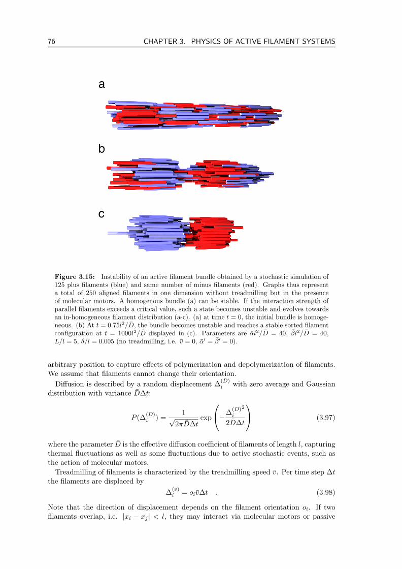
76 CHAPTER 3. PHYSICS OF ACTIVE FILAMENT SYSTEMS
a
c
b
Figure 3.15: Instability of an active filament bundle obtained by a stochastic simulation of125 plus filaments (blue) and same number of minus filaments (red). Graphs thus representa total of 250 aligned filaments in one dimension without treadmilling but in the presenceof molecular motors. A homogenous bundle (a) can be stable. If the interaction strength ofparallel filaments exceeds a critical value, such a state becomes unstable and evolves towardsan in-homogeneous filament distribution (a-c). (a) at time t = 0, the initial bundle is homoge-neous. (b) At t = 0.75l2/D, the bundle becomes unstable and reaches a stable sorted filamentconfiguration at t = 1000l2/D displayed in (c). Parameters are αl2/D = 40, βl2/D = 40,L/l = 5, δ/l = 0.005 (no treadmilling, i.e. v = 0, α′ = β′ = 0).
arbitrary position to capture effects of polymerization and depolymerization of filaments.We assume that filaments cannot change their orientation.
Diffusion is described by a random displacement ∆(D)i with zero average and Gaussian
distribution with variance D∆t:
P (∆(D)i ) =
1√2πD∆t
exp
−∆(D)i
2
2D∆t
(3.97)
where the parameter D is the effective diffusion coefficient of filaments of length l, capturingthermal fluctuations as well as some fluctuations due to active stochastic events, such asthe action of molecular motors.
Treadmilling of filaments is characterized by the treadmilling speed v. Per time step ∆tthe filaments are displaced by
∆(v)i = oiv∆t . (3.98)
Note that the direction of displacement depends on the filament orientation oi. If twofilaments overlap, i.e. |xi − xj | < l, they may interact via molecular motors or passive
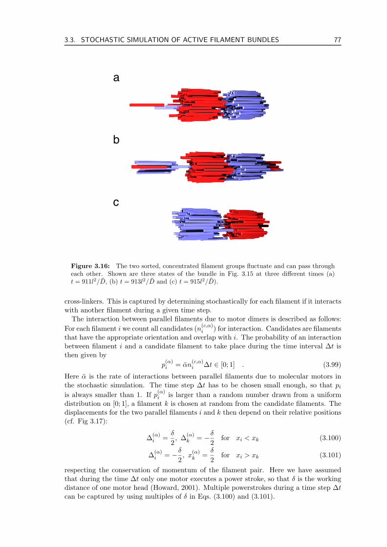
3.3. STOCHASTIC SIMULATION OF ACTIVE FILAMENT BUNDLES 77
a
c
b
Figure 3.16: The two sorted, concentrated filament groups fluctuate and can pass througheach other. Shown are three states of the bundle in Fig. 3.15 at three different times (a)t = 911l2/D, (b) t = 913l2/D and (c) t = 915l2/D).
cross-linkers. This is captured by determining stochastically for each filament if it interactswith another filament during a given time step.
The interaction between parallel filaments due to motor dimers is described as follows:For each filament i we count all candidates (n(c,α)
i ) for interaction. Candidates are filamentsthat have the appropriate orientation and overlap with i. The probability of an interactionbetween filament i and a candidate filament to take place during the time interval ∆t isthen given by
p(α)i = αn
(c,α)i ∆t ∈ [0; 1] . (3.99)
Here α is the rate of interactions between parallel filaments due to molecular motors inthe stochastic simulation. The time step ∆t has to be chosen small enough, so that pi
is always smaller than 1. If p(α)i is larger than a random number drawn from a uniform
distribution on [0; 1], a filament k is chosen at random from the candidate filaments. Thedisplacements for the two parallel filaments i and k then depend on their relative positions(cf. Fig 3.17):
∆(α)i =
δ
2, ∆(α)
k = −δ
2for xi < xk (3.100)
∆(α)i = −δ
2, x
(α)k =
δ
2for xi > xk (3.101)
respecting the conservation of momentum of the filament pair. Here we have assumedthat during the time ∆t only one motor executes a power stroke, so that δ is the workingdistance of one motor head (Howard, 2001). Multiple powerstrokes during a time step ∆tcan be captured by using multiples of δ in Eqs. (3.100) and (3.101).
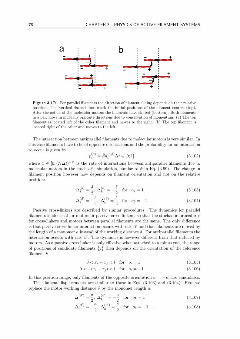
78 CHAPTER 3. PHYSICS OF ACTIVE FILAMENT SYSTEMS
a b- +
- +
- +
- +
- +
- +- +
- +
Figure 3.17: For parallel filaments the direction of filament sliding depends on their relativeposition. The vertical dashed lines mark the initial positions of the filament centers (top).After the action of the molecular motors the filaments have shifted (bottom). Both filamentsin a pair move in mutually opposite directions due to conservation of momentum. (a) The topfilament is located left of the other filament and moves to the right. (b) The top filament islocated right of the other and moves to the left.
The interaction between antiparallel filaments due to molecular motors is very similar. Inthis case filaments have to be of opposite orientations and the probability for an interactionto occur is given by
p(β)i = βn
(c,β)i ∆t ∈ [0; 1] . (3.102)
where β ∈ [0; (N∆t)−1] is the rate of interactions between antiparallel filaments due tomolecular motors in the stochastic simulation, similar to α in Eq. (3.99). The change infilament position however now depends on filament orientation and not on the relativeposition:
∆(β)i =
δ
2, ∆(β)
k = −δ
2for ok = 1 (3.103)
∆(β)i = −δ
2, ∆(β)
k =δ
2for ok = −1 . (3.104)
Passive cross-linkers are described by similar procedures. The dynamics for parallelfilaments is identical for motors or passive cross-linkers, so that the stochastic proceduresfor cross-linkers and motors between parallel filaments are the same. The only differenceis that passive cross-linker interaction occurs with rate α′ and that filaments are moved bythe length of a monomer a instead of the working distance δ. For antiparallel filaments theinteraction occurs with rate β′. The dynamics is however different from that induced bymotors. As a passive cross-linker is only effective when attached to a minus end, the rangeof positions of candidate filaments j then depends on the orientation of the referencefilament i:
0 < xi − xj < l for oi = 1 (3.105)0 < −(xi − xj) < l for oi = −1 . (3.106)
In this position range, only filaments of the opposite orientation oi = −oj are candidates.The filament displacements are similar to those in Eqs. (3.103) and (3.104). Here we
replace the motor working distance δ by the monomer length a:
∆(β′)i =
a
2, ∆(β′)
k = −a
2for ok = 1 (3.107)
∆(β′)i = −a
2, ∆(β′)
k =a
2for ok = −1 . (3.108)
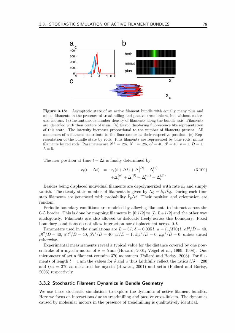
3.3. STOCHASTIC SIMULATION OF ACTIVE FILAMENT BUNDLES 79
plus
minus
bothc
0 1 2 3 4 50
100
200
300
400
x
a b
c x
x
Figure 3.18: Asymptotic state of an active filament bundle with equally many plus andminus filaments in the presence of treadmilling and passive cross-linkers, but without molec-ular motors. (a) Instantaneous number density of filaments along the bundle axis. Filamentsare identified with their centers of mass. (b) Graph displaying fluorescence like representationof this state. The intensity increases proportional to the number of filaments present. Allmonomers of a filament contribute to the fluorescence at their respective position. (c) Rep-resentation of the bundle state by rods. Plus filaments are represented by blue rods, minusfilaments by red rods. Parameters are N+ = 125, N− = 125, α′ = 40, β′ = 40, v = 1, D = 1,L = 5.
The new position at time t + ∆t is finally determined by
xi(t + ∆t) = xi(t + ∆t) + ∆(D)i + ∆(v)
i (3.109)
+∆(α)i + ∆(β)
i + ∆(α′)i + ∆(β′)
i
Besides being displaced individual filaments are depolymerized with rate kd and simplyvanish. The steady state number of filaments is given by N0 = kp/kd. During each timestep filaments are generated with probability kp∆t. Their position and orientation arerandom.
Periodic boundary conditions are modeled by allowing filaments to interact across the0-L border. This is done by mapping filaments in [0; l/2] to [L,L+ l/2] and the other wayanalogously. Filaments are also allowed to dislocate freely across this boundary. Fixedboundary conditions do not allow interaction nor displacement across 0-L.
Parameters used in the simulations are L = 5 l, δ = 0.005 l, a = (1/370) l, αl2/D = 40,βl2/D = 40, α′l2/D = 40, β′l2/D = 40, vl/D = 1, kpl
2/D = 0, kdl2/D = 0, unless stated
otherwise.Experimental measurements reveal a typical value for the distance covered by one pow-
erstroke of a myosin motor of δ = 5 nm (Howard, 2001; Veigel et al., 1999, 1998). Onemicrometer of actin filament contains 370 monomers (Pollard and Borisy, 2003). For fila-ments of length l = 1µm the values for δ and a thus faithfully reflect the ratios l/δ = 200and l/a = 370 as measured for myosin (Howard, 2001) and actin (Pollard and Borisy,2003) respectively.
3.3.2 Stochastic Filament Dynamics in Bundle Geometry
We use these stochastic simulations to explore the dynamics of active filament bundles.Here we focus on interactions due to treadmilling and passive cross-linkers. The dynamicscaused by molecular motors in the presence of treadmilling is qualitatively identical.
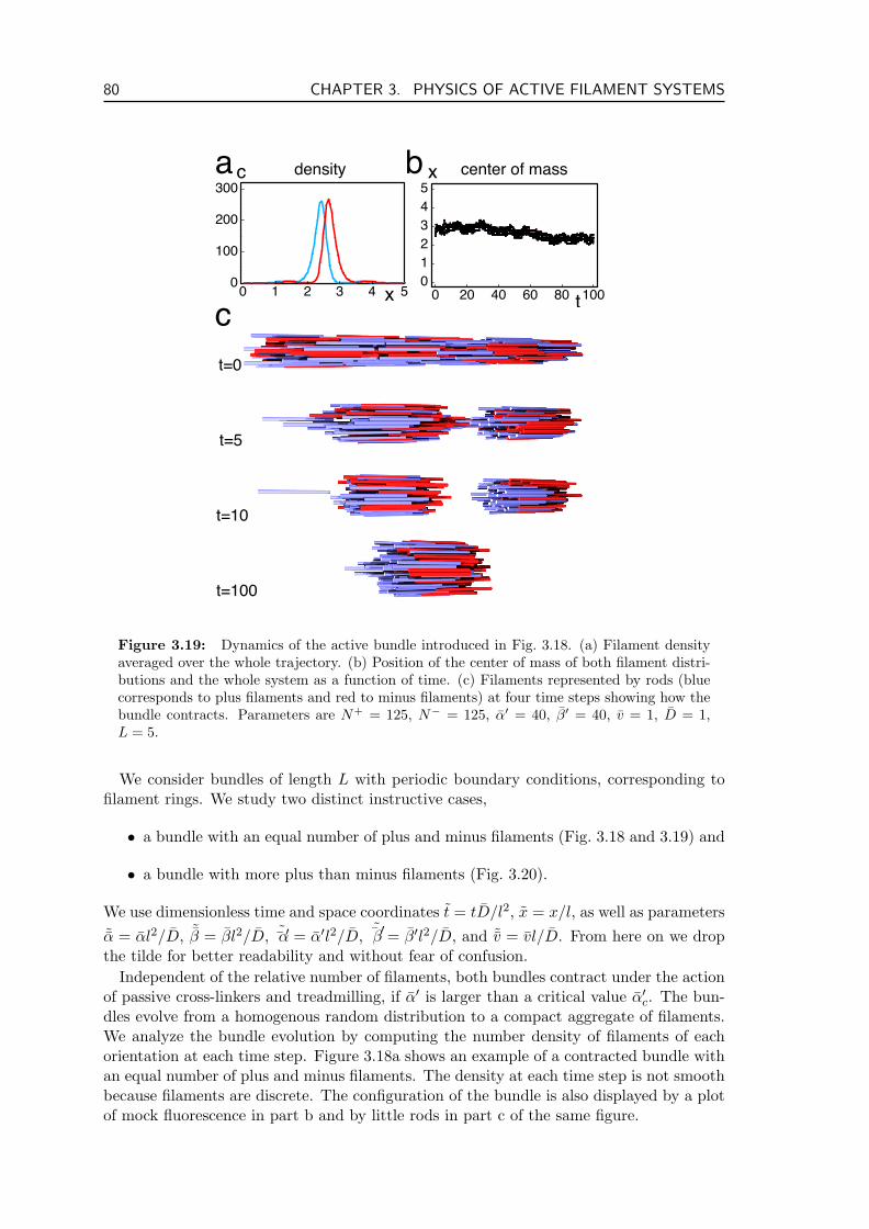
80 CHAPTER 3. PHYSICS OF ACTIVE FILAMENT SYSTEMS
0 20 40 60 80 100012345x
t0 1 2 3 4 5x0
100
200
300ca b
c
center of massdensity
t=0
t=100
t=10
t=5
Figure 3.19: Dynamics of the active bundle introduced in Fig. 3.18. (a) Filament densityaveraged over the whole trajectory. (b) Position of the center of mass of both filament distri-butions and the whole system as a function of time. (c) Filaments represented by rods (bluecorresponds to plus filaments and red to minus filaments) at four time steps showing how thebundle contracts. Parameters are N+ = 125, N− = 125, α′ = 40, β′ = 40, v = 1, D = 1,L = 5.
We consider bundles of length L with periodic boundary conditions, corresponding tofilament rings. We study two distinct instructive cases,
• a bundle with an equal number of plus and minus filaments (Fig. 3.18 and 3.19) and
• a bundle with more plus than minus filaments (Fig. 3.20).
We use dimensionless time and space coordinates t = tD/l2, x = x/l, as well as parameters˜α = αl2/D, ˜β = βl2/D, ˜′α = α′l2/D, ˜′
β = β′l2/D, and ˜v = vl/D. From here on we dropthe tilde for better readability and without fear of confusion.
Independent of the relative number of filaments, both bundles contract under the actionof passive cross-linkers and treadmilling, if α′ is larger than a critical value α′c. The bun-dles evolve from a homogenous random distribution to a compact aggregate of filaments.We analyze the bundle evolution by computing the number density of filaments of eachorientation at each time step. Figure 3.18a shows an example of a contracted bundle withan equal number of plus and minus filaments. The density at each time step is not smoothbecause filaments are discrete. The configuration of the bundle is also displayed by a plotof mock fluorescence in part b and by little rods in part c of the same figure.
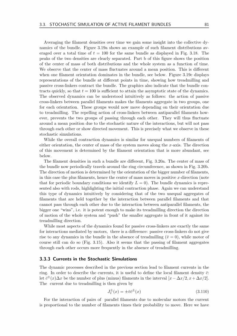
3.3. STOCHASTIC SIMULATION OF ACTIVE FILAMENT BUNDLES 81
Averaging the filament densities over time we gain some insight into the collective dy-namics of the bundle. Figure 3.19a shows an example of such filament distributions av-eraged over a total time of t = 100 for the same bundle as displayed in Fig. 3.18. Thepeaks of the two densities are clearly separated. Part b of this figure shows the positionof the center of mass of both distributions and the whole system as a function of time.We observe that the center of mass fluctuates around a mean position. This is differentwhen one filament orientation dominates in the bundle, see below. Figure 3.19c displaysrepresentations of the bundle at different points in time, showing how treadmilling andpassive cross-linkers contract the bundle. The graphics also indicate that the bundle con-tracts quickly, so that t = 100 is sufficient to attain the asymptotic state of the dynamics.The observed dynamics can be understood intuitively as follows: the action of passivecross-linkers between parallel filaments makes the filaments aggregate in two groups, onefor each orientation. These groups would now move depending on their orientation dueto treadmilling. The repelling action of cross-linkers between antiparallel filaments how-ever, prevents the two groups of passing through each other. They will thus fluctuatearound a mean position due to the stochastic nature of the interactions, but will not passthrough each other or show directed movement. This is precisely what we observe in thesestochastic simulations.
While the overall contraction dynamics is similar for unequal numbers of filaments ofeither orientation, the center of mass of the system moves along the x-axis. The directionof this movement is determined by the filament orientation that is more abundant, seebelow.
The filament densities in such a bundle are different, Fig. 3.20a. The center of mass ofthe bundle now periodically travels around the ring circumference, as shown in Fig. 3.20b.The direction of motion is determined by the orientation of the bigger number of filaments,in this case the plus filaments, hence the center of mass moves in positive x-direction (notethat for periodic boundary conditions we identify L = 0). The bundle dynamics is repre-sented also with rods, highlighting the initial contraction phase. Again we can understandthis type of dynamics intuitively by considering that of the two unequal aggregates offilaments that are held together by the interaction between parallel filaments and thatcannot pass through each other due to the interaction between antiparallel filaments, thebigger one “wins”, i.e. it is potent enough to make its treadmilling direction the directionof motion of the whole system and “push” the smaller aggregate in front of it against itstreadmilling direction.
While most aspects of the dynamics found for passive cross-linkers are exactly the samefor interactions mediated by motors, there is a difference: passive cross-linkers do not giverise to any dynamics in the bundle in the absence of treadmilling (v = 0), while motor ofcourse still can do so (Fig. 3.15). Also it seems that the passing of filament aggregatesthrough each other occurs more frequently in the absence of treadmilling.
3.3.3 Currents in the Stochastic Simulations
The dynamic processes described in the previous section lead to filament currents in thering. In order to describe the currents, it is useful to define the local filament density c:let c±(x)∆x be the number of plus (minus) filaments in the interval [x−∆x/2, x+∆x/2].The current due to treadmilling is then given by
J±v (x) = ±vc±(x) (3.110)
For the interaction of pairs of parallel filaments due to molecular motors the currentis proportional to the number of filaments times their probability to move. Here we have
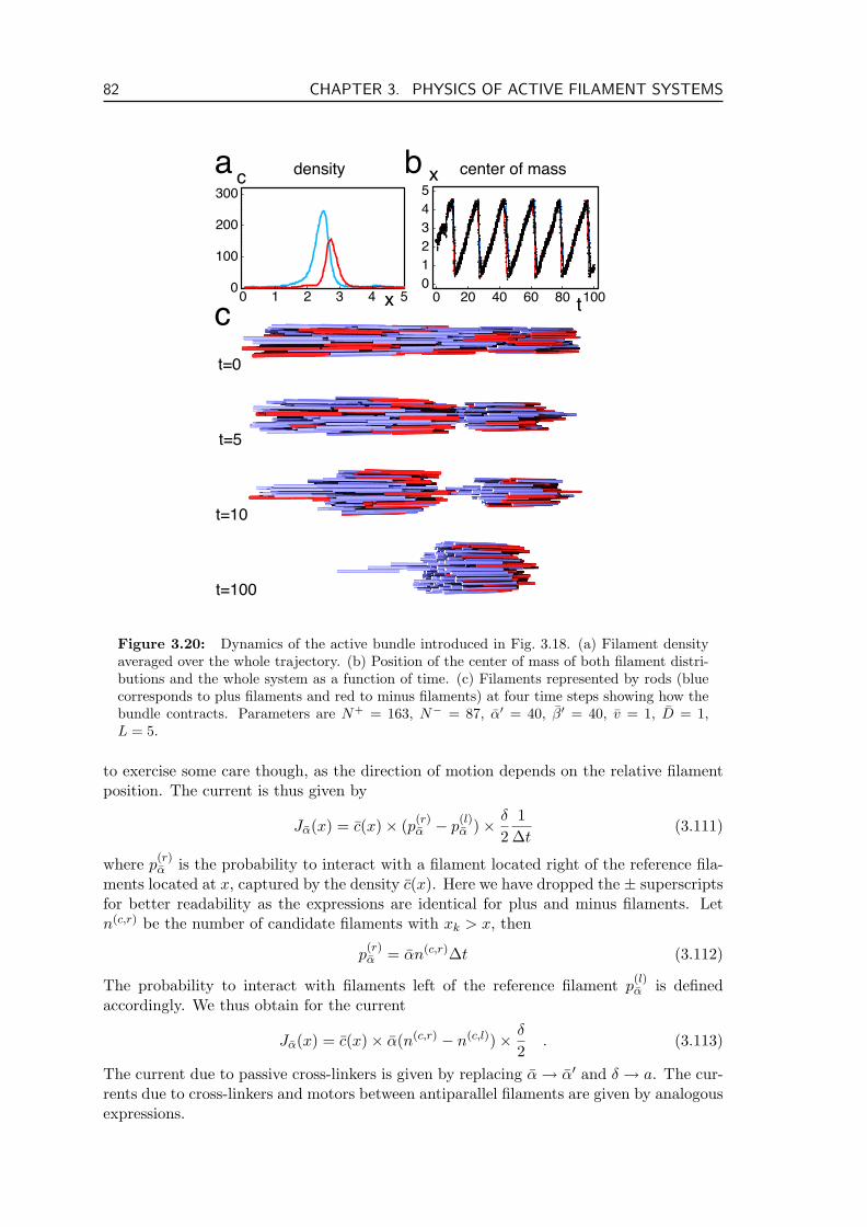
82 CHAPTER 3. PHYSICS OF ACTIVE FILAMENT SYSTEMS
a b
c
center of massdensity
t=0
t=100
t=10
t=5
0 20 40 60 80 100012345x
t0 1 2 3 4 50
100
200
300
x
c
Figure 3.20: Dynamics of the active bundle introduced in Fig. 3.18. (a) Filament densityaveraged over the whole trajectory. (b) Position of the center of mass of both filament distri-butions and the whole system as a function of time. (c) Filaments represented by rods (bluecorresponds to plus filaments and red to minus filaments) at four time steps showing how thebundle contracts. Parameters are N+ = 163, N− = 87, α′ = 40, β′ = 40, v = 1, D = 1,L = 5.
to exercise some care though, as the direction of motion depends on the relative filamentposition. The current is thus given by
Jα(x) = c(x)× (p(r)α − p
(l)α )× δ
21
∆t(3.111)
where p(r)α is the probability to interact with a filament located right of the reference fila-
ments located at x, captured by the density c(x). Here we have dropped the ± superscriptsfor better readability as the expressions are identical for plus and minus filaments. Letn(c,r) be the number of candidate filaments with xk > x, then
p(r)α = αn(c,r)∆t (3.112)
The probability to interact with filaments left of the reference filament p(l)α is defined
accordingly. We thus obtain for the current
Jα(x) = c(x)× α(n(c,r) − n(c,l))× δ
2. (3.113)
The current due to passive cross-linkers is given by replacing α → α′ and δ → a. The cur-rents due to cross-linkers and motors between antiparallel filaments are given by analogousexpressions.
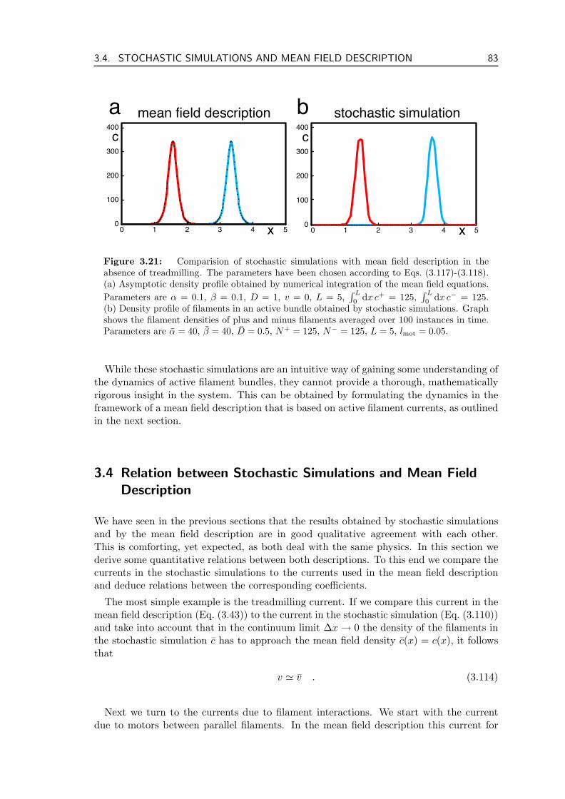
3.4. STOCHASTIC SIMULATIONS AND MEAN FIELD DESCRIPTION 83
0 1 2 3 4 50
100
200
300
400
0 1 2 3 4 50
100
200
300
400c
x
c
x
a bmean field description stochastic simulation
Figure 3.21: Comparision of stochastic simulations with mean field description in theabsence of treadmilling. The parameters have been chosen according to Eqs. (3.117)-(3.118).(a) Asymptotic density profile obtained by numerical integration of the mean field equations.Parameters are α = 0.1, β = 0.1, D = 1, v = 0, L = 5,
∫ L
0dx c+ = 125,
∫ L
0dx c− = 125.
(b) Density profile of filaments in an active bundle obtained by stochastic simulations. Graphshows the filament densities of plus and minus filaments averaged over 100 instances in time.Parameters are α = 40, β = 40, D = 0.5, N+ = 125, N− = 125, L = 5, lmot = 0.05.
While these stochastic simulations are an intuitive way of gaining some understanding ofthe dynamics of active filament bundles, they cannot provide a thorough, mathematicallyrigorous insight in the system. This can be obtained by formulating the dynamics in theframework of a mean field description that is based on active filament currents, as outlinedin the next section.
3.4 Relation between Stochastic Simulations and Mean FieldDescription
We have seen in the previous sections that the results obtained by stochastic simulationsand by the mean field description are in good qualitative agreement with each other.This is comforting, yet expected, as both deal with the same physics. In this section wederive some quantitative relations between both descriptions. To this end we compare thecurrents in the stochastic simulations to the currents used in the mean field descriptionand deduce relations between the corresponding coefficients.
The most simple example is the treadmilling current. If we compare this current in themean field description (Eq. (3.43)) to the current in the stochastic simulation (Eq. (3.110))and take into account that in the continuum limit ∆x → 0 the density of the filaments inthe stochastic simulation c has to approach the mean field density c(x) = c(x), it followsthat
v ' v . (3.114)
Next we turn to the currents due to filament interactions. We start with the currentdue to motors between parallel filaments. In the mean field description this current for
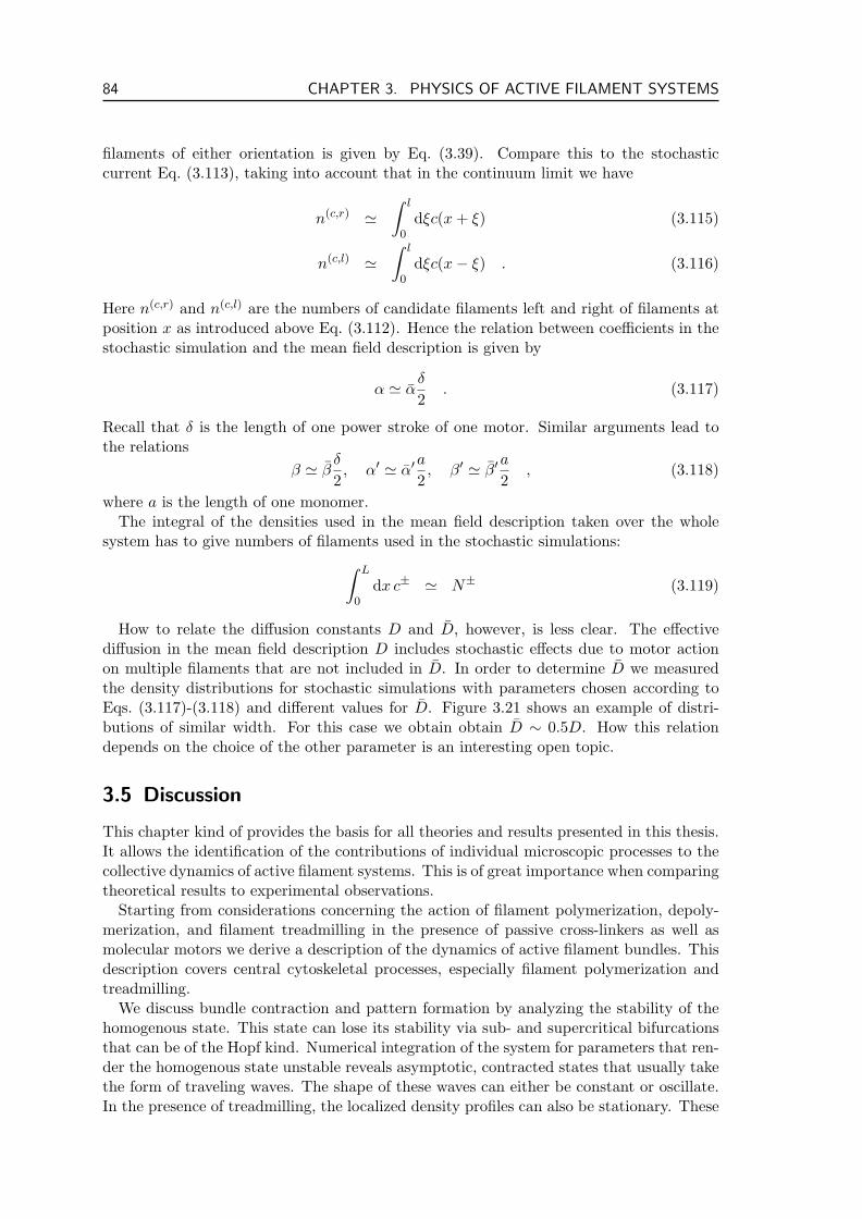
84 CHAPTER 3. PHYSICS OF ACTIVE FILAMENT SYSTEMS
filaments of either orientation is given by Eq. (3.39). Compare this to the stochasticcurrent Eq. (3.113), taking into account that in the continuum limit we have
n(c,r) '∫ l
0dξc(x + ξ) (3.115)
n(c,l) '∫ l
0dξc(x− ξ) . (3.116)
Here n(c,r) and n(c,l) are the numbers of candidate filaments left and right of filaments atposition x as introduced above Eq. (3.112). Hence the relation between coefficients in thestochastic simulation and the mean field description is given by
α ' αδ
2. (3.117)
Recall that δ is the length of one power stroke of one motor. Similar arguments lead tothe relations
β ' βδ
2, α′ ' α′
a
2, β′ ' β′
a
2, (3.118)
where a is the length of one monomer.The integral of the densities used in the mean field description taken over the whole
system has to give numbers of filaments used in the stochastic simulations:∫ L
0dx c± ' N± (3.119)
How to relate the diffusion constants D and D, however, is less clear. The effectivediffusion in the mean field description D includes stochastic effects due to motor actionon multiple filaments that are not included in D. In order to determine D we measuredthe density distributions for stochastic simulations with parameters chosen according toEqs. (3.117)-(3.118) and different values for D. Figure 3.21 shows an example of distri-butions of similar width. For this case we obtain obtain D ∼ 0.5D. How this relationdepends on the choice of the other parameter is an interesting open topic.
3.5 Discussion
This chapter kind of provides the basis for all theories and results presented in this thesis.It allows the identification of the contributions of individual microscopic processes to thecollective dynamics of active filament systems. This is of great importance when comparingtheoretical results to experimental observations.
Starting from considerations concerning the action of filament polymerization, depoly-merization, and filament treadmilling in the presence of passive cross-linkers as well asmolecular motors we derive a description of the dynamics of active filament bundles. Thisdescription covers central cytoskeletal processes, especially filament polymerization andtreadmilling.
We discuss bundle contraction and pattern formation by analyzing the stability of thehomogenous state. This state can lose its stability via sub- and supercritical bifurcationsthat can be of the Hopf kind. Numerical integration of the system for parameters that ren-der the homogenous state unstable reveals asymptotic, contracted states that usually takethe form of traveling waves. The shape of these waves can either be constant or oscillate.In the presence of treadmilling, the localized density profiles can also be stationary. These
3.5. DISCUSSION 85
states are also obtained by stochastic computer simulations of active filament bundles.The parameters of the stochastic simulation can be quantitatively related to those of theminimal model, allowing a deeper understanding of the contributions of the microscopicprocesses involved.
Bundle contraction is due to tension generated in the bundle by active processes betweenfilament pairs, such as the action of motor dimers or passive cross-linkers in the presenceof treadmilling. We derive an expression for the tension in such bundles and discussthe contribution of various microscopic processes. Motor dimers can only contribute tothe tension when bound to parallel filaments. Passive, end-tracking cross-linkers in thepresence of treadmilling can contribute independent of the orientation of the filaments theybind to. If they track the depolymerizing end, they increase the tension in the bundle, ifthey track the polymerizing end they lower it.
The minimal model is limited to the action of motors on filaments. In bacteria, ringsof FtsZ protein filaments are thought to initiate cytokinesis by contraction, although nomolecular motors like myosins are known to exist (Moller-Jensen and Lowe, 2005). Ourdescription of filament treadmilling in the presence of passive cross-linkers offers a possiblephysical mechanism for ring contraction even in the absence of molecular motors andprovides an attractive framework of thought for these processes.
As cytoskeletal waves have been found in various motile cells (Vicker, 2002; Bretschnei-der et al., 2004; Giannone et al., 2004; Dubin-Thaler et al., 2004; Dobereiner et al., 2004)it is tempting to link the solitary waves found in the minimal model to cell locomotion.Momentum conservation however prohibits a net filament transport by these waves. Thisconstraint can be released by coupling the system to the environment, e.g. by allowingfilaments to attach to a substrate. The minimal model with stabilized filaments has alsobeen studied in situations where filaments were allowed to attach to a substrate (Kruseet al., 2001; Kruse and Julicher, 2003) and with dynamics motor concentrations (Kruseand Julicher, 2003). Attachment of filaments may change the critical value of α but theset of asymptotic states of the system remains unchanged. When the homogenous stateloses stability, it evolves either to solitary or oscillatory waves. In the absence of interac-tion with filaments of the opposite orientation (β = 0) stationary localized states are alsopossible. Because of a possible momentum exchange with the substrate, the waves arenow accompanied by a net filament current, I 6= 0,
Allowing for a dynamic motor density reproduces all types of asymptotic states presentedin this chapter. In addition a few interesting new features appear. First, oriented bundlesalso support solitary waves. Interestingly it is only necessary to change the value (andnot the sign) of the average motor velocity on filaments Γ, as introduced in Eqs. (3.13)and (3.14), in order to reverse the direction of propagation of solitary waves. Second, anew intrinsic length scale emerges: the instability of the homogenous state towards thesewaves can occur at wave numbers different from 2π/L. Third, the homogenous state inbundles of mixed orientation, can become unstable even in the absence of an interactionbetween filaments of the same orientation. The generation of tension in the homogenousstate however still requires interactions between filaments of the same orientation. Fourth,in bundles of mixed orientations the homogenous state can lose stability with respect tostationary localized states if c+
0 = c−0 . This is reminiscent of the stationary localized statesobtained in the presence of treadmilling, cf. Fig. 3.11b.
The treatment of microscopic processes in active filament systems in more than onedimension is technically more cumbersome than for filament bundles, due to additionaldegrees of freedom, e.g. filament rotations. A generalization of the minimal model to higherdimensions in the absence of filament polymerization that takes rotations of filaments
86 CHAPTER 3. PHYSICS OF ACTIVE FILAMENT SYSTEMS
into account has been proposed by Liverpool and Marchetti (2003) and was subsequentlydeveloped in (Liverpool and Marchetti, 2005; Liverpool, 2005). The homogenous isotropicstate is a stationary solution of the resulting equations. Assuming that friction is isotropicthe linear stability of this state was analyzed (Liverpool and Marchetti, 2003; Ziebert andZimmermann, 2004). As in one-dimension the homogenous isotropic state loses stabilityat a critical value αc. For small densities, density fluctuations drive the instability, whilefor larger densities fluctuations in the polarization are responsible. In either case thebifurcation is stationary. If β 6= 0, the instability can be oscillatory if the density c0 is largeenough (Liverpool and Marchetti, 2003). The nature of the states beyond the instabilityremains to be explored. Note that a similar derivation of active filament dynamics in morethan one dimension has revealed additional terms (Tanase, 2004).
It will be interesting future work to investigate how filament polymerization and espe-cially treadmilling alters the dynamics of active systems with these extensions.
4 Stability of the Mitotic Spindle
4.1 Introduction
The mitotic and meiotic spindles that separate chromosomes during the cell cycle arefascinating dynamic cytoskeletal structures that have captured the attention of biologistsand physicists alike. While aspects of aster formation and dynamics as well as spindleformation have been studied by numerical simulations (Nedelec, 2002a; Chakravarty et al.,2004; Joglekar and Hunt, 2002), a comprehensive analytical description of spindle dynamicsis still lacking. Here we present first steps towards this goal developing a microscopicdescription for cytoskeletal spindles.
We focus on the question of what determines the length of stable spindles, as e.g. mitoticand meiotic spindles of the same organism often differ in size. Even more strikingly spindlesin Xenopus egg extract are longer when the minus-end directed dynein-dynactin complexis inhibited. Our theory reproduces this observation. Furthermore we calculate conditionsfor the stability of these spindles. We are confident that this description will also behelpful in answering many other questions regarding mitotic and meiotic spindles, such ase.g. spindle oscillations (Grill et al., 2005).
4.1.1 From Filament Bundles to the Mitotic Spindle
We describe a bipolar cytoskeletal spindle consisting of two interacting microtubule asters.This corresponds to a model of mitotic spindles that is widely used in the literature. Theasters are characterized by a length distribution, which determines the microtubule den-sity as well as the densities of microtubule ends. Due to the rotational symmetry of thespindle we may project the system onto the spindle axis. This results in an effectivelyone-dimensional, fiber-like geometry, Fig. 4.1. We consider pair-wise filament interactionsthat are mediated by molecular motors. This approach is similar in spirit to the micro-scopic description of motor-filament systems presented in chapter 3. In addition to theconcepts employed in the minimal model, here we also include a force dependent motorvelocity captured by a force-velocity relation. This allows us to discuss the influence ofaster movement on motor dimers bound to microtubules originating from both asters.We furthermore explicitly consider motor binding to filament ends, which has importantconsequences for the formation of stable spindles.
The geometry of the spindle determines the orientation of microtubules in the system.Microtubules are bound with their minus end to the aster centers, so that the plus endsalways point outwards from each aster. Plus-end directed motor dimers that are bound toone MT from each aster between the asters will thus push the asters apart, while minus enddirected complexes will pull them together. Furthermore due to the attachment of MTsto the aster center, molecular motors cannot induce relative filament sliding between MTsoriginating from the same aster. Forces generated by motors bound to MTs originatingfrom two different asters, contribute to an effective force that acts on both asters. Wecalculate the resulting force between the two asters by summing up all contributions frommotors bound. Assuming that this active force is balanced by viscous forces that act on
87
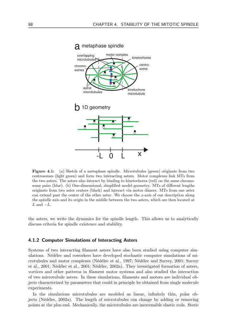
88 CHAPTER 4. STABILITY OF THE MITOTIC SPINDLE
metaphase spindle
astral
microtubules
overlapping
microtubules
kinetochore
microtubule
kinetochores
a
b
motor complex
chromo-
somes
1D geometry
centro-
some
0-L L x
Figure 4.1: (a) Sketch of a metaphase spindle. Microtubules (green) originate from twocentrosomes (light green) and form two interacting asters. Motor complexes link MTs fromthe two asters. The asters also interact by binding to kinetochores (red) on the same chromo-some pairs (blue). (b) One-dimensional, simplified model geometry. MTs of different lengthsoriginate from two aster centers (black) and interact via motor dimers. MTs from one astercan extend past the center of the other aster. We choose the x-axis of our description alongthe spindle axis and its origin in the middle between the two asters, which are then located atL and −L.
the asters, we write the dynamics for the spindle length. This allows us to analyticallydiscuss criteria for spindle existence and stability.
4.1.2 Computer Simulations of Interacting Asters
Systems of two interacting filament asters have also been studied using computer sim-ulations. Nedelec and coworkers have developed stochastic computer simulations of mi-crotubules and motor complexes (Nedelec et al., 1997; Nedelec and Surrey, 2001; Surreyet al., 2001; Nedelec et al., 2001; Nedelec, 2002a). They investigated formation of asters,vortices and other patterns in filament motor systems and also studied the interactionof two microtubule asters. In these simulations, filaments and motors are individual ob-jects characterized by parameters that could in principle be obtained from single moleculeexperiments.
In the simulations microtubules are modeled as linear, infinitely thin, polar ob-jects (Nedelec, 2002a). The length of microtubules can change by adding or removingpoints at the plus end. Mechanically, the microtubules are inextensible elastic rods. Steric
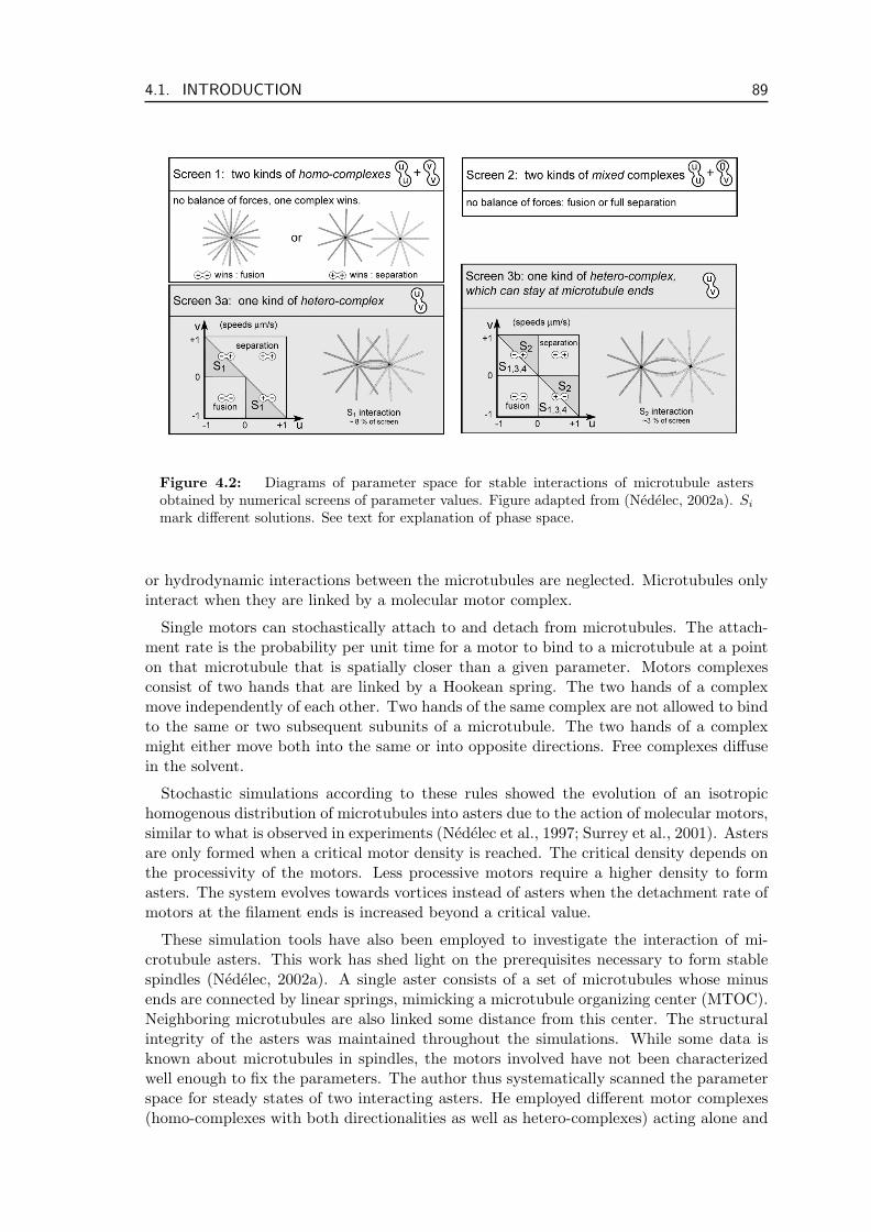
4.1. INTRODUCTION 89
Figure 4.2: Diagrams of parameter space for stable interactions of microtubule astersobtained by numerical screens of parameter values. Figure adapted from (Nedelec, 2002a). Si
mark different solutions. See text for explanation of phase space.
or hydrodynamic interactions between the microtubules are neglected. Microtubules onlyinteract when they are linked by a molecular motor complex.
Single motors can stochastically attach to and detach from microtubules. The attach-ment rate is the probability per unit time for a motor to bind to a microtubule at a pointon that microtubule that is spatially closer than a given parameter. Motors complexesconsist of two hands that are linked by a Hookean spring. The two hands of a complexmove independently of each other. Two hands of the same complex are not allowed to bindto the same or two subsequent subunits of a microtubule. The two hands of a complexmight either move both into the same or into opposite directions. Free complexes diffusein the solvent.
Stochastic simulations according to these rules showed the evolution of an isotropichomogenous distribution of microtubules into asters due to the action of molecular motors,similar to what is observed in experiments (Nedelec et al., 1997; Surrey et al., 2001). Astersare only formed when a critical motor density is reached. The critical density depends onthe processivity of the motors. Less processive motors require a higher density to formasters. The system evolves towards vortices instead of asters when the detachment rate ofmotors at the filament ends is increased beyond a critical value.
These simulation tools have also been employed to investigate the interaction of mi-crotubule asters. This work has shed light on the prerequisites necessary to form stablespindles (Nedelec, 2002a). A single aster consists of a set of microtubules whose minusends are connected by linear springs, mimicking a microtubule organizing center (MTOC).Neighboring microtubules are also linked some distance from this center. The structuralintegrity of the asters was maintained throughout the simulations. While some data isknown about microtubules in spindles, the motors involved have not been characterizedwell enough to fix the parameters. The author thus systematically scanned the parameterspace for steady states of two interacting asters. He employed different motor complexes(homo-complexes with both directionalities as well as hetero-complexes) acting alone and
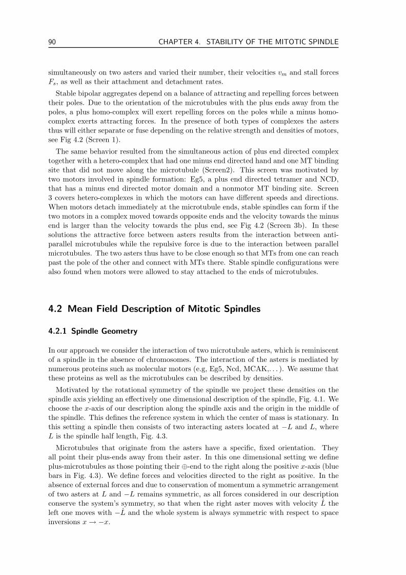
90 CHAPTER 4. STABILITY OF THE MITOTIC SPINDLE
simultaneously on two asters and varied their number, their velocities vm and stall forcesFs, as well as their attachment and detachment rates.
Stable bipolar aggregates depend on a balance of attracting and repelling forces betweentheir poles. Due to the orientation of the microtubules with the plus ends away from thepoles, a plus homo-complex will exert repelling forces on the poles while a minus homo-complex exerts attracting forces. In the presence of both types of complexes the astersthus will either separate or fuse depending on the relative strength and densities of motors,see Fig 4.2 (Screen 1).
The same behavior resulted from the simultaneous action of plus end directed complextogether with a hetero-complex that had one minus end directed hand and one MT bindingsite that did not move along the microtubule (Screen2). This screen was motivated bytwo motors involved in spindle formation: Eg5, a plus end directed tetramer and NCD,that has a minus end directed motor domain and a nonmotor MT binding site. Screen3 covers hetero-complexes in which the motors can have different speeds and directions.When motors detach immediately at the microtubule ends, stable spindles can form if thetwo motors in a complex moved towards opposite ends and the velocity towards the minusend is larger than the velocity towards the plus end, see Fig 4.2 (Screen 3b). In thesesolutions the attractive force between asters results from the interaction between anti-parallel microtubules while the repulsive force is due to the interaction between parallelmicrotubules. The two asters thus have to be close enough so that MTs from one can reachpast the pole of the other and connect with MTs there. Stable spindle configurations werealso found when motors were allowed to stay attached to the ends of microtubules.
4.2 Mean Field Description of Mitotic Spindles
4.2.1 Spindle Geometry
In our approach we consider the interaction of two microtubule asters, which is reminiscentof a spindle in the absence of chromosomes. The interaction of the asters is mediated bynumerous proteins such as molecular motors (e.g, Eg5, Ncd, MCAK,. . . ). We assume thatthese proteins as well as the microtubules can be described by densities.
Motivated by the rotational symmetry of the spindle we project these densities on thespindle axis yielding an effectively one dimensional description of the spindle, Fig. 4.1. Wechoose the x-axis of our description along the spindle axis and the origin in the middle ofthe spindle. This defines the reference system in which the center of mass is stationary. Inthis setting a spindle then consists of two interacting asters located at −L and L, whereL is the spindle half length, Fig. 4.3.
Microtubules that originate from the asters have a specific, fixed orientation. Theyall point their plus-ends away from their aster. In this one dimensional setting we defineplus-microtubules as those pointing their ⊕-end to the right along the positive x-axis (bluebars in Fig. 4.3). We define forces and velocities directed to the right as positive. In theabsence of external forces and due to conservation of momentum a symmetric arrangementof two asters at L and −L remains symmetric, as all forces considered in our descriptionconserve the system’s symmetry, so that when the right aster moves with velocity L theleft one moves with −L and the whole system is always symmetric with respect to spaceinversions x → −x.
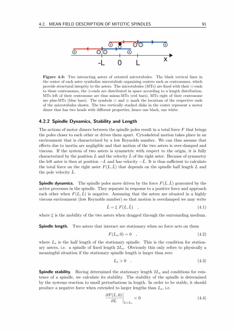
4.2. MEAN FIELD DESCRIPTION OF MITOTIC SPINDLES 91
x0-L L
++ --
++ - -
Figure 4.3: Two interacting asters of oriented microtubules. The black vertical lines inthe center of each aster symbolize microtubule organizing centers such as centrosomes, whichprovide structural integrity to the asters. The microtubules (MTs) are fixed with their -endsto these centrosomes, the ⊕-ends are distributed in space according to a length distribution.MTs left of their centrosome are thus minus-MTs (red bars), MTs right of their centrosomeare plus-MTs (blue bars). The symbols and ⊕ mark the locations of the respective endsof the microtubules shown. The two vertically stacked disks in the center represent a motordimer that has two heads with different properties, hence one black, one white.
4.2.2 Spindle Dynamics, Stability and Length
The actions of motor dimers between the spindle poles result in a total force F that bringsthe poles closer to each other or drives them apart. Cytoskeletal motion takes place in anenvironment that is characterized by a low Reynolds number. We can thus assume thateffects due to inertia are negligible and that motion of the two asters is over-damped andviscous. If the system of two asters is symmetric with respect to the origin, it is fullycharacterized by the position L and the velocity L of the right aster. Because of symmetrythe left aster is then at position −L and has velocity −L. It is thus sufficient to calculatethe total force on the right aster F (L, L) that depends on the spindle half length L andthe pole velocity L.
Spindle dynamics. The spindle poles move driven by the force F (L, L) generated by theactive processes in the spindle. They separate in response to a positive force and approacheach other when F (L, L) is negative. Assuming that the asters are situated in a highlyviscous environment (low Reynolds number) so that motion is overdamped we may write
L = ξ F (L, L) , (4.1)
where ξ is the mobility of the two asters when dragged through the surrounding medium.
Spindle length. Two asters that interact are stationary when no force acts on them
F (Ls, 0) = 0 , (4.2)
where Ls is the half length of the stationary spindle. This is the condition for station-ary asters, i.e. a spindle of fixed length 2Ls. Obviously this only refers to physically ameaningful situation if the stationary spindle length is larger than zero
Ls > 0 . (4.3)
Spindle stability. Having determined the stationary length 2Ls and conditions for exis-tence of a spindle, we calculate its stability. The stability of the spindle is determinedby the systems reaction to small perturbations in length. In order to be stable, it shouldproduce a negative force when extended to larger lengths than Ls, i.e.
∂F (L, 0)∂L
∣∣∣∣L=Ls
< 0 (4.4)
92 CHAPTER 4. STABILITY OF THE MITOTIC SPINDLE
is the condition for a stationary spindle of length 2Ls to be stable.
4.2.3 Force on Asters
The total force that acts on the right aster is the combination of the force contributionsfrom anywhere along the spindle axis
F (L, L) =∫ ∞
−∞F (L, L, x) dx , (4.5)
where F (L, L, x) is the average force per MT hetero-dimer due to motor dimers at positionx. It is the sum of the forces exerted by various motor dimers types at different locationsin the spindle that are bound to the bulk or ends of microtubules:
F (L, L, x) =∑
dimer type i
∑zone j
∑link type k
di(x)wi,j,k(x)Fi,j,k . (4.6)
Here i ∈ p, m, h denotes the three types of dimers: plus-plus, minus-minus, and hetero-dimers, j ∈ (a), (b), (c) is summed over the three regions of a spindle, cf. blue regionsin Fig. 4.5, and k ∈ b,⊕, and marks the three types of possible links: bulk-bulk,bulk-⊕-end, and bulk--end. The motor dimer number density of motor dimers of type iis denoted by di. The effective probability of a dimer of type i to form a link of type k atposition x in zone j is given by wi,j,k(x) and the average force contribution of such dimersby Fi,j,k.
4.2.4 Interaction between Filament Pairs
Let us now discuss the forces that act on two asters due to molecular motors in thespindle. Individual motors are characterized by a force-velocity relation. Depending ontheir position in the spindle their contribution to the total force acting on both asters canchange.
Motor dimers consist of two linked motor heads that bind to MTs. We assume thebending rigidity of the microtubules to be large. Hence we neglect MT bending by motorsin our one dimensional scenario. Thus we need not consider motor actions between MTsoriginating from the same aster. In our description we only consider asters that do at leastpartially overlap, so that motor dimers can bind to MTs from both asters simultaneously.When bound to two different microtubules they will not only experience forces due to themovement of the asters but they also actively exert forces on these MTs. Their contributionto the total force on the asters, which is due to the collective action of all motors, dependson their position in the spindle and also if they are attached to the bulk or the ends of themicrotubules.
We investigate the force a single motor dimer can exert when interacting with bothasters. This corresponds to a situation where the motor is not free to move with itsunloaded velocity v0 anymore, because it forms part of a dimer that is attached to a MTfrom the other aster and is thus subject to a force. In our description a single motorwith unloaded velocity v0 is characterized by a linear force-velocity curve, Eq. (3.3). Ifthe microtubule itself moves with a velocity V with respect to the laboratory system, themotor’s velocity in this system is given by
x = ±v + V (4.7)
where the sign in front of v depends on the orientation of the microtubule (negative signwhen it is a minus MT). A free ⊕-end directed motor on a minus-microtubule has a
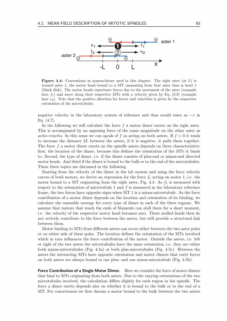
4.2. MEAN FIELD DESCRIPTION OF MITOTIC SPINDLES 93
x0-L L
++
++
2
1
aster 2
aster 1v1
v2
f1
f2
Figure 4.4: Conventions in nomenclature used in this chapter. The right aster (at L) istermed aster 1, the motor head bound to a MT emanating from that aster thus is head 1(black disk). The motor heads experience forces due to the movement of the aster (examplehere f1) and move along their respective MTs with a velocity given by Eq. (3.3) (examplehere v2). Note that the positive direction for forces and velocities is given by the respectiveorientation of the microtubules.
negative velocity in the laboratory system of reference and thus would enter as −v inEq. (4.7).
In the following we will calculate the force f a motor dimer exerts on the right aster.This is accompanied by an opposing force of the same magnitude on the other aster asactio=reactio. In this sense we can speak of f as acting on both asters. If f > 0 it tendsto increase the distance 2L between the asters, if it is negative, it pulls them together.The force f a motor dimer exerts on the spindle asters depends on three characteristics:first, the location of the dimer, because this defines the orientation of the MTs it bindsto. Second, the type of dimer, i.e. if the dimer consists of plus-end or minus-end directedmotor heads. And third if the dimer is bound to the bulk or to the end of the microtubules.These three topics are discussed in the following.
Starting from the velocity of the dimer in the lab system and using the force velocitycurves of both motors, we derive an expression for the force f1 acting on motor 1, i.e. themotor bound to a MT originating from the right aster, Fig. 4.4. As f1 is measured withrespect to the orientation of microtubule 1 and f is measured in the laboratory referenceframe, the two forces have opposite signs when MT 1 is a minus-microtubule. As the forcecontribution of a motor dimer depends on the location and orientation of its binding, wecalculate the ensemble average for every type of dimer in each of the three regions. Weassume that motors that reach the ends of filaments can stall there for a short moment,i.e. the velocity of the respective motor head becomes zero. These stalled heads then donot actively contribute to the force between the asters, but still provide a structural linkbetween them.
Motor binding to MTs from different asters can occur either between the two aster polesor on either side of these poles. The location defines the orientation of the MTs involvedwhich in turn influences the force contribution of the motor. Outside the asters, i.e. leftor right of the two asters the microtubules have the same orientation, i.e. they are eitherboth minus-microtubules (Fig. 4.5a) or both plus-microtubules (Fig. 4.5c). Between theasters the interacting MTs have opposite orientation and motor dimers that exert forceson both asters are always bound to one plus- and one minus-microtubule (Fig. 4.5b).
Force Contribution of a Single Motor Dimer. Here we consider the force of motor dimersthat bind to MTs originating from both asters. Due to the varying orientations of the twomicrotubules involved, the calculation differs slightly for each region in the spindle. Theforce a dimer exerts depends also on whether it is bound to the bulk or to the end of aMT. For concreteness we first discuss a motor bound to the bulk between the two asters
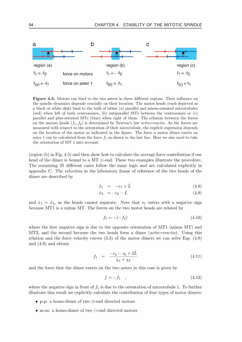
94 CHAPTER 4. STABILITY OF THE MITOTIC SPINDLE
a b c
region (a) region (c)region (b)
f1 = -f2 f1 = -f2f1 = - -f2
f(a) = -f1 f(c) = f1f(b) = -f1
force on motors
force on aster 1
Figure 4.5: Motors can bind to the two asters in three different regions. Their influence onthe spindle dynamics depends crucially on their location. The motor heads (each depicted asa black or white disk) bind to the bulk of either (a) parallel and minus-oriented microtubules(red) when left of both centrosomes, (b) antiparallel MTs between the centrosomes or (c)parallel and plus-oriented MTs (blue) when right of them. The relation between the forceson the motors heads (f1, f2) is determined by Newton’s law actio=reactio. As the forces aremeasured with respect to the orientation of their microtubule, the explicit expression dependson the location of the motor as indicated in the figure. The force a motor dimer exerts onaster 1 can be calculated from the force f1 as shown in the last line. Here we also need to takethe orientation of MT 1 into account.
(region (b) in Fig. 4.5) and then show how to calculate the average force contribution if onehead of the dimer is bound to a MT ⊕-end. These two examples illustrate the procedure.The remaining 25 different cases follow the same logic and are calculated explicitly inappendix C. The velocities in the laboratory frame of reference of the two heads of thedimer are described by
x1 = −v1 + L (4.8)x2 = v2 − L (4.9)
and x1 = x2, as the heads cannot separate. Note that v1 enters with a negative signbecause MT1 is a minus MT. The forces on the two motor heads are related by
f1 = −(−f2) (4.10)
where the first negative sign is due to the opposite orientation of MT1 (minus MT) andMT2, and the second because the two heads form a dimer (actio=reactio). Using thisrelation and the force velocity curves (3.3) of the motor dimers we can solve Eqs. (4.8)and (4.9) and obtain
f1 =−va − vb + 2L
χa + χb(4.11)
and the force that the dimer exerts on the two asters in this case is given by
f = −f1 , (4.12)
where the negative sign in front of f1 is due to the orientation of microtubule 1. To furtherillustrate this result we explicitly calculate the contribution of four types of motor dimers:
• p-p: a homo-dimer of two ⊕-end directed motors
• m-m: a homo-dimer of two -end directed motors
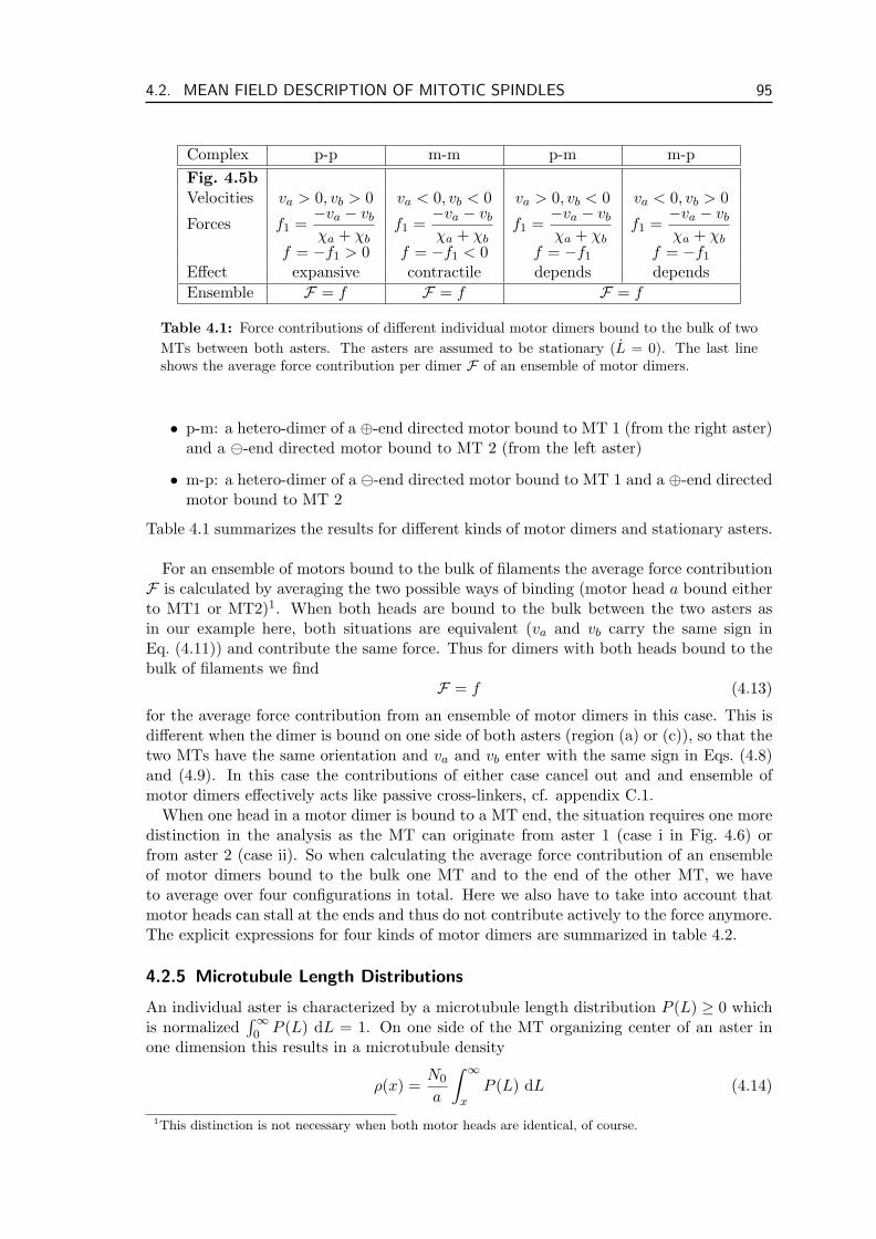
4.2. MEAN FIELD DESCRIPTION OF MITOTIC SPINDLES 95
Complex p-p m-m p-m m-pFig. 4.5bVelocities va > 0, vb > 0 va < 0, vb < 0 va > 0, vb < 0 va < 0, vb > 0
Forces f1 =−va − vb
χa + χbf1 =
−va − vb
χa + χbf1 =
−va − vb
χa + χbf1 =
−va − vb
χa + χbf = −f1 > 0 f = −f1 < 0 f = −f1 f = −f1
Effect expansive contractile depends dependsEnsemble F = f F = f F = f
Table 4.1: Force contributions of different individual motor dimers bound to the bulk of twoMTs between both asters. The asters are assumed to be stationary (L = 0). The last lineshows the average force contribution per dimer F of an ensemble of motor dimers.
• p-m: a hetero-dimer of a ⊕-end directed motor bound to MT 1 (from the right aster)and a -end directed motor bound to MT 2 (from the left aster)
• m-p: a hetero-dimer of a -end directed motor bound to MT 1 and a ⊕-end directedmotor bound to MT 2
Table 4.1 summarizes the results for different kinds of motor dimers and stationary asters.
For an ensemble of motors bound to the bulk of filaments the average force contributionF is calculated by averaging the two possible ways of binding (motor head a bound eitherto MT1 or MT2)1. When both heads are bound to the bulk between the two asters asin our example here, both situations are equivalent (va and vb carry the same sign inEq. (4.11)) and contribute the same force. Thus for dimers with both heads bound to thebulk of filaments we find
F = f (4.13)
for the average force contribution from an ensemble of motor dimers in this case. This isdifferent when the dimer is bound on one side of both asters (region (a) or (c)), so that thetwo MTs have the same orientation and va and vb enter with the same sign in Eqs. (4.8)and (4.9). In this case the contributions of either case cancel out and and ensemble ofmotor dimers effectively acts like passive cross-linkers, cf. appendix C.1.
When one head in a motor dimer is bound to a MT end, the situation requires one moredistinction in the analysis as the MT can originate from aster 1 (case i in Fig. 4.6) orfrom aster 2 (case ii). So when calculating the average force contribution of an ensembleof motor dimers bound to the bulk one MT and to the end of the other MT, we haveto average over four configurations in total. Here we also have to take into account thatmotor heads can stall at the ends and thus do not contribute actively to the force anymore.The explicit expressions for four kinds of motor dimers are summarized in table 4.2.
4.2.5 Microtubule Length Distributions
An individual aster is characterized by a microtubule length distribution P (L) ≥ 0 whichis normalized
∫∞0 P (L) dL = 1. On one side of the MT organizing center of an aster in
one dimension this results in a microtubule density
ρ(x) =N0
a
∫ ∞
xP (L) dL (4.14)
1This distinction is not necessary when both motor heads are identical, of course.
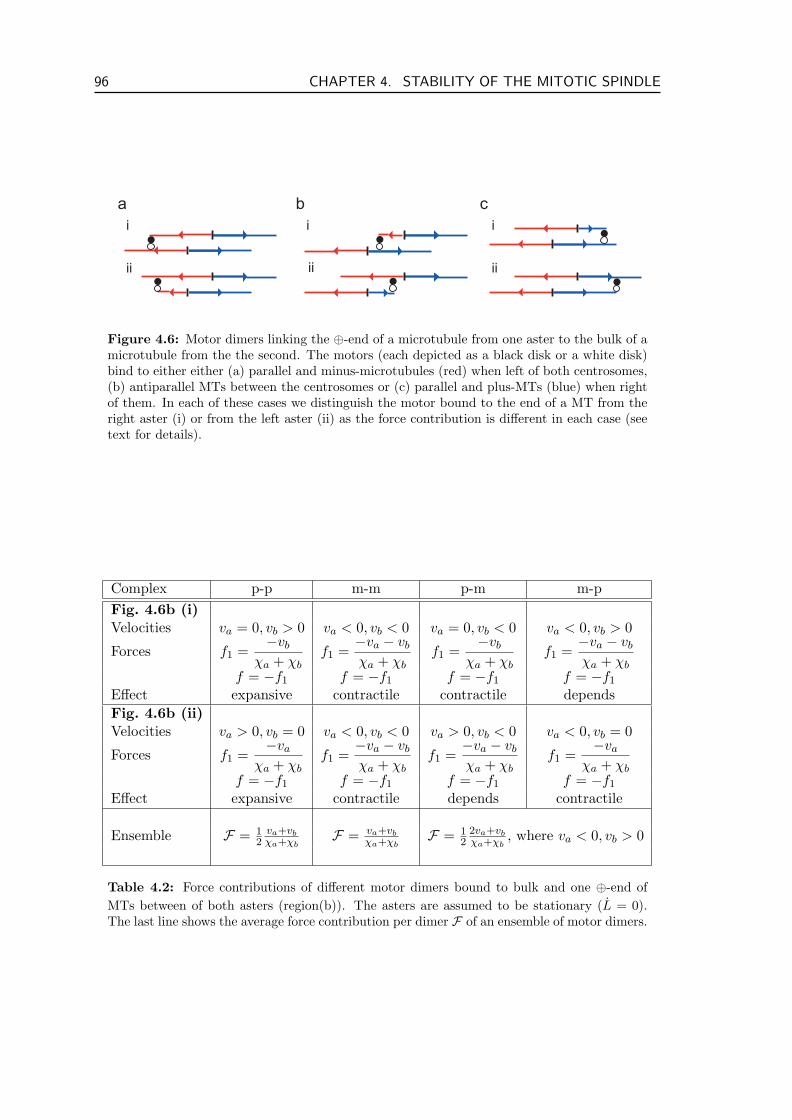
96 CHAPTER 4. STABILITY OF THE MITOTIC SPINDLE
a b ci
ii
i
ii
i
ii
Figure 4.6: Motor dimers linking the ⊕-end of a microtubule from one aster to the bulk of amicrotubule from the the second. The motors (each depicted as a black disk or a white disk)bind to either either (a) parallel and minus-microtubules (red) when left of both centrosomes,(b) antiparallel MTs between the centrosomes or (c) parallel and plus-MTs (blue) when rightof them. In each of these cases we distinguish the motor bound to the end of a MT from theright aster (i) or from the left aster (ii) as the force contribution is different in each case (seetext for details).
Complex p-p m-m p-m m-pFig. 4.6b (i)Velocities va = 0, vb > 0 va < 0, vb < 0 va = 0, vb < 0 va < 0, vb > 0
Forces f1 =−vb
χa + χbf1 =
−va − vb
χa + χbf1 =
−vb
χa + χbf1 =
−va − vb
χa + χbf = −f1 f = −f1 f = −f1 f = −f1
Effect expansive contractile contractile dependsFig. 4.6b (ii)Velocities va > 0, vb = 0 va < 0, vb < 0 va > 0, vb < 0 va < 0, vb = 0
Forces f1 =−va
χa + χbf1 =
−va − vb
χa + χbf1 =
−va − vb
χa + χbf1 =
−va
χa + χbf = −f1 f = −f1 f = −f1 f = −f1
Effect expansive contractile depends contractile
Ensemble F = 12
va+vbχa+χb
F = va+vbχa+χb
F = 12
2va+vbχa+χb
, where va < 0, vb > 0
Table 4.2: Force contributions of different motor dimers bound to bulk and one ⊕-end ofMTs between of both asters (region(b)). The asters are assumed to be stationary (L = 0).The last line shows the average force contribution per dimer F of an ensemble of motor dimers.
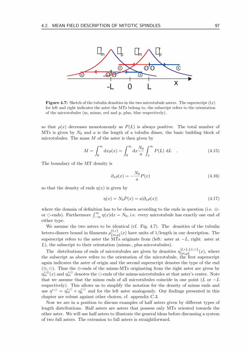
4.2. MEAN FIELD DESCRIPTION OF MITOTIC SPINDLES 97
rlp
++ - -
++ - -
x0-L L
rlm
rrprr
m
Figure 4.7: Sketch of the tubulin densities in the two microtubule asters. The superscript (l,r)for left and right indicates the aster the MTs belong to, the subscript refers to the orientationof the microtubules (m, minus, red and p, plus, blue respectively).
so that ρ(x) decreases monotonously as P (L) is always positive. The total number ofMTs is given by N0 and a is the length of a tubulin dimer, the basic building block ofmicrotubules. The mass M of the aster is then given by
M =∫ ∞
0dxρ(x) =
∫ ∞
0dx
N0
a
∫ ∞
xP (L) dL . (4.15)
The boundary of the MT density is
∂xρ(x) = −N0
aP (x) (4.16)
so that the density of ends η(x) is given by
η(x) = N0P (x) = a|∂xρ(x)| (4.17)
where the domain of definition has to be chosen according to the ends in question (i.e. ⊕-or -ends). Furthermore
∫∞−∞ η(x)dx = N0, i.e. every microtubule has exactly one end of
either type.We assume the two asters to be identical (cf. Fig. 4.7). The densities of the tubulin
hetero-dimers bound in filaments ρl,rm,p(x) have units of 1/length in our description. The
superscript refers to the aster the MTs originate from (left: aster at −L, right: aster atL), the subscript to their orientation (minus-, plus-microtubules).
The distributions of ends of microtubules are given by densities ηl,r,⊕,m,p (x), where
the subscript as above refers to the orientation of the microtubule, the first superscriptagain indicates the aster of origin and the second superscript denotes the type of the end(⊕,). Thus the ⊕-ends of the minus-MTs originating from the right aster are given byηr,⊕
m (x) and ηr,m denotes the -ends of the minus-microtubules at that aster’s center. Note
that we assume that the minus ends of all microtubules coincide in one point (L or −Lrespectively). This allows us to simplify the notation for the density of minus ends anduse ηr, = ηr,
m + ηr,p and for the left aster analogously. Our findings presented in this
chapter are robust against other choices, cf. appendix C.3.Now we are in a position to discuss examples of half asters given by different types of
length distributions. Half asters are asters that possess only MTs oriented towards theother aster. We will use half asters to illustrate the general ideas before discussing a systemof two full asters. The extension to full asters is straightforward.
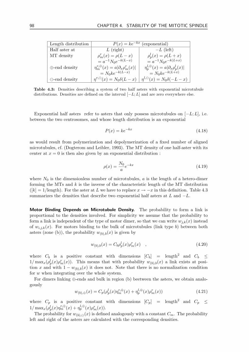
98 CHAPTER 4. STABILITY OF THE MITOTIC SPINDLE
Length distribution P (x) = ke−kx (exponential)Half aster at L (right) −L (left)MT density ρr
m(x) = ρ(L− x) ρlp(x) = ρ(L + x)
= a−1N0e−k(L−x) = a−1N0e
−k(L+x)
⊕-end density ηr,⊕m (x) = a|∂xρr
m(x)| ηl,⊕p (x) = a|∂xρl
p(x)|= N0ke−k(L−x) = N0ke−k(L+x)
-end density ηr,(x) = N0δ(L− x) ηl,(x) = N0δ(−L− x)
Table 4.3: Densities describing a system of two half asters with exponential microtubuledistributions. Densities are defined on the interval [−L;L] and are zero everywhere else.
Exponential half asters refer to asters that only possess microtubules on [−L;L], i.e.between the two centrosomes, and whose length distribution is an exponential
P (x) = ke−kx (4.18)
as would result from polymerization and depolymerization of a fixed number of alignedmicrotubules, cf. (Dogterom and Leibler, 1993). The MT density of one half-aster with itscenter at x = 0 is then also given by an exponential distribution :
ρ(x) =N0
ae−kx (4.19)
where N0 is the dimensionless number of microtubules, a is the length of a hetero-dimerforming the MTs and k is the inverse of the characteristic length of the MT distribution([k] = 1/length). For the aster at L we have to replace x → −x in this definition. Table 4.3summarizes the densities that describe two exponential half asters at L and −L.
Motor Binding Depends on Microtubule Density. The probability to form a link isproportional to the densities involved. For simplicity we assume that the probability toform a link is independent of the type of motor dimer, so that we can write wj,k(x) insteadof wi,j,k(x). For motors binding to the bulk of microtubules (link type b) between bothasters (zone (b)), the probability w(b),b(x) is given by
w(b),b(x) = Cbρlp(x)ρr
m(x) , (4.20)
where Cb is a positive constant with dimensions [Cb] = length2 and Cb ≤1/ maxx(ρl
p(x)ρrm(x)). This means that with probability w(b),b(x) a link exists at posi-
tion x and with 1 − w(b),b(x) it does not. Note that there is no normalization conditionfor w when integrating over the whole system.
For dimers linking ⊕-ends and bulk in region (b) beetween the asters, we obtain analo-gously
w(b),⊕(x) = Cp(ρlp(x)ηr,⊕
m (x) + ηl,⊕p (x)ρr
m(x)) (4.21)
where Cp is a positive constant with dimensions [Cp] = length2 and Cp ≤1/ maxx(ρl
p(x)ηr,⊕m (x) + ηl,⊕
p (x)ρrm(x)).
The probability for w(b),(x) is defined analogously with a constant Cm. The probabilityleft and right of the asters are calculated with the corresponding densities.
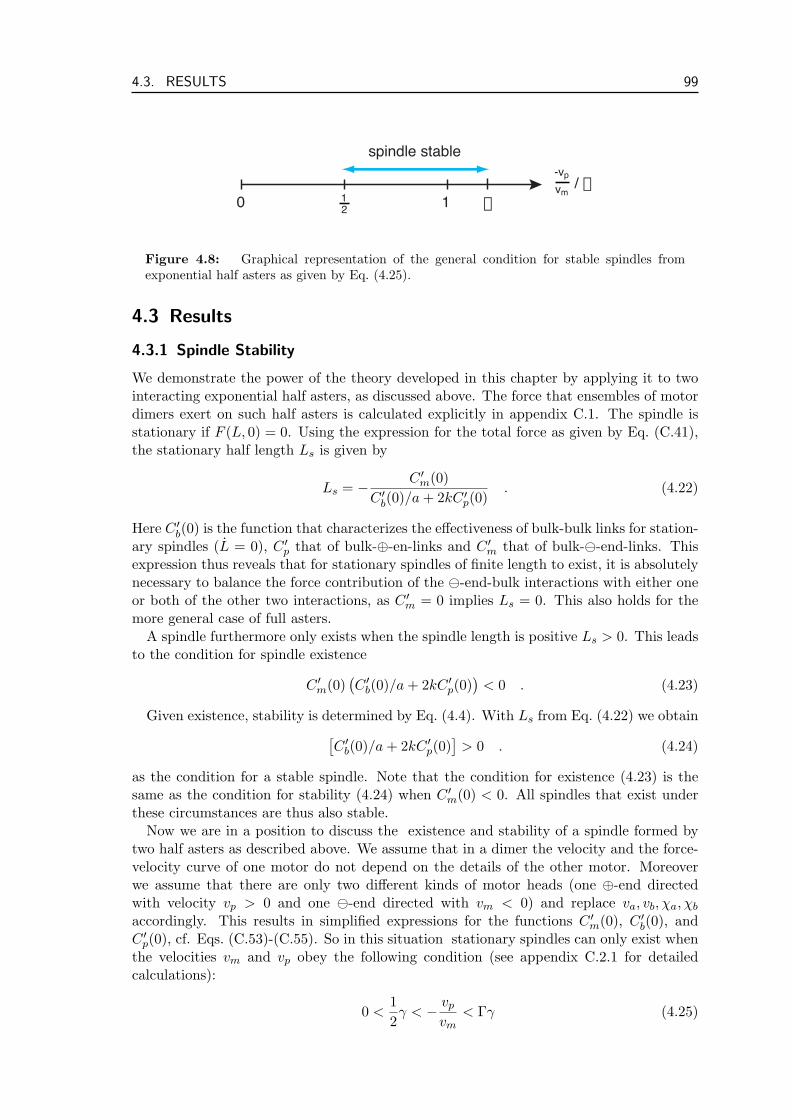
4.3. RESULTS 99
-vpvm
/ g0 12
1 G
spindle stable
Figure 4.8: Graphical representation of the general condition for stable spindles fromexponential half asters as given by Eq. (4.25).
4.3 Results
4.3.1 Spindle Stability
We demonstrate the power of the theory developed in this chapter by applying it to twointeracting exponential half asters, as discussed above. The force that ensembles of motordimers exert on such half asters is calculated explicitly in appendix C.1. The spindle isstationary if F (L, 0) = 0. Using the expression for the total force as given by Eq. (C.41),the stationary half length Ls is given by
Ls = − C ′m(0)
C ′b(0)/a + 2kC ′
p(0). (4.22)
Here C ′b(0) is the function that characterizes the effectiveness of bulk-bulk links for station-
ary spindles (L = 0), C ′p that of bulk-⊕-en-links and C ′
m that of bulk--end-links. Thisexpression thus reveals that for stationary spindles of finite length to exist, it is absolutelynecessary to balance the force contribution of the -end-bulk interactions with either oneor both of the other two interactions, as C ′
m = 0 implies Ls = 0. This also holds for themore general case of full asters.
A spindle furthermore only exists when the spindle length is positive Ls > 0. This leadsto the condition for spindle existence
C ′m(0)
(C ′
b(0)/a + 2kC ′p(0)
)< 0 . (4.23)
Given existence, stability is determined by Eq. (4.4). With Ls from Eq. (4.22) we obtain[C ′
b(0)/a + 2kC ′p(0)
]> 0 . (4.24)
as the condition for a stable spindle. Note that the condition for existence (4.23) is thesame as the condition for stability (4.24) when C ′
m(0) < 0. All spindles that exist underthese circumstances are thus also stable.
Now we are in a position to discuss the existence and stability of a spindle formed bytwo half asters as described above. We assume that in a dimer the velocity and the force-velocity curve of one motor do not depend on the details of the other motor. Moreoverwe assume that there are only two different kinds of motor heads (one ⊕-end directedwith velocity vp > 0 and one -end directed with vm < 0) and replace va, vb, χa, χb
accordingly. This results in simplified expressions for the functions C ′m(0), C ′
b(0), andC ′
p(0), cf. Eqs. (C.53)-(C.55). So in this situation stationary spindles can only exist whenthe velocities vm and vp obey the following condition (see appendix C.2.1 for detailedcalculations):
0 <12γ < − vp
vm< Γγ (4.25)
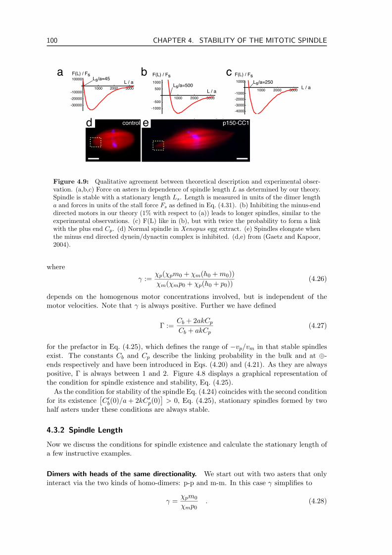
100 CHAPTER 4. STABILITY OF THE MITOTIC SPINDLE
d e
1000 2000 3000
-1000-500
5001000
L / a
F(L) / Fs
Ls/a=5001000 2000 3000
-30000-20000-10000
10000 L / a
F(L) / FsLs/a=45
baL / a
F(L) / Fs
1000 2000 3000
-4000-3000-2000-1000
1000 Ls/a=250c
Figure 4.9: Qualitative agreement between theoretical description and experimental obser-vation. (a,b,c) Force on asters in dependence of spindle length L as determined by our theory.Spindle is stable with a stationary length Ls. Length is measured in units of the dimer lengtha and forces in units of the stall force Fs as defined in Eq. (4.31). (b) Inhibiting the minus-enddirected motors in our theory (1% with respect to (a)) leads to longer spindles, similar to theexperimental observations. (c) F(L) like in (b), but with twice the probability to form a linkwith the plus end Cp. (d) Normal spindle in Xenopus egg extract. (e) Spindles elongate whenthe minus end directed dynein/dynactin complex is inhibited. (d,e) from (Gaetz and Kapoor,2004).
where
γ :=χp(χpm0 + χm(h0 + m0))χm(χmp0 + χp(h0 + p0))
(4.26)
depends on the homogenous motor concentrations involved, but is independent of themotor velocities. Note that γ is always positive. Further we have defined
Γ :=Cb + 2akCp
Cb + akCp(4.27)
for the prefactor in Eq. (4.25), which defines the range of −vp/vm in that stable spindlesexist. The constants Cb and Cp describe the linking probability in the bulk and at ⊕-ends respectively and have been introduced in Eqs. (4.20) and (4.21). As they are alwayspositive, Γ is always between 1 and 2. Figure 4.8 displays a graphical representation ofthe condition for spindle existence and stability, Eq. (4.25).
As the condition for stability of the spindle Eq. (4.24) coincides with the second conditionfor its existence
[C ′
b(0)/a + 2kC ′p(0)
]> 0, Eq. (4.25), stationary spindles formed by two
half asters under these conditions are always stable.
4.3.2 Spindle Length
Now we discuss the conditions for spindle existence and calculate the stationary length ofa few instructive examples.
Dimers with heads of the same directionality. We start out with two asters that onlyinteract via the two kinds of homo-dimers: p-p and m-m. In this case γ simplifies to
γ =χpm0
χmp0. (4.28)
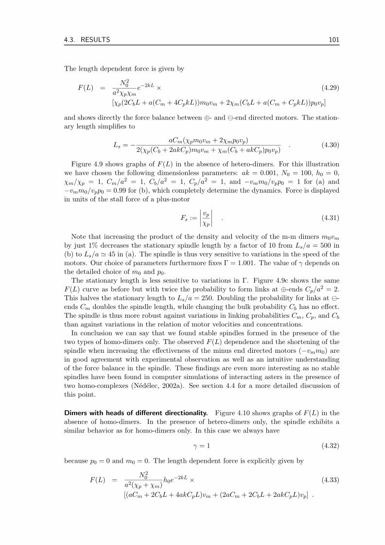
4.3. RESULTS 101
The length dependent force is given by
F (L) =N2
0
a2χpχme−2kL × (4.29)
[χp(2CbL + a(Cm + 4CpkL))m0vm + 2χm(CbL + a(Cm + CpkL))p0vp]
and shows directly the force balance between ⊕- and -end directed motors. The station-ary length simplifies to
Ls = − aCm(χpm0vm + 2χmp0vp)2(χp(Cb + 2akCp)m0vm + χm(Cb + akCp)p0vp)
. (4.30)
Figure 4.9 shows graphs of F (L) in the absence of hetero-dimers. For this illustrationwe have chosen the following dimensionless parameters: ak = 0.001, N0 = 100, h0 = 0,χm/χp = 1, Cm/a2 = 1, Cb/a2 = 1, Cp/a2 = 1, and −vmm0/vpp0 = 1 for (a) and−vmm0/vpp0 = 0.99 for (b), which completely determine the dynamics. Force is displayedin units of the stall force of a plus-motor
Fs :=∣∣∣∣ vp
χp
∣∣∣∣ . (4.31)
Note that increasing the product of the density and velocity of the m-m dimers m0vm
by just 1% decreases the stationary spindle length by a factor of 10 from Ls/a = 500 in(b) to Ls/a ' 45 in (a). The spindle is thus very sensitive to variations in the speed of themotors. Our choice of parameters furthermore fixes Γ = 1.001. The value of γ depends onthe detailed choice of m0 and p0.
The stationary length is less sensitive to variations in Γ. Figure 4.9c shows the sameF (L) curve as before but with twice the probability to form links at ⊕-ends Cp/a2 = 2.This halves the stationary length to Ls/a = 250. Doubling the probability for links at -ends Cm doubles the spindle length, while changing the bulk probability Cb has no effect.The spindle is thus more robust against variations in linking probabilities Cm, Cp, and Cb
than against variations in the relation of motor velocities and concentrations.In conclusion we can say that we found stable spindles formed in the presence of the
two types of homo-dimers only. The observed F (L) dependence and the shortening of thespindle when increasing the effectiveness of the minus end directed motors (−vmm0) arein good agreement with experimental observation as well as an intuitive understandingof the force balance in the spindle. These findings are even more interesting as no stablespindles have been found in computer simulations of interacting asters in the presence oftwo homo-complexes (Nedelec, 2002a). See section 4.4 for a more detailed discussion ofthis point.
Dimers with heads of different directionality. Figure 4.10 shows graphs of F (L) in theabsence of homo-dimers. In the presence of hetero-dimers only, the spindle exhibits asimilar behavior as for homo-dimers only. In this case we always have
γ = 1 (4.32)
because p0 = 0 and m0 = 0. The length dependent force is explicitly given by
F (L) =N2
0
a2(χp + χm)h0e
−2kL × (4.33)
[(aCm + 2CbL + 4akCpL)vm + (2aCm + 2CbL + 2akCpL)vp] .
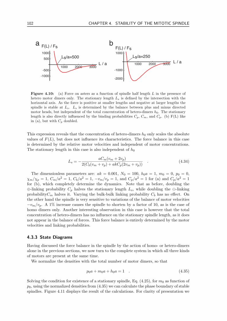
102 CHAPTER 4. STABILITY OF THE MITOTIC SPINDLE
L / a
F(L) / Fs
L / a
F(L) / Fs ba
1000 2000 3000
-1000-500
5001000
1000 2000 3000
1000
-1000
-2000
Ls/a=500 Ls/a=250
Figure 4.10: (a) Force on asters as a function of spindle half length L in the presence ofhetero motor dimers only. The stationary length Ls is defined by the intersection with thehorizontal axis. As the force is positive at smaller lengths and negative at larger lengths thespindle is stable at Ls. Ls is determined by the balance between plus and minus directedmotor heads, but independent of the total concentration of hetero-dimers h0. The stationarylength is also directly influenced by the binding probabilities Cp, Cm, and Cp. (b) F(L) likein (a), but with Cp doubled.
This expression reveals that the concentration of hetero-dimers h0 only scales the absolutevalues of F (L), but does not influence its characteristics. The force balance in this caseis determined by the relative motor velocities and independent of motor concentrations.The stationary length in this case is also independent of h0
Ls = − aCm(vm + 2vp)2(Cb(vm + vp) + akCp(2vm + vp))
. (4.34)
The dimensionless parameters are: ak = 0.001, N0 = 100, h0a = 1, m0 = 0, p0 = 0,χm/χp = 1, Cm/a2 = 1, Cb/a2 = 1, −vm/vp = 1, and Cp/a2 = 1 for (a) and Cp/a2 = 1for (b), which completely determine the dynamics. Note that as before, doubling the⊕-linking probability Cp halves the stationary length Ls, while doubling the -linkingprobabilityCm halves it. Varying the bulk-bulk linking probability Cb has no effect. Onthe other hand the spindle is very sensitive to variations of the balance of motor velocities−vm/vp. A 1% increase causes the spindle to shorten by a factor of 10, as is the case ofhomo dimers only. Another interesting observation in this case is however that the totalconcentration of hetero-dimers has no influence on the stationary spindle length, as it doesnot appear in the balance of forces. This force balance is entirely determined by the motorvelocities and linking probabilities.
4.3.3 State Diagrams
Having discussed the force balance in the spindle by the action of homo- or hetero-dimersalone in the previous sections, we now turn to the complete system in which all three kindsof motors are present at the same time.
We normalize the densities with the total number of motor dimers, so that
p0a + m0a + h0a = 1 . (4.35)
Solving the condition for existence of a stationary spindle, Eq. (4.25), for m0 as function ofp0, using the normalized densities from (4.35) we can calculate the phase boundary of stablespindles. Figure 4.11 displays the result of the calculations. For clarity of presentation we
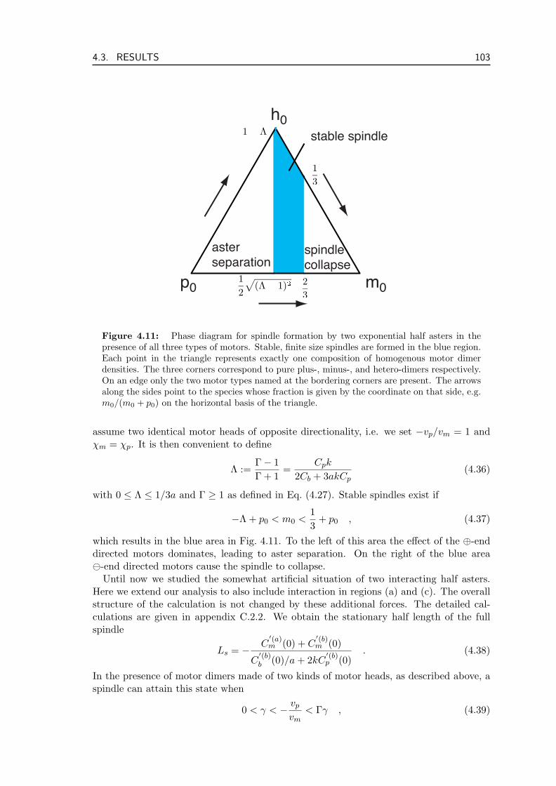
4.3. RESULTS 103
h0
m0p0
stable spindle
spindle collapse
aster separation
Figure 4.11: Phase diagram for spindle formation by two exponential half asters in thepresence of all three types of motors. Stable, finite size spindles are formed in the blue region.Each point in the triangle represents exactly one composition of homogenous motor dimerdensities. The three corners correspond to pure plus-, minus-, and hetero-dimers respectively.On an edge only the two motor types named at the bordering corners are present. The arrowsalong the sides point to the species whose fraction is given by the coordinate on that side, e.g.m0/(m0 + p0) on the horizontal basis of the triangle.
assume two identical motor heads of opposite directionality, i.e. we set −vp/vm = 1 andχm = χp. It is then convenient to define
Λ :=Γ− 1Γ + 1
=Cpk
2Cb + 3akCp(4.36)
with 0 ≤ Λ ≤ 1/3a and Γ ≥ 1 as defined in Eq. (4.27). Stable spindles exist if
−Λ + p0 < m0 <13
+ p0 , (4.37)
which results in the blue area in Fig. 4.11. To the left of this area the effect of the ⊕-enddirected motors dominates, leading to aster separation. On the right of the blue area-end directed motors cause the spindle to collapse.
Until now we studied the somewhat artificial situation of two interacting half asters.Here we extend our analysis to also include interaction in regions (a) and (c). The overallstructure of the calculation is not changed by these additional forces. The detailed cal-culations are given in appendix C.2.2. We obtain the stationary half length of the fullspindle
Ls = − C′(a)m (0) + C
′(b)m (0)
C′(b)b (0)/a + 2kC
′(b)p (0)
. (4.38)
In the presence of motor dimers made of two kinds of motor heads, as described above, aspindle can attain this state when
0 < γ < − vp
vm< Γγ , (4.39)
104 CHAPTER 4. STABILITY OF THE MITOTIC SPINDLE
h0
m0p0
stable spindle
spindle collapse
aster separation
Figure 4.12: State diagram for spindle formation by two exponential full asters in thepresence of all three types of motors. Stable, finite size spindles are formed in the blue region,which is smaller than for two half asters, cf. Fig. 4.11. The region of spindle collapse on theother hand has increased.
which is the same as Eq. (4.25) except that here the factor of 1/2 is missing. Also allspindles that form under this regime are stable.
Assuming two identical kinds of motor heads we can again calculate the concentrationphase diagram, shown in Figure 4.12. Note that the obtained result is qualitatively similarto that obtained for half asters. The additional forces from the outside regions increasethe tendency of the two asters to collapse, reducing the region in which stable spindlescan form.
4.3.4 Comparison to Computer Simulations
An important theoretical study of the interaction of microtubule asters was performedwith the help of computer simulations (Nedelec, 2002a). As many parameters of thesesimulations were not known, e.g. from experiments or independent theoretical considera-tions, the author employed a screening technique to discover combinations of parametersthat give rise to stable interactions. The results from these screens are summarized inFig. 4.2. Here we briefly compare them with our findings.
An important difference is brought up by screen 1: two kinds of homo-dimers. Whileour calculations indicate that stable spindles with finite length, Eq. (4.30), exist for arange of velocities, no such interactions were found in computer simulations. One possibleexplanation is that they just slipped through the mashes of parameters used in the screen.For full asters the parameter region can be narrow depending on the value of Γ (compareFigs. 4.11 and 4.12). Another possibility is that these kinds of solutions are due to specialproperties of our 1D description. As all microtubules are arranged aligned along a common
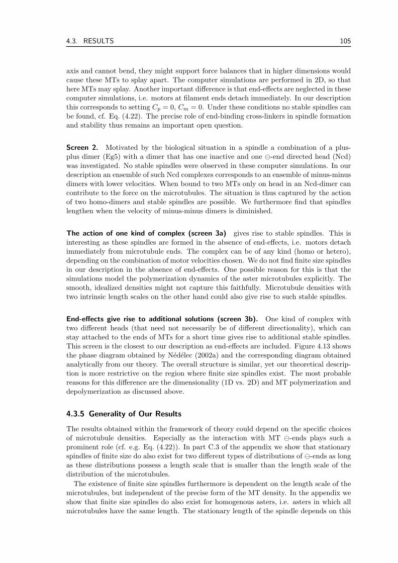
4.3. RESULTS 105
axis and cannot bend, they might support force balances that in higher dimensions wouldcause these MTs to splay apart. The computer simulations are performed in 2D, so thathere MTs may splay. Another important difference is that end-effects are neglected in thesecomputer simulations, i.e. motors at filament ends detach immediately. In our descriptionthis corresponds to setting Cp = 0, Cm = 0. Under these conditions no stable spindles canbe found, cf. Eq. (4.22). The precise role of end-binding cross-linkers in spindle formationand stability thus remains an important open question.
Screen 2. Motivated by the biological situation in a spindle a combination of a plus-plus dimer (Eg5) with a dimer that has one inactive and one -end directed head (Ncd)was investigated. No stable spindles were observed in these computer simulations. In ourdescription an ensemble of such Ncd complexes corresponds to an ensemble of minus-minusdimers with lower velocities. When bound to two MTs only on head in an Ncd-dimer cancontribute to the force on the microtubules. The situation is thus captured by the actionof two homo-dimers and stable spindles are possible. We furthermore find that spindleslengthen when the velocity of minus-minus dimers is diminished.
The action of one kind of complex (screen 3a) gives rise to stable spindles. This isinteresting as these spindles are formed in the absence of end-effects, i.e. motors detachimmediately from microtubule ends. The complex can be of any kind (homo or hetero),depending on the combination of motor velocities chosen. We do not find finite size spindlesin our description in the absence of end-effects. One possible reason for this is that thesimulations model the polymerization dynamics of the aster microtubules explicitly. Thesmooth, idealized densities might not capture this faithfully. Microtubule densities withtwo intrinsic length scales on the other hand could also give rise to such stable spindles.
End-effects give rise to additional solutions (screen 3b). One kind of complex withtwo different heads (that need not necessarily be of different directionality), which canstay attached to the ends of MTs for a short time gives rise to additional stable spindles.This screen is the closest to our description as end-effects are included. Figure 4.13 showsthe phase diagram obtained by Nedelec (2002a) and the corresponding diagram obtainedanalytically from our theory. The overall structure is similar, yet our theoretical descrip-tion is more restrictive on the region where finite size spindles exist. The most probablereasons for this difference are the dimensionality (1D vs. 2D) and MT polymerization anddepolymerization as discussed above.
4.3.5 Generality of Our Results
The results obtained within the framework of theory could depend on the specific choicesof microtubule densities. Especially as the interaction with MT -ends plays such aprominent role (cf. e.g. Eq. (4.22)). In part C.3 of the appendix we show that stationaryspindles of finite size do also exist for two different types of distributions of -ends as longas these distributions possess a length scale that is smaller than the length scale of thedistribution of the microtubules.
The existence of finite size spindles furthermore is dependent on the length scale of themicrotubules, but independent of the precise form of the MT density. In the appendix weshow that finite size spindles do also exist for homogenous asters, i.e. asters in which allmicrotubules have the same length. The stationary length of the spindle depends on this
106 CHAPTER 4. STABILITY OF THE MITOTIC SPINDLE
separation
fusion
-1 -0.5 0 0.5 1-1
-0.5
0
0.5
1vb
va
stable spindle
-1 -0.5 0 0.5 1-1
-0.5
0
0.5
1vb
va
a b
Figure 4.13: Comparision of phase diagrams for one type of motor dimers obtained bycomputer simulations (a, adapted from (Nedelec, 2002a)) and analytical theory (b). Theregions of the stable solutions S1 − S4 obtained by computer simulations are indicated in (a),the blue region in (b) corresponds to stable spindles supported by the analytical theory.
length scale directly, be it k−1 as in Eq. (4.22) or the microtubule length l for homogenousasters, cf. Eq. (C.91) in the appendix.
4.3.6 Microtubule Dynamics, Chromosomes and Motor Transport
Our analytical description of two interacting stationary microtubule asters is a first steptowards a theory of the mitotic spindle. Other aspects that are known about spindlestructure and dynamics can be added to this theory.
One of the most prominent features of microtubules in the spindle besides dynamicinstability (cf. section 2.3.1) is their continuous poleward flux (Mitchison, 1989; Mitchisonand Salmon, 2001). The expression refers to a treadmilling motion of microtubules towardsthe spindle poles. In our description this kind of dynamics could be captured by addinga -end directed bias to all motor velocities. It will then depend on the size of thisbias if the resulting spindles are still stable or if they collapse. Dynamic instabilityof microtubules on the other hand is a stochastic event of individual microtubules. Inour mean field description this is accounted for by the filament densities. Its effect on thebinding of motor dimers is reflected in the effective binding constants Cb, Cp and Cm. Realspindles also feature microtubules that are not attached to the spindle poles. These “freemicrotubules” could have interesting effects on the dynamics. They could be included inour description by a density of free mircotubules in addition to the densities of MTs thatbelong to the asters.
Moreover, real spindles are formed around chromosomes to which they attach via kine-tochore microtubules. These kinetochore microtubules do not undergo dynamic instabilityand give more structural stability to the spindle. Spindles forming entirely from chromo-somes in the absence of microtubule organizing centers have received a lot of attentionrecently (Karsenti and Nedelec, 2004). They present an interesting, complementary wayof spindle formation, which is not in the scope of the theoretical approach presented here.
Another important aspect is the transport of motors and the resulting inhomogenousmotor densities in the spindle. So far we have considered situations where the motorconcentrations are homogenous and not influenced by the dynamics. This is the case
4.4. DISCUSSION 107
when motors are abundant and/or when the motors are not very processive and diffuserapidly when free. A straightforward form of the transport equations is
∂tp(f)(x) = D(f)∂2
xp(f)(x)− ωp,ap(f)(x) + ωp,dp
(b)(x) (4.40)
∂tp(b)(x) = D(b)∂2
xp(b)(x) + ωp,ap(f)(x)− ωp,dp
(b)(x) (4.41)
−∂x
[⟨vpa + vp
b
2
⟩(ρp(x)− ρm(x)) p(b)(x)
]and for the other motors analogously. The superscript refers to the bound or unboundmotor dimers, respectively. Free motors are subject to diffusion in the surrounding fluidand may attach to microtubule pairs with rate ωp,a. Detachment occurs with ωp,d. Themean field current due to motor interaction with the asters in the last line is proportionalto the average velocity of motor heads, the difference in orientation of microtubules andof course the motor concentration. It is also possible to extend the description to motorsthat are attached to asters with only one head.
While it is straightforward to write down dynamic equations including motor transport,their solution is more involved and beyond the scope of this thesis.
4.4 Discussion
In this chapter we have shown how our analytic description of cytoskeletal spindles formedby two interacting asters of microtubules allows us to gain a more in depth understandingof the essential processes involved in spindle formation. A key result is that the formationof stable spindles of finite length is only possible when motor dimers stay attached to theminus end of spindle microtubules.
Our theory is based on considerations about the microscopic action of motor dimersin the spindle. It is thus an application and extension of the microscopic descriptionspresented in chapter 3. We investigate two interacting filament asters that resemble asimplified mitotic spindle. The symmetry of the spindle geometry allows us to projectthe system on the spindle axis, yielding an effectively one-dimensional description. Weexplicitly take force-velocity relations of motor dimers into account.
This analytical theory of the mitotic spindle reveals interesting results about essentialaspects such as forces in the spindle, spindle existence, length, and stability. Althoughsimplified, our one dimensional mean field description already captures many central as-pects of spindle dynamics. For example it puts the hypothesis and ad hoc models of howthe balance of forces generated by molecular motors influences the spindle length on afirmer physical ground.
We employ the theory to discuss the length scale of mitotic spindles and conditionsfor the existence of stable, stationary spindles of finite length. Our theory qualitativelyreproduces observations of spindle formation in Xenopus egg extract, that found thatspindles are longer when minus-end directed motors are inhibited. It provides a frameworkthat also facilitates the study of spindle dynamics such as spindle oscillations.
Our description of the mitotic spindle already includes many of the crucial effects forspindle formation. Although real spindles are three dimensional objects, their rotationalsymmetry suggests that much of the essential physics can be captured by a one dimensionaldescription. This is even more likely, as most of the spindle material is concentrated aroundthe spindle axis, see appendix C.4 for an example.
But the extension to higher dimensions also introduces novel physics to the problem. Wealready mentioned the possibility of microtubules to splay apart, i.e. MT in two or more
108 CHAPTER 4. STABILITY OF THE MITOTIC SPINDLE
dimensions do not necessarily support arbitrary stresses anymore. Another interestingaspect is microtubule bending. Molecular motors are strong enough to bend MTs and thisis observed in spindles as well. MT bending could be captured by introducing an elasticenergy in the description. Finally, molecular motors in two or more dimension induceMT rotation besides MT sliding (Liverpool and Marchetti, 2003; Tanase, 2004). This haseffects on microtubule bending as well as on the distribution of MTs in the asters.
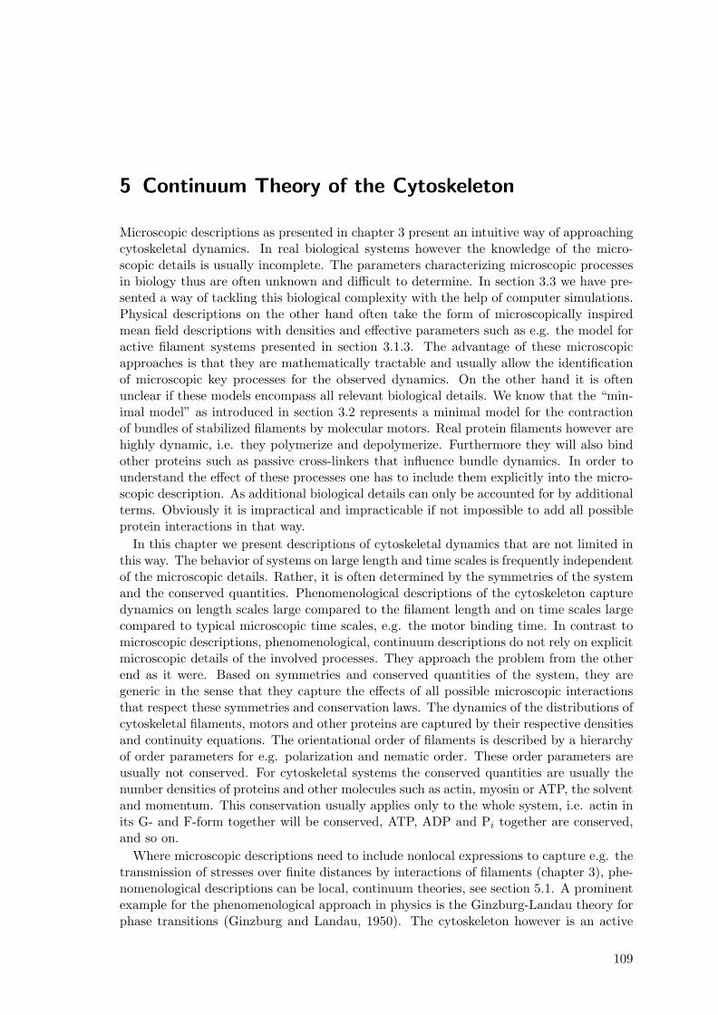
5 Continuum Theory of the Cytoskeleton
Microscopic descriptions as presented in chapter 3 present an intuitive way of approachingcytoskeletal dynamics. In real biological systems however the knowledge of the micro-scopic details is usually incomplete. The parameters characterizing microscopic processesin biology thus are often unknown and difficult to determine. In section 3.3 we have pre-sented a way of tackling this biological complexity with the help of computer simulations.Physical descriptions on the other hand often take the form of microscopically inspiredmean field descriptions with densities and effective parameters such as e.g. the model foractive filament systems presented in section 3.1.3. The advantage of these microscopicapproaches is that they are mathematically tractable and usually allow the identificationof microscopic key processes for the observed dynamics. On the other hand it is oftenunclear if these models encompass all relevant biological details. We know that the “min-imal model” as introduced in section 3.2 represents a minimal model for the contractionof bundles of stabilized filaments by molecular motors. Real protein filaments however arehighly dynamic, i.e. they polymerize and depolymerize. Furthermore they will also bindother proteins such as passive cross-linkers that influence bundle dynamics. In order tounderstand the effect of these processes one has to include them explicitly into the micro-scopic description. As additional biological details can only be accounted for by additionalterms. Obviously it is impractical and impracticable if not impossible to add all possibleprotein interactions in that way.
In this chapter we present descriptions of cytoskeletal dynamics that are not limited inthis way. The behavior of systems on large length and time scales is frequently independentof the microscopic details. Rather, it is often determined by the symmetries of the systemand the conserved quantities. Phenomenological descriptions of the cytoskeleton capturedynamics on length scales large compared to the filament length and on time scales largecompared to typical microscopic time scales, e.g. the motor binding time. In contrast tomicroscopic descriptions, phenomenological, continuum descriptions do not rely on explicitmicroscopic details of the involved processes. They approach the problem from the otherend as it were. Based on symmetries and conserved quantities of the system, they aregeneric in the sense that they capture the effects of all possible microscopic interactionsthat respect these symmetries and conservation laws. The dynamics of the distributions ofcytoskeletal filaments, motors and other proteins are captured by their respective densitiesand continuity equations. The orientational order of filaments is described by a hierarchyof order parameters for e.g. polarization and nematic order. These order parameters areusually not conserved. For cytoskeletal systems the conserved quantities are usually thenumber densities of proteins and other molecules such as actin, myosin or ATP, the solventand momentum. This conservation usually applies only to the whole system, i.e. actin inits G- and F-form together will be conserved, ATP, ADP and Pi together are conserved,and so on.
Where microscopic descriptions need to include nonlocal expressions to capture e.g. thetransmission of stresses over finite distances by interactions of filaments (chapter 3), phe-nomenological descriptions can be local, continuum theories, see section 5.1. A prominentexample for the phenomenological approach in physics is the Ginzburg-Landau theory forphase transitions (Ginzburg and Landau, 1950). The cytoskeleton however is an active
109
110 CHAPTER 5. CONTINUUM THEORY OF THE CYTOSKELETON
system, i.e. all terms allowed by symmetry have to be included, regardless of their signif-icance for the energy of the system. Phenomenological descriptions have been applied tocytoskeletal systems in situations, in which only motors are allowed to move in space (Leeand Kardar, 2001; Kim et al., 2003; Sankararaman et al., 2004). The filament densityis taken to be homogenous at all times so that motors are influenced mainly by filamentorientation. The complementary case of filaments moving freely on a plane of localizedmotors is reminiscent of e.g. microtubule motility assays and has also been studied (Bour-dieu et al., 1995; Bassetti et al., 2000). We proposed a first phenomenological descriptionof the cytoskeleton as an active fluid, i.e. allowing motors and filaments to move in Kruseet al. (2003). It is explained in greater detail in section 5.1 below.
The organization of this chapter is as follows: the following section 5.1 introduces thegeneral ideas behind our description of active fluids or gels. We then discuss the dynam-ics of contractile fibers, i.e. linear aggregates of active material such as stress fibers orcontractile rings formed by cytoskeletal protein filaments and motors in section 5.2. Weanalyze bundle contraction driven by stress release and show the emergence of sarcomerelike structures by self-organization. In section 5.3 we discuss these active gels in cylindricalgeometries such as found e.g. in the cell cortex. We show that rings in the cell cortex suchas the contractile ring or the pre-prophase band can form by self-organization phenomena.The rings can be stationary or oscillate. Oscillating cytoskeletal rings have been observedin various different cell types (Bornens et al., 1989; Paluch et al., 2005).
5.1 Phenomenological Description of Active Fluids
In (Kruse et al., 2003) we proposed a first phenomenological description for the dynamicsof the cytoskeleton as an active polar fluid. We investigated linear structures such ascontractile rings or stress fibers, taking into account polar order. This one-dimensionaldescription has been generalized to higher dimensions and nematic order (Zumdieck et al.,2005a; Banik et al., 2005), see Fig. 5.1.
5.1.1 Dynamic Equations
The general idea is as follows: We describe the dynamics of filaments and free subunitswith respect to a non-moving solvent. This situation corresponds, e.g., to filaments andmotors in the vicinity of a stationary surface, such as e.g. a cell wall. The concentration ofsubunits and motors is assumed to be homogenous and constant for all times, so that theirdynamics does not appear explicitly.1 In this case, the dynamics is completely specified bythe conservation law for the filaments and the dynamic equations for orientational orderparameters:
∂tc + ∇ · j = s (5.1)∂tp = ψ (5.2)∂tq = ω (5.3)
where c is the filament density, p is the polar and q is the nematic order parameter. We as-sume local friction and neglect hydrodynamic interactions between filaments. Disregardingfilament treadmilling, we can write the filament current as
jα = η−1∂βσαβ . (5.4)1The values of e.g. the motor concentration do of course implicitly influence the phenomenological
constants of the theory.
5.1. PHENOMENOLOGICAL DESCRIPTION OF ACTIVE FLUIDS 111
a b
Figure 5.1: Order parameters used in this chapter. (a) Polar order captures orientationsand directions of filaments. It can thus be described by a vector p which is invariant underrotations of 2π. (b) Nematic order captures only the direction of the filaments. It correspondsto rods that do not have a orientation, i.e. are invariant under rotations of π. Mathematicallythis can be described by a symmetric, traceless tensor.
Here, η is a parameter with dimensions of a friction coefficient and σαβ is the stress tensor.We close the equations with a constitutive equation for the stress tensor σ and equations forthe rates of change in the orientational order parameters p and q. As the exact functionaldependence of the stress on the filament density and the order parameters is not known,we systematically expand the stress in terms of these quantities with respect to a referencestate. We treat the rates of change ψ and ω of the orientation order parameters in thesame way. The details of this calculation are given in section 5.2. In this chapter we chosethe homogenous isotropic state as the reference state.
5.1.2 Order Parameters
We now briefly present the two types of order parameters used in this chapter. We startout with polar order which is characterized by a vectorial order parameter, see Fig. 5.1a.Second we discuss nematic order (Fig. 5.1b) that is familiar from the field of liquid crys-tals (de Gennes and Prost, 1993) and characterized by a symmetric, traceless tensor.
Polar Order
Cytoskeletal filaments such as microtubules or actin filaments are typically extended ob-jects that thus lie in a certain direction in space. They are furthermore structurally polar,i.e. they are oriented along the direction in one of two possible ways. In a one dimensionalgeometry the direction is the same for all filaments, but the orientation may be different.We denoted the two different orientations “+” and “−” in the previous chapter.
In higher dimensions the direction and orientation of a filament i can be characterizedby a unit vector ui located at the filament center. Considering filaments in a volume Vwe can define averages of the tensor products of u. The zeroth of these “moments” is thenumber density c(V ) = 〈u0〉V , where 〈·〉V denotes the average over the filaments locatedin V .
The polar order parameter is given by the next higher tensor product
p(V ) = 〈u〉V . (5.5)
112 CHAPTER 5. CONTINUUM THEORY OF THE CYTOSKELETON
This order has vectorial character, the direction and orientation of p are the averagedirection and orientation of filaments in V . The length of p is a measure of the magnitudeof the order, where 0 describes a completely disordered system and 1 corresponds to perfectorder (i.e. all filaments are aligned and oriented in the same way).
Nematic Order
Nematic order describes the direction of extended objects, but ignores their orientation,see Fig. 5.1b. This type of order is invariant under rotations of π. Mathematically nematicorder is based on the tensor product of u that is of the next higher, i.e. quadratic order.It is represented by a symmetric and traceless tensor of rank d, where d is the dimensionof space. The definition of the tensor components is given by
qαβ(V ) = 〈uαuβ −1dδαβ〉V (5.6)
where α, β are summed over the spatial dimension. In this thesis we only consider up totwo dimensional geometries. As the nematic order is trivial in one dimension, where allfilaments are aligned, we will focus on d = 2 for the rest of this section.
Physically nematic order describes only a direction in space (but no orientation). It isthus instructive to interpret the components of the nematic tensor qαβ in this way. Byconstruction we have
q =(
qxx qxy
qxy −qxx
), (5.7)
i.e. there are only two independent components. From these components we can derivetwo quantities that are more intuitive to interpret:
S = 2√
q2xx + q2
xy (5.8)
tanφ =S
2qxy− qxx
qxy(5.9)
Here S measures the magnitude of the order with S = 0 for a completely disordered systemand S = 1 for perfect order. The angle φ ∈ [−π/2;π/2] is the angle the nematic directorforms with the x-axis. Table 5.1 shows some examples of nematic order parameters.
For both perfect horizontal and perfect vertical alignment qxy = 0 which complicates thecalculation of tanφ. We obtain the values presented in table 5.1 by expanding Eq. (5.9)up to second order in qxy:
tanφ =
√q2xx + q2
xy − qxx
qxx
'|qxx|
(1 + 1
2
q2xy
q2xx
)− qxx
qxy+O(q3
xy) (5.10)
→
qxy
2 qxx→ 0 for qxx > 0
2 |qxx|qxy
+ qxy
2 |qxx| → ±∞ for qxx < 0(5.11)
This calculation shows that the perfect horizontal and the perfect vertical orientation aredetermined by the sign of qxx.
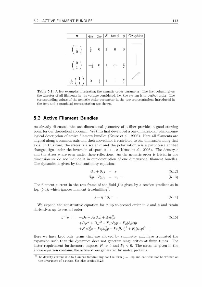
5.2. ACTIVE FILAMENT BUNDLES 113
n qxx qxy S tanφ φ Graphics
(10
)12 0 1 0 0
(01
)−1
2 0 1 ∞ π2
1√2
(11
)0 1
2 1 1 π4
Table 5.1: A few examples illustrating the nematic order parameter. The first column givesthe director of all filaments in the volume considered, i.e. the system is in perfect order. Thecorresponding values of the nematic order parameter in the two representations introduced inthe text and a graphical representation are shown.
5.2 Active Filament Bundles
As already discussed, the one dimensional geometry of a fiber provides a good startingpoint for our theoretical approach. We thus first developed a one dimensional, phenomeno-logical description of active filament bundles (Kruse et al., 2003). Here all filaments arealigned along a common axis and their movement is restricted to one dimension along thataxis. In this case, the stress is a scalar σ and the polarization p is a pseudo-scalar thatchanges sign under the inversion of space x → −x (Kruse et al., 2003). The density cand the stress σ are even under these reflections. As the nematic order is trivial in onedimension we do not include it in our description of one dimensional filament bundles.The dynamics is given by the continuity equations
∂tc + ∂xj = s (5.12)∂tp + ∂xjp = sp . (5.13)
The filament current in the rest frame of the fluid j is given by a tension gradient as inEq. (5.4), which ignores filament treadmilling2:
j = η−1∂xσ . (5.14)
We expand the constitutive equation for σ up to second order in c and p and retainderivatives up to second order:
η−1σ = −Dc + A1∂xp + A2∂2xc (5.15)
+B1c2 + B2p
2 + E1c∂xp + E2(∂xc)p+F1c∂
2xc + F2p∂2
xp + F3(∂xc)2 + F4(∂xp)2 .
Here we have kept only terms that are allowed by symmetry and have truncated theexpansion such that the dynamics does not generate singularities at finite times. Thelatter requirement furthermore imposes F1 > 0 and F3 < 0. The stress as given in theabove equation contains the active stress generated by motor proteins.
2The density current due to filament treadmilling has the form j = −vp and can thus not be written asthe divergence of a stress. See also section 5.2.5
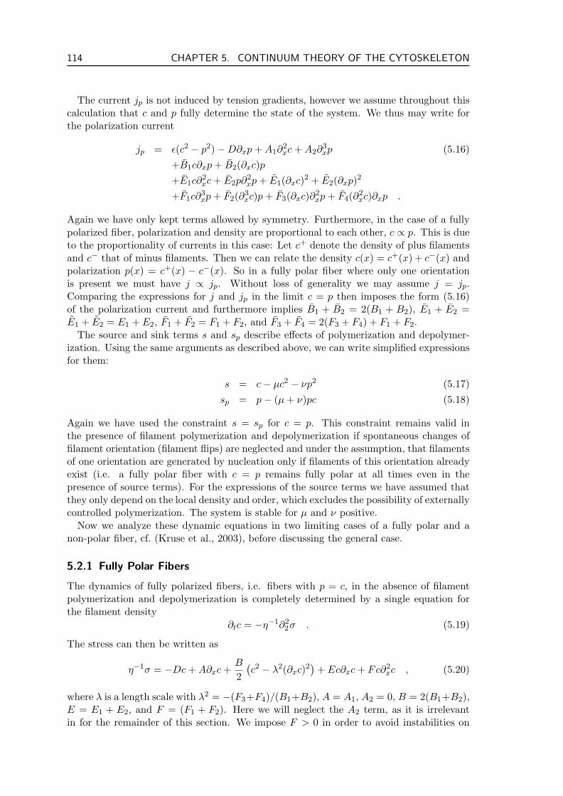
114 CHAPTER 5. CONTINUUM THEORY OF THE CYTOSKELETON
The current jp is not induced by tension gradients, however we assume throughout thiscalculation that c and p fully determine the state of the system. We thus may write forthe polarization current
jp = ε(c2 − p2)−D∂xp + A1∂2xc + A2∂
3xp (5.16)
+B1c∂xp + B2(∂xc)p+E1c∂
2xc + E2p∂2
xp + E1(∂xc)2 + E2(∂xp)2
+F1c∂3xp + F2(∂3
xc)p + F3(∂xc)∂2xp + F4(∂2
xc)∂xp .
Again we have only kept terms allowed by symmetry. Furthermore, in the case of a fullypolarized fiber, polarization and density are proportional to each other, c ∝ p. This is dueto the proportionality of currents in this case: Let c+ denote the density of plus filamentsand c− that of minus filaments. Then we can relate the density c(x) = c+(x) + c−(x) andpolarization p(x) = c+(x) − c−(x). So in a fully polar fiber where only one orientationis present we must have j ∝ jp. Without loss of generality we may assume j = jp.Comparing the expressions for j and jp in the limit c = p then imposes the form (5.16)of the polarization current and furthermore implies B1 + B2 = 2(B1 + B2), E1 + E2 =E1 + E2 = E1 + E2, F1 + F2 = F1 + F2, and F3 + F4 = 2(F3 + F4) + F1 + F2.
The source and sink terms s and sp describe effects of polymerization and depolymer-ization. Using the same arguments as described above, we can write simplified expressionsfor them:
s = c− µc2 − νp2 (5.17)sp = p− (µ + ν)pc (5.18)
Again we have used the constraint s = sp for c = p. This constraint remains valid inthe presence of filament polymerization and depolymerization if spontaneous changes offilament orientation (filament flips) are neglected and under the assumption, that filamentsof one orientation are generated by nucleation only if filaments of this orientation alreadyexist (i.e. a fully polar fiber with c = p remains fully polar at all times even in thepresence of source terms). For the expressions of the source terms we have assumed thatthey only depend on the local density and order, which excludes the possibility of externallycontrolled polymerization. The system is stable for µ and ν positive.
Now we analyze these dynamic equations in two limiting cases of a fully polar and anon-polar fiber, cf. (Kruse et al., 2003), before discussing the general case.
5.2.1 Fully Polar Fibers
The dynamics of fully polarized fibers, i.e. fibers with p = c, in the absence of filamentpolymerization and depolymerization is completely determined by a single equation forthe filament density
∂tc = −η−1∂22σ . (5.19)
The stress can then be written as
η−1σ = −Dc + A∂xc +B
2(c2 − λ2(∂xc)2
)+ Ec∂xc + Fc∂2
xc , (5.20)
where λ is a length scale with λ2 = −(F3+F4)/(B1+B2), A = A1, A2 = 0, B = 2(B1+B2),E = E1 + E2, and F = (F1 + F2). Here we will neglect the A2 term, as it is irrelevantin for the remainder of this section. We impose F > 0 in order to avoid instabilities on
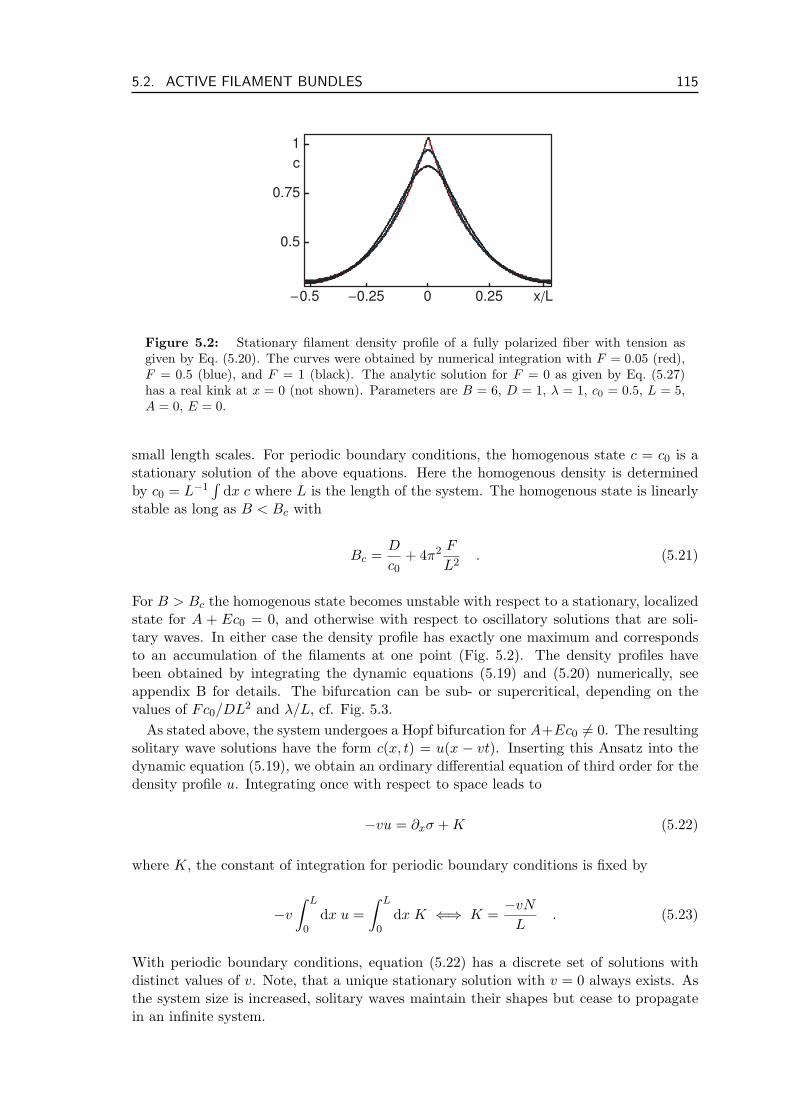
5.2. ACTIVE FILAMENT BUNDLES 115
Figure 5.2: Stationary filament density profile of a fully polarized fiber with tension asgiven by Eq. (5.20). The curves were obtained by numerical integration with F = 0.05 (red),F = 0.5 (blue), and F = 1 (black). The analytic solution for F = 0 as given by Eq. (5.27)has a real kink at x = 0 (not shown). Parameters are B = 6, D = 1, λ = 1, c0 = 0.5, L = 5,A = 0, E = 0.
small length scales. For periodic boundary conditions, the homogenous state c = c0 is astationary solution of the above equations. Here the homogenous density is determinedby c0 = L−1
∫dx c where L is the length of the system. The homogenous state is linearly
stable as long as B < Bc with
Bc =D
c0+ 4π2 F
L2. (5.21)
For B > Bc the homogenous state becomes unstable with respect to a stationary, localizedstate for A + Ec0 = 0, and otherwise with respect to oscillatory solutions that are soli-tary waves. In either case the density profile has exactly one maximum and correspondsto an accumulation of the filaments at one point (Fig. 5.2). The density profiles havebeen obtained by integrating the dynamic equations (5.19) and (5.20) numerically, seeappendix B for details. The bifurcation can be sub- or supercritical, depending on thevalues of Fc0/DL2 and λ/L, cf. Fig. 5.3.
As stated above, the system undergoes a Hopf bifurcation for A+Ec0 6= 0. The resultingsolitary wave solutions have the form c(x, t) = u(x − vt). Inserting this Ansatz into thedynamic equation (5.19), we obtain an ordinary differential equation of third order for thedensity profile u. Integrating once with respect to space leads to
−vu = ∂xσ + K (5.22)
where K, the constant of integration for periodic boundary conditions is fixed by
−v
∫ L
0dx u =
∫ L
0dx K ⇐⇒ K =
−vN
L. (5.23)
With periodic boundary conditions, equation (5.22) has a discrete set of solutions withdistinct values of v. Note, that a unique stationary solution with v = 0 always exists. Asthe system size is increased, solitary waves maintain their shapes but cease to propagatein an infinite system.
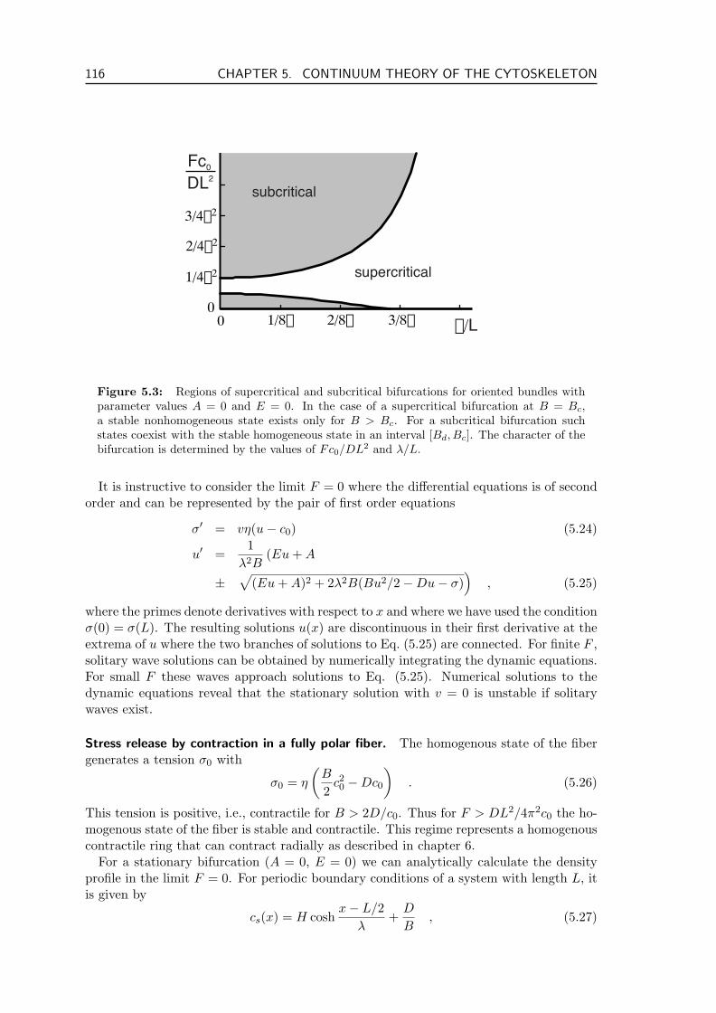
116 CHAPTER 5. CONTINUUM THEORY OF THE CYTOSKELETON
1/8p0 2/8p 3/8p
3/4p2
2/4p2
1/4p2
0
Fc0
l/L
subcritical
supercritical
DL2
Figure 5.3: Regions of supercritical and subcritical bifurcations for oriented bundles withparameter values A = 0 and E = 0. In the case of a supercritical bifurcation at B = Bc,a stable nonhomogeneous state exists only for B > Bc. For a subcritical bifurcation suchstates coexist with the stable homogeneous state in an interval [Bd, Bc]. The character of thebifurcation is determined by the values of Fc0/DL2 and λ/L.
It is instructive to consider the limit F = 0 where the differential equations is of secondorder and can be represented by the pair of first order equations
σ′ = vη(u− c0) (5.24)
u′ =1
λ2B(Eu + A
±√
(Eu + A)2 + 2λ2B(Bu2/2−Du− σ))
, (5.25)
where the primes denote derivatives with respect to x and where we have used the conditionσ(0) = σ(L). The resulting solutions u(x) are discontinuous in their first derivative at theextrema of u where the two branches of solutions to Eq. (5.25) are connected. For finite F ,solitary wave solutions can be obtained by numerically integrating the dynamic equations.For small F these waves approach solutions to Eq. (5.25). Numerical solutions to thedynamic equations reveal that the stationary solution with v = 0 is unstable if solitarywaves exist.
Stress release by contraction in a fully polar fiber. The homogenous state of the fibergenerates a tension σ0 with
σ0 = η
(B
2c20 −Dc0
). (5.26)
This tension is positive, i.e., contractile for B > 2D/c0. Thus for F > DL2/4π2c0 the ho-mogenous state of the fiber is stable and contractile. This regime represents a homogenouscontractile ring that can contract radially as described in chapter 6.
For a stationary bifurcation (A = 0, E = 0) we can analytically calculate the densityprofile in the limit F = 0. For periodic boundary conditions of a system with length L, itis given by
cs(x) = H coshx− L/2
λ+
D
B, (5.27)
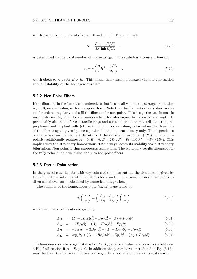
5.2. ACTIVE FILAMENT BUNDLES 117
which has a discontinuity of c′ at x = 0 and x = L. The amplitude
H =L(c0 −D/B)2λ sinhL/2λ
. (5.28)
is determined by the total number of filaments c0L. This state has a constant tension
σs = η
(B
2H2 − D2
2B
). (5.29)
which obeys σs < σ0 for B > Bc. This means that tension is relaxed via fiber contractionat the instability of the homogeneous state.
5.2.2 Non-Polar Fibers
If the filaments in the fiber are disordered, so that in a small volume the average orientationis p = 0, we are dealing with a non-polar fiber. Note that the filaments at very short scalescan be ordered regularly and still the fiber can be non-polar. This is e.g. the case in musclemyofibrils (see Fig. 2.30) for dynamics on length scales larger than a sarcomere length. Itpresumably also holds for contractile rings and stress fibers in animal cells and the pre-prophase band in plant cells (cf. section 5.3). For vanishing polarization the dynamicsof the fiber is again given by one equation for the filament density only. The dependenceof the tension on the filament density is of the same form as in Eq. (5.20) but the non-polarity additionally requires A = 0, E = 0, B = 2B1, F = F1, and λ2 = −F3/(2B1). Thisimplies that the stationary homogenous state always looses its stability via a stationarybifurcation. Non-polarity thus suppresses oscillations. The stationary results discussed forthe fully polar bundle thus also apply to non-polar fibers.
5.2.3 Partial Polarization
In the general case, i.e. for arbitrary values of the polarization, the dynamics is given bytwo coupled partial differential equations for c and p. The same classes of solutions asdiscussed above can be obtained by numerical integration.
The stability of the homogenous state (c0, p0) is governed by
∂t
(cp
)=(
A11 A12
A21 A22
)(cp
)(5.30)
where the matrix elements are given by
A11 = (D − 2Bc0)∂2x − Ep0∂
3x − (A2 + Fc0)∂4
x (5.31)A12 = −2Bp0∂
2x − (A1 + Ec0)∂3
x − Fp0∂4x (5.32)
A21 = −2εc0∂x − 2Bp0∂2x − (A1 + Ec0)∂3
x − Fp0∂4x (5.33)
A22 = 2εp0∂x + (D − 2Bc0))∂2x − Ep0∂
3x − (A2 + Fc0)∂4
x (5.34)
The homogenous state is again stable for B < Bc, a critical value, and loses its stability viaa Hopf-bifurcation if A + Ec0 > 0. In addition the parameter ε, introduced in Eq. (5.16),must be lower than a certain critical value εc. For ε > εc the bifurcation is stationary.
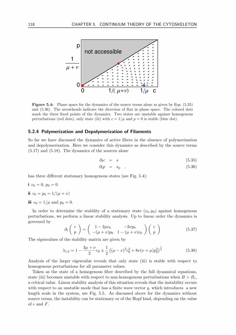
118 CHAPTER 5. CONTINUUM THEORY OF THE CYTOSKELETON
Figure 5.4: Phase space for the dynamics of the source terms alone as given by Eqs. (5.35)and (5.36). The arrowheads indicate the direction of flux in phase space. The colored dotsmark the three fixed points of the dynamics. Two states are unstable against homogenousperturbations (red dots), only state (iii) with c = 1/µ and p = 0 is stable (blue dot).
5.2.4 Polymerization and Depolymerization of Filaments
So far we have discussed the dynamics of active fibers in the absence of polymerizationand depolymerization. Here we consider this dynamics as described by the source terms(5.17) and (5.18). The dynamics of the sources alone
∂tc = s (5.35)∂tp = sp , (5.36)
has three different stationary homogenous states (see Fig. 5.4):
i c0 = 0, p0 = 0
ii c0 = p0 = 1/(µ + ν)
iii c0 = 1/µ and p0 = 0.
In order to determine the stability of a stationary state (c0, p0) against homogenousperturbations, we perform a linear stability analysis. Up to linear order the dynamics isgoverned by
∂t
(cp
)=(
1− 2µc0 −2νp0
−(µ + ν)p0 1− (µ + ν)c0
)(cp
)(5.37)
The eigenvalues of the stability matrix are given by
λ1,2 = 1− 3µ + ν
2c0 ±
12((µ− ν)2c2
0 + 8ν(ν + µ)p20
) 12 (5.38)
Analysis of the larger eigenvalue reveals that only state (iii) is stable with respect tohomogenous perturbations for all parameter values.
Taken as the state of a homogenous fiber described by the full dynamical equations,state (iii) becomes unstable with respect to non-homogenous perturbations when B > Bc,a critical value. Linear stability analysis of this situation reveals that the instability occurswith respect to an unstable mode that has a finite wave vector q, which introduces a newlength scale in the system, see Fig. 5.5. As discussed above for the dynamics withoutsource terms, the instability can be stationary or of the Hopf kind, depending on the valueof ε and F .
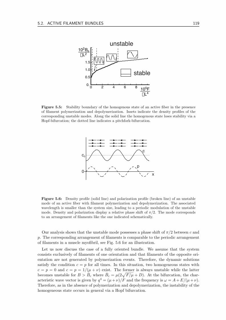
5.2. ACTIVE FILAMENT BUNDLES 119
20 4 6 8 105F mL4
0.5
0.
1.0
1.5
102Bc mL2
stable
unstable
Figure 5.5: Stability boundary of the homogenous state of an active fiber in the presenceof filament polymerization and depolymerization. Insets indicate the density profiles of thecorresponding unstable modes. Along the solid line the homogenous state loses stability via aHopf-bifurcation; the dotted line indicates a pitchfork-bifurcation.
0
c0
p
c
x
Figure 5.6: Density profile (solid line) and polarization profile (broken line) of an unstablemode of an active fiber with filament polymerization and depolymerization. The associatedwavelength is smaller than the system size, leading to a periodic modulation of the unstablemode. Density and polarization display a relative phase shift of π/2. The mode correspondsto an arrangement of filaments like the one indicated schematically.
Our analysis shows that the unstable mode possesses a phase shift of π/2 between c andp. The corresponding arrangement of filaments is comparable to the periodic arrangementof filaments in a muscle myofibril, see Fig. 5.6 for an illustration.
Let us now discuss the case of a fully oriented bundle. We assume that the systemconsists exclusively of filaments of one orientation and that filaments of the opposite ori-entation are not generated by polymerization events. Therefore, the dynamic solutionssatisfy the condition c = p for all times. In this situation, two homogeneous states withc = p = 0 and c = p = 1/(µ + ν) exist. The former is always unstable while the latterbecomes unstable for B > Bc where Bc = µ(2
√F/µ + D). At the bifurcation, the char-
acteristic wave vector is given by q4 = (µ + ν)/F and the frequency is ω = A + E/(µ + ν).Therefore, as in the absence of polymerization and depolymerization, the instability of thehomogeneous state occurs in general via a Hopf bifurcation.
120 CHAPTER 5. CONTINUUM THEORY OF THE CYTOSKELETON
The source terms presented and discussed above are the simplest source terms in theframe work of this generic continuum description that, when studied alone, do not havetrivial dynamics. We can extend these expressions in order to accommodate the poly-merization dynamics discussed in the microscopic mean field description, section 3.2.4.Neglecting explicit monomer dynamics, the corresponding expressions are
∂tc+ = kp − kdc
+ (5.39)∂tc
− = kp − kdc− (5.40)
so that using c = c+ + c− and p = c+ − c− we immediately obtain
∂tc = kc − kdc (5.41)∂tp = −kdp (5.42)
where we define a new constant polymerization rate kc = 2kp. The only stationary stateof this dynamics is given by c = kc/kd and p = 0, which is globally stable.
The situation becomes more interesting when we merge these expressions with the sim-plified expressions in Eqs. (5.17) and (5.18):
∂tc = c− µ′c2 − ν ′p2 + k′c (5.43)∂tp = p− (µ′ + ν ′)pc (5.44)
where we have rescaled time and the primes mark the resulting rescaled parameters. Thissystem has two types of fixed points
i c = ±1+√
1+4k′cµ′
2µ′ , p = 0
ii c = 1µ+ν , p = ±
√k′
cν + 1
(µ+ν)2
The linear stability is governed by the larger eigenvalue given in Eq. (5.38) with theappropriate rescaled parameters. This reveals that fixed point (ii) is always unstable andthat (i) is stable for µ′ 6= 0. This fixed point is qualitatively the same as point (iii) of thesimplified expressions, see Fig. 5.4. Thus its properties are not different and the resultspresented in the previous section qualitatively hold also for these extended source terms.
5.2.5 Filament Treadmilling
As the filament current due to filament treadmilling is not induced by gradients in thetension, it cannot be included by adding terms to Eq. (5.15). We thus have to alter thecurrents in the theory directly by adding the following terms for treadmilling:
jv = −vp (5.45)jp,v = −vc (5.46)
The dynamics of fully polar fibers in the presence of treadmilling is given by
∂tc = v∂xc + D∂2xc−A∂3
xc− B
2∂2
x
(c2 − λ2(∂xc)2
)+ Ec∂3
xc + Fc∂4xc . (5.47)
Writing c as a Fourier sum c = Σkck exp(ikx) reveals immediately that the treadmillingcurrent can only contribute to the oscillation frequency of the critical mode, but not toits stability. Hence even in the presence of treadmilling the homogenous state is stable
5.2. ACTIVE FILAMENT BUNDLES 121
for B < Bc, where the critical value Bc is given by Eq. (5.21). As discussed above, wegenerally expect the homogenous state to loose stability via a Hopf bifurcation towardsoscillation solutions. The presence of treadmilling will thus not alter the generic behaviorof the system qualitatively.
The stability of unpolar fibers in the presence of treadmilling is the same as withouttreadmilling. As outlined above, the dynamics is described by Eq. (5.47) with A = 0 andE = 0. In addition the treadmilling term is not present, as p = 0 implies jv = 0, cf.Eq. (5.45). Thus literally nothing changes in the presence of treadmilling, as the dynamicequation is unchanged.
For arbitrary polarization we expect the same types of solutions as discussed in sec-tion 5.2.3. The homogenous state is stable for B < Bc a critical value.
5.2.6 Connection to the Minimal Model
The types of asymptotic state solutions of the generic continuum description of an activefiber presented above are the same as found in the minimal model presented in chapter 3.This is comforting as we can view the minimal model as a microscopic theory correspondingto the generic continuum description. Interestingly the minimal model seems to capture thegeneric behavior of active filament fibers, although it is based on simplifying assumptionsand limited to pair-wise filament interactions. In appendix A we put this statement on firmgrounds by coarse graining the minimal model and comparing the resulting expressionswith the generic description. The ensuing expressions are of the form presented above.
When derived from the minimal model, most coefficients of the expansion (5.15) and(5.16) are non-zero. Only A1, A2, E1, E2, F3 and F4 vanish. The corresponding termsthus are either generated by higher order processes involving three or more filaments, area consequence of anisotropy effects that manifest themselves only in higher dimensions orare due to a different form of filament-filament interactions not included in the minimalmodel. The equations derived from the minimal model show a higher degree of symmetrythan the generic description. Some coefficients mutually depend on each other (explicitexpressions given in Eqs. (A.20) - (A.25)), which further reduces the phase space of thesystem.
The detailed dependence of the coarse grained expansion coefficients on the parametersα and β (cf. Figs. 3.5 and 3.6) is given in tables A.2 and A.3. Here we note that B1
and F1 are proportional to α, while E1 is proportional to β. This confirms the findingthat instabilities in the minimal model are driven by interactions between filaments of thesame orientation and that oscillatory solutions in the absence of filament treadmilling aredriven by interactions between filaments of opposite orientation.
Furthermore we can compare the tension for the homogenous state with concentrationc0 and polarization p0 derived by coarse graining the minimal model (cf. Eq. (A.26))
σ = −c0 +l2
8[(2(α + α′) + β′)c2
0 + (2(α + α′)− β′)p20
](5.48)
and in the continuum theory derived from Eq. (5.15)
η−1σ = −Dc0 + B1c20 + B2p
20 . (5.49)
These expressions agree (cf. tables A.2 and A.3) for D = 1 and η = 1, which are thechoices made for the minimal model and the continuum description respectively.
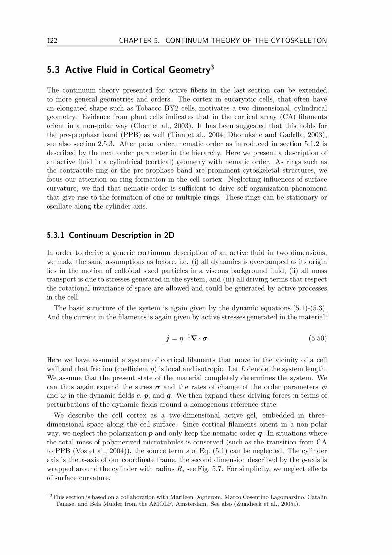
122 CHAPTER 5. CONTINUUM THEORY OF THE CYTOSKELETON
5.3 Active Fluid in Cortical Geometry3
The continuum theory presented for active fibers in the last section can be extendedto more general geometries and orders. The cortex in eucaryotic cells, that often havean elongated shape such as Tobacco BY2 cells, motivates a two dimensional, cylindricalgeometry. Evidence from plant cells indicates that in the cortical array (CA) filamentsorient in a non-polar way (Chan et al., 2003). It has been suggested that this holds forthe pre-prophase band (PPB) as well (Tian et al., 2004; Dhonukshe and Gadella, 2003),see also section 2.5.3. After polar order, nematic order as introduced in section 5.1.2 isdescribed by the next order parameter in the hierarchy. Here we present a description ofan active fluid in a cylindrical (cortical) geometry with nematic order. As rings such asthe contractile ring or the pre-prophase band are prominent cytoskeletal structures, wefocus our attention on ring formation in the cell cortex. Neglecting influences of surfacecurvature, we find that nematic order is sufficient to drive self-organization phenomenathat give rise to the formation of one or multiple rings. These rings can be stationary oroscillate along the cylinder axis.
5.3.1 Continuum Description in 2D
In order to derive a generic continuum description of an active fluid in two dimensions,we make the same assumptions as before, i.e. (i) all dynamics is overdamped as its originlies in the motion of colloidal sized particles in a viscous background fluid, (ii) all masstransport is due to stresses generated in the system, and (iii) all driving terms that respectthe rotational invariance of space are allowed and could be generated by active processesin the cell.
The basic structure of the system is again given by the dynamic equations (5.1)-(5.3).And the current in the filaments is again given by active stresses generated in the material:
j = η−1∇ · σ (5.50)
Here we have assumed a system of cortical filaments that move in the vicinity of a cellwall and that friction (coefficient η) is local and isotropic. Let L denote the system length.We assume that the present state of the material completely determines the system. Wecan thus again expand the stress σ and the rates of change of the order parameters ψand ω in the dynamic fields c, p, and q. We then expand these driving forces in terms ofperturbations of the dynamic fields around a homogenous reference state.
We describe the cell cortex as a two-dimensional active gel, embedded in three-dimensional space along the cell surface. Since cortical filaments orient in a non-polarway, we neglect the polarization p and only keep the nematic order q. In situations wherethe total mass of polymerized microtubules is conserved (such as the transition from CAto PPB (Vos et al., 2004)), the source term s of Eq. (5.1) can be neglected. The cylinderaxis is the x-axis of our coordinate frame, the second dimension described by the y-axis iswrapped around the cylinder with radius R, see Fig. 5.7. For simplicity, we neglect effectsof surface curvature.
3This section is based on a collaboration with Marileen Dogterom, Marco Cosentino Lagomarsino, CatalinTanase, and Bela Mulder from the AMOLF, Amsterdam. See also (Zumdieck et al., 2005a).
5.3. ACTIVE FLUID IN CORTICAL GEOMETRY 123
Figure 5.7: Cortical geometry. The system is described by a two dimensional gel that iswrapped on a cylinder of radius R. The x-axis corresponds to the cylinder axis, the y-axisis wrapped around the cylinder. Shown is a ring like state of the gel with no flux boundaryconditions in x-direction, similar to a contractile ring or pre-prophase band in a cell’s cortex.The density of filaments is represented by the grey level on the cylinder. The blue bars indicatethe nematic order of filaments by their orientation and length.
We expand the stress σ and the rate of change ω around a state with constant concen-tration c and order parameter q. Up to second order in c and q, and up to second orderderivatives the most general expression for σ is
−η−1σαβ = a1δαβc + a2δαβc2 + a3δαβ∆c + a4∂α∂βc (5.51)+a5qαβ + a6δαβ∂γ∂δqγδ
+a7(∂αc)(∂βc)+a8δαβqγδqγδ + a9δαβc∂α∂βc .
Here we have written all terms permitted by symmetry (under reflection x 7→ −x thedensity c and the nematic order q are even, which limits the number of possible terms).Assuming that the rate of change in the order parameter ωαβ is determined by the stateof the system we may expand it similarly:
ωαβ = b1qαβ + b2∆qαβ + b3∆2qαβ (5.52)
+b4
(∂α∂βc− 1
2δαβ∆c
)+b5
((∂αc)(∂βc)− 1
2δαβ (∇c)2
)+b6
(c∂α∂βc− 1
2δαβc∆c
)+ b7q
3αβ
where we have added the term with coefficient b7 in order to stabilize the dynamics.
5.3.2 Rotationally Invariant Equations
As we focus on the formation of rotationally symmetric objects like rings etc., we mayproject the above equations on the longitudinal axis so that they only depend on x and are
124 CHAPTER 5. CONTINUUM THEORY OF THE CYTOSKELETON
thus essentially one dimensional. The dynamics of configurations, which are rotationallyinvariant, obey a set of equations projected on the cylinder axis:
η−1σxx = A1c + A2c2 + A3c∂
2xc + A4(∂xc)2 + A5qxx (5.53)
ωxx = −B1qxx + B2∂2xqxx + B3∂
4xqxx + B4∂
2xc (5.54)
+B5(q2xx + q2
xy)qxx
ωxy = −B1qxy + B2∂2xqxy + B3∂
4xqxy (5.55)
+B5(q2xx + q2
xy)qxy
where we have neglected higher order terms.For the following it is convenient to introduce dimensionless densities, time, space,
marked with a tilde:
c = cL2 (5.56)t = tτ (5.57)x = x/L (5.58)
The corresponding dimensionless parameters are
A1 = A1τL2 , B1 = B1
τ
A2 = A2τL4 , B2 = B2
τL2
A3 = A3τL6 , B3 = B3
τL4
A4 = A4τL6 , B4 = B4
τL4
A5 = A5τ , B5 = B5
τ .
(5.59)
Here L denotes a typical length scale such as the system length, and τ has units of inversetime.
Dimensional analysis reveals that these equations contain six independent parameters.Four parameters can be fixed by measuring time in units of, say B5 and rescaling c, qxx,and qxy. The values of only three of the remaining independent parameters turn out toinfluence the dynamics qualitatively; they can be identified with A2, B2, and
F = −A5B4 . (5.60)
The other parameters describe nonlinear terms which are required to stabilize the dynam-ics. We verified that stability requires A3 > 0, A4 < 0, B3 < 0, and B5 < 0. The specificvalues of these parameters do not qualitatively influence the asymptotic dynamics.
We study these equations with two types of boundary conditions in the x-direction, cf.Fig. 5.8:
• Periodic boundary conditions (Fig. 5.8a) are useful to gain a general insight intothe problem, as they are easier to access mathematically and often allow analyticaltreatment.
• No flux or fixed boundary conditions (Fig. 5.8b) are biologically more realistic. Theyobey j(0) = 0, j(L) = 0, which implies that the cortical material cannot leave thecell. Additional boundary conditions have to be specified to fully determine theasymptotic solutions.
Periodic boundary conditions are discussed in section 5.3.3 and fixed boundary condi-tions in section 5.3.4.
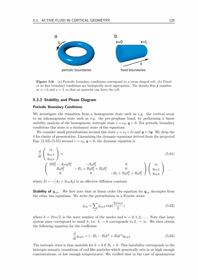
5.3. ACTIVE FLUID IN CORTICAL GEOMETRY 125
x
x=0 x=Lx
a b
periodic boundaries fixed boundaries
Figure 5.8: (a) Periodic boundary conditions correspond to a torus shaped cell. (b) Fixedor no flux boundary conditions are biologically more appropriate. The density flux j vanishesat x = 0 and x = L so that no material can leave the cell.
5.3.3 Stability and Phase Diagram
Periodic Boundary Conditions
We investigate the transition from a homogenous state such as e.g. the cortical arrayto an inhomogenous state such as e.g. the pre-prophase band, by performing a linearstability analysis of the homogenous, isotropic state c = c0, q = 0. For periodic boundaryconditions this state is a stationary state of the equations.
We consider small perturbations around this state c = c0 + δc and q = δq. We drop theδ for clarity of presentation. Linearizing the dynamic equations derived from the projectedEqs. (5.53)-(5.55) around c = c0, q = 0, the dynamic equation is
ddt
ck
qxx,k
qxy,k
= (5.61)
D∂2x −A3c0∂
4x −A5∂
2x 0
B4∂2x −B1 + B2∂
2x + B3∂
4x 0
0 0 −B1 + B2∂2x + B3∂
4x
ck
qxx,k
qxy,k
,
where D = −(A1 + 2c0A2) is an effective diffusion constant.
Stability of qxy. We first note that at linear order the equation for qxy decouples fromthe other two equations. We write the perturbation in a Fourier series
qxy =∑
n
qxy,k exp(2πinx
L) (5.62)
where k = 2πn/L is the wave number of the modes and n = 0, 1, 2, . . . . Note that largesystem sizes correspond to small k, i.e. k → 0 corresponds to L → ∞. We then obtainthe following equation for the coefficient
ddt
qxy,k = (−B1 −B2k2 + B3k
4)qxy,k . (5.63)
The isotropic state is thus unstable for k = 0 if B1 < 0. This instability corresponds to theisotropic-nematic transitions of rod-like particles which generically sets in at high enoughconcentrations, or low enough temperatures. We verified that in the case of spontaneous
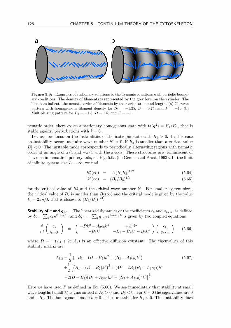
126 CHAPTER 5. CONTINUUM THEORY OF THE CYTOSKELETON
Figure 5.9: Examples of stationary solutions to the dynamic equations with periodic bound-ary conditions. The density of filaments is represented by the grey level on the cylinder. Theblue bars indicate the nematic order of filaments by their orientation and length. (a) Chevronpattern with homogeneous filament density for B2 = −1.25, D = 0.75, and F = −1. (b)Multiple ring pattern for B2 = −1.5, D = 1.5, and F = −1.
nematic order, there exists a stationary homogenous state with tr(q2) = B1/B5, that isstable against perturbations with k = 0.
Let us now focus on the instabilities of the isotropic state with B1 > 0. In this casean instability occurs at finite wave number k∗ > 0, if B2 is smaller than a critical valueB∗
2 < 0. The unstable mode corresponds to periodically alternating regions with nematicorder at an angle of π/4 and −π/4 with the x-axis. These structures are reminiscent ofchevrons in nematic liquid crystals, cf. Fig. 5.9a (de Gennes and Prost, 1993). In the limitof infinite system size L →∞, we find
B∗2(∞) = −2(B1B3)1/2 (5.64)
k∗(∞) = (B1/B3)1/4 (5.65)
for the critical value of B∗2 and the critical wave number k∗. For smaller system sizes,
the critical value of B2 is smaller than B∗2(∞) and the critical mode is given by the value
kc = 2πn/L that is closest to (B1/B3)1/4.
Stability of c and qxx. The linearized dynamics of the coefficients ck and qxx,k, as definedby δc =
∑n cke2πinx/L and δqxx =
∑n qxx,ke2πinx/L is given by two coupled equations
ddt
(ck
qxx,k
)=
(−Dk2 −A3c0k
4 +A5k2
−B4k2 −B1 −B2k
2 + B3k4
)(ck
qxx,k
), (5.66)
where D = −(A1 + 2c0A2) is an effective diffusion constant. The eigenvalues of thisstability matrix are
λ1,2 =12(−B1 − (D + B2)k2 + (B3 −A3c0)k4
)(5.67)
±12
[(B1 − (D −B2)k2
)2 + (4F − 2B1(B3 + A3c0))k4
+2(D −B2)(B3 + A3c0)k6 + (B3 + A3c0)2k8] 1
2
Here we have used F as defined in Eq. (5.60). We see immediately that stability at smallwave lengths (small k) is guaranteed if A3 > 0 and B3 < 0. For k = 0 the eigenvalues are 0and −B1. The homogenous mode k = 0 is thus unstable for B1 < 0. This instability does
5.3. ACTIVE FLUID IN CORTICAL GEOMETRY 127
not respect mass conservation. In the following we will concentrate on pattern formationin the case B1 > 0, so that the homogenous mode is always stable.
It is instructive to study a simplified case in which we only consider terms in k upto quadratic order. Although truncated, the resulting expressions already exhibit keyfeatures of the phase space of the full system. It is thus possible to analytically identifythe terms that determine the stability of the homogenous state, for example. AssumingB3 = −A3c0, which does not influence the results qualitatively, the eigenvalues read in thetruncated form:
λ1,2 =12
(−B1 − (D + B2)k2 ±
√(B1 − (D −B2)k2)2 + 4Fk4
)+O(k3) (5.68)
As the instability is driven by the eigenvalue with the largest real part, it suffices to focuson the eigenvalue with the plus sign. For large k, terms ∝ k2 dominate the eigenvalue.The homogenous state can only be stable if
D + B2 > 0 ⇐⇒ B2 > −D , (5.69)
because the eigenvalue can only be negative if the first term is negative (as the square rootalways has a positive real part by definition). In order to further discuss the stability ofthe homogenous state, we now discuss two cases:
1. F > 0: in this case the argument of the square root is always positive and thehomogenous state is only stable for large k, if in addition to condition (5.69) the realpart of the square root is smaller than the first term (D + B2)k2:
(D −B2)2 + 4F < (D + B2)2 (5.70)
⇒
B2 > F/D > 0 for D > 0B2 < F/D < 0 for D < 0
The resulting region of stability is sketched blue in Fig. 5.10a.
2. F < 0: here the argument of the square root can become negative, so that it doesnot influence the stability but only the type of bifurcation (Hopf or stationary). Let
Γ = (D −B2)2 + 4F (5.71)
denote the argument of the square root for large k. The homogenous state is stablefor large k if −(D + B2) <
√Γ. We distinguish two sub-cases:
a) Γ ≤ 0: in this case√
Γ is purely imaginary, the homogenous state becomesunstable via a Hopf bifurcation, but the stability boundary does not depend onΓ. The criterion for negative Γ leads to the condition
Γ ≤ 0 ⇐⇒ |D −B2| ≤ 2√|F |
⇐⇒ D −B2 ≤ 2√|F | < G < D −B2 ≤ 2
√|F | . (5.72)
If this is true, the stability is determined by condition (5.69). Both conditionshave to be fulfilled simultaneously. The borders of the resulting stripe-like areain the B2-D-plane are indicated in Fig. 5.10b.
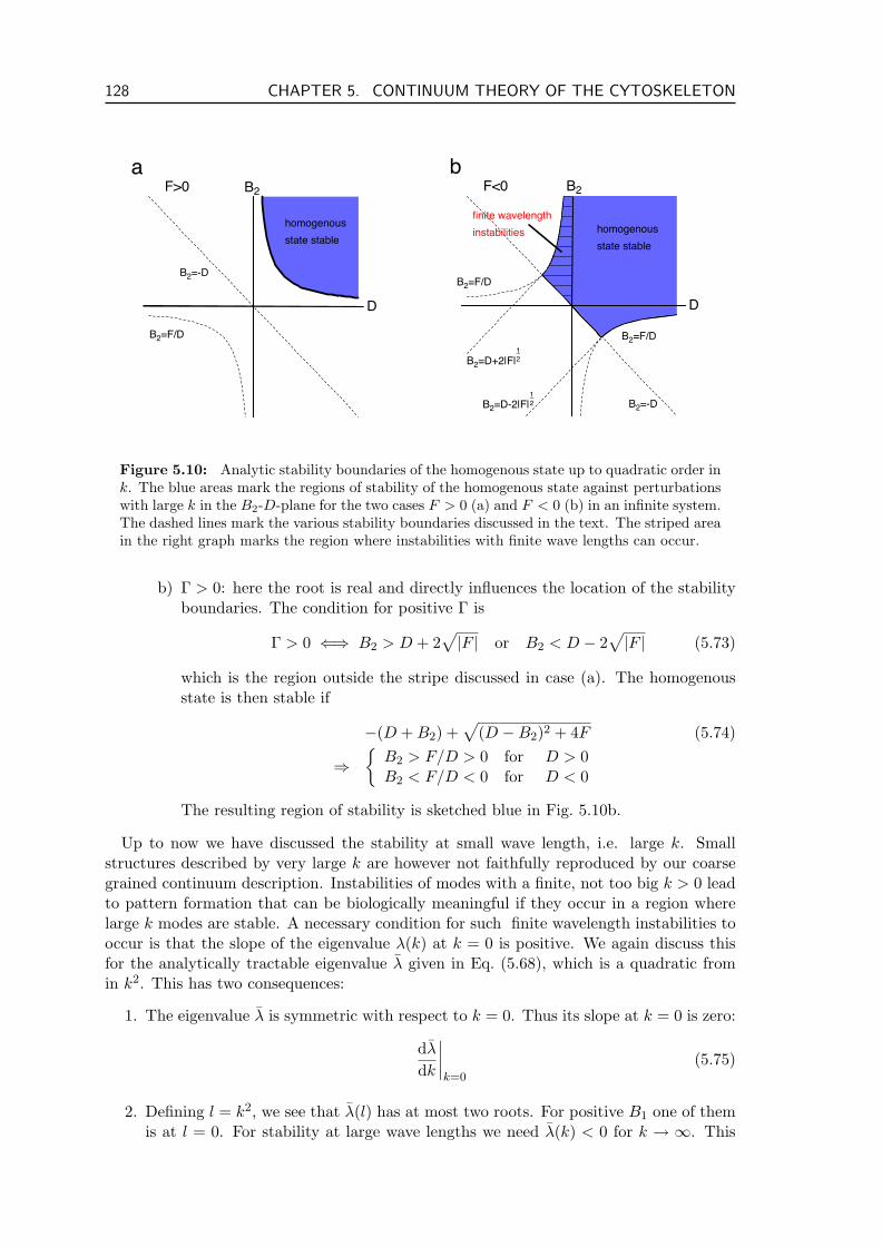
128 CHAPTER 5. CONTINUUM THEORY OF THE CYTOSKELETON
homogenousstate stable
B2=-D
B2=F/D
D
B2F>0a
D
B2
B2=F/D
B2=-D
finite wavelengthinstabilities homogenous
state stable
B2=F/D
12B2=D-2|F|_
12B2=D+2|F|_
F<0b
Figure 5.10: Analytic stability boundaries of the homogenous state up to quadratic order ink. The blue areas mark the regions of stability of the homogenous state against perturbationswith large k in the B2-D-plane for the two cases F > 0 (a) and F < 0 (b) in an infinite system.The dashed lines mark the various stability boundaries discussed in the text. The striped areain the right graph marks the region where instabilities with finite wave lengths can occur.
b) Γ > 0: here the root is real and directly influences the location of the stabilityboundaries. The condition for positive Γ is
Γ > 0 ⇐⇒ B2 > D + 2√|F | or B2 < D − 2
√|F | (5.73)
which is the region outside the stripe discussed in case (a). The homogenousstate is then stable if
−(D + B2) +√
(D −B2)2 + 4F (5.74)
⇒
B2 > F/D > 0 for D > 0B2 < F/D < 0 for D < 0
The resulting region of stability is sketched blue in Fig. 5.10b.
Up to now we have discussed the stability at small wave length, i.e. large k. Smallstructures described by very large k are however not faithfully reproduced by our coarsegrained continuum description. Instabilities of modes with a finite, not too big k > 0 leadto pattern formation that can be biologically meaningful if they occur in a region wherelarge k modes are stable. A necessary condition for such finite wavelength instabilities tooccur is that the slope of the eigenvalue λ(k) at k = 0 is positive. We again discuss thisfor the analytically tractable eigenvalue λ given in Eq. (5.68), which is a quadratic fromin k2. This has two consequences:
1. The eigenvalue λ is symmetric with respect to k = 0. Thus its slope at k = 0 is zero:
dλ
dk
∣∣∣∣k=0
(5.75)
2. Defining l = k2, we see that λ(l) has at most two roots. For positive B1 one of themis at l = 0. For stability at large wave lengths we need λ(k) < 0 for k → ∞. This
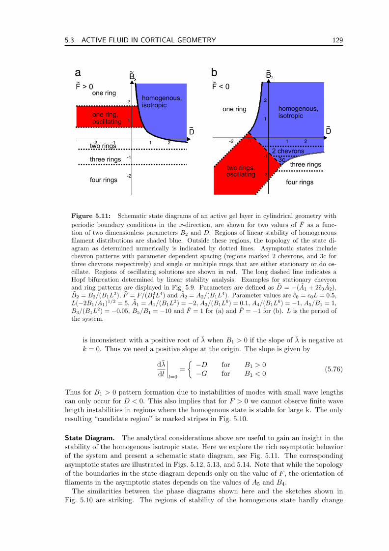
5.3. ACTIVE FLUID IN CORTICAL GEOMETRY 129
Figure 5.11: Schematic state diagrams of an active gel layer in cylindrical geometry withperiodic boundary conditions in the x-direction, are shown for two values of F as a func-tion of two dimensionless parameters B2 and D. Regions of linear stability of homogeneousfilament distributions are shaded blue. Outside these regions, the topology of the state di-agram as determined numerically is indicated by dotted lines. Asymptotic states includechevron patterns with parameter dependent spacing (regions marked 2 chevrons, and 3c forthree chevrons respectively) and single or multiple rings that are either stationary or do os-cillate. Regions of oscillating solutions are shown in red. The long dashed line indicates aHopf bifurcation determined by linear stability analysis. Examples for stationary chevronand ring patterns are displayed in Fig. 5.9. Parameters are defined as D = −(A1 + 2c0A2),B2 = B2/(B1L
2), F = F/(B21L4) and A2 = A2/(B1L
4). Parameter values are c0 = c0L = 0.5,L(−2B1/A1)1/2 = 5, A1 = A1/(B1L
2) = −2, A3/(B1L6) = 0.1, A4/(B1L
6) = −1, A5/B1 = 1,B3/(B1L
2) = −0.05, B5/B1 = −10 and F = 1 for (a) and F = −1 for (b). L is the period ofthe system.
is inconsistent with a positive root of λ when B1 > 0 if the slope of λ is negative atk = 0. Thus we need a positive slope at the origin. The slope is given by
dλ
dl
∣∣∣∣l=0
=−D for B1 > 0−G for B1 < 0
(5.76)
Thus for B1 > 0 pattern formation due to instabilities of modes with small wave lengthscan only occur for D < 0. This also implies that for F > 0 we cannot observe finite wavelength instabilities in regions where the homogenous state is stable for large k. The onlyresulting “candidate region” is marked stripes in Fig. 5.10.
State Diagram. The analytical considerations above are useful to gain an insight in thestability of the homogenous isotropic state. Here we explore the rich asymptotic behaviorof the system and present a schematic state diagram, see Fig. 5.11. The correspondingasymptotic states are illustrated in Figs. 5.12, 5.13, and 5.14. Note that while the topologyof the boundaries in the state diagram depends only on the value of F , the orientation offilaments in the asymptotic states depends on the values of A5 and B4.
The similarities between the phase diagrams shown here and the sketches shown inFig. 5.10 are striking. The regions of stability of the homogenous state hardly change
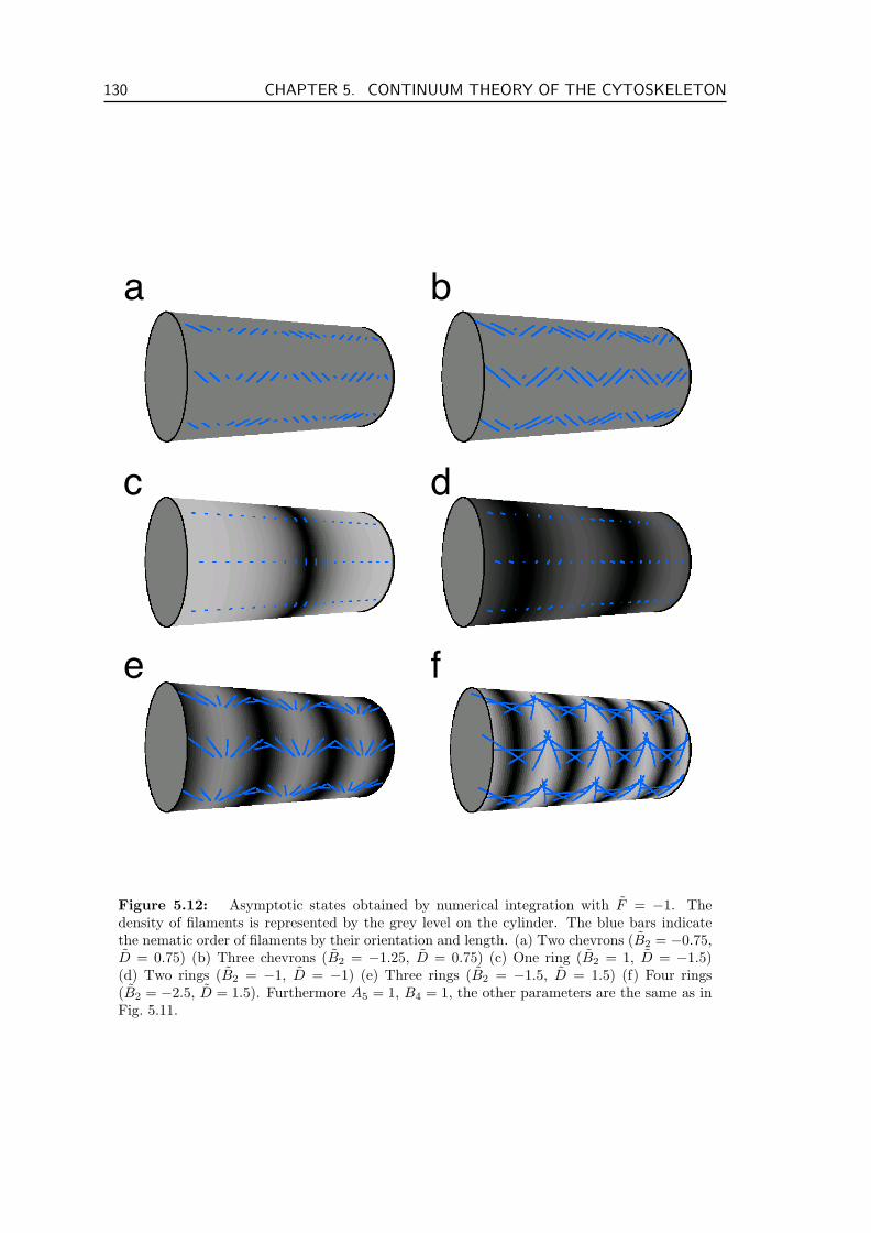
130 CHAPTER 5. CONTINUUM THEORY OF THE CYTOSKELETON
a
dc
b
fe
Figure 5.12: Asymptotic states obtained by numerical integration with F = −1. Thedensity of filaments is represented by the grey level on the cylinder. The blue bars indicatethe nematic order of filaments by their orientation and length. (a) Two chevrons (B2 = −0.75,D = 0.75) (b) Three chevrons (B2 = −1.25, D = 0.75) (c) One ring (B2 = 1, D = −1.5)(d) Two rings (B2 = −1, D = −1) (e) Three rings (B2 = −1.5, D = 1.5) (f) Four rings(B2 = −2.5, D = 1.5). Furthermore A5 = 1, B4 = 1, the other parameters are the same as inFig. 5.11.
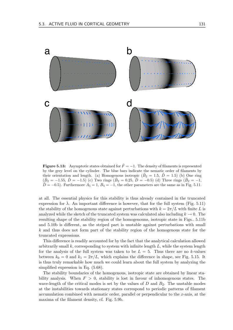
5.3. ACTIVE FLUID IN CORTICAL GEOMETRY 131
a
dc
b
Figure 5.13: Asymptotic states obtained for F = −1. The density of filaments is representedby the grey level on the cylinder. The blue bars indicate the nematic order of filaments bytheir orientation and length. (a) Homogenous isotropic (B2 = 1.5, D = 1.5) (b) One ring(B2 = −1.55, D = −1.5) (c) Two rings (B2 = 0.25, D = −0.5) (d) Three rings (B2 = −1,D = −0.5). Furthermore A5 = 1, B4 = −1, the other parameters are the same as in Fig. 5.11.
at all. The essential physics for this stability is thus already contained in the truncatedexpression for λ. An important difference is however, that for the full system (Fig. 5.11)the stability of the homogenous state against perturbations with k = 2π/L with finite L isanalyzed while the sketch of the truncated system was calculated also including k → 0. Theresulting shape of the stability region of the homogenouns, isotropic state in Figs.. 5.11band 5.10b is different, as the striped part is unstable against perturbations with smallk and thus does not form part of the stability region of the homogenous state for thetruncated expressions.
This difference is readily accounted for by the fact that the analytical calculation allowedarbitrarily small k, corresponding to system with infinite length L, while the system lengthfor the analysis of the full system was taken to be L = 5. Thus there are no k-valuesbetween k0 = 0 and k1 = 2π/L, which explains the difference in shape, see Fig. 5.15. Itis thus truly remarkable how much we could learn about the full system by analyzing thesimplified expression in Eq. (5.68).
The stability boundaries of the homogenous, isotropic state are obtained by linear sta-bility analysis. When F > 0, stability is lost in favour of inhomogenous states. Thewave-length of the critical modes is set by the values of D and B2. The unstable modesat the instabilities towards stationary states correspond to periodic patterns of filamentaccumulation combined with nematic order, parallel or perpendicular to the x-axis, at themaxima of the filament density, cf. Fig. 5.9b.
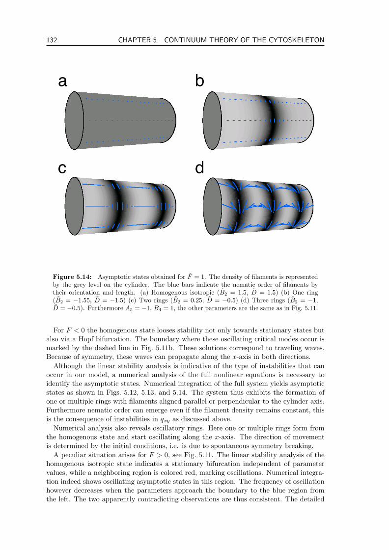
132 CHAPTER 5. CONTINUUM THEORY OF THE CYTOSKELETON
a
dc
b
Figure 5.14: Asymptotic states obtained for F = 1. The density of filaments is representedby the grey level on the cylinder. The blue bars indicate the nematic order of filaments bytheir orientation and length. (a) Homogenous isotropic (B2 = 1.5, D = 1.5) (b) One ring(B2 = −1.55, D = −1.5) (c) Two rings (B2 = 0.25, D = −0.5) (d) Three rings (B2 = −1,D = −0.5). Furthermore A5 = −1, B4 = 1, the other parameters are the same as in Fig. 5.11.
For F < 0 the homogenous state looses stability not only towards stationary states butalso via a Hopf bifurcation. The boundary where these oscillating critical modes occur ismarked by the dashed line in Fig. 5.11b. These solutions correspond to traveling waves.Because of symmetry, these waves can propagate along the x-axis in both directions.
Although the linear stability analysis is indicative of the type of instabilities that canoccur in our model, a numerical analysis of the full nonlinear equations is necessary toidentify the asymptotic states. Numerical integration of the full system yields asymptoticstates as shown in Figs. 5.12, 5.13, and 5.14. The system thus exhibits the formation ofone or multiple rings with filaments aligned parallel or perpendicular to the cylinder axis.Furthermore nematic order can emerge even if the filament density remains constant, thisis the consequence of instabilities in qxy as discussed above.
Numerical analysis also reveals oscillatory rings. Here one or multiple rings form fromthe homogenous state and start oscillating along the x-axis. The direction of movementis determined by the initial conditions, i.e. is due to spontaneous symmetry breaking.
A peculiar situation arises for F > 0, see Fig. 5.11. The linear stability analysis of thehomogenous isotropic state indicates a stationary bifurcation independent of parametervalues, while a neighboring region is colored red, marking oscillations. Numerical integra-tion indeed shows oscillating asymptotic states in this region. The frequency of oscillationhowever decreases when the parameters approach the boundary to the blue region fromthe left. The two apparently contradicting observations are thus consistent. The detailed
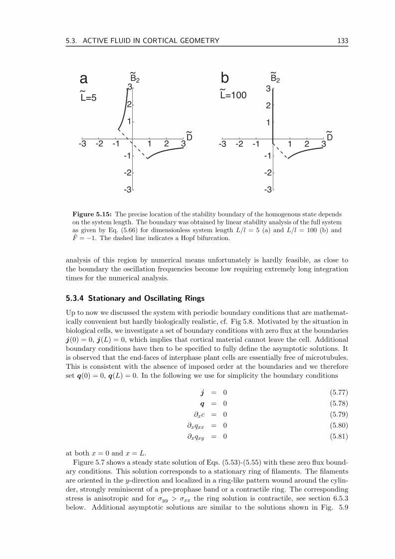
5.3. ACTIVE FLUID IN CORTICAL GEOMETRY 133
B2
-3 -2 -1 1 2 3D
-3
-2
-1
1
2
3
-3 -2 -1 1 2 3D
-3
-2
-1
1
2
3
B2
L=5 L=100
a b~ ~
~~
~~
Figure 5.15: The precise location of the stability boundary of the homogenous state dependson the system length. The boundary was obtained by linear stability analysis of the full systemas given by Eq. (5.66) for dimensionless system length L/l = 5 (a) and L/l = 100 (b) andF = −1. The dashed line indicates a Hopf bifurcation.
analysis of this region by numerical means unfortunately is hardly feasible, as close tothe boundary the oscillation frequencies become low requiring extremely long integrationtimes for the numerical analysis.
5.3.4 Stationary and Oscillating Rings
Up to now we discussed the system with periodic boundary conditions that are mathemat-ically convenient but hardly biologically realistic, cf. Fig 5.8. Motivated by the situation inbiological cells, we investigate a set of boundary conditions with zero flux at the boundariesj(0) = 0, j(L) = 0, which implies that cortical material cannot leave the cell. Additionalboundary conditions have then to be specified to fully define the asymptotic solutions. Itis observed that the end-faces of interphase plant cells are essentially free of microtubules.This is consistent with the absence of imposed order at the boundaries and we thereforeset q(0) = 0, q(L) = 0. In the following we use for simplicity the boundary conditions
j = 0 (5.77)q = 0 (5.78)
∂xc = 0 (5.79)∂xqxx = 0 (5.80)∂xqxy = 0 (5.81)
at both x = 0 and x = L.Figure 5.7 shows a steady state solution of Eqs. (5.53)-(5.55) with these zero flux bound-
ary conditions. This solution corresponds to a stationary ring of filaments. The filamentsare oriented in the y-direction and localized in a ring-like pattern wound around the cylin-der, strongly reminiscent of a pre-prophase band or a contractile ring. The correspondingstress is anisotropic and for σyy > σxx the ring solution is contractile, see section 6.5.3below. Additional asymptotic solutions are similar to the solutions shown in Fig. 5.9
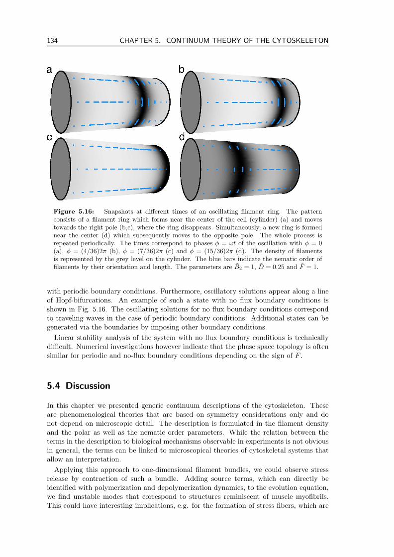
134 CHAPTER 5. CONTINUUM THEORY OF THE CYTOSKELETON
Figure 5.16: Snapshots at different times of an oscillating filament ring. The patternconsists of a filament ring which forms near the center of the cell (cylinder) (a) and movestowards the right pole (b,c), where the ring disappears. Simultaneously, a new ring is formednear the center (d) which subsequently moves to the opposite pole. The whole process isrepeated periodically. The times correspond to phases φ = ωt of the oscillation with φ = 0(a), φ = (4/36)2π (b), φ = (7/36)2π (c) and φ = (15/36)2π (d). The density of filamentsis represented by the grey level on the cylinder. The blue bars indicate the nematic order offilaments by their orientation and length. The parameters are B2 = 1, D = 0.25 and F = 1.
with periodic boundary conditions. Furthermore, oscillatory solutions appear along a lineof Hopf-bifurcations. An example of such a state with no flux boundary conditions isshown in Fig. 5.16. The oscillating solutions for no flux boundary conditions correspondto traveling waves in the case of periodic boundary conditions. Additional states can begenerated via the boundaries by imposing other boundary conditions.
Linear stability analysis of the system with no flux boundary conditions is technicallydifficult. Numerical investigations however indicate that the phase space topology is oftensimilar for periodic and no-flux boundary conditions depending on the sign of F .
5.4 Discussion
In this chapter we presented generic continuum descriptions of the cytoskeleton. Theseare phenomenological theories that are based on symmetry considerations only and donot depend on microscopic detail. The description is formulated in the filament densityand the polar as well as the nematic order parameters. While the relation between theterms in the description to biological mechanisms observable in experiments is not obviousin general, the terms can be linked to microscopical theories of cytoskeletal systems thatallow an interpretation.
Applying this approach to one-dimensional filament bundles, we could observe stressrelease by contraction of such a bundle. Adding source terms, which can directly beidentified with polymerization and depolymerization dynamics, to the evolution equation,we find unstable modes that correspond to structures reminiscent of muscle myofibrils.This could have interesting implications, e.g. for the formation of stress fibers, which are
5.4. DISCUSSION 135
transient contractile filament bundles. In contrast to myofibrils, stress fibers seem to formwithout any apparent structural cues such as Z-disks.
We furthermore investigate ring formation in the cell cortex. We apply the theory to atwo-dimensional geometry that corresponds to the surface of a cylinder, reminiscent of anelongated cell. We find that single as well as multiple rings can form by dynamic instabil-ities. The rings can be stationary or oscillate along the cylinder axis. Our theory couldbe extended to include filament elasticity, which probably would tend to align filamentsalong the cylinder axis rather than perpendicular to it. An alternative way of treating theboundaries is to write explicit evolution equations for the quantities at the boundaries.
The phenomenological descriptions of cytoskeletal dynamics presented in the previoussections all focused on the system’s behavior on long time scales. They thus neglectedthat the cytoskeleton shows elastic behavior on short time scales (Thoumine et al., 1996;Thoumine and Ott, 1997; Fabry et al., 2001; Beil et al., 2003; Mahaffy et al., 2004; Mi-coulet et al., 2005; Balland et al., 2005). The viscoelastic response of an isotropic solutionof entangled, polar, semiflexible polymers in the presence of motor like forces has beeninvestigated in (Liverpool et al., 2001). Recently, a description of active gels has beenpresented that includes viscoelastic behavior (Kruse et al., 2004, 2005). See (Kruse, 2005)for a detailed discussion on how elastic effects can be incorporated into the theory ofcytoskeletal filament systems based on this description of active polar viscoelastic gels.

136 CHAPTER 5. CONTINUUM THEORY OF THE CYTOSKELETON
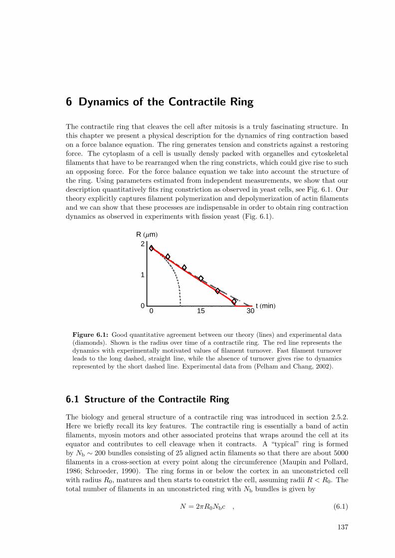
6 Dynamics of the Contractile Ring
The contractile ring that cleaves the cell after mitosis is a truly fascinating structure. Inthis chapter we present a physical description for the dynamics of ring contraction basedon a force balance equation. The ring generates tension and constricts against a restoringforce. The cytoplasm of a cell is usually densly packed with organelles and cytoskeletalfilaments that have to be rearranged when the ring constricts, which could give rise to suchan opposing force. For the force balance equation we take into account the structure ofthe ring. Using parameters estimated from independent measurements, we show that ourdescription quantitatively fits ring constriction as observed in yeast cells, see Fig. 6.1. Ourtheory explicitly captures filament polymerization and depolymerization of actin filamentsand we can show that these processes are indispensable in order to obtain ring contractiondynamics as observed in experiments with fission yeast (Fig. 6.1).
0 15 30t HminL0
1
2R HΜmL
Figure 6.1: Good quantitative agreement between our theory (lines) and experimental data(diamonds). Shown is the radius over time of a contractile ring. The red line represents thedynamics with experimentally motivated values of filament turnover. Fast filament turnoverleads to the long dashed, straight line, while the absence of turnover gives rise to dynamicsrepresented by the short dashed line. Experimental data from (Pelham and Chang, 2002).
6.1 Structure of the Contractile Ring
The biology and general structure of a contractile ring was introduced in section 2.5.2.Here we briefly recall its key features. The contractile ring is essentially a band of actinfilaments, myosin motors and other associated proteins that wraps around the cell at itsequator and contributes to cell cleavage when it contracts. A “typical” ring is formedby Nb ∼ 200 bundles consisting of 25 aligned actin filaments so that there are about 5000filaments in a cross-section at every point along the circumference (Maupin and Pollard,1986; Schroeder, 1990). The ring forms in or below the cortex in an unconstricted cellwith radius R0, matures and then starts to constrict the cell, assuming radii R < R0. Thetotal number of filaments in an unconstricted ring with Nb bundles is given by
N = 2πR0Nbc , (6.1)
137
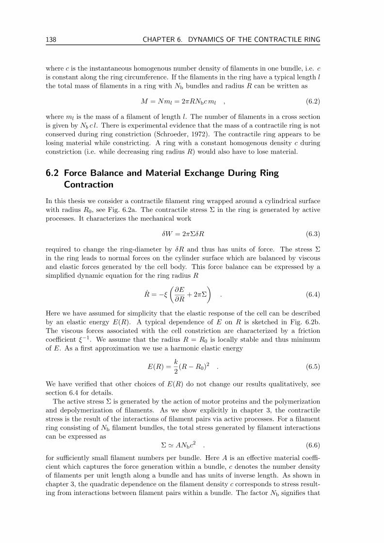
138 CHAPTER 6. DYNAMICS OF THE CONTRACTILE RING
where c is the instantaneous homogenous number density of filaments in one bundle, i.e. cis constant along the ring circumference. If the filaments in the ring have a typical length lthe total mass of filaments in a ring with Nb bundles and radius R can be written as
M = Nml = 2πRNbcml , (6.2)
where ml is the mass of a filament of length l. The number of filaments in a cross sectionis given by Nb c l. There is experimental evidence that the mass of a contractile ring is notconserved during ring constriction (Schroeder, 1972). The contractile ring appears to belosing material while constricting. A ring with a constant homogenous density c duringconstriction (i.e. while decreasing ring radius R) would also have to lose material.
6.2 Force Balance and Material Exchange During RingContraction
In this thesis we consider a contractile filament ring wrapped around a cylindrical surfacewith radius R0, see Fig. 6.2a. The contractile stress Σ in the ring is generated by activeprocesses. It characterizes the mechanical work
δW = 2πΣδR (6.3)
required to change the ring-diameter by δR and thus has units of force. The stress Σin the ring leads to normal forces on the cylinder surface which are balanced by viscousand elastic forces generated by the cell body. This force balance can be expressed by asimplified dynamic equation for the ring radius R
R = −ξ
(∂E
∂R+ 2πΣ
). (6.4)
Here we have assumed for simplicity that the elastic response of the cell can be describedby an elastic energy E(R). A typical dependence of E on R is sketched in Fig. 6.2b.The viscous forces associated with the cell constriction are characterized by a frictioncoefficient ξ−1. We assume that the radius R = R0 is locally stable and thus minimumof E. As a first approximation we use a harmonic elastic energy
E(R) =k
2(R−R0)2 . (6.5)
We have verified that other choices of E(R) do not change our results qualitatively, seesection 6.4 for details.
The active stress Σ is generated by the action of motor proteins and the polymerizationand depolymerization of filaments. As we show explicitly in chapter 3, the contractilestress is the result of the interactions of filament pairs via active processes. For a filamentring consisting of Nb filament bundles, the total stress generated by filament interactionscan be expressed as
Σ ' ANbc2 . (6.6)
for sufficiently small filament numbers per bundle. Here A is an effective material coeffi-cient which captures the force generation within a bundle, c denotes the number densityof filaments per unit length along a bundle and has units of inverse length. As shown inchapter 3, the quadratic dependence on the filament density c corresponds to stress result-ing from interactions between filament pairs within a bundle. The factor Nb signifies that
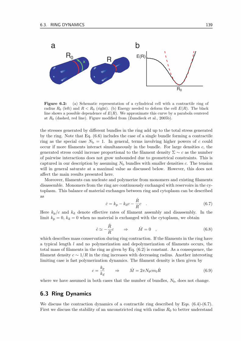
6.3. RING DYNAMICS 139
RR0
x
R0
E(R)
a b
Figure 6.2: (a) Schematic representation of a cylindrical cell with a contractile ring ofradius R0 (left) and R < R0 (right). (b) Energy needed to deform the cell E(R). The blackline shows a possible dependence of E(R). We approximate this curve by a parabola centeredat R0 (dashed, red line). Figure modified from (Zumdieck et al., 2005b).
the stresses generated by different bundles in the ring add up to the total stress generatedby the ring. Note that Eq. (6.6) includes the case of a single bundle forming a contractilering as the special case Nb = 1. In general, terms involving higher powers of c couldoccur if more filaments interact simultaneously in the bundle. For large densities c, thegenerated stress could increase proportional to the filament density Σ ∼ c as the numberof pairwise interactions does not grow unbounded due to geometrical constraints. This iscaptured in our description by assuming Nb bundles with smaller densities c. The tensionwill in general saturate at a maximal value as discussed below. However, this does notaffect the main results presented here.
Moreover, filaments can nucleate and polymerize from monomers and existing filamentsdisassemble. Monomers from the ring are continuously exchanged with reservoirs in the cy-toplasm. This balance of material exchanges between ring and cytoplasm can be describedas
c = kp − kdc−R
Rc . (6.7)
Here kp/c and kd denote effective rates of filament assembly and disassembly. In thelimit kp = 0, kd = 0 when no material is exchanged with the cytoplasm, we obtain
c ' −R
Rc ⇒ M = 0 , (6.8)
which describes mass conservation during ring contraction. If the filaments in the ring havea typical length l and no polymerization and depolymerization of filaments occurs, thetotal mass of filaments in the ring as given by Eq. (6.2) is constant. As a consequence, thefilament density c ∼ 1/R in the ring increases with decreasing radius. Another interestinglimiting case is fast polymerization dynamics. The filament density is then given by
c =kp
kd⇒ M = 2πNbcmlR (6.9)
where we have assumed in both cases that the number of bundles, Nb, does not change.
6.3 Ring Dynamics
We discuss the contraction dynamics of a contractile ring described by Eqs. (6.4)-(6.7).First we discuss the stability of an unconstricted ring with radius R0 to better understand
140 CHAPTER 6. DYNAMICS OF THE CONTRACTILE RING
the onset of ring contraction, section 6.3.1. Then we show the time course of contractiondetermined by numerical integration and discuss the choice of parameters as well as thedependence of the dynamics on these parameters.
6.3.1 Contraction of the Ring
When a ring forms in the cell cortex it usually does not contract right away but it “matures”and then starts contraction upon a cellular signal. In the framework of the ring dynamicsas presented in the previous section this means changing a parameter so that a ring withradius R0 becomes unstable towards smaller radii. Here we discuss the linear stability ofsuch a ring.
No Polymerization and Depolymerization
We start with the instructive case of a constricting ring in the absence of polymeriza-tion and depolymerization. In this case the total number of filaments N = Nb2πR0c0 isconserved. The filament density therefore is given by
c(t) =N
2πR(t). (6.10)
The contraction velocity is thus given by
R = −ξ
[k(R−R0) +
NbAN2
2π
1R2
]. (6.11)
The equation R = 0 has three solutions in R, indicating three possible radii at which thering stalls. Typically only one of them is real and thus physically meaningful. If A > 0, aring with radius R0 will always constrict
R(R0) = −ξNbAN2
2π
1R2
0
< 0 . (6.12)
If A is positive but smaller than some critical value Ac the ring will constrict, but stallat an radius R(A) > 0 at which R = 0. The explicit form of R(A) in the absence ofpolymerization and depolymerization is given in appendix D. The critical value Ac canthus be determined by R(Ac) = 0. As this is technically difficult, we chose a different pathto obtain Ac:
R < 0 ⇐⇒ A(R) > −2πkR2(R−R0)N2Nb
(6.13)
⇒ Ac = maxR∈[0;R0]
(−2πkR2(R−R0)
N2Nb
)=
8π
27k
R30
N2Nb, (6.14)
which defines the critical Ac that is necessary for the ring to fully contract (i.e R → 0) inthe absence of polymerization and depolymerization.
Fast Polymerization and Depolymerization
The other limiting case which allows us to discuss the conditions for ring contraction isthat of fast polymerization and depolymerization, so that
c(t) =kp
kd. (6.15)
6.3. RING DYNAMICS 141
150 300 4500 t (min)252627282930c(mm )-1
0 150 300 450 t (min)0
1
2R(mm)
a b
Figure 6.3: Dynamics of a contracting ring as a function of time for A larger and smallerthan Ac. (a) Ring radius R as a function of time. For A > Ac (dashed line) the ringconstricts completely in around 30 min while for A < Ac (solid line) it approaches a radiusRs > 0. (b) Corresponding filament density c as a function of time shown for the samenumerical calculations as in (a). Parameters are as in Fig. 6.4, so that by Eq. (6.18) Ac '9.7×10⁻¹⁵ Nµm2. Plots show A = 3.2×10⁻¹⁴ Nµm2 (dashed lines) and A = 3.2×10⁻¹⁵ Nµm2
(solid lines). The curves are calculated as described in section 6.3.2.
This leads to a dynamic equation for the radius
R = −ξ
[k(R−R0) + 2πNbA
(kp
kd
)2]
. (6.16)
Therefore R(R0) < 0 for A > 0, so that a ring with radius R0 would start to contractimmediately. For any given A the ring contracts to the radius
R(A) = R0 −2πNbAk2
p
kk2d
. (6.17)
The critical value of A is determined by the condition R(A) = 0:
Ac =kk2
dR0
2πk2pNb
(6.18)
Intermediate Polymerization Rates
The general case of intermediate polymerization rates is described by Eqs. (6.4)-(6.7). Asin the two limiting cases a ring with radius R0 will start to contract as for A > 0 wehave R(R0) < 0. The system has a fixed point at
cs =kp
kd, Rs = R0 −
2πNbAk2p
kk2d
. (6.19)
The stability of this fixed point at linear order is given by(δc˙δR
)=(−kd − 6πNbAξc2
s/Rs −ξcs(2πNbAc2s − k)/Rs
−2Aξcs −ξk
)(δcδR
)(6.20)
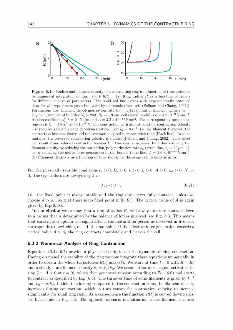
142 CHAPTER 6. DYNAMICS OF THE CONTRACTILE RING
aR
(µ
m)
t (min)0 15 30 450
1
2 b
t (min)
c (µ
m-1
)
0 15 30 45
20
25
30
35
Figure 6.4: Radius and filament density of a contracting ring as a function of time obtainedby numerical integration of Eqs. (6.4)-(6.7) . (a) Ring radius R as a function of time tfor different choices of parameters. The solid red line agrees with experimentally obtaineddata for wildtype fission yeast indicated by diamonds (from ref. (Pelham and Chang, 2002)).Parameters are: filament depolymerization rate kd = 1/(25s), initial filament density c0 =25 µm−1, number of bundles Nb = 200, R0 = 1.9 µm, cell elastic modulus k = 4×10⁻⁹ Nµm−1,friction coefficient ξ−1 = 20 Ns/m and A = 3.2× 10⁻¹⁴ Nµm2. The corresponding mechanicaltension is Σ = ANbc
2 ' 4×10⁻⁹ N. The contraction with almost constant contraction velocity−R requires rapid filament depolymerization. For kd = 0 s−1, i.e. no filament turnover, thecontraction becomes faster and the contraction speed increases with time (black line). In somemutants, the observed contraction velocity is smaller (Pelham and Chang, 2002). This effectcan result from reduced contractile tension Σ. This can be achieved by either reducing thefilament density by reducing the nucleation/polymerization rate kp (green line, c0 = 20µm−1),or by reducing the active force generation in the bundle (blue line, A = 2.6 × 10⁻¹⁴ Nµm2).(b) Filament density c as a function of time shown for the same calculations as in (a).
For the physically sensible conditions cs > 0, Rs > 0, k > 0, ξ > 0, A > 0, kd > 0, Nb >0, the eigenvalues are always negative
λ1,2 < 0 , (6.21)
i.e. the fixed point is always stable and the ring does never fully contract, unless wechoose A > Ac, so that there is no fixed point in [0, R0]. The critical value of A is againgiven by Eq.(6.18).
In conclusion we can say that a ring of radius R0 will always start to contract downto a radius that is determined by the balance of forces involved, see Fig. 6.3. This meansthat constriction upon a cell signal after a the maturation period as observed in live cellscorresponds to “switching on” A at some point. If the effective force generation exceeds acritical value A > Ac the ring contracts completely and cleaves the cell.
6.3.2 Numerical Analysis of Ring Contraction
Equations (6.4)-(6.7) provide a physical description of the dynamics of ring contraction.Having discussed the stability of the ring we now integrate these equations numerically inorder to obtain the whole trajectories R(t) and c(t). We start at time t = 0 with R = R0
and a steady state filament density c0 = kp/kd. We assume that a cell signal activates thering (i.e. A > 0 at t = 0), which then generates tension according to Eq. (6.6) and startsto contract as described by Eq. (6.4). The turnover time of actin filaments is given by k−1
d
and kp = c0kd. If this time is long compared to the contraction time, the filament densityincreases during contraction, which in turn causes the contraction velocity to increasesignificantly for small ring radii. As a consequence the function R(t) is curved downwards,see black lines in Fig. 6.4. The opposite scenario is a situation where filament turnover
6.3. RING DYNAMICS 143
(measured by k−1d ) is fast compared to the contraction time. In this case, the filament
density is controlled by the assembly and disassembly kinetics of the filaments, and duringcontraction c ' kp/kd. As a consequence, the generated stress Σ remains constant. Ifcontractile stresses dominate over elastic stresses, as is required for robust contraction,the contraction velocity is constant during contraction, see green lines in Fig 6.4. Theparameters for the numerical integration are determined by comparison with experimentalobservations as explained in the following section.
6.3.3 Estimate of Parameter Values
We can compare our calculations to experiments that observe the kinetics of contractionand the turnover of the ring components in fission yeast (Pelham and Chang, 2002). Inthis case the initial cell radius is R0 ' 1.9 µm. The total contraction time is T ' 30 min.The fluorescent signals of GFP-Cdc4 (a myosin light chain) does not change remarkablyduring contraction which is consistent with a scenario where the ring density is constant.The fluorescence recovery of GFP-Cdc8 (tropomyosin) is shorter than 30 s, which suggestsa choice of filament turnover rate
kd '125
s−1 . (6.22)
This estimate is consistent with the regime of constant density c and constant contractionvelocity vR as is indeed observed, see experimental data points in Fig. 6.4a, where vR 'R0/T ' 1.1 nms−1. This observed contraction kinetics allows us to estimate
ξΣ ' vR
2π' 0.2 nm · s−1 (6.23)
if contractile stresses dominates, i.e. Σ kR0.In order to estimate kp, we need the number density of filaments in the ring. Electron
microscopy of human HeLa cells1 suggests that filament bundles forming the ring containabout 25 filaments each in its crossection (Maupin and Pollard, 1986). A “typical” con-tractile ring displays in total about 5000 filaments in its crossection (Schroeder, 1990). Asa rough estimate, we thus assume that
Nb ' 200 (6.24)
bundles exist with 25 parallel MTs each exist.Treadmilling exchanges all actin in a filament of length 1µm in about 20 minutes (Pol-
lard, 1986). This can be sped up more than 30 times by proteins such as ADF/cofilin (Car-lier et al., 1999) and formins (Pollard and Borisy, 2003) that are present in the ring. Giventhat actin in the ring completely exchanges within 60 s, we use an average filament lengthof l ' 1µm in our description. This suggests an initial concentration
c(0) = c0 ' 25 µm−1 (6.25)
and thuskp ' kd · c0 ' 1 s−1µm−1 . (6.26)
Here c0 is the density that is established by polymerization and depolymerization withoutring contraction. We choose the initial concentration c(0) = c0.
1It is not obvious that HeLa cells posses the same ring structure as yeast. Equivalent data on yeast isunfortunately not available. There are however many similarities between rings in very diverse speciesso that Schroeder (1990) speaks of the typical ring, cf. section 2.5.2.
144 CHAPTER 6. DYNAMICS OF THE CONTRACTILE RING
The elastic modulus of cells as a function of position on the cell surface has been mea-sured by atomic force microscopy (AFM) for PtK2 cells by Matzke et al. (2001). In theseexperiments, the observed Young modulus was Yi ' 1 kPa during interphase and increasedduring cytokinesis up to Yc ' 10 kPa in the equatorial zone. Using the Young modulus atinterphase suggests an elastic modulus of PtK2 cells of the order of
k ' YiR0 ' 4× 10⁻⁹ Nµm−1 , (6.27)
where R0 ' 4 µm for PtK2 cells. The value of the Youngs modulus of the cleavage furrowduring cytokinesis provides a rough estimate for the tension generated in the contractilering of PtK2 cells:
Σ ' YcR20 ' 160× 10−9 N . (6.28)
Motivated by these measurements and taking into account that fission yeast is smallerthan PtK2 cells but could possess a more rigid cell wall, we suggest
k ' 4× 10⁻⁹ Nµm−1 (6.29)
for yeast. Note that the contractile tension 2πΣ must exceed kR0 ' 10 nN. We use
Σ = 4× 10⁻⁹ N , (6.30)
which can be compared with direct measurements of ring forces. In echinoderm eggs forexample, the ring can generate contractile forces up to 3×10⁻⁸ N (Rappaport, 1967). Thisforce was obtained by inserting glass needles in the cell and measuring their deflection.An unperturbed ring probably does not contract with maximal force. Using our estimatefrom above allows us to fit the inverse friction coefficient ξ and the effective materialcoefficient A so that the dynamics reproduces the experimental behavior. We obtain
ξ = 5× 104 µm ·N−1s−1 (6.31)A = 3.2× 10⁻¹⁴ Nµm2 . (6.32)
The contraction dynamics with these parameter corresponds to the solid red lines displayedin Fig. 6.4, and is consistent with the experimental data observed in yeast (Pelham andChang, 2002). For comparison, the experimentally observed ring diameter as a functionof time is shown as diamonds. For kd = 0, i.e. no polymerization and depolymerization,the contraction velocity increases rapidly with time (Fig. 6.4, black line). Mutations anddrugs that affect the rates of filament nucleation and polymerization typically lead to slowercontraction velocities (Pelham and Chang, 2002). We imitate such effects by modifyingthe contraction mechanics via a reduction of the parameter A (Fig. 6.4, blue line) or ofthe polymerization rate (Fig. 6.4, green line).
6.3.4 Parameter Dependence of Ring Dynamics
In this section we discuss how the ring contraction dynamics depends on the parametersinvolved. The parameters that lead to the contraction dynamics shown in Fig. 6.4 havebeen determined directly and indirectly from various experimental sources. While some ofthem are set with a high confidence, others could vary considerably e.g. because they areobtained from another organism or inferred indirectly. It is thus important to investigatehow changes in the parameters will affect out results.
The two parameters that have been measured with the highest confidence are the ringdiameter R and the total contraction time T . Both parameters have been directly observed
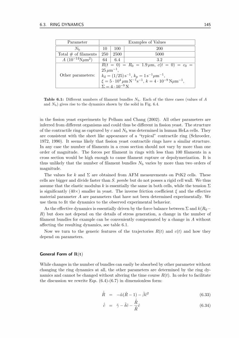
6.3. RING DYNAMICS 145
Parameter Examples of ValuesNb 10 100 200
Total # of filaments 250 2500 5000A (10−14Nµm2) 64 6.4 3.2
Other parameters:
R(t = 0) = R0 = 1.9 µm, c(t = 0) = c0 =25 µm−1,kd = (1/25) s−1, kp = 1 s−1µm−1,ξ = 5 · 104 µm N−1s−1, k = 4 · 10−9 Nµm−1,Σ = 4 · 10−9 N
Table 6.1: Different numbers of filament bundles Nb. Each of the three cases (values of Aand Nb) gives rise to the dynamics shown by the solid in Fig. 6.4.
in the fission yeast experiments by Pelham and Chang (2002). All other parameters areinferred from different organisms and could thus be different in fission yeast. The structureof the contractile ring as captured by c and Nb was determined in human HeLa cells. Theyare consistent with the sheet like appearance of a “typical” contractile ring (Schroeder,1972, 1990). It seems likely that fission yeast contractile rings have a similar structure.In any case the number of filaments in a cross section should not vary by more than oneorder of magnitude. The forces per filament in rings with less than 100 filaments in across section would be high enough to cause filament rupture or depolymerization. It isthus unlikely that the number of filament bundles Nb varies by more than two orders ofmagnitude.
The values for k and Σ are obtained from AFM measurements on PtK2 cells. Thesecells are bigger and divide faster than S. pombe but do not posses a rigid cell wall. We thusassume that the elastic modulus k is essentially the same in both cells, while the tension Σis significantly (40×) smaller in yeast. The inverse friction coefficient ξ and the effectivematerial parameter A are parameters that have not been determined experimentally. Weuse them to fit the dynamics to the observed experimental behavior.
As the effective dynamics is essentially driven by the force balance between Σ and k(R0−R) but does not depend on the details of stress generation, a change in the number offilament bundles for example can be conveniently compensated by a change in A withoutaffecting the resulting dynamics, see table 6.1.
Now we turn to the generic features of the trajectories R(t) and c(t) and how theydepend on parameters.
General Form of R(t)
While changes in the number of bundles can easily be absorbed by other parameter withoutchanging the ring dynamics at all, the other parameters are determined by the ring dy-namics and cannot be changed without altering the time course R(t). In order to facilitatethe discussion we rewrite Eqs. (6.4)-(6.7) in dimensionless form:
˙R = −α(R− 1)− βc2 (6.33)
˙c = γ − δc−˙RR
c (6.34)
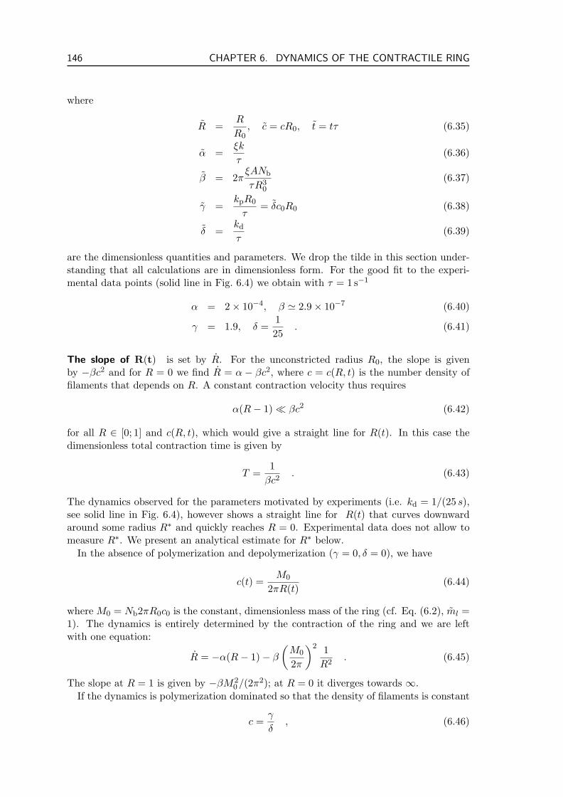
146 CHAPTER 6. DYNAMICS OF THE CONTRACTILE RING
where
R =R
R0, c = cR0, t = tτ (6.35)
α =ξk
τ(6.36)
β = 2πξANb
τR30
(6.37)
γ =kpR0
τ= δc0R0 (6.38)
δ =kd
τ(6.39)
are the dimensionless quantities and parameters. We drop the tilde in this section under-standing that all calculations are in dimensionless form. For the good fit to the experi-mental data points (solid line in Fig. 6.4) we obtain with τ = 1 s−1
α = 2× 10⁻⁴, β ' 2.9× 10⁻⁷ (6.40)
γ = 1.9, δ =125
. (6.41)
The slope of R(t) is set by R. For the unconstricted radius R0, the slope is givenby −βc2 and for R = 0 we find R = α − βc2, where c = c(R, t) is the number density offilaments that depends on R. A constant contraction velocity thus requires
α(R− 1) βc2 (6.42)
for all R ∈ [0; 1] and c(R, t), which would give a straight line for R(t). In this case thedimensionless total contraction time is given by
T =1
βc2. (6.43)
The dynamics observed for the parameters motivated by experiments (i.e. kd = 1/(25 s),see solid line in Fig. 6.4), however shows a straight line for R(t) that curves downwardaround some radius R∗ and quickly reaches R = 0. Experimental data does not allow tomeasure R∗. We present an analytical estimate for R∗ below.
In the absence of polymerization and depolymerization (γ = 0, δ = 0), we have
c(t) =M0
2πR(t)(6.44)
where M0 = Nb2πR0c0 is the constant, dimensionless mass of the ring (cf. Eq. (6.2), ml =1). The dynamics is entirely determined by the contraction of the ring and we are leftwith one equation:
R = −α(R− 1)− β
(M0
2π
)2 1R2
. (6.45)
The slope at R = 1 is given by −βM20 /(2π2); at R = 0 it diverges towards ∞.
If the dynamics is polymerization dominated so that the density of filaments is constant
c =γ
δ, (6.46)
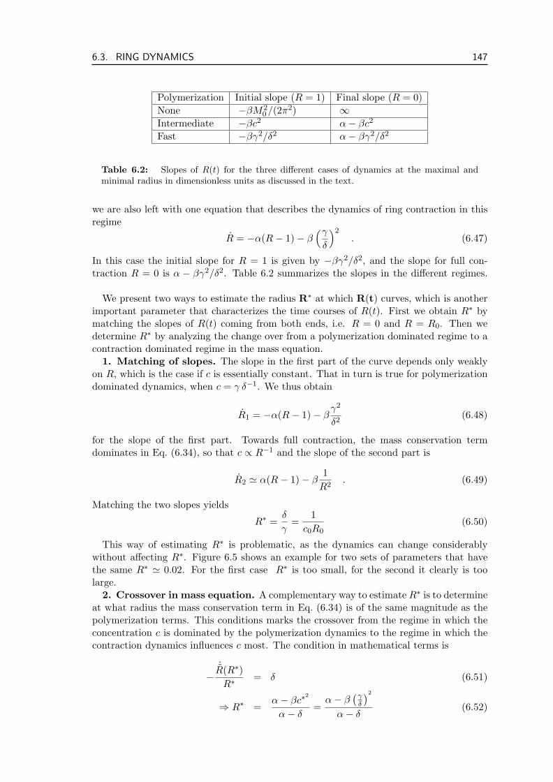
6.3. RING DYNAMICS 147
Polymerization Initial slope (R = 1) Final slope (R = 0)None −βM2
0 /(2π2) ∞Intermediate −βc2 α− βc2
Fast −βγ2/δ2 α− βγ2/δ2
Table 6.2: Slopes of R(t) for the three different cases of dynamics at the maximal andminimal radius in dimensionless units as discussed in the text.
we are also left with one equation that describes the dynamics of ring contraction in thisregime
R = −α(R− 1)− β(γ
δ
)2. (6.47)
In this case the initial slope for R = 1 is given by −βγ2/δ2, and the slope for full con-traction R = 0 is α − βγ2/δ2. Table 6.2 summarizes the slopes in the different regimes.
We present two ways to estimate the radius R∗ at which R(t) curves, which is anotherimportant parameter that characterizes the time courses of R(t). First we obtain R∗ bymatching the slopes of R(t) coming from both ends, i.e. R = 0 and R = R0. Then wedetermine R∗ by analyzing the change over from a polymerization dominated regime to acontraction dominated regime in the mass equation.
1. Matching of slopes. The slope in the first part of the curve depends only weaklyon R, which is the case if c is essentially constant. That in turn is true for polymerizationdominated dynamics, when c = γ δ−1. We thus obtain
R1 = −α(R− 1)− βγ2
δ2(6.48)
for the slope of the first part. Towards full contraction, the mass conservation termdominates in Eq. (6.34), so that c ∝ R−1 and the slope of the second part is
R2 ' α(R− 1)− β1
R2. (6.49)
Matching the two slopes yields
R∗ =δ
γ=
1c0R0
(6.50)
This way of estimating R∗ is problematic, as the dynamics can change considerablywithout affecting R∗. Figure 6.5 shows an example for two sets of parameters that havethe same R∗ ' 0.02. For the first case R∗ is too small, for the second it clearly is toolarge.
2. Crossover in mass equation. A complementary way to estimate R∗ is to determineat what radius the mass conservation term in Eq. (6.34) is of the same magnitude as thepolymerization terms. This conditions marks the crossover from the regime in which theconcentration c is dominated by the polymerization dynamics to the regime in which thecontraction dynamics influences c most. The condition in mathematical terms is
−˙R(R∗)R∗ = δ (6.51)
⇒ R∗ =α− βc∗
2
α− δ=
α− β(γ
δ
)2α− δ
(6.52)
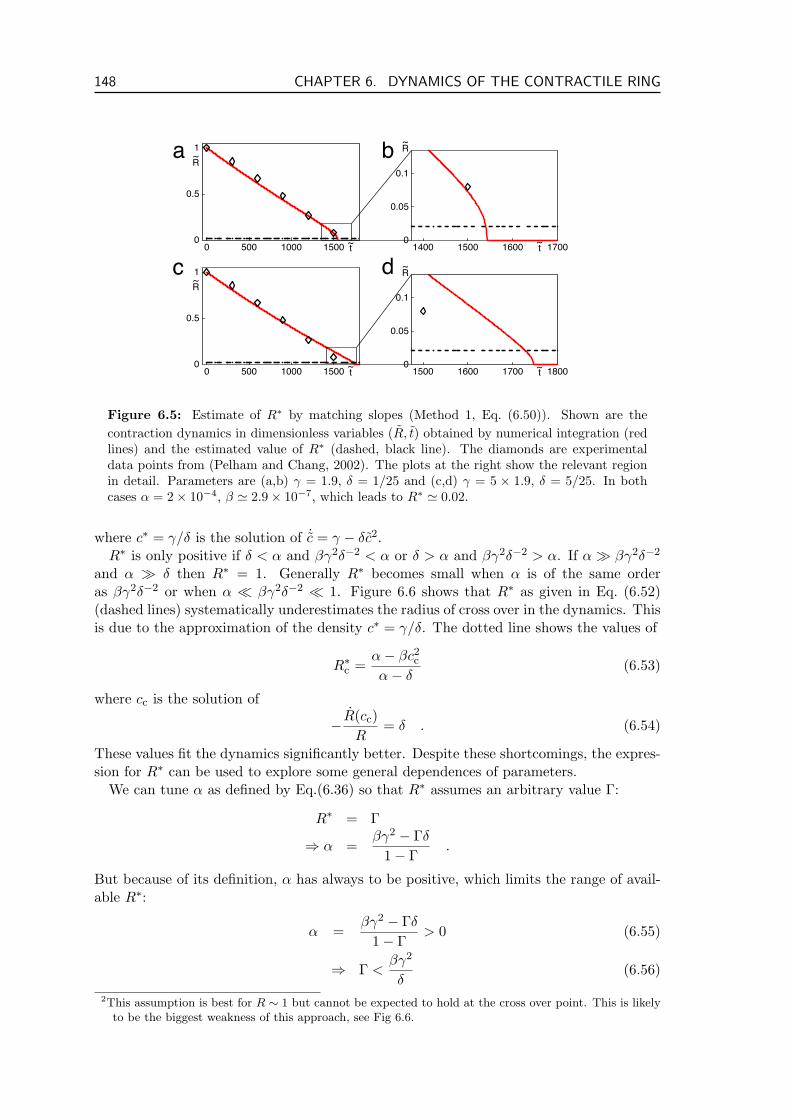
148 CHAPTER 6. DYNAMICS OF THE CONTRACTILE RING
~0 500 1000 1500 t0
0.5
R~1
~1400 1500 t1600 17000
0.05
0.1
R~
0 500 1000 1500 t~0
0.5
R~1
~1500 1600 1700 t 18000
0.05
0.1
R~
a
dc
b
Figure 6.5: Estimate of R∗ by matching slopes (Method 1, Eq. (6.50)). Shown are thecontraction dynamics in dimensionless variables (R, t) obtained by numerical integration (redlines) and the estimated value of R∗ (dashed, black line). The diamonds are experimentaldata points from (Pelham and Chang, 2002). The plots at the right show the relevant regionin detail. Parameters are (a,b) γ = 1.9, δ = 1/25 and (c,d) γ = 5 × 1.9, δ = 5/25. In bothcases α = 2× 10⁻⁴, β ' 2.9× 10⁻⁷, which leads to R∗ ' 0.02.
where c∗ = γ/δ is the solution of ˙c = γ − δc2.R∗ is only positive if δ < α and βγ2δ−2 < α or δ > α and βγ2δ−2 > α. If α βγ2δ−2
and α δ then R∗ = 1. Generally R∗ becomes small when α is of the same orderas βγ2δ−2 or when α βγ2δ−2 1. Figure 6.6 shows that R∗ as given in Eq. (6.52)(dashed lines) systematically underestimates the radius of cross over in the dynamics. Thisis due to the approximation of the density c∗ = γ/δ. The dotted line shows the values of
R∗c =
α− βc2c
α− δ(6.53)
where cc is the solution of
−R(cc)R
= δ . (6.54)
These values fit the dynamics significantly better. Despite these shortcomings, the expres-sion for R∗ can be used to explore some general dependences of parameters.
We can tune α as defined by Eq.(6.36) so that R∗ assumes an arbitrary value Γ:
R∗ = Γ
⇒ α =βγ2 − Γδ
1− Γ.
But because of its definition, α has always to be positive, which limits the range of avail-able R∗:
α =βγ2 − Γδ
1− Γ> 0 (6.55)
⇒ Γ <βγ2
δ(6.56)
2This assumption is best for R ∼ 1 but cannot be expected to hold at the cross over point. This is likelyto be the biggest weakness of this approach, see Fig 6.6.
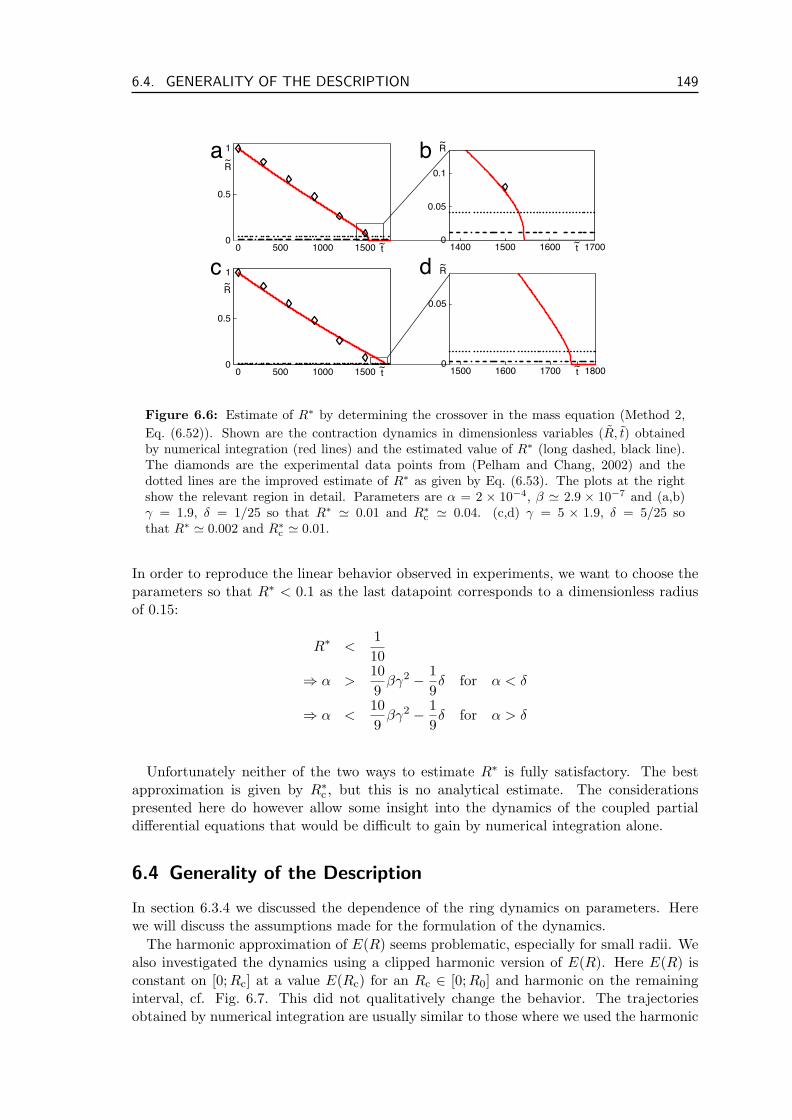
6.4. GENERALITY OF THE DESCRIPTION 149
a
dc
b
~
~
0 500 1000 1500 t0
0.5
R
1
~1400 1500 t1600 17000
0.05
0.1
R~
~1500 1600 1700 t 18000
0.05
R~
~
~
0 500 1000 1500 t0
0.5
R
1
Figure 6.6: Estimate of R∗ by determining the crossover in the mass equation (Method 2,Eq. (6.52)). Shown are the contraction dynamics in dimensionless variables (R, t) obtainedby numerical integration (red lines) and the estimated value of R∗ (long dashed, black line).The diamonds are the experimental data points from (Pelham and Chang, 2002) and thedotted lines are the improved estimate of R∗ as given by Eq. (6.53). The plots at the rightshow the relevant region in detail. Parameters are α = 2 × 10⁻⁴, β ' 2.9 × 10⁻⁷ and (a,b)γ = 1.9, δ = 1/25 so that R∗ ' 0.01 and R∗
c ' 0.04. (c,d) γ = 5 × 1.9, δ = 5/25 sothat R∗ ' 0.002 and R∗
c ' 0.01.
In order to reproduce the linear behavior observed in experiments, we want to choose theparameters so that R∗ < 0.1 as the last datapoint corresponds to a dimensionless radiusof 0.15:
R∗ <110
⇒ α >109
βγ2 − 19δ for α < δ
⇒ α <109
βγ2 − 19δ for α > δ
Unfortunately neither of the two ways to estimate R∗ is fully satisfactory. The bestapproximation is given by R∗
c , but this is no analytical estimate. The considerationspresented here do however allow some insight into the dynamics of the coupled partialdifferential equations that would be difficult to gain by numerical integration alone.
6.4 Generality of the Description
In section 6.3.4 we discussed the dependence of the ring dynamics on parameters. Herewe will discuss the assumptions made for the formulation of the dynamics.
The harmonic approximation of E(R) seems problematic, especially for small radii. Wealso investigated the dynamics using a clipped harmonic version of E(R). Here E(R) isconstant on [0;Rc] at a value E(Rc) for an Rc ∈ [0;R0] and harmonic on the remaininginterval, cf. Fig. 6.7. This did not qualitatively change the behavior. The trajectoriesobtained by numerical integration are usually similar to those where we used the harmonic
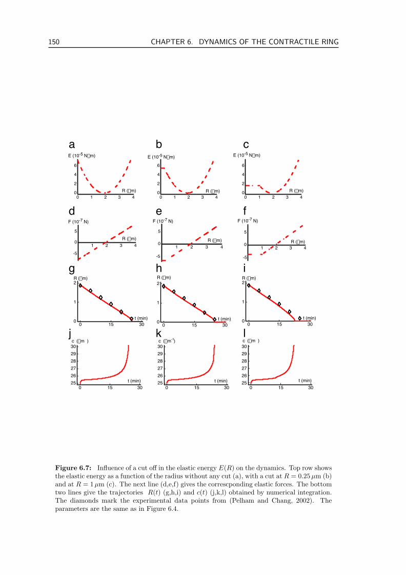
150 CHAPTER 6. DYNAMICS OF THE CONTRACTILE RING
1 2 3 4
5
-5
0R (mm)
F (10-7 N)
1 2 3 4
5
-5
0R (mm)
F (10-7 N)
1 2 3 4
5
-5
0 R (mm)
F (10-7 N)
0 1 2 3 4
6
4
2
0 R (mm)
E (10-5 Nmm)
0 1 2 3 4
6
4
2
0 R (mm)
E (10-5 Nmm)
0 1 2 3 4
6
4
2
0 R (mm)
E (10-5 Nmm)
t (min)0 15 300
1
2R (mm)
0 15 300
1
2
t (min)
R (mm)
0 15 300
1
2
t (min)
R (mm)
0 15 30252627282930
t (min)
c (mm )
t (min)0 15 30
252627282930c (mm )-1
0 15 30252627282930
t (min)
c (mm )
a cb
g ih
d fe
j lk
Figure 6.7: Influence of a cut off in the elastic energy E(R) on the dynamics. Top row showsthe elastic energy as a function of the radius without any cut (a), with a cut at R = 0.25 µm (b)and at R = 1µm (c). The next line (d,e,f) gives the correscponding elastic forces. The bottomtwo lines give the trajectories R(t) (g,h,i) and c(t) (j,k,l) obtained by numerical integration.The diamonds mark the experimental data points from (Pelham and Chang, 2002). Theparameters are the same as in Figure 6.4.
6.5. STRESSES AND RING CONTRACTION 151
approximation over the whole range of R, see Fig. 6.7. This behavior can be understood ifwe assume that for smaller R the contraction dynamics is dominated by the active tension.In that case a change in the exact form of the potential would not have a dramatic effecton the dynamics.
This prompts us to take a closer look at the active tension. We assume that the tension isgenerated by active processes in the ring. Motivated by the analysis of pairwise interactionsbetween filaments discussed in chapter 3, we propose a quadratic dependence of Σ on c.This seems sensible as long as the density of filaments is low, so that the probability ofpairwise interactions is proportional to c2. When the filament density becomes large andthe filament bundle has a larger diameter, it is unlikely for filaments to interact withfilaments that are spatially distant. That is why for large densities the stress will probablygrow ∝ c, simply because the probability of filament pair interactions in a thicker bundlegrow linearly. The contractile ring as found e.g. in human HeLa cells appears to fitwell with these considerations: the ring is a flat, band-like structure composed of manydifferent filament bundles that are aligned next to each other. In every bundle the densityof filaments can be small enough so that Σ ∝ c2 holds. The stress of the various bundlesthen just adds up, similar to Σ ∝ c in one thick bundle.
When the ring forms it can either form all bundles at the same time, so that Nb remainsconstant over the period of ring constriction. In this case the structure of the ring justleads to a rescaling of the coefficient of stress generation A as seen above. If however thering forms with only one bundle which consecutively splits during ring contraction, then Nwould always increase monotonously, while c(t) should increase monotonously and thendecrease suddenly everytime a bundle splits. This behavior could lead to a different kindof dynamics of the ring, that is beyond the scope of this thesis.
6.5 Stresses and Ring Contraction
Throughout this chapter we assumed that radial stresses in cytoskeletal structures suchas the contractile ring or the actin cortex can lead to forces normal to the cell surface, i.e.forces that could lead to the contraction of this cytoskeletal structure. In this section webriefly show how the normal forces are related to radial stresses and under which conditionsan active material in cortical geometry can generate normal forces.
6.5.1 Radial Stress and Normal Force
We have seen in section 3.2.5 that a ring of active filaments and molecular motors cangenerate tension in the radial direction. If this ring is wound around the equator of a celland contracts like a contractile ring, this radial stress has to lead to normal forces directedtowards the center of the cell. Here we calculate this relation explicitly.
Consider a ring with radius R = 1 that exercises stress only in the radial direction, i.e.in polar coordinates (x = R cos φ, y = R sinφ) the stress tensor is given by
σ =(
σrr σrφ
σφr σφφ
)=(
0 00 σφφ
)(6.57)
which in cartesian coordinates leads to
σ =(
σxx σxy
σyx σyy
)= R
(0 00 σφφ
)R−1 =
(y2 −xy−xy x2
)σφφ (6.58)
152 CHAPTER 6. DYNAMICS OF THE CONTRACTILE RING
where
R =(
cos φ − sinφsinφ cos φ
)(6.59)
is the rotation operator. The force is given by the divergence of σ
F = divσ = − 1R2
σφφer , (6.60)
where er is the unit vector pointing outward normal to the ring. The radial stress thusindeed causes a normal force, which is proportional to its magnitude.
6.5.2 Forces of Arbitrary Stress Tensor
While the example presented in the last section is instructive in order to understand radialstress generation in rings, here we consider forces pointing in arbitrary direction resultingfrom stress tensors of the most general form:
σ =(
σxx σxy
σyx σyy
)= R
(σrr σrφ
σφr σφφ
)R−1 (6.61)
=1
R2
(σrrx
2 − (σrφ + σφr)xy + σφφy2 σrφx2 − (σφφ − σrr)xy − σφry2
σφrx2 − (σrr − σφφ)xy − σrφy2 σφφx2 + (σφr + σrφ)xy + σrry
2
)where (x = R cos φ, y = R sin φ) and R is the rotation operator introduced in Eq. (6.59).This stress gives rise to a force
F = divσ
=1
R2[(σrr − σφφ)er + (σrφ + σφr)eφ] (6.62)
where er = (cos φ, sinφ), eφ = (− sinφ, cos φ) are the unit vectors radial and tangential tothe cylinder. It is then trivial to see that e.g. a ring will contract radially if
σφφ > σrr , (6.63)
because in this case the force is oriented radially towards the cylinder axis.
6.5.3 Generic Condition for Radial Contraction
The condition for ring contraction σφφ > σrr (Eq. (6.63)) is a consequence of the symmetryof the system. It is thus independent of the choice of coordinate system. Here we showthat this is indeed the case by presenting a generic calculation based on the symmetryproperties of the stress tensor.
Without fixing a coordinate system, we split the stress tensor σ into a diagonal, sym-metric part σsδαβ that effectively describes an isotropic surface tension and a traceless partσa
αβ that is symmetric by construction (cf. Eq. (5.51)) and describes anisotropic tension:
σαβ = σsδαβ + σaαβ (6.64)
6.6. DISCUSSION 153
where
σs =σ11 + σ22
2(6.65)
σa =(
σ∗ σ12
σ12 −σ∗
)(6.66)
σ∗ =σ11 − σ22
2(6.67)
are the diagonal and traceless components of σ and σ∗ is a constant. The ring exerts aforce in the radial direction, when σ∗ < 0, i.e. when σ22 > σ11. For polar coordinates thisargument thus leads to the same condition for radial contraction as the direct calculationin the previous section, cf. Eq. (6.63).
6.6 Discussion
In this chapter we present a phenomenological description of cytoskeletal ring contractionbased on force balance arguments. We explicitly take into account filament polymeriza-tion and depolymerization and show that they are indispensable for dynamics observed inexperiments. Using parameters derived from independent experiments we obtain quanti-tative agreement with contraction trajectories measured in fission yeast.
The stress generated in the ring can result from the interaction between cytoskeletalfilaments and molecular motors as well as filament polymerization dynamics. In chapter 3we discuss microscopic mechanisms that give rise to tension in filament rings which are ofthe same form as Eq. (6.6). This allows us to identify how interfering with mechanisms atwork in the ring, such as actin polymerization, can influence its contraction dynamics.
The contractile ring is central for cell division in many cells. From our analysis it becomesclear that its contraction trajectory yields much information about the processes that drivecontraction. Our approach can be furthered to include other effects like e.g. differentpressures in and outside the cell and in various regions of the cell. These pressure gradientscan give rise to currents in the cytoplasm, which might also influence the contractiondynamics. Moreover the contribution of other organelles like e.g. the mitotic spindle toring contraction can be approached using the tools introduced here. This will allow us togain insight into this central question of cell biology from a novel point of view.

154 CHAPTER 6. DYNAMICS OF THE CONTRACTILE RING
7 Summary and Perspectives
7.1 Summary of the Results
In this thesis we studied physical aspects of active filament systems, like those thatform the basis of the cytoskeleton, i.e. the protein scaffold that e.g. allows cells tomove and determines their shape. The central focus of our investigations was the role ofpolymerization and depolymerization of protein filaments for the formation and dynamicsof prominent cytoskeletal structures such as the contractile ring, stress fibers or themitotic spindle. These structures are indispensable for vital cellular processes such ascell division and cell locomotion, which play a crucial role e.g. for the development oforganisms, in wound healing, or diseases such as cancer.
The processes that drive the dynamics of these structures are far from equilibrium anddepend on a constant supply of chemical energy. While the energy delivered to motorsis used to generate directed motion along protein filaments, these protein filamentsthemselves use energy to assemble and disassemble. The filaments are structurallypolar and polymerization occurs with different rates at both ends due to the suppliedenergy. Filament polymerization and depolymerization together with the action ofmolecular motors and other cross-linking proteins generates forces at the microscopicscale, whose interplay gives rise to complex phenomena on the cellular level. Weexemplified explicitly how physical tools and concepts such as self-organization and dy-namic instability can contribute to our understanding of these truly fascinating structures.
In chapter 3 we presented a microscopic mean field description of active filamentsystems. Our focus was on the role of filament polymerization and depolymerization forthe dynamics of filament bundles. We showed that filament treadmilling in the presenceof end-tracking cross-linkers can lead to tension in the bundle and to bundle contractioneven in the absence of molecular motors. Filament polymerization and depolymerizationalso change the type of bifurcation by which a homogenous bundle loses its stability. Aparticularly striking result is that passive, end-tracking cross-linkers in the presence offilament treadmilling do always generate stress in a bundle, while molecular motors haveto be bound between filaments of the same polar orientation to contribute to the stress.
The second part (chapter 4) shows an extension and application of the microscopicdescription developed in chapter 3 to mitotic and meiotic spindles. Meiotic and mitoticspindles of the same organism can have vastly different lengths, although in principle theyfulfill the same task. We showed how the action of many proteins gives rise to interestingcollective behavior such as the formation of stable, finite size spindles. Our theory allowsa detailed, analytical discussion of the contributions of different microscopic aspects ofcytoskeletal dynamics such as motor force-velocity curves and binding probabilities onspindle formation and dynamics. In particular we showed how the balance of motorsinfluences the spindle length.
155
156 CHAPTER 7. SUMMARY AND PERSPECTIVES
Chapter 5 introduced phenomenological descriptions of cytoskeletal systems basedon generic symmetry considerations. These theories are helpful tools to investigate thephysics of these systems, because they highlight properties independent of microscopicdetails, which are often unknown. We showed in particular that bundle contraction is aconsequence of the system’s symmetry and calculate explicitly how stress is released bycontraction. We linked this phenomenological description to the microscopic mean fieldtheory presented in chapter 3. Applying this description to a cylindrical geometry, weuncovered physical mechanisms of ring formation in the cell cortex.
Finally in the last part of this thesis (chapter 6) we studied the dynamics and mechanicsof contractile actin rings, which cleave cells during cytokinesis. Quantitative comparisonof experimental data from S. pombe with the results obtained with a phenomenologicaldescription of ring contraction allowed us to estimate the essential parameters that char-acterize the mechanical and dynamical properties of such a contractile ring. We relatedour theoretical findings to experiments, which showed that ring contraction in fission yeastproceeds with constant velocity. We found that filament turnover due to polymeriza-tion and depolymerization is indispensable for such ring contraction with constant velocity.
In summary we presented ways to approach the dynamics of active filament systemsfrom different angles and on different length and time scales. Starting out from consider-ations about the microscopic processes in active filament systems we presented a theoryfor active bundles that explicitly takes filament polymerization and depolymerization intoaccount. This microscopic description is helpful as it provides an intuitive way of relatingtheoretical results to concrete processes in the cytoskeleton. Extending this theory withforce dependent motor dynamics allowed us to discuss spindle formation, stability andlength in chapter 4. The following chapter showed a generic way to analyze the physics ofactive filament systems on larger length and time scales. The phenomenological descrip-tions are useful to investigate situations in which the precise nature of the microscopicdetails is not known, as is often the case in biological systems. The power of such phe-nomenological approaches is demonstrated by investigations about ring formation in thecell cortex as well as by our study of the contraction dynamics of the contractile ring inchapter 6.
7.2 Outlook and Perspectives
The physics of the cytoskeleton has attracted the attention of many physicists for yearsnow. Many important insights have been gained, but many fundamental questions arestill open. It is safe to say that most of the work still lies ahead.
In the context of the topics presented in this thesis there are two main directions inwhich we may further our considerations. One is to apply the tools to other cytoskeletalstructures and try to uncover more physical processes underlying the observed cellulardynamics. Detailed, microscopic descriptions are getting very complex and are hardto deal with when many players are involved. Furthermore, much of the biologicaldetail remains yet to be discovered, which makes it impossible to cover them faithfully.Phenomenological descriptions such as those presented in chapter 5 might prove to beextremely valuable tools in these settings. Being independent of microscopic details andonly based on symmetry considerations, they will help to clarify the physics of complex
7.2. OUTLOOK AND PERSPECTIVES 157
situations involving many (even partially unknown) proteins and mechanisms.
The investigation of physical mechanisms behind biological phenomena is more thanjust purely academic. Concepts originally developed in a more classical physical setting,such as e.g. self-organization in systems out of equilibrium (Cross and Hohenberg, 1993),phase transitions or bifurcation have been shown to be useful also for the description ofbiological systems and thus changed the way we think about them. Hopf bifurcationsthat mark the transition to oscillations are particularly fascinating and appear often inbiological systems (Kruse and Julicher, 2005).
The other direction is relating our theoretical approaches more closely to experiments.Investigations of how the cell achieves what it does profited remarkably from advances inexperimental manipulation techniques, such as optical tweezers, atomic force microscopyor micro-pipettes that allowed better controlled and more quantitative experiments invivo and in vitro. Equally impressive advances in microscopy enabled scientists to obtainmore detailed information about cellular structures, e.g. by (cryo-) electron microscopy.Light microscopy, especially in combination with fluorescence based techniques such asfluorescence resonance energy transfer (FRET), fluorescence recovery after photobleach-ing (FRAP) or fluorescence correlation spectroscopy (FCS) now enable us to follow thedynamic processes of individual molecules and living cells (Schwille and Kettling, 2001).They also allow us to follow microscopic details of cytoskeletal dynamics even inside livingcells. The advances in manipulation and observation are furthermore complemented byadvanced in reconstitution of biological systems from purified components. Biomimeticsystems and in vitro assays now enable us to quantify more and more aspects of cellulardynamics. This allows the fruitful combination and comparison of physical descriptionswith (quantitative) experiments, see e.g. (Leduc et al., 2004; Boukellal et al., 2004).
Our theories make several predictions that could be tested in real cytoskeletal systems.Prominent examples are traveling density profiles in actin rings or the observation thatbinding to filament minus ends is crucial for spindle formation. A crucial step will beto make these results and the theoretical considerations that lead to them more easilyaccessible to experimentalists, e.g. by providing them with directly measurable quantities.This should go along well with the encouraging trend towards more quantitative mea-surements on biological systems supported by the advent of systems biology (Sorger, 2005).
More concretely, future work should extend our theories to higher dimensions. Thisseems to be especially interesting for the mitotic spindle. Furthermore the elasticityand pole-ward flux of the microtubules are new aspects that could be included in thedescription explicitly. The same is true for chromosomes and microtubules that are notattached to asters. The spindle will also interact with other cytoskeletal structures, beit another scaffold in the central region of the spindle or with the actin cortex of cells.Moreover, it is also believed to influence ring formation and dynamics.
Our understanding of the formation of the contractile ring will profit by linking thephenomenological description explicitly with microscopic processes in higher dimensions.Considering the microscopic action of other proteins besides motors and cross-linkers willbe useful to understand ring and bundle dynamics. Another open question is the influenceof arbitrary filament polymerization and depolymerization, which gives rise to filamentsof various lengths. To incorporate these effects explicitly into microscopic theories is an
158 CHAPTER 7. SUMMARY AND PERSPECTIVES
important open challenge. Microscopic descriptions also seem to be a good starting pointto investigate effects of fluctuations on cytoskeletal dynamics. This will strengthen thelink to real cytoskeletal systems in which e.g. motor binding and unbinding seem to bestochastic events.
Independent of the tools employed, the effects of polymerization on the dynamics ofcytoskeletal structures will continue to be a fascinating topic of research. This is certainlyalso due to the importance of the cytoskeleton for many cellular processes such as celllocomotion, which in turn are prominent in diseases, such as metastasis formation incancer. A better understanding of the physics of the basic and collective processes involvedin cytoskeletal dynamics will contribute to a more comprehensive appreciation of the cell’stoolbox and its behavior. This knowledge has a great potential for application in medicine,e.g. development of drugs that target cytoskeletal structures, or in the design of novelmaterials. Ultimately the physics of the cytoskeleton will also help us to understandfundamental processes in living organisms. I am sure the long quest (Frixione, 2000) for abetter understanding of the cytoskeleton will go on and am happy if I could contribute atiny bit.
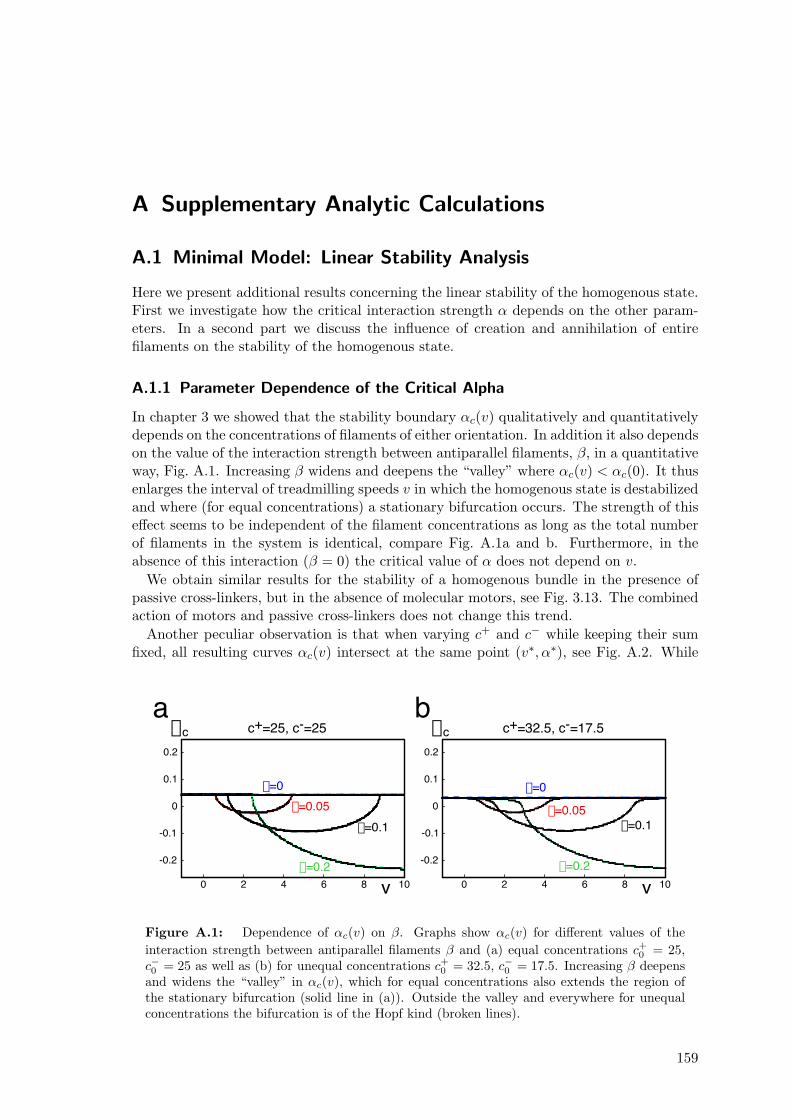
A Supplementary Analytic Calculations
A.1 Minimal Model: Linear Stability Analysis
Here we present additional results concerning the linear stability of the homogenous state.First we investigate how the critical interaction strength α depends on the other param-eters. In a second part we discuss the influence of creation and annihilation of entirefilaments on the stability of the homogenous state.
A.1.1 Parameter Dependence of the Critical Alpha
In chapter 3 we showed that the stability boundary αc(v) qualitatively and quantitativelydepends on the concentrations of filaments of either orientation. In addition it also dependson the value of the interaction strength between antiparallel filaments, β, in a quantitativeway, Fig. A.1. Increasing β widens and deepens the “valley” where αc(v) < αc(0). It thusenlarges the interval of treadmilling speeds v in which the homogenous state is destabilizedand where (for equal concentrations) a stationary bifurcation occurs. The strength of thiseffect seems to be independent of the filament concentrations as long as the total numberof filaments in the system is identical, compare Fig. A.1a and b. Furthermore, in theabsence of this interaction (β = 0) the critical value of α does not depend on v.
We obtain similar results for the stability of a homogenous bundle in the presence ofpassive cross-linkers, but in the absence of molecular motors, see Fig. 3.13. The combinedaction of motors and passive cross-linkers does not change this trend.
Another peculiar observation is that when varying c+ and c− while keeping their sumfixed, all resulting curves αc(v) intersect at the same point (v∗, α∗), see Fig. A.2. While
a bc+=25, c-=25 c+=32.5, c-=17.5
0 2 4 6 8 10
0.1
0
-0.1
-0.2
0.2
v
ac
b=0
b=0.2
b=0.1b=0.05
0 2 4 6 8 10
0.1
0
-0.1
-0.2
0.2
v
ac
b=0
b=0.2
b=0.1b=0.05
Figure A.1: Dependence of αc(v) on β. Graphs show αc(v) for different values of theinteraction strength between antiparallel filaments β and (a) equal concentrations c+
0 = 25,c−0 = 25 as well as (b) for unequal concentrations c+
0 = 32.5, c−0 = 17.5. Increasing β deepensand widens the “valley” in αc(v), which for equal concentrations also extends the region ofthe stationary bifurcation (solid line in (a)). Outside the valley and everywhere for unequalconcentrations the bifurcation is of the Hopf kind (broken lines).
159
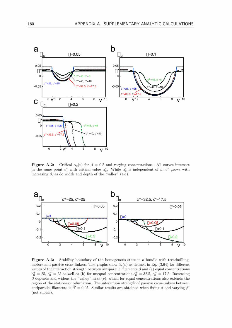
160 APPENDIX A. SUPPLEMENTARY ANALYTIC CALCULATIONS
a bb=0.05
c 0 2 4 6 8 10
0.05
0
-0.05
v
ac
c+=25, c-=25c+=32.5, c-=17.5
c+=40, c-=10
c+=45, c-=5
v*
a*
0 2 4 6 8 10
0.05
0
-0.05
v
ac
c+=25, c-=25
c+=32.5, c-=17.5
c+=40, c-=10
c+=45, c-=5
v*
a*
0 2 4 6 8 10
0.05
0
-0.05
v
ac
c+=25, c-=25
c+=32.5, c-=17.5 c+=40, c-=10
c+=45, c-=5
v*
a*
b=0.2
b=0.1
Figure A.2: Critical αc(v) for β = 0.5 and varying concentrations. All curves intersectin the same point v∗ with critical value α∗
c . While α∗c is independent of β, v∗ grows with
increasing β, as do width and depth of the “valley” (a-c).
a b
0 2 4 6 8 10
0.1
0
-0.1
-0.2
0.2
v
ac
b=0
b=0.2
b=0.1b=0.05
b'=0.05
0 2 4 6 8 10
0.1
0
-0.1
-0.2
0.2
v
ac
b=0
b=0.2
b=0.1b=0.05
b'=0.05
c+=25, c-=25 c+=32.5, c-=17.5
Figure A.3: Stability boundary of the homogenous state in a bundle with treadmilling,motors and passive cross-linkers. The graphs show αc(v) as defined in Eq. (3.64) for differentvalues of the interaction strength between antiparallel filaments β and (a) equal concentrationsc+0 = 25, c−0 = 25 as well as (b) for unequal concentrations c+
0 = 32.5, c−0 = 17.5. Increasingβ depends and widens the “valley” in αc(v), which for equal concentrations also extends theregion of the stationary bifurcation. The interaction strength of passive cross-linkers betweenantiparallel filaments is β′ = 0.05. Similar results are obtained when fixing β and varying β′
(not shown).
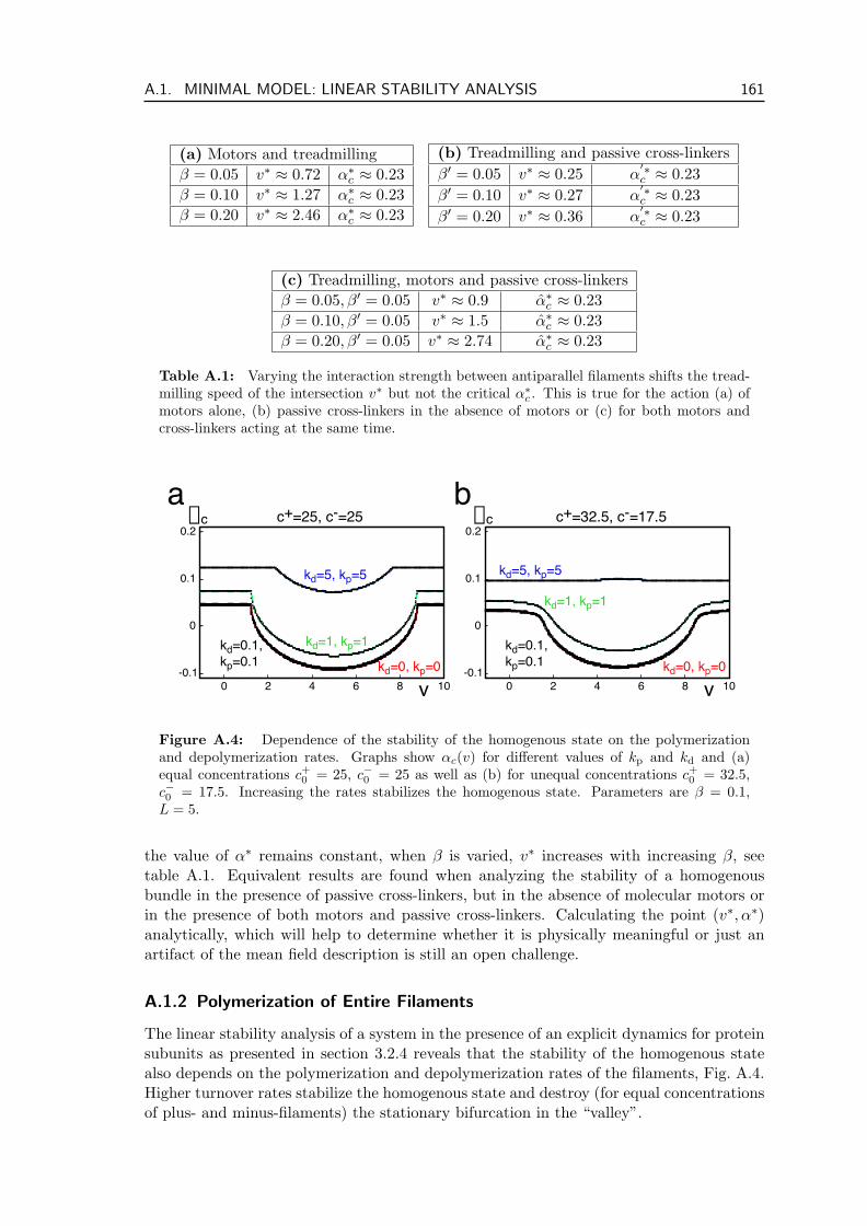
A.1. MINIMAL MODEL: LINEAR STABILITY ANALYSIS 161
(a) Motors and treadmillingβ = 0.05 v∗ ≈ 0.72 α∗c ≈ 0.23β = 0.10 v∗ ≈ 1.27 α∗c ≈ 0.23β = 0.20 v∗ ≈ 2.46 α∗c ≈ 0.23
(b) Treadmilling and passive cross-linkersβ′ = 0.05 v∗ ≈ 0.25 α
′∗c ≈ 0.23
β′ = 0.10 v∗ ≈ 0.27 α′∗c ≈ 0.23
β′ = 0.20 v∗ ≈ 0.36 α′∗c ≈ 0.23
(c) Treadmilling, motors and passive cross-linkersβ = 0.05, β′ = 0.05 v∗ ≈ 0.9 α∗c ≈ 0.23β = 0.10, β′ = 0.05 v∗ ≈ 1.5 α∗c ≈ 0.23β = 0.20, β′ = 0.05 v∗ ≈ 2.74 α∗c ≈ 0.23
Table A.1: Varying the interaction strength between antiparallel filaments shifts the tread-milling speed of the intersection v∗ but not the critical α∗
c . This is true for the action (a) ofmotors alone, (b) passive cross-linkers in the absence of motors or (c) for both motors andcross-linkers acting at the same time.
a b
0 2 4 6 8 10
0.1
0
-0.1
0.2
v
ac
kd=5, kp=5
kd=1, kp=1
kd=0, kp=0kd=0.1, kp=0.1
0 2 4 6 8 10
0.1
0
-0.1
0.2
v
ac
kd=5, kp=5
kd=1, kp=1
kd=0, kp=0kd=0.1, kp=0.1
c+=25, c-=25 c+=32.5, c-=17.5
Figure A.4: Dependence of the stability of the homogenous state on the polymerizationand depolymerization rates. Graphs show αc(v) for different values of kp and kd and (a)equal concentrations c+
0 = 25, c−0 = 25 as well as (b) for unequal concentrations c+0 = 32.5,
c−0 = 17.5. Increasing the rates stabilizes the homogenous state. Parameters are β = 0.1,L = 5.
the value of α∗ remains constant, when β is varied, v∗ increases with increasing β, seetable A.1. Equivalent results are found when analyzing the stability of a homogenousbundle in the presence of passive cross-linkers, but in the absence of molecular motors orin the presence of both motors and passive cross-linkers. Calculating the point (v∗, α∗)analytically, which will help to determine whether it is physically meaningful or just anartifact of the mean field description is still an open challenge.
A.1.2 Polymerization of Entire Filaments
The linear stability analysis of a system in the presence of an explicit dynamics for proteinsubunits as presented in section 3.2.4 reveals that the stability of the homogenous statealso depends on the polymerization and depolymerization rates of the filaments, Fig. A.4.Higher turnover rates stabilize the homogenous state and destroy (for equal concentrationsof plus- and minus-filaments) the stationary bifurcation in the “valley”.
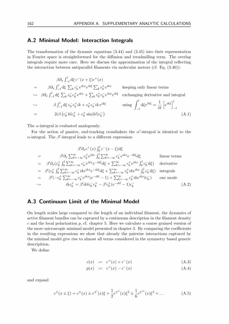
162 APPENDIX A. SUPPLEMENTARY ANALYTIC CALCULATIONS
A.2 Minimal Model: Interaction Integrals
The transformation of the dynamic equations (3.44) and (3.45) into their representationin Fourier space is straightforward for the diffusion and treadmilling term. The overlapintegrals require more care. Here we discuss the approximation of the integral reflectingthe interaction between antiparallel filaments via molecular motors (cf. Eq. (3.40)):
β∂x
∫ l−l dξ c−(x + ξ)c+(x)
= β∂x
∫ l−l dξ
∑k c−k eikxeikξ
∑k c+
k eikx keeping only linear terms
; β∂x
∫ l−l dξ
∑k c−0 c+
k eikx +∑
k c+0 c−k eikxeikξ exchanging derivative and integral
; β∫ l−l dξ c−0 c+
k ik + c+0 c−k ik eikξ using
∫ l
−ldξeikξ =
1ik
[eikξ]l−l
= 2iβ(c−0 klc+
k + c+0 sin(kl)c−k
)(A.1)
The α-integral is evaluated analogously.For the action of passive, end-tracking crosslinkers the α′-integral is identical to the
α-integral. The β′-integral leads to a different expression:
β′∂xc+(x)∫ l0 c−(x− ξ)dξ
= β′∂x∑∞
k=−∞ c+k eikx
∫ l0
∑∞k=−∞ c−k eikxe−ikξdξ linear terms
= β′∂x(c+0
∫ l0
∑∞k=−∞ c−k eikxe−ikξdξ +
∑∞k=−∞ c+
k eikx∫ l0 c−0 dξ) derivative
= β′(c+0
∫ l0
∑∞k=−∞ c−k ikeikxe−ikξdξ +
∑∞k=−∞ c+
k ikeikx∫ l0 c−0 dξ) integrals
= β′(−c+0
∑∞k=−∞ c−k eikx(e−ikl − 1) +
∑∞k=−∞ c+
k ikeikxlc−0 ) one mode
; ∂tc+k = β′iklc−0 c+
k − β′c+0 (e−ikl − 1)c−k (A.2)
A.3 Continuum Limit of the Minimal Model
On length scales large compared to the length of an individual filament, the dynamics ofactive filament bundles can be captured by a continuum description in the filament densityc and the local polarization p, cf. chapter 5. Here we calculate a coarse grained version ofthe more microscopic minimal model presented in chapter 3. By comparing the coefficientsin the resulting expressions we show that already the pairwise interactions captured bythe minimal model give rise to almost all terms considered in the symmetry based genericdescripition.
We define
c(x) := c+(x) + c−(x) (A.3)p(x) := c+(x)− c−(x) (A.4)
and expand
c±(x± ξ) = c±(x)± c±′(x)ξ +
12c±
′′(x)ξ2 ± 1
6c±
′′′(x)ξ3 + . . . (A.5)
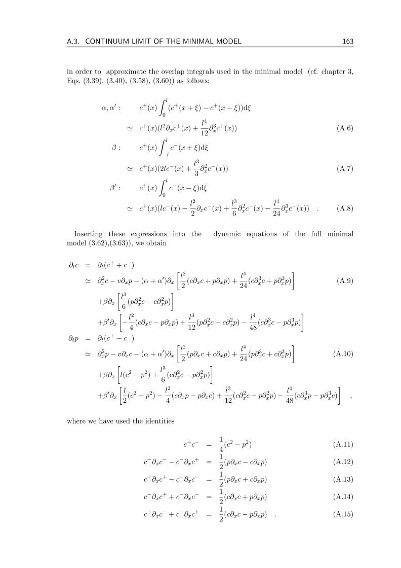
A.3. CONTINUUM LIMIT OF THE MINIMAL MODEL 163
in order to approximate the overlap integrals used in the minimal model (cf. chapter 3,Eqs. (3.39), (3.40), (3.58), (3.60)) as follows:
α, α′ : c+(x)∫ l
0(c+(x + ξ)− c+(x− ξ))dξ
' c+(x)(l2∂xc+(x) +l4
12∂3
xc+(x)) (A.6)
β : c+(x)∫ l
−lc−(x + ξ)dξ
' c+(x)(2lc−(x) +l3
3∂2
xc−(x)) (A.7)
β′ : c+(x)∫ l
0c−(x− ξ)dξ
' c+(x)(lc−(x)− l2
2∂xc−(x) +
l3
6∂2
xc−(x)− l4
24∂3
xc−(x)) . (A.8)
Inserting these expressions into the dynamic equations of the full minimalmodel (3.62),(3.63)), we obtain
∂tc = ∂t(c+ + c−)
' ∂2xc− v∂xp− (α + α′)∂x
[l2
2(c∂xc + p∂xp) +
l4
24(c∂3
xc + p∂3xp)]
(A.9)
+β∂x
[l3
6(p∂2
xc− c∂2xp)]
+β′∂x
[− l2
4(c∂xc− p∂xp) +
l3
12(p∂2
xc− c∂2xp)− l4
48(c∂3
xc− p∂3xp)]
∂tp = ∂t(c+ − c−)
' ∂2xp− v∂xc− (α + α′)∂x
[l2
2(p∂xc + c∂xp) +
l4
24(p∂3
xc + c∂3xp)]
(A.10)
+β∂x
[l(c2 − p2) +
l3
6(c∂2
xc− p∂2xp)]
+β′∂x
[l
2(c2 − p2)− l2
4(c∂xp− p∂xc) +
l3
12(c∂2
xc− p∂2xp)− l4
48(c∂3
xp− p∂3xc)]
,
where we have used the identities
c+c− =14(c2 − p2) (A.11)
c+∂xc− − c−∂xc+ =12(p∂xc− c∂xp) (A.12)
c+∂xc+ − c−∂xc− =12(p∂xc + c∂xp) (A.13)
c+∂xc+ + c−∂xc− =12(c∂xc + p∂xp) (A.14)
c+∂xc− + c−∂xc+ =12(c∂xc− p∂xp) . (A.15)
164 APPENDIX A. SUPPLEMENTARY ANALYTIC CALCULATIONS
Term in Factor in coarse grained Coefficient incurrent j microscopic model, Eq. (A.9) continuum description
∂xc 1 D
∂2xp −A1
∂3xc −A2
c∂xc −l2(2(α + α′) + β′)/4 −2B1
p∂xp −l2(2(α + α′)− β′)/4 −2B2
(∂xc)∂xp −2(E1 + E2)c∂2
xp −l3(2β + β′)/12 −E1
p∂2xc l3(2β + β′)/12 −E2
(∂xc)∂2xc −(F1 + 2F3)
c∂3xc −l4(2α + β′)/48 −F1
(∂xp)∂2xp −(F2 + 2F4)
p∂3xp −l4(2α− β′)/48 −F2
p −v −v
Table A.2: Relation of the coefficients used in the density currents from the generic con-tinuum description presented in chapter 5 and the coarse grained minimal model given byEqs. (A.9) and (A.10).
This coarse grained continuum limit of the minimal model can be compared with thegeneric continuum description, cf. chapter 5. In that description the respective currentsread (cf. Eqs. (5.14), (5.15), (5.16))
j = η−1∂xσ
= D∂xc−A1∂2xp−A2∂
3xc− 2B1c∂xc− 2B2p∂xp− E1
((∂xc)∂xp + c∂2
xp)
−E2
((∂xc)∂xp + p∂2
xc)− F1
((∂xc)∂2
xc + c∂3xc)− F2
((∂xp)∂2
xp + p∂3xp)
−2F3(∂xc)∂2xc− 2F4(∂xp)∂2
xp (A.16)
and
jp = ε(c2 − p2) + D∂xc−A1∂2xc−A2∂
3xp− B1c∂xp− B2p∂xc
−E1c∂2xc− E2p∂2
xp− E1(∂xc)2 − E2(∂xp)2
−F1c∂3xp− F2p∂3
xc− F3(∂xc)∂2xp− F4(∂xp)∂2
xc . (A.17)
In addition to these currents we also have to take into account the treadmilling currents,Eqs. (5.45) and (5.46):
jv = −vp (A.18)jp,v = −vc (A.19)
The tables A.2 and A.3 summarize the resulting relations between the coefficients in thecoarse grained model and the continuum description.
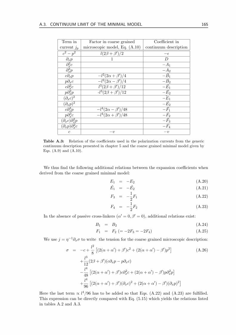
A.3. CONTINUUM LIMIT OF THE MINIMAL MODEL 165
Term in Factor in coarse grained Coefficient incurrent jp microscopic model, Eq. (A.10) continuum descriptionc2 − p2 l(2β + β′)/2 −ε
∂xp 1 D
∂2xc −A1
∂3xp −A2
c∂xp −l2(2α + β′)/4 −B1
p∂xc −l2(2α− β′)/4 −B2
c∂2xc l3(2β + β′)/12 −E1
p∂2xp -l3(2β + β′)/12 −E2
(∂xc)2 ˜−E1
(∂xp)2 −E2
c∂3xp −l4(2α− β′)/48 −F1
p∂3xc −l4(2α + β′)/48 −F2
(∂xc)∂2xp −F3
(∂xp)∂2xc −F4
c −v −v
Table A.3: Relation of the coefficients used in the polarization currents from the genericcontinuum description presented in chapter 5 and the coarse grained minimal model given byEqs. (A.9) and (A.10).
We thus find the following additional relations between the expansion coefficients whenderived from the coarse grained minimal model:
E1 = −E2 (A.20)E1 = −E2 (A.21)
F3 = −12F1 (A.22)
F4 = −12F2 (A.23)
In the absence of passive cross-linkers (α′ = 0, β′ = 0), additional relations exist:
B1 = B2 (A.24)F1 = F2 (= −2F3 = −2F4) (A.25)
We use j = η−1∂xσ to write the tension for the coarse grained microscopic description:
σ = −c +l2
8[(2(α + α′) + β′)c2 + (2(α + α′)− β′)p2
](A.26)
+l3
12(2β + β′)(c∂xp− p∂xc)
− l4
48[(2(α + α′) + β′)c∂2
xc + (2(α + α′)− β′)p∂2xp]
+l4
96[(2(α + α′) + β′)(∂xc)2 + (2(α + α′)− β′)(∂xp)2
]Here the last term ∝ l4/96 has to be added so that Eqs. (A.22) and (A.23) are fulfilled.This expression can be directly compared with Eq. (5.15) which yields the relations listedin tables A.2 and A.3.
166 APPENDIX A. SUPPLEMENTARY ANALYTIC CALCULATIONS

B Numerical Methods
B.1 Numerical Integration of the Mean Field Description
We numerically solve the equations (3.44) and (3.45) that describe the evolution of thefilament densities c± in the minimal model. In this appendix we present a detailed de-scription of the methods used to this end. For the integration in time we employ theforward Euler scheme (Press et al., 2002) in which the partial derivative of a function f isapproximated by
∂tf(t) =f(t + ∆t)− f(t)
∆t. (B.1)
This simple scheme is sufficient for the temporal integration of our system. The spatialintegration of the partial integro-differential equations requires more care. We now describethe discretization scheme explicitely.
The mean field descriptions presented in chapter 3 capture linear structures of lengthL. We discretize space and introduce a one dimensional lattice with lattice constant∆x. The concentrations of filaments and monomers are sampled on the sites. We definethe concentrations c±i = c±(i∆x, t), with i = 0, 1, . . . NL = L/∆x and the monomerconcentrations accordingly. Quantities with a dagger † denote the distributions at timet + ∆t, i.e. c±,†
i = c±(i∆x, t + ∆t). Currents in these quantities exist between sites, cf.Fig. B.1.
In the bulk, i.e. for i ∈ [1;NL−1] the discretization of the various currents is then givenby the following expressions:
Diffusion The diffusion current between two sites depends on the difference of the con-centrations on the respective sites:
j(D)±i =
D
∆x
(c±i−1 − c±i
)(B.2)
Motors between parallel filaments (Eq. (3.39)) The current is given by
j(α)±±i = α
(c±i−1S
±i − c±i S±i−`+1
)(B.3)
ii-3 i-2 i-1 i+1 i+2 i+3
ji
ci+1
pi+1
si+1
Figure B.1: Discretization scheme for mean field and continuum description. The densities,order parameters or stresses represented by c, p, σ respectively, are defined on the sites (hereexemplified on site i+1). The currents are defined between two sites. They point to and havethe same index as the site with the larger index, shown for ji.
167
168 APPENDIX B. NUMERICAL METHODS
where
` =⌊
l
∆x
⌋(B.4)
is the length of one filaments in units of ∆x. The symbol b·c denotes the floor, i.e.the next lower integer of the argument. We only consider cases when ` is an integer,odd number, as an even number would leave the center of the filaments between twosites. Furthermore we define Si, the number of filaments on sites i to i + `− 2:
S±i =i+`−2∑j=i
c±j ∆x (B.5)
Here the range of j = i· · · + ` − 2 represents interval in which filaments located atsite i can interact with other filaments located to their right.
Motors between antiparallel filaments (Eq. (3.40)) The direction of the current is dif-ferent for either filament orientation:
j(β)+−i = −βc+
i
(S−i−`+1 + c−i + S−i+1
)(B.6)
j(β)−+i = βc−i−1
(S+
i−` + c+i−1 + S+
i
)(B.7)
Treadmilling (Eq. (3.43)) The treadmilling current depends on the orientation of thefilaments
j(v)+i = vc+
i−1 (B.8)
j(v)−i = −vc−i (B.9)
Passive cross-linkers between parallel filaments (Eqs. (3.58) and (3.59)) The currentis identical to that for motors between parallel filaments (Eq. (B.3)) for α′ = α:
j(α′)±±i = α′
(c±i−1S
±i − c±i S±i−`+1
)(B.10)
Passive cross-linkers between antiparallel filaments (Eqs. (3.60) and (3.61)) The cur-rent is given by
j(β′)+−i = −β′c+
i S−i−`+1 (B.11)
j(β′)−+i = β′c−i−1S
+i (B.12)
All these partial currents are added up to give the effective filament current
j±i = = j(D)±i + j
(α)±±i + j
(β)±∓i + j
(v)±i + j
(α′)±±i + j
(β′)±∓i . (B.13)
The new concentrations are then given by
c†±i = c±i +∆t
∆x
[j±i − j±i+1
](B.14)
= c±i +∆t
∆x
[(j(D)±i − j
(D)±i+1
)+(j(α)±±i − j
(α)±±i+1
)+(j(β)±∓i − j
(β)±∓i+1
)+(j(v)±i − j
(v)±i+1
)+(j(α′)±±i − j
(α′)±±i+1
)+(j(β′)±∓i − j
(β′)±∓i+1
)]
B.2. NUMERICAL INTEGRATION OF THE CONTINUUM THEORY 169
B.2 Numerical Integration of the Continuum Theory
The integration of the continuum theory is not trivial and features a few caveats. Againwe introduce a lattice as in section B.1 on which the concentration c and the componentsof the order parameter px, qxx, qxy as well as the tension σ are defined. Denoting p = px
in one dimension the discretization of σ defined in Eq. (5.15) is given by
η−1σi = −Dci + A1pi+1 − pi−1
2∆x+ A2
ci+1 + ci−1 − 2ci
(∆x)2(B.15)
+B1c2i + B2p
2i + E1ci
pi+1 − pi−1
2∆x+ E2pi
ci+1 − ci−1
2∆x
+F1cici+1 + ci−1 − 2ci
(∆x)2+ F2pi
pi+1 + pi−1 − 2pi
(∆x)2
+F3
(ci+1 − ci−1
2∆x
)2
+ F4
(pi+1 − pi−1
2∆x
)2
.
Note that here we have used the symmetric first order derivative
∂xf(x) =f(x + ∆x)− f(x−∆x)
2∆x(B.16)
for c and p to assure that σ is localized on the sites. An asymmetric derivative wouldlead to contributions to σ that are not located on the lattice sites. The change in theconcentration for the bulk terms i ∈ [1;NL − 1] is then given by
c†i = ci + ∆tσi+1 + σi−1 − 2σi
(∆x)2(B.17)
for η = 1. The change in the polarization p is discretized analogously. The filament currentbetween sites i− 1 and i is given by
ji = −σi − σi−1
∆x. (B.18)
B.2.1 Description with Nematic Order
The discretization of the projected tension (Eq. (5.53)) is given by
η−1σxx,i = A1ci + A2c2i + A3ci
ci+1 + ci−1 − 2ci
(∆x)2(B.19)
+A4
(ci+1 − ci−1
2∆x
)2
+ A5qxx,i
Here again we have to use the symmetric first order derivative in order to assure that σ islocated on the sites. And the change in concentration c is then again given by Eq. (B.17).
For the changes in the components of the nematic order parameter, Eqs. (5.54) and(5.55), we obtain analogously:
ωxx,i = −B1qxx,i + B2qxx,i+1 + qxx,i−1 − 2qxx,i
(∆x)2+ B3
q(2)xx,i+1 + q
(2)xx,i−1 − 2q
(2)xx,i
(∆x)2
+B4ci+1 + ci−1 − 2ci
(∆x)2+ B5(q2
xx,i + q2xy,i)qxx,i (B.20)
ωxy = −B1qxy,i + B2qxy,i+1 + qxy,i−1 − 2qxy,i
(∆x)2+ B3
q(2)xy,i+1 + q
(2)xy,i−1 − 2q
(2)xy,i
(∆x)2
+B4ci+1 + ci−1 − 2ci
(∆x)2+ B5(q2
xx,i + q2xy,i)qxy,i (B.21)
170 APPENDIX B. NUMERICAL METHODS
where q(2)xx,i is the second order derivative at site i:
q(2)xx,i =
qxx,i+1 + qxx,i−1 − 2qxx,i
(∆x)2(B.22)
and for qxy analogously. The update in the order parameter is then given by
q†xx,i = qxx,i + ωxx,i∆t (B.23)
and qxy analogously.
B.2.2 Boundary Conditions
The update rules for the sites in the bulk i ∈ [1;NL − 1] have been given above. How toupdate the sites 0 and NL depends on the boundary conditions, which can have a hugeinfluence on the observed dynamics and asymptotic states.
Periodic Boundary Conditions
Periodic boundary conditions are readily implemented by using
c†0 = c0 + ∆tσ2 + σNL
− 2σ1
(∆x)2, c†NL
= cNL+ ∆t
σ0 + σNL−1 − 2σNL
(∆x)2, (B.24)
and calculating ωxx,1, ωxy,1, ωxx,NLand ωxy,NL
accordingly.
No Flux Boundary Conditions
No flux boundary conditions can be more complicated to implement correctly. Theirnumerical application is somewhat subtle. We illustrate the approach employed here,using the boundary conditions presented in Eqs. (5.77)-(5.81):
j = 0 (B.25)q = 0 (B.26)
∂xc = 0 (B.27)∂xqxx = 0 (B.28)∂xqxy = 0 (B.29)
at both x = 0 and x = L.Condition (B.25) is discretized by setting j0 = 0 and jNL+1 = 0. This can be realized by
introducing virtual sites i = −1 and i = NL + 1 and setting σ−1 = σ0 and σNL+1 = σNL
at each time step before updating the concentration. The across the boundaries currentsas given by Eq. (B.18) are then zero.
Condition (B.26) is trivially implemented by setting qxx,0 = 0, qxy,0 = 0, qxx,NL= 0,
qxy,NL= 0.
The remaining three conditions (B.27)-(B.29) are again captured by introducing quan-tities on the virtual sites. For the concentration choosing c−1 = c0 and cNL+1 = cNL
ateach time step prior to calculating σ and ω does the trick. We treat qxx and qxy in thesame way.
These ad-hoc choices of virtual values may seem problematic as they need not be selfconsistent, i.e. the choices for c and q on the virtual sites determine the stresses on thesesites. The filament current determined by the stresses could thus be different from zero.
B.2. NUMERICAL INTEGRATION OF THE CONTINUUM THEORY 171
While this is the case for many possible choices of boundary conditions, the boundaryconditions discussed above can always be made self consistent as the calculation of σi
requires values from sites i− 1, i, i + 1, which e.g. for σ−1 means it depends on the virtualvalue of e.g. ci−2 that is not restricted otherwise and can always be chosen so, that allboundary conditions are fulfilled.

172 APPENDIX B. NUMERICAL METHODS
C Supplementary Calculations to the Spindle
C.1 Forces between Asters
The general idea of hoe to determine the force contribution of motor dimers in the spindlehas been outlined in section 4.2.4. Here we complete the list of explicitly calculatedinstructive examples and show in detail how to calculate the force between two half andfull asters. This section concludes with a concise overview of the force contributions of allkinds of motors bound at all positions to two asters in section C.1.5. Explicit calculationsfor all possible cases are given in section C.5 at the end of this chapter.
C.1.1 Motors Bound to the Bulk
A motor dimer can bind to parallel microtubules of either minus- or plus-orientation,regions (a) and (c) of Fig. 4.5 respectively. Because it is the easiest (as all MTs involvedare plus-microtubules), we discuss region (c) first.
Region (c): parallel plus-microtubules. Here the velocity of the motor bound to thefirst MT (motor 1, black disk) and the second motor (motor 2, white disk) individuallyare given by Eq. (4.7):
x1 = v1 + L (C.1)x2 = v2 − L (C.2)
where the different signs in front of L are due to the opposing directions of movement ofthe two asters. Note that the subscripts 1, 2 refer to the aster the motor is bound to.
The two motors in the dimer are referred to as a, b, so that va is the load-free velocity ofmotor head a, and v1 is the speed of the motor bound to MT 1, which could in principlebe either motor a or b. Here we assume for simplicity and without loss of generality thatmotor a is bound to MT 1 and and b to 2. In terms of the force-velocity curves (Eq. (3.3)):
v1 = va + χaf1 (C.3)v2 = vb + χbf2 , (C.4)
where f1, f2 are the forces acting on motors bound to MT 1 and 2 respectively, measuredwith respect to the microtubule orientation. As the motors form a dimer we know that
x1 = x2 ⇒ v1 + L = v2 − L . (C.5)
We thus obtainva + χaf1 + L = vb + χbf2 − L . (C.6)
Furthermore the dimer impliesf1 = −f2 . (C.7)
173
174 APPENDIX C. SUPPLEMENTARY CALCULATIONS TO THE SPINDLE
Complex p-p m-m p-m m-pFig. 4.5cVelocities va > 0, vb > 0 va < 0, vb < 0 va > 0, vb < 0 va < 0, vb > 0
Forces f1 =vb − va
χa + χbf1 =
vb − va
χa + χbf1 =
vb − va
χa + χb< 0 f1 =
vb − va
χa + χb> 0
f = f1 f = f1 f = f1 < 0 f = f1 > 0Effect depends depends contractile expansive
Table C.1: Force contributions of different individual motor dimers bound to the bulk of twoMTs right of both asters (region (c), cf. Fig. 4.5c). The asters are assumed to be stationary(L = 0).
Hence we can solve Eq. (C.6) to obtain
f1 =vb − va − 2L
χa + χb(C.8)
x =χavb + χbva
χa + χb+
χb − χa
χa + χbL (C.9)
The force that this single dimer exerts on the two asters in this case is given by
f = f1 =vb − va − 2L
χa + χb. (C.10)
To further illustrate this result we explicitly calculate the contribution of four types ofmotor dimers:
• p-p: a homo-dimer of two ⊕-end directed motors
• m-m: a homo-dimer of two -end directed motors
• p-m: a hetero-dimer of a ⊕-end directed motor bound to MT 1 (from the right aster)and a -end directed motor bound to MT 2 (from the left aster)
• m-p: a hetero-dimer of a -end directed motor bound to MT 1 and a ⊕-end directedmotor bound to MT 2
Table C.1 summarizes the results for different kinds of motor dimers and stationary asters(L = 0).
For the calculation above and the expressions presented in table C.1 we assumed thatmotor a is bound to MT 1, and b to 2. For an ensemble of motors however it is equallylikely that b binds to MT 1. Thus when considering an ensemble of many motors, theaverage force contribution due to a single motor bound to the bulk of both MTs right ofboth asters is
F = 〈f1〉 =12
vb − va − 2L
χa + χb+
12
va − vb − 2L
χa + χb=
−2L
χa + χb(C.11)
where 〈·〉 denotes the average over all possible binding configurations. On average thesemotors thus do not contribute to the force acting on the asters, but oppose aster movement,because they lead to forces of opposite sign than the velocity of the asters. In conclusion:an ensemble of motors right of both asters acts essentially like passive cross-linkers. Notethat this result holds independent of the type of motor dimer (p-p, m-m, etc.).
C.1. FORCES BETWEEN ASTERS 175
Region (a): parallel minus-microtubules. The case of a dimer between two parallelminus-microtubules left of both asters is very similar to the case above. The details of thecalculation are given in C.5.1. We obtain for the force that a single dimer exerts on thetwo asters
f = −f1 = −vb − va + 2L
χa + χb(C.12)
where the negative sign in front of f1 is due to the orientation of microtubule 1. As f1 ismeasured with respect to the microtubule orientation and f is measured in the laboratoryreference frame, the two forces have opposite signs as MT 1 is a minus-microtubule. Ta-ble C.13 summarizes the resulting forces for different kinds of motor dimers and stationaryasters.
Considering an ensemble of many motors the average force contribution of a single motoris given by
F = −〈f1〉 = −12
vb − va + 2L
χa + χb− 1
2va − vb + 2L
χa + χb=
−2L
χa + χb. (C.13)
Not surprisingly the motors on the left of both asters act the same way as the motors rightof both asters, i.e. an ensemble of motors left of both asters acts essentially like passivecross-linkers.
Region (b): Between the Asters: Antiparallel Microtubules Here we consider motordimers that bind to plus-MTs originating from the left aster and to minus-MTs fromthe right aster. Due to the different orientations of the two microtubules involved, thecalculation is slightly different than above. The equations for the velocity of the dimerread
x1 = −v1 + L (C.14)x2 = v2 − L . (C.15)
Note that v1 and v2 enter with opposite signs due to the orientation of their respectivemicrotubules. The next important difference is that
f1 = −(−f2) (C.16)
where the first negative sign is due to the opposite orientation of both MTs (more pre-cisely because MT 1 is a minus-MT) and the second because the two heads form a dimer(actio=reactio). This yields
f1 =−va − vb + 2L
χa + χb(C.17)
x =χavb − χbva
χa + χb+
χb − χa
χa + χbL (C.18)
and the force that the dimer exerts on the two asters in this case is given by
f = −f1 =va + vb − 2L
χa + χb(C.19)
where again the negative sign in front of f1 is due to the orientation of microtubule 1.Table C.14 summarizes the results for different kinds of motor dimers and stationary
176 APPENDIX C. SUPPLEMENTARY CALCULATIONS TO THE SPINDLE
asters. For an ensemble of motors the average force contribution due to a motor bound tothe bulk of both MTs and right of both asters is
F = −〈f1〉 = −12−vb − va + 2L
χa + χb− 1
2−va − vb + 2L
χa + χb=
va + vb − 2L
χa + χb. (C.20)
This average force F will generally not be proportional to −L. Thus, an ensemble ofmotors between both asters may exert an active force on the asters.
C.1.2 Motors at the ⊕-Ends
When one motor head of a dimer reaches the end of its MT, it may either detach andthe dimer will not exert any force on the asters anymore, or it may stall at the end (atleast for a short time) and provide a mechanical link between the two asters. We consideronly dimers that remain attached to both MTs when reaching the end, as only they maycontribute to the dynamics directly. The motion of the other motor of the dimer is assumednot to be influenced by the stalling of the first. Here we describe the contribution of dimerswith one stalled head to the force on the asters.
Region (a): Left of Both Asters: Parallel Minus-Microtubules. The force contributionof a dimer between two parallel minus-microtubules when the dimer is bound to the bulkis given explicitly by Eq. (C.12). Either one of the two motor heads may be bound toan end of a MT originating from either aster, Fig. 4.6a (i) and (ii). Depending on thedetails of the situation this may change the force contribution. Table C.2 summarizes theresults for stationary asters (L = 0), which clearly reveals the effects binding to ends hason the force contributions. Being attached to an end only affects motors that have thecorresponding directionality (e.g. a plus-motor at a ⊕-end enters with velocity 0, whilethe velocity of a minus-motor remains unchanged) the force contribution depends on thetype of motor dimer under consideration. The motion of a dimer with two -end directedmotors for example is not at all influenced by being attached to a ⊕-end, but all othertypes are, compare the respective columns for end-binding cross-linkers in table C.2 andfor bulk-binding cross-linkers in table C.13. Especially the columns showing the resultsm-p and p-m dimers reveal the structure.
Ensemble averaging yields
F = −〈f1〉 = −12
vb − va + 2L
χa + χb− 1
2va − vb + 2L
χa + χb(C.21)
where the first term represents motor a bound to MT 1 and the second motor b boundto MT 1. As being attached to an end only affects motors that have the correspondingdirectionality (e.g. a plus-motor at a ⊕-end enters with velocity 0, while the velocity of aminus-motor remains unchanged) it depends on the type of motor dimer under consider-ation how we have to calculate the average of Eq. (C.21).
As an example, let us consider an ensemble of one type of hetero-dimers (w.o.l.g: va ≤0 ≤ vb). As va < 0 the a motor is not affected by the ⊕-end. In case (i) the b motor isonly affected when bound to MT 1:
F = −〈f1〉 = −12
vb − va + 2L
χa + χb− 1
2va + 2L
χa + χb=
12−vb − 4L
χa + χb(C.22)
and in case (ii) it is only affected when bound to MT2:
F = −〈f1〉 = −12−va + 2L
χa + χb− 1
2va − vb + 2L
χa + χb=
12
vb − 4L
χa + χb(C.23)
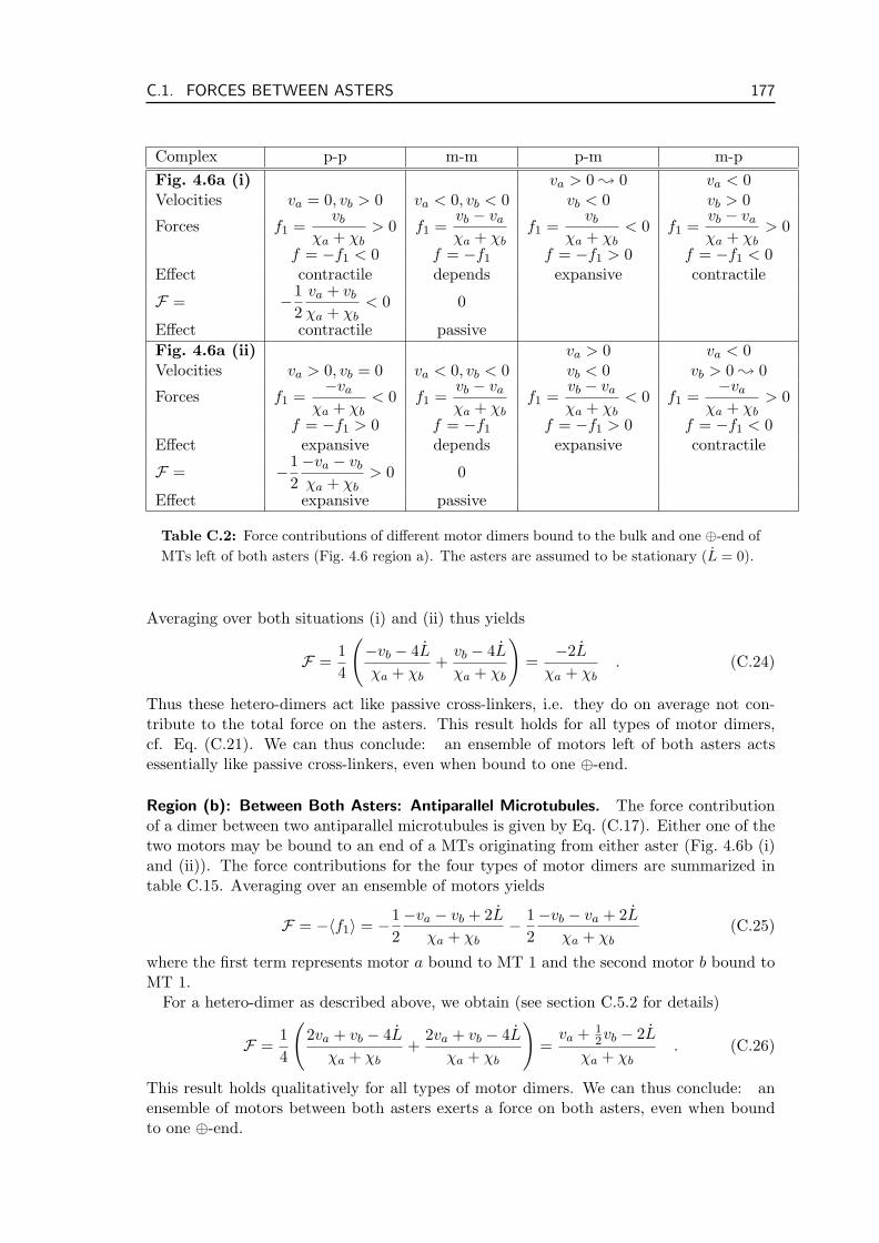
C.1. FORCES BETWEEN ASTERS 177
Complex p-p m-m p-m m-pFig. 4.6a (i) va > 0 ; 0 va < 0Velocities va = 0, vb > 0 va < 0, vb < 0 vb < 0 vb > 0
Forces f1 =vb
χa + χb> 0 f1 =
vb − va
χa + χbf1 =
vb
χa + χb< 0 f1 =
vb − va
χa + χb> 0
f = −f1 < 0 f = −f1 f = −f1 > 0 f = −f1 < 0Effect contractile depends expansive contractile
F = −12
va + vb
χa + χb< 0 0
Effect contractile passiveFig. 4.6a (ii) va > 0 va < 0Velocities va > 0, vb = 0 va < 0, vb < 0 vb < 0 vb > 0 ; 0
Forces f1 =−va
χa + χb< 0 f1 =
vb − va
χa + χbf1 =
vb − va
χa + χb< 0 f1 =
−va
χa + χb> 0
f = −f1 > 0 f = −f1 f = −f1 > 0 f = −f1 < 0Effect expansive depends expansive contractile
F = −12−va − vb
χa + χb> 0 0
Effect expansive passive
Table C.2: Force contributions of different motor dimers bound to the bulk and one ⊕-end ofMTs left of both asters (Fig. 4.6 region a). The asters are assumed to be stationary (L = 0).
Averaging over both situations (i) and (ii) thus yields
F =14
(−vb − 4L
χa + χb+
vb − 4L
χa + χb
)=
−2L
χa + χb. (C.24)
Thus these hetero-dimers act like passive cross-linkers, i.e. they do on average not con-tribute to the total force on the asters. This result holds for all types of motor dimers,cf. Eq. (C.21). We can thus conclude: an ensemble of motors left of both asters actsessentially like passive cross-linkers, even when bound to one ⊕-end.
Region (b): Between Both Asters: Antiparallel Microtubules. The force contributionof a dimer between two antiparallel microtubules is given by Eq. (C.17). Either one of thetwo motors may be bound to an end of a MTs originating from either aster (Fig. 4.6b (i)and (ii)). The force contributions for the four types of motor dimers are summarized intable C.15. Averaging over an ensemble of motors yields
F = −〈f1〉 = −12−va − vb + 2L
χa + χb− 1
2−vb − va + 2L
χa + χb(C.25)
where the first term represents motor a bound to MT 1 and the second motor b bound toMT 1.
For a hetero-dimer as described above, we obtain (see section C.5.2 for details)
F =14
(2va + vb − 4L
χa + χb+
2va + vb − 4L
χa + χb
)=
va + 12vb − 2L
χa + χb. (C.26)
This result holds qualitatively for all types of motor dimers. We can thus conclude: anensemble of motors between both asters exerts a force on both asters, even when boundto one ⊕-end.
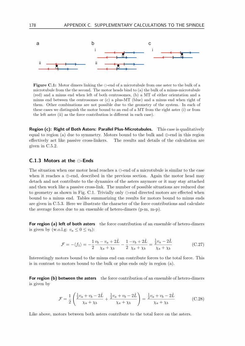
178 APPENDIX C. SUPPLEMENTARY CALCULATIONS TO THE SPINDLE
a b c
ii
i
ii
i
Figure C.1: Motor dimers linking the -end of a microtubule from one aster to the bulk of amicrotubule from the the second. The motor heads bind to (a) the bulk of a minus-microtubule(red) and a minus end when left of both centrosomes, (b) a MT of either orientation and aminus end between the centrosomes or (c) a plus-MT (blue) and a minus end when right ofthem. Other combinations are not possible due to the geometry of the system. In each ofthese cases we distinguish the motor bound to an end of a MT from the right aster (i) or fromthe left aster (ii) as the force contribution is different in each case).
Region (c): Right of Both Asters: Parallel Plus-Microtubules. This case is qualitativelyequal to region (a) due to symmetry. Motors bound to the bulk and ⊕-end in this regioneffectively act like passive cross-linkers. The results and details of the calculation aregiven in C.5.2.
C.1.3 Motors at the -Ends
The situation when one motor head reaches a -end of a microtubule is similar to the casewhen it reaches a ⊕-end, described in the previous section. Again the motor head maydetach and not contribute to the dynamics of the asters anymore or it may stay attachedand then work like a passive cross-link. The number of possible situations are reduced dueto geometry as shown in Fig. C.1. Trivially only -end directed motors are effected whenbound to a minus end. Tables summarizing the results for motors bound to minus endsare given in C.5.3. Here we illustrate the character of the force contributions and calculatethe average forces due to an ensemble of hetero-dimers (p-m, m-p).
For region (a) left of both asters the force contribution of an ensemble of hetero-dimersis given by (w.o.l.g: va ≤ 0 ≤ vb):
F = −〈f1〉 = −12
vb − va + 2L
χa + χb− 1
2−vb + 2L
χa + χb=
12va − 2L
χa + χb(C.27)
Interestingly motors bound to the minus end can contribute forces to the total force. Thisis in contrast to motors bound to the bulk or plus ends only in region (a).
For region (b) between the asters the force contribution of an ensemble of hetero-dimersis given by
F =12
(12va + vb − 2L
χa + χb+
12va + vb − 2L
χa + χb
)=
12va + vb − 2L
χa + χb(C.28)
Like above, motors between both asters contribute to the total force on the asters.
C.1. FORCES BETWEEN ASTERS 179
Dimer type Velocities of heads Densityp: plus-plus 0 ≤ vp
a ≤ vpb p(x)
m: minus-minus vma ≤ vm
b ≤ 0 m(x)h: hetero-dimer vh
a ≤ 0 ≤ vhb or vh
b ≤ 0 ≤ vha h(x)
Table C.3: Three different kinds of motor dimers. The densities of the two homo-dimersin which both heads move towards the same end are marked by p(x) and m(x) respectively.As it is impossible to distinguish an m-p from a p-m complex in solution they are describedby only one density for hetero-dimers h(x). We assume that a hetero-dimer binds with equalprobability either way to the two MTs.
For region (c) right of both asters the force contribution of an ensemble of hetero-dimersis given by
F = 〈f1〉 =12
vb − 2L
χa + χb+
12
va − vb − 2L
χa + χb=
12va − 2L
χa + χb(C.29)
Like the motors bound left of both asters, also motors bound to the minus end right ofboth asters contribute to the total force. In conclusion: motors bound to minus ends doalways contribute to the total force.
An overview of the force contributions of ensembles of the three different types of motordimers (p-p, m-m, p-m/m-p) under the three different ways of attachment (bulk-bulk,bulk-⊕-end, bulk--end) in all three zones of a spindle (a, b, and c) is given in C.1.5.
C.1.4 Example: Forces Between two Half Asters
As given by Eq. (4.6) the total force on both asters is the sum of the forces exerted by allthe motor dimers bound to MTs from both asters. In order to demonstrate the procedurewe calculate the forces acting on two half asters for three different types of motor dimers:homo-dimers p and m, and hetero-dimers h, cf. table C.3. The constraint to half asterseliminates all interactions left or right of both aster poles (zones (a) and (c)). It turns outthat the essential physics is already contained in this simplified scenario. The extensionto full asters is straightforward and discussed in section C.2.2. We furthermore discusshere only the forces between asters with an exponential microtubule distribution. Anapplication to homogenous asters is given in C.3.2.
Forces due to bulk-bulk bound motors. The forces per MT dimer on two half asterscharacterized by L and L due to bulk-bulk -interactions at x are given by (cf. Eq. (C.19)):
Fb(L, L, x) = −Cbρlp(x)ρr
m(x)
(p(x)
−vpa − vp
b + 2L
χpa + χp
b
(C.30)
+m(x)−vm
a − vmb + 2L
χma + χm
b
+ h(x)−vh
a − vhb + 2L
χha + χh
b
)= −Cbρ
lp(x)ρr
m(x)(p(x)f ′p + m(x)f ′m + h(x)f ′h
+2L[p(x)f ′′p + m(x)f ′′m + h(x)f ′′h ])
180 APPENDIX C. SUPPLEMENTARY CALCULATIONS TO THE SPINDLE
where the superscripts on the velocities denote the dimer type as introduced in table C.3and we have introduced the following variables:
f ′p =−vp
a − vpb
χpa + χp
b
≤ 0 , f ′′p =1
χpa + χp
b
> 0 (C.31)
f ′m =−vm
a − vmb
χma + χm
b
≥ 0 , f ′′m =1
χma + χm
b
> 0 (C.32)
f ′h =−vh
a − vhb
χha + χh
b
≤ 0 vh
a + vhb ≥ 0
≥ 0 vha + vh
b ≤ 0, f ′′h =
1χh
a + χhb
> 0 (C.33)
The constants f ′ describe the force on the 1st head of a dimer between stationary asters.For homogenous motor densities p(x) = p0 ≥ 0, m(x) = m0 ≥ 0, h(x) = h0 ≥ 0 and
exponential MT-densities as given by the equations in table 4.3 we obtain
Fb(L, L, x) = −Cba−2N2
0 e−2kL(p0f
′p + m0f
′m + h0f
′h (C.34)
+2L[p0f′′p + m0f
′′m + h0f
′′h ])
.
This expression is independent of the position x. The force on both asters is thus givenby
Fb(L, L) =∫ L
−LFb(L, L, x)dx = 2LFb(L, L, x) (C.35)
= −2Cba−2N2
0 Le−2kL(p0f
′p + m0f
′m + h0f
′h + 2L[p0f
′′p + m0f
′′m + h0f
′′h ])
.
As 2Cba−2N2
0 Le−2kL is always strictly positive, we can only have a stationary spindle ifthe term in the brackets is zero. This does not depend on the spindle length 2L, so thathalf asters which only interact via motors bound to the bulk can form stable, stationary(L = 0) spindles when p0f
′p + m0f
′m + h0f
′h = 0.
Forces due to bulk-⊕-end bound motors. The same procedure can be applied to dimerslinking the bulk and the ⊕-end of their two microtubules. For homogenous motor densitiesp(x) = p0 ≥ 0, m(x) = m0 ≥ 0, h(x) = h0 ≥ 0 and exponential MT-densities as given bythe equations in table 4.3 we obtain
Fp(L, L, x) = −2Cpa−1kN2
0 e−2kL
(12p0f
′p + m0f
′m +
12h0f
′h (C.36)
+12h0 min(vh
a , vhb )f ′′h + 2L[p0f
′′p + m0f
′′m + h0f
′′h ])
This expression is again independent of the position x. The force on both asters is thusgiven by
Fp(L, L) =∫ L
−LFp(L, L, x)dx = 2LFp(L, L, x) (C.37)
= −4Cpa−1kN2
0 Le−2kL
(12p0f
′p + m0f
′m +
12h0f
′h
+12h0 min(vh
a , vhb )f ′′h + 2L[p0f
′′p + m0f
′′m + h0f
′′h ])
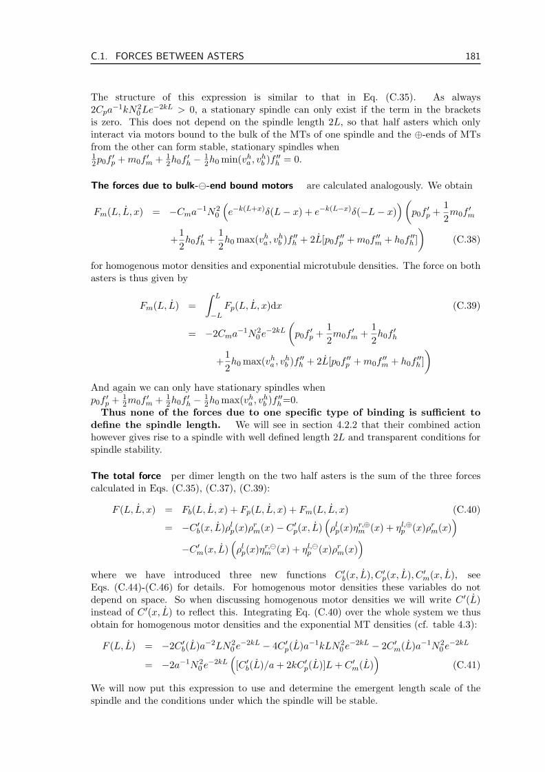
C.1. FORCES BETWEEN ASTERS 181
The structure of this expression is similar to that in Eq. (C.35). As always2Cpa
−1kN20 Le−2kL > 0, a stationary spindle can only exist if the term in the brackets
is zero. This does not depend on the spindle length 2L, so that half asters which onlyinteract via motors bound to the bulk of the MTs of one spindle and the ⊕-ends of MTsfrom the other can form stable, stationary spindles when12p0f
′p + m0f
′m + 1
2h0f′h −
12h0 min(vh
a , vhb )f ′′h = 0.
The forces due to bulk--end bound motors are calculated analogously. We obtain
Fm(L, L, x) = −Cma−1N20
(e−k(L+x)δ(L− x) + e−k(L−x)δ(−L− x)
)(p0f
′p +
12m0f
′m
+12h0f
′h +
12h0 max(vh
a , vhb )f ′′h + 2L[p0f
′′p + m0f
′′m + h0f
′′h ])
(C.38)
for homogenous motor densities and exponential microtubule densities. The force on bothasters is thus given by
Fm(L, L) =∫ L
−LFp(L, L, x)dx (C.39)
= −2Cma−1N20 e−2kL
(p0f
′p +
12m0f
′m +
12h0f
′h
+12h0 max(vh
a , vhb )f ′′h + 2L[p0f
′′p + m0f
′′m + h0f
′′h ])
And again we can only have stationary spindles whenp0f
′p + 1
2m0f′m + 1
2h0f′h −
12h0 max(vh
a , vhb )f ′′h=0.
Thus none of the forces due to one specific type of binding is sufficient todefine the spindle length. We will see in section 4.2.2 that their combined actionhowever gives rise to a spindle with well defined length 2L and transparent conditions forspindle stability.
The total force per dimer length on the two half asters is the sum of the three forcescalculated in Eqs. (C.35), (C.37), (C.39):
F (L, L, x) = Fb(L, L, x) + Fp(L, L, x) + Fm(L, L, x) (C.40)
= −C ′b(x, L)ρl
p(x)ρrm(x)− C ′
p(x, L)(ρl
p(x)ηr,⊕m (x) + ηl,⊕
p (x)ρrm(x)
)−C ′
m(x, L)(ρl
p(x)ηr,m (x) + ηl,
p (x)ρrm(x)
)where we have introduced three new functions C ′
b(x, L), C ′p(x, L), C ′
m(x, L), seeEqs. (C.44)-(C.46) for details. For homogenous motor densities these variables do notdepend on space. So when discussing homogenous motor densities we will write C ′(L)instead of C ′(x, L) to reflect this. Integrating Eq. (C.40) over the whole system we thusobtain for homogenous motor densities and the exponential MT densities (cf. table 4.3):
F (L, L) = −2C ′b(L)a−2LN2
0 e−2kL − 4C ′p(L)a−1kLN2
0 e−2kL − 2C ′m(L)a−1N2
0 e−2kL
= −2a−1N20 e−2kL
([C ′
b(L)/a + 2kC ′p(L)]L + C ′
m(L))
(C.41)
We will now put this expression to use and determine the emergent length scale of thespindle and the conditions under which the spindle will be stable.
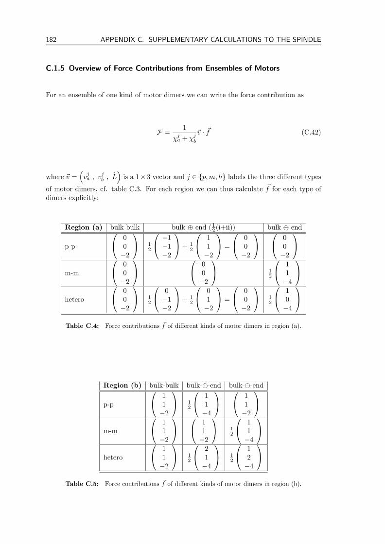
182 APPENDIX C. SUPPLEMENTARY CALCULATIONS TO THE SPINDLE
C.1.5 Overview of Force Contributions from Ensembles of Motors
For an ensemble of one kind of motor dimers we can write the force contribution as
F =1
χja + χj
b
~v · ~f (C.42)
where ~v =(vja , vj
b , L)
is a 1× 3 vector and j ∈ p, m, h labels the three different types
of motor dimers, cf. table C.3. For each region we can thus calculate ~f for each type ofdimers explicitly:
Region (a) bulk-bulk bulk-⊕-end (12(i+ii)) bulk--end
p-p
00−2
12
−1−1−2
+ 12
11−2
=
00−2
00−2
m-m
00−2
00−2
12
11−4
hetero
00−2
12
0−1−2
+ 12
01−2
=
00−2
12
10−4
Table C.4: Force contributions ~f of different kinds of motor dimers in region (a).
Region (b) bulk-bulk bulk-⊕-end bulk--end
p-p
11−2
12
11−4
11−2
m-m
11−2
11−2
12
11−4
hetero
11−2
12
21−4
12
12−4
Table C.5: Force contributions ~f of different kinds of motor dimers in region (b).
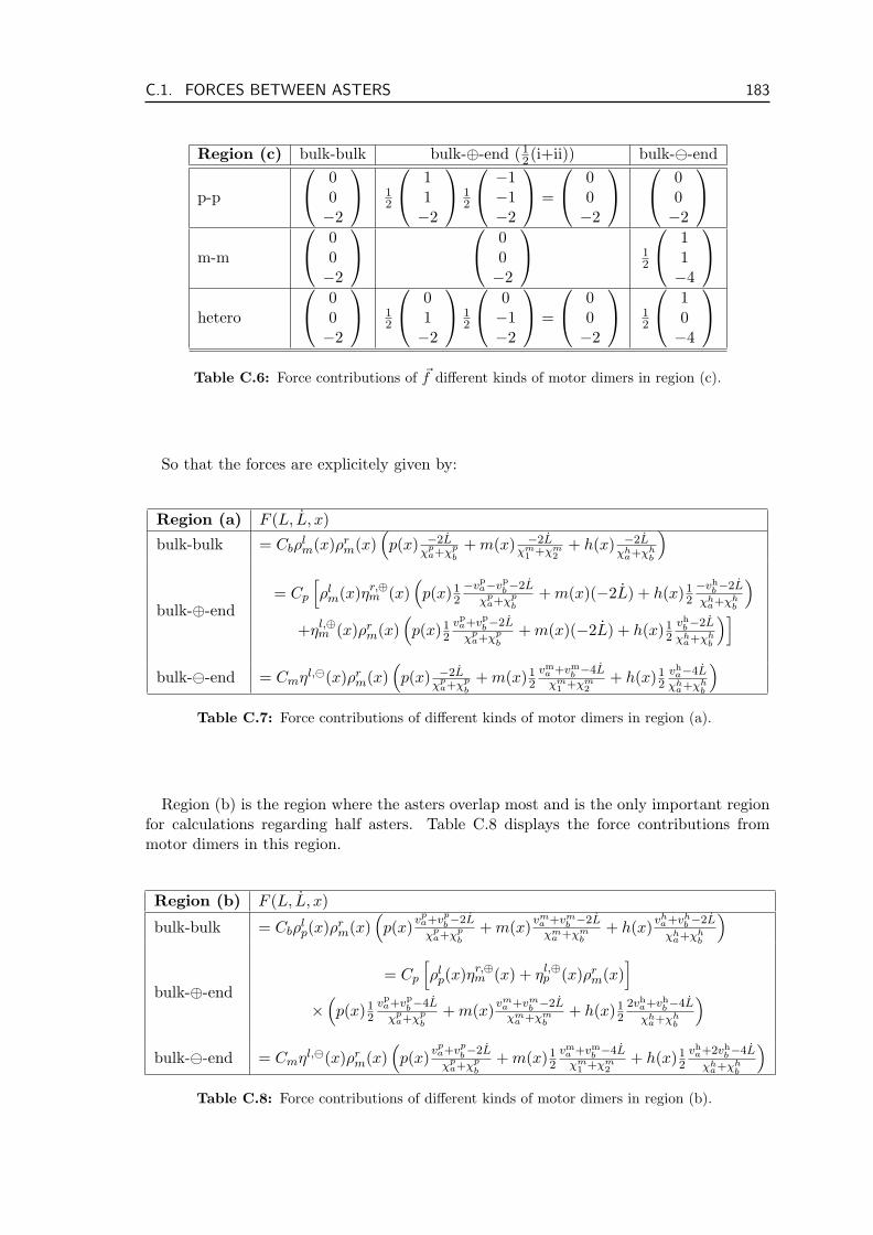
C.1. FORCES BETWEEN ASTERS 183
Region (c) bulk-bulk bulk-⊕-end (12(i+ii)) bulk--end
p-p
00−2
12
11−2
12
−1−1−2
=
00−2
00−2
m-m
00−2
00−2
12
11−4
hetero
00−2
12
01−2
12
0−1−2
=
00−2
12
10−4
Table C.6: Force contributions of ~f different kinds of motor dimers in region (c).
So that the forces are explicitely given by:
Region (a) F (L, L, x)
bulk-bulk = Cbρlm(x)ρr
m(x)(p(x) −2L
χpa+χp
b+ m(x) −2L
χm1 +χm
2+ h(x) −2L
χha+χh
b
)
bulk-⊕-end= Cp
[ρl
m(x)ηr,⊕m (x)
(p(x)1
2
−vpa−vp
b−2L
χpa+χp
b+ m(x)(−2L) + h(x)1
2−vh
b−2L
χha+χh
b
)+ηl,⊕
m (x)ρrm(x)
(p(x)1
2
vpa+vp
b−2L
χpa+χp
b+ m(x)(−2L) + h(x)1
2vh
b−2L
χha+χh
b
)]bulk--end = Cmηl,(x)ρr
m(x)(p(x) −2L
χpa+χp
b+ m(x)1
2vm
a +vmb −4L
χm1 +χm
2+ h(x)1
2vh
a−4L
χha+χh
b
)Table C.7: Force contributions of different kinds of motor dimers in region (a).
Region (b) is the region where the asters overlap most and is the only important regionfor calculations regarding half asters. Table C.8 displays the force contributions frommotor dimers in this region.
Region (b) F (L, L, x)
bulk-bulk = Cbρlp(x)ρr
m(x)(p(x)vp
a+vpb−2L
χpa+χp
b+ m(x)vm
a +vmb −2L
χma +χm
b+ h(x)vh
a+vhb −2L
χha+χh
b
)
bulk-⊕-end= Cp
[ρl
p(x)ηr,⊕m (x) + ηl,⊕
p (x)ρrm(x)
]×(p(x)1
2
vpa+vp
b−4L
χpa+χp
b+ m(x)vm
a +vmb −2L
χma +χm
b+ h(x)1
22vh
a+vhb−4L
χha+χh
b
)bulk--end = Cmηl,(x)ρr
m(x)(p(x)vp
a+vpb−2L
χpa+χp
b+ m(x)1
2vm
a +vmb −4L
χm1 +χm
2+ h(x)1
2vh
a+2vhb−4L
χha+χh
b
)Table C.8: Force contributions of different kinds of motor dimers in region (b).
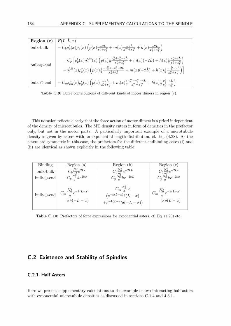
184 APPENDIX C. SUPPLEMENTARY CALCULATIONS TO THE SPINDLE
Region (c) F (L, L, x)
bulk-bulk = Cbρlp(x)ρr
p(x)(p(x) −2L
χpa+χp
b+ m(x) −2L
χm1 +χm
2+ h(x) −2L
χha+χh
b
)
bulk-⊕-end= Cp
[ρl
p(x)ηr,⊕p (x)
(p(x)1
2
vpa+vp
b−2L
χpa+χp
b+ m(x)(−2L) + h(x)1
2vh
b−2L
χha+χh
b
)+ηl,⊕
p (x)ρrp(x)
(p(x)1
2
−vpa+−vp
b−2L
χpa+χp
b+ m(x)(−2L) + h(x)1
2−vh
b−2L
χha+χh
b
)]bulk--end = Cmηr
m(x)ρlp(x)
(p(x) −2L
χpa+χp
b+ m(x)1
2vm
a +vmb −4L
χm1 +χm
2+ h(x)1
2vh
a−4L
χha+χh
b
)Table C.9: Force contributions of different kinds of motor dimers in region (c).
This notation reflects clearly that the force action of motor dimers is a priori independentof the density of microtubules. The MT density enters in form of densities in the prefactoronly, but not in the motor parts. A particularly important example of a microtubuledensity is given by asters with an exponential length distribution, cf. Eq. (4.38). As theasters are symmetric in this case, the prefactors for the different endbinding cases (i) and(ii) are identical as shown explicitly in the following table:
Binding Region (a) Region (b) Region (c)
bulk-bulk CbN2
0a2 e2kx Cb
N20
a2 e−2kL CbN2
0a2 e−2kx
bulk-⊕-end CpN2
0a ke2kx Cp
N20
a ke−2kL CpN2
0a ke−2kx
bulk--end CmN2
0
ae−k(L−x)
×δ(−L− x)
CmN2
0a ×(
e−k(L+x)δ(L− x)
+e−k(L−x)δ(−L− x)) Cm
N20
ae−k(L+x)
×δ(L− x)
Table C.10: Prefactors of force expressions for exponential asters, cf. Eq. (4.20) etc..
C.2 Existence and Stability of Spindles
C.2.1 Half Asters
Here we present supplementary calculations to the example of two interacting half asterswith exponential microtubule densities as discussed in sections C.1.4 and 4.3.1.
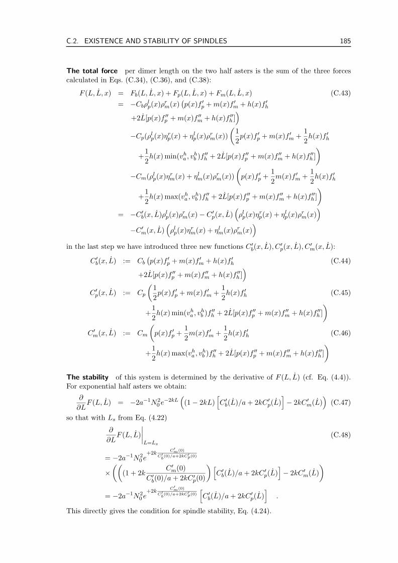
C.2. EXISTENCE AND STABILITY OF SPINDLES 185
The total force per dimer length on the two half asters is the sum of the three forcescalculated in Eqs. (C.34), (C.36), and (C.38):
F (L, L, x) = Fb(L, L, x) + Fp(L, L, x) + Fm(L, L, x) (C.43)= −Cbρ
lp(x)ρr
m(x)(p(x)f ′p + m(x)f ′m + h(x)f ′h
+2L[p(x)f ′′p + m(x)f ′′m + h(x)f ′′h ])
−Cp(ρlp(x)ηr
p(x) + ηlp(x)ρr
m(x))(
12p(x)f ′p + m(x)f ′m +
12h(x)f ′h
+12h(x) min(vh
a , vhb )f ′′h + 2L[p(x)f ′′p + m(x)f ′′m + h(x)f ′′h ]
)−Cm(ρl
p(x)ηrm(x) + ηl
m(x)ρrm(x))
(p(x)f ′p +
12m(x)f ′m +
12h(x)f ′h
+12h(x) max(vh
a , vhb )f ′′h + 2L[p(x)f ′′p + m(x)f ′′m + h(x)f ′′h ]
)= −C ′
b(x, L)ρlp(x)ρr
m(x)− C ′p(x, L)
(ρl
p(x)ηrp(x) + ηl
p(x)ρrm(x)
)−C ′
m(x, L)(ρl
p(x)ηrm(x) + ηl
m(x)ρrm(x)
)in the last step we have introduced three new functions C ′
b(x, L), C ′p(x, L), C ′
m(x, L):
C ′b(x, L) := Cb
(p(x)f ′p + m(x)f ′m + h(x)f ′h (C.44)
+2L[p(x)f ′′p + m(x)f ′′m + h(x)f ′′h ])
C ′p(x, L) := Cp
(12p(x)f ′p + m(x)f ′m +
12h(x)f ′h (C.45)
+12h(x) min(vh
a , vhb )f ′′h + 2L[p(x)f ′′p + m(x)f ′′m + h(x)f ′′h ]
)C ′
m(x, L) := Cm
(p(x)f ′p +
12m(x)f ′m +
12h(x)f ′h (C.46)
+12h(x) max(vh
a , vhb )f ′′h + 2L[p(x)f ′′p + m(x)f ′′m + h(x)f ′′h ]
)
The stability of this system is determined by the derivative of F (L, L) (cf. Eq. (4.4)).For exponential half asters we obtain:
∂
∂LF (L, L) = −2a−1N2
0 e−2kL((1− 2kL)
[C ′
b(L)/a + 2kC ′p(L)
]− 2kC ′
m(L))
(C.47)
so that with Ls from Eq. (4.22)
∂
∂LF (L, L)
∣∣∣∣L=Ls
(C.48)
= −2a−1N20 e
+2kC′
m(0)
C′b(0)/a+2kC′
p(0)
×((
(1 + 2kC ′
m(0)C ′
b(0)/a + 2kC ′p(0)
)[C ′
b(L)/a + 2kC ′p(L)
]− 2kC ′
m(L))
= −2a−1N20 e
+2kC′
m(0)
C′b(0)/a+2kC′
p(0)
[C ′
b(L)/a + 2kC ′p(L)
].
This directly gives the condition for spindle stability, Eq. (4.24).
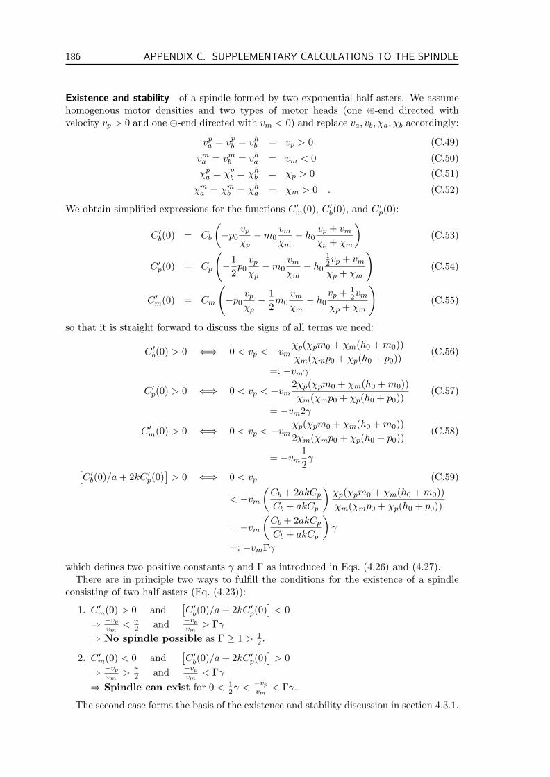
186 APPENDIX C. SUPPLEMENTARY CALCULATIONS TO THE SPINDLE
Existence and stability of a spindle formed by two exponential half asters. We assumehomogenous motor densities and two types of motor heads (one ⊕-end directed withvelocity vp > 0 and one -end directed with vm < 0) and replace va, vb, χa, χb accordingly:
vpa = vp
b = vhb = vp > 0 (C.49)
vma = vm
b = vha = vm < 0 (C.50)
χpa = χp
b = χhb = χp > 0 (C.51)
χma = χm
b = χha = χm > 0 . (C.52)
We obtain simplified expressions for the functions C ′m(0), C ′
b(0), and C ′p(0):
C ′b(0) = Cb
(−p0
vp
χp−m0
vm
χm− h0
vp + vm
χp + χm
)(C.53)
C ′p(0) = Cp
(−1
2p0
vp
χp−m0
vm
χm− h0
12vp + vm
χp + χm
)(C.54)
C ′m(0) = Cm
(−p0
vp
χp− 1
2m0
vm
χm− h0
vp + 12vm
χp + χm
)(C.55)
so that it is straight forward to discuss the signs of all terms we need:
C ′b(0) > 0 ⇐⇒ 0 < vp < −vm
χp(χpm0 + χm(h0 + m0))χm(χmp0 + χp(h0 + p0))
(C.56)
=: −vmγ
C ′p(0) > 0 ⇐⇒ 0 < vp < −vm
2χp(χpm0 + χm(h0 + m0))χm(χmp0 + χp(h0 + p0))
(C.57)
= −vm2γ
C ′m(0) > 0 ⇐⇒ 0 < vp < −vm
χp(χpm0 + χm(h0 + m0))2χm(χmp0 + χp(h0 + p0))
(C.58)
= −vm12γ[
C ′b(0)/a + 2kC ′
p(0)]
> 0 ⇐⇒ 0 < vp (C.59)
< −vm
(Cb + 2akCp
Cb + akCp
)χp(χpm0 + χm(h0 + m0))χm(χmp0 + χp(h0 + p0))
= −vm
(Cb + 2akCp
Cb + akCp
)γ
=: −vmΓγ
which defines two positive constants γ and Γ as introduced in Eqs. (4.26) and (4.27).There are in principle two ways to fulfill the conditions for the existence of a spindle
consisting of two half asters (Eq. (4.23)):
1. C ′m(0) > 0 and
[C ′
b(0)/a + 2kC ′p(0)
]< 0
⇒ −vp
vm< γ
2 and −vp
vm> Γγ
⇒ No spindle possible as Γ ≥ 1 > 12 .
2. C ′m(0) < 0 and
[C ′
b(0)/a + 2kC ′p(0)
]> 0
⇒ −vp
vm> γ
2 and −vp
vm< Γγ
⇒ Spindle can exist for 0 < 12γ <
−vp
vm< Γγ.
The second case forms the basis of the existence and stability discussion in section 4.3.1.
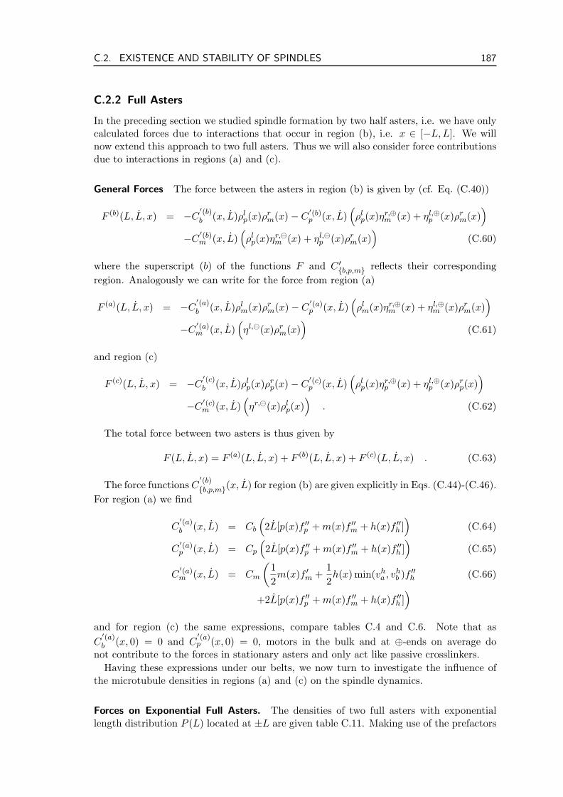
C.2. EXISTENCE AND STABILITY OF SPINDLES 187
C.2.2 Full Asters
In the preceding section we studied spindle formation by two half asters, i.e. we have onlycalculated forces due to interactions that occur in region (b), i.e. x ∈ [−L,L]. We willnow extend this approach to two full asters. Thus we will also consider force contributionsdue to interactions in regions (a) and (c).
General Forces The force between the asters in region (b) is given by (cf. Eq. (C.40))
F (b)(L, L, x) = −C′(b)b (x, L)ρl
p(x)ρrm(x)− C
′(b)p (x, L)
(ρl
p(x)ηr,⊕m (x) + ηl,⊕
p (x)ρrm(x)
)−C
′(b)m (x, L)
(ρl
p(x)ηr,m (x) + ηl,
p (x)ρrm(x)
)(C.60)
where the superscript (b) of the functions F and C ′b,p,m reflects their corresponding
region. Analogously we can write for the force from region (a)
F (a)(L, L, x) = −C′(a)b (x, L)ρl
m(x)ρrm(x)− C
′(a)p (x, L)
(ρl
m(x)ηr,⊕m (x) + ηl,⊕
m (x)ρrm(x)
)−C
′(a)m (x, L)
(ηl,(x)ρr
m(x))
(C.61)
and region (c)
F (c)(L, L, x) = −C′(c)b (x, L)ρl
p(x)ρrp(x)− C
′(c)p (x, L)
(ρl
p(x)ηr,⊕p (x) + ηl,⊕
p (x)ρrp(x)
)−C
′(c)m (x, L)
(ηr,(x)ρl
p(x))
. (C.62)
The total force between two asters is thus given by
F (L, L, x) = F (a)(L, L, x) + F (b)(L, L, x) + F (c)(L, L, x) . (C.63)
The force functions C′(b)b,p,m(x, L) for region (b) are given explicitly in Eqs. (C.44)-(C.46).
For region (a) we find
C′(a)b (x, L) = Cb
(2L[p(x)f ′′p + m(x)f ′′m + h(x)f ′′h ]
)(C.64)
C′(a)p (x, L) = Cp
(2L[p(x)f ′′p + m(x)f ′′m + h(x)f ′′h ]
)(C.65)
C′(a)m (x, L) = Cm
(12m(x)f ′m +
12h(x) min(vh
a , vhb )f ′′h (C.66)
+2L[p(x)f ′′p + m(x)f ′′m + h(x)f ′′h ])
and for region (c) the same expressions, compare tables C.4 and C.6. Note that asC
′(a)b (x, 0) = 0 and C
′(a)p (x, 0) = 0, motors in the bulk and at ⊕-ends on average do
not contribute to the forces in stationary asters and only act like passive crosslinkers.Having these expressions under our belts, we now turn to investigate the influence of
the microtubule densities in regions (a) and (c) on the spindle dynamics.
Forces on Exponential Full Asters. The densities of two full asters with exponentiallength distribution P (L) located at ±L are given table C.11. Making use of the prefactors
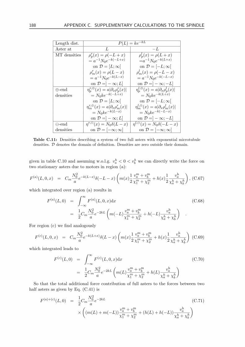
188 APPENDIX C. SUPPLEMENTARY CALCULATIONS TO THE SPINDLE
Length dist. P (L) = ke−kL
Aster at L −L
MT densities ρrp(x) = ρ(−L + x) ρl
p(x) = ρ(L + x)= a−1N0e
−k(−L+x) =a−1N0e−k(L+x)
on D = [L;∞[ on D = [−L;∞[ρr
m(x) = ρ(L− x) ρlm(x) = ρ(−L− x)
= a−1N0e−k(L−x) = a−1N0e
−k(−L−x)
on D =]−∞;L] on D =]−∞;−L]⊕-end ηr,⊕
p (x) = a|∂xρrp(x)| ηl,⊕
p (x) = a|∂xρlp(x)|
densities = N0ke−k(−L+x) = N0ke−k(L+x)
on D = [L;∞[ on D = [−L;∞[ηr,⊕
m (x) = a|∂xρrm(x)| ηl,⊕
m (x) = a|∂xρlm(x)|
= N0ke−k(L−x) = N0ke−k(−L−x)
on D =]−∞;L] on D =]−∞;−L]-end ηr,(x) = N0δ(L− x) ηl,(x) = N0δ(−L− x)densities on D = [−∞;∞] on D = [−∞;∞]
Table C.11: Densities describing a system of two full asters with exponential microtubuledensities. D denotes the domain of definition. Densities are zero outside their domain.
given in table C.10 and assuming w.o.l.g. vha < 0 < vh
b we can directly write the force ontwo stationary asters due to motors in region (a):
F (a)(L, 0, x) = CmN2
0
ae−k(L−x)δ(−L− x)
(m(x)
12
vma + vm
b
χm1 + χm
2
+ h(x)12
vha
χha + χh
b
), (C.67)
which integrated over region (a) results in
F (a)(L, 0) =∫ ∞
−∞F (a)(L, 0, x)dx (C.68)
=12Cm
N20
ae−2kL
(m(−L)
vma + vm
b
χm1 + χm
2
+ h(−L)vha
χha + χh
b
).
For region (c) we find analogously
F (c)(L, 0, x) = CmN2
0
ae−k(L+x)δ(L− x)
(m(x)
12
vma + vm
b
χm1 + χm
2
+ h(x)12
vha
χha + χh
b
)(C.69)
which integrated leads to
F (c)(L, 0) =∫ ∞
−∞F (c)(L, 0, x)dx (C.70)
=12Cm
N20
ae−2kL
(m(L)
vma + vm
b
χm1 + χm
2
+ h(L)vha
χha + χh
b
)So that the total additional force contribution of full asters to the forces between two
half asters as given by Eq. (C.41) is
F (a)+(c)(L, 0) =12Cm
N20
ae−2kL (C.71)
×(
(m(L) + m(−L))vma + vm
b
χm1 + χm
2
+ (h(L) + h(−L))vha
χha + χh
b
)
C.2. EXISTENCE AND STABILITY OF SPINDLES 189
For homogenous motor densities this expression simplifies further and leads to
F (a)+(c)(L, 0) = CmN2
0
ae−2kL
(m0
vma + vm
b
χm1 + χm
2
+ h0vha
χha + χh
b
)(C.72)
The total force on two stationary full asters with exponential microtubule distributiondue to homogenous motor from all three regions is then
F (L, 0) = −2N2
0
ae−2kL
([C
′(b)b (0)/a + 2kC
′(b)p (0)]L + C
′(a)m (0) + C
′(b)m (0)
)(C.73)
The conditions for existence and stability of stationary finite size spindles are thus onlyquantitatively changed with respect to the half asters discussed in section 4.3.1. Thestationary half length Ls of the spindle is given by
F (L, 0) = 0 ⇐⇒ Ls = − C′(a)m (0) + C
′(b)m (0)
C′(b)b (0)/a + 2kC
′(b)p (0)
. (C.74)
Again this expression reveals that in order for stationary spindles of finite length to exist,it is absolutely necessary to balance the force contribution of the -end-bulk interactionswith either one or both of the other two interactions. A spindle furthermore only existswhen
Ls > 0 ⇐⇒(C
′(a)m (0) + C
′(b)m (0)
)(C
′(b)b (0)/a + 2kC
′(b)p (0)
)< 0 . (C.75)
The stability of the spindle is again determined by Eq. (4.4). For the exponential asterswe obtain from Eq. (C.73):
∂
∂LF (L, 0) (C.76)
= −2N2
0
ae−2kL
((1− 2kL)
[C
′(b)b (0)/a + 2kC
′(b)p (0)
]− 2k
[C
′(a)m (0) + C
′(b)m (0)
])so that with Eq. (4.38)
∂
∂LF (L, 0)
∣∣∣∣L=Ls
= −2N2
0
ae+2kLs (C.77)
×(((1 + 2kLs)
[C
′(b)b (0)/a + 2kC
′(b)p (0)
]− 2k
[C
′(a)m (0) + C
′(b)m (0)
])= −2a−1N2
0 e+2k
C′(a)m (0)+C
′(b)m (0)
C′(b)b
(0)/a+2kC′(b)p (0)
[C
′(b)b (0)/a + 2kC
′(b)p (0)
].
As the prefactor is always negative, the sign is determined by the expression in thesquare brackets. A stationary spindle is stable if[
C′(b)b (0)/a + 2kC
′(b)p (0)
]> 0 . (C.78)
The conditions for existence and stability of spindles in the presence of motor dimersmade of two different motor heads, i.e. motor characteristics as given by Eqs. (C.49)-(C.52) do hardly change with respect to the case of half asters. The same calculation asdetailed in section 4.3.1 leads to
0 < γ < − vp
vm< Γγ (C.79)
which is the same as Eq. (4.25) except for missing the factor of 1/2 on the left. Again allspindles formed are stable.

190 APPENDIX C. SUPPLEMENTARY CALCULATIONS TO THE SPINDLE
C.3 Generality of Our Description
In chapter 4 we applied our description to asters with exponential MT densities, whichinteract via motor dimers that stay attached to the ends of the microtubules. For theemergence of a stationary spindle length, motors that stall at -ends were particularlyimportant. In this section we show that this effect is independent of a specific choice ofa distribution of -ends, as long as the intrinsic length scale of the distribution is smallcompared to k−1, the length scale of the exponential distribution of aster MTs.
Furthermore we show that the scale of the stationary length is set by the length scaleof the MT density. For exponential asters this is given by k−1 (Eq. 4.38). In section C.3.2we present calculations regarding homogenous asters, i.e. asters in which all MTs havethe same length l and show that this is sufficient for stable, finite size spindles to exist.
C.3.1 Various distributions of -ends
In chapter 4 we consider asters in which the -ends are precisely aligned in space, math-ematically described by a δ-distribution, which is singular and represents a special case.Here we investigate if the phenomena described above persist for two half asters when thedensity of -ends has a different form. We consider half a Gaussian distribution with halfwidth λ:
ηr,(x) =2N0
λ√
2πe−(L−x)2/2λ2
, ηl,m (x) =
2N0
λ√
2πe−(L+x)2/2λ2
(C.80)
both defined on D = [−L;L], and an exponential distribution:
ηr,(x) = N0kme−km(L−x) , ηl,(x) = N0kme−km(L+x) (C.81)
also both defined D = [−L;L]. The MT density as well as the ⊕-end distribution of thehalf asters are exponential as given in table 4.3. The domains of definition assure that thereare no MTs of the left half aster at x < −L and no MTs of the right half aster at x > L.The forces due to bulk-bulk and bulk-⊕-end interactions as calculated in Eqs. (C.34) and(C.36) remain unchanged.
Motivated by the biological system where the centrosome is small compared to thespindle, we assume the characteristic lengths of both distributions to be small compared tothe length of the MTs. The perturbation of the microtubule density due to the distributionof -ends is thus taken to be negligible:
λ k−1 and k−1m k−1 respectively. (C.82)
Now we calculate the overlap for bulk--end interactions as given in Eq. (C.38). Webegin with the Gaussian distributions, Eq. (C.80):∫ ∞
−∞dx (ρl
p(x)ηr,(x) + ηl,(x)ρrm(x)) (C.83)
=∫ ∞
−∞dx
N0
a
2N0
λ√
2π
(e−k(L−x)e−(L+x)2/2λ2
+ e−k(L+x)e−(L−x)2/2λ2)
=N2
0
ae−2kL+ 1
2k2λ2
(erf(
kλ√2) + erf(
2L− kλ2
√2λ
))
= a−1N20 e−2kL+ 1
2k2λ2
E(k, λ, L)
where we have introduced E(k, λ, L) := erf( kλ√2) + erf(2L−kλ2
√2λ
). As generally k L and
λ L, we may approximate E(k, λ, L) ≈ 1 and −2kL + 12k2λ2 ≈ −2kL and thus obtain
F (L, L) ≈ C ′mN2
0 e−2kL/a . (C.84)
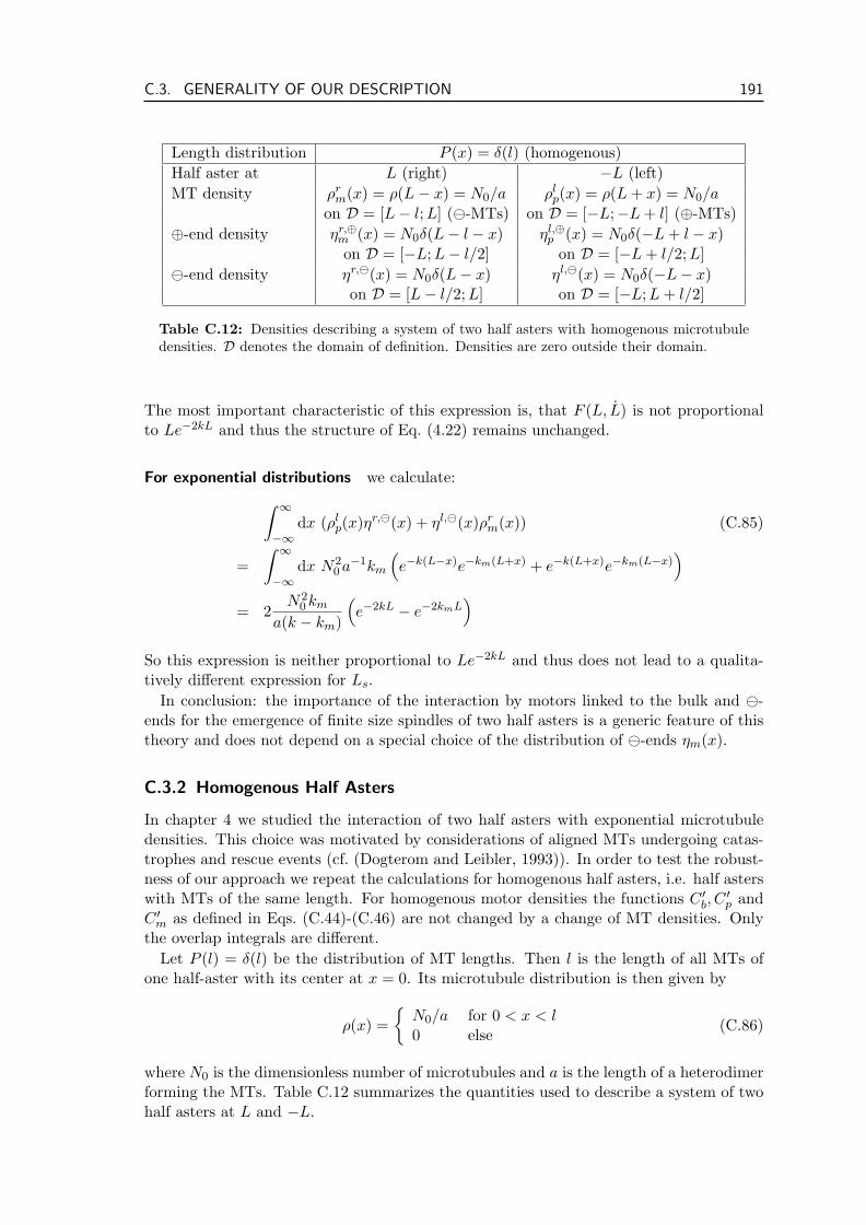
C.3. GENERALITY OF OUR DESCRIPTION 191
Length distribution P (x) = δ(l) (homogenous)Half aster at L (right) −L (left)MT density ρr
m(x) = ρ(L− x) = N0/a ρlp(x) = ρ(L + x) = N0/a
on D = [L− l;L] (-MTs) on D = [−L;−L + l] (⊕-MTs)⊕-end density ηr,⊕
m (x) = N0δ(L− l − x) ηl,⊕p (x) = N0δ(−L + l − x)
on D = [−L;L− l/2] on D = [−L + l/2;L]-end density ηr,(x) = N0δ(L− x) ηl,(x) = N0δ(−L− x)
on D = [L− l/2;L] on D = [−L;L + l/2]
Table C.12: Densities describing a system of two half asters with homogenous microtubuledensities. D denotes the domain of definition. Densities are zero outside their domain.
The most important characteristic of this expression is, that F (L, L) is not proportionalto Le−2kL and thus the structure of Eq. (4.22) remains unchanged.
For exponential distributions we calculate:∫ ∞
−∞dx (ρl
p(x)ηr,(x) + ηl,(x)ρrm(x)) (C.85)
=∫ ∞
−∞dx N2
0 a−1km
(e−k(L−x)e−km(L+x) + e−k(L+x)e−km(L−x)
)= 2
N20 km
a(k − km)
(e−2kL − e−2kmL
)So this expression is neither proportional to Le−2kL and thus does not lead to a qualita-tively different expression for Ls.
In conclusion: the importance of the interaction by motors linked to the bulk and -ends for the emergence of finite size spindles of two half asters is a generic feature of thistheory and does not depend on a special choice of the distribution of -ends ηm(x).
C.3.2 Homogenous Half Asters
In chapter 4 we studied the interaction of two half asters with exponential microtubuledensities. This choice was motivated by considerations of aligned MTs undergoing catas-trophes and rescue events (cf. (Dogterom and Leibler, 1993)). In order to test the robust-ness of our approach we repeat the calculations for homogenous half asters, i.e. half asterswith MTs of the same length. For homogenous motor densities the functions C ′
b, C′p and
C ′m as defined in Eqs. (C.44)-(C.46) are not changed by a change of MT densities. Only
the overlap integrals are different.Let P (l) = δ(l) be the distribution of MT lengths. Then l is the length of all MTs of
one half-aster with its center at x = 0. Its microtubule distribution is then given by
ρ(x) =
N0/a for 0 < x < l0 else
(C.86)
where N0 is the dimensionless number of microtubules and a is the length of a heterodimerforming the MTs. Table C.12 summarizes the quantities used to describe a system of twohalf asters at L and −L.
192 APPENDIX C. SUPPLEMENTARY CALCULATIONS TO THE SPINDLE
We obtain the following results for overlap of bulk-bulk, bulk-⊕-ends, and bulk--ends:∫ L
−Ldx ρl
p(x)ρrm(x) =
2(N0/a)2(l − L) for L ≤ l ≤ 2L
2(N0/a)2L for l > 2L2(N0/a)l for l < L
(C.87)
∫ L
−Ldx
(ρl
p(x)ηrp(x) + ηl
p(x)ρrm(x)
)=
2N2
0 /a for L ≤ l ≤ 2L0 else
(C.88)∫ L
−Ldx
(ρl
p(x)ηrm(x) + ηl
m(x)ρrm(x)
)=
2N2
0 /a for l > 2L0 else
(C.89)
For our discussion, we distinguish three cases:
1. l < L: the half asters do not overlap, no interaction due to motors, no formation ofspindles
2. L ≤ l < 2L: the half asters overlap but the MTs of one asters do not overlap withMT organizing center (centrosome) of the other half aster. In this case an overlapexists only in region (b) and the total force between the two asters is given by (cf.Eq. (C.41))
F (L, L) = 2N2
0
a
(C ′
b(L)(l − L)/a + C ′p(L)
)(C.90)
⇒ Ls = l + aC ′
p(0)C ′
b(0)(C.91)
and∂F (L, L)
∂L= −2
N20
a2C ′
b(L) . (C.92)
This leads to the following condition for a stationary spindle to exist (as we needL ≤ l < 2L):
−Ls < aC ′
p(0)C ′
b(0)≤ 0 (C.93)
and for stability we obtainC ′
b(0) > 0 . (C.94)
3. 2L ≤ l: the half asters overlap completely, i.e. no interaction between the bulk andthe ⊕-ends.
In this case the total force is given by
F (L, L) = 2N2
0
a
(LC ′
b(L)/a + C ′m(L)
)(C.95)
⇒ Ls = −aC ′
m(0)C ′
b(0)(C.96)
and∂F (L, L)
∂L= 2
N20
a2C ′
b(L) . (C.97)
This leads to the following condition for a stationary spindle to exist (as we need2L ≤ l):
0 < aC ′
m(0)C ′
b(0)≤ l
2(C.98)
and for stability we obtainC ′
b(0) < 0 . (C.99)
C.4. MICROTUBULE DISTRIBUTIONS IN 2D 193
Example: Two Types of Motor Heads. We consider two asters in the presence of motordimers made up of two types of motor heads with velocities vp and vm only. UsingEqs. (C.49)-(C.52) we can now discuss conditions for the existence of stable, finite sizespindles.
Case 2: L ≤ l < 2L The condition for a stable, finite size spindle is
C ′b(0) > 0 and C ′
p(0) ≥ 0 and aC ′
p(0)C ′
b(0)> −Ls (C.100)
⇐⇒ 0 <−vp
vm< γ and l > 0
Stable spindles thus can exist in this case.
Case 3: l ≥ 2L The condition for a stable, finite size spindle is
C ′b(0) < 0 and C ′
m(0) > 0 (C.101)
which can never be fulfilled. In this case the asters do not form stable spindles.
In conclusion we have shown that homogenous asters do also support finite size spindles.The existence of spindles is thus robust against the choice of different microtubule lengthdistributions.
C.4 Microtubule Distributions in 2D
Finally, we extend the description of microtubule asters to two spatial dimensions. Like insection 4.2.5 asters are primarily characterized by a distribution of microtubule lengths.An aster in two dimensions is characterized by a MT length distribution P (L, θ) which isnormalized ∫ ∞
0dL L
∫ 2π
0dθ P (L, θ) = 1 . (C.102)
The angle θ determines the direction in space, L the length of the microtubules. For anygiven direction θ the MT density is given by
ρ(r, θ) =N0
a
∫ ∞
rdL P (L, θ) (C.103)
so that the MT density on a circle of radius r is given by
ρ(r) =∫ 2π
0dθ rρ(r, θ) (C.104)
and the mass of the aster by
M =∫ ∞
0dr
∫ 2π
0dθ rρ(r, θ) =
N0
a
∫ ∞
0dr
∫ 2π
0dθ r
∫ ∞
rdL P (L, θ) . (C.105)
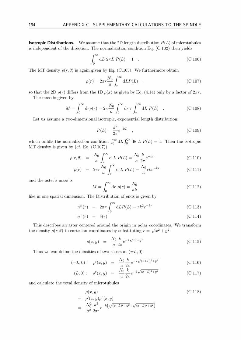
194 APPENDIX C. SUPPLEMENTARY CALCULATIONS TO THE SPINDLE
Isotropic Distributions. We assume that the 2D length distribution P (L) of microtubulesis independent of the direction. The normalization condition Eq. (C.102) then yields∫ ∞
0dL 2πL P (L) = 1 . (C.106)
The MT density ρ(r, θ) is again given by Eq. (C.103). We furthermore obtain
ρ(r) = 2πrN0
a
∫ ∞
rdLP (L) , (C.107)
so that the 2D ρ(r) differs from the 1D ρ(x) as given by Eq. (4.14) only by a factor of 2πr.The mass is given by
M =∫ ∞
0drρ(r) = 2π
N0
a
∫ ∞
0dr r
∫ ∞
rdL P (L) . (C.108)
Let us assume a two-dimensional isotropic, exponential length distribution:
P (L) =k2
2πe−kL , (C.109)
which fulfills the normalization condition∫∞0 dL
∫ 2π0 dθ L P (L) = 1. Then the isotropic
MT density is given by (cf. Eq. (C.107))
ρ(r, θ) =N0
a
∫ ∞
rd L P (L) =
N0
a
k
2πe−kr (C.110)
ρ(r) = 2πrN0
a
∫ ∞
rd L P (L) =
N0
arke−kr (C.111)
and the aster’s mass isM =
∫ ∞
0dr ρ(r) =
N0
ak(C.112)
like in one spatial dimension. The Distribution of ends is given by
η⊕(r) = 2πr
∫ ∞
0dLP (L) = rk2e−kr (C.113)
η(r) = δ(r) (C.114)
This describes an aster centered around the origin in polar coordinates. We transformthe density ρ(r, θ) to cartesian coordinates by substituting r =
√x2 + y2:
ρ(x, y) =N0
a
k
2πe−k
√x2+y2
(C.115)
Thus we can define the densities of two asters at (±L, 0):
(−L, 0) : ρl(x, y) =N0
a
k
2πe−k
√(x+L)2+y2
(C.116)
(L, 0) : ρr(x, y) =N0
a
k
2πe−k
√(x−L)2+y2
(C.117)
and calculate the total density of microtubules
ρ(x, y) (C.118)= ρl(x, y)ρr(x, y)
=N2
0
a2
k2
2π2e−k
“√(x+L)2+y2+
√(x−L)2+y2
”
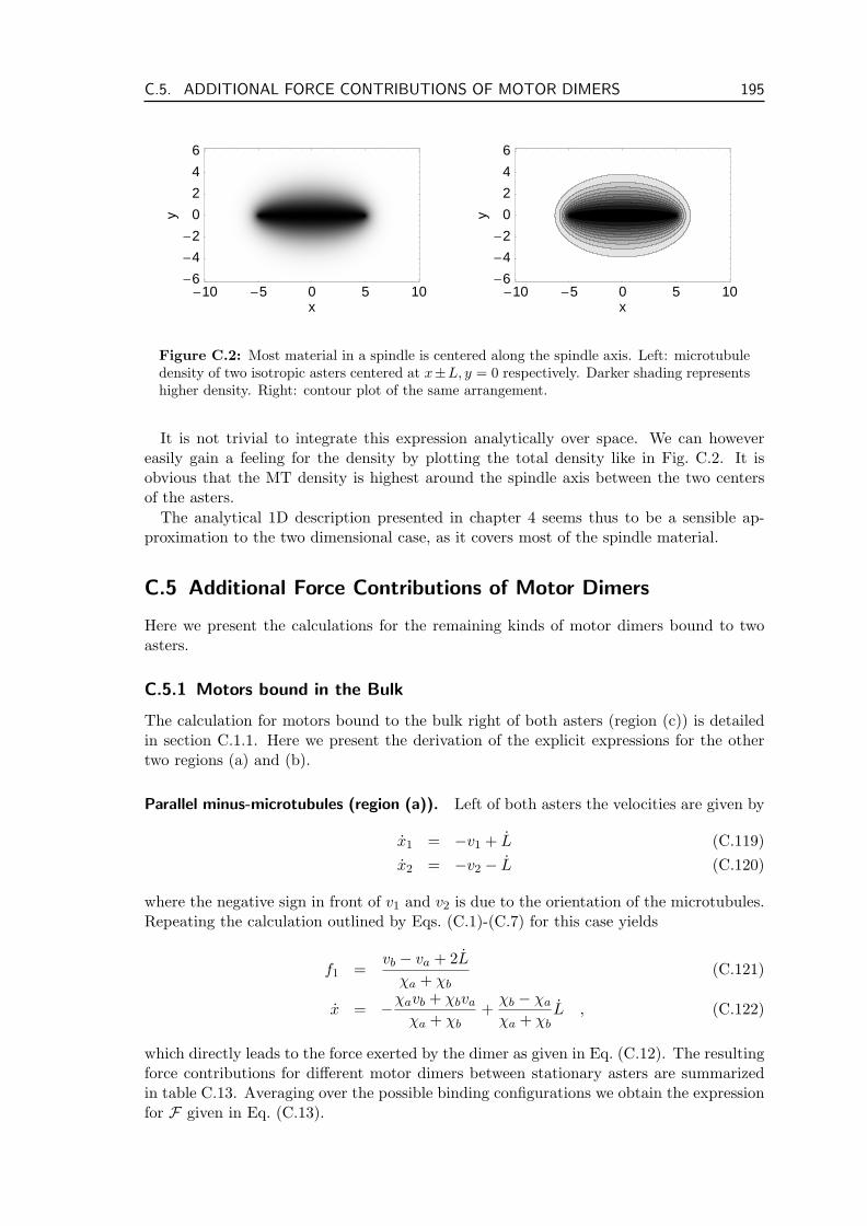
C.5. ADDITIONAL FORCE CONTRIBUTIONS OF MOTOR DIMERS 195
10 5 0 5 10x
6
4
2
0
2
4
6y
10 5 0 5 10x
6
4
2
0
2
4
6
y
Figure C.2: Most material in a spindle is centered along the spindle axis. Left: microtubuledensity of two isotropic asters centered at x±L, y = 0 respectively. Darker shading representshigher density. Right: contour plot of the same arrangement.
It is not trivial to integrate this expression analytically over space. We can howevereasily gain a feeling for the density by plotting the total density like in Fig. C.2. It isobvious that the MT density is highest around the spindle axis between the two centersof the asters.
The analytical 1D description presented in chapter 4 seems thus to be a sensible ap-proximation to the two dimensional case, as it covers most of the spindle material.
C.5 Additional Force Contributions of Motor Dimers
Here we present the calculations for the remaining kinds of motor dimers bound to twoasters.
C.5.1 Motors bound in the Bulk
The calculation for motors bound to the bulk right of both asters (region (c)) is detailedin section C.1.1. Here we present the derivation of the explicit expressions for the othertwo regions (a) and (b).
Parallel minus-microtubules (region (a)). Left of both asters the velocities are given by
x1 = −v1 + L (C.119)x2 = −v2 − L (C.120)
where the negative sign in front of v1 and v2 is due to the orientation of the microtubules.Repeating the calculation outlined by Eqs. (C.1)-(C.7) for this case yields
f1 =vb − va + 2L
χa + χb(C.121)
x = −χavb + χbva
χa + χb+
χb − χa
χa + χbL , (C.122)
which directly leads to the force exerted by the dimer as given in Eq. (C.12). The resultingforce contributions for different motor dimers between stationary asters are summarizedin table C.13. Averaging over the possible binding configurations we obtain the expressionfor F given in Eq. (C.13).
196 APPENDIX C. SUPPLEMENTARY CALCULATIONS TO THE SPINDLE
Complex p-p m-m p-m m-pFig. 4.5aVelocities va > 0, vb > 0 va < 0, vb < 0 va > 0, vb < 0 va < 0, vb > 0
Forces f1 =vb − va
χa + χbf1 =
vb − va
χa + χbf1 =
vb − va
χa + χb< 0 f1 =
vb − va
χa + χb> 0
f = −f1 f = −f1 f = −f1 > 0 f = −f1 < 0Effect depends depends expansive contractile
Table C.13: Force contributions of different motor dimers bound to the bulk of two MTs leftof both asters (region (a)). The asters are assumed to be stationary (L = 0).
Complex p-p m-m p-m m-pFig. 4.5bVelocities va > 0, vb > 0 va < 0, vb < 0 va > 0, vb < 0 va < 0, vb > 0
Forces f1 =−va − vb
χa + χbf1 =
−va − vb
χa + χbf1 =
−va − vb
χa + χbf1 =
−va − vb
χa + χbf = −f1 > 0 f = −f1 < 0 f = −f1 f = −f1
Effect expansive contractile depends depends
Table C.14: Force contributions of different individual motor dimers bound to the bulk oftwo MTs between both asters. The asters are assumed to be stationary (L = 0).
Between the Asters: Antiparallel Microtubules (region (b)) The detailed calculationfor this region is given by Eqs. (C.14)-(C.20). Table C.14 gives the explicit force contri-butions for the various kinds of motor dimers.
C.5.2 Forces due to Interactions between Bulk and ⊕-end
The results for motors left of both asters in region (a) is given in the main text in table C.2and Eq. (C.21). Here we present the explicit results for the remaining two regions (b) and(c).
Between Both Asters: Antiparallel Microtubules (region (b)). The explicit expressionsfor four kinds of motor dimers are summarized in table C.15.
C.5. ADDITIONAL FORCE CONTRIBUTIONS OF MOTOR DIMERS 197
Complex p-p m-m p-m m-pFig. 4.6b (i)Velocities va = 0, vb > 0 va < 0, vb < 0 va = 0, vb < 0 va < 0, vb > 0
Forces f1 =−vb
χa + χbf1 =
−va − vb
χa + χbf1 =
−vb
χa + χbf1 =
−va − vb
χa + χbf = −f1 f = −f1 f = −f1 f = −f1
Effect expansive contractile contractile dependsFig. 4.6b (ii)Velocities va > 0, vb = 0 va < 0, vb < 0 va > 0, vb < 0 va < 0, vb = 0
Forces f1 =−va
χa + χbf1 =
−va − vb
χa + χbf1 =
−va − vb
χa + χbf1 =
−va
χa + χbf = −f1 f = −f1 f = −f1 f = −f1
Effect expansive contractile depends contractile
Table C.15: Force contributions of different motor dimers bound to bulk and one ⊕-end ofMTs between of both asters (region(b)). The asters are assumed to be stationary (L = 0).
We have to exercise some care as the force contribution generally depends on which ofthe two binding possibilities (i) or (ii) the motor is in, cf. Fig. 4.6. We illustrate this pointconsidering a hetero-dimer (w.o.l.g: va ≤ 0 ≤ vb). As va < 0 the a motor is not affectedby the ⊕-end. In case (i) the b motor is only affected when bound to MT 1:
F = −〈f1〉 = −12−va − vb + 2L
χa + χb− 1
2−va + 2L
χa + χb=
12
2va + vb − 4L
χa + χb(C.123)
and in case (ii):
F = −〈f1〉 = −12−va + 2L
χa + χb− 1
2−va − vb + 2L
χa + χb=
12
2va + vb − 4L
χa + χb(C.124)
Averaging over these two cases leads to the average force contribution of a heterodimerbound to a ⊕-end in region (b):
F =12
(12
2va + vb − 4L
χa + χb+
12
2va + vb − 4L
χa + χb
)=
va + 12vb − 2L
χa + χb(C.125)
Right of Both Asters: Parallel Plus-Microtubules (region (c)). The force contributionof a dimer between two parallel ⊕-microtubules is given by Eq. (C.8). Either one of thetwo motors may be bound to an end of a MTs originating from either aster (cf. Fig. 4.6c(i) and (ii)). Table C.16 summarizes the results:
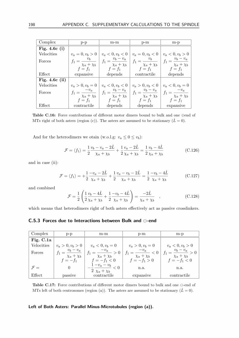
198 APPENDIX C. SUPPLEMENTARY CALCULATIONS TO THE SPINDLE
Complex p-p m-m p-m m-pFig. 4.6c (i)Velocities va = 0, vb > 0 va < 0, vb < 0 va = 0, vb < 0 va < 0, vb > 0
Forces f1 =vb
χa + χbf1 =
vb − va
χa + χbf1 =
vb
χa + χbf1 =
vb − va
χa + χbf = f1 f = f1 f = f1 f = f1
Effect expansive depends contractile dependsFig. 4.6c (ii)Velocities va > 0, vb = 0 va < 0, vb < 0 va > 0, vb < 0 va < 0, vb = 0
Forces f1 =−va
χa + χbf1 =
vb − va
χa + χbf1 =
vb − va
χa + χbf1 =
−va
χa + χbf = f1 f = f1 f = f1 f = f1
Effect contractile depends depends expansive
Table C.16: Force contributions of different motor dimers bound to bulk and one ⊕end ofMTs right of both asters (region (c)). The asters are assumed to be stationary (L = 0).
And for the heterodimers we otain (w.o.l.g: va ≤ 0 ≤ vb):
F = 〈f1〉 =12
vb − va − 2L
χa + χb+
12
va − 2L
χa + χb=
12
vb − 4L
χa + χb(C.126)
and in case (ii):
F = 〈f1〉 = +12−va − 2L
χa + χb+
12
va − vb − 2L
χa + χb=
12−vb − 4L
χa + χb(C.127)
and combined
F =12
(12
vb − 4L
χa + χb+
12−vb − 4L
χa + χb
)=
−2L
χa + χb, (C.128)
which means that heterodimers right of both asters effectively act as passive crosslinkers.
C.5.3 Forces due to Interactions between Bulk and -end
Complex p-p m-m p-m m-pFig. C.1aVelocities va > 0, vb > 0 va < 0, vb = 0 va > 0, vb = 0 va < 0, vb > 0
Forces f1 =vb − va
χa + χbf1 =
−va
χa + χb> 0 f1 =
−va
χa + χb< 0 f1 =
vb − va
χa + χb> 0
f = −f1 f = −f1 < 0 f = −f1 > 0 f = −f1 < 0
F = 0 −12−va − vb
χa + χb< 0 n.a. n.a.
Effect passive contractile expansive contractile
Table C.17: Force contributions of different motor dimers bound to bulk and one -end ofMTs left of both centrosomes (region (a)). The asters are assumed to be stationary (L = 0).
Left of Both Asters: Parallel Minus-Microtubules (region (a)).
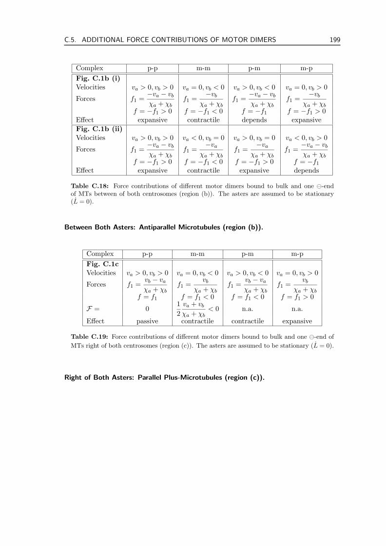
C.5. ADDITIONAL FORCE CONTRIBUTIONS OF MOTOR DIMERS 199
Complex p-p m-m p-m m-pFig. C.1b (i)Velocities va > 0, vb > 0 va = 0, vb < 0 va > 0, vb < 0 va = 0, vb > 0
Forces f1 =−va − vb
χa + χbf1 =
−vb
χa + χbf1 =
−va − vb
χa + χbf1 =
−vb
χa + χbf = −f1 > 0 f = −f1 < 0 f = −f1 f = −f1 > 0
Effect expansive contractile depends expansiveFig. C.1b (ii)Velocities va > 0, vb > 0 va < 0, vb = 0 va > 0, vb = 0 va < 0, vb > 0
Forces f1 =−va − vb
χa + χbf1 =
−va
χa + χbf1 =
−va
χa + χbf1 =
−va − vb
χa + χbf = −f1 > 0 f = −f1 < 0 f = −f1 > 0 f = −f1
Effect expansive contractile expansive depends
Table C.18: Force contributions of different motor dimers bound to bulk and one -endof MTs between of both centrosomes (region (b)). The asters are assumed to be stationary(L = 0).
Between Both Asters: Antiparallel Microtubules (region (b)).
Complex p-p m-m p-m m-pFig. C.1cVelocities va > 0, vb > 0 va = 0, vb < 0 va > 0, vb < 0 va = 0, vb > 0
Forces f1 =vb − va
χa + χbf1 =
vb
χa + χbf1 =
vb − va
χa + χbf1 =
vb
χa + χbf = f1 f = f1 < 0 f = f1 < 0 f = f1 > 0
F = 012
va + vb
χa + χb< 0 n.a. n.a.
Effect passive contractile contractile expansive
Table C.19: Force contributions of different motor dimers bound to bulk and one -end ofMTs right of both centrosomes (region (c)). The asters are assumed to be stationary (L = 0).
Right of Both Asters: Parallel Plus-Microtubules (region (c)).

200 APPENDIX C. SUPPLEMENTARY CALCULATIONS TO THE SPINDLE
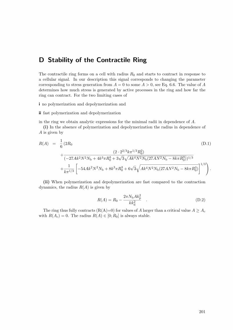
D Stability of the Contractile Ring
The contractile ring forms on a cell with radius R0 and starts to contract in response toa cellular signal. In our description this signal corresponds to changing the parametercorresponding to stress generation from A = 0 to some A > 0, see Eq. 6.6. The value of Adetermines how much stress is generated by active processes in the ring and how far thering can contract. For the two limiting cases of
i no polymerization and depolymerization and
ii fast polymerization and depolymerization
in the ring we obtain analytic expressions for the minimal radii in dependence of A.(i) In the absence of polymerization and depolymerization the radius in dependence of
A is given by
R(A) =16
(2R0 (D.1)
+(2 · 22/3kπ1/3R2
0)(−27Ak2N2Nb + 4k3πR3
0 + 3√
3√
Ak4N2Nb(27AN2Nb − 8kπR30))1/3
+1
kπ1/3
[−54Ak2N2Nb + 8k3πR3
0 + 6√
3√
Ak4N2Nb(27AN2Nb − 8kπR30)]1/3
).
(ii) When polymerization and depolymerization are fast compared to the contractiondynamics, the radius R(A) is given by
R(A) = R0 −2πNbAk2
p
kk2d
. (D.2)
The ring thus fully contracts (R(A)=0) for values of A larger than a critical value A ≥ Ac
with R(Ac) = 0. The radius R(A) ∈ [0;R0] is always stable.
201
202 APPENDIX D. STABILITY OF THE CONTRACTILE RING
Bibliography
Akhmanova, A. and Hoogenraad, C. (2005). Microtubule plus-end-tracking proteins:mechanisms and functions. Curr Opin Cell Biol, 17(1):47–54.
Alberts, B., Johnson, A., Lewis, J., Raff, M., Roberts, K., and Walter, P. (2002). MolecularBiology of the Cell. Garland Science.
Andersen, S. (2000). Spindle assembly and the art of regulating microtubule dynamics byMAPs and Stathmin/Op18. Trends Cell Biol, 10(7):261–7.
Anderson, D., Gueiros-Filho, F., and Erickson, H. (2004). Assembly dynamics of FtsZrings in Bacillus subtilis and Escherichia coli and effects of FtsZ-regulating proteins. JBacteriol, 186(17):5775–81.
Asbury, C. (2005). Kinesin: world’s tiniest biped. Curr Opin Cell Biol, 17(1):89–97.
Badoual, M., Julicher, F., and Prost, J. (2002). Bidirectional cooperative motion of molec-ular motors. Proc Natl Acad Sci U S A, 99(10):6696–701.
Balasubramanian, M., Bi, E., and Glotzer, M. (2004). Comparative analysis of cytokinesisin budding yeast, fission yeast and animal cells. Curr Biol, 14(18):R806–18.
Balland, M., Richert, A., and Gallet, F. (2005). The dissipative contribution of myosin IIin the cytoskeleton dynamics of myoblasts. Eur Biophys J, 34(3):255–61.
Bamburg, J., McGough, A., and Ono, S. (1999). Putting a new twist on actin:ADF/cofilins modulate actin dynamics. Trends Cell Biol, 9(9):364–70.
Banik, S., Kruse, K., and Julicher, F. (2005). Ring Formation by Polar Order. in prepa-ration.
Bassetti, B., Cosentino-Lagomarsino, M., and Jona, P. (2000). A model for the self-organization of microtubules driven by molecular motors. Eur. Phys. J. B, 15:483–492.
Beil, M., Micoulet, A., von Wichert, G., Paschke, S., Walther, P., Omary, M., Van Veld-hoven, P., Gern, U., Wolff-Hieber, E., Eggermann, J., Waltenberger, J., Adler, G.,Spatz, J., and Seufferlein, T. (2003). Sphingosylphosphorylcholine regulates keratinnetwork architecture and visco-elastic properties of human cancer cells. Nat Cell Biol,5(9):803–11.
Bi, E., Maddox, P., Lew, D., Salmon, E., McMillan, J., Yeh, E., and Pringle, J. (1998).Involvement of an actomyosin contractile ring in Saccharomyces cerevisiae cytokinesis.J Cell Biol, 142(5):1301–12.
Biron, D., Alvarez-Lacalle, E., Tlusty, T., and Moses, E. (2005). Molecular Model of theContractile Ring. Phys Rev Lett, 95:098102.
Blanchoin, L. and Pollard, T. (1999). Mechanism of interaction of Acanthamoeba ac-tophorin (ADF/Cofilin) with actin filaments. J Biol Chem, 274(22):15538–46.
203
204 Bibliography
Blanchoin, L. and Pollard, T. (2002). Hydrolysis of ATP by polymerized actin dependson the bound divalent cation but not profilin. Biochemistry, 41(2):597–602.
Block, S., Asbury, C., Shaevitz, J., and Lang, M. (2003). Probing the kinesin reactioncycle with a 2D optical force clamp. Proc Natl Acad Sci U S A, 100(5):2351–6.
Block, S., Goldstein, L., and Schnapp, B. (1990). Bead movement by single kinesinmolecules studied with optical tweezers. Nature, 348(6299):348–52.
Bornens, M., Paintrand, M., and Celati, C. (1989). The cortical microfilament systemof lymphoblasts displays a periodic oscillatory activity in the absence of microtubules:implications for cell polarity. J Cell Biol, 109(3):1071–83.
Boukellal, H., Campas, O., Joanny, J., Prost, J., and Sykes, C. (2004). Soft Listeria:actin-based propulsion of liquid drops. Phys Rev E Stat Nonlin Soft Matter Phys,69(6):061906.
Bourdieu, L., Duke, T., Elowitz, M., Winkelmann, D., Leibler, S., and Libchaber, A.(1995). Spiral defects in motility assays: A measure of motor protein force. Phys RevLett, 75(1):176–179.
Bray, D. (2001). Cell movements: from molecules to motility. Garland, New York, 2ndedition.
Bretschneider, T., Diez, S., Anderson, K., Heuser, J., Clarke, M., Muller-Taubenberger,A., Kohler, J., and Gerisch, G. (2004). Dynamic actin patterns and Arp2/3 assemblyat the substrate-attached surface of motile cells. Curr Biol, 14(1):1–10.
Bringmann, H., Skiniotis, G., Spilker, A., Kandels-Lewis, S., Vernos, I., and Surrey,T. (2004). A kinesin-like motor inhibits microtubule dynamic instability. Science,303(5663):1519–22.
Bucciarelli, E., Giansanti, M., Bonaccorsi, S., and Gatti, M. (2003). Spindle assembly andcytokinesis in the absence of chromosomes during Drosophila male meiosis. J Cell Biol,160(7):993–9.
Burton, K. and Taylor, D. (1997). Traction forces of cytokinesis measured with opticallymodified elastic substrata. Nature, 385(6615):450–4.
Carlier, M. and Pantaloni, D. (1986). Direct evidence for ADP-Pi-F-actin as the major in-termediate in ATP-actin polymerization. Rate of dissociation of Pi from actin filaments.Biochemistry, 25(24):7789–92.
Carlier, M., Pantaloni, D., Evans, J., Lambooy, P., Korn, E., and Webb, M. (1988).The hydrolysis of ATP that accompanies actin polymerization is essentially irreversible.FEBS Lett, 235(1-2):211–4.
Carlier, M., Ressad, F., and Pantaloni, D. (1999). Control of actin dynamics in cellmotility. Role of ADF/cofilin. J Biol Chem, 274(48):33827–30.
Chakravarty, A., Howard, L., and Compton, D. (2004). A mechanistic model for theorganization of microtubule asters by motor and non-motor proteins in a mammalianmitotic extract. Mol Biol Cell, 15(5):2116–32.
Bibliography 205
Chan, J., Calder, G., Doonan, J., and Lloyd, C. (2003). EB1 reveals mobile microtubulenucleation sites in Arabidopsis. Nat Cell Biol, 5(11):967–71.
Chan, J., Calder, G., Fox, S., and Lloyd, C. (2005). Localization of the MicrotubuleEnd Binding Protein EB1 Reveals Alternative Pathways of Spindle Development inArabidopsis Suspension Cells. Plant Cell, 17(6):1737–48.
Condeelis, J. and Taylor, D. (1977). The contractile basis of amoeboid movement. V. Thecontrol of gelation, solation, and contraction in extracts from Dictyostelium discoideum.J Cell Biol, 74(3):901–27.
Cooper, J. and Schafer, D. (2000). Control of actin assembly and disassembly at filamentends. Curr Opin Cell Biol, 12(1):97–103.
Cosentino-Lagomarsino, M. (2004). Biologically Inspired Problems Concerning SemiflexibleFilaments. PhD thesis, Univ. Leiden.
Cramer, L., Siebert, M., and Mitchison, T. (1997). Identification of novel graded polarityactin filament bundles in locomoting heart fibroblasts: implications for the generationof motile force. J Cell Biol, 136(6):1287–305.
Cross, M. and Hohenberg, P. C. (1993). Pattern formation outside of equilibrium. RevMod Phys, 65:851–1112.
Cytrynbaum, E., Rodionov, V., and Mogilner, A. (2004). Computational model of dynein-dependent self-organization of microtubule asters. J Cell Sci, 117:1381–97.
de Gennes, P. and Prost, J. (1993). The Physics of Liquid Crystals. Clarendon Press,Oxford, 2nd edition.
De La Cruz, E., Ostap, E., Brundage, R., Reddy, K., Sweeney, H., and Safer, D. (2000).Thymosin-beta(4) changes the conformation and dynamics of actin monomers. BiophysJ, 78(5):2516–27.
DeBiasio, R., LaRocca, G., Post, P., and Taylor, D. (1996). Myosin II transport, orga-nization, and phosphorylation: evidence for cortical flow/solation-contraction couplingduring cytokinesis and cell locomotion. Mol Biol Cell, 7(8):1259–82.
Desai, A. (2000). Kinetochores. Curr Biol, 10(14):R508.
Desai, A. and Mitchison, T. (1997). Microtubule polymerization dynamics. Annu Rev CellDev Biol, 13:83–117.
Dewar, H., Tanaka, K., Nasmyth, K., and Tanaka, T. (2004). Tension between two kine-tochores suffices for their bi-orientation on the mitotic spindle. Nature, 428(6978):93–7.
Dhonukshe, P. and Gadella, Jr, T. (2003). Alteration of microtubule dynamic instabil-ity during preprophase band formation revealed by yellow fluorescent protein-CLIP170microtubule plus-end labeling. Plant Cell, 15(3):597–611.
DiBella, L. and King, S. (2001). Dynein motors of the Chlamydomonas flagellum. Int RevCytol, 210:227–68.
Dickinson, R., Caro, L., and Purich, D. (2004). Force generation by cytoskeletal filamentend-tracking proteins. Biophys J, 87(4):2838–54.
206 Bibliography
Didry, D., Carlier, M., and Pantaloni, D. (1998). Synergy between actin depolymer-izing factor/cofilin and profilin in increasing actin filament turnover. J Biol Chem,273(40):25602–11.
Dobereiner, H., Dubin-Thaler, B., Giannone, G., Xenias, H., and Sheetz, M. (2004). Dy-namic phase transitions in cell spreading. Phys Rev Lett, 93(10):108105.
Dogterom, M., Janson, M., Faivre-Moskalenko C., van der Horst, A., KerssesmakersJ.W.J., Tanase, C., and Mulder, B. (2002). Force generation by polymerizing micro-tubules. Appl Phys A, 75:331–336.
Dogterom, M., Kerssemakers, J., Romet-Lemonne, G., and Janson, M. (2005). Forcegeneration by dynamic microtubules. Curr Opin Cell Biol, 17(1):67–74.
Dogterom, M. and Leibler, S. (1993). Physical aspects of the growth and regulation ofmicrotubule structures. Phys Rev Lett, 70(9):1347–1350.
Dogterom, M. and Yurke, B. (1997). Measurement of the force-velocity relation for growingmicrotubules. Science, 278(5339):856–60.
dos Remedios, C., Chhabra, D., Kekic, M., Dedova, I., Tsubakihara, M., Berry, D., andNosworthy, N. (2003). Actin binding proteins: regulation of cytoskeletal microfilaments.Physiol Rev, 83(2):433–73.
dos Remedios, C. and Thomas, D. (2001). Molecular Interactions of Actin. Actin Structureand Actin Binding Proteins. Springer Verlag, Heidelberg.
Dubin-Thaler, B., Giannone, G., Dobereiner, H., and Sheetz, M. (2004). Nanometeranalysis of cell spreading on matrix-coated surfaces reveals two distinct cell states andSTEPs. Biophys J, 86(3):1794–806.
Duke, T. (1999). Molecular model of muscle contraction. Proc Natl Acad Sci U S A,96(6):2770–5.
Duke, T. (2002a). Modelling Motor Protein Systems, chapter 3, pages 95–143. Les HouchesLecture Notes, Springer.
Duke, T. (2002b). Push or pull? Teams of motor proteins have it both ways. Proc NatlAcad Sci U S A, 99(10):6521–3.
Fabry, B., Maksym, G., Butler, J., Glogauer, M., Navajas, D., and Fredberg, J. (2001).Scaling the microrheology of living cells. Phys Rev Lett, 87(14):148102.
Faruki, S., Cole, R., and Rieder, C. (2002). Separating centrosomes interact in the ab-sence of associated chromosomes during mitosis in cultured vertebrate cells. Cell MotilCytoskeleton, 52(2):107–21.
Feierbach, B. and Chang, F. (2001). Cytokinesis and the contractile ring in fission yeast.Curr Opin Microbiol, 4(6):713–9.
Finer, J., Simmons, R., and Spudich, J. (1994). Single myosin molecule mechanics: pi-conewton forces and nanometre steps. Nature, 368(6467):113–9.
Fishkind, D. and Wang, Y. (1993). Orientation and three-dimensional organization ofactin filaments in dividing cultured cells. J Cell Biol, 123(4):837–48.
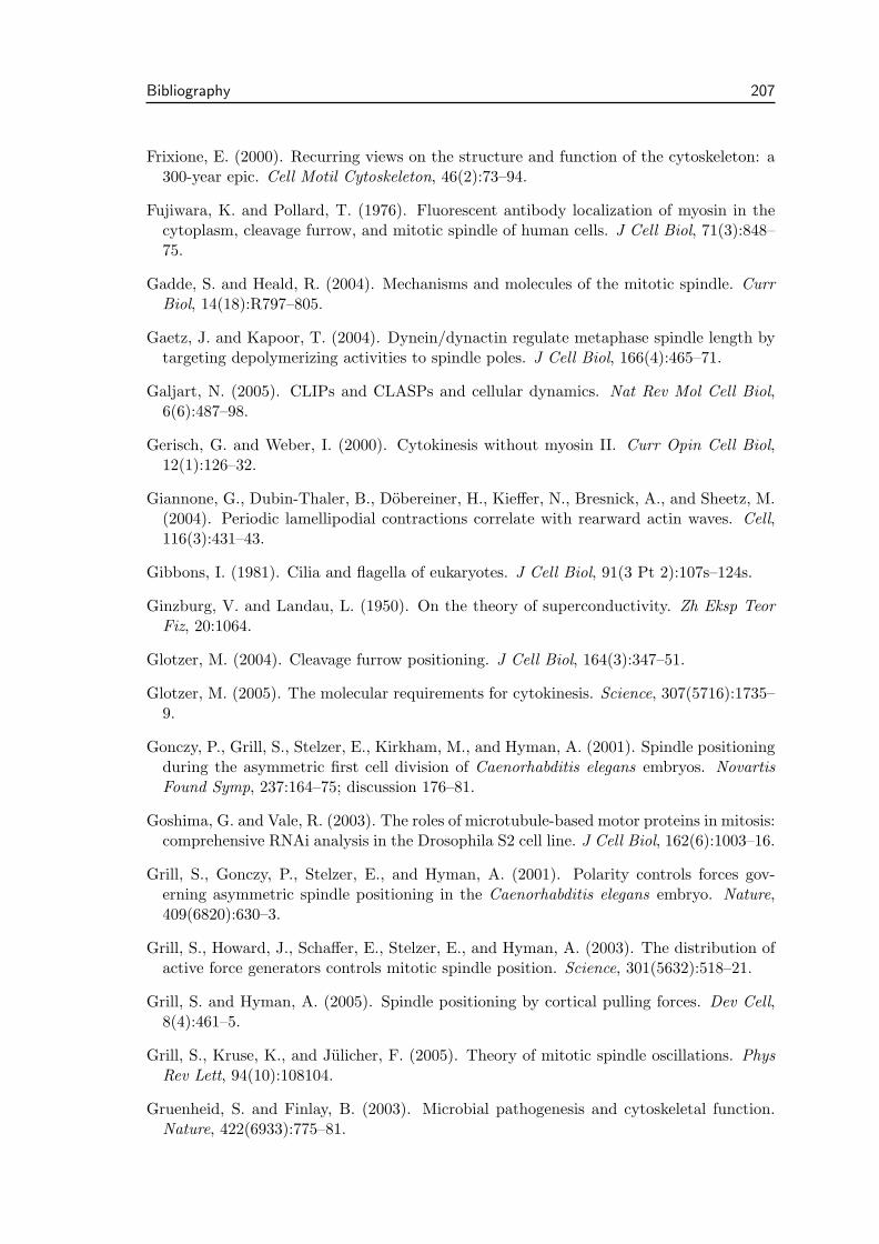
Bibliography 207
Frixione, E. (2000). Recurring views on the structure and function of the cytoskeleton: a300-year epic. Cell Motil Cytoskeleton, 46(2):73–94.
Fujiwara, K. and Pollard, T. (1976). Fluorescent antibody localization of myosin in thecytoplasm, cleavage furrow, and mitotic spindle of human cells. J Cell Biol, 71(3):848–75.
Gadde, S. and Heald, R. (2004). Mechanisms and molecules of the mitotic spindle. CurrBiol, 14(18):R797–805.
Gaetz, J. and Kapoor, T. (2004). Dynein/dynactin regulate metaphase spindle length bytargeting depolymerizing activities to spindle poles. J Cell Biol, 166(4):465–71.
Galjart, N. (2005). CLIPs and CLASPs and cellular dynamics. Nat Rev Mol Cell Biol,6(6):487–98.
Gerisch, G. and Weber, I. (2000). Cytokinesis without myosin II. Curr Opin Cell Biol,12(1):126–32.
Giannone, G., Dubin-Thaler, B., Dobereiner, H., Kieffer, N., Bresnick, A., and Sheetz, M.(2004). Periodic lamellipodial contractions correlate with rearward actin waves. Cell,116(3):431–43.
Gibbons, I. (1981). Cilia and flagella of eukaryotes. J Cell Biol, 91(3 Pt 2):107s–124s.
Ginzburg, V. and Landau, L. (1950). On the theory of superconductivity. Zh Eksp TeorFiz, 20:1064.
Glotzer, M. (2004). Cleavage furrow positioning. J Cell Biol, 164(3):347–51.
Glotzer, M. (2005). The molecular requirements for cytokinesis. Science, 307(5716):1735–9.
Gonczy, P., Grill, S., Stelzer, E., Kirkham, M., and Hyman, A. (2001). Spindle positioningduring the asymmetric first cell division of Caenorhabditis elegans embryos. NovartisFound Symp, 237:164–75; discussion 176–81.
Goshima, G. and Vale, R. (2003). The roles of microtubule-based motor proteins in mitosis:comprehensive RNAi analysis in the Drosophila S2 cell line. J Cell Biol, 162(6):1003–16.
Grill, S., Gonczy, P., Stelzer, E., and Hyman, A. (2001). Polarity controls forces gov-erning asymmetric spindle positioning in the Caenorhabditis elegans embryo. Nature,409(6820):630–3.
Grill, S., Howard, J., Schaffer, E., Stelzer, E., and Hyman, A. (2003). The distribution ofactive force generators controls mitotic spindle position. Science, 301(5632):518–21.
Grill, S. and Hyman, A. (2005). Spindle positioning by cortical pulling forces. Dev Cell,8(4):461–5.
Grill, S., Kruse, K., and Julicher, F. (2005). Theory of mitotic spindle oscillations. PhysRev Lett, 94(10):108104.
Gruenheid, S. and Finlay, B. (2003). Microbial pathogenesis and cytoskeletal function.Nature, 422(6933):775–81.
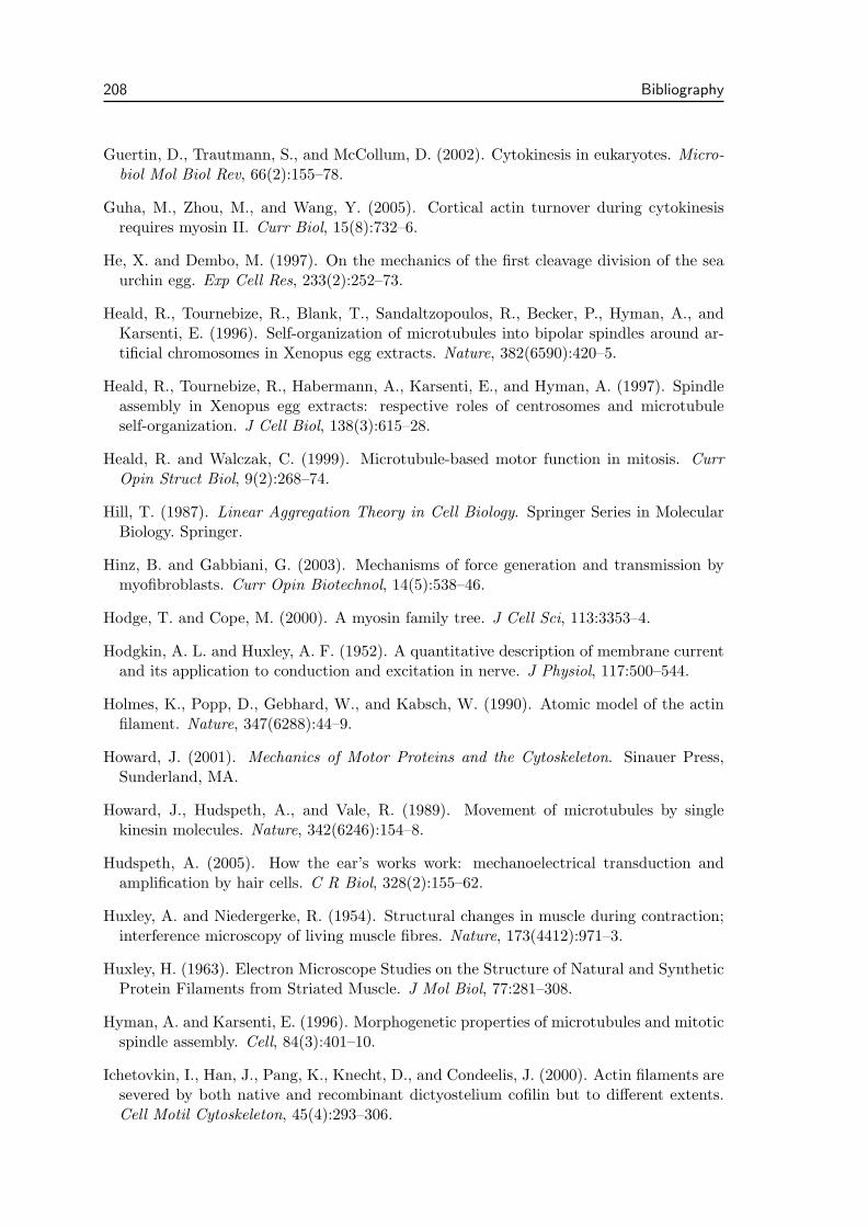
208 Bibliography
Guertin, D., Trautmann, S., and McCollum, D. (2002). Cytokinesis in eukaryotes. Micro-biol Mol Biol Rev, 66(2):155–78.
Guha, M., Zhou, M., and Wang, Y. (2005). Cortical actin turnover during cytokinesisrequires myosin II. Curr Biol, 15(8):732–6.
He, X. and Dembo, M. (1997). On the mechanics of the first cleavage division of the seaurchin egg. Exp Cell Res, 233(2):252–73.
Heald, R., Tournebize, R., Blank, T., Sandaltzopoulos, R., Becker, P., Hyman, A., andKarsenti, E. (1996). Self-organization of microtubules into bipolar spindles around ar-tificial chromosomes in Xenopus egg extracts. Nature, 382(6590):420–5.
Heald, R., Tournebize, R., Habermann, A., Karsenti, E., and Hyman, A. (1997). Spindleassembly in Xenopus egg extracts: respective roles of centrosomes and microtubuleself-organization. J Cell Biol, 138(3):615–28.
Heald, R. and Walczak, C. (1999). Microtubule-based motor function in mitosis. CurrOpin Struct Biol, 9(2):268–74.
Hill, T. (1987). Linear Aggregation Theory in Cell Biology. Springer Series in MolecularBiology. Springer.
Hinz, B. and Gabbiani, G. (2003). Mechanisms of force generation and transmission bymyofibroblasts. Curr Opin Biotechnol, 14(5):538–46.
Hodge, T. and Cope, M. (2000). A myosin family tree. J Cell Sci, 113:3353–4.
Hodgkin, A. L. and Huxley, A. F. (1952). A quantitative description of membrane currentand its application to conduction and excitation in nerve. J Physiol, 117:500–544.
Holmes, K., Popp, D., Gebhard, W., and Kabsch, W. (1990). Atomic model of the actinfilament. Nature, 347(6288):44–9.
Howard, J. (2001). Mechanics of Motor Proteins and the Cytoskeleton. Sinauer Press,Sunderland, MA.
Howard, J., Hudspeth, A., and Vale, R. (1989). Movement of microtubules by singlekinesin molecules. Nature, 342(6246):154–8.
Hudspeth, A. (2005). How the ear’s works work: mechanoelectrical transduction andamplification by hair cells. C R Biol, 328(2):155–62.
Huxley, A. and Niedergerke, R. (1954). Structural changes in muscle during contraction;interference microscopy of living muscle fibres. Nature, 173(4412):971–3.
Huxley, H. (1963). Electron Microscope Studies on the Structure of Natural and SyntheticProtein Filaments from Striated Muscle. J Mol Biol, 77:281–308.
Hyman, A. and Karsenti, E. (1996). Morphogenetic properties of microtubules and mitoticspindle assembly. Cell, 84(3):401–10.
Ichetovkin, I., Han, J., Pang, K., Knecht, D., and Condeelis, J. (2000). Actin filaments aresevered by both native and recombinant dictyostelium cofilin but to different extents.Cell Motil Cytoskeleton, 45(4):293–306.
Bibliography 209
Inoue, S. and Salmon, E. (1995). Force generation by microtubule assembly/disassemblyin mitosis and related movements. Mol Biol Cell, 6(12):1619–40.
Janmey, P., Euteneuer, U., Traub, P., and Schliwa, M. (1991). Viscoelastic properties ofvimentin compared with other filamentous biopolymer networks. J Cell Biol, 113(1):155–60.
Janson, M., de Dood, M., and Dogterom, M. (2003). Dynamic instability of microtubulesis regulated by force. J Cell Biol, 161(6):1029–34.
Janson, M. and Dogterom, M. (2004a). A bending mode analysis for growing microtubules:evidence for a velocity-dependent rigidity. Biophys J, 87(4):2723–36.
Janson, M. and Dogterom, M. (2004b). Scaling of microtubule force-velocity curves ob-tained at different tubulin concentrations. Phys Rev Lett, 92(24):248101.
Joglekar, A. and Hunt, A. (2002). A simple, mechanistic model for directional instabilityduring mitotic chromosome movements. Biophys J, 83(1):42–58.
Julicher, F., Ajdari, A., and Prost, J. (1997). Modeling molecular motors. Rev Mod Phys,69(4):1269–1281.
Julicher, F. and Prost, J. (1995). Cooperative molecular motors. Phys Rev Lett,75(13):2618–2621.
Julicher, F. and Prost, J. (1997). Spontaneous Oscillations of Collective Molecular Motors.Phys Rev Lett, 78(23):4510–4513.
Jurgens, G. (2005). Plant cytokinesis: fission by fusion. Trends Cell Biol, 15(5):277–83.
Kabsch, W., Mannherz, H., Suck, D., Pai, E., and Holmes, K. (1990). Atomic structureof the actin:DNase I complex. Nature, 347(6288):37–44.
Kapitein, L., Peterman, E., Kwok, B., Kim, J., Kapoor, T., and Schmidt, C. (2005).The bipolar mitotic kinesin Eg5 moves on both microtubules that it crosslinks. Nature,435(7038):114–8.
Kapoor, T. and Mitchison, T. (2001). Eg5 is static in bipolar spindles relative to tubulin:evidence for a static spindle matrix. J Cell Biol, 154(6):1125–33.
Karki, S. and Holzbaur, E. (1999). Cytoplasmic dynein and dynactin in cell division andintracellular transport. Curr Opin Cell Biol, 11(1):45–53.
Karsenti, E. and Nedelec, F. (2004). The mitotic spindle and actin tails. Biol Cell,96(3):237–40.
Khodjakov, A., Cole, R., Oakley, B., and Rieder, C. (2000). Centrosome-independentmitotic spindle formation in vertebrates. Curr Biol, 10(2):59–67.
Kim, J., Park, B., Kahng, B., and Lee, H. (2003). Self-organized patterns in mixtures ofmicrotubules and motor proteins. J Korean Phys Soc, 42:162.
Kline-Smith, S., Sandall, S., and Desai, A. (2005). Kinetochore-spindle microtubule inter-actions during mitosis. Curr Opin Cell Biol, 17(1):35–46.
210 Bibliography
Kodama, A., Lechler, T., and Fuchs, E. (2004). Coordinating cytoskeletal tracks to polarizecellular movements. J Cell Biol, 167(2):203–7.
Koka, S., Neudauer, C., Li, X., Lewis, R., McCarthy, J., and Westendorf, J. (2003). Theformin-homology-domain-containing protein FHOD1 enhances cell migration. J CellSci, 116:1745–55.
Kolomeisky, A. and Fisher, M. (2001). Force-velocity relation for growing microtubules.Biophys J, 80(1):149–54.
Kovar, D., Kuhn, J., Tichy, A., and Pollard, T. (2003). The fission yeast cytokinesis forminCdc12p is a barbed end actin filament capping protein gated by profilin. J Cell Biol,161(5):875–87.
Kovar, D. and Pollard, T. (2004). Progressing actin: Formin as a processive elongationmachine. Nat Cell Biol, 6(12):1158–9.
Kreis, T. and Vale, R., editors (1999). Guidebook to the Cytoskeletal and Motor Proteins.Oxford UP, 2nd edition.
Kruse, K. (2005). Physical Aspects of Pattern Formation and Force Generation in theCytoskeleton. Habilitationsschrift TU Dresden.
Kruse, K., Camalet, S., and Julicher, F. (2001). Self-propagating patterns in active filamentbundles. Phys Rev Lett, 87(13):138101.
Kruse, K., Joanny, J., Julicher, F., Prost, J., and Sekimoto, K. (2004). Asters, vortices,and rotating spirals in active gels of polar filaments. Phys Rev Lett, 92(7):078101.
Kruse, K., Joanny, J., Julicher, F., Prost, J., and Sekimoto, K. (2005). Generic theoryof active polar gels: a paradigm for cytoskeletal dynamics. Eur Phys J E Soft Matter,16(1):5–16.
Kruse, K. and Julicher, F. (2000). Actively contracting bundles of polar filaments. PhysRev Lett, 85(8):1778–81.
Kruse, K. and Julicher, F. (2003). Self-organization and mechanical properties of activefilament bundles. Phys Rev E Stat Nonlin Soft Matter Phys, 67:051913.
Kruse, K. and Julicher, F. (2005). Oscillations in cell biology. Curr Opin Cell Biol,17(1):20–6.
Kruse, K. and Sekimoto, K. (2002). Growth of fingerlike protrusions driven by molecularmotors. Phys Rev E Stat Nonlin Soft Matter Phys, 66(3):031904.
Kruse, K., Zumdieck, A., and Julicher, F. (2003). Continuum theory of contractile fibres.Europhys Lett, 64(5):716–722.
Kuchnir Fygenson, D., Flyvbjerg, H., Sneppen, K., Libchaber, A., and Leibler, S. (1995).Spontaneous nucleation of microtubules. Phys Rev E Stat Nonlin Soft Matter Phys,51(5):5058–5063.
Lawrence, C., Dawe, R., Christie, K., Cleveland, D., Dawson, S., Endow, S., Goldstein,L., Goodson, H., Hirokawa, N., Howard, J., Malmberg, R., McIntosh, J., Miki, H.,Mitchison, T., Okada, Y., Reddy, A., Saxton, W., Schliwa, M., Scholey, J., Vale, R.,
Bibliography 211
Walczak, C., and Wordeman, L. (2004). A standardized kinesin nomenclature. J CellBiol, 167(1):19–22.
Leduc, C. (2005). Systeme biomimetique d’intermediares de transport tubulaires: Etudequantitative. PhD thesis, Universite Paris 7.
Leduc, C., Campas, O., Zeldovich, K., Roux, A., Jolimaitre, P., Bourel-Bonnet, L., Goud,B., Joanny, J., Bassereau, P., and Prost, J. (2004). Cooperative extraction of membranenanotubes by molecular motors. Proc Natl Acad Sci U S A, 101(49):17096–101.
Lee, H. and Kardar, M. (2001). Macroscopic equations for pattern formation in mixturesof microtubules and molecular motors. Phys Rev E Stat Nonlin Soft Matter Phys,64(5):056113.
Lin, H., Schneider, M., and Kachar, B. (2005). When size matters: the dynamic regulationof stereocilia lengths. Curr Opin Cell Biol, 17(1):55–61.
Liverpool, T. (2005). Some aspects of the dynamics of active filament solutions. J Phys:Condens Matter, 17:S1153–S1163.
Liverpool, T., Maggs, A., and Ajdari, A. (2001). Viscoelasticity of solutions of motilepolymers. Phys Rev Lett, 86(18):4171–4.
Liverpool, T. and Marchetti, M. (2003). Instabilities of isotropic solutions of active polarfilaments. Phys Rev Lett, 90(13):138102.
Liverpool, T. and Marchetti, M. (2005). Bridging the microscopic and the hydrodynamicin active filament solutions. Europhys Lett, 69:846–852.
Lombillo, V., Stewart, R., and McIntosh, J. (1995). Minus-end-directed motion of kinesin-coated microspheres driven by microtubule depolymerization. Nature, 373(6510):161–4.
Lutkenhaus, J. (2003). Another cytoskeleton in the closet. Cell, 115(6):648–50.
Machesky, L., Mullins, R., Higgs, H., Kaiser, D., Blanchoin, L., May, R., Hall, M., andPollard, T. (1999). Scar, a WASp-related protein, activates nucleation of actin filamentsby the Arp2/3 complex. Proc Natl Acad Sci U S A, 96(7):3739–44.
Maciver, S., Pope, B., Whytock, S., and Weeds, A. (1998). The effect of two actin de-polymerizing factors (ADF/cofilins) on actin filament turnover: pH sensitivity of F-actin binding by human ADF, but not of Acanthamoeba actophorin. Eur J Biochem,256(2):388–97.
Maciver, S., Zot, H., and Pollard, T. (1991). Characterization of actin filament severingby actophorin from Acanthamoeba castellanii. J Cell Biol, 115(6):1611–20.
Mahadevan, L. and Mitchison, T. (2005). Cell biology: powerful curves. Nature,435(7044):895–7.
Mahaffy, R., Park, S., Gerde, E., Kas, J., and Shih, C. (2004). Quantitative analysis ofthe viscoelastic properties of thin regions of fibroblasts using atomic force microscopy.Biophys J, 86(3):1777–93.
Maiato, H., Sampaio, P., and Sunkel, C. (2004). Microtubule-associated proteins and theiressential roles during mitosis. Int Rev Cytol, 241:53–153.
212 Bibliography
Mallik, R., Carter, B., Lex, S., King, S., and Gross, S. (2004). Cytoplasmic dyneinfunctions as a gear in response to load. Nature, 427(6975):649–52.
Mallik, R. and Gross, S. (2004). Molecular motors: strategies to get along. Curr Biol,14(22):R971–82.
Marsland, D. (1970). High Pressure Effects on Cellular Processes, pages 259–312. Aca-demic Press, New York.
Marsland, D. and Landau J.V. (1954). The Mechanisms of Cytokinesis: Temperatur-Pressure Studies on the Cortical Gel System in various Marine Eggs. J Exp Zool,125:507–539.
Matzke, R., Jacobson, K., and Radmacher, M. (2001). Direct, high-resolution measure-ment of furrow stiffening during division of adherent cells. Nat Cell Biol, 3(6):607–10.
Maupin, P. and Pollard, T. (1986). Arrangement of actin filaments and myosin-like fila-ments in the contractile ring and of actin-like filaments in the mitotic spindle of dividingHeLa cells. J Ultrastruct Mol Struct Res, 94(1):92–103.
McGough, A., Pope, B., Chiu, W., and Weeds, A. (1997). Cofilin changes the twist ofF-actin: implications for actin filament dynamics and cellular function. J Cell Biol,138(4):771–81.
Miao, L., Vanderlinde, O., Stewart, M., and Roberts, T. (2003). Retraction in amoeboidcell motility powered by cytoskeletal dynamics. Science, 302(5649):1405–7.
Micoulet, A., Spatz, J., and Ott, A. (2005). Mechanical response analysis and powergeneration by single-cell stretching. Chemphyschem, 6(4):663–70.
Mitchison, T. (1989). Polewards microtubule flux in the mitotic spindle: evidence fromphotoactivation of fluorescence. J Cell Biol, 109(2):637–52.
Mitchison, T., Maddox, P., Gaetz, J., Groen, A., Shirasu, M., Desai, A., Salmon, E., andKapoor, T. (2005). Roles of Polymerization Dynamics, Opposed Motors and a TensileElement in Governing the Length of Xenopus Extract Meiotic Spindles. Mol Biol Cell.
Mitchison, T. and Salmon, E. (2001). Mitosis: a history of division. Nat Cell Biol,3(1):E17–21.
Mogilner, A. and Oster, G. (1996). Cell motility driven by actin polymerization. BiophysJ, 71(6):3030–45.
Mogilner, A. and Oster, G. (1999). The polymerization ratchet model explains the force-velocity relation for growing microtubules. Eur Biophys J, 28:235–242.
Moller-Jensen, J. and Lowe, J. (2005). Increasing complexity of the bacterial cytoskeleton.Curr Opin Cell Biol, 17(1):75–81.
Moore, A. and Wordeman, L. (2004). The mechanism, function and regulation of depoly-merizing kinesins during mitosis. Trends Cell Biol, 14(10):537–46.
Mullins, R., Heuser, J., and Pollard, T. (1998). The interaction of Arp2/3 complex withactin: nucleation, high affinity pointed end capping, and formation of branching net-works of filaments. Proc Natl Acad Sci U S A, 95(11):6181–6.
Bibliography 213
Murthy, K. and Wadsworth, P. (2005). Myosin-II-Dependent Localization and Dynamicsof F-Actin during Cytokinesis. Curr Biol, 15(8):724–31.
Nakazawa, H. and Sekimoto, K. (1996). Polarity sorting in a bundle of actin filaments bytwo-headed myosins. J Phys Soc Jpn, 65:2404–2407.
Nedelec, F. (2002a). Computer simulations reveal motor properties generating stableantiparallel microtubule interactions. J Cell Biol, 158(6):1005–1015.
Nedelec, F. (2002b). Studying the balance of forces in the mitotic spindle with computersimulations. Mol Biol Cell, 13:445a–445a.
Nedelec, F. and Surrey, T. (2001). Dynamics of Microtubule Aster Formation by MotorComplexes. CR Acad Sci Paris, pages 841–847.
Nedelec, F., Surrey, T., and Karsenti, E. (2003). Self-organisation and forces in the mi-crotubule cytoskeleton. Curr Opin Cell Biol, 15(1):118–24.
Nedelec, F., Surrey, T., and Maggs, A. (2001). Dynamic concentration of motors inmicrotubule arrays. Phys Rev Lett, 86(14):3192–5.
Nedelec, F., Surrey, T., Maggs, A., and Leibler, S. (1997). Self-organization of microtubulesand motors. Nature, 389(6648):305–8.
Niebuhr, K., Ebel, F., Frank, R., Reinhard, M., Domann, E., Carl, U., Walter, U., Gertler,F., Wehland, J., and Chakraborty, T. (1997). A novel proline-rich motif present in ActAof Listeria monocytogenes and cytoskeletal proteins is the ligand for the EVH1 domain,a protein module present in the Ena/VASP family. EMBO J, 16(17):5433–44.
Nurse, P. (2003). The great ideas of biology. Clin Med, 3(6):560–8.
Oiwa, K. and Sakakibara, H. (2005). Recent progress in dynein structure and mechanism.Curr Opin Cell Biol, 17(1):98–103.
Oosawa, F. and Asakura, S. (1975). Thermodynamics of the Polymerization of Proteins.Molecular Biology. Academic Press, London.
Otto, J. and Schroeder, T. (1990). Association of actin and myosin in the contractile ring.Ann N Y Acad Sci, 582:179–84.
Paluch, E. (2005). Motilite cellulaire sur des systemes simplifies: de l’oscillation au mou-vement dirige. PhD thesis, Universite Paris 7.
Paluch, E., Piel, M., Prost, J., Bornens, M., and Sykes, C. (2005). Cortical actomyosinbreakage triggers shape oscillations in cells and cell fragments. Biophys J, 89(1):724–33.
Pantaloni, D., Boujemaa, R., Didry, D., Gounon, P., and Carlier, M. (2000). The Arp2/3complex branches filament barbed ends: functional antagonism with capping proteins.Nat Cell Biol, 2(7):385–91.
Pantaloni, D., Le Clainche, C., and Carlier, M. (2001). Mechanism of actin-based motility.Science, 292(5521):1502–6.
Pardo, M. and Nurse, P. (2003). Equatorial retention of the contractile actin ring bymicrotubules during cytokinesis. Science, 300(5625):1569–74.
214 Bibliography
Pelham, R. and Chang, F. (2002). Actin dynamics in the contractile ring during cytokinesisin fission yeast. Nature, 419(6902):82–6.
Peskin, C., Odell, G., and Oster, G. (1993). Cellular motions and thermal fluctuations:the Brownian ratchet. Biophys J, 65(1):316–24.
Peterson, L., Rajfur, Z., Maddox, A., Freel, C., Chen, Y., Edlund, M., Otey, C., andBurridge, K. (2004). Simultaneous stretching and contraction of stress fibers in vivo.Mol Biol Cell, 15(7):3497–508.
Piehl, M. and Cassimeris, L. (2003). Organization and dynamics of growing microtubuleplus ends during early mitosis. Mol Biol Cell, 14(3):916–25.
Piel, M. and Bornens, M. (2001). Centrosome reproduction in vitro: mammalian centro-somes in Xenopus lysates. Methods Cell Biol, 67:289–304.
Plastino, J., Lelidis, I., Prost, J., and Sykes, C. (2004). The effect of diffusion, depolymer-ization and nucleation promoting factors on actin gel growth. Eur Biophys J, 33(4):310–20.
Plastino, J. and Sykes, C. (2005). The actin slingshot. Curr Opin Cell Biol, 17(1):62–6.
Pollard, T. (1986). Rate constants for the reactions of ATP- and ADP-actin with the endsof actin filaments. J Cell Biol, 103(6):2747–54.
Pollard, T. (2003). The cytoskeleton, cellular motility and the reductionist agenda. Nature,422(6933):741–5.
Pollard, T. and Beltzner, C. (2002). Structure and function of the Arp2/3 complex. CurrOpin Struct Biol, 12(6):768–74.
Pollard, T., Blanchoin, L., and Mullins, R. (2000). Molecular mechanisms controlling actinfilament dynamics in nonmuscle cells. Annu Rev Biophys Biomol Struct, 29:545–76.
Pollard, T. and Borisy, G. (2003). Cellular motility driven by assembly and disassemblyof actin filaments. Cell, 112(4):453–65.
Pollard, T. D. and Earnshaw, W. C. (2002). Cell Biology. Elsevier Science (USA).
Press, W. H., Teukolsky, S. A., Vetterling, W. T., and Flannery, B. P. (2002). NumericalRecipes in C. Cambridge UP.
Rafelski, S. and Theriot, J. (2004). Crawling toward a unified model of cell mobility:spatial and temporal regulation of actin dynamics. Annu Rev Biochem, 73:209–39.
Rappaport, R. (1967). Cell division: direct measurement of maximum tension exerted byfurrow of echinoderm eggs. Science, 156(779):1241–3.
Rappaport, R. (1996). Cytokinesis in animal cells. Cambridge UP.
Reichl, E., Effler, J., and Robinson, D. (2005). The stress and strain of cytokinesis. TrendsCell Biol, 15(4):200–6.
Reimann, P. (2002). Brownian Motors: Noisy transport far from equilibrium. Phys Rep,361:57–265.
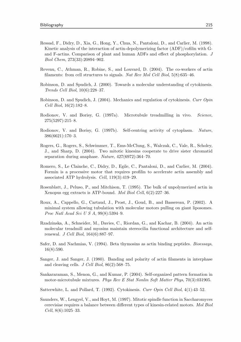
Bibliography 215
Ressad, F., Didry, D., Xia, G., Hong, Y., Chua, N., Pantaloni, D., and Carlier, M. (1998).Kinetic analysis of the interaction of actin-depolymerizing factor (ADF)/cofilin with G-and F-actins. Comparison of plant and human ADFs and effect of phosphorylation. JBiol Chem, 273(33):20894–902.
Revenu, C., Athman, R., Robine, S., and Louvard, D. (2004). The co-workers of actinfilaments: from cell structures to signals. Nat Rev Mol Cell Biol, 5(8):635–46.
Robinson, D. and Spudich, J. (2000). Towards a molecular understanding of cytokinesis.Trends Cell Biol, 10(6):228–37.
Robinson, D. and Spudich, J. (2004). Mechanics and regulation of cytokinesis. Curr OpinCell Biol, 16(2):182–8.
Rodionov, V. and Borisy, G. (1997a). Microtubule treadmilling in vivo. Science,275(5297):215–8.
Rodionov, V. and Borisy, G. (1997b). Self-centring activity of cytoplasm. Nature,386(6621):170–3.
Rogers, G., Rogers, S., Schwimmer, T., Ems-McClung, S., Walczak, C., Vale, R., Scholey,J., and Sharp, D. (2004). Two mitotic kinesins cooperate to drive sister chromatidseparation during anaphase. Nature, 427(6972):364–70.
Romero, S., Le Clainche, C., Didry, D., Egile, C., Pantaloni, D., and Carlier, M. (2004).Formin is a processive motor that requires profilin to accelerate actin assembly andassociated ATP hydrolysis. Cell, 119(3):419–29.
Rosenblatt, J., Peluso, P., and Mitchison, T. (1995). The bulk of unpolymerized actin inXenopus egg extracts is ATP-bound. Mol Biol Cell, 6(2):227–36.
Roux, A., Cappello, G., Cartaud, J., Prost, J., Goud, B., and Bassereau, P. (2002). Aminimal system allowing tubulation with molecular motors pulling on giant liposomes.Proc Natl Acad Sci U S A, 99(8):5394–9.
Rzadzinska, A., Schneider, M., Davies, C., Riordan, G., and Kachar, B. (2004). An actinmolecular treadmill and myosins maintain stereocilia functional architecture and self-renewal. J Cell Biol, 164(6):887–97.
Safer, D. and Nachmias, V. (1994). Beta thymosins as actin binding peptides. Bioessays,16(8):590.
Sanger, J. and Sanger, J. (1980). Banding and polarity of actin filaments in interphaseand cleaving cells. J Cell Biol, 86(2):568–75.
Sankararaman, S., Menon, G., and Kumar, P. (2004). Self-organized pattern formation inmotor-microtubule mixtures. Phys Rev E Stat Nonlin Soft Matter Phys, 70(3):031905.
Satterwhite, L. and Pollard, T. (1992). Cytokinesis. Curr Opin Cell Biol, 4(1):43–52.
Saunders, W., Lengyel, V., and Hoyt, M. (1997). Mitotic spindle function in Saccharomycescerevisiae requires a balance between different types of kinesin-related motors. Mol BiolCell, 8(6):1025–33.
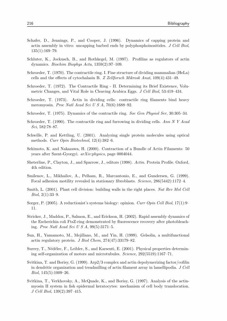
216 Bibliography
Schafer, D., Jennings, P., and Cooper, J. (1996). Dynamics of capping protein andactin assembly in vitro: uncapping barbed ends by polyphosphoinositides. J Cell Biol,135(1):169–79.
Schluter, K., Jockusch, B., and Rothkegel, M. (1997). Profilins as regulators of actindynamics. Biochim Biophys Acta, 1359(2):97–109.
Schroeder, T. (1970). The contractile ring. I. Fine structure of dividing mammalian (HeLa)cells and the effects of cytochalasin B. Z Zellforsch Mikrosk Anat, 109(4):431–49.
Schroeder, T. (1972). The Contractile Ring - II. Determining its Brief Existence, Volu-metric Changes, and Vital Role in Cleaving Arabica Eggs. J Cell Biol, 53:419–434.
Schroeder, T. (1973). Actin in dividing cells: contractile ring filaments bind heavymeromyosin. Proc Natl Acad Sci U S A, 70(6):1688–92.
Schroeder, T. (1975). Dynamics of the contractile ring. Soc Gen Physiol Ser, 30:305–34.
Schroeder, T. (1990). The contractile ring and furrowing in dividing cells. Ann N Y AcadSci, 582:78–87.
Schwille, P. and Kettling, U. (2001). Analyzing single protein molecules using opticalmethods. Curr Opin Biotechnol, 12(4):382–6.
Sekimoto, K. and Nakazawa, H. (2000). Contraction of a Bundle of Actin Filaments: 50years after Szent-Gyorgyi. arXiv:physics, page 0004044.
Sheterline, P., Clayton, J., and Sparrow, J., editors (1998). Actin. Protein Profile. Oxford,4th edition.
Smilenov, L., Mikhailov, A., Pelham, R., Marcantonio, E., and Gundersen, G. (1999).Focal adhesion motility revealed in stationary fibroblasts. Science, 286(5442):1172–4.
Smith, L. (2001). Plant cell division: building walls in the right places. Nat Rev Mol CellBiol, 2(1):33–9.
Sorger, P. (2005). A reductionist’s systems biology: opinion. Curr Opin Cell Biol, 17(1):9–11.
Stricker, J., Maddox, P., Salmon, E., and Erickson, H. (2002). Rapid assembly dynamics ofthe Escherichia coli FtsZ-ring demonstrated by fluorescence recovery after photobleach-ing. Proc Natl Acad Sci U S A, 99(5):3171–5.
Sun, H., Yamamoto, M., Mejillano, M., and Yin, H. (1999). Gelsolin, a multifunctionalactin regulatory protein. J Biol Chem, 274(47):33179–82.
Surrey, T., Nedelec, F., Leibler, S., and Karsenti, E. (2001). Physical properties determin-ing self-organization of motors and microtubules. Science, 292(5519):1167–71.
Svitkina, T. and Borisy, G. (1999). Arp2/3 complex and actin depolymerizing factor/cofilinin dendritic organization and treadmilling of actin filament array in lamellipodia. J CellBiol, 145(5):1009–26.
Svitkina, T., Verkhovsky, A., McQuade, K., and Borisy, G. (1997). Analysis of the actin-myosin II system in fish epidermal keratocytes: mechanism of cell body translocation.J Cell Biol, 139(2):397–415.
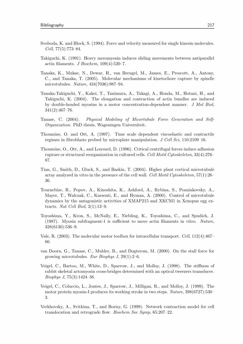
Bibliography 217
Svoboda, K. and Block, S. (1994). Force and velocity measured for single kinesin molecules.Cell, 77(5):773–84.
Takiguchi, K. (1991). Heavy meromyosin induces sliding movements between antiparallelactin filaments. J Biochem, 109(4):520–7.
Tanaka, K., Mukae, N., Dewar, H., van Breugel, M., James, E., Prescott, A., Antony,C., and Tanaka, T. (2005). Molecular mechanisms of kinetochore capture by spindlemicrotubules. Nature, 434(7036):987–94.
Tanaka-Takiguchi, Y., Kakei, T., Tanimura, A., Takagi, A., Honda, M., Hotani, H., andTakiguchi, K. (2004). The elongation and contraction of actin bundles are inducedby double-headed myosins in a motor concentration-dependent manner. J Mol Biol,341(2):467–76.
Tanase, C. (2004). Physical Modeling of Micortubule Force Generation and Self-Organization. PhD thesis, Wageningen Universiteit.
Thoumine, O. and Ott, A. (1997). Time scale dependent viscoelastic and contractileregimes in fibroblasts probed by microplate manipulation. J Cell Sci, 110:2109–16.
Thoumine, O., Ott, A., and Louvard, D. (1996). Critical centrifugal forces induce adhesionrupture or structural reorganization in cultured cells. Cell Motil Cytoskeleton, 33(4):276–87.
Tian, G., Smith, D., Gluck, S., and Baskin, T. (2004). Higher plant cortical microtubulearray analyzed in vitro in the presence of the cell wall. Cell Motil Cytoskeleton, 57(1):26–36.
Tournebize, R., Popov, A., Kinoshita, K., Ashford, A., Rybina, S., Pozniakovsky, A.,Mayer, T., Walczak, C., Karsenti, E., and Hyman, A. (2000). Control of microtubuledynamics by the antagonistic activities of XMAP215 and XKCM1 in Xenopus egg ex-tracts. Nat Cell Biol, 2(1):13–9.
Toyoshima, Y., Kron, S., McNally, E., Niebling, K., Toyoshima, C., and Spudich, J.(1987). Myosin subfragment-1 is sufficient to move actin filaments in vitro. Nature,328(6130):536–9.
Vale, R. (2003). The molecular motor toolbox for intracellular transport. Cell, 112(4):467–80.
van Doorn, G., Tanase, C., Mulder, B., and Dogterom, M. (2000). On the stall force forgrowing microtubules. Eur Biophys J, 29(1):2–6.
Veigel, C., Bartoo, M., White, D., Sparrow, J., and Molloy, J. (1998). The stiffness ofrabbit skeletal actomyosin cross-bridges determined with an optical tweezers transducer.Biophys J, 75(3):1424–38.
Veigel, C., Coluccio, L., Jontes, J., Sparrow, J., Milligan, R., and Molloy, J. (1999). Themotor protein myosin-I produces its working stroke in two steps. Nature, 398(6727):530–3.
Verkhovsky, A., Svitkina, T., and Borisy, G. (1999). Network contraction model for celltranslocation and retrograde flow. Biochem Soc Symp, 65:207–22.
218 Bibliography
Vicker, M. (2002). Eukaryotic cell locomotion depends on the propagation of self-organizedreaction-diffusion waves and oscillations of actin filament assembly. Exp Cell Res,275(1):54–66.
Vinson, V., De La Cruz, E., Higgs, H., and Pollard, T. (1998). Interactions ofAcanthamoeba profilin with actin and nucleotides bound to actin. Biochemistry,37(31):10871–80.
Vorobjev, I., Malikov, V., and Rodionov, V. (2001). Self-organization of a radial micro-tubule array by dynein-dependent nucleation of microtubules. Proc Natl Acad Sci U SA, 98(18):10160–5.
Vos, J., Dogterom, M., and Emons, A. (2004). Microtubules become more dynamic but notshorter during preprophase band formation: a possible ”search-and-capture” mechanismfor microtubule translocation. Cell Motil Cytoskeleton, 57(4):246–58.
Voter, W. and Erickson, H. (1984). The kinetics of microtubule assembly. Evidence for atwo-stage nucleation mechanism. J Biol Chem, 259(16):10430–8.
Walker, D., Wang, D., Jin, Y., Rath, U., Wang, Y., Johansen, J., and Johansen, K.(2000). Skeletor, a novel chromosomal protein that redistributes during mitosis providesevidence for the formation of a spindle matrix. J Cell Biol, 151(7):1401–12.
Wang, H. and Nogales, E. (2005). Nucleotide-dependent bending flexibility of tubulinregulates microtubule assembly. Nature, 435(7044):911–5.
Wasteneys, G. (2002). Microtubule organization in the green kingdom: chaos or self-order?J Cell Sci, 115:1345–54.
Watanabe, N., Madaule, P., Reid, T., Ishizaki, T., Watanabe, G., Kakizuka, A., Saito, Y.,Nakao, K., Jockusch, B., and Narumiya, S. (1997). p140mDia, a mammalian homologof Drosophila diaphanous, is a target protein for Rho small GTPase and is a ligand forprofilin. EMBO J, 16(11):3044–56.
Waterman-Storer, C., Desai, A., Bulinski, J., and Salmon, E. (1998). Fluorescent specklemicroscopy, a method to visualize the dynamics of protein assemblies in living cells.Curr Biol, 8(22):1227–30.
Weaver, A., Young, M., Lee, W., and Cooper, J. (2003). Integration of signals to theArp2/3 complex. Curr Opin Cell Biol, 15(1):23–30.
Weber, I. (2001). On the mechanism of cleavage furrow ingression in Dictyostelium. CellStruct Funct, 26(6):577–84.
Welch, M., Rosenblatt, J., Skoble, J., Portnoy, D., and Mitchison, T. (1998). Interaction ofhuman Arp2/3 complex and the Listeria monocytogenes ActA protein in actin filamentnucleation. Science, 281(5373):105–8.
Wolfe, B. and Gould, K. (2005). Split decisions: coordinating cytokinesis in yeast. TrendsCell Biol, 15(1):10–8.
Wolpert (1960). The Mechanics and Mechanism of Cleavage. Int Rev Cytol, 10:163–216.
Bibliography 219
Woodrum, D., Rich, S., and Pollard, T. (1975). Evidence for biased bidirectional polymer-ization of actin filaments using heavy meromyosin prepared by an improved method. JCell Biol, 67(1):231–7.
Wordeman, L. (2005). Microtubule-depolymerizing kinesins. Curr Opin Cell Biol,17(1):82–8.
Wordeman, L. and Mitchison, T. (1995). Identification and partial characterization ofmitotic centromere-associated kinesin, a kinesin-related protein that associates withcentromeres during mitosis. J Cell Biol, 128(1-2):95–104.
Wu, J., Kuhn, J., Kovar, D., and Pollard, T. (2003). Spatial and temporal pathway forassembly and constriction of the contractile ring in fission yeast cytokinesis. Dev Cell,5(5):723–34.
Zhang, D. and Nicklas, R. (1995). The impact of chromosomes and centrosomes on spindleassembly as observed in living cells. J Cell Biol, 129(5):1287–300.
Zhang, W. and Robinson, D. (2005). Balance of actively generated contractile and resistiveforces controls cytokinesis dynamics. Proc Natl Acad Sci U S A, 102(20):7186–91.
Ziebert, F. and Zimmermann, W. (2004). Comment on ”Instabilities of isotropic solutionsof active polar filaments”. Phys Rev Lett, 93(15):159801; author reply 159802.
Zigmond, S., Evangelista, M., Boone, C., Yang, C., Dar, A., Sicheri, F., Forkey, J., andPring, M. (2003). Formin leaky cap allows elongation in the presence of tight cappingproteins. Curr Biol, 13(20):1820–3.
Zumdieck, A., Cosentino Lagomarsino, M., Tanase, C., Kruse, K., Mulder, B., Dogterom,M., and Julicher, F. (2005a). Continuum description of the cytoskeleton: ring formationin the cell cortex. Phys Rev Lett, 95(25):258103.
Zumdieck, A., Kruse, K., and Julicher, F. (2005b). Quantitative description of ring con-striction during cytokinesis: The role of filament polymerization. in preparation.
220 Bibliography
Versicherung
Hiermit versichere ich, daß ich die vorliegende Arbeit ohne unzulassige Hilfe Dritterund ohne Benutzung anderer als der angegebenen Hilfsmittel angefertigt habe; die ausfremden Quellen direkt oder indirekt ubernommenen Gedanken sind als solche kenntlichgemacht. Die Arbeit wurde bisher weder im Inland noch im Ausland in gleicher oderahnlicher Form einer anderen Prufungsbehorde vorgelegt.
Die vorgelegte Arbeit wurde vom 1.10.2002 bis 25.08.2005 unter wissenschaftlicherBetreung durch Prof. Dr. Frank Julicher am Max-Planck-Institut fur Physik komplexerSysteme in Dresden durchgefuhrt.
Ich versichere, daß ich bisher keine erfolglosen Promotionsverfahren unternommen habe.Ich erkenne die Promotionsordnung der Fakultat Mathematik und Naturwissenschaftender Technischen Universitat Dresden an.
Dresden, den 25.08.2005,
Alexander Zumdieck
221