analysis of the gaia orbit around l2

TREBALL DE FI DE CARRERA

TÍTOL DEL TFC: Analysis of the Gaia orbit around L2

TITULACIÓ: Enginyeria Tècnica Aeronàutica, especialitat Aeronavegació

AUTOR: Jordi Carlos García García

DIRECTORS: Santiago Torres Gil, Enrique GarcíaBerro Montilla

2 Analysis of the Gaia orbit around L2

DATA: 27 de juliol de 2009

Títol: Analysis of the Gaia orbit around L2

Autor: Jordi Carlos García García

Directors: Santiago Torres Gil, Enrique GarcíaBerro Montilla

Data: 27 de juliol de 2009

Resum

Gaia és una missió astromètrica de l’Agència Espacial Europea (ESA) amb l’ambiciós objectiu de fer el mapa en tres dimensions de la nostra Galàxia més gran i precís fet fins ara. Per aconseguirho Gaia escanejarà l’espai contínuament i proporcionarà informació molt precisa sobre la posició, velocitat i espectre d’aproximadament mil milions d’estrelles de la Via Làctia. Això proporcionarà una informació molt valuosa sobre la composició, formació i evolució de la nostra Galàxia. Gaia també detectarà milers de petits objectes del sistema solar, planetes extrasolars, galàxies llunyanes, etc.

Per tal de fer les observacions el més precises possibles Gaia descriurà una òrbita de tipus Lissajous al voltant del punt Lagrangià L2 del sistema SolTerra. Aquesta és una òrbita molt adequada ja es molt estable. Així mateix, aquesta òrbita té una gran estabilitat tèrmica. A més té unes característiques d’observació molt bones ja que el Sol, la Terra, la Lluna i els planetes interiors estan sempre per darrere del camp d’observació.

En aquest treball final de carrera, en un primer lloc, estudiarem les òrbites de Lissajous, simularem l’orbita de Lissajous prevista per la missió Gaia i analitzarem les seves característiques. En segon lloc integrarem l’orbita de Lissajous simulada a la llei d’escanejat de Gaia, la qual estarà afectada pels moviments de rotació, precessió de l’eix de rotació, i translació al voltant del Sol, i estudiarem els seus efectes. Finalment, en un tercer lloc, per fer un anàlisis més realista, afegirem soroll i calibracions periòdiques, i estudiarem els seus efectes sobre la llei d’escanejat tenint en compte l’orbita Lissajous.

Analysis of the Gaia orbit around L2 3

Title: Analysis of the Gaia orbit around L2

Author: Jordi Carlos García García

Directors: Santiago Torres Gil, Enrique GarcíaBerro Montilla

Date: July, 27th 2009

Overview

Gaia is an astrometric mission of the European Space Agency (ESA) with the ambitious goal of obtaining the largest and most accurate spatial map in three dimensions up to now. To achieve this, Gaia will scan the space continuously and will provide very precise information about the position, speed and spectra of about a billion stars in the Milky Way. This will provide valuable information on the composition, formation and evolution of our galaxy. Gaia will also detect thousands of small solar system objects, extrasolar planets, distant galaxies, and so on.

To make the observations as accurate as possible Gaia will use a Lissajous type orbit around the L2 Lagrangian point of the SunEarth system. This is a very appropriate orbit because it can provide during a long time a very large positional stability to the spacecraft and a very large thermal stability. This orbit also has very good observational features because the Sun, Earth, Moon and inner planets are always behind the field of observation.

In this work, we will firstly study Lissajous orbits, simulate the expected Lissajous orbit for Gaia mission and analyze its characteristics. Secondly, we will integrate the simulated Lissajous orbit according to the Gaia scanning law, which can be obtained from rotation motion, the precession of the axis of rotation and the translation around the Sun, and study its effects. Finally, to do a more realistic analysis, we will add noise and periodical recalibrations, and study their effects on the scanning law of the Lissajous orbit.


INDEX

CHAPTER 1: INTRODUCTION ........................................................................... 7

1.1 Gaia mission.........................................................................................................................7

1.2 Gaia general features...........................................................................................................7

1.3 Gaia scanning law................................................................................................................9

1.4 Purpose of our work...........................................................................................................10

CHAPTER 2: SIMULATION OF THE LISSAJOUS ORBIT AROUND L2 ........................................................................................... 11

2.1 Lissajous orbits..................................................................................................................11

2.2 General equations..............................................................................................................11

2.3 Reduced equations............................................................................................................13

2.4 Orbit simulation model......................................................................................................142.4.1 Mission duration time constraint..............................................................................142.4.2 SunGaiaEarth angle constraint..............................................................................142.4.3 Simulation data........................................................................................................16

CHAPTER 3: THE LISSAJOUS ORBIT OF GAIA ........................................... 18

3.1 The role of the initial conditions......................................................................................20

CHAPTER 4: THE 3DIMENSIONAL MOTION OF GAIA ................................ 25

4.1 Introduction........................................................................................................................25

4.2 Results................................................................................................................................254.2.1 Translation...............................................................................................................254.2.2 Translation + Precession.........................................................................................274.2.3 Translation + Precession + Spin..............................................................................29

CHAPTER 5: THE EFFECTS OF NOISE ......................................................... 32

5.1 Introduction........................................................................................................................32

5.2 Results................................................................................................................................325.2.1 Translation + Precession with noise........................................................................325.2.2 Translation + Precession with noise + Spin with noise............................................355.2.3 Translation + Precession with noise + Spin with noise + Pointing errors.................38

CHAPTER 6: CONCLUSIONS .......................................................................... 41


BIBLIOGRAPHY ............................................................................................... 43

APPENDIX A: LAGRANGIAN POINTS ........................................................... 44

APPENDIX B: LISSAJOUS CURVES .............................................................. 46

APPENDIX C: THE SCANNING LAW OF GAIA .............................................. 47

C.1 The translation motion.....................................................................................................47

C.2 The precession motion.....................................................................................................48

C.3 The spin motion................................................................................................................49

APPENDIX D: NUMERICAL CODE .................................................................. 51


CHAPTER 1: INTRODUCTION

1.1 Gaia mission

Gaia is an ambitious astrometric mission of the European Space Agency (ESA). Gaia will produce the largest and most precise threedimensional space map of our Galaxy. In particular, Gaia will obtain extremely accurate positional and radial velocity measurements for about one billion stars in our Galaxy and throughout the Local Group of galaxies. The Gaia spacecraft, which is shown in Fig. 1.1, will also detect a large number of minor objects in our Solar System, extrasolar planets, galaxies in the nearby Universe and distant quasars, and will provide new tests for theory of General Relativity. The technical solutions envisaged to perform these tasks are very challenging, and involve all the relevant aspects of the spacecraft, from its instrumentation and onboard data handling to the onground data processing and analysis.

Figure 1.1: An artist impression of Gaia.

1.2 Gaia general features

Gaia is the successor of the ESA’s Hipparcos mission, which was launched on 1989 and produced a catalogue of over 2 million stars. Gaia aims to improve significantly the Hipparcos catalogue because its photometric sensitivity will be 30 times larger and, moreover, it will measure the positions and motions of stars and other objects with a much better accuracy (by a factor ≈200).


The Gaia spacecraft will be launched on 2012 from the European Spaceport in Kourou, French Guiana, using a SoyuzST rocket with an additional Fregat stage. The launch vector will insert Gaia on a transfer orbit and then, after 4 months, the spacecraft will manoeuvre to enter into a Lissajous orbit around the Lagrange point L2 of the EarthSun system. The expected mission lifetime is 5 years, but it could be extended up to 6 years, depending on the performance of the onboard instruments.

The Gaia communications system will transmit the science data to the ground station at about 4 Mbps during about 8 hours per day and the complete raw database will have a size of approximately 100 Tb. The estimated Gaia overall budget is about 550 million Euros and the main contractor is EADS Astrium with a contract of more than 300 million Euros to build the spacecraft. The spacecraft is composed by three different modules: a payload module, a mechanical service module and an electrical service module. A schematic representation of Gaia payload is shown in Fig. 1.2

Figure 1.2: Schematic figure of the Gaia payload.

The payload module consists basically of two telescopes, with a single focal plane. This scientific payload has three instruments: the astrometric instrument, the broad band photometer and the radial velocity spectrometer. The astrometric instrument will be in charge of measuring five astrometric parameters: the projected position of the star in the sky (2 angles), the proper motion (2 time derivatives of position, one for each angle) and the trigonometric parallax (which provides the distance to each source). The broad band


photometer provides continuous star multiband photometry in the 3201000 nm band, and it is also used to calibrate the chromaticity of the astrometric instrument. Finally, the radial velocity spectrometer is intended to provide radial velocity measurements and high resolution spectral data in the narrow band 847874 nm. All these tasks are performed in a dedicated area of the focal plane, which consists of 106 CCDs, working in Time Delayed Integration (TDI) mode. In this mode the charge of each of the pixels of the CCDs is transferred to the next one at the same rate the satellite scans the sky. Each of the telescopes of Gaia, one for each field of view, consists in one primary mirror of size 1.45 m × 0.5 m, a secondary mirror and a tertiary mirror – see Fig. 1.2.

The mechanical service module comprises the spacecraft main structure, which will be hexagonal conical shaped and will be optimised to guarantee the stability of the basic angle (the angle between the two telescopes). This module also comprises a flat deployable sunshield which prevents illumination from the Sun of the payload module, a thermal tent which provides additional protection and the thrusters of the chemical propulsion system and the complete micropropulsion system.

Finally, the electrical service module basically houses the communication subsystem, the central computer and data handling subsystem, and the power subsystem.

1.3 Gaia scanning law

The Gaia scanning law, which we display in Fig. 1.3, relies on the systematic and repeating observation of the positions of the star along the two fields of view. The spacecraft will be slowly rotating at a constant angular rate around an axis perpendicular to those two fields of view (the spin axis). With a constant basic angle and a known spin rate it is easy to know how much time it takes for a star to transit the focal plane. The spacecraft spin axis will make an angle of 45° with the direction of the Sun. This is the optimal tradeoff between the astrometric requirements (basically, payload shading) and solar array efficiency. This scan axis further describes a slow precession motion around the spin axis. As already mentioned, Gaia will also describe a circular orbit around the Sun. Finally, the spacecraft itself will describe a Lissajous orbit around the EarthSun point L2.


Figure 1.3: Gaia scanning law.

1.4 Purpose of our work

In this work we focus on the future Gaia orbit around the EarthSun L2 point. First of all, we will study and simulate in a realistic way the Lissajoustype orbit. Then we will take into account the other motions which affect the Gaia scanning law: the translation around the Sun, and the precession and the spin motions. Secondly, we will study and simulate these motions and then we will analyze the effect when the Lissajous orbit motion is added. After that, we will introduce Gaussian perturbations and different noise distributions to our model in order to study the effects of noise in the Gaia scanning law. We will also implement in the model periodic recalibrations which correct the noise disturbances as it will be done in the real mission. Finally, we will analyze the effects of the implementation of the Lissajous orbit in the performance of Gaia.


CHAPTER 2: SIMULATION OF THE LISSAJOUS

ORBIT AROUND L2

2.1 Lissajous orbits

Lagrangian points, also known as libration points, are named after the FrenchItalian mathematician JosephLouis Lagrange (17361813) who discovered them in the eighteenth century as equilibrium solutions of the threebody problem. The Lagrangian points (L1L5) are five points in an orbital configuration (see Appendix A for additional information about Lagrangian points) where a small object (in our case, a satellite) can be stationary relative to two larger objects (in our case, the Sun and the Earth). The orbit of a satellite around a Lagrangian point is a quasiperiodic orbit, which does not require propulsion. Generally speaking, the orbit has components in the plane of the two main bodies (in our case, the ecliptic) and in the perpendicular plane, and is mathematically well described by means of a Lissajous curve in the three dimensional space (see Appendix B for additional information about Lissajous curves). Several space missions have been placed in Lissajous orbits around the Lagrangian points of the SunEarth system. Examples of such missions are the ACE, SOHO and WIND missions, which orbit around the Lagrangian L1 point, or the WMAP, Herschel and Planck missions which do so around the Lagrangian L2 point. Gaia will orbit around the L2 SunEarth Lagrangian point. In this way Gaia will take advantage of excellent observation conditions since the Sun, the Earth and the Moon do not interfere with the observations.

These orbits have special interest because they have a highly stable position around Lagrangian points. This results in very accurate observations and very low fuel consumption due to orbital corrections. Other important advantages are the very high thermal stability and the absence of planets or other large space bodies eclipsing the line of sight. However, it must be said that although in theory Lissajous orbits are highly stable in practice any orbit around a Lagrangian point is dynamically unstable. This means that small departures from equilibrium grow exponentially as time passes by and, as a result, a spacecraft located in an orbit around any libration point must use its own propulsion systems to perform periodical orbital corrections.

2.2 General equations

To simulate the Gaia Lissajous orbit we must first define a reference frame. Our coordinate frame is shown in Fig. 2.1 and uses 3D Cartesian coordinates, so the position of an object is represented by three coordinates x, y and z. We take the coordinate origin at the SunEarth L2 Lagrangian point and we define the


ecliptic plane as the xyplane, where the xaxis is the line between the Sun and the Earth and it is positive in the direction going from Sun to the Earth. The yaxis is positive in the direction of Earth translation. The zaxis is perpendicular to the ecliptic plane and its positive direction is fixed by the y and xaxis in accordance with the right hand rule – see Fig 2.1. Note that when the Earth is moving around the Sun the coordinate frame also does it.

Figure 2.1: Coordinate frame used in this work.

Once the reference frame has been defined, we can write the differential equations of the motion using the linear approximation for the circular restricted threebody problem:

(2.1)

In these equations K is a constant which depends on the mass of Sun (m1) and the mass of Earth + Moon (m2):

(2.2)

(2.3)


In these expressions, xL depends on the masses of the intervening bodies and is one of the three real roots (for each Lagrange point) of the 2.3 equation. Solving these equations it turns out that for our case K is equal to 3.9405221845259. Substituting this value in the equations of motion and solving for x, y, z, we find the following general equations of motion:

(2.4)

In these expressions the coefficients are linear functions of the initial conditions in accordance with the following expression:

(2.5)

And the constants are:

(2.6)

(2.7)

(2.8)

2.3 Reduced equations

The previous equations can be further simplified adopting adequate initial values. In particular, we adopt A1=A2=0. With these initial values the general equations are reduced to the following equations:


(2.9)

These are the Lissajous orbit reduced equations and, as can be seen, the x, y frequencies and phases are coupled, while the motion around the zaxis is completely independent, so the equations represent an harmonic xy motion and a z oscillation. Also the x and y amplitudes are closely related:

(2.10)where c2 = 3.1872293 is a constant.

2.4 Orbit simulation model

2.4.1 Mission duration time constraint

One of the main constraints that we must take into account in order to select the orbital parameters is the mission duration which depends, among other things, on the level of Sun radiation at each moment. As can be seen in Fig. 2.2, around the L2 point there is a circular zone where the Sun is always semieclipsed by the Earth. This is the Earthpenumbra zone and if Gaia enters into this zone it would have two problems: first of all, their solar panels would be unable to generate enough electrical power since they would not receive sufficient Sun light. On the other hand, entering into this zone for a few minutes would generate a detrimental thermal shock in the spacecraft.

Figure 2.2: Earth shadow and penumbra

The provided mission duration is over 5 years, with the possibility of extending it to 6 years. Consequently, the orbit must be chosen in such a way that a minimum time of 6 years without any solar eclipse must be provided. The time without eclipse depends on the initial conditions of the orbit and the Earth penumbra radius near the L2 point is approximately 13000 km.

2.4.2 SunGaiaEarth angle constraint

Another constraint to the specific selection of the orbital parameters that must be taken into account is the angle between the Sun, Gaia, and the Earth at


each time. This angle depends on the spacecraft position at each moment and it must be less than 15 degrees all the time, so the maximum orbit amplitudes must be chosen according to this. The situation is described in Fig. 2.3. Although it may seem that the angle varies only in a plane, we remind that the Lissajous orbit is a threedimensional trajectory and, thus, the angle varies accordingly.

Figure 2.3: SunGaiaEarth angle

To calculate the angle we use the scalar product given by the following expression:

(2.11)

The variables are the GaiaEarth and GaiaSun vectors, and their modules, are defined at each time step. They are calculated using the following expressions:

(2.12)

(2.13)

To obtain the GaiaEarth and GaiaSun vectors the values for the SunEarth distance and the EarthL2 distance are needed. We adopt for them the values 1.49598×108 km (1 Astronomical Unit) and 1507683 km, respectively.


2.4.3 Simulation data

The simulation of the Lissajous orbit of Gaia has been done using a numerical code which performs all the necessary calculations. The necessary input data for these simulations is the initial position of the spacecraft. The implemented code can be found in Appendix B. Hence, here we will only briefly summarize the main simulation data. In particular, the values adopted for the amplitudes, frequencies and phases of the Lissajous orbit for each one of the axis are shown in Table 2.1.


x axis y axis z axisAmplitude (km) Ax = Ay∙c2 Ay = 100000 Az = 100000Frequency (days1) ωxy = 2∙π/Txy ωxy = 2∙π/Txy ωz = 2∙π/Tz

Phase (rad) Φxy = asin(y0/Ay) Φxy = asin(y0/Ay) Φz = acos(z0/Az)

Table 2.1: Parameters of the Lissajous orbit.

As clearly shown in Table 2.1, the phase depends on the initial coordinates, y0, z0 but not on x0 because it is coupled with y0. The specific values of the other constants that are used in the simulation are summarized in Table 2.2.

Constant ValueEarth shadow radium (km) r = 13000xy period (days) Txy = 177.566z period (days) Tz = 184.0

Table 2.2: Constants of the orbit of Gaia.


CHAPTER 3: THE LISSAJOUS ORBIT OF GAIA

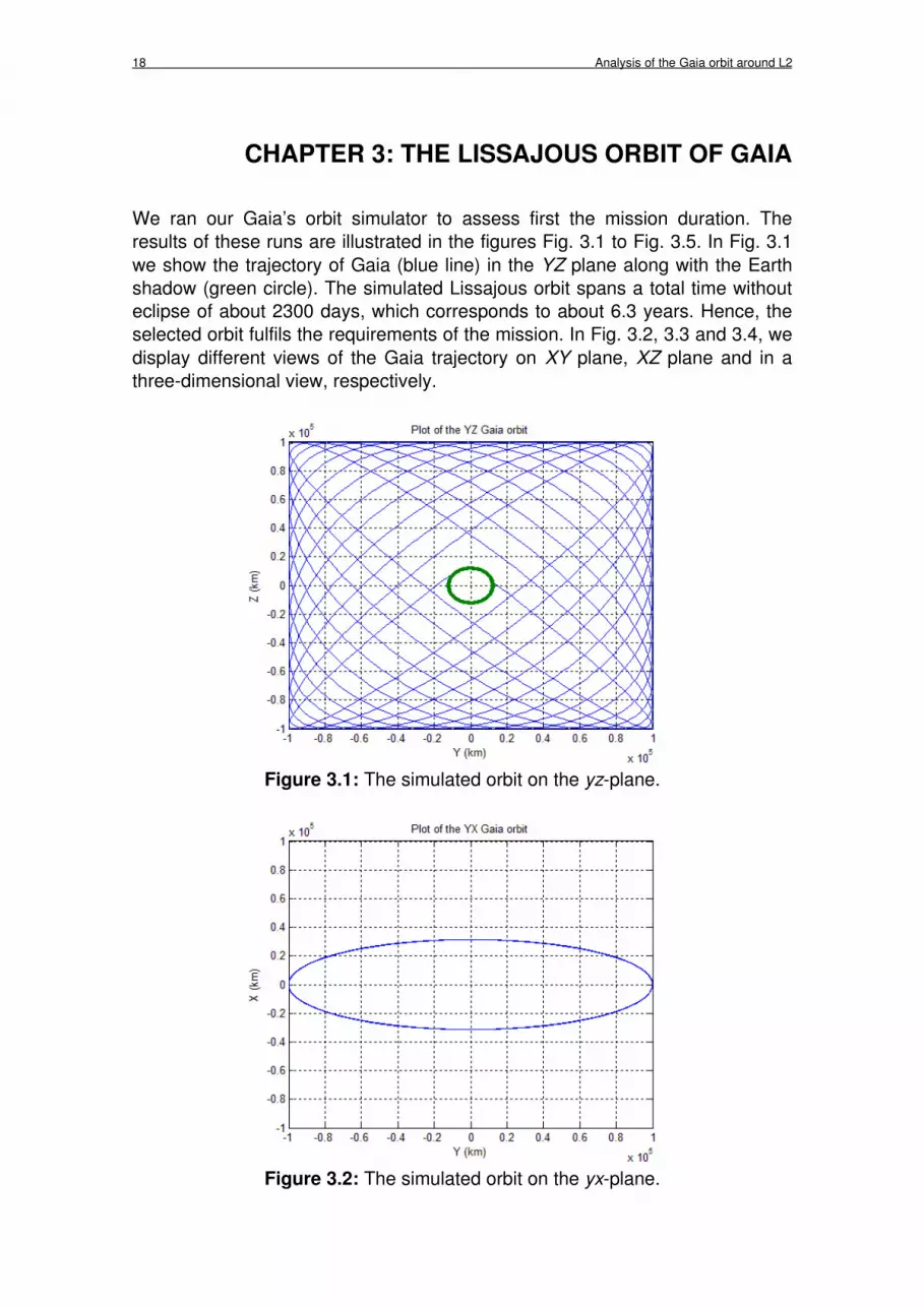
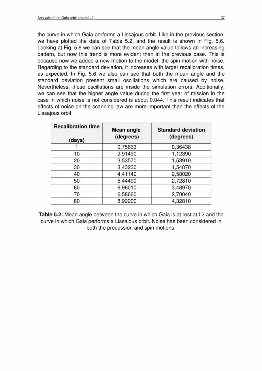
We ran our Gaia’s orbit simulator to assess first the mission duration. The results of these runs are illustrated in the figures Fig. 3.1 to Fig. 3.5. In Fig. 3.1 we show the trajectory of Gaia (blue line) in the YZ plane along with the Earth shadow (green circle). The simulated Lissajous orbit spans a total time without eclipse of about 2300 days, which corresponds to about 6.3 years. Hence, the selected orbit fulfils the requirements of the mission. In Fig. 3.2, 3.3 and 3.4, we display different views of the Gaia trajectory on XY plane, XZ plane and in a threedimensional view, respectively.

Figure 3.1: The simulated orbit on the yzplane.

Figure 3.2: The simulated orbit on the yxplane.


Figure 3.3: The simulated orbit on the xzplane.

Figure 3.4: A threedimensional view of the simulated orbit.

Finally, in Fig. 3.5 we present the time evolution of the SunGaiaEarth angle. As we can observed, this angle evolves with time following an oscillatory convergent motion until an inflexion point over half the mission time, and after this evolves following an oscillatory divergent motion until the mission ends. The angle value is always between 0.4 and 5.3 degrees so our solution also fulfils the SGE angle constraint and, thus, it is a valid Lissajous orbit.


Figure 3.5: The evolution of the SGE angle for the simulated orbit.

3.1 The role of the initial conditions

To understand more deeply the behavior of the Lissajous orbits we did some additional simulations varying the initial position. In fact, the initial position of Gaia will be related to the transfer orbit from the geostationary orbit to the L2 point. Although it is beyond the scope of the present work to analyze the exact injection point, we will do some preliminary analysis to determine the influence of the initial condition on the mission time. The basic idea is that in order to avoid the solar eclipse during the maximum time the best initial distance to the L2 point is precisely that which has the boundary of the eclipse zone (that is 13000 km). In Table 3.1 we show some examples of initial distances to L2 and their corresponding orbit time without eclipse. As can be seen, the farther the initial position with respect to the L2 point, the shorter the time without an eclipse. Graphical representations of the Gaia orbit for different values of the initial distance to L2 are shown in Figs. 3.6 to 3.9.

Initial distance to L2 (km)

Orbit time without eclipse (years)

13000 6.310720000 6.064330000 5.815240000 5.566150000 5.0732

100000 3.3374140000 0.3696


Table 3.1: Mission lifetime as a function of the initial distance to L2.

Figure 3.6: Gaia orbit when the initial position (red circle) is at 13000 km from the L2 Lagrangian point.

Figure 3.7: Same as Fig. 3.6 for a distance of 50000 km.


Similar results are obtained for the time variation of the SGE angle. We show these results in Figs. 3.10 to 3.13.

Figure 3.10: Evolution of the SGE angle for an initial position of 13000 km from the Lagrangian L2 point.

Figure 3.11: Same as Fig. 3.10 for an initial position of 50000 km from the Lagrangian L2 point.


CHAPTER 4: THE 3DIMENSIONAL MOTION OF GAIA

4.1 Introduction

The 3dimensional motion of Gaia is relatively complex since it results from the combination of four motions. The first and most obvious one is translation around the Sun. This orbit has obviously a period of one year, the same as that of the Earth. The second important motion is the orbit that Gaia describes around the Lagrangian L2 point, and it has been described and characterized in previous chapters. To these motions the rotation of Gaia around its own spin axis must be added. Finally, there is also a precession motion: it is the change in the direction of the Gaia spin axis following a circle. Up to now we only have simulated the Lissajous orbit. In order to simulate the complete scanning law we need to add the other three motions. In previous efforts [1] a simulator of the Gaia scanning law was implemented. In this simulator Gaia was considered to be fixed at the L2 Lagrangian point, and the Lissajous orbit was disregarded. In this chapter we describe the results of coupling our own simulator of the Lissajous orbit to the previously built simulator. The resulting code, which fully describes the 3dimensional motion of Gaia, can be found in Appendix D.

4.2 Results

4.2.1 Translation

Although Gaia will orbit around the Sun, for the sake of clarity we will consider that Gaia is fixed in a reference frame and, thus, the Sun orbits around it. Hence, the path of the Sun mirrors the translation motion of Gaia. In Fig. 4.1 we display the path of the Sun for the 6.3 years of maximum mission duration time, as seen from Gaia, when the Lissajous orbit is disregarded (blue line), and when we take it into account (green line).


10.5

00.5

1

1

0.5

0

0.5

11

0.5

0

0.5

1

z ax

is

x axisy axis

10.5

00.5

1

1

0.5

0

0.5

11

0.5

0

0.5

1

x axisy axis

z ax

is

Figure 4.1: The translation curve with (green line) and without (blue line) taking into account the Lissajous orbit.

As can be seen, the two plots look identical. The differences between the two plots are very small because the maximum amplitude of the Lissajous orbit is only 105 km, while the GaiaSun distance is about 1.5 x 108 km. On the other hand, we can also compute the differences in the variation of the angle between the two curves as seen from Gaia. This is shown in Fig. 4.2. As can be seen, the angle is not zero at any moment, which would be the case if the two curves were the same. Instead, the evolution of the angle clearly follows a pattern similar to that of the SGE angle, which was studied in Chapter 2. This is an expected behavior since we just added the Lissajous orbit to the translation motion, so its effects should be clearly visible.


0 10 20 30 40 50 60 70 800

.0 01

.0 02

.0 03

.0 04

.0 05

.0 06

Time (months)

Ang

le (d

egre

es)

Figure 4.2 Time evolution of the angle between the real position of Gaia and the translation curve when the Lissajous orbit is taken into account.

4.2.2 Translation + Precession

The addition of the translation and the precession motions yields the instantaneous direction of the spin axis of Gaia. In Fig 4.3 we show the computed orbit when the Lissajous orbit is neglected (blue line) and when it is taken into account (green line). In both cases we plot the motion during 6.3 years, the total foreseen mission duration. As in the previous case, the two plots look identical but actually they are not. The differences between those two curves can be best appreciated when looking at the time variation of the angle between the two curves, as we did before. The time evolution of the angle is shown in Fig. 4.4. In this case, as in the previous one, the differences follow the same pattern obtained for the SGE angle in Chapter 2. However, now it is not as evident as it was in the previous case. This is a consequence of the considering a new motion, precession of the axis of Gaia.


1 .0 5

0.0 5

1

1

.0 5

0

.0 5

11

.0 5

0

.0 5

1

x axisy axis

z ax

is

10.5

00.5

1

1

0.5

0

0.5

11

0.5

0

0.5

1

x axisy axis

z ax

is

Figure 4.3: Time evolution of the spin axis of Gaia when the Lissajous orbit is not taken into account (blue line) and the same when the Lissajous orbit is

added (green line).


0 10 20 30 40 50 60 70 800

.0 005

.0 01

.0 015

.0 02

.0 025

.0 03

.0 035

.0 04

Time (months)

Ang

le (d

egre

es)

Figure 4.4: Time evolution of the angle between the instantaneous spin axis of Gaia with and without including the Lissajous orbit.

4.2.3 Translation + Precession + Spin

Finally, in Fig 4.5 we show the curve when the translation, precession and spin motions are included (blue line) and the same when we additionally take into account the Lissajous orbit (green line). In this case, unlike in the previous two cases, we only plotted one month and not the 6.3 years of mission duration because the curves are more complex than the previous ones. The curve encompassing 6.3 years would cover the complete sphere, as required by the mission strategy, which demands a complete sky coverage.

1 .0 5

0.0 5

1

1

.0 5

0

.0 5

11

.0 5

0

.0 5

1

x axisy axis

z ax

is


1 .0 5

0.0 5

1

1

.0 5

0

.0 5

11

.0 5

0

.0 5

1

x axisy axis

z ax

is

Figure 4.5: Direction of the telescope field of view when the Lissajous orbit is disregarded (blue line) and the same when the Lissajous orbit is considered

(green line). We show only one month.

To better appreciate the differences between the two curves we plot in Fig. 4.6 the time evolution of the angle between the two curves. The first thing to be noted is that now the frequency of the resulting curve is much larger. The reason for this is the inclusion of the spin motion which, unlike the other two motions, has a much higher frequency – see Ref. [1]. A closeup of these high frequency variations can be seen in Fig. 4.7.

0 0.2 0.4 0.6 0.8 10

0.005

0.01

0.015

0.02

0.025

0.03

0.035

0.04

Time (months)

Ang

le (d

egre

es)

Figure 4.6: Time variation of the angle between the telescope field of view when the Lissajous orbit is disregarded and when the Lissajous orbit is

considered.


0.06 0.07 0.08 0.09 0.1

0

1

2

3

4

5

6

x 103

Time (months)

Ang

le (d

egre

es)

Figure 4.7: Closeup of Fig.4.6.

The second thing to be noticed in Fig.4.7 is that it seems that the pattern of variation of the angle does not follow the SGE angle pattern, as it was the case for the two previously studied motions. Actually, it is following the SGE angle pattern but the time scale is too short (1 month) to notice it. Consequently, in Fig.4.8 we increased the time span of the plot to 1 year and, as can be seen, now the pattern is consistent with our expectations. Finally, we remark that the largest value that this angle reaches is 0.045o. This is the largest difference that the field of view of the telescope of Gaia reaches with respect to the nominal motion of Gaia.

0 .0 5 1 .1 5 2 .2 5 3 .3 5

x 107

0

.0 005

.0 01

.0 015

.0 02

.0 025

.0 03

.0 035

.0 04

.0 045

Time (seconds)

Ang

le (d

egre

es)

Figure 4.8: Same as Fig.4.6 but for a time span of one year.


CHAPTER 5: THE EFFECTS OF NOISE

5.1 Introduction

Once we have simulated the complete scanning law of Gaia and compared the differences when the Lissajous orbit of Gaia is taken into account, we also wanted to study the effects of adding noise to the motion. This means introducing some perturbations in the scanning law, and also the need to incorporate occasional recalibrations to periodically correct the errors caused by the noise. The noise introduced aims to represent the perturbations that Gaia will have due to the solar wind, to gravitational distortions, to spacecraft shortcomings and so on. This is indeed a complex task, which can be simplified when the characteristics of Gaia are fully taken into account. First of all, we can consider that noise does not affect Gaia translation orbit around the Sun neither the Lissajous orbit around L2. This stems from the fact that those two motions are very stable and their time scales are very large compared with that of the spacecraft. Thus, these errors can be considered negligible. According to this, in our work noise will only affect the precession and spin motions, resulting in a jitter of the field of view of Gaia. To implement this noise in our code we added the model of jitter developed in Ref. [1] to our model for the motion around the Lissajous orbit. The noise is realistically modeled using Gaussian and uniform distributions, and a Butterworth filter to attenuate high frequencies. The reader can found additional details in Ref. [1].

5.2 Results

5.2.1 Translation + Precession with noise

First of all, we have simulated the translation and precession motions when noise has been introduced to the precession motion. After that we have included the Lissajous motion and then we have compared the two simulations. In Fig.5.1 we show the curve corresponding to the orbit taking into account the Lissajous orbit. For the sake of clarity we do not show the curve corresponding to the orbit without Lissajous, given that, as already demonstrated in the previous chapter, the differences are not visible except at very small scales. As can be seen, again the two curves look identical although they are not. This is because the noise level is too small to be seen.


1 .0 5

0.0 5

1

1

.0 5

0

.0 5

11

.0 5

0

.0 5

1

x axisy axis

z ax

is

Figure 5.1: Motion of the instantaneous rotation axis of Gaia when noise is included. The time elapsed is the 6.3 years of mission duration time and the

recalibration period is two months.

However, we can observe the differences between the curve in which Gaia rests at L2 and that in which the Lissajous orbit has been included, looking at Fig. 5.2, which shows the behavior of the angle between them, during the 6.3 years of mission duration. As can be seen, now it is impossible to see the pattern of the SGE angle produced by the Lissajous orbit because the noise masks it. In fact, comparing this figure with Fig. 4.4 we notice that in the case in which noise has been considered the angle is larger than in the case in which noise was not taken into account. This is so despite the fact that in the former case we have applied periodic recalibrations, which reset the error periodically. We have used a recalibration period of two months, which can be clearly seen in Fig. 5.2.

0 10 20 30 40 50 60 70 800

0.2

0.4

0.6

0.8

1

1.2

1.4

1.6

1.8

Time (months)

Ang

le (d

egre

es)

Figure 5.2: Time variation of the angle between the axis of Gaia when the Lissajous orbit is taken into account and disregarded for the case in which noise


is considered, during the 6.3 years mission duration time, and with a recalibration period of 2 months.

In order to view more clearly the importance of the effects of the Lissajous orbit, the noise and the recalibration periods we have tabulated in Table 5.1 as a function of the recalibration time the mean value of the angle between the two previously described curves, namely, those in which the Lissajous orbit is disregarded and considered. The table also shows the standard deviation. The data of Table 5.1 (and also Table 5.2, and 5.3) was calculated as the mean of five independent simulations. In each of these simulations we computed the value of the mean angle and its standard deviation for nine different recalibration times. The mean angle and the standard deviation are defined by the following equations respectively.

(5.1)

(5.2)

Recalibration time

(days)

Mean angle (degrees)

Standard deviation (degrees)

1 0,023659 0,01233410 0,087091 0,04434220 0,087039 0,04705930 0,127310 0,07214540 0,112970 0,07385450 0,172780 0,13860060 0,103260 0,07517170 0,158810 0,08662380 0,228060 0,179070

Table 5.1: Mean value and standard deviation for the angle between the curves in which the Lissajous orbit is considered or disregarded.

In Fig 5.3 we display graphically the behavior of the mean angle as a function of the recalibration time for the data of Table 5.1. As can be seen, the value of the mean angle is clearly affected by the presence of noise, which causes some oscillations. Besides, it is easy to see that in general the value of the mean angle grows with increasing recalibration times. The same occurs for the standard. This is the expected behavior: the larger the time of recalibration, the


bigger the difference between the ideal case and the one in which noise is added. Additionally, if we compare with Fig.4.4 we can see that the largest value of the angle in the ideal case is about 0.036. Thus, we can say that when the recalibration time is bigger than about 12 days, the effects of noise on the scanning law are more important than the effects of considering the Lissajous orbit.

0 20 40 60 80 1000

.0 05

.0 1

.0 15

.0 2

.0 25

.0 3

.0 35

.0 4

.0 45

Recalibration time (days)

Mea

n an

gle

(deg

rees

)

Figure 5.3: The mean value and standard deviation of the angle between the curves obtained taking into account the Lissajous orbit or disregarding it.

5.2.2 Translation + Precession with noise + Spin with noise

In this section we study the effects of adding noise to the spin motion in addition of considering the effects of the Lissajous orbit. The spin noise, like the precession noise, is modeled by a normal distribution filtered with a Butterworth filter [1]. In Fig.5.4 we show the simulated curve when the Lissajous orbit is considered. In this case, unlike in the previous case, we only plotted one month and not 6.3 years because these curves are much more complex than the previous one. The differences between this case and the one corresponding to the nominal motion of Gaia, like in the previous section, are very small because the noise level is too low to be detected at this scale and also the Lissajous motion is too small compared with the GaiaSun distance.


10.5

00.5

1

1

0.5

0

0.5

11

0.5

0

0.5

1

x axisy axis

z ax

is

Figure 5.4: The curve described by the field of view of Gaia when both the effects of noise and of the Lissajous orbit are taken into account. The duration

of the plot is one month and the recalibration period is 10 days.

In Fig. 5.5 we can see the behavior of the angle between the simulated and the nominal curves. Like in the previous case, the SGE pattern is not visible. Instead of that, now is clearly visible the effects of the precession and spin noises and also the effect of the recalibration time. If we compare this result with the plot obtained without noise (Fig. 4.6) we notice that now the value of the angle is much larger. Of course it depends on the recalibration frequency, which in this simulation is 10 days.

0 .0 2 .0 4 .0 6 .0 8 10

2

4

6

8

10

12

Time (months)

Ang

le (d

egre

es)

Figure 5.5: Time evolution of the angle between the curve in which Gaia is at rest at L2 and the curve in which Gaia performs a Lissajous orbit, during one

month and with recalibration period of 10 days.

Table 5.2 shows, for different recalibration times, the mean value of the angle (and its standard deviation) between the curve in which Gaia is at rest at L2 and


the curve in which Gaia performs a Lissajous orbit. Like in the previous section, we have plotted the data of Table 5.2, and the result is shown in Fig. 5.6. Looking at Fig. 5.6 we can see that the mean angle value follows an increasing pattern, but now this trend is more evident than in the previous case. This is because now we added a new motion to the model: the spin motion with noise. Regarding to the standard deviation, it increases with larger recalibration times, as expected. In Fig. 5.6 we also can see that both the mean angle and the standard deviation present small oscillations which are caused by noise. Nevertheless, these oscillations are inside the simulation errors. Additionally, we can see that the higher angle value during the first year of mission in the case in which noise is not considered is about 0.044. This result indicates that effects of noise on the scanning law are more important than the effects of the Lissajous orbit.

Recalibration time

(days)



1 0,75633 0,3643810 2,91490 1,1239020 3,53570 1,5391030 3,43230 1,5487040 4,41140 2,5802050 5,44490 2,7281060 6,96010 3,4897070 6,58660 2,7004080 8,92200 4,32810

Table 5.2: Mean angle between the curve in which Gaia is at rest at L2 and the curve in which Gaia performs a Lissajous orbit. Noise has been considered in

both the precession and spin motions.


0 20 40 60 80 1000

2

4

6

8

10

12

14


Mea

n an

gle

(deg

rees

)

Figure 5.6: Mean angle between the curve in which Gaia is at rest at L2 and the curve in which Gaia performs a Lissajous orbit. Noise has been considered

in both the precession and spin motions.

5.2.3 Translation + Precession with noise + Spin with noise + Pointing errors

Finally, we considered another source of error: the pointing error. Unlike the two previous errors, this error is not provided by any motion. It is provided by some inaccuracies in the pointing of the field of view of Gaia caused by shortcomings of the instruments, by structural weaknesses, and others.In Fig. 5.7 we show the resulting instantaneous field of view of Gaia when the Lissajous orbit is considered.

1 .0 5

0.0 5

1

1

.0 5

0

.0 5

11

.0 5

0

.0 5

1

x axisy axis

z ax

is

Figure 5.7: Evolution of the instantaneous field of view of Gaia when all sources of error are considered. The duration of the plot is one month and the

recalibration period is 10 days.


0 0.2 0.4 0.6 0.8 10

2

4

6

8

10

12

Time (months)

Ang

le (d

egre

es)

Figure 5.8: The time evolution of the angle between the real and the nominal position of the field of view of Gaia when all error sources are taken into

account.

In Fig.5.8 we graphically display the time evolution of the angle between the two previously discussed curves. Like in the previous case, the effects of precession, spin and pointing errors are clearly visible. Also, the periodic recalibrations (every 10 days) are quite apparent. However, the effects of the Lissajous orbit are no evident. This occurs because the time plotted is too small (1 month) and the recalibration period (10 days) too big for the effects of the Lissajous orbit to be appreciable. When comparing this figure with that in which no noise was considered (Fig. 4.6) we notice that now the angles are much larger. Clearly, this is due to the noise effects, and obviously depends on the recalibration frequency. Additionally, if we compare this figure with that in which no pointing errors were considered (Fig. 5.5), we notice that the two figures look very similar. Nevertheless, they are different. There are some small differences caused by the pointing errors. Table 5.3 shows for different recalibration periods the mean value of the angle and standard deviation when the Lissajous orbit is considered or disregarded.

Recalibration time

(days)



1 0,75737 0,3639510 2,91520 1,1237020 3,53590 1,5389030 3,43240 1,5486040 4,41160 2,5802050 5,44500 2,7280060 6,96030 3,48970


70 6,58670 2,7004080 8,92210 4,32810

Table 5.3: Mean value and standard deviation of the angle between the real and the nominal position of the field of view of Gaia when all error sources are

taken into account.

0 20 40 60 80 1000

2

4

6

8

10

12

14


Mea

n an

gle

(deg

rees

)

Figure 5.9: Mean value and standard deviation of the angle between the real and the nominal position of the field of view of Gaia when all error sources are

taken into account.

The data of Table 5.3 is shown graphically in Fig. 5.9. This figure, again, looks very similar to Fig. 5.6, although subtle differences can be found. These small differences can be better found when tables 5.2 and 5.3 are compared. In fact the differences are small because the pointing errors are indeed very small.


CHAPTER 6: CONCLUSIONS

In this work we have studied and simulated the Lissajous orbit that Gaia will perform around the Lagrangian point L2 of the SunEarth system. Lissajous orbits around L2 are very useful for space observation because they can provide a large time without solar eclipse and, moreover, they are very stable in dynamical terms and in thermal conditions. Specifically, we have shown that with selected and realistic orbital parameters for the orbit of Gaia a mission duration time of about 6.3 years can be obtained, as required by the mission strategy. Moreover, varying the initial conditions of the spacecraft we can obtain different mission lifetimes. In particular, we have obtained that the highest mission durations were obtained when the initial position of the spacecraft was close enough to the shadow of the Earth.

We have also incorporated the Lissajous orbits into the Gaia orbit simulator fully explained in Ref. [1]. We have studied the effects of adding the Lissajous motion to the Gaia scanning law, which is obtained by adding the translation, precession and spin motions. We have also demonstrated that the effects of including the Lissajous orbit in the Gaia scanning law are very small. In fact, they are so small that in a first order approximation they could be neglected. Nevertheless an accurate description of the tracking is needed to measure microarc seconds, and, consequently, this new module must be incorporated in Gaia Telemetry Simulator. The reason of the small effects obtained when the Lissajous orbit is incorporated is that the maximum amplitude is too small compared with the SunGaia distance. This, in turn, implies that generally speaking, the use of Lissajous orbits in space missions yields many more advantages than drawbacks. In particular, these orbits practically do not perturb the scientific observations and, moreover, they provide very stable positional and thermal conditions.

Finally, we also studied a more realistic case, in which noise was considered in the precession and spin motions, and also in the pointing of the field of view. We did not consider noise in the translation and Lissajous motions because we considered these motions to be very stable. We have seen that, in this case, the effects of the Lissajous orbit on the Gaia scanning law are superseded by the effects of noise. This occurs whatever case is considered. The effects of noise in the precession and spin motions, and especially the field of view pointing errors, are much larger than the effects of the Lissajous orbit. All in all, we conclude that periodical recalibration maneuvers are essential, and if they are not realized the accumulation of errors will not allow accurate measurements.

In summary, we have studied the effects of the Lissajous orbit on the Gaia scanning law. To do this we have built a piece of software that we have incorporated in the simulator of the scanning law of Gaia. The new simulator


produces realistic scanning laws of a spacecraft, including the effects of jitter. This piece of software also produces all the plots necessary to model and understand the scanning law of Gaia. Finally, this software can be incorporated to more complex simulators, like the Gaia Telemetry Simulator. In this way the effects of the Lissajous orbit and of noise on the performance of the foreseen solutions for the Gaia Optimal Compression Algorithm can be assessed in a realistic way.


BIBLIOGRAPHY

[1] Bartrons, E., “The impact of jitter on the scanning law of Gaia”, EPSC (February 2009).

[2] “Gaia Consolidated Report on Mission Analysis”, GAIAESCRP0001, ESA, (October 2008).

[3] Jordan, S. “The Gaia Project – technique, performance and status”Astron. Nachr., 329, 875880 (2008).

[4] Lindegren, L., Proceedings of Gaia Symposium “The ThreeDimensional Universe with Gaia” (ESA SP576), Editors: C. Turon, K.S. O’Flaherty, M.A.C. Perryman, 2004, p. 29.

[5] http://sci.esa.int/sciencee/www/area/index.cfm?fareaid=26

[6] http://www.mathworks.com/products/matlab/


APPENDIX A: LAGRANGIAN POINTS

Lagrangian points, also known as libration points, are five points in an orbital configuration where a small object can be stationary relative to two larger objects. This is possible because at these points, the combined gravitational pull of the two large masses provides exactly the centripetal force required to rotate with them. A more technical definition is that the Lagrangian points are the stationary solutions of the circular restricted threebody problem.

In Fig.A.1 the five Lagrangian points of the SunEarth system are shown. As can be seen, the points L1, L2 and L3 are on the line formed by Sun and Earth, while L4 and L5 are on a line which has a 60 degrees angle with SunEarth line. In the figure it seems that L3, L4 and L5 are on the Earth translation trajectory but actually they are out of it.

Figure A.1: Lagrangian points of the SunEarth system.


Figure A.2: Dynamic stability of the Lagrangian points.

In Fig.A.2 the dynamic stability of the Lagrangian points is displayed. As can be seen, L1, L2 and L3 are dynamically unstable towards the radial direction but stable on the tangential direction. On the other hand, L4 and L5 are dynamically unstable in any direction.


APPENDIX B: LISSAJOUS CURVES

A Lissajous curve is the graph of the system of parametric equations which describes complex harmonic motion.

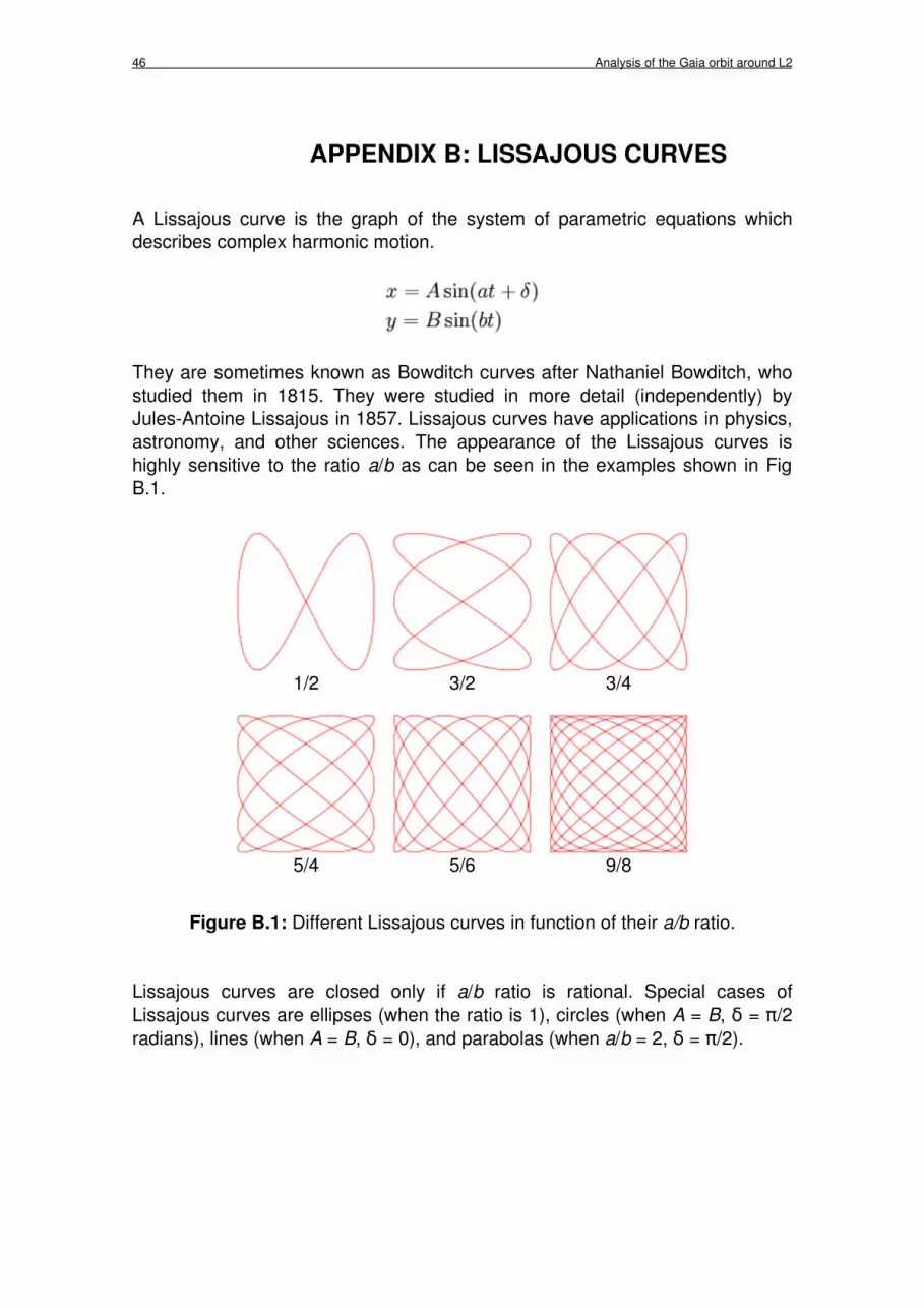
They are sometimes known as Bowditch curves after Nathaniel Bowditch, who studied them in 1815. They were studied in more detail (independently) by JulesAntoine Lissajous in 1857. Lissajous curves have applications in physics, astronomy, and other sciences. The appearance of the Lissajous curves is highly sensitive to the ratio a/b as can be seen in the examples shown in Fig B.1.

1/2 3/2 3/4

5/4 5/6 9/8

Figure B.1: Different Lissajous curves in function of their a/b ratio.

Lissajous curves are closed only if a/b ratio is rational. Special cases of Lissajous curves are ellipses (when the ratio is 1), circles (when A = B, δ = π/2 radians), lines (when A = B, δ = 0), and parabolas (when a/b = 2, δ = π/2).

http://en.wikipedia.org/wiki/File:Lissajous_curve_1to2.svg







APPENDIX C: THE SCANNING LAW OF GAIA

Gaia will perform its observations from a controlled Lissajoustype orbit around the L2 Lagrange point of the Sun and EarthMoon system. During its operational lifetime, the satellite will continuously spin around its axis. As a result, the two astrometric fields of view will scan across all objects located along the great circle perpendicular to the spin axis. The combination of these motions is known as the scanning law of Gaia and it is basically described by three motions: the translation motion, the precession motion and the spin motion. These motions are characterized by their respective rates. The orbital rate is the velocity of translation around the Sun, the precession rate is the velocity of precession of the spin axis around the axis, and the scan rate is the spin velocity around the spin axis. They are shown in Table C.1.

Angular velocity rad h1 arc sec s1

Orbital rate (ω )

⋅

36001

87662π

0,041

Precession rate (ω p)

⋅

×

360 0

1

360

21 7,0 π0,17

Scan rate (ω s)

⋅

×

360 0

1

360

21 20 π120

Table C.1: Nominal values adopted for the three angular velocities of Gaia..

C.1 The translation motion

To show the Gaia translation motion around the Sun, we represented in Fig. C.1 the normalized Sun path around Gaia (the reference system is that in which Gaia does not move in the coordinate origin and the Sun orbits around it). To plot this figure it is used the vector 1r

, which represents the direction pointing

towards the position of the Sun and is the result of applying the following simple rotation matrix around the zaxis:

(C.1)


Figure C.1: The path of the Sun in a 1 year period, as seen from Gaia.

C.2 The precession motion

In Fig C.2 we show the result of adding the motion of the spin axis of Gaia. To plot this figure we have used the vector 2r

which represents the precession of

the Gaia spin axis and is found using the following combination of rotations.

(C.2)

The vector 2pr

is the result of making a rotation in the yzplane according to the precession rate iteratively:

(C.3)

The vector ( )111 ,, −−− ip

ip

ip zyx is the vector 2pr

obtained in the previous time step

and s is the corresponding time step.


Figure C.2: Motion of the spin axis of Gaia during a period of time of one year.

C.3 The spin motion

Finally, the result of adding the motion of the field of view of Gaia is shown in Fig. C.3. In order to obtain this figure we used the vector 3r

which is, unlike the

previous two motions, the result of a rotation around a dynamic axis ( 2r

) and not around a static axis, so the calculations are a somewhat more difficult.

(C.4)

(C.5)

(C.6)


(C.7)

The vector ( )13

13

13 ,, −−− iii zyx the vector 3r

obtained at the previous time step

and s the corresponding time step.

Figure C.3: Motion of the field of view of Gaia during three months.


APPENDIX D: NUMERICAL CODE

%%%%%%%%%%%%%%%%%%%%%%%%%%%%%%%% START %%%%%%%%%%%%%%%%%%%%%%%%%%%%%%%%%%%% clear all the previous data, plots and commands:clear allclose allclc

%%%%%%%%%%%%%%%%%%%%%%%%%%%%%%%%%%%%%%%%%%%%%%%%%%%%%%%%%%%%%%%%%%%%%%%%%%% DEFINITION OF PARAMETERS:%%%%%%%%%%%%%%%%%%%%%%%%%%%%%%%%%%%%%%%%%%%%%%%%%%%%%%%%%%%%%%%%%%%%%%%%%%

% INPUT DATA:%%%%%%%%%%%%%% time lenght (s):lenght = 10*24*3600;% sample time (s):s = 100;% recalibration times (s):rec = 5*24*3600;

% Inital coordinates y,z in the Lissajous orbit (km)% (only necessary for calculating Lissajous phases):Y0=-13000*sin(45*(pi/180));Z0=13000*cos(45*(pi/180));

% DEFINING LISSAJOUS ORBIT PARAMETERS:%%%%%%%%%%%%%%%%%%%%%%%%%%%%%%%%%%%%%%% Lissajous orbit periods (days):Txy=177.655*24*3600;Tz=184.0*24*3600;

% Lissajous orbit amplitudes (km):Az=100000;Ay=100000;Ax=Ay/3.1872293; %Ax is related with Ay by the constant C2 = 3.1872293

%Maximum Lissajous orbit total time (with or without solar eclipses)(years)years=8; %for example: 8 years

% Astronomic unit (distance Earh-Sun)(km):AU=1.49598*10^8;

% Earth-L2 distance (km):XL=1507683;

% Earth shadow radium (km):r=13000;

% Creating Earth shadow in the yz-plane:for tes=[0:1:10000]; ry(tes+1)=r*-sin(tes); rz(tes+1)=r*cos(tes);end

% Calculating Lissajous orbit rates:Wxy=2*pi/Txy;Wz=2*pi/Tz;

% Calculating Lissajous orbit phases:


Pxy=asin(Y0/-Ay);Pz=acos(Z0/Az);

% DEFINING SCANNING LAW PARAMETERS:%%%%%%%%%%%%%%%%%%%%%%%%%%%%%%%%%%%% Defining motion rates:w = ((2*pi)/8766)*(1./3600); % translationwp = ((0.17*2*pi)/360)*(1./3600); % precessionws = ((120*2*pi)/360)*(1./3600); % spinning

% Initial value for precession vector:p1n = sqrt(0.5); p2n = -sqrt(0.5); p3n = 0;

% Initial value for spinning vector:p1(1) = 0.0; p2(1) = 1.0; p3(1) = 0.0;

%initializing errors:sigma_wp = ((0.1*2*pi)/(3*360))*(1./3600); % precessionsigma_ws = ((1.2*2*pi)/(3*360))*(1./3600); % spinningsigma_point = ((5*2*pi)/(3*60*360)); % pointing

% INITIALIZING VECTORS:%%%%%%%%%%%%%%%%%%%%%%%% (This reserves enough memory space and optimizes the simulation process)vl=(lenght/s)+1;x=zeros(1,vl); y=zeros(1,vl); z=zeros(1,vl);x1=zeros(1,vl); y1=zeros(1,vl); z1=zeros(1,vl);x1L=zeros(1,vl); y1L=zeros(1,vl); z1L=zeros(1,vl);x2=zeros(1,vl); y2=zeros(1,vl); z2=zeros(1,vl);x2i=zeros(1,vl); y2i=zeros(1,vl); z2i=zeros(1,vl);x3=zeros(1,vl); y3=zeros(1,vl); z3=zeros(1,vl);x31=zeros(1,vl); y31=zeros(1,vl); z31=zeros(1,vl);x3i=zeros(1,vl); y3i=zeros(1,vl); z3i=zeros(1,vl);xp2=zeros(1,vl); yp2=zeros(1,vl); zp2=zeros(1,vl);xp2i=zeros(1,vl); yp2i=zeros(1,vl); zp2i=zeros(1,vl);nlx=zeros(1,vl); nly=zeros(1,vl); nlz=zeros(1,vl);nx=zeros(1,vl); ny=zeros(1,vl); nz=zeros(1,vl);nx1_nol=zeros(1,vl); ny1_nol=zeros(1,vl); nz1_nol=zeros(1,vl);nx1=zeros(1,vl); ny1=zeros(1,vl); nz1=zeros(1,vl);nx3=zeros(1,vl); ny3=zeros(1,vl); nz3=zeros(1,vl);nx31=zeros(1,vl); ny31=zeros(1,vl); nz31=zeros(1,vl);nx31L=zeros(1,vl); ny31L=zeros(1,vl); nz31L=zeros(1,vl);nx3L=zeros(1,vl); ny3L=zeros(1,vl); nz3L=zeros(1,vl);nx3i=zeros(1,vl); ny3i=zeros(1,vl); nz3i=zeros(1,vl);nxL=zeros(1,vl); nyL=zeros(1,vl); nzL=zeros(1,vl);nxi=zeros(1,vl); nyi=zeros(1,vl); nzi=zeros(1,vl);lx=zeros(1,vl); ly=zeros(1,vl); lz=zeros(1,vl);nxi_nol=zeros(1,vl); nyi_nol=zeros(1,vl); nzi_nol=zeros(1,vl);nx3i_nol=zeros(1,vl); ny3i_nol=zeros(1,vl); nz3i_nol=zeros(1,vl);anglenr1=zeros(1,vl); anlgenr2=zeros(1,vl); anglenr3=zeros(1,vl);anglenr2noise=zeros(1,vl); anlgenr31noise=zeros(1,vl); anglenr3noise=zeros(1,vl);new_theta=zeros(1,vl); new_fi=zeros(1,vl);wpe=zeros(1,vl); wse=zeros(1,vl);x=zeros(1,vl);k=zeros(1,vl);

%%%%%%%%%%%%%%%%%%%%%%%%%%%%%%%%%%%%%%%%%%%%%%%%%%%%%%%%%%%%%%%%%%%%%%%%%%% LISSAJOUS ORBIT SIMULATION:%%%%%%%%%%%%%%%%%%%%%%%%%%%%%%%%%%%%%%%%%%%%%%%%%%%%%%%%%%%%%%%%%%%%%%%%%%

cont=1;ld=r+1;


for t = 0:s:lenght;

if (ld >= r) %(if the orbit didn't cross the Earth-shadow:) % Calculating position with the Lissajous orbit equations: lx(cont)=Ax*cos(Wxy*t+Pxy); ly(cont)=-Ay*sin(Wxy*t+Pxy); lz(cont)=Az*cos(Wz*t+Pz);

% Normalizing vector: nlx(cont) = lx(cont)/sqrt(lx(cont)^2+ly(cont)^2+lz(cont)^2); nly(cont) = ly(cont)/sqrt(lx(cont)^2+ly(cont)^2+lz(cont)^2); nlz(cont) = lz(cont)/sqrt(lx(cont)^2+ly(cont)^2+lz(cont)^2);

% calculating distance to Earth shadow % (only necessary for stop the Lissajous orbit when enters to Earth shadow) ld=sqrt(((ly(cont))^2)+((lz(cont))^2))+1;

dlo=lenght; % duration of the Lissajous orbit cont=cont+1;

else %(if the orbit crossed the Earh-shadow:) dlo=t; % duration of the Lissajous orbit break %stops the Lissajous orbit simulation endend

%%%%%%%%%%%%%%%%%%%%%%%%%%%%%%%%%%%%%%%%%%%%%%%%%%%%%%%%%%%%%%%%%%%%%%%%%%% SCANNING LAW WITHOUT NOISE (WITH AND WITHOUT LISSAJOUS):%%%%%%%%%%%%%%%%%%%%%%%%%%%%%%%%%%%%%%%%%%%%%%%%%%%%%%%%%%%%%%%%%%%%%%%%%%

cont = 1;for t = 0:s:lenght

% TRANSLATION (WITHOUT LISSAJOUS): %%%%%%%%%%%%%%%%%%%%%%%%%%%%%%%%%% x1(cont) = (AU+XL)*cos(w*t); y1(cont) = (AU+XL)*sin(w*t); z1(cont) = 0*t;

% Normalizing vector: nx1_nol(cont) = x1(cont)/sqrt(x1(cont)^2+y1(cont)^2+z1(cont)^2); ny1_nol(cont) = y1(cont)/sqrt(x1(cont)^2+y1(cont)^2+z1(cont)^2); nz1_nol(cont) = 0;

% TRANSLATION (WITH LISSAJOUS): %%%%%%%%%%%%%%%%%%%%%%%%%%%%%%% x1L(cont)=lx(cont)+x1(cont); y1L(cont)=ly(cont)+y1(cont); z1L(cont)=lz(cont)+z1(cont);

% Normalizing vector: nx1(cont) = x1L(cont)/sqrt(x1L(cont)^2+y1L(cont)^2+z1L(cont)^2); ny1(cont) = y1L(cont)/sqrt(x1L(cont)^2+y1L(cont)^2+z1L(cont)^2); nz1(cont) = z1L(cont)/sqrt(x1L(cont)^2+y1L(cont)^2+z1L(cont)^2);

% PRECESSION (WITHOUT LISSAJOUS): %%%%%%%%%%%%%%%%%%%%%%%%%%%%%%%%% if cont==1 xp2i(cont) = 0; yp2i(cont) = 1; zp2i(cont) = 0; else


xp2i(cont) = 0; yp2i(cont) = yp2i(cont-1).*cos(wp*s)-zp2i(cont-1).*sin(wp*s); zp2i(cont) = yp2i(cont-1).*sin(wp*s)+zp2i(cont-1).*cos(wp*s); end

x2i(cont) = nx1_nol(cont)+xp2i(cont).*cos(w*t)-yp2i(cont).*sin(w*t); y2i(cont) = ny1_nol(cont)+xp2i(cont).*sin(w*t)+yp2i(cont).*cos(w*t); z2i(cont) = nz1_nol(cont)+zp2i(cont);

% Normalizing vector: nxi_nol(cont) = x2i(cont)./sqrt(x2i(cont).^2+y2i(cont).^2+z2i(cont).^2); nyi_nol(cont) = y2i(cont)./sqrt(x2i(cont).^2+y2i(cont).^2+z2i(cont).^2); nzi_nol(cont) = z2i(cont)./sqrt(x2i(cont).^2+y2i(cont).^2+z2i(cont).^2);

% PRECESION (WITH LISSAJOUS): %%%%%%%%%%%%%%%%%%%%%%%%%%%%% if cont==1 xp2i(cont) = 0; yp2i(cont) = 1; zp2i(cont) = 0; else xp2i(cont) = 0; yp2i(cont) = yp2i(cont-1).*cos(wp*s)-zp2i(cont-1).*sin(wp*s); zp2i(cont) = yp2i(cont-1).*sin(wp*s)+zp2i(cont-1).*cos(wp*s); end

x2i(cont) = nx1(cont)+xp2i(cont).*cos(w*t)-yp2i(cont).*sin(w*t); y2i(cont) = ny1(cont)+xp2i(cont).*sin(w*t)+yp2i(cont).*cos(w*t); z2i(cont) = nz1(cont)+zp2i(cont);

% Normalizing vector: nxi(cont) = x2i(cont)./sqrt(x2i(cont).^2+y2i(cont).^2+z2i(cont).^2); nyi(cont) = y2i(cont)./sqrt(x2i(cont).^2+y2i(cont).^2+z2i(cont).^2); nzi(cont) = z2i(cont)./sqrt(x2i(cont).^2+y2i(cont).^2+z2i(cont).^2);

% SPINNIG (WITHOUT LISSAJOUS): %%%%%%%%%%%%%%%%%%%%%%%%%%%%%% costheta = cos(ws*s); sintheta = sin(ws*s); if cont==1 xp31i = (costheta+(1.0-costheta).*nxi_nol(cont).*nxi_nol(cont)).*p1(1); xp32i = ((1.0-costheta).*nxi_nol(cont).*nyi_nol(cont)-nzi_nol(cont).*sintheta).*p2(1); xp33i = ((1.0-costheta).*nxi_nol(cont).*nzi_nol(cont)+nyi_nol(cont).*sintheta).*p3(1);

yp31i = ((1.0-costheta).*nxi_nol(cont).*nyi_nol(cont)+nzi_nol(cont).*sintheta).*p1(1); yp32i = (costheta+(1.0-costheta).*nyi_nol(cont).*nyi_nol(cont)).*p2(1); yp33i = ((1.0-costheta).*nyi_nol(cont).*nzi_nol(cont)-nxi_nol(cont).*sintheta).*p3(1);

zp31i = ((1.0-costheta).*nxi_nol(cont).*nzi_nol(cont)-nyi_nol(cont).*sintheta).*p1(1); zp32i = ((1.0-costheta).*nyi_nol(cont).*nzi_nol(cont)+nxi_nol(cont).*sintheta).*p2(1); zp33i = (costheta+(1.0-costheta).*nzi_nol(cont).*nzi_nol(cont)).*p3(1); else xp31i=(costheta+(1.0-costheta).*nxi_nol(cont).*nxi_nol(cont)).*nx3i_nol(cont-1); xp32i=((1.0-costheta).*nxi_nol(cont).*nyi_nol(cont)-nzi_nol(cont).*sintheta).*ny3i_nol(cont-1);


xp33i=((1.0-costheta).*nxi_nol(cont).*nzi_nol(cont)+nyi_nol(cont).*sintheta).*nz3i_nol(cont-1);

yp31i=((1.0-costheta).*nxi_nol(cont).*nyi_nol(cont)+nzi_nol(cont).*sintheta).*nx3i_nol(cont-1); yp32i=(costheta+(1.0-costheta).*nyi_nol(cont).*nyi_nol(cont)).*ny3i_nol(cont-1); yp33i=((1.0-costheta).*nyi_nol(cont).*nzi_nol(cont)-nxi_nol(cont).*sintheta).*nz3i_nol(cont-1);

zp31i=((1.0-costheta).*nxi_nol(cont).*nzi_nol(cont)-nyi_nol(cont).*sintheta).*nx3i_nol(cont-1); zp32i=((1.0-costheta).*nyi_nol(cont).*nzi_nol(cont)+nxi_nol(cont).*sintheta).*ny3i_nol(cont-1); zp33i=(costheta+(1.0-costheta).*nzi_nol(cont).*nzi_nol(cont)).*nz3i_nol(cont-1); end

x3i(cont) = xp31i+xp32i+xp33i; y3i(cont) = yp31i+yp32i+yp33i; z3i(cont) = zp31i+zp32i+zp33i;

% Normalizing vector: nx3i_nol(cont) = x3i(cont)./sqrt(x3i(cont).^2+y3i(cont).^2+z3i(cont).^2); ny3i_nol(cont) = y3i(cont)./sqrt(x3i(cont).^2+y3i(cont).^2+z3i(cont).^2); nz3i_nol(cont) = z3i(cont)./sqrt(x3i(cont).^2+y3i(cont).^2+z3i(cont).^2);

% SPINNIG (WITH LISSAJOUS): %%%%%%%%%%%%%%%%%%%%%%%%%%% costheta = cos(ws*s); sintheta = sin(ws*s); if cont==1 xp31i = (costheta+(1.0-costheta).*nxi(cont).*nxi(cont)).*p1(1); xp32i = ((1.0-costheta).*nxi(cont).*nyi(cont)- xp33i = ((1.0-costheta).*nxi(cont).*nzi(cont)

yp31i = ((1.0-costheta).*nxi(cont).*nyi(cont) yp32i = (costheta+(1.0-costheta).*nyi(cont).*nyi(cont)).*p2(1); yp33i = ((1.0-costheta).*nyi(cont).*nzi(cont)-

zp31i = ((1.0-costheta).*nxi(cont).*nzi(cont)- zp32i = ((1.0-costheta).*nyi(cont).*nzi(cont) zp33i = (costheta+(1.0-costheta).*nzi(cont).*nzi(cont)).*p3(1); else xp31i=(costheta+(1.0-costheta).*nxi(cont).*nxi(cont)).*nx3i(cont-1); xp32i=((1.0-costheta).*nxi(cont).*nyi(cont)-nzi(cont).*sintheta).*ny3i(cont-1); xp33i=((1.0-costheta).*nxi(cont).*nzi(cont)+nyi(cont).*sintheta).*nz3i(cont-1);

yp31i=((1.0-costheta).*nxi(cont).*nyi(cont)+nzi(cont).*sintheta).*nx3i(cont-1); yp32i=(costheta+(1.0-costheta).*nyi(cont).*nyi(cont)).*ny3i(cont-1); yp33i=((1.0-costheta).*nyi(cont).*nzi(cont)-nxi(cont).*sintheta).*nz3i(cont-1);

zp31i=((1.0-costheta).*nxi(cont).*nzi(cont)-nyi(cont).*sintheta).*nx3i(cont-1); zp32i=((1.0-costheta).*nyi(cont).*nzi(cont)+nxi(cont).*sintheta).*ny3i(cont-1); zp33i=(costheta+(1.0-costheta).*nzi(cont).*nzi(cont)).*nz3i(cont-1); end


x3i(cont) = xp31i+xp32i+xp33i; y3i(cont) = yp31i+yp32i+yp33i; z3i(cont) = zp31i+zp32i+zp33i;

% Normalizing vector: nx3i(cont) = x3i(cont)./sqrt(x3i(cont).^2+y3i(cont).^2+z3i(cont).^2); ny3i(cont) = y3i(cont)./sqrt(x3i(cont).^2+y3i(cont).^2+z3i(cont).^2); nz3i(cont) = z3i(cont)./sqrt(x3i(cont).^2+y3i(cont).^2+z3i(cont).^2);

cont = cont+1;end

%%%%%%%%%%%%%%%%%%%%%%%%%%%%%%%%%%%%%%%%%%%%%%%%%%%%%%%%%%%%%%%%%%%%%%%%%%% SCANNING LAW WITH NOISE (WITH LISSAJOUS):%%%%%%%%%%%%%%%%%%%%%%%%%%%%%%%%%%%%%%%%%%%%%%%%%%%%%%%%%%%%%%%%%%%%%%%%%%

% CREATING PRECESSION AND SPINNING NOISES:%%%%%%%%%%%%%%%%%%%%%%%%%%%%%%%%%%%%%%%%%%% creating normal distribution (mean=0, std=1)cont = 1;for t = 0:s:lenght x(cont) = randn; while ((x(cont) < - 2) || (x(cont) > 2)) x(cont) = randn; end cont=cont+1;end% creating butterworth filter:[b,a] = butter(100,0.5);% getting filtered signal:y = filter(b,a,x);% getting the new precession and spinning rates:% (there's a factor to achieve the same standard deviation% we had at the beginning (1.488))wpe = wp + (sigma_wp*1.6066).*y;wse = ws + (sigma_ws*1.6083).*y;

it = 0; % used to find multiples of reccont = 1;for t = 0:s:lenght if t==it*rec

% RECALIBRATION: %%%%%%%%%%%%%%%% xp2(cont) = xp2i(cont); yp2(cont) = yp2i(cont); zp2(cont) = zp2i(cont);

nx(cont) = nxi(cont); ny(cont) = nyi(cont); nz(cont) = nzi(cont);

nxL(cont) = nx(cont); nyL(cont) = ny(cont); nzL(cont) = nz(cont);

nx3(cont) = nx3i(cont); ny3(cont) = ny3i(cont); nz3(cont) = nz3i(cont);

nx3L(cont) = nx3(cont);


ny3L(cont) = ny3(cont); nz3L(cont) = nz3(cont);

nx31L(cont) = nx3i(cont); ny31L(cont) = ny3i(cont); nz31L(cont) = nz3i(cont);

it=it+1; else

% PRECESSION WITH NOISE (WITH LISSAJOUS): %%%%%%%%%%%%%%%%%%%%%%%%%%%%%%%%%%%%%%%%%%%% xp2(cont) = 0; yp2(cont) = yp2(cont-1).*cos(wpe(cont)*s)-zp2(cont-1).*sin(wpe(cont)*s); zp2(cont) = yp2(cont-1).*sin(wpe(cont)*s)+zp2(cont-1).*cos(wpe(cont)*s);

x2(cont) = nx1(cont)+xp2(cont).*cos(w*t)-yp2(cont).*sin(w*t); y2(cont) = ny1(cont)+xp2(cont).*sin(w*t)+yp2(cont).*cos(w*t); z2(cont) = nz1(cont)+zp2(cont);

% Normalizing vector: nx(cont) = x2(cont)./sqrt(x2(cont).^2+y2(cont).^2+z2(cont).^2); ny(cont) = y2(cont)./sqrt(x2(cont).^2+y2(cont).^2+z2(cont).^2); nz(cont) = z2(cont)./sqrt(x2(cont).^2+y2(cont).^2+z2(cont).^2);

nxL(cont) = nx(cont); nyL(cont) = ny(cont); nzL(cont) = nz(cont);

% SPINNING WITH NOISE (WITH LISSAJOUS): %%%%%%%%%%%%%%%%%%%%%%%%%%%%%%%%%%%%%%%% costheta = cos(wse(cont)*s); sintheta = sin(wse(cont)*s);

xp31 = (costheta+(1.0-costheta).*nx(cont).^2).*nx3(cont-1); xp32 = ((1.0-costheta).*nx(cont).*ny(cont)-nz(cont).*sintheta).*ny3(cont-1); xp33 = ((1.0-costheta).*nx(cont).*nz(cont)+ny(cont).*sintheta).*nz3(cont-1);

yp31 = ((1.0-costheta).*nx(cont).*ny(cont)+nz(cont).*sintheta).*nx3(cont-1); yp32 = (costheta+(1.0-costheta).*ny(cont).*ny(cont)).*ny3(cont-1); yp33 = ((1.0-costheta).*ny(cont).*nz(cont)-nx(cont).*sintheta).*nz3(cont-1);

zp31 = ((1.0-costheta).*nx(cont).*nz(cont)-ny(cont).*sintheta).*nx3(cont-1); zp32 = ((1.0-costheta).*ny(cont).*nz(cont)+nx(cont).*sintheta).*ny3(cont-1); zp33 = (costheta+(1.0-costheta).*nz(cont).*nz(cont)).*nz3(cont-1);

x31(cont) = xp31+xp32+xp33; y31(cont) = yp31+yp32+yp33; z31(cont) = zp31+zp32+zp33;

% Normalizing vector: nx31(cont) = x31(cont)./sqrt(x31(cont).^2+y31(cont).^2+z31(cont).^2); ny31(cont) = y31(cont)./sqrt(x31(cont).^2+y31(cont).^2+z31(cont).^2); nz31(cont) = z31(cont)./sqrt(x31(cont).^2+y31(cont).^2+z31(cont).^2);

nx31L(cont) = nx31(cont); ny31L(cont) = ny31(cont);


nz31L(cont) = nz31(cont);

% SPINNING WITH NOISE AND POINTING ERRORS (WITH LISSAJOUS): %%%%%%%%%%%%%%%%%%%%%%%%%%%%%%%%%%%%%%%%%%%%%%%%%%%%%%%%%%% %calculating angle fi from spherical coordinates taking %into account each quadrant: if (nx31(cont)>0) && (ny31(cont)>0) fi = atan(ny31(cont)./nx31(cont)); elseif (nx31(cont)<0) && (ny31(cont)<0) fi = atan(ny31(cont)./nx31(cont)); fi = pi + fi; elseif (nx31(cont)>0) && (ny31(cont)<0) fi = atan((-ny31(cont))./nx31(cont)); fi = 2*pi - fi; elseif (nx31(cont)<0) && (ny31(cont)>0) fi = atan(ny31(cont)./(-nx31(cont))); fi = pi - fi; elseif (nx31(cont)==0) && (ny31(cont)>0) fi = pi/2; elseif (nx31(cont)==0) && (ny31(cont)<0) fi = 3*pi/2; elseif (ny31(cont)==0) && (nx31(cont)>0) fi = 0; elseif (ny31(cont)==0) && (nx31(cont)>0) fi = pi; end

%calculating angle theta from spherical coordinates: if nz31(cont) >= 0 theta = acos(nz31(cont)); else theta = pi - acos(-nz31(cont)); end

%introducing normal distribution to theta: %(theta delimited at the interval [0;pi]. NOT higher than %(theta+2*sigma_point). NOT smaller than (theta-2*sigma_point)) new_theta(cont) = normrnd(theta,sigma_point); while ((new_theta(cont) < (theta - 2*sigma_point)) || (new_theta(cont) > (theta + 2*sigma_point))) new_theta(cont) = normrnd(theta,sigma_point); while ((new_theta(cont) < 0) || (new_theta(cont) > pi)) new_theta(cont) = normrnd(theta,sigma_point); end end while ((new_theta(cont) < 0) || (new_theta(cont) > pi)) new_theta(cont) = normrnd(theta,sigma_point); while ((new_theta(cont) < (theta - 2*sigma_point)) || (new_theta(cont) > (theta + 2*sigma_point))) new_theta(cont) = normrnd(theta,sigma_point); end end

%introducing uniform distribution to fi: %(fi delimited at the interval [0;2*pi]. NOT higher than %(fi+2*sigma_point). NOT smaller than (fi-2*sigma_point)) new_fi(cont) = fi + sigma_point*randn(size(fi)); while ((new_fi(cont) < (fi - 2*sigma_point)) || (new_fi(cont) > (fi + 2*sigma_point))) new_fi(cont) = fi + sigma_point*randn(size(fi)); while ((new_fi(cont) < 0) || (new_fi(cont) > 2*pi)) new_fi(cont) = fi + sigma_point*randn(size(fi)); end


end while ((new_fi(cont) < 0) || (new_fi(cont) > 2*pi)) new_fi(cont) = fi + sigma_point*randn(size(fi)); while ((new_fi(cont) < (fi - 2*sigma_point)) || (new_fi(cont) > (fi + 2*sigma_point))) new_fi(cont) = fi + sigma_point*randn(size(fi)); end end

%new cartesian coordinates after new angles taking into account %each quadrant: if (new_theta(cont) >=0) && (new_theta(cont) <= pi/2) if (new_fi(cont) >= 0) && (new_fi(cont) <= pi/2) z3(cont) = cos(new_theta(cont)); p = sin(new_theta(cont)); y3(cont) = sin(new_fi(cont)).*p; x3(cont) = sqrt(p.^2-y3(cont).^2); elseif (new_fi(cont) > pi/2) && (new_fi(cont) <= pi) z3(cont) = cos(new_theta(cont)); p = sin(new_theta(cont)); x3(cont) = -sin(new_fi(cont) - pi/2)*p; y3(cont) = sqrt(p.^2-x3(cont).^2); elseif (new_fi(cont) > pi) && (new_fi(cont) <= 3*pi/2) z3(cont) = cos(new_theta(cont)); p = sin(new_theta(cont)); x3(cont) = -sin(3*pi/2 - new_fi(cont))*p; y3(cont) = -sqrt(p.^2-x3(cont).^2); elseif (new_fi(cont) > 3*pi/2) && (new_fi(cont) <= 2*pi) z3(cont) = cos(new_theta(cont)); p = sin(new_theta(cont)); x3(cont) = sin(new_fi(cont) - 3*pi/2)*p; y3(cont) = -sqrt(p.^2-x3(cont).^2); end elseif (new_theta(cont) > pi/2) && (new_theta(cont) <= pi) if (new_fi(cont) >= 0) && (new_fi(cont) <= pi/2) z3(cont) = - cos(pi - new_theta(cont)); p = sin(pi - new_theta(cont)); y3(cont) = sin(new_fi(cont)).*p; x3(cont) = sqrt(p.^2-y3(cont).^2); elseif (new_fi(cont) > pi/2) && (new_fi(cont) <= pi) z3(cont) = - cos(pi - new_theta(cont)); p = sin(pi - new_theta(cont)); x3(cont) = - sin(new_fi(cont) - pi/2)*p; y3(cont) = sqrt(p.^2-x3(cont).^2); elseif (new_fi(cont) > pi) && (new_fi(cont) <= 3*pi/2) z3(cont) = - cos(pi - new_theta(cont)); p = sin(pi - new_theta(cont)); x3(cont) = - sin(3*pi/2 - new_fi(cont))*p; y3(cont) = - sqrt(p.^2-x3(cont).^2); elseif (new_fi(cont) > 3*pi/2) && (new_fi(cont) <= 2*pi) z3(cont) = - cos(pi - new_theta(cont)); p = sin(pi - new_theta(cont)); x3(cont) = sin(new_fi(cont) - 3*pi/2)*p; y3(cont) = - sqrt(p.^2-x3(cont).^2); end end


nx3L(cont) = nx3(cont);


ny3L(cont) = ny3(cont); nz3L(cont) = nz3(cont); end cont = cont+1;end

%%%%%%%%%%%%%%%%%%%%%%%%%%%%%%%%%%%%%%%%%%%%%%%%%%%%%%%%%%%%%%%%%%%%%%%%%%% SCANNING LAW WITH NOISE (WITHOUT LISSAJOUS):%%%%%%%%%%%%%%%%%%%%%%%%%%%%%%%%%%%%%%%%%%%%%%%%%%%%%%%%%%%%%%%%%%%%%%%%%%

% CREATING PRECESSION AND SPINNING NOISES:%%%%%%%%%%%%%%%%%%%%%%%%%%%%%%%%%%%%%%%%%%% creating normal distribution (mean=0, std=1)cont = 1;for t = 0:s:lenght x(cont) = randn; while ((x(cont) < - 2) || (x(cont) > 2)) x(cont) = randn; end cont=cont+1;end% creating butterworth filter:[b,a] = butter(100,0.5);% getting filtered signal:y = filter(b,a,x);% getting the new precession and spinning rates:% (there's a factor to achieve the same standard deviation% we had at the beginning (1.488))wpe = wp + (sigma_wp*1.6066).*y;wse = ws + (sigma_ws*1.6083).*y;

it = 0; % used to find multiples of reccont = 1;for t = 0:s:lenght if t==it*rec

% RECALIBRATION: %%%%%%%%%%%%%%%% xp2(cont) = xp2i(cont); yp2(cont) = yp2i(cont); zp2(cont) = zp2i(cont);

nx(cont) = nxi_nol(cont); ny(cont) = nyi_nol(cont); nz(cont) = nzi_nol(cont);

nx3(cont) = nx3i_nol(cont); ny3(cont) = ny3i_nol(cont); nz3(cont) = nz3i_nol(cont);

nx31(cont) = nx31L(cont); ny31(cont) = ny31L(cont); nz31(cont) = nz31L(cont);

it=it+1; else

% PRECESSION WITH NOISE (WITHOUT LISSAJOUS): %%%%%%%%%%%%%%%%%%%%%%%%%%%%%%%%%%%%%%%%%%%% xp2(cont) = 0; yp2(cont) = yp2(cont-1).*cos(wpe(cont)*s)-zp2(cont-1).*sin(wpe(cont)*s); zp2(cont) = yp2(cont-1).*sin(wpe(cont)*s)+zp2(cont-1).*cos(wpe(cont)*s);


x2(cont) = nx1_nol(cont)+xp2(cont).*cos(w*t)-yp2(cont).*sin(w*t); y2(cont) = ny1_nol(cont)+xp2(cont).*sin(w*t)+yp2(cont).*cos(w*t); z2(cont) = nz1_nol(cont)+zp2(cont);

% Normalizing vector: nx(cont) = x2(cont)./sqrt(x2(cont).^2+y2(cont).^2+z2(cont).^2); ny(cont) = y2(cont)./sqrt(x2(cont).^2+y2(cont).^2+z2(cont).^2); nz(cont) = z2(cont)./sqrt(x2(cont).^2+y2(cont).^2+z2(cont).^2);

% SPINNING WITH NOISE (WITHOUT LISSAJOUS): %%%%%%%%%%%%%%%%%%%%%%%%%%%%%%%%%%%%%%%%%% costheta = cos(wse(cont)*s); sintheta = sin(wse(cont)*s);

xp31 = (costheta+(1.0-costheta).*nx(cont).^2).*nx3(cont-1); xp32 = ((1.0-costheta).*nx(cont).*ny(cont)-nz(cont).*sintheta).*ny3(cont-1); xp33 = ((1.0-costheta).*nx(cont).*nz(cont)+ny(cont).*sintheta).*nz3(cont-1);

yp31 = ((1.0-costheta).*nx(cont).*ny(cont)+nz(cont).*sintheta).*nx3(cont-1); yp32 = (costheta+(1.0-costheta).*ny(cont).*ny(cont)).*ny3(cont-1); yp33 = ((1.0-costheta).*ny(cont).*nz(cont)-nx(cont).*sintheta).*nz3(cont-1);

zp31 = ((1.0-costheta).*nx(cont).*nz(cont)-ny(cont).*sintheta).*nx3(cont-1); zp32 = ((1.0-costheta).*ny(cont).*nz(cont)+nx(cont).*sintheta).*ny3(cont-1); zp33 = (costheta+(1.0-costheta).*nz(cont).*nz(cont)).*nz3(cont-1);

x31(cont) = xp31+xp32+xp33; y31(cont) = yp31+yp32+yp33; z31(cont) = zp31+zp32+zp33;


% SPINNING WITH NOISE AND POINTING ERRORS (WITHOUT LISSAJOUS): %%%%%%%%%%%%%%%%%%%%%%%%%%%%%%%%%%%%%%%%%%%%%%%%%%%%%%%%%%%%%% %calculating angle fi from spherical coordinates taking %into account each quadrant: if (nx31(cont)>0) && (ny31(cont)>0) fi = atan(ny31(cont)./nx31(cont)); elseif (nx31(cont)<0) && (ny31(cont)<0) fi = atan(ny31(cont)./nx31(cont)); fi = pi + fi; elseif (nx31(cont)>0) && (ny31(cont)<0) fi = atan((-ny31(cont))./nx31(cont)); fi = 2*pi - fi; elseif (nx31(cont)<0) && (ny31(cont)>0) fi = atan(ny31(cont)./(-nx31(cont))); fi = pi - fi; elseif (nx31(cont)==0) && (ny31(cont)>0) fi = pi/2; elseif (nx31(cont)==0) && (ny31(cont)<0) fi = 3*pi/2; elseif (ny31(cont)==0) && (nx31(cont)>0) fi = 0;


elseif (ny31(cont)==0) && (nx31(cont)>0) fi = pi; end

%calculating angle theta from spherical coordinates: if nz31(cont) >= 0 theta = acos(nz31(cont)); else theta = pi - acos(-nz31(cont)); end

%introducing normal distribution to theta: %(theta delimited at the interval [0;pi]. NOT higher than %(theta+2*sigma_point). NOT smaller than (theta-2*sigma_point)) new_theta(cont) = normrnd(theta,sigma_point); while ((new_theta(cont) < (theta - 2*sigma_point)) || (new_theta(cont) > (theta + 2*sigma_point))) new_theta(cont) = normrnd(theta,sigma_point); while ((new_theta(cont) < 0) || (new_theta(cont) > pi)) new_theta(cont) = normrnd(theta,sigma_point); end end while ((new_theta(cont) < 0) || (new_theta(cont) > pi)) new_theta(cont) = normrnd(theta,sigma_point); while ((new_theta(cont) < (theta - 2*sigma_point)) || (new_theta(cont) > (theta + 2*sigma_point))) new_theta(cont) = normrnd(theta,sigma_point); end end

%introducing uniform distribution to fi: %(fi delimited at the interval [0;2*pi]. NOT higher than %(fi+2*sigma_point). NOT smaller than (fi-2*sigma_point)) new_fi(cont) = fi + sigma_point*randn(size(fi)); while ((new_fi(cont) < (fi - 2*sigma_point)) || (new_fi(cont) > (fi + 2*sigma_point))) new_fi(cont) = fi + sigma_point*randn(size(fi)); while ((new_fi(cont) < 0) || (new_fi(cont) > 2*pi)) new_fi(cont) = fi + sigma_point*randn(size(fi)); end end while ((new_fi(cont) < 0) || (new_fi(cont) > 2*pi)) new_fi(cont) = fi + sigma_point*randn(size(fi)); while ((new_fi(cont) < (fi - 2*sigma_point)) || (new_fi(cont) > (fi + 2*sigma_point))) new_fi(cont) = fi + sigma_point*randn(size(fi)); end end

% new cartesian coordinates after new angles taking into % account each quadrant: if (new_theta(cont) >=0) && (new_theta(cont) <= pi/2) if (new_fi(cont) >= 0) && (new_fi(cont) <= pi/2) z3(cont) = cos(new_theta(cont)); p = sin(new_theta(cont)); y3(cont) = sin(new_fi(cont)).*p; x3(cont) = sqrt(p.^2-y3(cont).^2); elseif (new_fi(cont) > pi/2) && (new_fi(cont) <= pi) z3(cont) = cos(new_theta(cont)); p = sin(new_theta(cont)); x3(cont) = -sin(new_fi(cont) - pi/2)*p; y3(cont) = sqrt(p.^2-x3(cont).^2); elseif (new_fi(cont) > pi) && (new_fi(cont) <= 3*pi/2)


z3(cont) = cos(new_theta(cont)); p = sin(new_theta(cont)); x3(cont) = -sin(3*pi/2 - new_fi(cont))*p; y3(cont) = -sqrt(p.^2-x3(cont).^2); elseif (new_fi(cont) > 3*pi/2) && (new_fi(cont) <= 2*pi) z3(cont) = cos(new_theta(cont)); p = sin(new_theta(cont)); x3(cont) = sin(new_fi(cont) - 3*pi/2)*p; y3(cont) = -sqrt(p.^2-x3(cont).^2); end elseif (new_theta(cont) > pi/2) && (new_theta(cont) <= pi) if (new_fi(cont) >= 0) && (new_fi(cont) <= pi/2) z3(cont) = - cos(pi - new_theta(cont)); p = sin(pi - new_theta(cont)); y3(cont) = sin(new_fi(cont)).*p; x3(cont) = sqrt(p.^2-y3(cont).^2); elseif (new_fi(cont) > pi/2) && (new_fi(cont) <= pi) z3(cont) = - cos(pi - new_theta(cont)); p = sin(pi - new_theta(cont)); x3(cont) = - sin(new_fi(cont) - pi/2)*p; y3(cont) = sqrt(p.^2-x3(cont).^2); elseif (new_fi(cont) > pi) && (new_fi(cont) <= 3*pi/2) z3(cont) = - cos(pi - new_theta(cont)); p = sin(pi - new_theta(cont)); x3(cont) = - sin(3*pi/2 - new_fi(cont))*p; y3(cont) = - sqrt(p.^2-x3(cont).^2); elseif (new_fi(cont) > 3*pi/2) && (new_fi(cont) <= 2*pi) z3(cont) = - cos(pi - new_theta(cont)); p = sin(pi - new_theta(cont)); x3(cont) = sin(new_fi(cont) - 3*pi/2)*p; y3(cont) = - sqrt(p.^2-x3(cont).^2); end end

% Normalizing vector: nx3(cont) = x3(cont)./sqrt(x3(cont).^2+y3(cont).^2+z3(cont).^2); ny3(cont) = y3(cont)./sqrt(x3(cont).^2+y3(cont).^2+z3(cont).^2); nz3(cont) = z3(cont)./sqrt(x3(cont).^2+y3(cont).^2+z3(cont).^2); end cont = cont+1;end

%%%%%%%%%%%%%%%%%%%%%%%%%%%%%%%%%%%%%%%%%%%%%%%%%%%%%%%%%%%%%%%%%%%%%%%%%%% CALCULATION OF THE ANGLES:%%%%%%%%%%%%%%%%%%%%%%%%%%%%%%%%%%%%%%%%%%%%%%%%%%%%%%%%%%%%%%%%%%%%%%%%%%

cont=1;for t=0:s:lenght % data used in the angle plots to represent the time in months: k(cont)=t/(30*24*3600);

% SGE ANGLE: %%%%%%%%%%%% % Vectors Gaia-Earth and Gaia-Sun: GE=[(XL-lx(cont)) (0-ly(cont)) (0-lz(cont))]; GS=[(AU+XL-lx(cont)) (0-ly(cont)) (0-lz(cont))]; % Calculation of Sun-Gaia-Earth angle: GEmod=sqrt(((GE(1))^2)+((GE(2))^2)+((GE(3))^2)); GSmod=sqrt(((GS(1))^2)+((GS(2))^2)+((GS(3))^2)); SGEang(cont)=(180/pi)*acos((GE(1)*GS(1)+GE(2)*GS(2)+GE(3)*GS(3))/(GEmod*GSmod));


% ANGLES WITHOUT NOISE: %%%%%%%%%%%%%%%%%%%%%%% % Angle between the "transition" vector and the % "transition + Lissajous" vector: nr1=[nx1_nol(cont) ny1_nol(cont) nz1_nol(cont)]; nr1L=[nx1(cont) ny1(cont) nz1(cont)]; anglenr1(cont)=(180/pi)*acos(nr1(1)*nr1L(1)+nr1(2)*nr1L(2)+nr1(3)*nr1L(3));

% Angle between the "transition + precession" vector and the % "transition + precession + Lissajous" vector: nr2=[nxi_nol(cont) nyi_nol(cont) nzi_nol(cont)]; nr2L=[nxi(cont) nyi(cont) nzi(cont)]; anglenr2(cont)=(180/pi)*acos(nr2(1)*nr2L(1)+nr2(2)*nr2L(2)+nr2(3)*nr2L(3));

% Angle between the "transition + precession + spinning" vector and the % "transition + precession + spinning + Lissajous" vector: nr3=[nx3i_nol(cont) ny3i_nol(cont) nz3i_nol(cont)]; nr3L=[nx3i(cont) ny3i(cont) nz3i(cont)]; anglenr3(cont)=(180/pi)*acos(nr3(1)*nr3L(1)+nr3(2)*nr3L(2)+nr3(3)*nr3L(3));

% ANGLES WITH NOISE: %%%%%%%%%%%%%%%%%%%% % Angle between the "transition + precession with noise" vector and the % "transition + precession with noise + Lissajous" vector: nr2NL=[nxL(cont) nyL(cont) nzL(cont)]; nr2N=[nx(cont) ny(cont) nz(cont)]; anglenr2noise(cont)=(180/pi)*acos(nr2NL(1)*nr2N(1)+nr2NL(2)*nr2N(2)+nr2NL(3)*nr2N(3));

% Angle between the "transition + precession with noise + spinning with % noise" vector and the "transition + precession with noise + spinning % with noise + Lissajous" vector: nr31NL=[nx31L(cont) ny31L(cont) nz31L(cont)]; nr31N=[nx31(cont) ny31(cont) nz31(cont)]; anglenr31noise(cont)=(180/pi)*acos(nr31NL(1)*nr31N(1)+nr31NL(2)*nr31N(2)+nr31NL(3)*nr31N(3));

% Angle between the "transition + precession with noise + spinning with % noise and pointing errors" vector and the "transition + precession % with noise + spinning with noise and pointing errors + Lissajous" % vector: nr3NL=[nx3L(cont) ny3L(cont) nz3L(cont)]; nr3N=[nx3(cont) ny3(cont) nz3(cont)]; anglenr3noise(cont)=(180/pi)*acos(nr3NL(1)*nr3N(1)+nr3NL(2)*nr3N(2)+nr3NL(3)*nr3N(3));

cont=cont+1;end

%%%%%%%%%%%%%%%%%%%%%%%%%%%%%%%%%%%%%%%%%%%%%%%%%%%%%%%%%%%%%%%%%%%%%%%%%%% PLOTS:%%%%%%%%%%%%%%%%%%%%%%%%%%%%%%%%%%%%%%%%%%%%%%%%%%%%%%%%%%%%%%%%%%%%%%%%%%

% LISSAJOUS ORBIT:%%%%%%%%%%%%%%%%%%

figure('Name','Lissajous YZ')plot(ly,lz,ry,rz,'-')axis([-100000 100000 -100000 100000])xlabel('Y (km)')ylabel('Z (km)')title('Plot of the YZ Gaia orbit')grid on


figure('Name','Lissajous YX')plot(ly,lx,'-')axis([-100000 100000 -100000 100000])xlabel('Y (km)')ylabel('X (km)')title('Plot of the YX Gaia orbit')grid on

figure('Name','Lissajous XZ')plot(lx,lz,'-')axis([-100000 100000 -100000 100000])xlabel('X (km)')ylabel('Z (km)')title('Plot of the XZ Gaia orbit')grid on

figure('Name','Lissajous 3D')plot3(lx,ly,lz,'-')axis([-100000 100000 -100000 100000 -100000 100000])xlabel('X (km)')ylabel('Y (km)')zlabel('Z (km)')title('Plot of the 3D Gaia orbit')grid on

figure('Name','SGE angle')plot(k,SGEang,'-')xlabel('time (months)')ylabel('angle (degrees)')title('Plot of the Sun-Gaia-Earth angle')grid on

% SCANNING LAW WITHOUT NOISE:%%%%%%%%%%%%%%%%%%%%%%%%%%%%%figure('Name','Translation')plot3(nx1_nol,ny1_nol,nz1_nol,nx1,ny1,nz1,'-')axis ([-1 1 -1 1 -1 1])axis squarexlabel('x axis')ylabel('y axis')zlabel('z axis')title('Translation')grid on

figure('Name','Translation + Precession')plot3(nyi_nol,nzi_nol,nxi,nyi,nzi,nxi_nol,'-')axis ([-1 1 -1 1 -1 1])axis squarexlabel('x axis')ylabel('y axis')zlabel('z axis')title('Translation + Precession')grid on

figure('Name','Translation + Precession + Spin')plot3(nx3i_nol,ny3i_nol,nz3i_nol,nx3i,ny3i,nz3i,'-')axis ([-1 1 -1 1 -1 1])axis squarexlabel('x axis')ylabel('y axis')zlabel('z axis')title('Translation + Precession + Spin')


grid on

% ANGLES WITHOUT NOISE:%%%%%%%%%%%%%%%%%%%%%%%figure('Name','Angle "Translation"')plot(k,anglenr1)axis squarexlabel('Time (months)')ylabel('Angle (degrees)')title('Angle "Translation"')grid on

figure('Name','Angle "Translation + Precession"')plot(k,anglenr2)axis squarexlabel('Time (months)')ylabel('Angle (degrees)')title('Angle "Translation + Precession"')grid on

figure('Name','Angle "Translation + Precession + Spin"')plot(k,anglenr3)axis squarexlabel('Time (months)')ylabel('Angle (degrees)')

grid on

% SCANNING LAW WITH NOISE:%%%%%%%%%%%%%%%%%%%%%%%%%%figure('Name','Translation + Precession with noise')plot3(nx,ny,nz,nxL,nyL,nzL,'-')axis ([-1 1 -1 1 -1 1])axis squarexlabel('x axis')ylabel('y axis')zlabel('z axis')title('Translation + Precession with noise')grid on

figure('Name','Translation + Precession with noise + Spin with noise')plot3(nx31,ny31,nz31,nx31L,ny31L,nz31L,'-')axis ([-1 1 -1 1 -1 1])axis squarexlabel('x axis')ylabel('y axis')zlabel('z axis')title('Translation + Precession with noise + Spin with noise')grid on

figure('Name','Translation + Precession with noise + Spin with noise + Pointing errors')plot3(nx3,ny3,nz3,nx3L,ny3L,nz3L,'-')axis ([-1 1 -1 1 -1 1])axis squarexlabel('x axis')ylabel('y axis')zlabel('z axis')title('Translation + Precession with noise + Spin with noise + Pointing errors')grid on

% ANGLES WITH NOISE:%%%%%%%%%%%%%%%%%%%%


figure('Name','Angle "Translation + Precession with noise"')plot(k,anglenr2noise)axis squarexlabel('Time (months)')ylabel('Angle (degrees)')title('Angle "Translation + Precession with noise"')grid on

figure('Name','Angle "Translation + Precession with noise + Spin with noise"')plot(k,anglenr31noise)axis squarexlabel('Time (months)')ylabel('Angle (degrees)')title('Angle "Translation + Precession with noise + Spin with noise"')grid on

figure('Name','Angle "Translation + Precession with noise + Spin with noise + Pointing errors"')plot(k,anglenr3noise)axis squarexlabel('Time (months)')ylabel('Angle (degrees)')title('Angle "Translation + Precession with noise + Spin with noise + Pointing errors"')grid on

% LISSAJOUS ORBIT TIME:%%%%%%%%%%%%%%%%%%%%%%%%%%%% indicating the duration of the Lissajous orbit (years):disp('* Duration of the Lissajous orbit (years):')disp(dlo/(365.25*24*3600))

%%%%%%%%%%%%%%%%%%%%%%%%%%%%%%%% END %%%%%%%%%%%%%%%%%%%%%%%%%%%%%%%%%%%%%

analysis of the gaia orbit around l2

Documents