General rights Copyright and moral rights for the publications made accessible in the public portal are retained by the authors and/or other copyright owners and it is a condition of accessing publications that users recognise and abide by the legal requirements associated with these rights.

Users may download and print one copy of any publication from the public portal for the purpose of private study or research.

You may not further distribute the material or use it for any profit-making activity or commercial gain

You may freely distribute the URL identifying the publication in the public portal If you believe that this document breaches copyright please contact us providing details, and we will remove access to the work immediately and investigate your claim.

Downloaded from orbit.dtu.dk on: Jul 28, 2022

Mechanical Resonators for Material Characterization: Sensor Development andApplications

Casci Ceccacci, Andrea

Publication date:2017

Document VersionPublisher's PDF, also known as Version of record

Link back to DTU Orbit

Citation (APA):Casci Ceccacci, A. (2017). Mechanical Resonators for Material Characterization: Sensor Development andApplications. DTU Nanotech.

TECHNICAL UNIVERSITY OF DENMARK DEPARTMENT OF MICRO AND NANOTECHNOLOGY

KONGENS LYNGBY,DENMARK

Mechanical Resonators For Material

Characterization Sensor Development and Applications

Andrea Casci Ceccacci

PhD Thesis

3/31/2017

Preface

This thesis has been written as a partial fulfilment of the requirements for obtaining the PhD degree at the Technical University of Denmark (DTU), Department of Micro and Nanotechnology during the period from April 1st 2014 to March 31st 2017. The PhD project was carried out within the ERC project HERMES.

Main Supervisor: Professor Anja Boisen

Co-Supervisor: Alberto Cagliani Researcher

Co-Supervisor: Filippo Giacomo Bosco, CEO and Founder of BluSense Diagnostic

i

ii

Acknowledgments

It is not about of being rhetoric, but I would like to thank you first Anja. You have made this possible and guide me through my achievements. Your guidance and your unconditional optimism even in the toughest moments have been simply fundamental. Thanks for giving me the chance to do my PhD in the Nanoprobes group. Here I feel to have grown personally and scientifically.

A special thanks go to Albi, for simply transmitting the passion for science and giving me the criticism a scientist must have. Thanks for having “adopted” me as your student and for all the suggestions you have been giving me (work-wise and life-wise).

Filo, thanks for all the strategy meetings in the most unusual places of Copenhagen. Thanks for being the ”the devil’s advocate” and pushing me beyond the comfort zone. Thanks for going straight to the point and quickly trying to put me back on the right track. But actually, thanks for making me seeing things from a different perspective maybe more business-like.

Thanks to Sanjukta and Kinga for all your support especially in this last period, and the precious feedback you gave me for the thesis.Then I would like to acknowledge Edwin for all the technical support you have been providing me with the Blu-Ray system and get me acquainted with the philosophy of “trial and error”. Thanks also to Albert for all the efforts you have been put in the designing the software, and the funny moments in the lab. Thanks to Professor Ole Hansen, for his infinite help with rather complex mathematical modelling.

Thanks to all the Italian firm at Nanotech, plus Olly Edo and the good old Marco De Paolis mates of memorable moments.Thanks to my master students Luca and Cristoforo for all their wonderful work. I would like to say thank you to Lidia my officemate, you´ve probably the best officemate I could ever have; maybe sometimes we have been slightly pessimistic regarding the outcomes of our “scientific” results, but all in all, it was more than 1 out of 100. Thanks to Letizia for opening me the world of research -back in time- for having believed in me and for the invaluable help you have been giving me since I have arrived here in Denmark.

I would like to say thank you to my flatmates, Fani and Juan for allowing me to invade the living room with laptops monitors papers and the stuff a PhD student needs during the writing time. Thanks to Vale and Luci, first officemates, then being mates of parties, discussions but moreover gossip. Thank you Paolo, for trying to give me a more chemistry side but for be great friend.

Thanks to my parents my sister, for their endless support and love especially in this last year where I have not been very present.

iii

To all my hometown friends “Quelli del Quindi”, for make me feel like I have never left home, giving me mindless fun and support. Especially, I would like to say thank you to Balo, Uba, Alessandra, and Michele for always be there whenever I need.

Thank you Lalli. I know that you would probably upset that I decided to acknowledge you of something but I will take the risk. Thanks for reminding me that work is not the only thing that matters, for tolerating me and making me aware what I need.

Andre

iv

Abstract

The goals of this PhD project were to provide new approaches and developing new systems for material characterization, based on micro and nanomechanical sensors.

Common issues that have shown to hinder large-scale integration of sensing techniques based on a micromechanical sensor are the readout and sample handling. To address the first point, a semi-automatic characterization platform based on the optics and the mechanics of a commercial Blu-Ray pickup head unit was developed. Microbridges were chosen instead of microcantilevers to provide more robustness to the sensor. By embedding the sensor in a single-use microfluidic cartridge, the experimental condition was improved. The sample handling, as well as the environmental condition of the phenomena under test, are better controlled. As proof of concept to test the capabilities of the system, we studied the biopolymer degradation of Poly Lactic-co-Glycolic Acid (PLGA), which is of high relevance in the biomedical research field. A second version of the system is currently under development, and it aims to increase the throughput of the system allowing to read out multiple microbridge arrays.

For material characterization, spectroscopy analysis is often considered a benchmark technology. Conventional infrared spectroscopy approaches commonly require milligram amount of sample. Considering the frame of reference given by the overall aim of the project, mechanical sensors can be exploited to provide a unique tool for performing spectroscopy on a limited amount of sample. In this project, a nanomechanical photothermal sensor has been designed, developed and exploited to perform thin film Infrared Spectroscopy. Contrary to what has been previously shown, this work has focused on a membrane sensor providing a robust experimental approach which better suit sample quantification and preparation. The purpose of the studies presented here is to show the real potential of photothermal spectroscopy based on a nanomechanical sensor and to provide a method to maximise the signal to noise ratio (SNR) from a single acquisition. The methodology presented showed that it is possible obtaining a high SNR of 300 on a 20nm thick polymer layer showing a substantial improvement compared to the benchmark technique, attenuated total reflectance spectroscopy (ATR-FTIR).This high sensitivity allowed us to observe the chemical modification occurring during the gelification of a submicron thick layer of poly-vinyl-pyrrolidone (PVP) corresponding to picogram quantity of material.

v

vi

Resume

Målet med dette ph.d.-projekt var at udvikle et nyt system til karakterisering af materialer baseret på mikro og nanosensorer.

Nogle af de største udfordringer når det kommer til integration af mikromekaniske sensor-teknikker er readout’et samt håndteringen af prøver. For at forbedre readout’et udvikledes en semi-automatisk karakteriseringsplatform, baseret på optikken og mekanikken fra et pickuphoved i en Blu-Ray afspiller. For at gøre sensoren mere robust blev der brugt mikro-broer fremfor mikro-cantilevere. Det eksperimentielle setup blev væsentligt forbedret ved at integrere sensoren i et halv-lukket mikrofluid-system. Hermed blev håndtering af prøver gjort nemmere og miljøet omkring eksperimenterne mere kontrolleret. For at teste systemet undersøgte vi nedbrydningen af biopolymeren Poly Lactic-co-Glycolic Acid (PLGA) som en en yderst relevant biopolymer indenfor biomedicinsk forskning. En ny version af systemet med flere mikro-bro-arrays, og dermed et højere gennemløb, er lige nu under udvikling.

Indenfor materiale karakterisering er spektroskopi ofte opfattet som en standartteknik, men for eksempel traditionel infrarød spektroskopi kræver normalt en prøvestørrelse på nogle miligram. Mekaniske sensorer som den udviklet i dette projekt vil kunne bruges som et unikt værktøj til at udføre spektroskopi selv når kun en meget begrænset mængde prøve er tilgængelig. For eksempel kan den nanomekaniske phototermiske sensor designet, udviklet og testet i dette projekt kan udnyttes til tyndfilm infrarød spektroskopi. I modsætning til tidligere studier har dette projekt fokuseret på membransensorer i stedet for strenge hvilket har givet et mere robust setup som passer bedre til forberedelsen og kvantificeringen af prøver. Formålet med dette studie var at vise det store potentiale der er i at bruge nanomekaniske sensorer til fototermisk spektroskopi, samt at udvikle en metode til at maksimere forholdet mellem signal of støj (SNR) i hver enkelt måling. Med denne metode var det muligt at opnå en høj SNR på 300 ved 20 nm. Dette er en signifikant forbedring sammelignet med standart teknikken ’Attenuated totoal relflectance spectroscopy’ (ATR-FTIR). Den høje sensitivitet gjorde det muligt at se den kemiske modifikation der sker under geleringen af et mikrometer tyndt lag a poly-vinyl-pyrrolidone (PVP), svarende til en ændring i materiale på nogle få picogram.

vii

viii

Paper Contribution

Paper1. I directed the development of the automated system. I planned and performed the experiments for the optimisation of the automated algorithm. I fabricated the microbridge structures and optimised the spray coating parameters for sensor functionalization. I further performed all the data analysis and gave the major contribution in the manuscript writing.

Paper 2. I fabricated the membrane resonators, planned the experiments, and performed all experiments. I developed the Matlab code for the analysis of the results; analysed the results and give the main contribution in the manuscript writing.

Paper 3. I designed and performed the calibration experiments (Figure 3). I participated in the design of the experiments and supervised the execution of the crosslinking experiments (Figure 4). I analysed the data, and did the main contribution in the manuscript writing.

ix

x

Table of Contents

Preface ..................................................................................................................................... i

Acknowledgments ................................................................................................................. iii

Paper Contribution ............................................................................................................... ix

List of Figures ....................................................................................................................... xv

1. Introduction ................................................................................................................... 1

1.1. The Scientific Scenario .............................................................................................. 1

1.2. Aim of the project ...................................................................................................... 7

2. Theoretical Background for Mechanical Based Sensing .............................................. 9

2.1. Damped And Forced Vibration ................................................................................. 9

2.2. Lumped Model ........................................................................................................ 10

2.3. Resonance Frequency For a Double Clamped Beam .............................................. 14

2.4. Resonance Frequency of Pre-Stressed Membrane ................................................... 16

2.5. Effective Parameters ................................................................................................ 18

2.6. Mass Sensing ............................................................................................................ 18

2.7. Point Mass Responsivity .......................................................................................... 19

2.7.1. Distributed Mass Responsivity ................................................................................ 20

2.8. Resonance Frequency of a Layered Structure .......................................................... 21

2.9. Frequency Response in Liquid Environment .......................................................... 23

2.9.1. The Hydrodynamic Function .................................................................................. 23

2.9.2. Q factor for vibrating structures in a liquid environment ........................................ 25

2.9.3. Increase of the Effective Mass ................................................................................. 27

2.10. Conclusion ............................................................................................................... 29

3. Finite Element Simulations for Nanomechanical Infrared spectroscopy ................... 31

3.1. Steady state model for photothermal induced frequency shift ................................. 31

3.2. Model Definition ..................................................................................................... 32

3.2.1. Boundary Condition ................................................................................................ 33

3.3. Linearity of the photothermal induced frequency shift ........................................... 35

3.4. Time Dependent Simulations .................................................................................. 38

3.4.1. Accuracy of the Analytical Model ............................................................................ 39

xi

3.4.2. Initial Temperature Distribution ............................................................................. 39

3.5. Transient for an external power source .................................................................... 41

3.5.1. Constant Heat Source Confined In a Circular Area of Radius r ............................. 41

3.5.2. Alternative approaches for evaluating 𝝉𝝉 ................................................................... 43

3.5.3. Gaussian Power Distribution ................................................................................... 44

3.6. Experimental Validation .......................................................................................... 46

4. Materials and Methods ............................................................................................... 49

4.1. Cleanroom Fabrication ............................................................................................ 49

4.1.1. Silicon Microbridges ................................................................................................ 49

4.1.1.1. Mask Design ............................................................................................................ 49

4.1.1.2. Process Flow ............................................................................................................. 50

4.1.2. Membranes............................................................................................................... 53

4.1.2.1. Mask design ............................................................................................................. 53

4.1.2.2. Process Flow ............................................................................................................. 53

4.2. Structure functionalization ....................................................................................... 56

4.2.1. Spray coating ............................................................................................................ 56

4.2.2. Spin Coating ............................................................................................................ 57

4.3. Thickness Measurement .......................................................................................... 58

4.3.1. Profilometry ............................................................................................................. 58

4.3.2. Ellipsometry ............................................................................................................. 59

4.4. Readout Integration ................................................................................................. 60

4.4.1. The Blu-Ray pickup head unit (PUH) .................................................................... 60

4.4.1.1. The Voice Coil Motor (VCM) ................................................................................ 61

4.4.2. Astigmatic Detection ............................................................................................... 62

4.4.3. Integration of the Blu-Ray based readout ................................................................ 64

4.4.3.1. System V1 ................................................................................................................ 64

4.4.3.2. System V2 ................................................................................................................ 66

4.5. Algorithms for tracking microbridges position ........................................................ 68

4.5.1. Auto Focusing .......................................................................................................... 71

4.6. Nanomechanical Infrared Spectroscopy Setup ........................................................ 72

4.6.1. Characterization Of The Quantum Cascade Infrared Laser Source ....................... 73

4.6.2. The measurement acquisition chain......................................................................... 77

xii

4.6.2.1. The Phase locked loop (PLL) .................................................................................. 78

4.6.2.1.1. Influence of the PLL Bandwidth on NAM-IR spectra........................................... 79

4.7. Polymer Solution Preparation .................................................................................. 81

5. Summary of Papers ...................................................................................................... 83

6. Conclusions ................................................................................................................. 85

References ............................................................................................................................ 89

xiii

xiv

List of Figures

Figure 1.1 The iteration approach involved in the development of new materials. The synthesis and the characterization. ......................................................................................... 1 Figure 2.1 A single degree of freedom system. Adapted from [89] ..................................... 10 Figure 2.2 Frequency response of the amplitude of the motion in case of a sinusoidal force. .............................................................................................................................................. 12 Figure 2.3 Phase diagram in the case of an exciting sinusoidal force. ................................. 12 Figure 2.4 Schematic representation of double clamped beam or bridge ............................ 14 Figure 2.5 Mode shapes of the first three modes for a doubly clamped beam. ................... 15 Figure 2.6 Mode shapes of the first two even modes for a membrane resonator. ............... 17 Figure 2.7 Effect of the addition of a polymer layer on a double clamped beam. For thickness smaller than the beam thickness the main effect is the decrease in the resonance frequency, whereas once this threshold is overcome the enhancement of stiffness is also sensed and becoming the leading cause of frequency when the thickness of the polymer layer is higher 2.25times the thickness of the beam. ............................................................ 22 Figure 2.1 Hydrodynamic function[95] for a rectangular beam immersed in water. .......... 24 Figure 2.2 Resonance frequency drop due to the hydrodynamic load. Comparison of the Sader and Chu(inviscid model) with the experimental results ............................................ 25 Figure 2.3 Q factor for microbridges in water environment. ............................................... 26 Figure 2.4 Resonance frequency of 1000µm 300µm wide and 5µm thick bridges in air a-c, and in water, d- f. For the sake of clarity, only one spectrum are reported. The standard deviation ranges from 3 to 5% on a sample size of n=20 ..................................................... 27 Figure 3.1Schematic representation of the geometry and BC used in this work: a) only the membrane T0 =293.15 K; b) the membrane chip is allowed to exchange heat with the body chip, acting as heat sink. The rim temperature is set at T0 =293.15 K c) adiabatic boundary condition the thermal energy provided by the heat source is dissipated only within the domain; d) difference in the temperature evaluated in the centre of the membrane considering the BC a and b and c, the three temperature profile perfectly overlap; e) average temperature profile for the three boundary condition .......................................................... 34 Figure 3.2 Simulated relative frequency shift vs Analytical model. The relative frequency yielded by the model also simulating the body chip yield to a relative frequency shift which is almost 2 times smaller. This is due to the lower temperature established in the membrane when it is not treated as isolated system. ............................................................................. 36 Figure 3.3 Steady-state simulations.a) Effect of the heat source dimension; b) and of heat source location. ..................................................................................................................... 37 Figure 3.4. a)Cosine-like initial temperature distribution colorbar Temperature in K ; b) Relative temperature shift evaluated by the FEM model and the analytical one. ............... 40 Figure 3.5 Effect of the spot size and time constant. a)The heat source is spread over a different area; b) average temperature transient, dashed represents the single exponential fit;

xv

c) value of the time constant as function of the relative radius of the heat source normalised by the dimension of the membrane ...................................................................................... 42 Figure 3.6 Dependence of the thermal time constant from the width of the distribution. Either the circular a) or the square geometry follows the same trend. The dashed lines represent the value given by the analytical solutions. For the sake of clarity, the values are extended all over the horizontal axis. ................................................................................... 45 Figure 3.7 Transient curves and distribution of the thermal time constant for a 500µm wide membrane. a-b) Bare Silicon Nitride, c-d) PVP coated Silicon Nitride Membrane. ......... 46 Figure 4.1 Microbridges front mask. a) wafer layout; b) 1000µm long and c) 750 µm long; d) 500µm long. All the structure employed in this thesis were 300 µm wide. ..................... 50 Figure 4.2 Process scheme of microbridge fabrication. For the sake of clarity in the scheme, it is represented the fabrication of a cantilever beam (single clamped) instead of a double clamped cantilever. The resist strip steps are omitted, and the same positive lithography is applied in step c and g. ......................................................................................................... 51 Figure 4.3 Optical microscope images of the microbridge fabricated during this thesis. Scalebar 300µm .................................................................................................................... 52 Figure 4.4 Mask design of the membrane chip used in this thesis. a) Wafer layout and b) single chip.1000µm2 membrane and 500µm2 membrane were fabricated. ........................... 53 Figure 4.5 Process Scheme of Membrane resonator fabrication. HMDS surface treatment prior to c is omitted and resist strip before step g is omitted ............................................... 54 Figure 4.6 Outcome of the fabrication process for Silicon Nitride Membrane. Complete wafer, yield close to 100% and single 1000µm squared membrane. Scalebar 200µm. ......... 55 Figure 4.7: a: Scheme of a spray coater nozzle. Adapted from [104]; b) 1000µm long 300 µm wide microbridge coated with PLGA dissolved in DCM 0.5%. Scalebar 300 µm. ...... 56 Figure 4.8 Standard operating procedure for spin coating. The solution is applied on the substrate which makes rotate. Adapted from [105] ............................................................. 57 Figure 4.9. Profilometer Scheme and a typical curve. a) Scheme of a stylus profiler adapted from [107]. b) An example of profilometer raw data. Here, the thickness of a membrane chip coated with a thin layer of PVP. .................................................................................. 58 Figure 4.10 Schematic representation of the spectroscopic Ellipsometry. Adapted from [108] ..................................................................................................................................... 59 Figure 4.11 Blu-ray Pickup head unit. ................................................................................. 60 Figure 4.12 Voice coil motor, adapted from[109] ............................................................... 61 Figure 4.13 Astigmatic detection scheme. Adapted from[83] ............................................ 62 Figure 4.14 Focus Error Signal. Adapted from [83] ........................................................... 63 Figure 4.15 First generation of the system measurement: a) system and chip holder, b) detection scheme based on the Blu-ray pickup head unit; c) system in action. The position of the PUH can be monitored in real time by an external USB microscope. ...................... 65 Figure 4.16 Microfluidic device used in Paper 1. the three layer of PMMA are cut by CO2 laser cutting.The microfluidic channels are embedded in the PSA tape bonding the middle and the top plate. The microfluidic access is provided on the top plate, and tubings are sealed with cured PDMS. .................................................................................................... 66

xvi

Figure 4.17. System v2 a) Design of the system V2; b) implementation of multiple microbridges chips in the same microfluidic device; c) close up. For the sake of clarity, the top plate of the microfluidic device has not been installed. ................................................. 67 Figure 4.18 First implementation of the bridge localisation algorithm. The FE signal is acquired for a singular working distance, defined during the manual alignment phase. ..... 69 Figure 4.19 Bridge localisation algorithm V2. The PUH is moved within a predefined number of VCM position, and the FE signals are recorded accordingly. Once the cumulative sum of the FE signal overcome a certain threshold, the bridge is identified, and its position saved. ................................................................................................................. 70 Figure 4.20 Focus error signal recorded on one bridge before the frequency response acquisition. The VCM coil motor is actuated, and the FES acquired. The central spot of the FES is used as a focal point to perform the measurement. ............................................ 71 Figure 4.21.The NAM –IR setup. The IR laser is produced by a Quantum Cascade Laser, QCL block engineering. The light can be mechanically chopped, providing a periodic thermal excitation. The path light is deviated on the membrane resonator by an off-axis parabolic mirror that collimates the laser light on a spot of diameter 100 µm. The membrane chip is placed into a customs mated vacuum chamber holder providing electrical access for the actuation of the piezoelectric crystal. ............................................................. 72 Figure 4.22. Schematic working principle of the QCL.Adapted from[110]. ...................... 74 Figure 4.23 Power spectrum of the QCL. a) the DC was set at 1% (to= 100ns T= 1µs) step size 1cm-1 constant throughout all the power range used; b) DC set at 0.3-4% step size 10cm-1. .................................................................................................................................. 74 Figure 4.24 QCL power as function of duty cycle. Different output wavelength are different duty cycle values: a) measured through membrane photothermal sensor; b) measured through the optical based power meter; c) comparison of the normalised signal obtained from the thermal power source and the membrane photothermal sensor. ........... 76 Figure 4.25 Block Diagram of the acquisition chain of the NAM-IR setup. ..................... 77 Figure 4.26 Block diagram of the PLL. The phase for the reference signal is compared to one of the input signals. The PID controls the open loop gain, providing a signal that will pilot the Voltage-controlled Oscillator that will finally pilot the piezoelectric crystal with the same frequency and phase of the input signal. ............................................................... 78 Figure 4.27 Effect of the Phase detector bandwidth on the recording. The cross-correlation function b) has been used to see if between two different PLL settings would influence the phase of the signal. The main effect depending on the settings is due to the low-pass filter effect that a lower bandwidth has on the recordings. .......................................................... 79

xvii

xviii

Good times bad times you know I had my share

xix

xx

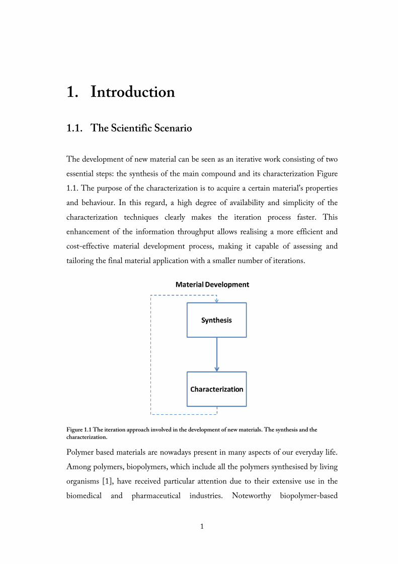
1. Introduction

1.1. The Scientific Scenario

The development of new material can be seen as an iterative work consisting of two

essential steps: the synthesis of the main compound and its characterization Figure

1.1. The purpose of the characterization is to acquire a certain material’s properties

and behaviour. In this regard, a high degree of availability and simplicity of the

characterization techniques clearly makes the iteration process faster. This

enhancement of the information throughput allows realising a more efficient and

cost-effective material development process, making it capable of assessing and

tailoring the final material application with a smaller number of iterations.

Figure 1.1 The iteration approach involved in the development of new materials. The synthesis and the characterization.

Polymer based materials are nowadays present in many aspects of our everyday life.

Among polymers, biopolymers, which include all the polymers synthesised by living

organisms [1], have received particular attention due to their extensive use in the

biomedical and pharmaceutical industries. Noteworthy biopolymer-based

1

applications are; drug delivery devices [2–6], scaffolds for tissue engineering [7–9],

bioabsorbable surgical sutures [10] ophthalmic system [11] and implantable devices

[2,12]. Furthermore, biopolymers have been used to form a coating of functional

parts[13,14], enabling the modification of the physio-chemical properties of the

surface without interfering with bulk material properties. Such refinement of the

surface properties by the simple application of a polymer layer has gained attention

in the recent years. The vast library of available polymers and the ample processes

enabled the tailoring of the final properties with infinite possibilities [5,7,15–20].

Hence, the development of novel, cost-effective and information-rich

characterization methods of both physical and chemical properties of biopolymers

throughout their life-cycle, is a challenge of primary importance.

Lactide-based polymers have aroused interest for application the pharmaceutical

and biomedical devices compartment as they are biodegradable, meaning that they

can be degraded in a natural environment yielding non-toxic degradation products.

The ester bonds on the backbone of the chain undergo hydrolytic cleavage,

catalysed by the presence of enzymes[21,22] or by an alkaline environment[23].

The knowledge of the biopolymer degradation rate is important as it defines the

release profile of an active pharmaceutical ingredient (API) [5,24,25] or the stability

of the implantable device[26]. The biopolymer properties can be modified using

crosslinking to engineer their 3D structure and the crosslinking of biopolymers such

as poly(vinylpyrrolidone) [27–29], hydroxypropyl methylcellulose (HPMC) [25], or

chitosan [30] have been exploited to form a novel class of material commonly

known as hydrogels. Hydrogels are hydrophilic water insoluble materials, wich have

the ability to swollen in water or humid environment. Their properties can be easily

tuned to fit a particular application, from drug delivery [31–33] to tissue

engineering [34] or becoming the functional part of sensing device [13,35,36].

The current conventional approaches for measuring the biopolymer degradation are

cumbersome [24] and extremely time-consuming requiring an experimental

timeframe lasting from weeks to months [24,37–39].A possible route to boost the

2

degradation is studying the polymer behaviour in very harsh condition[40] i.e. very

high or very low pH or high temperature. Indeed, this methodology does not

represent a validation of the biopolymer properties for many of the biomedical

applications. Enzymatic degradation of biopolymer has been studied using quartz

crystal microbalance(QCM) and surface plasmon resonance(SPR) [16,41–43]. This

method was employed to measure the enzymatic degradation on sub-micron thick

layer biopolymer. Although the experimental time frame was drastically reduced,

QCM bases studies are limited to submicron film thickness and request a high

uniformity of the polymer coating [44,45].

It is known[46] that the behaviour of material may change drastically between the

thin film regime(<1µm) and the bulk regime[47–49]. Therefore there is the need to

provide a scheme able to bridge between these two regimes.

The advances of micro and nanofabrication techniques allowed the production of

the micromechanical sensor, which has been used for biosensing [50,51],

environmental sensing [52,53] and material characterization[54–57].

Micromechanical sensors such as cantilever or bridges offer the possibility to study

behaviour biopolymer in the thin film regime and in bulk. Del Ray et. al. [54],

monitored the swelling and deswelling behaviour of submicron-thick layers of

poly(hydroxyl ethyl methacrylate) PHEMA. In this study, they showed an inverse

relation of the swelling properties as a function of the molecular weight. Bose et. al.,

used microcantilevers to characterise the enzymatic degradation behaviour of

polymer films [56,58]. The results here presented showed that the degradation

parameters obtained from micromechanical-based studies, matches with the

conventional ones that achievable with conventional approach.

A powerful analytical tool to characterise the chemical structure of polymers

is the infrared spectroscopy. An example of its importance it is the use of such

technique to monitor the crosslinking, a fundamental chemical reaction in polymer

chemistry, exploited to modify the physical and chemical properties of a polymer. In

this case, the infrared spectroscopy is able to track the changes happening in the

3

polymer structure during the crosslinking, providing useful information on the

evolution of different chemical bonds. Among the infrared spectroscopies

techniques, Fourier Transform Infrared Spectroscopy (FTIR) and its

implementations, have been the most widely used infrared spectroscopic analysis

methods [17,59]. The most common implementation for infrared analysis is the

attenuated total reflectance Fourier transforms infrared spectroscopy (ATR-FTIR)

which exploits a single reflection crystal. Infrared analysis has been performed down

to the single-molecule layer using advanced infrared spectroscopy analysis such as

infrared reflection absorption spectroscopy (IRRAS), but it is limited to the study of

a thin layer on metallic substrates[60,61]. IRRAS and ATR-FTIR suffer from

extremely low signal to noise ratio (SNR) for film thickness in the nanometers

range. The common and most intuitive route to overcome this issue is to perform

several acquisitions[62] or decreasing the spectral resolution, leveraging on the

averaging effect. This kind of solution clearly limits the throughput of the analysis

and calls for new approaches for thin film infrared spectroscopy.

Photothermal spectroscopy methods are based on the recordings of signals which

are generated as a side effect of light absorption. When a photon is absorbed in the

sample, there is a consequent photoinduced modification in the thermal state of the

sample that results in sample heating. A measurement of such sample heating, by

probing the temperature as well as other thermodynamic parameters becomes a

measurement of the wavelength-specific light absorption[63]. Photothermal signals

are generated only upon light absorption since scattering and refraction losses do

not contribute to the formation of the photothermal signal. Moreover, the

photothermal response is dependent on the thermal properties of the material, these

allow the photothermal signal to be used to derive such properties from an accurate

study and modelling of the photothermal signal.

Micromechanical sensors, fabricated by conventional microfabrication technologies

have been used as photothermal sensors. The variation of temperature, localised on

a small sensor such as a cantilever or a string, induces thermal stress, which can be

4

probed as bending [35,64–71] or change in the resonance frequency of the

structure[72–78]. The majority of the mechanical based photothermal spectroscopy

studies are based on single clamped structures (cantilever) and as sensing variable is

used the deflection of the cantilever tip. A more robust sensing scheme has been

demonstrated by measuring the resonance frequency instead of the displacement of

the tip [74].

At the same time, microcantilever-based studies [44,58] represent a breakthrough

compared to the currently available methods for biopolymer degradation studies. An

added benefit of analysing - biopolymer degradation using mechanical resonators

consist in the possibility to integrating them within an automated sensing device.

The readout of the cantilever resonance frequency could be directly embedded in

the sensor [79,80], but this requires a more complex fabrication scheme. Instead, a

more cost effective solution is leveraging on an optical readout, which has shown to

allow high throughput measurements [81]. Furthermore, micromechanical sensor

can be easily integrated with microfluidic devices [81,82] providing a higher degree

of control of the degradation environment.

Given all these technical advantages, there is a great opportunity in developing

mechanical sensors, dedicated not only for polymer degradation studies, but also for

studying the chemical modifications occurring during the crosslinking process.

In this respect, several general considerations should be addressed regarding the

robustness and simplicity of such micromechanical sensors. In particular, string

based photothermal analysis has shown to be able to record the infrared spectra on

femtogram amount of material [72], but the limited type of samples that can be

analysed and a complex experimental setup hinder a large scale integration of the

method. Hence there is the need to develop a more robust sensor which would

better comply with agile sample preparation and straightforward analysis.

Regarding the polymer degradation studies, the principal point to be addressed is

the implementation of an automated readout. Integrating an electrical based

5

readout, for instance, piezoelectric or magnetomotive, complicates the fabrication

process of the sensor. In order to keep the sensor simple, an alternative solution to

the readout is represented by optical readout. In particular DVD unit have shown to

resolve linear displacement up to 1.3 pmHz-1/2 [83,84]. Blu-Ray or DVD optical

unit can be easily programmed and controlled[81,85], and they are available on the

market at a very low cost.

The goal of this work has been to provide tools based on mechanical sensors for

promoting a fast feedback during the material characterization. Pharmaceutical

relevant materials are used to test their feasibility and capability.

6

1.2. Aim of the project

The Ph.D. project is carried out in the framework of the High Exponential Rise in

Miniaturised cantilever-like Sensing (HERMES) project funded by the European

Research Council (ERC). The primary goal of the project is the creation of

cantilever based sensing technology and their integration in automated readout

setups. Focus is on the development of tailored sensors capable of fitting to high-

throughput sensing scenario.

The activities which have been carried out to address the focal point of the overall

project aim were:

i) The development of a high-throughput system for studying the

biopolymer behaviour in a natural environment. This task has been

carried out in collaboration with Academia Sinica Taiwan (Professor

En-Te Hwu).

ii) Improve the knowledge on the nanomechanical photothermal signal,

understanding the limit of detection, and providing a mechanical

photothermal sensor capable of providing high throughput material

characterization.

1.3 Thesis Outline

Chapter 2: Describes the principle of mechanical based sensing applied on the

resonators designed and developed in this thesis. The focus is on the sensing

properties useful for designing a micromechanical sensor for biopolymer

characterization

Chapter 3: Contains the discussion of the analytical model describing the

photothermal signal and finite element simulations which have been done to

7

evaluate the accuracy of the models. The chapter ends with an experimental

validation of the analytical method.

Chapter 4: Describes the methodologies developed in this thesis: the two version of

the automated system used in this thesis are presented. Furthermore, the

nanomechanical infrared spectroscopy (NAM-IR) setup and acquisition methods

are described.

Chapter 5: Includes a summary of the published papers and the prepared

manuscripts.

Chapter 6: Contains concluding remarks and the future perspective.

Appendix: Analytical models (developed by Professor Ole Hansen) and standard

operating procedures for operating the system V2.

8

2. Theoretical Background for Mechanical Based Sensing

In this chapter, the mathematical background for mechanical based sensing is

described. Starting from the equation of motion, the mass sensing properties are

derived, showing how the environment surrounding the microresonator affects the

mass sensing performance.

2.1. Damped And Forced Vibration1

Membranes and microbridges can store potential energy in the form of deformation

energy. During oscillations, these structures are moving between equilibrium

positions and the mechanical system converts the potential energy into kinetic

energy and vice versa. In the absence of dissipative forces, this conversion of energy

would infinitely continue. In a real system, energy dissipation occurs and at each

cycle part of the potential energy is not converted into kinetic energy, causing the

motion to stop. Micro and nanomechanical system have been engineered to provide

structures aimed to minimise the loss of energy and finally enhancing the sensing

performances [86–88].

1 This section adapted from[1] except where elsewhere referred.

9

Figure 2.1 A single degree of freedom system. Adapted from [89]

2.2. Lumped Model

Vibration can be represented by a simple harmonic oscillator (Figure 2.1). When a

mass connected to a spring is displaced from its equilibrium position, it will

experience a force, proportional to the elastic constant of the spring and the

magnitude of the displacement x. In the absence of dissipative forces, the mass m

will oscillate between equilibrium positions undergoing to simple harmonic motion.

Natural systems are damped and the amplitude of the oscillation decades over time.

In a lumped system, the effect damping mechanisms are summarised by the dashpot

b. As a consequence of this damping, the vibration can only be maintained if the mass

is subjected to a force. If the amplitude of the forced oscillations is small such that

any non-linear behaviour can be neglected the equation of motion for a periodic

sinusoidal force is

mx+bx+kx =f0sin (ω0t) (1)

where m is the concentrated mass, k the spring constant and b is the damping

factor.

10

The solution of the homogeneous differential equation led to the definition of the

eigenfrequency described by:

𝜔𝜔𝑛𝑛= 12π

� 𝑘𝑘𝑚𝑚

. (2)

The eigenfrequency describes the frequency of the free oscillations, in the absence

of any losses. The damping factor can be described as:

𝜉𝜉= 𝑏𝑏2√

𝑘𝑘𝑚𝑚 (3)

The homogeneous solution of the differential equation leads to the following

equation of motion:

𝑥𝑥(𝑡𝑡) = 𝑒𝑒−𝜔𝜔𝑝𝑝𝑡𝑡[𝑐𝑐1 cos�𝜔𝜔𝑝𝑝𝑡𝑡� + 𝑐𝑐2 cos�𝜔𝜔𝑝𝑝𝑡𝑡�] (4)

Equation 4 indicates the amplitude is decaying exponentially due to damping,

whereas 𝜔𝜔𝑝𝑝 represents frequency of the damped oscillations, commonly known as

resonance frequency, and it is equal to:

𝜔𝜔𝑝𝑝 = 𝜔𝜔𝑛𝑛�1 − 𝜉𝜉2 (5)

The particular solution of the equation of motion in case of a sinusoidal force of

amplitude 𝑓𝑓0 leads to:

𝑥𝑥(𝑡𝑡) = 𝐻𝐻𝑐𝑐𝐻𝐻𝐻𝐻(𝜔𝜔𝑡𝑡 + 𝜑𝜑) (6)

𝐻𝐻 =

𝑓𝑓0𝑘𝑘�

�[(𝜔𝜔2 − 𝜔𝜔𝑛𝑛2)]2 + (2𝜉𝜉𝜔𝜔𝜔𝜔𝑛𝑛)2

(7)

𝜑𝜑 = 𝑎𝑎𝑎𝑎𝑐𝑐𝑡𝑡𝑎𝑎𝑎𝑎� 2𝜉𝜉𝜔𝜔𝜔𝜔𝑛𝑛𝜔𝜔2 − 𝜔𝜔𝑛𝑛

2� (8)

Where the term 𝑓𝑓0𝑘𝑘� is called static defelection. H is the amplitude of the

oscillations 𝜑𝜑 is the phase lag between the exicitation force and the sustem response

Equation 7 and Equation 8 are represented in Figure 2.2 and Figure 2.3

11

Figure 2.2 Frequency response of the amplitude of the motion in case of a sinusoidal force.

Figure 2.3 Phase diagram in the case of an exciting sinusoidal force.

12

The sharpness of the resonance peak is commonly defined by the quality factor Q.

The quality factor determines the ability f the resonator of store energy in a single

cycle. The ratio between the energy loss 𝑊𝑊 and the energy stored ΔW defines the

Q factor.

𝑄𝑄 = 2𝜋𝜋 𝑊𝑊ΔW

=�1 − 𝜉𝜉2

2𝜉𝜉 (9)

From a sensor perspective, a high Q factor resonator intrinsically increases the limit

of detection of the nanomechanical based sensor[86,90]. The quality factor, in fact,

determines the smallest frequency shift measurable. In other terms, the value of the

quality factor can be seen as the summation of the overall dissipation mechanisms of

the system being those:

1𝑄𝑄

= 1𝑄𝑄𝑚𝑚𝑚𝑚𝑚𝑚𝑚𝑚𝑚𝑚𝑚𝑚

+ 1𝑄𝑄𝑚𝑚𝑛𝑛𝑡𝑡𝑖𝑖𝑚𝑚𝑖𝑖𝑚𝑚𝑖𝑖

+ 1𝑄𝑄𝑜𝑜𝑡𝑡ℎ𝑚𝑚𝑖𝑖𝑖𝑖

+ 1𝑄𝑄𝑖𝑖𝑐𝑐𝑐𝑐𝑚𝑚𝑝𝑝𝑚𝑚𝑛𝑛𝑐𝑐

(10)

𝑄𝑄𝑚𝑚𝑚𝑚𝑚𝑚𝑚𝑚𝑚𝑚𝑚𝑚 indicates the losses due to interaction of the mechanical structure with the

surrounding fluid, 𝑄𝑄𝑚𝑚𝑛𝑛𝑡𝑡𝑖𝑖𝑚𝑚𝑖𝑖𝑚𝑚𝑖𝑖 are all the dissipation mechanism taking place in the

resonator, 𝑄𝑄𝑜𝑜𝑡𝑡ℎ𝑚𝑚𝑖𝑖𝑖𝑖 indicates all the loss mechanism not considered in the other

terms, and finally 𝑄𝑄𝑖𝑖𝑐𝑐𝑐𝑐𝑚𝑚𝑝𝑝𝑚𝑚𝑛𝑛𝑐𝑐 considers energy losses atscribed to clamping.

In Section 2.9 the effect of the damping related to the viscous environment is

treated, and a review of the models used to predict the behaviour of beams is

provided.

13

2.3. Resonance Frequency For a Double Clamped Beam2

Figure 2.4 Schematic representation of double clamped beam or bridge

In this thesis, microbridges structures (Figure 2.4) are designed, developed,

characterised and finally exploited for performing biopolymer degradation

experiments. Considering high aspect ratio beams (L/h>10), it is possible to neglect

both the rotational inertia and the shear deformation. In this case, the bending

behaviour can be derived by the Euler-Bernoulli beam equation, under the

assumption of small deflection for linear elastic beams.

𝐸𝐸𝐸𝐸 𝜕𝜕4𝑈𝑈(𝑥𝑥, 𝑡𝑡)𝜕𝜕𝑥𝑥4 + 𝜌𝜌𝜌𝜌𝜕𝜕2𝑈𝑈(𝑥𝑥, 𝑡𝑡)

𝜕𝜕𝑡𝑡2= 0 (11)

𝑈𝑈(𝑥𝑥, 𝑡𝑡) describes the displacement of the beam, E is the Young’s modulus, I the

moment of inertia and 𝜌𝜌 is the density and 𝐴𝐴 is the cross sectional area (W x h).

The free vibrations are described by the linear superposition of the eigenmodes

multiplied by a time-dependent term.

𝑢𝑢(𝑥𝑥, 𝑡𝑡) = �𝑈𝑈𝑛𝑛(𝑥𝑥)𝑐𝑐𝐻𝐻𝐻𝐻 (𝜔𝜔, 𝑡𝑡)∞

𝑛𝑛=1 (12)

Where Un(x)is the eigenfunction and the general solution can be written as:

2 This section is mainly adapted from[114]

14

𝑈𝑈𝑛𝑛(𝑥𝑥) = 𝑎𝑎𝑛𝑛 cos(𝛽𝛽𝑛𝑛𝑥𝑥) + 𝑏𝑏𝑛𝑛 𝑐𝑐𝐻𝐻𝐻𝐻(𝛽𝛽𝑛𝑛𝑥𝑥) + 𝑐𝑐𝑛𝑛𝑐𝑐𝐻𝐻𝐻𝐻ℎ(𝛽𝛽𝑛𝑛𝑥𝑥) + 𝑑𝑑𝑛𝑛sinh (𝛽𝛽𝑛𝑛𝑥𝑥) (13)

βn is the wavenumber and it depends on the boundary conditions(i.e., the

clamping). By inserting (12) in (11) the differential equation becomes

−𝜌𝜌𝜌𝜌𝜔𝜔2𝑢𝑢(𝑥𝑥, 𝑡𝑡) + 𝐸𝐸𝐸𝐸𝛽𝛽𝑛𝑛4𝑢𝑢(𝑥𝑥, 𝑡𝑡) = 0 (14)

𝛬𝛬𝑛𝑛 = 𝜔𝜔 = 𝛽𝛽𝑛𝑛2�𝐸𝐸𝐸𝐸

𝜌𝜌𝜌𝜌 (15)

Considering a beam with a rectangular cross-section characterised by a moment of

inertia I= Ah212� and assuming a flexural rigidity DE :

𝐷𝐷𝑚𝑚 = 𝐸𝐸ℎ3

12 (16)

The eigenfrequencies can be expressed as:

𝛬𝛬𝑛𝑛 = 𝜔𝜔 = 𝛽𝛽𝑛𝑛2 = �𝐷𝐷𝑚𝑚

𝜌𝜌𝜌𝜌 (17)

If the width to height ratio of the beam becomes larger than w/h>5, the flexural

rigidity of the beam is described by the rigidity of a plate.

𝐷𝐷𝑚𝑚 = 𝐸𝐸ℎ3

12(1 − 𝑣𝑣2) (18)

The final mode shape Figure 2.5 is determined by the values of the wavenumber,

resulting in the coefficient 𝑎𝑎𝑛𝑛 , 𝑏𝑏𝑛𝑛 , 𝑐𝑐𝑛𝑛 , 𝑑𝑑𝑛𝑛 which are specific for each boundary

condition. Thus, they will depend on the type of structure.

Figure 2.5 Mode shapes of the first three modes for a doubly clamped beam.

15

2.4. Resonance Frequency of Pre-Stressed Membrane

In this thesis, pre-stressed Silicon Nitride Membranes are fabricated to be used as

sensing elements in a nanomechanical photothermal spectrophotometer (NAM-

IR). In this section, the mathematical description of the eigenfrequency of a pre-

stressed structure is presented.

If the membrane is fabricated with a linear elastic material, the equation of motion

of a pre-stressed rectangular membrane can be derived adopting the two-

dimensional wave equation:

𝜎𝜎∇2𝑢𝑢 − 𝜌𝜌 𝑑𝑑2𝑢𝑢𝑑𝑑𝑡𝑡2

= 0 (19)

As in the case of a beam resonator the equation of motion can be thought of as a

superposition of the mode shape with the time dependent term via separation of

variables.

𝑢𝑢(𝑥𝑥, 𝑦𝑦, 𝑡𝑡) = 𝑈𝑈(𝑥𝑥, 𝑦𝑦)𝑒𝑒𝑚𝑚𝜔𝜔𝜔𝜔 (20)

The mode shape (Figure 2.6) has to fulfil the boundary conditions, and it can be

expressed as:

𝑈𝑈(𝑥𝑥, 𝑡𝑡) = ��𝑈𝑈0,𝑛𝑛𝑛𝑛

∞

𝑛𝑛=0𝐻𝐻𝑠𝑠𝑎𝑎�𝑎𝑎𝜋𝜋𝑥𝑥

𝐿𝐿𝑥𝑥� sin �𝑗𝑗𝜋𝜋𝑦𝑦

𝐿𝐿𝑦𝑦�

∞

𝑛𝑛=0 (21)

16

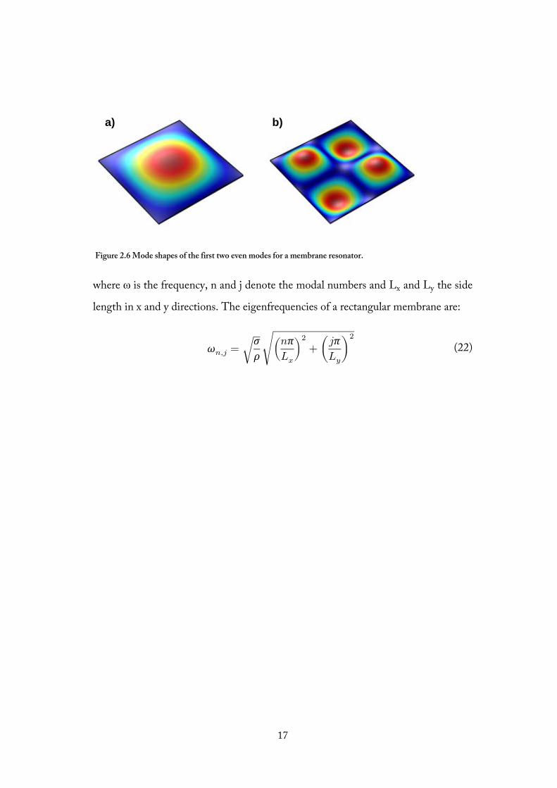
where ω is the frequency, n and j denote the modal numbers and Lx and Ly the side

length in x and y directions. The eigenfrequencies of a rectangular membrane are:

𝜔𝜔𝑛𝑛,𝑛𝑛 = �𝜎𝜎𝜌𝜌

��𝑎𝑎𝜋𝜋𝐿𝐿𝑥𝑥

�2+ �𝑗𝑗𝜋𝜋

𝐿𝐿𝑦𝑦�

2

(22)

b) a)

Figure 2.6 Mode shapes of the first two even modes for a membrane resonator.

17

2.5. Effective Parameters The dynamic characteristics of the structure can be represented in terms of effective

parameters. Each mode can be studied by a single lumped system which describes

the nth eigenfrequency of the system:

Λ𝑛𝑛2 =

𝑘𝑘𝑚𝑚𝑒𝑒𝑒𝑒

𝑚𝑚𝑚𝑚𝑒𝑒𝑒𝑒 (23)

where the effective stiffness and effective mass are mode dependent quantities

defined as:

𝑚𝑚𝑚𝑚𝑒𝑒𝑒𝑒 = 𝜌𝜌𝜌𝜌 � 𝜙𝜙(𝑥𝑥)2𝑑𝑑𝑥𝑥𝐿𝐿

0 (24)

𝑚𝑚𝑚𝑚𝑒𝑒𝑒𝑒 = 𝐸𝐸𝐸𝐸𝑧𝑧 � 𝜙𝜙(𝑥𝑥) 2𝑑𝑑𝑥𝑥𝐿𝐿

0 (25)

2.6. Mass Sensing

Thanks to their very tiny mass, micromechanical sensors have been widely

employed for mass sensing purposes[88,91–93]. Variation in the effective mass of

the resonator can be sensed as a resonance frequency shift. In general, the

responsivity of the mechanical sensor is defined as the slope of the sensing variables,

i.e., the resonance frequency, as a function of the input parameter to be measured.

In this chapter, the mass responsivity is discussed. The responsivity to the local

heating induced by light absorption is discussed in Chapter 3.

In general terms, the sensor responsivity R can be defined as

R=∂Λ∂ψ�

ψ=ψ0

(26)

Where Λ is the measured parameter(the resonance frequency), and ψ is the

parameter that needs to be quantified, in this case, the mass. Assuming a linear

18

response of the resonance, and a given ΔΛmin as the smallest resolvable frequency

shift, the smallest detectable value for the parameter:

Δψmin=R-1ΔΛmin (27)

The case of a mechanical resonator used as a mass sensor is explained. In this

context, ∆ψ represents the mass variation andΔΛ is the consequent variation of

the resonance frequency. The mass detection thorough mechanical resonator applies

in two specific cases; the point mass detection and the distributed mass detection.

2.7. Point Mass Responsivity3

Point mass detection is when the added mass is localised. In this case, the location

of the added mass is defined by two coordinates 𝑥𝑥Δ𝑚𝑚 and 𝑦𝑦Δ𝑚𝑚. Considering the

deposition of a particle of a certain mass ∆m the effect of the mass deposition on

the resonance frequency can be investigated by the Raylegh-Ritz method[53],

which states that, at resonance, the time average kinetic energy equals the time

average strain energy. Thereby,

𝐸𝐸𝑘𝑘𝑚𝑚𝑛𝑛 = 12

𝑚𝑚𝑚𝑚𝑒𝑒𝑒𝑒𝛽𝛽𝑛𝑛2𝜔𝜔Δ𝑚𝑚

2, (28)

where, 𝑚𝑚𝑚𝑚𝑒𝑒𝑒𝑒 is the effective mass defined in Equation 24.

Substituting the Equation 24 in Equation 27, the latter becomes:

𝐸𝐸𝑘𝑘𝑚𝑚𝑛𝑛,Δ𝑚𝑚 = 12Δ𝑚𝑚[𝛽𝛽𝑛𝑛 U(𝑥𝑥Δm,𝑦𝑦Δm)]2𝜔𝜔Δ𝑚𝑚

2 (29)

By assumption, the mode shape and the 𝑘𝑘𝑚𝑚𝑒𝑒𝑒𝑒 are not changed.

The resonance frequency due to the addition of the mass:

𝜔𝜔Δ𝑚𝑚 = 𝜔𝜔0 − Δ𝜔𝜔 (30)

Hence, the point mass responsivity (PMR):

3 This section is mainly adapted from [116]

19

𝑅𝑅 = Δ𝑓𝑓Δ𝑚𝑚

�𝑃𝑃𝑃𝑃𝑃𝑃

= 𝑓𝑓02𝑚𝑚𝑒𝑒𝑓𝑓𝑓𝑓

U(𝑥𝑥𝛥𝛥𝑚𝑚,𝑦𝑦𝛥𝛥𝑚𝑚)2 (31)

2.7.1. Distributed Mass Responsivity4

Contrary to what has been discussed so far, relatively to the point mass detection,

the deposited mass displacement is not constant. Therefore, the kinetic energy of

the resonator due to the deposition characterised by a density distribution

𝜌𝜌Δ𝑚𝑚(𝑥𝑥, 𝑦𝑦) and thickness distribution 𝑡𝑡Δ𝑚𝑚(𝑥𝑥, 𝑦𝑦), becomes:

𝐸𝐸𝑘𝑘𝑚𝑚𝑛𝑛 + 𝐸𝐸𝑘𝑘𝑚𝑚𝑛𝑛,Δ𝑚𝑚

= 12𝑚𝑚𝑚𝑚𝑒𝑒𝑒𝑒𝛽𝛽𝑛𝑛

2𝜔𝜔Δ𝑚𝑚2

+ 12𝛽𝛽𝑛𝑛

2𝜔𝜔Δ𝑚𝑚2 � 𝜌𝜌Δ𝑚𝑚(𝑥𝑥, 𝑦𝑦)

𝐴𝐴 𝑡𝑡Δ𝑚𝑚(𝑥𝑥, 𝑦𝑦)U(𝑥𝑥𝛥𝛥𝑚𝑚,𝑦𝑦𝛥𝛥𝑚𝑚)2 𝑑𝑑𝑥𝑥 𝑑𝑑𝑦𝑦

(32)

𝑚𝑚𝑚𝑚𝑒𝑒𝑒𝑒

∫ 𝜌𝜌𝛥𝛥𝑚𝑚(𝑥𝑥, 𝑦𝑦)𝐴𝐴

𝑡𝑡𝛥𝛥𝑚𝑚(𝑥𝑥, 𝑦𝑦)U(𝑥𝑥𝛥𝛥𝑚𝑚,𝑦𝑦𝛥𝛥𝑚𝑚)2 𝑑𝑑𝑥𝑥 𝑑𝑑𝑦𝑦= 𝜔𝜔𝛥𝛥𝑚𝑚

2

𝜔𝜔02 − 𝜔𝜔𝛥𝛥𝑚𝑚

2 (33)

Equation 32 is found by applying the Rayleigh-Ritz theorem and considering the

strain energy 𝐸𝐸𝑘𝑘𝑚𝑚𝑛𝑛 = 12 𝑚𝑚𝑚𝑚𝑒𝑒𝑒𝑒𝛽𝛽𝑛𝑛

2𝜔𝜔02.

If we consider 𝜔𝜔𝛥𝛥𝑚𝑚 = 𝜔𝜔0 − ∆𝜔𝜔𝛥𝛥𝑚𝑚. Let 𝜔𝜔0 ≫ ∆𝜔𝜔𝛥𝛥𝑚𝑚 the total frequency shift,

𝛥𝛥𝑓𝑓𝑚𝑚, is given by (considering the density and the thickness of the added layer

constant over the resonator surface)

𝛥𝛥𝑓𝑓𝑚𝑚 = (𝑡𝑡𝑐𝑐𝜌𝜌𝑐𝑐)𝑓𝑓0

2𝑚𝑚𝑚𝑚𝑒𝑒𝑒𝑒� 𝑈𝑈𝑎𝑎(𝑥𝑥, 𝑦𝑦)2 𝑑𝑑𝑥𝑥 𝑏𝑏𝑦𝑦𝜌𝜌

. (34)

The distributed mass responsivity (DMR) can be finally defined as:

𝑅𝑅 = Δ𝑓𝑓Δ𝑚𝑚

�𝐷𝐷𝑃𝑃𝑃𝑃

= 𝑓𝑓02𝑚𝑚𝑒𝑒𝑓𝑓𝑓𝑓

𝜌𝜌𝑚𝑚𝑒𝑒𝑒𝑒 (35)

4 This paragraph is adapted from [116]

20

Where the value of the effective area:

𝜌𝜌𝑚𝑚𝑒𝑒𝑒𝑒 = � U(𝑥𝑥, 𝑦𝑦)2 𝑑𝑑𝑥𝑥 𝑑𝑑𝑦𝑦𝜌𝜌

(36)

In both the cases (point mass detection and distributed mass detection) the

minimum detectable mass depends on to the uncertainty affecting the

measurement. This the noise measured by means of Allan Deviation or the

uncertainty of independent measurements called here 𝛿𝛿𝑒𝑒 . In both cases, the limit of

detection described in equation 26 can be rewritten as:

𝛿𝛿𝑃𝑃,𝑝𝑝𝑜𝑜𝑚𝑚𝑛𝑛𝑡𝑡 𝑚𝑚𝑐𝑐𝑖𝑖𝑖𝑖 =𝛿𝛿𝑒𝑒

𝑓𝑓02𝑚𝑚𝑒𝑒𝑓𝑓𝑓𝑓 U(𝑥𝑥𝛥𝛥𝑚𝑚,𝑦𝑦𝛥𝛥𝑚𝑚)2

(37)

𝛿𝛿𝑃𝑃,𝐷𝐷𝑚𝑚𝑖𝑖𝑡𝑡𝑖𝑖𝑚𝑚𝐷𝐷𝑚𝑚𝑡𝑡𝑚𝑚𝑚𝑚 =𝛿𝛿𝑒𝑒

𝑓𝑓02𝑚𝑚𝑒𝑒𝑓𝑓𝑓𝑓 𝜌𝜌𝑚𝑚𝑒𝑒𝑒𝑒

(38)

2.8. Resonance Frequency of a Layered Structure

For a multilayer structure, the resonance frequency can be written as [44]

fn≈12π

βn2

L2⎷

��� ∑ 𝐸𝐸𝑚𝑚𝐸𝐸𝑚𝑚

𝑁𝑁𝑚𝑚=1

𝑤𝑤∑ 𝜌𝜌𝑚𝑚𝑡𝑡𝑚𝑚𝑁𝑁𝑚𝑚=1

(39)

Considering non-coated structure Equation 36 reduces to Equation 17 matching

the resonance frequency of a beam, according to the Euler-Bernoulli theory.

Considering a beam coated with a uniform layer of polymer, the resonance

frequency changes compared to the non-coated beam. The Young’s modulus of a

polymer is typically orders of magnitude lower than the Young’s modulus of the

silicon. The increase in the mass of the resonating structure can be detected as a

change in the resonance frequency shift. This condition holds only below a certain

21

value of polymer thickness, where the bending stiffness of the polymer layer is

neglectable.

A finite element model can be used to estimate this effect. Considering the

structures utilised in paper 1, which are 1000µm long 300 µm wide and 5µm thick

and considering the polymer properties showed in [4], this limit is seen to be found

equal to the beam thickness of polymer coating where there is an inversion in the

trend of the relative frequency shift.

The effect of the addition of a polymer coating5 is shown in Figure 2.7 where the

relative frequency is represented as a function of the added polymer layer. In the

graph, three different regimes can be identified. The first regimes for tPOLtBRIDGE

< 1,

here the main effect on the resonance frequency is due to the added mass, 1 <tPOL

tBRIDGE< 2.25, where the effect of the increased thickness due to the polymer layer

counteract the effect of the added mass, and finally tPOLtBRIDGE

> 2.25 where the

stiffness due to the polymer layer is predominant. The width of the structure instead

is seen not to play a significant role.

Figure 2.7 Effect of the addition of a polymer layer on a double clamped beam. For thickness smaller than the beam thickness the main effect is the decrease in the resonance frequency, whereas once this threshold is overcome the enhancement of stiffness is also sensed and becoming the leading cause of frequency when the thickness of the polymer layer is higher 2.25times the thickness of the beam.

5 For these simulations these elastomechanical properties pf the polymer are used: E=2GPa, p=1.3g cm-3.

22

2.9. Frequency Response in Liquid Environment

In this thesis, the resonating behaviour of microbridges is tested. The Blu-Ray

readout system that is designed and employed to characterise the degradation of

biopolymer is described in Paper 1. The system allowed a characterization of the

frequency response in air and water environment. The theoretical background of the

frequency response of microstructure in a liquid environment is illustrated

accompanied with by experimental results.

2.9.1. The Hydrodynamic Function

The frequency response of a mechanical structure is highly dependent on the fluid

in which it is vibrating. The benchmark theoretical studies describing the behaviour

in liquid environment were done by Sader and colleagues [94–96].

The theoretical treatment exposed in the previous paragraphs holds for vacuum and

air environment, where the effect of the load due to the liquid and so the viscous

damping can be neglected. In the model proposed by Chu[97], the liquid is treated

as inviscid, and it gives a reasonable approximation of the value of the resonance

frequency of a beam when immersed in liquid environment for high working

frequency. On the other hand, the validity of the inviscid model may not be

accurate depending on the structure properties. According to this model, the

resonance frequency drops due to the hydrodynamic load caused by the surrounding

water

ωfluidωvac

=�1+ πρlw4ρct

�-12 (40)

where 𝜌𝜌𝑐𝑐 and 𝜌𝜌𝑖𝑖 are the density of the liquid and the beam respectively, whereas w and t are the width and the thickness. Equation (37) is often considered as

benchmark to evaluate the decrease in the resonance frequency due to added

apparent mass of the layer of fluid which load the structures. Sader’s works[95,98–

100] extends the validity of this equation considering the effect of the viscosity.

23

The formulations of the frequency response in viscous environment are described in

terms of Reynolds number Re���� and T and the hydrodynamic function Γ:

Re�������= ρl2πfnw4η

(41)

T= ρlwρct

(42)

ή is the cinematic viscosity of the fluid and fn the resonance frequency. In the light

of this, the extension of the Chu model becomes:

ωfluidωvac

= �1+πρw2

4μΓr(ωfluid)�

-1/2

(43)

where μ=ρA is the linear density of the beam and Γr is the real part of the

hydrodynamic function 𝛤𝛤 [95]. For the sake of clarity, a representation of the

hydrodynamic function is reported Figure 2.8. The real part of this function takes

into account the inertial forces which are leading the dynamics for very high

Reynolds number where the viscous effects vanish. In this regime, the inviscid

model is a good approximation of the dynamic behaviour of the beam.

Figure 2.1 Hydrodynamic function[95] for a rectangular beam immersed in water.

10 1 10 2 10 3 10 4 10 5

Reynolds Number

0

0.5

1

1.5

2

2.5

3

()

Re( )Im( )

24

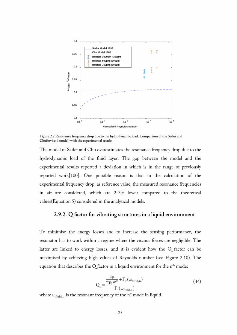
Figure 2.2 Resonance frequency drop due to the hydrodynamic load. Comparison of the Sader and Chu(inviscid model) with the experimental results

The model of Sader and Chu overestimates the resonance frequency drop due to the

hydrodynamic load of the fluid layer. The gap between the model and the

experimental results reported a deviation in which is in the range of previously

reported work[100]. One possible reason is that in the calculation of the

experimental frequency drop, as reference value, the measured resonance frequencies

in air are considered, which are 2-3% lower compared to the theoretical

values(Equation 5) considered in the analytical models.

2.9.2. Q factor for vibrating structures in a liquid environment

To minimise the energy losses and to increase the sensing performance, the

resonator has to work within a regime where the viscous forces are negligible. The

latter are linked to energy losses, and it is evident how the Q factor can be

maximised by achieving high values of Reynolds number (see Figure 2.10). The

equation that describes the Q factor in a liquid environment for the nth mode:

Qn=

4μπρlw2 +Γr(ωfluid,n)

Γi(ωfluid,n)

(44)

where ωfluid,n is the resonant frequency of the nth mode in liquid.

10 1 10 2 10 3 10 4 10 5

Normalized Reynolds number

0.1

0.15

0.2

0.25

0.3

0.35

0.4

wat

er/

vacu

m

Sader Model 1998Chu Model 1968

Bridges 1000µm x300µmBridges 500µm x300µmBridges 750µm x300µm

25

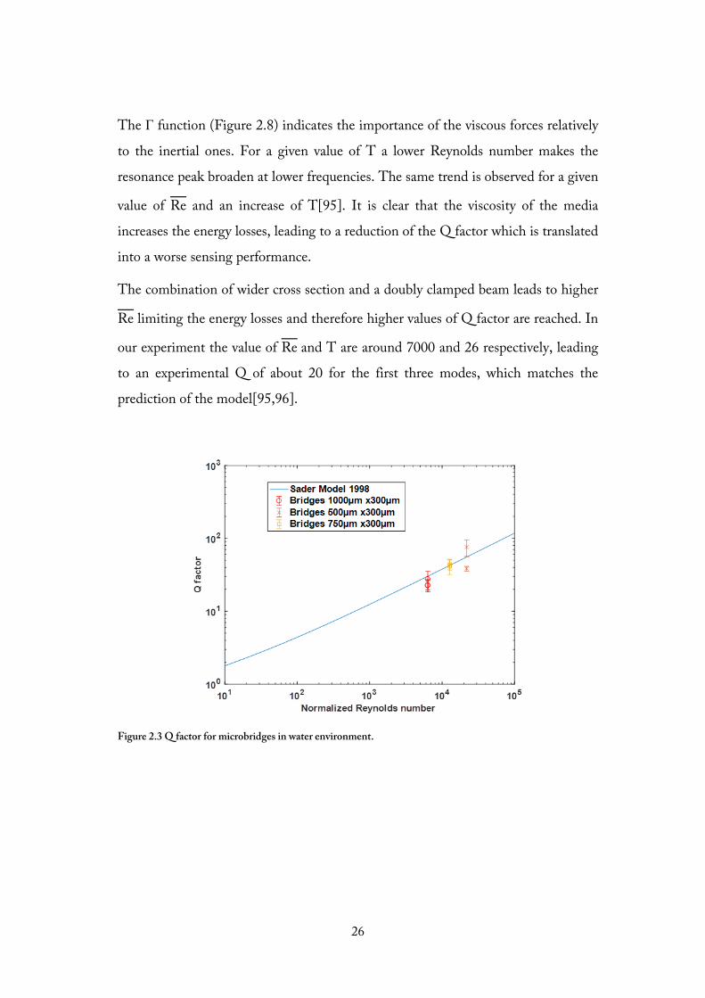
The Γ function (Figure 2.8) indicates the importance of the viscous forces relatively

to the inertial ones. For a given value of T a lower Reynolds number makes the

resonance peak broaden at lower frequencies. The same trend is observed for a given

value of Re and an increase of T[95]. It is clear that the viscosity of the media

increases the energy losses, leading to a reduction of the Q factor which is translated

into a worse sensing performance.

The combination of wider cross section and a doubly clamped beam leads to higher

Re limiting the energy losses and therefore higher values of Q factor are reached. In

our experiment the value of Re and T are around 7000 and 26 respectively, leading

to an experimental Q of about 20 for the first three modes, which matches the

prediction of the model[95,96].

Figure 2.3 Q factor for microbridges in water environment.

26

Figure 2.4 Resonance frequency of 1000µm 300µm wide and 5µm thick bridges in air a-c, and in water, d- f. For the sake of clarity, only one spectrum are reported. The standard deviation ranges from 3 to 5% on a sample size of n=20

2.9.3. Increase of the Effective Mass

The mass sensing characteristics are explained in Section 2.6 and it has been shown

that the lower the effective mass the higher will be the mass responsivity.

From a mass sensing perspective, working in a viscous environment is translated to

an increase of the effective mass of the resonator, yielding to a decrease of the mass

responsivity of the sensor. Under the assumption that the effective stiffness of the

structure is not influenced by the liquid environment, the ratio between the

resonance frequency in air and the resonance frequency in water is

� ωAirωwater

�2=

meff,water

meff,air (45)

Considering the 1000µm long 300 µm wide and 5 µm thick bridges, the effective

mass is in air is 1.75µg. The decrease of the resonance frequency can be seen as an

increase in the effective mass of the resonator. In water environment the effective

27

mass is seen to increase by a factor of 13, yielding an effective mass of around 20 µg.

The experimental uncertainty on the resonance frequency measurements does not

allow a proper monitoring of the degradation phenomena. Higher modes can be

used to perform mass sensing in liquid environment[98], on the other hand

integrating a readout able to monitor this condition can be challenging.

In this thesis, the microbridges are used for characterising the biopolymer

degradation of polymer layer with thickness that ranges between 1 to 5 microns.

The values of the mass responsivities for the first three flexural modes are shown in

Table 1. The minimum detectable distributed mass for each mode in air

environment allows us to correctly follow the degradation phenomena. Instead, in

liquid environment, the mass responsivity is on the same order of magnitude as the

deposited mass, hence tracking the degradation phenomena would be unfeasible.

Therefore, to characterise biopolymer degradation, a wet & dry approach has been

used as discussed in Paper 1.

Table 1 Minimum detectable mass sensitivity for 1000µm long 300 µm wide and 5 µm thick microbridges. Analogous trivial calculation leads to similar results for different sized microbridges.

Mode Mass Responsivity [𝑯𝑯𝑯𝑯 𝝁𝝁𝝁𝝁−𝟏𝟏 𝒎𝒎𝒎𝒎𝟐𝟐]

Uncertainty 𝚫𝚫𝒇𝒇[𝑯𝑯𝑯𝑯]

Minimum Detectable Distributed Mass

[𝝁𝝁𝝁𝝁 𝒎𝒎𝒎𝒎−𝟐𝟐]

Air Water Air Water Air Water

I flexural 2304 114.7 103.68 594 0.09 10.34

II flexural 5344 308.82 187.04 1125 0.07 7.92

III flexural 11304 1941 395.64 3250 0.07 3.34

28

2.10. Conclusion

In this chapter, the theoretical background of a micromechanical resonator is

provided. The variables that play a major role in determining the performances for

mass sensing application are discussed. Micromechanical bridges have shown a

sufficient minimum detectable mass in air environment to perform mass sensing.

Despite a good Q factor even in aqueous environment, the increase of the effective

mass does not allow the use of the structure as mass sensor. The deposited mass is

in the same order of magnitude as the minimum detectable mass. This, combined

with the uncertainty on the measurement does not allow to properly monitor the

degradation mechanism. Instead, working in air environment, yields an increase of

the mass responsivity two orders of magnitude less than the deposited mass,

allowing a proper tracking of the degradation process. The employment of the

microbridge structure as a biopolymer degradation sensor is discussed in Paper 1.

29

30

3. Finite Element Simulations for Nanomechanical Infrared spectroscopy

This chapter provides the in-silico validation of the analytical model used to

describe the steady state and the transient response of the mechanical photothermal

signal.

3.1. Steady state model for photothermal induced frequency shift

The phenomena involved in generation of the photothermal signal have been

modelled to provide a better understanding of the experimental variables’ roles in

the production of the signal. The analytical model describing the resonance

frequency shift for a membrane-like structure was developed by Professor Ole

Hansen, DTU Nanotech6. Considering the high aspect ratio of the membrane

structures considered in this thesis, the problem can be solved as a 2D thin

membrane. To obtain an analytical representation of the photothermal response,

there are three problems to be solved. First, the heat transport equation throughout

the membrane when heated in response to the local absorbed power P; then the

thermal stress field induced by the heating load; iii) the eigenproblem solved for the

thermal stress field caused by the power absorption. Addressing this problem for a

square geometry is ill-posed, and deriving a closed analytical solution is not possible.

Instead, this is possible only for a circular geometry. In this section, the accuracy of

the analytical model is compared with the finite element model.

The analytical solution for the photothermal a circular membrane is:

∆𝑓𝑓𝑓𝑓

≈ − 𝛼𝛼𝐸𝐸𝛼𝛼8𝜋𝜋𝑘𝑘ℎ𝜎𝜎0

�2 − 𝑣𝑣1 − 𝑣𝑣

− 0.642� (46)

6 The analytical solution of the model is reported in Appendix 1

31

Where 𝛼𝛼 is the thermal expansion coefficient of the material, 𝐸𝐸 is the elastic

modulus, 𝛼𝛼 is the absorbed power, 𝑘𝑘 is the thermal conductivity, ℎ the thickness of

the structures, 𝜎𝜎0 is the native tensile stress and 𝑣𝑣 is the Poisson ratio. It is

noteworthy remind that the model was solved for a point-like power source.

In the experimental phase, the heat source is represented by the IR laser source,

having a defined diameter of 100µm. Intuitively, the magnitude of the frequency

shift is directly linked with the average temperature established upon heat

absorption. Thus, the location of the laser spot and its size clearly plays a

fundamental role in defining the magnitude of the frequency shift. The analytical

model represents the optimal case of a perfect collimated light. This approximation

may lead to an overestimation of the absorbed power calculated for a given

frequency shift. Therefore the role of the spot size is discussed.

3.2. Model Definition

To simulate these phenomena the Heat Transfer in thin shell and the Membrane

Comsol tool packages are used. The FEM model replicates the membrane

geometry employed in the experimental case; 1000µm wide, 100nm thick and

fabricated in low-stress silicon nitride. The used parameters are presented in Table

2.

32

Table 2 Summary of the properties used in the FEM modelling, with Comsol Multiphysics v 5.2 ®. The results were obtained setting a 2D geometry and the thermal stress physics interface.

Properties Value

Thermal Conductivity 20 W m-1 K-1

Density 3100 kg m-3

Young Modulus 250 GPa

Poisson Ratio 0.23

Initial stress 250 MPa

Heat Capacity at

Constant Pressure

700 J kg-1 K-1

Thickness 100nm

Width 1000µm

3.2.1. Boundary Condition

A consideration regarding the boundary condition (BC) assumed in the derivation

of the analytical model must be done. Both analytical formulations (the steady state

and the transient problem) bear the temperature of the membrane rim to be fixed at

a certain value T0(considered equal to 293.15K). Such approximation corresponds

to the assumption that the body chip acts as a perfect heat sink. In the experimental

condition, the boundary of the membrane will exchange heat with the rest of the

body chip and with the surrounding gas. The model that better fits the

experimental condition corresponds to a membrane of silicon nitride, surrounded by

a silicon body chip isolated from the surroundings. The temperature field will vary

according to the boundary condition, and the effects of the approximation are

represented in Figure 3.1

33

Figure 3.1Schematic representation of the geometry and BC used in this work: a) only the membrane T0 =293.15 K; b) the membrane chip is allowed to exchange heat with the body chip, acting as heat sink. The rim temperature is set at T0 =293.15 K c) adiabatic boundary condition the thermal energy provided by the heat source is dissipated only within the domain; d) difference in the temperature evaluated in the centre of the membrane considering the BC a and b and c, the three temperature profile perfectly overlap; e) average temperature profile for the three boundary condition

34

The three boundary conditions simulated consist of: i) a fixed temperature on the

rim of 293.15K Figure 3.1a; ii) a fixed temperature of 293.15K on the bodychip,

rim Figure 3.1b iii) and adiabatic condition on the rim of the bodychip Figure 3.1c.

The average steady temperature profile is showed in Figure 3.1d calculated for each

of the BCs showed in Figure 3.1a-c. The three profiles are completely overlapping,

and the differences between models are less than 1%. The average temperature of

the membrane is also evaluated in the time domain where, also in this case, no

remarkable differences are noticed. All the simulations consider an incident power

of 100µW over a circular area of 100µm in diameter. The Silicon bodychip has a

higher thermal conductivity than the membrane chip. Therefore, the heat will be

dissipated towards the bodychip and rapidly the temperature of the membrane’s rim

will reach the boundary condition temperature.

These simulations reveal that average temperature within the membrane domain

does not depend on the BC used. Since the temperature field within the membrane

upon heat absorption determines the magnitude of the frequency shift, we can say

that for the sake of simplicity all the simulations in this thesis are performed using

the BC illustrated in Figure 3.1a, as they do not give rise to any further error.

3.3. Linearity of the photothermal induced frequency shift

The first simulation aims to test the linearity of the photothermal induced

frequency shift upon heat absorption. The analytical model is solved for the mode

(1,1) and the match with the finite element method is shown in Figure 3.2. The

relative frequency shift yielded by the models matches with the analytical one, the

difference is in the order of 1-2 ppm for 100 µW of absorbed power. This value, in

the experimental case scenario, is within the limit of detection, meaning that the

error introduced by the approximation will not induce to a significant quantitative

errors in terms of absorbed power. The limit of detection, concerning the structure

used in this thesis ranges from 3 to 20nW depending on the thickness of the

d

35

Figure 3.2 Simulated relative frequency shift vs Analytical model. The relative frequency yielded by the model also simulating the body chip yield to a relative frequency shift which is almost 2 times smaller. This is due to the lower temperature established in the membrane when it is not treated as isolated system.

coating layer which yields a different noise background. These arguments are

described in paper 2 and paper 3.

Compared to the analytical model, the finite element model slightly underestimates

the relative frequency shift. Such gap might be because the analytical solution is

drawn from a Delta function heat source, instead, in the FEM model, the heat

source is meant to simulate the laser source of 100 µm diameter.

The effect of the spot size dimension (Irradiance) on the relative frequency shift was

simulated. An incident power of 100µW is used and the diameter of the laser spot

size is varied from 1µm up to 1mm. The magnitude of the relative frequency shift

decreases for higher laser spot size. The relative frequency shift is normalised

relatively to the value of the analytical frequency shift (43). The normalised

frequency shift then drops down to the 50% for a laser spot size that matches with

the dimension of the membrane. Instead, it remains above the 90% for a heat source

size smaller than half of the membrane width. The reason for this decrease is

because the photothermal induced frequency shift is also sensitive to the location

where the heat is generated, being maximum in the centre and minimum in the

proximity of the border as shown in Figure 3.3a.

0 20 40 60 80 100

Absorbed Power ( W)

-8000

-7000

-6000

-5000

-4000

-3000

-2000

-1000

0

Rel

ativ

e Fr

eque

ncy

shift

(ppm

)

FEM model only membraneMembrane and BodychipAnalytical model

36

Figure 3.3 Steady-state simulations.a) Effect of the heat source dimension; b) and of heat source location.

In the experimental setup, the laser spot has to be aligned with the membrane

resonator. The site of the laser plays a major role in determining the magnitude of

the relative frequency shift. In the light of this, the spatial sensitivity is modelled. A

heat source is swept across the membrane domain. The relative frequency shift is

maximum when the membrane is heated in the centre and decades towards the

boundary of the membrane, being zero for a heat source placed at the border.

Intuitively, the closer the heat source is located in the proximity of the heatsink the

lower the average temperature will be within the membrane domain and ultimately

the relative frequency shift.

37

3.4. Time Dependent Simulations

The membrane resonator upon heat absorption reaches a stable value of

temperature and therefore a stable stress field which finally yields a particular

frequency shift. The transient problem is exclusively related to the thermal transport

phenomena, and therefore only the thermal property (and the geometry of the

structure) regulates such dynamics. Professor Ole Hansen developed the analytical

model and the calculations are reported in Appendix.

The knowledge of the thermal transient is fundamental for two main reasons:

i. The time the sensor needs to reach a stable temperature and therefore a

stable resonance frequency determines the rapidity of the system to follow

transition between subsequent heat absorption. Therefore this parameter

determines how fast a spectral sweep can be run and intrinsically determines

the acquisition parameters of the lock-in scheme used to track the resonance

frequency shift, hence the noise. These arguments are discussed in the paper

II.

ii. The transient dynamics depends on the thermal properties of the domain; it

may allow the identification of the thermal properties of the analytes and the

chip material.

The analytical model that characterise the transient behaviour for a squared layered

structure is

𝜏𝜏0 = �2𝜋𝜋2

𝐿𝐿2

∑ ℎ𝑚𝑚𝑘𝑘𝑚𝑚𝑁𝑁𝑚𝑚=1

∑ ℎ𝑚𝑚𝑐𝑐𝑚𝑚𝑛𝑛𝐼𝐼=1

+ 𝐻𝐻∑ ℎ𝑚𝑚𝑐𝑐𝑚𝑚

𝑛𝑛𝐼𝐼=1

�−1

(47)

𝐻𝐻1𝑚𝑚𝐷𝐷𝑐𝑐𝑖𝑖 = 92.21𝑊𝑊𝑚𝑚2𝐾𝐾� (48)

𝐻𝐻10−5𝑚𝑚𝐷𝐷𝑐𝑐𝑖𝑖 = 9.221 10−4 𝑊𝑊𝑚𝑚2𝐾𝐾 � (49)

38

Where the ℎ𝑚𝑚𝑘𝑘𝑚𝑚 𝑐𝑐𝑚𝑚 are respectively the thickness and thermal conductivity and the

heat capacity for the ith layer L is the width of the membrane. The parameter H

instead takes into account the dissipation of the heat due to the convective heat

transport phenomena taking place at different pressure. For a silicon nitride

membrane of width 1000 µm in high vacuum condition the time constant is 5.5 ms.

3.4.1. Accuracy of the Analytical Model

The analytical time constant is drawn from the resolution of the heat transport

equation in 2 dimensions. The time constant results from the solution of the

homogeneous part of the partial differential equation problem (PDE). The

resolution of this mathematical problem can be solved by means of eigenfunction.In

the expression we consider only the first mode(henceforth called fundamental)

being the one that decays slower.

3.4.2. Initial Temperature Distribution

In order to assess the accuracy of the analytical model, the transient led by a

different initial condition is tested.

The boundary condition illustrated in Figure 3.1a are used. The decay showed

Figure 3.4b is evaluated by considering the average temperature of the membrane

when the temperature is let to relax to the temperature boundary considering an

initial temperature distribution of 𝑇𝑇0(𝑥𝑥, 𝑦𝑦) = 𝑇𝑇𝐷𝐷𝑜𝑜𝑚𝑚𝑛𝑛𝑚𝑚𝑐𝑐𝑖𝑖𝑦𝑦 + ∆𝑇𝑇 cos (𝜋𝜋 𝑥𝑥𝐿𝐿 )cos (𝜋𝜋 𝑦𝑦

𝐿𝐿 ),

being ∆𝑇𝑇 = 10𝐾𝐾.

39

Figure 3.4. a)Cosine-like initial temperature distribution colorbar Temperature in K ; b) Relative temperature shift evaluated by the FEM model and the analytical one.

The finite element model prediction of the transient, considering the initial

temperature distribution, matches the transient behaviour predicted by the

analytical model. In this particular case of study, the initial temperature distribution

is one of the possible solutions that satisfy the PDE, hence the match with the

analytical transient is trivial. The full thermal response is described by a

superposition of eigenfunctions [101]. Hence the complete description of the

thermal transient will depend on particular initial condition as well as the kind of

heat source used. In this perspective, we investigate how the thermal transient varies

for different types of heat sources aiming to mimic the experimental case scenario.

40

3.5. Transient for an external power source

In the experimental case, the membrane is heated with an external power source

with a spatial distribution P(x,y). Here we simulate i) constant heat source confined

within a circular area of radius r ii) Gaussian power distribution. The aim is to

investigate how the power distribution influences the thermal time constant.

3.5.1. Constant Heat Source Confined In a Circular Area of Radius r

The case studied in Section 3.4.2, represents the ideal case of temperature

distribution led by a Delta function as a heat source, which is unlikely to be

available in the experimental phase. Here we studied the influence of the heat spot

size on the transient when the power is kept constant. The larger the effective

heated area, the faster the membrane will reach the steady average temperature.

Similarly, on what we have discussed relatively to the effect of the heat source size

on the magnitude of the relative frequency shift, the reached temperature is

inversely related to the size of the heat source. Concerning the transient, if the heat

source is placed close to the boundary, hence closer to the heat sink, the transient

will be shorter, and the reached temperature smaller.

41

Figure 3.5 Effect of the spot size and time constant. a)The heat source is spread over a different area; b) average temperature transient, dashed represents the single exponential fit; c) value of the time constant as function of the relative radius of the heat source normalised by the dimension of the membrane

42

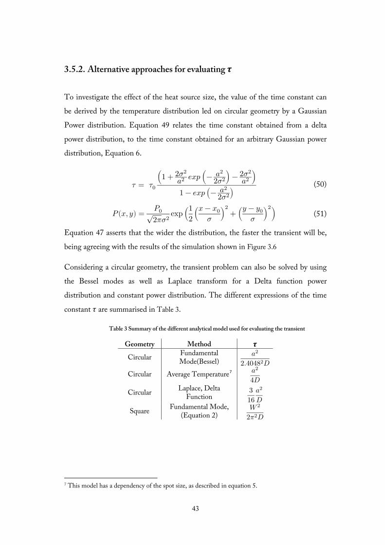
3.5.2. Alternative approaches for evaluating 𝝉𝝉

To investigate the effect of the heat source size, the value of the time constant can

be derived by the temperature distribution led on circular geometry by a Gaussian

Power distribution. Equation 49 relates the time constant obtained from a delta

power distribution, to the time constant obtained for an arbitrary Gaussian power

distribution, Equation 6.

𝜏𝜏 = 𝜏𝜏0

�1 + 2𝜎𝜎2

𝑎𝑎2 𝑒𝑒𝑥𝑥𝑒𝑒 �− 𝑎𝑎2

2𝜎𝜎2� − 2𝜎𝜎2

𝑎𝑎2 �

1 − 𝑒𝑒𝑥𝑥𝑒𝑒 �− 𝑎𝑎2

2𝜎𝜎2� (50)

𝛼𝛼(𝑥𝑥, 𝑦𝑦) = 𝛼𝛼0√2𝜋𝜋𝜎𝜎2

exp �12

�𝑥𝑥 − 𝑥𝑥0𝜎𝜎

�2+ �𝑦𝑦 − 𝑦𝑦0

𝜎𝜎�

2� (51)

Equation 47 asserts that the wider the distribution, the faster the transient will be,

being agreeing with the results of the simulation shown in Figure 3.6

Considering a circular geometry, the transient problem can also be solved by using

the Bessel modes as well as Laplace transform for a Delta function power

distribution and constant power distribution. The different expressions of the time

constant 𝜏𝜏 are summarised in Table 3.

Table 3 Summary of the different analytical model used for evaluating the transient

Geometry Method 𝝉𝝉

Circular Fundamental Mode(Bessel)

𝑎𝑎2

2.40482𝐷𝐷

Circular Average Temperature7 𝑎𝑎2

4𝐷𝐷

Circular Laplace, Delta Function

316

𝑎𝑎2

𝐷𝐷

Square Fundamental Mode, (Equation 2)

𝑊𝑊2

2𝜋𝜋2𝐷𝐷

7 This model has a dependency of the spot size, as described in equation 5.

43

3.5.3. Gaussian Power Distribution

The transient for a Gaussian power distribution (Equation 47) is studied for a

circular and a square geometry. Here 𝜎𝜎 is the width of the distribution 𝑥𝑥0 and 𝑦𝑦0

represent the localization of the peak.

Regardless of the geometry, the wider the distribution, the faster will be the

response, according to what is stated in Equation 47.

For a circular geometry, the Bessel mode does not consider the influence of the

power distribution in a calculation of the time constant. The Laplace solution

calculated for Delta and uniform power distribution matches with the value yielded

for simulations evaluated for a power distribution which is sufficiently narrow or

spread.

Considering a square geometry, a narrow distribution led to a value of the time

constant which is higher compared to the fundamental one.

To understand this behaviour, it is necessary to recall that the solution of the heat

transport equations is described by a superposition of eigenfunctions, that singularly

represent an eigenmode which will decay with a particular time constant. The first

mode is the one that decays slower, hence is leading the dynamic. However,

depending on the characteristics of the heat source the weight of each one of the

eigenmodes will change leading to a different value of measured time constant. The

value of 𝜏𝜏 given by the analytical solution is seen to match the value yielded by a

Gaussian power distribution characterised with a 2𝜎𝜎𝐿𝐿2 equal to 0.5.

44

Figure 3.6 Dependence of the thermal time constant from the width of the distribution. Either the circular a) or the square geometry follows the same trend. The dashed lines represent the value given by the analytical solutions. For the sake of clarity, the values are extended all over the horizontal axis.

The dimension of the heat source plays a major role in determining the measured

value of the thermal time constant in the experimental phase, hence in the

extrapolated values of the thermal properties of the material. The trend in the time

constant for the circular and the square geometry are shown in Figure 3.6. Despite a

different relative trend, for both the circular and square geometry, the wider the

laser spot, the faster the response will be. These findings are correlated with the

value of the average temperature established in the membrane upon heat absorption.

A narrower distribution leads to a higher average temperature in the membrane that

is translated to a higher time constant.

45

3.6. Experimental Validation

The model described in Equation 44 was validated by studying the transient signal

of the mechanical resonance, when the membrane is undergoing periodic IR

radiation as described elsewhere[66,69]. The IR light is mechanically chopped at an

arbitrary frequency, and the frequency shifts are recorded in the same way as

described in Paper II and III. For these experiments, 500µm wide membranes are

used. The reason for this choice is that spot size the IR laser which has a diameter

of 100µm which places the expected experimental value reasonably close to the 𝜏𝜏

yielded by the fundamental mode. The value of the thermal diffusivity of the silicon

nitride is drawn from Equation 2. For a composite structure, such as a coated

membrane, the value of the thermal diffusivity D is:

𝐷𝐷 =∑ ℎ𝑚𝑚𝑘𝑘𝑚𝑚

𝑁𝑁𝑚𝑚=1

∑ ℎ𝑚𝑚𝑐𝑐𝑚𝑚𝑛𝑛𝐼𝐼=1

(52)

Figure 3.7 Transient curves and distribution of the thermal time constant for a 500µm wide membrane. a-b) Bare Silicon Nitride, c-d) PVP coated Silicon Nitride Membrane.

46

For a single layer structure, i.e. the bare Silicon Nitride membrane, it is possible to

extract directly the thermal diffusivity of the material, which is seen to reasonably

match the previously reported results[102] as shown in Table 3.

The thermal diffusivity of a composite structure was evaluated for silicon nitride

coated with poly(vinylpyrrolidone) (PVP) layer by applying the same experimental

procedure with a thickness layer of 106nm and 110nm respectively. Due to the

addition of a polymer layer, the thermal diffusivity of the structure. As reference

value is used the value given by Equation 7 and adopting previously published

results of thermal conductivity and heat capacity [103]. The error between the

experimental thermal diffusivity and the reference thermal diffusivity equal to the

10.5%.

In order to decouple the two thermal diffusivities(of the polymer and the silicon

nitride membrane), a calibration procedure has to be performed. The thermal time

constant has to be evaluated for increasing thickness of polymer. A fitting of the

estimated value thermal time constant as a function of the polymers thickness would

be able to disclose the value of the polymer thermal diffusivity and further highlight

possible thickness dependent effects, as previously reported for other material

properties such as elastic modulus [48] and glass transition temperature [47].

Table 4 Experimental and theoretical values of thermal diffusivities.

Material Membrane

Width Tau Experimental Diffusivity

Reference Value

µm ms m2/s m2/s

SiN 500 8.85±0.05 1.40 e-6 1.3-1.7e-6

SiN and PVP(100nm

&110nm) 500 12±0.05 1.05e-6 8.88e-7

47

3.7. Conclusions

This chapter illustrates the accuracy of the analytical models describing the steady

state and the transient description of the nanomechanical photothermal signal. The

assumptions made in the analytical description of the model resulted in being

reasonably correct considering the geometry of the membrane resonator studied in

this thesis.

The steady state model allows determining the resonance frequency shift upon heat

absorption, this model was used in paper 2 and paper 3 to estimate the power

absorption for a given relative frequency shift, and then the temperature of the

membrane. Since photothermal spectroscopy is based on the recording of

exothermal events, the knowledge of the magnitude of the temperature shift driven

by the heat absorption is fundamental. In particular working at low pressure the

temperature shift could be high, and in principle cause a phase transition in the

material.

The thermal transient is in principle described by a linear superposition of

eigenmodes. The first mode is the one that decay slower hence it is dominating the

description of the transient. Different initial conditions lead to a diverse

superposition of the eigenmodes hence a different transient behaviour. The

dependence of the laser spot size and beam width was investigated. Both the

circular and the squared geometry reveal an inverse relationship with the beam

width, reaching a plateau value for a width larger than the membrane size.

48

4. Materials and Methods

This chapter provides the description of the process and the experimental

approaches employed in this thesis. In particular, the fabrication processes related to

the mechanical resonator used for performing biopolymer degradation studies and

Nanomechanical infrared spectroscopy (NAM-IR). The working principles of the

custom made Blu-Ray based device and of the NAM-IR setup are described.

4.1. Cleanroom Fabrication

All the mechanical structures developed in this thesis were fabricated with standard

cleanroom fabrication method. The fabrication phase took place in the cleanroom

of DTU Danchip.

4.1.1. Silicon Microbridges

For performing biopolymer degradation studies(Paper 1) double clamped beams are

developed. The starting substrate is Silicon on insulator wafer (SOI) with a device

layer of 5µm. Conventional fabrication processes are used, and the fabrication

parameters are optimised by a trial and error approach. Here we report the design,

the process flow and the fabrication process scheme.

4.1.1.1. Mask Design

The fabrication of the microbridge structure is a two masks process (Figure 4.1).

The first mask is needed to define the microbridge geometry and it is used to

pattern the device layer of the wafer. The bulk removal of the Silicon is performed

by anisotropic etching (KOH) upon patterning of the Silicon Nitride masking layer.

49

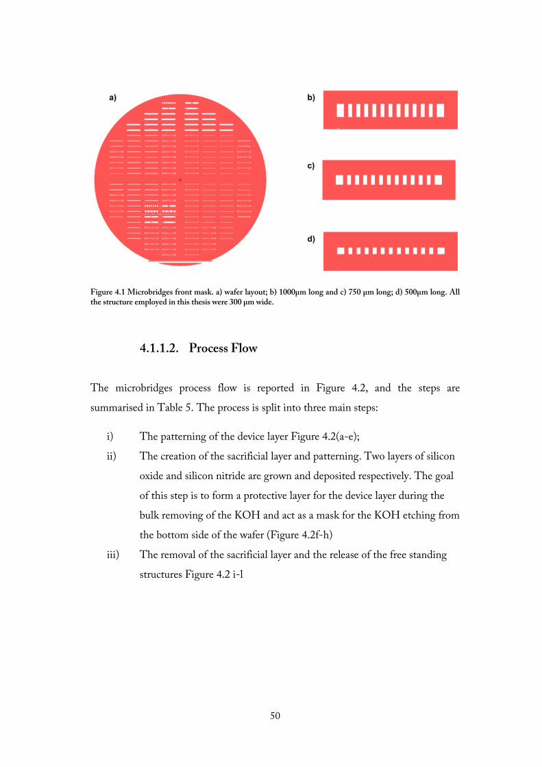
Figure 4.1 Microbridges front mask. a) wafer layout; b) 1000µm long and c) 750 µm long; d) 500µm long. All the structure employed in this thesis were 300 µm wide.

4.1.1.2. Process Flow

The microbridges process flow is reported in Figure 4.2, and the steps are

summarised in Table 5. The process is split into three main steps:

i) The patterning of the device layer Figure 4.2(a-e);

ii) The creation of the sacrificial layer and patterning. Two layers of silicon

oxide and silicon nitride are grown and deposited respectively. The goal

of this step is to form a protective layer for the device layer during the

bulk removing of the KOH and act as a mask for the KOH etching from

the bottom side of the wafer (Figure 4.2f-h)

iii) The removal of the sacrificial layer and the release of the free standing

structures Figure 4.2 i-l

50

Figure 4.2 Process scheme of microbridge fabrication. For the sake of clarity in the scheme, it is represented the fabrication of a cantilever beam (single clamped) instead of a double clamped cantilever. The resist strip steps are omitted, and the same positive lithography is applied in step c and g.

Table 5 Microbridges fabrication process flow.

Mask LabelStep Equipment Notes Goal

Surface Pre-treatment HMDS oven 30 min Improve resist adhesion Phothoresist spinning SSE spinner AZ-5412E 1.5µm

UV exposure 6'' Aligner 3.5 sec Positive lithographyDeveloper TMAH Developer 1 min remove the exposed pattern

Dryer Spin drier 1 minDevice layer dry etch Pegasus DRIE 55 sec Defining the resonator geometry

Phthoresist Strip Plasma Asher 30minRCA cleaning RCA bath

Silicon Oxide Growth Furnace B1 200nm

Silicon Nitride deposition Furnace E3 300nm

Surface Pre-treatment HMDS oven 30 min Improve resist adhesion Phothoresist spinning SSE spinner AZ-5412E 1.5µm

UV exposure 6'' Aligner 3.5 sec Positive lithographyDeveloper TMAH Developer 1 min remove the exposed pattern

Dryer Spin drier 1 minDevice layer dry etch ICP Etcher 4min Etch rate 70nm/min measured

Phthoresist Strip Plasma Asher 30minKOH wet etching KOH bath(1 or 3) 3.5h @80C Remove silicon

Silicon Nitride etch HPO3 etch 165C Remove the Sacrificial Silcon Nitride layerSilicon Oxide etch HF bath

Dryer Ethanol fume dry

Calbrate the dep time accoridng to the last dep rate

Microbridge process flow: Author Andrea Casci CeccacciBridge front& Bridge Back

Lithography front side

Sacrifical layer

Lithography back side

Device Release

51

Figure 4.3 Optical microscope images of the microbridge fabricated during this thesis. Scalebar 300µm

52

4.1.2. Membranes

Low-stress Silicon Nitride membranes are fabricated for NAM-IR spectroscopy application.

4.1.2.1. Mask design

The fabrication of silicon nitride membrane is rather straightforward. It is a single mask process. On a single chip 1cmx1cm, there have been located two pairs of square membrane resonators sized 1mm and 500µm respectively.

Figure 4.4 Mask design of the membrane chip used in this thesis. a) Wafer layout and b) single chip.1000µm2

membrane and 500µm2 membrane were fabricated.

4.1.2.2. Process Flow

The process scheme is similar what has been shown in Section 4.1.1.2 for

microbridges resonators. Here, the starting substrate is a double polished silicon

wafer, and only one lithography step is necessary to define the membrane geometry.

The process flow is reported in Table 6 and the process scheme is indicated in

Figure 4.5. The final results of a Silicon wafer for obtaining the membrane

resonator is showed in Figure 4.6

53

Figure 4.5 Process Scheme of Membrane resonator fabrication. HMDS surface treatment prior to c is omitted and resist strip before step g is omitted

Table 6 Membrane Fabrication process.

54

Process flow Author: Andrea Casci CeccacciMask: Membrane front, BF KOH,DF

Step Equipment Notes GoalWafer Selection

Device layer Low stress silicon Nitride LPCVD furnace B1 20 min dep time 100nm

Surface Pre-treatment HMDS oven 30 min Improve resist adhesion Phothoresist spinning SSE spinner AZ-5412E, 1 min bake 90 C 1.5µm

UV exposure 6'' Aligner 3.5 sec Positive lithographyDeveloper TMAH Developer 1 min remove the exposed pattern

Dryer Spin drier 1 minBackside SiN Etch ICP 2 min open areas for KOH etchingPhthoresist Strip Plasma Asher 30minSilicon wet etch KOH bath 3.5h Define membrane clamping points

Silicon Nitride wet etch HF bath 10 min Removal of the sacrifical layerDryer Ethanol fume dry Drying of the wafers at low vapour pressure

Lithography Backside

Release of the device

No wafer pretreatement needed

Plasma enanched chemical deposition

PECVD 2 8 min, Front side 500nmSacrifical layer Deposition

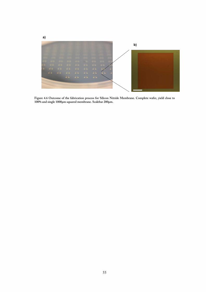
Figure 4.6 Outcome of the fabrication process for Silicon Nitride Membrane. Complete wafer, yield close to 100% and single 1000µm squared membrane. Scalebar 200µm.

55

4.2. Structure functionalization 4.2.1. Spray coating

Microbridges are functionalized using spray coating Figure 4.7. An extensive

description of the role of the experimental parameters involved is intensely studied

in [55]. From a general point of view, a spray coating process includes: i) the

atomization of the coating solution in the nozzle, where minute droplets are

formed, ii) the deposition of the atomised droplets on the substrate, iii) and finally

the coalescence of the droplets upon solvent evaporation. The nozzle is actuated

ultrasonically, and it causes the atomization of small droplets in the micrometer

size. A Nitrogen flow is used to focus the atomised solution on the target sprayed

surface.

Figure 4.7: a: Scheme of a spray coater nozzle. Adapted from [104]; b) 1000µm long 300 µm wide microbridge coated with PLGA dissolved in DCM 0.5%. Scalebar 300 µm.

56

4.2.2. Spin Coating

Figure 4.8 Standard operating procedure for spin coating. The solution is applied on the substrate which makes rotate. Adapted from [105] Another sample preparation method used for deposit a polymer layer onto the

sensor is spin coating. A standard operating procedure for spin coating is shown in

Figure 4.8. Spin coating is widely applied in the semiconductor fabrication process

to form a photoresist layer. In this thesis, spin coating is used to form a

poly(vinylpyrrolidone) (PVP) film on membrane resonator device. Spin coating

particularly fit the purposes of this study as it allows forming a thin uniform

polymer film. On the contrary, besides being a high throughput method for creating

thin polymer layer, it does not fit the functionalization of microbridge chips. The

working principle of spin coating is rather simple. The solution that has to be

deposited on the substrate is cast on the target surface. The substrates are put into

rotation at a certain speed, and the centrifugal force spreads the polymer on the

substrate. The thinning of the film takes pace in two different stages. The first one

is caused by the only radial outflow of the excess solution. In this stage, the

evaporation of the solvent is neglected. Subsequently [106], the evaporation rate

reaches a stable value, and the film can be considered as immobile, the thinning of

the film is due primarily to the solvent evaporation.

57

4.3. Thickness Measurement

Regardless of the method used for depositing the biopolymer layer on the sensor the

knowledge of the thickness is a fundamental parameter for calibrating the sensing

performances of the nanomechanical sensor. In this thesis, two methods are used to

characterise the thickness of the deposited polymer layer: profilometry and

ellipsometry.

4.3.1. Profilometry

A diamond stylus (Figure 4.9a) approach first the analysed surface once the surface is

reached the tip is moved laterally across the sample the output variable is the surface

height as a function of the stylus position, i.e., the scan length. The range of the

measurable thicknesses ranges from 10nm up to 1mm.The vertical tip displacement

represents the height of the surface. A profilometer curve is showed in Figure 4.9b

Figure 4.9. Profilometer Scheme and a typical curve. a) Scheme of a stylus profiler adapted from [107]. b) An example of profilometer raw data. Here, the thickness of a membrane chip coated with a thin layer of PVP.

58

4.3.2. Ellipsometry

Ellipsometry is a non-destructive measurement method where the information

about the thickness and the refractive index of the layer can be obtained.

Ellipsometry detection scheme is represented in Figure 4.10. Ellipsometry assesses

the thickness of the layer indirectly by measuring the changes in the polarisation of

an incident light upon reflection of the target surface. The principle of

measurement, in fact, stands on the difference in the polarisation of the light once it

has been reflected on the target surface. This method particularly fits for very thin

layer, being the minimum measurable thickness in the order of tens of angstrom.

Differently from the profilometer, an apriori knowledge of the optical property of

the substrate layer is needed. The obtained thickness will be in fact the results of a

fitting.

Figure 4.10 Schematic representation of the spectroscopic Ellipsometry. Adapted from [108]

59

4.4. Readout Integration

In this section, the principles and the building blocks of the optical detection based

on a commercial Blu-Ray pickup head unit are presented. The section further

includes the description of the integration of an astigmatic detection scheme onto

automated systems aimed to characterise the frequency response of the

micromechanical resonators.

4.4.1. The Blu-Ray pickup head unit (PUH)

The readout of the frequency response is performed optically, by integrating a

readout based on a Blu-Ray ® technology.

Figure 4.11 Blu-ray Pickup head unit.

The Blu-Ray pickup head unit (PUH) is illustrated in Figure 4.11. It consists of a

semiconductor laser emitting diode at three wavelengths, 405nm, 605nm and

780nm8; a lens system needed for driving the laser beam, grating, polarisation beam

splitter, 𝜆𝜆4 plate and a voice coil motor. The optical and electrical component

embedded inside the OPU are designed to work at very high frequency as they have

to be capable to handle data stream in the order of GHz. This makes the OPU the

8 Blu-Ray OPU integrate also the lasers related to the previous generation of OPU, being those the one available in DVD/CD-ROM based technologies

60

ideal candidate for the integration of an automated readout for micromechanical

sensor. The integration of the PUH in the readout system is presented in Figure

4.13.

4.4.1.1. The Voice Coil Motor (VCM)

The distance between the reflective surface and the objective lens can be finely

calibrated by the VCM embedded in the PUH. The VCM Figure 4.12 uses a

permanent magnetic field and a coil producing a force proportional to the current

applied to the coil. The electromechanical conversion is generated by the Lorentz

force principle, according to which, if a conductor material which is carrying a

current is located in a magnetic field force will act on it. During the conventional

operation (i.e. a readout of the Blu-Ray or DVD) the PUH detects changes in the

distance between the refractive surface and OPU. The generated focus error signal

(FE) signal is used to evaluate the current necessary to drive the VCM such that the

focal point will be on the reflective surface, the disc.

The VCM can move along the x and z-direction, within 1mm range and a

resolution of tens of nm. The capability of moving in the z-direction has been used

for performing the autofocusing function as described in Section 4.5.1.

Figure 4.12 Voice coil motor, adapted from[109]

61

4.4.2. Astigmatic Detection

An optical system which is not symmetric relatively to the optical axis is defined

astigmatic. In cylindrical lenses, the optical system is designed to be not symmetric

as in the case of DVD or Blu-Ray PUH. An astigmatic optical detection scheme is

presented in Figure 4.13, which matches with the detection scheme embedded in

the Blu-Ray PUH. The laser light is focused onto a reflecting surface, i.e., the

silicon microbridges. The reflected laser light passes through a polarising beam

splitter, and an astigmatic lens, finally the reflected light impinges the four

quadrants photodetector (PIDC). The four element of the PIDC is equipped with a

current preamplifier. The PDIC output signal is named as Focus Error Signal

(FES) is defined as:

FES=(SA+Sc)-(SB+SD) (53)

When the laser spot is perfectly focused on the object surface the FES =0 (Figure

4.14). If the incident light is not focused on the surface the shape of the laser spot

on the PIDC is distorted, and the FES signal differs from 0.The shape change of

the laser spot in the PIDC sensor corresponds to a specific value of FES.

Figure 4.13 Astigmatic detection scheme. Adapted from[83]

62

Figure 4.14 Focus Error Signal. Adapted from [83]

It is evident how a specific position of the measured object is univocally transduced

in terms of FES value. The linear working range depends on the characteristics of

the optical lens as well as by the wavelength of the laser beam. The objective lens

used in this thesis for both the system has a numerical aperture NA= 0.6. Under

these conditions, the linear range corresponds to about 6µm; the working distance is

1.2-1.4mm.

63

4.4.3. Integration of the Blu-Ray based readout

The Blu-Ray pickup head unit is integrated into custom made systems9 aimed to

provide a (semi)-automatic characterization of the frequency response of the

microbridge structures. The final goal of these systems is to provide a device that

can improve the experimental condition as well as the throughput of

micromechanical-based biopolymer degradation experiments as previously described

by Bose and co-workers [44]. A biopolymer degradation study based on system v1

is described in Paper 1.

Regardless of the system version, the measurement routine relies on the following

steps:

i) installation of the microfluidic cartridge in the chip holder;

ii) alignment of the OPU with the microbridges array;

iii) actuation of the piezoelectric crystal and measurement of the frequency

response.

4.4.3.1. System V1

The purpose of this system is to provide a device able to:

i) recognise the position of microbridges resonator,

ii) performing autofocus of the probing light on the microresonator surface;

iii) automatically records the frequency response of micromechanical

resonators.

9The systems (V1 and V2) design and manufacturing was done by En-Te Hwu, Academia Sinica Taiwan. The control software were developed by Ching Hsu-Chen Acadamia Sinica, Taiwan. The microfluidic cartridge used in system V1 was designed and developed by Lidia Morelli, PhD student DTU Nanotech

64

The height of the chip holder is regulated by adjusting the position of 4 screws that

provide the chip holder with 6 degrees of freedom (translation and rotation along

the main axes) Figure 4.15a. The chip height is manually regulated by the user, and

the PUH microbridge distance is adjusted in such a way that all microbridges will

be roughly in the linear range allowing the detection of the position. The fine

adjustment of the focus is then handled by the measurement routine where the

central position of the S-curve is found, and the measurement is performed.

In the first version of the system a single microbridge array chip is embedded in a

microfluidic cartridge (Figure 4.16) which is installed in the chip holder that is kept

tight by four screws avoiding any slippery motion of the cartridge.

The microfluidic chip is composed of three PMMA plate(Figure 4.16), bonded

together with the microfluidic double sided tape which has also been used to bond

the microresonator on the bottom plate.

Figure 4.15 First generation of the system measurement: a) system and chip holder, b) detection scheme based on the Blu-ray pickup head unit; c) system in action. The position of the PUH can be monitored in real time by an external USB microscope.

65

Figure 4.16 Microfluidic device used in Paper 1. the three layer of PMMA are cut by CO2 laser cutting.The microfluidic channels are embedded in the PSA tape bonding the middle and the top plate. The microfluidic access is provided on the top plate, and tubings are sealed with cured PDMS.

4.4.3.2. System V2

The System V2 aimed to improve the throughput of the measurement. To pursue

this goal, the chip holder (Figure 4.17a) is equipped with a stepper motor providing

motion in the y direction. In this way measurements are possible in the x-y plane,

allowing to locate and measure multiple arrays of bridges. In the light of this, in the

microfluidic cartridge was modified up to three microbridges array can be installed.

The width of the microfluidic chamber was modified to match the width of the

microbridge array Figure 4.17b-c reducing possible tilting of the microbridge sensor

in in the x-y plane.

66

Figure 4.17. System v2 a) Design of the system V2; b) implementation of multiple microbridges chips in the same microfluidic device; c) close up. For the sake of clarity, the top plate of the microfluidic device has not been installed.

67

4.5. Algorithms for tracking microbridges position

During the tracking phase, the PUH moves along the x direction as shown in

Figure 4.17b-c a predefined amount of time and the FES is recorded.

The BR-PHU scans the microbridge arrays and records the FES (Figure 4.18).

When the light is reflected a step change in the FES is recorded. The absolute value

of the signal is evaluated, and an edge detection is performed on the recorded

signal. Once the value overcomes an internal threshold, the central point of the

bridge is found, and the bridge position is saved. The procedure iterate until all the

bridges have been found.

In its first implementation (Figure 4.18a) the distance between the PUH is kept

fixed throughout the whole phase, and it is determined by the manual adjustment

performed through the screws. It is essential that all the bridges be well aligned in

the x-z plane to have a working distance such that the profile of the bridge can be

univocally identified. For instance, as reported in Figure 4.18b the first bridges are

well identified instead the last ones are slightly above the SNR level.

68

Figure 4.18 First implementation of the bridge localisation algorithm. The FE signal is acquired for a singular working distance, defined during the manual alignment phase.

To improve the experimental conditions and to reduce the number of operation

requested by the user, a new tracking algorithm is developed. The FES is acquired

for subsequent VCM position allowing the FES signal to be recorded at a different

working distance (Figure 4.19). Moreover, at each iteration, the recorded FE signal

is evaluated and summed with the already recorded one. Once the cumulative sum

overcomes a threshold value, defined by the user the bridges are localised and

identified. This implementation drastically reduces the number of operation needed

by the user to operate and provide a more stable and robust device.

69

Figure 4.19 Bridge localisation algorithm V2. The PUH is moved within a predefined number of VCM position, and the FE signals are recorded accordingly. Once the cumulative sum of the FE signal overcome a certain threshold, the bridge is identified, and its position saved.

70

4.5.1. Auto Focusing

After the localisation of the bridges in the array, the system steps into the

measurement phase. Before actuating the piezoelectric crystal, the software needs to

identify the best working distance in such a way that the measurement will take

place with a perfectly focused spot. To do so, the VCM is actuated, and the S-curve

recorded. The central part of the S-curve is identified(Figure 4.20), saved and used

for the next measurement. Finally, after the localisation of the focal point, the piezo

crystal is actuated, and the mechanical spectra are recorded.

Figure 4.20 Focus error signal recorded on one bridge before the frequency response acquisition. The VCM coil motor is actuated, and the FES acquired. The central spot of the FES is used as a focal point to perform the measurement.

71

4.6. Nanomechanical Infrared Spectroscopy Setup

The goal of this section is to describe the setup and the acquisition parameters used

for photothermal spectroscopy through nanomechanical sensor henceforth called

(NAM-IR). The components of the acquisition chain are described. All the main

component of the Nam-IR setup are shown in Figure 4.21.

Figure 4.21.The NAM –IR setup. The IR laser is produced by a Quantum Cascade Laser, QCL block engineering. The light can be mechanically chopped, providing a periodic thermal excitation. The path light is deviated on the membrane resonator by an off-axis parabolic mirror that collimates the laser light on a spot of diameter 100 µm. The membrane chip is placed into a customs mated vacuum chamber holder providing electrical access for the actuation of the piezoelectric crystal.

The membrane resonator is placed in a custom made vacuum chamber, which

provides optical access from the top, where the readout laser for the laser Doppler

Vibrometer can probe the membrane motion and from the bottom, where the IR

light is shined through a KBr window. The chamber provides an electrical

connection for the actuation of a piezoelectric crystal. The low vacuum (LV) regime

is provided by a conventional pump that can reach 1 mbar. Instead, the high

vacuum (HV) regime is provided by a turbo pump that allows reaching the 10-

72

5mbar. The possibility to run experiments at two different pressures allow

investigating the phenomena involved in the generation of the mechanical

photothermal signal.

4.6.1. Characterization Of The Quantum Cascade Infrared Laser Source

Quantum cascade lasers (QCLs) were developed at the Bell Laboratories in

1994[110]. They are semiconductor based apparatus able of emitting a photon from

the mid-infrared to the far-infrared portion of the spectrum. A QCL substantially

differs from diode lasers. The latter can emit photons in the process of electron-hole

recombination where a single photon is involved resulting in a wavelength that

exclusively depends on the band gap about the combination of the material used.

Quantum Cascade Lasers consist of sandwich structures of semiconductor

materials. These sandwich structures are organised to form regions of local minima

of potential energy commonly known as quantum energy well that limit the

electrons in a precise energy state. When the electrons, driven by an externally

applied voltage moves through subsequent energy barriers (Figure 4.23), which are

characterised by a specific energy, the electron transition from one valence band to

the lower one yield in a photon emission. The sandwich structure above described,

is designed such that they can emit a particular wavelength. The emitted

wavelength depends on mostly on the structure rather than the constituting

material, allowing fabricating devices that emit up to 25 µm.

73

Figure 4.22. Schematic working principle of the QCL.Adapted from[110].

A quantum cascade laser source (QCLs) block was used for all the experiment done

during this thesis. The wavelength interval that such device can provide ranges from

768cm-1 to 1953cm-1, providing a non-constant power spectrum (see Figure 4.23).

The laser is operated in a pulsed mode, and therefore the output power can be

modulated throughout the modification of the duty cycle. The output power of the

QCL (Block-Engineering) laser source is quantified using a thermal power sensor

for different duty-cycle settings.

Figure 4.23 Power spectrum of the QCL. a) the DC was set at 1% (to= 100ns T= 1µs) step size 1cm-1 constant throughout all the power range used; b) DC set at 0.3-4% step size 10cm-1.

The output power is non-linear throughout the portion of the electromagnetic

spectrum. In the region 1400-1800cm-1, several local minima characterise output

b) a)

74

which are inevitably reflected in the recorded signal during the spectroscopy

application. This may cause that some of the spectral features of a particular analyte

will not be sensed.

In the perspective to obtain a quantitative analysis through Nanomechanical

infrared spectroscopy an accurate characterization of the laser source is done. A

relation that describes the duty cycle and the output power of the IR source are

needed therefore a general procedure for obtaining such relation is described.

The output power seems to reach a saturation level after a DC of 4%. The use of

higher duty cycle causes an overheating of the device and the control software

automatically switch off the emission.

The same trend is noticed either with the membrane photothermal sensor or with

the thermal power meter. The normalised curves are shown in Figure 4.24c for the

frequency of 1850 cm-1. The fitted curves are described by parameters having

reasonable same values Table 7. Consider such similarity the law describing the

relation between the duty cycle and the output power is assumed to be the same

throughout the entire possible wavelength ranged by the QCL.

75

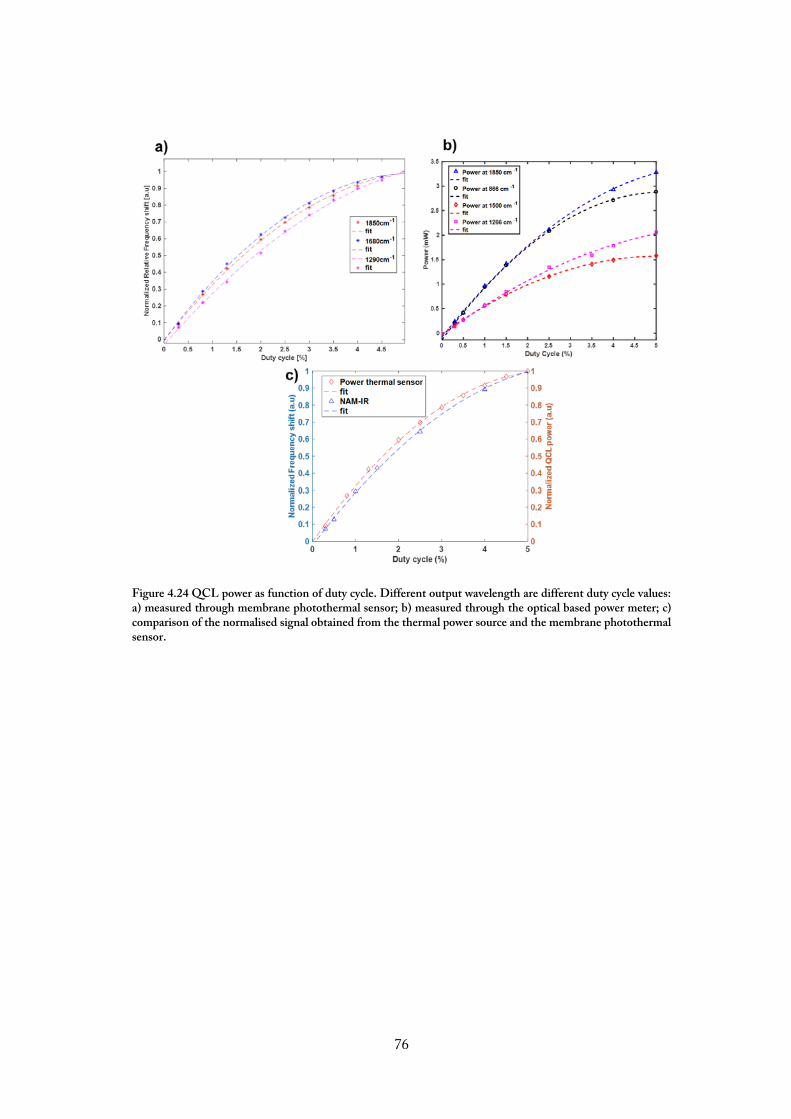
Figure 4.24 QCL power as function of duty cycle. Different output wavelength are different duty cycle values: a) measured through membrane photothermal sensor; b) measured through the optical based power meter; c) comparison of the normalised signal obtained from the thermal power source and the membrane photothermal sensor.

76

Table 7 Values of the fitted parameter describing the second order polynomial expression that the relationship between the normalised output power and the duty-cycle

Frequency

(cm-1)

Fitted

parameter p1

Fitted

parameter p2

Fitted

parameter p3

866 -0.0398 0.4078 0.0468

1850 -0.0238 0.3158 0.0194

1500 -0.0386 0.3934 0.0079

1266 -0.0265 0.3366 0.0240

4.6.2. The measurement acquisition chain

The acquisition of the spectra by NAM-IR is a time-varying process; the resonance

frequency shift can be written as:

δf (t)=f�ωIR(t)� (54)

Figure 4.25 Block Diagram of the acquisition chain of the NAM-IR setup.

The QCL sweeps a certain interval of wavelengths by quantizing the wavelength

range in a discrete manner. A certain wavelength 𝜔𝜔𝑖𝑖 is kept as output for a certain

dwell time 𝜔𝜔0, therefore the time needed for sweep across a wavelength range ∆𝜔𝜔 is

𝑇𝑇 = 𝑡𝑡0 ∗ ∆𝜔𝜔.The measurement of the photothermal signal matches with the

measurement of a thermal process, commonly described by a time constant. As

described in chapter 4 and Paper 1, the membrane time constant regulates the

minimum amount of time (dwell time, 𝑡𝑡0) that a single IR frequency has to be

activated for being properly recorded by the membrane resonator. Furthermore, the

integration time of the PLL has to be set according to the response of time of the

membrane.

77

4.6.2.1. The Phase locked loop (PLL)

All the frequency shifts are recorded through a phase locked loop detection

scheme(Figure 4.26). Although it is not the goal of this project investigating on the

capabilities of such device, it is noteworthy to introduce its working principle and

the settings parameters as they have a fundamental role in determining the outcome

of recorded signal in terms of time responsivity and noise.

The phase locked loop was introduced in the field of telecommunication as key

component of frequency (de) modulation transmission based technology. In its

broad definition, a phase locked loop is a closed control system that provides a

signal that is proportional to the phase difference between the phase of the

reference signal and the phase of the system under study (SOS).

A reference signal, generally a sine wave is internally produced and multiplied to the

signal of the SOS hence the phases of these two signal are compared and used as

input of a PID block which controls a voltage controlled oscillator (VCO) such that

its output will have the same frequency of the entry signal. During a measurement,

the reference signal is set at the resonance of the (SOS) hence, in the absence any

source that can deviate the resonance frequency for the set value; the VCO will

oscillate at the same frequency of the SOS. As the signal input is varying the PID

will regulate the output of the VCO such that to minimise the error.

Figure 4.26 Block diagram of the PLL. The phase for the reference signal is compared to one of the input signals. The PID controls the open loop gain, providing a signal that will pilot the Voltage-controlled Oscillator that will finally pilot the piezoelectric crystal with the same frequency and phase of the input signal.

78

4.6.2.1.1. Influence of the PLL Bandwidth on NAM-IR spectra

The PLL bandwidth is by far the most important parameter that determines the

time responsivity of the detection scheme and the gain of the PID control. A

smaller bandwidth cut out value determines a higher Signal to noise ratio (SNR)

which come at the cost of a slower system (higher value of integration time), on the

contrary, a higher bandwidth allows following faster changes of the input signal

decreasing the quality of the signal in terms of SNR [111].

Figure 4.27 Effect of the Phase detector bandwidth on the recording. The cross-correlation function b) has been used to see if between two different PLL settings would influence the phase of the signal. The main effect depending on the settings is due to the low-pass filter effect that a lower bandwidth has on the recordings.

In the present work, the choice of the right bandwidth value revealed to be

fundamental to maximise the SNR.

c)

a) b)

d)

79

In Figure 4.27 is represented the difference of the NAM-IR spectra recorded at 200

Hz and 500 Hz PLL bandwidth for a 20nm PVP coated membrane. 200 Hz

provides a higher integration time which does not comply with the speed of

frequency shift transitions taking place upon heat absorption. The two recordings

are perfectly aligned, and the cross-correlation function has the maximum at 0

meaning that the NAM-IR shifts are recorded without significant lags. The effect

of the lower value of bandwidth can be seen in Figure 3c-d where the spectra

recorded with 200Hz bandwidth resulted in being low pass filtered. If the time

constant of the PLL is not set at least smaller than the time constant of the analysed

phenomenon, this will not be recorded properly.

For photothermal resonance spectroscopy application, the PLL bandwidth has to be

chosen to match the thermal time constant of the membrane sensor. In this work

for all the spectra recorded the bandwidth was set at least to 500Hz which provides

an integration time smaller than the thermal time constant of the membrane

resonator. Finally, the sampling frequency of the A/D converter has to fulfil the

Nyquist-Shannon theorem and therefore has to be set at least two times the highest

frequency component and in the experiment was performed at 3600 sample/sec.

80

4.7. Polymer Solution Preparation

The polymer used in the paper were: poly(lactic-co-glycolic acid) PLGA and

poly(vinylpyrrolidone) PVP, both obtained and used as received from Sigma-

Aldrich.

For polymer degradation studies PLGA(Mw=16kDa) was used, and it was

dissolved in dichloromethane (DCM, 99% HPLC grade Sigma-Aldrich) dissolved

in 0.5% wt. and stirred overnight before being sprayed.

For NAM-IR, experiments were focused on the study of PVP. Membranes were

coated with poly(vinylpyrrolidone). In this case, the polymer was dissolved in a

mixture of water and hydrogen peroxide (H2O2:H2O 30% wv.) in different

concentrations: 1%wt. and 5% wt. For performing the experiments reported in

paper 2 and paper 3. However, for performing the crosslinking experiments the of

paper 3 the polymer concentration was lowered to 0.1%wt to deposit few

nanograms of material on the membrane resonator by direct drop casting.

81

82

5. Summary of Papers

Paper 1

The working principle of the first version of the Blu-Ray based system for

characterising the enzymatic degradation of PLGA is presented. In this paper, an

improved methodology of biopolymer degradation studies by micromechanical

resonator is shown. The following elements were combined: i)double clamped

microbeams as mass sensor, ii) a microfluidic setup where the degradation

environment can be easily simulated, and iii) a readout based on a Blu-Ray device

which can be easily programmed to perform measurement in an automatic fashion.

Paper 2

This paper shows the working principle of a micromechanical membrane as

photothermal sensor. The sensing capabilities of the sensor were characterised

studying the photothermal response of membranes coated by thin layer of PVP

prepared by spin coating. The behaviour of the nanomechanical photothermal

signal is studied in high vacuum and low vacuum showing what effect that the

atmosphere has on the overall acquisition of the NAM-IR spectra. NAM-IR

spectra were recorded on different polymer thicknesses. The achieved Signal to

Noise Ratio is compared to the one obtained by conventional ATR-FTIR

spectroscopy on similar samples. Membrane-based NAM-IR spectroscopy provides

on a single acquisition an SNR 43 time higher than the conventional ATR. The

extracted limit of detection for membrane resonator is in the attomolar range

indicating that the analysis of single molecule layer is possible.

Paper 3

In this paper, we want to highlight how an analysis based on membrane

photothermal resonators facilitates the study of the modification of chemical

properties of thin polymer layer. The linearity of the photothermal response across

83

two orders of magnitude of polymer coating is showed. The evaluation of the

responsivity curve as function of the deposited polymer thickness obtained by spin

coating, serves as calibration tool for estimate the deposited thickness by other

methods such as drop casting. Films of PVP obtained by drop casting are

crosslinked by UV. In the paper is also analysed the phenomena of photooxidation

that occurs simultaneously to the gelification. Membrane photothermal sensor

allowed featuring the gelification process on picogram quantity of PVP.

84

6. Conclusions In this thesis, the goal was to develop technologies to facilitate biopolymer

characterization. This was accomplished by working on two different tasks.

i) The development of a Blu-Ray based device to perform biopolymer

degradation studies using micromechanical resonators.

ii) The design, modelling and optimisation of a mechanical based

photothermal sensor.

Two generation of a semi-automatic system for measuring the biopolymer

degradation were developed. In this framework, silicon microbridges were designed

and fabricated. Microbridges have shown a reasonably good mass sensing

performance, and have been used to monitor the biopolymer degradation. The

measured limit of detection was ∆𝑚𝑚 = 0.09 µ𝑔𝑔 𝑚𝑚𝑚𝑚−2, which enables to describes

the biopolymer degradation phenomena, considering the biopolymer density of 1-5

𝜇𝜇𝑔𝑔𝑚𝑚𝑚𝑚−2. In water environment the limit of detection was ∆𝑚𝑚 = 3.34 µ𝑔𝑔 𝑚𝑚𝑚𝑚−2

of bridges hindering their use for a real-time monitoring of the biopolymer

degradation phenomena. In order to overcome this limitation a wet and dry

approach has been used. The first generation of the system (system V1) has been

used to characterize the enzymatic degradation of poly-lactide-co-glicolyde

(PLGA). The enzymatic degradation rate obtained in this work was 25µgcm-2h-1

comparable to the one obtained under similar environmental conditions with a

conventional approach. Looking at these results from a statistical point of view, the

ratio of analysed samples vs total experimental time is 3 orders of magnitude higher

compared to the conventional studies. These results were summarized in paper 1.

The second version of the system (systemV2) aims to improve the throughput of

the measurements. Compared to the first version, system V2 can perform

measurements on two axes, allowing to increase the throughput of degradation

analysis. Moreover, system V2 aims to reduce the interaction of the user. The

robustness of the controlling algorithms is improved. In particular, the initialization

85

routines of the measurement sequence: autofocus and tracking of the position of the

microresonator have been improved.

Relatively to the second task of this project, micromechanical sensors have also

been designed and developed to perform nanomechanical based photothermal

spectroscopy (NAM-IR).

The use of a 2D resonator as photothermal sensor is new. Membrane resonators

have shown to have several experimental advantages compared to strings. First of all

is the simplicity and robustness of the sample preparation on the membrane.

Membrane resonators can be easily functionalized by spin coating or drop casting,

instead of bulky spray coating or aerosol system which would have been used for

string based photothermal analyses.

The nanomechanical photothermal signal has been modelled both analytically and

using finite element simulations. The goal was to understand the effects that the

experimental variables have on the generation of the photothermal signal. In

particular, an accurate knowledge of the transient allowed us to correctly couple the

dynamics of the IR source with the acquisition parameters. Thanks to the

modelling, the absorbed incident power, but more importantly, the temperature

field reached in the membrane for any single power absorption was calculated. The

incredibly high SNR (307) obtained on a 20nm thick layer of poly(vinylpyrrolidone)

indicates that obtaining the IR fingerprint of single molecule layer is within reach.

The high sensitivity was exploited to characterise the crosslinking mechanism of the

picomolar quantity of poly(vinylpyrrolidone), biopolymer for pharmaceutical

applications.

Finally, a proof of concept of the potential of the photothermal response was used

to evaluate the thermal diffusivity of the silicon nitride and of the bilayer polymer-

silicon nitride. These results are seen to reasonably match the values of the thermal

diffusivity reported previously reported in literature.

86

6.1. Outlook

The semi-automated system that was used to characterise the biopolymer

degradation can be easily used for measuring other pharmaceutical relevant physical

phenomena. For instance, the concept of degradation study can be expanded by

exploring the dissolution of drug-polymer mixtures and further characterise the

effect of drug on the degradation of a polymer matrix.

Microbridges structures can be optimised to work in liquid environment aiming to

perform real-time degradation studies. To accomplish this goal, the design has to

take into account that the structure should have a high resonance frequency and a

wide cross section to minimise the energy losses.

The development of the photothermal studies performed in this work concerns the

possibility of integrating the readout[79], eliminating the need for expensive and

bulky readout technology such as the Laser-Doppler Vibrometer used in this thesis.

One of the hidden advantages of the NAM-IR technique is that the signal can be

obtained by impinging the sensor at any angle and with any polarisation. Applying

these concepts and considering the limit of detection demonstrated in Paper 2 a

potential application of photothermal spectroscopy is the analysis of the chemical

structure of self-assembly monolayers.

The studies presented in Paper 3 can be implemented on hollow structures, which

would enable the real-time monitoring of crosslinking of polymer. Indeed, the

gelification induces changes in the polymer solution whose rheological properties

transit from a purely viscous to a viscoelastic solid. Such modification in a polymer-

filled hollow structure would be reflected as changes in the Q.

Mechanical resonators have shown to be able to work as a thermal characterising

tool for polymers [56,57,112]. The creation of a setup able to perform a

temperature dependent photothermal spectroscopy would enable the disclosure of

properties of materials in the form of thin films, while they undergo a multitude of

relevant thermal events, such as glass and phase transitions. This technique is going

87

to contribute more and more to the lively debate in the scientific community around

this important topic [47,113].

88

References

[1] Biopolymers - Latest research and news | Nature, (n.d.). http://www.nature.com/subjects/biopolymers (accessed April 5, 2017).

[2] a. C. Vieira, J.C. Vieira, J.M. Ferra, F.D. Magalhães, R.M. Guedes, a. T. Marques, Mechanical study of PLA-PCL fibers during in vitro degradation, J. Mech. Behav. Biomed. Mater. 4 (2011) 451–460. doi:10.1016/j.jmbbm.2010.12.006.

[3] R.S. Petersen, S.S. Keller, A. Boisen, Hot punching of high-aspect-ratio 3D polymeric microstructures for drug delivery, Lab Chip. 15 (2015) 2576–2579. doi:10.1039/C5LC00372E.

[4] P. Gentile, V. Chiono, I. Carmagnola, P. V Hatton, An overview of poly(lactic-co-glycolic) acid (PLGA)-based biomaterials for bone tissue engineering., Int. J. Mol. Sci. 15 (2014) 3640–59. doi:10.3390/ijms15033640.

[5] C.L. Huang, T.W. Steele, E. Widjaja, F.Y. Boey, S.S. Venkatraman, J.S. Loo, The influence of additives in modulating drug delivery and degradation of PLGA thin films, NPG Asia Mater. 5 (2013) e54. doi:10.1038/am.2013.26.

[6] H.K. Makadia, S.J. Siegel, Poly Lactic-co-Glycolic Acid (PLGA) as biodegradable controlled drug delivery carrier, Polymers (Basel). 3 (2011) 1377–1397. doi:10.3390/polym3031377.

[7] R.H. Harrison, J.A.M. Steele, R. Chapman, A.J. Gormley, L.W. Chow, M.M. Mahat, L. Podhorska, R.G. Palgrave, D.J. Payne, S.P. Hettiaratchy, I.E. Dunlop, M.M. Stevens, Modular and Versatile Spatial Functionalization of Tissue Engineering Scaffolds through Fiber-Initiated Controlled Radical Polymerization, Adv. Funct. Mater. 25 (2015) 5748–5757. doi:10.1002/adfm.201501277.

[8] R. Izquierdo, N. Garcia-Giralt, M.T. Rodriguez, E. Cáceres, S.J. García, J.L. Gómez Ribelles, M. Monleón, J.C. Monllau, J. Suay, Biodegradable PCL scaffolds with an interconnected spherical pore network for tissue engineering, J. Biomed. Mater. Res. Part A. 85A (2008) 25–35. doi:10.1002/jbm.a.31396.

[9] T. Patrício, M. Domingos, A. Gloria, P. Bártolo, Characterisation of PCL and PCL/PLA Scaffolds for Tissue Engineering, Procedia CIRP. 5 (2013) 110–114. doi:10.1016/j.procir.2013.01.022.

[10] C.K.S. Pillai, C.P. Sharma, Review Paper: Absorbable Polymeric Surgical Sutures: Chemistry, Production, Properties, Biodegradability, and Performance, J. Biomater. Appl. 25 (2010) 291–366. doi:10.1177/0885328210384890.

[11] L. Xinming, C. Yingde, A.W. Lloyd, S. V. Mikhalovsky, S.R. Sandeman, C.A. Howel, L. Liewen, Polymeric hydrogels for novel contact lens-based ophthalmic drug delivery systems: A review, Contact Lens Anterior Eye. 31 (2008) 57–64. doi:10.1016/j.clae.2007.09.002.

[12] K.S. Walline, Drug Delivery Coatings for Cardiovascular Stents: Silicone Elastomer and Thrombin Responsive Hydrogel Coatings, (2004). http://citeseerx.ist.psu.edu/viewdoc/download?doi=10.1.1.484.1937&rep=rep1&type=pdf (accessed April 2, 2017).

89

[13] B. Yu, C. Wang, Y.M. Ju, L. West, J. Harmon, Y. Moussy, F. Moussy, Use of hydrogel coating to improve the performance of implanted glucose sensors, Biosens. Bioelectron. 23 (2008) 1278–1284. doi:10.1016/j.bios.2007.11.010.

[14] B. Butruk, M. Trzaskowski, T. Ciach, Fabrication of biocompatible hydrogel coatings for implantable medical devices using Fenton-type reaction, Mater. Sci. Eng. C. 32 (2012) 1601–1609. doi:10.1016/j.msec.2012.04.050.

[15] Poly(N-vinyl-2-pyrrolidone) hydrogel production by ultraviolet radiation: new methodologies to accelerate crosslinking, Polymer (Guildf). 45 (2004) 4705–4709.

[16] K. Yamashita, T. Funato, Y. Suzuki, S. Teramachi, Y. Doi, Characteristic Interactions between Poly(hydroxybutyrate) Depolymerase and Poly[(R)-3-hydroxybutyrate] Film Studied by a Quartz Crystal Microbalance, Macromol. Biosci. 3 (2003) 694–702. doi:10.1002/mabi.200300004.

[17] Y. Wang, S. Ge, M. Rafailovich, J. Sokolov, Y. Zou, H. Ade, J. Lu, A. Lustiger, G. Maron, Crystallization in the Thin and Ultrathin Films of Poly(ethylene-vinyl acetate) and Linear Low-Density Polyethylene, (2003). doi:10.1021/ma030456b.

[18] G. Bakan, S. Ayas, E. Ozgur, K. Celebi, A. Dana, Thermally Tunable Ultrasensitive Infrared Absorption Spectroscopy Platforms Based on Thin Phase-Change Films, ACS Sensors. (2016) acssensors.6b00591. doi:10.1021/acssensors.6b00591.

[19] G.S. Y Yeh, R. Hosemann, J. Loboda-C, Annealing effects of polymers and their underlying molecular mechanisms*, (n.d.). https://deepblue.lib.umich.edu/bitstream/handle/2027.42/21799/0000198.pdf?sequence=1 (accessed April 2, 2017).

[20] S.M. Louie, J.M. Gorham, E.A. McGivney, J. Liu, K.B. Gregory, V.A. Hackley, Photochemical transformations of thiolated polyethylene glycol coatings on gold nanoparticles, Environ. Sci. Nano. 3 (2016) 1090–1102. doi:10.1039/C6EN00141F.

[21] R. Auras, Poly(lactic acid) : synthesis, structures, properties, processing, and applications, Wiley, 2010.

[22] K.S. Soppimath, T.M. Aminabhavi, A.R. Kulkarni, Biodegradable polymeric nanoparticles as drug delivery devices, 70 (2001) 1–20.

[23] H. Tsuji, Y. Ikada, Properties and morphology of poly(L-lactide). II. hydrolysis in alkaline solution, J. Polym. Sci. Part A Polym. Chem. 36 (1998) 59–66. doi:10.1002/(SICI)1099-0518(19980115)36:1<59::AID-POLA9>3.0.CO;2-X.

[24] Q. Cai, G. Shi, J. Bei, S. Wang, Enzymatic degradation behavior and mechanism of poly(lactide-co-glycolide) foams by trypsin., Biomaterials. 24 (2003) 629–38. doi:10.1016/S0142-9612(02)00377-0.

[25] M. Rahmouni, F. Chouinard, F. Nekka, V. Lenaerts, J.C. Leroux, Enzymatic degradation of cross-linked high amylose starch tablets and its effect on in vitro release of sodium diclofenac, Eur. J. Pharm. Biopharm. 51 (2001) 191–198. doi:10.1016/S0939-6411(01)00127-8.

[26] S. Lyu, D. Untereker, Degradability of Polymers for Implantable Biomedical Devices, Int. J. Mol. Sci. Int. J. Mol. Sci. 10 (2009) 4033–4065. doi:10.3390/ijms10094033.

[27] L.C. Lopérgolo, A.B. Lugão, L.H. Catalani, Direct UV photocrosslinking of poly(N-vinyl-2-pyrrolidone) (PVP) to produce hydrogels, (n.d.). doi:10.1016/S0032-3861(03)00686-4.

90

[28] G.J.M. Fechine, J.A.G. Barros, L.H. Catalani, Poly(N-vinyl-2-pyrrolidone) hydrogel production by ultraviolet radiation: new methodologies to accelerate crosslinking, (n.d.). doi:10.1016/j.polymer.2004.05.006.

[29] P. Marizza, M. Abrami, S.S. Keller, P. Posocco, E. Laurini, K. Goswami, A.L. Skov, A. Boisen, D. Larobina, G. Grassi, M. Grassi, Synthesis and characterization of UV photocrosslinkable hydrogels with poly(N-vinyl-2-pyrrolidone): Determination of the network mesh size distribution, Int. J. Polym. Mater. Polym. Biomater. 65 (2016) 516–525. doi:10.1080/00914037.2015.1129964.

[30] N. Bhattarai, J. Gunn, M. Zhang, Chitosan-based hydrogels for controlled, localized drug delivery, Adv. Drug Deliv. Rev. 62 (2010) 83–99. doi:10.1016/j.addr.2009.07.019.

[31] P. Marizza, M. Abrami, S.S. Keller, P. Posocco, E. Laurini, K. Goswami, A.L. Skov, A. Boisen, D. Larobina, G. Grassi, M. Grassi, Synthesis and characterization of UV photocrosslinkable hydrogels with poly(N-vinyl-2-pyrrolidone): Determination of the network mesh size distribution, Int. J. Polym. Mater. Polym. Biomater. 65 (2016) 516–525. doi:10.1080/00914037.2015.1129964.

[32] R.K. Mishra, M. Datt, A.K. Banthia, Synthesis and characterization of pectin/PVP hydrogel membranes for drug delivery system., AAPS PharmSciTech. 9 (2008) 395–403. doi:10.1208/s12249-008-9048-6.

[33] N.A. Peppas, P. Bures, W. Leobandung, H. Ichikawa, Hydrogels in pharmaceutical formulations, Eur. J. Pharm. Biopharm. 50 (2000) 27–46. doi:10.1016/S0939-6411(00)00090-4.

[34] O. Chaudhuri, L. Gu, D. Klumpers, M. Darnell, S.A. Bencherif, J.C. Weaver, N. Huebsch, H. Lee, E. Lippens, G.N. Duda, D.J. Mooney, Hydrogels with tunable stress relaxation regulate stem cell fate and activity, Nat. Mater. 15 (2015) 326–334. doi:10.1038/nmat4489.

[35] I. Chae, M.F. Khan, J. Song, T. Kang, J. Lee, T. Thundat, Standoff Mechanical Resonance Spectroscopy Based on Infrared- Sensitive Hydrogel Microcantilevers, (n.d.). doi:10.1021/acs.analchem.6b02540.

[36] A. Mateescu, Y. Wang, J. Dostalek, U. Jonas, Thin hydrogel films for optical biosensor applications, Membranes (Basel). 2 (2012) 49–69. doi:10.3390/membranes2010040.

[37] H. Tsuji, A. Mizuno, Y. Ikada, Properties and morphology of poly(L-lactide). III. Effects of initial crystallinity on long-termin vitro hydrolysis of high molecular weight poly(L-lactide) film in phosphate-buffered solution, J. Appl. Polym. Sci. 77 (2000) 1452–1464. doi:10.1002/1097-4628(20000815)77:7<1452::AID-APP7>3.0.CO;2-S.

[38] A. Södergård, J.-F. Selin, J.H. Näsman, Hydrolytic degradation of peroxide modified poly(L-lactide), Polym. Degrad. Stab. 51 (1996) 351–359. doi:10.1016/0141-3910(95)00271-5.

[39] D. Cam, S.H. Hyon, Y. Ikada, Degradation of high molecular weight poly(L-lactide) in alkaline medium., Biomaterials. 16 (1995) 833–43. http://www.ncbi.nlm.nih.gov/pubmed/8527598 (accessed April 2, 2017).

[40] L. Xu, K. Crawford, C.B. Gorman, Effects of Temperature and pH on the Degradation of Poly ( lactic acid ) Brushes, Macromolecules. 44 (2011) 4777–4782.

[41] K. Yamashita, Y. Kikkawa, K. Kurokawa, Y. Doi, Enzymatic Degradation of Poly ( L -lactide ) Film by Proteinase K : Quartz Crystal Microbalance and Atomic Force Microscopy

91

Study, (2005) 850–857.

[42] L.T. Kearney, J.A. Howarter, QCM-Based Measurement of Chlorine-Induced Polymer Degradation Kinetics, (n.d.). doi:10.1021/la501922u.

[43] C. Sumner, S. Krause, A. Sabot, K. Turner, C.J. McNeil, Biosensor based on enzyme-catalysed degradation of thin polymer films, Biosens. Bioelectron. 16 (2001) 709–714. doi:10.1016/S0956-5663(01)00210-X.

[44] S. Bose, S.S. Keller, A. Boisen, K. Almdal, Microcantilever sensors for fast analysis of enzymatic degradation of poly (d, l-lactide), Polym. Degrad. Stab. 119 (2015) 1–8. doi:10.1016/j.polymdegradstab.2015.04.021.

[45] S. Bose, Micromechanical resonators as a tool for polymer characterization, (2014).

[46] G. Reiter, S. Napolitano, Possible origin of thickness-dependent deviations from bulk properties of thin polymer films, J. Polym. Sci. Part B Polym. Phys. 48 (2010) 2544–2547. doi:10.1002/polb.22134.

[47] † Jae Hyun Kim, *,† and Jyongsik Jang, ‡ Wang-Cheol Zin*, Thickness Dependence of the Glass Transition Temperature in Thin Polymer Films, (2001). doi:10.1021/LA001125K.

[48] A.I. Fedorchenko, A.-B. Wang, H.H. Cheng, Thickness dependence of nanofilm elastic modulus, Appl. Phys. Lett. 94 (2009) 152111. doi:10.1063/1.3120763.

[49] R.M. Michell, I. Blaszczyk-Lezak, C. Mijangos, A.J. Müller, Confinement effects on polymer crystallization: From droplets to alumina nanopores, (2013). doi:10.1016/j.polymer.2013.05.029.

[50] J.W. Ndieyira, N. Kappeler, S. Logan, M.A. Cooper, C. Abell, R.A. McKendry, G. Aeppli, Surface-stress sensors for rapid and ultrasensitive detection of active free drugs in human serum, Nat. Nanotechnol. 9 (2014) 225–232. doi:10.1038/nnano.2014.33.

[51] S.B. Patil, M. Vögtli, B. Webb, G. Mazza, M. Pinzani, Y.-A. Soh, R.A. McKendry, J.W. Ndieyira, Decoupling competing surface binding kinetics and reconfiguration of receptor footprint for ultrasensitive stress assays, Nat. Nanotechnol. 10 (2015) 899–907. doi:10.1038/nnano.2015.174.

[52] A.O.N. T. Larsen,a S. Schmid, L. Grönberg, Ultrasensitive string-based temperature sensors, Appl. Phys. Lett. 98 (2011).

[53] S. Schmid, S. Dohn, A. Boisen, Real-Time Particle Mass Spectrometry Based on Resonant Micro Strings, Sensors. 10 (2010) 8092–8100. doi:10.3390/s100908092.

[54] M. del Rey, R. a. da Silva, D. Meneses, D.F.S. Petri, J. Tamayo, M. Calleja, P.M. Kosaka, Monitoring swelling and deswelling of thin polymer films by microcantilever sensors, Sensors Actuators B Chem. 204 (2014) 602–610. doi:10.1016/j.snb.2014.08.021.

[55] S. Bose, S.S. Keller, T.S. Alstrøm, A. Boisen, K. Almdal, Process optimization of ultrasonic spray coating of polymer films., Langmuir. 29 (2013) 6911–9. doi:10.1021/la4010246.

[56] S. Bose, S. Schmid, T. Larsen, S. Sylvest Keller, A. Boisen, K. Almdal, Micromechanical fast quasi-static detection of α and β relaxations with nanograms of polymer, J. Polym. Sci. Part B Polym. Phys. 53 (2015) 1035–1039. doi:10.1002/polb.23745.

[57] S. Bose, S. Schmid, T. Larsen, S.S. Keller, P. Sommer-Larsen, A. Boisen, K. Almdal, Micromechanical string resonators: Analytical tool for thermal characterization of polymers,

92

ACS Macro Lett. 3 (2014) 55–58. doi:10.1021/mz400470n.

[58] S.S. Keller, L. Gammelgaard, M.P. Jensen, S. Schmid, Z.J. Davis, a. Boisen, Micromechanical sensors for the measurement of biopolymer degradation, Proc. IEEE Int. Conf. Micro Electro Mech. Syst. (2011) 457–460. doi:10.1109/MEMSYS.2011.5734460.

[59] P.C. Blainey, P.J. Reid, FTIR studies of intermolecular hydrogen bonding in halogenated ethanols, Spectrochim. Acta Part A. 57 (2001) 2763–2774. www.elsevier.com/locate/saa (accessed June 30, 2016).

[60] M.A. Ramin, G. Le Bourdon, N. Daugey, B. Bennetau, L. Vellutini, T. Buffeteau, PM-IRRAS Investigation of Self-Assembled Monolayers Grafted onto SiO 2 /Au Substrates, Langmuir. 27 (2011) 6076–6084. doi:10.1021/la2006293.

[61] R. Mendelsohn, G. Mao, C.R. Flach, Infrared reflection-absorption spectroscopy: principles and applications to lipid-protein interaction in Langmuir films., Biochim. Biophys. Acta. 1798 (2010) 788–800. doi:10.1016/j.bbamem.2009.11.024.

[62] Q. Liu, S. Xiao, Effects of spectral resolution and signal-to- noise ratio of hyperspectral sensors on retrieving atmospheric parameters, (2013). doi:10.1364/OL.39.000060.

[63] S. Bialkowski, Photothermal spectroscopy methods for chemical analysis, Wiley, 1996.

[64] M. Yun, S. Kim, D. Lee, N. Jung, I. Chae, S. Jeon, T. Thundat, Photothermal cantilever deflection spectroscopy of a photosensitive polymer, Appl. Phys. Lett. 100 (2012) 204103. doi:10.1063/1.4719521.

[65] E. Finot, V. Rouger, L. Markey, R. Seigneuric, M.-H. Nadal, T. Thundat, Visible photothermal deflection spectroscopy using microcantilevers, Sensors Actuators B Chem. 169 (2012) 222–228. doi:10.1016/j.snb.2012.04.072.

[66] M.F. Khan, N. Miriyala, J. Lee, M. Hassanpourfard, A. Kumar, T. Thundat, Heat capacity measurements of sub-nanoliter volumes of liquids using bimaterial microchannel cantilevers, 108 (2016). http://dx.doi.org/10.1063/1.4952614 (accessed September 26, 2016).

[67] A. Wig, E.T. Arakawa, A. Passian, T.L. Ferrell, T. Thundat, Photothermal spectroscopy of Bacillus anthracis and Bacillus cereus with microcantilevers, Sensors Actuators B Chem. 114 (2006) 206–211. doi:10.1016/j.snb.2005.04.029.

[68] M.S. Ghoraishi, J.E. Hawk, A. Phani, M.F. Khan, T. Thundat, Clustering mechanism of ethanol- water mixtures investigated with photothermal microfluidic cantilever deflection spectroscopy, Nat. Publ. Gr. (2016). doi:10.1038/srep23966.

[69] N. Miriyala, M.F. Khan, T. Thundat, Thermomechanical behavior of a bimaterial microchannel cantilever subjected to periodic IR radiation, Sensors Actuators B Chem. 235 (2016) 273–279. doi:10.1016/j.snb.2016.05.043.

[70] J.R. Barnes, R.J. Stephenson, M.E. Welland, C. Gerber, J.K. Gimzewski, Photothermal spectroscopy with femtojoule sensitivity using a micromechanical device, Nature. 372 (1994) 79–81. doi:10.1038/372079a0.

[71] J.R. Barnes, R.J. Stephenson, C.N. Woodburn, S.J. O’Shea, M.E. Welland, T. Rayment, J.K. Gimzewski, C. Gerber, A femtojoule calorimeter using micromechanical sensors, Rev. Sci. Instrum. 65 (1994) 3793. doi:10.1063/1.1144509.

[72] T.S. Biswas, N. Miriyala, C. Doolin, X. Liu, T. Thundat, J.P. Davis, Femtogram-scale photothermal spectroscopy of explosive molecules on nanostrings., Anal. Chem. 86 (2014)

93

11368–72. doi:10.1021/ac503318e.

[73] A. Andersen, Alina Joukainen; Yamada, Shoko; Ek, Pramod Kumar; Andresen, Thomas Lars; Boisen, S. Schmid, Nanomechanical IR spectroscopy for fast analysis of liquid-dispersed engineered nanomaterials, Sens. Actuators B. 233 (2016) 667–673.

[74] T. Larsen, S. Schmid, L.G. Villanueva, A. Boisen, Photothermal analysis of individual nanoparticulate samples using micromechanical resonators., ACS Nano. 7 (2013) 6188–93. doi:10.1021/nn402057f.

[75] M. Kurek, M. Carnoy, P.E. Larsen, L.H. Nielsen, O. Hansen, T. Rades, S. Schmid, A. Boisen, Nanomechanical Infrared Spectroscopy with Vibrating Filters for Pharmaceutical Analysis, Angew. Chemie Int. Ed. 56 (2017) 3901–3905. doi:10.1002/anie.201700052.

[76] S. Yamada, S. Schmid, T. Larsen, O. Hansen, A. Boisen, Photothermal Infrared Spectroscopy of Airborne Samples with Mechanical String Resonators, Anal. Chem. 85 (2013) 10531–10535. doi:10.1021/ac402585e.

[77] X.C. Zhang, E.B. Myers, J.E. Sader, M.L. Roukes, Nanomechanical Torsional Resonators for Frequency-Shift Infrared Thermal Sensing, Nano Lett. 13 (2013) 1528–1534. doi:10.1021/nl304687p.

[78] S. Schmid, K. Wu, P.E. Larsen, T. Rindzevicius, A. Boisen, Low-Power Photothermal Probing of Single Plasmonic Nanostructures with Nanomechanical String Resonators, Nano Lett. 14 (2014) 2318–2321. doi:10.1021/nl4046679.

[79] A. Talukdar, M. Faheem Khan, D. Lee, S. Kim, T. Thundat, G. Koley, Piezotransistive transduction of femtoscale displacement for photoacoustic spectroscopy, Nat. Commun. 6 (2015) 7885. doi:10.1038/ncomms8885.

[80] S. Shin, J.-K. Paik, N.-E. Lee, J.-S. Park, H.-D. Park, J. Lee, Gas Sensor Application of Piezoelectric Cantilever Nanobalance; Electrical Signal Read-Out, Ferroelectrics. 328 (2005) 59–65. doi:10.1080/00150190500311060.

[81] F.G. Bosco, E.-T. Hwu, C.-H. Chen, S. Keller, M. Bache, M.H. Jakobsen, I.-S. Hwang, A. Boisen, High throughput label-free platform for statistical bio-molecular sensing., Lab Chip. 11 (2011) 2411–6. doi:10.1039/c1lc20116f.

[82] A. Mostafazadeh, G.G. Yaralioglu, H. Urey, Optical fiber array based simultaneous parallel monitoring of resonant cantilever sensors in liquid, Sensors Actuators, A Phys. 242 (2016) 132–139. doi:10.1016/j.sna.2016.03.004.

[83] E.-T. Hwu, S.-K. Hung, C.-W. Yang, K.-Y. Huang, I.-S. Hwang, Real-time detection of linear and angular displacements with a modified DVD optical head, Nanotechnology. 19 (2008) 115501. doi:10.1088/0957-4484/19/11/115501.

[84] E.T. Hwu, S.K. Hung, C.W. Yang, I.S. Hwang, K.Y. Huang, Simultaneous detection of translational and angular displacements of micromachined elements, Appl. Phys. Lett. 91 (2007). doi:10.1063/1.2817750.

[85] M. Donolato, P. Antunes, T. Zardán, G. De, E. Hwu, C. Chen, R. Burger, G. Rizzi, F.G. Bosco, M. Strømme, A. Boisen, M.F. Hansen, Quantification of rolling circle amplified DNA using magnetic nanobeads and a Blu-ray optical pick-up unit, 67 (2015) 1–24. doi:10.1016/j.bios.2014.09.097.

[86] S. Schmid, L.G. Villanueva, M.L. Roukes, Quality Factor, in: Fundam. Nanomechanical Reson., Springer International Publishing, Cham, 2016: pp. 57–90. doi:10.1007/978-3-319-

94

28691-4_2.

[87] S. Schmid, K.D. Jensen, K.H. Nielsen, A. Boisen, Damping mechanisms in high- Q micro and nanomechanical string resonators, Phys. Rev. B. 84 (2011) 165307. doi:10.1103/PhysRevB.84.165307.

[88] S. Schmid, S. Dohn, A. Boisen, Real-Time Particle Mass Spectrometry Based on Resonant Micro Strings, Sensors. 10 (2010) 8092–8100. doi:10.3390/s100908092.

[89] Control Tutorials for MATLAB and Simulink - Introduction: System Modeling, (n.d.). http://ctms.engin.umich.edu/CTMS/index.php?example=Introduction&section=SystemModeling#2 (accessed March 16, 2017).

[90] † Y. T. Yang, ‡ C. Callegari, X. L. Feng, § and K. L. Ekinci, M.L. Roukes*, Zeptogram-Scale Nanomechanical Mass Sensing, (2006). doi:10.1021/NL052134M.

[91] S. Schmid, L.G. Villanueva, M.L. Roukes, Responsivity, in: Fundam. Nanomechanical Reson., Springer International Publishing, Cham, 2016: pp. 91–114. doi:10.1007/978-3-319-28691-4_3.

[92] a K. Naik, M.S. Hanay, W.K. Hiebert, X.L. Feng, M.L. Roukes, Towards single-molecule nanomechanical mass spectrometry., Nat. Nanotechnol. 4 (2009) 445–450. doi:10.1038/nnano.2009.152.

[93] M.S. Hanay, S. Kelber, a K. Naik, D. Chi, S. Hentz, E.C. Bullard, E. Colinet, L. Duraffourg, M.L. Roukes, Single-protein nanomechanical mass spectrometry in real time., Nat. Nanotechnol. 7 (2012) 602–8. doi:10.1038/nnano.2012.119.

[94] J.W.M. Chon, P. Mulvaney, J.E. Sader, Experimental validation of theoretical models for the frequency response of atomic force microscope cantilever beams immersed in fluids, J. Appl. Phys. 87 (2000) 3978. doi:10.1063/1.372455.

[95] J.E. Sader, Frequency response of cantilever beams immersed in viscous fluids with applications to the atomic force microscope, J. Appl. Phys. 84 (1998) 64. doi:10.1063/1.368002.

[96] C.P. Green, J.E. Sader, Frequency response of cantilever beams immersed in viscous fluids near a solid surface with applications to the atomic force microscope, J. Appl. Phys. 98 (2005) 114913. doi:10.1063/1.2136418.

[97] W.-H. Chu, Tech. Rep. No. 2, DTMB, Contract NObs-86396(X), Southwest Research Institute, San Antonio, Texas (1963)., (1963).

[98] M.K. Ghatkesar, V. Barwich, T. Braun, A.H. Bredekamp, U. Drechsler, M. Despont, H.P. Lang, M. Hegner, C. Gerber, Real-time mass sensing by nanomechanical resonators in fluid, Proc. IEEE Sensors, 2004. 3 (2004) 1060–1063. doi:10.1109/ICSENS.2004.1426357.

[99] F. Elmer, M. Dreier, Eigenfrequencies of a rectangular atomic force microscope cantilever in a medium Eigenfrequencies of a rectangular atomic force microscope cantilever in a medium, 7709 (1997). doi:10.1063/1.365379.

[100] M.K. Ghatkesar, T. Braun, V. Barwich, J.P. Ramseyer, C. Gerber, M. Hegner, H.P. Lang, Resonating modes of vibrating microcantilevers in liquid, Appl. Phys. Lett. 92 (2008) 3–5. doi:10.1063/1.2838295.

[101] M.J. Hancock, Solutions to Problems for 2D &amp; 3D Heat and Wave Equations 18.303 Linear Partial Differential Equations, (n.d.). https://ocw.mit.edu/courses/mathematics/18-

95

303-linear-partial-differential-equations-fall-2006/assignments/probpde3dsolns.pdf (accessed March 29, 2017).

[102] X. Zhang, C.P. Grigoropoulos, Thermal conductivity and diffusivity of free‐standing silicon nitride thin films, Rev. Sci. Instrum. 66 (1995) 1115–1120. doi:10.1063/1.1145989.

[103] X. Xie, D. Li, T.-H. Tsai, J. Liu, P. V Braun, D.G. Cahill, Thermal Conductivity, Heat Capacity, and Elastic Constants of Water- Soluble Polymers and Polymer Blends, (n.d.). doi:10.1021/acs.macromol.5b02477.

[104] AccuMist Precision Ultrasonic Nozzle Spray Shaping Technology, (n.d.). http://www.sono-tek.com/accumist/ (accessed March 20, 2017).

[105] S.A. Kandjani, S. Mirershadi, A. Nikniaz, Inorganic–Organic Perovskite Solar Cells, in: Sol. Cells - New Approaches Rev., InTech, 2015. doi:10.5772/58970.

[106] D.B. Hall, P. Underhill, &john M. Torkelson~, Spin Coating of Thin and Ultrathin Polymer Films, (n.d.). http://homepages.rpi.edu/home/40/underp3/public_html/Pubs/Underhill_PolyEngSci_1998.pdf (accessed March 20, 2017).

[107] D.-H. Lee, N.-G. Cho, Assessment of surface profile data acquired by a stylus profilometer, Meas. Sci. Technol. 23 (2012) 105601. doi:10.1088/0957-0233/23/10/105601.

[108] Spectroscopic Ellipsometry Characterization of Thin Films Used in the Food Packaging Industry | American Laboratory, (n.d.). http://www.americanlaboratory.com/914-Application-Notes/138874-Spectroscopic-Ellipsometry-Characterization-of-Thin-Films-Used-in-the-Food-Packaging-Industry/ (accessed March 23, 2017).

[109] Y.-C. Liu, K.-C. Fan, C.-L. Chu, C.A. Werner, G. Jäger, Development of an optical accelerometer for low-frequency vibration using the voice coil on a DVD pickup head, Meas. Sci. Technol. 19 (2008) 84012. doi:10.1088/0957-0233/19/8/084012.

[110] J. Faist, F. Capasso, D.L. Sivco, C. Sirtori, A.L. Hutchinson, A.Y. Cho, Quantum Cascade Laser, Science (80-. ). 264 (1994) 553–556. doi:10.1126/science.264.5158.553.

[111] Z. Instruments, Principles of lock-in detection and the state of the art, (n.d.). http://www.zhinst.com/sites/default/files/li_primer/zi_whitepaper_principles_of_lock-in_detection.pdf (accessed March 8, 2017).

[112] N. Jung, H. Seo, D. Lee, C.Y. Ryu, S. Jeon, Nanomechanical Thermal Analysis of the Glass Transition of Polystyrene Using Silicon Cantilevers, Macromolecules. 41 (2008) 6873–6875. doi:10.1021/ma801539m.

[113] M.K. Mundra, C.J. Ellison, R.E. Behling, J.M. Torkelson, Confinement, composition, and spin-coating effects on the glass transition and stress relaxation of thin films of polystyrene and styrene-containing random copolymers: Sensing by intrinsic fluorescence, Polymer (Guildf). 47 (2006) 7747–7759. doi:10.1016/j.polymer.2006.08.064.

[114] S. Schmid, L.G. Villanueva, M.L. Roukes, Fundamentals of Nanomechanical Resonators, Springer International Publishing, Cham, 2016. doi:10.1007/978-3-319-28691-4.

[115] C. Buzea, I.I. Pacheco, K. Robbie, Nanomaterials and nanoparticles: Sources and toxicity, Biointerphases. 2 (2007) MR17. doi:10.1116/1.2815690.

[116] A. Cagliani, High frequency bulk resonators for bio/chemical diagnostics and monitoring applications, 2012. http://orbit.dtu.dk/ws/files/51130208/AlbertoCaglianiPHDthesis..PDF

96

(accessed April 7, 2017).

97

Paper 1

Blu-Ray-based micromechanical characterization

platform for biopolymer degradation assessment

Sensors and Actuators B 241 (2017) 1303–1309

Contents lists available at ScienceDirect

Sensors and Actuators B: Chemical

jo ur nal home page: www.elsev ier .com/ locate /snb

Blu-Ray-based micromechanical characterization platform forbiopolymer degradation assessment

Andrea Casci Ceccaccia,∗, Ching-Hsiu Chenb, En-Te Hwub, Lidia Morelli a, Sanjukta Bosea,Filippo Giacomo Boscoa, Silvan Schmidc, Anja Boisena

a Department of Micro- and Nanotechnology, Technical University of Denmark, DTU Nanotech, Building 345 East, DK-2800 Kgs. Lyngby, Denmarkb Institute of Physics, Academia Sinica, Nangang, Taipei 11529, Taiwanc Institute of Sensor and Actuator Systems, TU Wien, Gusshausstraße 27-29, A-1040 Vienna, Austria

a r t i c l e i n f o

Article history:Received 21 June 2016Received in revised form27 September 2016Accepted 30 September 2016Available online 1 October 2016

Keywords:Biopolymer degradationSensing systemMicromechanical resonatorBlu-RayInstrumentationHigh throughput sensing system

a b s t r a c t

Degradable biopolymers are used as carrier materials in drug delivery devices. A complete understandingof their degradation behaviour is thus crucial in the design of new delivery systems. Here we combine areliable method, based on spray coated micromechanical resonators and a disposable microfluidic chip,to characterize biopolymer degradation under the action of enzymes in controlled flow condition. Thesensing platform is based on the mechanics and optics from a Blu-Ray player, which automatically localizeindividual sensors within the array, and sequentially measure and record the resonance frequency of upto twelve resonators within 4 min. Such fast and automated measuring technology, combined with theuse of thin polymers layers in the degradation experiments, allows to reduce the experimental timeneeded for degradation studies from 6 weeks to 8 h. We first present a full characterization of sensorproperties and then perform degradation studies of poly(lactic-co-glycolic acid) (PLGA) in steady flowfor three different enzyme concentrations. The degradation has been performed in liquid environment.Before each resonator measurement, the measuring chamber has been automatically dried, since theresonator characteristics are much approved when measuring in air compared to liquid. The obtaineddegradation profiles are comparable to profiles obtained by conventional approaches, which have shownto require up to 6 weeks of experimental time frame.

© 2016 Elsevier B.V. All rights reserved.

1. Introduction

The biopolymer PLGA, poly(lactic-co-glycolic acid) plays a cru-cial role in biomedical research. PLGA has been FDA approved andis being used in a wide range of biomedical applications suchas: grafts, sutures, micro and nanoparticles, and scaffold mate-rial for tissue engineering applications [1]. PLGA has also beenused in commercially available drug delivery devices for treatingprostate cancer (Lupron Depot®) and type-2 diabetes (Byclureon®)[1]. Monitoring mechanical and degradation properties of thebiopolymer matrix is crucial in the development of drug deliverydevices. PLGA undergoes degradation by a hydrolysis where waterattacks the ester bonds present in the PLGA backbone, a reactionwhich is catalysed in the presence of acid, alkali, salt and specificenzymes [2]. Conventional degradation studies [3] have requiredlarge amount of material, which results in expensive and time

∗ Corresponding author.E-mail address: ancace@nanotech.dtu.dk (A.C. Ceccacci).

consuming degradation experiments (days to weeks [3]) limitingexperimental throughput and thereby also the statistical signifi-cance of the obtained results. These studies are often performed athigh temperature or high/low value of pH [4], in order to acceler-ate the experimental time frame. Such methods do not comply withdemand of high throughput and with the often limited availabilityof material in the formulation phase. Polymer degradation stud-ies on sub-micrometer thick polymer layers have been performedusing QCM [5] and SPR [6]. Although the QCM approach has alloweda time effective analysis, it has shown some limitations: i) mea-surements are limited to the thin film regime [5,7,8], ii) thin filmproperties often differs from the bulk properties [9] and iii) mea-surements are to be performed onto high homogeneous layer [10].Micromechanical resonators have already shown their potential assensors for temperature [11], biomarker detection [12] and mate-rial characterization [13–16]. Recently, studies on the behaviourof micrometer-sized thin film biopolymers have been performed[17–19] through the monitoring of the resonance frequency ofspray-coated micromechanical cantilevers. The studies demon-strate that micromechanical resonators can characterize polymer

http://dx.doi.org/10.1016/j.snb.2016.09.1900925-4005/© 2016 Elsevier B.V. All rights reserved.

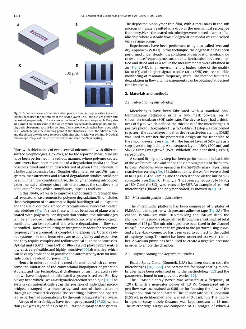
1304 A.C. Ceccacci et al. / Sensors and Actuators B 241 (2017) 1303–1309

Fig. 1. Schematic view of the fabrication process flow. A deep reactive ion etch-ing has been used for patterning of the device layer; B SiO2and SiN are grown anddeposited, respectively, to form a protective layer for the anisotropic etch. They alsoact as mask on the backside of the wafer, which has been defined by photolithogra-phy and subsequent reactive ion etching; C Anisotropic etching has been done withKOH, which defines the clamping point of the structures. Then, the silicon nitrideand the silicon dioxide were removed with phosphoric acid wet etching; D Opticalmicroscope images of the structures before and after the PLGA coating.

films with thicknesses of even several microns and with differentsurface morphologies. However, so far the reported measurementshave been performed in a tedious manner, where polymer coatedcantilevers have been taken out of a degradation media (no flowpossible), dried and then characterized at given time intervals ina bulky and expensive laser Doppler vibrometer set-up. With suchsystem, measurements and related degradation studies could notbe run under flow conditions. Also, the polymer coating introducesexperimental challenges since this often causes the cantilevers tobend out of plane, which complicates/impedes read-out.

In this study, we wish to improve and optimize micromechani-cal resonator measurements for polymer degradation. This includesthe development of an automated liquid handling/read-out systemand the use of double clamped microcantilevers, henceforth calledmicrobridges (Fig. 1), since these will not bend out of plane whencoated with polymers. For degradation studies, the microbridgeswill be embedded inside a microfluidic chip, where physiologicalconditions can be replicated and where degradation in flow canbe studied. However, tailoring an integrated readout for resonancefrequency measurements is complex and expensive. Optical read-out systems like interferometers are usually bulky and expensive,and they require complex and tedious optical alignment processes.Optical units (OPU) from DVD or Blu-Ray(BR) player represents alow-cost, very flexible, and highly- sensitive [20] alternative, whichcan be easily embedded in portable and automated system for mul-tiple optical readout purposes [21].

Hence, in order to match the need of a method which can over-come the limitation of the conventional biopolymer degradationstudies, and the technological challenges of an integrated read-out, we have designed and fabricated a system based on a Blu-Raypickup head which uses an astigmatic detection technique [20]. Thesystem can automatically scan the position of individual micro-bridges, arranged in a linear array, and control their actuationthrough a piezoelectric crystal. The recording of vibrational spectrais also performed automatically by the controlling system software.

Arrays of microbridges have been spray coated [17,22] with athin (1–2 �m) layer of PLGA by an ultrasonic spray coater system.

The deposited biopolymer thin film, with a total mass in the submicrogram range, resulted in a drop of the mechanical resonancefrequency. Next, the coated microbridges were placed in a microflu-idic chip where a steady flow of degradation media was controlledvia a syringe pump.

Experiments have been performed using a so-called ‘wet anddry’ approach (W & D). In this technique, the degradation has beenperformed under steady flow condition of degradation media. Priorto resonance frequency measurements, the chamber has been emp-tied and dried and as a result the measurements were obtained inair (Fig. 2D–E). In air environment, a higher value of the qualityfactor (Q) and a higher signal to noise ratio (SNR) ensure a reliablemonitoring of resonance frequency shifts. The method facilitatesdegradation in flow and measurements can be obtained at desiredtime intervals.

2. Materials and methods

2.1. Fabrication of microbridges

Microbridges have been fabricated with a standard pho-tolithography technique using a two mask process, on 4”silicon-on-insulator (SOI) substrate. The device layer had a thick-ness of 5 �m, which defined the thickness of the microbridges. Apositive photolithography (1.5 �m AZ-Mir701) step was performedto pattern the device layer and then deep reactive ion etching (DRIE)was used to transfer the photoresist design on the front side tothe silicon device layer (Fig. 1A). The buried layer of SiO2 acts as astop layer during etching. A subsequent layer of SiO2 (200 nm) andSiN (200 nm) was grown (Wet Oxidation) and deposited (LPCVD)respectively.

A second lithography step has been performed on the backsideof the wafer to release and define the clamping points of the micro-bridges. Windows were opened in the SiN/SiO2 mask layer usingreactive ion etching (Fig. 1B). Subsequently, the wafers were etchedin KOH (80 ◦C 4 h: 30 min), and the etch stopped on the buried sili-con oxide layer (Fig. 1C). Finally, SiN has been etched away by H3P04at 180 ◦C and the SiO2 was removed by BHF. An example of realizedmicrobridges (blank and polymer coated) is showed in Fig. 1D.

2.2. Microfluidic platform fabrication

The microfluidic platform has been composed of 3 plates ofPMMA bonded together with pressure adhesive tape (Fig. 2A). Thechannel is 500−�m wide, 10.5 mm long and 150 �m deep, thechamber in the middle plate defined through laser cutting had totalvolume of 193 �l. The microbridges have been fixed in the channelusing fluidic connectors that are glued to the platform using PDMSand a Luer-Lock connector has been used to connect to the outletof a syringe pump. The outlet has been connected to a waste cham-ber. A vacuum pump has been used to create a negative pressurein order to empty the chamber.

2.3. Polymer coating and degradation studies

Exacta Spray Coater (Sonotek, USA) has been used to coat themicrobridges [16,17,22]. The parameters for spray coating micro-bridges have been optimized using the methodology [22] and theparameters found in our previous works [17].

The ultrasonic spray nozzle was actuated at a frequency of120 kHz with a generator power of 1.3 W. Compressed nitro-gen flow was maintained at 0.06 bar for focusing the flow of thesprayed solution to the substrate. The infusion rate of PLGA solution(0.5% wt. in dichloromethane) was set at 0.05 ml/min. The micro-bridges to spray nozzle distance was kept constant at 15 mm.The microbridge arrays are composed of 12 bridges, of which 4

A.C. Ceccacci et al. / Sensors and Actuators B 241 (2017) 1303–1309 1305

Fig. 2. A: Exploded view of the single-use microfluidc chip and the encapsulation of the resonator. B: Design of the system. The microfluidic plaform is placed inside a chipholder, which can be moved along the three planes thanks to three alignment screws. C: Blu-Ray OPU building blocks. The OPU can move along the microbridges arrayaccording to the algorithm explained in the SI.D-E Wet and Dry Approach. D: A syringe pump is connected to the inlet of the chamber and then the degradation media flowsinside the camber and ends in the waste reservoir. E: The degradation media flow is stopped and the inlet is unplugged from the syringe pump and left at atmosphericpressure. A negative pressure is generated in the waste reservoir using a vacuum pump, and the measuring chamber is first emptied and then dried with air.

are left uncoated and used as references, see Fig. 1D. Hundredsof nanograms of polymer have been sprayed as it was shown inthe results section. PLGA undergoes hydrolytic degradation catal-ysed by the presence of an enzyme [2]. Here we test the effectof the enzymatic reaction of Proteinase-K in three different con-centrations (20–50–100 �g/ml in Tris-HCl buffer solution pH 8.6 at23 ◦C) in steady flow. We have further compared these results withthe degradation inducted by only water under same flow condi-tions. The microfluidic chamber was first filled with the degradationmedia at a flow rate of 200 �l/min. When the system has been com-pletely filled, the flow was reduced to 20 �l/min. The microfluidicplatform has been mounted inside a chip holder (Fig. 2A), and it hasbeen kept tight and clamped by four screws. The chip holder hasbeen placed into a custom-built PMMA box where the temperaturehas been maintained at 37 ◦C using a heat control system (Air-Therm ATX, with 0.1 ◦C precision) to simulate at best the humanphysiological condition. The degradation media was degassed forone hour in a vacuum chamber prior to the beginning of the exper-iment, in order to avoid bubble formation inside the microfluidicchamber.

2.4. Detection method and system layout

Astigmatic detection system (ADS) has previously been usedto monitor deflection and resonance frequency changes of micro-cantilevers [20,21]. A Blu-Ray (BR) laser diode emits light with awavelength of 405 nm, focused onto the surface of the microbridges

using an internal mirror, collimator and a modified objective lenswith high numerical aperture (NA = 0.6), which guarantees a focal-ized beam and a ∼350 nm size laser spot (Fig. 2C).

The reflected laser light from the sample surface (i.e. themicrobridges) passes through a polarized beam splitter, a set ofcylindrical lenses, and impinges on a quadrant photodetector inte-grated chip (PDIC). The PDIC consists of four single sensors withindividual current preamplifiers, which converts photon signal tovoltage signal with a bandwidth of 160 MHz. Here, a laser powermonitor diode is used to monitor laser power. A voice coil motor(VCM) has been used to control the position of the objective lens inorder to focus the light at a desired location.

Fig. 2B illustrates the system. It is composed of two blocks:the chip holder and a frame where a BR-OPU can move along onedirection thanks to a sled motor. Blu-Ray optical pick-up head unit(BR-OPU) is equipped with a VCM that gives a 1 �m vertical motionallowing fine adjustment of the focal distance to get the highestpossible sensitivity from the ADS. The chip holder is placed on threealignment screws used to do coarse adjustment of the focal dis-tance. The position of the holder can be adjusted in three planes(x–y, x–z and y–z). The working algorithm is shown in the Supple-mentary information (SI).

Resonance frequencies were measured in air. Microbridges wereactuated by means of a piezoelectric crystal, which was set to lin-early sweep a range of frequencies in the vicinity of the theoreticallypredicted resonance frequency. The values of the resonance fre-quencies and Q factors were obtained from a Lorentzian fittingperformed on the recorded spectra.

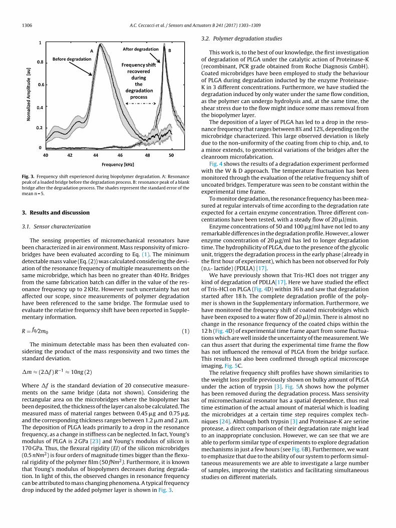
1306 A.C. Ceccacci et al. / Sensors and Actuators B 241 (2017) 1303–1309

Fig. 3. Frequency shift experienced during biopolymer degradation. A: Resonancepeak of a loaded bridge before the degradation process. B: resonance peak of a blankbridge after the degradation process. The shades represent the standard error of themean n = 5.

3. Results and discussion

3.1. Sensor characterization

The sensing properties of micromechanical resonators havebeen characterized in air environment. Mass responsivity of micro-bridges have been evaluated according to Eq. (1). The minimumdetectable mass value (Eq. (2)) was calculated considering the devi-ation of the resonance frequency of multiple measurements on thesame microbridge, which has been no greater than 40 Hz. Bridgesfrom the same fabrication batch can differ in the value of the res-onance frequency up to 2 KHz. However such uncertainty has notaffected our scope, since measurements of polymer degradationhave been referenced to the same bridge. The formulae used toevaluate the relative frequency shift have been reported in Supple-mentary information.

R = f0⁄2m0 (1)

The minimum detectable mass has been then evaluated con-sidering the product of the mass responsivity and two times thestandard deviation.

�m ≈ (2�f ) R−1 ≈ 10ng (2)

Where �f is the standard deviation of 20 consecutive measure-ments on the same bridge (data not shown). Considering therectangular area on the microbridges where the biopolymer hasbeen deposited, the thickness of the layer can also be calculated. Themeasured mass of material ranges between 0.45 �g and 0.75 �g,and the corresponding thickness ranges between 1.2 �m and 2 �m.The deposition of PLGA leads primarily to a drop in the resonancefrequency, as a change in stiffness can be neglected. In fact, Young’smodulus of PLGA is 2 GPa [23] and Young’s modulus of silicon is170 GPa. Thus, the flexural rigidity (EI) of the silicon microbridges(0.5 nNm2) is four orders of magnitude times bigger than the flexu-ral rigidity of the polymer film (50 fNm2). Furthermore, it is knownthat Young’s modulus of biopolymers decreases during degrada-tion. In light of this, the observed changes in resonance frequencycan be attributed to mass changing phenomena. A typical frequencydrop induced by the added polymer layer is shown in Fig. 3.

3.2. Polymer degradation studies

This work is, to the best of our knowledge, the first investigationof degradation of PLGA under the catalytic action of Proteinase-K(recombinant, PCR grade obtained from Roche Diagnosis GmbH).Coated microbridges have been employed to study the behaviourof PLGA during degradation inducted by the enzyme Proteinase-K in 3 different concentrations. Furthermore, we have studied thedegradation induced by only water under the same flow condition,as the polymer can undergo hydrolysis and, at the same time, theshear stress due to the flow might induce some mass removal fromthe biopolymer layer.

The deposition of a layer of PLGA has led to a drop in the reso-nance frequency that ranges between 8% and 12%, depending on themicrobridge characterized. This large observed deviation is likelydue to the non-uniformity of the coating from chip to chip, and, toa minor extends, to geometrical variations of the bridges after thecleanroom microfabrication.

Fig. 4 shows the results of a degradation experiment performedwith the W & D approach. The temperature fluctuation has beenmonitored through the evaluation of the relative frequency shift ofuncoated bridges. Temperature was seen to be constant within theexperimental time frame.

To monitor degradation, the resonance frequency has been mea-sured at regular intervals of time according to the degradation rateexpected for a certain enzyme concentration. Three different con-centrations have been tested, with a steady flow of 20 �l/min.

Enzyme concentrations of 50 and 100 �g/ml have not led to anyremarkable differences in the degradation profile. However, a lowerenzyme concentration of 20 �g/ml has led to longer degradationtime. The hydrophilicity of PLGA, due to the presence of the glycolicunit, triggers the degradation process in the early phase (already inthe first hour of experiment), which has been not observed for Poly(d,l- lactide) (PDLLA) [17].

We have previously shown that Tris-HCl does not trigger anykind of degradation of PDLLA[17]. Here we have studied the effectof Tris-HCl on PLGA (Fig. 4D) within 36 h and saw that degradationstarted after 18 h. The complete degradation profile of the poly-mer is shown in the Supplementary information. Furthermore, wehave monitored the frequency shift of coated microbridges whichhave been exposed to a water flow of 20 �l/min. There is almost nochange in the resonance frequency of the coated chips within the12 h (Fig. 4D) of experimental time frame apart from some fluctua-tions which are well inside the uncertainty of the measurement. Wecan thus assert that during the experimental time frame the flowhas not influenced the removal of PLGA from the bridge surface.This results has also been confirmed through optical microscopeimaging, Fig. 5C.

The relative frequency shift profiles have shown similarities tothe weight loss profile previously shown on bulky amount of PLGAunder the action of trypsin [3]. Fig. 5A shows how the polymerhas been removed during the degradation process. Mass sensivityof micromechanical resonator has a spatial dependence, thus realtime estimation of the actual amount of material which is loadingthe microbridges at a certain time step requires complex tech-niques [24]. Although both trypsin [3] and Proteinase-K are serineprotease, a direct comparison of their degradation rate might leadto an inappropriate conclusion. However, we can see that we areable to perform similar type of experiments to explore degradationmechanisms in just a few hours (see Fig. 6B). Furthermore, we wantto emphasize that due to the ability of our system to perform simul-taneous measurements we are able to investigate a large numberof samples, improving the statistics and facilitating simultaneousstudies on different materials.

A.C. Ceccacci et al. / Sensors and Actuators B 241 (2017) 1303–1309 1307

Fig. 4. Degradation profile obtained from different proteinase concentration of A: 100 �g/ml; B: 50 �g/ml; C: 20 �g/ml. D: Relative frequency shift measured when thedegradation media is substituted by water and Tris-HCl. Red curves shown the relative frequency shift on the uncoated bridges used as reference. (For interpretation of thereferences to colour in this figure legend, the reader is referred to the web version of this article.)

3.3. Degradation rate

The mean degradation rate for each enzyme concentrationhas been derived considering the initial mass deposited on themicrobridges and the time needed to reach the 0% in the relative fre-quency shift curves. Proteinase-K does not possess a specific site torecognize the polyester [5]. The concentration of enzyme reachesthe saturation level between 50 �g/ml and 100 �g/ml [5]. Whenthe saturation level is reached, higher concentrations do not leadto any faster degradation as the substrate is completely covered bythe enzyme.

The degradation rates per unit area are in the same order ofmagnitude of the 25 �g/cm2h reported in literature [3], where thedegradation of thick films (200 �m) of PLGA has been studied underthe action of trypsin (degradation rate of 67 �g/cm2h). This con-clusion is obtained by evaluating the amount of material they haveanalysed and considering the time needed for reaching the 0% inour weight loss curve. In Fig. 6 we have compared the degradationrate observed in our work with the degradation rate obtained by[5] who studied the degradation rate of PDLLA under the actionof Proteinase-K. Besides a difference of two orders of magnitudedue to the faster degradation of PLGA because of its hydrophilicity,we may notice that the degradation rate it has seemed to reach aplateau around 100 �g/ml.

4. Conclusion

We have developed and tested an automatic platform aimed tocharacterize the dynamic characteristics of microbridges and theiremployment as sensors for monitoring biopolymer degradation.The integration of a microfluidic platform allowed characterizingPLGA degradation under steady flow conditions in a Proteinase-K degradation buffer. The simple experimental setup, combined

with high level of automation, reduces the time needed to sta-tistically characterize biopolymer degradation. By increasing theparallelization of the microfluidic device, it could be possible tostudy different degradation conditions simultaneously. The fab-ricated microbridges have allowed us to study degradation inthe sub microgram regime. Although, real time monitoring is notactually possible, as in viscous environments the mass responsiv-ity drops beyond the intrinsic noise level of the readout system,the degradation can be easily studied by employing the W & Dmethod that allows a good time resolution of the investigatedphenomena. The combination of the microfluidic setup with theautomatic readout platform facilitates an effective evaluation ofbiopolymer degradation of micrometer-thick biopolymer film byemploying micromechanical resonators. Furthermore, the imple-mentation of the microfluidic device has allowed us to simulatea more physiologically realistic condition for polymer degrada-tion. The degradation parameters as well as the degradation profilederived from our approach matches previous study performed over6 weeks on bulk amount of material. The degradation profile, aswell as the degradation rate show similarities with similar workspreviously done by other groups using bulk amount of material andconventional methods. A full comparison is difficult since the otherstudies differ in either enzyme or polymer.

Acknowledgments

The authors would like to acknowledge machine shop in Insti-tute of Physics, Academia Sinica, Taiwan for precision machining.The research leading to these results has received funding from theEuropean Research Council under the European Union’s SeventhFramework Programme (FP7/2007–2013)/ERC grant agreement no[320535]. This research is further supported by the Villum Foun-dation Young Investigator Program (Project No. VKR023125). The

1308 A.C. Ceccacci et al. / Sensors and Actuators B 241 (2017) 1303–1309

Fig. 5. Optical microscope images of coated microbridges which have undergone to degradation experiments. A Bridges exposed to 50 �g/ml. After 3 h the polymer wascompletely removed from the surface of the resonator, the few spot are clearly far beyond the detection limit of the resonator. B Bridges exposed at a flow of Tris-HCl at 37 ◦Cat 2 �l/min.C Bridges exposed at a flow of DI water at 20 �l/min. White scale bar 300 �m.

Fig. 6. A Degradation rate dependence from the proteinase concentration. The profile seems to resemble the profile shown from Yamashita et al. B Normalized frequencyshift (error bar omitted) and comparison with weight loss curve from Cai et al.

research is funded by the Danish National Research Foundation(DNRF122) and Villum Fonden (Grant No. 9301)

Appendix A. Supplementary data

Supplementary data associated with this article can be found, inthe online version, at http://dx.doi.org/10.1016/j.snb.2016.09.190.

References

[1] J.-M. Lu, X. Wang, C. Marin-Muller, H. Wang, P.H. Lin, Q. Yao, C. Chen, Currentadvances in researcn and clinical applications of PLGA-based nanotechnology,

Expert Rev. Mol. Daign. 9 (2009) 325–341, http://dx.doi.org/10.1586/erm.09.15, Current.

[2] H.K. Makadia, S.J. Siegel, Poly Lactic-co-Glycolic Acid (PLGA) as biodegradablecontrolled drug delivery carrier, Polymers (Basel) 3 (2011) 1377–1397, http://dx.doi.org/10.3390/polym3031377.

[3] Q. Cai, G. Shi, J. Bei, S. Wang, Enzymatic degradation behavior and mechanismof poly(lactide-co-glycolide) foams by trypsin, Biomaterials 24 (2003)629–638, http://dx.doi.org/10.1016/S0142-9612(02)00377-0.

[4] L. Xu, K. Crawford, C.B. Gorman, Effects of temperature and pH on thedegradation of Poly (lactic acid) brushes, Macromolecules 44 (2011)4777–4782, http://dx.doi.org/10.1021/ma2000948.

[5] K. Yamashita, Y. Kikkawa, K. Kurokawa, Y. Doi, Enzymatic Degradation of Poly(L – Lactide) Film by Proteinase K: Quartz Crystal Microbalance and AtomicForce Microscopy Study, Biomacromolecules (2005) 850–857, http://dx.doi.org/10.1021/bm049395v.

A.C. Ceccacci et al. / Sensors and Actuators B 241 (2017) 1303–1309 1309

[6] L.G. Sun, Z.Y. Xie, Y.J. Zhao, H.M. Wei, Z.Z. Gu, Optical monitoring thedegradation of PLGA inverse opal film, Chin. Chem. Lett. 24 (2013) 9–12,http://dx.doi.org/10.1016/j.cclet.2013.01.012.

[7] K. Yamashita, T. Funato, Y. Suzuki, S. Teramachi, Y. Doi, Characteristicinteractions between poly(hydroxybutyrate) depolymerase andpoly[(R)-3-hydroxybutyrate] film studied by a quartz crystal microbalance,Macromol. Biosci. 3 (2003) 694–702, http://dx.doi.org/10.1002/mabi.200300004.

[8] O. Wolþ, D. Johannsmann, Viscoelastic properties of thin fims studied withquartz crystal resonators, Faraday Discus. 107 (1997) 91–94, http://dx.doi.org/10.1039/A703017G.

[9] G. Reiter, S. Napolitano, Possible origin of thickness-dependent deviationsfrom bulk properties of thin polymer films, J. Polym. Sci. Part B Polym. Phys.48 (2010) 2544–2547, http://dx.doi.org/10.1002/polb.22134.

[10] B.D. Vogt, C.L. Soles, H.J. Lee, E.K. Lin, W.L. Wu, Moisture absorption intoultrathin hydrophilic polymer films on different substrate surfaces, Polymer(Guildf) 46 (2005) 1635–1642, http://dx.doi.org/10.1016/j.polymer.2004.11.114.

[11] T. Larsen, S. Schmid, L. Gronberg, a. O. Niskanen, J. Hassel, S. Dohn, A. Boisen,Ultrasensitive string-based temperature sensors, Appl. Phys. Lett. 98 (2011)121901, http://dx.doi.org/10.1063/1.3567012.

[12] G. Wu, R.H. Datar, K.M. Hansen, T. Thundat, R.J. Cote, A. Majumdar, Bioassay ofprostate-specific antigen (PSA) using microcantilevers, Nat. Biotechnol. 19(2001) 856–860, http://dx.doi.org/10.1038/nbt0901-856.

[13] C. Yim, M. Yun, S. Kim, N. Jung, S. Lim, M. Lee, Nanomechanical thermalanalysis of indium films using silicon microcantilevers nanomechanicalthermal analysis of indium films using silicon microcantilevers, Jpn. J. Appl.Phys. 07 (2012) 0–4.

[14] S. Bose, S. Schmid, T. Larsen, S. Sylvest Keller, A. Boisen, K. Almdal,Micromechanical fast quasi-static detection of � and � relaxations withnanograms of polymer, J. Polym. Sci. Part B Polym. Phys. 53 (2015)1035–1039, http://dx.doi.org/10.1002/polb.23745.

[15] S. Bose, S. Schmid, T. Larsen, S.S. Keller, P. Sommer-Larsen, A. Boisen, K.Almdal, Micromechanical string resonators: analytical tool for thermalcharacterization of polymers, ACS Macro Lett. 3 (2014) 55–58, http://dx.doi.org/10.1021/mz400470n.

[16] S.S. Keller, L. Gammelgaard, M.P. Jensen, S. Schmid, Z.J. Davis, A. Boisen,Micromechanical sensors for the measurement of biopolymer degradation,Proc. IEEE Int. Conf. Micro Electro Mech. Syst. (2011) 457–460, http://dx.doi.org/10.1109/MEMSYS.2011.5734460.

[17] S. Bose, S.S. Keller, A. Boisen, K. Almdal, Microcantilever sensors for fastanalysis of enzymatic degradation of poly (d, l-lactide), Polym. Degrad. Stab.119 (2015) 1–8, http://dx.doi.org/10.1016/j.polymdegradstab.2015.04.021.

[18] N. Jung, H. Seo, D. Lee, C.Y. Ryu, S. Jeon, Nanomechanical thermal analysis ofthe glass transition of polystyrene using silicon cantilevers, Macromolecules41 (2008) 6873–6875, http://dx.doi.org/10.1021/ma801539m.

[19] M. del Rey, R. a. da Silva, D. Meneses, D.F.S. Petri, J. Tamayo, M. Calleja, P.M.Kosaka, Monitoring swelling and deswelling of thin polymer films bymicrocantilever sensors, Sensors Actuators B Chem. 204 (2014) 602–610,http://dx.doi.org/10.1016/j.snb.2014.08.021.

[20] E.T. Hwu, S.K. Hung, C.W. Yang, I.S. Hwang, K.Y. Huang, Simultaneousdetection of translational and angular displacements of micromachinedelements, Appl. Phys. Lett. 91 (2007), http://dx.doi.org/10.1063/1.2817750.

[21] F.G. Bosco, E.-T. Hwu, C.-H. Chen, S. Keller, M. Bache, M.H. Jakobsen, I.-S.Hwang, A. Boisen, High throughput label-free platform for statisticalbio-molecular sensing, Lab Chip 11 (2011) 2411–2416, http://dx.doi.org/10.1039/c1lc20116f.

[22] S. Bose, S.S. Keller, T.S. Alstrøm, A. Boisen, K. Almdal, Process optimization ofultrasonic spray coating of polymer films, Langmuir 29 (2013) 6911–6919,http://dx.doi.org/10.1021/la4010246.

[23] P. Gentile, V. Chiono, I. Carmagnola, P.V. Hatton, An overview ofpoly(lactic-co-glycolic) acid (PLGA)-based biomaterials for bone tissueengineering, Int. J. Mol. Sci. 15 (2014) 3640–3659, http://dx.doi.org/10.3390/ijms15033640.

[24] A.K. Naik, M.S. Hanay, W.K. Hiebert, X.L. Feng, M.L. Roukes, Towardssingle-molecule nanomechanical mass spectrometry, Nat. Nanotechnol. 4(2009) 445–450, http://dx.doi.org/10.1038/nnano.2009.152.

Biographies

Andrea Casci Ceccacci received his B.Sc. in Biomedical engineering from Univer-sitá Politecnica delle Marche, in 2011 and his M.Sc in Biomedical Engineering fromPolitecnico di Torino in 2014. Since 2014 he is a PhD student at the Departmentof Micro and Nanotechnology at Technical University of Denmark. His researchinterests concern the design and the use of micromechanical resonator for thecharacterization of biopolymer and drugs.

Ching-Hsiu Chen received the B.S. degree in Automatic Control Engineering fromFeng Chia University, Taiwan, in 2002 and the M.S. degrees in Mechanical andElectro-Mechanical Engineering from National Sun Yat-Sen University, Taiwan, in2004. He now works in Institute of Physics, Academia Sinica, Taiwan. His majorresearches are in scanning probe microscopy, biochemical detection techniques,MEMS/NEMS applications, precision measurement system, signal processing andquantum science.

En-Te Hwu is associate research scientist of institute of physics, Academia Sinica,Taiwan. He received his Ph.D. from National Taiwan University in 2006. He got firstprize award of Taiwan National Innovation & Startups project in 2014. In 2015, hereceived national discover innovation award. He is currently focused on nanoscalesensing/positioning based instrumentation and applications.

Lidia Morelli received her B.Sc. and M.Sc. in biomedical engineering from the Uni-versity of Pisa in 2011 and 2014, respectively. Since 2014 she is a PhD student at theDepartment of Micro and Nanotechnology, Technical University of Denmark. Herresearch interests include centrifugal microfluidics, Surface Enhanced Raman Scat-tering technologies for sensing, and the integration of these fields for automatedand high-throughput sensing of biological samples

Sanjukta Bose Goswami received her M.Tech in Polymer Science and Technologyfrom the Indian Institute of Technology, Delhi in 2011. Then she moved to Tech-nical University of Denmark and started her Ph.D. studies in the Department ofMicro and Nanotechnology. She obtained her Ph.D. degree in 2014 on the use ofmicromechanical sensors as tools for polymer characterizations. She is currentlyworking as a Postdoc in the same department and her current research interestis in using micromechanical sensors for measuring polymer degradation for drugdelivery applications.

Filippo Giacomo Bosco is CEO of BluSense Diagnostics, a spin-off from the Tech-nical University of Denmark. He completed his education with MS.c. in PhysicsEngineering at Politecnico of Milano in 2008. He obtained his PhD in micro- andNano-engineering at DTU Nanotech in 2011. He was awarded by DTU central com-mittee as “Best DTU young researcher” for his thesis with high innovation degree.In 2012 he received the Strategic Award Prize from the Danish Ministry of Researchand Innovation for his strategic research focus during his PhD. From 2011 to 2014he has been working as Postdoc at DTU Nanotech at the Nanoprobes group, workingon developing diagnostics biosensors based on low-cost optical readout. Since 2015he is full-time employed at BluSense Diagnostics.

Silvan Schmid is associate professor of micro and nanotechnology at the TechnicalUniversity of Denmark. He completed his education with the degree of Dipl. Ing.ETH from the Swiss Federal Institute of Technology Zurich in 2003. He performedhis doctorate in the Micro and Nanosystems Group at ETH Zurich and received hisdoctoral degree in 2009. He got awarded with the ETH medal 2009 for an outstand-ing doctoral thesis. In 2013 he received the Villum Foundation’s Young InvestigatorProgramme grant which supports especially talented young Danish researchers inscience and technology. His research focus is in micro- and nanomechanical res-onators for sensor applications and fundamental research.

Anja Boisen is professor at DTU Nanotech and has many years experience innanomechanical sensors. She is heading a DNRF and Villum Center of excellencefocusing on nanomechanical sensors and new microfabricated solutions for oraldrug delivery.

Supplementary information:

1. Astigmatic Detection:

FIG S 1 Focus error signal for a Blu ray-OPU.

Figure S1 shows the signal calculation of the astigmatic detection method. The quadrant

photodetector is defined as four independent sensing areas A, B, C and D. The converted

output voltage can be defined as VA, VB, VC and VD. The signal focus error SFE, is defined as

(VA+VC)-(VB+VD). If the beam is perfectly focused in the center the output voltage is zero.

The output signal, also known as the S-curve, depends on the working distance Δz(fig 2) . In

a certain range the behavior of the sensor is linear, and we will use such range to make our

measurement.

2. Measurement Routine

FIG S 2 Measurement routine for automatic positon detection actuation and readout:

As the first step the user has to focus on one bridge, making the distance between the

bridges and the lens within a reasonable range such that by the motion of the VCM all the

bridges are in the linear range. In the automatic system routine (reds) the sled motor is

moving along the chip and the position of the bridges are found and saved. In the

measurement routine(blue) the blu-ray pickup head moves on the position of the bridges, the

VCM coil motor is actuated and the best position within the linear range in found. Then the

piezo element is actuated and recorded. At the end of ith measurment the spectra are

recorded into one file.

3. Theoretical background

The resonance frequencies of the bridges have been recorded both in air and water

environment. For multilayer structures the resonance frequency can be approximated as

(Bose et al., 2015a; Keller et al., 2011)

𝑓𝑓𝑛𝑛 ≈1

2𝜋𝜋𝛽𝛽𝑛𝑛2

𝐿𝐿2��𝐼𝐼𝑖𝑖𝐸𝐸𝑖𝑖

𝑁𝑁

𝑖𝑖=1

𝑤𝑤�𝜌𝜌𝑖𝑖𝑡𝑡𝑖𝑖

𝑁𝑁

𝑖𝑖=1

� (1)

where 𝛽𝛽𝑛𝑛 represents the mode number which for a doubly clamped beam is 4.73, 7.85, 10.99,

for n =1,2,3, L is the length of the beam,𝐼𝐼𝑖𝑖 and 𝐸𝐸𝑖𝑖 are the beam’s moment of inertia and the

Young’s modulus respectively, 𝜌𝜌𝑖𝑖𝑡𝑡𝑖𝑖 are the density and the thickness of the ith layer. The

degradation process is evaluated in terms of relative frequency shift of the coated

microbridges. The mass responsivity can be written as:

𝑅𝑅 = 𝜕𝜕𝑓𝑓𝜕𝜕𝜕𝜕� ≈ 𝑓𝑓𝑛𝑛

2𝜕𝜕0� [𝐻𝐻𝐻𝐻/𝑔𝑔] (2)

𝑓𝑓𝑛𝑛 is the value of the resonance frequency and 𝜕𝜕0 is the mass of the resonator.

In order to obtain the frequency values that are comparable to the degradation experiments,

we can consider as a reference value, for the i th microbridge its resonance frequency at the

end of the degradation when the polymer has been completely removed from the surface.

The degradation on the ith coated microbridge at the jth time step is evaluated in terms of

relative frequency shift ∆𝑓𝑓𝑖𝑖,𝑡𝑡𝑡𝑡:

∆𝑓𝑓𝑖𝑖,𝑡𝑡𝑡𝑡% = 𝑓𝑓𝑖𝑖,𝑡𝑡𝑓𝑓 − 𝑓𝑓𝑖𝑖,𝑡𝑡𝑡𝑡𝑓𝑓𝑖𝑖,𝑡𝑡𝑓𝑓� 100. (3)

This shift is measured n times on the same bridges and then averaged:

∆𝑓𝑓𝑓𝑓,𝑡𝑡𝑡𝑡������=1𝑛𝑛�(∆𝑓𝑓𝑖𝑖,𝑡𝑡𝑡𝑡)𝑘𝑘

𝑛𝑛

𝑘𝑘=1

(4)

The N frequency shifts measured on the array are then averaged on N microbridges

employed to perform the degradation analysis.

∆𝑓𝑓,𝑡𝑡𝑡𝑡������=1𝑁𝑁�(∆𝑓𝑓𝑓𝑓,𝑡𝑡𝑡𝑡������)𝑘𝑘

𝑁𝑁

𝑘𝑘=1

(5)

The mean degradation rate is evaluated considering the time taken for the degradation

process to remove the initial mass deposited.

𝐷𝐷𝑅𝑅 = 𝜕𝜕 (𝐴𝐴∆𝑡𝑡) [µ𝑔𝑔/ℎ]⁄ (6)

Where m is the initially mass deposited on the microbridges, A is the area of the microbridges

(lw) and ∆𝑡𝑡 is the time needed to reach 0% in the relative frequency shift (the resonance

frequency returns to the value for an uncoated microbridge).

The stability of the readout has been monitored thorough a lock-in amplifier. The shift in the

resonance frequency has been monitored through a lock-in amplifier for 4 minutes.

Figure S 3. Fluctuation on the resonance frequency measured through the lock-in amplifier The root mean square of the noise is of 143 ppm and the max value +/- 200 ppm which is translated with a minimum detectable mass of 2.6 ng.

This value is greater in the actual configuration used during the degradation experiments. The

shift in the resonance frequency was not followed during the degradation experiments through

the lock-in amplifier but by repeating the measurement at different time step; the minimum

detectable mass is thus higher, since independent measurement they are seen to have a

larger variation than the fluctuation of the resonance frequency recorded with the lock-in

amplifier.

0 1 2 3 4-200

-100

0

100

200

300

time[min]

Fre

quen

cy sh

ift ∆

f [ppm

]

4. Degradation experiments

We report here the complete degradation profile under the action of the only Tris-Hcl at 20 µl/min.

PLGA showed to be degraded in 33 hours of experiment..

Nevertheless, in the experimental time frame that was used for all the enzymatic degradation studies of PLGA, Tris-HCl did not show any degradation effect. The degradation starts around 18h and ended after 33 hours.

Figure S4 Degradation profile of PLGA under the action of Tris-HCl at 20 µl/min

PAPER 2

Thin Film Analysis by Nanomechanical Infrared Spectroscopy

1

2

Thin Film Analysis by Nanomechanical Infrared Spectroscopy

Andrea Casci Ceccacci1, Alberto Cagliani1, Paolo Marizza1, Silvan Schmid2 and Anja Boisen1

1 Department of Micro and Nanotechnology, Technical University of Denmark, 2800 Kgs. Lyngby,

Denmark.

2 Institute of Sensor and Actuator Systems, TU Wien, 1040 Vienna, Austria.

Abstract

There is a fundamental need for techniques to characterise materials in the thin film regime.The

current options for obtaining infrared spectra suffer from low signal to noise ratio (SNR) for sample

thickness confined on few nanometers. We demonstrate how, through a detailed study of the

fundamental parameters of nanomechanical infrared spectroscopy, it is now possible to obtain a

complete fingerprint of a polymer layer of down to 20 nm in thickness with an SNR of 307. A frequency

stability of 2ppm upon IR absorption indicates an effective minimum detectable film thickness of only

160 pm corresponding to 3 attomol. We show that nanomechanical infrared spectroscopy can improve

the SNR by a factor of 43 compared to a conventional ATR-FTIR system on a single acquisition.These

results are paving the way for potent sensing tools applicable on minute sample sizes where

confinement effects can reveal unexpected behaviour.

Introduction

The ability to engineer chemical and physical properties of surfaces using dedicated functionalization

methods is of fundamental importance for the advancement in many technological fields, e.g. bio- and

chemical sensing1, drug delivery2, tissue engineering3, solar cells4, thin films batteries5 and fabrication

of semiconductor devices6. In recent years, the possibility of engineering the chemical and physical

properties of a surface by applying a thin polymer film has attracted considerable attention due to its

3

simplicity, robustness and flexibility, thanks to the vast selection of polymer films2,3,7–9. Thin polymer

films can exhibit, confinement induced peculiar physico-chemical properties, such as changes in glass

transition temperature10, elastic moduli11, and crystallization12. Characterising the properties of such

thin films is therefore of high relevance both technologically and scientifically.

The chemical behaviour and structure of thin films13–16 is often characterised by infrared (IR)

absorption spectroscopy. One of the most commonly used implementations for thin films IR

spectroscopy is the attenuated total reflectance Fourier transform infrared spectroscopy (ATR-FTIR),

with the typical configuration with only one reflection within the crystal16–18. An issue connected with

the use of ATR-FTIR is that the signal-to-noise-ratio (SNR) degrades quickly when the sample

thickness is much smaller than the sampling depth 13, thereby effectively limiting the thickness range

that can be studied. One possibility to overcome such problem is using very long acquisition times16,

but this restricts the throughput of the analytical system. A multi-reflection ATR accessory could also

be used to boost the signal, but such approach is suitable only when the crystal is in contact with a

liquid or the thin functionalization layer to be studied is irreversibly attached to the very expensive

crystal. These drawbacks make ATR-FTIR unsuitable for testing a large variety of very thin

functionalization layers with a high throughput, high spectroscopically precision and at a reasonable

low cost. There is thus a need for a fast, reliable, non-destructive and preferably less expensive

method to characterise very thin layers.

Photothermal spectroscopy methods are based on the transduction of the light absorbed by the

sample, and its subsequent change in temperature, into a signal that can be recorded. There are

different types of transduction depending on which physico-chemical property of the sample is

monitored. Typically, density, pressure or temperature changes induced by wavelength specific light

absorption, have been exploited to obtain an IR absorption fingerprint of the sample19–21.

4

A main advantage of the photothermal spectroscopy is that it does not suffer from the typical artefacts

of ATR-FTIR or absorbance-reflection techniques in the recorded spectra. Moreover, it allows the user

to hit the sample at any angle or light polarization, giving much more freedom in terms of optical

design and analysis possibilities.

Nanomechanical based IR absorption sensing (NAM-IR) has been widely exploited in the last fifteen

years for biosensing purposes23–26 and material characterization27. Nanomechanical sensors have also

been employed to perform photothermal based analysis, implementing both the deflection and

resonance frequency detection schemes20,21,28–34. However, the samples examined so far have been

limited to airborne deposited materials or liquids. This limitation is due to the lack of mechanical

robustness of previous nanomechanical transducers, such as nanostrings and microcantilevers.

Moreover, such nanomechanical structures suffer from the AFM-like readout laser alignment issues

that can drastically limit the final analysis throughput A filter-like structure35 has been developed to

improve the efficiency of the inertial sampling for airborne particles. However, the perforated geometry

of the structure hinders their employment for thin film analysis. Membranes better support sampling

techniques typical of surface functionalization such as drop casting spin coating, immersion in liquid

solutions, thanks to their much higher mechanical robustness.

Our IR spectroscopy system is based on 1 mm × 1 mm large and 100 nm thick pre-stressed SiN

membranes.These structures not only show even better performance that previously discussed IR

photothermal schemes but also offers the mechanical robustness to withstand treatments in liquid,

including spray coating or spin coating, which is often essential in the field of surface functionalization.

As a demonstrator of the capabilities of our IR spectroscopic system, we present infrared

photothermal spectroscopy characterization of polyvinylpyrrolidone (PVP) thin films with thicknesses

down to 20 nm. PVP polymer thin films have recently attracted much attention thanks to their high

versatility in drug delivery devices36, and hydrogels37, where its thin film physical and chemical

5

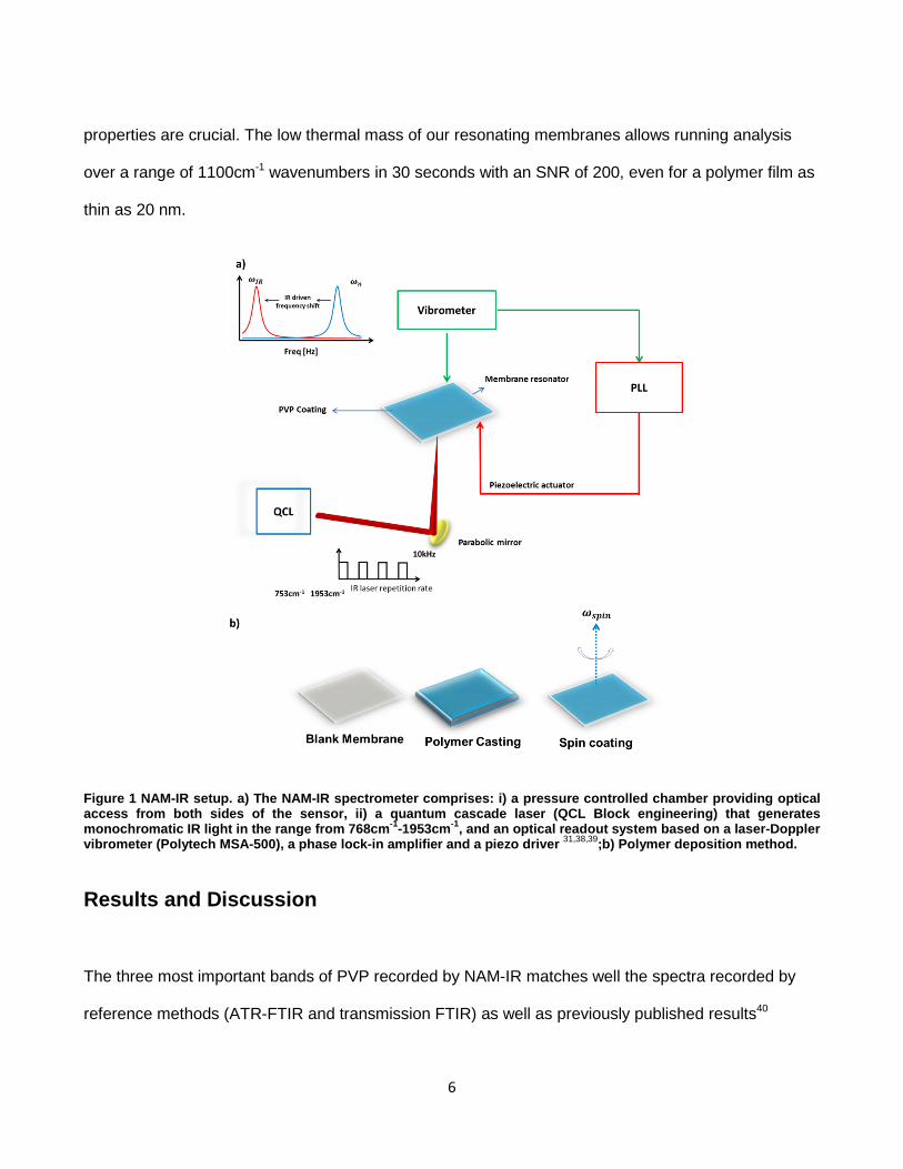
properties are crucial. The low thermal mass of our resonating membranes allows running analysis

over a range of 1100cm-1 wavenumbers in 30 seconds with an SNR of 200, even for a polymer film as

thin as 20 nm.

Figure 1 NAM-IR setup. a) The NAM-IR spectrometer comprises: i) a pressure controlled chamber providing optical access from both sides of the sensor, ii) a quantum cascade laser (QCL Block engineering) that generates monochromatic IR light in the range from 768cm-1-1953cm-1, and an optical readout system based on a laser-Doppler vibrometer (Polytech MSA-500), a phase lock-in amplifier and a piezo driver 31,38,39;b) Polymer deposition method.

Results and Discussion

The three most important bands of PVP recorded by NAM-IR matches well the spectra recorded by

reference methods (ATR-FTIR and transmission FTIR) as well as previously published results40

6

(Figure 2). NAM-IR spectra did not reveal further spectral features. However, some of the bands are

not visible due to the local minima of the IR laser source (e.g. small peak at 1390cm-1) (SI). The shift in

the ATR-FTIR bands is due to the modification of the refractive index of the sample upon IR light

absorption22.This phenomenon is clearly visible in the carbonyl band visible around 1680cm-1 which

appears shifted towards lower frequency in the ATR-FTIR spectra.

Figure 2 Comparison of the NAM-IR spectrum of a PVP film with respect to ATR and FTIR ones. Three main bands characterize the polymer fingerprint: the signal at 1300 cm-1 is referred to the C-N bond stretching and the CH2ring wag mode. The band with three peaks between 1400 and 1500 cm-1 corresponds to the ring-CH2 wag and the C-N stretching. The peak at 1680 cm-1 corresponds to the C=O stretching mode.

Upon IR absorption the mechanical resonance frequency of the membranes decreases following a

first order exponential decay (Figure 3a).The knowledge of the thermal time constant of the membrane

allows to determine the minimum settling time for each wavelength of the IR source and the optimal

signal integration time, for maximising the SNR. The time transient of the resonance frequency shift of

the membrane sensor upon periodic IR irradiation41 at a fixed IR wavelength was characterized in

order to extract the thermal relaxation time constant (see Figure 3a). Each cycle was fitted with an

exponential decay function δf(t)=∆f(1-e-tτM� ) and extracting the correspondent 𝜏𝜏𝑀𝑀. The transient

1200 1300 1400 1500 1600 1700 1800 1900 2000

Wavenumber (cm- 1 )

-0.2

0

0.2

0.4

0.6

0.8

1

Nor

mal

ized

freq

uenc

y sh

ift (a

u)

NAM-IRATR-FTIRFTIR

1200 1300 1400 1500 1600 1700 1800 1900Wavenumber (cm

1)

0

0.1

0.2

0.3

0.4

0.5

0.6

0.7

0.8

0.9

1

Abs

orba

nce

(a.u

)

7

was evaluated for 2 different vacuum pressures, which yielded (for a 20nm PVP coated membrane)

𝜏𝜏𝑀𝑀 = 4.1 ± 0.08 ms at a low vacuum of 1 mbar and 𝜏𝜏𝑀𝑀 = 17 ± 0.9 𝑚𝑚𝑚𝑚 at a high vacuum of 10-5mbar.

These two regimes result in two different behaviours. In high vacuum and at room temperature the

mean free path of the gas molecules becomes roughly 10 m, which is significantly larger than the

critical dimension of the nanomechanical resonator. Hence, the heat transport due to natural

convection can be neglected and all, heat generated in the membrane is dissipated by conduction

through the body chip alone. Contrary, at 1 mbar, the mean free path corresponds to roughly 100 µm,

which is comparable to the dimensions of the device, hence, allowing part of the heat to be dissipated

by conduction through the surrounding gas. The two regimes threfore have very different time

transient responses. The response time is also influenced by the sample and the corresponding

values are reported in the supplementary information. Precise knowledge of the thermal time constant

𝜏𝜏𝑀𝑀 is required in order to choose an optimal settling time for each wavelength emitted by the QCL. The

settling time was set such that the membrane would be exposed for no less than 3 x 𝜏𝜏𝑀𝑀 for each

discrete IR wavelength, in order to ensure that the membrane reaches the maximum frequency shift at

each wavelenght step. Considering that the QCL sweeps 1185cm-1 with steps of 0.5 cm-1, the total

acquisition time for a 20 nm thin polymer layer becomes 28.4 seconds, given a 𝜏𝜏𝑀𝑀 of ~4 ms in low

vacuum.

The membranes transient thermal constant further influences the choice of the integration time of the

PLL detection scheme. To correctly follow the resonance frequency shift upon light absorptions, the

lock-in amplifier bandwidth has to be set sufficiently high to follow the full dynamics of the resonance

frequency signal variations for each IR wavelength step. At the same time, a low bandwidth is

desirable to reduce the frequency acquisition noise. In particular, such noise is typically quantified as

the Allan deviation of the frequency signal as function of the PLL bandwidth42 ( see supplementary

information).

8

Finally, as shown Figure 3c, these settings permit to clearly resolve each distinct IR wavelength step

of 0.5 cm-1, since the exponential thermal response of the membrane frequency is clearly visible and

the signal arrives at the maximum amplitude within each step.

In the present work, the integration time was set to 1.5 ms for low vacuum experiments and 7 ms for

high vacuum experiments leading to a resolvable frequency shift of 2 ppm calculated for a 20 nm

coated membrane.

An analytical model can be used to estimate the power absorbed by the membranes35and in our case,

considering a frequency noise floor of 2ppm, the minimum power that can be detected is 5 nW for an

integration time of 7ms and an SNR of one, which corresponds to a local temperature increase in the

membrane center of 3 mK (see supporting information). In the case of a 20nm coated membrane, the

maximum absorbed power is 3.5 µW (at 1680 cm-1), which is about 1% of the incident QCL laser

power at that wavelength. Such power gives rise to a temperature increase of 0.9 K in the centre of

the membrane (see supporting information), indicating that an SNR on the temperature estimation as

high as 300. Finally, a calibrated power absorption spectrum is shown in Figure 3d (see SI), where the

temperature reached through the all spectrum is shown.

9

Figure 3. a) Relative frequency shift upon periodic light absorption. Values recorded on a 200 nm coated membrane at 1 mbar; shades represent the standard deviation of 485 overlapped cycles; b) Raw NAM IR spectra, highlighted region are represented in subfigure (c) ;c) zoom in of two regions of the spectra. Membrane NAM-IR spectrophotometer can recognise the QCL steps of 0.5cm-1 d) Absorbed power throughout the wavelength range, and relative temperature reached during a sweep on a 20 nm PVP coated membrane in HV. On the right-hand vertical axis, the relative temperature shift established in the membrane upon absorption. As reference value the baseline temperature was considered as 293.15K.

Figure 4 shows spectra of various PVP thicknesses ranging from 20 nm to 500 nm recorded by ATR-

FTIR with (Perkin Elmer Spectrum 100) and our membrane-based NAM-IR system. Signal acquisition

parameters and post-processing techniques are shown in the supplementary information. ATR-FTIR

spectra were acquired at 4 cm-1 and 2 cm-1 resolution, finer resolution did not provide any reliable

results due to a too low SNR. When ATR-FTIR was used, the three bands of PVP were clearly visible

10

for sample thicknesses higher than 100 nm, but only a very broad peak corresponding to the carbonyl

frequency at 1680 cm-1 was observable for thinner samples (Figure 4a). Instead, our NAM-IR

spectroscopy reveals all the expected features in the spectra, resolving clearly the three PVP

spectroscopic bands down to 20 nm sample thickness, both in low and high vacuum (Figure 4b-c).

To compare the performance of the ATR-FTIR and our NAM-IR systems, SNRs were calculated on

baseline corrected spectra. The noise was calculated as the standard deviation of the spectra

between 1800 cm-1 and 1953 cm-1 since, in this range, no light absorption occurs. As signal, we

analysed the amplitude of the carbonyl peak around 1680 cm-1. For all the examined thicknesses the

SNRs of NAM-IR (Figure 5a-b) were always at least one order of magnitude higher than ATR-FTIR

values. For NAM-IR the SNR is further increased for spectra recorded at 10-5 mbar. It is worth to note

that the high vacuum measurements, due to the higher values of the thermal time constant, need a

longer settling time of the QLC source for each wavelength to match the transient characteristics of

the sensor. SNR of NAM-IR spectroscopy reveals to be nearly independent of the total acquisition

time (Figure 5b), as long as the settling time at each IR wavelength is larger than the thermal

response time of the nanomechanical resonator.

The SNR of ATR-FTIR spectra depends on the resolution of the acquisitions44, which is typically 4cm-1

or 2cm-1, and the comparison of the SNR between spectra are made considering such spectral

resolutions. Although FTIR based spectrophotometers increase the SNR of spectra by coarsening the

resolution, spectra acquired at 4cm-1 on 20 and 40nm sample thick, did not lead to a remarkable

difference regarding SNR.

11

Figure 4 a) ATR spectra b)NAM-IR spectra at 1 mbar c) close up of 20 nm and 40 nm spectra at 1 mbar and 10-55 mbar. For the sake of comparison, all the spectra were offset, and the NAM-IR spectra were mirrored on the horizontal axis.

Considering that the NAM-IR spectra recorded on 20nm thick layer showed an impressive SNR of 307

in high vacuum, we are confident that this technique is now capable of recording the IR spectrum of a

single molecule PVP layer. In fact, extrapolating the SNR versus thickness relation towards smaller

thicknesses(SI) and considering an SNR of 2 as the lowest value needed to clearly recognise a

spectral feature of PVP, the limit of detection regarding mass per unit area for NAM-IR is 0.13 fg/um2.

This mass per unit area limit corresponds to an equivalent thickness of PVP of 112 pm, approximately

corresponding to 3 attomoles of PVP. This data strongly indicate that single-molecule layers can be

probed with NAM-IR, with very high performance regarding SNR and short acquisition time.

12

The NAM-IR spectroscopy not only outperforms the ATR-FTIR in terms of SNR, but potentially also in

terms of simplicity in the interpretation of the spectrum. In fact, another important feature to bear in

mind when comparing our photothermal NAM-IR with an ATR-FTIR spectrometer regards which

vibrational modes can be excited by the IR light in case the sample is a thin film that presents good

molecular ordering13,16,22. ATR-FTIR probes the surface sample with the IR beam obliquely oriented to

the normal of the sample surface with a nearly fixed angle. Therefore, the IR radiation is probing the

perpendicular as well as the horizontal (with respect to the surface) molecular vibrational modes. In

this case the resulting spectra contain both the information about the horizontal as well as the

perpendicular modes, calling for precautions in the interpretation of spectra from thin layers ordered at

molecular level. Moreover, ATR-FTIR spectra further depend on the reflection occurring at the

substrate and sample interface13. In fact, when the sampling depth is higher than the sample

thickness, the evanescent wave is partially reflected by the substrate leading to an extinctions of the

transversal mode and enhancement of the longitudinal ones13,46.

Instead, the NAM-IR approach is much more flexible, and the IR light can probe the sample with any

angle and any polarisation. This flexibility simplifies the interpretation of spectra for samples where

molecules follow a specific orientation on the surface, like self-assembled monolayers, Langmuir block

monolayers or partially crystallised polymer layers. A spectrum acquired with the IR light impinging the

sample surface perpendicularly would contain information only on the vibrational modes that have a

component of the dipole moment parallel to the sample surface. Changing the impinging angle of the

IR light, the vibrational modes with a dipole moment component orthogonally oriented to the sample

surface will be probed. These advantages and the much higher SNR for sub-50 nm layers make

membrane based NAM-IR a very strong candidate for a new generation of single molecule layer IR

spectroscopy tools.

13

Finally, we would like to discuss the benefits of using a resonant membrane structure on nanostring

resonators30,31,34. The use of a membrane allows to efficiently focus the light within the membrane area

employing all the given power by the IR source and close up to 1% of the incident light a considerably

higher fraction compared to string based photothermal spectroscopy34. The use of strings31,34,38,39

would require using a highly collimated light source which can be difficult to handle.

Figure 5: Comparison of SNR between NAM-IR spectroscopy and ATR-FTIR for different thickness the size of the marker represents the standard deviation on the SNR calculation. SNR of 200nm PVP coated membrane for different acquisition times. The SNR is not sensitive to a prolonged acquisition time, instead ATR-FTIR spectrophotometer increment the SNR for increased number of scans.

14

Conclusions

Membrane resonator based NAM-IR spectroscopy enabled new possibilities for performing IR

spectroscopy on sub-50 nm organic films. The SNR of 307 obtained on a 20nm PVP polymer layer,

combined with a detection limit in the attomol range, position membrane based NAM-IR as a possible

technique for single molecule layer analysis. NAM-IR spectroscopy measurements were performed in

less than 30 seconds on a 20 nm PVP layer, whereas using commercial ATR-FTIR technique the

same SNR would be achieved with an acquisition time 43 times longer.

Moreover, the vibrational modes in ordered organic thin layers can be potentially selectively probed

since the IR light can hit the surface with virtually any angle. and the interaction of the electric field in

the case of reflection of the incident beam at the substrate sample interface13.

In term of the mechanical robustness, the membranes comply better with the experimental conditions

typical of surface functionalization experiments compared to microstrings, allowing the user to prepare

the samples in an ample kind of methods. The high capability to dissipate heat makes the response

one order of magnitude faster compared to microstrings.

Finally, the read-out of the membrane motion can be integrated using a more advanced design,

creating a compact yet extremely sensitive, versatile and fast IR spectroscopy tool for ultra-thin

organic layers.

15

METHODS

MEMBRANE FABRICATION. Details of the membrane fabrication process are described in the supplementary information.

SAMPLE PREPARATION Polymer solution was prepared by dissolving polyvinylpyrrolidone powder (PVP, Sigma-Aldrich Mw 360000) in an aqueous solution hydrogen peroxide )(H2O230% w/v) in 2 different concentration 1 % wt. and 5% wt. The deposition on the membrane was performed by spin-coating: the solution (4 mL) was poured on a silicon wafer containing the membrane chip and then spun at various rotational speeds. The sample was let dry at room temperature and atmospheric pressure. Ellipsometry was used to measures the thickness of the polymer layers.

NAM-IR SPECTRA RECORDING NAM-IR signal was recorded through a lock-in scheme. The membrane resonator is placed in a vacuum chamber which guarantees optical access from the top and from the bottom side of the sensor of the membrane. The resonance frequency of the membrane resonator is probed optically (Polytech MSA-500), the infrared light is provided by a tunable quantum cascade laser (QCL, Block Engineering 768 cm-1 -1953 cm-1) and collimated by a parabolic mirror on the membrane resonator providing a laser spot size of 100 µm. A lock-in amplifier records the frequency shift. The phase detector bandwidth was 500 Hz for LV measurement, and 200 Hz for HV measurement and the sampling rate was set at 3600 Hz. The thermal time constant was determined by irradiating the membrane resonator periodically at a certain wavelength as described elsewhere41. The IR radiation was mechanically chopped providing an irradiation time of 50 ms for LV measurement. In HV mode the irradiation time was increased to 250 ms to allow the membrane to reach the steady value of resonant frequency shift at each cycle.

ATR SPECTRA ACQUISITION The ATR spectra were recorded with (Perkin Elmer Spectrum 100) providing a constant power throughout the spectral range of 5 mW. The spectra were acquired sample composed by a silicon nitride substrate and a PVP layer, prepared in the same way as membrane resonator. The PVP layer is placed in tight contact with a single reflection ZnSe crystal. The gauge force of the crystal was set to its optimal value achieving the highest signal intensity. For all spectra at least 3 signals were recorded for each sample thickness. A single acquisition spectrum is acquired at the spectral resolution of 2cm-1 and 4cm-1. The amplitude of the acquired spectra is then corrected to compensate the different absorption amplitude throughout the spectral range using the built-in function of the software.

1. Sun, F. et al. Hierarchical zwitterionic modification of a SERS substrate enables real-time drug monitoring in blood plasma. Nat. Commun. 7, 13437 (2016).

2. Huang, C. L. et al. The influence of additives in modulating drug delivery and degradation of PLGA thin films. NPG Asia Mater. 5, e54 (2013).

3. Harrison, R. H. et al. Modular and Versatile Spatial Functionalization of Tissue Engineering Scaffolds through Fiber-Initiated Controlled Radical Polymerization. Adv. Funct. Mater. 25,

16

5748–5757 (2015).

4. Green, M. A. Thin-film solar cells: review of materials, technologies and commercial status. J. Mater. Sci. Mater. Electron. 18, 15–19 (2007).

5. Jie Lin, Jianlai Guo, Chang Liu, and H. G. Ultrahigh-Performance Cu2ZnSnS4 Thin Film and Its Application in Microscale Thin-Film Lithium-Ion Battery: Comparison with SnO2.

6. Ross, C. A., Berggren, K. K., Cheng, J. Y., Jung, Y. S. & Chang, J.-B. Three-Dimensional Nanofabrication by Block Copolymer Self-Assembly. Adv. Mater. 26, 4386–4396 (2014).

7. Hashizume, M., Murata, Y., Iijima, K. & Shibata, T. Drug loading and release behaviors of freestanding polysaccharide composite films. Polym. J. 48, 545–550 (2016).

8. Rahman, A. et al. Non-native three-dimensional block copolymer morphologies. Nat. Commun. 7, 13988 (2016).

9. Mishra, R. K., Datt, M. & Banthia, A. K. Synthesis and characterization of pectin/PVP hydrogel membranes for drug delivery system. AAPS PharmSciTech 9, 395–403 (2008).

10. Jae Hyun Kim, †, Jyongsik Jang, *,† and & Wang-Cheol Zin*, ‡. Thickness Dependence of the Glass Transition Temperature in Thin Polymer Films. (2001). doi:10.1021/LA001125K

11. Fedorchenko, A. I., Wang, A.-B. & Cheng, H. H. Thickness dependence of nanofilm elastic modulus. Appl. Phys. Lett. 94, 152111 (2009).

12. Michell, R. M., Blaszczyk-Lezak, I., Mijangos, C. & Müller, A. J. Confinement effects on polymer crystallization: From droplets to alumina nanopores. (2013). doi:10.1016/j.polymer.2013.05.029

13. Laroche, G., Fitremann, J. & Gherardi, N. FTIR-ATR spectroscopy in thin film studies: The importance of sampling depth and deposition substrate. Appl. Surf. Sci. 273, 632–637 (2013).

14. Wang, Y. et al. Crystallization in the Thin and Ultrathin Films of Poly(ethylene-vinyl acetate) and Linear Low-Density Polyethylene. (2003). doi:10.1021/ma030456b

15. Ohta, K. Experimental Proof of the Relation Between Thickness of the Probed Surface Layer and Absorbance in FT-IR/ATR Spectroscopy.

16. Ramin, M. A. et al. PM-IRRAS Investigation of Self-Assembled Monolayers Grafted onto SiO 2 /Au Substrates. Langmuir 27, 6076–6084 (2011).

17. Kim, J., Cho, J., Seidler, P. M., Kurland, N. E. & Yadavalli, V. K. Investigations of Chemical Modifications of Amino-Terminated Organic Films on Silicon Substrates and Controlled Protein Immobilization. Langmuir 26, 2599–2608 (2010).

18. Shiyong Song, †,‡, Ruiqing Chu, §, Jinfang Zhou, †, Shengrong Yang, *,† and & Junyan Zhang*, †. Formation and Tribology Study of Amide-Containing Stratified Self-Assembled Monolayers:  Influences of the Underlayer Structure. (2008). doi:10.1021/JP7100144

19. Bialkowski, S. Photothermal spectroscopy methods for chemical analysis. (Wiley, 1996).

20. Barnes, J. R. et al. A femtojoule calorimeter using micromechanical sensors. Rev. Sci. Instrum.

17

65, 3793 (1994).

21. Barnes, J. R., Stephenson, R. J., Welland, M. E., Gerber, C. & Gimzewski, J. K. Photothermal spectroscopy with femtojoule sensitivity using a micromechanical device. Nature 372, 79–81 (1994).

22. Nunn, S. & Nishikida, K. Advanced ATR Correction Algorithm.

23. Bosco, F. G. et al. High throughput label-free platform for statistical bio-molecular sensing. Lab Chip 11, 2411–6 (2011).

24. Ndieyira, J. W. et al. Surface-stress sensors for rapid and ultrasensitive detection of active free drugs in human serum. Nat. Nanotechnol. 9, 225–232 (2014).

25. Patil, S. B. et al. Decoupling competing surface binding kinetics and reconfiguration of receptor footprint for ultrasensitive stress assays. Nat. Nanotechnol. 10, 899–907 (2015).

26. Alsteens, D. et al. Nanomechanical mapping of first binding steps of a virus to animal cells. Nat. Nanotechnol. 12, 177–183 (2016).

27. Bose, S. et al. Micromechanical string resonators: Analytical tool for thermal characterization of polymers. ACS Macro Lett. 3, 55–58 (2014).

28. Khan, M. F. et al. Heat capacity measurements of sub-nanoliter volumes of liquids using bimaterial microchannel cantilevers. Cit. Appl. Phys. Lett. Sci. Instrum 108, 211906–4191 (2016).

29. Larsen, T., Schmid, S., Villanueva, L. G. & Boisen, A. Photothermal Analysis of Individual Nanoparticulate Samples Using Micromechanical Resonators. ACS Nano 7, 6188–6193 (2013).

30. Yamada, S., Schmid, S., Larsen, T., Hansen, O. & Boisen, A. Photothermal infrared spectroscopy of airborne samples with mechanical string resonators. Anal. Chem. 85, 10531–10535 (2013).

31. Andersen, Alina Joukainen; Yamada, Shoko; Ek, Pramod Kumar; Andresen, Thomas Lars; Boisen, A. & Schmid, S. Nanomechanical IR spectroscopy for fast analysis of liquid-dispersed engineered nanomaterials. Sens. Actuators B 233, 667–673 (2016).

32. Ghoraishi, M. S., Hawk, J. E., Phani, A., Khan, M. F. & Thundat, T. Clustering mechanism of ethanol- water mixtures investigated with photothermal microfluidic cantilever deflection spectroscopy. Nat. Publ. Gr. (2016). doi:10.1038/srep23966

33. Wig, A., Arakawa, E. T., Passian, A., Ferrell, T. L. & Thundat, T. Photothermal spectroscopy of Bacillus anthracis and Bacillus cereus with microcantilevers. Sensors Actuators B Chem. 114, 206–211 (2006).

34. Biswas, T. S. et al. Femtogram-scale photothermal spectroscopy of explosive molecules on nanostrings. Anal. Chem. 86, 11368–72 (2014).

35. Kurek, M. et al. Nanomechanical Infrared Spectroscopy with Vibrating Filters for Pharmaceutical Analysis. Angew. Chemie Int. Ed. 56, 3901–3905 (2017).

18

36. Marizza, P. et al. Synthesis and characterization of UV photocrosslinkable hydrogels with poly(N-vinyl-2-pyrrolidone): Determination of the network mesh size distribution. Int. J. Polym. Mater. Polym. Biomater. 65, 516–525 (2016).

37. Plungpongpan, K. et al. Preparation of PVP/MHEC Blended Hydrogels via Gamma Irradiation and their Calcium ion Uptaking and Releasing Ability. Energy Procedia 34, 775–781 (2013).

38. Yamada, S., Schmid, S., Larsen, T., Hansen, O. & Boisen, A. Photothermal Infrared Spectroscopy of Airborne Samples with Mechanical String Resonators. Anal. Chem. 85, 10531–10535 (2013).

39. Larsen, T., Schmid, S., Villanueva, L. G. & Boisen, A. Photothermal analysis of individual nanoparticulate samples using micromechanical resonators. ACS Nano 7, 6188–93 (2013).

40. Zhu, X., Lu, P., Chen, W. & Dong, J. Studies of UV crosslinked poly(N-vinylpyrrolidone) hydrogels by FTIR, Raman and solid-state NMR spectroscopies. Polymer (Guildf). 51, 3054–3063 (2010).

41. Miriyala, N., Khan, M. F. & Thundat, T. Thermomechanical behavior of a bimaterial microchannel cantilever subjected to periodic IR radiation. Sensors Actuators B Chem. 235, 273–279 (2016).

42. Cleland, A. N. & Roukes, M. L. Noise processes in nanomechanical resonators. doi:10.1063/1.1499745

43. Schmid, S., Wu, K., Larsen, P. E., Rindzevicius, T. & Boisen, A. Low-Power Photothermal Probing of Single Plasmonic Nanostructures with Nanomechanical String Resonators. Nano Lett. 14, 2318–2321 (2014).

44. Liu, Q. & Xiao, S. Effects of spectral resolution and signal-to- noise ratio of hyperspectral sensors on retrieving atmospheric parameters. (2013). doi:10.1364/OL.39.000060

45. Fan, J. & Trenary, M. Symmetry and the Surface Infrared Selection Rule for the Determination of the Structure of Molecules on Metal Surfaces. Langmuir 10, 3649–3657 (1994).

46. Dupont, G., Caquineau, H., Despax, B., Berjoan, R. & Dollet, A. Structural properties of N-rich a-Si - N:H films with a low electron-trapping rate. J. Phys. D. Appl. Phys. 30, 1064–1076 (1997).

19

SUPPLEMENTARY INFORMATION

MEMBRANE FABRICATION. Silicon-Rich silicon Nitride membrane(Figure 1) were fabricated by standard lithography techniques. A double side polished wafer was RC cleaned and a 100nm thick layer of low-stress Silicon Nitride( 250MPa) was deposited by LPCVD. A sacrificial layer of silcon nitride is deposited through PECVD. The Inductively Coupled Plasma (ICP) etching performed on the backside after lithography to remove the LPCVD SiN layer but keeping intact the one on the front side protected by the PECVD SiN. KOH. The release of the membrane structure is done through KOH etching (4.5h) which defines the clamping of the membranes and then the PECVD SiN is removed through HF etch. The membrane has side length are 1000µm.

Figure s6 Silicon-Rich Silicon Nitride Membrane 1000µm side length. The initial stress was measured to be 250MPa

SAMPLE PREPARATION The membranes were functionalized using a spin coating. The spun solution consisted of the mixture(5% and 1 % wt) of PVP k-90 Mw 360000 in H2O2: H2O(30%). The thickness layer was measured with ellipsometry(Filmtek). Spinning curves are reported in Figure s2 and the thickness of the polymer layer on the body chip of a membrane chip Figure s3

200 µm

20

Figure s7 Spinning curves of PVP measured through ellipsometry.

Figure s8 Profile for a PVP coated Silicon substrate spun at 5000 rpm.

TIME CONSTANT

The value of the thermal time constant was evaluated as described elsewhere[1] for different polymer coatings both in high vacuum and in low vacuum. The higher the thickness, the higher the time constant. High vacuum measurement yields to a higher value of time constant Figure s4

0 50 100 150 200 250

scan length ( m)

-5

0

5

10

15

20

25

30

thic

knes

s (n

m)

21

Figure s9 Thermal time constant for PVP coated membranes at low vacuum and high vacuum. CHARACTERIZATION OF THE QCLLASER SOURCE The QCL power spectra is shown in figure s5

Figure s10 QCL laser power curve at 1% DC and 4% DC. It can be noted that the power does not scale linearly. This is due, according to the manufacturer specification to an overheating of the device which influences the linearity of the output. The power spectra at 4% DC are recorded with a coarser quantization (10cm-1).

22

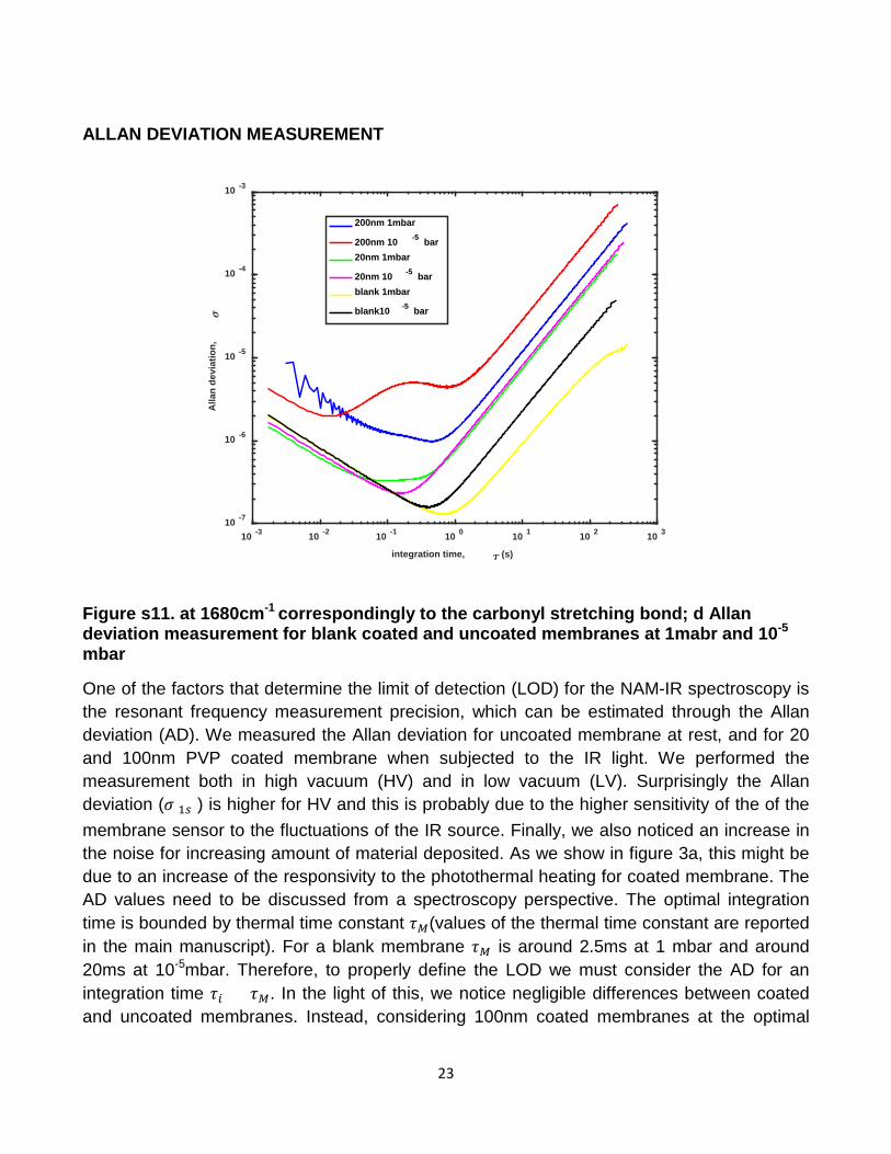
ALLAN DEVIATION MEASUREMENT

Figure s11. at 1680cm-1 correspondingly to the carbonyl stretching bond; d Allan deviation measurement for blank coated and uncoated membranes at 1mabr and 10-5 mbar

One of the factors that determine the limit of detection (LOD) for the NAM-IR spectroscopy is the resonant frequency measurement precision, which can be estimated through the Allan deviation (AD). We measured the Allan deviation for uncoated membrane at rest, and for 20 and 100nm PVP coated membrane when subjected to the IR light. We performed the measurement both in high vacuum (HV) and in low vacuum (LV). Surprisingly the Allan deviation (𝜎𝜎(1𝑠𝑠)) is higher for HV and this is probably due to the higher sensitivity of the of the membrane sensor to the fluctuations of the IR source. Finally, we also noticed an increase in the noise for increasing amount of material deposited. As we show in figure 3a, this might be due to an increase of the responsivity to the photothermal heating for coated membrane. The AD values need to be discussed from a spectroscopy perspective. The optimal integration time is bounded by thermal time constant 𝜏𝜏𝑀𝑀(values of the thermal time constant are reported in the main manuscript). For a blank membrane 𝜏𝜏𝑀𝑀 is around 2.5ms at 1 mbar and around 20ms at 10-5mbar. Therefore, to properly define the LOD we must consider the AD for an integration time 𝜏𝜏𝑖𝑖 < 𝜏𝜏𝑀𝑀. In the light of this, we notice negligible differences between coated and uncoated membranes. Instead, considering 100nm coated membranes at the optimal

10 -3 10 -2 10 -1 10 0 10 1 10 2 10 3

integration time, (s)

10 -7

10 -6

10 -5

10 -4

10 -3

Alla

n de

viat

ion,

200nm 1mbar

200nm 10 -5 bar20nm 1mbar

20nm 10 -5 barblank 1mbar

blank10 -5 bar

23

integration time (𝜏𝜏𝑀𝑀 = 5𝑚𝑚𝑚𝑚 and 40𝑚𝑚𝑚𝑚 for 1mbar and 10-5 mbar respectively) the AD values are in the order of 3ppm and 5ppm. In the main manuscript the LOD was evaluated for a 20nm PVP coated membrane and it has shown to be 2.5nW in terms of absorbed power.

NAM-IR SIGNAL POST PROCESSING

The NAM-IR spectra are caused by the release of the initial stress of the membrane resulting in a negative resonance frequency shift. For the sake of clarity, the spectra are finally mirrored on the horizontal axis.

1) Averaging (figure s7a-b)The QCL laser source (Block-Engineering) used in this work has a laser linewidth of 2cm-1. The QCL sweeps stepwise the investigated wavelength range with a step size of 0.5cm-1. According to the sweeping speed, the dwell time is automatically regulated. The dwell time has to be higher than 3𝜏𝜏 allowing the membrane to reach the steady value upon IR absorption. The PLL bandiwth was set at 500Hz for all the recorded spectra, ensuring an integration time of 1.5ms or lower the sampling frequency was set at 3600sample/sec.For high vaucm measuremnt the QCL dwell time was reduced to match the thermal time constant of the device and the integration time of the PLL was set to 10ms.

24

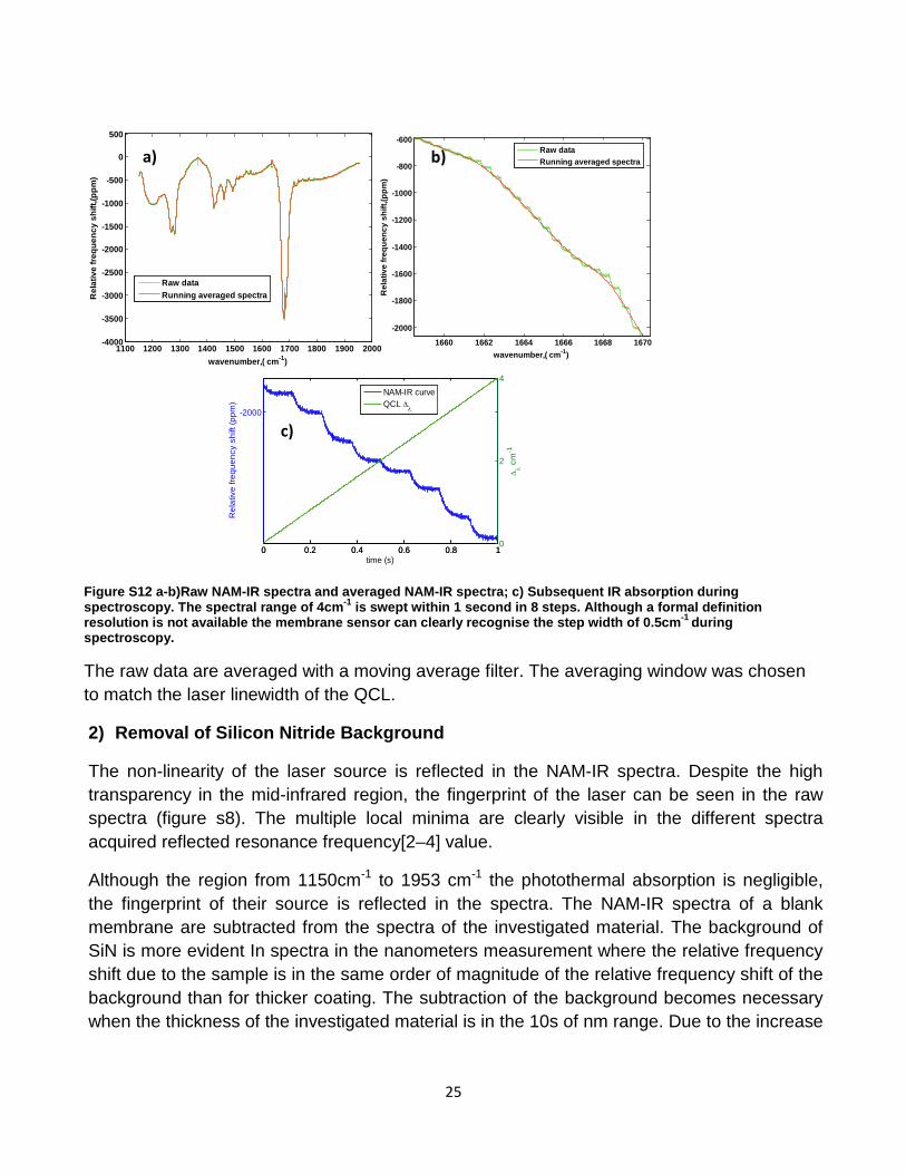
Figure S12 a-b)Raw NAM-IR spectra and averaged NAM-IR spectra; c) Subsequent IR absorption during spectroscopy. The spectral range of 4cm-1 is swept within 1 second in 8 steps. Although a formal definition resolution is not available the membrane sensor can clearly recognise the step width of 0.5cm-1 during spectroscopy.

The raw data are averaged with a moving average filter. The averaging window was chosen to match the laser linewidth of the QCL.

2) Removal of Silicon Nitride Background

The non-linearity of the laser source is reflected in the NAM-IR spectra. Despite the high transparency in the mid-infrared region, the fingerprint of the laser can be seen in the raw spectra (figure s8). The multiple local minima are clearly visible in the different spectra acquired reflected resonance frequency[2–4] value.

Although the region from 1150cm-1 to 1953 cm-1 the photothermal absorption is negligible, the fingerprint of their source is reflected in the spectra. The NAM-IR spectra of a blank membrane are subtracted from the spectra of the investigated material. The background of SiN is more evident In spectra in the nanometers measurement where the relative frequency shift due to the sample is in the same order of magnitude of the relative frequency shift of the background than for thicker coating. The subtraction of the background becomes necessary when the thickness of the investigated material is in the 10s of nm range. Due to the increase

1100 1200 1300 1400 1500 1600 1700 1800 1900 2000-4000

-3500

-3000

-2500

-2000

-1500

-1000

-500

0

500

wavenumber,( cm-1)

Rel

ativ

e fr

eque

ncy

shift

,(ppm

)

Raw dataRunning averaged spectra

1660 1662 1664 1666 1668 1670

-2000

-1800

-1600

-1400

-1200

-1000

-800

-600

wavenumber,( cm-1)

Rel

ativ

e fr

eque

ncy

shift

,(ppm

)

Raw dataRunning averaged spectra

0 0.2 0.4 0.6 0.8 1

-2000

time (s)

Rel

ativ

e fre

quen

cy s

hift

(ppm

)

0 0.2 0.4 0.6 0.8 10

2

4

∆λ c

m-1

NAM-IR curveQCL ∆λ

a) b)

c)

25

in the relative frequency shift of coated sensor (figure 3a), before subtraction, the background is scaled according to the ratio of the SiN peak at 861cm-1.

Figure S13 NAM-IR spectra of Silicon Nitride recorded at 4%DC at 1mbar. Analogous spectra are recorded in a high vacuum.

3) Baseline Correction. The same baseline correction is performed in ATR spectra and

NAM-IR spectra figure s9.

26

Figure s14 Averaged spectra are subtracted from the silicon nitride background. Afterwards, a baseline correction is performed. Here spectra of 40nm PVP coated device recorded at 10-5 mbar is showed.

Signal and noise calculation The signal to noise ratio of the spectra was evaluated considering as noise the standard deviation of the portion of the spectra ranging from 1800 to 1953cm-1 where there is no absorption of the investigated material(Figure s9 and figure s10). The same approach was used for the definition of the SNR for ATR and NAM-IR. As a signal, it was used the amplitude of the peak led from the carbonyl bond located around 1680cm-1. All the calculation were performed on the data after the baseline correction. The raw data the Matlab-script for used for post-processing the date upon reasonable request

1100 1200 1300 1400 1500 1600 1700 1800 1900 2000-3500

-3000

-2500

-2000

-1500

-1000

-500

0

500

σ=6.0782

Signal=3396.6642

wavenumber (cm-1)

rela

tive

frequ

ency

shi

ft (p

pm)

Silicon NitridePolymer coatedCorrectedBaseline

27

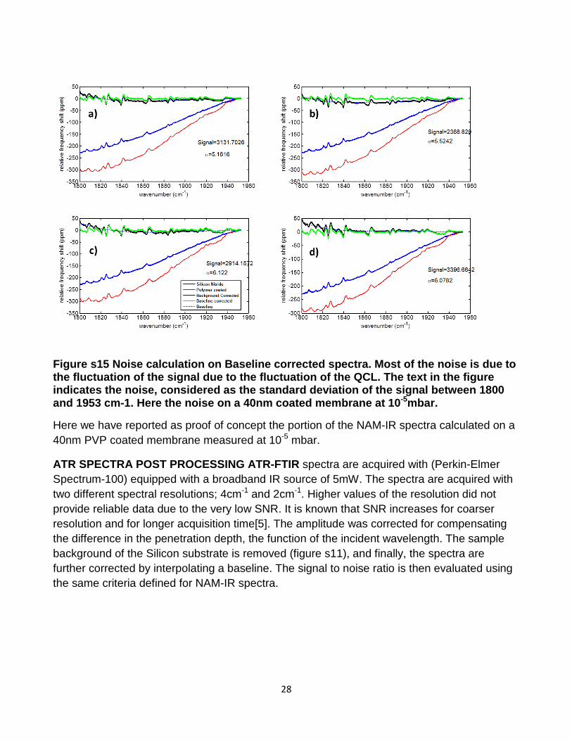
Figure s15 Noise calculation on Baseline corrected spectra. Most of the noise is due to the fluctuation of the signal due to the fluctuation of the QCL. The text in the figure indicates the noise, considered as the standard deviation of the signal between 1800 and 1953 cm-1. Here the noise on a 40nm coated membrane at 10-5mbar.

Here we have reported as proof of concept the portion of the NAM-IR spectra calculated on a 40nm PVP coated membrane measured at 10-5 mbar.

ATR SPECTRA POST PROCESSING ATR-FTIR spectra are acquired with (Perkin-Elmer Spectrum-100) equipped with a broadband IR source of 5mW. The spectra are acquired with two different spectral resolutions; 4cm-1 and 2cm-1. Higher values of the resolution did not provide reliable data due to the very low SNR. It is known that SNR increases for coarser resolution and for longer acquisition time[5]. The amplitude was corrected for compensating the difference in the penetration depth, the function of the incident wavelength. The sample background of the Silicon substrate is removed (figure s11), and finally, the spectra are further corrected by interpolating a baseline. The signal to noise ratio is then evaluated using the same criteria defined for NAM-IR spectra.

28

Figure s16 ATR signal of 200nm PVP thin film. The spectral resolution of 4cm-1.The baseline is obtained such that the three main bands of the PVP can be easily identified. The signal to noise ratio is the evaluated considering the baseline corrected spectra.

EVALUATION OF THE ABSORBED POWER

The absorbed power from the membrane resonator results only in a fraction of the incident power. The absorbed power can be calculated by the model[6]:

𝑃𝑃𝑎𝑎𝑎𝑎𝑠𝑠 =8𝜋𝜋𝛼𝛼𝑘𝑘�ℎ�𝜎𝜎0���𝐸𝐸

∆𝑓𝑓𝑓𝑓

(2 − 𝑣𝑣1 − 𝑣𝑣

− 0.642) −1

Considering a membrane resonator coated with 20 nm of PVP characterised by a time with an integration time of 7ms the Ad values is 2 pmm hence the absorption power LOD is 5nW.

These values once plugged in the equation above reported describing the absorption power, considering these parameters for the SiN[6] and PVP[7]. The values were averaged correspondingly to the thickness of the two layers. These values are reported in Table s1

1100 1200 1300 1400 1500 1600 1700 1800 1900 2000

-0.05

0

0.05

0.1

wavenumber (cm-1)

Abs

orba

nce

unit

(a.u

.)

Raw spectraBaselineBaseline corrected spectra

29

Material k a sigma E Wm-1 ppm Mpa Gpa

PVP 0.27 70 ~ 2 SIN 2.5 2.3 250 250 Table s 1Values for evaluating the absorbed power.

The thermal and mechanical parameters of the are averaged correspondingly to the sample and membrane thickness. The absorption power spectra for a 20nm membrane at 10-5mbar is shown in (figure s12). The shades represent 5 times the standard deviation of spectra recorded on 4 different membrane coated chips.

Figure s17 The absorbed power for 20nm thick PVP coating evaluated from (1). The absorbed power spectra is then used as input for the calculation of the temperature shift driven by the heat absorption

FINITE ELEMENT MODELLING

The temperature shift due to the light absorption is evaluated through a finite element model. We simulated the thermal transport throughout the entire device: bodychip and membrane resonator. The heat transport was assumed to be purely conductive throughout the device. A multi-layered structure was simulated to predict the heat transport in the presence of the PVP coating. The thermal properties of the PVP can be found elsewhere[8].

At the boundary, the temperature was set at 293.15K, and the heat source was placed in the centre of the membrane. The temperature reached for each absorbed power were calculated by solving the heat transport equation and the corresponding wavelength dependent

1200 1400 1600 1800 2000-0.5

0

0.5

1

1.5

2

2.5

3

3.5

4

Wavenumber cm-1

Abs

orbe

d po

wer

(µW

)

30

temperature field is evaluated (figure s13). The highest temperature reached matches with the absorption at 1680cm-1 of the carbonyl bond, and it is around 294K well below the glass transition temperature of the PVP which is around 453K [9].

Using the same approach we were able to define the noise equivalent temperature of 3mK, considering the standard deviation of the absorbed power spectra in the region where no absorption occurs.

Figure s18 Temperature shift spectra and temperature field for a 20 nm PVP coated membrane, correspondingly to the power spectra. The membrane is located in the centre of the bodychip of 1cm side length.

31

SNR

The signal to noise ratio of PVP spectra recorded in a high vacuum were used to perform a linear fit and extrapolate a limit of detection Figure s14.

Figure s19 linear fit extrapolation of the SNR in high vacuum n=3

From the linear fit equation of the SNR, we can extrapolate the limit of detection.

The thickness that would give rise to a SNR of 2 for an incident power of 900 µW is

𝑇𝑇ℎ𝑖𝑖𝑖𝑖𝑘𝑘𝑖𝑖𝑖𝑖𝑚𝑚𝑚𝑚 𝑑𝑑𝑖𝑖𝑑𝑑𝑖𝑖𝑖𝑖𝑑𝑑𝑖𝑖𝑑𝑑𝑖𝑖 𝑙𝑙𝑖𝑖𝑚𝑚𝑖𝑖𝑑𝑑 =2

12.5= 0.16𝑖𝑖𝑚𝑚 = 160𝑝𝑝𝑚𝑚

160pm of material corresponds over the sampling area given by the laser spot size of 100µm in diameter.

PVP density is 1.3 pg um-3,

The sampling volume is 1.25 µm3

The sampling mass is 1.66pg of PVP corresponding to roughly 4 attomol. Considering the PVP Mw is 360kDa

REFERENCE

[1] N. Miriyala, M.F. Khan, T. Thundat, Thermomechanical behavior of a bimaterial microchannel cantilever subjected to periodic IR radiation, Sensors Actuators B Chem. 235 (2016) 273–279. doi:10.1016/j.snb.2016.05.043.

[2] S. Bose, S. Schmid, T. Larsen, S.S. Keller, P. Sommer-Larsen, A. Boisen, K. Almdal, Micromechanical string resonators: Analytical tool for thermal characterization of polymers, ACS Macro Lett. 3 (2014) 55–58.

0 20 40 60 80 100 120

thickness (nm)

0

200

400

600

800

1000

1200

1400

1600

SNR

SNR=12.5 nm -1

DataLinear fit

32

doi:10.1021/mz400470n.

[3] S. Bose, S. Schmid, T. Larsen, S. Sylvest Keller, A. Boisen, K. Almdal, Micromechanical fast quasi-static detection of α and β relaxations with nanograms of polymer, J. Polym. Sci. Part B Polym. Phys. 53 (2015) 1035–1039. doi:10.1002/polb.23745.

[4] S. Asad, M. Bukhari, M.F. Khan, A. Goswami, R. Mcgee, T. Thundat, Thermomechanical analysis of picograms of polymers using a suspended microchannel cantilever, (n.d.). doi:10.1039/c6ra25455a.

[5] Q. Liu, S. Xiao, Effects of spectral resolution and signal-to- noise ratio of hyperspectral sensors on retrieving atmospheric parameters, (2013). doi:10.1364/OL.39.000060.

[6] M. Kurek, M. Carnoy, P.E. Larsen, L.H. Nielsen, O. Hansen, T. Rades, S. Schmid, A. Boisen, Nanomechanical Infrared Spectroscopy with Vibrating Filters for Pharmaceutical Analysis, Angew. Chemie Int. Ed. 56 (2017) 3901–3905. doi:10.1002/anie.201700052.

[7] X. Xie, D. Li, T.-H. Tsai, J. Liu, P. V Braun, D.G. Cahill, Thermal Conductivity, Heat Capacity, and Elastic Constants of Water- Soluble Polymers and Polymer Blends, (n.d.). doi:10.1021/acs.macromol.5b02477.

[8] X. Xie, D. Li, T.-H. Tsai, J. Liu, P. V. Braun, D.G. Cahill, Thermal Conductivity, Heat Capacity, and Elastic Constants of Water-Soluble Polymers and Polymer Blends, Macromolecules. 49 (2016) 972–978. doi:10.1021/acs.macromol.5b02477.

[9] R. Chadha, V.K. Kapoor, A. Kumar, Analytical techniques used to characterize drug-polyvinylpyrrolidone systems in solid and liquid states – An overview, J. Sci. Ind. Res. 65 (2006) 459–469.

33

Paper 3

Nanomechanical photothermal analysis of crosslinking reaction in thin polymeric layers

1

Nanomechanical photothermal analysis of crosslinking reaction in thin polymeric layers

Andrea Casci Ceccacci, Alberto Cagliani, Luca Carnevali, Paolo Marizza, Danilo Demarchi,

Silvan Schmid, Anja Boisen.

Abstract The understanding of crosslinking reactions is of the higher interest especially for polymers and

peptides of recent discovery and synthesis. Conventional spectroscopic infrared techniques used for

featuring the chemical modifications are well established and widely used, although they need a

milligrams quantity of samples and requiring time-consuming sampling technique. Newly discovered

polymer are often available in small amounts. Hence techniques which enable to study the

crosslinking chemistry on small quantities of material represents a valuable asset. Nanomechanical

sensors can probe the light absorption of very thin polymeric layer, therefore enabling infrared analysis

on sub-picogram amount of sample. In this work, we have developed nanomechanical membrane

resonators which permit the characterization of the gelification reaction in submicron thick layer of

poly(vinylpyrrolidone) starting from a 535 pg of polymer. This approach further allows to identify the

various phenomena occurring upon exposure to the UV light, in particular the photo-oxidation. The

presented method can be easily parallelized and scaled for high sensitive infrared fingerprinting.

HYDROGEL THIN FILM; THIN FILM SPECTROSCOPY; HIGH SENSITIVITY; SUB MICROMON

GELIFICATION

Introduction

Understanding the mechanism of polymer crosslinking is of paramount importance due to its

relevance in material engineering [1], for several biological applications [2] and represents a key

reaction mechanism in polymer chemistry. In this work, we focus on the crosslinking of hydrogels,

2

which are hydrophilic three-dimensional networks, able to swell and retain a significant amount of

water [3]. Thanks to these characteristics these materials resemble biological tissues, making them

suitable for a broad range of applications, such as tissue engineering [4,5], biomedical technology

such as ophthalmic systems [6,7], wound dressings [4,8,9], and drug delivery [10–12]. Furthermore,

hydrogel coatings have shown to improve the performance of implantable glucose sensors [13] and

optical sensors[14]. Drug delivery systems based on hydrogels can be used to provide distinct release

kinetics of therapeutics by tuning the crosslinking density [10]. The tuning of the gelification process is

also fundamental when hydrogels are used as a synthetic matrix for living tissue. The crosslinking

density is directly connected to the viscoelastic behaviour of hydrogels which has a strong effect on

the mechanical driving force determining the fate of stem living cell [5]. Hence, regardless of the final

aim of a hydrogel based device, the ability to define and control hydrogel characteristics is crucial.

Poly(vinylpyrrolidone) (PVP) has been extensively studied for biomedical and pharmaceutical

applications [10,15,16], and it has been shown to form chemical hydrogels by exposure to UV light or

electron beam [10,17–19]. The addition of hydrogen peroxide enhances the reaction and increases

the gel fraction[19]. However, in the presence of oxygen, UV exposure also causes photo-oxidation,

which deconstructs the polymer network, converting polymer strand into macroradicals [17,20–22].

Recently, top-down approaches for creating very thin hydrogels layers have attracted attention, since

the formation of hydrogel thin films was typically limited to layer by layer or, hybrid methods [23,24].In

this case, the formation of such hydrogels relies on the mutual interaction between the layers. The

production of hydrogels by direct exposure to light simplify the gel production significantly.

However probing the chemical modification taking place in the film throughout the gelification process

is often challenging[17,25], and it requires tedious and cumbersome approaches [17,26] or combining

multiple characterization techniques such as quartz crystal microbalance(QCM) and Surface Plasmon

Resonance(SPR)[25]. Infrared spectroscopic analysis provides information in terms of chemical bonds

3

forming during the crosslinking process. Therefore, Fourier transform infrared spectroscopy(FTIR) and

its implementation like attenuated total reflectance (ATR) are widely used to assess the formation of

chemical bonds for gel structures [10,17,27]. Nevertheless, such techniques need a minimum amount

of material in the mg range to perform the analysis, and the ATR-FTIR spectra are affected by

artefacts when the film thickness is smaller than the sampling depth. These artefacts are due mainly

on the reflection phenomena taking place at the sample substrate interface [28–30]. These

phenomena add complexity to the spectra, and they have to be considered during the interpretation of

the results. With this work, we present the application of nanomechanical infrared method (NAM-IR) to

PVP hydrogel crosslinking analysis. Such spectroscopic method is capable of extracting the same IR

spectra as the ATR-FTIR, but does not suffer from artefacts for very thin films and can work with only

a few picograms of a polymer. NAM-IR spectroscopy is based on nano-resonating structures capable

of transducing the minute temperature changes happening in the polymer upon IR photon absorption.

The heat generation is translated into a change of the mechanical resonance frequency, thanks to a

release of stress in the mechanical structure [31–33]. It has been shown how string based NAM-IR

spectroscopy can recognise spectral features even for few femtograms of material [33], thanks to their

ability to resolve minute temperature variation [34]. However, the mechanical fragility of nanostring

significantly limits the possibilities of sample preparation (i.e., typically only for particle based sensing),

making such structures not suitable for analysis of large arrays of assays [31,35].

By using membrane resonators, the robustness of the sensor, sample handling, and the overall

experimental procedure can be improved. Membrane-like structures better comply with agile sample

preparation methods such as drop casting or spin coating and facilitate precise analysis of the thin

films [36]. The gelification is followed directly on a membrane prepared using drop casting and

subsequently irradiated to initiate the crosslinking process. The NAM-IR spectra show the typical IR

spectral fingerprint of PVP hydrogel after 20 minutes of UV exposure.

4

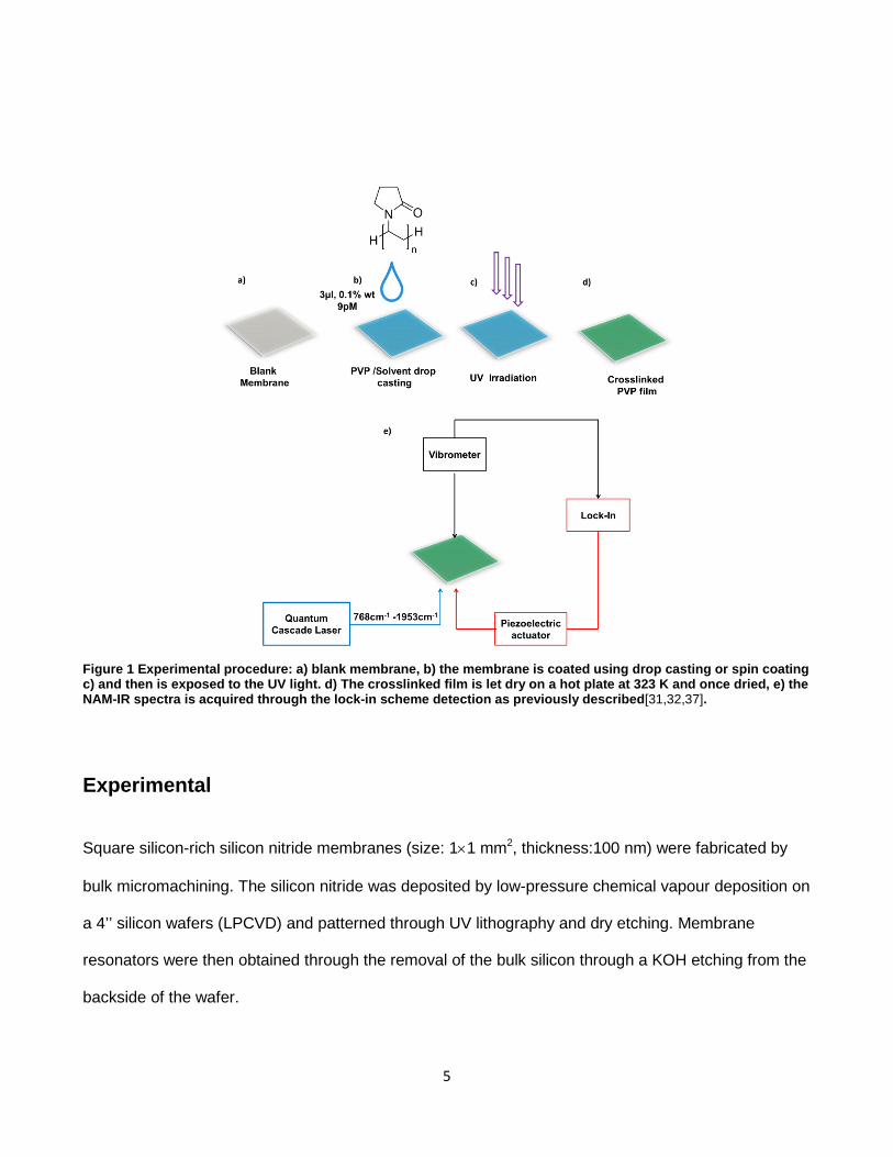
Figure 1 Experimental procedure: a) blank membrane, b) the membrane is coated using drop casting or spin coating c) and then is exposed to the UV light. d) The crosslinked film is let dry on a hot plate at 323 K and once dried, e) the NAM-IR spectra is acquired through the lock-in scheme detection as previously described[31,32,37].

Experimental

Square silicon-rich silicon nitride membranes (size: 1×1 mm2, thickness:100 nm) were fabricated by

bulk micromachining. The silicon nitride was deposited by low-pressure chemical vapour deposition on

a 4’’ silicon wafers (LPCVD) and patterned through UV lithography and dry etching. Membrane

resonators were then obtained through the removal of the bulk silicon through a KOH etching from the

backside of the wafer.

5

The polymer solution was prepared by dissolving poly(vinylpyrrolidone) K90 powder (Mw=360 kDa,

Sigma-Aldrich) with concentrations 1% and 5% wt. in aqueous solutions of hydrogen peroxide (H2O2,

30% Sigma-Aldrich). Hydrogen peroxide was added to achieve a faster and more efficient crosslinking

process [17,19].

The experimental procedure is illustrated in Figure 1. A blank membrane (Figure 1a) is coated using

two different approaches: i) spin coating aimed to obtain a fine control of the film thickness needed

during the calibration phase, and then by drop casting a 3µl of polymer solution (Figure 1b) for the

gelification experiments.The thickness of the spin-coated films was measured by ellipsometry. Prior to

the exposure, the polymer film is wet by pipetting the same (H2O2 30% v/v ) solution. The coated

sensor chip was then exposed to UV in a chamber providing UV-B (313 nm) and UV-C radiation (256

nm) (Figure 1b-d).

For photothermal measurements, the sensor chip was mounted in a custom made vacuum chamber

providing electrical connection, a glass window for optical readout, and a KBr window for IR irradiation

(Figure 1e). Membranes were actuated with an external piezoelectric element and the readout with a

laser-Doppler vibrometer (MSA-500, Polytech GmbH) equipped with a 632.8 nm Helium-Neon readout

laser. The mechanical resonance frequency was monitored using a phase-locked loop (HF2LI-PLL,

Zurich Instruments). The steps showed in Figure 1b-e are iterated to obtain and characterise a fully

crosslinked film.

6

Results and discussion

Figure 2 NAM IR spectra of PVP recorded on a 100nm coated membrane resonator. NAM-IR spectra are recorded as a negative frequency shift. Here, the spectra are mirrored along the horizontal axis achieving absorbance-like infrared spectra.

The IR spectra of PVP (see figure 2) consist of 3 main bands. The band at 1680cm-1 corresponds to

the carbonyl bond of the pyrrolidone ring; at a lower frequency, there are two bands related to a triple

peak due to the C-N stretching and CH2-ring wagging [17,20].

To quantify the sensing performance of the photothermally induced heating by the membrane

resonators, the responsivity R from a PVP coated membrane in two different IR spectral regions was

studied (Figure 2 b-c).The responsivity curves were obtained by measuring the resonance frequency

upon periodic IR irradiation, analogously on what previously shown by Miriyala et al. [38]. The

procedure to obtain the responsivity curves is showed in the supplementary information.The

wavelengths corresponding to the carbonyl bond stretching at 1680 cm-1 and to the Carbon-Nitrogen

(C-N) stretch at 1290 cm-1 were used to test the membrane responsivity. Each point in the figure 3a-b

1200 1300 1400 1500 1600 1700 1800 1900

wavenumber (cm-1

)

0

0.2

0.4

0.6

0.8

1

Nor

mal

ized

freq

uenc

y sh

ift (a

.u.)

C-N stretch

C=O stretch

CH2 –ring wag

7

is the average of at least 150 points recorded on a single membrane chip. The magnitude of the

photothermal response strongly depends on how efficiently the heat is transported towards the heat

sinks, i.e. the body chip or the residual air in the chamber. Therefore, the responsivities were studied

under two different pressure conditions: high vacuum (HV, 10-5 mbar) and low vacuum (LV, 1 mbar).

The two pressure regimes determine different behaviours in the thermal transport; in HV conditions

the heat is mainly lost by conduction throughout the body chip, instead, in LV part of the generated

heat during light absorption is also dissipated by convection through the surrounding air.

These two different regimes give rise to two responsivity values, at HV, R=47 ppm µW-1 and at LV is

R=3.8 ppm µW-1 on a membrane with a 200 nm PVP.

Interestingly, the responsivity curves obtained for the two different IR bands showed a linear trend

relatively to the incident power, as happened for string resonators and bimaterial cantilevers[33,38]

This indicates that the photothermally induced expansion of the polymer film maintains a linear

behaviour throughout the incident power range tested. Such linearity clearly supports the assumption

that the polymer does not reach the glass transition even at the highest incident power since the

thermomechanical parameters would change drastically, and an abrupt change would be reflected in

the resonance frequency [39–42]. Therefore, this linear behaviour confirms the capability of the

system of obtaining IR spectra without inducing phase changes in the polymer morphology. Finally, it

is interesting to notice that the responsitivity increases for polymer coated membranes compared to

blank SiN ( see supporting information SI).

The responsivity was further evaluated for different PVP coating thicknesses for an irradiating power

of 400 µW at 10-5 mbar and 900 µW at 1 mbar considering the absorption peak at 1680 (Figure 3c).

The same curves (figure 3c) were used as a calibration curve to estimate the thickness of the

deposited layer of PVP when the drop-casting technique was used. It can be noticed that the

responsivity increases for a higher amount of material deposited, due to a higher power absorption

8

(Figure3d) and consequently a higher heat generation. The absorbed power [43] is reported in Figure

3d. It linearly increases with the thickness of the deposited layer analogously to what has been

previously showed for string based photothermal sensor [33,38]. The model used to calculate the

absorbed power can be found in [43]

For resonator sensors, the frequency noise affecting the complete measurement chain is quantified by

the Allan Deviation 𝜎𝜎(𝜏𝜏) therefore, the noise measurements are reported in the supplementary

information. In particular, the noise measured for a membrane with 200 nm of PVP coated membrane

is 𝜎𝜎(1𝑠𝑠) = 4𝑝𝑝𝑝𝑝𝑝𝑝, corresponding to a lowest detectable absorbed power at 1680 cm-1 of 3 nW,

according to the model in [43] (see supplementary information).

9

Figure 3.Responsivity and power absorption curves as a function of the polymer thickness. a) Responsivity measured on the absorption peak of the C-N bond at 10-5 mbar and 1 mbar;b) responsivity at the absorption peak of the carbonyl group at 1680cm-1, for a 200 nm thick polymer coating at 10-5 mbar and 1 mbar error bars represents the standard deviation of multiple recordings on the same chip; c) amplitude of the relative frequency shift of the carbonyl peak for different PVP coating thickness at 10-5 mbar and 1 mbar obtained with an incident power of 400 µW and 900 µW, recorded on 3 different coated membrane ;d) absorbed power at 1 mbar and 10-5 mbar. PVP was deposited through spin coating and the thickness measured by ellipsometry. The spinning curves are showed in the supplementary material.

10

Photothermal spectra of UV crosslinked PVP

The UV crosslinking mechanism of PVP was elucidated by Zhu and co-workers [17]. They studied the

gelification at different irradiation times on macroscopic hydrogel specimens. In this work, the samples

were individually purified from the unreacted solution for 24 hours in deionized water and then dried in

vacuum for further 24 hours. After this long sample preparation, the specimens were analysed. Such

conventional approach is extremely time-consuming and is not suitable for fast analysis of a large

array of polymer samples. In our work instead, we present a quicker and simpler method for realising

submicron thin films of PVP hydrogel. Moreover, the NAM-IR system we used is also significantly

faster and able to record the spectra with higher signal to noise ratio. In fact, NAM-IR allows recording

spectra with a single acquisition with a signal to noise ratios of 200 in LV on 100 nm polymer thick

layer, whereas our commercial ATR-FTIR equipment for the same polymer thickness yielded an SNR

five times smaller [36]. The high SNR for NAM-IR recorded on a single acquisition allowed us to

acquire each spectrum 43 times faster compared to ATR-FTIR apparatus as it would need multiple

acquisitions to reach the same SNR.

The estimated thickness ranged from 80 to 300 nm (see supplementary information). To the best of

our knowledge, this study is the first showing a gel formation on a submicron thick layer of PVP by

direct UV illumination.

The IR spectrum of PVP can be analysed focusing on the three main bands from 1150 cm-1 to

2000cm-1.The bands at 1300 cm-1 and 1450 cm-1 undergo significant changes during the crosslinking

process and the gelification within the studied time frame of 90 min.

Variations in the spectroscopic pattern can be seen after 10 minutes of UV exposure (see Figure 3).

The carbonyl group is involved in the formation of the intermolecular bonds with other polymer chains,

which can be observed with shifts towards the lower frequency of the corresponding peak [17]. For

11

exposure times longer than 20 minutes a substantial change can be noticed in the carbonyl band at

1680 cm-1. In the gel spectra, the peak shows a significant splitting, resulted in a broadening towards a

lower frequency. Noteworthy, the dip is appearing in the middle of the band at 1684 cm-1 also present

in unexposed PVP, and it is due to local power minima of the laser source (see supplementary

information).

The hydrogel formation is further confirmed by assessing bands at 1400 cm-1 1415 cm-1 and 1420cm-1,

respectively related to the bond wagging of C4-H and CH2, and C-N bond stretching at 1257 cm-1 [17].

At the same time, the conversion of the pyrrolidone ring into succinimide ring is characterised by a

strong band in the proximity of 1700 cm-1 related to the two carbonyl groups [17,20] which are a strong

sign of the PVP gelification process [17].

The peak at 1280cm-1 became wider and shifted towards a higher frequency, and a new peak appears

at 1215 cm-1 also attributed to the C-N stretching of the succinimide ring. The gel structure is further

characterised by N-C-O-C bands which can be identified in spectra at 1170 cm-1-1180 cm-1.

Overexposure to UV light in the presence of H2O and H2O2 and O2 triggers the degradation of the

polymer backbone known as photo-oxidation [22]. This phenomenon brings to the demolition of the

polymer chains accompanied by the formation of degradation products [17,26,44].

With respect to PVP, UV overexposure leads to the formation of imide groups [17,26], undergoing

hydrolysis and producing amide-II groups. These latter were probed by a band occurring at 1540-1550

cm-1 related to the N-H bending mode. Furthermore, at 1735 cm-1, we noticed a shoulder of the main

carbonyl peak due to the formation of carboxyl terminated non-cyclic imides [21,26,44] (Figure-3).

After 90 min of exposure, the IR spectra differs sensibly from any of the previous gelificated structures

[17] and the non-treated polymer. Nevertheless, the bands around 1400 cm-1 and 1170 cm-1 still show

characteristic peaks related to PVP gel structure.

12

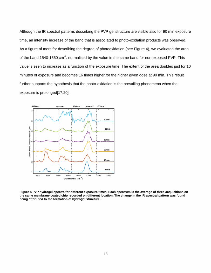
Although the IR spectral patterns describing the PVP gel structure are visible also for 90 min exposure

time, an intensity increase of the band that is associated to photo-oxidation products was observed.

As a figure of merit for describing the degree of photooxidation (see Figure 4), we evaluated the area

of the band 1540-1560 cm-1, normalised by the value in the same band for non-exposed PVP. This

value is seen to increase as a function of the exposure time. The extent of the area doubles just for 10

minutes of exposure and becomes 16 times higher for the higher given dose at 90 min. This result

further supports the hypothesis that the photo-oxidation is the prevailing phenomena when the

exposure is prolonged[17,20].

Figure 4 PVP hydrogel spectra for different exposure times. Each spectrum is the average of three acquisitions on the same membrane coated chip recorded on different location. The change in the IR spectral pattern was found being attributed to the formation of hydrogel structure.

13

Figure 5 Effects of prolonged exposure time on the IR spectra of PVP. a) Area ascribed to the amide-II group a product of the photooxidation; b) Trend in the value of the area of the amide-II for different exposure times.

Conclusions

We have shown that the employment of prestressed membrane resonator as a photothermal sensor

for characterising the gelification of thin PVP film can be a powerful analytical tool to study crosslinking

of thin polymer films. The use of NAM-IR spectroscopy for monitoring the crosslinking of thin polymer

film brought several advantages. The ratio SNR vs. acquisition time increased 5 times compared to

conventional ATR-FTIR spectroscopy[28]. Moreover, the robustness of the membrane geometry better

suits drop casting and spin coating of thin polymer layers, simplifying the sample preparation

considerably.

In particular, the thickness of the dry hydrogel films and the typical IR spectral features allowed to

assess the formation of gelified structures. The membrane resonators showed a responsivity up to

200 ppm nm-1 mW-1 and able to resolve up to 3 nW as absorbed power, which is in the same order of

magnitude of string based photothermal spectrophotometer. The high sensitivity even at moderate

vacuum conditions shown by membrane resonators allowed performing a highly defined in situ

14

infrared analysis of the gelification product and as well as characterise the photooxidation of the

polymer which is important for long exposure times. A deeper understanding of the process might be

obtained by investigating the transition from purely elastic film to a viscoelastic behaviour occurring

during the crosslinking reaction. This might be possible by monitoring the evolution of the damping

mechanism of the film on the resonating behaviour of the membrane. Finally, we envision that by

tailoring the sensor features as well as the experimental setup this method can be integrated on high

throughput sensing devices capable of assessing several other the physical and chemical properties.

[1] P. Ghosh, S. Katare, P. Patkar, J.M. Caruthers, V. Venkatasubramanian, K.A. Walker, SULFUR VULCANIZATION OF NATURAL RUBBER FOR BENZOTHIAZOLE ACCELERATED FORMULATIONS: FROM REACTION MECHANISMS TO A RATIONAL KINETIC MODEL, (n.d.). http://cepac.cheme.cmu.edu/pasi2008/slides/venkat/library/reading/RCT-ReviewPublishedPaper.pdf (accessed March 12, 2017).

[2] R. Kluger, A. Alagic, Chemical cross-linking and protein–protein interactions—a review with illustrative protocols, Bioorg. Chem. 32 (2004) 451–472. doi:10.1016/j.bioorg.2004.08.002.

[3] NILIMANKA DAS, PREPARATION METHODS AND PROPERTIES OF HYDROGEL: A REVIEW, Int. J. Pharm. Pharm. Sci. 5 (2013) 112–117.

[4] K.R. Kirker, Y. Luo, J.H. Nielson, J. Shelby, G.D. Prestwich, Glycosaminoglycan hydrogel films as bio-interactive dressings for wound healing, Biomaterials. 23 (2002) 3661–3671. doi:10.1016/S0142-9612(02)00100-X.

[5] O. Chaudhuri, L. Gu, D. Klumpers, M. Darnell, S.A. Bencherif, J.C. Weaver, N. Huebsch, H. Lee, E. Lippens, G.N. Duda, D.J. Mooney, Hydrogels with tunable stress relaxation regulate stem cell fate and activity, Nat. Mater. 15 (2015) 326–334. doi:10.1038/nmat4489.

[6] L. Xinming, C. Yingde, A.W. Lloyd, S. V Mikhalovsky, S.R. Sandeman, C.A. Howel, L. Liewen, Polymeric hydrogels for novel contact lens - based ophthalmic drug delivery systems : A review, (n.d.). doi:10.1016/j.clae.2007.09.002.

[7] L. Xinming, C. Yingde, A.W. Lloyd, S. V. Mikhalovsky, S.R. Sandeman, C.A. Howel, L. Liewen, Polymeric hydrogels for novel contact lens-based ophthalmic drug delivery systems: A review, Contact Lens Anterior Eye. 31 (2008) 57–64. doi:10.1016/j.clae.2007.09.002.

[8] M. Ishihara, K. Nakanishi, K. Ono, M. Sato, M. Kikuchi, Y. Saito, H. Yura, T. Matsui, H. Hattori, M. Uenoyama, A. Kurita, Photocrosslinkable chitosan as a dressing for wound occlusion and accelerator in healing process, Biomaterials. 23 (2002) 833–840. doi:10.1016/S0142-9612(01)00189-2.

15

[9] Z. Ajji, I. Othman, J.M. Rosiak, Production of hydrogel wound dressings using gamma radiation, Nucl. Instruments Methods Phys. Res. Sect. B Beam Interact. with Mater. Atoms. 229 (2005) 375–380. doi:10.1016/j.nimb.2004.12.135.

[10] P. Marizza, M. Abrami, S.S. Keller, P. Posocco, E. Laurini, K. Goswami, A.L. Skov, A. Boisen, D. Larobina, G. Grassi, M. Grassi, Synthesis and characterization of UV photocrosslinkable hydrogels with poly(N-vinyl-2-pyrrolidone): Determination of the network mesh size distribution, Int. J. Polym. Mater. Polym. Biomater. 65 (2016) 516–525. doi:10.1080/00914037.2015.1129964.

[11] N. Bhattarai, J. Gunn, M. Zhang, Chitosan-based hydrogels for controlled, localized drug delivery, Adv. Drug Deliv. Rev. 62 (2010) 83–99. doi:10.1016/j.addr.2009.07.019.

[12] C. Le Bourlais, L. Acar, H. Zia, P.A. Sado, T. Needham, R. Leverge, Ophthalmic drug delivery systems—Recent advances, Prog. Retin. Eye Res. 17 (1998) 33–58. doi:10.1016/S1350-9462(97)00002-5.

[13] B. Yu, C. Wang, Y.M. Ju, L. West, J. Harmon, Y. Moussy, F. Moussy, Use of hydrogel coating to improve the performance of implanted glucose sensors, Biosens. Bioelectron. 23 (2008) 1278–1284. doi:10.1016/j.bios.2007.11.010.

[14] A. Mateescu, Y. Wang, J. Dostalek, U. Jonas, Thin hydrogel films for optical biosensor applications, Membranes (Basel). 2 (2012) 49–69. doi:10.3390/membranes2010040.

[15] R.K. Mishra, M. Datt, A.K. Banthia, Synthesis and characterization of pectin/PVP hydrogel membranes for drug delivery system., AAPS PharmSciTech. 9 (2008) 395–403. doi:10.1208/s12249-008-9048-6.

[16] L. Perioli, V. Ambrogi, F. Angelici, M. Ricci, S. Giovagnoli, M. Capuccella, C. Rossi, Development of mucoadhesive patches for buccal administration of ibuprofen, J. Control. Release. 99 (2004) 73–82. doi:10.1016/j.jconrel.2004.06.005.

[17] X. Zhu, P. Lu, W. Chen, J. Dong, Studies of UV crosslinked poly(N-vinylpyrrolidone) hydrogels by FTIR, Raman and solid-state NMR spectroscopies, Polymer (Guildf). 51 (2010) 3054–3063. doi:10.1016/j.polymer.2010.05.006.

[18] K. Plungpongpan, K. Koyanukkul, A. Kaewvilai, N. Nootsuwan, P. Kewsuwan, A. Laobuthee, Preparation of PVP/MHEC Blended Hydrogels via Gamma Irradiation and their Calcium ion Uptaking and Releasing Ability, Energy Procedia. 34 (2013) 775–781. doi:10.1016/j.egypro.2013.06.813.

[19] L.C. Lopérgolo, A.B. Lugão, L.H. Catalani, Direct UV photocrosslinking of poly(N-vinyl-2-pyrrolidone) (PVP) to produce hydrogels, (n.d.). doi:10.1016/S0032-3861(03)00686-4.

[20] F. Hassouna, S. Therias, G. Mailhot, J.-L. Gardette, Photooxidation of poly(N-vinylpyrrolidone) (PVP) in the solid state and in aqueous solution, Polym. Degrad. Stab. 94 (2009) 2257–2266. doi:10.1016/j.polymdegradstab.2009.08.007.

[21] F. Hassouna, S. Morlat-Thérias, G. Mailhot, J.L. Gardette, Influence of water on the photodegradation of poly(ethylene oxide), (2007). doi:10.1016/j.polymdegradstab.2007.07.016.

[22] E. Yousif, A. Hasan, Photostabilization of poly(vinyl chloride) – Still on the run, J. Taibah Univ. Sci. 9 (2015) 421–448. doi:10.1016/j.jtusci.2014.09.007.

[23] B. Chollet, M. Li, E. Martwong, B. Bresson, C. Fretigny, P. Tabeling, Y. Tran, Multiscale Surface-Attached Hydrogel Thin Films with Tailored Architecture, ACS Appl. Mater. Interfaces. 8 (2016) 11729–11738. doi:10.1021/acsami.6b00446.

[24] E. Lee, H.-E. Jang, Y.Y. Kang, J. Kim, J.-H. Ahn, H. Mok, Submicron-sized hydrogels incorporating cyclic dinucleotides for selective delivery and elevated cytokine release in macrophages, Acta Biomater. 29

16

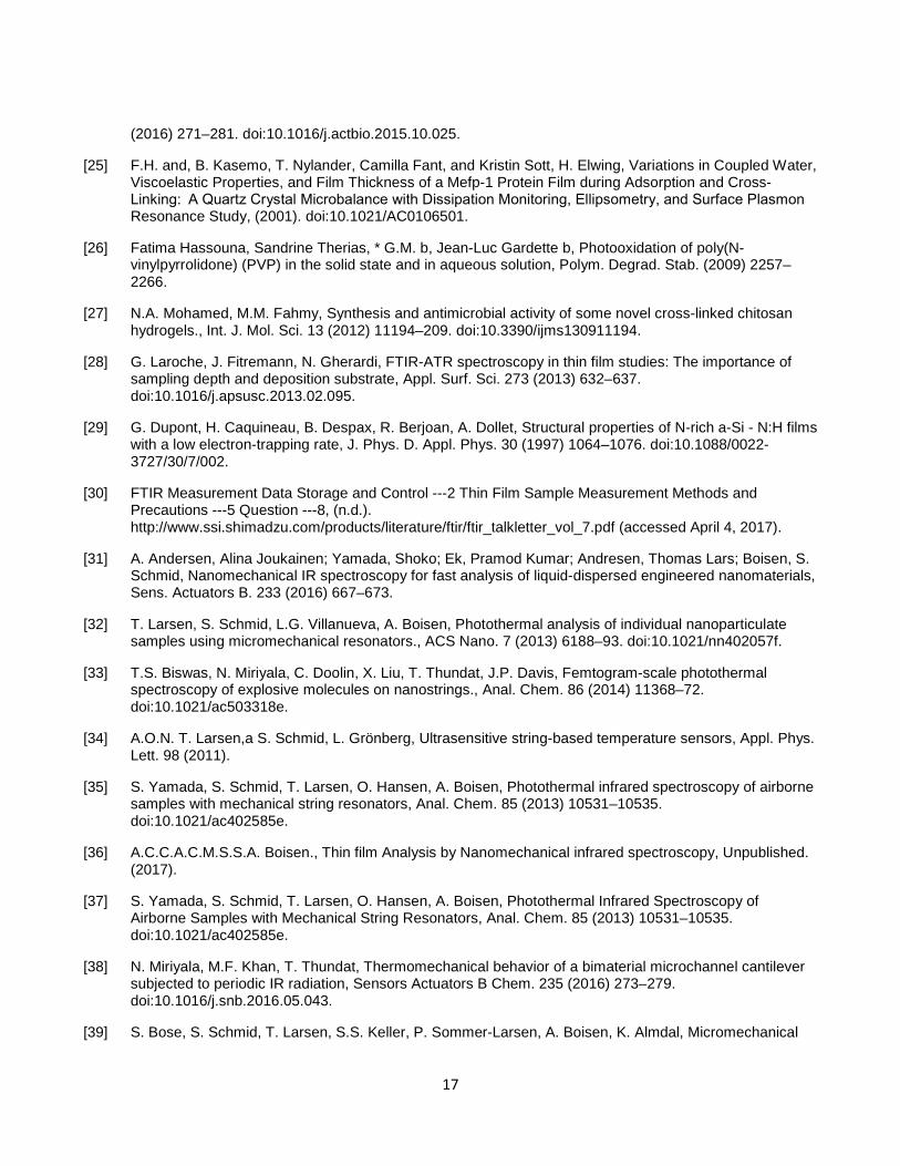
(2016) 271–281. doi:10.1016/j.actbio.2015.10.025.

[25] F.H. and, B. Kasemo, T. Nylander, Camilla Fant, and Kristin Sott, H. Elwing, Variations in Coupled Water, Viscoelastic Properties, and Film Thickness of a Mefp-1 Protein Film during Adsorption and Cross-Linking:  A Quartz Crystal Microbalance with Dissipation Monitoring, Ellipsometry, and Surface Plasmon Resonance Study, (2001). doi:10.1021/AC0106501.

[26] Fatima Hassouna, Sandrine Therias, * G.M. b, Jean-Luc Gardette b, Photooxidation of poly(N-vinylpyrrolidone) (PVP) in the solid state and in aqueous solution, Polym. Degrad. Stab. (2009) 2257–2266.

[27] N.A. Mohamed, M.M. Fahmy, Synthesis and antimicrobial activity of some novel cross-linked chitosan hydrogels., Int. J. Mol. Sci. 13 (2012) 11194–209. doi:10.3390/ijms130911194.

[28] G. Laroche, J. Fitremann, N. Gherardi, FTIR-ATR spectroscopy in thin film studies: The importance of sampling depth and deposition substrate, Appl. Surf. Sci. 273 (2013) 632–637. doi:10.1016/j.apsusc.2013.02.095.

[29] G. Dupont, H. Caquineau, B. Despax, R. Berjoan, A. Dollet, Structural properties of N-rich a-Si - N:H films with a low electron-trapping rate, J. Phys. D. Appl. Phys. 30 (1997) 1064–1076. doi:10.1088/0022-3727/30/7/002.

[30] FTIR Measurement Data Storage and Control ---2 Thin Film Sample Measurement Methods and Precautions ---5 Question ---8, (n.d.). http://www.ssi.shimadzu.com/products/literature/ftir/ftir_talkletter_vol_7.pdf (accessed April 4, 2017).

[31] A. Andersen, Alina Joukainen; Yamada, Shoko; Ek, Pramod Kumar; Andresen, Thomas Lars; Boisen, S. Schmid, Nanomechanical IR spectroscopy for fast analysis of liquid-dispersed engineered nanomaterials, Sens. Actuators B. 233 (2016) 667–673.

[32] T. Larsen, S. Schmid, L.G. Villanueva, A. Boisen, Photothermal analysis of individual nanoparticulate samples using micromechanical resonators., ACS Nano. 7 (2013) 6188–93. doi:10.1021/nn402057f.

[33] T.S. Biswas, N. Miriyala, C. Doolin, X. Liu, T. Thundat, J.P. Davis, Femtogram-scale photothermal spectroscopy of explosive molecules on nanostrings., Anal. Chem. 86 (2014) 11368–72. doi:10.1021/ac503318e.

[34] A.O.N. T. Larsen,a S. Schmid, L. Grönberg, Ultrasensitive string-based temperature sensors, Appl. Phys. Lett. 98 (2011).

[35] S. Yamada, S. Schmid, T. Larsen, O. Hansen, A. Boisen, Photothermal infrared spectroscopy of airborne samples with mechanical string resonators, Anal. Chem. 85 (2013) 10531–10535. doi:10.1021/ac402585e.

[36] A.C.C.A.C.M.S.S.A. Boisen., Thin film Analysis by Nanomechanical infrared spectroscopy, Unpublished. (2017).

[37] S. Yamada, S. Schmid, T. Larsen, O. Hansen, A. Boisen, Photothermal Infrared Spectroscopy of Airborne Samples with Mechanical String Resonators, Anal. Chem. 85 (2013) 10531–10535. doi:10.1021/ac402585e.

[38] N. Miriyala, M.F. Khan, T. Thundat, Thermomechanical behavior of a bimaterial microchannel cantilever subjected to periodic IR radiation, Sensors Actuators B Chem. 235 (2016) 273–279. doi:10.1016/j.snb.2016.05.043.

[39] S. Bose, S. Schmid, T. Larsen, S.S. Keller, P. Sommer-Larsen, A. Boisen, K. Almdal, Micromechanical

17

string resonators: Analytical tool for thermal characterization of polymers, ACS Macro Lett. 3 (2014) 55–58. doi:10.1021/mz400470n.

[40] S. Bose, S. Schmid, T. Larsen, S. Sylvest Keller, A. Boisen, K. Almdal, Micromechanical fast quasi-static detection of α and β relaxations with nanograms of polymer, J. Polym. Sci. Part B Polym. Phys. 53 (2015) 1035–1039. doi:10.1002/polb.23745.

[41] S. Asad, M. Bukhari, M.F. Khan, A. Goswami, R. Mcgee, T. Thundat, Thermomechanical analysis of picograms of polymers using a suspended microchannel cantilever, (n.d.). doi:10.1039/c6ra25455a.

[42] N. Jung, H. Seo, D. Lee, C.Y. Ryu, S. Jeon, Nanomechanical Thermal Analysis of the Glass Transition of Polystyrene Using Silicon Cantilevers, Macromolecules. 41 (2008) 6873–6875. doi:10.1021/ma801539m.

[43] M. Kurek, M. Carnoy, P.E. Larsen, L.H. Nielsen, O. Hansen, T. Rades, S. Schmid, A. Boisen, Nanomechanical Infrared Spectroscopy with Vibrating Filters for Pharmaceutical Analysis, Angew. Chemie Int. Ed. 56 (2017) 3901–3905. doi:10.1002/anie.201700052.

[44] A. Roger, D. Sallet, J. Lemaire, Photochemistry of aliphatic polyamides. 4. Mechanisms of photooxidation of polyamides 6, 11, and 12 at long wavelengths, Macromolecules. 19 (1986) 579–584. doi:10.1021/ma00157a015.

18

SUPPLEMENTARY INFORMATION

1. PVP CONCENTRATION ON A 3µl drop.

Density of H2O:H2O2 solvent 1.1mg/ml;

Molecular Weight of PVP k90= 360000 g/mol;

The PVP solution is concentrated at 0.1%wt. the polymer solution drop is 3µl having a mass of 3.3mg.

0.1% of 3.3 mg= corresponds to 3.3 µg which is an estimation of the mass of PVP in the drop which is cast on the total area of the membrane resonator chip plus the body-chip 1cm wide.

Considering the PVP molecular weight the amount of polymer in the whole drop corresponds to

𝑀𝑀𝑀𝑀𝑀𝑀𝑀𝑀 𝑜𝑜𝑜𝑜 𝑃𝑃𝑃𝑃𝑃𝑃

𝑀𝑀𝑀𝑀=

3.3 10−6𝑔𝑔3 105𝑔𝑔

𝑝𝑝𝑜𝑜𝑚𝑚�= 9.1𝑝𝑝𝑀𝑀

(1)

1.1 Mass quantification

The amount of polymer present in the drop is 3.3 µg, which result cast onto an approximately circular area of 8mm of diameter, yielding a surface density 65fg/µm2.

The signal is provided by photothermal induced heat in generated within the laser spot which has a diameter of 100µm, or equal to an area of 7583µm2.

Sensing mass = 7583µm2 * 65fg/µm2 =497pg (2)

Mass on the sensor = 65fg/um2 *106 µm2 =65ng (3)

2. PVP SPINNING CURVES

The membrane resonators were coated with this spinning parameters reported in figure s1. The spin-coated membranes were then used to obtain the calibration curve reported in the main manuscript in Figure 2c-d.

19

Figure s6 Spinning curves of PVP.

3. POWER SPECTRA OF THE IR LASER SOURCE

The quantum cascade laser used in this work has a non-constant power throughout the spectral range covered. The parameter that can be used to tune the power output of the laser is the duty cycle. The power spectra were recorded by a thermal sensor at the duty cycle of 1% and 4%. Which corresponds to the one used during the experiments.

a) b)

Figure s7 Power spectra for 1% DC a) and 4% DC b).

The two power spectra were recorded at two different spectral step size. For 1% DC the step size was of 1cm-1, instead, for 4% DC the step size was of 10cm-1. In the region between 1400 cm-1 and 1800 cm-1, we notice several dip in the power curves which are reflected in the NAM-IR spectra.

20

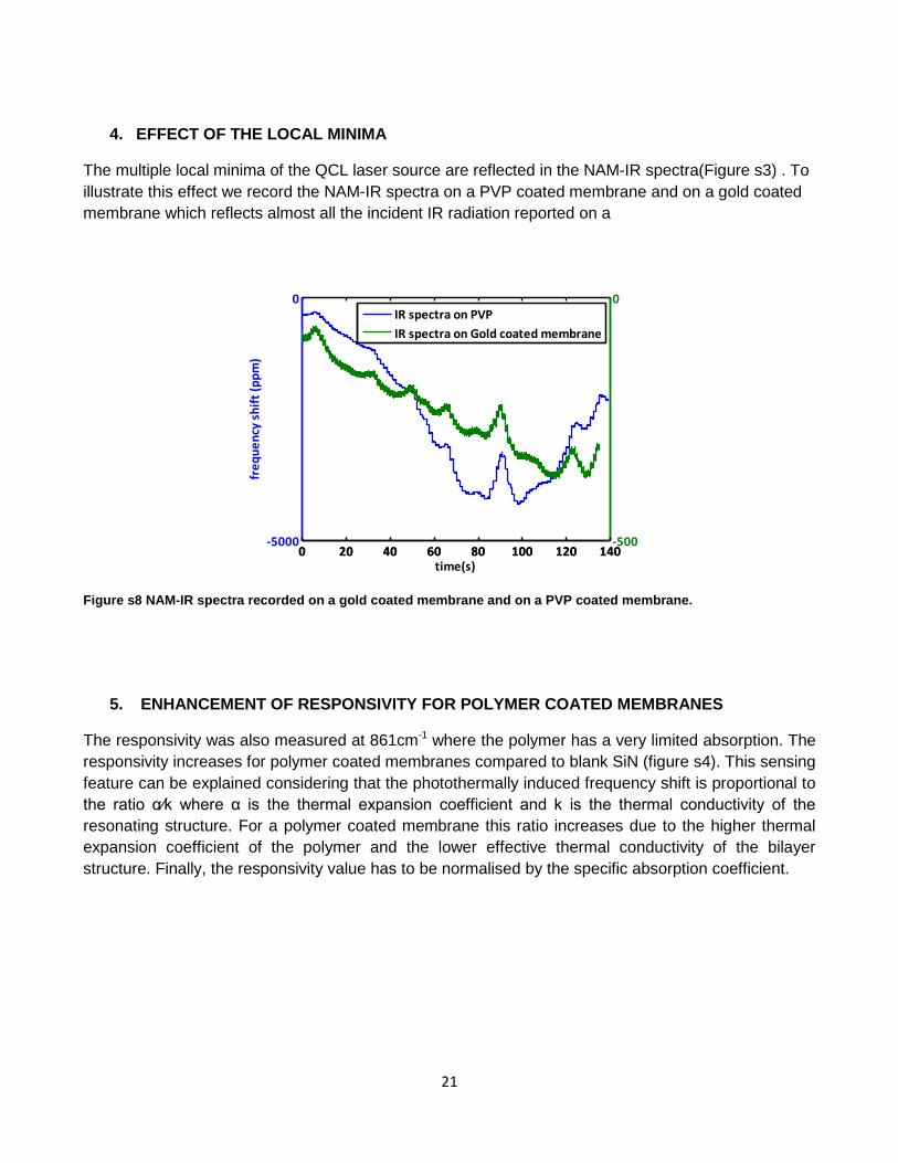
4. EFFECT OF THE LOCAL MINIMA

The multiple local minima of the QCL laser source are reflected in the NAM-IR spectra(Figure s3) . To illustrate this effect we record the NAM-IR spectra on a PVP coated membrane and on a gold coated membrane which reflects almost all the incident IR radiation reported on a

Figure s8 NAM-IR spectra recorded on a gold coated membrane and on a PVP coated membrane.

5. ENHANCEMENT OF RESPONSIVITY FOR POLYMER COATED MEMBRANES

The responsivity was also measured at 861cm-1 where the polymer has a very limited absorption. The responsivity increases for polymer coated membranes compared to blank SiN (figure s4). This sensing feature can be explained considering that the photothermally induced frequency shift is proportional to the ratio α⁄k where α is the thermal expansion coefficient and k is the thermal conductivity of the resonating structure. For a polymer coated membrane this ratio increases due to the higher thermal expansion coefficient of the polymer and the lower effective thermal conductivity of the bilayer structure. Finally, the responsivity value has to be normalised by the specific absorption coefficient.

0 20 40 60 80 100 120 140-5000

0

time(s)

freq

uenc

y sh

ift (p

pm)

0 20 40 60 80 100 120 140-500

0IR spectra on PVPIR spectra on Gold coated membrane

21

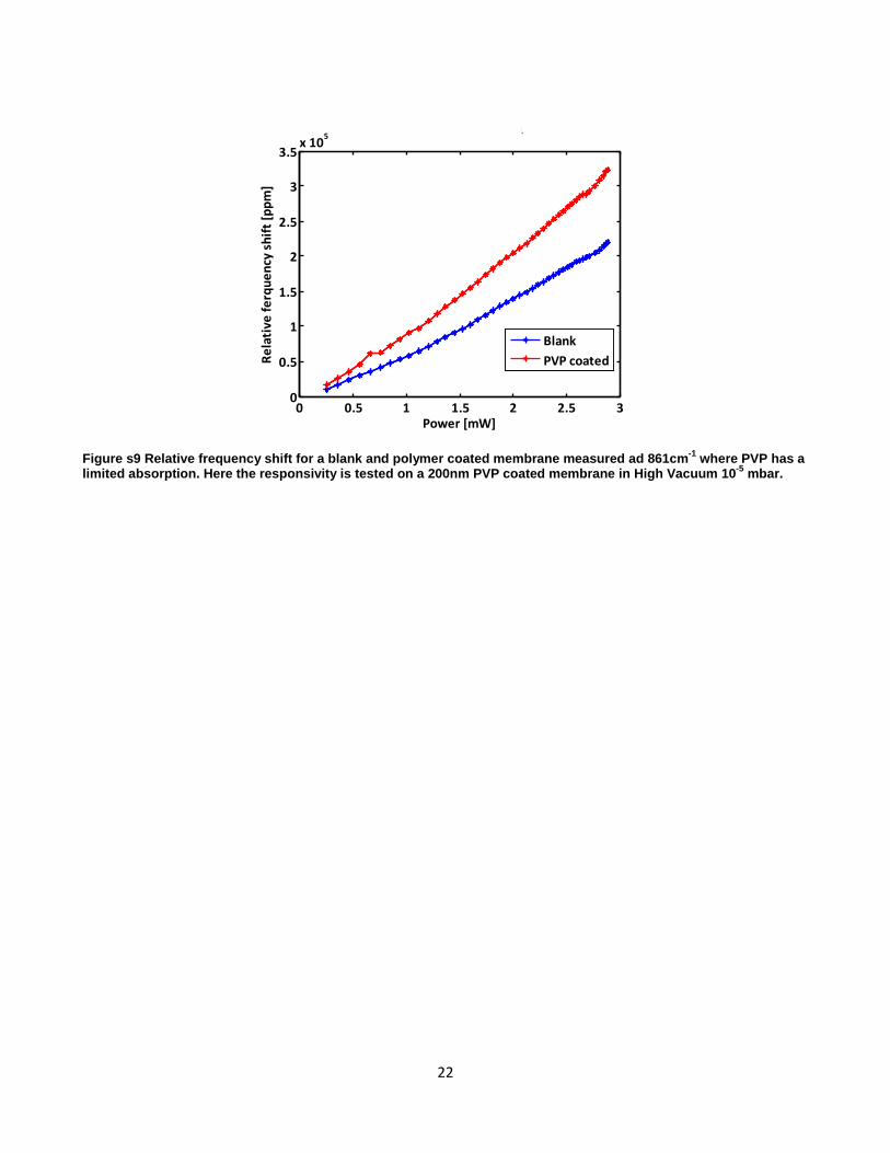
Figure s9 Relative frequency shift for a blank and polymer coated membrane measured ad 861cm-1 where PVP has a limited absorption. Here the responsivity is tested on a 200nm PVP coated membrane in High Vacuum 10-5 mbar.

0 0.5 1 1.5 2 2.5 30

0.5

1

1.5

2

2.5

3

3.5x 105

Power [mW]

Rela

tive

ferq

uenc

y sh

ift [p

pm]

Sensitivity at 861cm-1

BlankPVP coated

22

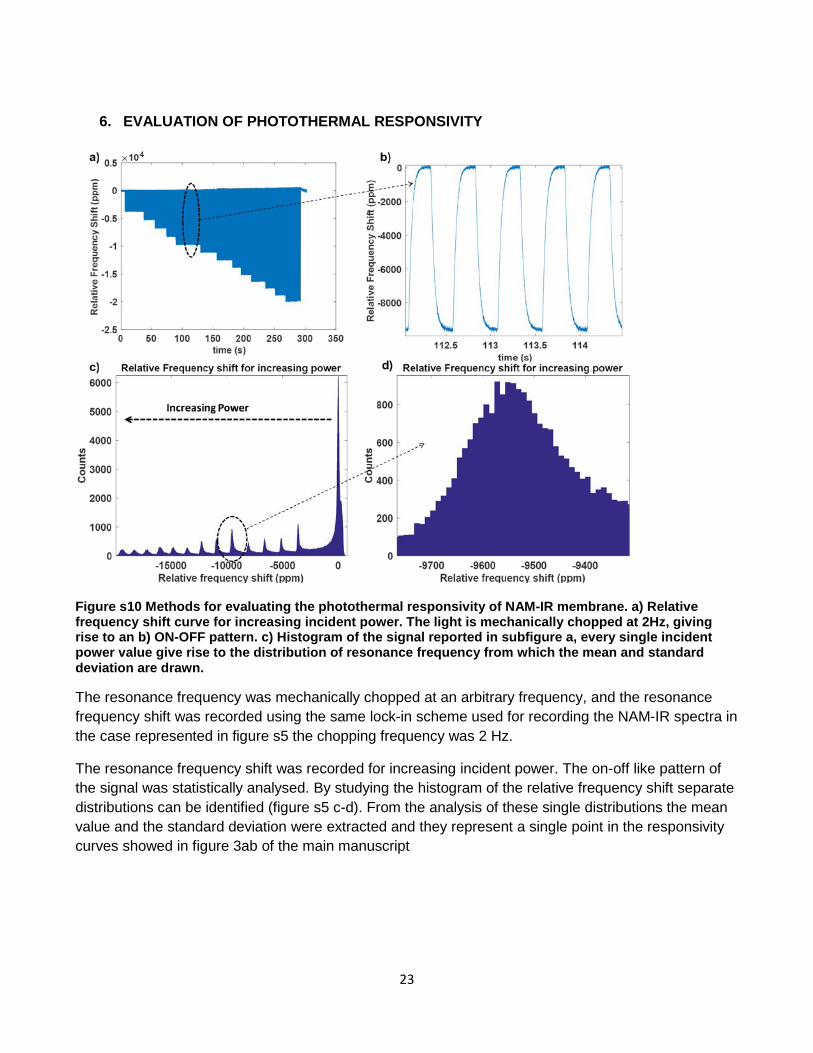
6. EVALUATION OF PHOTOTHERMAL RESPONSIVITY

Figure s10 Methods for evaluating the photothermal responsivity of NAM-IR membrane. a) Relative frequency shift curve for increasing incident power. The light is mechanically chopped at 2Hz, giving rise to an b) ON-OFF pattern. c) Histogram of the signal reported in subfigure a, every single incident power value give rise to the distribution of resonance frequency from which the mean and standard deviation are drawn.

The resonance frequency was mechanically chopped at an arbitrary frequency, and the resonance frequency shift was recorded using the same lock-in scheme used for recording the NAM-IR spectra in the case represented in figure s5 the chopping frequency was 2 Hz.

The resonance frequency shift was recorded for increasing incident power. The on-off like pattern of the signal was statistically analysed. By studying the histogram of the relative frequency shift separate distributions can be identified (figure s5 c-d). From the analysis of these single distributions the mean value and the standard deviation were extracted and they represent a single point in the responsivity curves showed in figure 3ab of the main manuscript

23

7. EVALUATION OF THE PVP thickness through the calibration curve

The thickness of the deposited PVP by drop casting is evaluated by the calibration curve showed in the main manuscript (figure 3c).

The responsivity measured at 1680cm-1 was of 24 ppm/nm in low vacuum for a given incident power of 900µW.

Here we show the amplitudes of the carbonyl peak obtained PVP drop cast membrane resonator and by using the responsivity curves the thickness is estimated.

Table s 1 Values of estimated thickness for drop casted membranes

Chip ID Relative frequency shift

at 1680cm-1

Estimated Thickness

M_125 8000 ppm 313 nm M_142 4000 ppm 165 nm M_133 6000 ppm 248 nm M_136 2000ppm 82 nm M_140 4000 ppm 165nm

Figure s11 Membrane n 133 0-90 min Figure s12 Membrane n 136 0-20 min

Figure s13 Membrane 140 0-20 min Figure s14 Membrane 140 0-60 min

1550 1600 1650 1700 1750 1800 1850

wavenumber (cm- 1

)

-6000

-5000

-4000

-3000

-2000

-1000

0

rela

tive

freq

uenc

y sh

ift (p

pm)

1600 1700 1800 1900

wavenumber (cm- 1

)

-2000

-1500

-1000

-500

0

rela

tive

freq

uenc

y sh

ift (p

pm)

1600 1650 1700 1750 1800 1850 1900

wavenumber (cm- 1

)

-4000

-3500

-3000

-2500

-2000

-1500

-1000

-500

0

rela

tive

freq

uenc

y sh

ift (p

pm)

1600 1650 1700 1750 1800 1850

wavenumber (cm- 1

)

-4000

-3500

-3000

-2500

-2000

-1500

-1000

-500

0

rela

tive

freq

uenc

y sh

ift (p

pm)

24

Figure s15 Membrane 125 0-60 min

4. ALLAN DEVIATION

Figure s16 Allan Deviation Measurement.

Allan Deviation measurements of PVP-coated and blank membrane resonators in high vacuum and in low vacuum and reported in Figure s11. The polymer coating worsens the stability of the sensor. For high vacuum measurement, the noise is increased, this is probably due to the higher sensitivity of the membranes to the laser fluctuation.

1550 1600 1650 1700 1750 1800 1850 1900

wavenumber (cm- 1

)

-8000

-7000

-6000

-5000

-4000

-3000

-2000

-1000

rela

tive

freq

uenc

y sh

ift (p

pm)

10 -4 10 -2 10 0 10 2

integration time, (s)

10 -6

10 -5

10 -4

10 -3

Alla

n de

viat

ion,

200 nm 1 mbar

200nm 10 -5 mbarblank 1mbar

blank 10 -5 mbar

25

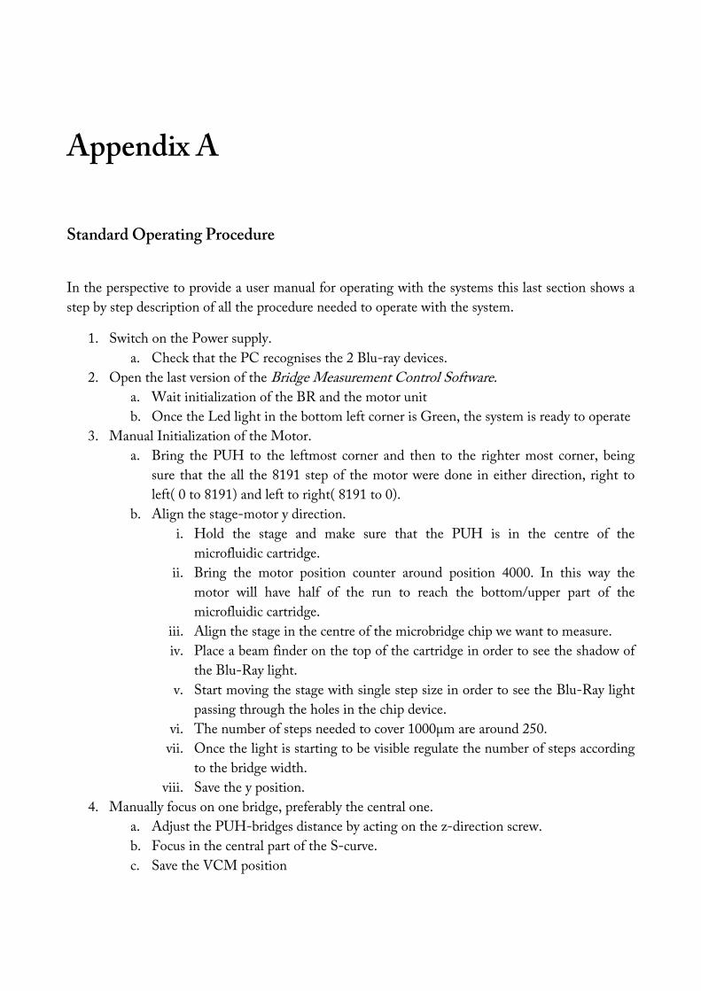
Appendix A

Standard Operating Procedure

In the perspective to provide a user manual for operating with the systems this last section shows a step by step description of all the procedure needed to operate with the system.

1. Switch on the Power supply. a. Check that the PC recognises the 2 Blu-ray devices.

2. Open the last version of the Bridge Measurement Control Software. a. Wait initialization of the BR and the motor unit b. Once the Led light in the bottom left corner is Green, the system is ready to operate

3. Manual Initialization of the Motor. a. Bring the PUH to the leftmost corner and then to the righter most corner, being

sure that the all the 8191 step of the motor were done in either direction, right to left( 0 to 8191) and left to right( 8191 to 0).

b. Align the stage-motor y direction. i. Hold the stage and make sure that the PUH is in the centre of the

microfluidic cartridge. ii. Bring the motor position counter around position 4000. In this way the

motor will have half of the run to reach the bottom/upper part of the microfluidic cartridge.

iii. Align the stage in the centre of the microbridge chip we want to measure. iv. Place a beam finder on the top of the cartridge in order to see the shadow of

the Blu-Ray light. v. Start moving the stage with single step size in order to see the Blu-Ray light

passing through the holes in the chip device. vi. The number of steps needed to cover 1000µm are around 250.

vii. Once the light is starting to be visible regulate the number of steps according to the bridge width.

viii. Save the y position. 4. Manually focus on one bridge, preferably the central one.

a. Adjust the PUH-bridges distance by acting on the z-direction screw. b. Focus in the central part of the S-curve. c. Save the VCM position

5. Repeat the step 4b-iii-vii for measuring different bridges array. a. Focus on one bridge of the ith, by only adjusting the VCM position b. Focus in the central part of the S-curve c. Save the VCM position once focused.

6. Repeat step 5 for the different bridge that we want to measure. 7. Repeat step n 3a. 8. Set Delay and threshold 10ms and 100 are reference value) 9. Set the number of Measurement 10. Press the ONE-button

Appendix B

Analytical Model for calculating the photothermal induced frequency shift

Developed by Professor Ole Hansen

Analytical Model for calculating the time constant of photothermally heated membrane

Developed by Professor Ole Hansen

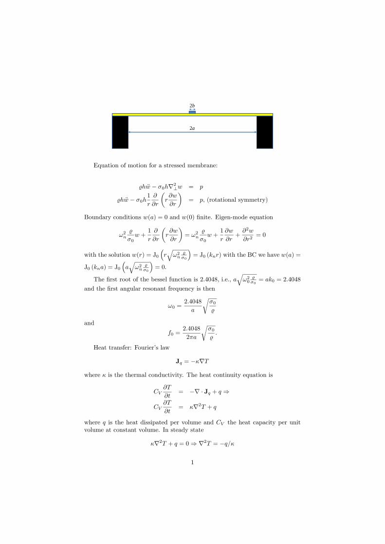
2a

2b

Equation of motion for a stressed membrane:

%hw − σ0h∇2⊥w = p

%hw − σ0h1

r

∂

∂r

(r∂w

∂r

)= p, (rotational symmetry)

Boundary conditions w(a) = 0 and w(0) finite. Eigen-mode equation

ω2n%

σ0w +

1

r

∂

∂r

(r∂w

∂r

)= ω2n

%

σ0w +

1

r

∂w

∂r+∂2w

∂r2= 0

with the solution w(r) = J0

(r√ω2n

%σ0

)= J0 (knr) with the BC we have w(a) =

J0 (kna) = J0

(a√ω2n

%σ0

)= 0.

The first root of the bessel function is 2.4048, i.e., a√ω20

%σ0

= ak0 = 2.4048

and the first angular resonant frequency is then

ω0 =2.4048

a

√σ0%

and

f0 =2.4048

2πa

√σ0%.

Heat transfer: Fourier’s law

Jq = −κ∇T

where κ is the thermal conductivity. The heat continuity equation is

CV∂T

∂t= −∇ · Jq + q ⇒

CV∂T

∂t= κ∇2T + q

where q is the heat dissipated per volume and CV the heat capacity per unitvolume at constant volume. In steady state

κ∇2T + q = 0⇒ ∇2T = −q/κ

1

by integration across the thickness of the membrane, and assuming zero tem-perature gradient in the z-direction, we have

∇2T = − Q

κh=

1

r

∂

∂r

(r∂T

∂r

)where Q is the heat dissipated per unit surface area. Assume now that thedissipation is confined to r < b an the temperature at r = a is fixed, then thetemperature varies logarithmically for r > b, i.e.,

∆T (r) = A lnr

a∂T

∂r=

A

rA

b= − P

κh

1

2πb⇒ A = − P

2πκh

∆T (r) = A lnr

a= − P

2πκhlnr

a, for a > r > b

where P = Qπb2. Inside the heated disc the temperature becomes

∆T =1

4

Q

κh

(b2 − r2

)− Qπb2

2πκhlnb

a=

1

4

P

πκh

(b2 − r2

)b2

− P

2πκhlnb

a

Stress-strain and displacement relations (assuming σz = 0 due to the freesurface, v = 0 due to rotational symmetry)

εr =1

E(σr − νσθ) + α∆T =

∂u

∂r

εθ =1

E(σθ − νσr) + α∆T =

u

r+

∂v

r∂θ=u

r

εz =1

E(−νσθ − νσr) + α∆T =

∂w

∂z

γrθ =∂u

r∂θ+∂v

∂r− v

r= 0

i.e.,

u = r

(1

E(σθ − νσr) + α∆T

)u =

∫ (1

E(σr − νσθ) + α∆T

)dr

Equation of equilibrium

∂σr∂r

+σr − σθ

r= 0

2

Timoshenko

σr = −αE 1

r2

∫ r

0

Trdr +E

1− ν2

(C1 (1 + ν)− C2

r2(1− ν)

)σθ = αE

1

r2

∫ r

0

Trdr − αET +E

1− ν2

(C1 (1 + ν) +

C2r2

(1− ν)

)u = (1 + ν)α

1

r

∫ r

0

Trdr + C1r +C2r

u(0) = 0⇒ C2 = 0, and u(a) = 0⇒ 0 = (1 + ν)α 1a∫ a0Trdr + C1a⇒

C1 = − (1 + ν)α1

a2

∫ a

0

Trdr

σr = −αE 1

r2

∫ r

0

Trdr − (1 + ν)2αE

1− ν21

a2

∫ a

0

Trdr

σr = −αE 1

r2

∫ r

0

Trdr − (1 + ν)αE

1− ν1

a2

∫ a

0

Trdr

σθ = αE1

r2

∫ r

0

Trdr − αET − (1 + ν)2αE

1− ν21

a2

∫ a

0

Trdr

= αE1

r2

∫ r

0

Trdr − αET − (1 + ν)αE

1− ν1

a2

∫ a

0

Trdr

0.1 Stress profile

Outside the heated area we have ∆T (r) = A ln ra = − P

2πκh ln ra , A = − P

2πκh andthen

σr = −αE 1

r2

∫ r

0

Trdr − (1 + ν)αE

1− ν1

a2

∫ a

0

Trdr

= −αE A

r2

∫ r

0

r ln( ra

)dr − (1 + ν)αE

1− νA

a2

∫ a

0

r ln( ra

)dr

since∫r ln

(ra

)dr = 1

2r2(ln r

a −12

)we have

∫ r0r ln

(ra

)dr = 1

2r2(ln r

a −12

)and∫ a

0r ln

(ra

)dr = − 14a

2, thus

σr = −αE A

r21

2r2(

lnr

a− 1

2

)− (1 + ν)αE

1− νA

a2

(−1

4a2)

=

= −αEA1

2

(lnr

a− 1

2

)+

(1 + ν)αE

1− νA

4=

σr =1

2AαE

(1

1− ν − lnr

a

)= − P

2πκh

αE

2

(1

1− ν − lnr

a

)σr = −αEP

4πκh

(1

1− ν − lnr

a

)=αEP

4πκh

(lnr

a− 1

1− ν

)

3

0.2 Equation of motion

When the stress is dependent on radial position the equation of motion mustbe modified

%hw − 1

r

∂

∂r

(σhr

∂w

∂r

)= p

%w − 1

r

∂

∂r

(σr∂w

∂r

)=

p

h

%w − σ[w′′rr +

1

rw′r

]− σ′rw′r =

p

h

where σ = σ0 + σr(r)This equation can probably not be solved with the logarithmic dependent

stress. But with Rayleighs quotiont we may get some progress anyway. Assum-ing harmonic solutions to the homogeneous equation we get

ω2%w + σ

[w′′rr +

1

rw′r

]+ σ′rw

′r = 0

and then

ω2 = −∫ (σ[w′′rr + 1

rw′r

]+ σ′rw

′r

)wrdr∫

(%w)wrdr= −

∫ a0

(σ[y′′rr + 1

ry′r

]+ σ′ry

′r

)yrdr∫ a

0(%y) yrdr

' −∫ a0

(σ0[y′′rr + 1

ry′r

])yrdr +

∫ a0

(σr[y′′rr + 1

ry′r

]+ σ′ry

′r

)yrdr∫ a

0(%y) yrdr

= ω20

[1 +

∫ a0

(σr[y′′rr + 1

ry′r

]+ σ′ry

′r

)yrdr∫ a

0

(σ0[y′′rr + 1

ry′r

])yrdr

]

where y(r) = J0 (k0r) is the eigenmode for σ = σ0. Here y′′rr+1ry′r = −k20 BesselJ0 (rk0) =

−k20yThus

ω2 = ω20

[1 +

∫ a0

(σr[y′′rr + 1

ry′r

]+ σ′ry

′r

)yrdr∫ a

0

(σ0[y′′rr + 1

ry′r

])yrdr

]= ω20

[1 +

∫ a0

(−k20yσr + σ′ry

′r

)yrdr∫ a

0(−k20yσ0) yrdr

]

= ω20

[1 +

∫ a0

(−k20y2σr + σ′ry

′ry)rdr∫ a

0(−k20y2σ0) rdr

]= ω20

1 +

∫ a0

(σry

2 − σ′rk20y′ry)rdr

σ0∫ a0y2rdr

The integrals∫ a0y2rdr =

∫ a0

J20 (k0r) rdr =[12r2(J20 (rk0) + J21 (rk0)

)]a0

= 12a2J21 (ak0)∫ a

0

(ln(ra

))y2rdr =

∫ a0

(ln(ra

))J20 (k0r) rdr =

[r2

4

[(2 ln r

a − 1)

J20 (k0r) + 2(ln r

a − 1)

J21 (k0r) + J0 (k0r) J2 (k0r)]]a0

=∫ a0

(ln(ra

))y2rdr = a2

4

[−2J21 (k0a)

]= −a22 J21 (k0a)

4

∫ a01ry′ryrdr = −k0

∫ a0

J1 (k0r) J0 (k0r) dr =[12J20 (k0r)

]a0

= − 12Since we have

σr = −αEP4πκh

(1

1− ν − lnr

a

)=αEP

4πκh

(lnr

a− 1

1− ν

)= B

(lnr

a− 1

1− ν

)σ′r =

B

r

we get

ω2 = ω20

1 +

∫ a0

(σry

2 − σ′rk20y′ry)rdr

σ0∫ a0y2rdr

= ω20

1 +−a22 J21 (k0a)B − 1

1−νB12a2J21 (ak0)− B

k20

(− 12)

σ012a2J21 (ak0)

= ω20

[1 +

B

σ0

(−1− 1

1− ν +1

k20a2J21 (ak0)

)]= ω20

[1 +

B

σ0

(−2− ν

1− ν +1

k20a2J21 (ak0)

)]=

= ω20

[1 +

B

σ0

(−2− ν

1− ν +1

1. 558 7

)]= ω20

[1 +

αEP

4πκh

1

σ0

(−2− ν

1− ν +1

1. 558 7

)]ω2 = ω20

[1− αEP

4πκh

1

σ0

(2− ν1− ν −

1

1. 558 7

)]= ω20

[1− αEP

4πκh

1

σ0

(1. 358 4− 0.358 44ν

1− ν

)]where ak0 = 2.4048The final result is that

ω2

ω20= 1− αEP

4πκh

1

σ0

(1. 358 4− 0.358 44ν

1− ν

)ω

ω0=

√1− αEP

4πκh

1

σ0

(1. 358 4− 0.358 44ν

1− ν

)' 1− αEP

8πκh

1

σ0

(1. 358 4− 0.358 44ν

1− ν

)or

∆f

f0' −αEP

8πκh

1

σ0

(1. 358 4− 0.358 44ν

1− ν

)

5

W

W h1

h2

JQb

JQt

T0

Here we consider a square membrane (side length W ) consisting of severalplanar layers with thicknesses hi, thermal conductivity κi and heat capacity pervolume ci, where i ∈ [1, 2 . . . N ]. The perimeter of the membrane is kept attemperature T = T0 and the membrane is heated by absorbing photons from acollimated light beam with a gaussian intensity profile, the absorbed power is P .The membrane may lose heat to the ambient gas at pressure p; the magnitudeof the heat flux densities are JQtop and JQbott at the top and bottom of themembrane, respectively.The heat continuity equation is

ci∂T

∂t= −∇·JQi+q(r, t) = ∇·(κi∇T )+q(r, t) ' κi∇2⊥T +

∂

∂z

(κi∂T

∂z

)+q(r, t)

where q(r, t) is the heat dissipation rate per unit volume and JQi = −κi∇T isthe heat current density, while ∇2⊥ is the two-dimensional Laplacian. Since themembrane is very thin compared to the width, we may take the temperatureas approximately constant in the z-direction; then an integral across the totalthickness of the membrane results in(∑

i

hici

)∂T

∂t=

(∑i

hiκi

)∇2⊥T − JQtop − JQbott +Q(x, y, t)

where Q(x, y, t) is the dissipated power area density.In a fairly large range of ambient pressures JQtop and JQbott may be expected

to vary linearily with pressure and membrane temperature, since the impingingmolecular flux density is 14nv and each molecule is expected to remove the energyf2kB(T −T0) where f is the number of degrees of freedom for the molecules (sayf = 6), n = p/ (kBT0) is the molecular density and v the mean molecular speed.It follows that

JQtop = JQbott =1

4nvf

2kB(T − T0) =

pvf

8T0(T − T0) =

1

2H (T − T0) .

1

And then the final PDE governing the temperature becomes(∑i

hici

)∂T

∂t=

(∑i

hiκi

)∇2⊥T −H (T − T0) +Q(x, y, t)

where we for convenience may take T0 = 0 such that the temperatures in theequation are the deviatory temperature, thus

C∂T

∂t= K∇2⊥T −HT +Q(x, y, t); C =

(∑i

hici

)and K =

(∑i

hiκi

)1

D

∂T

∂t= ∇2⊥T −

H

KT +

Q(x, y, t)

K; with D =

∑i hiκi∑i hici

At first we are only interessted in solutions that are symmetrical in x and y

and we may assume product solutions of the form ϕn = An cos(knx) cos(kny) exp(− tτn

)with cos(knW/2) = 0 ⇒ kn =

π(2n+1)W . For the homogeneous part of the PDE

we then get

− 1

Dτn= −2k2n −

H

K⇒ 1

τn= D

(2k2n +

H

K

)τn =

1

D(2k2n +

HK

)In particular for the first mode (n = 0) which decays slower than the highermodes

1

τ0= D

(2k20 +

H

K

)= D

(2π2

W 2+H

K

)=

2π2

W 2

∑i hiκi∑i hici

+H∑i hici

A numerical evaluation using:κ1 = 20Wm−1K−1

c1 = %Cp = 3100 kgm−3 × 700 J kg−1K−1

W = 1mmh1 = 100 nm

results in τ0 =(

2π2

(1mm)220Wm−1 K−1

3100 kgm−3×700 J kg−1 K−1

)−1= 5. 5ms which seems

to be in reasonable agreement with low pressure experiments.H = pvf

4T0

v =√

πkBT8m =

√π×1.3806568×10−23 JK−1×300K

8×(28×0.8+32×0.2)×1.6605402×10−27 kg = 184. 42ms

H1mbar =1mbar×184. 42 m

s ×64×300K = 92. 21 W

m2 K

Hlow =10−5mbar×184. 42 m

s ×64×300K = 9. 221× 10−4 W

m2 K

2

H1mbar

h1c1=

92. 21 Wm2 K

100 nm×3100 kgm−3×700 J kg−1 K−1 =424. 93

s

τ01mbar =1

2π2

(1mm)220Wm−1 K−1

3100 kgm−3×700 J kg−1 K−1+ 424. 93

s

= 1. 6ms

Hlow

h1c1=

9. 221×10−4 Wm2 K

100 nm×3100 kgm−3×700 J kg−1 K−1 =4. 249 3×10−3

s

τ0low =1

2π2

(1mm)220Wm−1 K−1

3100 kgm−3×700 J kg−1 K−1+ 4. 249 3×10−3

s

= 5. 5ms

Revised materials properties:Silicon Nitride: in ref (Review of Scientific Instruments 66, 1115 (1995); doi:

10.1063/1.1145989) we findκ1 = 12Wm−1K−1

D = (1.3− 1.7)× 10−6m2/ sτ0 =

(2π2

(1mm)212Wm−1 K−1

3100 kgm−3×700 J kg−1 K−1

)−1= 9. 161 1× 10−3 s

τ0 =(

2π2

(1mm)2D)−1

=(

2π2

(1mm)2(1.3)× 10−6m2/ s

)−1= 3. 897 0× 10−2 s(

2π2

(1mm)2(1.7)× 10−6m2/ s

)−1= 0.029 8 s

3

1 Circular membrane

Now, we consider a circular membrane of radius a and thickness h. The rim ofthe membrane is assumed to be at fixed temperature T0. The heat continuityequation is

c∂Θ

∂t= −∇ · JΘ + q(r, t)

where Θ = T − T0 is the temperature deviation, JΘ the heat flux density, andc is the heat capacity per unit volume. An integral over the volume of themembrane yields

c∂∫

ΘdV∂t

= πa2hc∂ 〈Θ〉∂t

= −∫

n·JΘdA+

∫q(r, t)dV =κh2πa

∂Θ(a, t)

∂r+P (a, t)

Here Gauss’s divergence theorem was used and 〈Θ〉 is the mean of the temper-ature deviation.In case of a Gaussian power distribution q(r, t) = q0 exp(−r2/(2σ2))× H(t)

(note q(r, t) is the power dissipated per unit volume and H(t) is Heavisides stepfunction) we have

P (r, t) = 2πhq0H(t)

∫ r

0

u exp(− u2

2σ2) du = πhq0H(t)2σ2

∫ r2

2σ2

0

exp(−z) dz

= πhq02σ2

(1− exp(− r2

2σ2)

)×H(t)

while

P (a, t) = πhq02σ2

(1− exp(− a2

2σ2)

)×H(t) = P0

[1− exp(− a2

2σ2)

]×H(t)

where P0 = πhq02σ2 is the full power in the beam and P (a, t) the power thatis received by the membrane.In steady state we have

0 = κh2πr∂Θ(r,∞)

∂r+ P (r,∞)

dΘs(r)

dr= − Ps(r)

κh2πr= −

P0

(1− exp(− r2

2σ2 ))

κh2πr

By integration we get

Θs(r) = −∫

Ps(r)

κh2πrdr = −

∫Ps(r)

κh4πr2dr2 =

= − P0

4πκh

∫ (1− exp(− r2

2σ2 ))

r2dr2 =

Θs(r) =P0

4πκh

(lna2

r2− Ei(

r2

2σ2) + Ei(

a2

2σ2)

)

1

where the exponential integral is Ei(z) =∫∞z

1t e−tdt, note, in some literature

E1(z) is used to signify this integral.The average temperature becomes

〈Θs〉 =1

πa2

∫ a

0

2πrΘs dr =1

a2

∫ a2

0

Θs dr2 =1

a2

P0

4πκh

∫ a2

0

(lna2

r2− Ei(

r2

2σ2) + Ei(

a2

2σ2)

)dr2

=P0

4πκh

1

a2

[a2 + 2σ2 exp

(− a2

2σ2

)− 2σ2

]=

P0

4πκh

[1 +

2σ2

a2exp

(− a2

2σ2

)− 2σ2

a2

]As a result, the thermal energy Q in the membrane is

Q = πa2hc 〈Θs〉 = τPs(a) = τP0

[1− exp(− a2

2σ2)

]and we may as indicated define a time constant τ by Q ≡ τPs(a), which resultsin

τ =πa2hc 〈Θs〉

P0

[1− exp(− a2

2σ2 )] =

a2c

4κ

1 + 2σ2

a2 exp(− a2

2σ2

)− 2σ2

a2

1− exp(− a2

2σ2 )

= τ0

1 + 2σ2

a2 exp(− a2

2σ2

)− 2σ2

a2

1− exp(− a2

2σ2 )

This time constant is seen to be dependent on the size of the beam as illustratedin the plot below. Note, τ0 = a2c

4κ = a2

4D is essentially the time constant expectedfor a delta-function power distribution.

Just for plotting1+ 2x2

12exp(− 12

2x2

)− 2x2

12

1−exp(− 12

2x2)

0.0 0.2 0.4 0.6 0.8 1.0

0.6

0.7

0.8

0.9

1.0

sigma/a

tau/tau_0

Figure 1: τ/τ0 as a function of σ/a.

U(r, a, σ) = ln a2

r2 − Ei( r2

2σ2 ) + Ei( a2

2σ2 )

2

U(r, 1, 0.1)

0.0 0.2 0.4 0.6 0.8 1.00

2

4

6

8

r/a

T­T0 in (au)

Temperature profile for σ/a = 0.01, 0.1, 0.2, and 0.5.

rU(r, 1, 0.1)

0.0 0.2 0.4 0.6 0.8 1.00.0

0.2

0.4

0.6

r/a

r(T­T0) in (au)

r(T − T0) profile for for σ/a = 0.01, 0.1, 0.2, and 0.5. In addition the profilefor a delta function beam.

2 Bessel modes

Separation of the variables in the circular geometry leads to the rotational sym-metric modes

ϕn(r, t) = J0(knr) exp(− t

τn)

for which any real transient or static temperature profile may be built. Theboundary condition T (a, t) = 0 requires that kna are zeroes of the Bessel func-tion, i.e. J0(kna) = 0. The first root is thus kna = 2.4048. The continuityequation requires τn = a2

D(kna)2 and thus the time constant for the slower mode

3

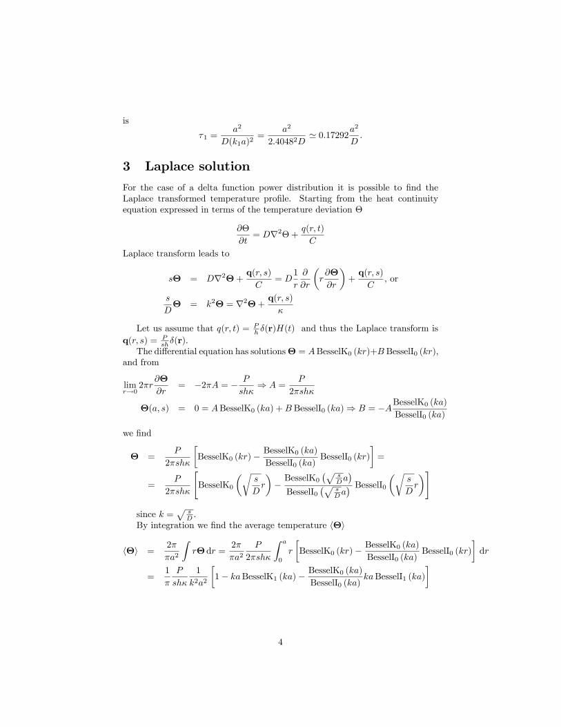
is

τ1 =a2

D(k1a)2=

a2

2.40482D' 0.17292

a2

D.

3 Laplace solution

For the case of a delta function power distribution it is possible to find theLaplace transformed temperature profile. Starting from the heat continuityequation expressed in terms of the temperature deviation Θ

∂Θ

∂t= D∇2Θ +

q(r, t)

C

Laplace transform leads to

sΘ = D∇2Θ +q(r, s)

C= D

1

r

∂

∂r

(r∂Θ

∂r

)+

q(r, s)

C, or

s

DΘ = k2Θ = ∇2Θ +

q(r, s)

κ

Let us assume that q(r, t) = Ph δ(r)H(t) and thus the Laplace transform is

q(r, s) = Pshδ(r).

The differential equation has solutionsΘ = ABesselK0 (kr)+B BesselI0 (kr),and from

limr→0

2πr∂Θ

∂r= −2πA = − P

shκ⇒ A =

P

2πshκ

Θ(a, s) = 0 = ABesselK0 (ka) +B BesselI0 (ka)⇒ B = −ABesselK0 (ka)

BesselI0 (ka)

we find

Θ =P

2πshκ

[BesselK0 (kr)− BesselK0 (ka)

BesselI0 (ka)BesselI0 (kr)

]=

=P

2πshκ

[BesselK0

(√s

Dr

)−

BesselK0

(√sDa)

BesselI0

(√sDa) BesselI0

(√s

Dr

)]

since k =√

sD .

By integration we find the average temperature 〈Θ〉

〈Θ〉 =2π

πa2

∫rΘ dr =

2π

πa2

P

2πshκ

∫ a

0

r

[BesselK0 (kr)− BesselK0 (ka)

BesselI0 (ka)BesselI0 (kr)

]dr

=1

π

P

shκ

1

k2a2

[1− kaBesselK1 (ka)− BesselK0 (ka)

BesselI0 (ka)kaBesselI1 (ka)

]

4

A Taylor expansion leads to

〈Θ〉 ' 1

π

P

4hκ

1

s

1

1 + 34×4 (ka)

2+ 5

576×4 (ka)4 '

' 1

π

P

4hκ

1

s

1

1 + 34×4 (ka)

2 =P

4πhκ

1

s

1

1 + 34×4

sa2

D

and thus a characteristic time constant of τ = 316a2

D .

3.1 Uniform heat distribution

If we now assume q(r, t) = Pπa2h×H(t) i.e. a uniform power distribution, we have

q(r, s) = Pπa2hs , then a particular solution is k

2Θp=P

πa2hκs ⇒ Θp=PD

πa2hκs2 =P

πa2hκs1k2 .

The homogeneous differential equation has solutions Θ = ABesselK0 (kr) +B BesselI0 (kr) in this case A = 0 and from the boundary conditions Θ(a, s) =B BesselI0 (ka) + P

πa2hκs1k2 = 0 we get B = − P

πa2hκs1

k2 BesselI0(ka) and thus

Θ(r, s) =P

πa2hκs

(1

k2− BesselI0 (kr)

k2 BesselI0 (ka)

)The average temperature becomes

〈Θ(s)〉 =2

a2

∫ a

0

rΘ(r, s)dr =P

πa2hκs× 2

a2

∫ a

0

r

(1

k2− BesselI0 (kr)

k2 BesselI0 (ka)

)dr

=P

πa2hκs× 2

a2

[a2

2k2− aBesselI1 (ka)

k3 BesselI0 (ka)

]=

P

πa2hκs×[

1

k2− 2 BesselI1 (ka)

ak3 BesselI0 (ka)

]=

P

πhκs×(

1

k2a2− 2 BesselI1 (ka)

a3k3 BesselI0 (ka)

)A Taylor expansion leads to

〈Θ(s)〉 ' P

πhκs

1

8

1

1 + 16 (ka)

2 =P

πhκs

1

8

1

1 + 16a2

D s⇒ τ =

1

6

a2

D,

but a better fit to 〈Θ(s)〉 over a wide range of Laplace frequencies is

〈Θ(s)〉 ' P

πhκs

1

8

1

1 + 16.45

a2

D s⇒ τ =

1

6.45

a2

D

which is obtained by integration.

Geometry Method τ τ NotesCircular Fundamental mode a2

2.40482D 0.173a2

D

Circular Average temperature Q/P a2

4D 0.25a2

D Beam width dependency

Circular Laplace, delta function 316a2

D 0.188a2

D

Circular Laplace, uniform 16.45

a2

D 0.155a2

D

Square Fundamental mode W 2

2π2D = 2(W/2)2

π2D 0.203 (W/2)2

D

5

0.0 0.5 1.0 1.5 2.0σ/a

4.0

4.2

4.4

4.6

4.8

5.0

5.2

τ(m

s)

FEM1st Bessel modeLaplace, deltaLaplace uniform

Figure 2: Time constants from FEM analysis and analytical models.

6

κ1 = 20 W m−1 K−1

c1 = %Cp = 3100 kg m−3 × 700 J kg−1 K−1

D = κ1c1

= 20 W m−1 K−1

3100 kg m−3×700 J kg−1 K−1= 9. 216 6× 10−6 m2

sa = 0.5 mm0.173a

2

D = 0.173× (0.5 mm)2

9. 216 6×10−6 m2

s

= 4. 692 6× 10−3 s

0.25a2

D = 0.25× (0.5 mm)2

9. 216 6×10−6 m2

s

= 6. 781 2× 10−3 s

316a2

D = 316 ×

(0.5 mm)2

9. 216 6×10−6 m2

s

= 5. 085 9× 10−3 s

1+2×(0.1)2

0.52exp(− 0.52

2×0.12

)− 2×0.12

0.52

1−exp(− 0.52

2×0.12 )× 6. 781 2× 10−3 s = 0.92× 6. 781 2× 10−3 s =

6. 238 7× 10−3 s

1 W cm−2 × 2× π × (100µm)2

= 6. 283 2× 10−4 m2

s3 kg

W = m2

s3 kg

P04πκh = 6. 0×10−4 W

4π×20 W m−1 K−1×0.1µm= 23. 873 tmpK = 25.0 tmpK

P04πκh

[1 + 2σ2

a2 exp(− a2

2σ2

)− 2σ2

a2

]=

1 + 2×0.12

0.52 exp(− 0.52

2×0.12

)− 2×0.12

0.52 = 0.92

23. 873× 0.92 = 21. 963 + 293.15 = 315. 11

1 + 2×0.22

0.52 exp(− 0.52

2×0.22

)− 2×0.22

0.52 = 0.694 06

0.694 06× 25.0 = 17. 352 + 293 = 310. 35

1 + 2×0.052

0.52 exp(− 0.52

2×0.052

)− 2×0.052

0.52 = 0.98

293.15 + 23. 873× 0.98 = 316. 55P0

4πκh

(ln a2

r2 − Ei( r2

2σ2 ) + Ei( a2

2σ2 ))

= 14πhκP0

(gamma + Ei

(12a2

σ2

)+ ln 1

2r2

σ2 + ln a2

r2

)−

18πh

r2

κσ2P0+ 164πh

r4

κσ4P0− 1576πh

r6

κσ6P0+ 16144πh

r8

κσ8P0− 176 800πh

r10

κσ10P0+ 11105 920πh

r12

κσ12

P0 − 118 063 360πh

r14

κσ14P0 + 1330 301 440πh

r16

κσ16P0 − 16688 604 160πh

r18

κσ18P0 +O(r20)

14πhκP0(gamma + Ei

(12

0.52

0.052

)+ ln 1

20.52

0.052

)ln 1

20.52

0.052 = 3. 912

Ei(

12

0.52

0.052

)= 3. 783 3× 10−24

ln 12

0.52

0.052 + gamma = 4. 489 2× 23. 873 = 107. 17 + 293.15 = 400. 32

∫r ln a2

r2 dr = 12a

2(

ln a2

a2 + 1)

= 12a

2

0.76 m−1 × 2π × 0.5 mm = 2. 387 6× 10−3

0.19 m−1 × 2π × 0.5 mm = 5. 969× 10−4

P04πκh

[1 + 2σ2

a2 exp(− a2

2σ2

)− 2σ2

a2

]P0

4πκh = 23. 873

7

1+ 2x2

12exp(− 12

2x2

)− 2x2

12

1−exp(− 12

2x2)

6.781 2sDΘ = k2Θ = ∇2Θ + q(r,s)

κ = 1r∂∂r

(r ∂Θ∂r

)+ q(r,s)

κThe homogeneous differential equation has solutions Θ = ABesselK0 (kr) +

B BesselI0 (kr)If we now assume q(r, t) = P

πa2h × H(t) i.e. a uniform power distribu-tion, we have q(r, s) = P

πa2hs , then a particular solution is k2Θp=

Pπa2hκs ⇒

Θp=PD

πa2hκs2 = Pπa2hκs

1k2 in this case A = 0 and from the boundary conditions

Θ(a, s) = B BesselI0 (ka) + Pπa2hκs

1k2 = 0 we get B = − P

πa2hκs1

k2 BesselI0(ka) andthus

Θ(r, s) =P

πa2hκs

(1

k2− BesselI0 (kr)

k2 BesselI0 (ka)

)

〈Θ(s)〉 =2

a2

∫ a

0

rΘ(r, s)dr =P

πa2hκs× 2

a2

∫ a

0

r

(1

k2− BesselI0 (kr)

k2 BesselI0 (ka)

)dr

=P

πa2hκs× 2

a2

[a2

2k2− aBesselI1 (ka)

k3 BesselI0 (ka)

]=

P

πa2hκs×[

1

k2− 2 BesselI1 (ka)

ak3 BesselI0 (ka)

]=

P

πhκs×(

1

k2a2− 2 BesselI1 (ka)

a3k3 BesselI0 (ka)

)' P

πhκs

1

8 + 43 (ka)

2 =P

πhκs

1

8

1

1 + 16 (ka)

2

=P

πhκs

1

8

1

1 + 16a2

D s⇒ τ =

1

6

a2

D∫rBesselI0 (kr) dr = rBesselI1(kr)

k1

1x2− 2 BesselI1(x)

x3 BesselI0(x)

= 8 + 43x

2 − 1144x

4 +O(x6)

16a2

D = 0.166 67a2

D = 16 ×

(0.5 mm)2

9. 216 6×10−6 m2

s

= 4. 520 8× 10−3 s

Pπhκ

18 = P

πhκs18 = 6. 0×10−4 W

8π×20 W m−1 K−1×0.1µm= 11. 937 tmpK

P04πκh = 6. 0×10−4 W

4π×20 W m−1 K−1×0.1µm

1− exp(− 12

2×12 ) = 0.393 47× 11. 937 = 4. 696 9

1k2 −

BesselI0(kr)k2 BesselI0(ka) =

(14a

2 − 14r

2)− k2

(364a

4 − 116a

2r2 + 164r

4)

+O(k4)(

14a

2 − 14r

2)2

= 116a

4 − 18a

2r2 + 116r

4

364a

4 − 116a

2r2 + 164r

4 − 12

(14a

2 − 14r

2)2

= 164a

4 − 164r

4

11k2− BesselI0(kr)

k2 BesselI0(ka)

= 114a

2− 14 r

2 + k2

( 14a2−14 r

2)2

(364a

4 − 116a

2r2 + 164r

4)

+O(k4)

1

( 14a2−14 r

2)2

(364a

4 − 116a

2r2 + 164r

4)

= 3a2−r24a2−4r2

11k2− BesselI0(kr)

k2 BesselI0(ka)

' 114a

2− 14 r

2 + k2 3a2−r24a2−4r2

8

1k2 −

BesselI0(kr)k2 BesselI0(ka) '

14 (a2−r2)

1+ 116k

2(3a2−r2)∫r

14 (a2−r2)

1+ 116k

2(3a2−r2)dr = 2

k4

(16 ln

(− 1k2

(3a2k2 − k2r2 + 16

))+ k2r2 + 2a2k2 ln

(− 1k2

(3a2k2 − k2r2 + 16

)))(

2 BesselI1(ka)a3k3 BesselI0(ka)

)−1

= a2k2 + 18a

4k4 − 1192a

6k6 +O(k8)

(1

k2a2 −2 BesselI1(ka)

a3k3 BesselI0(ka)

)−1

= 8 + 43a

2k2 − 1144a

4k4 +O(k6)

110 nm×1 cm2/( V s)×1017 cm−3×1.60217733×10−19 C = 6. 241 5×107

A2m2

s3 kg = 62415.A2

m2

s3 kg

310×√

22 = 219. 2

100/√

2 = 70. 71190/√

2 = 63. 640

BesselK0

(k

√(x− x0)

2+ y2

)− BesselK0

(k

√(−x+ x0 + d)

2+ y2

)q(k, x, y, d, x0) = BesselK0

(k

√(x− x0)

2+ y2

)−BesselK0

(k

√(−x+ x0 + d)

2+ y2

)BesselK0

(k

√(x− x0)

2+ y2

)−BesselK0

(k

√(−x+ x0 + d)

2+ y2

)=

(ln 1

2k

√(d− x+ x0)

2+ y2 − ln 1

2k

√(x− x0)

2+ y2

)−

k2

(((x− x0)

2+ y2

) (14 gamma− 1

4

)−(

(d− x+ x0)2

+ y2) (

14 gamma− 1

4

)+

(ln 1

2k

√(x− x0)

2+ y2

)(14 (x− x0)

2+ 1

4y2)−(

ln 12k

√(d− x+ x0)

2+ y2

)(14 (d− x+ x0)

2+ 1

4y2))−

k4

(((x− x0)

2+ y2

)2 (164 gamma− 3

128

)−(

(d− x+ x0)2

+ y2)2 (

164 gamma− 3

128

)+

(ln 1

2k

√(x− x0)

2+ y2

)((x− x0)

2+ y2

)(164 (x− x0)

2+ 1

64y2)−(

ln 12k

√(d− x+ x0)

2+ y2

)((d− x+ x0)

2+ y2

)(164 (d− x+ x0)

2+ 1

64y2))

+

O(k6)

BesselK0

(k

√(x− x0)

2+ y2

)+ αBesselI0

(k

√(x− x0)

2+ y2

)x2 + y2 = a2 ⇒ y2 = a2 − x2

BesselK0

(k

√(x− x0)

2+ a2 − x2

)+αBesselI0

(k

√(x− x0)

2+ a2 − x2

)=

0

α = −BesselK0

(k√

(x−x0)2+a2−x2)

BesselI0(k√

(x−x0)2+a2−x2)

(x− x0)2

+ a2 − x2 = a2 + x20 − 2xx0

BesselK0

(k√a2+x20−2xx0

)BesselI0

(k√a2+x20−2xx0

) = 1

BesselI0(k√a2+x20

) BesselK0

(k√a2 + x2

0

)+x

(k x0√

a2+x20 BesselI0(k√a2+x20

) BesselK1

(k√a2 + x2

0

)+ k x0√

a2+x20 BesselI0(k√a2+x20

)2 BesselI1

(k√a2 + x2

0

)BesselK0

(k√a2 + x2

0

))+

x2

1

BesselI0(k√a2+x20

) 1

2k2x2

0

BesselK0

(k√a2+x20

)+ 1

k√a2+x20

BesselK1

(k√a2+x20

)a2+x20

+ 12k

x20

(a2+x20)32

BesselK1

(k√a2 + x2

0

)−1

BesselI0

(k√a2+x20

) 1

2k2x20

BesselI0

(k√a2+x20

)− 1

k√a2+x20

BesselI1

(k√a2+x20

)a2+x20

− 12k

x20

(a2+x20)32

BesselI1(k√a2+x20

)−k2 x20

(a2+x20)BesselI0(k√a2+x20

)2 BesselI1(k√a2+x20

)2BesselI0

(k√a2+x20

) BesselK0

(k√a2 + x2

0

)+ k2 x20

(a2+x20) BesselI0(k√a2+x20

)2 BesselI1

(k√a2 + x2

0

)BesselK1

(k√a2 + x2

0

)+

9

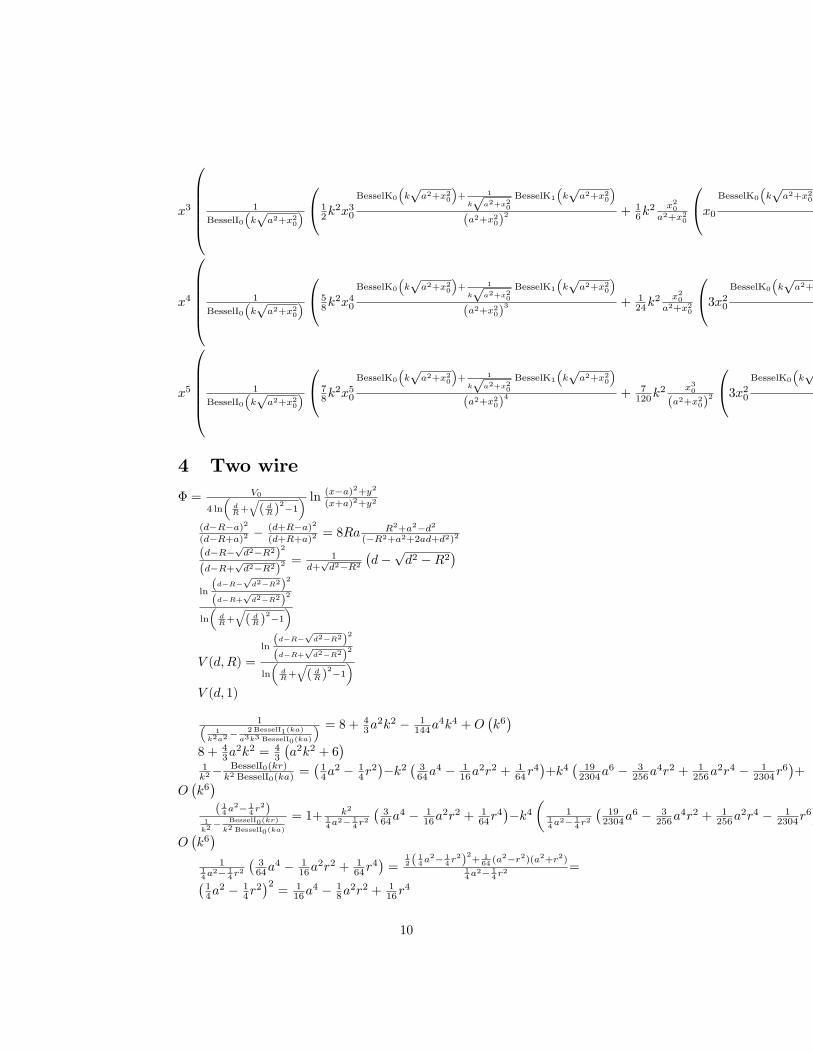
x3

1

BesselI0(k√a2+x20

) 1

2k2x3

0

BesselK0

(k√a2+x20

)+ 1

k√a2+x20

BesselK1

(k√a2+x20

)(a2+x20)

2 + 16k

2 x20a2+x20

x0

BesselK0

(k√a2+x20

)+ 1

k√a2+x20

BesselK1

(k√a2+x20

)a2+x20

+ k x0√a2+x20

BesselK1

(k√a2 + x2

0

)+ 1

kx0

(a2+x20)32

BesselK1

(k√a2 + x2

0

)+ 12k

x30

(a2+x20)52

BesselK1

(k√a2 + x2

0

)− 1

BesselI0(k√a2+x20

) BesselK0

(k√a2 + x2

0

)k x0√

a2+x20 BesselI0(k√a2+x20

)2 BesselI1

(k√a2 + x2

0

) 12k

2x20

BesselI0(k√a2+x20

)− 1

k√a2+x20

BesselI1(k√a2+x20

)a2+x20

− 12k

x20

(a2+x20)32

BesselI1

(k√a2 + x2

0

)− 1

BesselI0(k√a2+x20

) 1

6k2 x20a2+x20

k x0√a2+x20

BesselI1

(k√a2 + x2

0

)− x0

BesselI0(k√a2+x20

)− 1

k√a2+x20

BesselI1(k√a2+x20

)a2+x20

+ 1k

x0

(a2+x20)32

BesselI1

(k√a2 + x2

0

)− 12k

2x30

BesselI0(k√a2+x20

)− 1

k√a2+x20

BesselI1(k√a2+x20

)(a2+x20)

2 + 12k

x30

(a2+x20)52

BesselI1

(k√a2 + x2

0

)+ k x0√a2+x20

1

BesselI0

(k√a2+x20

) 1

2k2x20

BesselI0

(k√a2+x20

)− 1

k√a2+x20

BesselI1

(k√a2+x20

)a2+x20

− 12k

x20

(a2+x20)32

BesselI1(k√a2+x20

)−k2 x20

(a2+x20)BesselI0(k√a2+x20

)2 BesselI1(k√a2+x20

)2BesselI0

(k√a2+x20

) BesselI1

(k√a2 + x2

0

)+ k x0√

a2+x20 BesselI0(k√a2+x20

)2 BesselI1

(k√a2 + x2

0

) 12k

2x20

BesselK0

(k√a2+x20

)+ 1

k√a2+x20

BesselK1

(k√a2+x20

)a2+x20

+ 12k

x20

(a2+x20)32

BesselK1

(k√a2 + x2

0

)− k x0√a2+x20

1

BesselI0

(k√a2+x20

) 1

2k2x20

BesselI0

(k√a2+x20

)− 1

k√a2+x20

BesselI1

(k√a2+x20

)a2+x20

− 12k

x20

(a2+x20)32

BesselI1(k√a2+x20

)−k2 x20

(a2+x20)BesselI0(k√a2+x20

)2 BesselI1(k√a2+x20

)2BesselI0

(k√a2+x20

) BesselK1

(k√a2 + x2

0

)+

x4

1

BesselI0(k√a2+x20

) 5

8k2x4

0

BesselK0

(k√a2+x20

)+ 1

k√a2+x20

BesselK1

(k√a2+x20

)(a2+x20)

3 + 124k

2 x20a2+x20

3x20

BesselK0

(k√a2+x20

)+ 1

k√a2+x20

BesselK1

(k√a2+x20

)(a2+x20)

2 + x0a2+x20

x0

BesselK0

(k√a2+x20

)+ 1

k√a2+x20

BesselK1

(k√a2+x20

)a2+x20

+ k x0√a2+x20

BesselK1

(k√a2 + x2

0

)+ 1

kx0

(a2+x20)32

BesselK1

(k√a2 + x2

0

)+ k2x20

BesselK0

(k√a2+x20

)+ 1

k√a2+x20

BesselK1

(k√a2+x20

)a2+x20

+ 3k

x20

(a2+x20)52

BesselK1

(k√a2 + x2

0

)+ k

x20

(a2+x20)32

BesselK1

(k√a2 + x2

0

)+ 524k

2 x30

(a2+x20)2

x0

BesselK0

(k√a2+x20

)+ 1

k√a2+x20

BesselK1

(k√a2+x20

)a2+x20

+ k x0√a2+x20

BesselK1

(k√a2 + x2

0

)+ 1

kx0

(a2+x20)32

BesselK1

(k√a2 + x2

0

)+ 58k

x40

(a2+x20)72

BesselK1

(k√a2 + x2

0

)+ 1

BesselI0(k√a2+x20

) BesselK0

(k√a2 + x2

0

) 1

BesselI0(k√a2+x20

) 1

24k2 x20a2+x20

x0a2+x20

k x0√a2+x20

BesselI1

(k√a2 + x2

0

)− x0

BesselI0(k√a2+x20

)− 1

k√a2+x20

BesselI1(k√a2+x20

)a2+x20

+ 1k

x0

(a2+x20)32

BesselI1

(k√a2 + x2

0

)− 3x20

BesselI0(k√a2+x20

)− 1

k√a2+x20

BesselI1(k√a2+x20

)(a2+x20)

2 − k2x20

BesselI0(k√a2+x20

)− 1

k√a2+x20

BesselI1(k√a2+x20

)a2+x20

+ 3k

x20

(a2+x20)52

BesselI1

(k√a2 + x2

0

)+ k

x20

(a2+x20)32

BesselI1

(k√a2 + x2

0

)− 58k

2x40

BesselI0(k√a2+x20

)− 1

k√a2+x20

BesselI1(k√a2+x20

)(a2+x20)

3 + 524k

2 x30

(a2+x20)2

k x0√a2+x20

BesselI1

(k√a2 + x2

0

)− x0

BesselI0(k√a2+x20

)− 1

k√a2+x20

BesselI1(k√a2+x20

)a2+x20

+ 1k

x0

(a2+x20)32

BesselI1

(k√a2 + x2

0

)+ 58k

x40

(a2+x20)72

BesselI1

(k√a2 + x2

0

)+

1

BesselI0

(k√a2+x20

) 1

2k2x20

BesselI0

(k√a2+x20

)− 1

k√a2+x20

BesselI1

(k√a2+x20

)a2+x20

− 12k

x20

(a2+x20)32

BesselI1(k√a2+x20

)−k2 x20

(a2+x20)BesselI0(k√a2+x20

)2 BesselI1(k√a2+x20

)2BesselI0

(k√a2+x20

) 1

2k2x2

0

BesselI0(k√a2+x20

)− 1

k√a2+x20

BesselI1(k√a2+x20

)a2+x20

− 12k

x20

(a2+x20)32

BesselI1

(k√a2 + x2

0

)− k x0√a2+x20 BesselI0

(k√a2+x20

) BesselI1

(k√a2 + x2

0

)k x0√

a2+x20 BesselI0(k√a2+x20

)2 BesselI1

(k√a2 + x2

0

) 12k

2x20

BesselI0(k√a2+x20

)− 1

k√a2+x20

BesselI1(k√a2+x20

)a2+x20

− 12k

x20

(a2+x20)32

BesselI1

(k√a2 + x2

0

)− 1

BesselI0(k√a2+x20

) 1

6k2 x20a2+x20

k x0√a2+x20

BesselI1

(k√a2 + x2

0

)− x0

BesselI0(k√a2+x20

)− 1

k√a2+x20

BesselI1(k√a2+x20

)a2+x20

+ 1k

x0

(a2+x20)32

BesselI1

(k√a2 + x2

0

)− 12k

2x30

BesselI0(k√a2+x20

)− 1

k√a2+x20

BesselI1(k√a2+x20

)(a2+x20)

2 + 12k

x30

(a2+x20)52

BesselI1

(k√a2 + x2

0

)+ k x0√a2+x20

1

BesselI0

(k√a2+x20

) 1

2k2x20

BesselI0

(k√a2+x20

)− 1

k√a2+x20

BesselI1

(k√a2+x20

)a2+x20

− 12k

x20

(a2+x20)32

BesselI1(k√a2+x20

)−k2 x20

(a2+x20)BesselI0(k√a2+x20

)2 BesselI1(k√a2+x20

)2BesselI0

(k√a2+x20

) BesselI1

(k√a2 + x2

0

)+ k x0√

a2+x20 BesselI0(k√a2+x20

)2 BesselI1

(k√a2 + x2

0

) 16k

2 x20a2+x20

k x0√a2+x20

BesselI1

(k√a2 + x2

0

)− x0

BesselI0(k√a2+x20

)− 1

k√a2+x20

BesselI1(k√a2+x20

)a2+x20

+ 1k

x0

(a2+x20)32

BesselI1

(k√a2 + x2

0

)− 12k

2x30

BesselI0(k√a2+x20

)− 1

k√a2+x20

BesselI1(k√a2+x20

)(a2+x20)

2 + 12k

x30

(a2+x20)52

BesselI1

(k√a2 + x2

0

)−

1

BesselI0

(k√a2+x20

) 1

2k2x20

BesselI0

(k√a2+x20

)− 1

k√a2+x20

BesselI1

(k√a2+x20

)a2+x20

− 12k

x20

(a2+x20)32

BesselI1(k√a2+x20

)−k2 x20

(a2+x20)BesselI0(k√a2+x20

)2 BesselI1(k√a2+x20

)2BesselI0

(k√a2+x20

) 1

2k2x2

0

BesselK0

(k√a2+x20

)+ 1

k√a2+x20

BesselK1

(k√a2+x20

)a2+x20

+ 12k

x20

(a2+x20)32

BesselK1

(k√a2 + x2

0

)− k x0√a2+x20 BesselI0

(k√a2+x20

) BesselK1

(k√a2 + x2

0

)k x0√

a2+x20 BesselI0(k√a2+x20

)2 BesselI1

(k√a2 + x2

0

) 12k

2x20

BesselI0(k√a2+x20

)− 1

k√a2+x20

BesselI1(k√a2+x20

)a2+x20

− 12k

x20

(a2+x20)32

BesselI1

(k√a2 + x2

0

)− 1

BesselI0(k√a2+x20

) 1

6k2 x20a2+x20

k x0√a2+x20

BesselI1

(k√a2 + x2

0

)− x0

BesselI0(k√a2+x20

)− 1

k√a2+x20

BesselI1(k√a2+x20

)a2+x20

+ 1k

x0

(a2+x20)32

BesselI1

(k√a2 + x2

0

)− 12k

2x30

BesselI0(k√a2+x20

)− 1

k√a2+x20

BesselI1(k√a2+x20

)(a2+x20)

2 + 12k

x30

(a2+x20)52

BesselI1

(k√a2 + x2

0

)+ k x0√a2+x20

1

BesselI0

(k√a2+x20

) 1

2k2x20

BesselI0

(k√a2+x20

)− 1

k√a2+x20

BesselI1

(k√a2+x20

)a2+x20

− 12k

x20

(a2+x20)32

BesselI1(k√a2+x20

)−k2 x20

(a2+x20)BesselI0(k√a2+x20

)2 BesselI1(k√a2+x20

)2BesselI0

(k√a2+x20

) BesselI1

(k√a2 + x2

0

)+ k x0√

a2+x20 BesselI0(k√a2+x20

)2 BesselI1

(k√a2 + x2

0

) 12k

2x30

BesselK0

(k√a2+x20

)+ 1

k√a2+x20

BesselK1

(k√a2+x20

)(a2+x20)

2 + 16k

2 x20a2+x20

x0

BesselK0

(k√a2+x20

)+ 1

k√a2+x20

BesselK1

(k√a2+x20

)a2+x20

+ k x0√a2+x20

BesselK1

(k√a2 + x2

0

)+ 1

kx0

(a2+x20)32

BesselK1

(k√a2 + x2

0

)+ 12k

x30

(a2+x20)52

BesselK1

(k√a2 + x2

0

)+

x5

1

BesselI0(k√a2+x20

) 7

8k2x5

0

BesselK0

(k√a2+x20

)+ 1

k√a2+x20

BesselK1

(k√a2+x20

)(a2+x20)

4 + 7120k

2 x30

(a2+x20)2

3x20

BesselK0

(k√a2+x20

)+ 1

k√a2+x20

BesselK1

(k√a2+x20

)(a2+x20)

2 + x0a2+x20

x0

BesselK0

(k√a2+x20

)+ 1

k√a2+x20

BesselK1

(k√a2+x20

)a2+x20

+ k x0√a2+x20

BesselK1

(k√a2 + x2

0

)+ 1

kx0

(a2+x20)32

BesselK1

(k√a2 + x2

0

)+ k2x20

BesselK0

(k√a2+x20

)+ 1

k√a2+x20

BesselK1

(k√a2+x20

)a2+x20

+ 3k

x20

(a2+x20)52

BesselK1

(k√a2 + x2

0

)+ k

x20

(a2+x20)32

BesselK1

(k√a2 + x2

0

)+ 724k

2 x40

(a2+x20)3

x0

BesselK0

(k√a2+x20

)+ 1

k√a2+x20

BesselK1

(k√a2+x20

)a2+x20

+ k x0√a2+x20

BesselK1

(k√a2 + x2

0

)+ 1

kx0

(a2+x20)32

BesselK1

(k√a2 + x2

0

)+ 1120k

2 x20a2+x20

x0a2+x20

3x20

BesselK0

(k√a2+x20

)+ 1

k√a2+x20

BesselK1

(k√a2+x20

)(a2+x20)

2 + x0a2+x20

x0

BesselK0

(k√a2+x20

)+ 1

k√a2+x20

BesselK1

(k√a2+x20

)a2+x20

+ k x0√a2+x20

BesselK1

(k√a2 + x2

0

)+ 1

kx0

(a2+x20)32

BesselK1

(k√a2 + x2

0

)+ k2x20

BesselK0

(k√a2+x20

)+ 1

k√a2+x20

BesselK1

(k√a2+x20

)a2+x20

+ 3k

x20

(a2+x20)52

BesselK1

(k√a2 + x2

0

)+ k

x20

(a2+x20)32

BesselK1

(k√a2 + x2

0

)+ 5x20

(a2+x20)2

x0

BesselK0

(k√a2+x20

)+ 1

k√a2+x20

BesselK1

(k√a2+x20

)a2+x20

+ k x0√a2+x20

BesselK1

(k√a2 + x2

0

)+ 1

kx0

(a2+x20)32

BesselK1

(k√a2 + x2

0

)+ 15x30

BesselK0

(k√a2+x20

)+ 1

k√a2+x20

BesselK1

(k√a2+x20

)(a2+x20)

3 + 3k2x30

BesselK0

(k√a2+x20

)+ 1

k√a2+x20

BesselK1

(k√a2+x20

)(a2+x20)

2 + 15k

x30

(a2+x20)72

BesselK1

(k√a2 + x2

0

)+ k2 x20

a2+x20

x0

BesselK0

(k√a2+x20

)+ 1

k√a2+x20

BesselK1

(k√a2+x20

)a2+x20

+ k x0√a2+x20

BesselK1

(k√a2 + x2

0

)+ 1

kx0

(a2+x20)32

BesselK1

(k√a2 + x2

0

)+ 3kx30

(a2+x20)52

BesselK1

(k√a2 + x2

0

)+ 78k

x50

(a2+x20)92

BesselK1

(k√a2 + x2

0

)−1

BesselI0

(k√a2+x20

) 1

2k2x20

BesselI0

(k√a2+x20

)− 1

k√a2+x20

BesselI1

(k√a2+x20

)a2+x20

− 12k

x20

(a2+x20)32

BesselI1(k√a2+x20

)−k2 x20

(a2+x20)BesselI0(k√a2+x20

)2 BesselI1(k√a2+x20

)2BesselI0

(k√a2+x20

) 1

2k2x3

0

BesselK0

(k√a2+x20

)+ 1

k√a2+x20

BesselK1

(k√a2+x20

)(a2+x20)

2 + 16k

2 x20a2+x20

x0

BesselK0

(k√a2+x20

)+ 1

k√a2+x20

BesselK1

(k√a2+x20

)a2+x20

+ k x0√a2+x20

BesselK1

(k√a2 + x2

0

)+ 1

kx0

(a2+x20)32

BesselK1

(k√a2 + x2

0

)+ 12k

x30

(a2+x20)52

BesselK1

(k√a2 + x2

0

)− 1

BesselI0(k√a2+x20

) 1

2k2x2

0

BesselK0

(k√a2+x20

)+ 1

k√a2+x20

BesselK1

(k√a2+x20

)a2+x20

+ 12k

x20

(a2+x20)32

BesselK1

(k√a2 + x2

0

)k x0√

a2+x20 BesselI0(k√a2+x20

)2 BesselI1

(k√a2 + x2

0

) 12k

2x20

BesselI0(k√a2+x20

)− 1

k√a2+x20

BesselI1(k√a2+x20

)a2+x20

− 12k

x20

(a2+x20)32

BesselI1

(k√a2 + x2

0

)− 1

BesselI0(k√a2+x20

) 1

6k2 x20a2+x20

k x0√a2+x20

BesselI1

(k√a2 + x2

0

)− x0

BesselI0(k√a2+x20

)− 1

k√a2+x20

BesselI1(k√a2+x20

)a2+x20

+ 1k

x0

(a2+x20)32

BesselI1

(k√a2 + x2

0

)− 12k

2x30

BesselI0(k√a2+x20

)− 1

k√a2+x20

BesselI1(k√a2+x20

)(a2+x20)

2 + 12k

x30

(a2+x20)52

BesselI1

(k√a2 + x2

0

)+ k x0√a2+x20

1

BesselI0

(k√a2+x20

) 1

2k2x20

BesselI0

(k√a2+x20

)− 1

k√a2+x20

BesselI1

(k√a2+x20

)a2+x20

− 12k

x20

(a2+x20)32

BesselI1(k√a2+x20

)−k2 x20

(a2+x20)BesselI0(k√a2+x20

)2 BesselI1(k√a2+x20

)2BesselI0

(k√a2+x20

) BesselI1

(k√a2 + x2

0

)+ 1

BesselI0(k√a2+x20

) BesselK0

(k√a2 + x2

0

) 1

BesselI0(k√a2+x20

) 7

120k2 x30

(a2+x20)2

x0a2+x20

k x0√a2+x20

BesselI1

(k√a2 + x2

0

)− x0

BesselI0(k√a2+x20

)− 1

k√a2+x20

BesselI1(k√a2+x20

)a2+x20

+ 1k

x0

(a2+x20)32

BesselI1

(k√a2 + x2

0

)− 3x20

BesselI0(k√a2+x20

)− 1

k√a2+x20

BesselI1(k√a2+x20

)(a2+x20)

2 − k2x20

BesselI0(k√a2+x20

)− 1

k√a2+x20

BesselI1(k√a2+x20

)a2+x20

+ 3k

x20

(a2+x20)52

BesselI1

(k√a2 + x2

0

)+ k

x20

(a2+x20)32

BesselI1

(k√a2 + x2

0

)− 78k

2x50

BesselI0(k√a2+x20

)− 1

k√a2+x20

BesselI1(k√a2+x20

)(a2+x20)

4 + 724k

2 x40

(a2+x20)3

k x0√a2+x20

BesselI1

(k√a2 + x2

0

)− x0

BesselI0(k√a2+x20

)− 1

k√a2+x20

BesselI1(k√a2+x20

)a2+x20

+ 1k

x0

(a2+x20)32

BesselI1

(k√a2 + x2

0

)+ 1120k

2 x20a2+x20

x0a2+x20

x0a2+x20

k x0√a2+x20

BesselI1

(k√a2 + x2

0

)− x0

BesselI0(k√a2+x20

)− 1

k√a2+x20

BesselI1(k√a2+x20

)a2+x20

+ 1k

x0

(a2+x20)32

BesselI1

(k√a2 + x2

0

)− 3x20

BesselI0(k√a2+x20

)− 1

k√a2+x20

BesselI1(k√a2+x20

)(a2+x20)

2 − k2x20

BesselI0(k√a2+x20

)− 1

k√a2+x20

BesselI1(k√a2+x20

)a2+x20

+ 3k

x20

(a2+x20)52

BesselI1

(k√a2 + x2

0

)+ k

x20

(a2+x20)32

BesselI1

(k√a2 + x2

0

)+ 5x20

(a2+x20)2

k x0√a2+x20

BesselI1

(k√a2 + x2

0

)− x0

BesselI0(k√a2+x20

)− 1

k√a2+x20

BesselI1(k√a2+x20

)a2+x20

+ 1k

x0

(a2+x20)32

BesselI1

(k√a2 + x2

0

)− 15x30

BesselI0(k√a2+x20

)− 1

k√a2+x20

BesselI1(k√a2+x20

)(a2+x20)

3 − 3k2x30

BesselI0(k√a2+x20

)− 1

k√a2+x20

BesselI1(k√a2+x20

)(a2+x20)

2 + 15k

x30

(a2+x20)72

BesselI1

(k√a2 + x2

0

)+ k2 x20

a2+x20

k x0√a2+x20

BesselI1

(k√a2 + x2

0

)− x0

BesselI0(k√a2+x20

)− 1

k√a2+x20

BesselI1(k√a2+x20

)a2+x20

+ 1k

x0

(a2+x20)32

BesselI1

(k√a2 + x2

0

)+ 3kx30

(a2+x20)52

BesselI1

(k√a2 + x2

0

)+ 78k

x50

(a2+x20)92

BesselI1

(k√a2 + x2

0

)−1

BesselI0

(k√a2+x20

) 1

2k2x20

BesselI0

(k√a2+x20

)− 1

k√a2+x20

BesselI1

(k√a2+x20

)a2+x20

− 12k

x20

(a2+x20)32

BesselI1(k√a2+x20

)−k2 x20

(a2+x20)BesselI0(k√a2+x20

)2 BesselI1(k√a2+x20

)2BesselI0

(k√a2+x20

) 1

6k2 x20a2+x20

k x0√a2+x20

BesselI1

(k√a2 + x2

0

)− x0

BesselI0(k√a2+x20

)− 1

k√a2+x20

BesselI1(k√a2+x20

)a2+x20

+ 1k

x0

(a2+x20)32

BesselI1

(k√a2 + x2

0

)− 12k

2x30

BesselI0(k√a2+x20

)− 1

k√a2+x20

BesselI1(k√a2+x20

)(a2+x20)

2 + 12k

x30

(a2+x20)52

BesselI1

(k√a2 + x2

0

)+ 1

BesselI0(k√a2+x20

) 1

2k2x2

0

BesselI0(k√a2+x20

)− 1

k√a2+x20

BesselI1(k√a2+x20

)a2+x20

− 12k

x20

(a2+x20)32

BesselI1

(k√a2 + x2

0

)k x0√

a2+x20 BesselI0(k√a2+x20

)2 BesselI1

(k√a2 + x2

0

) 12k

2x20

BesselI0(k√a2+x20

)− 1

k√a2+x20

BesselI1(k√a2+x20

)a2+x20

− 12k

x20

(a2+x20)32

BesselI1

(k√a2 + x2

0

)− 1

BesselI0(k√a2+x20

) 1

6k2 x20a2+x20

k x0√a2+x20

BesselI1

(k√a2 + x2

0

)− x0

BesselI0(k√a2+x20

)− 1

k√a2+x20

BesselI1(k√a2+x20

)a2+x20

+ 1k

x0

(a2+x20)32

BesselI1

(k√a2 + x2

0

)− 12k

2x30

BesselI0(k√a2+x20

)− 1

k√a2+x20

BesselI1(k√a2+x20

)(a2+x20)

2 + 12k

x30

(a2+x20)52

BesselI1

(k√a2 + x2

0

)+ k x0√a2+x20

1

BesselI0

(k√a2+x20

) 1

2k2x20

BesselI0

(k√a2+x20

)− 1

k√a2+x20

BesselI1

(k√a2+x20

)a2+x20

− 12k

x20

(a2+x20)32

BesselI1(k√a2+x20

)−k2 x20

(a2+x20)BesselI0(k√a2+x20

)2 BesselI1(k√a2+x20

)2BesselI0

(k√a2+x20

) BesselI1

(k√a2 + x2

0

)+ k x0√

a2+x20 BesselI0(k√a2+x20

) BesselI1

(k√a2 + x2

0

) 1

BesselI0(k√a2+x20

) 1

24k2 x20a2+x20

x0a2+x20

k x0√a2+x20

BesselI1

(k√a2 + x2

0

)− x0

BesselI0(k√a2+x20

)− 1

k√a2+x20

BesselI1(k√a2+x20

)a2+x20

+ 1k

x0

(a2+x20)32

BesselI1

(k√a2 + x2

0

)− 3x20

BesselI0(k√a2+x20

)− 1

k√a2+x20

BesselI1(k√a2+x20

)(a2+x20)

2 − k2x20

BesselI0(k√a2+x20

)− 1

k√a2+x20

BesselI1(k√a2+x20

)a2+x20

+ 3k

x20

(a2+x20)52

BesselI1

(k√a2 + x2

0

)+ k

x20

(a2+x20)32

BesselI1

(k√a2 + x2

0

)− 58k

2x40

BesselI0(k√a2+x20

)− 1

k√a2+x20

BesselI1(k√a2+x20

)(a2+x20)

3 + 524k

2 x30

(a2+x20)2

k x0√a2+x20

BesselI1

(k√a2 + x2

0

)− x0

BesselI0(k√a2+x20

)− 1

k√a2+x20

BesselI1(k√a2+x20

)a2+x20

+ 1k

x0

(a2+x20)32

BesselI1

(k√a2 + x2

0

)+ 58k

x40

(a2+x20)72

BesselI1

(k√a2 + x2

0

)+

1

BesselI0

(k√a2+x20

) 1

2k2x20

BesselI0

(k√a2+x20

)− 1

k√a2+x20

BesselI1

(k√a2+x20

)a2+x20

− 12k

x20

(a2+x20)32

BesselI1(k√a2+x20

)−k2 x20

(a2+x20)BesselI0(k√a2+x20

)2 BesselI1(k√a2+x20

)2BesselI0

(k√a2+x20

) 1

2k2x2

0

BesselI0(k√a2+x20

)− 1

k√a2+x20

BesselI1(k√a2+x20

)a2+x20

− 12k

x20

(a2+x20)32

BesselI1

(k√a2 + x2

0

)− k x0√a2+x20 BesselI0

(k√a2+x20

) BesselI1

(k√a2 + x2

0

)k x0√

a2+x20 BesselI0(k√a2+x20

)2 BesselI1

(k√a2 + x2

0

) 12k

2x20

BesselI0(k√a2+x20

)− 1

k√a2+x20

BesselI1(k√a2+x20

)a2+x20

− 12k

x20

(a2+x20)32

BesselI1

(k√a2 + x2

0

)− 1

BesselI0(k√a2+x20

) 1

6k2 x20a2+x20

k x0√a2+x20

BesselI1

(k√a2 + x2

0

)− x0

BesselI0(k√a2+x20

)− 1

k√a2+x20

BesselI1(k√a2+x20

)a2+x20

+ 1k

x0

(a2+x20)32

BesselI1

(k√a2 + x2

0

)− 12k

2x30

BesselI0(k√a2+x20

)− 1

k√a2+x20

BesselI1(k√a2+x20

)(a2+x20)

2 + 12k

x30

(a2+x20)52

BesselI1

(k√a2 + x2

0

)+ k x0√a2+x20

1

BesselI0

(k√a2+x20

) 1

2k2x20

BesselI0

(k√a2+x20

)− 1

k√a2+x20

BesselI1

(k√a2+x20

)a2+x20

− 12k

x20

(a2+x20)32

BesselI1(k√a2+x20

)−k2 x20

(a2+x20)BesselI0(k√a2+x20

)2 BesselI1(k√a2+x20

)2BesselI0

(k√a2+x20

) BesselI1

(k√a2 + x2

0

)+ k x0√

a2+x20 BesselI0(k√a2+x20

)2 BesselI1

(k√a2 + x2

0

) 16k

2 x20a2+x20

k x0√a2+x20

BesselI1

(k√a2 + x2

0

)− x0

BesselI0(k√a2+x20

)− 1

k√a2+x20

BesselI1(k√a2+x20

)a2+x20

+ 1k

x0

(a2+x20)32

BesselI1

(k√a2 + x2

0

)− 12k

2x30

BesselI0(k√a2+x20

)− 1

k√a2+x20

BesselI1(k√a2+x20

)(a2+x20)

2 + 12k

x30

(a2+x20)52

BesselI1

(k√a2 + x2

0

)+ k x0√

a2+x20 BesselI0(k√a2+x20

)2 BesselI1

(k√a2 + x2

0

) 124k

2 x20a2+x20

x0a2+x20

k x0√a2+x20

BesselI1

(k√a2 + x2

0

)− x0

BesselI0(k√a2+x20

)− 1

k√a2+x20

BesselI1(k√a2+x20

)a2+x20

+ 1k

x0

(a2+x20)32

BesselI1

(k√a2 + x2

0

)− 3x20

BesselI0(k√a2+x20

)− 1

k√a2+x20

BesselI1(k√a2+x20

)(a2+x20)

2 − k2x20

BesselI0(k√a2+x20

)− 1

k√a2+x20

BesselI1(k√a2+x20

)a2+x20

+ 3k

x20

(a2+x20)52

BesselI1

(k√a2 + x2

0

)+ k

x20

(a2+x20)32

BesselI1

(k√a2 + x2

0

)− 58k

2x40

BesselI0(k√a2+x20

)− 1

k√a2+x20

BesselI1(k√a2+x20

)(a2+x20)

3 + 524k

2 x30

(a2+x20)2

k x0√a2+x20

BesselI1

(k√a2 + x2

0

)− x0

BesselI0(k√a2+x20

)− 1

k√a2+x20

BesselI1(k√a2+x20

)a2+x20

+ 1k

x0

(a2+x20)32

BesselI1

(k√a2 + x2

0

)+ 58k

x40

(a2+x20)72

BesselI1

(k√a2 + x2

0

)+ k x0√

a2+x20 BesselI0(k√a2+x20

) BesselK1

(k√a2 + x2

0

) 1

BesselI0(k√a2+x20

) 1

24k2 x20a2+x20

x0a2+x20

k x0√a2+x20

BesselI1

(k√a2 + x2

0

)− x0

BesselI0(k√a2+x20

)− 1

k√a2+x20

BesselI1(k√a2+x20

)a2+x20

+ 1k

x0

(a2+x20)32

BesselI1

(k√a2 + x2

0

)− 3x20

BesselI0(k√a2+x20

)− 1

k√a2+x20

BesselI1(k√a2+x20

)(a2+x20)

2 − k2x20

BesselI0(k√a2+x20

)− 1

k√

a2+x20

BesselI1(k√a2+x20

)a2+x20

+ 3k

x20

(a2+x20)52

BesselI1

(k√a2 + x2

0

)+ k

x20

(a2+x20)32

BesselI1

(k√a2 + x2

0

)− 58k

2x40

BesselI0(k√a2+x20

)− 1

k√a2+x20

BesselI1(k√a2+x20

)(a2+x20)

3 + 524k

2 x30

(a2+x20)2

k x0√a2+x20

BesselI1

(k√a2 + x2

0

)− x0

BesselI0(k√a2+x20

)− 1

k√a2+x20

BesselI1(k√a2+x20

)a2+x20

+ 1k

x0

(a2+x20)32

BesselI1

(k√a2 + x2

0

)+ 58k

x40

(a2+x20)72

BesselI1

(k√a2 + x2

0

)+

1

BesselI0

(k√a2+x20

) 1

2k2x20

BesselI0

(k√a2+x20

)− 1

k√a2+x20

BesselI1

(k√a2+x20

)a2+x20

− 12k

x20

(a2+x20)32

BesselI1(k√a2+x20

)−k2 x20

(a2+x20)BesselI0(k√a2+x20

)2 BesselI1(k√a2+x20

)2BesselI0

(k√a2+x20

) 1

2k2x2

0

BesselI0(k√a2+x20

)− 1

k√a2+x20

BesselI1(k√a2+x20

)a2+x20

− 12k

x20

(a2+x20)32

BesselI1

(k√a2 + x2

0

)− k x0√a2+x20 BesselI0

(k√a2+x20

) BesselI1

(k√a2 + x2

0

)k x0√

a2+x20 BesselI0(k√a2+x20

)2 BesselI1

(k√a2 + x2

0

) 12k

2x20

BesselI0(k√a2+x20

)− 1

k√a2+x20

BesselI1(k√a2+x20

)a2+x20

− 12k

x20

(a2+x20)32

BesselI1

(k√a2 + x2

0

)− 1

BesselI0(k√a2+x20

) 1

6k2 x20a2+x20

k x0√a2+x20

BesselI1

(k√a2 + x2

0

)− x0

BesselI0(k√a2+x20

)− 1

k√a2+x20

BesselI1(k√a2+x20

)a2+x20

+ 1k

x0

(a2+x20)32

BesselI1

(k√a2 + x2

0

)− 12k

2x30

BesselI0(k√a2+x20

)− 1

k√a2+x20

BesselI1(k√a2+x20

)(a2+x20)

2 + 12k

x30

(a2+x20)52

BesselI1

(k√a2 + x2

0

)+ k x0√a2+x20

1

BesselI0

(k√a2+x20

) 1

2k2x20

BesselI0

(k√a2+x20

)− 1

k√a2+x20

BesselI1

(k√a2+x20

)a2+x20

− 12k

x20

(a2+x20)32

BesselI1(k√a2+x20

)−k2 x20

(a2+x20)BesselI0(k√a2+x20

)2 BesselI1(k√a2+x20

)2BesselI0

(k√a2+x20

) BesselI1

(k√a2 + x2

0

)+ k x0√

a2+x20 BesselI0(k√a2+x20

)2 BesselI1

(k√a2 + x2

0

) 16k

2 x20a2+x20

k x0√a2+x20

BesselI1

(k√a2 + x2

0

)− x0

BesselI0(k√a2+x20

)− 1

k√a2+x20

BesselI1(k√a2+x20

)a2+x20

+ 1k

x0

(a2+x20)32

BesselI1

(k√a2 + x2

0

)− 12k

2x30

BesselI0(k√a2+x20

)− 1

k√a2+x20

BesselI1(k√a2+x20

)(a2+x20)

2 + 12k

x30

(a2+x20)52

BesselI1

(k√a2 + x2

0

)+ k x0√

a2+x20 BesselI0(k√a2+x20

)2 BesselI1

(k√a2 + x2

0

) 58k

2x40

BesselK0

(k√a2+x20

)+ 1

k√a2+x20

BesselK1

(k√a2+x20

)(a2+x20)

3 + 124k

2 x20a2+x20

3x20

BesselK0

(k√a2+x20

)+ 1

k√a2+x20

BesselK1

(k√a2+x20

)(a2+x20)

2 + x0a2+x20

x0

BesselK0

(k√a2+x20

)+ 1

k√a2+x20

BesselK1

(k√a2+x20

)a2+x20

+ k x0√a2+x20

BesselK1

(k√a2 + x2

0

)+ 1

kx0

(a2+x20)32

BesselK1

(k√a2 + x2

0

)+ k2x20

BesselK0

(k√a2+x20

)+ 1

k√a2+x20

BesselK1

(k√a2+x20

)a2+x20

+ 3k

x20

(a2+x20)52

BesselK1

(k√a2 + x2

0

)+ k

x20

(a2+x20)32

BesselK1

(k√a2 + x2

0

)+ 524k

2 x30

(a2+x20)2

x0

BesselK0

(k√a2+x20

)+ 1

k√a2+x20

BesselK1

(k√a2+x20

)a2+x20

+ k x0√a2+x20

BesselK1

(k√a2 + x2

0

)+ 1

kx0

(a2+x20)32

BesselK1

(k√a2 + x2

0

)+ 58k

x40

(a2+x20)72

BesselK1

(k√a2 + x2

0

)+O

(x6)

4 Two wire

Φ = V0

4 ln

(dR+√

( dR )2−1

) ln (x−a)2+y2

(x+a)2+y2

(d−R−a)2

(d−R+a)2− (d+R−a)2

(d+R+a)2= 8Ra R2+a2−d2

(−R2+a2+2ad+d2)2

(d−R−√d2−R2)

2

(d−R+√d2−R2)

2 = 1d+√d2−R2

(d−√d2 −R2

)ln

(d−R−√d2−R2)

2

(d−R+√d2−R2)

2

ln

(dR+√

( dR )2−1

)

V (d,R) =

ln(d−R−

√d2−R2)

2

(d−R+√d2−R2)

2

ln

(dR+√

( dR )2−1

)V (d, 1)

1(1

k2a2− 2 BesselI1(ka)

a3k3 BesselI0(ka)

) = 8 + 43a

2k2 − 1144a

4k4 +O(k6)

8 + 43a

2k2 = 43

(a2k2 + 6

)1k2−

BesselI0(kr)k2 BesselI0(ka) =

(14a

2 − 14r

2)−k2

(364a

4 − 116a

2r2 + 164r

4)+k4

(19

2304a6 − 3

256a4r2 + 1

256a2r4 − 1

2304r6)+

O(k6)( 14a

2− 14 r

2)1k2− BesselI0(kr)

k2 BesselI0(ka)

= 1+ k214a

2− 14 r

2

(364a

4 − 116a

2r2 + 164r

4)−k4

(1

14a

2− 14 r

2

(19

2304a6 − 3

256a4r2 + 1

256a2r4 − 1

2304r6)− 1

( 14a2−14 r

2)2

(364a

4 − 116a

2r2 + 164r

4)2)

+

O(k6)

114a

2− 14 r

2

(364a

4 − 116a

2r2 + 164r

4)

=12 ( 14a

2− 14 r

2)2+ 164 (a2−r2)(a2+r2)

14a

2− 14 r

2 =(14a

2 − 14r

2)2

= 116a

4 − 18a

2r2 + 116r

4

10

(364a

4 − 116a

2r2 + 164r

4)− 1

2

(14a

2 − 14r

2)2

= 164a

4 − 164r

4 =164a

4 − 164r

4 = 164 (a2 − r2)(a2 + r2) is true

1214 (a2−r2)

2+ 164 (a2−r2)(a2+r2)

14 (a2−r2)

=1214 (a2−r2)+ 1

64 (a2+r2)14

= 916a

2 − 716r

2 = 18a

2 +716

(a2 − r2

)(1k2 −

BesselI0(k0)k2 BesselI0(ka)

)−1

= 4a2 + 3

4k2 + 5

576a2k4 +O

(k6)(

1k2 −

BesselI0(ka/2)k2 BesselI0(ka)

)−1

= 163a2 + 11

12k2 − 1

2304a2k4 +O

(k6)

1112

316(1k2 −

BesselI0(kr)k2 BesselI0(ka)

)−1

= 114a

2− 14 r

2 + k2

( 14a2−14 r

2)2

(364a

4 − 116a

2r2 + 164r

4)−

k4

114a2− 1

4r2

( 192304a

6− 3256a

4r2+ 1256a

2r4− 12304 r

6)− 1

( 14 a2− 14r2)

2 ( 364a

4− 116a

2r2+ 164 r

4)2

14a

2− 14 r

2 +O(k6)

1

( 14a2−14 r

2)

(364a

4 − 116a

2r2 + 164r

4)

16

3( 14 12− 14 r

2)

(36414 − 1

1612r2 + 164r

4)

0.0 0.1 0.2 0.3 0.4 0.5 0.6 0.7 0.8 0.9 1.0

0.7

0.8

0.9

1.0

x

y

(1

k2a2 −2 BesselI1(ka)

a3k3 BesselI0(ka)

)−1

= 8 + 43a

2k2 − 1144a

4k4 +O(k6)(

1k2a2 −

2 BesselI1(ka)a3k3 BesselI0(ka)

)= 1

8 −148a

2k2 + 113072a

4k4 +O(k6)

akBesselI0 (ka)− 2 BesselI1 (ka) = 18a

3k3 + 196a

5k5 + 13072a

7k7 +O(k9)

a3k3 BesselI0 (ka) = a3k3 + 14a

5k5 + 164a

7k7 +O(k9)

18a

3k3+ 196a

5k5+ 13072a

7k7

a3k3+ 14a

5k5+ 164a

7k7= a4k4+32a2k2+384

48a4k4+768a2k2+30727683072 = 1

432384 = 1

12

11

3843072 = 1

848

3072 = 164

D(a, k) =(

1k2a2 −

2 BesselI1(ka)a3k3 BesselI0(ka)

)D(1,

√s) = 1

s −2

s32 BesselI0(

√s)

BesselI1 (√s)

11s−

2

s32 BesselI0(

√s)

BesselI1(√s)

= 8 + 43s−

1144s

2 + 14320s

3 − 7829 440s

4 + 1134 836 480

s5 +O(s6)

11s−

2

s32 BesselI0(

√s)

BesselI1(√s)× 1

8 = 1 + 16s −

11152s

2 + 134 560s

3 − 76635 520s

4 +

11278 691 840s

5 − 797535 088 332 800s

6 + 1813210 529 996 800s

7 +O(s8)

(D(1,√x))−1

0 10 20 30 40 50

10

20

30

40

50

60

70

x

y

L(s, α) = 11s−

2

s32 BesselI0(

√s)

BesselI1(√s)× 1

8(1+s/α)

L(s, 6.45)

12

0 10 20 30 40 50

0.92

0.94

0.96

0.98

1.00

1.02

x

y

∫ 6×10

01

1s−

2

s32 BesselI0(

√s)

BesselI1(√s)× 1

8ds = 332. 91 = 100. 37 = 43. 815 = 8.

945 5∫ 6×10

0(1 + αs)ds = 1800α+ 60 = 450α+ 30 = 162α+ 18 = 18α+ 6

18α+ 6 = 8. 945 5, Solution is: (0.163 64)−1

= 6. 111 0

162α+ 18 = 43. 815, Solution is: (0.159 35)−1

= 6. 275 5450/α+ 30 = 100. 37, Solution is: 6. 394 81800/α+ 60 = 332. 91, Solution is: 6. 595 6

P (K) =

∫ 6×K0

11s− 2

s32 BesselI0(

√s)

BesselI1(√s)× 18−1

ds∫ 6×K0

sds

(P (20))−1

= 6. 822 2 = 6. 200 7 = 6. 394 8 = 6. 595 6

(P (x))−1

13

…And There Was Light