HAL Id: hal-03045922https://hal.archives-ouvertes.fr/hal-03045922

Submitted on 22 Nov 2021

HAL is a multi-disciplinary open accessarchive for the deposit and dissemination of sci-entific research documents, whether they are pub-lished or not. The documents may come fromteaching and research institutions in France orabroad, or from public or private research centers.

L’archive ouverte pluridisciplinaire HAL, estdestinée au dépôt et à la diffusion de documentsscientifiques de niveau recherche, publiés ou non,émanant des établissements d’enseignement et derecherche français ou étrangers, des laboratoirespublics ou privés.

Distributed under a Creative Commons Attribution| 4.0 International License

Gaia Early Data Release 3: The Gaia Catalogue ofNearby Stars

Richard Smart, L. Sarro, J. Rybizki, C. Reylé, A. Robin, N.C. Hambly, U.Abbas, M.A. Barstow, J.H.J. De Bruijne, B. Bucciarelli, et al.

To cite this version:Richard Smart, L. Sarro, J. Rybizki, C. Reylé, A. Robin, et al.. Gaia Early Data Release 3: The GaiaCatalogue of Nearby Stars. Astronomy and Astrophysics - A&A, EDP Sciences, 2021, 649, pp.A6.10.1051/0004-6361/202039498. hal-03045922

Astronomy&AstrophysicsSpecial issue

A&A 649, A6 (2021)https://doi.org/10.1051/0004-6361/202039498© ESO 2021

Gaia Early Data Release 3

Gaia Early Data Release 3

The Gaia Catalogue of Nearby Stars?

Gaia Collaboration: R. L. Smart1,??, L. M. Sarro2, J. Rybizki3, C. Reylé4, A. C. Robin4, N. C. Hambly5, U. Abbas1,M. A. Barstow6, J. H. J. de Bruijne7, B. Bucciarelli1, J. M. Carrasco8, W. J. Cooper9,1, S. T. Hodgkin10, E. Masana8,

D. Michalik7, J. Sahlmann11, A. Sozzetti1, A. G. A. Brown12, A. Vallenari13, T. Prusti7, C. Babusiaux14,15,M. Biermann16, O. L. Creevey17, D. W. Evans10, L. Eyer18, A. Hutton19, F. Jansen7, C. Jordi8, S. A. Klioner20,

U. Lammers21, L. Lindegren22, X. Luri8, F. Mignard17, C. Panem23, D. Pourbaix24,25, S. Randich26, P. Sartoretti15,C. Soubiran27, N. A. Walton10, F. Arenou15, C. A. L. Bailer-Jones3, U. Bastian16, M. Cropper28, R. Drimmel1,D. Katz15, M. G. Lattanzi1,29, F. van Leeuwen10, J. Bakker21, J. Castañeda30, F. De Angeli10, C. Ducourant27,

C. Fabricius8, M. Fouesneau3, Y. Frémat31, R. Guerra21, A. Guerrier23, J. Guiraud23, A. Jean-Antoine Piccolo23,R. Messineo32, N. Mowlavi18, C. Nicolas23, K. Nienartowicz33,34, F. Pailler23, P. Panuzzo15, F. Riclet23, W. Roux23,

G. M. Seabroke28, R. Sordo13, P. Tanga17, F. Thévenin17, G. Gracia-Abril35,16, J. Portell8, D. Teyssier36,M. Altmann16,37, R. Andrae3, I. Bellas-Velidis38, K. Benson28, J. Berthier39, R. Blomme31, E. Brugaletta40,

P. W. Burgess10, G. Busso10, B. Carry17, A. Cellino1, N. Cheek41, G. Clementini42, Y. Damerdji43,44, M. Davidson5,L. Delchambre43, A. Dell’Oro26, J. Fernández-Hernández45, L. Galluccio17, P. García-Lario21,

M. Garcia-Reinaldos21, J. González-Núñez41,46, E. Gosset43,25, R. Haigron15, J.-L. Halbwachs47, D. L. Harrison10,48,D. Hatzidimitriou49, U. Heiter50, J. Hernández21, D. Hestroffer39, B. Holl18,33, K. Janßen51, G. Jevardat de Fombelle18,

S. Jordan16, A. Krone-Martins52,53, A. C. Lanzafame40,54, W. Löffler16, A. Lorca19, M. Manteiga55, O. Marchal47,P. M. Marrese56,57, A. Moitinho52, A. Mora19, K. Muinonen58,59, P. Osborne10, E. Pancino26,57, T. Pauwels31,

A. Recio-Blanco17, P. J. Richards60, M. Riello10, L. Rimoldini33, T. Roegiers61, C. Siopis24, M. Smith28, A. Ulla62,E. Utrilla19, M. van Leeuwen10, W. van Reeven19, A. Abreu Aramburu45, S. Accart63, C. Aerts64,65,3, J. J. Aguado2,

M. Ajaj15, G. Altavilla56,57, M. A. Álvarez66, J. Álvarez Cid-Fuentes67, J. Alves68, R. I. Anderson69,E. Anglada Varela45, T. Antoja8, M. Audard33, D. Baines36, S. G. Baker28, L. Balaguer-Núñez8, E. Balbinot70,

Z. Balog16,3, C. Barache37, D. Barbato18,1, M. Barros52, S. Bartolomé8, J.-L. Bassilana63, N. Bauchet39,A. Baudesson-Stella63, U. Becciani40, M. Bellazzini42, M. Bernet8, S. Bertone71,72,1, L. Bianchi73,

S. Blanco-Cuaresma74, T. Boch47, A. Bombrun75, D. Bossini76, S. Bouquillon37, A. Bragaglia42, L. Bramante32,E. Breedt10, A. Bressan77, N. Brouillet27, A. Burlacu78, D. Busonero1, A. G. Butkevich1, R. Buzzi1, E. Caffau15,

R. Cancelliere79, H. Cánovas19, T. Cantat-Gaudin8, R. Carballo80, T. Carlucci37, M. I Carnerero1, L. Casamiquela27,M. Castellani56, A. Castro-Ginard8, P. Castro Sampol8, L. Chaoul23, P. Charlot27, L. Chemin81, A. Chiavassa17,

M.-R. L. Cioni51, G. Comoretto82, T. Cornez63, S. Cowell10, F. Crifo15, M. Crosta1, C. Crowley75, C. Dafonte66,A. Dapergolas38, M. David83, P. David39, P. de Laverny17, F. De Luise84, R. De March32, J. De Ridder64, R. de Souza85,

P. de Teodoro21, A. de Torres75, E. F. del Peloso16, E. del Pozo19, A. Delgado10, H. E. Delgado2, J.-B. Delisle18,P. Di Matteo15, S. Diakite86, C. Diener10, E. Distefano40, C. Dolding28, D. Eappachen87,65, B. Edvardsson88, H. Enke51,

P. Esquej11, C. Fabre89, M. Fabrizio56,57, S. Faigler90, G. Fedorets58,91, P. Fernique47,92, A. Fienga93,39, F. Figueras8,C. Fouron78, F. Fragkoudi94, E. Fraile11, F. Franke95, M. Gai1, D. Garabato66, A. Garcia-Gutierrez8,

M. García-Torres96, A. Garofalo42, P. Gavras11, E. Gerlach20, R. Geyer20, P. Giacobbe1, G. Gilmore10, S. Girona67,G. Giuffrida56, R. Gomel90, A. Gomez66, I. Gonzalez-Santamaria66, J. J. González-Vidal8, M. Granvik58,97,

R. Gutiérrez-Sánchez36, L. P. Guy33,82, M. Hauser3,98, M. Haywood15, A. Helmi70, S. L. Hidalgo99,100, T. Hilger20,N. Hładczuk21, D. Hobbs22, G. Holland10, H. E. Huckle28, G. Jasniewicz101, P. G. Jonker65,87, J. Juaristi Campillo16,

F. Julbe8, L. Karbevska18, P. Kervella102, S. Khanna70, A. Kochoska103, M. Kontizas49, G. Kordopatis17, A. J. Korn50,Z. Kostrzewa-Rutkowska12,87, K. Kruszynska104, S. Lambert37, A. F. Lanza40, Y. Lasne63, J.-F. Le Campion105,

Y. Le Fustec78, Y. Lebreton102,106, T. Lebzelter68, S. Leccia107, N. Leclerc15, I. Lecoeur-Taibi33, S. Liao1, E. Licata1,H. E. P. Lindstrøm1,108, T. A. Lister109, E. Livanou49, A. Lobel31, P. Madrero Pardo8, S. Managau63, R. G. Mann5,

J. M. Marchant110, M. Marconi107, M. M. S. Marcos Santos41, S. Marinoni56,57, F. Marocco111,112, D. J. Marshall113,L. Martin Polo41, J. M. Martín-Fleitas19, A. Masip8, D. Massari42, A. Mastrobuono-Battisti22, T. Mazeh90,

? Tables are only available at the CDS via anonymous ftp to cdsarc.u-strasbg.fr (130.79.128.5) or via http://cdsarc.u-strasbg.fr/viz-bin/cat/J/A+A/649/A6?? Corresponding author; e-mail: richard.smart@inaf.it

Article published by EDP Sciences A6, page 1 of 44

A&A 649, A6 (2021)

P. J. McMillan22, S. Messina40, N. R. Millar10, A. Mints51, D. Molina8, R. Molinaro107, L. Molnár114,115,116,P. Montegriffo42, R. Mor8, R. Morbidelli1, T. Morel43, D. Morris5, A. F. Mulone32, D. Munoz63, T. Muraveva42,

C. P. Murphy21, I. Musella107, L. Noval63, C. Ordénovic17, G. Orrù32, J. Osinde11, C. Pagani6, I. Pagano40,L. Palaversa117,10, P. A. Palicio17, A. Panahi90, M. Pawlak118,104, X. Peñalosa Esteller8, A. Penttilä58,

A. M. Piersimoni84, F.-X. Pineau47, E. Plachy114,115,116, G. Plum15, E. Poggio1, E. Poretti119, E. Poujoulet120, A. Prša103,L. Pulone56, E. Racero41,121, S. Ragaini42, M. Rainer26, C. M. Raiteri1, N. Rambaux39, P. Ramos8, M. Ramos-Lerate122,

P. Re Fiorentin1, S. Regibo64, V. Ripepi107, A. Riva1, G. Rixon10, N. Robichon15, C. Robin63, M. Roelens18,L. Rohrbasser33, M. Romero-Gómez8, N. Rowell5, F. Royer15, K. A. Rybicki104, G. Sadowski24, A. Sagristà Sellés16,

J. Salgado36, E. Salguero45, N. Samaras31, V. Sanchez Gimenez8, N. Sanna26, R. Santoveña66, M. Sarasso1,M. Schultheis17, E. Sciacca40, M. Segol95, J. C. Segovia41, D. Ségransan18, D. Semeux89, S. Shahaf90, H. I. Siddiqui123,

A. Siebert47,92, L. Siltala58, E. Slezak17, E. Solano124, F. Solitro32, D. Souami102,125, J. Souchay37, A. Spagna1,F. Spoto74, I. A. Steele110, H. Steidelmüller20, C. A. Stephenson36, M. Süveges33,126,3, L. Szabados114,

E. Szegedi-Elek114, F. Taris37, G. Tauran63, M. B. Taylor127, R. Teixeira85, W. Thuillot39, N. Tonello67, F. Torra30,J. Torra†,8, C. Turon15, N. Unger18, M. Vaillant63, E. van Dillen95, O. Vanel15, A. Vecchiato1, Y. Viala15, D. Vicente67,

S. Voutsinas5, M. Weiler8, T. Wevers10, Ł. Wyrzykowski104, A. Yoldas10, P. Yvard95, H. Zhao17, J. Zorec128,S. Zucker129, C. Zurbach130, and T. Zwitter131

(Affiliations can be found after the references)

Received 22 September 2020 / Accepted 30 October 2020

ABSTRACT

Aims. We produce a clean and well-characterised catalogue of objects within 100 pc of the Sun from the Gaia Early Data Release 3.We characterise the catalogue through comparisons to the full data release, external catalogues, and simulations. We carry out a firstanalysis of the science that is possible with this sample to demonstrate its potential and best practices for its use.Methods. The selection of objects within 100 pc from the full catalogue used selected training sets, machine-learning procedures,astrometric quantities, and solution quality indicators to determine a probability that the astrometric solution is reliable. The training setconstruction exploited the astrometric data, quality flags, and external photometry. For all candidates we calculated distance posteriorprobability densities using Bayesian procedures and mock catalogues to define priors. Any object with reliable astrometry and a non-zero probability of being within 100 pc is included in the catalogue.Results. We have produced a catalogue of 331 312 objects that we estimate contains at least 92% of stars of stellar type M9 within100 pc of the Sun. We estimate that 9% of the stars in this catalogue probably lie outside 100 pc, but when the distance probabilityfunction is used, a correct treatment of this contamination is possible. We produced luminosity functions with a high signal-to-noiseratio for the main-sequence stars, giants, and white dwarfs. We examined in detail the Hyades cluster, the white dwarf population,and wide-binary systems and produced candidate lists for all three samples. We detected local manifestations of several streams,superclusters, and halo objects, in which we identified 12 members of Gaia Enceladus. We present the first direct parallaxes of fiveobjects in multiple systems within 10 pc of the Sun.Conclusions. We provide the community with a large, well-characterised catalogue of objects in the solar neighbourhood. This is aprimary benchmark for measuring and understanding fundamental parameters and descriptive functions in astronomy.

Key words. catalogs – astrometry – stars: luminosity function, mass function – Hertzsprung-Russell and C-M diagrams –stars: low-mass – solar neighborhood

1. Introduction

The history of astronomical research is rich with instances inwhich improvements in our observational knowledge have led tobreakthroughs in our theoretical understanding. The protractedastronomical timescales have required astronomers to employsignificant ingenuity to extrapolate today’s snapshot in time tounderstanding the history and evolution of even the local part ofour Galaxy. This is hampered by the fact that our knowledge andcensus of the Galaxy, including the local region, is incomplete.The difficulty has primarily been in the resources required todetermine distances and the lack of a sufficiently deep and com-plete census of nearby objects, both of which will be resolved bythe ESA Gaia mission. Gaia will determine distances, motions,and colours of all the stars, except for the very brightest, in thesolar neighbourhood.

The solar neighbourhood has been considerably studiedsince the beginning of the past century when astronomers began† Deceased.

to routinely measure stellar parallaxes. In 1957 this effort wasformalised with the publication of 915 known stars within 20 pc(Gliese 1957). Various updates and extensions to larger distancesproduced what became the Catalogue of Nearby Stars, includingall known stars, 3803, within 25 pc released in 1991 (CNS, Gliese& Jahreiß 1991). The HIPPARCOS mission increased the quan-tity and quality of the CNS content; however, the magnitude limitof HIPPARCOS resulted in an incompleteness for faint objects. In1998 the CNS dataset was moved online1 and currently has 5835entries, but it is no longer updated. The most recent update ofthe CNS by Stauffer et al. (2010) was to provide accurate coordi-nates and near-infrared magnitudes taken from the Two MicronSky Survey (2MASS, Skrutskie et al. 2006).

The CNS has been used in various investigations, gather-ing over 300 citations from the studies of wide-binary systems(Caballero 2010; Lowrance et al. 2002; Poveda et al. 1994;

1 https://wwwadd.zah.uni-heidelberg.de/datenbanken/aricns/

A6, page 2 of 44

Gaia Collaboration (Smart, R. L., et al.): Gaia Early Data Release 3

Latham et al. 1991), searches for solar twins (Friel et al. 1993),statistics for extra-solar planet hosts (Biller et al. 2007; Johnsonet al. 2007; Pravdo et al. 2006), the local luminosity function(Reid et al. 2002; Gizis & Reid 1999; Martini & Osmer 1998;Wielen et al. 1983; Reid & Gizis 1997), the mass-luminosityrelation (Henry et al. 1999), to galactic and local kinematics(Bienayme & Sechaud 1997; Wielen 1974). The utility of theCNS has been limited by its incompleteness and the lack ofhigh-precision parallaxes. Other compilations of nearby objectshave either limited the type of objects to, for example, ultra-cool dwarfs and 25 pc (Bardalez Gagliuffi et al. 2019), coolerT/Y dwarfs and 20 pc (Kirkpatrick et al. 2019), complete spectralcoverage but limited volume, such as the REsearch ConsortiumOn Nearby Stars 10 pc sample (Henry et al. 2018), or, with theinclusion of substellar objects and an 8 pc volume (Kirkpatricket al. 2012). However, these catalogues have by necessity allbeen based on multiple observational sources and astrometryof limited precision. The high astrometric precision and faintmagnitude survey mode of Gaia will provide a census that willbe more complete, in a larger volume, and homogeneous. It istherefore easier to characterise.

In this contribution we present the Gaia Catalogue of NearbyStars (GCNS), a first attempt to make a census of all stars in thesolar neighbourhood using the Gaia results. In the GCNS wedefine the solar neighbourhood to be a sphere of radius 100 pccentred on the Sun. This will be volume-complete for all objectsearlier than M8 at the nominal G = 20.7 magnitude limit of Gaia.Later type objects will be too faint for Gaia at 100 pc, resulting inprogressively smaller complete volumes with increasing spectraltype. In Sect. 2 we discuss the generation of the GCNS, in Sect. 3we present an overview of the catalogue contents and availabil-ity, in Sect. 4 we carry out some quality assurance tests, and inSect. 5 we report an example for a scientific exploitation of theGCNS.

2. GCNS generation

In this section we describe the process by which we have gen-erated the GCNS starting from a selection of all sources in theGaia EDR3 archive with measured parallaxes $ > 8 mas (weuse $ for true parallaxes and $ for measured parallaxes). Theprocess is composed of two phases: in the first phase (Sect. 2.1),we attempt to remove sources with spurious astrometric solu-tions using a random forest classifier (Breiman 2001); and in thesecond phase (Sect. 2.2), we infer posterior probability densitiesfor the true distance of each source. The GCNS is then definedbased on the classifier probabilities and the properties of the dis-tance posterior distribution according to criteria specified below.These procedures are critical for the catalogue generation, andthe details pertain to the area of machine-learning.

2.1. Removal of spurious sources

In order to generate the first selection of sources inside 100 pc,we constructed a classifier to identify poor astrometric solutionsthat result in observed parallaxes greater than 10 mas from truesources within the 100 pc radius. For objects with Gaia, G = 20,the median uncertainty of Gaia EDR3 parallaxes is 0.5 mas(Seabroke et al. 2021) and the global zero-point is between−20 and −40 µas (Lindegren et al. 2021a), therefore the 10 masboundary is extremely well defined. We started by selecting asample with $ ≥ 8 mas to minimise the sample size and avoidintroducing a large loss of sources due to the parallax measure-ment uncertainty. Using the GeDR3mock catalogue (Rybizki

et al. 2020, cf. Sect. 2.2), we estimate that about 55 sources lietruly within 100 pc but are lost in the primary selection at 8 mas.We find a total of 121 1740 sources with measured parallaxes$ ≥ 8 mas.

Spurious astrometric solutions can be due to a number ofreasons, but the causes that produce such large parallaxes aremostly related to the inclusion of outliers in the measured posi-tions because close pairs are only resolved for certain transitsand scan directions (see Sect. 7.9 of Gaia Collaboration 2018b).This is more likely to occur in regions of high surface densityof sources or for close binary systems (either real or due to per-spective effects). Parallax errors of smaller magnitude are morelikely due to the presence of more than one object in the astro-metric window or to binary orbital motion that is not accountedfor.

We aim at classifying sources into two categories basedsolely on astrometric quantity and quality indicators. We explic-itly leave photometric measurements out of the selection in orderto avoid biases from preconceptions relative to the loci in thecolour-absolute magnitude diagram (CAMD) where sources areexpected. A classifier that uses the position of sources in theCAMD, and is therefore trained with examples from certainregions in this diagram, such as the main sequence, red clump,or white dwarf (hereafter WD) sequences, might yield an incom-plete biased catalogue in the sense that sources out of theseclassical loci would be taken for poor astrometric solutions. Incontrast, we aim at separating the two categories (loosely speak-ing, good and poor astrometric solutions) based on predictivevariables other than those arising from the photometric measure-ments, and use the resulting CAMD as external checks of theselection procedure. This will allow us to identify true nearbyobjects with problematic photometry, as we show in subsequentsections.

In order to construct the classification model, we created atraining set with examples in both categories as follows. For theset of poor astrometric solutions, we queried the Gaia EDR3archive for sources with parallaxes $ < −8 mas. The queryreturned 512 288 sources. We assumed that the mechanism bywhich large (in absolute value) spurious parallaxes are producedis the same regardless of the sign and that the distribution ofastrometric quantities that the model infers from this set of largenegative parallaxes is therefore equivalent (i.e. unbiased withrespect) to that of the set of large spurious parallaxes. We includein Appendix A.2 a series of histograms with the distributions ofthe predictive variables in both the training set and the resultingclassification. The latter is inevitably a consequence of the for-mer (the training set), but the good match of the distributions forthe $ < −8 mas (training set) and $ > 8 mas (sources classifiedas poor astrometric solutions) is reassuring.

Sources with poor astrometric solutions are expected to havesmall true parallaxes (we estimate their mean true parallax to be0.25 mas, as justified below) and are scattered towards high abso-lute values due to data reduction problems, as those describedabove. By using the large negative parallax sample as training setfor the class of poor astrometric solutions, we avoided potentialcontamination by sources that lie truly within the 125 pc radiusor the incompleteness (and therefore bias) associated with theselection of only very clear cases of poor astrometry.

The set of examples of good astrometric solutions withinthe 8 mas limit was constructed as follows. We first selectedsources in low-density regions of the sky (those with absolutevalues of the Galactic latitudes greater than 25 and at angu-lar distances from the centres of the Large and Small MagellanicClouds greater than 12 and 9 degrees, respectively) and kept only

A6, page 3 of 44

A&A 649, A6 (2021)

sources with a positive cross-match in the 2MASS catalogue. Asa result, we assembled a set of 291 030 sources with photometryin five bands: G, GRP, J,H, and K. We avoided the use of GBPmagnitudes because they have known limits for faint red objects(see Sect. 8 of Riello et al. 2021).

From these we constructed a representation space withone colour index (G − J) and four absolute magnitudes(MG,MRP,MH , and MK). We fit models of the source distribu-tion in the loci of WDs, the red clump and giant branch, andthe main sequence. The models for the WDs, giant branch, andred clump stars are Gaussian mixture models, while the main-sequence model is based on the 5D principal curve (Hastie &Stuetzle 1989). We used these models to reject sources with posi-tions in representation space far from these high-density loci(presumably due to incorrect cross-matches or poor astrometry).As a result, we obtained a set of 274 108 sources with consis-tent photometry in the Gaia and 2MASS bands. This is less thanhalf the number of sources with parallaxes more negative than -8 mas. We recall that the selection of this set of examples of goodastrometric solutions is based on photometric measurements andparallaxes, but we only required that the photometry in the fivebands is consistent. The photometric information is not used lateron, and the subsequent classification of all sources into the twocategories of good and spurious astrometric measurements isbased only on the astrometric quantities described below. Thisselection would therefore only bias the resulting catalogue if itexcluded sources with good astrometric solutions whose astro-metric properties were significantly different from those of thetraining examples.

The classification model consists of a random forest(Breiman 2001) trained on predictor variables selected from a setof 41 astrometric features listed in Table A.1. Table A.1 includesthe feature names as found in the Gaia archive and its impor-tance measured with the mean decrease in accuracy (Breiman2002, two leftmost columns) or Gini index (Gini 1912, two right-most columns). We selected features (based on the Gini index)even though random forests inherently down-weight the effect ofunimportant features. We did this for the sake of efficiency. Theselected features are shaded in grey in Table A.1, and we shadein red one particular variable (astrometric_params_solved)that can only take two values and was not selected despite thenominal relevance. The set of 2× 274 108 examples (we selectedexactly the same number of examples in the two categories andverify the validity of this balanced training set choice below) wasdivided into a training set (67%) and a test set (33%) in order toassess the accuracy of the classifier and determine the proba-bility threshold that optimises completeness and contamination.We find the optimum probability in the corresponding receiveroperating curve (ROC), which is p = 0.38, yielding a sensitivityof 0.9986 (the fraction of correctly classified good examples inthe test set) and a specificity of 0.9991 (the same fraction, but forthe poor category). The random forest consists of 5000 decisiontrees built by selecting amongst three randomly selected predic-tors at each split. Variations in the number of trees or candidatepredictors did not produce better results, as evaluated on the testset. These can be summarised by the confusion matrix shown inTable 1.

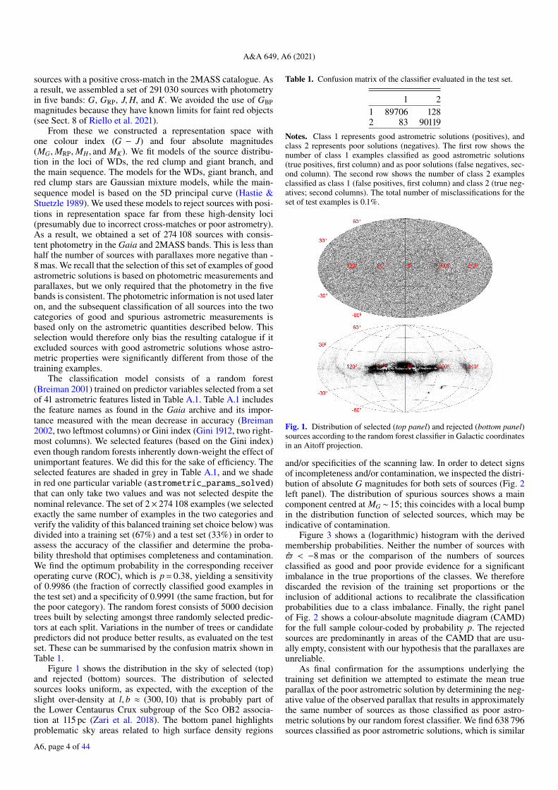
Figure 1 shows the distribution in the sky of selected (top)and rejected (bottom) sources. The distribution of selectedsources looks uniform, as expected, with the exception of theslight over-density at l, b ≈ (300, 10) that is probably part ofthe Lower Centaurus Crux subgroup of the Sco OB2 associa-tion at 115 pc (Zari et al. 2018). The bottom panel highlightsproblematic sky areas related to high surface density regions

Table 1. Confusion matrix of the classifier evaluated in the test set.

1 21 89706 1282 83 90119

Notes. Class 1 represents good astrometric solutions (positives), andclass 2 represents poor solutions (negatives). The first row shows thenumber of class 1 examples classified as good astrometric solutions(true positives, first column) and as poor solutions (false negatives, sec-ond column). The second row shows the number of class 2 examplesclassified as class 1 (false positives, first column) and class 2 (true neg-atives; second columns). The total number of misclassifications for theset of test examples is 0.1%.

Fig. 1. Distribution of selected (top panel) and rejected (bottom panel)sources according to the random forest classifier in Galactic coordinatesin an Aitoff projection.

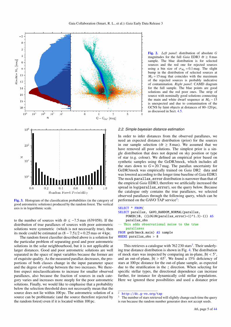
and/or specificities of the scanning law. In order to detect signsof incompleteness and/or contamination, we inspected the distri-bution of absolute G magnitudes for both sets of sources (Fig. 2left panel). The distribution of spurious sources shows a maincomponent centred at MG ∼ 15; this coincides with a local bumpin the distribution function of selected sources, which may beindicative of contamination.

Figure 3 shows a (logarithmic) histogram with the derivedmembership probabilities. Neither the number of sources with$ < −8 mas or the comparison of the numbers of sourcesclassified as good and poor provide evidence for a significantimbalance in the true proportions of the classes. We thereforediscarded the revision of the training set proportions or theinclusion of additional actions to recalibrate the classificationprobabilities due to a class imbalance. Finally, the right panelof Fig. 2 shows a colour-absolute magnitude diagram (CAMD)for the full sample colour-coded by probability p. The rejectedsources are predominantly in areas of the CAMD that are usu-ally empty, consistent with our hypothesis that the parallaxes areunreliable.

As final confirmation for the assumptions underlying thetraining set definition we attempted to estimate the mean trueparallax of the poor astrometric solution by determining the neg-ative value of the observed parallax that results in approximatelythe same number of sources as those classified as poor astro-metric solutions by our random forest classifier. We find 638 796sources classified as poor astrometric solutions, which is similar

A6, page 4 of 44

Gaia Collaboration (Smart, R. L., et al.): Gaia Early Data Release 3

Fig. 2. Left panel: distribution of absolute Gmagnitudes for the full Gaia EDR3 $ ≥ 8 massample. The blue distribution is for selectedsources and the red one for rejected sourcesusing a bin size of σMG = 0.1 mag. The slightbump in the distribution of selected sources atMG = 15 mag that coincides with the maximumof the rejected sources is probably indicativeof contamination. Right panel: CAMD diagramfor the full sample. The blue points are goodsolutions and the red poor ones. The strip ofsource with nominally good solutions connectingthe main and white dwarf sequence at MG ∼ 15is unexpected and due to contamination of theGCNS by faint objects at distances of 80–120 pc,as discussed in Sect. 4.5.

Fig. 3. Histogram of the classification probabilities (in the category ofgood astrometric solutions) produced by the random forest. The verticalaxis is in logarithmic scale.

to the number of sources with $ ≤ −7.5 mas (639 058). If thedistribution of true parallaxes of sources with poor astrometricsolutions were symmetric (which is not necessarily true), thenits mode could be estimated as (8 − 7.5)/2 = 0.25 mas or 4 kpc.

The random forest classifier described above is a solution forthe particular problem of separating good and poor astrometricsolutions in the solar neighbourhood, but it is not applicable atlarger distances. Good and poor astrometric solutions are wellseparated in the space of input variables because the former areof exquisite quality. As the measured parallax decreases, the pro-portions of both classes change in the input parameter spaceand the degree of overlap between the two increases. We there-fore expect misclassifications to increase for smaller observedparallaxes, also because the fraction of sources in each cate-gory varies and increases more steeply for the poor astrometricsolutions. Finally, we would like to emphasise that a probabilitybelow the selection threshold does not necessarily mean that thesource does not lie within 100 pc. The astrometric solution of asource can be problematic (and the source therefore rejected bythe random forest) even if it is located within 100 pc.

2.2. Simple bayesian distance estimation

In order to infer distances from the observed parallaxes, weneed an expected distance distribution (prior) for the sourcesin our sample selection ($ ≥ 8 mas). We assumed that wehave removed all poor solutions. The simplest prior is a sin-gle distribution that does not depend on sky position or typeof star (e.g. colour). We defined an empirical prior based onsynthetic samples using the GeDR3mock, which includes allthe stars down to G = 20.7 mag. The parallax uncertainty forGeDR3mock was empirically trained on Gaia DR2 data andwas lowered according to the longer time baseline of Gaia EDR3.The mock parallax_error distribution is narrower than that ofthe empirical Gaia EDR3, therefore we artificially increased thespread in log(parallax_error), see the query below. Becausethe catalogue only contains the true parallaxes, we selectedobserved parallaxes through the following query, which can beperformed on the GAVO TAP service2:

SELECT * FROM(SELECT parallax, GAVO_RANDOM_NORMAL(parallax,

POWER(10, ((LOG10(parallax_error)+1)*1.3)-1)) ASparallax_obs

-- This adds observational noise to the trueparallaxes

FROM gedr3mock.main) AS sampleWHERE parallax_obs > 8

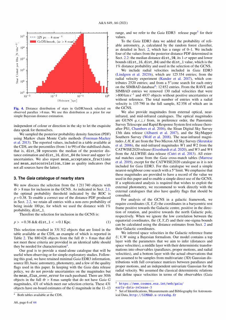
This retrieves a catalogue with 762 230 stars3. Their underly-ing true distance distribution is shown in Fig. 4. The distributionof mock stars was inspected by comparing an in-plane, |b| < 5,and an out-of-plane, |b| > 65. We found a 15% deficiency ofstars at 100 pc distance for the out-of-plane sample, as expecteddue to the stratification in the z direction. When selecting forspecific stellar types, the directional dependence can increasefurther, for instance for dynamically cold stellar populations.Here we ignored these possibilities and used a distance prior

2 http://dc.g-vo.org/tap3 The number of stars retrieved will slightly change each time the queryis run because the random number generator does not accept seeds.

A6, page 5 of 44

A&A 649, A6 (2021)

Fig. 4. Distance distribution of stars in GeDR3mock selected onobserved parallax >8 mas. We use this distribution as a prior for oursimple Bayesian distance estimation.

independent of colour or direction in the sky to let the exquisitedata speak for themselves.

We sampled the posterior probability density function (PDF)using Markov chain Monte Carlo methods (Foreman-Mackeyet al. 2013). The reported values, included in a table available atthe CDS, are the percentiles (from 1 to 99) of the stabilised chain,that is, dist_50 represents the median of the posterior dis-tance estimation and dist_16, dist_84 the lower and upper 1σuncertainties. We also report mean_acceptance_fractionsand mean_autocorrelation_time as quality indicators (butnot all sources have the latter).

3. The Gaia catalogue of nearby stars

We now discuss the selection from the 1 211 740 objects with$ > 8 mas for inclusion in the GCNS. As indicated in Sect. 2.1,the optimal probability threshold indicated by the ROC isp = 0.38. To enable a correct use of the distance PDF producedin Sect. 2.2, we retain all entries with a non-zero probability ofbeing inside 100 pc, for which we used the distance with 1%probability, dist_1.

Therefore the selection for inclusion in the GCNS is:

p > = 0.38 && dist_1 < = 0.1 Kpc. (1)

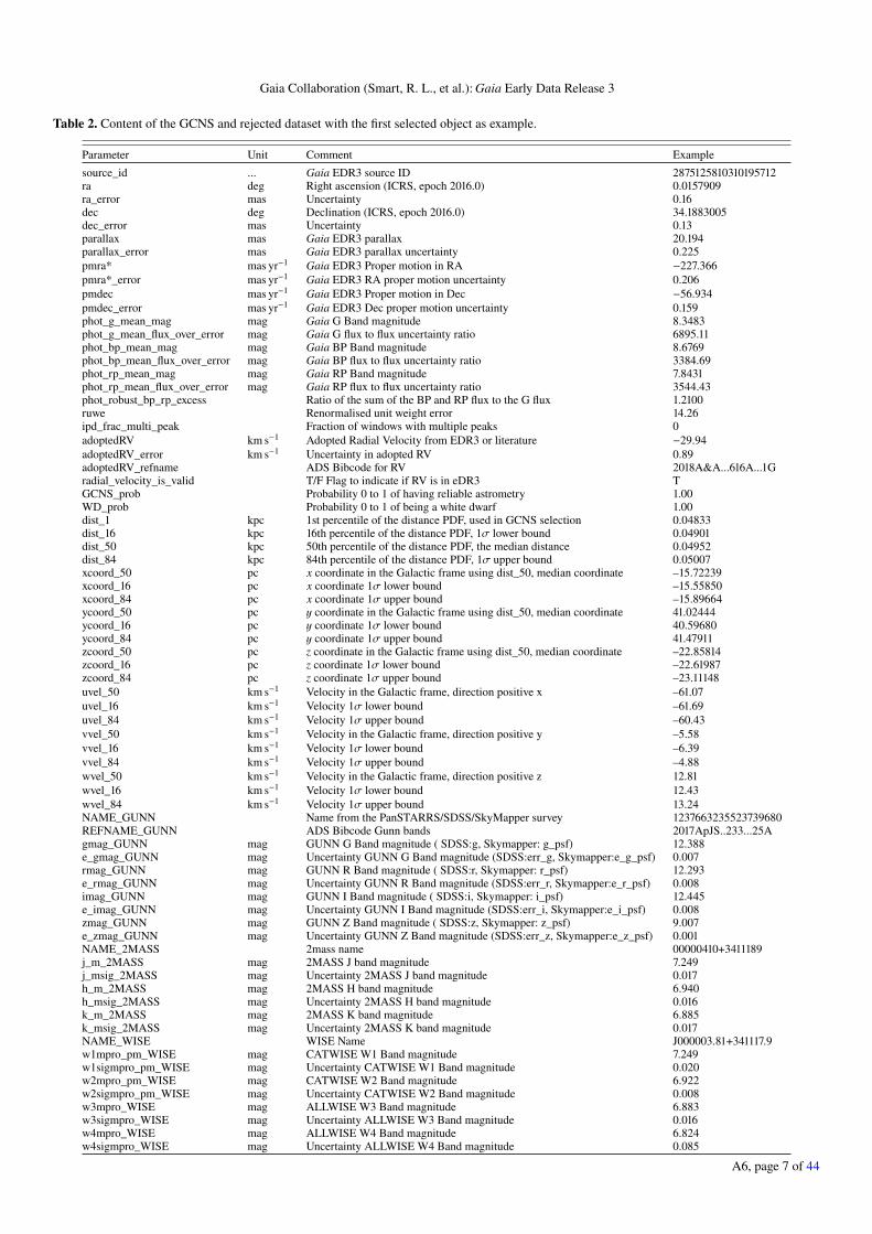
This selection resulted in 331 312 objects that are listed in thetable available at the CDS, an example of which is reported inTable 2. The 880 428 objects from the full $ > 8 mas that didnot meet these criteria are provided in an identical table shouldthey be needed for characterisation4.

Our goal is to provide a stand-alone catalogue that will beuseful when observing or for simple exploratory studies. Follow-ing this goal, we have retained minimal Gaia EDR3 information,source ID, basic astrometry, photometry, and a few of the qualityflags used in this paper. In keeping with the Gaia data releasepolicy, we do not provide uncertainties on the magnitudes butthe mean_flux_over_error for each passband. There are 3016objects in the full $ > 8 mas sample that do not have Gaia Gmagnitudes, 431 of which meet our selection criteria. These 431objects have on-board estimates of the G magnitude in the 11–134 Both tables available at the CDS.

range, and we refer to the Gaia EDR3 release page5 for theirvalues.

To the Gaia EDR3 data we added the probability of reli-able astrometry, p, calculated by the random forest classifier,as detailed in Sect. 2, which has a range of 0–1. We includefour of the values from the posterior distance PDF determined inSect. 2.2: the median distance dist_50, its 1-σ upper and lowerbounds (dist_16, dist_84) and the dist_1 value, which is the1% distance probability and used in the selection of the GCNS.

We include radial velocities included in Gaia EDR3(Lindgren et al. 2021b), which are 125 354 entries; from theradial velocity experiment (Kunder et al. 2017), which con-tributes 2520 entries; and from a 5′′cone search for each entryon the SIMBAD database6: 12 852 entries. From the RAVE andSIMBAD entries we removed 130 radial velocities that were>800 km s−1 and 4937 objects without positive uncertainties orwithout reference. The total number of entries with a radialvelocity is 135 790 in the full sample, 82 358 of which are inthe GCNS.

We also provide magnitudes from external optical, near-infrared, and mid-infrared catalogues. The optical magnitudesare GUNN g, r, z, i from, in preference order, the PanoramicSurvey Telescope and Rapid Response System first release (here-after PS1, Chambers et al. 2016), the Sloan Digital Sky Survey13th data release (Albareti et al. 2017), and the SkyMapperSouthern Survey (Wolf et al. 2018). The near-infrared magni-tudes J,H,K are from the Two Micron All Sky Survey (Skrutskieet al. 2006), the mid-infrared magnitudes W1 and W2 from theCATWISE2020 release (Eisenhardt et al. 2020), and W3 and W4from the ALLWISE data release (Cutri et al. 2013). All exter-nal matches came from the Gaia cross-match tables (Marreseet al. 2019), except for the CATWISE2020 catalogue as it is notincluded for Gaia EDR3. For this catalogue we used a simplenearest-neighbour cone search with a 5′′limit. We emphasise thatthese magnitudes are provided to have a record of the value weused in this paper and to enable a simple direct use of the GCNS.If a sophisticated analysis is required that wishes to exploit theexternal photometry, we recommend to work directly with theexternal catalogues that also have quality flags that should beconsulted.

For analysis of the GCNS in a galactic framework, werequire coordinates (X,Y,Z) the coordinates in a barycentric restframe positive towards the Galactic centre, positive in the direc-tion of rotation, and positive towards the north Galactic pole,respectively. When we ignore the low correlation between theequatorial coordinates, the (X,Y,Z) and their one-sigma boundscan be calculated using the distance estimates from Sect. 2 andtheir Galactic coordinates.

We inferred space velocities in the Galactic reference frameU,V,W using a Bayesian formalism. Our model contains a toplayer with the parameters that we aim to infer (distances andspace velocities), a middle layer with their deterministic transfor-mations into observables (parallaxes, proper motions, and radialvelocities), and a bottom layer with the actual observations thatare assumed to be samples from multivariate (3D) Gaussian dis-tributions with full covariance matrices between parallaxes andproper motions, and an independent univariate Gaussian for theradial velocity. We assumed the classical deterministic relationsthat define space velocities in terms of the observables (Gaia

5 https://www.cosmos.esa.int/web/gaia/early-data-release-36 Set of Identifications, Measurements and Bibliography for Astronom-ical Data, http://SIMBAD.u-strasbg.fr

A6, page 6 of 44

Gaia Collaboration (Smart, R. L., et al.): Gaia Early Data Release 3

Table 2. Content of the GCNS and rejected dataset with the first selected object as example.

Parameter Unit Comment Example

source_id ... Gaia EDR3 source ID 2875125810310195712ra deg Right ascension (ICRS, epoch 2016.0) 0.0157909ra_error mas Uncertainty 0.16dec deg Declination (ICRS, epoch 2016.0) 34.1883005dec_error mas Uncertainty 0.13parallax mas Gaia EDR3 parallax 20.194parallax_error mas Gaia EDR3 parallax uncertainty 0.225pmra* mas yr−1 Gaia EDR3 Proper motion in RA −227.366pmra*_error mas yr−1 Gaia EDR3 RA proper motion uncertainty 0.206pmdec mas yr−1 Gaia EDR3 Proper motion in Dec −56.934pmdec_error mas yr−1 Gaia EDR3 Dec proper motion uncertainty 0.159phot_g_mean_mag mag Gaia G Band magnitude 8.3483phot_g_mean_flux_over_error mag Gaia G flux to flux uncertainty ratio 6895.11phot_bp_mean_mag mag Gaia BP Band magnitude 8.6769phot_bp_mean_flux_over_error mag Gaia BP flux to flux uncertainty ratio 3384.69phot_rp_mean_mag mag Gaia RP Band magnitude 7.8431phot_rp_mean_flux_over_error mag Gaia RP flux to flux uncertainty ratio 3544.43phot_robust_bp_rp_excess Ratio of the sum of the BP and RP flux to the G flux 1.2100ruwe Renormalised unit weight error 14.26ipd_frac_multi_peak Fraction of windows with multiple peaks 0adoptedRV km s−1 Adopted Radial Velocity from EDR3 or literature −29.94adoptedRV_error km s−1 Uncertainty in adopted RV 0.89adoptedRV_refname ADS Bibcode for RV 2018A&A...616A...1Gradial_velocity_is_valid T/F Flag to indicate if RV is in eDR3 TGCNS_prob Probability 0 to 1 of having reliable astrometry 1.00WD_prob Probability 0 to 1 of being a white dwarf 1.00dist_1 kpc 1st percentile of the distance PDF, used in GCNS selection 0.04833dist_16 kpc 16th percentile of the distance PDF, 1σ lower bound 0.04901dist_50 kpc 50th percentile of the distance PDF, the median distance 0.04952dist_84 kpc 84th percentile of the distance PDF, 1σ upper bound 0.05007xcoord_50 pc x coordinate in the Galactic frame using dist_50, median coordinate –15.72239xcoord_16 pc x coordinate 1σ lower bound –15.55850xcoord_84 pc x coordinate 1σ upper bound –15.89664ycoord_50 pc y coordinate in the Galactic frame using dist_50, median coordinate 41.02444ycoord_16 pc y coordinate 1σ lower bound 40.59680ycoord_84 pc y coordinate 1σ upper bound 41.47911zcoord_50 pc z coordinate in the Galactic frame using dist_50, median coordinate –22.85814zcoord_16 pc z coordinate 1σ lower bound –22.61987zcoord_84 pc z coordinate 1σ upper bound –23.11148uvel_50 km s−1 Velocity in the Galactic frame, direction positive x –61.07uvel_16 km s−1 Velocity 1σ lower bound –61.69uvel_84 km s−1 Velocity 1σ upper bound –60.43vvel_50 km s−1 Velocity in the Galactic frame, direction positive y –5.58vvel_16 km s−1 Velocity 1σ lower bound –6.39vvel_84 km s−1 Velocity 1σ upper bound –4.88wvel_50 km s−1 Velocity in the Galactic frame, direction positive z 12.81wvel_16 km s−1 Velocity 1σ lower bound 12.43wvel_84 km s−1 Velocity 1σ upper bound 13.24NAME_GUNN Name from the PanSTARRS/SDSS/SkyMapper survey 1237663235523739680REFNAME_GUNN ADS Bibcode Gunn bands 2017ApJS..233...25Agmag_GUNN mag GUNN G Band magnitude ( SDSS:g, Skymapper: g_psf) 12.388e_gmag_GUNN mag Uncertainty GUNN G Band magnitude (SDSS:err_g, Skymapper:e_g_psf) 0.007rmag_GUNN mag GUNN R Band magnitude ( SDSS:r, Skymapper: r_psf) 12.293e_rmag_GUNN mag Uncertainty GUNN R Band magnitude (SDSS:err_r, Skymapper:e_r_psf) 0.008imag_GUNN mag GUNN I Band magnitude ( SDSS:i, Skymapper: i_psf) 12.445e_imag_GUNN mag Uncertainty GUNN I Band magnitude (SDSS:err_i, Skymapper:e_i_psf) 0.008zmag_GUNN mag GUNN Z Band magnitude ( SDSS:z, Skymapper: z_psf) 9.007e_zmag_GUNN mag Uncertainty GUNN Z Band magnitude (SDSS:err_z, Skymapper:e_z_psf) 0.001NAME_2MASS 2mass name 00000410+3411189j_m_2MASS mag 2MASS J band magnitude 7.249j_msig_2MASS mag Uncertainty 2MASS J band magnitude 0.017h_m_2MASS mag 2MASS H band magnitude 6.940h_msig_2MASS mag Uncertainty 2MASS H band magnitude 0.016k_m_2MASS mag 2MASS K band magnitude 6.885k_msig_2MASS mag Uncertainty 2MASS K band magnitude 0.017NAME_WISE WISE Name J000003.81+341117.9w1mpro_pm_WISE mag CATWISE W1 Band magnitude 7.249w1sigmpro_pm_WISE mag Uncertainty CATWISE W1 Band magnitude 0.020w2mpro_pm_WISE mag CATWISE W2 Band magnitude 6.922w2sigmpro_pm_WISE mag Uncertainty CATWISE W2 Band magnitude 0.008w3mpro_WISE mag ALLWISE W3 Band magnitude 6.883w3sigmpro_WISE mag Uncertainty ALLWISE W3 Band magnitude 0.016w4mpro_WISE mag ALLWISE W4 Band magnitude 6.824w4sigmpro_WISE mag Uncertainty ALLWISE W4 Band magnitude 0.085

A6, page 7 of 44

A&A 649, A6 (2021)

coordinates, parallaxes and proper motions, and radial veloci-ties), which we explicitly develop in Appendix B. We neglecthere for the sake of simplicity and speed the uncertainties in thecelestial coordinates and their correlations with parallaxes andproper motions. The full covariance matrices are given by thecatalogue uncertainties and correlations.

We used the same empirical prior for the distance asdescribed in Sect. 2.2 and defined three independent priors forthe space velocities U, V, and W (see Appendix B for details).In all three cases we use a modified Gaussian mixture model(GMM) fit to the space velocities found in a local (140 pc) simu-lation from the Besançon Galaxy model (Robin et al. 2003). Thenumber of GMM components is defined by the optimal Bayesianinformation criterion. The modification consists of decreasingthe proportion of the dominant Gaussian component in each fitby 3% and adding a new wide component of equal size centredat 0 km s−1 and with a standard deviation of 120 km s−1 to allowfor potential solutions with high speeds typical of halo stars thatare not sufficiently represented in the Besançon sample to jus-tify a separate GMM component. We then used Stan (Carpenteret al. 2017) to produce 2000 samples from the posterior distribu-tion and provide the median U,V,W, and their one-sigma upperand lower bounds in the output catalogue with suffixes vel_50,vel_16, and vel_84, respectively.

4. Catalogue quality assurance

4.1. Sky variation

In this section we discuss the completeness of the GCNS in thecontext of the full Gaia EDR3. In particular, we examine thechanges in completeness limit with the direction on the sky as aresult of our distance cut and as a result of separation of sources.

4.1.1. G magnitude limits over the sky

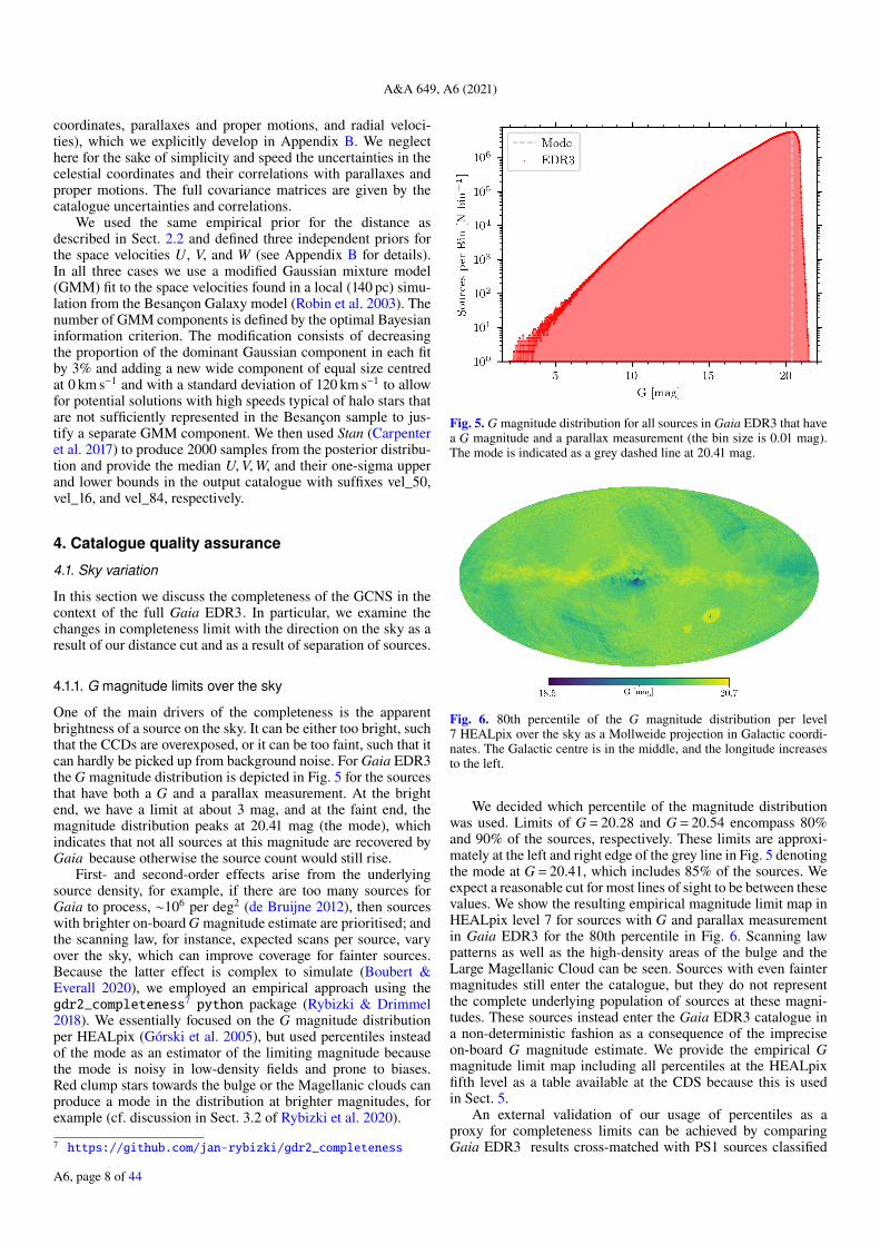
One of the main drivers of the completeness is the apparentbrightness of a source on the sky. It can be either too bright, suchthat the CCDs are overexposed, or it can be too faint, such that itcan hardly be picked up from background noise. For Gaia EDR3the G magnitude distribution is depicted in Fig. 5 for the sourcesthat have both a G and a parallax measurement. At the brightend, we have a limit at about 3 mag, and at the faint end, themagnitude distribution peaks at 20.41 mag (the mode), whichindicates that not all sources at this magnitude are recovered byGaia because otherwise the source count would still rise.

First- and second-order effects arise from the underlyingsource density, for example, if there are too many sources forGaia to process, ∼106 per deg2 (de Bruijne 2012), then sourceswith brighter on-board G magnitude estimate are prioritised; andthe scanning law, for instance, expected scans per source, varyover the sky, which can improve coverage for fainter sources.Because the latter effect is complex to simulate (Boubert &Everall 2020), we employed an empirical approach using thegdr2_completeness7 python package (Rybizki & Drimmel2018). We essentially focused on the G magnitude distributionper HEALpix (Górski et al. 2005), but used percentiles insteadof the mode as an estimator of the limiting magnitude becausethe mode is noisy in low-density fields and prone to biases.Red clump stars towards the bulge or the Magellanic clouds canproduce a mode in the distribution at brighter magnitudes, forexample (cf. discussion in Sect. 3.2 of Rybizki et al. 2020).

7 https://github.com/jan-rybizki/gdr2_completeness

Fig. 5. G magnitude distribution for all sources in Gaia EDR3 that havea G magnitude and a parallax measurement (the bin size is 0.01 mag).The mode is indicated as a grey dashed line at 20.41 mag.

Fig. 6. 80th percentile of the G magnitude distribution per level7 HEALpix over the sky as a Mollweide projection in Galactic coordi-nates. The Galactic centre is in the middle, and the longitude increasesto the left.

We decided which percentile of the magnitude distributionwas used. Limits of G = 20.28 and G = 20.54 encompass 80%and 90% of the sources, respectively. These limits are approxi-mately at the left and right edge of the grey line in Fig. 5 denotingthe mode at G = 20.41, which includes 85% of the sources. Weexpect a reasonable cut for most lines of sight to be between thesevalues. We show the resulting empirical magnitude limit map inHEALpix level 7 for sources with G and parallax measurementin Gaia EDR3 for the 80th percentile in Fig. 6. Scanning lawpatterns as well as the high-density areas of the bulge and theLarge Magellanic Cloud can be seen. Sources with even faintermagnitudes still enter the catalogue, but they do not representthe complete underlying population of sources at these magni-tudes. These sources instead enter the Gaia EDR3 catalogue ina non-deterministic fashion as a consequence of the impreciseon-board G magnitude estimate. We provide the empirical Gmagnitude limit map including all percentiles at the HEALpixfifth level as a table available at the CDS because this is usedin Sect. 5.

An external validation of our usage of percentiles as aproxy for completeness limits can be achieved by comparingGaia EDR3 results cross-matched with PS1 sources classified

A6, page 8 of 44

Gaia Collaboration (Smart, R. L., et al.): Gaia Early Data Release 3

14 16 18 20 22

r [mag]

0.0

0.2

0.4

0.6

0.8

1.0

[N∗

&E

DR

3$

]/

[N∗]

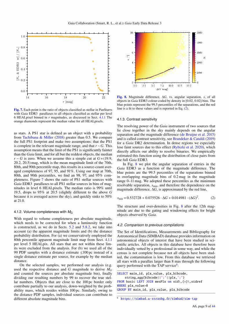
Fig. 7. Each point is the ratio of objects classified as stellar in PanStarrswith Gaia EDR3 parallaxes to all objects classified as stellar per level6 HEALpixel binned in r magnitudes, as discussed in Sect. 4.1.1 Theorange diamonds represent the median value for all HEALpixels.

as stars. A PS1 star is defined as an object with a probabilityfrom Tachibana & Miller (2018) greater than 0.5. We comparethe full PS1 footprint and make two assumptions: that the PS1is complete in the relevant magnitude range, and that r∼G. Thisassumption means that the limit of the PS1 is significantly fainterthan the Gaia limit, and for all but the reddest objects, the medianr − G is zero. When we assume this a simple cut at G = (19.9,20.2, 20.5) mag, which is the mean magnitude limit of the 70th,80th, and 90th percentile map, this results in a source-count aver-aged completeness of 97, 95, and 91%. Using our map at 70th,80th, and 90th percentiles, we find an 98, 97, and 95% com-pleteness. Figure 7 shows the ratio of PS1 stellar sources withGaia EDR3 parallaxes to all PS1 stellar sources in bins of mag-nitudes in level 6 HEALpixels. The median ratio is 99% until19.5, drops to 95% at 20.5 (slightly different to the above Gbecause it is averaged across the sky), and quickly sinks to 50%at 21.0.

4.1.2. Volume completeness with MG

With regard to volume completeness per absolute magnitude,which needs to be corrected for when a luminosity functionis constructed, as we do in Sects. 5.2 and 5.8.2, we take intoaccount (a) the apparent magnitude limits and (b) the distanceprobability distribution. For (a) we conservatively employed the80th percentile apparent magnitude limit map from Sect. 4.1.1per level 5 HEALpix. All stars that are not within these lim-its were excluded from the analysis. For (b) we used all of the99 PDF samples with a distance estimate ≤100 pc instead of asingle distance estimate per source, for example by the mediandistance.

On the selected samples, we performed our analysis (e.g.used the respective distance and G magnitude to derive MGand counted the sources per absolute magnitude bin), finallydividing our resulting numbers by 99 to recover the true stel-lar numbers. Objects that are close to the 100 pc border onlycontribute partially to our analysis, down-weighted by the prob-ability mass, which resides within 100 pc. Similarly, owing tothe distance PDF samples, individual sources can contribute todifferent absolute magnitude bins.

Fig. 8. Magnitude difference, ∆G, vs. angular separation, s, of allobjects in Gaia EDR3 colour-coded by density in [0.02, 0.02] bins. Theblue points represent the 99.5 percentiles of the separations, and the redline is a fit to these values and is reported in Eq. (2).

4.1.3. Contrast sensitivity

The resolving power of the Gaia instrument of two sources thatlie close together in the sky mainly depends on the angularseparation and the magnitude difference (de Bruijne et al. 2015)and is called contrast sensitivity, see Brandeker & Cataldi (2019)for a Gaia DR2 determination. In dense regions we especiallylose faint sources due to this effect (Rybizki et al. 2020), whichdirectly affects our ability to resolve binaries. We empiricallyestimated this function using the distribution of close pairs fromthe full Gaia EDR3.

In Fig. 8 we plot the angular separation of entries in theGaia EDR3 as a function of the magnitude difference. Theblue points are the 99.5 percentiles of the separations binnedin overlapping magnitude bins of 0.2 mag in the magnituderange 0–11 mag. We adopted these percentiles as the minimumresolvable separation, smin, and therefore the dependence on themagnitude difference, ∆G, is approximated by the red line,

smin = 0.532728 + 0.075526 · ∆G + 0.014981 · (∆G)2. (2)

The structure and over-densities in Fig. 8 after the 12th mag-nitude are due to the gating and windowing effects for brightobjects observed by Gaia.

4.2. Comparison to previous compilations

The Set of Identifications, Measurements and Bibliography forAstronomical Data (SIMBAD) database provides information onastronomical objects of interest that have been studied in sci-entific articles. All objects in this database have therefore beenindividually vetted by a professional in some way, and while thecensus is not complete because not all objects have been stud-ied, the contamination is low. From this database we retrievedall stars with a parallax larger than 8 mas through the followingquery performed with the TAP service8:

SELECT main_id, plx_value, plx_bibcode,string_agg(bibcode||’;’||plx,’;’)

FROM basic LEFT JOIN mesPlx on oid\,=\,oidrefWHERE plx_value>8GROUP BY main_id, plx_value, plx_bibcode

8 https://simbad.u-strasbg.fr/simbad/sim-tap

A6, page 9 of 44

A&A 649, A6 (2021)

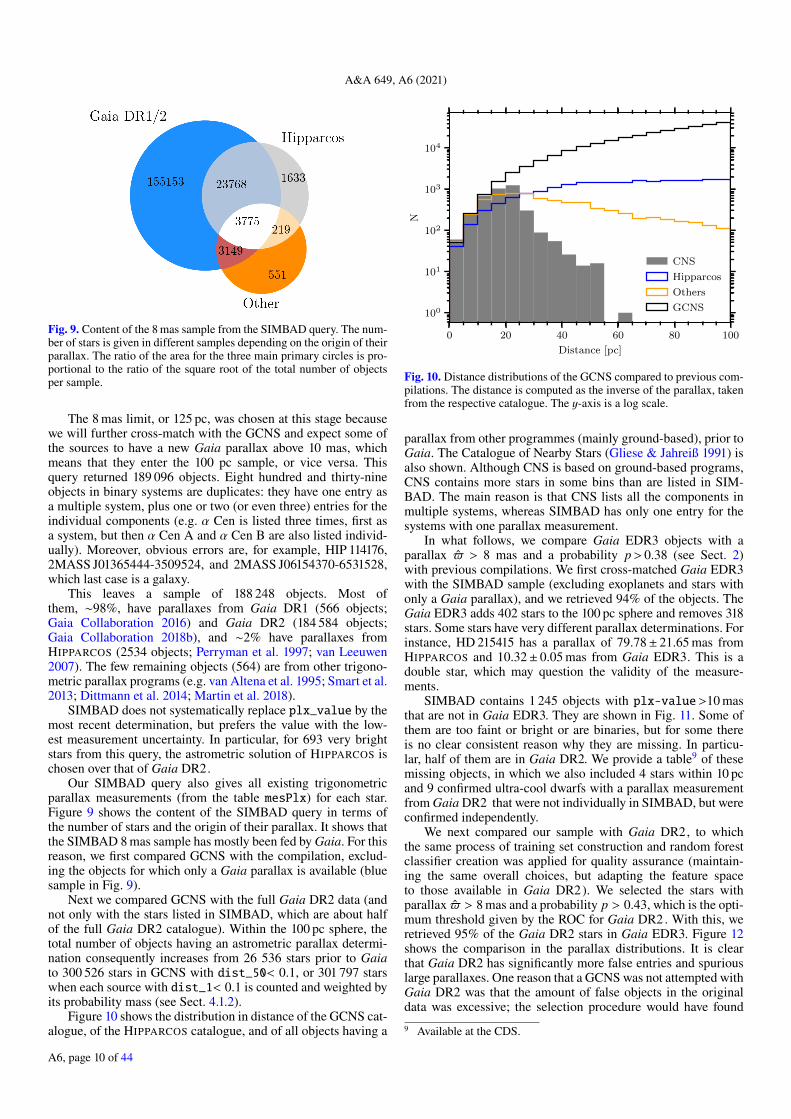
Fig. 9. Content of the 8 mas sample from the SIMBAD query. The num-ber of stars is given in different samples depending on the origin of theirparallax. The ratio of the area for the three main primary circles is pro-portional to the ratio of the square root of the total number of objectsper sample.

The 8 mas limit, or 125 pc, was chosen at this stage becausewe will further cross-match with the GCNS and expect some ofthe sources to have a new Gaia parallax above 10 mas, whichmeans that they enter the 100 pc sample, or vice versa. Thisquery returned 189 096 objects. Eight hundred and thirty-nineobjects in binary systems are duplicates: they have one entry asa multiple system, plus one or two (or even three) entries for theindividual components (e.g. α Cen is listed three times, first asa system, but then α Cen A and α Cen B are also listed individ-ually). Moreover, obvious errors are, for example, HIP 114176,2MASS J01365444-3509524, and 2MASS J06154370-6531528,which last case is a galaxy.

This leaves a sample of 188 248 objects. Most ofthem, ∼98%, have parallaxes from Gaia DR1 (566 objects;Gaia Collaboration 2016) and Gaia DR2 (184 584 objects;Gaia Collaboration 2018b), and ∼2% have parallaxes fromHIPPARCOS (2534 objects; Perryman et al. 1997; van Leeuwen2007). The few remaining objects (564) are from other trigono-metric parallax programs (e.g. van Altena et al. 1995; Smart et al.2013; Dittmann et al. 2014; Martin et al. 2018).

SIMBAD does not systematically replace plx_value by themost recent determination, but prefers the value with the low-est measurement uncertainty. In particular, for 693 very brightstars from this query, the astrometric solution of HIPPARCOS ischosen over that of Gaia DR2.

Our SIMBAD query also gives all existing trigonometricparallax measurements (from the table mesPlx) for each star.Figure 9 shows the content of the SIMBAD query in terms ofthe number of stars and the origin of their parallax. It shows thatthe SIMBAD 8 mas sample has mostly been fed by Gaia. For thisreason, we first compared GCNS with the compilation, exclud-ing the objects for which only a Gaia parallax is available (bluesample in Fig. 9).

Next we compared GCNS with the full Gaia DR2 data (andnot only with the stars listed in SIMBAD, which are about halfof the full Gaia DR2 catalogue). Within the 100 pc sphere, thetotal number of objects having an astrometric parallax determi-nation consequently increases from 26 536 stars prior to Gaiato 300 526 stars in GCNS with dist_50< 0.1, or 301 797 starswhen each source with dist_1< 0.1 is counted and weighted byits probability mass (see Sect. 4.1.2).

Figure 10 shows the distribution in distance of the GCNS cat-alogue, of the HIPPARCOS catalogue, and of all objects having a

0 20 40 60 80 100

Distance [pc]

100

101

102

103

104

N

CNS

Hipparcos

Others

GCNS

Fig. 10. Distance distributions of the GCNS compared to previous com-pilations. The distance is computed as the inverse of the parallax, takenfrom the respective catalogue. The y-axis is a log scale.

parallax from other programmes (mainly ground-based), prior toGaia. The Catalogue of Nearby Stars (Gliese & Jahreiß 1991) isalso shown. Although CNS is based on ground-based programs,CNS contains more stars in some bins than are listed in SIM-BAD. The main reason is that CNS lists all the components inmultiple systems, whereas SIMBAD has only one entry for thesystems with one parallax measurement.

In what follows, we compare Gaia EDR3 objects with aparallax $ > 8 mas and a probability p> 0.38 (see Sect. 2)with previous compilations. We first cross-matched Gaia EDR3with the SIMBAD sample (excluding exoplanets and stars withonly a Gaia parallax), and we retrieved 94% of the objects. TheGaia EDR3 adds 402 stars to the 100 pc sphere and removes 318stars. Some stars have very different parallax determinations. Forinstance, HD 215415 has a parallax of 79.78± 21.65 mas fromHIPPARCOS and 10.32± 0.05 mas from Gaia EDR3. This is adouble star, which may question the validity of the measure-ments.

SIMBAD contains 1 245 objects with plx-value>10 masthat are not in Gaia EDR3. They are shown in Fig. 11. Some ofthem are too faint or bright or are binaries, but for some thereis no clear consistent reason why they are missing. In particu-lar, half of them are in Gaia DR2. We provide a table9 of thesemissing objects, in which we also included 4 stars within 10 pcand 9 confirmed ultra-cool dwarfs with a parallax measurementfrom Gaia DR2 that were not individually in SIMBAD, but wereconfirmed independently.

We next compared our sample with Gaia DR2, to whichthe same process of training set construction and random forestclassifier creation was applied for quality assurance (maintain-ing the same overall choices, but adapting the feature spaceto those available in Gaia DR2). We selected the stars withparallax $ > 8 mas and a probability p > 0.43, which is the opti-mum threshold given by the ROC for Gaia DR2. With this, weretrieved 95% of the Gaia DR2 stars in Gaia EDR3. Figure 12shows the comparison in the parallax distributions. It is clearthat Gaia DR2 has significantly more false entries and spuriouslarge parallaxes. One reason that a GCNS was not attempted withGaia DR2 was that the amount of false objects in the originaldata was excessive; the selection procedure would have found

9 Available at the CDS.

A6, page 10 of 44

Gaia Collaboration (Smart, R. L., et al.): Gaia Early Data Release 3

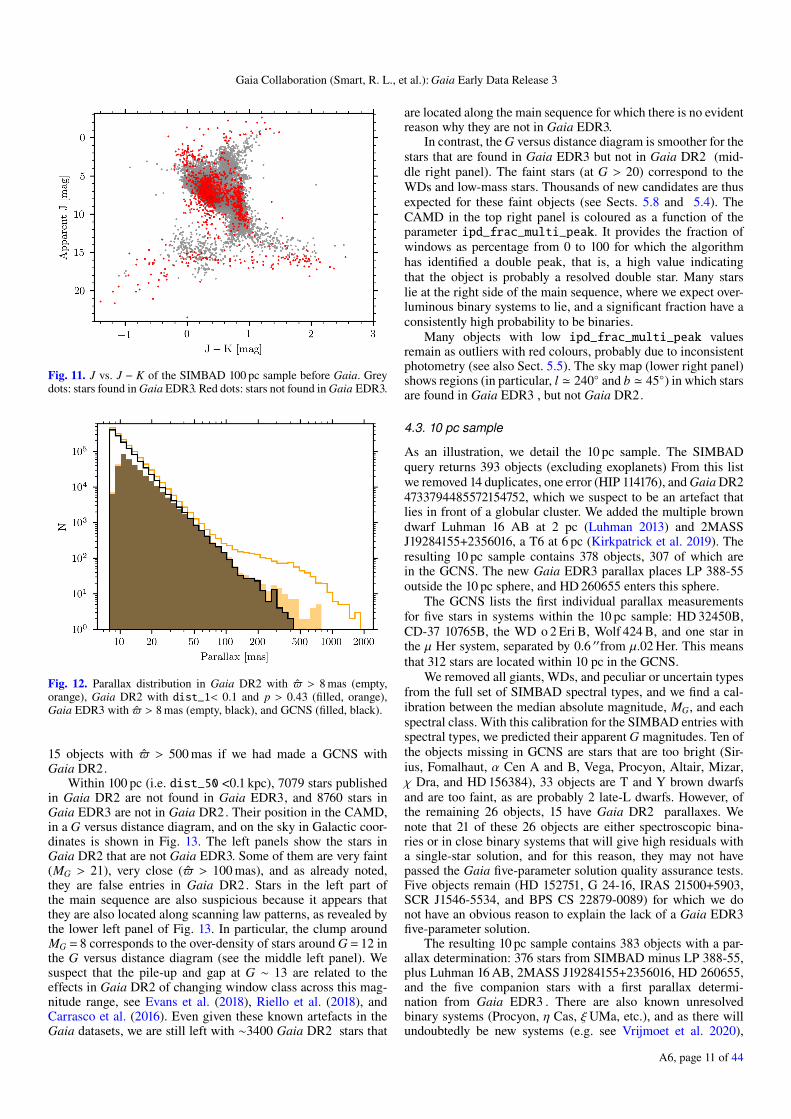
Fig. 11. J vs. J − K of the SIMBAD 100 pc sample before Gaia. Greydots: stars found in Gaia EDR3. Red dots: stars not found in Gaia EDR3.

Fig. 12. Parallax distribution in Gaia DR2 with $ > 8 mas (empty,orange), Gaia DR2 with dist_1< 0.1 and p > 0.43 (filled, orange),Gaia EDR3 with $ > 8 mas (empty, black), and GCNS (filled, black).

15 objects with $ > 500 mas if we had made a GCNS withGaia DR2.

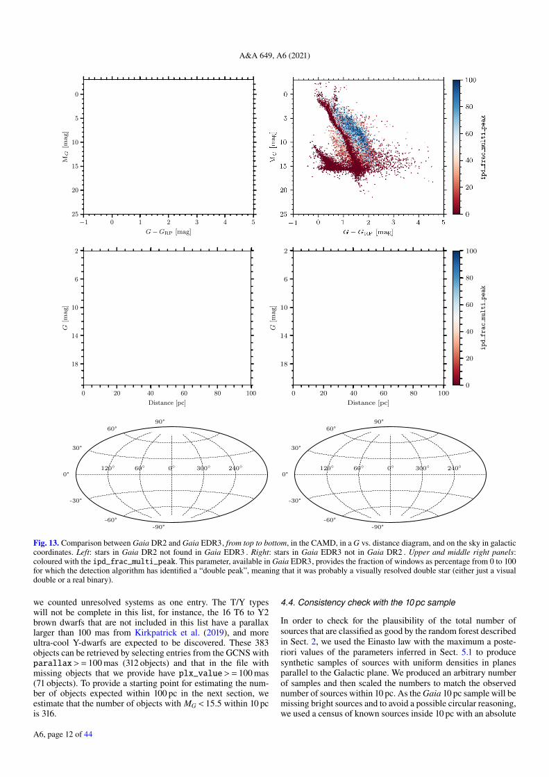
Within 100 pc (i.e. dist_50 <0.1 kpc), 7079 stars publishedin Gaia DR2 are not found in Gaia EDR3, and 8760 stars inGaia EDR3 are not in Gaia DR2. Their position in the CAMD,in a G versus distance diagram, and on the sky in Galactic coor-dinates is shown in Fig. 13. The left panels show the stars inGaia DR2 that are not Gaia EDR3. Some of them are very faint(MG > 21), very close ($ > 100 mas), and as already noted,they are false entries in Gaia DR2. Stars in the left part ofthe main sequence are also suspicious because it appears thatthey are also located along scanning law patterns, as revealed bythe lower left panel of Fig. 13. In particular, the clump aroundMG = 8 corresponds to the over-density of stars around G = 12 inthe G versus distance diagram (see the middle left panel). Wesuspect that the pile-up and gap at G ∼ 13 are related to theeffects in Gaia DR2 of changing window class across this mag-nitude range, see Evans et al. (2018), Riello et al. (2018), andCarrasco et al. (2016). Even given these known artefacts in theGaia datasets, we are still left with ∼3400 Gaia DR2 stars that

are located along the main sequence for which there is no evidentreason why they are not in Gaia EDR3.

In contrast, the G versus distance diagram is smoother for thestars that are found in Gaia EDR3 but not in Gaia DR2 (mid-dle right panel). The faint stars (at G > 20) correspond to theWDs and low-mass stars. Thousands of new candidates are thusexpected for these faint objects (see Sects. 5.8 and 5.4). TheCAMD in the top right panel is coloured as a function of theparameter ipd_frac_multi_peak. It provides the fraction ofwindows as percentage from 0 to 100 for which the algorithmhas identified a double peak, that is, a high value indicatingthat the object is probably a resolved double star. Many starslie at the right side of the main sequence, where we expect over-luminous binary systems to lie, and a significant fraction have aconsistently high probability to be binaries.

Many objects with low ipd_frac_multi_peak valuesremain as outliers with red colours, probably due to inconsistentphotometry (see also Sect. 5.5). The sky map (lower right panel)shows regions (in particular, l ' 240 and b ' 45) in which starsare found in Gaia EDR3 , but not Gaia DR2.

4.3. 10 pc sample

As an illustration, we detail the 10 pc sample. The SIMBADquery returns 393 objects (excluding exoplanets) From this listwe removed 14 duplicates, one error (HIP 114176), and Gaia DR24733794485572154752, which we suspect to be an artefact thatlies in front of a globular cluster. We added the multiple browndwarf Luhman 16 AB at 2 pc (Luhman 2013) and 2MASSJ19284155+2356016, a T6 at 6 pc (Kirkpatrick et al. 2019). Theresulting 10 pc sample contains 378 objects, 307 of which arein the GCNS. The new Gaia EDR3 parallax places LP 388-55outside the 10 pc sphere, and HD 260655 enters this sphere.

The GCNS lists the first individual parallax measurementsfor five stars in systems within the 10 pc sample: HD 32450B,CD-37 10765B, the WD o 2 Eri B, Wolf 424 B, and one star inthe µ Her system, separated by 0.6 ′′from µ.02 Her. This meansthat 312 stars are located within 10 pc in the GCNS.

We removed all giants, WDs, and peculiar or uncertain typesfrom the full set of SIMBAD spectral types, and we find a cal-ibration between the median absolute magnitude, MG, and eachspectral class. With this calibration for the SIMBAD entries withspectral types, we predicted their apparent G magnitudes. Ten ofthe objects missing in GCNS are stars that are too bright (Sir-ius, Fomalhaut, α Cen A and B, Vega, Procyon, Altair, Mizar,χ Dra, and HD 156384), 33 objects are T and Y brown dwarfsand are too faint, as are probably 2 late-L dwarfs. However, ofthe remaining 26 objects, 15 have Gaia DR2 parallaxes. Wenote that 21 of these 26 objects are either spectroscopic bina-ries or in close binary systems that will give high residuals witha single-star solution, and for this reason, they may not havepassed the Gaia five-parameter solution quality assurance tests.Five objects remain (HD 152751, G 24-16, IRAS 21500+5903,SCR J1546-5534, and BPS CS 22879-0089) for which we donot have an obvious reason to explain the lack of a Gaia EDR3five-parameter solution.

The resulting 10 pc sample contains 383 objects with a par-allax determination: 376 stars from SIMBAD minus LP 388-55,plus Luhman 16 AB, 2MASS J19284155+2356016, HD 260655,and the five companion stars with a first parallax determi-nation from Gaia EDR3 . There are also known unresolvedbinary systems (Procyon, η Cas, ξUMa, etc.), and as there willundoubtedly be new systems (e.g. see Vrijmoet et al. 2020),

A6, page 11 of 44

A&A 649, A6 (2021)

−1 0 1 2 3 4 5

G−GRP [mag]

0

5

10

15

20

25

MG

[mag]

0 20 40 60 80 100

Distance [pc]

2

6

10

14

18

G[m

ag]

0 20 40 60 80 100

Distance [pc]

2

6

10

14

18

G[m

ag]

0

20

40

60

80

100

ipdfracmultipeak

120 60 0 300 240

-90°-60°

-30°

0°

30°

60°90°

120 60 0 300 240

-90°-60°

-30°

0°

30°

60°90°

Fig. 13. Comparison between Gaia DR2 and Gaia EDR3, from top to bottom, in the CAMD, in a G vs. distance diagram, and on the sky in galacticcoordinates. Left: stars in Gaia DR2 not found in Gaia EDR3 . Right: stars in Gaia EDR3 not in Gaia DR2 . Upper and middle right panels:coloured with the ipd_frac_multi_peak. This parameter, available in Gaia EDR3, provides the fraction of windows as percentage from 0 to 100for which the detection algorithm has identified a “double peak”, meaning that it was probably a visually resolved double star (either just a visualdouble or a real binary).

we counted unresolved systems as one entry. The T/Y typeswill not be complete in this list, for instance, the 16 T6 to Y2brown dwarfs that are not included in this list have a parallaxlarger than 100 mas from Kirkpatrick et al. (2019), and moreultra-cool Y-dwarfs are expected to be discovered. These 383objects can be retrieved by selecting entries from the GCNS withparallax>= 100 mas (312 objects) and that in the file withmissing objects that we provide have plx_value>= 100 mas(71 objects). To provide a starting point for estimating the num-ber of objects expected within 100 pc in the next section, weestimate that the number of objects with MG < 15.5 within 10 pcis 316.

4.4. Consistency check with the 10 pc sample

In order to check for the plausibility of the total number ofsources that are classified as good by the random forest describedin Sect. 2, we used the Einasto law with the maximum a poste-riori values of the parameters inferred in Sect. 5.1 to producesynthetic samples of sources with uniform densities in planesparallel to the Galactic plane. We produced an arbitrary numberof samples and then scaled the numbers to match the observednumber of sources within 10 pc. As the Gaia 10 pc sample will bemissing bright sources and to avoid a possible circular reasoning,we used a census of known sources inside 10 pc with an absolute

A6, page 12 of 44

Gaia Collaboration (Smart, R. L., et al.): Gaia Early Data Release 3

magnitude brighter than 15.5 mag regardless of whether thesources are detected by Gaia.

In our simulations we assumed for the sake of simplicitythat the binary population properties are dominated by the Mspectral type regime. We set a binarity fraction of 25% and adistribution of binary separations (a) that is Gaussian in loga-rithmic scale, with the mean and standard deviation equal to 1:log10(a)∼N(µ= 1, σ= 1) (see Robin et al. 2012; Arenou 2010,and references therein). We assumed that the orientation of theorbital planes are random and uniform in space, giving rise tothe usual law for the inclinations i with respect to the line ofsight given by p(i)∼ sin(i). Furthermore, we assigned a magni-tude difference between the two components (we did not includehigher order systems) based on the relative frequencies encoun-tered in the GCNS and discussed in Sect. 5.6. Based on theseparations and inclinations, we computed the fraction f ofthe orbit where the apparent angular separation of the binarycomponents is larger than the angular separation in Eq. (2).The probability of detecting the binary system as two separatesources was then approximated with the binomial distribution fora number of trials equal to 22 (which is the mode of the distri-bution of the number of astrometric transits in our dataset) andsuccess probability f . This is an optimistic estimate because itassumes that one single separate detection suffices to resolve thebinary system.

Using the procedure described above, we generated ten sim-ulations with 40 million sources each, distributed in a cubeof 110× 110× 110 pc. From each simulation we extracted thenumber of sources within 10 and 100 pc (N10 and N100, respec-tively) and the ratio between the two (N100/N10). The averagevalue of this ratio from our simulations is 878.2± 28.2. Whenwe apply this scale to the observed number of sources within10 pc (316 sources), the expected number of sources in the GCNSselection is 277 511± 8911. This prediction has to be comparedwith the number of sources in the GCNS catalogue with an abso-lute magnitude brighter than 15.5 and within 100 pc. In orderto obtain this number, we proceeded as described in Sect. 4.1.2and obtained a total number of sources of 282 652, which agreeswell with the prediction given the relatively large uncertaintiesand the fact that the number of sources within 10 pc (316) isitself a sample from a Poisson distribution. It has to be bornein mind, however, that the expected number (277 511) does nottake incompleteness due to variations across the sky of the Gmagnitude level or due to the contrast sensitivity into account.GeDR3mock simulations show that 1.8k sources are fainter thanthe Gaia EDR3 85th percentile magnitude limits (cf. Sect. 4.1.1).Additional 0.3k sources are lost due to the contrast sensitiv-ity, which will be a lower limit because GeDR3mock does notinclude binaries, so that this is only the contribution of chancealignments in crowded regions.

4.5. Contamination and completeness

As described in Lindegren et al. (2018), every solution in Gaiais the result of iteratively solving with different versions ofthe input data and varying the calibration models. The finalsolutions do not use all the observations and not all solutionsare published, many quality assurance tests are applied topublish only high-confidence solutions. Internal parametertests that were applied to publish the five-parameter solution inGaia EDR3 were G <= 21.0; astrometric_sigma5d_max<1.2× 100.2max(6−G,0,G−18) mas; visibility_periods_used> 8;longestsemiMajorAxis of the position uncertainty ellipse<=100 mas; and duplicateSourceID= 0. The tests were

calibrated to provide a balance between including poor solu-tions and rejecting good solutions for the majority of objects,that is, distant, slow-moving objects whose characteristicsare different from those of the nearby sample. In the currentpipeline, the astrometric solution considers targets as singlestars, and for nearby unresolved or close binary systems theresiduals of the observed motion to the predicted motion can bequite large, so that this causes some nearby objects to fail theastrometric_sigma5d_max test.

For example, as we saw in Sect. 4.2, we expect 383 objectswithin the 10 pc sample. When the 35 L/T objects that we con-sider too faint are removed, 348 objects remain that Gaia shouldsee (we include the bright objects for the purpose of this exer-cise). Twenty-six of these 348 objects do not have five-parametersolutions in Gaia EDR3 because they fail the solution qualitychecks. The fact that many of the lost objects were in spectro-scopic or close binary systems is also an indication that the use ofa single-star solution biases the solutions for the nearby sample.If we take these numbers directly, this loss is still relatively small:26 of 348, or 7.4%. While this loss is biased towards binary sys-tems, it probably does not depend on direction and the loss willdiminish as the distance increases because the effect of binarymotion on the solutions decreases. The excess of objects found inthe GCNS compared to the prediction in Sect. 4.4 supports thisconclusion, and the comparison of objects found in SIMBAD tothose in the GCNS shows that only 6% are missing, therefore weconsider the 7.4% as a worst-case estimate of the GCNS stellarincompleteness.

Section 4.1.1 showed that the mode, or peak, of the appar-ent G distribution is at G = 20.41 mag, which includes 85%of the sources. The median absolute magnitude of an M9 isMG = 15.48 mag, which would translate into G = 20.48 mag at100 pc; therefore we should see at least 50% of the M9-typestars at our catalogue limit. Our comparison to the PS1 catalogueindicates that Gaia EDR3 is 98% complete at this magnitude.As discussed further in Sect. 5.4, the complete volume for laterspectral types becomes progressively smaller, but for spectraltypes up to M8, they are volume limited and not magnitudelimited.

We lose small numbers of objects because we started witha sample that was selected with $ > 8 mas, which from theGDR3Mock is estimated to be 55. We will lose objects thatare separated by less than 0.6′′ due to contrast sensitivity(Sect. 4.1.3), which for chance alignments from the GDR3Mockwe have estimated to be 300 sources, but it will be muchhigher for close binary systems and will bias our sample to notinclude these objects. Finally, we lose objects that are incor-rectly removed because they have p < 0.38. Based on Table 1and Sect. 2, we estimate this to be approximately 0.1% of thegood objects.

The incompleteness for non-binary objects to spectral typeM8 is therefore dominated by the 7.4% of objects for whichGaia does not provide a parallax. For objects later than M8,the complete volume decreases, as shown in Sect. 5.4. We didnot consider unresolved binary systems, which are considered inSects. 5.7 and 5.6.

We also considered the contamination of the GCNS. Thereare two types of contamination: objects that pass our probabil-ity cut but have poor astrometric solutions, and objects that arebeyond our 100 pc limit. The contamination of the good solutionsis evident in the blue points that populate the horizontal fea-ture at MG = 15–16 mag and between the main and WD sequence(Fig. 2, right panel). These are faint objects (G > 20. mag) thatlie at the limit of our distance selection (dist_50= 80–120 pc),

A6, page 13 of 44

A&A 649, A6 (2021)

for example with a distance modulus of ∼5 mag), and that there-fore populate the MG >15 mag region. These faint objects havethe lowest signal-to-noise ratio, and their parameters, used inthe random forest procedure, therefore have the largest uncer-tainties. Because objects with poor astrometric solutions wereaccepted, we estimate this contamination based on Table 1 to be∼0.1%, the false positives. This means about 3000 objects forthe GCNS.

The contamination by objects beyond the 100 pc sphere canbe estimated by summing the number of distance probabilityquantiles inside and outside 100 pc. We find that 91.2% of theprobability mass lies within 100 pc and the rest outside. Thismeans 29k sources, or 9%. The use of the full distance PDFwill allow addressing this possible source of bias in any analysis.

These known shortcomings should be considered when theGCNS is used. If the science case requires a clean 100 pc sample,where no contamination is a priority and completeness is of sec-ondary importance, objects with a dist_50< 0.1 kpc should beselected from the GCNS. If the science case requires a completesample, all objects with dist_1 < 0.1 kpc should be selectedand then weighted by the distance PDF. When a clean photomet-ric sample is required, the photometric flags should be applied,which we did not exploit to produce this catalogue. In the nextsection we investigate a number of science questions, for whichwe apply different selection procedures to the catalogue and usethe distance PDF in different ways to illustrate some optimal usesof the GNCS.

5. GCNS exploitation

5.1. Vertical stratification

In this section we study the vertical stratification as inferred fromthe GCNS volume-limited sample. We did this using a relativelysimple Bayesian hierarchical model that we describe in the fol-lowing paragraphs. First we describe the data we used to inferthe vertical stratification parameters, however. The data consistof the latitudes, observed parallaxes, and associated uncertain-ties of the sources in the GCNS with observed parallaxes greaterthan 10 mas. In order to include the effect of the truncationin the observed parallax, we also used the number of sourceswith observed parallaxes between 8 and 10 mas and their lati-tudes (but not their parallaxes). The reasons for this (and theapproximations underlying this choice) will become clear afterthe inference model specification. The assumptions underlyingthe model listed below.1. The data used for inference represent a sample of sources

with true parallaxes larger than 8 mas. This is only anapproximation, and we know that the observed sample isincomplete and contaminated. It is incomplete for severalreasons, but in the context of this model, the reason is thatsources with true parallaxes greater than 8 mas may haveobserved parallaxes smaller than this limit due to obser-vational uncertainties. It is also contaminated because theopposite is also true: true parallaxes smaller than 8 mas maybe scattered in as a result of observational uncertainties aswell. Because this effect is stronger than the first reason andmore sources lie at larger distances, we expect fewer truesources with true parallaxes greater than 8 mas (at distancescloser than 125 pc) than were found in the GCNS.

2. The source distribution in planes parallel to the Galacticplane is isotropic. That is, the values of the true GalacticCartesian coordinates x and y are distributed uniformly inany such plane.

3. The measurement uncertainties associated with the observedGalactic latitude values are sufficiently small that their effecton the distance inference is negligible. Uncertainties in themeasurement of the Galactic latitude have an effect on theinference of distances because we expect different distanceprobability distributions for different Galactic latitudes. Forexample, for observing directions in the plane that containsthe Sun, the true distance distribution is only dictated by theincrease in the volume of rings at increasing true distances(all rings are at the same height above the Galactic plane andtherefore have the same volume density of sources), while inother directions the effect of increasing or decreasing volumedensities due to the stratification modifies the true distancedistribution.

4. Galactic latitudes are angles measured with respect to aplane that contains the Sun. This plane is parallel to theGalactic plane but offset with respect to it by an unknownamount.

5. Parallax measurements of different sources are independent.This is known to be untrue but the covariances amongst Gaiameasurements are not available and their effect is assumed tocancel out over the entire celestial sphere.

For a constant volume density ρ and solid angle dΩ along a givenline of sight, the probability density for the distance r is propor-tional to r2. In a scenario with vertical stratification, however, thevolume density is not constant along the line of sight but dependson r through z, the Cartesian Galactic coordinate. For the case ofthe Einasto stratification law (Einasto 1979) that is used in theBesançon Galaxy model (Robin et al. 2003), the distribution ofsources around the Sun is determined by the ε parameter (theaxis ratio) and the vertical offset of the Sun , Z, with respect tothe fundamental plane that defines the highest density. The ana-lytical expression of the Einasto law for ages older than 0.15 Gyris

ρ ∝ ρ0 · exp

− (0.52 +

a2

R2+

) 12 − exp

− (0.52 +

a2

R2−

) 12, (3)

where a2 = R2 + z2

ε2 , R is the solar galactocentric distance, z isthe Cartesian Galactic coordinate (which depends on the Galac-tic latitude b and the offset as z = r · sin(b) + Z), ε is theaxis ratio, and we used the same values as in the Besançonmodel, R+ = 2530 pc and R− = 1320 pc. The value of ε in generaldepends on age. We assumed a single value for all GCNS sourcesindependent of the age or the physical parameters of the sourcesuch as mass, effective temperatures, and evolutionary state.

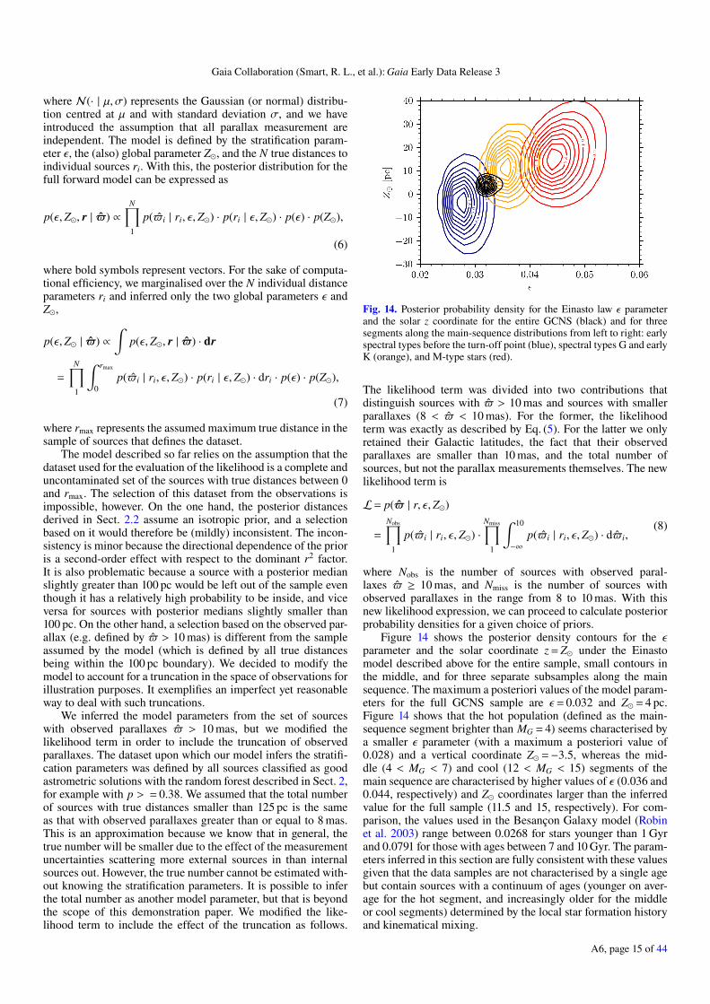
In our inference model we have the vertical stratification lawparameters (ε and Z) at the top. We defined a prior for the εparameter given by a Gaussian distribution centred at 0.05 andwith a standard deviation equal to 0.1, and a Gaussian prior cen-tred at 0 and with a standard deviation of 10 pc for the offsetof the Sun with respect to the Galactic plane. Then, for a givensource with Galactic latitude b, the probability density for thetrue distance r is given by

p(r | ε,Z) ∝ ρ(z(r) | ε,Z) · r2. (4)

Equation (4) is the natural extension of the constant volumedensity distribution of the distances. Finally, for N observa-tions of the parallax $i with associated uncertainties σ$i , thelikelihood is defined as

L=

N∏1

p($i | ri, ε,Z) =

N∏1

N($i | ri, σ$i ), (5)

A6, page 14 of 44

Gaia Collaboration (Smart, R. L., et al.): Gaia Early Data Release 3

where N(· | µ, σ) represents the Gaussian (or normal) distribu-tion centred at µ and with standard deviation σ, and we haveintroduced the assumption that all parallax measurement areindependent. The model is defined by the stratification param-eter ε, the (also) global parameter Z, and the N true distances toindividual sources ri. With this, the posterior distribution for thefull forward model can be expressed as

p(ε,Z, r | $) ∝N∏1

p($i | ri, ε,Z) · p(ri | ε,Z) · p(ε) · p(Z),

(6)

where bold symbols represent vectors. For the sake of computa-tional efficiency, we marginalised over the N individual distanceparameters ri and inferred only the two global parameters ε andZ,

p(ε,Z | $) ∝∫

p(ε,Z, r | $) · dr

=

N∏1

∫ rmax

0p($i | ri, ε,Z) · p(ri | ε,Z) · dri · p(ε) · p(Z),

(7)

where rmax represents the assumed maximum true distance in thesample of sources that defines the dataset.

The model described so far relies on the assumption that thedataset used for the evaluation of the likelihood is a complete anduncontaminated set of the sources with true distances between 0and rmax. The selection of this dataset from the observations isimpossible, however. On the one hand, the posterior distancesderived in Sect. 2.2 assume an isotropic prior, and a selectionbased on it would therefore be (mildly) inconsistent. The incon-sistency is minor because the directional dependence of the prioris a second-order effect with respect to the dominant r2 factor.It is also problematic because a source with a posterior medianslightly greater than 100 pc would be left out of the sample eventhough it has a relatively high probability to be inside, and viceversa for sources with posterior medians slightly smaller than100 pc. On the other hand, a selection based on the observed par-allax (e.g. defined by $ > 10 mas) is different from the sampleassumed by the model (which is defined by all true distancesbeing within the 100 pc boundary). We decided to modify themodel to account for a truncation in the space of observations forillustration purposes. It exemplifies an imperfect yet reasonableway to deal with such truncations.

We inferred the model parameters from the set of sourceswith observed parallaxes $ > 10 mas, but we modified thelikelihood term in order to include the truncation of observedparallaxes. The dataset upon which our model infers the stratifi-cation parameters was defined by all sources classified as goodastrometric solutions with the random forest described in Sect. 2,for example with p > = 0.38. We assumed that the total numberof sources with true distances smaller than 125 pc is the sameas that with observed parallaxes greater than or equal to 8 mas.This is an approximation because we know that in general, thetrue number will be smaller due to the effect of the measurementuncertainties scattering more external sources in than internalsources out. However, the true number cannot be estimated with-out knowing the stratification parameters. It is possible to inferthe total number as another model parameter, but that is beyondthe scope of this demonstration paper. We modified the like-lihood term to include the effect of the truncation as follows.

Fig. 14. Posterior probability density for the Einasto law ε parameterand the solar z coordinate for the entire GCNS (black) and for threesegments along the main-sequence distributions from left to right: earlyspectral types before the turn-off point (blue), spectral types G and earlyK (orange), and M-type stars (red).

The likelihood term was divided into two contributions thatdistinguish sources with $ > 10 mas and sources with smallerparallaxes (8 < $ < 10 mas). For the former, the likelihoodterm was exactly as described by Eq. (5). For the latter we onlyretained their Galactic latitudes, the fact that their observedparallaxes are smaller than 10 mas, and the total number ofsources, but not the parallax measurements themselves. The newlikelihood term is

L= p($ | r, ε,Z)

=

Nobs∏1

p($i | ri, ε,Z) ·Nmiss∏

1

∫ 10

−∞p($i | ri, ε,Z) · d$i,

(8)

where Nobs is the number of sources with observed paral-laxes $ ≥ 10 mas, and Nmiss is the number of sources withobserved parallaxes in the range from 8 to 10 mas. With thisnew likelihood expression, we can proceed to calculate posteriorprobability densities for a given choice of priors.

Figure 14 shows the posterior density contours for the εparameter and the solar coordinate z = Z under the Einastomodel described above for the entire sample, small contours inthe middle, and for three separate subsamples along the mainsequence. The maximum a posteriori values of the model param-eters for the full GCNS sample are ε = 0.032 and Z = 4 pc.Figure 14 shows that the hot population (defined as the main-sequence segment brighter than MG = 4) seems characterised bya smaller ε parameter (with a maximum a posteriori value of0.028) and a vertical coordinate Z =−3.5, whereas the mid-dle (4 < MG < 7) and cool (12 < MG < 15) segments of themain sequence are characterised by higher values of ε (0.036 and0.044, respectively) and Z coordinates larger than the inferredvalue for the full sample (11.5 and 15, respectively). For com-parison, the values used in the Besançon Galaxy model (Robinet al. 2003) range between 0.0268 for stars younger than 1 Gyrand 0.0791 for those with ages between 7 and 10 Gyr. The param-eters inferred in this section are fully consistent with these valuesgiven that the data samples are not characterised by a single agebut contain sources with a continuum of ages (younger on aver-age for the hot segment, and increasingly older for the middleor cool segments) determined by the local star formation historyand kinematical mixing.

A6, page 15 of 44

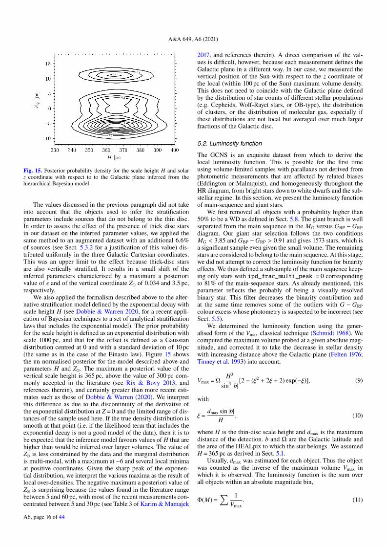
A&A 649, A6 (2021)

Fig. 15. Posterior probability density for the scale height H and solarz coordinate with respect to to the Galactic plane inferred from thehierarchical Bayesian model.

The values discussed in the previous paragraph did not takeinto account that the objects used to infer the stratificationparameters include sources that do not belong to the thin disc.In order to assess the effect of the presence of thick disc starsin our dataset on the inferred parameter values, we applied thesame method to an augmented dataset with an additional 6.6%of sources (see Sect. 5.3.2 for a justification of this value) dis-tributed uniformly in the three Galactic Cartesian coordinates.This was an upper limit to the effect because thick-disc starsare also vertically stratified. It results in a small shift of theinferred parameters characterised by a maximum a posteriorivalue of ε and of the vertical coordinate Z of 0.034 and 3.5 pc,respectively.

We also applied the formalism described above to the alter-native stratification model defined by the exponential decay withscale height H (see Dobbie & Warren 2020, for a recent appli-cation of Bayesian techniques to a set of analytical stratificationlaws that includes the exponential model). The prior probabilityfor the scale height is defined as an exponential distribution withscale 1000 pc, and that for the offset is defined as a Gaussiandistribution centred at 0 and with a standard deviation of 10 pc(the same as in the case of the Einasto law). Figure 15 showsthe un-normalised posterior for the model described above andparameters H and Z. The maximum a posteriori value of thevertical scale height is 365 pc, above the value of 300 pc com-monly accepted in the literature (see Rix & Bovy 2013, andreferences therein), and certainly greater than more recent esti-mates such as those of Dobbie & Warren (2020). We interpretthis difference as due to the discontinuity of the derivative ofthe exponential distribution at Z = 0 and the limited range of dis-tances of the sample used here. If the true density distribution issmooth at that point (i.e. if the likelihood term that includes theexponential decay is not a good model of the data), then it is tobe expected that the inference model favours values of H that arehigher than would be inferred over larger volumes. The value ofZ is less constrained by the data and the marginal distributionis multi-modal, with a maximum at −6 and several local minimaat positive coordinates. Given the sharp peak of the exponen-tial distribution, we interpret the various maxima as the result oflocal over-densities. The negative maximum a posteriori value ofZ is surprising because the values found in the literature rangebetween 5 and 60 pc, with most of the recent measurements con-centrated between 5 and 30 pc (see Table 3 of Karim & Mamajek

2017, and references therein). A direct comparison of the val-ues is difficult, however, because each measurement defines theGalactic plane in a different way. In our case, we measured thevertical position of the Sun with respect to the z coordinate ofthe local (within 100 pc of the Sun) maximum volume density.This does not need to coincide with the Galactic plane definedby the distribution of star counts of different stellar populations(e.g. Cepheids, Wolf-Rayet stars, or OB-type), the distributionof clusters, or the distribution of molecular gas, especially ifthese distributions are not local but averaged over much largerfractions of the Galactic disc.

5.2. Luminosity function

The GCNS is an exquisite dataset from which to derive thelocal luminosity function. This is possible for the first timeusing volume-limited samples with parallaxes not derived fromphotometric measurements that are affected by related biases(Eddington or Malmquist), and homogeneously throughout theHR diagram, from bright stars down to white dwarfs and the sub-stellar regime. In this section, we present the luminosity functionof main-sequence and giant stars.

We first removed all objects with a probability higher than50% to be a WD as defined in Sect. 5.8. The giant branch is wellseparated from the main sequence in the MG versus GBP −GRPdiagram. Our giant star selection follows the two conditionsMG < 3.85 and GBP −GRP > 0.91 and gives 1573 stars, which isa significant sample even given the small volume. The remainingstars are considered to belong to the main sequence. At this stage,we did not attempt to correct the luminosity function for binarityeffects. We thus defined a subsample of the main sequence keep-ing only stars with ipd_frac_multi_peak = 0 correspondingto 81% of the main-sequence stars. As already mentioned, thisparameter reflects the probably of being a visually resolvedbinary star. This filter decreases the binarity contribution andat the same time removes some of the outliers with G − GRPcolour excess whose photometry is suspected to be incorrect (seeSect. 5.5).

We determined the luminosity function using the gener-alised form of the Vmax classical technique (Schmidt 1968). Wecomputed the maximum volume probed at a given absolute mag-nitude, and corrected it to take the decrease in stellar densitywith increasing distance above the Galactic plane (Felten 1976;Tinney et al. 1993) into account,

Vmax = ΩH3

sin3 |b| [2 − (ξ2 + 2ξ + 2) exp(−ξ)], (9)

with

ξ =dmax sin |b|

H, (10)

where H is the thin-disc scale height and dmax is the maximumdistance of the detection. b and Ω are the Galactic latitude andthe area of the HEALpix to which the star belongs. We assumedH = 365 pc as derived in Sect. 5.1.

Usually, dmax was estimated for each object. Thus the objectwas counted as the inverse of the maximum volume Vmax inwhich it is observed. The luminosity function is the sum overall objects within an absolute magnitude bin,

Φ(M) =∑ 1

Vmax. (11)

A6, page 16 of 44

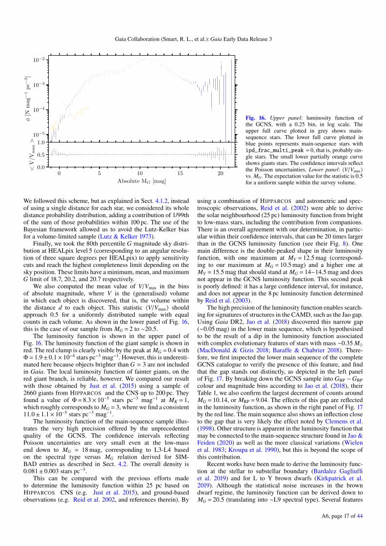
Gaia Collaboration (Smart, R. L., et al.): Gaia Early Data Release 3

10−5

10−4

10−3

10−2

φ[N

mag−

1p

c−3]

0 5 10 15 20

Absolute MG [mag]

0.0

0.5

1.0

<V/V

max>

Fig. 16. Upper panel: luminosity function ofthe GCNS, with a 0.25 bin, in log scale. Theupper full curve plotted in grey shows main-sequence stars. The lower full curve plotted inblue points represents main-sequence stars withipd_frac_multi_peak = 0, that is, probably sin-gle stars. The small lower partially orange curveshows giants stars. The confidence intervals reflectthe Poisson uncertainties. Lower panel: 〈V/Vmax〉vs. MG. The expectation value for the statistic is 0.5for a uniform sample within the survey volume.

We followed this scheme, but as explained in Sect. 4.1.2, insteadof using a single distance for each star, we considered its wholedistance probability distribution, adding a contribution of 1/99thof the sum of those probabilities within 100 pc. The use of theBayesian framework allowed us to avoid the Lutz-Kelker biasfor a volume-limited sample (Lutz & Kelker 1973).

Finally, we took the 80th percentile G magnitude sky distri-bution at HEALpix level 5 (corresponding to an angular resolu-tion of three square degrees per HEALpix) to apply sensitivitycuts and reach the highest completeness limit depending on thesky position. These limits have a minimum, mean, and maximumG limit of 18.7, 20.2, and 20.7 respectively.

We also computed the mean value of V/Vmax in the binsof absolute magnitude, where V is the (generalised) volumein which each object is discovered, that is, the volume withinthe distance d to each object. This statistic 〈V/Vmax〉 shouldapproach 0.5 for a uniformly distributed sample with equalcounts in each volume. As shown in the lower panel of Fig. 16,this is the case of our sample from MG = 2 to ∼20.5.

The luminosity function is shown in the upper panel ofFig. 16. The luminosity function of the giant sample is shown inred. The red clump is clearly visible by the peak at MG = 0.4 withΦ = 1.9± 0.1× 10−4 stars pc−3 mag−1. However, this is underesti-mated here because objects brighter than G ' 3 are not includedin Gaia. The local luminosity function of fainter giants, on thered giant branch, is reliable, however. We compared our resultwith those obtained by Just et al. (2015) using a sample of2660 giants from HIPPARCOS and the CNS up to 200 pc. Theyfound a value of Φ = 8.3× 10−5 stars pc−3 mag−1 at MK = 1,which roughly corresponds to MG = 3,where we find a consistent11.0± 1.1× 10−5 stars pc−3 mag−1.

The luminosity function of the main-sequence sample illus-trates the very high precision offered by the unprecedentedquality of the GCNS. The confidence intervals reflectingPoisson uncertainties are very small even at the low-massend down to MG ' 18 mag, corresponding to L3-L4 basedon the spectral type versus MG relation derived for SIM-BAD entries as described in Sect. 4.2. The overall density is0.081± 0.003 stars pc−3.

This can be compared with the previous efforts madeto determine the luminosity function within 25 pc based onHIPPARCOS CNS (e.g. Just et al. 2015), and ground-basedobservations (e.g. Reid et al. 2002, and references therein). By

using a combination of HIPPARCOS and astrometric and spec-troscopic observations, Reid et al. (2002) were able to derivethe solar neighbourhood (25 pc) luminosity function from brightto low-mass stars, including the contribution from companions.There is an overall agreement with our determination, in partic-ular within their confidence intervals, that can be 20 times largerthan in the GCNS luminosity function (see their Fig. 8). Onemain difference is the double-peaked shape in their luminosityfunction, with one maximum at MV = 12.5 mag (correspond-ing to our maximum at MG = 10.5 mag) and a higher one atMV = 15.5 mag that should stand at MG = 14−14.5 mag and doesnot appear in the GCNS luminosity function. This second peakis poorly defined: it has a large confidence interval, for instance,and does not appear in the 8 pc luminosity function determinedby Reid et al. (2003).

The high precision of the luminosity function enables search-ing for signatures of structures in the CAMD, such as the Jao gap.Using Gaia DR2, Jao et al. (2018) discovered this narrow gap(∼0.05 mag) in the lower main sequence, which is hypothesisedto be the result of a dip in the luminosity function associatedwith complex evolutionary features of stars with mass ∼0.35 M(MacDonald & Gizis 2018; Baraffe & Chabrier 2018). There-fore, we first inspected the lower main sequence of the completeGCNS catalogue to verify the presence of this feature, and findthat the gap stands out distinctly, as depicted in the left panelof Fig. 17. By breaking down the GCNS sample into GBP −GRPcolour and magnitude bins according to Jao et al. (2018), theirTable 1, we also confirm the largest decrement of counts aroundMG = 10.14, or MRP = 9.04. The effects of this gap are reflectedin the luminosity function, as shown in the right panel of Fig. 17by the red line. The main sequence also shows an inflection closeto the gap that is very likely the effect noted by Clemens et al.(1998). Other structure is apparent in the luminosity function thatmay be connected to the main-sequence structure found in Jao &Feiden (2020) as well as the more classical variations (Wielenet al. 1983; Kroupa et al. 1990), but this is beyond the scope ofthis contribution.

Recent works have been made to derive the luminosity func-tion at the stellar to substellar boundary (Bardalez Gagliuffiet al. 2019) and for L to Y brown dwarfs (Kirkpatrick et al.2019). Although the statistical noise increases in the browndwarf regime, the luminosity function can be derived down toMG = 20.5 (translating into ∼L9 spectral type). Several features

A6, page 17 of 44

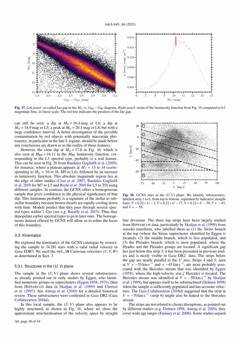
A&A 649, A6 (2021)

1.8 2.0 2.2 2.4 2.6 2.8 3.0 3.2

GBP −GRP [mag]

7

8

9

10

11

12

13

MG

[mag]

6 7 8 9 10 11 12 13 14

MG [mag]

0.004

0.006

0.008

0.010

0.012

0.014

φ[s

tars

/m

ag/

pc3

]

Fig. 17. Left panel: so-called Jao gap in the MG vs. GRP −GBP diagram. Right panel: zoom of the luminosity function from Fig. 16 computed in 0.1magnitude bins, in linear scale. The red line indicates the position of the Jao gap.

can still be seen: a dip at MG = 16.4 mag or L0; a dip atMG = 18.9 mag or L5; a peak at MG = 20.1 mag or L8, but with alarge confidence interval. A better investigation of the possiblecontamination by red objects with potentially inaccurate pho-tometry, in particular in the late-L regime, should be made beforeany conclusions are drawn as to the reality of these features.

However, the clear dip at MG = 17.6 in Fig. 16, which isalso seen at MRP = 16.11 in the MRP luminosity function, cor-responding to the L3 spectral type, probably is a real feature.This can be seen in Fig. 26 from Bardalez Gagliuffi et al. (2019),for instance, where a plateau appears at MJ ' 13 to 14 (corre-sponding to MG ' 16 to 18, M9 to L4), followed by an increasein luminosity function. This absolute magnitude region lies atthe edge of other studies (Cruz et al. 2007; Bardalez Gagliuffiet al. 2019 for M7 to L5 and Reylé et al. 2010 for L5 to T0) usingdifferent samples. In contrast, the GCNS offers a homogeneoussample that gives confidence to the physical significance of thatdip. This minimum probably is a signature of the stellar to sub-stellar boundary because brown dwarfs are rapidly cooling downwith time. Models predict that they pass through several spec-tral types within 1 Gyr (see e.g. Baraffe et al. 2015). Thus theydepopulate earlier spectral types to go to later ones. The homoge-neous dataset offered by GCNS will allow us to refine the locusof this boundary.

5.3. Kinematics

We explored the kinematics of the GCNS catalogue by restrict-ing the sample to 74 281 stars with a valid radial velocity inGaia EDR3. We used the vel_50 Cartesian velocities (U,V,W)as determined in Sect. 3.

5.3.1. Structures in the (U, V) plane

The sample in the (U,V) plane shows several substructures,as already pointed out in early studies by Eggen, who identi-fied numerous groups or superclusters (Eggen 1958, 1971), thenfrom HIPPARCOS data in Skuljan et al. (1999) and Chereulet al. (1997). See Antoja et al. (2010) for a detailed historicalreview. These substructures were confirmed in Gaia DR2 (GaiaCollaboration 2018d).

In this local sample, the (U,V) plane also appears to behighly structured, as shown in Fig. 18, where we show theapproximate structuralisation of the velocity space by straight

Fig. 18. GCNS stars in the (U,V) plane. We identify substructures,labelled strip 1 to 6, from top to bottom, separated by indicative straightlines: V = 0.22 ∗U − 3, V = 0.22 ∗U − 17, V = 0.22 ∗U − 39, V = − 43,and V = − 58.

line divisions. The three top strips have been largely studiedfrom HIPPARCOS data, particularly by Skuljan et al. (1999) fromwavelet transform, who labelled them as (1) the Sirius branchat the top (where the Sirius supercluster identified by Eggen islocated), (2) the middle branch, which is less populated, and(3) the Pleiades branch, which is most populated, where theHyades and the Pleiades groups are located. A significant gaplies just below this strip 3; it has been presented in previous stud-ies and is nicely visible in Gaia DR2 data. The strips belowthe gap are nearly parallel to the U axis. Strips 4 and 5, seenat V ≈ −35 km s−1 and ≈ −45 km s−1, are most probably asso-ciated with the Hercules stream that was identified by Eggen(1958), where the high-velocity star ζ Hercules is located. TheHercules stream was identified at V ≈ −50 km s−1 by Skuljanet al. (1999), but appears itself to be substructured (Dehnen 1998)when the sample is sufficiently populated and has accurate veloc-ities. The Gaia Collaboration (2018d) suggested that the strip atV ≈ −70 km s−1 (strip 6) might also be linked to the Herculesstream.

The strips are not related to cluster disruptions, as pointed outby different studies (e.g. Dehnen 1998; Antoja et al. 2010), theycover wide age ranges (Famaey et al. 2008). Some studies argued

A6, page 18 of 44

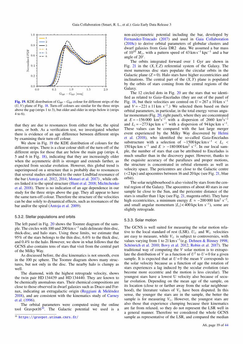
Gaia Collaboration (Smart, R. L., et al.): Gaia Early Data Release 3

Fig. 19. KDE distribution of GBP −GRP colour for different strips of the(U,V) plane of Fig. 18. Turn-off colours are similar for the three stripsabove the gap (strips 1 to 3), but older and older in strips below it (strips4 to 6).

that they are due to resonances from either the bar, the spiralarms, or both. As a verification test, we investigated whetherthere is evidence of an age difference between different stripsby examining their turn-off colour.

We show in Fig. 19 the KDE distribution of colours for thedifferent strips. There is a clear colour shift of the turn-off of thedifferent strips for those that are below the main gap (strips 4,5 and 6 in Fig. 18), indicating that they are increasingly olderwhen the asymmetric drift is stronger and extends farther, asexpected from secular evolution. However, this global trend issuperimposed on a structure that is probably due to resonancesthat several studies attributed to the outer Lindblad resonance ofthe bar (Antoja et al. 2012, 2014; Monari et al. 2017) , while oth-ers linked it to the spiral structure (Hunt et al. 2018; Michtchenkoet al. 2018). There is no indication of an age dependence in ourstudy for the three strips above the gap. They all appear to havethe same turn-off colour. Therefore the structure of the velocitiescan be due solely to dynamical effects, such as resonances of thebar and/or the spiral (Antoja et al. 2009).

5.3.2. Stellar populations and orbits

The left panel in Fig. 20 shows the Toomre diagram of the sam-ple. The circles with 100 and 200 km s−1 radii delineate thin-disc,thick-disc, and halo stars. Using these limits, we estimate that95% of the stars belongs to the thin disc, 6.6% to the thick disc,and 0.4% to the halo. However, we show in what follows that theGCNS also contains tens of stars that visit from the central partof the Milky Way.

As discussed before, the disc kinematics is not smooth, evenin the 100 pc sphere. The Toomre diagram shows many struc-tures, but not only in the disc. The nearby halo is clumpy aswell.

The diamond, with the highest retrograde velocity, showsthe twin pair HD 134439 and HD 134440. They are known tobe chemically anomalous stars. Their chemical compositions areclose to those observed in dwarf galaxies such as Draco and For-nax, indicating an extragalactic origin (Reggiani & Meléndez2018), and are consistent with the kinematics study of Carneyet al. (1996).

The orbital parameters were computed using the onlinetool Gravpot1610. The Galactic potential we used is a

10 https://gravpot.utinam.cnrs.fr/

non-axisymmetric potential including the bar, developed byFernandez-Trincado (2017) and used in Gaia Collaboration(2018c) to derive orbital parameters of globular clusters anddwarf galaxies from Gaia DR2 data. We assumed a bar massof 1010 M, with a pattern speed of 43 km s−1 kpc−1 and a barangle of 20.

The orbits integrated forward over 1 Gyr are shown inFig. 21 in the (X,Y,Z) referential system of the Galaxy. Themost numerous disc stars populate the circular orbits in theGalactic plane (Z = 0). Halo stars have higher eccentricities andinclinations. The central part of the (X,Y) plane is populatedby the orbits of stars coming from the central regions of theGalaxy.

The 12 circled dots in Fig. 20 are the stars that we identi-fied as related to Gaia–Enceladus (they are out of the panel ofFig. 18, but their velocities are centred on U = 267± 10 km s−1

and V =−221± 11 km s−1.) We selected them based on theirorbital parameters, in particular, in the total energy versus angu-lar momentum (Fig. 20, right panel), where they are concentratedat E =−156 000 km2s−2 with a dispersion of 2660 km2s−2

and Lz =−273 kpc km s−1 with a dispersion of 94 kpc km s−1.These values can be compared with the last large mergerevent experienced by the Milky Way discovered by Helmiet al. (2018), who identified the so-called Gaia-Enceladussubstructure with a selection of −1500 kpc km s−1 < Lz <150 kpc km s−1 and E > −180 000 km2 s−2. In our local sam-ple, the number of stars that can be attributed to Enceladus ismuch smaller than in the discovery paper. However, thanks tothe exquisite accuracy of the parallaxes and proper motions,the structure is concentrated in orbital elements as well asvelocity space. The pericentres are close to the Galactic centre(<2 kpc) and apocentres between 16 and 20 kpc (see Fig. 21, blueorbit).

The solar neighbourhood is also visited by stars from the cen-tral region of the Galaxy. The apocentres of about 40 stars in oursample lie close to the Sun, and the pericentre distance of thestars is smaller than 1 kpc (see Fig. 21, magenta orbit). They havehigh eccentricities, a minimum energy E ≈ −200 000 km2 s−2,and small angular momentum |Lz|< 400 kpc km s−1), some areslightly retrograde.

5.3.3. Solar motion

The GCNS is well suited for measuring the solar motion rela-tive to the local standard of rest (LSR). U and W velocitiesare easy to measure, while V is subject to controversies, withvalues varying from 1 to 21 km s−1(e.g. Dehnen & Binney 1998;Schönrich et al. 2010; Bovy et al. 2012; Robin et al. 2017). Thetraditional way of computing the V solar motion is to extrapo-late the distribution of V as a function of U2 to U = 0 for a givensample. It is expected that at U = 0 the mean V corresponds tothe solar velocity because as a function of age the rotation ofstars experiences a lag induced by the secular evolution (starsbecome more eccentric and the motion is less circular). Theyoungest stars have a lowest U velocity also because of secu-lar evolution. Depending on the mean age of the sample, onits location (close to or farther away from the solar neighbour-hood), the literature values of V have been disputed. In thissense, the younger the stars are in the sample, the better thesample is for measuring V. However, the youngest stars arealso those that experience clumping because their kinematicsare far from relaxed, so they do not represent the LSR well ina general manner. Therefore we considered the whole GCNSsample as representative of the LSR, and compared the median

A6, page 19 of 44

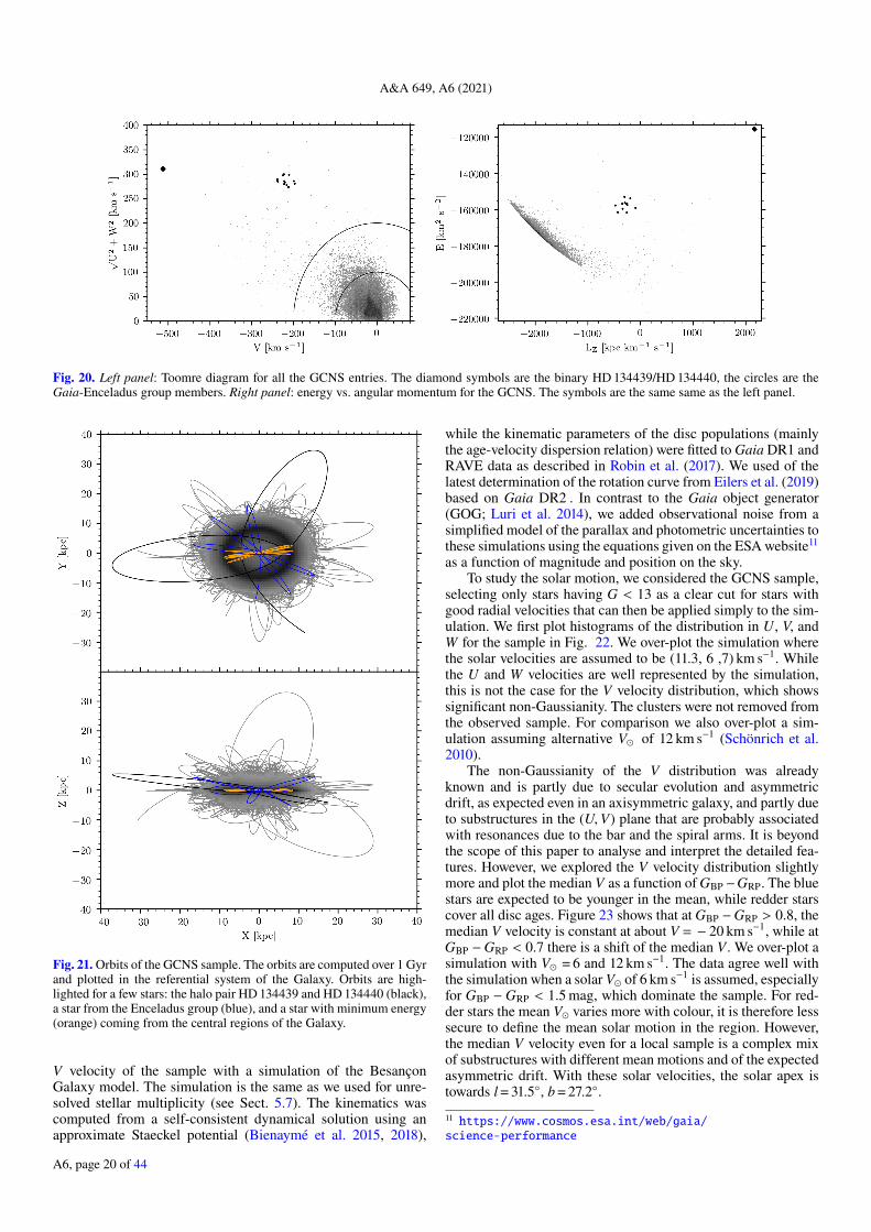
A&A 649, A6 (2021)

Fig. 20. Left panel: Toomre diagram for all the GCNS entries. The diamond symbols are the binary HD 134439/HD 134440, the circles are theGaia-Enceladus group members. Right panel: energy vs. angular momentum for the GCNS. The symbols are the same same as the left panel.

Fig. 21. Orbits of the GCNS sample. The orbits are computed over 1 Gyrand plotted in the referential system of the Galaxy. Orbits are high-lighted for a few stars: the halo pair HD 134439 and HD 134440 (black),a star from the Enceladus group (blue), and a star with minimum energy(orange) coming from the central regions of the Galaxy.

V velocity of the sample with a simulation of the BesançonGalaxy model. The simulation is the same as we used for unre-solved stellar multiplicity (see Sect. 5.7). The kinematics wascomputed from a self-consistent dynamical solution using anapproximate Staeckel potential (Bienaymé et al. 2015, 2018),

while the kinematic parameters of the disc populations (mainlythe age-velocity dispersion relation) were fitted to Gaia DR1 andRAVE data as described in Robin et al. (2017). We used of thelatest determination of the rotation curve from Eilers et al. (2019)based on Gaia DR2 . In contrast to the Gaia object generator(GOG; Luri et al. 2014), we added observational noise from asimplified model of the parallax and photometric uncertainties tothese simulations using the equations given on the ESA website11

as a function of magnitude and position on the sky.To study the solar motion, we considered the GCNS sample,

selecting only stars having G < 13 as a clear cut for stars withgood radial velocities that can then be applied simply to the sim-ulation. We first plot histograms of the distribution in U, V, andW for the sample in Fig. 22. We over-plot the simulation wherethe solar velocities are assumed to be (11.3, 6 ,7) km s−1. Whilethe U and W velocities are well represented by the simulation,this is not the case for the V velocity distribution, which showssignificant non-Gaussianity. The clusters were not removed fromthe observed sample. For comparison we also over-plot a sim-ulation assuming alternative V of 12 km s−1 (Schönrich et al.2010).

The non-Gaussianity of the V distribution was alreadyknown and is partly due to secular evolution and asymmetricdrift, as expected even in an axisymmetric galaxy, and partly dueto substructures in the (U,V) plane that are probably associatedwith resonances due to the bar and the spiral arms. It is beyondthe scope of this paper to analyse and interpret the detailed fea-tures. However, we explored the V velocity distribution slightlymore and plot the median V as a function of GBP −GRP. The bluestars are expected to be younger in the mean, while redder starscover all disc ages. Figure 23 shows that at GBP −GRP > 0.8, themedian V velocity is constant at about V = − 20 km s−1, while atGBP −GRP < 0.7 there is a shift of the median V . We over-plot asimulation with V = 6 and 12 km s−1. The data agree well withthe simulation when a solar V of 6 km s−1 is assumed, especiallyfor GBP −GRP < 1.5 mag, which dominate the sample. For red-der stars the mean V varies more with colour, it is therefore lesssecure to define the mean solar motion in the region. However,the median V velocity even for a local sample is a complex mixof substructures with different mean motions and of the expectedasymmetric drift. With these solar velocities, the solar apex istowards l = 31.5, b = 27.2.

11 https://www.cosmos.esa.int/web/gaia/science-performance

A6, page 20 of 44

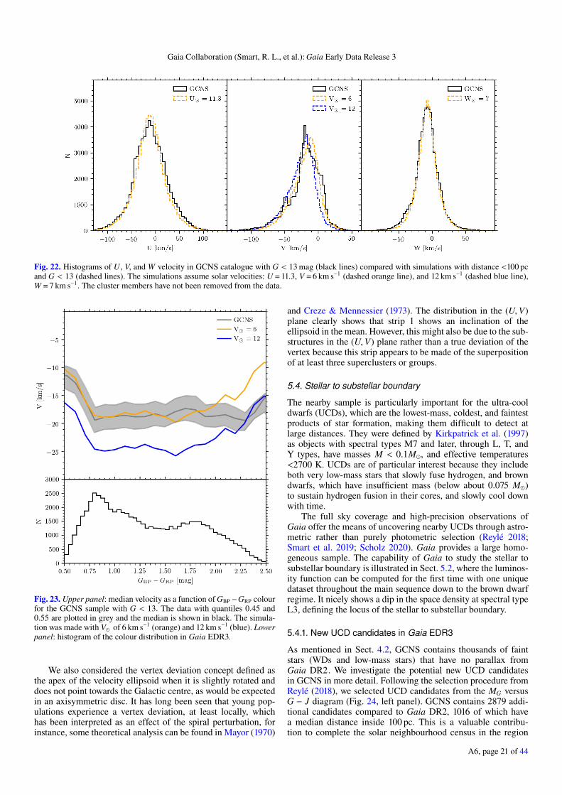
Gaia Collaboration (Smart, R. L., et al.): Gaia Early Data Release 3

Fig. 22. Histograms of U, V, and W velocity in GCNS catalogue with G < 13 mag (black lines) compared with simulations with distance <100 pcand G < 13 (dashed lines). The simulations assume solar velocities: U = 11.3, V = 6 km s−1 (dashed orange line), and 12 km s−1 (dashed blue line),W = 7 km s−1. The cluster members have not been removed from the data.

Fig. 23. Upper panel: median velocity as a function of GBP −GRP colourfor the GCNS sample with G < 13. The data with quantiles 0.45 and0.55 are plotted in grey and the median is shown in black. The simula-tion was made with V of 6 km s−1 (orange) and 12 km s−1 (blue). Lowerpanel: histogram of the colour distribution in Gaia EDR3.

We also considered the vertex deviation concept defined asthe apex of the velocity ellipsoid when it is slightly rotated anddoes not point towards the Galactic centre, as would be expectedin an axisymmetric disc. It has long been seen that young pop-ulations experience a vertex deviation, at least locally, whichhas been interpreted as an effect of the spiral perturbation, forinstance, some theoretical analysis can be found in Mayor (1970)

and Creze & Mennessier (1973). The distribution in the (U,V)plane clearly shows that strip 1 shows an inclination of theellipsoid in the mean. However, this might also be due to the sub-structures in the (U,V) plane rather than a true deviation of thevertex because this strip appears to be made of the superpositionof at least three superclusters or groups.

5.4. Stellar to substellar boundary

The nearby sample is particularly important for the ultra-cooldwarfs (UCDs), which are the lowest-mass, coldest, and faintestproducts of star formation, making them difficult to detect atlarge distances. They were defined by Kirkpatrick et al. (1997)as objects with spectral types M7 and later, through L, T, andY types, have masses M < 0.1M, and effective temperatures<2700 K. UCDs are of particular interest because they includeboth very low-mass stars that slowly fuse hydrogen, and browndwarfs, which have insufficient mass (below about 0.075 M)to sustain hydrogen fusion in their cores, and slowly cool downwith time.

The full sky coverage and high-precision observations ofGaia offer the means of uncovering nearby UCDs through astro-metric rather than purely photometric selection (Reylé 2018;Smart et al. 2019; Scholz 2020). Gaia provides a large homo-geneous sample. The capability of Gaia to study the stellar tosubstellar boundary is illustrated in Sect. 5.2, where the luminos-ity function can be computed for the first time with one uniquedataset throughout the main sequence down to the brown dwarfregime. It nicely shows a dip in the space density at spectral typeL3, defining the locus of the stellar to substellar boundary.

5.4.1. New UCD candidates in Gaia EDR3

As mentioned in Sect. 4.2, GCNS contains thousands of faintstars (WDs and low-mass stars) that have no parallax fromGaia DR2. We investigate the potential new UCD candidatesin GCNS in more detail. Following the selection procedure fromReylé (2018), we selected UCD candidates from the MG versusG − J diagram (Fig. 24, left panel). GCNS contains 2879 addi-tional candidates compared to Gaia DR2, 1016 of which havea median distance inside 100 pc. This is a valuable contribu-tion to complete the solar neighbourhood census in the region

A6, page 21 of 44

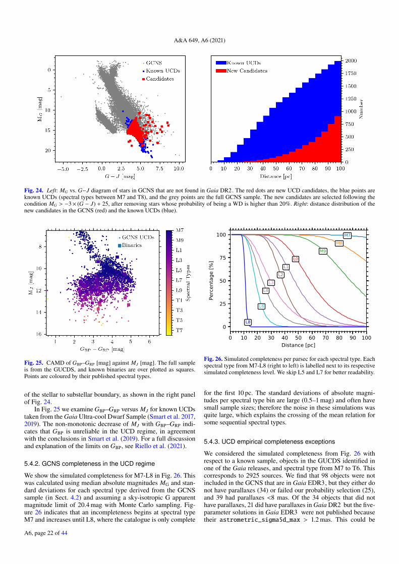
A&A 649, A6 (2021)

Fig. 24. Left: MG vs. G−J diagram of stars in GCNS that are not found in Gaia DR2. The red dots are new UCD candidates, the blue points areknown UCDs (spectral types between M7 and T8), and the grey points are the full GCNS sample. The new candidates are selected following thecondition MG > −3× (G − J) + 25, after removing stars whose probability of being a WD is higher than 20%. Right: distance distribution of thenew candidates in the GCNS (red) and the known UCDs (blue).

Fig. 25. CAMD of GBP–GRP [mag] against MJ [mag]. The full sampleis from the GUCDS, and known binaries are over plotted as squares.Points are coloured by their published spectral types.

of the stellar to substellar boundary, as shown in the right panelof Fig. 24.

In Fig. 25 we examine GBP–GRP versus MJ for known UCDstaken from the Gaia Ultra-cool Dwarf Sample (Smart et al. 2017,2019). The non-monotonic decrease of MJ with GBP–GRP indi-cates that GBP is unreliable in the UCD regime, in agreementwith the conclusions in Smart et al. (2019). For a full discussionand explanation of the limits on GBP, see Riello et al. (2021).

5.4.2. GCNS completeness in the UCD regime

We show the simulated completeness for M7-L8 in Fig. 26. Thiswas calculated using median absolute magnitudes MG and stan-dard deviations for each spectral type derived from the GCNSsample (in Sect. 4.2) and assuming a sky-isotropic G apparentmagnitude limit of 20.4 mag with Monte Carlo sampling. Fig-ure 26 indicates that an incompleteness begins at spectral typeM7 and increases until L8, where the catalogue is only complete

0 10 20 30 40 50 60 70 80 90 100Distance [pc]

0

25

50

75

100

Perc

enta

ge [%

]

M7M8

M9L0

L1L2

L3L4

L6

L8

Fig. 26. Simulated completeness per parsec for each spectral type. Eachspectral type from M7-L8 (right to left) is labelled next to its respectivesimulated completeness level. We skip L5 and L7 for better readability.

for the first 10 pc. The standard deviations of absolute magni-tudes per spectral type bin are large (0.5–1 mag) and often havesmall sample sizes; therefore the noise in these simulations wasquite large, which explains the crossing of the mean relation forsome sequential spectral types.

5.4.3. UCD empirical completeness exceptions

We considered the simulated completeness from Fig. 26 withrespect to a known sample, objects in the GUCDS identified inone of the Gaia releases, and spectral type from M7 to T6. Thiscorresponds to 2925 sources. We find that 98 objects were notincluded in the GCNS that are in Gaia EDR3, but they either donot have parallaxes (34) or failed our probability selection (25),and 39 had parallaxes <8 mas. Of the 34 objects that did nothave parallaxes, 21 did have parallaxes in Gaia DR2 but the five-parameter solutions in Gaia EDR3 were not published becausetheir astrometric_sigma5d_max > 1.2 mas. This could be

A6, page 22 of 44

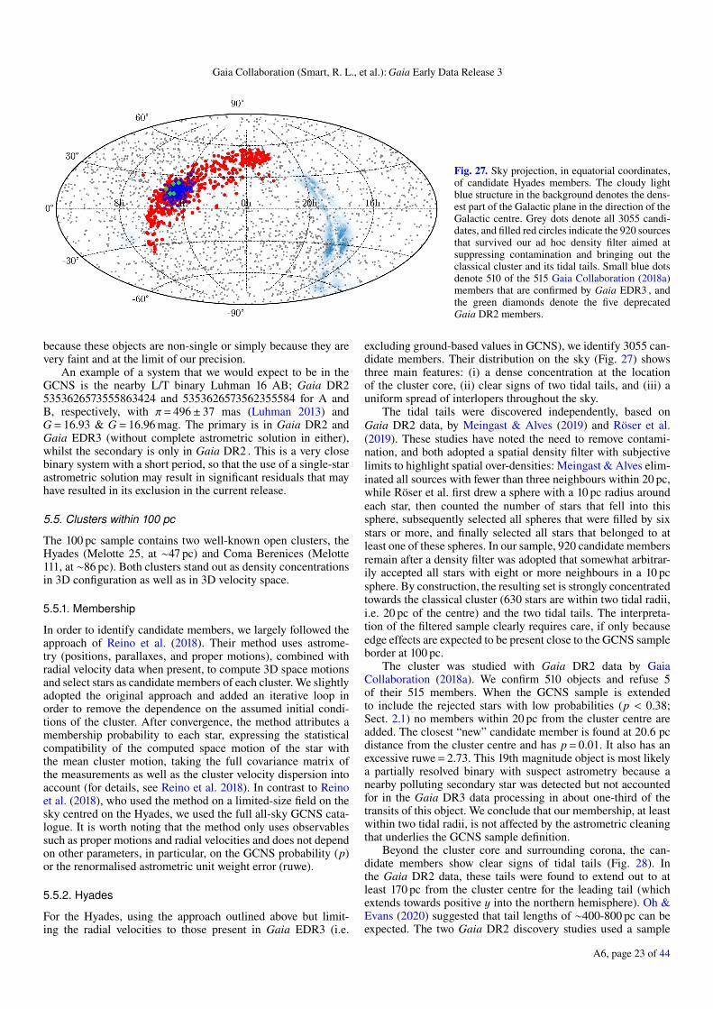
Gaia Collaboration (Smart, R. L., et al.): Gaia Early Data Release 3

Fig. 27. Sky projection, in equatorial coordinates,of candidate Hyades members. The cloudy lightblue structure in the background denotes the dens-est part of the Galactic plane in the direction of theGalactic centre. Grey dots denote all 3055 candi-dates, and filled red circles indicate the 920 sourcesthat survived our ad hoc density filter aimed atsuppressing contamination and bringing out theclassical cluster and its tidal tails. Small blue dotsdenote 510 of the 515 Gaia Collaboration (2018a)members that are confirmed by Gaia EDR3 , andthe green diamonds denote the five deprecatedGaia DR2 members.

because these objects are non-single or simply because they arevery faint and at the limit of our precision.

An example of a system that we would expect to be in theGCNS is the nearby L/T binary Luhman 16 AB; Gaia DR25353626573555863424 and 5353626573562355584 for A andB, respectively, with π= 496± 37 mas (Luhman 2013) andG = 16.93 & G = 16.96 mag. The primary is in Gaia DR2 andGaia EDR3 (without complete astrometric solution in either),whilst the secondary is only in Gaia DR2 . This is a very closebinary system with a short period, so that the use of a single-starastrometric solution may result in significant residuals that mayhave resulted in its exclusion in the current release.

5.5. Clusters within 100 pc

The 100 pc sample contains two well-known open clusters, theHyades (Melotte 25, at ∼47 pc) and Coma Berenices (Melotte111, at ∼86 pc). Both clusters stand out as density concentrationsin 3D configuration as well as in 3D velocity space.

5.5.1. Membership

In order to identify candidate members, we largely followed theapproach of Reino et al. (2018). Their method uses astrome-try (positions, parallaxes, and proper motions), combined withradial velocity data when present, to compute 3D space motionsand select stars as candidate members of each cluster. We slightlyadopted the original approach and added an iterative loop inorder to remove the dependence on the assumed initial condi-tions of the cluster. After convergence, the method attributes amembership probability to each star, expressing the statisticalcompatibility of the computed space motion of the star withthe mean cluster motion, taking the full covariance matrix ofthe measurements as well as the cluster velocity dispersion intoaccount (for details, see Reino et al. 2018). In contrast to Reinoet al. (2018), who used the method on a limited-size field on thesky centred on the Hyades, we used the full all-sky GCNS cata-logue. It is worth noting that the method only uses observablessuch as proper motions and radial velocities and does not dependon other parameters, in particular, on the GCNS probability (p)or the renormalised astrometric unit weight error (ruwe).

5.5.2. Hyades

For the Hyades, using the approach outlined above but limit-ing the radial velocities to those present in Gaia EDR3 (i.e.

excluding ground-based values in GCNS), we identify 3055 can-didate members. Their distribution on the sky (Fig. 27) showsthree main features: (i) a dense concentration at the locationof the cluster core, (ii) clear signs of two tidal tails, and (iii) auniform spread of interlopers throughout the sky.

The tidal tails were discovered independently, based onGaia DR2 data, by Meingast & Alves (2019) and Röser et al.(2019). These studies have noted the need to remove contami-nation, and both adopted a spatial density filter with subjectivelimits to highlight spatial over-densities: Meingast & Alves elim-inated all sources with fewer than three neighbours within 20 pc,while Röser et al. first drew a sphere with a 10 pc radius aroundeach star, then counted the number of stars that fell into thissphere, subsequently selected all spheres that were filled by sixstars or more, and finally selected all stars that belonged to atleast one of these spheres. In our sample, 920 candidate membersremain after a density filter was adopted that somewhat arbitrar-ily accepted all stars with eight or more neighbours in a 10 pcsphere. By construction, the resulting set is strongly concentratedtowards the classical cluster (630 stars are within two tidal radii,i.e. 20 pc of the centre) and the two tidal tails. The interpreta-tion of the filtered sample clearly requires care, if only becauseedge effects are expected to be present close to the GCNS sampleborder at 100 pc.

The cluster was studied with Gaia DR2 data by GaiaCollaboration (2018a). We confirm 510 objects and refuse 5of their 515 members. When the GCNS sample is extendedto include the rejected stars with low probabilities (p < 0.38;Sect. 2.1) no members within 20 pc from the cluster centre areadded. The closest “new” candidate member is found at 20.6 pcdistance from the cluster centre and has p = 0.01. It also has anexcessive ruwe = 2.73. This 19th magnitude object is most likelya partially resolved binary with suspect astrometry because anearby polluting secondary star was detected but not accountedfor in the Gaia DR3 data processing in about one-third of thetransits of this object. We conclude that our membership, at leastwithin two tidal radii, is not affected by the astrometric cleaningthat underlies the GCNS sample definition.

Beyond the cluster core and surrounding corona, the can-didate members show clear signs of tidal tails (Fig. 28). Inthe Gaia DR2 data, these tails were found to extend out to atleast 170 pc from the cluster centre for the leading tail (whichextends towards positive y into the northern hemisphere). Oh &Evans (2020) suggested that tail lengths of ∼400-800 pc can beexpected. The two Gaia DR2 discovery studies used a sample

A6, page 23 of 44

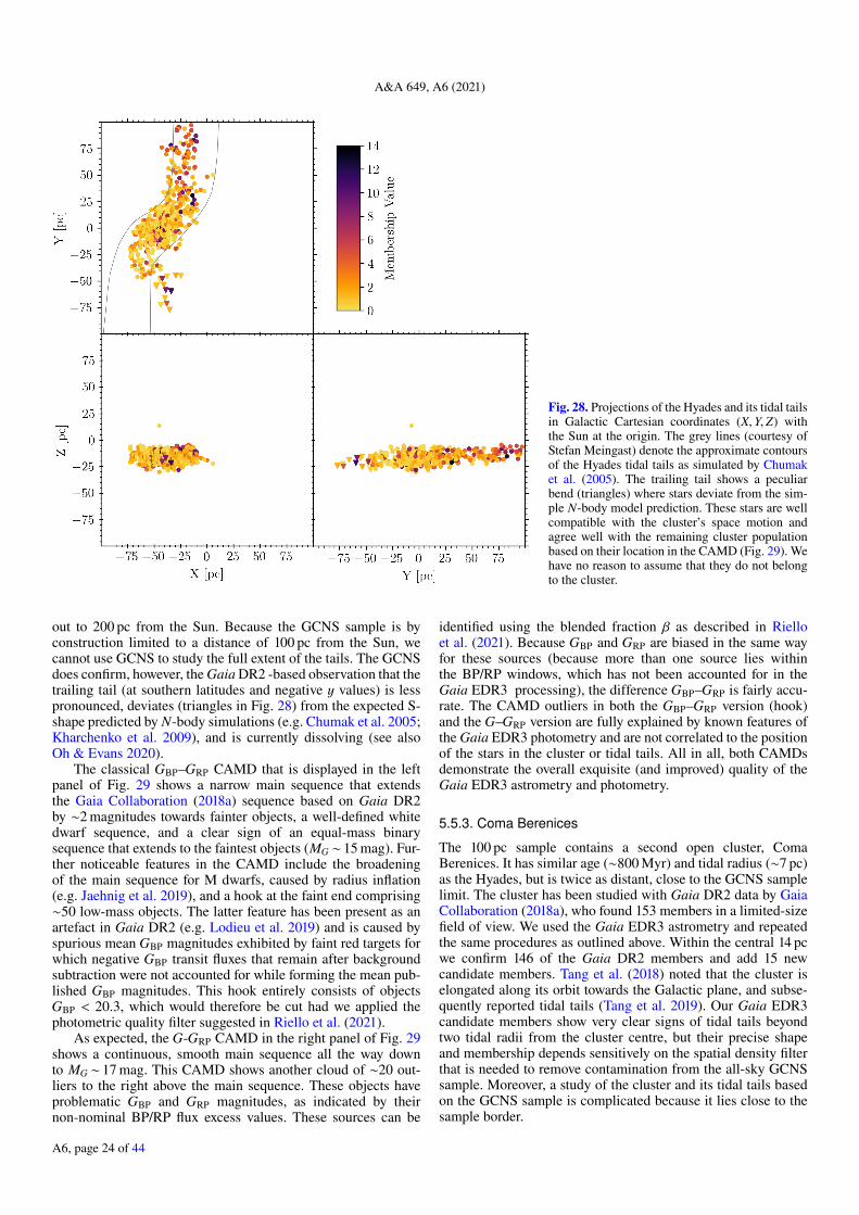
A&A 649, A6 (2021)

Fig. 28. Projections of the Hyades and its tidal tailsin Galactic Cartesian coordinates (X,Y,Z) withthe Sun at the origin. The grey lines (courtesy ofStefan Meingast) denote the approximate contoursof the Hyades tidal tails as simulated by Chumaket al. (2005). The trailing tail shows a peculiarbend (triangles) where stars deviate from the sim-ple N-body model prediction. These stars are wellcompatible with the cluster’s space motion andagree well with the remaining cluster populationbased on their location in the CAMD (Fig. 29). Wehave no reason to assume that they do not belongto the cluster.

out to 200 pc from the Sun. Because the GCNS sample is byconstruction limited to a distance of 100 pc from the Sun, wecannot use GCNS to study the full extent of the tails. The GCNSdoes confirm, however, the Gaia DR2 -based observation that thetrailing tail (at southern latitudes and negative y values) is lesspronounced, deviates (triangles in Fig. 28) from the expected S-shape predicted by N-body simulations (e.g. Chumak et al. 2005;Kharchenko et al. 2009), and is currently dissolving (see alsoOh & Evans 2020).

The classical GBP–GRP CAMD that is displayed in the leftpanel of Fig. 29 shows a narrow main sequence that extendsthe Gaia Collaboration (2018a) sequence based on Gaia DR2by ∼2 magnitudes towards fainter objects, a well-defined whitedwarf sequence, and a clear sign of an equal-mass binarysequence that extends to the faintest objects (MG ∼ 15 mag). Fur-ther noticeable features in the CAMD include the broadeningof the main sequence for M dwarfs, caused by radius inflation(e.g. Jaehnig et al. 2019), and a hook at the faint end comprising∼50 low-mass objects. The latter feature has been present as anartefact in Gaia DR2 (e.g. Lodieu et al. 2019) and is caused byspurious mean GBP magnitudes exhibited by faint red targets forwhich negative GBP transit fluxes that remain after backgroundsubtraction were not accounted for while forming the mean pub-lished GBP magnitudes. This hook entirely consists of objectsGBP < 20.3, which would therefore be cut had we applied thephotometric quality filter suggested in Riello et al. (2021).

As expected, the G-GRP CAMD in the right panel of Fig. 29shows a continuous, smooth main sequence all the way downto MG ∼ 17 mag. This CAMD shows another cloud of ∼20 out-liers to the right above the main sequence. These objects haveproblematic GBP and GRP magnitudes, as indicated by theirnon-nominal BP/RP flux excess values. These sources can be

identified using the blended fraction β as described in Rielloet al. (2021). Because GBP and GRP are biased in the same wayfor these sources (because more than one source lies withinthe BP/RP windows, which has not been accounted for in theGaia EDR3 processing), the difference GBP–GRP is fairly accu-rate. The CAMD outliers in both the GBP–GRP version (hook)and the G–GRP version are fully explained by known features ofthe Gaia EDR3 photometry and are not correlated to the positionof the stars in the cluster or tidal tails. All in all, both CAMDsdemonstrate the overall exquisite (and improved) quality of theGaia EDR3 astrometry and photometry.

5.5.3. Coma Berenices

The 100 pc sample contains a second open cluster, ComaBerenices. It has similar age (∼800 Myr) and tidal radius (∼7 pc)as the Hyades, but is twice as distant, close to the GCNS samplelimit. The cluster has been studied with Gaia DR2 data by GaiaCollaboration (2018a), who found 153 members in a limited-sizefield of view. We used the Gaia EDR3 astrometry and repeatedthe same procedures as outlined above. Within the central 14 pcwe confirm 146 of the Gaia DR2 members and add 15 newcandidate members. Tang et al. (2018) noted that the cluster iselongated along its orbit towards the Galactic plane, and subse-quently reported tidal tails (Tang et al. 2019). Our Gaia EDR3candidate members show very clear signs of tidal tails beyondtwo tidal radii from the cluster centre, but their precise shapeand membership depends sensitively on the spatial density filterthat is needed to remove contamination from the all-sky GCNSsample. Moreover, a study of the cluster and its tidal tails basedon the GCNS sample is complicated because it lies close to thesample border.

A6, page 24 of 44

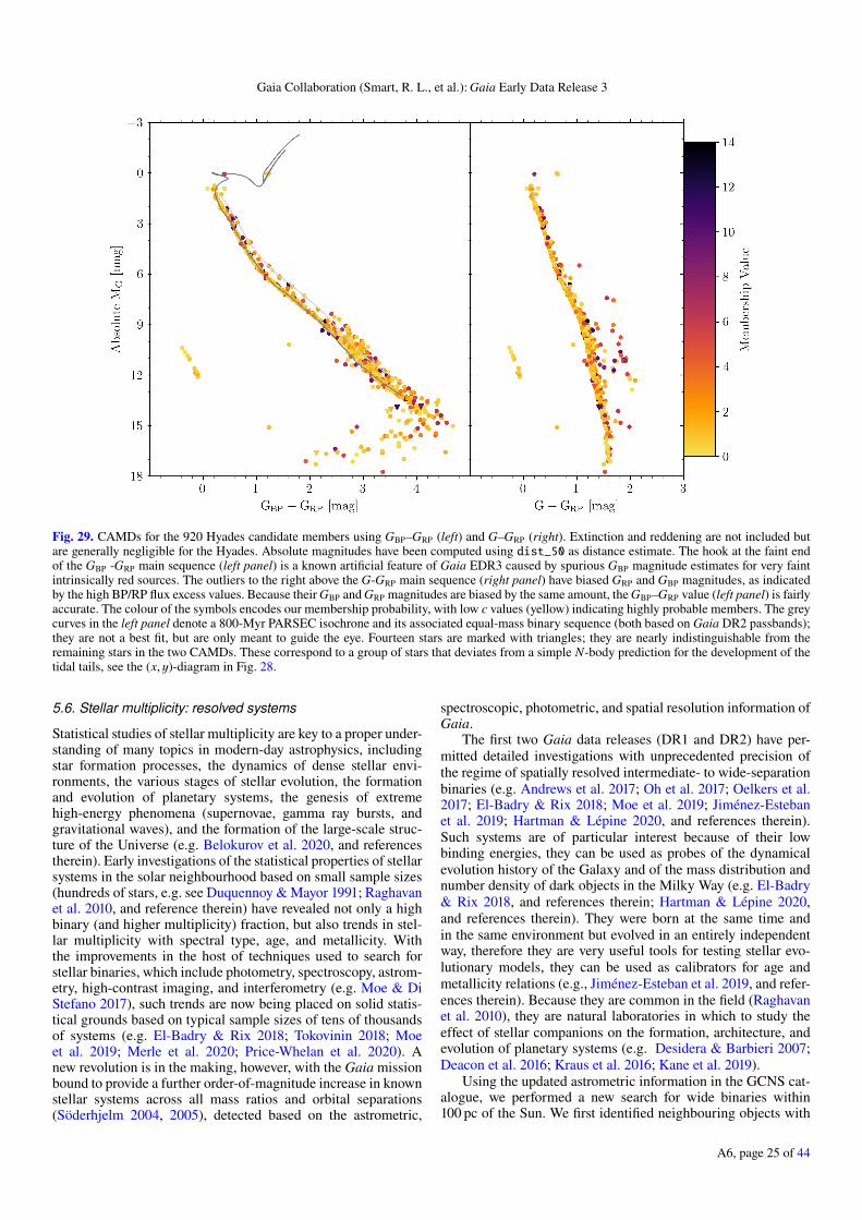
Gaia Collaboration (Smart, R. L., et al.): Gaia Early Data Release 3

Fig. 29. CAMDs for the 920 Hyades candidate members using GBP–GRP (left) and G–GRP (right). Extinction and reddening are not included butare generally negligible for the Hyades. Absolute magnitudes have been computed using dist_50 as distance estimate. The hook at the faint endof the GBP -GRP main sequence (left panel) is a known artificial feature of Gaia EDR3 caused by spurious GBP magnitude estimates for very faintintrinsically red sources. The outliers to the right above the G-GRP main sequence (right panel) have biased GRP and GBP magnitudes, as indicatedby the high BP/RP flux excess values. Because their GBP and GRP magnitudes are biased by the same amount, the GBP–GRP value (left panel) is fairlyaccurate. The colour of the symbols encodes our membership probability, with low c values (yellow) indicating highly probable members. The greycurves in the left panel denote a 800-Myr PARSEC isochrone and its associated equal-mass binary sequence (both based on Gaia DR2 passbands);they are not a best fit, but are only meant to guide the eye. Fourteen stars are marked with triangles; they are nearly indistinguishable from theremaining stars in the two CAMDs. These correspond to a group of stars that deviates from a simple N-body prediction for the development of thetidal tails, see the (x, y)-diagram in Fig. 28.

5.6. Stellar multiplicity: resolved systems

Statistical studies of stellar multiplicity are key to a proper under-standing of many topics in modern-day astrophysics, includingstar formation processes, the dynamics of dense stellar envi-ronments, the various stages of stellar evolution, the formationand evolution of planetary systems, the genesis of extremehigh-energy phenomena (supernovae, gamma ray bursts, andgravitational waves), and the formation of the large-scale struc-ture of the Universe (e.g. Belokurov et al. 2020, and referencestherein). Early investigations of the statistical properties of stellarsystems in the solar neighbourhood based on small sample sizes(hundreds of stars, e.g. see Duquennoy & Mayor 1991; Raghavanet al. 2010, and reference therein) have revealed not only a highbinary (and higher multiplicity) fraction, but also trends in stel-lar multiplicity with spectral type, age, and metallicity. Withthe improvements in the host of techniques used to search forstellar binaries, which include photometry, spectroscopy, astrom-etry, high-contrast imaging, and interferometry (e.g. Moe & DiStefano 2017), such trends are now being placed on solid statis-tical grounds based on typical sample sizes of tens of thousandsof systems (e.g. El-Badry & Rix 2018; Tokovinin 2018; Moeet al. 2019; Merle et al. 2020; Price-Whelan et al. 2020). Anew revolution is in the making, however, with the Gaia missionbound to provide a further order-of-magnitude increase in knownstellar systems across all mass ratios and orbital separations(Söderhjelm 2004, 2005), detected based on the astrometric,

spectroscopic, photometric, and spatial resolution information ofGaia.

The first two Gaia data releases (DR1 and DR2) have per-mitted detailed investigations with unprecedented precision ofthe regime of spatially resolved intermediate- to wide-separationbinaries (e.g. Andrews et al. 2017; Oh et al. 2017; Oelkers et al.2017; El-Badry & Rix 2018; Moe et al. 2019; Jiménez-Estebanet al. 2019; Hartman & Lépine 2020, and references therein).Such systems are of particular interest because of their lowbinding energies, they can be used as probes of the dynamicalevolution history of the Galaxy and of the mass distribution andnumber density of dark objects in the Milky Way (e.g. El-Badry& Rix 2018, and references therein; Hartman & Lépine 2020,and references therein). They were born at the same time andin the same environment but evolved in an entirely independentway, therefore they are very useful tools for testing stellar evo-lutionary models, they can be used as calibrators for age andmetallicity relations (e.g., Jiménez-Esteban et al. 2019, and refer-ences therein). Because they are common in the field (Raghavanet al. 2010), they are natural laboratories in which to study theeffect of stellar companions on the formation, architecture, andevolution of planetary systems (e.g. Desidera & Barbieri 2007;Deacon et al. 2016; Kraus et al. 2016; Kane et al. 2019).

Using the updated astrometric information in the GCNS cat-alogue, we performed a new search for wide binaries within100 pc of the Sun. We first identified neighbouring objects with

A6, page 25 of 44

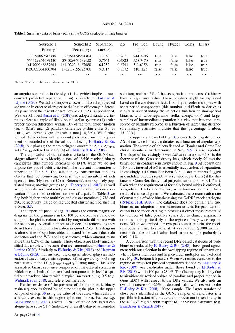
A&A 649, A6 (2021)

Table 3. Summary data on binary pairs in the GCNS catalogue of wide binaries.

SourceId 1 SourceId 2 Separation ∆G Proj. Sep. Bound Hyades Coma Binary(Primary) (Secondary) (arcsec) (au)

83154862613888 83154861954304 3.8353 3.2631 244.7406 true false false true554329954689280 554329954689152 3.7164 0.4823 358.7470 true false false true1611029348657664 1611029348487680 6.1252 0.8744 513.6358 true false false true1950331764866304 1962117155125760 9.3117 6.8372 810.1125 false false false true

. . . . . . . . . . . . . . . . . . . . . . . . . . .

Notes. The full table is available at the CDS.

an angular separation in the sky <1 deg (which implies a non-constant projected separation in au), similarly to Hartman &Lépine (2020). We did not impose a lower limit on the projectedseparation in order to characterise the loss in efficiency in detect-ing pairs when the resolution limit of Gaia EDR3 is approached.We then followed Smart et al. (2019) and adopted standard crite-ria to select a sample of likely bound stellar systems: (1) scalarproper motion difference within 10% of the total proper motion(∆µ < 0.1µ), and (2) parallax difference within either 3σ or1 mas, whichever is greater (∆$ < max[1.0, 3σ]). We furtherrefined the selection with a second pass based on the require-ment of boundedness of the orbits, following El-Badry & Rix(2018), but placing the more stringent constraint ∆µ < ∆µorbit,with ∆µorbit defined as in Eq. (4) of El-Badry & Rix (2018).

The application of our selection criteria to the GCNS cat-alogue allowed us to identify a total of 16 556 resolved binarycandidates (this number increases to 19 176 when we do notimpose the bound orbit criterion). The relevant information isreported in Table 3. The selection by construction containsobjects that are co-moving because they are members of richopen clusters (Hyades and Coma Berenices), more sparsely pop-ulated young moving groups (e.g. Faherty et al. 2018), as wellas higher-order resolved multiples in which more than one com-panion is identified to either member of a pair. In Table 3 weflag both higher-order multiples and cluster members (1758 and286, respectively) based on the updated cluster membership listin Sect. 5.5.

The upper left panel of Fig. 30 shows the colour-magnitudediagram for the primaries in the 100 pc wide-binary candidatesample. The plot is colour-coded by magnitude difference withthe secondary. A small number of objects are removed as theydo not have full colour information in Gaia EDR3. The diagramis almost free of spurious objects located in between the mainsequence and the WD cooling sequence, which amount to nomore than 0.2% of the sample. These objects are likely misclas-sified due a variety of reasons that are summarised in Hartman &Lépine (2020). Similarly to El-Badry & Rix (2018) and Hartman& Lépine (2020), for instance, the diagram also displays an indi-cation of a secondary main sequence, offset upward by ∼0.5 magparticularly in the 1.0 . (GBP−GRP) .2.0 mag range. This is theunresolved binary sequence composed of hierarchical systems inwhich one or both of the resolved components is itself a spa-tially unresolved binary with a typical mass ratio q & 0.5 (e.g.Widmark et al. 2018, and references therein).

Further evidence of the presence of the photometric binarymain-sequence is found by colour-coding the plot in the upperleft panel of Fig. 30 using the value of the ruwe, which exhibitsa notable excess in this region (plot not shown, but see e.g.Belokurov et al. 2020). Overall, ∼24% of the objects in our cat-alogue have ruwe &1.4 (indicative of an ill-behaved astrometric

solution), and in ∼2% of the cases, both components of a binaryhave a high ruwe value. These numbers might be explainedbased on the combined effects from higher-order multiples withshort-period components (this number is difficult to derive asit entails understanding the selection function of short-periodbinaries with wide-separation stellar companions) and largersamples of intermediate-separation binaries that become unre-solved or partially resolved as a function of increasing distance(preliminary estimates indicate that this percentage is about15−20%).

The upper right panel of Fig. 30 shows the G mag difference∆G of our wide-binary candidates as a function of angular sep-aration. The sample of objects flagged as Hyades and Coma Bercluster members, as determined in Sect. 5.5, is also reported.The slope of increasingly lower ∆G at separations <10′′ is thefootprint of the Gaia sensitivity loss, which nicely follows thebehaviour in contrast sensitivity shown in Fig. 9 At separations&10′′, the interval of ∆G is essentially independent of separation.Interestingly, all Coma Ber bona fide cluster members flaggedas candidate binaries reside at very wide separations (at the dis-tance of Coma Ber, the typical projected separation &4× 104 au).Even when the requirement of formally bound orbits is enforced,a significant fraction of the very wide binaries could still be aresult of chance alignment. We estimated the contamination rateof our sample of wide binaries using the GeDR3 mock catalogue(Rybizki et al. 2020). The catalogue does not contain any truebinaries: an adoption of our selection criteria for pair identifi-cation in the mock catalogue provides a direct measurement ofthe number of false positives (pairs due to chance alignment)in our sample, particularly in the regime of very wide separa-tions. When we applied our two-pass search criteria, the mockcatalogue returned five pairs, all at a separation &1000 au. Thismeans that the contamination level in our sample probably is0.05−0.1%.

A comparison with the recent DR2-based catalogue of widebinaries produced by El-Badry & Rix (2018) shows good agree-ment with our selection in the overlapping regime of separationswhen cluster members and higher-order multiples are excluded(see Fig. 30, bottom left panel). When we restrict ourselves to theregime of projected physical separations defined by El-Badry &Rix (2018), our candidates match those found by El-Badry &Rix (2018) within 100 pc to 78.1%. The discrepancy is likely dueto significantly revised values of parallax and proper motion inGaia EDR3 with respect to the DR2 values. We also note anoverall increase of ∼20% in detected pairs with respect to theEl-Badry & Rix (2018) 100 pc sample. The larger number ofclose pairs identified in the GCNS samples of candidates is apossible indication of a moderate improvement in sensitivity inthe ≈1′′–3′′ regime with respect to DR2-based estimates (e.g.Brandeker & Cataldi 2019).

A6, page 26 of 44

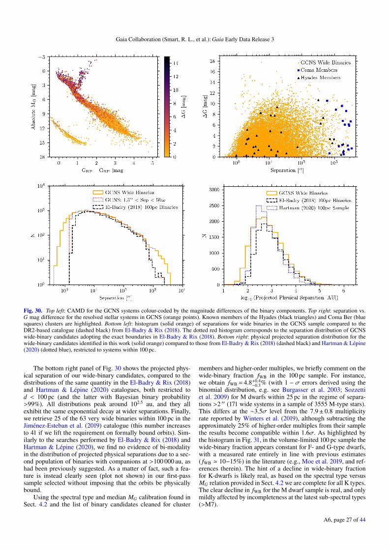
Gaia Collaboration (Smart, R. L., et al.): Gaia Early Data Release 3

Fig. 30. Top left: CAMD for the GCNS systems colour-coded by the magnitude differences of the binary components. Top right: separation vs.G mag difference for the resolved stellar systems in GCNS (orange points). Known members of the Hyades (black triangles) and Coma Ber (bluesquares) clusters are highlighted. Bottom left: histogram (solid orange) of separations for wide binaries in the GCNS sample compared to theDR2-based catalogue (dashed black) from El-Badry & Rix (2018). The dotted red histogram corresponds to the separation distribution of GCNSwide-binary candidates adopting the exact boundaries in El-Badry & Rix (2018). Bottom right: physical projected separation distribution for thewide-binary candidates identified in this work (solid orange) compared to those from El-Badry & Rix (2018) (dashed black) and Hartman & Lépine(2020) (dotted blue), restricted to systems within 100 pc.

The bottom right panel of Fig. 30 shows the projected phys-ical separation of our wide-binary candidates, compared to thedistributions of the same quantity in the El-Badry & Rix (2018)and Hartman & Lépine (2020) catalogues, both restricted tod < 100 pc (and the latter with Bayesian binary probability>99%). All distributions peak around 102.5 au, and they allexhibit the same exponential decay at wider separations. Finally,we retrieve 25 of the 63 very wide binaries within 100 pc in theJiménez-Esteban et al. (2019) catalogue (this number increasesto 41 if we lift the requirement on formally bound orbits). Sim-ilarly to the searches performed by El-Badry & Rix (2018) andHartman & Lépine (2020), we find no evidence of bi-modalityin the distribution of projected physical separations due to a sec-ond population of binaries with companions at >100 000 au, ashad been previously suggested. As a matter of fact, such a fea-ture is instead clearly seen (plot not shown) in our first-passsample selected without imposing that the orbits be physicallybound.

Using the spectral type and median MG calibration found inSect. 4.2 and the list of binary candidates cleaned for cluster

members and higher-order multiples, we briefly comment on thewide-binary fraction fWB in the 100 pc sample. For instance,we obtain fWB = 4.8+0.4

−0.3% (with 1 − σ errors derived using thebinomial distribution, e.g. see Burgasser et al. 2003; Sozzettiet al. 2009) for M dwarfs within 25 pc in the regime of separa-tions >2 ′′ (171 wide systems in a sample of 3555 M-type stars).This differs at the ∼3.5σ level from the 7.9± 0.8 multiplicityrate reported by Winters et al. (2019), although subtracting theapproximately 25% of higher-order multiples from their samplethe results become compatible within 1.6σ. As highlighted bythe histogram in Fig. 31, in the volume-limited 100 pc sample thewide-binary fraction appears constant for F- and G-type dwarfs,with a measured rate entirely in line with previous estimates( fWB ' 10−15%) in the literature (e.g., Moe et al. 2019, and ref-erences therein). The hint of a decline in wide-binary fractionfor K-dwarfs is likely real, as based on the spectral type versusMG relation provided in Sect. 4.2 we are complete for all K types.The clear decline in fWB for the M dwarf sample is real, and onlymildly affected by incompleteness at the latest sub-spectral types(>M7).

A6, page 27 of 44

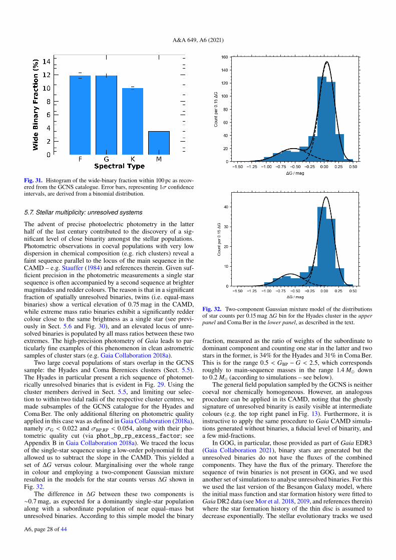
A&A 649, A6 (2021)

Fig. 31. Histogram of the wide-binary fraction within 100 pc as recov-ered from the GCNS catalogue. Error bars, representing 1σ confidenceintervals, are derived from a binomial distribution.

5.7. Stellar multiplicity: unresolved systems

The advent of precise photoelectric photometry in the latterhalf of the last century contributed to the discovery of a sig-nificant level of close binarity amongst the stellar populations.Photometric observations in coeval populations with very lowdispersion in chemical composition (e.g. rich clusters) reveal afaint sequence parallel to the locus of the main sequence in theCAMD – e.g. Stauffer (1984) and references therein. Given suf-ficient precision in the photometric measurements a single starsequence is often accompanied by a second sequence at brightermagnitudes and redder colours. The reason is that in a significantfraction of spatially unresolved binaries, twins (i.e. equal-massbinaries) show a vertical elevation of 0.75 mag in the CAMD,while extreme mass ratio binaries exhibit a significantly reddercolour close to the same brightness as a single star (see previ-ously in Sect. 5.6 and Fig. 30), and an elevated locus of unre-solved binaries is populated by all mass ratios between these twoextremes. The high-precision photometry of Gaia leads to par-ticularly fine examples of this phenomenon in clean astrometricsamples of cluster stars (e.g. Gaia Collaboration 2018a).

Two large coeval populations of stars overlap in the GCNSsample: the Hyades and Coma Berenices clusters (Sect. 5.5).The Hyades in particular present a rich sequence of photomet-rically unresolved binaries that is evident in Fig. 29. Using thecluster members derived in Sect. 5.5, and limiting our selec-tion to within two tidal radii of the respective cluster centres, wemade subsamples of the GCNS catalogue for the Hyades andComa Ber. The only additional filtering on photometric qualityapplied in this case was as defined in Gaia Collaboration (2018a),namely σG < 0.022 and σBP,RP < 0.054, along with their pho-tometric quality cut (via phot_bp_rp_excess_factor; seeAppendix B in Gaia Collaboration 2018a). We traced the locusof the single-star sequence using a low-order polynomial fit thatallowed us to subtract the slope in the CAMD. This yielded aset of ∆G versus colour. Marginalising over the whole rangein colour and employing a two-component Gaussian mixtureresulted in the models for the star counts versus ∆G shown inFig. 32.

The difference in ∆G between these two components is∼0.7 mag, as expected for a dominantly single-star populationalong with a subordinate population of near equal–mass butunresolved binaries. According to this simple model the binary

Fig. 32. Two-component Gaussian mixture model of the distributionsof star counts per 0.15 mag ∆G bin for the Hyades cluster in the upperpanel and Coma Ber in the lower panel, as described in the text.

fraction, measured as the ratio of weights of the subordinate todominant component and counting one star in the latter and twostars in the former, is 34% for the Hyades and 31% in Coma Ber.This is for the range 0.5 < GBP − G < 2.5, which correspondsroughly to main-sequence masses in the range 1.4 M downto 0.2 M (according to simulations – see below).

The general field population sampled by the GCNS is neithercoeval nor chemically homogeneous. However, an analogousprocedure can be applied in its CAMD, noting that the ghostlysignature of unresolved binarity is easily visible at intermediatecolours (e.g. the top right panel in Fig. 13). Furthermore, it isinstructive to apply the same procedure to Gaia CAMD simula-tions generated without binaries, a fiducial level of binarity, anda few mid-fractions.

In GOG, in particular, those provided as part of Gaia EDR3(Gaia Collaboration 2021), binary stars are generated but theunresolved binaries do not have the fluxes of the combinedcomponents. They have the flux of the primary. Therefore thesequence of twin binaries is not present in GOG, and we usedanother set of simulations to analyse unresolved binaries. For thiswe used the last version of the Besançon Galaxy model, wherethe initial mass function and star formation history were fitted toGaia DR2 data (see Mor et al. 2018, 2019, and references therein)where the star formation history of the thin disc is assumed todecrease exponentially. The stellar evolutionary tracks we used

A6, page 28 of 44

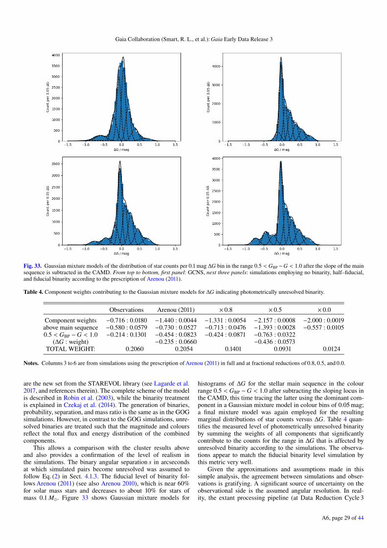
Gaia Collaboration (Smart, R. L., et al.): Gaia Early Data Release 3

Fig. 33. Gaussian mixture models of the distribution of star counts per 0.1 mag ∆G bin in the range 0.5 < GBP −G < 1.0 after the slope of the mainsequence is subtracted in the CAMD. From top to bottom, first panel: GCNS, next three panels: simulations employing no binarity, half–fiducial,and fiducial binarity according to the prescription of Arenou (2011).

Table 4. Component weights contributing to the Gaussian mixture models for ∆G indicating photometrically unresolved binarity.

Observations Arenou (2011) × 0.8 × 0.5 × 0.0

Component weights −0.716 : 0.0180 −1.440 : 0.0044 −1.331 : 0.0054 −2.157 : 0.0008 −2.000 : 0.0019above main sequence −0.580 : 0.0579 −0.730 : 0.0527 −0.713 : 0.0476 −1.393 : 0.0028 −0.557 : 0.01050.5 < GBP −G < 1.0 −0.214 : 0.1301 −0.454 : 0.0823 −0.424 : 0.0871 −0.763 : 0.0322

(∆G : weight) −0.235 : 0.0660 −0.436 : 0.0573TOTAL WEIGHT: 0.2060 0.2054 0.1401 0.0931 0.0124

Notes. Columns 3 to 6 are from simulations using the prescription of Arenou (2011) in full and at fractional reductions of 0.8, 0.5, and 0.0.

are the new set from the STAREVOL library (see Lagarde et al.2017, and references therein). The complete scheme of the modelis described in Robin et al. (2003), while the binarity treatmentis explained in Czekaj et al. (2014). The generation of binaries,probability, separation, and mass ratio is the same as in the GOGsimulations. However, in contrast to the GOG simulations, unre-solved binaries are treated such that the magnitude and coloursreflect the total flux and energy distribution of the combinedcomponents.

This allows a comparison with the cluster results aboveand also provides a confirmation of the level of realism inthe simulations. The binary angular separation s in arcsecondsat which simulated pairs become unresolved was assumed tofollow Eq. (2) in Sect. 4.1.3. The fiducial level of binarity fol-lows Arenou (2011) (see also Arenou 2010), which is near 60%for solar mass stars and decreases to about 10% for stars ofmass 0.1 M. Figure 33 shows Gaussian mixture models for

histograms of ∆G for the stellar main sequence in the colourrange 0.5 < GBP −G < 1.0 after subtracting the sloping locus inthe CAMD, this time tracing the latter using the dominant com-ponent in a Gaussian mixture model in colour bins of 0.05 mag;a final mixture model was again employed for the resultingmarginal distributions of star counts versus ∆G. Table 4 quan-tifies the measured level of photometrically unresolved binarityby summing the weights of all components that significantlycontribute to the counts for the range in ∆G that is affected byunresolved binarity according to the simulations. The observa-tions appear to match the fiducial binarity level simulation bythis metric very well.

Given the approximations and assumptions made in thissimple analysis, the agreement between simulations and obser-vations is gratifying. A significant source of uncertainty on theobservational side is the assumed angular resolution. In real-ity, the extant processing pipeline (at Data Reduction Cycle 3

A6, page 29 of 44

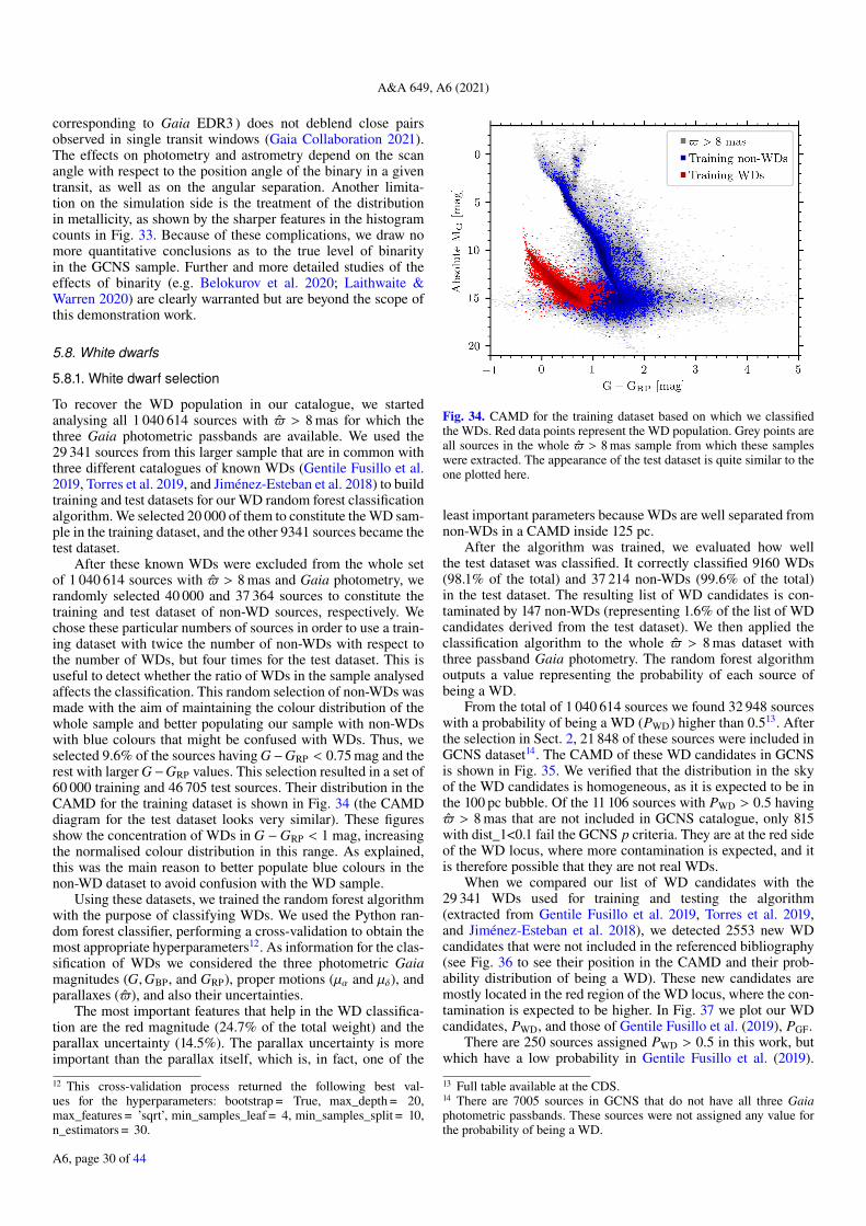
A&A 649, A6 (2021)

corresponding to Gaia EDR3 ) does not deblend close pairsobserved in single transit windows (Gaia Collaboration 2021).The effects on photometry and astrometry depend on the scanangle with respect to the position angle of the binary in a giventransit, as well as on the angular separation. Another limita-tion on the simulation side is the treatment of the distributionin metallicity, as shown by the sharper features in the histogramcounts in Fig. 33. Because of these complications, we draw nomore quantitative conclusions as to the true level of binarityin the GCNS sample. Further and more detailed studies of theeffects of binarity (e.g. Belokurov et al. 2020; Laithwaite &Warren 2020) are clearly warranted but are beyond the scope ofthis demonstration work.

5.8. White dwarfs

5.8.1. White dwarf selection

To recover the WD population in our catalogue, we startedanalysing all 1 040 614 sources with $ > 8 mas for which thethree Gaia photometric passbands are available. We used the29 341 sources from this larger sample that are in common withthree different catalogues of known WDs (Gentile Fusillo et al.2019, Torres et al. 2019, and Jiménez-Esteban et al. 2018) to buildtraining and test datasets for our WD random forest classificationalgorithm. We selected 20 000 of them to constitute the WD sam-ple in the training dataset, and the other 9341 sources became thetest dataset.

After these known WDs were excluded from the whole setof 1 040 614 sources with $ > 8 mas and Gaia photometry, werandomly selected 40 000 and 37 364 sources to constitute thetraining and test dataset of non-WD sources, respectively. Wechose these particular numbers of sources in order to use a train-ing dataset with twice the number of non-WDs with respect tothe number of WDs, but four times for the test dataset. This isuseful to detect whether the ratio of WDs in the sample analysedaffects the classification. This random selection of non-WDs wasmade with the aim of maintaining the colour distribution of thewhole sample and better populating our sample with non-WDswith blue colours that might be confused with WDs. Thus, weselected 9.6% of the sources having G−GRP < 0.75 mag and therest with larger G−GRP values. This selection resulted in a set of60 000 training and 46 705 test sources. Their distribution in theCAMD for the training dataset is shown in Fig. 34 (the CAMDdiagram for the test dataset looks very similar). These figuresshow the concentration of WDs in G −GRP < 1 mag, increasingthe normalised colour distribution in this range. As explained,this was the main reason to better populate blue colours in thenon-WD dataset to avoid confusion with the WD sample.

Using these datasets, we trained the random forest algorithmwith the purpose of classifying WDs. We used the Python ran-dom forest classifier, performing a cross-validation to obtain themost appropriate hyperparameters12. As information for the clas-sification of WDs we considered the three photometric Gaiamagnitudes (G,GBP, and GRP), proper motions (µα and µδ), andparallaxes ($), and also their uncertainties.

The most important features that help in the WD classifica-tion are the red magnitude (24.7% of the total weight) and theparallax uncertainty (14.5%). The parallax uncertainty is moreimportant than the parallax itself, which is, in fact, one of the

12 This cross-validation process returned the following best val-ues for the hyperparameters: bootstrap = True, max_depth = 20,max_features = ’sqrt’, min_samples_leaf = 4, min_samples_split = 10,n_estimators = 30.

Fig. 34. CAMD for the training dataset based on which we classifiedthe WDs. Red data points represent the WD population. Grey points areall sources in the whole $ > 8 mas sample from which these sampleswere extracted. The appearance of the test dataset is quite similar to theone plotted here.

least important parameters because WDs are well separated fromnon-WDs in a CAMD inside 125 pc.

After the algorithm was trained, we evaluated how wellthe test dataset was classified. It correctly classified 9160 WDs(98.1% of the total) and 37 214 non-WDs (99.6% of the total)in the test dataset. The resulting list of WD candidates is con-taminated by 147 non-WDs (representing 1.6% of the list of WDcandidates derived from the test dataset). We then applied theclassification algorithm to the whole $ > 8 mas dataset withthree passband Gaia photometry. The random forest algorithmoutputs a value representing the probability of each source ofbeing a WD.

From the total of 1 040 614 sources we found 32 948 sourceswith a probability of being a WD (PWD) higher than 0.513. Afterthe selection in Sect. 2, 21 848 of these sources were included inGCNS dataset14. The CAMD of these WD candidates in GCNSis shown in Fig. 35. We verified that the distribution in the skyof the WD candidates is homogeneous, as it is expected to be inthe 100 pc bubble. Of the 11 106 sources with PWD > 0.5 having$ > 8 mas that are not included in GCNS catalogue, only 815with dist_1<0.1 fail the GCNS p criteria. They are at the red sideof the WD locus, where more contamination is expected, and itis therefore possible that they are not real WDs.

When we compared our list of WD candidates with the29 341 WDs used for training and testing the algorithm(extracted from Gentile Fusillo et al. 2019, Torres et al. 2019,and Jiménez-Esteban et al. 2018), we detected 2553 new WDcandidates that were not included in the referenced bibliography(see Fig. 36 to see their position in the CAMD and their prob-ability distribution of being a WD). These new candidates aremostly located in the red region of the WD locus, where the con-tamination is expected to be higher. In Fig. 37 we plot our WDcandidates, PWD, and those of Gentile Fusillo et al. (2019), PGF.

There are 250 sources assigned PWD > 0.5 in this work, butwhich have a low probability in Gentile Fusillo et al. (2019).

13 Full table available at the CDS.14 There are 7005 sources in GCNS that do not have all three Gaiaphotometric passbands. These sources were not assigned any value forthe probability of being a WD.

A6, page 30 of 44

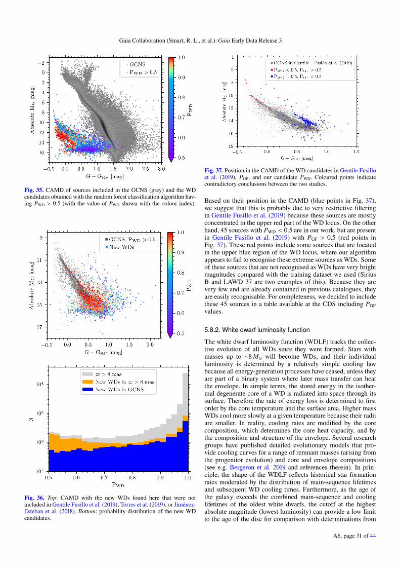
Gaia Collaboration (Smart, R. L., et al.): Gaia Early Data Release 3

Fig. 35. CAMD of sources included in the GCNS (grey) and the WDcandidates obtained with the random forest classification algorithm hav-ing PWD > 0.5 (with the value of PWD shown with the colour index).

Fig. 36. Top: CAMD with the new WDs found here that were notincluded in Gentile Fusillo et al. (2019), Torres et al. (2019), or Jiménez-Esteban et al. (2018). Bottom: probability distribution of the new WDcandidates.

Fig. 37. Position in the CAMD of the WD candidates in Gentile Fusilloet al. (2019), PGF, and our candidate PWD. Coloured points indicatecontradictory conclusions between the two studies.

Based on their position in the CAMD (blue points in Fig. 37),we suggest that this is probably due to very restrictive filteringin Gentile Fusillo et al. (2019) because these sources are mostlyconcentrated in the upper red part of the WD locus. On the otherhand, 45 sources with PWD < 0.5 are in our work, but are presentin Gentile Fusillo et al. (2019) with PGF > 0.5 (red points inFig. 37). These red points include some sources that are locatedin the upper blue region of the WD locus, where our algorithmappears to fail to recognise these extreme sources as WDs. Someof these sources that are not recognised as WDs have very brightmagnitudes compared with the training dataset we used (SiriusB and LAWD 37 are two examples of this). Because they arevery few and are already contained in previous catalogues, theyare easily recognisable. For completeness, we decided to includethese 45 sources in a table available at the CDS including PGFvalues.

5.8.2. White dwarf luminosity function

The white dwarf luminosity function (WDLF) tracks the collec-tive evolution of all WDs since they were formed. Stars withmasses up to ∼8 M will become WDs, and their individualluminosity is determined by a relatively simple cooling lawbecause all energy-generation processes have ceased, unless theyare part of a binary system where later mass transfer can heatthe envelope. In simple terms, the stored energy in the isother-mal degenerate core of a WD is radiated into space through itssurface. Therefore the rate of energy loss is determined to firstorder by the core temperature and the surface area. Higher massWDs cool more slowly at a given temperature because their radiiare smaller. In reality, cooling rates are modified by the corecomposition, which determines the core heat capacity, and bythe composition and structure of the envelope. Several researchgroups have published detailed evolutionary models that pro-vide cooling curves for a range of remnant masses (arising fromthe progenitor evolution) and core and envelope compositions(see e.g. Bergeron et al. 2019 and references therein). In prin-ciple, the shape of the WDLF reflects historical star formationrates moderated by the distribution of main-sequence lifetimesand subsequent WD cooling times. Furthermore, as the age ofthe galaxy exceeds the combined main-sequence and coolinglifetimes of the oldest white dwarfs, the cutoff at the highestabsolute magnitude (lowest luminosity) can provide a low limitto the age of the disc for comparison with determinations from

A6, page 31 of 44

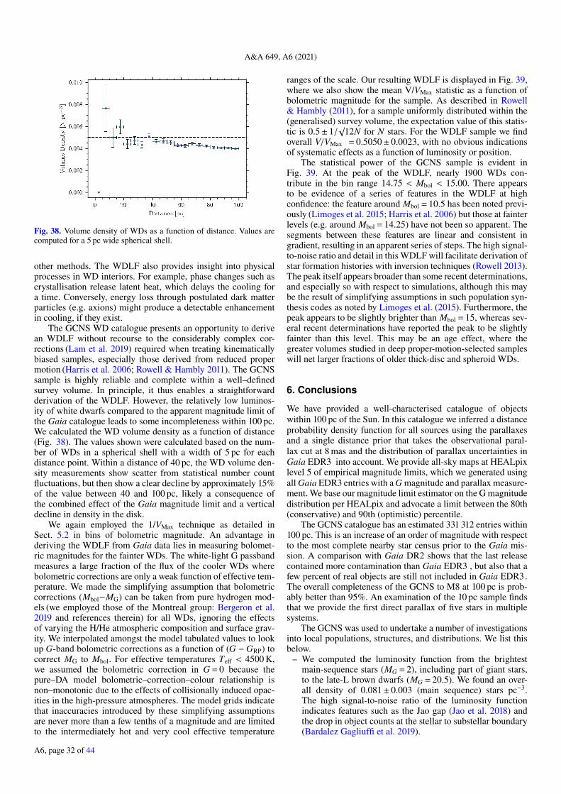
A&A 649, A6 (2021)

Fig. 38. Volume density of WDs as a function of distance. Values arecomputed for a 5 pc wide spherical shell.

other methods. The WDLF also provides insight into physicalprocesses in WD interiors. For example, phase changes such ascrystallisation release latent heat, which delays the cooling fora time. Conversely, energy loss through postulated dark matterparticles (e.g. axions) might produce a detectable enhancementin cooling, if they exist.

The GCNS WD catalogue presents an opportunity to derivean WDLF without recourse to the considerably complex cor-rections (Lam et al. 2019) required when treating kinematicallybiased samples, especially those derived from reduced propermotion (Harris et al. 2006; Rowell & Hambly 2011). The GCNSsample is highly reliable and complete within a well–definedsurvey volume. In principle, it thus enables a straightforwardderivation of the WDLF. However, the relatively low luminos-ity of white dwarfs compared to the apparent magnitude limit ofthe Gaia catalogue leads to some incompleteness within 100 pc.We calculated the WD volume density as a function of distance(Fig. 38). The values shown were calculated based on the num-ber of WDs in a spherical shell with a width of 5 pc for eachdistance point. Within a distance of 40 pc, the WD volume den-sity measurements show scatter from statistical number countfluctuations, but then show a clear decline by approximately 15%of the value between 40 and 100 pc, likely a consequence ofthe combined effect of the Gaia magnitude limit and a verticaldecline in density in the disk.

We again employed the 1/VMax technique as detailed inSect. 5.2 in bins of bolometric magnitude. An advantage inderiving the WDLF from Gaia data lies in measuring bolomet-ric magnitudes for the fainter WDs. The white-light G passbandmeasures a large fraction of the flux of the cooler WDs wherebolometric corrections are only a weak function of effective tem-perature. We made the simplifying assumption that bolometriccorrections (Mbol−MG) can be taken from pure hydrogen mod-els (we employed those of the Montreal group: Bergeron et al.2019 and references therein) for all WDs, ignoring the effectsof varying the H/He atmospheric composition and surface grav-ity. We interpolated amongst the model tabulated values to lookup G-band bolometric corrections as a function of (G −GRP) tocorrect MG to Mbol. For effective temperatures Teff < 4500 K,we assumed the bolometric correction in G = 0 because thepure–DA model bolometric–correction–colour relationship isnon–monotonic due to the effects of collisionally induced opac-ities in the high-pressure atmospheres. The model grids indicatethat inaccuracies introduced by these simplifying assumptionsare never more than a few tenths of a magnitude and are limitedto the intermediately hot and very cool effective temperature

ranges of the scale. Our resulting WDLF is displayed in Fig. 39,where we also show the mean V/VMax statistic as a function ofbolometric magnitude for the sample. As described in Rowell& Hambly (2011), for a sample uniformly distributed within the(generalised) survey volume, the expectation value of this statis-tic is 0.5± 1/

√12N for N stars. For the WDLF sample we find

overall V/VMax = 0.5050± 0.0023, with no obvious indicationsof systematic effects as a function of luminosity or position.

The statistical power of the GCNS sample is evident inFig. 39. At the peak of the WDLF, nearly 1900 WDs con-tribute in the bin range 14.75 < Mbol < 15.00. There appearsto be evidence of a series of features in the WDLF at highconfidence: the feature around Mbol = 10.5 has been noted previ-ously (Limoges et al. 2015; Harris et al. 2006) but those at fainterlevels (e.g. around Mbol = 14.25) have not been so apparent. Thesegments between these features are linear and consistent ingradient, resulting in an apparent series of steps. The high signal-to-noise ratio and detail in this WDLF will facilitate derivation ofstar formation histories with inversion techniques (Rowell 2013).The peak itself appears broader than some recent determinations,and especially so with respect to simulations, although this maybe the result of simplifying assumptions in such population syn-thesis codes as noted by Limoges et al. (2015). Furthermore, thepeak appears to be slightly brighter than Mbol = 15, whereas sev-eral recent determinations have reported the peak to be slightlyfainter than this level. This may be an age effect, where thegreater volumes studied in deep proper-motion-selected sampleswill net larger fractions of older thick-disc and spheroid WDs.

6. Conclusions

We have provided a well-characterised catalogue of objectswithin 100 pc of the Sun. In this catalogue we inferred a distanceprobability density function for all sources using the parallaxesand a single distance prior that takes the observational paral-lax cut at 8 mas and the distribution of parallax uncertainties inGaia EDR3 into account. We provide all-sky maps at HEALpixlevel 5 of empirical magnitude limits, which we generated usingall Gaia EDR3 entries with a G magnitude and parallax measure-ment. We base our magnitude limit estimator on the G magnitudedistribution per HEALpix and advocate a limit between the 80th(conservative) and 90th (optimistic) percentile.

The GCNS catalogue has an estimated 331 312 entries within100 pc. This is an increase of an order of magnitude with respectto the most complete nearby star census prior to the Gaia mis-sion. A comparison with Gaia DR2 shows that the last releasecontained more contamination than Gaia EDR3 , but also that afew percent of real objects are still not included in Gaia EDR3.The overall completeness of the GCNS to M8 at 100 pc is prob-ably better than 95%. An examination of the 10 pc sample findsthat we provide the first direct parallax of five stars in multiplesystems.

The GCNS was used to undertake a number of investigationsinto local populations, structures, and distributions. We list thisbelow.

– We computed the luminosity function from the brightestmain-sequence stars (MG = 2), including part of giant stars,to the late-L brown dwarfs (MG = 20.5). We found an over-all density of 0.081± 0.003 (main sequence) stars pc−3.The high signal-to-noise ratio of the luminosity functionindicates features such as the Jao gap (Jao et al. 2018) andthe drop in object counts at the stellar to substellar boundary(Bardalez Gagliuffi et al. 2019).

A6, page 32 of 44

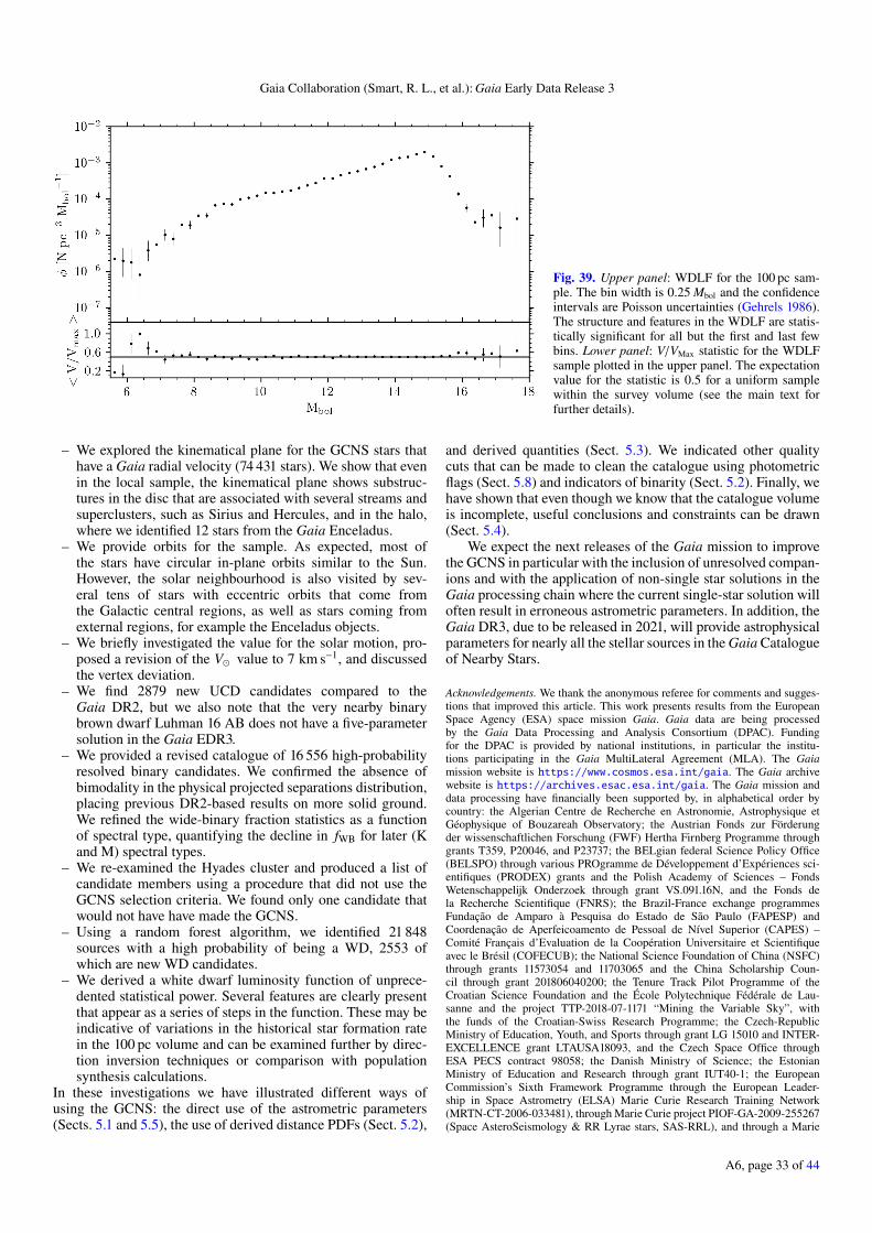
Gaia Collaboration (Smart, R. L., et al.): Gaia Early Data Release 3

Fig. 39. Upper panel: WDLF for the 100 pc sam-ple. The bin width is 0.25 Mbol and the confidenceintervals are Poisson uncertainties (Gehrels 1986).The structure and features in the WDLF are statis-tically significant for all but the first and last fewbins. Lower panel: V/VMax statistic for the WDLFsample plotted in the upper panel. The expectationvalue for the statistic is 0.5 for a uniform samplewithin the survey volume (see the main text forfurther details).

– We explored the kinematical plane for the GCNS stars thathave a Gaia radial velocity (74 431 stars). We show that evenin the local sample, the kinematical plane shows substruc-tures in the disc that are associated with several streams andsuperclusters, such as Sirius and Hercules, and in the halo,where we identified 12 stars from the Gaia Enceladus.

– We provide orbits for the sample. As expected, most ofthe stars have circular in-plane orbits similar to the Sun.However, the solar neighbourhood is also visited by sev-eral tens of stars with eccentric orbits that come fromthe Galactic central regions, as well as stars coming fromexternal regions, for example the Enceladus objects.

– We briefly investigated the value for the solar motion, pro-posed a revision of the V value to 7 km s−1, and discussedthe vertex deviation.

– We find 2879 new UCD candidates compared to theGaia DR2, but we also note that the very nearby binarybrown dwarf Luhman 16 AB does not have a five-parametersolution in the Gaia EDR3.

– We provided a revised catalogue of 16 556 high-probabilityresolved binary candidates. We confirmed the absence ofbimodality in the physical projected separations distribution,placing previous DR2-based results on more solid ground.We refined the wide-binary fraction statistics as a functionof spectral type, quantifying the decline in fWB for later (Kand M) spectral types.

– We re-examined the Hyades cluster and produced a list ofcandidate members using a procedure that did not use theGCNS selection criteria. We found only one candidate thatwould not have have made the GCNS.

– Using a random forest algorithm, we identified 21 848sources with a high probability of being a WD, 2553 ofwhich are new WD candidates.

– We derived a white dwarf luminosity function of unprece-dented statistical power. Several features are clearly presentthat appear as a series of steps in the function. These may beindicative of variations in the historical star formation ratein the 100 pc volume and can be examined further by direc-tion inversion techniques or comparison with populationsynthesis calculations.

In these investigations we have illustrated different ways ofusing the GCNS: the direct use of the astrometric parameters(Sects. 5.1 and 5.5), the use of derived distance PDFs (Sect. 5.2),

and derived quantities (Sect. 5.3). We indicated other qualitycuts that can be made to clean the catalogue using photometricflags (Sect. 5.8) and indicators of binarity (Sect. 5.2). Finally, wehave shown that even though we know that the catalogue volumeis incomplete, useful conclusions and constraints can be drawn(Sect. 5.4).

We expect the next releases of the Gaia mission to improvethe GCNS in particular with the inclusion of unresolved compan-ions and with the application of non-single star solutions in theGaia processing chain where the current single-star solution willoften result in erroneous astrometric parameters. In addition, theGaia DR3, due to be released in 2021, will provide astrophysicalparameters for nearly all the stellar sources in the Gaia Catalogueof Nearby Stars.

Acknowledgements. We thank the anonymous referee for comments and sugges-tions that improved this article. This work presents results from the EuropeanSpace Agency (ESA) space mission Gaia. Gaia data are being processedby the Gaia Data Processing and Analysis Consortium (DPAC). Fundingfor the DPAC is provided by national institutions, in particular the institu-tions participating in the Gaia MultiLateral Agreement (MLA). The Gaiamission website is https://www.cosmos.esa.int/gaia. The Gaia archivewebsite is https://archives.esac.esa.int/gaia. The Gaia mission anddata processing have financially been supported by, in alphabetical order bycountry: the Algerian Centre de Recherche en Astronomie, Astrophysique etGéophysique of Bouzareah Observatory; the Austrian Fonds zur Förderungder wissenschaftlichen Forschung (FWF) Hertha Firnberg Programme throughgrants T359, P20046, and P23737; the BELgian federal Science Policy Office(BELSPO) through various PROgramme de Développement d’Expériences sci-entifiques (PRODEX) grants and the Polish Academy of Sciences – FondsWetenschappelijk Onderzoek through grant VS.091.16N, and the Fonds dela Recherche Scientifique (FNRS); the Brazil-France exchange programmesFundação de Amparo à Pesquisa do Estado de São Paulo (FAPESP) andCoordenação de Aperfeicoamento de Pessoal de Nível Superior (CAPES) –Comité Français d’Evaluation de la Coopération Universitaire et Scientifiqueavec le Brésil (COFECUB); the National Science Foundation of China (NSFC)through grants 11573054 and 11703065 and the China Scholarship Coun-cil through grant 201806040200; the Tenure Track Pilot Programme of theCroatian Science Foundation and the École Polytechnique Fédérale de Lau-sanne and the project TTP-2018-07-1171 “Mining the Variable Sky”, withthe funds of the Croatian-Swiss Research Programme; the Czech-RepublicMinistry of Education, Youth, and Sports through grant LG 15010 and INTER-EXCELLENCE grant LTAUSA18093, and the Czech Space Office throughESA PECS contract 98058; the Danish Ministry of Science; the EstonianMinistry of Education and Research through grant IUT40-1; the EuropeanCommission’s Sixth Framework Programme through the European Leader-ship in Space Astrometry (ELSA) Marie Curie Research Training Network(MRTN-CT-2006-033481), through Marie Curie project PIOF-GA-2009-255267(Space AsteroSeismology & RR Lyrae stars, SAS-RRL), and through a Marie

A6, page 33 of 44

A&A 649, A6 (2021)

Curie Transfer-of-Knowledge (ToK) fellowship (MTKD-CT-2004-014188); theEuropean Commission’s Seventh Framework Programme through grant FP7-606740 (FP7-SPACE-2013-1) for the Gaia European Network for Improved dataUser Services (GENIUS) and through grant 264895 for the Gaia Research forEuropean Astronomy Training (GREAT-ITN) network; the European ResearchCouncil (ERC) through grants 320360 and 647208 and through the EuropeanUnion’s Horizon 2020 research and innovation and excellent science pro-grammes through Marie Skłodowska-Curie grant 745617 as well as grants 670519(Mixing and Angular Momentum tranSport of massIvE stars – MAMSIE),687378 (Small Bodies: Near and Far), 682115 (Using the Magellanic Clouds toUnderstand the Interaction of Galaxies), and 695099 (A sub-percent distancescale from binaries and Cepheids – CepBin); the European Science Founda-tion (ESF), in the framework of the Gaia Research for European AstronomyTraining Research Network Programme (GREAT-ESF); the European SpaceAgency (ESA) in the framework of the Gaia project, through the Plan forEuropean Cooperating States (PECS) programme through grants for Slove-nia, through contracts C98090 and 4000106398/12/NL/KML for Hungary, andthrough contract 4000115263/15/NL/IB for Germany; the Academy of Finlandand the Magnus Ehrnrooth Foundation; the French Centre National d’EtudesSpatiales (CNES), the Agence Nationale de la Recherche (ANR) throughgrant ANR-10-IDEX-0001-02 for the “Investissements d’avenir” programme,through grant ANR-15-CE31-0007 for project “Modelling the Milky Way inthe Gaia era” (MOD4Gaia), through grant ANR-14-CE33-0014-01 for project“The Milky Way disc formation in the Gaia era” (ARCHEOGAL), and throughgrant ANR-15-CE31-0012-01 for project “Unlocking the potential of Cepheidsas primary distance calibrators” (UnlockCepheids), the Centre National de laRecherche Scientifique (CNRS) and its SNO Gaia of the Institut des Sciencesde l’Univers (INSU), the “Action Fédératrice Gaia” of the Observatoire deParis, the Région de Franche-Comté, and the Programme National de Gravi-tation, Références, Astronomie, et Métrologie (GRAM) of CNRS/INSU withthe Institut National Polytechnique (INP) and the Institut National de Physiquenucléaire et de Physique des Particules (IN2P3) co-funded by CNES; the GermanAerospace Agency (Deutsches Zentrum für Luft- und Raumfahrt e.V., DLR)through grants 50QG0501, 50QG0601, 50QG0602, 50QG0701, 50QG0901,50QG1001, 50QG1101, 50QG1401, 50QG1402, 50QG1403, 50QG1404, and50QG1904 and the Centre for Information Services and High PerformanceComputing (ZIH) at the Technische Universität (TU) Dresden for generousallocations of computer time; the Hungarian Academy of Sciences throughthe Lendület Programme grants LP2014-17 and LP2018-7 and through thePremium Postdoctoral Research Programme (L. Molnár), and the HungarianNational Research, Development, and Innovation Office (NKFIH) through grantKH_18-130405; the Science Foundation Ireland (SFI) through a Royal Soci-ety - SFI University Research Fellowship (M. Fraser); the Israel ScienceFoundation (ISF) through grant 848/16; the Agenzia Spaziale Italiana (ASI)through contracts I/037/08/0, I/058/10/0, 2014-025-R.0, 2014-025-R.1.2015, and2018-24-HH.0 to the Italian Istituto Nazionale di Astrofisica (INAF), contract2014-049-R.0/1/2 to INAF for the Space Science Data Centre (SSDC, for-merly known as the ASI Science Data Center, ASDC), contracts I/008/10/0,2013/030/I.0, 2013-030-I.0.1-2015, and 2016-17-I.0 to the Aerospace Logis-tics Technology Engineering Company (ALTEC S.p.A.), INAF, and the ItalianMinistry of Education, University, and Research (Ministero dell’Istruzione,dell’Università e della Ricerca) through the Premiale project “MIning The Cos-mos Big Data and Innovative Italian Technology for Frontier Astrophysics andCosmology” (MITiC); the Netherlands Organisation for Scientific Research(NWO) through grant NWO-M-614.061.414, through a VICI grant (A. Helmi),and through a Spinoza prize (A. Helmi), and the Netherlands ResearchSchool for Astronomy (NOVA); the Polish National Science Centre throughHARMONIA grant 2018/06/M/ST9/00311, DAINA grant 2017/27/L/ST9/03221,and PRELUDIUM grant 2017/25/N/ST9/01253, and the Ministry of Sci-ence and Higher Education (MNiSW) through grant DIR/WK/2018/12; thePortugese Fundação para a Ciência e a Tecnologia (FCT) through grantsSFRH/BPD/74697/2010 and SFRH/BD/128840/2017 and the Strategic Pro-gramme UID/FIS/00099/2019 for CENTRA; the Slovenian Research Agencythrough grant P1-0188; the Spanish Ministry of Economy (MINECO/FEDER,UE) through grants ESP2016-80079-C2-1-R, ESP2016-80079-C2-2-R, RTI2018-095076-B-C21, RTI2018-095076-B-C22, BES-2016-078499, and BES-2017-083126 and the Juan de la Cierva formación 2015 grant FJCI-2015-2671, theSpanish Ministry of Education, Culture, and Sports through grant FPU16/03827,the Spanish Ministry of Science and Innovation (MICINN) through grantAYA2017-89841P for project “Estudio de las propiedades de los fósiles este-lares en el entorno del Grupo Local” and through grant TIN2015-65316-P forproject “Computación de Altas Prestaciones VII”, the Severo Ochoa Centre ofExcellence Programme of the Spanish Government through grant SEV2015-0493, the Institute of Cosmos Sciences University of Barcelona (ICCUB,Unidad de Excelencia “María de Maeztu”) through grants MDM-2014-0369and CEX2019-000918-M, the University of Barcelona’s official doctoral pro-gramme for the development of an R+D+i project through an Ajuts de PersonalInvestigador en Formació (APIF) grant, the Spanish Virtual Observatory through

project AyA2017-84089, the Galician Regional Government, Xunta de Galicia,through grants ED431B-2018/42 and ED481A-2019/155, support received fromthe Centro de Investigación en Tecnologías de la Información y las Comunica-ciones (CITIC) funded by the Xunta de Galicia, the Xunta de Galicia and theCentros Singulares de Investigación de Galicia for the period 2016-2019 throughCITIC, the European Union through the European Regional Development Fund(ERDF) / Fondo Europeo de Desenvolvemento Rexional (FEDER) for the Gali-cia 2014-2020 Programme through grant ED431G-2019/01, the Red Española deSupercomputación (RES) computer resources at MareNostrum, the BarcelonaSupercomputing Centre – Centro Nacional de Supercomputación (BSC-CNS)through activities AECT-2016-1-0006, AECT-2016-2-0013, AECT-2016-3-0011,and AECT-2017-1-0020, the Departament d’Innovació, Universitats i Empresade la Generalitat de Catalunya through grant 2014-SGR-1051 for project “Mod-els de Programació i Entorns d’Execució Parallels” (MPEXPAR), and Ramony Cajal Fellowship RYC2018-025968-I; the Swedish National Space Agency(SNSA/Rymdstyrelsen); the Swiss State Secretariat for Education, Research,and Innovation through the Mesures d’Accompagnement, the Swiss ActivitésNationales Complémentaires, and the Swiss National Science Foundation; theUnited Kingdom Particle Physics and Astronomy Research Council (PPARC),the United Kingdom Science and Technology Facilities Council (STFC), andthe United Kingdom Space Agency (UKSA) through the following grantsto the University of Bristol, the University of Cambridge, the University ofEdinburgh, the University of Leicester, the Mullard Space Sciences Labo-ratory of University College London, and the United Kingdom RutherfordAppleton Laboratory (RAL): PP/D006511/1, PP/D006546/1, PP/D006570/1,ST/I000852/1, ST/J005045/1, ST/K00056X/1, ST/K000209/1, ST/K000756/1,ST/L006561/1, ST/N000595/1, ST/N000641/1, ST/N000978/1, ST/N001117/1,ST/S000089/1, ST/S000976/1, ST/S001123/1, ST/S001948/1, ST/S002103/1, andST/V000969/1. The Gaia project, data processing and this contribution havemade use of: the Set of Identifications, Measurements, and Bibliography forAstronomical Data (SIMBAD, Wenger et al. 2000), the “Aladin sky atlas”(Bonnarel et al. 2000; Boch & Fernique 2014), and the VizieR catalogueaccess tool (Ochsenbein et al. 2000), all operated at the Centre de Donnéesastronomiques de Strasbourg (CDS); the National Aeronautics and Space Admin-istration (NASA) Astrophysics Data System (ADS); the software productsTOPCAT, and STILTS (Taylor 2005, 2006); Astropy, a community-developedcore Python package for Astronomy (Astropy Collaboration 2018); data prod-ucts from the Two Micron All Sky Survey (2MASS, Skrutskie et al. 2006),which is a joint project of the University of Massachusetts and the InfraredProcessing and Analysis Center (IPAC) / California Institute of Technology,funded by the National Aeronautics and Space Administration (NASA) and theNational Science Foundation (NSF) of the USA; the first data release of thePan-STARRS survey (Chambers et al. 2016) The Pan-STARRS1 Surveys (PS1)and the PS1 public science archive have been made possible through contribu-tions by the Institute for Astronomy, the University of Hawaii, the Pan-STARRSProject Office, the Max-Planck Society and its participating institutes, the MaxPlanck Institute for Astronomy, Heidelberg and the Max Planck Institute forExtraterrestrial Physics, Garching, The Johns Hopkins University, Durham Uni-versity, the University of Edinburgh, the Queen’s University Belfast, the Harvard-Smithsonian Center for Astrophysics, the Las Cumbres Observatory GlobalTelescope Network Incorporated, the National Central University of Taiwan, theSpace Telescope Science Institute, the National Aeronautics and Space Admin-istration (NASA) through grant NNX08AR22G issued through the PlanetaryScience Division of the NASA Science Mission Directorate, the National ScienceFoundation through grant AST-1238877, the University of Maryland, EotvosLorand University (ELTE), the Los Alamos National Laboratory, and the Gordonand Betty Moore Foundation; data products from the Wide-field Infrared SurveyExplorer (WISE), which is a joint project of the University of California, LosAngeles, and the Jet Propulsion Laboratory/California Institute of Technology,and NEOWISE, which is a project of the Jet Propulsion Laboratory/Califor-nia Institute of Technology. WISE and NEOWISE are funded by the NationalAeronautics and Space Administration (NASA); the fifth data release of theRadial Velocity Experiment (RAVE DR5, Kunder et al. 2017). Funding for RAVEhas been provided by the Australian Astronomical Observatory, the Leibniz-Institut für Astrophysik Potsdam (AIP), the Australian National University, theAustralian Research Council, the French National Research Agency, the GermanResearch Foundation (SPP 1177 and SFB 881), the European Research Council(ERC-StG 240271 Galactica), the Istituto Nazionale di Astrofisica at Padova, TheJohns Hopkins University, the National Science Foundation of the USA (AST-0908326), the W. M. Keck foundation, the Macquarie University, the NetherlandsResearch School for Astronomy, the Natural Sciences and Engineering ResearchCouncil of Canada, the Slovenian Research Agency, the Swiss National ScienceFoundation, the Science & Technology Facilities Council of the UK, Opticon,Strasbourg Observatory, and the Universities of Groningen, Heidelberg, andSydney. The RAVE website is at https://www.rave-survey.org/; the thir-teenth release of the Sloan Digital Sky Survey (SDSS DR13, Albareti et al.2017). Funding for SDSS-IV has been provided by the Alfred P. Sloan Foun-dation, the United States Department of Energy Office of Science, and the

A6, page 34 of 44

Gaia Collaboration (Smart, R. L., et al.): Gaia Early Data Release 3

Participating Institutions. SDSS-IV acknowledges support and resources fromthe Center for High-Performance Computing at the University of Utah. TheSDSS web site is https://www.sdss.org/. SDSS-IV is managed by theAstrophysical Research Consortium for the Participating Institutions of the SDSSCollaboration including the Brazilian Participation Group, the Carnegie Institu-tion for Science, Carnegie Mellon University, the Chilean Participation Group,the French Participation Group, Harvard-Smithsonian Center for Astrophysics,Instituto de Astrofísica de Canarias, The Johns Hopkins University, Kavli Insti-tute for the Physics and Mathematics of the Universe (IPMU) / Universityof Tokyo, the Korean Participation Group, Lawrence Berkeley National Lab-oratory, Leibniz Institut für Astrophysik Potsdam (AIP), Max-Planck-Institutfür Astronomie (MPIA Heidelberg), Max-Planck-Institut für Astrophysik (MPAGarching), Max-Planck-Institut für Extraterrestrische Physik (MPE), NationalAstronomical Observatories of China, New Mexico State University, New YorkUniversity, University of Notre Dame, Observatário Nacional / MCTI, The OhioState University, Pennsylvania State University, Shanghai Astronomical Obser-vatory, United Kingdom Participation Group, Universidad Nacional Autónomade México, University of Arizona, University of Colorado Boulder, Universityof Oxford, University of Portsmouth, University of Utah, University of Virginia,University of Washington, University of Wisconsin, Vanderbilt University, andYale University; the second release of the SkyMapper catalogue (SkyMapperDR2, Onken et al. 2019, Digital Object Identifier 10.25914/5ce60d31ce759).The national facility capability for SkyMapper has been funded through grantLE130100104 from the Australian Research Council (ARC) Linkage Infrastruc-ture, Equipment, and Facilities (LIEF) programme, awarded to the Universityof Sydney, the Australian National University, Swinburne University of Tech-nology, the University of Queensland, the University of Western Australia, theUniversity of Melbourne, Curtin University of Technology, Monash University,and the Australian Astronomical Observatory. SkyMapper is owned and oper-ated by The Australian National University’s Research School of Astronomy andAstrophysics. The survey data were processed and provided by the SkyMapperTeam at the Australian National University. The SkyMapper node of the All-SkyVirtual Observatory (ASVO) is hosted at the National Computational Infrastruc-ture (NCI). Development and support the SkyMapper node of the ASVO hasbeen funded in part by Astronomy Australia Limited (AAL) and the AustralianGovernment through the Commonwealth’s Education Investment Fund (EIF) andNational Collaborative Research Infrastructure Strategy (NCRIS), particularlythe National eResearch Collaboration Tools and Resources (NeCTAR) and theAustralian National Data Service Projects (ANDS).

ReferencesAlbareti, F. D., Allende Prieto, C., Almeida, A., et al. 2017, ApJS, 233, 25Andrews, J. J., Chanamé, J., & Agüeros, M. A. 2017, MNRAS, 472, 675Antoja, T., Valenzuela, O., Pichardo, B., et al. 2009, ApJ, 700, L78Antoja, T., Figueras, F., Torra, J., Valenzuela, O., & Pichardo, B. 2010, The

Origin of Stellar Moving Groups, (Difusion Centro de Publicacion y Publica),4, 13

Antoja, T., Helmi, A., Bienayme, O., et al. 2012, MNRAS, 426, L1Antoja, T., Helmi, A., Dehnen, W., et al. 2014, A&A, 563, A60Arenou, F. 2010, GAIA-C2-SP-OPM-FA-054Arenou, F. 2011, AIP Conf. Ser., 1346, 107Astropy Collaboration (Price-Whelan, A. M., et al.) 2018, AJ, 156, 123Baraffe, I., & Chabrier, G. 2018, A&A, 619, A177Baraffe, I., Homeier, D., Allard, F., & Chabrier, G. 2015, A&A, 577,

A42Bardalez Gagliuffi, D. C., Burgasser, A. J., Schmidt, S. J., et al. 2019, ApJ, 883,

205Belokurov, V., Penoyre, Z., Oh, S., et al. 2020, MNRAS, 496, 1922Bergeron, P., Dufour, P., Fontaine, G., et al. 2019, ApJ, 876, 67Bienayme, O., & Sechaud, N. 1997, A&A, 323, 781Bienaymé, O., Robin, A. C., & Famaey, B. 2015, A&A, 581, A123Bienaymé, O., Leca, J., & Robin, A. C. 2018, A&A, 620, A103Biller, B. A., Close, L. M., Masciadri, E., et al. 2007, ApJS, 173, 143Boch, T., & Fernique, P. 2014, ASP Conf. Ser., 485, 277Bonnarel, F., Fernique, P., Bienaymé, O., et al. 2000, A&AS, 143, 33Boubert, D., & Everall, A. 2020, MNRAS, 497, 4246Bovy, J., Allende Prieto, C., Beers, T. C., et al. 2012, ApJ, 759, 131Brandeker, A., & Cataldi, G. 2019, A&A, 621, A86Breiman, L. 2001, Mach. Learn., 45, 5-32Breiman, L. 2002, unpublished technical noteBurgasser, A. J., Kirkpatrick, J. D., Reid, I. N., et al. 2003, ApJ, 586, 512Caballero, J. A. 2010, A&A, 514, A98Carney, B. W., Laird, J. B., Latham, D. W., & Aguilar, L. A. 1996, AJ, 112, 668Carpenter, B., Gelman, A., Hoffman, M., et al. 2017, J. Stat. Softw. Art,, 76, 1Carrasco, J. M., Evans, D. W., Montegriffo, P., et al. 2016, A&A, 595, A7

Chambers, K. C., Magnier, E. A., Metcalfe, N., et al. 2016, ArXiv e-prints[arXiv:1612.05560]

Chereul, E., Creze, M., & Bienayme, O. 1997, ESA SP, 402, 545Chumak, Y. O., Rastorguev, A. S., & Aarseth, S. J. 2005, Astron. Lett., 31, 308Clemens, J. C., Reid, I. N., Gizis, J. E., & O’Brien, M. S. 1998, ApJ, 496, 352Creze, M., & Mennessier, M. O. 1973, A&A, 27, 281Cruz, K. L., Reid, I. N., Kirkpatrick, J. D., et al. 2007, AJ, 133, 439Cutri, R. M., Wright, E. L., Conrow, T., et al. 2013, Explanatory Supplement to

the AllWISE Data Release ProductsCzekaj, M. A., Robin, A. C., Figueras, F., Luri, X., & Haywood, M. 2014, A&A,

564, A102Deacon, N. R., Kraus, A. L., Mann, A. W., et al. 2016, MNRAS, 455, 4212de Bruijne J. H. J. 2012, Ap&SS, 341, 31de Bruijne, J. H. J., Allen, M., Azaz, S., et al. 2015, A&A, 576, A74Dehnen, W. 1998, AJ, 115, 2384Dehnen, W., & Binney, J. J. 1998, MNRAS, 298, 387Desidera, S., & Barbieri, M. 2007, A&A, 462, 345Dittmann, J. A., Irwin, J. M., Charbonneau, D., & Berta-Thompson, Z. K. 2014,

ApJ, 784, 156Dobbie, P. S., & Warren, S. J. 2020, Open J. Astrophys., 3, 5Duquennoy, A., & Mayor, M. 1991, A&A, 500, 337Eggen, O. J. 1958, The Observatory, 78, 21Eggen, O. J. 1971, PASP, 83, 251Eilers, A.-C., Hogg, D. W., Rix, H.-W., & Ness, M. K. 2019, ApJ, 871, 120Einasto, J. 1979, IAU Symp., 84, 451Eisenhardt, P. R. M., Marocco, F., Fowler, J. W., et al. 2020, ApJS, 247, 69El-Badry, K., & Rix, H.-W. 2018, MNRAS, 480, 4884ESA 1997, ESA SP, 1200, The HIPPARCOS and TYCHO catalogues. Astromet-

ric and photometric star catalogues derived from the ESA HIPPARCOS SpaceAstrometry Mission

Evans, D. W., Riello, M., De Angeli, F., et al. 2018, A&A, 616, A4Faherty, J. K., Bochanski, J. J., Gagné, J., et al. 2018, ApJ, 863, 91Famaey, B., Siebert, A., & Jorissen, A. 2008, A&A, 483, 453Felten, J. E. 1976, ApJ, 207, 700Fernandez-Trincado, J. 2017, PhD thesis, http://theses.fr/s108979,

University Bourgogne-Franche-Comté, FranceForeman-Mackey, D., Hogg, D. W., Lang, D., & Goodman, J. 2013, PASP, 125,

306Friel, E., Cayrel de Strobel, G., Chmielewski, Y., et al. 1993, A&A, 274, 825Gaia Collaboration (Brown, A. G. A., et al.) 2016, A&A, 595, A2Gaia Collaboration (Babusiaux, C., et al.) 2018a, A&A, 616, A10Gaia Collaboration (Brown, A. G. A., et al.) 2018b, A&A, 616, A1Gaia Collaboration (Helmi, A., et al.) 2018c, A&A, 616, A12Gaia Collaboration (Katz, D., et al.) 2018d, A&A, 616, A11Gaia Collaboration (Brown, A. G. A., et al.) 2021, A&A, 649, A1

(Gaia EDR3 SI)Gehrels, N. 1986, ApJ, 303, 336Gentile Fusillo, N. P., Tremblay, P.-E., Gänsicke, B. T., et al. 2019, MNRAS, 482,

4570Gini, C. 1912, Variabilità e mutabilità: contributo allo studio delle distribuzioni e

delle relazioni statistiche. [Fasc. I.], Studi economico-giuridici pubblicati percura della facoltà di Giurisprudenza della R. Università di Cagliari (Tipogr.di P. Cuppini)

Gizis, J. E., & Reid, I. N. 1999, AJ, 117, 508Gliese, W. 1957, Astronomisches Rechen-Institut Heidelberg Mitteilungen Serie

A, 8, 1Gliese, W., & Jahreiß, H. 1991, Preliminary Version of the Third Catalogue

of Nearby Stars, On: The Astronomical Data Center CD-ROM: SelectedAstronomical Catalogs

Górski, K. M., Hivon, E., Banday, A. J., et al. 2005, ApJ, 622, 759Harris, H. C., Munn, J. A., Kilic, M., et al. 2006, AJ, 131, 571Hartman, Z. D., & Lépine, S. 2020, ApJS, 247, 66Hastie, T., & Stuetzle, W. 1989, J. Am. Stat. Assoc., 84, 502Helmi, A., Babusiaux, C., Koppelman, H. H., et al. 2018, Nature, 563, 85Henry, T. J., Franz, O. G., Wasserman, L. H., et al. 1999, ApJ, 512, 864Henry, T. J., Jao, W.-C., Winters, J. G., et al. 2018, AJ, 155, 265Hunt, J. A. S., Hong, J., Bovy, J., Kawata, D., & Grand, R. J. J. 2018, MNRAS,

481, 3794Jaehnig, K., Somers, G., & Stassun, K. G. 2019, ApJ, 879, 39Jao, W.-C., & Feiden, G. A. 2020, AJ, 160, 102Jao, W.-C., Henry, T. J., Gies, D. R., & Hambly, N. C. 2018, ApJ, 861, L11Jiménez-Esteban, F. M., Torres, S., Rebassa-Mansergas, A., et al. 2018, MNRAS,

480, 4505Jiménez-Esteban, F. M., Solano, E., & Rodrigo, C. 2019, AJ, 157, 78Johnson, J. A., Butler, R. P., Marcy, G. W., et al. 2007, ApJ, 670, 833Just, A., Fuchs, B., Jahreiß, H., et al. 2015, MNRAS, 451, 149Kane, S. R., Dalba, P. A., Li, Z., et al. 2019, AJ, 157, 252Karim, M. T., & Mamajek, E. E. 2017, MNRAS, 465, 472

A6, page 35 of 44

A&A 649, A6 (2021)

Kharchenko, N. V., Berczik, P., Petrov, M. I., et al. 2009, A&A, 495, 807Kirkpatrick, J. D., Henry, T. J., & Irwin, M. J. 1997, AJ, 113, 1421Kirkpatrick, J. D., Gelino, C. R., Cushing, M. C., et al. 2012, ApJ, 753, 156Kirkpatrick, J. D., Martin, E. C., Smart, R. L., et al. 2019, ApJS, 240, 19Kraus, A. L., Ireland, M. J., Huber, D., Mann, A. W., & Dupuy, T. J. 2016, AJ,

152, 8Kroupa, P., Tout, C. A., & Gilmore, G. 1990, MNRAS, 244, 76Kunder, A., Kordopatis, G., Steinmetz, M., et al. 2017, AJ, 153, 75Lagarde, N., Robin, A. C., Reylé, C., & Nasello, G. 2017, A&A, 601, A27Laithwaite, R. C., & Warren, S. J. 2020, MNRAS, 499, 2587Lam, M. C., Hambly, N. C., Rowell, N., et al. 2019, MNRAS, 482, 715Latham, D. W., Mazeh, T., Davis, R. J., Stefanik, R. P., & Abt, H. A. 1991, AJ,

101, 625Limoges, M. M., Bergeron, P., & Lépine, S. 2015, ApJS, 219, 19Lindegren, L., Hernández, J., Bombrun, A., et al. 2018, A&A, 616, A2Lindegren, L., Bastian, U., Biermann, M., et al. 2021a, A&A, 649, A4

(Gaia EDR3 SI)Lindegren, L., Klioner, S. A., Hernández, J., et al. 2021b, A&A, 649, A2 (Gaia

EDR3 SI)Lodieu, N., Smart, R. L., Pérez-Garrido, A., & Silvotti, R. 2019, A&A, 623, A35Lowrance, P. J., Kirkpatrick, J. D., & Beichman, C. A. 2002, ApJ, 572, L79Luhman, K. L. 2013, ApJ, 767, L1Luri, X., Palmer, M., Arenou, F., et al. 2014, A&A, 566, A119Lutz, T. E., & Kelker, D. H. 1973, PASP, 85, 573MacDonald, J., & Gizis, J. 2018, MNRAS, 480, 1711Marrese, P. M., Marinoni, S., Fabrizio, M., & Altavilla, G. 2019, A&A, 621,

A144Martin, E. C., Kirkpatrick, J. D., Beichman, C. A., et al. 2018, ApJ, 867, 109Martini, P., & Osmer, P. S. 1998, AJ, 116, 2513Mayor, M. 1970, A&A, 6, 60Meingast, S., & Alves, J. 2019, A&A, 621, L3Merle, T., Van der Swaelmen, M., Van Eck, S., et al. 2020, A&A, 635, A155Michtchenko, T. A., Lépine, J. R. D., Pérez-Villegas, A., Vieira, R. S. S., &

Barros, D. A. 2018, ApJ, 863, L37Moe, M., & Di Stefano R. 2017, ApJS, 230, 15Moe, M., Kratter, K. M., & Badenes, C. 2019, ApJ, 875, 61Monari, G., Kawata, D., Hunt, J. A. S., & Famaey, B. 2017, MNRAS, 466,

L113Mor, R., Robin, A. C., Figueras, F., & Antoja, T. 2018, A&A, 620, A79Mor, R., Robin, A. C., Figueras, F., Roca-Fàbrega, S., & Luri, X. 2019, A&A,

624, L1Ochsenbein, F., Bauer, P., & Marcout, J. 2000, A&AS, 143, 23Oelkers, R. J., Stassun, K. G., & Dhital, S. 2017, AJ, 153, 259Oh, S., & Evans, N. W. 2020, MNRAS, 498, 1920Oh, S., Price-Whelan, A. M., Hogg, D. W., Morton, T. D., & Spergel, D. N. 2017,

AJ, 153, 257Onken, C. A., Wolf, C., Bessell, M. S., et al. 2019, PASA, 36, e033Perryman, M. A. C., Lindegren, L., Kovalevsky, J., et al. 1997, A&A, 323, L49Poveda, A., Herrera, M. A., Allen, C., Cordero, G., & Lavalley, C. 1994, Rev.

Mex. Astron. Astrofis., 28, 43Pravdo, S. H., Shaklan, S. B., Wiktorowicz, S. J., et al. 2006, ApJ, 649, 389Price-Whelan, A. M., Hogg, D. W., Rix, H.-W., et al. 2020, ApJ, 895, 2Raghavan, D., McAlister, H. A., Henry, T. J., et al. 2010, ApJS, 190, 1Reggiani, H., & Meléndez, J. 2018, MNRAS, 475, 3502Reid, I. N., & Gizis, J. E. 1997, AJ, 113, 2246Reid, I. N., Gizis, J. E., & Hawley, S. L. 2002, AJ, 124, 2721Reid, I. N., Cruz, K. L., Laurie, S. P., et al. 2003, AJ, 125, 354Reino, S., de Bruijne, J., Zari, E., d’Antona, F., & Ventura, P. 2018, MNRAS,

477, 3197Reylé, C. 2018, A&A, 619, L8Reylé, C., Delorme, P., Willott, C. J., et al. 2010, A&A, 522, A112Riello, M., De Angeli, F., Evans, D. W., et al. 2018, A&A, 616, A3Riello, M., De Angeli, F., Evans, D. W., et al. 2021, A&A, 649, A3 (Gaia EDR3

SI)Rix, H.-W., & Bovy, J. 2013, A&ARv, 21, 61Robin, A. C., Reylé, C., Derrière, S., & Picaud, S. 2003, A&A, 409, 523Robin, A. C., Luri, X., Reylé, C., et al. 2012, A&A, 543, A100Robin, A. C., Bienaymé, O., Fernández-Trincado, J. G., & Reylé, C. 2017, A&A,

605, A1Röser, S., Schilbach, E., & Goldman, B. 2019, A&A, 621, L2Rowell, N. 2013, MNRAS, 434, 1549Rowell, N., & Hambly, N. C. 2011, MNRAS, 417, 93Rybizki, J., & Drimmel, R. 2018, gdr2_completeness: GaiaDR2 data retrieval

and manipulationRybizki, J., Demleitner, M., Bailer-Jones, C., et al. 2020, PASP, 132, 074501Schmidt, M. 1968, ApJ, 151, 393Scholz, R. D. 2020, A&A, 637, A45Schönrich, R., Binney, J., & Dehnen, W. 2010, MNRAS, 403, 1829

Seabroke, G., Fabricius, C., Teyssier, D., et al. 2021, A&A, submitted (GaiaEDR3 SI)

Skrutskie, M. F., Cutri, R. M., Stiening, R., et al. 2006, AJ, 131, 1163Skuljan, J., Hearnshaw, J. B., & Cottrell, P. L. 1999, MNRAS, 308, 731Smart, R. L., Tinney, C. G., Bucciarelli, B., et al. 2013, MNRAS, 433, 2054Smart, R. L., Marocco, F., Caballero, J. A., et al. 2017, MNRAS, 469, 401Smart, R. L., Marocco, F., Sarro, L. M., et al. 2019, MNRAS, 485, 4423Söderhjelm, S. 2004, ASP Conf. Ser., 318, 413Söderhjelm, S. 2005, ESA SP, 576, 97Sozzetti, A., Torres, G., Latham, D. W., et al. 2009, ApJ, 697, 544Stauffer, J. R. 1984, ApJ, 280, 189Stauffer, J., Tanner, A. M., Bryden, G., et al. 2010, PASP, 122, 885Tachibana, Y., & Miller, A. A. 2018, PASP, 130, 128001Tang, S.-Y., Chen, W. P., Chiang, P. S., et al. 2018, ApJ, 862, 106Tang, S.-Y., Pang, X., Yuan, Z., et al. 2019, ApJ, 877, 12Taylor, M. B. 2005, ASP Conf. Ser., 347, 29Taylor, M. B. 2006, ASP Conf. Ser., 351, 666Tinney, C. G., Reid, I. N., & Mould, J. R. 1993, ApJ, 414, 254Tokovinin, A. 2018, ApJS, 235, 6Torres, S., Cantero, C., Rebassa-Mansergas, A., et al. 2019, MNRAS, 485, 5573van Altena, W. F., Lee, J. T., & Hoffleit, E. D. 1995, The general catalogue of

trigonometric [stellar] parallaxes (Yale University Observatory)van Leeuwen, F. 2007, A&A, 474, 653Vrijmoet, E. H., Henry, T. J., Jao, W.-C., & Dieterich, S. B. 2020, AJ, 160, 215Wenger, M., Ochsenbein, F., Egret, D., et al. 2000, A&AS, 143, 9Widmark, A., Leistedt, B., & Hogg, D. W. 2018, ApJ, 857, 114Wielen, R. 1974, Highlights Astron., 3, 395Wielen, R., Jahreiß, H., & Krüger, R. 1983, IAU Colloq. 76: Nearby Stars and

the Stellar Luminosity Function, eds. A. G. D. Philip & A. R. Upgren, 163Winters, J. G., Henry, T. J., Jao, W.-C., et al. 2019, AJ, 157, 216Wolf, C., Onken, C. A., Luvaul, L. C., et al. 2018, PASA, 35, e010Zari, E., Hashemi, H., Brown, A. G. A., Jardine, K., & de Zeeuw P. T. 2018,

A&A, 620, A172

1 INAF – Osservatorio Astrofisico di Torino, Via Osservatorio 20,10025 Pino Torinese (TO), Italy

2 Departmento de Inteligencia Artificial, UNED, c/ Juan del Rosal 16,28040 Madrid, Spain

3 Max Planck Institute for Astronomy, Königstuhl 17, 69117Heidelberg, Germany

4 Institut UTINAM CNRS UMR6213, Université BourgogneFranche-Comté, OSU THETA Franche-Comté Bourgogne,Observatoire de Besançon, BP1615, 25010 Besançon Cedex, France

5 Institute for Astronomy, University of Edinburgh, Royal Observa-tory, Blackford Hill, Edinburgh EH9 3HJ, UK

6 School of Physics and Astronomy, University of Leicester, Univer-sity Road, Leicester LE1 7RH, UK

7 European Space Agency (ESA), European Space Research andTechnology Centre (ESTEC), Keplerlaan 1, 2201AZ, Noordwijk,The Netherlands

8 Institut de Ciències del Cosmos (ICCUB), Universitat de Barcelona(IEEC-UB), Martí i Franquès 1, 08028 Barcelona, Spain

9 Centre for Astrophysics Research, University of Hertfordshire,College Lane, AL10 9AB, Hatfield, UK

10 Institute of Astronomy, University of Cambridge, Madingley Road,Cambridge CB3 0HA, UK

11 RHEA for European Space Agency (ESA), Camino bajo del Castillo,s/n, Urbanizacion Villafranca del Castillo, Villanueva de la Cañada,28692 Madrid, Spain

12 Leiden Observatory, Leiden University, Niels Bohrweg 2, 2333 CALeiden, The Netherlands

13 INAF – Osservatorio astronomico di Padova, Vicolo Osservatorio 5,35122 Padova, Italy

14 Univ. Grenoble Alpes, CNRS, IPAG, 38000 Grenoble, France15 GEPI, Observatoire de Paris, Université PSL, CNRS, 5 Place Jules

Janssen, 92190 Meudon, France16 Astronomisches Rechen-Institut, Zentrum für Astronomie der

Universität Heidelberg, Mönchhofstr. 12-14, 69120 Heidelberg,Germany

17 Université Côte d’Azur, Observatoire de la Côte d’Azur, CNRS, Lab-oratoire Lagrange, Bd de l’Observatoire, CS 34229, 06304 NiceCedex 4, France

A6, page 36 of 44

Gaia Collaboration (Smart, R. L., et al.): Gaia Early Data Release 3

18 Department of Astronomy, University of Geneva, Chemin des Mail-lettes 51, 1290 Versoix, Switzerland

19 Aurora Technology for European Space Agency (ESA), Camino bajodel Castillo, s/n, Urbanizacion Villafranca del Castillo, Villanuevade la Cañada, 28692 Madrid, Spain

20 Lohrmann Observatory, Technische Universität Dresden,Mommsenstraße 13, 01062 Dresden, Germany

21 European Space Agency (ESA), European Space Astronomy Centre(ESAC), Camino bajo del Castillo, s/n, Urbanizacion Villafranca delCastillo, Villanueva de la Cañada, 28692 Madrid, Spain

22 Lund Observatory, Department of Astronomy and TheoreticalPhysics, Lund University, Box 43, 22100 Lund, Sweden

23 CNES Centre Spatial de Toulouse, 18 avenue Edouard Belin, 31401Toulouse Cedex 9, France

24 Institut d’Astronomie et d’Astrophysique, Université Libre deBruxelles CP 226, Boulevard du Triomphe, 1050 Brussels,Belgium

25 F.R.S.-FNRS, Rue d’Egmont 5, 1000 Brussels, Belgium26 INAF – Osservatorio Astrofisico di Arcetri, Largo Enrico Fermi 5,

50125 Firenze, Italy27 Laboratoire d’astrophysique de Bordeaux, Univ. Bordeaux, CNRS,

B18N, allée Geoffroy Saint-Hilaire, 33615 Pessac, France28 Mullard Space Science Laboratory, University College London,

Holmbury St Mary, Dorking, Surrey RH5 6NT, UK29 University of Turin, Department of Physics, Via Pietro Giuria 1,

10125 Torino, Italy30 DAPCOM for Institut de Ciències del Cosmos (ICCUB), Universi-

tat de Barcelona (IEEC-UB), Martí i Franquès 1, 08028 Barcelona,Spain

31 Royal Observatory of Belgium, Ringlaan 3, 1180 Brussels,Belgium

32 ALTEC S.p.a, Corso Marche, 79, 10146 Torino, Italy33 Department of Astronomy, University of Geneva, Chemin d’Ecogia

16, 1290 Versoix, Switzerland34 Sednai Sàrl, Geneva, Switzerland35 Gaia DPAC Project Office, ESAC, Camino bajo del Castillo, s/n,

Urbanizacion Villafranca del Castillo, Villanueva de la Cañada,28692 Madrid, Spain

36 Telespazio Vega UK Ltd for European Space Agency (ESA),Camino bajo del Castillo, s/n, Urbanizacion Villafranca del Castillo,Villanueva de la Cañada, 28692 Madrid, Spain

37 SYRTE, Observatoire de Paris, Université PSL, CNRS, SorbonneUniversité, LNE, 61 avenue de l’Observatoire 75014 Paris, France

38 National Observatory of Athens, I. Metaxa and Vas. Pavlou, PalaiaPenteli, 15236 Athens, Greece

39 IMCCE, Observatoire de Paris, Université PSL, CNRS, SorbonneUniversité, Univ. Lille, 77 av. Denfert-Rochereau, 75014 Paris,France

40 INAF – Osservatorio Astrofisico di Catania, Via S. Sofia 78, 95123Catania, Italy

41 Serco Gestión de Negocios for European Space Agency (ESA),Camino bajo del Castillo, s/n, Urbanizacion Villafranca del Castillo,Villanueva de la Cañada, 28692 Madrid, Spain

42 INAF – Osservatorio di Astrofisica e Scienza dello Spazio diBologna, Via Piero Gobetti 93/3, 40129 Bologna, Italy

43 Institut d’Astrophysique et de Géophysique, Université de Liège,19c, Allée du 6 Août, 4000 Liège, Belgium

44 CRAAG – Centre de Recherche en Astronomie, Astrophysique etGéophysique, Route de l’Observatoire Bp 63 Bouzareah 16340Algiers, Algeria

45 ATG Europe for European Space Agency (ESA), Camino bajo delCastillo, s/n, Urbanizacion Villafranca del Castillo, Villanueva de laCañada, 28692 Madrid, Spain

46 ETSE Telecomunicación, Universidade de Vigo, Campus Lagoas-Marcosende, 36310 Vigo, Galicia, Spain

47 Université de Strasbourg, CNRS, Observatoire astronomique deStrasbourg, UMR 7550, 11 rue de l’Université, 67000 Strasbourg,France

48 Kavli Institute for Cosmology Cambridge, Institute of Astronomy,Madingley Road, Cambridge, CB3 0HA, USA

49 Department of Astrophysics, Astronomy and Mechanics, Nationaland Kapodistrian University of Athens, Panepistimiopolis, Zografos,15783 Athens, Greece

50 Observational Astrophysics, Division of Astronomy and SpacePhysics, Department of Physics and Astronomy, Uppsala University,Box 516, 751 20 Uppsala, Sweden

51 Leibniz Institute for Astrophysics Potsdam (AIP), An der Sternwarte16, 14482 Potsdam, Germany

52 CENTRA, Faculdade de Ciências, Universidade de Lisboa, Edif. C8,Campo Grande, 1749-016 Lisboa, Portugal

53 Department of Informatics, Donald Bren School of Information andComputer Sciences, University of California, 5019 Donald BrenHall, 92697-3440 CA Irvine, USA

54 Dipartimento di Fisica e Astronomia “Ettore Majorana”, Universitàdi Catania, Via S. Sofia 64, 95123 Catania, Italy

55 CITIC, Department of Nautical Sciences and Marine Engineering,University of A Coruña, Campus de Elviña s/n, 15071, A Coruña,Spain

56 INAF – Osservatorio Astronomico di Roma, Via Frascati 33, 00078Monte Porzio Catone (Roma), Italy

57 Space Science Data Center – ASI, Via del Politecnico SNC, 00133Roma, Italy

58 Department of Physics, University of Helsinki, PO Box 64, 00014Helsinki, Finland

59 Finnish Geospatial Research Institute FGI, Geodeetinrinne 2, 02430Masala, Finland

60 STFC, Rutherford Appleton Laboratory, Harwell, Didcot, OX110QX, UK

61 HE Space Operations BV for European Space Agency (ESA),Keplerlaan 1, 2201AZ, Noordwijk, The Netherlands

62 Applied Physics Department, Universidade de Vigo, 36310 Vigo,Spain

63 Thales Services for CNES Centre Spatial de Toulouse, 18 avenueEdouard Belin, 31401 Toulouse Cedex 9, France

64 Instituut voor Sterrenkunde, KU Leuven, Celestijnenlaan 200D,3001 Leuven, Belgium

65 Department of Astrophysics/IMAPP, Radboud University, PO Box9010, 6500 GL Nijmegen, The Netherlands

66 CITIC – Department of Computer Science and Information Tech-nologies, University of A Coruña, Campus de Elviña s/n, 15071, ACoruña, Spain

67 Barcelona Supercomputing Center (BSC) – Centro Nacional deSupercomputación, c/ Jordi Girona 29, Ed. Nexus II, 08034Barcelona, Spain

68 University of Vienna, Department of Astrophysics, Türkenschanzs-traße 17, A1180 Vienna, Austria

69 European Southern Observatory, Karl-Schwarzschild-Str. 2, 85748Garching, Germany

70 Kapteyn Astronomical Institute, University of Groningen,Landleven 12, 9747 AD Groningen, The Netherlands

71 Center for Research and Exploration in Space Science and Technol-ogy, University of Maryland Baltimore County, 1000 Hilltop Circle,Baltimore MD, USA

72 GSFC – Goddard Space Flight Center, Code 698, 8800 GreenbeltRd, 20771 MD Greenbelt, USA

73 EURIX S.r.l., Corso Vittorio Emanuele II 61, 10128 Torino,Italy

74 Harvard-Smithsonian Center for Astrophysics, 60 Garden St., MS15, Cambridge, MA 02138, USA

75 HE Space Operations BV for European Space Agency (ESA),Camino bajo del Castillo, s/n, Urbanizacion Villafranca del Castillo,Villanueva de la Cañada, 28692 Madrid, Spain

76 CAUP – Centro de Astrofisica da Universidade do Porto, Rua dasEstrelas, Porto, Portugal

77 SISSA – Scuola Internazionale Superiore di Studi Avanzati, ViaBonomea 265, 34136 Trieste, Italy

78 Telespazio for CNES Centre Spatial de Toulouse, 18 avenue EdouardBelin, 31401 Toulouse Cedex 9, France

79 University of Turin, Department of Computer Sciences, CorsoSvizzera 185, 10149 Torino, Italy

A6, page 37 of 44

A&A 649, A6 (2021)

80 Departmento de Matemática Aplicada y Ciencias de laComputación, Univ. de Cantabria, ETS Ingenieros de Caminos,Canales y Puertos, Avda. de los Castros s/n, 39005 Santander,Spain

81 Centro de Astronomía – CITEVA, Universidad de Antofagasta,Avenida Angamos 601, Antofagasta 1270300, Chile

82 Vera C Rubin Observatory, 950 N. Cherry Avenue, Tucson, AZ85719, USA

83 University of Antwerp, Onderzoeksgroep Toegepaste Wiskunde,Middelheimlaan 1, 2020 Antwerp, Belgium

84 INAF – Osservatorio Astronomico d’Abruzzo, Via MentoreMaggini, 64100 Teramo, Italy

85 Instituto de Astronomia, Geofìsica e Ciências Atmosféricas, Uni-versidade de São Paulo, Rua do Matão, 1226, Cidade Universitaria,05508-900 São Paulo, SP, Brazil

86 Mésocentre de calcul de Franche-Comté, Université de Franche-Comté, 16 route de Gray, 25030 Besançon Cedex, France

87 SRON, Netherlands Institute for Space Research, Sorbonnelaan 2,3584CA, Utrecht, The Netherlands

88 Theoretical Astrophysics, Division of Astronomy and SpacePhysics, Department of Physics and Astronomy, Uppsala University,Box 516, 751 20 Uppsala, Sweden

89 ATOS for CNES Centre Spatial de Toulouse, 18 avenue EdouardBelin, 31401 Toulouse Cedex 9, France

90 School of Physics and Astronomy, Tel Aviv University, Tel Aviv6997801, Israel

91 Astrophysics Research Centre, School of Mathematics and Physics,Queen’s University Belfast, Belfast BT7 1NN, UK

92 Centre de Données Astronomique de Strasbourg, Strasbourg, France93 Université Côte d’Azur, Observatoire de la Côte d’Azur, CNRS,

Laboratoire Géoazur, Bd de l’Observatoire, CS 34229, 06304 NiceCedex 4, France

94 Max-Planck-Institut für Astrophysik, Karl-Schwarzschild-Straße 1,85748 Garching, Germany

95 APAVE SUDEUROPE SAS for CNES Centre Spatial de Toulouse,18 avenue Edouard Belin, 31401 Toulouse Cedex 9, France

96 Área de Lenguajes y Sistemas Informáticos, Universidad Pablo deOlavide, Ctra. de Utrera, km 1. 41013, Sevilla, Spain

97 Onboard Space Systems, Luleå University of Technology, Box 848,981 28 Kiruna, Sweden

98 TRUMPF Photonic Components GmbH, Lise-Meitner-Straße 13,89081 Ulm, Germany

99 IAC – Instituto de Astrofisica de Canarias, Via Láctea s/n, 38200 LaLaguna S.C., Tenerife, Spain

100 Department of Astrophysics, University of La Laguna, Via Lácteas/n, 38200 La Laguna S.C., Tenerife, Spain

101 Laboratoire Univers et Particules de Montpellier, CNRS Univer-sité Montpellier, Place Eugène Bataillon, CC72, 34095 MontpellierCedex 05, France

102 LESIA, Observatoire de Paris, Université PSL, CNRS, SorbonneUniversité, Université de Paris, 5 Place Jules Janssen, 92190Meudon, France

103 Villanova University, Department of Astrophysics and PlanetaryScience, 800 E Lancaster Avenue, Villanova PA 19085, USA

104 Astronomical Observatory, University of Warsaw, Al. Ujazdowskie4, 00-478 Warszawa, Poland

105 Laboratoire d’astrophysique de Bordeaux, Univ. Bordeaux, CNRS,B18N, allée Geoffroy Saint-Hilaire, 33615 Pessac, France

106 Université Rennes, CNRS, IPR (Institut de Physique de Rennes) -UMR 6251, 35000 Rennes, France

107 INAF – Osservatorio Astronomico di Capodimonte, Via Moiariello16, 80131, Napoli, Italy

108 Niels Bohr Institute, University of Copenhagen, Juliane Maries Vej30, 2100 Copenhagen Ø, Denmark

109 Las Cumbres Observatory, 6740 Cortona Drive Suite 102, Goleta,CA 93117, USA

110 Astrophysics Research Institute, Liverpool John Moores University,146 Brownlow Hill, Liverpool L3 5RF, UK

111 IPAC, Mail Code 100-22, California Institute of Technology, 1200E. California Blvd., Pasadena, CA 91125, USA

112 Jet Propulsion Laboratory, California Institute of Technology, 4800Oak Grove Drive, M/S 169-327, Pasadena, CA 91109, USA

113 IRAP, Université de Toulouse, CNRS, UPS, CNES, 9 Av. colonelRoche, BP 44346, 31028 Toulouse Cedex 4, France

114 Konkoly Observatory, Research Centre for Astronomy and EarthSciences, MTA Centre of Excellence, Konkoly Thege Miklós út 15-17, 1121 Budapest, Hungary

115 MTA CSFK Lendület Near-Field Cosmology Research Group,Konkoly Observatory, CSFK, Konkoly Thege Miklós út 15-17, 1121Budapest, Hungary

116 ELTE Eötvös Loránd University, Institute of Physics, 1117, PázmányPéter sétány 1A, Budapest, Hungary

117 Ruder Boškovic Institute, Bijenicka cesta 54, 10000 Zagreb,Croatia

118 Institute of Theoretical Physics, Faculty of Mathematics andPhysics, Charles University in Prague, Czech Republic

119 INAF – Osservatorio Astronomico di Brera, Via E. Bianchi 46,23807 Merate (LC), Italy

120 AKKA for CNES Centre Spatial de Toulouse, 18 avenue EdouardBelin, 31401 Toulouse Cedex 9, France

121 Departmento de Física de la Tierra y Astrofísica, UniversidadComplutense de Madrid, 28040 Madrid, Spain

122 Vitrociset Belgium for European Space Agency (ESA), Caminobajo del Castillo, s/n, Urbanizacion Villafranca del Castillo,Villanueva de la Cañada, 28692 Madrid, Spain

123 Department of Astrophysical Sciences, 4 Ivy Lane, Princeton Uni-versity, Princeton NJ 08544, USA

124 Departamento de Astrofísica, Centro de Astrobiología (CSIC-INTA), ESA-ESAC. Camino Bajo del Castillo s/n, 28692Villanueva de la Cañada, Madrid, Spain

125 naXys, University of Namur, Rempart de la Vierge, 5000 Namur,Belgium

126 EPFL – Ecole Polytechnique fédérale de Lausanne, Instituteof Mathematics, Station 8 EPFL SB MATH SDS, Lausanne,Switzerland

127 H H Wills Physics Laboratory, University of Bristol, TyndallAvenue, Bristol BS8 1TL, UK

128 Sorbonne Université, CNRS, UMR7095, Institut d’Astrophysiquede Paris, 98bis bd. Arago, 75014 Paris, France

129 Porter School of the Environment and Earth Sciences, Tel AvivUniversity, Tel Aviv 6997801, Israel

130 Laboratoire Univers et Particules de Montpellier, UniversitéMontpellier, Place Eugène Bataillon, CC72, 34095 MontpellierCedex 05, France

131 Faculty of Mathematics and Physics, University of Ljubljana,Jadranska ulica 19, 1000 Ljubljana, Slovenia

A6, page 38 of 44

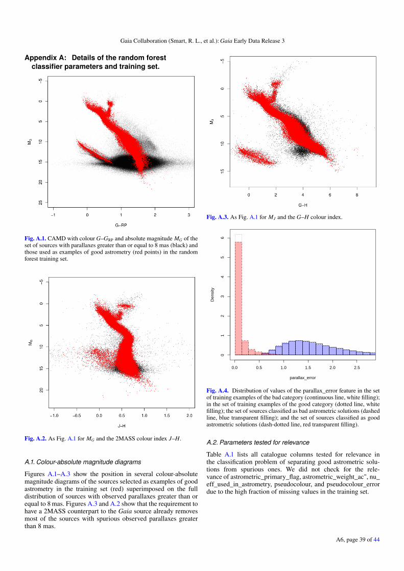
Gaia Collaboration (Smart, R. L., et al.): Gaia Early Data Release 3

Appendix A: Details of the random forestclassifier parameters and training set.

Fig. A.1. CAMD with colour G–GRP and absolute magnitude MG of theset of sources with parallaxes greater than or equal to 8 mas (black) andthose used as examples of good astrometry (red points) in the randomforest training set.

Fig. A.2. As Fig. A.1 for MG and the 2MASS colour index J–H.

A.1. Colour-absolute magnitude diagrams

Figures A.1–A.3 show the position in several colour-absolutemagnitude diagrams of the sources selected as examples of goodastrometry in the training set (red) superimposed on the fulldistribution of sources with observed parallaxes greater than orequal to 8 mas. Figures A.3 and A.2 show that the requirement tohave a 2MASS counterpart to the Gaia source already removesmost of the sources with spurious observed parallaxes greaterthan 8 mas.

Fig. A.3. As Fig. A.1 for MJ and the G–H colour index.

parallax_error

Den

sity

0.0 0.5 1.0 1.5 2.0 2.5

01

23

45

6

Fig. A.4. Distribution of values of the parallax_error feature in the setof training examples of the bad category (continuous line, white filling);in the set of training examples of the good category (dotted line, whitefilling); the set of sources classified as bad astrometric solutions (dashedline, blue transparent filling); and the set of sources classified as goodastrometric solutions (dash-dotted line, red transparent filling).

A.2. Parameters tested for relevance

Table A.1 lists all catalogue columns tested for relevance inthe classification problem of separating good astrometric solu-tions from spurious ones. We did not check for the rele-vance of astrometric_primary_flag, astrometric_weight_ac", nu_eff_used_in_astrometry, pseudocolour, and pseudocolour_errordue to the high fraction of missing values in the training set.

A6, page 39 of 44

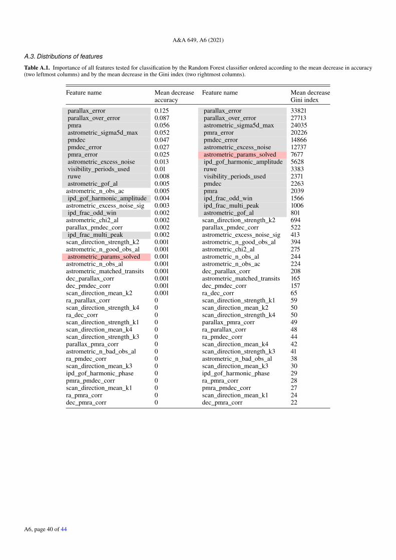
A&A 649, A6 (2021)

A.3. Distributions of features

Table A.1. Importance of all features tested for classification by the Random Forest classifier ordered according to the mean decrease in accuracy(two leftmost columns) and by the mean decrease in the Gini index (two rightmost columns).

Feature name Mean decrease Feature name Mean decreaseaccuracy Gini index

parallax_error 0.125 parallax_error 33821parallax_over_error 0.087 parallax_over_error 27713pmra 0.056 astrometric_sigma5d_max 24035astrometric_sigma5d_max 0.052 pmra_error 20226pmdec 0.047 pmdec_error 14866pmdec_error 0.027 astrometric_excess_noise 12737pmra_error 0.025 astrometric_params_solved 7677astrometric_excess_noise 0.013 ipd_gof_harmonic_amplitude 5628visibility_periods_used 0.01 ruwe 3383ruwe 0.008 visibility_periods_used 2371astrometric_gof_al 0.005 pmdec 2263

astrometric_n_obs_ac 0.005 pmra 2039ipd_gof_harmonic_amplitude 0.004 ipd_frac_odd_win 1566

astrometric_excess_noise_sig 0.003 ipd_frac_multi_peak 1006ipd_frac_odd_win 0.002 astrometric_gof_al 801

astrometric_chi2_al 0.002 scan_direction_strength_k2 694parallax_pmdec_corr 0.002 parallax_pmdec_corr 522ipd_frac_multi_peak 0.002 astrometric_excess_noise_sig 413

scan_direction_strength_k2 0.001 astrometric_n_good_obs_al 394astrometric_n_good_obs_al 0.001 astrometric_chi2_al 275astrometric_params_solved 0.001 astrometric_n_obs_al 244

astrometric_n_obs_al 0.001 astrometric_n_obs_ac 224astrometric_matched_transits 0.001 dec_parallax_corr 208dec_parallax_corr 0.001 astrometric_matched_transits 165dec_pmdec_corr 0.001 dec_pmdec_corr 157scan_direction_mean_k2 0.001 ra_dec_corr 65ra_parallax_corr 0 scan_direction_strength_k1 59scan_direction_strength_k4 0 scan_direction_mean_k2 50ra_dec_corr 0 scan_direction_strength_k4 50scan_direction_strength_k1 0 parallax_pmra_corr 49scan_direction_mean_k4 0 ra_parallax_corr 48scan_direction_strength_k3 0 ra_pmdec_corr 44parallax_pmra_corr 0 scan_direction_mean_k4 42astrometric_n_bad_obs_al 0 scan_direction_strength_k3 41ra_pmdec_corr 0 astrometric_n_bad_obs_al 38scan_direction_mean_k3 0 scan_direction_mean_k3 30ipd_gof_harmonic_phase 0 ipd_gof_harmonic_phase 29pmra_pmdec_corr 0 ra_pmra_corr 28scan_direction_mean_k1 0 pmra_pmdec_corr 27ra_pmra_corr 0 scan_direction_mean_k1 24dec_pmra_corr 0 dec_pmra_corr 22

A6, page 40 of 44

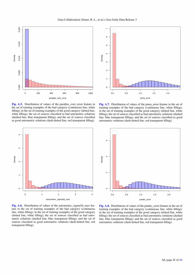
Gaia Collaboration (Smart, R. L., et al.): Gaia Early Data Release 3

parallax_over_error

Den

sity

0 200 400 600 800 1000

0.00

00.

005

0.01

00.

015

0.02

0

Fig. A.5. Distribution of values of the parallax_over_error feature inthe set of training examples of the bad category (continuous line, whitefilling); in the set of training examples of the good category (dotted line,white filling); the set of sources classified as bad astrometric solutions(dashed line, blue transparent filling); and the set of sources classifiedas good astrometric solutions (dash-dotted line, red transparent filling).

astrometric_sigma5d_max

Den

sity

0 1 2 3 4

01

23

4

Fig. A.6. Distribution of values of the astrometric_sigma5d_max fea-ture in the set of training examples of the bad category (continuousline, white filling); in the set of training examples of the good category(dotted line, white filling); the set of sources classified as bad astro-metric solutions (dashed line, blue transparent filling); and the set ofsources classified as good astrometric solutions (dash-dotted line, redtransparent filling).

pmra_error

Den

sity

0.0 0.5 1.0 1.5 2.0

01

23

45

67

Fig. A.7. Distribution of values of the pmra_error feature in the set oftraining examples of the bad category (continuous line, white filling);in the set of training examples of the good category (dotted line, whitefilling); the set of sources classified as bad astrometric solutions (dashedline, blue transparent filling); and the set of sources classified as goodastrometric solutions (dash-dotted line, red transparent filling).

pmdec_error

Den

sity

0.0 0.5 1.0 1.5 2.0

02

46

Fig. A.8. Distribution of values of the pmdec_error feature in the set oftraining examples of the bad category (continuous line, white filling);in the set of training examples of the good category (dotted line, whitefilling); the set of sources classified as bad astrometric solutions (dashedline, blue transparent filling); and the set of sources classified as goodastrometric solutions (dash-dotted line, red transparent filling).

A6, page 41 of 44

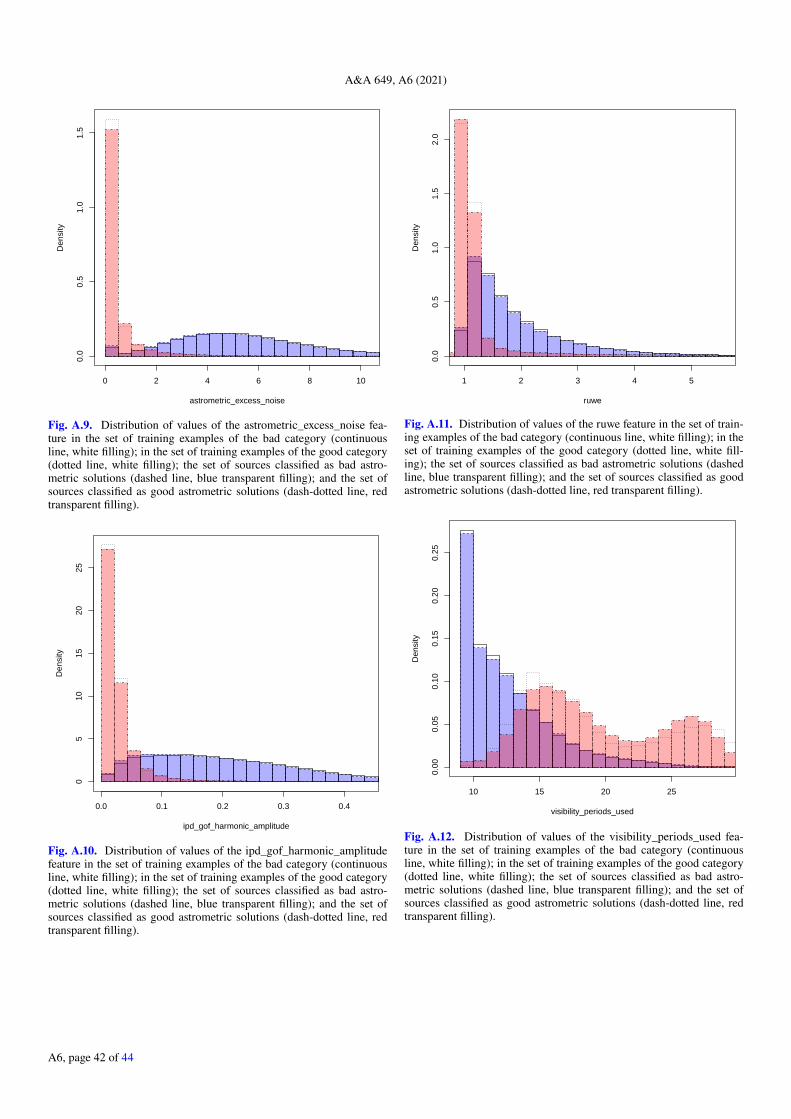
A&A 649, A6 (2021)

astrometric_excess_noise

Den

sity

0 2 4 6 8 10

0.0

0.5

1.0

1.5

Fig. A.9. Distribution of values of the astrometric_excess_noise fea-ture in the set of training examples of the bad category (continuousline, white filling); in the set of training examples of the good category(dotted line, white filling); the set of sources classified as bad astro-metric solutions (dashed line, blue transparent filling); and the set ofsources classified as good astrometric solutions (dash-dotted line, redtransparent filling).

ipd_gof_harmonic_amplitude

Den

sity

0.0 0.1 0.2 0.3 0.4

05

1015

2025

Fig. A.10. Distribution of values of the ipd_gof_harmonic_amplitudefeature in the set of training examples of the bad category (continuousline, white filling); in the set of training examples of the good category(dotted line, white filling); the set of sources classified as bad astro-metric solutions (dashed line, blue transparent filling); and the set ofsources classified as good astrometric solutions (dash-dotted line, redtransparent filling).

ruwe

Den

sity

1 2 3 4 5

0.0

0.5

1.0

1.5

2.0

Fig. A.11. Distribution of values of the ruwe feature in the set of train-ing examples of the bad category (continuous line, white filling); in theset of training examples of the good category (dotted line, white fill-ing); the set of sources classified as bad astrometric solutions (dashedline, blue transparent filling); and the set of sources classified as goodastrometric solutions (dash-dotted line, red transparent filling).

visibility_periods_used

Den

sity

10 15 20 25

0.00

0.05

0.10

0.15

0.20

0.25

Fig. A.12. Distribution of values of the visibility_periods_used fea-ture in the set of training examples of the bad category (continuousline, white filling); in the set of training examples of the good category(dotted line, white filling); the set of sources classified as bad astro-metric solutions (dashed line, blue transparent filling); and the set ofsources classified as good astrometric solutions (dash-dotted line, redtransparent filling).

A6, page 42 of 44

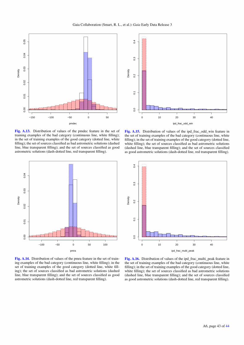
Gaia Collaboration (Smart, R. L., et al.): Gaia Early Data Release 3

pmdec

Den

sity

−150 −100 −50 0 50

0.00

0.01

0.02

0.03

0.04

0.05

Fig. A.13. Distribution of values of the pmdec feature in the set oftraining examples of the bad category (continuous line, white filling);in the set of training examples of the good category (dotted line, whitefilling); the set of sources classified as bad astrometric solutions (dashedline, blue transparent filling); and the set of sources classified as goodastrometric solutions (dash-dotted line, red transparent filling).

pmra

Den

sity

−100 −50 0 50 100

0.00

0.01

0.02

0.03

0.04

Fig. A.14. Distribution of values of the pmra feature in the set of train-ing examples of the bad category (continuous line, white filling); in theset of training examples of the good category (dotted line, white fill-ing); the set of sources classified as bad astrometric solutions (dashedline, blue transparent filling); and the set of sources classified as goodastrometric solutions (dash-dotted line, red transparent filling).

ipd_frac_odd_win

Den

sity

0 10 20 30 40

0.0

0.1

0.2

0.3

0.4

Fig. A.15. Distribution of values of the ipd_frac_odd_win feature inthe set of training examples of the bad category (continuous line, whitefilling); in the set of training examples of the good category (dotted line,white filling); the set of sources classified as bad astrometric solutions(dashed line, blue transparent filling); and the set of sources classifiedas good astrometric solutions (dash-dotted line, red transparent filling).

ipd_frac_multi_peak

Den

sity

0 10 20 30 40

0.0

0.1

0.2

0.3

0.4

Fig. A.16. Distribution of values of the ipd_frac_multi_peak feature inthe set of training examples of the bad category (continuous line, whitefilling); in the set of training examples of the good category (dotted line,white filling); the set of sources classified as bad astrometric solutions(dashed line, blue transparent filling); and the set of sources classifiedas good astrometric solutions (dash-dotted line, red transparent filling).

A6, page 43 of 44

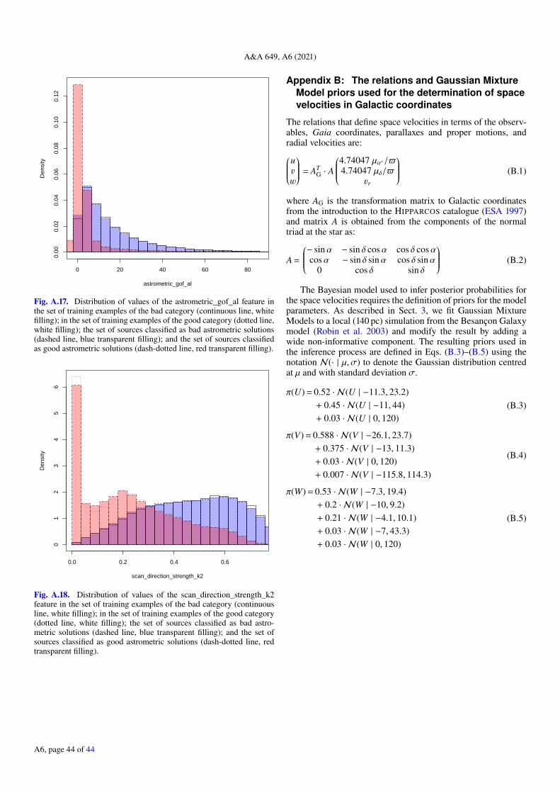
A&A 649, A6 (2021)

astrometric_gof_al

Den

sity

0 20 40 60 80

0.00

0.02

0.04

0.06

0.08

0.10

0.12

Fig. A.17. Distribution of values of the astrometric_gof_al feature inthe set of training examples of the bad category (continuous line, whitefilling); in the set of training examples of the good category (dotted line,white filling); the set of sources classified as bad astrometric solutions(dashed line, blue transparent filling); and the set of sources classifiedas good astrometric solutions (dash-dotted line, red transparent filling).

scan_direction_strength_k2

Den

sity

0.0 0.2 0.4 0.6

01

23

45

6

Fig. A.18. Distribution of values of the scan_direction_strength_k2feature in the set of training examples of the bad category (continuousline, white filling); in the set of training examples of the good category(dotted line, white filling); the set of sources classified as bad astro-metric solutions (dashed line, blue transparent filling); and the set ofsources classified as good astrometric solutions (dash-dotted line, redtransparent filling).

Appendix B: The relations and Gaussian MixtureModel priors used for the determination of spacevelocities in Galactic coordinates

The relations that define space velocities in terms of the observ-ables, Gaia coordinates, parallaxes and proper motions, andradial velocities are:uvw

= ATG · A

4.74047 µα∗/$4.74047 µδ/$

vr

(B.1)

where AG is the transformation matrix to Galactic coordinatesfrom the introduction to the HIPPARCOS catalogue (ESA 1997)and matrix A is obtained from the components of the normaltriad at the star as:

A =

− sinα − sin δ cosα cos δ cosαcosα − sin δ sinα cos δ sinα

0 cos δ sin δ

(B.2)

The Bayesian model used to infer posterior probabilities forthe space velocities requires the definition of priors for the modelparameters. As described in Sect. 3, we fit Gaussian MixtureModels to a local (140 pc) simulation from the Besançon Galaxymodel (Robin et al. 2003) and modify the result by adding awide non-informative component. The resulting priors used inthe inference process are defined in Eqs. (B.3)–(B.5) using thenotation N(· | µ, σ) to denote the Gaussian distribution centredat µ and with standard deviation σ.

π(U) = 0.52 · N(U | −11.3, 23.2)+ 0.45 · N(U | −11, 44)+ 0.03 · N(U | 0, 120)

(B.3)

π(V) = 0.588 · N(V | −26.1, 23.7)+ 0.375 · N(V | −13, 11.3)+ 0.03 · N(V | 0, 120)+ 0.007 · N(V | −115.8, 114.3)

(B.4)

π(W) = 0.53 · N(W | −7.3, 19.4)+ 0.2 · N(W | −10, 9.2)+ 0.21 · N(W | −4.1, 10.1)+ 0.03 · N(W | −7, 43.3)+ 0.03 · N(W | 0, 120)

(B.5)

A6, page 44 of 44