overview of kagra - archive ouverte hal
TRANSCRIPT
HAL Id: hal-03453575https://hal.archives-ouvertes.fr/hal-03453575
Submitted on 29 Nov 2021
HAL is a multi-disciplinary open accessarchive for the deposit and dissemination of sci-entific research documents, whether they are pub-lished or not. The documents may come fromteaching and research institutions in France orabroad, or from public or private research centers.
L’archive ouverte pluridisciplinaire HAL, estdestinée au dépôt et à la diffusion de documentsscientifiques de niveau recherche, publiés ou non,émanant des établissements d’enseignement et derecherche français ou étrangers, des laboratoirespublics ou privés.
Overview of KAGRA: KAGRA scienceT Akutsu, M Ando, K Arai, Y Arai, S Araki, A Araya, N Aritomi, H Asada,
Y Aso, S Bae, et al.
To cite this version:T Akutsu, M Ando, K Arai, Y Arai, S Araki, et al.. Overview of KAGRA: KAGRA science. Progressof Theoretical and Experimental Physics [PTEP], Oxford University Press on behalf of the PhysicalSociety of Japan, 2021, 2021 (5), �10.1093/ptep/ptaa120�. �hal-03453575�
Prog. Theor. Exp. Phys. 2020, 05A103 (68 pages)DOI: 10.1093/ptep/ptaa120
Overview of KAGRA: KAGRA scienceKAGRA CollaborationT. Akutsu1,2, M. Ando1,3,4, K. Arai5, Y. Arai5, S. Araki6, A. Araya7, N. Aritomi3, H. Asada8,Y. Aso9,10, S. Bae11, Y. Bae12, L. Baiotti13, R. Bajpai14, M. A. Barton1, K. Cannon4, Z. Cao15,E. Capocasa1, M. Chan16, C. Chen17,18, K. Chen19, Y. Chen18, C.-Y. Chiang20, H. Chu19, Y.-K. Chu20, S. Eguchi16,Y. Enomoto3, R. Flaminio1,21,Y. Fujii22, F. Fujikawa23, M. Fukunaga5,M. Fukushima2, D. Gao24, G. Ge24, S. Ha25, A. Hagiwara5,26, S. Haino20, W.-B. Han27,K. Hasegawa5, K. Hattori28, H. Hayakawa29, K. Hayama16, Y. Himemoto30, Y. Hiranuma31,N. Hirata1, E. Hirose5, Z. Hong32, B. H. Hsieh5, C.-Z. Huang32, H.-Y. Huang20, P. Huang24,Y. Huang20, Y.-C. Huang18, D. C. Y. Hui33, S. Ide34, B. Ikenoue2, S. Imam32, K. Inayoshi35,Y. Inoue19, K. Ioka36, K. Ito37, Y. Itoh38,39, K. Izumi40, C. Jeon41, H.-B. Jin42,43, K. Jung25,P. Jung29, K. Kaihotsu37, T. Kajita44, M. Kakizaki28, M. Kamiizumi29, N. Kanda38,39,G. Kang11, K. Kashiyama4, K. Kawaguchi5, N. Kawai45, T. Kawasaki3, C. Kim41,J. Kim46, J. C. Kim47, W. S. Kim12, Y.-M. Kim25, N. Kimura26, N. Kita3, H. Kitazawa37,Y. Kojima48, K. Kokeyama29, K. Komori3, A. K. H. Kong18, K. Kotake16, C. Kozakai9,R. Kozu49, R. Kumar50, J. Kume4, C. Kuo19, H.-S. Kuo32, Y. Kuromiya37, S. Kuroyanagi51,K. Kusayanagi45, K. Kwak25, H. K. Lee52, H. W. Lee47, R. Lee18, M. Leonardi1, K. L. Li18,T. G. F. Li73, C.-Y. Lin53, F.-K. Lin20, F.-L. Lin32, H. L. Lin19, L. C.-C. Lin25, G. C. Liu17,L.-W. Luo20, E. Majorana54, M. Marchio1, Y. Michimura3, N. Mio55, O. Miyakawa29,A. Miyamoto38,Y. Miyazaki3, K. Miyo29, S. Miyoki29,Y. Mori37, S. Morisaki5,Y. Moriwaki28,K. Nagano40, S. Nagano56, K. Nakamura1, H. Nakano57, M. Nakano5,28, R. Nakashima45,Y. Nakayama28, T. Narikawa5, L. Naticchioni54, R. Negishi31, L. Nguyen Quynh58,W.-T. Ni24,42,59, A. Nishizawa4,∗, S. Nozaki28, Y. Obuchi2, W. Ogaki5, J. J. Oh12, K. Oh33,S. H. Oh12, M. Ohashi29, N. Ohishi9, M. Ohkawa23, H. Ohta4, Y. Okutani34, K. Okutomi29,K. Oohara31, C. P. Ooi3, S. Oshino29, S. Otabe45, K. Pan18, H. Pang19, A. Parisi17, J. Park1,F. E. Peña Arellano29, I. Pinto60, N. Sago61, S. Saito2, Y. Saito29, K. Sakai62, Y. Sakai31,Y. Sakuno16, S. Sato63, T. Sato23, T. Sawada38, T. Sekiguchi4, Y. Sekiguchi64, L. Shao35,S. Shibagaki16, R. Shimizu2, T. Shimoda3, K. Shimode29, H. Shinkai65, T. Shishido10,A. Shoda1, K. Somiya45, E. J. Son12, H. Sotani66, R. Sugimoto37,40, J. Suresh5, T. Suzuki23,T. Suzuki5, H. Tagoshi5, H. Takahashi67, R. Takahashi1,A. Takamori7, S. Takano3, H. Takeda3,M. Takeda38, H. Tanaka68, K. Tanaka38, K. Tanaka68, T. Tanaka5, T. Tanaka69, S. Tanioka1,10,E. N. Tapia San Martin1, S. Telada70, T. Tomaru1,Y. Tomigami38, T. Tomura29, F. Travasso71,72,L. Trozzo29, T. Tsang73, J.-S. Tsao32, K. Tsubono3, S. Tsuchida38, D. Tsuna4, T. Tsutsui4,T. Tsuzuki2, D. Tuyenbayev20, N. Uchikata5, T. Uchiyama29, A. Ueda26, T. Uehara74,75,K. Ueno4, G. Ueshima67, F. Uraguchi2, T. Ushiba5, M. H. P. M. van Putten76, H. Vocca72,J. Wang24, T. Washimi1, C. Wu18, H. Wu18, S. Wu18, W.-R. Xu32, T.Yamada68, K.Yamamoto28,K. Yamamoto68, T. Yamamoto29, K. Yamashita28, R. Yamazaki34, Y. Yang77, K. Yokogawa37,J. Yokoyama4,3, T. Yokozawa29, T. Yoshioka37, H. Yuzurihara5, S. Zeidler78, M. Zhan24,H. Zhang32, Y. Zhao1, and Z.-H. Zhu15
1Gravitational Wave Science Project, National Astronomical Observatory of Japan (NAOJ), Mitaka City, Tokyo
181-8588, Japan
© The Author(s) 2020. Published by Oxford University Press on behalf of the Physical Society of Japan.This is an Open Access article distributed under the terms of the Creative Commons Attribution License (http://creativecommons.org/licenses/by/4.0/),which permits unrestricted reuse, distribution, and reproduction in any medium, provided the original work is properly cited.
Dow
nloaded from https://academ
ic.oup.com/ptep/article/2021/5/05A103/5891669 by guest on 29 N
ovember 2021
PTEP 2020, 05A103 T. Akutsu et al.
2Advanced Technology Center, National Astronomical Observatory of Japan (NAOJ), Mitaka City, Tokyo 181-8588, Japan3Department of Physics, The University of Tokyo, Bunkyo-ku, Tokyo 113-0033, Japan4Research Center for the Early Universe (RESCEU), The University of Tokyo, Bunkyo-ku, Tokyo 113-0033,Japan5Institute for Cosmic Ray Research (ICRR), KAGRA Observatory, The University of Tokyo, Kashiwa City,Chiba 277-8582, Japan6Accelerator Laboratory, High Energy Accelerator Research Organization (KEK), Tsukuba City, Ibaraki 305-0801, Japan7Earthquake Research Institute, The University of Tokyo, Bunkyo-ku, Tokyo 113-0032, Japan8Department of Mathematics and Physics, Hirosaki University, Hirosaki City, Aomori 036-8561, Japan9Kamioka Branch, National Astronomical Observatory of Japan (NAOJ), Kamioka-cho, Hida City, Gifu 506-1205, Japan10The Graduate University for Advanced Studies (SOKENDAI), Mitaka City, Tokyo 181-8588, Japan11Korea Institute of Science and Technology Information (KISTI), Yuseong-gu, Daejeon 34141, Korea12National Institute for Mathematical Sciences, Daejeon 34047, Korea13International College, Osaka University, Toyonaka City, Osaka 560-0043, Japan14School of High Energy Accelerator Science, The Graduate University for Advanced Studies (SOKENDAI),Tsukuba City, Ibaraki 305-0801, Japan15Department of Astronomy, Beijing Normal University, Beijing 100875, China16Department of Applied Physics, Fukuoka University, Jonan, Fukuoka City, Fukuoka 814-0180, Japan17Department of Physics, Tamkang University, Danshui Dist., New Taipei City 25137, Taiwan18Department of Physics and Institute of Astronomy, National Tsing Hua University, Hsinchu 30013, Taiwan19Department of Physics, Center for High Energy and High Field Physics, National Central University, ZhongliDistrict, Taoyuan City 32001, Taiwan20Institute of Physics, Academia Sinica, Nankang, Taipei 11529, Taiwan21Université Grenoble Alpes, Laboratoire d’Annecy de Physique des Particules (LAPP), Université SavoieMont Blanc, CNRS/IN2P3, F-74941 Annecy, France22Department of Astronomy, The University of Tokyo, Mitaka City, Tokyo 181-8588, Japan23Faculty of Engineering, Niigata University, Nishi-ku, Niigata City, Niigata 950-2181, Japan24State Key Laboratory of Magnetic Resonance and Atomic and Molecular Physics, Innovation Academy forPrecision Measurement Science and Technology (APM), Chinese Academy of Sciences, Xiao Hong Shan,Wuhan 430071, China25Department of Physics, School of Natural Science, Ulsan National Institute of Science and Technology(UNIST), Ulsan 44919, Korea26Applied Research Laboratory, High EnergyAccelerator Research Organization (KEK),Tsukuba City, Ibaraki305-0801, Japan27Chinese Academy of Sciences, Shanghai Astronomical Observatory, Shanghai 200030, China28Faculty of Science, University of Toyama, Toyama City, Toyama 930-8555, Japan29Institute for Cosmic Ray Research (ICRR), KAGRA Observatory, The University of Tokyo, Kamioka-cho,Hida City, Gifu 506-1205, Japan30College of Industrial Technology, Nihon University, Narashino City, Chiba 275-8575, Japan31Graduate School of Science and Technology, Niigata University, Nishi-ku, Niigata City, Niigata 950-2181,Japan32Department of Physics, National Taiwan Normal University, Sec. 4, Taipei 116, Taiwan33Astronomy & Space Science, Chungnam National University, 9 Daehak-ro, Yuseong-gu, Daejeon 34134,Korea, Korea34Department of Physics and Mathematics,Aoyama Gakuin University, Sagamihara City, Kanagawa 252-5258,Japan35Kavli Institute forAstronomy andAstrophysics, Peking University,Yiheyuan Road 5, Haidian District, Beijing100871, China36Yukawa Institute for Theoretical Physics (YITP), Kyoto University, Sakyou-ku, Kyoto City, Kyoto 606-8502,Japan37Graduate School of Science and Engineering, University of Toyama, Toyama City, Toyama 930-8555, Japan
2/68
Dow
nloaded from https://academ
ic.oup.com/ptep/article/2021/5/05A103/5891669 by guest on 29 N
ovember 2021
PTEP 2020, 05A103 T. Akutsu et al.
38Department of Physics, Graduate School of Science, Osaka City University, Sumiyoshi-ku, Osaka City, Osaka558-8585, Japan39Nambu Yoichiro Institute of Theoretical and Experimental Physics (NITEP), Osaka City University,Sumiyoshi-ku, Osaka City, Osaka 558-8585, Japan40Institute of Space andAstronautical Science (JAXA), Chuo-ku, Sagamihara City, Kanagawa 252-0222, Japan41Department of Physics, Ewha Womans University, Seodaemun-gu, Seoul 03760, Korea42National Astronomical Observatories, Chinese Academic of Sciences, 20A Datun Road, Chaoyang District,Beijing, China43School of Astronomy and Space Science, University of Chinese Academy of Sciences, 20A Datun Road,Chaoyang District, Beijing, China44Institute for Cosmic Ray Research (ICRR), The University of Tokyo, Kashiwa City, Chiba 277-8582, Japan45Graduate School of Science andTechnology,Tokyo Institute ofTechnology, Meguro-ku,Tokyo 152-8551, Japan46Department of Physics, Myongji University, Yongin 17058, Korea47Department of Computer Simulation, Inje University, Gimhae, Gyeongsangnam-do 50834, Korea48Department of Physical Science, Hiroshima University, Higashihiroshima City, Hiroshima 903-0213, Japan49Institute for Cosmic Ray Research (ICRR), Research Center for Cosmic Neutrinos (RCCN), The Universityof Tokyo, Kamioka-cho, Hida City, Gifu 506-1205, Japan50California Institute of Technology, Pasadena, CA 91125, USA51Institute for Advanced Research, Nagoya University, Furocho, Chikusa-ku, Nagoya City, Aichi 464-8602,Japan52Department of Physics, Hanyang University, Seoul 133-791, Korea53National Center for High-performance computing, National Applied Research Laboratories, Hsinchu Sci-ence Park, Hsinchu City 30076, Taiwan54Istituto Nazionale di Fisica Nucleare (INFN), Sapienza University, Roma 00185, Italy55Institute for Photon Science and Technology, The University of Tokyo, Bunkyo-ku, Tokyo 113-8656, Japan56TheApplied Electromagnetic Research Institute, National Institute of Information and CommunicationsTech-nology (NICT), Koganei City, Tokyo 184-8795, Japan57Faculty of Law, Ryukoku University, Fushimi-ku, Kyoto City, Kyoto 612-8577, Japan58Department of Physics, University of Notre Dame, Notre Dame, IN 46556, USA59Department of Physics, National Tsing Hua University, Hsinchu 30013, Taiwan60Department of Engineering, University of Sannio, Benevento 82100, Italy61Faculty of Arts and Science, Kyushu University, Nishi-ku, Fukuoka City, Fukuoka 819-0395, Japan62Department of Electronic Control Engineering, National Institute of Technology, Nagaoka College, NagaokaCity, Niigata 940-8532, Japan63Graduate School of Science and Engineering, Hosei University, Koganei City, Tokyo 184-8584, Japan64Faculty of Science, Toho University, Funabashi City, Chiba 274-8510, Japan65Faculty of Information Science and Technology, Osaka Institute of Technology, Hirakata City, Osaka 573-0196, Japan66iTHEMS (Interdisciplinary Theoretical and Mathematical Sciences Program), The Institute of Physical andChemical Research (RIKEN), Wako, Saitama 351-0198, Japan67Department of Information and Management Systems Engineering, Nagaoka University of Technology,Nagaoka City, Niigata 940-2188, Japan68Institute for Cosmic Ray Research (ICRR), Research Center for Cosmic Neutrinos (RCCN), The Universityof Tokyo, Kashiwa City, Chiba 277-8582, Japan69Department of Physics, Kyoto University, Sakyou-ku, Kyoto City, Kyoto 606-8502, Japan70National Metrology Institute of Japan, National Institute of Advanced Industrial Science and Technology,Tsukuba City, Ibaraki 305-8568, Japan71University of Camerino, via Madonna delle Carderi 9, 62032 Camerino (MC), Italy72Istituto Nazionale di Fisica Nucleare, University of Perugia, Perugia 06123, Italy73Faculty of Science, Department of Physics, The Chinese University of Hong Kong, Shatin, N.T., Hong Kong74Department of Communications, National Defense Academy of Japan, Yokosuka City, Kanagawa 239-8686,Japan75Department of Physics, University of Florida, Gainesville, FL 32611, USA76Department of Physics and Astronomy, Sejong University, Gwangjin-gu, Seoul 143-747, Korea77Department of Electrophysics, National Chiao Tung University, 101 Univ. Street, Hsinchu, Taiwan78Department of Physics, Rikkyo University, Toshima-ku, Tokyo 171-8501, Japan∗Email: [email protected]
3/68
Dow
nloaded from https://academ
ic.oup.com/ptep/article/2021/5/05A103/5891669 by guest on 29 N
ovember 2021
PTEP 2020, 05A103 T. Akutsu et al.
Received April 12, 2020; Revised July 31, 2020; Accepted July 31, 2020; Published Month 00, 0000
... . . . . . . . . . . . . . . . . . . . . . . . . . . . . . . . . . . . . . . . . . . . . . . . . . . . . . . . . . . . . . . . . . . . . . . . . . . . . . . . . . . . . . . . . . . . . . . . . . . . . . . . . . . . . . . . .KAGRA is a newly build gravitational wave observatory, a laser interferometer with 3 km armlength, located in Kamioka, Gifu, Japan. In this paper, one of a series of articles featuringKAGRA, we discuss the science targets of KAGRA projects, considering not only the baselineKAGRA (current design) but also its future upgrade candidates (KAGRA+) for the near to middleterm (∼5 years).. . . . . . . . . . . . . . . . . . . . . . . . . . . . . . . . . . . . . . . . . . . . . . . . . . . . . . . . . . . . . . . . . . . . . . . . . . . . . . . . . . . . . . . . . . . . . . . . . . . . . . . . . . . . . . . . . . .
Subject Index E02
1. Introduction
Advanced LIGO (aLIGO) [1] and advancedVirgo (AdV) [2] have detected gravitational waves (GWs)from 10 mergers of binary black holes (BBHs) [3] and one merger of binary neutron stars (BNSs) [4]in the O1 and O2 observing run1. The observations of these GW events have broadened many scienceopportunities: the astrophysical formation scenarios of BBH and BNS, the emission mechanisms ofshort gamma-ray bursts (sGRBs) and the following electromagnetic (EM) counterparts associatedwith BNS mergers, the equation of state (EOS) of a neutron star (NS), measurement of the Hubbleconstant, the tests of gravity, the no-hair theorem of a black hole (BH) and so on. In addition tothese topics studied based on the observational data, there are still several sources of GWs to beobserved in the future with ground-based detectors, such as those from supernovae, isolated NSs,intermediate-mass BHs, and the early Universe.
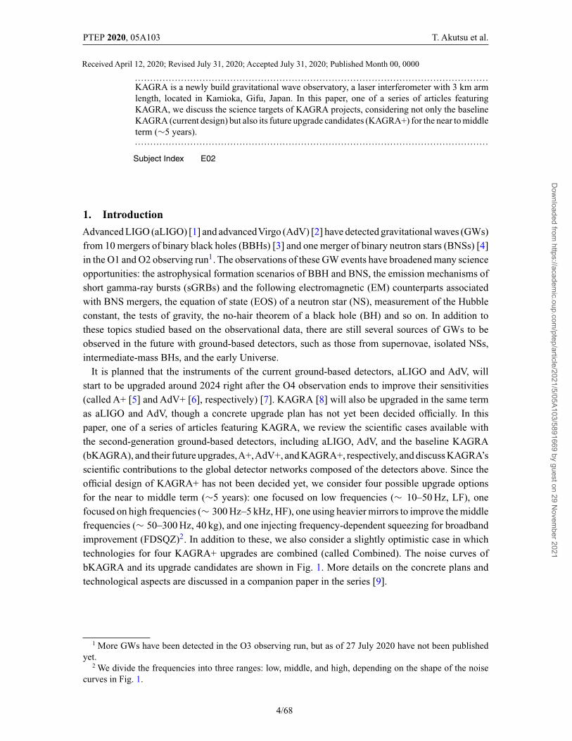
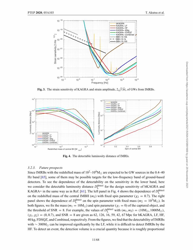
It is planned that the instruments of the current ground-based detectors, aLIGO and AdV, willstart to be upgraded around 2024 right after the O4 observation ends to improve their sensitivities(called A+ [5] and AdV+ [6], respectively) [7]. KAGRA [8] will also be upgraded in the same termas aLIGO and AdV, though a concrete upgrade plan has not yet been decided officially. In thispaper, one of a series of articles featuring KAGRA, we review the scientific cases available withthe second-generation ground-based detectors, including aLIGO, AdV, and the baseline KAGRA(bKAGRA), and their future upgrades,A+,AdV+, and KAGRA+, respectively, and discuss KAGRA’sscientific contributions to the global detector networks composed of the detectors above. Since theofficial design of KAGRA+ has not been decided yet, we consider four possible upgrade optionsfor the near to middle term (∼5 years): one focused on low frequencies (∼ 10–50 Hz, LF), onefocused on high frequencies (∼ 300 Hz–5 kHz, HF), one using heavier mirrors to improve the middlefrequencies (∼ 50–300 Hz, 40 kg), and one injecting frequency-dependent squeezing for broadbandimprovement (FDSQZ)2. In addition to these, we also consider a slightly optimistic case in whichtechnologies for four KAGRA+ upgrades are combined (called Combined). The noise curves ofbKAGRA and its upgrade candidates are shown in Fig. 1. More details on the concrete plans andtechnological aspects are discussed in a companion paper in the series [9].
1 More GWs have been detected in the O3 observing run, but as of 27 July 2020 have not been publishedyet.
2 We divide the frequencies into three ranges: low, middle, and high, depending on the shape of the noisecurves in Fig. 1.
4/68
Dow
nloaded from https://academ
ic.oup.com/ptep/article/2021/5/05A103/5891669 by guest on 29 N
ovember 2021
PTEP 2020, 05A103 T. Akutsu et al.
Fig. 1. Sensitivity curves for bKAGRA and upgrade candidates for KAGRA+. Sensitivity curves for aLIGO,A+, and bKAGRA are shown for comparison [10].
2. Stellar-mass binary black holes2.1. Formation scenarios
2.1.1. Scientific objectiveThe existence of massive stellar-mass BBH provides us with new insight about the formation path-ways of such heavy compact binaries [11,12]. Since massive stars likely lose their masses by stellarwinds driven by metal lines, dust, and pulsations of the stellar surface, heavy BHs with masses of� 20 M� are not expected to be left as remnants at the end of the lifetime of massive stars withmetallicity of the solar value [13]. In fact, the masses of the BHs that have ever been observed inEM waves (e.g., X-ray binaries) are significantly lower than those detected in GWs [3]. This factmotivates us to explore the astrophysical origin of such massive stellar-mass BBH populations inlow-metallicity environments (below 50% of solar metallicity or possibly less) [13]. So far, a numberof authors have proposed formation channels: the evolution of low-metallicity isolated binaries in thefield [14–17], dynamical processes in dense cluster systems (globular clusters, nuclear stellar clus-ters, or compact gaseous disks in active galactic nuclei) [18–24], massive stars formed in extremelylow-metallicity gas in the high-redshift Universe (Population III stars, hereafter Pop III stars) [25–28], etc. As an alternative non-astrophysical possibility, a primordial BH (PBH) population in theextremely early Universe (e.g., originating from phase transitions, a temporary softening in the EOS,quantum fluctuations) has been attracting attention [29,30] (see Ref. [31] for a review).
2.1.2. Observations and measurementsIn order to reveal the astrophysical origin of stellar-mass BBHs detected by LIGO and Virgo, we needto explore the properties of coalescing BBHs, depending on their formation pathway and environmentin which they form. In particular, the effective spin parameters of a BBH χeff (the dimensionlessspin components aligned or anti-aligned with the orbital angular momentum) are expected to beuseful to discriminate the evolution models [32,33]. In the field binary scenario, concerning binariesformed in a galactic plane, tidal torque exerted on two stars (or one star and one BH) in a closebinary transports the orbital angular momentum into stellar spins, resulting in χeff � 0. Since tidalsynchronization occurs as quickly as � ∝ (R�/a)6, a binary with a short GW coalescence timescale(i.e., a small orbital separation) would be significantly spun to χeff ∼ 1. Since BBH populationsformed at high redshift have a long GW coalescence timescale, their BBHs are hardly affected bytidal torque [34]. The underlying assumption is that the orbital angular momentum is not significantly
5/68
Dow
nloaded from https://academ
ic.oup.com/ptep/article/2021/5/05A103/5891669 by guest on 29 N
ovember 2021
PTEP 2020, 05A103 T. Akutsu et al.
changed via natal kicks that newborn BHs could receive during the core collapse of their progenitors[35]. Although a strong natal kick � 500 km s−1 is required to affect the effective spin parameter,observations of low-mass X-ray binaries show no evidence of such strong natal kicks of BHs (see,e.g., Ref. [36]).
On the other hand, in the dynamical formation scenario concerning binaries formed in densestellar environments, the distribution of effective spin would be isotropic at −1 ≤ χeff ≤ 1, andnegative values are allowed, unlike the isolated binary scenario, because the directions of stellarspins could be chosen randomly. As a robust result of the formation channel, the effective spin canhave negative values at −1 � χeff � 0. Moreover, in the dynamical capture model, a small fractionof the binaries/BBHs could gain significantly high eccentricities (e � 0.1), which will be imprintedin the GW waveform [19].
For PBHs formed in the early Universe (the radiation-dominated era), the spin is suppressedto χeff � 0.4 [37] or even smaller [38] because they are formed from the collapses of densityinhomogeneities right after the cosmological horizon entry. However, if the early matter phase existsafter inflation, the spin can be large [39]. Because of the uncertainty in the early-Universe scenario,it would be difficult to distinguish the PBH origin from astrophysical ones.
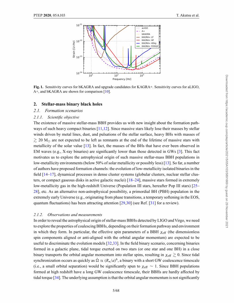
In addition to the BBH population within a detection horizon of z � 0.2, BBHs that coalesce athigher redshifts due to small initial separations are unresolved individually, but contribute to a GWbackground (GWB). The spectral shape of a GWB caused by compact binary mergers is characterizedby a single-power law of �GW ∝ f 2/3 at lower frequencies (f < f0), is flattened from it at f � f0,and has a cutoff at higher frequencies (f > f0) [40]. Importantly, this result hardly depends on themerger history of the BBH population qualitatively. Therefore, a GWB produced from a low-redshift,relatively less massive BBH population is robustly given by �GW ∝ f 2/3 in the frequency range.This GWB signal could be detected by a future observing run O5 with aLIGO and AdV [41], asshown in Fig. 2. In fact, the spectral flattening occurs outside the GWB sensitive frequency range(f0 � 100 Hz). On the other hand, a GWB caused by merger events of the higher-redshift, massive
Fig. 2. Expected sensitivity of the network of aLIGO and AdV to a GWB from BBHs in the fiducial modelin Ref. [41]. Energy density spectra are shown in blue (solid for the total background; dashed for the residualbackground, excluding resolved sources, assuming final aLIGO and AdV sensitivity). The pink shaded region,“Poisson”, shows the 90% CL statistical uncertainty, propagated from the local rate measurement, on the totalbackground. The black power-law integrated curves show the 1σ sensitivity of the network expected for thetwo first observing runs O1 and O2, and for 2 years at the design sensitivity in O5. Adapted from Ref. [41].
6/68
Dow
nloaded from https://academ
ic.oup.com/ptep/article/2021/5/05A103/5891669 by guest on 29 N
ovember 2021
PTEP 2020, 05A103 T. Akutsu et al.
BBH population suggested by Pop III models is expected to be flattened at a lower frequency off0 � 30 Hz [27], where LIGO/Virgo/KAGRA are the most sensitive. Detection of unique flattening atsuch low frequencies will indicate the existence of a high-chirp mass, high-redshift BBH population,which is consistent with a Pop III origin. A detailed study of the GWB would enable us to explorethe properties of massive binary stars at higher redshift and in the epoch of cosmic reionization.
2.1.3. Future prospectsLIGO–Virgo’s sensitivities during O1 and O2 have been proved to be efficient to detect stellar-massBBHs with a mass range between O(1) and (100) [3]. The typical detection frequency of thesestellar-mass BBHs is between 30 and 500 Hz. bKAGRA’s sensitivity would be similar to aLIGOand AdV and we expect that the observable sample for bKAGRA would be similar to those listedin GWTC-1 [3], i.e., stellar-mass BBHs. The LIGO–Virgo–KAGRA (LVK) configuration wouldprovide a better sky localization but without finding a host galaxy (via EM waves), it would bechallenging to identify the location of a BBH (e.g., in a galactic disk or in a cluster).
Toward the upgrades of bKAGRA, we expect that improved sensitivity toward the lower frequencieswould be useful to increase the signal-to-noise ratio (SNR) for BBH populations. More observationmeans better number statistics in event rate estimation and distributions for underlying propertiessuch as BH mass distribution. Furthermore, by observing earlier inspiral phase signals available atlower frequencies, it will be possible to achieve better accuracy in parameter estimation for individualmasses and spin parameters. For a BBH population with small masses, say total mass below 10 M�,by improving the so-called “bucket” sensitivity around a few hundred Hz would be most effectiveto increase the detectability as well as the precision of parameter estimation.
From stellar-mass to supermassive populations, BHs are considered to have a broad mass spectrum.While a standard binary evolution scenario prefers a compact binary consisting of similar masses[42], some binaries may have mass ratios 1/q ≡ m1/m2 much larger than 1, where m1 is theprimary mass and m2 is the secondary mass of the binary. A dense stellar system is consideredto be a factory generating compact binaries through dynamical interactions; see, e.g., Ref. [43].However, a toy model for the dynamic formation scenario for compact binaries still prefers BBHs with1/q < 3; see, e.g., Ref. [23]. Unequal-mass BBHs with 1/q > a few are particularly interesting as themodulations in amplitude that are expected by the post-Newtonian formalism in the inspiral phasebecome significant. Higher multiple modes (with the existence of spin(s)) are also more importantfor binaries with large mass ratios than they are for equal-mass binaries [44]. Therefore, detectionsof unequal-mass binaries require an overall improvement in the detector sensitivity correspondingto the detection frequency band in the “bucket”. Indeed, a recent event, GW190412, has provided uswith evidence to support the detection of higher multiple modes and proved that a broader frequencyband plays a crucial role in the detection [45].
In Table 1, we present the innermost stable circular orbit (ISCO) frequencies [46] correspondingto stellar-mass BBHs or BH–NS binaries with various masses. GW signals from binaries with totalmass of O(10) M� or larger would be spanned between flow of an interferometer and around theestimated fISCO, assuming the duration of ringdown signals to be much shorter than inspiral signals.The actual detectability will depend on the sensitivity of the interferometer within the frequencyrange given for the binary.
In Tables 2 and 3, the measurement errors of the binary parameters for equal-mass BBHs with30 M� and 10 M� at z = 0.1 are estimated with the Fisher information matrix. We assume detectornetworks composed ofA+,AdV+, and bKAGRA or KAGRA+ (LF, HF, 40 kg, FDSQZ, or combined).
7/68
Dow
nloaded from https://academ
ic.oup.com/ptep/article/2021/5/05A103/5891669 by guest on 29 N
ovember 2021
PTEP 2020, 05A103 T. Akutsu et al.
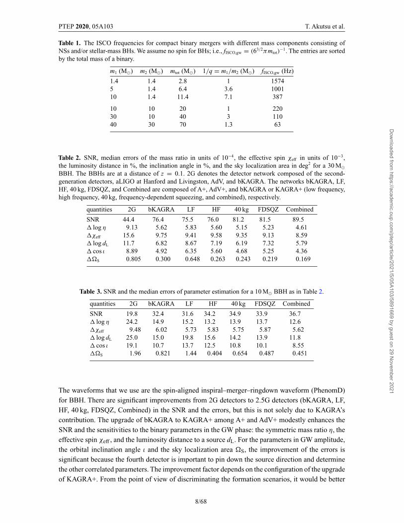
Table 1. The ISCO frequencies for compact binary mergers with different mass components consisting ofNSs and/or stellar-mass BHs. We assume no spin for BHs; i.e., fISCO,gw = (63/2πmtot)
−1. The entries are sortedby the total mass of a binary.
m1 (M�) m2 (M�) mtot (M�) 1/q = m1/m2 (M�) fISCO,gw (Hz)
1.4 1.4 2.8 1 15745 1.4 6.4 3.6 100110 1.4 11.4 7.1 387
10 10 20 1 22030 10 40 3 11040 30 70 1.3 63
Table 2. SNR, median errors of the mass ratio in units of 10−4, the effective spin χeff in units of 10−3,the luminosity distance in %, the inclination angle in %, and the sky localization area in deg2 for a 30 M�BBH. The BBHs are at a distance of z = 0.1. 2G denotes the detector network composed of the second-generation detectors, aLIGO at Hanford and Livingston, AdV, and bKAGRA. The networks bKAGRA, LF,HF, 40 kg, FDSQZ, and Combined are composed of A+, AdV+, and bKAGRA or KAGRA+ (low frequency,high frequency, 40 kg, frequency-dependent squeezing, and combined), respectively.
quantities 2G bKAGRA LF HF 40 kg FDSQZ Combined
SNR 44.4 76.4 75.5 76.0 81.2 81.5 89.5� log η 9.13 5.62 5.83 5.60 5.15 5.23 4.61�χeff 15.6 9.75 9.41 9.58 9.35 9.13 8.59� log dL 11.7 6.82 8.67 7.19 6.19 7.32 5.79� cos ι 8.89 4.92 6.35 5.60 4.68 5.25 4.36��S 0.805 0.300 0.648 0.263 0.243 0.219 0.169
Table 3. SNR and the median errors of parameter estimation for a 10 M� BBH as in Table 2.
quantities 2G bKAGRA LF HF 40 kg FDSQZ Combined
SNR 19.8 32.4 31.6 34.2 34.9 33.9 36.7� log η 24.2 14.9 15.2 13.2 13.9 13.7 12.6�χeff 9.48 6.02 5.73 5.83 5.75 5.87 5.62� log dL 25.0 15.0 19.8 15.6 14.2 13.9 11.8� cos ι 19.1 10.7 13.7 12.5 10.8 10.1 8.55��S 1.96 0.821 1.44 0.404 0.654 0.487 0.451
The waveforms that we use are the spin-aligned inspiral–merger–ringdown waveform (PhenomD)for BBH. There are significant improvements from 2G detectors to 2.5G detectors (bKAGRA, LF,HF, 40 kg, FDSQZ, Combined) in the SNR and the errors, but this is not solely due to KAGRA’scontribution. The upgrade of bKAGRA to KAGRA+ among A+ and AdV+ modestly enhances theSNR and the sensitivities to the binary parameters in the GW phase: the symmetric mass ratio η, theeffective spin χeff , and the luminosity distance to a source dL. For the parameters in GW amplitude,the orbital inclination angle ι and the sky localization area �S, the improvement of the errors issignificant because the fourth detector is important to pin down the source direction and determinethe other correlated parameters. The improvement factor depends on the configuration of the upgradeof KAGRA+. From the point of view of discriminating the formation scenarios, it would be better
8/68
Dow
nloaded from https://academ
ic.oup.com/ptep/article/2021/5/05A103/5891669 by guest on 29 N
ovember 2021
PTEP 2020, 05A103 T. Akutsu et al.
for KAGRA to improve the detector sensitivity at both low and middle frequencies. In addition,in order to increase the detectability of BBH coalescences at higher redshifts such as Pop III starbinaries and primordial BH binaries, it is important to increase the horizon distance for BBHs andanalyze together with the data of a GWB measuring the spectral index and the spectral cutoff.
3. Intermediate-mass binary black holes3.1. Formation scenarios
3.1.1. Scientific objectiveThe direct detections of GW emission have revealed the existence of massive BHs with masses of� 20–50 M�, which are significantly heavier than those ever observed in X-ray binaries [3,11,13].On the other hand, supermassive BHs of the order of 106–109 M� almost ubiquitously exist at thecenters of galaxies and are believed to be one of the most essential components of galaxies. However,the existence of a (binary) BH population between the stellar-mass and supermassive regimes, i.e.,100 � MBH/M� � 105, has not been confirmed yet (though there are some candidates). The lack ofsuch an intermediate-mass binary BH (IMBBH) population is one of the most intriguing unsolvedpuzzles in astrophysics. Detection of GWs from IMBBHs would be one of the best ways to probetheir existence and physical nature.
3.1.2. Observations and measurementsA plausible formation pathway for IMBHs is runaway collisions of massive stars in dense stellarsystems (e.g., globular clusters and/or nuclear stellar clusters) [47,48]. In a dense young star cluster,massive stars sink down to the center due to mass segregation and begin to physically collide. Duringthe collision processes, the most massive one gains more masses and grows to a very massive star(VMS) in a runaway fashion, and thus an IMBH with a mass of MIMBH � 100–104 M� is left aftergravitational collapse of the VMS. Even after IMBH formation, stellar-mass BHs (SBHs) migrateto the central region and could form a binary system with the IMBH, the so-called intermediatemass-ratio inspirals (IMRIs) [49,50]. GW emission from such IMRI systems can be detected notonly by space-borne GW observatories such as LISA but also by ground-based detectors whoseconfigurations are specifically designed to reach a better sensitivity at lower frequencies (e.g., A+or KAGRA LF). For MIMBH ∼ 100–103 M� and MSBH ∼ 10 M�, GWs produced from theIMRIs can be detected up to a distance of a few Gpc [51]. Since IMRI systems are likely to havehigh eccentricities due to the formation process, the GW energy distribution is shifted to higherfrequencies, increasing the SNR [52]. Although the IMRI coalescence rate is still highly uncertain,R � 1–30 events yr−1 would be expected from several theoretical studies [50,51]. In addition, Ref.[53] discussed the possibility that two IMBHs are formed in a massive dense cluster via runawaystellar collisions, and would form an IMBBH at a lower rate [49].
Alternatively, formation of VMSs in extremely low-metallicity environments (Pop III stars) caninitiate IMBHs with masses of � 100 M� [54]. Since a molecular cloud forming massive Pop III starswould be very unstable against its self-gravity, the cloud would be likely to fragment into massiveclumps with � 10 M� and leave a very massive binary system that will collapse into IMBBHswith ∼ 100 + 10 M� [55–57]. Assuming a Salpeter-like initial stellar-mass function and the mergerdelay-time distribution to be dN/dt ∝ t−1, the merger event rate for such an IMBBH is inferred tobe ∼ 0.1–1 Gpc−3 yr−1, and thus R ∼ a few events yr−1 [25].
9/68
Dow
nloaded from https://academ
ic.oup.com/ptep/article/2021/5/05A103/5891669 by guest on 29 N
ovember 2021
PTEP 2020, 05A103 T. Akutsu et al.
3.1.3. Future prospectsThe possible target source that is detectable with ground-based detectors is IMRIs. See Sect. 3.2.
3.2. Intermediate mass-ratio binaries
3.2.1. Scientific objectiveThe existence of IMBHs in globular clusters is suggested both by observational evidence and the-oretical prediction [58]. An IMBH in a globular cluster may capture a stellar-mass compact objectsurrounding it through some process (e.g., two-body relaxation), and may form an intermediate mass-ratio binary (IMRB) (where “intermediate” mass ratio means the range between the comparable massratio (∼ 1) and extreme mass ratio (� 10−4)).
The captured object in an IMRB orbits the IMBH many times during the inspiral phase beforeit plunges into the BH. Therefore, GW signals from IMRBs contain information on the geometryaround the IMBHs, which can be used to test the general relativity in the strong field, e.g., the no-hairtheorem of BHs and the tidal coupling between the central BH and the orbit of the captured object[59]. Also, if observations of IMRBs are accumulated, they may give a constraint on the event rateand population of IMBHs.
3.2.2. Observations and measurementsThe GW waveform from the inspiral phase of an IMRB can be estimated in the stationary phaseapproximation by
h(f ) = Af −7/6ei(f ), A = 1√30π2/3
M5/6
DL, (1)
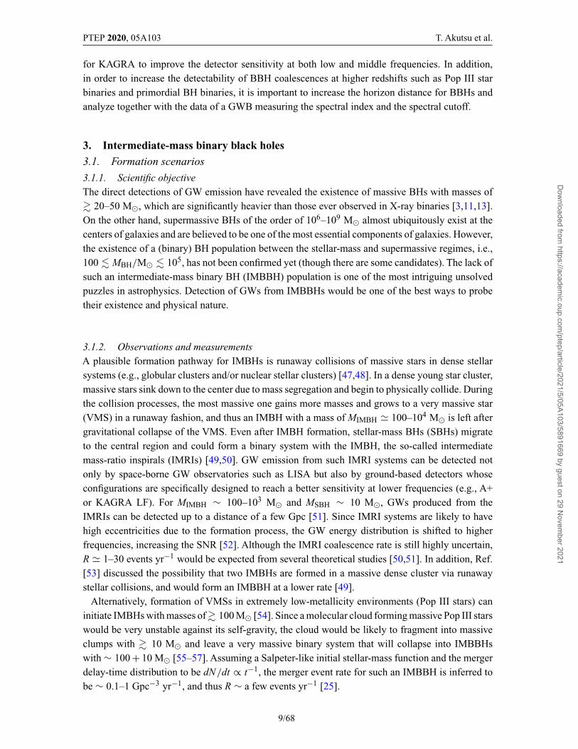
where M, DL, and (f ) are the redshifted chirp mass of the binary, the luminosity distance to thesource, and the GW phase, respectively [60,61]. The black (solid, dashed, dotted) lines in Fig. 3show the strain amplitude of GWs, 2
√f |h|, from IMRBs for three different cases, in which a BH
with 10 M� spirals into heavier BHs with masses of 102 M�, 103 M�, and 104 M� (these massesinclude the redshift factors) and the same spin parameter of 0.7 at a luminosity distance of 100 Mpc.The inspiral phase ceases around a certain cutoff frequency, which corresponds to the frequencyjust before the plunge phase. For circular orbit cases, the cutoff is estimated by the frequency for anISCO [46]. The ISCO frequency, fISCO mainly depends on the mass and spin of the central BH. Ifthe mass decreases or the spin increases, the ISCO frequency becomes higher and the overlap withthe sensitive band of ground-based detectors becomes larger.
After the inspiral phase, the orbit of the captured object changes to the plunge phase through thetransition phase. The shift of the frequency during the transition is roughly estimated by �f /fISCO ∼η2/5, where η is the mass ratio [62]. The plunge of the object to the central IMBH will induce ringdownGWs, whose frequency of the dominant mode is given by fRD ∼ 32.3 Hz × (m2/103M�)−1g(χ2),where m2 and χ2 are the redshifted mass and spin of the IMBH and g(χ2) shows the spin dependence(see Ref. [63] for details). Since the contribution from the transition phase and the ringdown phaseis smaller than that from the inspiral phase, here we do not consider them (an analysis including thetransition and ringdown is given in Ref. [64]).
10/68
Dow
nloaded from https://academ
ic.oup.com/ptep/article/2021/5/05A103/5891669 by guest on 29 N
ovember 2021
PTEP 2020, 05A103 T. Akutsu et al.
Fig. 3. The strain sensitivity of KAGRA and strain amplitude, 2√
f |h|, of GWs from IMRBs.
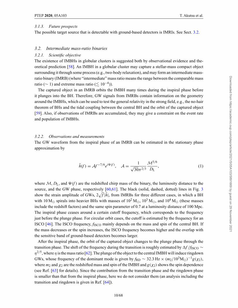
Fig. 4. The detectable luminosity distance of IMRIs.
3.2.3. Future prospectsSince IMRBs with the redshifted mass of 102–104M� are expected to be GW sources in the 0.4–40Hz band [65], some of them may be possible targets for the low-frequency band of ground-baseddetectors. To see the dependence of the detectability on the sensitivity in the lower band, herewe consider the detectable luminosity distance Ddetect
L for the design sensitivity of bKAGRA andKAGRA+ in the same way as in Ref. [61]. The left panel in Fig. 4 shows the dependence of Ddetect
Lon the redshifted mass of the central IMBH (m2) with fixed spin parameter (χ2 = 0.7). The rightpanel shows the dependence of Ddetect
L on the spin parameter with fixed mass (m2 = 103M�). Inboth figures, we fix the mass (m1 = 10M�) and spin parameter (χ1 = 0) of the captured object, andthe threshold of SNR = 8. For example, the values of Ddetect
L with (m1, m2) = (10M�, 1000M�),(χ1, χ2) = (0, 0.7), and SNR = 8 are given as 62, 126, 16, 59, 42, 67 Mpc for bKAGRA, LF, HF,40 kg, FDSQZ, and Combined, respectively. From the figures, we find that the detectability of IMRBswith ∼ 300M� can be improved significantly by the LF, while it is difficult to detect IMRBs by theHF. To detect an event, the detection volume is a crucial quantity because it is roughly proportional
11/68
Dow
nloaded from https://academ
ic.oup.com/ptep/article/2021/5/05A103/5891669 by guest on 29 N
ovember 2021
PTEP 2020, 05A103 T. Akutsu et al.
to the event rate. Using a detector network composed of two A+, AdV+, and bKAGRA or KAGRA+(LF, HF, 40 kg, FDSQZ, and Combined), the improvement factors of the detection volume are LF8.29, 40 kg 0.85, FDSQZ 0.30, HF 0.02, Combined 1.27 for a 103 M�–10 M� BBH with spin 0.7.
4. Neutron-star binaries4.1. Binary evolution
4.1.1. Scientific objectiveFormation scenarios of BNSs are similar to those of stellar-mass BBHs. One is based on the standardbinary evolution in a galactic disk (see, e.g., Refs. [66,67]) and the other involves dynamical inter-actions in dense stellar environments such as globular clusters (see, e.g., Ref. [68]). By precisionmeasurements of the NS masses and orbital parameters such as eccentricity by GW observations,it should be possible to shed light on the origin of BNS formation as pointed out many previousworks on the BNS population, including Ref. [66]. Although the expected kick involved in the BNSformation is small [66], the role of the natal kick from a supernova explosion can be relativelymore significant for the BNS formation than that of BBH formation. The evidence of the natal kickis observed in the known BNSs in our Galaxy, such as the Hulse–Taylor binary pulsar where theeccentricity is 0.67 [69]. Even though a binary’s orbit could be significantly eccentric at the timeof formation, the BNS orbit becomes circularized quite efficiently [70] and typical BNSs withinthe detection frequency band of KAGRA are expected to have eccentricities below 10−4. Similar toBBHs, if there are eccentric NS binaries within the KAGRA frequency band, they are more likelyto be formed through stellar interactions in dense stellar environments [20,23]. If eccentric binariesexist, measuring eccentricity would be one useful probe to distinguish the field population (formedby a standard binary evolution scenario) and the cluster population (formed by stellar interactions).We note that the measurement of eccentricity requires a much better sensitivity toward the lower-frequency band below 20 Hz; therefore it is more plausible that a third-generation detector may bebetter suited for searching for eccentric BNSs.
Another difference between NS and BH populations is the mass range.While the BH mass spectrumspans over nine orders of magnitudes, the NS mass range is narrow. For example, the NS mass rangeshould depend on the formation mechanism but is estimated, assuming a Gaussian distribution, tobe 1.33 ± 0.09 M� for double NSs, 1.54 ± 0.23 M� for recycled NSs, and 1.49 ± 0.19 M� for slowpulsars, which are likely to be NSs right after their birth [71]. These are based on the known NS–pulsar binaries in our Galaxy before 2016 and do not include a possibly heavy NS recently discoveredby GWs [72]. However, even if this is included, the mass range of NSs is much narrower than that ofBHs, which is advantageous for the establishment of a template bank. In addition, spin distributionwould be something to be compared between NS and BH populations. NS spin distribution for thosein BNSs is not well constrained and we expect that GW observations would shed light on the NSspin distribution by parameter estimation.
4.1.2. Observations and measurementsAs of early 2019, there were 15 BNSs known in the Galactic disk (see, e.g., Table 1 in Ref. [73]),where all systems consist of at least one active radio pulsar [74,75]. Eight of them are expected tomerge within a Hubble time. Measurements of the binary orbital decay and other post-Keplerianparameters clearly showed the effects of gravitational radiation in these NS–pulsar binaries.
GW170817 is the first BNS discovered by GW observation. It is also the first extragalactic BNS.The binary is identified as a BNS based on mass estimation, where both m1 and m2 estimates are
12/68
Dow
nloaded from https://academ
ic.oup.com/ptep/article/2021/5/05A103/5891669 by guest on 29 N
ovember 2021
PTEP 2020, 05A103 T. Akutsu et al.
consistent with the expected NS masses [76]. The detection of GW170817 also makes it possibleto constrain the BNS merger rate. Considering the first and second observing runs, the merger ratesolely based on GW observation is estimated to be 110–3840 Gpc−3 yr−1 at the 90% confidenceinterval [3]. GW observation can observe extragalactic BNSs, which are not accessible with currentradio telescopes. The GW and radio observations of BNSs would be complementary to reveal theunderlying properties of BNSs.
In addition to the BNS population, GW observation would be able to provide rich informationabout NS interiors (see Sects. 4.2 and 4.3) or the formation of young NSs (see also Sects. 6.3 and7.1) if late-inspiral, merger, or even ringdown phases are observed by future detectors.
4.1.3. Future prospectsIn terms of an observation, improving sensitivities toward lower and higher frequencies has significantimplications for understanding the astrophysics of BNSs. The typical chirp mass of a BNS is ≈1.13 M� assuming m1 = m2 = 1.3 M�. This implies that the frequencies of the merger and ringdownphases would be around 2 kHz where the current generation of GW detectors is not sensitive.However, the merger and ringdown phases of BNS coalescence would provide crucial hints to theremnant of the merger. On the other hand, the lower cutoff frequency of a detector is crucial tomeasure the early-inspiral phase.
The effects of improved detector sensitivity can be considered to be twofold: (a) At higher fre-quencies, better sensitivity would allows us to set stronger constraints for the NS EOS than aLIGOand AdV could do for GW170817 [77], not to mention improving the accuracy for the mass andspin parameters at higher post-Newtonian (PN) orders. Therefore, better sensitivities at high fre-quencies will be useful to have the observed sample of BNSs via GWs as complete as possible in themass–spin parameter space. (b) Improved sensitivity toward lower frequencies below 20 Hz allowsus to observe early-inspiral signals. This would be crucial to constrain the orbital eccentricity anddetermine the origin of the binary formation.
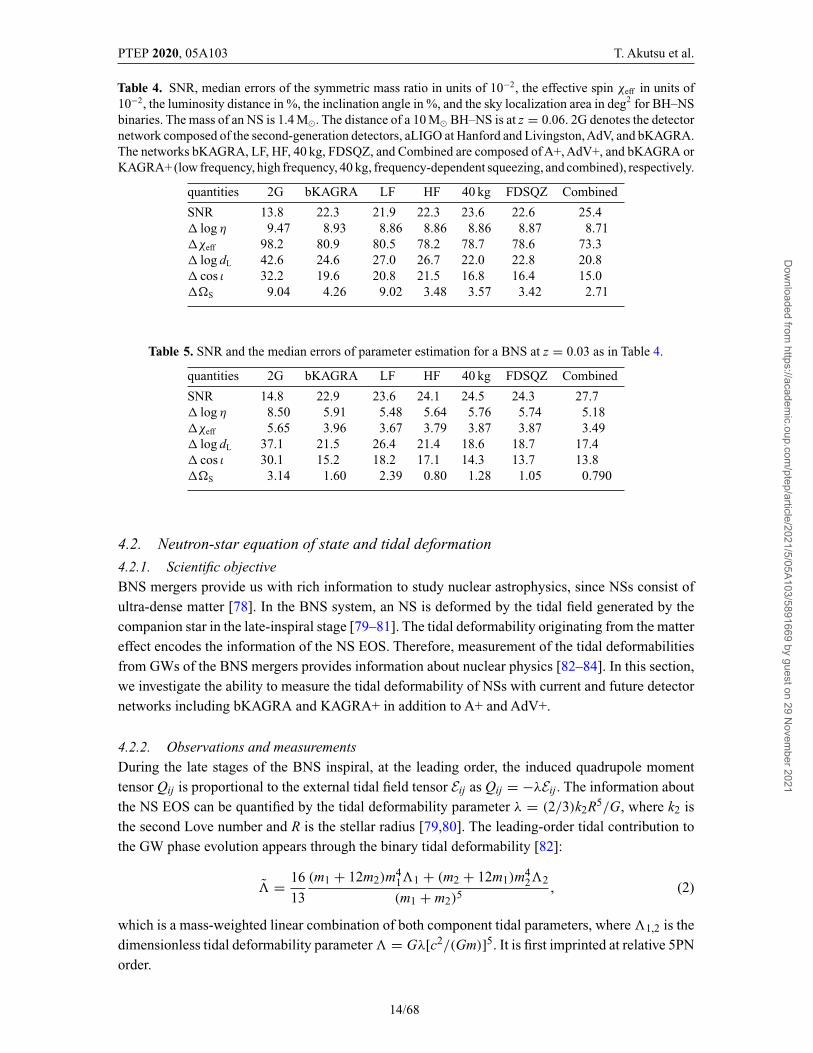
BH–NS binaries are expected to exist and their evolution would be similar to those of stellar-massBBHs and BNSs. As mentioned above, as there are several parameters that need to be measured inorder to discriminate the formation scenarios; with the Fisher information matrix we estimate themeasurement errors of the binary parameters for a 10 M� BH–NS binary at z = 0.06 and those fora BNS at z = 0.03. The waveform that we use is the spin-aligned inspiral waveform up to 3.5PN inphase. The maximum frequency for the inspiral part is set to the ISCO frequency. We assume detectornetworks composed ofA+,AdV+, and bKAGRA or KAGRA+ (LF, HF, 40 kg, FDSQZ, or combined).The measurement errors of the binary parameters are shown in Tables 4 and 5. There are significantimprovements from 2G detectors to 2.5G detectors (bKAGRA, LF, HF, 40 kg, FDSQZ, Combined).But this is not solely due to KAGRA’s contribution. The upgrade of bKAGRA to KAGRA+ amongA+ and AdV+ modestly enhances the SNR and the sensitivities to the binary parameters in the GWphase: the symmetric mass ratio η, the effective spin χeff , and the luminosity distance to a sourcedL. For the parameters in GW amplitude, the orbital inclination angle ι and the sky localization area�S, the improvement in the errors is significant because the fourth detector is important for pinningdown the source direction and determining the other correlated parameters. The improvement factordepends on the configuration of the upgrade of KAGRA+. From the point of view of discriminationof the formation scenarios, it would be better for KAGRA to improve the detector sensitivity at bothlow and middle frequencies.
13/68
Dow
nloaded from https://academ
ic.oup.com/ptep/article/2021/5/05A103/5891669 by guest on 29 N
ovember 2021
PTEP 2020, 05A103 T. Akutsu et al.
Table 4. SNR, median errors of the symmetric mass ratio in units of 10−2, the effective spin χeff in units of10−2, the luminosity distance in %, the inclination angle in %, and the sky localization area in deg2 for BH–NSbinaries. The mass of an NS is 1.4 M�. The distance of a 10 M� BH–NS is at z = 0.06. 2G denotes the detectornetwork composed of the second-generation detectors, aLIGO at Hanford and Livingston,AdV, and bKAGRA.The networks bKAGRA, LF, HF, 40 kg, FDSQZ, and Combined are composed of A+, AdV+, and bKAGRA orKAGRA+ (low frequency, high frequency, 40 kg, frequency-dependent squeezing, and combined), respectively.
quantities 2G bKAGRA LF HF 40 kg FDSQZ Combined
SNR 13.8 22.3 21.9 22.3 23.6 22.6 25.4� log η 9.47 8.93 8.86 8.86 8.86 8.87 8.71�χeff 98.2 80.9 80.5 78.2 78.7 78.6 73.3� log dL 42.6 24.6 27.0 26.7 22.0 22.8 20.8� cos ι 32.2 19.6 20.8 21.5 16.8 16.4 15.0��S 9.04 4.26 9.02 3.48 3.57 3.42 2.71
Table 5. SNR and the median errors of parameter estimation for a BNS at z = 0.03 as in Table 4.
quantities 2G bKAGRA LF HF 40 kg FDSQZ Combined
SNR 14.8 22.9 23.6 24.1 24.5 24.3 27.7� log η 8.50 5.91 5.48 5.64 5.76 5.74 5.18�χeff 5.65 3.96 3.67 3.79 3.87 3.87 3.49� log dL 37.1 21.5 26.4 21.4 18.6 18.7 17.4� cos ι 30.1 15.2 18.2 17.1 14.3 13.7 13.8��S 3.14 1.60 2.39 0.80 1.28 1.05 0.790
4.2. Neutron-star equation of state and tidal deformation
4.2.1. Scientific objectiveBNS mergers provide us with rich information to study nuclear astrophysics, since NSs consist ofultra-dense matter [78]. In the BNS system, an NS is deformed by the tidal field generated by thecompanion star in the late-inspiral stage [79–81]. The tidal deformability originating from the mattereffect encodes the information of the NS EOS. Therefore, measurement of the tidal deformabilitiesfrom GWs of the BNS mergers provides information about nuclear physics [82–84]. In this section,we investigate the ability to measure the tidal deformability of NSs with current and future detectornetworks including bKAGRA and KAGRA+ in addition to A+ and AdV+.
4.2.2. Observations and measurementsDuring the late stages of the BNS inspiral, at the leading order, the induced quadrupole momenttensor Qij is proportional to the external tidal field tensor Eij as Qij = −λEij. The information aboutthe NS EOS can be quantified by the tidal deformability parameter λ = (2/3)k2R5/G, where k2 isthe second Love number and R is the stellar radius [79,80]. The leading-order tidal contribution tothe GW phase evolution appears through the binary tidal deformability [82]:
� = 16
13
(m1 + 12m2)m41�1 + (m2 + 12m1)m4
2�2
(m1 + m2)5 , (2)
which is a mass-weighted linear combination of both component tidal parameters, where �1,2 is thedimensionless tidal deformability parameter � = Gλ[c2/(Gm)]5. It is first imprinted at relative 5PNorder.
14/68
Dow
nloaded from https://academ
ic.oup.com/ptep/article/2021/5/05A103/5891669 by guest on 29 N
ovember 2021
PTEP 2020, 05A103 T. Akutsu et al.
The first detection of a GW signal from a BNS system, GW170817 [4], provides an opportunity toextract information about NSs by measuring the tidal deformability. The LIGO–Virgo Collaborationhas placed an upper bound on the tidal deformability of � ≤ 800 when restricting the magnitudeof the component spins [4] using the restricted TF2 model [85,86] (this limit is later corrected to� ≤ 900 in Ref. [76]). In Refs. [3,76], an updated analysis by the LIGO–Virgo Collaboration usinga numerical-relativity (NR) calibrated waveform model, NRTidal [87] has been reported. By usingEOS-insensitive relations among several properties of NSs [88], the constraints on � can be improved[77] (but see also Ref. [89]). As found in Refs. [76,90], stiffer EOSs (large radii) yielding larger tidaldeformabilities such as MS1 and MS1b [91] are disfavored by the data of GW170817. Independentanalyses have also been done by assuming a common EOS for both NSs [92,93]. In Ref. [94], theauthors indicate that there is a difference in estimates of � for GW170817 between NR calibratedwaveform models (the KyotoTidal and NRTidalv2models). Here, the KyotoTidalmodel isone of the NR calibrated waveform models of inspiraling BNSs [95,96] and the NRTidalv2modelis an upgrade of the NRTidalmodel [97]. Several other studies have also derived constraints on theNS EOS by measuring tidal deformability from GW170817 [98–108]. A review of these and otherresults is available in Ref. [109].
4.2.3. Future prospectsIn order to investigate the expected error in the measurement �, we use the Fisher matrix analysiswith respect to the source parameters {ln dL, tc, φc, M, η, �}, where dL is the luminosity distance,tc and φc are the time and phase at coalescence, M is the chirp mass, and η is the symmetric massratio. We use the restricted TF2_PNTidal model, which employs the 3.5PN-order formula for thephase and only the Newtonian-order evolution for the amplitude as the point-particle part [85,86]and the 1PN-order (relative 5+1PN-order) tidal-part phase formula (see, e.g., Ref. [81]). We take thefrequency range from 23 Hz to the ISCO frequency. Here, we consider a non-spinning binary forsimplicity.
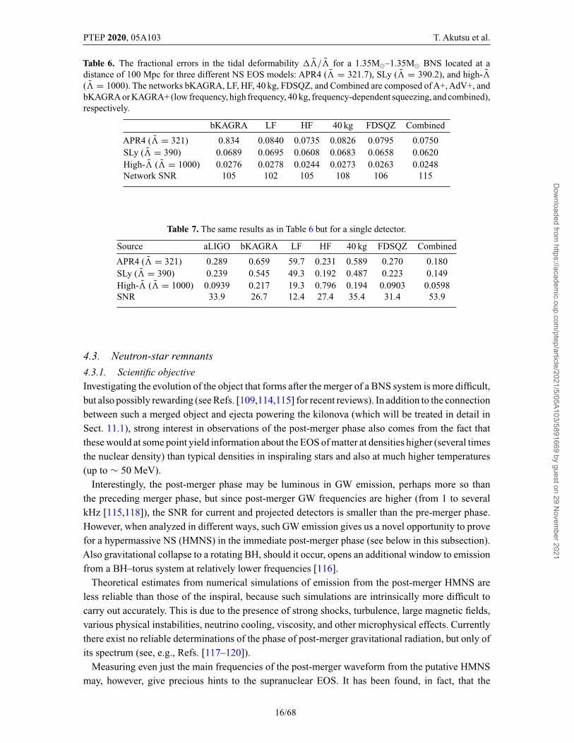
In Table 6, we show the fractional errors in the tidal deformability ��/� in the cases of some NSEOS models, using the inspiral PN waveform, theTF2_PNTidalmodel. We assume future detectornetworks including bKAGRA and KAGRA+ in addition to twoA+ andAdV+. We assume a 1.35M�–1.35M� BNS located at a distance of 100 Mpc and study three different NS EOS models [110]:APR4 [111] (� = 321.7), SLy [112] (� = 390.2), and high-� (� = 1000). In one example, for theSLy, the fractional errors on the tidal deformability are 0.069, 0.070, 0.061, 0.068, 0.067, and 0.062for bKAGRA, LF, HF, 40 kg, FDSQZ, and Combined, respectively. We find that the measurementprecision of the tidal deformability can be slightly improved for the HF, but not for the LF. We alsopresent the fractional errors in the tidal deformability for the single detector case in Table 7 to seehow much KAGRA can contribute to the global networks.
In Ref. [113], the authors have found a discrepancy in the tidal deformability of GW170817 betweenthe Hanford and Livingston detectors of aLIGO. While the two distributions look consistent witheach other and also consistent with what we would expect from noise realization, the Livingstondata are not very useful for determining the tidal deformability of GW170817. Their results suggestthat measurement of the tidal deformability by a third detector such as AdV or bKAGRA might behelpful in order to improve the constraint on the tidal deformability. In Ref. [94], their results indicatethat the systematic error for the NR calibrated waveform models will be significant to measure �
from upcoming GW detections. It is necessary to improve current waveform models for the BNSmergers.
15/68
Dow
nloaded from https://academ
ic.oup.com/ptep/article/2021/5/05A103/5891669 by guest on 29 N
ovember 2021
PTEP 2020, 05A103 T. Akutsu et al.
Table 6. The fractional errors in the tidal deformability ��/� for a 1.35M�–1.35M� BNS located at adistance of 100 Mpc for three different NS EOS models: APR4 (� = 321.7), SLy (� = 390.2), and high-�(� = 1000). The networks bKAGRA, LF, HF, 40 kg, FDSQZ, and Combined are composed of A+, AdV+, andbKAGRA or KAGRA+ (low frequency, high frequency, 40 kg, frequency-dependent squeezing, and combined),respectively.
bKAGRA LF HF 40 kg FDSQZ Combined
APR4 (� = 321) 0.834 0.0840 0.0735 0.0826 0.0795 0.0750SLy (� = 390) 0.0689 0.0695 0.0608 0.0683 0.0658 0.0620High-� (� = 1000) 0.0276 0.0278 0.0244 0.0273 0.0263 0.0248Network SNR 105 102 105 108 106 115
Table 7. The same results as in Table 6 but for a single detector.
Source aLIGO bKAGRA LF HF 40 kg FDSQZ Combined
APR4 (� = 321) 0.289 0.659 59.7 0.231 0.589 0.270 0.180SLy (� = 390) 0.239 0.545 49.3 0.192 0.487 0.223 0.149High-� (� = 1000) 0.0939 0.217 19.3 0.796 0.194 0.0903 0.0598SNR 33.9 26.7 12.4 27.4 35.4 31.4 53.9
4.3. Neutron-star remnants
4.3.1. Scientific objectiveInvestigating the evolution of the object that forms after the merger of a BNS system is more difficult,but also possibly rewarding (see Refs. [109,114,115] for recent reviews). In addition to the connectionbetween such a merged object and ejecta powering the kilonova (which will be treated in detail inSect. 11.1), strong interest in observations of the post-merger phase also comes from the fact thatthese would at some point yield information about the EOS of matter at densities higher (several timesthe nuclear density) than typical densities in inspiraling stars and also at much higher temperatures(up to ∼ 50 MeV).
Interestingly, the post-merger phase may be luminous in GW emission, perhaps more so thanthe preceding merger phase, but since post-merger GW frequencies are higher (from 1 to severalkHz [115,118]), the SNR for current and projected detectors is smaller than the pre-merger phase.However, when analyzed in different ways, such GW emission gives us a novel opportunity to provefor a hypermassive NS (HMNS) in the immediate post-merger phase (see below in this subsection).Also gravitational collapse to a rotating BH, should it occur, opens an additional window to emissionfrom a BH–torus system at relatively lower frequencies [116].
Theoretical estimates from numerical simulations of emission from the post-merger HMNS areless reliable than those of the inspiral, because such simulations are intrinsically more difficult tocarry out accurately. This is due to the presence of strong shocks, turbulence, large magnetic fields,various physical instabilities, neutrino cooling, viscosity, and other microphysical effects. Currentlythere exist no reliable determinations of the phase of post-merger gravitational radiation, but only ofits spectrum (see, e.g., Refs. [117–120]).
Measuring even just the main frequencies of the post-merger waveform from the putative HMNSmay, however, give precious hints to the supranuclear EOS. It has been found, in fact, that the
16/68
Dow
nloaded from https://academ
ic.oup.com/ptep/article/2021/5/05A103/5891669 by guest on 29 N
ovember 2021
PTEP 2020, 05A103 T. Akutsu et al.
frequencies of the main peaks of the post-merger power spectrum strongly correlate with prop-erties (radius at a fiducial mass, compactness, tidal deformability, etc.) of a zero-temperaturespherical equilibrium star (see, among others, Refs. [117–119,121] and, for applications, Refs.[120,122–124]). For example, finding the tidal deformability of the post-merger object to bevery different from that estimated from the inspiral may hint at phase transitions in the high-density matter (see Ref. [109] for a review). A similar hint would be given by an abruptchange in the post-merger main frequency [125,126]. The complicated morphology of these post-merger signals makes constructing accurate templates challenging and thus matched filtering lessefficient [120].
In addition to predictions on the GW spectrum, simulations also show, in most cases, delayedgravitational collapses to a rotating BH with dimensionless spin parameter a/M � 0.76–0.84 [127], surrounded by a disk. Strong magnetic fields [128] and baryon-rich disk windsare also predicted, though with inferior accuracy, and they are prescient to kilonova lightcurves [129].
However, simulations cannot accurately predict the time of delay in gravitational collapse of theputative HMNS to a BH, representative of the lifetime of the HMNS initially supported againstcollapse by differential rotation. The lifetime of the HMNS may be measured in EM–GW observa-tions. Furthermore, because of constraints in computational resources, simulations of post-mergerBH–disk or torus systems are limited to tens of ms; see, e.g., Refs. [114,130]. Yet, rotating BHsprovide a window to powerful emission over a secular Kelvin–Helmholtz timescale τKH = EJ /LH ,where EJ = 2Mc2 sin2(λ/4) (sin λ = a/M ) is the spin-energy in angular momentum J of a KerrBH of mass M [131], c is the velocity of light and LH is the total BH luminosity, most of which maybe irradiating surrounding matter [132]. For gamma-ray bursts, canonical estimates show τKH to betens of seconds [116].
EM–GW observations promise to fill the missing links in our picture of BNS mergers, namely thelifetime of the HMNS in delayed gravitational collapse to a BH; see, e.g., Refs. [133,134]. If finite,continuing emission may extend over the lifetime of BH spin by τKH above. For GW170817, if theHMNS experienced delayed collapse, the merger sequence
NS + NS −→a
HMNS −→b
BH + GW + GRB170817A + AT2017gfo (3)
offers a unique window to post-merger EM–GW emission powered by the energy reservoir EJ of theremnant compact object. Crucially, gravitational collapse b to a BH in the process (3) can increaseEJ significantly above canonical bounds on the same at formation a of the progenitor HMNS [135]in the immediate aftermath of the merger.
In the following subsection, we will focus only on calorimetric studies of the post-merger object,leaving the other topics to the above-mentioned reviews [109,114,115].
4.3.2. Observations and measurementsPost-merger EM calorimetry on GRB170817A and the kilonova AT 2017gfo [136–139] show acombined post-merger energy in EM radiation limited to EEM � 0.5%M�c2. This output is wellbelow the scale of total energy output in GW170817, and is insufficient to break the degeneracybetween an HMNS or BH remnant.
Gravitational radiation provides a radically new opportunity to probe a transient source that, “ifdetected, promises to reveal the physical nature of the trigger” [140]. GW calorimetry builds on
17/68
Dow
nloaded from https://academ
ic.oup.com/ptep/article/2021/5/05A103/5891669 by guest on 29 N
ovember 2021
PTEP 2020, 05A103 T. Akutsu et al.
earlier applications of indirect calorimetry to, notably, PSR1913+105 [141] and pulsar wind nebulae[142]. Power-excess methods [143,144] have thus far proven ineffective, however, by a threshold ofEgw = 6.5 M�c2 [145], given a total mass M < 3M� of the BNS progenitor and hence the mass ofits remnant compact object.
Independent EM and GW observations corroborate the process (3) with a lifetime tb − ta of theHMNS of less than about one second [116,146]. In EM, the lifetime of the HMNS is inferred froman initially blue component in the kilonova AT 2017gfo [130,146–150], whereas the same is inferredfrom the time-of-onset ts of post-merger GW-emission in time–frequency spectrograms producedby butterfly filtering, originally developed to identify broadband Kolmogorov spectra of light curvesof long GRBs in the BeppoSAX catalog [151,152]. Application to the LIGO snippet of 2048 s ofH1–L1 O2 data covering GW170817 serendipitously shows observational evidence of ∼ 5 s post-merger gravitational radiation [153]. Subsequent signal injection experiments indicate an outputEgw = (3.5 ± 1)%M�c2 in this extended emission [116]. Its time-of-onset ts < 1 s post-mergerfalls in the 1.7 s gap between GW170817 and GRB170817A, satisfying causality at birth of a centralengine of GRB170817A.
Egw exceeds the maximal spin-energy of an (HM)NS [135], yet it readily derives from EJ of aBH following gravitational collapse thereof at b in the process (3). Moreover, the aforementionedEEM is quantitatively consistent with model predictions of ultra-relativistic baryon-poor jets andbaryon-rich disk winds from a BH–torus system, the size of which derives from the frequency of itsGW emission [116].
At current detector sensitivities, witnessing the formation and evolution of the progenitor HMNS inthe immediate aftermath of a merger is extremely challenging. Null results on GW170817 [154] areentirely consistent with the energetically moderate and relatively high-frequency (> 1kHz) spectraexpected from numerical simulations [114].
4.3.3. Future prospectsOnce the BH forms, it has no memory of its progenitor except for total mass and angular momentum.This suggests pursuing GW calorimetry in Eq. (3) to catastrophic events more generally, includingmergers of an NS with a BH companion and nearby core-collapse supernovae (CCSNe), notablythe progenitors of type Ib/c of long gamma-ray bursts (GRBs) [155]. While the latter is rare, thefraction of failed GRB supernovae that are nevertheless luminous in gravitational radiation mayexceed the local GRB rate and hence the rate of mergers involving an NS; see, e.g., Ref. [151]. Blindall-sky butterfly searches may thus produce candidate signals with and without merger precursorsfrom events within distances on a par with GW170817, which may be followed up by time-slidecorrelation analysis and optical–radio signals from existing transient surveys of the local Universe.It also appears opportune to consider directed searches for events in neighboring galaxies (see, e.g.,Ref. [156]), notably M51 (D � 7 Mpc) and M82 (D � 3.5 Mpc), each offering about one radio-loudCCSN per decade. By their close proximity, these also appear to be of interest independent of anyassociation with progenitors of GRBs [157,158].
For a planned KAGRA upgrade, the above suggests optimizing the broadband window of 50–1000 Hz to pursue GW calorimetry on extreme transient sources using modern heterogeneouscomputing, in multi-messenger approaches involving existing and planned high-energy missionssuch as THESEUS [159,160]. Jointly with LIGO and Virgo, KAGRA is expected to give us awindow to modeled and unmodeled transient events out to tens of Mpc.
18/68
Dow
nloaded from https://academ
ic.oup.com/ptep/article/2021/5/05A103/5891669 by guest on 29 N
ovember 2021
PTEP 2020, 05A103 T. Akutsu et al.
5. Accreting binaries5.1. Continuous GWs from X-ray binaries
5.1.1. Scientific objectiveThere are several classes of continuous GWs (CWs). One major population of CW sources is systemsinvolving a spinning NS that has an asymmetry with respect to its rotation axis [161]. Potentialcandidates include pulsars, NSs in supernova remnants, and NSs in binary systems. In particular, anaccreting NS in a low-mass X-ray binary is a promising target. In this system, the central NS accretesmaterials from an orbiting late-type companion star. A finite quadrupole moment of an accreting NScan be possibly induced by various processes such as the laterally asymmetric distribution of accretedmaterial and elastic strain in the crust as well as magnetic deformation [162].
Sco X–1 is the prime target for directed searches of CWs from X-ray binaries because it is thebrightest persistent X-ray binary. The source is relatively nearby (∼ 2.8 kpc) and its X-ray luminositysuggests that the source is accreting near the Eddington limit for an NS. If the torque-balance (i.e.,balance between accretion-induced spin-up torque and the total spin-down torque due to gravitationaland EM radiation) can be maintained in the binary system, Sco X–1 is a promising target for CWsignals [163].
Current theoretical understanding of the torque-balance and spin-wandering effects of X-ray bina-ries is poor [163,164]. By combining CWs from X-ray binaries and multi-wavelength observations,we may track the evolution of spin torques and orbit, shedding light on disk dynamics and themaximum rotation frequency of an NS in a binary system [161].
No CW signal from X-ray binaries has been observed so far. During the LIGO S6 observing run,upper limits were estimated for Sco X–1 and XTE J1751–305 while the O1 observation of ScoX–1 yielded a null detection as well [165–167]. In the O2 observing run, by using a hidden Markovmodel (HMM) to track spin wandering, a more sensitive search for Sco X–1 was performed [168]. Noevidence of CW can be found in the frequency range of 60–650 Hz. An upper limit (95% confidence)of h ∼ 3.5 × 10⁻²⁵ is placed at 194.6 Hz, which is the tightest constraint placed on this system sofar [168].
5.1.2. Observations and measurementsCW signals from accreting X-ray binaries are extremely small compared to all known compactbinary mergers. Assuming a torque-balance, the GW amplitude can be linked with the X-ray fluxpresumably associated with the accretion rate [163]:
h ≈ 4 × 10⁻²⁷(
FX
10−8 erg cm−2 s−1
)1/2 ( νs
300 Hz
)−1/2(
R
10 km
)3/4 ( M
1.4M�
)−1/4
. (4)
Sco X–1 is the brightest persistent X-ray binary (FX ∼ 4 × 10⁻⁷ erg cm−2 s−1) and the expectedGW signals are of the order of h ∼ 10−25 or smaller. To search for such a weak signal, we need tointegrate the data over a long period of time. One major challenge for Sco X–1 is that the spin periodis unknown. We therefore need to search for a broad range of frequencies. Moreover, because of thespin-wandering effect due to changing accretion rates onto the NS [164], it is difficult to integratethe signals with a long coherence time (hence better sensitivity). If we could discover the pulsationof Sco X–1 via X-ray observations in the future, it will narrow the parameter space, increasing ourchances of achieving the first detection of CWs from an X-ray binary.
Apart from Sco X–1, there are other luminous X-ray binaries such as GX 5–1 and GX 349+2.However, their X-ray fluxes are at least an order of magnitude lower than that of Sco X–1, making them
19/68
Dow
nloaded from https://academ
ic.oup.com/ptep/article/2021/5/05A103/5891669 by guest on 29 N
ovember 2021
PTEP 2020, 05A103 T. Akutsu et al.
even more difficult to detect with current GW detectors. Although Sco X–1 is still the only promisingpersistent X-ray binary for CW signals, we may detect CWs from a very luminous outburst of anNS X-ray binary in the future. For example, the X-ray outbursts from Cen X–4 were even brighterthan Sco X–1 although they only lasted for about a month [169].
5.1.3. Future prospectsIn order to optimize the search for CWs from X-ray binaries and Sco X–1 in particular, the bestfrequencies should be from a few tens of to a few hundred Hz. A stable (with high duty cycle)long-term (months to years) observing run is required to integrate the data for the weak signalsof the order of h ∼ 10−25 or smaller. Unless we know the spin frequency of the NS from EMobservations, we have to search for a large frequency range, implying a high demand for computationtime. In any case, better computing algorithms have to be developed along with implementation ofGPU computation in order to increase the detection efficiency [170,171]. If we define the SNRratio averaged over relevant frequencies, we can quantitatively compare performances of variousconfigurations of possible KAGRA upgrades. We define the ratio rα/β ≡ rα/rβ for the configurationsα and β where
rα ≡√∫ fhigh
flow
1
Sαh (f )
df ; (5)
a similar equation holds for the β configuration. In the case of an accreting X-ray binary, for a typicalfrequency range between flow = 30 Hz and fhigh = 200 Hz, the SNR ratios of KAGRA+ to bKAGRAare LF 0.04, 40 kg 1.62, FDSQZ 1.38, HF 0.89, Combined 2.25.
Recently, a novel methodology of searching for CWs by deep learning has been proposed [172].Since the CW is expected to be weak, it is necessary to integrate the data with a very long timespan to result in SNR above the detection threshold. This poses a computational challenge to thetraditional coherent matched-filtering search. First, it is difficult to apply such method to a data spanlonger than weeks. Moreover, as we do not know the spin period and period derivatives precisely,we have to perform a blind search in a large parameter space at the same time, which makes theproblem more computationally demanding. On the other hand, once a deep learning network hasbeen trained, prediction on any inputs can be executed very fast, which is very favorable for CWsearches. Although the sensitivity of the first proof-of-principle deep learning CW search is far frombeing optimal [172], it does demonstrate an excellent ability in generalization. Further investigationof this methodology (e.g., exploring which network architecture is optimal for CW searches) couldbe fruitful.
6. Isolated neutron stars6.1. Pulsar ellipticity
6.1.1. Scientific objectiveGWs that last more than ∼ 30 minutes, when we search for them using ground-based GW detectors,are susceptible to Doppler modulation due to the Earth spin and orbital motion. Those long-lastingGWs are called “continuous” GWs, or CWs.
Spinning stars with non-axisymmetric deformations may emit CWs. Pulsars may have such non-axisymmetric deformations and are good candidates for GW observatories. It is estimated that thereare roughly ∼ 160 000 normal pulsars and ∼ 40 000 millisecond pulsars in our Galaxy. At the time
20/68
Dow
nloaded from https://academ
ic.oup.com/ptep/article/2021/5/05A103/5891669 by guest on 29 N
ovember 2021
PTEP 2020, 05A103 T. Akutsu et al.
of writing this paper, the ATNF pulsar catalogue [74,75] includes ∼ 2800 pulsars, among which ∼480 pulsars (∼ 17%) spin at more than 10 Hz. While ∼ 10% of pulsars are in binaries, the fractionincreases to more than 57% when limited to pulsars with fspin ≥ 10 Hz. The Square Kilometer Array(SKA) is expected to find many more pulsars in the near future [173].
A rapidly spinning NS may emit GWs (roughly) at its spin frequency fspin, 4/3, and/or twice its value,depending on emission mechanisms. If an NS emits at ∼ fspin, it may mean that the NS is “wobbling”(freely precessing). Detection of “wobbling-mode” CWs gives information on interactions betweenthe crust and fluid core of the NS. If an NS has a non-axisymmetric mass quadrupole deformation, itmay emit CWs at 2fspin. CW frequency can be different from twice the spin frequency estimated froman EM observation, if a component producing EM radiation does not completely couple with thatproducing GWs. We sometimes call the 2fspin mode “mountain mode”. “Mountains” on a star may bedue to, e.g., fossil deformations developed during NS formation supported by crustal strain and/or astrong magnetic field within the NS, or a thermal gradient (in the case of an accreting NS in a binary).If both GWs of the wobbling mode and the mountain mode are detected from a single NS, one maybe able to determine its mass [174]. The r-mode may be unstable within a young NS and it may emitCWs at ∼ 4fspin/3. Detection of “r-mode” CWs gives us information on the evolution history of thestar, as the damping timescale depends on the interior temperature. See, e.g., Refs. [117,175,176],for recent reviews on the physics of possible mountain-mode, r-mode, and wobbling-mode CWs.
Due to the lack of space, we focus on isolated NSs that emit mountain-mode CWs in this section.The LIGO–Virgo Collaboration has been searching for mountain-mode CWs [177,178]. Readers arereferred to Ref. [178] for a wobbling-mode CW search (or more generally, m = 1-mode CWs) andRef. [179] for an r-mode search. Mountain-mode CWs typically last for more than the observationtime T0 (∼ year). As such, the detectable CW amplitude h at frequency fgw scales as
h = C
√Sh(fgw)
T0(6)
where C depends on the search method and a predefined threshold for detection. The LSC Bayesiantime-domain search for known pulsars [177] adopts C � 10.8, where “known” means that theirtiming solutions as well as their positions on the sky are known to sufficient accuracies and there islittle, if any, need to search over parameter space in the search.
6.1.2. Observations and measurementsA mountain-mode CW depends on the strain amplitude h, GW frequency fgw, its higher-order timederivatives, direction to the source, inclination angle between the line of sight and the spin angularmomentum, GW initial phase, and polarization angle. As a persistent source, a single detector candetect and locate a CW source. Since the detector beam pattern changes during the observation time,one can test general relativity (GR) by searching for CWs with non-tensorial polarizations [180].GW frequency and its higher time derivatives together with h may tell us how the source loses itsenergy and spin angular momentum.
The amplitude h of the dominant mountain-mode CW depends on � = m = 2 mass quadrupoledeformation Q22, distance to the source r, and the GW frequency as
h � 1.4 × 10⁻²⁷(
Q22
1038 g cm2
)(r
1 kpc
)−1 ( fgw
100 Hz
)2
. (7)
21/68
Dow
nloaded from https://academ
ic.oup.com/ptep/article/2021/5/05A103/5891669 by guest on 29 N
ovember 2021
PTEP 2020, 05A103 T. Akutsu et al.
Q22 is related to the stellar ellipticity ε in the literature as εI3 = √8π/15Q22 where I3 is the moment
of inertia of the star with respect to its spin axis.Roughly speaking, Q22,max ∝ μσR6/M where μ is the shear modulus, σ is the breaking strain of
the crust, R is the stellar radius, and M is its mass. As it depends on the stellar radius and mass, themaximum possible Q22,max depends on the EOS [181,182]. For a normal NS [183],
Q22,max � 2.4 × 1039 g cm2( σ
0.1
)( R
10 km
)6.26 ( M
1.4M�
)−1.2
. (8)
If we find that some “NS” has Q22 much larger than Q22,max, it means that that particular star maynot be a “normal NS” (or we do not understand “normal NSs” well enough to predict Q22,max).
Real NSs may have Q22 much smaller than Q22,max. The LIGO–Virgo Collaboration has reportedupper limits on Q22 for more than 200 pulsars, many of which have already surpassed the theoreticalupper limit significantly. For those pulsars, even if their GWs are detected, we may not be able toobtain information on the NS EOS from measurement of Q22.
6.1.3. Future prospectsFigures of merit for isolated pulsar searches may be the h value given by Eq. (7) for possible Q22
values, and the so-called spin-down upper limit. Many pulsars show spin-downs that indicate therate of loss of stellar rotational energy. Assuming that some of the rotational energy is radiated asGWs, we can estimate the maximum possible GW amplitude, called the spin-down upper limit onGW amplitude:
hsd0 =
(5ηGI3 fspin
2c3fspinr2
)1/2
� 8.06 × 10⁻¹⁹η1/2( I3
1045 g cm2
)1/2 ( r
1 kpc
)−1√
|(fspin/Hz s−1)|(fspin/Hz)
; (9)
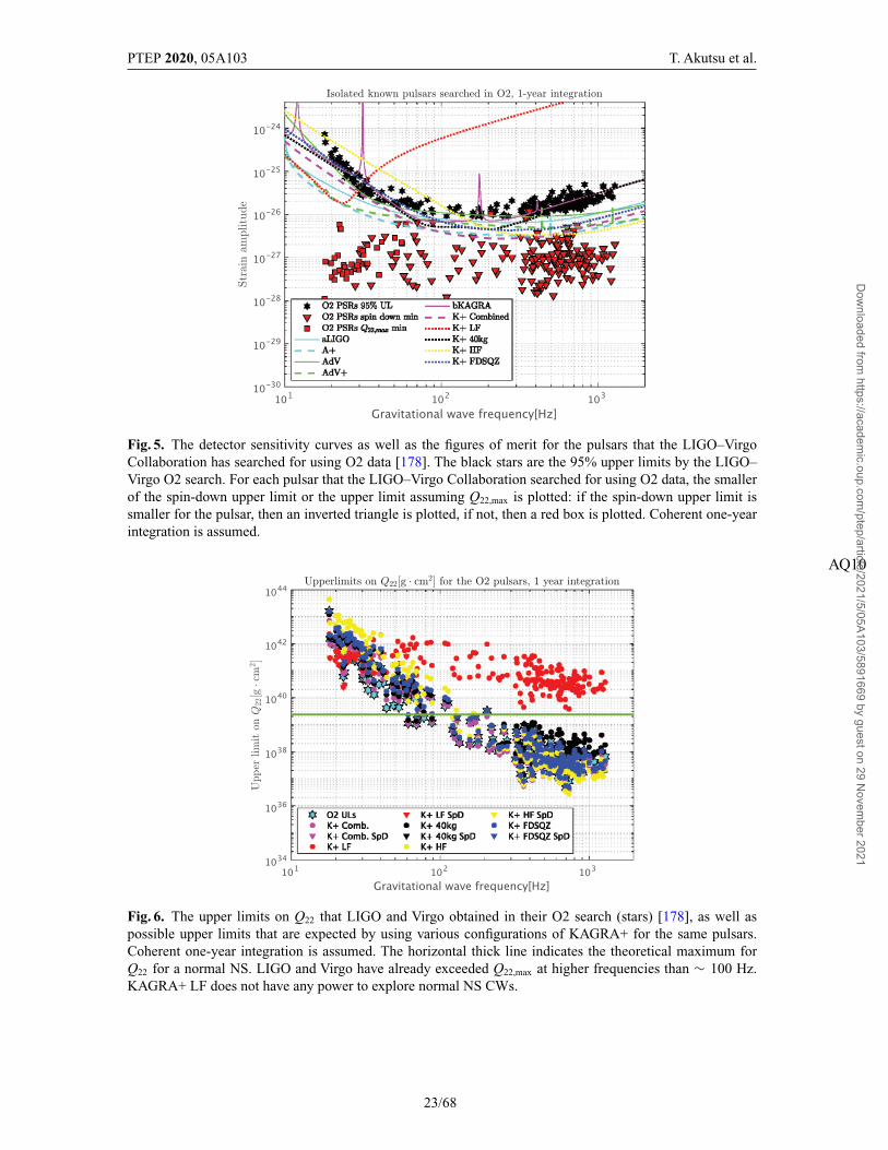
this equation assumes that 100η% of energy is radiated as GWs.Figure 5 shows the detector sensitivity curves for the CW search (assuming one-year integration,
coherent search) as well as the figures of merit for the pulsars that the LIGO–Virgo Collaborationhas searched for using O2 data [178]. It is clear that KAGRA+ HF is more useful for the CW search.
Figure 6 shows the upper limits on Q22 that LIGO and Virgo obtained in their O2 search (stars), aswell as possible upper limits that are expected by using various configurations of KAGRA+ for thesame pulsars. The horizontal thick line indicates the theoretical maximum for Q22 for a normal NS.The LIGO–Virgo Collaboration has already exceeded Q22,max at higher frequencies than ∼ 100Hz.KAGRA+ LF does not have any power to explore normal NS CWs.
It is possible to conduct unknown pulsar searches (e.g., all-sky search, wide-band frequency search).In this case, a possible figure of merit is the reach of a detector, which is shown for various detectorconfigurations in Fig. 7, assuming coherent one-year integration (although it is impossible in practiceto conduct a fully coherent unknown pulsar search due to computational resource limitations). Thisplot again shows that we may increase the chances of detection if we put more emphasis on higherfrequencies.
We can quantitatively compare the performances of various configurations of possible KAGRAupgrades by introducing the gain in the SNR averaged over relevant frequencies. Namely, we definethe ratio rα/β ≡ rα/rβ for the configurations α and β where rα is defined in Eq. (5) and a similar
22/68
Dow
nloaded from https://academ
ic.oup.com/ptep/article/2021/5/05A103/5891669 by guest on 29 N
ovember 2021
PTEP 2020, 05A103 T. Akutsu et al.
Fig. 5. The detector sensitivity curves as well as the figures of merit for the pulsars that the LIGO–VirgoCollaboration has searched for using O2 data [178]. The black stars are the 95% upper limits by the LIGO–Virgo O2 search. For each pulsar that the LIGO–Virgo Collaboration searched for using O2 data, the smallerof the spin-down upper limit or the upper limit assuming Q22,max is plotted: if the spin-down upper limit issmaller for the pulsar, then an inverted triangle is plotted, if not, then a red box is plotted. Coherent one-yearintegration is assumed.
AQ10
Fig. 6. The upper limits on Q22 that LIGO and Virgo obtained in their O2 search (stars) [178], as well aspossible upper limits that are expected by using various configurations of KAGRA+ for the same pulsars.Coherent one-year integration is assumed. The horizontal thick line indicates the theoretical maximum forQ22 for a normal NS. LIGO and Virgo have already exceeded Q22,max at higher frequencies than ∼ 100 Hz.KAGRA+ LF does not have any power to explore normal NS CWs.
23/68
Dow
nloaded from https://academ
ic.oup.com/ptep/article/2021/5/05A103/5891669 by guest on 29 N
ovember 2021
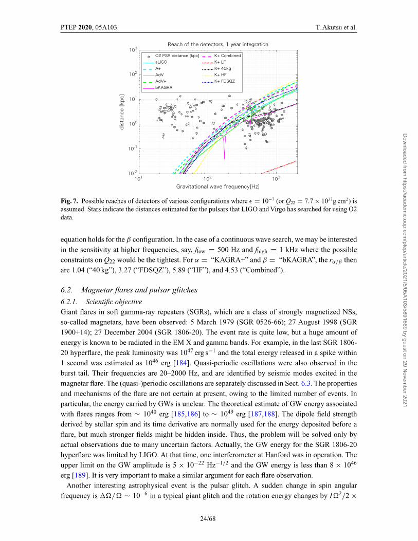
PTEP 2020, 05A103 T. Akutsu et al.
Fig. 7. Possible reaches of detectors of various configurations where ε = 10−7 (or Q22 = 7.7 × 1037g cm2) isassumed. Stars indicate the distances estimated for the pulsars that LIGO and Virgo has searched for using O2data.
equation holds for the β configuration. In the case of a continuous wave search, we may be interestedin the sensitivity at higher frequencies, say, flow = 500 Hz and fhigh = 1 kHz where the possibleconstraints on Q22 would be the tightest. For α = “KAGRA+” and β = “bKAGRA”, the rα/β thenare 1.04 (“40 kg”), 3.27 (“FDSQZ”), 5.89 (“HF”), and 4.53 (“Combined”).
6.2. Magnetar flares and pulsar glitches
6.2.1. Scientific objectiveGiant flares in soft gamma-ray repeaters (SGRs), which are a class of strongly magnetized NSs,so-called magnetars, have been observed: 5 March 1979 (SGR 0526-66); 27 August 1998 (SGR1900+14); 27 December 2004 (SGR 1806-20). The event rate is quite low, but a huge amount ofenergy is known to be radiated in the EM X and gamma bands. For example, in the last SGR 1806-20 hyperflare, the peak luminosity was 1047 erg s−1 and the total energy released in a spike within1 second was estimated as 1046 erg [184]. Quasi-periodic oscillations were also observed in theburst tail. Their frequencies are 20–2000 Hz, and are identified by seismic modes excited in themagnetar flare. The (quasi-)periodic oscillations are separately discussed in Sect. 6.3. The propertiesand mechanisms of the flare are not certain at present, owing to the limited number of events. Inparticular, the energy carried by GWs is unclear. The theoretical estimate of GW energy associatedwith flares ranges from ∼ 1040 erg [185,186] to ∼ 1049 erg [187,188]. The dipole field strengthderived by stellar spin and its time derivative are normally used for the energy deposited before aflare, but much stronger fields might be hidden inside. Thus, the problem will be solved only byactual observations due to many uncertain factors. Actually, the GW energy for the SGR 1806-20hyperflare was limited by LIGO. At that time, one interferometer at Hanford was in operation. Theupper limit on the GW amplitude is 5 × 10⁻²² Hz−1/2 and the GW energy is less than 8 × 1046
erg [189]. It is very important to make a similar argument for each flare observation.Another interesting astrophysical event is the pulsar glitch. A sudden change in spin angular
frequency is ��/� ∼ 10−6 in a typical giant glitch and the rotation energy changes by I�2/2 ×
24/68
Dow
nloaded from https://academ
ic.oup.com/ptep/article/2021/5/05A103/5891669 by guest on 29 N
ovember 2021
PTEP 2020, 05A103 T. Akutsu et al.
��/� ∼ 1041 erg as for a maximum value. The change is likely to be much smaller, since therearrangement of stellar structure is partial in the transition.
6.2.2. Observations and measurementsThese burst events will be probably first detected in EM signs, and GW signals should be carefullysearched at the burst epoch. There is no reliable waveform, so that GW signals are identified bycombinations of multiple detectors. The burst is a dynamical event on a timescale of milliseconds,and therefore a sharp peak in the kHz range is expected. Coincidence among different GW/EMdetectors is crucial. The observational strategy of GW analysis may depend on the EM information.When quasi-periodic oscillation frequencies are identified in EM data, we should search for GWcounterparts in the same frequency range. GW signals in LIGO O2 data [190] were searched formagnetar bursts, which are less-energetic events. Two software packages, X-Pipeline and STAMP,were used: Clusters of bright pixels above a threshold in each time–frequency map are searched inX-Pipeline, directional excess power due to arrival time delay between detectors in STAMP.
6.2.3. Future prospectsAs for the future extension of bKAGRA, improvements in a higher-frequency band are favored forthese events. If we fix the frequency of the signal to 1 kHz, the SNR ratios of KAGRA+ to bKAGRAat 1 kHz are 40 kg 1.03, FDSQZ 3.98, HF 7.47, Combined 5.01. However, it is not clear at presenthow to predict the detection level of meaningful signals by improvements. We will catch them orupper limits by chance, when bursts happen. Stable operation is desirable.
6.3. Stellar oscillations
6.3.1. Scientific objectiveIn order to observationally extract the properties of astronomical objects, asteroseismology is a verypowerful technique, where one can get information about objects via their specific frequencies.This is similar to seismology in the Earth and helioseismology in the Sun. For this purpose, GWsprovide the most suitable astronomical information, owing to their high permeability. In fact, severalmodes in GWs are expected to be radiated from compact objects [191], and each mode depends ondifferent aspect of internal physics. The GWs have complex frequencies, because the GWs carry outthe oscillation energy, where the real and imaginary parts correspond to the oscillation frequencyand damping rate, respectively. So, by identifying the observed frequencies (and damping times)of GWs to the corresponding specific modes, one would get the physics behind the phenomena.In general, the GWs are classified into two families with their parity. The axial parity (toroidal)oscillations are incompressible oscillations, which do not involve density variation, while the polarparity (spheroidal) oscillations involve density variation and stellar deformation. Thus, from anobservational point of view, polar-type oscillations are more important, although these are coupledwith axial-type oscillations on the non-spherical background.
6.3.2. Observations and measurementsSome of the GWs from NSs are classified in the same way as the oscillations of the usual (Newtonian)stars. That is, the fundamental (f ) and the pressure (pi) modes are excited as acoustic oscillationsof NSs, while the gravity (gi) modes are excited by the buoyancy force due to the existence of thedensity discontinuity or composition gradients inside the star. The Rossby (r) modes are also excitedby the Coriolis force in rotating stars, although they are axial parity oscillations. In addition to these
25/68
Dow
nloaded from https://academ
ic.oup.com/ptep/article/2021/5/05A103/5891669 by guest on 29 N
ovember 2021
PTEP 2020, 05A103 T. Akutsu et al.
modes associated with the fluid motions, the oscillations related to the spacetime curvature are alsoexcited, i.e., the so-called GW (wi) modes, which can be discussed only in the relativistic framework.The typical frequencies of the f , p1, g1, and w1 modes for standard NSs are around a few kHz, higherthan 4–7 kHz, smaller than a hundred Hz, and around 10 kHz, respectively [191]. With these specificmodes from the NSs, extraction of NS information via direct detection of GWs has been discussed.
A good example of GW asteroseismology may be the results shown by Andersson and Kokko-tas [192,193], where they found universal relations for the frequencies of the f and w1 modes as afunction of the average density of the star and the compactness, respectively, almost independentlyof the EOS for NS matter. This is because the frequency of the f mode, which is an acoustic wave,should depend on the crossing time inside the star with the sound velocity, while the frequencyof the w mode is strongly associated with the strength of the gravitational field. So, if one simul-taneously detect, could two modes in GWs from the NS, one could get the average density andcompactness of the source object, which tells us the NS mass and radius. On the other hand, g-modeGWs may tell us the existence of the density discontinuity due to the phase transition [194–197],or they may become more important in newborn NSs or proto-neutron stars (PNSs) [198–200]. Thenon-axisymmetric r-mode oscillations may also be interesting due to their instability against gravita-tional radiations [201,202]. That is, for the rapidly rotating case, the GW amplitude can exponentiallyincrease due to the instability, which may become a detectable signal. Eventually, the GW ampli-tude would be suppressed via non-linear coupling [203]. We note that even the f -mode oscillationsmay become unstable in rapidly rotating relativistic NSs [204]. In any case, detection of GWs froman isolated (cold) NS may be quite difficult with the current GW detectors, because most of theirfrequencies are more than around kHz.
On the other hand, the detection of GWs from PNSs would be more likely if they are formed withinour Galaxy. This is because, since the PNSs are initially less massive and have larger radii, i.e., theiraverage density is smaller than that of cold NSs, one can expect the frequency of f -mode GWs tobe smaller than the typical one for cold NSs. In practice, the f -mode frequency of PNSs is arounda few hundred Hz in the early phase after core-bounce [205]. However, studies of asteroseismologyin PNSs are very few, unlike in cold NSs. This is because of the difficulty of providing backgroundmodels. That is, cold NSs can be constructed with the zero-temperature EOS, i.e., the relation betweenenergy density and pressure, while one has to consider the distribution of the electron fraction andentropy per baryon together with the pressure distribution as a function of density to construct thePNS models. However, such distributions can be determined only after the numerical simulationof core-collapse supernovae. Even so, the study of asteroseismology in PNSs is becoming possiblewith numerical data of simulation.
So far, two different approaches have been proposed for providing the PNS models; one is that thePNS surface is defined with a specific density around 1010–12 g/cm3 [205–209], and the other is thatoscillations inside the shock radius are considered [210,211], where different boundary conditionsshould be adopted according to the approaches. In contrast to the cold NSs, matter widely existsoutside the PNSs, which makes it difficult to treat the boundary of the background models. Anyway,with either approach, it seems that the mode frequencies of GWs are expected to range over widefrequencies and that such frequencies would change with time. If one could identify the frequenciesof GWs with a specific mode, it would be very helpful for understanding the physics of PNS coolingvia understanding of the PNS properties. In practice, the time evolution of the identified frequenciesis considered as a result of the changing of the PNS mass and radius, i.e., the mass increases dueto accretion and the radius decreases due to both the relativistic effect and neutrino cooling, with
26/68
Dow
nloaded from https://academ
ic.oup.com/ptep/article/2021/5/05A103/5891669 by guest on 29 N
ovember 2021
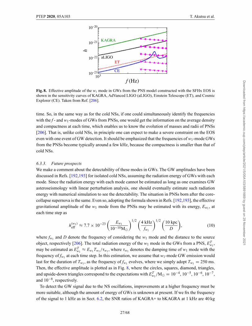
PTEP 2020, 05A103 T. Akutsu et al.
Fig. 8. Effective amplitude of the w1 mode in GWs from the PNS model constructed with the SFHx EOS isshown in the sensitivity curves of KAGRA, AdVanced LIGO (aLIGO), Einstein Telescope (ET), and CosmicExplorer (CE). Taken from Ref. [206].
time. So, in the same way as for the cold NSs, if one could simultaneously identify the frequencieswith the f - and w1-modes of GWs from PNSs, one would get the information on the average densityand compactness at each time, which enables us to know the evolution of masses and radii of PNSs[206]. That is, unlike cold NSs, in principle one can expect to make a severe constraint on the EOSeven with one event of GW detection. It should be emphasized that the frequencies of w1-mode GWsfrom the PNSs become typically around a few kHz, because the compactness is smaller than that ofcold NSs.
6.3.3. Future prospectsWe make a comment about the detectability of these modes in GWs. The GW amplitudes have beendiscussed in Refs. [192,193] for isolated cold NSs, assuming the radiation energy of GWs with eachmode. Since the radiation energy with each mode cannot be estimated as long as one examines GWasteroseismology with linear perturbation analysis, one should eventually estimate such radiationenergy with numerical simulation to see the detectability. The situation in PNSs born after the core-collapse supernova is the same. Even so, adopting the formula shown in Refs. [192,193], the effectivegravitational amplitude of the w1 mode from the PNSs may be estimated with its energy, Ew1 , ateach time step as
h(w1)eff ≈ 7.7 × 10⁻²³
(Ew1
10−10M�
)1/2 (4 kHz
fw1
)1/2 (10 kpc
D
), (10)
where fw1 and D denote the frequency of considering the w1 mode and the distance to the sourceobject, respectively [206]. The total radiation energy of the w1 mode in the GWs from a PNS, ET
w1,
may be estimated as ETw1
≈ Ew1Tw1/τw1 , where τw1 denotes the damping time of w1 mode with thefrequency of fw1 at each time step. In this estimation, we assume that w1-mode GW emission wouldlast for the duration of Tw1 , as the frequency of fw1 evolves, where we simply adopt Tw1 = 250 ms.Then, the effective amplitude is plotted as in Fig. 8, where the circles, squares, diamond, triangles,and upside-down triangles correspond to the expectations with ET
w1/M� = 10−4, 10−5, 10−6, 10−7,
and 10−8, respectively.To detect the GW signal due to the NS oscillations, improvements at a higher frequency must be
more suitable, although the amount of energy of GWs is unknown at present. If we fix the frequencyof the signal to 1 kHz as in Sect. 6.2, the SNR ratios of KAGRA+ to bKAGRA at 1 kHz are 40 kg
27/68
Dow
nloaded from https://academ
ic.oup.com/ptep/article/2021/5/05A103/5891669 by guest on 29 N
ovember 2021
PTEP 2020, 05A103 T. Akutsu et al.
1.03, FDSQZ 3.98, HF 7.47, Combined 5.01. Improvements even in the middle-frequency band maybe suitable for detecting f -mode GWs from the PNS, but this would only be acceptable in the earlyphase after core-bounce, because the frequency increases with time and eventually becomes ∼ kHz.
7. Supernovae7.1. The explosion mechanisms and the GW signatures
7.1.1. Scientific objectiveAccumulating observational evidence from multi-wavelength EM observations of, e.g., ejecta mor-phologies and spatial distributions of heavy elements have all pointed toward CCSNe being generallyaspherical (see, e.g., Refs. [212,213] and references therein). However, these signals are secondaryfor probing the multi-dimensionality of the supernova engine because they are only able to provideimages of optically thin regions far away from the central core. The GWs from CCSNe are theprimary observables, which imprint live information on the central engine.
From a theoretical point of view, understanding the origin of the explosion multi-dimensionality isindispensable for clarifying the as-yet-uncertain CCSN mechanisms. After half a century of contin-uing effort, theory and neutrino radiation-hydrodynamics simulations are now converging to a pointthat multi-dimensional (multi-D) hydrodynamics instabilities play a pivotal role in the neutrino mech-anism [214], the most favored scenario to trigger explosions. In fact, self-consistent simulations inthree spatial dimensions (3D) now report shock revival of the stalled bounce shock into explosionby the multi-D neutrino mechanism (see Refs. [215–218] for recent reviews).
7.1.2. Observations and measurementsThe most distinct GW emission process commonly seen in recent self-consistent 3D models is asso-ciated with the excitation of core/PNS oscillatory modes (see, e.g., Refs. [219–222]). The dominantmodes are quadrupolar (� = 2) deformations of the PNS excited by non-spherical mass accretiononto it (see also Sect. 6.3). The characteristic GW frequency increases almost monotonically withtime due to an accumulating accretion onto the PNS, which ranges from ∼ 500 to 1000 Hz (see Ref.[223] for a dedicated scheme to detect the ramp-up GW signature from the noises).
In addition to the prime GW signature, standing accretion shock instability (SASI) (see, e.g., Ref.[224]) has also been considered as a key to generate GW emission in the post-bounce supernova core.It has become apparent [219,220,222] that the predominant GW emission from CCSNe is producedin the same region behind the post-shock region where both SASI and neutrino-driven convectionvigorously develop (see, e.g., Ref. [225] for a review). The GW emission from this region—fromjust above the neutrinospheres at densities of roughly 1011 g/cm3 and inward—is determined by theeffects of the super-nuclear EOS, as well as the impact of hydrodynamic instabilities present in thepost-shock flow (see, e.g., Ref. [221]). The typical frequency of SASI-induced GWs is in the rangeof ∼100–250 Hz, which is in the best sensitivity range of the currently running interferometers.
Rapid rotation in the iron core leads to significant rotational flattening of the collapsing andbouncing core, which produces a time-dependent quadrupole (or higher) GW emission (see, e.g.,Ref. [226] for a review). For bounce signals with a strong and characteristic signature, the iron coremust rotate rapidly enough3. The GW frequency associated with the rapidly rotating collapse andbounce is in the range of ∼ 600–1000 Hz.
3 Although rapid rotation and the strong magnetic fields in the core are attracting great attention as the keyto solving the dynamics of collapsars and magnetars, one should keep in mind that recent stellar evolution
28/68
Dow
nloaded from https://academ
ic.oup.com/ptep/article/2021/5/05A103/5891669 by guest on 29 N
ovember 2021
PTEP 2020, 05A103 T. Akutsu et al.
Another feature distinguishing GWs from CCSNe is circular polarization. The importance ofdetecting circular GW polarization from CCSNe was first discussed in Ref. [228] in the context ofrapidly rotating core-collapse. More recently, Ref. [229] presented an analysis of the GW polariza-tion using results from 3D general-relativistic simulations of a non-rotating 15M� star [222]. Theamplitude of the GW polarization was shown to become larger for the 3D general-relativistic modelthat exhibits strong SASI activity. The non-axisymmetric flows associated with spiral SASI give riseto the circular polarization. If detected, it will provide us with a new probe into the SASI activityin the pre-explosion supernova core. Note that spiral SASI develops mainly outside of the PNS, sothat circular polarization from spiral SASI has different features in the spectrogram compared to thestochastic, weak circular polarization from the PNS oscillations that have no preferential direction ofdevelopment [229]. By estimating the SNR of the GW polarization, they pointed out the possibilitythat the detection horizon of circular polarization could extend by more than a factor of several timesfarther compared to that of the GW amplitude. In order to detect the GW circular polarization with ahigh SNR, joint GW observation with KAGRA in addition to two LIGOs and Virgo is indispensable.
7.1.3. Future prospectsEach phase of a CCSN has a range of characteristic GW signatures and GW polarization that canprovide diagnostic constraints on the evolution and physical parameters of a CCSN and on theexplosion hydrodynamics. The GW signatures described in this section commonly appear in thefrequency range of 100–1000 Hz in recent simulations of CCSNe. Among them, the PNS oscillatorymodes are currently recognized as a model-independent GW signature. The characteristic frequenciesof the fundamental (f /g) modes are predominantly dependent on the PNS mass (M ) and the radius(R), however, in a non-trivial manner [206]. In order to break the degeneracy, the detection of othereigenmodes (p, w modes) of the PNS oscillations is mandatory. In fact, GW asteroseismology ofPNSs has just started [206,207,211] (see also Sect. 6.3). The outcomes of this should reveal therequirement of KAGRA (and the next-generation detectors) to detect the whole of the eigenmodes(presumably extending up to several kHz) for future CCSN events. This could be done in the nextfive years.
For the detectability of GWs from PNSs, see Sect. 6.3. The GWs due to SASI for a Galactic eventmay be detected with the SNR of the GW signals predicted in the most recent 3D CCSN models in therange of ∼4–10 for aLIGO [221]. With the third-generation detectors online (e.g., Cosmic Explorer),these signals would never be missed for CCSN events throughout the Milky Way. A current estimateof SNR for GWs from rapidly rotating collapse and bounce based on predictions from a set of 3Dmodels using a coherent network analysis shows that these GW signals could be detectable up toabout ∼ 20 kpc for the most rapidly rotating model ([230]; see also Refs. [231,232]). If the spectra ofthe supernovae are assumed to be flat in the frequency range of 100 Hz–1 kHz, we can quantitativelycompare performances of various configurations of possible KAGRA upgrades by defining the SNRratio rα/β ≡ rα/rβ for the configurations α and β where rα is defined in Eq. (5) and a similar equationholds for the β configuration. For the frequency range between flow = 100 Hz and fhigh = 1 kHz,the SNR ratios of KAGRA+ to bKAGRA averaged over relevant frequencies are 40 kg 1.51, FDSQZ2.35, HF 3.43, Combined 3.55. However, since the spectral evolution of the CCSN GWs has notbeen completely clarified yet and it does depend upon the details of CCSN modeling (such as on
calculations predict that such an extreme condition can be realized only in a special case [227] (� 1% ofmassive star population).
29/68
Dow
nloaded from https://academ
ic.oup.com/ptep/article/2021/5/05A103/5891669 by guest on 29 N
ovember 2021
PTEP 2020, 05A103 T. Akutsu et al.
the initial rotation rates and the progenitor masses), it is too early to have a quantitative discussionabout the best-suited sensitivity curves for KAGRA+. Because recent CCSN simulations indicatethat the important GW frequency to unveil the physics of CCSNe will be ≥ 100 Hz, all the candidateupgrades except for LF should help enhance the chance of detection.
8. The early Universe8.1. GWs from inflation
8.1.1. Scientific objectiveInflation, an accelerated expansion phase of the very early Universe, was proposed in the 1980s tosolve problems in the standard model of the Big Bang theory, such as the horizon, flatness, andmonopole problems [233–236]. A key feature of inflation is that the rapid expansion stretches quan-tum fluctuations in a scalar field to classical scales and generates primordial density fluctuations[237–241], which become the seeds of galaxies. The nearly scale-invariant spectrum of scalar per-turbations, predicted by the inflationary theory, is strongly supported by cosmological observationsof the cosmic microwave background and galaxy surveys. The same mechanism also applies to quan-tum fluctuations in spacetime, which produce a stochastic background of GWs over a wide rangeof frequencies with a scale-invariant power spectrum [242–244]. The detection of inflationary GWsis a key to test inflation and distinguish a number of models since the amplitude and spectral indexstrongly depend on the model.
8.1.2. Observations and measurementsThe amplitude of the GWs is typically far below the sensitivity of the ground-based detectors.The dimensionless parameter, �GW, which describes the energy density of GWs per logarithmicfrequency interval, is roughly given by �GW � 10−15(Hinf /1014 GeV)2 for a scale-invariant pri-mordial spectrum �GW ∝ f 0, where Hinf is the Hubble expansion rate during inflation. Inflationpredicts a slightly red-tilted spectrum, which further reduces the amplitude at high frequency. Forexample, the model predicts �GW ∼ 10−16 at 100 Hz for chaotic inflation and �GW ∼ 10−17 forR2 inflation, while the cross correlation between LIGO, Virgo, and KAGRA with their final designsensitivities is expected to reach a stochastic background of �GW ∼ 10−9. For details on the shapeof the spectrum, see Refs. [245,246].
Note that a search for a stochastic GW background is performed by cross-correlating data fromdifferent detectors over a long time period. The sensitivity is determined by noise curves of themultiple detectors as well as the observation time. Since the two detectors of LIGO have advantagesin both sensitivity and observation time, the sensitivity of the four-detector network �GW ∼ 10−9
will be dominated by LIGO detectors, while KAGRA with the current design sensitivity would notcontribute to an increase in the overall sensitivity. Currently LIGO–Virgo O2 data provide an upperlimit of �GW < 6.0 × 10⁻⁸ for a scale-invariant spectrum [247].
Although the ground-based detectors are not sensitive enough to detect standard inflationary GWs,some models going beyond the standard picture predict a blue-tilted spectrum, e.g., string gas cosmol-ogy [248], super-inflation models [249,250], G-inflation [251], non-commutative inflation [252,253],particle production during inflation [254,255], Hawking radiation during inflation [256], a spectatorscalar field with small sound speed [257], massive gravity [258], and so on. The amplitude of theinflationary GW spectrum is constrained at low frequencies by the cosmic microwave background
30/68
Dow
nloaded from https://academ
ic.oup.com/ptep/article/2021/5/05A103/5891669 by guest on 29 N
ovember 2021
PTEP 2020, 05A103 T. Akutsu et al.
�GW � 10−15, but the amplitude can be large at a frequency of ∼ 100 Hz if the spectrum is blue-tilted. There would be a chance for the ground-based detectors to detect inflationary GWs if thespectral index of the spectrum nT is larger than ∼ 0.5.
Another possibility for the ground-based detectors is to probe a non-standard Hubble expansionhistory of the early Universe [259–264]. Information on the expansion rate, which is determined bythe dominant component of the Universe, is imprinted in the spectrum of inflationary GWs. For ascale-invariant primordial spectrum, the spectral dependence of the stochastic background becomes�GW ∝ f 2(3w−1)/(3w+1), where w is the EOS of the Universe. In the standard cosmological model,the matter-dominated (w = 0) and radiation-dominated (w = 1/3) phases yield �GW ∝ f −2 andf 0, respectively. When one considers a kination-dominated phase (w = 1) soon after inflation, thespectral amplitude is enhanced at high frequency by the dependence �GW ∝ f and peaks at afrequency corresponding to the size of the Universe at the end of inflation, which is typically higherthan ∼ 100 Hz. Although it is difficult to find a case where GWs are detectable by ground-basedexperiments satisfying the Big Bang nucleosynthesis (BBN) bound [265,266], �GW � 10−5 forf � 10−10 Hz, the upper bound on the stochastic background is still helpful to explore early-Universephysics beyond the standard cosmology.
8.1.3. Future prospectsThe SNR for a stochastic GW background is computed by taking cross correlation between detectorsignals [267], and given by
SNRIJ = 3H 20
10π2
√2Tobs
[∫ ∞
0df
|γIJ (f )|2�GW(f )2
f 6Sn,I (f )Sn,J (f )
]1/2
, (11)
where H0 is the Hubble constant, Tobs is the observation time, and Sn,I (f ) is the noise spectral densitywith I and J labeling two different detectors. The overlap reduction function γIJ (f ) is given by thedetector responses of the two polarization modes F+ and F× as
γIJ (f ) ≡ 5
8π
∫d�(F+
I F+J + F×
I F×J )e−2π if �·(xI −xJ ), (12)
where x describes the position of the detector and � specifies the propagation direction of GWs. Fora network of N detectors, the total SNR is given by
SNR =[
N∑I=1
N∑J<I
SNR2IJ
]1/2
. (13)
As seen in the overlap reduction function, the SNR depends on the distance and relative orientationof the detectors. For KAGRA, correlating with AdV+ is better than with A+ because of the relativeorientation. Assuming a flat spectrum of �GW(f ), the sensitivities of the pair of KAGRA and AdV+to �GW with SNR = 5 are 1.1 × 10⁻⁷ for bKAGRA, 3.4 × 10⁻⁸ for LF, 8.3 × 10⁻⁸ for 40 kg,1.1 × 10−7 for FDSQZ, 3.3 × 10⁻⁷ for HF, and 5.0 × 10⁻⁸ for Combined. The lower-frequencyupgrades give better sensitivities. However, the sensitivity between two A+ is 4.0 × 10⁻⁹, whichis an order of magnitude better than those with KAGRA because of the much closer separation ofthe detector pair. Therefore, KAGRA is not good for detection but will be able to play an importantrole in determining the spectral shape and measuring anisotropy, non-Gaussianity, and polarizations,which are discussed in Sect. 8.3.
31/68
Dow
nloaded from https://academ
ic.oup.com/ptep/article/2021/5/05A103/5891669 by guest on 29 N
ovember 2021
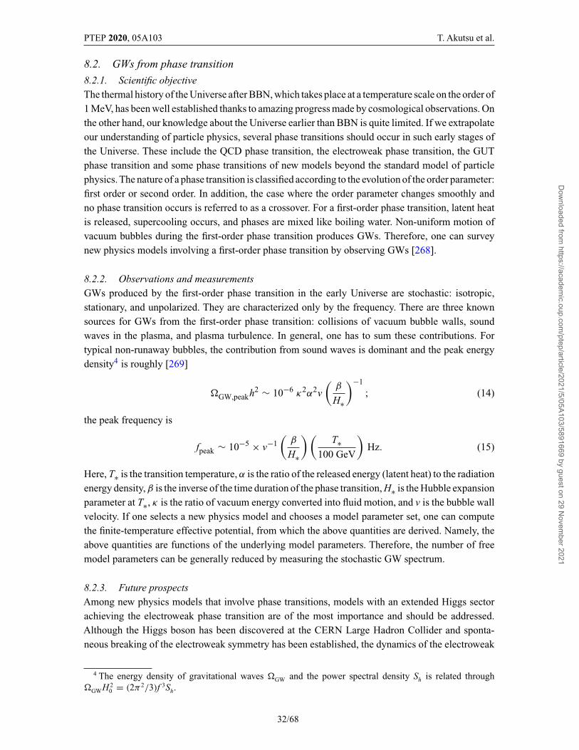
PTEP 2020, 05A103 T. Akutsu et al.
8.2. GWs from phase transition
8.2.1. Scientific objectiveThe thermal history of the Universe after BBN, which takes place at a temperature scale on the order of1 MeV, has been well established thanks to amazing progress made by cosmological observations. Onthe other hand, our knowledge about the Universe earlier than BBN is quite limited. If we extrapolateour understanding of particle physics, several phase transitions should occur in such early stages ofthe Universe. These include the QCD phase transition, the electroweak phase transition, the GUTphase transition and some phase transitions of new models beyond the standard model of particlephysics. The nature of a phase transition is classified according to the evolution of the order parameter:first order or second order. In addition, the case where the order parameter changes smoothly andno phase transition occurs is referred to as a crossover. For a first-order phase transition, latent heatis released, supercooling occurs, and phases are mixed like boiling water. Non-uniform motion ofvacuum bubbles during the first-order phase transition produces GWs. Therefore, one can surveynew physics models involving a first-order phase transition by observing GWs [268].
8.2.2. Observations and measurementsGWs produced by the first-order phase transition in the early Universe are stochastic: isotropic,stationary, and unpolarized. They are characterized only by the frequency. There are three knownsources for GWs from the first-order phase transition: collisions of vacuum bubble walls, soundwaves in the plasma, and plasma turbulence. In general, one has to sum these contributions. Fortypical non-runaway bubbles, the contribution from sound waves is dominant and the peak energydensity4 is roughly [269]
�GW,peakh2 ∼ 10−6 κ2α2v
(β
H∗
)−1
; (14)
the peak frequency is
fpeak ∼ 10−5 × v−1(
β
H∗
)(T∗
100 GeV
)Hz. (15)
Here, T∗ is the transition temperature, α is the ratio of the released energy (latent heat) to the radiationenergy density, β is the inverse of the time duration of the phase transition, H∗ is the Hubble expansionparameter at T∗, κ is the ratio of vacuum energy converted into fluid motion, and v is the bubble wallvelocity. If one selects a new physics model and chooses a model parameter set, one can computethe finite-temperature effective potential, from which the above quantities are derived. Namely, theabove quantities are functions of the underlying model parameters. Therefore, the number of freemodel parameters can be generally reduced by measuring the stochastic GW spectrum.
8.2.3. Future prospectsAmong new physics models that involve phase transitions, models with an extended Higgs sectorachieving the electroweak phase transition are of the most importance and should be addressed.Although the Higgs boson has been discovered at the CERN Large Hadron Collider and sponta-neous breaking of the electroweak symmetry has been established, the dynamics of the electroweak
4 The energy density of gravitational waves �GW and the power spectral density Sh is related through�GWH 2
0 = (2π 2/3)f 3Sh.
32/68
Dow
nloaded from https://academ
ic.oup.com/ptep/article/2021/5/05A103/5891669 by guest on 29 N
ovember 2021
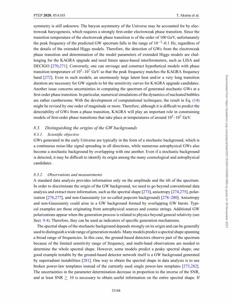
PTEP 2020, 05A103 T. Akutsu et al.
symmetry is still unknown. The baryon asymmetry of the Universe may be accounted for by elec-troweak baryogenesis, which requires a strongly first-order electroweak phase transition. Since thetransition temperature of the electroweak phase transition is of the order of 100 GeV, unfortunatelythe peak frequency of the predicted GW spectrum falls in the range of 10−3–0.1 Hz, regardless ofthe details of the extended Higgs models. Therefore, the detection of GWs from the electroweakphase transition and determination of the model parameters of extended Higgs models are chal-lenging for the KAGRA upgrade and need future space-based interferometers, such as LISA andDECIGO [270,271]. Conversely, one can envisage and construct hypothetical models with phasetransition temperature of 105–107 GeV so that the peak frequency matches the KAGRA frequencyband [272]. Even in such models, an enormously large latent heat and/or a very long transitionduration are necessary for GW signals to hit the sensitivity curves for KAGRA upgrade candidates.Another issue concerns uncertainties in computing the spectrum of generated stochastic GWs at afirst-order phase transition. In particular, numerical simulations of the dynamics of nucleated bubblesare rather cumbersome. With the development of computational techniques, the result in Eq. (14)might be revised by one order of magnitude or more. Therefore, although it is difficult to predict thedetectability of GWs from a phase transition, KAGRA will play an important role in constrainingmodels of first-order phase transitions that take place at temperatures of around 105–107 GeV.
8.3. Distinguishing the origins of the GW backgrounds
8.3.1. Scientific objectiveGWs generated in the early Universe are typically in the form of a stochastic background, which isa continuous noise-like signal spreading in all directions, while numerous astrophysical GWs alsobecome a stochastic background by overlapping with one another. Even if a stochastic backgroundis detected, it may be difficult to identify its origin among the many cosmological and astrophysicalcandidates.
8.3.2. Observations and measurementsA standard data analysis provides information only on the amplitude and the tilt of the spectrum.In order to discriminate the origin of the GW background, we need to go beyond conventional dataanalysis and extract more information, such as the spectral shape [273], anisotropy [274,275], polar-ization [276,277], and non-Gaussianity (or so-called popcorn background) [278–280]. Anisotropyand non-Gaussianity could arise in a GW background formed by overlapping GW bursts. Typi-cal examples are those originating from astrophysical sources and cosmic strings. Additional GWpolarizations appear when the generation process is related to physics beyond general relativity (seeSect. 9.4). Therefore, they can be used as indicators of specific generation mechanisms.
The spectral shape of the stochastic background depends strongly on its origin and can be generallyused to distinguish a wide range of generation models. Many models predict a spectral shape spanninga broad range of frequencies. In this case, the ground-based detectors observe part of the spectrumbecause of the limited sensitivity range of frequency, and multi-band observations are needed todetermine the whole spectral shape. However, some models predict a peaky spectral shape; onegood example testable by the ground-based detector network itself is a GW background generatedby superradiant instabilities [281]. One way to obtain the spectral shape in data analysis is to usebroken power-law templates instead of the currently used single power-law templates [273,282].The uncertainties in the parameter determination decrease in proportion to the inverse of the SNR,and at least SNR � 10 is necessary to obtain useful information on the entire spectral shape. If
33/68
Dow
nloaded from https://academ
ic.oup.com/ptep/article/2021/5/05A103/5891669 by guest on 29 N
ovember 2021
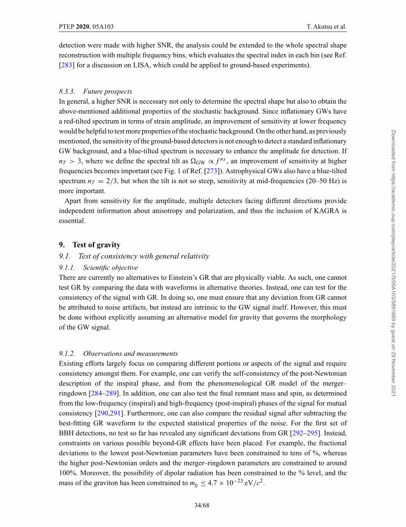
PTEP 2020, 05A103 T. Akutsu et al.
detection were made with higher SNR, the analysis could be extended to the whole spectral shapereconstruction with multiple frequency bins, which evaluates the spectral index in each bin (see Ref.[283] for a discussion on LISA, which could be applied to ground-based experiments).
8.3.3. Future prospectsIn general, a higher SNR is necessary not only to determine the spectral shape but also to obtain theabove-mentioned additional properties of the stochastic background. Since inflationary GWs havea red-tilted spectrum in terms of strain amplitude, an improvement of sensitivity at lower frequencywould be helpful to test more properties of the stochastic background. On the other hand, as previouslymentioned, the sensitivity of the ground-based detectors is not enough to detect a standard inflationaryGW background, and a blue-tilted spectrum is necessary to enhance the amplitude for detection. IfnT > 3, where we define the spectral tilt as �GW ∝ f nT , an improvement of sensitivity at higherfrequencies becomes important (see Fig. 1 of Ref. [273]). Astrophysical GWs also have a blue-tiltedspectrum nT = 2/3, but when the tilt is not so steep, sensitivity at mid-frequencies (20–50 Hz) ismore important.
Apart from sensitivity for the amplitude, multiple detectors facing different directions provideindependent information about anisotropy and polarization, and thus the inclusion of KAGRA isessential.
9. Test of gravity9.1. Test of consistency with general relativity
9.1.1. Scientific objectiveThere are currently no alternatives to Einstein’s GR that are physically viable. As such, one cannottest GR by comparing the data with waveforms in alternative theories. Instead, one can test for theconsistency of the signal with GR. In doing so, one must ensure that any deviation from GR cannotbe attributed to noise artifacts, but instead are intrinsic to the GW signal itself. However, this mustbe done without explicitly assuming an alternative model for gravity that governs the morphologyof the GW signal.
9.1.2. Observations and measurementsExisting efforts largely focus on comparing different portions or aspects of the signal and requireconsistency amongst them. For example, one can verify the self-consistency of the post-Newtoniandescription of the inspiral phase, and from the phenomenological GR model of the merger–ringdown [284–289]. In addition, one can also test the final remnant mass and spin, as determinedfrom the low-frequency (inspiral) and high-frequency (post-inspiral) phases of the signal for mutualconsistency [290,291]. Furthermore, one can also compare the residual signal after subtracting thebest-fitting GR waveform to the expected statistical properties of the noise. For the first set ofBBH detections, no test so far has revealed any significant deviations from GR [292–295]. Instead,constraints on various possible beyond-GR effects have been placed. For example, the fractionaldeviations to the lowest post-Newtonian parameters have been constrained to tens of %, whereasthe higher post-Newtonian orders and the merger–ringdown parameters are constrained to around100%. Moreover, the possibility of dipolar radiation has been constrained to the % level, and themass of the graviton has been constrained to mg ≤ 4.7 × 10⁻²³ eV/c2.
34/68
Dow
nloaded from https://academ
ic.oup.com/ptep/article/2021/5/05A103/5891669 by guest on 29 N
ovember 2021
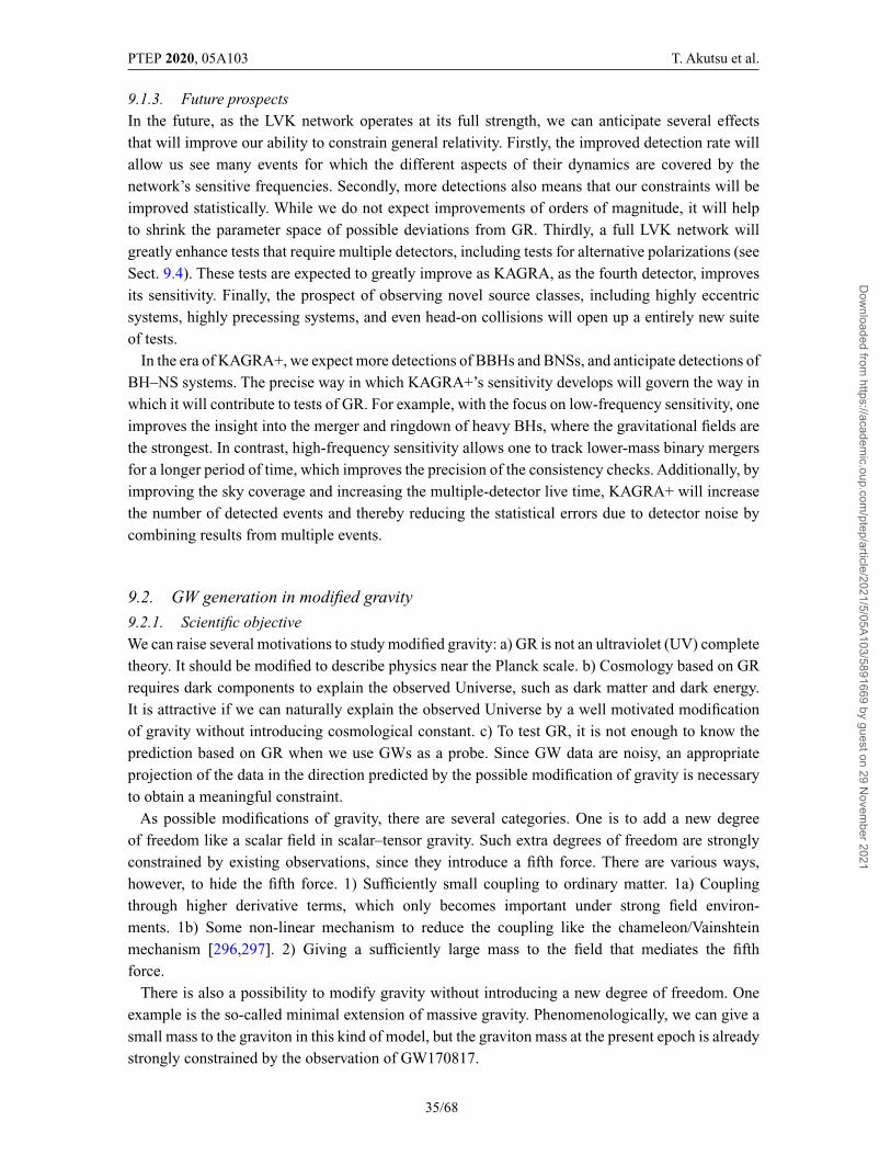
PTEP 2020, 05A103 T. Akutsu et al.
9.1.3. Future prospectsIn the future, as the LVK network operates at its full strength, we can anticipate several effectsthat will improve our ability to constrain general relativity. Firstly, the improved detection rate willallow us see many events for which the different aspects of their dynamics are covered by thenetwork’s sensitive frequencies. Secondly, more detections also means that our constraints will beimproved statistically. While we do not expect improvements of orders of magnitude, it will helpto shrink the parameter space of possible deviations from GR. Thirdly, a full LVK network willgreatly enhance tests that require multiple detectors, including tests for alternative polarizations (seeSect. 9.4). These tests are expected to greatly improve as KAGRA, as the fourth detector, improvesits sensitivity. Finally, the prospect of observing novel source classes, including highly eccentricsystems, highly precessing systems, and even head-on collisions will open up a entirely new suiteof tests.
In the era of KAGRA+, we expect more detections of BBHs and BNSs, and anticipate detections ofBH–NS systems. The precise way in which KAGRA+’s sensitivity develops will govern the way inwhich it will contribute to tests of GR. For example, with the focus on low-frequency sensitivity, oneimproves the insight into the merger and ringdown of heavy BHs, where the gravitational fields arethe strongest. In contrast, high-frequency sensitivity allows one to track lower-mass binary mergersfor a longer period of time, which improves the precision of the consistency checks. Additionally, byimproving the sky coverage and increasing the multiple-detector live time, KAGRA+ will increasethe number of detected events and thereby reducing the statistical errors due to detector noise bycombining results from multiple events.
9.2. GW generation in modified gravity
9.2.1. Scientific objectiveWe can raise several motivations to study modified gravity: a) GR is not an ultraviolet (UV) completetheory. It should be modified to describe physics near the Planck scale. b) Cosmology based on GRrequires dark components to explain the observed Universe, such as dark matter and dark energy.It is attractive if we can naturally explain the observed Universe by a well motivated modificationof gravity without introducing cosmological constant. c) To test GR, it is not enough to know theprediction based on GR when we use GWs as a probe. Since GW data are noisy, an appropriateprojection of the data in the direction predicted by the possible modification of gravity is necessaryto obtain a meaningful constraint.
As possible modifications of gravity, there are several categories. One is to add a new degreeof freedom like a scalar field in scalar–tensor gravity. Such extra degrees of freedom are stronglyconstrained by existing observations, since they introduce a fifth force. There are various ways,however, to hide the fifth force. 1) Sufficiently small coupling to ordinary matter. 1a) Couplingthrough higher derivative terms, which only becomes important under strong field environ-ments. 1b) Some non-linear mechanism to reduce the coupling like the chameleon/Vainshteinmechanism [296,297]. 2) Giving a sufficiently large mass to the field that mediates the fifthforce.
There is also a possibility to modify gravity without introducing a new degree of freedom. Oneexample is the so-called minimal extension of massive gravity. Phenomenologically, we can give asmall mass to the graviton in this kind of model, but the graviton mass at the present epoch is alreadystrongly constrained by the observation of GW170817.
35/68
Dow
nloaded from https://academ
ic.oup.com/ptep/article/2021/5/05A103/5891669 by guest on 29 N
ovember 2021
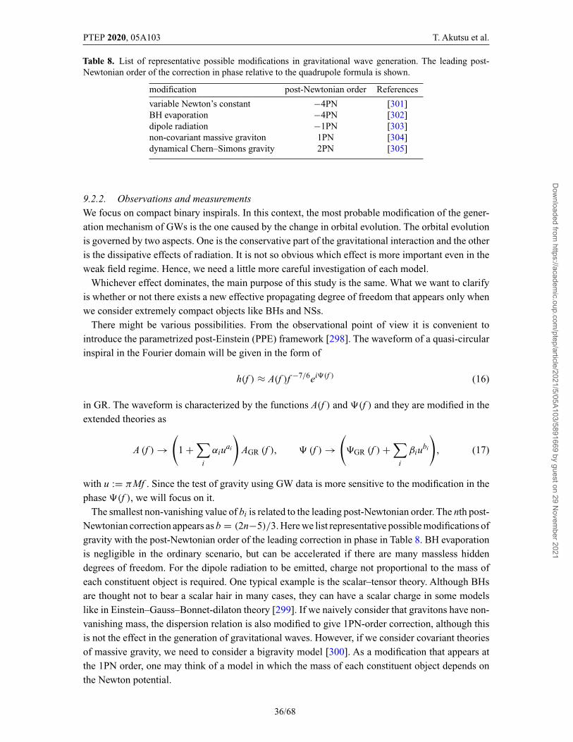
PTEP 2020, 05A103 T. Akutsu et al.
Table 8. List of representative possible modifications in gravitational wave generation. The leading post-Newtonian order of the correction in phase relative to the quadrupole formula is shown.
modification post-Newtonian order References
variable Newton’s constant −4PN [301]BH evaporation −4PN [302]dipole radiation −1PN [303]non-covariant massive graviton 1PN [304]dynamical Chern–Simons gravity 2PN [305]
9.2.2. Observations and measurementsWe focus on compact binary inspirals. In this context, the most probable modification of the gener-ation mechanism of GWs is the one caused by the change in orbital evolution. The orbital evolutionis governed by two aspects. One is the conservative part of the gravitational interaction and the otheris the dissipative effects of radiation. It is not so obvious which effect is more important even in theweak field regime. Hence, we need a little more careful investigation of each model.
Whichever effect dominates, the main purpose of this study is the same. What we want to clarifyis whether or not there exists a new effective propagating degree of freedom that appears only whenwe consider extremely compact objects like BHs and NSs.
There might be various possibilities. From the observational point of view it is convenient tointroduce the parametrized post-Einstein (PPE) framework [298]. The waveform of a quasi-circularinspiral in the Fourier domain will be given in the form of
h(f ) ≈ A(f )f −7/6ei(f ) (16)
in GR. The waveform is characterized by the functions A(f ) and (f ) and they are modified in theextended theories as
A (f ) →(
1 +∑
i
αiuai
)AGR (f ), (f ) →
(GR (f ) +
∑i
βiubi
), (17)
with u := πMf . Since the test of gravity using GW data is more sensitive to the modification in thephase (f ), we will focus on it.
The smallest non-vanishing value of bi is related to the leading post-Newtonian order. The nth post-Newtonian correction appears as b = (2n−5)/3. Here we list representative possible modifications ofgravity with the post-Newtonian order of the leading correction in phase in Table 8. BH evaporationis negligible in the ordinary scenario, but can be accelerated if there are many massless hiddendegrees of freedom. For the dipole radiation to be emitted, charge not proportional to the mass ofeach constituent object is required. One typical example is the scalar–tensor theory. Although BHsare thought not to bear a scalar hair in many cases, they can have a scalar charge in some modelslike in Einstein–Gauss–Bonnet-dilaton theory [299]. If we naively consider that gravitons have non-vanishing mass, the dispersion relation is also modified to give 1PN-order correction, although thisis not the effect in the generation of gravitational waves. However, if we consider covariant theoriesof massive gravity, we need to consider a bigravity model [300]. As a modification that appears atthe 1PN order, one may think of a model in which the mass of each constituent object depends onthe Newton potential.
36/68
Dow
nloaded from https://academ
ic.oup.com/ptep/article/2021/5/05A103/5891669 by guest on 29 N
ovember 2021
PTEP 2020, 05A103 T. Akutsu et al.
As a typical modification of GR, the scalar–tensor theory is often discussed. If the binary membershave some scalar charges coupled to the extra degree of freedom, we have dipolar radiation.Althoughthe overall magnitude also depends on the coupling strength, if we focus only on the frequencydependence, the flux due to dipolar radiation is larger at a low frequency by the factor (v/c)−2 ∼(mω)−2/3 compared with that due to GW radiation. On the other hand, the extra scalar degree offreedom changes the conservative part of the force, but there is no such enhancement in the sense ofpost-Newtonian order. Hence, at low frequency, where v/c � 1 the modification to the conservativegravitational interaction can be neglected.
For the modification that predicts negative post-Newtonian order, the deviation from GR is rela-tively larger at lower frequencies, compared with GR contributions. Therefore, it is not so easy forGW observations to compete with the constraint from the observations at lower frequencies, such aspulsar timing.
There are some more detailed aspects that cannot be expressed by the PPE framework. Onepossibility is spontaneous scalarization. When we consider BNSs, each NS in isolation may not havea scalar charge. However, there is a region in the model parameter space in which instability occursas the binary separation decreases and both NSs get charged. Another possibility is that the mediatingscalar field is massive. This is quite likely to avoid instability similar to spontaneous scalarizationoccurring in the whole Universe after the temperature of the Universe becomes 10 MeV or lower.If the instability occurs, the success of the Big Bang nucleosynthesis will be significantly damaged.This gives the constraint on the mass of the mediating field as greater than 10−16 eV or so [306],which is comparable to the constraint from pulsar timing (PSRJ0348+0432). On the other hand,ground-based detectors are sensitive to modification if the mass is smaller than 10−12 eV. If the massis in the range between these two, the existence of the extra degree of freedom might be probed onlyby GWs.
Basically we check the deviation of the observed GW signal from GR templates. For this purpose,it is better to have a better theoretical template based on each candidate of modified gravity. Inparticular this demand is higher when we consider the models whose leading-order modificationappears at the positive post-Newtonian order. In such models, we have more chances to observethe largest deviation at the final stage of inspirals. In many cases, this task remains a challenge fortheorists.
9.2.3. Future prospectsAs long as we consider BHs with masses larger than a few times the solar mass and NSs, it seemsdifficult to use a high-frequency band to give constraints on modified gravity. In the case of BHs,we do not have many signals at very high frequencies. In the case of binary NSs, high-frequencysignals can be expected but it might be difficult to disentangle the effects of modified gravity fromthe uncertainty of the complex physics of NSs.
In general, when we wish to give a tighter constraint on the parameters contained in the waveformtemplate, a broader observational sensitivity band is advantageous. A broadband observation is notnecessarily realized by a single detector. It would work well if a wider range of the frequency bandis covered by plural detectors as a whole. In this sense, it would be necessary to negotiate among thevarious plans of future upgrade of detectors.
In the near future we will establish a network composed of LIGO, Virgo, and KAGRA. Fromthe point of view of detecting modification in GW generation, the improvement of the constraints
37/68
Dow
nloaded from https://academ
ic.oup.com/ptep/article/2021/5/05A103/5891669 by guest on 29 N
ovember 2021
PTEP 2020, 05A103 T. Akutsu et al.
depends on the increase of statistics and finding of some golden events with appropriate binaryparameters and a large SNR.
9.3. GW propagation test
9.3.1. Scientific objectiveThe properties of GW propagation are changed when a gravity theory is modified from GR. Inparticular, a great deal of attention is paid to such modifications at cosmological distances becausethe extended theories of gravity may explain the accelerating expansion of the Universe. In otherwords, testing GW propagation can constrain the possible modification of gravity at cosmologicaldistances and give us an implication about the physical mechanism of the accelerating cosmicexpansion [307]. According to Ref. [308], the modifications of GW propagation in the effective fieldtheory are expressed in general as
h′′ij + (2 + ν)Hh′
ij + (c2Tk2 + a2μ2)hij = a2�γij , (18)
and are characterized by four properties: propagation speed cT, amplitude damping rate ν, gravitonmass μ, and a source term �. Each modification appears differently in a specific theory, but thisframework allows us to test many classes of gravity theory at the same time.Among the modifications,the propagation speed is important to test the violation of the Lorentz symmetry and the quantumnature of spacetime (modified dispersion relation). The amplitude damping rate is equivalent to thevariation of the gravitational constant for GWs and enables us to test the equivalence principle.The graviton mass is a characteristic quantity in massive gravity. If parity in gravity is violated, itmodifies in general the propagation speeds and the amplitude damping rates in Eq. (18) differentlyfor left-handed and right-handed polarizations with opposite signs as shown in Refs. [309,310].
9.3.2. Observations and measurementsThe coincidence detection of GW170817/GRB170817A [4] gave us the first opportunity to measurethe speed of a GW from the arrival time difference between a GW and an EM radiation5, as waspredicted in Ref. [313], and constrained the deviation from the speed of light at the level of 10−15
[143]. Based on this constraint on GW speed, a large class of theories as alternatives to dark energyhave already been almost ruled out [314–317]. The graviton mass μ has been tightly constrainedfrom the observation of BBH mergers in the range of μ < 5.0 × 10⁻²³ eV [295], which is tighterthan that obtained in the Solar system [318]. On the other hand, the amplitude damping rate ν wasalso measured from GW170817/GRB170817A for the first time in Ref. [319], but the constraint isstill too weak, −75.3 ≤ ν ≤ 78.4. However, the anomalous amplitude damping rate is one of theprominent signatures of modified gravity, which is likely to be accompanied by a gravity modificationexplaining the cosmic acceleration, and plays a crucial role when we test gravity at cosmologicaldistances [320].
In generic parity-violating gravity including recently proposed ghost-free theories with parityviolation [321], not only the amplitude damping rate but also the propagation speed are modified,in contrast to Chern–Simons modified gravity in which the GW speed is the speed of light. FromGW170817/GRB170817A, since a GW is required to propagate almost at the speed of light, the
5 Before GW170817/GRB170817A, measurements of the speed of a GW had been done with GWs fromBBHs based on the arrival time difference between detectors [311,312].
38/68
Dow
nloaded from https://academ
ic.oup.com/ptep/article/2021/5/05A103/5891669 by guest on 29 N
ovember 2021
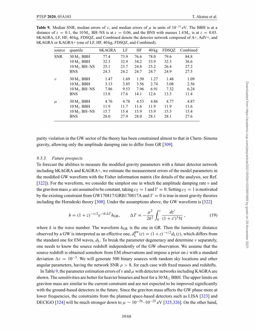
PTEP 2020, 05A103 T. Akutsu et al.
Table 9. Median SNR, median errors of ν, and median errors of μ in units of 10−23 eV. The BBH is at adistance of z = 0.1, the 10 M� BH–NS is at z = 0.06, and the BNS with masses 1.4 M� is at z = 0.03.bKAGRA, LF, HF, 40 kg, FDSQZ, and Combined denote the detector network composed of A+, AdV+, andbKAGRA or KAGRA+ (one of LF, HF, 40 kg, FDSQZ, and Combined).
source quantile bKAGRA LF HF 40 kg FDSQZ Combined
SNR 30 M� BBH 77.4 73.9 76.6 78.0 79.6 84.810 M� BBH 32.3 32.9 34.2 33.9 32.3 36.610 M� BH–NS 25.1 23.7 24.8 25.2 26.4 27.2BNS 24.3 24.2 24.7 24.7 24.9 27.5
ν 30 M� BBH 1.47 1.69 1.50 1.27 1.48 1.0910 M� BBH 3.13 3.85 3.56 2.74 3.08 2.5610 M� BH–NS 7.86 9.53 7.96 6.91 7.32 6.24BNS 13.8 17.6 14.1 12.6 13.3 11.4
μ 30 M� BBH 4.76 4.78 4.53 4.86 4.77 4.8710 M� BBH 11.9 11.7 11.6 11.9 11.9 11.610 M� BH–NS 15.7 15.4 15.9 15.9 15.5 15.4BNS 28.0 27.9 28.0 28.1 28.1 27.6
parity violation in the GW sector of the theory has been constrained almost to that in Chern–Simonsgravity, allowing only the amplitude damping rate to differ from GR [309].
9.3.3. Future prospectsTo forecast the abilities to measure the modified gravity parameters with a future detector networkincluding bKAGRA and KAGRA+, we estimate the measurement errors of the model parameters inthe modified GW waveform with the Fisher information matrix (for details of the analysis, see Ref.[322]). For the waveform, we consider the simplest one in which the amplitude damping rate ν andthe graviton mass μ are assumed to be constant, taking cT = 1 and � = 0. Setting cT = 1 is motivatedby the existing constraint from GW170817/GRB170817A and � = 0 is true in most gravity theoriesincluding the Horndeski theory [308]. Under the assumptions above, the GW waveform is [322]
h = (1 + z)−ν/2e−ik�T hGR, �T = − μ2
2k2
∫ z
0
dz′
(1 + z′)3H , (19)
where k is the wave number. The waveform hGR is the one in GR. Then the luminosity distanceobserved by a GW is interpreted as an effective one, dgw
L (z) = (1 + z)−ν/2dL(z), which differs fromthe standard one for EM waves, dL. To break the parameter degeneracy and determine ν separately,one needs to know the source redshift independently of the GW observation. We assume that thesource redshift is obtained somehow from EM observations and impose a prior on z with a standarddeviation �z = 10−3. We will generate 500 binary sources with random sky locations and otherangular parameters, having the network SNR ρ > 8, for each case with fixed masses and redshifts.
In Table 9, the parameter estimation errors of ν and μ with detector networks including KAGRA areshown. The sensitivities are better for heavier binaries and best for a 30 M� BBH. The upper limits ongraviton mass are similar to the current constraint and are not expected to be improved significantlywith the ground-based detectors in the future. Since the graviton mass affects the GW phase more atlower frequencies, the constraints from the planned space-based detectors such as LISA [323] andDECIGO [324] will be much stronger down to μ ∼ 10−26–10−25 eV [325,326]. On the other hand,
39/68
Dow
nloaded from https://academ
ic.oup.com/ptep/article/2021/5/05A103/5891669 by guest on 29 N
ovember 2021
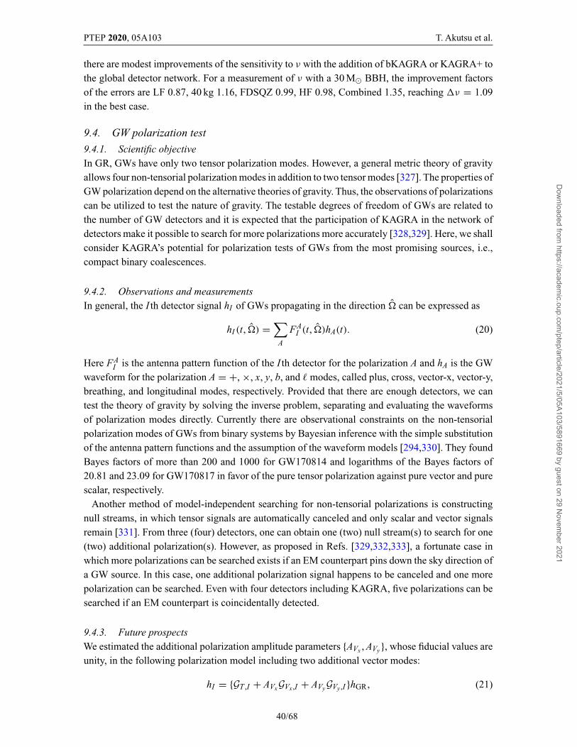
PTEP 2020, 05A103 T. Akutsu et al.
there are modest improvements of the sensitivity to ν with the addition of bKAGRA or KAGRA+ tothe global detector network. For a measurement of ν with a 30 M� BBH, the improvement factorsof the errors are LF 0.87, 40 kg 1.16, FDSQZ 0.99, HF 0.98, Combined 1.35, reaching �ν = 1.09in the best case.
9.4. GW polarization test
9.4.1. Scientific objectiveIn GR, GWs have only two tensor polarization modes. However, a general metric theory of gravityallows four non-tensorial polarization modes in addition to two tensor modes [327]. The properties ofGW polarization depend on the alternative theories of gravity. Thus, the observations of polarizationscan be utilized to test the nature of gravity. The testable degrees of freedom of GWs are related tothe number of GW detectors and it is expected that the participation of KAGRA in the network ofdetectors make it possible to search for more polarizations more accurately [328,329]. Here, we shallconsider KAGRA’s potential for polarization tests of GWs from the most promising sources, i.e.,compact binary coalescences.
9.4.2. Observations and measurementsIn general, the I th detector signal hI of GWs propagating in the direction � can be expressed as
hI (t, �) =∑
A
FAI (t, �)hA(t). (20)
Here FAI is the antenna pattern function of the I th detector for the polarization A and hA is the GW
waveform for the polarization A = +, ×, x, y, b, and � modes, called plus, cross, vector-x, vector-y,breathing, and longitudinal modes, respectively. Provided that there are enough detectors, we cantest the theory of gravity by solving the inverse problem, separating and evaluating the waveformsof polarization modes directly. Currently there are observational constraints on the non-tensorialpolarization modes of GWs from binary systems by Bayesian inference with the simple substitutionof the antenna pattern functions and the assumption of the waveform models [294,330]. They foundBayes factors of more than 200 and 1000 for GW170814 and logarithms of the Bayes factors of20.81 and 23.09 for GW170817 in favor of the pure tensor polarization against pure vector and purescalar, respectively.
Another method of model-independent searching for non-tensorial polarizations is constructingnull streams, in which tensor signals are automatically canceled and only scalar and vector signalsremain [331]. From three (four) detectors, one can obtain one (two) null stream(s) to search for one(two) additional polarization(s). However, as proposed in Refs. [329,332,333], a fortunate case inwhich more polarizations can be searched exists if an EM counterpart pins down the sky direction ofa GW source. In this case, one additional polarization signal happens to be canceled and one morepolarization can be searched. Even with four detectors including KAGRA, five polarizations can besearched if an EM counterpart is coincidentally detected.
9.4.3. Future prospectsWe estimated the additional polarization amplitude parameters {AVx , AVy}, whose fiducial values areunity, in the following polarization model including two additional vector modes:
hI = {GT ,I + AVxGVx ,I + AVyGVy ,I }hGR, (21)
40/68
Dow
nloaded from https://academ
ic.oup.com/ptep/article/2021/5/05A103/5891669 by guest on 29 N
ovember 2021
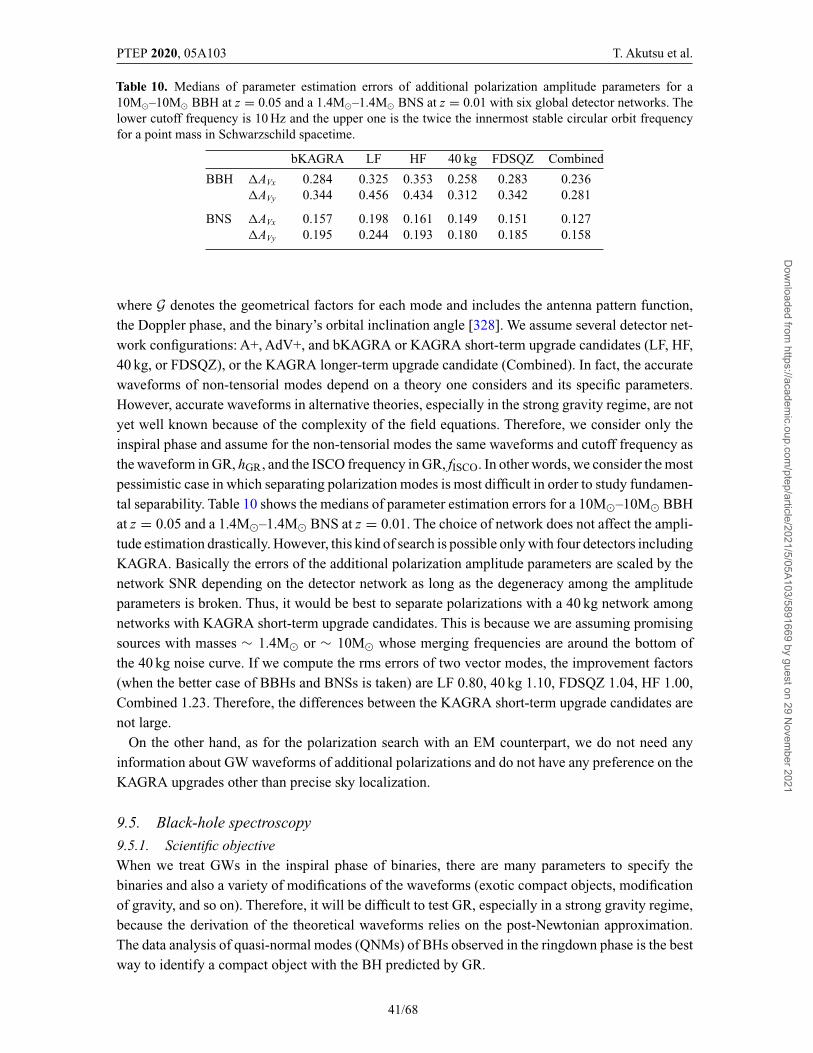
PTEP 2020, 05A103 T. Akutsu et al.
Table 10. Medians of parameter estimation errors of additional polarization amplitude parameters for a10M�–10M� BBH at z = 0.05 and a 1.4M�–1.4M� BNS at z = 0.01 with six global detector networks. Thelower cutoff frequency is 10 Hz and the upper one is the twice the innermost stable circular orbit frequencyfor a point mass in Schwarzschild spacetime.
bKAGRA LF HF 40 kg FDSQZ Combined
BBH �AVx 0.284 0.325 0.353 0.258 0.283 0.236�AVy 0.344 0.456 0.434 0.312 0.342 0.281
BNS �AVx 0.157 0.198 0.161 0.149 0.151 0.127�AVy 0.195 0.244 0.193 0.180 0.185 0.158
where G denotes the geometrical factors for each mode and includes the antenna pattern function,the Doppler phase, and the binary’s orbital inclination angle [328]. We assume several detector net-work configurations: A+, AdV+, and bKAGRA or KAGRA short-term upgrade candidates (LF, HF,40 kg, or FDSQZ), or the KAGRA longer-term upgrade candidate (Combined). In fact, the accuratewaveforms of non-tensorial modes depend on a theory one considers and its specific parameters.However, accurate waveforms in alternative theories, especially in the strong gravity regime, are notyet well known because of the complexity of the field equations. Therefore, we consider only theinspiral phase and assume for the non-tensorial modes the same waveforms and cutoff frequency asthe waveform in GR, hGR, and the ISCO frequency in GR, fISCO. In other words, we consider the mostpessimistic case in which separating polarization modes is most difficult in order to study fundamen-tal separability. Table 10 shows the medians of parameter estimation errors for a 10M�–10M� BBHat z = 0.05 and a 1.4M�–1.4M� BNS at z = 0.01. The choice of network does not affect the ampli-tude estimation drastically. However, this kind of search is possible only with four detectors includingKAGRA. Basically the errors of the additional polarization amplitude parameters are scaled by thenetwork SNR depending on the detector network as long as the degeneracy among the amplitudeparameters is broken. Thus, it would be best to separate polarizations with a 40 kg network amongnetworks with KAGRA short-term upgrade candidates. This is because we are assuming promisingsources with masses ∼ 1.4M� or ∼ 10M� whose merging frequencies are around the bottom ofthe 40 kg noise curve. If we compute the rms errors of two vector modes, the improvement factors(when the better case of BBHs and BNSs is taken) are LF 0.80, 40 kg 1.10, FDSQZ 1.04, HF 1.00,Combined 1.23. Therefore, the differences between the KAGRA short-term upgrade candidates arenot large.
On the other hand, as for the polarization search with an EM counterpart, we do not need anyinformation about GW waveforms of additional polarizations and do not have any preference on theKAGRA upgrades other than precise sky localization.
9.5. Black-hole spectroscopy
9.5.1. Scientific objectiveWhen we treat GWs in the inspiral phase of binaries, there are many parameters to specify thebinaries and also a variety of modifications of the waveforms (exotic compact objects, modificationof gravity, and so on). Therefore, it will be difficult to test GR, especially in a strong gravity regime,because the derivation of the theoretical waveforms relies on the post-Newtonian approximation.The data analysis of quasi-normal modes (QNMs) of BHs observed in the ringdown phase is the bestway to identify a compact object with the BH predicted by GR.
41/68
Dow
nloaded from https://academ
ic.oup.com/ptep/article/2021/5/05A103/5891669 by guest on 29 N
ovember 2021
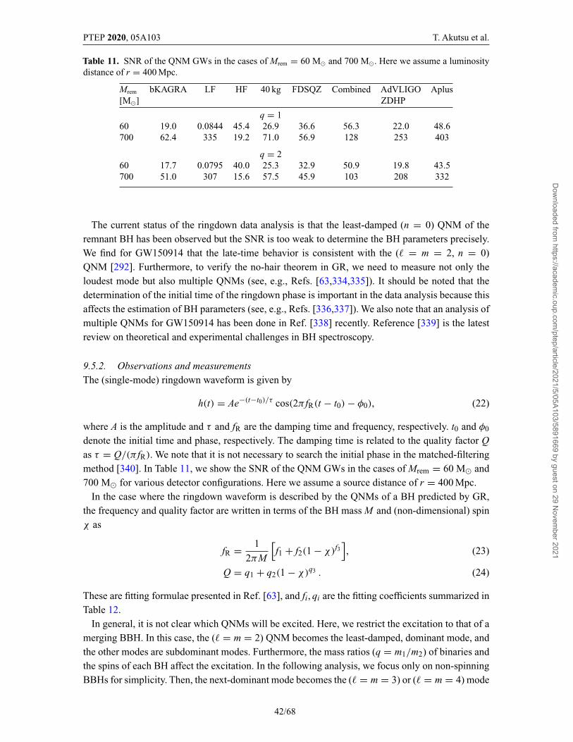
PTEP 2020, 05A103 T. Akutsu et al.
Table 11. SNR of the QNM GWs in the cases of Mrem = 60 M� and 700 M�. Here we assume a luminositydistance of r = 400 Mpc.
Mrem bKAGRA LF HF 40 kg FDSQZ Combined AdVLIGO Aplus[M�] ZDHP
q = 160 19.0 0.0844 45.4 26.9 36.6 56.3 22.0 48.6700 62.4 335 19.2 71.0 56.9 128 253 403
q = 260 17.7 0.0795 40.0 25.3 32.9 50.9 19.8 43.5700 51.0 307 15.6 57.5 45.9 103 208 332
The current status of the ringdown data analysis is that the least-damped (n = 0) QNM of theremnant BH has been observed but the SNR is too weak to determine the BH parameters precisely.We find for GW150914 that the late-time behavior is consistent with the (� = m = 2, n = 0)QNM [292]. Furthermore, to verify the no-hair theorem in GR, we need to measure not only theloudest mode but also multiple QNMs (see, e.g., Refs. [63,334,335]). It should be noted that thedetermination of the initial time of the ringdown phase is important in the data analysis because thisaffects the estimation of BH parameters (see, e.g., Refs. [336,337]). We also note that an analysis ofmultiple QNMs for GW150914 has been done in Ref. [338] recently. Reference [339] is the latestreview on theoretical and experimental challenges in BH spectroscopy.
9.5.2. Observations and measurementsThe (single-mode) ringdown waveform is given by
h(t) = Ae−(t−t0)/τ cos(2π fR(t − t0) − φ0), (22)
where A is the amplitude and τ and fR are the damping time and frequency, respectively. t0 and φ0
denote the initial time and phase, respectively. The damping time is related to the quality factor Qas τ = Q/(π fR). We note that it is not necessary to search the initial phase in the matched-filteringmethod [340]. In Table 11, we show the SNR of the QNM GWs in the cases of Mrem = 60 M� and700 M� for various detector configurations. Here we assume a source distance of r = 400 Mpc.
In the case where the ringdown waveform is described by the QNMs of a BH predicted by GR,the frequency and quality factor are written in terms of the BH mass M and (non-dimensional) spinχ as
fR = 1
2πM
[f1 + f2(1 − χ)f3
], (23)
Q = q1 + q2(1 − χ)q3 . (24)
These are fitting formulae presented in Ref. [63], and fi, qi are the fitting coefficients summarized inTable 12.
In general, it is not clear which QNMs will be excited. Here, we restrict the excitation to that of amerging BBH. In this case, the (� = m = 2) QNM becomes the least-damped, dominant mode, andthe other modes are subdominant modes. Furthermore, the mass ratios (q = m1/m2) of binaries andthe spins of each BH affect the excitation. In the following analysis, we focus only on non-spinningBBHs for simplicity. Then, the next-dominant mode becomes the (� = m = 3) or (� = m = 4) mode
42/68
Dow
nloaded from https://academ
ic.oup.com/ptep/article/2021/5/05A103/5891669 by guest on 29 N
ovember 2021
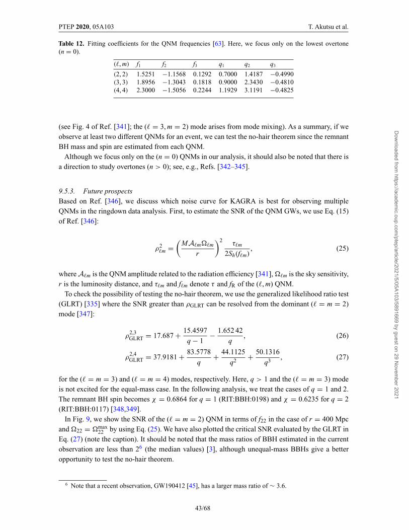
PTEP 2020, 05A103 T. Akutsu et al.
Table 12. Fitting coefficients for the QNM frequencies [63]. Here, we focus only on the lowest overtone(n = 0).
(�, m) f1 f2 f3 q1 q2 q3
(2, 2) 1.5251 −1.1568 0.1292 0.7000 1.4187 −0.4990(3, 3) 1.8956 −1.3043 0.1818 0.9000 2.3430 −0.4810(4, 4) 2.3000 −1.5056 0.2244 1.1929 3.1191 −0.4825
(see Fig. 4 of Ref. [341]; the (� = 3, m = 2) mode arises from mode mixing). As a summary, if weobserve at least two different QNMs for an event, we can test the no-hair theorem since the remnantBH mass and spin are estimated from each QNM.
Although we focus only on the (n = 0) QNMs in our analysis, it should also be noted that there isa direction to study overtones (n > 0); see, e.g., Refs. [342–345].
9.5.3. Future prospectsBased on Ref. [346], we discuss which noise curve for KAGRA is best for observing multipleQNMs in the ringdown data analysis. First, to estimate the SNR of the QNM GWs, we use Eq. (15)of Ref. [346]:
ρ2�m =
(MA�m��m
r
)2τ�m
2Sh(f�m), (25)
where A�m is the QNM amplitude related to the radiation efficiency [341], ��m is the sky sensitivity,r is the luminosity distance, and τ�m and f�m denote τ and fR of the (�, m) QNM.
To check the possibility of testing the no-hair theorem, we use the generalized likelihood ratio test(GLRT) [335] where the SNR greater than ρGLRT can be resolved from the dominant (� = m = 2)mode [347]:
ρ2,3GLRT = 17.687 + 15.4597
q − 1− 1.652 42
q, (26)
ρ2,4GLRT = 37.9181 + 83.5778
q+ 44.1125
q2 + 50.1316
q3 , (27)
for the (� = m = 3) and (� = m = 4) modes, respectively. Here, q > 1 and the (� = m = 3) modeis not excited for the equal-mass case. In the following analysis, we treat the cases of q = 1 and 2.The remnant BH spin becomes χ = 0.6864 for q = 1 (RIT:BBH:0198) and χ = 0.6235 for q = 2(RIT:BBH:0117) [348,349].
In Fig. 9, we show the SNR of the (� = m = 2) QNM in terms of f22 in the case of r = 400 Mpcand �22 = �max
22 by using Eq. (25). We have also plotted the critical SNR evaluated by the GLRT inEq. (27) (note the caption). It should be noted that the mass ratios of BBH estimated in the currentobservation are less than 26 (the median values) [3], although unequal-mass BBHs give a betteropportunity to test the no-hair theorem.
6 Note that a recent observation, GW190412 [45], has a larger mass ratio of ∼ 3.6.
43/68
Dow
nloaded from https://academ
ic.oup.com/ptep/article/2021/5/05A103/5891669 by guest on 29 N
ovember 2021
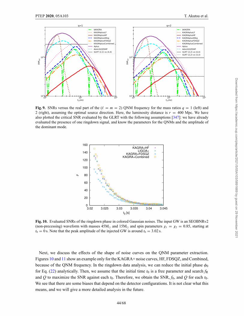
PTEP 2020, 05A103 T. Akutsu et al.
Fig. 9. SNRs versus the real part of the (� = m = 2) QNM frequency for the mass ratios q = 1 (left) and2 (right), assuming the optimal source direction. Here, the luminosity distance is r = 400 Mpc. We havealso plotted the critical SNR evaluated by the GLRT with the following assumptions [347]: we have alreadyevaluated the presence of one ringdown signal, and know the parameters for the QNMs and the amplitude ofthe dominant mode.
Fig. 10. Evaluated SNRs of the ringdown phase in colored Gaussian noises. The input GW is an SEOBNRv2(non-precessing) waveform with masses 45M� and 15M� and spin parameters χ1 = χ2 = 0.85, starting att0 = 0 s. Note that the peak amplitude of the injected GW is around t0 = 3.02 s.
Next, we discuss the effects of the shape of noise curves on the QNM parameter extraction.Figures 10 and 11 show an example only for the KAGRA+ noise curves, HF, FDSQZ, and Combined,because of the QNM frequency. In the ringdown data analysis, we can reduce the initial phase φ0
for Eq. (22) analytically. Then, we assume that the initial time t0 is a free parameter and search fRand Q to maximize the SNR against each t0. Therefore, we obtain the SNR, f0, and Q for each t0.We see that there are some biases that depend on the detector configurations. It is not clear what thismeans, and we will give a more detailed analysis in the future.
44/68
Dow
nloaded from https://academ
ic.oup.com/ptep/article/2021/5/05A103/5891669 by guest on 29 N
ovember 2021
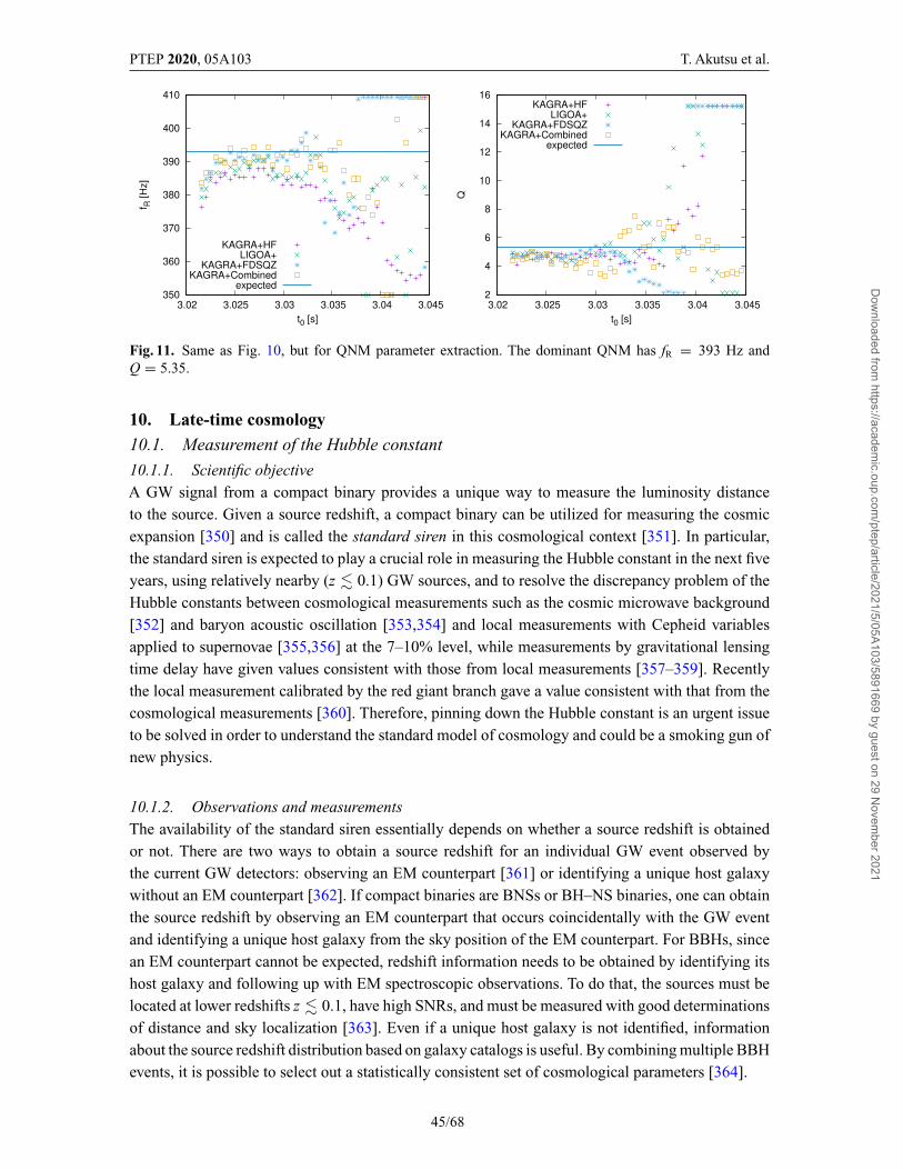
PTEP 2020, 05A103 T. Akutsu et al.
Fig. 11. Same as Fig. 10, but for QNM parameter extraction. The dominant QNM has fR = 393 Hz andQ = 5.35.
10. Late-time cosmology10.1. Measurement of the Hubble constant
10.1.1. Scientific objectiveA GW signal from a compact binary provides a unique way to measure the luminosity distanceto the source. Given a source redshift, a compact binary can be utilized for measuring the cosmicexpansion [350] and is called the standard siren in this cosmological context [351]. In particular,the standard siren is expected to play a crucial role in measuring the Hubble constant in the next fiveyears, using relatively nearby (z � 0.1) GW sources, and to resolve the discrepancy problem of theHubble constants between cosmological measurements such as the cosmic microwave background[352] and baryon acoustic oscillation [353,354] and local measurements with Cepheid variablesapplied to supernovae [355,356] at the 7–10% level, while measurements by gravitational lensingtime delay have given values consistent with those from local measurements [357–359]. Recentlythe local measurement calibrated by the red giant branch gave a value consistent with that from thecosmological measurements [360]. Therefore, pinning down the Hubble constant is an urgent issueto be solved in order to understand the standard model of cosmology and could be a smoking gun ofnew physics.
10.1.2. Observations and measurementsThe availability of the standard siren essentially depends on whether a source redshift is obtainedor not. There are two ways to obtain a source redshift for an individual GW event observed bythe current GW detectors: observing an EM counterpart [361] or identifying a unique host galaxywithout an EM counterpart [362]. If compact binaries are BNSs or BH–NS binaries, one can obtainthe source redshift by observing an EM counterpart that occurs coincidentally with the GW eventand identifying a unique host galaxy from the sky position of the EM counterpart. For BBHs, sincean EM counterpart cannot be expected, redshift information needs to be obtained by identifying itshost galaxy and following up with EM spectroscopic observations. To do that, the sources must belocated at lower redshifts z � 0.1, have high SNRs, and must be measured with good determinationsof distance and sky localization [363]. Even if a unique host galaxy is not identified, informationabout the source redshift distribution based on galaxy catalogs is useful. By combining multiple BBHevents, it is possible to select out a statistically consistent set of cosmological parameters [364].
45/68
Dow
nloaded from https://academ
ic.oup.com/ptep/article/2021/5/05A103/5891669 by guest on 29 N
ovember 2021
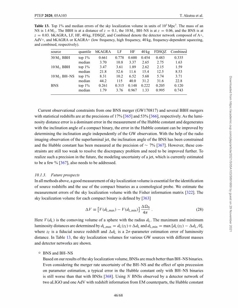
PTEP 2020, 05A103 T. Akutsu et al.
Table 13. Top 1% and median errors of the sky localization volume in units of 103 Mpc3. The mass of anNS is 1.4 M�. The BBH is at a distance of z = 0.1, the 10 M� BH–NS is at z = 0.06, and the BNS is atz = 0.03. bKAGRA, LF, HF, 40 kg, FDSQZ, and Combined denote the detector network composed of A+,AdV+, and bKAGRA or KAGRA+ (low frequency, high frequency, 40 kg, frequency-dependent squeezing,and combined, respectively).
source quantile bKAGRA LF HF 40 kg FDSQZ Combined
30 M� BBH top 1% 0.661 0.778 0.600 0.454 0.483 0.335median 3.70 10.8 3.37 2.65 2.75 1.63
10 M� BBH top 1% 3.47 3.61 1.89 2.62 2.15 1.59median 21.8 52.6 11.6 15.4 12.5 8.53
10 M� BH–NS top 1% 8.31 10.2 6.52 5.68 5.74 3.71median 44.2 115 40.0 31.2 31.6 22.8
BNS top 1% 0.261 0.315 0.148 0.222 0.205 0.120median 1.79 3.76 0.967 1.33 0.995 0.743
Current observational constraints from one BNS merger (GW170817) and several BBH mergerswith statistical redshifts are at the precisions of 17% [365] and 53% [366], respectively. As the lumi-nosity distance error is a dominant error in the measurement of the Hubble constant and degenerateswith the inclination angle of a compact binary, the error in the Hubble constant can be improved bydetermining the inclination angle independently of the GW observation. With the help of the radioimaging observation of the superluminal jet, the inclination angle of the BNS has been constrainedand the Hubble constant has been measured at the precision of ∼ 7% [367]. However, these con-straints are still too weak to resolve the discrepancy problem and need to be improved further. Torealize such a precision in the future, the modeling uncertainty of a jet, which is currently estimatedto be a few % [367], also needs to be addressed.
10.1.3. Future prospectsIn all methods above, a good measurement of sky localization volume is essential for the identificationof source redshifts and the use of the compact binaries as a cosmological probe. We estimate themeasurement errors of the sky localization volume with the Fisher information matrix [322]. Thesky localization volume for each compact binary is defined by [363]
�V ≡ [V (dL,max) − V (dL,min)
] ��S
4π. (28)
Here V (dL) is the comoving volume of a sphere with the radius dL. The maximum and minimumluminosity distances are determined by dL,max = dL(zf )+�dL and dL,min = max [dL(zf ) − �dL, 0],where zf is a fiducial source redshift and �dL is a 2σ -parameter estimation error of luminositydistance. In Table 13, the sky localization volumes for various GW sources with different massesand detector networks are shown.
◦ BNS and BH–NSBased on our results of the sky localization volume, BNSs are much better than BH–NS binaries.Even considering the merger rate uncertainty of the BH–NS and the effect of spin precessionon parameter estimation, a typical error in the Hubble constant only with BH–NS binariesis still worse than that with BNSs [368]. Using N BNSs observed by a detector network oftwo aLIGO and one AdV with redshift information from EM counterparts, the Hubble constant
46/68
Dow
nloaded from https://academ
ic.oup.com/ptep/article/2021/5/05A103/5891669 by guest on 29 N
ovember 2021
PTEP 2020, 05A103 T. Akutsu et al.
error is estimated to be �H0/H0 ∼ 2√
50/N% [369,370]. With the network of KAGRA+ short-term upgrades, the network SNR is larger by about 1.5 times and the Hubble constant error is�H0/H0 ∼ 1.5
√50/N%. However, the number of sources accompanied by EM counterparts is
still significantly uncertain and 50 sources roughly correspond to ∼ 10% redshift identification,which is an intermediate value of theoretical predictions [371–373]. Based on the comparisonof the sky localization volume in Table 13, the improvement factors for BNSs (median) areLF 0.476, 40 kg 1.35, FDSQZ 1.80, HF 1.85, and Combined 2.41. The upgrades at higherfrequencies lead to a smaller localization volume and better sensitivity to the Hubble constant.
◦ BBHAs seen from our results of the sky localization volume, 30 M� BBHs are better than 10 M�BBHs and it is easier to identify a unique host galaxy (the number density of galaxies thatcovers roughly 90% of the total luminosity in the B band [374] is ngal = 0.01 Mpc−3) and thenobtain redshift information. Assuming the number density of galaxies, the top 1% events of30 M� BBHs at distances closer than z � 0.03 can marginally identify a unique host galaxy.Extrapolating the result obtained for the bKAGRA detector network [363] to the KAGRA+short-term upgrade networks, the Hubble constant error is �H0/H0 ∼ 0.8
√10/N%. Based on
the comparison of the sky localization volume in Table 13, the improvement factors for 30 M�BBHs (top 1%) are LF 0.85, 40 kg 1.46, FDSQZ 1.37, HF 1.10, Combined 1.97. For BBHs,the upgrades at middle frequencies lead to a smaller localization volume and better sensitivityto the Hubble constant.
In conclusion, we cannot tell which source gives better determination of the Hubble constantbecause of uncertainties in the merger rates of BNSs and BBHs, the success fraction of redshiftidentification, and the mass function of BBHs. In addition, there would be potential contribu-tions from systematic errors, e.g., the modeling of the EM counterparts and the calibration errorsof GW detectors. Although all of these uncertainties must be reduced or improved, the standardsiren has the potential to achieve a 1% precision measurement of the Hubble constant in thefuture and resolve the discrepancy problem, to which KAGRA can contribute mainly by better skylocalization.
10.2. GW lensing
10.2.1. Scientific objectiveGravitational lensing is a well established subject in the EM observation of the Universe [375,376].For GWs, there are controversial claims that lensing was also already observed from LIGO–VirgoO1/O2 detections [377,378], while the LIGO–Virgo Collaboration claimed that the observed eventsare fully consistent with unlensed GWs [3]. From an astrophysical viewpoint on the lensing rate, it isunlikely that the observed events are multiple-imaged by stellar-mass objects [379], interveninggalaxy population [380], or massive galaxy clusters [381]. However, for the second-generationground-based GW detectors, it is possible to observe several lensing events at design sensitivity [380–382], and it is almost certain that the third-generation detectors can detect lensed events [379,382]. The scientific rewards from lensing of GWs are huge [383–385], ranging from probing smallstructures such as compact dark matter or primordial BHs with mass M ≈ 10–105 M� [386], todiscovering intermediate-mass BHs [387], to testing gravity theories and cosmography [350,383],to name but a few.
47/68
Dow
nloaded from https://academ
ic.oup.com/ptep/article/2021/5/05A103/5891669 by guest on 29 N
ovember 2021
PTEP 2020, 05A103 T. Akutsu et al.
10.2.2. Observations and measurementsThe detection of possible lensing events has multiple implications for measurement. First, the lensedevent is magnified in its SNR by
√μ where μ is the magnification [384]; thus, if the possibility for
lensing is not considered, one will underestimate its luminosity distance by√
μ, and overestimatethe masses in the source frame with a relevant redshift rescaling thereof [381,384,385,388]. Second,because of the magnification effect, for events at large z whose unlensed SNR is below the detectionthreshold, lensing might increase it to be detectable [384]. Therefore, lensing affects the inference onthe event rate and underlying mass distributions (and stellar evolution) of coalescing binaries. Third,if the size of the lens is comparable to or smaller than the GW wavelength, diffraction introducesfrequency-dependent time delays and modulation of the waveform [379,385,388], thus reducing thematched-filter capability if unlensed waveforms are used as templates. Fourth, for GW events withobservable EM counterparts, it is important to associate them with each other in a convincing mannerthat enables tests of the speed of gravity and inference of cosmological parameters [350,383,389,390].A precise localization with multiple detectors helps with such statistical association.
10.2.3. Future prospectsFor KAGRA, it will help in localizing GW events significantly together with LIGO and Virgo obser-vations, thus increasing the possibility of detecting lensed events. No specific hardware requirementis additionally requested to achieve the gravitational lensing science goal. However, advanced dataanalysis including the possibility of lensing events is required. For the operation, coincident obser-vation with LIGO and Virgo detectors would be advantageous. The contribution of KAGRA datato the cooperative parameter estimation with lensing effects encoded in the waveform template willbenefit the overall science output. Therefore, the same suggestion as for the measurement of theHubble constant with BBHs in Sect. 10.1 is applied here.
11. Multi-messenger observations11.1. Kilonovae/macronovae
11.1.1. Scientific objectiveA kilonova (also known as a macronova) is the emission that is expected to be associated with an NS–NS or BH–NS merger as a consequence of mass ejection from the system; see, e.g., Refs. [391,392].Since the ejected material is composed of neutron-rich matter, heavy radioactive nuclei would besynthesized in the ejecta by the so-called r-process nucleosynthesis [393–396], and EM emissioncould occur by radioactive decays of heavy elements [397–401]. Kilonova emission is expected tobe bright in the optical and near-infrared wavelengths and lasts for 1–10 days after the merger. Wenote that the event rate is currently highly uncertain; it could be ∼ 103 Gpc−3 yr−1 if kilonovae areassociated with all NS–NS mergers.
The light curves of kilonovae reflect the merger process and the late-time evolution of the mergerremnant [397,400,402–406]. The presence of kilonova emission suggests that a substantial amount ofmaterial is ejected from the system, and this gives constraints on the binary parameters by combiningwith a theoretical prediction obtained by numerical simulations. Furthermore, detailed properties ofkilonova light curves, such as their brightness and color evolution, provide information on the massand composition of the ejected material; see, e.g., Refs. [407–413]. Such information is useful tounderstand the merger process of binaries and the late-time evolution of merger remnants as well asthe chemical evolution of the Universe.
48/68
Dow
nloaded from https://academ
ic.oup.com/ptep/article/2021/5/05A103/5891669 by guest on 29 N
ovember 2021
PTEP 2020, 05A103 T. Akutsu et al.
11.1.2. Observations and measurementsAn improvement in the source localization is important to identify the host galaxy of a GW event.Source localization from GW data analysis alone will not be tight enough to uniquely identify the hostgalaxy even after KAGRA has joined the observation [361] (see Tables 4 and 5). Thus, detection of theEM counterparts will play an important role in identifying the host galaxy. In particular, searchingfor kilonovae could have an advantage for this purpose because their emission is expected to beapproximately isotropic (cf. short GRBs). However, detection of kilonovae will be more challengingat large distances because a kilonova will be dimmer as the distance to the event increases and thenumber of galaxies in the localized area significantly increases. For example, assuming the sameintrinsic brightness as in GW170817, the peak r-band brightness of the kilonova would be fainterthan ≈ 21 mag at dL ≥200 Mpc, which is dimmer than the typical 5σ limiting magnitude of 1-mclass telescopes with 60 s exposure [414]. Thus, improvement of the source localization via GWdetection is still a key point to restrict the number of host candidates and to achieve simultaneousdetection of the kilonova of an event.
Low-latency GW alerts are also a key point for the follow-up of EM counterparts. They help usto find kilonovae because the light curves, in particular at wavelengths shorter than optical bands,are brightest within a few days. Moreover, the light curves of the EM counterparts at < 1 day are ofparticular interest. For example, in addition to the kilonova emission, the so-called cocoon emission,which is powered by internal energy deposited by relativistic jets, can contribute to the early partof the light curve in the optical and UV wavelengths [415]. It is pointed out that the observeddata of light curves in < 1 day can be used to distinguish between these different components ofemission [416,417].
Tighter constraints on the inclination angle have a great impact on maximizing the scientific returnfrom observations of kilonovae. Light curves of kilonovae are expected to depend on the observationangle [402,404,411,413]. Much more information on the properties of the ejecta can be extracted ifa tighter constraint on the inclination angle is given. Indeed, for the recent BH–NS-like merger eventGW190814 [72], the constraint on the ejecta mass is obtained by the upper limits to the EM signals,while the tightness of the constraint is shown to be strongly dependent on the viewing angle [418,419](by a factor of ≈ 3).
11.1.3. Future prospectsImprovements in the source localization both in speed and accuracy are crucial and would berequired as the first priority for kilonova follow-up observations. The detector sensitivity shouldbe broadband because a low-frequency band is important for quick localization (early warning) anda high-frequency band is important for accurate localization. According to Tables 4 and 5, the medianlocalized area is improved by up to a factor of ≈ 2 by including KAGRA+ in the detector network (byupgrading bKAGRA to one of the KAGRA+ configurations). This enables us to search the localizedfields with deeper limiting magnitudes or with lower latency. For example, deepening the EM searchby ≈ 1 magnitude is in principle possible if the improvement in the localization area enabled usto have a 10 times longer exposure time. Follow-ups by a 2-m or larger class telescopes, such asPan-STARRS [420] and CTIO-Dark Energy Camera [421], are crucial for the detection of such asituation [414]. We also note that an increase in the number of detectors with stable operations willenhance the chance of multiple detectors being operated at the same time, which is crucial for thesource localization.
49/68
Dow
nloaded from https://academ
ic.oup.com/ptep/article/2021/5/05A103/5891669 by guest on 29 N
ovember 2021
PTEP 2020, 05A103 T. Akutsu et al.
Tables 4 and 5 show that the determination of the inclination angle is improved by up to ≈ 23%by including KAGRA+ in the detector network (by upgrading bKAGRA to one of the KAGRA+configurations. As mentioned above, such improvement will help us to provide tighter constraints onthe ejecta properties and provide us with a good opportunity to study the spatial distribution of ejecta.For example, numerical-relativity simulations of an NS–binary merger (e.g., Refs. [411,422–424])predict that the typical polar opening angle of the lanthanide-rich dynamical ejecta component (�30◦) is comparable to or larger than the determination error of the inclination angle for � cos ι ≈ 0.15(see Tables 4 and 5). Since the presence of lanthanide-rich material in the line of sight strongly affectsthe light curves [402], observations of kilonovae with improved measurement of the inclination anglewould enable us to examine the presence of such ejecta components.
11.2. Short gamma-ray bursts
11.2.1. Scientific objective
The origin of sGRBs has been a long-standing problem for more than 40 years [425,426]. A BNSmerger was thought to be the most promising candidate [394,427,428], although unequivocal evi-dence was missing. Although it is widely accepted that a GRB is produced by a relativistic jet witha Lorentz factor larger than ∼ 100, there remain unresolved issues. (1) The central engine is mostlikely a spinning BH surrounded by an accretion disk, while a millisecond magnetar remains a can-didate. (2) The jet formation mechanism is one of the central subjects in astrophysics. It could bethe Blandford–Znajek mechanism or the neutrino annihilation mechanism. For the former case, itis not known how to realize the large-scale, poloidal configuration of the magnetic field. (3) The jetcomposition is unknown. It is likely dominated by baryon kinetic energy or magnetic energy. (4)The emission mechanism is a puzzle. The emission radius still has uncertainty of approximately fourorders of magnitude. A popular mechanism is synchrotron emission, while there is no consensus onhow to realize the observed spectral relations such as the Amati and Yonetoku relations [429,430].(5) The jet structure is unknown in both the radial and polar directions. The long-lasting emissionfollowing the main prompt emission such as extended emission (∼ 102 s) and plateau emission(∼ 104 s) suggests long-lived central engine activity [431].
The detection of the GW event GW170817 [4] and the associated EM counterparts [361] revolu-tionized the situation. In particular, sGRB 170817A detected two seconds (∼ 1.7 s) after GW170817[137,143,432] and the following afterglows in radio to X-ray [433–438] give the first direct cluesto the origin of sGRBs. However, the situation is not so simple because sGRB 170817A was veryweak with an isotropic-equivalent energy Eγ ,iso ∼ 5.35 × 1046 erg, which is many orders of mag-nitude smaller than ordinary values. On the other hand, the afterglow observations, in particular ofsuperluminal motion in radio [139,439] and the consistency between the spectral index and the lightcurve slope after the luminosity peak [440–442], strongly suggest that a relativistic jet is launchedand successfully breaks out of the merger ejecta in this event [443]. The jet power should be similarto those in other normal sGRBs, otherwise the jet cannot penetrate the merger ejecta [444]. Themost likely scenario is that the jet is off-axis to our line of sight and therefore faint in this event[143,445,446], although the emission mechanism is controversial [407,447–449]. The afterglowobservation, in particular the slowly rising light curve, is not consistent with a top-hat jet [138], butfor the first time strongly suggests a structured jet [438–440,442,450–454]. The angular structure isalso important for solving the spectral puzzles of GRB 170817A [447,455–457].
50/68
Dow
nloaded from https://academ
ic.oup.com/ptep/article/2021/5/05A103/5891669 by guest on 29 N
ovember 2021
PTEP 2020, 05A103 T. Akutsu et al.
11.2.2. Observations and measurementsThe GW signal is basically the same as that of NS mergers with the dimensionless amplitudehc ∝ f −1/6 and fmax ∼ a few kHz (see Sect. 4.1). The mass and mass ratio are important for revealingthe jet formation mechanism since they determine the BH and disk masses after the merger.
Sky localization is essential for following up EM counterparts [7]. In GW170817, the error regionshrinks from 190 deg2 to 31 deg2 by adding Virgo data even though the SNR was 2.0. The surveywith Subaru/Hyper Suprime-Cam (one of the most powerful telescope in the world) covered 23.6deg2 and reached a 50% completeness magnitude of 20.6 mag [458]. At the design sensitivities ofaLIGO, AdV, and KAGRA, the typical source distance is further (or events closer than 40 Mpc arerare given the estimated event rate 1 × 10²–4 × 10³ Gpc−3 yr−1 [3]). Thus the localization errorshould ideally be less than ∼ 30 deg2; this is achievable with detector networks including KAGRA,as shown in Tables 4 and 5. Low latency should also be mandatory. In GW170817, the alert with thelocalization error ∼ 31 deg2 was sent ∼ 5 hours after the merger, although the actual observationsstarted ∼ 10 hours after the merger because of the interruption of the sea. In a couple of years, atleast minutes or even lower latency will be realized. Ground-based detectors should try localizationbefore the merger [459] to allow other messengers (in particular those with small fields of view) toobserve the source at the merger time as well as possible precursor emissions.
The inclination (or viewing angle) of the merging binary is also a crucial parameter for sGRBstudies. It affects all the prompt, afterglow, and kilonova emissions.
Post-merger signals are also worth searching to reveal the central engines of sGRBs [154]. Theyinclude GW emission from a hypermassive NS (or supramassive NS) and BH (see Sect. 4.3). Thereare many possibilities for GW emission mechanisms, such as BH ringdown, NS quadrupolar f -mode,magnetic-field-induced ellipticities, unstable bar modes, unstable r-modes, and so on. The possiblerange of GW duration is broad, from ∼ 10−3–∼ 104 s or even longer, as implied by the long-lastingactivity of sGRBs.
A magnetar giant flare is also observed as an sGRB. Some GWs are expected from giant flares (seeSect. 6.2) [185]. Currently there is no evidence of GWs associated with giant flares [460], althoughthe f mode may not be the correct target [461]. Possible candidates for giant flares include GRB070201 [462], GRB 051103 [463], and GRB 150906B [464].
11.2.3. Future prospectsIn summary, the frequency band is required to be broadband, where the low-frequency band isimportant for quick localization (early warning) and the high-frequency band is important for themerger time and the post-merger signals. In addition, inclination measurements are crucial. These arethe same as those for a kilonova. See Sect. 11.1.As the typical distance to GW sources increases, onlysGRBs remain as detectable EM counterparts. Collaboration with X- and gamma-ray observatoriessuch as SVOM, Einstein Probe, HiZ-GUNDAM, and CTA will become more important.
11.3. Long gamma-ray bursts
11.3.1. Scientific objectiveLong GRBs, whose duration is longer than about 2 s, originate in the collapse of a massive star[465,466]. Prompt gamma-ray emissions and subsequent afterglows are emitted at the head of arelativistically moving, narrowly collimated jet toward us. The Lorentz factor of the jet is typicallylarger than ∼ 102. Currently the jet launch mechanism as well as the radiation process is not yetfully understood. The central engine of the relativistic jet is also unclear, but is most likely to be
51/68
Dow
nloaded from https://academ
ic.oup.com/ptep/article/2021/5/05A103/5891669 by guest on 29 N
ovember 2021
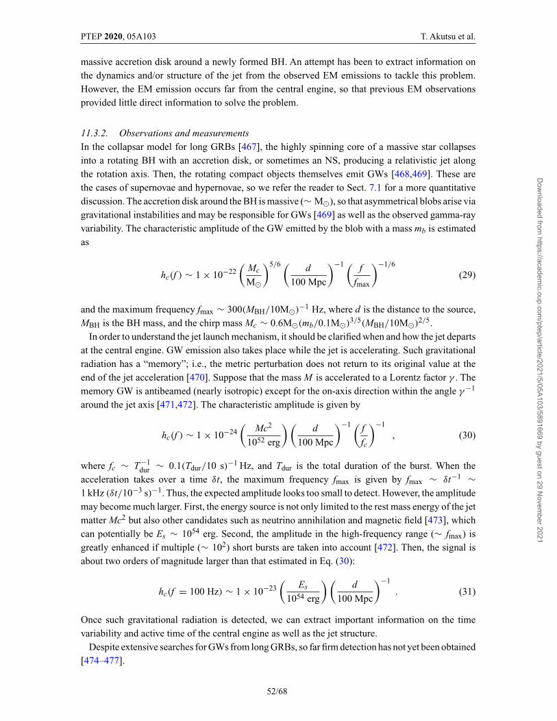
PTEP 2020, 05A103 T. Akutsu et al.
massive accretion disk around a newly formed BH. An attempt has been to extract information onthe dynamics and/or structure of the jet from the observed EM emissions to tackle this problem.However, the EM emission occurs far from the central engine, so that previous EM observationsprovided little direct information to solve the problem.
11.3.2. Observations and measurementsIn the collapsar model for long GRBs [467], the highly spinning core of a massive star collapsesinto a rotating BH with an accretion disk, or sometimes an NS, producing a relativistic jet alongthe rotation axis. Then, the rotating compact objects themselves emit GWs [468,469]. These arethe cases of supernovae and hypernovae, so we refer the reader to Sect. 7.1 for a more quantitativediscussion. The accretion disk around the BH is massive (∼ M�), so that asymmetrical blobs arise viagravitational instabilities and may be responsible for GWs [469] as well as the observed gamma-rayvariability. The characteristic amplitude of the GW emitted by the blob with a mass mb is estimatedas
hc(f ) ∼ 1 × 10⁻²²(
Mc
M�
)5/6 ( d
100 Mpc
)−1 ( f
fmax
)−1/6
(29)
and the maximum frequency fmax ∼ 300(MBH/10M�)−1 Hz, where d is the distance to the source,MBH is the BH mass, and the chirp mass Mc ∼ 0.6M�(mb/0.1M�)3/5(MBH/10M�)2/5.
In order to understand the jet launch mechanism, it should be clarified when and how the jet departsat the central engine. GW emission also takes place while the jet is accelerating. Such gravitationalradiation has a “memory”; i.e., the metric perturbation does not return to its original value at theend of the jet acceleration [470]. Suppose that the mass M is accelerated to a Lorentz factor γ . Thememory GW is antibeamed (nearly isotropic) except for the on-axis direction within the angle γ −1
around the jet axis [471,472]. The characteristic amplitude is given by
hc(f ) ∼ 1 × 10⁻²⁴(
Mc2
1052 erg
)(d
100 Mpc
)−1 ( f
fc
)−1
, (30)
where fc ∼ T−1dur ∼ 0.1(Tdur/10 s)−1 Hz, and Tdur is the total duration of the burst. When the
acceleration takes over a time δt, the maximum frequency fmax is given by fmax ∼ δt−1 ∼1 kHz (δt/10−3 s)−1. Thus, the expected amplitude looks too small to detect. However, the amplitudemay become much larger. First, the energy source is not only limited to the rest mass energy of the jetmatter Mc2 but also other candidates such as neutrino annihilation and magnetic field [473], whichcan potentially be Es ∼ 1054 erg. Second, the amplitude in the high-frequency range (∼ fmax) isgreatly enhanced if multiple (∼ 102) short bursts are taken into account [472]. Then, the signal isabout two orders of magnitude larger than that estimated in Eq. (30):
hc(f = 100 Hz) ∼ 1 × 10⁻²³(
Es
1054 erg
)(d
100 Mpc
)−1
. (31)
Once such gravitational radiation is detected, we can extract important information on the timevariability and active time of the central engine as well as the jet structure.
Despite extensive searches for GWs from long GRBs, so far firm detection has not yet been obtained[474–477].
52/68
Dow
nloaded from https://academ
ic.oup.com/ptep/article/2021/5/05A103/5891669 by guest on 29 N
ovember 2021
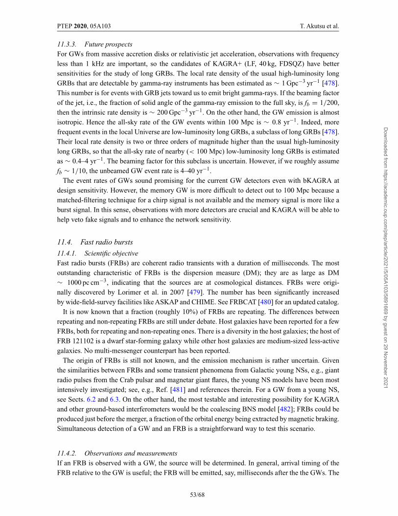
PTEP 2020, 05A103 T. Akutsu et al.
11.3.3. Future prospectsFor GWs from massive accretion disks or relativistic jet acceleration, observations with frequencyless than 1 kHz are important, so the candidates of KAGRA+ (LF, 40 kg, FDSQZ) have bettersensitivities for the study of long GRBs. The local rate density of the usual high-luminosity longGRBs that are detectable by gamma-ray instruments has been estimated as ∼ 1 Gpc−3 yr−1 [478].This number is for events with GRB jets toward us to emit bright gamma-rays. If the beaming factorof the jet, i.e., the fraction of solid angle of the gamma-ray emission to the full sky, is fb = 1/200,then the intrinsic rate density is ∼ 200 Gpc−3 yr−1. On the other hand, the GW emission is almostisotropic. Hence the all-sky rate of the GW events within 100 Mpc is ∼ 0.8 yr−1. Indeed, morefrequent events in the local Universe are low-luminosity long GRBs, a subclass of long GRBs [478].Their local rate density is two or three orders of magnitude higher than the usual high-luminositylong GRBs, so that the all-sky rate of nearby (< 100 Mpc) low-luminosity long GRBs is estimatedas ∼ 0.4–4 yr−1. The beaming factor for this subclass is uncertain. However, if we roughly assumefb ∼ 1/10, the unbeamed GW event rate is 4–40 yr−1.
The event rates of GWs sound promising for the current GW detectors even with bKAGRA atdesign sensitivity. However, the memory GW is more difficult to detect out to 100 Mpc because amatched-filtering technique for a chirp signal is not available and the memory signal is more like aburst signal. In this sense, observations with more detectors are crucial and KAGRA will be able tohelp veto fake signals and to enhance the network sensitivity.
11.4. Fast radio bursts
11.4.1. Scientific objectiveFast radio bursts (FRBs) are coherent radio transients with a duration of milliseconds. The mostoutstanding characteristic of FRBs is the dispersion measure (DM); they are as large as DM∼ 1000 pc cm−3, indicating that the sources are at cosmological distances. FRBs were origi-nally discovered by Lorimer et al. in 2007 [479]. The number has been significantly increasedby wide-field-survey facilities like ASKAP and CHIME. See FRBCAT [480] for an updated catalog.
It is now known that a fraction (roughly 10%) of FRBs are repeating. The differences betweenrepeating and non-repeating FRBs are still under debate. Host galaxies have been reported for a fewFRBs, both for repeating and non-repeating ones. There is a diversity in the host galaxies; the host ofFRB 121102 is a dwarf star-forming galaxy while other host galaxies are medium-sized less-activegalaxies. No multi-messenger counterpart has been reported.
The origin of FRBs is still not known, and the emission mechanism is rather uncertain. Giventhe similarities between FRBs and some transient phenomena from Galactic young NSs, e.g., giantradio pulses from the Crab pulsar and magnetar giant flares, the young NS models have been mostintensively investigated; see, e.g., Ref. [481] and references therein. For a GW from a young NS,see Sects. 6.2 and 6.3. On the other hand, the most testable and interesting possibility for KAGRAand other ground-based interferometers would be the coalescing BNS model [482]; FRBs could beproduced just before the merger, a fraction of the orbital energy being extracted by magnetic braking.Simultaneous detection of a GW and an FRB is a straightforward way to test this scenario.
11.4.2. Observations and measurementsIf an FRB is observed with a GW, the source will be determined. In general, arrival timing of theFRB relative to the GW is useful; the FRB will be emitted, say, milliseconds after the the GWs. The
53/68
Dow
nloaded from https://academ
ic.oup.com/ptep/article/2021/5/05A103/5891669 by guest on 29 N
ovember 2021
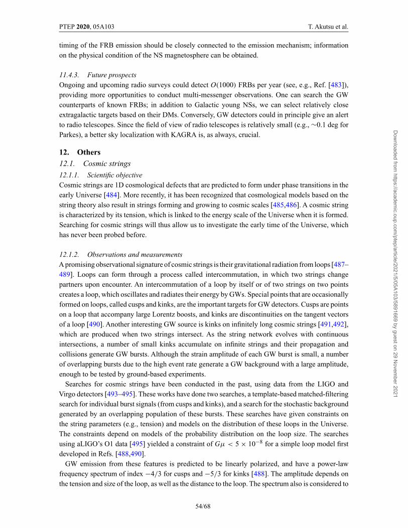
PTEP 2020, 05A103 T. Akutsu et al.
timing of the FRB emission should be closely connected to the emission mechanism; informationon the physical condition of the NS magnetosphere can be obtained.
11.4.3. Future prospectsOngoing and upcoming radio surveys could detect O(1000) FRBs per year (see, e.g., Ref. [483]),providing more opportunities to conduct multi-messenger observations. One can search the GWcounterparts of known FRBs; in addition to Galactic young NSs, we can select relatively closeextragalactic targets based on their DMs. Conversely, GW detectors could in principle give an alertto radio telescopes. Since the field of view of radio telescopes is relatively small (e.g., ∼0.1 deg forParkes), a better sky localization with KAGRA is, as always, crucial.
12. Others12.1. Cosmic strings
12.1.1. Scientific objectiveCosmic strings are 1D cosmological defects that are predicted to form under phase transitions in theearly Universe [484]. More recently, it has been recognized that cosmological models based on thestring theory also result in strings forming and growing to cosmic scales [485,486]. A cosmic stringis characterized by its tension, which is linked to the energy scale of the Universe when it is formed.Searching for cosmic strings will thus allow us to investigate the early time of the Universe, whichhas never been probed before.
12.1.2. Observations and measurementsA promising observational signature of cosmic strings is their gravitational radiation from loops [487–489]. Loops can form through a process called intercommutation, in which two strings changepartners upon encounter. An intercommutation of a loop by itself or of two strings on two pointscreates a loop, which oscillates and radiates their energy by GWs. Special points that are occasionallyformed on loops, called cusps and kinks, are the important targets for GW detectors. Cusps are pointson a loop that accompany large Lorentz boosts, and kinks are discontinuities on the tangent vectorsof a loop [490]. Another interesting GW source is kinks on infinitely long cosmic strings [491,492],which are produced when two strings intersect. As the string network evolves with continuousintersections, a number of small kinks accumulate on infinite strings and their propagation andcollisions generate GW bursts. Although the strain amplitude of each GW burst is small, a numberof overlapping bursts due to the high event rate generate a GW background with a large amplitude,enough to be tested by ground-based experiments.
Searches for cosmic strings have been conducted in the past, using data from the LIGO andVirgo detectors [493–495]. These works have done two searches, a template-based matched-filteringsearch for individual burst signals (from cusps and kinks), and a search for the stochastic backgroundgenerated by an overlapping population of these bursts. These searches have given constraints onthe string parameters (e.g., tension) and models on the distribution of these loops in the Universe.The constraints depend on models of the probability distribution on the loop size. The searchesusing aLIGO’s O1 data [495] yielded a constraint of Gμ < 5 × 10⁻⁸ for a simple loop model firstdeveloped in Refs. [488,490].
GW emission from these features is predicted to be linearly polarized, and have a power-lawfrequency spectrum of index −4/3 for cusps and −5/3 for kinks [488]. The amplitude depends onthe tension and size of the loop, as well as the distance to the loop. The spectrum also is considered to
54/68
Dow
nloaded from https://academ
ic.oup.com/ptep/article/2021/5/05A103/5891669 by guest on 29 N
ovember 2021
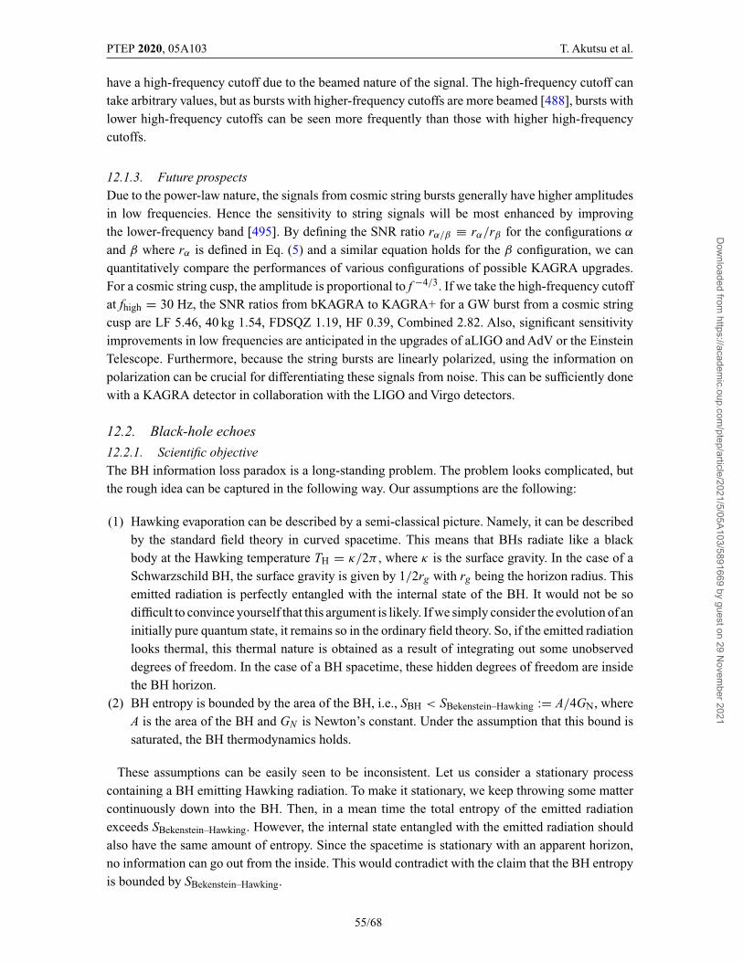
PTEP 2020, 05A103 T. Akutsu et al.
have a high-frequency cutoff due to the beamed nature of the signal. The high-frequency cutoff cantake arbitrary values, but as bursts with higher-frequency cutoffs are more beamed [488], bursts withlower high-frequency cutoffs can be seen more frequently than those with higher high-frequencycutoffs.
12.1.3. Future prospectsDue to the power-law nature, the signals from cosmic string bursts generally have higher amplitudesin low frequencies. Hence the sensitivity to string signals will be most enhanced by improvingthe lower-frequency band [495]. By defining the SNR ratio rα/β ≡ rα/rβ for the configurations α
and β where rα is defined in Eq. (5) and a similar equation holds for the β configuration, we canquantitatively compare the performances of various configurations of possible KAGRA upgrades.For a cosmic string cusp, the amplitude is proportional to f −4/3. If we take the high-frequency cutoffat fhigh = 30 Hz, the SNR ratios from bKAGRA to KAGRA+ for a GW burst from a cosmic stringcusp are LF 5.46, 40 kg 1.54, FDSQZ 1.19, HF 0.39, Combined 2.82. Also, significant sensitivityimprovements in low frequencies are anticipated in the upgrades of aLIGO and AdV or the EinsteinTelescope. Furthermore, because the string bursts are linearly polarized, using the information onpolarization can be crucial for differentiating these signals from noise. This can be sufficiently donewith a KAGRA detector in collaboration with the LIGO and Virgo detectors.
12.2. Black-hole echoes
12.2.1. Scientific objectiveThe BH information loss paradox is a long-standing problem. The problem looks complicated, butthe rough idea can be captured in the following way. Our assumptions are the following:
(1) Hawking evaporation can be described by a semi-classical picture. Namely, it can be describedby the standard field theory in curved spacetime. This means that BHs radiate like a blackbody at the Hawking temperature TH = κ/2π , where κ is the surface gravity. In the case of aSchwarzschild BH, the surface gravity is given by 1/2rg with rg being the horizon radius. Thisemitted radiation is perfectly entangled with the internal state of the BH. It would not be sodifficult to convince yourself that this argument is likely. If we simply consider the evolution of aninitially pure quantum state, it remains so in the ordinary field theory. So, if the emitted radiationlooks thermal, this thermal nature is obtained as a result of integrating out some unobserveddegrees of freedom. In the case of a BH spacetime, these hidden degrees of freedom are insidethe BH horizon.
(2) BH entropy is bounded by the area of the BH, i.e., SBH < SBekenstein–Hawking := A/4GN, whereA is the area of the BH and GN is Newton’s constant. Under the assumption that this bound issaturated, the BH thermodynamics holds.
These assumptions can be easily seen to be inconsistent. Let us consider a stationary processcontaining a BH emitting Hawking radiation. To make it stationary, we keep throwing some mattercontinuously down into the BH. Then, in a mean time the total entropy of the emitted radiationexceeds SBekenstein–Hawking. However, the internal state entangled with the emitted radiation shouldalso have the same amount of entropy. Since the spacetime is stationary with an apparent horizon,no information can go out from the inside. This would contradict with the claim that the BH entropyis bounded by SBekenstein–Hawking.
55/68
Dow
nloaded from https://academ
ic.oup.com/ptep/article/2021/5/05A103/5891669 by guest on 29 N
ovember 2021
PTEP 2020, 05A103 T. Akutsu et al.
To resolve the contradiction mentioned above, some of our assumptions must be violated. An easyway is to abandon assumption (2). However, many people believe that the BH entropy identified withits area is not just a theoretical illusion but has a deep physical meaning. If we wish to keep assumption(2), we would be required to abandon assumption (1). One possibility is that the Hawking radiationis wrong. However, this is unlikely, although it is true that the explicit calculation of the Hawkingradiation based on the field theory in curved spacetime is given only in weak coupling perturbativecalculations. Thus, one way, at first glance radical but in a certain sense most conservative, to resolvethe contradiction would be to abandon the semi-classical picture. From the point of view of relativity,the horizon is not a special surface at all, unless we care about the global structure of the spacetime.Therefore it is difficult to imagine that something unusual happens particularly on the horizon.However, if we trace back the quanta emitted as the Hawking radiation, they infinitely blue-shift inthe near-horizon limit. Hence, field theoretically the horizon might be somehow special, althoughthe argument sounds a little acausal.
From the discussion mentioned above, it would be understandable to doubt if the physics describingthe region close to the BH horizon might be significantly modified from our familiar low-energyphysics. One simple but radical possibility is that the BH horizon is covered by a wall that reflectsall the low-energy excitations including GWs. Ordinary matter whose energy scale is much higherthan the energy of the typical gravitons excited in the binary system will be absorbed by BHs, whilethe quanta whose energy is comparable to or lower than TH, i.e., whose wavelength is as long as theBH size, are selectively reflected by the wall. Interestingly, this critical energy scale also follows ifwe assume that the BH area is quantized by the Planck length squared [496–498].
12.2.2. Observations and measurementsIt is difficult to predict the exact waveform of the expected echoes, since the theoretical backgroundis not so sound. What we can expect generically is a repetition of signals similar to the ringdownsignal after merger with an equal time interval. Here, the uncertainties are in the boundary conditionat the wall and the wall location. One possible ansatz about the properties of the wall is that thereflection rate at the wall is unity and the wall is placed at about a Planck distance from the horizon.Furthermore, we also need to make an assumption about the phase shift at the reflection. One simpleassumption is that the phase shift is frequency independent or the frequency dependence is sufficientlyweak. Under such an assumption, we could construct a template by solving the master equation forBH perturbation [499].
There was a claim that some echo signal has already been detected [500]. However, a very simplerepetition of the same waveform was assumed in that analysis. Such an analysis is an interesting trial,but it is difficult to invent a theoretical model that supports that simple-minded assumption. In fact,our reanalysis indicates that the significance of the echo signal does not survive once we replace thetemplate with a slightly more realistic one [501]; i.e., the reflection rate at the angular momentumbarrier calculated by using the BH perturbation theory is employed. However, it is also true that thesignal claimed in Ref. [500] does not disappear just by increasing the number of BH merger eventsincluding the events from the LIGO/Virgo O2 observing run.
12.2.3. Future prospectsAs the number of events increases, the nature of the signal that seems to exist will definitely beuncovered in the near future. In order to discriminate the real signal coming from the sky from theunidentified noise of detectors correlated with GW events, it would be better to analyze the data
56/68
Dow
nloaded from https://academ
ic.oup.com/ptep/article/2021/5/05A103/5891669 by guest on 29 N
ovember 2021
PTEP 2020, 05A103 T. Akutsu et al.
from completely different detectors that have a similar sensitivity. In this sense it is quite interestingto analyze the data obtained by Virgo and KAGRA in the same manner.
13. Conclusion
In this article we have reviewed the scientific cases available with second-generation ground-baseddetectors, including aLIGO, AdV, and the baseline KAGRA (bKAGRA), and their future upgrades,A+, AdV+, and KAGRA+, respectively, and discuss KAGRA’s scientific contributions to the globaldetector networks composed of the detectors above. For compact binaries composed of stellar-massBHs and/or NSs, at least three detectors are necessary to localize sources and more detectors includingKAGRA are preferable to obtain smaller sky areas to be searched. This is also true for science basedon these binaries such as tests of gravity (except for BH ringdown), measurement of the Hubbleconstant, GW lensing, the measurement of the EOS of an NS, and multi-messenger observations ofsGRBs and kilonovae. On the other hand, the discovery of new GW sources such as binary IMBHs,supernovae, magnetors, isolated pulsars, and low-mass X-ray binaries can be done with a singledetector, though multiple detectors are preferable for events detected only by GWs. Therefore, forthese sources, the higher duty cycle of a detector network is more important not to miss signalsduring detector down times. In summary, KAGRA will be able to contribute to broad science topicsand play an important role in joint observations by the global detector networks.
Acknowledgements
This work was supported by MEXT, the Japan Society for the Promotion of Science (JSPS) Leading-edgeResearch Infrastructure Program, a JSPS Grant-in-Aid for Specially Promoted Research 26000005, JSPSGrants-in-Aid for Scientific Research on InnovativeAreas 2905: JP17H06358, JP17H06361, and JP17H06364,JSPS Core-to-Core Program A. Advanced Research Networks, a JSPS Grant-in-Aid for Scientific Research(S) 17H06133, the joint research program of the Institute for Cosmic Ray Research, University of Tokyo,the National Research Foundation (NRF) and Computing Infrastructure Project of KISTI-GSDC in Korea,Academia Sinica (AS), AS Grid Center (ASGC) and the Ministry of Science and Technology (MoST) inTaiwan under grants including AS-CDA-105-M06, the Advanced Technology Center (ATC) of NAOJ, theMechanical Engineering Center of KEK, the LIGO project, and the Virgo project.
References[1] J. Aasi et al. [LIGO Scientific and Advanced VIRGO Collaborations], Class. Quantum Grav.
32, 074001 (2015).[2] F. Acernese et al., Class. Quantum Grav. 32, 024001 (2015).[3] B. P. Abbott et al. [LIGO Scientific and Virgo Collaborations], Phys. Rev. X 9, 031040 (2019).[4] B. P. Abbott et al. [LIGO Scientific and Virgo Collaborations], Phys. Rev. Lett. 119, 161101 (2017).[5] J. Miller, L. Barsotti, S. Vitale, P. Fritschel, M. Evans, and D. Sigg, Phys. Rev. D 91, 062005 (2015).[6] J. Degallaix for the Virgo Collaboration, Advanced Virgo+ preliminary studies, VIR-0300A-18 (2018).[7] B. P. Abbot et al. [KAGRA, LIGO Scientific and Virgo Collaborations], Living Rev. Relat. 21, 3
(2018).[8] T. Akutsu et al. [KAGRA Collaboration], Nat. Astron. 3, 35 (2019).[9] T. Akutsu et al. [KAGRA Collaboration], in preparation as the series of article. Overview of KAGRA:
Future plans.[10] Y. Michimura et al., Phys. Rev. D 102, 022008 (2020).[11] B. P. Abbott et al. [LIGO Scientific and Virgo Collaborations], Phys. Rev. Lett. 116, 061102 (2016).[12] B. P. Abbott et al. [LIGO Scientific and Virgo Collaborations], Phys. Rev. Lett. 116, 241103 (2016).[13] B. P. Abbott et al. [LIGO Scientific and Virgo Collaborations], Astrophys. J. Lett. 818, L22 (2016).[14] K. Belczynski, T. Bulik, and B. Rudak, Astrophys. J. Lett. 608, L45 (2004).[15] M. Dominik, K. Belczynski, C. Fryer, D. E. Holz, E. Berti, T. Bulik, I. Mandel, and
R. O’Shaughnessy, Astrophys. J. 759, 52 (2012).
57/68
Dow
nloaded from https://academ
ic.oup.com/ptep/article/2021/5/05A103/5891669 by guest on 29 N
ovember 2021
PTEP 2020, 05A103 T. Akutsu et al.
[16] K. Belczynski, D. E. Holz, T. Bulik, and R. O’Shaughnessy, Nature 534, 512 (2016).[17] M. Mapelli, Mon. Not. R. Astron. Soc. 459, 3432 (2016).[18] S. F. Portegies Zwart and S. L. W. McMillan, Astrophys. J. Lett. 528, L17 (2000).[19] R. M. O’Leary, B. Kocsis, and A. Loeb, Mon. Not. R. Astron. Soc. 395, 2127 (2009).[20] C. L. Rodriguez, C.-J. Haster, S. Chatterjee, V. Kalogera, and F. A. Rasio, Astrophys. J. Lett.
824, L8 (2016).[21] F. Antonini and F. A. Rasio, Astrophys. J. 831, 187 (2016).[22] N. C. Stone, B. D. Metzger, and Z. Haiman, Mon. Not. R. Astron. Soc. 464, 946 (2017).[23] Y.-B. Bae, C. Kim, and H. M. Lee, Mon. Not. R. Astron. Soc. 440, 2714 (2014).[24] D. Park, C. Kim, H. M. Lee, Y.-B. Bae, and K. Belczynski, Mon. Not. R. Astron. Soc.
469, 4665 (2017).[25] T. Kinugawa, K. Inayoshi, K. Hotokezaka, D. Nakauchi, and T. Nakamura, Mon. Not. R. Astron. Soc.
442, 2963 (2014).[26] T. Hartwig, M. Volonteri, V. Bromm, R. S. Klessen, E. Barausse, M. Magg, and A. Stacy, Mon. Not.
R. Astron. Soc. 460, L74 (2016).[27] K. Inayoshi, K. Kashiyama, E. Visbal, and Z. Haiman, Mon. Not. R. Astron. Soc. 461, 2722 (2016).[28] K. Inayoshi, R. Hirai, T. Kinugawa, and K. Hotokezaka, Mon. Not. R. Astron. Soc. 468, 5020 (2017).[29] B. Carr, F. Kühnel, and M. Sandstad, Phys. Rev. Lett. 94, 083504 (2016).[30] M. Sasaki, T. Suyama, T. Tanaka, and S. Yokoyama, Phys. Rev. Lett. 117, 061101 (2016);
121, 059901 (2018) [erratum].[31] M. Sasaki, T. Suyama, T. Tanaka, and S. Yokoyama, Class. Quantum Grav. 35, 063001 (2018).[32] D. Kushnir, M. Zaldarriaga, J. A. Kollmeier, and R. Waldman, Mon. Not. R. Astron. Soc.
462, 844 (2016).[33] C. L. Rodriguez, M. Zevin, C. Pankow, V. Kalogera, and F. A. Rasio, Astrophys. J. Lett.
832, L2 (2016).[34] K. Hotokezaka and T. Piran, Astrophys. J. 842, 111 (2017).[35] H.-T. Janka, Mon. Not. R. Astron. Soc. 434, 1355 (2013).[36] I. Mandel, Mon. Not. R. Astron. Soc. 456, 578 (2016).[37] T. Chiba and S. Yokoyama, Prog. Theor. Exp. Phys. 2017, 083E01 (2017).[38] V. De Luca, V. Desjacques, A. Malhotra, and A. Riotto, J. Cosmol. Astropart. Phys. 1905, 018 (2019).[39] T. Harada, Y. Chul-Moon, K. Kohri, and K.-I. Nakao, Phys. Rev. D 96, 083517 (2017);
99, 069904 (2019) [erratum].[40] E. S. Phinney, arXiv:astro-ph/0108028 [Search INSPIRE].[41] B. P. Abbott et al. [LIGO Scientific and Virgo Collaborations], Phys. Rev. Lett. 116, 131102 (2016).[42] K. A. Postnov and L. R. Yungelson, Living Rev. Relat. 17, 3 (2014).[43] M. J. Benacquista, Living Rev. Relat. 5, 2 (2002).[44] L. Pekowsky, J. Healy, D. Shoemaker, and P. Laguna, Phys. Rev. D 87, 084008 (2013).[45] B. P. Abbott et al. [LIGO Scientific and Virgo Collaborations], Phys. Rev. D 102, 043015 (2020)
[arXiv:2004.08342 [astro-ph.HE]] [Search INSPIRE].[46] J. M. Bardeen, W. H. Press, and S. A. Teukolsky, Astrophys. J. 178, 347 (1972).[47] S. F. Portegies Zwart and S. L. W. McMillan, Astrophys. J. 576, 899 (2002).[48] M. Freitag, M. A. Gürkan, and F. A. Rasio, Mon. Not. R. Astron. Soc. 368, 141 (2006).[49] P. Amaro-Seoane and L. Santamaría, Astrophys. J. 722, 1197 (2010).[50] G. Fragione, I. Ginsburg, and B. Kocsis, Astrophys. J. 856, 92 (2018).[51] H.-a. Shinkai, N. Kanda, and T. Ebisuzaki, Astrophys. J. 835, 276 (2017).[52] P. Amaro-Seoane, Phys. Rev. D 98, 063018 (2018).[53] M. A. Gürkan, J. M. Fregeau, and F. A. Rasio, Astrophys. J. Lett. 640, L39 (2006).[54] S. Hirano, T. Hosokawa, N. Yoshida, H. Umeda, K. Omukai, G. Chiaki, and H. W. Yorke, Astrophys.
J. 781, 60 (2014).[55] A. Stacy and V. Bromm, Mon. Not. R. Astron. Soc. 433, 1094 (2013).[56] H. Susa, K. Hasegawa, and N. Tominaga, Astrophys. J. 792, 32 (2014).[57] K. Inayoshi and Z. Haiman, Mon. Not. R. Astron. Soc. 445, 1549 (2014).[58] M. C. Miller and E. J. M. Colbert, Int. J. Mod. Phys. D 13, 1 (2004).[59] D. A. Brown, J. Brink, H. Fang, J. R. Gair, C. Li, G. Lovelace, I. Mandel, and K. S. Thorne, Phys.
Rev. Lett. 99, 201102 (2007).[60] E. Berti, A. Buonanno, and C. M. Will, Phys. Rev. D 71, 084025 (2005).
58/68
Dow
nloaded from https://academ
ic.oup.com/ptep/article/2021/5/05A103/5891669 by guest on 29 N
ovember 2021
PTEP 2020, 05A103 T. Akutsu et al.
[61] S. Isoyama, H. Nakano, and T. Nakamura, Prog. Theor. Exp. Phys. 2018, 073E01 (2018).[62] A. Ori and K. S. Thorne, Phys. Rev. D 62, 124022 (2000).[63] E. Berti, V. Cardoso, and C. M. Will, Phys. Rev. D 73, 064030 (2006).[64] E. A. Huerta and J. R. Gair, Phys. Rev. D 83, 044020 (2011).[65] M. C. Miller, Class. Quantum Grav. 26, 094031 (2009).[66] T. M. Tauris et al., Astrophys. J. 846, 170 (2017).[67] M. Chruslinska, K. Belczynski, J. Klencki, and M. Benacquista, Mon. Not. R. Astron. Soc.
474, 2937 (2018).[68] D. Pooley et al., Astrophys. J. Lett. 591, L131 (2003).[69] J. M. Weisberg, D. J. Nice, and J. H. Taylor, Astrophys. J. 722, 1030 (2010).[70] P. C. Peters, Phys. Rev. 136, B1224 (1964).[71] F. Özel and P. Freire, Ann. Rev. Astron. Astrophys. 54, 401 (2016).[72] R. Abbott et al. [LIGO Scientific and Virgo Collaborations], Astrophys. J. Lett. 896, L44 (2020).[73] N. Pol, M. McLaughlin, and D. R. Lorimer, Astrophys. J. 870, 71 (2019); 874, 186 (2019) [erratum].[74] R. N. Manchester, G. B. Hobbs, A. Teoh, and M. Hobbs, Astrophys. J. 129, 1993 (2005).[75] ATNF Pulsar Catalogue webpage, http://www.atnf.csiro.au/research/pulsar/psrcat/[76] B. P. Abbott et al. [LIGO Scientific and Virgo Collaborations], Phys. Rev. X 9, 011001 (2019).[77] B. P. Abbott et al. [LIGO Scientific and Virgo Collaborations], Phys. Rev. Lett. 121, 161101 (2018).[78] J. M. Lattimer and M. Prakash, Phys. Rept. 621, 127 (2016).[79] E. E. Flanagan and T. Hinderer, Phys. Rev. D 77, 021502 (2008).[80] T. Hinderer, Astrophys. J. 677, 1216 (2008); 697, 964 (2009) [erratum].[81] T. Damour, A. Nagar, and L. Villain, Phys. Rev. D 85, 123007 (2012).[82] L. Wade, J. D. E. Creighton, E. Ochsner, B. D. Lackey, B. F. Farr, T. B. Littenberg, and V. Raymond,
Phys. Rev. D 89, 103012 (2014).[83] T. Hinderer, B. D. Lackey, R. N. Lang, and J. S. Read, Phys. Rev. D 81, 123016 (2010).[84] K. Hotokezaka, K. Kyutoku, H. Okawa, M. Shibata, and K. Kiuchi, Phys. Rev. D 83, 124008 (2011).[85] A. Buonanno, B. R. Iyer, E. Ochsner, Y. Pan, and B. S. Sathyaprakash, Phys. Rev. D
80, 084043 (2009).[86] L. Blanchet, Living Rev. Rel. 17, 2 (2014).[87] T. Dietrich, S. Bernuzzi, and W. Tichy, Phys. Rev. D 96, 121501(R) (2017).[88] K. Yagi and N. Yunes, Phys. Rept. 681, 1 (2017).[89] W. Kastaun and F. Ohme, Phys. Rev. D 100, 103023 (2019).[90] B. P. Abbott et al. [LIGO Scientific and Virgo Collaborations], Class. Quantum Grav.
37, 045006 (2020).[91] H. Müeller and B. D. Serot, Nucl. Phys. A 606, 508 (1996).[92] S. De, D. Finstad, J. M. Lattimer, D. A. Brown, E. Berger, and C. M. Biwer, Phys. Rev. Lett.
121, 091102 (2018); 121, 259902 (2018) [erratum].[93] C. D. Capano, I. Tews, S. M. Brown, B. Margalit, S. De, S. Kumar, D. A. Brown, B. Krishnan,
and S. Reddy, Nat. Astron. 4, 625 (2020).[94] T. Narikawa, N. Uchikata, K. Kawaguchi, K. Kiuchi, K. Kyutoku, M. Shibata, and H. Tagoshi,
arXiv:1910.08971 [gr-qc] [Search INSPIRE].[95] K. Kiuchi, K. Kawaguchi, K. Kyutoku, Y. Sekiguchi, M. Shibata, and K. Taniguchi, Phys. Rev. D
96, 084060 (2017).[96] K. Kawaguchi, K. Kiuchi, K. Kyutoku, Y. Sekiguchi, M. Shibata, and K. Taniguchi, Phys. Rev. D
97, 044044 (2018).[97] T. Dietrich, A. Samajdar, S. Khan, N. K. Johnson-McDaniel, R. Dudi, and W. Tichy, Phys. Rev. D
100, 044003 (2019).[98] B. Margalit and B. D. Metzger, Astrophys. J. Lett. 850, L19 (2017).[99] A. Bauswein, O. Just, H.-T. Janka, and N. Stergioulas, Astrophys. J. Lett. 850, L34 (2017).
[100] M. Ruiz, S. L. Shapiro, and A. Tsokaros, Phys. Rev. D 97, 021501(R) (2018).[101] E. Annala, T. Gorda, A. Kurkela, and A. Vuorinen, Phys. Rev. Lett. 120, 172703 (2018).[102] E.-P. Zhou, X. Zhou, and A. Li, Phys. Rev. D 97, 083015 (2018).[103] F. J. Fattoyev, J. Piekarewicz, and C. J. Horowitz, Phys. Rev. Lett. 120, 172702 (2018).[104] V. Paschalidis, K. Yagi, D. Alvarez-Castillo, D. B. Blaschke, and A. Sedrakian, Phys. Rev. D
97, 084038 (2018).[105] R. Nandi and P. Char, Astrophys. J. 857, 12 (2018).
59/68
Dow
nloaded from https://academ
ic.oup.com/ptep/article/2021/5/05A103/5891669 by guest on 29 N
ovember 2021
PTEP 2020, 05A103 T. Akutsu et al.
[106] E. R. Most, L. R. Weih, L. Rezzolla, and J. Schaffner-Bielich, Phys. Rev. Lett. 120, 261103 (2018).[107] C. Raithel, F. Özel, and D. Psaltis, Astrophys. J. Lett. 857, L23 (2018).[108] P. Landry and R. Essick, Phys. Rev. D 99, 084049 (2019).[109] L. Baiotti, Prog. Part. Nucl. Phys. 109, 103714 (2019).[110] K. Takami, L. Rezzolla, and L. Baiotti, Phys. Rev. D 91, 064001 (2015).[111] A. Akmal, V. R. Pandharipande, and D. G. Ravenhall, Phys. Rev. C 58, 1804 (1998).[112] F. Douchin and P. Haensel, Astron. Astrophys. 380, 151 (2001).[113] T. Narikawa, N. Uchikata, K. Kawaguchi, K. Kiuchi, K. Kyutoku, M. Shibata, and H. Tagoshi, Phys.
Rev. Res. 1, 033055 (2019).[114] L. Baiotti and L. Rezzolla, Rep. Prog. Phys. 80, 096901 (2017).[115] M. D. Duez and Y. Zlochower, Rep. Prog. Phys. 82, 016902 (2019).[116] M. H. P. M. van Putten, M. Della Valle, and A. Levinson, Astrophys. J. Lett. 876, L2 (2019).[117] V. Paschalidis and N. Stergioulas, Living Rev. Relat. 20, 7 (2017).[118] K. Takami, L. Rezzolla, and L. Baiotti, Phys. Rev. Lett. 113, 091104 (2014).[119] F. Maione, R. De Pietri, A. Feo, and F. Löffler, Phys. Rev. D 96, 063011 (2017).[120] M. Breschi, S. Bernuzzi, F. Zappa, M. Agathos, A. Perego, D. Radice, and A. Nagar, Phys. Rev. D
100, 104029 (2019).[121] A. Bauswein and H.-T. Janka, Phys. Rev. Lett. 108, 011101 (2012).[122] S. Bose, K. Chakravarti, L. Rezzolla, B. S. Sathyaprakash, and K. Takami, Phys. Rev. Lett.
120, 031102 (2018).[123] K. Chatziioannou, J. A. Clark, A. Bauswein, M. Millhouse, T. B. Littenberg, and N. Cornish, Phys.
Rev. D 96, 124035 (2017).[124] A. Torres-Rivas, K. Chatziioannou, A. Bauswein, and J. A. Clark, Phys. Rev. D 99, 044014 (2019).[125] L. R. Weih, M. Hanauske, and L. Rezzolla, Phys. Rev. Lett. 124, 171103 (2020).[126] A. Bauswein, S. Blacker, V. Vijayan, N. Stergioulas, K. Chatziioannou, J. A. Clark, N.-U. Bastian,
D. B. Blaschke, M. Cierniak, and T. Fischer, arXiv:2004.00846 [astro-ph.HE] [Search INSPIRE].[127] L. Baiotti, B. Giacomazzo, and L. Rezzolla, Phys. Rev. D 78, 084033 (2008).[128] L. Rezzolla, B. Giacomazzo, L. Baiotti, J. Granot, C. Kouveliotou, and M. A. Aloy, Astrophys. J. Lett.
732, L6 (2011).[129] K. Kiuchi, Y. Sekiguchi, K. Kyutoku, M. Shibata, K. Taniguchi, and T. Wada, Phys. Rev. D
92, 064034 (2015).[130] D. Radice, A. Perego, K. Hotokezaka, S. A. Fromm, S. Bernuzzi, and L. F. Roberts, Astrophys. J.
869, 130 (2018).[131] R. P. Kerr, Phys. Rev. Lett. 11, 237 (1963).[132] M. H. P. M. van Putten, Science 284, 115 (1999).[133] R. De Pietri, A. Drago, A. Feo, G. Pagliara, M. Pasquali, S. Traversi, and G. Wiktorowicz, Astrophys.
J. 881, 122 (2019).[134] J. Klimo, M. Veselsky, G. A. Souliotis, and A. Bonasera, Nucl. Phys. A 992, 121640 (2019).[135] P. Haensel, J. L. Zdunik, M. Bejger, and J. M. Lattimer, Astron. Astrophys. 502, 605 (2009).[136] V. Connaughton, GCN 21505 (2017) (available at: https://gcn.gsfc.nasa.gov/gcn3/21505.gcn3).[137] V. Savchenko et al., Astrophys. J. Lett. 848, L15 (2017).[138] K. P. Mooley et al., Nature 554, 207 (2018).[139] K. P. Mooley, A. T. Deller, O. Gottlieb, E. Nakar, G. Hallinan, S. Bourke, D. A. Frail, A. Horesh,
A. Corsi, and K. Hotokezaka, Nature 561, 355 (2018).[140] C. Cutler and K. S. Thorne, arXiv:gr-qc/0204090 [Search INSPIRE].[141] R. A. Hulse and J. H. Taylor, Astrophys. J. 195, L51 (1975).[142] K. W. Weiler and N. Panagia, Astron. Astrophys. 70, 419 (1978).[143] B. P. Abbott et al. [INTEGRAL], Astrophys. J. Lett. 848, L13 (2017).[144] B. P. Abbott et al., Astrophys. J. 875, 160 (2019).[145] L. Sun and A. Melatos, Phys. Rev. D 99, 123003 (2019).[146] R. Gill, A. Nathanail, and L. Rezzolla, Astrophys. J. 876, 139 (2019).[147] S. J. Smartt et al., Nature 551, 75 (2017).[148] E. Pian et al., Nature 551, 67 (2017).[149] M. Lucca and L. Sagunski, J. High Energy Astrophys. 27, 33 (2020).[150] D. Pooley, P. Kumar, J. C. Wheeler, and B. Grossan, Astrophys. J. Lett. 859, L23 (2018).[151] M. H. P. M. van Putten, C. Guidorzi, and F. Frontera, Astrophys. J. 786, 146 (2014).
60/68
Dow
nloaded from https://academ
ic.oup.com/ptep/article/2021/5/05A103/5891669 by guest on 29 N
ovember 2021
PTEP 2020, 05A103 T. Akutsu et al.
[152] M. H. P. M. van Putten, Prog. Theor. Exp. Phys. 2017, 093F01 (2017).[153] M. H. P. M. van Putten and M. Della Valle, Mon. Not. R. Astron. Soc. 482, L46 (2019).[154] B. P. Abbott et al. [LIGO Scientific and Virgo Collaborations], Astrophys. J. Lett. 851, L16 (2017).[155] M. H. P. M. van Putten, A. Levinson, F. Frontera, C. Guidorzi, L. Amati, and M. Della Valle, Eur.
Phys. J. Plus 134, 537 (2019).[156] J.-E. Heo, S. Yoon, D.-S. Lee, I.-t. Kong, S.-H. Lee, M. H. P. M. van Putten, and M. D. Valle, New
Astron. 42, 24 (2016).[157] S. Ando et al., Rev. Mod. Phys. 85, 1401 (2013).[158] J. Aasi et al. [LIGO Scientific and Virgo Collaborations], Phys. Rev. D 89, 122004 (2014).[159] L. Amati et al., Adv. Space Res. 62, 191 (2018).[160] G. Stratta et al., Adv. Space Res. 62, 662 (2018).[161] K. Riles, Mod. Phys. Lett. A 32, 1730035 (2017).[162] G. Ushomirsky, C. Cutler, and L. Bildsten, Mon. Not. R. Astron. Soc. 319, 902 (2000).[163] L. Bildsten, Astrophys. J. Lett. 501, L89 (1998).[164] A. Mukherjee, C. Messenger, and K. Riles, Phys. Rev. D 97, 043016 (2018).[165] G. D. Meadors, E. Goetz, K. Riles, T. Creighton, and F. Robinet, Phys. Rev. D 95, 042005 (2017).[166] B. P. Abbott et al., Astrophys. J. 847, 47 (2017).[167] B. P. Abbott et al. [LIGO Scientific and Virgo Collaborations], Phys. Rev. D 95, 122003 (2017).[168] B. P. Abbott et al. [LIGO Scientific and Virgo Collaborations], Phys. Rev. D 100, 122002 (2019).[169] L. J. Kaluzienski, S. S. Holt, and J. H. Swank, Astrophys. J. 241, 779 (1980).[170] C. Messenger et al., Phys. Rev. D 92, 023006 (2015).[171] G. D. Meadors, B. Krishnan, M. A. Papa, J. T. Whelan, and Y. Zhang, Phys. Rev. D 97, 044017 (2018).[172] C. Dreissigacker, R. Sharma, C. Messenger, R. Zhao, and R. Prix, Phys. Rev. D 100, 044009 (2019).[173] R. Smits, S. J. Tingay, N. Wex, M. Kramer, and B. Stappers, Astron. Astrophys. 528, A108 (2011).[174] K. Ono, K. Eda, and Y. Itoh, Phys. Rev. D 91, 084032 (2015).[175] L. Rezzolla, P. Pizzochero, D. I. Jones, N. Rea and I. Vidaña. The Physics and Astrophysics of
Neutron Stars (Springer, 2018).[176] M. Sieniawska and M. Bejger, Universe 5, 217 (2019).[177] B. P. Abbott et al. [LIGO Scientific and Virgo Collaborations], Astrophys. J. 851, 71 (2017).[178] B. P. Abbott et al. [LIGO Scientific and Virgo Collaborations], Astrophys. J. 879, 10 (2019).[179] B. P. Abbott et al. [LIGO Scientific and Virgo Collaborations], Astrophys. J. 875, 122 (2019).[180] B. P. Abbott et al. [LIGO Scientific and Virgo Collaborations], Phys. Rev. Lett. 120, 031104 (2018).[181] N. K. Johnson-McDaniel and B. J. Owen, Phys. Rev. D 88, 044004 (2013).[182] N. K. Johnson-McDaniel, Phys. Rev. D 88, 044016 (2013).[183] M. Pitkin, Mon. Not. R. Astron. Soc. 415, 1849 (2011).[184] G. L. Israel, T. Belloni, L. Stella, Y. Rephaeli, D. E. Gruber, P. Casella, S. Dall’Osso, N. Rea,
M. Persic, and R. E. Rothschild, Astrophys. J. Lett. 628, L53 (2005).[185] K. Ioka, Mon. Not. R. Astron. Soc. 327, 639 (2001).[186] A. Corsi and B. J. Owen, Phys. Rev. D 83, 104014 (2011).[187] Y. Levin and M. van Hoven, Mon. Not. R. Astron. Soc. 418, 659 (2011).[188] B. Zink, P. D. Lasky, and K. D. Kokkotas, Phys. Rev. D 85, 024030 (2012).[189] B. Abbott et al. [LIGO Scientific Collaboration], Phys. Rev. D 76, 062003 (2007).[190] B. P. Abbott et al. [LIGO Scientific Collaboration], Astrophys. J. 874, 163 (2019).[191] K. Kokkotas and B. G. Schmidt, Living Rev. Relat. 2, 2 (1999).[192] N. Andersson and K. D. Kokkotas, Phys. Rev. Lett. 77, 4134 (1996).[193] N. Andersson and K. D. Kokkotas, Mon. Not. R. Astron. Soc. 299, 1059 (1998).[194] L. S. Finn, Mon. Not. R. Astron. Soc. 227, 265 (1987).[195] H. Sotani, K. Tominaga, and K.-i. Maeda, Phys. Rev. D 65, 024010 (2001).[196] G. Miniutti, J. A. Pons, E. Berti, L. Gualtieri, and V. Ferrari, Mon. Not. R. Astron. Soc.
338, 389 (2003).[197] H. Sotani, N. Yasutake, T. Maruyama, and T. Tatsumi, Phys. Rev. D 83, 024014 (2011).[198] A. Reisenegger and P. Goldreich, Astrophys. J. 395, 240 (1992).[199] V. Ferrari, L. Gualtieri, and J. A. Pons, Class. Quantum Grav. 24, 5093 (2007).[200] A. Passamonti, N. Andersson, and W. C. G. Ho, Mon. Not. R. Astron. Soc. 455, 1489 (2016).[201] N. Andersson, Astrophys. J. 502, 708 (1998).[202] J. L. Friedman and S. M. Morsink, Astrophys. J. 502, 714 (1998).
61/68
Dow
nloaded from https://academ
ic.oup.com/ptep/article/2021/5/05A103/5891669 by guest on 29 N
ovember 2021
PTEP 2020, 05A103 T. Akutsu et al.
[203] P. Arras, E. E. Flanagan, S. M. Morsink, A. K. Schenk, S. A. Teukolsky, and I. Wasserman, Astrophys.J. 591, 1129 (2003).
[204] E. Gaertig, K. Glampedakis, K. D. Kokkotas, and B. Zink, Phys. Rev. Lett. 107, 101102 (2011).[205] H. Sotani and T. Takiwaki, Phys. Rev. D 94, 044043 (2016).[206] H. Sotani, T. Kuroda, T. Takiwaki, and K. Kotake, Phys. Rev. D 96, 063005 (2017).[207] V. Morozova, D. Radice, A. Burrows, and D. Vartanyan, Astrophys. J. 861, 10 (2018).[208] H. Sotani, T. Kuroda, T. Takiwaki, and K. Kotake, Phys. Rev. D 99, 123024 (2019).[209] H. Sotani and K. Sumiyoshi, Phys. Rev. D 100, 083008 (2019).[210] A. Torres-Forné, P. Cerdá-Durán, A. Passamonti, and J. A. Font, Mon. Not. R. Astron. Soc.
474, 5272 (2018).[211] A. Torres-Forné, P. Cerdá-Durán, A. Passamonti, M. Obergaulinger, and J. A. Font, Mon. Not. R.
Astron. Soc. 482, 3967 (2019).[212] B. W. Grefenstette et al., Astrophys. J. 802, 15 (2015).[213] M. Tanaka, K. Maeda, P. A. Mazzali, K. S. Kawabata, and K. Nomoto, Astrophys. J. 837, 105 (2017).[214] H. A. Bethe, Rev. Mod. Phys. 62, 801 (1990).[215] B. Müller, Publ. Astron. Soc. Aust. 33, e048 (2016).[216] H.-T. Janka, T. Melson, and A. Summa, Ann. Rev. Nucl. Part. Sci. 66, 341 (2016).[217] A. Burrows, Rev. Mod. Phys. 85, 245 (2013).[218] K. Kotake, K. Sumiyoshi, S. Yamada, T. Takiwaki, T. Kuroda, Y. Suwa, and H. Nagakura, Prog. Theor.
Exp. Phys. 2012, 01A301 (2012).[219] D. Radice, V. Morozova, A. Burrows, D. Vartanyan, and H. Nagakura, Astrophys. J. Lett.
876, L9 (2019).[220] H. Andresen, E. Müller, H.-Th. Janka, A. Summa, K. Gill, and M. Zanolin, Mon. Not. R. Astron. Soc.
486, 2238 (2019).[221] H. Andresen, B. Müller, E. Müller, and H.-Th. Janka, Mon. Not. R. Astron. Soc. 468, 2032 (2017).[222] T. Kuroda, K. Kotake, and T. Takiwaki, Astrophys. J. Lett. 829, L14 (2016).[223] P. Astone, P. Cerdá-Durán, I. Di Palma, M. Drago, F. Muciaccia, C. Palomba, and F. Ricci, Phys. Rev.
D 98, 122002 (2018).[224] T. Foglizzo et al., Publ. Astron. Soc. Aust. 32, e009 (2015).[225] K. Kotake, Compt. Rendus Phys. 14, 318 (2013).[226] C. D. Ott, Class. Quantum Grav. 26, 063001 (2009).[227] S. E. Woosley and A. Heger, Astrophys. J. 637, 914 (2006).[228] K. Hayama, T. Kuroda, K. Nakamura, and S. Yamada, Phys. Rev. Lett. 116, 151102 (2016).[229] K. Hayama, T. Kuroda, K. Kotake, and T. Takiwaki, Mon. Not. R. Astron. Soc. 477, L96 (2018).[230] K. Hayama, T. Kuroda, K. Kotake, and T. Takiwaki, Phys. Rev. D 92, 122001 (2015).[231] S. Suvorova, J. Powell, and A. Melatos, Phys. Rev. D 99, 123012 (2019).[232] S. E. Gossan, P. Sutton, A. Stuver, M. Zanolin, K. Gill, and C. D. Ott, Phys. Rev. D 93, 042002 (2016).[233] A. A. Starobinsky, Phys. Lett. B 91, 99 (1980).[234] K. Sato, Mon. Not. R. Astron. Soc. 195, 467 (1981).[235] D. Kazanas, Astrophys. J. 241, L59 (1980).[236] A. H. Guth, Phys. Rev. D 23, 347 (1981).[237] V. F. Mukhanov and G. V. Chibisov, JETP Lett. 33, 532 (1981) [Pisma Zh. Eksp. Teor. Fiz.
33, 532 (1981)].[238] A. D. Linde, Phys. Lett. B 116, 335 (1982).[239] S. W. Hawking, Phys. Lett. B 115, 295 (1982).[240] A. A. Starobinsky, Phys. Lett. B 117, 175 (1982).[241] A. H. Guth and S.-Y. Pi, Phys. Rev. Lett. 49, 1110 (1982).[242] A. A. Starobinsky, JETP Lett. 30, 682 (1979) [Pisma Zh. Eksp. Teor. Fiz. 30, 682 (1979)].[243] V. A. Rubakov, M. V. Sazhin, and A. V. Veryaskin, Phys. Lett. B 115, 189 (1982).[244] L. F. Abbott and M. B. Wise, Nucl. Phys. B 244, 541 (1984).[245] S. Kuroyanagi, T. Chiba, and N. Sugiyama, Phys. Rev. D 79, 103501 (2009).[246] S. Kuroyanagi, S. Tsujikawa, T. Chiba, and N. Sugiyama, Phys. Rev. D 90, 063513 (2014).[247] B. P. Abbott et al. [LIGO Scientific/Virgo Collaborations], Phys. Rev. D 100, 061101(R) (2009).[248] R. H. Brandenberger, A. Nayeri, S. P. Patil, and C. Vafa, Phys. Rev. Lett. 98, 231302 (2007).[249] Y.-S. Piao and Y.-Z. Zhang, Phys. Rev. D 70, 063513 (2004).[250] M. Baldi, F. Finelli, and S. Matarrese, Phys. Rev. D 72, 083504 (2005).
62/68
Dow
nloaded from https://academ
ic.oup.com/ptep/article/2021/5/05A103/5891669 by guest on 29 N
ovember 2021
PTEP 2020, 05A103 T. Akutsu et al.
[251] T. Kobayashi, M. Yamaguchi, and J. Yokoyama, Phys. Rev. Lett. 105, 231302 (2010).[252] G. Calcagni and S. Tsujikawa, Phys. Rev. D 70, 103514 (2004).[253] G. Calcagni, S. Kuroyanagi, J. Ohashi, and S. Tsujikawa, J. Cosmol. Astropart. Phys.
1403, 052 (2014).[254] J. L. Cook and L. Sorbo, Phys. Rev. D 85, 023534 (2012); 86, 069901 (2012) [erratum].[255] S. Mukohyama, R. Namba, M. Peloso, and G. Shiu, J. Cosmol. Astropart. Phys. 1408, 036 (2014).[256] S. Mohanty and A. Nautiyal, arXiv:1404.2222 [hep-ph] [Search INSPIRE].[257] M. Biagetti, M. Fasiello, and A. Riotto, Phys. Rev. D 88, 103518 (2013).[258] T. Fujita, S. Kuroyanagi, S. Mizuno, and S. Mukohyama, Phys. Lett. B 789, 215 (2019).[259] P. J. E. Peebles and A. Vilenkin, Phys. Rev. D 59, 063505 (1999).[260] M. Giovannini, Phys. Rev. D 58, 083504 (1998).[261] M. Giovannini, Phys. Rev. D 60, 123511 (1999).[262] M. Giovannini, Class. Quantum Grav. 16, 2905 (1999).[263] H. Tashiro, T. Chiba, and M. Sasaki, Class. Quantum Grav. 21, 1761 (2004).[264] M. Giovannini, Class. Quantum Grav. 26, 045004 (2009).[265] D. G. Figueroa and E. H. Tanin, J. Cosmol. Astropart. Phys. 1910, 050 (2019).[266] S. Ahmad, A. De Felice, N. Jaman, S. Kuroyanagi, and M. Sami, Phys. Rev. D 100, 103525 (2019).[267] B. Allen and J. D. Romano, Phys. Rev. D 59, 102001 (1999).[268] C. Grojean and G. Servant, Phys. Rev. D 75, 043507 (2007).[269] C. Caprini et al., J. Cosmol. Astropart. Phys. 1604, 001 (2016).[270] M. Kakizaki, S. Kanemura, and T. Matsui, Phys. Rev. D 92, 115007 (2015).[271] K. Hashino, R. Jinno, M. Kakizaki, S. Kanemura, T. Takahashi, and M. Takimoto, Phys. Rev. D
99, 075011 (2019).[272] P. S. Bhupal Dev and A. Mazumdar, Phys. Rev. D 93, 104001 (2016).[273] S. Kuroyanagi, T. Chiba, and T. Takahashi, J. Cosmol. Astropart. Phys. 1811, 038 (2018).[274] B. Allen and A. C. Ottewill, Phys. Rev. D 56, 545 (1997).[275] B. P. Abbott et al. [LIGO Scientific and Virgo Collaborations], Phys. Rev. Lett. 118, 121102 (2017).[276] A. Nishizawa, A. Taruya, K. Hayama, S. Kawamura, and M.-a. Sakagami, Phys. Rev. D
79, 082002 (2009).[277] B. P. Abbott et al. [LIGO Scientific and Virgo Collaborations], Phys. Rev. Lett. 120, 201102 (2018).[278] S. Drasco and É. É. Flanagan, Phys. Rev. D 67, 082003 (2003).[279] E. Thrane, Phys. Rev. D 87, 043009 (2013).[280] L. Martellini and T. Regimbau, Phys. Rev. D 89, 124009 (2014).[281] R. Brito, S. Ghosh, E. Barausse, E. Berti, V. Cardoso, I. Dvorkin, A. Klein, and P. Pani, Phys. Rev.
Lett. 119, 131101 (2017).[282] S. Bose, Phys. Rev. D 71, 082001 (2005).[283] D. G. Figueroa, E. Megías, G. Nardini, M. Pieroni, M. Quiros, A. Ricciardone, and G. Tasinato, PoS
GRASS2018, 036 (2018).[284] T. G. F. Li, W. Del Pozzo, S. Vitale, C. Van Den Broeck, M. Agathos, J. Veitch, K. Grover, T. Sidery,
R. Sturani, and A. Vecchio, Phys. Rev. D 85, 082003 (2012).[285] T. G. F. Li, W. Del Pozzo, S. Vitale, C. Van Den Broeck, M. Agathos, J. Veitch, K. Grover, T. Sidery,
R. Sturani, and A. Vecchio, J. Phys.: Conf. Ser. 363, 012028 (2012).[286] M. Agathos, W. Del Pozzo, T. G. F. Li, C. Van Den Broeck, J. Veitch, and S. Vitale, Phys. Rev. D
89, 082001 (2014).[287] N. Cornish, L. Sampson, N. Yunes, and F. Pretorius, Phys. Rev. D 84, 062003 (2011).[288] L. Sampson, N. Cornish, and N. Yunes, Phys. Rev. D 89, 064037 (2014).[289] J. Meidam et al., Phys. Rev. D 97, 044033 (2018).[290] A. Ghosh et al., Phys. Rev. D 94, 021101(R) (2016).[291] A. Ghosh, N. K. Johnson-McDaniel, A. Ghosh, C. K. Mishra, P. Ajith, W. Del Pozzo, C. P. L. Berry,
A. B. Nielsen and L. London, Class. Quantum Grav. 35, 014002 (2017).[292] B. P. Abbott et al. [LIGO Scientific and Virgo Collaborations], Phys. Rev. Lett. 116, 221101 (2016);
121, 129902 (2018) [erratum].[293] B. P. Abbott et al. [LIGO Scientific and Virgo Collaborations], Phys. Rev. X 6, 041015 (2016);
8, 039903 (2018) [erratum].[294] B. P. Abbott et al. [LIGO Scientific and Virgo Collaborations], Phys. Rev. Lett. 123, 011102 (2019).[295] B. P. Abbott et al. [LIGO Scientific and Virgo Collaborations], Phys. Rev. D 100, 104036 (2019).
63/68
Dow
nloaded from https://academ
ic.oup.com/ptep/article/2021/5/05A103/5891669 by guest on 29 N
ovember 2021
PTEP 2020, 05A103 T. Akutsu et al.
[296] J. Khoury and A. Weltman, Phys. Rev. D 93, 171104 (2004).[297] A. I. Vainshtein, Phys. Lett. B 39, 393 (1972).[298] N. Yunes and F. Pretorius, Phys. Rev. D 80, 122003 (2009).[299] K. Yagi, L. C. Stein, N. Yunes, and T. Tanaka, Phys. Rev. D 85, 064022 (2012); 93, 029902 (2016)
[erratum].[300] S. F. Hassan and R. A. Rosen, J. High Energy Phys. 1202, 126 (2012).[301] N. Yunes, F. Pretorius, and D. Spergel, Phys. Rev. D 81, 064018 (2010).[302] K. Yagi, N. Tanahashi, and T. Tanaka, Phys. Rev. D 83, 084036 (2011).[303] C. M. Will and H. W. Zaglauer, Astrophys. J. 346, 366 (1989).[304] C. M. Will, Phys. Rev. D 57, 2061 (1998).[305] K. Yagi, N. Yunes, and T. Tanaka, Phys. Rev. Lett. 109, 251105 (2012); 116, 169902 (2016);
124, 029901 (2020) [errata].[306] F. M. Ramazanoglu and F. Pretorius, Phys. Rev. D 93, 064005 (2016).[307] L. Lombriser and A. Taylor, J. Cosmol. Astropart. Phys. 1603, 031 (2016).[308] I. D. Saltas, I. Sawicki, L. Amendola, and M. Kunz, Phys. Rev. Lett. 113, 191101 (2014).[309] A. Nishizawa and T. Kobayashi, Phys. Rev. D 98, 124018 (2018).[310] W. Zhao, T. Zhu, J. Qiao, and A. Wang, Phys. Rev. D 101, 024002 (2020).[311] D. Blas, M. M. Ivanov, I. Sawicki, and S. Sibiryakov, JETP Lett. 103, 624 (2016).[312] N. Cornish, D. Blas, and G. Nardini, Phys. Rev. Lett. 119, 161102 (2017).[313] A. Nishizawa and T. Nakamura, Phys. Rev. D 90, 044048 (2014).[314] T. Baker, E. Bellini, P. G. Ferreira, M. Lagos, J. Noller, and I. Sawicki, Phys. Rev. Lett.
119, 251301 (2017).[315] P. Creminelli and F. Vernizzi, Phys. Rev. Lett. 119, 251302 (2017).[316] J. Sakstein and B. Jain, Phys. Rev. Lett. 119, 251303 (2017).[317] J. M. Ezquiaga and M. Zumalacárregui, Phys. Rev. Lett. 119, 251304 (2017).[318] L. Bernus, O. Minazzoli, A. Fienga, M. Gastineau, J. Laskar, and P. Deram, Phys. Rev. Lett.
123, 161103 (2019).[319] S. Arai and A. Nishizawa, Phys. Rev. D 97, 104038 (2018).[320] A. Nishizawa and S. Arai, Phys. Rev. D 99, 104038 (2019).[321] M. Crisostomi, K. Noui, C. Charmousis, and D. Langlois, Phys. Rev. D 97, 044034 (2018).[322] A. Nishizawa, Phys. Rev. D 97, 104037 (2018).[323] P. Amaro-Seoane et al. [LISA Collaboration], arXiv:1702.00786 [astro-ph.IM] [Search INSPIRE].[324] S. Sato et al., J. Phys.: Conf. Ser. 840, 012010 (2017).[325] K. Yagi and T. Tanaka, Phys. Rev. D 81, 064008 (2010); 81, 109902 (2010) [erratum].[326] K. Yagi and T. Tanaka, Prog. Theor. Phys. 123, 1069 (2010).[327] D. M. Eardley, D. L. Lee, A. P. Lightman, R. V. Wagoner, and C. M. Will, Phys. Rev. Lett.
30, 884 (1973).[328] H. Takeda, A. Nishizawa, Y. Michimura, K. Nagano, K. Komori, M. Ando, and K. Hayama, Phys.
Rev. D 98, 022008 (2018).[329] Y. Hagihara, N. Era, D. Iikawa, and H. Asada, Phys. Rev. D 98, 064035 (2018).[330] B. P. Abbott et al. [LIGO Scientific and Virgo Collaborations], Phys. Rev. Lett. 119, 141101 (2017).[331] K. Chatziioannou, N. Yunes, and N. Cornish, Phys. Rev. D 86, 022004 (2012); 95, 129901 (2017)
[erratum].[332] Y. Hagihara, N. Era, D. Iikawa, A. Nishizawa, and H. Asada, Phys. Rev. D 100, 064010 (2019).[333] Y. Hagihara, N. Era, D. Iikawa, N. Takeda, and H. Asada, Phys. Rev. D 101, 041501(R) (2020).[334] O. Dreyer, B. Kelly, B. Krishnan, L. S. Finn, D. Garrison, and R. Lopez-Aleman, Class. Quantum
Grav. 21, 787 (2004).[335] E. Berti, J. Cardoso, V. Cardoso, and M. Cavaglià, Phys. Rev. D 76, 104044 (2007).[336] K. Sakai, K.-i. Oohara, H. Nakano, M. Kaneyama, and H. Takahashi, Phys. Rev. D 96, 044047 (2017).[337] G. Carullo et al., Phys. Rev. D 98, 104020 (2018).[338] G. Carullo, W. Del Pozzo, and J. Veitch, Phys. Rev. D 99, 123029 (2019); 100, 089903 (2019)
[erratum].[339] E. Berti, K. Yagi, H. Yang, and N. Yunes, Gen. Relat. Gravit. 50, 49 (2018).[340] S. D. Mohanty, Phys. Rev. D 57, 630 (1998).[341] V. Baibhav, E. Berti, V. Cardoso, and G. Khanna, Phys. Rev. D 97, 044048 (2018).[342] M. Giesler, M. Isi, M. A. Scheel, and S. A. Teukolsky, Phys. Rev. X 9, 041060 (2019).
64/68
Dow
nloaded from https://academ
ic.oup.com/ptep/article/2021/5/05A103/5891669 by guest on 29 N
ovember 2021
PTEP 2020, 05A103 T. Akutsu et al.
[343] M. Isi, M. Giesler, W. M. Farr, M. A. Scheel, and S. A. Teukolsky, Phys. Rev. Lett. 123, 111102 (2019).[344] S. Bhagwat, X. J. Forteza, P. Pani, and V. Ferrari, Phys. Rev. D 101, 044033 (2020).[345] I. Ota and C. Chirenti, Phys. Rev. D 101, 104005 (2020).[346] V. Baibhav and E. Berti, Phys. Rev. D 99, 024005 (2019).[347] E. Berti, A. Sesana, E. Barausse, V. Cardoso, and K. Belczynski, Phys. Rev. Lett. 117, 101102 (2016).[348] J. Healy, C. O. Lousto, Y. Zlochower, and M. Campanelli, Class. Quantum Grav.
34, 224001 (2017).[349] RIT Waveform Catalog webpage, https://ccrg.rit.edu/content/data/rit-waveformcatalog.[350] B. F. Schutz, Nature 323, 310 (1986).[351] D. E. Holz and S. A. Hughes, Astrophys. J. 629, 15 (2005).[352] N. Aghanim et al. [Planck Collaboration], arXiv:1807.06209 [astro-ph.CO] [Search INSPIRE].[353] N. Schöneberg, J. Lesgourgues, and D. C. Hooper, J. Cosmol. Astropart. Phys. 1910, 029 (2019).[354] A. Cuceu, J. Farr, P. Lemos, and A. Font-Ribera, J. Cosmol. Astropart. Phys. 1910, 044 (2019).[355] A. G. Riess et al., Astrophys. J. 861, 126 (2018).[356] A. G. Riess, S. Casertano, W. Yuan, L. M. Macri, and D. Scolnic, Astrophys. J. 876, 85 (2019).[357] T. Collett, F. Montanari, and S. Räsänen, Phys. Rev. Lett. 123, 231101 (2019).[358] K. C. Wong et al., arXiv:1907.04869 [astro-ph.CO] [Search INSPIRE].[359] G. C.-F. Chen et al., Mon. Not. R. Astron. Soc. 490, 1743 (2019).[360] W. L. Freedman et al., Astrophys. J. 882, 34 (2019).[361] B. P. Abbott et al., Astrophys. J. Lett. 848, L12 (2017).[362] C. Cutler and D. E. Holz, Phys. Rev. D 80, 104009 (2009).[363] A. Nishizawa, Phys. Rev. D 96, 101303(R) (2017).[364] C. L. MacLeod and C. J. Hogan, Phys. Rev. D 77, 043512 (2008).[365] B. P. Abbott et al. [LIGO Scientific, Virgo, 1M2H, Dark Energy Camera GW-E, DES, DLT40, Las
Cumbres Observatory, VINROUGE, and MASTER Collaborations], Nature 551, 85 (2017).[366] M. Soares-Santos et al. [DES, LIGO Scientific, and Virgo Collaborations], Astrophys. J. Lett.
876, L7 (2019) [arXiv:1901.01540 [astro-ph.CO]] [Search INSPIRE].[367] K. Hotokezaka, E. Nakar, O. Gottlieb, S. Nissanke, K. Masuda, G. Hallinan, K. P. Mooley, and
A. T. Deller, Nat. Astron. 3, 940 (2019).[368] S. Vitale and H.-Y. Chen, Phys. Rev. Lett. 121, 021303 (2018).[369] N. Seto and K. Kyutoku, Mon. Not. R. Astron. Soc. 475, 4133 (2018).[370] H.-Y. Chen, M. Fishbach, and D. E. Holz, Nature 562, 545 (2018).[371] N. Gupte and I. Bartos, arXiv:1808.06238 [astro-ph.HE] [Search INSPIRE].[372] E. J. Howell, K. Ackley, A. Rowlinson, and D. Coward, Mon. Not. R. Astron. Soc. 485, 1435 (2019).[373] K. Mogushi, M. Cavaglià, and K. Siellez, Astrophys. J. 880, 55 (2019) [arXiv:1811.08542
[astro-ph.HE]] [Search INSPIRE].[374] N. Gehrels, J. K. Cannizzo, J. Kanner, M. M. Kasliwal, S. Nissanke, and L. P. Singer, Astrophys. J.
820, 136 (2016).[375] E. L. Turner, J. P. Ostriker, and J. R. Gott III, Astrophys. J. 284, 1 (1984).[376] T. Treu, Ann. Rev. Astron. Astrophys. 48, 87 (2010).[377] T. Broadhurst, J. M. Diego, and G. Smoot III, arXiv:1802.05273 [astro-ph.CO] [Search INSPIRE].[378] T. Broadhurst, J. M. Diego, and G. F. Smoot III, arXiv:1901.03190 [astro-ph.CO] [Search INSPIRE].[379] P. Christian, S. Vitale, and A. Loeb, Phys. Rev. D 98, 103022 (2018).[380] K. K. Y. Ng, K. W. K. Wong, T. Broadhurst, and T. G. F. Li, Phys. Rev. D 97, 023012 (2018).[381] G. P. Smith, M. Jauzac, J. Veitch, W. M. Farr, R. Massey, J. Richard, Mon. Not. R. Astron. Soc.
475, 3823 (2018).[382] S.-S. Li, S. Mao, Y. Zhao, and Y. Lu, Mon. Not. R. Astron. Soc. 476, 2220 (2018).[383] L. S. Finn, Phys. Rev. D 53, 2878 (1996).[384] Y. Wang, A. Stebbins, and E. L. Turner, Phys. Rev. Lett. 77, 2875 (1996).[385] T. T. Nakamura, Phys. Rev. Lett. 80, 1138 (1998).[386] S. Jung and C. S. Shin, Phys. Rev. Lett. 122, 041103 (2019).[387] K.-H. Lai, O. A. Hannuksela, A. Herrera-Martín, J. M. Diego, T. Broadhurst, and T. G. F. Li, Phys.
Rev. D 98, 083005 (2018).[388] R. Takahashi and T. Nakamura, Astrophys. J. 595, 1039 (2003).[389] T. E. Collett and D. Bacon, Phys. Rev. Lett. 118, 091101 (2017).
65/68
Dow
nloaded from https://academ
ic.oup.com/ptep/article/2021/5/05A103/5891669 by guest on 29 N
ovember 2021
PTEP 2020, 05A103 T. Akutsu et al.
[390] X.-L. Fan, K. Liao, M. Biesiada, A. Piórkowska-Kurpas, and Z.-H. Zhu, Phys. Rev. Lett.118, 091102 (2017).
[391] S. Rosswog, M. Liebendöerfer, F.-K. Thielemann, M. B. Davies, W. Benz, and T. Piran, Astron.Astrophys. 341, 499 (1999).
[392] K. Hotokezaka, K. Kiuchi, K. Kyutoku, H. Okawa, Y. Sekiguchi, M. Shibata, and K. Taniguchi, Phys.Rev. D 87, 024001 (2013).
[393] J. M. Lattimer and D. N. Schramm, Astrophys. J. Lett. 192, L145 (1974).[394] D. Eichler, M. Livio, T. Piran, and D. N. Schramm, Nature 340, 126 (1989).[395] O. Korobkin, S. Rosswog, A. Arcones, and C. Winteler, Mon. Not. R. Astron. Soc. 426, 1940 (2012).[396] S. Wanajo, Y. Sekiguchi, N. Nishimura, K. Kiuchi, K. Kyutoku, and M. Shibata, Astrophys. J. Lett.
789, L39 (2014).[397] L.-X. Li and B. Paczynski, Astrophys. J. Lett. 507, L59 (1998).[398] S. R. Kulkarni, arXiv:astro-ph/0510256 [Search INSPIRE].[399] B. D. Metzger, G. Martínez-Pinedo, S. Darbha, E. Quataert, A. Arcones, D. Kasen, R. Thomas,
P. Nugent, I. V. Panov, and N. T. Zinner, Mon. Not. R. Astron. Soc. 406, 2650 (2010).[400] D. Kasen, N. R. Badnell, and J. Barnes, Astrophys. J. 774, 25 (2013).[401] M. Tanaka and K. Hotokezaka, Astrophys. J. 775, 113 (2013).[402] D. Kasen, R. Fernández, and B. Metzger, Mon. Not. R. Astron. Soc. 450, 1777 (2015).[403] J. Barnes, D. Kasen, M.-R. Wu, and G. Martínez-Pinedo, Astrophys. J. 829, 110 (2016).[404] R. T. Wollaeger, O. Korobkin, C. J. Fontes, S. K. Rosswog, W. P. Even, C. L. Fryer, J. Sollerman,
A. L. Hungerford, D. R. van Rossum, and A. B. Wollaber, Mon. Not. R. Astron. Soc. 478, 3298 (2018).[405] M. Tanaka et al., Publ. Astron. Soc. Jpn. 69, 102 (2017).[406] M. Tanaka et al., Astrophys. J. 852, 109 (2018).[407] M. M. Kasliwal et al., Science 358, 1559 (2017).[408] P. S. Cowperthwaite et al., Astrophys. J. Lett. 848, L17 (2017).[409] D. Kasen, B. Metzger, J. Barnes, E. Quataert, and E. Ramirez-Ruiz, Nature 551, 80 (2017).[410] V. A. Villar et al., Astrophys. J. Lett. 851, L21 (2017).[411] A. Perego, D. Radice, and S. Bernuzzi, Astrophys. J. Lett. 850, L37 (2017).[412] N. R. Tanvir et al., Astrophys. J. Lett. 848, L27 (2017).[413] K. Kawaguchi, M. Shibata, and M. Tanaka, Astrophys. J. Lett. 865, L21 (2018).[414] S. Nissanke, M. Kasliwal, and A. Georgieva, Astrophys. J. 767, 124 (2013).[415] O. Gottlieb, E. Nakar, and T. Piran, Mon. Not. R. Astron. Soc. 473, 576 (2018).[416] I. Arcavi, Astrophys. J. Lett. 855, L23 (2018).[417] T. Matsumoto, Mon. Not. R. Astron. Soc. 481, 1008 (2018).[418] I. Andreoni et al., Astrophys. J. 890, 131 (2020).[419] K. Kawaguchi, M. Shibata, and M. Tanaka, Astrophys. J. 893, 153 (2020).[420] Pan-STARRS project webpage, http://pan-starrs.ifa.hawaii.edu.[421] J. P. Bernstein et al., Astrophys. J. 753, 152 (2012).[422] D. Radice, F. Galeazzi, J. Lippuner, L. F. Roberts, C. D. Ott, and L. Rezzolla, Mon. Not. R. Astron.
Soc. 460, 3255 (2016).[423] Y. Sekiguchi, K. Kiuchi, K. Kyutoku, and M. Shibata, Phys. Rev. D 91, 064059 (2015).[424] Y. Sekiguchi, K. Kiuchi, K. Kyutoku, M. Shibata, and K. Taniguchi, Phys. Rev. D 93, 124046 (2016).[425] E Nakar, Phys. Rep. 442, 166 (2007).[426] E. Berger, Ann. Rev. Astron. Astrophys. 52, 43 (2014).[427] B. Paczynski, Astrophys. J. 308, L43 (1986).[428] J. Goodman, Astrophys. J. 308, L47 (1986).[429] L. Amati et al., Astron. Astrophys. 390, 81 (2002).[430] D. Yonetoku, T. Murakami, T. Nakamura, R. Yamazaki, A. K. Inoue, and K. Ioka, Astrophys. J.
609, 935 (2004).[431] S. Kisaka, K. Ioka, and T. Sakamoto, Astrophys. J. 846, 142 (2017).[432] A. Goldstein et al., Astrophys. J. Lett. 848, L14 (2017).[433] E. Troja et al., Nature 551, 71 (2017).[434] R. Margutti et al., Astrophys. J. Lett. 848, L20 (2017).[435] D. Haggard, M. Nynka, J. J. Ruan, V. Kalogera, S. B. Cenko, P. Evans, and J. A. Kennea, Astrophys. J.
Lett. 848, L25 (2017).[436] G. Hallinan et al., Science 358, 1579 (2017).
66/68
Dow
nloaded from https://academ
ic.oup.com/ptep/article/2021/5/05A103/5891669 by guest on 29 N
ovember 2021
PTEP 2020, 05A103 T. Akutsu et al.
[437] K. D. Alexander et al., Astrophys. J. Lett. 848, L21 (2017).[438] J. D. Lyman et al., Nat. Astron. 2, 751 (2018).[439] G. Ghirlanda et al., Science 363, 968 (2019).[440] E. Troja, H. van Eerten, G. Ryan, R. Ricci, J. M. Burgess, M. H. Wieringa, L. Piro, S. B. Cenko,
and T. Sakamoto, Mon. Not. R. Astron. Soc. 489, 1919 (2019).[441] K. P. Mooley et al., Astrophys. J. Lett. 868, L11 (2018).[442] G. P. Lamb et al., Astrophys. J. Lett. 870, L15 (2019).[443] H. Nagakura, K. Hotokezaka, Y. Sekiguchi, M. Shibata, and K. Ioka, Astrophys. J. Lett.
784, L28 (2014).[444] H. Hamidani, K. Kiuchi, and K. Ioka, Mon. Not. R. Astron. Soc. 491, 3192 (2020).[445] K. Ioka and T. Nakamura, Prog. Theor. Exp. Phys. 2018, 043E02 (2018).[446] J. Granot, D. Guetta, and R. Gill, Astrophys. J. Lett. 850, L24 (2017).[447] S. Kisaka, K. Ioka, K. Kashiyama, and T. Nakamura, Astrophys. J. 867, 39 (2018).[448] E. Nakar, O. Gottlieb, T. Piran, M. M. Kasliwal, and G. Hallinan, Astrophys. J. 867, 18 (2018).[449] E. Nakar, arXiv:1912.05659 [astro-ph.HE] [Search INSPIRE].[450] E. Troja, L. Piro, G. Ryan, H. van Eerten, R. Ricci, M. H. Wieringa, S. Lotti, T. Sakamoto, and
S. B. Cenko, Mon. Not. R. Astron. Soc. 478, L18 (2018).[451] J. J. Ruan, M. Nynka, D. Haggard, V. Kalogera, and P. Evans, Astrophys. J. Lett. 853, L4 (2018).[452] R. Margutti et al., Astrophys. J. Lett. 856, L18 (2018).[453] P. D’Avanzo et al., Astron. Astrophys. 613, L1 (2018).[454] D. Lazzati, R. Perna, B. J. Morsony, D. Lopez-Camara, M. Cantiello, R. Ciolfi, B. Giacomazzo, and
J. C. Workman, Phys. Rev. Lett. 120, 241103 (2018).[455] K. Ioka and T. Nakamura, Mon. Not. R. Astron. Soc. 487, 4884 (2019).[456] T. Matsumoto, E. Nakar, and T. Piran, Mon. Not. R. Astron. Soc. 483, 1247 (2019).[457] T. Matsumoto, E. Nakar, and T. Piran, Mon. Not. R. Astron. Soc. 486, 1563 (2019).[458] N. Tominaga et al., Publ. Astron. Soc. Jpn. 70, 28 (2018).[459] K. Cannon et al., Astrophys. J. 748, 136 (2012).[460] J. Abadie et al. [LIGO Scientific and Virgo Collaborations], Astrophys. J. Lett. 734, L35 (2011).[461] K. Kashiyama and K. Ioka, Phys. Rev. D 83, 081302(R) (2011).[462] B. Abbott et al. [LIGO Scientific Collaboration], Astrophys. J. 681, 1419 (2008).[463] J. Abadie et al. [LIGO Scientific Collaboration], Astrophys. J. 755, 2 (2012).[464] B. P. Abbott et al. [LIGO Scientific and Virgo and IPN Collaborations], Astrophys. J. 841, 89 (2017).[465] T. Piran, Rev. Mod. Phys. 76, 1143 (2005).[466] P. Kumar and B. Zhang, Phys. Rep. 561, 1 (2015).[467] A. I. MacFadyen and S. E. Woosley, Astrophys. J. 524, 262 (1999).[468] R. F. Stark and T. Piran, Phys. Rev. Lett. 55, 891 (1985); 56, 97 (1986) [erratum].[469] S. Kobayashi and P. Mészáros, Astrophys. J. 589, 861 (2003).[470] V. B. Braginsky and K. S. Thorne, Nature 327, 123 (1987).[471] E. B. Segalis and A. Ori, Phys. Rev. D 64, 064018 (2001).[472] N. Sago, K. Ioka, T. Nakamura, and R. Yamazaki, Phys. Rev. D 70, 104012 (2004).[473] Y. Suwa and K. Murase, Phys. Rev. D 80, 123008 (2009).[474] P. Astone et al., Phys. Rev. D 71, 042001 (2005).[475] B. Abbott et al. [LIGO Scientific Collaboration], Phys. Rev. D 72, 042002 (2005).[476] J. Aasi et al. [LIGO Scientific, Virgo, and IPN Collaborations], Phys. Rev. Lett. 113, 011102 (2014).[477] B. P. Abbott et al. [LIGO Scientific and Virgo Collaborations], Astrophys. J. 886, 75 (2019).[478] E. Liang, B. Zhang, F. Virgili, and Z. G. Dai, Astrophys. J. 662, 1111 (2007).[479] D. R. Lorimer, M. Bailes, M. A. McLaughlin, D. J. Narkevic, and F. Crawford, Science
318, 777 (2007).[480] FRBCAT, http://frbcat.org/.[481] K. Kashiyama and K. Murase, Astrophys. J. Lett. 839, L3 (2017).[482] T. Totani, Publ. Astron. Soc. Jpn. 65, L12 (2013).[483] P. Chawla et al., Astrophys. J. 844, 140 (2017).[484] T. W. B. Kibble, J. Phys. A: Math. Gen 9, 1387 (1976).[485] S. Sarangi and S.-H. H. Tye, Phys. Lett. B 536, 185 (2002).[486] R. Jeannerot, J. Rocher, and M. Sakellariadou, Phys. Rev. D 68, 103514 (2003).[487] T. Damour and A. Vilenkin, Phys. Rev. Lett. 85, 3761 (2000).
67/68
Dow
nloaded from https://academ
ic.oup.com/ptep/article/2021/5/05A103/5891669 by guest on 29 N
ovember 2021
PTEP 2020, 05A103 T. Akutsu et al.
[488] T. Damour and A. Vilenkin, Phys. Rev. D 64, 064008 (2001).[489] T. Damour and A. Vilenkin, Phys. Rev. D 71, 063510 (2005).[490] A. Vilenkin and E. Shellard, Cosmic Strings and Other Topological Defects (Cambridge University
Press, Cambridge, UK, 2000).[491] Y. Matsui, K. Horiguchi, D. Nitta, and S. Kuroyanagi, J. Cosmol. Astropart. Phys. 1611, 005 (2016).[492] Y. Matsui and S. Kuroyanagi, Phys. Rev. D 100, 123515 (2019).[493] B. P. Abbott et al. [LIGO Scientific Collaboration], Phys. Rev. D 80, 062002 (2009).[494] J. Aasi et al. [LIGO Scientific and Virgo Collaborations], Phys. Rev. Lett. 112, 131101 (2014).[495] B. P. Abbott et al. [LIGO Scientific and Virgo Collaborations], Phys. Rev. D 97, 102002 (2018).[496] J. D. Bekenstein, Lett. Nuovo Cimento 11, 467 (1974).[497] V. F. Mukhanov, JETP Lett. 44, 63 (1986) [Pisma Zh. Eksp. Teor. Fiz. 44, 63 (1986)].[498] C. Barceló, R. Carballo-Rubio, and L. J. Garay, J. High Energy Phys. 1705, 054 (2017).[499] H. Nakano, N. Sago, H. Tagoshi, and T. Tanaka, Prog. Theor. Exp. Phys. 2017, 071E01 (2017).[500] J. Abedi, H. Dykaar, and N. Afshordi, Phys. Rev. D 96, 082004 (2017).[501] N. Uchikata, H. Nakano, T. Narikawa, N. Sago, H. Tagoshi, and T. Tanaka, Phys. Rev. D
100, 062006 (2019).
68/68
Dow
nloaded from https://academ
ic.oup.com/ptep/article/2021/5/05A103/5891669 by guest on 29 N
ovember 2021