an online method for interpolating linear parametric reduced-order models

Copyright © by SIAM. Unauthorized reproduction of this article is prohibited.

SIAM J. SCI. COMPUT. c© 2011 Society for Industrial and Applied MathematicsVol. 33, No. 5, pp. 2169–2198

AN ONLINE METHOD FOR INTERPOLATING LINEARPARAMETRIC REDUCED-ORDER MODELS∗

DAVID AMSALLEM† AND CHARBEL FARHAT‡

Abstract. A two-step online method is proposed for interpolating projection-based linear para-metric reduced-order models (ROMs) in order to construct a new ROM for a new set of parametervalues. The first step of this method transforms each precomputed ROM into a consistent set ofgeneralized coordinates. The second step interpolates the associated linear operators on their appro-priate matrix manifold. Real-time performance is achieved by precomputing inner products betweenthe reduced-order bases underlying the precomputed ROMs. The proposed method is illustratedby applications in mechanical and aeronautical engineering. In particular, its robustness is demon-strated by its ability to handle the case where the sampled parameter set values exhibit a modeveering phenomenon.

Key words. interpolation, matrix manifolds, mode veering, parametric model reduction, real-time computing

AMS subject classifications. 37M99, 65L99, 74H45, 74H15, 37N10

DOI. 10.1137/100813051

1. Introduction. Real-time numerical capabilities for the prediction of the be-havior of complex systems are desired in many engineering domains to enable rou-tine analysis, practical uncertainty quantification, control, and fast design optimiza-tion. High-dimensional computational models—also known as high-fidelity models(HFMs)—currently provide the needed accuracy for many of these applications. How-ever, they are usually computationally intensive and therefore unsuitable for real-timeprocessing. Consequently, sufficiently accurate lower-dimensional computational mod-els, also known as reduced-order models (ROMs), are often sought by practitionersto enable real-time operations. In this context, a “sufficiently accurate” ROM is alower-dimensional computational model which can faithfully reproduce the essentialfeatures of a higher-dimensional model at a fraction of its computational cost. Sucha ROM is often constructed by projecting the higher-dimensional counterpart onto asubspace.

For many computational engineering applications, the construction of a projection-based ROM can, however, be computationally expensive, as it typically relies onquerying the underlying HFM (see [1] for sample CPU details). For example, thebalanced truncation method [2] requires the solution of a high-dimensional Lyapunovequation. The proper orthogonal decomposition (POD) [3] and classical modal trunca-tion methods incur the solution of a large-scale generalized eigenvalue problem. Modelreduction methods based on snapshots of the response of the system of interest require

∗Submitted to the journal’s Computational Methods in Science and Engineering section October27, 2010; accepted for publication (in revised form) June 3, 2011; published electronically September1, 2011. This work was partially supported by a research grant from the Academic Excellence Al-liance program between King Abdullah University of Science and Technology (KAUST) and StanfordUniversity, by a research grant from King Abdulaziz City for Science and Technology (KACST), byThe Boeing Company under contract 45047, and by the Air Force Office of Scientific Research undergrant FA9550-10-1-0539.

http://www.siam.org/journals/sisc/33-5/81305.html†Department of Aeronautics and Astronautics, Stanford University, Stanford, CA 94305-4035

([email protected]).‡Department of Aeronautics and Astronautics, Department of Mechanical Engineering, and In-

stitute for Computational and Mathematical Engineering, Stanford University, Stanford, CA 94305-4035 ([email protected]). 2169

Dow

nloa

ded

01/2

9/16

to 1

71.6

4.16

3.23

7. R

edis

trib

utio

n su

bjec

t to

SIA

M li

cens

e or

cop

yrig

ht; s

ee h

ttp://

ww

w.s

iam

.org

/jour

nals

/ojs

a.ph

p


2170 DAVID AMSALLEM AND CHARBEL FARHAT

accumulating solutions of problems formulated using the HFM; they can be compu-tationally expensive, but are tractable for very large-scale systems. Among thesemethods, one can mention the POD when it is based on the method of snapshots [4],as well as moment-matching methods based on Krylov subspace iterations [5].

Engineering systems are almost always parameterized to allow, for example, vari-ations in shape, material, loading, and boundary and initial conditions during theirdesign or analysis. Consequently, the ROMs for these systems depend on such param-eters in two ways: (1) through the dependence on these parameters of the underlyingHFMs, and (2) through the dependence on these parameters of the associated reduced-order bases (ROBs). Unfortunately, it was shown that for many applications, ROBsare not robust with respect to variations in boundary conditions [6], initial condi-tions [7], physical parameters [7, 8], and engineering operating points [9, 10]. Errorestimates for the numerical predictions obtained with ROMs built at perturbed valuesof a set of parameters but a single ROB constructed for a baseline set of values ofthese parameters can be found in [7, 8].

To address the nonrobustness issue raised above, model reduction methods basedon the concept of a global ROB constructed by sampling a wide range of values of theparameters of interest were proposed in [11, 12]. In two cases, such methods lead tosimple analytical expressions for describing the dependence of the sought-after ROMson their parameters: when the underlying HFMs feature an affine [13] or separable [14,15] dependence on these parameters, and when small perturbations are considered forthese parameters in order to enable Taylor expansions of the HFMs around baselineoperating points [16, 17]. Both cases correspond to rather limiting assumptions.Moreover, global methods tend to lose the optimal approximation property and assuch lead to ROMs of larger dimensions than otherwise possible [18]. Furthermore,for aerodynamic applications, these methods were shown to fail to produce a ROMthat can operate in the transonic regime, for example, when the parameter set includesthe free-stream Mach number [9]. Most recently, an attempt was made at remedyingthe nonrobustness of a POD-based ROM of the dynamics of a flow past a cylinderwith respect to variations in the shape of the cylinder relied on including snapshotsensitivities in the set of snapshots. However, this approach was shown to lead tounphysical results [19].

In [10], an alternative method based on interpolation on a manifold was pro-posed to adapt to a new value of a given parameter set, a collection of linearized,equal-dimension, projection-based ROMs that were precomputed for different sam-pled values of this parameter set. This method consists of two steps: (1) adaptingto the new desired value of the parameter set the precomputed projection subspacesand constructing a corresponding ROB, (2) evaluating the underlying HFM at thenew desired value of the parameter set and projecting it on the newly constructedROB. This method generates for the desired value of the parameter set a ROM ofthe same small dimension as that of its precomputed counterparts. When appliedto the subspaces spanned by a set of precomputed ROBs characterized by an opti-mal approximation property, this method was numerically shown—in the context ofchallenging three-dimensional computational fluid dynamics (CFD) applications—togenerate new ROBs that retain this optimal approximation property, and correspond-ing ROMs that are as accurate as their precomputed counterparts [10, 20].

The two-step ROM adaptation method outlined above proved to be successful forchallenging applications [10, 20]. However, because it requires for each query of theparameter set the offline re-evaluation of the underlying HFM, it does not lead at anystage of the process to an exclusively online computational method, it cannot achieve

Dow

nloa

ded

01/2

9/16

to 1

71.6

4.16

3.23

7. R

edis

trib

utio

n su

bjec

t to

SIA

M li

cens

e or

cop

yrig

ht; s

ee h

ttp://

ww

w.s

iam

.org

/jour

nals

/ojs

a.ph

p


ONLINE INTERPOLATION OF LINEAR PARAMETRIC ROMs 2171

in general real-time processing, and therefore its potential is limited. For example,for complex CFD problems, it was shown to reduce the CPU time associated withrebuilding a linear ROM at a new desired value of the parameter set by about anorder of magnitude only [20]. To eliminate the offline component of this method andachieve greater CPU time reduction, a first variant approach in which the precom-puted ROMs themselves are directly interpolated on a suitable manifold [21, 22] andanother one in which the transfer functions instead are interpolated in Cn×m [23] weresubsequently proposed. An additional benefit of the first variant approach is its morepractical applicability to nonlinear model reduction methods where linear operatorsarise during a Newton or Newton-like solution step [24], or when a nonlinear modelis piecewise linearized [25, 18]. However, this online approach has so far encounteredonly mixed success. For example, it performed well for some linear structural dynam-ics applications [21] and some other linear fluid problems [22]. However, it performedpoorly for linearized CFD applications conducted by the authors of this paper.

In this work, it is explained that the observed irregular performance of the methodof direct interpolation of ROMs on a suitable manifold is due to the fact that thismethod ignores the parameter dependence of the generalized coordinates system inwhich the ROM is expressed. To some extent, a similar issue was recently addressedin [26, 27, 28] where two methods for interpolating reduced-order operators expressedin local bases were proposed. One of them relies on the singular value decomposi-tion (SVD) of a global basis matrix that is weighted according to the target valueof the parameter set. Hence, the computational complexity of this method scaleswith the size of the underlying HFM. This prevents it from operating in real time.Furthermore, this method does not lead at any stage of the process to an exclusivelyonline computational strategy either, because for each query of the parameter set,it requires recomputing the aforementioned global basis matrix. The other methodproposed in [28] does not require this weighting and has online capabilities.

Hence, the main objective of this paper is to present an online method for adapt-ing ROMs to changes in parameter values that can operate in real time. The proposedmethod is fully developed in the context of linear problems. However, it is equallyapplicable to the linearized operators arising from the solution of nonlinear problemsby a Newton-like method. It is organized around two steps as follows. In the firststep, each precomputed ROM of interest is transformed into a consistent set of gen-eralized coordinates by solving a minimization problem analytically, which simplifiesnumerical implementation. In the second step, the precomputed ROMs of interestare interpolated on their appropriate matrix manifold. The overall computationalcomplexity of the proposed ROM adaptation method scales with the small dimensionof the precomputed ROMs. Its real-time performance is achieved by precomputinginner products between the ROBs associated with the precomputed ROMs. Its po-tential is highlighted by its successful application to the solution of several academicproblems involving linear oscillators, a simple mechanical problem featuring a modeveering phenomenon, and a more complex problem from aeronautical engineering.

2. Projection-based model reduction of linear time-invariant paramet-ric dynamical systems.

2.1. Linear time-invariant systems. In this paper, a general linear time-invariant (LTI) dynamical system of the following form is considered:

dx

dt(t) = A(μ)x(t) +B(μ)u(t),(2.1)

y(t) = C(μ)x(t) +D(μ)u(t),(2.2)

Dow

nloa

ded

01/2

9/16

to 1

71.6

4.16

3.23

7. R

edis

trib

utio

n su

bjec

t to

SIA

M li

cens

e or

cop

yrig

ht; s

ee h

ttp://

ww

w.s

iam

.org

/jour

nals

/ojs

a.ph

p



where t denotes the time variable, x ∈ Rn the vector of state variables, u ∈ Rp thevector of inputs, and y ∈ Rq the vector of outputs. Here, μ ∈ RNp is a vector ofparameters defining an operating point for the system and belonging to a connectedset D ⊂ RNp . As such, the system matrices A ∈ Rn×n, B ∈ Rn×p, C ∈ Rq×n, andD ∈ R

q×p depend on this parameter vector. It is assumed in the rest of this paperthat this dependence is smooth. The initial conditions for the above dynamical systemare defined as

(2.3) x(0) = x0 ∈ Rn.

A transfer function describing the input-output behavior of the above system canbe defined in the frequency domain as

(2.4) H(s;μ) = C(μ) (sIn −A(μ))−1

B(μ) +D(μ), s ∈ C.

2.2. Petrov–Galerkin projection-based model reduction. The goal ofmodel reduction is to generate a dynamical system of dimension k that is much lowerthan the dimension n of the HFM defined by (2.1)–(2.2), while retaining the main dy-namical properties of this higher-order model. One approach to achieve this objectiveis to project the high-dimensional set of equations on a lower-dimensional subspaceusing a well-suited Petrov–Galerkin projector. This approach can be described in twosteps as follows:

1. Define a trial basis V(μ) ∈ Rn×k having full-column rank and describing atrial subspace SV(μ) belonging to the Grassmann manifold G(k, n) [3, 10]. The statevector x(t) will be subsequently approximated as a linear combination of the columnvectors of V(μ)—that is,

(2.5) x(t) ≈ V(μ)xr(t),

where the reduced size vector xr ∈ Rk defines the components of x in the trial basisV(μ). The linear system (2.1)–(2.2) becomes

V(μ)dxr

dt(t) = A(μ)V(μ)xr(t) +B(μ)u(t) + r(t),(2.6)

yr(t) = C(μ)V(μ)xr(t) +D(μ)u(t),(2.7)

where r(t) denotes the residual resulting from the state vector approximation.2. Define a test basis W(μ) ∈ Rn×k having full-column rank and describing a

test subspace SW(μ) belonging also to the Grassmann manifold G(k, n), and constrainr(t) to be orthogonal to this basis. Premultiply (2.6) by the test basis to obtain

W(μ)TV(μ)dxr

dt(t) = W(μ)TA(μ)V(μ)xr(t) +W(μ)TB(μ)u(t),(2.8)

yr(t) = C(μ)V(μ)xr(t) +D(μ)u(t).(2.9)

Assuming that the matrix W(μ)TV(μ) is nonsingular, the reduced dynamical systemis subsequently obtained in the same form as that of (2.1)–(2.2),

dxr

dt(t) = Ar(μ)xr(t) +Br(μ)u(t),(2.10)

yr(t) = Cr(μ)xr(t) +Dr(μ)u(t),(2.11)

Dow

nloa

ded

01/2

9/16

to 1

71.6

4.16

3.23

7. R

edis

trib

utio

n su

bjec

t to

SIA

M li

cens

e or

cop

yrig

ht; s

ee h

ttp://

ww

w.s

iam

.org

/jour

nals

/ojs

a.ph

p



where

Ar(μ) =(W(μ)TV(μ)

)−1W(μ)TA(μ)V(μ) ∈ R

k×k,(2.12)

Br(μ) =(W(μ)TV(μ)

)−1W(μ)TB(μ) ∈ R

k×p,(2.13)

Cr(μ) = C(μ)V(μ) ∈ Rq×k,(2.14)

Dr(μ) = D(μ) ∈ Rq×p.(2.15)

An initial condition for the reduced system can then be defined by projecting theinitial condition (2.5) as follows:

(2.16) xr(0) =(W(μ)TV(μ)

)−1W(μ)Tx(0) =

(W(μ)TV(μ)

)−1W(μ)Tx0 ∈ R

k.

The reduced system (2.10)–(2.11) corresponds to an oblique projection of the high-dimensional system (2.1)–(2.2) onto SV(μ) orthogonally to SW(μ).

A transfer function Hr(s;μ) can be defined for the reduced dynamical system as

(2.17) Hr(s;μ) = Cr(μ) (sIk −Ar(μ))−1 Br(μ) +Dr(μ), s ∈ C.

Since Dr(μ) is identical to D(μ), this term can be dropped in the following studywithout any loss of generality.

In the remainder of this paper, R1(p, k, q) is defined as the set of triplets definingROMs with an input-space, a state-space, and an output-space of dimensions p, k,and q, respectively. Hence,

(2.18) R1(p, k, q) ={(Ar,Br,Cr) | Ar ∈ R

k×k, Br ∈ Rk×p, Cr ∈ R

q×k}.

2.3. Equivalent classes of LTI ROMs. The triplet of reduced-order linearoperators (Ar(μ),Br(μ),Cr(μ)) determined by (2.12)–(2.14) defines the ROM inthe representative bases (V(μ),W(μ)). The generation of such a ROM througha projection process leads to invariance properties of the reduced system [5]. Forinstance, the input-output behavior of a ROM is independent from the choice of thebases defining the trial and test subspaces.

This property justifies focusing in the remainder of this paper on trial and testbases characterized by orthogonality properties. Indeed, any basis can be transformedinto an orthogonal one by, for example, a Gram–Schmidt procedure. These orthogonalbases belong to the compact Stiefel manifold ST (k, n) defined as

(2.19) ST (k, n) = {Φ ∈ Rn×k, such that ΦTΦ = Ik},

where Ik denotes the identity matrix of dimension k.The following proposition demonstrates how the reduced-order operators are

transformed when different ROBs are chosen inside the trial and test subspaces.Proposition 2.1. Considering the reduced-order system defined by (2.10)–(2.14),

and let (V(μ),W(μ)) denote another doublet of trial and test bases defining the samesubspaces as the doublet (V(μ),W(μ)). Since all bases considered here belong tothe compact Stiefel manifold and as such have orthogonal columns, there exist twoorthogonal matrices P and Q in the set of orthogonal matrices of size k, O(k), suchthat

(2.20) W(μ) = W(μ)P, V(μ) = V(μ)Q.

Dow

nloa

ded

01/2

9/16

to 1

71.6

4.16

3.23

7. R

edis

trib

utio

n su

bjec

t to

SIA

M li

cens

e or

cop

yrig

ht; s

ee h

ttp://

ww

w.s

iam

.org

/jour

nals

/ojs

a.ph

p



Let (Ar(μ), Br(μ), Cr(μ)) denote the ROM defined by the Petrov–Galerkin projectionof the HFM (2.1)–(2.2) using (V(μ),W(μ)). Then

Ar(μ) = QTAr(μ)Q,

Br(μ) = QTBr(μ),

Cr(μ) = Cr(μ)Q.

(2.21)

The proof of this proposition directly follows from the substitution of the newexpressions (2.20) of the ROBs in (2.12)–(2.14). The above result is important becauseit demonstrates that transforming the ROBs using the matrices P and Q results in acongruence transformation of the ROM that is only based on Q. Consequently, onecan consider the following group action α1 [29]:

α1 : O(k)×R1(p, k, q) −→ R1(p, k, q)

(Q, (Ar,Br,Cr)) �−→ (QTArQ,QTBr,CrQ).(2.22)

The orbit of an element (Ar , Br, Cr, ) belonging to R1(p, k, q) is then

F1

(Ar, Br, Cr

)=

{α1

(Q, (Ar, Br, Cr)

)| Q ∈ O(k)

}=

{(QT ArQ,QT Br, CrQ) | Q ∈ O(k)

},

(2.23)

and the corresponding equivalence relation∼ between elementsR1 andR2 ofR1(p, k, q)is

(2.24) R1 ∼ R2 ⇔ ∃Q ∈ O(k) | α1(Q, R1) = R2.

To summarize, any given ROM can be expressed in a variety of orthogonal bases.The resulting set of expressions of its equivalent ROMs forms its orbit F1(·). Thereforewhen several ROMs {Ri}Nµ

i=1 are to be compared—as is the case, for example, inan interpolation process—a real challenge is to be able to express these ROMs inconsistent sets of generalized coordinates. This is equivalent to finding for each ROMRi a consistent representative element inside its orbit F1(Ri).

2.4. Role of the ROBs. Oftentimes, reduced operators of the form Ar(μ) =(W(μ)TV(μ))−1W(μ)TA(μ)V(μ) are computed and compared for various values ofthe parameter vector μ. When the reduced bases do not depend on μ, these can bewritten in terms of their components as

(2.25) V(μ) = V =[v1, . . . , vk

], W(μ) = W =

[w1, . . . , wk

].

In this case, the comparison of the linear ROMs is straightforward because all op-erators are written in the same bases, and therefore each entry of a reduced linearoperator has the same interpretation for all values of the parameter set. For example,the (i, j)-entry of Ar(μ) is

(2.26) arij(μ) = zTi A(μ)vj ,

where zi denotes the ith column vector of Z = W(VTW)−1.

Dow

nloa

ded

01/2

9/16

to 1

71.6

4.16

3.23

7. R

edis

trib

utio

n su

bjec

t to

SIA

M li

cens

e or

cop

yrig

ht; s

ee h

ttp://

ww

w.s

iam

.org

/jour

nals

/ojs

a.ph

p



On the other hand, when the bases V(μ) and W(μ) depend on the parameterμ, the ROBs may not correspond to the same generalized coordinates system, andthe direct comparison of the linear ROMs may become incorrect. In fact, this mayalso occur in cases where the subspaces SV(μ) and SW(μ) spanned by the columnvectors of V(μ) and W(μ), respectively, do not depend on the vector of parametersμ, as demonstrated by the following example.

Example 1. Full-order operators A ∈ Rn×n depending continuously on μ areconsidered here for two values μl, l = 1, 2, of the parameter vector. Let {e1, . . . , en}denote the canonical basis of Rn. Each entry aij(μ1) = eTi A(μ1)ej defined for a givenparameter value μ1 can be compared to its counterpart aij(μ2) since both operatorsare expressed in the same generalized coordinates system. Consider now two sets ofROBs defined by

(2.27) W(μ1) =[e1 e2

], V(μ1) =

[e1

1√2(e2 + e3)

]and

(2.28) W(μ2) =[e1 e2

], V(μ2) =

[−e1

1√2(e2 + e3)

].

The projection subspaces associated with the two parameter values are in this caseSW(μ1) = SW(μ2) = span{e1, e2} and SV(μ1) = SV(μ2) = span{e1, e2 + e3}.However,

(2.29) Ar(μ1) =

[a11(μ1)

1√2(a12(μ1) + a13(μ1))

a21(μ1)1√2(a22(μ1) + a23(μ1))

]

and

(2.30) Ar(μ2) =

[−a11(μ2)

1√2(a12(μ2) + a13(μ2))

−a21(μ2)1√2(a22(μ2) + a23(μ2))

],

which shows that in this case a direct comparison of the entries of the first columnsof Ar(μl), l = 1, 2, is ill-advised. This is a consequence of the fact that the reducedoperators are in this case written in different sets of generalized coordinates systems.

When the subspaces SW(μ) and SV(μ) depend continuously on the parameterμ (i.e., they are not invariant), it is possible however to interpolate the reduced-order operators as long as they are expressed in consistent generalized coordinatesystems. This is illustrated by the following example, in which the entries of thereduced operators depend continuously on the parameters as well, resulting in a well-defined problem for interpolation.

Example 2. Let

W(μ) =[e1 cos(‖μ‖2)e2 + sin(‖μ‖2)e3

],

V(μ) =[e1 cos(‖μ‖2 + π

4 )e2 + sin(‖μ‖2 + π4 )e3

].

(2.31)

In this case,

(2.32) Ar(μ) =

[ar11(μ) ar12(μ)ar21(μ) ar22(μ)

],

Dow

nloa

ded

01/2

9/16

to 1

71.6

4.16

3.23

7. R

edis

trib

utio

n su

bjec

t to

SIA

M li

cens

e or

cop

yrig

ht; s

ee h

ttp://

ww

w.s

iam

.org

/jour

nals

/ojs

a.ph

p



with

ar11(μ) =a11(μ),

ar12(μ) = cos(‖μ‖2 +

π

4

)a12(μ) + sin

(‖μ‖2 +

π

4

)a13(μ),

ar21(μ) =√2 (cos(‖μ‖2)a21(μ) + sin(‖μ‖2)a31(μ)) ,

ar22(μ) =√2[cos

(‖μ‖2 +

π

4

)(cos(‖μ‖2)a22(μ) + sin(‖μ‖2)a32(μ))

+ sin(‖μ‖2 +

π

4

)(cos(‖μ‖2)a23(μ) + sin(‖μ‖2)a33(μ))

].

(2.33)

Hence, when A depends continuously on μ, Ar also depends continuously on this pa-rameter vector. This justifies interpolating precomputed operators such asAr(μl), l =1, . . . , Nµ. However, this does not prevent a mode veering or mode crossing phe-nomenon from occurring. Therefore, attention must be paid to this issue when solvingthe main problem addressed in this paper, formulated in the following section.

3. Problem formulation. Let

{(Arl,Brl,Crl)}Nµ

l=1 = {(Ar(μl),Br(μl),Cr(μl))}Nµ

l=1

denote a sequence of triplets defining ROMs for several values of the parameter vec-tor μ. The ROMs are assumed to have the same dimension k and to be obtainedby Petrov–Galerkin projection of their HFM counterparts as derived in (2.12)–(2.14).The physical systems associated to these HFMs are assumed to share the same topol-ogy. Furthermore, it is assumed that the underlying high-dimensional operators aswell as the subspaces SW(μ) and SV(μ) depend continuously on μ. However, neitherthe high-dimensional operators (A(μl),B(μl),C(μl)) nor the sets of ROBs W(μl)and V(μl) are assumed to be known in the online phase.1

Online problem. Let μNµ+1 �= μl, l = 1, . . . , Nµ, define a new value of the param-

eter set. Assume that the quantities {Pi,j}Nµ

i,j=1 = {V(μi)TV(μj)}

Nµ

i,j=1 have been

precomputed. Interpolate the triplets {(Arl,Brl,Crl)}Nµ

l=1 to compute a new triplet(ArNµ+1,BrNµ+1,CrNµ+1) defining a ROM at the new operating point μNµ+1.

2

4. Proposed solution method. The solution method proposed for solving theinterpolation problem formulated above is organized around two steps, denoted in theremainder of this paper by Step A and Step B. In Step A, an element of the orbitof each precomputed ROM is chosen so that all elements associated with all sampledvalues of μ are expressed in consistent sets of generalized coordinates systems. Hence,Step A determines a set of congruence transformations of the precomputed ROMs.In Step B, the transformed ROMs are interpolated to compute a ROM for the targetvalue of the parameter set.

Although higher-order linear dynamical systems can be recast in the form of afirst-order ordinary differential equation (ODE), a distinction is made here betweensecond-order and first-order systems. The reason is that linear second-order systems—which represent linear oscillators in general and linear structural dynamics systems in

1Hence, the respective dimensions of the quantities of interest do not depend on the dimensionof the high-dimensional state space n, thereby guaranteeing the real-time property of the proposedmethod.

2Pi,j ∀i, j ∈ 1, . . . , Nµ are small-size k×k matrices, and therefore the complexity of any algorithmfor solving the online problem should scale with k � n.

Dow

nloa

ded

01/2

9/16

to 1

71.6

4.16

3.23

7. R

edis

trib

utio

n su

bjec

t to

SIA

M li

cens

e or

cop

yrig

ht; s

ee h

ttp://

ww

w.s

iam

.org

/jour

nals

/ojs

a.ph

p



particular—are characterized by linear operators with distinct mathematical proper-ties and specialized numerical algorithms. Hence, first-order linear dynamical systemsare considered first in section 4.1. Then second-order linear dynamical systems areconsidered in section 4.2.

4.1. First-order dynamical systems.

4.1.1. Step A: Congruence transformations. As shown in section 2.3, agiven ROM can be expressed in a variety of equivalent bases. However, it was ex-plained in section 2.4 why the validity of an interpolation may crucially depend onthe choice of the representative element within each equivalent class. Hence, a dis-criminative criterion must be introduced to choose this representative element.

As stated in the formulation of the online problem, it is assumed here that thefollowing matrices associated with the precomputed ROMs are also precomputed:

(4.1) Pi,j = V(μi)TV(μj).

These matrices provide information about the relative configurations of the precom-puted ROBs and the subspaces they define. Therefore, they enable re-expressing theprecomputed ROMs into consistent sets of generalized coordinates.

Let l0 ∈ {1, . . . , Nµ} designate the parameter set μ = μl0 for which the pre-computed ROM Rl0 is chosen as a reference ROM.3 The first idea here is to recognizethat Rl differs from Rl0 when l �= l0 for two different reasons, namely, μl �= μl0 and Rl

and Rl0 may not have been precomputed in the same generalized coordinates system.The second idea is to eliminate the second reason by solving the following sequenceof minimization problems:

(4.2) minRl∈F1(Arl,Brl,Crl),l �=l0

‖V(Rl)−V(Rl0)‖2F ,

where V(Rl) ∈ ST (k, n) denotes a possible choice of test basis, that is, a possiblechoice of generalized coordinates, associated with the ROM Rl ∈ R1(p, k, q). Henceif Rl belongs to F1(Arl,Brl,Crl), there exists a matrix Q ∈ O(k) such that Rl =α1 (Q, (Arl,Brl,Crl)) and

(4.3) V(Rl) = V (Arl,Brl,Crl)Q = V(μl)Q.

Therefore, each minimization problem (4.2) can also be written as

(4.4) minQ∈O(k)

‖V(μl)Q−V(μl0)‖2F ,

or equivalently as

(4.5) maxQ∈O(k)

tr(QTV(μl)

TV(μl0 ))= max

Q∈O(k)〈Q,Pl,l0〉,

where

(4.6) 〈M,N〉 = tr(MTN), M,N ∈ Rm×n

denotes the scalar product associated with the Frobenius norm.

3An optimal choice of the reference configuration, if it exists, remains an open problem.

Dow

nloa

ded

01/2

9/16

to 1

71.6

4.16

3.23

7. R

edis

trib

utio

n su

bjec

t to

SIA

M li

cens

e or

cop

yrig

ht; s

ee h

ttp://

ww

w.s

iam

.org

/jour

nals

/ojs

a.ph

p



Proposition 4.1. An analytical solution of the maximization problem (4.5) isgiven by

(4.7) Q�l,l0 = Ul,l0Z

Tl,l0 ,

where Ul,l0Σl,l0ZTl,l0

is an SVD of Pl,l0 .Problem (4.4) is the classical orthogonal Procrustes problem. A derivation of its

solution can be found in [30].In summary, Step A of the ROM interpolation method proposed in this paper is

carried out by Algorithm 1 described below.

Algorithm 1. Step A Algorithm (identification of congruence transformation).

Input: Nµ matrices P1,l0 , . . . ,PNµ,l0 belonging to Rk×k

Output: Nµ rotations matrices Q�1,l0

, . . . ,Q�Nµ,l0

1: for l = 1, . . . , Nµ do2: Compute Pl,l0 = Ul,l0Σl,l0Z

Tl,l0

(SVD).

3: Compute Q�l,l0

= Ul,l0ZTl,l0

.

4: Set Rl = α1

(Q�

l,l0, (Arl,Brl,Crl)

).

5: end for

Step A described above is related to mode tracking procedures based on themodal assurance criterion (MAC) [31]. The MAC between two eigenmodes φ and ψis defined as

(4.8) MAC(φ,ψ) =|φTψ|2

(φTφ)(ψTψ).

When φ and ψ are normalized, MAC(φ,ψ) = |φTψ|2. Hence, Pl,l0 is the matrix ofsquare roots of the MACs between the modes contained in V(μl) and those containedin V(μl0). It pertains to the modal assurance criterion square root (MACSR) [32].For the case of a simple mode crossing exemplified by

(4.9) V(μl0) = [v1, . . . ,vi−1,vi,vi+1,vi+2, . . . ,vk]

and

(4.10) V(μl) = [v1, . . . ,vi−1,vi+1,vi,vi+2, . . . ,vk],

the reader can check that

(4.11) MAC(V(μl),V(μl0)

)= Pl,l0 =

⎡⎢⎢⎢⎢⎢⎢⎢⎢⎢⎢⎢⎢⎣

1. . . (0)

10 11 0

1

(0). . .

1

⎤⎥⎥⎥⎥⎥⎥⎥⎥⎥⎥⎥⎥⎦,

Dow

nloa

ded

01/2

9/16

to 1

71.6

4.16

3.23

7. R

edis

trib

utio

n su

bjec

t to

SIA

M li

cens

e or

cop

yrig

ht; s

ee h

ttp://

ww

w.s

iam

.org

/jour

nals

/ojs

a.ph

p



which is simply a permutation matrix. In references [33] and [34], the authors ex-ploited the matrix MAC

(V(μl),V(μl0)

)in order to address the impact of mode

crossing on their applications. More specifically, they permuted the vectors in V(μl)to obtain a MAC matrix that is the identity matrix, thereby achieving a perfect cor-relation between the two sets of modes at hand. For the case where the modes dependon the parameter μ, they proposed to explicitly permute the vectors in V(μl) to ob-tain a MAC matrix that is as close to the identity matrix as possible. The algorithmassociated with Step A of the proposed ROM interpolation method is based on a moregeneral concept than permutation. It is also capable of automatically detecting situ-ations where mode crossing occurs. Indeed, in the case where Pl,l0 is a permutationmatrix, Σl,l0 is equal to identity and, as such, Q�

l,l0is also equal to the permutation

matrix Pl,l0 . As a result, the basis V(μl) becomes V(μl)Q�l,l0

, which corresponds tothe desired permutation of the columns in V(μl). More importantly, however, thepresent algorithm can also address the more frequent situations where reference modesare not only permuted but also combined as in mode veering phenomena [35]. For suchproblems, the transformations of the bases do not correspond to simple permutations,but to rotations. Consequently, the procedure proposed in [33, 34] is inapplicable tosuch problems, as demonstrated in [36]. However, the algorithm associated with StepA of this work performs well in such cases (see section 5.3).

4.1.2. Step B: Interpolation on matrix manifolds. Let M denote a man-ifold contained in RM×N whose elements are characterized by properties such asnonsingularity, symmetry, positive definiteness, or orthogonality. The interpolationof these elements must be performed on their manifold in order to preserve their dis-tinctive properties. To this effect, this section summarizes a suitable interpolationalgorithm that was first proposed in [10].

Let X ∈ M denote a reference point on M and Γ an element of the tangent spaceTXM at X. Let also Y ∈ M denote a point on M belonging to a neighborhood ofX on M. The following mappings can be defined:

(i) The exponential mapping ExpX from the tangent space TXM to M.(ii) The logarithm mapping LogX from a subset UX ⊆ M to the tangent space

TXM. Such a subset is characterized by the property that for any of its elements Y,the equation ExpX(Γ) = Y has a unique solution Γ satisfying LogX(Y) = Γ.

For example, Figure 4.1 graphically depicts the above mappings in the case wherethe manifold is a circle.

In this work, the following matrix manifolds are of interest:(i) The manifold of nonsingular matrices of size k, GL(k), or the manifold of

square matrices of size k, Rk×k, for Arl.(ii) The manifold of k × p real matrices, Rk×p, for Brl.(iii) The manifold of q × k real matrices, Rq×k, for Crl.

Table 4.1, where exp and log denote the matrix exponential and logarithm, respec-tively, gives the expressions of their exponential and logarithm mappings.

Step B of the ROM interpolation method proposed in this paper is carried outby Algorithm 2 described below. Here, the main idea is to first map all precomputedelements to the tangent space to the matrix manifold of interest at a point usingthe logarithm mapping, interpolate the mapped data in this linear space, and finallymap the interpolated result back to the manifold of interest using the associatedexponential map.

Remark. In step 5 of Algorithm 2, any preferred interpolation method can beused, as TYi0

M is a vector space.

Dow

nloa

ded

01/2

9/16

to 1

71.6

4.16

3.23

7. R

edis

trib

utio

n su

bjec

t to

SIA

M li

cens

e or

cop

yrig

ht; s

ee h

ttp://

ww

w.s

iam

.org

/jour

nals

/ojs

a.ph

p



Fig. 4.1. Schematic representation of the exponential and logarithm mappings associated witha circle.

Table 4.1

Exponential and logarithm mappings for matrix manifolds of interest.

Manifold RM×N Nonsingular matrices SPD matrices

ExpX(Γ) X+ Γ exp(Γ)X X1/2 exp(Γ)X1/2

LogX(Y) Y −X log(YX−1) log(X−1/2YX−1/2

)

Algorithm 2. Step B Algorithm (interpolation on a manifold M).

Input: Nµ matrices Y1, . . . ,YNµ belonging to MOutput: Interpolated matrix YNµ+1

1: Choose i0 ∈ 1, . . . , Nµ. {The interpolation process takes place in the linear spaceTYi0

M}2: for i = 1, . . . , Nµ do3: Compute Γi = LogYi0

(Yi).4: end for5: Interpolate each entry of the matrices Γi, i = 1, . . . , Nµ, independently to obtain

ΓNµ+1.6: Compute Y(μNµ+1) = YNµ+1 = ExpYi0

(ΓNµ+1).

4.2. Second-order dynamical systems. Second-order parametric ODEs suchas those arising from the discretization of parametric linear structural dynamics sys-tems4 can be written as

M(μ)d2x

dt2(t) +D(μ)

dx

dt(t) +K(μ)x(t) = B(μ)u(t),(4.12)

y(t) = C(μ)x(t),(4.13)

4Such ODEs also arise in the context of electronic systems.

Dow

nloa

ded

01/2

9/16

to 1

71.6

4.16

3.23

7. R

edis

trib

utio

n su

bjec

t to

SIA

M li

cens

e or

cop

yrig

ht; s

ee h

ttp://

ww

w.s

iam

.org

/jour

nals

/ojs

a.ph

p



where x(t) ∈ Rn is the time-dependent field vector of interest, M is a symmetricpositive definite (SPD) matrix known as the mass matrix, D is an SPD dampingmatrix, and K is another SPD matrix known as the stiffness matrix. Hence, all threen×n real matrices M, D, and K belong to the matrix manifold SPD(n). The entitiesB ∈ R

n×p, u ∈ Rp, C ∈ R

q×n, and y ∈ Rq are defined as in section 2.1. The matrices

M, D, K, B, and C are parameterized by μ ∈ RNp .Here, (4.12)–(4.13) are orthogonally projected by the Galerkin method onto a

subspace S(μ) ∈ G(k, n) spanned by the columns of a full-column rank ROB matrixV(μ) ∈ ST (k, n). Such a projection is a special case of the Petrov–Galerkin methodpresented in section 2.2, with W(μ) = V(μ). The extension of this approach to aprojection based on different test and trial bases for second-order ODEs is straight-forward. Then x(t) is approximated as in (2.5), which transforms the dynamicalsystem (4.12), (4.13) into

Mr(μ)d2xr

dt2(t) +Dr(μ)

dxr

dt(t) +Kr(μ)xr(t) = Br(μ)u(t),(4.14)

yr(t) = Cr(μ)xr(t),(4.15)

where Mr(μ) = V(μ)TM(μ)V(μ), Dr(μ) = V(μ)TD(μ)V(μ), Kr(μ) = V(μ)T

K(μ)V(μ), Br(μ) = V(μ)TB(μ), and Cr(μ) = C(μ)V(μ). The matrices Mr(μ),Dr(μ), and Kr(μ) belong to the manifold of SPD matrices of size k, SPD(k).

In the remainder of this paper, R2(p, k, q) is defined as the set of quintupletsdescribing second-order ROMs with an input-space, a state-space, and an output-space of dimensions p, k, and q, respectively. Hence, this can be written as

R2(p, k, q) ={(Mr,Dr,Kr,Br,Cr), | Mr ∈ SPD(k), Dr ∈ SPD(k),

Kr ∈ SPD(k), Br ∈ Rk×p, Cr ∈ R

q×k}.

(4.16)

As in the case of first-order systems, a group action α2 is considered, and an orbit isassociated to each element (Mr,Dr,Kr,Br,Cr) ∈ R2(p, k, q). This can be writtenas

F2

(Mr, Dr, Kr, Br, Cr

)=

{α2

(Q, (Mr, Dr, Kr, Br, Cr)

)| Q ∈ O(k)

}=

{(QTMrQ,QT DrQ,QT KrQ,QT Br, CrQ) | Q ∈ O(k)

}.

(4.17)

Then, the online problem defined in section 3 can be naturally extended to second-order systems by substituting the triplets (Arl,Brl,Crl) belonging to R1(p, k, q) bythe quintuplets (Mrl,Drl,Krl,Brl,Crl), l = 1, . . . , Nµ + 1, belonging to R2(p, k, q).Similarly, the interpolation method for ROMs is extended as follows.

4.2.1. Step A: Congruence transformations. Here, the minimization prob-lem to be solved is the same as that formulated for first-order systems—that is,

(4.18) minQ∈O(k)

‖V(μl)Q−V(μl0)‖2F .

Therefore, the Step A algorithm outlined in section 4.1.1 is applicable here as is.

4.2.2. Step B: Interpolation on matrix manifolds. In this case, the matrixmanifolds of interest are as follows:

(i) The manifold of symmetric positive matrices of size k, SPD(k), for Mrl,Drl, and Krl.

Dow

nloa

ded

01/2

9/16

to 1

71.6

4.16

3.23

7. R

edis

trib

utio

n su

bjec

t to

SIA

M li

cens

e or

cop

yrig

ht; s

ee h

ttp://

ww

w.s

iam

.org

/jour

nals

/ojs

a.ph

p



(ii) The manifold of k × p real matrices, Rk×p, for Brl.(iii) The manifold of q × k real matrices, Rq×k, for Crl.

Expressions of the exponential and logarithmmappings for the above matrix manifoldsM are given in Table 4.1, where the notation has the same meaning as in section 4.1.2.Using these expressions, the Step B algorithm (Algorithm 2) described in section 4.1.2can be applied to interpolate the elements of the sets R(μl), l = 1, . . . , Nµ.

5. Applications. The online method for interpolating linear parametric ROMsproposed in this paper is illustrated here with many examples of increasing complexity.Sections 5.1 and 5.2 focus on sample first-order dynamical problems. Sections 5.3 and5.4 focus on sample second-order dynamical problems.

5.1. A simple academic problem. This first example problem focuses onan academic single-input single-output system characterized by a single parameterμ ∈ R. Its objective is to highlight Steps A and B of the proposed interpolationmethod individually.

Consider the high-dimensional operators(5.1)

A(μ) =

[A11(μ) A12(μ)A21(μ) A22(μ)

], B(μ) =

[b1(μ)b2(μ)

], C(μ) =

[c1(μ) c2(μ)

],

whereA11(μ) ∈ R3×3,A12(μ) ∈ R3×(n−3),A21(μ) ∈ R(n−3)×3,A22(μ) ∈ R(n−3)×(n−3),b1(μ) ∈ R3, b2(μ) ∈ Rn−3, c1(μ) ∈ R1×3, and c2(μ) ∈ R1×(n−3). Here, the full state-space dimension n is an arbitrary integer. The matrix blocks associated with the firstthree coordinates are

(5.2) A11(μ) = A011 + μA1

11 ∈ R3×3, b1(μ) =

⎡⎣ 1

00

⎤⎦ , c1(μ) =

[1 1 1

],

where A011 and A1

11 are randomly generated as

(5.3) A011 =

⎡⎣ 0.54 0.86 −0.43

1.83 0.32 0.34−2.26 −1.31 3.58

⎤⎦ , A1

11 =

⎡⎣ 2.77 0.73 −0.21

−1.35 −0.06 −0.123.03 0.71 1.49

⎤⎦ .

The subspaces spanned by the ROBs are set to be the same as those considered insection 2.4—that is,

SW(μ) = span {e1, cos(μ)e2 + sin(μ)e3} ,

SV(μ) = span{e1, cos

(μ+

π

4

)e2 + sin

(μ+

π

4

)e3

}.

(5.4)

Three Petrov–Galerkin ROMs {(Arl,Brl,Crl)}3l=1 based on the ROBs W(μl)and V(μl), l = 1, 2, 3, spanning SW(μl) and SV(μl), l = 1, 2, 3, are precomputed forμ1 = 0, μ2 = 0.5, and μ3 = 1. The aforementioned ROBs can be written as

W(μl) =[e1 cos(μ)e2 + sin(μ)e3

]P(μl),

V(μl) =[e1 cos

(μ+ π

4

)e2 + sin

(μ+ π

4

)e3

]Q(μl),

(5.5)

where P(μl),Q(μl) ∈ O(2). For the sake of simplicity, it is assumed here that bothP(μ2) and Q(μ2) are equal to the identity matrix I2. Therefore, the bases of thereference system are set here to(5.6)[

e1 cos(μ)e2 + sin(μ)e3],

[e1 cos

(μ+ π

4

)e2 + sin

(μ+ π

4

)e3

], μ ∈ R.

Dow

nloa

ded

01/2

9/16

to 1

71.6

4.16

3.23

7. R

edis

trib

utio

n su

bjec

t to

SIA

M li

cens

e or

cop

yrig

ht; s

ee h

ttp://

ww

w.s

iam

.org

/jour

nals

/ojs

a.ph

p



0 0.2 0.4 0.6 0.8 10

1

1.5

2

2.5

3

3.5

4

μ

ar11

(a) ar11(μ)

0 0.2 0.4 0.6 0.8 1−1

−0.8

−0.6

−0.4

−0.2

0

0.2

0.4

μ

ar12

(b) ar12(μ)

0 0.2 0.4 0.6 0.8 1−1

−0.5

0

0.5

?

1.5

μ

br1

(c) br1(μ)

0 0.2 0.4 0.6 0.8 1−3

−2

−1

0

1

2

3

μ

ar21

(d) ar21(μ)

0 0.2 0.4 0.6 0.8 1−1

0

1

2

3

4

5

6

7

μ

ar22

(e) ar22(μ)

0 0.2 0.4 0.6 0.8 1−0.45

−0.4

−0.35

−0.3

−0.25

−0.2

−0.15

−0.01

−0.05

??

0.05

μ

b r2

(f) br2(μ)

0 0.2 0.4 0.6 0.8 1−1.5

−1

−0.5

0

0.5

?

1.5

μ

c r1

(g) cr1(μ)

0 0.2 0.4 0.6 0.8 10.2

0.4

0.6

0.8

1

1.2

1.4

1.6

μ

c r2

(h) cr2(μ)

Fig. 5.1. Academic problem: Performance of Step A and Step B of the proposed ROM inter-polation method.

The matrices P(μl) and Q(μl), l = 1, 3, are randomly generated as

(5.7) P(μ1) =

[−0.6672 −0.7449−0.7449 0.6672

], Q(μ1) =

[−0.9675 −0.2527−0.2527 0.9675

]

and

(5.8) P(μ3) =

[−0.9864 −0.1645−0.1645 0.9864

], Q(μ3) =

[−0.9097 −0.4152−0.4152 0.9097

].

In Figure 5.1, the entries of the matrices defining the precomputed ROMs arerepresented by squares. Their counterparts associated with the exact expression ofthese matrices in the single reference system specified by (5.6) are represented bystars. Their counterparts obtained by applying Step A of the proposed ROM in-terpolation method to the precomputed ROM matrices are represented by triangles.The superposition of the stars and triangles demonstrate the accuracy of the Step Aalgorithm.

In the same chosen reference system (5.6), the exact variations with μ of theentries of the sought-after ROMs are shown in Figure 5.1 by dotted lines. Their coun-

Dow

nloa

ded

01/2

9/16

to 1

71.6

4.16

3.23

7. R

edis

trib

utio

n su

bjec

t to

SIA

M li

cens

e or

cop

yrig

ht; s

ee h

ttp://

ww

w.s

iam

.org

/jour

nals

/ojs

a.ph

p



Fig. 5.2. Schematic representation of a mass-damper-spring system.

Table 5.1

Parameterized mechanical properties of a mass-damper-spring system.

Masses Dampers Springs

(kg) (Ns/m) (N/m)

m1 125 c1 μ k1 2 + 2μm2 25 c2 1.6 k2 1m3 5 c3 0.4 k3 3m4 1 c4 0.1 k4 9

k5 27k6 1 + 2μ

terparts obtained by the direct application of the Lagrange interpolation method tothe precomputed matrix entries are shown by solid lines; therefore, these are foundto be very inaccurate approximations. On the other hand, the interpolation on thematrix manifolds R2×2, R2×1, and R1×2 of the matrices {Arl}3l=1, {Brl}3l=1, and

{Crl}3l=1, respectively, obtained after Step A of the proposed method leads to varia-tions with μ of the matrix entries which, as shown by the dashed lines in Figure 5.1,are in excellent agreement with their exact counterparts; these illustrate the accuracyof the Step B algorithm.

5.2. A mass-damper-spring system. Here, the mass-damper-spring systempreviously studied in [26] is considered. This system is schematically represented inFigure 5.2. Each of its operating points is defined by a single parameter μ, as shownin Table 5.1, where the masses {mj}4j=1, springs {kj}6j=1, and dampers {cj}4j=1 arespecified as constants or functions of μ.

First, two different predictions of the input-output behavior of this dynamicalsystem are considered for μ = 0.25: (a) that obtained by the HFM of dimensionn = 8, and (b) that obtained by a ROM of dimension k = 4, built using the two-sidedKrylov moment matching technique described in [5] and referred to in the figures andremainder of this section as the “direct ROM” (meaning that it is computed directlyfor the operating point of interest). The amplitude Bode plots reported in Figure 5.3show that the magnitudes of the transfer functions associated with these two modelsare in excellent agreement in the frequency band [0.01, 1] (note that the variables ofboth axes for these plots are represented in the logarithmic scale). This conclusion isconfirmed by the amplitude Bode plot of the corresponding error system reported inFigure 5.4. Here, an “error system” is defined by its transfer function, which in turnis defined as the difference between the transfer function of the HFM and that of acorresponding ROM.

Dow

nloa

ded

01/2

9/16

to 1

71.6

4.16

3.23

7. R

edis

trib

utio

n su

bjec

t to

SIA

M li

cens

e or

cop

yrig

ht; s

ee h

ttp://

ww

w.s

iam

.org

/jour

nals

/ojs

a.ph

p



10–2 10–1 100 101–100

–80

–60

–40

–20

0

20

40

Mag

nit

ude

(dB

)

Frequency (rad/sec)

HFMDirect ROMGPOD-Based ROMInterpolated ROM (Panzer et al.) – No Weights

Interpolated ROM (Panzer et al.) – Weights

Interpolated ROM (Amsallem and Farhat)

Fig. 5.3. Mass-damper-spring system: Bode plots of the HFM and various ROMs for μ = 0.25.

10–2 10–1 100 101–300

–250

–200

–150

–100

–50

0

50

Mag

nit

ude

(dB

)

Frequency (rad/sec)

Direct ROMGPOD-Based ROMInterpolated ROM (Panzer et al.) – No Weights



Fig. 5.4. Mass-damper-spring system: Bode plots of various error systems for μ = 0.25.

In the remainder of this section, the frequency band [0.01, 1] is chosen as thefrequency interval of reference for assessing the quality of a ROM for the mass-damper-spring system considered herein.

Next, the accuracy of the proposed ROM interpolation method is assessed byits application to the numerical prediction of the frequency response of the abovemass-damper-spring system—that is, the evaluation of the magnitude of its transferfunction—for μ = 0.25, using precomputed reduced-order information for μ1 = 0,μ2 = 0.5, and μ3 = 1. It is also contrasted with the accuracy of the two followingROM approaches applied to the solution of the same problem:

(i) A ROM based on global ROBs computed by the global POD (GPOD)method of [12]. More specifically, this ROM is computed by constructing left and

Dow

nloa

ded

01/2

9/16

to 1

71.6

4.16

3.23

7. R

edis

trib

utio

n su

bjec

t to

SIA

M li

cens

e or

cop

yrig

ht; s

ee h

ttp://

ww

w.s

iam

.org

/jour

nals

/ojs

a.ph

p



right global ROBs of size k = 4 and projecting the HFM assembled at μ = 0.25 ontothem. In general, the evaluation of this ROM cannot be performed in real time fortwo reasons. First, the corresponding HFM needs to be recomputed for the targetparameter (here μ = 0.25). Second, the computation of the left and right global ROBsrequires the SVD of a matrix whose size scales with that of the HFM.

(ii) The weighted ROM interpolation method proposed in [28]. This methodtoo involves in the online phase the SVD of a matrix whose size scales with that ofthe HFM. Therefore, it is not capable in general of real-time processing.

(iii) The nonweighted version of the above method which is amenable to onlinecomputations.

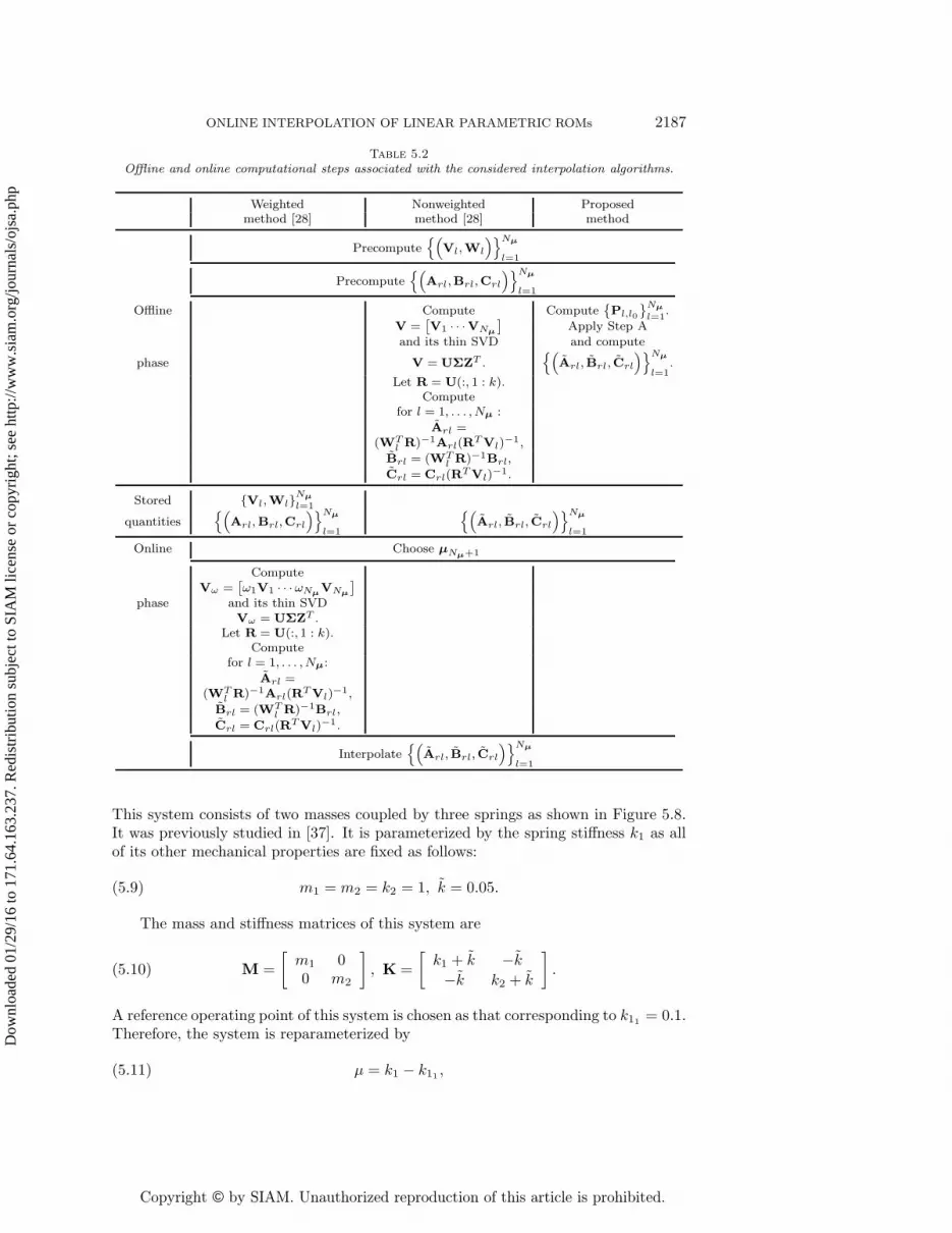
Table 5.2 summarizes the computational characteristics of algorithms (ii) and(iii), as well as those of the proposed method. Excluding the precomputation of theROBs and ROMs which is required by all compared algorithms, the computationalcomplexity of the proposed method is approximated by (Nµ−1)k2(2n+26k+2(p+q))operations, and that of the nonweighted algorithm proposed in [28] by Nµk

2(6Nµn+11N2

µk + 2k(2k + p+ q)). Both methods require storing Nµk(k + p+ q) words. Theweighted algorithm exposed in [28] does not require additional precomputations, butrequires storing Nµk(2n+ k + p+ q) words. During the online phase, this algorithmincurs, in addition to the interpolation cost, Nµk

2(6Nµn + 11N2µk + 2k(2k + p +

q)) operations, while the other two methods do not incur any additional cost. Tosummarize, only the method proposed in this paper and the nonweighted methodproposed in [28] have online capabilities. The proposed method requires, however,less preprocessing overhead.

The results reported in Figure 5.3 show that, for this problem, all consideredadaptation methods deliver the same excellent performance. Regarding the ROMbuilt using the GPOD technique [12], it should be mentioned, however, that Figure 5.5reveals that this ROM predicts an erroneous peak of the frequency response of themass-damper-spring system considered here. Similarly, Figure 5.5 shows that theeigenvalues with the largest real part of all interpolated ROMs match those of theHFM, but the counterpart eigenvalues of the GPOD-based ROM do not. This suggeststhat ROM interpolation, when properly performed, is a better alternative to a globalROM approach.

Finally, the performance of the ROM approaches considered in this section is as-sessed in the full parameter range μ ∈ [0, 1]. For this purpose, the relative H2- andH∞-norms of their error systems are computed and reported in Figures 5.6 and 5.7.The associated average errors in the same norms are reported in Table 5.3. Again,the largest error is observed for the global method. Both considered interpolationmethods deliver ROMs whose performances are comparable to that of the directlycomputed ROM. However, the reader is reminded once again that among these threeinterpolation methods, only that proposed in this paper and the nonweighted methodpresented in [28] have an online computational complexity which scales with the sizeof the ROM and not that of the HFM. The method presented in this paper requiresless preprocessing than its counterparts proposed in [28]. Furthermore, this methodhas a geometric interpretation that the two other methods presented in [28] lack. Forthe latter methods, the construction of operators of the form (WT

l R)−1Ar,l(RTVl)

−1

depends on the well-posedness of RTVl and WTl R, which is not necessarily guaran-

teed.

5.3. A dynamical system exhibiting mode veering. A simple mechanicalsystem presenting nevertheless a mode veering phenomenon [35] is considered here.

Dow

nloa

ded

01/2

9/16

to 1

71.6

4.16

3.23

7. R

edis

trib

utio

n su

bjec

t to

SIA

M li

cens

e or

cop

yrig

ht; s

ee h

ttp://

ww

w.s

iam

.org

/jour

nals

/ojs

a.ph

p



Table 5.2

Offline and online computational steps associated with the considered interpolation algorithms.

Weighted Nonweighted Proposedmethod [28] method [28] method

Precompute{(

Vl,Wl

)}Nµ

l=1

Precompute{(

Arl,Brl,Crl

)}Nµ

l=1

Offline Compute Compute{Pl,l0

}Nµ

l=1.

V =[V1 · · ·VNµ

]Apply Step A

and its thin SVD and compute

phase V = UΣZT .{(

Arl, Brl, Crl

)}Nµ

l=1.

Let R = U(:, 1 : k).Compute

for l = 1, . . . , Nµ :

Arl =(WT

l R)−1Arl(RTVl)

−1,

Brl = (WTl R)−1Brl,

Crl = Crl(RTVl)

−1.

Stored {Vl,Wl}Nµ

l=1

quantities{(

Arl,Brl,Crl

)}Nµ

l=1

{(Arl, Brl, Crl

)}Nµ

l=1

Online Choose µNµ+1

ComputeVω =

[ω1V1 · · ·ωNµVNµ

]phase and its thin SVD

Vω = UΣZT .Let R = U(:, 1 : k).

Computefor l = 1, . . . , Nµ:

Arl =(WT

l R)−1Arl(RTVl)

−1,

Brl = (WTl R)−1Brl,

Crl = Crl(RTVl)

−1.

Interpolate{(

Arl, Brl, Crl

)}Nµ

l=1

This system consists of two masses coupled by three springs as shown in Figure 5.8.It was previously studied in [37]. It is parameterized by the spring stiffness k1 as allof its other mechanical properties are fixed as follows:

(5.9) m1 = m2 = k2 = 1, k = 0.05.

The mass and stiffness matrices of this system are

(5.10) M =

[m1 00 m2

], K =

[k1 + k −k

−k k2 + k

].

A reference operating point of this system is chosen as that corresponding to k11 = 0.1.Therefore, the system is reparameterized by

(5.11) μ = k1 − k11 ,

Dow

nloa

ded

01/2

9/16

to 1

71.6

4.16

3.23

7. R

edis

trib

utio

n su

bjec

t to

SIA

M li

cens

e or

cop

yrig

ht; s

ee h

ttp://

ww

w.s

iam

.org

/jour

nals

/ojs

a.ph

p



–0.06 –0.05 –0.04 –0.03 –0.02 –0.01 0–8

–6

–4

–2

0

2

4

6

8

Real Part

Imag

inar

yP

art

HFMDirect ROMGPOD-Based ROMInterpolated ROM (Panzer et al.) – No Weights



Fig. 5.5. Mass-damper-spring system: Eigenvalues of the HFM and various ROMs for μ = 0.25.

0 0.1 0.2 0.3 0.4 0.5 0.6 0.7 0.8 0.9 110–3

10–2

10–1

100

μ

Rel

ativ

eE

rror

Direct ROMGPOD-Based ROMInterpolated ROM (Panzer et al.) – No Weights



Fig. 5.6. Ratio of the H2-norm of various error systems and H2-norm of the HFM.

and the domain of variation for μ is chosen as D = [0, k12 − k11 ], where k12 = 3. Theeigenvalues of this dynamical system are given by(5.12)

λ1,2 =k1m2 + k2m1 + k(m1 +m2)∓

√((k1 + k)m2 − (k2 + k)m1)2 + 4m1m2k2

2m1m2.

For the chosen values of the mechanical properties (5.9), the above eigenvalues become

(5.13) λ1,2(μ) =μ+ 1.2∓

√((μ− 0.9)2 + 0.01

2.

Dow

nloa

ded

01/2

9/16

to 1

71.6

4.16

3.23

7. R

edis

trib

utio

n su

bjec

t to

SIA

M li

cens

e or

cop

yrig

ht; s

ee h

ttp://

ww

w.s

iam

.org

/jour

nals

/ojs

a.ph

p



0 0.1 0.2 0.3 0.4 0.5 0.6 0.7 0.8 0.9 110–3

10–2

10–1

100

μ

Rel

ativ

eE

rror

Direct ROMGPOD-Based ROMInterpolat ed ROM (Panzer et al.) – No Weights

Interpolat ed ROM (Panzer et al.) – Weights

Interpolat ed ROM (Amsallem and Farhat)

Fig. 5.7. Ratio of the H∞-norm of various error systems and H∞-norm of the HFM.

Table 5.3

Comparison of the errors obtained with various adaptation methods over the μ-interval [0, 1].

Method Average relative error Average relative errorin the H2-norm in the H∞-norm

Direct ROM 1.81% 1.96%GPOD-based ROM 41.0% 51.7%

Interpolated ROM (Panzer et al.) 2.54% 2.92%- no weights

Interpolated ROM (Panzer et al.) 2.38% 2.69%- with weights

Interpolated ROM 1.86% 1.96%(Amsallem and Farhat)

Fig. 5.8. A two-mass three-spring mechanical system.

Figures 5.9 and 5.10 graphically depict the behavior of these eigenvalues when μ isvaried in the interval D = [0, 2.9]. In Figure 5.10, the first eigendirection is shown bya full line, and the second one by a dashed line. For the critical value μcr = 0.9—thatis, k1 = 1—a mode veering phenomenon can be observed. The modes undergo arotation of π

2 between μ = 0 and μ = 2.9. For μcr = 0.9, the angle of this rotation isequal to π

4 , and the eigenvalues of the dynamical system are

(5.14) λcr1 = 1.0, λcr

2 = 1.1.

Dow

nloa

ded

01/2

9/16

to 1

71.6

4.16

3.23

7. R

edis

trib

utio

n su

bjec

t to

SIA

M li

cens

e or

cop

yrig

ht; s

ee h

ttp://

ww

w.s

iam

.org

/jour

nals

/ojs

a.ph

p



0 0.5 1 1.5 2 2.5 30

0.5

1

1.5

2

2.5

3

3.5

μ

λ

Fig. 5.9. Eigenvalues loci for the two-mass three-spring mechanical system parameterized by μ.

0 0.5 1 1.5 2 2.5 3μ

Fig. 5.10. Variation of the orientations of the eigenmodes of the two-mass three-spring me-chanical system with μ.

Next, the two operating points of the above system defined by

(5.15) μ1 = 0, μ2 = 2.9

are considered and the following corresponding information is precomputed:(i) Diagonalized matrices (and therefore eigenvalues for each operating point)

(5.16) Mr(μ1) = I2, Kr(μ1) = Λ(μ1) =

[0.1472 0

0 1.0528

],

(5.17) Mr(μ2) = I2, K2(μ2) = Λ(μ2) =

[1.0488 0

0 3.0512

].

(ii) Inner products between the eigenmodes for each operating point

(5.18) P1,2 = X(μ1)TX(μ2) =

[0.0802 0.9968

−0.9968 0.0802

].

Dow

nloa

ded

01/2

9/16

to 1

71.6

4.16

3.23

7. R

edis

trib

utio

n su

bjec

t to

SIA

M li

cens

e or

cop

yrig

ht; s

ee h

ttp://

ww

w.s

iam

.org

/jour

nals

/ojs

a.ph

p



0 0.5 1 1.5 2 2.5 30

0.5

1

1.5

2

2.5

3

3.5

μ

λ

Fig. 5.11. Eigenvalues loci of the systems interpolated by Step B of the proposed methodand the complete (Steps A and B) method. Squares designate precomputed points, x’s designateexact eigenvalues, triangles designate eigenvalues obtained by Step B only, and circles designateeigenvalues computed by the proposed method.

The objective is set to numerically predict the variations of the eigenvalues of thetwo-mass three-spring system when μ is varied in D = [0, 2.9]—that is, to reproducethe results shown in Figure 5.9—by interpolating the precomputed information de-scribed above using the method proposed in this paper. Because of the mode veeringphenomenon exhibited in D = [0, 2.9], this objective is rather difficult. At this point,it is noted that whereas the precomputed matrices Mr(μl) and Kr(μl), l = 1, 2, arenot exactly reduced-order matrices, they derive from the classical modal reductiontechnique. However, no truncation is performed in this case because the consideredmechanical system has already a very small size. Therefore, despite the lack of modelreduction per se, the problem stated above is a good problem for illustrating theperformance of the proposed ROM interpolation method for parametric problemsfeaturing a curve veering phenomenon.

More specifically, the interpolation method proposed in this paper and the variantconsisting of Step B alone are applied to the solution of the above problem. In bothcases, the chosen manifold is SPD(2) because the matrices obtained after Step Aof the proposed interpolation method and the precomputed matrices (5.16), (5.17)are SPD. The obtained results are reported in Figure 5.11. The reader can observethat the variations with μ of the eigenvalues computed by the proposed interpolationmethod are found to be indistinguishable from the exact counterparts. However, thosecomputed by Step B alone are erroneous.

For the critical value μcr = 0.9, performing Step B of the proposed interpolationmethod alone returns

(5.19) MBr (μcr) = I2, KB

r (μcr) =

[0.427 00 1.6730

],

Dow

nloa

ded

01/2

9/16

to 1

71.6

4.16

3.23

7. R

edis

trib

utio

n su

bjec

t to

SIA

M li

cens

e or

cop

yrig

ht; s

ee h

ttp://

ww

w.s

iam

.org

/jour

nals

/ojs

a.ph

p



Fig. 5.12. Finite element structural model of the wing-store configuration.

which is consistent with the mathematical result established in [21], and stating thatthe interpolation in a tangent space to the manifold SPD(k) preserves the pattern ofa diagonal matrix. On the other hand, performing both Step A and Step B of theproposed interpolation method returns

(5.20) MABr (μcr) = I2, KAB

r (μcr) =

[1.0438 0.02430.0243 1.0735

].

As can be expected, Step B of the proposed method alone can neither capture noraddress the effect of the veering phenomenon. Therefore, as can be seen from (5.14)and the diagonal entries of KB

r (μcr) (5.19)—or from Figure 5.11—Step B deliverserroneous eigenvalues of the dynamical system at the critical parameter value μcr =0.9. Step A of the proposed interpolation method chooses the first operating point asreference and returns

(5.21) Q2 =

[0.0802 −0.99680.9968 0.0802

].

This reveals that the proposed interpolation method correctly matches the first andsecond eigenmodes for the second operating point of the dynamical system with thesecond and first eigenmodes for its first operating point, respectively. This explainshow it captures in this case the veering curve phenomenon.

5.4. Aircraft wing with store configuration. Finally, the following exampleis chosen to illustrate the application of the proposed ROM interpolation method toa more realistic, larger-scale mechanical system. This system consists of the AGARDWing 445.6 [38] equipped with a fuel tank (the store). The wing is discretized by 800composite shell elements, and the store by 1408 shell elements. The two subsystemsare connected by two sets of linear multipoint constraints, as illustrated in Figure 5.12.The finite element model of the assembled system has 6834 degrees of freedom andtherefore a dimension n = 6834. It is referred to in the remainder of this section asthe HFM of this realistic system.

The wing-store configuration outlined above is parameterized by the percentageof fill of the store by JP-8 fuel (the fill level). This percentage is denoted here by μand is varied between 14.6% and 99.9%. It is also referred to in this section as the

Dow

nloa

ded

01/2

9/16

to 1

71.6

4.16

3.23

7. R

edis

trib

utio

n su

bjec

t to

SIA

M li

cens

e or

cop

yrig

ht; s

ee h

ttp://

ww

w.s

iam

.org

/jour

nals

/ojs

a.ph

p



Table 5.4

Variations with the fill level of the first eight eigenfrequencies of the HFM of the wing-storesystem.

Frequency (Hz)Mode # 14.6% fill 30.9% fill 50.0% fill 69.1% fill 99.9% fill

1 11.508 11.421 11.293 11.177 11.0482 38.312 35.518 31.508 28.162 25.7063 43.151 37.935 33.578 31.245 29.5044 55.650 53.609 52.482 51.871 51.6685 95.833 93.001 90.383 88.478 85.9006 128.06 126.35 124.11 110.54 91.7117 156.36 146.70 130.06 125.86 125.498 163.06 162.37 161.51 158.57 152.42

20 40 60 80 1000

20

40

60

80

100

120

140

160

180

μ (in %)

Freq

uenc

y(H

z)

Fig. 5.13. Variations with the fill level μ of the first eight eigenfrequencies of the wing-storesystem.

operating point. JP-8 is considered to be an incompressible fluid and is modeled bya hydroelastic added mass [35]. As a result, for all possible fill levels, the HFM ofthe wing-store system has the same number of degrees of freedom and therefore thesame dimension, but represents a different dynamic behavior (further details aboutthis computational modeling procedure can be found in [39]). Studying this dynamicbehavior is an arduous task because for each new fill level, this requires regeneratinga mesh for the region of space enclosed by the tank and occupied by the fuel, andreassembling the HFM with the new added mass. For this reason, the fast predictionof the dynamic behavior of this parametric system without remeshing is desirable.Consequently, the problem is defined here as that of precomputing the eigenvalues ofthe wing-store structural system for two different operating points and interpolatingthem to quickly determine their values at three other operating points—that is, threeother fill levels.

For reference, Table 5.4 reports and Figure 5.13 plots the eigenfrequencies f—that is, the square roots of the eigenvalues divided by 2π—of the wing-store systemcomputed for various fill levels using the HFM. The reader can observe that modes 2and 3 on one hand and modes 6 and 7 on the other hand see their eigenfrequencies

Dow

nloa

ded

01/2

9/16

to 1

71.6

4.16

3.23

7. R

edis

trib

utio

n su

bjec

t to

SIA

M li

cens

e or

cop

yrig

ht; s

ee h

ttp://

ww

w.s

iam

.org

/jour

nals

/ojs

a.ph

p



Table 5.5

Variations with the fill level of the first eight eigenfrequencies of the wing-store system computedby Step B alone.

Frequency (Hz)Mode Relative error with respect to HFM-provided reference solutions shown in parentheses

14.6% fill 30.9% fill 50.0% fill 69.1% fill 99.9% fill

1 11.508 (0.00) 11.420 (0.01) 11.316 (0.21) 11.212 (0.32) 11.048 (0.00)2 38.312 (0.00) 35.911 (1.11) 33.060 (4.92) 30.208 (7.27) 25.706 (0.00)3 43.151 (0.00) 40.552 (6.90) 37.465 (11.65) 34.378 (10.03) 29.504 (0.00)4 55.65 (0.00) 54.892 (2.39) 53.991 (2.87) 53.090 (2.35) 51.668 (0.00)5 95.833 (0.00) 93.941 (1.01) 91.694 (1.45) 89.448 (1.09) 85.900 (0.00)6 128.06 (0.00) 121.14 (−4.13) 112.92 (−9.02) 104.69 (−5.29) 91.711 (0.00)7 156.36 (0.00) 150.48 (2.58) 143.50 (10.33) 136.52 (8.47) 125.49 (0.00)8 163.06 (0.00) 161.03 (−0.82) 158.63 (−1.79) 156.22 (−1.48) 152.42 (0.00)

getting closer to each other for μ4 = 50%, thereby suggesting the possibility of yetanother veering phenomenon.

The two configurations to be precomputed are set to be the “end point” configu-rations defined by μ1 = 14.6% and μ2 = 99.9%. For each of them, eight eigenmodes ofthe HFM are computed and exploited to construct reduced-order mass and stiffnessmatrices similar to those described in (5.16) and (5.17), but of dimension k = 8. Eachpair of these matrices defines a ROM counterpart of the HFM for the sampled filllevel. The inner products between the eigenmodes of the two precomputed operatingpoints are also computed and stored in the matrix P12 of dimension k = 8. The threeintermediate operating points are chosen as those defined by the fill levels μ3 = 30.9%,μ4 = 50.0%, and μ5 = 69.1%.

As in section 5.3, the interpolation method proposed in this paper and the variantconsisting of Step B alone are applied to the solution of the problem formulated above.In both cases, the chosen manifold is SPD(8) for the same reason stated in the caseof the problem of section 5.3, but in this case with k = 8.

Table 5.5 reports the eigenfrequencies associated with the intermediate operatingpoints computed using only Step B of the interpolation method proposed in this paperand their relative errors with respect to the HFM-provided reference solutions. It alsoincludes the data for the two precomputed operating points. In general, the obtainedresults are found to be tainted by less than 12% relative error and therefore areacceptable as fast numerical predictions. However, the reader can observe that Step Bof the proposed method alone does not reproduce the tendency of the eigenfrequenciesof modes 2 and 3 on one hand and modes 6 and 7 on the other hand to get closer forμ4 = 50% than they are for μ1 = 14.6% and μ2 = 99.9%.

Table 5.6 reports the eigenfrequencies associated with the intermediate operatingpoints computed by both steps of the proposed interpolation method, their relativeerrors with respect to the HFM-provided reference solutions, and the similar data forthe two precomputed operating points. The accuracy of the obtained results is foundto be in general at least as good as that obtained with Step B alone of the proposedmethod. Interestingly, it can be observed that the relative errors associated with thepredictions of the eigenfrequencies of modes 2 and 3 (roughly 10%) are much largerthan those for modes 6 and 7 (roughly 1%). This may be due to a strong nonlinearbehavior of the second and third eigenfrequencies when μ is varied between μ1 and μ2

that cannot be properly captured using two precomputed operating points only. Moreimportantly, however, whereas Step B of the proposed ROM interpolation method

Dow

nloa

ded

01/2

9/16

to 1

71.6

4.16

3.23

7. R

edis

trib

utio

n su

bjec

t to

SIA

M li

cens

e or

cop

yrig

ht; s

ee h

ttp://

ww

w.s

iam

.org

/jour

nals

/ojs

a.ph

p



Table 5.6

Variations with the fill level of the first eight eigenfrequencies of the wing-store system computedby the proposed ROM interpolation method.

Frequency (Hz)Mode Relative error with respect to HFM-provided reference solutions shown in parentheses

14.6% fill 30.9% fill 50.0% fill 69.1% fill 99.9% fill

1 11.508 (0.00) 11.436 (0.13) 11.340 (0.42) 11.234 (0.51) 11.048 (0.00)2 38.312 (0.00) 38.496 (14.67) 36.130 (8.38) 32.346 (14.86) 25.706 (0.00)3 43.151 (0.00) 40.524 (6.83) 38.283 (14.01) 35.437 (13.42) 29.504 (0.00)4 55.650 (0.00) 52.854 (−1.41) 50.907 (−3.00) 50.668 (−2.32) 51.668 (0.00)5 95.833 (0.00) 95.136 (2.30) 93.773 (3.75) 91.722 (3.67) 85.900 (0.00)6 128.06 (0.00) 125.25 (−0.87) 121.29 (−2.27) 110.57 (0.02) 91.711 (0.00)7 156.36 (0.00) 142.71 (−2.72) 129.07 (−0.76) 124.51 (−1.07) 125.49 (0.00)8 163.06 (0.00) 159.69 (−1.65) 156.68 (−2.99) 154.53 (−2.55) 152.42 (0.00)

1

2

3

4

5

6

7

8

12

34

56

78

0

0.2

0.4

0.6

0.8

1

Mode NumberMode Number

MA

C V

alue

0.1

0.2

0.3

0.4

0.5

0.6

0.7

0.8

0.9

(a) before Step A transformation

1

2

3

4

5

6

7

8

12

34

56

78

0

0.2

0.4

0.6

0.8

1

Mode NumberMode number

MA

C V

alue

0.1

0.2

0.3

0.4

0.5

0.6

0.7

0.8

0.9

(b) after Step A transformation

Fig. 5.14. Three-dimensional representation of the MAC values of the bases of natural modesprecomputed for μ = 14.9% and μ = 99.9% before (left) and after (right) transformation by the StepA algorithm of the basis precomputed for μ = 99.9%.

alone was found to be incapable of detecting the narrowing of the frequency gapsbetween modes 2 and 3 on one hand and modes 6 and 7 on the other hand for μ4 =50%, the results reported in Table 5.6 reveal that the proposed ROM interpolationmethod with both of its steps reproduces qualitatively this frequency gap narrowing.This is because, as shown in Figure 5.14, the precomputed natural bases are notconsistent (there is no reason why they should be consistent a priori), but Step A ofthe proposed ROM interpolation method transforms the natural basis of dimension 8associated with the second operating point into one that is almost perfectly consistentwith that associated with the first operating point.

For convenience, a summary of all of the results discussed above is given in graphform in Figure 5.15.

6. Summary and conclusions. Amethod for interpolating parametric reduced-order models (ROMs) on matrix manifolds has been presented. This method accountsfor the fact that parameterization typically results in ROMs that are naturally con-structed in inconsistent reduced-order bases—that is, in different generalized coordi-nates systems. It requires relatively little storage offline. It is also characterized by acomputational complexity which scales with the small size of the ROM. Therefore, it is

Dow

nloa

ded

01/2

9/16

to 1

71.6

4.16

3.23

7. R

edis

trib

utio

n su

bjec

t to

SIA

M li

cens

e or

cop

yrig

ht; s

ee h

ttp://

ww

w.s

iam

.org

/jour

nals

/ojs

a.ph

p



20 40 60 80 1000

20

40

60

80

100

120

140

160

180

200

220

μ (in %)

Freq

uenc

y(H

z)

Fig. 5.15. Variations with the fill level μ of the eigenfrequencies of the wing-store systemcomputed by the proposed ROM interpolation method and its Step B alone.

suitable for real-time processing. Like any other interpolation method, the dimensionof the parameter space on which it can operate is limited by practical considerations.Therefore for high-dimensional parameter spaces, it should be applied together witha parameter space reduction scheme [40]. The results of the application of this ROMinterpolation method to both academic and realistic dynamical systems pertaining tomechanical and aerospace engineering suggest that it is robust, capable of detectingand handling mode crossing and veering, and can deliver in general a good accuracy.

REFERENCES

[1] T. Lieu, C. Farhat, and M. Lesoinne, Reduced-order fluid/structure modeling of a completeaircraft configuration, Comput. Methods Appl. Mech. Engrg., 195 (2006), pp. 5730–5742.

[2] B.C. Moore, Principal component analysis in linear systems: Controllability, observability,and model reduction, IEEE Trans. Automat. Control, 26 (1981), pp. 17–32.

[3] M. Rathinam and L.R. Petzold, A new look at proper orthogonal decomposition, SIAM J.Numer. Anal., 41 (2003), pp. 1893–1925.

[4] L. Sirovich, Turbulence and the dynamics of coherent structures. Part 1: Coherent structures,Quart. Appl. Math., 45 (1987), pp. 561–571.

[5] A.C. Antoulas, Approximation of Large-Scale Dynamical Systems, Adv. Des. Control 6,SIAM, Philadelphia, 2005.

[6] B.I. Epureanu, A parametric analysis of reduced order models of viscous flows in turboma-chinery, J. Fluid. Struct., 17 (2003), pp. 971–982.

[7] C. Homescu, L.R. Petzold, and R. Serban, Error estimation for reduced-order models ofdynamical systems, SIAM J. Numer. Anal., 43 (2005), pp. 1693–1714.

[8] R. Serban, C. Homescu, and L.R. Petzold, The effect of problem perturbations on nonlin-ear dynamical systems and their reduced-order models, SIAM J. Sci. Comput., 29 (2007),pp. 2621–2643.

[9] T. Lieu and C. Farhat, Adaptation of aeroelastic reduced-order models and application to anF-16 configuration, AIAA J., 45 (2007), pp. 1244–1269.

[10] D. Amsallem and C. Farhat, Interpolation method for adapting reduced-order models andapplication to aeroelasticity, AIAA J., 46 (2008), pp. 1803–1813.

Dow

nloa

ded

01/2

9/16

to 1

71.6

4.16

3.23

7. R

edis

trib

utio

n su

bjec

t to

SIA

M li

cens

e or

cop

yrig

ht; s

ee h

ttp://

ww

w.s

iam

.org

/jour

nals

/ojs

a.ph

p



[11] K. Ito and S.S. Ravindran, A reduced-order method for simulation and control of fluid flows,J. Comput. Phys., 143 (1998), pp. 403–425.

[12] J. Taylor and M. Glauser, Towards practical flow sensing and control via POD and LSEbased low-dimensional tools, in Proceedings of the 2002 ASME Fluids Engineering DivisionSummer Meeting, 2002, pp. 1–9.

[13] T. Bechtold, D. Hohlfeld, E.B. Rudnyi, and M. Gunther, Efficient extraction of thin-film thermal parameters from numerical models via parametric model order reduction, J.Micromec. Microeng., 20 (2010), 045030.

[14] G. Rozza, D.B.P. Huynh, and A.T. Patera, Reduced basis approximation and a posteriorierror estimation for affinely parametrized elliptic coercive partial differential equations:Application to transport and continuum mechanics, Arch. Comput. Method Engrg., 15(2007), pp. 229–275.

[15] B. Haasdonk and M. Ohlberger, Efficient reduced models and a-posteriori error estima-tion for parametrized dynamical systems by offline/online decomposition, Math. Comput.Model. Dynam., 17 (2011), pp. 145–161.

[16] L. Daniel, O.C. Siong, L.S. Chay, K.H. Lee, and J. White, A multiparameter moment-matching model-reduction approach for generating geometrically parameterized intercon-nect performance models, IEEE Trans. Comput. Aided Des., 23 (2004), pp. 678–693.

[17] T. Bui-Thanh, K. Willcox, and O. Ghattas, Parametric reduced-order models for proba-bilistic analysis of unsteady aerodynamic applications, AIAA J., 46 (2008), pp. 2520–2529.

[18] C. Gu and J. Roychowdhury, Model reduction via projection onto nonlinear manifolds, withapplications to analog circuits and biochemical systems, in Proceedings of the IEEE/ACM2008 International Conference on Computer-Aided Design, 2008, pp. 85–92.

[19] A. Hay, J. Borggaard, I. Akhtar, and D. Pelletier, Reduced-order models for parameterdependent geometries based on shape sensitivity analysis, J. Comput. Phys., 229 (2010),pp. 1327–1352.

[20] D. Amsallem, J. Cortial, and C. Farhat, Toward real-time CFD-based aeroelastic compu-tations using a database of reduced-order information, AIAA J., 48 (2010), pp. 2029–2037.

[21] D. Amsallem, J. Cortial, K. Carlberg, and C. Farhat, A method for interpolating onmanifolds structural dynamics reduced-order models, Internat. J. Numer. Methods Engrg.,80 (2009), pp. 1241–1258.

[22] J. Degroote, J. Virendeels, and K. Willcox, Interpolation among reduced-order matrices toobtain parameterized models for design, optimization and probabilistic analysis, Internat.J. Numer. Methods Fluids, 63 (2010), pp. 207–230.

[23] U. Baur and P. Benner, Modellreduktion fur parametrisierte systeme durch balanciertes ab-schneiden und interpolation, Automatisierungstechnik, 57 (2009), pp. 411–419.

[24] K. Carlberg, C. Bou-Mosleh, and C. Farhat, Efficient nonlinear model reduction via aleast-squares Petrov-Galerkin projection and compressive tensor approximations, Internat.J. Numer. Methods Engrg., 86 (2011), pp. 155–181.

[25] M. Rewienski and J. White, Model order reduction for nonlinear dynamical systems based ontrajectory piecewise-linear approximations, Linear Algebra Appl., 415 (2006), pp. 426–454.

[26] B. Lohmann and R. Eid, Efficient order reduction of parametric and nonlinear models bysuperposition of locally reduced models, in Methoden und Anwendungen der Regelung-stechnik. Erlangen-Munchener Workshops 2007 und 2008, Shaker Verlag, Aachen, 2009,pp. 1–20.

[27] R. Eid, B. Lohmann, and H. Panzer, Interpolation-based parametric model reduction usingKrylov subspaces, in Autumn School on Future Developments in MOR, Terschelling, 22September 2009, pp. 1–9.

[28] H. Panzer, J. Mohring, R. Eid, and B. Lohmann Parametric model order reduction bymatrix interpolation, Automatisierungstechnik, 58 (2010), pp. 475–484.

[29] U. Helmke and J.B. Moore, Optimization and Dynamical Systems, Springer-Verlag, London,1994.

[30] G.H. Golub and C.F. Van Loan,Matrix Computations, 3rd ed., The Johns Hopkins UniversityPress, Baltimore, MD, 1996.

[31] D.J. Ewins, Modal Testing, Theory, Practice and Application, 2nd ed., Research Study PressLTD, Philadelphia, 2000.

[32] J. O’Callahan, Correlation considerations—Part 4 (Modal vector correlation techniques), inProceedings of the International Modal Analysis Conference, 1998, pp. 197–206.

[33] T.S. Kim and Y.Y. Kim, Mac-based mode tracking in structural topology optimization, Comput.Struct., 74 (2000), pp. 375–383.

[34] O. Bruls, P. Duysinx, and J.C. Golinval, The global modal parameterization for non-linearmodel-order reduction in flexible multibody dynamics, Internat. J. Numer. Methods Engrg.,69 (2007), pp. 958–977.

Dow

nloa

ded

01/2

9/16

to 1

71.6

4.16

3.23

7. R

edis

trib

utio

n su

bjec

t to

SIA

M li

cens

e or

cop

yrig

ht; s

ee h

ttp://

ww

w.s

iam

.org

/jour

nals

/ojs

a.ph

p



[35] H.J.-P. Morand and R. Ohayon, Fluid-Structure Interaction, Wiley, New York, 1995.[36] G.H.K. Heirman, F. Naets, and W. Desmet, A system-level model reduction technique for

the efficient simulation of flexible multibody systems, Internat. J. Numer. Methods Engrg.,85 (2011), pp. 330–354.

[37] N.G. Stephen, On veering of eigenvalue loci, J. Vib. Acoust., 131 (2009), 054501.[38] E.C. Yates, Agard standard aeroelastic configurations for dynamic response, candidate config-

uration I. Wing 445.6, NASA TM-100462, Langley Research Center, Hampton, VA, 1987.[39] E.K. Chiu and C. Farhat, Effects of Fuel Slosh on Flutter Prediction, AIAA Paper 2009-2682,

AIAA, Reston, VA, 2009.[40] C. Lieberman, K. Willcox, and O. Ghattas, Parameter and state model reduction for large-

scale statistical inverse problems, SIAM J. Sci. Comput., 32 (2010), pp. 2523–2542.

Dow

nloa

ded

01/2

9/16

to 1

71.6

4.16

3.23

7. R

edis

trib

utio

n su

bjec

t to

SIA

M li

cens

e or

cop

yrig

ht; s

ee h

ttp://

ww

w.s

iam

.org

/jour

nals

/ojs

a.ph

p

an online method for interpolating linear parametric reduced-order models

Documents