a method for interpolating on manifolds structural dynamics reduced-order models
TRANSCRIPT
INTERNATIONAL JOURNAL FOR NUMERICAL METHODS IN ENGINEERINGInt. J. Numer. Meth. Engng 2009; 0:1–16 Prepared using nmeauth.cls [Version: 2002/09/18 v2.02]
A method for interpolating on manifolds structural dynamicsreduced-order models
David Amsallem1∗, Julien Cortial2, Kevin Carlberg1 and Charbel Farhat3
1 Department of Aeronautics and Astronautics2 Institute for Computational and Mathematical Engineering
3 Vivian Church Hoff Professor of Aircraft Structures, Department of Aeronautics and Astronautics,Department of Mechanical Engineering and Institute for Computational and Mathematical Engineering
Stanford University, Mail Code 3035, Stanford, CA 94305, U.S.A.
SUMMARY
A rigorous method for interpolating a set of parameterized linear structural dynamics reduced-ordermodels (ROMs) is presented. By design, this method does not operate on the underlying set ofparameterized full-order models. Hence, it is amenable to an on-line real-time implementation. It isbased on mapping appropriately the ROM data onto a tangent space to the manifold of symmetricpositive definite matrices, interpolating the mapped data in this space and mapping back the resultto the aforementioned manifold. Algorithms for computing the forward and backward mappings areoffered for the case where the ROMs are derived from a general Galerkin projection method andthe case where they are constructed from modal reduction. The proposed interpolation methodis illustrated with applications ranging from the fast dynamic characterization of a parameterizedstructural model to the fast evaluation of its response to a given input. In all cases, good accuracy isdemonstrated at real-time processing speeds. Copyright c© 2009 John Wiley & Sons, Ltd.
key words: reduced-order modeling; matrix manifolds; real-time prediction; surrogate modeling;
linear structural dynamics
1. INTRODUCTION
The concept of model reduction is old in structural dynamics. It has — and is still — beenused for many purposes ranging from the design of a test-analysis model to provide a basis forcomparing computational and experimental results, to the alleviation of the computationalburden associated with large-scale finite element models. Among the many linear modelreduction techniques that have been or remain popular in industry, one can mention Guyan’s
∗Correspondence to: Department of Aeronautics and Astronautics, Stanford University, Mail Code 3035,Stanford, CA 94305, U.S.A.
Contract/grant sponsor: Air Force Office of Scientific Research; contract/grant number: 49620-01-1-0129
Contract/grant sponsor: National Science Foundation; contract/grant number: 0540419
Copyright c© 2009 John Wiley & Sons, Ltd.
2 D. AMSALLEM, J. CORTIAL, K. CARLBERG AND C. FARHAT
reduction method [1] and the related superelement dynamic reduction approaches, the IRSdynamic reduction method [2], and of course, the ubiquitous modal reduction method. Morerecently, the Proper Orthogonal Decomposition (POD) [3] method, which can be used togenerate a reduced-order model (ROM) capable of accurately reproducing the dynamics ofthe underlying full-order model for a given set of input forces, has gained status in the linearstructural dynamics community [4, 5, 6]. All of these methods can be described as Galerkinprojection techniques onto carefuly chosen reduced-order bases. They are back in voguefor incorporating computational models in design operations [7], designing effective controlsystems for large-scale flexible structures [8], generating surrogate models for acceleratingthe speed of optimization procedures [9] and developing realistic uncertainty quantificationanalysis methods [10]. In all of these applications, structural dynamics ROMs are sought afterbecause of their potential for operating in real-time.
Unfortunately in all of the above and many other applications, structural dynamics modelsare usually parameterized, their reduced-order counterparts tend to lack robustness[12, 11]with respect to parameter changes, and the reconstruction of these small-size counterpartsfor each new set of parameters can be computationally prohibitive. Hence, there is a pressingneed for a fast ROM adaptation procedure which can operate on-line and in real-time. Here,on-line characterizes a procedure which does not operate on the full-order model at the originof a ROM and therefore which avoids the manipulation of a large-scale complex simulationsoftware and the associated implementation burden. The real-time requirement is to preservethe reason why ROMs are desired in the first place for the target applications — that is,computational speed.
To develop a structural dynamics ROM adaptation procedure that meets the aforementionedrequirements, a database of reduced-order information can be precomputed for selected valuesof the parameter set and interpolation can be invoked for generating ROMs for other valuesof this parameter set. However, it turns out that interpolating reduced-order data is not aneasy task. For example, reduced-order bases are often orthogonal and the straightforwardinterpolation of sets of orthogonal vectors does not necessarily generate a new set of orthogonalvectors. Similarly, the straightforward interpolation of ROMs does not necessarily yield a ROM.This is because neither reduced-order bases nor ROMs live in vector spaces.
Most recently, a numerical method based on interpolation in a tangent space to theGrassmann manifold was developed for adapting CFD (computational fluid dynamics)-basedreduced-order POD bases to parameter changes in real-time [11, 13]. However, the applicationof such a method to the interpolation of projection-based ROMs can neither be performed on-line nor in real-time, because it requires first evaluating the underlying full-order model at thenew value of the parameter set, then projecting this model onto the interpolated reduced-orderbasis. In this work, the symmetric positive definite nature of linear structural dynamics modelsis exploited to develop an interpolation method which directly operates on linear structuraldynamics ROMs rather than on their associated reduced-order bases and therefore can beimplemented on-line and perform in real-time. To this effect, the remainder of this paper isorganized as follows.
In Section 2, the representation of a linear structural dynamic ROM is abstracted andthe ROM adaptation problem is formulated. In Section 3.2, a method based on mappingappropriately the ROM data onto a tangent space to the manifold of symmetric positivedefinite matrices of size n, SPD(n), interpolating the mapped data in this space and mappingback the result to the aforementioned manifold is presented. Algorithms for computing the
Copyright c© 2009 John Wiley & Sons, Ltd. Int. J. Numer. Meth. Engng 2009; 0:1–16Prepared using nmeauth.cls

A METHOD FOR INTERPOLATING ON MANIFOLDS STRUCTURAL DYNAMICS ROMS 3
forward and backward mappings are offered in Section 3.3.1 for the special case where theROMs are constructed by modal reduction and in Section 3.3.2 for the case where they areconstructed by a general Galerkin projection method. The proposed interpolation method isillustrated in Section 4 with simple applications which nevertheless highlight its ability todeliver good accuracy at real-time processing speeds.
2. PROBLEM FORMULATION
In this work, a parameterized linear structural dynamics (full-order) model of size N isabstracted as a triplet of the form(
M(s), C(s), K(s))∈
(RN×N , RN×N , RN×N
), (1)
where M , C and K are symmetric positive definite mass, damping and stiffness matrices,respectively, and s = (s0, s1, . . . , sNp−1) denotes a set of Np model parameters. Theseparameters can be physical, non-physical, or a combination of both.
Similarly, a corresponding ROM of size n << N is abstracted here as
• A1: a triplet of reduced mass, damping and stiffness matrices that are assumed here tobe symmetric positive definite
R(s) =(M?(s), C?(s), K?(s)
)∈
(Rn×n, Rn×n, Rn×n
), (2)
or
• A2: a quintuplet of the form
R(s) =(M?(s), C?(s), K?(s), X(s), Z(s)
)∈
(Rn×n, Rn×n, Rn×n, RN×n, RN×n
),
(3)where
M?(s) = XT (s)M(s)X(s), C?(s) = XT (s)C(s)X(s),
K?(s) = XT (s)K(s)X(s), Z(s) = A(s)X(s),(4)
A ∈ RN×N is a real symmetric positive definite matrix, X(s) denotes a projection matrixrelating the full- and reduced-order displacement vectors u ∈ RN and q ∈ Rn via
u(t, s) = X(s)q(t, s) (5)
and satisfying the orthogonality condition
XT (s)Z(s) = In, (6)
t denotes time, In ∈ Rn×n is the identity matrix of size n and the superscript T designatesthe transpose operation.
Indeed, the governing equations associated with a linear structural dynamics ROM can bewritten in general as
M?(s)q(t, s) + C?(s)q(t, s) + K?(s)q(t, s) = F ?(t, s), (7)
where a dot designates a time derivative. Hence, definition A1 is appropriate when the loadingon the structure is not of any particular interest and therefore F ?(t, s) = 0 — for example, when
Copyright c© 2009 John Wiley & Sons, Ltd. Int. J. Numer. Meth. Engng 2009; 0:1–16Prepared using nmeauth.cls
4 D. AMSALLEM, J. CORTIAL, K. CARLBERG AND C. FARHAT
the main interest is in determining a set of natural frequencies of the full-order parameterizedstructural model. In this case, M?, C? and K? do not necessarily result from a projectiontechnique but are assumed here to be symmetric positive definite. Definition A2 is appropriateas soon as F ?(t, s) 6= 0 or the mapping between u(t, s) and q(t, s) is required. It covers mostlinear ROMs constructed by popular projection techniques where X(s) ∈ RN×n is a realrectangular matrix whose columns form a reduced-order basis and A(s) is associated with ametric. In this case, F ?(t, s) = XT (s)F (t) and X(s) satisfies an orthogonality constraint. Forexample, when X(s) is generated by the POD method, this matrix satisfies XT (s)X(s) = In
and therefore A(s) = IN . Alternatively, X(s) can be a set of eigenvectors of the pencil(M(s), K(s)
), in which case A(s) = M(s) and therefore the ROM is essentially a truncated
modal representation of the structure. In all cases, M?, C? and K? are symmetric positivedefinite and therefore belong to the manifold SPD(n).
Using the above nomenclature, the focus of this paper is on solving the following problem.Problem. Let s(i) =
(s(i)0 , s
(i)1 , . . . , s
(i)Np−1
)denote a specific configuration of the set of Np
parameters s. In the remainder of this paper, s(i) is referred to as the (i + 1)-th point of a setof operating points
S =(s(0), s(1), . . . , s(NR−1)
). (8)
Let also RiNR−1i=0 =
R
(s(i)
)NR−1
i=0denote a set of NR linear structural dynamics ROMs of
the same dimension n constructed at the operating pointss(i)
NR−1
i=0. Given a new operating
point s(NR) /∈ S, compute on-line and in real-time RNR= R
(s(NR)
).
The remainder of this paper proposes a solution to the above problem based on a suitableinterpolation method.
3. ROM ADAPTATION METHODS
Three different but related ROM adaptation methods are presented here: one for the casewhere the ROMs RiNR−1
i=0 are of type A1 and two for the case where they are of type A2.All three methods share the concept of interpolation in a tangent space to a manifold. Unlikeany straightforward interpolation scheme, this concept enables all three methods to producefor any new operating point s(NR) a result R
(s(NR)
)that is a genuine ROM — that is, a result
RNRwhose matrices M?
(s(NR)
), C?
(s(NR)
)and K?
(s(NR)
)are symmetric positive definite
and whose matrix X(s(NR)
)in the case of type A2 satisfies the constraints
(6). All of these
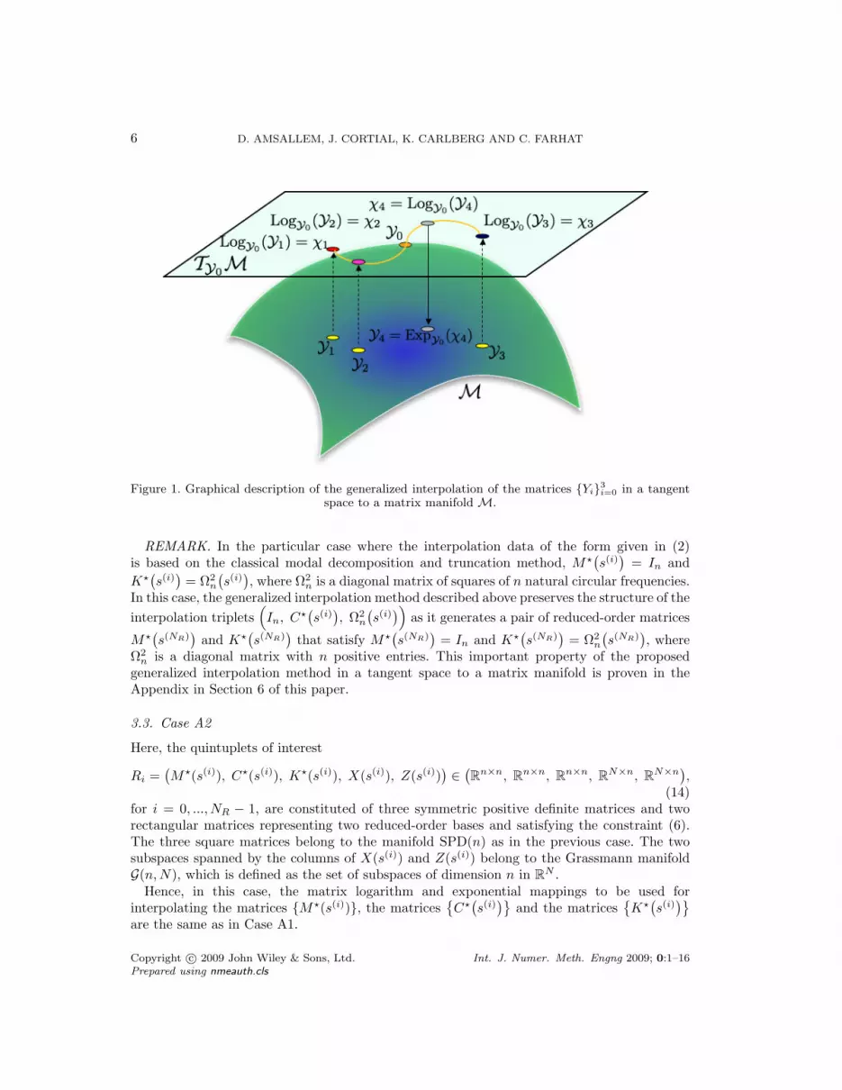
methods are based on the approach presented in Section 3.1 which can be summarized asfollows: first, the data to be interpolated is mapped appropriately onto a tangent space tothe appropriate manifold, then the mapped data is interpolated in this space and finally theinterpolation result is mapped back to the same manifold (see Figure 1).
For a background on interpolation in a tangent space to a manifold, the reader can consultreferences [11, 13], among others.
3.1. Interpolation in a Tangent Space to a Manifold
LetYi = Y
(s(i)
)NR−1
i=0denote a set of elements of a manifold M associated with a set
of different operating points s(i)NR−1i=0 . Each element Yi is represented here by a matrix
Copyright c© 2009 John Wiley & Sons, Ltd. Int. J. Numer. Meth. Engng 2009; 0:1–16Prepared using nmeauth.cls
A METHOD FOR INTERPOLATING ON MANIFOLDS STRUCTURAL DYNAMICS ROMS 5
Yi ∈ Rm×p that belongs to some matrix manifold M′ and verifies one or more specificproperties that characterize M′. (The m-dimensional sphere, Sm, the group of orthogonalmatrices of size m, O(m), and the set of symmetric positive matrices of size m SPD(m) areexamples of simple matrix manifolds.) The following four-step method is proposed to constructa new element YNR
∈ M associated with a new operating point s(NR) and its representativematrix YNR
— that is, an element YNR∈ M and its representative matrix YNR
∈ M′ whichhave the same properties as each element Yi and its representative matrix Yi, i = 0, ..., NR−1,respectively.
• Step 0. Choose an element Yi0 in the data set YiNR−1i=0 as a reference element of the
manifold M.• Step 1. Consider a few elements of the set YiNR−1
i=0 that lie in a neighborhood ofYi0 . Map each of them onto the tangent space to M at Yi0 denoted here by TYi0
M.More specifically, map each element Yi that is sufficiently close to Yi0 to an elementχi ∈ TYi0
M represented by a matrix Γi, using the logarithm map LogYi0which provides
an appropriate continuous mapping to the tangent space of the manifold at Yi0 . Thiscan be written as:
χi = LogYi0(Yi). (9)
• Step 2. Compute each entry of an m×p matrix ΓNRassociated with the target operating
point s(NR) by interpolating the corresponding entries of the m × p matrices Γiassociated with the operating points s(i) using any preferred multi-variate interpolationalgorithm.
• Step 3. Map the element χNR∈ TYi0
M represented by the matrix ΓNRto an element
YNR∈ M represented by a matrix YNR
∈ M′ using the exponential map ExpYi0. This
can be written asYNR
= ExpYi0(χNR
). (10)
In the remainder of this paper, the above method is referred to as the “generalized” (becauseit involves more than) interpolation of a set of elements Yi in a tangent space to a matrixmanifold M. The specific algorithms for computing the logarithm and exponential mappingsdepend of the manifold M and are discussed next.
3.2. Case A1
Here, M = M′ = SPD(n) as the triplets of interest
Ri =(M?(s(i)), C?(s(i)), K?(s(i))
)∈
(Rn×n, Rn×n, Rn×n
), i = 0, ..., NR − 1 (11)
are constituted of symmetric positive definite matrices. In this case, the matrix logarithm andexponential mappings are given by[14]
LogYi0(Yi) = logm
(Y−1/2i0
YiY−1/2i0
)(12)
andExpYi0
(Γ) = Y1/2i0
expm(Γ)Y 1/2i0
, (13)
where logm and expm denote the matrix logarithm and exponential, respectively.
Copyright c© 2009 John Wiley & Sons, Ltd. Int. J. Numer. Meth. Engng 2009; 0:1–16Prepared using nmeauth.cls
6 D. AMSALLEM, J. CORTIAL, K. CARLBERG AND C. FARHAT
Figure 1. Graphical description of the generalized interpolation of the matrices Yi3i=0 in a tangentspace to a matrix manifold M.
REMARK. In the particular case where the interpolation data of the form given in (2)is based on the classical modal decomposition and truncation method, M?
(s(i)
)= In and
K?(s(i)
)= Ω2
n
(s(i)
), where Ω2
n is a diagonal matrix of squares of n natural circular frequencies.In this case, the generalized interpolation method described above preserves the structure of theinterpolation triplets
(In, C?
(s(i)
), Ω2
n
(s(i)
))as it generates a pair of reduced-order matrices
M?(s(NR)
)and K?
(s(NR)
)that satisfy M?
(s(NR)
)= In and K?
(s(NR)
)= Ω2
n
(s(NR)
), where
Ω2n is a diagonal matrix with n positive entries. This important property of the proposed
generalized interpolation method in a tangent space to a matrix manifold is proven in theAppendix in Section 6 of this paper.
3.3. Case A2
Here, the quintuplets of interest
Ri =(M?(s(i)), C?(s(i)), K?(s(i)), X(s(i)), Z(s(i))
)∈
(Rn×n, Rn×n, Rn×n, RN×n, RN×n
),
(14)for i = 0, ..., NR − 1, are constituted of three symmetric positive definite matrices and tworectangular matrices representing two reduced-order bases and satisfying the constraint (6).The three square matrices belong to the manifold SPD(n) as in the previous case. The twosubspaces spanned by the columns of X(s(i)) and Z(s(i)) belong to the Grassmann manifoldG(n, N), which is defined as the set of subspaces of dimension n in RN .
Hence, in this case, the matrix logarithm and exponential mappings to be used forinterpolating the matrices M?(s(i)), the matrices
C?
(s(i)
)and the matrices
K?
(s(i)
)are the same as in Case A1.
Copyright c© 2009 John Wiley & Sons, Ltd. Int. J. Numer. Meth. Engng 2009; 0:1–16Prepared using nmeauth.cls
A METHOD FOR INTERPOLATING ON MANIFOLDS STRUCTURAL DYNAMICS ROMS 7
The computation of the two matrices X(s(NR)
)and Z
(s(NR)
)requires the generalized
interpolation of two different sets of matricesX
(s(i)
)and
Z
(s(i)
)that are however
connected by the orthogonality condition (6). Hence, this computation cannot be performedusing the generalized interpolation method presented in Section 3.1 as is. Instead, it is proposedto simultaneously interpolate the set of matrices X
(s(i)
)and set of matrices Z
(s(i)
)column-
block per column-block while enforcing the orthogonality constraint (6). For this purpose,two sub-cases are distinguished: the sub-case where X
(s(NR)
)is associated with the classical
modal decomposition and truncation method and that where X(s(NR)
)is associated with an
arbitrary Galerkin projection method.
3.3.1. Modal Truncation The modal truncation approach differs from the general Galerkinprojection approach in that each individual column of a matrix X(s(i)) has a specific meaningand importance that must be preserved during the interpolation process. More specifically, ifthe columns of the matrices
X
(s(i)
)to be interpolated are ordered so that the j-th column
of each of them refers to the same eigenmode, then the j-th column of the interpolated matrixX
(s(NR)
)must refer to the same eigenmode. This is not true however for a set of matrices
X(s(i)
)associated with an arbitrary Galerkin projection method. Therefore, the generalized
interpolation method proposed here loops on the eigensubspacesSX
ij
and subspaces
SZ
ij
(where i refers to s(i)
)of the parameterized system underlying all matrices
X
(s(i)
)and
Z(s(i)
)and interpolates each of such set of matrices while enforcing the orthogonality
constraint (6) as described below. For clarity, the proposed generalized interpolation methodis first described in the simple case where each eigensubspace is of dimension 1. In this case,SX
ij ∈ G(1, N) and SZij ∈ G(1, N).
For j = 1, . . . , n
• Step 0. Interpolate the eigensubspacesSX
ij ∈ G(1, N)
using the generalizedinterpolation algorithm described in Section 3.1 with M = G(1, N) and M′ the noncompact Stiefel manifold of non zero vectors of size N . The matrix logarithm andexponential mappings associated with G(1, N) are given by(
IN −Xi0j
(XT
i0jXi0j
)−1XT
i0j
)Xij
(XT
i0jXij
)−1 (XT
i0jXi0j
) 12 = UΣV T (Thin SVD)
(15)
LogSi0j(Sij) = span
(U tan−1(Σ)V T
)(16)
and
Γ = UΣV T (Thin SVD) (17)
ExpSi0j(χ) = span
(Xi0j
(XT
i0jXi0j
)− 12 V cos(Σ) + U sin(Σ)
), (18)
where Xij denotes the j-th column of X(s(i)
).
• Step 1. Perform a Gram-Schmidt procedure on XNRj to enforce the orthogonalityconditions XT
NRjZNRl = 0, l = 1, . . . , j − 1, where Zij denotes the j-th column ofZ
(s(i)
).
Copyright c© 2009 John Wiley & Sons, Ltd. Int. J. Numer. Meth. Engng 2009; 0:1–16Prepared using nmeauth.cls
8 D. AMSALLEM, J. CORTIAL, K. CARLBERG AND C. FARHAT
• Step 2. Interpolate the subspacesSZ
ij ∈ G(1, N)
using the generalized interpolationalgorithm described in Section 3.1 with M = G(1, N) and M′ the non compact Stiefelmanifold of non zero vectors of size N .
• Step 4. Perform a Gram-Schmidt procedure on ZNRj to enforce the orthogonalityconditions XT
NRlZNRj = 0, l = 1, . . . , j − 1 and XTNRjZNRj = 1.
• Step 5. Scale XNRj and ZNRj so that their two-norms are comparable to the two-normsof Xij and Zij, respectively.
The extension of the above generalized interpolation algorithm to the case where eacheigensubspace SX
ij is of the same dimension kj > 1 is straightforward. The extension tothe case where kj is variable requires book keeping.
3.3.2. Arbitrary Galerkin Projection In this case, the proposed generalized interpolationmethod is identical to that described in the previous section for kj = 1.
4. APPLICATIONS
Here, the proposed interpolation method is illustrated with two simple applications thathighlight its potential for adapting on-line a structural dynamics ROM to a new operatingpoint.
4.1. Case A1: a Mass-Damper-Spring System
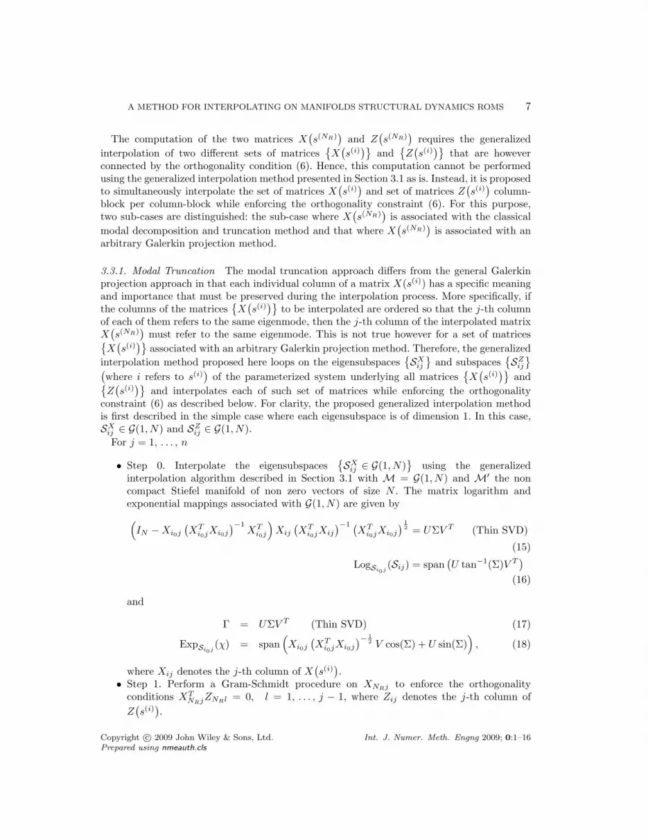
The dynamic equations of equilibrium governing the mass-damper-spring system shown inFigure 2 (and previously studied by Kim [15]) can be reduced by Galerkin projection andwritten in state-space form as follows
z(t, s) = H(s)z(t, s) + b(s), (19)
where
z(t, s) =[q(t, s)q(t, s)
], H(s) =
[−M?(s)−1
C?(s) −M?(s)−1K?(s)
In 0n
], b(s) =
[M?(s)−1
F ?(s)0
](20)
and 0n denotes the zero matrix of size n, where n denotes the size of the reduced-order basis.Each operating point of this mechanical system consists of 3p parameters corresponding to
the 3p values of the masses mjpj=1, dampers cjp
j=1 and springs kjpj=1. However for the
sake of simplicity, it is assumed here that: ∀j = 1, . . . , p, mj = m, cj = c, and kj = k, sothat each operating point is uniquely defined by the three parameters (m, c, k), only.
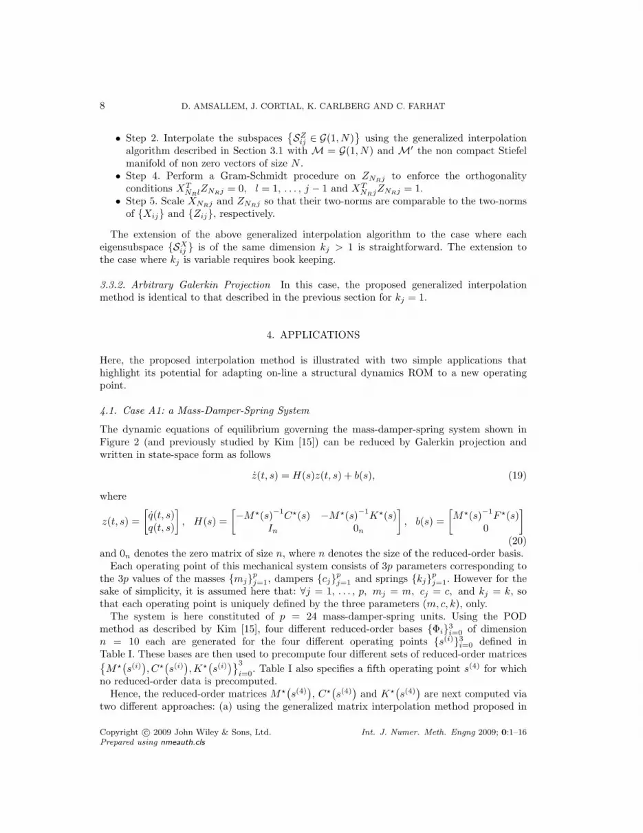
The system is here constituted of p = 24 mass-damper-spring units. Using the PODmethod as described by Kim [15], four different reduced-order bases Φi3i=0 of dimensionn = 10 each are generated for the four different operating points s(i)3i=0 defined inTable I. These bases are then used to precompute four different sets of reduced-order matricesM?
(s(i)
), C?
(s(i)
),K?
(s(i)
)3
i=0. Table I also specifies a fifth operating point s(4) for which
no reduced-order data is precomputed.Hence, the reduced-order matrices M?
(s(4)
), C?
(s(4)
)and K?
(s(4)
)are next computed via
two different approaches: (a) using the generalized matrix interpolation method proposed in
Copyright c© 2009 John Wiley & Sons, Ltd. Int. J. Numer. Meth. Engng 2009; 0:1–16Prepared using nmeauth.cls
A METHOD FOR INTERPOLATING ON MANIFOLDS STRUCTURAL DYNAMICS ROMS 9
Figure 2. Mass-damper-spring system.
Table I. Five operating points of a mass-damper-spring system.
m c k
s(0) 0.3 0.6 0.7
s(1) 0.7 0.6 1.3
s(2) 0.9 0.6 1.0
s(3) 1.1 0.6 0.4
s(4) 0.8 0.6 1.1
this paper and (b) by generating first a new POD basis Φ4 for the operating point s(4) andthen projecting the full-order matrices M
(s(4)
), C
(s(4)
)and K
(s(4)
)onto this basis. In both
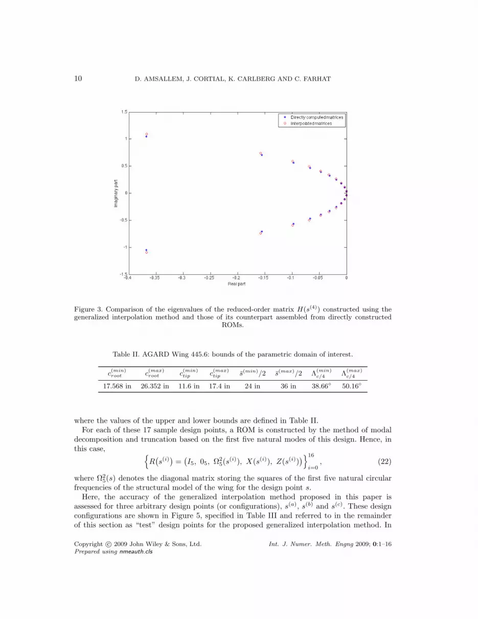
cases, the matrix H(s(4)) is next constructed and its eigenvalues are computed. These aregraphically reported in Figure 3 which reveals that the eigenvalues of the interpolated ROMmatrix H(s(4)) are in good agreement with those of its directly constructed counterpart.
4.2. Case A2: the AGARD Wing 445.6
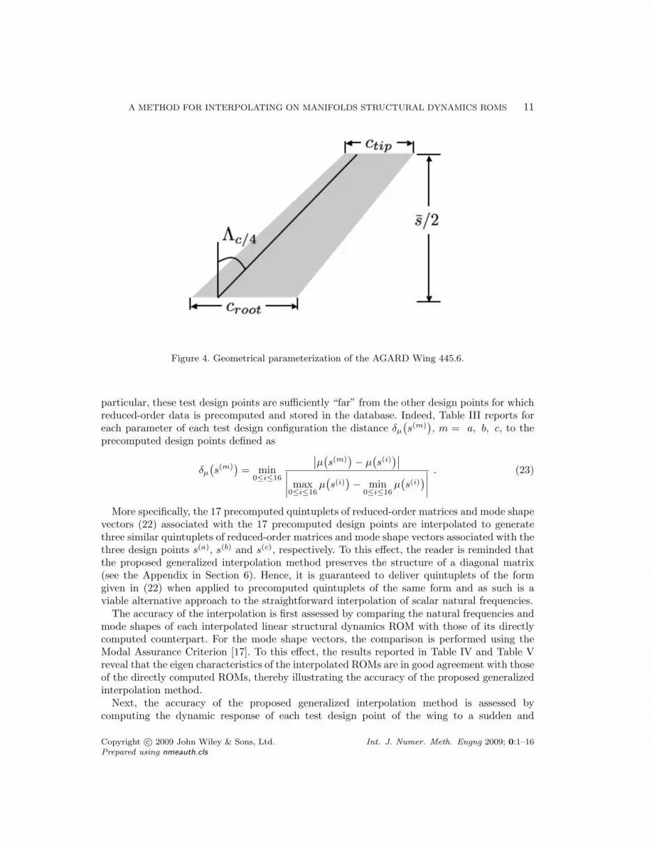
The AGARD Wing 445.6[16] is considered here and represented by an undamped (C = 0) finiteelement (FE) model composed of 800 shell elements that generate 2646 degrees of freedom.The geometry of the wing is parameterized by four shape parameters as shown in Figure 4:
the root chord croot, the tip chord ctip, the half span lengths
2and the quarter-chord sweep
angle Λc/4.A database of linear structural dynamics ROMs is constructed for this wing by precomputing
a set of 17 quintupletsR
(s(i)
)=
(M?(s(i)), C?(s(i)), K?(s(i)), X(s(i)), Z(s(i))
)16
i=0for 17
different design points s(i)16i=0 that can be viewed as the vertices and center of a hypercubein a design space — that is, a subset of R4 — defined by
croot×ctip×s
2×Λc/4 ∈
[c(min)root , c
(max)root
]×
[c(min)tip , c
(max)tip
]×
[s(min)
2,s(max)
2
]×
[Λ(min)
c/4 ,Λ(max)c/4
],
(21)
Copyright c© 2009 John Wiley & Sons, Ltd. Int. J. Numer. Meth. Engng 2009; 0:1–16Prepared using nmeauth.cls
10 D. AMSALLEM, J. CORTIAL, K. CARLBERG AND C. FARHAT
Figure 3. Comparison of the eigenvalues of the reduced-order matrix H(s(4)) constructed using thegeneralized interpolation method and those of its counterpart assembled from directly constructed
ROMs.
Table II. AGARD Wing 445.6: bounds of the parametric domain of interest.
c(min)root c
(max)root c
(min)tip c
(max)tip s(min)/2 s(max)/2 Λ
(min)
c/4 Λ(max)
c/4
17.568 in 26.352 in 11.6 in 17.4 in 24 in 36 in 38.66 50.16
where the values of the upper and lower bounds are defined in Table II.For each of these 17 sample design points, a ROM is constructed by the method of modal
decomposition and truncation based on the first five natural modes of this design. Hence, inthis case,
R(s(i)
)=
(I5, 05, Ω2
5(s(i)), X(s(i)), Z(s(i))
)16
i=0, (22)
where Ω25(s) denotes the diagonal matrix storing the squares of the first five natural circular
frequencies of the structural model of the wing for the design point s.Here, the accuracy of the generalized interpolation method proposed in this paper is
assessed for three arbitrary design points (or configurations), s(a), s(b) and s(c). These designconfigurations are shown in Figure 5, specified in Table III and referred to in the remainderof this section as “test” design points for the proposed generalized interpolation method. In
Copyright c© 2009 John Wiley & Sons, Ltd. Int. J. Numer. Meth. Engng 2009; 0:1–16Prepared using nmeauth.cls
A METHOD FOR INTERPOLATING ON MANIFOLDS STRUCTURAL DYNAMICS ROMS 11
Figure 4. Geometrical parameterization of the AGARD Wing 445.6.
particular, these test design points are sufficiently “far” from the other design points for whichreduced-order data is precomputed and stored in the database. Indeed, Table III reports foreach parameter of each test design configuration the distance δµ
(s(m)
), m = a, b, c, to the
precomputed design points defined as
δµ
(s(m)
)= min
0≤i≤16
∣∣µ(s(m)
)− µ
(s(i)
)∣∣∣∣∣∣ max0≤i≤16
µ(s(i)
)− min
0≤i≤16µ(s(i)
)∣∣∣∣ . (23)
More specifically, the 17 precomputed quintuplets of reduced-order matrices and mode shapevectors (22) associated with the 17 precomputed design points are interpolated to generatethree similar quintuplets of reduced-order matrices and mode shape vectors associated with thethree design points s(a), s(b) and s(c), respectively. To this effect, the reader is reminded thatthe proposed generalized interpolation method preserves the structure of a diagonal matrix(see the Appendix in Section 6). Hence, it is guaranteed to deliver quintuplets of the formgiven in (22) when applied to precomputed quintuplets of the same form and as such is aviable alternative approach to the straightforward interpolation of scalar natural frequencies.
The accuracy of the interpolation is first assessed by comparing the natural frequencies andmode shapes of each interpolated linear structural dynamics ROM with those of its directlycomputed counterpart. For the mode shape vectors, the comparison is performed using theModal Assurance Criterion [17]. To this effect, the results reported in Table IV and Table Vreveal that the eigen characteristics of the interpolated ROMs are in good agreement with thoseof the directly computed ROMs, thereby illustrating the accuracy of the proposed generalizedinterpolation method.
Next, the accuracy of the proposed generalized interpolation method is assessed bycomputing the dynamic response of each test design point of the wing to a sudden and
Copyright c© 2009 John Wiley & Sons, Ltd. Int. J. Numer. Meth. Engng 2009; 0:1–16Prepared using nmeauth.cls

12 D. AMSALLEM, J. CORTIAL, K. CARLBERG AND C. FARHAT
Figure 5. “Test” design points: shaded geometry corresponds to the wing configuration for the valuesof the shape parameters at the center of the hypercube and geometry shown in wireframe corresponds
to the “test” wing configuration.
Table III. “Test” design points.
croot ctip s/2 Λc/4
s(a) 25.484 in 15.715 in 32.852 in 42.21
δcroot
`s(a)
´= 0.099 δctip
`s(a)
´= 0.21 δs/2
`s(a)
´= 0.24 δΛc/4
`s(a)
´= 0.19
s(b) 23.414 in 13.549 in 24.200 in 47.76
δcroot
`s(b)
´= 0.17 δctip
`s(b)
´= 0.16 δs/2
`s(b)
´= 0.02 δΛc/4
`s(b)
´= 0.21
s(c) 22.056 in 17.398 in 26.915 in 42.31
δcroot
`s(c)
´= 0.01 δctip
`s(c)
´= 3× 10⁻⁴ δs/2
`s(c)
´= 0.24 δΛc/4
`s(c)
´= 0.18
Table IV. Comparison of the first five natural frequencies (in Hz) of the three “test” design pointsdelivered by the generalized interpolation method with their counterparts obtained from direct ROM
constructions.
Test design point (a) Test design point (b) Test design point (c)
Mode Direct Interp. Relative Direct Interp. Relative Direct Interp. RelativeROM ROM discrepancy ROM ROM discrepancy ROM ROM discrepancy
1 9.11 9.00 1.2 % 14.5 14.8 2.1 % 12.3 12.8 4.1 %2 35.4 35.1 0.8 % 51.7 53.4 3.3 % 41.2 42.5 3.2 %3 44.7 43.9 1.8 % 72.8 73.8 1.4 % 61.9 63.9 3.2 %4 88.6 87.7 1.0 % 128 131 2.7 % 107 110 2.8 %5 117 117 0.0 % 186 186 0.0 % 158 164 3.7 %
Copyright c© 2009 John Wiley & Sons, Ltd. Int. J. Numer. Meth. Engng 2009; 0:1–16Prepared using nmeauth.cls
A METHOD FOR INTERPOLATING ON MANIFOLDS STRUCTURAL DYNAMICS ROMS 13
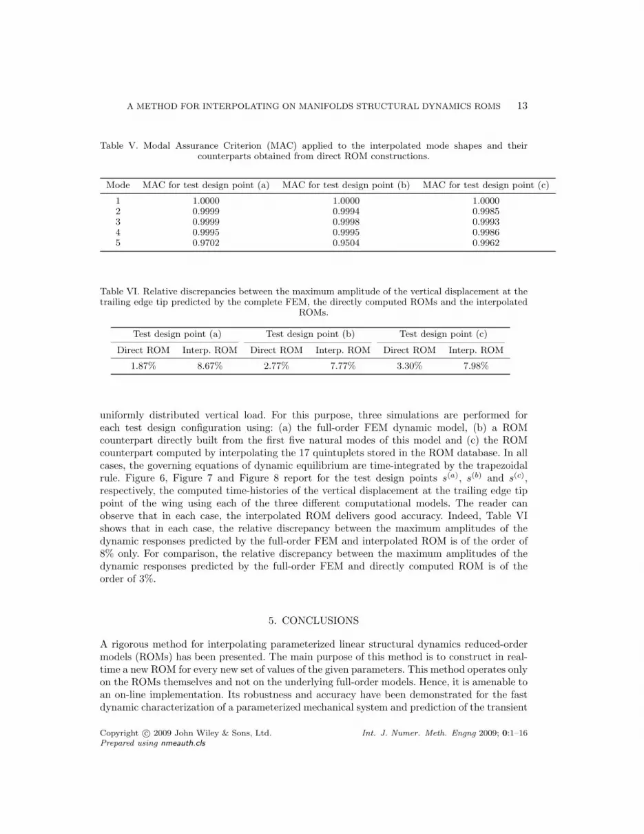
Table V. Modal Assurance Criterion (MAC) applied to the interpolated mode shapes and theircounterparts obtained from direct ROM constructions.
Mode MAC for test design point (a) MAC for test design point (b) MAC for test design point (c)
1 1.0000 1.0000 1.00002 0.9999 0.9994 0.99853 0.9999 0.9998 0.99934 0.9995 0.9995 0.99865 0.9702 0.9504 0.9962
Table VI. Relative discrepancies between the maximum amplitude of the vertical displacement at thetrailing edge tip predicted by the complete FEM, the directly computed ROMs and the interpolated
ROMs.
Test design point (a) Test design point (b) Test design point (c)
Direct ROM Interp. ROM Direct ROM Interp. ROM Direct ROM Interp. ROM
1.87% 8.67% 2.77% 7.77% 3.30% 7.98%
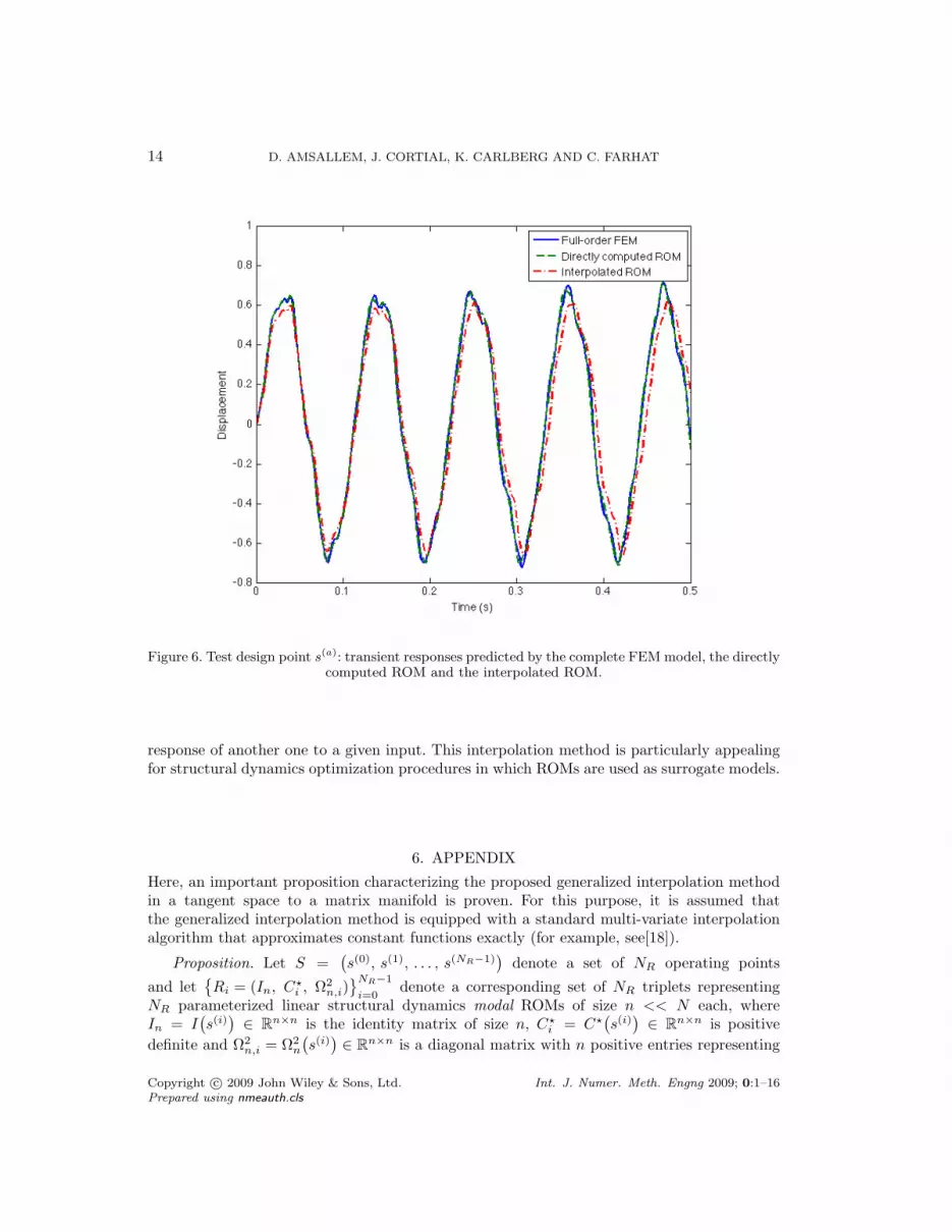
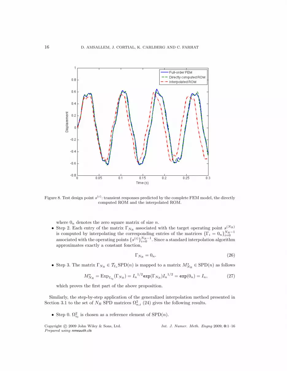
uniformly distributed vertical load. For this purpose, three simulations are performed foreach test design configuration using: (a) the full-order FEM dynamic model, (b) a ROMcounterpart directly built from the first five natural modes of this model and (c) the ROMcounterpart computed by interpolating the 17 quintuplets stored in the ROM database. In allcases, the governing equations of dynamic equilibrium are time-integrated by the trapezoidalrule. Figure 6, Figure 7 and Figure 8 report for the test design points s(a), s(b) and s(c),respectively, the computed time-histories of the vertical displacement at the trailing edge tippoint of the wing using each of the three different computational models. The reader canobserve that in each case, the interpolated ROM delivers good accuracy. Indeed, Table VIshows that in each case, the relative discrepancy between the maximum amplitudes of thedynamic responses predicted by the full-order FEM and interpolated ROM is of the order of8% only. For comparison, the relative discrepancy between the maximum amplitudes of thedynamic responses predicted by the full-order FEM and directly computed ROM is of theorder of 3%.
5. CONCLUSIONS
A rigorous method for interpolating parameterized linear structural dynamics reduced-ordermodels (ROMs) has been presented. The main purpose of this method is to construct in real-time a new ROM for every new set of values of the given parameters. This method operates onlyon the ROMs themselves and not on the underlying full-order models. Hence, it is amenable toan on-line implementation. Its robustness and accuracy have been demonstrated for the fastdynamic characterization of a parameterized mechanical system and prediction of the transient
Copyright c© 2009 John Wiley & Sons, Ltd. Int. J. Numer. Meth. Engng 2009; 0:1–16Prepared using nmeauth.cls
14 D. AMSALLEM, J. CORTIAL, K. CARLBERG AND C. FARHAT
Figure 6. Test design point s(a): transient responses predicted by the complete FEM model, the directlycomputed ROM and the interpolated ROM.
response of another one to a given input. This interpolation method is particularly appealingfor structural dynamics optimization procedures in which ROMs are used as surrogate models.
6. APPENDIX
Here, an important proposition characterizing the proposed generalized interpolation methodin a tangent space to a matrix manifold is proven. For this purpose, it is assumed thatthe generalized interpolation method is equipped with a standard multi-variate interpolationalgorithm that approximates constant functions exactly (for example, see[18]).
Proposition. Let S =(s(0), s(1), . . . , s(NR−1)
)denote a set of NR operating points
and letRi = (In, C?
i , Ω2n,i)
NR−1
i=0denote a corresponding set of NR triplets representing
NR parameterized linear structural dynamics modal ROMs of size n << N each, whereIn = I
(s(i)
)∈ Rn×n is the identity matrix of size n, C?
i = C?(s(i)
)∈ Rn×n is positive
definite and Ω2n,i = Ω2
n
(s(i)
)∈ Rn×n is a diagonal matrix with n positive entries representing
Copyright c© 2009 John Wiley & Sons, Ltd. Int. J. Numer. Meth. Engng 2009; 0:1–16Prepared using nmeauth.cls
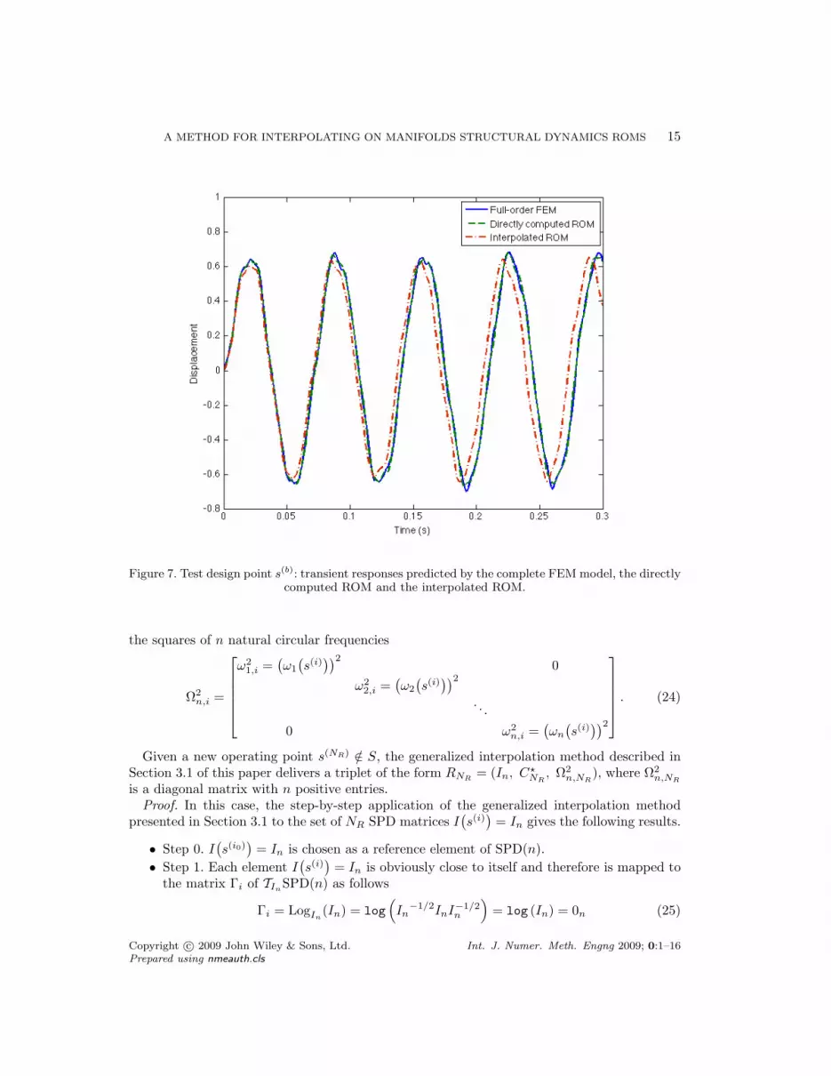
A METHOD FOR INTERPOLATING ON MANIFOLDS STRUCTURAL DYNAMICS ROMS 15
Figure 7. Test design point s(b): transient responses predicted by the complete FEM model, the directlycomputed ROM and the interpolated ROM.
the squares of n natural circular frequencies
Ω2n,i =
ω2
1,i =(ω1
(s(i)
))20
ω22,i =
(ω2
(s(i)
))2
. . .
0 ω2n,i =
(ωn
(s(i)
))2
. (24)
Given a new operating point s(NR) /∈ S, the generalized interpolation method described inSection 3.1 of this paper delivers a triplet of the form RNR
= (In, C?NR
, Ω2n,NR
), where Ω2n,NR
is a diagonal matrix with n positive entries.Proof. In this case, the step-by-step application of the generalized interpolation method
presented in Section 3.1 to the set of NR SPD matrices I(s(i)
)= In gives the following results.
• Step 0. I(s(i0)
)= In is chosen as a reference element of SPD(n).
• Step 1. Each element I(s(i)
)= In is obviously close to itself and therefore is mapped to
the matrix Γi of TInSPD(n) as follows
Γi = LogIn(In) = log
(In−1/2InI−1/2
n
)= log (In) = 0n (25)
Copyright c© 2009 John Wiley & Sons, Ltd. Int. J. Numer. Meth. Engng 2009; 0:1–16Prepared using nmeauth.cls
16 D. AMSALLEM, J. CORTIAL, K. CARLBERG AND C. FARHAT
Figure 8. Test design point s(c): transient responses predicted by the complete FEM model, the directlycomputed ROM and the interpolated ROM.
where 0n denotes the zero square matrix of size n.• Step 2. Each entry of the matrix ΓNR
associated with the target operating point s(NR)
is computed by interpolating the corresponding entries of the matrices Γi = 0nNR−1i=0
associated with the operating points s(i)NR−1i=0 . Since a standard interpolation algorithm
approximates exactly a constant fonction,
ΓNR= 0n. (26)
• Step 3. The matrix ΓNR∈ TIn
SPD(n) is mapped to a matrix M?NR
∈ SPD(n) as follows
M?NR
= ExpIi0(ΓNR
) = In1/2exp(ΓNR
)In1/2 = exp(0n) = In, (27)
which proves the first part of the above proposition.
Similarly, the step-by-step application of the generalized interpolation method presented inSection 3.1 to the set of NR SPD matrices Ω2
n,i (24) gives the following results.
• Step 0. Ω2i0
is chosen as a reference element of SPD(n).
Copyright c© 2009 John Wiley & Sons, Ltd. Int. J. Numer. Meth. Engng 2009; 0:1–16Prepared using nmeauth.cls

A METHOD FOR INTERPOLATING ON MANIFOLDS STRUCTURAL DYNAMICS ROMS 17
• Step 1. Each matrix Ω2i that is sufficiently close to Ω2
i0is mapped to a matrix Γi of
TΩ2i0
SPD(n) as follows
Γi = LogΩ2n,i0
(Ω2n,i)
= log(Ω2
n,i0
−1/2Ω2
n,iΩ2n,i0
−1/2)
= log
ω−11,i0
0ω−1
2,i0. . .
0 ω−1n,i0
ω21,i 0
ω22,i
. . .0 ω2
n,i
ω−11,i0
0ω−1
2,i0. . .
0 ω−1n,i0
= log
(ω1,i
ω1,i0
)2
0(ω2,i
ω2,i0
)2
. . .
0(
ωn,i
ωn,i0
)2
=
2 log
(ω1,i
ω1,i0
)0
2 log(
ω2,i
ω2,i0
). . .
0 2 log(
ωn,i
ωn,i0
)
. (28)
• Step 2. Each entry of the matrix ΓNRassociated with the target operating point s(NR)
is computed by interpolating the corresponding entries of the matrices Γi ∈ Rn×n
associated with the operating points s(i). Since each matrix Γi (28) is in this casediagonal, ΓNR
is also diagonal and can be written as
ΓNR=
α1 0
α2
. . .0 αn
. (29)
• Step 3. The matrix ΓNR∈ TΩ2
n,i0SPD(n) is mapped to a matrix K?
NRon SPD(n) as
Copyright c© 2009 John Wiley & Sons, Ltd. Int. J. Numer. Meth. Engng 2009; 0:1–16Prepared using nmeauth.cls
18 D. AMSALLEM, J. CORTIAL, K. CARLBERG AND C. FARHAT
follows
K?NR
= ExpΩ2n,i0
(ΓNR)
= Ω2n,i0
1/2exp(ΓNR
)Ω2n,i0
1/2
=
ω1,i0 0
ω2,i0
. . .0 ωn,i0
exp(α1) 0exp(α2)
. . .0 exp(αn)
ω1,i0 0ω2,i0
. . .0 ωn,i0
=
ω2
1,i0exp(α1) 0
ω22,i0
exp(α2). . .
0 ω2n,i0
exp(αn)
=
ω2
1,NR0
ω22,NR
. . .0 ω2
n,NR
= Ω2n,NR
,
which proves the second and last part of the above proposition.
ACKNOWLEDGEMENTS
This material is based upon work supported partially by the Air Force Office of Scientific Researchunder Grant F49620-01-1-0129 and partially by the National Science Foundation under Grant CNS-0540419. Any opinions, findings and conclusions or recommendations expressed in this material arethose of the authors and do not necessarily reflect the views of the Air Force Office of ScientificResearch or the National Science Foundation.
REFERENCES
1. Guyan RJ. Reduction of stiffness and mass matrices. AIAA Journal 1965; 3(2):380.2. Flanigan CC. Development of the IRS component dynamic reduction method for substructure analysis.
AIAA Paper 1991-1056 1991.3. Holmes P, Lumley J, Berkooz G. Turbulence, Coherent Structures, Dynamical Systems and Symmetry.
Cambridge University Press, 1996.4. Kerschen G, Golinval JC, Vakakis AF, Bergman LA. The method of proper orthogonal decomposition for
dynamical characterization and order reduction of mechanical systems: an overview. Nonlinear dynamics2005; 41:147–169.
5. Amabili M, Sarkar A, Paidoussis MP. Reduced-order models for nonlinear vibrations of cylindrical shellsvia the proper orthogonal decomposition method. Journal of Fluids and Structures 2003; 18(2): 227–250.
Copyright c© 2009 John Wiley & Sons, Ltd. Int. J. Numer. Meth. Engng 2009; 0:1–16Prepared using nmeauth.cls
A METHOD FOR INTERPOLATING ON MANIFOLDS STRUCTURAL DYNAMICS ROMS 19
6. Han S, Feeny BF. Enhanced proper orthogonal decomposition for the modal analysis of homogeneousstructures. Journal of Vibration and Control 2002; 8(1):19–40.
7. Leibfritz F, Volkwein S. Reduced-order Output Feedback Control Design for PDE Systems Using ProperOrthogonal Decomposition and Nonlinear Semidefinite Programming. Linear Algebra and its Applications,Special Issue on Order Reduction of Large-Scale Systems 2004; 415(2–3):542–575.
8. Georgiou IT, Schwartz IB. Dynamics of large scale coupled structural/mechanical systems: a singularperturbation/proper orthogonal decomposition approach. SIAM Journal of Applied Mathematics 2002;59(4):1178–1207.
9. Hinze M, Volkwein S. Proper orthogonal decomposition surrogate models for nonlinear dynamical systems:error estimates and suboptimal control. In Dimension Reduction of Large-Scale Systems, Lecture Notesin Computational Science and Engineering, Springer 45, 2006; 261–306.
10. Danowsky B, Chrstos J, Klyde D, Farhat C, Brenner M. Application of multiple methods for aeroelasticuncertainty analysis. AIAA Paper 2008-6371, AIAA Atmospheric Flight Mechanics Conference andExhibit , Honolulu, Hawaii, August 18-21, 2008.
11. Amsallem D, Farhat C. An interpolation method for adapting reduced-order models and application toaeroelasticity. AIAA Journal 2008; 46(7):1803–1813.
12. Epureanu BI. A parametric analysis of reduced order models of viscous flows in turbomachinery. Journalof Fluids and Structures 2003; 17(7):971–982.
13. Amsallem D, Cortial J, Farhat C. On-demand CFD-based aeroelastic predictions using a database ofreduced-order bases and models. AIAA Paper 2009-800, 47th AIAA Aerospace Sciences Meeting includingThe New Horizons Forum and Aerospace Exposition, Orlando, Florida, Jan. 5-8, 2009.
14. Pennec X, Fillard P, Ayache N. A Riemannian framework for tensor computation. International Journalof Computer Vision 2006; 66(1):41–66.
15. Kim T. Frequency-domain Karhunen-Loeve method and its application to linear dynamic systems. AIAAJournal 1998; 36(11):2117–2123.
16. Yates EC. Agard standard aeroelastic configurations for dynamic response, candidate configuration I,-Wing 445.6. NASA TM-100462 1987.
17. Ewins DJ. Modal Testing, Theory, Practice and Application (2nd edn). Research Study Press LTD, 2000.18. Spath H. Two Dimensional Spline Interpolation Algorithms. K Peters, Ltd., 1995.
Copyright c© 2009 John Wiley & Sons, Ltd. Int. J. Numer. Meth. Engng 2009; 0:1–16Prepared using nmeauth.cls