interpolating subspaces in approximation theory
TRANSCRIPT
JOURNAL OF APPROXIMATION THEORY 3, 164-182 (1970)
Interpolating Subspaces in Approximation Theory
D. A. AULT, F. R. DEUTSCH,* P. D. MORRIS,* AND J. E. OLSON
Department of Mathematics, Pennsylvania State University, University Park, Pennsylvania 16802
Communicated by E. W. Cheney
Received July 5, 1969
1. INTRODUCTION
There is a very beautiful, now classical, theory associated with the problem of best approximation in C[a, b] by elements of an n-dimensional Haar subspace. In particular (cf., e.g., [4]), best approximations are always unique and are characterized by an alternation property; a de la Vallte Poussin theorem provides lower bounds on the error of approximation; best approxi- mations are strongly unique (in the sense of Newman and Shapiro [14]); the metric projection, or best approximation operator, is pointwise Lipschitz continuous; and the so-called “first and second algorithms” of Remez provide effective means for the actual computation of best approximations.
It is natural to ask whether one can extend the notion of a Haar subspace so as to be valid in an arbitrary normed linear space, and at the same time preserve as much of the C[a, b] theory as possible. In this paper we introduce the notion of an interpolating subspace of a normed linear space. In the particular space C(T), T compact Hausdorff, the interpolating subspaces turn out to be precisely the Haar subspaces. (Recall that an n-dimensional subspace M of C(T) is called a Huar subspace if every function in M - (0) has at most n - 1 zeros in T.) We shall verify that corresponding to each one of the classical results mentioned in the preceding paragraph for Haar subspaces in C[a, b], there is a strictly analogous result valid for interpolating subspaces in an arbitrary normed linear space.
Because the richness of the classical Haar subspace theory carries over in toto to the more general case of interpolating subspaces, it might be suspected that interpolating subspaces are rather rare in general normed linear spaces. Indeed, we show (Theorem 3.1) that interpolating subspaces do not exist in those spaces having strictly convex dual spaces. On the other hand, we show (Theorem 3.2) that in C,(T), T locally compact Hausdorff,
* These authors were supported by grants from the National Science Foundation.
164
INTERPOLATING SUBSPACES 165
the interpolating subspaces are precisely the Haar subspaces again. (The definition of a Haar subspace in C,(T) is the same as given for C(T), above.) Also, if (T, 2, p) is a o-finite measure space, then (Theorem 3.3) Lr(T, 2, p) contains an interpolating subspace of dimension n > 1 if, and only if, T is the union of at least n atoms. Further, L,(T, Z, p) contains a one-dimensional interpolating subspace if, and only if, T contains an atom. In particular (Corollary 3.4) the space Z, has interpolating subspaces of every finite dimension.
2. DEFINITIONS, NOTATION, AND Two BASIC RESULTS
Let X be a real normed linear space and X* its dual space. We denote the norm-closed unit balls in each of these spaces by S(X) and S(X*), respectively. If K is any subset of X, ext K denotes the set of extreme points of K. If Xl ,.**, x, are linearly independent vectors in X, then [x1 ,..., x,J denotes the n-dimensional linear subspace of X generated by these vectors. By subspace we always mean a linear subspace. If K is a subset of X and x E X, an element x,, E K is called a best approximation to x from K if
11 x - x,, I/ = inf{ll x - y I/ : y E K} = d(x, K).
If each x E X has a unique best approximation from K, then K is called a Tchebychefset. If M is a subspace of X, then
Ml = {x* E X* : x*(y) = 0 for every y E M}.
All other notation or terminology is defined in [7].
DEFINITION. An n-dimensional subspace M of X is called an interpolating subspace if, for each set of n linearly independent functionals x1*,..., x,,* in ext S(X*) and each set of n real scalars c1 ,..., c,, , there is a unique element y E M such that xi*(y) = ci for i = l,..., n.
THEOREM 2.1. Let M = [x, ,..., x,] be an n-dimensional subspace of X, The following statements are equivalent.
(1) M is an interpolating subspace.
(2) For each set of n linearly independentfunctionals x1*,..., x,* in ext S(X*), det[xi*(xj)J f 0.
(3) If x1*,..., x, * are n linearly independent functionals in ext S(X*), y E M, and xi*( y) = Ofor i = l,..., n, then y = 0.
(4) M-L n (u {[x1* ,..., x,*1 : x1* ,..., x,* are linearly independent and lie in ext S(X*)}) = {O}.
640/3/2-4
166 AULT, DEUTSCH, MORRIS, AND OLSON
(5) iw- l-l [xl*,..., x,*] = (0) for every set of n linearly independent functionals x1*,..., x,* in ext S(X*).
(6) X* = ML @ [x1*,..., x,* ] for every set of n linearly independent functionals x1*,..., xn* in ext S(X*).
The proof of this theorem is a straightforward application of the definition of an interpolating subspace and is, therefore, omitted.
THEOREM 2.2. Every interpolating subspace is a Tchebycheflsubspace.
The proof is a simple modification of standard arguments ([16], [6]) and is omitted. Corollary 3.1 below shows that the converse is false.
3. EXISTENCE OF INTERPOLATING SUBSPACES IN CONCRETE SPACES
We begin this section by first establishing a “nonexistence” theorem. (Recall that a normed linear space X is called strictly convex if ext S(X) = {x E X : II x I( = l}.)
THEOREM 3.1. If X is a normed linear space whose dual X* is strictly convex, then X has no proper interpolating subspace.
Proof. Clearly, we may assume dim X > 1. Fix an arbitrary integer n, 1 < n < dim X, and let M be an n-dimensional subspace of X. Since M f X, ML must contain a nonzero element x* by the Hahn-Banach theorem. By the strict convexity of X*, y* = (x*/II x* 11) E ext S(X*). In particular, ML n ext S(X*) r) { y*} and, a fortiori,
Ml n (U {[xl* )...) x,*1 : x1* )...) x,* are linearly independent and lie in
ext S(X*)}) r) {y*}.
By Theorem 2.1, M is not an interpolating subspace and the proof is complete.
COROLLARY 3.1. In an inner product space or any L,(T, Z’, p) space, 1 < p < 00, there are no proper interpolating subspaces.
Remark. If X is n-dimensional and M = X, then A4 is trivially an interpolating subspace. Indeed, det[xi*(xj)] f 0 for any set of n linearly independent functionals x1* ,..., xn* in X* and any basis x1 ,..., x,, of X (cf., e.g., [5], p. 26).
If T is a locally compact Hausdorff space, let C,,(T) denote the space of all real-valued continuous functions on T which vanish at infinity, with the supremum norm. Thus, x E C,(T) if, and only if, x is continuous and for
INTERPOLATING SUBSPACES 167
each E > 0, the set {t E T: 1 x(t)1 > E} is compact. In particular, if T is compact, C,(T) = C(T), the space of all real-valued continuous functions on T.
THEOREM 3.2. Let M be a finite-dimensional subspace of C,,(T). The following statements are equivalent.
(1) M is an interpoluting subspace. (2) M is a Tchebycheff subspace.
(3) M is a Haar subspace.
Proof. The equivalence of (1) and (3) follows from part (3) of Theorem 2.1 and the known result that the extreme points of S[C,,(T)*] are (plus or minus) the point evaluation functionals. The equivalence of (2) and (3) is due to Phelps ([ 151, p. 250).
COROLLARY 3.2. A subspace of c0 is a Tchebycheff subspace if, and only if, it is an interpolating subspace.
This corollary follows by first recalling [lo] that c0 has no infinite-dimensional Tchebycheflsubspaces, and then applying Theorem 3.2.
Let (T, Z, CL) be a u-finite measure space. An atom is a set A E .Z with 0 < p(A) < co, such that B E 2, B C A implies that either p(B) = 0 or p(B) = p(A). It is well-known (and easy to prove) that T can have at most countably many atoms. The measure space(T, 2: ,u) is called nonatomic if T has no atoms, and it is called purely atomic if T is the union of atoms. R. R. Phelps and Henry Dye [15] have shown that if T has no atoms then L,(T, Z, p) has no finite-dimensional Tchebycheff subspaces (and, a fortiori, no interpolating subspaces). Sharpening this result, Garkavi [9] established that L,(T, Z, p) has an n-dimensional Tchebychefi subspace if, and only if, T contains at least n atoms.
The main result on the existence of interpolating subspaces in L,(T, 2, p) is the following
THEOREM 3.3. The space L,(T, Z, IL) contains an interpolating subspace qf dimension n > 1 if, and only tf, T is the union of at least n atoms. Also, L,(T, 2, p) contains a one-dimensional interpolating subspace if, and only if, T contains an atom.
As immediate consequences of this theorem, we obtain the following two corollaries.
COROLLARY 3.3. If the space L,(T, Z, p) contains an interpolating subspace of dimension > 1, then T is purely atomic.
168 AULT, DEUTSCH, MORRIS, AND OLSON
COROLLARY 3.4. The space I, has interpolating subspaces of every (finite) dimension.
We remark that if (T, Z, cc) is o-finite, the condition that T be the union of atoms is equivalent to the condition that &(T, Z, p) be isometrically isomorphic to I1 or 11”, depending on whether T is a countable union of atoms or a finite union of m atoms, respectively.
In contrast to Theorem 3.2, not every finite-dimensional Tchebycheff subspace in I1 is an interpolating subspace. Indeed, let X = I1 and M = [el ,..., e,], where ei is the i-th unit vector: ei = (& , SSi ,... ). It is easy to verify that A4 is a Tchebycheff subspace. In fact, if x = (& , .& ,...) E II, then its unique best approximation in M is given by (& ,..., &, , O,...). We identify 11* with I, in the usual way. Then each functional x* E ext S(&*) is of the form x* = (ul , u2, . ..). where ui = +l for each i. Let x1* ,..., xn* be any n linearly independent elements of ext S(I1*), each of whose first n coordinates is + 1. Then xi*(ej) = 1 for i, j = l,..., n, so that det[xi*(ej)] = 0. By Theorem 2.1, M is not as interpolating subspace.
We shall postpone the (rather involved) verification of Theorem 3.3 until the last section, where we also include some results helpful in recognizing and constructing interpolating subspaces in I1 .
4. CHARACTERIZATION OF BEST APPROXIMATIONS
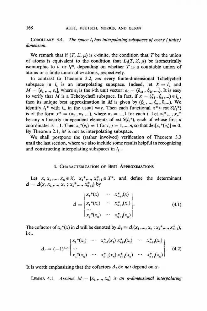
Let x, x1 ,..., x, E X, x1* ,..., x:.+~ E X*, and define the determinant A = A(x, x1 ,...) x, ; x1* ,‘..)
A=
~~+3 by
x,*(x) **- x:+1(4
x1 *(xl) . * * x;+&q . . . x1*&J . . *
(4.1)
The cofactor of xi*(x) in A will be denoted by Ai z Ai(xl ,..., x, ; x1*,..., x,*+& i.e.,
x1 *(xl) ... xi*-&,) $++;1<x,> *-* x,*,,(q) Ai = (-l)i+l . . . . (4.2)
x1*&J * * - &G-J Xi*,l<X,> *** x,*,&J
It is worth emphasizing that the cofactors A, do not depend on x.
LEMMA 4.1. Assume M = [x1 ,..., x,] is an n-dimensional interpolating

INTERPOLATING SUBSPACES 169
suyaace in X, x1*,..., x,* are m < n + 1 i;dependentfunctionaIs in ext S(X*), 1 ,..., 01, are nonzero scalars. Then x1 aiXi* E MI of, and only tf,
(i) m=n+l,and
(ii) OIi = CL,+lAi/An+l (i = l,..., n + l), where Ai are given by (4.2).
In particular, Cy” Aixi* E Ml.
Proof. If m < n + 1, choose y EM SO that xi*(y) = ai (i = l,..., m). Then
0 = f oliXi*(y) = 2 (yi2, 1 1
which is absurd. Part (ii) follows by using Cramer’s rule to solve for 01~ ,..., CI~~ . The converse follows by observing that CyLt Aixi*(xi) is just the expansion of the determinant A with x replaced by xj , and is, therefore, zero.
The following “alternation” theorem characterizes best approximations from interpolating subspaces.
THEOREM 4.1. Let M = [x1 ,..., x,] be an n-dimensional interpolating subspace in X, let x E X N M, and let x0 E M. Then the following statements are equivalent.
(1) x,, is a best approximation to x from M.
(2) There exist n + 1 linearly independent ftmctionals x1*,..., x:+~ in ext S(X*) such that
(a) x~*(x - x0) = II x - x0 Ij (i = l,..., n + l), (b) The determinants Ai , defined by Eq. (4.2), all have the same sign.
(3) There exist n + 1 linearly independent functionals x1*,..., x:+~ in ext S(X*) such that
(a) xi*(x - x0) = /j x - x0 /I (i = l,..., n + l), (b) s&Aid) = 1 (i = l,..., n + l), where A and Ai are as defined in
Eqs. (4.1) and (4.2).
(4) There exist n + 1 linearly independent functionals xl*,..., x,*,~ in ext S(X*) and n + 1 nonzero scalars (Ye ,..., a,+l such that
(a) I Xi*(X - X0)1 = II X - Xg 11 (i = l,..., n + l), (b) Cy” aixi* E ML, (c) sgn[qx,*(x - x,)] = ..* = sgn[a,+,xz+,(x - x0)].
(5) The zero n tuple (O,..., 0) is in the convex hull of the set of n tuples
{(x*(x,),..., x*(xn)) : x* E ext S(X*), x*(x - x0) = jl x - x0 /I}.
170 AULT, DEUTSCH, MORRIS, AND OLSON
The proof is, again, a modification of standard arguments, using lemma 4.1. In particular, in proving the equivalence of (1) and (5), one uses the main characterization theorem of [ 161.
For our first application of Theorem 4.1, we consider the space X = C,,(T), T locally compact. We can readily deduce:
THEOREM 4.2. Let M = [x1 ,..., x,] be an n-dimensional interpolating subspace in C,(T), let x E C,(T) - M, and let x,, E M. Then x0 is a best approximation to x from M tf, and only tf, there exist n + 1 distinct points t 1 ,..., tn+I E T such that
W - xo(ti) = sfNW) II x - x0 II (i = l,..., n + l), (a)
where
X(h) . . . x(tn+l) Xl(h) ... x1(tn+J f 0 @I . . .
I X,(h) ... x,(tn+l) 1
and Di is the cofactor of x(ti) in D.
Theorem 4.2 was, in essence, established by Bram [2], who gave a direct proof. In the particular case when T is compact, Theorem 4.2 was proved by Zuhovitki [18]. If we further specialize and take T to be an interval on the real line, we obtain the classical alternation theorem.
As another application of Theorem 4.1, we consider the space L, = L,(T, ,?Y, II), where T is the union of (at most) countably many atoms, say T = UiarAi . Since each measurable function x must be constant almost everywhere on an atom and since L,* = L, , it is easy to verify that each x* E ext S&*) has the representation
X*(X) = C x(Ai) dAi) A4 XELl, isI
where 1 o(A& = 1 and where x(Ai) denotes the constant value which x has a.e. on Ai . For any x E L, , we denote the set {i E I : x(&) = 0) by Z(x). If 5’ is a set, then card S will denote the cardinality of S.
THROREM 4.3. Let M = [x1 ,..., x,] be an n-dimensional interpolating subspace in & , let x E L N M, and let x0 E M. The following statements are equivalent.
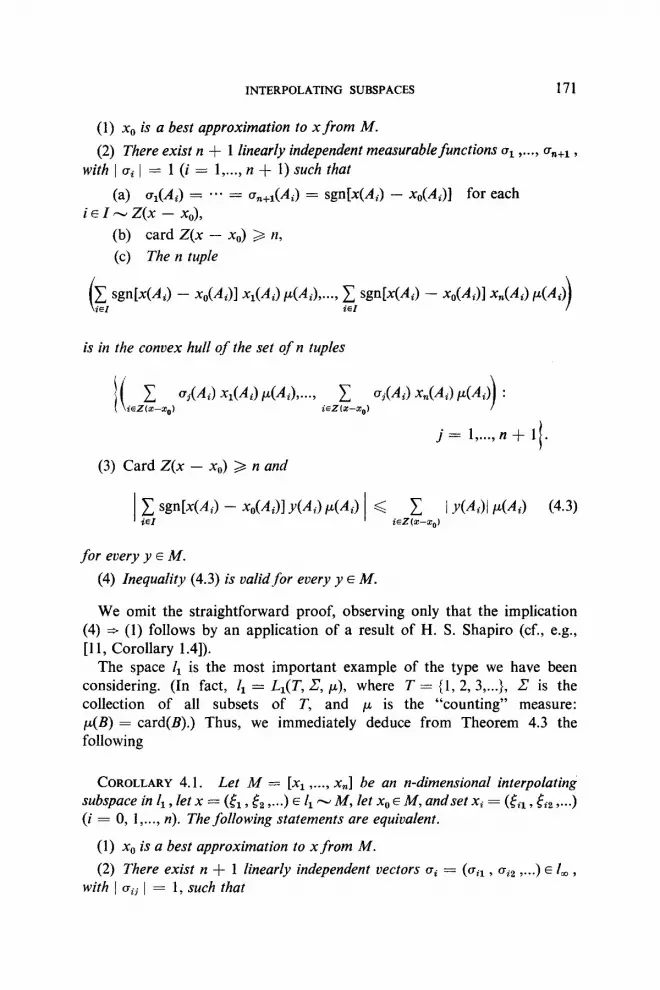
INTERPOLATING SUBSPACES 171
(1) x0 is a best approximation to x from M.
(2) There exist n + 1 linearly independent measurablefunctions CQ ,..., a,,,, , with 1 ui / = 1 (i = l,..., n + 1) such that
(a) aI = em* = u,+&4J = sgn[x(A,) - x&4,)] for each iEZwZ(x - x0),
(b) card 2(x - x0) > n, (c) The n tuple
is in the convex hull of the set of n tuples
ii iczzp, ) aj(Ai) -QCAi) /44,~*~7 itlzws ) oi(Ai) xn(Ai) AAJ ’
0 0 1
j = l,..., n + 1 . I
(3) Card Z(x - x,,) > n and
1 5 sgn[X(Ai) - x0(41 YCAi) AAi) / G iEZz-z ) 1 Y&)1 A4 (4.3) 0
for every y E M.
(4) Inequality (4.3) is validfor every y E M.
We omit the straightforward proof, observing only that the implication (4) 3 (1) follows by an application of a result of H. S. Shapiro (cf., e.g., [ 11, Corollary 1.41).
The space II is the most important example of the type we have been considering. (In fact, II = L,(T, ,J7, p), where T = (1, 2, 3 ,... }, Z is the collection of all subsets of T, and p is the “counting” measure: p(B) = card(B).) Thus, we immediately deduce from Theorem 4.3 the following
COROLLARY 4.1. Let M = [x1 ,..., x,] be an n-dimensional interpolating subspace in I, , let x = (tl , tz ,...) E II - M, let x0 E M, andset Xi = (4i1, tit ,...) (i = 0, l,..., n). The foIlowing statements are equivalent.
(1) x0 is a best approximation to x from M.
(2) There exist n + 1 linearly independent vectors ui = (cil, (Ti2 ,...) E I, , with I uij I = 1, such that
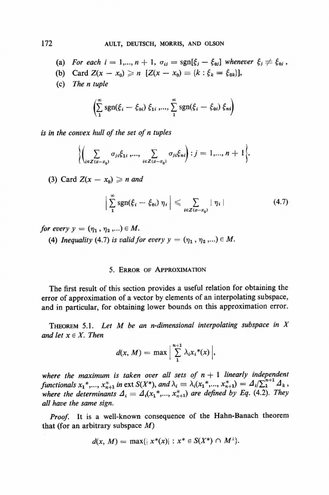
172 AULT, DEUTSCH, MORRIS, AND OLSON
(a) For each i = l,..., n + 1, uii = sgn& - &I whenever 6i If & , (b) Card 2(x - x0) > n [2(x - XO) = {k : tk = &>l, (c) The n tuple
is in the convex hull of the set of n tuples
ii c ujitli >---9 1 ujifni 1
:j = l,..., n + 1 I
. iEZkc--mo) ioZ(z-z,)
(3) Card Z(x - x0) > n and
(4.7)
for every y = (Q, q2 ,...) E M.
(4) Inequality (4.7) is valid for every y = (Q , q2 ,...) E 44.
5. ERROR OF APPROXIMATION
The first result of this section provides a useful relation for obtaining the error of approximation of a vector by elements of an interpolating subspace, and in particular, for obtaining lower bounds on this approximation error.
THEOREM 5.1. Let A4 be an n-dimensional interpolating subspace in X and let x E X. Then
d(x, M) = max 1 a$ &X,*(x) 1,
where the maximum is taken over all sets of n $ 1 linearly independent functionals x1*,..., x,“,~ in ext S(X*), and hi E &(x1*,*.*, x:+1) = Ai/Cy” A, , where the determinants A, = Ai(xl*y..., xc+J are defined by Eq. (4.2). They all have the same sign.
Proof. It is a well-known consequence of the Hahn-Banach theorem that (for an arbitrary subspace M)
d(x, M) = max(1 x*(x)\ : x* E S(X*) n ML}.
INTERPOLATING SUBSPACES 173
Moreover, when M is n-dimensional, we may restrict the search for a maximum to those x* of the form x* = Cy &xi*, where Xi* E ext S(X*), hi > 0, CT hi = 1, and m < n + 1 (cf., e.g., [17]). Our conclusion now follows immediately from Lemma 4.1.
With the help of Theorem 5.1, we can deduce the following generalized “de la Vallte Poussin theorem,” from which the classical result under that name follows easily.
THEOREM 5.2. Let M be an n-dimensional interpolating subspace of X and let x E X. Suppose there exist a y E M and n + 1 linearly independent functionals x1*,.,., x,*,~ in ext S(X*) such that
[Aixi*(x - YW,+,X,*,,(X - Y>l > 0 (i = I,..., n),
where the determinants Ai are defined by Eq. (4.2). Then
mm / x(*(x - y)i < d(x, M).
Also, if equality holds, then ) x(*(x - y)J = d(x, M) for every i.
6. CONTINUITY OF BEST APPROXIMATIONS
We now state a “strong uniqueness” theorem which generalizes a result of Newman and Shapiro [14]. If M is an interpolating subspace in X, we denote the unique best approximation from A4 to any x E X by B,(x). The operator BM is called the metric projection onto M.
THEOREM 6.1. Let M be an interpolating subspace in X. Then, for each x E X, there exists a constant y = y(x) with 0 < y < 1, such that
II x - Y II 3 II x - h&)II + Y II h&) - Y II for every y E M.
Cheney and Wulbert (unpublished, 1967) have obtained a result slightly stronger than Theorem 6.1. Their proof, as well as ours, is an obvious modification of the proof of the Newman-Shapiro Theorem as given by Cheney [3], [4].
Freud [8], in essence, showed that the metric projection onto a Haar subspace in C[a, b] is pointwise Lipschitz continuous. Cheney [4], p. 82, observed that this fact is a consequence only of the strong uniqueness theorem, so that it is equally valid for our situation. Thus, we immediately obtain from Theorem 6.1,
174 AULT, DEUTSCH, MORRIS, AND OLSON
THEOREM 6.2. Let M be an interpolating subspace of X. Then for each x E X there exists a constant X = X(x) > 0 such that
for every z E X.
II &f(x) - &(z)ll < h II x - z II
7. ALGORITHMS FOR CONSTRUCTING BEST APPROXIMATIONS
We shall consider two algorithms for the construction of best approxima- tions from interpolating subspaces.
Let M be an n-dimensional subspace of X, let x E X - M, and let r be any set of functionals in X* of norm 1 such that for each z E M @ [xl, there is an x* E r with x*(z) = /I z 11. In [l], Akilov and Rubinov have described an algorithm-a generalization of the “first algorithm” of Remez- for the construction of a best approximation to x from M. If we specialize their result to the case where M is an interpolating subspace and where r = ext S(X*), the algorithm may be described as follows.
Let x1*,..., x,* E lY For each m > n, select y, E M and x$+~ E r so that
and
I x;+,<x - YJ = II x - Y, II*
Introducing the notation e, = II x - y, 11, II z Ilm = maxkim I x~*(z)], and X, = I/ x - y, llTn , the effectiveness of this algorithm can be summarized in the following
THEOREM. (9 A, < L+, G *-- < d(x, M) < e, for all m > n, and lim h, = d(x, M) = lim elrL .
(ii) The sequence {ym} converges to the unique best approximation of x from M.
Laurent [ 121 has recently given a generalization of the “second algorithm” of Remez. It is valid for n-dimensional subspaces M = [x1 ,..., x,] of a normed linear space X which satisfy the condition:
(L) For each set of n linearly independent functionals x1* . . . . x,,* in the weak* closure of ext S(X*), det[xi*(xj)] f 0.
In particular, any subspace with property (L) is necessarily an interpolating subspace. In the special cases when X = C(T), T compact Hausdorff, or
INTERPOLATING SUBSPACES 175
when X = L,(T, 2, p), where T is (at most) a countable union of atoms, it can be shown that ext S(X*) is weak* closed. Hence, in these special cases property (L) is equivalent to the condition that M be an interpolating subspace. However, in the space co, for example, there are interpolating subspaces of every finite dimension. Since 0 is in the weak” closure of ext S(c,*), it follows that no subspace of c,, has property (L). We do not know whether this algorithm is still valid for interpolating subspaces in X for which ext S(X*) is not weak* closed.
A detailed description of the algorithm of Laurent would take us too far astray. We mention, only, that it is a convergent scheme.
We conclude this section by observing that if the n + 1 functionals * x1*,.-, &+1 in the characterization Theorem 4.1 are known, then it is possible
to determine the best approximation, as well as the error of approximation, by simple solving a linear system of n + 1 equations. Indeed, suppose M = [Xl )...) xJ is an n-dimensional interpolating subspace in X, x E X - M, and x,, = CT olixi is the best approximation to x from M. Suppose that
* x1*,-., -%+1 are any 12 + 1 linearly independent functionals in ext S(X*), whose existence is guaranteed by Theorem 4.1. Then, in particular,
xi*(xo) + d = xi*(x) (i = l...., M + l),
where d = d(x, M). Substituting for x,, in these equations, we get
j$l “ixi*(xi) + d = xi*(x) Q = ,,..., n + l>e
This system can now be solved by Cramer’s rule to determine the unknowns 01~ (and hence, x0) and d.
We remark that the Laurent algorithm involves solving a sequence of such (n + I)-st order linear systems.
8. PROOF OF THEOREM 3.3
The proof of Theorem 3.3 will be based on a number of preliminary results which we now establish.
Throughout this section, iz denotes a fixed positive integer. For each m > n, we consider the linear space &m of all real n x m matrices E = (eij), with the norm 11 E 11 = maxi,j 1 eij I. If E is an n x k matrix, with k < m, we identify E with e, where E E JY~ is the partitioned matrix
I? = [E ; OJ}n, k m-k
176 AULT, DEUTSCH, MORRIS, AND OLSON
and 0 is the at x (m - k) matrix consisting entirely of zeros. In this way, we have J%‘,~ C Am, if ml < m2.
LEMMA 8.1. Assume m >, n, B, E ~9‘~ , E is an m x n matrix of rank n, and E > 0. Then there is a matrix Bl E .M, such that
(1) II BI - 4, II < E, (2) det B,E f 0.
Proof. Define a function of nm real variables xij (1 < i < n, 1 < j < m) by
Phi ,***, xnm) = deW4, + W El, where
[
x11 u= . . .
&l
p is a polynomial in the variables xij which is not identically 0, since there clearly is some matrix BE J%‘~~ such that det BE # 0. It follows that p cannot vanish identically on any neighborhood of the origin. Hence, there are values xii with 1 xii / < E so that p(xll ,..., x,,) f 0. Taking Bl = B0 + U completes the proof.
LEMMA 8.2. Assume m > n, B, E Jl, , El ,..., E, are m x n matrices of rank n, and e > 0. Then there exist B, E Mm and S > 0, with the following properties:
(1) II 4 - Bo II < E; (2) if B E .4!, , I( B - B, jj < 6, and U is an n x n matrix with 1) U 11 < S,
then det(BEi + U) f 0 (i = I,..., r).
Proof. We proceed by induction on r. Assume r = 1. Then by Lemma 8.1, there is a matrix Bl E ~.4’, such that // Bl - B, II < E and det BIE, f 0. Now, det(BE, + U), regarded as a function of nm + n2 variables (as B varies over &m and U varies over all n x n matrices), is continuous. Hence, there exists a S > 0 such that if I/ B - Bl 11 < S and 11 U/j < 6, then det(BE, + U) f 0. Now assume r > 1 and that a matrix B,’ E JV~ and a 6’ > 0 have been determined so that 11 B,’ - B, II < 42 and such that II B - B,’ /I < S’, II U/I < 6’ imply det(BE, + U) # 0 for i = l,..., r - 1. From the case r = 1, there is a matrix B; E JZ~ and a 6, > 0 such that Ij B,’ - B; (I < min{E/2, S’/2} and such that I/ B - B; /I < 6, , /I UI/ -C 6,
INTERPOLATING SUBSPACES 177
imply det(BE, + U) f 0. The lemma now follows by taking Bl = B; and 6 = min(6, , P/2).
LEMMA 8.3. There exists an n x co matrix B = (biJ (i = l,..., n; j = 1, 2,...) with CrS, 1 bij 1 < co, having the property that det BE f 0 for every 03 x n matrix E of rank n whose entries are restricted to the values k 1.
Proof. We shall obtain B as the limit of a sequence of matrices B, which we now construct. For each k = 0, 1, 2 ,..., let 8k denote the finite set of all (n + k) x n matrices of rank n with entries f 1. By Lemma 8.2, we construct a sequence of matrices B,, , Bl ,..., where B, = (b$‘) E J%‘*+~, and a corre- sponding sequence of positive numbers 6,) 6, ,..., having the following properties:
(i) 0 < 6, < 1, 0 < a,+, < &/2. (ii) II B, - Bk+1 II < S,/4 (k = 0, l,...). (iii) If B E A,,,, , with I/ B - BI, // < 13, , and if U is any n x n matrix
with /j U II < 6, , then det(B& + U) f 0 for every E, E ~9~.
In particular, it follows from (ii) that I b~$$,+, I < &/4 for i = l,..., n, and k = 1, 2,... . If we identify each B, with the n x cc partitioned matrix
[& ; ;*-; -],
then the sequence Bk: converge entrywise to some n x cc matrix, B = (biJ. To see this, we note that for each i = l,..., n, j = I,2 ,..., and p > 0,
/ b:;) - b$+p) / < 11 B, - B,,, 11
d II & - B,,, II + a.3 + II &+z+-l - B,,, I!
<6,/4+ 0.. + &+,-,I4 -=E t@, + &+, + --*>
< is, )
and 6, + 0 as k --+ co. For each k = 0, I,..., let B,’ be the matrix in J?‘~+~ consisting of the first n + k columns of B. By our construction, we have
II 4’ - BI, II < 3% < 6,. Also,
I bi,,+k+j I < I bi,lz+k+j - bjlcn+:‘:+j I + I b!“+j’ I z.?w+3
178 AULT, DEUTSCH, MORRIS, AND OLSON
Hence, for each i = I,..., IZ,
In particular, each row vector of B is in & . Now, let E = (Q) be any co x n matrix with rank 12 and entries q5 = fl.
Then, for some k > 0, the (n + k) x IZ matrix Ek consisting of the first n + k rows of E has rank n. By definition, Ek E 6k . Let C = BE = (Q). Then, for 1 < i, j f n,
r=1 9+1 r=n+h+1
Thus, BE = B,‘EI, + (I, where U is the n x n matrix whose i, j-th entry is
Hence, j uij / d zTqn+k+r I bi, ) < 6,) for 1 < i, j < n, i.e., I/ U II < 6,. Since II Bk’ - BI, I/ < 8, and E, E &k , it follows from the construction that
det BE = det(B,‘& + U) # 0,
and this completes the proof. We can now easily prove half of Theorem 3.3.
THEOREM 8.1. Let (T, Z, p) be a u-finite measure space such that T is the union of at least n atoms. Then L,(T, Z, CL) contains an interpolating subspace of dimension n.
Proof. We shall assume that T is a countable union of atoms: T = & Ai , where p(Ai n Aj) = 0 if i # j. The case where T is only a finite union of atoms can be treated in a similar manner. We assume that Ai n Aj = I# if i # j (by neglecting certain sets of measure zero). Each functional x* E ext S(L,*) is of the form
for some g E L, with / g ( = 1. Hence,
x*(x) = i 44 ~(4, 1
where x(Ai) is the constant value which x has a.e. on A+ , and g = ui(= &l)
INTERPOLATING SUBSPACES 179
on Ai . Let B = (bij) be the n x co matrix whose existence is guaranteed by Lemma 8.3. Define n functions x1 ,..., x,, by
&c(t) = hcd44)-‘, if t E Ai (i = 1, 2,...).
Then
1 I x/s I 4 = f I hi I < ~0, for k = l,..., n, T i=l
i.e., x1 ,..., x, are in L, . Also, x1 ,..., x, are linearly independent. This follows from the fact that B has rank n. If x1*,..., xn* are linearly independent functionals in ext S(&*), then
xi*(x) = f x(.4,) Uj&ij) (i = l,..., n), i=l
where aii = ~1. It follows that the vectors (qi , uzi ,...) are linearly inde- pendent (as elements of l,). Hence, letting E denote the co x n matrix
we see that E has rank n, so that, by Lemma 8.3,
det[xi*(xj)] = det BE f- 0.
Thus, [x1 ,..., x,] is an n-dimensional interpolating subspace in L1 and the proof is complete.
By using the remark following Corollary 3.4, the above proof could have been slightly simplified by assuming L,(T, Z, p) = II or liWl.
LEMMA 8.4. Let (T, Z, p) be a a-$nite non-atomic measure space and let .x E L(T, .X:, 1~). For any positive integer n, there exist n linearly independent functions y, ,..., yn in ext S[L,(T, Z, p)] such that
1 yix dp = 0, for i = I,..., n. T
Proof. Define a (signed) measure v by
$3) = j-, x dp, for every S E Z:
Then v is nonatomic, i.e., both vf and v- are nonatomic. An application of

180 AULT, DEUTSCH, MORRIS, AND OLSON
Liapounoff’s convexity theorem [13] shows that T may be decomposed into disjoint sets A and B such that
1 z T s
xdp = j, x dp = s x dp. B
By repeated application of the above, if k is a positive integer, T may be decomposed into disjoint sets Tl , T, ,..., T,r such that
1 2’i s xdp = x dp, for i = l,..., 2”. T I Ti
Now, if y is a function constantly equal to 1 on exactly half of the 2” sets and constantly -1 on the other half, then y E ext S[L,(T, .Z, p)] and
s yx dp = 0. T
To complete the proof, we observe that it is possible to choose k large enough so that there exists a linearly independent set of n such functions y. Indeed, if 2k > 2n and if we choose yi (i = I,..., n) to be 1 on half of the 2” sets and - 1 on the other half, and so that we also have
Y&l = -; I if t E T, v T2 u --+ v Ti , iftET,+,v**.vT,,
then these yi work. The above result is related to a theorem of Phelps ([15], Theorem 1.8).
If the a-Jnite measure space (T, .Z, p) contains an atom, then &(T, Z, p) always contains a one-dimensional interpolating subspace. For if A is an atom, define x by
x(t) = i
if t E A, otherwise.
Then x E IJT, Z, p) and x*(x) = &p(A) f 0 for each x* E ext S(L,*). Hence, [x] is a one-dimensional interpolating subspace in & .
The above remark along with the following theorem establish the second half of Theorem 3.3.
THEOREM 8.2. Let (T, 2, p) be a a-finite measure space. If T is not a union of atoms, then L,(T, .Z, CL) has no interpolating subspace of dimension n > 1. If T contains no atoms, then L,(T, Z, CL) contains no interpolating subspace.
INTERPOLATING SUBSPACES 181
Proof. The second assertion is clear from Lemma 8.4. (It is also a consequence of the theorem of Phelps and Dye mentioned in Section 3.) For the first assertion, we may assume that T contains some atoms. Let A be the union of the atoms in T. Let M be a subspace of L1 of dimension n > 1. Then there is a nonzero x E A4 such that
s xdp = 0. A
Applying Lemma 8.4 to the measure space (T - A, 2, p), we get IZ linearly independent functions y1 ,..., yn in ext S[L,(T - A, Z, p)] such that
I yix dp = 0 (i = I,..., n). T-A
Now define
yir = ;i I
,“; A’- 4
Then yl’,..., y,’ are linearly independent functions in ext S[L,(T, 2, CL)] and
s Yi’X dp = 0 (i = I,..., n). T
Defining xi* by
xi*(z) = s, zyi’ dp for all z 6 L, ,
we see that x1*,..., x,* are linearly independent functionals in ext S(L,*) and Xi*(X) = 0 (i = I,.**, n). Thus, M is not an interpolating subspace and the proof is complete.
It would be of some practical use to have a constructive proof of Theorem 8.1. Along these lines we make the following conjecture:
The vectors xi = (1, ri , ri2, ri3 ,...) E Z, (i = I,..., n, IZ > 1) span an n-dimensional interpolating subspace, if 0 < r, < r2 < -0. < r,, < 8 and the ratio rj/ri+l is “sufficiently” small (j = I,..., n - 1).
We have thus far verified this conjecture for II < 4. In the absence of a complete proof of the conjecture, the following results, which can be easily verified, might be useful in recognizing interpolating subspaces in II .
PROPOSITION 8.1. Let M = [x1 ,..., x,J, n > 2, be an n-dimensional interpolating subspace in II . Then for no j is it possible that the j-th coordinates of Xl , x2 ,.“, x, are all zero.
PROPOSITION 8.2. Let M be an interpolating subspace of dimension n > 2 in II . Then for every pair of linearly independent vectors in M, the number of j’s, such that the j-th coordinate of both vectors is 0, is < n - 2.
640/3/2-5
182 AULT, DEUTSCH, MORRIS, AND OLSON
REFERENCES
1. G. P. AKILOV AND A. M. RUBINOV, The method of successive approximations for determining the polynomial of best approximation, Soviet Math. Dokl. 5 (1964), 951-953.
2. J. BRAM, Chebychev approximation in locally compact spaces, Proc. Amer. Math. Sot. 9 (1958), 133-136.
3. E. W. CHENEY, “Some Relationships Between the Tchebycheff Approximations on an Interval and on a Discrete Subset of that Interval,” Math. Note no. 262, Boeing Scientific Research Labs., Seattle, Wash., 1962.
4. E. W. CHENEY, “Introduction to Approximation Theory,” McGraw-Hill, New York, 1966.
5. P. J. DAVIS, “Interpolation and Approximation,” Blaisdell, New York, 1963. 6. F. R. DEUT~CH AND P. H. MASERICK, Applications of the Hahn-Banach theorem in
approximation theory, SIAM Rev. 9 (1967), 516-530. 7. N. DUNF~RD AND J. T. SCHWARTZ, “Linear Operators I.,” Interscience, New York,
1958. 8. G. FREUD, Eine Ungleichung fur Tschebyscheffsche Approximationspolynome, Acta
Sci. (Szeged) 19 (1958), 162-164. 9. A. I. GARKAVI, On uniqueness of the solutions of the L-problem of moments (Russian),
Izv. Akad. Nauk S.S.S.R. 28 (1964), 553-570. 10. A. L. GARKAVI, On CebySev and almost-CebySev subspaces (Russian), Izv. Akud.
Nuuk S.S.S.R. 28 (1964), 799-818. 11. B. R. KRIPKE AND T. J. RIVLIN, Approximation in the metric of C(X, p), Trans. Amer.
Math. Sot. 119 (1965), 101-122. 12. P. J. LAURENT, Theorems de caracterisation dune meilleure approximation dans un
espace norme et generalisation de l’algorithme de Rem&s, Num. Math. 10 (1967), 190-208.
13. A, A. LIAPOUNOFF, On completely additive vector-functions, Zzv. Akad. Nauk S.S.S.R. 4 (194O), 465-478.
14. D. J. NEWMAN AND H. S. SHAPIRO, Some theorems on Cebybv approximation, Duke Math. J. 30 (1963), 673-682.
15. R. R. F%ELPS, Uniqueness of Hahn-Banach extensions and unique best approximation, Trans. Amer. Math. Sot. 95 (1960), 238-255.
16. I. SINGER, Caracterisation des elements de meilleure approximation dans un espace de Banach quelconque, Acta. Sci. Math. 17 (1956), 181-189.
17. I. SINGER, “On Best Approximation in Normed Vector Spaces by Elements of Vector Subspaces (Rumanian),” Bucarest, 1967.
18. S. I. ZUHOVITKI, On the approximation of real functions in the sense of P. L. Cebykv (Russian), Uspehi Mat. Nauk 11 (1956), 125-159.