arX

iv:h

ep-t

h/03

1120

4v1

21

Nov

200

3

Preprint typeset in JHEP style - HYPER VERSION hep-th/0311

Interpolating State in String Field Theory

D. Mamone

International School for Advanced Studies (SISSA/ISAS)

Via Beirut 2–4, 34014 Trieste, Italy, and INFN, Sezione di Trieste

E-mail: mamone@sissa.it

Abstract: We derive an oscillator form for the Butterflies in terms of Sliver matrix S

and its twisted version T as was already done for the Wedges in term of T . We write

a General Squeezed state depending on a matrix U and we show in a compact way the

interpolation between Identity state and the Sliver and between the Nothing state and the

Sliver, growing in powers of T and S matrices, respectively, in the choice of such matrix

U . Furthermore, we define a class of states which we call Laguerre states and we give a

formal derivation of such interpolating state in terms of them.

Keywords: String Field Theory, D-branes, Noncommutative Solitons .

Contents

1. Introduction 1

2. A short review of surface states and star projectors 4

2.1 Operator representation of surface states 4

2.2 Oscillator representation of surface states 5

2.3 Wedge states 6

2.3.1 Oscillator representation of wedge states 9

2.4 The Butterfly State 10

2.4.1 Operator representation of the butterfly state 11

2.4.2 Oscillator representation of the butterfly state 11

2.5 The Nothing State 12

2.6 Generalized butterflies 12

3. Oscillator representation of Butterflies 13

4. The General squeezed state form 16

4.1 U = 0 or the Sliver 17

4.2 U = 1 or the Identity 17

4.3 U = C or the Nothing 17

4.4 U = −S or the Butterfly 18

4.5 U = (−T )N−1 or the Wedge state 18

4.6 U = (−S)2N−1 or the Generalized Butterfly 18

5. General state from Laguerre states 20

6. Partial Isometry symmetry 22

7. Conclusions 25

1. Introduction

In Witten’s Open String Field Theory [1], the information about open strings interaction is

encoded in an associative but noncommutative multiplication between Open String Fields.

This multiplication is the Witten’s star product and defines an algebra. The main problem

in Witten’s Open SFT is that we don’t know how to solve the equation of motion. Rastelli,

Sen and Zwiebach [9, 35] proposed a new formulation of SFT, conjectured to be the SFT

written at the “true” vacuum, the minimum of the tachyon potential. This formulation is

know as Vacuum String Field Theory. The advantage of this theory is that we are able

– 1 –

to find exact solutions: D–branes are seen to correspond to open string fields that are

projectors of the star algebra [25, 35]. This happens because the Witten’s kinetic operator

which contains both matter and ghost operators, is replaced by a purely ghost one and

this simplifies the equation of motion, which for the matter sector becomes just a projector

condition

Ψ ∗ Ψ = Ψ (1.1)

under the Witten’s star product. For this reason, star projectors are important in VSFT.

There are several of such states that were found: the identity string field, the “Sliver” and

the family of so called “Butterflies” [38]. They can be described in a conformal formalism

as Riemann surface whose boundary consists of a parametrized open string and a piece with

boundary conditions. Such states are called surface states and are defined by a conformal

map, the configuration of the open string. In oscillator formalism, using creation and

annihilation operators of the BCFT, these states have a squeezed form involving infinite

dimensional matrices. The Sliver, for instance, has the form

|Ξ〉 = exp

−1

2

∞∑

m,n=1

(S)mn a†ma

†n

|0〉 . (1.2)

where S is a matrix which can be expressed in terms of the Neumann coefficients of the

interaction vertex of SFT [7, 8, 33, 34]or as residues of poles using the corresponding

conformal map. In [35] Rastelli, Sen and Zwiebach derived the Sliver in an algebraic way

using the oscillator representation and showed numerically that this solution is the same

found with the conformal formalism and representing the D25 brane. Okuda proved it

analitically in [12].

There are two big families of surface states studied in SFT, the so called “Wedge” states

and the Butterflies. For Wedge states, the Riemann surface is an angular sector of the unit

disk, with the left-half and the right-half of the open string being the two radial segments

and the arc having open string boundary condition. Such state is thus defined by the

angle at the midpoint of the string and this angle adds under star moltiplication since star

product between two string fields can be seen as the joining of the right-half part of the

first string with the left-half part of the second one. In this picture, the Identity state and

the Sliver, which belong to wedge states, can be interpreted respectevely as the zero and

the infinity angle wedge state. Indeed, they are the only projectors among wedge states:

the sum of two zero or two infinities angle is still a zero or an infinite angle. Wedge states

form an abelian subalgebra of star algebra. Butterflies, on the other hand, are all star

projectors. They are singular configuration in which the midpoint of the open string is

sent to infinity. We will see they depends on a real paramenter α. They share only one

state with the wedges: the Sliver belongs also to Butterflies. The Sliver can be seen at the

same time as the Nth wedge with N going to infinity or as the αth butterflies with α going

to zero.

The first aim of this paper is to investigate the star algebra and to recognise in those

projectors like Butterflies which were not found with algebraic oscillator formalism, a com-

– 2 –

mon structure with the Wedges, studying the crucial difference which makes them pro-

jectors. This is done in order to look for new tools to do calculations in the algebraic

operatorial formalism and to guess which could be the form of a good basis on which

expand and hopefully solve the equation of motion of the Witten’s SFT.

For this reason we derive an oscillator representation for Butterflies and we show that

both Wedges and Butterflies States can be rewritten in a General squeezed state form

|GU 〉 =NΞ

(det (1 + TU))1/2e−

12

CG a†a† |0〉 (1.3)

where

G =U + T

1 + TU(1.4)

depends on a matrix U . The interesting point is that if we choose matrix U to be

powers of the Sliver S matrix we obtain the family of Butterflies, on the other hand, if

we choose to be powers of its twisted version T , we get Wedge states, which are not all

projectors. In other words, such state interpolates between Wedges and Butterflies. In

particular we have:

• U = 0 corresponds to the Sliver state

• U = 1 corresponds to the Identity state

• U = C corresponds to the Nothing state

• U = −S corresponds to the Butterfly state

• U = (−T )N−1 corresponds to the Nth Wedge state

• U = (−S)N−1 (N even) corresponds to the α = 2N Generalized Butterfly state

The second aim is to suggest a formal way to obtain such General state using a suitable

resummation of states that we call “Laguerre” states which are a modification of “Ances-

tors” solutions found in [43]. These latter are an infinite class of projectors defined acting

with a Laguerre polynomial expression of string creation operators on the Sliver, whose

low-energy limit give rise to GMS solitons. For this reason they were called “Ancestors”. In

the final part, we will point out that partial isometry symmetry of VSFT seems to suggest

that Ancestors solutions behave like a complete basis, maybe for a star subalgebra.

The paper is organized as follows. In section 2 we review definitions of surface states

following [38]. In section 3 we derive an oscillator representation for the Butterflies starting

from the Moyal wave-functional one given in [37], which we will recognise in section 4 in

our interpolating state. In section 4, we write the General Squeezed State showing various

choices for matrix U that give rise to various string fields. For our calculations, we will use

the diagonal basis used in [37], which consists of eigenvectors of the operator K21 , instead

of the usual K1 = L1 + L−1 and allows us to rewrite Sliver and twist matrices as two

– 3 –

dimensional matrices. This turns out to be very useful for Butterflies representation.

In section 5 we define Laguerre states and a function of them that we will identify with

the General Squeezed state written in section 4.

2. A short review of surface states and star projectors

In this section we brifly review the definition of surface states through the conformal maps

which define them and we will recall the oscillator representation of each of them, which

has the form of a squeezed state. We mainly refer to [38]. These surface states are Riemann

surfaces whose boundary consists of a parametrized open string and a piece with open string

boundary conditions. Thinking of a surface state as a string field, it is possible to define a

geometric operation which corresponds to star product in SFT: one glues the right-half of

the open string in the first surface to the left-half of the open string in the second surface,

and the surface state corresponding to the glued surface is the desired product. Usually,

multiplication of a surface state to itself leads to a surface state that looks different from

the initial state. This is the reason why it is not trivial to find projectors. Let us define

the thing more precisely.

A surface state 〈Σ is a state related with a Riemann surface Σ with the topology of

a disk D, with a marked point P , the puncture, lying on the boundary of D, and a local

coordinate around it. Local coordinate at a puncture is obtained from an analytic map m

taking a canonical half-disk HU defined as

HU : {|ξ| ≤ 1, Im(ξ) ≥ 0} (2.1)

into D, where ξ = 0 maps to the puncture P , and the image of the real segment {|ξ| ≤1,ℑ(ξ) = 0} lies on the boundary of D. The coordinate ξ of the half disk is called the local

coordinate. Using any global coordinate u on the disk D, the map m can be described by

some analytic function f :

u = f(ξ), u(P ) = f(0) (2.2)

Given a BCFT with state space H, the state 〈Σ| ∈ H∗ associated to the surface Σ is defined

as follows. For any local operator φ(ξ), with associated state φ〉 = limξ→0 φ(ξ)|0〉 we set

〈Σφ〉 = 〈f ◦ φ(0)〉D (2.3)

where 〈 〉D is the correlation function on D and s ◦ φ(0) is the transform of the operator

by the map f(ξ). The gluing of surfaces, conformal analog of star product of string field

states, requires a well defined full map of the half disk HU into the disk D.

2.1 Operator representation of surface states

Let us see the representation of surface states in terms of Virasoro operators acting on the

SL(2,R) invariant vacuum.

We can write the surface state 〈Σ| as

〈Σ| = 〈0|Uf ≡ 〈0| exp

( ∞∑

n=2

v(f)n Ln

)

, (2.4)

– 4 –

where the coefficients v(f)n are determined by the condition that the vector field

v(ξ) =

∞∑

n=2

v(f)n ξn+1 , (2.5)

exponentiates to f ,

exp (v(ξ)pξ) ξ = f(ξ) . (2.6)

We now consider the one-parameter family of maps

fβ(ξ) = exp(β v(ξ)

∂

∂ξ

)ξ . (2.7)

This givesd

dβfβ(ξ) = v(fβ(ξ)) . (2.8)

Solution, taking into account the boundary condition fβ=0(ξ) = ξ, gives:

fβ(ξ) = g−1(β + g(ξ)) , (2.9)

where

g′(ξ) =1

v(ξ). (2.10)

Thus

f(ξ) = g−1(1 + g(ξ)) . (2.11)

Equations (2.10) and (2.11) give f(ξ) if v(ξ) is known.

2.2 Oscillator representation of surface states

We consider the matter part of the state and the oscillators will be associated to free scalar

fields of the Boundary CFT. If am, a†m denote the annihilation and creation operators we

have:

|Σ〉 = exp

−1

2

∞∑

m,n=1

a†mVfmna

†n

|0〉 . (2.12)

and

V fmn =

(−1)m+n+1

√mn

∮

0

dw

2πi

∮

0

dz

2πi

1

zmwn

f ′(z)f ′(w)

(f(z) − f(w))2. (2.13)

Both w and z integration contours are circles around the origin, inside the unit circle

and with the w contour outside the z contour.

The crucial point is that when the vector field v(ξ), generating the conformal map f(ξ),

is known we can put the integral expression for the matrix V f of Neumann coefficients in

another form. We consider the matrix V (β) associated to the family of maps (2.7), and

rewrite (2.13) as

Vmn(β) ≡ Vfβmn =

(−1)m+n+1

√mn

∮

0

dw

2πi

∮

0

dz

2πi

1

zmwn

∂

∂z

∂

∂wlog(fβ(z) − fβ(w)) . (2.14)

– 5 –

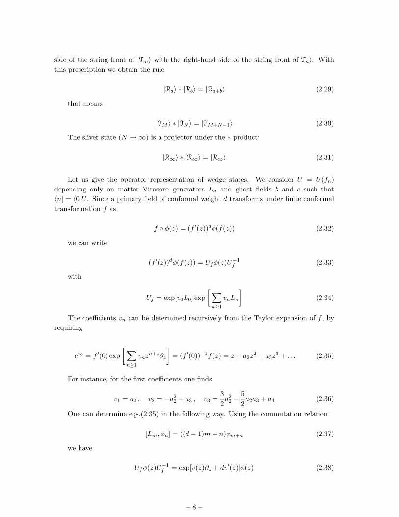
Taking a derivative with respect to the parameter β,

d

dβVmn(β) =

(−1)m+n+1

√mn

∮

0

dw

2πi

∮

0

dz

2πi

1

zmwn

∂

∂z

∂

∂w

(v(fβ(z)) − v(fβ(w))

fβ(z) − fβ(w)

), (2.15)

Integrating by parts in z and w:

d

dβVmn(β) = (−1)m+n+1√mn

∮

0

dw

2πi

∮

0

dz

2πi

1

zm+1wn+1

v(fβ(z)) − v(fβ(w))

fβ(z) − fβ(w). (2.16)

Neumann coefficients Vmn(β = 1) can be calculated integrating over β.

There are two big families of surface states studied in SFT: the Wedge states and the

Butterflies.

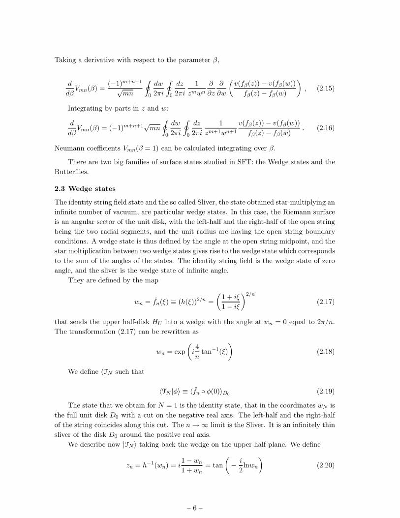
2.3 Wedge states

The identity string field state and the so called Sliver, the state obtained star-multiplying an

infinite number of vacuum, are particular wedge states. In this case, the Riemann surface

is an angular sector of the unit disk, with the left-half and the right-half of the open string

being the two radial segments, and the unit radius arc having the open string boundary

conditions. A wedge state is thus defined by the angle at the open string midpoint, and the

star moltiplication between two wedge states gives rise to the wedge state which corresponds

to the sum of the angles of the states. The identity string field is the wedge state of zero

angle, and the sliver is the wedge state of infinite angle.

They are defined by the map

wn = fn(ξ) ≡ (h(ξ))2/n =

(1 + iξ

1 − iξ

)2/n

(2.17)

that sends the upper half-disk HU into a wedge with the angle at wn = 0 equal to 2π/n.

The transformation (2.17) can be rewritten as

wn = exp

(i4

ntan−1(ξ)

)(2.18)

We define 〈TN such that

〈TN |φ〉 ≡ 〈fn ◦ φ(0)〉D0 (2.19)

The state that we obtain for N = 1 is the identity state, that in the coordinates wN is

the full unit disk D0 with a cut on the negative real axis. The left-half and the right-half

of the string coincides along this cut. The n→ ∞ limit is the Sliver. It is an infinitely thin

sliver of the disk D0 around the positive real axis.

We describe now |TN 〉 taking back the wedge on the upper half plane. We define

zn = h−1(wn) = i1 − wn

1 + wn= tan

(− i

2lnwn

)(2.20)

– 6 –

Putting (2.18) and (2.20) we have

zn = tan

(2

ntan−1(ξ)

)≡ fn(ξ) (2.21)

and

〈TN |φ〉 = 〈fn ◦ φ(0)〉DH(2.22)

The description of the Sliver as the N → ∞ wedge looking at (2.19) and (2.22)seems

to be singular, in the sense that the maps fN (ξ) and fN (ξ) are singular in the N → ∞limit. This apparent singular behaviour is solved by noticing the SL(2,R) invariance of the

correlation functions on the upper half plane. Given any SL(2,R) map R(z) we have the

relation

〈∏

i

Øi(xi)〉DH= 〈∏

i

R ◦ Øi(xi)〉DH(2.23)

for any set of operators Øi and with DH denoting the upper half plane. Since the

sliver |Ξ〉 is defined through a correlation function, we can set

RN (z) =N

2z (2.24)

so that

〈Ξ|φ〉 = 〈f ◦ φ(0)〉DH(2.25)

where

f(ξ) = limN→∞

RN ◦ fN (ξ) = limN→∞

N

2tan

(2

Ntan−1(ξ)

)= tan−1 ξ (2.26)

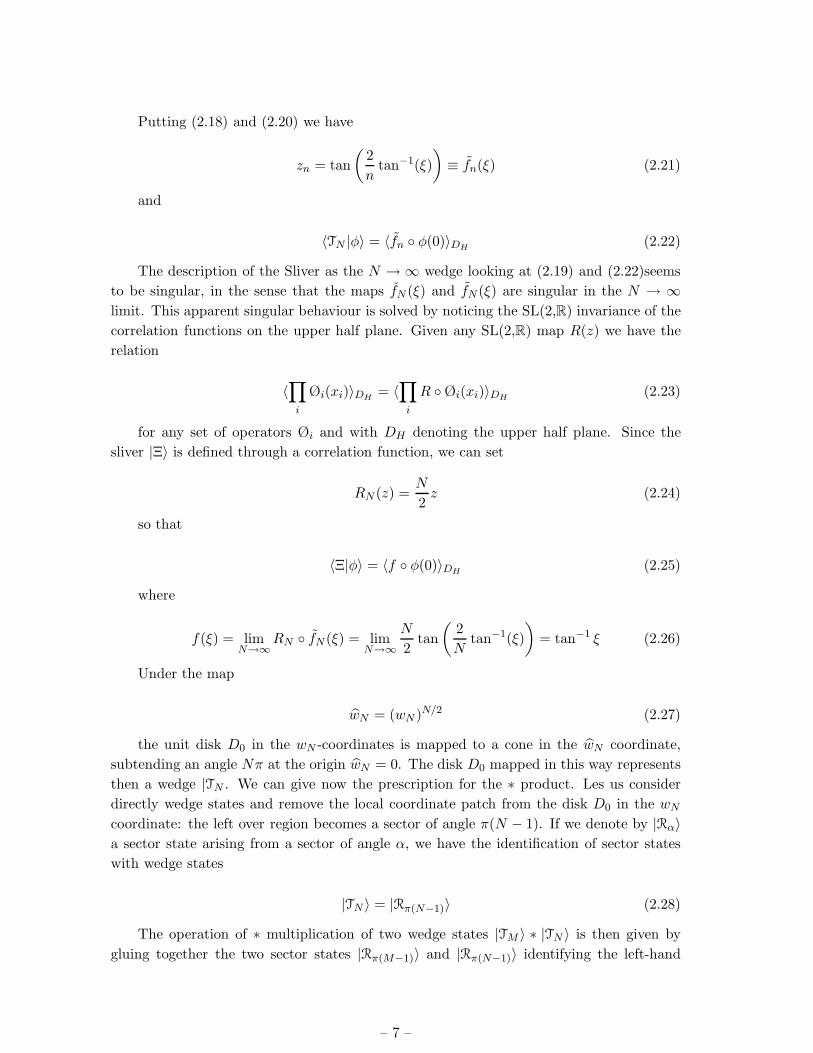
Under the map

wN = (wN )N/2 (2.27)

the unit disk D0 in the wN -coordinates is mapped to a cone in the wN coordinate,

subtending an angle Nπ at the origin wN = 0. The disk D0 mapped in this way represents

then a wedge |TN . We can give now the prescription for the ∗ product. Les us consider

directly wedge states and remove the local coordinate patch from the disk D0 in the wN

coordinate: the left over region becomes a sector of angle π(N − 1). If we denote by |Rα〉a sector state arising from a sector of angle α, we have the identification of sector states

with wedge states

|TN 〉 = |Rπ(N−1)〉 (2.28)

The operation of ∗ multiplication of two wedge states |TM 〉 ∗ |TN 〉 is then given by

gluing together the two sector states |Rπ(M−1)〉 and |Rπ(N−1)〉 identifying the left-hand

– 7 –

side of the string front of |Tm〉 with the right-hand side of the string front of Tn〉. With

this prescription we obtain the rule

|Ra〉 ∗ |Rb〉 = |Ra+b〉 (2.29)

that means

|TM 〉 ∗ |TN 〉 = |TM+N−1〉 (2.30)

The sliver state (N → ∞) is a projector under the ∗ product:

|R∞〉 ∗ |R∞〉 = |R∞〉 (2.31)

Let us give the operator representation of wedge states. We consider U = U(fn)

depending only on matter Virasoro generators Ln and ghost fields b and c such that

〈n| = 〈0|U . Since a primary field of conformal weight d transforms under finite conformal

transformation f as

f ◦ φ(z) = (f ′(z))dφ(f(z)) (2.32)

we can write

(f ′(z))dφ(f(z)) = Ufφ(z)U−1f (2.33)

with

Uf = exp[v0L0] exp

[∑

n≥1

vnLn

](2.34)

The coefficients vn can be determined recursively from the Taylor expansion of f , by

requiring

ev0 = f ′(0) exp

[∑

n≥1

vnzn+1∂z

]= (f ′(0))−1f(z) = z + a2z

2 + a3z3 + . . . (2.35)

For instance, for the first coefficients one finds

v1 = a2 , v2 = −a22 + a3 , v3 =

3

2a2

2 −5

2a2a3 + a4 (2.36)

One can determine eqs.(2.35) in the following way. Using the commutation relation

[Lm, φn] = ((d− 1)m− n)φm+n (2.37)

we have

Ufφ(z)U−1f = exp[v(z)∂z + dv′(z)]φ(z) (2.38)

– 8 –

where the function v(z) is such that

ev(z)∂zz = f(z) (2.39)

Choosing fN (z) = tan ( 2N tan−1(z)) to define the wedge states |TN 〉, we have

|TN 〉 = exp

[−N

2 − 4

3N2L−2 +

N4 − 16

30N4L−4 −

(N2 − 4)(176 + 128N2 + 11N4)

1890N6L−6 + · · ·

]|0〉

(2.40)

Among them, it is possible to recognise, for particular value of N :

the Identity State (N = 1) (see [46]):

|I〉 = exp

[L−2 −

1

2L−4 +

1

2L−6 + · · ·

]|0〉 (2.41)

and the Sliver State (N → ∞):

|Ξ〉 = exp

[−1

3L−2 +

1

30L−4 −

11

1890L−6 + · · ·

]|0〉 (2.42)

2.3.1 Oscillator representation of wedge states

The oscillator representation of the Sliver as given in [25, 35] is

|Ξ〉 = exp

−1

2

∞∑

m,n=1

(CT )mn a†ma

†n

|0〉 . (2.43)

where the T matrix was found algebraically and written as

T =1

2X(1 +X −

√(1 + 3X)(1 −X)) . (2.44)

in terms of the infinite dimensional matrix X = CV 11 which is known: V re the Neu-

mann coefficients and C = (−1)mδmn. Matrix elements of S match with those calculated

in the conformal way

Smn =(−1)m+n+1

√mn

∮

0

dw

2πi

∮

0

dz

2πi

1

zmwn

f ′(z)f ′(w)

(f(z) − f(w))2. (2.45)

with f(z) = tan−1z.

Similarly, for the Identity state we have

|I〉 = exp

−1

2

∞∑

m,n=1

(C)mn a†ma

†n

|0〉 . (2.46)

As we already said, the previous state are particular cases of the Nth Wedge state

which is

– 9 –

|TN 〉m = exp

−1

2

∞∑

m,n=1

(CTN )mn a†ma

†n

|0〉 . (2.47)

where TN is the matrix

TN =(−T )N−1 + T

1 − (−T )N(2.48)

This relation between the Nth wedge matrix and the twisted sliver matrix T will be

useful in the following.

2.4 The Butterfly State

The Butterfly and the Nothing state are particular Butterflies [38]. We already said that

Generalized Butterfly depends on a parameter α in a way we will see later on. The Butterfly,

the first of the family to be found, is simply the α = 1 case, while the so called Nothing

state corresponds to α = 2.

The butterfly state is defined by a map from ξ to the upper half z plane

z =ξ√

1 + ξ2≡ fB(ξ) , (2.49)

more precisely the surface state |B〉 that defines the butterfly is such:

〈B|φ〉 = 〈fB ◦ φ(0)〉UHP . (2.50)

In the ξ-plane we have the half-disk: the circumference is the string, the point ξ = i

the midpoint.

In the z-coordinate, the open string |ξ| = 1,ℑ(ξ) ≥ 0 is mapped to the hyperbola

x2 − y2 = 12 with z = x + iy. The fact that z(ξ = i) = ∞ means that the open string

midpoint coincides with the boundary of the disk. If we define

z = sin−1 ξ√1 + ξ2

(2.51)

and

w = e2iz = e2isin−1 ξ√

1+ξ2 (2.52)

The Riemann surface associated to the Butterfly is the following: the half-disk of the

ξ-plane is mapped to the right-half of the disk in the w-plane. The midpoint is sent to the

center of the disk and the open string is the vertical diameter. All the rest of the upper half

plane is mapped to the left-half of the disk with a cut along the negative real axis, which

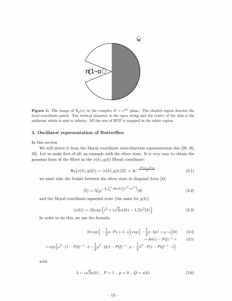
represents that fact that the midpoint touchs the boundary. (See figure 1, with α = 1.)

– 10 –

2.4.1 Operator representation of the butterfly state

We can represent the butterfly |Bt〉 in the operator formalism. We will use the “reguleted”

butterfly |Bt〉 defined by the map

z = ft(ξ) =ξ√

1 + t2ξ2= exp

(vt(ξ)

∂

∂ξ

)ξ . (2.53)

The regulator parameter t must therefore satisfy t < 1. (See [38] for details). We

recover the butterfly when t = 1.

Eqs. (2.11), (2.10) give

vt(ξ) = −t2 ξ3/2 . (2.54)

Eq. (2.4), (2.6) now gives:

|B t〉 = exp

(− t

2

2L−2

)|0〉 . (2.55)

2.4.2 Oscillator representation of the butterfly state

Let us represent the matter part of the regulated butterfly state in the oscillator represen-

tation. Take β ≡ t2,

v(ξ) = −ξ3

2, fβ(ξ) =

ξ√1 + βξ2

. (2.56)

Eq. (2.16) gives

d

dβV B

mn(β) = (−1)m+n

√mn

2

∮

0

dw

2πi

∮

0

dz

2πi

1

zm+1wn+1

fβ(z)3 − fβ(w)3

fβ(z) − fβ(w)(2.57)

= (−1)m+n

√mn

2

∮

0

dw

2πi

fβ(w)

wm+1

∮

0

dz

2πi

fβ(z)

zm+1= (−1)m+n

√mn

2xmxn ,

where

xm =

∮

0

dw

2πi

fβ(w)

wm+1= (−β)

m−12

Γ[m2 ]√πΓ[m+1

2 ]for m odd , (2.58)

xm = 0 for m even . (2.59)

Integrating (??) with the initial condition V (β = 0) = 0, we find the Neumann coeffi-

cients of the regulated butterfly (β → t2):

V Bmn(t) = −(−1)

m+n2

√mn

m+ n

Γ[m2 ]Γ[n2 ]

πΓ[m+12 ]Γ[n+1

2 ]tm+n , for m and n odd , (2.60)

V Bmn(t) = 0 , for m or n even . (2.61)

– 11 –

2.5 The Nothing State

The nothing state is defined by the map:

fN(ξ) =ξ

ξ2 + 1(2.62)

V fmn computed using (2.13), (2.62) turns out to be equal to δmn. Thus the oscillator

representation of the matter part of the nothing state is given by:

|N〉 = exp

−1

2

∞∑

m,n=1

a†na†n

|0〉 . (2.63)

2.6 Generalized butterflies

The generalized butterfly state |Bg(α)〉 is defined through a generalization of eq. (2.49) to

z =1

αsin(α tan−1 ξ) ≡ fα(ξ) . (2.64)

Note that the case α = 1:

fBg

α=1 =ξ√

1 + ξ2. (2.65)

so |Bg(α = 1)〉 is nothing but the butterfly while for α = 0 we have :

fBg

α=0 = tan−1 ξ . (2.66)

so |Bg(α = 0)〉 is the sliver.

|Bg(α)〉 is a family of projectors, interpolating between the butterfly and the sliver. For

α = 2 we have the map

fBg

α=2 =ξ

1 + ξ2. (2.67)

which corresponds to the ‘nothing’ state.

We can regularize the singularity at the midpoint and define the regularized butterfly

by generalizing ?? to

z = fBg,t(ξ) =1

α

tan(α tan−1 ξ)√1 + t2 tan2(α tan−1 ξ)

. (2.68)

In the z plane we get

〈Bg(α, t)|φ〉 = 〈f (0) ◦ φ(0)〉Cα,t, (2.69)

where Cα,t is the image of the upper half z plane in the z coordinate system and f (0)(ξ) =

tan−1 ξ.

For α = 2 the region of Cα,t collapses to nothing. For this reason the associated surface

state is called the “Nothing” state.

– 12 –

π(1−α)

w

Figure 1: The image of Bg(α) in the complex w = e2iz plane. The shaded region denotes the

local coordinate patch. The vertical diameter is the open string and the center of the disk is the

midpoint which is sent to infinity. All the rest of HUP is mapped in the white region.

3. Oscillator representation of Butterflies

In this section

We will derive it from the Moyal coordinate wave-function representation due [29, 30,

32]. Let us make first of all, an example with the sliver state. It is very easy to obtain the

gaussian form of the Sliver in the x(k), y(k) Moyal coordinate:

ΨΞ(x(k), y(k)) = 〈x(k), y(k)|Ξ〉 = 2e−x2(k)+y2(k)

θ (3.1)

we must take the braket between the sliver state in diagonal form [31]

|Ξ〉 = NΞe− 1

2

∫∞

0dks(k)

(e†

2+o†

2)

|0〉 (3.2)

and the Moyal coordinate squeezed state (the same for y(k))

〈x(k)| = 〈0|exp(e2 + i

√2ex(k) − 1/2x2(k)

)(3.3)

In order to do this, we use the formula

〈0| exp(− 1

2a · Pa+ λ · a

)exp

(− 1

2a ·Qa† + µ · a

)|0〉 (3.4)

= det(1 − PQ)−1 × (3.5)

× exp(µT · (1 − PQ)−1 · λ− 1

2µT ·Q(1 − PQ)−1 · µ− 1

2λT · P (1 − PQ)−1 · λ

),

with

λ = i√

2x(k) , P = 1 , µ = 0 , Q = s(k) (3.6)

– 13 –

Now, if we would like to do the opposite, starting from the Moyal function representa-

tion and get the oscillator one, we should start from the coefficient p of x(k) (or y(k), for

the sliver is the same) and, after some algebra, obtain the coefficient Q from

Q

1 +Q− 1

2= p (3.7)

In our case

p = −1

θ(3.8)

θ(κ) = 2 tanh(κπ

4

), (3.9)

then

Q =θ − 2

θ + 2= s(k) (3.10)

which is the well-known coefficient of the diagonal form of the sliver [31].

Starting from the Moyal function form of the butterfly, [37], the same game leads to

Qx

1 +Qx− 1

2= px (3.11)

Qy

1 +Qy− 1

2= py (3.12)

with

px = −1

2, py = − 2

θ2(3.13)

thus

Qx = 0, Qy =θ2 − 4

θ2 + 4=

2s

1 + s2(3.14)

and we obtain

|B〉 = NB e− 1

22s

1+s2o†

2

|0〉 (3.15)

which satisfies the fact simple Butterfly is twist odd.

Moyal wave functions in this diagonal coordinate space ~Xκ ≡ (xκ, yκ) are proportional

to the Gaussian

exp

(−1

2

∫ ∞

0

~XκLκ~Xκdκ

). (3.16)

The generalized butterfly |Bg〉 in this representation is [37]

Lκ = coth(κπ

4

)( tanh(κπ(2−α)4α ) 0

0 coth(κπ(2−α)4α )

)(3.17)

– 14 –

The sliver is limit α→ 0

Lκ = coth(κπ

4

)( 1 0

0 1

)=

2

θ

(1 0

0 1

)(3.18)

We want to derive the diagonal oscillator form for the generalized butterflies. We put

n =2 − α

α(3.19)

N = n+ 1 =2

α(3.20)

and we write down

Qx

1 +Qx− 1

2= −1

2coth

(kπ

4

)tanh

(kπn

4

)(3.21)

Qy

1 +Qy− 1

2= −1

2coth

(kπ

4

)coth

(kπn

4

)(3.22)

It is useful to define

t = e−kπ2 (3.23)

in order to simplify calculations:

coth

(kπ

4

)=

1 + t

1 − t(3.24)

coth

(kπn

4

)=

1 + tn

1 − tn(3.25)

tanh

(kπn

4

)=

1 − tn

1 + tn(3.26)

Easily we get

Qx =−t+ tn

1 − tn+1(3.27)

Qy =−t− tn

1 + tn+1(3.28)

so

|Bg〉 = NBg e− 1

2

(−t+tn

1−tn+1 e†2+ −t−tn

1+tn+1 o†2)

|0〉 (3.29)

Note that for n = 1 or alternatevely, α = 1, we find the simple Butterfly,as it must be.

|Bg(n = 1)〉 = NB e− 1

22s

1+s2o†

2

|0〉 (3.30)

For our calculation in the next section we will use the diagonal basis used in [37], which

is the basis of eigenvectors of the operator K21 instead of the usual K1. This allows us,

– 15 –

for instance, to write the sliver matrix in a simple two times two matrix form (see [37] for

details)

S = −s(k)(

0 1

1 0

)(3.31)

where

s(k) = −e− kπ2 (3.32)

is the Sliver eigenvalue. In the same basis the twist matrix C is

C =

(0 −1

−1 0

)(3.33)

and thus T = CS becomes

T = s(k)

(1 0

0 1

)(3.34)

In this representation the matrix VB of the simple Butterfly was written as

VB =1

2ch(kπ/2)

(1 1

1 1

)(3.35)

Rewriting it in terms of (??)

VB =S − T

1 − ST(3.36)

thus

|B〉 = NB e− 1

2S−T1−ST

a†2 |0〉 (3.37)

which is immediately understood to be twist odd: the matrix elements Vnm with n+m

even are zero while the odd ones are not, as it must be and according also with the diagonal

form of such state

|Bg(n = 1)〉 = NB e− 1

22s

1+s2o†

2

|0〉 (3.38)

4. The General squeezed state form

In this section we will show that all the string fields and star-algebra projectors we described

in the previous section, can be written in a general squeezed state form involving a matrix

U :1

|GU 〉 =NΞ

(det (1 + TU))1/2e−

12

CG a†a† |0〉 (4.1)

1Kawano and Okuyama wrote down the same state with u beeing a number in [20]: in particular they

showed that this state interpolates between the Sliver (u = 0) and the Identity (u = 1). In a certain sense

we generalize their idea in the “twisted” sector of the star-algebra which is not abelian as the wedges.

– 16 –

where

G =U + T

1 + TU(4.2)

The interesting point here is that in order to obtain all relevant squeezed states studied

in the star algebra, it is enough to choose the matrix U in a very simple group of possibilities:

the null matrix, the identity and powers of the sliver matrix and its twisted version.

The G-matrix for the “General” state then takes the form

G =U + s(k)1

1 + s(k)U(4.3)

We will refer to [37] for other equivalent representation of star projectors we will use

in the following steps.

4.1 U = 0 or the Sliver

Choosing U = 0 in 4.3 it is immediately to see

G = s(k)1 = T (4.4)

Since there is a C matrix multiplication between the diagonal oscillator basis and the

basis of the a oscillators, we will write

|GU=0〉 = NΞ e− 1

2S a†a† |0〉 = |Ξ〉 (4.5)

which is the Sliver with the correct constant in front of the exponential factor.

4.2 U = 1 or the Identity

Putting U = 1, we have

G = 1 (4.6)

then

|GU=1〉 =NΞ

det(1 + T )e−

12

C a†a† |0〉 = |I〉 (4.7)

which has also the correct constant factor. From now on, we will skip such constant

factor.

4.3 U = C or the Nothing

If we take for the matrix U = C,

G =C + T

1 + S= C (4.8)

and recalling the oscillator representation of the Nothing state

|GU=C〉 = e−121 a†a† |0〉 = |N〉 (4.9)

– 17 –

4.4 U = −S or the Butterfly

Choosing U = −S and using for S the form

S = −s(k)(

0 1

1 0

)(4.10)

we have

G =

s(k)

(0 1

1 0

)+ s(k)

(1 0

0 1

)

(1 0

0 1

)+ s(k)s(k)

(0 1

1 0

) (4.11)

then

G =s(k)

1 + s2(k)

(1 1

1 1

)= − 1

2ch(kπ/2)

(1 1

1 1

)(4.12)

which is the diagonal K21 representation of the butterfly, as showed in [37]. Thus

|GU=−S〉 = e−12

VBa†a† |0〉 = |B〉 (4.13)

4.5 U = (−T )N−1 or the Wedge state

Putting U = (−T )N−1 and recalling that T is simply proportional to the identity matrix

in two dimension

G =

(−s(k))N−1

(1 0

0 1

)N−1

+ s(k)

(1 0

0 1

)

(1 0

0 1

)+ s(k) (−s(k))N−1

(1 0

0 1

)N(4.14)

which gives

G =(−s(k))N−1 + s(k)

1 − (−s(k))N(

1 0

0 1

)(4.15)

which is exactly the definition of the Nth wedge state matrix TN , recalling that in our

basis. So, we get

|GU=(−T )N−1〉 = e−12

CTN a†a† |0〉 = |TN 〉 (4.16)

4.6 U = (−S)2N−1 or the Generalized Butterfly

It is important to notice that in this formalism, apart the constant s(k), the matrix T

behaves as an even power of the matrix S. In this sense, even powers of matrix S lead

to wedge states, odd ones to generalized butterflies as we will see now. Indeed, taking

U = (−S)N−1 with N even, we get

– 18 –

G =

(−s(k))N−1

(0 1

1 0

)N−1

+ s(k)

(1 0

0 1

)

(1 0

0 1

)+ (s(k))N

(0 1

1 0

)N−1(4.17)

with N even. After a bit of algebra

G =

(s sN−1

sN−1 s

)

(1 sN

sN 1

) =s

1 − s2N

(1 − s2N−2 sN−2(1 − s2)

sN−2(1 − s2) 1 − s2N−2

)(4.18)

which can be rewritten as

G =s

1 − s2N

[(1 − s2N−2)I − sN−2(1 − s2)C

](4.19)

Let us separate the twist even and twist odd sectors

Geven =s

1 − s2N

[(1 − s2N−2) − sN−2(1 − s2)

](4.20)

Godd =s

1 − s2N

[(1 − s2N−2) + sN−2(1 − s2)

](4.21)

in order to write

|G〉 = e− 1

2

(Geven e†

2+Godd o†

2)

|0〉 (4.22)

with

Geven =s− sN−1

1 − sN(4.23)

and

Godd =s+ sN−1

1 + sN(4.24)

In order to compare this with the expected state, we need the diagonal oscillator

representation of generalized butterflies we derived in the previous section

|Bg〉 = NBg e− 1

2

(−t+tn

1−tn+1 e†2+ −t−tn

1+tn+1 o†2)

|0〉 (4.25)

Now, we compare the form for the Generalized Butterfly we found with the General

state with U = (−S)N−1, N even

|GU=(−S)N−1〉 = e− 1

2

(s−sN−1

1−sNe†

2+ s+sN−1

1+sNo†

2)

|0〉 (4.26)

Recalling −t = s, N = n+ 1, it is straightforward to see that the even sector of |Bg〉

– 19 –

−t+ tn

1 − tn+1=s+ (−s)N−1

1 − (−s)N =s− sN−1

1 − sN(4.27)

coincides with Geven and the odd sectors of |Bg〉

−t− tn

1 + tn+1=s+ sN−1

1 + sN(4.28)

coincides with Godd.

5. General state from Laguerre states

Kawano and Okuyama showed in [20] that if Pn are projectors and form a complete basis,

the function

P (u) =∞∑

n=0

unPn (5.1)

with u real constant, can be written as

|P (u)〉 =1

(det (1 + Tu))1/2e−

12

u+CS1+Tu

a†a† |0〉 (5.2)

and has the property

P (u) ∗ P (v) = P (uv) (5.3)

under star product, as can be checked using the formula [20]

e12a†CT1a† |0〉 ∗ e 1

2a†CT2a† |0〉 = det−

12 [1 −X(T1 + T2) +XT1T2] e

12a†CT12a† |0〉 (5.4)

with

T12 =X −X(T1 + T2) + T1T2

1 −X(T1 + T2) +XT1T2(5.5)

obtained assumig that C, T1 , T2 and X commute with each other.

P (U) interpolates between the Sliver (u = 0) and the Identity state (u = 1). Indeed,

P (u = 1) =∞∑

n=0

Pn = |I〉 (5.6)

In [43] was defined an infinite class of star projectors obtained acting on the Sliver

with a Laguerre polynomial expression of quadratic creation operators. They were called

“Ancestors” because in the low energy limit give rise to all GMS solitons. In this section

we will use a modified form of such Ancestors as Pn: we will call them “Laguerre” states

and following [20] we will define a similar function with a generalization about the constant

u: we will use a matrix U . We will see that the Laguerre form of such states will lead to

– 20 –

the General Squeezed state we saw in the previous section interpolating between Wedges

and Butterflies. Let us recall the definition and properties of Ancestors

|Λn〉 = (−κ)nLn

(x

κ

)|Ξ〉 (5.7)

where

x = (a†ξ) (a†C ′ζ) (5.8)

and the two vectors inside ξ = {ξµn} and ζ = {ζµ

n} are chosen to satisfy the conditions

ρ1ξ = 0, ρ2ξ = ξ, and ρ1ζ = 0, ρ2ζ = ζ, (5.9)

and

ξT 1

1 − T 2ζ = −1, ξT T

1 − T 2ζ = −κ (5.10)

and κ is an arbitrary real constant. |Ξ〉 is the sliver.

Hermiticity requires that

(aξ∗)(aCζ∗) = (aCξ)(aζ) (5.11)

We know that

|Λn〉 ∗ |Λm〉 = δn,m|Λn〉 (5.12)

〈Λn|Λm〉 = δn,m〈Λ0|Λ0〉 (5.13)

Now we define Laguerre states |Λn〉 as

|Λn = (−κ)nLn

( x

κ

)|Ξ〉 (5.14)

where κ is chosen to be

κ = Tr(T ) (5.15)

and x is defined

x = −1

2

(C(1 − S2

))mn

a†ma†n (5.16)

In the diagonal basis these assumptions, omitting the integral over the continous pa-

rameter k, become

κ = s(k) (5.17)

x = −1

2

(1 − s2(k)

) (e†

2+ o†

2)

(5.18)

After this modification respect to Ancestors |Λn〉, we cannot say they are still projectors

because it is not trivial to check conditions (5.9) and (5.10). In any case, we do not need

Laguerre states |Λn〉 to be projectors: we use their explicit form. If we define the function

– 21 –

G(U) =

∞∑

n=0

Un|Λn〉 (5.19)

using a well–known resummation formula for Laguerre polynomials

∞∑

n=0

znLn(x) =1

1 − ze−

zx1−z (5.20)

and putting

z = −s(k)U (5.21)

x = −1

2

(1 − s2(k)

) (e†

2+ o†

2)

(5.22)

and recalling the argument of Laguerre polynomial is x

κ , we obtain

G(U) =NΞ

(det(1 + s(k)U))1/2e

U1+s(k)U

[− 1

2(1−s2(k))(e†

2+o†

2)]

− 12s(k)

(e†

2+o†

2)

|0〉 (5.23)

and finally

G(U) =NΞ

(det (1 + TU))1/2e− 1

2U+T1+TU

(e†

2+o†

2)

|0〉 (5.24)

which coincides with the General Squeezed state |GU 〉 = G(U).

Although it is far to be proved that |Λn〉 are still projectors, they seem to behave as a

basis for surface states. In particular, we notice

|G(U = 1)〉 =∞∑

n=0

|Λn〉 = |I〉 (5.25)

In the next section we will remark that looking at the partial isometry symmetry of

SFT, also the sum of the |Λn which are certainly projectors behaves in some sense as a

sort of Identity, perhaps of a star subalgebra.

6. Partial Isometry symmetry

Let us recall the general definition of partial isometry. Given a lagrangian invariant under

a group of unitary transformations on Hilbert space U(H), then

φ→ UφU † (6.1)

with

UU † = U †U = 1 (6.2)

– 22 –

leaves the action invariant and takes solutions of the equation of motion to solutions

since

∂V

∂φ→ U

(∂V

∂φ

)U † (6.3)

But, in order to show that solutions transform into solutions, it is only necessary to

use U †U = 1, since it is required that fields transform covariantly.Operators U such that

are called isometries because they preserve metric on Hilbert space:

〈χ|ψ〉 → 〈χ|U †U |ψ〉 = 〈χ|ψ〉 (6.4)

If it is also true that UU † = 1 then U is unitary. In a finite dimensional Hilbert

space it is always true but not in a infinite dimensional one. Thus if we find a nonunitary

isometry it will still map solutions to solutions, but these solutions will not be related by

the global symmetry (or gauge symmetry if we add gauge fields) of the action. So, you

will obtain new solutions. A typical example of nonunitary isometry is the shift operator

S : |n〉 → |n+ 1〉 :

S =

∞∑

n=0

|n+ 1〉〈n| (6.5)

Obviously,

S†S = 1 (6.6)

but

SS† = 1 − P = 1 − |0〉〈0| (6.7)

More generally, U = Sn is a nonunitary isometry and

UU † = 1 − Pn (6.8)

with

Pn =n−1∑

k=0

|k〉〈k| (6.9)

Partial isometry can be applied in a solution generating technique in noncommutative

field theories (see for instance [26] and reference therein): we can start with a trivial

constant solution φ = λiI with I the identity operator and λ a global miminum for the

potential and transforming with U = Sn we obtain the new solution

φ = SnλiIS†n

= λi (1 − Pn) (6.10)

This solution, for instance, will describe a finite energy excitation above the vacuum.

A similar structure arise also in VSFT. In fact we can easily construct the correspondents

– 23 –

of the operators |n〉〈m| [6] and then of the shift operator.

Let us first define

X = a†τξ Y = a†C ′ζ (6.11)

so that x = XY . The definitions we are looking for are as follows

|Λn,m〉 =

√n!

m!(−κ)n Y m−nLm−n

n

(x

κ

)|S⊥〉, n ≤ m (6.12)

|Λn,m〉 =

√m!

n!(−κ)mXn−mLn−m

m

(x

κ

)|S⊥〉, n ≥ m (6.13)

where Lm−nn (z) =

∑mk=0

(m

n− k

)(−z)k/k!. With the same techniques as in [43] one

can prove that

|Λn,m〉 ∗ |Λr,s〉 = δm,r|Λn,s〉 (6.14)

for all natural numbers n,m, r, s. It is clear that the previous states |Λn〉 coincide with

|Λn,n〉. Therefore, following [42], [26], we can apply to the construction of projectors in the

VSFT star algebra the solution generating technique, in the same way as in the harmonic

oscillator Hilbert space H. We write the analog of the shift operator in VSFT as

S =

∞∑

n=0

|Λn+1,n〉 (6.15)

S† =∞∑

m=0

|Λm,m+1〉 (6.16)

Then follows

S ∗ S† =

∞∑

n,m=0

|Λn+1,n〉 ∗ |Λm,m+1〉 =

∞∑

n=0

|Λn〉 − |Λ0〉 (6.17)

S† ∗ S =∞∑

n,m=0

|Λn,n+1〉 ∗ |Λm+1,m〉 =∞∑

n=0

|Λn〉 (6.18)

which looks like the partial isometry relations

SS† = 1 − P = 1 − |0〉〈0| (6.19)

S†S = 1 (6.20)

and it works among Ancestors as the solution generating technique we recalled [26]

since

Λn+m = SmΛnS†m

(6.21)

Thus, at least among such solutions, the sum of Ancestors takes the role of the identity

string field.

– 24 –

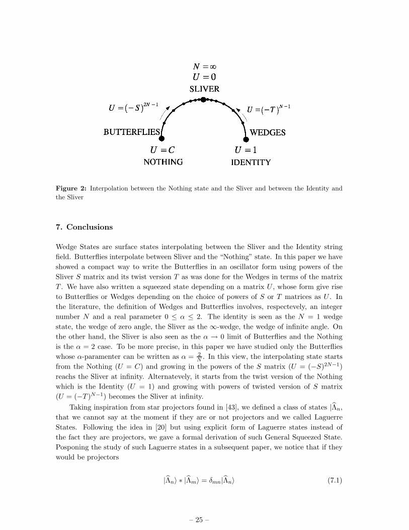
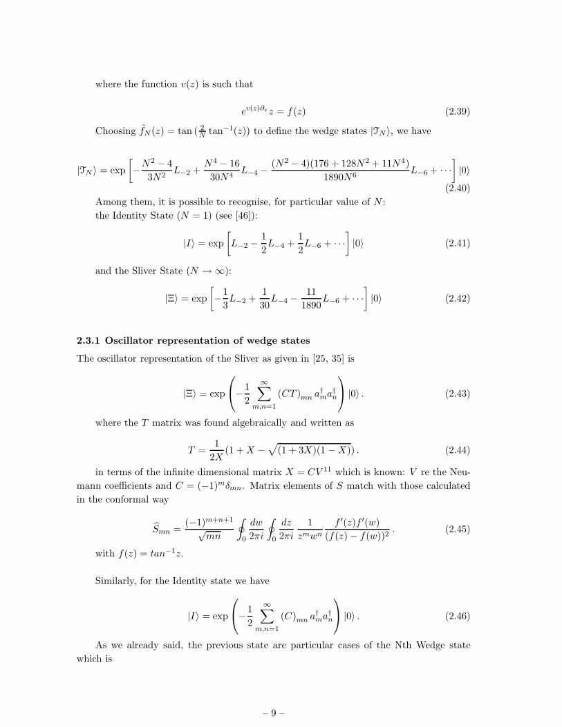
Figure 2: Interpolation between the Nothing state and the Sliver and between the Identity and

the Sliver

7. Conclusions

Wedge States are surface states interpolating between the Sliver and the Identity string

field. Butterflies interpolate between Sliver and the “Nothing” state. In this paper we have

showed a compact way to write the Butterflies in an oscillator form using powers of the

Sliver S matrix and its twist version T as was done for the Wedges in terms of the matrix

T . We have also written a squeezed state depending on a matrix U , whose form give rise

to Butterflies or Wedges depending on the choice of powers of S or T matrices as U . In

the literature, the definition of Wedges and Butterflies involves, respectevely, an integer

number N and a real parameter 0 ≤ α ≤ 2. The identity is seen as the N = 1 wedge

state, the wedge of zero angle, the Sliver as the ∞-wedge, the wedge of infinite angle. On

the other hand, the Sliver is also seen as the α → 0 limit of Butterflies and the Nothing

is the α = 2 case. To be more precise, in this paper we have studied only the Butterflies

whose α-paramenter can be written as α = 2N . In this view, the interpolating state starts

from the Nothing (U = C) and growing in the powers of the S matrix (U = (−S)2N−1)

reachs the Sliver at infinity. Alternatevely, it starts from the twist version of the Nothing

which is the Identity (U = 1) and growing with powers of twisted version of S matrix

(U = (−T )N−1) becomes the Sliver at infinity.

Taking inspiration from star projectors found in [43], we defined a class of states |Λn,

that we cannot say at the moment if they are or not projectors and we called Laguerre

States. Following the idea in [20] but using explicit form of Laguerre states instead of

the fact they are projectors, we gave a formal derivation of such General Squeezed State.

Posponing the study of such Laguerre states in a subsequent paper, we notice that if they

would be projectors

|Λn〉 ∗ |Λm〉 = δmn|Λn〉 (7.1)

– 25 –

although the derivation of the interpolating state is rather formal since every state of

the resummation formula is a squeezed state times a matrix, it would be possible to see

the multiplication rule between wedge states because we would have:

|TN 〉 ∗ |TM 〉 =∞∑

n=0

((−T )N−1

)n |Λn〉 ∗∞∑

m=0

((−T )M−1

)m |Λm〉 =∞∑

n=0

((−T )M+N−1−1

)n |Λn〉

(7.2)

thus

|TN 〉 ∗ |TM 〉 = |TM+N−1〉 (7.3)

In any case, despite Laguerre states are or not star projectors, the same check for

Butterflies using oscillator formalism is complicated by the fact S matrix does not commute

with X = CV 11 matrix of the Witten’s vertex.

Acknoledgements

I would like to thank Loriano Bonora for useful comments and discussions. I would

like to thank also Luis F. Alday, Carlo Maccaferri and Serguey Petcov.

References

[1] E.Witten, Noncommutative Geometry and String Field Theory, Nucl.Phys. B268 (1986) 253.

[2] A.Sen Descent Relations among Bosonic D–Branes, Int.J.Mod.Phys. A14 (1999) 4061,

[hep-th/9902105]. Tachyon Condensation on the Brane Antibrane System JHEP 9808 (1998)

012, [hep-th/9805170]. BPS D–branes on Non–supersymmetric Cycles, JHEP 9812 (1998)

021, [hep-th/9812031].

[3] K.Ohmori, A review of tachyon condensation in open string field theories, [hep-th/0102085].

[4] I.Ya.Aref’eva, D.M.Belov, A.A.Giryavets, A.S.Koshelev, P.B.Medvedev, Noncommutative

field theories and (super)string field theories, [hep-th/0111208].

[5] W.Taylor, Lectures on D-branes, tachyon condensation and string field theory,

[hep-th/0301094].

[6] L. Bonora, C. Maccaferri, D. Mamone and M. Salizzoni, Topics in String Field Theory,

[hep-th/0304270].

[7] A.Leclair, M.E.Peskin, C.R.Preitschopf, String Field Theory on the Conformal Plane. (I)

Kinematical Principles, Nucl.Phys. B317 (1989) 411.

[8] A.Leclair, M.E.Peskin, C.R.Preitschopf, String Field Theory on the Conformal Plane. (II)

Generalized Gluing, Nucl.Phys. B317 (1989) 464.

[9] L.Rastelli, A.Sen and B.Zwiebach, String field theory around the tachyon vacuum, Adv.

Theor. Math. Phys. 5 (2002) 353 [hep-th/0012251].

[10] D.Gaiotto, L.Rastelli, A.Sen and B.Zwiebach, Ghost Structure and Closed Strings in Vacuum

String Field Theory, [hep-th/0111129].

[11] H.Hata and T.Kawano, Open string states around a classical solution in vacuum string field

theory, JHEP 0111 (2001) 038 [hep-th/0108150].

– 26 –

[12] T. Okuda, The equality of solutions in vacuum string field theory, [hep-th/0201149].

[13] H.Hata and H.Kogetsu Higher Level Open String States from Vacuum String Field Theory,

JHEP 0209 (2002) 027, [hep-th/0208067].

[14] K.Okuyama, Siegel Gauge in Vacuum String Field Theory, JHEP 0201 (2002) 043

[hep-th/0111087].

[15] K.Okuyama, Ghost Kinetic Operator of Vacuum String Field Theory, JHEP 0201 (2002) 027

[hep-th/0201015].

[16] L.Rastelli, A.Sen and B.Zwiebach, Star Algebra Spectroscopy, JHEP 0203 (2002) 029

[hep-th/0111281].

[17] I.Kishimoto, Some properties of string field algebra, JHEP 0112 (2001) 007 [hep-th/0110124].

[18] L.Rastelli, A.Sen and B.Zwiebach, Half-strings, Projectors, and Multiple D-branes in Vacuum

String Field Theory, JHEP 0111 (2001) 035 [hep-th/0105058].

[19] D.J.Gross and W.Taylor, Split string field theory. I, JHEP 0108 (2001) 009

[hep-th/0105059], D.J.Gross and W.Taylor, Split string field theory. II, JHEP 0108 (2001)

010 [hep-th/0106036].

[20] T.Kawano and K.Okuyama, Open String Fields as Matrices, JHEP 0106 (2001) 061

[hep-th/0105129].

[21] N.Moeller, Some exact results on the matter star–product in the half–string formalism, JHEP

0201 (2002) 019 [hep-th/0110204].

[22] J.R.David, Excitations on wedge states and on the sliver, JHEP 0107 (2001) 024

[hep-th/0105184].

[23] P.Mukhopadhyay, Oscillator representation of the BCFT construction of D–branes in vacuum

string field theory, JHEP 0112 (2001) 025 [hep-th/0110136].

[24] M.Schnabl, Wedge states in string field theory, JHEP 0301 (2003) 004, [hep-th/0201095].

Anomalous reparametrizations and butterfly states in string field theory, Nucl. Phys. B 649

(2003) 101, [hep-th/0202139].

[25] V.A.Kostelecky and R.Potting, Analytical construction of a nonperturbative vacuum for the

open bosonic string, Phys. Rev. D 63 (2001) 046007 [hep-th/0008252].

[26] J. A. Harvey, Komaba lectures on noncommutative solitons and D-branes, [hep-th/0102076].

[27] E.Witten, Noncommutative Tachyons and String Field Theory, [hep-th/0006071].

[28] M.Schnabl, String field theory at large B-field and noncommutative geometry, JHEP 0011,

(2000) 031 [hep-th/0010034].

[29] I.Bars, Map of Witten’s * to Moyal’s *, Phys.Lett. B517 (2001) 436. [hep-th/0106157].

[30] M.R. Douglas, H. Liu, G. Moore, B. Zwiebach, Open String Star as a Continuous Moyal

Product, JHEP 0204 (2002) 022 [hep-th/0202087].

[31] B. Chen, F. L. Lin,D-branes as GMS solitons in vacuum string field theory [hep-th/0204233].

[32] D. M. Belov, Diagonal representation of open string star and Moyal product,

[hep-th/0204164].

– 27 –

[33] D.J.Gross and A.Jevicki, Operator Formulation of Interacting String Field Theory,

Nucl.Phys. B283 (1987) 1.

[34] D.J.Gross and A.Jevicki, Operator Formulation of Interacting String Field Theory, 2,

Nucl.Phys. B287 (1987) 225.

[35] L.Rastelli, A.Sen and B.Zwiebach, Classical solutions in string field theory around the

tachyon vacuum, Adv. Theor. Math. Phys. 5 (2002) 393 [hep-th/0102112].

[36] N.Seiberg and E.Witten, String Theory and Noncommutative Geometry, JHEP 9909, (1999)

032 [hep-th/9908142].

[37] E.Fuchs, M.Kroyter and A.Marcus, Squeezed States Projectors in String Field Theory, JHEP

0209 (2002) 022 [hep-th/0207001].

[38] D. Gaiotto, L. Rastelli, A. Sen and B. Zwiebach, Star Algebra Projectors, JHEP 0204 (2002)

060 [hep-th/0202151].

[39] Y.Okawa, Open string states and D–brane tension form vacuum string field theory, JHEP

0207 (2002) 003 [hep-th/0204012].

[40] K.Okuyama, Ratio of Tensions from Vacuum String Field Theory, JHEP 0203 (2002) 050

[hep-th/0201136].

[41] G.Moore and W.Taylor The singular geometry of the sliver, JHEP 0201 (2002) 004

[hep-th/0111069].

[42] R. Gopakumar, S. Minwalla and A. Strominger, Noncommutative solitons, JHEP 0005

(2000) 020 [hep-th/0003160].

[43] L. Bonora, D. Mamone and M. Salizzoni, Vacuum String Field Theory ancestors of the GMS

solitons, JHEP 0301 (2003) 013 [hep-th/0207044].

[44] L. Rastelli, A. Sen and B. Zwiebach, Boundary CFT construction of D-branes in vacuum

string field theory, JHEP 0111 (2001) 045, [hep-th/0105168].

[45] L. Rastelli and B. Zwiebach, Tachyon Potentials, Star Products and Universality, JHEP

0109 (2001) 038 [hep-th/0006240]

[46] I. Ellwood, B. Feng, Y. H. He and N. Moeller, “The identity string field and the tachyon

vacuum,” JHEP 0107, 016 (2001) [arXiv:hep-th/0105024].

– 28 –